Region and Active Contour-Based Segmentation Technique for Medical and Weak-Edged Images

Computational and Applied Mathematics 2015; 1(3): 72-78 Published online April 30, 2015 (http://www.aascit.org/journal/cam)

Keywords Image Segmentation,

Multiple-Thresholding,

Correlation Matching,

Level-Set Algorithm,

Image Guided Surgery

Received: March 3, 2015

Revised: March 23, 2015

Accepted: March 24, 2015

Region and Active Contour-Based Segmentation Technique for Medical and Weak-Edged Images

Abdulfattah A. Aboaba1, Shihab A. Hameed

2, Othman O. Khalifa

2,

Aisha H. Abdalla2

1Computer Engineering Department, University of Maiduguri, Maiduguri Nigeria 2Department of Electrical & Computer Engineering, International Islamic University Malaysia,

Kuala Lumpur Malaysia

Email address [email protected] (A. A. Aboaba), [email protected] (S. A. Hameed),

[email protected] (O. O. Khalifa), [email protected] (A. H. Abdalla)

Citation Abdulfattah A. Aboaba, Shihab A. Hameed, Othman O. Khalifa, Aisha H. Abdalla. Region and

Active Contour-Based Segmentation Technique for Medical and Weak-Edged Images.

Computational and Applied Mathematics. Vol. 1, No. 3, 2015, pp. 72-78.

Abstract One of the key requirement in image guided surgery (IGS)/ computer aided surgery

(CAS) planning is accurate segmentation of the images concerned. It is also a

challenging issue for the purpose of image analysis and understanding in general, and

surgical intervention involving image guided surgery (IGS) in particular. Thus, in this

paper, a technique employing two-stage segmentation in which one of the stage is also an

hybrid of two segmentation methods is developed for medical images in particular, and

weak-edged images in general. The first stage employs hybrid of multiple-thresholding

and correlation matching. The output image of the first stage was use as the input image

to the second stage to generate the final output using the modified Chan-Vese level-set

algorithm (MLSA). The results obtained is accurate as showed in figures 2, 3, and 4.

1. Introduction

Image segmentation is one of most important steps leading to analysis and

understanding of processed image data. Its main goal is to divide image into parts that

have a strong correlation with objects or areas of the real world contained in the image

[1], [2] or segments that are intelligently distinguishable. Segmentation using energy

functional called level-set algorithm was carried out by [3], it is a good and fast

segmentation technique especially if the regions in the image are distinguishable to some

extent. The work in [4] used the hybrid of edge detection and region-growing to achieve

better segmentation result. Construction of brain atlas from images obtained from MRI

using some Chinese people as experiment was carried out by [5]. Combinations of

several methods which include spatial normalization using statistical parametric mapping,

Gaussian smoothing, and non-linear transformation were step wisely applied on the MRI

images. A 3D-structure digitalized Atlas of Chinese Brain was established with more

work left to be done on making the cerebral region clearer. The research of [6] explored

the development of a new technique for localizing small pulmonary nodules (lump)

before thoracoscopic (related to chest) surgery using image guided navigation system.

Using animals for experiment, lesions were created with a mixture of oily radiographic

contrast and tissue adhesive was percutaneously placed under fluoroscopic guidance

through a 22 gauge. The result is that all lesions were successfully localized in the

thoracoscope image, and all resection margins were microscopically clear as confirmed

Computational and Applied Mathematics 2015; 1(3): 72-78 73

by the pathology examination. There were no surgical

complications and the work’s major limitation was that the

movement of diaphragm and chest wall during respiration

affected the accuracy of localization.

Furthermore, the hybrid of local geodesic active contours and

a more global region-based active contour was presented in [7].

The resulting technique is more versatile than either of the two

methods that produced it owing to its robustness to noise and

reduced dependency on initial curve placement. [8] hybridized

region growing method and edge detection method as a way of

getting better result. Initial results are promising but further work

is still on-going. In [9] a successful segmentation result was

obtained using level-set where energy model based on the metric

was incorporated into the geometric active contour framework.

Finally, a self-learning, and fully automatic segmentation

technique was realized based on the use of adaptive region-

growing method by [10]. Like the work of [3], it allows region-

specific variation of the homogeneity criterion. Furthermore, [11]

segmented occluded, cluttered, and noisy images by

conditioning the zero level-set curve to stop based on prior

shape. This approach is not able to segment many object

simultaneously but good at single object segmentation.

The research by [12] is such that the use of Quantum Dot

of targeted tumor was investigated as a way of helping

surgeons to find tumor boundary. Also, it was seen in [13]

where an evaluation of interstitial microwave probe as a

means of estimating the boundary of tumor was conducted.

Of equal interest is the use of sparse finite element to

enhance level-set algorithm by [14] which has resulted in

good and faster segmentation as compared with Chan-Vese

level-set algorithm but limited to 2D images unlike its

improved version by [15] that in addition to having 3D

capability, it is equally fast like its predecessor.

Nonetheless, as shown by the review of segmentation

methods, no segmentation method is perfect for all types of

images [16], and most often, combination of two or more

methods are required to attain accurate segmentation result as

was reported in [17], and expanded upon in the current work.

Medical images like all other weak-edge images are difficult

to perfectly segment. In spite of numerous advantages of

Image guided surgery (IGS) over the traditional more invasive

method of surgical operation, incomplete ablation or over-

resection due to improper segmentation has been known to be

the likely outcome of surgical intervention involving brain

tumor removal. The implication of these is either tumor

recurrence or damage to healthy tissues. With about 95% of

tumor recurrence close to the primary site of initial resection,

the author believes that with accurate segmentation, precise

tumor resection would be possible. Hence, in this paper, the

hybrid and bi-level image segmentation technique useful for

weak-edge and medical image segmentation with high

accuracy is presented.

2. Methodology

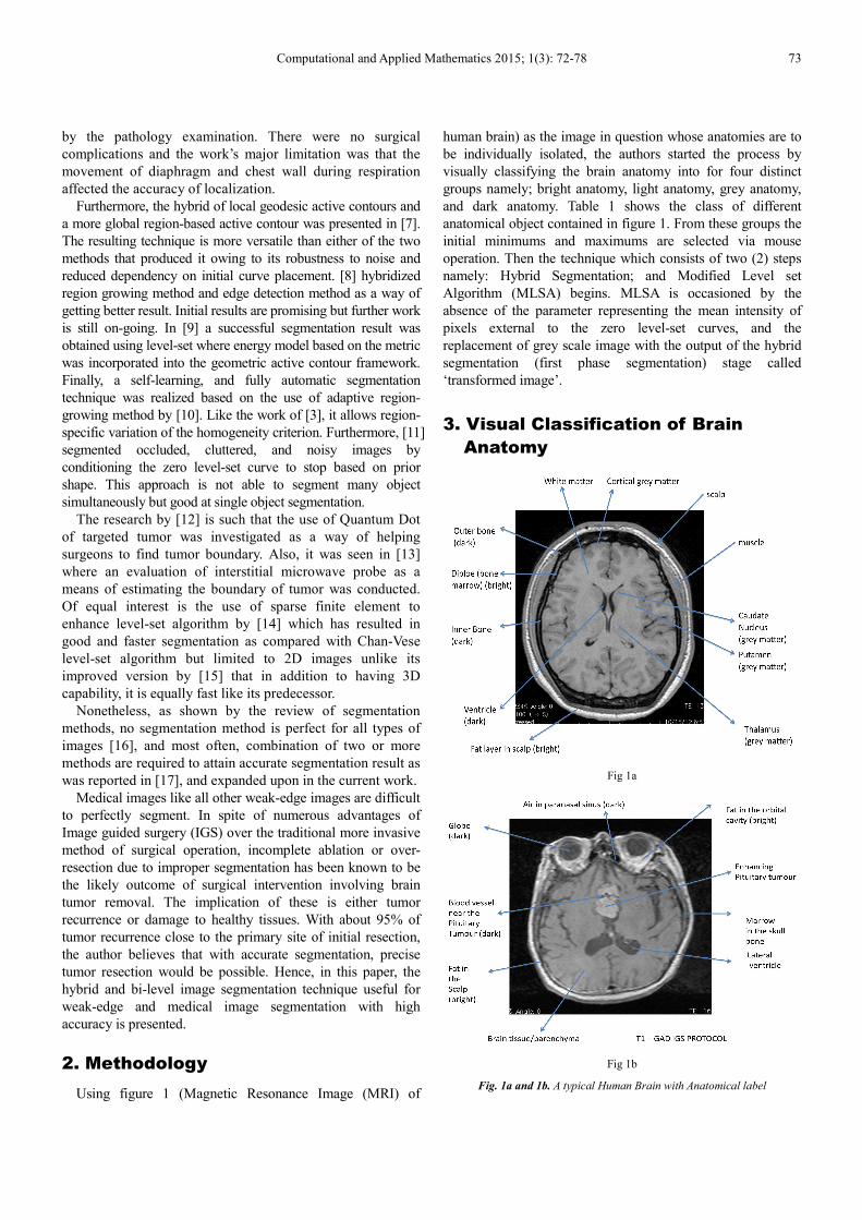
Using figure 1 (Magnetic Resonance Image (MRI) of

human brain) as the image in question whose anatomies are to

be individually isolated, the authors started the process by

visually classifying the brain anatomy into for four distinct

groups namely; bright anatomy, light anatomy, grey anatomy,

and dark anatomy. Table 1 shows the class of different

anatomical object contained in figure 1. From these groups the

initial minimums and maximums are selected via mouse

operation. Then the technique which consists of two (2) steps

namely: Hybrid Segmentation; and Modified Level set

Algorithm (MLSA) begins. MLSA is occasioned by the

absence of the parameter representing the mean intensity of

pixels external to the zero level-set curves, and the

replacement of grey scale image with the output of the hybrid

segmentation (first phase segmentation) stage called

‘transformed image’.

3. Visual Classification of Brain

Anatomy

Fig 1a

Fig 1b

Fig. 1a and 1b. A typical Human Brain with Anatomical label

74 Abdulfattah A. Aboaba et al.: Region and Active Contour-Based Segmentation Technique for Medical and Weak-Edged Images

Figure 1 is the visual classification of brain MRI protocol

image and in Table 1 the classification is grouped and

tabulated according to the visual classification.

Table 1. Classification of Anatomical Structure Appearances in IGS Protocol MRI slice of the Brain

S.No/ Appearance Bright (Bgt) Light (Lgt) Grey (Gry) Dark (Drk)

1 Fat layer in Scalp

Grey Matter/ Cell Bodies (Substantia Grisea)

Ventricle

(a) Cortical

White Matter/ Nerve Fibers (substantia alba) (b)Caudate Nucleus

(a)Corpus Callosum (c)Putamen

(b)Internal Capsule (d)Thalamus

(e)Insula

(f)Periaqueductal

2 Bone Marrow Tumor Muscle Inner Bone

3 Scalp Outer Bone

4. The Bi-Level Segmentation

Technique

The technique comprises of hybrid segmentation

(intelligent combination of multiple thresholding and 2D

template matching) as the first phase of the segmentation

process, which could be classified as basic image

segmentation. The second phase of segmentation which is

related to advanced image segmentation uses active contour-

based segmentation called modified level-set algorithm

(MLSA) resulting from chan-vese level-set algorithm (LSA).

This is a two phase segmentation plan in which the outputs of

the first phase called binary space (BS) transform image is

used as input to the second phase. This enables proper

isolation of region of interest (ROI) and enhances good

guidance during surgical planning and intervention. Thus, it

implies separation of the four classes of anatomy in table (1)

into individual group or regions on separate but same

intensity background (black). Thus, equation (1) is a set of all

element of IGS protocol image, and equation (2) is an

expression of the image intended at the end of the hybrid and

bi-level segmentation technique.

G = �B, B��, L��, G, D� (1)

where G is the set of all anatomy of IGS protocol image, B is

the black background, and BgtLgtGryDrk respectively stands

for bright anatomy, light anatomy, grey anatomy, and dark

anatomy as labeled in figure 1, and g(i,j) represents an

element of the anatomical class in table 1.

g�i, j� =��1forf�i, j�ϵB��2forf�i, j�ϵL��3forf�i, j�ϵG4forf�i, j�ϵD�0forf�i, j�ϵB

(2)

If the intensity for normal brain tissue giving as Gry in

equation (2) is separated on a uniform background, using

region of interest (ROI) processing, its boundary could be

determined during the second phase of the segmentation that

uses MLSA. The goal of the first phase processing is to have

an image represented by equation (3).

G = �B, G (3)

The formulation of mathematical analogy that enables this

then follows:

4.1. Formulating the Model for Boundary

Pixels

In this paper, only the bright, light, and grey anatomies

will be identified and processed leaving-out the dark anatomy

in order to reduce computational workload since the anatomy

of interest is tumor designated as light anatomy (!"#) which

is embedded in-between the bright ($"#) and grey (%&' )

anatomies. Hence, the background and the dark anatomy are

assumed same leaving us with an image comprising of four

regions namely bright, light, and grey anatomies, and the

background assigned A, B, C, and D. Medical images being

weak-edge images, the first step is to determine the number

of threshold points and intercepts areas for a given image,

and this is related by equations (4) and (5).

(( = 2) − 2 (4)

+ = ) − 1 (5)

where ) is the number of regions in an image inclusive of the

boundary,(( is the number of threshold points needed to

segment the image into different objects, and+ is the number

of intercept points required to segment weak-edge images

into different regions that the image is made up of.

According to equations (4) and (5), a weak-edged image

with four (4) regions would have six (6) threshold points and

three (3) intercepts points. The threshold points designed to

be chosen by mouse operation are assigned correspondingly

as,-./, $-01, $-./, 2-01, 2-./, 0/34-01 respectively.

These are perceivable minimums and maximums in each

region while the absolute minimum for regions A, B, and C,

and the absolute maximum for regions B, C, and D hang in

the intercept regions. Therefore, one of the tasks is to find the

three absolute minimum or maximum threshold equations in

compliance with the number of intercepts points. Thus if we denote the six (6) absolute threshold points for

the four-region image as: ,-./5 , $-015 , $-./5 , 2-015 , 2-./5 , and 4-015 respectively, and the intercept points between the regions are labeled as: Intercept of region A


(bright anatomy) and B(light anatomy) as 1 , Intercept of

region B (light anatomy) and C(grey anatomy) as ' , and Intercept of region C (grey anatomy) and D (dark anatomy)

as 6. Therefore the pixels within the intercept regions whose

affinity is to be determined are called target pixels (#7) and

are separately designated according to their intercepts as 1#7, '#7, and 6#7 respectively. A suitable way is to approach this is intercept by intercept basis. Again within an intercept, the

pixels are individually treated as target pixel #7 one after the

other, where #7 ranges from the first #7 (#71 ) to the last #7(#7809#) In order to determine in which intercept a target pixel

belong to, the use of quadrance ;<03is employed. In this

approach, the target pixel inside an intercept is conceptually

made the centre between the minimum or maximum

thresholds from each of the adjacent regions to the intercept

(for instance regions A and B). Thus, the quadrance between

the target pixel and the two threshold points are determined,

then the infimum./=of two quadrances;<03is determined

to know which of the thresholds from the adjacent regions

shares more affinity with the target pixel#7. Equation (6) is

the basic quadrance equation.

><03 = �? − @�A (6)

where?stands for a threshold and @stands for target pixel #7. Equations (7) and (8) are equations representing array of two

quadrances, and infimum of the array for 1 intercept. 1#7B represents the first target pixel in the 1 intercept. ,CDEand$CFG are the minimum threshold point in region A and maximum threshold point in region B respectively

HG = {�,CDE − 1#7B�A, �$CFG − 1#7B�A} (7)

K�1� = inf{HG} (8)

Since the objective is to locate a point of similarity

between regions of an image and not from one point to

another, it is preferable to use a tool for pattern recognition

such as correlation matching whose prove for use in pattern

recognition is shown in equation (9). More so, equations (6)

and (9) are similar as a measure of separation between two

point.

∑ �N�.� − K�1 + .��APQDRSPQ = ∑ TNA�.� + KA�1 + .�−2N�.�K�1 + .� UPQDRSPQ (9)

In Equation (9)VW is the size of the array or matrix, image

or threshold point isK , and N represents image template or

filter or target pixel #7.

4.2. Hybridization of Multiple Thresholding

and Correlation Matching

This is the hybridization of multiple thresholding and

template matching in which the threshold points are

considered images and the target pixels are filters.

Furthermore, the immediate neighbours of each threshold

point and target pixel are incorporated into the calculation to

form an by n matrix with the threshold point as the center of

the n by n matrix for the image side, and target pixel as the

center of the n by n matrix for the filter side respectively. The

correlation equation proving the possibility of this operation

is given in equation (10) such that f◙g is correlation of f and

g and the limit is specified on the integral functions (2D

correlation)

�="��@, X� ≝ Z Z =�[, \�"�@ + [, X + \�3[3\]S]S^ (10)

Resolving the affinity of each pixel in individual region requires going pixel by pixel, thus if the total number of

pixels in each of the intercept (1, ', &6) is numbered from

one (1) to 8, -, &/, then we shall have 8, -, &/ numbers of iteration in each intercept before the absolute minimum or maximum would be arrived at. Therefore, the target pixels

are labeled 1#7B to 1#7_ , '#7B to '#7C , and 6#7B to 6#7E respectively.This implies that at the end of every iteration, the chosen minimum or maximum may take on a new value depending on which region the target pixel falls into. This means a new minimum or maximum is computed at the end of every iteration. Thence, given that the initial (mouse operation chosen) minimum and maximum for regions A, B

and C are designated as; ,CDE` & $CFG` , $CDEa& 2CFGa ,0/32CDEb &4CFGb ,while the final minimum and maximum for

the same regions are; ,CDE`c_ & $CFG`c_ , $CDEacC & 2CFGacC, 0/32CDEbcE&4CFGbcE. The quadrance vector and infimum

for the first pixel for each intercept are shown in equations (11) to(16):

HG = {�,CDE` − 1#7B�A, �$CFG` − 1#7B�A} = �,1#7, $1#7�(11)

K�1� = inf{HG} (12)

Hd = ef$CDEa − '#7BgA, f2CFGa − '#7BgAh = �$'#7, 2'#7�(13)

K�'� = inf�Hd (14)

Hi = {�2CDEb − 6#7B�A, �4CFGb − 6#7B�A} = �26#7, 46#7� (15)

K�6� = inf{Hi} (16)

The implementation is such that the center correlation CC between an image (threshold point) and a filter (target pixel) is determined as represented by equation (17). Once equation (17) is applied on two adjacent threshold points, equation (18) is used to find the infimum between the two and equation (19) then places the target pixel to either of the adjacent regions, and instantaneously updates the two concerned thresholds. Equations (19) to (24) are the models for the first and last pixels in each of the intercept regions. In these equations, ,CDE` &$CFG` are the initial chosen thresholds from adjacent

regions A and B, 1#7Bis the first #7 in intercept 1, and,CDE`cB,

&$CFG`cB are the first updates ,CDE` &$CFG` after the #7 has been classified into either of the regions.

22�,1#7� = �,CDE` ��1#7B� = �,CDE` �j5, k5��1#7B� = ∑ ∑ f1#7B�., l�,CDE` �j5 + ., k5 + l�gAPmDRSPmPmnRSPm (17)


o�1_� = inf{22�,1#7B�, 22�$1#7B�} (18)

The first infimum calculated from intercept 1is:

o�1B� =

�� 22�,1#7�, 1#7B ∈ ,#ℎr/,CDE`cB = ,CDE` − �,CDE` − 1#7B�0/3$CFG`cB = $CFG`

22�$1#7�, 1#7B ∈ $#ℎr/$CFG`cB = $CFG` + �6#7B − $CFG` �0/3,CDE`cB = ,CDE`

(19)

And for the last 1#7called 1#7_ , the last infimum called ./=1_ is given by:

o�1_� =

�� 22�,1#7�, 1#7_ ∈ ,#ℎr/,CDE`c_ = ,CDE`c_SB − f,CDE`c_SB − 1#7_g0/3$CFG`c_ = $CFG`c_SB

22�$1#7�, 1#7_ ∈ $#ℎr/$CFG`c_ = $CFG`c_SB + �1#7_ − $CFG`c_SB�0/3,CDE`c_ = ,CDE`c_SB

(20)

Likewise, the first infimum calculated from intercept 'is:

o�'B� =

�� 22�$'#7�, '#7B ∈ $#ℎr/$CDEacB = $CDEa − f$CDEa − 1#7Bg0/32CFGacB = 2CFGa

22�2'#7�, '#7B ∈ 2#ℎr/2CFGacB = 2CFGa + f'#7B − 2CFGa g0/3$CDEacB = $CDEa

(21)

And its last infimum is:

o�'C� =

�� 22�$'#7�, '#7C ∈ $#ℎr/$CDEacC = $CDEacCSB − f$CDEacCSB − '#7Cg0/32CFGacC = 2CFGacCSB

22�2'#7�, '#7C ∈ 2#ℎr/2CFGacC = 2CFGacCSB + f'#7C − 2CFGacCSBg0/3

$CDEacC = $CDEacCSB

(22)

Moreso, from intercept z, first infimum is:

o�6B� =

�� 22�26#7�, 6#7B ∈ 2#ℎr/2CDEbcB = 2CDEb − �2CDEb − 6#7B�0/34CFGbcB = 4CFGb

22�46#7�, 6#7B ∈ 4#ℎr/4CFGbcB = 4CFGb + �6#7B − 4CFGb �0/32CDEbcB = 2CDEb

(23)

Again the last infimum in intercept z is:

o�6E� =

�� 22�26#7�, 6#7E ∈ 2#ℎr/2CDEbcE = 2CDEbcESB − �2CDEbcESB − /�0/34CFGbcE = 4CFGbcESB

22�46#7�, 6#7C ∈ 4#ℎr/4CFGbcE = 4CFGbcESB + �6#7E − 4CFGbcESB�0/32CDEbcE = 2CDEbcESB

(24)

The process continues until the last target pixel in all the

intercepts are classified. Hence, the last updates on each of

the initial chosen thresholds are the absolute minimums and

absolute maximum as shown in equations (25) to (30).

,-./5 = ,CDE`c_ (25)

$-015 = $CFG`c_ (26)

$-./5 = $CDEacC (27)

2-015 = 2CFGacC (28)

2-./5 = 2CDEEcC (29)

4-015 = 4CFGEcC (30)

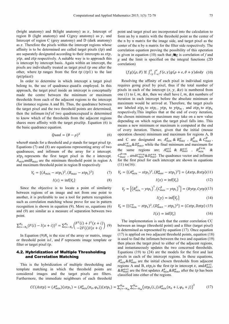
Figure 2 is the result obtained when the absolute thresholds are used in the segmentation of an MR axial image (in grayscale) of a human head (top left) into bright anatomy (top right), light anatomy (bottom left), and grey anatomy (bottom right). This operation is reckoned as transformation Ks from the grey-scale (GS) MR image to three different anatomical structures as a consequence of the hybrid segmentation technique. Moreover the anatomy of interest is

the tumor found amidst light anatomy L�� noted after

transformation as K_s(bottom left).This is categorized as first phase segmentation.

Fig. 2a

MRI Tumorous Brain Slice Bright Anatomical Structures

Light Anatomical Structures Grey Anatomical Structures


Fig. 2b

Fig. 2a and 2b. Grey scale image (upper left) and the other three anatomical

divisions

This transformation is reckoned as Ks, but each one of the transformation images is called binary space (BS) transform

image designated as Kts , K_s , 0/3Kus for bright, light, and grey

anatomies respectively. This is noted as the first phase of the proposed bi-level segmentation technique.

4.3. The Modified Level-Set Algorithm

The modified level-set algorithm (MLSA) is a modified form of the Chan-Vese (10) energy functional occasioned by the zerolization of the parameter representing the mean intensity of pixels external to the zero level-set curve, and also, the replacement of grey scale image with any of the

transformed image, in this case K_s.Hence, equations (31) and (32):

∅w.yzcB {1 O ∆th δ�f∅w,yz gμ�CB O CA O C� O C�� ∅w,yz O ∆th δ�f∅w,yz gμ �CB∅wcB,yzcB O CA∅wSB,yzcB O C�∅w,ycBzcB OC�∅w,ySBzcB �

*∆tδ�f∅w,yz g �v O λB �Iw,y� * aB�∅z��A *

λAfIw,y� gA � (31)

pw,y � ∅w,yz * ∆tδ�f∅w,yz g {v O λB �Iw,y� * aB�∅z��A * λAfIw,y� gA� (32)

in which ∅D,nE stands for the value of ∅ at pixel ., l and at /

iteration, ∆# is the time step, smoothed version of the Dirac

function � is here represented by �� , pixel spacing q .

Also((length of level-set curve), �(area of level-set curve), �B (inner uniformity factor), and �A (outer uniformity

factor).0Brepresents the mean intensities of the interior of the

level-set curve 2�∅� , and Iw,y� is the transform image

representing light anatomical structure.( , � , �B , and �A are � 0 2B � 2B∅DcB,nEcB - value of ∅ by next iteration �/ O 1� at next

row �. O 1� 2A � 2A∅DSB,nEcB - value of ∅ by next iteration �/ O 1� at

previous row �. O 1� 2� � 2�∅D,ncBEcB - value of ∅ by next iteration �/ O 1� at

next column �. O 1� 2� � 2�∅D,nSBEcB - value of ∅ by next iteration �/ O 1� at

previous column �. O 1� Equations (31) and (32) being modified form of Chan-Vese

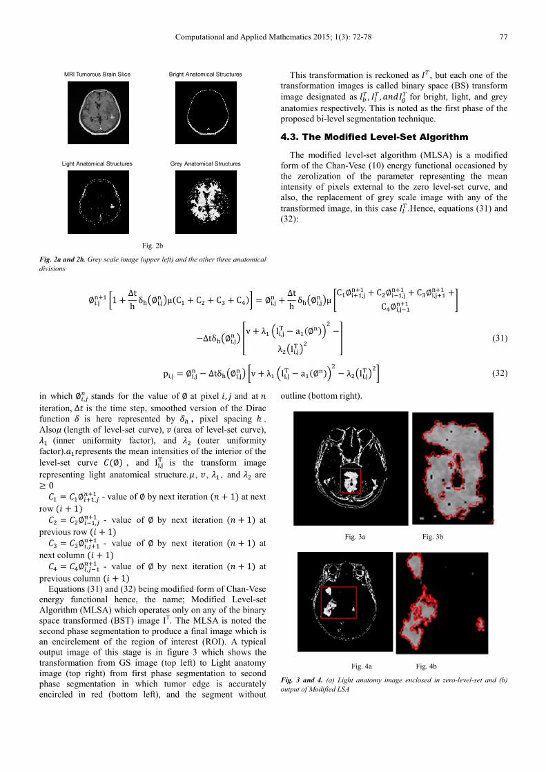
energy functional hence, the name; Modified Level-set Algorithm (MLSA) which operates only on any of the binary space transformed (BST) image IT. The MLSA is noted the second phase segmentation to produce a final image which is an encirclement of the region of interest (ROI). A typical output image of this stage is in figure 3 which shows the transformation from GS image (top left) to Light anatomy image (top right) from first phase segmentation to second phase segmentation in which tumor edge is accurately encircled in red (bottom left), and the segment without

outline (bottom right).

Fig. 3a Fig. 3b

Fig. 4a Fig. 4b

Fig. 3 and 4. (a) Light anatomy image enclosed in zero-level-set and (b)

output of Modified LSA

MRI Tumorous Brain Slice Bright Anatomical Structures

Light Anatomical Structures Grey Anatomical Structures


5. Summary

The novel hybrid segmentation for weak edge images in

general and medical images in particular is presented. It

begins with visual classification of brain anatomy in bright,

light, grey, and dark anatomies which led to the

determination of number of possible threshold points and

intercept regions such division would have. Having done that,

initial threshold points are picked by a human user, which are

then automatically compared with individual pixels (called

target pixels) within the intercept regions to determine which

of the two thresholds the pixel is closer to. It is at that point

of comparison that the authors decided to change the

approach to using 2D correlation matching for it proven

record in image segmentation instead of mare quadrance and

infimum/supremum. The pixel information is used in

continuous update of initial threshold points until an absolute

threshold for each of the region is achieved. The absolute

thresholds are then use to segment the grey scale image into

the desired four anatomical groups.

6. Conclusion

The results obtained showed high accuracy and could be

extended to include the use of active contour like level-set

algorithm for proper boundary definition. It could also be

useful in volume quantification for purposes of surgical

intervention.

References

[1] Sonka, M., Hlavac, V., & Boyle R., (2008).Image Processing, Analysis, and Machine Vision. (3rd Ed.), Thomson Corporation Toronto Canada.

[2] Svoboda, T., Kybic J., &Hlavac, V., (2008). Image Processing, Analysis, and Machine Vision – A MATLAB Companion. Thomson Corporation Toronto Canada.

[3] Chan, T. F., &Vese, L. A. (2001). Active contours without edges. IEEE transactions on image processing, 10(2), 266‐277.

[4] FupingZhu, and JieTian (2003). Modified fast marching and level set method for medical image segmentation, Journal of X-Ray Science and Technology 11, 193-204.

[5] Jianhua Lu, Zhiwei Chen, Zhong Chen, Zhiping Yan, Yi Yao, WannengLuo, &Sulian Su (2009). Three-dimensional digital atlas construction of Chinese brains by magnetic resonance imaging. IEEExplore.ieee.org

[6] Chen, W.,Chen, L. Chen, G. Qiang, Z. Chen, J. Jing, & S. Xiong (2007). Using an image-guided navigation system for localization of small pulmonary nodules before thoracoscopicsurgery A feasibility study. SurgEndosc. Vol. 21, 1883–1886.

[7] Shawn Lankton, Delphine Nain, Anthony Yezzi, and Allen tannenbaum (2007). Hybrid Geodesic Region-Based Curve Evolution for Image Segmentation. http://www.shawnlankton.com, Downloaded October 2011.

[8] Theo Pavlidis and Yuh-TayLiow (1988). Integrating Region Growing and Edge Detection. CH2605-4/88/0000/0208$01.00 IEEExplore.org

[9] RomeilSandhu, Tryphon Georgiou, and Allen tannenbaum (2008). A New Distribution Metric for Image Segmentation. Proceeding of 2008 SPIE--The International Society for Optical Engineering, San Diego, CA, USA.

[10] Regina Pohle and Klaus D. Toennies (2001). Segmentation of Medical Images Using Adaptive Region Growing. http://wwwisg.cs.uni-magdeburg.de/bv/pub/pdf /mi_4322_153.pdf Viewed in Dec. 2011

[11] Mezghich Mohamed Amine, M’hiri Slim, &GhorbelFaouzi (2012). Fourier-based multi-reference shape prior for region-based active contours. 978-1-4673-0784-0/12/$31.00 ©2012 IEEExplore.ieee.org.661-664

[12] Donna Arndt-Jovin, Sven R. Kantelhardt, WouterCaarls, Antony H.B. de Vries, Alf Giese, and Thomas M. Jovin (2009). Tumor-targeted quantum dots can help surgeons find tumor boundaries. IEEE Transaction on NanoBioscience, Vol. 8 No. 1, 65-71.

[13] Peng Wang, Christopher L. Brace, Mark C. Converse, and John G. Webster (2009). Tumor boundary estimation through time-domain peaks monitoring: Numerical predictions and experimental results in tissue-mimicking phantoms, IEEE Transactions on Biomedical Engineering, Vol. 56, No. 11

[14] Weber Martin,Blake Andrew &Cipolla Roberto (2004). Sparse finite elements for geodesic contours with Level-Sets. http://mi.eng.cam.ac. uk/research/vision/ Viewed in Dec. 2012.

[15] Weber Martin,Blake Andrew &Cipolla Roberto (2005). Sparse finite element Level-Sets for anisotropic boundary detection in 3D images. http://mi.eng.cam.ac. uk/research/vision/ Viewed in Dec. 2012.

[16] Park Hyunwook, Kwon Min Jeong, & Han Yeji (2005). Techniques in image segmentation and 3D visualization in Brain MRI and their applications. In Cornelius T. Leondes (Ed), Medical imaging systems technology – Methods in Cardiovascular and Brain Systems. World Scientific Publishing Company, Singapore.

[17] Aboaba Abdulfattah, Hameed Shihab, Khalifa Othman, & Abdalla Aisha (2014). Medical image segmentation using novel hybrid technique, Proceedings of the 2nd International conference on digital signal processing (MIC-SigProc-2014) 3-5 Oct., 2014 Dubai, UAE. ISSN: 2227-331X

Region and Active Contour-Based Segmentation Technique for Medical and Weak-Edged Images

Documents

Transcript of Region and Active Contour-Based Segmentation Technique for Medical and Weak-Edged Images