Loss of Energy at Sharp-Edged Pipe Junctions
167
Loss of Energy at Sharp-Edged Pipe Junctions in Water Conveyance Systems Technical Bulletin No. 1283 Agricultural Research Service U.S. DEPARTMENT OF AGRICULTURE In Cooperation With MINNESOTA AGRICULTURAL EXPERIMENT STATION and ST. ANTHONY FALLS HYDRAULIC LABORATORY of the University of Minnesota
-
Upload
khangminh22 -
Category
Documents
-
view
0 -
download
0
Transcript of Loss of Energy at Sharp-Edged Pipe Junctions

Loss of Energy at
Sharp-Edged Pipe Junctions in
Water Conveyance Systems
Technical Bulletin No. 1283
Agricultural Research Service U.S. DEPARTMENT OF AGRICULTURE
In Cooperation With
MINNESOTA AGRICULTURAL EXPERIMENT STATION
and
ST. ANTHONY FALLS HYDRAULIC LABORATORY
of the
University of Minnesota

This bulletin is the report of a 5-year test program to determine energy loases at sharp-edged pipe junctions that was conducted at the St. Anthony Falls Hydraulic Laboratory of the University of Minne- sota. It describes previous work on determining energy losses at pipe junctions» presents the theory of converging pipe junctions, describes the apparatus and procedure, gives the test data, explains the analysis of the data, summarizes the results obtained, compares the results with those obtained by other investigatory, presents equations, tables, and curves for use in the design of junctions, and shows how the results can be applied.

Loss of Energy at
Sharp-Edged Pipe Junctions in
Water Conveyance Systems
By FRED W. BLAISDELL
Hydraulic Engineer Soil and Water Conservation Research Division
Agricultural Research Service and
PHILIP W. MANSON Professor of Agricultural Engineering
University of Minnesota
Technical Bulletin No. 1283
Agricultural Research Service
U.S. DEPARTMENT OF AGRICULTURE
In Cooperation With MINNESOTA AGRICULTURAL EXPERIMENT STATION
and ST. ANTHONY FALLS HYDRAULIC LABORATORY
of the University of Minnesota

Contents Page
Previous work 1 Germany 2 Japan 2 United States of America 3 Switzerland 6 Great Britain 7
Theory of converging pipe junc- tions 8
Loss coefficient for main 8 Loss coefficient for lateral 9 Effect of nonuniform velocity
distribution 10 Program of tests 11 Apparatus 11 Experimental procedure 15 Analysis of test data 19
Preliminary analysis of test data 19
Analysis of loss coefficients 19 Results of tests 22
Page Equations of curves 22 Evaluation of results for least
squares data 27 Discussion of results 45
Comparison of results with those of other investigators 47
Design data 47 Equations 48 Tables 48 Curves 48
Application of results 48 Summary and conclusions 57 Literature cited 59 Terminology 60 Appendix 63
Figures 27 to 90 63 Figures 91 to 106 122 Table 12 131 Table 13 146
Washington, D.C. Issued August 1963

Loss of Energy at Sharp-Edged Pipe Junctions in Water Conveyance Systems
By FEED W. BLAISDELL AND PHILIP W. MANSON ^
Little factual information or the energy loss at pipe junctions is available. This is surprising; in view of the fact that pipe junctions are used in many different fidds. Joining pipes are used in \^ater collection and distribution systems, sewage systems, air-conditio aing systems, agricultural tile drauiage systems, and so forth.
Yet, most of the five studies on joining streams, discovered as a residt of library research, lack the scope or completeness required for the design of junctions. Use of even the available information is hindered by the fact that the better
studies have been published in foreign languages.
The studies reported here were made because of the need for factual information on the energy losses resulting from joining pipe flows in the field of agricultural tUe drainage. The importance of jirnc- tion energy losses to the field of agricultural drainage is emphasized by the fact that some 300 million feet of drain tile and many thou- sands of junctions are installed each year in the United States alone. The 5-year investigation conducted at the St. Anthony Falls Hydraulic Laboratory of the University of Minnesota was begim in 1954.
PREVIOUS WORK
Many statements regarding the design of junctions can be found in textbooks. However, attempts to locate a factual basis for the textbook statements have been uni- formly imsuccessful. Apparently, most statements are based on
^ The necessity for the study reported here was first recognized by the junior author, and the study was actively pro- moted by him. The details of the experi- ment were carried out under the direction of the senior author. The tests were con- ducted at various times by students Paul Ruud, Harry Gordon, Halford Erick- son, Harold W. Krueger, and Duane Zwiers. Charles E. Gates, station statis-
opinions and incomplete reasoning. But they have been expressed for so long a time it is now (1963) usual for them to be accepted without question. Typical of the statements or implications foimd in many textbooks (5, jp, SöO; 4, V- ^^/
tician, Minnesota Agricultural Experi- ment Station, planned, directed, and re- viewed the machine and statistical anal- yses. Mrs. May Wright, statistician, per- formed the statistical analyses and assisted with the reportine: of the statistical phases of the study. The American Concrete Pipe Association contributed funds in ad- dition to those supplied by the cooperating agencies.
1

TECHNICAL BULLETIN 1283, U.S. DEPT. OF AGRICULTURE
6, p. 118; IS, p, 113; 17, p. U; 21, p. 251; 22, p. 105; 23, p. 255) ^ IS the statement made by Pickels in regard to agricultural drainage {21, p, 251):
One tile drain should never enter another at right angles.
At the junction of a lateral with a submain a special junction tile or Y- branch should be used in which the angle between the branches is 45 degrees or less.
An attempt was made to locate all studies that have been made to determine the energy losses at pipe junctions. A few publications covering this research were dis- covered.
The work conducted in Germany and Japan is somewhat limited in scope and applicability. The work done in the United States of America, with the exception of comprehensive tests on storm drain junctions at the University of Missouri, has been largely confined to ship-lock hydraulic systems and right-angle pipe junctions.
The two Swiss studies were discovered after the experiments reported here had been completed. The first was a theoretical study, written in Zurich but published in Belgium, in which the theoretical equations were compared with the German experimental results. The second Swiss study is an investiga- tion of junctions between power supply tunnels and surge tanks conducted at Lausanne in which 11 different forms of the junction were studied. The second study is broader than the study reported herein in that both joining and diverging streams were tested, but it is narrower in the range of pipe sizes and angles of entry investi- gated. At Lausanne, aU joining edges were rounded.
The experimental work in Great Britain is that done on junctions of rectangular pipes.
* Italic numbers in parentheses refer to Literature Cited, p. 59.
Germany
The tests in Germany were conducted at the Hydraulic Insti- tute of the Technical University at Munich under the direction of D. Thoma. In 1923 and 1924, Gustav Vogel {31) initiated the tests using 90° junctions. About one year later Franz Petermann (20, pp. 65-77) conducted a series of tests on 45° and 135° junctions. The Munich tests were completed by EmU Kinne {15, pp. 70-93; 12), who used 60° and 120° junctions; he also completed the work begim by Vogel on 90° junctions.
The main in each case was 43 mm. (1.41 inches) in diameter with lat- erals of 15-mm., 25-mm., and 43- mm. diameter. The resulting area ratios AdjAi, were 8.22, 2.96, and 1.00. Converging and diverging flows were used. The junction forms tried were sharp-edged, rounded, and conical.
The data were presented in the form of dimensionless curves, and no attempt was made to develop theo- retical or empirical equations. In the case of converging flows, round- ing the junction edges made little difference for the 45° junction angle, but rounding did reduce losses some- what for the 60° and 90° junction angles. Petermann and Kinne noted apparent negative junction losses, which they ascribed to the suction produced by the lateral entering the main at an angle. The phenomenon is noted, in view of a comment by Soucek and Zelnick to be mentioned later.
Both Vogel and Kinne note that the junction loss coefficient does not noticeably vary with the veloc- ity of flow. This is an indication that the Reynolds number does not affect the junction loss coefficient.
Japan
The Japanese work was per- formed in the Hydraulic Laboratory

LOSS OF ENERGY AT SHARP-EDGED PEPE JUNCTIONS
TABLE 1.—Range oj sizes and angles oj pipes tested by Naramoto and Kasai {18)
Experiment series
Diameter of—
^6 e Main Lateral
1 Mm.
25 30 30 30 30 30
Í 1 30 1 2 36
Mm. 25 15 17.32 20 24.5 30 20
1 4 3 2.25 L5 1 2.25
Degrees 90, 75, 60, 45, 30 90, 85, 80, 75, 70, 60, 45, 30, 90,60 90, 75, 60, 45, 30, 15 90 90 90
2__ 15 3 4 5 6 7 __-
1 Upstream of junction. ' Downstream of junction.
of the Kyushu Imperial University at Fukuoka, Kyushu {18), It was initiated by Itaru Naramoto. After June 1927, Taijiro Kasai conducted the tests, owing to the death of Naramoto.
The range of sizes and angles of pipes tested was quite large, as is indicated in table 1.
Much of the experimental data is given in tables, but most of the tables show combined losses for the lateral and the main. Only for 90° junctions with area ratios A^jAit of 1 and 4 are data presented in such a manner that the losses for the main and the lateral can be sepa- rated. Fiulhermore, the complete range of possible flow combinations between the lateral and the main was not covered, because of the manner in which the tests were conducted.
With regard to negative junction losses, Naramoto and Kasai, like Petermann and Kinne, make the following comments, which help to explain the apparent anomaly re- ported by Soucek and Zelnick : When the velocity of the impinging stream is very small the water in the impinging passage is drawn out by the main flow, but when the velocity of the
impinging stream attains a certain extent the water in the main passage is drawn out by it. And the phenomenon grows greater as the velocity of the impinging stream increases and the angle of impact decreases.
United States of America
Work on pipe junctions in the United States has been done at the Agricultural and Mechanical Col- lege of Texas, at the State Univer- sity of Iowa, in the Panama Canal Zone, at the University of Missoiui, and a theoretical analysis was pre- pared by J. C. Stevens.
/. C. Steven» The earliest work done in the
United States was a theoretical analysis of junction losses reported by J. C. Stevens in 1926 {SO). Mr. Stevens presented a theoretical equation giving the junction energy loss based on the change of mo- mentum. His equation applied to any number of joining pipes, and he modified it to show how it would also apply to bends, sudden enlarge- ments, and sudden contractions. Mr. Stevens' treatment is entirely theoretical, and no supporting ex- perimental evidence is presented.

TECHNICAL BULLETIN 1283, U.S. DEPT. OF AGRICULTURE
Agricultural and Mechanical College of Texas
Cast iron pipe tees, 1 by 1 by 1 inch, were tested at the Agricultural and Mechanical College of Texas, and the results reported by F. E. Giesecke and W. H. Badgett (11). Only the 90° junction was tested. Vanous combinations of flows in the branches were tried. The data were plotted by using dimensionless coordmates, and curves were drawn to fit the data. Two of the curves can be compared with data from the tests reported in this bulletin. No theory and very little discussion accompany the curves.
State University of Iowa
A number of students, working imder the direction of John S. McNown, have conducted experi- ments on junctions. Sadiq M. •Niaz ^ worked with converging flows. The results of these studies were reported by Dr. McNown in 1954 (16).
The main for all tests was a brass pipe 2.06 inches in diameter. The laterals were of brass pipe 2.06 inches, 1 inch, and % inch in di- ameter. The resulting area ratios Aal At were 1, 4, and 16 and covered the range of the tests reported here. However, only the 90° junction angle was tested. All junctions were sharp edged.
McNown develops what he calls a ''simplified analysis.'' He writes: . . . one can write the momentum equation for the flow at the junction, provided that a term is included for (a) the indetermi- nate momentum of the flow in the lateral at the junction, or (6) the corresponding unbalanced force component acting on the wall at the lateral. In either equa- tion, lack of knowledge of this one sig- nificant unknown makes direct appHca-
• NIAZ, S. M. A STUDY OP CONVERGING FLOW IN PIPE LINES. Master's Thesis. (On file at Iowa State University, Iowa aty.) 1947.
tion of the results impossible without recourse to experiment.
McNown uses a force term in his momentum equation. The authorè did not include such a term, and ii remains for the presentation of thö results of the authors' tests to see if the force term can be neglected.
With regard to his simplified analysis, McNown writes: Actually ... no simplified analysis iè valid throughout a sufficient range of th¿ significant variables to have general appli^ cation beyond use as a reference for the comparison and evaluation of laboratory measurement.
and . . . the characteristics of flow through manifolds must be predicted empirically, at least in part.
McNown's lack of faith in the theoretical approach was given great weight in designing the present au- thors' experimental program; a com- prehensive empirical approach was employed in order to cover as much as possible of the range of field con- ditions. Fortunately, the picture turned out to be not nearly so black as McNown had indicated, and the theory developed by the authors fitted the data reasonably well.
The Panama Canal
Tests on lock intake and discharge ports were undertaken at the Pan- ama Canal HydrauUcs Laboratory dming 1939 and 1940. These tests have been reported by Edward Soucek and E. W. Zehiick (28).
Much of the Panama Canal in- formation has little bearing on the present problem, but some points are worth attention.
The theory developed by Soucek and Zelnick preceded McNown's presentation, but the approach is similar in that a term is provided in the momentum equation to take care of that part of the momentum change in the lateral flow produced by pressure changes in the conduit.

LOSS OF ENERGY AT SHARP-EDGED PIPE JUNCTIONS
As noted previously, such a term was not used by the authors.
The statement is made in* the paper (28, p. 1363) : It is evident . . . that Bernoulli's the- orem is not applicable to the phenomenon under consideration . . .
and the statement is more fully explained in the closing discussion (28, p. 1397): In intake manifolds . . . where flows from sources of differing energy content converge and mix in the culvert . . . Bernoulli's theorem would have to be modified by weighting the head from the two sources in proportion to the respec- tive discharges, even if energy losses did not occur. . . . However, there is [the] . . . possibility—that in some manner mechanically similar to that in which water does work on a turbine blade, the lateral discharge actually yields a portion of its energy to the conduit flow.
It is now proper to refer back to the comments by Petermann and Kinne that when the lateral enters the main at an angle there is a negative jimction loss, and by Naramoto and Kasai regarding what might be termed "ejector action.'' In view of these com- ments it seems likely that the last statement by Soucek and Zelnick is correct. But even this explana- tion cannot repeal the principle of conservation of energy embodied in the BemouUi equation. Both it and the momentum equation must apply with equal force to junction hydraulics as well as to all other hydraulic problems!
University of Missouri
Storm drain jimctions were tested for 4 years beginning in 1953 at the University of Missouri. W. M. Sangster, H. W. Wood, E. T. Smerdon, and H. G. Bossy reported the results of these tests {25, 26).
Although square and round man- holes were tested, most of the work was done on rectangular grate drop
inlets 6 by 15 inches in plan and of various heights. Since the drop inlet was also used as a drain junction, various combinations of drains entering and leaving the drop inlet and the manholes were tested. Pipe sizes used were 3.00, 3.75, 4.75, and 5.72 mches. AU pipes were fuU for all tests.
Many different arrangements of pipes and combinations of sizes were used in order to evaluate the pressure change at various storm drain junctions. However, the only data that are comparable with the drain tile jimction data are those obtained when the upstream and downstream mains are the same size {Ai=Au) and the lateral enters at a right angle. Lateral sizes corresponding to area ratios AAIAU of 1.00, 1.44, 2.34, 2.50, and 3.65 were tested.
The basic difference between the storm drain junctions and the drain tue junctions is that the joining of the streams takes place m an open rectangular box for the storm drain, whereas the joining is within the pipes for the drain tile.
A check was made to determine if the pressure change coefficient was independent of the actual dis- charge (related to the R^nolds number) and the actual Froude nmnber. Independency was es- tablished.
Theoretical analyses were at- tempted by Sangster and coworkers {26). Agreement between theory and test results was obtained when the flows joined in the rectangular drop inlet for the two-pipe in-line system, for the inlet witn main and lateral corresponding to the drain tile junction, and for the inlet with opposed laterals. However, no theoretical agreement was obtained for the inlet with offset opposed laterals, for the inlet with grate flow, or, more significantly, for manholes.

TECHNICAL BULLETIN 1283, U.S. DEPT. OF AGRICULTURE
Switzerland
Work has been done in Switzer- land both at Ziu'ich and at Lau- sanne.
Zurich A theoretical analysis of the en-
ergy losses at pipe junctions was made by H. Favre at ¿urich and the results werepublished in Belgium in 1937 (6). This analysis resulted in equations identical to those devel- oped independently by the present authors (equations 12 and 19, except for the last term of equation 19).
Favre compares his equations with the German experimental re- sults by using only those experi- ments ^'which relate to discharge laterals joining with zero radius, laterals for which our formulas have been established.'^ Regarding the agreement, Favre writes : In summary we can say that the formulas presented . . . have been confirmed by the experiments when [the angle between the lateral and the main] is between 45° and 90°, [the ratio of the area of the lateral to the area of the main] is between 0.1 and 1, [the ratio of the discharge from the lateral to the discharge in the main] is between 0 and 1. The region thus de- fined embraces most of the practical applications.
Confirming the observations of other experimenters, Favre notes that the energy loss coefficients for each branch can be either positive or negative, indicating a loss or a gain of energy head, respectively.
Lausanne The tests at Lausanne were con-
ducted at the University of Lau- sanne and are reported by André Gardel (^, 9) and ödön Starosolszljy
Eleven différent forms of the junction were studied. The first group of tests was conducted on five 90° tees. The diameter of the main was 150 mm. (5.9 inches) in all cases. The five laterals ranged in
diameter from 150 mm. (5.9 inches) to 60 mm. (2.4 inches). The ratios of the area of the main to the area of the branch were 1.00, 1.44, 2.25, 3.52, and 6.25. In the second group of six tests the diameters of the three branches were constant and equal to 150 mm. (5.9 inches), but the angle of the lateral with the main ranged from 45° to 135°—angles of 45°, 60°, 75°, 105°, 120°, and 135° were tested. The ratio of the ra- dius of rounding of the junction to the diameter of the main ranged from 0.02 to 0.12 in an irregidar manner. No sharp-edged junctions were tested, and in this respect the Lausanne junctions are dissimilar to the junctions tested by the writers.
The Lausanne tests were made with both joining and diverging flows. Over 400 tests were made.
GardePs results are presented in the form of dimensionless plots on which he has superimposed com- puted curves. Gardel mentions the theoretical work of Favre and notes that the theoretical equa- tions could be developed only for the case of joining flows. Gardel states : We have compared the results obtained by Mr. Favre with those arising from our measurements. One finds several differences, especially when the loss of head is small. . . . The investigations made by Professor Favre have neverthe- less rendered us grand service in per- mitting us to know the form of the formulas of the loss of head, the latter being supphed with experimental co- efläcients. . . .
GardePs equations for the junc- tion energy loss coefficient f, trans- posed to the form and symbols used m this paper, are:
r.=o.o<.-|)%(.-¿,XI) -[2+(1.62-v'5V^)(|j cos e-
+-<-¿í.)](D- 0

LOSS OF ENERGY AT SHARP-EDGED PIPE JUNCTIONS
and
r.=-o.92(i-|y
A^/A.!,
+ (1.20-V^)(^cos<?-l)
+0.8 Hm -(t-«)0-¿r.)}(D'
where A is the cross-sectional area of the
pipe, Q IS the discharge, r is the radius of rounding of the
junction edge, D is the diameter of the pipe, 0 is the angle between the lateral
and the upstream main, u is Si subscript denoting the
upstream main (fig. 1), 6 is a subscript denoting the
lateral, or branch (fig. 1), ¿ is a subscript denoting the
downstream main (fig. 1).
^j}
FIGURE 1.—Diagram of pipe junction.
In developing these equations Gardel used the German data on sharp-edged junctions as well as his own data on rounded junctions. If the radius of rounding r is set equal to zero, GardeFs equations should apply to the writers' data
obtained for sharo-edged junctions. Starosolszky (^P), commenting
on GardePs results and Favre's theoretical analysis, states: Remarkably, the experimental values show very little deviation from those obtained by using the theoretical equa- tions developed by Professor Favre for inlets, so that the curves drawn accord- ing to these equations may be considered as characteristic of the measured points.
Starosolszky and Favre disagree somewhat with GardePs statement that there are ''several differences'' between the experimental and theo- retical results.
Great Britain
The British tests were conducted at the Engineering Department of University College, Dundee, Scot- land, under the direction of A. H. Gibson about 1912 (10, pp. 381- 383),
AU pipes used in the investigation were rectangular and were 1 inch high. The lateral pipe was % inch wide and the main pipe ranged in width from K to 2K inches by )^-iiich increments to give area ratios Aal Al, of 1, 2, 3, 4, and 5. Angles tested by Gibson {10) for each area ratio are listed below.
e Area ratio: Degrees
1 5,15,30,45,60,90 2 15, 30, 45, 60, 90 3 15, 30, 45, 60, 90 4 45 5 60,90
Piezometeric pressures were meas- ured 1.5 inches upstream of the junction and 12 inches downstream from the jimction. It seems likely that the velocity distribution down- stream of the junction had not returned to normal at the piezom- eter and probably the full junction losses were not measured.
Gibson's results are presented in the form of curves and tables

8 TECHNICAL BULLETIN 1283, U.S. DEPT. OF AGRICULTURE
giving values of a and b in the equation
Loss=a -^—h 6 TT
where Vu and Vi, are the velocities in the upstream main and the lateral,
respectively. Like Naramoto and Kasai, Gibson's loss is the combined loss for both the lateral and the main and, except for no flow from either the lateral or the upstream main, it is not possible to separate the losses.
THEORY OF CONVERGING PIPE JUNCTIONS
The theory of converging pipe junctions is based on the pressure- momentum, energy, and continuity relationships that form the basis of much hydraulic theory. The pressure-momentum relationship theory states that the pressure plus the momentum forces up- stream of the junction must equal the pressure plus the momentum forces downstream of the junction, friction forces being neglected. The energy relationship theory states that the energy upstream of the junction must equal the energy downstream of the junction plus the intervening losses. By equat- ing the two equations and by making use of the continuity rela- tionship, one can develop equations giving the junction energy loss (1) for the main and (2) for the lateral.*
Loss Coefficient for Main If the main is considered and
the pressure plus momentiun up- stream of the junction is equated to that downstream of the junction one can write the following equation :
A^yhu+Qu - Vu+Qi, - V, cos 6
=AyK+Q,lV, (1) •7
* See Terminology, p. 60, for explana- tion of terms and symbols used in this bulletin.
where ^is the cross-sectional area of
the pipe, y is the specific weight of water, h is the piezometric head, Q is the discharge, g is the acceleration due to grav-
ity, Vis the velocity, 6 is the angle between the lateral
and the upstream main, u is Si subscript denoting the up-
stream main (fig. 1), 6 is a subscript denoting the
lateral, or branch (fig. 1), d is a subscript denoting the down-
stream main (fig. 1).
Assembling terms
AuK-A^K=^ (QaVa-QuVu
^Q,V,cosd) (2)
A, Substituting Au=Aa "T^ and noting
that y=^

LOSS OF ENERGY AT SHARP-EDGED PIPE JUNCTIONS
Defining the velocity head down- it equal to f t, stream of the junction h^d SLS , zn \2
_ Oil h^=^=^,± (4)
and dividing equation 3 by equa- tion 4
Au hu—ha
-2^(|Jcos. (5)
One may now consider the energy in the main upstream and down- stream of the junction
By the equation of continuity
Qu=Qä-Q, (11)
If one substitutes equation 11 in equation 10 and combines terms,
f: ■-S-(' +2 ^ cos Ö )(!:)'
(12)
TV 2p
+A„= 29
(6)
This puts the entrance loss coeffi- cient for the main in a convenient form for later use.
Loss Coefficient for Lateral If the lateral is now considered
where hiu is the energy lost at the junction. By assemblmg the terms and dividing by equation 4 one and the pressure plus momentum obtains upstream of the junction is equated
to that downstream of the junction, hu—hd h =-p+l
flvd
/^tzV /yx one can write the following equation :
'Y "Y Substituting for V its equivalent ATA^+Ç« - F„+Q»-F* cos e QJA,
flu lid i^lu ï+'-(0(l)' <« hvd
Equations 5 and 8 can be equated if Au=Adj which is the only condition encountered in this technical bul- letin.
fe+'-(iy-Ki)'
If one solves for hijhvd and sets
=Ayhd+Qd~Vd (13)
As was done for the main, assem- bling terms, dividing both sides of the equation by Ad, noting that V=QIA, and dividing both sides bv the velocity head downstream oí the jimction, one obtains
-j- hb—hd --td)' -^t(l)'^" <■«

10 TECHNICAL BULLETIN 1283, U.S. DEPT. OF AGRICULTURE
Considering now the energy in the branch upstream of the junction and in the main downstream of the junction,
-2r+^&=~2^+^d+^iö (15)
Following the same steps as for the main, one obtains
f^h—% i^ih I 1 -^m <■« The energy equation (equation
16) and the momentum equation (equation 13) can be equated if ^6/^d=l, and this is not the case for the problem under consideration. This difficulty is overcome by solving both equations for hajh^a and equating so that
-Aft
K,
cos
(17)
Now solve for |^*=f,
^—4.(|-)'+[(t)'-t
If one substitutes Qu=Qa—Qb according to the continuity equa- tion, remembering that Au=Aa,
f,=_l+4 Ç. cos ß
m The last term in equation 19
reduces to zero when the lateral and
the main are the same size, since A}jlAa—\ and the term within the parentheses becomes zero. The last term is positive when the lateral is smaller than the main. How- ever, the last term was dropped because it was not possible to ra- tionalize the fact that variations in the relative pressure head in the lateral h^jh^d would have an effect on the junction energy loss coeffi- cient and because of the fact that the term was later found to have an apparently undetectable effect on the agreement of the theory with the test data.
EflFect of Nonuniform Velocity Distribution
The mean velocity of flow when used in the energy or momentum equations does not give true values of the energy or tne momentum. It has become customary for hy- draulic researchers to multiply the energy by a factor a and the momentum by a factor ß to give true values when the mean velocity is used in computations. As mean velocities are used in equations 1 to 19, these correction factors, when applied to equation 10, give
f^=2 ^' 1 P^^^M (9-^ "" OLa \ otd /\Qd/
Rouse (24, P- 401) gives the following values for a and ß:
a= 1+2.93/-1.55/
ß= 1 + 0.098/
(21)
(22)
where / is the Weisbach friction factor. The values of a and /3, as computed by equations 21 and 22, were inserted in equation 20. The results obtained from equation 20 and from equation 10 were com-

LOSS OF ENERGY AT SHARP-EDGED PIPE JUNCTIONS 11
pared with some observed values of f„. However, the differences be- tween the observed values and the equation 20 values of f« were still several times the correction obtained
through the use of a and ß. Only a few computations were made, but they appear to be representa- tive. It is anticipated that a test of f 6 would yield similar results.
PROGRAM OF TESTS
The planning of the tests was mentally determined for many com- based largely on McNown's {16) binations of several variables. Each statement that ". . . no simplified variable tested and its magnitude or analysis is valid throughout a range is: sufficient range of the significant variables to have general applica- Variable: Range or magnitude tion beyond use as a reference for daldt 1, 1.46, 2, 2.67, 4 the comparison and evaluation of QÍO'' \'t^\' ^' ^^^' ^^ laboratory measurement." Because $''__''_..I///... 15° 30°, 45°, 60° 75° it appeared necessary to depend on 90°, 105°, 120°, laboratory measurements for an 135°, 150°, 165° evaluation of the energy loss at f^'^f" l- 2, 5, 10, 15 f.p.s. junctions, the range of test variables VJnter 55 junctions was made to encompass almost all Top 9 junctions situations that might be encoun- tered in the field. On 64 different junctions, 2,217
The energy loss at the junction tests were made. AH the test data of a lateral with a main was experi- are summarized in table 12, p. 131.
APPARATUS
The experiments were performed along the wall at the left side, with on the especially designed apparatus the downstream main at the top left shown in figure 2. The main is of the photograph. The lateral ex-
FiGTjBE 2.—General view of test apparatus.

12 TECHNICAL BULLETIN 12 83, U.S. DEPT. OF AGRICULTURE
FIGURE 3.—Water supply reservoir and pump.
tends off to the right. The top transparent Une is the test pipe, and the bottom copper pipes are the supply and return lines. From front to rear along the wall at the left are the supply reservoir, the piimp and its controls, the elbow meter manometer board, the grade line manometer board, and the op- erator using a cathetometer to read the grade Ime manometers.
The water supply reservoir and piunp are shown in figure 3. The pump added so much heat to the system that it was necessary to cool the water to insure a constant tem- perature and constant Reynolds niunber during each test run. The soil thermograph on the wall over the pump has its temperature-sens- ing bulb m the supply reservoir, and the thermograph was used to insure that the temperature was main- tained constant during each run. Temperature control was obtained by bleeding cool water into the supply reservoir and wasting part of the warm water. The water supply line enters the reservoir just above the pimip suction. Actual water temperatures were read from
the mercury thermometer shown just below the cooling water-control valve. By careful adjustment of the cooling water it was possible to maintain the circulating water tem- perature constant to within 1° or 2°F.
Water flows were measured with elbow meters. The upstream main elbow meter is shown in figure 4. It is at the end of the long straight supply line where it turns to connect with the transparent main. The support system for the pipes is also shown. Elbow meters were located also at the upstream end of the lateral and at the downstream end of the main. The simis of the lat- eral and upstream main flows ordi- narily equaled the total flow meas- ured by the downstream main elbow meter to within 1 or 2 percent, which is about the limit of precision
FIGURE 4.—Elbow meter for upstream main.

LOSS OF ENERGY AT SHARP-EDGED PIPE JUNCTIONS 13
FIGURE 5.—Elbow meter manometers.
of elbow meters. This also pro- vided a check on the measurements.
Pressure taps from all elbow meters were grouped together as shown in figure 5. The pairs of manometers are, from left to right, for the downstream main, for the lateral, and for the upstream main. The left U-tube manometer of each pair contained mercury and was used to measure the larger flows. The right manometer, which con- tained carbon tetrachloride, was more sensitive and was used to measure the smaller flows with greater precision. The bank of elbow meter manometers was lo- cated close to the flow control valves so that the flow rate in each line could be readily and quickly set at the desired value.
The flow control valves are labeled in flgure 6. The lateral sup- ply line takes off from the main supply line directly under the junc- tion. This arrangement is made so
Downstream ma iH^e^er \»"*^ Supply to upstream main
FIGURE 6.—Junction and flow control valves.

14 TECHNICAL BULLETIN 1283, U.S. DEPT. OF AGRICULTURE
FIGURE 7.—Grade-line manometers and cathetometer.
the junction plus 10 inches of each line can be removed, the union in the lateral supply line loosened, and the lateral turned to any desired angle before the new junction is slipped into place. Connections between the sections of the lines and between the lines and the junc- tion were made by O-ring couplers, which could be slipped off to make changes.
Piezometer taps were located along each line to measure the hydraulic grade line. Two of these taps are shown in figure 6. Each of five taps in each of the three lines was connected to manometers on the board shown in figure 7. Each line had its own common manom- eter pot into which all five manom- eter tubes dipped. The liquid in each pot could be mercury with a density of 13.5, Meriam No. 3 fluid with a density of 2.95, or carbon tetrachloride with a density of 1.59.
The lightest fluid possible was always used so the deflections of the manometers would be a maximum and the accuracy as high as possible. The pots were washed and flushed when the liquids were changed in order to prevent dilution of the manometer liquids. Also, the mer- cury was cleaned as necessary, the density of the Meriam No. 3 and the carbon tetrachloride was checked occasionally with a specific gravity balance, and the carbon tetrachloride was changed as a pre- caution when it had been in use for some time. All these efforts were to keep the precision of the tests as high as possible.
All readings of the hydraulic grade line manometers were made with a cathetometer—a level riding on a vertical scale. The cathetom- eter was read to 0.1 mm. The cathetometer and an observer are shown in figure 7.

LOSS OF ENERGY AT SHARP-EDGED PIPE JUNCTIONS 15
The pipelines were simulated by transparent plastic pipe having a nominal inside diameter of 2 inches. The pipe was found to be not ex- actly 2 inches in diameter and the diameter was found to vary slightly along the pipe. Since the hydraulic grade Hne losses are a function of the velocity head in the pipe and the velocity head is a function of the diameter to the fourth power, small variations in diameter caused significant variations in the hy- draulic grade Une. (This is shown in figs. 8 and 9 and explained in the
accompanying text.) Therefore, the pipe diameter was measured at each piezometer tap and the ob- served pressures corrected to give pressures for a line of true nominal diameter.
The lateral, the upstream main, and the downstream main were each 20 feet 10 inches, or 125 di- ameters, long. The five pressure taps along each line were located at 20, 70, 120, 170, and 220 inches, or 10, 35, 60, 85, and 110 diameters, from the junction.
EXPERIMENTAL PROCEDURE
The tests were conducted by adjusting the flow in the lateral and the upstream main to the de- sired rate. The manometers were then read to obtain the pressures in the various lines. Innumerable im- portant details required constant alertness, such as making sure there was no air in the many long ma- nometer lines or that the cooling- water feed was just sufficient to compensate for the heat generated by the pump.
Several velocities in the down- stream main were tested. Ordi- narily these velocities were 2, 5, 10, and 15 f.p.s. Eleven runs were made at each velocity, each run having a different ratio of dis- charge in tne lateral, or branch (Qj,) to the combined or total flow in the downstream main (Qd)- For the first test the entire flow might be in the upstream main (Q^/Q¿=0). The second test might have 10 per- cent of the flow entering from the lateral {QJQa=0.1). The flow in the lateral was then increased by 10 percent increments until all the flow entered from the lateral (Qi,/ Q.= 1.0).
The data were recorded on pre- pared data-computation sheets similar to that shown in flgure 8.
671042 O—63 2
The recorded data included the series number made up of the angle and the area ratio, the run number, the date, the observer, the lateral size, the water temperature, the deflections of each elbow meter en- tered in the column corresponding to the manometer fluid used, the zero flow, and test flow readings of the grade line manometers and grade line datum manometers. Checks of the water temperature and elbow meter readings were made at the end of each rim. If drift occurred, the data were dis- carded and the run was repeated.
The discharge, velocity, and ve- locity head in each line have been computed and are listed in the top box of figiu*e 8.
Most of the computation shown in figure 8 involves the data ob- tained from the manometers shown in figure 7. A line through the top of the fluid columns in each ma- nometer bank represents, from left to right, the hydraulic grade line in the downstream main, the lateral, and the upstream main, respec- tively. The projection of these hydraulic grade lines to the junction provides a means of correcting for the friction in each pipe and, after velocity head differences are ac-

16 TECHNICAL BULLETIN 1283, U.S. DEPT. OF AGRICULTURE
IXUIV TILE JUfCTIQNS Data and Ccnputation Sheet
Series 90-4
Run 24
Tewp,23.0 ^ C \) X 10^ 10.12 fiVgac Date 8-28-56 d^ - d^ - 2.00 In, - 0.16? ft d^ - 1.0 in, - .0833 ft Observer H<
^u " ^d " O'Q^IS sq ft A^ ■ .0054680 ft Checked
r ELBCW MLTKR: 1 Uownstrean 1 Branch 1 Upstream
Hg cc\ Hg CClj^ Hg CCl^
Left leg 1.98 6.00 14.55
Right leg 1.95 6.06 15.40
Sum 3.93 12.06 29.95
Q 0.2200 0.0871 0.1306
V 10.094 15.956 5.989
^ 1.582 3.953 0.557
GRADE LINEMANOMETHl] uownstream Branch upstream Liquid Unit en
Hater ft c»
Water ft cm
Water ft
Dist trm junct lOd 31.78 + .045 2.033 70.02 ?-?.8% 79.13 1.531
n 35^ 42.92 2.746 61.14 7M 65.70 n n n ^Od 50.52 3:232 52.35 zV^h 51.47 0996 •* ■• « 85¿ 61.76 ?:si 44.16 lêWç 38.98 h''7%^ n n n nOd 71.24 SHK7 36.83 slW's 25.23 5:°4%
No flow « • •» 60(i 49.40 3.160 50.30 20.703 50.30 0.973
A#60d (Plow - no flow) +0.190 + 1.047 + 0.030
0.015 0.035 0.018
0.167 0.131 0.099
•»éOd 3.350 21.750 1.003
^d 1.885 30.000 1.620
^rfOd to f^iA) 1.465 8.250 0.617 / ■
91.10
11.21
GRADE LINE DATUM CORRECTION h,
U-tube Manometer | ¿ranch Plow
Downstream (+)
Other leg (-) No flow
Downstream (-)
Other leg (♦)
Sum cm Hg
Sum ft Water
Upstream'
77.43
24.83
27.29
11.233
JUNCTION ENIROY LOSS
59.00 56.60
54.60
61.M 8.91 3.667
•h; ^vd>
'(A - Ad)60d "*/(Oa to 6O<0 \ -AO)
C
Branch upstream + 2.371 -1.025
-0.857 + 0.160
-9.715 -2.082
+ 11.233 + 3.667
3.032 + 0.720 -.005
+ 1.915 .oM^ 0.396 0.594
Sum 0.990
5-31-55
FIGURE 8.—Data-computation sheet for series C90-4, run 24.
counted for, permits the separation of the pipe friction loss from the junction energy loss.
The grade line manometer data in the center box of figure 8 are all converted to feet of water from

LOSS
4.6 30
4.4 29
OF ENERGY AT SHARP-EDGED PIPE JUJSICTlü^JÖ 17
J.8
1.7 A ^ /
4.2 28
4.0 27
3.8 26
3.6 25
^ \ )owr stream mam- / 16
M\ /Branc^ r 1
\ J 7 15 \
\ / 14
\
\ / r^ 3in^
y i 3.4 24
I '■' 1 " 1 3.0 ¿ 22
i 2.8 21 O
1 1 Unstrenm mi \ / 1.2 1
Ê 11
1—•'^
\ A r / \
E LO °
0.9 % y / ho
/ \ >
° 2.6 20 f V N 0.8
/ \ •>» 2.4 19 / \ 'S 0.7
/ \ \ \ / *s \ 0.6 2.2 18
2.0 17 A N
V \
/ \ ¥ ÏU.D
V 04 1.8 16 \ i r*i 1 c \ \i^^ , 1.6 15
) lOD 35D 60D 85D lOOD II OD
Distance from junction
Symbols
Reading Reading corrected for diameter
Upstream main ^ A
Branch * x
D< >wns1 ̂ reanr \ ma in -€ >- O
FIGURE 9.—Grade-line manometer readings for series C90-4, run 24.
centimeters of whatever liquid was varied from —0.100 to +0.168 used for the measurements. Also foot—a trulj^ significant correction entered above the grade line ma- and an indication of the nonuni- nometer readings are corrections to formity of the pipe diameter, be applied for the divergence of the The grade line manometer read- pipe area from its nominal value, ings were then plotted as in figure 9. Corrections for this particular run The slopes of the grade lines are the

18 TECHNICAL BULLETIN 1283, U.S. DEPT. OF AGRICULTURE
friction slopes, and from them the Weisbach friction coefficient is de- termined and recorded on the typi- cal computation sheet of figm*e 8. The Reynolds number is computed and recorded because it is Imown that the friction coefficient is a function of the Reynolds number. It is stated by some of the previous experimenters that the junction loss coefficient may be a fimction of the Reynolds number also.
The manometer pots were under pressure, but each pot might be under a différent pressure. This, in effect, changed the datum of readings for each group of ma- nometers. The grade line datmn correction is computed in the lower left hand box of figure 8.
The junction energy loss in the lower right hand box of figure 8 is computed by (1) adding the differ- ence between the velocity heads in therline in question and the down- stream main, (2) subtracting the
Energy grade line-
FiGURB 10.—Determination of the junc- tion energy loss from the grade-line manometer readings.
difference in pressure heads at piezo- meters QOD for the line in question and the downstream main, (3) sub- tracting the sums of the friction losses between piezometer ßOD in each line in question and the junc- tion, and (4) adding the grade line datum corrections between the line in question and the downstream main.
This computation procedure is illustrated in figiu'e 10. The main is shown, but the branch location is indicated only. The subscript d refers to the downstream main (to the left) and the subscript u refers to the upstream main (to the right). The diagram and the analysis will apply to the lateral or branch if the subscript b is substituted for the subscript u.
The diagram above the pipe in figure 10 snows how the losses are separated. The hydraulic grade line can be plotted'from the manom- eter readings. The slope of the hydraulic grade line is indicative of the rate of friction loss. The en- ergy grade line is plotted above the hydraulic grade line a distance cor- responding to the velocity head in the respective pipes. The greater velocity head for the downstream main is because of the additional flow in the downstream pipe due to the added flow from the branch. When the energy grade lines are projected to the junction, they do not meet. The difference between them, hi, represents the energy head loss at the junction. This is the answer—the energy loss at the junc- tion separated from the friction in the pipes and the differences in velocity head.
The final step in the analysis is to divide the actual junction energy head loss by the velocity head in the downstream main to obtain a dimensionless junction loss coeffi- cient f.
The relative discharge Q/Qd from each line is the discharge from the

LOSS OF ENERGY AT SHARP-EDGED PIPE JUNCTIONS 19
line in question divided by the dis- charge in the downstream main. The sums of the relative discharges from each line should equal 1.000. In the example the sum is 0.990. The sum is then in error by 1 per- cent, which is within the limits of precision of the elbow meters.
Only the more important details of the computations have been presented; the other details are more complicated than are nec- essary to present in this bulletin.
With the completion of the data computations, the data are ready for analysis.
ANALYSIS OF TEST DATA
The analysis of the data is facilitated by the fact that the dimensionless junction energy loss coeJEcient has the same value for all velocities if the junctions have the same geometric lorm and ¿arry the same proportion of flow in each line. In other words, except for inherent experimental variations, the same junction energy loss coefficient curve shoiüd be obtained for each velocity tested. This fact provides the basis for the pre- liminary analysis of the data.
Preliminary Analysis of Test Data
The first step in the analysis was to plot the junction energy loss coefficient for the upstream main f M and the corresponding coefficient for the lateral f^ against the dis- charge ratio Q.DJQd' This was done for each junction, in order to check the consistency of the test data. Typical plots for one junction are presented in figure 11. The agree- ment of the data for the several velocities shown is as good as or better than was ordinarily obtained.
The 2-f.p.s. velocity tests show the greatest scatter. A part of this scatter is due to the lack of precision of the measurements at these low velocities. A small error in deter- mining the head loss results in a very large error in the loss co- efficient, because the divisor is a very small value.
The 10-f.p.s. and 15-f.p.s. veloci- ties do not cover the entire range of
discharge ratios. This is because the capacity of the apparatus to measure the large absolute losses is exceeded at the higher discharge ratios.
All data were entered on plots similar to figure 11 as soon as they were computed. Any excessive deviation from the average curve was reason to check first the accuracy of the computations and then to run the test over if the computations were not in error. Not always were the deviations decreased by repeating a rim, but a measure of normal scatter of the test data was always obtained.
This preliminary analysis of the test data thus provided an im- mediate and useful check on the adequacy of the experimental data at a time when something could be done to correct any discrepancies discovered.
Analysis of Loss Coefficients
The serious work of analyzing the data was begun after the experi- mental data had received its pre- liminary analysis and check. The data were analyzed in three ways: (1) Empirical coefficients for the theoretical equations for each series—the data obtained on each jimction—and for the general theo- retical equations were determined by the method of least squares; (2) second order parabolic equations were fitted to curves drawn by eye through points plotted similar to

20 TECHNICAL BULLETIN 1283, U.S. DEPT. OF AGRICULTURE
13
12
II
10
9
8
7
6
4
3
2
I
-I
-2
X 2f.p.s. A Sf.p.S.
'^Â
o lOf.p.s. ° I5fnc A* j(
1 A
> :
A
X
A pJ ..
—A
X
0-. •-A
^, ■ A . ..
q X
.°^ X
ÎA ̂̂o )(
-o (a)
0 0.1 0.2 0.3 0.4 0.5 0.6 07 0.8 0.9 10
Qb/Qd
X AXI A \' V-' AA ^'\
-I
~rPi x-.:-A r •.-^^^ ^i'
(b) 0 0.1 0.2 0.3 0.4 0.5 0.6 07 0.8 0.9 1.0
Qb/Qd
FIGURE 11.—Energy loss coefläcients for series C90-4.

LOSS OF ENERGY AT SHARP-EDGED PIPE JUNCTIONS 21
those shown in figure 11, and the constants of the equations were determined; (3) statistical tests of fit were applied to the series and general empirical equations, and to the theoretical equations.
Least Squares Curve Fitting
The first step in the least squares curve fitting was to pimch on IBM cards all pertinent information for which a future use was anticipated. This included the location of the lateral at the center or top of the main, the junction angle, the area ratio, the run number, the velocity in the main downstream from the junction and the corresponding Keynolds number, the discharge ratio, and the junction energy loss coeJB5cients for the lateral and the main. These were the data made available to the IBM 650 digital computer used for the analysis.'^
The next step was to determine the coefficients of parabolic equa- tions by the least squares method. This was done for each series com- prising a given junction angle and given area ratio. For the upstream main the parabolic equations had the form
and for the lateral
f.-A+fi(|)+0(|)' (24)
A similar analysis included all the series and resulted in the deter- mination of the coefficients for the
* The use of this equipment does not imply approval of tMe computer by the Department to the exclusion of others that may also be suitable for the data.
general equations for the upstream main
f._^+j,(D+c(|)'+z,
(t«-)(l)" '-> and for the branch
(t-')(t)+<t)'(IJ (26)
Equations 25 and 26 were made similar to equations 12 and 19.
In making this analysis, such 2-f.p.s. data as were obtained for A4/Ab=ly 2.12, and 4 were excluded because of their low precision. The 2-f.p.s. data for ^/Aô=7.11 and 16 were included because of a lack of data at the higher velocities due to the limitations of the test appa- ratus.
Graphical Analysis
A semigraphical method for com- puting the constants of equations 23 and 24 was also employed. The first step in this procedure was to draw curves of best fit through data plotted as in figure 11. In the case of equation 24, one de- termined the constant A by averag- ing the intercept at Qb/Qd=0. (In equation 23 the curve passes through the origin and the intercept is zero.) The coefficients B and C in equations 23 and 24 were deter- mined by reading from the curves of best fit values of f« and f& at QJQa=0.2 and 0.8 (0.2 and 0.5 for Aa/Ab=lQ), inserting these values in equations 23 and 24,

22 TECHNICAL BULLETIN 1283, U.S. DEPT. OF AGRICULTURE
and determining B and C by solving the equations simultaneously.
This method of determining the constants of the parabohc equa- tions, although less elegant than the least squares method, does have some advantages. The least squares method assumes that all data have equal weight and that a point far from the mass of data is as reliable as a point within the mass of data. This is not necessarily true for the drain tile junction data. The graphical meth- od can give more weight to the data close to the curve—presum- ably the more accurate data if only an occasional point deviates from the mass of data close to the curve. In an effort to overcome this weakness in the least squares method, the obviously erroneous data were discarded. In the graph- ical method this discarding and weighting the data is almost auto- matically taken care of when the curves are drawn.
The fit of the graphical equation for each series was tested by com- Î)uting values of f at each 0.1 QalQb rom the developed equation and
noting on the plot where the com- puted values fell. A second deter- mination of the constants was made if it was felt the fit could be im- proved.
The analysis of the coefficients for the series data was carried further to develop general equations for the values of f„ and f^.
Statistical Analysis All the data were subjected to
statistical tests of significance, but this analysis was confined to the equations developed by the use of least squares methods. After the series and general equations had been developed by the least squares method, these two sets of equations, plus the theoretical equations, were used to compute f for each test value of QnlQd' The residuals from the experimentally determined values of f for the 2,217 individual test runs were computed. Sums, products, and squares of the resid- uals provided the data required for the statistical tests of fit. All the computation prior to the statistical tests «were performed on an IBM 650 electronic digital computer.
RESULTS OF TESTS
The section on analysis of the test data has suggested the range of results that can be discussed. Most of this section will evaluate the results of the tests. This evalua- tion will be preceded by a listing of the coefficients of the various equa- tions—the basis of the evaluation.
Equations of Curves
As noted previpusly, equations giving the values of the junction energy loss coefficient f were de- veloped by using both least squares and graphical methods. Further-
more, coefficients were determined both for the individual series equa- tions 23 and 24 as well as for the general equations 25 and 26. As a further separation, the data for the lateral entering at the center of the main were separated from the data for the lateral entering at the top of the main.
Least Squares Coefficients Series equations.—The least
squares coefficients for the series equations are listed in table 2 for both the center lateral and the top lateral.

LOSS OF ENERGY AT SHARP-EDGED PIPE JUNCTIONS 23
TABLE 2.-^Valv£S of series equation coefficients obtained from least squares fit for junction energy losses of center and top laterals
CENTER LATERAL
rt f6 Ad e Ad —r cos e
Ah Ab B C A B C
Degrees Í 15 + 0. 966 +1. 076 -L984 -0.9550 + 2.830 -L730
30 + .865 +1. 044 -1.761 -. 8707 + 2. 657 -1.624 45 + .699 + 1. 112 -1. 672 -L0024 + 3. 102 -1.761 60 + .496 + L 110 -1.325 -. 8953 + 3.034 -1.600 75 + .257 + L255 -L 106 -. 8728 + 2.991 -1.248
1 90 -.006 +1. 498 -1. 122 -. 8700 + 3.249 -L311 105 -.257 + L465 -.571 -.9167 + 3.366 -L030 120 -.496 +1. 603 -.305 -.9171 + 3.480 -. 8307 135 -.699 +1. 688 + . 119 -1. 0254 + 3. 713 -. 4480 150 -.865 + L650 + .413 -. 8540 + 3.281 + .0537 165 -.966 + 2.609 -.296 -. 5823 + 3.749 -. 4253
Í 15 + 2.050 + L765 -4. 482 -. 9802 + 3. 670 -1.373 30 + 1.839 + 1.683 -4. 117 -.9249 + 3.347 -.213 45 + 1.495 +1. 420 -3.080 -. 8169 + 2. 747 + .671 60 + 1.057 +1. 481 -2.492 -.8776 + 2.864 + 1.001 75 + .540 + L392 -1.397 -.8094 + 2.987 + 1.555
2.12 90 -.003 + 1.401 -.594 -.7858 + 2.957 + L760 105 -.540 + L279 + .205 -. 7877 + 2.956 + 1.788 120 -1.057 + L365 + 1. 161 -.6014 + .942 + 5.451 135 -1.495 + 1.527 +1. 659 -. 7030 + 2.209 + 4. 117 150 -1. 839 + L522 + 2.334 -.9297 + 4.211 + 2.244 165 -2.050 + L803 + 2. 166 -. 5981 + 3.636 + 2.381
Í 15 + 3.869 + 2.044 -8.753 -.9978 + 4. 212 + 5.883 30 + 3. 464 +1. 854 -7.638 -. 9327 + 3.825 + 9. 170 45 + 2.828 + 1.912 -6.023 -.9571 + 3. 552 + 8. 634 60 + 2.010 + L 151 -4. 105 -.8536 + L809 +13. 490 75 + 1.052 +1. 780 -2. 589 -.7321 + 1.216 + 13.546
4 90 + .014 +1. 600 -.824 -1.0063 + 2.990 + n. 729 105 -1.052 + L490 + 1.315 -. 3807 -2.765 + 20.040 120 -2.010 + 1.226 + 3.799 -.4187 -2. 179 + 20.812 135 -2.828 + .846 + 4.685 -.8526 + 2.079 + 12.911 150 -3.464 + . 524 + 6.951 -.8081 + 2.958 +13. 236
I 165 -3.869 +1. 403 + 6.819 -. 6906 + 3. 924 + 10.555
Í 15 + 6.868 + 2. 197 -14. 685 -. 8880 + 3. 603 + 26.674 30 + 6. 173 + 2.605 -13. 161 -1. 0963 + 5.090 + 30.940 45 + 5.028 + L762 -9.099 -.8671 + 3.488 + 32.942 60 + 3. 582 + L498 -6.361 -. 6665 -L443 + 43. 217 75 +1. 860 + 1.742 -3.478 -. 5266 -3. 106 + 47. 849
7.11 90 -.083 + 2.245 -.921 -. 0263 -10.021 + 57.694 105 -1. 860 + 2.446 + 1.501 -. 1385 -9.008 + 57.088 120 -3. 582 + 2.482 + 5.327 + . 2063 -9.768 + 50.642 135 -5.028 + 2.652 + 8.228 -.0003 -7.088 + 48. 602 150 -6. 173 + 2. 199 + 11.732 -.0463 -7.478 + 52.600 165 -6.868 + 2.264 + 13.206 -. 2140 -5.888 + 50. 136

24 TECHNICAL BULLETIN 1283, U.S. DEPT. OF AGRICULTURE
TABLE 2.—VcUiies of series equation coefficients obtained from least squares fit Jor junction energy losses oj center and top laterals—Continued
CENTER LATERAL—Ccntinued
Ai e Ad —r- COS e Ah
f« U
^6 B C A B C
16.
Degrees Í 15
30 45 60 75 90
105 120 135 150 165
+ 15.455 +13. 786 + n. 313 + 8.040 + 4. 365 + . 140
-4. 365 -8.040
-11.313 -13.786 -15.455
+ 2.393 + 2.343 + 2. 130 + 2.728 + 2.838 + L722 + 4. 174 + 3.869 + 2.304 + 2.409 + 3. 144
-30. 816 -24. 507 -19.763 -14.920 -6.022 + 2. 959 + 5. 155
+ 13.583 + 22. 475 + 26.769 + 29.529
-0. 5948 -. 8442 -.9751 -.9336 -.9378 -. 5796 -.3047 -. 7861 -. 7206 -. 5919 -. 2409
+0. 860 + 5.335 + 5.743 -.253
-4. 739 -1L207 -18.029 -5.306
-16.417 -12.603 -25. 266
+ 209. 187 + 20L956 + 219. 156 + 255.775 + 260. 684 + 280.453 + 291.825 + 248.214 + 263. 156 + 255. 812 + 276.603
TOP LATERAL
2.12 Í 30
45 I 90
+ L836 + L493
.000
+ 1.0714 + .7865 + . 3069
-3. 114 -2. 185 + .998
-0.9344 -. 8687 -.3944
+ 2.786 + 2. 236 -2. 455
+ 0.0144 + L 1186 + 9.2037
4 Í 30
45 90
+ 3.464 + 2.804
.000
+ L0151 +.3917
+ L2040
-5.291 -2.829 +1. 206
-. 9210 -. 6753 -.4000
+ 3.051 + .340
-6.782
+ 10.7220 + 15.2078 + 34. 1372
7.11 r 30
45 90
+ 6.110 + 5. 115 -. 062
+ L7948 + L3779 + 2.0880
-9. 686 -6.431 + L644
-L0440 -. 8159
-L 1155
+ 2.806 -.535
-3. 143
+ 37.4627 + 46. 7073 + 72.0603
General equations,—The least squares'coefficients for the general equations are listed in table 3,
The theoretical coefficients are also listed so they can be compared with the general coefficients.
TABLE 3.—Values oj general equation coeffixnents obtained from least squares fit and values of theoretical junction energy loss coefiicients
General and theoretical coeflScients for—
A B C D E
Main (equation 25) : Center lateral- ___ 0
0 0
-. 7593 -. 7951
-1
+ 2. 777 + L106 + 2
+ 2. 1628 -. 2129
+ 4
-2. 151 +. 7135
-1
-L606 + 5. 145 -2
-L907 -L583 -2
-. 5552 -3. 9698 -2
Top lateral.-_ Theoretical-_ _
Lateral (equation 26) : Center lateral . + 0. 8432 Top lateral--_ __ _ +1. 228 Theoretical- _ - 4-1

LOSS OF ENERGY AT SHARP-EDGED PIPE JUNCTIONS 25
Graphical Coefficients Series equations,—The series
equation coefficients determined graphically are listed in table 4 for each series' group of data. These coefficients were not subjected to
statistical tests of fit, but they were used to develop the general graphi- cal equations. They are presented so comparisons can be made with the least squares coefficients if this is desired.
TABLE 4.—Values of series equation coefficients determined from graphical jit Jor junction energy losses oj center and top laterals
[Superior figures in boxbeads are footnote designations]
CENTER LATERAL
Ai e Ah
i '.' w Ah
B3 C» B» C3
Degree» Í 15 + 0. 966 + 0. 900 -L80 + 2. 690 -L60
30 + .865 + 1.000 -L70 + 2.900 -L80 45 -f. 699 + L 120 -L70 + 3. 025 -L76 60 +.496 + L090 -L30 + 3. 258 -1.77 75 +.257 + 1.315 -L15 + 3. 345 -1.55
1 ... 90 -.006 + 1.275 -.75 + 3.385 -L35 105 -.257 + L480 -.60 + 3. 325 -.96 120 -.496 + L610 -.30 + 3. 570 -.90 135 -.699 + 1.650 +.20 + 3. 595 -.45 150 -.865 + L590 +.50 + 3.500 0
I 165 -.966 + 2. 275 + .08
Í 15 + 2. 050 +1. 192 -3.71 + 3. 412 -1.06 30 + L839 + 1.392 -3.71 + 3. 454 -.27 45 +1. 495 + L254 -2.77 + 3. 870 -.60 60 + 1.057 + 1.366 -2. 33 +3. 788 -. 19 75 + .540 + L366 -1.33 + 3. 970 +.40
2.12. 90 —. 003 +1. 562 —. 81 + 4 584 -. 17 105 -.540 + 1.400 0 + 4 400 0 120 -L057 +1. 400 + 1.00 + 4 092 + 1.29 135 -1. 495 + L884 + L08 + 4 516 + L17 150 -L839 +1. 830 +1. 85 + 4 016 + 2.67 165 -2. 050 + L896 + 2.02 + 5.246 + L02
Í 15 + 3. 869 +1. 534 -8. 17 + 3. 530 + 6.85 30 + 3. 464 +1. 438 -7. 19 + 4 470 +a4o 45 + 2. 828 +1. 639 -5.67 + 3. 820 + 8.40 60 + 2. 010 + 1. 174 -4. 12 + 3.246 +n. 77 75 + 1.052 + 1.504 -2.27 + 4 074 + 10.38
4 90 + . 014 +1. 600 —. 75 + 3. 658 + n. 21 105 -1. 052 + L 166 + 1.67 + 4 472 + 9.64 120 -2. 010 + L058 + 3.96 + 4 566 +n. 17 135 -2.828 + 1.296 + 4 27 + 4 374 + 9.88 150 -3. 464 + 1.000 + 6.00 + 4 696 + 10.77
I 165 -3. 869 + 2. 466 + 5. 17 + 5. 438 +9.06 See footnotes at end of table.

26 TECHNICAL BULLETIN 1283, U.S. DEPT. OF AGRICULTURE
TABLE 4.—Values oj series equation coefficients determined from graphical fit jor junction energy losses oj center and top laterals—Continued
CENTER LATERAL--Continued
A, e Ad -7- COS d Ab
? u ? I?
Ab B3 C3 B3 C3
Degrees Í 15 + 6.868 + 2.230 -14.90 + 4.850 + 24. 50
30 + 6. 173 +1. 938 -12. 19 + 4. 562 + 30.94 45 + 5.028 +1. 854 -9.27 + 4.270 + 32.40 60 + 3.582 + .542 -5. 21 + L562 + 39. 69 75 + 1.860 + L000 -2.50 + 2.312 + 42. 19
7.11 90 105
-.083 -L860
+ .792 +1. 396
+ 1.04 + 3.02
+ .480 + L730
+ 43. 85 + 45. 10
120 -3. 582 + 1.730 + 6.35 + 2.806 + 34.92 135 -5.028 + 2.208 + 8.96 + 3. 646 + 35. 52 150 -6. 173 + 1.500 +12. 50 + 3.812 + 39.69 165 -6.868 + 2.666 +12. 92 + 2. 104 + 40. 73
Í 15 + 15.455 + L716 -29.83 + L084 + 210.83 30 + 13.786 + 2.784 -25. 17 + n. 384 + 19L83 45 + 11.313 + 2.000 -20.00 + 4. 916 + 219. 17 60 + 8.040 + 2.234 -13.67 + .550 + 253. 50 75 + 4.365 +1. 034 -2.67 -3.516 + 258.83
16 90 + . 140 + 1. 616 + 3. 17 — 11. 450 + 283. 50 105 -4. 365 + 3.800 + 6.00' -8.650 + 279.50 120 -8.040 + 3. 200 +14. 00 -10.016 + 253.83 135 -11.313 +1. 200 + 24.00 -19.016 + 273.83 150 -13.786 + 2.234 + 26. 33 -11.016 + 253.83 165 -15.455 + 3.684 + 27.83 -10.316 + 242.83
TOP LATERAL
2.12.
7.11-
30 45 90
30 45 90
30 45 90
+ 1.836 +1. 493
0
+ 3.464 + 2.804
0
+ 6. 110 + 5. 115 -.062
+ 0.770 + .954 + .542
+ L 124 + .424 + .608
+ .842 + .624 + .888
-2.85 -2.52 + .54
-5.62 -2.87 + 1.96
-8.71 -5.62 + 3.06
+ 2.962 + 3.312 + 3. 542
+ 3.280 + 2.758 + .520
+ 2.980 + 1.230 -4. 604
-0.31 -.31
+ 1.04
+10. 35 + 12.96 + 27.40
+ 37. 60 + 45. 10 + 74.27
1 A=0. 3 A=-0.950. 3 From data curve values at QblQd=0.2 and 0.8, except 0.2 and 0.5 for AdlAi,= lG,
inserted in equations 23 and 24.
The A coefficient in equation 24 was determined by reading the value of fö at Qj,/Q¿=o from the curve and noting that it was about constant. The average value of
coefficient A turned out to be —0.95, and this value was used when computing the B and C co- efficients. Since the curves for equation 23 were drawn to pass

LOSS OF ENERGY AT SHAEP-EDGED PIPE JUNCTIONS 27
through the origin, A is zero for equation 23 and it was dropped from the equation. (The average value of coefficient A turned out to be 0.00.) The curve values of f« and fö at QblQd=0.2 and 0.8 (0.2 and 0.5 for Ad/Aj,= lQ) were used to compute the coefficients B and C.
General equations.—The general graphical equations were developed from the graphical constants listed in table 4 for the center lateral.
Theoretically, the coefficients B should be constant, so they were averaged. The average value of B for the upstream main is 1.490, and a value of 1.50 is assumed for the equation. The theoretical value is 2.00. For the lateral, coefficient B averaged (except for Ad/Ab=^lß) 3.697, and a value of 3.70 is as- sumed as sufficiently close in view of the variations in the individual coefficients. The theoretical value is 4.00.
The coefficients B have been plotted in figures 12,6 for the up- stream main and 13,6 for the lateral. Average and theoretical curves have been drawn to show their relation- ship to the data.
The coefficients C for the up- stream main are plotted in figure 12,a. A straight line drawn by eye to fit the data has the equation
í7=--('o.75+1.90 ^ cos e) (27)
which may be compared with the theoretical value of (7, also shown in figure 12,a,
C= -(l+2^cosö) (28)
The C coefficient for the lateral is plotted in figure 13,a. According to theoretical equation 19
The theoretical curves for C have been drawn through the data. It is apparent that they do not fit well and that average values of C give about as good a fit. The equation of the average curves is
<7=^(^-l)-1.20 (30)
From the values determined in this section, the equations for f„ and f Ö become
r.=i.5o(|)
-[o .75+1.90^ coso
(31) and
j-,=-0.950+3.70 (1^)
-[—t(è-o](iy (32)
Evaluation of Results for Least Squares Data
The results were evaluated by the use of the least squares data because the data were already on punched cards and their analysis was thus easier to accomplish. If the graphical data had been ana- lyzed in the same manner, it is reasonable to expect that the re- sults would have been similar to the results obtained for the least squares data.
Agreement of Series Equations With Data
Both graphical and analytical tests were made of the fit of the ex- perimental data with the series equations.
Graphical comparison,—The print-out of IBM computations in-

28 TECHNICAL BULLETIN 1283, TT.S. DEPT. OF AGRICULTURE
30
20
10
C 0
10
20
30
H Ad . :^v,pv«i •N^NI
^ 1 0 X J
12 o 0 A - II + n ml
'^ V 2 4
1 h 7 16
^ È. ^
^^ r
Q
'A
^ s L"' /Ab J /Il 1
'^ ^t /
/
1 1 1 Theoretical
^ 5^i (
1 sv
^ L Ab -J
1 1 ^^^ V f-
(a) ^^
16 14 12 10 8 6 4 2 0 2 4 6 8 10 12 14 16
■COSÖ + Ad
B 2
D
1
□
G 1
+ -r ieor(
p îtica
E 1 = 2 .00
U + X ^
>• ^
•rj L A. + ■ r
□ B A
A f A ^ Ä°i .° Tied ave rage ̂ 1. 50
H f^-*
4.
^:>&ui
(b)
16 14 12 10 8 6 4 2 0 2 4 6 8 10 12 14 16
+ Ad -ft^COSÖ ^b
FIGURE 12.—CoeflScients of general graphical equation for upstream main and center lateral: a, coefficient C; 6, coefficient B.

LOSS OF ENERGY AT SHARP-EDGED PIPE JUNCTIONS 29
300
280
260
240
220
200
40
30
20
10
10
n 'tr 1- ---,
E 1
Jl_ 3
' ] "^ ^-, --.
u D
7 --, .^^
/ /u
□ - 1
1 —v;- . ̂ _ Vi rn \
^ V "^ H p=; L -- 1
+^ *■ y V 1 •i
-+_ / / + "0 \/)
^(^,-')-'2° \
-+ / + i\
y / /
' j 1 1
X
\, / /+
/ s
N //
1.0 X 2.12 o [/
-fim u i / /
4 ̂ .0 A 7.11 + ^W —ùsr ==-^i—
^ù^ j 1 8.0 c 3
TU^ .. ^ I ft »s^ ^ ^ /
r
1 Mcurciit.ui ^
Aw ■ . /Aw\'l ^
^V\
!> / u = -V ¿: + k
•Ab cose '-[J ̂ n \ / E (a)
16 14 12 10 8 6 4 2 0 2 4 6 8 10 12 14 16
■COSÖ + Ad. Ab
B
6
4
2
0
-2
-4
-6
-8
-10
-12
'III
Thç9rçtical = 4.Q0>k , i
H WrA, JÁ . + h + □
4. + ->•* \^ Y^, ivera ge(ej <cept
^- 16)=3.70
• +
I ] □
□
E
U D
L J
i 3 (b)
16 14 12 10 8 6 4 2 0 2 4 6 8 10 12 14 16
+ -^cos© Ab
FIGURE 13.—Coefficients of general graphical equation for lateral and center lateral: a, coefficient C; b, coefficient B.

30 TECHNICAL BULLETIN 1283, U.S. DEPT. OF AGRICULTURE
eluded the difference between the observed and the computed junction loss coefficients. These differences were plotted for each series com- prised of a given angle and lateral size. The plots are shown in fig- ures 27 to 90, appendix. (The scale of the graphs did not permit plotting all the points for the high- est QnlQd ratios.) In all cases the series data, represented by circles, were plotted randomly about the line of zero difference. However, the junction loss coefficients in- crease in magnitude with increase in the AJAi, ratio and the spread of the differences between the ob- served and computed values also increases with the A^IA^ ratio, al- though the larger differences still fall randomly about the line of zero difference.
From the data plotted in figures 27 to 90, the overall conclusion that can be drawn is that the series équations well represent the data.
Comparison of the constants for the series equations, as determined by the least squares fit of the data, with the theoretical constants is made in figiu*es 14 and 15. Both B and C constants in equations 23 and 24 for the upstream main, shown in figure 14, fit the theoretical curves quite well. The fit for the lateral, shown in figure 15, is good for AalAi,= l^ but for other area ratios the fit is poorer for the larger angles. The agreement seems also to decrease with the area ratio.
Statistical tests,—The least squares coefficients determined for the indi- vidual series listed in table 2 were subjected to various statistical tests of agreement with the experimental data. Also made were statistical comparisons of the individual least squares coefficients with the the- oretical coefficients.
The coefficients of the equations for each series were used in an analysis of variance. The mean squares for regression were tested
against the deviations from regres- sion (error). The 7^-test {27, p. 244) was used for this purpose. The values of F resulting from this analysis are given in table 5. For the number of measurements made in each series, a value of F greater than 6 (7 for Ad/Ai,= lQ) indicates that the regression is real at the 1 percent level. In other words, the very high F values indicate that the quadratic regression equations fit the data for each series very well.
Owing to limitations of the ap- paratus it was possible to obtain measurements only for values of Qb/Qd of 0.5 or less when Ad/Ab= 16. It seems probable that, if all values of Qb/Qd could have been tested, the Ps for Ad/Ab=lQ in table 5 probably would have been larger and more comparable with the F^s for the other Ad/Ai, ratios.
Perhaps a more easily understood test is finding the percentage of the total variation for each series that is accounted for by its regres- sion formula. The results of these tests are given in table 6. Again, because of the very high percent- ages, the table shows that the series formulas fit the observed data very well. The comments made regard- ing the Ad/Ab=lQ tests when dis- cussing table 5 also apply to table 6.
In order to see how well the series regression formulas agreed with the theoretical formidas, ¿-tests (27, p. 4^) were made for each series. By these tests the series regression coefficients {B and C in equations 23 and 24) were compared with the theoretical coefficients. The re- sults of these tests are given in table 7. An absolute t value greater than about 2, corresponding to about the 5 percent probability point, is con- sidered to indicate a significant difference in the coefficients. Like the graphical comparisons presented in the previous section, some of the t values indicate an agreement of the

LOSS OF ENERGY AT SHARP-EDGED PIPE JUNCTIONS 31
30
20
10
C 0 -
-10
-20
-30
1 1
Ad Qv/m KnI
1 ■ ■
JM :í! 1 ^b .0 X . .12 o
kO A . .11 + >.0 □
^"
2 4 /
7 16 /^
] .M- Theoretical
1 1 1 /r
/ 1 ^ ^ I^ v4
-Ai, .. JA y\ß^ H n I2.I2
il
^■^zih=^^ f^ : ' ÇS ^ ^ ) ('
2.12
4^ V^TA n ̂
-Tíl- i.-"^"^ -^^
r /
r i/ V
r ] y y
.>/ /
lela A^ (a)
0 15 30 45 60--75 90 105 120 135 150 165 180 Ö-Degrees
10
B 0
-5
r-2ûrx^x »-
O 15 30 45 60 75 90 105 120 135 150 165 180 B - Degrees
FIGURE 14.—Comparison of least squares and theoretical equation constants for upstream main and center lateral: a, coefficient C; 6, coefficient B.
671042 O—65 3

32 TECHNICAL BULLETIN 1283, U.S. DEPT. OF AGRICULTURE
300
280
260
240
220
200
60
50
40
30
20
10
-10
I . 16
_^ D t
Ad Ab c b '■ ^
c =:=^
^ 1—= 7.11
H ■ y ^
/ y • ■
h
■ y 1 ^
- K Ä^ Symbo
y 1.0 X 2.12 o 4.0 A 7.11 + V
•
■ ■
Ib.U □ Theoretical
} . ^ A . 4
^^ ^ L ̂ J n \ I i i-
^
L
L }}. r ( ̂ -i 2.12
5 1 \ ^ >-^ M )-^ H ¿ ¿, < H> J
("■"^ ^
(a)
0 15 30 45 60 75 90 105 120 135 150 165 !80 Ö-Degrees
10
B -10
-20
A tj h
__n ^ ̂ >â^^^A&q^r ^ o^^4^^^^ 7=D 4
(b)
0 15 30 45 60 75 90 105 120 135 150 165 180 Ö-Degrees
FIGURE 16.—Comparison of least squares and theoretical equation constants for lateral and center lateral: a, coefläcient C; b, coefficient B.

TABLE 5.—Results of F-tests of regression by series for various angles between lateral and main and for various area ratios ^
A^ 6 in degrees
^6 15 30 45 60 75 90 105 120 135 150 165
CENTER LATERAL—UPSTREAM
1 958** 3, 225** 7, 615** 11,421** 5, 582**
1,531** 3, 563** 6, 053** 3, 238** 384**
1, 787** 1, 758** 1,411**
10, 618** 1, 597**
622** 1, 010** 1, 087** 4, 234**
159**
304** 526** 111** 354**
5*
128** 2, 469**
412** 563** 265**
2, 408** 3, 732** 1,511** 1, 375** 879**
6, 016** 4, 636** 1,035** 8, 988** 1, 503**
18, 369** 7, 810** 3, 026**
12, 683** 849**
9, 794** 4, 745** 3, 519** 9, 811** 3, 093**
2 725** 2.12 _ 6 759** 4 5 175** 7.11 15 466**
16 4 825**
CENTER LATERAL—LATERAL
1 2, 979** 510**
3, 484** 4, 595** 2, 278**
3, 706** 686**
4, 142** 4, 679** 4, 268**
7, 370** 3, 007** 6, 041** 9, 784** 8, 410**
3, 118** 2, 747** 8,311** 2, 808** 7, 979**
1, 358** 2, 130** 5, 417** 2, 465**
27, 043**
4, 432** 3, 321** 4, 534** 3, 236**
11, 400**
5, 827** 2, 409**
751** 3, 777** 2, 632**
5, 953** 478** 875**
3, 404** 3, 049**
25, 052** 964**
2, 577** 5, 854** 2, 601**
7, 627** 10, 191**
837** 6, 170** 1, 203**
1 100** 2.12 2, 485** 4 1 970** 7.11_ 7 602**
16 2 378**
TOP LATERAL—UPSTREAM
2.12 2, 919** 3, 316** 4, 837**
1, 231** 990**
4, 341**
476** 1, 399** 843**
4 7.11
TOP LATERAL—LATERAL
2.12 1, 305** 4, 721** 3, 372**
1, 482** 2, 892**
13, 378**
238** 2, 590**
15, 644** 4 7.11
* Significant at 5-percent level; *♦ significant at 1-percent level.
IT« O CO GO
O
I
Ö O w
CD
CO CO

TABLE 6,—Percentage of total variation accounted for by regression by series for various angles between lateral and main and for various area ratios
A^ 0 in degrees
Ab 15 30 45 60 75 90 105 120 135 150 165
CENTER LATERAL—UPSTREAM
1 98.42 99.46 99.78 99.86 99.88
98.83 99. 52 99.77 99. 54 98.34
98. 11 99. 12 98.95 99.85 99.59
97.54 98. 15 98.60 99.59 95.79
95. 44 96.47 86.04 95.29 44. 95
80.05 99.23 96.50 96. 99 97.60
99. 12 99.58 99.02 98. 74 99.27
99.73 99.63 98. 29 99.81 99.57
99.91 99.78 99.34 99.86 99.36
99.85 99.69 99.45 99.82 99.81
2.12 99. 40 4 99. 78 7.11 99. 67
16 ._ __ _ 99. 89 99. 86
CENTER LATERAL—LATERAL
1 99.49 96.77 99. 54 99.67 99.74
99.56 97.65 99. 68 99.67 99.86
99.54 99.50 99.76 99.85 99.93
99.52 99.33 99.82 99.40 99.92
98.97 99. 12 99.68 99.32 99. 98
99.30 99. 45 99.68 99.48 99. 95
99. 64 99.38 98. 11 99. 55 99. 77
99.73 96.56 98.04 99. 50 99.80
99.94 9&32 99.25 99.71 99.81
99.81 99.86 97.78 99.73 99.54
2.12 98. 57 4 99. 42 7.11 99. 17
16 99. 78 99. 73
TOP LATERAL—UPSTREAM
2.12 4 .
99. 47 99. 55 99.72
98.76 98. 50 99. 69
96.65 98.66 98.37 7.11
TOP LATERAL—LATERAL
2.12 4
98.86 99.69 99.62
99. 00 99. 50 99.90
93.70 99.29 99.91 7.11
'
CO
o
w d
ts9 00 CO
d
Ö
O
> O
d

LOSS OF ENERGY AT SHARP-EDGED PIPE JUNCTIONS 35
series and the theoretical coeffi- cients. However, in about two- thirds of the series (the starred figures in table 7) the results indi- cate that the differences are greater than can be attributed to chance. This means that many series co- efficients are not statistically close to the theoretical coefficients.
The ¿-tests are based on the sampling • error for each series. Since these errors vary with the area ratio, a small difference in the small area ratios might be indicated as significantly different, whereas a large difference in the large area ratios might be indicated as non- significant. In other words, be- cause the denominator of the ¿-test ratio is small for the small area ratios, a small error results in a high t value. On the contrary, because the denominator for the larger area ratios is large, even a large error may result in a small t value. Thus, a large t value does not necessarily indicate a large actual variation of the series coefficient from the theoretical coefficient. A large t value may arise as a result of extremely precise experimental work, because precise work pro- duces small errors. Small errors, appearing as they do in the de- nominator of the ¿-test, cause large t values, indicating significant differ- ences between the series and the theoretical coefficients. Actually, the differences between the series and theoretical coefficients may be smaller for the higher t values than for the lower t values. This is likely because the higher t values generally appear for the smaller area ratios where the experimental work is more precise (table 7), whereas the lower t values generally occur at the higher area ratios where the experimental work is less precise.
Table 7 indicates that for the smaller area ratios better predic- tions can be obtained by using
experimentally determined coeffi- cients. The table also indicates that equally good results can be obtained at the higher area ratios if either the experimental coefficients or the theoretical coefficients are used. However, the actual errors involved in using the theoretical coefficients for all area ratios will, as indicated by the graphical compari- sons, be so smaU as to have only minor practical significance, at least for the upstream main.
Both the ¿-tests presented in table 7 and the graphical results pre- sented in figures 14 and 15 show that the lateral B coefficient does not fit the theoretical value as well as the B coefficient for the upstream main. The same comment applies to a lesser degree to the C coefficient.
Agreement of General Least Squares and Theoretical Equations with Series Equa- tions
The series equation constants can be compared graphically with the general least squares and the theo- retical equations. In addition, sta- tistical tests can be applied to the deviation between the observed junction loss coefficients and those computed by the general least squares and the theoretical equa- tions.
Oraphicai comparison,—The se- ries equation constants for the up- stream main have been plotted m figure 16 for the center lateral. Superimposed on the data are curves for the general least squares and the theoretical coefficients. In this figure the theoretical equation agrees with the series equation bet- ter than does the least squares equation.
A similar plot for the top lateral is shown in figure 17. There are less data involved here, and the least squares equation fits the data better than does the theoretical equation.

TABLE 7,—tatest of series coefficients with theoretical coejficients B and C jor various angles between lateral and main and for various area ratios ^
CO
B COEFFICIENT
Aé e in degrees A,
15 30 45 60 75 90 105 120 135 150 165
CENTEB LATERAL—UPSTREAM
1 -15.9** -2.0 +.3 +.7
+ 1.0
-25. 6** -3. 7** -1. 1 + L5 +.3
-33. 6** -7. 3** -.5
-1.5 +.3
-2& 2** -8. 3** -5. 4** -2. 6* +.9
-10.3** -12.5** -1.6 -1.2 +.9
-3. 0** -10.3** -3. 2** + 1.2 -.6
-9. 1** -10.7** -3. 2** + 1.4 + 3. 7**
-& 1** -6. 5** -2.3* + 2. 1* + 2.8*
-8. 3** -4. 9** -4.9** + 2.4* +.3
-6. 1** -3. 5** -5. 4** +.5 +.6
2.12 + 16.6** 4 -1.7 7.11 -2.3*
16 +.8 + L7
CENTER LATERAL—LATERAL
1 -20. 2** -1.2 +.5 -.3 -.6
-26. 7** -2.1* -.3 +.8 +.3
-20. 3** -7. 6** -1.2 -.5 +.6
-13.6** -5. 7** -5. 4** -2.3* -1. 2
-&0** -3. 8** -5. 5** -2.7* -4.7**
-9. 7** -4.6** -1.9 -5. 6** -5. 1**
-7. 8** -4. 1** -4 4** -5. 6** -3. 6**
-5. 6** -3. 6** -4.0** -6. 6** -1.8
-5. 3** -3. 2** -2.3* -6. 9** -3. 6**
-7. 2** + 1.3 -.7
-6. 7** -2.0
2.12 -3. 1** 4 -1.2 7.11 -.9
16 -6. 5** -4.7**
TOP LATERAL—UPSTREAM
2.12 4
-11.8** -7.2** -.9
-14.7** -11. 1** -4. 1**
-n. 2** -5. 2** +.3 7.11
TOP LATERAL—LATERAL
2.12 4
-5. 9** -1.9 -.7
-7. 7** -5. 1** -4.4**
-5. 2** -7. 4** -5. 1** 7.11

C COEFFICIENT
CENTER LATERAL—UPSTREAM
1 + 13.3** + 4. 5** -. 1 + .2
+ 1.2
+ 21.3** + 5.2** + 1.7 + .3
+ L5
+ 22.8** + 9.3** -2.6* + 9.8** + 3.7**
+ 17.4** + 8. 1** + 4. 4** + 7.6** + 1.1
+ 4. 6** + 12.0** + 2.7* + 4. 7** + 1.5
-0.6 + 5.8** + L1 + .3
+ 3. 3**
-1.2 + L3 + 1.2 -3. 1** -L5
-5.0** + .4
+ 1.8 -2.8** -.9
-6.4** -2.9** + .1
-2.6* + .3
-4. 5** -L9 + 3. 0** + .9 + .04
-7.8** 2. 12 — 6. 2** 4 + .3 7. 11 + 1. 1
16 —. 2
CBNTBB LATERAL—LATERAL
1_ + 21.5** + .9 -.9
-6.7** -1.3
+ 2L9** + 3. 1** + 4. 1** -2.9* -3.0*
+ 15. 1** + 7.4** + .7
-5.5** -2.0
+ 5.9** + 3.3** + 8. 3** + .8
+ 2.5*
+ 2.2* + .6
+ 3.2** + 1.1 + 3.9**
-4. 1** -3.4** -4. 2** + 3.8** + 4.4**
-7.0** -7.3** + 2.5* + 2. 1* + 2.4*
-9.2** + 1.1 + 1.7 -2.5* -2.0
-16.5** -2.6* -8. 5** -6.4** -1.2
-7. 0** -23.9** -5. 3** -4. 9** -L5
-137.3** 2.12 — 13. 7** 4 -12.8** 7. 11 — 8. 1**
16 —. 7
TOP LATERAL—UPSTREAM
o 19 + 16.0** + 15.1** + 12.7**
+ 17.8** + 20.7** + 23. 9**
+ 10.6** + 1L5** + 6.8**
A
7 11 i. 11
TOP LATERAL—LATERAL
9 19 + 6.0** + 7. 3** +.7
+ 7.3** + 9. 5** + 7.7**
+ 5.5** + 14. 1** + 16.3**
A
7 11 i. 11
1 *Sigmficant at 5-perceiit level; **sigmficant at l-percent level
O CD OD
O
I
o ö
a
00

38 TECHNICAL BULLETIN 1283, U.S. DEPT. OF AGRICULTURE
30
20
10
C 0
-10
-20
-30
N ^, Ad 1
Q\/nr>Krkl
\ :5^ Th eore Meal
Ab "''""' 1.0 X 2.12 o 4.0 A 7.11 +
Gftr ïftrnl i>i \^s
Least Sq 1
uares ^ 1 k V
^ k D.U
1 ^ k ^ W s
^ 3 I +
\ 's. . 1
^ \ \ r y . ^í
16 14 12 10 8 6 4 2 0 2 4 6 8 101214^6
4^C0SÔ +
B 2
¿ 3
□ .C^i ̂ r\arr ll 1 Û/ 3StS quar es- r\\
+ +—
■ V ^ J
J □ + - ^ , / + □ E Q
c U¿í 1 + V -The oret col
i
z ri ^ A
A
(b)
16 14 12 10 8 6 4 2 0 2 4 6 8 10 12 14 16
■^cos 9 +
FIGURE 16.—Least squares equation constants for upstream main and center lateral: a, coefficient C; &, coefficient B.

LOSS OP ENERGY AT SHARP-EDGED PIPE JUNCTIONS 39
30
20
10
C 0
-10
-20
-30
\ AH T^ Symbol
\ S X 2.12 o
4.0 A 7.11 +
K >$
heoretical 1 L _
n.a narrt 1/^
i^^ ^ s_
Least Square s X N N
'^ L N
K 1 W
\ X N, \ S.
\ ^N,(a)
16 14 12 10 8 6 4 2 0 2 4 6 8 10 12 14 16
B 2 /~ -Th€ ►oretical
f
¿ ̂ ^Gener Q\ L 1
east Squ ares
o
c A (b)
16 14 12 10 8 6 4 2 0 2 4 6 8 10 12 14 16
■^cos e + ^b
FIGURE 17.—Least squares equation constants for upstream main and top lateral: a, coefficient C; 6, coefficient B.

40 TECHNICAL BULLETIN 1283, U.S. DEPT. OF AGRICULTURE
Series equation constants for the lateral are plotted in figure 18 for the center lateral. Here again the theoretical coefficient C seems to be equally as representative of the series coefficients as does the general least squares coefficients for the low AJAi, ratios and much superior at the high Aal Al, ratios. In the case of coefficient B, the theoretical coefficient seems to be as representa- tive of the mass of data as does the least squares coefficient. Only in the case of coefficient A does the least squares coefficient seem some- what more representative than the theoretical coefficient.
Figure 19 is a similar plot for the top lateral. In this case the C coefficients for the top lateral are better represented by the general least squares equation, either equa- tion might be used for the B coeffi- cient, and the A coefficient is bet- ter represented by the theoretical equation.
The rather wide spread of the data is apparently due to uncon- trolled or uncontrollable experi- mental fluctuations. In view of this, it is difficult to say that the theoretical equations do not repre- sent the data.
Graphical comparison of the the- oretical and general least squares equations with the experimentally determined junction loss coefficients is made in figures 27 to 90. For the upstream main, the theoretical values, represented by squares, show less deviation from the observed values, except for the largest QblQa^, than do the general least squares values, represented by tri- angles. It is to be expected that the least deviation from the experi- mental values would occur for the values, represented by circles, de- termined from the series equations. In the case of the lateral, the generaí pattern is for the least squares
differences to become increasingly positive with Qb/Qdy whereas the theoretical values become increas- ingly negative with Qb/Qa- For Ad/Ai,= 7.11y both the least squares and the theoretical differences be- come increasingly negative with Qb/Qd' In general, the absolute differences for the lateral are less for the general least squares than for the theoretical.
Statistical tssts.—The coefficients of the general equations 25 and 26 were obtained by the method of least squares, with the data used as a whole rather than separating them by angle and area ratio as was done in the statistical analysis of the series equations. The constants were separately determined for the center and top laterals.
The F values for regression fit according to these coefficients are shown in table 8. The F values are in the tens of thousands for the center lateral and in thousands for the top lateral, as compared with values of 3 for the 5-percent level and 4 for the 1-percent level needed to show that the regression is not due to chance. There is, therefore, Httle doubt that the regression equa- tion fits the data well.
TABLE 8.—Results oj F-tests of re- gression when general least squares and'theoretical equations are used to compute energy loss coefficients of center and top laterals
Lateral General
least squares ^
Theoreti- cal 1
Center lateral : Upstream Lateral
Top lateral: Upstream Lateral
30, 495** 26, 166**
1, 084** 6, 974**
31, 291** 3, 574**
213** 1, 327**
** Significant at 1-percent level.

LOSS OF ENERGY AT SHARP-EDGED PIPE JUNCTIONS 41
300
280
260
240
220
200
-O
. ^ I □ n -- -^ -i 1 ,
c 1 "■""" •^- — ._ t
— — -= = =: :—; - — — b; — -- =^ ^^ ̂ ̂ ̂ ̂, h = "n^n
^v ■\
2'j2 o 4.0 A 7.11 + 6.0 Q
+ ^ N ■•
^^ ̂ \* -^ --
+ f
+
kJ i Û 1
"^ ^Theoretical 1 1 1 1 ■
T!te^ "--; á ener ol Least Squares
Vi 1 Wf
^ ■^ *i
^ (a)
16 14 12 10 8 6 4 2 0 2 4 6 8 10 12 14 16
^. COS 9
0.2
0
02
0.4
0.6
0.8
1.0
1.2
^ , n ^ 1 ^ h *o<r*^ * * Theoretical^
1 1
o A Í 's ^át neral Lee
1- St Squares^
1 1 °
* ! 1
1 1 G 1
- +
h
b n
Q
f (b)
864202468 10 12 1416
■^ COS Ö + Ab
Y
D C
A
J3_ i ■ ^ -û_ * Gen« irai LMSt Squares^
^ ̂ ̂ u D + . Î nl ' '"^ Theoreticol
1 I (c)
16 14 12 10 8 6 4 2 0 2 4 6 8 10 12 14 16
+ ^cose
FIGURE 18.—Least squares equation constants for lateral and center lateral: o, coeflBcient C; h, coefficient B; c, coefficient A.

42 TECHNICAL BULLETIN 1283, U.S. DEPT. OF AGRICULTURE
40
C 30
K ^ Symbo
— \ Mb
2.12 o ~ 4.0 A 711 +
k \ \,
^N \ ^N \
^t. /\
\ S
v> ' ̂ x i y^Theoreticol
\ \
^>< ^General Least Squares
> '^■9
1 w
(0)
I6I4(2K)8642 0246 8I0I2I4I6
Ad ^COSÖ
4
2
, 1 1
-Theoretical
fí A 1
A 1 +
2 ^ Êenerol Least Sqi ore«
10
12
14
16
18
; 1
1
1 (b)
16 14 12 10 8 6 4 2 0 2 4 6 8 10 12 14 16
-^cosö Ab
0.2
O
0L2
0.4
A Oj6
0J8
1.0
L2
1.4
r« enerol Le ost Squores
A
% A r fhec )retic Ql (■
(c) 16 14 12 10 8 6 4 2 0 2 4 6 8 10 12 14 16
^.-«
FIGURE 19.—Least squares equation constants for lateral and top lateral: a, coefficient C; 6, coefficient B] c, coefficient A.

LOSS OF ENERGY AT SHARP-EDGED PIPE JUNCTIONS 43
The F values for regression fit according to the theoretical co- efficients are also shown in table 8. The lvalues were calculated by (1) determining the sum of squares of deviations of the observed values from the theoretical values and (2) calculating the sum of squares due to regression by subtraction of the sum of squares of deviations from the total sum of squares. The F values are the usual ratio of the respective mean squares. These F^^ are Ukewise very large as com- pared with the values required to show significance, showing that the theoretical equations also well repre- sent the data.
How do the general least squares and the theoretical equations com- pare? Except for the upstream main and center lateral, the general least squares coefficients indicate a closer fit than those for the theoreti- cal coefficients. This is shown by table 6. For the upstream main and center lateral and for the lateral and top lateral there is little differ- ence. Therefore, one might ini- tially conclude that the general least squares equation is better thW the theoretical equation. How- ever, one must keep in mind that the data for AalAi,= \% were taken only over the lower values of Qb/Qd' Detailed analysis shows that the regression sums of squares for Ad/Ai,= lQ is probably lower than it should be and that, as a result, the general least squares equation entails a bias at the larger area ratios. The fact that more data were taken for the lower area ratios than for the larger area ratios causes the general least squares equation to be a better fit at the lower area ratios than at the higher area ratios. On the contrary, the theoretical equations—which are not based on observed data—are free from these inequalities.
It is the bias mentioned above
that led to the observation during the discussion of the graphicd comparison that the theoretical equation agrees with the series equation for the upstream main better than does the general least squares equation.
In spite of the superiority of the general least squares equation indi- cated by the higher F values listed in table 8, the F values listed for the theoretical equation are also very high as compared with the values of 3 or 4 required for significance. This implies that, al- though better representation of the data can be expected by using the general least squares equations, the theoretical equations give good results.
Effect of Reynolds Number It is known that the viscosity
effects measured by the Reynol(k number (Ä) affect bend loss coeffi- cients (2). Tests were made to see if a similar effect existed for these drain tile junction experiments. The only data that are complete enough to permit a valid compari- son is that obtained for the area ra- tio of 1; angles of 15°, 30°, 45°, 60°, 75°, and 90°; and the center lateral. The comparison was made only for the upstream main coefficients. It is presumed that the same trends observed for this area ratio and these angles apply to all other area ratios, other angles, and for the lateral.
Tables of junction energy loss coefficients arranged by velocities and discharge ratios and similar tables arranged by velocities and angles (not reproduced here) gen- erally showed that the junction energy loss coefficient slightly de- creased as the velocity increased until the velocity became 10 f.p.s. No consistent difference was appar- ent between the coefficients for the 10- and 15-f.p.s. velocities.

44 TECHNICAL BULLETIN 1283, U.S. DEPT. OF AGRICULTURE
The statistical tests show that there is no significant difference between the junction energy loss coefficients measured for the 15- f.p.s. and 10-f.p.s. velocities (Ä=240,000 and 160,000, respec- tively). Similarly, no significant difference was found between the coefficients for the 5-f.p.s. and 2-f.p.s. velocities (Ä=80,000 and 30,000, respectively). However, the difference between the coeffi- cients for the 2- and 5-f.p.s. group of data and those for the 10- and 15-f.p.s. group of data was statis- tically significant at both the 5- and 1-percent levels. When the 2-f.p.s. data are eliminated, because of their lower precision, and the coeffi- cients for the 5-f.p.s. velocity are compared with the coefficients for the 10- and 15-f.p.s. grouped veloci- ties, the differences that result are statistically signfficant at the 5-percent level but not significant at the 1-percent level.
The conclusion to be drawn from an analysis of the available data is that the energy loss coefficient will decrease slightly as the Reynolds number increases for Reynolds numbers somewhat below about
1.0
0.9
OB
0.7
0.6
0^0 5
Qdo.4
0.3
0.2
.0.1
0.0 Velocity 2 5 100 2 51015 2 5 100 2 5 1015 2 5 1015
fps Ad>A5 I 2.12 4 7.11 16
FiGUBB 20.—Range of discharge ratios used in least squares analysis.
150,000. However, natural varia- tions in the experimental data make it impossible to say definitely that this trend is significant from a statistical point of view. Anderson (S)j in discussing the effect of the Reynolds number on the loss in a bend, makes a comparable state- ment as follows: *\ . . experiments on smooth-walled bends . . . show that the bend coefficient decreases as the Reynolds number increases to a value ranging between 120,000 and 200,000, . . . Beyond these values, the bend coefficient remains constant within the range of the experiments.'' It appears, there- fore, that the Reynolds number effects on the loss coefficients are similar for both bends and junctions.
Figure 20 shows the ranges cov- ered by the data used for analyzing the trends of the results by least squares. The 2-f.p.s. data were not used for area ratios of 1 and 2.12 because of their low precision and because sufficient data were available at the higher velocities, limitations of the experimental apparatus made it impossible to obtain the data for the higher velocities and large discharge ratios when AJAb was 4 or greater. This limitation of the experimental appa- ratus made it necessary to use the 2-f.p.s. data in the analysis despite their lower precision and possible Reynolds number effect. It seems likely, therefore, that the least squares analysis would result in values of the junction loss coeffi- cients that would tend to be sHghtly high and would increase with both Ad/At, and Qt/Qd.
From a practical standpoint, the errors involved probably are not so serious as might at first appear. The reason is that there will almost always be a fairly large proportion of the flow entering the jimction from the upsti'eam main when AJ Al, is large. If this is the case, the

LOSS OF ENERGY AT SHARP-EDGED PIPE JUNCTIONS 45
practically useful values of QhlQd will undoubtedly decrease as AalA^ increases. Values of the junction energy loss coeJEcient were obtained for ^ velocities and all area ratios for the lower discharge ratios where they assume greater importance from the point of view of practical appHcation. Thus, the error in the junction energy loss coefficient at the higher area and discharge ratios due to Reynolds number eflFects is probably insignificant from a prac- tical point of view.
If the application of the labora- tory results to field conditions is considered from another point of view, it should be noted that the Reynolds numbers for the labora- tory junctions will, in some cases, approximate the Reynolds numbers observed in practice in spite of the relatively small size of the labora- tory pipes. The Reynolds number itself is written R=VD/v. If the kinematic viscosity v, which varies with the temperature only, can be assumed, for purposes of discussion, to be equal in both the model and its prototype, then the Reynolds number is proportional to VD— the product of the velocity and the pipe diameter. In the labora- tory the VD product in the main downstream from the junction ranges from 0.333 square foot per second for the 2-f.p.s. velocity to 2.5 square feet per second for the 15-f.p.s. velocity. In many proto- type installations the velocity is limited by practical considerations to, say, 4 f.p.s. If 4 f.p.s. is assumed for the velocity, the largest size of pipe for which the Reynolds number could indicate exact simi- larity is 7M inches. If the proto- type velocity were 2 f.p.s., then the laboratory results would be directly applicable to pipe sizes up to 15 inches. Fortunately, the Reynolds number effect is not large at the higher Rejniolds numbers and the
error involved in extrapolating the laboratory results beyond the test range also will be not large.
Discussion of Results
If the individual values of the junction loss coefficient f are con- sidered, the circles in figures 27 to 90 show that the series equations can be used to predict f with assur- ance that the computed coefficients wiU agree very weU with those actually obtained during the experi- ments. This impUes that the con- stants of the series equations are correct.
The general equation inevitably represents the data with less preci- sion than do the series equations. This is shown in figures 27 to 90 where the triangles deviate from the zero fine more than do the circles. Whether or not this loss of precision is serious from a practical standpoint must be determined for each individual appUcation.
The theoretical equation con- stants agree weU with the individual series constants. This is shown in figures 16 to 19. In fact, the theo- retical constants in some cases show as good or better agreement with the series constants than do the general equation constants devel- oped from the least squares analysis. This somewhat surprising finding suggests that the use of the theo- retical equations may yield results that are as good as or better than those that can be obtained from the general equations. This find- ing also suggests the possibihty that the theory may better represent the actual junction energy loss coefficients than the experiments and that the primary value of the experiments is that they verify the theory.
The difference between the ob- served data and the theoretical equations is least when a small pro-

46 TECHNICAL BULLETIN 12 83, U.S. DEPT. OF AGRICULTURE
portion of the flow downstream from a junction enters from the lateral, as can be seen from the squares plotted in figures 27 to 90. This is important from a practical stand- point. A large proportion of the flow downstream from a junction can enter from a given lateral only for the one or two laterals farthest upstream. Since the difference be- tween the observed and theoretical junction loss coefficients ordinarily decreases as more laterals enter the main and the ratio of the flow from the lateral to the flow downstream from the junction decreases, the possible error in using the theoret- ical equation to predict the junction loss coefficient decreases with the number of entering laterals. Thus, the difference between the observed and theoretical junction energy loss coefficients is not as serious from a practical standpoint as might at first appear. This is illustrated in the section entitled ^^Application of Results,^' where it is shown that the use of the theoretical junction en- ergy loss coefficients can give en- tirely satisfactory results in the design of agricultural drain tile systems.
In general, the theoretical junc- tion loss coefficients are greater than the observed loss coefficients. Use of the theoretical coefficients in place of the observed coefficients would thus err on the side of con- servatism.
The empirical coefficients for the theoretical form of the equations, developed by Gard el from the ex- periments conducted in Lausanne and Germany, show better agree- ment with the experimental data in almost every case than do the theoretical coefficients. See figures 91 to 106, pages 122 to 130.
When the plots of figures 27 to 90 for the center and top laterals are compared, it is found, except for the lateral with an area ratio of 2, that the junction loss coefficient for the top lateral is larger than that for the center lateral. However, the superiority of the center lateral is not great, and the theoretical equa- tion can be used to compute the loss coefficients for the top or bot- tom laterals as well as for the center lateral. The high F values for the top lateral presented in table 8, which indicate significance at the 1-percent level, make this statement possible. Therefore, the results of the experiments reported here do not support the statements of Frevert and coworkers (7, p. 333) and Parsons (iP, jp, 21) that the tops of the two intersecting lines should be on about the same level; the test results indicate slightly smaller losses for the center lateral than for the top lateral.
The results do not support the generally held opinion exemplified by Pickels' statement {21, p. 251) that, ''One tile drain should never enter another at right angles.'' This investigation shows that the energy loss for a 45° junction is only shghtly smaller than for a 90° junction. For all practical pur- poses in agricultural tile drainage systems, the 90° junction, where convenient, will prove as satis- factory as the 45° junction. The 90° junction will frequently reduce the cost of installation and will improve the flow efficiency through better workmanship. The same finding undoubtedly applies to other fields of use.

LOSS OF ENERGY AT SHARP-EDGED PIPE JUNCTIONS 47
COMPARISON OF RESULTS WITH THOSE OF OTHER INVESTIGATORS
Most of the publications men- tioned in the section on ^Trevious Work'^ present some data that can be compared with the results ob- tained during the present study. These comparisons are made in figures 91 to 106.
In some cases direct comparison of the experimental data is possible and the data points are shown where data are available for plotting. In other cases it was necessary to scale the curves presented by others. The scaling was done with care, but small errors are a distinct possi- bility so the presented curves may, on occasion, deviate somewhat from the curves published by the other workers cited. In every case the theoretical curve has been included as a basis of comparison. Com- parisons with the Lausanne experi- ments have been made on the basis of the equations developed by Gardel rather than on the experi- mental data, because the junctions tested at Lausanne had rounded edges, whereas the junctions used by the authors were sharp edged. Some of the German junctions were rounded also, and no comparison with them has been shown. Al- though data for the Missouri junc- tion boxes are shown, the large difference between the forms of the
Missouri junctions and the junc- tions tested by the authors is prob- ably sufficient justification for not showing them.
The authors' data generally com- pare very well with the Iowa, German, and Japanese data. The agreement of the authors' data for the 120° junction with the German data, shown in figure 105, is the poorest. The few comparisons pos- sible with the Great Britain experi- ments on rectangular pipes gen- erally indicate good agreement with the Iowa, German, Japanese, and authors' experiments. The general trend of the Missouri data is to follow the theoretical curves. The reason why the Texas curve shown in figure 91 is so completely at odds with all the other curves is un- known. The form of the junction was undoubtedly dissimilar for one thing, but this should not com- pletely explain the difference.
The agreement of the experi- mental data with the empirical curves developed by Gardel at Lausanne is almost always better than with the theoretical curves. This is to be expected.
In summary, the data obtained by the various experimenters com- pares quite well with the present data in all cases where comparisons can be made on similar junctions.
DESIGN DATA
The authors conclude, from a thorough consideration of all the information presented in this bulle- tin, that satisfactory results ordi- narily will be obtained if the theoretical relations for the junc- tion energy loss coefficients are used for practical application. Should
someone wish to refine their calcu- lations to produce losses closer to those observed during the experi- ments, this will be possible if the theoretical coefficients are corrected by using the results shown by squares in figures 27 to 90, pages 64 to 121.
671042 O—63-

48 TECHNICAL BULLETIN 1283, U.S. DEPT. OF AGRICULTURE
Equations
The theoretical equations for the junction energy loss are, for the upstream main:
(12)
and, for the lateral after dropping the last term of equation 19:
f,= -~l+4|^-[2+2^^cos0
-(t)l(S)' <-'
Tables Equations 12 and 33 have been
solved and printed by a Bendix G-15D digital computer. The re- sults of these computations for a number of angles, area ratios, and discharge ratios are listed in table 13, Appendix.
Curves The junction energy loss coeffi-
cients for the angles, area ratios, and discharge ratios listed in table 13 have been drawn as smooth curves in figiu'es 21 to 25 for the convenience of those who prefer this manner of presentation of design data and to aid in the inter- polation for values not listed in the tables.
APPLICATION OF RESULTS
The use of table 13 (or figs. 21 to 25) will be illustrated by applying it to the solution of an agricultural drain tile system. The computations for sewage, water supply, or other systems could pro- ceed in a similar manner. The system will be assumed to consist of 6 lateral lines spaced at 200- foot intervals along a main line with the main line extending 200 feet downstream of the last junc- tion. The slope of the main line is 0.001. The laterals enter the main at an angle of 90°. Each lateral discharges a flow of 0.2 c.f.s. The depth of flow in the ditch into which the main dis- charges is 1.2 feet above the invert of the main at its exit.
The capacity of the pipe will be computed by the Yarnell-Wood- ward formula tentatively recom- mended by th^ American Society of Agricultural Engineers (1)
F= 138^2/3^1/2
where V is the velocity, R the hydraulic radius, and S the pipe slope. The loss of head at each increase required in the size of the main will be computed by the equation for the loss at a sudden enlargement hen (H, pp- 6-16)
Kn = (V^-v^y
2g
where Vi and V2 are the velocities upstream and downstream of the enlargement.
The computations are entered in figure 26. Computations applying to the junction are entered directly below each junction. Computa- tions applying to the pipe between junctions are entered directly below each section of pipe. Letters in the first two lines of the table indicate the junction or pipe section referred to. The third line is the flow in cubic feet per second through each pipe Section. The fourth Une is the ratio of the flow from each lateral (0.2 c.f.s.) to the flow in the main downstream from the junction.

LOSS OF ENERGY AT SHARP-EDGED PIPE JUNCTIONS 49
Cu +IJO
-1.0 0
FIGURE 21.—Theoretical junction energy loss coefficient for 2)^/1)6=1.00; AdlAh= 1.00: A, upstream main; ß, lateral.

50 TECHNICAL BULLETIN 1283, U.S. DEPT. OF AGRICULTURE
C„..
Cb+5
FIGURE 22.—Theoretical junction energy loss coefficient for Dd/Db=1.50; Ad/Ab 2.25: A, upstream main; B, lateral.

LOSS OF ENERGY AT SHARP-EDGED PIPE JUNCTIONS 51
A- A- / ° 7 7
Z^ ^^ y^ ^
+6 -^t^ ^^- ^^;,^ ^^ ^-i^^-»^
AZ^^^ ^^ + 4 ^t^^ ^'^^ ^^''
^<^V^^ ,-='' ^^ ^ Í-Í ^ ^^"^ -^'^^
^::::::i:-jsSsH:E=il::!::E:::::::::::: °l fH f|]TO^y¿¿ljjti^
^5-^jj^«*.^ "^"""ai "" o 5'*«»^^'*«^^!*5
"^ "~ "^^S "^^^ ""=5.^ ^S^^^s- ^^
i^s^^^^K -4 ^ - ^^.^S.^^^ 4 . ^^;^^ ^s,^
- ^^^ ^O^,
-fi i^r^:^ ^s
165»
150«»
135"
120»
' 75"
45»
FIGURE 23.—Theoretical junction energy loss coefficient for Dd/i)6=2.00; Ad/Ab = 4.00: A, upstream main; B, lateral.

52 TECHNICAL BULLETIN 1283, U.S. DEPT. OF AGRICULTURE
+ 8
+100
FIGURE 24.—Theoretical junction energy loss coefficient for DdlIh=Z.OO; AdlAi,= 9.00: Ay upstream main; B, lateral.

LOSS OF ENERGY AT SHARP-EDGED PIPE JUNCTIONS 53 +32
Cu 0
+280
+240
+200
+ 160
+ 120
+ 80
+ 40
FIGURE 25.—Theoretical junction energy loss coefficient for Z>d/D5=4.00; AJAh^ 16.00: A, upstream main; ß, lateral.

6" 6" 6" 8" 10" 10" 12" 12"
A B C D E F .1
1. Junction A B C D E F Outl
2. Pipe A-B B-C C-D D-E E-F F-O
3.Q 0.2 0.4 0.6 0.8 1.0 1.2
^'%^% 1.00 0.50 0.33 0.25 0.20 0.17
5-V\ 1.00 1.78 2.78 2.78 4.00 4.00
^•^u 1.00 .75 .55 .44 .36 .31
^•^d 1.02 1.15 1.10 1.47 1.27 1.53
8.v//2g = h^ .0161 .0205 .0188 .0336 .0250 .0363
'•K .016 .015 .010 .015 .009 .011
'''\n .003 .003 .003
11. h^ .175 .150 .103 .183 .108 .156
Hydraulic grade line elevation:
12. Downstream 2.144 1.951 1.788 1.670 1.475 1.356 1.20
13. Upstream 2.160 1.969 1.801 1.685 1.487 1.367 1.20
FIGURE 26.—Computations for example drain tile system, consisting of six 6-inch lateral lines spaced at 200-foot intervals along a main 0 OOn ^^^^^ ^^^ ^^^^ downstream of the last junction (junction angles, 90°; lateral discharge flows, 0.2 c.f.s.; slope of main,
O
>
w el tr"
1^
00 00
Ö
O
> O Pd I—I
O d
d

LOSS OF ENERGY AT SHARP-EDGED PIPE JUNCTIONS 55
Solution of the Yamell-Wood- ward formula for various assumed sizes of pipe gives the capacity of the pipe for the assumed conditions. For this purpose the formula may be written
/n\2/3 Q=13SA (^] S'^'
where the hydraulic radius for a full pipe D/4: is substituted for R. The computations are shown in
table 9. In order for pipe section A-B to carry the 0.2 c.f.s. listed in line 3 at the slope of 0.001, the pipe must be at least 6 inches in diam- eter. This size is noted in figure 26. Section B-C carries 0.4 c.f.s. and the 6-inch pipe has insufficient capacity so the size of the main is increased to 8 inches, which is adequate. The size of the main line for its remaining sections is similarly determined and noted on the sketch.
TABLE 9.—Solution of Yarnell-Woodward formula for discharge of several commercial sizes of pipe
D (inches) 138 {Di4.y iSl/2 = Q
6 138 X 8 138 X 10 138 X 12 138 X
1 D is in feet. IS is in feet per foot.
If the size of the main line is known, the ratio of the area of the main downstream from the junction A a to the area of the lateral Aj^ can be computed. All laterals are 6 inches in diameter, the minimum size recommended by the Minnesota Agricultural Experiment Station. The ratio is recorded in line 5, figure 26.
The value of f « in line 6 is ob- tained from table 13 either directly or by interpolation, when one uses the values of Q^IQa and AaJAi, computed in lines 4 and 5, figure 26.
The velocity in each pipe length downstream from each junction is computed from the formula Va = Q/A and listed in line 7. Line 8 is VaV2g where 0^=32.2.
The junction energy loss A« at each junction is given in line 9. It is the product of the junction energy loss coefficient f«, line 6, and the velocity head in the pipe
Sq.ft. 0. 196 0.349 0.545 0.785
X X X X
(1)
0.250 0.303 0.351 0.397
X X X X
(j)
0. 0316 0. 0316 0. 0316 0. 0316
C.f.8. 0.214 0.461 0.834 1.359
downstream from the junction Ap, line 8.
The enlargement loss hen is given in line 10 for each change in pipe size. It is computed by the formiila given previously, which has been modified to read
he^ EL "2p Hm
If the previously given form of the equation is used, V2 is the velocity in the larger pipe for the same dis- charge as flows in the upstream pipe, since there is a short length of the larger pipe between the end of the smaU pipe and the junction and the enlargement loss occurs just upstream of the junction. How- ever, the enlargement loss occurs so close to the junction that it will be considered to be at the junction when the separate losses are summed.
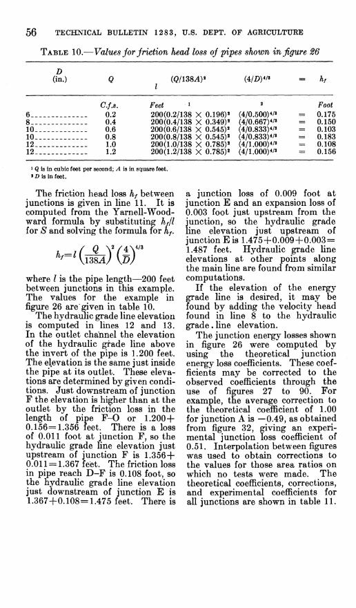
56 TECHNICAL BULLETIN 1283, U.S. DEPT. OF AGRICULTURE
TABLE 10.—Values jor jriction head loss of pipes shown in figure
D (in.) Q
I (4/D)*/» = hf
6___ 8--. 10-- 10-- 12_- 12__
C.f.s. 0.2 0.4 0.6 0.8 1.0 1.2
Feet 1 200(0.2/138 X 0.196)« 200(0.4/138 X 0.349)« 200(0.6/138 X 0.545)« 200(0.8/138 X 0.545)« 200(1.0/138 X 0.785)« 200(1.2/138 X 0.785)«
2
(4/0.500)*/» (4/0.667)*/» (4/0.833)*/» (4/0.833)*/» (4/1.000)*/» (4/1.000)*/»
=
Foot 0.175 0.150 0.103 0.183 0.108 0.156
1 Q is in cubic feet per second; ^ is in square feet. > i) is in feet.
The friction head loss hf between junctions is given in hne 11. It is computed from the Yamell-Wood- ward formula by substituting hf/l for S and solving the formula for h/.
where I is the pipe length—200 feet between junctions in this example. The values for the example in figure 26 are ffiven in table 10.
The hydraulic grade line elevation is computed in lines 12 and 13. In the outlet channel the elevation of the hydraulic grade line above the invert of the pipe is 1.200 feet. The elevation is the same just inside the pipe at its outlet. These eleva- tions are determined by given condi- tions. Just downstream of junction F the elevation is higher than at the outlet by the friction loss in the length of pipe F-0 or 1.200+ 0.156=1.356 feet. There is a loss of 0.011 foot at junction F, so the hydrauUc grade line elevation just upstream of junction F is 1.356+ 0.011 = 1.367 feet. The friction loss in pipe reach D-F is 0.108 foot, so the hydraulic grade Une elevation just downstream of junction E is 1.367+0.108=1.475 feet. There is
a junction loss of 0.009 foot at junction E and an expansion loss of 0.003 foot just upstream from the junction, so the hydraulic grade line elevation just upstream of junction E is 1.475+0.009+0.003 = 1.487 feet. Hydraulic grade hne elevations at other points along the main line are found from similar computations.
If the elevation of the energy grade hne is desired, it may be found by adding the velocity head found in hne 8 to the hydraulic grade. Hne elevation.
The junction energy losses shown in figure 26 were computed by using the theoretical junction energy loss coefiicients. These coef- ficients may be corrected to the observed coefficients through the use of figures 27 to 90. For example, the average correction to the theoretical coefficient of 1.00 for junction A is —0.49, as obtained from figure 32, giving an experi- mental junction loss coefficient of 0.51. Interpolation betw een figures was used to obtain corrections to the values for those area ratios on which no tests were made. The theoretical coefficients, corrections, and experimental coefficients for all junctions are shown in table 11.

LOSS OF ENERGY AT SHARP-EDGED PIPE JUNCTIONS 57
TABLE 11.—Theoretical and experimental values oj coefficients and head losses adjunctions of pipes shown in figure 26
Coefläcients, corrections, and head losses
Junction
B E
fu, theoretical-_. ftt, correction \u) experimental. Au, experimental Ä«, theoretical-_.
1.00 -.49
.51
.008
.016
0.75 -.24
.51
.010
.015
0.55 -. 13
.42
.008
.010
0.44 -.09
.35
.012
.015
0.36 -.07
.29
.007
.009
0.31 -.06
.25
.009
.011
The experimental loss at each junction has been summarized above and the theoretical loss has been copied from figure 26 to permit comparison of the losses. The losses are higher for the theoretical in every case. The sum of the junction losses for the theoretical is 0.076 and for the experimental it is 0.054, a differ- ence in favor of the experimental of only 0.022 foot in 1,200 feet of main. If the experimental loss
coefficients are used in place of the theoretical loss coefficients, it would be possible to lower the upper end of the main bji about one-fourth inch. The pern^issible reduction in slope of the main would be 0.000,018, or 0.|)18 foot per 1,000 feet. These amounts for an tile system and
are insignificant agricultural drain quite likely could
be considered insignificant for many other types of systems.
SUMMARY AND CONCLUSIONS This bulletin is a report of a 5-
i>ear test program on the energy OSS at sharp-edged pipe junctions that was conducted at the St. Anthony Falls Hydraulic Labora- tory.
Some experiments on junction energy losses have been performed by others, but most of the studies were limited in scope or complete- ness. However, the studies are summarized in this bulletin, be- cause most of them were performed in foreign countries and the results of the experiments are not generally available in the United States.
In the present investigation, the energy losses at the junction of two pipes were determined for a
range of discharges that encom- passed all possible combinations of flow from tjie joining pipes. The angle between the lateral and the main ranged from 15° to 165° in 15° increments. The ratio of the area of the main pipe to the area of the lateral pipe ranged between the linjits of 1 and 16. All joining edges were sharp. The pipes were flowing full in every case. Tests werb performed with the lateral enteripg the side of the main at the cenierline and at the top (or bottom). '
The results of the tests were evaluated both graphically and statistically, an4 the agreement between the data and the series, the

58 TECHNICAL BULLETIN 1283, U.S. DEPT. OF AGRICULTURE
general least squares, and the theoretical equations is shown in figures 27 to 90, Appendix.
The conclusions regarding the junction energy loss coeflicients re- ported here can be summarized as follows :
The fit of the equations developed from the experimental data for each junction with the experimental data itself is excellent. Both graphical and statistical tests show this excellent fit. The series equations thus represent the data very well.
Agreement between the series and theoretical equations is not indi- cated statistically in about two- thirds of the cases for the main. However, there is reason to question the validity of the deductions based on the statistical tests. In the case of the lateral, the empirical equa- tions give slightly better predictions of the junction energy loss coeflii- cients than do the theoretical equa- tions.
Graphical analysis of the general equations for determining the junc- tion energy loss coefficient in the main shows that the theoretical equations generally give predictions as good as or better than the least squares developed equations. For the lateral, the situation is reversed with the least squares equations giving predictions of the junction energy loss coefficient that are in better agreement with the observed values than are the theoretical coefficients.
Statistical tests of the general equations show that the theoretical equations well represent the ob-
served data even though the least squares equations are more repre- sentative.
The junction energy loss de- creases slightly as the Reynolds number increases up to values of about 150,000, but the magnitude of this decrease is so small that it is of questionable statistical significance. In any case, it appears that the Reynolds number will have little practical effect on the application of the results.
The junction energy loss coeffi- cient for the top lateral is greater than the coefficient for the corre- sponding center lateral. However, the superiority of the center lateral entry is not great.
The data from these tests agree well with the available data ob- tained by other investigators.
The theoretical junction energy loss coefficient is generally larger than the coefficient determined ex- perimentally. Use of the theoreti- cal coefficient will result in junc- tions having a conservative design. Data are provided so the theoretical coefficients can be adjusted to the experimental coefficients if this re- finement is desired.
The results are presented in such a way that they can be used in the design of junctions for water, sew- age, drainage, oil, air, or other types of collection systems where two pipes containing any fluid or gas converge into a single pipe.
In agricultural tile drainage sys- tems, the 90° junction, where con- venient, will prove as satisfactory as junction angles less than 90°.

LOSS OF ENERGY AT SHARP-EDGED PIPE JUNCTIONS 59
LITERATURE CITED
(1) AMERICAN SOCIETY OF AGRICULTURAL ENGINEERS. 1963. DESIGN AND CONSTRUCTION OF TILE DRAINS IN HUMID AREAS. Amer.
Soc. Agr. Engin. Yearbook 1963: 298-307, St. Joseph, Mich. (2) ANDERSON, A. G.
1948. HYDRAULICS OF CONDUIT BENDS. Minn. Univ. St. Anthony Falls Hydraul. Lab. Bui. 1, 22 pp., illus. Minneapolis.
(3) AYRES, Q. C, and SCOATES, D. 1928. LAND DRAINAGE AND RECLAMATION. 419 pp., iUliS. NeW York.
(4) ELLIOTT, C. G. 1908. PRACTICAL FARM DRAINAGE. Ed. 2, 188 pp., illus. New York.
(5) ] 1912. ENGINEERING FOR LAND DRAINAGE. Ed. 2, 339 bp., illus. New York.
(6) FAVRE, H. 1937. SUR LES LOIS REGISSANT LE MOUVEMENT DES FLUIDES DANS LES CON-
DUITES EN CHARGE AVEC ADDUCTION LATERAL [ON THE LAWS GOVERNING THE MOVEMENT OF FLUIDS IN CONDUITS UNDER PRESSURE WITH LATERAL FLOW]. [Belgium] Univ. des Mines Rev. (ser. 8, t. 13) 12: 502-512. [Translation supplied by Agr, Res. Serv., St. Anthony Falls Hydraul. Lab., Minneapolis.]
(7) FREVERT, R. K., SCHWAB, G. O., EDMINSTER, T. W., an^ BARNES, K. K. 1955. SOIL AND WATER CONSERVATION ENGINEERING. 479 pp., illus. New
York. ! (8) GARDEL, A.
1956. CHAMBRES D'EQUILIBRE [SURGE TANKS]. [Switz.] Lausanne Univ. Libr. pp. 57-71, illus. Lausanne. |
(9) 1957. LES PERTES DE CHARGE DANS LES ECOULEMENTS AU TRAVERS DE BRANCHE-
MENTS EN TE [THE LOSS OF HEAD IN THE FLOW THROUGH TEE BRANCHES]. [Switz.] Lausanne Univ. Polytech. École Pub. 44, pp. 1-13. [Trans- lation supplied by Agr. Res. Serv., St. Anthony! Falls Hydraul. Lab., Minneapolis.]
(10) GIBSON, A. H. 1948. HYDRAULICS AND ITS APPLICATIONS. Ed. 4, 801 p^p., iUus. Londou.
(11) GiESECKE, F. E., and BADGETT, W. H. 1932. SUPPLEMENTARY FRICTION HEADS IN ONE-INCH CAST-IRON TEES. Amer.
Soc. Heating and Ventilating Engin. Trans. 38:111-120. (12) HALMOS, E. E.
1932. LOSS OF HEAD AT BRANCHES DETERMINED FOR WATER PIPES. Engin. News-Rec. 108:684.
(13) JEFFERY, J. A. 1919. TEXT-BOOK OF LAND DRAINAGE. 256 pp., illus. NeW York.
(14) KING, H. W. 1954. HANDBOOK OF HYDRAULICS. Ed. 4, 556 pp., illus. New York.
(15) KiNNE, E. 1931. BEITRÄGE ZUR KENNTNIS DER HYDRAULISCHEN VERLUSTE IN ABZWEIG-
STÜCKEN [CONTRIBUTION TO THE KNOWLEDGE OF HYDRAULIC LOSSES IN BRANCHES]. München Tech. Hochsch. Hydraulischen Inst. Mitt. No. 4, pp. 70-93. [Translation 323, U.S. Bureau of Reclamation, 1955.]
(16) McNowN, J. S. 1954. MECHANICS OF MANIFOLD FLOW. Amer. Soc. Civ. Engin. Trans.
119:1103-1142. (17) METCàLF, L., and EDDY, H. P.
1914. AMERICAN SEWERAGE PRACTICE, V. I. DESIGN OF SEWERS. 3 V., NeW York.
(18) NARAMOTO, I., and KASAI, T. 1931. ON THE LOSS OF ENERGY AT IMPACT OF TWO CONFINED STREAMS OF
WATER. Kyushu Imp. Univ. College of Engin. Mem., v. 6, No. 3, pp. 189-261. Fukuoka, Japan.
(19) PARSONS, J. L. 1915. LAND DRAINAGE. 165 pp., illus. ChiCagO.

60 TECHNICAL BULLETIN 1283, U.S. DEPT. OF AGRICULTURE
(20) PETERMANN, F. 1929. DER VERLUST IN SCHIEFWINKLIGEN ROHRVBRZWEIGUNGEN [LOSS IN
OBLIQUE-ANGLED PIPE BRANCHES]. München Tech. Hochsch. Hydrau- lischen Inst. Mitt. No. 3, pp. 65-77. [Translated by H. N. Eaton and K. H. Beij, Amer. Soc. Mech. Engin. Spec. Pub., 1935.]
(21) PICKELS, G. W. 1941. DRAINAGE AND FLOOD-CONTROL ENGINEERING. Ed. 2, 476 pp., iUuS.
New York. (22) POWERS, W. L., and TEETER, T. A. H.
1922. LAND DRAINAGE. 270 pp., illus. New York. (23) ROE, H. B., and AYRES, Q. C.
1954. ENGINEERING FOR AGRICULTURAL DRAINAGE. 501 pp., illus. NeW York.
(24) ROUSE, H. 1950. ENGINEERING HYDRAULICS. 1013 pp., illus. New York and London.
(25) SANGSTER, W. M., WOOD, H. W., SMERDON, E. T., and BOSSY, H. G. 1958. PRESSURE CHANGES AT STORM DRAIN JUNCTIONS. Mo. Engin. Ser. Bul.
41 (v. 59, No. 35), 132 pp. illus. (26) WOOD, H. W., SMERDON, E. T., and BOSSY, H. G.
1961. PRESSURE CHANGES AT OPEN JUNCTIONS IN CONDUITS. Amer. SoC. Civ. Engin. Trans. 126, pt. 1: 364-396.
(27) SNEDECOR, G. W. 1956. STATISTICAL METHODS. Ed. 5, 534 pp, illus. Ames, Iowa.
(28) SoucEK, E., and ZELNICK, E. W. 1945. LOCK MANIFOLD EXPERIMENTS. Amer. Soc. Civ. Engin. Trans. 110:
1357-1400. (29) STAROSOLSZKY, Ö.
1958. A CSÖELXGAZXSOK NYOMÁSVISZONYAI [PRESSURE CONDITIONS IN PIPE BRANCHES]. (Budapest), Vízüg3a Kozlemenyék, Imprimerie Uni- versitaire 1958/1: 115-121. [In Hungarian. Translation supplied by Language Service Bureau in Washington, D.C., through Agr. Res. Serv., St. Anthony Falls Hydraul. Lab., MinneapoUs.]
(30) STEVENS, J. C. 1926. THEORETICAL ENERGY LOSS IN INTERSECTING PIPES. Engin. NeWS-ReC.
97 (4): 140-141; Discussion: 97 (11): 437 and (22): 883-884. (31) VOGEL, G.
1926; 1928. UNTERSUCHUNGEN üBER DEN VERLUST IN RECHTWINKLIGEN ROHRVERZWEIGUNGEN [EXPERIMENTS TO DETERMINE THE LOSS IN RIGHT
ANGLE PIPE TEES]. München Tech. Hochsch. Hydraulischen Inst. Mitt. No. 1, pp. 75-90; Mitt. No. 2, pp. 61-64. [Translation, Tech. JNo. 1, pp.
3. 299, U.S. Memo. 299, U.S. Dept. Interior, Denver, 1932.]
TERMINOLOGY
To prevent misunderstanding, certain terms are defined as follows:
Branch.—Used synonymously with ''lateral." The subscript "&" refers to "branch.''
Bottom lateral.—A lateral in which the invert of the lateral intersects the invert of the main.
Center lateral.—A lateral in which the projected centerline of the lateral intersects the centerline of the main.
Downstream.—The portion of the main downstream of its junction with the lateral. Junction energy loss.—The modifiers "upstream main" or "main" refer to the energy
loss in passing from the upstream main to the downstream main across the junction. (See the section "Theory of converging pipe junctions: Loss coefficient for main.") The modifier "lateral" refers to the energy loss in passing from the lateral to the downstream main across the junction. (See the section "Theory of converging pipe junctions: Loss coefficient for lateral.")
Lateral.—The pipe that enters the main from the side. (See fig. 1.) Main.—The straight pipe into which the lateral enters. (See fig. 1.) Top lateral.—A lateral in which the crown of the lateral intersects the crown of the
main.

LOSS OF ENERGY AT SHARP-EDGED PIPE JUNCTIONS 61
Upstream.—The portion of the main upstream of its junction with the lateral.
The following notations list symbols used in the study: A Cross-sectional area of pipe.i A CoeflBcient in the junction energy loss equation. b Subscript referring to the lateral, or branch. B Coefläcient in the junction energy loss equation. C Coefläcient in the junction energy loss equation. d Subscript referring to the main downstream of the junction. D Coefläcient in the junction energy loss equation. D Diameter of pipe.^ E Coefläcient in the junction energy loss equation. g Acceleration due to gravity. h Piezometric head. hen Loss of head at a sudden enlargement. hf Head loss due to pipe friction. hi Energy head lost at the junction. ht Velocity head. I Length of pipe. Q Discharge.! R Hydraulic radius. R Reynolds number. r Radius of rounding of junction edge. S. Slope of pipe. u Subscript referring to the main upstream of the junction. K... :. Velocity=QM.i a Energy correction factor. ß Momentum correction factor. y Specific weight of water. f Junction energy loss coefläcient—hilh^. e Angle between the lateral and the main upstream of the junction. V Kinematic viscosity.
1 Always used with a subscript.


APPENDIX
Figures 27 to 90
Difference Between Observed and Computed Junction Energy Loss CoeflGicients
63
671042 O—63-

64 TECHNICAL BULLETIN 1283, U.S. DEPT. OF AGRICULTURE
0.7
0.6
0.5
0.4
0.3
,02
0.1
-r- Vd
-n —r- -r- —r- Symbol
f.prs. Sample General Theoretical
2 e ^ Ö
5 0 Jr Z
10 <a A. ^
15 o A o
8 0.1 ¡^1 T I
«OJ ^^
^ 02
0.3
0.4
0.5
0.6
0.7
^n^
02
9-°é
'Tar
£¿L :^
0.4 0.6 Qb/Qd
QB
^ ^
U)
0.7
0.6
0.5
a4
03 g.0.2
§0.1
io.i i^O.2
0.3
0.4
0.5
0.6
0.7
g_ ' A ^% ■ «.^ 'n^ k y-«j K^ „.4^^.iâ 1^ î^ ̂
^^^^ ¿^ r1 .^1i kK ̂ IS. , ii D^ I
D 1
^ 5^ ^ •^^ lar
0 Ö.2 0.4 0.6 0.8 1
Qb/Qd
FIGURE 27.—Difference between observed and computed junction energy loss coeffi- cients for series C15-1.
0.7
0.6
0.5
0.4
03
0-0.2
8 0.1
^ 0
•8 0.1 ^0.2
0.3
0.4
as 0.6 0.7
1 1 1 1—I 1 1 Vd Symbol
-f.p.s. Sample General Theoretical-
2 e Ar Ô
'5 0 M 0 -10 s A. Ki -
15 o A D i^
iä, 1
' «L 1 Í '3 u ?K.J I , ' > ■5^ fe'l D b 1 .°- • J ^ u; A—
o-
K »A J •:^ a
i '"^ '% ¡A r^
i L-A¿l ^ r ^
0.2 0.4 0.6 Qb/Qd
as 1.0
a7 a6 03
a4 03
cia2
§0.1 1^ 0
^0..
iuAO.2
03
0.4
0.5
a6 0.7,
/n
^, ^ 9^ ^ /! > <^ 1^ '/p^ y \k7 •d .^^ rt-l 4 i-^i
•TefiT ^\ ^ ■!^
/ n i0^
k' V^
^ ̂■^ & V m ^' JZK ̂ p^N [^ ' f l^
02 0.4 0.6 Qb/Qd
as 1.0
FIGURE 28.—Difference between observed and computed junction energy loss coeffi- cients for series C30-1.

LOSS OF ENERGY AT SHARP-EDGED PIPE JUNCTIONS 65
0.4 0.6 Qb/Qd
0.4 06 Qt/Qd
FIGURE 29.—Difference between observed and computed junction energy loss coeffi- cients for series C45-1.
IcxiMV
0.4 0.6 Qb/Qd
^It^ W.m
0.2
^ M -ff
"04 OB Qb/Qd
,/ ^
^ TH^
4^
FIGURE 30.—Difference between observed and computed junction energy loss coeffi- cients for series C60-1.

66 TECHNICAL BULLETIN 1283, U.S. DEPT. OF AGRICULTURE
ae 0.5
0.4
03
g. 02
8 0.1
Vd Symbol f.p.s. Sample General Theoreticol
2 ^ Ar s
5 0 > 0
10 S A. ^ . 15 o A D
-8 0.1 ^
as 04
as OJ6
!fe
^
^.
■^
■5--5J
^KVi^
\
-*<r
°v H^
AV
I
06
05
04
a3
ö.a2
8 ai -^ ¡¿ 5 V íZís
PA''- ||ai ¡^
i-'ïT
02 04 06 Qb/Qd
0.8 1.0
,02
03
04
0.5
06.
^ DO.
T^
^.
o, ^
■^v
02 0.4 ae Qb/Qd
08 1.0
FIGURE 31.—Difference between observed and computed junction energy loss coeflS- cients for series C75-1.
0.4 06 Qb/Qd
FIGURE 32.—Difference between observed and computed junction energy loss coeflä- cients for series C90-1.

LOSS OF ENERGY At SHARP-EDGED PIPE JUNCTIONS 67
CX8
ae
a4
a2
0 "^
iJ'Q2
ae
08
1.0
12
I 1 r- j ■ T 1 —r Vd Symbol
-f.p.s. Sample General Theoreticol-
2 e A. e
"5 0 M 0 ' -10 s A. Kl -
15 o A D 1 1 1 1 1 1 1
i^ ^ ■ s «5 ^ '^ C>| \
J 0^ ^^ ■■ 0- «^
■-< ^.^l^ ti ~^t fif^ *^ ¿iJ .^^ •^ o-
19^
^^3 tlfn ̂^ ik t- §î^ 0-
0> • 1 i\ \ A^
A^ Ij rè :i^ ;¿ ̂^ >É^ A-
^ in 1 »•i. ^ a 5 1^ V «k
OB
ae
a4
02
*jro2
wra4
o.e
a2 a4 ae 08 i.o Qb/Qd
08
1.0
12
A. ^ \ ^ \
^ i> '■^ Of-
á>
^v ^•^ S^
■■ Ar
\^ .^ Ac;
A >^; \t: 1^ 1 i^ . ff ^ «s
§^ á ̂^< ^^N i^ .4-^ r?^\^ ^^ »-v «1- °^ «-^ X 'S "^ -^ 'v 0^
^ la^ 0v S. "'
la- ^
2>i •i?
jzf'l S^ n-^
^ 14- "\ a"
^ n'
02 04 oe 08 Qb/Qd
1.0
FiQUBE 33.—Difference between observed and computed junction energy loss coeffi- cients for series C105-1.

68 TECHNICAL BULLETIN 1283, U.S. DEPT. OF AGRICULTURE
I.
0.9
OB
0.7
ae 05
a4
03
02
0.1
0
ai
02
a3
a4
a5
06
a?
0.8
0.9
1.0
I.I
1.2
1.3,
ja
Vd Symbol f.p.s. Sample General Theoretical
2 e^ A e
5 0 M 0 10 s Ae ^ 15 o A p
1^ «^
^ i^ *'-'
-2^ ^
Í-AÍ W^
02
SÚ
-i^U V
^. o^
as 08
07
ae as a4
a3
02
ai Iä
04 OS
Qb/Qd
^
iqnr'
\ W
^
08
'S M 05
1.0
06
07
0.8
09
1.0
1.1
12
1.3:
r^
^ »-
-0^
02 04
-o
■^
^^ Al
^
ae Qb/Qd
08 to
FiGUBB 34.^Difiference between observed and computed junction energy loss coefficients for series C120-1.

LOSS OF ENERGY AT SHARP-EDGED PIPE JUNCTIONS 69
l.¿
1.0
— 1 1 1 1 1 r I
Vd Symbol -f.p.s. Sample General Theoretical-
2 e A s '5 0 M 0 ' -10 s A. ^ -
'5, .o , ,. . ,□ ,
—
0.8
0.6
0.4
d.a2
.^ o
Y 0 o
1 ̂ /0 o« h ^ ^
^ ^1 fíí f
^ -' o
^02 ^^ 1 t 'A. "^m^ â.
0.4 1 3^ ^1
Í f-Ll
y ? S^ tS
0^ i \
0.8
IP
lO
\z
IX)
QB
OB
0.4
■0.2
--«02
04
OB
08
LO
A
■Ai-
4
^ ^^
02 0.4 0.6 03 IJO L2
r§
: %
^ j*.'
02 04 a6 03 UD
Qb/Qd Qb/Qd
FIGURE 35.—Difference between observed and computed junction energy loss coefficients for series C135-1.

70 TECHNICAL BULLETIN 1283, U.S. DEPT. OF AGRICULTURE
l.t
Vd --f.D.S.
1 -r ■ -1 1 1 1
Symbol Samóle General Theoretical
1.4
L2
IJO
<! 1
\z 2 e ^ e ■~ 5 0 A 0 --I0 » â. Kl -
15 o A D - ' 1 1 1 1 1 1 1
% ^ 1
IjO ^ ^ !
OJB t 4. !
0J5 Ar-
T
04
d.02
A- ■
04 AK
JK
E 0.2 1 t 5*— oí J:
' 0 m '1 -& r^f^ fe oj (ai .^ 0-
S^ 0
r 0
04
06
OB
1.0
1.2
^r¿§u Â. o> . 0- 1-0^
18-
0- 0~
IT
o i^ 1,^ 0- O' flt;
2:1 :^'^ ^ iá '^- n Q- a-
4j?^2 ^A 1 u 1—,—1
< A-. « 1 1
> .^ H -^ d"*- •^ 04
—A Ar-' 1^ è A.! 1 oJ
^ ^^ S-
CL
0.6 s: S^i. 1 B-! ^
08 f
-3^ 51^
10 1
!
1.2 1
_È 1.4
^- 0 0 2 O
c 4
)b/C
OJ 5 0 8 iX ) a 2 0 4
Qb/
0. 6 0 8 üo
FIGURE 36.^—Difference between observed and computed junction energy loss coefficients for series C150-1.

LOSS OF ENERGY AT SHARP-EDGED FIFE JUNCTIONS 71
1.7
1.6
1.5
1.4
L3
L2
U
1.0
0.9
OB
a? ae
§04
of
*-^0.l
0
0,1
02
a3 0.4
05
0L6
a? CUB
as 1.0
-f.p.î
2
" 5
-10
15
». S
1 1
amp
■e
(S
IS
o
. ., c
e ¿ 1
>ymb enere
et
M
A.
A
1 Ol
1 Th
■■ 1
ioretical-
0 Kl
° 1
fa :^
\ % i^^ S-- (ü 5. 2\ «»N
^ r 1 i ̂ k i^
1/ s? t î^ ^ <
1 A' M tu
V B-q ri^ a\
\ °\.
02 a4 qß Qb/Q^
03 1.0
1.7
16
1.5
1.4
1.3
L2
Ll
LO
Q9
OB
0.7
06
§a4 *^0.3
|a2
0
0.1
02
03
a4 05
as a7
OB
a9
1.0
i.i
A^
AJ
A-<
^
A^ <
Si ^
*^ p Ä> 1
'JBI A~
:> ^ V «^
^^ Í il'' f°\ **\
ti' la^ ^
■°> <y s^ Q,, «k or- «1^
o/ < \ i^J S:: e^
*\ r 5^ L (9^ er' 0^
°. 0^
Q 0-
CT 0-
cr' —Ä-
^, i
02 0.4 OB
Qb/Qd
OB 1.0
FIGURE 37.-—DifiPerence between observed and computed junction energy loss coefläcients for series C165-1.

72 TECHNICAL BULLETIN 1283, U.S. DEPT. OF AGRICULTURE
a?
ae as a4
03
02
0.1
0
ai
02
g03 o
KJOA
A^O.6
a?
as 09
1.0
i.i
12
1.3
\A
15
A^
X A.-.
I ^. s> s^ ^N
0, ■^
J% 0 2-^ 0- 1^ a^
CK.
ws ON §: i^r. 0 »»^ «»x
^ti Mo, "ET A;?
2l •S'
Q-
4 ̂ ^ ': î^ o- §- •*d A-
—
1 I I ■ I 1 1 I Vd Symbol
-f.p.s. Sample General Theoretical-
2 e ^ Ô _ "5 0 M 0 -10 5» A. H -
15 o A D
02 04 06
Qb/Qd
08 1.0
Qb/Qd
FIGURE 38.—Différence between observed and computed junction energy loss coefläcients for series C15-2.

LOSS OF ENERGY AT SHARP-EDGED PIPE JUNCTIONS 73
0.7
ae Q5
04
03
|o.i
04 0£
Qb/Qd
FiGURB 39.-—Difference between observed and computed junction energy loss coeflBcients for series C30-2.
07 Vd Symbol
Q6 -f.p.s. Sample General Theoretical
2 e ^ e 5 0 M Z
-10 s A. «3 15 o A a
as 0.4
03
^02
8 0.1
oai
*-«02
03
04 05
06 a7
FIGURE 40.—Difference between observed and computed junction energy loss coefficients for series C45-2.

74 TECHNICAL BULLETIN 1283, U.S. DEPT. OF AGRICULTURE
FIGURE 41.—Difference between observed and computed junction energy loss coefficients for series C60-2.
09
08
07
06
05
0.4
03
s--
Ar. A-
-- A^
V i
A^ Ar~ »-
«.! A
A^ ^ ér-
g-02
8 0.1
f 0 ■g 0.1
.^ Aï
l^ ^ ^
0r^
^ Í
fe Ar- 0-
g^,
- h d r i
o- o-
o~ «-
0.3 P 0- ^1
04 S^ «l^
05 Tí" 5^- 0-
06 n~
Äf-
07 o-
0- n- ta— 0-
OJB
OS ;5-
DN.
02 Qb/Qd
0.4 Oß 08 Ob/Qd
10
FiGUBE 42.—Difference between observed and computed junction energy loss coefficients for series C75-2.

LOSS OF ENERGY AT SHARP-EDGED PIPE JUNCTIONS 75
06
02 0.4 06 Oß ' 1.0
Qb/Qd
02 04 0J6 OJB IP
Qb/Qd
FiGUBB 43.—Difference between observed and computed junction energy loss coefläcients for series C90-2.

76 TECHNICAL BULLETIN 1283, U.S. DEPT. OF AGRICULTURE
0J5
0.4
CX3
02
ai
0
ai
a2
03
a4
0i5
0J6
i OS
^09
Ja 1.0 o *-^ I.I
1.2
1.3
1.4
1.5
1.6
1.7
\Jß
1.9
2X)
2.1
2.2
23,
o
ÇL
Aw^ &
1 1-^ -^ S^ Ä ^x Qv Cl
-o;; A
If (a^ 0-v 0- ^
1 ^^-î ^ *^ 5 Í5^s> —M—
^*d
: a^ ^ ^^
1 ts: B- |: ^ _^ k LQ
AT *3 .*>v
p^ 0^
M ^ ^ -^ ^>
-f.p.$. Sample Ge
2 e " 5 0 .10 s
15 o 1 1 J L
ymb< nero
-Ar
A.
A
>l The oreti
D L
col-
05
04
03
02
ai
0
.\ 2>
m^ ^1 BO
O 0 ai ^ 02 (^
02 a4 06
Qb/Qd
oe LO
03
04
03
06
|06
I 1.0 *^ I.I
I
13
1.4
13
1.6
1.7
\Z
13
^0
2.1
2.2
^3
-i^r
^. ^
^ ^st;:
A^ ^
^ -^.
02 a4 06 08
Qb/Qd
LO
FIGURE 44.—Difference between observed and computed junction energy loss coefficients for series C105-2.

LOSS OF ENERGY AT SHARP-EDGED PIPE JUNCÎTIONS 77
a? Ou6
CX5
a4
03
02
Ol
0
Ol
02
03
04
05
06
j.07
^OB
^09
^1.0
f" I.I
12
1.3
1.4
1.5
1.6
\J
IB
13
2J0
^l
22
23
ZA
2.5
1 1 1 T 1 T I Vd Symbol
-f.p,s. Sample General Theoret
2 e ^ Ô '5 0 M Z -10 s A. Bi
15 o A D 1 1 1 1 1 1 1
cal-
«X S^ ê« ^
îi, gl Hi 2^ "K
^>v
jx 0^ ft, <>- mar P -D=í u- ^ »«k
Q., '»v
^S 1 S^ 0^ Q^'
•x n^
^ 0v D>. A<.
tt^
^, S^ Í 7 *-J A,<^
a^ -H^
O^
-^ A-
02 04 06
Ob/Qd
08 LO
07
06
05
04
03
02
Ol
0
Ol
02
03
04
05
06
0.O7
§08
A^a9
12
1.3
1.4
1.5
1.6
1.7
U8
13
2.0
2.1
22
23
2/^
23
^^
A A ^1 ▲ V.
^\. O,.
è! 1
X^- Â2> A^
.A^ Os.
or i- fe 0- ^ »^
4 ̂ !^ ■»-•
4 Sa o^ i: BffI
:^ û
> 0
"N 0Í^
^ g^ 0^
^'N
n-"
o^
^ e^
fl>. O.I s.
I">.
o^
ñ: 0-
a^
S^ Ck
Bs ^
«x
la^
Ov
N
02 04 06
Qb/Qd
08 \J0
FIGURE 45.—Difference between observed and computed junction energy loss coeflBcients for series C120-2.

78 TECHNICAL BULLETIN 1283, U.S. DEPT. OF AGRICULTURE
a?
0.6
OS
a4
03
02
aiü^
^•"^ 02
03
04
05
0.6
f07
03
*J? 0L9
^ I.I
1.2
1.3
1.4
13
1.6
1.7
IB
1.9
2.0
2.1
2.2
23
2.4
23
-T- -P- -1— T- -T- "T- Symbol
f.p.s. Sample General Theoretical
2 -e A -B
5 0 ^ 0
10 St A. 13
'5. o A D
T^S-TF-
-«td ^
^ ■^
■CC
^
'* QJ, ^
s* 0-
-tSi^r- °>.
^
-0^
a?
06
03
a4
03
02
^
02 a4 Qb/Qd
0£ 08 IJO
03
a4
03
OJ6
a?
OB
09
»^ I.I
1:2
13
1.4
13
1.6
1.7
IB
\S
2X)
2.1
2.2
2.3
2.4
23
^ 1 ^-5 ^- 1 A^
A ¿-v 1 ^-
1^. >Ä^ A- «»^v
A ^ A^ °-v
^ 0.
■ V A>>.: «i>.
ïu^^ 0- 0\
5S^ B- Ü-
Sr 2^ «>, ^ Qv
1^ ! a- fi>- flk.
4 i.° S\ 6t-
BL^ B-. Ov ^^
Si ^
°^ ^ ON
S-
0-
¡^ —od
0>
Dv By IS>
°N.
02 04 OB
Qb/Qd
08 1.0
FIGURE 46.*—Difference between observed and computed junction energy loss coeflScients for series C135-2.

LOSS OF ENERGY AT SHARP-EDGED PIPE JUNCTIONS 79
1.0 v; r
Symbol r UD
08
06
04
02
0
02
|-04
Y 06
*5a8
IX)
12
1.4
1.6
1.8
ao
^ 1 -T.p.s. oampie oenerai ineoreiicai-
2 ^ ^ Ö _ '5 9i M Z ~ -10 s A. Ï3 -
15 O A a
^- as
^ Ar A..
M-
0.6 ^
0.4
á -0 o-
o-. .
^ 02
Î ^ 1 ^ ^ 0^ 0-
^ -« 3^ -* ^0 o- o- Î 0. 0~
8=- -E s-i^ 0 ^Wñ ^•r^^wz^ A- ^ ^ !^ \^J o-
""Üí^FSí^ o- <J ^ ià' «- _a. 02 1 ^h 4 ^ ^- í|
. t r A. A- ^ ^^
c 0.4 1^-^ .d- D- ITTI
P^
^nA
"ÎT ■a? ■^' Lk.
1 OJB 1
o
*J?a8 X ja-
'
a^ M-
S:^
IJO
ti 12 D-
1.4
1.6 ^
1.8
2J0
^ 2.2
0 C 2 c 14
Qb
C IJ6
1
0 B 1 0 ^ 0 c ).2 C ».4
Qb
c ).6
1
c IS U
FiGUBE 47.—Difference between observed and computed junction energy loss coeflScients for series C150-2.
671042 0—63 6

80 TECHNICAL BULLETIN 1283, U.S. DEPT. OF AGRICULTURE
1.01 1 \ 1 1 1 1 ] 1 1 1 1.0
0.8
06
a4
02
02
^a4 8
V^OJS É o
1.0
12
1.4
IJS
1.8
2X)
22
I 1 —r—1 1 T 1 Vd Symbol
-f.p.s. Sample General Theoretical-
2 e ^ e "5 0 M 0 ~ -10 (a A. 13 -
^ -«
r o- O-
a <9 -u
eg -o -o ^
*-^!^i^ -S »I 4- «- ^ !^ -s 0H
9- (»-
k J .Ji
rT Ä-
t A-
^ ^
j»'
15H >4^ A-
;.J 0^
0- 51-
OB
OJ6
04
02
02
I 0.4
É o
IJO
12
1.4
|J6
\B
20
02 04 OJ6 08
Qb/Qd
10 22
Ar-
A- A-
«^ A^
_n >- A-
-«I âc- t ^
4> -^ ift-
V^
-A k ^
-Jr O-
-«> •-J* u-
-O- -ß
n- 2^ ^ -« 4r 1Í- ef-
0-
w o-
-Í ^flr J- Bh- r^ ^ "1
^« 0-
o~
0- ^-
O-
5-
0-
0- BI-
02 04 06 08
Qb/Qd
U)
FIGURE 48.^—Difference between observed and computed junction energy loss coefficients for series C165-2.

LOSS OF ENERGY AT SHARP-EDGED PIPE JUNCTIONS 81
U.O
0.4 # <l <? ifT
02 <« 8:J -^A- -4 ^ s ^
0 f ̂ f 2Ï
02 ^!
^^^ -1* 1- fc n ár- w ^ :tb -^ -Kk
0.4
OB
g-OjB
i° o
1.4
\B
IJB
20
22
2.4
Va Symbol -f.p.s. Somple Generol Theorelicol-
"5 0 * 0 " -10 B ». H -
'5, ,°, ,' , ,°.
Ub 9-
0.4 fS..
*" Sh-
02 r| ^
-B- /? f*
-0 ^
JBll! á t. f SH 0 ^i 1^ i^ 02
-^ 1 ^ 1^ ̂ /5-
■—
-■«- 'S "^ ^ ■a..
0.4
-A
0.6
^*»-
• A^ 2^ ^ •e^
^ .o
Î ^ o
*5 1.2
1.4
IJB M^
1.8 A«.
2J0 \
22
2.4
oc 02 04 06 Q8 1.0
Qb/Qd
02 04 06 08 UD
Qb/Qd
FIGURE 49.—Difference between observed and computed junction energy loss coefläcients for series C15-4.

82 TECHNICAL BULLETIN 1283, U.S. DEPT. OF AGRICULTURE
¿Jo
2A
1— I 1 1 1 1 1 1 Vd Symbol
-f.p.s. Sample General Theoreticalr
2 e Ar Ô _
"5 0 M 0 ~
-10 s A. IS -
¿2
2.0
IB
1.6
1.4
1,2
1.0
OB
0u6
0.4
02 ^ —Q— QL..
0 Is B^ «i: O^
0 1^ 1^ Is. s^ ^, • 0- 0^
^.
ih SiJ g^ ̂ r
a2 h^ ■r /^ A- BT'
A^ A.
^>s.
04
í¿J6
24 0-
22
^o
IB e^
1.6
Bi-.
1.4 •^
g. \2 «x
a.
a
^.
^ 1.0
*^ OB
<■ ^
~^v
^
06 e-
jr
^ 0--
0- *v A^
04 • ^s >k>- ••
A g^.
1 ^- ^ « N.
02 â^ df '^ï^- A
0 â g fi o-
0^ ^> «V
02 > \ «^ '»v. ^-.
^
0.4 ^ «^
02 04 06 08
Qb/Qd
IX) 02 04 06 08
Qb/Qd
1.0
FiGUBE 50:—Difference between observed and computed junction energy loss coefläcients for series C30-4.

LOSS OF ENERGY AT SHARP-EDGED PIPE JUNCTIONS 83
as
0.6
0.4
0.2
(0 •SO-2 o
04
0.6
Oß
1.0
A'
«'
^0 1
^e -* Mr-
Sí-. /S -1* -*r "^
■4 ^ -A 1 .-+a
-* _^ !*■
-a- •^ï ^. -♦ I -0^
4 0 í? -s -^ à ^1 ^f -Ai
n^-ñ- ü -b -0 -0 -er- l^ A
^^ -A
1 1 1 1 1 1 1 Vd Symbol
-f.p.s. Sample General Theoretical-
2 ^ ^ e ~ 5 0 ik 0 ' -10 (S *. Bi -
15 ^ , ° , , ^ , , D ,
0.2 0.4 0.6 0.8
Qb^Qd
U.Ö 1
0.6
04 .^ 0
1
0.2 .U.U
^j^ -r |4 /§
u .. 1
_^ tC o r\ 5^ i\\0_^^_i_A. —■e-
/« -» 1 -r" " É'iüfi^ á u • -Ar .j.- _ni L.^ ^ -jer
-* • ' o ^-^
O?
04
^ r0_ ! ''^^
'« per 0_J 1
^-.
0.6 a^-
0.8
-A-
1 n
0.1 0.4 0.6 0.8
Qb/Qd
1.0
FIGURE 51.—Difference between observed and computed junction energy loss coeflScients for series C45-4.

84 TECHNICAL BULLETIN 1283, U.S. DEPT. OF AGRICULTURE
2.6
2A
2Z
2J0
1.8
1.6
1.4
1.2
o
I
È O
IJO
'Oß
06
0.4
02
02
04
OJ6
Vd Symbol -f.p.s. Sample Genero! Theoreticol-
2 e ^ Ö _ '5 0 M 0 ' -10 s â. Kl -
15 o A D
•O^-
^ «.. ^ ^
a x^ (1 0- flS 0^
4.
'k'à ^ ^ 0- 0- 1
-0d
\ ^ ^ ¡j JM- 5q
^U - ! i ^ -: -itiV 1 -r
2J6
2.4
2.2
2.0
IB
1.6
1.4
g- 1.2 o
.o *-^0B
06
OA
02
0.2 0.4 06 0.8 1.0
QbAîd
02
0.4
06
A-
1
Jc- ^- A.
▲-•
0^
0- e. ■Uk.
^_ O-
Jk- Bk 0-
«-
/S «•-
♦- ♦v.
4J «•- &,
^ ^^ ««. 0-
QjV
i ^ ^
•4 -«• 'ÍÍ
Ai-
flr— ^
Si-
02 04 0.6 OB LO
FIGURE 52.'—Difference between observed and computed junction energy loss coeffi- cients for series C60-4.

LOSS OF ENERGY AT SHARP-EDGED PIPE JUNCTIONS 85
1.8
02 0.4 Q6 0.8 IX)
Qb/Qd
a2 0.4 0J6 OS \0
Qb/öd
FIGURE 53.—Difference between observed and computed junction energy loss coefficients for series C75-4.

86 TECHNICAL BULLETIN 1283, U.S. DEPT. OF AGRICULTURE
08
0.6
04
02
02
04
0. 0.6
»^ 0J8
UÍ 1.0
[2
1.4
|J6
\B
2.0
2.2
2.4
-f.p.«
2 " 5 -10
15
>. S Symbol
>ample General Theoretical-
e A. e
0 M 0 ' s à. la -
0^
€► A^
JL
& «I «i CT 0^
ê| ^ ^U: !|| -Off) S~ 0. 1 or t; A^
e- -^
|l '1 £. 2 \ A- » 1 A *- jd"
«k Bis. 0l.
^ AT -V '. t <■ ^ e-
^. •a^
OB
OJ6
0.4
02
02
04
06
^ 08
XÍ 1.0
1.2
1.4
1.6
IJB
ZX)
2.2
Q2 04 06 OB
Qb/Qd
IJO ¿4
A/
>*^ J0^^
A^
*" ^ \ '^. oil °-. A^
fellii "^v
r □v. ô_
^ «^ >*^
ê* 0^ A-
"^ ^ e—
A' ■^1 t: <! A^ 0--
V
in €L_ «^.
0,
e^ §::
r 0-
~B
ïi^
Í3\
-^ e^
-Bv^
0^ 0-^
av e^
0\
0>v
^
i^
02 04 06 08
Qb/Qd
IJO
FIGURE 54.'—Difference between observed and computed junction energy loss coeffi- cients for series C90-4.

LOSS OF ENERGY AT SHARP-EDGED PIPE JUNCTIONS 87
U.Ö r 1 1 \ 1 1 r-- Symbol
QnmnU d^nmrni Thmnrtti'tcru-
n<s 2 ^ A Ö _ "5 0 >k ÍÍ " -10 S A. ^ -
U.D
OA 1 -^ /*\ o -■e- -«-
-■&
OZ J-IU -«-
-«• .A ^
°î J k -e -« -'f^r?
-a/ 1 ñ' "2
-a .u 't ...
"j
0.2 ^" HZÍ -?hi cSI ̂ ^¿¿ ■ ̂ A =tk. -^L^-
--^■.
0.4
tí.
L -.?•
« 0.6 "-♦ ..
|o.8 3
1.0
1.2
1.4
1.6
1.8
2.0
2.2
o A
0.8
0.6
0.4
0.2
0.2
§ o 0.6
I v>
■gO.8
1.0
1.2
1.4
1.6
1.8
2D
2.2
0.2 0.4 06 0.8 1.0 2.4,
-«^
_ -f «-.
>e^ -S
^ -^ -Ä
. U
m ^* -^ ^A
=^ j '0 ^^
M '^S
W •^;A ^A
y^__, ̂^ "-A
~Ä
á -o -H
^«- u ■ -*'
-e- 1 -0
—A
si^.
-^
<s -0^ -B
-la
e^' •-0
.Q,
-©■
-" 1 0.2 a4 06 08 10
Qb/Qd
FIGURE 55. —Difiference between observed and computed junction energy loss coeffi- cients for series O105-4.

88 TECHNICAL BULLETIN 1283, U.S. DEPT. OF AGRICULTURE
U.Ö á:
0.D ^
^ 0.4 -•» -«■
(^O ^ :^
^•B- A. ^
"^a -^ \
\4 -« \ ^ 0-, Ss t
v
111 -^ ■ -0
■v-g'-
-áP s> I»- n
f\'7 «V.
0y U.C.
1 -1*
^ ^ r ¡^
AA "¥ f^ U.*T
4 ■HD
-A- ^
|0.6
O
-^
1 0.8
1 *^ 1.0
~B
f>'
-^
'
1.2
1.4
i.6
1.8
1
Vd -f.p.s.
2 " 5 -10
lililí
Symbol Somple Generol Theoretical-
e Ar Ö
0 A 0
s *. Kï - o A a
j j 1 1 1 1
Uj0
0.6
-^ ^^
-« -9
0.4 ^ ^.
«^ -« : A 02
^ - t ^ 0-
< \
«Ç
À\-^ e-
0
02
-0 \
^ * -o
-* 1 d} <^ ■O^-
0.4
^ ^1
T-^ -■o-
Í ■ ■ ■
g-oe :HÎ ^
^ iJ^
*f OB «^.
o
*^ IX)
■!4 0-
12 0-
^
14 0^
■©^.
1.6 itfr-
e-
IB
2J0
^2 Y<
OA «S 0 0.2 0.4 OB OB I.0 a2 0.4 06 OB ID
Qb/Qd
FIGURE 56.—Difference between observed and computed junction energy loss coeffi- cients for series C120--4.

LOSS OF ENERGY AT SHARP-EDGED PIPE JUNCTIONS 89
as ■
0.6 -
m ■e—
0.4 - V »-
1 0L2
-0 ^ Í
-0
<8 0- 1 0^1
o i- 1 !3 ! -o N> i Ot i*r 4i -s ^ •e-
■^ J ^Ci- -.0- •*^
f ^ ^. -0 ■< ; . A-
Q2 ■" -^ LS xo
^ ^ «- Jl^
0.4 V ^ -a ^ M-
iOB ^- ^
-e- s..0> jA - e—
-^Ofl „^ gJ -■
1. OjB ^ »-
% ^ P *^ \P ^ ■ 4 ^ _
^ \Z
■■^
a
e^ 1.4
e
IJ5
1.8
2,0
22
2A
— V
--f.p
_ 2 ~ s
--IC
15
1 r— 1 1 1 I 1 j, Symbol .s. Sample General Theoretical
0 A 0 s A. 19 o A . o ,
1 1 1 1 1 1 '—
UÖ -
.. — 06 -
^_ 0.4 -
» _rk ,«}
--¡1 V ^ A--
02 I. A\-M
^ ■< :
^^ri ^i •o- r- 0 «a— •> ^
<§ / .* -^ .•» V. '^^
KXC. 4 f>1^ ': " -■a-
■k 04
-•©• *- <^ ^*"
g.OB -•A-
/ • \ |J(
»^ 08
--» -a •*-j
r V^
'S 4 ,^
o
*^ 1.0
:^r-
-0 /'
L2
1.4 <
.^
IJ6 A-
>
1.8
20
"bs^-
ZZ
2.4 1 ■ /
Ob/Qd Qb/Od
FIGURE 57.—Diflference between observed and computed junction energy loss coeffi- cients for series C135-4.

90 TECHNICAL BULLETIN 1283, U.S. DEPT. OF AGRICULTURE
I,
v^.o
0,6 1 ~o
0.4 ^^- v^- ^
Ér-"
0.2
£ ^
:^
l^- -a —0 r:
n ik. 1 rf- A. -fir «-•
S :! ^L^ -•e- —« T" —>*
0.2 4 :s 4U —Oi -^
.^^^ r s';^
« _A —a '-e -e^ «r'
0.4 ^:t -^ < -A
0 .- "5 *^ \. -e
<l —0
—A
e-
06
^_ -A
«C
^A. tig "Bt
0.8 -& :.
&■ •^0
-^ •^e
1.0
—À k '
r ^°
1.2 A '
1.4
1.6
1 p
p o
9 9
-f.p.s. Sample G«
2 e
ymb oero
I r ol 1 Theoret ical-
5 0 A 0 in m ^ n
?A 15
X , o L ^.. a
v^.o
0.6 A-
-A
04 ^*':i - k Â-
—e- tl-î -4. .-er 1 —A
0.2
o r ->«*
■K— \ —M.
-=3I ,^ 1
/° bo —A. .-« —a-
r» "S --^- -Ä
~A —or
.?_ A
i$5 "^ —A
n o STA -e-
—A ^^ e- ^ ^ ^a
0.4 ^^ r^ _-^
—D —A
tí. 0.6 .-■-0- .-¿ •-* A-«
"S '-*'
^0.8
J? IX)
0 1 .'S
•-e- ■-» 0r
—0 J»
- «
1.2
1.4 —0
1.6 '■
-A
1.8 —bi •e-
20
2.2
P4
' 0 0.2 0.4 0.6 OS 1,0 * 0 02 0.4 0.6 0.8 1.0
Qb/Qd Qb/Qd
FIGURE 58.^—Difference between observed and computed junction energy loss coeffi- cients for series C150-4.

LOSS OF ENERGY AT SHARP-EDGED PIPE JUNCTIONS
ae
02
91
08 A^
^ ae
^V
0-
^ flL 0.4 .A-.
e
«Ï, ^ ^v
02 b 0^ «; «V ■í'
tof na ^ e^ ^x e^ 0
^'^^*^- '»N d *^ »^ ^L
F. ^ISk A ^ «^ ä
0.2 Ar. âr-. ^ S:. jfv.
^^. S^ ^ fi^. S.- 0.4 r ^ t>
0- 0. .¿.06
m r^^ 08
Î 'Jt IX)
e—
s.
1.2
1.4
1.6
# IB
2.0
2.2
Ve -f.p.
2 " 5 -10
15
S. Sample G
0
s
o 1 J—
Symbol eneral Theoretical-
^ 0 A. El
A D lili
02
0.4
d.0.6
AJ?0L8
iJ? IX)
1.2
1.4
1.6
1.8
2.0
22
02 04 06 08 1.0
Qb/Qd
2,4
^- ^ .B »>. »x.
O ^x ^
^ *\ :i ^ fK
C^-^ «K. e^ ^
m Ar.' ^^ Av >*^ ^,
r4 9 ^ »s. «>^ i»^
"0/
1 «> ^, -*v
«< '^i^ «s ib^ o^ «*-. 0^
0^ <*-»
la^
B<- «w
Ck. ^>. A-^
fl'. ^x ^^
^ i^ e^
^
Bk ^ A..
0-
-Ä^
A-.,
02 04 06 08 1.0
Qb/Od
FiGUBE 59.—Difference between observed and computed junction energy loss coeffi- cients for series C165-4.

92 TECHNICAL BULLETIN 1283, U.S. DEPT. OF AGRICULTURE
UB
06 \k Bs.
Û4 ^ e-
e ^ «^ a. e^ o^
02 r¿i ^, ^ A. -^ «^ 0- Ss
S^ ^
0 fíi*^ a ^ 0^
^ 0^ A^ «< ▲
^ 1 "'v ^-. ^. i^i
02 Û-Î *^ Ä A. As. A
■"sz:
5 Ar- «s ^
a4 A^.
♦- ^
¿s Û6 V
*^ 1.0
L2
1.4
l£
1.8
on
22
1 1 1 1 Vd s
-f.p.s. Sample G« 2 ^
■ 5 0 -10 s
15 o 1 1 1 1
ymbol merol Theoretical-
^ e
02 04 06 OB IP
QbA5d
QjB
06
Oj2
0
02
04
0.6
*^08
4 *i? IX)
12
1.4
1.6
1.8
2J0
22
2.4,
e: ^\ ^
«^ ^.
S «k
eSs «s «V
fe^<^ ^ flk i
¡r V /»^ \ ft f
A- «^ ^ A-
iá- ^-.
A^ ^^ «L
O^ ^^ ^
^ ^^
^^ 0^
V ,-/ 0
02 04 06 OS IjO
Qb/Qd
FIGURE 60.—Difference between observed and computed junction energy loss coeffi- cients for series C15-7.

LOSS OF ENERGY AT SHARP-EDGED PIPE JUNCTIONS 93
OB - J Ar— j
OB ■ Ss, 1
s>. Sx «s. ^
e^
0.4 ■ .»
A" e^ A^
A^
f\9 1É 0^ fl^
«., A^ ^ V
UÛL
n ^ A- «<! A^v
A0 ^ -A^
0 II» f c^ ^
As -»V «-
^ v;5^ AN • Ä. «^
««^ «^ 0.2 ä V ^- ^.
0.4
0.CX6
8 1
*^ IJO
l»Z
1.4
\B
\ß
20 -r 1 1 1 1 1 1 Vd Symbol
-f.p.s. Sample Generol Theoretical- 2 ^ Ar e
'5 0 .* 0 -10 s A. ^ -
15 o A D .
OB
OB «^
0.4 «>-
0.2 Mr- «^
9 ^ rn
»-
-0^ ¿^ ^, -..^1 ^ 0
^ ■>>
0i2 •^ Ar-
e^ »>
Ax «>^
0.4 / »N
O-
« ^ A^
0.016
»^ «^ A^ ^, \
»s IJO
iz^-
^ Ô-
A^ ^.
«k.
1.2 «<
«^^ «^
1.4 0^ 0.
*s
\B
' A- A^
\B - *^.
fV e^
Ax
2.0
2.2
o A Sx
i 02 Q4 Ct6 Q8 1.0
Qb/Qd
02 a4 0.6 oa 1.0 Qb/Qd
FIGURE 61.—Difference between observed and computed junction energy loss coeffi- cients for series C30-7.

94 TECHNICAL BULLETIN 1283, U.S. DEPT. OF AGRICULTURE
OS
0.6
0.4
02
02
0.4
A^I.O
1.2
i.4
1.6
1.8
^0
2.2
24
e- Av.
A-
0- ^>.
^ "^ -Ä-
S^ 0^ ▲.
e^
^k e- ■©s Il rit. ■ »J. Ä. ^ ^N «X.
iPll^l^ ^ ^- e.^
§î| ^i ^>^ O-^
j/ ^v
-f.p.s. Sample G<
2 e " 5 0 -10 s
15 o
1 1 I »ymbol. snerol Theoret
A 0 A. 19
^ . . °.
ical-
\JO
ft-
06 ^^
04 «s ^.
^. <»->.
02
0
^ Ax
!|| 4a. e^s e-
"to «s «^ ^^ d-
02 > "x e-,^ 0-
AV
04 A.«^
a^
• 06 >Ä^
BK, «k.
^08 >»^ \ e-
1
*^ IJO
0^
Mr- ■\
0- A-
e^
12 Ax
^.
1.4 ^v.
A^
16 0v
IB »X *..
2J0 e^v
A^
2.2 e^ a-
9a, *v.
0.2 0.4 06 0.8 1.0
Qb/Qd
0.2 0.4 0.6 08 I JO
Qb/Qd
FIGURE 62.^—DifiFerence between observed and computed junction energy loss coeflä- cients for series C45-7.

LOSS OF ENERGY AT SHARP-EDGED PIPE JUNCTIONS 95
0.8 - 1 ^" &- ^^
0.6 -
04 ^ Ar-*
0.4 - jf-.
^! —
0^ *^-
02 - ê> Çh- ■e^ ^ «•-
&\ h 11 ■e--
0 %m ^ ■-9 ■e- ■e--
^Ñ -1*
-«■
■©•- ^1 0.2
^ r -*
-^ 0.4
-A
^ Ê 0-6
V^..« I 0.8
O
^ 1.0
1.2
1.4
1.6
1.8
2,0
—
V --f.p
_ 2
--IC
IÍ
.s.
1 1
Sample
0
o _j 1—
1 1 1 1 Symbol
Senerol Theoretical
Ar e
^ 0 «. ia
1 r
0.8 - ^^
0.6 - A-
—
0.4 - -^ -e—
A-
zS. -0 -«■
0.2 - ki:t^ —r» ■"O—
0 -is Rû ''■
^ A- ■e~
0.2 T -A. -51 A-
^_ ^
0.4 CO ^ ■e- V
^^^ -0 -Í4
-A 'i- ^.
g-0.6 -a --- ^ A^
A' ■a-
1 0.8 £1
-^ •B- V o
^ 1.0 --? ^~
1.2 ^
-51 -B-
1.4
1.6 -0
1.8 0-
■B
ao •B-
--B^
2.2 e
ZA 1 _l_s :^ •s-
1/'
Qb/Qd Qb/Qd
FIGURE 63.—Difference between observed and computed junction energy loss coeffi- cients for series C60-7.
671042 O—63

96 TECHNICAL BULLETIN 1283
OB
0.6
0.4
02
0.2
0.4
d.0£
^OB
'4 *J? 1.0
1.2
1.4
1.6
1.8
2.0
2.2
2.4
P •B-
tJ n
o. ^ B'
A>
N
2^ % A-
^ ^
0>^ é^
e\ ^. e^
«- 1^ ^
^ «s
F*0 A- ^ 5; »^ ^«.
«s S. !%| â 0^ li!.^ ■a,^
-^ ^ J M^ l^ •:^! ^ ♦^
r^ ¿^
«s *v
Or
1
Vd Î -f.p.s. Sample G
2 e ■ 5 0 -10 s
15 o . 1_ i ... 1
1 >ymbol enerol Th
jt
^ . 1
ioret
er
icol-
, U.S. DEPT. OF AGRICULTURE
1 0.8
06
0.4
02
02
0.4
w06
iJ?OB
'J? 1.0
1.2
1.4
1.6
IB
2.0
2.2
02 04 06 08 1.0 Qb/Qd
2.4
e^
^N
0- A- A-^ «^ A-
e-. «~
o^ fl^ >-
A
! 0-
^ •i- A^
1 *, »^ • A~
^1 ^\ >-> ' A-^
M ̂ a- ^ ^ A^
^ ^ Os
'Î a- «^
»1
^A
D> *^
^ ^ 0>. ^ >
Bl-
;» 0-
«^
«V. Bs^.
e. ÖL
0^
^>. A~
e^
■
0 0.2 0.4 OB 0.8 1.0
Qb/Qd
FiGUEK 64.—Difference between observed and computed junction energy loes coeffi- cients for series C75-7.

LOSS OF ENERGY AT SHARP-EDGED PIPE JUNCTIONS 97
OB
OJ6
0.4
02
h
0.2
0.4
*J?a8
Ï
\z
1.4
i.6
IB
2.0
22
24
W
^^>^1
^!
aï ::r.i
^
Vd Symbol f.p.s. Somple Generol Theoreticol
2 e 5 0
10 (a 15 o
ta D
0.2 0.4 OB 08
Qb/Qd
OB - o->-,
AC
a' fl^
^ 0- -e^
0-
^^ *x.
04 0-
02 «^
„fe^ A^
"H ^>. «^
02 A*s ^ ^ fie? <
0.4 .^^ A A, I: o-
06 ^ ^. ^ A>. A>, «^
^- A~. A^.
8 -^OB
Ï ^ 1.0
CH V «V
< «:, I s. ^. «^
12
1.4 /**
0^ «^ »..
IB Bs
IB
*K
2.0 e«.
22 «S
9 A. e^ »s
1.0 0.2 0.4 OB OS
Qb/Qd
10
FIGURE 65.—Difference between observed and computed junction energy loss coeffi- cients for series C90-7.

98 TECHNICAL BULLETIN 1283, U.S. DEPT. OF AGRICULTURE
V.O
06 J. Q4 «^
^i « 02
^ 0> ï^J «t.
0 ^ •t-i P,- l&l □ 1 ^ fc ÈJ:t - êj^
02 iîi ̂
^1 •»-T i-. "- o- o-
i ^' -^^ tr' e-- e-.
A^ A^ i> 04
^ 1 e^ ^ o 1 €t\ ^ d-
r^
H^-^ A-
*J? 1.0
Ss 1^ ^ A- 1
»s
e
1.2 e^
14
IJ6
1 R
2.0
22 -
2.4 -
-f.p.s. Sample Ge 2 ^
" 5 0 10 s 15 o 1 1 1 L
I r ymbol neral The
A.
A
oreti
0 Et n
cal--
—
0.2 0.4 0.6 08
Qb/Qd
UA
n A «-
Q6 0-
1 ^ A^
«-.. ^N ^
0.4
/
0 ^1 o-
0- ■ «^
02 «'^ ■
0 1 bl e-
02 pD
A-x. A-
''x «^1 1
.^ ^-
04 ^ > >fc^
>*, ^A A^
^06
5 ON
4 8 jJ?Q3 <\
1
4 '^ 1.0 Í
-O ^^
\2 A ^-
A^
14 A^
e^. ^^
16 «x
^©d
1 ft
-ra.
20 -0> A^
22
A
2.4 - A^
0.2 0.4 0.6 08
Qb/Qd
1.0
FIGURE 66.—Difference between observed and computed junction energy loss coeffi- cients for series C105-7.

íiOSS OF ENERGY AT SHARP-EDGED PIPE JUNCTIONS 99
U.Ö 1
0.6 A- *
0.4 ^^ ^ u-o- 1-^
f^
-.
02
-A ^ *" J 4 A
0 S^ -■&
^ IH ss ̂ -0 ^ ̂ -A-
^
02
*b ^ä, Ú r* ^ 1 «- J5 ■B—1 ■e^
04 ■©■-
Í.0.6 ^ €S-
*î^0.8
o
»J 1.0
\2
1.4
1.6
1.8
ao
22 —
T 1 1
Vd» -f.p.s. Somple G
2 e " 5 0 -10 s
Symbol encrol Theoretical-
^ -B Jr 0
U.b -« ■-«I
— 1
0.6 ■fr-j
r\A •©■- 0.4 ~*
ÍÍ 0.2
ï 3 "Î 0
=&a -^ ^
0.2 -A.
—A 1 —A-
0.4 -A.
■e--
-©-
^•0.6 - — ■e--
fo.8 13 ^ -•A- ^- O
•^1.0 -81 ■©■-
--e^
1.2 ^ •e-
1.4
1.6 A-
1.8 """ A"
20
22 A- ^
o yl - 02 0.4 0.6 08 LO
Qb/Qd
02 0.4 0.6 08 10
Qb/Qd
FiGUBB 67.—Difiference between observed and computed junction energy loss coeffi- cients for series C120-7.

100 TECHNICAL BULLETIN 1283, U.S. DEPT. OF AGRICULTURE
uo A- 1 1 |-
0.6 S=i " 1 a'' A A^
04
*-
r 0.2 <^
4 J -« i ▲'
S: ■e-
0 .^ £ t ■B- Si ♦-
*- ^ â'a^ 3 • «^ •e-
•B-
09 ^^ \x ■ 5>-
■B- •e^
^ -Äk nar t?
0.4 -e-- &-
•B-
com
p.
T^O.8
1 ^ 1.0
1?
1.4
1.6 —
1.8
?o
2.2
24
-f.p.s. Sompl« Ge
2 e " 5 0 -10 s
15 o
f —t ymbol nerol The
A
oreU
e
0 Kl D
col-
^•^0 0. 2 a <^ Oí S 01 3 LO
U.Ö
b 06 C «•-
^ -«
0.4
—O- -- 02 •0 !=?, •e^ •e--
■e—
•9^- fl^
n L^ LIS.
"O— -•B-
■e- 02 -^
-£i 0- .
04 -^
-A-
|0.6 «—
Vo3 1 ^ .xBl
■e-
*^ 10 :t. -A ■e—
-^tf
1 9
14 .^
16 1
1.8 i
.ár-
90
-&'
A^'
22
-«• ■»-
?4 A-
"•^0 o; 2 0/ * OA 5 Of 3 1,0 Qb/Qd Qb/Qd
FIGURE 68.--Difiference between observed and computed junction energy loss coeffi- cients for series C135-7.

LOSS OF ENERGY AT SHARP-EDGED PIPE JUNCTIONS 101
OB ■ î^i ^ J^l ÖS.
ae - «^1 1
O^ e-l e-.
0.4 - e< ss«
B-.
V M
^1 V. ^~■
e- e<. ^
^^ «^ t^
0^ «^ Ä^.
0 U^ sJ 18s t «-
ñt\ \ ÖS ■o^
«s
^»^
0.2
1 0-; L
«^ O-
«^ 0.4 e-
^ A^ ^ae
^,
O? IX)
1.2
1.4
IB
IB
2.0
2.2 —
V --f.p
2 ■" 5 --I0
15
d .s. Samp
0
o 1
^e (
Till Symbol Senerol Theoretical
^ e
A. ^
OB - ri e- 1 «^
A->.
OB «^~.
a4 0
'^. e>^
4 02 t
pú «iï. e^
A^.
0 «>,
2ft A^
*- ^
0.2 e^ A^
*- A,
«i^.
0.4 e^ e^.-
«^. g.OB
i ^
.■^?/^o
,0
^, *J* OB
*J? 1.0
^^ «s
A-
«> 1
A^
1.2 «V
^.
14
IB
*^.
A- IB A,
2.0 >A t, _
2.2 A
«. .—A.
9A l-i 1 02 04 0.6 OB 1.0
QbA3d
02 04 06 0.8 1.0 Qb/Qd
FiGUBB 69.—Difference between observed and computed junction energy loss coeffi- cients for series C150-7.

102 TECHNICAL BULLETIN 1283, U.S. DEPT. OF AGRICULTURE
0.8
0.6
0.4
0.2
0.4
^ 0.6 o o
V 0.8 to
o *-? 1.0
1.2
1.4
1.6
1.8
2.0
2.2
2.4,
^ •ei-
^! ,^Ä-
e- «•- «V
-r ^-^ '-■Ç'
s- •&- ^
S. -A
Ar- •o^^ ^
k ^-gí-^ --a- ■ ^ t!
^ /ü -9 -M ::± —^
^t ^
^l^bl -^2r
—
■e-
"^ á ^ ^ ^ V ^ S -*
-íT ;%
1 ^
i 1
Vd Symbol -f.p.s. Sample General Theoretical-
2 ^ ^ Ô "5 0 M 0 ~ -10 s A, ia -
15 o A D —1—1—1—1_ 1. J 1
0.2 0.4 0.6 0.8 LO
Qb/Qd
0.8
0.6 •e-
-•B -•e-
•~©-
a4 -0 <8
3- -jif
'9 -ijr •e-
0.2 -IQ
-^ 0
-5^
-« ^
a2 c§
-♦ _^
0.4 -o < -^ A^
-<l "
•A' ^
g-a6 "M
0- JZ^
•o^ -e^.
VoB ■»-1
! -A •e—
e- -Ji ^ ^
1.2 ^ S4.
•Ä--
-^
1.4 -0
1.6 A"
1.8 ■Ä—
2.0
2.2 -lir ■Ä-
2.4 '02 0.4 0.6 CL8 1.0
Qb/Qd
FIGURE 70.—Difference between observed and computed junction energy loss coeflS- cients for series C165-7.

1.6
1.4
1.2
1.0
0.8
0.6
0.4
L02
LOSS OF ENERGY AT SHARP-EDGED PIPE JUNCTIONS 103
1.6
14
1.2
10
*-^0.2
04
OB
0.8
1.0
1.2
1.4
1.6
1 1 1 1 1 r Symbol
2 e A e 5 0 M 0
10 Si A. S 15 o A D
1 1 1 1 1 1 1
S-
e. e.
Is Q> A 1 f^-
0 a -! -
m u Í r L«| ^- «^
--
0.8
0.6
0.4
L0I2
^02
02 04 OB OB IJO
Qb/Qd
tX4^^
OB
OB
1.0
1.2
1.4
IB
A-
e~
A~
e^
& -A
,e
A-
fix A^
la U%:
^- A^
^0
^ ^.
o-
A^
0- •e^
02 0.4 OB OB 1.0
Qb/Qd
FIGURE 71.—Difference between observed and computed junction energy loss coeffi- cients for series C15-16.

104 TECHNICAL BULLETIN 1283, U.S. DEFT. OF AGRICULTURE
1.6 -
e- 1.4 ■
1.2
•A- 1.0 "=ij
0.8 ^B-
ae ,.'*
-Í 0.4
-a- -*
ciO^ -•B '^ -* -^
^ -0
V 0 4
=¿ -G-
^n -g o
^0.2
<8 ^ -<*
0.4
0.6
as
LO
1.2
1.4
L€
Ï Vd ' ' Symbol
--f.p.s. Sample General Theoretical
2 e A Ö "5 0 M 0 --I0 Q A. ^
15 o A D 1 1 1 1 1 1 1
0.2 0.4 06 as 1.0 Qb/Qd
1.6 ■
1.4
-« 1.2
-©• _^ -■o-
1.0
0.8 -^ -"O-
-* 0.6 -^
a4 -A
-e- -flf
g. 0.2 -•O-
■*
->* *f 0 k f^ o r -:ir
â- -« ^ '■-*>
0.4 -Sf
a6 -jif
1 0.8 -A-
-A- 1.0
\2 —©•
1.4 -O-
1.6 0.2: 0.4 0.6 0.8 UO
Qb/Qd
FIGURE 72.^—Difference between observed and computed junction energy loss coefla- cients for series C30-16.

LOSS OF ENERGY AT SHARP-EDGED PIPE JUNCTIONS 105
1.4
1.2
-f.p. 2
■ 5 -10
15
1 1
Î. S
1 1
>amp
0
o
1
e G
r —1 »ymb enere
A.
A
1 1 01 1 Th
1 1
eoret
a
1—
ical-
1.0 .^e
*^ OS
p
ae o^ A^
A e.
0.4
E\
A-
Ö.02 h^ e~ «s «^
^0
^02
m ^ *•- P
^ ^|i ^ ^ ^A^/ >*.
»-
0.4
0.6
08
1.0
1.2
1.4
Iß 02 0.4 0.6 OB lO
Qb/Qd
16
1.4
\2
1.0
OB
06
0.4
0,0.2
*JÎ 0
0.4
06
OB
1.0
1.2
1.4
IB
éf .
A^
«k
>
B>.
«^ «k
S > «k
«^
J0 '^ «v
■^
F ^ ^
A
O^
ïh 0^
«-. e< e,,
a.
"
0.2 0.4 OB OB 10
Qb/Qd
FiGUKB 73.—Difference between observed and computed junction energy loss coeflB- cients for series C45-16.

106 TECHNICAL BULLETIN 1283, U.S. DEPT. OF AGRICULTURE
iJb
1.4
- ■ I -T
Vd -f.p.s. £
2 5
-10 15
1
èymbol ample General Theoretical-
•e- A e (UM Z ' SA. ^ - o A a
1 ^ I 11 1.2
-6 -B
1.0
OB >
0.6 -e
^ JB ^ 0.4 ^.
> Je
A > ^
d.02 ^4 JB
^ 0 1
*^0.2
4 fSS e
ÍA >
^ ^ ^
f ^ .J»
¿e
04
.^
0.6
0.8
1.0
1.2
1.4
1 c
I.O .A
14 .^
1.2
10 -e
0.8 ;B
> >
0.6
0.4 X^
,e
p. 0.2
AJ?0.2
.o JB
a
Í ^ ▲
> .To -5
^ rB
_«
0.4
*Ä ^ > ,9
~o
0.6 -0
'H
0.8 >»
1.0
1.2 ^e
1.4
ift 0.2 04 06 08 10
Qb/Qd 0.2 04 0.6 OB 1.0
Qb/Qd
FIGURE 74.—Difference between observed and computed junction energy loss coeffi- cients for series C60-16.

LOSS OF ENERGY AT SHARP-EDGED PIPE JUNCTIONS 107
1.6
1.4
\Z ^
-Ö
-■B
1.0 -A
—A -«■
0.8 MEe_
-A
0.6 —» -•^
04 ■
"^
cL OL2 P^- ■^
á -0
Y 0 :¿ ^ -^ --e-
o *J?0.2
NÇ —9 -«• ^
0.4
OJ6
OJB
1.0
12
L4
1.6
Vd Symbol -f.p.s. Sample Generol Theoretical-
2 e ^ s ~ 5 0 A 0 "
-10 «a A. ^ -
15. o A D - 11 1 1 1 1 1
0.2 0.4 0.6 0.8 1.0
Qb/Qd
1.6
1.4
1.2
(.0 -*
0.8 -e-
— 06
0.4 -IR
0*02 i a ,_^ --
1 "8"- ̂ . s
-T*.
^0.2 ^ -b 4 -•k -■e- --e-
0.4 ^ —e-
0.6 ^0
0,8
1 n -«■
1 2
1 4 .-a- . -y-
ifi 0.2 0.4 0,6 0,8 1.0
Qb/Qd
FIGURE 75.—Difference between observed and computed junction energy loss coeflB- cients for series C75-16.

108 TECHNICAL BULLETIN 1283, U.S. DEPT. OF AGRICULTURE
1.6
1.4
1 1
2 5
-10 15
1
1 1 1 1 Symbol
»ample General Th
0 Jr
S A.
O A 1 1 1
Boretical-
il D
1.2
1.0 ^
0.8 .*
^
06 ^
~e
0.4 ,B
-A
.e p f
02 U >©
1 ^ e
-«
i 1 >e >e
^ 8
xj?02
*J?a4
i." i* ^ ^
x^
06
OB
1.0
1.2
14
iß
1.6
14
1.2 J»
IJO
OB ^e
0.6
04 -* -€
^
02 /> .A ,«
p -A
^ 0 ^a .■^
^«
^
*/02
1 -^04
^ ,0 ^ .e
'0 .S -o
-o
06
-4 <^
'B ^
OB ^
IX)
1.2
14 rS
ift 02 04 a6 OB IJO
Qb/Qd
02 04 06 08 ID Qb/Qd
FIGURE 76.—Difiference between observed and computed junction energy loss coeflBi- cients for series C9Q-16.

LOSS OF ENERGY AT SHARP-EDGED PIPE JUNCTIONS 109
1.6 ■
1.4
Vd Symbol f.p.s. Sample General Theoretical--
2 ^ ^ s 5 0 M Z "
■ 10 s A. S - '5. . o . .A . . D.
1.2
i n
0.8 ^ j^
0.6 ^
M- >*
'W
0.4 í^^ ■^
•
J^ ^ \ j^
Î.0.2 >■
^
is^r ^
i° A /»
jp-
"^02 f ̂ -o-
u— ^
0.4
0.6
0.8
1.0
1.2
1.4
1.6
1.6-
1.4 ■
1.2
1 o ^ I.U
0.8 > r^ ^*
0.6
0.4 >
flr
^•» ^ /" /-
|-a2
o 0 /.
¡^ -A
o
^0^2 A /• A, \>^ ■■7^
0.4 ^
■-0
06 i
-o
OB ^ -«■
1.0
\2 J» ^
1.4 e-
1.6 1 Qb/Qd
0.2 0.4 0.6 OB 1.0
Qb/Qd
FIGURE 77.—Difiference between observed and computed junction energy loss coeffi- cients for series C105-16.

no TECHNICAL BULLETIN 1283, U.S. DEPT. OF AGRICULTURE
1.6 - r r
c ' Symbol
I.P.S. sJU.MK-^ v.p^..^.«. ...«w.^,.
2 e A. Ô 5 0 >* ja
10 s A. ^ 15, _ o _ _ A , ^ D ^
1.4 -
1.2 ■
1.0
i ;&
0.8 > J^
\ -A>
0.6 '*
0.4 ^
j«-
d.0.2 t % zM -^
'1 r Lt ,9
A.J» 0.2
0.4
0.6
08
1.0
1.2
1.4
1.6
1.6 -
1.4 i^
1.2
1.0
0.8 >
M
0.6
0.4 >
.9 ^ /*
i 0.2
Si
1 ^0.2
"
^ ^«-
^ ^A >
0.4 1 -«■
06 ^
.^
0.8
1.0 >
Sf 1.2
d 1.4 1 M
1.6 Í 0.2 0.4 0.6 OB 1.0
Qb/Qd
02 0.4 0.6 OB 1.0
Qb/Qd
FiGUKE 78.—Difference between observed and computed junction energy loss coeffi- cients for series C120-16.

LOSS OF ENERGY AT SHARP-EDGED PIPE JUNCTIONS 111
IJ6
1.4
1.2
1.0
0.8
0.6
0.4
L0.2
o
o *J*0.2
04
OJ6
0.8
1.0
1.2
1.4
1.6
r Vd r
c
-[
Symbol
2 •& ^ e 5 0 ^ Z
lO SA, H -
'5, , °, ," ^ ^°,
Ix*
1 1 1
^ ve-
^ .*
.• bA
1 '.-»
;^ i á ^-^ ^■«- .-«■
^Plb
M ^«^
.-or 1
1.6
14
1.2
1.0
08
0.6
04
o0.2
o ij* 0.2
04
0.6
OB
1.0
1.2
1.4
0.2 04 06 0.8 1.0
Qb/Qd
1.6
^e-
/*
> J*
(g
^^
/^
-^ ^
A "■■©•.
-flr > •A-
/
.;^
,♦
0 ;^
/■
0.2 0.4 0.6 OB
Qb/Qd
FIGURE 79.—Difference between observed and computed junction energy loss coeffi- cients for series C135-16.
671042 a—63 8

112 TECHNICAL BULLETIN 12 83, U.S. DEPT. OF AGRICULTURE
l£
1.4
( 1 1 1 1 r — I Vd Symbol
-f.p.s. Sample General Theoretical-
2 e ^ Ö "5 0 M Z ' -10 s A. H -
'5. . o. .A . . D.
■^
1.2
1.0
OB
^* 0.6 >»
0.4 >
0.OL2 U ^e- .*
a <;» ,^
i ^02
9 1^ -JÏ .♦
i. 13*
r ^
04
OB
OB
1.0
\2
1.4
1 e
IB
1.4
L2
1.0
OB A.
.^ x^
OB ^
04 0r
f»-
g.a2 ,íí
a
*^0L2
^ bar-
4 «■
^ 0L4 ^^
4r
OB ^
>' -^
OB P
1.0 -Ä
^ > 1.2
1.4
i ß 02 04 OB OB 1.0
Qb/Qd
02 04 OB OB IX)
Qb/Qd
FIGURE 80.—Difiference between observed and computed junction energy loss coeflä- cients for series C150-16.

LOSS OF ENERGY AT SHARP-EDGED PIPE JUNCTIONS 113
1.4 —
-1 r 1 1 1 »" Vd Symbo
--f.p.s. Sample Generol
2 e A,
"5 0 ^ - -10 a A
'5. .o. .A ,
The( }retical
d
0
□ 1.2 —
1.0 — ^A
A 0.8 — •-< d
0£ — ,^
OA^ ^ -■»
^ . -A ,9 .»
.♦
•- Í.0L2 — 3 «4
,♦ ^0^ 1 ° fi 1^'-: -♦
r* -«-
*-*Q2 - —b«^
a4 -
06 -
no SJS -
1.0 -
1.2 -
1.4
1.6
16
1.4
CNJ
1.0
—b«»^ OB
rti- ff ü.b ^>*-
naê- 0.4 -is
^ ¿0.2 b-t:;^ —f- 3 i"^ 1 -*• 8 S«
*^ Ö — —^
C(« 25 O
*j»a2
\^- ^ 04 »^- ^-^i— "*
OJB
ÜB 1
'OMT- 1.2
Ä 1.4 ^^—
,.± _. .. . Q2 0.4 OS Ofl 1.0 0 Û2 a4 06 Q8 1.0
Ob/Qd °b/Qd FiGUBB 81.-Difference between observed and computed junction energy loss coeffi-
cients for series C165-10.

114 TECHNICAL BULLETIN 1283, U.S. DEPT. OF AGRICULTURE
0J6
0,4 o. E o "3O.2
É O in:- U:
rr-si
^
l^ ^-0 u
0.2
0,4
06
Of \^ LI
y^ \H3
P#^^ivN
_L
-^.^-
0.6
0.4
0 a2 .0
o
r^~r
oM
ñ It
51
i^
02!c| ia <;
0,2 04
Qb/Qd
OJ6 08 1.0
0.4
0.6
\l^ 1^0 .Z I * -«a > D-
1 ET T° 'i? ^
-PD—Lü- .Ü .-□
a2 04 0.6
Qb/Qd
0.8 1.0
FIGURE 82.—Difiference between observed and computed junction energy loss coefl5- cients for series T30-2.
0.6
0,4
0^
E o <^0.2
o 0,4
0,6
0,8
•.2,
T. 1
ta
..1° jBf .U 1^"
M ja ^ö'
J-O 1 -' r! á Os
^.s ;§ ^r • /«I
A- U ^■^
^0 -^
? 'G
-A -A >
^A -u^ ,-*f
-ik
-fn«
■
-A u 1 A 1 ^^1
1 1 1 1 1 1 Symbot A-^ -r
.2 e ^ s 5 0 A 0 "
- in IQ ^ n
15 1 1
0 1 1 1 ... 1 °,
0^
0.4
0.2
E o o 0.2!=
0.6
02 0.4 0.6
Qb/Qd
OJB
03
IJD
1.2
Jr ^r ,iî ^ -A
A>
-Sí ^ -A
'^ -^ «r 4 x"^
^1 ^0 "§, ̂ ^ 1 A
0- 0 k°1
1; l^^A n
.lo 'S 1 1 '^ u
''A in
\' -G
-S^ A 1
. -0 .in ^n •
'° 1 .A .A
^ -^ 1
A—,
A
0.2 0.4 0.6
Qb/Qd
0.8 1.0
FIGURE 83.—Difference between observed and computed junction energy loss coeffi- cients for series T45-2.

LOSS OF ENERGY AT SHARP-EDGED PIPE JUNCTIONS 115
0.6
1 1 1 1 r— -r 1 Vd Symbol
■ f.p.s. Sample General Theoretical-
2 e ^ e
"5 0 M Z " -10 s A. Bl -
»5. .o. .A.. .D,
0-
0.4
-0 T iS'' 0.2
-0 n L0
f\ i\ 70
Í 'O 'cT
1-1 _fc ^- 0 %^. ^i'tl -0 r * Ï
,0 Ik^ñl ^0 U ! 0.2 -^S" xi-i r
Tiff « ?- JSL
-0
0.4 ^= .k* : -n .'-Ja ^
■^i A''
o 06 i> . A
|0.8
!-A
iuft
1.0
1.2
14
1.6
1.8
2.0
o o
U.Ö
.
/^ c 0.6 0
.0
^ ' -0
04 -■ Ha .«
-la.
lb "0
0.2
h ^
• :-o I ̂ 0
a ,Ä
0 ^'À 1^
1 ̂ 0
r^
ta' A
~» -0—
,0
0.2 ^ 1^
j-0 04 1 D U.0 - -0
,0- ± r*
,0
50.6 .0
^ s ^
-A
S OB ^0
<«l jt ^0
.^ 0 1.0
-.^- l^ D
I.Z M^ 1.4
,A
1.6
1.0
2.0 A4
0 0
0.2 0.4 0.6 Oß
Qb/Qd
10 0.2 0.4 OB OB
Qb/Qd
IX)
FIGURE 84.—Difference between observed and computed junction energy loss coeffi- cients for series T90--2.

116 TECHNICAL BULLETIN 1283, U.S. DEPT. OF AGRICULTURE
Z,4
2.2
Vd Symbol -f.p.s. Sample General The
2 e ^ "5 0 jr -10 S A.
1—
oretical-
s
2.0
1.8 e>.
1.6
-B<:
^ 1.4
1.2 ^
i'° f
z
ro.8 o
iLj'o.e ^
0.4
.-**
0.2 ■e'
!-0 1^ pr
^ •» -«^
ñ ^
ja .& J*
•».
/% .s a. >cSi;:p 9
-o —» 4ék ^a J*
02 O A ¿^^ ̂ '^
-M -e- ^ Bf- r ^
.^ /■
04 -à,
'^ A.
0.6 > Jr-'
nn
¿.•»
•■v.
.' 1
Q-'-i
o 9
.» C.0
pf
1.8 "^
^M
1.6 4B
ß
14 ^ -A
,Ä ^
1.2 ;»
/' A
1.0
^ ,*
^if
0.8 ^A ^0
>■ >&
^0.6
^ Ja ß-
0.4 M ^flr
> .2 J«
0.2
-Bf .^ .^ •^ i- ̂
.«"
0
0.2
\M^T r.L ,^ -ar
í M hr ^»
.0 !^ ^
ñ / /
04 ^A '
_^ 1/ ^
0.6 -^
r\a 0.2 0.4 0.6 0.8 1.0 0.2 0.4 0.6 0.8 1.0
Qb/Qd
FIGURE 85.—Difference between observed and computed junction energy loss coeffi- cients for series T30-4.

LOSS OF ENERGY AT SHARP-EDGED PIPE JUNCTIONS 117
2.4 r Vd
-f.p.s
2
1 1 1 1 7 1 Symbol
. Sample General Theoretical- 0-
2.2 5 0 >» 0
o r\ 15 o A
1 1 1 1 1 D
¿x)
^- 1.8
l.o
^- 1.4
1.2
t *^ / —Q
1 0.8 È o
JÏ
0.4 4
ji^
0.2 _ ^ A A
0
1 DL
•> .-• -«r 'V
^! ^FS 'JÍ.C: f* «c
"L4, :%^^^ 3f: I.
0.2 ta»
í:- ^ il? ^ -» -A
0.4
-*
0.6
Oft 0.2 0.4 0.6 0.8 1.0
Z.4 If 1
1/ I e
2.2
^ 2.0
^ 1.8
1.6 ^- ^
1.4
1.2 /■
e-
d. 1.0 o
_?v
-M
-*- -*- o V*0.8
1 ij*0.6
>
> ^e J^
> .0
0.4 1 .' ,«_ ^--^ ^ 1-:;
J*
i^^ !U \J9- B s^_
^
0
0.2
ix i^^ r > — JU« ^*
-A-
^o ^
04 r 1
xi^
u «■-
OJ6
ae Q2 0.4 0.6 0.8 1.0
Qb/Qd
FIGURE 86.—Difference between observed and computed junction energy loss coeffi- cients for series T45-4.

118 TECHNICAL BULLETIN 1283, U.S. DEPT. OF AGRICULTURE
1.4
1.2
1.0
0.8
0.6
0.4
CL 02
02
a4
06
0.8
1.0
1.2
1.4
1.6
Symbol
2 •& A- s '5 0 A Z _ in (Q A n
15 o 1 1 1 1 'Í?'
" 1-*
>*
_ lEi
1 ^ u \.^ I.I. •>
LJ.>U¿^ y-^
>tf
^ .^ -2 '.^ ■A-
L-e- ' «. 1- 1«
L i A^-i Ar 1 ri^ r; ^^^^ :ri^^ -d-
a '^- 5e- -i^
CX2 0.4 Q6 OJB IJO
Qb/Qd
I.O 1 >
1.4
1.2 ^•^ ^
ID 0L ^" 1 <S
0.8 1 .^
0.6 •A- /** .>«
^o 0
0.4 /> ...0
^ '* ,0
d.a2 ki .^ J^ -0
'**
ps r ,^
1° *^02
/Ä .0 :i K
:: ^-g
A 1^ /^ ^: -A -^
>^
0.4
,*• ^ '^
^^ f>-©-
U- ̂ .-«■
OJB >o
^ -■&
a8 '" y"
> .* 10
.» :^*. ,^. 6
;e^
1.2 A if
14 P»; 1 •
1^ a2 0.4 OJ6 0.8 10
Qb/Qd
FIGURE 87.—Difference between observed and computed junction energy loss coeffi- cients for series T90-4.

LOSS OF ENERGY AT SHARP-EDGED PIPE JUNCTIONS 119
L6
1.4
-III! Vd S
-f.p.s. Sample Ge
2 e " 5 0 -10 s
'5.. .°, .
r- - 7 I ymbol nerol Theorett
^ 0 A. El
A D 1 1 1
col-
IcL u 1.0
0.8 pf ^-B-
0.6
0.4 >A ^.
r* •
^•B ^^ ^
Q.0.2 ¿E. *!>! .>* —^— ^^
'9^ ?*•„
> ^ ^"A^ >f >o-
|„ ^^ "í^- -■e^ «f U- /^ ^r-
^^¡B^5 "^ ^
^..0 h o
^02 > } ^o ^^ ^«- ""«■
\ ^^
0.4 *v
0.6
0.8
1.0
1.2
1.4
1 c
1.6
1.4
1.2 •h "^
IjO ,-B-
-Ö-
0.8 ' '"^
0.6 ' ̂ u 1 »
0.4 --
M ÍÍ • ̂
d.a2
Jo 1 *:Sa2
.u -^M
> ":* •«^ •^^•C?^ -^r«»
^0 ^■©■
o -° -° k y^- -^
^ ^!i - ¡^ ^^ ^* -^
*^
.0.4
^^^ ^^ ;fci
I* J2^
-e '^ 0.6
0.8 ^
L IJD
1
^«-
i.2
\^ 1.4
Iß 0 a2 0.4 0.6 0.8 1.0 * 0 0.2 0.4 0.6 08 1.0
QbA)d Qb/Qd
FIGURE 88.—Difference between observed and computed junction energy loss coeffi- cients for series T30-7.

120 TECHNICAL BULLETIN 1283, U.S. DEPT. OF AGRICULTURE
1.6
1.2
I.O
0.8
0.6
0.4
d.a2
i^
i:
^ o W4^^
^0,2^
0,4
0.6
0,8
1.0
t^
1.2
1.4
1.6
' ^.
..-'^
Symbol f-pTs. Sample General Theoretical
2 -e ^ « 5 0 Jr 0
10 s A. IS 15 o A a
■ ■ I 1 1—
1.6 r T ■ 1
1.4 - -B-
- 1
- 1.2 -
- - 1.0 1 ^-O-
0.8
^à,
0.6
/^ V ^
0.4 -0 ^
^%'4 iq ^
CLO.2 i a ^gr .
1 ^a2
'^J^ÏX ^i" ^fif
rta— ^r^ ^■o- r^ 4[
^A 'if >«■
& -k V
P 1 . ^■e- ,>it
^Xi 1 -e-
0.4 r ^^ ^^ A-
1
^s- su A-
0.6 ^-e^ >4,
08 •L ^j-.
.-•^ 1.0 ^
.r^ 1.2
.^ ^A
1.4
1 c
a2 a4 a6 0.8 1.0 0.2 0.4 0.6 0.8 1.0
Qb/Qd
FIGURE 89.—Difference between observed and computed junction energy loss coeffi- cients for series T45-7.

LOSS OF ENERGY AT SHARP-EDGED PIPE JUNCTIONS 121
i.b S u 1
1.4 ■^
1.2 ^* i ̂A
1 n
^-L 0.8 V
^* ^> ,»
0.6 >» "JÏ
/*o ^ ^ .
0.4 V .^ ^ L >» ^—
^ '.>*
g.0.2
3
^o- ^' .>■ .;»■
.^? >©. ;•- ^^ X«-
^/ - ^■«- ^■o- -^
'Í ° k ̂ .^^ '" ^
N^ "*" O
*-«0.2 ■§''%-'t'^ N^ V
^0 NR ♦v
0.4
0.6 -■#
0.8
1.0
1.2
1.4
— -f.p
2 " 5 -10
15
1 s.
j
Somple C
0 s
(III Symbol »enero! Theoretical-
> 0 A. ^
0.2 0.4 0.6 0.8 1.0
Qb/Qd
I.b
1.2
1 n
^(T 1 ^ >ar
0.6 • -0 .^ WT
> ^ yo-
0.4 ^ "0 ^^ ^ ^ft.
v^- ^
|-0.2
vQ" ^i. /^
^9 M. ^^ y*' ^^
^ 0 lii ^
o
*5o.2
1 u ^ >.
.• ^ ^ <<^-
i^ -* ^ "iJ
04 >o
^Ar .^Sl
06 '•? ••->? ^ -^^
0.8 "^A
^fl. ^*
1.0 •\ ^> ■o-
V
1.2
4s»B-
^ér
1.4
V
1
1.6 Lp 0.2 0.4 0.6 0.8 1.0
Qb/Qd
FIGURE 90.—Difference between observed and computed junction energy loss coeflS- cients for series T90--7.

122 TECHNICAL BULLETIN 1283, U.S. DEPT. OF AGRICULTURE
Figures 91 to 106
Comparison With Results of Other Investigations
FIGURE 91.—Comparison with investigations in Germany (15), Great Britain (10), Iowa (16), Japan (18), Lausanne (9), Missouri (26), and Texas (11) for 0=90°: AdlAb= 1.00.
FIGURE 92.—Comparison with investigations in Lausanne (9) and Missouri (25) for 0=90° M¿M6= 1.44.

1.2
I.I
1.0
0.9
0.8
0.7
0.5
0.4
0.3
0.2
0.1
0
LOSS OF ENERGY AT SHARP-EDGED PIPE JUNCTIONS 123
7
■
A
^^--Theoretical
/^^^ Missouri
/^^^ Lausanne
/
.2 .3 .4 .5 .6 .7 .8 .9 1.0
Qb/Qd
0 .1 .2 .3 .4 .5 .6 .7 B .9 10
Qfa/Qd
FIGURE 93.—Comparison with investigations in Lausanne iß) and Missouri {25) for 0=90°; ^dM6=2.34.
2 3 .4 .5 .6 7 .8 .9 1.0
Qb^Qd
0 .1 .2 .3 4 .5 .6 .7 ß S 1.0
VQd
FIGURE 94.—Comparison with investigations in Germany {IS) and Lausanne {9) for 0=90°; ^d/A6=2.96.

124 TECHNICAL BULLETIN 1283, U.S. DEPT. OF AGRICULTURE
0 .1 2 .3 .4 ^ .6 .7 JÔ .9 1.0
FIGURE 95.—Comparison with investigations in Lausanne (9) and Missouri (25) for 0=90°; AdM6=3.65.
J .2 .3 .4 .5 £
Qb/Qd
I .2 .3 .4 .5 .6 .7 .8 .9 1.0
Qb/Qd
FIGURE 96.—Comparison with investigations in Japan (18) and Lausanne (9) for 0=90°; ^dM5=4.00.

LOSS OF ENERGY AT SHARP-EDGED PIPE JUNCTIONS 125
Cb'O
0 .1 .2 .3 .4 .5 .6 .7 ^ .9 10
Qb/Qd
FIGURE 97.—Comparison with investigations in Germany (15) and Lausanne (9) for 0=90°; Aä/Ab=S.22.
0 .1 .2 .3 .4 .5 £ .7 ^ .9 1.0
Qb/Qd
,2 .3 .4 .5 .6 .7 ß 3 1.0
Qb/Qd
FIGURE 98.—Comparison with investigations in Iowa (16) and Lausanne (9) for 6=90°; AälAi,= l&.

126 TECHNICAL BULLETIN 1283, U.S. DEPT. OF AGRICULTURE
0.6
0.5
0.4
0.3
0.2 -
0.1 -
-0.1
-0.2
-0.3
-0.4
-0.5
-0.6
-0.7
-0.8
X ^Si rTheoretical / ___^Germany
/^ "^Authors *V \
Lausanne^ > V \ -
^ \
\\
\
- (
0 .1 .2 .3 .4 .5 .6 .7 .8 .9 LO
Qb/Qd
1.0
0.8
06
04
a2
ib 0 -0.2
-0.4
-0.6
-as - 1.0
. Theoretical ^v.^,-' ^ ̂
A^ Lausanne
>^Germanyj;3^_j^. •"=^1
^►♦-Authors
1 1 1 1 1
0 .1 .2 .3 .4 .5 .6 7 .8 .9 1.0
Qb/Qd
FiGUBE 99.—Comparison with investigations in Germany {20) and Lausanne {0) for 0=45°; AdM6= 1.00.
-I
Su -2
Germany-'"'^^v-' Lausanne
Theoretical-^^^\
-
0 .1 .2 .3 .4 .5 .6 .7 & .9 1.0
Qb/Qd
0 .1 .2 .3 A .5 .6 .7 B .9 1.0
Qb/Qd
FIGURE 100.—Comparison with investigations in Germany {2Ö) and Lausanne {0) for ö=45°;^dM6=2.96.

LOSS OF ENERGY AT SHARP-EDGED PIPE JUNCJTIONS 127
TO
1
0
^^^^ ' — 1
-2 ^^\ /Lausanne
-3
Cu-" \^. vGermany Theoretical^^V(^\
-5
\\ -6 \\\
-7 v\ -8 \\\ -9
-10 \
C ) .1 .2 .3 .4 .5 .6 .7 S .9 1.0
Qb/Qd
60
0 .1 .2 .3 .4 .5 .6 .7 .8 .9 1.0
Qb/Qd
FIGURE 101.—Comparison with investigations in Germany (SO) and Lausanne (9) for 0=45°; Ad/Ab=S.22.
0.7
0.6
0.5
0.4
03
02
'0,\
0
-0
-02
-0.3
-0.4 :3 .4 .5 .6 .7 .8 ,9, 1.0
Qb/Qd
FIGURE 102.—Comparison with investigations in Germany (15) and Lausanne (9) for 0=60°; AdlAb=l.OO.
671042 O—63 9

128 TECHNICAL BULLETIN 1283, U.S. DEPT. OF AGRICULTURE
7 I
Cu
0.4
0.2
0
-0.2
-0.4
-0.6
-0.8
1.0
-1.2
-1.4
-1.6
-1.8
-2.0
-2.2
^^*=5>^
Germany-^ N\
TheoreticoK ^^ /Lausanne -
\\ \\ \\ \\ \\ V - V^
v\ \\
1 1 1 1 1—
\>
0 .1 .2 .3 .4 .5 .6 .7 .8 .9 1.0
Qb/Qd
C. 3-
.2 .3 .4 .5 .6 ,7 .8 .9 1.0
Qb/Qd
FIGURE 103.—Comparison with investigations in Germany (16) and Lausanne (9) for 0=60°; ^dM6=2.96.

LOSS OF ENERGY AT SHARP-EDGED PIPE JUNCTIONS 129
60
V^Germony
/^Lausanne
0 .1 .2 .3 .4 .5 .6 .7 .8 .9 lO
FIGURE 104.—Comparison with investigations in Germany (16) and Lausanne (9) for 0=60°; ^dM6=8.22.

130 TECHNICAL BULLETIN 1283, U.S. DEPT. OF AGRICULTURE
0 .1
FIGURE 105.-
.2 .3 A .5 .6 7 .8 .9 1.0
Qb/Qd
0 .1 .2 .7 ß .9 1.0
Qb/Qd
-Comparison with investigations in Germany {15) and Lausanne (9) for 6=120°; Ad/Ab=1.00.
Qb/Qd
FIGURE 106.—Comparison with investigations in Germany 6=135°; AdlAb= l.OO.
I .2 .3 .4 .5 .6 .7 3 .9 1.0
Qb/Qd
and Lausanne (9) for

LOSS OF ENERGY AT SHARP-EDGED PIPE JUNCTIONS 131
TABLE 12.^—Summary of test data
[Superior figures in boxheads are footnote designations]
Posi- ö°2 i ̂^ T> P6 Posi- \\AA 1 _ Qh
tion! y 47^^' 1 R Qä r«* f6< tion! Ö- ^^ Run R
Qd f.* fb*
C 15 1 1 160400 0.000 0.096 0. 947- C 30 1 32 261200 0.997 0.699- 0.173 C 15 1 2 161100 .101 .120 .706- C 30 1 33 253500 .900 .502- .213 C 16 1 3 163100 .200 .161 .461- c 30 1 34 248100 .897 .492- .196 C 16 1 4 243600 .000 .060 .956- c 30 1 36 248000 .801 .294- .213 C 16 1 6 240000 .098 .118 .715- c 30 1 36 249700 .699 .132- .177 C 16 1 6 241800 .200 .141 .476- c 30 1 37 249300 .606 .100- .050 C 16 1 7 243000 .302 .130 .263- c 30 1 38 154300 .000 .040 .880- C 16 1 8 247600 .401 .094 .107- c 30 1 39 157800 .000 .023 .891- C 16 1 9 251200 .500 .072 .066 c 30 1 40 161200 .000 .039 .892- C 16 1 10 164100 .300 .133 .278- c 30 1 41 158900 .000 .043 .866- C 16 1 11 164200 .400 .046 .103- c 30 1 42 166400 .100 .126 .623- C 15 1 12 162400 .503 .016 .008 c 30 1 43 160700 .200 .161 .402- C 16 1 13 167200 .601 .097- .113 c 30 1 44 247500 .000 .001 .877- C 16 1 14 162600 .703 .258- .140 c 30 1 46 250400 .100 .105 .626- C 16 1 16 160200 .808 .410- .231 c 30 1 46 251200 .200 .148 .376- C 16 1 16 161400 .904 .661- .184 c 30 1 47 253500 .308 .170 .174- C 16 1 17 168700 1.000 .90i- .140 c 30 1 48 251700 .400 .130 .043- C 16 1 18 248800 .604 .095- .094 C 15 1 19 249200 .699 .245- .167 c 45 1 1 235600 .000 .010- 1.014- c 15 1 20 247000 .800 .502- .146 c 45 1 2 235000 .102 .105 .721- c 16 1 21 255500 .900 .647- .178 c 45 1 3 235600 .200 .190 .412- c 15 1 22 250900 .998 .891- .134 c 46 1 4 236200 .301 .181 .202- c 16 1 23 87000 .000 .112 .937- c 45 1 5 240600 .397 .189 .011- c 15 1 24 84900 .102 .166 .661- c 45 1 6 162500 .000 .004- 1. 012- c 16 1 26 84000 .201 .256 .444- c 45 1 7 231000 .000 .014- 1.022- c 16 1 26 83300 .302 .132 .245- c 45 1 8 234400 .101 .088 .709- c 16 1 27 415400 .416 .134 .077- c 46 1 9 236800 .198 .146 .462- c 15 1 28 77200 .601 .060 .024 c 46 1 10 236000 .299 .186 .173- c 16 1 29 77100 .598 .051- .141 c 45 1 11 167800 .097 .142 .761- c 16 1 30 77400 .719 .224- .254 c 45 1 12 157300 .203 .171 .431- c 16 1 31 78100 .807 .394- .245 c 45 1 13 156600 .000 .002 1.020- c 16 1 32 78600 .906 .692- .255 c 45 1 14 154000 .100 .096 .706- c 15 1 33 79600 1.000 .896- .109 c 45 1 15 156600 .199 .160 .424- c 15 1 34 30700 .000 .146 .967- c 45 1 16 234000 .000 .070- 1.013- c 15 1 35 31200 .121 .259 .628- c 45 1 17 243400 .100 .096 .704- c 15 1 36 32800 .211 .324 .257- c 46 1 18 240300 .398 .161 .018- c 16 1 37 33300 .321 .275 .001 c 45 1 19 235400 .697 .064 .234 c 16 1 38 34100 .411 .001 .257- c 46 I 20 236500 .697 .043- .281 c 16 1 39 33600 .602 .063- .001 c 45 I 21 230400 .793 .176- .326 c 16 1 40 32800 .603 .144- .082 c 45 I 22 238900 .897 .372- .319 c 16 1 41 33400 .697 .047- .356 c 45 I 23 231100 .990 .580- .302 c 16 1 42 33400 .798 .370- .291 c 45 I 24 243100 .997 .568- .347 c 16 1 43 33000 .901 .628- .324 c 45 I 25 242700 .899 .282- .435 c 15 I 44 32800 1.000 .918- .195 c 45 I 26 241900 .797 .183- .311
c 45 L 27 242200 .700 .052- .283 c 30 I 1 31700 .000 1.178 .963- c 45 L 28 242900 .601 .080 .233 c 30 I 2 32100 .108 .114 .757- c 45 ] L 29 157600 1.000 .578- .334 c 30 I 3 29600 .217 .523- .483- c 45 L 30 157300 .908 .327- .382 c 30 I 4 31800 .299 .323 .386- c 45 ] [ 31 154800 .809 .187- .338 c 30 I 5 32300 .403 .275 .080- c 45 ] L 32 153600 1.000 .570- .319 c 30 L 6 33300 .505 .001 .251- c 45 ] 33 152900 .904 .321- .376 c 30 ] L 7 31400 .610 .114 .032- c 45 1 34 152500 .804 .154- .320 c 30 ] L 8 31300 .710 .064- .227 c 45 1 35 158700 .701 .052- .293 c 30 ] 9 33000 .799 .033 .275 c 45 1 36 158800 .600 .053 .206 c 30 ] I 10 31600 .901 .177- .275 c 45 1 37 155500 .501 .142 .091 c 30 ] 11 31500 1.000 .710 .259 c 45 1 38 156200 .400 .225 .018- c 30 ] 12 83800 .000 .043 .838- c 45 1 39 159600 .303 .193 .191- c 30 1 13 81800 .102 .162 .639- c 45 1 40 233000 .501 .151 .100 c 30 ] 14 83700 .202 .175 .395- c 45 1 41 157100 .701 .101- .267 c 30 ] 15 79800 .310 .196 .193- c 45 1 42 161500 .602 .047 .226 c 30 1 16 80700 .406 .159 .053- c 45 1 43 161200 .501 .113 .119 c 30 ] 17 80500 .609 .101 .036 c 45 1 44 161600 .399 .162 .006- c 30 1 18 81800 .609 .009- .138 c 45 1 45 159200 .300 .202 .178- c 30 1 19 86600 .710 .121- .169 c 45 1 46 240200 .498 .116 .090 c 30 1 20 81300 .808 .358- .276 c 45 1 47 80400 .000 .033 1.006- c 30 1 21 79000 .908 .485- .224 c 45 1 48 76000 .097 .164 .705- c 30 1 22 80300 1.000 .697- .115 c 45 1 49 76000 .201 .232 .412- c 30 1 23 163600 .300 .117 .228- c 45 1 60 81900 .304 .175 .202- c 30 1 24 166100 .400 .142 .029- c 45 1 61 78600 .407 .208 .097- c 30 1 25 165200 .501 .052 .057 c 45 1 52 75500 .507 .134 .109 c 30 1 26 164900 .601 .027- .118 c 45 1 53 76500 .000 .014 1.037- c 30 1 27 166800 .701 .168 .168- c 45 1 64 77100 .097 .092 .765- c 30 1 28 242600 .601 .079 .068 c 45 1 55 78000 .209 .138 . 408- c 30 1 29 165100 1.000 .699- .175 c 45 1 56 77300 .303 .056 .195- c 30 1 30 164300 .908 .489- .220 c 45 1 57 80S0O .406 .154 .053- c 30 1 31 1 167100 .808 .289- .244 c 45 1 58 74500 .506 !• .100 .097
See footnotes at end of table.

132 TECHNICAL BULLETIN 1283, U.S. DEPT. OF AGRICULTURE
TABLE 12.—Summary of test data^—Continued
[Superior figures in boxheads are footnote designations]
Posi tion ■ 0°. ^ 1 R
Qd f.* fö* Posi- tion!
ö°* ^Run R Qb Qd f.* f6*
C 45 1 69 77400 0.601 0.068 0.223 C 60 43 31900 0.609 0.214 0.165 C 45 1 60 76000 .701 .045- - .277 C 60 44 32000 .623 .423 .197 c 46 1 61 76100 .602 .064 .157 c 45 1 62 79500 .703 .035- .269 C 76 1 78000 .000 .072 .892- c 46 1 63 78600 .806 .209- .334 C 75 2 79600 .102 .197 .604- c 46 1 64 78900 .901 .303- ■ .446 C 75 3 78900 .201 .236 .296- c 45 1 66 77700 1.000 .593- - .376 C 75 4 78600 .304 .328 .296— c 46 1 66 31900 .000 .223 .826- C 75 6 79700 .405 .311 .140 c 45 1 67 76500 .819 .175- .388 C 75 6 79100 .510 .373 .336 c 46 1 68 78700 .902 .336- .378 C 75 7 76600 .610 .376 .457 c 45 1 69 31300 .211 .336 .567- C 75 8 77400 .705 .354 .635 c 46 1 70 76200 1.000 .678- .393 C 75 9 79000 .808 .305 .726 c 46 1 71 30900 ..000 .029 1.067- C 76 10 77000 .905 .243 .902 c 45 1 72 31900 .173 .271 .374- C 75 11 79100 1.000 .186 .917 c 46 1 73 32500 .243 .803 .051- C 76 12 31900 .000 .036 .883- c 45 1 74 32200 .323 .465 .164- C 76 13 31700 .144 .084 .399— c 46 1 76 32600 .403 .046 .164- C 76 14 31800 .270 .158- .206— c 46 1 76 32600 .501 .084- .148- C 75 16 32600 .309 .342 .335- c 45 1 77 32800 .602 .146- .060 C 75 16 30200 .412 .326 ,222— c 46 1 78 31600 .724 .115- .949 C 75 17 31600 .603 .294 .213 c 46 1 79 32100 .229 .529 .180- C 75 18 31800 .624 .262 .665 c 45 1 80 32000 .339 .372 .028 C 75 19 30700 .697 .342 .766 c 46 1 81 31700 .456 .126 .084- C 76 20 32200 .809 .213 .713 c 46 1 82 31600 .560 .126 .164- C 75 21 32700 .891 .353 .877 c c c
46 1 83 32500 .629 .078 .078 C 76 22 31100 1.000 .326 .875 45 1 84 32100 .707 .142 .239 C 76 23 169600 .304 .364 .012 46 1 86 31600 .789 .062 .320 c 75 26 161400 .500 .317 .319 c 45 1 86 31400 .890 .389- .223 c 75 26 161600 .600 .338 .458 c c c
46 1 87 32700 1.000 .487- .239 c 75 27 161100 .699 • .280 .542 46 1 88 30400 .805 .293- .271 c 75 28 233800 .499 .133 .335 46 1 89 30800 .901 1.422- 1.449 c 76 29 162100 .000 .052 .896— c c
45 1 90 31000 1.000 .746- .400 c 75 30 156400 .103 .198 .552— 45 1 91 31600 .243 .175 .293- c 76 31 158900 .199 .214 .294-
c c c c c c c c c c c c
c 75 '32 238700 .000 ..012— .905— 60 1 1 242700 .997 .222- .664 c 75 33 240700 .099 .158 .684— 60 1 2 237200 .895 .054- .568 c 75 34 240100 .199 .214 .281— 60 1 3 234600 .797 .043 .604 c 75 36 246600 .301 .365 .010— 60 1 4 240900 .698 .136 .426 c 75 1 36 240900 .400 .354 .201 60 1 6 248500 .606 .214 .377 c 76 37 168300 .806 .290 .679 60 1 6 160600 1.000 .240- .666 c 75 38 166500 .924 .227 .825 60 1 7 160700 .912 .081- .661 c 75 39 157200 1.000 .161 .871 60 1 8 160600 .806 .006 .474 c 76 40 243400 .601 .352 .489 60 1 9 161600 .000 .031- .929- c 75 41 213700 .691 .340 .686 60 1 10 162700 .107 .076 .663- c 75 42 223300 .796 .224 .612 60 60
I 11 I 12
169700 234800
.194
.000 .200 .024-
.347-
.908- c 76 44 240600 .994 .176 .865
c c c c c c c c c c c c c c c c c c c c c c c c c c c c c c
60 I 13 237900 .099 .087 .617- c 90 0 77800 .606 .544 .575 60 I 14 238200 .199 .183 .315- c 90 1 78300 .506 .617 Í450 60 t 16 241600 .306 .213 .061- c 90 2 78400 .408 .474 .245 60 ] I 16 239900 .406 .224 .096 c 90 3 77600 .306 ' .383 040 60 ] 60 ] 60 ]
I 17 246400 .502 .243 .226 c 90 4 78200 .201 .291 Í260- 18 .301 .231 .092- c 90 5 78700 .104 .114 .616— 19 Ï5730Ô' .401 .232 .074 c 90 6 80000 .000 .005 .922— 60 20 169600 .603 .139 .154 c 90 7 78800 .709 .632 780 60 ] 60 1 60 1 60 1 60 1 60 1
21 22
166200 166300
.600
.701 .167 .118
.327
.409 c c
90 90
8 9
77700 78200
.749
.923 .579 .536
.766 1.002 23 78200 .000 .028 .931- c 90 10 79100 1.000 .508 1.081 24 78900 .097 .087 .698- c 90 11 232200 .300 .415 076 26
26 78500 79200
.201
.300 .182 .265
.367-
.124- c c
90 90
12 13
232700 .398 .506
.394
.486 .237 . 468 60 1
60 1 60 1 60 1 60 1 60 1 60 1 60 1 60 1 60 1 60 1 60 1 60 1 60 1 60 1 60 1
27 80900 .404 .267 .054 c 90 14 238350' .694 .502 Í604 28 75700 .610 .216 .242 c 90 15 234800 .701 .586 843 29 30
80700 75600
.602
.726 .161 .113
.306
.444 c c
90 V 90
16 17
236700 242300
.798
.891 .523 .418
.848 964 31
32 33 34 35 36 37 38 39 40 41 42
78900 80100 79900 31800 32600 33100 33900 34000 32800 31800 32200 31500
.814
.899 1.000 .000 .120 .208 .316 .412 1.000 .899 .803 .699
.020
.019-
.201-
.045-
.645
.333
.264
.220
.383-
.367-
.077-
.099 1
.647
.606
.465
.770-
.020
.277-
.011-
.196-
.052
.068
.197
.337
c c c c c c c c c c c c
90 90 90 90 90 90 90 90 90 90 90 90
18 19 20 21 22 23 24 25 26 27 28 29
239700 79400 77700 77500 78700 79400 78000 77400 32300 32700 31800 31700
.982
.399
.504
.599
.701
.797
.897
.998
.000
.171
.211
.384
.494
.428
.481
.500
.409
.626
.625
.503
.056
.330
.363
.008-
1.028 .257 .448 .576 .706 .860 .970
1.053 .702- .299- .266- .008-
See footnotes at end of table.

LOSS OF ENERGY AT SHARP-EDGED PIPE JUNCTIONS 133
TABLE 12.—Summary of test data—Continued
[Superior figures in boxheads are footnote designations]
Posi- tion
eoi ± 1 R r.* ri>< Posi- tion! 0°' -
"05
^ Run R f.< Tb*
C 90 1 30 31100 0.390 0.319 0.042- C 1 19 78300 0.709 0.744 0.973 C 90 1 31 30600 .600 .430 .396 C 05 1 20 78000 .801 .772 1.128 C 90 1 32 31900 .595 .621 .669 c 05 1 21 77700 .902 .860 1.313 c 90 1 33 31900 .707 .217 .475 c •05 1 22 78000 1.000 1.007 1.468 c 90 1 34 32300 .805 .605 .701 c 05 1 23 78300 .297 .406 .004- c 90 1 35 31500 .908 .459 .895 c 05 1 24 168400 .302 .342 .017- c 90 1 36 31500 1.000 .895 .975 c .06 1 25 167700 .400 .416 .223 c 90 1 37 21800 .000 .020 .916- c 05 1 26 160200 .601 .649 .466 c 90 1 38 233900 .000 .000 .902- c 05 1 27 162000 .602 .611 .690 c 90 1 39 235500 .071 .218 .570- c :05 1 28 162300 .690 .726 .892 c 90 1 40 236500 .201 .272 .216- c '06 1 29 244600 .605 .679 .662 c 90 1 41 236800 .302 .343 .041 c ^05 1 30 167000 .000 .008 .946- c 90 1 42 244200 .398 .450 .210 c •05 1 31 163900 .100 .150 .686- c 90 1 43 238300 .500 .424 .410 c 106 1 32 162000 .200 .294 .281- c 90 1 44 246700 .609 .474 .587 c 106 1 33 241800 .000 .040- .951- c 90 1 45 245300 .695 .507 .683 c 105 1 34 247900 .098 .139 .614- c 90 1 46 244100 .798 .531 .836 c 106 1 36 248800 .203 .267 .269- c 90 1 47 247700 .899 .514 1.075 c 105 1 36 261000 .302 .400 .010- c 90 1 48 238900 .989 .523 1.164 c 105 1 37 249900 .406 .496 .300 c 90 1 61 157600 1.000 .507 1.122 c 105 1 38 164200 .801 .714 1.056 c 90 1 62 157600 .904 1.059- 1.060 c 105 1 39 163400 .900 .802 1.240 c 90 1 63 154800 1.000 .509 1.133 c 105 1 40 163900 1.000 .866 1.389 c 90 1 64 157700 .869 .530 .946 c 105 1 41 246300 .604 .626 .718 c 90 1 65 157000 .787 .515 .833 c 105 1 42 246800 .702 .720 .910 c 90 1 66 154800 .811 .491 .867 c 106 1 43 246400 .801 .796 1.087 c 90 1 67 142000 .703 .485 .768 c 105 1 44 245800 .896 .823 1.201 c 90 1 68 151100 .602 .477 .560 c 106 1 46 244600 .989 .907 1.382 c 90 1 69 154900 .503 .522 .468 c 90 1 70 153100 .399 .273 .161 c 120 1 1 163100 1.000 1.342 1.778 c 90 1 71 158600 .298 .293 .075 c 120 1 2 163400 .900 1.154 1.437 c 90 1 72 155400 -.707 .513 .748 c 120 1 3 163400 .801 1.056 1.317 c 90 1 73 .610 .537 .471 c 120 1 4 245800 .993 1.312 1.710 c 90 1 74 'Í566ÓO' .605 .411 .393 c 120 1 6 250500 .897 1.198 1.631 c 90 1 75 155800 .410 .391 .231 c 120 1 6 260500 .798 1.072 1.330 c 90 I 76 155000 .300 .314 .002- c 120 1 7 250500 .701 .980 1.132 c 90 I 77 158400 .200 .265 .258- c 120 1 8 260500 .602 .849 .892 c 90 I 78 159200 .098 .135 .506- c 120 1 9 170600 .303 .398 .027 c 90 1 79 158900 .000 .033 .885- c 120 1 10 169000 .402 .547 .309 c 90 I 80 230400 .000 .007 .898- c 120 I 11 168000 .499 .690 .602 c 90 I 81 230400 .106 .128 .544- c 120 1 12 167800 .600 .770 .809 c 90 I 82 230100 .200 .306 .245- c 120 1 13 170400 .712 .930 1.109 c 90 I 83 153100 .201 .248 .243- c 120 1 14 268800 .606 .722 .647 c 90 I 84 156800 .098 .114 .575- c 120 1 16 84900 .000 .031 .933- c 90 I 86 31100 .000 ■314 .862- c 120 I 16 83300 .100 .144 .724- c 90 I 86 31600 .076 .605 .476- c 120 I 17 82200 .203 .378 .208- c 90 ] I 87 32800 .203 .389 .065- c 120 I 18 81700 .300 .487 .069 c 90 ] L 88 31200 .317 .443 .072 c 120 I 19 81900 .400 .698 .384 c 90 ] L 89 31600 .426 .697 .351 c 120 I 20 81700 .600 .703 .687 c 90 ] L 90 30200 .617 .614 .461 c 120 I 21 .600 .876 .848 c 90 ] L 91 31300 .626 .614 .696 c 120 I 22 "82ÍÓO" .700 .971 1.126 c 90 ] 92 31600 .701 .648 .778 c 120 23 82100 .801 1.087 1.368 c 90 1 93 31600 .798 .640 .943 c 120 L 24 82300 .900 1.229 1.686 c 90 ] 94 31600 .904 .640 1.201 c 120 L 26 82500 1.000 1.316 1.766 c 90 1 96 31900 1.000 .596 1.230 c 120 ] L 26 82300 .108 .223 .623- c 90 1 96 79000 .000 .054- .988- c 120 1 L 27 82600 .201 .376 .237- c 90 1 97 78600 .097 .174 .699- c 120 ] L 28 167000 .000 .040 .913- c 90 1 98 79000 .196 .249 .221- c 120 1 29 167000 .100 .\m .694- c 90 1 99 79600 .310 .600 .138 c 120 1 30 167000 .199 .406 .160-
c 120 ] 31 250600 .000 .016 .901- c J0Ö 1 1 81800 .000 .085 .962- c 120 ] 32 243400 .100 .128 .697- c 105 1 2 77000 .106 .300 .479- c 120 ] 33 247000 .201 .367 .222- c 106 1 3 78400 .206 .410 .225- c 120 1 U 248800 .303 .609 .091 c 106 1 4 78600 .329 .365 .138 c 120 Í 36 248800 .401 .629 .376 c 105 1 6 78600 .401 .448 .275 c 106 1 6 78700 .603 .694 .627 c 136 1 1 157700 .000 .029 .998- c 106 1 7 77900 .607 .763 .797 c 135 1 2 158100 .103 .176 .686- c 106 1 8 77600 .716 .781 .963 c 136 1 3 160200 .200 .342 .297- c 105 I 9 77100 .817 .807 1.193 c 136 1 4 239900 .000 .017 .999- c 105 1 10 77900 .897 .867 1.306 c 135 1 6 240600 .098 .164 .700- c 105 1 11 77700 1.000 .927 1.517 c 136 1 6 239900 .198 .344 .302- c 105 1 12 78800 .000 .089 .911- c 136 1 7 238300 .300 .529 .067 c 106 1 13 78700 .097 .133 .638- c 136 1 8 237200 .399 .704 .406 c 105 1 14 79800 .201 .334 .259- c 136 1 9 244200 .502 .849 .721 c 106 1 15 81000 .699 .710 .697 c 136 1 10 162000 .304 .662 .082 c 105 1 16 80600 .307 .326 .048 c 136 1 11 160400 .403 .699 .386 c 05 1 17 79100 .413 .579 .347 c 135 1 12 161200 .500 .880 .721 c 105 1 18 78700 .623 .690 .630 c 135 1 13 162000 .600 1.021 1.036
See footnotes at end of table.

134 TECHNICAL BULLETIN 1283, U.S. DEPT. OF AGRICULTURE
TABLE 12.—Summary of test data—Continued
[Superior figures in boxheads are footnote designations]
Posi- tion 1
d°l Al Run i? Qd r.< fö* Posi-
tion 1 e^i
Ad»
Ab Run R Qd r.< fft«
C 135 14 162300 0.700 1.223 1.372 C 165 23 86900 0.000 0.191 0.338- C 135 15 163100 .799 1.403 1.680 C 165 24 84500 .108 .271 .139- C 135 16 162800 .903 1.558 1.927 C 166 25 84100 .201 .464 .093 C 135 17 163400 1.000 1.842 2.240 C 166 26 84000 .299 .735 .358 C 135 18 245800 .992 1.848 2.194 C 165 27 84000 .400 .966 .745 C 135 19 248000 .899 1.586 1.946 C 165 28 84000 .500 1.186 1.007 C 135 20 247000 .800 1.455 1.731 C 165 29 86000 .600 1.389 1.461 C 135 21 246300 .700 1.225 1.379 C 165 30 84000 .700 1.541 1.791 C 135 22 247000 .601 1.051 1.070 C 165 31 86000 .400 .763 .634 C 135 23 81500 .000 .076 1.006- C 165 32 82000 .800 1.786 1.961 C 135 24 79600 .100 .197 .690- C 165 33 84600 .899 2.103 2.683 C 135 25 79200 .206 .378 .287- C 165 34 86000 1.000 2.659 3.006 C 135 26 78800 .311 .575 .089 C 165 35 85000 .797 1.825 2.136 C 135 27 78700 .411 .781 .405 C 135 28 80600 .501 .883 .687 c 16 2 1 271000 .600 .514- .757 C 135 29 80900 .599 1.043 .989 c 16 2 2 271000 .700 .917- 1.008 c 135 30 82500 .705 1.215 1.355 c 16 2 3 271000 .800 1.482- .900 c 135 31 82500 .802 1.409 1.656 c 15 2 4 277000 .900 2.210- 1.381 c 135 32 82300 .900 1.592 1.976 c 16 2 5 277000 .988 2.833- .887 c 135 33 82300 1.000 X.855 2.221 c 15 2 6 277000 .499 .331- .609
c 15 2 7 274000 .400 .014- .277 c 150 1 83100 .000 .140 .761- c 16 2 8 182000 .600 .666- .814 c 150 2 82900 .100 .228 .537- c 15 2 9 181000 .700 .921- .993 c 150 3 82900 .201 .370 .223- c 15 2 10 182000 .799 1.600- 1.081 c 150 4 82700 .300 .597 .115 c 16 2 11 184000 .900 2.012- 1.192 c 150 5 82900 .400 .743 .429 c 15 2 12 181000 1.000 2.765- 1.316 c 150 6 83100 .500 .893 ,790 c 16 2 13 272000 .000 .033- .968- c 150 7 82700 .600 1.143 1.148 c 15 2 14 274000 .100 .060 .671- c 150 8 82500 .700 1.318 1.466 c 15 2 15 277000 .200 .087 .272- c 150 9 82500 .800 1.506 1.872 c 15 2 16 277000 .300 .010 .069- c 150 10 82100 .900 1.741 2.174 c 16 2 17 174000 .000 .052- .948- c 150 12 246500 .506 .943 .845 c 16 2 18 181000 .100 .073 .637- c 150 13 163900 .300 .567 .115 c 16 2 19 181000 .200 .069 .392- c 150 14 163900 .400 .786 .405 c 16 2 20 183000 .300 .008 .096- c 150 15 167300 .500 .938 .773 c 15 2 21 180000 .400 .047- .197 c 150 16 166700 .600 1.154 1.104 c 16 2 22 184000 .500 .264- .506 c 150 17 166700 .700 1.346 1.457 c 16 2 23 93000 1.000 2.697- 1.773 c 150 18 242300 .993 2.103 2.403 c 15 2 25 91000 .800 1.296- 1.167 c 150 19 2451Ö0 .899 1.836 2.155 c 15 2 27 91000 .600 .449- .858 c 150 20 246300 .800 1.571 1.865 c 15 2 28 93000 .501 .238- .401 c 150 21 247000 .702 1.406 1.556 c 15 2 29 94000 .401 .076 .294 c 150 22 247500 .600 1.126 1.173 c 16 2 30 94000 .300 .028 .081- c 150 23 154800 1.000 2.053 2.388 c 15 2 31 94000 .200 .242 .282- c 150 24 163100 .898 1.791 2.104 c 16 2 32 94000 .097 .061 .591- c 150 25 162800 .^03 1.590 1.877 c 15 2 33 94000 .000 .053 .900- c 150 26 1.000 2.133 2.465 c 15 2 34 96000 1.000 2.689- 1.468 c 150 27 'Í662ÓO" .000 .033 .822- c 16 2 35 96000 .900 1. 735- 1.156 c 150 28 165300 .100 .144 .563- c 15 2 36 94000 .800 1.333- 1.071 c 150 29 165000 .200 .331 .291- c 15 2 37 94000 .699 .823- .990 c 150 30 .000 .038 .793- c 15 2 38 283000 .992 2. 824- .980 c 150 31 '24820Ô" .100 .164 .571- c 15 2 39 221000 1.000 2. 728- 1.274 c 150 32 248000 .200 .315 .231- c 150 33 250400 .303 .473 .128 c 30 2 1 279000 .990 2.490- 2.041 c 150 34 .391 .723 .439 c 30 2 2 277000 .899 1.951- 1.764
c 30 2 3 273000 .800 1.285- 1.497 c 165 1 164200 .000 .175 .350- c 30 2 4 272000 .700 .867- 1.283 c 165 2 164200 .101 .268 .189- c 30 2 6 276000 .600 .492- .962 c 165 3 164000 .200 .421 .049 c 30 2 6 274000 .600 .228- .685 c 165 4 247500 .000 .138 .314- c 30 2 7 186000 1.000 2.483- 2.086 c 165 5 247000 .102 .299 .213- c 30 2 8 184000 .900 1. 776- 1.969 c 165 6 247000 .199 .467 .137 c 30 2 9 184000 .799 1.233- 1.790 c 165 7 255900 .302 .647 .661 c 30 2 10 183000 .700 .857- 1.344 c 165 8 253000 .403 .884 .776 c 30 2 11 181000 .799 1.267- 1.637 c 165 9 238400 .498 1.140 1.103 c 30 2 12 181000 .600 .499- 1.003 c 165 10 161100 .300 .694 .415 c 30 2 13 276000 .400 .080- .438 c 165 11 162000 .397 .847 .739 c 30 2 14 277000 .300 .066 .064 c 165 12 156700 .504 1.176 1.086 c 30 2 16 276000 .200 .088 .268- c 165 13 159200 .602 1.431 1.495 c 30 2 16 286000 .100 .057 .613- c 165 14 160400 .696 1.653 1.764 c 30 2 17 276000 .000 .071- .911- c 165 15 169000 .799 1.917 2.164 c 30 2 18 181000 .000 .034- .916- c 165 16 164000 .900 2.196 2.616 c 30 2 19 181000 .100 .128 .635- c 165 17 166000 1.000 2.555 2.840 c 30 2 20 181000 .200 .081 .273- c 165 18 248800 .989 2.448 2.810 c 30 2 21 181000 .300 .110 .042 c 165 19 256000 .901 2.203 2.523 c 30 2 22 181000 .400 .038- .368 c 165 20 255000 .800 1.900 2.171 c 30 2 23 181000 .600 .252- .586 c 165 21 253000 .700 1.643 1.818 c 30 2 24 89000 1.000 2.509- 2.347 c 165 22 252000 .600 1.405 1.464 c 30 2 26 90000 .900 1.713- 2.135
See footnotes at end of table.

LOSS OF ENERGY AT SHARP-EDGED PIPE JUNCTIONS
TABLE 12.—Summary of test data—Continued
[Superior figures in boxheads are footnote designations]
135
Posi- tion 1 0°' A, Run R
Qä f.* Cb* Posi- tion! d°l
A^ Ab Run i? r.* fö*
C C
30 2 27 89000 0.699 0.736- 1.836 C 60 2 32 82000 0.900 0.652- 2.471 30 2 29 89000 .699 .728- .731 C 60 2 33 79000 .501 .054 .680 C 30 2 30 88000 .800 1.138- 1.641 C 60 2 34 79000 .401 .224 .616 c 30 2 31 88000 .701 .725- 1.326 c 60 2 35 77000 .501 .106 .812 c 30 2 32 90000 .599 .460- 1.032 c 60 2 36 78000 .300 .296 .208 c 30 2 33 90000 .501 .081- .746 c 60 2 37 77000 .300 .198 .162 c 30 2 34 88000 .401 .025 .403 c 60 2 38 77000 .201 .201 .206— c 30 2 35 87000 .300 .140 .045 c 60 2 39 75000 .097 .121 .531 — c 30 2 36 87000 .201 .159 .249- c 60 2 40 76000 .000 .072 .969— c 30 2 37 87000 .097 .125 .645- c 30 2 38 87000 .000 .068 .929- c 75 2 1 76000 .601 .349 1.006 c 75 2 2 76000 .401 .349 .679 c 45 2 1 86000 .000 .029 .845- c 75 2 3 76000 .300 .346 .269 c 45 2 2 86000 .099 .158 .520- c 75 2 4 78000 .201 .282 .131- c 45 2 3 87000 .201 .106 .159- c 75 2 5 76000 .097 .124 .651— c 45 2 4 87000 .300 .068 .102 c 75 2 6 77000 .000 .027 .950- c 45 2 5 86000 .401 .047 .415 c 75 2 7 76000 .699 .390 1.426 c 45 2 6 86000 .501 .036- .735 c 75 2 8 78000 .699 .328 2.042 c 45 2 7 85000 .599 .265- 1.114 c 75 2 9 76000 .800 .256 2.436 c 45 2 8 85000 .699 .448- 1.343 c 75 2 10 77000 .900 .114 2.911 c 45 2 9 84000 .800 .688- 1.934 c 75 2 11, 77000 1.000 .019 3.929 c 45 2 10 84000 .900 1.020- 2.212 c 75 2 12 78000 1.000 .049 3.846 c 45 2 11 83000 1.000 1. 716- 2.812 c 75 2 13 79000 1.000 .012- 3.766 c 45 2 12 167000 .500 .101- .664 c 75 2 14 165000 .500 .361 .997 c 45 2 13 167000 .400 .062 .407 c 75 2 15 157000 .400 .327 .598 c 45 2 14 165000 .300 .115 .087 c 75 2 16 165000 .400 .339 .618 c 45 2 15 165000 .200 .180 .206- c 75 2 17 160000 .300 .137 .269 c 45 2 16 165000 .100 .124 .548- c 75 2 18 160000 .200 .236 .188 c 45 2 17 165000 .000 .046 .871- c 75 2 19 160000 .300 .289 .271 c 45 2 18 248000 .300 .116 .124 c 75 2 20 160000 .100 .115 .491- c 45 2 19 248000 .200 .154 .183- c 75 2 21 157000 .000 .908- c 45 2 20 248000 .100 .177 .514- c 75 2 22 153000 .600 '.'295'" 1.830 c 45 2 21 248000 .000 .001 .894- c 75 2 23 152000 .700 .262 2.009 c 45 2 23 165000 .700 .500- 1.461 c 75 2 24 167000 .600 .283 1.673 c 45 2 24 165000 .799 .745- 1.905 c 75 2 26 157000 .700 .240 2.018 c 45 2 25 162000 .600 .240- .992 c 75 2 26 157000 .799 .202 2.615 c 45 2 26 163000 .900 1.161- 2.218 c 75 2 27 162000 .900 .077 3.043 c 45 2 27 244000 .400 .060 .421 c 75 2 28 234000 .400 .324 .683 c 45 2 28 163000 1.000 1. 749- 2.632 c 75 2 29 165000 1.000 .029- 4.177 c 45 2 31 236000 .987 1.740- 2.381 c 75 2 30 233000 .400 .306 .604 c 45 2 32 238000 .902 1.246- 2.149 c 75 2 31 166000 1.000 .052- 3.691 c 45 2 33 241000 .800 .873- 1.628 c 75 2 32 234000 .988 .038- 3.438 c 45 2 34 237000 .700 .580- 1.400 c 76 2 33 231000 .900 .221 3.074 c 45 2 35 239000 .600 .289- 1.016 c 76 2 35 229000 .700 .314 1.867 c 45 2 36 242000 .500 .077- .660 c 75 2 36 225000 .600 .272 1.386 c 76 2 37 220000 .500 .473 1.260 c 60 2 1 242000 .500 .160 .806 c 75 2 38 239000 .800 .246 2.409 c 60 2 2 236000 .600 .099 1.169 c 75 2 39 242000 -.300 .280 .273 c 60 2 3 235000 .700 .167- 1.543 c 76 2 40 242000 .200 .217 .072- c 60 2 4 235000 .800 .405- 1.989 c 76 2 41 244000 .100 .108 .476- c 60 2 5 23400 .902 .718- 2.452 c 75 2 42 242000 .000 .011 .899- c 60 2 6 232000 .990 1.071- 2.835 c 60 2 7 245000 .301 .187 .138 c 90 2 1 242000 .300 .367 .342 c 60 2 8 242000 .200 .146 .195- c 90 2 2 241000 .200 .264 .026- c 60 2 9 230000 .100 .063 .569- c 90 2 3 241000 .100 .130 .463- c 60 2 10 231000 .000 .033- .995- c 90 2 4 241000 .000 .047 .922- c 60 2 11 150000 .000 .020- 1.003- c 90 2 6 158000 .300 .379 .322 c 60 2 12 153000 .100 .097 .622- c 90 2 6 158000 .200 .261 .036- c 60 2 13 154000 .200 .210 .212- c 90 2 7 159000 .100 .161 .469- c 60 2 14 153000 .300 .140 .134 c 90 2 8 168000 .000 .022 .920- c 60 2 15 153000 .200 .218 .176- c 90 2 9 23800 .400 .469 .719 c 60 2 16 229000 .400 .151 .432 c 90 2 10 157000 .600 .614 1.763 c 60 2 17 153000 1.000 1.087- 3.165 c 90 2 11 167000 .700 .632 2.141 c 60 2 18 154000 .900 .720- 2.573 c 90 2 12 167000 .799 .668 2.890 c 60 2 19 154000 1.000 1.074- 3.024 c 90 2 13 167000 .900 .737 3.276 c 60 2 20 154000 .799 .436- 1.997 c 90 2 14 167000 1.000 .794 4.068 c 60 2 21 150000 .700 .176- 1.522 c 90 2 15 167000 .799 .650 2.660 c 60 2 22 151000 .600 .069- 1.131 c 90 2 16 235000 .500 .538 1.102 c 60 2 23 152000 .600 .084- 1.211 c 90 2 17 236000 .600 .739 1.613 c 60 2 24 157000 .600 .057 .714 c 90 2 18 237000 .700 .709 2.002 c 60 2 25 156000 .400 .179 .478 c 90 2 19 237000 .800 .801 2.567 c 60 2 26 73000 .599 .029- 1.108 c 90 2 20 236000 .902 .833 3.260 c 60 2 27 75000 .699 .047- 1.876 c 90 2 21 234000 .600 .674 1.641 c 60 2 28 76000 .699 .127- 1.520 c 90 2 22 236000 .800 .822 2.672 c 60 2 29 76000 .800 .335- 1.956 c 90 2 23 236000 .900 .874 3.291 c 60 2 30 77000 .900 .547- 2.343 c 90 2 24 236000 .987 .907 3.818 c 60 2 31 77000 1.000 .959- 3.242 c 90 2 26 1 167000 1 .600 .512 1.061
See footnotes at end of table.

136 TECHNICAL BULLETIN 1283, U.S. DEPT. OF AGRICULTURE
TABLE 12.^—Summary of test data—Continued
[Superior figures In boxheads are footnote designations]
Posi- tion 1
ept ^5
Run R Qd f.* f6*
Posi- tion!
d°t Al, Run R P6 Qd r.* r6<
C 90 2 27 157000 0.400 0.414 0.936 C 120 2 28 79000 1.000 2.731 6.818 C 90 2 28 166000 .400 .441 .66.S C 120 2 29 1.000 2.733 6.717 C 90 2 29 76000 .599 .585 1.486 C 120 2 30 "780ÖÖ" .501 .991 1.403 C 90 2 30 76000 .699 .648 2.042 C 120 2 31 78000 .401 .823 .908 C 90 2 31 77000 .800 .694 2.609 C 120 2 32 79000 .401 .786 .886 0 90 2 32 77000 .900 .733 3.099 C 120 2 33 78000 .300 .576 .421 C 90 2 33 76600 .900 .730 3.206 C 120 2 34 78000 .201 .362 .086- C 90 2 34 76000 1.000 .743 4.126 C 120 2 36 78000 .097 .274 .388- C 90 2 35 77400 1.000 .844 4.163 C 120 2 36 79000 .201 .429 .006 C 90 2 36 78000 .601 .550 1.042 C 120 2 37 76000 .000 .060 .947- C 90 2 37 78000 .401 .624 .681 C 90 2 38 80800 .303 .383 .359 C 136 2 1 80000 .601 1.176 1.467 C 90 2 39 79500 .200 .292 .035 C 136 2 2 79000 .401 .905 1.008 C 90 2 40 77000 .097 .215 .411- C 136 2 3 82000 .300 .681 .461 C 90 2 41 77000 .000 .060 .932- C 136 2 4 82000 .201 .623 .080
C 136 2 6 81000 .097 .294 .332- C 106 2 1 83000 .498 .638 1.231 C 135 2 6 81000 .000 .062 .865- C 105 2 2 79000 .401 .566 .769 C 135 2 7 77000 .699 1.603 2.069 C 106 2 3 78000 .300 .411 .403 C 136 2 8 79000 .699 1.828 2.830 C 105 2 4 78000 .201 .357 .009- C 135 2 9 79000 .800 2.217 3.480 C 105 2 5 77000 .097 .208 .611- C 135 2 10 79000 .900 2.567 4.263 C 105 2 6 77000 .000 .053 .947- 0 136 2 11 79000 1.000 3.343 6.090 c 105 2 7 80600 .599 .800 1.488 C 136 2 12 81000 1.000 3.353 6.286 c 105 2 8 80200 .699 .988 2.060 C 135 2 13 162000 .600 1.278 1.426 c 105 2 9 79400 .800 1.078 2.666 C 136 2 14 161000 .400 .987 1.100 c 105 2 10 78500 .900 1.248 3.269 c 136 2 16 163000 .300 .602 .305 c 105 2 11 77000 1.000 1.640 4.372 c 136 2 16 163000 .200 .376 .064- G 105 2 13 151000 .399 .589 .749 c 136 2 17 166000 .100 .164 .496- C 105 2 14 154000 .500 .697 1.142 c 135 2 18 167000 .000 .002 .915- C 105 2 15 161000 .300 .392 .341 c 136 2 19 260000 .300 .691 .436 C 105 2 16 160000 .200 .280 .029- c 136 2 20 249000 .200 .379 .004 c 105 2 17 160000 .100 .162 .419- c 135 2 21 262000 .100 .160 .469- c 105 2 18 160000 .000 .021 .930- c 136 2 22 262000 .000 .061 .886- c 105 2 19 236000 .300 .390 .342 c 136 2 23 164000 .600 1.490 2.102 c 106 2 20 235000 .200 .266 .039- c 136 2 24 162000 .700 1.772 2.842 c 106 2 21 239000 .100 .140 .412- c 135 2 26 162000 .799 2.153 3.444 c 105 2 22 237000 .000 .016 .913- c 136 2 26 161000 .900 2.571 4.690 c 105 2 23 158000 .600 .816 1.603 c 136 2 27 242000 .400 .859 .983 c 105 2 24 157000 .700 .957 2.068 c 136 2 28 161000 1.000 3.116 6.714 c 105 2 25 159000 .799 1.118 2.630 c 136 2 29 246000 .500 1.170 1.567 c 106 2 26 159000 .900 1.247 3.267 c 136 2 30 243000 .600 1.631 2.479 c 106 2 27 148000 1.000 1.394 4.023 c 136 2 31 243000 .600 1.490 2.136 c 106 2 28 224000 .396 .664 .730 c 136 2 32 246000 .700 1.857 2.766 c 105 2 29 236000 .604 .704 1.089 c 135 2 33 247000 .800 2.362 2.902 c 105 2 30 231500 .597 .866 1.649 c 136 2 34 239000 .800 2.240 3.361 c 106 2 31 .693 1.024 2.044 c 136 2 36 236000 .901 2.735 4.027 c 106 2 32 .799 1.134 2.664 c 135 2 36 234000 .981 3.229 6.740 c 106 2 33 .902 1.384 3.168 c 105 2 34 .988 1.666 3.961 c 160 2 1 255000 .600 1.258 1.689
c 160 2 2 246000 .600 1.692 2.412 c 120 2 1 222000 .499 .943 1.267 c 160 2 3 246000 .700 2.223 3.173 c 120 2 2 228000 .699 1.311 1.930 c 160 2 4 267000 .800 2.739 3.966 c 120 2 3 220000 .695 1.678 2.658 c 150 2 6 248000 .900 3.610 4.632 c 120 2 4 220000 .805 1.733 3.029 c 150 2 6 236000 .981 4.007 6.152 c 120 2 5 228000 .905 1.983 3.754 c 150 2 7 180000 .600 1.739 2.477 c 120 2 6 23500 .983 2.476 5.929 c 150 2 8 178000 .700 2.144 3.208 c 120 2 7 239000 .980 2.605 5.992 c 150 2 9 172000 .800 2.607 3.967 c 120 2 8 164000 .600 1.258 1.983 c 160 2 10 166000 .896 3.089 4.496 c 120 2 9 153000 .700 1.447 2.601 c 160 2 11 249000 .400 .989 1.049 c 120 2 10 156000 .799 1.698 3.166 c 160 2 12 156000 1.000 3.864 6.612 c 120 2 11 162000 .896 1.965 3.744 c 160 2 13 236000 .300 .706 .486 c 120 2 12 161000 .997 2.538 6.005 c 160 2 14 238000 .200 .379 .054- c 120 2 13 243000 .400 .724 .899 c 160 2 16 246000 .100 .136 .613- c 120 2 14 248000 .300 .499 .386 c 150 2 16 246000 .000 .056 .883- c 120 2 16 249000 .200 .313 .088- c 160 2 17 168000 .300 .714 .473 c 120 2 16 246000 .100 .142 .389- c 160 2 18 167000 .200 .441 .018- c 120 2 17 24600 .000 .014 .880- c 150 2 19 169000 .100 .204 .480- c 120 2 18 161000 .300 .509 .386 c 150 2 20 168000 .000 .016 .882- c 120 2 19 161000 .200 .301 .090- c 160 2 21 162000 .400 .950 1.035 c 120 2 20 158000 .100 .173 .630- c 150 2 22 160000 .600 1.291 1.692 c 120 2 21 167000 .000 .026 .988- c 150 2 23 80000 .599 1.717 2.428 c 120 2 22 160000 .600 .927 1.356 c 150 2 24 79000 .699 2.099 3.168 c 120 2 23 167000 .400 .727 .844 c 150 2 26 78000 .800 2. 678 3.993 c 120 2 24 78000 .599 1.233 1.916 c 150 2 26 77000 .900 3.114 4.800 c 120 2 25 78000 .701 1.546 2.609 c 160 2 28 83000 .000 .073 .860- 0 120 2 26 79000 .800 1.823 3.292 c 160 2 29 83000 .097 .261 .463- c 120 2 27 78000 .'900 2.099 3.906 c 160 2 30 79000 .201 .470 .033-
See footnotes at end of table.

LOSS OF ENERGY AT SHARP-EDGED PIPE JUNCTIONS 137
TABLE 12.'—Summary of test data—Continued [Superior figures in boxheads are footnote designations]
Posi- tion!
ö°l Ai, Run R
Qh Qd r.< r«>* Posi-
tioni d°*
Aä^ Ai Run R r«* ffc*
C 160 2 31 79000 0.300 0.949 0.475 C 30 6 159000 0.197 0.012- 0.120 C 160 2 32 80000 .401 1.122 1.101 C 30 6 233000 .198 .047- .146 C 160 2 33 81000 .501 1.354 1.777 c
c 30 30
7 8
233000 156000
.298
.290 .229- .029-
.923
.831 C 166 2 1 85000 .000 .186 .623- c 30 9 167000 .394 .675- 1.798 C 165 2 2 86000 .097 .247 .338- c 30 10 157000 .492 1.067- 2.763 C 166 2 3 87000 .200 .460 .084 c 30 11 76300 .606 1. 717- 4.590 c 166 2 4 87000 .300 .713 .600 c 30 12 77200 .700 2. 447- 6.138 c 166 2 6 87000 .401 1.063 1.097 c 30 13 77600 .799 3.447- 8.037 c 165 2 6 84000 .601 1.404 1.777 c 30 14 78600 .891 4.602- 9.680 c 165 2 7 84000 .599 1.778 2.298 c 30 16 78200 .991 6.911- 12. 319 c 166 2 8 84000 .699 2.131 2.942 c 30 16 32000 .971 6.317- 11.243 c 166 2 9 88000 .800 2.706 3.847 c 30 17 32000 .873 3.938- 9.092 c 166 2 10 84C00 .900 3.226 4.641 c 30 18 32000 .773 3.031- 7.677 c 165 2 11 84000 1.000 4.036 6.236 c 30 19 31000 .696 2.430- 5.826 c 165 2 12 175000 .500 1.427 1.716 c 30 20 74200 .303 .104- 1.067 c 165 2 13 174000 .400 1.093 1.177 c 30 21 75100 .403 .533- 2.004 c 166 2 14 175000 .000 .057 .448- c 30 22 76000 .504 1.025- 3.322 c 166 2 16 171000 .100 .218 .267- c 30 23 31000 .695 1.459- 5.080 c 166 2 16 177000 .200 .460 .132 c 30 24 31000 .497 .761- 3.779 c 166 2 17 177000 .301 .966 .782 c 30 25 31000 .396 .491- 2.318 c 165 2 18 268000 .000 .063 .391- c 30 26 31000 .298 .047- 1.176 c 165 2 19 266000 .100 .209 .230- c 30 30 75800 .200 .053 .287 c 165 2 20 268000 .200 .436 .129 c 30 31 76300 .101 .148 .342- c 166 2 21 269000 .300 .728 .692 c 30 32 76800 .000 .063 .940- c 166 2 22 177000 .601 1.864 2.662 c 30 33 29200 .206 .069 .292 c 166 2 23 177000 .700 2.290 3.191 c 166 2 24 177000 .800 2.766 4.268 c 45 1 78200 .000 .031 .977- c 166 2 25 177000 .900 3.273 4.673 c 45 2 78700 .101 .082 .366- c 166 2 26 174000 1.000 4.047 6.239 c 46 3 78700 .200 .126 .180 c 166 2 27 267000 .400 1.097 1.247 c 46 4 32000 .000 .302 .937- c 166 2 28 266000 .600 1.428 2.004 c 45 5 32000 .100 .366 .397- c 165 2 30 264000 .600 1.908 2.708 c 45 6 32000 .198 .381 .063 c 166 2 31 266000 .700 2.457 3.215 c 46 7 32000 .298 .063 .619 c 165 2 32 267000 .800 3.027 3.847 c 45 8 32000 .396 1.810 c 165 2 33 267000 .902 3.624 4.542 c
c 46 46
9 10
32000 32000
.494
.596 "."¡76- .730-
3.048 4.566
c 16 1 76200 .200 .012- .104 c 46 11 78700 .300 .077- .848 c 16 2 76000 .101 .109 .484- c 46 12 78700 .399 .346- 1.626 c 16 3 768000 .000 .037 .976- c 46 13 77900 .504 .695- 2.837 c 16 4 29000 .000 .374 .890- c 46 14 30000 .700 1.403- 6.962 c 16 6 30000 .104 .470 .444- c 46 16 31000 .793 2.143- 7.333 c 16 6 30000 .208 .030- .177 c 45 16 31000 .893 3.000- 9.286 c 16 7 31000 .300 .099 .776 c 45 17 31000 .993 3.921- 10.651 c 16 8 30000 .411 .647- 1.763 c 46 18 75100 .612 1.147- 4.471 c 16 9 31000 .492 .983- 2.601 c 45 19 75700 .706 1.765- 6.700 c 15 10 31000 .699 1.691- 3.905 c 46 20 76600 .799 2.387- 7.667 c 16 11 76800 .300 .200- .779 c 46 21 77600 .893 3.250- 9.492 c 16 12 76000 .403 .604- 1.636 c 45 22 77600 .991 4.202- 10.816 c 16 13 76000 .504 1.217- 2.583 c 46 23 169000 .494 .703- 2.769 c 16 14 31000 .700 2.863- 4.889 c 45 24 169000 .396 .098 1.694 c 15 16 31000 .798 3.936- 6.438 c 46 26 169000 .296 .104- .767 c 15 16 31000 .899 6.175- 7.244 c 46 26 238000 .298 .128- .833 c 15 17 31000 .993 6.538- 8.462 c 46 27 238000 .198 .013 .117 c 16 18 76000 .606 1.993- 3.917 c 45 28 236000- .098 .038 .449- c 16 19 75800 .700 2.866- 4.864 c 45 29 165000 .198 .013 .104 c 16 20 76800 .801 3.996- 6.634 c 45 30 156000 .099 .028 .424- c 16 21 77200 .886 5.179- 7.890 c 46 31 156000 .000 .092 .990- c 16 22 76800 1.000 6.790- 9.473 c 46 32 236000 .000 .089 1.000- c 16 23 155000 .496 1.242- 2.369 c 16 24 165000 .396 .640- 1.461 c 60 1 251000 .000 .104- 1.053- c 15 26 165000 .296 .260- .679 c 60 2 168000 .000 .086- 1.060- c 15 26 240000 .296 .294- .680 c 60 3 167000 .099 .024 .427- c 15 27 243000 .196 .079- .042 c 60 4 176000 .198 .059 .211 c 16 28 248000 .097 .021- .561 c 60 5 277000 .099 .027 .416- c 16 29 162000 .198 .033- .031 c 60 e 248000 .198 .027 .186 c 16 30 238000 .000 .098- 1.011- c 60 7 260000 .297 .068- .936 c 15 31 165000 .000 .063- 1.021- c 60 8 164000 .296 .040- .859 c 16 32 165000 .098 .045- .660- c 60 9 164000 .396 .228- 1.820 c 15 33 31600 .765 3.552- 6.560 c 60 10 164000 .493 .505- 2.941 c 15 34 31600 .864 4.682- 7.274 c 60 11 81400 .991 3.039- 14.522 c 16 36 30400 .982 6.483- 8.704 c
c 60 60
12 13
81400 81400
.891
.792 2.307- 1.668-
11.453 9.471
c 30 1 167000 .098 .066 .453- c 60 14 80600 .700 1.122- 6.654 c 30 2 168000 .000 .014- 1.007- c 60 15 80600 .601 .771- 4.878 c 30 3 240000 .000 .081- .984- c 60 16 80000 .603 .431- 3.370 c 30 4 241000 .098 .022 .459- c 60 17 81000 .400 .301- 1.904
See footnotes at end of table.

138 TECHNICAL BULLETIN 1283, U.S. DEPT. OF AGRICULTURE
TABLE 12.^—Summary of test data^—Continued
[Superior figures in boxheads are footnote designations]
Posi- tion 1
ö°l Ab
Run R Qd r.* rb* Posi-
tion I 0Ot
A^ Al, Run R
Qd f.* fö<
C 60 18 81000 0.299 0.043 0.935 C 90 22 84000 0.983 0.848 12.858 C 60 19 33000 .971 2. 787- 13. 259 C 90 23 167000 .496 .555 3.060 C 60 20 33000 .873 2.196- 10.986 C 90 24 167000 .396 .453 2.071 C 60 21 33000 .786 1.342- 8.956 C 90 25 167000 .297 .408 .001 C 60 22 33000 .688 .826- 6.924 C 90 26 264000 .298 .340 .996 C 60 4 23 81000 .200 .159 .208 C 90 27 250000 .198 .233 .300 C 60 4 24 81000 .100 .255- .378- C 90 28 168000 .197 .270 .237 C 60 25 81000 .000 .012 1.039- C 90 29 255000 .097 .104 .342- C 60 26 32000 .000 .238 .962- C 90 30 252000 .000 .081 1.004- C 60 27 31500 .098 .069 .633- C 90 31 168000 .000 .059 1.012- C 60 28 31700 .200 .036 .134 C 90 32 168000 .098 .096 .362- C 60 29 32000 .300 .110- .867 C 60 30 32000 .397 .093- 2.177 C 106 1 33000 .000 .008- 1.018- C 60 31 32000 .600 .609- 3.369 C 106 2 32500 .101 .394 .253- C 60 32 32000 .601 .860- 5.237 C 105 3 32500 .207 .586 .516 C 60 33 78200 .101 .164 .346- C 105 4 32000 .318 .785 1.145
C 105 5 32000 .418 .806 2.010 C 75 1 262000 .000 .106- 1.016- C 106 6 32000 .533 1.256 3.783 C 76 2 174000 .000 .086- 1.026- C 106 7 33600 .603 1.000 6.179 C 75 3 174000 .100 .025 .369- C 106 8 84500 .000 .031 .977- C 76 4 263000 .098 .049 .361- C 105 9 86400 .100 .131 .306- C 76 6 174000 .197 .144 .182 C 105 10 84500 .200 .383 .383 C 76 6 259000 .197 .079 .184 0 106 11 34000 .993 2.706 17.055 C 75 7 260000 .297 .150 .925 C 105 12 34000 .893 2.662 13.865 C 76 8 171000 .296 .167 .885 c 106 13 34000 .793 2.103 7.865 c 76 9 171000 .396 .161 1.697 c 106 14 34000 .695 1.770 6.087 c 75 10 171000 .496 .186 3.056 c 106 15 83000 .303 .560 1.013 c 75 11 86400 .991 .752- 14. 281 c 105 16 84100 .403 .842 2.074 c 76 12 86000 .886 .462- 10.963 c 105 17 84900 .499 1.087 3.193 c 76 13 84500 .799 .283- 8.820 c 105 18 84200 .606 1.463 4.984 c 76 14 82100 .705 .046- 6.706 c 106 19 86300 .698 1.721 6.672 c 76 16 83000 .601 .086 4.864 c 106 20 85000 .799 2.111 8.698 c 76 16 83000 .607 .161 3.347 c 105 21 86000 .891 2.280 14.441 c 75 17 83000 .405 .226 1.851 c 105 22 86000 .986 2.596 17.421 c 75 18 83000 .301 .190 .964 c 105 23 173000 .296 .439 1.009 c 76 19 34000 .978 .869- 12.870 c 105 24 173000 .394 .692 1.939 c 75 20 34000 .893 .366- 11.437 c 105 26 173000 .493 .962 3.258 c 76 21 34000 .793 .340- 8.263 c 105 26 264000 .293 .462 1.012 c 76 22 34000 .696 . 197- 6.676 c 106 27 265000 .195 .284 .286 0 76 23 82600 .200 .202 .233 c 106 28 263000 .098 .087 .333- c 76 24 83500 .100 .167 .366- c 106 29 176000 .196 .286 .299 c 75 26 82700 .000 .014 1.002- c 105 30 174000 .099 .122 .333- c 76 26 32200 .000 .095 1.000- c 106 31 176000 .000 .082 1.004- c 76 27 30000 .107 .389 .196- c 105 32 266000 .000 .114 1.009- c 76 28 31000 .207 .424 .527 c 76 29 31000 .320 .629 1.338 c 120 1 84200 .982 4.460 19.231 c 76 30 31000 .422 .476 2.647 c 120 2 84000 .885 3.861 16.488 c 76 31 31100 .620 .238 3.227 c 120 3 83800 .792 3.404 9.556 c 76 32 31600 .610 .315 4.705 c 120 4 82700 .696 2.776 7.825 c 75 33 32100 .102 .156 .592- c 120 6 82000 .606 2.203 6.224 c 75 34 32400 .201 .444 .106 c 120 6 168000 .496 1.532 3.619 c 75 36 32400 .287 .396 .863 c 120 7 168000 .396 1.072 2.334 c 76 36 32200 .402 .400 2.042 c 120 8 169000 .297 .691 1.281 c 76 37 33000 .595 .247 4.486 c 120 9 265000 .296 .383 1.340 c 76 38 32400 .998 .667- 14. 437 c 120 10 264000 .168 .260 .136
c 120 11 260000 .099 .343 .313- c 90 1 81600 .299 .416 .890 c 120 12 171000 .199 .408 .326 c 90 2 81500 .399 .526 2.032 c 120 13 260000 .000 .114- 1.051- c 90 3 81500 .499 .635 3.191 c 120 14 174000 .000 .110- 1.072- c 90 4 34000 .971 .650 12.877 c 120 16 169000 .099 .034 .436- c 90 6 33000 .899 .756 11.224 c 120 16 84000 .000 .122- .954- c 90 6 33000 .793 .669 8.760 c 120 17 84000 .100 .272 . 301- c 90 7 33000 .684 .460 6.183 c 120 18 84000 .200 .386 .393 c 90 8 81500 .000 .006 1.007- c 120 19 32100 .000 .465- 1.047- c 90 9 81700 .101 .160 .314- c 120 20 32400 .104 .376- .122- c 90 10 81900 .199 .328 .268 c 120 21 32100 .205 .191- .671 c 90 11 32000 .000 .150 1. 612- c 120 22 33000 .310 .632 1.507 c 90 12 32000 .103 .167 .561- c 120 23 33000 .411 1.009 2.639 c 90 13 33000 .201 .293 .100- c 120 24 33000 .516 1.644 4.124 c 90 14 33000 .303 .473 .637 c 120 26 32400 .617 1.690 5.768 c 90 15 33000 .402 .605 1.703 c 120 26 34000 .984 4.730 18.730 c 90 16 32800 .600 .678 3.261 c 120 27 33000 .906 4.424 16.258 c 90 17 32600 .699 .766 6.070 c 120 28 83700 .303 .814 1.351 c 90 18 81500 .601 .606 5.204 c 120 29 83700 .403 1.175 2.530 c 90 19 81500 .700 .807 7.114 c 120 30 83700 .504 1.641 4.009 c 90 20 81600 .799 1.066 9.369 c 120 31 34700 .684 2.614 7.056 c 90 21 83000 .887 .812 11.187 c 120 32 35000 .770 4.097 8.812
See footnotes at end of table.

LOSS OF ENERGY AT SHARP-EDGED PIPE JUNCTIONS 139 TABLE 12.—Summary of test data^—Continued
[Superior figures in boxheads are footnote designations]
Posi- tion!
ßO, Al, Run R
Qd r«* Tb* Posi- tion!
ö°f Ad» Ai Run R
0.305
r.* Tb*
C 120 33 35000 0.770 3.363 8.988 C 160 33 162000 0.881 1.493 C 120 34 35100 .861 3.890 10.988 C 150 34 77600 .637 2.666 6.513 C 120 35 33000 .000 .189 .909- c 160 36 79000 .313 .979 1.622 C 120 36 32000 .108 .629 .405- c 160 36 79000 .52? 2.060 4.363 C 120 37 33000 .205 .777 .446 c 160 37 32600 .302 1.217 .819 C 120 38 34000 .699 2.299 6.466 • c 150 38 32400 .388 1.217 2.197
c 160 39 32100 .63C 1.717 4.114 C 135 1 31400 .000 .010 1.328- c 150 40 32100 .728 3.789 8.498 C 135 2 31600 .126 .168 .449- c 150 41 34900 .755 4.462 9.194 C 135 3 31200 .223 .786 .426- c 150 42 34100 .875 5.968 10.076 c 135 4 31400 .314 .670 1.277 c 160 43 33200 .991 7.437 14.215 c 135 6 31100 .406 1.291 1.941 c 160 44 67300 .991 7.574 14.384 c 135 6 31600 .622 1.087 3.790 c 160 46 66600 .896 6.397 11.793 c 135 7 31600 .621 2.306 5.592 c 160 46 66300 .796 4.996 8.968 c 135 g 31400 .717 2.624 6.635 c 135 9 82000 .000 .016- 1.078- c 166 1 83700 .991 8.471 14.208 c 136 10 81500 .099 .293 .394- c 165 2 84800 .888 6.678 10.843 c 135 11 81600 .202 .399 .304 c 165 3 82900 .810 6.5U 9.296 c 135 12 32600 .807 3.181 9.028 c 165 4 83700 .700 4.138 7.571 c 135 13 32600 .905 4.261 11.802 c 165 6 82000 .607 3.315 6.454 c 135 16 80000 .308 .849 1.301 c 166 4 6 170000 .496 2.282 3.663 c 135 16 78800 .418 1.246 2.460 c 166 7 171000 .393 1.659 2.539 c 135 17 78800 .523 1.808 3.830 c 165 8 172000 .294 .991 1.597 c 135 18 77800 .637 2.426 5.951 c 165 9 263000 .296 1.140 1.440 c 135 19 77800 .741 3.154 7.836 c 165 10 251000 .159 .311 .171 c 135 20 78800 .833 3.918 9.616 c 165 11 260000 .098 .250 .189- c 135 21 80000 .927 4.777 11.427 c 166 12 169000 .197 .620 .446 c 135 22 79200 1.000 6.849 14. 437 c 165 13 259000 .000 .027- .610- c 136 23 160000 .304 .726 1.249 c 165 14 168000 .100 .190 .150- 0 136 24 162000 .404 1.208 2.386 c 165 16 171000 .000 .036- .698- c 136 25 162000 .607 1.718 3.774 c 166 16 84000 .201 .727 .163 c 136 26 261000 .200 .421 .315 c 165 17 84000 .100 .677 .696- c 135 27 263000 .301 .747 1.246 c 165 18 83000 .000 .069 .588- c 135 28 261000 .100 .144 .374- c 165 23 32900 .401 1.900 2.786 c 135 29 167000 .201 .443 .389 c 165 26 33000 .700 4.446 6.538 c 135 30 258000 .000 .051- 1.000- c 165 27 33100 ,798 5.066 8.631 c 135 31 173000 .000 .045- .994- c 165 28 33000 .901 6.360 10.418 c 135 32 169000 .100 .166 .329- c 166 29 33000 1.000 8.744 14.493 c 135 33 33400 .242 .491 .378 c 166 30 82000 .303 1.191 1.328 c 135 34 33200 .506 1.819 3.297 c 166 31 82600 .402 1.628 2.486 c 135 36 1.000 6.006 16.102 c 165 32 82600 .499 2.411 3.942 c 135 36 "823Ö5" .307 .869 1.013 c 166 33 33000 .000 .121 .344- c 135 37 1.000 5.664 16.276 c 166 34 33000 .104 .412 .354- c 135 38 "8Ï600" .920 4.839 11.319 c 165 36 33100 .203 .966 .418 c 135 39 83000 .803 4.002 8.895 c 166 36 33000 .298 1.207 1.095 c 135 40 81600 .713 3.133 6.360 c 166 38 V 33000 .599 3.188 5.652 c 135 41 34100 .766 3.227 7.902 c 166 39 82500 .101 .264 .215- c 135 42 33600 .867 3.860 9.664 c 166 40 82500 .799 6.283 9.210 c 135 43 33100 .682 2.777 7.206 c 166 41 .893 6.703 10.420
c 166 42 82000 .704 4.164 7.940 c 150 1 86600 .000 .074- .898- c 166 43 82000 .606 3.260 6.244 c 160 2 87100 .116 .349 .473- c 150 3 601000 .210 .471 .207- c 16 1 758Ö0 .200 .200- 1.012 c 160 4 163000 .514 2.060 4.140 c 15 2 31100 .595 3. 652- 10.369 c 150 6 165000 .419 1.290 2.644 c 15 3 31700 .493 2.350- 7.373 c 150 6 178000 .375 1.705 2.382 c 15 4 30900 .394 1.091- 5.116 c 150 7 31600 .000 .066- .834- c 15 5 31000 .300 .722- 2.230 c 150 8 39700 .096 .499 .085- c 15 6 32000 .202 .286- .891 c 150 9 31100 .222 .838 .782 c 15 7 32000 .101 .343 .190- c 150 11 38400 .329 .664 1.719 c 16 8 31000 .000 .294 .931- c 150 13 29900 .667 2.678 6.882 c 15 9 78000 .000 .034- 1.001- c 150 17 29400 1.000 7.413 19.002 c 16 10 79000 .100 .091 .144- 0 160 18 81000 .302 1.059 1.667 c 15 11 31200 .982 11.887- 27.667 c 150 19 80700 .410 1.539 2.951 c 15 12 32300 .858 8. 670- 21.078 c 160 20 80300 .621 2.326 6.406 c 15 13 32100 .763 7.158- 17.842 c 160 21 80500 .614 3.002 7.366 c 15 14 32100 .668 5.143- 12.886 c 160 22 80300 .717 3.774 7.341 c 16 15 76800 .300 .723- 2.824 c 160 23 80700 .819 4.891 9.649 c 16 16 76000 .403 1.617- 4.828 c 160 24 80800 .916 6.185 13.104 c 15 17 76800 .499 2.437- 7.699 c 150 25 78800 1.000 7.690 15.876 c 15 18 76800 .601 4.001- 10.040 c 150 26 251000 .000 .082- .937- c 16 19 31000 .692 6.346- 14.274 c 160 27 166000 .000 .166- 1.119- c 16 20 31000 .793 7.683- 17. 666 c 150 28 164000 .103 .233 .467- c 16 21 31000 .893 9.694- 24.290- c 160 29 250000 .099 .146 .413- c 15 22 31000 .993 12.329- 29.099 c 150 30 166000 .198 .463 .363 c 15 23 156000 .099 .048 .243- c 160 31 249000 .198 .440 .463 c 15 24 156000 .197 .213- 1.049 c 150 32 247000 .302 .920 1.669 c 16 25 166000 .296 .716- 2.632
See footnotes at end of table.

140 TECHNICAL BULLETIN 1283, U.S. DEPT. OF AGRICULTURE
TABLE 12.—Summary of teat data—Continued (Superior figures in boxheads are footnote designations]
Posi- tion!
0°» Al Run R
Qä f.* f6^ Posi- tion!
ö°* AJi Ai Run R
Qä f.* th*
C 15 26 231000 0.199 0.235- 0.904 C 60 1 30900 0.700 1.981- 19.211 C 15 27 237000 .098 .031- .206 C 60 2 30900 .798 3.060- 27.729 c 15 28 159000 .000 .620 .989- C 60 3 30700 .901 3.945- 32.336 c 15 29 241000 .000 .042- .987- C 60 4 31200 .982 4.766- 40.813 c 15 30 31000 1.000 12.480- 30.101 C 60 6 76000 .606 1.297- 14.724 c 15 31 31000 .899 9.948- 23.133 C 60 6 76800 .602 .807- 9.608 c 15 32 31000 .793 7.768- 20.877 C 60 7 77300 .402 .430- 6.747 c 15 33 32000 .700 6.093- 16.375 C 60 8 77700 .300 .160- 2.943
C 60 9 30600 .700 1.884- 19.710 c 30 1 29200 .700 4.486- 17.206 C 60 10 30600 .798 2.995- 26.409 c 30 2 29600 .798 6.369- 22.295 C 60 11 30700 .901 3.865- 30.789 c 30 3 30500 .895 8.246- 28.262 C 60 12 31600 .982 4.666- 38.683 c 30 4 31200 .969 10.006- 31.162 C 60 13 30600 .688 1.813- 18.766 c 30 5 74200 .607 3.406- 13.424 C 60 14 30300 .798 2.738- 24.879 c 30 6 74200 .504 2.176- 9.003 c 60 15 30600 .901 3.929- 32.979 c 30 7 76000 .406 1.274- 6.206 c 60 16 31200 .976 4.796- 41.244 c 30 8 76000 .303 .781- 3.624 c 60 17 30300 .700 1.707- 19.179 c 30 9 32000 .970 10.128- 33.524 c 60 18 32000 .798 2.903- 21.146 c 30 10 31000 .899 8.024- 30.314 c 60 19 32000 .899 3.726- 36.484 c 30 11 31000 .798 6.492- 21.427 c 60 20 32000 1.000 4.710- 40.823 c 30 12 31000 .697 4.137- 18.766 c 60 21 32000 .404 .597- 6.032 c 30 13 30200 .695 4.585- 17.408 c 60 22 32000 .600 .726- 9.616 c 30 14 31300 .770 5.901- 22.236 0 60 23 32000 .699 1.097- 14.323 c 30 16 30500 .895 8.325- 27.976 c 60 24 80000 .201 .005- 1.026 c 30 17 75000 .201 .123- .541 c 60 25 76800 .100 .062 .031- c 30 18 30000 .608 1.969- 12.924 c 60 26 78000 .000 .030 .977- c 30 19 30000 .510 2.009- 9.641 c 60 27 31000 .298 .366- 2.919 c 30 20 30000 .413 1.376- 6.641 c 60 28 31000 .200 .161- .903 c 30 21 75400 .100 .063 .182- 0 60 29 31000 .101 .016 .226- c 30 22 76400 .000 .060 .963- c 60 , 30 31000 .000 .268- 1.032- c 30 23 30300 .296 .614- 2.767 c 60 31 156000 .000 .081- 1.016- c 30 24 30700 .193 .008- .917 c 60 32 239000 .000 .108- 1.016- c 30 26 30300 .108 .378 .314- c 60 33 232000 .098 .004 .146- c 30 26 30100 .000 .233 1.136- c 60 34 224000 .198 .022- .846 c 30 27 161000 .000 .026- .993- c 60 36 156000 .296 .425- 2.471 c 30 28 242000 .000 .083- 1.002- c 60 36 157000 .196 .018- .892 c 30 29 236000 .098 .030- .192- c 60 37 168000 .099 .110 .166- c 30 30 234000 .196 .216- 1.077 c 30 31 156000 .296 .630- 3.005 c 76 1 233000 .198 .037 1.066 c 30 32 159000 .198 .060 1.166 c 76 2 236000 .098 .006- .184- c 30 33 166000 .098 .016 .177- c 76 3 156000 .296 .050- 3.939
c 75 4 156000 .198 .117 .903 c 45 1 229000 .197 .198 1.221 c 76 6 166000 .099 .045 .133- c 45 2 230000 .098 .034 .101- c 76 6 161000 .000 .169- 1.172- c 45 3 162000 .296 .351- 2.893 , c 76 7 244000 .000 .140- 1.171- c 45 4 153000 .197 .093- 1.109 c 76 8 30000 .000 .086- 1.296- c 45 5 164000 .098 .039 .086- c 76 9 30000 .101 .247- .216- c 45 6 156000 .000 .001 .884- c 76 10 30000 .200 .833 1.269 c 45 7 236000 .000 .058 .891- c 76 11 30000 .300 .387 3.666 c 45 8 76800 .100 .063 .086- c 76 12 75000 .000 .002- 1.126- c 45 9 76300 .000 .068 .928- c 76 13 76000 .099 .109 .129- c 45 10 30100 .000 .076 .746- c 76 14 81000 .201 .102 1.066 c 45 11 30100 .101 .124 .085- c 76 16 34000 .399 .076 6.269 c 45 12 30100 .199 .092 1.429 c 76 16 33000 .600 .183- 8.627 c 45 13 30100 .300 .262- 3.063 c 76 17 33000 .699 .091 16.414 c 46 14 31000 .399 .827- 4.737 c 75 18 29400 .700 .440- 20.639 c 45 15 31000 .600 1.392- 8.431 c 75 19 30600 .798 1.004- 27.981 c 45 16 31000 .599 2.369- 13.447 c 75 20 30700 .901 1.278- 36.597 c 45 17 78000 .197 .163- 1.073 c 75 21 30100 .991 1.686- 46.672 c 45 18 29800 .702 3.002- 18.338 c 75 22 30600 .700 .601- 21.218 c 45 19 32400 .753 3.808- 19.200 c 76 7 23 31100 .793 .692- 24.380 c 45 20 31600 .895 5.458- 29.726 c 75 24 31100 .895 1.218- 38.208 c 45 21 30900 .991 7.165- 34.271 c 75 25 31300 .982 1.724- 43.968 c 45 22 76000 .606 2.264- 13.667 c 76 26 76800 .606 .162- 15.191 c 45 23 76800 .499 1.373- 9.037 c 76 27 77700 .499 .018 10.649 c 45 24 77000 .407 .764- 5.921 c 75 28 76000 .402 .090 6.274 c 45 25 79000 .296 .389- 2.694 c 75 29 75800 .300 .123 3.422 c 45 26 31000 1.000 7.617- 36.673 c 75 30 31000 .998 1.893- 41.769 c 45 27 31000 .899 6.730- 28.705 c 76 31 31000 .899 1.086- 34.946 c 45 28 31000 .798 4.569- 22.979 c 76 32 31000 .796 .812- 26.172 c 45 7 29 31000 .700 3.279- 18. 612 c 76 33 31000 .697 .360- 20.204 c 45 7 30 30700 .695 2.876- 18.178 c 76 34 31000 1.000 1.817- 45.914 c 45 31 31900 .766 4.114- 21.606 c 76 35 31000 .894 1.204- 31.866 c 45 32 31000 .899 6.859- 28.167 c 76 36 31000 .796 .828- 24.398 c 45 33 31000 1.000 7.230- 35.628 c 76 37 31000 .700 .366- 20.285
See footnotes at end of table.

LOSS OF ENERGY AT SHARP-EDGED PIPE JUNCTIONS 141
TABLE 12.'—Summary of test data—Continued
[Superior figures in boxheads are footnote designations]
Posi- tion!
e°» Al Run R f.* r** Posi- tion I
e°» A^ Ah
Run R f.* Ch*
C 90 1 30000 1.000 1.194 48.339 C 120 1 80000 0.604 3.268 12.912 C 90 2 31000 .899 1.339 35.645 C 120 2 78000 .507 2.460 8.861 C 90 3 31000 .800 1.387 24.806 C 120 3 77000 .403 1.702 5.410 C 90 4 30000 .700 1.323 19.774 C 120 4 77000 .300 1.069 2.871 C 90 6 30000 .993 1.097 49.403 C 120 5 29000 1.000 7.625 41.861 0 90 6 31000 .894 1.226 36.694 C 120 6 29000 .899 6.835 33.399 C 90 7 31000 .796 1.661 28.000 C 120 7 30000 .798 5.286 24.141 C 90 8 30000 .697 1.306 20.268 C 120 8 30000 .697 4.383 17.561 C 90 9 31000 1.000 1.194 49.177 C 120 9 29000 1.000. 7.463 42.915 C 90 10 31000 .888 1.323 38.032 C 120 10 30000 .899 6.673 31.399 C 90 11 31000 .782 1.258 26.462 C 120 11 30000 .798 5.415 23.819 C 90 12 30000 .700 1.129 20.774 C 120 12 30000 .695 4.577 16.867 C 90 13 31000 .998 1.113 47.419 C 120 13 31800 .700 4.424 15.986 C 90 14 31000 .892 1.161 38.823 C 120 14 30100 .798 5.519 22.969 C 90 15 31000 .794 1.323 26.661 C 120 15 29900 .901 6.518 32.186 C 90 16 30000 .700 1.268 20.306 C 120 7 16 29700 1.000 7.597 42.621 C 90 17 76000 .610 1.000 16.866 C 120 17 30300 .700 4.763 17.500 C 90 18 76000 .511 .826 10.507 C 120 18 31200 .798 5.745 22.460 C 90 19 76000 ,406 .650 6.979 C 120 19 32300 .901 6.743 31.397 c 90 20 77000 .298 .456 3.067 C 120 20 29600 1.000 7.581 42.508 c 90 21 77000 .200 .400 1.076 C 120 21 29000 .599 3.302 12.673 c 90 22 31000 .601 1.081 14. 697 C 120 22 29000 .495 2.431 8.302 c 90 23 31000 .492 1.094 9.578 C 120 23 39000 .399 2.141 4.802 c 90 24 31000 .394 .645 6.823 C 120 24 74000 .201 .624 1.174 c 90 25 30000 .300 .290 3.161 C 120 25 78700 .100 .321 .048- c 90 26 30000 .200 .306 .726 C 120 26 78700 .000 .019 .960- c 90 27 30000 .101 .129 .323- c 120 27 31500 .000 .141 .809- c 90 28 30000 .000 .339- 1.372- c 120 28 31300 .101 .334 .126 0 90 29 76000 .000 .008- .997- c 120 29 31300 .199 .527 1.091 c 90 30 77000 .100 .116 .122- c 120 30 31500 .298 1.204 2.830 c 90 31 157000 .000 .084- 1.016- c 120 31 245000 .000 .038- .984- c 90 32 239000 .000 .085- .999- c 120 32 163000 .000 .086 .927- c 90 33 231000 .098 .076 .081- c 120 33 156000 .099 .184 .044- c 90 34 227000 .198 .236 .981 c 120 34 157000 .197 .478 .982 c 90 35 152000 .296 .389 2.872 c 120 35 158000 .296 .967 2.642 c 90 36 162000 .197 .281 .966 c 120 36 237000 .198 .517 1.114 c 90 37 162000 .098 .126 .114- c 120 37 241000 .098 .171 .107-
c 106 1 240000 .098 .070 .149- c 135 1 237000 .198 .644 1.118 c 105 2 233000 .198 .369 1.178 c 135 2 238000 .098 .266 .003- c 105 3 162000 .296 .663 2.842 c 135 3 237000 .000 .018- .834- c 106 4 163000 .197 .298 .983 c 135 4 156000 .000 .004 .829- c 105 6 157000 .099 .088 .106- c 135 5 153000 .099 .260 .027 c 106 6 151000 .000 .128- 1.144- c 135 6 153000 .198 .694 1.244 c 106 7 232000 .000 .174- 1.166- c 135 7 153000 .296 1.218 2.744 c 106 8 82000 .100 .136 .098- c 135 8 31000 1.000 10.232 41.700 c 106 9 83000 .000 .002 1.109- c 135 9 29000 .899 8.652 32.942 0 105 10 31000 .000 .063 1.066- c 135 10 28000 .798 7.442 24.700 c 106 11 29000 .106 .263 .086 c 135 11 28000 .700 5.861 17.990 c 106 12 30000 .202 .601 1.246 c 135 12 31800 1.000 10.731 41.343 c 106 13 30000 .300 .037 3.230 c 135 13 31700 .901 9.185 33.276 c 106 14 31100 .397 1.116 6.608 c 135 14 31500 .798 7.800 23.388 c 106 15 30100 .600 1.679 9.409 c 135 15 31500 .700 6.126 18.219 c 105 16 29800 .699 1.953 13.663 c 135 16 31300 1.000 11.053 42.826 c 105 17 76300 .200 .368 1.007 c 135 17 31100 .901 9.201 33.742 c 105 18 30500 .700 2.983 20.086 c 135 18 31000 .798 7.672 26.464 0 105 19 30900 .798 3.289 25.431 c 135 19 30800 .700 6.335 19.089 c 106 20 30000 .901 2.983 36.945 c 135 20 31000 .700 6.184 18.039 c 106 21 29400 1.000 3.901 47.911 c 135 21 31000 .798 7.135 23.103 c 105 22 31000 1.000 3.653 49.924 c 135 22 31000 .899 8.990 34.248 c 105 23 33000 .886 3.440 37.112 c 135 23 31000 1.000 10.974 41.619 0 106 24 32000 .798 3.198 28.892 c 135 24 75000 .612 4.580 13.591 c 105 25 31000 .702 2.472 22.101 c 135 25 75000 .607 3.232 9.017 c 106 26 32000 .984 3.456 47.737 c 135 26 76000 .404 2.337 5.398 0 106 27 33000 .899 3.617 39.779 c 135 27 76000 .303 1.461 2.569 c 105 28 31000 .796 2.988 29.472 c 135 28 79600 .200 .757 1.082 c 105 29 31000 .700 2.650 22.037 c 135 29 31600 .593 4.462 11. 915 c 106 30 30700 1.000 3.901 46.317 c 135 30 31700 .493 3.290 8.625 0 106 31 30700 .901 3.306 38.845 c 135 31 31700 .391 2.243 4.775 c 106 32 30600 .798 3.177 29.360 c 135 32 33000 .300 1.474 3.345 c 105 33 30300 .700 2.774 18.968 c 135 33 33000 .200 .910 1.216 c 105 34 76800 .300 .747 2.891 c 135 34 34000 .101 .458 .026- c 106 36 76000 .403 1.177 6.874 c 135 35 34000 .000 .232 .703- c 105 36 77300 .499 1.605 9.443 c 135 36 84000 .000 .159 .797- c 105 37 75900 .609 2.181 15.737 c 135 37 84000 .100 .371 .100
See footnotes at end of table.

142 TECHNICAL BULLETIN 1283, U.S. DEPT. OF AGRICULTURE
TABLE 12.'—Summary of test data—Continued
[Superior figiires in boxheads are footnote designations]
Posi- tion!
d°l Ai Run R Q6
f«* ft* Posi- tion 1
e°t Ai Run R Qd ru< To*
C 150 1 30900 0.300 1.542 3.265 C 15 16 1 30000 0.500 6.615- 50.143 C 150 2 30200 .200 .882 1.799 C 15 16 2 31000 .399 3.873- 32.708 C 150 3 30200 .101 .382 .036- C 15 16 3 31000 .300 2.083- 17. 450 C 150 4 30000 .000 .093 .793- C 15 16 4 31000 .200 .776- 7.643 C 150 5 75000 .000 .079 .908- C 15 16 5 31000 .101 .196- 2.466 C 150 6 75000 .101 .352 . 009- C 15 16 6 31000 .000 .240 .034- C 150 7 81000 .199 ■ .876 1.342 C 15 16 7 31500 .500 6.540- 54.378 0 150 8 31000 .500 4.028 8.931 C 15 16 8 31300 .397 3. 786- 32.623 C 150 9 30000 .601 5.722 3.802 C 15 16 9 30900 .298 1.886- 19.483 C 150 10 30000 .399 2.802 5.335 C 15 16 10 77300 .200 .837- 7.712 c 150 11 33000 .984 13.387 t5.059 C 15 16 11 78200 .101 .087- 1.828 c 150 12 31000 .899 11.109 m. 851 C 15 16 12 78700 .000 .001 .809- c 150 13 30000 .798 9.399 7.351 C 15 16 13 238000 .000 .064- 1.004- c 150 14 30000 .700 7.399 Î0.222 C 15 16 14 158300 .000 .059- .944- c 150 15 32000 .971 12.982 41. 709 C 15 16 15 157000 .099 .138- 1.419 c 150 16 31000 .899 10.738 36.286 c 150 17 30000 .798 9.931 IS. 206 C 30 16 1 230000 .000 .104- 1.075- c 150 18 31000 .700 7.431 Í0.173 C 30 16 2 157000 .000 .036- 1.071- c 150 19 30400 .700 7.258 19. 593 C 30 16 3 155000 .098 .125- 1.299 c 150 20 30100 .798 9.255 ^6. 550 C 30 16 4 32000 .500 5.075- 52. 409 c 150 21 30500 .901 11.300 31856 C 30 16 5 32000 .397 2.946- 33.345 c 150 22 31600 .976 12.819 41425 C 30 16 6 32000 .300 1.443- 17.667 c 150 23 30700 .700 7.870 19.207 c 30 16 7 30300 .500 4.728- 53.082 c 150 24 30700 .798 9.738 27.838 c 30 16 8 30300 .397 3.150- 31.697 c 150 25 30700 .901 12.395 33.603 c 30 16 9 30300 .300 1. 508- 19.104 c 150 26 31600 .976 13.350 43.730 c 30 16 10 30300 .200 . 300- 9.442 c 150 27 74000 .612 5.504 14.134 c 30 16 11 30300 .096 .151 2.582 c 150 28 74000 .504 3.815 9.425 c 30 16 13 76600 .200 .602- 8.676 c 150 29 74000 .406 2.571 5.480 c 30 16 14 78000 .101 .071- 1.609 c 150 30 74000 .303 1.588 3.296 c 30 16 15 78200 .000 .058 1.285- c 150 31 233000 .198 .705 1.250 c 30 16 18 32000 .000 .990 .655- c 150 32 236000 .098 .202 .156- c 150 33 240000 .000 .074- .901- G 45 16 1 29800 .500 3.883- 56.375 c 150 34 155000 .000 .006- .836- C 45 16 2 29800 .399 2.192- 36. 520 c 150 35 158000 .099 .257 .071- c 45 16 3 30100 .300 1.242- 20.030 c 150 36 158000 .197 .699 1.192 c 45 16 4 30500 .200 .388- 9.386 c 150 37 155000 ,296 1.403 2.959 c 45 16 5 30700 .101 .111 2.623
c 45 16 6 30700 .000 .046 .517- c 165 1 241000 .198 .740 1.066 c 45 16 7 31000 .300 .921- 20.159 c 165 2 250000 .098 .257 .115- c 45 16 8 29000 .399 2.195- 37.434 c 165 3 256000 .000 .050- .601- c 45 16 9 30000 .500 4.002- 56.321 c 165 4 170000 .000 .025- .680- c 45 16 10 75000 .200 .580- 8.296 c 165 5 170000 .099 .265 .144- c 45 16 11 75000 .101 .015- 1.776 c 165 6 169000 .198 .810 1.067 c 45 16 12 75000 .000 .041 1.015- c 165 7 169000 .297 1.563 2. 735 c 45 16 13 247000 .000 .102- 1.100- c 165 8 29000 .700 8.456 21.129 c 45 16 14 160000 .000 .030 1.047- c 165 9 30400 .798 10.292 29.132 c 45 16 15 160000 .099 .076- .886 c 165 10 31000 .901 12.353 35.074 c 165 11 32000 .976 14.448 41.322 c 60 16 1 242000 .000 .038 1.051- c 165 12 29800 .700 7.555 20.888 c 60 16 2 162000 .000 .013- 1.034- c 165 13 30000 .798 10.340 27.361 c 60 16 3 160000 .098 .000 1.052 c 165 14 30000 .901 12.482 36.427 c 60 16 4 30100 .500 2.599- 61.685 c 165 15 30900 .976 14.296 43.052 c 60 16 5 29400 .399 1.617- 41.106 c 165 16 77700 .300 1.605 2.855 c 60 16 6 30000 .298 .699- 20.912 c 165 17 79600 .399 2.639 5.087 c 60 16 7 32000 .500 2.168- 63.639 c 165 18 79400 .499 4.218 8.724 c 60 16 8 31000 .399 .829- 39. 461 c 165 19 77400 .600 6.095 13.731 c 60 16 9 31000 .300 .490- 21.929 c 165 20 31000 .700 8.437 21.067 c 60 16 10 32000 .200 .155 9.691 c 165 21 31000 .796 10.583 26.373 c 60 16 11 32000 .101 .397 2.671 c 165 22 31000 .899 13.034 34.147 c 60 16 13 76800 .200 .221- 8.781 c 165 23 32000 .969 14.638 40. 714 c 60 16 14 76800 .101 .000 1.536 c 165 7 24 31000 .700 8.405 19.550 c 60 16 15 76800 .000 .041 .897- c 165 25 31000 .796 10.357 25.841 c 60 16 16 30700 .000 .187 .795- c 165 7 26 31000 .899 13.292 34.502 c 60 16 17 30700 .105 .139 1.685 c 165 27 31000 .982 14. 815 41.705 c 165 28 76800 .200 .871 .927 c 75 16 1 29600 .500 .022- 61.395 c 165 29 30700 .599 6.266 13.271 c 75 16 2 29700 .397 .445 38.078 c 165 30 30700 .500 4.607 8.649 c 75 16 3 30400 .298 .960 20.509 c 165 31 30700 .399 2.852 4.189 c 75 16 4 30000 .500 .377- 62. 627 c 165 32 32000 .300 1.889 3.050 c 75 16 6 30000 .300 .139 20.961 c 165 33 31000 .200 1.002 1.179 c 75 16 7 30000 .200 .042 8.268 c 165 34 30000 .096 .647 .014- c 75 16 8 30000 .101 .123 1.252 c 165 35 31000 .000 .196 .482- c 75 16 9 30000 .000 .055- .974- c 165 36 80000 .000 .151 .537- 0 75 16 10 78200 .200 .188 9.224 c 165 37 82000 .101 .422 .127- c 75 16 11 77300 .101 .183 1.263
See footnotes at end of table.

LOSS OF ENERGY AT SHARP-EDGED PIPE JUNCTIONS 143
TABLE 12.r—Summary of test daiw—Continued
[Superior figures in boxheads are footnote designations]
Posi- tion 1
GP* Ai Run R f.* fb* Posi- tion!
d°i A^ Ah Run R r.* r^*
C 76 16 12 76800 0.000 0.096 1.041- C 160 16 10 77300 0.197 1.462 6.339 C 75 16 13 30400 .399 .123 38.612 C 160 16 11 76000 .101 .396 1.143 C 75 16 14 158000 .099 .057 1.513 C 150 16 12 76800 .000 .024- .782- C 76 16 16 160000 .000 .046- 1.028- C 160 16 13 82000 .200 1.274 7.401 C 75 16 16 244000 .000 .091- 1.024- C 150 16 14 31000 .101 .662 1.630
C 00 16 1 157000 .099 .182 1.637 C 166 16 1 32000 .000 .416 .690- c 90 16 2 168000 .000 .030- 1.266- C 166 16 2 32600 .101 .837 .177 c 90 16 3 239000 .000 .062- .996- C 165 16 3 78600 .000 .066 .664- c 90 16 4 30000 .600 1.332 64.170 C 165 16 4 30000 .200 1.742 6.646 c 90 16 6 30000 .399 1.058 39.364 C 165 16 6 33000 .300 3.806 16.790 c 90 16 6 30000 .300 .816 21.106 C 165 16 6 33000 .399 6.887 33.268 c 90 16 7 30000 .200 .412 8.461 C 165 16 7 32000 .600 8.806 68.403 c 90 16 8 30000 .101 .170 1.832 C 165 16 8 77000 .199 1.777 6.869 c 90 16 9 30000 .000 .150 .281- C 165 16 9 77000 .099 .660 .668 c 90 16 10 74600 .200 .326 7.606 C 166 16 10 30000 .476 8.452 50.161 c 90 16 11 75000 .099 .201 2.179 C 166 16 11 29700 .495 8.776 56.163 c 90 16 12 76000 .000 .056 .904- C 166 16 12 30100 .404 5.894 31.498 c 90 16 13 31000 .600 1.767 64.316 C 166 16 13 30100 .300 3.623 16.661 c 90 16 14 31000 .397 1.396 38.690 C 166 16 14 149000 .099 .378 .783 c 90 16 15 31000 .298 .864 20.946 C 166 16 16 151000 .000 .015- .612-
C 165 16 16 260000 .000 .060- .696- c 106 16 1 32000 .600 3.288 65.820 c 106 16 2 32000 .399 2.35a, 37.646 T 30 2 1 171000 .295 .023 .076- c 106 16 3 32000 .300 1.740^ 19.401 T 30 2 2 267000 .197 .061 .346- c 106 16 6 31100 .397 2.494 37.373 T 30 2 3 269000 .297 .016 .072- c 106 16 6 30900 .298 2.043 19.434 T 30 2 4 269000 .397 .073- .206 c 106 16 7 31000 .200 1.143 8.788 T 30 2 6 257000 .098 .002- .680- c 106 16 8 31000 .106 .611 2.707 T 30 2 6 259000 .000 .072- 1.002- c 105 16 9 31000 .000 .018- .647- T 30 2 7 173000 .000 .046- 1.006- c 106 16 10 77000 .000 .076 .880- T 30 2 8 173000 .100 .021 .674- c 106 16 11 78000 .099 .352 1.616 T 30 2 9 173000 .197 »030 .366- c 106 16 12 77000 .200 .811 8.166 T 30 2 10 266000 .491 .268- .434 c 106 16 13 31000 .600 3.433 63.417 T 30 2 11 267000 .597 .492- .688 c 106 16 14 160000 .099 .209 1.639 T 30 2 12 269000 .694 .830- .893 c 105 16 16 159000 .000 .044- .929- T 30 2 13 260000 .794 1.229- 1.137 c 106 16 16 240000 .000 .126- .974- T 30 2 14 262000 .894 1.660- 1.354
T 30 2 16 262000 .985 1.989- 1.732 c 120 16 1 248000 .000 .082- .966- T 30 2 16 171000 1.000 1.982- 1.864 c 120 16 2 164000 .000
.302 .927- T 30 2 17 171000 .891 1.601- 1.486
c 120 16 3 163000 .099 1.360 T 30 2 18 172000 .796 1.144- 1.236 c 120 16 4 30900 .496 6.082 68.738 T 30 2 19 173000 .692 .743- .968 c 120 16 6 30900 .399 3.663 36.886 T 30 2 20 171000 .693 .439- .728 c 120 16 6 30700 .298 2.606 19.607 T 30 2 21 172000 ^ .493 .276- .408 c 120 16 7 30600 .200 1.137 7.611 T 30 2 22 173000 .396 .075- .180 c 120 16 8 30500 .101 .493 .761 T 30 2 23 84500 1.000 2.116- 2.247 c 120 16 9 28900 .000 .074 .296- T 30 2 24 84600 .899 1.423- 1.666 c 120 16 10 72200 .000 .103 .677- T 30 2 26 84600 .800 1.044- 1.363 c 120 16 11 76800 .100 .389 1.647 T 30 2 26 84500 .699 .719- 1.010 c 120 16 12 76000 .200 1.163 6.905 T 30 2 27 84500 .601 .346- .801 c 120 16 13 30400 .500 6.324 56.274 T 30 2 28 84600 .601 .119- .628 c 120 16 14 30700 .397 3.891 37.916 T 30 2 29 84600 .400 .067- .224 c 120 16 16 30700 .298 2.764 19.897 T 30 2 30 84600 .302 .082
T 30 2 31 84500 .203 .077 ".■333"- c 136 16 3 31000 .200 1.180 6.618 T 30 2 32 84500 .107 .072 .696- c 135 16 4 32000 .300 2.663 16.841 T 30 2 33 84500 .000 .038 .961- c 136 16 6 32000 .399 4.438 36.147 c 136 16 6 32000 .600 6.421 67.889 T 46 2 1 86000 .000 .027- .960- c 136 16 7 83000 .000 .160- 1.088- T 46 2 2 86000 .107 .032 .666- c 136 16 8 85000 .100 .391 .968 T 46 2 3 86000 .203 .102 .282- c 136 16 9 86000 .200 .914 7.120 T 46 2 4 85500 .302 .094 .014 c 136 16 10 30700 .500 6.749 56.620 T 46 2 6 86000 .400 .060 .290 c 135 16 11 30400 .403 5.126 33.631 T 45 2 6 84500 .601 .105- .660 c 135 16 12 30900 .298 3.191 19.062 T 45 2 7 84500 .693 .276- .864 c 136 16 13 249000 .000 .063- 1.007- T 45 2 8 84500 .699 .476- 1.169 c 136 16 14 163000 .000 .048- .974- T 45 2 9 84500 .800 .764- 1.612 c 136 16 16 161000 .098 .277 1.176 T 46 2 10 84500 .899 .916- 2.179
T 46 2 11 84500 1.000 1.316- 2.772 c 160 16 1 215000 .000 .074- .906- T 45 2 12 171000 .296 .101 .004 c 160 16 2 148000 .000 .048- .925- T 46 2 13 171000 .396 .048 .27S^ c 160 16 3 153000 .098 .368 1.123 T 45 2 14 171000 .493 .077- .628 c 150 16 4 30100 .486 7.228 60.546 T 46 2 16 171000 .693 .303- .868 c 160 16 6 30100 .399 5.264 34.893 T 45 2 16 171000 .692 .638- 1.109 c 160 16 6 30000 .300 3.122 16.648 T 46 2 17 171000 .787 .773- 1.456 c 160 16 7 30000 .298 3.320 19.208 T 46 2 18 171000 .891 1.092- 2.003 c 150 16 8 30000 .399 5.695 36.256 T 46 2 19 171000 .991 1.339- 2.428 c 150 16 9 30000 .500 7.869 69.837 T 45 2 20 266000 .491 .180- .468
See footnotes at end of table. 671042 O—63 10

144 TECHNICAL BULLETIN 1283, U.S. DEPT. OF AGRICULTURE
TABLE 12.'—Summary of test data^—Continued [Superior figures in boxheads are footnote designations]
Posi- tion 1
ffOI Ai Run R r«* U Posi-
tion» ô°«
A^ Ah
Run R U fk*
T 45 2 21 266000 0.697 0.340- o.rib T 30 28 176000 0.099 0.007- 0.474- T 45 2 22 266000 .694 .633- 1.013 T 30 29 175000 .000 .046- .990- T 46 2 23 266000 .796 .916- 1.377 T 30 30 262000 .000 .081- 1.000- T 46 2 24 266000 .894 1.166- 1.966 T 30 31 173000 .197 .060- .167 T 46 2 26 264000 .991 1.332- 2.621 T 30 32 260000 .099 .017- .463- T 46 2 26 263000 .200 .016 .314- T 46 2 27 266000 .100 .008- .631- T 46 1 174000 .197 .021- .144 T 46 2 28 266000 .000 .097- 1.008- T 46 2 266000 .099 .000 .440- T 46 2 29 171000 .000 .060- 1.001- T 45 3 175000 .099 .003 .409- T 46 2 30 171000 .100 .031 .622- T 45 4 175000 .000 .055- .989- T 46 2 31 171000 .197 .010 .313- T 45 6 263000 .000 .072- .984- T 46 2 32 264000 .298 .019 .009- T 45 6 266000 .298 .091- .633 T 46 2 33 266000 .397 .020- .249 T
T 45 45
7 8
268000 176000
.198
.493 .005 .468-
.174 2.778
T 90 2 1 261000 .298 .246 .201 T 45 9 177000 .394 .289- 1.703 T 90 2 2 263000 .397 .329 .649 T 45 10 177000 .296 .066- .836 T 90 2 3 163000 .197 .112 .194- T 45 11 87400 .991 2.241- 15.395 T 90 2 4 163000 .100 .071 .646- T 45 12 87000 .901 1.829- 12.367 T 90 2 6 163000 .000 .079- .988- T 45 13 86400 .801 1,347- 9.787 T 90 2 6 244000 .000 .141- 1.010- T 45 14 87000 .702 .870- 7.426 T 90 2 7 244000 .100 .003- .663- T 45 15 87400 .600 .769- 4.934 T 90 2 8 244000 .198 .116 .171- T 46 16 86400 .499 .546- 2.813 T 90 2 9 163000 .692 .614 1.734 T 46 17 86400 .402 .244- 1.604 T 90 2 10 163000 .787 .663 2.161 T 45 18 86400 .300 .047- .823 T 90 2 11 163000 .891 .967 4.739 T 45 19 34600 .700 1.328- 6.610 T 90 2 12 163000 .991 1.293 6.922 T 45 20 34600 .800 1.747- 8.623 T 90 2 13 244000 .491 .406 .892 T 45 21 34600 .901 2.247- 11.602 T 90 2 14 244000 .697 .461 1.326 T 45 22 34600 1.000 2.391- 14.420 T 90 2 16 244000 .694 .684 1.774 T 45 23 86400 .199 .020- .266 T 90 2 16 244000 .796 .840 2.963 T 45 24 86400 .101 .112 .360- T 90 2 17 163000 .787 .620 2.221 T 46 26 86400 .000 .001 .958- T 90 2 18 244000 .894 1.268 4.873 T 45 26 34600 .000 .089- .781- T 90 2 19 244000 .796 .963 3.261 T 45 27 34600 .101 .137 .201- T 90 2 20 244000 .973 1.362 7.018 T 45 28 34600 .199 .073- .443 T 90 2 21 163000 .296 .266 .184 T 45 29 34600 .300 .218- 1.161 T 90 2 22 163000 .396 .336 .624 T 45 30 33400 .399 .479- 2.134 T 90 2 23 163000 .493 .410 .933 T 45 31 34200 .495 .607- 3.309 T 90 2 24 163000 .693 .617 1.368 T 46 32 34600 .601 .766- 6.080 T 90 2 26 80600 .699 .633 1.967 T 90 2 26 80600 .800 .694 2.488 T 90 1 33000 .599 1.499 7.328 T 90 2 27 80600 .901 1.202 4.671 T 90 2 33000 .498 .838 3.044 T 90 2 28 80600 1.000 1.666 7.686 T 90 3 33000 .397 .468 1.821 T 90 2 29 78700 .601 .604 1.367 T 90 4 33000 .300 .581 .822 T 90 2 30 78700 .606 .491 1.017 T 90 5 33000 .199 .549 .196 T 90 2 31 78700 .400 .462 .612 T 90 6 33000 .101 .114 .647- T 90 2 32 78700 .302 .398 .241 T 90 7 33000 .000 .001 1.126- T 90 2 33 78700 .206 .207 .166- T 90 8 82500 .000 .006 1.027- T 90 2 34 78700 .107 .117 .666- T 90 9 82600 .101 .145 .378- T 90 2 36 78700 .000 .031- .978- T
T 90 90
10 11
2600 33000
.200
.601 .251 1.418
.344 7.119
T 30 1 34000 .601 1.426- 4.678 T 90 12 33000 .298 .452 .854 T 30 2 34200 .600 .878- 3.277 T 90 13 33000 .203 .242 .015- T 30 3 34400 .399 .469- 2.006 T 90 14 83500 .496 .666 3.215 T 30 4 34600 .300 .218- 1.216 T 90 16 83500 .402 .632 2.053 T 30 6 34400 .199 .008 .186 T 90 16 83500 .300 .431 1.078 T 30 6 34200 .106 .201 .330- T 90 17 33400 .998 2.272 24.945 T 30 7 34200 .000 .169 1.162- T 90 18 33400 .901 1.998 20.146 T 30 8 86900 .000 .014 1.020- T 90 19 33400 .800 1.917 15.782 T 30 9 86400 .101 .094 .422- T 90 20 33400 .700 1.676 11.257 T 30 10 86400 .200 .034 .127 T 90 21 84600 .600 1.168 8.078 T 30 11 86000 .300 .092- .903 T 90 22 84500 .700 1.602 12.086 T 30 12 86900 .399 .360- 1.886 T 90 23 85000 .801 1.759 17.037 T 30 13 86400 .499 .777- 3.202 T 90 24 85500 .897 2.130 22.140 T 30 14 34600 .998 4.131- 12.367 T 90 26 85600 .991 2.223 27.333 T 30 16 34600 .901 3.148- 10.378 T 90 26 86400 .600 1.199 8.032 T 30 16 34600 .800 2.391- 7.947 T 90 27 86400 .700 1.601 11.846 T 30 17 34600 .700 2.021- 6.821 T 90 28 86400 .799 1.821 16.942 T 30 18 86000 .600 1.394- 4.789 T 90 29 86400 .901 2.081 22.045 T 30 19 86900 .700 1.867- 6.787 T 90 30 86400 .991 2.205 26.460 T 30 20 86400 .801 2.696- 8.626 T 90 31 176000 .493 .650 3.466 T 30 21 86400 .901 3.468- 10.939 T 90 32 175000 .396 .488 1.992 T 30 22 86400 .991 4.412- 13.199 T 90 33 175000 .296 .349 1.047 T 30 23 176000 .493 .848- 3.206 T 90 34 262000 .297 .358 1.120 T 30 24 176000 .396 .473- 1.971 T 90 36 262000 .198 .179 .337 T 30 26 176000 .296 .214- .996 T 90 36 175000 .099 ,082 .355- T 30 26 262000 .298 .102 1.007 T 90 37 176000 .000 .076- 1.007- T 30 27 262000 .198 .027- .181 T 90 38 266000 .000 .090- 1.003-
See footnotes at end of table.

LOSS OP ENERGY AT SHARP-EDGED PIPE JUNCTIONS 145
TABLE 12.'—Summary of test data-—Continued [Superior figures in boxheads are footnote designations]
Posi- tion 1
ep» A^ Run R Qk
Qi r.* r6* Posi- tion I
0°t Aé^ ^6
Run R f.« r**
T 90 39 177000 0.198 0.199 9.307 T 46 15 77000 0.600 1.381- 16.166 T 90 40 265000 .099 .087 .342- T 46 16 77500 .496 .868- 10.467 " T 45 17 77600 .402 .533- 6.699 T 30 1 235000 .198 .160- 1.026 T 46 18 77200 .300 .267- 3.294 T 30 2 241000 .098 .027- .210- T 46 19 30800 .972 4.930- 43.122 T 30 3 245000 .000 .063- 1.036- T 45 20 30800 .901 3.900- 36.101 T 30 4 164000 .000 .064- 1.069- T 46 21 30800 .803 3.013- 28.436 T 30 5 161000 .099 .032 .231- T 46 22 30700 .700 2.079- 21.608 T 30 6 158000 .200 .132- .900 T 46 23 236000 .198 .037- 1.089 T 30 7 159000 .297 .681- 2.977 T 45 24 236000 .098 .020- .227- T 30 8 31600 .700 3.313- 20.036 T 46 25 240000 .000 .124- 1.030- T 30 9 31500 .800 4.907- 26.300 T 46 26 167000 .000 .023- .947- T 30 10 31600 .901 6.131- 28.687 T 45 27 167000 .099 .001 .762- T 30 11 31300 .989 7.323- 38.603 T 46 28 167000 .197 .033 1.292 T 30 12 77700 .600 2.460- 14.736 T 45 29 167000 .297 .241- 3.328 T 30 13 77700 .499 1.632- 9.228 T 30 14 32600 1.000 8.367- 39.876 T 90 1 234000 .198 .223 1.052 T 30 15 33200 .901 6.335- 32.001 T 90 2 236000 .099 .062 ,104- T 30 16 32800 .800 4.722- 26.407 T 90 3 239000 .000 .117- 1.026- T 30 17 32400 .700 3.173- 19.891 T 90 4 166000 .297 .548 3.188 T 30 18 76800 .402 .777- 6.674 T 90 5 166000 .197 .224 1.167 T 30 19 76800 .301 .286- 3.336 T 90 6 155000 .099 .068 .080- T 30 20 77700 .200 .066- 1.172 T 90 7 155000 .000 .092- 1.036- T 30 21 30900 .601 2.689- 13.160 T 90 8 30700 .702 2.701 32.589 T 30 22 30700 .500 1.658- 8.82d T 90 9 30700 .800 2.862 42.927 T 30 23 30700 .397 .769- 6.769, T 90 10 30700 .901 3.297 64.730 T 30 24 30700 .300 .264- 2.967 T 90 11 30700 .998 3.732 66.631 T 30 25 30700 .203 .166 .841 T 90 12 76800 .600 1.774 23.882 T 30 26 30700 .097 .117 .611- T 90 13 76800 .499 1.449 16.761 T 30 27 30700 .000 .213 1.091- T 90 14 76800 .398 1.114 8.831 T 30 28 76800- .000 .036 1.032- T 90 15 76800 .300 .892 2.963 T 30 29 76800 .100 .017 .269- T 90 16 30700 .998 3.468 66.872
T 90 17 30700 .892 3.297 53.651 T 45 1 31100 .300 ,116- 3.074 T 90 18 30700 .800 2.782 43.040 T 45 2 31000 .199 .336 1.167 T 90 19 30700 .700 1.606 31.832 T 45 3 31500 .105 .159 .211- T 90 20 30700 .700 2.283 32.283 T 45 4 30700 .000 .176 .984- T 90 21 30700 .601 1.945 23.490 T 45 5 76800 .m .011 .981- T 90 22 30700 .509 1.736 16.698 T 45 6 76800 .101 .047 .242- T 90 23 30700 .397 1.262 8.615 T 45 7 79100 .199 .048- 1.279 T 90 24 76800 .200 .333 1.226 T 46 8 32000 .601 1.612- 14.426 T 90 26 30700 .300 .640 2.524 T 45 9 32200 .484 1.033- 9.193 T 90 26 30700 .199 .763 .850 T 45 10 32100 .397 .340- 6.101 T 90 27 30700 .101 .628 .423- T 45 11 31400 .700 2.208- 22.929 T 90 28 30700 .000 .611 1.212- T 45 12 30900 .803 3.046- 29.096 T 90 29 76800 .000 .057 1.007- T 45 13 30700 .901 3.979- 36.198 T 90 30 76800 .100 .189 .100- T 45 14 30700 .972 4.640- 43.236
1 C indicates that the lateral entered the main at the center line and T Indicates that the lateral entered at the top of the main.
> Junction angles as listed are intended values. Actual constructed values are: Ad/Ahi Actual junction angle 6 with upstream main for center lateral—
1 16°00', 30°10', 46°40', 60°15', 76°05', 90*^', 104°66', 119°46', 134'>20', 149°50'. 166°00'. 2 14°45', 29^50', 44°60', 60°06', 76°15', 90°06', 104°45', 119°56', 135*»10', löO^lOS 166°16'. 4 14°42', 30°00', 46°00', 69''60', 74°46', 89°48', 105°15', 120°10', 135°00', 150°00', 166°18'. 7 16°00', 29°46', 46°00', 59°45', 74°60', 90°40', 105°10', 120°15', 135°00', 150°15', 165°00'. 16 15°00'. 30°30', 46°00', 59°60', 74°10', 89°30', 106°50', 120°10', 136°00', 149°30', 166°00'.
Actual junction angle d witn upstream main for top lateral— 2 30^00', 45^6', 90°00'. 4- dO^Oty, 45°30', 90°00'. 7 _ 30°45' 44°00' 90°30'.
* The values of Äd/Ab Usted are ^*key" values. Actual values to the second decimal place corrected to the nominal diameters of the pipes are: 1.00, 2.12, 4.00, 7.11, and 16.00.
* Negative signs following the values of i" indicate negative values.

146 TECHNICAL BULLETIN 1283, U.S. DEPT. OF AGRICULTURE
TABLE 13.^—Theoretical junction
16° 30° 46° 60° 75°
r. fb f. th r. r» r. n f« r» Dä/Di,= = 1.00;^dMb=1.00
0.00 0.000 -1.000 0.000 -1.000 0.000 -1.000 0.000 -1.000 0.000 -1.000 .01 .020 -.960 .020 -.960 .020 -.960 .020 -.960 .020 —.960 .02 .039 -.921 .039 -.921 .039 -.921 .039 -.921 .039 -.921 .03 .067 -.883 .068 -.882 .068 -.882 .058 -.882 .069 -.881 .04 .076 -.846 .076 -.844 .076 -.844 .077 -.843 .078 -.842 .05 .093 -.807 .093 -.807 .094 -.806 .096 -.805 .096 — .804 .06 .109 -.771 .110 -.770 .111 -.769 .113 -.767 .115 —.766 .07 .126 -.734 .127 -.733 .128 -.732 .130 -.730 .133 —.727 .08 .141 -.699 .142 -.697 .146 -.696 .147 -.693 .150 -.690 .09 .166 -.664 .168 -.662 .160 -.660 .164 -.656 .168 -.662 .10 .171 -.629 .173 -.627 .176 -.624 .180 -.620 .185 — .616 . 11 .186 -.695 .187 -.593 .191 -.589 .196 -.684 .202 -.578 .12 .198 -.662 .201 -.659 .206 -.566 .211 -.649 .218 —.542 .13 .210 -.630 .214 -.626 .219 -.621 .226 -.514 .234
-.^0 .14 .223 -.497 .226 -.494 .233 -.487 .241 -.479 .260 .16 .234 -.466 .239 -.461 .246 -.464 .266 -.445 .266 -.434 .16 .246 -.436 .250 -.430 .258 -.422 .^9 -.411 .281 -.399 .17 .266 -.406 .261 -.399 .270 -.390 .^2 -.378 .296 —.364 .18 .266 -.376 .271 -.369 .282 -.358 .296 -.346 .311 -.329 .19 .274 -.346 .281 -.339 .293 -.327 1308 -.312 .326 -.296 .20 .283 -.317 ,291 --.309 .303 -.297 .320 -.280 .339 -.261 .21 .291 -.289 .300 -.280 .314 -.266 -.248 .363 -.227 .22 .298 -.262 .308 -.262 .323 -.237 843 -.217 .367 -.193 .23 .306 -.236 .316 -.226 .332 -.208 . 354 -.186 .380 —.160 .24 .311 -.209 .323 -.197 .341 -.179 Í366 -.166 .393 -.127 .26 .317 -.183 .329 -.171 .349 -.151 .376 -.125 .406 -.196 .26 .322 -.168 .336 -.146 .367 -.123 .386 -.096 .417 -.063 .27 .326 -.134 .341 -.119 .364 -.096 .394 -.066 .429 -.031 .28 .330 -.110 .346 -.094 .371 -.069 .403 -.037 .441 .001 .29 .333 -.087 .360 -.070 .377 -.043 .412 -.008 .462 .032 .30 .31 .32
.336 -.064 .364 -.046 .383 -.017 .420 .020 .463 .063 .338 -.042 .367 -.023 .388 .008 .428 .048 .474 .094 .340 -.020 .360 .000 .393 .033 .436 .076 .486 .126 .33 .341 .001 .362 .022 .397 .067 .442 .102 .496 .166 .34 .341 .021 .364 .044 .401 .081 .449 .129 .505 .186 .36 .36
.341 .041 .366 .066 .404 .104 .456 .165 .614 .214 .340 .060 .366 .086 .407 .127 .461 .181 .623 .243 .37 .339 .079 .366 .106 .409 .149 .466 .206 .532 .272 .38 .337 .097 .366 .126 .411 .171 .471 .231 .641 .301 .39 .334 .114 .364 .144 .413 .193 .476 .266 .649 .329 .40 .331 .131 .363 .163 .414 .214 .480 .280' .667 .367 .41 .327 .147 .361 .181 .414 .234 .484 .304 .565 .386 .42 .43
.323 .163 .368 .198 .414 .264 .487 .327 .672 .412 .318 .178 .366 .216 .414 .274 .490 .360 .679 .439 .44 .312 .192 .361 .231 .413 .293 .493 .373 .586 .466 .46 .306 .206 .347 .247 .411 .311 .496 .396 .593 .493 .46 .300 .220 .342 .262 .409 .329 .497 .417 .599 .619 .47 .292 .232 .336 .276 .407 .347 .498 .438 .606 .645 .48 .284 .244 .331 .291 .404 .364 .499 .469 .610 .670 .49 .276 .256 .324 .304 .400 .380 .600 .480 .616 .696 .60 .61
.267 .267 .317 .317 .396 .396 .600 .600 .621 .621 .267 .277 .309 .329 .392 .412 .600 .620 .625 .646 .62 .63
.247 .287 .301 .341 .387 .427 .499 .639 .630 .670 .236 .296 .293 .363 .382 .442 .498 .668 .634 .694 .64 .226 .306 .283 .363 .376 .456 .497 .677 .637 .717 .66 .66
.213 .313 .274 .374 .370 .470 .496 .596 .641 .741 .201 .321 .263 .383 .363 .483 .493 .613 .644 .764 .67 .187 .327 .262 .392 .356 .496 .490 .630 .647 .787 .68 .69
.174 .334 .241 .401 .348 .608 .487 .647 .649 .809 .169 .339 .229 .409 .340 .520 .484 .664 1 .662 .832

LOSS OF ENERGY AT SHARP-EDGED PIPE JUNCTIONS
energy loss coefficients
147
90° 106° 120° 135° 150° 165°
r« r6 r. r» r. i-b f- Tk r. r* r« r*
DdlDh=l.O0; AdlAi>=1.0Q
0.000 -1.000 0.000 -1.000 0.000 -1.000 0.000 -1.000 0.000 -1.000 0.000 -1.000 .020 -.960 .020 -.960 .020 -.960 .020 -.960 .020 -.960 .020 -.960 .040 -.920 .040 -.920 .040 -.920 .040 -.920 .040 -.920 .040 -.920 .059 -.881 .060 -.880 .060 -.880 .060 -.880 .061 -.879 .061 -.879 .078 -.842 .079 -.841 .080 -.840 .081 -.839 .081 -.839 .081 -.838
.097 -.802 .099 -.801 .100 -.800 .101 -.799 .102 -.798 .102 -.798
.116 -.764 .118 -.762 .120 -.760 .121 -.758 .123 -.757 .123 -.757
.135 -.725 .138 -.722 .140 -.720 .142 -.718 .144 -.716 .145 -.716
.154 -.686 .167 -.683 .160 -.680 .163 -.677 .166 -.676 .166 -.674
.172 -.648 .176 -.644 .180 -.640 .183 -.637 .186 -.634 .188 -.632
.190 -.610 .195 -.605 .200 -.600 .204 -.596 .207 -.593 .209 -.591
.208 -.572 .214 -.566 .220 -.560 .225 -.555 .229 -.551 .231 -.649
.226 -.534 .233 -.527 .240 -.620 .246 -.514 .251 -.609 .253 -.507
.243 -.497 .252 -.488 .260 -.480 .267 -.473 .272 -.468 .276 -.464
.260 -.460 .271 -.449 .280 -.440 .288 -.432 .294 -.426 .298 -.422
.277 -.422 .289 -.411 .300 -.400 .309 -.391 .316 -.384 .321 -.379
.294 -.386 .308 -.372 .320 -.360 .331 -.349 .339 -.341 .344 -.336
.311 -.349 .326 -.334 .340 -.320 .362 -.308 .361 -.299 .367 -.293
.328 -.312 .344 -.296 .360 -.280 .373 -.267 .384 -.266 .390 -.250
.344 -.276 .363 -.257 .380 -.240 .396 -.226 .406 -.214 .414 -.206
.360 -.240 .381 -.219 .400 -.200 .417 -.183 .429 -.171 .437 -.163
.376 -.204 .399 -.181 .420 -.160 .438 -.142 .462 -.128 .461 -.119
.392 -.168 .417 -.143 .440 -.120 .460 -.100 .475 -.086 .485 -.076
.407 -.133 .434 -.106 .460 -.080 .482 -.058 .499 -.041 .509 -.031
.422 -.098 .452 -.068 .480 -.040 .504 -.016 .522 .002 .634 .014
.437 -.062 .470 -.030 .500 .000 .526 .026 .546 .046 .558 .068
.452 -.028 .487 .007 .520 .040 .648 .068 .569 .089 .583 .103
.467 .007 .605 .046 .540 .080 .670 .110 .693 .133 .608 .148
.482 .042 .622 .082 .560 .120 .592 .152 .617 .177 .633 .193
.496 .076 .539 .119 .580 .160 .615 .196 .642 .222 .658 .238
'.610 .110 .567 .157 .600 .200 .637 .237 .666 .266 .684 .284 .524 .144 .674 .194 .620 .240 .660 .280 .690 .310 .710 .330 .638 .178 .591 .231 .640 .280 .682 .322 .716 .355 .735 .375 .551 .211 .607 .267 .660 .320 .705 .365 .740 .400 .761 .421 .664 .244 .624 .304 .680 .360 .728 .408 .766 .446 .788 .468
.677 .277 .641 .341 .700 .400 .761 .461 .790 .490 .814 .614
.690 .310 .657 .377 .720 .440 .774 .494 .816 .635 .841 .661
.603 .343 .674 .414 .740 .480 .797 .637 .840 .580 .868 .608
.616 .376 .690 .460 .760 .620 .820 .580 .866 .626 .895 .666
.628 .408 .707 .487 .780 .660 .843 .623 .891 .671 .922 .702
.640 .440 .723 .523 .800 .600 .866 .666 .917 .717 .949 .749
.652 .472 ,739 .669 .820 .640 .890 .710 .943 .763 .977 .797
.664 .504 .765 .696 .840 .680 .913 .763 .969 .809 1.004 .844
.676 .535 .771 .631 .860 .720 .937 .797 .996 .866 1.032 .892
.686 .566 .787 .667 .880 .760 .960 .840 1.022 .902 1.060 .940
.697 .597 .802 .702 .900 .800 .984 .884 1.048 .948 1.089 .989
.708 .628 .818 .738 .920 .840 1.008 .928 1.075 .995 1.117 1.037
.719 .659 .833 .773 .940 .880 1.031 .971 1.102 1.042 1.146 1.086
.730 .690 .849 .809 .960 .920 1.065 1.015 1.129 1.089 1.175 1.136
.740 .720 .864 .844 .980 .960 1.079 1.059 1.166 1.136 1.204 1.184
.750 .760 .879 .879 1.000 1.000 1.104 1.104 1.183 1.183 1.233 1.233
.760 .780 .895 .916 1.020 1.040 1.128 1.148 1.210 1.230 1.262 1.282
.770 .810 .910 .960 1.040 1.080 1.152 1.192 1.238 1.278 1.292 1.332
.779 .839 .925 .984 1.060 1.120 1.176 1.236 1.266 1.326 1.322 1.382
.788 .868 .939 1.019 1.080 1.160 1.201 1.281 1.293 1.373 1.362 1.432
.797 .897 .954 1.064 1.100 1.200 1.225 1.326 1.321 1.421 1.382 1.482
.806 .926 .969 1.089 1.120 1.240 1.250 1.370 1.360 1.470 1.412 1.632
.815 .955 .983 1.123 1.140 1.280 1.275 1.415 1.378 1.618 1.443 1.583
.824 .984 .998 1.168 1.160 1.320 1.299 1.469 1.406 1.666 1.473 1.633
.832 1.012 1.012 1.192 1.180 1.360 1.324 1.504 1.435 1.616 1.604 1.684

148 TECHNICAL BULLETIN 1283, U.S . DEPT OF AGRICULTURE
TABLE 13.—Theoretical junction
16« 30° 46° 60° 76°
r« f6 f. f6 r. fb f. fk f. fk
Dd/Dh-l.OO; Ad/Ah =1.00—Continued
0.60 0.146 0.346 0.216 0.416 0.331 0.631 0.480 0.680 0.664 0.864 .61 .129 .349 .203 .423 .322 .642 .476 .696 .666 .875 .62 .113 .353 .190 .430 .312 .562 .471 711 .657 .897 .63 .096 .366 .176 .436 .302 .662 .466 .726 .668 .918 .64 .079 .369 .161 .441 .291 .671 .461 .741 .668 .938
.65 .061 .361 .146 .446 .280 .680 .456 .766 .659 .969
.66 .043 .363 .130 .460 .268 .688 .449 .769 .659 .979
.67 .024 .364 .114 .464 .266 .696 .442 .782 .669 .999
.68 .004 .364 .097 .467 .244 .604 .436 .796 .658 1.018
.69 -.016 .364 .079 .469 .231 .611 .428 .808 .667 1.037
.70 -.037 .363 .061 .461 .217 .617 .420 .820 .666 1.066 .71 -.058 .362 .043 .463 .203 .623 .412 .832 .666 1.075 .72 -.080 .360 .024 .464 .188 .628 .403 .843 .663 1.093 .73 -.102 .368 .004 .464 .173 .633 .394 .854 .661 1.111
.74 -.125 .366 -.016 .464 .168 .638 .386 .866 .649 1.129
.7ß -.149 .361 -.037 .463 .142 .642 .376 .876 .646 1.146 .76 -.173 .347 -.058 .462 .126 .646 .366 .885 .643 1.163
.77 -.198 .342 -.080 .460 .109 .649 .364 .894 .640 1.180 .78 -.224 .336 -.102 .458 .091 .661 .343 .903 .637 1.197 .79 -.250 .330 -.126 .466 .073 .653 .332 .912 .633 1.213
.80 -.276 .324 -.149 .461 .056 .666 .320 .920 .629 1.229 .81 -.304 .316 -.172 .447 .036 .666 .308 .928 .624 1.244 .82 -.331 .309 -.197 .443 .017 .667 .296 .935 .620 1.260 .83 -.360 .300 -.222 .438 -.003 .667 .282 .942 .614 1.274 .84 -.389 .291 -.248 .432 -.023 .657 .269 .949 .609 1.289
.86 -.418 .282 -.274 .426 -.044 .666 .256 .966 .604 1.303 .86 -.448 .272 -.301 .419 -.066 .654 .241 .961 .698 1.318 .87 —.479 .261 -.328 .412 -.087 .663 .226 .966 .691 1.331 .88 -.510 .250 -.366 .404 -.110 .650 .211 .971 .585 1.345 .89 -.542 .238 -.384 .396 -.132 .648 .196 .976 .678 1.368
.90 -.575 .225 -.413 .387 -.166 .644 .180 .980 .671 1.371 .91 -.608 .212 -.442 .378 -.179 .641 .164 .984 .663 1.383 .92 -.641 .198 -.472 .368 -.203 .637 .147 .987 .666 1.396 .93
.94 -.676 .184 -.503 .357 -.228 .632 .130 .990 .647 1.407 -.711 .169 -.634 .346 -.253 .627 .113 .993 .639 1.419
.96 -.746 .164 -.566 .334 -.279 .621 .095 .996 .530 1.430 .96 —.782 .138 -.698 .322 -.305 .615 .077 .997 .621 1.441 .97 -.819 .121 -.631 .309 -.332 .608 .068 .998 .512 1.462 .98 -.866 .104 -.664 .296 -.359 .601 .039 .999 .502 1.462 .99 -.893 .086 -.698 .282 -.386 .594 .020 1.000 .493 1.473
1.00 -.914 .086 -.732 .268 -.414 .686 .000 1.000 .480 1.480
Bd/Di^l .50; Ad/Ai -2.26
0.00 0.000 -1.000 . 0.000 -1.000 0.000 -1.000 0.000 -1.000 0.000 -1.000 .01 .019 -.960 .019 -.960 .020 -.960 .020 -.960 .020 -.960 .02 .038 -.921 .038 -.920 .038 -.920 .039 -.920 .039 —.919 .03 .055 -.881 .056 -.881 .066 -.880 .067 -.879 .058 —.878 .04 .071 -.842 .072 -.841 .073 -.840 .076 -.839 .077 -.837
.05 .087 -.803 .088 -.802 .090 -.800 .092 -.798 .096 -.795 .06 .101 -.766 .102 -.763 .105 -.760 .108 -.757 .112 —.753 .07 .114 -.726 .116 -.724 .119 -.721 .124 -.716 .129 -.711 .08 .126 -.688 .129 -.685 .133 -.681 .139 -.676 .146 —.668 .09 .137 -.660 .140 -.647 .146 -.641 .154 -.633 .162 -.625
.10 .147 -.613 .161 -.608 .158 -.601 .167 -.692 .178 -.581 .11 .155 -.576 .161 -.670 .169 -.561 .181 -.650 .194 —.537 .12 .163 -.538 .169 -.532 .180 -.522 .193 -.508 .209 -.493 .13 .170 -.502 .177 -.494 .189 -.482 .206 -.466 223 —.448 .14 .175 -.465 .184 -.456 .198 -.442 .216 -.424 .238 -.403

LOSS OF ENERGY AT SHARP-EDGED PIPE JUNCTIONS 149
energy lo88 coefficient»—Continued
90° 106*» 120*» 135° 150° 166°
r. r* f. r* r. fb r« U r« r» r. r»
DdJDb-1.00; Ad/Ab = 1.00—Continued
0.840 1.040 1.026 1.226 1.200 1.400 1.349 1.649 1.464 1.664 1.636 1.736 .848 1.068 1.040 1.260 1.220 1.440 1.374 1.594 1.492 1.712 1.667 1.787 .866 1.096 1.066 1.296 1.240 1.480 1.399 1.639 1.621 1.761 1.598 1.838 .863 1.123 1.069 1.329 1.260 1.620 1.424 1.684 1.561 1.811 1.630 1.890 .870 1.160 1.082 1.362 1.280 1.560 1.450 1.730 1.680 1.860 1.662 1.942
.877 1.177 1.096 1.396 1.300 1.600 1.476 1.776 1.609 1.909 1.694 1.994
.884 1.204 1.110 1.430 1.320 1.640 1.500 1.820 1.639 1.959 1.726 2.046
.891 1.231 1.123 1.463 1.340 1.680 1.626 1.866 1.669 2.009 1.768 2.098
.898 1.258 1.137 1.497 1.360 1.720 1.662 1.912 1.698 2.058 1.791 2.161
.904 1.284 1.160 1.630 1.380 1.760 1.677 1.967 1.729 2.109 1.824 2.204
.910 1.310 1.164 1.664 1.400 1.800 1.603 2.003 1.769 2.159 1.867 2.257
.916 1.336 1.177 1.697 1.420 1.840 1.629 2.049 1.789 2.209 1.890 2.310
.922 1.362 1.190 1.630 1.440 1.880 1.666 2.096 1.819 2.269 1.923 2.363
.927 1.387 1.203 1.663 1.460 1.920 1.681 2.141 1.860 2.310 1.957 2.417
.932 1.412 1.216 1.696 1.480 1.960 1.707 2.187 1.881 2.361 1.990 2.470
.937 1.437 1.229 1.729 1.600 2.000 1.733 2.233 1.912 2.412 2.024 2.524
.942 1.462 1.241 1.761 1.620 2.040 1.759 2.279 1.943 2.463 2.068 2.678
.947 1.487 1.264 1.794 1.640 2.080 1.786 2.326 1.974 2.614 2.092 2.632
.962 1.612 1.267 1.827 1.660 2.120 1.812 2.372 2.006 2.565 2.127 2.687
.966 1.636 1.279 1.869 1.680 2.160 1.838 2.418 2.037 2.617 2.162 2.742
.960 1.660 1.291 1.891 1.600 2.200 1.866 2.465 2.068 2.668 2.196 2.796
.964 1.684 1.304 1.923 1.620 2.240 1.892 2.612 2.100 2.720 2.231 2.861
.968 1.608 1.316 1.966 1.640 2.280 1.918 2.568 2.132 2.772 2.267 2.907
.971 1.631 1.328 1.988 1.660 2.320 1.946 2.606 2.164 2.824 2.302 2.962
.974 1.664 1.340 2.020 1.680 2.360 1.972 2.662 2.197 2.877 2.337 3.017
.977 1.677 1.361 2.061 1.700 2.400 1.999 2.699 2.229 2.929 2.373 3.073
.980 1.700 1.363 2.083 1.720 2.440 2.026 2.746 2.261 2.981 2.409 3.129
.983 1.723 1.376 2.116 1.740 2.480 2.064 2.793 2.294 3.034 2.445 3.186
.986 1.746 1.386 2.146 1.760 2.620 2.081 2.841 2.327 3.087 2.482 3.242
.988 1.768 1.398 2.178 1.780 2.660 2.108 2.888 2.360 3.140 2. 618. 3.298
.990 1.790 1.409 2.209 1.800 2.600 2.136 2.936 2.393 3.193 2.666 3.366
.992 1.812 1.421 2.241 1.820 2.640 2.163 2.983 2.426 3.246 2.692 3.412
.994 1.834 1.432 2.272 1.840 2.680 2.191 3.031 2.460 3.300 2.629 3.469
.996 1.866 1.443 2.303 1.860 2.720 2.218 3.078 2.493 3.363 2.666 3.626
.996 1.876 1.464 2.334 1.880 2.760 2.246 3.126 2.627 3.407 2.703 3.683
.997 1.897 1.466 2.366 1.900 2.800 2.274 3.174 2.661 3.461 2.741 3.641
.998 1.918 1.476 2.396 1.920 2.840 2.302 3.222 2.696 3.616 2.779 3.699
.999 1.939 1.486 2.426 1.940 2.880 2.330 3.270 2.629 3.569 2.817 3.767 1.000 1.960 1.497 2.467 1.960 2.920 2.368 3.318 2.663 3,623 2.856 3.816 1.000 1.980 1.607 2.487 1.980 2.960 2.386 3.366 2.697 3.677 2.893 3.873
1.000 2.000 1.620 2.620 2.000 3.000 2.414 3.414 2.732 3.732 2.932 3.932
Dil 2)6-1.60; AilA^~2 .26
0.000 -1.000 0.000 -1.000 0.000 -1.000 0.000 -1.000 0.000 -1.000 0.000 .020 -.960 .020 -.960 .020 -.969 .020 -.969 .020 -.969 .020 .040 -.919 .040 -.918 .040 -.918 .041 -.917 .041 -.917 .041 .069 -.877 .060 -.876 .061 -.876 .062 -.874 .063 -.874 .063 .078 -.836 .080 -.833 .082 -.831 .083 -.830 .086 -.829 .086
.097 -.792 .100 -.789 .103 -.787 .106 -.784 .107 -.783 .108
.116 -.749 .121 -.745 .125 -.741 .128 -.738 .130 -.736 .132
.136 -.706 .141 -.699 .146 -.694 .161 -.689 .154 -.686 .156
.164 -.660 .161 -.663 .168 -.646 .174 -.640 .179 —.636 .181
.172 -.616 .181 -.606 .190 -.697 .198 -.689 .203 -.684 .207
.190 -.669 .202 -.558 .212 -.647 .222 -.638 .229 -.630 .233
.208 -.623 .222 -.609 .235 -.496 .246 -.484 .266 -.476 .260
.226 -.476 .242 -.469 .268 -.443 .271 -.430 .282 -.420 .288
.243 -.428 .263 -.409 .281 -.390 .297 -. 374 .309 -.362 .317
.260 -.380 .283 -.367 .304 -.336 .323 -.318 .337 -.304 .346
-1.000 -.969 -.917- -.873
-.781 -.733 -.684 -.633 -.680
-.526 -.470 -.413 -.366 -.296

150 TECHNICAL BULLETIN 1283, U.S. DEPT. OF AGRICULTURE
TABLE 13.^—Theoretical junction
Oh 15° 30° 45° 60° 75«
Qd
r« i-b r. fö f. fb f. fö f« Tb
Dd/Di, = 1.50; Ad/Ab-- =2.25—Continued
0.15 0.180 -0.429 0.190 -0.419 0.206 -0.403 0.227 -0.382 0.251 -0. 357 .16 .183 -.393 .195 -.381 .213 -.363 .237 -.339 .265 -.311 .17 .185 -.357 .198 -.344 .219 -.323 .246 -.296 .277 -.265 .18 .187 -.322 .201 -.307 .225 -.284 .255 -.254 .290 -.218 .19 .187 -.286 .203 -.270 .229 -.244 .263 -.211 .302 -.171
.20 .186 -.251 .204 -.233 .233 -.205 .270 -.167 .313 -.124
.21 .184 -.217 .204 -.197 .236 -.165 .277 -.124 .325 -.076
.22 .181 -.182 .203 -.160 .238 -.126 .283 -.081 .335 -.028
.23 .177 -.148 .201 -.124 .239 -.086 .288 -.037 .345 .020
.24 .172 -.114 .198 -.088 .239 -.047 293 .007 .355 .069
.25 .166 -.080 .194 -.052 .239 -.007 .297 .051 .365 .119
.28 .169 -.047 .189 -.016 .237 .032 .300 .095 .374 .168
.27 .150 -.014 .183 .019 .236 .071 .303 .189 .382 .218
.28 .141 .019 .176 .055 .232 .111 .305 .184 .390 .269
.29 .130 .052 .168 .090 .228 .150 .307 .228 .398 .320
.30 .119 .084 .169 .125 .224 .189 .307 .273 .405 .371
.31 .106 .117 .149 .160 .218 .229 .308 .318 .412 .422
.32 .092 .149 .139 .195 .212 .268 .307 .363 .418 .474
.33 .078 .180 .127 .229 .205 .307 .306 .408 .424 .527
.34 .062 .212 .114 .263 .197 .346 .304 .454 .430 .679
.35 .046 .243 .100 .298 .188 .385 .302 .500 .435 .632
.36 .027 .274 .086 .332 .178 .425 299 .545 .439 .686
.37 .008 .304 .070 .366 .167 .464 .295 .591 .444 .740
.38 -.012 .335 .063 .399 .166 .603 291 .637 .447 .794
.39 -.033 .366 .036 .433 .144 .642 .286 .684 .461 .849
.40 -.065 .395 .016 .466 .131 .681 .280 .730 .464 .904
.41 -.079 .424 -.003 .500 .117 .620 .274 .777 .456 .959
.42 -.103 .453 -.024 .533 .102 .659 .267 .823 .458 1.016
.43 -.129 .483 -.046 .666 .(87 .698 .269 .870 .460 1.071
.44 -.155 .511 -.068 .598 .070
.053
.737 .251 .917 .461 1.127
.45 -.183 .540 -.092 .631 .776 .242 .965 .462 1.184
.46 -.211 .668 -.116 .663 .1035 .815 .232 1.012 .462 1.242
.47 -.241 .596 -.142 .696 .016 .854 .222 1.059 .462 1.299
.48 -.272 .624 -.168 .728 -.004 .892 .211 1.107 .461 1.357
.49 -.304 .652 -.196 .760 -.024 .931 .200 1.155 .460 1.416
.60 -.337 .679 -.224 .791 -.046 .970 .187 1.203 .459 1.474
.61 -.371 .706 -.264 .823 -.068 1.009 .175 1.251 .457 1.534
.62 -.406 .733 -.284 .854 -.091 1.048 .161 1.300 .455 1.593
.53 -.442 .759 -.316 .886 -.116 1.086 .147 1.348 .452 1.653
.54 -.479 .786 -.348 .917 -.139 1.125 .132 1.397 .449 1.713
.65 -.617 .812 -.381 .948 -.166 1.Í164 .117 1.446 .446 1.774
.66 -.657 .837 -.416 .978 -.191 1.203 .101 1.495 .441 1.835
.57 -.697 .863 -.451 1.009 -.219 1.241 .084 1.544 .437 1.897
.68 -.639 .888 -.487 1.039 -.247 1.280 .067 1.593 .432 1.958
.69 -.681 .913 -.526 1.069 -.276 1.318 .049 1.643 .426 2.021
.60 -.726 .938 -.663 1.100 -.306 1.357 .030 1.692 .421 2.083
.61 -.769 .962 -.602 1.129 -.336 1.396 .011 1.742 .415 2.146
.62 -.816 .986 -.642 1.159 -.368 1.434 -.009 1.792 .408 2.209
.63 -.862 1.010 -.684 1.189 -.400 1.473 -.030 1.842 .401 2.273
.64 -.910 1.034 -.726 1.218 -.433 1.511 -.051 1.893 .393 2.337
.65 -.959 1.057 -.769 1.247 -.467 1.550 -.073 1.943 .385 2.402
.66 -1.009 1.081 -.813 1.276 -.502 1.688 -.096 1.994 .377 2.467
.67 -1.060 1.104 -.858 1.305 -.537 1.626 -.119 2.045 .368 2.532
.68 -1.112 1.126 -.904 1.334 -.674 1.665 -.143 2.096 .359 2.698
.69 -1.166 1.149 -.952 1.363 -.611 1.703 -.167 2.147 .349 2.664
.70 -1.220 1.171 -1.000 1.391 -.649 1.741 -.192 2.198 .339 2.730
.71 -1.275 1.193 -1.049 1.419 -.688 1.780 -.218 2.250 .329 2.797
.72 -1.332 1.214 -1.099 1.447 -.728 1.818 -.246 2.301 .318 2.864
.73 -1.389 1.236 -1.150 1.476 -.769 1.856 -.272 2.353 .306 2.931
.74 -1.448 1.267 -1.202 1.603 -.810 1.896 -.300 2.405 .295 2.999

LOSS OF ENERGY AT SHARP-EDGED PIPE JUNCTIONS
energy loss coefficients-—Continued
151
90° 105° 120° 135° 150° 165°
r. fb r« f6 r- tb r. fft r. rt r. r6
2)d/Z)b= 1.50; AdMb=2.25—Continued
0.277 -0.331 .294 -.282 .311 -.231 .328 -.181 .344 -.129
.360 -.078
.376 -.025
.392 .028
.407 .082
.422 .136
.437 .191
.462 .247
.467 .303
.482 .360
.496 .418
.610
.624
.638
.661
.664
.677
.690
.603
.616
.640
.664
.676
.708
.719
.730
.740
.760
.760
.770
.779
.788
.797
.806
.816
.824
.840
.848
.856
.863
.870
.877
.884
.891
.898
.904
.910
.916
.922
.927
.932
.476
.534
.594
.653
.714
.775
.837
.899
.962
1.090 1.156 1.220 1.286 1.353
1.420 1.488 1.556 1.626 1.695
1.766 1.837 1.908 1.980 2.063
2.126 2.200 2.276 2.350 2.426
2.502 2.680 2.667 2.735 2.814
2.894 2.974 3.066 3.136 3.218
3.301 3.384 3.468 3.652 3.637
0.304 .324 .345 .365
.407
.427
.448
.469
.489
.510
.531
.552
.573
.594
.615
.6.36
.657
.678
.720
.741
.763
.784
.806
.848
.869
.890
.912
.933
.955
.976
.998 1.020
1.041 1.063 1.086 1.106 1.128
1.160 1.172 1.193 1.215 1.237
1.259 1.281 1.303 1.325 1.347
1.370 1.392 1.414 1.436 1.458
1.481 1.503 1.625 1.648 1.570
-0.305 -.252 -.198 -.143 -.087
-.031 .026 .085 .144 .203
.264
.326
.388
.451
.516
.580
.646
.713
.780
.849
.918
.988 1.059 1.130 1.203
1.276 1.351 1.426 1.602 1.578
1.666 1.734 1.814 1.894 1.975
2.057 2.139 2.223 2.307 2.393
2:479 2.566 2.653 2.742 2.831
2.922 3.013 3.105 3.198 3.291
3.386 3.481 3.578 3.675 3.773
3.871 3.971 4.071 4.173 4.275
0.328 -0.280 0.349 -0. 269 0.365 -0. 243 0.375 .352 -.224 .376 -.200 .394 -.182 .406 .376 -.166 .403 -.140 .424 -.119 .437 .401 -.108 .431 -.078 .454 -.055 .468 .425 -.048 .459 -.015 .486 .011 .501
.450 .012 .487 .050 .616 .078 .534
.475 .074 .516 .116 .648 .147 .568
.600 .137 .546 .182 .580 .217 .602 626 .201 .675 .250 .613 .288 .637
.552 .266 .606 .320 .647 .361 .673
.578 .332 .636 .390 .681 .435 .709
.604 .399 .667 .462 .716 .510 .746
.6.31 .467 .699 .535 .751 .687 .784
.668 .536 .731 .610 .787 .666 .822
.685 .607 .763 .685 .824 .746 .861
.712 .678 .796 .762 .861 .826 .901
.740 .751 .830 .840 .898 .909 .942
.768 .824 .863 .919 .937 .993 .983
.796 .899 .898 1.000 .975 1.078 1.024
.824 .974 .932 1.082 1.015 1.166 1.067
.853 1.051 .967 1.165 1.056 1.253 1.110
.882 1.128 1.003 1.249 1.095 1.342 1.154
.911 1.207 1.039 1.335 1.137 1.433 1.198
.940 1.287 1.075 1.422 1.178 1.525 1.243
.970 1.368 1.112 1.510 1.221 1.619 1.289
1.000 1.450 1.149 1.699 1.264 1.714 1.335 1.030 1.533 1.187 1.690 1.307 1.810 1.383 1.060 1.617 1.225 1.782 1.361 1.908 1.430 1.091 1.702 1.263 1.875 1.396 2.007 1.479 1.122 1.788 1.302 1.969 1.441 2.107 1.528
1.153 1.876 1.342 2.064 1.487 2.209 1.578 1.184 1.964 1.382 2.161 1.533 2.313 1.628 1.216 2.054 1.422 2.269 1.580 2.417 1.679 1.248 2.144 1.463 2.369 1.627 2.523 1.731 1.280 2.236 1.604 2.459 1.676 2.631 1.784
1.312 2.328 1.646 2.661 1.724 2.740 1.837 1.346 2.422 1.588 2.664 1.774 2.860 1.890 1.378 2.616 1.630 2.768 1.823 2.962 1.945 1.411 2.612 1.673 2.874 1.874 3.075 2.000 1.444 2.709 1.716 2.981 1.925 3.189 2.056
1.478 2.807 1.760 3.089 1.976 3.306 2.112 1.612 2.906 1.804 3.198 2.029 3.423 2.169 1.646 3.006 1.849 3.309 2.081 3.541 2.227 1.680 3.107 1.894 3.421 2.136 3.661 2.286 1.616 3.209 1.940 3.534 2.188 3.783 2.346
1.650 3.312 1.985 3.648 2.243 3.905 2.405 1.685 3.417 2.032 3.764 2.298 4.030 2.466 1.720 3.622 2.079 3.880 2.354 4.155 2.626 1.756 3.629 2.126 3.998 2.410 4.282 2.588 1.792 3.736 2.174 4.118 2.467 4.411 2.661
1.828 3.844 2.222 4.238 2.624 4.540 2.714 1.864 3.954 2.270 4.360 2.682 4.672 2.778 1.901 4.066 2.319 4.483 2.640 4.804 2.842 1.938 4.176 2.369 4.607 2.700 4.938 2.907 1.975 4.289 2.419 4.733 2.759 5.073 2.973
2.012 4.403 2.469 4.860 2.820 5.210 3.040 2.060 4.518 2.520 4.988 2.880 6.348 3.107 2.088 4.634 2.571 6.117 2.942 5.488 3.176 2.126 4.751 2.623 6.248 3.004 6.629 3.243 2.164 4.869 2.676 6.379 3.066 6.771 3.313
-0.233 -.170 -.106 -.040
.027
.096
.167
.239
.312
.387
.463
.641
.620
.701
.783
.867
.952 1.039 1.127 1.216
1.308 1.400 1.494 1.690 1.687
1.786 1.886 1.987 2.090 2.194
2.300 2.408 2.617 2.627 2.739
2.852 2.967 3.083 3.201 3.320
3.441 3.663 3.687 3.812 3.939
4.067 4.197 4.328 4.461 4.595
4.730 4.867 5.006 6.146 5.287
6.430 6.576 6.721 6.868 6.017

152 TECHNICAL BULLETIN 1283, U.S. DEPT. OF AGRICULTURE
TABLE 13.^—Theoretical junction
Qh 1 .» 30° 45° 60° 7Í 0
Qd r. tb r. To f. fb r. Tb f. th
2)á/i>6=l. 50; yldMb=2.25—Continued
0.75 -1.507 1.278 -1. 255 1.531 -0.852 1.933 -0.328 2.457 0.282 3.067 .76 -1.568 1.298 -1.309 1.568 -.895 1.971 -.357 2.509 .270 3.136 .77 -1.630 1.319 -1.363 1.585 -.939 2.009 -.387 2.562 .257 3.205 .78 -1.693 1.339 -1.419 1.612 -.984 2.047 -.417 2.614 .243 3.275 .79 -1.767 1.359 -1.476 1.639 -1.030 2.085 -.448 2.667 .229 3.344
.80 -1.822 1.378 -1.534 1.666 -1.076 2.124 -.480 2.720 .215 3.415
.81 -1.888 1.397 -1.593 1.692 -1.124 2.162 -.512 2.773 .200 3.485
.82 -1. 955 1.416 -1.653 1.719 -1.172 2.200 -.645 2.826 .184 3.556
.83 -2.023 1.435 -1.714 1.745 -1.221 2.238 -.579 2.880 .169 3.627
.84 -2.093 1.454 -1.775 1.771 -1.271 2.276 -.613 2.933 .163 3.699
.85 -2.163 1.472 -1.838 1.797 -1.321 2.314 -.648 2.987 .136 3.771
.86 -2.234 1.490 -1.902 1.823 -1.373 2.352 -.684 3.041 .119 3.844
.87 -2.307 1.508 -1.967 1.848 -1.425 2.390 -.720 3.095 .102 3.916
.88 -2.380 1.526 -2.032 1.874 -1.479 2.427 -.757 3.149 .084 3.990
.89 -2.455 1.543 -2.099 1.899 -1.533 2.465 -.794 3.204 .065 4.063
.90 -2.531 1.560 -2.167 1.924 -1.587 2.503 -.832 3.258 .047 4.137
.91 -2.608 1.577 -2.235 1.949 -1.643 2.541 -.871 3.313 .027 4.212
.92 -2.685 1.593 -2.305 1.974 -1.700 2.579 -.911 3.368 .008 4.286
.93 -2.764 1.609 -2.375 1.998 -1.757 2.617 -.951 3.423 -.012 4.361
.94 -2.844 1.625 -2.447 2.023 -1.815 2.654 -.992 3.478 -.033 4.437
.95 -2.926 1.641 -2.520 2.047 -1.874 2.692 -1.033 3.533 -.054 4.513
.96 -3.007 1.656 -2.593 2.071 -1.934 2.730 -1.075 3.589 -.075 4.589
.97 -3.091 1.672 -2.668 2.095 -1.995 2.768 -1.118 3.644 -.097 4.666
.98 -3.176 1.687 -2. 743 2.118 -2.056 2.805 -1.161 3.700 -.119 4.743
.99 -3.260 1.701 -2.820 2.142 -2.119 2.843 -1.206 3.756 -.142 4.820
1.00 -3.347 1.716 -2.897 2.166 -2.182 2.881 -1.260 3.813 -.169 4.894
Dd/Di,'. 2.00: Ad/A k=4.00
0.00 0.000 -1.000 0.000 -1.000 0.000 -1.000 0.000 -1.000 0.000 -1.000 .01 .019 -.959 .019 -.969 .019 -.969 .019 -.969 .020 -.969 .02 .036 -.917 .037 -.917 .037 -.917 .038 -.916 .039 -.916 .03 .062 -.874 .063 -.874 .064 -.872 .066 -.871 .067 -.869 .04 .066 -.830 .067 -.829 .069 -.827 .072 -.824 .076 -.821
.06 .078 -.784 .080 -.782 .083 -.779 .087 -.776 .092 -.770
.06 .089 -.737 .091 -.736 .096 -.730 .102 -.724 .109 -.717
.07 .097 -.689 .101 -.686 .107 -.679 .116 -.671 .126 -.662
.08 .104 -.640 .109 -.636 .117 -.627 .128 -.616 .140 -.604
.09 .109 -.689 .116 -.683 .126 -.672 .139 -.569 .166 -.643
.10 .113 -.637 .121 -.629 .133 -.617 .160 -.600 .169 -.481
.11 .114 -.484 .124 -.474 .139 -.469 .159 -.439 .183 -.416
.12 .114 -.430 .126 -.418 .144 -.400 .168 -.376 .196 -.348
.13 .112 -.374 .126 -.360 .147 -.339 .176 -.311 .208 -.278
.14 .109 -.317 .126 -.301 .150 -.276 .182 -.244 .220 -.206
.16 .104 -.269 .122 -.241 .160 -.212 .187 -.176 .231 -.132
.16 .097 -.199 .117 -.179 .150 -.146 .192 -.104 .241 -.066
.17 .088 -.139 .111 .-.Hir .148 -.079 .196 -.031 .251 .026
.18 .077 -.077 .103 -.061 .144 -.010 .198 .044 .260 .107
.19 .066 -.014 .094 .016 .140 .061 .199 .121 .269 .191
.20 .061 .061 .083 .083 .134 .134 .200 .200 .277 .277
.21 .036 .117 .070 .162 .126 .208 .199 .281 .286 .366
.22 .018 .184 .066 .222 .118 .284 .198 .364 .291 .467
.23 -.002 .262 .041 .294 .108 .361 .196 .449 .298 .651
.24 -.023 .321 .023 .367 .097 .441 .192 .636 .303 .647
.26 -.046 .392 .004 .442 .084 .521 .187 .626 .308 .746
.26 -.070 .464 -.016 .618 .070 .604 .182 .716 .312 .846
.27 -.096 .637 -.038 .696 .065 .688 .176 .809 .316 .950
.28 -.124 .612 -.062 .674 .038 .774 .168 .904 .319 1.066
.29 -.154 .688 -.087 .766 .020 .862 .169 1.001 .322 1.163

LOSS OF ENERGY AT SHARP-EDGED PIPE JUNCTIONS
energy loss coefficients—Continued
153
90« 106" 120° 136° 160° 166°
r. th r. rb f- fb f. fb r. Tb r. fb
Dd/Z>6=l. 50; Ad/Ah=2,25—Continued
.937 3.723 1.593 4.378 2.203 4.988 2.727 5.512 3.130 5.915 3.382 6.168
.942 3.809 1.615 4.482 2.242 5.108 2.780 5.647 3.193 6.060 3.453 6.319
.947 3.896 1.638 4.586 2.281 5.230 2.834 5.782 3.258 6.206 3.524 6.473
.952 3.983 1.660 4.692 2.320 5.352 2.888 5.919 3.323 6.354 3.596 6.628
.956 4.071 1.683 4.798. 2.360 5.476 2.942 6.067 3.388 6.503 3.669 6.784
.960 4.160 1.705 4.906 2.400 6.600 2.996 6.196 3.454 6.664 3.742 6942
.964 4.249 1.728 5.013 2.440 5.726 3.052 6.337 3.621 6.806 3.816 7.101
.968 4.339 1. 751 5.122 2.480 5.852 3.107 6.479 3.688 6.960 3.890 7.262
.971 4.430 1.773 5.232 2.521 5.980 3.163 6.622 3.656 7.114 3.965 7.424
.974 . 4.521 1.796 5.343 2.562 6.108 3.220 6.766 3.724 7.271 4.041 7.588
.977 4.613 1.819 5.454 2.603 6.238 3.276 6.912 3.793 7.428 4.118 7.753
.980 4.705 1.842 5.566 2.644 6.369 3.334 7.068 3.863 7.587 4.196 7.920
.983 4.798 1.865 6.680 2.686 6.501 3.392 7.206 3.933 7.748 4.273 8.088
.986 4.892 1.888 6.793 2.728 6.634 3.450 7.366 4.004 7.909 4.362 8.258
.988 4.986 1.910 6.908 2.770 6.768 3.608 7.606 4.075 8.073 4.431 8.429
.990 5.081 1.933 6.024 2.812 6.903 3.567 7.668 4.147 8.237 4.511 8.601
.992 5.176 1.956 6.140 2.855 7.039 3.627 7.811 4.219 8.403 4.591 8.776
.994 5.272 1.979 6.258 2.898 7.176 3.687 7.965 4.292 8.571 4.673 8.951
.995 5.369 2.002 6.376 2.941 7.315 3.747 8.121 4.366 8.739 4.755 9.128
.996 5.466 2.026 6.495 2.984 7.454 .3.808 8.278 4.440 8.909 4.837 9.307
.997 5.564 2.049 6.615 3.028 7.694 3.869 8.436 4.615 9.081 4.920 9.487
.998 5.662 2.072 6.736 3.072 7.736 3.931 8.695 4.690 9.264 6.004 9.668
.999 5.761 2.095 6.867 3.116 7.878 3.993 8.756 4.666 9.428 6.089 9.861 1.000 5.861 2.118 6.980 3.160 8.022 4.056 8.917 4.742 9.604 6.174 10.036 1.000 6.962 2.141 7.103 3.205 8.167 4.119 9.080 4.819 9.781 6.260 10.222
1.000 6.063 2.169 7.232 3.250 8.313 4.182 9.246 4.897 9.960 6.347 10.409
Ddli D6-2.00;. 4rfM6-4. 00
0.000 -1.000 0.000 -1.000 0.000 -1.000 0.000 -1.000 0.000 -1.000 0.000 -1.000 .020 -.959 .020 -.958 .020 -.968 .020 -.968 .021 -.968 .021 -.968 .040 -.914 .040 -.914 .041 -.913 .042 -.912 .042 -.912 .043 -.911 .059 -.867 .061 -.866 .063 -.864 .064 -.862 .066 -.861 .066 -.860 .078 -.818 .082 -.814 .086 -.811 .087 -.809 .089 -.807 .091 -.806
.097 -.766 .103 -.760 .107 -.766 .112 -.761 .116 -.748 .117 -.746
.116 -.710 .124 -.702 .131 -.696 .137 -.689 .141 -.686 .144 -.682
.136 -.661 .146 - 641 .165 -.632 .163 -.624 .169 -.617 .173 -.614
.154 -.690 .167 -.677 .179 -.666 .190 -.664 .198 -.546 .203 -.641
.172 -.627 .189 -.610 .204 -.494 .218 -.481 .228 -.470 .234 -.464
.190 -.460 .211 -.439 .230 -.420 .247 -.403 .269 -.391 .267 -.383
.208 -.391 .233 -.366 .266 -.342 .276 -.322 .292 -.307 .301 -.297
.226 -.318 .266 -.289 .283 -.261 .307 -.237 .326 -.219 .337 -.207
.243 -.243 .278 -.208 .311 -.176 .339 -.148 .360 -.126 .374 -.113
.260 -.166 .301 -.126 .339 -.087 .371 -.056 .396 -.030 .412 -.014
.277 -.086 .324 -.038 .367 .006 .405 .042 .433 .071 .461 .089
.294 -.002 .347 .061 .397 .101 .439 .143 .472 .176 .492 .196
.311 .086 .371 .144 .427 .200 .476 .248 .611 .286 .634 .308
.328 .174 .396 .241 .467 .303 .611 .367 .662 .398 .678 ,424
.344 .266 .419 .340 .488 .410 .648 .470 .694 .616 .623 .644
.360 .360 .443 .443 .620 .520 .686 .686 .637 .637 .669 .669
.376 .457 .467 .649 .562 .634 .626 .707 .681 .763 .717 .798
.392 .658 .492 .668 .685 .761 .666 .831 .727 .893 .766 .932
.407 .661 .517 .770 .619 .872 .706 .960 .774 1.027 .816 1.069
.422 .766 .642 .886 .663 .997 .748 1.092 .821 1.166 .867 1.211
.437 .876 .667 1.004 .687 1.126 .791 1.229 .870 1.308 .920 1.368
.452 .986 .692 1.126 .723 1.267 .836 1.369 .921 1.466 .976 1.609
.467 1.101 .618 1.262 .769 1.392 .879 1.613 .972 1.606 1.030 1.664
.482 1.218 .644 1.380 .795 1.631 .926 1.661 1.026 1.761 1.087 1.823
.496 1.337 .670 1.612 .832 1.674 .972 1.813 1.079 1.920 1.146 1.987

154 TECHNICAL BULLETIN 1283, U.S. DEPT. OF AGRICULTURE
TABLE 13.^—Theoretical junction
9± 15 0 30 o 45 o 60 0 75
Qd
f. tb f. fb r« Tb r. fb f« fb
Z)d/Z)i,=2.00;^dMb= 4.00—Continued
0.30 -0.186 0.766 -0.114 0.836 0.001 0.951 0.150 1.100 0.324 1.274
.31 —.219 .843 -.142 .920 -.020 1.042 .139 1.201 .325 1.386
.32 -.264 .922 -.172 1.004 -.042 1.134 .128 1.304 .326 1.502
33 — 290 1.003 -.203 1.090 -.066 1.229 .115 1.409 .326 1.619
.34 -.329 1.085 -.236 1.177 -.090 1.324 .102 1.616 .325 1.739
.35 —.369 1.168 -.271 1.266 -.115 1.422 .087 1.625 .324 1.861
.36 — .411 1.263 -.307 1.366 -.143 1.621 .072 1.736 .322 1.986
.37 — .455 1.339 -.346 1.448 -.171 1.622 .065 1.849 .320 2.113
38 — 600 1 426 -.386 1.641 -.201 1.725 .038 1.964 .317 2.243
.39 -.647 1.614 -.426 1. 636 -.232 1.829 .019 2.081 .313 2.374
.40 —.596 1.604 -.468 1.731 -.265 1.936 .000 2.200 .309 2.609
.41 —.647 1.694 -.613 1.829 -.299 2.042 -.020 2.321 .304 2.646 ^.784 .42 —.699 1.786 -.659 1.927 -.334 2.152 -.042 2.444 .298
.43 —.764 1.880 -.606 2.028 -.371 2.263 -.064 2.669 .292 2.926
.44 -.810 1.974 -.656 2.129 -.409 2. 376 -.088 2.696 .286 3.070
.45 —.867 2.070 -.706 2.232 -.448 2.489 -.112 2.826 .278 3.216
.46 —Í927 2.167 -.758 2.336 -.489 2.605 -.138 2.956 .270 3.364
.47 —.988 2.266 -.811 2.442 -.530 2.723 -.164 3.089 .262 3.615
.48 — 1 051 2 366 -.867 2.549 -.574 2.842 -.192 3.224 .253 3.669
.49 -l". 115 2.466 -,924 2.658 -.618 2.963 -.220 3.361 .243 3.824
.50 — 1.182 2.668 -.982 2.768 -.664 3.086 -.260 3.600 .232 3.982
.61 — 1.250 2.671 -1.042 2.879 -.711 3.210 -.280 3.641 .221 4.143
.52 — 1.320 2.776 -1.104 2.992 -.760 3.336 -.312 3. 784 .210 4.306
.63 -1.391 2.882 -1.167 3.106 -.810 3.464 -. 344 3.929 .197 4.471
.54 -1.466 2.989 -1.232 3.222 -.861 3.593 -.378 4.076 .186 4.639
.55 — 1.540 3.097 -1.298 3.339 -.914 3.724 -.412 4.226 .171 4.809
.56 — 1.617 3.207 -1.366 3.468 -.968 3.866 -.448 4.376 . 157 4.981
.57 —1.696 3.318 -1.436 3.578 -1.023 3.991 -.484 4.629 .142 5.166
.58 — 1.776 3.430 -1.507 3.699 -1.079 4.127 -.522 4.684 .127 5.333 6.513
.59 -1.868 3.643 -1.680 3.822 -1.137 4.264 -.560 4.841 . Ill
.60 -1.942 3.658 -1.664 3.946 -1.196 4.404 -.600 6.000 .096 6.696
.61 —2.027 3.774 -1.730 4.071 -1.257 4.644 -.640 5.161 .077 5.879
.62 —2.115 3.891 -1.808 4.198 -1.319 4.687 -.682 6.324 .060 6.066
.63 -2.204 4.010 -1.887 4.327 -1.382 4.831 -.724 5.489 .041 6.256
.64 -2.296 4.129 -1.967 4.457 -1.447 4.977 -.768 6.656 .022 6.446
.66 -2.387 4.250 -2.050 4.588 -1.512 5.126 -.812 5.826 .003 6.640 6.836
.66 —2.482 4.372 -2.134 4.720 -1.580 5.274 -.858 5.996 —.018
.67 —2.678 4.496 -2.219 4.866 -1.648 5.426 -.904 6.169 -.038 7.035
,68 —2.676 4.620 -2.306 4.990 -1.718 5.678 -.^52 6.344 —.060 7.236
.69 -2.775 4.746 -2.396 6.127 -1.789 5.732 -1.000 6.621 -.082 7.440
.70 —2.876 4.874 -2.486 6.265 -1.862 5.888 -1.0.50 6.700 -.105 7.645
.71 —2.979 5.002 -2.677 6.406 -1.936 6.046 -1.100 6.881 -.128 7.864 8.064
.72 —3.084 6.132 -2.670 6.646 -2. Oil 6.206 -1.152 7.064 — .162
.73 -3.191 6.263 -2.766 6.689 -2.087 6.366 -1.204 7.249 —.176 8.277 8.493
.74 -3.299 6.396 -2.861 6.832 -2.166 6.629 -1.268 7.436 —.201
.75 —3.409 6.628 -2.960 5.978 -2.244 6.693 -1.31-2 7.626 -.227 8.710 8.930 9.163 .76 -3.621 6.663 -3.069 6.126 -2. 326 6.859 -1.368 7.816 —.264
.77 —3.634 6.799 -3.161 6.273 -2.407 7.027 -1.424 8.009 — .281
.78 -3.760 5.936 -3.263 6.422 -2.490 7.196 -1.482 8.204 —.308 9. 378
.79 -3. 867 6.075 -3.368 6.573 -2. 676 7.367 -1.640 8.401 —.336 9. 606
.80 -3.986 6.214 -3.474 6.726 -2.660 7.640 -1.600 8.600 -.366 9.835 10.067 10.301 10.538
.81 -4.106 6.356 -3.682 6.880 -2. 748 7.714 -1.660 8.801 — .396
.82 —4.228 6.498 -3.691 7.036 -2.836 7.890 -1.722 9.004 — .426
.83 -4. 352 6.641 -3.802 7.192 -2.926 8.068 -1. 784 9.209 —.466
.84 -4.478 6.786 -3.914 7.360 -3.017 8.247 -1.848 9.416 — .487 10.777
.86 —4.606 6.932 -4.028 7.609 -3.110 8.428 -1.912 9.626 -.518 11.019 11.263
.86 -4. 735 7.079 -4.144 7.670 -3.203 8.611 -1.978 9.836 -.551
,87 —4.866 7,228 -4. 261 7.833 -3.299 8.796 -2. 044 10.049 — .584 11.509
.88 -4.998 7.377 -4.380 7.996 -3. 395 8.981 -2.112 10.264 -.618 11.758 12.009
.89 -6.133 7.628 -4.600 8.162 -3.493 9.169 -2.180 10. 481 — .662

LOSS 01" ENERGY AT SHARP-EDGED PIPE JUNCTIONS
energy loss coefficients^—Continued
155
90° 105° 120° 136° 150° 165°
r. fb r. th tu rb r. fö r. fb r. tb
Dd/Di,=2.00;AdlAi =4.00—Continued
0.610 1.460 0.696 1.646 0.870 1.820 1.019 1.969 1.134 2.084 1.205 2.166 .524 1.585 .723 1.784 .908 1.970 1.608 2.129 1.190 2.251 1.266 2.328 .538 1.714 .750 1.926 .947 2.123 1.117 2.293 1.247 2.423 1.329 2.505 .551 1.845 .777 2.070 .987 2.280 1.167 2.461 1.306 2.599 1.393 2.686 .564 1.978 .804 2.218 1.027 2.441 1.218 2.632 1.366 2.779 1.458 2.872
.577 2.115 .831 2.369 1.067 2.606 1.270 2.808 1.426 2.964 1.624 3.062
.590 2.254 .859 2.623 1.109 2.773 1.324 2.988 1.488 3.162 1.592 3.256
.603 2.397 .887 2.680 1.151 2.944 1.378 3.171 1.552 3.345 1.661 3.454
.616 2.642 .916 2.841 1.193 3.119 1.432 3.358 1.616 3.542 1.731 3.657
.628 2.689 .943 3.004 1.236 3.298 1.488 3.550 1.682 3.743 1.803 3.865
.640 2.840 .971 3.171 1.280 3.480 1.545 3.745 1.749 3.949 1.876 4.076
.652 2.993 1.000 3.341 1.324 3.666 1.063 3.944 1.817 4.158 1.951 4.292
.664 3.160 1.029 3.516 1.369 3.866 1.661 4.147 1.886 4.372 2.027 4.513
.675 3.309 1.068 3.691 1.415 4.048 1.721 4.366 1.966 4.590 2.104 4.737
.686 3.470 1.087 3.871 1.461 4.245 1.782 4.666 2.028 4.812 2.182 4.966
.697 3.635 1.117 4.054 1.607 4.446 1.843 4.781 2.100 5.038 2.262 5.200
.708 3.802 1.147 4.240 1.565 4.649 1.905 4.999 2.174 5.268 2.343 5.437
.719 3.973 1.176 4.430 1.603 4.856 1.969 5.222 2.250 5.503 2.426 6.680
.730 4.146 1.207 4.623 1.651 5.067 2.033 5.449 2.326 5.742 2.610 6.926
.740 4.321 1.237 4.819 1.700 6.282 2.098 6.680 2.403 5.985 2.695 6.177
.760 4.600 1.268 6.018 1.750 6.600 2.164 6.914 2.482 6.232 2.682 6.432
.760 4.681 1.298 6.220 1.800 6.722 2.231 6.163 2.662 6.483 2.770 6.691
.770 4.866 1.329 6.425 1.851 6.947 2.299 6.395 2.643 6.739 2.859 6.955
.779 6.053 1.361 5.634 1.903 6.176 2.368 6.642 2.725 6.999 2.950 7.223
.788 5.242 1.392 5.846 1.966 6.409 2.438 6.892 2.809 7.263 3.042 7.496
.797 6.436 1.424 6.061 2.007 6.645 2.609 7.146 2.893 7.631 3.136 7.773
.806 6.630 1.466 6.280 2.061 6.885 2.680 7.404 2.979 7.803 3.230 8.054
.816 6.829 1.488 6.501 2.115 7.128 2.653 7.666 3.066 8.080 3.326 8.339
.824 6.030 1.620 6.726 2.169 7.375 2.727 7.933 3.154 8.360 3.423 8.629
.832 6.233 1.653 6.954 2.224 7.626 2.801 8.203 3.244 8.646 3.622 8.923
.840 6.440 1.685 7.185 2.280 7.880 2.876 8.476 3.334 8.934 3.622 9.222
.848 6.649 1.618 7.420 2.336 8.138 2.953 8.754 3.426 9.227 3.723 9.525
.856 6.862 1.662 7. 657. 2.393 8.399 3.030 9.036 3.519 9.626 3.826 9.832
.863 7.077 1.685 7.898 2.451 8.664 3.108 9.322 3.613 9.826 3.930 10.144
.870 7.294 1.718 8.142 2.609 8.933 3.187 9.611 3. 708 10.132 4.036 10.460
.877 7.516 1.752 8.390 2.667 9.205 3.268 9.906 3.806 10.442 4.142 10.780
.884 7.738 1.786 8.640 2.627 9.481 3.349 10.203 3.902 10.766 4.250 11.104
.891 7.965 1.821 8.894 2.687 9.760 3.430 10.604 4.001 11.075 4.360 11.433
.898 8.194 1.855 9.151 2.747 10.043 3.613 10.809 4.101 11.397 4.471 11.767
.904 8.425 1.890 9.411 2.808 10.330 3.697 11.119 4.202 11.724 4.583 12.104
.910 8.660 1.926 9.676 2.870 10.620 3.682 11.432 4.305 12.065 4.696 12.446
.916 8.897 1.960 9.941 2.932 10. 914 3.768 11.749 4.408 12.390 4.811 12.793
.922 9.138 1.996 10.211 2.995 11.211 3.864 12.070 4.513 12.729 4.927 13.143
.927 9.381 2.030 10. 484 3.069 11. 512 3.942 12.396 4.619 13.073 6.045 13.499
.932 9.626 2.066 10.760 3.123 11.817 4.030 12.724 4.726 13.420 5.164 13.858
.937 9.876 2.102 11.040 3.187 12.126 4.119 13.067 4.835 13.772 5.284 14.222
.942 10.126 2.138 11.322 3.253 12.437 4.210 13.394 4.944 14.128 5.406 14.690
.947 10.381 2.176 11.608 3.319 12.762 4.301 13.736 6.056 14.488 5.629 14.962
.952 10.638 2.211 11.897 3.385 13.071 4.393 14.079 6.167 14.863 5.653 16.339
.956 10.897 2.248 12.190 3.462 13.394 4.486 14.428 5.280 16.221 5.779 15.720
.960 11.160 2.285 12.486 3.520 13.720 4.680 14.780 5.394 15.694 5.906 16.106
.964 11.426 2.322 12. 784 3.588 14.050 4.675 15.137 6.609 16.971 6.034 16.495
.968 11.694 2.360 13.086 3.657 14.383 4.771 15. 497 5.626 16.362 6.163 16.889
.971 11.966 2.397 13.391 3.727 14.720 4.868 15. 862 6.744 16.737 6.294 17.288
.974 12.238 2.436 13.699 3.797 15.061 4.966 16.230 6.863 17.127 6.427 17.691
.977 12. Ö1Ö 2.473 14.011 3.867 15.406 6.066 16.602 6.983 17. 621 6.561 18.098
.980 12.794 2.612 14.326 3.939 16.753 6.164 16.978 6.104 17.918 6.696 18.510
.983 13.077 2.550 14.644 4.011 16.104 6.265 17.358 6.227 18.321 6.832 18.925
.986 13.362 2.589 14.966 4.083 16. 459 5.366 17.742 6.361 18.727 6.970 19.346
.988 13.649 2.628 15.289 4.166 1 16.818 6.469 18.130 6.476 19.137 7.109 19.770

156 TECHNICAL BULLETIN 1283, U.S. DEPT. OF AGRICULTURE
TAB LE 13.^— Theoretical junction
Qh 15° 30° 46° 60° 76°
Qd f. r6 r. r* f« Tb f. fb tu f6
Z>d/2)6=2.00;AdM6 = =4.00—Continued
0.90 -6.269 7.681 -4.622 8.328 -3.592 9.368 -2.260 10.700 -0.687 12.263 .91 -5.407 7.834 -4.745 8.496 -3.693 9.549 -2.320 10.921 -.723 12. 619 .92 -5.547 7.989 -4.870 8.666 -3.794 9.742 -2.392 11.144 -.769 12. 777 .93 -5.688 8.145 -4.997 8.836 -3.897 9.936 -2.464 11.369 -.796 13.038 .94 -6.832 8.302 -6.126 9.009 -4.002 10.132 -2.638 11.596 -.833 13.301
.95 -5.976 8.461 -6. 255 9.182 -4.108 10.330 -2. 612 11.825 -.871 13.566
.96 -6.123 8.621 -5.387 9.367 -4. 216 10.629 -2.688 12.056 -.910 13.834
.97 -6.272 8.782 -6.620 9.534 -4. 323 10.730 -2.764 12.289 -.949 14.104
.98 -6.422 8.944 -6.654 9.712 -4. 433 10.933 -2.842 12.624 -.989 14.377
.99 -6. 574 9.108 -6.790 9.891 -4.644 11.137 -2.920 12. 761 -1.029 14.662
1.00 -6. 727 9.273 -6.928 10.072 -4.667 11.343 -3.000 13.000 -1.078 14.922
Dd/n, =3.00; A dM 6 =9.00
0.00 0.000 -1.000 0.000 -1.000 0.000 -1.000 0.000 -1.000 0.000 -1.000 .01 .018 -.954 .018 -.964 .019 -.953 .019 -.963 .019 -.963 .02 .033 -.895 .033 -.896 .034 -.893 .036 -.892 .038 -.890 .03 .043 -.826 .045 -.823 .048 -.820 .051 -.817 .055 -.813 .04 .051 -.741 .053 -.739 .068 -.734 .064 -.728 .071 -.721
.05 .054 -.646 .059 -.641 .066 -.634 .076 -.625 .086 -.614
.06 .054 -.538 .060 -.532 .071 -.621 .084 -.508 .100 -.492
.07 .060 -.418 .069 -.409 .073 -.395 .091 -.377 .112 -.366
.08 .042 -.286 .054 -.274 .072 -.256 .096 -.232 .124 -.204
.09 .031 -.141 .046 -.126 .069 -.103 .099 -.073 .134 -.038
.10 .016 .016 .034 .034 .063 .063 .100 .100 .143 .143
.11 -.002 .186 .019 .207 .054 .242 .099 .287 .162 .340
.12 -.025 .367 .001 .393 .042 .434 .096 .488 .169 .651
.13 -.051 .561 -.020 .592 .028 .640 .091 .703 .164 ,776
.14 -.080 .768 -.045 .803 .011 .869 .084 .932 .169 1.017
.15 -.114 .986 -.073 1.027 -.009 1.091 .075 1.176 .173 1.273
.16 -.151 1.217 -.106 1.263 -.031 1.337 .064 1.432 .176 1.543
.17 -.191 1.461 -.139 1.613 -. 057 1.695 .051 1.703 .176 1.828
.18 -.236 1.716 -.177 1.776 -.085 1.867 .036 1.988 .177 2.129
.19 -.284 1.984 -.219 2.049 -.116 2.152 .019 2.287 .176 2.444
.20 -.335 2.266 -.264 2.336 -.149 2.461 .000 2.600 .174 2.774
.21 -.391 2.557 -.312 2.636 -.185 2.763 -.021 2.927 .170 3.118
.22 -.450 2.862 -.363 2.949 -.224 3.088 -.044 3.268 .166 3.478
.23 -.513 3.179 -.417 3.274 -.266 3.426 -.069 3.623 .161 3.853
.24 -.579 3.509 -.476 3.612 -.311 3.777 -.096 3.992 .154 4.242
.25 -.649 3.851 -.637 3.963 -.358 4.142 -.125 4.376 ,146 4.646
.26 -.723 4.205 -.601 4.327 -.408 4.520 -.156 4.772 .137 5.066
.27 -.800 4.672 -.669 4.703 -.461 4.911 -.189 6.183 .127 6.499
.28 -.881 4.950 -.741 5.091 -.616 5.316 -.224 6.608 .116 6.-948
.29 -.966 6.342 -.815 5.493 -.575 5.733 -.261 6.047 .104 6.412
.30 -1.055 6.746 -.893 6.907 -.635 6.164 -.300 6.600 .091 6.891
.31 -1.147 6.161 -.974 6.334 -.699 6.609 -.341 6.967 .076 7.384
.32 -1.243 6.589 -1.059 6.773 -.766 7.066 -.384 7.448 .061 7.893
.33 -1.342 7.030 .-1.146 7.226 -.835 7.537 -.429 7.943 .044 8.416
.34 -1.445 7.482 -1.238 7.690 -.907 8.021 -.476 8.452 .026 8.954
.35 -1.652 7.948 -1.332 8.168 -.982 8.518 -.526 8.976 .007 9.507
.36 -1.663 8.425 -1.430 8.658 -1.069 9.029 -.676 9.612 -.013 10.076
.37 -1.777 8.916 -1.631 9.161 -1.139 9.563 -.629 10.063 -.036 10.657
.38 -1.896 9.417 -1.635 9.677 -1.222 10.090 -.684 10.628 -.067 11.266
.39 -2.017 9.931 -1.743 10.205 -1.308 10.640 -.741 11.207 -.081 11.867
.40 -2.142 10.468 -1.854 10.746 -1.396 11.204 -.800 11.800 -.106 12.496
.41 -2.271 10.997 -1.968 11.299 -1.488 11.780 -.861 12.407 -.131 13.137
.42 -2.403 11.549 -2.086 11.866 -1.682 12.370 -.924 13.028 -.158 13.794
.43 -2.640 12.112 -2.207 12.446 -1.678 12.974 -.989 13.663 -.186 14.466
.44 -2.680 12.688 -2.332 13.036 -1.778 13.590 -1.056 14.312 -.216 16.152

LOSS OF ENERGY AT SHARP-EDGED PIPE JUNCTIONS
energy loss coefficients^—Continued
157
90° 106° 120° 135° 160° 166°
r. ih r. th r. th r« th f. ih r- rk
DdlDh=2m; Ad/Ai =»4.00—Continued
0.990 13.940 2.667 16.617 4.230 17.180 6.572 18.622 6.602 19.652 7.249 20.199 .992 14.233 2.707 16.948 4.304 17.646 5.676 18.918 6.729 19. 971 7.391 20.632 .994 14.630 2.746 16.282 4.379 17.916 5.782 19.318 6.868 20.394 7.634 21.070 .996 14.829 2.786 16.619 4.456 18.288 6.888 19.721 6.987 20.821 7.679 21. 612 .996 16.130 2.826 16.960 4.631 18.665 6.996 20.129 7.118 21.252 7.824 21.968
.997 15.435 2.866 17.304 4.607 19.045 6.103 20.640 7.250 21.688 7.971 22.409
.998 16.742 2.907 17.651 4.685 19.429 6.212 20.956 7.383 22.127 8.120 22.864
.999 16.063 2.947 18.001 4.763 19.816 6.322 21.376 7.618 22.571 8.270 23.323 1.000 16.366 2.988 18.354 4.841 20.207 6.432 21.798 7.663 23.019 8.421 23.787 1.000 16.681 3.029 18.711 4.920 20.602 6.644 22.226 7.790 23.472 8.674 24.265
1.000 17.000 3.078 19.078 5.000 21.000 6.667 22.667 7.928 23.928 8.727 24.727
Ddh Do =3.00; Ad/Ab'^9.00
0.000 -1.000 0.000 -1.000 0.000 -1.000 0.000 -1.000 0.000 -1.000 0.000 -1.000 .020 -.952 .020 -.962 .021 -.951 .021 -.951 .021 -.961 .022 -.960 .040 -.888 .041 -.887 .043 -.886 .045 -.883 .046 -.882 .047 -.881 .059 -.809 .063 -.805 .067 -.801 .071 -.797 .073 -.796 .076 -.793 .078 -.714 .086 -.706 .093 -.699 .099 -.693 .103 -.689 .106 -.686
.097 -.602 .109 -.591 .120 -.680 .129 -.571 .136 -.664 .141 -.669
.116 -.476 .133 -.459 .149 -.443 .162 -.430 .173 -.419 .179 -.413
.136 -.333 .168 -.310 .179 -.289 .197 -.271 .211 -.266 .220 -.248
.164 -.174 .183 -.146 .211 -.117 .235 -.093 .263 -.076 .266 -.063
.172 -.000 .210 .038 .246 .073 .275 .103 .298 .126 .313 .141
.190 .190 .237 .237 .280 .280 .317 .317 .346 .346 .364 .364
.208 .396 .264 .462 .317 .506 .362 .550 .397 .685 ,418 .606
.226 .618 .293 .685 .355 .747 .409 .801 .450 .842 .476 .868
.243 .866 .322 .934 .396 1.007 .468 1.070 .507 1.119 .637 1.149
.260 1.108 .362 1.200 .437 1.286 .610 1.358 .566 1.414 .601 1.449
.277 1.377 .382 1.482 .480 1.680 .564 1.664 .628 1.728 .669 1.769
.294 1.662 .414 1.782 .626 1.893 .620 1.988 .693 2.061 .739 2.107
.311 1.963 .446 2.098 .671 2.223 .679 2.331 .762 2.414 .814 2.466
.328 2.280 .479 2.431 .619 2.571 .740 2.692 .833 2.786 .891 2.843
.344 2.612 .612 2.780 .669 2.937 .803 3.071 .907 3.175 .972 3.240
.360 2.960 .646 3.146 .720 3.320 .869 3.469 .984 3.684 1.066 3.656
.376 3.324 .681 3.629 .773 3.721 .937 3.886 1.063 4.011 1.143 4.091
.392 3.704 .617 3.929 .827 4.139 1.008 4.320 1.145 4.468 1.233 4.646
.407 4.099 .654 4.346 .883 4.576 1.080 4.772 1.232 4.924 1.327 6.019
.422 4.610 .691 4.779 .941 5.029 1.156 6.244 1.320 6.408 1.424 6.612
.437 4.937 .729 6.229 1.000 6.600 1.233 5.733 1.412 6.912 1.624 6.024
.452 6.380 .767 6.696 1.061 6.989 1.313 6.241 1.506 6.434 1.628 6.666
.467 6.839 .807 6.179 1.123 6.496 1.395 6.767 1.603 6.976 1.736 7.107
.482 6.314 .847 6.679 1.187 7.019 1.479 7.311 1.704 7.636 1.845 7.677
.496 6.804 .888 7.196 1.263 7.661 1.566 7.874 1.807 8.116 1.958 8.266
.610 7.310 .929 7.729 1.320 8.120 1.656 8.456 1.913 8.713 2.076 8.876
.624 7.832 .972 8.280 1.389 8.697 1.747 9.066 2.022 9.330 2.196 9.603
.638 8.370 1.016 8.847 1.459 9.291 1.841 9.673 2.134 9.966 2.318 10.160
.551 8.923 1.068 9.430 1.631 9.903 1.937 10.309 2.249 10.621 2.444 10.816
.564 9.492 1.103 10.031 1.606 10.633 2.036 10.964 2.366 11.294 2.674 11.602
.677 10.077 1.148 10.648 1.680 11.180 2.137 11.637 2.487 11.987 2.707 12.207
.690 10.678 1.194 11.282 1.757 11.846 2.240 12.328 2.611 12.699 2.844 12.932
.603 11.296 1.241 11.933 1.836 12.627 2.346 13.038 2.737 13.429 2.983 13.676
.616 11.928 1.288 12.600 1.916 13.227 2.464 13.766 2.867 14.179 3.126 14.438
.628 12.676 1.336 13.284 1.997 13.946 2.664 14. 512 2.999 14.947 3.272 16.220
.640 13.240 1.385 13.986 2.080 14.680 2.676 16.276 3.134 16.734 3.422 16.022
.652 13.920 1.436 14.703 2.166 16.433 2.791 16.069 3.272 16.540 3.676 16.843
.664 14.616 1.486 15.437 2.251 16.203 2.909 16.861 3.413 17.365 3.731 17.683
.676 16.327 1.536 16.188 2.339 16.991 3.028 17.680 3.567 18.209 3.890 18.642
.686 16.064 1.688 16.966 2.429 17.797 3.151 18.619 3.704 19.072 4.052 19.420

158 TECHNICAL BULLETIN 1283, tJ.S. DEPT. OF AGRICULTURE
TABLE 13.^—Theoretical junction
Qh 16° 30° 46° 60° 75°
Qd r. fb r. Tb f. fb f. fb f« Tb
2)d/2>6=3.00; Ad/At,-- =9.00—Continued
0.45 -2.823 13.277 -2.459 13.641 -1.880 14.220 -1.125 14.976 -0.246 15.854 .46 -2.971 13.877 -2.690 14.268 -1.985 14.863 -1.196 16.662 -.277 16.571 .47 -3.122 14.490 -2.724 14.888 -2.092 16. 619 -1.269 16.343 -.310 17.302 .48 -3.276 16.116 -2.862 16.530 -2.203 16.189 -1.344 17.048 -.344 18.048 .49 -3.436 15.763 -3.003 16.185 -2.316 16.872 -1.421 17.767 -.379 18.809
.50 -3. 697 16.403 -3.147 16.863 -2.432 17.668 -1.600 18.600 -.416 19.685
.61 -3.762 17.066 -3.296 17.633 -2. 551 18.277 -1.581 19.247 -.462 20.376
.52 -3.932 17.740 -3.446 18.226 -2.672 19.000 -1.664 20.008 -.490 21.182
.53 -4.106 18.427 -3.600 18.932 -2.796 19.736 -1. 749 20.783 -.630 22.002
.54 -4.282 19.126 -3.767 19.651 -2.923 20.486 -1.836 21. 572 -.670 22.838
.56 -4.462 19.838 -3.918 20.382 -3.053 21.247 -1.926 22.376 -.612 23.688
.56 -4.646 20.662 -4.082 21.126 -3.186 22.023 -2.016 23.192 -.655 24.653
.57 -4.834 21.298 -4.250 21.882 -3.320 22.812 -2.109 24.023 -.699 26.433
.58 -6.025 22.047 -4.420 22.662 -3.468 23.614 -2.204 24.868 -.744 26.328
.59 -6.220 22.808 -4.594 23.434 -3.699 24.429 -2.301 26.727 -.790 27.238
.60 -5.419 23.681 -4.772 24.228 -3.742 26.258 -2.400 26.600 -.837 28.163
.61 -5.622 24.366 -4.963 26.036 -3.888 26.100 -2.601 27.487 -.886 29.102
.62 -5.828 26.164 -6.137 26.855 -4.037 26.955 -2.604 28.388 -.935 30.067
.63 -6.038 26.974 -5.324 26.688 -4.189 27.823 -2.709 29.303 -.986 31.026
.64 -6.251 26.797 -6. 616 27.633 -4.343 28.705 -2.816 30.232 -1.038 32.010
.66 -6.468 27.632 -6.709 28.391 -4.600 29.600 -2.926 31.175 -1.091 33.009
.66 -6.689 28.479 -5.906 29.262 -4.660 30.608 -3.036 32.132 -1.145 34.023
.67 -6. 914 29.338 -6.107 30.146 -4.822 31.430 -3.149 33.103 -1.200 36.052
.68 -7.142 30.210 -6.310 31.041 -4.988 32.364 -3.264 34.088 -1.257 36.095
.69 -7.374 31.094 -6. 618 31.960 -6.156 33.312 -3.381 36.087 -1.314 37.154
.70 -7.609 31.991 -6.728 32.872 -5.327 34.273 -3.500 36.100 -1. 373 38.227
.71 -7.849 32.899 -6.942 33.806 -5.500 35.248 -3.621 37.127 -1.433 39.315
.72 -8.092 33.820 -7.159 34.753 -5.677 36.236 -3.744 38.168 -1.493 40.418
.73 -8.338 34.764 -7.380 35.712 -5.856 37.236 -3.869 39.223 -1.556 41.536
.74 -8.589 36.699 -7.604 36.684 -6.037 38.251 -3.996 40.292 -1. 619 42.669
.76 -8.842 36.667 -7.831 37.669 -6.222 39.278 -4.125 41.376 -1.683 43.817
.76 -9.100 37.628 -8.061 38.666 -6.409 40.319 -4.256 42.472 -1.748 44.980
.77 -9.361 38.611 -8.296 39.677 -6.599 41.373 -4.389 43.683 -1.816 46.157
.78 -9.626 39.606 -8.632 40.700 -6. 792 42.440 -4.624 44.708 -1.883 47.349
.79 -9.895 40.613 -8.773 41. 736 -6.988 43.620 -4.661 45.847 -1.952 48.656
.80 -10.167 41.633 -9.017 42.783 -7.186 44.614 -4.800 47.000 -2.022 49.778
.81 -10.443 42.664 -9.264 43.844 -7.387 46. 721 -4.941 48.167 -2.093 51.015
.82 -10.723 43.709 -9.514 44.918 -7.591 46.841 -5.084 49.348 -2.165 62.267
.83 -11.007 44.765 -9.768 46.004 -7.797 47.976 -6.229 60.543 -2.238 53.634
.84 -11.294 46.834 -10.025 47.103 -8.006 49.122 -6.376 51.762 -2.313 64.816
.85 -11. 684 46.916 -10.286 48.216 -8.218 50.282 -5.625 52.976 -2.388 66.112
.86 -11.879 48.009 -10. 649 49.339 -8.433 61.466 -5.676 64.212 -2.465 67.423
.87 -12.177 49.115 -10.816 50.476 -8.661 62.641 -6.829 55.463 -2.543 58.749
.88 -12.479 60.233 -11.086 61.626 -8.871 63.841 -6.984 56.728 -2.622 60.090
.89 -12.784 61.364 -11.360 62.788 -9.094 66.064 -6.141 58.007 -2.702 61.446
.90 -13.093 62.607 -11.637 63.963 -9.320 56.280 -6.300 69.300 -2.784 62.816
.91 -13.406 53.662 -11.917 65.161 -9.548 67.620 -6.461 60.607 -2.866 64.202
.92 -13.722 64.830 -12.200 66.362 -9.779 68.773 -6.624 61.928 -2.950 65.602
.93 -14.043 66.009 -12.487 57.665 -10.013 60.039 -6.789 63.263 -3.034 67.018 94 -14.366 67.202 -12.778 58.790 -10.260 61.318 -6.966 64.612 -3.120 68.448
.96 -14.694 68.406 -13.071 60.029 -10.489 62.611 -7.125 65.975 -3.207 69.893
.96 -16.026 69.623 -13.368 61.280 -10.732 63.916 -7.296 67.352 -3.296 71.363
.97 -16.360 60.862 -13.668 62.544 -10.977 65.235 -7.469 68.743 -3.384 72.828
.98 -16.699 62.093 -13.972 63.820 -11.224 66.668 -7.644 70.148 -3.476 74.317
.99 -16.041 63.347 -14.278 66.110 -11.475 67. 913 -7.821 71.567 -3.666 75.822
1.00 -16.386 64.614 -14.688 66.412 -11.728 69.272 -8.000 73.000 -3.676 77.324

LOSS OF ENERGY AT SHARP-EDGED PIPE JUNCTIONS 159
energy loss coefficients—Continued
^« 106*» 120° 136° 160° 165°
r. ih U fb r. Tb r. fb r. r» f. r*
2>¿/Z)6»3.00; Ad/Ai, =9.00—CJontlnued
0.697 16.798 1.641 17.741 2.620 18.620 3.275 19.375 3.854 19.964 4.218 20.318 .708 17.566 1.694 18.542 2.613 19.461 3.402 20.250 4.007 20.855 4.387 21.236 .719 18.331 1.748 19.360 2.707 20.319 3.631 21.143 4.163 21.775 4.560 22.172 .730 19.122 1.803 20.195 2.803 21.195 3.662 22.054 4.321 22.713 4.735 23.127 .740 19.928 1.868 21.046 2.901 22.089 3.796 22.984 4.483 23.671 4.914 24.102
.750 20.750 1.915 21.915 3.000 23.000 3.932 23.932 4.647 24.647 5.097 26.097
.760 21.588 1.972 22.800 3.101 23.929 4.070 24.898 4.814 25.642 5.282 26.110
.770 22.442 2.029 23.701 3.203 24.875 4.211 25.883 4.985 26.657 5.471 27.143
.779 23.311 2.088 24.620 3.307 25.839 4.354 26.886 5.158 27.690 5.663 28.195
.788 24.196 2.147 25.566 3.413 26.821 4.500 27.908 5.334 28.742 5.868 29.266
.797 25.097 2.207 26.507 3.620 27.820 4.648 28.948 6.513 29.813 6.067 30.357
.806 26.014 2.267 27.475 3.629 28.837 4.798 30.006 5.695 30.903 6.259 31.467
.815 26.947 2.329 28.461 3.739 29.871 4.950 31.082 5.880 32.012 6.464 32.696
.824 27.896 2.391 29.463 3.861 30.923 5.105 32.177 6.068 33.140 6.672 33.744
.832 28.860 2.454 30.482 3.966 31.993 6.262 33.290 6.258 34.286 6.884 34.912
.840 29.840 2.517 31.517 4.080 33.080 5.422 34.422 6.452 35.462 7.099 36.099
.848 30.836 2.581 32.569 4.197 34.186 5.584 35. 572 6.648 36.636 7.317 37.306
.856 31.848 2.646 33.638 4.316 36.307 5.748 36.740 6.848 37.840 7.539 38.531
.863 32.876 2.712 34.724 4.435 36.447 6.916 37.927 7.050 39.062 7.764 39.776
.870 33.918 2.779 35.827 4.567 37.605 6.084 39.132 7.256 40.303 7.992 41.040
.877 34.977 2.846 36.946 4.680 38.780 6.256 40.355 7.464 41.564 8.223 42.323
.884 36.052 2.914 38.082 4.805 39.973 6.429 41.697 7.675 42.843 8.468 43.626
.891 37.143 2.982 39.234 4.931 41.183 6.605 42.857 7.889 44.141 8.696 44.948
.898 38.250 3.052 40.404 6.059 42.411 6.783 44.135 8.106 46.458 8.937 46.289
.904 39.372 3.122 41.690 6.189 43.657 6.964 46.432 8.326 46.794 9.182 47.650
.910 40.510 3.193 42.793 6.320 44.920 7.147 46.747 8.648 48.148 9.429 49.029
.916 41.664 3.264 44.012 5.453 46.201 7.332 48.080 8.774 49.622 9.681 50.429
.922 42.834 3.337 45.249 5.687 47.499 7.520 49.432 9.003 50.915 9.935 51.847
.927 44.019 3.410 46.602 5.723 48.815 7.710 60.802 9.234 52.326 10.192 53.284
.932 46.220 3.484 47.772 5.861 50.149 7.902 62.190 9.469 63.767 10.453 64.741
.937 46.437 3.558 49.058 6.000 51.500 8.097 63.697 9.706 65.206 10.717 56.217
.942 47.670 3.633 60.361 6.141 52.869 8.294 66.022 9.946 66.674 10.986 57.713
.947 48.919 3.709 61.681 6.283 54.255 8.493 56.465 10.189 58.161 11.256 59.228
.962 60.184 3.786 53.018 6.427 66.669 8.696 67.927 10.436 59.668 11.630 60.762
.966 61.464 3.863 64.371 6.573 67.081 8.899 69.407 10.686 61.193 11.807 62.315
.960 62.760 3.942 65.742 6.720 68.620 9.106 60.906 10.937 62.737 12.087 63.887
.964 64.072 4.020 67.128 6.869 59.977 9.316 62.423 11.191 64.299 12.371 65.479
.968 66.400 4.100 68.632 7.019 61.451 9.626 63.968 11.449 66.881 12.668 67.090
.971 66.743 4.180 59.953 7.171 62.943 9.739 65.611 11.710 67.482 12.949 68.721
.974 68.102 4.262 61.390 7.326 64.453 9.965 67.083 11.974 69.102 13.242 70.370
.977 59.477 4.343 62.843 7.480 66.980 10.173 68.673 12.240 70.740 13.539 72.039
.980 60.868 4.426 64.314 7.637 67.625 10.394 70.282 12.510 72.398 13.840 73.728
.983 62.275 4.509 65.801 7.795 69.087 10.617 71.909 12.782 74.074 14.143 76.436
.986 63.698 4.693 67.306 7.955 70.667 10.842 73.664 13.057 75.769 14.460 77.162
.988 66.136 4.678 68.826 8.117 72.265 11.070 76.218 13.336 77.484 14.760 78.908
.990 66.590 4.764 70.364 8.280 73.880 11.300 76.900 13.617 79.217 16.073 80.673
.992 68.060 4.860 71.918 8.445 76.513 11.632 78.600 13.901 80.969 16.390 82.468
.994 69.546 4.937 73.489 8.611 77.163 11.766 80.318 14.188 82.740 15.710 84.262
.996 71.047 6.024 76.076 8.779 78.831 12.003 82.056 14.478 84.530 16.033 86.085
.996 72.664 6.113 76.681 8.949 80.517 12.243 83.811 14.770 86.338 16.369 87.927
.997 74.098 6.202 78.302 9.120 82.220 12.484 86.684 16.066 88.166 16.689 89.789
.998 75.646 6.292 79.940 9.293 83.941 12.728 87.376 16.366 90.013 17.022 91.670
.999 77.211 6.383 81.594 9.467 86.679 12.976 89.187 15.666 91.878 17.358 93.670 1.000 78.792 6.474 83.266 9.643 87.436 13.223 91.016 16.971 93.763 17.698 95.490 1.000 80.388 6.566 84.964 9.821 89.209 13.476 92.863 16.278 96.666 18.041 97.429
1.000 82.000 6.676 86.676 10.000 91.000 13.728 94.728 16.688 97.588 18.386 99.386
671042 O—63 11

160 TECHNICAL BULLETIN 1283, U.S. DEPT. OF AGRICULTURE
TABLE 13.^—Theoretical junction
Qh 16" 30° 45° 60° 75°
Qd r. Tb r. th f. r6 f. Cb r« f6
Dd/Di='i,00;Aä/Ai, »16.00
0.00 0.000 -1.000 0.000 -1.000 0.000 -1.000 0.000 -1.000 0.000 -1.000 .01 .017 -.938 .017 -.937 .018 -.937 .018 -.936 .019 -.935 .02 .027 -.831 .029 -.829 .031 -.827 .033 -.825 .036 -.822 .03 .031 -.679 .034 -.676 .039 -.672 .045 -.666 .052 -.659 .04 .029 -.483 .034 -.478 .042 -.470 .063 -.459 .066 -.447
.05 .020 -.242 .028 -.234 .041 -.222 .057 -.205 .077 -.186
.06 .006 .043 .017 .065 .035 .073 .069 .097 .087 .126
.07 -.016 .373 -.001 .389 .024 .414 .057 .446 .094 .484
.08 -.044 .748 -.024 .768 .009 .801 .051 .843 .101 .893
.09 -.078 1.167 -.053 1.193 -.011 1.234 .042 1.288 .105 1.360
.10 -.119 1.631 -.087 1.663 -.036 1.714 .030 1.780 .107 1.857
.11 -.166 2.139 -.127 2.178 -.066 2.240 .014 2.320 .108 2.413
.12 -.219 2.692 -.173 2.739 -.100 2.812 -.006 2.907 .106 3.018
.13 -.279 3.290 -.225 3.344 -.139 3.430 -.027 3.642 .103 3.673
.14 -.345 3.933 -.283 3.995 -.183 4.095 -.063 4.225 .098 4.376
.15 -.418 4.620 -.346 4.691 -.232 4.806 -.082 4.956 .091 6.129
.16 -.497 5.351 -.415 6.433 -.286 6.663 -.116 6.733 .082 6.930
.17 -.682 6.127 -.490 6.220 -.343 6.367 -.151 6.668 .072 6.781
.18 -.674 6.948 -.670 7.052 -.406 7.216 -.191 7.431 .059 7.681
.19 -.772 7.814 -.667 7.929 -.473 8.113 -.234 8.362 .046 8.630
.20 -.876 8.724 -.749 8.851 -.645 9.055 -.280 9.320 .029 9.629
.21 -.987 9.678 -.846 9.819 -.622 10.044 -.330 10.336 .011 10.676
.22 -1.104 10.678 -.960 10.832 -.704 11.078 -.383 11.399 -.009 11.773
.23 -1.228 11.721 -1.069 11.891 -.790 12.160 -.439 12.510 -.031 12.918
.24 -1.358 12.810 -1.174 12.994 -.881 13.287 -.499 13.669 -.065 14.113
.25 -1.494 13.943 -1.295 14.143 -.977 14.461 -.562 14.876 -.080 15.357
.26 -1.637 15.121 -1.421 16.337 -1.077 16.681 -.629 16.129 -.107 16.651
.27 -1.786 16.343 -1.553 16.676 -1.182 16.947 -.699 17.430 -.137 17.993
.28 -1.942 17. 610 -1.691 17.861 -1.292 18.260 -.773 18.779 -.168 19.384
.29 -2.104 18.922 -1.835 19.191 -1.407 19.618 -.860 20.176 -.201 20.825
.30 -2.272 20.278 -1.984 20.666 -1.626 21.024 -.930 21.620 -.235 22.316
.31 -2.447 21.679 -2.139 21.986 -1.661 22.476 -1.014 23.112 -.272 23.853
.32 -2.628 23.124 -2.300 23.462 -1.779 23.973 -1.101 24.651 -.310 25.441
.33 -2.815 24.616 -2.467 24.963 -1.913 25.516 -1.191 26.238 -.361 27.079
.34 -3.009 26.149 -2.639 26.619 -2.061 27.107 -1.286 27.873 -.393 28.765
.35 -3.209 27.729 -2.817 28.120 -2.194 28.748 -1.382 29.656 -.437 30.600
.36 -3.415 29.353 -3.001 29.767 -2.342 30.426 -1.483 31.286 -.483 32.286
.37 -3.628 31.021 -3.191 31.469 -2.496 32.166 -1.687 33.062 -.531 34.119
.38 -3.848 32.734 -3.386 33.196 -2.662 33.930 -1.696 34.887 -.680 36.002
.39 -4.073 34.492 -3.687 34.978 -2.814 36.762 -1.806 36.760 -.632 37.934
.40 -4.306 36.294 -3.794 36.806 -2.980 37.620 -1.920 38.680 -.686 39.915
.41 -4.544 38.141 -4.007 38.679 -3.152 39.534 -2.038 40.648 -.740 41.945
.42 -4. 789 40.033 -4.226 40.597 -3.328 41.494 -2.169 42.663 -.797 44.025
.43 -6.040 41.969 -4.449 42.660 -3.509 43.601 -2.283 44.726 -.856 46.153
.44 -6.298 43.950 -4.679 44.669 -3.694 45.564 -2.411 46.837 -.917 48.331
.45 -6.562 45.976 -4.914 46.623 -8.885 47.663 -2.642 48.995 -.980 60.658
.46 -5.832 48.046 -6.166 48.722 -4.080 49.798 -2.677 61.201 -1.044 62.834
.47 -6.109 50.161 -6.403 60.867 -4.279 61.990 -2.816 63.454 -1.110 65.159
.48 -6.392 62.320 -5.666 63.067 -4.484 64.228 -2.957 66.756 -1.179 67.633
.49 -6.681 64.524 -5. 914 66.292 -4.693 66.613 -3.102 68.104 -1.249 69.967
.50 -6.977 66.773 -6.178 67.572 -4.907 68.843 -3.250 60.600 -1.321 62.429
.51 -7.280 69.066 -6.448 69.897 -6.126 61.220 -3.402 62.944 -1.394 64.961
.52 -7.588 61.404 -6. 724 62.268 -5.349 63.643 -3.667 66.436 -1.470 67.622
.53 -7.903 63.786 -7.005 64.684 -6.677 66.113 -3.715 67.974 -1.547 70.142
.64 -8.225 66.213 -7.293 67.146 -6.810 68.628 -3.877 70.661 -1.627 72.811
.65 -8.553 68.686 -7.686 69.652 -6.047 71.190 -4.042 73.195 -1.708 75.530
.66 -8.887 71.201 -7.884 72.204 -6.290 73.798 -4.211 76.877 -1.791 78.297
.67 -9.227 73.762 -8.189 74.801 -6.537 76.463 -4.383 78.606 -1.876 81.114
.68 -9.574 76.368 -8.499 77.443 -6.788 79.164 -4.669 81.383 -1.963 83.979
.69 -9.928 79.018 -8.816 80.131 -7.046 81.901 -4.738 84.208 -2.051 86.894

LOSS OF ENERGY AT SHARP-EDGED PIPE JUNCTIONS 161
energy loss coeßcients"—Continued
90° 106° 120° 135° 150° 165°
r. fb r. i-6 r. fb f« ffc f« fk r« r*
Dá/i>6=4.00; Ad/Ai=cí6.00
0.000 -1.000 0.000 -1.000 0.000 -1.000 0.000 -1.000 0.000 -1.000 0.000 -1.000 .020 -.935 .021 -.934 .021 -.933 .022 -.932 .023 -.932 .023 -.932 .040 -.818 .043 -.815 .046 -.812 .049 -.809 .061 -.807 .052 -.806 .059 -.661 .067 -.644 .073 -.637 .079 -.631 .084 -.626 .087 -.624 .078 -.434 .092 -.420 .104 -.408 .116 -.397 .123 -.389 .128 -.384
.097 -.166 .118 -.144 .137 -.126 .154 -.108 .167 -.096 .176 -.088
.116 .164 .146 .184 .174 .212 .198 .236 .216 .254 .228 .266
.135 .525 .176 .565 .213 .603 .246 .636 .271 .660 .287 .676
.164 .946 .207 .999 .256 1.048 .298 1.090 .331 1.123 .351 1.143
.172 1.417 .239 1.484 .301 1.647 .365 1.601 .396 1.642 .422 1.668
.190 1.940 .273 2.023 .360 2.100 .416 2.166 .467 2.217 .499 2.249
.208 2.613 .308 2.614 .401 2.707 .482 2.787 .643 2.849 .582 2.887
.226 3.138 .345 3.257 .466 3.368 .661 3.463 .626 3.637 .671 3.583
.243 3.813 .383 3.953 .613 4.083 .626 4.196 .711 4.281 .765 4.336
.260 4.638 .423 4.701 .674 4.852 .704 4.982 .804 6.082 .866 5.144
.277 6.315 .464 5.501 .637 5.676 .787 6.824 .901 6.939 .973 6.010
.294 6.142 .606 6.354 .704 6.55Í2 .874 6.722 1.004 6.862 1.086 6.934
.311 7.021 .650 7.260 .773 7.483 .966 7.676 1.112 7.821 1.204 7.914
.328 7.960 .596 8.218 .846 8.468 1.061 8.683 1.226 8.847 1.329 8.961
.344 8.929 .643 9.228 .921 9.607 1.161 9.746 1.344 9.930 1.460 10.045
.360 9.960 .691 10.291 1.000 10.600 1.265 10.865 1.468 11.068 1.596 11.196
.376 11.041 .741 11.407 1.081 11.747 1.374 12.039 1.598 12.264 1.739 12.406
.392 12.174 .792 12.574 1.166 12.948 1.487 13.269 1.733 13.615 1.888 13.670
.407 13.367 .845 13. 796 1.253 14.203 1.604 14.554 1.873 14.823 2.042 14.992
.422 14.690 .899 16.067 1.344 15. 612 1.726 16.894 2.019 16.187 2.203 16.371
.437 16.875 .956 16.393 1.437 16.876 1.862 17.289 2.170 17.607 2.369 17.807
.452 17.210 1.012 17.770 1.534 18.292 1.982 18.740 2.326 19.084 2.542 19.300
.467 18.697 1.071 19.200 1.633 19.763 2.117 20.246 2.487 20.617 2.720 20.860
.482 20.034 1.131 20.683 1.736 21.288 2.256 21.808 2.664 22.206 2.905 22.457
.496 21.621 1.192 22.218 1.841 22.867 2.399 23.424 2.827 23.852 3.095 24.121
.510 23.060 1.266 23.806 1.960 24.600 2.646 26.096 3.004 26.564 3.292 26.842
.624 24.649 1.320 26.446 2.061 26.187 2.698 26.824 3.187 27.313 3.494 27.620
.638 26.290 1,386 27.138 2.176 27.928 2.865 28.607 3.376 29.127 3.703 29.456
.661 27.981 1.463 28.883 2.293 29.723 3.016 30.446 3.669 30.999 3.917 31.347
.664 29.722 1.622 30.680 2.414 31.572 3.180 32.338 3.768 32.926 4.138 33.296
.677 31.616 1.692 32.630 2.637 33.476 3.349 34.287 3.972 34.910 4.364 36.301
.690 33.368 1.664 34.432 2.664 36.432 3.623 36.291 4.182 36.960 4.696 37.364
.603 36.263 1.737 36.386 2.793 37.443 3.701 38.360 4.397 39.046 4.835 39.484
.616 37.198 1.812 38.394 2.926 39.608 3.883 40.466 4.617 41.199 6.079 41.661
.628 39.193 1.888 40.463 3.061 41.627 4.070 42.636 4.843 43.409 6.329 43.896
.640 41.240 1.966 42.665 3.200 43.800 4.260 44.860 6.074 46.674 6.586 46.186
.662 43.337 2.044 44..730 3.341 46.027 4.466 47.141 6.310 47.996 5.848 48.533
.664 46.486 2.125 46.947 3.486 48.308 4.665 49.477 6.652 60.374 6.116 60.938
.676 47.686 2.206 49.216 3.633 60.643 4.869 51.868 6.799 52.809 6.390 63.400
.686 49.934 2.290 61.538 3.784 53.032 6.067 64.316 6.052 65.300 6.671 66.918
.697 62.236 2.376 53.912 3.937 65.476 6.280 66.817 6.309 67.847 6.967 68.494
.708 64.686 2.461 66.339 4.094 57.972 6.496 59.374 6.672 60.460 7.249 61.127
.719 66.989 2.649 68.818 4.263 60.523 5.717 61.987 6.841 63.110 7.647 63.817
.730 69.442 2.638 61.360 4.416 63.128 6.943 64.656 7.116 66.827 7.851 66.663
.740 61.945 2.728 63.934 4.681 65.787 6.173 67.378 7.394 68.699 8.161 69.367
.760 64.600 2.821 66.671 4.760 68.500 6.407 70.167 7.678 71.428 8.477 72.227
.760 67.106 2.914 69.260 4.921 71.267 6.645 72.991 7.968 74.313 8.799 76.146
.770 69.762 3.009 72.001 6.096 74.088 6.888 76.880 8.263 77.266 9.128 78.120
.779 72.469 3.106 74. 795 6.273 76.963 7.135 78.826 8.664 80.263 9.462 81.161
.788 76.226 3.203 77.641 5.464 79.892 7.387 81.826 8.869 83.307 9.802 84.240
.797 78.036 3.303 80.540 6.637 82.875 7.642 84.880 9.181 86.418 10.148 87.386
.806 80.894 3.404 83.492 6.824 86.912 7.902 87.990 9.497 89.686 10.600 90.688
.816 83.806 3.606 86.496 6.013 89.003 8.167 91.166 9.819 92.808 10.868 93.847
.824 86.766 3.610 89.662 6.206 92.148 8.435 94.377 lO. 146 96.088 11.222 97.164
.832 89.777 3.716 92.660 6.401 96.347 8.708 97.664 lO. 479 99.424 11.692 100.637

162 TECHNICAL BULLETIN 1283, TJ.S. DEPT. OF AGRICULTURE
TABLE 13.^—Theoretical junction
Qh 15° 30° 45° 60° 76°
Qd r« fb r. f6 r. f6 r. f6 r« f»
Dd/Z)b-4.00; Ad/Ai = 16.00—Continued
0.60 -10.287 81.713 -9.137 82.863 -7.306 84.694 -4.920 87.080 -2.142 89.858 .61 -10.654 84.452 -9.464 85.641 -7. 572 87.534 -5.106 90.000 -2.234 92.872 .62 -11.026 87.236 -9.797 88.465 -7.842 90.420 -5.295 92.967 -2.328 95.934 .63 -11.405 90.065 -10.136 91.333 -8.118 93.352 -5.487 95.982 -2.424 99.045 .64 -11. 790 92.938 -10.481 94.247 -8.398 96.330 -5.683 99.045 -2.622 102.206
.65 -12.182 95.856 -10.831 97.206 -8.683 99.355 -5.882 102.156 -2.622 105.416
.66 -12.580 98.818 -11.187 100.211 -8.972 102.426 -6.085 105.313 -2.723 108.675
.67 -12.984 101.825 -11.549 103.260 -9.266 105.543 -6.291 108. 518 -2.827 111.983
.68 -13.395 104.877 -11.917 106.355 -9.565 108. 707 -6.501 111.771 -2.932 116.340
.69 -13.812 107. 973 -12.290 109.495 -9.869 111.916 -6. 714 115.072 -3.039 118. 746
.70 -14.236 111.114 -12.669 112.681 -10.177 115.173 -6.930 118.420 -3.148 122.202
.71 -14.666 114.300 -13.054 115.911 -10.491 118.475 -7.150 121.816 -3.259 126.706
.72 -15.102 117.530 -13.445 119.187 -10.808 121.824 -7.373 125.259 -3.372 129.260
.73 -15.545 120.805 -13.841 122.508 -11.131 125.218 -7.599 128.750 -3.486 132.863
.74 -15.994 124.124 -14.243 125.875 -11.458 128.660 -7.829 132.289 -3.603 136.616
\ .75 -16.449 127.488 -14.651 129.287 -11.790 132.147 -8.062 136.876 -3.721 140.216 .76 -16.911 130.897 -15.065 132. 743 -12.127 135.681 -8.299 139.609 -3.841 143.967 .77 -17.379 134.350 -15.484 136.246 -12.469 139. 261 -8.639 143.190 -3.963 147. 766 .78 -17.854 137.848 -15.909 139. 793 -12.815 142.887 -8.783 146.919 -4.087 151. 615 .79 -18.335 141.391 -16.340 143.386 -13.166 146.560 -9.030 160.696 -4.213 166.612
.80 -18.822 144.978 -16.776 147.024 -13.522 150.278 -9.280 154.620 -4.341 169.469
.81 -19.316 148.610 -17.218 150.707 -13.882 164.044 -9.634 168.392 -4.470 163.456
.82 -19.816 152.286 -17.666 154.436 -14.247 157.856 -9. 791 162.311 -4.601 167.501
.83 -20.323 156.007 -18.120 158.209 -14.617 161.713 -10.061 166.278 -4. 734 171.596
.84 -20.835 159. 773 -18.580 162,028 -14. 991 166.617 -10.316 170.293 -4.869 175.738
.85 -21.355 163.583 -19.045 165.893 -15.371 169.667 -10.682 174.355 -6.006 179.931
.86 -21.880 167.438 -19.616 169.802 -15. 766 173.663 -10.863 178.465 -5.146 184.173
.87 -22.412 171.337 -19.993 173.757 -16.144 177.606 -11.127 182.622 -5.286 188.464
.88 -22.951 175.281 -20.475 177.757 -16.537 181.696 -11.405 186.827 -6.428 192.804
.89 -23.496 179.270 -20.963 181.802 -16.935 185.830 -11.686 191.080 -6.672 197.193
.90 -24.047 183.303 -21.457 185.893 -17.338 190.012 -11.970 195.380 -5. 719 201.631
.91 -24.604 187.381 -21. 967 190.028 -17.746 194.240 -12.258 199.728 -6.867 206.119
.92 -25.168 191.504 -22.463 194.209 -18.168 198.614 -12.549 204.123 -6.016 210.666
.93 -25.739 195.671 -22.974 198.436 -18.575 202.834 -12.843 208.666 -6.168 216.241
.94 -26.315 199.883 -23.491 202.707 -18.997 207.201 -13.141 213.057 -6.322 219.876
.95 -26.898 204.139 -24.013 207.024 -19.424 211.614 -13.442 217.596 -6.477 224.660
.96 -27.488 208.440 -24.642 211.386 -19.865 216.073 -13.747 222.181 -6.634 229.294
.97 -28.084 212. 786 -25.076 215. 794 -20.291 220.678 -14.066 226.814 -6.794 234.076
.98 -28.686 217.176 -25.616 220.246 -20.732 226.130 -14.367 231.496 -6.*966 238.907
.99 -29.295 221.611 -26.161 224.744 -21.177 229.728 -14.682 236.224 -7.117 243.788
1.00 -29.909 226.091 -26.712 229.288 -21.627 234.373 -16.000 241.000 -7.314 248.686

LOSS OF ENERGY AT SHARP-EDGED PIPE JUNCTIONS 163
energy loss coefficients—Continued
90° 106° 120° 135° 150° 165°
r. •/ f. r6 r. f* f. i-fc f« ffc r- f6
Dá/D6=4.00; y4dM 6 =-16.00—Continued
.840
.848
.856
.863
.870
.877
.884
.801
.898
.904
.910
.916
.922
.927
.937
.942
.947
.952
.956
.960
.964
.968
.971
.974
.977
.980
.983
.992
Í995 .996
.997
1.000 1.000
1.000
92.840 95.953 99.118 102.333 105.598
108.915 112.282 115.701 119.170 122.689
126.260 129.881 133.654 137.277 141.050
144.876 148.750 152.677 156.654 160.681
164.760 168.889 173.070 177.301 181.682
185.915 190.298 194.733 199.218 203.753
208.340 212.977 217.666 222.405 227.194
232.036 236.926 241.869 246.862 251.905
257.000
3.822 3.930 4.039 4.150 4.263
4.377 4.492 4.609 4.727 4.847
4.968 5.091 5.215 5.341 6.468
5.696 5.726 5.858 5.990 6.125
6.261 6.398 6.637 6.677 6.818
6.961 7.106 7.252 7.399 7.548
7.699 7.850 8.004 8.158 8.315
8.472 8.631 8.792 8.954 9.117
9.317
95.822 99.035 102.301 105.620 108.991
112.414 115.890 119.418 122.999 126.633
130.318 134.056 137.847 141.690 146.586
149.534 163.534 157.587 161.693 166.850
170.061 174.323 178.639 183.006 187.426
191.899 196.424 201.001 205.631 210.314
215.049 219.836 224.676 229.568 234.513
239.610 244.559 249.661 254.816 260.023
265.317
6.600 6.802 7.006 7.213 7.424
7.637 7.854 8.073 8.296 8.621
8.750 8.981 9.216 9.453 9.694
9.937 10.184 10.433 10.686 10.941
11.200 11.461 11.726 11.993 12.264
12.637 12.814 13.093 13.376 13.661
13.960 14.241 14.536 14.833 15.134
15.437 16.744 16.053 16.366 16.682
17.000
98.600 101.907 106.268 108.683 112.162
115.675 119.252 122.883 126.568 130.307
134.100 137.947 141.848 145.803 149.812
153.875 157.992 162.163 166.388 170.667
176.000 179.387 183.828 188.323 192.872
197.475 202.132 208.843 211.608 216.427
221.300 226.227 231.208 236.243 241.332
246.475 251.672 256.923 262.228 267.587
273.000
8.986 9.268 9.554 9.844 10.139
10.438 10.741 11.049 11.360 11. 677
11.997 12.322 12.662 12.986 13.323
13.665 14. 012 14.363 14.718 15.087
15.442 15.810 16.182 16.559 16.940
17.326 17.716 18.110 18.508 18.911
19.318 19.730 20.145 20. 666 20.990
21.419 21.862 22.289 22.731 23.177
23.627
100.986 104.373 107. 816 111.313 114.867
118.475 122.139 125.858 129.633 133.462
137.347 141.283 145.284 149.335 153.441
157.603 161. 820 166.092 170.420 174.803
179.242 183.736 188.284 192.8S9 197.548
202.263 207.034 211.859 216.740 221.677
226.668 231.716 236.817 241.975 247.188
252.466 257.780 263.159 268.593 274.083
279.627
10.817 11.160 11.608 11. 862 12.222
12.586 12.956 13.331 13. 712 14.098
14.489 14.886 15.288 15.695 16.108
16. 626 16.949 17.378 17. 812 18.251
18.696 19.146 19.602 20.062 20.529
21.000 21.477 21.959 22.446 22.939
23.437 23.941 24.450 24.964 25.483
26.008 26.539 17.074 27.615 28.161
28.712
102.817 106.265 109.770 113.332 116.960
120.624 124.354 128.141 131.984 135.883
139.839 143.851 147.920 152.045 166.226
160.463 164.757 169.108 173. 514 177.977
182.496 187.072 191.704 196.392 201.137
205.938 210.795 215.708 220.678 225.706
230.787 235.926 241.122 246.373 251.681
267.046 262.467 267.944 273.477 279.067
284.712
11.967 12.349 12. 737 13.131 13.631
13.937 14.349 14.766 16.190 15.620
16.056 16.497 16.945 17.399 17.859
18.324 18.796 19.273 19.767 20.247
20.742 21.244 21.751 22.265 22.784
23.310 23.841 24.379 24.922 25.471
26.027 26.588 27.156 27.729 28.308
28.893 29.486 30.082 30.685 31.294
31.909
103.967 107.456 110.999 114.601 118.259
121.974 125.747 129.576 133.462 137.405
141.406 145.463 149. 577 153.748 167.977
162.262 166.604 171.003 175.459 179.972
184.542 189.169 193.853 198.594 203.392
208.247 213.169 218.128 223.164 228.237
233.377 238.674 243.828 249.138 254.506
259.931 265.413 270.952 276.647 282.200
287.909
U.S. GOVERNMENT PRINTING OFFFCE ; 1963 O—671-042