NUMERICAL AND NEURAL STUDY OF THE TURBULENT FLOW AROUND SHARP-EDGED BODIES

Copyright © 2002 by ASME 1

Proceedings of ASME FEDSM2002: 2002 Joint US ASME-European Fluids Engineering Division Summer Meeting

July 14-18, 2002, Montreal, Canada

FEDSM2002-31269

NUMERICAL AND NEURAL STUDY OF THE TURBULENT FLOW AROUND SHARP-EDGED BODIES

Ahmed F. Abdel Gawad Assist. Prof., Mech. Power Eng. Dept. Faculty of Eng., Zagazig Univ., Egypt

Assoc. Member ASME, [email protected]

ABSTRACT The study is based on K-ε turbulence modeling using both

structured and unstructured grids. The pressure distributions in the flow field and on the surfaces of the bodies are determined. Different parameters that affect the flow field such as Reynolds number, aspect ratio of the body, and flow direction are considered. Special concern is paid to the separations at the corners of the body and the circulations behind the body. The thermal behavior due to the flow field is also considered. Nusselt number on the heated surfaces of the body is examined. The thermal behavior of a given body is strongly dependent on its aerodynamic characteristics. Comparisons are made between the present results and the available experimental data. Artificial Neural Network (ANN) was used to predict the values of the drag coefficient. Many useful conclusions and suggestions were drawn from the study.

I. INTRODUCTION

Sharp-edged bodies can be found in many actual cites and practical applications. Studying the flow field around sharp-edged buildings (e.g. cubic and rectangular buildings) is very important for civil, architecture and air conditioning engineering. Fencing characteristics and sand dune control can be investigated by studying sharp-edged bodies. Also, many other applications such as chimneys, suspension bridges, heat exchangers, bases of marine bridges and offshore structures can be presented by sharp-edged bodies. Many researchers tried to investigate the complex problem of the flow around sharp-edged bodies. Numerical as well as experimental investigations were reported. However, the majority is based on numerical modeling and simulation of the turbulent flow field. Peterka et al. [1] investigated the performance of different modeling and simulation techniques for external atmospheric flows around buildings. Zhou and Stathopoulos [2] used a two-layer method combining the K-ε model in fully turbulent regions with a one-equation model in near wall area to

compute wind conditions around a cubic building. Lakehal [3] applied the K-ε model to flow over a building placed in different roughness sublayers. Murakami [4] studied the application of both K-ε model and large eddy simulation to predict the flow field around a cubic model. Tamura and Kuwahara [5] studied the unsteady flow around a square cylinder by direct integration of the 2-D and 3-D incompressible Navier-Stokes equations in the generalized coordinate system. Frank [6] calculated the turbulent flow around a sharp-edged body using large eddy simulation. Rodi et al. [7] summarized the results of a workshop about using LES in complex flows such as sharp-edged bodies. Majumdar and Amon [8] reported direct numerical simulations of transitional flows in communicating channels. They stated that the kinetic energy budget of the fluctuating velocity components reveals that the pressure fluctuation and the production terms are mainly responsible for the exchange of energy between the mean and fluctuating flow. Liou and chen [9] presented computations and measurements of time mean velocities, total fluctuation intensities, and Reynolds stress for spatially periodic flows past an array of bluff bodies aligned along the channel axis. Letchford and Robertson [10] studied experimentally the mean wind loads on panels within freestanding walls. Various methods to reduce the end-panel loading were tried in the wind tunnel. Zhou et al. [11, 12] evaluated the fluctuating static equivalent wind load as mean, background and resonant components according to the actual response characteristics of the tall buildings to gusty wind. Uematsu and Isyumov [13] reviewed the gathered data from a number of field and laboratory experiments concerned with wind pressures acting on low-rise buildings. Farell and Iyengar [14] carried out experimental investigation of the characteristics of a boundary layer for urban terrain conditions in a wind tunnel. Ginger and Letchford [15] measured external and internal pressures measured on a test building to determine the net pressures at selected points, representative of cladding elements and fixtures on the walls and roof of the building. Meroney et al.


[16] studied the flow and dispersion of gases emitted by sources located near different building shapes, experimentally in wind tunnels, and numerically by the commercial code FLUENT. Ahmadi and Li [17] calculated the flow field and particle transport near an isolated hut. The instantaneous turbulence fluctuating velocity is simulated as a continuous random vector field.

In the present work, a numerical study is carried out to calculate incompressible steady turbulent flow fields around buildings of different configurations (Fig. 1). Artificial Neural Network (ANN) is used to predict the values of the drag (load) coefficient. The principal aim of the study is to provide building designers and planners of urban communities with useful information on the aerodynamic behavior of the exterior surfaces of buildings.

II. NOMENCLATURE

AR = aspect ratio of the building = height buildinglength building .

CD = drag (load) coefficient.

Cp = static pressure coefficient = q

P P f− .

H = height of the building. hf = convective heat transfer coefficient of air. K = turbulence kinetic energy. kf = conductive heat transfer coefficient of air. L = length of the building. Lch = characteristic length of the building = H L× . Lref = reference length of the building = H.

Nu = Nusselt number = )T - (T k

L h

fsf

chf××

Nuav. = average value of the Nusselt number. P = static pressure. Pf = inlet (freestream) pressure. q = inlet (freestram) dynamic pressure. Re = Reynolds number based on characteristic length, Lch, of

the building and upwind (freestream) velocity =

νchf L U .

T = mean temperature. Tf = inlet (freestream) temperature. Ts = temperature of the surface of the building. Uf = inlet (freestream) velocity. X = coordinates in the flow (streamwise) direction. Xf = diameter of the horseshoe vortex in front of the

building. Xr = length of the wake behind the building. Xt = length of the separation bubble on the top wall (roof) of

the building. Xwc & Ywc = coordinates of the location of the center of the

major recirculation zone behind the building. Y = coordinates in the direction normal to flow. Ys = height of upwind face stagnation location. α = wind direction relative to x-axis. λ = molecular diffusivity for heat. λt = eddy diffusivity for heat. ν = kinematic viscosity of air.

III. GOVERNING EQUATIONS AND K-ε MODEL

The governing equations for the mean velocity and pressure are the Reynolds averaged Navier-Stokes equations for incompressible flow. The continuity equation is modified with the artificial compressibility. The governing equations and K-ε model can be written as:

- Mass conservation: 0 x U

t

j

j =∂

∂β+

∂ρ∂ (1)

Where β is the artificial compressibility parameter. - Momentum equation:

)u u - x U

( x

xP 1 - )U U(

x

tU

jij

i

jiij

j

i∂∂

ν∂∂

+∂∂

ρ=

∂∂

+∂∂ (2)

εφ=ν μμ

2

tK C (3)

ij ijtji K32 -D 2 u u δν=− (4)

) x U

x U

( 21

iDi

j

j

ij ∂

∂+

∂∂

= (5)

ε−∂∂

ν+σν

∂∂

=∂∂

+∂∂ - D u u]

xK )[(

x K) (U

x

tK

ijjijk

t

jj

j (6)

K C-

)D u u (- K

C ] x ) [(

x ) (U

x

t

2

22

ijji11j

t

jj

j

εφ

εφ+

∂ε∂

ν+σν

∂∂

=ε∂∂

+∂ε∂

ε

εε (7)

- Energy equation:

) xT ) ((

x

xT U

tT

jt

jjj ∂

∂λ+λ

∂∂

=∂∂

+∂∂ (8)

Where K is the turbulence kinetic energy, ε is the rate of dissipation of turbulence kinetic energy, ui, and Ui are the fluctuation and average velocity in xi-direction, and τ is the shear stress. ν is the viscosity, νt is the turbulent kinematic viscosity, ρ is the density. σk (= 1.0), and σε (= 1.3) are the Prandtl numbers for kinetic energy of turbulence and rate of dissipation, respectively. Cμ (= 0.09), Cε1 (= 1.44), and Cε2 (= 1.92) are numerical constants. T is the mean temperature. λ, and λt are the molecular and eddy diffusivities for heat, respectively. For the solution using the structured grid the values of β, ϕμ, ϕ1, and ϕ2 are put equal to 1.0.

Also, the unsteady terms ) t

(∂∂ are suppressed. For the

unstructured grid, the functions ϕμ, ϕ1, and ϕ2 are expressed, according to Lam-Bremhorst K-ε model [18], as follows:

]Re20.5 [1 )]Re 0.0165 (- exp - [1

t

2y +=φμ (9)

νε=

ν=

K Re ,y K Re2

ty (10)

)exp(-Re - 1 ,]0.06[ 1 2t2

31 =φ

φ+=φ

μ (11)

where 0 < ϕμ < 1.


IV. COMPUTATIONAL ASPECTS AND BOUNDARY CONDITIONS IV.1 STRUCTURED GRID

The above equations are approximated by second-order-accurate central differences on a 2-D staggered grid. The grid is very fine next to the solid boundaries of the buildings. Then, it is stretched gradually away from the solid boundaries. The maximum grid size is 197 × 141 points in x- and y-direction, respectively (Fig. 2). SIMPLE algorithm (semi-implicit method for pressure-linked equations) of Patanker and Spalding [19] is used to solve the velocity and pressure fields. Each equation is solved by a line-by-line solution procedure using the Tri-Diagonal Matrix Algorithm. The approaching velocity profile is prescribed by a power law. Zero gradients in the flow direction are imposed on the outlet plane. IV.2 UNSTRUCTURED GRID

A node-based algorithm is used in which all dependent variables are stored at the vertices of the mesh. Non-overlapping control volumes surrounding each node are defined by connecting the centroid of each cell to the midpoint of each edge. The equations are integrated in time using 4-stage Runge-Kutta time stepping scheme. To accelerate the convergence of the solution to steady state, local time stepping is used [20]. IV.3 BOUNDARY CONDITIONS

For the solid wall, zero normal velocity implies no flux contribution for continuity equation, so the residual for the pressure calculated through the remainder of control surface gives the total residual for the pressure at the wall. The no-slip boundary condition gives Dirichlet type condition for the velocity. For the far field, a locally one-dimensional characteristic-type boundary condition is used [21]. On the solid surface, K = 0 is used and ε is

extrapolated from the neighborhood using 0 n=

∂ε∂ . At the inflow

boundary denoted by subscript i, turbulence kinetic energy Ki is given by

2ufi )T (U

23 K = (12)

Where Uf is the inlet freestream velocity and Tu is inlet freestream turbulence intensity. The inlet turbulence dissipation rate εi is given by:

i

3/2i

i lK

=ε (13)

Where li is a length scale of the freestream turbulence. IV.4 UNSTRUCTURED GRID GENERATION

Advancing layer method [22] is adapted to generate viscous grid around a body (Fig. 9b). Based on the points of latest layer, the normal directions are calculated at each point. The normal directions are smoothed by averaging

) ( 21 k

1ik

1-i1k

i ++ ψ+ψ=ψ (14)

Where kiψ is angle of the normal direction at i-th node and k

is index for averaging step. Based on the smoothed normal directions and height of the new layer, new nodes are generated.

Since each quadrilateral is divided into two triangles by dividing the largest angle, loss of orthogonality due to smoothing does not degrade the triangle quality. The nodes on the body make up the first layer and the heights of each layer are increased by a geometric series. After generating enough layers to cover the boundary layer thickness, Delaunay triangulation method [21] is used for the rest of the domain (Fig. 9a). An initial triangulation simply consists of a square divided into two triangles and whose four corner points are located far enough to enclose all node points. Then whenever each new node is inserted, triangle connection is modified to satisfy Delaunay criterion: no point lies inside of the circumcircle of the other triangle. At first, each boundary point is inserted as a new node point. The inner boundary points are set to the last layer of advancing layer method and the outer boundary points are given by the building arrangement. V. RESULTS AND DISCUSSIONS V.1 K-ε MODEL USING THE STRUCTURED GRID V.1.1 EXPERIMENTAL VALIDATION

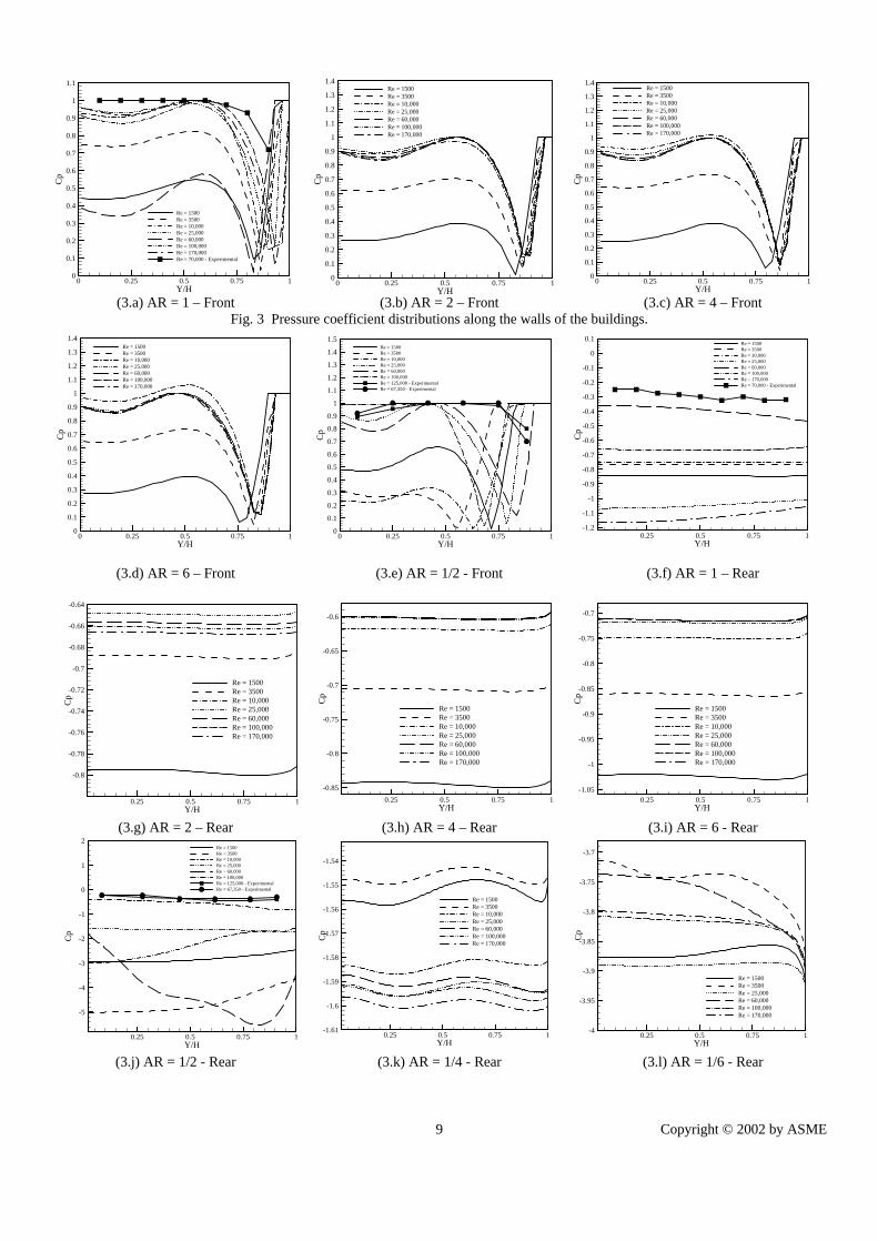
To validate the present computational results, comparisons are made with some experimental results obtained by the author. A delivery-type wind tunnel of a square cross-section (30×30 cm2) was used for the experimental work. Two wooden models of dimensions 10×10×10 cm3 (cube) and 60×60×120 cm3 (AR=1/2) were used for wind tunnel testing. The cubic model and the other model were equipped with 27 and 17 pressure tappings, respectively. These tappings were used to measure the surface pressure along the centerline of the front, top, and rear surfaces of the model. Experiments were carried out at one Reynolds number of 70,000 for the cubic model. Two Reynolds numbers of 67,350 and 125,000 were used for the other model (AR=1/2). Figs. 3a and 3f show comparison of Cp between the experimental and numerical results for the cubic model (AR=1) on the front and rear surfaces, respectively. Similar results of the other model AR=1/2 are shown in Figs. 3e, 3j and 3q for front, rear, and top surfaces, respectively. The numerical results compare very well to the experimental data especially on the front and rear surfaces. Numerical results tend to predict higher negative values of Cp. However, the same trend is kept. Generally, the above comparisons give confidence in the present numerical results.

V.1.2 EFFECT OF REYNOLDS NUMBER

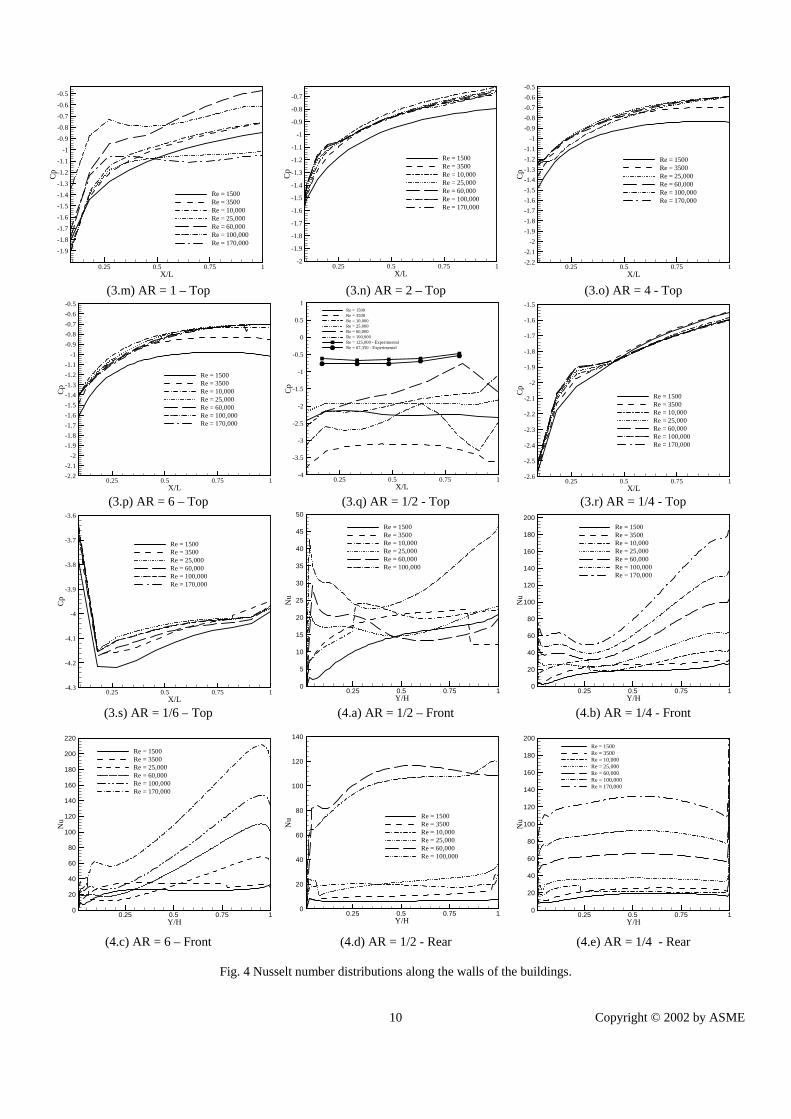
The results cover a wide range of Reynolds numbers, namely: 1500, 3500, 10,000, 25,000, 60,000, 100,000, and 170,000. The effect of Reynolds number on the static pressure distributions on front, rear, and top surfaces are shown in Figs. 3a-3s. As mentioned before the numerical results compare very well to the present experimental data. Figs. 3a-3e show the pressure coefficient (Cp) distribution on the front surface for different aspect ratios (AR). Aspect ratio is defined as the ratio of the length of the building to its height. For Re=10,000 and above, Cp takes almost a constant value (ranging between 0.9 and 1.0) up to Y/H≈0.75. Then, a sudden drop of Cp is noticed (Cp≈0.1). Again, Cp increases rapidly to a value of 1.0. The same behavior is noticed for the experimental data. The location (Y/H) of the minimum value of Cp varies considerably for AR=1 and AR=1/2. For Re=1500 and 3500, the model underpredicts the values of Cp


up till Y/H≈0.75. Figs. 3f-3l show Cp distributions on the rear surface. For AR=1, 2, 4, and 6, Cp has almost a constant negative value (base pressure) along the rear surface. Numerical results compare well to the experimental data. For AR=2, 4, and 6, Cp takes higher negative values for Re=1500. Values of Cp become very close to each other for the range of Reynolds number from 10,000 to 170,000. Figs. 3m-3s illustrate Cp distributions along the top (roof) surface. Values of Cp increase towards the leeward corner of the roof. The effect of Reynolds number is limited except for AR=1 and 1/2. It’s clear that Cp has a large negative value near the windward corner of the roof. Figs. 4a-4i show the distributions of Nusselt number (Nu) along front, rear, and top surfaces for AR=1/2, 1/4, and 1/6. On the front surface (Figs. 4a-4c), there is a local peak of Nu near the ground (Y/H≈0.025). Nu values increase gradually towards the top of the front surface (Y/H≈1.0). The values of Nusselt number increase with the increase of Reynolds number. Nu on the rear surface (Figs. 4d-4f) is almost constant along the surface. Values of Nu on the rear surface are less than those on the front surface. Figs. 4g-4i show the variation of Nu along the top surface. Values of Nu become almost constant from X/L=0.5 to 1.0. Nu increases with the increase of the value of the Reynolds number. For AR=1/4, at X/L=0.5, Nu=332 for Re=170,000 while Nu=63 for Re=10,000.

V.1.3 EFFECT OF THE ASPECT RATIO (AR)

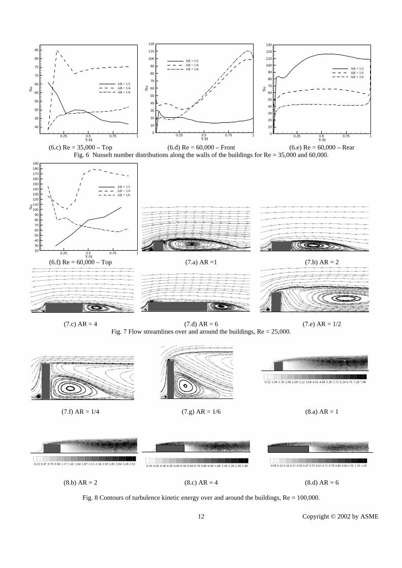
The distributions of Cp on the building surfaces are shown in Figs. 5a-5c for Re=35,000 and Figs. 5d-5f for Re=60,000. The effect of AR is mainly noticed on the top surface (roof) of the building. Figs. 6a-6f demonstrate the distributions of Nu on the building surfaces for Re=35,000, and 60,000, respectively. The effect of aspect ratio (AR) is obvious on the three surfaces. However, a dramatic change is noticed on the rear surface when Reynolds number changes from 35,000 to 60,000. For Re=35,000, AR=1/6 gives the highest values of Nu. While, for Re=60,000, the highest values of Nu are found for AR=1/2. This may be attributed to the change of the pattern of the wake behind the building as can be seen in Fig. 7. V.1.4 DRAG COEFFICIENT AND MEAN NUSSELT NUMBER

The values of the drag (load) coefficient for the different cases are illustrated in table (1). As the aspect ratio increases from AR=1 to AR=6, the drag coefficient (CD) decreases slightly. The decrease of CD is related to the enhancement of pressure on the leeward surface, this is due to the decrease in the energy losses in the recirculation zone of reduced size. For the aspect ratios 1/4 and 1/6, the values of CD increase considerably due to the increase of the negative pressure on the leeward surface. For Re=60,000, CD=1.88 for AR=1 and CD=3.965 for AR=1/6. Table (2) illustrates the average values of the Nusselt number (Nuav) on the three surfaces of the building in different cases. These average values are found by numerical integration along each surface. Generally, the values of Nuav increases as the Reynolds number increases. The maximum values of Nuav are found on the rear surface for AR = 1/2 and 1/4, and on the top surfaces for AR=1/6.

V.1.5 STREAMLINE PATTERNS AND KINETIC ENERGY CONTOURS

The streamline patterns for the different cases at Re=25,000 are shown in Figs. 7a-7g. The main features of the flow structures can be seen. Heads of the horseshoe vortex are found in front of the building. Separation bubble is seen on the top (roof) of the building (Fig. 7d). The recirculation zone is found behind the building. Details of the characteristic lengths of the flow structure for all the cases are shown in table (3). At Re=25,000, xr/Lre=7.8 for AR=1 and Xr/Lref=4.0 for AR=6. Thus, the size of the recirculation zone decreases as the aspect ratio increases. The size of the recirculation zone gives an estimate of the energy dissipated in the building wake. For the tall buildings (AR=1/2, 1/4, and 1/6) a minor recirculation zone appears next to the leeward surface of the building. The center of the vortex of the main recirculation zone in the wake of the building is shifted forward in the streamwise direction as the building height increases. The center core of the recirculation zone having zero velocity is important in building design for comfort purposes. The relative location of the upwind face stagnation Ys/Lref slightly changes for aspect ratios 1, 2, 4, and 6. However, for the tall buildings Ys/Lref decreases as the building becomes taller. At Re=100,000, Ys/Lref=0.198 for AR=1/6 and Ys/Lref=0.32 for AR=1/2. A similar behavior is noticed for the normalized diameter of the horseshoe vortex (Xf/Lref) in front of the building. Figs. 8a-8g show the contours of the turbulence kinetic energy (K) for all cases. Maximum turbulence energy contours take place near the building top level in the wake region. Turbulence energy is produced by the shear stress at the building top surface (roof). For AR=1, 2, 4, and 6, turbulence energy contours of the building AR=1 have the highest values. Increasing the aspect ratio seems to damp the turbulence energy and the longer roof smoothes the flow. The characteristics of the turbulence energy contours, which are useful in building aerodynamics, where the position of the high turbulence zone exists, are of specific interest to the designers.

V.2 K-ε MODEL USING THE UNSTRUCTURED GRID

The two-dimensional predictions of the flow around a cube by the K-ε model using the unstructured grid are shown in Figs. 10a-10d. The calculations are made in the plan of the top view of the flow field. The results cover Reynolds numbers of 1500, 2000, and 3500 for wind directions (α) of 0o, 26o, and 45o. Figs. 10a-10d demonstrate the contours of the pressure coefficient (CP), velocity vectors, and streamline patterns. It’s clear from the figures that the pair of vortices, behind the cube, forms a horseshoe-shaped vortex. In Fig. 10c, the heads of the arch vortex behind the building are clearly shown. The pressure contours are affected by the vortex-pattern of the flow around the building. In Figs. 10a and 10b, for α=0o, the velocity vectors trace the two side vortices next to the side walls of the building. For α=26o, and 45o, the side vortex of the lower wall disappears while the other one of the upper wall becomes bigger. From the above discussion, it’s obvious that for an interpretation of the complicated three-dimensional structure in turbulent flows, top and side views must be taken into account to be sure that no misinterpretation of the flow is made.


VI. ARTIFICIAL NEURAL NETWORK (ANN) An artificial neural network (ANN) is used to predict the

values of the drag (load) coefficient (CD) for different building configurations. A robust learning heuristic for multi-layered feed forward neural network called the Generalized Delta Rule (GDR) or ‘Back Propagation Learning Rule’ has been implemented in the present work. Input vectors and corresponding output vectors are used to train a network till it can approximate a function that associates input vectors with specific output vectors. Networks with biases, at least one sigmoid neuron layer, and a linear output neuron layer are capable of approximating any reasonable function. The backpropagation learning rules are used to adjust the weights and biases of networks to minimize the sum-squared error of the network. This is done by continually changing the values of the network weights and biases in the direction of steepest descent with respect to error. The Neural Network toolbox of the Matlab 4.0 package [23] was chosen to train the ANN. Trained backpropagation networks tend to give reasonable answers when presented with inputs that they have never seen. Typically, a new input will lead to an output similar to the correct output for input vectors used in training that are similar to the new input being presented. The used backpropagation network is shown in Fig. 11. The layers of a multilayer network play different roles. Layers whose output becomes the network output are called output layers. All other layers are called hidden layers. The network shown in Fig. 11 has R inputs, S1 neurons in the first layer, and S2 neurons in the second layer. It is common for different layers to have different numbers of neurons. A constant input 1 is fed to the biases for each neuron. Note that the outputs of each intermediate layer are the inputs to the following layer. Thus layer 2 can be analyzed as a one layer network with R= S1 inputs, S = S2 neurons and an S × R weight matrix W = W2. The input to layer 2 is P = A1, the output is A =A2. As all the vectors and matrices of layer 2 have been identified, it can be treated as a single layer network on its own. This approach can be taken with any layer of the network. It may be required to present a batch of Q input vectors to this network, at which time the matrix P will have the dimensions R × Q and the matrix A1 will have the dimensions S1 × Q. When a specific transfer function is to be used, the symbol for that transfer function will replace the ‘F’ shown in Fig. 11. Fig 12 shows some examples of the transfer functions. The function trainbpx is used to train the network. To pick initial weights and biases that are better than purely random values, Nguyen-Widrow function has been used. The initial weights as well as the initial biases employed random values between 1 & -1. The nodes in the hidden layer were varied from 5 to 30 for every input pattern and the evaluation of the performance of the network in determining the optimum hidden nodes was carried out. Also, many training cases were operated to get the optimum transfer functions arrangement. The input to the neural network consists of the values of the Reynolds number and the building configuration (aspect ratio), resulting in a neural network consisting of 2 input nodes and 1 output node. The input pattern of the neural network is a feature vector consisting of 2 features and the output pattern of the neural network is a feature vector consisting of 1 feature corresponding to the values of the drag coefficient (CD). The neural network is trained for 40 different cases. After the ANN has been trained, a separate set of unseen test patterns is supplied as

input to the ANN and its performance is evaluated. Results for many training cases that were operated to get the optimum transfer functions arrangement is presented in table (4) for the two-layer network. These results are obtained after 20,000 epochs (epoch: the presentation of the set of training (input and/or target) vectors to a network and the calculation of new weights and biases).

CASE F1 F2 S1 SSE SSET 1 logsig Purelin 5 0.0646 0.0888 2 logsig Purelin 10 0.0573 0.0734 3 logsig Purelin 15 0.0607 0.0764 4 logsig Purelin 20 0.0497 0.0668 5 logsig Purelin 30 0.0432 0.0823 6 Tansig Purelin 5 0.0608 0.0870 7 Tansig Purelin 10 0.0559 0.0780 8 Tansig Purelin 15 0.0418 0.0697 9 Tansig Purelin 20 0.0217 0.0415

10 Tansig Purelin 30 0.0069 0.0408

Table 4. Results of the training cases. Where: F1: Transfer function of the first layer. F2: Transfer function of the second layer. S1: Number of neurons in the hidden layer. SSE: Sum-squared error for training vector. SSET: Sum-squared error for testing vector.

From the presented trials, it is clear that the best result with minimum sum-squared error for training and testing is obtained in case (10). Fig. (13) shows the network error and its learning rate performance throughout training. Table (5) gives some samples of the test results of case (10). It is clearly evident that the results are very promising.

No. Desired output (CD) (Numerical Results)

Actual output (CD)-Case (10) (ANN Results)

1 1.745 1.732 2 1.864 1.820 3 1.530 1.599 4 1.611 1.637 5 1.825 1.634 6 2.20 1.954 7 2.30 2.2698 2.376 2.317 9 4.1100 3.9548

Table 5. Results of the test cases.

VII. CONCLUSIONS Numerical and neural investigations were carried out to study

the aerodynamic characteristics as well as flow and thermal fields of various model buildings. Many interesting remarks and observations were recorded. Thus, the following conclusions can be driven: 1. The present numerical results compare very well to the

experimental data obtained by the author. 2. The location of the local drop in the pressure coefficient (Cp)

on the front surface depends on both Reynolds number and aspect ratio.

3. The maximum suction pressure coefficient on the top surface (roof) increases as the height of the building increases.


4. The value of the Nusselt number on all surfaces increases with the increase of the Reynolds number for all values of aspect ratio.

5. Maximum turbulence energy contours take place near the building top level in the wake region.

6. Increasing the aspect ratio from 1 to 6 seems to damp the turbulence energy and the longer roof smoothes the flow.

7. The drag (load) coefficient is affected mainly by the height of the building.

8. The streamlines converge to a throat section near the upper front corner where the horizontal velocity is a maximum and the vertical velocity is zero. The maximum suction at the top surface (roof) occurs because the streamlines diverge again till far downstream.

9. The size of the recirculation zone in the wake behind the building decreases as the aspect ratio increases from 1 to 6.

10. For high-rise buildings, in the wake region, another minor vortex appears next to the rear surface in addition to the main vortex that moves far downstream as the building height increases.

11. The flexibility of generating the unstructured grids helps greatly in solving the flow field around bluff bodies of complex geometries.

12. For solving viscous flows using the unstructured grids, careful clustering should be applied next to the solid boundaries (to cover the boundary layer thickness) for accurate prediction of the flow field.

13. For a good interpretation of the complicated three-dimensional structure in turbulent flows, top and side views must be taken into account to be sure that no misinterpretation of the flow is made.

14. ANN proves to be an effective tool in predicting important parameters of such complex flow.

15. The values of the drag coefficient (CD) predicted numerically and by ANN are very close to each other.

16. It is expected to minimize the sum-squared error to get better results using ANN when increasing the number of the studied cases.

REFERENCES [1] Peterka, J. A., Cochran, L. S., Pielke, R. A., and Nicholls,

M. E., 1996, “Progrss in Modelling External Atmospheric Flows around Buildings,” ASME Fluids Eng. Division Conference, Vol. 238, pp. 535-539.

[2] Zhou, Y., and Stathopoulos, T., 1997, “A New Technique for the Numerical Simulation of Wind Flow around Buildings,” J. Wind Eng. Ind. Aerodyn., Vol. 72, pp. 137-147.

[3] Lakehal, D., 1998, “Application of the K-ε Model to Flow over a Building Placed in Different Roughness Sublayers,” J. Wind Eng. Ind. Aerodyn., Vol. 73, pp. 59-77.

[4] Murakami, S., 1990, “Numerical Simulation of Turbulent Flowfield around Cubic Model Current Status and Applications of K-ε Model and LES,” J. Wind Eng. Ind. Aerodyn., Vol. 33, pp. 139-152.

[5] Tamura, T., and Kuwahara, K., 1990, “Numerical Study of Aerodynamic Behavior of a Square Cylinder,” J. Wind Eng. Ind. Aerodyn., Vol. 33, pp. 161-170.

[6] Frank, W., 1996, “Three-Dimensional Numerical Calculation of the Turbulent Flow around a Sharp-Edged Body by Means of Large-Eddy-Simulation,” J. Wind Eng. Ind. Aerodyn., 65, pp. 415-424.

[7] Rodi, W., Ferziger, J. H., Breuer, M., and Pourquie, M., 1997, “Status of Large Eddy Simulation: Results of a Workshop,” ASME Fluids Engineering, Vol. 119, pp. 248-262.

[8] Majumdar, D., Amon, C. H., 1997, “Oscillatory Momentum Transport Mechanisms in Transitional Complex Geometry Flows,” ASME Fluids Engineerig, Vol. 119, pp. 29-35.

[9] Liou, T.-M., and Chen, S.-H., 1998, “Turbulent Flow Past an Array of Bluff Bodies Aligned Along the Channel Axis,” ASME Fluids Engineering, Vol. 120, pp. 520-529.

[10] Letchford, C. W., and Robertson, A. P., 1999, “Mean Wind Loading at the Leading Ends of Free Standing Walls,” J. Wind Eng. Ind. Aerodyn., Vol. 79, pp. 123-134.

[11] Zhou, Y., Gu, M., and Xiang, H., 1999, “Alongwind Static Equivalent Wind Loads and Responses of Tall Buildings. Part I: Unfavorable Distributions of Static Equivalent Wind Loads,” J. Wind Eng. Ind. Aerodyn., Vol. 79, pp. 135-150.

[12] Zhou, Y., Gu, M., and Xiang, H., 1999, “Alongwind Static Equivalent Wind Loads and Responses of Tall Buildings. Part II: Effects of Mode Shapes,” J. Wind Eng. Ind. Aerodyn., Vol. 79, pp. 151-158.

[13] Uematsu, Y., and Isyumov, N., 1999, “Wind Pressures Acting on Low-Rise Buildings,” J. Wind Eng. Ind. Aerodyn., Vol. 82, pp. 1-25.

[14] Farell, C., and Iyengar, A. K. S., 1999, “Experiments on the Wind Tunnel Simulation of Atmospheric Boundary Layers,” J. Wind Eng. Ind. Aerodyn., Vol. 79, pp. 11-35.

[15] Ginger, J. D., and Letchford, C. W., 1999, “Net Pressures on a Low-Rise Full-Scale Building,” J. Wind Eng. Ind. Aerodyn., Vol. 83, pp. 239-250.

[16] Meroney, R. N., Leitl, B. M., Rafailidis, S., and Schatzmann, M., 1999, “Wind-Tunnel and Numerical Modeling of Flow and Dispersion about Several Building Shapes,” J. Wind Eng. Ind. Aerodyn., Vol. 81, pp. 333-345.

[17] Ahmadi, G., and Li, A., 2000, “Computer Simulation of Particle Transport and Deposition near a Small Isolated Building,” J. Wind Eng. Ind. Aerodyn., Vol. 84, pp. 23-46.

[18] Lam, C. K. G., and Bremhorst, K., 1981, “A Modified Form of the K-ε Model for Predicting Wall Turbulence,” J. Fluids Eng., Vol. 103, pp. 456-460.

[19] Patanker, S. V., and Spalding, D. B., 1972, “A Calculation Procedure for Heat, Mass and Momentum Transfer in Three-Dimensional Parabolic Flows,” Int. J. Heat and Mass Transfer, Vol. 15, pp. 1787-1806.

[20] Anderson, W. K., and Bonhaus, D. L., 1994, “An Implicit Algorithm for Computing Turbulent Flows on Unstructured Grids,” Computers & Fluids, Vol. 23, No. 1, pp. 1-21.

[21] Shin, S., Ragab, S. A., and Devenport, W. J., 1999, “Numerical Simulation of Highly Staggered Cascade Flow Using an Unstructured Grid,” 30th AIAA Fluid Dynamics Conf., 28 June-1 July, 1999, Norfolk, VA, USA.

[22] Marcum, D. L., 1995, “Generation of Unstructured Grids for Viscous Flow Applications,” AIAA 95-0212.

[23] Demuth, H., and Beale, M., 1992, Neural Network-Toolbox-For Use with Matlab, The Math Works, Inc.


Fig. 1 Lengths of separation zones around the building.

Fig. 2 General view of the structured grid.

No. Case CD No. Case CD No. Case CD 1 AR=1, Re=1500 1.77 2* AR=1, Re=3500 1.75 3* AR=1, Re=10,000 1.86 4 AR=1, Re=25,000 1.90 5 AR=1, Re=60,000 1.88 6 AR=1, Re=100,000 1.87 7 AR=1, Re=170,000 2.10 8 AR=2, Re=1500 1.59 9* AR=2, Re=3500 1.53

10 AR=2, Re=10,000 1.56 11 AR=2, Re=25,000 1.67 12 AR=2, Re=60,000 1.71 13 AR=2, Re=100,000 1.73 14 AR=2, Re=170,000 1.76 15 AR=4, Re=1500 1.66 16 AR=4, Re=3500 1.55 17 AR=4, Re=10,000 1.53 18 AR=4, Re=25,000 1.59 19* AR=4, Re=60,000 1.61 20 AR=4, Re=100,000 1.62 21 AR=4, Re=170,000 1.63 22 AR=6, Re=1500 1.96 23 AR=6, Re=3500 1.82 24 AR=6, Re=10,000 1.75 25 AR=6, Re=25,000 1.80 26 AR=6, Re=60,000 1.81 27* AR=6, Re=100,000 1.83 28 AR=6, Re=170,000 1.84 29* AR=1/2, Re=1500 2.20 30 AR=1/2, Re=3500 1.90 31 AR=1/2, Re=10,000 1.80 32 AR=1/2, Re=25,000 1.40 33 AR=1/2, Re=60,000 1.80 34 AR=1/2, Re=100,000 1.77 35 AR=1/2, Re=170,000 1.80 36* AR=1/4, Re=1500 2.30 37 AR=1/4, Re=3500 2.294 38 AR=1/4, Re=10,000 2.36 39* AR=1/4, Re=25,000 2.376 40 AR=1/4, Re=60,000 2.38 41 AR=1/4, Re=100,000 2.38 42 AR=1/4, Re=170,000 2.388 43 AR=1/6, Re=1500 4.03 44 AR=1/6, Re=3500 3.936 45 AR=1/6, Re=10,000 4.0 46* AR=1/6, Re=25,000 4.11 47 AR=1/6, Re=60,000 3.9645 48 AR=1/6, Re=100,000 4.02 49 AR=1/6, Re=170,000 4.011

( * ) indicates the cases used to test the artificial neural network (ANN).

Table 1. The values of the drag (load) coefficient (CD) for different cases.

Copyright © 2002 by ASME

8

No. Case Nuav No. Case Nuav 1 AR=1/2, Re=1500-Front/ Top/ Rear 13.35/ 20.46/ 6.5 2 AR=1/2, Re=3500-Front/ Top/ Rear 17.44/ 49.03/ 10.91

3 AR=1/2, Re=10,000-Front/ Top/ Rear 18.91/ 35.4/ 18.22 4 AR=1/2, Re=25,000-Front/ Top/ Rear 17.62/ 50.13/ 21.61 5 AR=1/2, Re=60,000-Front/ Top/ Rear 17.69/ 70.34/ 105.76 6 AR=1/2, Re=100,000-Front/ Top/ Rear 30.61/ 84.61/ 99.2 7 AR=1/2, Re=170,000-Front/ Top/ Rear 50.7/ 101.1/ 121.3 8 AR=1/4, Re=1500-Front/ Top/ Rear 16.72/ 62.17/ 16.6 9 AR=1/4, Re=3500-Front/ Top/ Rear 23/ 71.88/ 22.38 10 AR=1/4, Re=10,000-Front/ Top/ Rear 26.8/ 64.97/ 22 11 AR=1/4, Re=25,000-Front/ Top/ Rear 38.1/ 91.5/ 35.4 12 AR=1/4, Re=60,000-Front/ Top/ Rear 56.73/ 148.5/ 60.8 13 AR=1/4, Re=100,000-Front/ Top/ Rear 73.42/ 201.87/ 85.95 14 AR=1/4, Re=170,000-Front/ Top/ Rear 96.15/ 279.3/ 122.5 15 AR=1/6, Re=1500-Front/ Top/ Rear 22.85/ 38.94/ 21.7 16 AR=1/6, Re=3500-Front/ Top/ Rear 31.2/ 47.7/ 34.07 17 AR=1/6, Re=10,000-Front/ Top/ Rear 33.3/ 49.1/ 36.3 18 AR=1/6, Re=25,000-Front/ Top/ Rear 35.84/ 33.3/ 27.56 19 AR=1/6, Re=60,000-Front/ Top/ Rear 54.36/ 75.32/ 40.6 20 AR=1/6, Re=100,000-Front/ Top/ Rear 73.78/ 83.18/ 45.82 21 AR=1/2, Re=170,000-Front/ Top/ Rear 106.96/ 117.3/ 63.93

Table 2. The average values of the nusselt number (Nuav) for the three surfaces of the building.

No. Case Xt/Lref Xf/Lref Xr/Lref Xwc/Lref Ywc/Lref Ys/Lref 1 AR=1, Re=1500 --- 0.448 5.6 1.76 0.637 0.448 2 AR=1, Re=3500 --- 0.5 6.4 2.2 0.657 0.552 3 AR=1, Re=10,000 --- 0.51 8.0 2.78 0.68 0.552 4 AR=1, Re=25,000 --- 0.67 7.8 2.88 0.76 0.566 5 AR=1, Re=60,000 --- 0.67 7.4 3.32 0.755 0.59 6 AR=1, Re=100,000 --- 0.8 9.5 2.67 0.744 0.7 7 AR=1, Re=170,000 0.95 0.75 9.0 2.7 0.744 0.61 8 AR=2, Re=1500 --- 0.5 5.2 2.2 0.588 0.54 9 AR=2, Re=3500 --- 0.65 5.8 2.48 0.565 0.68 10 AR=2, Re=10,000 --- 0.6 6.6 2.83 0.588 0.61 11 AR=2, Re=25,000 --- 0.6 7.8 3.16 0.623 0.6 12 AR=2, Re=60,000 --- 0.73 8.4 3.4 0.623 0.6 13 AR=2, Re=100,000 --- 0.75 8.5 3.44 0.64 0.63 14 AR=2, Re=170,000 --- 0.9 8.45 3.47 0.654 0.58 15 AR=4, Re=1500 --- 0.42 3.7 1.02 0.56 0.55 16 AR=4, Re=3500 --- 0.5 3.8 1.3 0.53 0.55 17 AR=4, Re=10,000 --- 0.55 4.5 1.46 0.54 0.545 18 AR=4, Re=25,000 --- 0.6 4.9 1.48 0.54 0.554 19 AR=4, Re=60,000 1.5 0.63 5.1 1.5 0.545 0.56 20 AR=4, Re=100,000 1.6 0.9 5.15 1.51 0.55 0.554 21 AR=4, Re=170,000 1.6 0.9 5.2 1.5 0.545 0.554 22 AR=6, Re=1500 --- 0.5 3.4 1.02 0.55 0.504 23 AR=6, Re=3500 1.5 0.6 3.7 1.2 0.55 0.53 24 AR=6, Re=10,000 1.5 0.6 4.1 1.44 0.53 0.513 25 AR=6, Re=25,000 1.6 0.6 4.0 1.45 0.53 0.52 26 AR=6, Re=60,000 2.2 0.7 4.5 1.45 0.536 0.47 27 AR=6, Re=100,000 1.98 0.7 4.4 1.45 0.535 0.485 28 AR=6, Re=170,000 2.2 0.65 4.5 1.44 0.536 0.495 29 AR=1/2, Re=1500 0.51 0.58 6.97 3.37 0.67 0.44 30 AR=1/2, Re=3500 0.4 0.5 6.67 2.17 0.82 0.42 31 AR=1/2, Re=10,000 0.5 0.42 7.17 2.29 0.77 0.42 32 AR=1/2, Re=25,000 0.5 0.468 6.67 3.38 0.71 0.45 33 AR=1/2, Re=60,000 0.51 0.52 6.7 3.6 0.7 0.43 34 AR=1/2, Re=100,000 0.29 0.577 7.25 3.96 0.71 0.32 35 AR=1/2, Re=170,000 0.4 0.58 7.3 4.1 0.72 0.4 36 AR=1/4, Re=1500 0.19 0.32 7.4 3.81 0.585 0.3 37 AR=1/4, Re=3500 0.19 0.31 7.47 3.81 0.58 0.29 38 AR=1/4, Re=10,000 0.19 0.3 7.5 3.8 0.587 0.31 39 AR=1/4, Re=25,000 0.19 0.28 7.6 3.79 0.59 0.28 40 AR=1/4, Re=60,000 0.19 0.255 7.68 3.8 0.6 0.24 41 AR=1/4, Re=100,000 0.19 0.25 7.7 3.82 0.61 0.25 42 AR=1/4, Re=170,000 0.19 0.251 7.72 3.82 0.61 0.25 43 AR=1/6, Re=1500 0.19 0.183 5.21 2.6 0.82 0.193 44 AR=1/6, Re=3500 0.19 0.21 5.3 2.61 0.83 0.195 45 AR=1/6, Re=10,000 0.19 0.2 5.4 2.6 0.83 0.194 46 AR=1/6, Re=25,000 0.19 0.19 5.45 2.59 0.828 0.195 47 AR=1/6, Re=60,000 0.19 0.201 5.62 2.611 0.831 0.197 48 AR=1/6, Re=100,000 0.19 0.22 5.65 2.6 0.832 0.198 49 AR=1/6, Re=170,000 0.19 0.21 5.73 2.62 0.829 0.196

Table 3. The values of the characteristic lengths of the flow structure.


(3.a) AR = 1 – Front (3.b) AR = 2 – Front (3.c) AR = 4 – Front Fig. 3 Pressure coefficient distributions along the walls of the buildings.

(3.d) AR = 6 – Front (3.e) AR = 1/2 - Front (3.f) AR = 1 – Rear

(3.g) AR = 2 – Rear (3.h) AR = 4 – Rear (3.i) AR = 6 - Rear

(3.j) AR = 1/2 - Rear (3.k) AR = 1/4 - Rear (3.l) AR = 1/6 - Rear

0 0.25 0.5 0.75 1Y/H

0

0.1

0.2

0.3

0.4

0.5

0.6

0.7

0.8

0.9

1

1.1

Cp

Re = 1500Re = 3500Re = 10,000Re = 25,000Re = 60,000Re = 100,000Re = 170,000Re = 70,000 - Experimental

0 0.25 0.5 0.75 1Y/H

0

0.1

0.2

0.3

0.4

0.5

0.6

0.7

0.8

0.9

1

1.1

1.2

1.3

1.4

Cp

Re = 1500Re = 3500Re = 10,000Re = 25,000Re = 60,000Re = 100,000Re = 170,000

0 0.25 0.5 0.75 1Y/H

0

0.1

0.2

0.3

0.4

0.5

0.6

0.7

0.8

0.9

1

1.1

1.2

1.3

1.4

Cp

Re = 1500Re = 3500Re = 10,000Re = 25,000Re = 60,000Re = 100,000Re = 170,000

0 0.25 0.5 0.75 1Y/H

0

0.1

0.2

0.3

0.4

0.5

0.6

0.7

0.8

0.9

1

1.1

1.2

1.3

1.4

Cp

Re = 1500Re = 3500Re = 10,000Re = 25,000Re = 60,000Re = 100,000Re = 170,000

0 0.25 0.5 0.75 1Y/H

0

0.1

0.2

0.3

0.4

0.5

0.6

0.7

0.8

0.9

1

1.1

1.2

1.3

1.4

1.5

Cp

Re = 1500Re = 3500Re = 10,000Re = 25,000Re = 60,000Re = 100,000Re = 125,000 - ExperimentalRe = 67,350 - Experimental

0.25 0.5 0.75 1Y/H

-1.2

-1.1

-1

-0.9

-0.8

-0.7

-0.6

-0.5

-0.4

-0.3

-0.2

-0.1

0

0.1

Cp

Re = 1500Re = 3500Re = 10,000Re = 25,000Re = 60,000Re = 100,000Re = 170,000Re = 70,000 - Experimental

0.25 0.5 0.75 1Y/H

-0.8

-0.78

-0.76

-0.74

-0.72

-0.7

-0.68

-0.66

-0.64

Cp

Re = 1500Re = 3500Re = 10,000Re = 25,000Re = 60,000Re = 100,000Re = 170,000

0.25 0.5 0.75 1Y/H

-0.85

-0.8

-0.75

-0.7

-0.65

-0.6

Cp

Re = 1500Re = 3500Re = 10,000Re = 25,000Re = 60,000Re = 100,000Re = 170,000

0.25 0.5 0.75 1Y/H

-1.05

-1

-0.95

-0.9

-0.85

-0.8

-0.75

-0.7

Cp

Re = 1500Re = 3500Re = 10,000Re = 25,000Re = 60,000Re = 100,000Re = 170,000

0.25 0.5 0.75 1Y/H

-5

-4

-3

-2

-1

0

1

2

Cp


0.25 0.5 0.75 1Y/H

-1.61

-1.6

-1.59

-1.58

-1.57

-1.56

-1.55

-1.54

Cp

Re = 1500Re = 3500Re = 10,000Re = 25,000Re = 60,000Re = 100,000Re = 170,000

0.25 0.5 0.75 1Y/H

-4

-3.95

-3.9

-3.85

-3.8

-3.75

-3.7

Cp

Re = 1500Re = 3500Re = 25,000Re = 60,000Re = 100,000Re = 170,000


(3.m) AR = 1 – Top (3.n) AR = 2 – Top (3.o) AR = 4 - Top

(3.p) AR = 6 – Top (3.q) AR = 1/2 - Top (3.r) AR = 1/4 - Top

(3.s) AR = 1/6 – Top (4.a) AR = 1/2 – Front (4.b) AR = 1/4 - Front

(4.c) AR = 6 – Front (4.d) AR = 1/2 - Rear (4.e) AR = 1/4 - Rear

Fig. 4 Nusselt number distributions along the walls of the buildings.

0.25 0.5 0.75 1X/L

-1.9

-1.8-1.7

-1.6

-1.5-1.4

-1.3

-1.2

-1.1-1

-0.9

-0.8

-0.7-0.6

-0.5

Cp

Re = 1500Re = 3500Re = 10,000Re = 25,000Re = 60,000Re = 100,000Re = 170,000

0.25 0.5 0.75 1X/L

-2

-1.9

-1.8

-1.7

-1.6

-1.5

-1.4

-1.3

-1.2

-1.1

-1

-0.9

-0.8

-0.7

Cp

Re = 1500Re = 3500Re = 10,000Re = 25,000Re = 60,000Re = 100,000Re = 170,000

0.25 0.5 0.75 1X/L

-2.2-2.1

-2-1.9-1.8-1.7-1.6-1.5-1.4-1.3-1.2-1.1

-1-0.9-0.8-0.7-0.6-0.5

Cp

Re = 1500Re = 3500Re = 25,000Re = 60,000Re = 100,000Re = 170,000

0.25 0.5 0.75 1X/L

-2.2-2.1

-2-1.9-1.8-1.7-1.6-1.5-1.4-1.3-1.2-1.1

-1-0.9-0.8-0.7-0.6-0.5

Cp

Re = 1500Re = 3500Re = 10,000Re = 25,000Re = 60,000Re = 100,000Re = 170,000

0.25 0.5 0.75 1X/L

-4

-3.5

-3

-2.5

-2

-1.5

-1

-0.5

0

0.5

1

Cp


0.25 0.5 0.75 1X/L

-2.6

-2.5

-2.4

-2.3

-2.2

-2.1

-2

-1.9

-1.8

-1.7

-1.6

-1.5

Cp

Re = 1500Re = 3500Re = 10,000Re = 25,000Re = 60,000Re = 100,000Re = 170,000

0.25 0.5 0.75 1X/L

-4.3

-4.2

-4.1

-4

-3.9

-3.8

-3.7

-3.6

Cp

Re = 1500Re = 3500Re = 25,000Re = 60,000Re = 100,000Re = 170,000

0.25 0.5 0.75 1Y/H

0

5

10

15

20

25

30

35

40

45

50

Nu

Re = 1500Re = 3500Re = 10,000Re = 25,000Re = 60,000Re = 100,000

0.25 0.5 0.75 1Y/H

0

20

40

60

80

100

120

140

160

180

200N

uRe = 1500Re = 3500Re = 10,000Re = 25,000Re = 60,000Re = 100,000Re = 170,000

0.25 0.5 0.75 1Y/H

0

20

40

60

80

100

120

140

160

180

200

220

Nu

Re = 1500Re = 3500Re = 25,000Re = 60,000Re = 100,000Re = 170,000

0.25 0.5 0.75 1Y/H

0

20

40

60

80

100

120

140

Nu Re = 1500

Re = 3500Re = 10,000Re = 25,000Re = 60,000Re = 100,000

0.25 0.5 0.75 1Y/H

0

20

40

60

80

100

120

140

160

180

200

Nu

Re = 1500Re = 3500Re = 10,000Re = 25,000Re = 60,000Re = 100,000Re = 170,000


(4.f) AR = 1/6 – Rear (4.g) AR = 1/2 - Top (4.h) AR = 1/4- Top

(4.i) AR = 1/6 – Top (5.a) Re = 35,000 – Front (5.b) Re = 35,000 - Rear

(5.c) Re = 35,000 – Top (5.d) Re = 60,000 – Front (5.e) Re = 60,000 - RearFig. 5 Pressure coefficient distributions along the walls of the buildings for Re = 35,000 and 60,000.

(5.f) Re = 60,000 – Top (6.a) Re = 35,000 – Front (6.b) Re = 35,000 - Rear

0.25 0.5 0.75 1Y/H

0

20

40

60

80

100

Nu

Re = 1500Re = 3500Re = 25,000Re = 60,000Re = 100,000Re = 170,000

0.25 0.5 0.75X/L

0

20

40

60

80

100

120

140

160

180

Nu

Re = 1500Re = 3500Re = 10,000Re = 25,000Re = 60,000Re = 100,000

0.25 0.5 0.75X/L

0

50

100

150

200

250

300

350

400

Nu

Re = 1500Re = 3500Re = 10,000Re = 25,000Re = 60,000Re = 100,000Re = 170,000

0.25 0.5 0.75X/L

0

50

100

150

200

250

300

Nu

Re = 1500Re = 3500Re = 25,000Re = 60,000Re = 100,000Re = 170,000

0 0.25 0.5 0.75 1Y/H

0.1

0.2

0.3

0.4

0.5

0.6

0.7

0.8

0.9

1

1.1

1.2

Cp

AR = 1AR = 2AR = 4AR = 6

0 0.25 0.5 0.75 1Y/H

-5

-4.5

-4

-3.5

-3

-2.5

-2

-1.5

-1

-0.5

Cp

AR = 1AR = 2AR = 4AR = 6AR = 1/2AR = 1/4AR = 1/6

0 0.25 0.5 0.75 1Y/H

-5

-4.5

-4

-3.5

-3

-2.5

-2

-1.5

-1

-0.5

Cp

AR = 1AR = 2AR = 4AR = 6AR = 1/2AR = 1/4AR = 1/6

0 0.25 0.5 0.75 1Y/H

0

0.1

0.2

0.3

0.4

0.5

0.6

0.7

0.8

0.9

1

1.1

Cp

AR = 1AR = 2AR = 4AR = 6AR = 1/2

0 0.25 0.5 0.75 1Y/H

-5.5

-5

-4.5

-4

-3.5

-3

-2.5

-2

-1.5

-1

-0.5

0C

p

AR = 1AR = 2AR = 4AR = 6AR = 1/2AR = 1/4AR = 1/6

0 0.25 0.5 0.75 1Y/H

-4.5

-4

-3.5

-3

-2.5

-2

-1.5

-1

-0.5

0

Cp AR = 1

AR = 2AR = 4AR = 6AR = 1/2AR = 1/4AR = 1/6

0.25 0.5 0.75 1Y/H

0

5

10

15

20

25

30

35

40

Nu

AR = 1/2AR = 1/4AR = 1/6

0.25 0.5 0.75 1Y/H

0

5

10

15

20

25

30

35

40

45

Nu

AR = 1/2AR = 1/4AR = 1/6


(6.c) Re = 35,000 – Top (6.d) Re = 60,000 – Front (6.e) Re = 60,000 – Rear Fig. 6 Nusselt number distributions along the walls of the buildings for Re = 35,000 and 60,000.

(6.f) Re = 60,000 – Top (7.a) AR =1 (7.b) AR = 2

(7.c) AR = 4 (7.d) AR = 6 (7.e) AR = 1/2 Fig. 7 Flow streamlines over and around the buildings, Re = 25,000.

(7.f) AR = 1/4 (7.g) AR = 1/6 (8.a) AR = 1

(8.b) AR = 2 (8.c) AR = 4 (8.d) AR = 6

Fig. 8 Contours of turbulence kinetic energy over and around the buildings, Re = 100,000.

0.25 0.5 0.75 1Y/H

40

45

50

55

60

65

70

75

80

85

Nu

AR = 1/2AR = 1/4AR = 1/6

0.25 0.5 0.75 1Y/H

0

10

20

30

40

50

60

70

80

90

100

110

120

Nu

AR = 1/2AR = 1/4AR = 1/6

0.25 0.5 0.75 1Y/H

0

10

20

30

40

50

60

70

80

90

100

110

120

130

Nu

AR = 1/2AR = 1/4AR = 1/6

0.25 0.5 0.75 1Y/H

2030405060708090

100110120130140150160170180190

Nu

AR = 1/2AR = 1/4AR = 1/6

0.52 1.04 1.56 2.08 2.60 3.12 3.64 4.16 4.68 5.20 5.72 6.24 6.76 7.28 7.80

0.23 0.47 0.70 0.94 1.17 1.41 1.64 1.87 2.11 2.34 2.58 2.81 3.04 3.28 3.51 0.10 0.20 0.30 0.39 0.49 0.59 0.69 0.79 0.89 0.99 1.08 1.18 1.28 1.38 1.48 0.08 0.16 0.24 0.31 0.39 0.47 0.55 0.63 0.71 0.78 0.86 0.94 1.02 1.10 1.18


(8.e) AR = 1/2 (8.f) AR = 1/4 (8.g) AR = 1/6

(9.a) General view (9.b) Near building (10.a) Re = 1500 - α = 0o Fig. 9 Unstructured grid for a cubic building.

(10.b) Re = 2000 - α = 0o (10.c) Re = 3500 - α = 26o (10.d) Re = 3500 - α = 45o

Fig. 10 Flow vectors, streamlines, and pressure contours using the unsrtructured grid. Fig. 11 The backpropagation of two-layer

network with one output layer (layer 2) and one hidden layer (layer 1).

Fig. 12 Some transfer functions. Fig. 13 The sum-squared error and learning rate of ANN for 20,000 epochs.

1.32 2.64 3.96 5.28 6.59 7.91 9.23 10.55 11.87 13.19 14.51 15.83 17.14 18.46 19.78 2.21 4.42 6.62 8.83 11.04 13.25 15.46 17.67 19.87 22.08 24.29 26.50 28.71 30.91 33.12 0.97 1.94 2.91 3.88 4.85 5.82 6.79 7.76 8.74 9.71 10.68 11.65 12.62 13.59 14.56

Cp

Cp Cp

Cp

0 5 0 0 0 1 0 0 0 0 1 5 0 0 0 2 0 0 0 0E p o c h

1 0 - 2

1 0 - 1

1 0 0

1 0 1

1 0 2

Sum

-Squ

ared

Erro

r

0 5 0 0 0 1 0 0 0 0 1 5 0 0 0 2 0 0 0 0E p o c h

0 . 0 1

0 . 0 2

0 . 0 3

0 . 0 4

0 . 0 5

0 . 0 6

0 . 0 7

Lear

ning

Rat

e

NUMERICAL AND NEURAL STUDY OF THE TURBULENT FLOW AROUND SHARP-EDGED BODIES

Documents

Transcript of NUMERICAL AND NEURAL STUDY OF THE TURBULENT FLOW AROUND SHARP-EDGED BODIES