Applied Energy 120 (2014) 133–146

Contents lists available at ScienceDirect

Applied Energy

journal homepage: www.elsevier .com/locate /apenergy

Reducing energy consumption and CO2 emissions by energy efficiencymeasures and international trading: A bottom-up modeling for the U.S.iron and steel sector

http://dx.doi.org/10.1016/j.apenergy.2014.01.0550306-2619/� 2014 Elsevier Ltd. All rights reserved.

⇑ Corresponding author. Tel.: +1 510 495 8185; fax: +1 510 486 6996.E-mail address: NKarali@lbl.gov (N. Karali).

Nihan Karali ⇑, Tengfang Xu, Jayant SathayeEnergy Analysis and Environmental Impacts Department, Environmental Energy Technologies Division, Lawrence Berkeley National Laboratory, 1 Cyclotron Road, MS90R2002, Berkeley, CA 94720, USA

h i g h l i g h t s

� Use ISEEM to evaluate energy and emission reduction in U.S. Iron and Steel sector.� ISEEM is a new bottom-up optimization model for industry sector energy planning.� Energy and emission reduction includes efficiency measure and international trading.� International trading includes commodity and carbon among U.S., China and India.� Project annual energy use, CO2 emissions, production, and costs from 2010 to 2050.

a r t i c l e i n f o

Article history:Received 9 July 2013Received in revised form 26 November 2013Accepted 26 January 2014

Keywords:Industry Sector Energy Efficiency Modeling(ISEEM)Energy consumptionCO2 emissionTradingBottom-up optimization modeling

a b s t r a c t

Using the ISEEM modeling framework, we analyzed the roles of energy efficiency measures, steel com-modity and international carbon trading in achieving specific CO2 emission reduction targets in the U.Siron and steel sector from 2010 to 2050. We modeled how steel demand is balanced under three alter-native emission reduction scenarios designed to include national energy efficiency measures, commoditytrading, and international carbon trading as key instruments to meet a particular emission restriction tar-get in the U.S. iron and steel sector; and how production, process structure, energy supply, and systemcosts change with those scenarios. The results advance our understanding of long-term impacts of differ-ent energy policy options designed to reduce energy consumption and CO2 emissions for U.S. iron andsteel sector, and generate insight of policy implications for the sector’s environmentally and economicallysustainable development. The alternative scenarios associated with 20% emission-reduction target areprojected to result in approximately 11–19% annual energy reduction in the medium term (i.e., 2030)and 9–20% annual energy reduction in the long term (i.e., 2050) compared to the Base scenario.

� 2014 Elsevier Ltd. All rights reserved.

1. Introduction

Interests in energy consumption and greenhouse gas (GHG)emission reductions in the United States (U.S.) industry sector haverisen with the international obligations towards reducing carbonemissions and introduction of new climate-change legislationsand initiatives around the world. It is important to understandthe impacts of various technologies and strategies on energy sav-ings and emission reduction potentials. Advancing such under-standing benefits from various integrated assessments of GHG

emission reduction and energy policy options (together with theireconomic impacts, technology and resource requirements) in theindustry sectors in the short-, medium-, and long-term perspec-tives. With this strategic need in mind, particular attentions weregiven to the energy intensive manufacturing sectors such as ironand steel, pulp and paper, chemicals, petroleum refining, andcement.

Iron and steel industry is one of the highest energy and emis-sion intensive sectors. According to International Energy Agency(IEA) [1], iron and steel sector accounts for about 5% of the totalworld carbon dioxide (CO2) emissions. The U.S. is the third largeststeelmaking country in the world with a production of 80.5 Milliontonnes (Mtonnes) in 2010 [2]. This paper examines the emissionreduction potentials of the U.S. iron and steel sector in the long

134 N. Karali et al. / Applied Energy 120 (2014) 133–146

term by giving particular attention to the energy efficiencyimprovements and potential trading opportunities.

Recent studies have evaluated the energy savings and emissionreduction associated with energy efficiency measures in country-specific industry sectors [3–18]. These studies concluded thatsignificant potentials exist in energy savings and CO2 emissionreduction with the mitigation technologies. While the studies areuseful for evaluating efficiency measures for a specific sector in aselected country from a technology-oriented perspective, sectoralfeedbacks (e.g. increasing production, energy, and raw materialrequirements in the related technologies and processes) are none-theless often neglected. There is lack of representation of overallrelations between technologies and the rest of the production sys-tem. For example, the amount of emission reduction attributed toone single measure when the measure was isolated from the rest ofthe production system might in fact change the process structureand the need for energy and raw material supply, leading to in-crease in final production costs or total emissions of the industry.A common practice to evaluate sector-wide performance of an en-ergy efficiency measure is the application of the measure as a com-ponent in a large-scale energy optimization models.

Energy optimization models are often applied for more compre-hensive analysis of sectoral and national costs of emission reduc-tion. Common approaches apply bottom-up perspective andinclude detailed technological representations. The majority ofexisting bottom-up models are based on the theoretical represen-tation of an ideal closed market, e.g., MESSAGE (Model for EnergySupply Systems and Their General Environment [19]), EFOM(Energy Flow Optimization Model [20]), MIDAS (MultinationalIntegrated Demand and Supply Model [21]), MARKAL (MarketAllocation Model [22]), and BUEM (Bottom-Up Energy Model[23]). In reality, however, few economies can be described ade-quately using closed market assumptions, which exclude anyinterference of trade policies that are likely to affect sector produc-tion, energy consumption, and emissions; while alternative emis-sion reduction policies may be deployed along withcomprehensive trading strategies. To date, existing models usedfor trade policy analysis generally employ top-down approachesand lack of technological detail (e.g., EPPA (The MIT Emissions Pre-diction and Policy Analysis Model [24]), SGM (The Second Genera-tion Model [25], and GTAP (Global Trade and Analysis ProjectModel [26])). In order to improve bottom up representation inthe modeling analysis of the U.S. iron and steel sector, a new typeof modeling approach combining technological representations ofthe bottom-up models with the trading representations of thetop-down models is necessary. This paper will introduce and usea new energy modeling framework – Industry Sector Energy Effi-ciency Modeling (ISEEM), which was recently developed [27].ISEEM framework is a global bottom-up optimization model,developed specifically for industry sector energy supply–demandplanning, and capable of evaluating alternative emission reductionpolicies under cost minimization objective.

The objective of this paper is to understand the CO2 emissionreduction impacts of national energy efficiency measures, and po-tential commodity and international carbon trading in the U.S. ironand steel sector in the long term (i.e., from year 2010 to 2050) byapplying ISEEM modeling. In this paper, we will select three alter-native emission reduction scenarios and illustrate how steel de-mand is balanced under each scenario. All three scenarios aim tomeet the same emission restriction target (i.e., 20% reduction) inthe U.S. iron and steel sector, but are specifically designed to em-ploy different reduction instruments. Three scenarios are definedas: (1) a national emission reduction scenario, in which nationalenergy efficiency measures are available without any other instru-ment of trading, (2) a commodity trading emission reduction sce-nario, in which commodity trading from China and India is

available, in addition to national energy efficiency measures, (3)a carbon trading emission reduction scenario, in which interna-tional carbon trading with China and India is available, in additionto national energy efficiency measures. The results in this paperwill particularly focus on changes in the U.S. steel productionand process structure, annual energy consumption, energy andemission intensity, and system costs.

2. Material and methods

ISEEM is a new mathematical model developed in this study toemulate the energy system, raw material and commodity flow,production systems, and trading mechanisms of industrial prod-ucts. Specifically, ISEEM was built on GAMS (General AlgebraicModeling System) optimization modeling interface as a technolog-ically detailed linear optimization model that minimizes the totalsystem cost over a set of constraints. In addition to detailed repre-sentation of industrial production, ISEEM has the capabilities thatallows commodity and carbon trading across regions and coun-tries, thus, provides users the ability to support specific energystudies or more general energy and emission reduction policies.

The complex relationships of supplying and producing energysources, raw materials, intermediate products, and final productsare represented as realistically as possible. In addition, this newframework allows to analyze the effects of various trading charac-teristics such as tariffs, import/export taxes, emissions due to com-modity trading (i.e., international shipping), which are notavailable for analysis using the other modeling frameworks.

The ISEEM’s main modeling system is a unified structure of submodules. Fig. 1 shows the basic structure of the ISEEM model, withits four sub modules and major relationships among them, inputdata requirements, and main outputs.

Any mechanism processing, producing, supplying, or convertinga product (i.e. energy sources, raw materials, intermediate prod-ucts, final product) is referred to as a technology in the framework.Therefore, production processes and energy source/raw materialsupply options are all represented as technologies. In other words,supply and process modules are structured over technology defini-tions and characteristics. Each technology has a unique parameterstructure that determines its impacts on the system (such as rawmaterial consumption, energy source requirements, and environ-mental impacts). Costs, availability factors, limitations, inputrequirements, and unit output generation per technological activ-ity can be listed as the main parameters related with the technol-ogies. The technologies are linked to each other via product flows(i.e. input–output relationships) in the model framework. Fromthis point of view, any output product produced by a technologyis an input product to another technology. Technology characteris-tics (parameter and constraint structures) are formed based on themodule the technology belongs to. Each technology in a module isassociated with the same parameters and should satisfy the sameconstraints.

Supply module includes the supply technologies that areresponsible to supply raw materials and energy sources to the sys-tem. Those technologies can be defined for any type of supplieswith a unit cost and limitations on supply levels. Supply technolo-gies do not need any input source to operate. In other words, theyare the starting point of the process.

Process module defines the production system of the sector ineach region. It includes the process technologies that generate aproduct by using another product as an input. Thus, the technolo-gies in this module produce the intermediate and the final prod-ucts of the system. Sector production facilities and onsiteelectricity generation facilities in the sector can be given as exam-ples of technologies that can be defined under this module. The

Fig. 1. Basic ISEEM framework structure.

N. Karali et al. / Applied Energy 120 (2014) 133–146 135

technologies responsible for producing the final product processthe intermediate products to produce the final output that will sat-isfy either demand of the region, in which the final product is pro-duced, or demands of the other regions via trading relationships.Demands of the regions are determined outside of the model andexogenously placed to the system. Export and import levels, onthe other hand, are endogenously determined in the trading mod-ule of the system and they are parts of the regional productions.Import of a region is basically produced in other regions and iscalled as export from those regions to the importing region. Theproduction for import is included in the total production level ofthe exporting country. According to optimization process, if it iscost effective for a region to satisfy its demand via imports fromanother region or regions, the production in the region may be re-duced and import can be increased, while production and exportlevels of the other regions increase simultaneously. Therefore, im-port and export levels between the regions are balanced each per-iod. Environmental module represents the GHGs emissions due toindustry and trading activities. The objective function considersenvironmental costs like penalties or taxes as well. These costscan be applied as a cost of each ton of global, regional, national,or sectoral emission or a cost of each ton of excess emissions.

Constraints of the ISEEM framework are of several kinds and ex-press the relationships that must be satisfied for proper represen-tation of the associated industrial systems. Parameters are the datainput. They indicate the inputs and outputs to/from each technol-ogy, describe the operation and limitations (e.g., availability fac-tors, cumulative or annual bounds on resource supplies,production, and trading) of the individual technologies, representthe demand for energy and raw material services, and provideadditional technical information (e.g., costs, efficiency, emission

factors, etc.). Demand for final product is placed into the modelfor the entire planning horizon. It bases on exogenous projectionsdeveloped outside of the ISEEM model. Costs parameters, on theother hand, define the objective function of the system and essen-tial for the minimum cost solution. Raw material and energysource supply costs, subsidies, technology investment costs, pro-cess operation costs, tariffs and transport costs of trading materi-als, environmental taxes and costs can be listed as the mainitems of the ISEEM total cost objective function.

Capacity, investment, and activity of the technologies are themain decision variables associated with the process technologies,and supply technologies only have activity (i.e., operation levels)as decision variables. Typical units are displayed in tonne/yearand PJ/year. Capacity level is a cumulative variable that grows withnew investments and decreases when the lifetime of any invest-ment is over. New investment on a technology is generated basedon several parameters, such as unit investment and operationalcosts, lifetime, annual limitations, input requirement per unitactivity and related fuel expenses, and output generation per unitactivity. Activity level of a process technology is determined basedon the capacity level and annual availability of the capacity. Inaddition, import and export levels of the regions are the other maindecision variables of the ISEEM framework associated with thetrading module. Import and export levels of regions are to be deter-mined for each period as well. Typical units are displayed in tonne/year.

The bottom-up structure of the ISEEM model is mainly deter-mined by the industry sector constraints covering energy, rawmaterial, production, and environmental relations, and potentialtrading constraints covering import and export relations. The rela-tions are applied over the technology and region sets. Therefore,

136 N. Karali et al. / Applied Energy 120 (2014) 133–146

the total number of the constraints in the model is simply relatedto the total number of technologies and regions. The objectivefunction of the model (represented in Formula 1) is the minimiza-tion of the total discounted system cost (i.e., totalcost) aggregatedover all periods. This cost is the cumulative sum of the annualizeddiscounted costs of each region across a predefined period of time.It includes the primary cost items such as supply costs, investmentcosts, operational costs, trading costs, and environmental costs.Supply cost is the summation of all the expenses of supplyingraw materials and energy sources to region r at each period andoperational costs include all fixed and variable operation andmaintenance costs. Trading costs is the net cost of import and ex-port of the final product in region r at period t. In addition, environ-mental costs are designed to represent possible negativeenvironmental impacts on system costs.

totalcost ¼ X

t

Xr

df ðrÞ � X

m2s

supcostðm; r; tÞ � actðm; r; tÞ

þX

m

anninvcostðm; r; tÞ � residðm; r; tÞ

þX

m

Xt

i¼um ;t�um<lifeðm;rÞ

nyrs �

anninvcostðm; r; iÞ � invðm; r; iÞ

þXm2p

fixcostðm; r; tÞ � capðm; r; tÞ

þXm2p

varcostðm; r; tÞ � actðm; r; tÞ

þ X

tr

ðtransportcostðr; tr; tÞ þ tariffiðr; tÞ

þ tariffeðtr; tÞ!�importðr; tr; tÞ

þX

venvcostðv; r; tÞ � ðemis iðv ; r; tÞ

þ emis tðv ; r; tÞÞ!

ð1Þ

(m: any technology, s: supply technology, p: process technology, r:region, tr: trading regions of region r, t: period, v: emitter)

where totalcost is the total discounted system cost, df(r) is thegeneral discount rate for region r, supcost(m,r,t), anninvcost(m,r,t),fixcost(m,r,t), and varcost(m,r,t) are the unit supply cost of any tech-nology m that is responsible for energy source and raw materialsupply, the annualized investment cost per unit capacity, the fixedoperational and maintenance cost per unit capacity, and variableoperational and maintenance costs per unit activity of the technol-ogy m in period t and region r, respectively. resid(m,r,t), life(m,r),and nyrs represent the residual capacity of technology m in regionr and period t, lifetime of technology m in region r, and number ofyears in a period (e.g., 1 year, 5 years, etc.). Residual capacity rep-resents the capacities that were invested prior to the start of theplanning horizon, but still alive in the current period.

Whether a new technology investment is alive or not in a perioddepends on its lifetime and the period in which the investment isoccurred. (t � um) = max{0,t-life(m,r)/nyrp} gives the interval forinvestments of technology m that are still available at period t. Thisinterval also includes the new investments realized in the currentperiod. This way, the retired capacity additions of technology m atthe previous periods are not included in the period t’s total capac-ity. transportcost(r,tr,t), tariffi(r,t), and tariffe(tr,t) are the transpor-tation cost per unit import between region r and tr, the tariff rateapplied on imported products of region r, and the tariff rate appliedon exported products of region tr in period t, respectively.act(m,r,t), inv(m,r,t), and cap(m,r,t), represent the activity of tech-

nology m, new investments in technology m, capacity of technol-ogy m at period t and region r. import(r,tr,t) is import of region rfrom region tr at period t. emis_i(v,r,t), and emis_t(v,r,t) are emis-sion of emitter v from industrial production, and emission of emit-ter v during transportation of imported product between tradingregions at period t and region r, respectively. envcost(v,r,t) is theenvironmental costs applied on emitter v at period t and region r.This cost is not active in a standard ISEEM model and used for sce-nario purposes. The objective function is optimized over a numberof constraints presented below.

2.1. Energy and material balances constraint

That constraint (represented in Formula 2) is used to ensurethat total consumption of any material or energy source used inthe process activities cannot exceed its total supply and/or produc-tion. The energy and material flows result from the combination ofprocess activities and input/output coefficients.Xm2me

outputeðm; e; r; tÞ � actðm; r; tÞ

PXm2ke

ðinputeðm; e; r; tÞ=ð1� contentðe; r; tÞÞÞ � actðm; r; tÞ ð2Þ

(e: any commodity used to produce the final product (e.g., energysources, raw materials, intermediate products, me: set of technolo-gies supplying or producing the commodity e, ke: set of technologiesexporting or consuming the commodity e)

where outpute(m,e,r,t) is output generation (of commodity e)per unit activity of technology m in region r at period t, inpute(-m,e,r,t) is input requirement (for commodity e) per unit activityof technology m in region r at period t, and content(e,r,t) is the rateof impurity in the input e.

2.2. Process capacity constraint

That constraint (represented in Formula 3) ensures that currentperiod capacity consist of residual capacity, remaining capacityfrom the previous periods (but still exists in the current period)and any new investment in the current period.

capðm; r; tÞ ¼ residðm; r; tÞ þXt

i¼um ;t�um<lifeðm;rÞ

nyrs

invðm; r; iÞ;m 2 p ð3Þ

2.3. Activity – Capacity constraint

That constraint (represented in Formula 4) requires that activityof any process technology cannot exceed its available capacity.

actðm; r; tÞ 6 af ðm; r; tÞ � capðm; r; tÞ;m 2 p ð4Þ

where af(m,r,t) is the annual availability factor of technology m inregion r at period t.

2.4. Demand satisfaction constraint

That constraint (represented in Formula 5) ensures that there isalways sufficient final product availability (either from nationalproduction or import) to meet the demand requirements.Xm2mdm

outputcðm;dm; r; tÞ � unitðmÞ � actðm; r; tÞ

þX

w;wherew–r

importðr;w; tÞP demandðdm; r; tÞ ð5Þ

(dm: demand, mdm: set of technologies serving the demand servicedm, w: any region)

0.0

20.0

40.0

60.0

80.0

100.0

120.0

140.0

160.0

The

U.S

. Ste

el P

rodu

ctio

n (M

tonn

es)

Steel Production Steel Import

N. Karali et al. / Applied Energy 120 (2014) 133–146 137

where outputc(m,dm,r,t), unit(m) and demand(dm,r,t) are level ofdemand service dm satisfied per unit activity of technology m in re-gion r at period t, the unit conversion factor for technology m, andlevel of demand service dm that has to be satisfied in region r atperiod t.

2.5. Trade constraints

1. Export satisfaction: that relation (represented in Formula 6)indicates that import from a region should be equal to exportof that region to importing region.

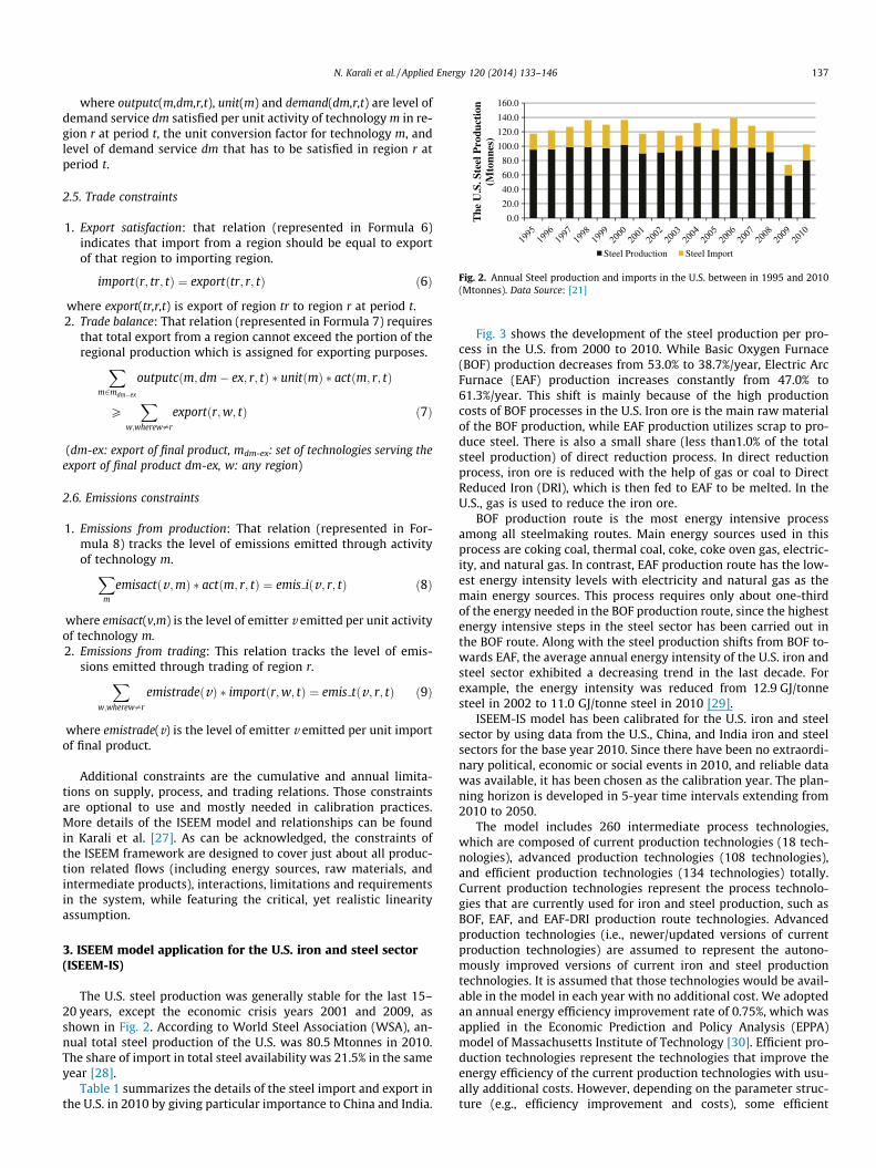
Fig. 2. Annual Steel production and imports in the U.S. between in 1995 and 2010

importðr; tr; tÞ ¼ exportðtr; r; tÞ ð6Þ (Mtonnes). Data Source: [21]

where export(tr,r,t) is export of region tr to region r at period t.2. Trade balance: That relation (represented in Formula 7) requires

that total export from a region cannot exceed the portion of theregional production which is assigned for exporting purposes.

X

m2mdm�ex

outputcðm;dm� ex; r; tÞ � unitðmÞ � actðm; r; tÞ

PX

w;wherew–r

exportðr;w; tÞ ð7Þ

(dm-ex: export of final product, mdm-ex: set of technologies serving theexport of final product dm-ex, w: any region)

2.6. Emissions constraints

1. Emissions from production: That relation (represented in For-mula 8) tracks the level of emissions emitted through activityof technology m.

X

m

emisactðv;mÞ � actðm; r; tÞ ¼ emis iðv; r; tÞ ð8Þ

where emisact(v,m) is the level of emitter v emitted per unit activityof technology m.2. Emissions from trading: This relation tracks the level of emis-

sions emitted through trading of region r.

Xw;wherew–r

emistradeðvÞ � importðr;w; tÞ ¼ emis tðv ; r; tÞ ð9Þ

where emistrade(v) is the level of emitter v emitted per unit importof final product.

Additional constraints are the cumulative and annual limita-tions on supply, process, and trading relations. Those constraintsare optional to use and mostly needed in calibration practices.More details of the ISEEM model and relationships can be foundin Karali et al. [27]. As can be acknowledged, the constraints ofthe ISEEM framework are designed to cover just about all produc-tion related flows (including energy sources, raw materials, andintermediate products), interactions, limitations and requirementsin the system, while featuring the critical, yet realistic linearityassumption.

3. ISEEM model application for the U.S. iron and steel sector(ISEEM-IS)

The U.S. steel production was generally stable for the last 15–20 years, except the economic crisis years 2001 and 2009, asshown in Fig. 2. According to World Steel Association (WSA), an-nual total steel production of the U.S. was 80.5 Mtonnes in 2010.The share of import in total steel availability was 21.5% in the sameyear [28].

Table 1 summarizes the details of the steel import and export inthe U.S. in 2010 by giving particular importance to China and India.

Fig. 3 shows the development of the steel production per pro-cess in the U.S. from 2000 to 2010. While Basic Oxygen Furnace(BOF) production decreases from 53.0% to 38.7%/year, Electric ArcFurnace (EAF) production increases constantly from 47.0% to61.3%/year. This shift is mainly because of the high productioncosts of BOF processes in the U.S. Iron ore is the main raw materialof the BOF production, while EAF production utilizes scrap to pro-duce steel. There is also a small share (less than1.0% of the totalsteel production) of direct reduction process. In direct reductionprocess, iron ore is reduced with the help of gas or coal to DirectReduced Iron (DRI), which is then fed to EAF to be melted. In theU.S., gas is used to reduce the iron ore.

BOF production route is the most energy intensive processamong all steelmaking routes. Main energy sources used in thisprocess are coking coal, thermal coal, coke, coke oven gas, electric-ity, and natural gas. In contrast, EAF production route has the low-est energy intensity levels with electricity and natural gas as themain energy sources. This process requires only about one-thirdof the energy needed in the BOF production route, since the highestenergy intensive steps in the steel sector has been carried out inthe BOF route. Along with the steel production shifts from BOF to-wards EAF, the average annual energy intensity of the U.S. iron andsteel sector exhibited a decreasing trend in the last decade. Forexample, the energy intensity was reduced from 12.9 GJ/tonnesteel in 2002 to 11.0 GJ/tonne steel in 2010 [29].

ISEEM-IS model has been calibrated for the U.S. iron and steelsector by using data from the U.S., China, and India iron and steelsectors for the base year 2010. Since there have been no extraordi-nary political, economic or social events in 2010, and reliable datawas available, it has been chosen as the calibration year. The plan-ning horizon is developed in 5-year time intervals extending from2010 to 2050.

The model includes 260 intermediate process technologies,which are composed of current production technologies (18 tech-nologies), advanced production technologies (108 technologies),and efficient production technologies (134 technologies) totally.Current production technologies represent the process technolo-gies that are currently used for iron and steel production, such asBOF, EAF, and EAF-DRI production route technologies. Advancedproduction technologies (i.e., newer/updated versions of currentproduction technologies) are assumed to represent the autono-mously improved versions of current iron and steel productiontechnologies. It is assumed that those technologies would be avail-able in the model in each year with no additional cost. We adoptedan annual energy efficiency improvement rate of 0.75%, which wasapplied in the Economic Prediction and Policy Analysis (EPPA)model of Massachusetts Institute of Technology [30]. Efficient pro-duction technologies represent the technologies that improve theenergy efficiency of the current production technologies with usu-ally additional costs. However, depending on the parameter struc-ture (e.g., efficiency improvement and costs), some efficient

Table 1Steel imports and exports in the U.S. in 2010. Data Source: [21]

Import (Mtonnes) Import share in total steel availability (%) Export (Mtonnes) Export share in total steel production (%)

Total 22.0 21.5 11.0 13.6From/To China 0.8 0.8 2.2 2.7From/To India 0.8 0.8 0.1 0.1From/To Others* 20.4 19.9 8.7 10.8

* Import/Export from/to the rest of the world.

0%10%20%30%40%50%60%70%80%90%

100%

2000 2001 2002 2003 2004 2005 2006 2007 2008 2009 2010

Pro

cess

Bas

ed S

teel

P

rodu

ctio

n (%

)

EAFBOF

Fig. 3. Steel production in the U.S. by process (2000–2010). Data Source: [21]

138 N. Karali et al. / Applied Energy 120 (2014) 133–146

production technologies can bring cost-effectiveness to the optimi-zation objective. On the other hand, the variety of technologies de-pends on the country. For example, there is not EAF-DRIproduction in China.

The database for input to the ISEEM-IS model consists of up-dated data and information compiled from various resources suchas WSA [2], the U.S. Geographical Survey (USGS) [28], China Statis-tical and Steel Yearbooks [31,32], Indian Minerals Yearbook [33],Center for Science and Environment [34], Energy InformationAdministration (EIA) [35], Bureau of International Recycling [36],Bureau of Labor Statistics [37], some technical experts, literature(e.g. [38–47]), and recent Lawrence Berkeley National Laboratory(LBNL) studies (e.g., [48,49,29,8,9,50,51]). In addition to the exten-sive data compiled from recent studies, considerable technology,manufacturing, energy source, and raw material supply detailsare accurately represented.

Fig. 4 illustrates the production flow diagram displaying all thetechnologies, energy sources, raw materials, intermediate

Fig. 4. Production flow representations of the

products, and final product included in the iron and steel sector.There are six different energy sources and five different raw mate-rials in the model. The diagram shows three modules of the ISEEM-IS model: Supply Module, Process Module, and Trading Module.Production flow is designed on the supply and the process mod-ules, while trading module is separately represented on Fig. 5 topicture the circulation of the final product. The final product, steel,is used to satisfy both national steel demand and trading needs.

Transportation costs, which are (2005)$24.5 and (2005)$49.0/tonne steel from China and India, respectively, in 2010 [52], are as-sumed to increase through the planning horizon according to oilprice projections by the EIA [35]. For the U.S. import tariff rate, cur-rent average border tax rate (i.e., 1.5%) is used and remains con-stant for the period 2010–2050.

On the other hand, the demand levels used in this applicationare price insensitive (i.e., demand remains unchanged if the supplyprices change and vice versa) and are exogenous inputs to themodel. The price insensitiveness is a necessary assumption forthe current study as there is neither information on price elasticityavailable nor a macroeconomic representation integrated. This is acommon approach used in bottom-up energy sector models,although presenting a weakness in terms of microeconomic foun-dations. The annual projections of the steel demand in the U.S.,as shown in Fig. 6, were established through a previous LBNL study[53].

While some of the important parameters used in the ISEEM-ISmodel are presented in Appendix A to indicate their structure inthe model in this paper, more details of this modeling frameworkare available in the full documentation of ISEEM model publishedby the authors [54]. In this paper, we assumed that the followingconstraints are employed: (i) annual BOF production cannot

iron and steel sector in ISEEM-IS model.

Fig. 5. Representations of the U.S., China, and India steel trading in ISEEM-IS Model (SM: Supply Module, PM: Process Module).

0.0

20.0

40.0

60.0

80.0

100.0

120.0

140.0

2005 2010 2015 2020 2025 2030 2035 2040 2045 2050

The

U.S

. Ste

el D

eman

d (M

tonn

es)

Fig. 6. Annual steel demands of the U.S. employed in the ISEEM-IS Model(Mtonnes). Data Source: Annual projections of the U.S. steel demand are based onresults from LBNL-COBRA energy modeling analysis [46]

N. Karali et al. / Applied Energy 120 (2014) 133–146 139

decrease to less than 10% of the total U.S. steel production; (ii) an-nual EAF production cannot decrease to less than 10% of the totalU.S. steel production. In addition, a discount rate of 10% per yearfor system costs is adopted throughout the study.

4. Scenario definitions

First, a Base scenario that reflects the continuation of existingtrends in the U.S. iron and steel sector without imposing any spe-cific emission reduction targets was established and calibratedagainst production, trading, energy, emission, and cost statisticsobtained from the historical data (i.e., 2005 and 2010) of the U.S.iron and steel sector. Implementation of efficiency measures onthe national scale is assumed available in the Base scenario. There-fore, an investment in any of the efficiency measures is possible ifit brings cost reductions to the least cost objective in the Base sce-nario. In addition to the Base scenario, three alternative emissionreduction scenarios are defined and studied. All the three scenariosaim to meet the same annual emission reduction target, which is20% below of those in the Base scenario. Each alternative emissionreduction scenario is designed to represent different reductioninstruments. The scenarios are defined as:

(1) ER scenario: annual emissions are restricted 20% below ofthat of the Base scenario; additionally, investments inenergy efficiency measures on the national scale are allowedwithout other instrument via trading.

(2) ET scenario: annual emissions are restricted 20% below ofthat of the Base scenario; additionally, investments inenergy efficiency measures on the national scale are allowedwith commodity trading being available with China andIndia up to a limit.

(3) EC scenario: annual emissions are restricted 20% below ofthat of the Base scenario; additionally, investments inenergy efficiency measures on the national scale are allowedalong with international carbon trading being available withChina and India up to a limit.

In the Base and ER scenarios, steel import is fixed to currentshares (i.e., 25% of the total steel availability in the U.S. in 2012[28]) through the planning horizon. This share relaxed up to 45%in the ET and ER scenarios.

5. Results and discussion

Scenarios will enable us to understand the impacts of potentialemission reduction instruments, and can provide insights aboutthe pathways that the industry should follow if it wants to reduceits emissions to a specific level under different circumstances. Theimpacts of different circumstances can be observed through the re-sults in projected production, final energy consumption, mix of en-ergy sources, energy and emission intensities, and system costs. Inaddition, comparing alternative scenarios with the Base scenario interms of energy and cost can provide a measure for emissionreduction effectiveness of each instrument considered in thescenarios.

0.0

10.0

20.0

30.0

40.0

50.0

60.0

2010 2015 2020 2025 2030 2035 2040 2045 2050

Tot

al A

nnua

l Ste

el I

mpo

rt in

th

e E

T a

nd E

C S

cena

rios

(M

tonn

es)

Base and ER ET and EC

Fig. 7. Total annual steel imports of the U.S. in the ET and EC scenarios (Mtonnes).

0.0

2.0

4.0

6.0

8.0

10.0

12.0

2015 2020 2025 2030 2035 2040 2045 2050

Incr

ease

in t

he U

.S. S

teel

Im

port

in E

T a

nd E

C

Scen

ario

s (M

tonn

es)

from China from India

Fig. 8. Increase in the U.S. steel imports in the ET and EC scenarios relative to thebase scenario (Mtonnes).

50%

60%

70%

80%

90%

100%

tion

Sha

re in

the

Bas

e na

rio

(%)

EAF-DRI

EAF

140 N. Karali et al. / Applied Energy 120 (2014) 133–146

5.1. Annual steel production and imports

Table 2 and Fig. 7 show the projected annual steel productionand imports of the U.S. generated by the model in all scenarios.In the ER Scenario, annual production and import levels are thesame as that of the Base scenario because no trading instrumentis imposed thus leaving existing import shares unchanged. TheET and EC scenarios, in contrast, allow commodity and carbon trad-ing with China and India. As a result, the U.S. annual steel produc-tion is projected to be lower than its counterpart in the Base and ERscenarios. In addition, even though the basic assumptions for theET and EC scenarios are different, the annual increase in the U.S.import (i.e., decrease in the U.S. production) is the same for boththe ET and EC scenarios. The annual increases of import from bothChina and India relative to the Base scenario are shown in Fig. 8.

Fig. 9 shows that the use of EAF as a low-cost steel productionprocess dominates the U.S. steel production in the Base scenario.Due to high production costs, share of BOF process gradually de-creases until the lower limits set in the model assumptions arereached. EAF-DRI production is economically unattractive for theU.S. iron and steel sector as well. Investment in and use of EAF-DRI production totally disappears starting from 2040.

The composition of production processes in the emission reduc-tion scenarios is depicted in Table 3. Since EAF production is lessenergy intensive than any other production processes, one wouldexpect that there would be shifts from other processes to EAF un-der all three emission reduction scenarios. Because annual BOFproduction is already at the lower bounds in the Base scenario,there is no room for replacing BOF production with EAF produc-tion. As a result, there are minor shifts from EAF-DRI to EAF pro-duction in each emission reduction scenario shown in Table 3. Insummary, changes in production shares in each emission reductionscenario, when compared to the Base scenario, are rather negligi-bly small from 2010 to 2050.

0%

10%

20%

30%

40%

2010 2015 2020 2025 2030 2035 2040 2045 2050

Ann

ual P

rodu

cSc

e BOF

Fig. 9. Annual production shares in the U.S. iron and steel sector in the basescenario (%).

5.2. Annual energy consumption and CO2 emission

Fig. 10 shows the annual energy consumption of the U.S. ironand steel sector in the Base and three emission reduction scenarios.Annual energy consumption of the each scenario decreases withthe increasing share of EAF process, even though the total steelproduction continuously grows. Clearly, production increase inthe EAF process due to its low costs automatically improves the en-ergy efficiency of the U.S. iron and steel sector, independent fromthe scenario assumptions. In addition, annual energy consumptionin all emission reduction scenarios is lower than that of the Basescenario throughout the planning horizon.

In summary, we have found that the ET and EC scenarios appearto be more effective than the ER scenario in reducing annual en-ergy consumption in each year, while achieving the same emissionreduction target (i.e., 20% annual reduction compared to that of theBase scenario) throughout mid- and long-term projections. In 2030annual energy consumption decreases by 10.8%, 19.2%, and 19.2%,and in 2050 annual energy consumption decreases by 8.5%, 19.6%,and 19.6% when compared to the Base scenario for the ER, ET, andEC scenarios, respectively.

Table 2Total Annual Steel Productions in the U.S. (Mtonnes).

2010 2015 2020 2025 2030 2035 2040 2045 2050 Relativescenario

Base 80.5 82.1 83.0 84.6 88.4 91.9 94.4 96.0 96.9 –ER 80.5 82.1 83.0 84.6 88.4 91.9 94.4 96.0 96.9 0.0ET 80.5 79.3 66.5 68.2 71.8 75.2 77.4 78.9 79.5 �15.1EC 80.5 79.3 66.5 68.2 71.8 75.2 77.4 78.9 79.5 �15.1

Even though the energy consumption decreases in each sce-nario relative to the Base scenario, there seems to be no energyefficiency improvement over the Base scenario in the ET and ECscenarios. Fig. 11 displays the trends of average energy intensitiesachieved in all scenarios. In the Base scenario, energy intensity de-creases from 10.7 GJ/tonne steel in 2010 to 5.1 GJ/tonne steel in2050. In the ET and EC scenarios, energy intensity levels are pro-jected to be very close to that of the Base scenario, while intensityin the ER scenario is consistently lower. This indicates that de-creases in the annual energy consumption in the ET and EC scenar-ios actually come from the reduction in domestic production in theU.S. (i.e., increase in import), not necessarily improvement in

difference in total production (of the period 2010–2050) compared to base(%)

Table 3Annual production shares in the U.S. iron and steel sector in the base and emission reduction scenarios (%).

2010 (%) 2015 (%) 2020 (%) 2025 (%) 2030 (%) 2035 (%) 2040 (%) 2045 (%) 2050 (%)

BOF Base 38.7 30.0 25.0 20.0 15.0 10.0 10.0 10.0 10.0ER 38.7 30.0 25.0 20.0 15.0 10.0 10.0 10.0 10.0ET 38.7 30.0 25.0 20.0 15.0 10.0 10.0 10.0 10.0EC 38.7 30.0 25.0 20.0 15.0 10.0 10.0 10.0 10.0

EAF Base 60.4 68.7 73.2 78.3 83.4 89.2 90.0 90.0 90.0ER 60.4 68.9 74.0 79.0 84.2 90.0 90.0 90.0 90.0ET 60.4 68.6 73.4 78.5 83.6 89.5 90.0 90.0 90.0EC 60.4 68.6 73.4 78.5 83.6 89.5 90.0 90.0 90.0

EAF-DRI Base 0.9 1.3 1.8 1.7 1.6 0.8 0.0 0.0 0.0ER 0.9 1.1 1.0 1.0 0.8 0.0 0.0 0.0 0.0ET 0.9 1.4 1.6 1.5 1.4 0.5 0.0 0.0 0.0EC 0.9 1.4 1.6 1.5 1.4 0.5 0.0 0.0 0.0

0.0

200.0

400.0

600.0

800.0

1000.0

Ann

ual E

nerg

y C

onsu

mpt

ion

(PJ)

Base ER ET EC 2010 2015 2020 2025 2030 2035 2040 2045 2050

Fig. 10. Annual energy consumption in the U.S. iron and steel sector in the base and emission reduction scenarios (PJ).

0.0

2.0

4.0

6.0

8.0

10.0

12.0

2010 2015 2020 2025 2030 2035 2040 2045 2050

Ave

rage

Ene

rgy

Inte

nsit

y (G

J/to

nne

stee

l)

Base ER ET EC

Fig. 11. Average energy intensity of the U.S. iron and steel sector (GJ/tonne steel).

N. Karali et al. / Applied Energy 120 (2014) 133–146 141

energy efficiency. In contrast, energy intensity in the ER scenario isreduced 8.7% and 4.0% in 2030 and 2050, respectively, when com-pared to that of the Base scenario. Overall, energy intensity levelsof the all scenarios tend to converge and approach to each otherin the long term. For example, the gaps among them become smal-ler particularly after 2040. A high share of EAF process in each sce-nario (i.e., 90% of the production after 2040) is the primary reasonfor the convergence of overall energy intensity. Fig. 12 shows thatemission intensity of the ER scenario remains much lower than

0.0

0.2

0.4

0.6

0.8

1.0

1.2

1.4

2010 2015 2020 2025 2030 2035 2040 2045 2050

Ave

rage

CO

2E

mis

sion

In

tens

ity

(tC

O2/

tonn

e st

eel)

Base ER ET EC

Fig. 12. Average CO2 emission Intensity of the U.S. iron and steel sector (tCO2/tonnesteel).

those of the other scenarios throughout the planning horizon, eventhough energy intensity levels approaches to each other after 2040.This indicates that from 2040 onward, most of the emission reduc-tion in the ER scenario is achieved by the consumption of loweremission fuels, such as offsite coke and grid electricity, which isfurther supported by the composition of final energy supply exhib-ited in Fig. 13.

Because unit cost of steel production in the U.S. is higher thanunit cost of imported steel from China and India in both the ETand EC scenarios, the optimization processes in the ISEEM-IS mod-el respond to emission restriction target similarly. As a result, withthe production and import shares being almost identical for boththe ET and EC scenarios, annual energy consumption and averageenergy and emission intensity levels are similar.

5.3. Annual production costs

Fig. 14 and Fig. 15 show the unit cost of steel in the U.S. market(including imports from China and India) projected in the ET andEC scenarios, respectively. As shown in Fig. 14, in the ET scenario,unit costs of imported steel from both China and India are lowerthan the unit production cost in the U.S. starting in 2015, with Chi-na showing the lowest unit cost starting in 2010. Clearly, importingfrom China or India brings direct economic benefits to the U.S.market. The projections in the ET scenario show that annual importfrom China and India increases from year to year, until the allowedlimits are achieved (see Figs. 7 and 8). In the EC scenario, importcosts of steel from China and India include the additional cost fromthe investments in energy efficiency measures. Fig. 15 shows thatunit cost of imported steel from China is still less than unit produc-tion cost in the U.S. from 2010 to 2050; whereas unit cost of im-ported steel from India becomes very similar to the unitproduction cost in the U.S., and is even higher than that of theU.S. after 2040. However, it should be noted that the U.S. unit pro-duction cost reflects the cost of production without any investmentin energy efficiency. With the national scale efficiency investmentsthat would be needed for emission reduction in the U.S., unit

Fig. 13. Annual energy consumption by fuel in the U.S. iron and steel sector in the base and emission reduction scenarios (%).

0.0100.0200.0300.0400.0500.0600.0700.0800.0

2010 2015 2020 2025 2030 2035 2040 2045 2050

Ave

rage

Cos

t of

Ste

el in

the

ET

Sc

enar

io (

(200

5)$/

tonn

e st

eel)

Average Cost of Production in the U.S.

Average Cost of Importing from China

Average Cost of Importing from India

Fig. 14. Average unit cost of steel in the U.S. market in the ET scenario ((2005)$/tonne steel).

0.0100.0200.0300.0400.0500.0600.0700.0800.0

2010 2015 2020 2025 2030 2035 2040 2045 2050

Ave

rage

Cos

t of

Ste

el in

the

EC

Sc

enar

io (

(200

5)$/

tonn

e st

eel)

Average Cost of Production in the U.S.

Average Cost of Importing from China

Average Cost of Importing from India

Fig. 15. Average unit cost of steel in the U.S. market in the EC scenario ((2005)$/tonne steel).

0%

10%

20%

30%

40%

50%

60%

70%

80%

90%

100%

2010 2015 2020 2025 2030 2035 2040 2045 2050

Shar

e of

Cos

t It

ems

(%)

Raw Material Cost

Energy Cost

Variable O&M Cost

Fixed O&M Cost

Investment Cost

Fig. 16. Share of cost items in the U.S. steel production cost in the base scenario (%).

142 N. Karali et al. / Applied Energy 120 (2014) 133–146

production cost in the U.S. would be higher. The optimizationprocess (i.e. least cost objective) compares that cost of the U.S.

(i.e. the unit production cost, including additional costs of effi-ciency investments) with the import costs from China or India.

On the other hand, overall production cost includes costs of rawmaterials, energy, O&M, and investment. Fig. 16 shows the relativeshare of each cost item over the time in the Base scenario for theU.S. iron steel production. Raw material has the highest share ofthe U.S. iron and steel production cost in all scenarios, and exhib-ited an increasing trend over time. For example, the cost share ofraw materials grows from 44% in 2010 to 60% in 2035 and stabi-lizes from that year forward. The primary reason is the increasingusage of scrap corresponding to the growing EAF production. Scrapreplaces relatively cheaper iron ore that is the main raw material ofBOF production. Similarly, the decreasing trend in the shares of en-ergy cost can be attributed to the increase in EAF production –share of energy cost drops from 16% in 2010 to slightly higher than11% in 2035 and stabilizes around 11% afterward. Since investmentcost in BOF production is higher than that of EAF production, shareof total investment cost decreases gradually with the decreasingshare of BOF production.

Table 4 summarizes overall production costs and shares of costitems (i.e., cumulative from 2010 to 2050) in each scenario.

Table 4Overall Production Costs and Shares of Cost Items in The U.S. Iron and Steel Sector in the Base and Emission Reduction Scenarios (Cumulative from 2010 to 2050).

Base scenario ER scenario ET scenario EC scenario

Cumulative production cost between 2010 and 2050 (Billion (2005) dollar) 499.0 504.7 432.8 432.8Share of investment cost (%) 9.8 10.3 10.6 10.6Share of O&M cost (%) 21.2 21.3 21.7 21.7Share of raw material cost (%) 57.0 57.4 55.8 55.8Share of energy cost (%) 12.0 11.0 11.9 11.9

0%

2%

4%

6%

8%

10%

12%

14%

16%

2015 2020 2025 2030 2035 2040 2045 2050

Shar

e of

Ene

rgy

Cos

t in

P

rodu

ctio

n C

ost

(%)

Base ER ET EC

Fig. 18. Share of energy cost in the base and emission reduction scenarios (%).

0.0

2.0

4.0

6.0

8.0

10.0

12.0

0.0

20.0

40.0

60.0

80.0

100.0

120.0

2015 2020 2025 2030 2035 2040 2045 2050

Incr

aese

in A

vera

ge U

nit

Pro

duct

ion

Cos

t in

the

ER

Sc

enar

io (

(200

5)$/

tonn

e st

eel)

Em

issi

on R

educ

tion

Cos

t in

th

e E

R S

cena

rio

((20

05)$

/ton

C

O2)

Annual Emission Reduction Cost Increase in Average Unit Production Cost

Fig. 19. Annual emission reduction cost ((2005)$/ton CO2) and increase in averageproduction cost ((2005)$/tonne steel) in the ER scenario.

N. Karali et al. / Applied Energy 120 (2014) 133–146 143

Because emission reductions in the ER scenario is accomplished bythe additional investments in energy efficiency improvements, thecumulative production cost of the planning horizon (i.e., 2010–2050) increases by 5.7 Billion (2005) dollars in this scenario (whencompared to the Base scenario). As the share of investment costsincreases (from 9.8% to 10.3%), the share of energy cost is lower(from 12% to 11%), as shown in Table 4. In the ET and EC scenariosemissions are reduced as they correspond to decrease in domesticsteel production with the increase in steel import. Therefore, a sig-nificant reduction in total production cost is expected due todecreasing national production in both the ET and EC scenarios.

In addition, the level of emission reduction targets, most nota-bly for the ER scenario, largely influences investment cost and en-ergy costs. Fig. 17 and Fig. 18 show the relative shares ofinvestment cost and energy cost in each scenario, respectively. Inthe ER scenario, investments in energy efficiency contribute to ahigher share of investment cost, while lowering the share of energycost, compared to the Base scenario. In the ET and EC scenarios,share of investment cost is higher than that in the Base scenariothroughout the planning horizon, and is higher than that of ER sce-nario from 2010 to 2040. The main reason is the annualized pay-ments associated with the new capacity additions of the baseyear (i.e., 2010). Once the scenarios become active starting from2015, a part of those capacities get idle (due to decreasing produc-tion in both the ET and EC scenarios). However, the payments areannualized through the lifetime of the technology (i.e., 30 years).Thus, the model continues to pay for the capacities that are notin active production. This situation stresses the share of invest-ment cost until the annualized payments are done in 2040. Shareof energy costs, on the other hand, remain lower for the ET, andEC scenarios when compared to the Base scenario.

5.4. Annual CO2 emission reduction costs

Without the instrument of deploying commodity trading or thecarbon trading, the ER scenario is expected to seek for implement-ing more efficient technology and increasing low emission fuelusage to achieve the targeted emission restriction. Fig. 19 showsthe annual reduction cost of CO2 emission obtained in the ER sce-nario. It peaks in 2040 – an indication that the ER scenario needshuge investment expenditure to achieve 20% emission reductionin this particular year. The production capacities invested in thebase year are replaced with the high efficiency capacities (i.e.,

0%

2%

4%

6%

8%

10%

12%

14%

2015 2020 2025 2030 2035 2040 2045 2050Shar

e of

Inv

estm

ent

Cos

t in

P

rodu

ctio

n C

ost

(%)

Base ER ET EC

Fig. 17. Share of investment cost in the base and emission reduction scenarios (%).

autonomously improved versions of base year technologies) in allscenarios, once they reach end of their life in 2040, since thosetechnologies use less energy with no additional cost. As shown inFig. 20, the amount of annual CO2 emission in each scenario isthe lowest of the planning horizon in 2040. Thus, additional energyefficiency measures of the ER scenario, implemented starting in2040, need to produce higher emission reduction, while increasingemission abatement cost. In addition, Fig. 19 also exhibits the in-crease in average production cost per tonne steel in the ER scenariothroughout the planning horizon. The ER scenario results illustratethat 20% emission reduction is achieved with an increase of(2005)$4 to (2005)$10/tonne steel between the periods 2015 and2050.

On the other hand, emission reductions in the ET and EC scenar-ios are achieved via replacement of domestic production with im-port from China and India. There is not any investment foremission reduction, instead declining domestic production resultin a decrease of the production costs. Hence, in contrast to theER scenario, it is impossible to talk about the cost of emissionreduction in the ET and EC scenarios.

5.5. Discussion of results

The projections for both ET and EC scenarios indicate the samechanges when compared to the Base scenario. The main reason isthe much lower costs of Chinese steel import and Indian steel im-port to the U.S. market. Particularly, the unit cost of steel importfrom China in the model is much lower than that of the U.S. unit

0.0

20.0

40.0

60.0

80.0

100.0

120.0

2010 2015 2020 2025 2030 2035 2040 2045 2050A

nnua

l CO

2E

mis

sion

s (M

ton

CO

2)Base ER ET EC

Fig. 20. Annual CO2 emission of the U.S. iron and steel sector in the base and emission reduction scenarios.

144 N. Karali et al. / Applied Energy 120 (2014) 133–146

production cost in both commodity trading (ET scenario) and car-bon trading (EC scenario) scenarios. Even with additional costsassociated with carbon trading, the unit cost of imported steel re-mains much lower than that of the U.S. domestic cost. As a result,the optimization process prefers importing from China as long asthe amount of import is within the allowable import boundary.

In fact, there are many key factors that influence the optimiza-tion process (i.e., cost minimization objective), such as added costsdue to transportation, tariff structure, environmental regulationspertaining to steel production and local pollutions, capital andoperational expenses, raw material and energy costs, and laborcosts. A cheaper production cost in China alone does not necessar-ily mean that the U.S. would need to import from China beforeachieving the maximum import limitations. The optimization pro-cess makes the decision according to all information collected fromthe modeled system and provides the least cost fuel-technology-production-import combination that satisfies the specified de-mand (with respect to minimization cost objective). For example,one can argue that the magnitude of added cost for complying withenvironmental regulations in the U.S. can be quite different thanthat of other countries (e.g., China). In this perspective, it wouldbe useful to perform sensitivity analysis by applying different inputto the ISEEM-IS model runs to further investigate the influence ofmodel input. For discussion purpose, we assume that the magni-tudes of unit production cost in China will be increased by 10%,20% and 40% due to increased environmental regulations, anduse them in the ISEEM model runs while other input are held un-changed. The preliminary results indicate that an increase by 10%in unit production cost in China does not change the model outputon steel trading volumes. An increase of China production cost by20% decreases steel import of the U.S. only in the last two periods,even though the unit production cost in the U.S. is 10% lower thanthe China production cost through the planning horizon. An in-crease of China production cost by 40%, on the other hand, doeschange the landscape of steel trading volumes significantly reflect-ing the large increase in China production cost (20–30% higherthan the production cost in the U.S.).

In view of the results, it should be noted that these discussionsare made under a set of assumptions pertaining to the modelparameters and other inputs such as the prices and availabilitiesof energy sources, raw materials, and technologies (data set anddetails of the assumptions can be found in Karali et al. [54]). Forexample, we observe that the U.S. steel import volume from Chinastarts to decrease corresponding to an increase of 20% in unit pro-duction cost in China. Under a different set of model data, resultsmay indicate different options for the U.S. iron and steel market.In addition, there is a need to further investigate the impacts ofthose three scenarios in the China and India iron and steel sectorsto gain a better understanding of the emission effects of the U.S.policies. Future work on the ISEEM-IS model can include furtherimprovement and updating of the input data set, and the analysisof the China and India iron and steel sectors under the current U.S.scenarios.

Furthermore, the effect of technological learning associatedwith the efficient production technologies is not considered inthe current analysis. The results (in Fig. 19) show that there is atrivial additional cost (emission reduction cost) to hit the targetin the ER scenario – about 1%. In fact, if technological learning is in-cluded, the total cost might actually go down. Future analysis mayinclude the impact of technological learning on efficient produc-tion technologies.

6. Conclusions

Development of the ISEEM framework enables us to analyzehow technology, production, trading structure, efficiency improve-ment, and policy instrument would collectively influence emissionreduction potentials in industry sectors. The model, as a conse-quence of its structure, produces results favoring low-cost produc-tion processes and trading opportunities, unless there areconstraints limiting their activities. With the predefined assump-tions used in this study, the ISEEM-IS model has a tendency to-wards using EAF process (which constitutes the cheapest steelproduction route for the U.S.) and its coupled technologies at a con-siderably high proportion. As a result, the projected annual energyconsumption of the U.S. iron and steel sector declines with the lev-els of energy and emission intensity showing decreasing trendsfrom 2010 to 2050 in each scenario.

Under the model assumptions and the three scenarios, reducingemissions in the U.S. iron and steel sector via increasing steel im-port from China and India (with commodity or carbon trading op-tions) would become economically favored for the U.S. whencompared with investing in national scale emission reduction mea-sures. Impacts of commodity or carbon trading on annual energyconsumption, CO2 emission, and cost reductions are apparent inboth commodity and carbon trading scenarios. Corresponding tothe 20% annual carbon reduction target, annual energy consump-tion decreases by 11% in ER scenario and 19% in both ET and ECscenarios in 2030; and by 9% in ER scenario and 20% in both ETand EC scenarios in 2050. The larger reduction in ET and EC scenar-ios reflects domestic production decreases instead of improve-ments in energy and emission structure of the iron and steelsector, because importing steel from China and India is preferredin the model’s optimization process. The ER scenario, in contrast,forces the model to make relatively clean energy choices (such asimplementing energy efficiency measures and using fuels withlower emission factors), which correspond to additional invest-ments and expenses throughout the planning horizon. For exam-ple, the added cost associated with cleaner energy choices thatresult in 11% decline in annual energy consumption for the ER sce-nario is 0.8 billion US dollars in 2030.

Further sensitivity analyses of the U.S. import from other coun-tries such as China due to changes in energy, raw material, land,process, tariffs, transportation, and technology prices are recom-mended to better understand the dynamics between output andinput. This can provide additional insight as to the effectiveness

Table 5Some of The technology and region specific cost parameters used in the ISEEM-IS model. Data Source: [54]

2010 2015 2020 2025 2030 2035 2040 2045 2050

Unit supply costs Domestic scrap (2005$/tonne) U.S. 284 373 423 466 461 439 425 416 404China 337 413 443 473 430 381 374 373 366India 337 413 466 511 506 459 426 412 400

Coking coal (2005$/tonne) U.S. 163 178 201 220 218 208 202 208 197China 109 134 150 164 163 156 151 155 147India 178 203 233 259 256 243 234 242 228

Steam coal (2005$/GJ) U.S. 2.3 2.7 2.8 2.8 2.9 3.1 3.2 3.4 3.6China 4.1 4.8 4.9 5 5.2 5.4 5.7 6 6.4India 1.5 2.9 3.4 4 4.1 4.3 4.5 4.8 5.1

Electricity (2005$/GJ) U.S. 16.7 15.5 15.5 15.9 15.9 16.9 16.9 16.9 17China 14.8 16.4 16.5 16.8 16.9 17.9 17.9 17.9 18India 24 26.5 26.6 27.2 27.2 28.9 28.9 29 29.1

Fixed operation costs Coke plant (2005$/tonne) U.S. 8.3 8.3 8.4 8.4 8.5 8.5 8.5 8.6 8.6China 3.9 3.9 3.9 4.0 4.0 4.0 4.0 4.0 4.1India 7.0 7.0 7.0 7.1 7.1 7.1 7.2 7.2 7.2

BOF plant (2005$/tonne) U.S. 19.5 19.6 19.7 19.8 19.9 20.0 20.1 20.2 20.3China 9.2 9.2 9.3 9.3 9.3 9.4 9.4 9.5 9.5India 16.4 16.5 16.5 16.6 16.7 16.8 16.9 16.9 17.0

EAF plant (2005$/tonne) U.S. 16.6 16.7 16.8 16.8 16.9 17.0 17.1 17.2 17.2China 7.8 7.8 7.9 7.9 8.0 8.0 8.0 8.1 8.1India 13.9 14.0 14.1 14.1 14.2 14.3 14.4 14.4 14.5

Variable operation costs Coke plant (2005$/tonne) U.S. 26.2 27.2 28.8 30.0 31.2 32.3 33.3 34.1 34.8China 4.1 4.7 5.0 5.2 5.4 5.6 5.7 5.9 6.0India 8.0 9.1 9.6 10.0 10.4 10.8 11.1 11.4 11.6

BOF plant (2005$/tonne) U.S. 57.5 59.6 63.3 65.8 68.5 70.9 73.1 74.9 76.4China 6.5 7.4 7.9 8.2 8.5 8.8 9.1 9.3 9.5India 21.8 24.8 26.4 27.4 28.6 29.6 30.5 31.2 31.9

EAF plant (2005$/tonne) U.S. 41.9 43.4 46.1 48.0 49.9 51.7 53.3 54.6 55.7China 4.7 5.4 5.7 6.0 6.2 6.4 6.6 6.8 6.9India 15.9 18.1 19.2 20.0 20.8 21.5 22.2 22.8 23.2

Investment costs Coke plant (2005$/tonne) U.S. 210 210 210 210 210 210 210 210 210China 136 136 136 136 136 136 136 136 136India 157 157 157 157 157 157 157 157 157

BOF plant (2005$/tonne) U.S. 113 113 113 113 113 113 113 113 113China 73.7 73.7 73.7 73.7 73.7 73.7 73.7 73.7 73.7India 85.1 85.1 85.1 85.1 85.1 85.1 85.1 85.1 85.1

EAF plant (2005$/tonne) U.S. 91.8 91.8 91.8 91.8 91.8 91.8 91.8 91.8 91.8China 59.7 59.7 59.7 59.7 59.7 59.7 59.7 59.7 59.7India 68.9 68.9 68.9 68.9 68.9 68.9 68.9 68.9 68.9

⁄Fixed costs of iron and steel plants are considered as annual payments/renting for land, taxes, and other cost items that does not change over the mid-term. Variable costs ofiron and steel plants are considered as labor costs, delivery, utility, and other cost items that vary based on production volumes. The U.S. investment costs are discounted 35%and 25% in China and India, respectively, due to low capital costs in these countries compared to the U.S.

Table 6Emission factors used in the ISEEM-IS model. Data Source: [54,55,50,56]

Emission factors Steam coal (ton CO2/PJ) 92.2Coking coal (ton CO2/PJ) 94.6Miscellaeous oil (ton CO2/PJ) 73.3Natural gas (ton CO2/PJ) 56.1Coke (ton CO2/PJ) 107.0Coke gas (ton CO2/PJ) 45.0Coke production process (ton CO2/PJ) 20.5Electricity (ton CO2/PJ) U.S. 74.3

China 82.0India 81.0

N. Karali et al. / Applied Energy 120 (2014) 133–146 145

of possible policy tools and financial instruments designed toachieve specific emission reduction targets.

Acknowledgements

This work was supported by the U.S. Environmental ProtectionAgency through the U.S. Department of Energy under Contract No.

DE-AC02-05CH11231. The model calibration benefited from thediscussion with Ali Hasanbeigi and William Morrow who providedhelpful comments.

Appendix A

Tables 5 and 6.

References

[1] International Energy Agency. Tracking industrial energy efficiency and CO2

emission. <http://www.iea.org/publications/freepublications/publication/tracking_emissions.pdf> [accessed November 2013].

[2] World Steel Association. Steel statistical yearbook 2011. World steelcommittee on economic studies. Brussels. <http://www.worldsteel.org/dms/internetDocumentList/statistics-archive/yearbook-archive/Steel-statistical-yearbook-2011/document/Steel%20statistical%20yearbook%202011.pdf>[accessed November 2013.

[3] Worrell E, Price L, Martin N, Farla J, Schaeffer R. Energy intensity in the iron andsteel industry: a comparison of physical and economic indicators. EnergyPolicy 1997;25:727–44.

146 N. Karali et al. / Applied Energy 120 (2014) 133–146

[4] Worrell E, Blinde P, Neelis M, Blomen E, Masanet E. Energy efficiencyimprovement and cost saving opportunities for the U.S. iron and steelindustry. U.S. Environmental Protection Agency. Lawrence Berkeley NationalLaboratory. LBNL-4779E. <http://www.energystar.gov/ia/business/industry/downloads/ENERGY_STAR_Iron_and_Steel_Guide.pdf> [accessed November2013.

[5] Xu T, Sathaye J, Kramer K. Development of bottom-up representation ofindustrial energy efficiency technologies in integrated assessment models forthe pulp and paper sector. U.S. Environmental Protection Agency. LawrenceBerkeley National Laboratory. LBNL-5801E. Berkeley; 2012.

[6] Xu T, Sathaye J, Kramer K. Sustainability options in pulp and paper making:costs of conserved energy and carbon reduction in the U.S. Sustain Cities Soc2013;8:56–62.

[7] Xu T, Galama T, Sathaye J. Reducing carbon footprint in cement materialmaking: characterizing costs of conserved energy and reduced carbonemissions. Sustain Cities Soc 2013;9:54–61.

[8] Morrow W, Hasanbeigi A, Sathaye J, Masanet E, Xu T. Assessment of energyefficiency improvement and CO2 emission reduction potentials in India’s ironand steel industry. Berkeley: U.S. Environmental Protection Agency. LawrenceBerkeley National Laboratory; 2012.

[9] Hasanbeigi A, Morrow W, Sathaye J, Masanet E, Xu T. Assessment of energyefficiency improvement and CO2 emission reduction potentials in the iron andsteel industry in China. U.S. Environmental Protection Agency. LawrenceBerkeley National Laboratory. LBNL-5535E. <http://ies.lbl.gov/drupal.files/ies.lbl.gov.sandbox/CSC%20for%20the%20steel%20industry-FINAL-rev%2014Nov2012.pdf> [accessed November 2013.

[10] Hasanbeigi A, Morrow W, Sathaye J, Masanet E, Xu T. Energy efficiencyimprovement and CO2 emissions reduction opportunities in the cementindustry in China. Energy Policy 2013;57:287–97.

[11] Hasanbeigi A, Morrow W, Sathaye J, Masanet E, Xu T. A bottom-up model toestimate the energy efficiency improvement and CO2 emission reductionpotentials in the Chinese iron and steel industry. Energy – Int J2013;50:315–25.

[12] Siitonen S, Tuomaala M, Suominen M, Ahtila P. Implications of process energyefficiency improvements for primary energy consumption and CO2 emissionsat the national level. Appl Energy 2010;87:2928–37.

[13] Wang K, Lu B, Wei Y. China’s regional energy and environmental efficiency: Arange-adjusted measure based analysis. Appl Energy 2013;112:1403–15.

[14] Choi Y, Zhang N, Zhou P. Efficiency and abatement costs of energy-related CO2

emissions in China: a slacks-based efficiency measure. Appl Energy2012;98:198–208.

[15] Kong L, Price L, Hasanbeigi A, Liu H, Li J. Potential for reducing paper millenergy use and carbon dioxide emissions through plant-wide energy audits: acase study in China. Appl Energy 2013;102:1334–42.

[16] Porzio GF, Fornai B, Amato A, Matarese N, Vannucci M, Chiappelli L, et al.Reducing the energy consumption and CO2 emissions of energy intensiveindustries through decision support systems – an example of application tothe steel industry. Appl Energy 2013;112:818–33.

[17] Mikulcic H, Vujanovic M, Duic N. Reducing the CO2 emissions in Croatiancement industry. Appl Energy 2013;101:41–8.

[18] Jaber JO. Future energy consumption and greenhouse gas emissions inJordanian industries. Appl Energy 2002;71:15–30.

[19] Schrattenholzer L. The energy supply model MESSAGE. Laxenburg:International Institute for Applied Systems Analysis; 1981.

[20] Van der Voort E, Donnie E, Thonet C, Bois d’Enghien E, Dechamps C, Guilmot J.Energy supply modeling package EFOM-12C Mark 1 mathematical description.Commission of the European Comminities. Louvain-a-Neuve; 1984.

[21] Capros P, Karadeloglu P. Energy and carbon tax: a quantitative analysis usingthe HERMES MIDAS model. SEO Conference. Amsterdam; 1992.

[22] Loulou R, Goldstein G, Noble K. Documentation for the MARKAL family ofmodels. IEA-ETSAP. <http://www.etsap.org/MrklDoc-I_StdMARKAL.pdf>[accessed November 2013].

[23] Karali N. Design and development of a large scale energy model. Ph.D. Thesis.Bogazici University. Istanbul, Turkey; 2012.

[24] McFarland JR, Reilly J, Herzog HJ. Representing energy technologies in top-down economic models using bottom-up information. Energy Econ2004;26:685–707.

[25] Fawcett AA, Sands RD. The second generation model: model description andtheory. Pacific Northwest National Laboratory. PNNL-15432. <http://www.epa.gov/air/sgm_theory_final_1.pdf> [accessed November 2013].

[26] Hertel TW. Global applied general equilibrium analysis using the GTAPframework. In: Dixon PB, Jorgenson DW, editors. Handbook of computablegeneral equilibrium modeling. Elsevier Publishers; 2012.

[27] Karali N, Xu T, Sathaye J. Industrial sector energy efficiency modeling (ISEEM)framework documentation. U.S. Environmental Protection Agency. LawrenceBerkeley National Laboratory. LBNL-6078E. <http://eetd.lbl.gov/sites/all/files/iseem_framework_final_lbnl-6078e.pdf> [accessed November 2013.

[28] The U.S. Geographical Survey. Iron and steel statistics. <http://minerals.usgs.gov/minerals/pubs/commodity/iron_&_steel/> [accessed November 2013].

[29] Xu T, Sathaye J, Galitsky C. Development of bottom-up representation ofindustrial energy efficiency technologies in integrated assessment models forthe iron and steel sector. U.S. Environmental Protection Agency. LawrenceBerkeley National Laboratory. LBNL-4314E. <http://ies.lbl.gov/drupal.files/ies.lbl.gov.sandbox/4314E_0.pdf> [accessed November 2013.

[30] Webster MD. Uncertainty in future carbon emission: a preliminaryexploration. MIT Joint Program on the Science and Policy of Global Change.Cambridge, Massachusetts; 1997.

[31] National Bureau of Statistics of China. China Statistical Yearbook. NationalBureau of Statistics of China. China; 2011.

[32] China Steel Development Research Institute. China Steel Yearbook. China SteelDevelopment Research Institute. China; 2011.

[33] Indian Bureau of Mines. Indian minerals yearbook. <http://ibm.nic.in/imyb2011.htm> [accessed November 2013].

[34] Bhushan C. Challenge of the new balance: a study of the six most emissionintensive sectors to determine India’s low carbon growthoptions. India: Centre for Science and Environment; 2010.

[35] Energy Information Administration. Annual energy outlook. <ftp://ftp.eia.doe.gov/forecasting/0554(2011).pdf> [accessed November 2013].

[36] Bureau of International Recycling. World steel recycling in figures 2006–2010:steel scrap - a raw material for steelmaking. <http://www.bir.org/assets/Documents/publications/brochures/aFerrousReportFinal2006-2010.pdf>[accessed November 2013].

[37] Bureau of Labor Statistics. U.S. Department of Labor. <http://www.bls.gov/data/> [accessed November 2013].

[38] Firoz AS. Mineral policy issues in the context of export and domestic use ofiron ore in India. India: Indian Council for Research on International EconomicRelations; 2008.

[39] International Energy Agency. Petroleum product pricing in India – where haveall the subsidies gone? <http://www.iea.org/publications/freepublications/publication/name,3673,en.html> [accessed November 2013].

[40] International Energy Agency. Energy prices and taxes, quarterly statistics, 2ndquarter 2011. <http://www.cne.es/cgi-bin/BRSCGI.exe?CMD=VEROBJ&MLKOB=578594431818> [accessed November 2013].

[41] International Energy Agency-Energy Technology Systems Analysis Program.Iron and Steel, Technology Brief I02. <http://www.iea-etsap.org/web/e-techds/pdf/i02-iron&steel-gs-ad-gct.pdf> [accessed November 2013].

[42] In der Heiden PT. Chinese sectoral industrial policy shaping international tradeand investment patterns – evidence from the iron and steel industry. Instituteof East Asian Studies. <http://www.uni-due.de/in-east/fileadmin/publications/gruen/paper88.pdf> [accessed November 2013.

[43] International Maritime Organization. Second IMO GHG study 2009. <http://www.imo.org/blast/blastDataHelper.asp?data_id=27795&filename=GHGStudyFINAL.pdf> [accessed November 2013].

[44] Lin B, Jiang Z. Estimates of energy subsidies in China and impact of energysubsidy reform. Energy Econ 2011;33:273–83.

[45] Nill J. Technological competition, time, and windows of opportunity – the caseof iron and steel production. Berlin, Germany: Institute for Ecological EconomyResearch; 2003.

[46] Oda J, Akimoto K, Sano F, Tomoda T. Diffusion of energy efficient technologiesand CO2 emission reductions in iron and steel sector. Energy Econ2007;29:868–88.

[47] Oda J, Akimoto K, Sano F, Tomoda T. Diffusion of CCS and energy efficienttechnologies in power and iron & steel sectors. Energy Procedia2009;1:155–61.

[48] Sathaye J, De la Rue du Can S, Iyer M, McNeil M, Jan Kramer K, Roy J, Roy M,Chowdhury S. Strategies for low carbon growth in India: industry and nonresidential sectors. Lawrence Berkeley National Laboratory. <http://ies.lbl.gov/drupal.files/ies.lbl.gov.sandbox/Strategies%20for%20Low%20Carbon%20Growth%20in%20India.pdf> [accessed November 2013.

[49] Sathaye J, Xu T, Galitsky C. Bottom-up representation of industrial energyefficiency technologies in integrated assessment models for the cement sector.Lawrence Berkeley National Laboratory. LBNL-4395E. <http://ies.lbl.gov/drupal.files/ies.lbl.gov.sandbox/Cement%20IAM%20FinalReport%202010-2011v4.pdf> [accessed November 2013.

[50] Zhou N, Fridley D, McNeil M, Zheng N, Ke J, Levine M. China’s energy andcarbon emission outlook to 2050. Lawrence Berkeley National Laboratory.LBNL-4472E. <http://eaei.lbl.gov/sites/all/files/LBL_4472E_Energy_2050.April_.2011_1.pdf> [accessed November 2013].

[51] Aden N, Fridley D, Zheng N. China’s coal: demand, constraints, andexternalities. Lawrence Berkeley National Laboratory. LBNL-2334E. <http://china.lbl.gov/sites/china.lbl.gov/files/LBNL-2334E.pdf> [accessed November2013].

[52] Brown H. Big ships to cut 70 capesize cargoes from Brazil trades. <http://www.dvbbank.com/downloads/press_review/LloydsList22112010.pdf> [accessedNovember 2013].

[53] Wagner F, Sathaye J. Sharing the burden of climate change stabilization: anenergy sector perspective. Lawrence Berkeley National Laboratory. LBNL-52911. <http://ies.lbl.gov/iespubs/52911.pdf> [accessed November 2013].

[54] Karali N, Xu T, Sathaye J. Greenhouse gas mitigation options in ISEEM globalenergy model: scenario analysis for least-cost carbon reduction in iron andsteel sector. Lawrence Berkeley National Laboratory; 2013, in press.

[55] Energy Information Administration. U.S. electric power industry estimatedemissions by state, back to 1990 (EIA-767 and EIA-906). <http://www.eia.gov/electricity/data.cfm#elecenv> [accessed November 2013].

[56] Central Electricity Authority. Baseline carbon dioxide emissions from powersector. Government of India. Ministry of Power. <http://cea.nic.in/reports/planning/cdm_co2/cdm_co2.htm> [accessed November 2013].