European Journal of Operational Research 183 (2007) 1447–1465

www.elsevier.com/locate/ejor

Recent developments in consumer credit risk assessment

Jonathan N. Crook a,*, David B. Edelman b, Lyn C. Thomas c

a Credit Research Centre, Management School and Economics, 50 George Square, University of Edinburgh,

Edinburgh EH8 9JY, United Kingdomb Caledonia Credit Consultancy, 42 Milverton Road, Glasgow G46 7LP, United Kingdom

c School of Management, Highfield, Southampton SO17 1BJ, United Kingdom

Received 1 July 2006; accepted 1 September 2006Available online 15 February 2007

Abstract

Consumer credit risk assessment involves the use of risk assessment tools to manage a borrower’s account from the timeof pre-screening a potential application through to the management of the account during its life and possible write-off.The riskiness of lending to a credit applicant is usually estimated using a logistic regression model though researchers haveconsidered many other types of classifier and whilst preliminary evidence suggest support vector machines seem to be themost accurate, data quality issues may prevent these laboratory based results from being achieved in practice. The trainingof a classifier on a sample of accepted applicants rather than on a sample representative of the applicant population seemsnot to result in bias though it does result in difficulties in setting the cut off. Profit scoring is a promising line of researchand the Basel 2 accord has had profound implications for the way in which credit applicants are assessed and bank policiesadopted.� 2007 Elsevier B.V. All rights reserved.

Keywords: Finance; OR in banking; Risk analysis

1. Introduction

Between 1970 and 2005 the volume of consumercredit outstanding in the US increased by 231% andthe volume of bank loans secured on real estateincreased by 705%.1 Of the $3617.0 billion of out-

0377-2217/$ - see front matter � 2007 Elsevier B.V. All rights reserved

doi:10.1016/j.ejor.2006.09.100

* Corresponding author. Tel.: +44 131 6503820; fax: +44 1316683053.

E-mail addresses: j.crook@ed.ac.uk (J.N. Crook), davi-de24@ntlworld.com (D.B. Edelman), l.thomas@soton.ac.uk(L.C. Thomas).

1 Data from the Federal Reserve Board (series bcablci_ba.mand bcablcr_ba.m deflated), H8, Assets and Liabilities of Com-

mercial Banks in the United States.

standing commercial bank loans secured on realestate and of consumer loans in the personal sectorin December 2005, the former made up 80%.2 Thegrowth in debt outstanding in the UK has also beendramatic. Between 1987 and 2005 the volume ofconsumer credit (that is excluding mortgage debt)outstanding increased by 182% and the growth incredit card debt was 416%.3 Mortgage debt

.

2 Data from the Federal Reserve Board (series bcablci_ba.mand bcablcr_ba.m deflated), H8, Assets and Liabilities of Com-

mercial Banks in the United States.3 Data from ONS Online.

1448 J.N. Crook et al. / European Journal of Operational Research 183 (2007) 1447–1465

outstanding increased by 125%.4 Within Europegrowth rates have varied. For example between2001 and 2004 nominal loans to households andthe non-profit sector increased by 36% in Italy,but in Germany they increased by only 2.3% withthe Netherlands and France at 28% and 22%respectively.5

These generally large increases in lending andassociated applications for loans have been under-pinned by one of the most successful applicationsof statistics and operations research: credit scoring.Credit scoring is the assessment of the risk associ-ated with lending to an organization or an individ-ual. Every month almost every adult in the USand the UK is scored several times to enable a len-der to decide whether to mail information aboutnew loan products, to evaluate whether a credit cardcompany should increase one’s credit limit, and soon. Whilst the extension of credit goes back to Bab-ylonian times (Lewis, 1992) the history of creditscoring begins in 1941 with the publication by Dur-and (1941) of a study that distinguished betweengood and bad loans made by 37 firms. Since thenthe already established techniques of statistical dis-crimination have been developed and an enormousnumber of new classificatory algorithms have beenresearched and tested. Virtually all major banksuse credit scoring with specialised consultancies pro-viding credit scoring services and offering powerfulsoftware to score applicants, monitor their perfor-mance and manage their accounts. In this reviewwe firstly explain the basic ideas of credit scoringand then discuss a selection of very exciting currentresearch topics. A number of previous surveys havebeen published albeit with different emphasises.Rosenberg and Gleit (1994) review different typesof classifiers, (Hand and Henley, 1997) cover earlierresults concerning the performance of classifierswhilst (Thomas, 2000) additionally reviews behav-ioural and profit scoring. Thomas et al. (2002) dis-cuss research questions in credit scoring especiallythose concerning Basel 2.

2. Basic ideas of credit scoring

Consumer credit risk assessment involves the useof risk assessment tools to manage a borrower’saccount from the time of direct mailing of market-

4 Data from the Council of Mortgage Lenders.5 Source: OECDStatistics, Financial Balance Sheets – consol-

idated dataset 710.

ing material about a consumer loan through to themanagement of the borrower’s account during itslifetime. The same techniques are used in buildingthese tools even though they involve different infor-mation and are applied to different decisions. Appli-cation scoring helps a lender discriminate betweenthose applicants whom the lender is confident willrepay a loan or card or manage their currentaccount properly and those applicants about whomthe lender is insufficiently confident. The lender usesa rule to distinguish between these two subgroupswhich make up the population of applicants. Usu-ally the lender has a sample of borrowers whoapplied, were made an offer of a loan, who acceptedthe offer and whose subsequent repayment perfor-mance has been observed. Information is availableon many sociodemographic characteristics (such asincome and years at address) of each borrower atthe time of application from his/her applicationform and typically on the repayment performanceof each borrower on other loans and of individualswho live in the same neighbourhood. We will denoteeach characteristic as xi which may take on one ofseveral values (called ‘‘attributes’’) xij for case i.

The most common method of deriving a classifi-cation rule is logistic regression where, using maxi-mum likelihood, the analyst estimates theparameters in the equation:

Logpgi

1� pgi

!¼ b0 þ bTxi; ð1Þ

where pgi is the probability that case i is a good.This implies that the probability of case i being a

good is

pgi ¼ebTxi

1þ ebTxi

:

Traditionally the values of the characteristics foreach individual were used to predict a value for pgi

which is compared with a critical or cut off valueand a decision made. Since a binary decision is re-quired the model is required to provide no morethan a ranking. pgi may be used in other ways.For example in the case of a card product, pgi willalso determine a multiple of salary for the creditlimit. For a current account, pgi will determine thenumber of cheques in a cheque book and the typeof card that is issued. For a loan product pgi will of-ten determine the interest rate to be charged.

In practice the definition of a good varies enor-mously but is typically taken as a borrower who

J.N. Crook et al. / European Journal of Operational Research 183 (2007) 1447–1465 1449

defaulted within a given time period, usually withinone year. Default may be taken as missed threescheduled payments in the period or missed threesuccessive payments within the period.

In practice the characteristics in Eq. (1) may betransformed. Typically each variable, whether mea-sured at nominal, ordinal or ratio level is dividedinto ranges according to similarity of the proportionof goods at each value. Inferential tests are availableto test the null hypothesis that any one aggregationof values into a range separates the goods from thebads more clearly than another aggregation. Thisprocess is known as ‘‘coarse classification’’ and theavailable tests include the chi-square test, the infor-mation statistic and the Somer’s D concordance sta-tistic. A transformation of the proportion that isgood is performed for the cases in each band, a typ-ical example being to take the log of the proportionthat are good divided by the proportion that arebad. The transformed value, called the weight ofevidence, is used in place of the raw values for allcases in the range. This has the advantage of pre-serving degrees of freedom in a small dataset. How-ever most datasets are sufficiently large that thismethod confers few benefits over using eitherdummy variables to represent each range (nominaland continuous variables) or dummy variables.Coarse classification also has the advantage ofallowing a missing value (i.e. no response to a ques-tion) to be incorporated in the analysis of theresponses to that question.

The model is parameterised on a training sampleand tested on a holdout sample to avoid over-parameterisation whereby the estimated model fitsthe nuances in the training sample which are notrepeated in the population. Validation of an appli-cation scoring model involves assessing how well itseparates the distributions of observed goods andbads over the characteristics: its discriminatorypower. Fig. 1 shows two such observed distributions

score = f(x)

f(Sf

itted

)

GWBW

S CAB AG

GB

Fig. 1.

produced from a scoring model like Eq. (1). Sc is acut-off score used to partition the score range intothose to be labelled goods (i.e. to be accepted), thisgroup to be labelled AG, and those to be labelledbads (and so rejected), labelled AB. If the distribu-tions did not overlap the separation and so the dis-crimination would be perfect. If they do overlapthere are four subsets of cases. Bads classified asbad, bads classified as good, goods classified asgood and goods classified as bad. The proportionof bads classified as good is the area under the B

curve to the right of Sc, labelled BW. The proportionof goods classified as bad is the area under the G

curve to the left of Sc, labelled GW. One measureused in practice is to estimate the sum of these pro-portions for a given cut-off. A two by two matrix ofthe four possibilities is constructed, called a confu-sion matrix, an example of which is shown in Table1. In this table GW is nBG=ðnGG þ nBGÞ and BW isnGB=ðnGB þ nBBÞ. The cut off may be set in manyways for example such that the error rate is mini-mised or equal to the observed error rate in thetraining sample or in the holdout sample. Noticethat the appropriate test sample is the populationof all cases whereas in practice this is not availableand we must make do with a sample. Now theexpected value of the error rate estimated from allholdout samples is an unbiased estimate of the errorrate in the population, if the sample is selected ran-domly from all possible applicants. However since,in practice, the sample typically consists only ofaccepted applicants, the expected error rate fromall holdout samples may be a biased estimate ofthe error rate in the population of all applicants(see reject inference below).

A weakness of the error rate is that the predictiveaccuracy of the estimated model depends on the cut-off value chosen. On the other hand, the statisticsassociated with the receiver operating curve (ROC)give a summary measure of the discrimination of

Table 1A confusion matrix

Predicted class Observed class

Good Bad Row total

Good nGG nGB nGG + nGB

Bad nBG nBB nBG + nBB

Column total nGG + nBG nGB + nBB nGG + nBG +nGB + nBB

1450 J.N. Crook et al. / European Journal of Operational Research 183 (2007) 1447–1465

the scorecard since all possible cut-off scores are con-sidered. The ROC curve is a plot of the proportionof bads classified as bad against the proportion ofgoods classified as bad at all values of Sc. The formeris called ‘‘sensitivity’’ and the latter is 1 – ‘‘specific-ity’’ since specificity is the proportion of goods pre-dicted to be good. We can see these values in Table1 where sensitivity is nBB=ðnGB þ nBBÞ and 1-specific-ity is nBG=ðnGG þ nBGÞ. If the value of Sc is increasedfrom its lowest possible value the value of BW

increases faster than the value of GW decreases, even-tually the reverse happens. This gives the shape ofthe ROC curve shown in Fig. 2. If the distributionsare totally separated, as Sc increases, all of the badswill be correctly classified before any of the goodsare misclassified and the ROC curve will lie overthe vertical axis until point A and then along theupper horizontal axis. If there is no separation atall and the distributions are identical, the proportionof bads classified as bad will equal the portion ofgoods classified as bad and the ROC curve will lieover the diagonal straight line. One measure of theseparation yielded by a scoring model is thereforethe proportion of the area below the ROC curvewhich is above the diagonal line. The Gini coefficientis double this value. The Gini coefficient can be com-pared between scoring models to indicate whichgives better separation. If one is interested in predic-tive performance over all cut-off values the Ginicoefficient is more informative than looking atROC plots since the latter may cross. A useful prop-erty is that the area under the ROC curve down tothe right hand corner of Fig. 2 equals the Mann–Whitney statistic. Assuming this is normally distrib-uted one can place confidence intervals on this area.But the Gini may be very misleading when we areinterested only in a small range of cut-off valuesaround where the predicted bad rate is acceptable

(0,1) A

% of bads classified as bad

% of goods classified as bads

(1,1)

(0,0)

Fig. 2. The receiver operating curve.

because the Gini is the integral over all cut-offs.When we are interested in predictive performanceonly in a narrow range of cut-offs, the ROC plotswould give more information.

Other important measures of separation areavailable. One is the Kolmogorov–Smirnov statistic(KS). From Fig. 1 we can plot the cumulative distri-butions of scores for goods and bads from the scor-ing model, which are shown in Fig. 3, where F ðsjGÞdenotes the probability that a good has a score lessthan s and F ðsjBÞ denotes the probability that a Badhas a score less than s. The KS is the maximum dif-ference between F ðsjGÞ and F ðsjBÞ at any score.Intuitively the KS says: across all scores what isthe maximum difference between the probabilitythat a case is a good and is rejected and the proba-bility one is a bad and is rejected. However, like theGini, the KS may also give the maximum separationat cut-offs that the lender is, for operational reasons,not interested in. Many other measures are avail-able; see (Thomas et al., 2002; Tasche, 2005).

Hand (2005) has cast doubt on the value of anymeasure of scorecard performance which uses thedistribution of scores. Since the aim of, say, anapplication model is simply to divide applicants intothose to be accepted and the rest, it is only thenumbers of cases above and below the cut-off thatis relevant. The distance between the score and thecut-off is not. The proportion of accepted bad casesuses just this information and so is to be preferredover the area under the ROC curve, Gini or KSmeasure. If on the other hand, we are interested individing a sample into two groups where we canfollow the subsequent ex post performance of bothgroups, then we can find the proportion of bad casesthat turned out to be good and the proportion ofgood cases that turned out to be bad. Given thecosts of each type of misclassification the total such

F(s|B)

F(s|G)

f(s)

1

s=f(x)0

Fig. 3. The Kolmogrov–Smirnov statistic.

6 Or to the fact that some systems actually have the originaldebt cleared as the case is passed to an external debt collectionagency or written off.

J.N. Crook et al. / European Journal of Operational Research 183 (2007) 1447–1465 1451

costs from a scorecard can be estimated. Again onlythe sign of the classification and the costs of mis-classification are used, the distribution of scores isnot.

Once an applicant has been accepted and hasbeen through several repayment cycles a lendermay wish to decide if he/she is likely to default inthe next time period. Unlike application scoringthe lender now has information on the borrower’srepayment performance and usage of the creditproduct over time period t and may use this in addi-tion to the application characteristic values to pre-dict the chance of default over time period t + 1.This may be used to decide whether to increase acredit limit, grant a new loan or even post a mailshot. A weakness of this approach is that it assumesthat a model estimated from a set of policiestowards the borrower in the past (size of loan orlimit) is just as applicable when the policy is chan-ged (on the basis of the behavioural score – seebelow). This may well be false.

Another approach is to model the behaviour ofthe borrower as a Markov chain (MC). Each transi-tion probability, ptði; jÞ is the probability that anaccount moves from state i to state j one monthlater. The repayment states may be ‘‘no credit’’,‘‘has credit and is up to date’’, ‘‘has credit and isone payment behind’’ . . . ‘‘default’’. Typically ‘‘writ-ten off’’ and ‘‘loan paid off’’ are absorption states.Alternatively MCs may be more complex. Manybanks may use a compound definition for examplehow many payments are missed, whether theaccount is active, how much money is owed andso on. A good example, a model developed by BankOne, is given by (Trench et al., 2003). Notice thatthere are typically many structural zeros: transitionswhich are not possible between two successivemonths. For example an account cannot move frombeing up to date to being more than one periodbehind.

Those transition matrices that have been pub-lished typically show that, apart from those whohave missed one or more payments, at least 90%of credit card accounts (Till and Hand, 2001) or per-sonal loan accounts (Ho et al., 2004) remain up todate, that is move from up to date in period t toup to date in period t + 1. Till and Hand (2001)found that for credit cards, apart from those whomissed 1 or 2 payments in t, the majority of thosewho missed 3 or more payments in t missed a fur-ther payment in t + 1 and as we consider moremissed payments, this proportion of cases goes up

until five missed payments when the proportion lev-els off. They also found that the proportion of casesin a state that move directly to paid up to datedecreases up until five missed payments when itincreases again. This last result may be due to peo-ple taking out a consolidating loan to pay off previ-ous debts.6

If the transition probability matrix, Pt, is knownfor each t one can predict the distribution of thestates of accounts that a customer has n periods intothe future. A kth order non-stationary MC may bewritten as

PfX tþk ¼ jtþkjX tþk�1 ¼ jtþk�1;X tþk�2 ¼ jtþk�2;

. . . . . . . . . ;X 1 ¼ j1g¼ ptðjt; . . . . . . ; jtþk�1; jtþkÞ¼ ptðfjt; . . . . . . ; jtþk�1g; fjtþ1; . . . ; jtþkgÞ;

ð2Þ

where Xt takes on values representing the differentpossible repayment states.

A MC is stationary if the elements within thetransition matrix do not vary with time. A kth orderMC is one where the probability that a customer isin a state j in period t + k depends on the states thatthe customer has visited in the previous k periods. Ifan MC is non-stationary (but first order) the prob-ability that a customer moves from state i to statej over k periods is the product of the transitionmatrices which each contain the transition probabil-ities between two states for every two adjacent peri-ods. One may represent a kth order MC byredefining each ‘‘state’’ to consist of every possiblecombination of values of X t;X tþ1; . . . ;X tþk origi-nally defined states. Then the transition matrix ofprobabilities over t to t + k periods is the productof the matrix containing transition probabilitiesover the ðt; . . . ; t þ k � 1Þ periods and ðt þ 1; . . . ;t þ kthÞ period. Anderson and Goodman (1957)give tests for stationarity and order. Evidence sug-gests that MCs describing repayment states arenot first order and may not even be second order(Till and Hand, 2001). Ho et al. (2004) find that aMC describing states for a bank are not first, secondor third order, where each state is defined as a com-bination of how delinquent and how active theaccount is and the outstanding balance owed.

1452 J.N. Crook et al. / European Journal of Operational Research 183 (2007) 1447–1465

Results by Till and Hand (2001) also suggest MCsfor the delinquency states for credit products arenot stationary. Trench et al. (2003) consider redefin-ing the states by concatenation of previous histori-cal states to induce stationarity, but opt insteadfor segmenting the transition matrix for the wholesample into a matrix for each customer segment.The resulting model, when combined with an opti-misation routine to maximise NPV for each exitingaccount by choice of credit line and APR, has con-siderable success.

Often MC models are used for predicting thelong term distributions of accounts and so enablingpolicies to be followed to change these distributions.Early applications of MCs (Cyert and Thompson,1968) to credit risk involved segmenting borrowersinto risk groups with each group having its owntransition matrix. More recent applications haveinvolved Mover–Stayer Markov chains which arechains where the population of accounts is seg-mented into those which ‘‘stay’’ in the same stateand those which move (Frydman, 1984). So the j

period transition matrix consists of the probabilitythat an account is a stayer times the transitionmatrix given that it is a stayer, plus the probabilityit is a mover times the transition matrix given that itis a mover. So (if we assume stationarity):

Pð0; jÞ ¼ SIþ ðI� SÞMj; ð3Þwhere S = row vector consisting of the diagonal ofthe matrix of Si values where Si is the proportionof stayers in state i. M is the transition matrix formovers and I is the identity matrix. Notice thatthe stayers could be in any state of the transitionmatrix, and not just the up to date state. Studiesshow that between 44% and 72% of accounts neverleave the same state (the bulk of which are in the upto date state), which supports the applicability of astayer segment in credit portfolios. Recent researchhas decomposed the remaining accounts into severalsegments rather than just ‘‘movers’’. Thus Ho andThomas were able to statistically separate themovers into three groups according to the numberof changes of state made: those that move mod-estly ‘‘twitchers’’, those that move more substan-tially ‘‘shakers’’ and those that move considerably‘‘movers’’.

3. Classification algorithms

We now begin our discussion of a selection ofareas where recent research has been particularly

active. There are many other areas of rapid researchin this area and we do not mean to imply that theareas we have chosen are necessarily the most bene-ficial areas.

3.1. Statistical methods

Whilst logistic regression (LR) is a commonlyused algorithm it was not the first to be used andthe development of newer methods has been a longstanding research agenda which is likely to con-tinue. One of the earliest techniques was discrimi-nant analysis. Using our earlier notation we wishto develop a rule to partition a sample of applicants,A, into goods AG and bads AB which maximises theseparation between the two groups in some sense.Fisher (1936) argued that a natural solution is tofind the direction, w that maximises the differencebetween the sample mean values of xG and xB . Ifwe define yG ¼ wTxG and yB ¼ wTxB then we wishto maximise E(yG � yB) and so to maximisewTðxG � xBÞ. In terms of Fig. 1 we wish to findthe w matrix that maximises the difference betweenthe peaks of the B and G distributions in the hori-zontal direction. But although the sample meansmay be widely apart, the distributions of wTx valuesmay overlap considerably. The misclassifications inFig. 1 represented by the GW and BW areas wouldbe relatively large, but for a given difference inmeans would be lower if the distributions had smal-ler variances. If, for simplicity, we assume the twogroups have the same covariance matrices, denotedas S in the samples, the within-group variance iswTSw and dividing wTðxG � xBÞ by this makes theseparation between the two group means smallerfor larger variances. In fact the distance measurethat is used is

MðwÞ ¼ ½wTðxG � xBÞ�2

wTSw; ð4Þ

(where the numerator is squared for mathemati-cal convenience). Differentiating equation (4) withrespect to w gives estimators for w where w / S�1

ðxG � xBÞ. Since we just require a ranking of casesto compare with a cut-off value this is sufficient toclassify each case. S is taken as an estimate of thepopulation value X and xG and xB are taken as esti-mates of the corresponding population values, lG

and lB.Notice that we have made no assumptions about

the distributions of xG or xB. This is particularly

J.N. Crook et al. / European Journal of Operational Research 183 (2007) 1447–1465 1453

important for credit scoring because such assump-tions rarely hold even when weights of evidencevalues are used.

One can in fact deduce the same estimator inother ways. For example we could partition thesample to minimise the costs of doing this errone-ously. That is, in Fig. 1 minimise the sum of areasGW and BW, each weighted by the cost of misclassi-fication of each case. Assuming that the values ofthe characteristics, x are multivariate normal andthey have a common covariance matrix we have

AG : y 6 xTw; ð5Þ

where w ¼ X�1ðlG � lBÞ and y ¼ 0:5 lTG � X�1�

�lG � lT

BX�1lBÞ þ log DpB

LpG

� �where D is the expected

loss when a bad is accepted and L is the expectedforegone profit when a good is rejected. For estima-tion the population means lG and lB and thecovariance matrix are estimated by their samplevalues.

Another common rule is a simple linear modelestimated by Ordinary Least Squares where thedependent variable takes on the values of 1 or 0according to whether the applicant has defaultedor not. Unfortunately this has the disadvantage thatpredicted probabilities can lie outside the range [0,1]which is a characteristic not shared with logisticregression. This may not matter if one only requiresa ranking of probabilities of default, but may beproblematic if an estimated probability of default(PD) is required for capital adequacy purposes.

3.2. Mathematical programming

More recently non-statistical methods have beendeveloped. Mathematical programming derivedclassifiers have found favour in several consultan-cies. Here one wishes to use MP to estimate theweights in a linear classifier so that the weightedsum of the application values for goods is above acut-off and the weighted sum of values for the badsis below the cut-off. Since we cannot expect to gainperfect separation we need to add error term vari-ables which are positive or zero to the equationfor the goods and subtract them from the equationfor the bads. We wish to minimise the sum of theerrors over all cases, subject to the above classifica-tion rule. Arranging applicants so that the first nG

are good and the remaining nB cases are bad, theset up is

Min ai¼1þai¼2þ���� � � � � �þai¼nGþnB

s:t: w1x1iþw2x2i � � � � � �wpxpi > c�ai for 16 i6 nG;

w1x1iþw2x2i � � � � � �wpxpi6 cþai nGþ16 i6 nGþnB;

ai P 0 16 i6 nGþnB:

ð6Þ

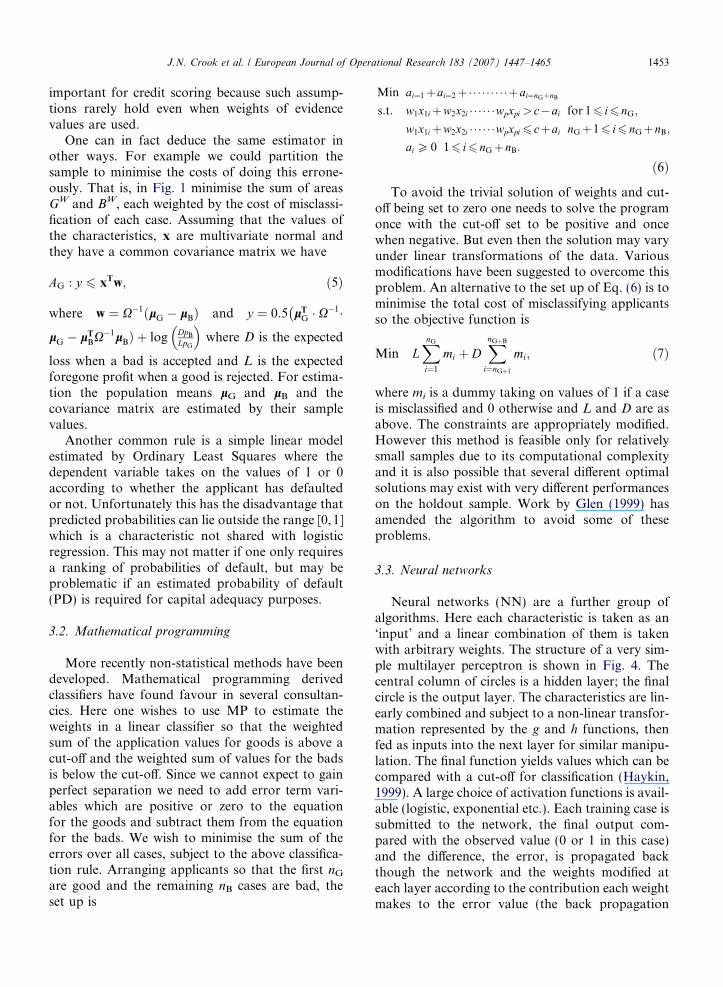
To avoid the trivial solution of weights and cut-off being set to zero one needs to solve the programonce with the cut-off set to be positive and oncewhen negative. But even then the solution may varyunder linear transformations of the data. Variousmodifications have been suggested to overcome thisproblem. An alternative to the set up of Eq. (6) is tominimise the total cost of misclassifying applicantsso the objective function is

Min LXnG

i¼1

mi þ DXnGþB

i¼nGþ1

mi; ð7Þ

where mi is a dummy taking on values of 1 if a caseis misclassified and 0 otherwise and L and D are asabove. The constraints are appropriately modified.However this method is feasible only for relativelysmall samples due to its computational complexityand it is also possible that several different optimalsolutions may exist with very different performanceson the holdout sample. Work by Glen (1999) hasamended the algorithm to avoid some of theseproblems.

3.3. Neural networks

Neural networks (NN) are a further group ofalgorithms. Here each characteristic is taken as an‘input’ and a linear combination of them is takenwith arbitrary weights. The structure of a very sim-ple multilayer perceptron is shown in Fig. 4. Thecentral column of circles is a hidden layer; the finalcircle is the output layer. The characteristics are lin-early combined and subject to a non-linear transfor-mation represented by the g and h functions, thenfed as inputs into the next layer for similar manipu-lation. The final function yields values which can becompared with a cut-off for classification (Haykin,1999). A large choice of activation functions is avail-able (logistic, exponential etc.). Each training case issubmitted to the network, the final output com-pared with the observed value (0 or 1 in this case)and the difference, the error, is propagated backthough the network and the weights modified ateach layer according to the contribution each weightmakes to the error value (the back propagation

.

.

.

.

.

.

.

.

.

.

.

w11

w21

W22

w12k1

k2

k q

X1

Age

X2

Income

Xp

Years at address

f1=exp(wTX+c1)

z=exp(kTf+d)

Good/Bad

f2=exp(wTX+c2)

fq=exp(wTX+c)

Input layer Hidden layer Output layer p neurons q neurons

Fig. 4. A two layer neural network.

1454 J.N. Crook et al. / European Journal of Operational Research 183 (2007) 1447–1465

algorithm). In essence the network takes data incharacteristics space, transforms it using the weightsand activation functions into hidden value space(the ‘g’ values) and then possibly into further hiddenvalue space, if further layers exist, and eventuallyinto output layer space which is linearly separable.In principle only one hidden layer is needed to sep-arate non-linearly separable data and only two hid-den layers are needed to separate data where theobservations are is in distinct and separate regions.Neural networks have a weakness when used toscore credit applicants: the resulting set of classifica-tion rules are not easily interpretable in terms of theoriginal input variables. This makes it difficult touse if, as is required in the US and UK, a rejectedapplicant is given a reason for being rejected. How-ever several algorithms are available that try toderive interpretable rules from a NN. These algo-rithms are generally of two types: decompositionaland pedagogical. The former take an estimated net-work and prune connections between neurons sub-ject to the difference in predictions between theoriginal network and the new one being within anaccepted tolerance. Pedagogical techniques estimatea simplified set of classification rules which is bothinterpretable and again gives acceptably similarclassifications as the original network. Neurolinearis an example of the first type and Trepan an exam-ple of the second. Baesens (2003) finds that theseapproaches can be successful. Of course there isno need to explain the outcomes when the networkis being used to detect fraud and whilst networks

have been and are used by consultancies for applica-tion scoring it is fraud scoring where arguably theyhave been most commonly used.

3.4. Other classifiers

A similar type of classifier uses fuzzy rather thancrisp rules to discriminate between classes. A crisprule is one which precisely defines a membership cri-terion (for example ‘‘poor’’ if income is less than$10 k) whereas a fuzzy rule allows membership cri-teria to be less precisely defined with membershipdepending possibly on several other less preciselydefined criteria. The predictive accuracy of fuzzyrule extraction techniques applied to credit scoringdata has been mixed relative to other classifiers.Baesens (2003) finds their performance to be poorerbut not significantly so than linear discriminantanalysis (LDA), NN and decision trees. But (Piram-uthu, 1999) found the performance of fuzzy classifi-ers to be significantly worse than NN when appliedto credit data.

Classification trees are another type of classifier.Here a characteristic is chosen and one splits theset of attributes into two classes that best separatethe goods from the bads. Each case is ascribed toone branch of the classification tree. Each subclassis again divided according to the attribute value ofa characteristic that again gives the best separationbetween the goods and bads in that sub-sample ornode. The sample splitting continues until few casesremain in each branch or the difference in good rate

J.N. Crook et al. / European Journal of Operational Research 183 (2007) 1447–1465 1455

between the subsets after splitting is small. This pro-cess is also called the Recursive Partitioning Algo-rithm. The tree is then pruned back until theresulting splits are thought to give an acceptableclassification performance in the population. Vari-ous statistics have been used to evaluate how wellthe goods and bads are separated at the end ofany one branch and so which combination of attri-bute values to allocate to one branch rather than tothe other if the characteristic is a nominal one. Oneexample is the KS statistic described above.Another common statistic advocated by Quinlan(1963) is the entropy index defined as

IðxÞ ¼ �PðGjxÞln2ðPðGjxÞÞ� PðBjxÞln2ðP ðBjxÞÞ ð8Þ

which relates to the number of different ways onecould get the good–bad split in a node and so indi-cates the information contained in the split. Theanalyst must decide which splitting rule to use, whento stop pruning, and how to assign terminal nodesto good and bad categories.

Logistic regression is the most commonly usedtechnique in developing scorecards, but linearregression, mathematical programming, classifica-tion trees and neural networks have also been usedin practice. A number of other classification tech-niques such as genetic algorithms, support vectormachines (SVM) and nearest neighbours have beenpiloted but have not become established in theindustry.

Genetic methods have also been applied to creditdata. In a genetic algorithm (GA) a solution consist-ing of a string (or chromosome) of values (alleles)may represent, for each characteristic, whether acharacteristic enters the decision rule and a rangeof values that characteristic may take. This is repre-sented in binary form. Many candidate solutions areconsidered and a measure of the predictive accuracyor fitness is computed for each solution. From thissample of solutions a random sample is selectedwhere the probability of selection depends on the fit-ness. Genetic operators are applied. In crossover thefirst n digits of one solution are swapped with thelast n digits of another. In mutation specific allelesare flipped. The new children are put back intothe population. The fitness of each solution isrecomputed and the procedures repeated until a ter-mination condition is met. GAs make use of theSchemata theorem (Holland, 1968) that essentiallyshows that if the average fitness of a schemata is

above the average in the population of possiblesolutions then the expected number of strings inthe population with this schemata will increaseexponentially. GAs are optimisation algorithmsrather than a class of classifier and may be appliedas described or to optimise NNs, decision treesand so on. For example when GAs are applied toa decision tree mutation involves randomly replac-ing the branches from a node in a tree and crossoverinvolves swapping branches from a node in one treewith those in another tree (Ong et al., 2005).

Support vector machines (SVM) can be consid-ered as an extension of the mathematical program-ming approach but where the scorecard is aweighted linear combination of functions of thevariables not just a weighted linear combination ofthe variables themselves. The objective is for allthe goods to have ‘‘scores’’ greater than c + 1 andthe bads to have ‘‘scores’’ below c � 1 so that thereis a normalized gap of 2/kwk between the twogroups. The objective is also extended to minimizea combination of the size of the misclassificationerrors and the inverse of this gap. In fact, the algo-rithms work by solving the dual problem when thedual kernel is chosen to be of a certain form. Unfor-tunately one cannot invert this to obtain the corre-sponding primal functions and thus an explicitexpression for the scorecard.

Many other classifiers may be used to divideapplicants into good and bad classes. These includeK-nearest neighbour techniques and various Bayes-ian methods. Some comparisons can be madebetween the classifiers. LR, LDA, and MP are alllinear classifiers: in input space the classifying func-tion is linear. This is not so for quadratic discrimi-nant analysis, where the covariances of the inputvariables are not the same in the goods and bads,nor in NNs, SVMs or decision trees. Second, alltechniques require some parameter selection by theanalyst. For example, in LR it is the assumptionthat a logistic function will best separate the twoclasses, in NN the number of hidden layers, thetypes of activation function, the type of error func-tion, the number of epochs and so on; in trees itis the splitting and stopping criteria etc. Third, acommon approach to devising a non-linear classifieris to map data from input space into a higherdimensional feature space. This is done with leastrestrictions in SVMs but is also done in NNs. Fur-thermore several researchers have experimentedwith combining classifiers. For example (Schebeschand Stecking, 2005) have used SVMs to select cases

1456 J.N. Crook et al. / European Journal of Operational Research 183 (2007) 1447–1465

(the support vectors) to present to a LDA. Othershave used trees to select variables to use in a LR.Yet others have used a stepwise routine in LDAto select the variables for inclusion in a NN (Leeet al., 2002)). Kao and Chiu (2001) have combineddecision trees and NNs.

Whilst many comparisons of the predictive per-formance of these classifiers have been made rela-tively few have been conducted using consumercredit data and it is possible that the data structuresin application data are more amenable to one typeof classifier rather than to others. Table 2 gives acomparison of published results, although cautionis required since the table shows only the error rate,the papers differ in how the cut-off was set, theerrors are not weighted according to the relativecosts of misclassifying a bad and a good and fewpapers use inferential tests to see if the differencesare significant. For these reasons the figures canonly be compared across a row not between studies.For example Henley’s results show a much lowerproportion correctly classified because the propor-tion of defaults in his sample was very different fromthat in other studies. Nevertheless it would seemfrom the table that SVMs when included do per-form better than other classifiers, a result that isconsistent with comparisons using data from othercontexts. Neural networks also perform well as wewould expect bearing in mind that a NN with alogistic activation function encompasses a LRmodel. Given that small improvements in classifica-tion accuracy results in millions of dollars of addi-tional profits attempts to increase accuracy bydevising new algorithms is likely to continue.

However (Hand, 2006) argues that the relativeperformances illustrated in comparisons like Table2 overemphasise the likely differences in predictiveperformance when classifiers are used in practice.One reason is associated with sampling issues. Overtime ‘‘population drift’’ occurs whereby changes inp(Gjx) occur due, in the case of LDA to changesin p(G) or p(xjG), or in the case of LR to changes,not in the parameters of the model, but to changesin the distributions of variables not included in themodel but which affect the posterior probability.Another reason is that the training sample maynot represent the population of all applicants, aswe explain below in Section 4. Further, since thedefinitions of ‘‘good’’ and ‘‘bad’’ which are usedare arbitrary, they may change between the timethe scorecard was developed and the time when itis implemented. A model which performs well rela-

tive to other classifiers on one definition may per-form relatively less well on another. Moreovereach classifier typically optimizes a measure of fit(for example maximum likelihood in the case ofLR) but its performance in practice may be judgedby a very different criterion, for example cost-weighted error rates, for which there are many pos-sibilities. So the relative performances of classifiersmay differ according to the fitness measure used inpractice.

3.5. Comparisons with corporate risk models

The methods used to predict the probability ofdefault for individuals that we have considered sofar may be contrasted with those applied in the cor-porate sector. One can distinguish between the riskof lending or extending a facility to an individualcompany and the collective risk of lending to a port-folio of companies. (A corresponding separationapplies to loans to individuals). For the former anumber of credit rating agencies offer opinions asto the credit worthiness of lending to large quotedcompanies which are typically indicated by analphabetic ordinal scale, for example S&P’s scaleof \AAA"; \AA" . . . \CCC" labels. Different agencies’scales often have different meanings. Moody’s scaleindicates a view of likely expected loss (includingPD and loss given default) of extending a facilitywhereas S&P’s scale reflects an opinion about thePD of an issuer across all of its loans. The detailsof the methods used to construct a scale are proprie-tary, however they involve both quantitative analy-ses of financial ratios and reviews of the competitiveenvironment, including regulations and actions ofcompetitors and also internal factors such as mana-gerial quality and strategies. The senior manage-ment of the firm to be rated is consulted and acommittee within the agency would discuss its pro-posed opinion before it is made public.

Although there are monotonic relationshipsbetween PDs and ordinal risk categories the riskcategory is not supposed to indicate a precise PDfor a borrower. Some agencies try to produce a clas-sification which is invariant through a business cycleunless a major deterioration in the credit worthinessof the firm is detected, (but in practice some varia-tion through the cycle is apparent (De Servignyand Renault, 2004)), while others give ratings whichreflect the point in time credit risk.

An alternative approach, which is typified byKMV’s Credit Monitor, is to deduce the probability

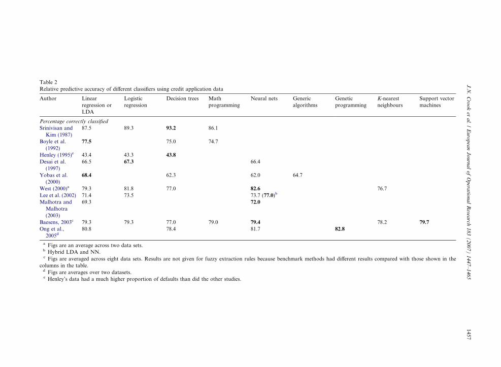
Table 2Relative predictive accuracy of different classifiers using credit application data

Author Linearregression orLDA

Logisticregression

Decision trees Mathprogramming

Neural nets Genericalgorithms

Geneticprogramming

K-nearestneighbours

Support vectormachines

Percentage correctly classified

Srinivisan andKim (1987)

87.5 89.3 93.2 86.1

Boyle et al.(1992)

77.5 75.0 74.7

Henley (1995)e 43.4 43.3 43.8

Desai et al.(1997)

66.5 67.3 66.4

Yobas et al.(2000)

68.4 62.3 62.0 64.7

West (2000)a 79.3 81.8 77.0 82.6 76.7Lee et al. (2002) 71.4 73.5 73.7 (77.0)b

Malhotra andMalhotra(2003)

69.3 72.0

Baesens, 2003c 79.3 79.3 77.0 79.0 79.4 78.2 79.7

Ong et al.,2005d

80.8 78.4 81.7 82.8

a Figs are an average across two data sets.b Hybrid LDA and NN.c Figs are averaged across eight data sets. Results are not given for fuzzy extraction rules because benchmark methods had different results compared with those shown in the

columns in the table.d Figs are averages over two datasets.e Henley’s data had a much higher proportion of defaults than did the other studies.

J.N

.C

roo

ket

al.

/E

uro

pea

nJ

ou

rna

lo

fO

pera

tiona

lR

esearch

18

3(

20

07

)1

44

7–

146

51457

1458 J.N. Crook et al. / European Journal of Operational Research 183 (2007) 1447–1465

of default from a variant of Merton’s (1974) modelof debt pricing. This type of model is called a ‘‘struc-tural model’’. The essential idea is that a firm willdefault on its debt if the debt outstanding exceedsthe value of the firm. When a firm issues debt theequity holders essentially give the firm’s assets tothe debt holders but have an option to buy theassets back by paying off the debt at a future date.If the value of the assets rises above the value ofthe debt the equity holders gain all of this excess.So the payoff to the equity holders is like a payofffrom a call option on the value of the firm at a strikeprice of the repayment amount of the debt. Mertonmakes many assumptions including that the value ofthe firm follows a Brownian motion process. Using(Black and Scholes, 1973) option pricing model thePD of the bond can be recovered. Whilst in Mertonthe PDs follow a cumulative normal distribution,PD ¼ N�1ðDDÞ where DD is distance to default,this is not assumed in KMV Credit Monitor whereDD is mapped to a default probability using a pro-prietary frequency distribution over DD values.

For non-quoted companies the market value ofthe firm is unavailable and the Merton model can-not be used. Then, corporate risk modelers oftenresort to methods used to model consumer creditas described in the last few sections.

4. Reject inference

A possible concern for credit risk modelers is thatwe want a model that will classify new applicantsbut we can only train on a sample of applicants thatwere accepted and who took up the offer of credit.The repayment performance of the rejected casesis missing. There are two possible problems here.First, the possibility that the parameters of such amodel may be biased estimates of those for theintended population arises. Second, without know-ing the distribution of goods and bads in the appli-cant population one cannot know the predictiveperformance of the new model on this population.

The first problem is related to Rubin’s classifica-tion of missing data mechanisms (Little and Rubin,1987). The two types of missing data mechanismsthat are relevant here are missing at random(MAR) and missing not at random (MNAR). Inthe MAR case the mechanism that causes the datato be missing is not related to the variable of inter-est. MNAR occurs when the missingness mecha-nism is closely related to the variable of interest.So if D denotes default, A denotes whether an appli-

cant was accepted, P(D) is to be predicted using pre-dictor variables X1 and we may try to explain P ðAÞin terms of X2, we can write:

P ðDjX1Þ ¼ P ðDjX1;A ¼ 1Þ � P ðA ¼ 1jX2Þþ P ðDjX1;A ¼ 0Þ � P ðA ¼ 0jX2Þ: ð9Þ

In MAR PðDjX1;A ¼ 1Þ ¼ P ðDjX1;A ¼ 0Þ soP ðDjX1Þ ¼ P ðDjX1;A ¼ 1Þ whereas in MNARP ðDjX1;A ¼ 1Þ 6¼ ðDjX1;A ¼ 0Þ and the sample ofaccepted applicants will give biased estimates ofthe population parameters. Hand and Henley(1994) have shown that if the X1 set encompassesthe original variables used to accept or reject appli-cants we have MAR, otherwise we have MNAR. Ifwe have MAR then a classifier like LR, NNets, andSVMs which do not make distributional assump-tions will yield unbiased estimates.

Researchers have experimented with several pos-sible ways of incorporating rejected cases in the esti-mation of a model applicable to all applicants.These have included the EM algorithm (Feelders,2000), and multiple imputation, but these togetherwith imputation by Markov Chain Monte Carlosimulation have usually assumed the missingnessmechanism is MAR when it is not known if this isthe case. If it is the case then such procedures willnot correct for bias since none would be expected.However if we face MNAR then we need to modelthe missingness mechanism. An example of this pro-cedure is Heckman’s two stage sample selectionmodel (Heckman, 1979).

In practice a weighting procedure known as aug-mentation (or variants of it) is used. Augmentationinvolves two stages. In the first stage one estimatesP ðAjX2Þ using an ex post classifier and the sampleof all applicants including those rejected. PðAjX2Þis then predicted for those previously accepted casesand each is ascribed a ‘‘sampling’’ weight of1=PðAjX2Þ in the final LR. Thus each accepted caserepresents 1=PðAjX2Þ cases and it is assumed that ateach P ðAjX2Þ value P ðDjX1, A ¼ 1Þ ¼ P ðDjX1;A ¼ 0Þ. That is, the proportion of goods at thatvalue of P ðAjX2Þ amongst the accepts equals thatamongst the rejects, and so the accepts at this levelof P ðAjX2Þ can be weighted up to represent the dis-tribution of goods and bads at that level of P ðAjX2Þin the applicant population as a whole.

An alternative possible solution is to use a vari-ant of Heckman’s sample selection method wherebyone estimates a bivariate probit model with selec-tion (BVP) which models the probability of default

PA

B

1 – FB(s) pB

Expected Bad Rate

0 1 – F(s) 0.95 1.0Acceptance Rate

Fig. 5. The strategy curve.

Expectedlosses

Expected Profit

Fig. 6. The efficiency curve.

J.N. Crook et al. / European Journal of Operational Research 183 (2007) 1447–1465 1459

and the probability of acceptance allowing for thefact that observed default is missing for those notaccepted (Crook and Banasik, 2003). However thismethod has several weaknesses including theassumption that the residuals for the two equationsare bivariate normal and that they are correlated.The last requirement prevents its use if the originalaccept model can be perfectly replicated.

There is little empirical evidence on the size ofthis possible bias because its evaluation dependson access to a sample where all those who appliedwere accepted and this is very rarely done by lend-ers. However a few studies have access to a samplewhich almost fits this requirement and they find thatthe magnitude of the bias and so scope for correc-tion is very small. Experimentation has shown thatthe size of the bias increases monotonically if thecut-off used on the legacy scoring model increasesand the accept rate decreases (Crook and Banasik,2004). Using the training sample rather than an allapplicant sample as holdout leads to a considerableoverestimate of a model’s performance, particularlyat high original cut-offs. Augmentation has beenfound to actually reduce performance comparedwith using LR for accepted cases only. Recent work,some of which is reported on in this issue, investi-gates combining both the BVP and augmentationapproaches, altering the BVP approach so that therestrictive distributional assumptions about theerror terms are relaxed and uses branch and boundalgorithms.

5. Profit scoring

Since the mid 1990s a new strand of research hasexplored various ways in which scorecards may beused to maximize profit. Much of this work is pro-prietary, but many significant contributions to theliterature have also been made. One active area con-cerns cut-off strategy. In a series of path breakingpapers Oliver and colleagues (Marshall and Oliver,1993; Hoadley and Oliver, 1998; Oliver and Wells,2001) have formulated the problem as follows. Fora given scoring model one can plot the expectedbad rate (i.e. the expected proportion of all acceptsthat turn out to be bad or ð1� F ðsÞÞpB where F(s) isthe proportion of applicants with a score less than s)against the acceptance rate (i.e. the proportion ofapplicants that are accepted or ð1� F ðsÞÞÞ. This isshown in Fig. 5 and is called a strategy curve. A per-fectly discriminating model will, as the cut-off scoreincreases, accept all goods amongst those that apply

and then accept only bads. In Fig. 5 if it is assumedthat 95% of applicants are good, the perfect score-card is represented by the straight line along thehorizontal axis until the accept rate is 95%, there-after the curve slopes up at 45�. A replacement scor-ing model may be represented by the dotted line.The bank may currently be at point P and the bankhas a choice of increasing the acceptance rate whilstmaintaining the current expected bad rate (A) orkeeping the current acceptance rate and decreasingthe expected bad rate (B), or somewhere in between.The coordinates of all of these points can be calcu-lated from parameters yielded by the estimation ofthe scorecard.

One can go further and plot expected lossesagainst expected profits (Fig. 6). For a given scoringmodel as one lowers the cut-off an increasing pro-portion of accepts are bad. Given that the loss froman accepted bad is many times greater than theprofit to be made from a good, this reduction incut-off at first increases profits and the expected loss,but eventually the increase in loss from the everincreasing proportion of bads outweighs theincrease in profits and profits fall. Now, the bankwill wish to be on the lower portion of the curve

1460 J.N. Crook et al. / European Journal of Operational Research 183 (2007) 1447–1465

which is called the efficiency frontier. The bank maynow find its current position and, by choice of cut-off and adoption of the new model, decide where onthe efficiency frontier of a new model it wishes tolocate: whether to maintain expected losses andincrease expected profits or maintain expected profitand reduce expected losses. Oliver and Wells (2001)derive a condition for maximum profits which is,unsurprisingly that the odds of being good equalthe ratio of the loss from a bad divided by the gainfrom a good (D/L). Interestingly, an expression forthe efficiency frontier can be gained by solving thenon-linear problem of minimizing expected loss sub-ject to expected profits being at least a certain valueP0. The implied cutoff is then expressed as H�1 P 0

L�pg

where H is an expression for expected profits andall values can be derived from a parameterized scor-ing model.

So far the efficiency frontier model has omittedinterest expense on funds borrowed, operating costsand the costs of holding regulatory capital asrequired under Basel 2. In ongoing work the modelhas been amended by Oliver and Thomas (2005) byincorporating these elements into the profit func-tion. They show that for a risk neutral bank therequirements of Basel 2 unambiguously increasethe cut-off score for any scorecard and so reducethe number of loans made compared with no mini-mum capital requirement.

Some recent theoretical models of bank lendinghave turned their attention to more general objec-tives of a bank than merely expected profit. Forexample Keeney and Oliver (2005) have consideredthe optimal characteristics of a loan offer from thepoint of view of a lender, given that the utility ofthe lender depends positively on expected profitand on market share. The lender’s expected profitdepends on the interest rate and on the amount ofthe loan made to a potential borrower. To maximizethis utility a lender has to consider the effects ofboth arguments on the probability that a potentialborrower will take a loan offered and so on marketshare. The utility of a potential borrower is assumedto depend positively on the loan amount and nega-tively on the interest rate. It is also cruciallyassumed that as the interest rate and amount bor-rowed increase, whilst keeping the borrower at thesame level of utility and so market share, theexpected profits of the lender increase, reach a max-imum and then decrease. By comparing the maxi-mum expected profit at each utility level the lendercan work out the combination of interest and loan

amount to offer to minimize its expected profit.Because levels of the interest rate have the oppositeeffects for a borrower and a lender, as one increasesthis rate and reduces the loan amount the probabil-ity of acceptance and so market share goes downwhilst at first expected profits rise. The lender hasto choose the combination of market share andexpected profit it desires and then compute theinterest rate and loan amount to offer to the appli-cant to achieve this. Notice however some limita-tions of this model. First it assumes that there isonly one lender, since the probability of acceptanceis not made dependent on the offers made by rivallenders. Second, the model omits learning by bothlender and potential borrower. Third, this is verydifficult to implement in practice since in principleone would need the utility function for every indi-vidual potential borrower.

This and associated models has spawned muchnew research. For example some progress has beenmade on finding the factors that affect the probabil-ity of acceptance. Seow and Thomas (2007) havepresented students with hypothetical offers of abank account and each potential borrower had adifferent set of (hypothetical) account characteristicsoffered to them. The aim was to find the applicantand account characteristics that maximized accep-tance probability. Unlike earlier work, by using aclassification tree in which offer characteristics var-ied according to the branch the applicant was on,this paper does not assume applicants have the sameutility function.

6. The Basel 2 accord

A major research agenda has developed from theBasel 2 Accord. The Basel Committee on Bankingand Supervision was set up in 1975 by the Governorsof the G10 most industrialised countries. It has noformal supervisory authority but it states supervi-sory guidelines and expects legal regulators in majoreconomies to implement them. The aims of theguidelines were to stabilize the international bankingsystem by setting standardised criteria for capitallevels and a common framework to facilitate fairbanking competition. The need for such standardswas perceived after major reorganisations in thebanking industry, certain financial crises and bankfailures, the very rapid development of new financialproducts and increased banking competition.

The first Basel accord (Basel, 1988), stated that abank’s capital had to exceed 8% of its risk weighted

J.N. Crook et al. / European Journal of Operational Research 183 (2007) 1447–1465 1461

assets. But the accord had many weaknesses (see DeServigny and Renault, 2004) and over the last sevenyears the BIS has issued several updated standardswhich have come to be known as the Basel 2 accord.It is due to be adopted from 2007-08. (Pillar 3 doesnot take effect until later.)

The Basel 2 Accord (Basel, 2005) states thatsound regulation consists of three ‘pillars’: mini-mum capital requirements, a Supervisory ReviewProcess and market discipline. We are concernedwith the first. Each bank has a choice of method itmay use to estimate values for the capital it needsto set aside. It may use a Standardised Approachin which it has to set aside 2.4% of the loan capitalfor mortgage loans and 6% for regulatory retailloans (to individuals or SMEs for revolving credit,lines of credit, personal loans and leases). Alterna-tively the bank may use Internal Ratings Basedapproaches, in which case parameters are estimatedby the bank. Notice that if a bank adopts an IRBfor, say, its corporate exposures it must do so forall types of exposures. The attraction of the IRBapproach over the Standardised Approach is thatthe former may enable a bank to have less capitaland so earn higher returns on equity than the latter.Therefore it is likely that most large banks willadopt the IRB approach.

Under the IRB approach a bank must retain cap-ital to cover both expected and unexpected losses.Expected losses are to be built into the calculationof profitability that underlie the pricing of the prod-uct, and so covered by these profits. The unexpectedlosses are what the regulatory capital seeks to cover.For each type of retail exposure that is not indefault the regulatory capital requirement, k, is cal-culated as

k ¼ LGD� N

"1ffiffiffiffiffiffiffiffiffiffiffiffi

1� Rp � N�1ðPDÞ

þffiffiffiffiffiffiffiffiffiffiffiffi

R1� R

r� N�1ð0:999Þ

#� PD� LGD; ð10Þ

where LGD is loss given default (the proportion ofan exposure which, if in default, would not be recov-ered); N is the cumulative distribution for a stan-dard normal random variable; N�1 is inverse of N;R is the correlation between the performance of dif-ferent exposures; and PD is the probability of de-fault. R is set at 0.15 for mortgage loans, at 0.04for revolving, unsecured exposures to individualsup to €100 k, and

R ¼ 0:03� ð1� expð�35� PDÞð1� expð�35ÞÞ

� �

þ 0:16� 1� 1� expð�35� PDÞ1� expð�35Þ

� � �ð11Þ

for other retail exposures.Intuitively the second term in Eq. (10) (involving

the square brackets) represents the probability thatthe PD lies between its predicted value and its99.9th percentile value. Its formal derivation isgiven in Schonbucher (2000) and Perli and Nayda(2004). The formula is derived by using the assump-tion that a firm will default when the value of itsassets falls below a threshold which is common forall firms. The value of the firm is standard normallydistributed and, crucially, the assets of all obligorsdepend on one common factor, and a random ele-ment which is particular to each firm. The thirdterm represents future margin income which couldbe used to reduce the capital required. This isincluded because the interest on each loan includesan element to cover for losses on defaulted loansand this can be used to cover losses before the bankwould need to use its capital. The size of this incomeis estimated as the expected loss.

For each type of exposure the bank has to divideits loans into ‘risk buckets’ i.e. groups which differin terms of the group’s PD but within which PDsare similar. When allocating a loan to a group thebank must take into account borrower risk variables(sociodemographics etc.), transaction risk variables(aspects of collateral) and whether the loan is cur-rently delinquent. To allocate loans into groupsbehavioural scoring models may be used with possi-ble overrides. The PD value for each group has tobe valid over a five year period to cover a businesscycle. For retail exposures several methods to esti-mate the PD of each pool are available but mostbanks will use a behavioural scoring model.

The Basel 2 Accord has led to many new lines ofresearch. The first issue is the appropriateness of theone factor model to estimate unexpected loss of arisk group for consumer debt since this model wasoriginally devised for corporate default. AlthoughPerli and Nayda (2004) build such a consumermodel several authors have questioned the plausibil-ity of a household defaulting on unsecured debt ifthe value of the household’s assets dip below athreshold. Instead new models involving reputa-tional assets and jump process models have beentried. De Andrade and Thomas (2007) assume thata borrower will default when his reputation dips

1462 J.N. Crook et al. / European Journal of Operational Research 183 (2007) 1447–1465

below a threshold. His reputation is a function of alatent unobserved variable representing his creditworthiness.

A second topic of research is the assumed param-eter values in the Basel formula, specifically theassumed correlation values. De Andrade and Tho-mas found that the calculated correlation coefficientfor ‘other retail exposures’ for a sample of Braziliandata was 2.28% which is lower than the correlationrange of 3% in Basel 2. Lopez (2002) found the cor-relation between asset sizes to be negatively relatedto default probability for firms, which is the oppo-site of the relationship implied by Eq. (11), and tobe positively related to firm size which is notincluded in Eq. (11).

A third source of research is how to estimate PDsfrom portfolios with very low default proportions.In very low risk groups, especially in mortgage port-folios, very few, sometimes no defaults, areobserved. Estimating the average PD in such agroup as close to zero would not reflect the conser-vatism implied by Basel 2. Pluto and Tasche (2005)assume the analyst knows at least the rating gradeinto which a borrower fits and calculates confidenceintervals so that by adopting a ‘most prudent esti-mation principle’ PD estimates can be made whichare monotone in the risk groups. For example con-sider the case of no defaults. Three groups, i = 1,2,3in decreasing order of risk each have n1, n2 and n3

cases respectively. The group risk ordering impliesP 1 6 P 2 6 P 3. The most prudent estimate of P1

implies P 1 ¼ P 2 ¼ P 3. Assuming independence ofdefaults the probability of observing zero defaultsis ð1� P 1Þn1þn2þn3 and the confidence region at levelc for P1 is such that P 1 6 1� ð1� cÞn1þn2þn3. At a99.9% confidence level, P1 = 0.86%. By similar rea-soning the most prudent value of P2 is P 2 ¼ P 3 andthe upper boundary may be calculated (at 99.9% itis 0.98%). The difference in values is a consequenceof the number of cases. In the case of a few defaultsand assuming the number of defaults follows a bino-mial distribution, the upper confidence interval canalso be calculated. Pluto and Tasche extend the cal-culations using a one factor probit model to find theconfidence interval for the PD when asset returnsare correlated. This increases the PDs considerablyand the new probabilities under the same assump-tions as above were P1 = 5.3%, P2 = 5.8% andP3 = 9.8%.

Forrest (2005) adopted a similar approach of cal-culating the 95%ile of the default distribution. Butunlike Pluto and Tasche he calculated the PD as

the value that maximises the likelihood of observingthe actual number of defaults. So for a portfolioconsisting of two grades, A with a higher PD thanB and da defaults and ð1� daÞ exposures, and Bwith db defaults and ð1� dbÞ exposures, and lettingPA and PB indicate their respective PDs, PA and PB

can be calculated by choosing their values tomaximise

Likelihood LðP A;P BÞ¼ P daA ð1�P AÞ1�da P db

B ð1�P BÞ1�db

ð12Þ

constrained so that P A > P B.A further issue is how to validate estimates of

PDs, LGDs and EADs. The application and behav-ioural scoring models outlined in Section 2 arerequired to provide only an ordinal ranking of caseswhereas ratio level values are required for Basel 2compliance. Validation of PDs has two aspects; dis-criminatory power, which refers to the degree ofseparation of the distributions of scores betweengroups, and calibration which refers to the accuracyof the PDs. We considered the former in an earliersection; here we consider the latter. The crucial issueis how to test whether the size of the differencebetween estimated ex ante PDs and ex post observeddefault rates is significant. Several tests have beenconsidered by the BIS Research Task Force (2005)(BISTF) as follows. The test is required for each riskpool. The binomial test, which assumes the defaultevents within the risk group are independent, teststhe null hypothesis the PD is underestimated.Although the BISTF argue that empirically esti-mated correlation coefficients between defaultswithin a risk group are around 0.5–3% they assessthe implications of different asset correlations byreworking the one factor model with this assump-tion. They find that when the returns are correlated,an unadjusted binomial test will be too conserva-tive: it will reject the null when the correct probabil-ity of doing so is in fact much lower than intended.The BISTF reports that a chi-square test could beused to test the same hypotheses as the binomial testbut is applied to the portfolio as a whole (i.e. to allrisk groups) to circumvent the well known problemthat multiple tests would be expected to indicate arejection of the null in 5% of cases. But again ithas the same problems as the binomial test whendefaults are correlated. The normal test allows forcorrelated defaults and uses the property that thedistribution of the standardised sum of differencesbetween the observed default rate in each year and

J.N. Crook et al. / European Journal of Operational Research 183 (2007) 1447–1465 1463

the predicted probability is normally distributed.The null is that ‘none of the true probabilities ofdefault in the years t ¼ 1; 2; . . . ; T is greater thanthe forecast P t’. However the BISTF find the testhas conservative bias: in too many cases the null isrejected. A further test is proposed by Blochwitzet al. (2004) and called the ‘traffic lights test’. Ignor-ing dependency in credit scores over t, the distribu-tion of the number of defaults is assumed to followa multinomial distribution over four categorieslabelled ‘green’, ‘yellow’, ‘orange’, and ‘red’. Theprobability that a linear combination of the numberof defaults in each category exceeds a critical valueis used to test the null that ‘none of the true proba-bilities of default in years t ¼ 1; 2; . . . ; T is greaterthan the corresponding forecast PDt’. Running sim-ulation tests the BISTF find the test is ratherconservative.

After comparisons of these four inferential teststatistics the BISTF concluded that currently ‘noreally powerful tests of adequate calibre are cur-rently available’ and call for more research.

7. Conclusion

In this paper we have reviewed a selection of cur-rent research topics in consumer credit risk assess-ment. Credit scoring is central to this process andinvolves deriving a prediction of the risk associatedwith making a loan. The commonest method of esti-mating a classifier of applicants into those likely torepay and those unlikely to repay is logistic regres-sion with the logit value compared with a cut off.Many alternative classifiers have been developed inthe last thirty years and the evidence suggests thatthe most accurate is likely to be support vectormachines although much more evidence is neededto confirm this tentative view. Behavioural scoringinvolves the same principles as application scoringbut now the analyst has evidence on the behaviourof the borrower with the lender and the scores areestimated after the loan product has been takenand so updated risk estimates can be made as theborrower services his account. Initial concerns thatthe estimation of classifiers based on only acceptedapplicants and not on a random sample of the pop-ulation of applicants seem to be rather over placed,but using applicants only to assess the predictiveperformance of a classifier does appear likely to leadto significant over optimism as to a predictor’s per-formance. Scoring for profit is a major research ini-tiative and has led to some important tools which

have been employed by consultancies over the lastfew years. Arguably the most significant factorimpacting on consumer credit scoring processes isthe passing of the Basel 2 accord. This has deter-mined the way in which banks in major countriescalculate their reserve capital. The amount dependson the use of updated scoring models to estimate theprobability of default and other methods to estimatethe loss given default and amount owing at default.The method is based on a one factor Merton modelbut has been subject to major criticisms. The effectof Basel 2 on the competitive advantage of an insti-tution is so large that research into the adequacy,applicability and validity of the adopted models isset to be a major research initiative in the foresee-able future.

There are many topics that we do not have spacein this paper to consider (see Thomas et al. (2002)for further details). Consumer credit scoring is alsoused to decide to whom to make a direct mailshot, itis used by government agencies (for example taxauthorities) when deciding who is likely to paydebts, it is used by utilities when deciding whetherto allow consumers to use electricity/gas etc. inadvance of payment. A major use of scoring tech-niques is in assessing small business loan applica-tions and their monitoring for credit limitadjustment, but this topic alone would fill a com-plete review paper.

Credit scoring and risk assessment has been oneof the most successful applications of statisticaland operational research concepts ever with consid-erable social implications. It has made practical theassessment and granting of hundreds of millions ofcredit card applications and applications for otherloan products and so it has considerably improvedthe lifestyles of millions of people throughout theworld. It has considerably increased competitionin credit markets and arguably reduced the cost ofborrowing to many. The techniques developed havebeen applied in a wide variety of decision makingcontexts so reducing costs to those who present min-imal risk to lenders.

References

Anderson, T.W., Goodman, L.A., 1957. Statistical inferenceabout Markov chains. Annals of Mathematical Statistics 28,89–110.

Baesens, B., 2003. Developing Intelligent Systems for CreditScoring Using Machine Learning Techniques, DoctoralThesis no 180 Faculteit Economische en Toegepaste Eco-nomische Wetebnschappen, Katholieke Universiteit, Leuven.

1464 J.N. Crook et al. / European Journal of Operational Research 183 (2007) 1447–1465

Basel, 1988. Basel Committee on Banking Supervision: Interna-tional Convergence of Capital Measurement and CapitalStandards. Bank for International Settlements, July 1988.

Basel, 2005. Basel Committee on Banking Supervision: Interna-tional Convergence of Capital Measurement and CapitalStandards: A Revised Framework. Bank for InternationalSettlements, November 2005.

Black, F., Scholes, M., 1973. The pricing of options andcorporate liabilities. Journal of Political Economy 81, 637–659.

Blochwitz, S., Hohl, S.D., Tasche, D., When, C.S., 2004.Validating Default Probabilities in Short Times Series.Mimeo, Deutsche Bundesbank.

Boyle, M., Crook, J.N., Hamilton, R., Thomas, L.C., 1992.Methods for credit scoring applied to slow payers. In:Thomas, L.C., Crook, J.N., Edelman, D.E. (Eds.), CreditScoring and Credit Control. Oxford University Press, Oxford.

Crook, J.N., Banasik, J., 2003. Sample selection bias in creditscoring models. Journal of the Operational Research Society54, 822–832.

Crook, J., Banasik, J., 2004. Does reject inference really improvethe performance of application scoring models? Journal ofBanking and Finance 28 857–874.

Cyert, R.M., Thompson, G.L., 1968. Selecting a portfolio of creditrisks by Markov chains. The Journal of Business 1, 39–46.

De Andrade, F.W.M., Thomas, L.C., 2007. Structural models inconsumer credit. European Journal of Operational Research,this issue, doi:10.1016/j.ejor.2006.07.049.

Desai, V.S., Conway, D.G., Crook, J.N., Overstreet, G.A., 1997.Credit scoring models in the credit union environment usingneural networks and genetic algorithms. IMA Journal ofMathematics Applied in Business and Industry 8, 323–346.

De Servigny, A., Renault, O., 2004. Measuring and ManagingCredit Risk. McGraw Hill, New York.

Durand, D., 1941. Risk Elements in Consumer InstalmentFinancing. National Bureau of Economic Research, NewYork.

Feelders, A.J., 2000. Credit scoring and reject inference withmixture models. International Journal of Intelligent Systemsin Accounting, Finance and Management 9, 1–8.

Fisher, R.A., 1936. The use of multiple measurements intaxonomic problems. Annals of Eugenics 7, 179–188.

Forrest, A., 2005. Low Default Portfolios – Theory and Practice.Presentation to Credit Scoring and Credit Control 9 confer-ence, Edinburgh, 7–9 September 2005.

Frydman, H., 1984. Maximum likelihood estimation in theMover–Stayer model. Journal of the American StatisticalAssociation 79, 632–638.

Glen, J., 1999. Integer programming models for normalisationand variable selection in mathematical programming modelsfor discriminant analysis. Journal of the OperationalResearch Society 50, 1043–1053.

Hand, D.J., 2005. Good practice in retail credit scorecardassessment. Journal of the Operational Research Society 56(9), September.

Hand, D.J., 2006. Classifier technology and the illusion ofprogress. Statistical Science 21, 1–14.

Hand, D.J., Henley, W.E., 1994. Inference about rejected cases indiscriminant analysis. In: Diday, E., Lechvallier, Y., Schader,P., Bertrand, P., Buntschy, B. (Eds.), New Approaches inClassification and Data Analysis. Springer-Verlag, Berlin,pp. 292–299.

Hand, D.J., Henley, W.E., 1997. Statistical classification methodsin consumer credit scoring: A review. Journal of the RoyalStatistical Society, Series A 160, 523–541.

Haykin, S., 1999. Neural Networks: A Comprehensive Founda-tion. Prentice Hall, New-Jersey.

Heckman, J.J., 1979. Sample selection bias as a specificationproblem. Econometrica 47, 153–161.

Henley, W.E., 1995. Statistical Aspects of Credit Scoring. Ph.D.thesis, Open University.

Hoadley, B., Oliver, R.M., 1998. Business measures of scorecardbenefit. IMA Journal of Mathematics Applied in Businessand Industry 9, 55–64.

Ho, J., Thomas, L.C., Pomroy, T.A., Scherer, W.T., 2004.Segmentation in Markov Chain consumer credit behaviouralmodels. In: Thomas, L.C., Edelman, D., Crook, J.N. (Eds.),Readings in Credit Scoring. Oxford University Press, Oxford.

Holland, J.H., 1968. Hierarchical Description of Universal andAdaptive Systems, Department of Computer and Communi-cations Sciences. University of Michigan, Ann Arbor.

Kao, L.J., Chiu, C.C., 2001. Mining the customer credit by usingthe neural network model with classification and regression.In: Joint 9th IFSA World Congress and 20th NAFIPSInternational Conference, Proceedings, vols. 1–5, pp. 923–928.

Keeney, R.L., Oliver, R.M., 2005. Designing win–win financialloan products for consumers and businesses. Journal of theOperational Research Society 56 (9), September.

Lee, T.S., Chiu, C.C., Lu, C.J., Chen, I.F., 2002. Credit scoringusing the hybrid neural discriminant technique. ExpertSystems with Applications 23, 245–254.

Lewis, E., 1992. Introduction to Credit Scoring. The AthenaPress, San Rafael.

Little, R.J., Rubin, D.B., 1987. Statistical Analysis with MissingData. Wiley, New York.

Lopez, J., 2002. The Empirical Relationship Between AverageAsset Correlation, Firm Probability Of Default And AssetSize. Working Paper, Federal Reserve Bank of San Francisco.

Malhotra, R., Malhotra, D.K., 2003. Evaluating consumer loansusing neural networks. Omega 31, 83–96.

Marshall, K.T., Oliver, R.M., 1993. Decision Making andForecasting. McGraw-Hill, New York, pp. 121–128.

Oliver, R.M., Thomas, L.C., 2005. How Basel Will AffectOptimal Cut-offs Basel Capital Requirements. Presented atCredit Scoring and Credit Control 9 Conference, Edinburgh,September.

Oliver, R.M., Wells, E., 2001. Efficient frontier cut-off policies incredit portfolios. Journal of Operational Research Society 52,1025–1033.

Ong, C.S., Huang, J.J., Tzeng, G.H., 2005. Building creditscoring systems using genetic programming. Expert Systemswith Applications 29, 41–47.

Perli, R., Nayda, W.I., 2004. Economic and regulatory capitalallocation for revolving retail exposures. Journal of Bankingand Finance 28, 789–809.

Piramuthu, S., 1999. Financial credit-risk evaluation with neuraland neurofuzzy systems. European Journal of OperationalResearch 112, 310–321.

Pluto, K., Tasche, D., 2005. Estimating Probabilities for LowDefault Portfolios. Presented at Credit Scoring and CreditControl 9 Conference, Edinburgh, 2005.

Quinlan, J., 1963. C4. 5 Programs for Machine Learning.Morgan-Kaufman, San Mateo, CA.

J.N. Crook et al. / European Journal of Operational Research 183 (2007) 1447–1465 1465

Rosenberg, E., Gleit, A., 1994. Quantitative methods in creditmanagement: A survey. Operations Research 42, 589–613.

Schebesch, K.B., Stecking, R., 2005. Support vector machines forclassifying and describing credit applicants: Detecting typicaland critical regions. Journal of the Operational ResearchSociety 56, 1082–1088.

Schonbucher, P.J., 2000. Factor Models For Portfolio CreditRisk. Mimeo, Department of Statistics, Bonn University,December 2000.

Seow, H.-V., Thomas, L.C., 2007. To ask or not to ask, that is thequestion. European Journal of Operational Research, thisissue, doi:10.1016/j.ejor.2006.08.061.

Srinivisan, V., Kim, Y.H., 1987. Credit granting a comparativeanalysis of classificatory procedures. Journal of Finance 42,655–683.

Tasche, D., 2005. Rating and probability of default validation inBIS Research Task Force (2005) Basel Committee on BankingSupervision: Studies on the Validation of Internal Rating

Systems. Bank for International Settlements, Working PaperNo. 14, May 2005.

Thomas, L.C., 2000. A survey of credit and behavioural scoring:Forecasting financial risk of lending to consumers. Interna-tional Journal of Forecasting 16, 149–172.

Thomas, L.C., Edelman, D.B., Crook, J.N., 2002. Credit Scoringand its Applications. SIAM, Philadelphia.

Till, R., Hand, D., 2001. Markov Models in Consumer Credit.Presented at Credit Scoring and Credit Control 7 Conference,Edinburgh, September.

Trench, M.S., Pederson, S.P., Lau, E.T., Ma, L., Wang, H., Nair,S.K., 2003. Managing credit lines and prices for bank onecredit cards. Interfaces 33 (5), 4–21.

West, D., 2000. Neural network credit scoring models. Comput-ers and Operational Research 27, 1131–1152.

Yobas, M.B., Crook, J.N., Ross, P., 2000. Credit scoring usingneural and evolutionary techniques. IMA Journal of Math-ematics Applied in Business and Industry 11, 111–125.