Real-time forecasting at weekly timescales of the SST and SLA of the

Ligurian Sea with a satellite-based ocean forecasting (SOFT) system

A. AlvarezInstituto Mediterraneo de Estudios Avanzados (IMEDEA), CSIC-UIB, Esporles, Spain

A. OrfilaSchool of Civil and Environmental Engineering, Cornell University, Ithaca, New York, USA

J. TintoreInstituto Mediterraneo de Estudios Avanzados (IMEDEA), CSIC-UIB, Esporles, Spain

Received 25 April 2003; revised 17 October 2003; accepted 11 December 2003; published 16 March 2004.

[1] Satellites are the only systems able to provide continuous information on thespatiotemporal variability of vast areas of the ocean. Relatively long-term time series ofsatellite data are nowadays available. These spatiotemporal time series of satelliteobservations can be employed to build empirical models, called satellite-based oceanforecasting (SOFT) systems, to forecast certain aspects of future ocean states. SOFTsystems can predict satellite-observed fields at different timescales. The forecast skill ofSOFT systems forecasting the sea surface temperature (SST) at monthly timescales hasbeen extensively explored in previous works. In this work we study the performance oftwo SOFT systems forecasting, respectively, the SST and sea level anomaly (SLA) atweekly timescales, that is, providing forecasts of the weekly averaged SST and SLA fieldswith 1 week in advance. The SOFT systems were implemented in the Ligurian Sea(Western Mediterranean Sea). Predictions from the SOFT systems are compared withobservations and with the predictions obtained from persistence models. Results indicatethat the SOFT system forecasting the SST field is always superior in terms of predictabilityto persistence. Minimum prediction errors in the SST are obtained during winter andspring seasons. On the other hand, the biggest differences between the performance ofSOFT and persistence models are found during summer and autumn. These changes in thepredictability are explained on the basis of the particular variability of the SST field in theLigurian Sea. Concerning the SLA field, no improvements with respect to persistencehave been found for the SOFT system forecasting the SLA field. INDEX TERMS: 4263

Oceanography: General: Ocean prediction; 4275 Oceanography: General: Remote sensing and electromagnetic

processes (0689); 3220 Mathematical Geophysics: Nonlinear dynamics; 4899 Oceanography: Biological and

Chemical: General or miscellaneous; KEYWORDS: ocean prediction, operational oceanography, genetic

programming

Citation: Alvarez, A., A. Orfila, and J. Tintore (2004), Real-time forecasting at weekly timescales of the SST and SLA of the

Ligurian Sea with a satellite-based ocean forecasting (SOFT) system, J. Geophys. Res., 109, C03023, doi:10.1029/2003JC001929.

1. Introduction

[2] Predicting future states of a given physical systemconstitutes a central problem in science. Successful predic-tions are indicative that the employed predictive modelcaptures the fundamental dynamics that controls the systemevolution. Besides, predictions of some physical systemslike ocean and atmosphere have an added operationalinterest on human related activities.[3] The classic approach to carry out predictions is to

build an explanatory model from first physical principles.Usually, explanatory models are based on conservation laws

and have the form of one or more coupled partial differen-tial equations which describe the time evolution of relevantprocesses. Forward integration in time of the model iscarried out after measuring initial conditions. Unfortunately,the above forecasting approach is not always possible. Insome cases, such as in economy, there is the lack of firstprinciples necessary to make good models. In other cases,such as fluid systems, models are good but initial data aredifficult to obtain. In either case, resorting to alternativesapproaches is required.[4] Building predictive models directly from observa-

tions of the system evolution has been the alternative toforecast with explanatory models. Traditionally, the modelis obtained assuming that the observed time series origi-nated by the system evolution is produced by a linear

JOURNAL OF GEOPHYSICAL RESEARCH, VOL. 109, C03023, doi:10.1029/2003JC001929, 2004

Copyright 2004 by the American Geophysical Union.0148-0227/04/2003JC001929

C03023 1 of 11

system excited by Gaussian noise. This is appropriatewhen complex phenomena result from complicated physicsamong many independent and irreducible degrees offreedom. However, apparent randomness and complexphenomena can be also due to the chaotic behavior of anonlinear but deterministic dynamics involving only a fewdegrees of freedom. In such cases, it is possible to modelthe behavior of the system deterministically, obtainingshort-term predictions of the system evolution that aremore accurate than those obtained from a linear stochasticmodel.[5] The works of Takens [1981], Casdagli [1989], and

many others have established the methodology for nonlinearmodeling time series. Explicitly, Takens’ Theorem [Takens,1981] establishes that given a deterministic time series{x(ti)}, i = 1. . .N, there exists a smooth map g : Rm ! Rsatisfying

x tð Þ ¼ g x t � tð Þ; x t � 2tð Þ; . . . ; x t � mtð Þð Þ; ð1Þ

where m is the embedding dimension obtained from a state-space reconstruction of the time series and t is a time lagunit. Takens’ Theorem implies that prediction of anobserved variable does not require the detailed knowledgeof the dynamics originating the evolution of the system butit is enough to determine the mapping g( ) in equation (1).During the past decade, various mathematical techniqueshave been developed to accomplish the task of approximat-ing the mapping g( ). Examples of these techniques aremethods based on nearest neighbors [Parlitz et al., 2001],polynomial fitting [Casdagli et al., 1992], neural networks[De Oliveira et al., 2000], and genetic programming[Szpiro, 1997; Alvarez et al., 2001], among others. Recently,these nonlinear predictions techniques have been expandedto consider also spatiotemporal time series [Parlitz andMerkwirth, 2000; Lopez et al., 2001].[6] Ocean forecasting systems are comprised of explan-

atory models based on the system of ocean hydrodynamical-thermodynamical equations which incorporate the law ofconservation of momentum, mass, and energy. This predic-tion methodology requires a detailed knowledge of oceaninitial conditions and forcing, implying the measurement offunctions over a three-dimensional domain. Acquisition ofsuch a large amount of data is sometimes impossiblebecause ocean observations are sparse, difficult, and expen-sive to acquire. Satellite remote sensing is the only observ-ing technique able to monitor continuously some aspects ofthe dynamic variability of spatially extended ocean areas.Spatiotemporal time series of sea surface temperature(SST), sea level anomaly (SLA), and ocean color are nowavailable from satellites. Explanatory models cannot operateonly on such a data set. Instead, predictive models ofsatellite-observed ocean fields can be built directly fromsatellite data using nonlinear prediction techniques, consti-tuting the so-called satellite based ocean forecasting (SOFT)systems. The working procedure of a SOFT system issketched in Figure 1 and briefly described in Appendix A.SOFT systems have been successfully implemented in theAlboran, Ligurian, and Adriatic Seas [Alvarez et al., 2000;Alvarez, 2003; Alvarez et al., 2003], providing accurate1-month-ahead forecast of monthly averaged SST patternsin the considered ocean regions.

[7] Predicting satellite-observed fields with a SOFT sys-tem at timescales smaller than months constitutes a complextask. Difficulties arise on the fact that the time series ofaverages becomes noisier when the averaging period isdecreased. Noise can be associated with the particularmeasurement process of the oceanic field or with the properdynamic nature of the observed variable. Thus, differentpredictabilities could be a priori expected for the differentsatellite observed fields.[8] The scope of this article is to investigate the perfor-

mance of a SOFT system, forecasting in real-time weeklyaveraged SST and SLA fields. Real-time modus operandiwas emulated providing at each time the present weeklyaveraged value of the satellite-observed field and requestingfrom the system a prediction from the next week. Knowl-edge about the time evolution of the field is provided up tothe present simulation time. This approach differs from anoff-line analysis where the complete time series is alreadyknown. The SOFT systems were implemented in the Lig-urian Sea, the northernmost area of the western Mediterra-nean Sea (Figure 2), where a protected cetacean sanctuaryexists. The overall goal of the work is the operationalcharacterization and prediction of the space-time variabilityof the marine area where the sanctuary is located. Thearticle is organized as follows: Section 2 briefly sketches the

Figure 1. Flowchart of a satellite-based ocean forecasting(SOFT) system.

C03023 ALVAREZ ET AL.: OCEAN FORECASTING WITH A SOFT SYSTEM

2 of 11

C03023

oceanography of the Ligurian Sea. A description of thesatellite data used in this study is provided in section 3.Details on the implementation of the SOFT systems aredescribed in section 4. Section 5 shows the results obtainedfrom the application of the SOFT systems. Discussion andconclusions are presented in section 6.

2. Surface Oceanographic Conditions of theLigurian Sea

[9] The Ligurian Sea is the northernmost area of thewestern Mediterranean Sea (Figure 2). Its geographicalboundaries are the island of Corsica to the east, thenorthwestern Italian coast to the north, and the eastern coastof France in the basin’s western boundary. The southernlimit of the basin is not well defined but it could be fixed ataround 42�N.[10] Different physical processes affect the SST pattern of

the Ligurian basin. The most notorious are the inflow ofdensity currents through the basin boundaries and theinteractions with the atmosphere [Astraldi et al., 1994].The Ligurian Sea receives the inflow of two currents, theTyrrhenian and West Corsica Currents, both flowing north-ward along each side of Corsica (Figure 2). The currentsjoin together north of the island, inducing high variabilitylocally. The resulting current, the Ligurian Current, flowswestward, following the coast of Italy and France andgenerating a well-defined cyclonic circulation. The flowgenerates a frontal structure parallel to the coast withmarked temperature differences with the basin interiorwhich shows lower sea surface temperature originated bya doming of the internal hydrologic structure. Thus, surfacewaters from the Ligurian Current have a distinct thermal

signature with respect to the basin interior, being detectedfrom the satellite IR imagery. This thermal pattern shows aclear seasonal variability. During winter, the Ligurian Sea isaffected by severe winter conditions caused by periodicintrusions of energetic, cold, and dry continental winds thatrapidly cool down the whole surface, making thermaldifferences less marked.[11] Seasonality is also evident in the time variability of

the SLA pattern in the Ligurian Sea. During winter andearly spring, negative SLA are found in the whole sub-basin. The SLA pattern is homogeneous, showing a verypoor spatial structure. This is induced by the severe winterconditions existing during that period. Unlike winter-springseasons, SLA are generally positive during summer andautumn. Very often, upwelling processes in the eastern coastof France generate negative onshore SLA, while the easternboundary of the sub-basin is influenced by warm waterscoming from the Tyrrhenian and Central Algerian basinsthat contribute to positive SLA in the area. This situationresults on a sub-basin scale gradient, increasing the hetero-geneity of the SSA field during that time period.

3. Data

[12] A time series of 393 weekly averaged SST images ofthe Ligurian Sea, from March 1, 1993, to August 28, 2000,has been obtained from the German Aerospace ResearchCenter-DLR. The AVHRR-MCSST product is a mixture ofunsupervised pre-processing steps and a supervised param-eterization of cloud test carried out at DLR. Each weeklyimage is composed using for every pixel’s position, theaverage of the daily maximum images. The weekly com-position normally consists of approximately 40 AVHRR

Figure 2. Geographic location and main oceanographic currents of the Ligurian Sea.

C03023 ALVAREZ ET AL.: OCEAN FORECASTING WITH A SOFT SYSTEM

3 of 11

C03023

passes. Several tests ensure that SST values are derived onlyfor cloud-free water surfaces. All pixels flagged as cloud areexcluded from further processing. Data are also manuallycontrolled regarding the navigation quality and the cloudtests. Detailed information about the major processing stepscan be found at http://eoweb.dlr.de. The images are consti-tuted by 245 � 207 pixels corresponding to a spatialresolution of 1.1 km.[13] SLA data from the Ligurian Sea ranging from March

1, 1993, to August 28, 2000, were obtained from theCollected Localisation Satellites (CLS) Space Oceanogra-phy Division. The altimeter product is part of the Environ-ment and Climate EU-ENACT project (ftp://ftp.cls.fr/pub/oceano/enact/mlsa). The weekly maps of SLA wereobtained from a complete reprocessing of TOPEX/Poseidonand ERS-1/2 data. SLA was computed using conventionalrepeat-track analysis. The CLS Mean Sea Surface was usedto correct for cross-track geoid gradient errors, and the SLAmaps were obtained using a global sub-optimal space/timeobjective analysis which takes into account along-trackcorrelated errors. The maps are provided on a Mercator1/3� grid corresponding to a spatial resolution of 37 km.

4. Implementation of the Soft Systems

[14] The period of time ranging from March 1, 1993, toOctober 4, 1999, was employed to build the SST and SLASOFT systems. Temporal variance EOF modes andcorresponding amplitude functions were first computedfor this period. Determination of predictive laws for theamplitude functions of the most relevant EOFs was thenattempted. Commonly, this step involves pre-processing theresulting amplitude functions to filter out existent noise(see Appendix A). In general, noise reduction involvesconvolution of the time series with a functional basisempirically found (e.g., in the singular spectrum analysis)or a priori prescribed (e.g., in the wavelet decomposition).Thus, each value of the filtered or reconstructed time seriesdepends somehow on past and future data. This fact has noimplications in off-line analysis of the time series, but ithas a notorious impact when prediction in real time isattempted. In such a case, recent values are only partiallyconvolved by filtering due to the unknown of future data.Thus, most immediate past values in equation (1) aredistorted by filtering border effects, complicating the com-putation of the mapping g( ) and reducing the performanceof the time series predictor. This spurious effect becomesmore relevant when the noise content of the time series isrelatively high as in the present case. Consequently, in thisstudy the genetic program called DARWIN [Alvarez et al.,2001] was directly applied to the raw amplitude functionsto obtain predictive laws in the form of equation (1). Thisapproach resulted in better forecasts for real-time predic-tions than pre-processing the signal.[15] To estimate the forecast skill of the time series

predictor, a retroactive method [Barnston et al., 1994] wasimplemented. The predictor DARWIN was trained withdata ranging from March 1, 1993, to November 11, 1998(300 samples), and validated in the subsequent period fromDecember 1, 1998, to October 4, 1999 (44 samples). Thisvalidation period (December 1, 1998, to October 4, 1999)was used to determine the number of EOFs to be considered

in expansion equation (A1) of Appendix A. Unlike inprevious works, an EOF PT

i (x, y) was selected if it accountsfor a significant percentage of the total temporal varianceand the corresponding amplitude function AT

i (t) showedsome predictability. The forecast skill of the time seriespredictor as well as the predictability of a given amplitudefunction were measured by the explained variance,

R2i ¼ 1�

XN

t¼1

AiT tð Þ � Ai

T tð Þ� �2

XN

t¼1

AiT tð Þ � �Ai

T

� �2; ð2Þ

where N is the number of points in the validation set, ATi (t)

is the predicted value of the amplitude function at time t,andA�T

i is the mean value of the amplitude function ATi (t) in

the validation period. Values of R2 close to 1 indicate goodperformance of the prediction system or high predictableamplitude functions, while values of R2 equal or less thanzero describe systems with poor prediction performance orunpredictable amplitudes. Notice that the above definedpredictability depends on the predictor employed, in thesense that an amplitude function could be unpredictablewith one predictor and show some predictability withanother. Thus an absolute measure of predictability wouldrequire comparison between all existent predictors. Thisbecomes unpractical, and comparisons are usually restrictedto a few prediction methods. Among them the persistencemodel, defined for a given amplitude function AT

i (t) likeATi (t + 1) = AT

i (t), is an excellent predictor to compare with.A predictor system showing better performance thanpersistence indicates a net information gain versus thehypothesis that the best forecast is provided by the presentstate.[16] DARWIN was configured in such a way that t = 1

and the maximum number of symbols allowed for eachtentative equation is 20. The value of the parameter m isonly restricted to be down bounded by the correlationdimension (de) of the time series (m � 2de + 1). Estimationof the correlation dimension from the time series is possibleif a large amount of data are available [Grassberger andProcaccia, 1983]. Unfortunately, this is not the case of mostexperimental time series, including the ones considered inthis work, and thus the value of m must be fixed ad hoc.Small values of m would avoid the system from gettingenough information from the past, while big values woulddegrade the performance of the genetic algorithm due todimensional increasing of the searching space. The value ofm = 8 employed in this work has been suggested ascommitment [Alvarez et al., 2001]. Each generation con-sisted of a population of 120 randomly generated equations.The number of generations considered in each simulationwas 10,000. With the described setup, DARWIN required5.8 min of computing time in a PC Pentium 4 at 1.8 GHzand 1024 Mb of SDRAM memory, to provide a predictivemodel for each time series.[17] SOFT systems were implemented in Matlab with

the analytical prediction models obtained from DARWIN.Approximately 0.1 s of elapsed time were required to get aprediction by the SOFT system in the previously mentionedcomputer. Real-time prediction of SST and SLA fields were

C03023 ALVAREZ ET AL.: OCEAN FORECASTING WITH A SOFT SYSTEM

4 of 11

C03023

carried out during the period ranging from October 11,1999, to August 28, 2000 (48 samples), with the imple-mented SOFT systems. This time period represents the trueout-of -sample period of the retroactive method since thesedata were used neither to compute the EOFs nor to obtainthe predictive laws. Thus, only the performance of the SSTand SLA SOFT systems from October 11, 1999, to August28, 2000, will be considered.

5. Results

5.1. SOFT System and Predictions of the SST Field

[18] Only the first four EOFs from the decomposition ofthe SST time variability were selected for physical inter-pretation based on their percentage of the total temporalvariance and the predictability of their corresponding am-plitude functions during the first validation period (Decem-ber 1, 1998, to October 4, 1999), Table 1. Figure 3 displaysthe time-averaged SST field subtracted from the imagesduring the EOF computation, while Figures 4a–4d show thespatial patterns associated with the selected EOFs. The firstEOF (Figure 4a) is characterized by a north-south gradientpossible associated to differential heating in winter andeffects of cold water from the Gulf of Lion through thesouthern boundary of the sub-basin in summer. This is inagreement with the seasonal variability found for this EOF.Second and third EOFs (Figures 4b and 4c) seem to berelated to the surface thermal signature of the Ligurian andWestern-Corsica Currents, respectively, as well as to thevariability in the location of the cold surface water massesin the center of the basin. Assignment of known oceano-graphic processes to the variability displayed by the remain-ing EOFs is more difficult. EOFs are mathematicallyconstrained to be orthogonal and thus their patterns arenot always easily related to physical features or processes(P. F. J. Lermusiaux, personal communication, 2003). Thisis especially the case for the EOFs of lower variance whosepatterns are usually influenced by the EOFs of largervariance. In this way, the fourth EOF (Figure 4d) closelyresembles the differential heating-cooling in the basindescribed by the first EOF.[19] Figures 5a–5d show raw values and 1-week-ahead

predictions of the considered amplitude functions fromOctober 11, 1999, to August 28, 2000. From these figuresit is possible to infer qualitatively the performance of thedeveloped time series predictors. A more quantitative mea-sure of this performance is provided in Table 2. Percentagesof explained variance are now bigger than values obtained

for the validation period from December 1, 1998, toOctober 4, 1999, in both persistence and DARWIN-devel-oped prediction models. Careful checking of data revealsthat the late spring-summer period of 1999 (May 31 toOctober 4) shows significant high-frequency variabilitywith periods of 1 to 2 weeks. This variability is responsiblefor the performance degradation of the prediction models.[20] The global performance of the SOFT system is

measured by the spatial averaged SST error DT in theprediction and the spatial correlation between the predictedand observed SST fields (Figures 6a and 6b). The firstmagnitude estimates the temperature error at each pixel,while the second provides an idea on the success of theSOFT system to predict the spatial SST structures. Also,Figures 6a and 6b compare the temperature error and spatialcorrelation obtained from the SOFT system with thoseobtained from the persistence model. Concerning the tem-perature error, results indicate that the SOFT system per-forms better than the persistence model during all thevalidation period. Differences in the forecast skill are

Figure 3. Time-averaged SST pattern in the Ligurian Sea.

Figure 4. Four most relevant SST EOFs ordered byrelevance (units: mili-Kelvin (mK)).

Table 1. Percentage of the Total Temporal Variance Accounted

for by the First Four EOFs and Predictability of the Corresponding

Amplitude Functions Obtained With DARWIN and the Persistence

Model During theValidation PeriodDecember 1, 1998, toOctober 4,

1999

EOF Number (SST)

1 2 3 4

Accounted variance, % 98.32 0.36 0.26 0.18Amplitude predictabilityDARWIN, %

97.65 12.53 18.83 14.54

Amplitude predictabilitypersistence model, %

97.16 �13.28 0.01 �26.77

C03023 ALVAREZ ET AL.: OCEAN FORECASTING WITH A SOFT SYSTEM

5 of 11

C03023

slightly bigger during summer and autumn. In winter andspring, the SOFT system still performs better than thepersistence model, but differences in the forecast skill areless marked. The analysis of the spatial correlation is morecomplex. During summer and autumn, the SOFT systemand the persistence model predict relatively well the spatialSST structure in the basin. This is manifested in highcorrelation coefficients during these seasons. Conversely,correlation coefficients are around zero during winter andspring for the persistence model and with sporadic signif-icant negative values for the fields predicted by the SOFTsystem. This behavior is probably induced by the fact thatduring these seasons the SST is essentially homogeneous onthe basin. Observed spatial structures are of small spatialscale, associated with small changes in the surface temper-ature or generated during the pre-processing steps due tocloud covering, airplane wakes, etc. This situation contrastswith the one found in summer and autumn when strongbasin-scale SST gradients are found. The appearance ofthese SST structures substantially increases the differencesbetween the forecast skills of the SOFT system andpersistence model. This fact is explicitly exemplified inFigures 7a–7c and 8a–8c. Specifically, Figure 7a shows theweekly averaged SST field observed during the weekAugust 21, 2000. One-week-ahead forecasts obtained bythe SOFT and persistence models for this week are shown inFigures 7b and 7c, respectively. In this case, the SOFTestimation of the SST pattern is more accurate than that

obtained by persistence. The incipient appearance duringthe week of August 21, 2000, of a frontal structure parallelto the basin boundaries with the central basin cooler than thesurrounding area was successfully inferred by the SOFTsystem, although the forecast temperature dropping wassmaller than the observed. In contrast, the persistence modelforecasts an almost homogeneous SST field. Notice that theexample shown corresponds to the time of the year, latesummer/beginning of autumn, with highest variability of theSST in the Ligurian Sea. Historical data from the high-resolution (6.5 km) BOLAM meteorological model imple-mented by theCentroMeteo Idrologico dellaRegioneLiguria(CMIRL) in the Ligurian basin (www.meteoliguria.it),revealed the existence of events of relatively cold andstrong continental wind blowing over the Ligurian basinduring August 22–24 and 27, 2000. Wind speed was higher

Figure 5. Amplitude functions (black line) and 1-week-ahead predictions (shaded line) during the validation periodranging from October 11, 1999, to August 28, 2000, for theamplitude functions corresponding to the (a–d) first tofourth SST EOF.

Table 2. One-Week-Ahead Predictability of the Amplitude

Functions During the Validation Period Ranging From October

11, 1999, to August 28, 2000

Amplitude Function (SST)

1 2 3 4

Amplitude predictability,DARWIN, %

96.43 28.44 19.45 36.24

Amplitude predictability,persistence model, %

95.59 10.71 2.39 33.72

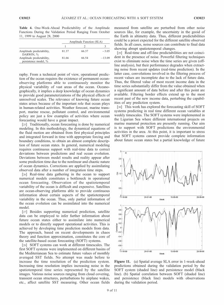
Figure 6. (a) Spatial average SST error in 1-week-aheadpredictions obtained during the validation period by theSOFT system (shaded line) and persistence model (blackline). (b) Spatial correlation between SOFT (shaded line)and persistence (black line) models with observationsduring the validation period.

C03023 ALVAREZ ET AL.: OCEAN FORECASTING WITH A SOFT SYSTEM

6 of 11

C03023

at the center of the basin than onshore. Conversely, warmwinds coming from the south dominated the week before(August 14–21), warming and homogenizing the sea sur-face in the area. Thus a good performance is not expectedfrom the persistence model. On the other hand, the com-paratively better forecast skill shown by the SOFT systemindicates that part of the observed short-time variability ispredictable.[21] Similarly to the summer case, Figures 8a–8c show

the weekly averaged SST field observed during (Figure 8a)the week starting on December 20, 1999, (Figure 8b) theforecast of the SOFT system obtained for that week, and(Figure 8c) the forecast of the persistence model, i.e., the

weekly averaged SST during the week starting on Decem-ber 13, 1999. Again, the SOFT predictor correctly estimatesthe drop in temperature observed in the coast of France.Also, Figures 8a and 8c exemplify cases where noise isinduced by the lack of data due to cloudy conditions. Thislack of data translates into grooves in the pictures thatseparate unmatched areas providing a collage appearance.These effects are not present when monthly averages areconsidered.

5.2. SOFT System and Predictions of the SLA Field

[22] Figures 9a–9d show the averaged SLA field and thefirst three EOFs resulting from the EOF decomposition of

Figure 7. (a) Weekly averaged SST during the weekstarting on August 21, 2000, and (b) 1-week-aheadprediction by the SOFT system of the weekly averagedSST for the week starting on August 21, 2000. (c) Same asFigure 7b, but prediction is obtained by the persistencemodel.

Figure 8. (a) Weekly averaged SST during the weekstarting on December 20, 1999, and (b) 1-week-aheadprediction by the SOFT system of the weekly averaged SSTfor the week starting on December 20, 1999. (c) Same asFigure 8b, but prediction is obtained by the persistencemodel.

C03023 ALVAREZ ET AL.: OCEAN FORECASTING WITH A SOFT SYSTEM

7 of 11

C03023

the temporal SLA variability, respectively. Notice thatrelatively small averaged anomalies are found in Figure 9a.This is an artifact from pre-processing altimeter data whenthe temporal average is subtracted from the field as a geoidapproximation. Physical interpretation of the consideredEOFs is less clear than in the case of the SST field. Thefirst EOF (Figure 9b) is characterized by a spatial patternshowing an eastward gradient in the measured SLA. Thisvariability is easily identified when data are visuallyinspected. Eastward gradients of SLA are formed duringlate spring and summer probably due to upwelling events inthe coast of France induced by wind. Also , a northwardspreading of rather cold waters from the Gulf of Lion couldamplify this effect. The SLA gradient reverses during someperiods in autumn and early winter. The physical origin ofthe gradient reversal still needs to be highlighted. Secondand third EOFs (Figures 9b and 9c) reinforce the west-eastvariability described by the first EOF. Although care shouldbe taken when interpreting these EOFs with low accountedvariance, the variability of the second EOF seems to befocused on the upwelling processes while the variabilitydescribed by the third EOF could be assigned to the inflowof warm waters from the Algerian basin. On the basis of theselection criterion previously described (see Table 3), nofurther EOFs were considered to build the SOFT system toforecast the SLA field.[23] Amplitude functions of the selected EOFs are dis-

played in Figures 10a–10c for the period ranging fromOctober 11, 1999, to August 28, 2000, together with the1-week-ahead forecast obtained by the time series predic-tor. Table 4 quantitatively shows that predictability is lostduring this period for the amplitude function correspondingto the third EOF. More significant is the fact that the timeseries predictor obtained from DARWIN provides the samepredictability as the persistence model. Thus, SOFT fore-casts will not provide more information about the 1-week-ahead SLA field than the prediction given by the properpresent state. This is confirmed in Figures 11a–11b wherethe spatial averaged SLA error in the prediction and thespatial correlation between the predicted and observedSLA fields are plotted for the developed SLA SOFT

system and persistence model. The spatial averaged SLAerror displayed shows noisy excursions around a meanvalue of 1.4 cm for both predictive models (Figure 11a).Conversely, high correlation values are found in Figure 11b.These results support the hypothesis that a red noise lawcould be adequate to describe the time variability shownby the SLA field in the Ligurian Sea.

6. Discussion

[24] Operational forecasting of ocean variability consti-tutes a major challenge in ocean sciences because itinvolves further development in technology and oceanog-

Figure 9. (a) Time average and (b–d) the three mostrelevant SLA EOFs ordered by relevance.

Figure 10. Amplitude functions (black line) and 1-week-ahead predictions (shaded line) during the validation periodranging from October 11, 1999, to August 28, 2000, for theamplitude functions corresponding to the (a–c) first to thirdSLA EOF.

Table 3. Percentage of the Total Temporal Variance Accounted

for by the First Three EOFs of the SLA Temporal Variability and

Predictability of the Corresponding Amplitude Functions Obtained

With DARWIN and the Persistence Model During the Validation

Period December 1, 1998 to October 4, 1999

EOF Number (SLA)

1 2 3

Accounted variance, % 90.18 3.89 2.13Amplitude predictability,DARWIN, %

87.23 41.96 43.36

Amplitude predictability,persistence model, %

85.84 32.82 42.73

C03023 ALVAREZ ET AL.: OCEAN FORECASTING WITH A SOFT SYSTEM

8 of 11

C03023

raphy. From a technical point of view, operational predic-tion of the ocean requires the existence of permanent ocean-observing platforms able to continuously monitor thephysical variability of vast areas of the ocean. Oceano-graphically, it implies a deep knowledge of ocean dynamicsto provide good parameterizations of the physical effects ofunresolved scales. The relevance of knowing future oceanstates arises because of the important role that ocean playsin human-related activities. Weather forecast, marine trans-port, marine rescue, pollutant control, and environmentalpolicy are just a few examples of activities where oceanforecasting would have a great impact.[25] Traditionally, ocean forecasting is done by numerical

modeling. In this methodology, the dynamical equations ofthe fluid motion are obtained from first physical principlesand integrated forward in time with appropriate forcing andboundary conditions, to obtain an almost complete descrip-tion of future ocean states. In general, numerical modelingrequires continuous support with real-time data to correctdeviations between predictions and real ocean evolution.Deviations between model results and reality appear aftersome prediction time due to the nonlinear and chaotic natureof ocean dynamics. Corrections are applied by assimilatingobserved data after a number of integration time steps.[26] Real-time data gathering in the ocean to support

numerical models constitutes a bottleneck in operationalocean forecasting. Observation of the spatiotemporalvariability of the ocean is difficult and expensive. Satellitesare ocean-observing platforms able to provide continuousinformation about certain aspects of the spatiotemporalvariability in the ocean. Thus, only partial information ofthe ocean evolution can be assimilated into the numericalmodel.[27] Besides supporting numerical prediction, satellite

data can be employed to infer further information aboutfuture ocean states either to assimilate into numericalmodels or to directly support operational activities. This isachieved by developing time prediction models from data.The approach, based on recent developments in chaostheory and function approximation, constitutes the core ofthe satellite-based ocean forecasting (SOFT) systems.[28] SOFT systems can work at different timescales. The

first SOFT systems were implemented on different basins ofthe Mediterranean Sea to estimate future values of monthlyaveraged SST fields. No attempt was made before toincrease the time resolution of the prediction system.Increasing time resolution implies increasing noise in thespatiotemporal time series represented by the satelliteimages. Various noise sources ranging from cloud covering,transient ocean structures, perturbations by airplane wakes,etc., affect satellite SST measuring. Other ocean fields

measured from satellite are perturbed from other noisesources like, for example, the uncertainty in the geoid ofthe Earth in altimetry data. Thus, different predictabilitiescould be a priori expected for the different satellite observedfields. In all cases, noise sources can contribute to final datashowing abrupt spatiotemporal changes.[29] Real-time and off-line predictabilities are not coinci-

dent in the presence of noise. Powerful filtering techniquesexist to eliminate noise when the time series are given (off-line analysis), but their performance degrades when extract-ing noise from recent updates (real-time prediction). In thelatter case, convolutions involved in the filtering process ofrecent values are incomplete due to the lack of future data.Thus, the filtered value of most recent income data in thetime series substantially differ from the value obtained whena significant amount of data before and after this point areavailable. Filtering border effects extend up to the mostrecent past of the new income data, perturbing the capabil-ities of any prediction system.[30] This work has explored the forecasting skill of SOFT

systems predicting in real time different ocean variables atweekly timescales. The SOFT systems were implemented inthe Ligurian Sea where different international projects onmarine mammal protection are presently running. Our aimis to support with SOFT predictions the environmentalactivities in the area. At this point, it is important to stressthat SOFT systems cannot provide complete informationabout future ocean states but a partial knowledge of future

Table 4. One-Week-Ahead Predictability of the Amplitude

Functions During the Validation Period Ranging From October

11, 1999 to August 28, 2000

Amplitude Function (SLA)

1 2 3

Amplitude predictability,DARWIN, %

81.37 66.37 �3.05

Amplitude predictability,persistence model, %

81.66 66.54 �13.09

Figure 11. (a) Spatial average SLA error in 1-week-aheadpredictions obtained during the validation period by theSOFT system (shaded line) and persistence model (blackline). (b) Spatial correlation between SOFT (shaded line)and persistence (black line) models with observationsduring the validation period.

C03023 ALVAREZ ET AL.: OCEAN FORECASTING WITH A SOFT SYSTEM

9 of 11

C03023

ocean evolution. This knowledge was restricted in this workto forecast the SST and SLA of the basin because relativelylong-term time series of these two fields are available,which constitute an important factor in empirical modeling.[31] Unlike previous works focused on forecasting

monthly averages, filtering the amplitude functions priorto extracting the forecasting rules did not result in a goodstrategy when weekly timescales and real-time predictionare simultaneously considered. The failure of the filteringmodule of the SOFT system arises in filtering border effects.For this reason, forecasting expressions were directlyobtained from raw amplitude functions. In principle, ifenough data is provided during the learning period, anynonlinear prediction methodology should be capable offinding the predictive function g( ) in equation (1) even inthe presence of noise [Magdon-Ismail et al., 1998]. Theamount of learning data required by the prediction method-ology to get an optimum predictor rapidly increase with thenoise level in the signal. Although noise in real-timeprediction at weekly timescales could not be filtered out,prediction chances remained for the length of the time seriesand the robustness of the prediction methodology to extractthe deterministic behavior from the raw signal.[32] Results obtained during this study indicate that the

performance of the SOFT system in predicting the SST fieldis superior to persistence for 1-week-ahead predictions. Thissuperiority is not homogeneous through all the year but isfocused during summer and autumn seasons. Instead, fore-cast skills of SOFT and persistence models are closer duringwinter and spring. During these two seasons, temperatureerrors are also smaller than those obtained in summer-autumn. This seasonal structure of the forecast skill canbe explained in terms of the SST variability showed by theLigurian Sea. In winter-spring, SST pattern in the Ligurianbasin can be roughly described by a homogeneous fieldwith relatively low surface temperature and absent SSTgradients. This pattern is mostly induced by the severeweather conditions occurring in the area during this period.The SST structure slightly changes from week to week, andthus the weekly averaged SST field of a week is a relativelygood approximation for the SST field of the next week. Inother words, the hypothesis of persistence roughly holds.The SST pattern in the basin drastically changes in summerand autumn. Basin-scale SST gradients appear as a result ofthe temperature differences between water masses comingfrom the Algerian and Tyrrhenian basins and the cold watersin the central part of the Ligurian Sea. Also, SST variabilityis higher at this time, showing substantial changes fromweek to week. Consequently, the persistence hypothesisdoes not hold, and differences in the performance skillbetween SOFT and persistence models increase. Notice thatthe SST field in the Ligurian Sea is less predictable duringthis period of time than during winter and spring seasons.Nevertheless, the SOFT system is able to predict part of thisvariability, providing lower SST errors in the predictionsthan the persistence model. No predictability was foundwhen real-time prediction was attempted at bigger timehorizons.[33] On average, the performance of the SOFT system

developed to forecast the SLA field and the persistencemodel, were similar during the validation period rangingfrom October 11, 1999, to August 28, 2000. This result is

mainly originated by the low signal-to-noise ratio found inthe SLA data of the Ligurian Sea. Unlike SST, SLA shows ahigher dynamical variability at short timescales. Also, thegeneration of SLA maps comes from the combination ofsatellite tracks carried out at different times. All thesefactors contribute to increase the noise level of the SLAsignal in the Ligurian Sea. Results show that the availabledata are not enough for the prediction methodology tocapture the deterministic behavior of the SLA field. Thus,the obtained prediction models closely resemble a red noiselaw, that is, a mathematical expression whose main term isthe value of the variable the instant before plus somemarginal nonlinearity. The solution to this problem couldbe geographically dependent. The failure of SOFT predic-tions of the SLA in the area studied might not be general-ized to other ocean areas with higher signal-to-noise ratio.To discern more about this point, future research on SLASOFT systems will be carried out on areas with strongeraltimeter signal like the Alboran Sea.

Appendix A: General Methodology of SoftPrediction

[34] Empirical prediction of satellite observations iscarried out in three major phases (Figure 1).[35] 1. Phase 1 is decomposition of space-time variability

of the satellite-observed data. The EOF technique[Preseindorfer, 1988; Kelly, 1985, 1988; Lagerloef andBernstein, 1988] is first employed to decompose space-and time-distributed satellite data into modes ranked bytheir temporal or spatial variance. EOF covariance analysishas been shown to be slightly superior to EOF gradientdecomposition in terms of predictability [Alvarez, 2003].Thus, the original time series of satellite images representedby a mathematical function F(x, y, t), is decomposed in EOFcovariance analysis into

F x; y; tð Þ ¼ A1T tð ÞP1

T x; yð Þ þ . . .þ ANT tð ÞPN

T x; yð Þ þ T x; yð Þ;ðA1Þ

where ATn (t), {n = 1,. . ., N}, are one-variable time series and

PTn(x, y), {n = 1,. . .N}, are spatial patterns. The subscripts T

refers to temporal variance decomposition and T(x, y) is thetime mean of the satellite images subtracted in thedecomposition.[36] 2. Phase 2 is noise reduction. Generally, spatial

patterns PTn (x, y), {n = 1,. . .N} and corresponding time

series ATn (t), {n = 1,. . ., N} show some degree of noisy

nature. To reduce the degree of noise in the reconstructedspatial pattern, EOFs of small variance are neglected inequation (A1). Also, singular spectral analysis (SSA) ordata adaptive approach [Broomhead and King, 1986;Pendland et al., 1991; Casdagli et al., 1992; Elsner andTsonis, 1996] is employed to remove noise in the time seriesATn(t), {n = 1, . . ., Nr} (Nr considered modes).[37] Phase 3 is time series prediction. The third task is

to obtain a dynamical model for each filtered time seriesATn(t), {n = 1, . . ., Nr}, which, using past values of the

corresponding time series, predicts the future values,

AnT tð Þ ¼ gn

~AnT t � tð Þ; ~An

T t � 2tð Þ; . . . ; ~AnT t � mtð Þ

� �; ðA2Þ

C03023 ALVAREZ ET AL.: OCEAN FORECASTING WITH A SOFT SYSTEM

10 of 11

C03023

where n = 1, . . ., Nr, m is an embedding dimension, and t isa time lag unit [Casdagli et al., 1992]. A genetic algorithmfor time series prediction, called DARWIN, is employed toapproximate the mapping gn( ) in equation (A2). DARWINis documented by Alvarez et al. [2001] and is downloadablefrom the Computer Physics Communication Library (http://cpc.cs.qub.ac.uk).[38] Prediction of a satellite-observed field is achieved by

adding the most relevant modes previously multiplied bytheir corresponding forecast amplitudes,

F x; y; t þ 1ð Þ ¼ A1T t þ 1ð ÞP1

T x; yð Þ þ . . .þ ANr

T t þ 1ð ÞPNr

T x; yð Þþ T x; yð Þ; ðA3Þ

where the circumflex indicates predicted magnitude.

[39] Acknowledgments. This work has been supported by the SOFT-EVK3-CT-2000-0028 European Project and the Spanish Project REN 2001-3982-E. Comments from Dr. P. F. J. Lermusiaux and anonymous reviewersare gratefully acknowledged.

ReferencesAlvarez, A. (2003), Performance of satellite based ocean forecasting(SOFT) systems: A study in the Adriatic Sea, J. Atmos. Oceanic Technol.,20, 717–729.

Alvarez, A., C. Lopez, M. Riera, E. Hernandez-Garcia, and J. Tintore(2000), Forecasting the SST space-time variability of the Alboran Seawith genetic algorithms, Geophys. Res. Lett., 27, 2709–2712.

Alvarez, A., A. Orfila, and J. Tintore (2001), DARWIN: An evolutionaryprogram for nonlinear modelling of chaotic time series, Comput. Phys.Commun., 136, 334–349.

Alvarez, A., A. Orfila, and J. Sellschopp (2003), Satellite based forecastingof sea surface temperature in the Tuscan Archipelago, Int. J. RemoteSens., 24, 2237–2251.

Astraldi, M., G. P. Gasparini, and S. Sparnocchia (1994), The seasonal andinterannual variability in the Lingurian-Provencal basin, in Seasonaland Interannual Variability of the Western Mediterranean Sea, CoastalEstuarine Stud., vol. 46, edited by P. E. La Violette, pp. 93–113, AGU,Washington, D. C.

Barnston, A. G., et al. (1994), Long-lead seasonal forecasts: Where do westand?, Bull. Am. Meteorol. Soc., 75, 2097–2114.

Broomhead, D. S., and G. P. King (1986), Extracting qualitative dynamicsfrom experimental data, Physica D, 20, 217–236.

Casdagli, M. (1989), Nonlinear prediction of chaotic time series, Physica D,35, 335–356.

Casdagli, M., D. Des Jardins, S. Eubank, J. D. Farmer, J. Gibson, J. Theiler,and N. Hunter (1992), Nonlinear modeling of chaotic time series: Theoryand applications, in Applied Chaos, edited by J. H. Kim and J. Stringer,pp. 335–379, John Wiley, New York.

De Oliveira, K. A., A. Vannucci, and E. Cesar da Silva (2000), Usingartificial neural networks to forecast chaotic time series, Physica A,284, 393–404.

Elsner, J. B., and A. A. Tsonis (1996), Singular Spectrum Analysis: A NewTool in Time Series Analysis, 164 pp., Plenum Press, New York.

Grassberger, P., and I. Procaccia (1983), Measuring the strangeness ofstrange attractors, Physica D, 9, 189–208.

Kelly, K. A. (1985), The influence of winds and topography on the seasurface temperature patterns over the northern California slope, J. Geo-phys. Res., 90, 11,783–11,798.

Kelly, K. A. (1988), Comment on ‘‘Empirical orthogonal function analysisof advance very high resolution radiometer surface temperature patternsin Santa Barbara channel’’ by G. S. E. Lagerloef and R. L. Bernstein,J. Geophys. Res., 93, 15,753–15,754.

Lagerloef, G. S. E., and R. L. Bernstein (1988), Empirical orthogonalfunction analysis of advance very high resolution radiometer surfacetemperature patterns in Santa Barbara channel, J. Geophys. Res., 93,6863–6873.

Lopez, C., A. Alvarez, and E. Hernandez-Garcia (2001), Forecastingconfined spatiotemporal chaos with genetic algorithms, Phys. Rev. Lett.,85, 2300–2303.

Magdon-Ismail, M., A. Nicholson, and Y. S. Abu-Mostafa (1998), Financialmarkets: Very noisy information processing, Proc. IEEE, 86, 2184–2195.

Parlitz, U., and C. Merkwirth (2000), Prediction of spatiotemporal timeseries based on reconstructed local states, Phys. Rev. Lett., 84, 1890–1893.

Parlitz, U., C. Merkwirth, and D. Engster (2001), Local modelling usingnearest neighbours, paper presented at 5th International Heinz NixdorfSymposium, Heinz Nixdorf Inst., Paderborn, Germany.

Pendland, C., G. Ghil, and K. M. Weickmann (1991), Adaptive filtering andmaximum entrophy spectrum with application to changes in atmosphericangular momentum, J. Geophys. Res., 96, 22,659–22,671.

Preseindorfer, R. W. (1988), Principal Component Analysis in Meteorologyand Oceanography, 425 pp., Elsevier Sci., New York.

Szpiro, G. G. (1997), Forecasting chaotic time series with genetic algo-rithms, Phys. Rev. E, 55, 2557–2568.

Takens, F. (1981), Detecting strange attractors in fluid turbulence, inDynamical Systems and Turbulence, Lecture Notes Math., vol. 898, editedby D. Rand and L. S. Yeung, pp. 366–369, Springer-Verlag, New York.

�����������������������A. Alvarez and J. Tintore, Instituto Mediterraneo de Estudios Avanzados

(IMEDEA), CSIC-UIB, Miquel Marques, 21, 07190 Esporles, Spain.(vieaaad@uib.es; dfsjts0@uib.es)A. Orfila, School of Civil and Environmental Engineering, Cornell

University Hollister Hall, Ithaca, NY 14853, USA. (ao57@cornell.edu)

C03023 ALVAREZ ET AL.: OCEAN FORECASTING WITH A SOFT SYSTEM

11 of 11

C03023