Real-time 3D radiation risk assessment supporting simulation of work in nuclear environment

J. Radiol. Prot. 34 (2014) 389–416

Society for Radiological Protection Journal of Radiological Protection

doi:10.1088/0952-4746/34/2/389

Real-time 3D radiation risk assessment

supporting simulation of work in nuclear

environments

I Sz

˝

oke

1, M N Louka

1, T R Bryntesen

1, J Bratteli

1,

S T Edvardsen

1, K K RøEitrheim

1and K Bodor

2

1 Institute for Energy Technology, Os Alle 5, NO-1777 Halden, Norway2 Centre for Energy Research, Hungarian Academy of Sciences, KFKI Campus29–33 Konkoly Thege Miklos street, 1121 Budapest, Hungary

E-mail: [email protected]

Received 9 October 2013, revised 20 February 2014Accepted for publication 4 March 2014Published 14 April 2014

Abstract

This paper describes the latest developments at the Institute for EnergyTechnology (IFE) in Norway, in the field of real-time 3D (three-dimensional)radiation risk assessment for the support of work simulation in nuclearenvironments. 3D computer simulation can greatly facilitate efficient workplanning, briefing, and training of workers. It can also support communicationwithin and between work teams, and with advisors, regulators, the media andpublic, at all the stages of a nuclear installation’s lifecycle. Furthermore, it isalso a beneficial tool for reviewing current work practices in order to identifypossible gaps in procedures, as well as to support the updating of internationalrecommendations, dissemination of experience, and education of the currentand future generation of workers.

IFE has been involved in research and development into the application of3D computer simulation and virtual reality (VR) technology to support work inradiological environments in the nuclear sector since the mid 1990s. During thisprocess, two significant software tools have been developed, the VRdose systemand the Halden Planner, and a number of publications have been produced tocontribute to improving the safety culture in the nuclear industry.

This paper describes the radiation risk assessment techniques applied inearlier versions of the VRdose system and the Halden Planner, for visualisingradiation fields and calculating dose, and presents new developments towardsimplementing a flexible and up-to-date dosimetric package in these 3D softwaretools, based on new developments in the field of radiation protection. The latest

Content from this work may be used under the terms of the Creative Commons Attribution 3.0licence. Any further distribution of this work must maintain attribution to the author(s) and the

title of the work, journal citation and DOI.

0952-4746/14/020389+28$33.00 c� 2014 IOP Publishing Ltd Printed in the UK 389

http://dx.doi.org/10.1088/0952-4746/34/2/389

mailto:[email protected]

http://creativecommons.org/licenses/by/3.0

http://creativecommons.org/licenses/by/3.0

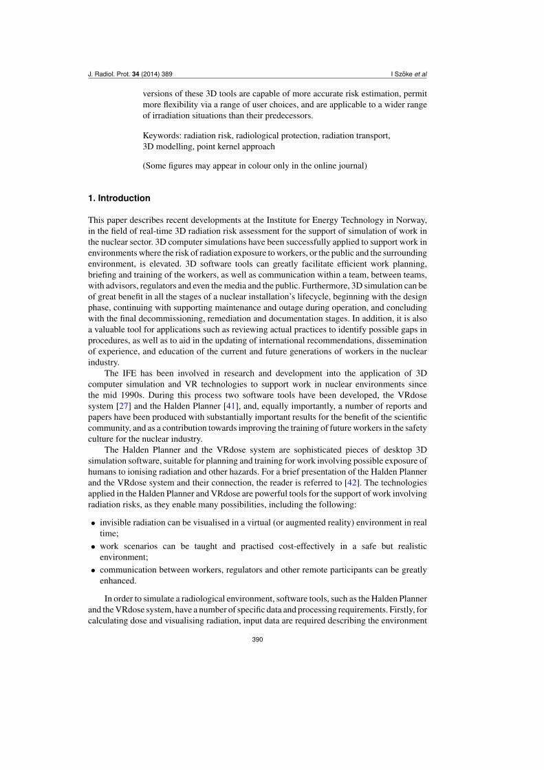
J. Radiol. Prot. 34 (2014) 389 I Szoke et al

versions of these 3D tools are capable of more accurate risk estimation, permitmore flexibility via a range of user choices, and are applicable to a wider rangeof irradiation situations than their predecessors.

Keywords: radiation risk, radiological protection, radiation transport,3D modelling, point kernel approach

(Some figures may appear in colour only in the online journal)

1. Introduction

This paper describes recent developments at the Institute for Energy Technology in Norway,in the field of real-time 3D radiation risk assessment for the support of simulation of work inthe nuclear sector. 3D computer simulations have been successfully applied to support work inenvironments where the risk of radiation exposure to workers, or the public and the surroundingenvironment, is elevated. 3D software tools can greatly facilitate efficient work planning,briefing and training of the workers, as well as communication within a team, between teams,with advisors, regulators and even the media and the public. Furthermore, 3D simulation can beof great benefit in all the stages of a nuclear installation’s lifecycle, beginning with the designphase, continuing with supporting maintenance and outage during operation, and concludingwith the final decommissioning, remediation and documentation stages. In addition, it is alsoa valuable tool for applications such as reviewing actual practices to identify possible gaps inprocedures, as well as to aid in the updating of international recommendations, disseminationof experience, and education of the current and future generations of workers in the nuclearindustry.

The IFE has been involved in research and development into the application of 3Dcomputer simulation and VR technologies to support work in nuclear environments sincethe mid 1990s. During this process two software tools have been developed, the VRdosesystem [27] and the Halden Planner [41], and, equally importantly, a number of reports andpapers have been produced with substantially important results for the benefit of the scientificcommunity, and as a contribution towards improving the training of future workers in the safetyculture for the nuclear industry.

The Halden Planner and the VRdose system are sophisticated pieces of desktop 3Dsimulation software, suitable for planning and training for work involving possible exposure ofhumans to ionising radiation and other hazards. For a brief presentation of the Halden Plannerand the VRdose system and their connection, the reader is referred to [42]. The technologiesapplied in the Halden Planner and VRdose are powerful tools for the support of work involvingradiation risks, as they enable many possibilities, including the following:

• invisible radiation can be visualised in a virtual (or augmented reality) environment in realtime;

• work scenarios can be taught and practised cost-effectively in a safe but realisticenvironment;

• communication between workers, regulators and other remote participants can be greatlyenhanced.

In order to simulate a radiological environment, software tools, such as the Halden Plannerand the VRdose system, have a number of specific data and processing requirements. Firstly, forcalculating dose and visualising radiation, input data are required describing the environment

390


we wish to model. These data may describe the characteristics of the radiation sources inthe environment, the entities affecting radiation transport (biological shields, walls, etc), theradiation field by means of measurements registered by various instruments, the movementof workers in the area of interest, etc. These data are then utilised by the algorithms toassess radiation risks (‘dosimetric approaches’). In the next step, the results calculated bythe dosimetric approach are visualised for the user, ideally in a sufficiently sophisticated butuser-friendly manner. The ultimate goal of these codes is to aid experts in making well-informeddecisions, to reasonably minimise (and keep to acceptable levels) the exposures of humansinvolved, to support the ALARA (as low as reasonably achievable) dose planning principle.

The variety of techniques applied in radiation protection and shielding design is vast[24, 28, 33, 34, 39]. The selection of the dosimetric method most suitable for a specificsituation is determined by (a) the radiological input data available (e.g. location of radiationsources or hot spots if any, geometry of the sources, available information on the energyspectrum or isotopic composition of the sources, existence of measurements, etc), (b) theexposure conditions, i.e. any parameters characterising the mode of the exposure (e.g. angulardependence of the radiation field, characteristics of the objects and media interacting withradiation, the route of the target, etc), (c) the output information required (e.g. dosimetric and/orradiometric quantities describing detector response), (d) the target of radiation that we wish tomonitor, (e) the allowable inaccuracy of the results and (f) time constraints (e.g. emergencysituation or non-stressful situation).

In this paper, we present the basic dosimetric approaches of the Halden Planner and thelatest VRdose system, applicable when the sources of radiation and any objects interactingwith the radiation field are ‘known’, i.e. there is information on the location, geometry andradiation emitted (energy spectrum or isotopic composition). In this fortunate situation, themost common techniques applied are Monte Carlo (MC) radiation transport simulations (e.g.MCNP, GEANT, etc), and point kernel (also called kernel integration) approaches [24, 26, 40](e.g. MicroShield [11], QAD [5]). The first group of methods are, in general, very accuratein comparison with the point kernel methods, but are also relatively slow and difficult to useby non-experts, due to the very sophisticated description of radiation transport. In contrast,due to a much simpler theoretical approach, point kernel techniques are faster. However, as aconsequence of the simplifications introduced, they are less precise and may break down inspecific situations (e.g. very short distances between source and detector).

Earlier versions of the Halden Planner provided only one, relatively simple, dosimetricapproach [43] for calculating radiation levels and visualising radiation fields generated bygamma sources. The underlying dosimetric technique is a basic point kernel approach, wellknown in the field of protection against gamma radiation. While this approach gives agood estimate in most simple irradiation situations (e.g. standard photon energy spectrum,shielding geometry and composition), recent developments in the field of radiation shieldingdesign, subsequent changes to the standard radiation protection strategy, and the availabilityof additional standard input data have paved the way for a more up-to-date and comprehensiveapproach.

The new model, developed in this work, adopts the results of recent developments inthe field of radiation shielding, and incorporates a larger variety of standard input data (e.g.dose conversion coefficients and buildup factors) stemming from modelling and experimentalefforts of various research groups around the globe. The new model is in line with newrecommendations issued by institutions with a significant impact on the evolution of theinternational radiation protection standards, such as the ICRP (International Commissionon Radiological Protection) [20], ICRU (International Commission on Radiation Units andMeasurements) [18], the Radiation Protection and Shielding Division of the American Nuclear

391


Society [2], the German Institute for Radiation Protection (Bundesamt fur Strahlensutz) [4],the International Atomic Energy Agency (IAEA) and the National Institute of Standards andTechnology.

2. Methods

2.1. The earlier point kernel approach

The dosimetric unit implemented in earlier versions of Halden Planner is based on a basicpoint kernel approach, developed some time ago in the field of radiological protection. Thisapproach quantifies the radiation burden originating from gamma sources based on the distancebetween the source and the detector, taking into account attenuation and buildup of photonsin the objects (shields) intersecting the direct path of radiation to the detector. The core of thepoint kernel approach is a simple formula for calculating the detector response due to gammaphotons emitted by a point isotropic source, at a specified distance in a homogeneous infinitemedium,

R =Z

dE ⇥ 14⇡r2 ⇥ S(E) ⇥ exp(�6r) ⇥ R(E) ⇥ B(6r, E) (1)

where R symbolises the detector response (dose), E is the photon energy, r is the distancebetween the source and the detector, S is the specific activity (the number of photons emitted perunit volume), 6r = µ⇥r is the optical thickness from the source to the detector, µ is the linearattenuation coefficient and B is the buildup factor. Integration over the source and the targetvolume have been omitted for simplicity. For more detail on the considerations underlying thepoint kernel approach the reader is referred to the literature [24, 33, 34, 39].

The calculation is based on the following consecutive steps.First, the initial (unshielded) particle fluence rate is calculated, and then the attenuation

of the uncollided beam is determined on the basis of the distance travelled by the photonsin the shield on their way to the detector. In the next step, the radiation burden from theuncollided photons reaching the detector is characterised by calculating the transfer of energyfrom photons to absorber by simple methods (described later), utilising related mass-energyabsorption coefficients.

To estimate the contribution of the scattered photons to the response of the detector,standard input data from the literature, so-called buildup factors [14, 35–37], are utilised.Calculation of the contribution of the collided photons, which may undergo multiple scatteringin the shield, is a very complex task, and requires experimental results, or results based onsophisticated radiation transport models. Buildup of radiation in matter depends on a numberof parameters, the most important of which are (a) the energy (or energy spectrum) of theradiation, (b) the atomic composition and (c) the density of the medium, (d) the distancetravelled by the radiation before reaching the detector, as well as (e) the quantity (detectorresponse) measured or calculated [33]. In more realistic situations we have a heterogeneousmedium between the source and the detector, e.g. multi-layers of shielding and a varietyof additional objects interacting with the radiation, which complicate things even further.However, standard data on photon buildup, for the most common photon energy range(15 keV–15 MeV), optical density (mfp) of the medium the photons traverse, engineeringmaterials applied in shielding design, and simple (e.g. infinite) shielding configuration areprovided in the literature for general use. These buildup factors are commonly appliedin radiation protection practice to account for buildup of photons in real (more complex)

392


irradiation situations, in cases where the inaccuracies introduced by the differences betweenthe standard and real exposure conditions are acceptable.

The final output quantity, referring to the biological effectiveness of the radiation, isobtained by multiplying the exposure rate (free in air), calculated as described above, by aconstant based on simple assumptions (explained later).

Based on the above, the dosimetric model is based on the following equations, as reportedin [43]:

Xair = 5.26 ⇥ 10�6 Ad2

X

i

yi Ei (µen/⇢)i ⇥ exp(�(µ/⇢)i⇢r) ⇥ Bs(Ei , ⇢, r) (2)

˙Dose = Xair ⇥ 9.7 ⇥ 1 (3)

where Xair is the exposure rate (R h�1), d is the distance to the detector (cm), A is the sourceactivity (Bq), yi is the yield of photons of energy Ei , Ei is the photon energy (MeV), (µen/⇢)i isthe mass-energy absorption coefficient at energy Ei (cm2 g�1), (µ/⇢)i is the mass attenuationcoefficient at energy Ei (cm2 g�1), ⇢ is the density of the shield (g cm�3), r is the distancetravelled in the shield (cm), Bs(Ei , ⇢, r) is the exposure buildup factor at energy Ei and ˙Doseis the dose equivalent rate (mSv h�1).

Equation (2) can be rewritten in the following form:

Xair = 6.6 ⇥ 10�5 ⇥X

i

✓A · yi

4⇡d2 ⇥ exp(�6r(Ei )) ⇥ Ei (µen/⇢)i ⇥ BX (6r(Ei ))

◆(4)

where the integral in equation (1) has been replaced by a rougher summation, 6r(Ei ) = µi ⇥ris the optical thickness (µi is the linear attenuation coefficient) at energy Ei , BX (6r(Ei )) isthe exposure buildup factor, and the constant (6.6 ⇥ 10�5) is a conversion of units, which canbe expressed as follows:

106

eVMeV

�⇥ 1

33.8

ion pair

eV

�⇥ 1

6.24⇥1018

C

ion pair

�

⇥ 103

gkg

�⇥ 3600

h sh

i⇥ 1

2.58⇥10�4

R

kgC

�. (5)

Equation (4) nicely reveals the consecutive steps of the radiation transport calculation describedabove and that the technique is, in fact, an application of equation (1).

The equations above, for modelling radiation transport and energy deposition, are based onstrong idealisations. In spite of the simplifications, this technique yields surprisingly accurateestimates for common situations, i.e. standard photon energies, simple irradiation situations(e.g. simple shielding composition), etc.

The first two terms in the summation in equation (4) calculate the initial and the attenuatedfluence rate of the uncollided photons. The third term in the summation in equation (4)calculates the energy transferred to the absorbing medium by multiplying the fluence rate(on the detector side of the shield) by the mass-energy absorption coefficient and photonenergy. The mass-energy absorption coefficient (µen/⇢) defines the ratio of photon energytransferred to the medium, excluding the energy retransferred to secondary photons throughradiative processes. Hence, in equation (4) the energy transferred to charged particles fromthe uncollided photons, not including energy converted to secondary photons, is calculated.However, the overall fluence rate of photons, generated by a point isotropic source at agiven detector position, includes Compton scattered photons, photons from emission ofBremsstrahlung, fluorescence x-ray photons and annihilation gamma photons [1, 26, 33],

393


generated by the medium surrounding the detector position. Since the photon fluence rate,calculated as described above, neglects these secondary photons, the calculated detectorresponse will be underestimated. Calculation of the fluence including secondary photons ismuch more complicated than calculation of the primary fluence. Instead, to solve commonradiation protection problems, a convenient simplification is usually applied.

A simple way of including the contribution of the scattered photons indirectly reachingthe detector is multiplication by a suitable buildup factor (last term in the summation inequation (4)), applicable to the photon energy, absorber (shield) type and distance travelledthrough the absorber (shield thickness). This simple method is frequently applied in currentradiological protection practice. If a more sophisticated characterisation of the energy spectrumof particle fluence is needed, then Monte Carlo radiation transport models are usually applied.While MC models provide a more detailed description of the radiation transport, they requirea more detailed description of the exposure conditions, and are not generally suitable fornon-expert users and real-time simulation.

In the following step, the rate of energy absorbed in matter at the detector is converted intothe exposure rate (free in air) by application of a constant (6.6⇥10�5) multiplier. In general, theconstant conversion from MeV g�1 s�1 to R h�1 slightly depends on energy. This is mainly dueto the fact that the number of ion pairs produced by 1 eV depends on the circumstances of theexposure. On the other hand, 1 eV corresponds to 33.8 ion pairs with a ±0.2 eV uncertainty forphoton energies between 20 keV and 3 MeV for 50% relative humidity and 22 �C temperature.

In the final steps of this dosimetric approach, the exposure rate (free in air) is multipliedby 9.7 to obtain the dose rate absorbed in tissue, expressed in mGy h�1, and then multiplied bythe so-called quality factor of the radiation, which equals one for gamma radiation, to obtainthe tissue dose equivalent rate (organ equivalent dose rate).

The constant conversion of 9.7 is determined by taking into account that 1 eV equals1.6 ⇥ 1012 J (joules). According to the above (see equation (5)), 1 R can be converted intomJ kg�1 s�1 as follows:

1 R = 2.58 ⇥ 10�4

Ckg

/R�

⇥ 6.24 ⇥ 1018

ion pairC

�

⇥ 33.8

eVion pair

�⇥ 1.6 ⇥ 1012

J

eV

�. (6)

Following from equation (6), we have 1 R h�1 = 8.7 mJ kg�1 h�1, which is a goodapproximation for energies ranging from 20 keV to 3 MeV. In terms of energy absorption, thereis no significant difference between air and soft tissue. Indeed, in the range from about 15 keVto 3 MeV, the ratio of the mass-energy absorption coefficients for soft tissue and air is quiteconstant [16], and is equal to roughly 1.1, which is equivalent to the ratio of the constant 9.7multiplier (see equation (3)) to the 8.7 conversion constant. Consequently, application of a 9.7constant to convert exposure (free in air) in R h�1 to energy absorbed in soft tissue mJ kg�1 h�1

is a good approximation in most cases.Absorbed dose is defined as the mean energy absorbed by matter per mass of the matter in

which the energy has been absorbed (de/dm). From the definition, it can be seen that while theexpression in equation (4) describes the energy transferred to charged particles per unit massdm, produced in dm but absorbed anywhere (partially outside dm), absorbed dose refers toenergy absorbed only in dm (partially from charged particles from outside dm). Thus, absorbeddose can be calculated as in equation (4), if the energy carried outside dm is equal to the energycoming from outside dm, i.e. charged particle equilibrium (CPE) exists, where energy transferand energy absorption are equal [1, 12].

394


Equilibrium of charged particles requires (a) negligible radiation loss, (b) uniformradiation field and (c) homogeneous matter (in terms of both density and atomic number). In ourcase, absorption of energy in the human body, usually immersed in air, is of most interest. Basedon [1], the first condition of CPE is fulfilled for photon energies up to ⇠10 MeV, above whichradiation loss becomes increasingly important, due to the high energy of the generated primaryelectrons. The second condition of CPE (uniform radiation field) requires that the radiation beonly negligibly attenuated in matter. By inspecting standard attenuation coefficients [15] forair and for soft tissue it is easy to see that both air and soft tissue have a low attenuating effecton high-energy gamma photons. However, soft tissue attenuates relatively strongly, comparedto air, in the region of low photon energies, compromising CPE in this region. This means thatat very low energies the skin absorbs most of the energy, and provides strong shielding forinternal organs. The third criterion of CPE is that the absorber is homogeneous, in terms ofboth density and atomic number. The human body can be regarded as relatively homogeneousin terms of interaction with gamma radiation. Inhomogeneity is only considerable, affectingCPE, near bone surfaces and the skin–air interface.

As mentioned previously, the selection of appropriate buildup factors also depends on thequantity we wish to calculate. In the model described above, developed during earlier work,exposure buildup factors are applied, conforming to the international recommendations of thattime. As explained earlier, the expression in equation (4) gives a good estimate of the exposure(free in air) for a wide photon energy range, and is especially accurate for photon energiesbetween 0.2 and 3 MeV. However, the calculated exposure rate is then converted into organequivalent dose rate (tissue dose equivalent rate), which, as explained above, has differentbehaviour (compared to exposure) at low photon energies. Since an exposure buildup factorB(E0), at a given energy E0, accounts for the contribution of scattered photons to the calculatedexposure [26],

B(E0) =R E0

0 X (E)dEX (E0)

, (7)

its application is only justified for the calculation of detector response types that, compared toexposure, have a similar energy dependence.

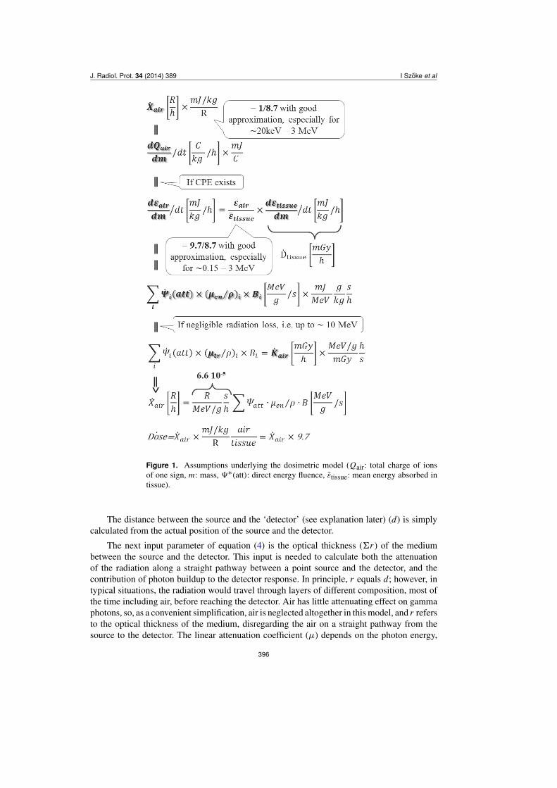
The assumptions of the dosimetric model, described above, and the connection to air kerma(Kair) are summarised in figure 1.

Based on the above, we can thus conclude that the dosimetric approach described providesa good approximation in most common radiation protection cases, and considerable inaccuracycan only be expected in, from a nuclear industry perspective, special situations, e.g. exposureto very low photon energy (below 0.2 MeV), especially at bone surfaces and red marrow, andexposure to very high-energy photons (above ⇠10 MeV).

Below, we present how the input parameters required by the basic formulae describedabove are calculated, and how this computational model is applied for the simulation ofradiation transport in more complex situations.

As can be seen from equation (4), one of the input parameters required is the energyspectrum (Ei , A ⇥ yi ) of the radiation emitted by the sources in the modelled scene. Thisis calculated based on the activity and the isotopic composition, defined by the user for eachradiation source. The characteristic energies and associated fractional yields are fetched froman internal database of the software tool, which was created based on standard data from theliterature [43]. At the time, input data for the four most interesting isotopes, i.e. 58Co, 60Co,110mAg, 137Cs (and 137mBa in secular equilibrium) were coded, with the possibility of addingsupplementary isotopes for later applications.

395


Figure 1. Assumptions underlying the dosimetric model (Qair: total charge of ionsof one sign, m: mass, 9⇤(att): direct energy fluence, "tissue: mean energy absorbed intissue).

The distance between the source and the ‘detector’ (see explanation later) (d) is simplycalculated from the actual position of the source and the detector.

The next input parameter of equation (4) is the optical thickness (6r ) of the mediumbetween the source and the detector. This input is needed to calculate both the attenuationof the radiation along a straight pathway between a point source and the detector, and thecontribution of photon buildup to the detector response. In principle, r equals d; however, intypical situations, the radiation would travel through layers of different composition, most ofthe time including air, before reaching the detector. Air has little attenuating effect on gammaphotons, so, as a convenient simplification, air is neglected altogether in this model, and r refersto the optical thickness of the medium, disregarding the air on a straight pathway from thesource to the detector. The linear attenuation coefficient (µ) depends on the photon energy,

396


and the type and density of the medium through which the photons travel before reachingthe detector. Since this parameter depends on the absorber material, the optical thickness hasto be calculated separately for each layer the radiation traverses. The total optical thicknessis then found by adding the optical thicknesses of all layers together (6r = 6◆µ ⇥ ri ).The earlier point kernel model was implemented with the application of standard linearattenuation coefficients for the four most important engineering materials (lead, iron, concreteand water) drawn from the literature of the time [43]. The linear attenuation coefficientsapplied in the model neglect coherent scattering, and consider free electrons in incoherentscattering.

The mass-energy absorption coefficient (µen/⇢) is a function of the photon energy andthe target absorber material. The target material in this model is air. The model appliesenergy-dependent values of this coefficient drawn from the literature of the time.

The last input of equation (4) is the buildup factor. As mentioned earlier, this parameteris also dependent on the material the photons travel through. Consequently, photon buildupis calculated in each consecutive layer of supported shielding material separately, similarly tothe technique applied for calculating attenuation, based on the energy of the photons passingthrough, and the same optical thickness that is used to determine the attenuation (i.e. based onthe intersection of the layer with a straight pathway from the source to the detector). Tabulatedvalues for different photon energies, optical thicknesses and four engineering materials areutilised by the model from the standard literature of the time [43]. For transitional parameters,linear interpolation of the buildup factors corresponding to tabulated energy and opticalthickness values is performed. The total buildup in all intersecting layers is computed by simplymultiplying the buildup of photons in each layer.

As mentioned above, buildup factors are usually produced using more sophisticatedradiation transport modelling results for standard irradiation situations (e.g. homogeneousinfinite medium). Hence, application of these factors for more special situations (e.g. complexshielding configuration of multiple layers, where photons may traverse layers in very slantedpathways) introduces increasing error depending on the complexity. However, for radiationprotection purposes, where conservatism is usually a requirement, this technique givesreliable results in practice, and is extensively utilised for solving standard radiation protectionproblems.

The technique described above is suitable for quick estimates of the risk of exposureto gamma sources that have negligible size in comparison with their distance from thedetector, i.e. point sources. However, modelling of a real radiation source using just onepoint source results in increasing error as the size-to-distance ratio of the source increases.Consequently, extended sources are decomposed into point sources in the dosimetric modelas follows. First, the detector response is calculated for an imaginary worst-case scenario,where all the activity is compressed to the point of the source that is closest to thedetector. The procedure is repeated considering that all activity is at the furthest point.Then, based on the difference between these two results, the source is uniformly splitinto equivalent pieces, each piece represented by a point source, to calculate the totaldetector response.

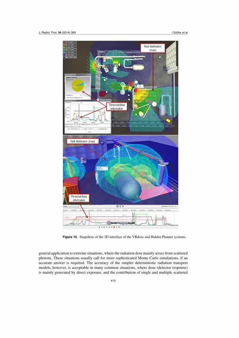
In terms of this dosimetric model, ‘detector’ means a virtual point isotropic detector,which can either be attached to a manikin, modelling a personal dosimeter worn by a humanparticipant, or can scan the whole scene in discrete steps, in order to map the scene interms of exposure. While the first case is used to monitor the radiation risks to workers, thesecond is utilised to visualise the distribution of the exposure within the whole 3D scene(figure 10).

397


2.2. The new point kernel approach

As indicated earlier, since the implementation of the dosimetric approach described above,numerous new developments have been made by the authors of this paper to better support riskassessment associated with work in nuclear environments. In the frame of these developments,a new dosimetric model has been elaborated to supplement the one just described. Themotivations for developing the new model are described below.

In the development of the earlier model, calculation speed and simplicity were of theutmost priority. Thus, the input data were integrated into the model implementation. Thisenables high computation speed, but prevents users from extending the list of supportedisotopes and materials, or updating the applied standard radiological input data (attenuationand absorption coefficients, buildup factors, etc). Additionally, the integrated approach does notprovide users with enough flexibility, for instance for selecting the desired output informationfrom a list of currently applied radiometric and dosimetric quantities. Since the primary purposeof the software tool is to support work involving possible radiation exposure so that the radiationrisk to humans is as low as reasonably achievable, it is important that the radiation burdencalculated can be compared with the limits applicable to a particular situation.

It is quite a common situation to have a source shielded by some solid and/or liquid layers,with the detector being at some distance in air from the shield. Since air is not supported as amaterial, both attenuation and buildup of photons in air are neglected. Although, air has a lowinteraction with penetrating radiation, extensive layers of air may have a non-negligible effect,resulting in increasing inaccuracy at long distances from the radiation sources.

In the earlier model, extended sources are uniformly disaggregated into point sources basedon the difference between a worst-case and best-case scenario. This uniform splitting techniqueresults in either high inefficiency (if a very fine splitting is performed), or lower accuracy (if arougher splitting is applied) when the detector is close to a large extended source.

Since the development of the earlier model, updates of earlier published buildup data [9],and buildup data for additional photon energies and shield thicknesses have been published,and the literature providing standard photon buildup data is continuously expanding. As usersof the earlier dosimetric model are not able to account for these new findings, the database isinaccessible to them. For example, the largest shield thickness reported in [2] is 40 mfp (meanfree path). In contrast, there are buildup factors associated with exposure and other quantitiesfor up to 100 mfp available in more recent publications (e.g. [30–32, 44]).

All the issues listed above narrow the scope of applicability of the model. In order to extendthe applicability, a new dosimetric approach has been implemented.

The international market for software tools that can be utilised for radiation transportsimulations and dosimetric calculations has been evolving and expanding for many years now.Some of these models implement a complex radiation transport approach. These very accuratemodels are, in general, unsuitable for rapid and real-time assessments in dynamically changingenvironments, due to the time required for setting up and completing computations for realisticexposure situations. In contrast, there are also very simple models that are able to yield areasonably reliable estimate much more quickly; but these are, of course, less accurate. Inaddition, some of the commercially available models have sophisticated visualisation toolscapable of 3D realistic representation of the results. It has to be stressed that advancedvisualisation of the results is just as important as state of the art simulation of radiationtransport. Ultimately, not the computer but humans utilising a model and looking at a computerdisplay will make decisions and perform jobs, based on their perception of the informationprovided by the model. 3D simulation tools for advanced planning and virtual reality toolsfor immersive training have undergone an immense evolution, due to the revolution of the

398


underlying computer technology. This area is in very rapid development, and has relativelyrecently gained focus in the nuclear sector. Hence, there is the room and a strong need forfurther development in this area. The new dosimetric model has been developed to supplementthe earlier model, and provide an even more powerful tool for improving the safety culture inthe nuclear industry.

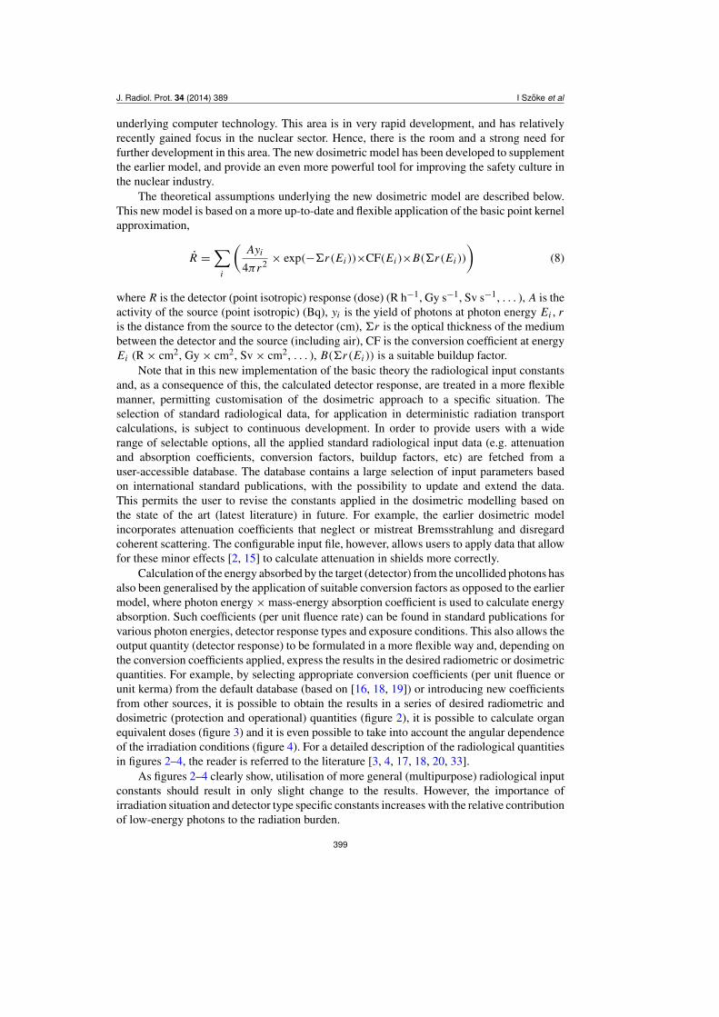
The theoretical assumptions underlying the new dosimetric model are described below.This new model is based on a more up-to-date and flexible application of the basic point kernelapproximation,

R =X

i

✓Ayi

4⇡r2 ⇥ exp(�6r(Ei ))⇥CF(Ei )⇥B(6r(Ei ))

◆(8)

where R is the detector (point isotropic) response (dose) (R h�1, Gy s�1, Sv s�1, . . . ), A is theactivity of the source (point isotropic) (Bq), yi is the yield of photons at photon energy Ei , ris the distance from the source to the detector (cm), 6r is the optical thickness of the mediumbetween the detector and the source (including air), CF is the conversion coefficient at energyEi (R ⇥ cm2, Gy ⇥ cm2, Sv ⇥ cm2, . . . ), B(6r(Ei )) is a suitable buildup factor.

Note that in this new implementation of the basic theory the radiological input constantsand, as a consequence of this, the calculated detector response, are treated in a more flexiblemanner, permitting customisation of the dosimetric approach to a specific situation. Theselection of standard radiological data, for application in deterministic radiation transportcalculations, is subject to continuous development. In order to provide users with a widerange of selectable options, all the applied standard radiological input data (e.g. attenuationand absorption coefficients, conversion factors, buildup factors, etc) are fetched from auser-accessible database. The database contains a large selection of input parameters basedon international standard publications, with the possibility to update and extend the data.This permits the user to revise the constants applied in the dosimetric modelling based onthe state of the art (latest literature) in future. For example, the earlier dosimetric modelincorporates attenuation coefficients that neglect or mistreat Bremsstrahlung and disregardcoherent scattering. The configurable input file, however, allows users to apply data that allowfor these minor effects [2, 15] to calculate attenuation in shields more correctly.

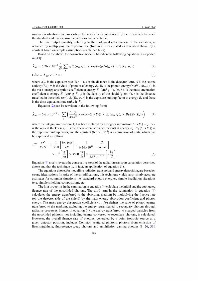
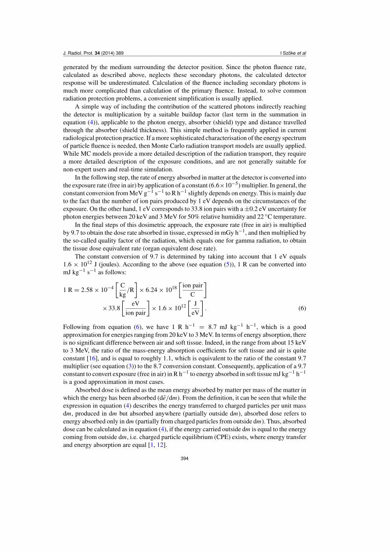
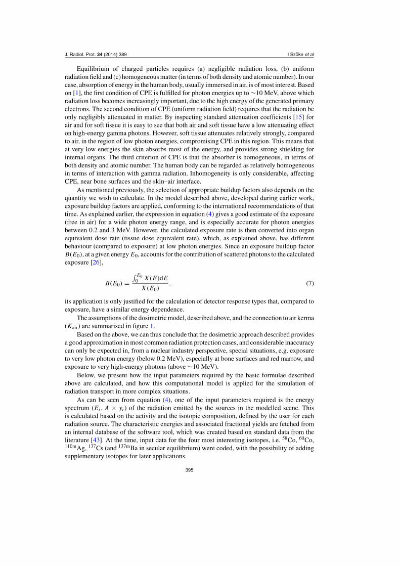
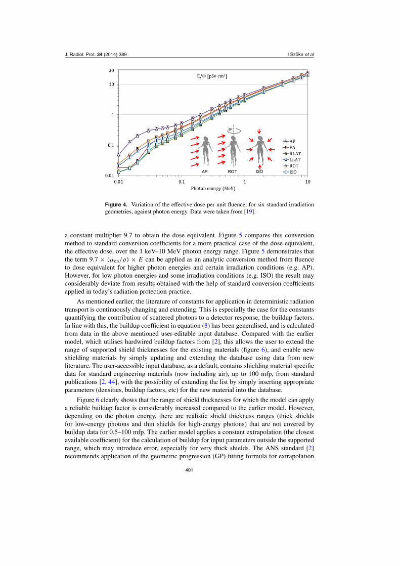
Calculation of the energy absorbed by the target (detector) from the uncollided photons hasalso been generalised by the application of suitable conversion factors as opposed to the earliermodel, where photon energy ⇥ mass-energy absorption coefficient is used to calculate energyabsorption. Such coefficients (per unit fluence rate) can be found in standard publications forvarious photon energies, detector response types and exposure conditions. This also allows theoutput quantity (detector response) to be formulated in a more flexible way and, depending onthe conversion coefficients applied, express the results in the desired radiometric or dosimetricquantities. For example, by selecting appropriate conversion coefficients (per unit fluence orunit kerma) from the default database (based on [16, 18, 19]) or introducing new coefficientsfrom other sources, it is possible to obtain the results in a series of desired radiometric anddosimetric (protection and operational) quantities (figure 2), it is possible to calculate organequivalent doses (figure 3) and it is even possible to take into account the angular dependenceof the irradiation conditions (figure 4). For a detailed description of the radiological quantitiesin figures 2–4, the reader is referred to the literature [3, 4, 17, 18, 20, 33].

As figures 2–4 clearly show, utilisation of more general (multipurpose) radiological inputconstants should result in only slight change to the results. However, the importance ofirradiation situation and detector type specific constants increases with the relative contributionof low-energy photons to the radiation burden.

399


Figure 2. Exposure X , kerma (free in air) K a, effective dose (anterior–posteriorirradiation) E , ambient H⇤, directional H 0, and personal dose equivalents H p per unitfluence (conversion factors). Data were taken from [16, 18, 19].

Figure 3. Organ equivalent doses and the effective dose, for anterior–posterior (AP)irradiation geometry, per unit air kerma, against photon energy. Data were takenfrom [19]. Note that according to the latest recommendations of the ICRP [20], adifferent categorisation of the organs and tissues of the human body has been proposed.

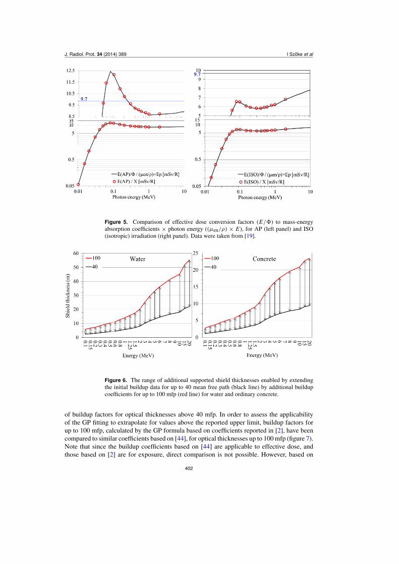
In order to check the validity of the affirmation above, standard fluence to detector responseconversion coefficients were compared with the conversion method applied in the earlier model.The earlier model applies (µen/⇢) ⇥ E to convert gamma fluence to exposure, and then

400


Figure 4. Variation of the effective dose per unit fluence, for six standard irradiationgeometries, against photon energy. Data were taken from [19].

a constant multiplier 9.7 to obtain the dose equivalent. Figure 5 compares this conversionmethod to standard conversion coefficients for a more practical case of the dose equivalent,the effective dose, over the 1 keV–10 MeV photon energy range. Figure 5 demonstrates thatthe term 9.7 ⇥ (µen/⇢) ⇥ E can be applied as an analytic conversion method from fluenceto dose equivalent for higher photon energies and certain irradiation conditions (e.g. AP).However, for low photon energies and some irradiation conditions (e.g. ISO) the result mayconsiderably deviate from results obtained with the help of standard conversion coefficientsapplied in today’s radiation protection practice.

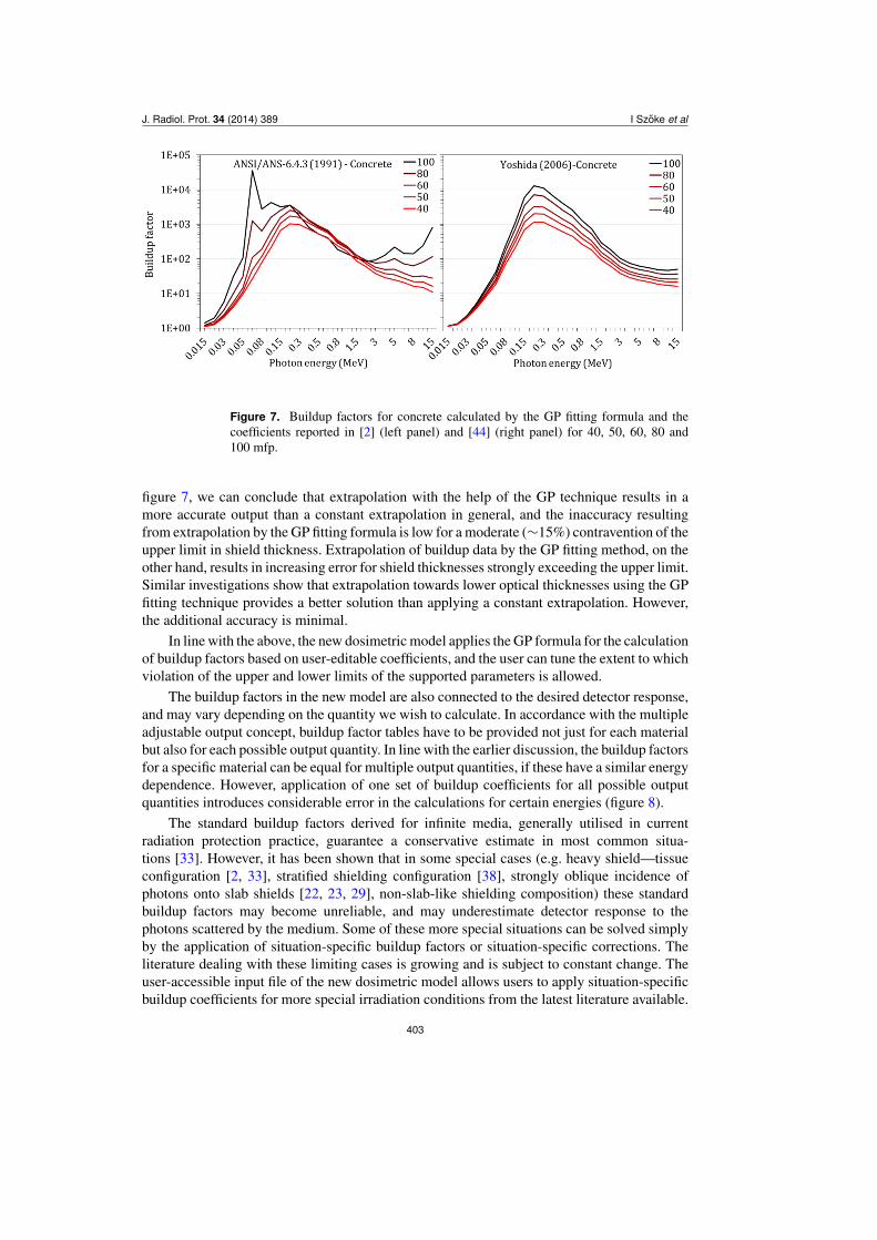
As mentioned earlier, the literature of constants for application in deterministic radiationtransport is continuously changing and extending. This is especially the case for the constantsquantifying the contribution of scattered photons to a detector response, the buildup factors.In line with this, the buildup coefficient in equation (8) has been generalised, and is calculatedfrom data in the above mentioned user-editable input database. Compared with the earliermodel, which utilises hardwired buildup factors from [2], this allows the user to extend therange of supported shield thicknesses for the existing materials (figure 6), and enable newshielding materials by simply updating and extending the database using data from newliterature. The user-accessible input database, as a default, contains shielding material specificdata for standard engineering materials (now including air), up to 100 mfp, from standardpublications [2, 44], with the possibility of extending the list by simply inserting appropriateparameters (densities, buildup factors, etc) for the new material into the database.

Figure 6 clearly shows that the range of shield thicknesses for which the model can applya reliable buildup factor is considerably increased compared to the earlier model. However,depending on the photon energy, there are realistic shield thickness ranges (thick shieldsfor low-energy photons and thin shields for high-energy photons) that are not covered bybuildup data for 0.5–100 mfp. The earlier model applies a constant extrapolation (the closestavailable coefficient) for the calculation of buildup for input parameters outside the supportedrange, which may introduce error, especially for very thick shields. The ANS standard [2]recommends application of the geometric progression (GP) fitting formula for extrapolation

401


Figure 5. Comparison of effective dose conversion factors (E/8) to mass-energyabsorption coefficients ⇥ photon energy ((µen/⇢) ⇥ E), for AP (left panel) and ISO(isotropic) irradiation (right panel). Data were taken from [19].

Figure 6. The range of additional supported shield thicknesses enabled by extendingthe initial buildup data for up to 40 mean free path (black line) by additional buildupcoefficients for up to 100 mfp (red line) for water and ordinary concrete.

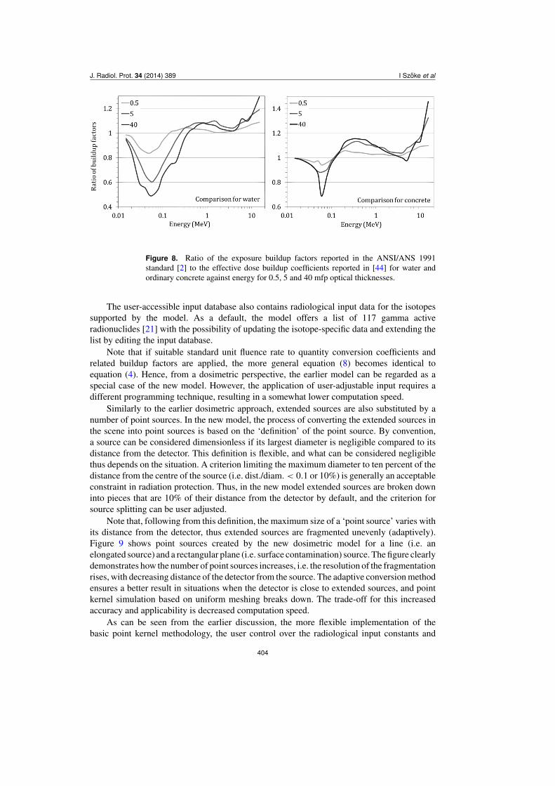
of buildup factors for optical thicknesses above 40 mfp. In order to assess the applicabilityof the GP fitting to extrapolate for values above the reported upper limit, buildup factors forup to 100 mfp, calculated by the GP formula based on coefficients reported in [2], have beencompared to similar coefficients based on [44], for optical thicknesses up to 100 mfp (figure 7).Note that since the buildup coefficients based on [44] are applicable to effective dose, andthose based on [2] are for exposure, direct comparison is not possible. However, based on

402


Figure 7. Buildup factors for concrete calculated by the GP fitting formula and thecoefficients reported in [2] (left panel) and [44] (right panel) for 40, 50, 60, 80 and100 mfp.

figure 7, we can conclude that extrapolation with the help of the GP technique results in amore accurate output than a constant extrapolation in general, and the inaccuracy resultingfrom extrapolation by the GP fitting formula is low for a moderate (⇠15%) contravention of theupper limit in shield thickness. Extrapolation of buildup data by the GP fitting method, on theother hand, results in increasing error for shield thicknesses strongly exceeding the upper limit.Similar investigations show that extrapolation towards lower optical thicknesses using the GPfitting technique provides a better solution than applying a constant extrapolation. However,the additional accuracy is minimal.

In line with the above, the new dosimetric model applies the GP formula for the calculationof buildup factors based on user-editable coefficients, and the user can tune the extent to whichviolation of the upper and lower limits of the supported parameters is allowed.

The buildup factors in the new model are also connected to the desired detector response,and may vary depending on the quantity we wish to calculate. In accordance with the multipleadjustable output concept, buildup factor tables have to be provided not just for each materialbut also for each possible output quantity. In line with the earlier discussion, the buildup factorsfor a specific material can be equal for multiple output quantities, if these have a similar energydependence. However, application of one set of buildup coefficients for all possible outputquantities introduces considerable error in the calculations for certain energies (figure 8).

The standard buildup factors derived for infinite media, generally utilised in currentradiation protection practice, guarantee a conservative estimate in most common situa-tions [33]. However, it has been shown that in some special cases (e.g. heavy shield—tissueconfiguration [2, 33], stratified shielding configuration [38], strongly oblique incidence ofphotons onto slab shields [22, 23, 29], non-slab-like shielding composition) these standardbuildup factors may become unreliable, and may underestimate detector response to thephotons scattered by the medium. Some of these more special situations can be solved simplyby the application of situation-specific buildup factors or situation-specific corrections. Theliterature dealing with these limiting cases is growing and is subject to constant change. Theuser-accessible input file of the new dosimetric model allows users to apply situation-specificbuildup coefficients for more special irradiation conditions from the latest literature available.

403


Figure 8. Ratio of the exposure buildup factors reported in the ANSI/ANS 1991standard [2] to the effective dose buildup coefficients reported in [44] for water andordinary concrete against energy for 0.5, 5 and 40 mfp optical thicknesses.

The user-accessible input database also contains radiological input data for the isotopessupported by the model. As a default, the model offers a list of 117 gamma activeradionuclides [21] with the possibility of updating the isotope-specific data and extending thelist by editing the input database.

Note that if suitable standard unit fluence rate to quantity conversion coefficients andrelated buildup factors are applied, the more general equation (8) becomes identical toequation (4). Hence, from a dosimetric perspective, the earlier model can be regarded as aspecial case of the new model. However, the application of user-adjustable input requires adifferent programming technique, resulting in a somewhat lower computation speed.

Similarly to the earlier dosimetric approach, extended sources are also substituted by anumber of point sources. In the new model, the process of converting the extended sources inthe scene into point sources is based on the ‘definition’ of the point source. By convention,a source can be considered dimensionless if its largest diameter is negligible compared to itsdistance from the detector. This definition is flexible, and what can be considered negligiblethus depends on the situation. A criterion limiting the maximum diameter to ten percent of thedistance from the centre of the source (i.e. dist./diam. < 0.1 or 10%) is generally an acceptableconstraint in radiation protection. Thus, in the new model extended sources are broken downinto pieces that are 10% of their distance from the detector by default, and the criterion forsource splitting can be user adjusted.

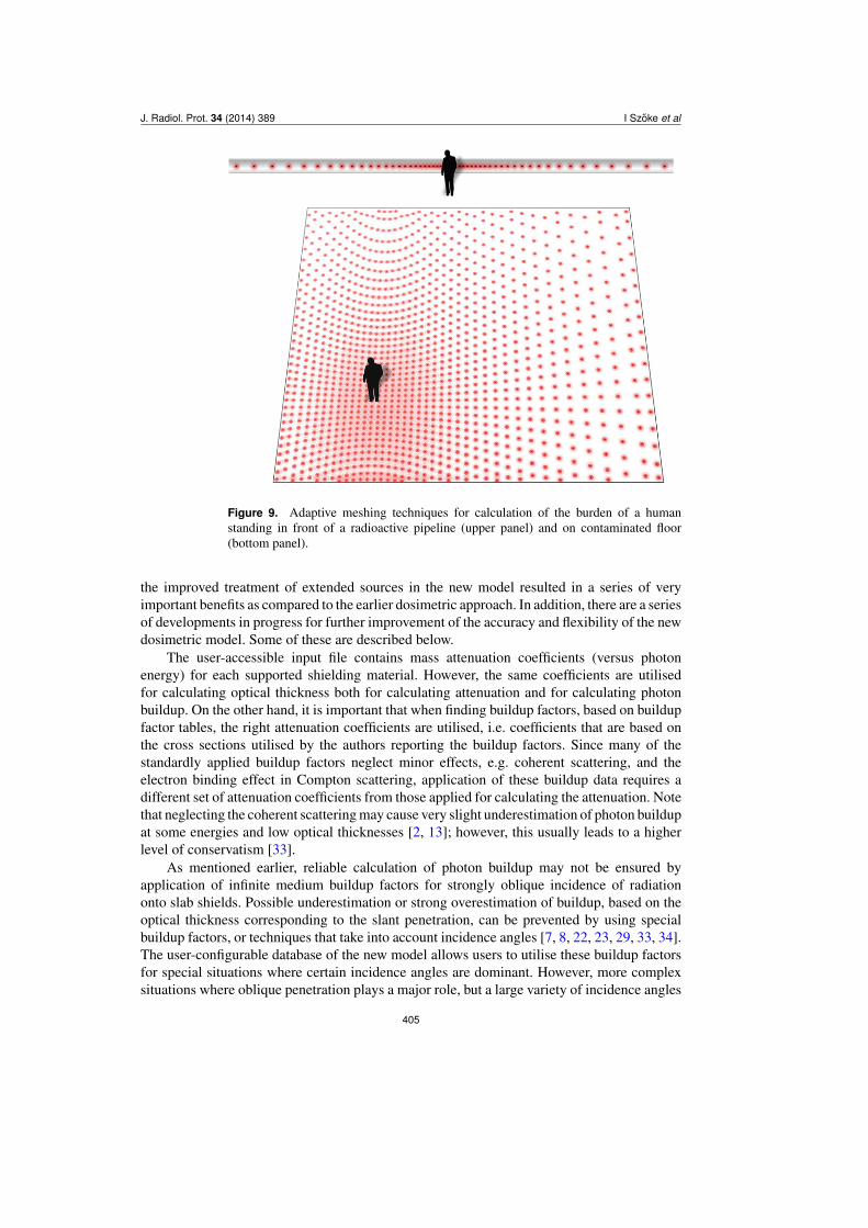
Note that, following from this definition, the maximum size of a ‘point source’ varies withits distance from the detector, thus extended sources are fragmented unevenly (adaptively).Figure 9 shows point sources created by the new dosimetric model for a line (i.e. anelongated source) and a rectangular plane (i.e. surface contamination) source. The figure clearlydemonstrates how the number of point sources increases, i.e. the resolution of the fragmentationrises, with decreasing distance of the detector from the source. The adaptive conversion methodensures a better result in situations when the detector is close to extended sources, and pointkernel simulation based on uniform meshing breaks down. The trade-off for this increasedaccuracy and applicability is decreased computation speed.

As can be seen from the earlier discussion, the more flexible implementation of thebasic point kernel methodology, the user control over the radiological input constants and

404


Figure 9. Adaptive meshing techniques for calculation of the burden of a humanstanding in front of a radioactive pipeline (upper panel) and on contaminated floor(bottom panel).

the improved treatment of extended sources in the new model resulted in a series of veryimportant benefits as compared to the earlier dosimetric approach. In addition, there are a seriesof developments in progress for further improvement of the accuracy and flexibility of the newdosimetric model. Some of these are described below.

The user-accessible input file contains mass attenuation coefficients (versus photonenergy) for each supported shielding material. However, the same coefficients are utilisedfor calculating optical thickness both for calculating attenuation and for calculating photonbuildup. On the other hand, it is important that when finding buildup factors, based on buildupfactor tables, the right attenuation coefficients are utilised, i.e. coefficients that are based onthe cross sections utilised by the authors reporting the buildup factors. Since many of thestandardly applied buildup factors neglect minor effects, e.g. coherent scattering, and theelectron binding effect in Compton scattering, application of these buildup data requires adifferent set of attenuation coefficients from those applied for calculating the attenuation. Notethat neglecting the coherent scattering may cause very slight underestimation of photon buildupat some energies and low optical thicknesses [2, 13]; however, this usually leads to a higherlevel of conservatism [33].

As mentioned earlier, reliable calculation of photon buildup may not be ensured byapplication of infinite medium buildup factors for strongly oblique incidence of radiationonto slab shields. Possible underestimation or strong overestimation of buildup, based on theoptical thickness corresponding to the slant penetration, can be prevented by using specialbuildup factors, or techniques that take into account incidence angles [7, 8, 22, 23, 29, 33, 34].The user-configurable database of the new model allows users to utilise these buildup factorsfor special situations where certain incidence angles are dominant. However, more complexsituations where oblique penetration plays a major role, but a large variety of incidence angles

405


are possible, require incidence angle dependent buildup calculations. Further development ofthe model to allow application of incidence angle specific input data is planned.

Similarly, the infinite homogeneous medium buildup factors are applied to stratifiedshielding configurations by simply multiplying the buildup in different layers. However,more sophisticated techniques, applicable to multilayer shielding configurations, have beenelaborated in the literature [38], and research continues, aimed at improving buildup estimationin non-homogeneous media.

One additional weakness originating from estimating the contribution of scatteredradiation only via simple buildup calculations based on buildup coefficients is that thismethodology disregards radiation ‘reflected’ (scattered) by surrounding objects, e.g. largesurfaces of heavy material (walls, ceiling, pavement). Radiation scatter is a highly complexphenomenon and, in general, sophisticated radiation transport modelling is required forits description, which is incompatible with real-time simulation. However, the effects of‘back-scattered’ radiation can be treated in a simplified manner by application of the so-called‘albedo’ method [6]. The albedo method offers a somewhat simplified approach to the problemwhich, due to its relative simplicity, could be used in a fast (real-time or semi-real-time)calculation. It is clear that the computing power required by this technique is significantlyhigher compared to the techniques described above. However, since in some real-worldcircumstances, for example a room having a strong source shielded, but not enclosed by,a massive slab-like shield, the detector response is mainly generated by scattered radiation,investigation of this issue is important.

The last issue that must be noted here is ray tracing. The optical thickness of the mediumbetween a point source and the detector is calculated based on the intersection of a straight linebetween the source and the detector with the objects defined as shields in the scene (the restis considered to be air). According to this, the medium between the source and the detector istreated as a series of layers (‘infinite’ slabs) of different materials when calculating attenuationand buildup. This hypothesis is reasonable in many cases. However, as previously explained,this approach is less applicable to highly complex shielding configurations, such as if the spacebetween the source and the detector is filled with a series of compact heavy objects. Thissituation is particularly problematic for extended sources when different parts of the source maybe shielded very differently. Firstly, in this case the standard buildup factors are only applieddue to the lack of more appropriate data. Secondly, calculation of the optical thickness betweenthe detector and an extended source, based on straight lines connecting the centres of the pointsources representing the extended source with the detector, may involve significant error. Raytracing is a very important and time-consuming part of the simulation and is strongly influencedby how realistically shaped sources are converted into idealised, dimensionless, point sources,to which the point kernels are applied.

All the completed improvements and those in progress significantly affect computationspeed. Since the main aim is to develop real-time (or semi-real-time) solutions, themethodologies implemented are always carefully inspected and optimised for speed. Inaddition, programming techniques such as parallel computing and exploitation of thecapabilities of modern graphics hardware in ray tracing are utilised for increased computationalspeed on high-end computers.

3. Results

The VRdose and Halden Planner systems are being developed to support real-world activitiesin nuclear environments by applying real-time 3D simulation and visualisation of workactivities and associated radiation exposure (figure 10). In line with the issues pointed out

406


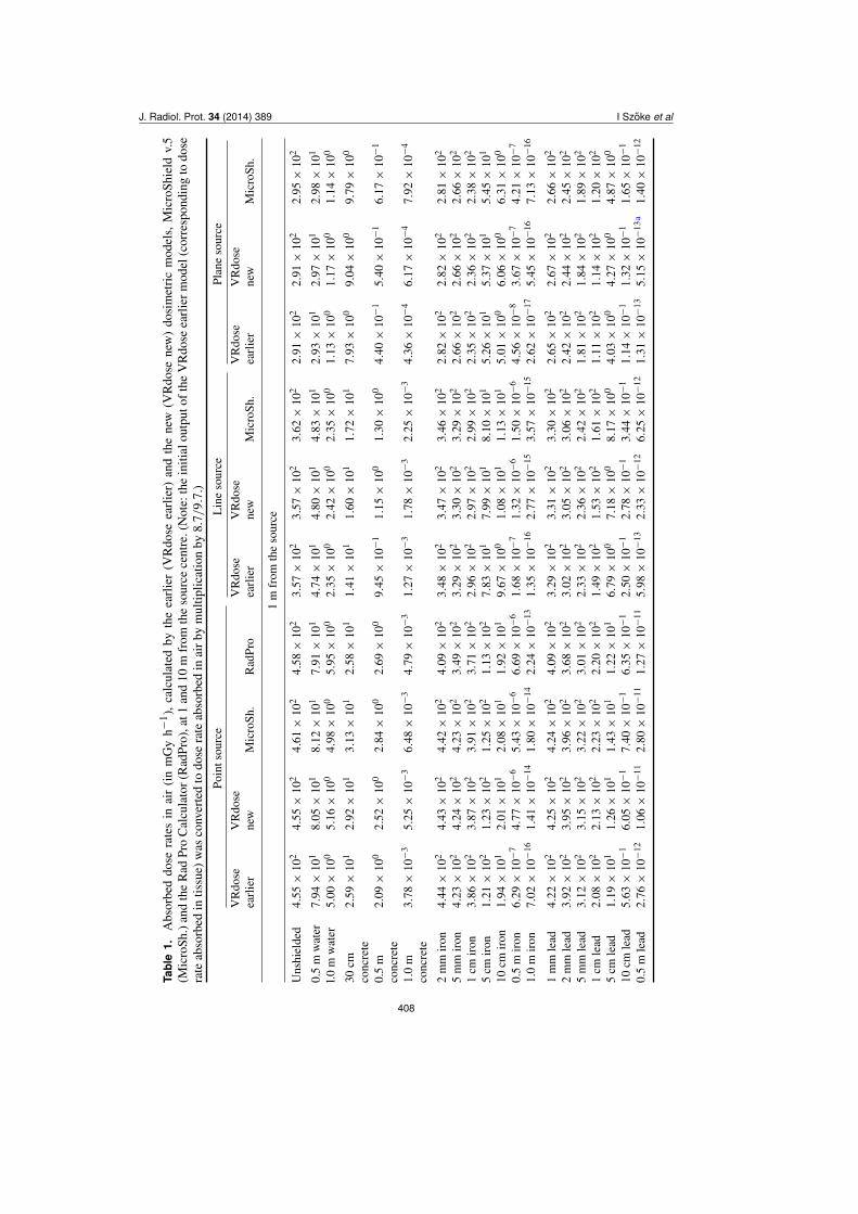
earlier, simple and quick dosimetric techniques, compatible with real-time 3D simulation,are not suitable for very accurate dose calculations in realistic environments. However, thesetechniques are very powerful for producing quick conservative dose estimates associated withwork procedures that are subject to dynamic variation of the exposure conditions. Validation ofthe techniques with the help of a complex realistic work scenario is challenging for a numberof reasons. Hence, as a first step, simple irradiation situations were chosen for validation;these are supported by internationally accepted alternative tools, and the error resulting fromsimplification of the radiation transport is expected to be low. In line with this, a sample problempackage has been designed which includes a series of calculations with common parametersbut varying parameter values for source geometry, source-to-detector distance, shield (slabshield) thickness and shielding material. Dosimetric calculations have been performed usingMicroShield (versions 5 and 6) [10, 11], the simple online Rad Pro Calculator [25] and thetwo dosimetric units described in this paper to calculate the absorbed dose rate in air. Note thatthe detector response type selected for the new dosimetric model, for comparison to the rate ofdose absorbed in air calculated by MicroShield and the Rad Pro Calculator, was the kerma rate.

The irradiation setup is demonstrated in figure 11.The source is a multi-isotopic source containing 500 GBq of 60Co and 4 TBq of 137Cs

(137mBa, the radioactive daughter generated by nuclear decay of the 137Cs, has naturally beenincluded). A 5 m ⇥ 5 m slab shield is positioned, with its centre 0.5 m from the centre of thesource, and perpendicular to the source-to-detector line. Calculations have been performed forvarious shield materials and thicknesses (including no shielding), source-to-detector distancesand source geometries (point, line and plane). In the case of extended sources (line andrectangular plane), the source is always centred relative to the shield, and orthogonal to thesource-to-detector line.

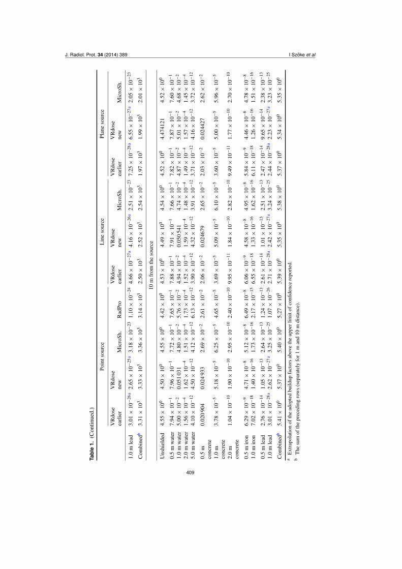
The results calculated using MicroShield v.5, the Rad Pro Calculator, the earlier (VRdoseearlier) and the new (VRdose new) models described in this paper, are listed in table 1, sortedby input parameters. Note that the two last rows, labelled ‘combined’, give the sum of allpreceding rows, corresponding to an irradiation condition combining all the simple situationsinvestigated.

Table 1 nicely shows that for all shielding configurations, dose rate decreases whenreplacing the point source with a line and then a plane source. This follows from the activitybeing more and more spread, which (a) causes some of the activity to be at greater distancefrom the detector and (b) improves shielding, due to the slanted pathway of the radiation fromthe distal parts of the extended source. As expected, the decrease in dose rate is less evident ifthe detector is 10 m from the source.

Table 2 quantifies the deviation of the VRdose and Rad Pro Calculator results from thoseobtained by the MicroShield v.5. More specifically, the table applies the following formula tocompare the results:

Deviance (VRdose) =

8>><

>>:

✓VRdose

MicroShield� 1

◆⇥ 100 if VRdose > MicroShield

�✓

MicroShieldVRdose

+ 1◆

⇥ 100 if VRdose < MicroShield.

(9)

Investigation of table 2 reveals that there is very good agreement between the resultsobtained by the different calculation tools for low optical thicknesses. For strong shielding,however, the deviance strongly increases with shield thickness, and reaches great proportionsfor extreme optical thicknesses. Nevertheless, as mentioned earlier, the simplified methodsapplied in the deterministic tools utilised in this benchmark exercise are not designed for

407


Ta

ble

1.

Abs

orbe

ddo

sera

tes

inai

r(in

mG

yh�

1 ),c

alcu

late

dby

the

earli

er(V

Rdo

seea

rlier

)an

dth

ene

w(V

Rdo

sene

w)

dosi

met

ricm

odel

s,M

icro

Shie

ldv.

5(M

icro

Sh.)

and

the

Rad

Pro

Cal

cula

tor(

Rad

Pro)

,at1

and

10m

from

the

sour

cece

ntre

.(N

ote:

the

initi

alou

tput

ofth

eV

Rdo

seea

rlier

mod

el(c

orre

spon

ding

todo

sera

teab

sorb

edin

tissu

e)w

asco

nver

ted

todo

sera

teab

sorb

edin

airb

ym

ultip

licat

ion

by8.

7/9.

7.)

Poin

tsou

rce

Line

sour

cePl

ane

sour

ceV

Rdo

seea

rlier

VR

dose

new

Mic

roSh

.R

adPr

oV

Rdo

seea

rlier

VR

dose

new

Mic

roSh

.V

Rdo

seea

rlier

VR

dose

new

Mic

roSh

.

1m

from

the

sour

ce

Uns

hiel

ded

4.55

⇥10

24.

55⇥

102

4.61

⇥10

24.

58⇥

102

3.57

⇥10

23.

57⇥

102

3.62

⇥10

22.

91⇥

102

2.91

⇥10

22.

95⇥

102

0.5

mw

ater

7.94

⇥10

18.

05⇥

101

8.12

⇥10

17.

91⇥

101

4.74

⇥10

14.

80⇥

101

4.83

⇥10

12.

93⇥

101

2.97

⇥10

12.

98⇥

101

l.0m

wat

er5.

00⇥

100

5.16

⇥10

04.

98⇥

100

5.95

⇥10

02.

35⇥

100

2.42

⇥10

02.

35⇥

100

1.13

⇥10

01.

17⇥

100

1.14

⇥10

0

30cm

conc

rete

2.59

⇥10

12.

92⇥

101

3.13

⇥10

12.

58⇥

101

1.41

⇥10

11.

60⇥

101

1.72

⇥10

17.

93⇥

100

9.04

⇥10

09.

79⇥

100

0.5

mco

ncre

te2.

09⇥

100

2.52

⇥10

02.

84⇥

100

2.69

⇥10

09.

45⇥

10�1

1.15

⇥10

01.

30⇥

100

4.40

⇥10

�15.

40⇥

10�1

6.17

⇥10

�1

1.0

mco

ncre

te3.

78⇥

10�3

5.25

⇥10

�36.

48⇥

10�3

4.79

⇥10

�31.

27⇥

10�3

1.78

⇥10

�32.

25⇥

10�3

4.36

⇥10

�46.

17⇥

10�4

7.92

⇥10

�4

2m

miro

n4.

44⇥

102

4.43

⇥10

24.

42⇥

102

4.09

⇥10

23.

48⇥

102

3.47

⇥10

23.

46⇥

102

2.82

⇥10

22.

82⇥

102

2.81

⇥10

2

5m

miro

n4.

23⇥

102

4.24

⇥10

24.

23⇥

102

3.49

⇥10

23.

29⇥

102

3.30

⇥10

23.

29⇥

102

2.66

⇥10

22.

66⇥

102

2.66

⇥10

2

1cm

iron

3.86

⇥10

23.

87⇥

102

3.91

⇥10

23.

71⇥

102

2.96

⇥10

22.

97⇥

102

2.99

⇥10

22.

35⇥

102

2.36

⇥10

22.

38⇥

102

5cm

iron

1.21

⇥10

21.

23⇥

102

1.25

⇥10

21.

13⇥

102

7.83

⇥10

17.

99⇥

101

8.10

⇥10

15.

26⇥

101

5.37

⇥10

15.

45⇥

101

10cm

iron

1.94

⇥10

12.

01⇥

101

2.08

⇥10

11.

92⇥

101

9.67

⇥10

01.

08⇥

101

1.13

⇥10

15.

01⇥

100

6.06

⇥10

06.

31⇥

100

0.5

miro

n6.

29⇥

10�7

4.77

⇥10

�65.

43⇥

10�6

6.69

⇥10

�61.

68⇥

10�7

1.32

⇥10

�61.

50⇥

10�6

4.56

⇥10

�83.

67⇥

10�7

4.21

⇥10

�7

1.0

miro

n7.

02⇥

10�1

61.

41⇥

10�1

41.

80⇥

10�1

42.

24⇥

10�1

31.

35⇥

10�1

62.

77⇥

10�1

53.

57⇥

10�1

52.

62⇥

10�1

75.

45⇥

10�1

67.

13⇥

10�1

6

1m

mle

ad4.

22⇥

102

4.25

⇥10

24.

24⇥

102

4.09

⇥10

23.

29⇥

102

3.31

⇥10

23.

30⇥

102

2.65

⇥10

22.

67⇥

102

2.66

⇥10

2

2m

mle

ad3.

92⇥

102

3.95

⇥10

23.

96⇥

102

3.68

⇥10

23.

02⇥

102

3.05

⇥10

23.

06⇥

102

2.42

⇥10

22.

44⇥

102

2.45

⇥10

2

5m

mle

ad3.

12⇥

102

3.15

⇥10

23.

22⇥

102

3.01

⇥10

22.

33⇥

102

2.36

⇥10

22.

42⇥

102

1.81

⇥10

21.

84⇥

102

1.89

⇥10

2

1cm

lead

2.08

⇥10

22.

13⇥

102

2.23

⇥10

22.

20⇥

102

1.49

⇥10

21.

53⇥

102

1.61

⇥10

21.

11⇥

102

1.14

⇥10

21.

20⇥

102

5cm

lead

1.19

⇥10

11.

26⇥

101

1.43

⇥10

11.

22⇥

101

6.79

⇥10

07.

18⇥

100

8.17

⇥10

04.

03⇥

100

4.27

⇥10

04.

87⇥

100

10cm

lead

5.63

⇥10

�16.

05⇥

10�1

7.40

⇥10

�16.

35⇥

10�1

2.50

⇥10

�12.

78⇥

10�1

3.44

⇥10

�11.

14⇥

10�1

1.32

⇥10

�11.

65⇥

10�1

0.5

mle

ad2.

76⇥

10�1

21.

06⇥

10�1

12.

80⇥

10�1

11.

27⇥

10�1

15.

98⇥

10�1

32.

33⇥

10�1

26.

25⇥

10�1

21.

31⇥

10�1

35.

15⇥

10�1

3a1.

40⇥

10�1

2

408


Ta

ble

1.

(Con

tinue

d.)

Poin

tsou

rce

Line

sour

cePl

ane

sour

ce

VR

dose

earli

erV

Rdo

sene

wM

icro

Sh.

Rad

Pro

VR

dose

earli

erV

Rdo

sene

wM

icro

Sh.

VR

dose

earli

erV

Rdo

sene

wM

icro

Sh.

1.0

mle

ad3.

01⇥

10�2

6a2.

65⇥

10�2

5a3.

18⇥

10�2

31.

10⇥

10�2

44.

66⇥

10�2

7a4.

16⇥

10�2

6a2.

51⇥

10�2

37.

25⇥

10�2

8a6.

55⇥

10�2

7a2.

05⇥

10�2

3

Com

bine

db3.

31⇥

103

3.33

⇥10

33.

36⇥

103

3.14

⇥10

32.

50⇥

103

2.52

⇥10

32.

54⇥

103

1.97

⇥10

31.

99⇥

103

2.01

⇥10

3

10m

from

the

sour

ce

Uns

hiel

ded

4.55

⇥10

04.

50⇥

100

4.55

⇥10

04.

42⇥

100

4.53

⇥10

04.

49⇥

100

4.54

⇥10

04.

52⇥

100

4.47

4121

4.52

⇥10

0

0.5

mw

ater

7.94

⇥10

�17.

96⇥

10�1

7.72

⇥10

�17.

65⇥

10�1

7.88

⇥10

�17.

91⇥

10�1

7.66

⇥10

�17.

82⇥

10�1

7.87

⇥10

�17.

60⇥

10�1

1.0

mw

ater

5.00

⇥10

�20.

051

031

4.80

⇥10

�25.

76⇥

10�2

4.94

⇥10

�20.

050

541

4.74

⇥10

�24.

87⇥

10�2

5.01

⇥10

�24.

68⇥

10�2

2.0

mw

ater

1.56

⇥10

�41.

62⇥

10�4

1.51

⇥10

�41.

73⇥

10�4

1.52

⇥10

�41.

59⇥

10�4

1.48

⇥10

�41.

49⇥

10�4

1.57

⇥10

�41.

45⇥

10�4

5.0

mw

ater

4.10

⇥10

�12

4.50

⇥10

�12

4.12

⇥10

�12

6.13

⇥10

�12

3.90

⇥10

�12

4.32

⇥10

�12

3.91

⇥10

�12

3.71

⇥10

�12

4.16

⇥10

�12

3.72

⇥10

�12

0.5

mco

ncre

te0.

020

904

0.02

493

32.

69⇥

10�2

2.61

⇥10

�22.

06⇥

10�2

0.02

4679

2.65

⇥10

�22.

03⇥

10�2

0.02

4427

2.62

⇥10

�2

1.0

mco

ncre

te3.

78⇥

10�5

5.18

⇥10

�56.

25⇥

10�5

4.65

⇥10

�53.

69⇥

10�5

5.09

⇥10

�56.

10⇥

10�5

3.60

⇥10

�55.

00⇥

10�5

5.96

⇥10

�5

2.0

mco

ncre

te1.

04⇥

10�1

01.

90⇥

10�1

02.

95⇥

10�1

02.

40⇥

10�1

09.

95⇥

10�1

11.

84⇥

10�1

02.

82⇥

10�1

09.

49⇥

10�1

11.

77⇥

10�1

02.

70⇥

10�1

0

0.5

miro

n6.

29⇥

10�9

4.71

⇥10

�85.

12⇥

10�8

6.49

⇥10

�86.

06⇥

10�9

4.58

⇥10

�84.

95⇥

10�8

5.84

⇥10

�94.

46⇥

10�8

4.78

⇥10

�8

1.0

miro

n7.

02⇥

10�1

81.

40⇥

10�1

61.

73⇥

10�1

62.

17⇥

10�1

56.

55⇥

10�1

81.

33⇥

10�1

61.

62⇥

10�1

66.

11⇥

10�1

81.

26⇥

10�1

61.

51⇥

10�1

6

0.5

mle

ad2.

76⇥

10�1

41.

05⇥

10�1

32.

64⇥

10�1

31.

24⇥

10�1

32.

61⇥

10�1

41.

01⇥

10�1

32.

51⇥

10�1

32.

47⇥

10�1

49.

65⇥

10�1

42.

38⇥

10�1

3

1.0

mle

ad3.

01⇥

10�2

8a2.

62⇥

10�2

7a3.

25⇥

10�2

51.

07⇥

10�2

62.

71⇥

10�2

8a2.

42⇥

10�2

7a3.

24⇥

10�2

52.

44⇥

10�2

8a2.

23⇥

10�2

7a3.

23⇥

10�2

5

Com

bine

db5.

41⇥

100

5.37

⇥10

05.

40⇥

100

5.27

⇥10

05.

39⇥

100

5.35

⇥10

05.

38⇥

100

5.37

⇥10

05.

34⇥

100

5.35

⇥10

0

aEx

trapo

latio

nof

the

adop

ted

build

upfa

ctor

sab

ove

the

uppe

rlim

itof

confi

denc

ere

porte

d.b

The

sum

ofth

epr

eced

ing

row

s(s

epar

atel

yfo

r1m

and

10m

dist

ance

).

409


Figure 10. Snapshots of the 3D interface of the VRdose and Halden Planner systems.

general application to extreme situations, where the radiation dose mainly arises from scatteredphotons. These situations usually call for more sophisticated Monte Carlo simulations, if anaccurate answer is required. The accuracy of the simpler deterministic radiation transportmodels, however, is acceptable in many common situations, where dose (detector response)is mainly generated by direct exposure, and the contribution of single and multiple scattered

410


Figure 11. Irradiation setup for benchmarking.

radiation is low. Indeed, in table 2 the two last rows, for the two detector distances, showthe discrepancy of the sum of the results for exposure to individual sources. These combinedcases correspond to exposure situations that combine exposure to multiple sources shieldedby different shields (including one unshielded case). Comparison of the combined resultsshows that the two dosimetric models presented in this paper are in very good agreement withMicroShield v.5.

The results also show that for more specialised situations, involving only shields of greatoptical thickness, the variation of the results provided by deterministic models is high. In thesesituations, the resulting detector response mainly depends on how the scatter of photons isaccounted for; that is, what kind of buildup factors, and how they are applied. Since the buildupfactors reported in the literature inherit a great uncertainty for high optical thicknesses, and thevalues reported vary from report to report, the deviance between the results is neither surprisingnor unexpected. Users of these radiation transport tools must recognise the inaccuracy inherentto the simplified methodology applied, and resort to more sophisticated Monte Carlo radiationtransport tools for more precise simulation.

Similar investigations have been performed using a newer version of MicroShield(MicroShield v.6). Table 3 shows the deviance of our results from MicroShield v.6 calculatedwith the same methodology as before:

Deviance (VRdose) =

8>><

>>:

✓VRdose

MicroShield� 1

◆⇥ 100 if VRdose > MicroShield

�✓

MicroShieldVRdose

+ 1◆

⇥ 100 if VRdose < MicroShield.

(10)

Comparing table 3 to table 2, its counterpart for the earlier MicroShield version, we can seethat the tendency of the deviance is very similar; the deviance strongly increases at high opticalthicknesses, but for more common shield thicknesses the agreement is, in general, good. It is

411


Table 2. Discrepancy (in %) from MicroShield v.5 results, at 1 and 10 m from thesource (centre). A minus sign indicates underestimation.

Point source Line source Plane sourceVRdoseearlier

VRdosenew RadPro

VRdoseearlier

VRdosenew

VRdoseearlier

VRdosenew

1 m from the source

Unshielded �1 �1 �1 �1 �1 �1 �10.5 m water �2 �1 �3 �2 �1 �2 01.0 m water 0 4 19 0 3 �1 330 cmconcrete

�21 �7 �21 �22 �8 �24 �8

0.5 mconcrete

�36 �13 �5 �38 �13 �40 �14

1.0 mconcrete

�72 �24 �35 �77 �26 �81 �28

2 mm iron 0 0 �8 0 0 0 05 mm iron 0 0 �21 0 0 0 01 cm iron �1 �1 �6 �1 �1 �1 �15 cm iron �3 �1 �11 �3 �1 �4 �110 cm iron �7 �4 �8 �17 �4 �26 �40.5 m iron �763 �14 23 �791 �14 �823 �151.0 m iron �2464 �27 1146 �2539 �29 �2618 �311 mm lead 0 0 �4 0 0 0 02 mm lead �1 0 �8 �1 0 �1 05 mm lead �3 �2 �7 �4 �2 �4 �31 cm lead �7 �5 �1 �8 �5 �8 �65 cm lead �20 �14 �17 �20 �14 �21 �1410 cm lead �31 �22 �17 �38 �24 �44 �250.5 m lead �914 �164 �120 �944 �168 �971 �1721.0 m lead �1.1 ⇥ 105 �1.2 ⇥ 104 �2.8 ⇥ 103 �5.4 ⇥ 105 �6.0 ⇥ 104 �2.8 ⇥ 106 �3.1 ⇥ 105

Combined �1.7 �1.0 �7.0 �1.7 �1.0 �1.7 �0.9

10 m from the source

Unshielded 0 �1 �3 0 �1 0 �10.5 m water 3 3 �1 3 3 3 41.0 m water 4 6 20 4 7 4 72.0 m water 3 7 15 3 8 3 85.0 m water 0 9 49 0 11 0 120.5 mconcrete

�29 �8 �3 �29 �7 �29 �7

1.0 mconcrete

�65 �21 �35 �65 �20 �66 �19

2.0 mconcrete

�183 �55 �23 �183 �54 �185 �52

0.5 m iron �714 �9 27 �716 �8 �718 �71.0 m iron �2364 �24 1157 �2373 �22 �2371 �200.5 m lead �856 �152 �114 �861 �149 �863 �1471.0 m lead �1.1 ⇥ 105 �1.2 ⇥ 104 �2.9 ⇥ 103 �1.2 ⇥ 105 �1.3 ⇥ 104 �1.3 ⇥ 105 �1.4 ⇥ 104

Combined 0.3 �0.5 �2.3 0.2 �0.5 0.3 �0.3

apparent that at 1 m from the source, the deviance is substantially larger at lower opticalthicknesses than it was in the comparison to MicroShield v.5. This can also be observed inthe difference for the combined case.

412


Table 3. Discrepancy (in %) from MicroShield v.6 results, at 1 and 10 m from thesource (centre). A minus sign indicates underestimation.

Point source Line source Plane sourceVRdoseearlier

VRdosenew RadPro

VRdoseearlier

VRdosenew

VRdoseearlier

VRdosenew

1 m from the source

Unshielded �1 �1 �1 �1 �1 �1 �10.5 m water �1 1 �1 0 1 0 11.0 m water 0 3 19 0 3 0 430 cmconcrete

�40 �24 �40 �40 �24 �41 �24

0.5 mconcrete

�48 �23 �15 �49 �23 �50 �22

1.0 mconcrete

�62 �17 �28 �64 �17 �65 �17

2 mm iron �1 �1 �10 �1 �1 �1 �15 mm iron �3 �3 �25 �3 �3 �4 �41 cm iron �7 �7 �12 �9 �8 �10 �95 cm iron �47 �44 �58 �49 �46 �53 �50l0 cm iron �71 �65 �73 �86 �67 �102 �670.5 m iron �1182 �69 �21 �1233 �70 �1275 �71l.0 m iron �3789 �93 721 �3878 �94 �3946 �941 mm lead �6 �5 �10 �7 �7 �8 �72 mm lead �13 �12 �20 �16 �14 �16 �155 mm lead �34 �32 �39 �44 �42 �44 �411 cm lead �76 �72 �67 �106 �101 �95 �895 cm lead �286 �265 �276 �293 �272 �300 �277l0 cm lead �322 �293 �275 �440 �386 �487 �4070.5 m lead �8665 �2178 �1806 �8997 �2235 �9289 �2288l.0 m lead �9.7 ⇥ 106 �1.1 ⇥ 106 �2.6 ⇥ 105 �4.9 ⇥ 107 �5.5 ⇥ 106 �2.6 ⇥ 108 �2.8 ⇥ 107

Combined �15.4 �14.6 �21.4 �18.0 �17.1 �16.8 �15.9

10 m from the source

Unshielded 0 �1 �3 0 �1 0 �10.5 m water 4 5 1 5 5 4 5l.0 m water 6 8 22 6 8 6 92.0 m water 4 8 15 3 8 4 105.0 m water 1 10 50 1 11 1 130.5 mconcrete

�40 �18 �12 �40 �17 �40 �17

l.0 mconcrete

�53 �12 �25 �53 �11 �53 �10

2.0 mconcrete

�98 �9 16 �99 �8 �99 �7

0.5 m iron �1111 �62 �17 �1115 �61 �1117 �591.0 m iron �3575 �85 741 �3579 �81 �3582 �790.5 m lead �8158 �2074 �1739 �8214 �2049 �8240 �2035l.0 m lead �9.7 ⇥ 106 �1.1 ⇥ 106 �2.7 ⇥ 105 �1.1 ⇥ 107 �1.2 ⇥ 106 �1.2 ⇥ 107 �1.3 ⇥ 106

Combined 0.5 �0.3 �2.1 0.4 �0.3 0.5 �0.1

413


4. Conclusions

In the scope of the work described in this paper, a new real-time point kernel based radiation riskassessment algorithm has been developed and implemented in the VRdose and Halden Planner3D real-time simulation systems, to supplement the point kernel based model implementedpreviously. The new dosimetric model is in line with recent international radiation protectionrecommendations, and offers several improvements over the earlier model. The drawbackof the new model is a slower modelling speed in some situations and on some computers,which follows from the greater time requirement of the programming techniques that enablegreater flexibility and provide more accurate results. Real-time 3D simulation enforcesvery strict speed restrictions on the risk assessment methodology, which places very highdemands on the theoretical and programming solutions utilised. This paper describes in detailthe theoretical assumptions underlying the VRdose and Halden Planner systems, and thechallenges associated with past and future developments in minimising the shortcomingsresulting from the speed–accuracy trade-off.

In the frame of a benchmarking exercise, results for simple irradiation situations werecompared to MicroShield (versions 5 and 6) and the online Rad Pro Calculator. The resultsshow that, for the majority of the common radiation protection tasks in nuclear installations(associated with maintenance, outage or decommissioning), these simple radiation transportmodels are able to provide reliable real-time radiation risk assessments. In addition, due to thehigh performance in speed and simplicity of the input required, these models are suitable for

• users with no experience in radiation transport theory or modelling,• modelling dynamically changing exposure conditions,• providing information rapidly for decision-making in stressful situations,• real-time optimisation of work tasks from a radiation protection perspective,• real-time simulation for education, training and briefing of personnel.

In many applications, these capabilities offer huge advantages over more sophisticatedmodels based on detailed, high accuracy simulation of radiation transport.

References

[1] Abdel-Rahman W and Podgorsak E B 2010 Energy transfer and energy absorption in photoninteractions with matter revisited: a step-by-step illustrated approach Radiat. Phys. Chem.79 552–66

[2] American Nuclear Society—Working Group ANS-6.4.3 1992 American National Standardfor Gamma-Ray Attenuation Coefficients and Buildup Factors for Engineering Materials(ANSI/ANS-6.4.3) (555 North Kensington Avenue, La Grange Park, IL 60525, USA)

[3] Andrasi A et al 2010 Sugarvedelem (Radiation Protection) (Budapest: Elte Eotvos Kiado)[4] Becker D et al 2005 Radiological Protection Landolt–Bornstein – Group VIII Advanced Materials

and Technologies — Numerical Data and Functional Relationships in Science and TechnologyVol 4, ed W Martienssen (Berlin: Springer)

[5] Broadhead B L and Emmett M B 1998 QADS: A Multidimensional Point-Kernel Analysis Module(Washington, DC: Oak Ridge National Laboratory)

[6] Brockhoff R C and Shultis J K 2006 Data for the calculation of albedos from concrete iron, lead,and water for photons and neutrons Report 301 Engineering Experiment Station College ofEngineering, Kansas State University, Manhattan, KS 66506

[7] Chucas S J 1996 Application Guide for Streaming Calculations with RANKERN (Dorchester: AEATechnology, Winfrith Technology Centre)

414

http://dx.doi.org/10.1016/j.radphyschem.2010.01.007

http://dx.doi.org/10.1016/j.radphyschem.2010.01.007


[8] Chucas S and Curl I 1999 Streaming calculations using the point-kernel code 9th Int. Conf. onRadiation Shielding (Tsukuba)

[9] Durani L A 2009 Update to ANSI/ANS-6.4.3-1991 for low-Z and compound materials and reviewof particle transport theory (Department of Mechanical Engineering 2009, University of Nevada,Las Vegas) p 221

[10] Grove Engineering 1998 MICROSHIELD—Version 5 User’s Manual[11] Grove Engineering 2003 MicroShield, Version 6.02 (Onley, MD)[12] Gurler O, Oz H, Yalcin S and Gundogdu O 2009 Mass absorption and mass energy transfer

coefficients for 0.4–10 MeV gamma rays in elemental solids and gases Appl. Radiat. Isot.67 201–5

[13] Harima Y, Tanaka S I, Sakamoto Y and Hirayama H 1991 Development of new gamma-raybuildup factor and application to shielding calculations J. Nucl. Sci. Technol. 28 74–84

[14] Harima Y 1993 An historical review and current status of buildup factor calculations andapplications Radiat. Phys. Chem. 41 631–72

[15] Hubbell J H 1982 Photon mass attenuation and energy-absorption coefficients from 1 keV to20 MeV Int. J. Appl. Radiat. Isot. 33 1269–90

[16] Hubbell J H and Seltzer S M 1996 Tables of x-ray mass attenuation coefficients and massenergy-absorption coefficients 1 keV to 20 MeV for elements Z = 1 to 92 and 48 additionalsubstances of dosimetric interest NIST Report, NISTIR 5632, ed S M Seltzer (US Departmentof Commerce, Technology Administration, National Institute of Standards and Technology,Gaithersburg, MD)

[17] International Commission on Radiological Protection (ICRP) 1991 1990 Recommendations ofthe International Commission on Radiological Protection ICRP Publication 60; Ann. ICRP21 (1–3)

[18] International Commission on Radiation Units and Measurements (ICRU) 1992 Measurements ofDose Equivalents from External Photon and Electron Radiations (Report 47) (Bethesda, MD:ICRU Publications)

[19] International Commission on Radiological Protection (ICRP) 1996 Conversion coefficients foruse in radiological protection against external radiation ICRP Publication 74; Ann. ICRP26 (3–4)

[20] International Commission on Radiological Protection (ICRP) 2007 The 2007 Recommendationsof the International Commission on Radiological Protection ICRP Publication 103; Ann. ICRP37 (2–4)

[21] Nichols A L, Aldama D L and Verpelli M 2008 Handbook of nuclear data for safeguards: databaseextensions, IAEA Nuclear Data Section, International Nuclear Data Committee INDC-0534Report, Distr. SQ

[22] Perkins J F 1995 Some Monte-Carlo calculations of gamma-ray penetrations J. Appl. Phys.26 1372–7

[23] Pieper A G and Beach L A 1963 Stochastic Estimates of the Penetration of Gamma Rays throughSlab Shields (Washington, DC: US Naval Research Laboratory)

[24] Prokhorets I M, Prokhorets S I, Khazhmuradov M A, Rudychev E V and Fedorchenko D V 2007Point-kernel method for radiation fields simulation Probl. At. Sci. Technol. 5 106–9

[25] Rad Pro Calculator (www.radprocalculator.com) Rad Pro Calculator Review: Ionactive ConsultingLtd Newsletter—January 2007 (issue 1, p 10) (www.ionactive.co.uk/pdfs/Ionactive RadiationProtection newsletter January 2007.pdf)

[26] Ragheb M 2011 Online courses by M Ragheb Nuclear Power Engineering (University of Illinoisat Urbana-Champaign, Nuclear, Plasma, and Radiological Engineering)

[27] Rindahl G and Mark N K 2008 VRDoseTM and emerging 3D software solutions to supportdecommissioning activities: experiences and expectations from development and deployment ofinnovative technology In Innovative and Adaptive Technologies in Decommissioning of NuclearFacilities (IAEA-TECDOC-1602) (Vienna: IAEA)

[28] Roussin R W, Kirk B L and Trubey D K 2001 Radiation Shielding and Protection (Encyclopaediaof Physical Science and Technology) 3rd edn, ed R A Meyers (Amsterdam: Elsevier) p 581

415

http://dx.doi.org/10.1016/j.apradiso.2008.10.001

http://dx.doi.org/10.1016/j.apradiso.2008.10.001

http://dx.doi.org/10.1080/18811248.1991.9731324

http://dx.doi.org/10.1080/18811248.1991.9731324

http://dx.doi.org/10.1016/0969-806X(93)90317-N

http://dx.doi.org/10.1016/0969-806X(93)90317-N

http://dx.doi.org/10.1016/0020-708X(82)90248-4

http://dx.doi.org/10.1016/0020-708X(82)90248-4

http://dx.doi.org/10.1063/1.1721910

http://dx.doi.org/10.1063/1.1721910

www.radprocalculator.com

























[29] Schirmers F G 2006 Improvement of Photon Buildup Factors for Radiological Assessment inNuclear Engineering North Carolina (Raleigh, NC: North Carolina State University)

[30] Shimizu A 2002 Calculation of gamma-ray buildup factors up to depths of 100 mfp by the methodof invariant embedding, (I)—analysis of accuracy and comparison with other data J. Nucl. Sci.Technol. 39 477–86

[31] Shimizu A and Hirayama H 2003 Calculation of gamma-ray buildup factors up to depths of100 mfp by the method of invariant embedding, (II) improved treatment of bremsstrahlungJ. Nucl. Sci. Technol. 40 192–200

[32] Shimizu A, Onda T and Sakamoto Y 2004 Calculation of gamma-ray buildup factors up to depthsof 100 mfp by the method of invariant embedding, (III)—generation of an improved data setJ. Nucl. Sci. Technol. 41 413–24

[33] Shultis J K and Faw R E 2000 Radiation Shielding (American Nuclear Society, 555 NorthKensington Avenue, La Grange Park, IL 60525, USA)

[34] Shultis J K and Faw R E 2005 Radiation shielding technology Health Phys. 88 297–322[35] Takeuchi K and Tanaka S I 1984 Exposure, Dose-Equivalent and Absorbed-Dose Buildup Factors

of Gamma Rays for Plane Normal and Isotropic Incidences on Water, Concrete, Iron and Lead(Japan: Japan Atomic Energy Research Institute) p 37

[36] Takeuchi K and Tanaka S I 1986 Absorbed-dose and dose-equivalent buildup factors ofgamma-rays including bremsstrahlung and annihilation radiation for water, concrete, iron andlead Appl. Radiat. Isot. 37 283–96

[37] Tanaka S I et al 1988 Annotated-bibliography and discussion of gamma-ray buildup factors Appl.Radiat. Isot. 39 241–52

[38] Trontl K, Smuc T and Pevec D 2007 Support vector regression model for the estimation ofgamma-ray buildup factors for multi-layer shields Ann. Nucl. Energy 34 939–52

[39] Shultis J K and Faw R E 2010 Radiation shielding and radiological protection Handbook ofNuclear Engineering ed D G Cacuci (New York: Springer) Chapter 11

[40] Subbaiah K V and Sarangapani R 2008 IGSHIELD: a new interactive point kernel gamma rayshielding code Ann. Nucl. Energy 35 2234–42

[41] Szoke I, Louka M N, Mark N K, Bryntesen T R, Bratteli J, Edvardsen S T, Gustavsen M A,Toppe A L, Johnsen T and Rindahl G 2012 New software tools for dynamic radiologicalcharacterisation and monitoring in nuclear sites Workshop on Radiological Characterisationfor Decommissioning (Nykoping, April 2012) (www.oecd-nea.org/rwm/wpdd/rcd-workshop/)

[42] Szoke I and Johnsen T 2013 Human-centred radiological software techniques supporting improvednuclear safety Nucl. Saf. Simul. 4 219–25

[43] Vabø R, Piotrowski L and Rindahl G 2010 3D representation of radioisotopic dose rates withinnuclear plants for improved radioprotection and plant safety Nucl. Saf. Simul. 1 127–33

[44] Yoshida Y 2006 Development of fitting methods using geometric progression formulae ofgamma-ray buildup factors J. Nucl. Sci. Technol. 43 1446–57

416

Real-time 3D radiation risk assessment supporting simulation of work in nuclear environment

Documents

Transcript of Real-time 3D radiation risk assessment supporting simulation of work in nuclear environment