Reachability Analysis of Nonlinear Systems Using Conservative Approximation

Reachability Analysis of Nonlinear SystemsUsing Conservative Approximation?

Eugene Asarin1, Thao Dang1, and Antoine Girard2

1 VERIMAG2 avenue de Vignate, 38610 Gieres, France

2 LMC-IMAG51 rue des Mathematiques, 38041 Grenoble, France

{Eugene.Asarin,Thao.Dang,Antoine.Girard}@imag.fr

Abstract. In this paper we present an approach to approximate reacha-bility computation for nonlinear continuous systems. Rather than study-ing a complex nonlinear system x = g(x), we study an approximatingsystem x = f(x) which is easier to handle. The class of approximatingsystems we consider in this paper is piecewise linear, obtained by inter-polating g over a mesh. In order to be conservative, we add a boundedinput in the approximating system to account for the interpolation error.We thus develop a reachability method for systems with input, based onthe relation between such systems and the corresponding autonomoussystems in terms of reachable sets. This method is then extended to theapproximate piecewise linear systems arising in our construction. Thefinal result is a reachability algorithm for nonlinear continuous systemswhich allows to compute conservative approximations with as great de-gree of accuracy as desired, and more importantly, it has good conver-gence rate. If g is a C2 function, our method is of order 2. Furthermore,the method can be straightforwardly extended to hybrid systems.

1 Introduction

Reachability computation is required by a variety of safety verification, anal-ysis, and design problems for hybrid systems. The importance of the problemhas motivated much research on reachability analysis of such systems (see [5,14]). For a class of hybrid systems with piecewise constant derivatives, methodsand tools for (exact) computation of reachable sets are well-developed [26,20,16]. For systems involving non-trivial continuous dynamics (described by differ-ential equations), exact reachability computation is difficult, and even for lineardifferential equations it is feasible only for certain classes of matrices, dependingon eigenstructure [19,2]. Alternatively, several approximate methods have beendeveloped, and some of them can be used for nonlinear continuous systems, suchas [13,8,7,22]. Basically, these methods numerically approximate reachable setsusing a variety of set representations (such as polyhedra, level sets). A common? Research supported by European IST project “CC - Computation and Control” and

CNRS project MathStic “Squash - Analyse Qualitative des Systemes Hybrides”.

O. Maler and A. Pnueli (Eds.): HSCC 2003, LNCS 2623, pp. 20–35, 2003.c© Springer-Verlag Berlin Heidelberg 2003

Reachability Analysis of Nonlinear Systems 21

point of these methods is that they work directly with the nonlinear differentialequations, more precisely, they track the evolution of the reachable sets accord-ing to the flows of the nonlinear equations. In this work, we take an approachwhich differs from these methods in this aspect. The main idea of the approachis as follows.

Rather than studying a complex nonlinear system x = g(x), we study anapproximating system x = f(x) which is easier to handle. The class of approx-imating systems we consider in this paper is piecewise linear, obtained by in-terpolating the function g over a mesh built on the state space of the system.Moreover, in order to be conservative, we add an input u to account for the errorinherent in approximating g with f , and the result is a system with (bounded)input x = f(x) + u. This construction gives rise to the question of how to dealwith the input in the approximating system efficiently. We thus consider the re-lation between a system with input and the corresponding autonomous systemin terms of reachable sets, and this study leads us to an abstract reachabilityalgorithm for systems with input, which can then be extended to deal with theapproximate interpolating systems. The final result is a reachability method fornonlinear systems which allows to compute conservative approximations with asgreat degree of accuracy as desired, and more importantly, it has good conver-gence rate. As we shall see later, if g is a C2 function our method is of order 2.Furthermore, the method can be straightforwardly extended to hybrid systemsand readily integrated in a verification tool.

The ‘hybridization’ approach has previously been explored in [25,17,24] wherethe approximating systems are systems with piecewise constant slopes or rect-angular inclusions. The idea of defining piecewise linear approximation basedon interpolation has been used for numerical integration of nonlinear differentialequations [9,11]; in this paper, we exploit this idea for reachability computationpurposes. In [13], linear approximation is also used in each integration step toobtain better approximations of the reachable sets in 2 dimensions. On the otherhand, our reachability method for systems with uncertain input has some similarflavor with the method of approximation of viability kernels of differential inclu-sions in [23]. Recently, in [15], a control problem for a class of piecewise linearsystems, similar to our approximating systems, is solved in terms of reachabilityconditions.

The paper is organized as follows. Section 2 is devoted to definitions andnotations. In Section 3 we consider the reachability problem for (general) con-tinuous systems with input. In Section 4 we present a method to approximatereachable sets of nonlinear systems by means of piecewise linear approximation.The theoretical result of Section 3 is the basis for the proof of the convergenceof the method. Section 5 contains some examples illustrating our approach.

2 Basic Definitions

We consider a nonlinear system

x(t) = g(x(t)), x ∈ X ⊂ Rn. (1)

22 E. Asarin, T. Dang, and A. Girard

As mentioned in the introduction, we approximate the system (1) with anothersystem (which is easier to solve):

x(t) = f(x(t)), x ∈ X ⊂ Rn. (2)

Let µ be the bound of ||f − g||, i.e. ||f(x) − g(x)|| ≤ µ for all x ∈ X where || · ||is some norm on Rn. We assume that the function f is L-Lipschitz. In order tobe able to capture all the behaviors of the original system (1), we introduce inthe system (2) an input to account for the approximation error.{

x(t) = s(x(t), u(t)) = f(x(t)) + u(t),u(·) ∈ Uµ

(3)

where Uµ is the set of admissible inputs which consists of piecewise continuousfunctions u of the form u : R+ → Rn such that ||u(·)|| ≤ µ. It is not hard tosee that the system (3) is an overapproximation of the original system (1) in thesense that all trajectories of (1) are contained in the set of trajectories of (3).

Given an initial point x ∈ X , let Φf (t, x) be the trajectory starting fromx of the system (2) and let Φs(t, x, u(·)) be the trajectory starting from x ofthe system (3) under input u(·) ∈ Uµ. For a set of initial points X0 ⊂ X andT > 0, the reachable sets of the autonomous system (2) during the interval [0, T ]is defined as: Kf (T, X0) = { y = Φf (t, x) | t ∈ [0, T ], x ∈ X0 }. Similarly, thereachable set of the system (3) from X0 during the interval [0, T ] is defined as:Ks(T, X0) = { y = Φs(t, x, u(·)) | t ∈ [0, T ], x ∈ X0, u(·) ∈ Uµ }.

3 Reachability Analysis for Systems with Input

As mentioned earlier, with a view to deal with the input in the approximatingsystem, we first consider the problem of deriving the reachable set of a systemwith input from the reachable set of the corresponding autonomous system. Moreconcretely, our goal is to compute the reacheable set Ks(T, X0) of the systemwith input (3), assuming that we are able to compute the image of a set X ⊂ Xby the flow Φf of the autonomous system (2) for a given time t ≥ 0, denoted byΦf (t, X).

We first describe an abstract algorithm to do so and then discuss the prop-erties of the algorithm concerning conservativeness and convergence of the ap-proximation. It is important to emphasize that these theoretical results are keyto the validation of the reachability method for nonlinear systems, developed inthe next section.

The idea to solve this problem relies on the following result, which is a con-sequence of the Fundamental Inequality theorem from the theory of dynamicalsystems (see Appendix).

Lemma 1. For all t ≥ 0 and for all u(·) ∈ Uµ,

||Φf (t, x) − Φs(t, x, u(·))|| ≤ µ

2(eLt − 1).


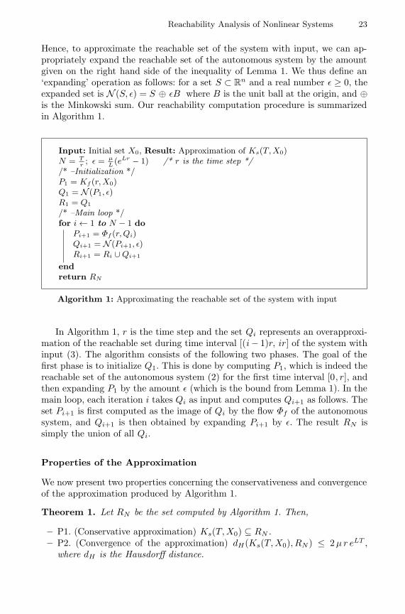
Hence, to approximate the reachable set of the system with input, we can ap-propriately expand the reachable set of the autonomous system by the amountgiven on the right hand side of the inequality of Lemma 1. We thus define an‘expanding’ operation as follows: for a set S ⊂ Rn and a real number ε ≥ 0, theexpanded set is N (S, ε) = S ⊕ εB where B is the unit ball at the origin, and ⊕is the Minkowski sum. Our reachability computation procedure is summarizedin Algorithm 1.

Input: Initial set X0, Result: Approximation of Ks(T, X0)N = T

r; ε = µ

L(eLr − 1) /* r is the time step */

/* –Initialization */P1 = Kf (r, X0)Q1 = N (P1, ε)R1 = Q1

/* –Main loop */for i← 1 to N − 1 do

Pi+1 = Φf (r, Qi)Qi+1 = N (Pi+1, ε)Ri+1 = Ri ∪Qi+1

endreturn RN

Algorithm 1: Approximating the reachable set of the system with input

In Algorithm 1, r is the time step and the set Qi represents an overapproxi-mation of the reachable set during time interval [(i − 1)r, ir] of the system withinput (3). The algorithm consists of the following two phases. The goal of thefirst phase is to initialize Q1. This is done by computing P1, which is indeed thereachable set of the autonomous system (2) for the first time interval [0, r], andthen expanding P1 by the amount ε (which is the bound from Lemma 1). In themain loop, each iteration i takes Qi as input and computes Qi+1 as follows. Theset Pi+1 is first computed as the image of Qi by the flow Φf of the autonomoussystem, and Qi+1 is then obtained by expanding Pi+1 by ε. The result RN issimply the union of all Qi.

Properties of the Approximation

We now present two properties concerning the conservativeness and convergenceof the approximation produced by Algorithm 1.

Theorem 1. Let RN be the set computed by Algorithm 1. Then,

– P1. (Conservative approximation) Ks(T, X0) ⊆ RN .– P2. (Convergence of the approximation) dH(Ks(T, X0), RN ) ≤ 2µ r eLT ,

where dH is the Hausdorff distance.


As we can see from the theorem, the approximate set produced by Algorithm 1is guaranteed to be an overapproximation of the exact reachable set. Moreover,it converges to the exact set with regard to the Hausdorff distance. The proof ofthe theorem can be found in Appendix.

4 Reachability Computation for Nonlinear SystemsUsing Piecewise Linear Approximation

In this section, we focus on the main problem of the paper, which is the com-putation of reachable sets for nonlinear continuous systems. Following the ‘hy-bridization’ idea, our method consists of two steps. We first approximate the(complex) nonlinear system by a piecewise (simple) linear system. A bound onthe approximation error is estimated and then added to the piecewise linear sys-tem as uncertain input, which guarantees that the resulting system is indeed anoverapproximation of the original system. The second step involves extendingAlgorithm 1, which is designed for continuous systems with input, to piecewiselinear systems. We first describe the two steps of the method and then discussthe convergence results.

4.1 Construction of Approximating Systems

We consider the nonlinear system

x(t) = g(x(t)), x ∈ X ⊂ Rn (4)

We assume that g is Lipschitz and the state space X is a bounded convex poly-hedron in Rn. To define an approximating system, we decompose the state spaceinto polyhedral regions and then associate with each region a linear system usinginterpolation. The procedure of decomposition of the state space is called meshgeneration. In the sequel, we will define these concepts formally.

Piecewise Linear Approximations Using Interpolation

Definition 1 (Mesh). A mesh M of the set X is a finite set of full-dimensionalconvex polyhedra in Rn, called cells, satisfying the following conditions: (1) Theunion of all cells

⋃k Ck = X , and (2) If Cj and Ck are cells with non-empty

intersection, then their intersection lies within the boundaries of both; we saythat Cj and Ck are adjacent and we denote their intersection by ∂(Cj , Ck).

For a cell Ck ∈ M, we denote by V (Ck) the set of its vertices and by ∂Ck theboundary of Ck. The size of Ck is h(Ck) = max{ ||x−y|| | x, y ∈ Ck }. Then, thesize (or granularity) of M is defined as h(M) = max{h(Ck) | Ck ∈ M }. Twotypes of meshes are of practical interest: rectangular and simplicial. A mesh iscalled rectangular if its cells are all boxes in Rn. If all the cells are simplices,then we say that M is a simplicial mesh or a triangulation of X . We recall that


a simplex in Rn is the convex hull of (n + 1) affinely independent points in Rn,and h(Ck) is simply the maximum edge length.

Given a mesh M of X , we can derive a piecewise linear approximation of thefunction g, using interpolation over the mesh. We restrict our attention to sim-plicial meshes and the motivation will become clear in subsequent development.A discussion on mesh construction is deferred to the end of this section.

Definition 2 (Piecewise linear approximation). For each cell Ck ∈ M, letlk : Rn → Rn be an affine map of the form lk(x) = Akx+bk which interpolates gon the vertices of Ck, that is, g(v) = lk(v) for all v ∈ V (Ck). Then, the piecewiselinear approximation of g is defined as: l(x) = lk(x) if x ∈ Ck.

The advantage of using simplicial meshes lies in the fact that the linear inter-polant lk can be defined uniquely since each cell Ck has (n+1) vertices and, more-over, for any two adjacent cells Ck and Cj , we have ∀x ∈ ∂(Ck, Cj) lk(x) = lj(x).This important property allows us to obtain the following approximating system:

x(t) = l(x(t))

which is continuous and Lipschitz. This not only guarantees the existence anduniqueness of solutions, but also allows to derive a priori bound on the error ofapproximation, as we will show in the following. This bound will then be usedto define a conservative approximating system.

Estimating interpolation error. The error in the approximation of g by theabovedescribed linear interpolation is defined by the bound η of ||g(x) − l(x)||for x ∈ X . We will estimate this bound for two cases: g is Lipschitz and g is aC2 function. For brevity, we denote by h the size of the underlying mesh M.

Lemma 2. If g is Lipschitz, then

η ≤ h2nL

n + 1

where L is the Lipschitz constant of the function g.

We remark is that the second partial derivatives of the linear approximationvanish; therefore, if g is a C2 function, we can obtain a better error bound.

Lemma 3. If g is a C2 function with a second derivative bound K, then

η ≤ h2 n2 K

2(n + 1)2.

As we can see from the above lemmas, the bound η is of order O(h) if g isLipschitz, and it is of order O(h2) if g is a C2 function with bounded secondderivative. The proofs of these results are presented in Appendix.


Defining conservative approximating systems. We can now use the boundη from the above lemmas to define an overapproximation of the nonlinear sys-tem (4), which has the form of the system with bounded input studied in Sec-tion 3: {

x(t) = s(x(t), u(t)) = l(x(t)) + u(t),u(·) ∈ Uη

(5)

Before continuing, we mention that it is straightforward to extend this method toa nonlinear systems with input of the form x(t) = g(x(t))+u(t) where u(·) ∈ Uµ

by defining an overapproximation of this system as: x(t) = l(x(t)) + u1(t) whereu1(·) ∈ Uν with ν = η + µ.

Using Lemma 1, we can show that the solution the approximate system (5)converges to the solution of the original system (4) and, moreover, the conver-gence is of the same order as the convergence of the interpolating function l tog. Indeed, for all t ≥ 0 and for all u(·) ∈ Uη, we have

||Φg(t, x) − Φs(t, x, u(·))|| ≤ η

2(eLt − 1) (6)

where Φg(t, x) and Φs(t, x, u(·)) are respectively the flows of the system (4) andof the system (5) under input u(·) ∈ Uη.

4.2 Reachability Algorithm for Piecewise Linear Systems

This section is concerned with the problem of computing reachable sets of thepiecewise linear systems resulting from the above approximation. Naturally, suchsystems can be thought of as a special class of hybrid automata [1], for whichexisting reachability tools (such as [7,6,4]) can be used. In this work, we ex-ploit the particular structure of these approximating systems in order to achievebetter efficiency. Our reachability algorithm is an extension of Algorithm 1 forcontinuous systems with bounded input, and the convergence result is preserved.

When the system stays inside a cell, to compute the reachable sets we cancombine Algorithm 1 with one of the available methods (e.g. [7,6,19,4]) for thelinear autonomous system. The remaining problem is to handle the changes inthe dynamics that happen when the system moves from one cell to another.

Without loss of generality, we assume that initial set X0 is a convex poly-hedron inside the cell C, and let ∂C be the boundary of C. We thus focus onthe problem of computing the set of exit points, that is, the set of points on ∂Cwhich the system, starting from X0, can reach to enter an adjacent cell. At thesepoints the system changes the dynamics, and therefore it is important to detectthis boundary crossing event.

Given a point x0 ∈ C, let t∗(x0) be the smallest time at which the system,starting at x0, reaches the boundary ∂C. More precisely,

t∗(x0) = min{ t ≥ 0 | ∃u(·) ∈ Uη Φs(x0, t, u(·)) ∈ ∂C }We can generalize the above definition to set X0 of initial points as follows:t∗(X0) = min{ t∗(x) | x ∈ X0 }. A method to underapproximate t∗(x) is proposed


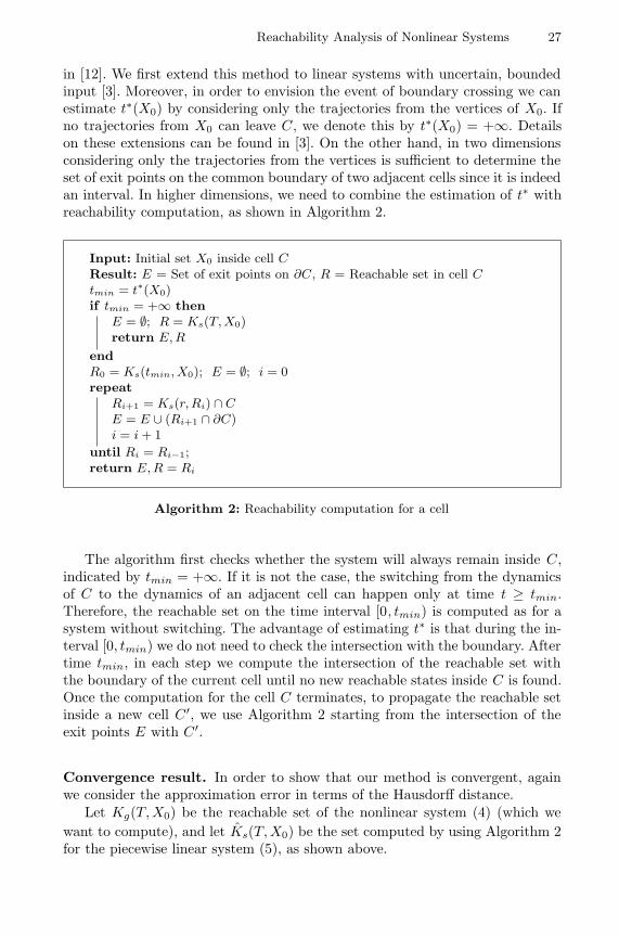
in [12]. We first extend this method to linear systems with uncertain, boundedinput [3]. Moreover, in order to envision the event of boundary crossing we canestimate t∗(X0) by considering only the trajectories from the vertices of X0. Ifno trajectories from X0 can leave C, we denote this by t∗(X0) = +∞. Detailson these extensions can be found in [3]. On the other hand, in two dimensionsconsidering only the trajectories from the vertices is sufficient to determine theset of exit points on the common boundary of two adjacent cells since it is indeedan interval. In higher dimensions, we need to combine the estimation of t∗ withreachability computation, as shown in Algorithm 2.

Input: Initial set X0 inside cell CResult: E = Set of exit points on ∂C, R = Reachable set in cell Ctmin = t∗(X0)if tmin = +∞ then

E = ∅; R = Ks(T, X0)return E, R

endR0 = Ks(tmin, X0); E = ∅; i = 0repeat

Ri+1 = Ks(r, Ri) ∩ CE = E ∪ (Ri+1 ∩ ∂C)i = i + 1

until Ri = Ri−1;return E, R = Ri

Algorithm 2: Reachability computation for a cell

The algorithm first checks whether the system will always remain inside C,indicated by tmin = +∞. If it is not the case, the switching from the dynamicsof C to the dynamics of an adjacent cell can happen only at time t ≥ tmin.Therefore, the reachable set on the time interval [0, tmin) is computed as for asystem without switching. The advantage of estimating t∗ is that during the in-terval [0, tmin) we do not need to check the intersection with the boundary. Aftertime tmin, in each step we compute the intersection of the reachable set withthe boundary of the current cell until no new reachable states inside C is found.Once the computation for the cell C terminates, to propagate the reachable setinside a new cell C ′, we use Algorithm 2 starting from the intersection of theexit points E with C ′.

Convergence result. In order to show that our method is convergent, againwe consider the approximation error in terms of the Hausdorff distance.

Let Kg(T, X0) be the reachable set of the nonlinear system (4) (which wewant to compute), and let Ks(T, X0) be the set computed by using Algorithm 2for the piecewise linear system (5), as shown above.


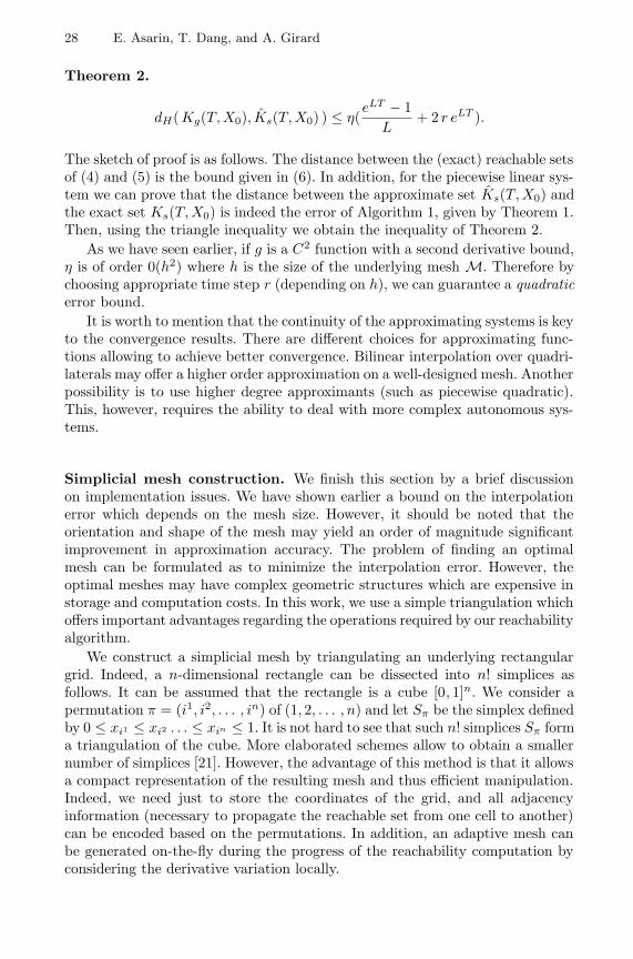
Theorem 2.

dH( Kg(T, X0), Ks(T,X0) ) ≤ η(eLT − 1

L+ 2 r eLT ).

The sketch of proof is as follows. The distance between the (exact) reachable setsof (4) and (5) is the bound given in (6). In addition, for the piecewise linear sys-tem we can prove that the distance between the approximate set Ks(T, X0) andthe exact set Ks(T, X0) is indeed the error of Algorithm 1, given by Theorem 1.Then, using the triangle inequality we obtain the inequality of Theorem 2.

As we have seen earlier, if g is a C2 function with a second derivative bound,η is of order 0(h2) where h is the size of the underlying mesh M. Therefore bychoosing appropriate time step r (depending on h), we can guarantee a quadraticerror bound.

It is worth to mention that the continuity of the approximating systems is keyto the convergence results. There are different choices for approximating func-tions allowing to achieve better convergence. Bilinear interpolation over quadri-laterals may offer a higher order approximation on a well-designed mesh. Anotherpossibility is to use higher degree approximants (such as piecewise quadratic).This, however, requires the ability to deal with more complex autonomous sys-tems.

Simplicial mesh construction. We finish this section by a brief discussionon implementation issues. We have shown earlier a bound on the interpolationerror which depends on the mesh size. However, it should be noted that theorientation and shape of the mesh may yield an order of magnitude significantimprovement in approximation accuracy. The problem of finding an optimalmesh can be formulated as to minimize the interpolation error. However, theoptimal meshes may have complex geometric structures which are expensive instorage and computation costs. In this work, we use a simple triangulation whichoffers important advantages regarding the operations required by our reachabilityalgorithm.

We construct a simplicial mesh by triangulating an underlying rectangulargrid. Indeed, a n-dimensional rectangle can be dissected into n! simplices asfollows. It can be assumed that the rectangle is a cube [0, 1]n. We consider apermutation π = (i1, i2, . . . , in) of (1, 2, . . . , n) and let Sπ be the simplex definedby 0 ≤ xi1 ≤ xi2 . . . ≤ xin ≤ 1. It is not hard to see that such n! simplices Sπ forma triangulation of the cube. More elaborated schemes allow to obtain a smallernumber of simplices [21]. However, the advantage of this method is that it allowsa compact representation of the resulting mesh and thus efficient manipulation.Indeed, we need just to store the coordinates of the grid, and all adjacencyinformation (necessary to propagate the reachable set from one cell to another)can be encoded based on the permutations. In addition, an adaptive mesh canbe generated on-the-fly during the progress of the reachability computation byconsidering the derivative variation locally.


5 Experimentation

Our reachability method was implemented and is being integrated in the toold/dt in order to analyze hybrid systems. We have experimented the method onvarious examples. We now present some examples for illustrative purposes.

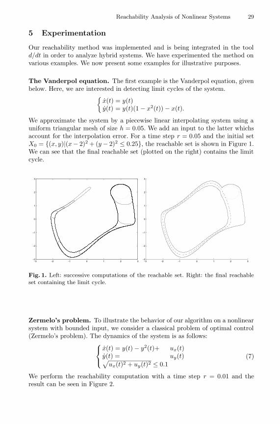
The Vanderpol equation. The first example is the Vanderpol equation, givenbelow. Here, we are interested in detecting limit cycles of the system.{

x(t) = y(t)y(t) = y(t)(1 − x2(t)) − x(t).

We approximate the system by a piecewise linear interpolating system using auniform triangular mesh of size h = 0.05. We add an input to the latter whichsaccount for the interpolation error. For a time step r = 0.05 and the initial setX0 = {(x, y)|(x − 2)2 + (y − 2)2 ≤ 0.25}, the reachable set is shown in Figure 1.We can see that the final reachable set (plotted on the right) contains the limitcycle.

−3 −2 −1 0 1 2 3−3

−2

−1

0

1

2

3

−3 −2 −1 0 1 2 3−3

−2

−1

0

1

2

3

Fig. 1. Left: successive computations of the reachable set. Right: the final reachableset containing the limit cycle.

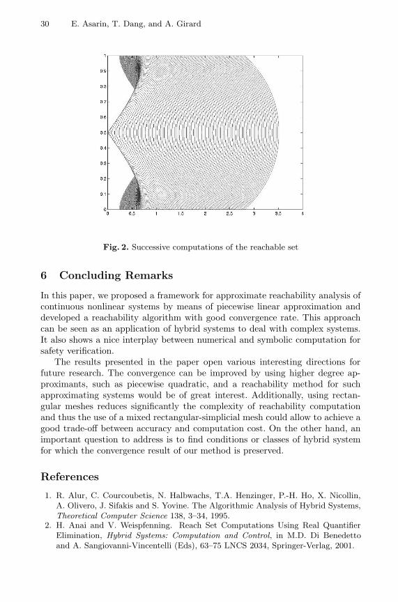
Zermelo’s problem. To illustrate the behavior of our algorithm on a nonlinearsystem with bounded input, we consider a classical problem of optimal control(Zermelo’s problem). The dynamics of the system is as follows:

x(t) = y(t) − y2(t)+ ux(t)y(t) = uy(t)√

ux(t)2 + uy(t)2 ≤ 0.1(7)

We perform the reachability computation with a time step r = 0.01 and theresult can be seen in Figure 2.


Fig. 2. Successive computations of the reachable set

6 Concluding Remarks

In this paper, we proposed a framework for approximate reachability analysis ofcontinuous nonlinear systems by means of piecewise linear approximation anddeveloped a reachability algorithm with good convergence rate. This approachcan be seen as an application of hybrid systems to deal with complex systems.It also shows a nice interplay between numerical and symbolic computation forsafety verification.

The results presented in the paper open various interesting directions forfuture research. The convergence can be improved by using higher degree ap-proximants, such as piecewise quadratic, and a reachability method for suchapproximating systems would be of great interest. Additionally, using rectan-gular meshes reduces significantly the complexity of reachability computationand thus the use of a mixed rectangular-simplicial mesh could allow to achieve agood trade-off between accuracy and computation cost. On the other hand, animportant question to address is to find conditions or classes of hybrid systemfor which the convergence result of our method is preserved.

References

1. R. Alur, C. Courcoubetis, N. Halbwachs, T.A. Henzinger, P.-H. Ho, X. Nicollin,A. Olivero, J. Sifakis and S. Yovine. The Algorithmic Analysis of Hybrid Systems,Theoretical Computer Science 138, 3–34, 1995.

2. H. Anai and V. Weispfenning. Reach Set Computations Using Real QuantifierElimination, Hybrid Systems: Computation and Control, in M.D. Di Benedettoand A. Sangiovanni-Vincentelli (Eds), 63–75 LNCS 2034, Springer-Verlag, 2001.


3. E. Asarin, T. Dang and A. Girard. Reachability Analysis of Nonlinear Systemsusing Conservative Approximations, Technical Report IMAG Oct 2002, Grenoblehttp://www-verimag.imag.fr/˜tdang/piecewise.ps.gz.

4. E. Asarin and T. Dang and O. Maler. d/dt: A tool for Verification of HybridSystems, Computer Aided Verification, Springer-Verlag, LNCS, 2002.

5. M.D. Di Benedetto and A. Sangiovanni-Vincentelli. Hybrid Systems: Computationand Control, LNCS 2034, Springer-Verlag, 2001.

6. O. Botchkarev and S. Tripakis. Verification of Hybrid Systems with Linear Differ-ential Inclusions Using Ellipsoidal Approximations, Hybrid Systems: Computationand Control, in B. Krogh and N. Lynch (Eds), 73–88 LNCS 1790, Springer-Verlag,2000.

7. A. Chutinan and B.H. Krogh. Verification of Polyhedral Invariant Hybrid Au-tomata Using Polygonal Flow Pipe Approximations, Hybrid Systems: Computa-tion and Control, in F. Vaandrager and J. van Schuppen (Eds), 76–90 LNCS 1569,Springer-Verlag, 1999.

8. T. Dang and O. Maler. Reachability Analysis via Face Lifting, Hybrid Systems:Computation and Control, in T.A. Henzinger and S. Sastry (Eds), 96–109 LNCS1386 Springer-Verlag, 1998.

9. J. Della Dora, A. Maignan, M. Mirica-Ruse, and S. Yovine. Hybrid Computation,Proc. of ISSAC’01, 2001.

10. J. Dieudonne. Calcul Infinitesimal, Collection Methodes, Hermann Paris, 1980.11. A. Girard. Approximate Solutions of ODEs Using Piecewise Linear Vector Fields,

Proc. CASC’02”, 2002.12. A. Girard. Detection of Event Occurence in Piecewise Linear Hybrid Systems,

Proc. RASC’02, December 2002, Nottingham, UK.13. M.R. Greenstreet and I. Mitchell. Reachability Analysis Using Polygonal Projec-

tions, Hybrid Systems: Computation and Control, in F. Vaandrager and J. vanSchuppen (Eds), 76–90 LNCS 1569 Springer-Verlag, 1999.

14. M. Greenstreet and C. Tomlin. Hybrid Systems: Computation and Control, LNCS,Springer-Verlag, 2002.

15. L.C.G.J.M. Habets and J.H. van Schuppen. Control of Piecewise-Linear HybridSystems on Simplices and Rectangles, Hybrid Systems: Control and Computation,in M.D. Di Benedetto and A. Sangiovanni-Vincentelli (Eds), 261–273 LNCS 2034,Springer-Verlag, 2001.

16. T.A. Henzinger, P.-H. Ho and H. Wong-Toi. HyTech: A Model Checker for HybridSystems, Software Tools for Technology Transfer 1, 110–122, 1997.

17. T.A. Henzinger, P.-H. Ho, and H. Wong-Toi. Analysis of Nonlinear Hybrid Systems,IEEE Transactions on Automatic Control 43, 540–554, 1998.

18. J. Hubbard and B. West. Differential Equations: A Dynamical Systems Approach,Higher-Dimensional Systems, Texts in Applied Mathematics, 18, Springer Verlag,1995.

19. G. Lafferriere, G. Pappas, and S. Yovine. Reachability computation for linearsystems, Proc. of the 14th IFAC World Congress, 7–12 E, 1999.

20. , K. Larsen, P. Pettersson, and W. Yi. Uppaal in a nutshell, Software Tools forTechnology Transfert 1, 1997.

21. T.H. Marshall. Volume formulae for regular hyperbolic cubes, Conform. Geom.Dyn., 25–28, 1998.

22. I. Mitchell and C. Tomlin. Level Set Method for Computation in Hybrid Systems,Hybrid Systems: Computation and Control, in B. Krogh and N. Lynch, 311–323LNCS 1790, Springer-Verlag, 2000.


23. P. Saint-Pierre. Approximation of Viability Kernels and Capture Basin for HybridSystems, Proc. of European Control Conference ECC’01, 2776–2783, 2001.

24. O. Stursberg, S. Kowalewski and S. Engell. On the generation of Timed Ap-proximations for continuous systems, Mathematical and Computer Modelling ofDynamical Systems 6–1, 51–70, 2000.

25. A. Puri and P. Varaiya. Verification of Hybrid Systems using Abstraction, HybridSystems II, in P. Antsaklis, W. Kohn, A. Nerode, and S. Sastry (Eds), LNCS 999,Springer-Verlag, 1995.

26. S. Yovine. Kronos: A Verification Tool for Real-time Systems, Software Tools forTechnology Transfer 1, 123–133, 1997.

Fundamental Inequality Theorem (see e.g. [18,10]) Let f be a functionwith values in Rn, continuous and L-Lipschitz on a set D ⊂ Rn. Let x1(t)and x2(t) be functions with values in Rn continuous, piecewise differentiable onan interval I ⊂ R containing 0 such that ∀t ∈ I, x1(t) ∈ D, x2(t) ∈ D, and||x1(t) − f(x1(t))|| ≤ ε1, ||x2(t) − f(x2(t))|| ≤ ε2. Then,

∀t ∈ I, ||x1(t) − x2(t)|| ≤ ||x1(0) − x2(0)||eL|t| +ε1 + ε2

L(eL|t| − 1).

Proof of Theorem 1 We start by proving the first property. To show thatKs(T, X0) ⊆ RN , we first observe that, by definition, RN =

⋃1≤i≤N Qi. Hence,

it suffices to show that for all i ∈ {0, . . . , N − 1}∀x ∈ X0 u(·) ∈ Uµ t ∈ [ir, (i + 1)r] Φs(t, x, u(·)) ∈ Qi+1. (8)

We will prove (8) by induction. We begin by the base case (i = 0). Let x bean element of X0, u(·) an admissible control, and t ∈ [0, r]. We denote ys =Φs(t, x, u(·)) and yf = Φf (t, x). Using the Fundamental Inequality, we have||yf − ys|| ≤ µ

L (eLt − 1) ≤ µL (eLr − 1). It is easy to see that yf is an element of

P1; therefore ys is an element of Q1, which implies that (8) holds for i = 0. Wenow assume that the formula (8) holds for some i ≥ 0. Given x ∈ X0, u(·) ∈ Uµ

and t ∈ [(i+1)r, (i+2)r] we denote ys = Φs(t, x, u(·)) and zs = Φs(t− r, x, u(·)).Since (8) holds for i, we have zs ∈ Qi+1. Let yf = Φf (r, zs). Again, by theFundamental Inequality, ||yf − ys|| ≤ µ

L (eLr − 1). In addition, yf ∈ Pi+2. It thenfollows that ys ∈ Qi+2, which shows that (8) holds for i + 1. ut

We now prove the convergence property, i.e. dH(Ks(T, X0), RN ) ≤ 2µ r eLT .We denote by δi the Hausdorff semi-distance from the set Ri, computed initeration i of Algorithm 1, to the corresponding exact set Ks(ir,X0): δi =supx∈Ri

infy∈Ks(ir,X0) ||x − y||. To estimate the error bound, we determine therelation between δi and δi+1.

Let x∗f be an element of Ri+1 with i ≥ 1. There are two cases: (1) x∗

f ∈ Ri,and (2) x∗

f /∈ Ri. For the first case where x∗f ∈ Ri, it is not hard to see that there

exists x∗s in Ks(ir,X0) ⊆ Ks((i + 1)r,X0) such that ||x∗

f − x∗s|| ≤ δi. We now

focus on the second case where x∗f /∈ Ri. Then, there exists y∗

f ∈ Pi+1 such that

||y∗f − x∗

f || ≤ µ

L(eLr − 1). (9)


zs

x

X0yf

Qi+2

ys

Qi+1

Pi+2

x∗fz∗

s

x∗s

y∗f

Pi+1

Ks((i + 1)r,X0)

Qi+1

z∗f

Qi

Ks(ir,X0)

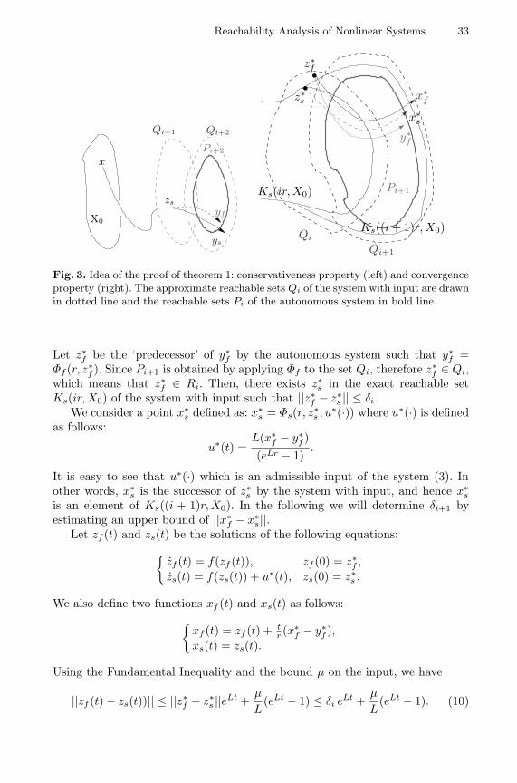
Fig. 3. Idea of the proof of theorem 1: conservativeness property (left) and convergenceproperty (right). The approximate reachable sets Qi of the system with input are drawnin dotted line and the reachable sets Pi of the autonomous system in bold line.

Let z∗f be the ‘predecessor’ of y∗

f by the autonomous system such that y∗f =

Φf (r, z∗f ). Since Pi+1 is obtained by applying Φf to the set Qi, therefore z∗

f ∈ Qi,which means that z∗

f ∈ Ri. Then, there exists z∗s in the exact reachable set

Ks(ir,X0) of the system with input such that ||z∗f − z∗

s || ≤ δi.We consider a point x∗

s defined as: x∗s = Φs(r, z∗

s , u∗(·)) where u∗(·) is definedas follows:

u∗(t) =L(x∗

f − y∗f )

(eLr − 1).

It is easy to see that u∗(·) which is an admissible input of the system (3). Inother words, x∗

s is the successor of z∗s by the system with input, and hence x∗

s

is an element of Ks((i + 1)r,X0). In the following we will determine δi+1 byestimating an upper bound of ||x∗

f − x∗s||.

Let zf (t) and zs(t) be the solutions of the following equations:{zf (t) = f(zf (t)), zf (0) = z∗

f ,

zs(t) = f(zs(t)) + u∗(t), zs(0) = z∗s .

We also define two functions xf (t) and xs(t) as follows:{xf (t) = zf (t) + t

r (x∗f − y∗

f ),xs(t) = zs(t).

Using the Fundamental Inequality and the bound µ on the input, we have

||zf (t) − zs(t))|| ≤ ||z∗f − z∗

s ||eLt +µ

L(eLt − 1) ≤ δi eLt +

µ

L(eLt − 1). (10)


On the other hand, since xf (r) = x∗f and xs(r) = x∗

s, we can write:

x∗f − x∗

s = xf (r) − xs(r) = (xf (0) − xs(0)) +∫ r

0(xf (s) − xs(s))ds.

In addition, ||xf (0) − xs(0)|| = ||z∗f − z∗

s || ≤ δi. Therefore,

||x∗f − x∗

s|| ≤ δi + ||∫ r

0(xf (s) − xs(s))ds||. (11)

We now focus on the term inside the integral of (11). Note that ||xf (s)−xs(s)|| =

||f(zf (s)) + (x∗f −y∗

f )r − f(zs(s)) − u∗(s)||. Since f is L-Lipschitz, ||f(zf (s)) −

f(zs(s))|| ≤ L ||zf (s) − zs(s)||. Using (9) and (10) yields

||xf (s) − xs(s)|| ≤ ||x∗f − y∗

f ||(1r

− L

eLr − 1) + L ||zf (s) − zs(s)||

≤ µ

2eLrLr + L (δi eLs +

µ

L(eLs − 1)).

Combining the above inequality with (11) and developing the integral gives

δi+1 ≤ δi eLr +µ

2eLrLr2 +

µ

L(eLr − 1 − Lr).

Observe that eLr − 1 − Lr ≤ 12 eLr (Lr)2, thus δi+1 ≤ δi eLr + µL eLr r2. Then,

δN ≤ δ1 eL(N−1)r + µL eLr r2N−2∑i=0

eiLr = δ1 eL(N−1)r + µL eLr r2 eL (N−1) r − 1eLr − 1

.

Since eLr − 1 ≥ Lr and, in addition, we can prove that δ1 ≤ µ r eLr. The abovethus leads to δN ≤ 2µ r eLT . This completes the proof of the theorem. ut

Proof of Lemma 2 We first estimate an upper bound of ||g(x) − lk(x)|| for allpoints x inside a cell Ck ∈ M. Let v be a vertex of Ck. By triangle inequality, wehave ||g(x)− lk(x)|| ≤ ||g(x)−g(v)||+ ||g(v)− lk(x)||. By definition, g(v) = lk(v).In addition, g is L-Lipschitz, it then follows that

||g(x) − lk(x)|| ≤ ||g(x) − g(v)|| + ||lk(v) − lk(x)|| ≤ 2L||x − v||. (12)

Note that the above inequality holds for any vertex v ∈ V (Ck). In order to geta tight upper bound on ||g(x) − lk(x)||, we can estimate a bound on ||x − v|| foreach vertex v and then choose the smallest bound. Let V (Ck) = {v1, v2, . . . , vn}be the set of vertices of Ck. A point x ∈ Ck can be written as:{

x =∑n

i=1 αi vi∑ni=1 αi = 1 and ∀i ∈ {1, . . . , n} αi ≥ 0. (13)


We observe, from the conditions (13), that there exists j ∈ {1, . . . , n} such thatαj ≥ 1

n+1 . Since∑n

i=1 αivj = vj , we can write x − vj =∑n

i=1,i6=j αi(vi − vj).Additionally, ||vi − vj || ≤ h(Ck); therefore,

||x − vj || ≤ h(Ck)n∑

i=1,i6=j

αi = h(Ck) (1 − αj) ≤ h(Ck)n

n + 1. (14)

Using this bound in (12) we get ∀x ∈ Ck ||g(x) − lk(x)|| ≤ h(Ck) 2 n Ln+1 . Note

that ∀Ck ∈ M, h(Ck) ≤ h(M) = h, which yields the result of the lemma. ut

Proof of Lemma 3 For a given cell Ck ∈ M, we define the function e(x) =g(x) − lk(x) and let x∗ = arg maxx∈Ck

||e(x)|| (note that the simplex Ck iscompact). Let v be a vertex of Ck, and all points in the line segment connectingx∗ and v can be written as: x(γ) = x∗ + γ (v − x∗), γ ∈ [0, 1]. To determine abound on e(x∗), we define a function z(γ) = e(x(γ)) for γ ∈ [0, 1]. Expanding zwith respect to γ gives

z(1) = z(0) +dz

dγ(0) +

∫ 1

0

d2z

dγ2 (s) (1 − s)ds. (15)

The ith coordinate of a point y ∈ Rn is denoted by yi. We can see that dxi/dγ =(vi − x∗

i ). Additionally, ∂2lk/∂xi∂xj vanish for all i, j ∈ {1, 2, . . . , n}. Thus,

dz

dγ(γ) =

n∑i=1

∂e

∂xi(x(γ)) (vi − x∗

i ),d2z

dγ2 (γ) =n∑

i=1

n∑j=1

∂2e

∂xi∂xj(x(γ)) (vi − x∗

i ) (vj − x∗j )

Since ∂2lk/∂xi∂xj vanish for all i, j ∈ {1, . . . , n}, then ∂2e/∂xi∂xj =∂2g/∂xi∂xj . Similar to the inequality (14) established in the proof of Lemma 2,we can show that there exists v ∈ V (Ck) such that ∀i ∈ {1, . . . , n} ||vi −x∗

i || ≤ h(Ck)n/(n + 1). Then, using the bound K on the second deriva-tives of the function g, we obtain || d2z

dγ2 (γ)|| ≤ (h(Ck))2 n2 K(n+1)2 . In addition,

||e(x∗)|| is maximum, which implies that dzdγ (0) = 0. By definition of the in-

terpolating function, g(v) = lk(v), then z(1) = 0. Therefore, (15) becomes:g(x∗) − lk(x∗) +

∫ 10

d2zdγ2 (s) (1 − s)ds = 0. Using the above bound on || d2z

dγ2 (γ)||,we get

||g(x∗) − lk(x∗)|| ≤ (h(Ck))2n2 K

(n + 1)2

∫ 1

0(1 − s)ds = (h(Ck))2

n2 K

2 (n + 1)2.

Hence, ∀x ∈ X ||g(x) − l(x)|| ≤ h2 n2 K2 (n+1)2 , and the proof is complete. ut

Reachability Analysis of Nonlinear Systems Using Conservative Approximation

Documents

Transcript of Reachability Analysis of Nonlinear Systems Using Conservative Approximation