Approximation of non-conservative hyperbolic systems

based on different shock curve definitions

N. Chalmers1,∗, and E. Lorin2

1 Department of AppliedMathematics, University of Waterloo, Waterloo, Canada, N2L 3G12 School of Mathematics and Statistics, Carleton University, Ottawa, Canada, K1S 5B6

Abstract. The aim of this paper is to lay a theoretical framework for developing numericalschemes for approximating Non-Conservative Hyperbolic Systems (NCHSs). We first recallsome key points of the theory of NCHSs, beginning with the definition non-conservativeproducts proposed by Dal Maso, LeFloch, and Murat [14]. Next, we briefly introduce thevanishing viscosity solutions and shock curves derived from Bianchini and Bressan’s centermanifold technique [7], and their partial generalization recently proposed by Alouges andMerlet [5]. Approximation of these shock curves also proposed by Alouges and Merlet arethen introduced and discussed. We then investigate the numerical implementation of theseanalytical approaches using Godunov-like schemes, which either use the approximate Shockcurves of Alouges and Merlet directly in a Riemann solver, or use the framework of DalMaso, LeFloch, and Murat, in combination with these approximate shock curves. To ourknowledge, this work is the first attempt to numerically implement shock curves derivedfrom Bianchini and Bressan’s center manifold approach.

Key words: non-conservative hyperbolic systems, finite volume methods, distribution products

1 Introduction

This paper is devoted to the numerical approximation of Non-Conservative Hyperbolic Sys-tems (NCHSs). Non-conservative hyperbolic systems arise in several areas, in particular inthe study of compressible multi-phase/fluid flows and have various industrial applications,such as two-phase flows in nuclear power plant reactors, solid rocket motors, chemical plants,detonations, shallow water bi-fluid flows, and others [16], [34], [26], [31]. These systems haveproven to be difficult to analyze and have been much less studied than Hyperbolic Systemsof Conservation Laws (HSCL). Nevertheless, their wide range of applications have recentlymotivated large efforts to better understand these systems and their numerical approximation.

An example of a system of interest is the model developed by Deledicque and Papalexan-dris in [15]. Their system is a two-phase, two pressure systemmodeling the dynamics of fluidswith a gaseous, g, and liquid, l, phase. Each phase is assigned a density ρα, pressure pα, specificinternal energy eα, velocity uα, and volume fraction φα, where α=g,l. The governing equationsconsist of mass, momentum, and energy balance laws for each phase, plus a convection equa-

∗Corresponding author. Email addresses: bnachalm@uwaterloo.ca (N. Chalmers)

tion for the solid volume fraction,

∂φlρl∂t

+∂φlρlul

∂x= 0,

∂φlρlul

∂t+

∂(φlρlu2l +φlpl)

∂x= pg

∂φl

∂x,

∂φlρlEl∂t

+∂(φlul(ρlEl+pl))

∂x= pgul

∂φl∂x,

∂φgρg

∂t+

∂φgρgug

∂x= 0,

∂φgρgug

∂t+

∂(φgρgu2g+φgpg)

∂x= −pg

∂φl

∂x,

∂φgρgEg

∂t+

∂(φgug(ρgEg+pg))

∂x= −pgug

∂φl∂x,

∂φl

∂t+ul

∂φl

∂x= 0,

where Eα = eα+u2α/2 is the total specific energy for each phase. The following saturation con-dition is also assumed

φg+φl=1.

Together with the equations of state for pg and pl , this system of balance laws can be writtenas a non-conservative system and is thus a special case of the general system which we willconsider. Note that most of multi-phase/fluid models (with one or two pressures) contain anon-conservative product. See for instance [31], [2], [35].More generally, in this paper we will be interested in one dimensional NCHS,

∂u

∂t+A(u)

∂u

∂x=0, u∈Ω⊆R

n, (x,t)∈R×R+, (1.1)

where Ω is open convex set and A is a smooth function A :Rn→Mn(R). We assume that thissystem is strictly hyperbolic, that is, A has n real and distinct eigenvalues λ1(u)< λ2(u)< . . .<λn(u) , ∀u ∈ Ω with linearly independent eigenvectors. Recall that when A is the Jacobianmatrix of some vector-valued function f :Rn→R

n, i.e. A(u)=Df(u), then this system reducesto a HSCL.Our primary goal when studying hyperbolic systems is to completely describe solutions of theRiemann problem for (1.1)

u(x,0)=

uL, x<0,

uR, x>0.

Because of the non-conservative term, A(u)ux, and the fact that products of distributions arenot defined by the theory of distributions [32], we cannot rigorously define the notion of weaksolutions for system (1.1) and we cannot derive a Rankine-Hugoniot Jump Condition, as inthe conservative case. Finally, we cannot define, a priori, the notion of shock wave for NCHSs.Although this constitutes an old problem, ‘recently’ two distinct ways of overcoming this issuein the framework of NCHSs have been proposed. The first considered in this paper is due toDal Maso, LeFloch and Murat (DLM) [14], [23]. Specifically, the authors propose a definitionof non-conservative products, and hence they can define weak solutions of (1.1). They suggestto introduce a family of paths, ψ : [0,1]×R

n×Rn→R

n which satisfies the following properties,

ψ(0;uL,uR)=uL, ψ(1;uL,uR)=uR,

2

∀uL,uR∈Rn. They then define the non-conservative product, A(u)ux, not as a distribution, but

as a bounded Borel measure which depends on this family of paths. This measure, denoted by[A(u)ux]ψ, is defined as

[A(u)ux]ψ(B)=∫

BA(u)ux dx,

when u is continuous on a Borel set B, and by

[A(u)ux]ψ((x0,t0))=∫ 1

0A(ψ(s;uL,uR))

∂ψ

∂s(s;uL,uR)ds,

when u has a jump discontinuity and uL and uR are the left and right limits of the discontinuity,respectively. It is important to note that this definition of a non-conservative product onlyapplies to functions which are piecewise differentiable with finite jump discontinuities, andnot for general distributions. However, a priori these functions are all we need in order tosolve the Riemann problem for NCHSs. In fact, this product extends the definition of non-conservative products given by Volpert [36], which can be recovered in this framework bychoosing the family of straight lines ψ(s;uL,uR)=uL+s(uR−uL). This formulation of the non-conservative product allows us to define weak solutions of the system, and furthermore itallows us to generalize the Rankine-Hugoniot jump condition [14] to

σ(uR−uL)=∫ 1

0A(ψ(s;uL,uR))

∂ψ

∂s(s;uL,uR)ds.

Using this condition, it is possible to proceed as done in the conservative case and solve theRiemann problem by using shock waves, rarefaction waves, and contact discontinuities toseparate at most n+1 constant states. The obvious drawback in this formulation is that thedefinition of the non-conservative product depends on the choice of path, ψ. Because of this,it is difficult, a priori, to select the paths that will give us the correct, physical solution. AsLeFloch remarks in [23], appropriate paths could be chosen so that they parametrize viscousprofiles. However, the question of how to determine the viscous profiles is made difficult sinceit involves finding bounded solutions of an ODE on an infinite domain. For a more completediscussion see [33].Another approach for finding solutions to NCHSs was developed in the recent works of Bian-chini and Bressan [7], and Alouges and Merlet [5] who partially generalized Bianchini andBressan’s work. In their very technical work, Bianchini and Bressan investigate the solutionsof the following viscous system,

uεt+A(uε)uε

x= εuεxx,

which is a parabolic regularization of the original system (1.1), with the specific viscosity ma-trix B(u)= I. They define solutions of (1.1) as vanishing viscosity solutions of the viscous system,i.e. solutions to (1.1) are constructed as the limit of the solution to this viscous system as ε→0.In a very general setting, they show that these vanishing viscosity solutions are unique and,in particular, they describe the shock curves and viscous shock profiles associated to this vis-cosity matrix B= I. The work of Bianchini and Bressan was then generalized by Alouges andMerlet in [5], who extended their results to the case where the viscosity matrix B commuteswith A. The authors also propose a definition of shock curves of non-conservative systems assolution of the following dynamical system

(A(u)−σI)du

dσ=u−uL,

u(λi(uL))=uL.

3

They prove that the shock curves given by this system are close to the shock curves deducedfrom the center manifold theory of Bianchini and Bressan, up to the third order. This resultgives us a way for selecting the admissible discontinuities and therefore allows us to solveRiemann Problems in NCHSs. Moreover Alouges and Merlet prove that the shock curves de-fined by the system above also agree with the viscous shock profiles up to the third order.These shock curves therefore give us a close approximation of the viscous profiles which wecan use for instance, as a path in the DLM theory. This leads us to investigate two interestingdesigns for numerical schemes. Note finally that Colombeau has proposed [12] to extend theset of distributions as a quotient algebra, allowing to define the product of “extended gener-alized functions”. Within this framework, shock waves solutions of non-conservative hyper-bolic systems can “easily” be defined as well as their discretization (for elasticity models inparticular) [11], [13] using weak-strong formulations of the considered system. See also [25]for a more recent work on numerical schemes for non-conservative hyperbolic systems basedon Colombeau’s generalized functions. In this paper, Colombeau’s approach will not be dis-cussed, but some of its links with Bianchini & Bressan’s, and LeFloch’s workswill be addressedin a forthcoming paper.The question of implementing the DLM theory in a numerical solver has been investigated byseveral authors. Originally Toumi and Kumbaro proposed a path-based approach [35] to builda Roe solver for NCHSs. Later other authors, in particular Pares and Castro [9], [8], [27], andRhebergen, Bokhove, and Van der Vegt, [29], [28] have investigated other numerical methods(Godunov, Discontinuous Galerkin, etc) for these systems which are based on DLM’s path-theory. Note that many other approaches have been proposed to treat the non-conservativeproduct, in particular in the multi-phase flow framework (see [18], for instance).In this paper, we will focus on the shock and approximate shock curves as defined by Alougesand Merlet. Our main scheme of interest will be a Godunov-like Scheme [20] using an exactRiemann solver:

Vn+1j =Vnj −∆t

∆x

(

Gn,−j+ 12

+Gn,+j− 12

)

.

Castro, Pares, et. al. show in [9] that using the DLM definitions in a Godunov solver leadsnaturally to select

Gn,−j+ 12

=∫ 1

0A(ψ(s;Vnj ,V

nj+ 12

))∂ψ

∂s(s;Vnj ,V

nj+ 12

)ds,

Gn,+j+ 12

=∫ 1

0A(ψ(s;Vn

j+ 12,Vnj+1))

∂ψ

∂s(s;Vn

j+ 12,Vnj+1)ds,

where Vnj+ 12is the value at x=0 of the solution to the Riemann Problem

V(x,0)=

Vnj , x<0,

Vnj+1, x>0.

Although the Godunov scheme is known to be very slow, at this point the goal of this paperis not to propose a fast and an accurate solver for NCHSs, but rather to propose a first (to ourknowledge) numerical implementation of Bianchini & Bressan and Alouges & Merlet’s shockand approximate shock curves in a finite volume solver. When implementing the shock curvesof Alouges and Merlet, we have to solve Riemann Problems at each interface and select thefluxes Gn,±j+1/2 dependent on the type of the wave solution (i.e. 1-shock and 2-shock, 1-shock

and 2-rarefaction, etc.). This first scheme is then a Godunov scheme based on an exact Rie-mann solver. We will first apply this scheme to a hyperbolic system of conservation laws andcompare their numerical solutions with solutions of reference to check that we recover correct

4

results.Wewill then implement Alouges-Merlet’s approximate shock curves in aDLMpath-dependentscheme and compare the numerical solutions with the ones found by Pares’ Godunov scheme,described above. To obtain a worth while comparison, we will apply these schemes to a trulynon-conservative system. We show that, in this particular example, the numerical solutiondoes indeed converge to the exact solution, seemingly overcoming the convergence problemfor non-conservative systems as studied in [10], [21], [24], [21] and [1]. Another interesting re-sult that we will show is that the two Godunov schemes we have constructed are in fact closein a sense that will be defined below.

The remainder of this paper is organized as follows. In Section 2, we present some keyelements of the theories developed by Dal Maso, LeFloch and Murat, Bianchini and Bressan,and Alouges and Merlet. We then move to the numerical implementation of these approachesin Section 3. Comparisons of the numerical solutions obtained with these different approacheswill then be presented. Section 4 is devoted to concluding remarks.

2 Non-Conservative Hyperbolic Systems

In this section we recall some important features of non-conservative hyperbolic systems. Asmentioned in the introduction, the first fundamental difficulty that we must address are howto define weak solutions of these systems, and how to properly define the shock curves inorder to solve the Riemann problem.

We begin this section by recalling some key elements of Dal Maso, LeFloch, and Mu-rat’s path-theory, in particular their definition of non-conservative products. We then givean overview of the vanishing viscosity solutions studied by Bianchini and Bressan. Finally,we present the approximate shock curves defined by Alouges and Merlet and recall when andhow they approach the shock curves deduced from Bianchini and Bressan’s center manifoldapproach. These shock curves will be referred in the following as Bianchini and Bressan’s shockcurves.

2.1 Dal Maso-LeFloch-Murat Non-Conservative Products

As we mentioned in the introduction, the main issue with non-conservative hyperbolic sys-tems is the presence of the non-conservative term A(u)ux. As a product of distributions, it isnot clear how this term should be defined, and thus we are unable to specify what disconti-nuity waves can be weak solutions. The idea proposed by Dal Maso, LeFloch, and Murat [14]was to regard this term not as a distribution, but as a bounded Borel measure. Let us quicklyrecall the principle. When u is smooth on a Borel set B, this measure is defined by

[A(u)ux](B)=∫

BA(u)ux dx.

The problem arises when u has a jump discontinuity, as:

u=

uL, x<0,

uR, x>0.

Regarding A(u)ux as a measure, we require that:

[A(u)ux]=Cδ0,

5

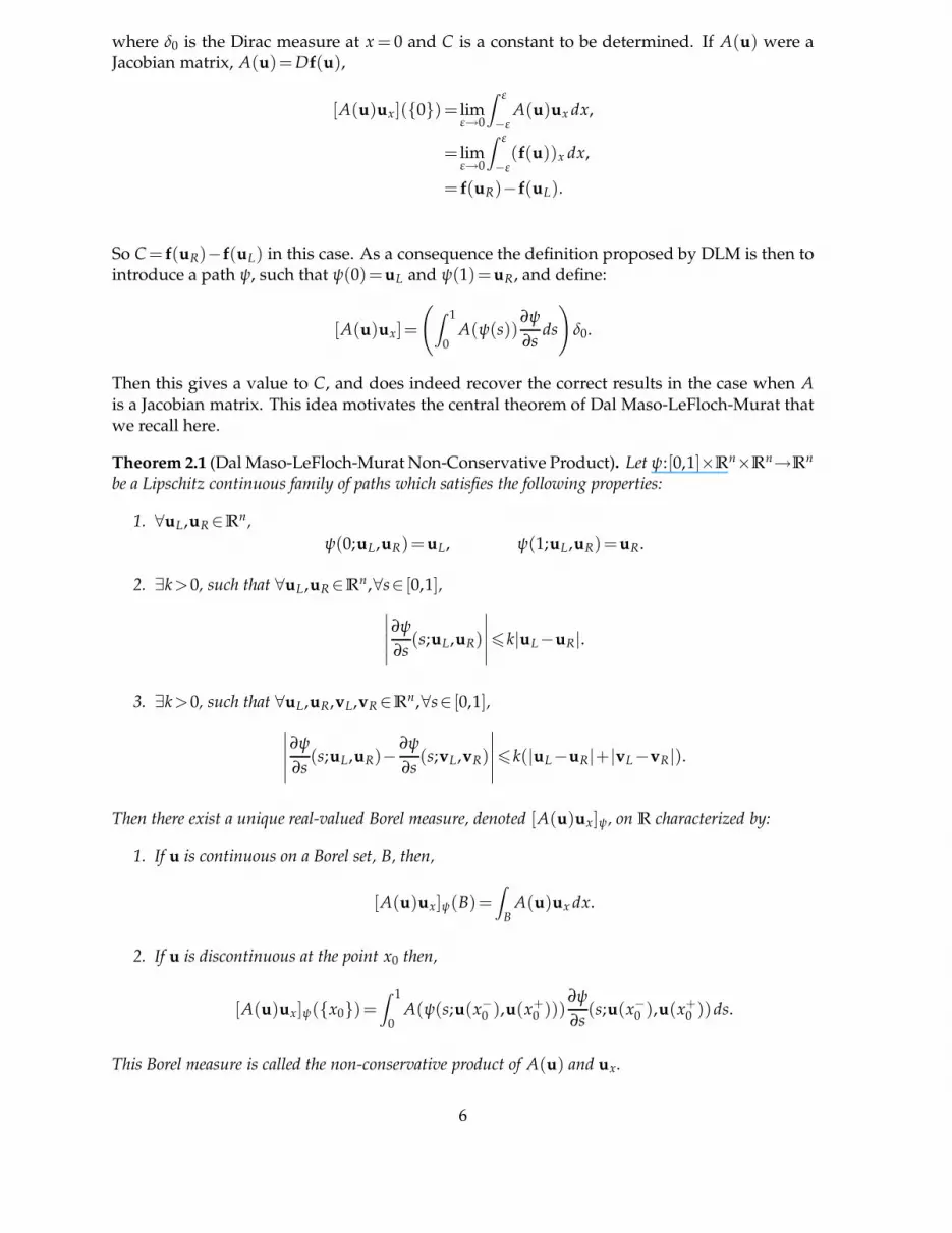
where δ0 is the Dirac measure at x= 0 and C is a constant to be determined. If A(u) were aJacobian matrix, A(u)=Df(u),

[A(u)ux](0)= limε→0

∫ ε

−εA(u)ux dx,

= limε→0

∫ ε

−ε(f(u))x dx,

= f(uR)−f(uL).

So C= f(uR)−f(uL) in this case. As a consequence the definition proposed by DLM is then tointroduce a path ψ, such that ψ(0)=uL and ψ(1)=uR, and define:

[A(u)ux]=

(

∫ 1

0A(ψ(s))

∂ψ

∂sds

)

δ0.

Then this gives a value to C, and does indeed recover the correct results in the case when Ais a Jacobian matrix. This idea motivates the central theorem of Dal Maso-LeFloch-Murat thatwe recall here.

Theorem 2.1 (Dal Maso-LeFloch-Murat Non-Conservative Product). Let ψ:[0,1]×Rn×R

n→Rn

be a Lipschitz continuous family of paths which satisfies the following properties:

1. ∀uL,uR∈Rn,

ψ(0;uL,uR)=uL, ψ(1;uL,uR)=uR.

2. ∃k>0, such that ∀uL,uR∈Rn,∀s∈ [0,1],

∣

∣

∣

∣

∣

∂ψ

∂s(s;uL,uR)

∣

∣

∣

∣

∣

6k|uL−uR|.

3. ∃k>0, such that ∀uL,uR,vL,vR∈Rn,∀s∈ [0,1],

∣

∣

∣

∣

∣

∂ψ

∂s(s;uL,uR)−

∂ψ

∂s(s;vL,vR)

∣

∣

∣

∣

∣

6k(|uL−uR|+|vL−vR|).

Then there exist a unique real-valued Borel measure, denoted [A(u)ux]ψ, on R characterized by:

1. If u is continuous on a Borel set, B, then,

[A(u)ux]ψ(B)=∫

BA(u)ux dx.

2. If u is discontinuous at the point x0 then,

[A(u)ux]ψ(x0)=∫ 1

0A(ψ(s;u(x−0 ),u(x+0 )))

∂ψ

∂s(s;u(x−0 ),u(x+0 ))ds.

This Borel measure is called the non-conservative product of A(u) and ux.

6

Remark 2.1. Note that this non-conservative product is defined only for functions uwhich arepiecewise differentiable and contain jump discontinuities, and it is therefore not defined for ageneral distribution. To use this product in the framework of NCHSs, we will regard the term,A(u)ux as a non-conservative product which also depends on the variable t.

Remark 2.2. It is clear that in this framework, the non-conservative product defined aboveis dependent on the choice of path, ψ. The question of how one chooses such a family ofpaths is far from trivial. As noted in [21] and [1], when using this definition to design nu-merical schemes, poor choices in the family of paths can result in the scheme converging tothe incorrect shock curves. In fact even an appropriate choice of paths implemented in a non-conservative scheme can lead to convergence to wrong solutions [1], [10] (and [21] to giveelements of explanation for understanding this fundamental issue).

Using this non-conservative product, weak solutions are defined as follows.

Definition 2.1. We say that u is a weak solution of (1.1) if and only if

∫

R+

∫

R

uφt+[A(u)ux]ψ φdxdt=0,

as measures, for all test functions φ∈C10(R×R+).

Moreover, this weak formulation allows us to define a Rankine-Hugoniot Jump Conditionas given by LeFloch in [23].

Theorem 2.2 (DLM Rankine-Hugoniot Jump Condition). Let ψ be the family of paths as in Theo-rem 2.1. Let u be a solution to (1.1) in the weak sense, with respect to this family of paths, and let u besmooth throughout a region D, except along a curve x=γ(t) which divides D into two regions DL andDR, and along which u has a jump discontinuity. Then,

γ′(t)(uR−uL)=∫ 1

0A(ψ(s;uL,uR))

∂ψ

∂s(s;uL,uR)ds, (2.1)

where,

uR(t)= lim(x,t)→(γ(t),t)

(x,t)∈DR

u(x,t), uL(t)= lim(x,t)→(γ(t),t)

(x,t)∈DL

u(x,t),

are the values of u at either side of the discontinuity.

Let us focus now on contact discontinuity curves. Suppose uL and uR are separated by ak-contact discontinuity. Then uL and uR lie on the same contact discontinuity curve v. Then vsolves

v′(ξ)= rk(v(ξ)),v(0)=uL,

and furthermore

A(v(ξ))rk(v(ξ))=λk(uL)rk(v(ξ))

for all ξ, since λk remains constant along v(ξ). We can re-parametrize v so that v(1)=uR. Then

7

ψ(s;uL,uR)=v(s) and we find

∫ 1

0A(ψ(s;uL,uR))

∂ψ

∂s(s;uL,uR)ds=

∫ 1

0A(v(s))v′(s)ds,

=∫ 1

0A(v(s))rk(v(s))ds,

=λk(uL)∫ 1

0rk(v(s))ds,

=λk(uL)∫ 1

0v′(s)ds,

=λk(uL)(uR−uL).

Hence, this discontinuity satisfies the DLM jump condition. Thus we can indeed use the def-inition of contact discontinuities as done in the conservative case. Furthermore, now that wehave a jump condition we can define the shock curves.

Theorem 2.3 (DLM shock Curves). Suppose that the k-th field is genuinely nonlinear. Then given aleft state uL∈Ω there exists a curve, Sk(uL), of right states that can be connected to uL on the right bya k-shock wave.

The proof of this theorem follows closely the arguments used to prove the existence ofshock curves in the conservative case. See Chapter 1, Section 4, Theorem 4.1 in [19].

Using the definition of k-shock curves for genuinely nonlinear fields, we can then invokeentropy conditions to identify admissible shock waves. In particular we apply the Lax shockentropy condition to identify the admissible portion of the k-shock curves. Thus, given twostates uL and uR, sufficiently close, we can uniquely solve their Riemann problem as a compo-sition of k-simple waves.

S1(uL)

R2(uR)

uL

uR

R1(uL)

S2(uR)

u1

Figure 1: Example of shock and rarefaction curves in a 2×2 system. The entropy condition allows us to determinethe admissible parts of the shock curves and we can then find the intersection to uniquely determine u1.

As we remarked earlier, when designing a numerical scheme, choosing the family of pathsis not trivial and different choices of paths can lead to vastly different numerical solutions.It is clear that we need some way of determining what paths will give us physical, entropic

8

solutions. To this end, let us consider the vanishing viscosity entropy condition and examinethe viscous profiles. First, we introduce an admissible viscosity matrix B(u) to the system.

uεt+A(uε)uε

x= ε(B(uε)uεx)x,

and we look for the viscous profiles uε(x,t)=v( x−σtε ). The resulting ODE is

(A(v)−σ)v′=(B(v)v′)′.

Next, let us suppose the vanishing viscosity limit of this viscous profile is a shock wave, i.e,

limε→0uε(x,t)=

uL, x<σt,

uR, x>σt.

Then the viscous profile will have the form

uε(x,t)=

uL, x<σt−ε,

φ( x−σt+ε2ε ), σt−ε6x6σt+ε,

uR, x>σt+ε,

where φ is a smooth function with the properties φ(0)=uL and φ(1)=uR. Considering uε as a

measure we see that

limε→0

[A(uε)uεx]=

(

∫ 1

0A(φ(s))

∂φ

∂sds

)

δx−σt,

with the convergence in the sense of measures. Thus, in order to obtain the vanishing viscositysolution, we choose our path, ψ to be precisely the viscous profile φ. A similar argument showsthe same results when uε limits to a rarefaction wave or a contact discontinuity, or any com-position of these simple waves. Notice that, as in the conservative case, the viscosity profileswill, in general, depend on the viscosity matrix, B. On the other hand, in the conservative casethe shock curves are defined using only the Rankine-Hugoniot jump condition and thus, donot depend on the choice of B. Let us state all of these ideas formally.

Criterion 2.4 (Choice of Paths). To obtain a vanishing viscosity entropic solution of the non-conservative system (1.1), we choose the family of paths, ψ, so that, ψ(s;uL,uR) is a parametriza-tion of the viscous profile connecting the states uL and uR. This path will, a priori, depend onthe viscosity matrix, B(u).

Moreover (as proposed by LeFloch et. al. in [10]),

• If the k-th field is linearly degenerate, given the k-contact discontinuity curve Ck(uL),and given that uR∈Ck(uL), then the path s 7→ψ(s;uL,uR) is a parametrization of the arcof Ck(uL) connecting uL and uR.

• If the k-th field is genuinely nonlinear, given the k-rarefaction curve Rk(uL), and giventhat uR∈Rk(uL), then the path s 7→ψ(s;uL,uR) is a parametrization of the arc of Rk(uL)connecting uL and uR.

We make this choice in the construction of ψ because contact discontinuity and rarefactioncurves are the same as in the conservative case, and are therefore not dependent on the choiceof B.

9

2.2 Vanishing Viscosity Solutions of Bianchini and Bressan

In order to define solutions to general non-conservative systems, Bianchini and Bressan [7]consider a regularization of the system (1.1),

uεt+A(uε)uε

x= ε(B(uε)uεx)x. (2.2)

More specifically, they consider the case where the viscosity matrix B(u) is the identity matrix,I. The authors define solutions to (1.1) as the unique limits of solutions to this viscous systemas ε → 0. The details are well beyond the scope of this paper, but we will state their mainresults. For a very general A(u) (no genuine nonlinearity assumptions, etc.), the authors solvethe Riemann Problem for uL and uR sufficiently close and recover the classical succession ofself-similar k-waves and characterize them.The obvious shortcoming of this study is that vanishing viscosity solutions of this system

for amore general viscosity matrix are not given by this theory. Moreover, theway inwhich theshock curves and viscous shock profiles are derived makes them very difficult in implementexplicitly in a numerical scheme. Although the theory presented by Bianchini and Bressanis very interesting from the theoretical perspective, this difficulty prevents us from applyingthese results in numerical schemes.Recently, in the paper by Alouges and Merlet [5] the results presented by Bianchini and

Bressan are extended to the case where the admissible viscositymatrix B(u) is assumed to com-mute with A(u). The authors establish the same results as Bianchini and Bressan in this moregeneral setting and also propose a new definition for shock curves in the non-conservativecase. Before we state this definition let us present its motivation. Suppose for the moment thatthe systemwe are considering is in fact conservative and consider an admissible k-shock wavewith left state uL, and right state uR, propagating with speed σ. If we consider uR as a functionof σ, the Rankine-Hugoniot jump condition writes

f(uR(σ))−f(uL)=σ(uR(σ)−uL),

with uR(λk(uL))=uL. Differentiating with respect to σ yields

(A(uR)−σI)duR

dσ=uR−uL,

uR(λk(uL))=uL.(2.3)

Alouges and Merlet use this system to define an approximate shock curve.

Definition 2.2 (Alouges-Merlet Shock Curves [5]). A non-constant solution of (2.3) is called anapproximate shock curve of the non-conservative system (1.1).

Notice that this differential equation is not classical since there is a degeneracy at the initialpoint uR(λk(uL))=uL, for each k. To overcome this, the authors prove the following result:

Proposition 2.1. Suppose that the k-th field is genuinely nonlinear. Then equation (2.3) has aunique, non-trivial solution in the neighborhood of λk(uL). Moreover, the non-trivial solutionsatisfies

uR(σ)=uL+2(σ−λk(uL))

∇λk(uL)·rk(uL)rk(uL)+O(|σ−λk(uL)|

2).

The degeneracy is then overcome by adding the initial condition

duR

dσ(λk(uL))=

2

∇λk(uL)·rk(uL)rk(uL),

to the differential equation. In fact, we can extend the above result to include the second orderterms which gives a more precise description of these shock curves.

10

Proposition 2.2. For a genuinely nonlinear k-field, the unique and non-trivial solution to (2.3)satisfies:

uR(σ)=uL+2(σ−λk(uL))

∇λk(uL)·rk(uL)rk(uL)+

4(σ−λk(uL))2

(∇λk(uL)·rk(uL))2Drk(uL)·rk(uL)

+O(|σ−λk(uL)|3).

Proof. Let us expand uR(σ) as

uR(σ)=uL+2(σ−λk(uL))

∇λk(uL)·rk(uL)rk(uL)+

1

2R(uL)(σ−λk(uL))

2+O(|σ−λk(uL)|3),

where R(uL)= d2uRdσ2

(uL) is to be determined. Using this expression, we can expand A(uR(σ))around σ=λk(uL) to obtain:

A(uR(σ))=A(uL)+2(σ−λk(uL))

∇λk(uL)·rk(uL)DA(uL)·rk(uL)+O(|σ−λk(uL)|

2).

Let us next perform the same expansion around σ = λk(uL) in system (2.3) and use the aboveexpressions to obtain,

[

A(uL)+2(σ−λk(uL))

∇λk(uL)·rk(uL)DA(uL)·rk(uL)+O(|σ−λk(uL)|

2)−λk(uL)I

−(σ−λk(uL))I

](

2(σ−λk(uL))

∇λk(uL)·rk(uL)rk(uL)+R(uL)+O(|σ−λk(uL)|

2)

)

=2

∇λk(uL)·rk(uL)rk(uL)+O(|σ−λk(uL)|

2).

Expanding and re-arranging, we obtain:

2

∇λk(uL)·rk(uL)[A(uL)−λk(uL)I]rk(uL)+

[

2

∇λk(uL)·rk(uL)DA(uL)·rk(uL)−2I

]

·2(σ−λk(uL))

∇λk(uL)·rk(uL)rk(uL)+[A(uL)−λk(uL)I]R(uL)(σ−λk(uL))

+O(|σ−λk(uL)|2)=0.

To satisfy this equation, the zeroth and first order terms must vanish. It is clear that the firstterm on the left (the zeroth order term) vanishes since rk(uL) is an eigenvector of A(uL) asso-ciated to the eigenvalue λk(uL). For the first order terms to vanish, we must have that

2

∇λk(uL)·rk(uL)

[

2

∇λk(uL)·rk(uL)DA(uL)·rk(uL)−2I

]

rk(uL)+[A(uL)−λk(uL)I]R(uL)=0.

(2.4)In order to determine R(uL), let us consider the identity

[A(uR(σ))−λk(uR(σ))I]rk(uR(σ))=0.

11

Differentiating this with respect to σ yields:

[

DA(uR(σ))duR

dσ−

(

∇λk(uR(σ))·duR

dσ

)

I

]

rk(uR(σ))

+[A(uR(σ))−λk(uR(σ))I]Drk(uR(σ))·duR

dσ=0,

and evaluating it at σ=λk(uL), we obtain:

[

2

∇λk(uL)·rk(uL)DA(uL)rk(uL)−2I

]

rk(uL)

+2

∇λk(uL)·rk(uL)[A(uL)−λk(uL)I]Drk(uL)·rk(uL)=0.

Comparing this expression with (2.4), we find that

R(uL)=d2uR

dσ2(uL)=

4

(∇λk(uL)·rk(uL))2Drk(uL)·rk(uL).

which completes the proof.

It is clear that when A is a Jacobian matrix, this definition will recover the correct shockcurves. Alouges and Merlet prove that these approximate shock curves agree with the onesfound by the vanishing viscosity process of Bianchini and Bressan up to the third order near agiven left state. Thus (2.3) gives us a simple way to approximate the shock curves as describedby Bianchini and Bressan, that is this gives us a way to approximate ‘true’ vanishing viscositysolutions of the Riemann problem in the non-conservative case, which are very complex toimplement numerically [5]. Moreover, since (2.3) is independent of B(u), the approximatesolutions are also B-independent.Another point of interest is that these approximate shock curves coincide with the viscous

shock profiles to the third order near a given left state. To see this, let us consider the viscoussystem (2.2) and let us examine the k-shock profiles, which have the form uε(x,t)=U( x−σt

ε ;σ)=U(ξ;σ). Then these shock profiles will solve the following system, ∀σ

(A(U)−σI)Uξ =(B(U)Uξ)ξ ,U(−∞;σ)=uL,U(ξ;λk(uL))≡uL.

The k-shock curve, Sk(uL), is defined by these profiles by uR(σ)=U(+∞;σ). Integrating thissystem along the profiles gives

σ(uR(σ)−uL)=∫

R

A(U)Uξ dξ,

and differentiating with respect to σ and integrating by parts we obtain

(A(uR(σ))−σI)duR

dσ=uR(σ)−uL+

∫

R

A(U)ξUσ−A(U)σUξ dξ.

So that we recover system (2.3) up to the term

R(U,σ)=∫

R

A(U)ξUσ−A(U)σUξ dξ.

12

Now we note that if A is indeed a Jacobian matrix then R(U,σ) vanishes. Also, if the shockcurves and the shock profiles coincide then R(U,σ) will again vanish. As noted earlier, ap-proximate shock curves defined by (2.3) do indeed recover the correct shock curves up to thethird order so R(U,σ)=O(|σ−λk(uL)|

3). This tells us that these approximate shock curves arein fact also close to viscous shock profiles. This result is interesting since it gives us a way toapproximate the viscous shock profiles which, as explained in the previous section, is a pieceof information useful to solve the Riemann problem using the DLM path-theory.

2.2.1 Reversibility of Alouges-Merlet Approximate Shock Curves

Recall that in the conservative case, when a state uR lies on a k-shock curve of a state uL, i.e.uR ∈Sk(uL), then from the Rankine-Hugoniot jump condition we know immediately that uLwill lie on the k-shock curve of the state uR. In their paper, Alouges andMerlet point out that itis unclear whether this property will hold in the non-conservative case using the approximateshock curves. Here, we establish the following result:

Theorem 2.5. Let Sk(uL) be the approximate k-Shock Curve of the state uL for the system (1.1).Suppose that uR ∈ Sk(uL), that is, suppose that a state uR can be connected to uL on the right bya k-shock wave traveling with speed σ. Furthermore, let uL(σ) ∈ Sk(uR) be the state which can beconnected to uR on the left by a k-shock wave, again traveling with speed σ. Then either uL(σ)≡uL,∀σ or uL(σ)=uL+O(|σ−λ(uL)|).

uL

Sk(uL)

uR

Sk(uR)

Figure 2: Reversibility of approximate shock curves of Alouges and Merlet: if the state uR lies on the k-shock curveof uL then uL lies on the k-shock curve of uR.

Proof. Let us consider a genuinely nonlinear k-th field and consider the approximate k-shockcurve of a fixed left state. Let us denote this curve by u1(ξ). Then u1(ξ) satisfies

(A(u1)−ξ I)du1

dξ=u1−uL,

u1(λk(uL))=uL.(2.5)

13

Let us select a point on this curve, say u1(σ), for some σ. We wish to determine the state uL(σ)which will lie on the k-shock curve of u1(σ), that we denote by u2(τ;σ). Then u2(τ;σ) satisfies

(A(u2)−τ I)∂u2

∂τ=u2−u1(σ),

u2(λk(u1(σ));σ)=u1(σ).(2.6)

In Figure 3, we have depicted the construction of these curves, u1(ξ) and u2(τ;σ). Let us

uL

u1(ξ)

u1(σ)

u2(τ)

uL(σ)

Figure 3: Graphical depiction of the k-shock curve of the left state uL and the k-shock curve of the right state u1(σ).

integrate (2.5) from λk(uL) to σ to obtain

∫ σ

λk(uL)(A(u1)−ξ I)

du1

dξdξ =

∫ σ

λk(uL)u1(ξ)−uL dξ,

∫ σ

λk(uL)A(u1)

du1

dξdξ =

∫ σ

λk(uL)ξdu1

dξ+u1(ξ)−uL dξ,

∫ σ

λk(uL)A(u1)

du1

dξdξ =σ(u1(σ)−uL).

Similarly, we integrate (2.6) from λk(u1(σ)) to σ to obtain

∫ σ

λk(u1(σ))A(u2)

∂u2

∂τdτ =σ(u2(σ;σ)−u1(σ)).

The point we are interested in is uL(σ)=u2(σ;σ). Adding these two equations, we obtain

∫ σ

λk(uL)A(u1)

du1

dξdξ+

∫ σ

λk(u1(σ))A(u2)

∂u2

∂τdτ =σ(uL(σ)−uL).

Note that this entire expression depends on the parameter σ. Let us differentiate this equation

14

with respect to σ, to obtain

A(u1(σ))du1

dξ(σ)+A(u2(σ;σ))

∂u2

∂τ(σ;σ)−

A(u2(λk(u1(σ));σ))∂u2

∂τ(λk(u1(σ));σ)

(

∇λk(u1(σ))·du1

dξ(σ)

)

+

∫ σ

λk(u1(σ))

d

dσ

[

A(u2)∂u2

∂τ

]

dτ = uL(σ)−uL+σduL

dσ(σ).

Using the initial condition u2(λk(u1(σ));σ)=u1(σ) and the fact that uL(σ)=u2(σ;σ), this reads:

A(u1(σ))du1

dξ(σ)+A(uL(σ))

∂u2

∂τ(σ;σ)−

A(u1(σ))∂u2

∂τ(λk(u1(σ));σ)·

(

∇λk(u1(σ))·du1

dξ(σ)

)

+

∫ σ

λk(u1(σ))

d

dσ

[

A(u2(τ;σ))∂u2

∂τ

]

dτ = uL(σ)−uL+σduL

dσ(σ). (2.7)

Let us examine the integral term in this expression. Expanding and integrating by parts weobtain

∫ σ

λk(u1(σ))

d

dσ

[

A(u2)∂u2

∂τ

]

dτ =∫ σ

λk(u1(σ))A(u2)σ

∂u2

∂τ+A(u2)

∂2u2∂τ∂σ

dτ

=A(u2(σ;σ))∂u2

∂σ(σ;σ)−A(u2(λk(u1(σ));σ))

∂u2

∂σ(λk(u1(σ));σ)

+∫ σ

λk(u1(σ))A(u2)σ

∂u2

∂τ−A(u2)τ

∂u2

∂σdτ

=A(uL(σ)∂u2

∂σ(σ;σ)−A(u1(σ))

∂u2

∂σ(λk(u1(σ));σ)+R(u2,σ).

Here we used the notation R(u2,σ) =∫ σ

λk(u1(σ))A(u2)σ

∂u2

∂τ−A(u2)τ

∂u2

∂σdτ. Inserting this

expression into (2.7), we obtain

A(uL(σ))

(

∂u2

∂τ(σ;σ)+

∂u2

∂σ(σ;σ)

)

+A(u1(σ))

[

du1

dξ(σ)−

∂u2

∂τ(λk(u1(σ));σ)

·

(

∇λk(u1(σ))·du1

dξ(σ)

)

−∂u2

∂σ(λk(u1(σ));σ)

]

+R(u2,σ)= uL(σ)−uL+σduL

dσ(σ).

Finally, note thatduL

dσ=

∂u2

∂τ(σ;σ)+

∂u2

∂σ(σ;σ) and notice that the term within the square

braces is simply the derivative of the initial condition in (2.6). Thus, this term vanishes and weobtain

(A(uL)−σI)duL

dσ+R(u2,σ)= uL(σ)−uL. (2.8)

15

This system is similar to the Shock Curve system proposed by Alouges and Merlet, thedifference being the additional term R(u2,σ). Since clearly R(u2,σ) is O(|σ−λk(uL)|) we canapply the existence and uniqueness result for these systems established by Alouges andMerletin their paper to conclude that either uL(σ)≡uL, ∀σ or uL(σ) is a smooth curve with uL(σ)=uL+O(|σ−λk(uL)|).

Note that if R(u2,σ)≡0, which is guaranteed if A(u) is a Jacobian matrix, then (2.8) is thedefining system for the k-shock curve at uL. By the existence and uniqueness results of Alougesand Merlet we can conclude that either uL(σ)≡uL, ∀σ or uL(σ) coincides completely with thek-shock curve of uL. It is clear that the latter case is not possible since by construction u2(σ,σ)cannot coincide with the point u1(σ), so we must have that uL(σ)≡uL.

Remark 2.3. Although the proof states that it is possible to have uL(σ) 6 ≡uL, we are not ableto provide an example of a non-conservative system for which this occurs. For the non-conservative system considered below the Alouges-Merlet Shock Curves seem reversible, i.e.uL(σ)≡uL.

3 Design of Numerical Schemes

We outline the design of some numerical schemes for approximating non-conservative hyper-bolic systems using the above analysis. A natural first choice of scheme is a Godunov-likescheme which utilizes an “exact” Riemann solver. The first scheme we propose is a Godunovscheme which utilizes the approximate Shock curves defined by Alouges and Merlet. Then,we describe a Godunov scheme which utilizes Dal Maso, LeFloch, and Murat’s path-theory incombination with Alouges and Merlet’s approximate shock curves.

3.1 Alouges-Merlet Shock Curve-based Godunov Scheme

Before describing the Godunov scheme for non-conservative systems, let us quickly recall itsprinciple for HSCLs, as it will be useful to justify and to understand its non-conservative ver-sions. We first discretize the space-time domain by a grid of points (xj,tn), j∈Z, n∈Z

+, withuniform spatial step, ∆x and a non-uniform time step ∆tn. The Godunov scheme is a finite vol-ume scheme, that is we approximate the solution of the systemby a piecewise constant functionU, defined by

U(x,t)=Unj for x∈ (xj− 12,xj+ 12

),t∈ (tn,tn+1),

where the xj±1/2 are the cell interface positions, i.e. xj±1/2 = xj±∆x2 . The values U

nj are the

averages of the exact solution in the cell (xj−1/2,xj+1/2), defined by

Unj =1

∆x

∫ xj+ 12

xj− 12

u(x,tn)dx,

where u is the exact solution to the system. Now suppose that at time tn, we are given anapproximation,Vnj , of these averages,U

nj . Then the Godunov scheme is constructed as follows:

first we solve exactly for all j∈Z the problem

ut+f(u)x=0, (3.1)

u(x,0)=Vnj , x∈ (xj− 12,xj+ 12

).

16

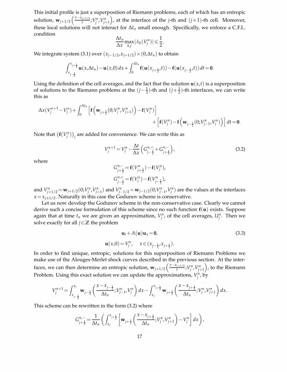
This initial profile is just a superposition of Riemann problems, each of which has an entropic

solution, wj+1/2

(

x−xj+1/2t ;Vnj ,V

nj+1

)

, at the interface of the j-th and (j+1)-th cell. Moreover,

these local solutions will not interact for ∆tn small enough. Specifically, we enforce a C.F.L.condition

∆tn∆xmaxk,j

|λk(Vnj )|6

1

2.

We integrate system (3.1) over (xj−1/2,xj+1/2)×(0,∆tn) to obtain

∫ xj+ 12

xj− 12

u(x,∆tn)−u(x,0)dx+∫

∆tn

0f(u(xj+ 12

,t))−f(u(xj− 12,t))dt=0.

Using the definition of the cell averages, and the fact that the solution u(x,t) is a superpositionof solutions to the Riemann problems at the (j− 12)-th and (j+ 12 )-th interfaces, we can writethis as

∆x(Vn+1j −Vnj )+∫

∆tn

0

[

f(

wj+ 12(0;Vnj ,V

nj+1)

)

−f(Vnj )]

+[

f(Vnj )−f(

wj− 12(0;Vnj−1,V

nj ))]

dt=0.

Note that(

f(Vnj ))

jare added for convenience. We can write this as

Vn+1j =Vnj −∆t

∆x

(

Gn,+j− 12

+Gn,−j+ 12

)

, (3.2)

whereGn,−j+ 12

= f(Vnj+ 12

)−f(Vnj ),

Gn,+j− 12

= f(Vnj )−f(Vnj− 12

),

and Vnj+1/2=wj+1/2(0;Vnj ,V

nj+1) and V

nj−1/2=wj−1/2(0;V

nj−1,V

nj ) are the values at the interfaces

x= xj±1/2. Naturally in this case the Godunov scheme is conservative.Let us now develop the Godunov scheme in the non-conservative case. Clearly we cannot

derive such a concise formulation of this scheme since no such function f(u) exists. Supposeagain that at time tn we are given an approximation, V

nj , of the cell averages, U

nj . Then we

solve exactly for all j∈Z the problem

ut+A(u)ux=0, (3.3)

u(x,0)=Vnj , x∈ (xj− 12,xj+ 12

).

In order to find unique, entropic, solutions for this superposition of Riemann Problems wemake use of the Alouges-Merlet shock curves described in the previous section. At the inter-

faces, we can then determine an entropic solution, wj+1/2

(

x−xj+1/2t ;Vnj ,V

nj+1

)

, to the Riemann

Problem. Using this exact solution we can update the approximations, Vnj , by

Vn+1j =∫ xj

xj− 12

wj− 12

( x−xj− 12∆tn

;Vnj−1,Vnj

)

dx−∫ x

j+ 12

xj

wj+ 12

( x−xj+ 12∆tn

;Vnj ,Vnj+1

)

dx.

This scheme can be rewritten in the form (3.2) where

Gn,−j+ 12

=1

∆tn

(

∫ xj+ 12

xj

[

wj+ 12

( x−xj+ 12∆tn

;Vnj ,Vnj+1

)

−Vnj

]

dx

)

,

17

Gn,+j− 12

=1

∆tn

(

∫ xj

xj− 12

[

Vnj −wj− 12

( x−xj− 12∆tn

;Vnj−1,Vnj

)]

dx

)

.

In order to give more explicit formulas of the interfacial fluxes let us consider now 2×2 sys-tems. However in principle what follows is still valid for general n×n systems.

3.1.1 Flux terms in 2×2 Systems

As it is well known, Riemann problems for 2×2 systems have different kinds of solution: 1-discontinuity waves and 2-discontinuity waves, or 1-discontinuity waves and 2-rarefactionwaves, or ... etc.† Let us, for instance, assume that at the interface between the j-th and (j+1)-th cell, the solution consists of a 1-discontinuity wave and a 2-discontinuity wave travelingwith speeds σ1 and σ2, respectively. The solution to the Riemann problem has then the form,

wj+ 12

( x

t;Vnj ,V

nj+1

)

=

Vnj ,xt <σ1,

V∗, σ1<xt <σ2,

Vnj+1,xt >σ2,

where V∗ is the intermediate state determined by the intersection of the 1-shock and 2-shockcurves (or contact discontinuity curves if the fields are linearly degenerate). Before calculatingthe general form of these fluxes, let us demonstrate how these flux terms are calculated. Let usassume for simplicity that σ160 and σ2>0. The interface flux becomes

Gn,+j+ 12

=1

∆tn

(

∫ xj+1

xj+ 12

[

Vnj+1−wj+ 12

( x−xj+ 12∆tn

;Vnj ,Vnj+1

)]

dx

)

,

=∫ ∆x2∆tn

0

[

Vnj+1−wj+ 12

(

ξ;Vnj ,Vnj+1

)]

dξ,

=∫ σ2

0Vnj+1−V

∗ dξ+∫ ∆x2∆tn

σ2Vnj+1−V

nj+1 dξ,

=σ2(Vnj+1−V

∗),

where, in the second line above, we have used the change of variables ξ =x−xj+1/2

∆tn. Similarly,

we calculate

Gn,−j+ 12

=σ1(V∗−Vnj ).

Thus, we have calculated the flux terms for this specific case. More generally (σ1,σ2∈R), theinterfacial fluxes Gn,±j+1/2 are given by

Gn,+j+ 12

=1+sgn(σ2)

2σ2(V

nj+1−V

∗)+1+sgn(σ1)

2σ1(V

∗−Vnj ),

Gn,−j+ 12

=1−sgn(σ2)

2σ2(V

nj+1−V

∗)+1−sgn(σ1)

2σ1(V

∗−Vnj ).

Let us now consider the case where, at the interface located in xj+1/2, the solution consistsof a 1-rarefaction wave and a 2-discontinuity wave, traveling with velocity σ2. The solution to

†The solution can obviously consists of only a single k-simple wave. In this case we choose any of the flux termswhich contain this k-simple wave, since every case is reduced to the same flux.

18

the Riemann problem then has the form,

w( x

t;Vnj ,V

nj+1

)

=

Vnj ,xt <λ1(V

nj ),

v(

xt

)

, λ1(Vnj )<

xt <λ1(V

∗),

V∗, λ1(V∗)<

xt <σ2,

Vnj+1,xt >σ2,

where V∗ is the intermediate state determined by the intersection of the 1-rarefaction and 2-shock (or 2-Contact discontinuity) curves, and v(x/t) is the section of the 1-rarefaction curvelinking Vnj and V

∗. Again, before presenting the general form of the flux terms in this case,

let us show a sample calculation. For the sake of the notations, let us assume for instance thatσ2>0, λ1(V

nj )60, and λ1(V

∗)>0. We repeat the above process and obtain

Gn,+j+ 12

=1

∆tn

(

∫ xj+1

xj+ 12

[

Vnj+1−wj+ 12

( x−xj+ 12∆tn

;Vnj ,Vnj+1

)]

dx

)

,

=∫ ∆x2∆tn

0

[

Vnj+1−wj+ 12

(

ξ;Vnj ,Vnj+1

)]

dξ,

=∫ λ1(V

∗)

0Vnj+1−v(ξ)dξ+

∫ σ2

λ1(V∗)Vnj+1−V

∗ dξ,∫ ∆x2∆tn

σ2Vnj+1−V

nj+1 dξ

=λ1(V∗)Vnj+1−

∫ λ1(V∗)

0v(ξ)dξ+σ2(V

nj+1−V

∗)−λ1(V∗)(Vnj+1−V

∗),

=σ2(Vnj+1−V

∗)−∫ λ1(V

∗)

0v(ξ)−V∗ dξ,

where again we have used the change of variables ξ =x−xj+1/2

∆tnin the second line. Similarly, we

calculate

Gn,−j+ 12

=∫ 0

λ1(Vnj+1)v(ξ)−Vnj dξ.

Generalizing this process for arbitrary choices of σ2, etc., the interfacial fluxes Gn,±j+1/2 are given

by

Gn,+j+ 12

=1+sgn(σ2)

2σ2(V

nj+1−V

∗)−1+sgn(λ1(V

∗))

2

∫ λ1(V∗)

0v(ξ)−V∗ dξ

+1+sgn(λ1(V

nj ))

2

∫ λ1(Vnj )

0v(ξ)−Vnj dξ,

Gn,−j+ 12

=1−sgn(σ2)

2σ2(V

nj+1−V

∗)−1−sgn(λ1(V

∗))

2

∫ 0

λ1(V∗)v(ξ)−V∗ dξ

+1−sgn(λ1(V

nj ))

2

∫ 0

λ1(Vnj )v(ξ)−Vnj dξ.

The remaining cases follow analogously from these.

An implementation of this scheme for 2×2 systems follows the blueprint:

19

1. At each cell interface xj+1/2, we numerically compute the 1-rarefaction and 1-shock curves(or 1-Contact discontinuity curves for linearly degenerate fields) from the state Vnj , and

the 2-rarefaction and admissible 2-shock curve (or 2-Contact discontinuity curves forlinearly degenerate fields) from the state Vnj+1, by using their corresponding differential

systems‡. Then an entropy condition is used to select admissible shock and rarefactionwaves (Lax shock condition in our case).

2. We determine the intermediate state at the (unique) intersection of these curves and con-struct the flux terms Gn,±j+1/2 using the equations described above.

3. We then update the solution to time tn+1 using (3.2).

It is clear that this procedure is extremely costly since at each cell interface we must in-tegrate four curves numerically and find their point of intersection. This is the unfortunatedrawback of using an exact Riemann solver. One possible way to reduce the complexity of thisscheme is to replace the exact Riemann solver with an approximate or linearized one, as it isdone in the Roe solver [30]. Although this is an extremely important point for real, physicalapplications, the question of how to reduce computational complexity is not the focus of thispaper.

3.2 DLM Godunov Scheme using Alouges-Merlet Shock Curves

The question of how to implement the DLM theory numerically has been thoroughly stud-ied, first by Toumi [35] then by Pares [27]. Specifically, in [9], Castro and Pares present anon-conservative (but path-conservative) Godunov scheme for non-conservative hyperbolicsystems using a Riemann solver based on DLM’s theory. The authors show that the schemehas the form (3.2), with the flux terms given by

Gn,+j+ 12

=∫ 1

0A(ψ(s;Vn

j+ 12,Vnj+1))

∂ψ

∂s(s;Vn

j+ 12,Vnj+1)ds,

Gn,−j+ 12

=∫ 1

0A(ψ(s;Vnj ,V

nj+ 12

))∂ψ

∂s(s;Vnj ,V

nj+ 12

)ds,

where(

Vnj+1/2)

jare the interface values of the solution to (3.3). In the case where the solution

to the Riemann problem is discontinuous at an interface, we replace Vnj+1/2 in G+,nj+1/2 by the

right limit of the discontinuity, and by the left limit of the discontinuity in G−,nj+1/2. The path

ψ(s;uL,uR) is chosen to be the composition of the k-Simple curves which we use to solve theRiemann problem with left state uL, and right state uR. Using the assumptions stated aboveon the choice of paths, the only missing piece of information we need to fully construct thisfamily of paths is how we select the shock curves. The approximate shock curves of Alougesand Merlet enable us to complete this family of paths.The implementation of this scheme for 2×2 systems is entirely analogous to the blueprint

detail above for the Godunov scheme using the Alouges-Merlet approximate shock curves:

1. At a cell interface, say xj+1/2, we numerically compute the 1-rarefaction and 1-shockcurves (or 1-contact discontinuity curves for linearly degenerate fields) at the state Vnj ,

and the 2-rarefaction and admissible 2-shock curve (or 2-Contact discontinuity curves forlinearly degenerate fields) at the state Vnj+1 by using their defining differential equations

‡In our implementation, a Runge-Kutta 4 method is used to numerically solve these differential systems.

20

(the shock curves we use are the Alouges-Merlet approximate shock curves). Then anentropy condition is used to select admissible shock and rarefaction waves (Lax shockcondition in our case).

2. We determine the intermediate state at the (unique) intersection of these curves and con-struct the paths ψ(s;Vnj ,V

nj+ 12

) and ψ(s;Vnj+ 12,Vnj+1) as we described above.

3. We calculate the flux terms Gn,±j+1/2 using the equations above.

4. We then update the solution to time tn+1 using (3.2).

Again, this scheme suffers from the same high levels of computational complexity as theGodunov scheme presented in the previous section. Indeed, in order to input the path ψ intothe expressions for the flux terms, we again need to integrate the rarefaction/shock curvesnumerically.

Remark 3.1. The schemes presented above are all derived from the classical Godunov scheme(see [19] for instance). As a consequence the stability analysis can easily be deduced fromthe analysis of the Godunov scheme for conservative hyperbolic systems. The convergenceanalysis is more complex due to the non-conservativity of the scheme. In particular, the con-vergence of the scheme to the exact solution (for a fixed path) is not a priori guarantied. Theorigin of this issue is the complex connection between the numerical viscosity and the measuresource term (supported by the discontinuity lines) in the path-conservative scheme equivalentequation [10], [1] and [21]. The approach developed in this paper does not a priori fix thisimportant open problem. We however conjecture that for instance the use of the zero-diffusivereservoir technique developed in [3], [4], applied to the above Godunov-like scheme could fixthis problem.

3.3 Numerical Experiments

3.3.1 The ShallowWater Equations

We first implement a Godunov scheme using the exact Riemann solver based on the Alouges-Merlet approximate shock curves, then the DLM Godunov scheme, again using the Alouges-Merlet approximate shock curves, in order to solve the shallow water equations. This systemis in fact conservative and hence we expect numerical solutions produced by these schemesto agree with the exact one. This is due to the fact that in the conservative case the Alouges-Merlet approximate shock curves recover the correct shock curves, and the flux terms of theDLM Godunov scheme will reduce to the classical fluxes of the Godunov scheme for systemsof conservation laws.We consider the Riemann problemwith left state uL=(5,0)T and right state uR=(1,0)T . The

reader can easily verify that for this system both the 1-field and 2-field are genuinely nonlinear.Hence, using the results from Section 2, we can construct the k-rarefaction and admissible k-shock curves for k=1,2. In Figure 4 we see that the 1-rarefaction and 2-shock curves intersectat the intermediate state u1≈ (2.54,10.22)T . Thus, the solution to this Riemann problem willconsist of a 1-rarefaction wave separating uL and u1, and a 2-shock wave separating u1 anduR.In Figure 5, we represent the solutions obtained by the two schemes. We examine the order

of convergence of these two schemes in Tables 1 and 2, where the solution of reference wasobtained with a VFFC solver (see [17]) with CFL number 0.99 and N=1280. From these tableswe can see that these schemes converge to the reference solution with, as expected, an order ofconvergence close to 1.

21

0 1 2 3 4 5 6−10

−5

0

5

10

15

h

q

uL

uR

u1

S1(uL)S2(uR)R1(uL)R2(uR)

Figure 4: We consider the Riemann problem for the shallow water equations with left state uL=(5,0)T , and right state

uR=(1,0)T. We plot the 1-shock and 1-rarefaction curves at the left state and the 2-shock and 2-rarefaction curves at

the right state. We determine the intermediate state u1∼ (2.54,10.22)T at the intersection of the 1-rarefaction curveand 2-shock curve.

−1 −0.5 0 0.5 10.5

1

1.5

2

2.5

3

3.5

4

4.5

5

x

h

−1 −0.5 0 0.5 1−2

0

2

4

6

8

10

12

x

q

VFFCAM GodunovDLM Godunov

Figure 5: Comparison of numerical solutions of the Riemann problem for the Shallow Water Equations. A VFFC solver,a Godunov scheme based on Alouges-Merlet’s approximate shock curves, and the DLM Godunov scheme based onAlouges-Merlet’s approximate shock curves are used. Shown at t=0.05, with N=200.

3.3.2 A Non-Conservative System

As expected, the two presented schemes recover the correct solutionswhere the studied systemis a conservative systemwritten in a non-conservative form. Let us now proceed to implementthem in the truly non-conservative case. We consider the following non-conservative system,

ut+uux+uvx=0,

vt+vux+vvx=0.

22

N h Error 1, Order, Error 2, Order,

e1= ||V−Vre f ||2∆loge1∆logh e2= ||V−Vre f ||∞

∆loge2∆logh

40 5.12E-2 4.48E-1 – 3.50E-1 –80 2.53E-2 1.96E-1 1.17 1.47E-1 1.23160 1.26E-2 1.07E-1 0.87 7.80E-2 0.91320 6.27E-3 4.82E-2 1.14 3.60E-2 1.11640 3.13E-3 1.87E-2 1.34 1.42E-2 1.34

Table 1: Order of convergence the Godunov scheme using the Alouges-Merlet approximate shock curves. Riemann

problem with left state uL=(5,0)T and right state uR=(1,0)T. Order of convergence found with respect to the L2

norm, ||·||2, and the L∞ norm, ||·||∞. Data calculated at t=0.04 and x∈ [−1,1].

N h Error 1, Order, Error 2, Order,

e1= ||V−Vre f ||2∆loge1∆logh e2= ||V−Vre f ||∞

∆loge2∆logh

40 5.12E-2 4.38E-1 – 3.42E-1 –80 2.53E-2 1.91E-1 1.17 1.41E-1 1.25160 1.26E-2 1.03E-1 0.86 7.48E-2 0.90320 6.27E-3 4.62E-2 1.15 3.42E-2 1.12640 3.13E-3 1.79E-2 1.37 1.32E-2 1.37

Table 2: Order of convergence of the Godunov schemes using Alouges-Merlet approximate shock curves as DLM’s

paths. Riemann problem with left state uL=(5,0)T and right state uR=(1,0)T. Order of convergence is found with

respect to the L2 norm, ||·||2, and the L∞ norm, ||·||∞. Data calculated at t=0.04 and x∈ [−1,1].

This systems was studied by C. Berthon in [6] and finds its origin in bifluid flows. The eigen-values of this system are λ1= 0 and λ2 = u+v. Therefore, this system is strictly hyperbolicwhen u 6=−v. The 1-field is linearly degenerate for this system and therefore we will considerthe 1-Contact discontinuity curve in our numerical solvers. The reader can also verify that the2-field is genuinely nonlinear. We consider a Riemann problem with left state uL=(4,3)T andright state uR=(2,0.5)T . The numerical solution is shown in Figure 6.As expected, the numerical solutions produced by these two schemes are very close, even

in this non-conservative case. As remarked in [21], a non-conservative form of the Godunov-like scheme used here can lead to the convergence of the numerical solution to the solution ofan inhomogeneous system with a Borel measure source term with support on the line of dis-continuity of the order of the entropy dissipation [6]. That is, in general “limhuh 6=uexact”. Thisis in particular what is observed in Abgrall-Karni [1], where examples of Pares’ path conser-vative schemes converging to wrong solutions are exhibited (numerical paths do not convergeto the chosen ones). However, from Figure 6 we see that in this case the measure source termis zero and indeed limhuh=uexact. This is an interesting point as we then have exhibited a non-trivial example where the non-conservative scheme is convergent to the exact solution. The questionof whether this scheme will converge to the exact solution for any non-conservative system ishowever still open and is the topic of an on-going research.

3.3.3 Equivalence of the schemes

In fact, the two Godunov schemes presented above are equivalent. In order to show it, wemust verify that their flux terms are equivalent, i.e. these fluxes are just a single flux written

23

−1 −0.5 0 0.5 12

2.5

3

3.5

4

4.5

5

5.5

6

x

u

−1 −0.5 0 0.5 10.5

1

1.5

2

2.5

3

x

v

ExactAM GodunovDLM Godunov

Figure 6: Comparison of the Alouges-Merlet shock curve-based Godunov Solver and the DLM Godunov solver, usingthe Alouges-Merlet shock curves, for the genuinely non-conservative system. The initial profile is a Riemann problem

with uL=(4,3)T and uR=(2,0.5)T. Shown at t=0.06 with N=400.

in different ways. To this end, let us consider an interface at which the Riemann problemcontains a k-shock wave separating the states u− on the left and u+ on the right, travelingwith positive speed σ > 0. At this interface, the positive flux term of the Godunov schemeusing the approximate shock curves of Alouges and Merlet will contain the term σ(u+−u−).Also, in the Godunov scheme based on DLM theory, the path ψwill contain the segment of theAlouges-Merlet approximate k-shock curve, parametrized by u(σ), which satisfies,

A(u(σ))du

dσ=σdu

dσ+u(σ)−u−,

u(λk(u−))=u−.

So the positive flux for the DLM Godunov scheme will contain the term

∫ σ

λk(u−)A(u(σ))

du

dσdσ.

Using the definition of the approximate shock curve yields,

∫ σ

λk(u−)A(u(σ))

du

dσdσ =

∫ σ

λk(u−)

(

σdu

dσ+u(σ)−u−

)

dσ

=[

σ(u(σ)−u−)∣

∣

σ

λk(u−)

= σ(u+−u−).

Thus, the positive flux term in the DLM Godunov scheme also contains the term σ(u+−u−).We can repeat this argument for shock waves which travel with negative speeds. Moreover,this argument can be used in a similar fashion to show that contributions in the flux termsdue to contact discontinuities and rarefaction waves will be the same in both schemes. Finally,this tells us that the flux terms in both schemes are equivalent. Note that, the slight numericaldifferences are due to the fact that although these flux terms are theoretically the same, they arecalculated numerically in entirely different ways. This remark does not, unfortunately, pleadin favour of the presented Godunov-like scheme (Section 3.1) as the path-conservative Paresscheme is known in general to converge to wrong solutions.

24

4 Concluding remarks

In this paper, we have proposed different numerical approaches for solving non-conservativehyperbolic systems. The proposed schemes are designed using exact Riemann solvers whichutilize the definitions recently proposed by Alouges and Merlet of approximate shock curvesin non-conservative systems. These shock curves have proven to be useful in several ways.They are accurate approximations of the shock curves constructed by Bianchini and Bressanin their vanishing viscosity process, so that the solutions constructed using these approximateshock curves are accurate approximations of the vanishing viscosity solutions. Using this fact,we first constructed a Godunov scheme for non-conservative hyperbolic systems using an ex-act Riemann solver which implements these approximate shock curves. On the other hand,we also know that these approximate shock curves approximate the viscous profiles and thusare useful in the theory of non-conservative products introduced by Dal Maso, LeFloch, andMurat. This fact gives us the possibility to construct several numerical schemes for NCHSsusing the framework proposed by Castro, Pares, et. al. An important result is that we areable to show that the two Godunov schemes we have constructed, which use exact Riemannsolvers, are in fact equivalent numerical schemes. This result shows a subtle connection be-tween these two different approaches to the analysis of NCHSs. An interesting result we haveshown is that these numerical schemes, when applied to a particular non-conservative system,in fact converge to the exact solution. This is an interesting result as it seems that, in this case,these schemes overcome the problem of convergence of non-conservative schemes as stud-ied by Hou and LeFloch [21], and Abgrall and Karni [1]. More generally, the convergence tothe correct solution of non-conservative schemes approximating non-conservative hyperbolicsystems is still an open problem. However, we conjecture that when the numerical viscositymatrix and the matrix A commute (which is typically satisfied for Roe or VFFC schemes witha “Karni-like” correction [22]), the numerical solution can converge to the exact solution, if acombination of Alouges&Merlet’s shock curves is chosen as a path. This will be studied in aforthcoming paper.

The main issue that arises in the implementation of these numerical schemes is their ex-treme computational cost. We indeed have to determine numerically the rarefaction, shock,and contact discontinuity curves of each state, at each interface of the mesh. This process in-volves numerically solving up to 2n ODEs per state. It is clear that our primary objective forfurther research of these numerical schemes is to design a scheme which produces accuratenumerical results but avoids this level of computational complexity (Roe- [30] and VFFC-typeschemes [17]).

Extension of the proposed approach to n×n systems, although simple in principle becomescomputationally challenging. Moreover, because the shock curves defined by Alouges andMerlet are merely approximations of the shock curves described by Bianchini and Bressan, itis still desirable to construct a numerical scheme which implements the true shock curves ofBianchini and Bressan directly. However, again due to the complexity of their derivation in [7],this is still challenging.

Another topic for future research is the question of how to extend these numerical schemesto the multidimensional case. Using the theory of Dal Maso, LeFloch, and Murat, Pares, Cas-tro, et. al. addressed this equation in [8], so our first goal will be to use this framework toextend our one-dimensional numerical scheme to the multidimensional case. Similarly, we arealso interested in the construction of high-order schemes.

Acknowledgment. The authors would like to thank the anonymous referees for their con-structive comments.

25

References

[1] R. Abgrall and S. Karni. A comment on the computation of non-conservative products. J. Comput.Phys., 229(8):2759–2763, 2010.

[2] R. Abgrall and R. Saurel. Unmodele numerique pour la simulation d’ecoulements multiphasiquescompressibles. Matapli, (68):39–54, 2002.

[3] F. Alouges, F. De Vuyst, G. Le Coq, and E. Lorin. Un procede de reduction de la diffusionnumerique des schemas a difference de flux d’ordre un pour les systemes hyperboliques nonlineaires. C. R. Math. Acad. Sci. Paris, 335(7):627–632, 2002.

[4] F. Alouges, F. De Vuyst, G. Le Coq, and E. Lorin. The reservoir technique: a way tomake godunov-type schemes zero or very low diffusive. application to Colella-Glaz. Eur. J. Mech. B Fluids, 27(6),2008.

[5] F. Alouges and B. Merlet. Approximate shock curves for non-conservative hyperbolic systems inone space dimension. J. Hyperbolic Differ. Equ., 1(4):769–788, 2004.

[6] C. Berthon. Schema nonlineaire pour l’approximation numerique d’un systeme hyperbolique nonconservatif. C. R. Math. Acad. Sci. Paris, 335(12):1069–1072, 2002.

[7] S. Bianchini and A. Bressan. Vanishing viscosity solutions of nonlinear hyperbolic systems. Ann.of Math. (2), 161(1):223–342, 2005.

[8] M. J. Castro, E. D. Fernandez-Nieto, A. M. Ferreiro, J. A. Garcıa-Rodrıguez, and C. Pares. Highorder extensions of Roe schemes for two-dimensional nonconservative hyperbolic systems. J. Sci.Comput., 39(1):67–114, 2009.

[9] M. J. Castro, J. M. Gallardo, M. L. Munoz, and C. Pares. On a general definition of the Godunovmethod for nonconservative hyperbolic systems. Application to linear balance laws. In Numericalmathematics and advanced applications, pages 662–670. Springer, Berlin, 2006.

[10] M. J. Castro, P. G. LeFloch, M. L.Munoz-Ruiz, andC. Pares. Whymany theories of shockwaves arenecessary: convergence error in formally path-consistent schemes. J. Comput. Phys., 227(17):8107–8129, 2008.

[11] J.-J. Cauret, J.-F. Colombeau, and A. Y. LeRoux. Solutions generalisees discontinues de problemeshyperboliques non conservatifs. C. R. Acad. Sci. Paris Ser. I Math., 302(12):435–437, 1986.

[12] J.-F. Colombeau. New generalized functions and multiplication of distributions, volume 84 of North-Holland Mathematics Studies. North-Holland Publishing Co., Amsterdam, 1984. Notas deMatematica [Mathematical Notes], 90.

[13] J.-F. Colombeau, A. Y. LeRoux, A. Noussaır, and B. Perrot. Microscopic profiles of shock wavesand ambiguities in multiplications of distributions. SIAM J. Numer. Anal., 26(4):871–883, 1989.

[14] G. Dal Maso, P. G. LeFloch, and F. Murat. Definition and weak stability of nonconservative prod-ucts. J. Math. Pures Appl. (9), 74(6):483–548, 1995.

[15] V. Deledicque andM. V. Papalexandris. An exact Riemann solver for compressible two-phase flowmodels containing non-conservative products. J. Comput. Phys., 222(1):217–245, 2007.

[16] D. A. Drew and S. L. Passman. Theory of multicomponent fluids, volume 135 of Applied MathematicalSciences. Springer-Verlag, New York, 1999.

[17] J.-M. Ghidaglia, A. Kumbaro, and G. Le Coq. Une methode “volumes finis” a flux caracteristiquespour la resolution numerique des systemes hyperboliques de lois de conservation. C. R. Acad. Sci.Paris Ser. I Math., 322(10):981–988, 1996.

[18] J.-M. Ghidaglia, A. Kumbaro, and G. Le Coq. On the numerical solution to two fluid models via acell centered finite volume method. Eur. J. Mech. B Fluids, 20(6):841–867, 2001.

[19] E. Godlewski and P.-A. Raviart. Numerical approximation of hyperbolic systems of conservation laws,volume 118 of Applied Mathematical Sciences. Springer-Verlag, New York, 1996.

[20] S. K. Godunov. A difference method for numerical calculation of discontinuous solutions of theequations of hydrodynamics. Mat. Sb. (N.S.), 47 (89):271–306, 1959.

[21] T. Y. Hou and P. G. LeFloch. Why nonconservative schemes converge to wrong solutions: erroranalysis. Math. Comp., 62(206):497–530, 1994.

[22] S. Karni. Viscous shock profiles and primitive formulations. SIAM J. Numer. Anal., 29(6):1592–1609,1992.

[23] P. G. LeFloch. Shock waves for nonlinear hyperbolic systems in nonconservative form. preprint593, Institute for Mathematics and its Applications, University of Minnesota, Minneapolis, 1989.

[24] P. G. LeFloch and M. Mohammadian. Why many theories of shock waves are necessary: kinetic

26

functions, equivalent equations, and fourth-ordermodels. J. Comput. Phys., 227(8):4162–4189, 2008.[25] G. Mophou and P. Poullet. A split Godunov scheme for solving one-dimensional hyperbolic sys-

tems in a nonconservative form. SIAM J. Numer. Anal., 40(1):1–25 (electronic), 2002.[26] M. Pailha andO. Pouliquen. A two-phase flow description of the initiation of underwater granular

avalanches. J. Fluid Mech., 633:115–135, 2009.[27] C. Pares. Numerical methods for nonconservative hyperbolic systems: a theoretical framework.

SIAM J. Numer. Anal., 44(1):300–321 (electronic), 2006.[28] S. Rhebergen, O. Bokhove, and J. J. W. van der Vegt. Discontinuous Galerkin finite element meth-

ods for hyperbolic nonconservative partial differential equations. J. Comput. Phys., 227(3):1887–1922, 2008.

[29] S. Rhebergen, O. Bokhove, and J. J. W. van der Vegt. Discontinuous Galerkin finite element methodfor shallow two-phase flows. Comput. Methods Appl. Mech. Engrg., 198(5-8):819–830, 2009.

[30] P. L. Roe. Approximate Riemann solvers, parameter vectors, and difference schemes. J. Comput.Phys., 43(2):357–372, 1981.

[31] R. Saurel and R. Abgrall. A multiphase Godunov method for compressible multifluid and multi-phase flows. J. Comput. Phys., 150(2):425–467, 1999.

[32] L. Schwartz. Sur l’impossibilite de la multiplication des distributions. C. R. Acad. Sci. Paris,239:847–848, 1954.

[33] D. Serre. Systems of conservation laws. 1. Cambridge University Press, Cambridge, 1999. Hyperbol-icity, entropies, shock waves, Translated from the 1996 French original by I. N. Sneddon.

[34] A. Tiwari and J. Abraham. A two-component two-phase dissipative particle dynamics model.Internat. J. Numer. Methods Fluids, 59(5):519–533, 2009.

[35] I. Toumi and A. Kumbaro. An approximate linearized Riemann solver for a two-fluid model. J.Comput. Phys., 124(2):286–300, 1996.

[36] A. I. Vol′pert. Spaces BV and quasilinear equations. Mat. Sb. (N.S.), 73 (115):255–302, 1967.

27