Geoderma 217–218 (2014) 74–82

Contents lists available at ScienceDirect

Geoderma

j ourna l homepage: www.e lsev ie r .com/ locate /geoderma

Rainfall erosivity mapping for Santiago Island, Cape Verde

Juan Francisco Sanchez-Moreno a,⁎, Chris M. Mannaerts b, Victor Jetten a

a Department of Earth System Analysis, Faculty of Geo-Information Science and Earth Observation (ITC), University of Twente, Netherlandsb Department of Water Resources, Faculty of Geo-Information Science and Earth Observation (ITC), University of Twente, Netherlands

⁎ Corresponding author at: Hengelosestraat 99, PO BoNetherlands.

E-mail addresses: sanchez@itc.nl (J.F. Sanchez-Moreno(C.M. Mannaerts), jetten@itc.nl (V. Jetten).

0016-7061/$ – see front matter © 2013 Elsevier B.V. All rihttp://dx.doi.org/10.1016/j.geoderma.2013.10.026

a b s t r a c t

a r t i c l e i n f o

Article history:Received 21 February 2012Received in revised form 25 October 2013Accepted 30 October 2013Available online 7 December 2013

Keywords:DisdrometerRainfall erosivityFournier indexKrigingCape Verde

Erosivity, the potential of rainfall to detach soil particles, is a parameter used in severalmodels to link rainfall andsoil losses. Erosivity is usually calculated from high temporal resolution rainfall during a long period of time, anddata is not always available. For Cape Verde, off the west coast of Africa, where data is limited, researchers havecalculated erosivity using 7 year precipitation data at 15 min time interval and using rainfall kinetic energy–intensity relationships developed for temperate areas. In this paper, using additional data collected with an op-tical disdrometer between 2008 and 2010 with a temporal resolution of 3 min, storm erosivity (EI30) was re-evaluated using a new rainfall kinetic energy–intensity relationship developed for Cape Verde. A new equationfor storm erosivity as a function of daily rainfall was developed. Annual erosivity R-factor resulting from addingEI30 values was correlated to annual precipitation and to the Modified Fournier Index, calculated from long termmonthly data available in Cape Verde. Monthly and long term annual erosivity weremapped using the ModifiedFournier Index, and the erosivity R-factor as a function of annual precipitationwasmapped for a dry, awet and anaverage year. Annual erosivity R-factor in Cape Verde can reach values above 1700 J mm m−2 h−1. Given thestrong relationship between rainfall and elevation, high erosivity in Santiago Island occurs on higher elevations,coinciding with steep slopes and shallow soils, which makes these areas susceptible to erosion.

© 2013 Elsevier B.V. All rights reserved.

1. Introduction

Rainfall erosion causes loss of fertile soil, damage to agricultureand infrastructure, and water pollution. Changes in rainfall pat-terns are aggravating the risk of erosion around the world(Bernstein, 2007). The effect of rainfall erosion is more evident incountries such as Cape Verde, off the west coast of Africa, whererainfall is highly variable and with strong erosive events(Mannaerts and Gabriels, 2000a,b; Sanchez-Moreno et al., inpress). The main parameter to relate soil losses to rainfall erosionis erosivity, which is the ability of rainfall to detach soil particles.Mapping erosivity is of importance to detect areas susceptible toerosion for management and conservation purposes.

The most commonly used index for rainfall erosivity is the EI30 de-veloped byWischmeier and Smith (1958) for the USLE and RUSLE equa-tions. Data measured byWischmeier and Smith shows that when otherfactors different to rainfall are constant, soil losses in cultivated fieldsare proportional to the storm energy E times the maximum 30-min in-tensity I30. EI30 values summed up and divided by the total number of

x 217, 7500 AE Enschede, The

), mannaerts@itc.nl

ghts reserved.

years of erosivity estimation result in the parameter R used in USLEand RUSLE. Wischmeier and Smith EI30 index relies on high temporalresolution rainfall data, observed during a long period of time, informa-tion that is not always available. When rainfall data is limited, R valuescan be calculated for the stations with recording rain gauges, then cor-related to readily available precipitation, and extrapolated using the as-sociated precipitation (Renard and Freimund, 1994).

To copewith lack of data, other indexes, sometimes better correlatedto measured erosivity than R, and using daily, monthly and annual rain-fall have been created, such as the KE N 25 (Hudson, 1971), theAIm (Lal,1976), the Fournier index (Fournier, 1960), theModified Fournier Index(Arnoldus, 1977) and the physically-based A index (Sukhanovski et al.,2002). Different indexes have been developed because erosivity de-pends on geographic conditions, scale, type of measurement, amongothers, and there is no single parameter better than other for erosivityestimation (Renard and Freimund, 1994; Stocking, 1987).

The Fournier index (Fournier, 1960), developed for thewest coast ofAfrica, has beenwidely usedwhen onlymonthly data is available, and isdefined as:

FI ¼ p2max

Pð1Þ

where pmax is the maximum monthly rainfall (mm) and P is the totalannual precipitation (mm). Arnoldus (1977) correlated the Fournierindex with R in Morocco, finding poor correlations, but higher when

75J.F. Sanchez-Moreno et al. / Geoderma 217–218 (2014) 74–82

using themonthly average instead of themaximummonthly rainfall, inwhat has been called the Modified Fournier Index:

MFI j ¼X12

i¼1p2i; j

P j: ð2Þ

In Eq. (2), p is the average precipitation in month i (mm) in year j,and P is total annual precipitation (mm) in year j. Eq. (2) can be usedfor long-term annual, annual or monthly erosivity replacing p and Pfor the appropriate rainfall values. Erosivity for a period of N years canbe calculated by (Ferro et al., 1999):

MFIMA ¼XN

j

X12

i¼1

p2i; jP j

ð3Þ

whereMFIMA is basically the average of theModified Fournier IndexMFIjover a period ofN years. According to Gabriels et al. (2003) and Apaydinet al. (2006), Eq. (3) captures inter annual variability and prevents un-derestimation of erosivity compared to using averages of ith rainfallamounts averaged again over a number of years.

Renard and Freimund (1994) suggest the use of the ModifiedFournier Index for areas where long term data is not available. TheFournier index has been used to map erosivity, either as a single factoror correlated with R, in several countries [e.g. Portugal (Coutinho andTomás, 1994), Germany (Sauerborn et al., 1999), Ghana (Oduro-Afriyie,1996), Brazil (Da Silva, 2004), Argentina (Busnelli et al., 2006), Malaysia(Shamshad et al., 2008), Spain (Angulo-Martínez and Beguería, 2009),Mauritius Islands (Nigel and Rughooputh, 2010), North Jordan (Eltaifet al., 2010)].

For Cape Verde, erosivity has been estimated by Mannaerts andGabriels (2000b) using Wischmeier and Smith (1958) and Brown andFoster (1987) rainfall kinetic energy–intensity relationships KE–I, withprecipitation data from 1980 to 1987 measured at a 15-min interval.

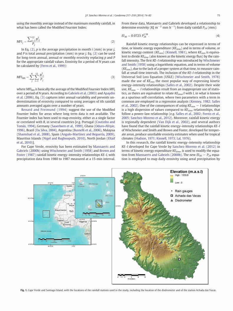
Fig. 1. Cape Verde and Santiago Island, with the locations of the rainfall stations used in the

From these data, Mannaerts and Gabriels developed a relationship todetermine erosivity (KJ m−2 mm h−1) from daily rainfall P24 (mm):

EI30 ¼ 0:0723 P1:5824 : ð4Þ

Rainfall kinetic energy relationships can be expressed in terms oftime, or kinetic energy expenditure (KEtime) and in terms of volume, orkinetic energy content (KEmm) (Kinnell, 1981), where KEmm is equiva-lent to divide KEtime (also known as the kinetic energy flux) by the rain-fall intensity. The first KE–I relationship was introduced by Wischmeierand Smith (1958) using a logarithmic equation, and in terms of volume(KEmm), due to the lack of a proper system at that time, tomeasure rain-fall at small time intervals. The inclusion of the KE–I relationship in theUniversal Soil Loss Equation (USLE) (Wischmeier and Smith, 1978)made the use of KEmm the most popular way of expressing kineticenergy–intensity relationships (Salles et al., 2002). Despite their wideuse, KEmm − I relationships result from an inappropriate use of statis-tics, as theirs are equivalent to relate KEtime/I with I, in what is knownas a spurious self-correlation, where two parameters with a term incommon are employed in a regression analysis (Kenney, 1982; Salleset al., 2002). One of the consequences of using KEmm − I relationshipsis a high dispersion of values compared to KEtime relationships, thatfollow a power-law relationship (e.g. Salles et al., 2002; Fornis et al.,2005; Sanchez-Moreno et al., 2012). Moreover, rainfall kinetic energyis regionally dependent (Van Dijk et al., 2002), and several authorshave found that the rainfall kinetic energy–intensity relationships KE–IofWischmeier and Smith and Brown and Foster, developed for temper-ate areas, produce unreliable erosivity estimates when used for tropicalclimates (Hudson, 1971; Kinnell, 1973; Lal, 1976).

In this research, the rainfall kinetic energy–intensity relationshipKE–I developed for Cape Verde by Sanchez-Moreno et al. (2012) interms of kinetic energy expenditure KEtime, is used to modify the equa-tion from Mannaerts and Gabriels (2000b). The new EI30 − P24 equa-tion is employed to map daily erosivity using areal precipitation by

study, including the location of the disdrometer and of the station Achada das Vacas.

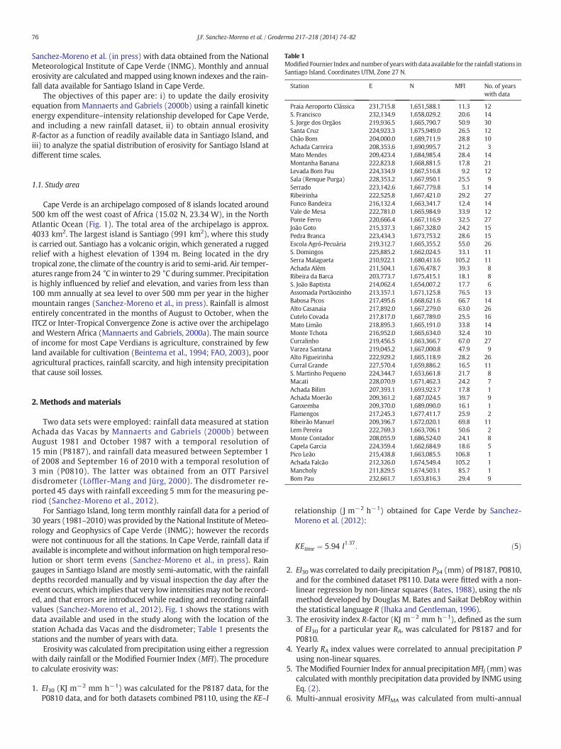
Table 1Modified Fournier Index and number of yearswith data available for the rainfall stations inSantiago Island. Coordinates UTM, Zone 27 N.

Station E N MFI No. of yearswith data

Praia Aeroporto Clássica 231,715.8 1,651,588.1 11.3 12S. Francisco 232,134.9 1,658,029.2 20.6 14S. Jorge dos Orgãos 219,936.5 1,665,790.7 50.9 30Santa Cruz 224,923.3 1,675,949.0 26.5 12Chão Bom 204,000.0 1,689,711.9 28.8 10Achada Carreira 208,353.6 1,690,995.7 21.2 3Mato Mendes 209,423.4 1,684,985.4 28.4 14Montanha Banana 222,823.8 1,668,881.5 17.8 21Levada Bom Pau 224,334.9 1,667,516.8 9.2 12Sala (Renque Purga) 228,353.2 1,667,950.1 25.5 9Serrado 223,142.6 1,667,779.8 5.1 14Ribeirinha 222,525.8 1,667,421.0 29.2 27Funco Bandeira 216,132.4 1,663,341.7 12.4 14Vale de Mesa 222,781.0 1,665,984.9 33.9 12Ponte Ferro 220,666.4 1,667,116.9 32.5 27João Goto 215,337.3 1,667,328.0 24.2 15Pedra Branca 223,434.3 1,673,753.2 28.6 15Escola Agró-Pecuária 219,312.7 1,665,355.2 55.0 26S. Domingos 225,885.2 1,662,024.5 33.1 11Serra Malagueta 210,922.1 1,680,413.6 105.2 11Achada Além 211,504.1 1,676,478.7 39.3 8Ribeira da Barca 203,773.7 1,675,415.1 18.1 8S. João Baptista 214,062.4 1,654,007.2 17.7 6Assomada Portãozinho 213,357.1 1,671,125.8 76.5 13Babosa Picos 217,495.6 1,668,621.6 66.7 14Alto Casanaia 217,892.0 1,667,279.0 63.0 26Cutelo Covada 217,817.0 1,667,789.0 25.5 16Mato Limão 218,895.3 1,665,191.0 33.8 14Monte Tchota 216,952.0 1,665,634.0 32.4 10Curralinho 219,456.5 1,663,366.7 67.0 27Varzea Santana 219,045.2 1,667,000.8 47.9 9Alto Figueirinha 222,929.2 1,665,118.9 28.2 26Curral Grande 227,570.4 1,659,886.2 16.5 11S. Martinho Pequeno 224,344.7 1,653,661.8 21.7 8Macati 228,070.9 1,671,462.3 24.2 7Achada Bilim 207,393.1 1,693,923.7 17.8 1Achada Moerão 209,361.2 1,687,024.5 39.7 9Ganxemba 209,370.0 1,689,090.0 16.1 1Flamengos 217,245.3 1,677,411.7 25.9 2Ribeirão Manuel 209,396.7 1,672,020.1 69.8 11Lem Pereira 222,769.3 1,663,706.1 50.6 2Monte Contador 208,055.9 1,686,524.0 24.1 8Capela Garcia 224,359.4 1,662,684.9 18.6 5Pico Leão 215,438.8 1,663,085.5 106.8 1Achada Falcão 212,326.0 1,674,549.4 105.2 1Mancholy 211,829.5 1,674,503.1 85.7 1Bom Pau 232,661.7 1,653,816.3 29.4 9

76 J.F. Sanchez-Moreno et al. / Geoderma 217–218 (2014) 74–82

Sanchez-Moreno et al. (in press) with data obtained from the NationalMeteorological Institute of Cape Verde (INMG). Monthly and annualerosivity are calculated andmapped using known indexes and the rain-fall data available for Santiago Island in Cape Verde.

The objectives of this paper are: i) to update the daily erosivityequation from Mannaerts and Gabriels (2000b) using a rainfall kineticenergy expenditure–intensity relationship developed for Cape Verde,and including a new rainfall dataset, ii) to obtain annual erosivityR-factor as a function of readily available data in Santiago Island, andiii) to analyze the spatial distribution of erosivity for Santiago Island atdifferent time scales.

1.1. Study area

Cape Verde is an archipelago composed of 8 islands located around500 km off the west coast of Africa (15.02 N, 23.34 W), in the NorthAtlantic Ocean (Fig. 1). The total area of the archipelago is approx.4033 km2. The largest island is Santiago (991 km2), where this studyis carried out. Santiago has a volcanic origin, which generated a ruggedrelief with a highest elevation of 1394 m. Being located in the drytropical zone, the climate of the country is arid to semi-arid. Air temper-atures range from24 °C inwinter to 29 °C during summer. Precipitationis highly influenced by relief and elevation, and varies from less than100 mm annually at sea level to over 500 mm per year in the highermountain ranges (Sanchez-Moreno et al., in press). Rainfall is almostentirely concentrated in the months of August to October, when theITCZ or Inter-Tropical Convergence Zone is active over the archipelagoand Western Africa (Mannaerts and Gabriels, 2000a). The main sourceof income for most Cape Verdians is agriculture, constrained by fewland available for cultivation (Beintema et al., 1994; FAO, 2003), pooragricultural practices, rainfall scarcity, and high intensity precipitationthat cause soil losses.

2. Methods and materials

Two data sets were employed: rainfall data measured at stationAchada das Vacas by Mannaerts and Gabriels (2000b) betweenAugust 1981 and October 1987 with a temporal resolution of15 min (P8187), and rainfall data measured between September 1of 2008 and September 16 of 2010 with a temporal resolution of3 min (P0810). The latter was obtained from an OTT Parsiveldisdrometer (Löffler-Mang and Jürg, 2000). The disdrometer re-ported 45 days with rainfall exceeding 5 mm for the measuring pe-riod (Sanchez-Moreno et al., 2012).

For Santiago Island, long term monthly rainfall data for a period of30 years (1981–2010)was provided by the National Institute of Meteo-rology and Geophysics of Cape Verde (INMG); however the recordswere not continuous for all the stations. In Cape Verde, rainfall data ifavailable is incomplete andwithout information on high temporal reso-lution or short term evens (Sanchez-Moreno et al., in press). Raingauges in Santiago Island are mostly semi-automatic, with the rainfalldepths recorded manually and by visual inspection the day after theevent occurs, which implies that very low intensitiesmay not be record-ed, and that errors are introduced while reading and recording rainfallvalues (Sanchez-Moreno et al., 2012). Fig. 1 shows the stations withdata available and used in the study along with the location of thestation Achada das Vacas and the disdrometer; Table 1 presents thestations and the number of years with data.

Erosivity was calculated from precipitation using either a regressionwith daily rainfall or the Modified Fournier Index (MFI). The procedureto calculate erosivity was:

1. EI30 (KJ m−2 mm h−1) was calculated for the P8187 data, for theP0810 data, and for both datasets combined P8110, using the KE–I

relationship (J m−2 h−1) obtained for Cape Verde by Sanchez-Moreno et al. (2012):

KEtime ¼ 5:94 I1:37: ð5Þ

2. EI30 was correlated to daily precipitation P24 (mm) of P8187, P0810,and for the combined dataset P8110. Data were fitted with a non-linear regression by non-linear squares (Bates, 1988), using the nlsmethod developed by Douglas M. Bates and Saikat DebRoy withinthe statistical language R (Ihaka and Gentleman, 1996).

3. The erosivity index R-factor (KJ m−2 mm h−1), defined as the sumof EI30 for a particular year RA, was calculated for P8187 and forP0810.

4. Yearly RA index values were correlated to annual precipitation Pusing non-linear squares.

5. TheModified Fournier Index for annual precipitationMFIj (mm)wascalculated with monthly precipitation data provided by INMG usingEq. (2).

6. Multi-annual erosivity MFIMA was calculated from multi-annual

Table 2Equation coefficients for EI30 as a function of daily rainfall P24. Quality of fit and predictedvalues of erosivity (minimum, maximum and mean) obtained from the different rainfalldatasets. EQ8187M: Equation coefficients from original EI30 − P relationship byMannaerts and Gabriels (2000b); EQ8187, EQ0810, EQ8110: Equation coefficients andcalculated and predicted values for new EI30 − P relationships calculated with Eq. (7)for corresponding datasets.

Erosivity R (KJ m−2 mm h−1)

Coefficients Quality of fit Calculated Predicted

Data a b R2 RMSE Min Max Mean Min Max Mean

EQ8187M 0.0723 1.58 0.90 11.4 0.90 185.2 34.0 2.32 280.7 38.8EQ8187N 0.14 1.39 0.85 21.2 0.90 185.2 34.0 3.10 212.6 36.3EQ0810 0.0005 2.84 0.84 27.2 0.47 332.2 38.1 0.41 295.8 35.8EQ8110 0.26 1.31 0.63 36.8 0.47 332.2 36.0 4.72 252.2 39.7EQ8110a 0.24 1.30 0.76 23.1 0.47 185.2 31.1 4.2 218.8 33.6

a Without erosivity outlier.

77J.F. Sanchez-Moreno et al. / Geoderma 217–218 (2014) 74–82

precipitation over the period N (1981–2010) using Eq. (3). Monthlyerosivity was calculated with Eq. (3) applied only on the months ofinterest i over the whole period N.

7. RA was correlated by non-linear squares to annual values of MFIjfor single stations (Achada das Vacas between 1981 and 1987,and Disdrometer in Saõ Jorge dos Orgaõs between 2008 and 2010),and to the average MFI j values of all the stations in the island(Table 1).

Monthly andmulti-annual erosivityMFIMAweremapped using Eq. (3)extrapolated to stations of Santiago Islandwith at least 3 years of data. Tocompare the inter annual variations of rainfall in Cape Verde, erosivity R-factor as a function of annual precipitation was mapped for a relativelydry year (1998), for an average year (2004), and for a year with a highamount of rainfall compared to the series of data (2009).

To obtain erosivity maps, the different erosivity equations were ap-plied using the interpolated rainfall maps from Sanchez-Moreno et al.(in press). Several parameters influence rainfall in Santiago Island.Short duration events and daily rainfall are strongly influenced bywind direction, slope, and position of the rain-gauges in the windwardor leeward sides of the island (Sanchez-Moreno et al., in press). Howev-er, monthly and long term rainfall are strongly influenced by elevation,therefore it was used as external drift for kriging interpolation, both forprecipitation (as input for calculation of the R-factor), and for the mapsmadewith theModified Fournier Index.With krigingwith external driftthe expected variable is considered a linear function of a second variablethat is usually continuous in space (Goovaerts, 1997; Hengl, 2003;Isaaks and Srivastava, 1990; Sanchez-Moreno et al., in press). The rele-vant parameters employed to fit the variogramof rainfall with elevationas external drift for multi-seasonal rainfall were a partial sill of 8500,zero nugget, and a range of 7000 m. The spatial correlation is weak

Fig. 2.Daily rainfall and daily storm erosivity EI30 calculated with the KE–I equations fromWisc(1987) (B&F) and the KE–I relationship for Cape Verde, for the events between September 1 o

even at short distances, due to the high variability of rainfall. Detailson the data, the procedure employed, and the quality assessment ofthe interpolations used to estimate rainfall for Santiago Island can befound in Sanchez-Moreno et al. (in press). Interpolation of rainfallusing elevation is described as well by Goovaerts (2000), and the useof elevation to improve the interpolation of erosivity is explained byGoovaerts (1999).

3. Results and discussion

3.1. Daily erosivity

Storm erosivity EI30 calculated with the KE–I relationship for CapeVerde (Eq. (5)) resulted in lower values for most of the rainfall

hmeier and Smith (1958) using Renard et al. (1997) coefficients (W&S), Brown and Fosterf 2008 and September 10 of 2010 with depths of 9 mm or higher.

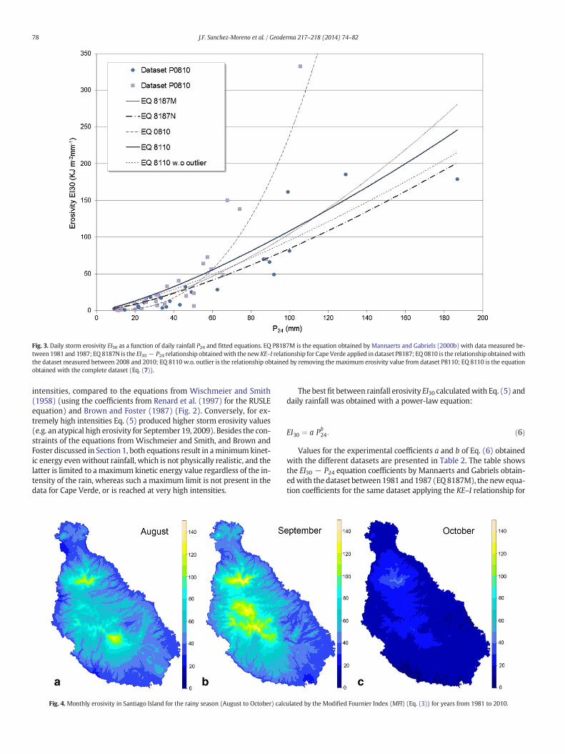
Fig. 3. Daily storm erosivity EI30 as a function of daily rainfall P24 and fitted equations. EQ P8187M is the equation obtained by Mannaerts and Gabriels (2000b) with data measured be-tween 1981 and 1987; EQ 8187N is the EI30 − P24 relationship obtainedwith the new KE–I relationship for CapeVerde applied in dataset P8187; EQ 0810 is the relationship obtainedwiththe dataset measured between 2008 and 2010; EQ 8110 w.o. outlier is the relationship obtained by removing the maximum erosivity value from dataset P8110; EQ 8110 is the equationobtained with the complete dataset (Eq. (7)).

78 J.F. Sanchez-Moreno et al. / Geoderma 217–218 (2014) 74–82

intensities, compared to the equations from Wischmeier and Smith(1958) (using the coefficients from Renard et al. (1997) for the RUSLEequation) and Brown and Foster (1987) (Fig. 2). Conversely, for ex-tremely high intensities Eq. (5) produced higher storm erosivity values(e.g. an atypical high erosivity for September 19, 2009). Besides the con-straints of the equations from Wischmeier and Smith, and Brown andFoster discussed in Section 1, both equations result in aminimumkinet-ic energy even without rainfall, which is not physically realistic, and thelatter is limited to a maximum kinetic energy value regardless of the in-tensity of the rain, whereas such a maximum limit is not present in thedata for Cape Verde, or is reached at very high intensities.

Fig. 4. Monthly erosivity in Santiago Island for the rainy season (August to October) calc

The bestfit between rainfall erosivity EI30 calculatedwith Eq. (5) anddaily rainfall was obtained with a power-law equation:

EI30 ¼ a Pb24: ð6Þ

Values for the experimental coefficients a and b of Eq. (6) obtainedwith the different datasets are presented in Table 2. The table showsthe EI30 − P24 equation coefficients by Mannaerts and Gabriels obtain-edwith thedataset between1981 and1987 (EQ 8187M), thenewequa-tion coefficients for the same dataset applying the KE–I relationship for

ulated by the Modified Fournier Index (MFI) (Eq. (3)) for years from 1981 to 2010.

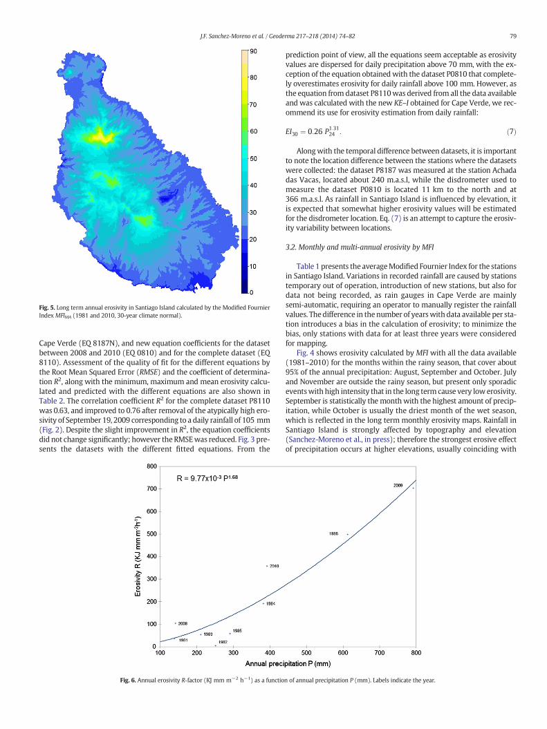
Fig. 5. Long term annual erosivity in Santiago Island calculated by the Modified FournierIndex MFIMA (1981 and 2010, 30-year climate normal).

79J.F. Sanchez-Moreno et al. / Geoderma 217–218 (2014) 74–82

Cape Verde (EQ 8187N), and new equation coefficients for the datasetbetween 2008 and 2010 (EQ 0810) and for the complete dataset (EQ8110). Assessment of the quality of fit for the different equations bythe Root Mean Squared Error (RMSE) and the coefficient of determina-tion R2, along with the minimum, maximum and mean erosivity calcu-lated and predicted with the different equations are also shown inTable 2. The correlation coefficient R2 for the complete dataset P8110was 0.63, and improved to 0.76 after removal of the atypically high ero-sivity of September 19, 2009 corresponding to a daily rainfall of 105 mm(Fig. 2). Despite the slight improvement in R2, the equation coefficientsdid not change significantly; however the RMSEwas reduced. Fig. 3 pre-sents the datasets with the different fitted equations. From the

Fig. 6. Annual erosivity R-factor (KJ mm m−2 h−1) as a functio

prediction point of view, all the equations seem acceptable as erosivityvalues are dispersed for daily precipitation above 70 mm, with the ex-ception of the equation obtained with the dataset P0810 that complete-ly overestimates erosivity for daily rainfall above 100 mm. However, asthe equation from dataset P8110was derived from all the data availableand was calculated with the new KE–I obtained for Cape Verde, we rec-ommend its use for erosivity estimation from daily rainfall:

EI30 ¼ 0:26 P1:3124 : ð7Þ

Alongwith the temporal difference between datasets, it is importantto note the location difference between the stations where the datasetswere collected: the dataset P8187 was measured at the station Achadadas Vacas, located about 240 m.a.s.l, while the disdrometer used tomeasure the dataset P0810 is located 11 km to the north and at366 m.a.s.l. As rainfall in Santiago Island is influenced by elevation, itis expected that somewhat higher erosivity values will be estimatedfor the disdrometer location. Eq. (7) is an attempt to capture the erosiv-ity variability between locations.

3.2. Monthly and multi-annual erosivity by MFI

Table 1 presents the averageModified Fournier Index for the stationsin Santiago Island. Variations in recorded rainfall are caused by stationstemporary out of operation, introduction of new stations, but also fordata not being recorded, as rain gauges in Cape Verde are mainlysemi-automatic, requiring an operator to manually register the rainfallvalues. Thedifference in thenumber of yearswith data available per sta-tion introduces a bias in the calculation of erosivity; to minimize thebias, only stations with data for at least three years were consideredfor mapping.

Fig. 4 shows erosivity calculated by MFI with all the data available(1981–2010) for the months within the rainy season, that cover about95% of the annual precipitation: August, September and October. Julyand November are outside the rainy season, but present only sporadiceventswith high intensity that in the long term cause very lowerosivity.September is statistically the month with the highest amount of precip-itation, while October is usually the driest month of the wet season,which is reflected in the long term monthly erosivity maps. Rainfall inSantiago Island is strongly affected by topography and elevation(Sanchez-Moreno et al., in press); therefore the strongest erosive effectof precipitation occurs at higher elevations, usually coinciding with

n of annual precipitation P (mm). Labels indicate the year.

Table 3Summary statistics of annual erosivity R-factor (J mm m−2 h−1) as a function of annualrainfall P (mm) calculated with Eq. (8) for a dry year (1998), an average year (2004)and a wet year (2009). Annual precipitation P and seasonal precipitation PS calculatedwith all the stations over the island.

Erosivity R (KJ m−2 mm h−1) Precipitation (mm)

Year Min Max Mean Median PS P

1998 12.62 198.5 45.07 37.26 164.3 173.92004 13.58 458.4 93.49 76.52 245.8 285.32009 87.62 1728 371.2 303.5 523.9 530.0

80 J.F. Sanchez-Moreno et al. / Geoderma 217–218 (2014) 74–82

steep slopes and shallow soils. The areas on top of the mountains aretherefore more susceptible to erosion. Erosivity in Santiago Island canbe classified as low for MFI below 50 mm, medium for tMFI between50 and 100 mm, and high for MFI higher than 100 mm. For the20 year period, the lowest erosivity values were found for Octoberwith minimums between 0 and 10 mm, while the highest were inSeptember with a maximum of 188 mm, compared to a maximum of147 mm for August and 123 mm for October.

Fig. 5 presents the long term annual erosivity for Santiago Island cal-culated using the Modified Fournier Index between 1981 and 2010. Forthe 30 year period, representing the last climate normal, the maximumannual erosivity with MFI was 90 mm, lower than the maximum longterm monthly erosivity, a result caused by several dry years duringthat period.

3.3. R-factor as a function of annual precipitation

The best fit between the erosivity R-factor (J mm m−2 h−1) and an-nual precipitation P (mm) for the whole data set was obtained with apower law equation (R2 = 0.92):

R ¼ 9:77 P1:68: ð8Þ

The data and fitted equation (in KJ mm m−2 h−1) are presented inFig. 6. Fig. 7 shows R-factor erosivity maps obtained by applyingEq. (8) to annual rainfall of 1998, 2004, and 2009, years considereddry, average and with high amounts of rainfall respectively, when com-pared to other years in the total series of data (Table 3).

3.4. R-factor as a function of MFI

Little to no correlation was found between annual R-factor andMFIjfor individual stations. This is due to the fact that the erosivity R-factor iscalculated from precipitation higher than 9 mm, while forMFIj the totalamount of precipitation reported in the station is employed. Also, veryhigh MFI values caused by months with extreme rainfalls result in out-liers for the correlation. The correlation between R-factor for individualstations and the average MFI j for the whole island (complete datasetP8110) resulted in an R2 of 0.58. The best fit was obtained with theequation:

R ¼ 487:8 MFI j1:66

: ð9Þ

Fig. 7. Erosivity R-factor (J mm m−2 h−1) as a function of annual precipitation P (mm) calcu

Fig. 4 presents the data and fitted curve of the correlation betweenR-factor and MFI j for the complete dataset P8110. The correlationbetween the dataset P8187 and MFI j improved the R2 to 0.85 but caus-ing an extreme overestimation of R-factor for values of MFI j above100 mm. Despite underestimation of erosivity for years 1984, 1986and 2009, representing years with extreme rainfall events, Eq. (9) over-estimates erosivity for the rest of the years, and seems to represent bet-ter the fluctuations on erosivity caused by the variability of rainfallpatterns in Cape Verde over a long period of time. The lower correlationcoefficient for the complete dataset is caused by months with extremerainfalls occurring between 2008 and 2010 (e.g. 545 mm reported fora single station in August 2008, and 468 mm in September 2009)(Fig. 8).

4. Conclusions

In this paper, daily, monthly, multi-annual, and long term annualerosivity estimates were calculated using available rainfall data forSantiago Island. The EI30 equation from Mannaerts and Gabriels(2000b)wasmodified using a rainfall kinetic energy–intensity relation-ship in terms of time KEtime developed for Cape Verde by Sanchez-Moreno et al. (2012). The erosivity R-factor was evaluated from databetween 1981 and 1987 and between 2008 and 2010. The ModifiedFournier Index (MFI) was calculated using long term monthly data be-tween 1981 and 2010. R-factor was correlated to annual precipitationand to the MFI. The main findings are:

• The KE − I relationship for Cape Verde (Eq. (5)) underestimates ero-sivity for low rainfall intensities and overestimates it for extreme in-tensities in comparison to the equations by Wischmeier and Smith(1958) and Brown and Foster (1987). Daily erosivity calculated withthe KE − I for Cape Verde can reach values between 200 and300 KJ mm m−2 h−1 for extreme precipitation.

lated with Eq. (8) for a dry year (1998), an average year (2004) and a wet year (2009).

Fig. 8. Correlation between R-factor erosivity (KJ mm m−2 h−1) and Modified Fournier Index (mean islandMFI j).

81J.F. Sanchez-Moreno et al. / Geoderma 217–218 (2014) 74–82

• Storm erosivity EI30 was well correlated to daily precipitation P24 fordata between 1981 to 1987 and 2008 to 2010 using a power-lawequation (Eq. (7)).

• Erosivity was calculated with the Modified Fournier Index (MFI). Thehighest monthly erosivity, for a 30 year period, occurs in September,with values up to 188 mm. The lowest erosivity values, rangingfrom 0 to 10 mm, are registered in October.

• Long term annual erosivity for a 30 year period (1981–2010 climatenormal) calculated by theModified Fournier Index resulted in a max-imum value of 90 mm for the highest elevations in Santiago Island.

• The erosivity R-factor was calculated as a function of annual precipita-tion and as a function of the Modified Fournier Index. The correlationbetween R-factor and annual precipitation produced a coefficient ofdetermination R2 of 0.92, while between R and MFI the coefficient ofdetermination was 0.58.

• Rainfall in Santiago Island is strongly influenced by elevation, there-fore the highest erosivity values appear at high elevations, coincidingwith steep slopes and shallow soils, making these areas susceptible toerosion.

• Long term annual data analysis and evaluation of erosivity indexessuch as the MFI are useful to understand the long term variations inrainfall erosivity; however, for countries such as Cape Verde with asingle rainy season presenting strong inter annual variations, erosivityshould be studied as well in terms of single events.

• The erosivity equations presented in this study are useful approxima-tions for Cape Verde, where high temporal resolution data is limited.The monthly and long term annual erosivity maps are useful for soilconservation planning and mitigation of erosion damages, as well asinputs for erosion risk models.

Acknowledgments

The authors would like to thank the personnel of the National Insti-tute of Meteorology and Geophysics of Cape Verde (INMG) for provid-ing the data employed in this study and the personnel of INIDA, theInstituto Nacional de Investigação e Desenvolvimento Agrário of CapeVerde for their support. The research described in this paper was con-ducted in the framework of the European 6th Framework Research Pro-gramme (sub-priority 1.1.6.3) — Research on Desertification — projectDESIRE: Desertification Mitigation and Remediation of land — a globalapproach for local solutions.

References

Angulo-Martínez, M., Beguería, S., 2009. Estimating rainfall erosivity from daily precipita-tion records: a comparison among methods using data from the Ebro Basin (NESpain). J. Hydrol. 379, 111–121.

Apaydin, H., Erpul, G., Bayramin, I., Gabriels, D., 2006. Evaluation of indices for character-izing the distribution and concentration of precipitation: a case for the region ofSoutheastern Anatolia Project, Turkey. J. Hydrol. 328, 726–732.

Arnoldus, H., 1977. Methodology used to determine the maximum potential average an-nual soil loss due to sheet and rill erosion in Morocco. FAO Soils Bull. 34, 39–51.

Bates, D., 1988. Nonlinear Regression Analysis and Its Applications, Wiley Series in Prob-ability and Mathematical StatisticsSecond edition. John Wiley & Sons, Inc.

Beintema, N.M., Pardey, P.G., Roseboom, J., 1994. Statistical Brief on the National Agricul-tural Research System of Cape Verde. Technical Report. International Service for Na-tional Agricultural Research with Support from the Government of Italy and SpecialProgram for African Agricultural Research (SPAAR).

Bernstein, L., 2007. Climate Change 2007: Synthesis Report, Summary for Policymakers.Intergovernmental Panel on Climate Change (IPCC). Un-edited copy Prepared forCOP-13 Edition.

Brown, L.C., Foster, G.R., 1987. Storm erosivity using idealized intensity distributions.Trans. Am. Soc. Agric. Eng. 30, 379–386.

Busnelli, J., del, V., Neder, L., Sayago, J., 2006. Temporal dynamics of soil erosion and rain-fall erosivity as geoindicators of land degradation in northwestern Argentina. Quat.Int. 158, 147–161.

Coutinho, M.A., Tomás, P.P., 1994. Comparison of Fournier with Wischmeier rainfall ero-sivity indices. Conserving soil resources: European perspectives. Selected papersfrom the First International Congress of the European Society for Soil Conservation,CAB International, pp. 192–200.

Da Silva, A.M., 2004. Rainfall erosivity map for Brazil. Catena 57, 251–259.Eltaif, N., Gharaibeh, M., Al-Zaitawi, F., Almahad, M., 2010. Approximation of rainfall ero-

sivity factors in North Jordan. Pedosphere 20, 711–717.FAO, 2003. Agriculture and Food in Cape Verde. Available at: http://earthtrends.wri.org/

pdf_library/country_profiles/agr_cou_132.pdf (Accessed: 2011).Ferro, V., Porto, P., Yu, B., 1999. A comparative study of rainfall erosivity estimation for

southern Italy and southeastern Australia. Hydrol. Sci. J. 44, 3–24.Fornis, R.L., Vermeulen, H.R., Nieuwenhuis, J.D., 2005. Kinetic energy–rainfall

intensity relationship for Central Cebu, Philippines for soil erosion studies.J. Hydrol. 300, 20–32.

Fournier, F., 1960. Climat et érosion; la relation entre l'érosion du sol par l'eau et les pre-cipitations atmospheriques, First edition. Presses Universitaires de France, Paris (InFrench).

Gabriels, D., Vermeulen, A., Verbist, K., Van Meirvenne, M., 2003. Assessment of rain ero-sivity and precipitation concentration in Europe. In: Gabriels, D., Cornelis, W. (Eds.),Proceedings of the International Symposium, 25 Years of Assessment of Erosion,Ghent, Belgium, pp. 87–92.

Goovaerts, P., 1997. Geostatistics for Natural Resources Evaluation. Applied GeostatisticsSeries.Oxford University Press, New York.

Goovaerts, P., 1999. Using elevation to aid the geostatistical mapping of rainfall erosivity.Catena 34.

Goovaerts, P., 2000. Geostatistical approaches for incorporating elevation into the spatialinterpolation of rainfall. J. Hydrol. 228, 113–129.

Hengl, T., 2003. Comparison of kriging with external drift and regression kriging. Techni-cal Report. ITC.

82 J.F. Sanchez-Moreno et al. / Geoderma 217–218 (2014) 74–82

Hudson, N., 1971. Soil Conservation, Second edition. B.T. Batsford, London.Ihaka, R., Gentleman, R., 1996. R: a language for data analysis and graphics. J. Comput.

Graph. Stat. 5, 299–314 (10618600).Isaaks, E., Srivastava, R., 1990. An Introduction to Applied Geostatistics. Oxford University

Press, New York.Kenney, B.C., 1982. Beware of spurious self-correlations! Water Resour. Res. 18,

1041–1048.Kinnell, P.I.A., 1973. The problem of assessing the erosive power of rainfall frommeteoro-

logical observations. Soil Sci. Soc. Am. J. 37, 617–621.Kinnell, P., 1981. Rainfall intensity–kinetic energy relationships for soil loss prediction.

Soil Sci. Soc. Am. Proc. 45, 153–155.Lal, R., 1976. Soil erosion on Alfisols in Western Nigeria. III. Effects of rainfall characteris-

tics. Geoderma 16, 389–401.Löffler-Mang, M., Jürg, J., 2000. An optical disdrometer for measuring size and velocity of

hydrometeors. J. Atmos. Ocean. Technol. 17, 130–139.Mannaerts, C.M., Gabriels, D., 2000a. A probabilistic approach for predicting rainfall soil

erosion losses in semiarid areas. Catena 40, 403–420.Mannaerts, C.M., Gabriels, D., 2000b. Rainfall erosivity in Cape Verde. Soil Tillage Res. 55,

207–212.Nigel, R., Rughooputh, S., 2010. Mapping of monthly soil erosion risk of mainland

Mauritius and its aggregation with delineated basins. Geomorphology 114,101–114.

Oduro-Afriyie, K., 1996. Rainfall erosivity map for Ghana. Geoderma 74, 161–166.Renard, K.G., Freimund, J.R., 1994. Using monthly precipitation data to estimate the

R-factor in the revised USLE. J. Hydrol. 157, 287–306.Renard, K.G., Foster, G.R., Weesies, G.A., McCool, D., Yode, D., 1997. Predicting soil erosion

by water: a guide to conservation planning with the Revised Universal Soil Loss

Equation (RUSLE). USDA Handbook, 703. United States Department of Agriculture(USDA), Washington, D.C.

Salles, C., Poesen, J., Sempere-Torres, D., 2002. Kinetic energy of rain and its functional re-lationship with intensity. J. Hydrol. 257, 256–270.

Sanchez-Moreno, J.F., Mannaerts, C.M., Jetten, V., Löffler-Mang, M., 2012. Rainfall kineticenergy–intensity and rainfall momentum–intensity relationships for Cape Verde.J. Hydrol. 454–455, 131–140.

Sanchez-Moreno, J., Mannaerts, C., Jetten, V., 2013. Influence of topography on rainfallvariability in Santiago Island, Cape Verde. Int. J. Climatol. http://dx.doi.org/10.1002/joc.3747 (in press).

Sauerborn, P., Klein, A., Botschek, J., Skowronek, A., 1999. Future rainfall erosivity derivedfrom large-scale climate models — methods and scenarios for a humid region.Geoderma 93, 269–276.

Shamshad, A., Azhari, M., Isa, M., Hussin, W.W., Parida, B., 2008. Development of an ap-propriate procedure for estimation of RUSLE EI30 index and preparation of erosivitymaps for Pulau Penang in Peninsular Malaysia. Catena 72, 423–432.

Stocking, M., 1987. A Methodology for Erosion Hazard Mapping of the SADCC Region. Soiland Water Conservation and Land Utilization Programme. Report no. 9.SADCC,Maseru, Lesotho; Overseas Development Group, Norwich, U.K.

Sukhanovski, Y.P., Ollesch, G., Khan, K.Y., Meißner, R., 2002. A new index for rainfall ero-sivity on a physical basis. J. Plant Nutr. Soil Sci. 165, 51–57.

Van Dijk, A.I.J.M., Bruijnzeel, L.A., Rosewell, C.J., 2002. Rainfall intensity–kinetic energy re-lationships: a critical literature appraisal. J. Hydrol. 261, 1–23.

Wischmeier, W.H., Smith, D.D., 1958. Rainfall energy and its relation to soil loss. Trans.Am. Geophys. Union 39, 285–291.

Wischmeier, W.H., Smith, D.D., 1978. Predicting rainfall erosion losses: a guide to conser-vation planning. US Department of Agriculture Handbook No. 537, vol. 58 (58 pp.).