Radon Transform Inversion using the Shearlet

Representation

Flavia Colonna

Department of Mathematics, George Mason University, Fairfax, Virginia

Glenn Easley ∗System Planning Corporation, Arlington, Virginia

Kanghui Guo

Department of Mathematics, Missouri State University, Springfield,Missouri65804, USA

Demetrio Labate 1

Department of Mathematics, University of Houston, Houston, TX 77204, USA

Abstract

The inversion of the Radon transform is a classical ill-posed inverse problem wheresome method of regularization must be applied in order to accurately recover theobjects of interest from the observable data. A well-known consequence of the tra-ditional regularization methods is that some important features to be recoveredare lost, as evident in imaging applications where the regularized reconstructionsare blurred versions of the original. In this paper, we show that the affine-like sys-tem of functions known as the shearlet system can be applied to obtain a highlyeffective reconstruction algorithm which provides near-optimal rate of convergencein estimating a large class of images from noisy Radon data. This is achieved byintroducing a shearlet-based decomposition of the Radon operator and applying athresholding scheme on the noisy shearlet transform coefficients. For a given noiselevel ε, the proposed shearlet shrinkage method can be tuned so that the estimatorwill attain the essentially optimal mean square error O(log(ε−1)ε4/5), as ε → 0.Several numerical demonstrations show that its performance improves upon similarcompetitive strategies based on wavelets and curvelets.

Key words: directional wavelets; inverse problems, Radon transform shearlets;wavelets1991 MSC: 42C15, 42C40

Preprint submitted to Elsevier 9 November 2009

1 Introduction

The Radon transform, introduced by Johann Radon in 1917 [28], is the un-derlying mathematical foundation for a number of methods employed to de-termine structural properties of objects by using projected information, suchas computerized X-ray tomography and magnetic resonance imaging (MRI).It also provides the basic mathematical principles employed by remote sensingdevices such as synthetic aperture radar (SAR) and inverse synthetic apertureradar (ISAR).

In its classical formulation (see, for example, [24]), in dimension n = 2, theRadon transform can be described as follows. For θ ∈ S1 and t ∈ R, considerthe lines in R2:

L(θ, t) = x ∈ R2 : x · θ = t.These are the lines perpendicular to θ with distance t from the origin, andrepresent, in X-ray tomography, the paths along which the X-rays travel. TheRadon transform is used to model the attenuation of an X-ray traveling acrossthe object f along the line L(θ, t), and, for f ∈ L1(R2), is defined by

(Rf)(θ, t) =∫

x∈L(θ,t)f(x) dx.

The problem of interest consists in inverting the transform to recover thefunction f from the Radon data (Rf)(θ, t) and was solved, in principle, byJ. Radon who (under some regularity assumptions on f) obtained the inversionformula

f(x) =1

4π2

∫

S1

∫

R

ddt

Rf(θ, t)

x · θ − tdt dθ.

However, how to convert this inversion formula into an accurate computationalalgorithm is far from obvious. Indeed, this inverse problem is technically ill-posed since the solution is unstable with respect to small perturbations in theprojection data Rf(θ, t). In practical applications, the data Rf(θ, t) are knownwith a limited accuracy (on a discrete set only) and are typically corruptedby noise, so that some method of regularization for the inversion is neededin order to accurately recover the function f and control the amplification ofnoise in the reconstruction.

Starting from the rediscovery of the Radon transform in the 60’s and its appli-cations to computerized tomography [6,7], several methods have been intro-

∗ Corresponding authorEmail addresses: fcolonna@gmu.edu (Flavia Colonna), geasley@sysplan.com

(Glenn Easley), KanghuiGuo@MissouriState.edu (Kanghui Guo),dlabate@math.uh.edu (Demetrio Labate).1 Partially supported by NSF grant DMS 0604561 and DMS (Career) 0746778.

2

duced to deal with the inverse problem associated with the Radon transform,including Fourier methods, backprojection and singular value decomposition[24]. A well known limitation of all these methods is that they usually yieldreconstructions where high frequency features, such as edges, are smoothedaway, with the result that the reconstructed images are blurred versions of theoriginal ones. While a number of heuristic methods have been introduced todeal with the phenomenon of blurring in the Radon inversion, only in recentyears, in the work of Candes and Donoho [4], a method was proposed to dealwith the efficient reconstruction of images with edges and with the preciseassessment of the method performance.

In fact, the approach developed in the work of Candes and Donoho relieson some recent advances in the theory of wavelets and multiscale methodswhich provide a new theoretical perspective on the problem of dealing withinformation associated with edges effectively. Following a similar theoreticalframework, in this paper, we propose a novel technique for regularizing the in-version of the Radon transform by means of a multiscale and multidirectionalrepresentation known as the shearlet representation. Our approach providesan algorithm for inverting the Radon transform which is particularly effec-tive in recovering data containing edges and other distributed discontinuities.In particular, by taking advantage of the sparsity properties of the shearletrepresentation, we prove that the shearlet-based inversion is optimally effi-cient in the reconstruction of images containing edges from noisy Radon data.In addition, thanks to some specific advantages of the discrete shearlet de-composition, the shearlet-based numerical algorithm allows for a significantperformance improvement over the wavelets– and curvelets–based results.

1.1 Historical Perspective and Motivation

To provide a more detailed perspective on the method that we propose, let usstart by recalling the general framework of the Wavelet-Vaguelette decompo-sition (WVD), introduced by Donoho [9]. This method applies a collection offunctionals called vaguelettes to simultaneously invert an operator and com-pute the wavelet coefficients of the desired function. The function is then es-timated by applying a nonlinear shrinkage to the noise-contaminated waveletcoefficients and inverting the wavelet transform. The ingenuity of the Wavelet-Vaguelette decomposition is that it emphasizes the estimating capabilities ofa representation best suited to approximate the underlying function. This isin contrast to constructions such as the Singular Value Decomposition (SVD)that use basis functions depending solely on the operator to regularize theinversion. Since the appearance of this work, this strategy has spurred muchinterest for the Radon inversion problems as well as for other inverse problems(e.g., [22,19,25]). We also recall that several other wavelet-based techniques

3

have been applied to the problem of inverting the Radon transform, including[2,26,29].

However, for the Radon inversion of images containing edges, while still out-performing other traditional methods, the WVD technique as well as the otherwavelet-based methods fall short from being optimal in terms of their estima-tion capabilities. Consider the problem of recovering an image f which issmooth away from regular edges, from the noisy data

Y = Rf + εW,

where εW is white Gaussian noise, and ε measures the noise level. Then aninversion based on the WVD approach yields a Mean Squared Error (MSE)that is bounded, within a logarithmic factor, by O(ε2/3) as ε → 0. This is betterthan the MSE rate of O(ε1/2), as ε → 0, which is achieved when the inversiontechniques are SVD-based [4]. To further improve the performance, one shouldreplace the wavelet system used in the WVD with a representation systemwhich is more capable of dealing with edges. This is exactly the motivationfor the introduction of the biorthogonal curvelet decomposition of the Radontransform in [4] whose application yields a MSE rate

O(log(ε−1)ε4/5) as ε → 0. (1)

This rate is essentially optimal for this class of functions.

The method that we propose also adapts the basic WVD framework. By tak-ing advantage of the shearlet representation, we obtain a novel decompositionof the Radon transform which is optimally efficient in dealing with imagescontaining edges and provides the same essentially optimal estimation rategiven by (1). Notice that, while offering similar approximation properties,the shearlet and curvelet representations have very different mathematicalconstructions. In particular, unlike the curvelet representation, the shearletapproach is based on the framework of affine systems, where the representa-tion elements are obtained by applying a countable collection of translationsand dilations to a finite set of generators. As a consequence, the shearletapproach provides a simpler and more flexible mathematical setting, and aunified treatment for both the continuous formulation and the correspondingdiscrete implementation (as also recently exploited in [21]). Indeed, while thecurrent curvelet description given in [3] theoretically is ideal for inverting theRadon transform from a continuous perspective, its implementation has todeal with the fact that the image to be estimated is to be described on afinite discrete set (typically, a rectangular grid). By exploiting this advantageof the shearlet setting, we can demonstrate that, in the practical numericalimplementation, the shearlet-based estimation process performs significantlybetter than the corresponding curvelet-based estimation process.

4

Finally, we would like to notice that the original argument provided in [4]to prove the MSE estimation rate (1) is based on an older and somewhatcumbersome formulation of the curvelet representation. By using the simplershearlet construction, we are able to provide a much more streamlined andstraightforward set of arguments to establish the MSE estimation rate resultfor our approach.

1.2 Paper Organization

The paper is organized as follows. In Section 2, we recall the basic definitionsand properties of the shearlet representation which are needed for the paper.In Section 3, we develop a decomposition of the Radon transform based onthe shearlet representation. In Section 4, we analyze the performance of theshearlet-based inversion algorithm when the Radon data are corrupted byadditive Gaussian noise. Finally, in Section 5 we present several numericalexperiments to illustrate the performance of the shearlet-based algorithm andcompare it against competing wavelet- and curvelet-based algorithms.

2 Shearlet Representation

Despite their spectacular success in a variety of applications from appliedmathematics and signal and image processing, it is now acknowledged thattraditional wavelets are not particularly efficient in dealing with multidimen-sional data. This limitation has stimulated a very active research during thelast ten years, which has led to the introduction of a new generation of mul-tiscale systems with improved capability to capture the geometry of multidi-mensional data. These systems include the curvelets [4], the bandlets [23], thecontourlets [8] and the composite wavelets [15–17] (of which the shearlets area special realization).

The theory of composite wavelets, in particular, provides a uniquely effectiveapproach which combines geometry and multiscale analysis by taking advan-tage of the theory of affine systems. In dimension n = 2, the affine systemswith composite dilations are the collections of functions of the form

AAB(ψ) = ψj,`,k(x) = | det A|j/2 ψ(B` Ajx− k) : j, ` ∈ Z, k ∈ Z2,

where ψ ∈ L2(R2), and A,B are 2 × 2 invertible matrices with | det B| = 1.The elements of this system are called composite wavelets if AAB(ψ) forms aParseval frame (also known as tight frame with frame bounds 1) for L2(R2);

5

that is, ∑

j,`,k

|〈f, ψj,`,k〉|2 = ‖f‖2,

for all f ∈ L2(R2). In these systems, the integer powers of the dilations ma-trices A are associated with scale transformations, while the integer powers ofthe matrices B are associated to area-preserving geometric transformations,such as rotations and shear. This framework allows one to construct Parsevalframes whose elements, in addition to ranging at various scales and locations,like ordinary wavelets, also range at various orientations.

In this paper, we will consider and apply a special example of affine sys-tems with composite wavelets in L2(R2), called the shearlet system. One ofthe reasons for the particular significance of this system is that it is the onlyconstruction, together with the curvelets, which provides optimally sparse rep-resentations for a large class of two-dimensional functions [14]. This propertywill play a prominent role in the decomposition of the Radon transform.

The shearlet system is an affine systems with composite dilations where A =A0 is an anisotropic dilation matrix and B = B0 is the shear matrix, whichare defined by

A0 =

4 0

0 2

, B0 =

1 1

0 1

.

For any ξ = (ξ1, ξ2) ∈ R2, ξ1 6= 0, let

ψ(0)(ξ) = ψ(0)(ξ1, ξ2) = ψ1(ξ1) ψ2

(ξ2

ξ1

), (2)

where ψ1, ψ2 ∈ C∞(R), supp ψ1 ⊂ [−12,− 1

16] ∪ [ 1

16, 1

2] and supp ψ2 ⊂ [−1, 1].

Hence, ψ(0) is a compactly-supported C∞ function with support contained in[−1

2, 1

2]2. In addition, we assume that

∑

j≥0

|ψ1(2−2jω)|2 = 1 for |ω| ≥ 1

8, (3)

and, for each j ≥ 0,

2j∑

`=−2j

|ψ2(2j ω − `)|2 = 1 for |ω| ≤ 1. (4)

From the conditions on the support of ψ1 and ψ2 one can easily deduce thatthe functions ψj,`,k have frequency support contained in the set

(ξ1, ξ2) : ξ1 ∈ [−22j−1,−22j−4] ∪ [22j−4, 22j−1], | ξ2ξ1

+ ` 2−j| ≤ 2−j.

6

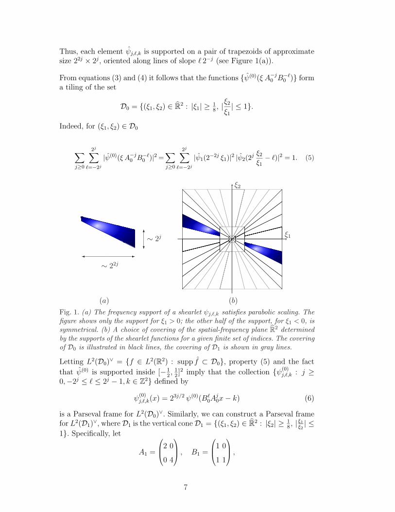
Thus, each element ψj,`,k is supported on a pair of trapezoids of approximatesize 22j × 2j, oriented along lines of slope ` 2−j (see Figure 1(a)).

From equations (3) and (4) it follows that the functions ψ(0)(ξ A−j0 B−`

0 ) forma tiling of the set

D0 = (ξ1, ξ2) ∈ R2 : |ξ1| ≥ 18, |ξ2

ξ1

| ≤ 1.

Indeed, for (ξ1, ξ2) ∈ D0

∑

j≥0

2j∑

`=−2j

|ψ(0)(ξ A−j0 B−`

0 )|2 =∑

j≥0

2j∑

`=−2j

|ψ1(2−2j ξ1)|2 |ψ2(2j ξ2

ξ1− `)|2 = 1. (5)

ξ1

ξ2

(b)(a)

-¾

∼ 22j

6

?∼ 2j

Fig. 1. (a) The frequency support of a shearlet ψj,`,k satisfies parabolic scaling. Thefigure shows only the support for ξ1 > 0; the other half of the support, for ξ1 < 0, issymmetrical. (b) A choice of covering of the spatial-frequency plane R2 determinedby the supports of the shearlet functions for a given finite set of indices. The coveringof D0 is illustrated in black lines, the covering of D1 is shown in gray lines.

Letting L2(D0)∨ = f ∈ L2(R2) : supp f ⊂ D0, property (5) and the fact

that ψ(0) is supported inside [−12, 1

2]2 imply that the collection ψ(0)

j,`,k : j ≥0,−2j ≤ ` ≤ 2j − 1, k ∈ Z2 defined by

ψ(0)j,`,k(x) = 23j/2 ψ(0)(B`

0Aj0x− k) (6)

is a Parseval frame for L2(D0)∨. Similarly, we can construct a Parseval frame

for L2(D1)∨, whereD1 is the vertical coneD1 = (ξ1, ξ2) ∈ R2 : |ξ2| ≥ 1

8, | ξ1

ξ2| ≤

1. Specifically, let

A1 =

2 0

0 4

, B1 =

1 0

1 1

,

7

and ψ(1) be given by

ψ(1)(ξ) = ψ(1)(ξ1, ξ2) = ψ1(ξ2) ψ2

(ξ1

ξ2

).

Then the collection ψ(1)j,`,k : j ≥ 0,−2j ≤ ` ≤ 2j − 1, k ∈ Z2 defined by

ψ(1)j,`,k(x) = 23j/2 ψ(1)(B`

1Aj1x− k) (7)

is a Parseval frame for L2(D1)∨.

Finally, let ϕ ∈ C∞0 (R2) be chosen to satisfy

1 = |ϕ(ξ)|2 +∑

j≥0

2j−1∑

`=−2j

|ψ(0)(ξA−j0 B−`

0 )|2 χD0(ξ)

+∑

j≥0

2j−1∑

`=−2j

|ψ(1)(ξA−j1 B−`

1 )|2 χD1(ξ),

where χD is the indicator function of the set D. This implies that supp ϕ ⊂[−1

8, 1

8]2, |ϕ(ξ)| = 1 for ξ ∈ [− 1

16, 1

16]2, and the collection ϕk : k ∈ Z2 defined

by ϕk(x) = ϕ(x− k) is a Parseval frame for L2([− 116

, 116

]2)∨.

An illustration of the frequency tiling provided by the shearlet system is shownin Figure 1(b).

Thus, we have the following result:

Theorem 2.1 Let ϕ and ψ(d)j,`,k be defined as above. Also, for d = 0, 1, let

ψ

(d)

j,`,k(ξ) = ψ(d)j,`,k(ξ) χDd

(ξ) . The collection of shearlets

ϕk : k ∈ Z2⋃ψ(d)

j,`,k(x) : j ≥ 0, −2j + 1 ≤ ` ≤ 2j − 2, k ∈ Z2, d = 0, 1⋃ψ(d)

j,`,k(x) : j ≥ 0, ` = −2j , 2j − 1, k ∈ Z2, d = 0, 1,

is a Parseval frame for L2(R2).

Notice that the “corner” elements ψ(d)j,`,k(x), ` = −2j, 2j−1, are simply obtained

by truncation on the cones χDdin the frequency domain and that the corner

elements in the horizontal cone D0 match nicely with those in the verticalcone D1. We refer to [14,17] for additional detail about the construction of theshearlet system.

In the following, for brevity of notation, it will be convenient to introduce the

8

index set M = N ∪M , where N = Z2, and

M = µ = (j, `, k, d) : j ≥ 0,−2j ≤ ` ≤ 2j − 1, k ∈ Z2, d = 0, 1.

Hence, we will denote the shearlet system as the collection sµ : µ ∈ M =

N∪M, where sµ = ψµ = ψ(d)j,`,k if µ ∈ M and sµ = ϕµ if µ ∈ N . For ψµ, µ ∈ M ,

it is understood that the corner elements are modified as in Theorem 2.1.

The shearlet transform is the mapping on L2(R2) defined by:

SH : f → SHf(µ) = 〈f, sµ〉, µ ∈M.

3 Inversion of Radon Transform via Shearlet Representation

We shall obtain a formula for the decomposition of the Radon transform basedon the shearlet representation. In order do that, some construction is needed.

3.1 Companion Representation

We start by introducing a companion representation of the shearlet systemwhich is obtained under the action of the fractional Laplacian.

Definition 3.1 For a rational number α and f ∈ C∞(R2), define (−∆)αf by

the relation ((−∆)αf ) (ξ) = |ξ|2αf(ξ). For µ ∈ M, let s+µ = 2−j(−∆)1/4sµ.

In particular, we use the notation ψ+µ = 2−j(−∆)1/4ψµ, for µ ∈ M , and

ϕ+µ = (−∆)1/4φµ, for µ ∈ N .

It is easy to verify that the functions s+µ : µ ∈M are smooth and compactly

supported in the frequency domain. In addition, since each element of the fine-scale shearlet system ψµ, µ ∈ M , is supported, in the frequency domain, onthe compact region Cj = [−22j−1, 22j−1]2 \ [−22j−4, 22j−4]2, it follows that, inthis region, 2−j|ξ|1/2 ≈ 1 and, thus, ‖ψ+

µ ‖ ≈ ‖ψµ‖. This is the key observationwhich is used in the following result and is similar to the one given in [4] forthe case of curvelets.

Theorem 3.2 The system ψ+µ µ∈M is a frame for L2(R2 \ [−1

8, 1

8]2)∨. That

is, there are positive constants A and B, with A ≤ B, such that

A ‖f‖2 ≤∥∥∥∥∥∑µ

〈f, ψ+µ 〉

∥∥∥∥∥`2

≤ B‖f‖2,

for all functions f such that supp f ⊂ R2 \ [−18, 1

8]2.

9

Notice that the larger system s+µ : µ ∈ M is not a frame for L2(R2) since

the lower frame bound condition is not satisfied. To enlarge ψ+µ µ∈M and

make it into a frame for the whole space L2(R2), one can include a “coarsescale” system of the form ϕ(x− k) : k ∈ Z2 as done for the original shearletsystem.

Proof. To show that the system ψ+µ µ∈M is a frame, we introduce the

following notation. For j ≥ 0, let Mj = µ = (j, `, k, d) : −2j ≤ ` ≤ 2j−1, k ∈Z2, d = 0, 1. Also, denote by C the set R2 \ [−1

8, 1

8]2.

Using the properties of the shearlet function ψ, for h ∈ L2(C)∨, we have:

∑

µ∈Mj

|〈h, ψµ〉|2 =∑

`,k,d

∣∣∣∣∫

Ch(ξ) ψ

(d)j`k(ξ) dξ

∣∣∣∣2

=∑

`,k,d

∣∣∣∣∫

Ch(ξ) ψ(d)(ξA−j

d B−`d ) e−2πiξA−j

dB−`

dkdξ

∣∣∣∣2

=∫

C|h(ξ)|2 ∑

`,d

|ψ(d)(ξA−jd B−`

d )|2 dξ

=∫

C|h(ξ)|2 Vj(ξ) dξ, (8)

where

Vj(ξ) = |ψ1(2−2jξ1)|2χD0(ξ) + |ψ1(2

−2jξ2)|2χD1(ξ).

Notice that the window function Vj is supported on the set

Cj = [−22j−1, 22j−1]2 \ [−22j−4, 22j−4]2,

and that, by the assumptions on ψ1,

∑

j≥0

Vj(ξ) = 1 for ξ ∈ R2 \ [−1/8, 1/8].

Let wj be a smooth window function supported in Cj−1 ∪ Cj ∪ Cj+1 which is

equal 1 on the set Cj. It follows that wj Vj = Vj and that wj ∗ g = g for eachfunction g such that g is supported on the set Cj. Hence, using the fact that

supp ψµ ⊂ Cj, when µ ∈ Mj, we have:

10

∑

µ∈Mj

|〈f, ψ+µ 〉|2 =

∑

µ∈Mj

|〈f, 2−j (−∆)1/4ψµ〉|2

=∑

µ∈Mj

|〈wj ∗ f, 2−j (−∆)1/4ψµ〉|2

=∑

µ∈Mj

|〈2−j (−∆)1/4(wj ∗ f), ψµ〉|2

=∑

µ∈Mj

|〈hj, ψµ〉|2,

where hj = 2−j (−∆)1/4(wj ∗ f). Notice that the smoothness assumption onwj guarantees that hj is well defined.

Using (8), we have:

∑

µ∈Mj

|〈hj, ψµ〉|2 =∫

C|hj(ξ)|2 Vj(ξ) dξ

= 2−2j∫

Cj

|ξ| |f(ξ)|2 Vj(ξ) dξ.

Notice that, for ξ ∈ Cj, the function 2−2j|ξ| is bounded above and below bypositive constants, independently of j. Hence, from the expression above, wehave that ∑

µ∈Mj

|〈hj, ψµ〉|2 '∫

Cj

|f(ξ)|2 Vj(ξ) dξ

Adding up over all j ≥ 0, it follows that

∑

µ∈M

|〈f, ψ+µ 〉|2 =

∑

j≥0

∑

µ∈Mj

|〈f, ψ+µ 〉|2

'∑

j≥0

∫

Cj

|f(ξ)|2 Vj(ξ) dξ

=∫

C|f(ξ)|2dξ

for all f ∈ L2(C)∨. 2

3.2 Shearlet Decomposition of the Radon Transform

We start by recalling some important properties of the Radon transform, whichwill be useful in the construction of our decomposition based on the shearletrepresentation. We refer to [18] for additional details about these propertiesand their derivation.

11

In dimension n = 2, the Radon operator R associates to each suitable functionf and each pair (θ, t) ∈ [0, 2π)× R, the value

Rf(θ, t) =∫

f(x, y) δ(x cos θ + y sin θ − t) dx dy,

where δ is the Dirac distribution at the origin. It is easy to verify that Rf ,the Radon transform of f , satisfies the antipodal symmetry Rf(θ + π,−t) =Rf(θ, t). Let DR denote the space of all functions in L2([0, 2π) × R) satisfy-ing the antipodal symmetry. For a rational number α, define the operator offractional differentiation (of a single variable) as

Dαf(t) =1

2π

∫ ∞

−∞|ω|αf(ω)eiωt dω,

and let

R = (I ⊗D1/2) R,

where I denotes the identity operator. The operator R is well-defined on func-tions on L2([0, 2π)× R) and it satisfies the Radon isometry condition

[Rf,Rg] = 〈f, g〉,

where [·, ·] is the inner product in L2([0, 2π) × R). Also, one can show thatR maps functions which are smooth and of rapid decay on R2 into functionswhich are smooth and of rapid decay on [0, 2π)× R.

Using the companion shearlet representations s+µ : µ ∈M from Section 3.1,

we define the system Uµ : µ ∈M by the formula

Uµ = Rs+µ , µ ∈M. (9)

Using the Radon isometry and Theorem 3.2, one can show that Uµ : µ ∈Mis a frame sequence (that is, a frame for its span), although it is not a framefor the whole Hilbert space DR since Uµ : µ ∈M is not a frame for L2(R2).

We are now ready to introduce a decomposition formula for the Radon opera-tor based on the shearlet representation. As mentioned above, our constructionadapts the general principles of the Wavelet-Vaguelette Decomposition [9] andis similar to the Curvelet Biorthogonal Decomposition given in [4].

Theorem 3.3 Let sµ : µ ∈ M be the Parseval frame of shearlets definedabove and let Uµ : µ ∈ M be the system defined by (9). For all f ∈ L2(R2)the following reproducing formula holds:

f =∑µ

[Rf, Uµ] 2jsµ.

12

Proof. This proof is very similar to the one in [4] and is based on theintertwining relation:

R (−∆)α = (I ⊗D2α) R.

Direct computations show that:

〈f, sµ〉= [Rf,R sµ]

= [(I ⊗D1/2) Rf, (I ⊗D1/2) R sµ]

= [Rf, (I ⊗D1/2) (I ⊗D1/2) R sµ]

= [Rf, (I ⊗D1/2) R (−∆)1/4 sµ]

= [Rf,R(2js+µ )]

= 2j [Rf, Uµ]. 2

4 Inversion of Noisy Radon Data

In our model, we assume that Radon transform data are corrupted by whiteGaussian noise, that is, we have the observations:

Y = Rf + εW, (10)

where f is the function to be recovered, W is a Wiener sheet and ε is measuringthe noise level. This means that each measurement [Y, Uµ] of the observed datais normally distributed with mean [Rf, Uµ] and variance ε2 ‖Uµ‖2

L2([0,2π)×R).

While the white noise model may not describe precisely the types of noisetypically found in practical applications, the asymptotic theory derived fromthis assumption in practice has been found to lead to very acceptable results.In addition, this framework allows one to derive a theoretical assessment of theperformance of the method which would be extremely complicated to handleotherwise.

In order to obtain an upper bound on the risk of the estimator, it is necessaryto specify the type of functions we are dealing with. Following [4], let A be apositive constant and STAR2(A) be a class of indicator functions of sets Bwith C2 boundaries ∂B satisfying the following conditions. In polar coordi-nates, let ρ(θ) : [0, 2π) → [0, 1]2 be a radius function and define B by x ∈ Bif and only if |x| ≤ ρ(θ). In particular, the boundary ∂B is given by the curvein R2:

β(θ) =

ρ(θ) cos(θ)

ρ(θ) sin(θ)

. (11)

13

The class of sets of interest to us consists of those sets B whose boundariesβ are parametrized as in (11), where ρ is a radius function satisfying thecondition

sup |ρ′′(θ)| ≤ A, ρ ≤ ρ0 < 1. (12)

We say that a set B ∈ STAR2(A) if B is in [0, 1]2 and is a translate of a setwhose boundary obeys (11) and (12). In addition, we set C2

0([0, 1]2) to be thecollection of twice differentiable functions supported inside [0, 1]2. Finally, wedefine the set E2(A) of functions which are C2 away from a C2 edge as thecollection of functions of the form

f = f0 + f1 χB,

where f0, f1 ∈ C20([0, 1]2), B ∈ STAR2(A) and ‖f‖C2 =

∑|α|≤2‖Dαf‖∞ ≤ 1.

Projecting the data (10) onto the frame Uµ : µ ∈ M, and rescaling, weobtain

yµ := 2j[Y, Uµ]

= 2j[Rf, Uµ] + ε 2j [W,Uµ]

= 〈f, ψµ〉+ ε 2j nµ, (13)

where nµ is a (non-i.i.d.) Gaussian noise with zero mean and variance σµ =‖ψ+

µ ‖2. In order to estimate f , we need to estimate the shearlet coefficients〈f, ψµ〉, µ ∈ M , from the data yµ. To accomplish this, we will devise a thresh-olding rule, to be applied to yµ : µ ∈ M, which exploits the sparsity prop-erties of the shearlet representation.

4.1 Modified Shearlet System

For the application of the shearlet representation to the estimation problem,it is useful to introduce the following simple variant of the shearlet systemgiven in Section 2, which is obtained by rescaling the coarse scale systemand changing the range of scales for which the directional fine-scale system isdefined. Namely, for a fixed j0 ∈ N , let ϕ ∈ C∞

0 (R2) be such that

1 = |ϕ(2−j0ξ)|2 +∑

j≥j0

2j−1∑

`=−2j

|ψ(0)(ξA−j0 B−`

0 )|2 χD0(ξ)

+∑

j≥j0

2j−1∑

`=−2j

|ψ(1)(ξA−j1 B−`

1 )|2 χD1(ξ).

14

Then we obtain the Parseval frame of shearlets:

2j0ϕ(2j0x− k) : k ∈ Z2⋃ψ(d)

j,`,k(x) : j ≥ j0, ` = −2j , 2j − 1, k ∈ Z2, d = 0, 1⋃ψ(d)

j,`,k(x) : j ≥ j0, −2j + 1 ≤ ` ≤ 2j − 2, k ∈ Z2, d = 0, 1.

As the original shearlet system given in Theorem 2.1, the modified shearletsystem is made of coarse and fine scale systems, with the coarse scale systemnow associated with the coarse scale j0. Proceeding as above, we introducethe index set M0 = N ∪M0, where N = Z2,

M0 = µ = (j, `, k, d) : j ≥ j0,−2j ≤ ` ≤ 2j − 1, k ∈ Z2, d = 0, 1,

and denote the new shearlet system using the compact notation sµ : µ ∈M0, where sµ = ψµ = ψ

(d)j,`,k if µ ∈ M0 and sµ = 2j0ϕ(2j0x − µ) if µ ∈ N .

For ψµ, µ ∈ M0, it is understood that the corner elements are modified as inTheorem 2.1.

In our construction, the selection of the scale j0 will depend on the noiselevel ε. Namely, we set j0 = 2

15log2(ε

−1). We also introduce the scale indexj1 = 2

5log2(ε

−1) (so that 2j0 = ε−2/15 and 2j1 = ε−2/5).

Hence, depending on the noise level ε, we may now define the set of significantcoefficients of a function f ∈ E2(A). Define the set of significant indices asso-ciated with the shearlets as the subset of M0 given by N (ε) = M1(ε)∪N0(ε),where

N0(ε) = µ = k ∈ Z2 : |k| ≤ 22j+1, and

M1(ε) = µ = (j, `, k, d) : j0 < j ≤ j1, |k| ≤ 22j+1, d = 0, 1.The significant coefficients in the shearlet representation of f are the elements〈f, sµ〉 for which µ belongs to N (ε).

We obtain the following result which is proved in the Appendix.

Theorem 4.1 Let ε denote the noise level, and N (ε) be the set of significantindices associated with the shearlets so that a function f is represented as

f =∑

µ∈M0

〈f, sµ〉 sµ.

Then there exist positive constants C ′, C ′′, and C ′′′ such that the followingproperties hold:

(1) The neglected shearlet coefficients 〈f, sµ〉 : µ /∈ N (ε) satisfy:

supf∈E2(A)

∑

µ/∈N (ε)

|〈f, sµ〉|2 ≤ C ′ε4/5.

15

(2) The risk proxy satisfies:

supf∈E2(A)

∑

µ∈N (ε)

min(|〈f, sµ〉|2, 22jε2) ≤ C ′′ε4/5.

(3) The cardinality of N (ε) obeys:

#N (ε) ≤ C ′′′ε−2.

4.2 Estimation Rate

To estimate f from the noisy observations (13), we will apply the soft thresh-olding function Ts(y, t) = sgn(y)(|y| − t)+. The analysis of the estimationerror follows the general framework of the wavelet shrinkage developed in [10].Letting #N (ε) be the number of significant coefficients of the shearlet repre-sentation of f , we estimate function f by

f =∑

µ∈M0

cµ sµ, (14)

where the coefficients are obtained by the rule

cµ =

Ts(yµ, ε√

2 log(#N (ε))2jσµ), µ ∈ N (ε),

0 otherwise.(15)

and σµ = ‖s+µ ‖2

2. Notice that the terms σµ, µ ∈M0, are uniformly bounded.

The main theorem can now be established (this is similar to Theorem 6 in [4],which uses the curvelet decomposition).

Theorem 4.2 Let f ∈ E2(A) be the solution of the problem Y = Rf + εWand let f be the approximation to f given by the formulas (14) and (15). Thenthere is a constant C > 0 such that

supE2(A)

E‖f − f‖22 ≤ C log(ε−1) ε4/5, as ε → 0,

where E is the expectation operator.

Proof. For µ ∈M0, let cµ = 〈f, sµ〉 and cµ be given by (15). By the Parsevalframe property of the shearlet system sµ : µ ∈M0, it follows that

‖ ∑

µ∈M0

cµ sµ‖22 ≤

∑

µ∈M0

|cµ|2,

and that

E‖f − f‖22 ≤ E

∑

µ∈M0

|cµ − cµ|2 . (16)

16

On the other hand, by the oracle inequality [10] we have

E

∑

µ∈N (ε)

|cµ − cµ|2 ≤ L(ε)

ε2

∑

µ∈N (ε)

(22jσ2

µ

#N (ε)+ min(c2

µ, ε222jσ2

µ)

)(17)

where L(ε) = (1 + 2 log(#N (ε)). Now observe that, by Theorem 4.1, thereexist positive constants C ′, C ′′, C ′′′ such that

∑

µ∈N (ε)

min(c2µ, ε

222jσ2µ) ≤ C ′ ε4/5,

∑

µ/∈N (ε)

c2µ ≤ C ′′ ε4/5,

log(#N (ε)) ≤ C ′′′ log(ε−1).

By the assumption on N (ε), there is a constant C1 > 0 such that

ε2∑

µ∈N (ε)

22j σ2µ

#N (ε)≤ C1 ε2 22j1 = C1ε

6/5.

Thus, using these observations and equations (16) and (17), we deduce thatthere is a constant C > 0 such that

E‖f − f‖22 ≤ E

∑

µ∈N (ε)

|cµ − cµ|2 +

∑

µ∈N (ε)c

c2µ ≤ C log(ε−1) ε4/5. 2

As also observed in [4], Theorem 4.2 remains valid if the soft thresholding oper-ator Ts(y, t) is replaced by the hard thresholding operator Th(y, t) = y χ|y|≥t.In fact, also in the case of hard thresholding, one can obtain estimates similarto (17).

Finally, for completeness, we recall the following theorem from [4] showingthat the rate of convergence of our estimator is near optimal; no estimatorcan achieve an essentially better rate uniformly over E2(A).

Theorem 4.3 ([4]) Let f ∈ E2(A) and consider the minimax mean squareerror

M(ε, E2(A)) = inff

supE2(A)

E‖f − f‖22.

This satisfies

M(ε, E2(A)) ≥ Cε4/5(log(ε−1))−2/5, ε → 0,

for some C ∈ R+.

17

5 Numerical Experiments

In this section, we demonstrate the derived estimation rates and compare ourproposed shearlet estimation method against a curvelet and wavelet-based ver-sion. The numerical implementations of curvelets and shearlets are describedin [3] and [13], respectively. The adaptation of these representation routinesfor the inversion of the Radon transform was done using the technique givenin [19] which describes the wavelet-based inversion method. That is, a back-projection algorithm is used to convert the array of projections into a squarearray that is then appropriately filtered.

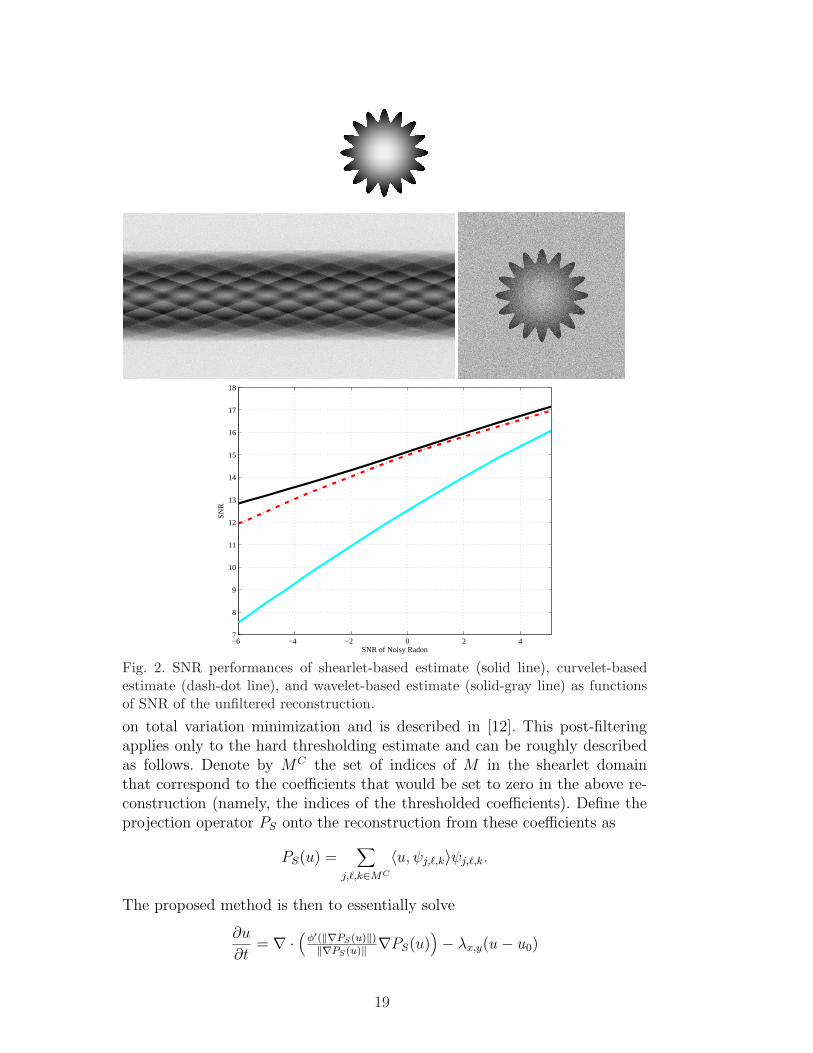
In the first experiment, we used the star image shown in the upper left-handside of Figure 2. White Gaussian noise with zero mean was added to the Radontransform of the image with various levels of standard deviations and theinversion processes was regularized by the proposed method. For comparison,a version using curvelets and wavelets was also included.

For another set of experiments, we tested both a soft thresholding and hardthresholding version for each of the methods using a modified Shepp-LoganPhantom image and an MRI brain scan image.

For the soft thresholding Ts(y, t), we estimated the standard deviation σµ of

[Y, Uµ] and set t = 2jσµ

√2 log(2j). For the hard thresholding, Monte Carlo

simulations were used to estimate the standard deviation of the noise througheach subband and a scalar multiple of the estimated standard deviations waschosen as the threshold value. In particular, the threshold for the finest scaleswas chosen to be four times the estimated standard deviation of the noise andthe threshold for the remaining scales except for the coarsest scale was chosento be three times the estimated standard deviation. To assess the performance,we used the measure

SNR(f, fest) = 10 log10

[var(f)

mean(f − fest)

],

where f ,fest , and var(f) are the original image, the estimated image, andthe variance of the image, respectively. Both the SNR of the noisy projections(treated as an image) and the unfiltered inversion are given in Tables I andII. Some results are also displayed in Figures 3, 4, and 5.

Note a considerable advantage of our proposed shearlet-based technique is thatit is better suited for use with generalized cross validation (GCV) functionsfor automatic determination of the threshold parameters (see [11] and [27]).

As subtle artifacts remained after reconstruction from the shearlet-based es-timates, we applied the following additional filtering scheme which is based

18

−6 −4 −2 0 2 47

8

9

10

11

12

13

14

15

16

17

18

SNR of Noisy Radon

SN

R

Fig. 2. SNR performances of shearlet-based estimate (solid line), curvelet-basedestimate (dash-dot line), and wavelet-based estimate (solid-gray line) as functionsof SNR of the unfiltered reconstruction.

on total variation minimization and is described in [12]. This post-filteringapplies only to the hard thresholding estimate and can be roughly describedas follows. Denote by MC the set of indices of M in the shearlet domainthat correspond to the coefficients that would be set to zero in the above re-construction (namely, the indices of the thresholded coefficients). Define theprojection operator PS onto the reconstruction from these coefficients as

PS(u) =∑

j,`,k∈MC

〈u, ψj,`,k〉ψj,`,k.

The proposed method is then to essentially solve

∂u

∂t= ∇ ·

(φ′(‖∇PS(u)‖)‖∇PS(u)‖ ∇PS(u)

)− λx,y(u− u0)

19

TABLE I - Estimates based on soft-thresholding(Performance in SNR)

Radon dom. Unfiltered Shearlet Curvelet Wavelet

Star image

41.38 dB 15.27 dB 20.46 dB 19.87 dB 19.70 dB

35.35 dB 10.68 dB 19.36 dB 18.63 dB 18.08 dB

31.83 dB 7.48 dB 18.62 dB 17.86 dB 17.14 dB

Phantom

39.63 dB 14.08 dB 18.82 dB 18.60 dB 17.81 dB

33.62 dB 9.23 dB 17.62 dB 17.45 dB 16.25 dB

30.09 dB 5.97 dB 16.80 dB 16.68 dB 15.36 dB

Brain scan

41.34 dB 15.01 dB 22.08 dB 21.36 dB 20.89 dB

35.32 dB 9.39 dB 20.79 dB 20.09 dB 19.43 dB

31.80 dB 5.95 dB 19.88 dB 19.25 dB 18.57 dB

with the boundary condition ∂u∂n

= 0 on ∂Ω and the initial condition u(x, y, 0) =u0(x, y) for x, y ∈ Ω, where Ω is the image domain and φ ∈ C2(R) is an evenregularization function. The quantity λx,y is a spatially varying penalty termbased on a measure of local variances that is updated after a number of iter-ations or progressions of artificial time step. For this post-processing step, weset λx,y = 0 and u0(x, y) to be the initial shearlet-based estimate.

Notice that, as shown in Table II, this post-filtering scheme produces a slightimprovement in performance. However, the numerical tests show that, evenwithout this filtering, the shearlet based method would still outperform thecorresponding wavelet- and curvelet-based tests.

20

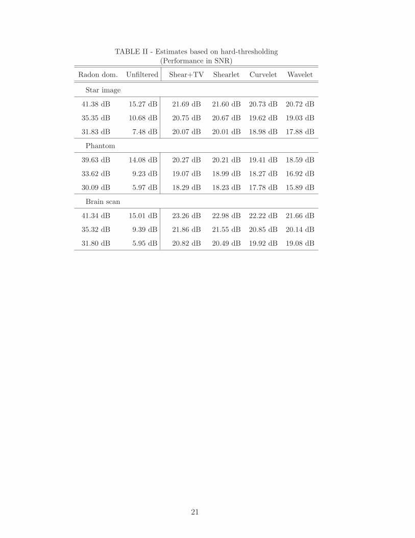
TABLE II - Estimates based on hard-thresholding(Performance in SNR)

Radon dom. Unfiltered Shear+TV Shearlet Curvelet Wavelet

Star image

41.38 dB 15.27 dB 21.69 dB 21.60 dB 20.73 dB 20.72 dB

35.35 dB 10.68 dB 20.75 dB 20.67 dB 19.62 dB 19.03 dB

31.83 dB 7.48 dB 20.07 dB 20.01 dB 18.98 dB 17.88 dB

Phantom

39.63 dB 14.08 dB 20.27 dB 20.21 dB 19.41 dB 18.59 dB

33.62 dB 9.23 dB 19.07 dB 18.99 dB 18.27 dB 16.92 dB

30.09 dB 5.97 dB 18.29 dB 18.23 dB 17.78 dB 15.89 dB

Brain scan

41.34 dB 15.01 dB 23.26 dB 22.98 dB 22.22 dB 21.66 dB

35.32 dB 9.39 dB 21.86 dB 21.55 dB 20.85 dB 20.14 dB

31.80 dB 5.95 dB 20.82 dB 20.49 dB 19.92 dB 19.08 dB

21

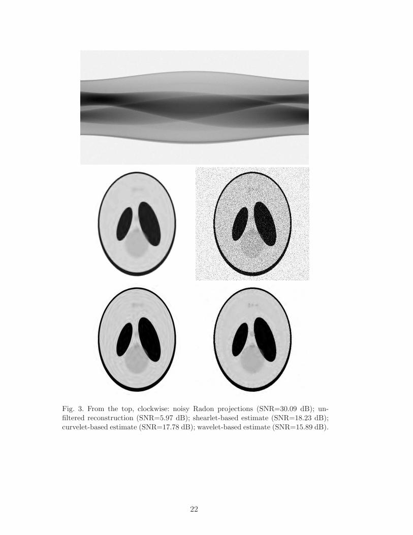
Fig. 3. From the top, clockwise: noisy Radon projections (SNR=30.09 dB); un-filtered reconstruction (SNR=5.97 dB); shearlet-based estimate (SNR=18.23 dB);curvelet-based estimate (SNR=17.78 dB); wavelet-based estimate (SNR=15.89 dB).

22

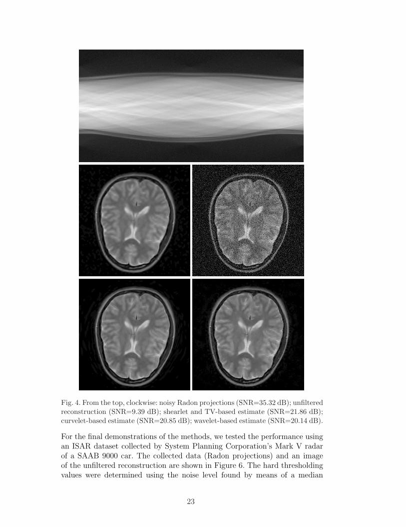
Fig. 4. From the top, clockwise: noisy Radon projections (SNR=35.32 dB); unfilteredreconstruction (SNR=9.39 dB); shearlet and TV-based estimate (SNR=21.86 dB);curvelet-based estimate (SNR=20.85 dB); wavelet-based estimate (SNR=20.14 dB).

For the final demonstrations of the methods, we tested the performance usingan ISAR dataset collected by System Planning Corporation’s Mark V radarof a SAAB 9000 car. The collected data (Radon projections) and an imageof the unfiltered reconstruction are shown in Figure 6. The hard thresholdingvalues were determined using the noise level found by means of a median

23

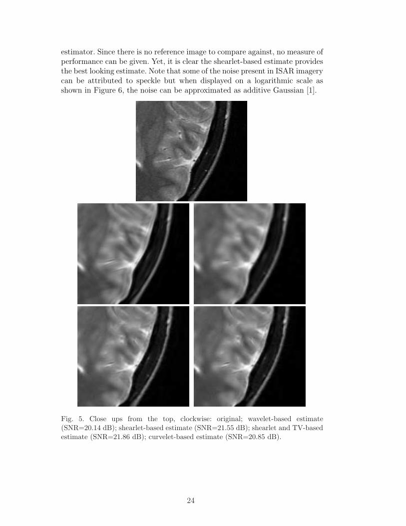
estimator. Since there is no reference image to compare against, no measure ofperformance can be given. Yet, it is clear the shearlet-based estimate providesthe best looking estimate. Note that some of the noise present in ISAR imagerycan be attributed to speckle but when displayed on a logarithmic scale asshown in Figure 6, the noise can be approximated as additive Gaussian [1].

Fig. 5. Close ups from the top, clockwise: original; wavelet-based estimate(SNR=20.14 dB); shearlet-based estimate (SNR=21.55 dB); shearlet and TV-basedestimate (SNR=21.86 dB); curvelet-based estimate (SNR=20.85 dB).

24

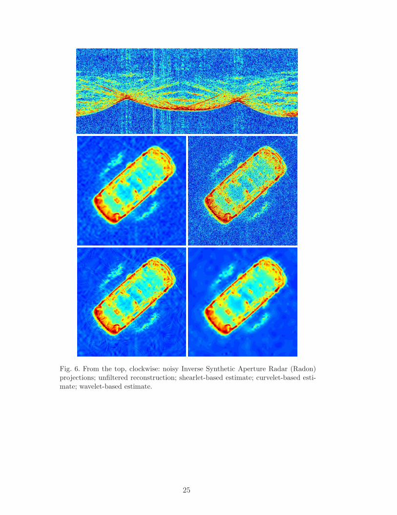
Fig. 6. From the top, clockwise: noisy Inverse Synthetic Aperture Radar (Radon)projections; unfiltered reconstruction; shearlet-based estimate; curvelet-based esti-mate; wavelet-based estimate.

25

6 Appendix. Proofs from Section 4

We are considering the modified shearlet system sµ : µ ∈ M0 introducedin Section 4.1. Recall that M0 = N ∪ M0, , where N = Z2, M0 = µ =(j, `, k, d) : j ≥ j0,−2j ≤ ` ≤ 2j−1, k ∈ Z2, d = 0, 1, and the system is madeof the coarse scale system sµ = 2j0ϕ(2j0x − µ) : µ ∈ N and the fine scale

system sµ = ψµ = ψ(d)j,`,k : µ ∈ M0.

In order to prove Theorem 4.1, we need the following lemma which providesan estimate for the size of the shearlet coefficients at a fixed scale j (wherej ≥ j0). For such j fixed, recall from Section 3 that Mj = (j, `, k, d) : −2j ≤` ≤ 2j, k ∈ Z2, d = 0, 1.

Lemma 6.1 Let f ∈ E2(A) and j ≥ j0. Then there is a positive constant Csuch that ∑

µ∈Mj

|〈f, ψµ〉|2 ≤ C 2−2j

Proof. It is useful to introduce a smooth localization of the function f neardyadic squares. Let Qj be the collection of dyadic squares of the form Q =[ν1

2j ,ν1+12j ] × [ν2

2j ,ν2+12j ], with ν1, ν2 ∈ Z. For a nonnegative C∞ function w with

support in [−1, 1]2, we define a smooth partition of unity

∑

Q∈Qj

w2Q(x) = 1, x ∈ R2,

where, for each dyadic square Q ∈ Qj, wQ(x) = w(2jx1 − ν1, 2jx2 − ν2).

Given f ∈ E2(A), the coefficients 〈f, ψµ〉 will exhibit a very different be-havior depending on whether the edge curve of f intersects the support of wQ

or not. We split Qj into the disjoint sets Q0j and Q1

j that indicate whetherthe collection of dyadic squares Q intersects an edge curve or not. Since eachdyadic square Q has side-length 2 · 2−j and f has compact support in [0, 1]2,there are O(2j) dyadic cubes in Q ∈ Q0

j intersecting the edge curve and O(22j)dyadic cubes in Q ∈ Q1

j not intersecting the edge curve.

For each such cube Q ∈ Q0j , it is shown in [14] that

∑

k∈Z2

|〈fQ, ψµ〉|2 ≤ C 2−3j (1 + |`|)−5.

More precisely, in the proof of Theorem 1.3 in [14], it is shown that

∑

k∈RK

|〈fQ, ψµ〉|2 ≤ C L−2K 2−3j (1 + |`|)−5,

26

where K ∈ Z2, ∪K∈Z2RK = Z2 and∑

K∈Z2 L−2K < ∞. Hence

∑

µ∈Mj

|〈fQ, ψµ〉|2 =∑

|`|≤2j

∑

k∈Z2

|〈fQ, ψµ〉|2 ≤ C 2−3j.

Adding up over all cubes in Q0j , we have that

∑

µ∈Mj

∑

Q∈Q0j

|〈fQ, ψµ〉|2 ≤ C 2−2j. (18)

For Q ∈ Q1j , it is shown in [14, Thm.1.4] that

∑

µ∈Mj

|〈fQ, ψµ〉|2 ≤ C 2−4j.

Hence adding up over all Q ∈ Q1j , it follows that

∑

µ∈Mj

∑

Q∈Q1j

|〈fQ, ψµ〉|2 ≤ C 2−2j. (19)

The proof is completed by combining the estimates (18) and (19). 2

We now proceed with the proof of Theorem 4.1.

Proof. (Theorem 4.1.1(1)) We need to establish

supf∈E2(A)

∑

µ/∈N (ε)

|〈f, sµ〉|2 ≤ C ′ε4/5.

(I) We start by examining the situation at fine scales, for j ≥ j1(ε) =25log2(ε

−1), so that 2−j ≤ ε25 . Notice that, for these values of the index j,

sµ = ψµ.

By Lemma 6.1, for each f ∈ E2(A) and each j ≥ j0, we have that

∑

µ∈Mj

|〈f, ψµ〉|2 ≤ C 2−2j.

Hence ∑

j>j1

∑

µ∈Mj

|〈f, ψµ〉|2 ≤ C∑

j>j1

2−2j ≤ C ε45 .

(II) Let Q0 = [0, 1]2 and supp f ⊂ Q0. We will show that the terms 〈f, sµ〉decay very rapidly for locations k away from Q0.

27

We will start by examining the decay of a fine-scale term 〈f, sµ〉, for µ =

(j, `, k, d) ∈ M0 and d = 0. Let Ej` = B`Aj =

22j `2j

0 2j

. By the assumptions

on ψ, it follows that, for each m ∈ N, there is a constant Cm > 0 such that

|ψ(x)| ≤ Cm (1 + ‖x‖)−m. (20)

It follows that

|ψ(0)j,`,k(x)| ≤ Cm 23j/2 (1 + ‖Ej`x− k‖)−m.

We will use two simple facts. The first one is ‖Ej` x‖ ≤ ‖Ej`‖‖x‖ = 22j‖x‖ ≤√2 22j for x ∈ Q0 and the second one is that for a > 0, 0 ≤ b ≤ c ≤ a, we

have a− b ≥ a− c.

It follows that, for |k| ≥ 22j+1, we have

|〈f, ψ(0)j,`,k〉|≤ ‖f‖∞

∫

Q|ψ(0)

j,`,k(x)| dx

≤Cm 232j

∫

Q0

(1 + ‖Ej`x− k‖

)−m

dx

≤Cm 232j

∫

Q0

(1 + |k| − ‖Ej` x‖

)−m

dx

≤Cm 232j

∫

Q0

(|k| − 22j‖x‖)−mdx

≤Cm 232j (|k| −

√2 22j)−m. (21)

Thus,

2j−1∑

`=−2j

∑

|k|≥22j+1

|〈f, ψ(0)j,`,k〉|2≤Cm

2j−1∑

`=−2j

23j∑

|k|≥22j+1

(|k| −√

2 22j)−2m

= Cm 24j+1∑

|k|≥22j+1

(|k| −√

2 22j)−2m

≤Cm 24j+1 2−2j(2m−2)

= Cm 28j+1 2−4jm

Now we can add up all contributions for j ≥ j0. Since we can choose marbitrarily, for an appropriate choice of the constant C, we have:

28

∑

j≥j0

2j−1∑

`=−2j

∑

|k|≥22j+1

|〈f, ψ(0)j,`,k〉|2 ≤ Cm

∑

j≥j0

28j+1 2−4jm ≤ C 2−6j0 = Cε45 .

The analysis in the case where µ ∈ M0 and d = 1 is essentially the same asthe one given above. For the coarse case terms, notice first that ϕ satisfies thesame decay behavior as (20) for ψ. Hence, letting ϕj0,k(x) = 2j0ϕ(2j0x − k)and proceeding as in (21), we have that

|〈f, ϕj0,k〉| ≤ ‖f‖∞∫

Q|ϕj0,k(x)| dx ≤ Cm 2j0 (|k| −

√2 2j0)−m.

Now we can proceed as above by summing over |k| ≥ 22j+1 and using the factthat m can be chosen arbitrarily, to conclude that

∑

|k|≥22j+1

|〈f, ϕj0,k〉|2 ≤ Cε45 .

Combining the estimates from parts (I) and (II) and of the proof, we finallyhave that ∑

µ/∈N (ε)

|〈f, sµ〉|2 ≤ C ε4/5. 2

Proof. (Theorem 4.1.1(2)) For µ ∈M0, we use the notation cµ = 〈f, sµ〉 andwe define the set

R(j, ε) = µ ∈ Mj : |cµ| > ε,to denote the set of “large” shearlet coefficients, at a fixed scale j.

By Corollary 1.5 in [14] (which is valid both for coarse and fine scale shearlets),there is a constant C > 0 such that, as ε → 0,

#R(j, ε) ≤ C ε−2/3.

It follows by rescaling that

#R(j, 2jε) ≤ C 2−2j/3ε−2/3.

Since ψ ∈ C∞0 (R2), for µ = (j, `, k, d) ∈ M0 and d = 0, we have that

|cµ|= |〈f, ψµ〉| =∣∣∣∣∫

R2f(x)23j/2ψ(B`Ajx− k)dx

∣∣∣∣

≤ 2−3j/2‖f‖∞∫

R2|ψ(z)|dz = C ′2−3j/2.

Thus, R(j, 2jε) = ∅ when 2j > ε−2/5 (that is, j > j1(ε) = 25

log2(ε−1)).

Similarly, R(j, ε) = ∅ when 2j > ε−2/3 (that is, j > j2(ε) = 23

log2(ε−1)). For

µ ∈ M0 and d = 1, we get exactly the same estimates.

29

For the risk proxy, notice that

∑

µ∈N (ε)min(c2

µ, 22jε2) = S1(ε) + S2(ε),

whereS1(ε) =

∑

µ∈N (ε): |cµ|≥2j εmin(c2

µ, 22jε2)

S2(ε) =∑

µ∈N (ε): |cµ|<2j εmin(c2

µ, 22jε2)

Hence, using the observations above, we have:

S1(ε) =∑

µ∈N (ε): |cµ|≥2j ε22j ε2

≤ ∑

j≤j1

∑

µ∈Mj : |cµ|≥2j ε22j ε2

≤C∑

j≤j1

(2−2j/3ε−2/3) 22j ε2

= C∑

j≤j1

243j ε

43

≤C ε45

For S2, we have

S2(ε) =∑

µ∈N (ε): |cµ|<2j ε|cµ|2

=∑

j0≤j≤j1

∞∑

n=0

∑

2j−n−1ε≤|cµ|<2j−nε|cµ|2

≤C∑

j0≤j≤j1

∞∑

n=0

2−23(j−n−1)ε−

23 22(j−n) ε2

= C∑

j0≤j≤j1

∞∑

n=0

2−43n2

23 2

43j ε

43

≤C∑

j0≤j≤j1

243j ε

43

≤C ε45 2

Proof. (Theorem 4.1.1(3)) For each fixed scale j0 ≤ j ≤ j1, the number ofindices µ in N (ε)∩Mj is of the order O(25j). In fact, N (ε)∩Mj ⊂ (j, `, k, d) :|k| ≤ 22j+1, |`| ≤ 2j and this set contains O(24j) terms for the k variable and

30

O(j) terms for the ` variable. Hence, adding up the contributions correspond-ing to the various scales, we obtain:

#N (ε) ≤ C∑

j≤j1

25j ≤ Cε−2. 2

References

[1] H. H. Arsenault, G. April, Properties of speckle integrated with a finite apertureand logarithmically transformed, J. Opt. Soc. Am. 66 (1976), 1160–1163.

[2] M. Bhatia, W. C. Karl, and A. S. Willsky, A wavelet-based method formultiscale tomographic reconstruction, IEEE Trans. Med. Imag., 15 (1996),92–101.

[3] E. J. Candes, L. Demanet, D. L. Donoho, and L. Ying, Fast discrete curvelettransforms, Multiscale Model. Simul., 5 (3) (2006), 861–899.

[4] E. J. Candes, and D. L. Donoho, Recovering edges in ill-posed inverse problems:optimality of curvelet frames, Annals Stat., 30(3) (2002), 784–842.

[5] O. Christensen, An introduction to frames and Riesz bases, Birkhauser, Boston,2003.

[6] A. M. Cormack, Representation of a function by its line integrals, with someradiological applications, J. Appl. Phys. 34 (1963), 2722–2727.

[7] A. M. Cormack, Representation of a function by its line integrals, with someradiological applications II, J. Appl. Phys., 35 (1964), 195–207.

[8] Do, M. N., and M. Vetterli, The contourlet transform: an efficient directionalmultiresolution image representation, IEEE Trans. Image Proc., 14(12) (2005),2091–2106.

[9] D. L. Donoho, Nonlinear solution of linear inverse problem by wavelet-vaguelettedecomposition, Appl. Comput. Harmon. Anal., 2 (1995), pp. 101–126.

[10] D. L. Donoho, I. M. Johnstone, Ideal spatial adaptation via wavelet shrinkage,Biometrika, 81 (1994), 425–455.

[11] G. R. Easley, F. Colonna, D. Labate, Improved Radon Based Imaging using theShearlet Transform, Proc. SPIE, Independent Component Analyses, Wavelets,Unsupervised Smart Sensors, and Neural Networks II, 7343 (2009), Orlando.

[12] G. R. Easley, D. Labate, F. Colonna, Shearlet-Based Total Variation Diffusionfor Denoising, IEEE Trans. Image Proc. 18 (2) (2009), 260–268.

[13] G. R. Easley, D. Labate, and W. Lim, Sparse Directional Image Representationsusing the Discrete Shearlet Transform, Appl. Comput. Harmon. Anal., 25 (1)(2008), 25–46.

31

[14] K. Guo, D. Labate, Optimally Sparse Multidimensional Representation usingShearlets, SIAM J. Math. Anal., 39 (2007), 298–318.

[15] K. Guo, W. Lim, D. Labate, G. Weiss, E. Wilson, Wavelets with compositedilations, ERA Amer. Math. Soc., 10 (2004), 78–87.

[16] K. Guo, W. Lim, D. Labate, G. Weiss, E. Wilson, The theory of wavelets withcomposite dilations, in: Harmonic Analysis and Applications, C. Heil (ed.), pp.231–249, Birkhauser, Boston, 2006.

[17] K. Guo, W. Lim, D. Labate, G. Weiss, E. Wilson, Wavelets with compositedilations and their MRA properties, Appl. Computat. Harmon. Anal., 20 (2006)231–249.

[18] S. Helgason, The Radon Transfrom, Birkhauser, Boston, 1980.

[19] E. D. Kolaczyk, A wavelet shrinkage approach to tomographic imagereconstruction, J. Amer. Statist. Assoc., 91 (1996), 1079–1090.

[20] G. Kutyniok and D. Labate, Resolution of the Wavefront Set using ContinuousShearlets, Trans. Am. Math. Soc., 361 (2009), 2719–2754.

[21] G. Kutyniok, M. Shahram and D. Donoho, Development of a Digital ShearletTransform Based on Pseudo-Polar FFT Shearlet-based deconvolution, preprint(2009).

[22] N.Y. Lee, and B. J. Lucier, Wavelet Methods for Inverting the Radon Transformwith Noisy Data, IEEE Trans. Image Proc., 10 (1) (2001), 79–94.

[23] Le Pennec, E., and S. Mallat, Sparse geometric image representations withbandelets, IEEE Trans. Image Proc., 14 (2005), 423–438.

[24] F. Natterer, and F. Wubbeling, Mathematical Methods in Image Reconstruction,SIAM Monographs on Mathematical Modeling and Computation, Philadelphia,2001.

[25] R. Neelamani, R. Nowak, and R. Baraniuk, Model-based inverse halftoning withWavelet-Vaguelette Deconvolution, in Proc. IEEE Int. Conf. Image ProcessingICIP 2000, (Vancouver, Canada), pp. 973-976, Sept. 2000.

[26] E. L. Miller, L. Nicolaides, and A. Mandelis, Nonlinear inverse scatteringmethods for thermal-wave slice tomography: A wavelet domain approach, J.Opt. Soc. Amer. A, 15 (1998), 1545–1556.

[27] V. M. Patel, G. R. Easley, D. M. Healy, Shearlet-based deconvolution, IEEETrans. Image Proc., to appear in 18 (12) (2009).

[28] J. Radon, Uber die Bestimmung von Funktionen durch ihre Integralwertelangs gewisser Mannigfaltigkeiten, Berichte Sachsische Akademie derWissenschaften, Leipzig, Math.–Phys. Kl., 69, 262–267, reprinted in [18] , 177–192, 1917.

[29] S. Y. Zhao, Wavelet filtering for filtered backprojection in computedtomography, Appl. Comput. Harmon. Anal., 6 (2009), 346–373.

32