Protection of Micro-data Subject to Edit Constraints AgainstStatistical Disclosure

Natalie Shlomo1 and Ton De Waal2

Before releasing statistical outputs, data suppliers have to assess if the privacy of statisticalunits is endangered and apply Statistical Disclosure Control (SDC) methods if necessary. SDCmethods perturb, modify or summarize the data, depending on the format for releasing thedata, whether as micro-data or tabular data. The goal is to choose an optimal method thatmanages disclosure risk while ensuring high-quality statistical data. In this article we discussthe effect of applying basic SDC methods on continuous and categorical variables for datamasking. Perturbative SDC methods alter the data in some way. Changing values, however,will likely distort totals and other sufficient statistics and also cause fully edited records inmicro-data to fail edit constraints, resulting in low-quality data. Moreover, an inconsistentrecord will signal that the record has been perturbed for disclosure control and attempts can bemade to unmask the data. In order to deal with these problems, we develop new strategies forimplementing basic perturbation methods that are often implemented at Statistical Agencieswhich minimize record level edit failures as well as overall measures of information loss.

Key words: Information loss; additive noise; micro-aggregation; post-randomization method;rank swapping; rounding.

1. Introduction

The aim of statistical disclosure control (SDC) is to prevent sensitive information about

individual respondents from being disclosed. SDC is becoming increasingly important due

to the growing demand for information provided by statistical agencies. The information

released by statistical agencies can be divided into two major forms of statistical data:

tabular data and micro-data. Whereas tables have been traditionally released by Statistical

Agencies, the releasing of micro-data sets to researchers is a relatively new phenomenon.

Nowadays, many Statistical Agencies have provisions for releasing micro-data from social

surveys for research purposes usually under special license agreements and through secure

data archives. Micro-data from business surveys are typically not released because of

their disclosive nature due to high sampling fractions and skewed distributions, although

this may possibly change in the future based on research in synthetic datasets (see Ronning

et al. 2005).

q Statistics Sweden

1 Southampton Statistical Sciences Research Institute, University of Southampton and Department of Statistics,Hebrew University. Email: n.shlomo@soton.ac.uk2 Statistics Netherlands, Department of Methodology Voorburg, P.O. Box 4000, 2270 JM Voorburg, TheNetherlands. Email: twal@cbs.nlAcknowledgments: The authors wish to thank the Editor, the Associate Editor and the referees for their helpfulcomments which improved the structure, coherence and quality of the article.

Journal of Official Statistics, Vol. 24, No. 2, 2008, pp. 229–253

In order to preserve the privacy and confidentiality of individuals responding to social

surveys, statistical agencies must assess the disclosure risk in respect of micro-data and if

required choose appropriate SDC methods to apply to the data. Measuring disclosure risk

for the SDC decision problem involves assessing and evaluating numerically the risk of

reidentifying statistical units. SDCmethods perturb, modify, or summarize the data in order

to prevent reidentification by a potential attacker. Higher levels of protection through SDC

methods, however, have a negative effect on the utility and quality of the data. The SDC

decision problem involves finding the optimum balance between managing disclosure risk

so as to maintain tolerable thresholds, depending on the mode for accessing the data, and

ensuring high utility for the data.

In any released micro-data set, directly identifying key variables such as name, address,

or identification numbers are removed. Disclosure risk typically arises from attribute

disclosure where small counts on cross-classified indirect identifying key variables (such as

age, sex, place of residence, marital status, occupation) can be used to identify an individual

and confidential information may be learnt. Generally, identifying variables are categorical

since statistical agencies will often carry out coarsening before releasing the data. Therefore

even a variable such as age will often be grouped into categories. Moreover, values of

categorical variables can often be assumed to be known to outsiders and can hence be used

for identifying individuals, whereas exact values of continuous variables can generally be

assumed to be unknown. Sensitive variables can be continuous (e.g., income) or categorical

(e.g., health status).

SDC techniques for micro-data include perturbative methods which alter the data and

nonperturbative methods which limit the amount of information released in the micro-data

without actually altering the data. Examples of nonperturbative SDC techniques are global

recoding, suppression and subsampling (see Willenborg and De Waal 2001). Perturbative

methods for continuous variables (see Section 2) include adding random noise (Kim 1986;

Fuller 1993; Brand 2002; Yancey, Winkler, and Creecy 2002), micro-aggregation (replacing

values with their average within groups of records) (Defays and Nanopoulos 1992; Anwar

1993; Domingo-Ferrer and Mateo-Sanz 2002), rounding to a preselected rounding base, and

rank swapping (swapping values between pairs of recordswithin small groups) (Dalenius and

Reiss 1982; Fienberg and McIntyre 2005). Perturbative methods for categorical variables

(see Section 3) include record swapping (typically swapping geography variables) and a

more general post-randomization probability mechanism (PRAM) where categories of

variables are changed or not changed according to a prescribed probability matrix and a

stochastic selection process (Gouweleeuw, Kooiman, Willenborg, and De Wolf 1998).

For more information on these methods see also: Domingo-Ferrer, Mateo-Sanz, and Torra

(2001), Willenborg and DeWaal (2001), Gomatam and Karr (2003), and references therein.

In order to protect a data set by means of perturbative techniques one can either perturb

the identifying variables or perturb the sensitive variables. In the first case identification of a

unit is rendered more difficult, and the probability of a unit’s being identified is hence

reduced. In the second case, even if an intruder succeeds in identifying a unit by using the

values of the indirectly identifying key variables, the sensitive variables will hardly disclose

any useful information on this particular unit as they have been perturbed. One can also

perturb both the identifying variables and the sensitive ones simultaneously. This offers

more protection, but also leads to more information loss.

Journal of Official Statistics230

With nonperturbative SDC methods, the logical consistency of the records remains

unchanged and the so-called edit rules, or edits for short, will not begin to fail as a result of

these methods. Edits describe either logical relationships that have to hold true, such as

“a two-year-old person cannot be married” or “the profit and the costs of an enterprise

should sum up to its turnover” or relationships that have to hold true in most cases, such as

“a 12-year-old girl cannot be a mother.” Perturbative methods, however, alter the data, and

therefore we can expect consistent records to start failing edits due to the perturbation.

In this article we focus on perturbative SDC techniques to protect micro-data against

disclosure. We provide an overview of the most common perturbative SDC techniques

that are typically in use at Statistical Agencies and show how they can be extended and

modified so as to take edits into account. We also demonstrate new implementation

methods that preserve sufficient statistics in the micro-data (totals, means and covariance

matrices). This ensures a high level of utility in the data. For each SDC method,

we provide results obtained from an evaluation study to illustrate the effects on

information loss.

SDC techniques have received ample attention in the literature. However, SDC

techniques for micro-data that take edits into account and ensure consistent data constitute

a new topic that only recently has received the attention of researchers from academia and

official statistics. As stated by Sarndal and Lundstrom (2005, p. 176) in the context of

imputation, “Whatever the imputation method used, the completed data should be

subjected to the usual checks for internal consistency. All imputed values should undergo

the editing checks normally carried out for the survey.” This holds even truer in our

context of protecting micro-data against disclosure as inconsistent perturbed records may

signal to potential intruders that these records have been protected.

The application of SDC measures to prevent the disclosure of sensitive data leads to a

loss of information. It is therefore important to develop quantitative information loss

measures in order to assess whether the resulting disclosure-controlled micro-data set is fit

for its purpose. Obviously, information loss measures should be minimized in order to

ensure high utility. Information loss measures assess the effect on statistical inference: the

effect on bias and variance of point estimates, the effect on distortions to distributions, the

effect on goodness-of-fit criteria for statistical modeling, etc. Assessing the information

loss of the various SDC methods that we consider is an important aspect of our article.

The article is split into two parts: Section 2 describes the perturbation of continuous

variables and Section 3 describes the perturbation of categorical key variables. In Section 2,

we describe basic SDC methods that will be analyzed: additive noise, micro-aggregation,

rounding, and rank swapping. The evaluation is carried out on survey micro-data from the

2000 Israel Income Survey where the variables that are perturbed are all continuous

variables from the Income Survey: gross income, net income and tax. In Section 3,

we describe the post-randomization (PRAM) methodology which generalizes other SDC

methods such as record swapping and impute/delete techniques. The evaluation dataset is

based on the 1995 Israel Census sample which has many edit constraints typical of

categorical data in a social survey. We present an algorithm for implementing PRAM

under various methods of controlling variables in order to minimize edit failures and

maximize data utility. Finally, we conclude in Section 4 with a discussion on the entire

analysis and future work.

Shlomo and De Waal: Protection of Micro-data Subject to Edit Constraints 231

2. Perturbation of Continuous Variables

In this section we focus on the protection of continuous variables using basic perturbation

methods: additive noise, micro-aggregation, rounding and rank swapping. For each of the

methods, we describe new implementation techniques that will preserve edit constraints

and sufficient statistics. These implementation techniques are applicable under more

sophisticated algorithms for the above perturbative methods. For example, advanced

multivariate micro-aggregation through sophisticated optimization algorithms have been

developed (see Samarati 2001; Sweeney 2002a, 2002b; Domingo-Ferrer and Sebe 2006),

although thus far statistical agencies generally prefer to use relatively simple techniques

such as univariate micro-aggregation.

For the purpose of this analysis, we use a dataset from the 2000 Israel Income Survey. This

file contains 32,896 individuals aged 15 and over, 16,232 of whom earned an income from

wages and 15,708 of whom paid taxes. The file includes basic geographic and demographic

characteristics as well as many variables relating to income. We will look at three basic

variables from the Income Survey: the gross income from earnings, the net income

from earnings and the difference between them (tax). We consider the following edits:

E1a: gross income (gross) $ 0,

E1b: net income (net) $ 0,

E1c: taxes (tax) $ 0

and

E2: IF age # 17 THEN gross income # mean income.

In addition, we will focus on an additivity edit constraint:

E3: net þ tax ¼ gross

We assume that the original micro-data set has undergone edit and imputation processing

and that there are no records that fail the above edit constraints.

2.1. Protecting Continuous Variables by Additive Noise

Additive noise is an SDC method that is carried out on continuous variables. In its basic

form random noise is generated independently and identically distributed with a positive

variance and a mean of zero in order to ensure that no bias is introduced into the original

variable. The random noise is then added to the original variable. It has been shown that

reidentification can occur using this SDC method based on probabilistic record linkage

techniques (Yancey, Winkler, and Creecy 2002). This has led to development of mixture

models for generating random noise which achieve higher protection levels. Adding

random noise will not change the mean of the variable for large datasets but may introduce

more variance. This will have an effect on the ability to make statistical inferences,

particularly for estimating parameters in a regression analysis. Researchers may have

suitable methodology to correct for this type of measurement error (Lechner and Pohlmeier

2004 and references therein) but it is good practice to minimize these errors through better

implementation of the method. In this section we examine several methods for adding

random noise which focus on preserving edits and minimizing information loss measures.

Journal of Official Statistics232

2.1.1. Additive Noise and Edit Constraints

Adding noise across the whole file may cause edits to start failing. It is clear that more

control should be placed into the perturbation scheme in order to minimize the number of

failed edits. A smaller number of edit failures can be achieved by generating random noise

within control strata, for example percentiles (e.g., quintiles) of the variable.

In order to reduce information loss, we can also use a method for generating additive

randomnoise that is correlatedwith the variable to beperturbed, thereby ensuring that not only

means are preserved but also the variance. Some methods for generating correlated random

noise based on transformations and fixed parameters (see references in Section 1) have been

discussed in the literature. We propose, however, an alternative method for generating

correlated random noise for a continuous variable z that is easy to implement as follows:

. Procedure 1 (univariate): Define a parameter d which takes a value larger than 0 and

less than or equal to 1. When d ¼ 1 we obtain the case of fully modeled synthetic data.

The parameter d controls the amount of random noise added to the variable z. After

selecting a d, calculate: d1 ¼ffiffiffiffiffiffiffiffiffiffiffiffiffiffiffiffiffið12 d2Þ

pand d2 ¼

ffiffiffiffiffid2

p. Now, generate random noise 1

independently for each record with a mean of m 0 ¼ ðð12 d1Þ=d2Þm and the original

variance of the variable s 2. Typically, data protectors will use a normal distribution

to generate the random noise. Calculate the perturbed variable z 0i for each record

i ði ¼ 1; : : : ; nÞ as a linear combination z 0i ¼ d1 £ zi þ d2 £ 1i. Note that Eðz 0Þ ¼

d1EðzÞ þ d2½ðð12 d1Þ=d2ÞEðzÞ� ¼ EðzÞ and Varðz 0Þ ¼ ð12 d2ÞVarðzÞ þ d2VarðzÞ ¼

VarðzÞ since the random noise is generated independently of the original variable z.

An additional problem when adding random noise is that there may be several variables to

perturb at once and these variables may be connected through an edit constraint. For

example, consider the additivity constraint of edit E3. Ifwe perturb each variable separately,

this edit constraint will not be guaranteed. One procedure to preserve the edit constraint

would be to perturb two of the variables and obtain the third from aggregating the perturbed

variables. However, this method will not preserve the total, mean and variance of the

aggregated variable. In general, it is not good practice to compound effects of perturbation

(i.e., aggregate perturbed variables) since this causes unnecessary information loss.

We propose next Procedure 1 for a multivariate setting where we add correlated noise to

the variables simultaneously. The method not only preserves the means of each of the three

variables and their covariance matrix, but also preserves the edit constraint of additivity.

. Procedure 1 (multivariate): Consider three variables x, y and z where xþ y ¼ z. This

procedure will generate random noise variables that a priori preserve the additivity

edit constraint as well as the means and covariance structure. Therefore when

combining the constrained random noise with the original values of the variables, the

additivity and the statistical properties of the final perturbed variables are also

preserved. The technique is as follows:

Generate multivariate random noise: ð1x; 1y; 1zÞT , Nðm 0;SÞ, where the superscript T

denotes the transpose. In order to preserve subtotals and limit the amount of noise, the

random noise can be generated within quintiles as mentioned above (note that we drop

the index for quintiles). The vector m0 contains the corrected means of each of the

three variables x, y and z based on the noise parameter d: m 0T ¼ ðm 0x;m

0y;m

0zÞ

Shlomo and De Waal: Protection of Micro-data Subject to Edit Constraints 233

¼ ððð12 d1Þ=d2Þmx; ðð12 d1Þ=d2Þmy; ðð12 d1Þ=d2ÞmzÞ. The matrix S is the original

covariance matrix. For each separate variable, calculate the linear combination of the

original variable and the random noise as described above. For example, for record i:

z 0i ¼ d1 £ zi þ d2 £ 1zi. Themeanvector and the covariancematrix remain the sameafter

the perturbation, and the additivity is exactly preserved.

2.1.2. Example of Implementation

In our example dataset from the 2000 Israel Income Survey, the mean of the gross income

from wages (the variable gross) is 6,910 IS (Israeli shekel), with a standard deviation of

7,180 IS. Random noise is generated using a normal distribution with a mean of 0 and a

variance that is 20% of the variance of the variable gross ð0:2 £ 7; 1802Þ. The amount of

variance for the random noise is typical of what a data protector would use in practice at a

statistical agency in order to control the amount of perturbation for this type of variable.

After adding the random noise to the variable gross, 1,685 individuals failed the

nonnegativity edit E1a and out of 119 individuals under the age of 17, 6 failed edit E2.

In addition, the standard deviation for the perturbed variable increased to 7,849.

Now we sort the file according to the variable gross and define quintiles. Random noise

is generated using 20% of the variance of the variable gross separately in each quintile as

described above. Based on this method, we see that now only 66 individuals fail the

nonnegativity edit E1a and no individuals under the age of 17 fail edit E2. Moreover,

compared to the first method which generated random noise using the overall variance of

the variable gross, the resulting perturbed variable now has a standard deviation of 7,487

as compared to 7,849.

Next we implement the method described in Procedure 1 for the univariate case within

quintiles of the variable gross and using d ¼ 0:3. This parameter was selected since

it generates the amount of noise that would typically be used at statistical agencies. We

see that now only nine individuals fail the nonnegativity edit E1a and no individuals

under the age of 17 fail edit E2. Moreover, the overall standard deviation of the

perturbed variable is 7,198 which is a negligible difference from the original standard

deviation of 7,180.

We now carry out the multivariate Procedure 1 for the three variables tax, net and gross

using the same parameter d ¼ 0:3. The results for our data set were as follows: there were

only three individuals that failed the nonnegativity edit E1c based on the variable tax and no

individuals failed the nonnegativity edits for the other income variables net and gross (edits

E1a and E1b). No individuals failed edit E2. To correct for the negativity of the variable tax

for the three individuals, their value was set to zero and the other variables gross and net

were adjusted accordingly to ensure the preservation of the additivity edit E3. This had a

negligible effect on the means and covariance structure of the variables. Thus we were able

to preserve all edit constraints, including the additivity constraint, as well as preserve the

sufficient statistics in the micro-data.

2.2. Protecting Continuous Variables by Micro-aggregation

Micro-aggregation is another disclosure control technique for continuous variables.

Records are grouped together in small groupings of size p. For each individual in a group k,

Journal of Official Statistics234

the value of the variable is replaced with the average of the values of the group to which the

individual belongs. This method can be carried out for either a univariate or a multivariate

setting where the latter can be implemented through sophisticated computer algorithms

(see references in Section 1). To demonstrate how we can preserve edit constraints and

minimize information loss, we focus on a simple univariate procedure which is often used

at statistical agencies for continuous variables, such as income variables. Replacing values

of variables with their average in a small group will not initiate edit failures of the types

described in E1 and E2, although there may be problems at the boundaries and the edits

may have to be adjusted slightly. When carrying out micro-aggregation simultaneously on

several variables within a group, the additivity constraint of E3 will be preserved since the

sum of themeans of the two variables will equal themean of the total variable. Thereforewe

focus on other information loss measures such as the preservation of variances.

2.2.1. Micro-aggregation and Preserving Variance

Micro-aggregation preserves the mean (and the overall total) of a variable z but will lead to

a decrease in the variance for the following reason:

Let n be the sample size andm the number of groups of size p. The variance components

are:

SST :Xmk¼1

Xp

j¼1

ðzkj 2 �zÞ2

SSB :Xmk¼1

pð�zk 2 �zÞ2

SSW :Xmk¼1

Xp

j¼1

ðzjk 2 �zkÞ2

The total sum of squares SST of the variable z can be broken down into the “within” sum of

squares SSW, which measures the variance within the groups and the “between” sum of

squares SSB, which measures the variance between the groups. When implementing

micro-aggregation and replacing values by the average of their group, the variance that is

calculated is based on SSB and not SST. In practice, there may not be that much difference

between SST and SSB since the size of the groups p is small and this results in a very small

SSW. In order to minimize the information loss due to a decrease in the variance, we can

generate random noise according to the magnitude of the difference between the “total”

variance and the “between” variance, and add it to the micro-aggregated variable. Besides

raising the variance back to its expected level, this method will also result in extra protection

against the risk of reidentification since it is known that algorithms exist that will decipher

micro-aggregation (and in particular univariate micro-aggregation (see Winkler 2002)).

The combination of micro-aggregation and additive random noise is discussed in Oganian

and Karr (2006). We focus our attention here on preserving edit constraints after adding

random noise to the micro-aggregated variables in order to regain the loss in variance.

In order to ensure the correct variance for the variables, we can generate random noise

separately for each variable as described above. However, generating random noise

Shlomo and De Waal: Protection of Micro-data Subject to Edit Constraints 235

separately will not result in preserving the additivity constraint E3. We therefore propose

two possibilities for perturbing the variables and preserving the additivity constraint as

well as the original variances.

1. Carry out Procedure 1 (multivariate) described in Section 2.1.1. For each of the

variables, we define the linear combination of the random noise and the group

mean mk where k is the small group. Let group k belong to the quintile Q. The

random noise variable is generated within quintiles. For example, the perturbed

variable z0ki for record i in group k within quintile Q is equal to z 0ki ¼

d1 £ mk þ d2 £ 1Qi where d1 ¼ffiffiffiffiffiffiffiffiffiffiffiffiffiffiffiffiffið12 d2Þ

pand d2 ¼

ffiffiffiffiffid2

p. Since the random

multivariate noise itself maintains the additivity property, the additivity will hold

when combining the random noise with the group means for each of the three

variables. However, this algorithm will not completely return the original level

of the true variance since within group k:

Varðz0kÞ ¼ ð12 d2ÞVarðmkÞ þ d2VarðzkÞ ¼ VarðmkÞ þ d2½VarðzkÞ2 VarðmkÞ�

The last term is the “within” variance and therefore the only way to get back the

original variance is to define d ¼ 1. This, however, defines modeled synthetic data,

which is beyond the scope of this article. Nevertheless, we can increase d somewhat

and gain back most of the original variance, keeping in mind that if d is too high then

edits of types E1 and E2 will likely begin to fail.

2. We propose applying random noise separately to each variable to regain the original

variance and then in a second step apply a linear programming technique to preserve

the additivity constraint as described in the following procedure:

† Procedure 2: We implement a second stage of post-editing for correcting the

additivity of the variables based on linear programming under a minimum change

paradigm. This linear programming can be carried out as follows:

Let the number of continuous variables in a record i be given by r. Denote the

perturbed continuous variables after micro-aggregation and adding random noise by

zqi ðq ¼ 1; : : : ; rÞ, and the adjusted perturbed continuous variables by adding

random noise by zqi. The linear programming problem for the second step can then

be formulated for each record i as

minimizeq

Xwqijzqi 2 zqij

subject to the constraint that the zqi ðq ¼ 1; : : : ; rÞ satisfy all edits. Here the wqi are

nonnegative weights expressing how serious a change to the qth perturbed value is

considered to be.

2.2.2. Example of Implementation

We demonstrate our algorithms of adding random noise to a micro-aggregated variable

for the individuals that paid tax in the example dataset. We define small groupings of size 5

(the last grouping may contain more or less than five units). We define the groupings

within the quintiles as defined in Section 2.1.2 in order to ensure that edits of types E1 and

E2 will not begin to fail as a result of adding random noise. In each small group k, the value

Journal of Official Statistics236

of the variable tax is replaced by the average of the group. To generate random noise for

each quintile, we calculate the difference between the “total” variance and the “between”

variance to obtain the “within” variance. We generate the random noise using a normal

distributed variable with a mean of zero and a variance equal to the “within” variance.

Table 1 presents the standard deviations for the variable tax at the different stages of the

micro-aggregation/additive random noise process. Note that eight individuals failed edit

E2 with a negative value for the perturbed variable tax. These individuals had their

perturbed value changed to zero.

In the first row of Table 1, we present the standard deviations of the original variable

tax. In the second row we see that the standard deviations on the micro-aggregated variable

are reduced by about 18% for the smaller quintiles and about 4% for the larger quintiles.

The third row presents the standard deviation used to generate the random noise and the

final row the resulting standard deviation for the micro-aggregated variable with random

noise. The final standard deviations are indeed similar to the original variances with only a

1% difference in the first quintile and a 20.3% difference in the fifth quintile.

For the case of micro-aggregation on several variables, we compare the procedures for

adding random noise and preserving additivity as well as ensuring correct variances. For

the first method in Section 2.2.1, we used Procedure 1 (multivariate) but added correlated

noise with a slightly higher d ¼ 0:5. This preserved the additivity constraint E3. Some edit

failures occurred using this high value for d: 47 out of the 16,232 records had negative

values on one of the variables. These were corrected automatically by setting them to zero

and adjusting the additivity of the other variables. This had a negligible effect on the mean

and variance of the other variables.

For the second method in Section 2.2.1 (Procedure 2 before applying the linear

programming to adjust the values), we added random noise separately to each variable

gross, net and tax, which resulted in correcting the variances but large discrepancies

occurred in the edit constraint between the sum of variables net and tax and the total

variable gross. Table 2 presents the absolute difference between the perturbed variable

gross and the sum of the perturbed variables net and tax.

From Table 2, we see large differences between the sum of the perturbed variables net

and tax and the total variable gross. Indeed, over 74% of the records had a difference of

Table 1. Standard deviation (STD) at different stages of micro-aggregation and additive random noise for

variable “tax”

Quintile 1 Quintile 2 Quintile 3 Quintile 4 Quintile 5 Total

STD of tax 79 149 253 555 2,998 2,119STD of micro-aggregated tax

61 122 220 502 2,864 2,082

STD for generatingrandom noise*

50 86 125 236 835 394

STD of micro-aggregated tax withrandom noise

78 149 252 552 2,981 2,126

*The value 50 in the cell is defined by “STD for generating random noise” and Quintile 1 is obtained by taking the

square root of the variance of tax (792) minus the variance of the micro-aggregated tax (612).

Shlomo and De Waal: Protection of Micro-data Subject to Edit Constraints 237

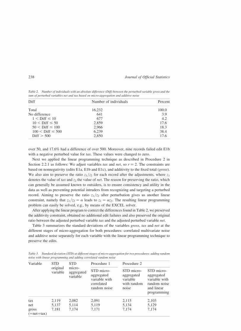
over 50, and 17.6% had a difference of over 500. Moreover, nine records failed edit E1b

with a negative perturbed value for tax. These values were changed to zero.

Next we applied the linear programming technique as described in Procedure 2 in

Section 2.2.1 as follows: We adjust variables tax and net, so r ¼ 2. The constraints are

based on nonnegativity (edits E1a, E1b and E1c), and additivity to the fixed total (gross).

We also aim to preserve the ratio z1=z2 for each record after the adjustments, where z1denotes the value of tax and z2 the value of net. The reason for preserving the ratio, which

can generally be assumed known to outsiders, is to ensure consistency and utility in the

data as well as preventing potential intruders from recognizing and targeting a perturbed

record. Aiming to preserve the ratio z1=z2 after perturbation gives us another linear

constraint, namely that z1=z2 ¼ a leads to z1 ¼ az2. The resulting linear programming

problem can easily be solved, e.g., by means of the EXCEL solver.

After applying the linear program to correct the differences found in Table 2, we preserved

the additivity constraint, obtained no additional edit failures and also preserved the original

ratio between the adjusted perturbed variable tax and the adjusted perturbed variable net.

Table 3 summarizes the standard deviations of the variables gross, tax and net at the

different stages of micro-aggregation for both procedures: correlated multivariate noise

and additive noise separately for each variable with the linear programming technique to

preserve the edits.

Table 2. Number of individuals with an absolute difference (Diff) between the perturbed variable gross and the

sum of perturbed variables net and tax based on micro-aggregation and additive noise

Diff Number of individuals Percent

Total 16,232 100.0No difference 641 3.9

1 , Diff # 10 677 4.210 , Diff # 50 2,859 17.650 , Diff # 100 2,966 18.3100 , Diff # 500 6,239 38.4Diff . 500 2,850 17.6

Table 3. Standard deviation (STD) at different stages of micro-aggregation for two procedures: adding random

noise with linear programming and adding correlated random noise

Variable STDoriginalvariable

STDmicro-aggregatedvariable

Procedure 1 Procedure 2

STD micro-aggregatedvariable withcorrelatedrandom noise

STD micro-aggregatedvariablewith randomnoise

STD micro-aggregatedvariable withrandom noiseand linearprogramming

tax 2,119 2,082 2,091 2,115 2,103net 5,137 5,114 5,119 5,134 5,129gross(¼netþtax)

7,181 7,174 7,171 7,174 7,174

Journal of Official Statistics238

Comparing these two methods in Table 3, it appears that the second procedure based on

adding random noise separately to each variable and the linear programming step to

preserve additivity provides final variances more similar to the original variances for each

of the variables. However, micro-aggregation distorts correlation structures between

variables. Whether adding correlated multivariate noise or adding univariate noise to each

variable separately and correcting edits via linear programming, neither of the methods

improves the distorted correlation structure.

2.3. Protecting Continuous Variables by Rounding

Rounding to a predefined base is a form of adding noise, although in this case the exact

value of the noise is known a priori and is controlled via the rounding base. Therefore it is

likely that edits of types E1 and E2 will not fail due to the rounding. However, rounding

continuous variables separately may cause edit failures of the type defined by E3 since the

sum of rounded variables will not necessarily equal their rounded total. We demonstrate a

method for preserving totals when carrying out an unbiased random rounding procedure.

2.3.1. Random Rounding and Preserving Totals

In our case, where we are dealing with micro-data with rather simple edit restrictions,

rounding procedures can be relatively easy to implement, similar to the problem of

rounding one- or two-dimensional tables. In this example, we describe a one-dimensional

random rounding procedure for a variable in a micro-data set which not only has the

property that it is stochastic and unbiased, but can also be carried out in such a way as to

preserve the exact overall total (and hence the mean) of the variable being rounded.

Moreover, the strategy that we propose reduces the extra variance induced by the

rounding. The algorithm is as follows:

Let m be the value to be rounded and let FloorðmÞ be the largest multiple k of the base b

such that bk , m. In addition, define the residual of m according to the rounding base b by

resðmÞ ¼ m2 FloorðmÞ. For an unbiased random rounding procedure, m is rounded up to

ðFloorðmÞ þ bÞ with probability resðmÞ=b and rounded down to FloorðmÞ with probability

ð12 resðmÞ=bÞ. Ifm is already a multiple of b, it remains unchanged. The expected value of

the rounded entry is the original entry. The rounding is usually implemented with

replacement in the sense that each entry is rounded independently, i.e., a random uniform

number u between 0 and 1 is generated for each entry. If u , resðmÞ=b then the entry is

rounded up, otherwise it is rounded down. The expectation of the rounding is zero and no

bias should remain in the table. However, the realization of this stochastic process on a finite

number of values in micro-data may lead to overall bias since the sum of the perturbations

(i.e., the difference between the original and rounded value) going down may not

necessarily equal the sum of the perturbations going up. In order to preserve the exact total

of the variable being rounded, we define a simple algorithm for selecting (without

replacement) which entries are rounded up and which entries are rounded down for those

entries having resðmÞ, randomly select a fraction of resðmÞ=b of the entries and round

upwards. Round the rest of the entries downwards. Repeat this process for all resðmÞ.

In the literature, random rounding is implemented using a “with replacement” strategy,

i.e., each value is rounded independently according to a random binomial draw.

Shlomo and De Waal: Protection of Micro-data Subject to Edit Constraints 239

The overall additional variance due to the rounding is the sum of the additional variances

for each rounded value. In our proposed selection strategy, we implement a “without

replacement” strategy for selecting values across the records to round up or down. This

makes the perturbation dependent across the values. Similar to the case of simple random

sampling without replacement, the covariance component between two values is negative

and therefore we expect a reduction in the additional variance induced by the rounding.

This reduction is most clearly seen if the overall total is a multiple of the rounding base.

In that case the overall total is exactly preserved and the additional variance to the overall

total obviously equals zero. When the overall total is not a multiple of the rounding base,

we obtain some additional variance but it is greatly reduced as compared to the “with

replacement” strategy.

The rounding procedure as described above should be carried out within subgroups in

order to benchmark important totals. For example, rounding income in each group defined

by age and sex will ensure that the total income in that group will remain unchanged. This

may, however, distort the overall total across the entire dataset. Users are typically more

interested in smaller subgroups for analysis and therefore preserving totals for subgroups

is generally more desirable than the overall total. Reshuffling algorithms can be applied for

changing the direction of the rounding for some of the values across the records in order to

correct the overall total or to preserve additivity constraints in the records. An example of a

simple reshuffling algorithm for preserving additivity is described in the example in the

next section.

2.3.2. Example of Implementation

For our example dataset from the 2000 Israel Income Survey, we randomly round each of

the variables net and tax to base 10. The method is carried out separately for each of the

variables using the algorithm that controls and preserves the overall total. In order to

ensure the additivity edit E3, we calculate the rounded variable gross by summing the

rounded variables net and tax. The rounded variable gross now has its overall total

preserved (since the individual variables net and tax had their totals preserved); however,

since it is derived by adding the two rounded variables, this has caused the resulting sum to

jump a base on some of the values in the records. We carry out a simple reshuffling

algorithm to correct this as follows:

. Select the records with more than a difference of the absolute value of the base

(in this case, 10) between the original variable gross and the rounded variable gross

that was obtained by summing the rounded variables, net and tax;

. Determine and select which of the variables net or tax had the most difference from

its original value;

. If the summed rounded variable gross jumped over the higher base, drop the selected

variable down a base and if the summed rounded variable gross jumped over the

lower base, raise the selected variable up a base.

The results of this procedure are presented in Table 4 and include the effect on the overall

totals of each of the variables. Note that ensuring that the summed rounded variable gross

is within the base has slightly distorted the controlled total. However, the distortion is not

large, especially when compared to the alternative of no controls in the totals.

Journal of Official Statistics240

Table 4. Results of the random rounding (RR) with and without controls and the reshuffling algorithm on the totals of rounded variables “net”, “tax” and “gross”

Variable True total RR – no controlson totals and noadditivity

Difference RR – controls on totalsand additivity but not allwithin the base

Difference RR – controls on totalsand additivity and allwithin the base

Difference

tax 25,443,623 25,444,410 2787 25,443,630 27 25,443,710 287net 86,724,755 86,725,330 2575 86,724,770 215 86,724,860 2105gross(¼netþtax)

112,168,378 112,169,740 21,362 112,168,400 222 112,168,570 2192

ShlomoandDeWaal:Protectio

nofMicro

-data

Subject

toEditConstra

ints

241

2.4. Protecting Continuous Variables by Rank Swapping

In its simplest version, rank swapping is carried out by sorting the continuous variables

and defining groupings of size p. In each group, random pairs are selected and their values

swapped (see references in Section 1). If the groupings are small, this method will not

likely cause edits of types E1 and E2 to fail. In particular, the concern is for edits that are

based on the logical consistency between highly correlated variables, such as edit E2

relating the level of income to age. This is because the method introduces bias on joint

distributions that involve the swapped variable. Information loss measures need to

consider minimizing distortions to distributions and the effects on statistical inference.

The larger the size of the groupings the more possibilities of edit failures and loss of

information; however, the size of the groupings also has an inverse effect on the disclosure

risk, i.e., the larger the groupings the less disclosure risk. Therefore, a balance must be

struck based on the parameter p which minimizes edit failures and information loss and

also manages the disclosure risk, maintaining a tolerable risk threshold. Note that in order

to preserve the edit of additivity as defined in edit E3, all variables involved in the edit

would need to be swapped using the same paired record. Otherwise, adjustments could be

carried out as defined by the linear programming approach described in Section 2.2.1 for

preserving the additivity.

2.4.1. Rank Swapping and Minimizing Bias

Several papers have dealt with information loss measures (see, for example, Gomatam and

Karr 2003; Oganian and Karr 2006 and references therein). In this analysis we have chosen

three information loss measures, which examine the effect of rank swapping on distortions

to distributions and its effect on basic statistical analysis tools, namely the chi-square test

for independence and an analysis of variance (ANOVA). These three measures give an

indication of the effect on both bias and variance using this SDCmethod. Note that in order

to assess information loss for micro-data, we examine distributions and tables in the data

that would typically be defined for statistical analysis by users of the data. We describe

next the three measures:

Hellinger Distance: Let zk be the original count in cell k for a joint distribution and zkthe perturbed cell count. Also, let n be the sample size. The Hellinger Distance metric is

defined as HD ¼ ð1=ffiffiffi2

pÞ

ffiffiffiffiffiffiffiffiffiffiffiffiffiffiffiffiffiffiffiffiffiffiffiffiffiffiffiffiffiffiffiffiffiffiffiffiffiffiffiffiffiffiffiffiffiPkð

ffiffiffiffiffiffiffiffiffizk=n

p2

ffiffiffiffiffiffiffiffiffizk=n

pÞ2

q. This is a symmetrical distance metric

and measures the difference between two probability distributions. Note that this measure

takes into account the relative sizes of the original cell counts, i.e., the smaller the original

cell count, themore effect on the Hellinger Distance. For example, a difference between cells

of Sizes 1 and 2 has a larger effect on this distance metric than a difference between cells

of Sizes 10 and 11. The smaller the Hellinger Distance, the less information loss.

Cramer’s V: It is common to carry out statistical analysis on a given micro-data set

based on measuring associations between categorical variables through the use of the x 2

standard test for independence. Let T define a 2-dimensional frequency table spanned by

two variables each having C1 and C2 number of cells, respectively, and n is again the

sample size. Define Cramer’s V by V1;2 ¼ffiffiffiffiffiffiffiffiffiffiffiffiffiffiffiffiffiffiffiffiffiffiffiffiffiffiffiffiffiffiffiffiffiffiffiffiffiffiffiffiffiffiffiffiffiffiffiffiffiffiffiffiffiffiffiffiffiffiffiffiffiffiffiffiffiffiffix2=ðn £ min ððC1 2 1Þ; ðC2 2 1ÞÞÞ

p. Cramer’s

V lies between 0 for no association and 1 for full association. The measure that defines the

Journal of Official Statistics242

loss in the association when comparing Torig and Tpert is CV1;2 ¼ V1;2ðTpertÞ2 V1;2ðTorigÞ.

The smaller the difference in Cramer’s V, the less information loss. Moreover, the sign of

the difference is important since this tells us whether we are attenuating a target variable or

adding more artificial association into the table.

Effect on R 2: For a univariate analysis of variance (ANOVA), we assess the effect on

the “between” variance, i.e., the effect on the R 2 statistic. R 2 is the ratio of the “between

sum” of squares SSB to the total sum of squares SST (see Section 2.2.1). The information

loss measure is the ratio of the “between” variance of the perturbed distribution and the

“between” variance of the original distribution, where the “between” variance is defined

by BV ¼ 1=ðm2 1ÞPm

k¼1pð�zk 2��zÞ2, andm is the number of groups, p is the sample size in

group k, �zk is the mean of the variable in group k and ��z is the overall mean. Note that an

information loss measure below one indicates attenuation, i.e., the means in groups

k ðk ¼ 1; : : : ;mÞ are flattened towards the overall mean of the distribution whereas a

value above one indicates more of a dispersion in the cell means.

2.4.2. Example of Implementation

We demonstrate this method on the individuals that earned an income in the 2000 Israel

Income Survey based on the income variable gross. After sorting the variable, we define

groupings of size p ¼ 10 and of size p ¼ 20, select random pairs in each group and swap

the values of gross between each pair. Edits of type E1 and E2 did not fail for either size

grouping, although in order to ensure the additivity of edit E3 the other income variables

would have to be swapped simultaneously or an adjustment carried out. In addition, the

original mean and variance for the univariate variable gross are preserved. Next we

examine the information loss measures based on a particular joint distribution defined by

cross-classifying age groups (14), sex (2) and income groups (22). For the Cramer’s V

statistic we define the frequency table by cross-classifying age groups £ sex for the rows

and the income groups on the columns. For the ANOVA analysis, we define the dependent

variable as gross and the independent variables as the cross-classified age groups £ sex.

Table 5 presents the results of these information loss measures.

From Table 5, as the size of the groupings increases, we obtain slightly more distortion

to the distribution examined. There is almost no effect on measures of association for the

frequency table examined nor on the ratio of the between variance for the ANOVA

analysis. The negative sign for the Cramer’s V and the ratio of BV smaller than one

Table 5. Information loss measures for the joint distribution of age group, sex and gross income

Information Loss Measures Groupings

of 10

Groupings

of 20

Number and percent of

cells with differences

616 possible combinations 106 (22%) 166 (34%)

Hellinger’s distance Age groups £ sex £ income

groups

0.011 0.013

Difference in Cramer’s V Income groups and age groups

£ sex ðVðTorigÞ ¼ 0:1300Þ0 20.0001

Ratio of BV Mean of gross within age groups

£ sex ðBVorig ¼ 3:83 £ 109Þ

1.004 0.998

Shlomo and De Waal: Protection of Micro-data Subject to Edit Constraints 243

indicates that as the size p of the groupings increases, we are indeed attenuating the target

variable across the distribution.

3. Perturbation of Categorical Key Variables

The dataset that has been used for evaluating the SDC techniques for continuous data is

less suited for evaluating SDC techniques on categorical data. For the evaluation of

categorical data, we use a file drawn from the 1995 Israel Census sample data which

comprised 20% of all households in Israel. The dataset for this analysis contains 35,773

individuals aged 15 and over in 15,468 households across all geographical areas and

household characteristics. For this analysis, we perturb the variable age. Age has 86

categories (since the evaluation dataset includes only individuals aged 15 and over).

The edits involve the original edits from the data processing phase that check for

inconsistencies with the variable age that is under perturbation. “Relation” as mentioned

in the edits refers to the relation to the head of household. The edits used for the evaluation

dataset are:

E1: {Under 16 and ever married} ¼ Failure;

E2: {Age of marriage under 14} ¼ Failure;

E3: {Age difference between spouse over 25} ¼ Failure;

E4: {Age of mother under 14} ¼ Failure;

E5: {Year of immigration less than year of birth} ¼ Failure;

E6: {Age of father under 14} ¼ Failure;

E7: {Under 16 and relation is spouse or parent} ¼ Failure;

E8: {Under 30 and relation is grandparent} ¼ Failure;

E9: {Under 16 and academic} ¼ Failure;

E10: {Under 16 and higher degree} ¼ Failure;

E11: {Age inconsistent with year of birth} ¼ Failure.

In addition, since other variables may be changed in the post-editing imputation stage for

correcting inconsistent records resulting from the perturbation, we add the following edits:

E12: {Single and year of marriage not null} ¼ Failure;

E13: {Single and has spouse in household} ¼ Failure;

E14: {Relation is spouse and not married} ¼ Failure.

3.1. Protecting Categorical Variables by PRAM

As presented in Shlomo and De Waal (2005), we examine the use of a technique called the

Post-randomization Method (PRAM) (Gouweleeuw, Kooiman, Willenborg, and De Wolf

1998) to perturb categorical variables. This can be seen as a general case of a more

common technique based on record swapping. Willenborg and De Waal (2001) describe

the process as follows:

Let P be an L £ L transition matrix containing conditional probabilities pij ¼

pðperturbed category is jjoriginal category is i Þ for a categorical variable with L categories.

Let t be the vector of frequencies and v the vector of relative frequencies: v ¼ t=n, where n

is the number of records in the micro-data set. In each record of the data set, the category of

Journal of Official Statistics244

the variable is changed or not changed according to the prescribed transition probabilities

in the matrix P and the result of a draw of a random multinomial variate u with parameters

pij ð j ¼ 1; : : : ; LÞ. If the jth category is selected, category i is moved to category j. When

i ¼ j, no change occurs.

Let t* be the vector of the perturbed frequencies. t* is a random variable and

Eðt*jtÞ ¼ tP. Assuming that the transition probability matrix P has an inverse P21, this

can be used to obtain an unbiased moment estimator of the original data: t ¼ t*P21.

Statistical analysis can be carried out on t. In order to ensure that the transition probability

matrix has an inverse and to control the amount of perturbation, the matrix P is chosen to

be dominant on the main diagonal, i.e., each entry on the main diagonal is over 0.5.

Place the condition of invariance on the transition matrix P, i.e., tP ¼ t. This relieves

the users of the perturbed file of the extra effort to obtain unbiased moment estimates of the

original data, since t* itself will be an unbiased estimate of t. The property of invariance

means that the expected values of the marginal distribution of the variable being perturbed

are maintained. In order to obtain the exact marginal distribution, we propose using a

“without” replacement strategy and select the expected number of categories to change

(see Section 2.3.1 for a similar strategy for the case of random rounding). This will ensure

exact marginal distributions as well as reduce the additional variance that is induced by the

perturbation. This method was used to perturb the Sample of Anonymized Records (SARs)

of the 2001 UK Census (Gross, Guiblin, and Merrett 2004).

The invariance applies to the variable being perturbed, so to do a full invariant PRAM

on several variables at once means that all of the variables will have to be compounded

into a single variable, i.e., the variables will have to be cross-classified. An example is

given by Van den Hout and Elamir (see Chapter 6 in Van den Hout 2004).

To obtain an invariant transition matrix, the following two-stage algorithm is

given in Willenborg and De Waal (2001). Let P be any transition probability matrix

pik ¼ pðc*¼ kjc ¼ i Þ where c represents the original category and c * represents

the perturbed category. Now calculate the matrix Q using Bayes formula by

Qkj ¼ pðc ¼ jjc*¼ kÞ ¼ ð pjkpðc ¼ jÞÞ=

Pl plkpðc ¼ l Þ. We estimate the entries Qkj of

this matrix by pjkvj=P

l plkvl, where vj is the relative frequency of category j. For R ¼ PQ

we obtain an invariant matrix where vR ¼ vPQ ¼ v since rij ¼P

k

�ðvjpikpjkÞ=

Pl plkvl

�and

Pi virij ¼

Pk vjpik ¼ vj. The vector of the original frequencies v is an eigenvector of

R. In practice, Q can be calculated by transposing matrix P, multiplying each column j by

vj and then normalizing its rows so that the sum of each row equals one. Since the property

of invariance distorts the desired probabilities on the diagonal (the probabilities of not

changing a category), we propose defining a parameter a and calculating R*¼

aRþ ð12 aÞI where I is the identity matrix of the appropriate size. R* will also be

invariant and the amount of perturbation is controlled by the value of a. See Shlomo and

De Waal (2005) for an example of calculating invariant probability matrices.

As in all perturbative SDC methods, joint distributions between perturbed and

unperturbed variables will be distorted, in particular for variables that are highly correlated

with each other. An initial analysis of the dependencies between the categorical variables

can provide insight into which variables should be perturbed for SDC. In particular those

variables that are highly dependent should be compounded and treated as a single variable

in the perturbation process. As more perturbation is introduced, the utility of the data will

Shlomo and De Waal: Protection of Micro-data Subject to Edit Constraints 245

be compromised. Variables that are generally perturbed are the demographic and

geographic identifiers in the micro-data which are typically used for statistical analysis as

explanatory independent variables (e.g., in regression models and ANOVA). Therefore,

the perturbation of these variables will have an effect on the ability to make statistical

inferences based on the perturbed micro-data.

3.2. PRAM and Preserving Edit Constraints

If no controls are taken into account in the perturbation process, edit failures may occur,

resulting in inconsistent and “silly” combinations such as married small children, small

children earning income, or an unfeasible age difference between a child and its parents.

Methods need to be developed for implementing PRAM that will place controls on the

perturbation process and will avoid edit failures as much as possible, reduce information

loss and raise the overall utility of the data. The controls in the perturbation are defined by

control variables which define groupings within which perturbations will be allowed.

These control variables are typically highly correlated with the variable being perturbed

and ensure a priori that failed edits and information loss will be minimal. The methods for

controlling the perturbation are the following:

. Before applying PRAM, the variable to be perturbed is divided into subgroups,

g ¼ 1; : : : ;G. The (invariant) transition probability matrix is developed for each

subgroup g, Rg. The transition matrices for each subgroup are placed on the main

diagonal of the overall final transition matrix where the off diagonal probabilities are

all zero, i.e., the variable is only perturbed within the subgroup and the difference in

the variable between the original value and the perturbed value will not exceed a

specified level. An example of this is perturbing age within broad age bands.

. The variable to be perturbed may be highly correlated with other variables. Those

variables should be compounded into one single variable. PRAM should be carried

out on the compounded variable. Alternatively, the variable to be perturbed is carried

out within subgroups defined by the second highly correlated variable. An example of

this is when age is perturbed within groupings defined by marital status.

The control variables in the perturbation process will minimize the amount of edit failures,

but they will not eliminate all edit failures, especially edit failures that are beyond the

scope of the variables that are being perturbed. Remaining edit failures need to be

manually or automatically corrected through imputation procedures depending on the

amount and the types of edit failures.

We have applied a hot-deck imputation method for correcting inconsistent records

and edit failures. This hot-deck imputation method was implemented by choosing a

neighboring donor matching on the control variables: district, number of persons in the

household, marital status, sex and perturbed age. All variables that are included in the

edits and are not control variables are imputed. The need for further imputation to

satisfy edits means that more perturbation is introduced into the micro-data for other

variables in the file interacting with the perturbed variable age. For example, the ages

of the spouse and/or parents may also need to be changed as well as marital status.

Therefore, the lower the number of overall edit failures resulting from the perturbation

Journal of Official Statistics246

process, the less need for imputation to correct inconsistencies and the higher the

utility maintained in the data. The next section presents results of the effectiveness of

putting into place controls in the perturbation of the micro-data, thereby minimizing

the number of failed edits.

3.3. Example of Implementation

The perturbation of age by PRAM was carried out using an invariant transition

probability matrix as described in Section 3.1. As mentioned, there are 86 categories of age

in the evaluation data for individuals aged 15 and over. To perturb age we use the

following methods:

. Random perturbation across all ages, i.e., the transition probability matrix is of size

86 £ 86, the diagonal pd is generated randomly and all other columns are given equal

entries ð12 pdÞ=85. The matrix is then made to be invariant and the diagonals

controlled through the use of a as explained in Section 3.1.

. Perturbation carried out within categories of marital status (four categories –

married, divorced, widowed, and single), i.e., four separate invariant transition

probability matrices are developed for perturbing age in each of the categories of

marital status and the perturbation is carried out separately within each category.

In other words, the final probability transition matrix is block diagonal containing the

four matrices on the diagonals and all other parts of the transition probability matrix

are zero.

. Perturbation carried out on marital status (four categories – married, divorced,

widowed, and single) £ age bands (five bands – 15–17, 18–24, 25–44, 45–64,

65–74, 75 þ ) as explained above.

. Perturbation only allowed within broad age bands (nine bands – 15–17, 18–24,

25–34, 35–44, 45–54, 55–64, 65–69, 70–74, 75 þ ) as explained above.

Because of the stochastic nature of the process, each method above resulted in a different

number of records being perturbed. The number of perturbations for Method 1 was 7,316

records. For Methods, 2, 3, and 4, 6,822, 7,535, and 8,068 records were perturbed,

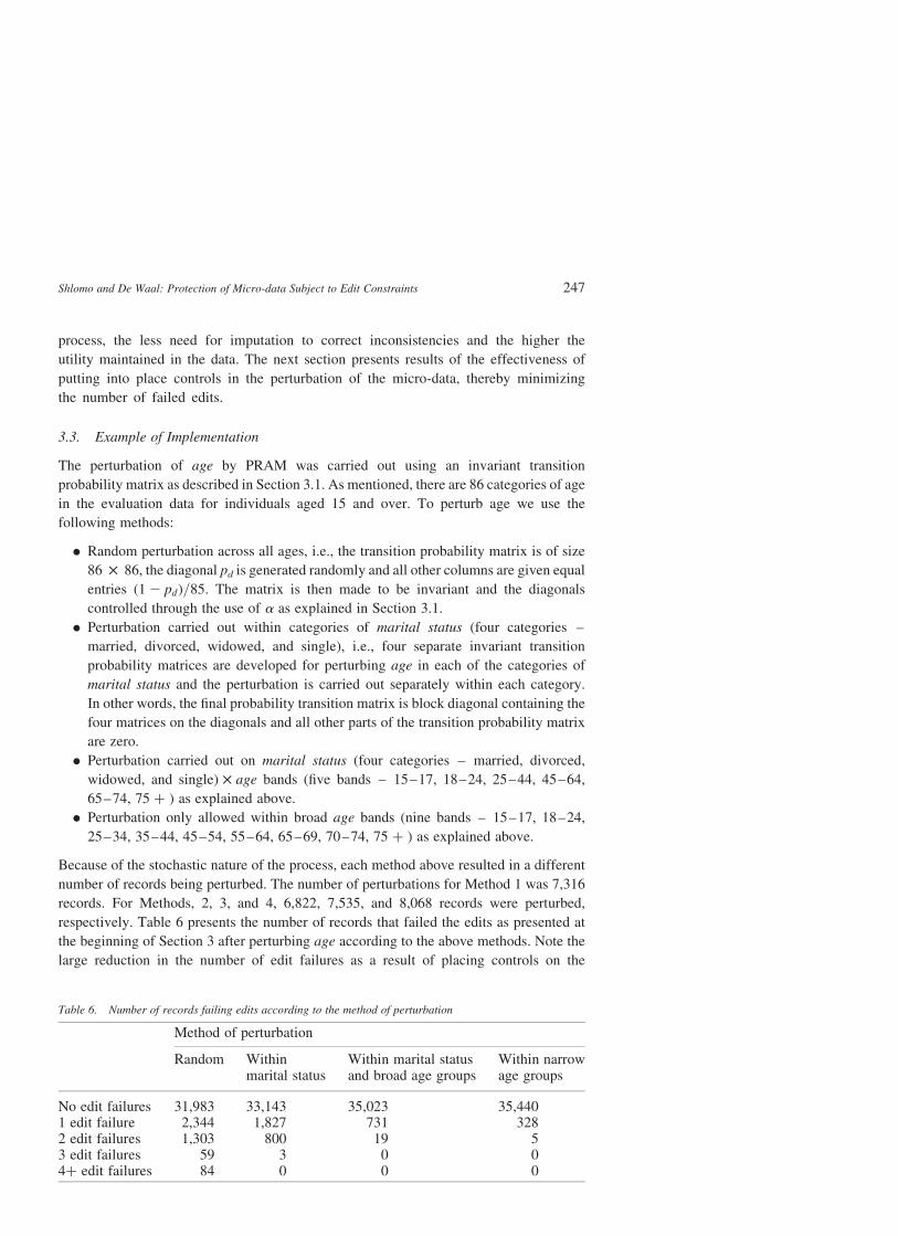
respectively. Table 6 presents the number of records that failed the edits as presented at

the beginning of Section 3 after perturbing age according to the above methods. Note the

large reduction in the number of edit failures as a result of placing controls on the

Table 6. Number of records failing edits according to the method of perturbation

Method of perturbation

Random Withinmarital status

Within marital statusand broad age groups

Within narrowage groups

No edit failures 31,983 33,143 35,023 35,4401 edit failure 2,344 1,827 731 3282 edit failures 1,303 800 19 53 edit failures 59 3 0 04þ edit failures 84 0 0 0

Shlomo and De Waal: Protection of Micro-data Subject to Edit Constraints 247

perturbation processes. In particular, perturbing within narrow age bands (which is highly

correlated with marital status) produced the best results.

For each of the perturbation methods above, the edit failures were corrected using a hot-

deck donor imputation method. In Method 1, 37 records could not be imputed since no

suitable donor was found so these records were unperturbed. In some cases, the control

variables for the hot-deck imputation had to be collapsed in order to be able to find a

suitable donor for the failed record. After the imputation process, all records satisfy the

edits. However, information loss measures are also affected and we need to choose the

method of perturbation that will minimize the number of information loss measures and

obtain high utility data.

We use the following distributions from the micro-data to assess information loss based

on the measures described in Section 2.4.1:

. We use the Hellinger Distance to measure the distortion to the distribution defined by

district (27) £ sex (2) £ age (86) before and after PRAM.

. We use the difference in Cramer’s V statistic on two-dimensional tables where the

rows contain the variable age (86) and the columns contain the following target

variables: labor force characteristics (4) and years of education (26). We compare

Cramer’s V before and after the perturbation.

. We use the ratio of the “between” variance BV for a target variable in groupings

defined by the perturbed variable age and the “between” variance BV for a target

variable in groupings defined by the original variable age. For this analysis we

banded age into nine groupings: 15–17, 18–24, 25–34, 35–44, 45–54, 55–64,

65–69, 70–74, and 75 þ . The target variables selected for this analysis are: percent

academics, percent belonging to the labor force and percent unemployed out of those

belonging to the labor force.

Table 7 presents the results of the information loss measures as defined in Section 2.4.

It is shown in Table 7 that putting more controls in the perturbation process raises the

level of the utility of the data. For example, the original value for Cramer’s V, which

measures the association between labor force characteristics (employed, unemployed

and outside the labor force) and age is 0.306. Through perturbing the variable age, the

measure of association decreases by 0.082 when age is perturbed across all possible ages,

but only decreases by 0.008 when age is perturbed within narrow age bands. Note that all

the information of loss measures are negative based on the Cramer’s V analysis. This

indicates the attenuation of the target variables. In another example, we assume that the

user is interested in carrying out an ANOVA analysis on the percentage of unemployed

out of those belonging to the labor force using age groups as an explanatory variable.

Before perturbing age, the value of the “between” variance BV was 8.8. However, when

age was perturbed across all possible ages, the BV decreased by almost a half. This

implies that the percent unemployed in each perturbed age grouping is tending towards

the overall mean and we would obtain a lower R 2 as a result of the analysis. Figure 1

shows the shrinkage of the unemployment percentages within randomly perturbed

age groups compared to the percentages within original age groups. Note that the

unemployment percentages are much flatter across the randomly perturbed age groups.

Journal of Official Statistics248

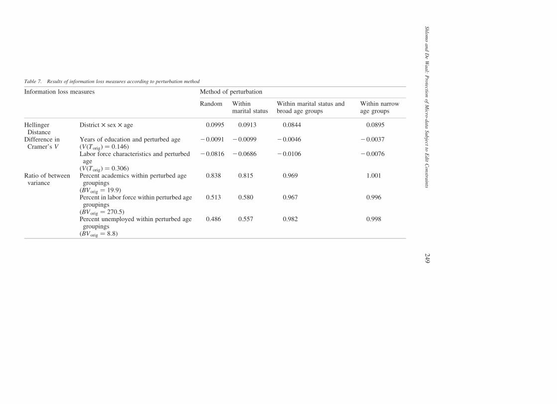
Table 7. Results of information loss measures according to perturbation method

Information loss measures Method of perturbation

Random Withinmarital status

Within marital status andbroad age groups

Within narrowage groups

HellingerDistance

District £ sex £ age 0.0995 0.0913 0.0844 0.0895

Difference inCramer’s V

Years of education and perturbed ageðVðTorigÞ ¼ 0:146Þ

20.0091 20.0099 20.0046 20.0037

Labor force characteristics and perturbedage

ðVðTorigÞ ¼ 0:306Þ

20.0816 20.0686 20.0106 20.0076

Ratio of betweenvariance

Percent academics within perturbed agegroupings

ðBVorig ¼ 19:9Þ

0.838 0.815 0.969 1.001

Percent in labor force within perturbed agegroupings

ðBVorig ¼ 270:5Þ

0.513 0.580 0.967 0.996

Percent unemployed within perturbed agegroupings

ðBVorig ¼ 8:8Þ

0.486 0.557 0.982 0.998

ShlomoandDeWaal:Protectio

nofMicro

-data

Subject

toEditConstra

ints

249

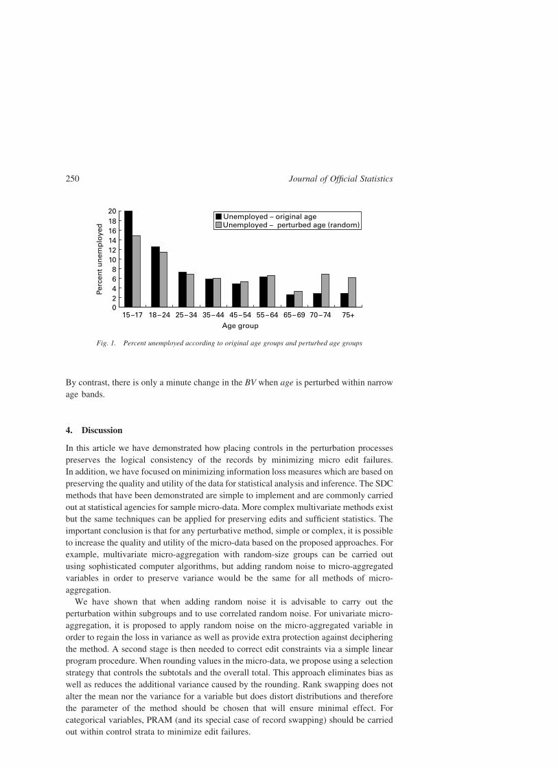
By contrast, there is only a minute change in the BV when age is perturbed within narrow

age bands.

4. Discussion

In this article we have demonstrated how placing controls in the perturbation processes

preserves the logical consistency of the records by minimizing micro edit failures.

In addition, we have focused on minimizing information loss measures which are based on

preserving the quality and utility of the data for statistical analysis and inference. The SDC

methods that have been demonstrated are simple to implement and are commonly carried

out at statistical agencies for sample micro-data. More complex multivariate methods exist

but the same techniques can be applied for preserving edits and sufficient statistics. The

important conclusion is that for any perturbative method, simple or complex, it is possible

to increase the quality and utility of the micro-data based on the proposed approaches. For

example, multivariate micro-aggregation with random-size groups can be carried out

using sophisticated computer algorithms, but adding random noise to micro-aggregated

variables in order to preserve variance would be the same for all methods of micro-

aggregation.

We have shown that when adding random noise it is advisable to carry out the

perturbation within subgroups and to use correlated random noise. For univariate micro-

aggregation, it is proposed to apply random noise on the micro-aggregated variable in

order to regain the loss in variance as well as provide extra protection against deciphering

the method. A second stage is then needed to correct edit constraints via a simple linear

program procedure. When rounding values in the micro-data, we propose using a selection

strategy that controls the subtotals and the overall total. This approach eliminates bias as

well as reduces the additional variance caused by the rounding. Rank swapping does not

alter the mean nor the variance for a variable but does distort distributions and therefore

the parameter of the method should be chosen that will ensure minimal effect. For

categorical variables, PRAM (and its special case of record swapping) should be carried

out within control strata to minimize edit failures.

Fig. 1. Percent unemployed according to original age groups and perturbed age groups

Journal of Official Statistics250

While this article mainly discusses aspects of utility, quality, and consistency, data

suppliers and statistical agencies must also focus on minimizing disclosure risk. The trade-

off between managing the disclosure risk and ensuring high data utility must be carefully

assessed before developing optimal SDC strategies. Future work will examine this trade-

off by measuring disclosure risk in micro-data before and after applying SDC methods

(see Elamir and Skinner 2006; Skinner and Shlomo 2006; Rinott and Shlomo 2006 and

references therein), and by comparing the methods with respect to information loss and the

preservation of edit constraints. By combining SDC methods and developing innovative

techniques for implementation, we can obtain consistent data, preserve totals, means, and

variance estimates, and release statistical outputs with higher degrees of utility at little cost

to the risk of disclosure.

We have applied relatively simple approaches to ensure that perturbed data satisfy the

specified edits. More sophisticated methods for ensuring that variables satisfy edits are

available from the area of statistical data editing and the area of imputation. For instance,

the Fellegi-Holt principle of minimum change (Fellegi and Holt 1976) can be applied. This

principle determines that the data of an inconsistent record should be made to satisfy all

edits by changing the lowest possible number of values. When applying the Fellegi-Holt

principle, one first identifies the erroneous fields. These erroneous fields can subsequently

be imputed by an imputation method. In a last step, the imputed values can be adjusted so

all edits become satisfied. An algorithm for implementing the Fellegi-Holt principle for

both categorical and continuous data is based on a branch-and-bound search (De Waal and

Quere 2003). Several alternative approaches and a method to adjust imputed fields so all

edits become satisfied are described by De Waal (2003). Another approach, called NIM

(Nearest-Neighbor Imputation Method), which is implemented in Statistic’s Canada

CANCEIS, has been successfully carried out for Canadian Censuses (Bankier 1999). This

approach implements a minimum change principle similar to the Fellegi-Holt principle.

Namely, the data in a record are made to satisfy all edits by changing the fewest possible

number of values given the available potential donor records. A logically consistent

nearest neighbor donor with a minimum number of variables to donate is selected for

imputing values for a failed record. Intuitively, using the Fellegi-Holt principle or the NIM

approach leads to results that are closer to optimality than using the relatively simple

methods for ensuring consistencies that we have used. Our intuition remains to be

confirmed by future work.

Based on a given threshold for disclosure risk, the “best” method to protect a micro-data

set is hard to determine in general. For a particular micro-data set, what is the “best” SDC

method depends on the intended uses of the data on the part of the users, the willingness of

the statistical agency to disseminate this data set, the legal aspects of releasing these data

and the structure of the data. For instance, homogeneous data require different SDC

techniques than heterogeneous data. To some extent, what is the “best” SDC method for a

micro-data set will always be a subjective choice. Levels of protection and tolerable

disclosure risk thresholds vary from country to country and depend on the different modes

for accessing the micro-data. A prerequisite, however, for making a well-founded choice

of SDC method is a solid understanding of a wide range of SDC methods and techniques

for implementation which minimize information loss. We hope that this article helps to

improve the understanding of several such SDC methods.

Shlomo and De Waal: Protection of Micro-data Subject to Edit Constraints 251

5. References

Anwar, N. (1993). Micro-aggregation – The Small Aggregates Method. Informe Intern.

Luxembourg: Eurostat.

Bankier, M. (1999). Experience with the New Imputation Methodology Used in the 1996

Canadian Census with Extensions for Future Censuses. Rome: U.N. Economic

Commission for Europe Work Session on Statistical Data Editing.

Brand, R. (2002). Micro-data Protection through Noise Addition. In Inference Control in

Statistical Databases, J. Domingo-Ferrer (ed.). New York: Springer, 97–116.

Dalenius, T. and Reiss, S.P. (1982). Data Swapping: A Technique for Disclosure Control.

Journal of Statistical Planning and Inference, 7, 73–85.

Defays, D. and Nanopoulos, P. (1992). Panels of Enterprises and Confidentiality: The

Small Aggregates Method. Proceedings of Statistics Canada Symposium 92, Design

and Analysis of Longitudinal Surveys, 195–204.

De Waal, T. (2003). Processing of Erroneous and Unsafe Data. Ph.D. Thesis, Erasmus

University, Rotterdam.

De Waal, T. and Quere, R. (2003). A Fast and Simple Algorithm for Automatic Editing of

Mixed Data. Journal of Official Statistics, 19, 383–402.

Domingo-Ferrer, J. and Mateo-Sanz, J. (2002). Practical Data-Oriented Microaggregation

for Statistical Disclosure Control. IEEE Transactions on Knowledge and Data

Engineering, 14, 189–201.

Domingo-Ferrer, J., Mateo-Sanz, J., and Torra, V. (2001). Comparing SDC Methods

for Micro-data on the Basis of Information Loss and Disclosure Risk. ETK-NTTS

Pre-Proceedings of the Conference, Crete, June.

Domingo-Ferrer, J. and Sebe, F. (2006). Optimal Multivariate 2-Microaggregation for

Microdata Protection: A 2-Approximation. In Privacy in Statistical Databases–

PSD2006, J. Domingo-Ferrer and L. Franconi (eds). Berlin: Springer LNCS 4302,

129–138.

Elamir, E. and Skinner, C.J. (2006). Record-Level Measures of Disclosure Risk for Survey

Micro-data. Journal of Official Statistics, 22, 525–539.

Fellegi, I.P. and Holt, D. (1976). A Systematic Approach to Automatic Edit and

Imputation. Journal of the American Statistical Association, 71, 17–35.

Fienberg, S.E. and McIntyre, J. (2005). Data Swapping: Variations on a Theme by

Dalenius and Reiss. Journal of Official Statistics, 9, 383–406.

Fuller, W.A. (1993). Masking Procedures for Micro-data Disclosure Limitation. Journal of

Official Statistics, 9, 383–406.

Gomatam, S. and Karr, A. (2003). Distortion Measures for Categorical Data Swapping.

Technical Report Number 131, National Institute of Statistical Sciences.

Gouweleeuw, J., Kooiman, P., Willenborg, L.C.R.J., and De Wolf, P.P. (1998). Post

Randomisation for Statistical Disclosure Control: Theory and Implementation. Journal

of Official Statistics, 14, 463–478.

Gross, B., Guiblin, P., and Merrett, K. (2004). Implementing the Post-Randomisation

Method to the Individual Sample of Anonymised Records (SAR) from the 2001 Census.

http://www.ccsr.ac.uk/sars/events/2004-09-30/gross.pdf

Journal of Official Statistics252

Kim, J.J. (1986). A Method for Limiting Disclosure in Micro-data Based on Random

Noise and Transformation. Proceedings of the American Statistical Association,

Section on Survey Research Methods, 370–374.

Lechner, S. and Pohlmeier, W. (2004). To Blank or Not to Blank. In Privacy in Statistical

Databases, J. Domingo-Ferrer and V. Torra (eds). Berlin: Springer LNCS 3050,

187–200.

Oganian, A. and Karr, A. (2006). Combinations of SDC Methods for Micro-data

Protection. In Privacy in Statistical Databases – PSD2006, J. Domingo-Ferrer and

L. Franconi (eds). Berlin: Springer LNCS 4302, 102–113.

Rinott, Y. and Shlomo, N. (2006). A Generalized Negative Binomial Smoothing Model

for Sample Disclosure Risk Estimation. In Privacy in Statistical Databases – PSD2006,

J. Domingo-Ferrer and L. Franconi (eds). Berlin: Springer LNCS 4302, 82–93.

Ronning, G., Sturm, R., Hohne, J., Lenz, R., Rosemann, M., Scheffler, M., and

Vorgrimmler, D. (2005). Handbuch zur Anonymisierung wirtschafstsstatistischer

Mikrodaten. Statistisches Bundesamt, Wiesbaden, Reihe “Statistik und Wissenschaft”,

Volume 4. [In German].

Samarati, P. (2001). Protecting Respondents’ Identities in Microdata Release. IEEE

Transactions on Knowledge and Data Engineering, 18, 1010–1027.

Sarndal, C.E. and Lundstrom, S. (2005). Estimation in Surveys with Nonresponse.

Chichester: Wiley.

Shlomo, N. and De Waal, T. (2005). Preserving Edits When Perturbing Micro-data for

Statistical Disclosure Control. Statistical Journal of the United Nations ECE, 22,

173–185.

Skinner, C.J. and Shlomo, N. (2006). Assessing Identification Risk in Survey Micro-data

Using Log-linear Models. JASA Applications and Case Studies (forthcoming) See:

http://eprints.soton.ac.uk/41842/01/s3ri-workingpaper-m06-14.pdf

Sweeney, L. (2002a). k-Anonymity: A Model for Protecting Privacy. International Journal

of Uncertainty, Fuzziness and Knowledge Based Systems, 10, 557–570.

Sweeney, L. (2002b). Achieving k-Anonymity Privacy Protection Using Generalization

and Suppression. International Journal of Uncertainty, Fuzziness and Knowledge Based

Systems, 10, 571–588.

Van den Hout, A. (2004). Analyzing Misclassified Data: Randomized Response and Post

Randomization. Ph.D. Thesis, University of Utrecht, Utrecht.

Willenborg, L. and De Waal, T. (2001). Elements of Statistical Disclosure Control in

Practice. Lecture Notes in Statistics. New York: Springer, 155.

Winkler, W.E. (2002). Single Ranking Micro-aggregation and Re-identification.

Statistical Research Division report RR 2002/08, U.S. Census Bureau, at http://www.

census.gov/srd/www/byyear.html

Yancey, W.E., Winkler, W.E., and Creecy, R.H. (2002). Disclosure Risk Assessment

in Perturbative Micro-data Protection. In Inference Control in Statistical Databases,

J. Domingo-Ferrer (ed.). New York: Springer, 135–151.

Received October 2006

Revised December 2007

Shlomo and De Waal: Protection of Micro-data Subject to Edit Constraints 253