Projecting Poverty Rates in 2020 for the 62 and Older Population: What Changes Can We Expect and...

PROJECTING POVERTY RATES IN 2020 FOR THE 62 AND OLDERPOPULATION: WHAT CHANGES CAN WE EXPECT AND WHY?

Barbara A. Butrica, The Urban InstituteKaren Smith, The Urban Institute

Eric Toder, Internal Revenue Service*

CRR WP 2002-3September 2002

Center for Retirement Research at Boston College550 Fulton Hall

140 Commonwealth Ave.Chestnut Hill, MA 02467

Tel: 617-552-1762 Fax: 617-552-1750http://www.bc.edu/crr

*Barbara A. Butrica is a Research Associate at The Urban Institute. Karen Smith is a Senior ResearchAssociate at The Urban Institute. Eric Toder is with the Internal Revenue Service. The research reportedherein was performed pursuant to a grant from the U.S. Social Security Administration (SSA) funded aspart of the Retirement Research Consortium. The opinions and conclusions are solely those of the authorsand should not be construed as representing the opinions or policies of SSA, the Internal Revenue Service,or any agency of the Federal Government or of the Center for Retirement Research at Boston College.They also do not necessarily reflect the views of The Urban Institute, its Board, or its Sponsors.

The authors wish to thank Jillian Berk for her superb research assistance and Howard Iams for his helpfulcomments.

© 2002, by Barbara A. Butrica, Karen Smith, and Eric Toder. All rights reserved. Short sections of text,not to exceed two paragraphs, may be quoted without explicit permission provided that full credit,including © notice, is given to the source.

About the Center for Retirement Research

The Center for Retirement Research at Boston College, part of a consortium that includesa parallel center at the University of Michigan, was established in 1998 through a 5-year$5.25 million grant from the Social Security Administration. The goals of the Center areto promote research on retirement issues, to transmit new findings to the policycommunity and the public, to help train new scholars, and to broaden access to valuabledata sources. Through these initiatives, the Center hopes to forge a strong link betweenthe academic and policy communities around an issue of critical importance to thenation’s future.

Center for Retirement Research at Boston College550 Fulton Hall

140 Commonwealth Ave.Chestnut Hill, MA 02467

phone: 617-552-1762 fax: 617-552-1750e-mail: [email protected]

http://www.bc.edu/crr

Affiliated Institutions:

Massachusetts Institute of TechnologySyracuse University

The Brookings InstitutionNational Academy of Social Insurance

Urban Institute

2

ABSTRACT

Over the past several decades, there have been a number of economic anddemographic changes that are expected to impact the economic well-being of the futureaged population. This paper analyzes the factors that may be related to increased ordecreased poverty among the 62- to 89-year-old population in 2020 using the SocialSecurity Administration’s Model of Income in the Near Term (MINT). We estimate thatthe poverty rate, when thresholds are indexed to the CPI, will decline from 7.8 percent inthe early 1990s to 4.2 percent in 2020, but the rate would increase from 7.8 percent to 9.9percent if the threshold were indexed to wages. We examine the impact of four specifictrends on future poverty rates: 1) the scheduled rise in the Social Security normalretirement age, 2) the changes in marital composition, 3) the change in the relativeearnings of men and women, and 4) the rise in earnings inequality.

We find that the increase in the normal retirement age and changes in maritalcomposition each explain about 25 percent of the projected increase in wage-adjustedpoverty. The changes in the relative earnings of men and women did not affect thepoverty rate—it only affected who was in poverty. The rise in earnings inequality hadalmost no effect on poverty rates largely because of the progressive Social Securitypayment formula. The projections of poverty rates are very sensitive to economic growthassumptions. Even with the substantial wage growth projected by the Social SecurityOffice of the Chief Actuary, however, high school dropouts, unmarried retirees, and olderretirees remain at high risk of poverty.

3

I. INTRODUCTION 1II. Background 21. Trends in Marriage and Divorce 22. Trends in Earnings and Labor Force Participation 33. Trends in Economic Growth 44. Trends in Poverty 5III. METHODOLOGY 51. Description of Model of Income in the Near Term (MINT) 52. Measuring Poverty Among the 62 and Over Population 7IV. RETIREMENT INCOME IN THE EARLY 1990s 91. Per Capita Income by Source 92. Family Income Divided by Poverty 113. Poverty Rates 124. Contribution to Poverty Rate by Subgroup 145. Importance of Sources of Income in Reducing Poverty 15V. RETIREMENT INCOME IN 2020 171. Per Capita Income by Source 172. Family Income Divided by Poverty 193. Poverty Rates 214. Contribution to Poverty Rate by Subgroup 225. Importance of Sources of Income in Reducing Poverty 24VI. EFFECTS OF USING DIFFERENT INCOME AND POVERTY MEASURES 241. Effects of Alternative Ways of Measuring Income 242. Indexing the Poverty Threshold by Wages Instead of Prices 27VII. CONTRIBUTIONS OF ECONOMIC, DEMOGRAPHIC, AND POLICYCHANGES TO POVERTY IN 2020 301. Effects of Changes in the Normal Retirement Age 312. Effects of Changes in Marital Composition of Retirees Between Early 1990s and2020. 323. Effects of Changes in Relative Earnings for Post-1950 Birth Cohorts 374. Effects of Changes in the Earnings Distribution for Post-1950 Birth Cohorts 38VIII. CONCLUSIONS 39

I. INTRODUCTION

The past 30 to 40 years have been accompanied by considerable changes in marriagepatterns, earnings and work patterns, the economy, and retirement policy. While these changeswill undoubtedly impact future retirees, it is difficult to know exactly how they will influencetheir economic well-being. The aim of this paper is to analyze the factors that may be related toincreased or decreased poverty among the 62- to 89-year-old population in 2020.

This paper projects future changes in poverty among the 62 and over population anddeconstructs the sources of those changes. Our analysis provides insights on how overallpoverty rates among retirees are likely to change between the early 1990s and 2020, whichgroups of retirees are most likely to be at risk of poverty, and what factors contribute most tochanges in poverty rates.

Our analysis is based on projections of the major sources of retirement income from theSocial Security Administration’s Model of Income in the Near Term (MINT). MINT starts withdata from the 1990 to 1993 U.S. Census Bureau’s Survey of Income and Program Participation(SIPP) matched to Social Security Administration’s (SSA) earnings and benefit records through1999. MINT then projects retirement income (Social Security benefits, pension income, assetincome, earnings—both before and after benefit take-up, Supplemental Security Income (SSI),and income from nonspouse co-resident family members) from the base SIPP year through 2032for individuals born between 1926 and 1965.1

In Section II, we provide some background information on some of the salient historictrends likely to influence the demographic characteristics and well-being of the future retiredpopulation. In Section III, we describe how MINT projects demographic changes and incomesand explain how we measure poverty. In Section VI, we present data on the economic status ofthe aged population in the early 1990s. We report per capita income by source, family incomedivided by poverty, poverty rates, and the marginal contribution each income source has onfamily income relative to poverty. In Section V, we report MINT projections of income andpoverty in 2020 and contrast them with those of the early 1990s. In Section VI, we explore thesensitivity of our income and poverty results to alternate measures of asset income.

In Section VII, we examine the effects of various economic, demographic, and policychanges on poverty rates in 2020. We estimate the effects on future poverty rates of

• the decline in Social Security benefits relative to the average wage, resulting from thescheduled increase in the normal retirement age (NRA),

• the increase in the proportion of retirees who are unmarried,

• changes in average relative earnings of males and females in post-1950 birth cohortscompared with earlier cohorts, and

1 MINT was designed to analyze the distribution of retirement incomes of individuals born between 1931

and 1960. In order to get spousal incomes for the key cohorts, MINT includes individuals born five years beforeand after the key cohorts. While it includes those born between 1926 and 1930, these individuals are included asspouses of the primary MINT cohorts. Spousal incomes are less certain for out-of-bound individuals.

2

• increases in earnings inequality for post-1950 birth cohorts, compared with earlier cohorts.

Finally, Section VIII presents a summary and conclusions. An Appendix to this papercompares these latest MINT results with earlier findings using a previous version of MINT anddescribes the source of the differences.

We find that price-adjusted poverty is projected to decline from 7.8 percent in the early1990s to 4.2 percent in 2020, but that wage-adjusted poverty is projected to increase from 7.8percent to 9.9 percent. Despite increased earnings of women and higher projected real wages,however, some subgroups of the population will continue to experience persistently high povertyrates in 2020.

We estimate that rising real wages are the major source of lower projected price-adjustedpoverty rates. Among the other sources of change between the early 1990s and 2020, povertyrates are influenced much more by changes in the NRA and marriage patterns than by changes inearnings patterns. We find that the increase in the normal retirement age and changes in maritalcomposition each explain about 25 percent of the projected increase in wage-adjusted poverty.The changes in the relative earnings of men and women did not affect the poverty rate—it onlyaffected who was in poverty. The rise in earnings inequality had almost no effect on povertyrates largely because of the progressive Social Security payment formula. The projections ofpoverty rates are very sensitive to economic growth assumptions. Independent of theseassumptions, high school dropouts, unmarried, and older retirees remain at high risk of bothprice-adjusted and wage-adjusted poverty in the future.

II. BACKGROUND

1. Trends in Marriage and Divorce

In recent years, it has become increasingly common for people to wait until older ages tomarry for the first time. Furthermore, many of those who marry will eventually divorce(Goldstein 1999; DaVanzo and Rahman 1993; Ahlburg and De Vita 1992; Norton and Miller1992). Although most people who divorce will remarry, the remarriage rate has decreased, andsecond marriages also often end in divorce (Norton and Miller 1992).

The overall trends mask large differences within gender and racial groups. Marriagerates among those not previously married are only slightly higher for women than for men, butwomen are much less likely than men to remarry after divorce or widowhood (U.S. Bureau of theCensus 1996, No. 149). Additionally, while it has long been established that Blacks are lesslikely than Whites to marry and remain married (Cherlin 1992; Ruggles 1997), the gap betweenthe groups is growing. Between 1970 and 2000, the proportion of the population 18 and overwho are married declined by 17.1 percent for Whites (from 72.6 to 60.2 percent) and by 42.7percent for Blacks (from 64.1 to 36.7 percent) (Saluter 1994, Table A-1; Fields and Casper 2001,Table A1).

These trends in marriage, combined with decreasing death rates, suggest that futureretirees are more likely to be never married or divorced and less likely to be married or widowed.If the trends continue, there will also be many more unmarried females and unmarried Blacks inthe future retiree population. Unmarried persons, ages 55 or older, have poverty rates that are 3-

https://www.researchgate.net/publication/13726180_The_Rise_of_Divorce_and_Separation_in_the_Unitd_States_1880-1990?el=1_x_8&enrichId=rgreq-b9bd284f-c82c-49c1-bb28-7a10ce55174e&enrichSource=Y292ZXJQYWdlOzQ4NDc3OTI7QVM6OTk0NTY4MzgwMTI5NjRAMTQwMDcyMzc2NjgxMw==

https://www.researchgate.net/publication/12826544_The_Leveling_of_Divorce_in_the_United_States?el=1_x_8&enrichId=rgreq-b9bd284f-c82c-49c1-bb28-7a10ce55174e&enrichSource=Y292ZXJQYWdlOzQ4NDc3OTI7QVM6OTk0NTY4MzgwMTI5NjRAMTQwMDcyMzc2NjgxMw==

https://www.researchgate.net/publication/11119668_American_Families_Trends_and_Correlates?el=1_x_8&enrichId=rgreq-b9bd284f-c82c-49c1-bb28-7a10ce55174e&enrichSource=Y292ZXJQYWdlOzQ4NDc3OTI7QVM6OTk0NTY4MzgwMTI5NjRAMTQwMDcyMzc2NjgxMw==

https://www.researchgate.net/publication/11120051_New_realities_of_the_American_family?el=1_x_8&enrichId=rgreq-b9bd284f-c82c-49c1-bb28-7a10ce55174e&enrichSource=Y292ZXJQYWdlOzQ4NDc3OTI7QVM6OTk0NTY4MzgwMTI5NjRAMTQwMDcyMzc2NjgxMw==

https://www.researchgate.net/publication/269747201_Marriage_Divorce_Remarriage?el=1_x_8&enrichId=rgreq-b9bd284f-c82c-49c1-bb28-7a10ce55174e&enrichSource=Y292ZXJQYWdlOzQ4NDc3OTI7QVM6OTk0NTY4MzgwMTI5NjRAMTQwMDcyMzc2NjgxMw==

3

4 times higher than those of married couples (Grad 2000, Table VIII.1). Additionally, Blacksand females are more likely to be poor than Whites and males. For these reasons, the recenttrends in marriage and divorce could increase poverty rates among future retirees.

2. Trends in Earnings and Labor Force Participation

Between 1970 and 2000, labor force participation rates increased by 39.0 percent forwomen and decreased by 6.3 percent for men (see Table 1). Although Black women were morelikely than White women to work during this period, White women experienced a larger increasein their labor force participation rate (40.4 percent) than Black women (27.7 percent). Blackmen, whose labor force participation rates started out lower than those of White men,experienced a larger decrease in their labor force participation rate (9.8 percent) during thisperiod than White men (5.7 percent). By 2000, the labor force participation rate of Blackfemales was only 5.8 percentage points lower than that of Black males. In comparison, thefemale-male gap in labor force participation rates for Whites was over 15 percentage points.

Table 1. Labor Force Participation Rates,by Race and Marital Status 1

1970 1980 1990 2000% Change1970-2000

Total Males 79.7 77.4 76.4 74.7 -6.3% Females 43.3 51.5 57.5 60.2 39.0%White Males 80.0 78.2 77.1 75.4 -5.7% Females 42.6 51.2 57.4 59.8 40.4%Black Males 76.5 70.3 71.0 69.0 -9.8% Females 49.5 53.1 58.3 63.2 27.7%

Females Total 43.3 51.5 57.5 60.2 39.0% Single 56.8 64.4 66.7 69.0 21.5% Married2 40.5 49.9 58.4 61.3 51.4% Other3 40.3 43.6 47.2 49.4 22.6%

Notes:1For civilian noninstitutional population 16 years old and over. Data are not strictly comparable across years.2Husband present.3Widowed, divorced, or separated.

Sources:U.S. Bureau of the Census 2000, No. 644.U.S. Bureau of the Census 2001, No. 568 and No. 576.

As Table 1 shows, married women experienced the largest gain in labor forceparticipation rates during this time period. Between 1970 and 2000, the labor force participationrate of married women increased by over 50 percent, while those of never-married, widowed,divorced, and separated women increased by only about 22 percent. The composition of thelabor force looked very different in 2000 than it did in 1970, as married women were much more

4

likely to work than widowed, divorced, or separated women and nearly as likely to work asnever-married women. Levy (1998) attributes the increased employment of married women tothe economic pressures on working husbands from stagnant wages and high inflation.

Finally, the female-male ratio of median weekly earnings of full-time wage and salaryworkers rose from 62.3 percent in 1970 to 76.0 percent in 2000 (see Table 2). The median Blackwage and salary worker earned only 79.2 percent of what the median White wage and salaryworker earned in 2000. However, the female-male ratio of median weekly earnings in 2000 washigher for wage and salary workers who were Black (85.3 percent) than it was for those whowere White (74.7 percent).

Table 2. Ratio of Median Weekly Earnings,by Sex and Race

1970 1980 1990 2000% Change1970-2000

Female/Male Total 62.3% 63.4% 71.9% 76.0% 22.1% White 60.5% 62.6% 71.5% 74.7% 23.5% Black 71.7% 76.5% 85.3% 85.3% 19.0%

Black/White 73.9% 79.9% 77.6% 79.2% 7.2%

Note: For civilian noninstitutional population 16 years old and over. Data are not strictly comparable acrossyears.

Sources:U.S. Bureau of the Census 1983, No. 671.U.S. Bureau of the Census 2001, No. 621.

Recent trends in work and earnings patterns will affect both private pensions and SocialSecurity benefits of future retirees. The biggest effect will be on female retirees. Because recentcohorts of women have higher labor force participation rates than earlier cohorts, they are morelikely to receive pension income and Social Security retirement benefits based on their ownearnings than women in earlier cohorts. However, because most women still earn less than menand most Blacks still earn less than Whites, many Black and female retirees will continue to beeconomically vulnerable.

3. Trends in Economic Growth

Average earnings (adjusted for inflation) grew at an average annual rate of about 2-3percent per year between 1947 and 1973. Between the mid-1970s and early 1990s, however,there was almost no real growth in earnings (Levy and Murnane 1992; Levy 1998). During thisperiod, women’s earnings grew faster than men’s earnings, but even their earnings grew moreslowly than they had in previous years. Since the early 1990s, earnings have begun to growmore quickly—with the largest increases in late 1990s. Between 1995 and 2000, real earningsgrowth averaged 2.85 percent annually (U.S. Board of Trustees (OASDI) 2002, Table V.B1).But the Office of the Chief Actuary (OCACT) is not expecting this high growth rate to besustained in the future. Under the intermediate cost scenario, the 2002 OASDI Trustees Report

https://www.researchgate.net/publication/4901903_US_Levels_and_Earnings_Inequality_A_Review_of_Recent_Trends_and_Proposed_Explanations?el=1_x_8&enrichId=rgreq-b9bd284f-c82c-49c1-bb28-7a10ce55174e&enrichSource=Y292ZXJQYWdlOzQ4NDc3OTI7QVM6OTk0NTY4MzgwMTI5NjRAMTQwMDcyMzc2NjgxMw==

https://www.researchgate.net/publication/247933263_The_New_Dollars_and_Dreams_American_Incomes_and_Economic_Change?el=1_x_8&enrichId=rgreq-b9bd284f-c82c-49c1-bb28-7a10ce55174e&enrichSource=Y292ZXJQYWdlOzQ4NDc3OTI7QVM6OTk0NTY4MzgwMTI5NjRAMTQwMDcyMzc2NjgxMw==


5

assumes that average wages will increase annually by 4.1 percent and that prices will increaseannually by 3.0 percent, which amounts to an annual real wage growth rate of 1.1 percent.

Between the mid-1970s and early 1990s, there was also accelerated growth in earningsinequality. Although the distribution of earnings was already more unequal among women thanmen, even women’s earnings inequality increased during this time period—though at a muchslower rate than men’s (Levy and Murnane 1992; Levy 1998). Much of the change in inequalityreflected declines in income at the bottom of the distribution (Levy and Murnane 1992;Gottschalk and Smeeding 1997).

Because the Social Security benefit base is indexed to wages, continued wage growthwould result in increased benefits for future retirees. However, lower relative earnings in thebottom of the income distribution will raise the poverty level of future retirees compared with thepoverty level if the earnings distribution had remained stable.

4. Trends in Poverty

Given the patterns in wage growth described above, it is not surprising that overallpoverty rates have declined dramatically during the past four decades. The largest decline inpoverty over this period has been for those age 65 and over. In 1959, the elderly had the highestpoverty rate of any age group—35.2 percent for those age 65 and older compared with 17.0percent for 18- to 64-year-olds and 27.3 percent for children under 18 years of age. The povertyrate of the 65 and over age group declined steadily to 24.6 percent in 1970, 15.7 percent in 1980,and 12.2 percent in 1990 (Federal Interagency Forum on Aging-Related Statistics 2000). Thepoverty rate of those age 65 and over achieved a record low of 9.7 percent in 1999 (U.S. Bureauof the Census 2001, No. 683), but increased slightly in 2000 to 10.2 percent (Dalaker 2001).2

III. METHODOLOGY

1. Description of Model of Income in the Near Term (MINT)

MINT projects the wealth and income of individuals born between 1926 and 1965 fromthe early 1990s until 2032. It was developed by SSA’s Office of Research, Evaluation, andStatistics, with substantial assistance from the Brookings Institution, the RAND Corporation, andthe Urban Institute. (For more information see Butrica, Iams, Moore and Waid 2001; Panis andLillard 1999; and Toder et al. 1999). The projections in this paper are based on the most recentversion of MINT, MINT3 (Toder et al. 2002).

For persons born between 1926 and 1965, MINT independently projects each person’smarital changes, mortality, entry to and exit from Social Security disability insurance (DI) rolls,and age of first receipt of Social Security retirement benefits. It also projects lifetime earnings,Social Security benefits, and other sources of income after age 49 from the early 1990s throughthe year 2032. These other sources of income include income from private pension plans,nonpension assets, SSI, and income of nonspouse co-residents. It also calculates a rate of return

2 These poverty rates are based on the March Current Population Survey (CPS). The poverty rates in thispaper are based on the Survey of Income and Program Participation (SIPP). SIPP poverty rates have historicallybeen lower than CPS poverty rates. Much of the difference is due to SIPP capturing more occasional incomes andcontrolling for changes in family composition over the calendar year.


https://www.researchgate.net/publication/242647149_Modeling_Income_in_the_Near_Term_-_Projections_of_Retirement_Income_Through_2020_for_the_1931-60_Birth_Cohorts?el=1_x_8&enrichId=rgreq-b9bd284f-c82c-49c1-bb28-7a10ce55174e&enrichSource=Y292ZXJQYWdlOzQ4NDc3OTI7QVM6OTk0NTY4MzgwMTI5NjRAMTQwMDcyMzc2NjgxMw==


6

on owner-occupied housing to reflect that homeowners are better off than nonhomeowners. Thebase data for these projections are the 1990-93 panels of the SIPP, matched to SSAadministrative records on earnings, benefits, and mortality.

MINT projects future marital histories and estimates characteristics of future and formerspouses. It estimates marital transitions from the reported marital status in the SIPP panels,using gender-specific continuous time hazard models for marriage and divorce. Explanatoryvariables that predict marital transitions in the equations are age, education, years unmarried,whether widowed, and calendar year after 1980. The last variable captures the stabilization ofdivorce rates at a relatively high level in the early 1980’s (Goldstein 1999).

MINT also identifies characteristics of spouses, in particular their earnings histories, forall married individuals. Individuals who were married in the 1990-93 SIPP panels and remainmarried throughout the projection period are exactly matched with their spouses from the survey.Former and future spouses are statistically assigned from a MINT observation with similarcharacteristics, or a “nearest neighbor.” Thus, MINT contains observed and estimated maritalhistories with the linkages to the characteristics of current, former, and future spouses that arenecessary for calculation of spousal and survivors benefits.

MINT imputes earnings histories and disability onset through age 67 using a “nearestneighbor” matching procedure. MINT starts with a person’s own SSA recorded earnings from1951 through 1999. The nearest neighbor procedure statistically assigns to each “recipient”worker the next five years of earnings and Social Security DI entitlement status, based on theearnings and DI status of a “donor” MINT observation born five years earlier with similarcharacteristics. The splicing of five-year blocks of earnings from donors to recipients continuesuntil earnings projections reach age 67. A number of criteria are used to match recipients withdonors in the same age interval. These criteria include gender, minority group status, educationlevel, DI entitlement status, average earnings over the five-year period, presence of earnings inthe 4th and 5th years of the five-year period, and age-gender group quintile of average prematchperiod earnings. An advantage of this approach is that it preserves the observed heterogeneity inage-earnings profiles for earlier birth cohorts in projecting earnings of later cohorts.

In a subsequent process, for all individuals who never become DI recipients, MINTprojects earnings, retirement, and benefit take-up from age 50 until death. These earningsreplace the earnings generated from the splicing method after age 50. This post-process allowsthe model to project behavioral changes in earnings, retirement, and benefit take-up in responseto policy changes. MINT then calculates Social Security benefits based on earnings histories andpast DI entitlement status of workers, marital histories, and earnings histories of current andformer spouses.

Separate modules in MINT impute defined benefit (DB) pension coverage and benefits,defined contribution (DC) pension coverage and wealth at retirement, and nonpension wealthfrom age 50 until death. The pension projections start with the self-reported pension coverageinformation in the SIPP. MINT then links individuals to pension plans and simulates newpension plans along with job changes. Pension accruals depend on the characteristics ofindividuals’ specific pension plan parameters. MINT also projects home equity and nonpensionwealth. These projections are based on random-effects models estimated from the Panel Surveyof Income Dynamics (PSID), Health and Retirement Study (HRS), and the SIPP. Explanatoryvariables include age, recent earnings and present value of earnings, number of years withearnings above the Social Security taxable maximum, marital status, gender, number and age of


7

children, education, race, health and disability status, pension coverage, self-employment, andage at death.

Finally, MINT projects family living arrangements, SSI income, and income ofnonspouse co-residents from age 62 until death. Living arrangements depend on the martialstatus, age, gender, race, ethnicity, nativity, number of children ever born, education, income andassets of the individual, and date of death. For those projected to co-reside, MINT uses a“nearest neighbor” match to assign the income and family characteristics of the other familymembers from a donor file of co-resident families from the 1990 to 1993 SIPP panels. After allincomes and assets are calculated, MINT calculates SSI eligibility and projects participation andbenefits for eligible participants.

MINT uses OCACT projections, based on economic assumptions external to MINT, ofdisability prevalence and mortality through age 65 and of the growth of average economy-widewages and the consumer price index (CPI).3 All projections of income and wealth in MINT areexpressed as ratios to the average economy-wide wage. Poverty rates, however, depend on thelevel of income in relation to the CPI. Changes in external projections of real wages, therefore,will change the projected poverty rates that are consistent with any given forecast of futurerelative earnings produced by MINT.

MINT is a useful tool for gaining insights of what we expect to happen to poverty rates offuture retirees. It projects Social Security benefits and other important sources of income inretirement. MINT also accounts for major changes in the growth of economy-wide real earnings,the distribution of earnings both between and within birth cohorts, the increase in the NRA forlater cohorts, and the composition of the 62 and over population by age, gender, and maritalstatus. All these factors will affect benefits in 2020.

2. Measuring Poverty Among the 62 and Over Population

We measure poverty rates using the official poverty thresholds of the U.S. Bureau of theCensus. These thresholds vary with family size; the poverty threshold for a married couple age65 and over is 1.26 times the poverty rate of a single individual. To avoid an arbitrary change inpoverty status when someone’s age increases from 64 to 65, we use the age 65 and over povertythresholds to calculate the ratio of income to poverty levels for all individuals age 62 and over.4

We modify the definition of income used by the Census Bureau for measuring poverty inseveral ways. First, we impute income from assets by multiplying projected wealth by a realreturn of 3 percent. This discount rate is meant to represent an estimate of the long-run yield onhigh-quality bonds. The Census Bureau, in contrast, measures people’s income from assetsdirectly, but their income measure is conceptually different from the one we use. Censusmeasures nominal income, which includes both the real return on assets and the portion of

3 MINT3 uses OCACT projections based on the intermediate cost scenario in the 2002 OASDI Trustees

Report.4 In 2000, the poverty threshold was $10,419 for a couple age 65 and older and $8,259 for a single

individual age 65 and older (Dalaker 2001). A couple with combined income of $12,000 would have income that is115 percent of poverty (above the poverty threshold). A single individual with half of the couple’s income ($6,000)would have income that is 73 percent of poverty (below the poverty threshold). On a per capita basis, the well-beingof these single and married individuals is the same. On a poverty equivalent basis, the single individual isconsiderably worse off.

https://www.researchgate.net/publication/258835430_Poverty_in_the_United_States_2000?el=1_x_8&enrichId=rgreq-b9bd284f-c82c-49c1-bb28-7a10ce55174e&enrichSource=Y292ZXJQYWdlOzQ4NDc3OTI7QVM6OTk0NTY4MzgwMTI5NjRAMTQwMDcyMzc2NjgxMw==

8

income that merely compensates asset owners for the decline in the value of their principal dueto inflation. We would have higher investment incomes, and therefore lower poverty, if we wereto impute a nominal return to projected wealth. 5 We use a measure of real income instead ofnominal income because we do not want to show people’s economic status improving ordeclining over time due to changes in nominal incomes attributable to changes in forecasts of theinflation rate. Changes that alter only nominal incomes do not affect living standards.

A second difference between our income measure and that used by the Census Bureau isthat we include the return of capital as a part of the income from financial assets, while theCensus includes only the interest and dividends from assets. Census does, however, include thefull amount of annual payments from private defined benefit pension plans and Social Security intheir definition of income, even though some of the payments from these and other annuitiesrepresent a return of contributions instead of income from wealth. To ensure consistencybetween the treatment of annuities and other assets, we also count the potential annual annuitypayments from other assets as income.

An issue, of course, is how to measure the potential annuity payments from other assets.If each person knew how long he or she would live or could purchase an actuarially fair annuity,we could calculate the annual consumption that his or her wealth could finance after age 62. Inreality, individuals must set aside part of their wealth to self-insure against the risk of outlivingtheir assets if they are unwilling to purchase an annuity at the rates available to them in privatemarkets. To measure income from assets, we calculate an actuarially fair annuity, using lifeexpectancy projections in MINT (Panis and Lillard 1999) that are based on age, gender, race,educational attainment, and disability status.6 We include only 80 percent of this annuity valuein income from assets. The reduction factor we apply in measuring income is meant toapproximate an adjustment for the risk of living beyond one’s life expectancy.

We include return of capital from financial assets that people hold in the form of definedcontribution wealth and assets outside of pension plans in our measure of retirement income tominimize the effect on measured poverty rates of the projected shift from DB to DC retirementplans. Without this adjustment, individuals would appear poorer from the shift in wealth fromDB plans (where the Census income measure includes return of capital) to DC plans (where theCensus measure excludes return from capital.)

Years of persistent real wage growth will inevitably increase incomes relative to theprice-adjusted poverty threshold and lower poverty rates. The poverty thresholds increaseannually with increases in prices as measured by the CPI. If wages increase faster than the CPI,virtually all individuals with Social Security entitlement will eventually have incomes abovepoverty because the Social Security initial benefit grows with wages. To test the sensitivity ofthe poverty projections, we also consider what poverty rates would be if the thresholds werewage-adjusted rather than price-adjusted. Wage-adjusting the poverty thresholds will make theprojected poverty rates in 2020 higher than the rates estimated with price-adjusted thresholds.

5 We would also impute a higher investment yield if we used a rate of return that reflected the average

return on a more representative portfolio of stocks and bonds. But, working in the other direction, Censusunderstates the nominal yield on assets because their measure of income excludes certain sources of income, mostnotably capital gains, and also undercounts income from dividends and interest relative to incomes reported to theIRS.

6 MINT3 adjusts the Panis and Lillard (1999) mortality projections to include disability status based onmortality differentials estimated from Zayatz (1999). See Toder et al. (2002) for more details.

9

IV. RETIREMENT INCOME IN THE EARLY 1990S

In this section, we describe average per capita family income by income source, averagefamily-size-adjusted income using family income divided by the poverty threshold, and povertyrates of 62- to 89-year-olds in the early 1990s by subgroup. We also show the relativeimportance of different sources of income for determining poverty rates. These results are basedon tabulations of aged families from the 1990 to 1993 SIPP panels.

1. Per Capita Income by Source

For the 62- to 89-year-olds in the early 1990s, average per capita income was 87 percentof the average economy-wide wage (see Table 3). On average, Social Security benefits were 24percent of the average wage, income from financial assets (defined contribution pension plans,IRAs, and other savings) 11 percent, income from earnings 14 percent, income from privatedefined benefit pension plans 12 percent, and imputed income from owner-occupied homes 5percent.7 In addition, other nonspouse family members (co-residents) contributed about 15percent of the average wage to family income. SSI was only 1 percent of the average wage andother incomes not projected in MINT (veterans benefits, railroad retirement, life insuranceannuities, other cash, lump sum payments, alimony, unemployment compensation, andmiscellaneous other sources) added about 4 percent of the average wage to family income.8

Per capita total income of 62- to 89-year-olds varied by educational attainment, race,gender, marital status, and age. Income of college graduates age 62 and over was about 133percent of the average wage, while income of high school dropouts was about 68 percent.Income of White non-Hispanics was 89 percent of the average wage, compared with 68 percentfor Blacks and 72 percent for Hispanics. Income of males was slightly higher as a percentage ofthe average wage (89 percent) than income of females (86 percent). Among gender-maritalstatus groups, per capita income was highest among widowed and divorced males (near or over100 percent of the average wage) and lowest among married women (about 80 percent of theaverage wage). Without co-resident income, unmarried women would have the lowest per capitaincome.

Per capita income was higher for the younger (below age 70) than for the older elderly,with the difference attributable primarily to higher earnings of those under age 70 (many ofwhom have not retired, have a nonretired spouse, or continue to work while receiving SocialSecurity benefits). As individuals age, average Social Security benefits increase and averageearnings decrease as older individuals replace earnings with benefits.

Social Security benefits were the largest source of income for the overall population, butthe relative importance of different income sources varied among subgroups. (For thesecalculations, people are grouped by per capita income of the individual or couple. Income of co-residents is included in total income, but is not included in the income measure used to classifypeople into income quintiles.) Income from assets was the largest income source for those in thehighest per capita income quintile and was a relatively more important income source for collegegraduates and Whites than for those with less education and non-Whites. Pension income was

7 Imputed rental income is based on a 3 percent real rate of return on the family’s home equity.8 Veterans benefits, railroad retirement, life insurance annuities, other retirement pensions are the major

sources of non-MINT income. They amount to about 70 percent of non-MINT income.

10

also concentrated among those in the top income quintile, but pension income was more evenlydistributed among different racial groups than asset income was.

Table 3. Average per Capita Income as a Percent of the Average Wage in theEarly 1990s by Income Source

Percentof

Retirees TotalSocial

Security

FinancialAsset

Income1 Earnings

DBPensionIncome

ImputedRentalIncome SSI

Co-residentIncome

OtherIncome

Total 100.0% 0.87 0.24 0.11 0.14 0.12 0.05 0.01 0.15 0.04 Educational Attainment High School Dropout 40.7% 0.68 0.23 0.05 0.07 0.06 0.04 0.01 0.18 0.03 High School Graduate 46.6% 0.91 0.25 0.13 0.15 0.14 0.06 0.00 0.14 0.04 College Graduate 12.7% 1.33 0.24 0.25 0.34 0.26 0.08 0.00 0.10 0.06Race White non-Hispanic 85.4% 0.89 0.26 0.13 0.15 0.13 0.06 0.00 0.13 0.04 Black 7.7% 0.68 0.19 0.01 0.11 0.09 0.03 0.02 0.20 0.02 Hispanic 4.7% 0.72 0.18 0.03 0.10 0.07 0.04 0.03 0.26 0.02 Asian/Native American 2.2% 1.09 0.15 0.06 0.17 0.08 0.04 0.05 0.50 0.04Gender Female 58.6% 0.86 0.25 0.11 0.12 0.10 0.05 0.01 0.19 0.04 Male 41.4% 0.89 0.24 0.12 0.18 0.15 0.05 0.00 0.10 0.04Marital Status by Gender Never-Married Male 2.0% 0.92 0.22 0.13 0.11 0.14 0.04 0.02 0.21 0.05 Married Male 32.1% 0.84 0.22 0.12 0.20 0.14 0.05 0.00 0.07 0.04 Widowed Male 4.5% 1.14 0.32 0.16 0.11 0.18 0.06 0.01 0.26 0.05 Divorced Male 2.7% 0.98 0.25 0.08 0.24 0.15 0.04 0.01 0.15 0.06 Never-Married Female 2.6% 0.94 0.23 0.11 0.09 0.16 0.04 0.03 0.27 0.03 Married Female 27.9% 0.80 0.24 0.12 0.17 0.13 0.05 0.00 0.05 0.04 Widowed Female 23.8% 0.92 0.28 0.10 0.05 0.07 0.06 0.01 0.32 0.04 Divorced Female 4.4% 0.85 0.20 0.06 0.15 0.07 0.04 0.02 0.26 0.03Age 62 to 64 15.5% 1.01 0.14 0.09 0.39 0.13 0.06 0.01 0.16 0.05 65 to 69 27.8% 0.89 0.23 0.10 0.19 0.14 0.06 0.01 0.14 0.04 70 to 74 23.2% 0.83 0.27 0.11 0.08 0.14 0.05 0.01 0.13 0.04 75 to 79 16.7% 0.83 0.29 0.13 0.05 0.11 0.05 0.01 0.15 0.03 80 to 84 12.4% 0.80 0.28 0.12 0.03 0.08 0.05 0.01 0.20 0.04 85 to 89 4.5% 0.81 0.28 0.13 0.01 0.07 0.05 0.01 0.24 0.03Per Capita Income Quintile 1 20.0% 0.54 0.17 0.02 0.01 0.01 0.02 0.03 0.26 0.01 2 20.0% 0.61 0.25 0.05 0.04 0.05 0.04 0.00 0.16 0.02 3 20.0% 0.74 0.27 0.08 0.07 0.10 0.05 0.00 0.14 0.03 4 20.0% 0.95 0.27 0.13 0.15 0.17 0.07 0.00 0.13 0.04 5 20.0% 1.51 0.26 0.28 0.44 0.27 0.10 0.00 0.08 0.09

Notes:1) Uses a real discount rate of 3.0% to convert wealth to asset income.2) Annuitizes 80% of wealth.3) Imputed rental income is excluded from total family income.Source: Authors’ calculations based on 1990-1993 SIPP.

11

Co-resident income was an important source of income for aged individuals in 1990-93.Co-resident income was higher among older individuals than younger individuals, higher forunmarried individuals than married individuals, and higher for females than males. It was alsohigher for individuals with the lowest per capita income than for higher-income individuals. Co-resident income, however, was also a relatively large source of income for individuals in the topper capita income quintile.9

Non-MINT sources of income are evenly distributed across all subgroups. The non-MINT income monotonically increases by per capita income quintile of the aged unit. Thisimplies that higher income individuals also have more non-MINT income. In many cases, non-MINT income is a very important contributor to family well-being.

2. Family Income Divided by Poverty

We divide family income by the family poverty threshold to adjust income fordifferences in family size. As with Census, we do not include imputed rent in the incomemeasure we use to determine poverty rates. The poverty threshold accounts for both the size andcomposition of the family in determining family need. This measure is a commonly usedequivalence measure. Average family income of the 62 and over population in the early 1990swas about 3.5 times the poverty level (see Table 4).10 Income in relation to the poverty level washigher for relatively younger individuals than for older individuals. Individuals between ages 62and 64 in the early 1990s had about 46 percent higher poverty-adjusted income than thosebetween ages 85 and 89 for three reasons. First, younger individuals in the 62 and overpopulation have higher earnings than older individuals. Second, the combination of wagegrowth and the indexing of starting benefits to the average wage makes Social Security benefitshigher for more recent than for earlier cohorts of beneficiaries. Third, the younger elderly aremore likely to be married than older individuals, who are mostly widowed. Because the povertythreshold for couples is less than twice the threshold for singles, a married couple with the sameper capita income as a single individual will have a higher income in relation to the poverty levelthan will the single person.

As expected, average income relative to poverty was higher for more-educated than forless-educated individuals, higher for White non-Hispanics than for Blacks and Hispanics, andhigher for males than for females. While poverty-adjusted income was over four times higherfor individuals in the top per capita income quintile compared to those in the bottom per capitaquintile, the dispersion widens as age decreases (mostly due to the increase in earnings atyounger ages).

9 Note that the co-resident income amount shown here is the total family co-resident income divided by the

number of people in the aged unit. It is not really a “per capita” measure because the co-resident income supportsmore individuals than just the aged unit.

10 Recall that the ratio of family income to the poverty level depends on both the level of income ofindividuals and their marital status. If two individuals age 65 and over who each have income at the poverty levelmarry, their per capita income remains constant, but their combined income rises to 1.59 times the poverty level.This change in the ratio of income to the poverty level reflects the fact that the poverty threshold for a marriedcouple is 1.26 times as high as the poverty threshold for a single individual.

12

Table 4. Average Family Income as a Percent of Poverty in the Early 1990s,by Age

AgeAll 62-64 65-69 70-74 75-79 80-84 85-89

Total 3.46 4.28 3.60 3.33 3.22 2.89 2.93Educational Attainment High School Dropout 2.45 2.85 2.48 2.36 2.39 2.32 2.38 High School Graduate 3.72 4.39 3.81 3.55 3.57 3.09 3.15 College Graduate 5.77 6.89 5.78 5.48 5.12 5.37 5.04Race White non-Hispanic 3.64 4.54 3.82 3.48 3.39 3.05 3.07 Black 2.18 2.81 2.27 2.16 1.86 1.73 1.87 Hispanic 2.33 2.74 2.51 2.08 1.98 2.09 2.00 Asian/Native American 3.31 4.05 3.04 3.96 2.68 2.43 2.19Gender Female 3.19 3.97 3.40 3.04 2.97 2.62 2.76 Male 3.85 4.68 3.87 3.72 3.58 3.38 3.31Marital Status by Gender Never-Married Male 2.68 3.04 2.60 2.82 2.62 2.31 2.29 Married Male 4.07 4.92 4.09 3.86 3.84 3.56 3.57 Widowed Male 3.31 4.73 3.40 3.41 2.96 3.17 3.08 Divorced Male 3.02 3.58 2.97 3.00 2.37 2.49 1.92 Never-Married Female 2.63 2.66 2.74 2.43 2.78 2.53 2.71 Married Female 4.01 4.67 4.00 3.71 3.86 3.57 3.53 Widowed Female 2.46 2.88 2.49 2.36 2.42 2.34 2.64 Divorced Female 2.27 2.52 2.20 2.20 2.18 2.20 2.29Per Capita Income Quintile 1 1.53 1.65 1.50 1.52 1.49 1.44 1.67 2 2.17 2.65 2.28 2.09 1.98 1.85 1.85 3 2.88 3.67 3.09 2.77 2.64 2.27 2.05 4 3.85 5.01 4.10 3.67 3.43 3.03 3.01 5 6.89 8.45 7.05 6.59 6.56 5.88 6.11


3. Poverty Rates

Using the income measure described above in Section II, we find that 7.8 percent of 62-to 89-year-olds had incomes below the poverty level in 1990 (see Table 5). Poverty rates amongolder individuals varied by educational attainment, race, gender, and marital status. Povertyrates were much higher among high school dropouts (13.7 percent) than among high schoolgraduates (4.0 percent) and college graduates (2.5 percent). They were also higher amongBlacks and Hispanics (23.8 percent and 18.8 percent, respectively) than among White non-Hispanics (5.6 percent).

13

Table 5. Percent of Individuals in Poverty in the Early 1990s,by Age

AgeAll 62-64 65-69 70-74 75-79 80-84 85-89

Total 7.8% 6.2% 6.4% 7.1% 8.7% 11.6% 11.2%Educational Attainment High School Dropout 13.7% 12.3% 12.2% 13.4% 15.1% 15.0% 15.8% High School Graduate 4.0% 3.7% 3.3% 3.4% 3.7% 8.4% 6.4% College Graduate 2.5% 1.4% 2.8% 1.9% 2.9% 3.6% 3.5%Race White non-Hispanic 5.6% 4.4% 4.2% 4.8% 6.2% 9.6% 9.1% Black 23.8% 16.3% 20.6% 22.8% 30.8% 29.9% 32.6% Hispanic 18.8% 18.6% 16.6% 22.5% 21.0% 16.0% 18.1% Asian/Native American 11.8% 5.3% 13.3% 12.3% 16.4% 13.6% 14.5%Race by Education Non-Black High School Dropout 11.2% 10.1% 9.6% 10.9% 12.1% 12.6% 13.3% High School Graduate 3.4% 3.4% 2.7% 2.8% 3.0% 7.6% 5.8% College Graduate 2.4% 1.5% 2.9% 2.0% 2.7% 3.1% 3.7% Black High School Dropout 29.5% 26.1% 25.8% 29.7% 34.6% 30.8% 35.2% High School Graduate 14.3% 8.4% 12.4% 16.0% 18.3% 25.4% 21.6% College Graduate 3.3% 0.0% 2.0% 0.0% 6.6% 18.9% 0.0%Gender Female 10.1% 8.1% 7.7% 9.5% 11.7% 14.7% 13.3% Male 4.5% 3.8% 4.8% 3.7% 4.2% 6.0% 6.6%Marital Status by Gender Never-Married Male 15.9% 11.1% 16.4% 13.2% 17.3% 26.0% 17.6% Married Male 2.3% 2.2% 2.6% 1.9% 1.7% 3.4% 3.2% Widowed Male 8.0% 5.1% 9.1% 6.8% 7.5% 9.8% 7.1% Divorced Male 15.2% 11.8% 14.7% 16.7% 19.8% 9.4% 49.4% Never-Married Female 20.5% 39.2% 20.5% 21.3% 17.8% 10.4% 18.2% Married Female 2.4% 1.7% 2.4% 2.2% 2.2% 5.4% 3.3% Widowed Female 15.3% 12.7% 12.3% 15.5% 16.6% 17.5% 14.4% Divorced Female 24.4% 25.5% 24.4% 23.1% 26.0% 23.3% 21.2%


Poverty rates among older individuals increased with age for several reasons. First, aswith family income, much of the increase in poverty with age reflected the fact that earningswere less than fully offset by Social Security benefits for older individuals. Second, the highershare of single people (predominantly widows) as individuals age increased measured poverty byraising the per capita income required to exceed the higher poverty threshold for singles than forcouples. Third, many defined benefit pensions were not updated for increases in prices, and hadno provision for paying survivor benefits. As a consequence, pension incomes declined withage, contributing to higher poverty rates.

14

4. Contribution to Poverty Rate by Subgroup

The contribution of any subgroup of the population to the overall poverty rate amongolder individuals equals the product of the group’s poverty rate and its share of the 62- to 89-year-old population. A subgroup of the population will contribute more to overall poverty if itsshare in the population is large and its own poverty rate is high (see Table 6).

Table 6. Contributions of Subgroups to Povertyin the Early 1990s

Percent ofRetirees

PovertyRate

Contributionto Poverty

Total 100.0% 7.8% 7.8%Educational Attainment High School Dropout 40.7% 13.7% 5.6% High School Graduate 46.6% 4.0% 1.9% College Graduate 12.7% 2.5% 0.3%Race White non-Hispanic 85.4% 5.6% 4.8% Black 7.7% 23.8% 1.8% Hispanic 4.7% 18.8% 0.9% Asian/Native American 2.2% 11.8% 0.3%Gender Female 58.6% 10.1% 5.9% Male 41.4% 4.5% 1.9%Marital Status Never-Married 4.6% 18.5% 0.9% Married 60.0% 2.3% 1.4% Widowed 28.2% 14.2% 4.0% Divorced 7.2% 20.9% 1.5%Marital Status by Gender Never-Married Male 2.0% 15.9% 0.3% Married Male 32.1% 2.3% 0.7% Widowed Male 4.5% 8.0% 0.4% Divorced Male 2.7% 15.2% 0.4% Never-Married Female 2.6% 20.5% 0.5% Married Female 27.9% 2.4% 0.7% Widowed Female 23.8% 15.3% 3.6% Divorced Female 4.4% 24.4% 1.1%Age 62 to 64 15.5% 6.2% 1.0% 65 to 69 27.8% 6.4% 1.8% 70 to 74 23.2% 7.1% 1.6% 75 to 79 16.7% 8.7% 1.5% 80 to 84 12.4% 11.6% 1.4% 85 to 89 4.5% 11.2% 0.5%


15

Among educational subgroups in the early 1990s, high school dropouts contributed 5.6percentage points to the overall 62- to 89-year-old poverty rate of 7.8 percent, high schoolgraduates contributed 1.9 points, and college graduates contributed only 0.3 points. White non-Hispanics contributed more to the overall poverty (4.8 percentage points) than other ethnicgroups because, although their poverty rates were the lowest among ethnic groups, theyrepresented over 85 percent of the 62- to 89-year-old population. Females contributed more toelderly poverty than males (5.9 percentage points for females compared with 1.9 percentagepoints for males) because they comprised 58.6 percent of the aged population and their povertyrate was more than twice as high as the poverty rate for males.

Widow(er)s contributed 4.0 percentage points to the overall poverty rate in the early1990s—more than any other marital group. Although they did not comprise the largest share ofthe aged population and their poverty rate was not the highest, they represented 28.2 percent ofthe 62- to 89-year-old population and 14.2 percent of them were in poverty. Widows contributed9 times more to the overall poverty rate (3.6 percentage points) than widowers (0.4 percentagepoints). Finally, for each successive age group among the 62- to 89-year-old population, theshare of retirees decreased more than poverty rates increased, so that the contribution to overallpoverty decreased with age.

5. Importance of Sources of Income in Reducing Poverty

In order to evaluate the contribution of various sources of income to raising total incomeabove the poverty line, we calculate poverty rates based on selected income sources only. Westack Social Security income and earnings first and then successively add defined benefitpension income, financial income, SSI, co-resident income, and other income not projected inMINT11 to compute the marginal impact of each income source on family poverty rates.12

If aged families in the early 1990s had only received their Social Security income andearnings, the overall poverty rate for them would have been 28.4 percent (see Table 7). Addingsuccessive income sources reduces the poverty rate—pension income to 20 percent, financialincome to 15.6 percent, SSI to 14.4 percent, co-resident income to 10 percent, and income notincluded in MINT to 7.8 percent. Note that the relative contribution of each income sourcewould have differed had we added the components in a different order.

11 Non-MINT income was a very important source of income for about 2 percent of the population in the

early 1990s. This income mostly reflects types of pensions that MINT will count in other categories – railroadretirement benefits (which MINT will project as Social Security benefits) and other retirement income and lifeinsurance annuities (which MINT will project as DB survivor pensions). Veterans benefits, unemployment benefits,and miscellaneous cash and lump sum payments are more likely to be excluded entirely from the MINT projections,thus producing some understatement of projected income in 2020 compared with income in the early 1990s. Butthese sources of income represent a small amount of income for a small share of the population, so the bias fromexcluding them is small.

12 We use the poverty threshold for the aged unit when considering only aged unit income. When we addco-resident income, we use the full family poverty threshold so that the reduction in income relative to poverty thatco-residents add by contributing income to the elderly household unit is offset to some degree by the higher povertythreshold associated with adding more people to the unit.

16

Table 7. Marginal Contributions of Income Sources to Poverty in the Early 1990s1

SocialSecurity

andEarnings

Add

Pensions

Add

FinancialIncome

Add

SSI

Add

Co-residentIncome

Add

OtherIncome

Total 28.4% 20.0% 15.6% 14.4% 10.0% 7.8%Educational Attainment High School Dropout 38.1% 31.6% 26.1% 24.0% 16.7% 13.7% High School Graduate 22.4% 13.2% 9.1% 8.5% 5.7% 4.0% College Graduate 19.4% 7.8% 5.5% 5.1% 3.7% 2.5%Race White non-Hispanic 24.5% 16.1% 11.3% 10.7% 7.6% 5.6% Black 52.7% 42.2% 40.5% 38.1% 27.7% 23.8% Hispanic 50.8% 42.7% 39.7% 34.7% 21.6% 18.8% Asian/Native American 49.8% 45.9% 41.4% 31.5% 14.2% 11.8%Gender Female 33.6% 25.2% 19.6% 18.3% 12.3% 10.1% Male 21.0% 12.7% 9.9% 8.8% 6.6% 4.5%Marital Status by Gender Never-Married Male 53.6% 40.1% 31.5% 29.0% 20.4% 15.9% Married Male 15.6% 8.3% 6.2% 5.3% 4.0% 2.3% Widowed Male 34.5% 22.3% 16.5% 15.3% 11.3% 8.0% Divorced Male 38.8% 29.4% 26.5% 24.5% 20.1% 15.2% Never-Married Female 55.6% 42.0% 37.0% 35.0% 21.6% 20.5% Married Female 15.0% 8.1% 5.8% 5.0% 3.8% 2.4% Widowed Female 48.7% 39.5% 30.0% 28.8% 18.4% 15.3% Divorced Female 57.1% 46.1% 40.0% 35.9% 27.8% 24.4%Age 62 to 64 24.0% 16.0% 13.4% 12.4% 7.9% 6.2% 65 to 69 24.5% 16.6% 13.5% 12.3% 8.6% 6.4% 70 to 74 26.8% 17.8% 13.8% 12.6% 9.4% 7.1% 75 to 79 29.6% 20.7% 16.3% 15.2% 10.8% 8.7% 80 to 84 38.9% 30.9% 22.3% 21.2% 14.1% 11.6% 85 to 89 43.6% 34.5% 24.0% 21.7% 13.5% 11.2%

Percentage Point Reduction -8.4% -4.4% -1.2% -4.4% -2.2%Percent Reduction -29.6% -22.0% -7.7% -30.6% -22.0%

1Poverty rates are calculated first including only Social Security and earnings. We add pensions, financial income, SSI, and co-resident incomeone at a time to measure the marginal impact of each income source to alleviating poverty.


While Social Security and earnings are the two largest sources of income for the aged,they are not enough by themselves to keep almost 30 percent of this population out of poverty.Even after adding pensions and financial income, nearly one-sixth of aged individuals wouldhave been in poverty.

Displaying the contribution of separate income sources highlights the fact that co-residentincome keeps many older individuals from falling into poverty. In the early 1990s, co-residentincome made the poverty rate for older individuals 30 percent below the rate that would have

17

prevailed based on all sources of income counted in MINT. Co-resident income was especiallyimportant for keeping unmarried individuals out of poverty.

V. RETIREMENT INCOME IN 2020

In this section, we report MINT projections of per capita family income, family incomedivided by the poverty threshold, and poverty rates in 2020 among the population aged 62 to 89and its subgroups. As with 1990, we describe how important various income sources are for theprojected economic well-being of retirees. After describing the projections, we compare the2020 projections with the observed values in the early 1990s.

1. Per Capita Income by Source

The ratio of per capita income to the average wage is projected to increase by 10 percentbetween the early 1990s and 2020, rising from 87 to 96 percent of the average wage over thattime interval (see Table 8). MINT projects that, as a percentage of the average wage, SocialSecurity benefits will increase from 24 to 27 percent, income from financial assets from 11 to 29percent, income from earnings from 14 to 17 percent, and imputed income from owner-occupiedhomes from 5 to 6 percent. Income from private defined benefit pension plans will decreasefrom 12 to 8 percent, reflecting the shift from defined benefits to defined contribution plans.Income from other nonspouse family members will drop by almost half, from 15 to 8 percent.While always a small program, SSI will mostly disappear, with average SSI benefits dropping toless than 1 percent of the average wage in 2020.

The growth in the ratio of average per capita income to the average wage for the 62 andover population between the early 1990s and 2020 reflects both changes in the relative sizes ofsubgroups of the population and increases in per capita income relative to the average wagewithin subgroups. Between the two periods, the share of high school dropouts is expected todecline by nearly 75 percent (from 40.7 to10.6 percent) and the share of college graduates isexpected to more than double (from 12.7 to 28.9 percent). Total income for high schooldropouts is projected to decrease from 68 to 57 percent of the average wage, while total incomefor college graduates is projected to increase from 133 to 139 percent of the average wage.

Per capita income is expected to increase for White non-Hispanics (from 89 to 100percent of the average wage) and Asian/Native Americans (from 109 to 116 percent of theaverage wage). But it will decrease slightly for Hispanics (from 72 to 70 percent of the averagewage) and for Blacks (from 68 to 67 percent of the average wage). Among gender/maritalgroups, the largest increases in total income are projected for divorced males (from 98 to 118percent of the average wage), never-married males (from 92 to 108 percent of the average wage),and married females (from 80 to 91 percent of the average wage).

18

Table 8. Average per Capita Income as a Percent of the Average Wage in 2020by Income Source

Percentof

Retirees TotalSocial

Security

FinancialAsset

Income1Earnings

DBPensionIncome

ImputedRentalIncome SSI

Co-residentIncome

Total 100.0% 0.96 0.27 0.29 0.17 0.08 0.06 0.00 0.08Educational Attainment High School Dropout 10.6% 0.57 0.21 0.07 0.07 0.03 0.03 0.01 0.14 High School Graduate 60.5% 0.82 0.27 0.20 0.15 0.07 0.05 0.00 0.07 College Graduate 28.9% 1.39 0.30 0.57 0.26 0.10 0.10 0.00 0.06Race White non-Hispanic 79.5% 1.00 0.28 0.33 0.18 0.08 0.07 0.00 0.06 Black 8.8% 0.67 0.24 0.09 0.12 0.07 0.03 0.00 0.11 Hispanic 7.6% 0.70 0.22 0.11 0.13 0.05 0.04 0.00 0.14 Asian/Native American 4.1% 1.16 0.24 0.38 0.22 0.06 0.08 0.01 0.18Gender Female 56.2% 0.93 0.27 0.27 0.16 0.08 0.07 0.00 0.09 Male 43.8% 0.99 0.27 0.33 0.19 0.08 0.06 0.00 0.05Marital Status by Gender Never-Married Male 2.1% 1.08 0.25 0.46 0.17 0.08 0.05 0.01 0.07 Married Male 32.8% 0.92 0.26 0.30 0.20 0.08 0.06 0.00 0.03 Widowed Male 3.1% 1.26 0.33 0.45 0.13 0.11 0.09 0.00 0.15 Divorced Male 5.8% 1.18 0.30 0.39 0.22 0.09 0.07 0.00 0.11 Never-Married Female 3.3% 0.96 0.22 0.19 0.26 0.07 0.05 0.01 0.15 Married Female 28.8% 0.91 0.27 0.30 0.17 0.08 0.06 0.00 0.03 Widowed Female 13.7% 0.98 0.30 0.27 0.07 0.08 0.09 0.00 0.17 Divorced Female 10.4% 0.91 0.26 0.19 0.19 0.06 0.06 0.00 0.15Age 62 to 64 19.6% 1.05 0.20 0.25 0.42 0.06 0.06 0.00 0.07 65 to 69 27.9% 0.99 0.29 0.30 0.20 0.07 0.07 0.00 0.07 70 to 74 22.5% 0.97 0.31 0.32 0.10 0.09 0.07 0.00 0.08 75 to 79 14.5% 0.88 0.29 0.31 0.06 0.08 0.07 0.00 0.07 80 to 84 9.6% 0.83 0.27 0.29 0.03 0.09 0.06 0.00 0.10 85 to 89 6.0% 0.82 0.25 0.30 0.02 0.10 0.05 0.00 0.10Shared AIME Quintile at 62 1 20.0% 0.48 0.15 0.10 0.06 0.03 0.03 0.01 0.11 2 20.0% 0.65 0.24 0.14 0.10 0.04 0.04 0.00 0.09 3 20.0% 0.81 0.28 0.19 0.14 0.07 0.06 0.00 0.07 4 20.0% 1.11 0.32 0.36 0.20 0.10 0.08 0.00 0.06 5 20.0% 1.73 0.36 0.69 0.36 0.15 0.12 0.00 0.06Per Capita Income Quintile 1 20.0% 0.34 0.16 0.03 0.01 0.01 0.02 0.01 0.11 2 20.0% 0.53 0.26 0.08 0.04 0.03 0.04 0.00 0.09 3 20.0% 0.72 0.29 0.14 0.10 0.07 0.05 0.00 0.06 4 20.0% 1.04 0.31 0.27 0.21 0.11 0.08 0.00 0.06 5 20.0% 2.16 0.34 0.96 0.50 0.16 0.14 0.00 0.06Notes:1) Uses a real discount rate of 3.0% to convert wealth to asset income.2) Annuitizes 80% of wealth.3) Imputed rental income is excluded from total family income.

Source: Authors’ calculations based on MINT3.

19

There will be a larger share of younger elderly in 2020 than in the early 1990s and asmaller share of the oldest elderly. This increases the share of those with higher incomes (theyoung) and reduces the share of those with lower incomes (the old). At the same time, totalincome is projected to increase for all age groups. The biggest gain in per capita income isprojected for 70- to 74-year-olds (16.9 percent—from 83 percent to 97 percent), while thesmallest gain in per capita income is projected for 85- to 89-year-olds (1.2 percent—from 81percent to 82 percent).

Between the early 1990s and 2020, the ratio of per capita income of 62 and overindividuals to the average wage is projected to decline for the three lowest per capita incomequintiles and to increase for the two highest per capita income quintiles. For the lowest quintile,total income will decline by 37.0 percent (from 54 to 34 percent of the average wage). For thehighest quintile, total income will increase by 43.1 percent (from 151 to 216 percent of theaverage wage).

MINT projects that Social Security benefits will increase as a percentage of the averagewage between the early 1990s and 2020 for the younger aged, but decrease for the older aged.The increase for the younger aged reflects higher benefits paid to women as they increase theirlifetime employment. It also reflects earlier benefit take-up among the younger aged in 2020than for the same age groups in the early 1990s. The decrease in benefits at older ages reflectsthe decline in the share of older retirees who are widowed in 2020 compared with 1990. Widowsreceiving survivor benefits typically receive higher per capita Social Security benefits than domarried women, who largely receive spousal benefits or lower worker benefits.

In 2020, a larger share of income will come from financial assets and a smaller sharefrom DB pensions than in the early 1990s. This reflects the large shift from defined benefitpensions to defined contribution pensions and other retirement savings over the 30-year period.The increase in financial assets between 1990 and 2020 is largest for the younger aged becausethey have had more years to contribute to retirement accounts.13 While the increase in financialassets is greater than the decline in DB pensions, most of the increase is for individuals in the topincome groups. Asset income is typically very unevenly distributed, and retirement savingaccounts accentuate this inequality.

2. Family Income Divided by Poverty

Average family income as a ratio of poverty is projected to increase between the early1990s and 2020 by 62.7 percent, from 3.46 to 5.69 times the poverty level (see Table 9). Theincrease in poverty-adjusted income largely reflects the wage growth assumptions of the Officeof the Chief Actuary that are incorporated in MINT. Because wages are expected to grow fasterthan prices, poverty-adjusted family income (where poverty thresholds increase by the CPI andincomes increase by wage growth) will be higher in the future. Even after adjusting for changesin family size, the ratio of total income to the poverty level is projected to increase for allsubgroups.

13 Many of the 62- to 64-year-olds have not yet retired and are still contributing to their retirement accounts.

20

Table 9. Average Family Income as a Percent of Poverty in 2020,by Age

AgeAll 62-64 65-69 70-74 75-79 80-84 85-89

Total 5.69 6.50 6.05 5.68 5.11 4.62 4.48Educational Attainment High School Dropout 2.98 3.29 3.09 2.87 2.87 2.76 2.81 High School Graduate 4.83 5.47 5.03 4.76 4.35 4.23 4.12 College Graduate 8.46 10.13 8.94 8.05 7.65 6.77 6.60Race White non-Hispanic 6.06 7.06 6.52 6.08 5.38 4.87 4.70 Black 3.65 4.29 3.72 3.43 3.33 2.88 3.08 Hispanic 3.77 4.28 3.93 3.66 2.97 3.11 3.06 Asian/Native American 6.34 7.49 6.67 5.93 6.24 4.90 3.45Gender Female 5.27 6.25 5.75 5.25 4.63 4.21 4.03 Male 6.22 6.78 6.38 6.21 5.81 5.31 5.47Marital Status by Gender Never-Married Male 4.88 4.56 5.20 5.11 4.12 4.82 5.17 Married Male 6.58 7.29 6.72 6.62 6.11 5.50 5.58 Widowed Male 5.36 6.29 5.55 5.37 5.24 4.29 5.22 Divorced Male 5.14 5.36 5.36 4.79 4.97 5.01 4.82 Never-Married Female 4.03 4.77 4.21 4.10 3.04 2.70 3.42 Married Female 6.55 7.29 6.85 6.34 5.99 5.45 5.69 Widowed Female 3.96 4.59 4.48 4.22 3.74 3.62 3.36 Divorced Female 3.81 4.50 3.99 3.89 3.15 3.17 3.02Shared AIME Quintile at 62 1 2.57 2.42 2.46 2.37 2.81 3.08 2.84 2 3.67 3.94 3.69 3.66 3.45 3.55 3.46 3 4.78 5.28 5.02 4.85 4.23 4.11 4.13 4 6.92 7.90 7.45 7.09 6.14 5.39 5.02 5 10.50 12.98 11.62 10.42 8.91 6.99 6.94Per Capita Income Quintile 1 1.75 1.76 1.76 1.74 1.74 1.76 1.72 2 2.99 3.29 3.12 2.99 2.73 2.66 2.59 3 4.31 4.98 4.49 4.32 3.81 3.62 3.55 4 6.27 7.56 6.59 6.14 5.44 5.07 4.92 5 13.12 14.93 14.27 13.19 11.83 10.02 9.61

Notes:1) Uses a real discount rate of 3.0% to convert wealth to asset income.2) Annuitizes 80% of wealth.3) Imputed rental income is excluded from total family income.Source: Authors’ calculations based on MINT3.

21

3. Poverty Rates

The projected increase in incomes between the early 1990s and 2020 will cause theoverall poverty rate for the 62- to 89-year-old population to decrease by 46.2 percent, from 7.8 to4.2 percent (see Table 10). This decline in poverty largely reflects the effects of higher realearnings on real Social Security benefits and other retirement income. Older retirees in 2020(young retirees today) had higher real earnings over their lifetimes than older retirees in the1990s, while younger retirees in 2020 are projected to have higher lifetime earnings (includingtheir projected real earnings over the next 20 years) than their counterparts who retired in the1990s.

Table 10. Percent of Individuals in Poverty in 2020,by Age

AgeAll 62-64 65-69 70-74 75-79 80-84 85-89

Total 4.2% 4.6% 4.1% 4.0% 4.0% 3.9% 4.7%Educational Attainment High School Dropout 11.9% 12.6% 10.8% 10.7% 13.0% 12.5% 12.5% High School Graduate 3.8% 4.2% 4.1% 4.0% 3.2% 2.8% 3.9% College Graduate 2.1% 2.5% 2.2% 2.1% 1.9% 1.8% 1.6%Race White non-Hispanic 3.1% 3.5% 3.1% 2.9% 3.0% 3.0% 3.7% Black 10.1% 10.1% 9.4% 10.9% 9.2% 11.2% 11.9% Hispanic 7.8% 6.8% 7.1% 8.8% 10.1% 7.8% 8.3% Asian/Native American 5.1% 5.4% 5.3% 3.3% 6.0% 3.7% 13.5%Race by Education Non-Black High School Dropout 10.4% 10.6% 10.2% 9.2% 11.8% 10.9% 10.2% High School Graduate 3.3% 3.6% 3.4% 3.3% 3.0% 2.4% 3.6% College Graduate 1.9% 2.2% 2.1% 1.8% 1.7% 1.7% 1.7% Black High School Dropout 19.0% 24.3% 13.5% 17.6% 18.5% 20.7% 28.1% High School Graduate 8.6% 8.3% 8.9% 10.7% 5.4% 7.6% 7.7% College Graduate 4.8% 5.6% 3.9% 6.8% 4.5% 3.3% 0.0%Gender Female 5.0% 5.1% 4.8% 4.8% 4.9% 5.4% 6.0% Male 3.1% 4.1% 3.3% 3.0% 2.8% 1.4% 1.9%Marital Status by Gender Never-Married Male 13.5% 10.9% 11.9% 17.9% 16.8% 12.1% 24.9% Married Male 1.7% 2.3% 2.2% 1.3% 1.2% 0.9% 1.1% Widowed Male 3.2% 3.0% 2.5% 5.0% 3.0% 1.4% 3.7% Divorced Male 7.2% 10.7% 6.0% 6.7% 8.3% 2.6% 0.0% Never-Married Female 16.5% 14.4% 12.3% 18.6% 20.5% 24.4% 23.9% Married Female 1.4% 1.8% 1.4% 1.2% 1.1% 1.2% 1.2% Widowed Female 5.2% 4.8% 5.2% 5.2% 4.6% 5.6% 5.6% Divorced Female 11.2% 12.1% 12.0% 9.8% 11.0% 9.4% 13.9%


22

While poverty rates decline for all age groups, the poverty rates for the younger agegroups do not decline as much as for older age groups. Between the early 1990s and 2020, theprevalence of poverty is projected to decrease from 6.2 to 4.6 percent for 62- to 64-year- olds (a26 percent reduction) and from 11.2 to 4.7 percent for 85- to 89-year-olds (a 58 percentreduction).

Poverty rates are projected to decrease for all educational groups. The percentage pointdrop will be greatest for those without a high school degree (from 13.7 to 11.9 percent). Povertyrates are also projected to decline for all ethnic groups, but they will decline more for Blacks(from 23.8 to 10.1 percent) and Hispanics (from 18.8 to 7.8 percent) than for White non-Hispanics (from 5.6 to 3.1 percent). Overall poverty will decline for both men and women, butwomen’s poverty rates decline more (from 10.1 to 5.0 percent) than men’s rates do (from 4.5 to3.1 percent). Despite the reduction in poverty for women, the prevalence of poverty amongwomen will remain higher than among men. Poverty rates are projected to decline among allmarital status groups, but will remain very high among those who have never-married.

4. Contribution to Poverty Rate by Subgroup

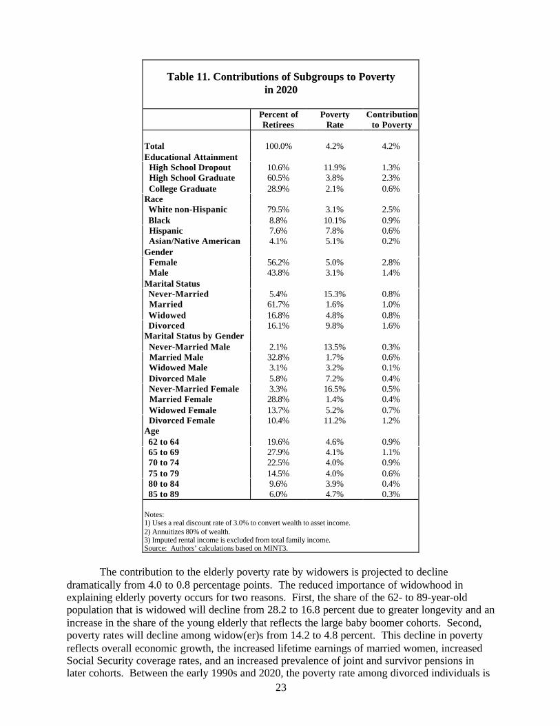
Between the early 1990s and 2020, the poverty rate among high school dropouts in the62- to 89-year-old population is projected to decrease from 13.7 percent to 11.9 percent. Highschool dropouts will be a much smaller share of this population (40.7 percent in the early 1990scompared with 10.6 percent in 2020). Consequently, high school dropouts will contribute 4.3percentage points less to the poverty rate in 2020 (see Table 11) than they did in the early 1990s(1.3 percentage points in 2020 compared with 5.6 percentage points in the early 1990s). Thecontribution of high school graduates to poverty will increase from 1.9 to 2.3 percentage points,however, because both their poverty rate and their share of the total population will rise. Thecontribution of college graduates to poverty will also increase from 0.3 to 0.6 percentage points.Although their poverty rate remains just over 2 percent between the early 1990s and 2020,college graduates’ share of the population is projected to rise from 12.7 to 28.9 percent.

The contributions to poverty of all ethnic groups are projected to decline between theperiods, but they decline more in absolute terms for White non-Hispanics (from 4.8 to 2.5percentage points) than for other ethnic groups. The larger poverty reductions for minoritiescompared with White non-Hispanics are offset by increases in their population share, yieldingonly small reductions in the contribution to poverty among minorities. White non-Hispanicshave both declining poverty rates and a declining population share, which result in a largeroverall reduction in their contribution to poverty.

Females will contribute far less to overall poverty among the elderly in 2020 (2.8percentage points) than in the 1990s (5.9 percentage points), while the male contribution topoverty will decline only slightly from 1.9 percentage points in the early 1990s to 1.4 percentagepoints in 2020. This is the consequence of a large decline in the poverty rate of females and aslight decline in the poverty rate of males; population shares of the two groups change onlyslightly. Males will become a slightly larger share of the population because, as the group withthe shorter life expectancy, projected increases in longevity increase their numbers in a given agerange by relatively more than those for females.

23

Table 11. Contributions of Subgroups to Povertyin 2020

Percent ofRetirees

PovertyRate

Contributionto Poverty



The contribution to the elderly poverty rate by widowers is projected to declinedramatically from 4.0 to 0.8 percentage points. The reduced importance of widowhood inexplaining elderly poverty occurs for two reasons. First, the share of the 62- to 89-year-oldpopulation that is widowed will decline from 28.2 to 16.8 percent due to greater longevity and anincrease in the share of the young elderly that reflects the large baby boomer cohorts. Second,poverty rates will decline among widow(er)s from 14.2 to 4.8 percent. This decline in povertyreflects overall economic growth, the increased lifetime earnings of married women, increasedSocial Security coverage rates, and an increased prevalence of joint and survivor pensions inlater cohorts. Between the early 1990s and 2020, the poverty rate among divorced individuals is

24

also projected to fall by more than 50 percent from 20.9 to 9.8 percent; however, their share ofthe aged population poverty is projected to increase sharply from 7.2 to 16.1 percent. As aresult, divorced individuals will contribute slightly more to overall poverty in 2020 (1.6percentage points) than in the early 1990s (1.5 percentage points).

Finally, the contribution to poverty of all age groups will decline between the early 1990sand 2020, but it will decline more for older than for younger age groups. Both the oldest andyoungest age groups increase their share of the age 62- to 89-year-old population between theearly 1990s and 2020, due to increased longevity and the baby boom cohorts moving intoretirement. Seventy- to 84-year-olds will be a smaller share of the population and have lowerpoverty rates in 2020 than in the early 1990s. These age groups will experience larger reductionsin their contributions to poverty than both the 62- to 69-year-olds and those ages 85 and over.

5. Importance of Sources of Income in Reducing Poverty

As with the 62- to 89-year-old population in the early 1990s, we display the contributionof various sources of income to raising income above the poverty line for the same age groups in2020. We first calculate poverty rates including only Social Security income and earnings. Thenwe individually add other income sources and measure the marginal impact of each additionalincome source on family poverty rates.

With increases in Social Security benefits through wage growth and increased SocialSecurity coverage rates, Social Security and earnings alone are projected to keep all but 10.4percent of the aged population out of poverty in 2020, compared with 28.4 percent in the early1990s (see Table 12). After adding pensions and financial income, 5.8 percent of agedindividuals remain in poverty (compared with 15.6 percent based on the same income sources inthe early 1990s). While SSI is a small program in 2020, including it in the income measurefurther reduces poverty to 5.4 percent (compared with 14.4 percent in the early 1990s). Co-resident income remains an extremely important source of income for reducing poverty of theaged. When co-resident income is added, poverty is reduced to 4.2 percent in 2020, comparedwith 10.0 percent in the early 1990s.

VI. EFFECTS OF USING DIFFERENT INCOME AND POVERTYMEASURES

1. Effects of Alternative Ways of Measuring Income

The general trends in estimated income and poverty remain about the same when oneuses different income measures (Tables 13, 14, and 15). In Table 13, we display two separatemeasures of poverty for the early 1990s. The first measure, labeled “Census Measure,” uses theCensus definition of income from assets (based on nominal income from interest, dividends, andother property income). In the second measure, labeled “UI Measure,” we use our definition ofasset income (based on a real annuity income from 80 percent of financial assets). Because thelatter measure includes a return on capital, it increases poverty-adjusted family income by 0.16and reduces poverty by 0.2 percentage points. While income for all subgroups is higher for theUI measure than the Census measure, poverty isn’t lower for all subgroups. With the UImeasure, the poverty rate is higher for college graduates, Hispanics and Asian/Native Americans,never-married females, and the youngest age group.

25

Table 12. Marginal Contributions of Income Sources to Poverty in 20201

SocialSecurity

andEarnings

Add

Pensions

Add

FinancialIncome

Add

SSI

Add

Co-residentIncome

Total 10.4% 8.8% 5.8% 5.4% 4.2%Educational Attainment High School Dropout 25.2% 22.9% 18.2% 16.4% 11.9% High School Graduate 9.2% 7.7% 5.0% 4.8% 3.8% College Graduate 7.4% 6.1% 2.8% 2.7% 2.1%Race White non-Hispanic 8.2% 6.7% 4.0% 3.8% 3.1% Black 19.2% 16.6% 14.0% 13.6% 10.1% Hispanic 19.3% 17.8% 12.6% 11.0% 7.8% Asian/Native American 17.3% 15.6% 9.9% 8.1% 5.1%Gender Female 12.3% 10.4% 7.0% 6.6% 5.0% Male 7.8% 6.7% 4.1% 3.9% 3.1%Marital Status by Gender Never-Married Male 28.3% 25.8% 19.2% 18.7% 13.5% Married Male 4.9% 4.0% 2.2% 2.1% 1.7% Widowed Male 12.6% 10.7% 5.5% 4.7% 3.2% Divorced Male 14.8% 12.9% 8.6% 8.2% 7.2% Never-Married Female 34.1% 30.4% 25.3% 24.2% 16.5% Married Female 4.7% 3.8% 2.0% 1.7% 1.4% Widowed Female 14.9% 11.9% 7.5% 6.8% 5.2% Divorced Female 23.2% 20.7% 14.6% 14.3% 11.2%Age 62 to 64 10.1% 9.0% 6.1% 5.9% 4.6% 65 to 69 8.7% 7.9% 5.5% 5.2% 4.1% 70 to 74 9.7% 8.6% 5.5% 5.2% 4.0% 75 to 79 11.1% 9.4% 5.6% 5.2% 4.0% 80 to 84 13.3% 9.5% 6.0% 5.1% 3.9% 85 to 89 15.4% 11.0% 6.7% 5.9% 4.7%

Percentage Point Reduction -1.6% -3.0% -0.4% -1.2%Percent Reduction -15.4% -34.1% -6.9% -22.2%

1Poverty rates are calculated first including only Social Security and earnings. We add pensions, financial income, SSI, and co-resident income one at a time to measure the marginal impact of each income source to alleviating poverty.


26

Table 13. Average Family Income as a Percent of Poverty and Percent of RetireesBelow Poverty in the Early 1990s

(Comparison of Census and UI Measure)

Average Family Income /Poverty Threshold

Percent of RetireesBelow Poverty

CensusMeasure1

UIMeasure2 Difference

CensusMeasure1

UIMeasure2 Difference

Total 3.30 3.46 0.16 8.0% 7.8% -0.2%Educational Attainment High School Dropout 2.31 2.45 0.14 14.4% 13.7% -0.7% High School Graduate 3.55 3.72 0.17 4.0% 4.0% 0.0% College Graduate 5.53 5.77 0.23 1.9% 2.5% 0.6%Race White non-Hispanic 3.46 3.64 0.18 5.8% 5.6% -0.2% Black 2.12 2.18 0.06 24.4% 23.8% -0.6% Hispanic 2.26 2.33 0.07 18.7% 18.8% 0.1% Asian/Native American 3.22 3.31 0.10 11.1% 11.8% 0.7%Gender Female 3.04 3.19 0.15 10.4% 10.1% -0.3% Male 3.67 3.85 0.19 4.6% 4.5% -0.1%Marital Status Never-Married 2.57 2.65 0.08 17.9% 18.5% 0.6% Married 3.85 4.04 0.20 2.4% 2.3% -0.1% Widowed 2.47 2.59 0.13 14.8% 14.2% -0.6% Divorced 2.46 2.56 0.10 21.1% 20.9% -0.2%Marital Status by Gender Never-Married Male 2.58 2.68 0.10 16.0% 15.9% -0.1% Married Male 3.88 4.07 0.19 2.4% 2.3% -0.1% Widowed Male 3.10 3.31 0.21 8.3% 8.0% -0.3% Divorced Male 2.85 3.02 0.17 15.7% 15.2% -0.5% Never-Married Female 2.56 2.63 0.07 19.3% 20.5% 1.2% Married Female 3.80 4.01 0.20 2.5% 2.4% -0.1% Widowed Female 2.35 2.46 0.11 16.0% 15.3% -0.7% Divorced Female 2.22 2.27 0.05 24.5% 24.4% -0.1%Age 62 to 64 4.14 4.28 0.14 5.8% 6.2% 0.4% 65 to 69 3.48 3.60 0.12 6.6% 6.4% -0.2% 70 to 74 3.19 3.33 0.13 7.4% 7.1% -0.3% 75 to 79 3.05 3.22 0.17 8.9% 8.7% -0.2% 80 to 84 2.65 2.89 0.24 12.2% 11.6% -0.6% 85 to 89 2.52 2.93 0.41 11.8% 11.2% -0.6%

Notes:1 The Census measure uses nominal income from interest, dividends, and other property income to represent income from assets. It alsoexcludes imputed rental income from total family income.2 The UI measure uses a real discount rate of 3.0% to convert 80% of wealth to asset income. It also excludes imputed rental incomefrom total family income.

Source: Authors’ calculations based on 1990-1993 SIPP.

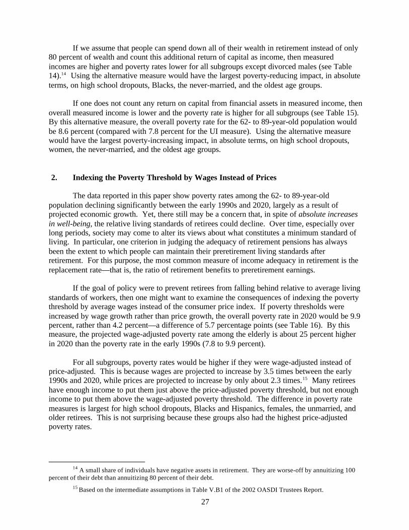
27

If we assume that people can spend down all of their wealth in retirement instead of only80 percent of wealth and count this additional return of capital as income, then measuredincomes are higher and poverty rates lower for all subgroups except divorced males (see Table14).14 Using the alternative measure would have the largest poverty-reducing impact, in absoluteterms, on high school dropouts, Blacks, the never-married, and the oldest age groups.

If one does not count any return on capital from financial assets in measured income, thenoverall measured income is lower and the poverty rate is higher for all subgroups (see Table 15).By this alternative measure, the overall poverty rate for the 62- to 89-year-old population wouldbe 8.6 percent (compared with 7.8 percent for the UI measure). Using the alternative measurewould have the largest poverty-increasing impact, in absolute terms, on high school dropouts,women, the never-married, and the oldest age groups.

2. Indexing the Poverty Threshold by Wages Instead of Prices

The data reported in this paper show poverty rates among the 62- to 89-year-oldpopulation declining significantly between the early 1990s and 2020, largely as a result ofprojected economic growth. Yet, there still may be a concern that, in spite of absolute increasesin well-being, the relative living standards of retirees could decline. Over time, especially overlong periods, society may come to alter its views about what constitutes a minimum standard ofliving. In particular, one criterion in judging the adequacy of retirement pensions has alwaysbeen the extent to which people can maintain their preretirement living standards afterretirement. For this purpose, the most common measure of income adequacy in retirement is thereplacement rate—that is, the ratio of retirement benefits to preretirement earnings.

If the goal of policy were to prevent retirees from falling behind relative to average livingstandards of workers, then one might want to examine the consequences of indexing the povertythreshold by average wages instead of the consumer price index. If poverty thresholds wereincreased by wage growth rather than price growth, the overall poverty rate in 2020 would be 9.9percent, rather than 4.2 percent—a difference of 5.7 percentage points (see Table 16). By thismeasure, the projected wage-adjusted poverty rate among the elderly is about 25 percent higherin 2020 than the poverty rate in the early 1990s (7.8 to 9.9 percent).

For all subgroups, poverty rates would be higher if they were wage-adjusted instead ofprice-adjusted. This is because wages are projected to increase by 3.5 times between the early1990s and 2020, while prices are projected to increase by only about 2.3 times.15 Many retireeshave enough income to put them just above the price-adjusted poverty threshold, but not enoughincome to put them above the wage-adjusted poverty threshold. The difference in poverty ratemeasures is largest for high school dropouts, Blacks and Hispanics, females, the unmarried, andolder retirees. This is not surprising because these groups also had the highest price-adjustedpoverty rates.

14 A small share of individuals have negative assets in retirement. They are worse-off by annuitizing 100

percent of their debt than annuitizing 80 percent of their debt.15 Based on the intermediate assumptions in Table V.B1 of the 2002 OASDI Trustees Report.

28

Table 14. Average Family Income as a Percent of Povertyand Percent of Retirees Below Poverty in the Early 1990s

(Comparison of Annuitization of 80% and 100% of Asset Income)



UI Measure1

(80%)

AlternativeMeasure2

(100%) Difference

UIMeasure1

(80%)

AlternativeMeasure2

(100%) Difference

Total 3.46 3.63 0.17 7.8% 7.5% -0.3%Educational Attainment High School Dropout 2.45 2.54 0.09 13.7% 13.4% -0.3% High School Graduate 3.72 3.90 0.18 4.0% 3.9% -0.1% College Graduate 5.77 6.11 0.35 2.5% 2.3% -0.2%Race White non-Hispanic 3.64 3.83 0.19 5.6% 5.4% -0.2% Black 2.18 2.21 0.03 23.8% 23.5% -0.3% Hispanic 2.33 2.38 0.05 18.8% 18.6% -0.2% Asian/Native American 3.31 3.40 0.09 11.8% 11.8% 0.0%Gender Female 3.19 3.34 0.15 10.1% 9.8% -0.3% Male 3.85 4.04 0.19 4.5% 4.3% -0.2%Marital Status Never-Married 2.65 2.77 0.11 18.5% 17.8% -0.7% Married 4.04 4.25 0.21 2.3% 2.2% -0.1% Widowed 2.59 2.71 0.12 14.2% 13.8% -0.4% Divorced 2.56 2.64 0.08 20.9% 20.6% -0.3%Marital Status by Gender Never Married Male 2.68 2.82 0.13 15.9% 15.1% -0.8% Married Male 4.07 4.27 0.20 2.3% 2.2% -0.1% Widowed Male 3.31 3.49 0.18 8.0% 7.8% -0.2% Divorced Male 3.02 3.12 0.11 15.2% 15.4% 0.2% Never-Married Female 2.63 2.73 0.10 20.5% 20.0% -0.5% Married Female 4.01 4.22 0.21 2.4% 2.3% -0.1% Widowed Female 2.46 2.57 0.11 15.3% 15.0% -0.3% Divorced Female 2.27 2.34 0.06 24.4% 23.9% -0.5%Age 62 to 64 4.28 4.43 0.14 6.2% 5.9% -0.3% 65 to 69 3.60 3.76 0.15 6.4% 6.3% -0.1% 70 to 74 3.33 3.49 0.16 7.1% 6.8% -0.3% 75 to 79 3.22 3.41 0.19 8.7% 8.4% -0.3% 80 to 84 2.89 3.08 0.19 11.6% 11.3% -0.3% 85 to 89 2.93 3.16 0.23 11.2% 10.7% -0.5%

Notes:1 The UI measure uses a real discount rate of 3.0% to convert 80% of wealth to asset income. It also excludes imputed rental incomefrom total family income.2 The alternative measure uses a real discount rate of 3.0% to convert 100% of wealth to asset income. It also excludes imputed rentalincome from total family income.


29

Table 15. Average Family Income as a Percent of Povertyand Percent of Retirees Below Poverty in the Early 1990s

(Comparison of Income With and Without a Return of Capital)



UIMeasure1

(With)

AlternativeMeasure2

(Without) Difference

UIMeasure1

(With)

AlternativeMeasure2

(Without) Difference

Total 3.46 3.08 -0.39 7.8% 8.6% 0.8%Educational Attainment High School Dropout 2.45 2.21 -0.24 13.7% 15.2% 1.5% High School Graduate 3.72 3.30 -0.42 4.0% 4.6% 0.6% College Graduate 5.77 5.02 -0.75 2.5% 2.5% 0.0%Race White non-Hispanic 3.64 3.21 -0.43 5.6% 6.5% 0.9% Black 2.18 2.10 -0.07 23.8% 24.6% 0.8% Hispanic 2.33 2.22 -0.11 18.8% 19.5% 0.7% Asian/Native American 3.31 3.12 -0.19 11.8% 12.4% 0.6%Gender Female 3.19 2.84 -0.35 10.1% 11.3% 1.2% Male 3.85 3.42 -0.43 4.5% 4.9% 0.4%Marital Status Never-Married 2.65 2.38 -0.27 18.5% 20.7% 2.2% Married 4.04 3.58 -0.46 2.3% 2.7% 0.4% Widowed 2.59 2.29 -0.30 14.2% 16.0% 1.8% Divorced 2.56 2.38 -0.18 20.9% 22.0% 1.1%Marital Status by Gender Never-Married Male 2.68 2.37 -0.31 15.9% 17.7% 1.8% Married Male 4.07 3.63 -0.45 2.3% 2.6% 0.3% Widowed Male 3.31 2.80 -0.50 8.0% 8.8% 0.8% Divorced Male 3.02 2.77 -0.25 15.2% 16.2% 1.0% Never-Married Female 2.63 2.39 -0.24 20.5% 22.9% 2.4% Married Female 4.01 3.53 -0.47 2.4% 2.8% 0.4% Widowed Female 2.46 2.20 -0.26 15.3% 17.3% 2.0% Divorced Female 2.27 2.14 -0.14 24.4% 25.6% 1.2%Age 62 to 64 4.28 4.03 -0.25 6.2% 6.2% 0.0% 65 to 69 3.60 3.30 -0.30 6.4% 6.8% 0.4% 70 to 74 3.33 2.96 -0.37 7.1% 7.7% 0.6% 75 to 79 3.22 2.73 -0.49 8.7% 9.7% 1.0% 80 to 84 2.89 2.36 -0.53 11.6% 14.2% 2.6% 85 to 89 2.93 2.24 -0.70 11.2% 13.9% 2.7%

Notes:1 The UI measure uses a real discount rate of 3.0% to convert 80% of wealth to asset income. It also excludes imputed rental incomefrom total family income.2 The alternative measure does not include any return on capital from asset income. It also excludes imputed rental income from totalfamily income.


30

Table 16. Price-Adjusted and Wage-Adjusted PovertyRates in 2020

Price-AdjustedPoverty

Wage-AdjustedPoverty Difference



VII. CONTRIBUTIONS OF ECONOMIC, DEMOGRAPHIC, ANDPOLICY CHANGES TO POVERTY IN 2020

In this section we consider how projections of future poverty rates are influenced bychanges in the Social Security NRA, the proportion of retirees who are unmarried, and averagerelative earnings and earnings inequality for post-1950 birth cohorts. We present results for bothprice-adjusted and wage-adjusted poverty rates. Our discussion will focus on how thesimulations affect wage-adjusted poverty rates.

31

1. Effects of Changes in the Normal Retirement Age

First, we consider what the poverty rate in 2020 would be if the NRA were not scheduledto increase. Under Social Security rules, individuals are paid their full Social Security benefit ifthey delay benefit take-up until the NRA. Individuals may take up benefits before the NRA(beginning at age 62), but annual benefits are then reduced to adjust for the fact that early retireesreceive benefits over a longer period.

The NRA is 65 for retirees born before 1938, and is scheduled to increase for those bornin the year 1938 or later. Table 17 describes how the NRA changes by year of birth. As long asindividuals wait until their NRA to collect Social Security benefits, they will receive the fullamount of their benefits. Currently, most individuals do not wait until age 65 to collect SocialSecurity retirement benefits. In 1999, more than half of the benefits awarded were to retireeswho opted to begin receiving Social Security benefits at age 62—despite the reduction inbenefits (Social Security Administration 2000, Table 6.A4).16 For individuals who retired in1999 (born prior to 1938), annual benefits can be reduced by as much as 20 percent for earlyretirement. As Table 17 shows, the annual benefit reduction for take-up at age 62 will be evengreater for retirees born in 1938 or later. Early retirees in the 2020 population will have theirbenefits reduced by as much as 28.3 percent. Those born in 1960 or later will have their benefitsreduced by as much as 30 percent.

Table 17. NRA and Social Security ReductionFactors by Year of Birth

Birthyear NRA

Reduction forTake-up at Age

62

1926-1937 65 20.0%1938 65.17 20.8%1939 65.33 21.7%1940 65.50 22.5%1941 65.67 23.3%1942 65.83 24.2%1943-1954 66 25.0%1955 66.17 25.8%1956 66.33 26.7%1957 66.50 27.5%1958 66.67 28.3%1959 66.83 29.2%1960+ 67 30.0%

Source: Social Security Administration (2000).

16 This figure represents retired-worker benefits only and includes conversions from nondisabled

widow(er)’s benefits to higher retired-worker benefits.

32

To simulate the effects of changes in the NRA, we calculate the impact of restoring theNRA to age 65, so that the benefits of those who retire at age 62 will be reduced by only 20percent. In this simulation, we continue to incorporate the MINT projections of changes amongcohorts in their lifetime earnings patterns and demographic characteristics. Though it is notrealistic, we also assume that individuals do not change their retirement behavior in response to achange in the NRA. The result should give us the marginal effect on 2020 poverty of changes inthe NRA for more recent birth cohorts. We expect that restoring the NRA to age 65 will reduceprojected poverty rates in 2020 by raising Social Security benefits for early retirees born in 1938or later.17

This is, in fact, the result we find. If the NRA were restored to 65, the overall wage-adjusted poverty rate in 2020 would be 9.3 percent—0.6 percentage points lower than thebaseline poverty rate that MINT projects (see Table 18). Poverty rates would be lower for allsubgroups of the population. While the NRA remains unchanged for individuals age 82 andolder in 2020, some of these older individuals will have younger spouses receiving reducedbenefits, and so their poverty is still slightly decreased by the simulation.

Changes in the NRA have differential effects on poverty rates among different subgroupsof the retiree population. Among racial and ethnic groups, the impact of increasing the NRA islarger for Hispanic retirees (from 18.5 percent to 17.4 percent) and for Asian/Native Americanretirees (from 11.9 percent to 11.1 percent) than for White non-Hispanic and Black retirees.Among marital status/gender groups, divorced women and never-married and divorced men areprojected to experience the largest absolute decline in their poverty rates. The projected povertyrate of divorced females declines from 22.9 percent under current law to 21.8 percent without theincrease in the NRA. Projected poverty rates also decline for never-married males (from 22.5 to21.1 percent) and divorced males (from 15.9 to 14.7 percent) without the increase in the NRA.These results suggest that the reduction in the current law Social Security replacement rate willpush a greater proportion of individuals with the lowest incomes below the poverty line. (Notethat Social Security benefits are actually rising over time under current law because of wageindexing; the increase in the NRA, however, lowers the ratio of benefits to Social Securityaverage indexed monthly earnings—AIME).

2. Effects of Changes in Marital Composition of Retirees Between Early 1990s and2020.

Second, we consider what the poverty rate in 2020 would be if the marital composition ofretirees in 2020 looked like that of retirees in 1990. Table 19 compares the marital compositionof retirees in the early 1990’s computed from SIPP data with the projected marital compositionof retirees in 2020 using the MINT projections. The findings suggest that future retirees aremore likely than their predecessors to be divorced and less likely to be widowed. The projectedchange is more pronounced for female retirees than for male retirees. The projected share ofdivorced females in the 2020 retiree population is nearly 2.5 times higher than the share for theircounterparts in the 1990 retiree population. Furthermore, the proportion of widowed females inthe 2020 retiree population is projected to be 60 percent of what it was in the 1990 retireepopulation. Finally, a larger share of female retirees will have never married in 2020 than in theearly 1990s. There are also pronounced differences in the marital composition of age groups.While the proportion of both widows and widowers increase at older ages, at all ages females are

17 If individuals retire earlier in response to a reduction in the NRA, then the lower NRA will not raise theirincomes or reduce poverty by as much as we estimate in the absence of this behavior.

33

much more likely to be widowed than males. For the oldest age group, 35.9 percent of maleswere widowed in the early 1990s compared to 80.6 percent of females. These large differencesare also expected for the future. These projections have implications for Social Security benefits,private pensions, and economic well-being in retirement.

Table 18. Simulation of the NRA at Age 65

Price Adjusted Poverty Wage Adjusted PovertyBase Sim. Impact Base Sim. Impact

Total 4.2% 3.9% -0.3% 9.9% 9.3% -0.6%Educational Attainment High School Dropout 11.9% 11.5% -0.4% 25.4% 24.2% -1.2% High School Graduate 3.8% 3.5% -0.3% 9.6% 8.9% -0.7% College Graduate 2.1% 2.0% -0.1% 4.8% 4.6% -0.2%Race White non-Hispanic 3.1% 2.9% -0.2% 7.7% 7.2% -0.5% Black 10.1% 9.6% -0.5% 21.4% 20.7% -0.7% Hispanic 7.8% 7.2% -0.6% 18.5% 17.4% -1.1% Asian/Native American 5.1% 5.0% -0.1% 11.9% 11.1% -0.8%Gender Female 5.0% 4.7% -0.3% 11.8% 11.2% -0.6% Male 3.1% 2.9% -0.2% 7.5% 6.8% -0.7%Marital Status Never Married 15.3% 14.8% -0.5% 25.8% 25.0% -0.8% Married 1.6% 1.4% -0.2% 4.5% 4.0% -0.5% Widowed 4.8% 4.6% -0.2% 14.4% 14.0% -0.4% Divorced 9.8% 9.0% -0.8% 20.4% 19.3% -1.1%Marital Status by Gender Never Married Male 13.5% 12.7% -0.8% 22.5% 21.1% -1.4% Married Male 1.7% 1.6% -0.1% 4.8% 4.3% -0.5% Widowed Male 3.2% 2.9% -0.3% 10.4% 9.7% -0.7% Divorced Male 7.2% 6.6% -0.6% 15.9% 14.7% -1.2% Never Married Female 16.5% 16.1% -0.4% 28.0% 27.5% -0.5% Married Female 1.4% 1.2% -0.2% 4.3% 3.8% -0.5% Widowed Female 5.2% 5.0% -0.2% 15.3% 14.9% -0.4% Divorced Female 11.2% 10.3% -0.9% 22.9% 21.8% -1.1%Age 62 to 64 4.6% 4.5% -0.1% 9.2% 8.7% -0.5% 65 to 69 4.1% 3.7% -0.4% 9.6% 8.8% -0.8% 70 to 74 4.0% 3.7% -0.3% 9.6% 8.9% -0.7% 75 to 79 4.0% 3.6% -0.4% 10.4% 9.6% -0.8% 80 to 84 3.9% 3.8% -0.1% 11.1% 11.0% -0.1% 85 to 89 4.7% 4.7% 0.0% 11.8% 11.8% 0.0%

Notes:1) Uses a real discount rate of 3.0% to convert wealth to asset income.2) Annuitizes 80% of wealth.3) Imputed rental income is excluded from total family income.4) No behavioral response to the change in the normal retirement age.Source: Authors’ calculations based on MINT3.

34

Table 19. Marital Status of Retirees in 1990 and 2020,by Age and Sex

Male Female1990 2020 1990 2020

All Never Married 4.9% 4.8% 4.4% 5.8% Married 77.7% 75.0% 47.5% 51.3% Widowed 10.8% 7.1% 40.5% 24.4% Divorced 6.6% 13.1% 7.5% 18.4% All 100.0% 100.0% 100.0% 100.0%62-64 Never Married 4.6% 6.6% 3.2% 7.6% Married 80.9% 74.6% 61.4% 61.5% Widowed 4.6% 4.1% 23.4% 11.8% Divorced 9.9% 14.7% 11.9% 19.1% All 100.0% 100.0% 100.0% 100.0%65-69 Never Married 6.1% 5.7% 4.4% 7.0% Married 79.7% 74.8% 57.5% 58.2% Widowed 6.2% 5.8% 28.8% 15.5% Divorced 7.9% 13.7% 9.2% 19.2% All 100.0% 100.0% 100.0% 100.0%70-74 Never Married 4.1% 4.0% 4.4% 5.3% Married 80.2% 74.3% 47.9% 52.0% Widowed 10.7% 7.7% 41.2% 22.6% Divorced 5.0% 13.9% 6.6% 20.0% All 100.0% 100.0% 100.0% 100.0%75-79 Never Married 4.8% 3.4% 4.6% 4.4% Married 74.4% 74.1% 36.1% 45.5% Widowed 16.1% 10.6% 53.5% 31.9% Divorced 4.8% 11.9% 5.8% 18.1% All 100.0% 100.0% 100.0% 100.0%80-84 Never Married 3.5% 2.8% 5.4% 4.4% Married 67.7% 77.3% 21.9% 38.3% Widowed 24.9% 10.3% 68.4% 41.0% Divorced 3.8% 9.6% 4.3% 16.3% All 100.0% 100.0% 100.0% 100.0%85+ Never Married 3.4% 2.5% 5.1% 3.8% Married 58.9% 79.5% 11.2% 30.5% Widowed 35.9% 10.5% 80.6% 52.9% Divorced 1.8% 7.6% 3.2% 12.9% All 100.0% 100.0% 100.0% 100.0%

Source: Authors’ calculations based on 1990-1993 SIPP and MINT3 data.

35

The Social Security Administration pays retired-worker benefits, which are based on anindividual’s earnings history, to insured retirees. Because of auxiliary benefits, marital historyalso plays an important role in the computation of Social Security benefits. Individuals who arenot insured based on their earnings may still be eligible for auxiliary benefits as (ex-)spouses orsurviving (ex-)spouses of retired workers. These benefits are based on the earnings history of aliving or deceased (ex-)spouse. When she becomes widowed, a woman may receive up to twiceas much in auxiliary benefits as she did when she was married. The same is true for a divorcedwoman when her ex-husband dies. However, in order to qualify for any auxiliary benefits,divorced individuals must have been married to their living or deceased ex-spouses for at leastten years. Finally, because auxiliary benefits are paid only to those currently or previouslymarried, individuals who never married are only eligible for retired-worker benefits atretirement. As the marital composition of retirees shifts toward more never-married anddivorced individuals, auxiliary benefits received will decline, for any given amount of a worker’sown earnings. Therefore, we expect projected changes in the marital composition of thepopulation to increase poverty rates among future retirees, particularly for women.

The simulation we perform re-weights the 2020 population to produce the same maritalcomposition within each sex and age group as existed in the early 1990s, holding constantaverage earnings and the distribution of average earnings in 2020. In most sex and age groups,this involves increasing the share of retirees who are married or widowed and decreasing theshare of retirees who are never-married or divorced. With this simulation we incorporate theprojected changes across cohorts in the NRA and lifetime earnings patterns. The result gives usthe marginal effect on 2020 poverty of changes in mortality and marital status for more recentbirth cohorts. We expect poverty to be lower under the simulation because there will be fewerunmarried retirees.

If the marital composition of the 2020 retiree population were identical to that of the1990’s retiree population, the result is that overall wage-adjusted poverty in 2020 would be 9.4percent—0.5 percentage points lower than the baseline projection (see Table 20). Compared tothe baseline, the simulation decreases the wage-adjusted poverty rate of individuals between age62 and 74 and increases the wage-adjusted poverty rate of individuals age 80 and older. In thesimulation, poverty rates decrease for the younger group because more of them are married withlower poverty rates and fewer are divorced with higher poverty rates. Poverty rates increase forthe older group because more of them are widowed with higher poverty rates and fewer aremarried with lower poverty rates. Because the younger group is larger than the older group in2020, the simulated reduction in the wage-adjusted poverty rates of the younger group dominatesthe increase in the poverty rates of the older group, and the overall poverty rate declines.

The simulation has the greatest impact on never-married females whose poverty rateincreases 1.3 percentage points—from 28.0 percent under the baseline projections to 29.3percent under the simulation. The simulation decreases the share of younger never-marriedfemales—those with higher incomes and lower poverty rates—and increases the share of oldernever-married females—those with lower incomes and higher poverty rates—to reflect the 1990composition. The result is an increase in the overall poverty rate of never-married females. Asimilar story explains the simulation's projected increase in the poverty rates of never marriedmen.

36

Table 20. Simulation Holding the Marital Composition of 1990 Constant

Percent ofRetirees Price Adjusted Poverty Wage Adjusted Poverty

Base Sim. Base Sim. Impact Base Sim. Impact

Total 100.0% 100.0% 4.2% 3.7% -0.5% 9.9% 9.4% -0.5%Educational Attainment High School Dropout 10.6% 11.1% 11.9% 11.0% -0.9% 25.4% 25.1% -0.3% High School Graduate 60.5% 60.5% 3.8% 3.3% -0.5% 9.6% 8.8% -0.8% College Graduate 28.9% 28.3% 2.1% 1.8% -0.3% 4.8% 4.3% -0.5%Race White non-Hispanic 79.5% 79.3% 3.1% 2.7% -0.4% 7.7% 7.1% -0.6% Black 8.8% 8.7% 10.1% 9.3% -0.8% 21.4% 20.9% -0.5% Hispanic 7.6% 7.7% 7.8% 7.0% -0.8% 18.5% 17.8% -0.7% Asian/Native American 4.1% 4.3% 5.1% 5.5% 0.4% 11.9% 12.3% 0.4%Gender Female 56.2% 56.2% 5.0% 4.4% -0.6% 11.8% 11.3% -0.5% Male 43.8% 43.8% 3.1% 2.8% -0.3% 7.5% 6.9% -0.6%Marital Status Never Married 5.4% 4.6% 15.3% 15.9% 0.6% 25.8% 26.6% 0.8% Married 61.7% 59.6% 1.6% 1.6% 0.0% 4.5% 4.4% -0.1% Widowed 16.8% 28.7% 4.8% 4.7% -0.1% 14.4% 14.2% -0.2% Divorced 16.1% 7.2% 9.8% 9.8% 0.0% 20.4% 19.8% -0.6%Marital Status by Gender Never Married Male 2.1% 2.1% 13.5% 13.7% 0.2% 22.5% 23.5% 1.0% Married Male 32.8% 33.9% 1.7% 1.7% 0.0% 4.8% 4.6% -0.2% Widowed Male 3.1% 4.8% 3.2% 2.9% -0.3% 10.4% 10.1% -0.3% Divorced Male 5.8% 2.9% 7.2% 7.4% 0.2% 15.9% 15.7% -0.2% Never Married Female 3.3% 2.5% 16.5% 17.7% 1.2% 28.0% 29.3% 1.3% Married Female 28.8% 25.6% 1.4% 1.4% 0.0% 4.3% 4.2% -0.1% Widowed Female 13.7% 23.8% 5.2% 5.1% -0.1% 15.3% 15.1% -0.2% Divorced Female 10.4% 4.3% 11.2% 11.3% 0.1% 22.9% 22.5% -0.4%Age 62 to 64 19.6% 19.6% 4.6% 3.8% -0.8% 9.2% 8.1% -1.1% 65 to 69 27.9% 27.9% 4.1% 3.4% -0.7% 9.6% 8.7% -0.9% 70 to 74 22.5% 22.5% 4.0% 3.5% -0.5% 9.6% 8.4% -1.2% 75 to 79 14.5% 14.5% 4.0% 3.6% -0.4% 10.4% 10.4% 0.0% 80 to 84 9.6% 9.6% 3.9% 4.1% 0.2% 11.1% 12.3% 1.2% 85 to 89 6.0% 6.0% 4.7% 5.2% 0.5% 11.8% 13.2% 1.4%


37

3. Effects of Changes in Relative Earnings for Post-1950 Birth Cohorts

Third, we consider what the poverty rate in 2020 would be if those born after 1950 hadthe same relative earnings as those born before 1950.18 Table 21 reports projected averagerelative lifetime earnings by cohort in the MINT data. The data suggest that average lifetimeearnings in relation to the national average wage will increase for retirees in each successivecohort born between 1931 and 1950, after which average lifetime earnings will decline slightly.The data also underscore changes between male and female earnings patterns. Male retireesborn after 1945 are projected to have lower average lifetime earnings than do their predecessors,while female retirees born after 1945 are projected to have higher average lifetime earnings thantheir predecessors.

Table 21. Average Lifetime Earnings, by Cohort

1931-35 1936-40 1941-45 1946-50 1951-55 1956-60

All 0.67 0.72 0.75 0.80 0.79 0.78Male 1.05 1.08 1.08 1.06 1.01 0.97Female 0.32 0.38 0.45 0.55 0.58 0.60

Note: Average lifetime earnings are computed as the average of relative earnings from age 22 through age 62.Source: Authors’ calculations based on the MINT3 data.

The simulation is to make the average earnings of male and female retirees in the post-1950 cohorts look like the average earnings of their counterparts born between 1946 and 1950.To do this, we increase average lifetime earnings for male retirees born after 1950 and decreaseaverage lifetime earnings for female retirees born after 1950. We continue to incorporateprojected changes in the NRA, the dispersion of earnings within cohorts, and demographiccharacteristics. The result gives us the marginal effect on 2020 poverty of undoing changes inaverage lifetime earnings relative to the national average wage for more recent birth cohorts.

Table 22 reports the results of the simulation. We find that giving post-1950 birthcohorts the same relative average lifetime earnings as those born between 1946 and 1950 wouldhave no impact on the overall wage-adjusted poverty rate. This finding may appearcounterintuitive because the simulation raises lifetime earnings of the entire population byundoing the decline in relative earnings for those born after 1950. But the decrease in povertyfrom the increase in earnings of males is almost entirely offset by the increase in poverty fromthe decrease in earnings of females. This is because women contribute more to the overallpoverty rate in 2020 than men by constituting a larger share of the population and by beingnearly twice as likely as to be poor in retirement (see Table 11). Restoring the average earningsof earlier cohorts to those of later cohorts has the greatest adverse impact on Asian/NativeAmericans and never-married females—increasing their poverty rates by 0.3 percentage points.The simulation has the greatest positive impact on never-married males—decreasing theirpoverty rate by 0.9 percentage points.

18 As discussed above in the methodology section, MINT projects the ratio of earnings to the national

average wage.

38

Table 22. Simulation Holding Earnings Constant Between Cohorts


Total 4.2% 4.2% 0.0% 9.9% 9.9% 0.0%Educational Attainment High School Dropout 11.9% 11.8% -0.1% 25.4% 25.0% -0.4% High School Graduate 3.8% 3.9% 0.1% 9.6% 9.6% 0.0% College Graduate 2.1% 2.2% 0.1% 4.8% 5.0% 0.2%Race White non-Hispanic 3.1% 3.2% 0.1% 7.7% 7.7% 0.0% Black 10.1% 10.1% 0.0% 21.4% 21.5% 0.1% Hispanic 7.8% 8.0% 0.2% 18.5% 18.3% -0.2% Asian/Native American 5.1% 5.3% 0.2% 11.9% 12.2% 0.3%Gender Female 5.0% 5.1% 0.1% 11.8% 11.8% 0.0% Male 3.1% 3.1% 0.0% 7.5% 7.4% -0.1%Marital Status Never Married 15.3% 15.7% 0.4% 25.8% 25.7% -0.1% Married 1.6% 1.6% 0.0% 4.5% 4.5% 0.0% Widowed 4.8% 4.8% 0.0% 14.4% 14.3% -0.1% Divorced 9.8% 9.9% 0.1% 20.4% 20.5% 0.1%Marital Status by Gender Never Married Male 13.5% 12.7% -0.8% 22.5% 21.6% -0.9% Married Male 1.7% 1.7% 0.0% 4.8% 4.7% -0.1% Widowed Male 3.2% 3.0% -0.2% 10.4% 10.2% -0.2% Divorced Male 7.2% 7.2% 0.0% 15.9% 15.8% -0.1% Never Married Female 16.5% 17.6% 1.1% 28.0% 28.3% 0.3% Married Female 1.4% 1.4% 0.0% 4.3% 4.3% 0.0% Widowed Female 5.2% 5.2% 0.0% 15.3% 15.2% -0.1% Divorced Female 11.2% 11.4% 0.2% 22.9% 23.0% 0.1%Age 62 to 64 4.6% 4.7% 0.1% 9.2% 9.1% -0.1% 65 to 69 4.1% 4.2% 0.1% 9.6% 9.5% -0.1% 70 to 74 4.0% 4.0% 0.0% 9.6% 9.5% -0.1% 75 to 79 4.0% 4.0% 0.0% 10.4% 10.5% 0.1% 80 to 84 3.9% 3.9% 0.0% 11.1% 11.1% 0.0% 85 to 89 4.7% 4.8% 0.1% 11.8% 11.8% 0.0%


4. Effects of Changes in the Earnings Distribution for Post-1950 Birth Cohorts

Finally, we examine what would happen to the poverty rate in 2020 if those born after1950 had the earnings distribution of those born between 1946 and 1950. Projections of averagelifetime earnings in the MINT data indicate that the earnings distribution will be less dispersedfor post-1950 cohorts than it was for earlier cohorts—suggesting less earnings inequality amongpost-1950 cohorts (see Table 23). The findings also highlight changes in the lifetime earningsdistributions between male and female retirees. The distribution of average lifetime earnings is

39

projected to be more dispersed for male retirees in the post-1950 cohorts (more inequality) andless dispersed for female retirees in the post-1950 cohorts (less inequality).

Table 23. Distribution of Average Lifetime Earnings, by Cohort

Ratio of Fifth toFirst Quintile 1926-35 1936-40 1941-45 1946-50 1951-55 1956-60

All 13.90 11.82 12.39 13.04 13.09 12.56Male 9.71 8.37 9.26 10.49 11.08 10.77Female 104.13 50.78 28.48 20.36 17.49 16.09

Note: Average lifetime earnings are computed as the average of relative earnings from age 22 through age 62.Source: Authors’ calculations based on the MINT data.

The simulation is to make the earnings distribution of male and female retirees in thepost-1950 cohorts look like the earnings distribution of their counterparts born between 1946 and1950, holding average earnings within each cohort constant. For male retirees in the post-1950cohorts, this means increasing the average lifetime earnings of those in the bottom quintiles anddecreasing the average lifetime earnings of those in the top quintiles. For female retirees in thepost-1950 cohorts, this means decreasing the average lifetime earnings of those in the bottomquintiles and increasing the average lifetime earnings of those in the top quintiles. Within eachcohort, we hold average lifetime earnings constant. With this simulation we incorporate thechanges between cohorts in their NRA, average lifetime earnings, and demographiccharacteristics that MINT projects. The result gives us the marginal effect on 2020 poverty ofchanges in the distribution of lifetime earnings for more recent birth cohorts.

We find that changes in the lifetime earnings distribution have no impact on the overallwage-adjusted poverty rate (see Table 24). For most subgroups of the population, the impact ofthe simulation is negligible. The simulation slightly increases the poverty rates of collegegraduates (from 4.8 to 4.9 percent) and Asian/Native American retirees (from 11.9 to 12.1percent). This suggests that the distribution of average lifetime earnings of members of thesesubgroups has changed since the 1946-50 cohorts—with fewer of their members located in thebottom income quintile. As a result, imposing a 1946-50 lifetime earnings distribution on thepost-1950 cohorts pushes a number of these people into poverty.

VIII. CONCLUSIONS

The Social Security Administration’s Model of Income in the Near Term (MINT)projects that the overall price-adjusted poverty rate of the aged population will decline from 7.8percent in the early 1990s to 4.2 percent in 2020 (a 46 percent reduction). For most subgroups ofthe 2020 retiree population, poverty rates are projected to be lower than for their predecessors.Despite increased earnings of women and projected real wage growth, however, some subgroupsof the population will continue to experience persistently high poverty rates in the future. Withincreases in Social Security benefits through wage growth and increased Social Security

40

coverage rates, Social Security and earnings alone are projected to keep all but 10 percent of theaged population out of poverty in 2020—a drop from 28 percent in the early 1990s.

Table 24. Simulation Holding the Earnings Distribution ConstantBetween Cohorts


Total 4.2% 4.3% 0.1% 9.9% 9.9% 0.0%Educational Attainment High School Dropout 11.9% 11.9% 0.0% 25.4% 25.3% -0.1% High School Graduate 3.8% 3.9% 0.1% 9.6% 9.6% 0.0% College Graduate 2.1% 2.2% 0.1% 4.8% 4.9% 0.1%Race White non-Hispanic 3.1% 3.2% 0.1% 7.7% 7.7% 0.0% Black 10.1% 10.1% 0.0% 21.4% 21.4% 0.0% Hispanic 7.8% 7.9% 0.1% 18.5% 18.2% -0.3% Asian/Native American 5.1% 5.4% 0.3% 11.9% 12.1% 0.2%Gender Female 5.0% 5.1% 0.1% 11.8% 11.7% -0.1% Male 3.1% 3.2% 0.1% 7.5% 7.5% 0.0%Marital Status Never Married 15.3% 15.7% 0.4% 25.8% 25.8% 0.0% Married 1.6% 1.6% 0.0% 4.5% 4.5% 0.0% Widowed 4.8% 4.9% 0.1% 14.4% 14.3% -0.1% Divorced 9.8% 9.9% 0.1% 20.4% 20.3% -0.1%Marital Status by Gender Never Married Male 13.5% 13.4% -0.1% 22.5% 22.4% -0.1% Married Male 1.7% 1.8% 0.1% 4.8% 4.8% 0.0% Widowed Male 3.2% 3.0% -0.2% 10.4% 10.4% 0.0% Divorced Male 7.2% 7.4% 0.2% 15.9% 15.8% -0.1% Never Married Female 16.5% 17.2% 0.7% 28.0% 27.9% -0.1% Married Female 1.4% 1.4% 0.0% 4.3% 4.2% -0.1% Widowed Female 5.2% 5.3% 0.1% 15.3% 15.2% -0.1% Divorced Female 11.2% 11.3% 0.1% 22.9% 22.8% -0.1%Age 62 to 64 4.6% 4.9% 0.3% 9.2% 9.2% 0.0% 65 to 69 4.1% 4.1% 0.0% 9.6% 9.5% -0.1% 70 to 74 4.0% 4.0% 0.0% 9.6% 9.5% -0.1% 75 to 79 4.0% 4.0% 0.0% 10.4% 10.4% 0.0% 80 to 84 3.9% 3.9% 0.0% 11.1% 11.1% 0.0% 85 to 89 4.7% 4.8% 0.1% 11.8% 11.8% 0.0%


This paper examines the factors affecting the projected changes in poverty among 62- to89-year-olds between the early 1990s and 2020. We focus on five possible factors: changes inwage growth, scheduled increases in the NRA, changes in the marital composition of futureretirees, and changes in the level and distribution of earnings among more recent birth cohorts.Not surprisingly, projections of overall real wage growth—determined outside of MINT—have

41

the largest effect on poverty rates in 2020. When we assume that poverty thresholds increasewith wages, instead of prices, projected overall poverty rates increase by 2.1 percentage points to9.9 percent in 2020 instead of declining by 3.6 percentage points to 4.2 percent. The hardest hitby the rise in wage-adjusted poverty would be those groups already at risk of absolute poverty—high school dropouts, Blacks and Hispanics, women, the unmarried, and the oldest of the agedpopulation.

Controlling for wage growth, we find that projected changes in poverty rates wereaffected much more by projected changes in the NRA and marriage patterns than by changes inearnings patterns. When we restored the NRA to age 65, thereby reducing the early retirementpenalty to Social Security benefits, we found that overall wage-adjusted poverty rates decreasedby 0.6 percentage points. By imposing the gender/age/marital status composition of the early1990s retirees on the 2020 retirees, we found that overall wage-adjusted poverty rates decreasedby 0.5 percentage points. Changes in the distribution of earnings between and within cohortshad no effect on future poverty rates.

Changes in the relative earnings of men and women had little impact on wage-adjustedpoverty rates, because the increases in female earnings were largely offset by decreases in maleearnings. Also, changes in the distribution of earnings had little impact on wage-adjustedpoverty rates partly because of the progressive Social Security payment formula. This formulareplaces a greater share of earnings for those in the bottom of the earnings distribution and alower share of earnings for those in the top of the distribution. The progressive payment formulamakes postretirement income much more equally distributed than preretirement income.

Our simulations explain only about half of the change in wage-adjusted poverty ratesbetween the early 1990s and 2020. Other possible sources, not examined in this paper, mightinclude: loss of manufacturing-based defined benefit pension coverage; low participation rates inemployer-sponsored defined contribution pension plans, especially among low-wage workers;poor investment returns in defined contribution plans and other retirement savings; otherreductions in Social Security replacement rates, such as the change from the average monthlywage (AMW) formula to the AIME formula; lower saving rates for low-income families; andchanges in disability insurance prevalence.

Finally, we note several limitations of MINT that may affect the results. MINT does notmodel behavioral responses to policy changes. MINT directly measures the experiences ofsurvey respondents up to the early 1990s and statistically projects their characteristics into thefuture, adjusting for expected demographic and socioeconomic changes. The model implicitlyassumes that future populations will behave the same way as past populations with regard tosuch choices as educational attainment, marriage partners, job types, and the decision to work.Furthermore, MINT assumes that the interdependence of the outcomes from such choices, likeeducation and earnings, will remain unchanged in the near future.

MINT does not project immigration. While it includes immigrants represented in thebase year SIPP surveys, it does not represent people who immigrated after the survey and thosewho will immigrate in future years. Because immigrants have lower average income thannative-born Americans, MINT understates true poverty by not including them. Projectedimmigration might be included in future modeling work. Also, MINT does not project allsources of income. While these nonimputed sources in aggregate are small, they can beimportant for measuring the number of people who fall below a fixed poverty threshold.

42

Finally, MINT does not include all the elderly. In 2020, it is missing those age 90 andover. These oldest old have historically had the highest poverty rates. MINT understates agedpoverty rates by omitting them. Although this group is very small and therefore contributes littleto the aggregate poverty rate, it is growing over time.

43

References

Ahlburg, Dennis A. and Carol J. De Vita. 1992. “New Realities of the American Family.”Population Bulletin. 47(August): 1-44.

Butrica, Barbara A., Howard M. Iams, James Moore, and Mikki Waid. 2001. Methods inModeling Income in the Near Term (MINT). ORES Working Paper No. 93. Office ofPolicy, Social Security Administration.

Cherlin, Andrew J. 1992. Marriage, Divorce, and Remarriage. Cambridge, MA: HarvardUniversity Press.

Dalaker, Joseph. 2001. “Poverty in the United States: 2000”, U. S. Census Bureau, CurrentPopulation Reports, Series P60-214. U.S. Government Printing Office, Washington, DC,2001.

DaVanzo, Julie and M. Omar Rahman. 1993. "American Families: Trends and Correlates."Population Index. 59(3): 350-386.

Federal Interagency Forum on Aging-Related Statistics. 2000. Older Americans 2000: KeyIndicators of Well-Being.

Fields, Jason and Lynne M. Casper. 2001. America’s Families and Living Arrangement: March2000. Current Population Reports, P20-537. Washington, DC: U.S. Bureau of the Census.

Goldstein, Joshua R. 1999. “The Leveling of Divorce in the United States.” Demography.36(3): 409-414.

Gottschalk, Peter and Timothy M. Smeeding. 1997. “Cross-National Comparisons of Earningsand Income Inequality.” Journal of Economic Literature. 35(2): 633-687.

Grad, Susan. 2000. Income of the Population 55 or Older, 1998. Social SecurityAdministration, Office of Policy, Office of Research and Statistics. Washington, DC: U.S.Government Printing Office.

Levy, Frank. 1998. The New Dollars and Dreams: American Incomes and Economic Change.New York: The Russell Sage Foundation.

Levy, Frank and Richard J. Murnane. 1992. “U.S. Earnings Levels and Earnings Inequality: AReview of Recent Trends and Proposed Explanations.” Journal of Economic Literature.30(3): 1333-1381.

Norton, Arthur J. and Louisa F. Miller. 1992. Marriage, Divorce, and Remarriage in the1990's. Current Population Reports: Special Studies, P23-180. Washington, DC: U.S.Bureau of the Census.




https://www.researchgate.net/publication/4725301_Cross-National_Comparison_of_Earnings_and_Income_Inequality?el=1_x_8&enrichId=rgreq-b9bd284f-c82c-49c1-bb28-7a10ce55174e&enrichSource=Y292ZXJQYWdlOzQ4NDc3OTI7QVM6OTk0NTY4MzgwMTI5NjRAMTQwMDcyMzc2NjgxMw==

https://www.researchgate.net/publication/4725301_Cross-National_Comparison_of_Earnings_and_Income_Inequality?el=1_x_8&enrichId=rgreq-b9bd284f-c82c-49c1-bb28-7a10ce55174e&enrichSource=Y292ZXJQYWdlOzQ4NDc3OTI7QVM6OTk0NTY4MzgwMTI5NjRAMTQwMDcyMzc2NjgxMw==












https://www.researchgate.net/publication/267720032_Methods_in_Modeling_Income_in_the_Near_Term_MINT_I?el=1_x_8&enrichId=rgreq-b9bd284f-c82c-49c1-bb28-7a10ce55174e&enrichSource=Y292ZXJQYWdlOzQ4NDc3OTI7QVM6OTk0NTY4MzgwMTI5NjRAMTQwMDcyMzc2NjgxMw==





44

Panis, Constantijn, and Lee Lillard. 1999. “Near Term Model Development.” Final Report,SSA Contract No:600-96-27335. Santa Monica, CA: RAND.

Ruggles, Steven. 1997. “The Rise of Divorce and Separation in the United States, 1880-1990.”Demography. 34(4): 455-466.

Saluter, Arlene F. 1994. Marital Status and Living Arrangements: March 1994. CurrentPopulation Reports, P20-484. Washington, DC: U.S. Bureau of the Census.

Smith, Karen E. and Eric J. Toder. 1999. “Projecting Retirement Incomes to 2020.” NationalTax Association Proceedings.

Social Security Administration. 2000. Annual Statistical Supplement, 2000 to the SocialSecurity Bulletin. Publication No. 13-11700. Washington, DC.

Toder, Eric, Cori Uccello, John O’Hare, Melissa Favreault, Caroline Ratcliffe, Karen Smith,Gary Burtless, and Barry Bosworth. 1999. “Modeling Income in the Near Term-Projections of Retirement Income Through 2020 for the 1931-1960 Birth Cohorts.” FinalReport, SSA Contract No: 600-96-27332. Washington, DC: The Urban Institute.

Toder, Eric, Lawrence Thompson, Melissa Favreault, Richard Johnson, Kevin Perese, CarolineRatcliffe, Karen Smith, Cori Uccello, Timothy Waidmann, Jillian Berk, and RominaWoldemariam. 2002. “Modeling Income in the Near Term: Revised Projections ofRetirement Income Through 2020 for the 1931-1960 Birth Cohorts.” Final Report, SSAContract No: 600-96-27332. Washington, DC: The Urban Institute.

U.S. Board of Trustees of the Federal Old-Age and Survivors Insurance and Disability InsuranceTrust Funds. 2002. Annual Report. Washington, DC: U.S. Government Printing Office.

U.S. Bureau of the Census. 1983. Statistical Abstract of the United States: 1982-83 (103rdedition). Washington, DC: U.S. Bureau of the Census.

U.S. Bureau of the Census. 1996. Statistical Abstract of the United States: 1996 (116th edition).Washington, DC: U.S. Bureau of the Census.



Zayatz, Tim. 1999. “Social Security Disability Insurance Program Worker Experience.”Actuarial Study No. 114, June. Baltimore: Office of the Chief Actuary of the SocialSecurity Administration.








45

APPENDIXCOMPARISON WITH MINT1 POVERTY RATES

Smith and Toder (1999) used projections from MINT1 to project poverty rates among theretired population in 2020. The authors estimated that the poverty rate among retirees wouldincrease from 7.9 percent in the early 1990s (about the same as the 7.8 percent poverty estimatein the same period in this paper) to 8.5 percent in 2020. Thus, Smith and Toder (1999) projectpoverty rates in 2020 that are about 4.3 percentage points above the poverty rates we projectusing MINT3.

Although changes in methodology in MINT3 account for some of the difference betweenthese results and those of Smith and Toder (1999), the main source of the more optimisticprojection of future poverty rates is the use of updated data on the growth in economy-widewages. The actual growth in productivity and real wages in the late 1990s was much greater thanthe projected wage growth used in MINT1; the higher baseline wages raise the level of 2020average earnings currently projected by OCACT. This change in economic assumptions isexternal to MINT. The large productivity gains of the late 1990s have made prospects for futureretirees look much better than they appeared even a few years ago.19

A second major difference in these projections compared to Smith and Toder (1999) isthat these projections include all individuals age 62 to 89. MINT1 projected retirement to beginat either age 62 or 67. Individuals in the later cohorts who did not retire at age 62 were notincluded in the analysis because of a limitation in the model. MINT3 projects incomes from age50 (or the SIPP interview age if older than 50) until death. MINT3 includes many moreindividuals who work. These workers tend to have higher incomes and lower poverty ratescompared to nonworkers. Including these workers lowers the aggregate poverty rates in 2020.

A third major difference in these projections compared to Smith and Toder (1999) is thatMINT3 projects two additional sources of incomes: SSI and nonspouse co-resident income. SSIspending is extremely small, but half of SSI recipients get benefits high enough to lift them outof poverty. Co-resident income is much more substantial and is always poverty reducing. About14 percent of individuals age 62 to 89 are projected to co-reside and about three percent willreceive SSI. Omitting co-resident income increases poverty rates in 2020 from 4.2 percent to 5.4percent. Omitting both co-resident income and SSI increases poverty rates in 2020 to 5.8percent.

19 The average earnings in 2020 in MINT1 was $69,334 and the poverty threshold for a couple was $21,426

(31 percent of the average wage). In MINT3, the average earnings in 2020 is $75,209 and the poverty threshold fora couple is $19,672 (26 percent of the average wage). A couple projected to have family income between 26 and 31percent of the average earnings would be in poverty in MINT1, but not in MINT3.

RECENT WORKING PAPERS FROM THE

CENTER FOR RETIREMENT RESEARCH AT BOSTON COLLEGE

Social Security and the Private Pension System: The Significance of IntegratedPlansPamela Perun, July 2002

Pension Reform in the Presence of Financial Market RiskBarry Bosworth and Gary Burtless, July 2002

Why Some Workers Remain in the Labor Force Beyond the Typical Age ofRetirementJohn B. Williamson and Tay K. McNamara, November 2001

Planning for Retirement: The Accuracy of Expected Retirement Dates and the Roleof Health ShocksDebra S. Dwyer, September 2001

Retirement Wealth and Its Adequacy: Assessing the Impact of Changes in the Ageof Eligibility for Full Social Security BenefitsCatherine P. Montalto, September 2001

The Supplemental Security Income Program and Incentives to Take up SocialSecurity Early Retirement: Empirical Evidence from the SIPP and Social SecurityAdministrative DataElizabeth T. Powers and David Neumark, September 2001

Explaining Why So Many Households Do Not SaveAnnamaria Lusardi, September 2001

Elderly Labor Supply: Work or Play?Steven Haider and David Loughran, September 2001

The Trend in Lifetime Earnings Inequality and Its Impact on the Distribution ofRetirement IncomeBarry Bosworth, Gary Burtless, and Claudia Sahm, August 2001

Annuity Markets and Retirement SecurityJames M. Poterba, June 2001

All working papers are available on the Center for Retirement Research website(http://www.bc.edu/crr) and can be requested by e-mail ([email protected]) or phone (617-552-1762).

Projecting Poverty Rates in 2020 for the 62 and Older Population: What Changes Can We Expect and...

Documents

Transcript of Projecting Poverty Rates in 2020 for the 62 and Older Population: What Changes Can We Expect and...