PROCEEDINGS OF THE SIXTH - CERN Document Server

na

n-

3.

;-

-

fl...

“9

'"

EUROPEAN ORGANIZATION FOR NUCLEAR RESEARCH CERN — SL DIVISION

CERN-SL-96-05 DI

- PROCEEDINGS OF THE SIXTH LEP PERFORMANCE WORKSHOP

Chamonix, January 15-19,1996

Edited by

J. Poole

Geneva, Switzerland

February, 1996

WE

E-v

- '

in

.

w

m EUROPEAN ORGANIZATION FOR NUCLEAR RESEARCH

CERN — SL DIVISION

CERN-SL-96-05 DI

- PROCEEDINGS OF THE SIXTH LEP PERFORMANCE WORKSHOP

Chamonix, January 15—19,1996

Edited by

J. Poole

Geneva, Switzerland

February, 1996


CERN-SL-96-05 DI

€

g I" .

. PROCEEDINGS OF THE SIXTH LEP PERFORMANCE WORKSHOP

,1 Chamonix, January 15—19, 1996

Edited by

J. Poole

Geneva, Switzerland

February, 1996

DEA Cho man by 4 3 96


CERN-SL-96-05 DI

F

5*?

» PROCEEDINGS OF THE SIXTH LEP PERFORMANCE WORKSHOP

.3, Chamonix, January 15—19, 1996

Edited by

J. Poole

Geneva, Switzerland

February, 1996

:DEgL Cho mm“) )X “f 3 96

Note from the Editor ' i”

The compilation of these proceedings would not have been possible without the help of the chairmen, scientific secretaries and speakers of all of the sessions. As in 1995, the proceedings have been published in paper and electronic form. Within CERN the proceedings are available to PC users on the LAN under the SL Division ,Group. Mac users can find them on the SL Data Disk which can be found in the Novell Zone by connecting to SRVZJ—IOME and looking in the folder DI/CHAMX96. The files are in Acrobat format and require the Adobe Ac— robat Reader, which is available in the public domain. For other users, electronic copies are available from the editor or can be retrieved through: http:flwww.cern.ch/CERN/Divisions/SL/news/newshtml

Note from the Editor ' Jr

The compilation of these proceedings would not have been possible without the help of the chairmen, scientific secretaries and speakers of all of the sessions. As in 1995, the proceedings have been published in paper and electronic form. Within CERN the proceedings are available to PC users on the LAN under the SL Division ,Group. Mac users can find them on the SL Data Disk which can be found in the Novell Zone by connecting to SRVZJ-IOME and looking in the folder DI/CHAMX96. The files are in Acrobat format and require the Adobe Ac— robat Reader, which is available in the public domain. For other users, electronic copies are available from the editor or can be retrieved through: http://www.cem.ch/CERN/Divisions/SL/news/newshtml

Heard in Chamonix 1996

I?

a fi

fifi

fifi

fi

ad

d

In answer to a survey made within the operations group, the following results were obtained (ML): Question Dont Know No Yes Is Giulio Morpurgo omnipotent ? 100% Can Alan Burns walk on water ? 120% Does Bernd Dehning have to take drugs to enable him to 100% spend 24 hours/day in the control for weeks on end

Do you trust the BOM data ? “Never, I’m a physicist, not a priest” (ML) “There’s nothing wrong with Lasse’s injection system” (RB) “Some of my dear colleagues have wooden heads” (AV) “It’s a bit like getting married - it solves one problem but creates a lot more” (WH) “You can gain 20% but you need some skill, which may be difficult for the OP Group” (AV) “Contrary to the rumours circulating, I was not arrested last night” (GR) — “But you should have been” (BG) , After the first night’s foray into the bars and clubs of Chamonix it was announced that the score was RF Group 0, OP Group and friends 1. By the end of the workshop it was RF Group 0, 01? Group and friends 4 and one night drawn. “BI have got their hands on their instruments” (ML) Concerning the streak camera:— “RIP” and “Can we get a better TV - this one is stuck on ARTE” “Ramping to 90 GeV takes 2.5 cups using TIMI-3X of 8, where 1 cup is defined as a Collier Unit at the Percolator and is approximately equal to 7 minutes and 42 seconds” (GR) “But with the pretzel .. . ” (JMJ)

.J'

The participants outside the Majestic Congress Centre, Chamonix. (N o snow in 1996!)

Heard in Chamonix 1996

W

4 4

44

44

4

44

4

In answer to a survey made within the operations group, the following results were obtained (ML): Question Dont Know No Yes Is Giulio Morpurgo omnipotent ? 100% Can Alan Burns walk on water ? 120% Does Bernd Dehning have to take drugs to enable him to 100% spend 24 hours/day in the control for weeks on end

Do you trust the BOM data ? “Never, I’m a physicist, not a priest” (ML) “There’s nothing wrong with Lasse’s injection system” (RB) “Some of my dear colleagues have wooden heads” (AV) “It’s a bit like getting married — it solves one problem but creates a lot more” (WH) “You can gain 20% but you need some skill, which may be difficult for the OP Group” (AV) “Contrary to the rumours circulating, I was not arrested last night” (GR) — “But you should have been” (BG) After the first night’s foray into the bars and clubs of Chamonix it was announced that the score was RF Group 0, OP Group and friends 1. By the end of the workshop it was RF Group 0, 01? Group and friends 4 and one night drawn. “BI have got their hands on their instruments” (ML) Concerning the streak camera:— “RIP” and “Can we get a better TV - this one is stuck on ARTE” “Ramping to 90 GeV takes 2.5 cups using TIMEX of 8, where 1 cup is defined as a Collier Unit at the Percolator and is approximately equal to 7 minutes and 42 seconds” (GR) “But with the pretzel .. . ” (JMJ)

The participants outside the Majestic Congress Centre, Chamonix. (No snow in 1996!)

Contents

Conclusions of the Sixth LEP Performance Workshop. (S. Myers)

I General Performance Issues What Do the Users Think of BI Facililities ? (M. Lamont)

What Improvements are Planned by BI ? (H. Schmickler)

New Utilities for Beam-beam Optimisation. (J. Wenninger)

Energy Measurement Possibilities at LEP2. (M. Placidi)

Water Cooling. (A. Scaramelli)

Temperature Measurements on the Bellows. (J .M. Jimenez)

Alignment Update. (M. Hublin) a?

Discussion (G. Arduini)

Summary (R. Bailey)

HA Injection Energy: Injection and Ramping Issues

Is Injection up to Scratch for All Filling Scenarios ? (R. Bailey)

How High Can We Push the Injection Energy of LEP ? (G. de Rijk)

Can We Really Control What Happens During the Ramp ? (M. J onker)

Is Injection and Ramping with the Squeezed Optics the Answer to Life, the Universe and Everything ? (G. Roy)

Can We Finally Stop Talking About Crossing Syncro-betatron Resonances During the Ramp ? (H. Schmickler)

Discussion (J. Wenninger)

Summary (P. Collier)

IIB Injection Energy: Accumulating High Intensities

Bunch Intensity Limitations I : What do we Expect ? (A. Hofmann)

Bunch Intensity Limitations 11 : How do Measurements with Bunch Trains Look ? (M. Meddahi)

TMCI and What to Do About It. (K. Cornelis)

Beam Break Up - Is There Any ? (B. Zotter)

Just How Are We Going to Get the Beam Currents We Want ”for LEPZ Into the Machine ? (D. Brandt)

Discussion (M. J onker) Summary (W. Herr)

ll

16

21

28

31

36

37

39

41

45

48

S3

58

61

62

65

68 72 75

79

83

85

Contents

Conclusions of the Sixth LEP Performance Workshop. (8. Myers)

I General Performance Issues What Do the Users Think of BI Facililities ? (M. Lamont)

What Improvements are Planned by BI ? (H. Schmickler)

New Utilities for Beam-beam Optimisation. (J. Wenninger)

Energy Measurement Possibilities at LEP2. (M. Placidi)

Water Cooling. (A. Scaramelli)

Temperature Measurements on the Bellows. (J .M. Jimenez)

Alignment Update. (M. Hublin) Discussion (G. Arduini)

Summary (R. Bailey)

IIA Injection Energy: Injection and Ramping Issues

Is Injection up to Scratch for All Filling Scenarios ? (R. Bailey)

How High Can We Push the Injection Energy of LEP ? (G. de Rijk)

Can We Really Control What Happens During the Ramp ? (M. J onker)

Is Injection and Ramping with the Squeezed Optics the Answer to Life, the Universe and Everything ? (G. Roy)

Can We Finally Stop Talking About Crossing Syncro-betatron Resonances During the Ramp ? (H. Schmickler)

Discussion (J. Wenninger) Summary (P. Collier)

IIB Injection Energy: Accumulating High Intensities

Bunch Intensity Limitations I : What do we Expect ? (A. Hofmann) Bunch Intensity Limitations 11 : How do Measurements with Bunch Trains Look ? (M. Meddahi) TMCI and What to Do About It. (K. Cornelis)

Beam Break Up — Is There Any ? (B. Zotter)

Just How Are We Going to Get the Beam Currents We Want for LEP2 Into the Machine ? (D. Brandt)

Discussion (M. J onker)

Summary (W. Herr)

11

16

21

28

31

36

37

39

41

45

48

53

58

61 62

65

68

72 75

'79

83

85

IHA High Energy: Optics Issues

Optics for Physics and Beta* Considerations. (A. Verdier) '88

Beam-beam Effects as a Function of the Tunes. (E. Keil) '94

LEP Optics with 108/90 Phase Advance. (J. J owett) 99

Can We Correct the Solenoid Coupling Better than in 1995 ? (G. Roy) 105

Expected Problems from RF Asymmetries. (J. J owett)

Discussion (M. Lamont) ' Summary (D. Brandt)

IIIB High Energy: Performance Issues n

Parameters and Performance. (J. Gareyte)

Bunch Trains at High Energy. (W. Herr)

Estimation of the Dynamic Aperture with Various Optics and Tunes. (F. Ruggiero)

The Loss Monitors at High Energy. (1. Reichel)

Summary (E. Keil)

IV Bunch Trains vs. Pretzel

How Many Bunches Would We Like to Run With for LEP2 ? (A. Hofmann)

Reyiew of 1995 Bunch Train Runnning and 1994 Pretzel Running. (R. Bailey) Separator Performance with Bunch Trains and with Pretzel. (B. Goddard) BI Performance with Bunch Trains and Pretzel. (C. Bovet)

Performance in Physics. (H. Burkhardt)

Discussion (H. Burkhardt)

Summary (K. Cornelis)

V Performance of RF

Operational Requirements. (G. Arduini) Production of Cavities and Modules. (K. Schirm)

Performance of Cavities. (J. Tiickmantel)

RF System for High Intensity. (E. Peschardt) LEP2 Upgrades and Planning : Cavities. (E. Chiaveri)

LEP2 Upgrades and Planning : RF System. (G. Geschonke) Discussion (J. Uythoven)

ii

BIA High Energy: Optics Issues

Optics for Physics and Beta* Considerations. (A. Verdier) '88

Beam-beam Effects as a Function of the Tunes. (E. Keil) '94

LEP Optics with 108/90 Phase Advance. (J. J owett) 99

Can We Correct the Solenoid Coupling Better than in 1995 ? (G. Roy) 105

Expected Problems from RF Asymmetries. (J. J owett) Discussion (M. Lamont)

Summary (D. Brandt)

[[[B High Energy: Performance Issues ,5?

Parameters and Performance. (J. Gareyte)

Bunch Trains at High Energy. (W. Herr)

Estimation of the Dynamic Aperture with Various Optics and Tunes. (F. Ruggiero)

The Loss Monitors at High Energy. (I. Reichel)

Summary (E. Keil)

IV Bunch Trains vs. Pretzel

How Many Bunches Would We Like to Run With for LEP2 ? (A. Hofmann)

Review of 1995 Bunch Train Runnning and 1994 Pretzel Running. (R. Bailey) Separator Performance with Bunch 'I‘rains and with Pretzel. (B. Goddard) BI Performance with Bunch Trains and Pretzel. (C. Bovet)

Performance in Physics. (H. Burkhardt)

Discussion (H. Burkhardt)

Summary (K. Cornelis)

V Performance of RF

Operational Requirements. (G. Arduini) Production of Cavities and Modules. (K. Schirm)

Performance of Cavities. (J. Tiickmantel)

RF System for High Intensity. (E. Peschardt) LEP2 Upgrades and Planning : Cavities. (E. Chiaveri) LEP2 Upgrades and Planning : RF System. (G. Geschonke) Discussion (J. Uythoven)

ii

Summary (D. Boussard)

List of Participants

Author Index

Index

iii

Ia: Jr

197

201

203 204

Summary (D. Boussard)

List of Participants

Author Index

Index

iii

F J

197

201

203 204

1 INTRODUCTION The Sixth LEP Performance Workshop was held from J an- uary 15, to January 19, 1996 in Chamonix, France. The workshop was divided into 9 major sessions each lasting one half working day. The titles of the sessions are given below with the names of the session chairmen given in parenthe- ses.

0 General Performance Issues (R. Bailey) 0 Performance at Injection Energy (2 sessions: P. Collier

and W. Herr) 0 Performance at High Energy (2 sessions: D. Brandt

and E. Keil) o Bunch Trains versus pretzel (K. Comelis) 0 Reserve (Operational Conditions in 1996; decisions)

(S. Myers) 0 Performance of the RF System (D. Boussard) 0 Summary of Sessions (S. Myers)

A summary of the conclusions and important issues raised at each of the sessions is given below.

2 GENERAL PERFORMANCE ISSUES During this session the following presentations were made;

0 What do the users think of the BI facilities? (M. Lam- ont)

- What improvements are planned by BI? (H. Schmick- ler) ‘

0 New utilities for beam-beam Optimization (J. Wen- ninger)

0 Energy measurement possibilities at LEP2 (M. Placidi)

- Water cooling (A. Scaramelli) 0 Temperature measurements on the bellows (M.

Jimenez) 0 Alignment update. (M. Hublin)

2.1 The BOM System (Orbits, 1000 turns, and trajectories)

From the user viewpoint the BOM system was reported to be reliable with a good user interface, support, and documentation. However, conceming the 1000 turns facility it was stated that there was a lack of availability of the data. For :gebwrdeband pick-ups in the straight sections there appears

e a Significant amount of jitter on the measurements.

Conclusions of the Sixth LEP Performance Workshop

S. Myers, SL Division

In 1996 there were many “missing” pick-ups due to operation with bunch trains, however there is now a project in progress to improve the situation for 1997.

One of the major concerns was related to the “gain jumps” in Wide Band system when the beam intensity decreased during a normal physics run. Although this is as yet an un— solved problem there is a pr0posal from the BI group to replace the present linear approximation of the characteristic function of the electronic modules by a higher order polynomial. In this proposal the linearity and offsets of the Beam Current Transformer are critical parameters. It is also critical that the closed orbit remains substantially constant during the calibration at different beam intensities.

2.2 BEUV (Synchrotron Light Monitor)

Again from the user viewpoint this device was reported to be very reliable and crucial for the luminosity Optimization of LEP. However the absolute calibration of the instrument was reported to be “scandalously bad”. In order to improve this situation it will be necessary, in the future, to perform more cross calibration with other devices (such as the wire scanner), and use accurate values of 0 , and dispersion at the locations of the instruments. The latter will require the use of the measured beam parameters as well as corrections for the influence of RF asymmetries and the perturbations caused by the beam-beam forces in collision.

2.3 Streak Camera

Although this instrument has great potential for improving the operation of LEP it has never been made fully operational. One of the camera tubes “died” in August 1995 and before that the use of the instrument was not user friendly, difficult to calibrate, and unreliable for measurement accuracy. Since the bunch length is a crucial parameter in the maximization of the bunch currents needed for LEP2 it is essential that this instrument be made fully operational as soon as possible in 1996.

A proposal was presented to calibrate the device not only using short laser pulses before installation but also to calibrate “in situ” by using the data from the experimenters central vertex detectors during the 2° calibration runs. During these calibration runs the bunch length would be changed by varying the synchrotron tune (Q,) .

2.4 Beam-beam Modes

The observation of beam-beam modes has, for many gen- erations of e+ e" colliders, provided an excellent means of optimization cf the luminosity by simply maximizing the split between the zero and r modes of oscillation. In LEP however these modes have not been operationally visible on a regular basis. Machine experiments performed in 1995 have shown that with a technique using noise excitation of one bunch with acquisition of e+ and e‘ oscillations using the 1000 turn system, the beam-beam modes become clearly visible. High priority should be given by the Beam Instrumentation Group to develop this instrument and make it operational as soon as possible.

2.5 New Q Meters The functionality of the new tune meter has been extended enormously during 1995. The list of possibilities is impressive and includes;

0 Continuous FFT mode of measurement o Tune history based on FFT peak finder o Connection to the measurement data-base system a Connection to the highly sensitive directional coupler

pick-up as an option Tune history based on “Phase Lock Loop” (PLL) mode.

The first new tune meter will be available for the June start-up and the second will be used to replace the existing Q meter in the summer shutdown.

2.6 BEXE Vertical Beam Profile Monitor

For the foreseen operation at higher energies it is necessary to move this instrument from its present position near the normal LEP bending magnets to a new position near the 10% bends in order to reduce the energy deposited in the filter/detector. In the new position the beam signal at 92 GeV is very similar to those experienced at 46 GeV in the old po- srtron.

2.7 Automatic Steering of Vertical Collision Offsets

In order to maximize the luminosity, the displacements between the “colliding” bunches of electrons and positrons must be controlled to a level of a fraction of a sigma of the beam size. This is particularly important in the vertical plane where the beam-beam forces are stronger. Histor- ically this optimization has been carried out using the LEP luminosity monitors and in 1995 it was demonstrated that a slow feedback mechanism could maintain the beams in reasonable collision. The main disadvantage of the luminosity measurement was the long measurement time needed and it is well known that the situation will degrade as the beam energies are increased due to the reduction in the cross-section of the Bha-bha process.

In 1995 it was shown that accurate measurement of the vertical deflection (angle) caused by the beam-beam force can be measured using the wide-band pick—ups at Q80 and Q84. There is a well known relationship between the beam- beam angle and the offset between the two beams. Conse- quently it is possible to estimate the vertical offsets by mea« surement of the beam-beam angular kick using these pickups. This will allow fast vernier scans and afeedback loop to maintain the beams in collision throughout physics. How- ever the performance of such a feedback system is critically dependent on the precision of the pick-ups concerned. Ev- ery effort should be made to maintain these particular pick-ups in perfect condition.

2.8 QSO Movements and Feedback The superconducting low-,6 quadrupoles (QSOS) around the LEP interaction points have high gradients and very high vertical [-3 values. Consequently any vertical movement of these quads results in large vertical closed orbit distortions. Until now these orbit variations were measured and corrected using the closed orbit measurement/correction system, which on occasions resulted in the excitation of the wrong correctors (at a multiple of 11' from the QSO). During 1995 the correction algorithm was successfully improved in order to obviate this problem. In addition a pilot hydrostatic level measurement system was installed on the QSOs in 1P8. Results from this new system clearly showed that vertical movements of the QSOs are responsible for a major part of the vertical orbit drifts. During the present shutdown the remaining IPs will be equipped with hydro-static level measurement systems. This will allow the measured movements of the QSOs to be fed back to one of the vertical correctors situated beside the quadrupole (CV-Q80) thereby compensating for the “kick” produced by the QSO movement. The second CV-QSO can be used in the closed orbit correction system.

2.9 Water Cooling ‘Tlow-Fix ” Saga The start—up of LEP in 1995 was plagued with water problems associated with the new flow-fixes which were installed during the preceding shutdown. In this report it was shown that there was a mechanical error in the design of the flow fixes which has since been rectified. The newly designed prototypes have been successfully tested on a test bench and the previous models are now being modified. Al- though the planning is very tight, it is still possible to complete the modifications and installation before the end of the present shutdown.

2.10 Measurements of the Temperature of the Bellows

This work aimed at measuring the power dissipated by the beam induced currents and by higher order cavity modes es— caping from the RF accelerating modules. The experimental set-up used two intennodule pumping stations equipped

with ferrite absorbers (one located near an accelerating module and one far away from any modules) and 7 bellows located at various positions around the LEP circumference. The temperature increase in the ferrite absorbers close to an accelerating module was measured to be a factor of 1.5 greater than the absorber located far away from all modules. It was also shown that the HOM power absorbed by the ferrite equipped intennodules was about a factor of 15 more than the standard intennodules. However, in the discussion it was emphasised that calculations and/or measurements of the transverse impedance of these ferrite loaded intermodules must be made urgently.

The results from the temperature increase in the various bellows around LEP was difficult to interpret, however the data suggests that the HOM power for a single module is around 50% of the total power dissipated and for 2 modules the value is around 65%. The bellows on the large vacuum chambers showed similar performance to the normal ones. Conceming the bellows with RF screens, there was a factor of 3 difference in the measured temperature for two apparently similar bellows.

3 PERFORMANCE AT INJECTION ENERGY

During this session the following presentations were made:

o Is injection up to scratch for all filling scenarios? (R. Bailey)

o How high can we push the injection energy of LEP? (G. de Rijk)

a Can we really control what happens during the ramp? (M. J onker)

o Is injection and ramping with the squeezed optics the answer to life, the universe and everything. (G. Roy)

0 Can we finally stop talking about crossing synchro- betatron resonances during the ramp. (H. Schmickler)

o Bunch intensity limitations 1: What do we expect? (A. Hofmann)

o Bunch intensity limitations II: How do measurements with bunch trains look? (M. Meddahi)

- TMCI and what to do about it? (K. Comelis) 0 Beam break-up: Is there any? (B. Zotter) 0 Just how are we going to get the beam currents we

want for LEP2 into the machine. (D. Brandt)

3.1 Injection and Ramping Issues EXperience in 1995 showed that the scheme for injection Into Synchrotron phase space was a major success. The Injection efficiency was higher than with betatron injec— tlon particularly as the level of the accumulated current in-

, creased. The new injection scheme allowed injection of 8 bunches in SPS into four in LEP thereby liberating two of

' the SPS lepton cycles for other uses. In addition, the scheme groved crucial for injection into the high tune, low emit- t$111166: lattices and allowed reasonably efficient injection into

e IOW'B physics optics. The only apparent drawback of

synchrotron injection is the range of prohibited values of Q8 (due to the circumference ratios of the SP8 and LEP) at around the fraction 1/7 (.14—.15).

During the discussion it was suggested that by increasing the horizontal dispersion at the injection points the range in Ap/ p of high injection efficiency could be increased. This would be very beneficial for injection into the “squeezed” optics since this optics has a reduced momentum acceptance compared with the “unsqueezed” optics normally used for injection. It was agreed that this possibility deserves more study in 1996.

It was also reported that the theoretical increase of 10% in the threshold for the Transverse Mode Coupling Instabil- ity (TMCI) was indeed achieved when the SPS energy was increased by 10%. Injection into LEP at 22GeV in now the standard scheme and will remain so. There is a further pos-, sibility of increasing "the SPS extraction as high as 24GeV, however this would leave absolutely no safety margin for the installed RF system. Injection at 23GeV looks reasonably safe provided the RF system is reliable, however it was emphasised that we should only embark on 23 GeV injection when we have the possibility of reverting to lower energy within a reasonable time (e. g. 1 shift).

The higher energies of LEP2 imply longer ramping times which will become a significant fraction of the total turn around time. It was proposed that the ramping should be increased by at least a factor of 2 and possibly 4. Increasing the-rampin g speed will require better control of the tunes, the chromaticity and finer control of the ramping of the separators.

In the final talk of this session it was shown that although the emittance increases when traversing synchro- betatron resonances at higher energies, there is no intensity loss. It was proposed that even the second order res~ onance (2g, = Q5) could be crossed with negligible particle loss at beam energies above 35GeV. In summary, we can finally stop talking about crossing synchro-betatron resonances during the ramp.

3.2 Injection; Accumulating High Intensities In this session it was pointed out once again that the fundamental limitation to the bunch current in LEP is still due to the Transverse Mode Coupling Instability. During machine studies, a maximum bunch current of .96mA was accumulated with a Q, of .164. It was stated that at .96mA the intensity was limited by Coherent resonant effects rather than the TMCI. More careful manipulations of the tunes, chromaticities etc. should allow the bunch currents to reach the ultimate design goal of 1 mA, imposed by TMCI. It was however shown that the single beam limit is decreasing slowly as a function of time. This led to the general consensus that much tighter control is needed of the transverse impedance of elements installed in the tunnel as well as more stringent control of the ,6 values at locations of high impedance. An impedance/optics police-person should be nominated.

It was also reported that the simulations and limited MD

on the transverse feedback provided some very promising results for possible increases in the threshold of the TMCI. This work will be pursued with high priority during 1996. .

Although the TMCI is the fundamental limitation to the bunch current, other limitations occur with two beams which are lower than the single bunch limit, but proportional to it. The maximum current per bunch estimated for summer 1996 with 2 beams Of 8 bunches per beam was in the range .63 - .70 mA, depending on the Optics used. It was confirmed that in order to maximize the bunch current in later years it is still necessary (and planned) to take out some of the copper cavities and replace them by superconducting ones. '

A previous potential current limitation due to the power handling capabilities Of the HOM coupler system has recently been eliminated by redesign Of the output power cables. However some “old” HOM couplers are already installed in the tunnel. These should be replaced as soon as possible by the new design. ,

In the final presentation of this session it was clearly shown that with the presently well known parameters and limitations on total current, the LEP luminosity will de— crease for bunch numbers greater than 8. In the ensuing discussion it was suggested that the 12 bunch option should be definitively shelved (see later).

4 PERFORMANCE AT HIGH ENERGY

During this session the following presentations were made:

0 Optics for physics and [3* considerations. (A. Verdier) o Beam-beam effects as afunction of the tunes. (E. Keil) o 108°/90° optics. (J. Jowett) 0 Can we correct the solenoid coupling better than in

1995? (G. Roy) o Expected problems with RF asymmetries. (J. J owett) o Pararneters and performance for high energy. (J.

Gareyte) o Bunch trains at high energy. (W. Herr) . Estimation of the dynamic aperture with various Optics

and tunes. (F. Ruggiero) o The loss monitors at high energy. (I. Reichel)

4.1 High Energy: Optics Issues

The results of beam-beam computations and simulations indicated the following:

o Even-numbered integer tunes are better from the coherent beam-beam viewpoint

o The highest luminosity (incoherent beam-beam) occurs with the 90°/ 60° optics, 20% higher than the 1080/ 60° optics, with the 108°/90° in third place.

0 The “good” working regions in the tune plane are similar for the 90°/ 60° and the 1080/ 60° optics, but different for the 108°/90° Optics.

However the simulation results for the incoherent effect need to be verified since the unperturbed beam-beam strength parameter (5) used was tOO small (.045). These simulations will be redone during the present shutdown to clarify the situation.

Dynamic Aperture In 1995 several measurements Of the dynamic aperture were found to be only ~10% less than the computer predicted one. During 1996 the end of fills MD may be used to perform many more measurements of the dynamic aperture in order to accumulate experience on this parameter which is so crucial to the performance of LEP2. Using the assumed beam envelope requirements Of 1002,, ,1Oa’y,7aE , (with the vertical emittance set to 50% of the uncoupled horizontal emittancel), the simulations indicate that the dynamic aperture is inadequate for beam energies above 91 GeV. In general it was felt that the en— velope requirements are extremely stringent particularly at high energy where the beam-beam effects are likely to be smaller and the emittance ratio is certain tO be much less (5% was measured at 65 GeV!). It is therefore strongly recommended that the envelope requirements are examined experimentally during ramping and physics with the view to defining a realistic worse case rather than hopelessly pessimistic one. It was also pointed Out in the discussions that the three dimensional emittance can be modified by variation of the damping partition numbers in order to match the form of the dynamic aperture. In the case Of the 1080/ 90° optics (where the limitationin dynamic aperture originates from the tune dependence on betatron amplitude), magnetic octupoles may be used to reduce this dependence and thereby increase the dynamic aperture.

It was also recommended that the influence of the dynamic aperture on the value of the E; be computed and measured.

New Proposed Optics 1080/900 A modified low emit— tance optics with 90° phase advance in the vertical plane was successfully tested in 1995. The possible advantages of this Optics are

o larger dynamic aperture (to be confirmed with even tunes)

0 increase in the threshold for the TMCI due to the reduced average ,6 value around the LEP circumference.

However as with the 900/900 Optics attempted in 1992 there are fears that there may be problems achieving very flat vertical closed orbits and polarization. Nevertheless it was shown that in 1995 (with the 1080/900 prototype Optics with Odd tunes) vertical closed orbit deviations of _<_ 0.4mm were achieved and a 10% level of polarization.

This optics is a worthy candidate for further study in 1996, but should be developed using a configuration compatible with LEP operation with bunch trains.

RF Asymmetries etc. In this presentation it was shown that asymmetries in the circumferential RF voltage can give

rise to significant tune splits and orbits differences between 6+ to e“. In order to compensate the tune splits the bunch train (“pretzel”) sextupoles should be left in place.

The Global Voltage Control system and an excess (1) RF volts can help ease the situation.

The computations also indicated that the effect of RF asymmetries on the horizontal offsets of the bunches at the IP are negligible and therefore horizontal “vernier” separators are not necessary.

In the discussion it was pointed out that the worst asymmetries ever likely to be encountered were experienced during the LEP1.4 run where the performance was found to be excellent.

LEPZ Parameters and Performance The LEP1.4 run at the end of 1995 was highlighted by the high value of 3, resulting from a very low value of the emittance ratio (910.5%). The very low value for the emittance ratio is due to the fact that the relative coupling coming from the experimental solenoids decreases with energy. Such low values of vertical emittance allow a new technique for the evaluation of the luminosity. Basically this technique involves tuning the parameters at the beginning of the coast to produce a 5., of ~.O45 with an emittance ratio of 2% so as to allow the value of y to be kept at .045 throughout the coast (by reducing the coupling) until the initial intensity has decreased by a factor of two and the emittance ratio has decreased to 5%. This technique maximizes the integrated luminosity.

The maximum luminosities forecasted were 21032cm“ 2 8‘1 with 8 bunches/beam and it was shown that such luminosities are easier to obtain with the high tune, low emit— tance lattices with 108° phase advance in the horizontal plane. It was also predicted that the 1996 performance goals of 25pb‘ 1 were comfortably within reach for the 80.SGeV run provided the machine reliability was not too reduced with respect to previous years. It also appeared that the ultimate goal of 180pb“ 1 per year is still within reach with the present parameters.

Finishing on a note of optimism, it was suggested that higher values of 5,, could be attained by LEP at high energy. A. reasonable aim was stated to be .065 which would con- stitute a world record!

Bunch 'll-ains at High Energies Operation with bunch trams at higher energies have several consequences

0 The bunch train bumps decrease linearly with energy since the electrostatic separator voltages remain at their maximum values. Smaller bumps result in larger residual beam-beam kicks, and a possible increase in the beam-beam orbit effects. However fewer bunches and Optimized bunch spacing can significantly reduce both these effects. Here it was pointed out that the ‘Pretzel” separators could be modified and used to increase the “injection bump” at the even points. On the positive side, smaller bumps mean a reduction in the dispersion generated by the bumps and higher energy means a reduction in the betatron coupling from

the experimental solenoids. Both these positive effects imply reductions in the vertical emittance at higher energies.

o Fewer bunches per train are needed; a maximum of three was assumed in preparation for the workshop. This allows minimization of the beam-beam tune shifts in both planes by a suitable choice of the bunch spacing within the experimental constraints. Based on these considerations, a shallow minimum in the residual beam-beam tune shifts occurs at bunch spacings between 126 and 132 ARF. It was also pointed out here that the length of the bunch train bumps in the odd IPs could now be reduced since 4 bunches per train are no longer considered. This would necessitate movement of the separators and a change in optics. With only two bunches per train (as proposed in other sessions), all of the unpleasant effects can be reduced considerably and even eliminated.

o The increased energy sawtoothing causes orbit and tune differences between the electrons and positrons and will undoubtedly cause a mismatch in the closure of the bumps. This is not however, considered to be a major problem.

Finally, calculations of future luminosities with bunch trains at high energies were presented with fairly pessimistic assumptions about the maximum bunch current and using the 1080/ 60° optics. In all scenarios presented, ranging from a single bunch per train to 3 bunches per train, the target integrated luminosity was reached (at least on paper!).

5 BUNCH TRAINS VERSUS PRETZEL During this session the following presentations were made;

o Overview from previous sessions (S. Myers) 0 How many bunches would we like to run with, for

LEP2? (A. Hofmann) 0 Review of 1995 bunch train running and 1994 pretzel

running (R. Bailey) 0 Separator performance with bunch trains and pretzel

(B. Goddard) o BI performance with bunch trains and pretzel (H.

Schmickler) o Performance in physics. (H. Burkhardt)

5.1 Operational Performance in Physics It was repeated here that 12 bunch operation was not attractive for operation of LEP2.

A comparison of pretzel operation in 1994 with bunch train operation in 1995 was not conclusive in favour of either scheme. Both schemes had given good performance, ' the pretzel with 8 bunches per beam and the bunch trains with 12 bunches per beam. The most critical experimental evidence against pretzel was a plot showing the probability of poor lifetime in physics against the bunch current. This showed an “exponential” increase in poor lifetime starting

with currents in excess of 300 uA/bunch. A similar plot for bunch trains showed a flat dependence.

For the separator system, the bunch train scheme was preferred for reasons of system reliability, standardization, flexibility. However it was evident that the Beam Orbit Measurement system would need a modest upgrade in order to retrieve the “lost” pi ck-ups caused by the bunch train scheme.

6 DECISIONS FOR 1996

6.1 Bunch Trains or Pretzel?

Although both schemes seem capable of meeting the requirements for LEP2, the bunch train scheme was preferred since it seems to allow the accumulation of higher currents at injection energy and collisions of higher intensities without beam-beam lifetime problems. There were also rather pragmatic worries (refuted by some members of the AP group) about “pretzeling” in the plane where the dynamic aperture is critical.

Decision: Bunch Trains for start-up in 1996. However the pretzel separators must be left in place until the confidence level in bunch trains is 100% for LEP2 operation.

6.2 Maximum Number of Bunches per Beam? (8 or 12)

In all discussions the 8 bunch scheme was preferred for performance at LEP2.

Decision: Operation with 8 bunches per beam in 1996. The important implication of this decision is that no re— sources should be used to upgrade systems so that they can cope with more than 8 bunch operation in the future.

6.3 Reduction ofLength of the BT Bumps in the Odd Points

It was decided that it was too soon to make a firm decision on this point for the start-up in 1996 but that the proposal should be studied during 1996.

6.4 Bunch Spacing Without modifications, the longitudinal feedback can damp instabilitiesif the bunch spacing is 1 18 ARF. However if it is possible to retune the cavities so that the system can damp any bunch spacing which is a multiple of 6 ARF, then the proposed bunch spacing of 126 ARF will be used.

Decision: Bunch spacing of 118 Amp, unless the longitudinal feedback cavities can be retuned, then prefer- ence to 126 ARF ,

6.5 Optics Decision: Operate for physics in 1996 with 1080/600 optics and with ,6; = 2.5m initially. The machine development optics will be the 1080/900 optics. Injection into “unsqueezed” optics but with ,8; = 10 -> 15cm.

7 PERFORMANCE OF THE RF SYSTEM During this session the following presentations were made:

Operational requirements. (G. Arduini) Production of cavities and modules. (K. Schirm) Performance of cavities. (J. Tiickmantel) RF system for high intensity. (E. Peschardt) LEP2 upgrades and planning: Cavities. (E. Chiaveri) LEP2 upgrades and planning: RF system (G. Geschonke)

(SC RF a Reality for the First Time in Chamonix!) . Operational Requirements

In general the operation of the SC cavities for LEPl .4 at the end of 1995 was very successful, however many suggestions emerged for improving the operation of the system. These included improvements in communications, alarms, surveillance, user friendliness, and the Global Voltage Con- trol system in general. These suggestions will be followed up in a collaboration between the Operations group and the RF group.

Cavity production A very interesting presentation was given of the tech-

niques currently used for the detection of defects on the sput— tered Niobium surfaces of the SC cavities. These techniques have allowed a significant increase in the acceptance levels of the manufactured cavities which will be maintained until the last unit is produced. In addition it was shown that cavities which have suffered incidents or accidents can be treated and the performance regained. The SC cavity production rate is no longer in the planning critical path.

7.1 Power Couplers The historical serious problems asso-

ciated with the power couplers now appear to be solved.

Performance of Cavities

o The multi-pactoring has been suppressed by a DC bias on the central conductor of 2.5kV

o Design improvements in the ceramic windows have eliminated the overheating problem.

0 The processing time needed for the couplers has been reduced by in-situ bake-out of the ceramic window, and design improvements in the extensions (“chemises”)

Higher Order Mode (HOM) Couplers The intensity limitation imposed by the power handling capabilities of the HOM couplers has been eliminated by replacing the power cables by rigid line power output lines. However, there are 10 modules already installed in LEP which have “old” type cables. A programme is needed to replace these cables as soon as possible since they are the present limit to the LEP2 intensity.

Cavities The LEP1.4 run at the end of 1995 showed that the cavities can work reliably at their design gradients of 6 MV/m. The major remaining problem is the mechanical

cavity instability which provokes oscillations of the cavity fields and phases. This instability can be suppressed by op— erating the cavities at the peak of their resonance curve instead of the traditional off-peak operation usually needed for damping of the Robinson instability. The additional power incurred in this mode of operation was considered to be “reasonable”.

7.2 RF Systems for High Intensity The cavity impedance at the fundamental frequency in— creases by about a factor of 13 with the installation of the SC cavities for LEP2 Phase IV. This large impedance coupled with the high intensities foreseen for LEP2 leads to a beam instability called the “Second Robinson Instability” which occurs when the beam induced current in the cavities reaches a phase shift of 1r with respect to the generator voltage. This can be a major problem at injection where the beam current is high and the generator voltage is low and it can also occur at 90 GeV with 12 mA of beam current. The most effective cure for this instabilityis the Vector Sum Feedback which compensates the beam induced cavity voltage and therefore maintains the total voltage (the vectorial sum of the beam induced and the generator voltage) equal to the generator voltage in both phase and amplitude. The vector sum feedback has a wide bandwidth of 2 ——> 6 kHz and provides the following additional advantages;

o Stabilises the oscillations of the sum cavity voltage (seen by the beam) which results from the mechanical instability

o Prevents the loss of cavity voltage induced by the trip of a different unit

0 Compensates phase offsets in the tuning system c Reduces the overvoltage produced by the loss of the

beam.

The main disadvantage of the vector sum feedback is that it makes klystron trips more likely due to the added feedback loops.

7.3 LEP2 Upgrades and Planning Here it was reported that the production of the Niobium COpper cavities (216) and modules (54) for phases II and III will be finished at the end of 1996. To date, 180 bare cavities and 39 modules have passed their acceptance tests. The retro—fitting of SC modules involves Opening each mod— ule received from industry after the acceptance test and as- sembling (in the clean room) the power couples and the two HOM couplers. By the end of 1995, 24 modules had already been retro-fitted. The retro-fitting for phases II and III will be completed by June 1997. .

The production of the additional 32 NiCu cavities for Phase IV is due to be completed by October 1997 and the retrofitting by the end of 1997.

The Planning for the installation of the LEP Upgrades is as follows,

o Shutdown 96/97

— IP2: remove 34 Cu cavities and install 32 NiCu cavities

- IP2: remove 34 Cu cavities and install 32 NiCu cavities

— IP4: install 16 NiCu cavities — 1P8: install 16 NiCu cavities

After this shutdown the total maximum “operational” RF voltage will be 249OMV, allowing an “operational” beam energy of 94.lGeV.

o Shutdown 97/98

— 1P6: remove 34 Copper cavities and install 32 NiCu cavities After this shutdown the total maximum “operational” RF voltage will be 2884MV allowing an “operational” beam energy of 96.2GeV.

What do the users think of BI facilities?

Mike Lamont, SL Division

Abstract

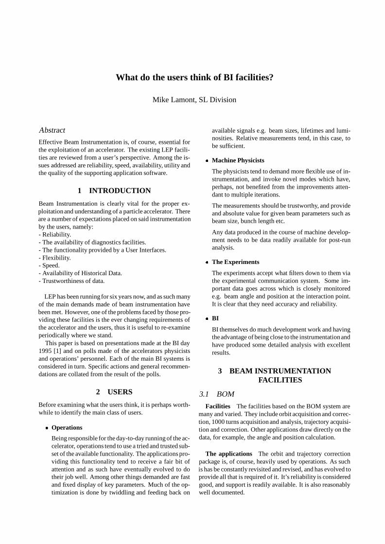
Effective Beam Instrumentation is, of course, essential forthe exploitation of an accelerator. The existing LEP facili-ties are reviewed from a user’s perspective. Among the is-sues addressed are reliability, speed, availability, utility andthe quality of the supporting application software.

1 INTRODUCTION

Beam Instrumentation is clearly vital for the proper ex-ploitationand understanding of a particle accelerator. Thereare a number of expectations placed on said instrumentationby the users, namely:- Reliability.- The availability of diagnostics facilities.- The functionality provided by a User Interfaces.- Flexibility.- Speed.- Availability of Historical Data.- Trustworthiness of data.

LEP has been running for six years now, and as such manyof the main demands made of beam instrumentation havebeen met. However, one of the problems faced by those pro-viding these facilities is the ever changing requirements ofthe accelerator and the users, thus it is useful to re-examineperiodically where we stand.

This paper is based on presentations made at the BI day1995 [1] and on polls made of the accelerators physicistsand operations’ personnel. Each of the main BI systems isconsidered in turn. Specific actions and general recommen-dations are collated from the result of the polls.

2 USERS

Before examining what the users think, it is perhaps worth-while to identify the main class of users.

Operations

Being responsible for the day-to-day running of the ac-celerator, operations tend to use a tried and trusted sub-set of the available functionality. The applications pro-viding this functionality tend to receive a fair bit ofattention and as such have eventually evolved to dotheir job well. Among other things demanded are fastand fixed display of key parameters. Much of the op-timization is done by twiddling and feeding back on

available signals e.g. beam sizes, lifetimes and lumi-nosities. Relative measurements tend, in this case, tobe sufficient.

Machine Physicists

The physicists tend to demand more flexible use of in-strumentation, and invoke novel modes which have,perhaps, not benefited from the improvements atten-dant to multiple iterations.

The measurements should be trustworthy, and provideand absolute value for given beam parameters such asbeam size, bunch length etc.

Any data produced in the course of machine develop-ment needs to be data readily available for post-runanalysis.

The Experiments

The experiments accept what filters down to them viathe experimental communication system. Some im-portant data goes across which is closely monitorede.g. beam angle and position at the interaction point.It is clear that they need accuracy and reliability.

BI

BI themselves do much development work and havingthe advantage of being close to the instrumentationandhave produced some detailed analysis with excellentresults.

3 BEAM INSTRUMENTATIONFACILITIES

3.1 BOM

Facilities The facilities based on the BOM system aremany and varied. They include orbit acquisition and correc-tion, 1000 turns acquisition and analysis, trajectory acquisi-tion and correction. Other applications draw directly on thedata, for example, the angle and position calculation.

The applications The orbit and trajectory correctionpackage is, of course, heavily used by operations. As suchis has be constantly revisited and revised, and has evolved toprovide all that is required of it. It’s reliability is consideredgood, and support is readily available. It is also reasonablywell documented.

Acquisitionof 1000 turns is still considered by some to bea specialist activity. In fact good documentation of the re-quite procedure is available and has be used successfully bythe uninitiated. The availability of the data was questionedand indeed it is difficult although not impossible to extracta subset of the large amount of data associated with a singleacquisition.

Trajectory acquisition is now a lot more reliable and somenice supporting software has been incorporated into the sys-tem. However until recently it was very slow, the acquisi-tion speed has significantly improved during the high energyrun.

A general criticism was the availability of diagnostics.Although the procedures exist, the software was inevitableburied away in an obscure place, requiringan amount of spe-cialist knowledge to access and use.

The pickups and their electronics Quoting from JorgWenninger’s contribution to the BI day proceedings [2]:

1. The performance of the narrow band pickups in 1995was very good.

2. The frequency of missing stations was much lower in1995 than in previous years.

3. There were, however, a lot of problems with BST jitterwhich affected the wide band pickups.

4. The beam current dependent gain jumps in wide bandpickups are still there.

5. There are 20 to 40 “faulty” pickups in a typical fill.

6. Angle & position calculation have been very success-ful. BOM can track the vertical IP position to about6 m.

Conclusions The orbit is an essential ingredient to ob-tain high performance. One clearly needs accurate measure-ments and a minimum of dead channels. The situation in1995 was clearly better than in previous years. However,there is still room for improvement.

3.2 BEUV

The interfaces to the BEUV system include fast display ofbeam sizes, fixed displays, the ability to work in a bunchtrain mode and a fairly sophisticated user interface. It wasfelt that these were on the whole reliable and fast.

The data is logged on the measurement database althoughthe acquisition system blocks up at times. It was felt that thisshould be better monitored.

Calibration It was universally considered that thisneeds to be taken more seriously. The absolute values of theemittances calculated from the BEUV ( together with cross-calibration from wire-scanners and BEXE) are not trusted.It was thought that this situation was unacceptable.

This issue was raised at BI day 95 and the followingpoints were made[3]:

Optics functions are required in the database, where theinstruments get the functions, which correspond to the realmachine. Frequent access to telescopes is required duringstable beams to fine tune the instruments. Cross-calibrationMD run(s) are required to check absolute precision of theinstruments. Improved logging facilities for off-line analy-sis should be available for all users. Emittances should belogged. One should also refrain from the temptation to use“private fudge factors” which work one period and give neg-ative emittances the next.

3.3 Bunch Current Transformers

Facilities include fast lifetime display, bunch current dis-plays, injection efficiency and the bunch current equalizer.All have been modified to work with bunch trains.

The facilities are reasonably reliable and fast. Thevideo displays are excellent and applications provide gooduser friendly interfaces. The Bunch Current Equalizer hasclearly proved vital to bunch train operation.

There was clear satisfaction with the facilities provided.Some minor points were raised:

1. The acquisition is a fairly complex chain. Specialistinvention is usually required when things go wrong. Itwas felt that the diagnostics were far from perfect.

2. Ib 6= IDC , the sum of the individual bunch currentsis not equal to the DC current.

3. Ib 1 mA, the system does not work for bunch cur-rents above 1 mA without specialist intervention.

At present there are two acquisitions systems. Things willbe rationalized in 96, thus addressing point 2. By the sametoken the system will become simpler, hopefully alleviatingthe problem raised in 1.

3.4 Luminosity monitors

The luminosity monitor manifest themselves as fixed dis-plays in the control room. These are regarded as good andas fast as they can be. The data is also written to the mea-surement database where it is used for retrospective analysisand in automatic vernier scans and the luminosity feedbackprogram.

Again some criticism was made of the diagnostics. Theabsolute calibration of the monitors is off, although notstrictly required for optimization, the poor calibration leadsto different values being quoted for beam-beam tune shiftsand so on.

3.5 Q-meter

The old Q-meter and associated applications has been re-placed in 1995 by a new incarnation. The new Q-meter metwith a generally good reception, driven by a good interface.

The data can be made available for later analysis. However,it is new and a series of user requests were apparent:

The reliability of the new interface need to be im-proved.

The PLL mode was not available with new Q-meter in95.

Easier adjustment of PLL to new optics is required.

Acquisition in time domain would be appreciated.

The spectra should be automatically saved after eachacquisition rather than on user request.

Another facility is the continuous tune display, which wasviewed as being extremely useful, for example, in diagnos-ing the onset of coherent transverse oscillations. Howeverit was felt that:

A more sophisticated display would be useful allow-ing the user to more accurately identify the values ofcoherent modes.

The ability to save the spectra on request would be use-ful.

3.6 Others

The above systems represent those used daily in operationand machine development. Other systems which are notfully operational are also of course used from time to time.Brief comments for each of these are presented.

BEXE BI have clearly had their problems, amongother things the X-ray signal has been blurred byphoto-electron production. However, it was clear thatthis was regarded as a potentially very useful instru-ment.

Wire Scanner Although not operational it has beenused for cross calibration only. The comment here:“Not very much use as long as it’s only for experts.”It is worth noting in passing that new software is be-ing considered. A different wire has been installed al-lowing it to operate at a higher current limit.

Beam-loss monitors These have been used in ma-chine development only. However they have per-formed well in tail scans. Together with scintillatorsthe loss monitors have proved a useful tool.

Streak camera

The lack of availability of this delicate instrument hascaused a lot of frustration, particularly among the ma-chine physicists. It was damaged last August and hasnot been available since. Before then it was noted that:

– Its operation needed a specialist.

– It was not user friendly.

– The users were not satisfied with the results:

It was practically impossible to calibrate. One could not trust the measured bunch

length. The average over 20 turns changed drasti-

cally all the time.

– The results should be available in the database.

4 CONCLUSIONS

There is general satisfaction with the performance of theBOM system. Attempts should be made to: reduce the gaineffects in the wide bands as much as possible, improve onthe number of missing pickups and improve the speed of ac-quisition.

With BEUV, the quality of calibration seems to be the out-standing complaint.

For the Q-meter, all modes need to be available and thereliability of interface should be improved. Some effort isrequired to ensure that the required data is saved.

From the survey the following general points appear tobe applicable to all systems:

Data logging: Again although much improved thereshould be more comprehensive coverage and better re-liability. Some form of on-line monitoring would ap-pear to be appropriate.

Diagnostics: This tends, on the whole, to be ad hoc.Trouble shooting facilities need to be incorporated inthe user interfaces.

Accuracy: attention to calibration. This can be anon-going, and time consuming business, but fromthe responses it is subject about which the users feelstrongly.

In general there was a good response. Clearly we havecome a long way, in terms of reliability, facilities, availabil-ity of data and consequent exploitation. Much work has, ofcourse, gone on this year to allow things to work success-fully with bunch trains. Of the heavily used facilities theniggles are generally minor. It would appear that the facil-ities meet expectations. (Whether the expectations are ashigh as they might be is another question.)

However there is general feeling of disappointment thatpotentially nice instruments exist that are not used in oper-ations. I quote: “It’s a pity: as a result we have an anecdo-tal knowledge of what is going on in LEP without knowingwhether this is typical or not.”

5 REFERENCES

[1] 6th BI Instrumentation Day, Ed. H.Schmickler, SL Note 96-02 (BI) (1996).

[2] Comments on BOM, J. Wenninger, 6th BI InstrumentationDay, SL Note 96-02 (BI) (1996).

[3] What does the emittance measurement team expect from AP,OP, DI via PERC &Chamonix 96? R. Jung, 6th BI Instru-mentation Day, SL Note 96-02 (BI) (1996).

What Improvements are forseen by BI?

H. Schmickler, CERN, Geneva, Switzerland

Abstract

This contribution describes the improvements on LEP in-strumentation scheduled for 1996. A summary of the MDtime requirements needed for the commissioning of the newfeatures is given at the end.

1 BOM-WB CALIBRATION

1.1 Outline of the problem

In the BOM wide band system (WB) the beam position isderived from four button signals, which are independentlydigitized. Several calibration constants enter into the calcu-lation (ADC offsets, relative gains of electronic channels).Those calibration constants can be determined preciselywith a calibration procedure and will therefor not be con-sidered in this presentation. One parameter can presentlyonly be determined with a poor precision and this parame-ter limits the overall precision of the position measurement.In the followingchapters this parameter, the present methodto measure it and a future improvement are described.

Figure 1: Illustration of the present parameterization of thenon linear behaviour of BOM-WB front end detector andthe corresponding calibration procedure (see text).

Each button signal passes through a detector card. Al-though this card has a wide linear dynamic range (24dB) theresponse for small signals is non linear. Fig. 1 shows an il-lustration of this curve. The x-axis represents the signal in-duced from the bunch into the detector and the y-axis the sig-nal delivered to the ADC for digitization. The system has tocope with bunch current variations of a factor 3 (before thegain of the detector is switched) and has to allow for largeorbit excursions giving at least another factor 3 in variationof x. This way the whole linear range of the detectors is usedfor the measurements. The detector characteristic curve isapproximated by a first order polynomial, where the largenegative offset (called threshold in the following text) is aconsequence of the non linear behaviour of the detector forsmall x. In the calibration procedure the threshold is deter-mined with two measurements of a test pulse generator. Onemeasurement direct (0 dB attenuation) and a second mea-surement through a 10 dB attenuator. The nominal value ofthis attenuation is -10dB i.e. a factor A of 0.3138 known toa precision of A

A= 1%. The threshold t is computed from

A and the two measured values U0dB and U10dB

t = =A U0dB U

10dB

1 A(1)

Error propagation yields for the error t:

t = a U0dB U

10dB

U0dB U10dB

(2)

For typical numbers of the measured ADC values this givesa relative error t

tof about 20% .

1.2 Simulations

It is very difficult to deduce from the above measurementerror of 20% on the calibration constant t the measurementerror on the beam position. Some observations are listed be-low

The position error depends on the bunch current, as forhigh bunch currents one is further away from the nonlinear region.

as the beam position is computed from two terms, wereeach term is computed from a pair of buttons on thediagonal of the position monitor. The electronics ofthese pairs is calibrated using the same test generatorsent via the same 10 dB attenuator. This hardware so-lution improves the knowledge of the relative value of

AD

C c

ou

nts

4000

3500

5000

2500

2000

1 5 0 0

1000

500

—500

2 calibration points

pulse generator with attenuator OdB and —l OdB

o f f s e t o n y—axis = cal ibra t ion cons tan t ca l l ed t h resho ld

0.2 0 ,4 0.6 0.8 1 button signal

the thresholds between button pairs by almost a factor10 although the absolute value is only known with theprecision mentioned above.

as a consequence of the calibration of the buttons inpairs the effect of the errors of the thresholds on theposition measurement almost vanishes for central or-bits

In order to quantify the above calibration error severalthousand beam position have been simulated in the regionof x and y below 1 cm. The bunch currents were varied be-tween 400 A and 100 A. The thresholds have been se-lected from a random generator witha variance of 20% . Thedifference in thresholds of button pairs has been limited toa variance of 5% .

Figure 2: Simulation of position measurement errors for400 =muA bunch currents and absolute positions smallerthan 1 cm in x and y

Fig. 2 shows the distribution of the simulated measure-ment errors for 400A bunch currents. The distributionhasa width of 24m indicating a very nice resolution of the sys-tem. Fig. 3 shows the same distribution for 100 A bunchcurrents. The width has increased to 130 m. This is aboutthe value of position error that is seen as ”gain jump” whenat a certain bunch current the gain of the wide band systemis increased during a physics fill in order to adapt the systemto the decreasing bunch currents.

For the interpolation of the orbit at the interaction pointthe LEP experiments require a very high precision for therunning at LEP200 beam energies. For low bunch currentsan improvement of the measurement resolution by a fac-tor three via better knowledge of the threshold parametersseems possible. According to the simulations this requires a

measurement of the threshold parameters has with a 5% pre-cision and the knowledge of the threshold for button pairshas down to 1 % uncertainty.

Figure 3: Simulation of position measurement errors for100 muA bunch currents and absolute positions smallerthan 1 cm in x and y

1.3 MD results with 8 bunches

The measurement of the threshold parameter down to a pre-cision as specified in the previous chapter is not possiblewith the present calibration system. For this reason in June1995 a calibration procedure using beam has been proposed.Eight bunches of bunch currents ranging from 20 A to 300A have been injected into the machine. The orbits of thebunches have been measured individually. For each buttonof the wide band system this gives a calibration curve similarto fig. 1 but this time comprising eight measurement points.The x axis is given by the bunch measurement system BCT.From the orbit system the number of bunches is limited to8.

The calibration data has been analyzed and can be sum-marized as follows:

The data is not well described by a first order polyno-mial. Taking either only points for low or high bunchcurrents the obtained thresholds vary as much as 40units (this means again about 20%.)

in order to distinguish the above non linear effect frompotential nonlinearities in the BCT measurements testswere performed in the laboratory on one electronicchannel. A nonlinearity of 2% was found to extendinto the so called linear region. This is well within the

num

ber

of s

imul

ated

beam

pos

ition

s

num

ber

of s

imul

ated

beam

pos

ition

s

70

60

50

4o

3 0

2O

0 —200

— | | | | l l l l l l l I l l l l l l l n n l l l l l l l l n l l l l l l l l l l l l l l l l l l l l

—120 —80 —4O 0 4O 80 120 160 200 error in y position in microns

—160

400 uA bunch

20

0 —200

[W t . H I I I I I I I I I I I I I I I I I I I I I I I I I I I I I I I I I I H I I —160 —120 —80 —4O 0 4O 80 120 160 200

error in y position in microns 100 uA bunch

specification, but at requested level of precision theseeffects have to be taken into account.

the measured values for the thresholds depend cru-cially on the offsets in the BCT. An offset of 5 Ashifts the thresholds by 40 units.

With the above measurements the threshold parameterscould not be determined with a better precision than ob-tained with the old calibration system.

1.4 Proposal for 1996

During the shutdown 1995/1996 the software of the wideband acquisitionsystem will be modified to parameterize thebehaviour of the front end detector by a third order polyno-mial. Eight bunches is probably not sufficient to determinethe coefficients of the polynomial by one parallel orbit mea-surement as described above. In this case one has to measuresequentially hoping that the orbit drifts during the measure-ment time remain small. The following procedure is pro-posed:

Set up the machine for single bunch injection.

As there is only one bunch one can measure its currentwith the DC monitor. The DC monitor uses a com-pensation technique for the measurement. This waysaturation effects for higher bunch currents can be ex-cluded.

Determine carefully the ”0” offset of the DC monitor.

Inject about 20 A

Measure the orbit

Continue in steps of 10 A until 300A bunch currentis reached

Dump beam and re-inject 20 A. Measure the orbitand compare to the orbit measured the first time. Theorbit difference is hopefully small and will be used toevaluate the error on the calibration constants.

The proposed procedure will demand a beam time of aboutone hour per particle type.

The calibration parameters are not expected to drift overlonger time intervals, hence only one calibration measure-ment is needed at start up. But it should be mentioned thatthe above calibration has to repeated as soon as electronicscomponents are exchanged during the year for a repair.

2 STREAK CAMERA

2.1 Schedule

The operation of the streak camera has not been lucky in1995. In late summer the tube of the camera has died. Orig-inally the spare tube worked, but finally the spare tube wasalso dead. Two new tubes have been ordered. The streakcamera will be equipped with one tube and will be back at

CERN for tests in April. In the laboratory the camera will betested with a sub-picosecond laser and hence the time reso-lutionof the system will be tested. The whole system shouldbe operational for the startup in June 1996.

2.2 Calibration in situ

In the past years the calibration of the system for bunchesshorter than 10 mm has been put into question on several oc-casions. For this reason a calibration with a source of infor-mation completely independent of the camera is proposed.The method has successfully used in 1992 for bunches of alength of about 11 mm. The proposed method is the crosscalibration with the longitudinal vertex distributionas mea-sured by the four LEP experiments. The following proce-dure seems feasible

The LEP experiments ask for about 3 to 4 days of cal-ibration runs at 45.6 GeV beam energy at the start ofthe 1996 running period.

In contrast to the measurements done in 1992 there isso much RFS voltage available now that the bunchescan be shortened to a few millimeters at 45.6 GeVbeam energy. This requires the full RF voltage of 1600MV and results in a synchrotron tune of 0.18.

At the end of each calibration run the RF voltageshould be raised to a higher limit and hence thebunches will be shortened. The bunch length will bemeasured with the streak camera and the measure-ments registered. After a few days of offline analy-sis the longitudinal vertex distribution will be avail-able and compared to the convolution of the measuredelectron and positron bunch length.

For each run the longitudinal motion of the beams willbe monitored with the streak camera itself and the dis-play of the longitudinal motion in the PCR. This has tobe used as a correction in case the motion is compara-ble to the bunch length or can be used as a test of thetiming jitter of the streak camera electronics.

With the luminosity from 300A bunches the data of afew hours running should give the longitudinal vertexdistribution with a resolution well below a millimeter.

3 LIFETIME MEASUREMENTS WITHTHE BCT

The present BCT system uses analog signal treatment be-fore the digitalization. With two sample and hold circuitsper acquisition channel the baseline of the current monitoris measured and the bunch signal is integrated. The differ-ence of the above signals is generated with an analog circuitand than digitized. The signal levels are very low and hencethe analog treatment of the signal is very sensitive to exter-nal noise. In addition the above integration gates render thesystem sensitive to timing jitters.

During a MD experiment a bunch current measurementbased on a peak hold technique has been tested. The ex-ploitation of a peak hold detector avoids any susceptibilityto timing jitter. The results of these measurements are verypromising. The rms noise of the old acquisition of about 50nA could be lowered to about 8 nA with the new technique.

Presently the possible dynamic range of the peak holddetector is optimized and the system is adapted to speedsneeded for bunch train operation. One electronics chassisfor either positron or electron bunch current measurementswill be installed for tests for the startup 1996. If these testsare successful the entire bunch current measurement systemwill be based on two such acquisition chassis from 1997 on-wards.

4 BEAM-BEAM DISPLAY

During machine experiments in 1993 the excitation of beambeam modes by simultaneous sinusoidal excitation of sev-eral bunches in collision has been studied. By varying thephases between the excitation signals either the commonbeam beam mode or the anti-phase mode could be enhancedin the transverse spectra measured with the q meter. Thismode of operation is no longer possible with bunch train, asthe excitation system has a pulse length that does not allowthe excitation of individual bunches in a train.

During a machine experiment in 1995 the followingprin-ciple could be demonstrated to work. Positron and Electronbunches are simultaneously excited with with noise randomkicks. The transverse motions are recorded turn by turn forboth particle types. The time domain signal of one particletype is passed through a phase shifter and then both signalsare added. Depending on the phase shift either the commonmode or anti-phase beam beam modes are enhanced in thetransverse spectra.

Based on this principle an online display of the bunchspectra in collisions is proposed. The separations betweenthe beam-beam modes could be a very useful tool for lumi-nosity optimization.

5 QMETER

5.1 Schedule for the new Qmeter

The following functionality will be developed during the1995/1996 shutdown:

Complete beam exciter mode. PLL oscillator runningat constant frequency.

terminal readout of spectrum history acquired in con-tinuous FFT mode and storage of several consecutivespectra on disc.

Q-loop based on PLL mode.

allow for frequency decrementation in swept fre-quency mode

time domain display of beam position data of the lastsingle shot FFT.

Loading of PLL phases from theoretical phase ad-vances between kicker and pickup as contained in thetwiss files.

As second priority the following items have been classi-fied. Their availability can not be guaranteed for the startup,but will be during the year.

GMT event triggered acquisitions

Simultaneous observationof electrons and positrons inFFT and swept frequency method. This is the basis forthe above beam-beam display.

5.2 The old q meter

In 1996 the old q meter is not supposed to be used for oper-ations but will be kept in a stand by mode. It will not be dis-mounted before the end of the summer technical stop. Dur-ing the technical stop its electronic part will be replaced bythat of a second new q meter.

6 BEXE

6.1 detector displacement

As already discussed in detail during the BI day 1995 thedetector will be displaced from its location in the arc to aplace in the dispersion suppressor. At this position the de-tector will receive synchrotron light from a source with atenth of the bending radius compared to the original loca-tion. This way the total power deposit in the detector willbe acceptable for operation with beam energies between 45and 100 GeV.

6.2 real time display

In order to make more use of the detector in daily opera-tion a PCR online display similar to the BEUV display isproposed. The vertical beam distribution will be plotted forelectrons and positrons. A correlation scatter plot of elec-tron beam size versus positron beam size on a turn by turnbasis will be available as well as FFT displays of the beamsize variations.

7 TOWARDS AUTOMATICCOLLIMATOR POSITIONING WITH

BEAM LOSS MONITORS?

For the 1996 running period each collimator will beequipped with two beam loss monitors based on PIN diodedetectors. (one detector mainly sensitive to electron losses,the other to positron losses). In the original proposal for theinstallation of the Beam loss monitors the use of the moni-tors for an automatic positioningof the collimators had beenincluded

Now the following experimental experience contradictssuch a type of application:

The monitor rates are not independent. Especially ifthe aperture limitingcollimatorsare moved most of thedetectors show different readings.

Some monitors close to the experiments see very lowcount rates of few Hertz. For an automatic positioningthe integration times would have to be of the order ofminutes.

The monitors in the arcs are flushed by photons. It isquestionable whether these monitors can be shieldedfor operation at the highest LEP200 beam energies.

it takes several week of running in order to establishreference rates for each monitor. The present detec-tor mounting supports do not allow absolute reposi-tioning of the monitors after a detector displacementfor installationsduring a shutdown or during a bakeoutof the vacuum system. As the absolute rates dependvery much on the detector positionbehind the collima-tor the reference rates would have to be reestablishedafter each machine re-installation.

8 EMITTANCE MEASUREMENTS WITHBEUV

The discussions from the BI day were recalled. The crosscalibrations of the emittance measurement instruments haveshown, that the BEUV readings of horizontal and verticalemittance are good to a few percent in case the beta valuesat the BEUV and the dispersion is known. It is demanded toinstall an online data base containing measurements and/orsimulations giving an image of the optical functions of themachine. The correction of the BEUV measurements withthese values and not the use of the theoretical values fromthe twiss file will result in emittance measurements to a pre-cision of a few percents.

9 MISCELLANEOUS

9.1 k-modulation

The back leg windings for the modulation of individualquadrupoles will be finished during this shutdown in the oddinteraction regions. These installations together with the in-stallations in the arcs around IP8 will be exploited during the1996 running period for the determination of more pickupmechanical offsets.

9.2 upgrade of luminosity monitors

By the introduction of a co-planarity cut between signalsfrom one monitor of each side of the interaction region thebackground in the luminosity reading will be further re-duced. This facility will be gradually introduced into all in-teraction regions during the 1996 running period.

9.3 NMR detectors

Two more measurement devices for the magnetic field ofthe LEP bending magnets based on Nuclear Magnetic Res-onance will be installed in the ring. This yields a total offour such measurement devices.

10 CONCLUSIONS AND MD REQUESTS

A large number of improvements for the LEP beam instru-mentation has been proposed and will be made availableduring the year 1996.

Some of the improvements require beam time. The BOMcalibration requires a few hours dedicated machine time andshould be done at startup.. This calibration has to be re-peated every time detector components are exchanged fora repair.

The streak camera calibration can be done at startup in theshadow of the calibration runs at the Z0 energy requested bythe experiments.

The commissioning of the new q meter requires the fol-lowing time:a) parameter adjustments and validation of PLL mode: 3times 3 hours in week 25.b) Q-loop based on PLL mode: 2 times 3 hours in June/July

One cross calibration run for the emittance measurementdevices is demanded during the year.

New Tools for Beam-beam Optimization

J. Wenninger

Abstract

To obtain the best machine performance the beams shouldbe colliding without transverse offsets at the interactionpoints. Present and future strategies to minimize colli-sion offsets using luminosityor beam-beam deflection scansand feedbacks will be discussed first. In the second part Iwill present recent improvements on closed orbit correctionstrategies as well as possible solutions for the problems ofthe large vertical orbit drifts due to the motion of the low-beta quadrupoles.

1 COLLISION OFFSET OPTIMIZATION

To achieve high beam-beam tune shifts and luminosities atLEP, the beams must be steered vertically to collide withimpact parameters that are small compared to the verticalbeam size at the interaction point (IP). For example, duringthe 1994 Pretzel run of LEP, beam-beam tune shifts y of0.04 have only been achieved after a fine tuning of the ver-tical collision offsets at the level of 0.5 microns or less. Inthe case of bunch trains, the unavoidable vertical collisionoffsets that are present for trains of 3 and 4 bunches mightexplain why y never significantly exceeded 0.03. On theother hand, during an MD with only 2 bunches per train, yexceeded 0.04 after careful tuning of the machine.

Another reason to minimize collision offsets is to avoidcentre-of-mass energy shifts due to difference dispersion atthe IP [1]. This points was very important during the 1995energy scan [2]. It triggered important improvements in thevernier scan procedure.

1.1 Luminosity Scans

Up to now only luminosity scans have been used opera-tionally at LEP to minimize collision offsets. During theseso-called “vernier” scans, the vertical separation of thebeams at the IP is varied in steps using a local electrostaticseparator bump. For each setting of the bump, the luminos-ity is recorded. The optimum separator setting can be ob-tained simply from the maximum of the luminosity curveor from a Gaussian fit to the data. These vernier scanshave been used extensively at LEP (more than 1000 scansin 1995) and are fully automated. The duration of a scan isabout 5-10 minutes per IP at 45 GeV.

At higher energies, it will take between 5 (108=60 lat-tice) and 25 (90=60 lattice) times longer to measure the lu-minosity with the same relative accuracy than at 45 GeV [3].

This is due to higher background rates and different collima-tor positions (related to the change in the horizontal emit-tances). This will obviously affect the length of the vernierscans. It is however not excluded that this degradation ofperformance can be reduced with the implementation of anacolinearity cut to improve the background rejection in theLEP luminosity detectors [4].

1.2 Beam-beam Deflection Scans

A new method to optimize the collision offsets using thebeam-beam deflection at the IP has been tested with successduring the LEP high energy run [5]. For such a scan the de-

-60

-40

-20

0

20

40

60

-20 -10 0 10

∆y (µm)

θ bb (

µrad

)

∆yopt = -3.6 +- 0.4 µm

IP 6

σx = 279 +- 16 µmσy = 3.42 +- 0.46 µm

εx = 31.1 +- 3.5 nmεy = 0.23 +- 0.06 nm

Ib e+/e- = 360 / 280 µA

L = 11.7 1030 cm-2s-1

ξx/ξy = 0.019 / 0.031

Figure 1: Example of a vertical beam-beam deflection scan per-formed at a beam energy of 68 GeV. The beam-beam deflectionbb is plotted as a function of the separator bump amplitudey.The solid line is a fit to the data. The beam sizes x and y

are extracted from the fit. The beam-beam tune shifts x and y ,the emittances "x and "y and the luminosity have been calculatedfrom x , y and from the bunch currents indicated above the fig-ure. The optimum separator bump amplitude is given byyopt .

flection angle due to the beam-beam force is measured as afunction of the separator bump amplitude. When the colli-sion offset is zero, the beam-beam deflection vanishes. Inpractice two pickups on each side of the IP (PU.QS0 andPU.QS4) are used to calculate the beam angles at the IP. Thetotal beam-beam deflection bb is calculated from the differ-ence of the beam-beam deflection of the positrons and theelectrons (which have opposite signs) :

bb = (+L +R) (L R) (1)

is the beam angle at the IP, L(R) labels the Left(Right)side of the IP and +() the positron(electron) beam. bb isnot too sensitive to systematics errors of the BPMs since itinvolves only difference measurements. Figure 1 shows anexample of a beam-beam scan. More details on the proce-dure and the fits can be found in [5]. The fits to the data alsoprovide measurements of the effective transverse beam sizesat the IP.

It is possible to speed up these scans if a special readout ofthe few pickups of interest for the scan can be implementedfor the future. In that case a 12 point scan in the range of 4to 5 vertical beam sizes would last only about 3 minutes.

2 COLLISION OFFSET FEEDBACKS

During the 1995 bunch train run of LEP, significant drifts ofthe collision offsets have been observed during coasts. Theorigin of the drifts is unknown and they have been affectingparticularly IP 6. This observation motivates the study andtest of possible feedbacks on the collision offset.

2.1 Luminosity Feedback

To minimize problems of center-of-mass energy shifts dueto dispersion at the IP [1], a feedback was proposed to sta-bilize and control possible drifts of the collision offsets [6].This feedback operates on one IP at a time. It compares theluminosity for 2 separator settings and moves the separatorbump in the direction of the higher luminosity. This is verysimilar to a fine tuningof the machine, provided nothingelseis affecting the luminosity during the comparison of the twosettings. In practice the luminosity was measured during 1minute for separator settings 0.8 m away from the setvalue. The luminosities were compared and the separatorbump moved by 0.4 m in the direction that gave the higherluminosity. This comparison was repeated 4 times for eachIP and the feedback could be set up to cycle between the 4IPs. Figure 2 shows the behavior of the feedback during fill3024. A significant drift of 3.5 m was tracked in IP 6. Thischange could be confirmed with a vernier scan.

The performance of the luminosity feedback is limitedduring coasts because of orbit and luminosity drifts whichreduce the speed at which it can converge. At higher ener-gies it will become slower because of the longer integrationtimes required for the luminosity measurements.

IP 2 IP 4

IP 6 IP 8

Time (min) - Fill 3024V

ER

NIE

R c

hang

e (µm

)

-4

-2

0

2

4

0 200 400-4

-2

0

2

4

0 200 400

-4

-2

0

2

4

0 200 400-4

-2

0

2

4

0 200 400

Figure 2: Example of the successful use of the luminosity feed-back in fill 3024. The change of the vernier setting is shown as afunction of time. The solid dots indicate vernier scans. The openpoints correspond to the setting found by the luminosity feedback.A drift of about 3.5 microns was tracked by the feedback.

2.2 Beam-beam Angle Feedback

A feedback on the beam-beam angle is potentiallyvery pow-erful and fast because orbit measurements can be obtainedroughly every 40 seconds at LEP. A feedback that would acton bb would also be insensitive to emittance changes whichperturb the luminosity feedback. On the other hand such amethod sets stringent requirements on the quality and sta-bility of the orbit measurements. When the collision offsetsare small, the sensitivity of bb to the separationy is givenby [5] :

bb

y=

4y

y(2)

where y is the betatron function at the IP. For a beam-beamtune shift y of 0.04 and y = 5 cm, a 0.5 m stability ofyrequires an error on bb that is smaller than 5 rad. It is notclear if such a high stabilitycan be achieved over longer timeintervals. Nevertheless a feedback with a stability of about1 to 2 m can probably be operated without problems.

3 LOW-BETA QUADRUPOLEMOVEMENTS

The superconducting low-beta quadrupoles (QS0) installedaround each collision points are the strongest quadrupolesin LEP with a strength k = 0:16 m2. The betatron func-tion reaches close to 400 m inside the QS0s for y = 5 cm.As a consequence the vertical orbit is very sensitive to dis-placements of the QS0s with squeezed beams. The phaseadvance between the QS0 on the left side and on the right

O©

O

O©

O

oo@ 0

0 V

O

|.

|

OO

OO

O©

O

1? 0

&0

0©

o

mo

On

o

0@

__

_I

-

_

__ _

OO

00

0

00

00

+ 0

@

©©

0

00

O©

O

OO

OO

___ _

__

__

uO

Corrector

Num

ber

of T

rims

Orbit-V

0

1000

2000

3000

KC

V2

6.L

4K

CV

24

.L4

KC

V2

2.L

4K

CV

18

.L4

KC

V1

6.L

4K

CV

A1

4.L

4K

CV

A1

2.L

4K

CV

A1

0.L

4K

CV

A8

.L4

KC

VA

6.L

4K

CV

A4

.L4

KC

VC

0.L

4K

CV

C0

.R4

KC

VA

4.R

4K

CV

A6

.R4

KC

VA

8.R

4K

CV

A1

0.R

4K

CV

A1

2.R

4K

CV

A1

4.R

4K

CV

16

.R4

KC

V1

8.R

4K

CV

22

.R4

KC

V2

4.R

4K

CV

26

.R4

Corrector

Num

ber

of T

rims

Orbit-V

0

1000

2000

3000

KC

V2

6.L

4K

CV

24

.L4

KC

V2

2.L

4K

CV

18

.L4

KC

V1

6.L

4K

CV

A1

4.L

4K

CV

A1

2.L

4K

CV

A1

0.L

4K

CV

A6

.L4

KC

VA

4.L

4K

CV

2.L

4K

CV

C0

.L4

KC

VC

0.R

4K

CV

2.R

4K

CV

A4

.R4

KC

VA

6.R

4K

CV

A1

0.R

4K

CV

A1

2.R

4K

CV

A1

4.R

4K

CV

16

.R4

KC

V1

8.R

4K

CV

22

.R4

KC

V2

4.R

4K

CV

26

.R4

Figure 3: Distribution of the vertical corrector trims used inphysics and adjust mode (y = 5 cm) around IP 4 in 1994 (top)and 1995 (bottom).

side of each IP is almost exactly . We can therefore sepa-rate the effects on the orbit in two cases. Let us define yand < y > as the difference and the average vertical posi-tion of the two QS0s around the IP. The RMS of the verticalorbit v depends on y and < y > :

v ' 40 jyj v ' 0:7 j < y > j (3)

The enhanced sensitivity toy is due to the fact that the ef-fects of the two QS0s add up for a movement in opposite di-rection (y 6= 0), but cancel very well for a parallel move-ment (< y > 6= 0). The phase advance of between theQS0s on the left and right sides is at the origin of this be-havior.

It has been shown already more than one year ago thata vertical movement of the QS0s is responsible for at least90% of the large vertical orbit drifts in LEP. The understand-ing of this phenomenon has been improved significantly in1995.

3.1 Orbit Correction Strategies

The analysis of the 1994 orbit correction trims [7] showedclearly that correctors n away from the QS0 were cho-sen to correct for the QS0 motion instead of the correctors

Figure 4: Average (< y >) and difference (y) of the verticalmovement of the quadrupoles QS0.L8 and QS0.R8 between Nov.18th and Nov. 21st 1995 during the LEP high energy run. When-ever the machine is at injection, the quadrupoles move upwards.The downward motion starts when the magnets are ramped to 45GeV and above (from F. Tecker).

CVC.QS0 which are installed just next to each QS0. Thisproblem was caused by the matrix reconditioning strategiesused in the COCU [8] orbit correction package. Two sepa-rate improvements were implemented for the 1995 LEP run :

The response matrix reconditioningalgorithm was im-proved [8]. The number of correctors disabled for acorrection was re-optimized.

A dedicated “knob” was implemented in the orbitcorrection application to force the MICADO [9] al-gorithm to use only the correctors next to the QS0quadrupoles. This knob was used extensively in 1995to correct for orbit drifts.

Following these two modifications, the problem of the cor-rectors n away from the QS0 disappeared in 1995 as canbe seen in Figure 3.

3.2 Quadrupole Movement Measurements

During the 1995 LEP run measurements of the vertical mo-tion of the QS0 quadrupoles became available for the firsttime. Hydrostatic systems were installed in IP 2 and IP 8and two systems based on potentiometers were installed inIP 4 and IP 8 by the ALEPH and DELPHI experiments.

These systems showed clearly the vertical movements ofthe QS0s as can be seen in Figure 4. The typical drifts of< y > were 40 m at 45 GeV and 70 m at 65-68GeV. The QS0s move downward after the start of the ramp.As soon as the magnets are back at their injection settings,

-2 90 -3()() -3 i 0

-320

330 340 -350

360 3 70

Y>

(1

1m

)

<

40

Ay

(

um

)

30

20

I|

|I

lllllll|

llll|

lllllll

II

%J

II

II

II

I:

l[l

l l

ll

l‘

I'

.

C:

-

time (h)

an upward movement starts. It is likely that a temperaturechange is at the origin of these movements. Figure 4 showsthat a fast turn-around of LEP reduces the total swing ofthe vertical movement. The vertical orbit drifts are due ofcourse to the difference in the movement on the left and theright sides.

An analysis made by F. Tecker [10] shows that the mea-surements made by the hydrostatic and potentiometer sys-tems can be used to predict the orbit drifts. Using the orbitsrecorded in physics, he calculated the bare drifts (unfoldingthe orbit correction made by the operation crews) which hetried to correct with the MICADO algorithm using only thecorrectors next to the QS0s. Figure 5 shows a very nice ex-ample of the comparison of the calculated kick for the cor-rector CVC.QS0.L4 and the measured vertical movement inIP4. The agreement is very good. The accuracy is limited bythe resolution of the measurement systems to about 2 mon y.

IP 4 fill 3108 02-03 Nov. 1995

time (hours)

calc

ulat

ed k

ick

(mra

d)

time (hours)

∆y (

µm)

0

0.005

0.01

0.015

0.02

0.025

0.03

0.035

20 22 24 26 28 30 32 34

20

40

60

80

100

120

140

160

180

22 24 26 28 30 32 34

Figure 5: Top : correction kick calculated with MICADO forthe corrector CVC.QS0.L4 from the vertical orbit drifts. Bot-tom : measured vertical difference position y between thequadrupoles QS0.L4 and QS0.R4. There is a very good correla-tion between the predicted kick and y. It should be noted thatfor this fill the drift is particularly large because of a cooling prob-lem (from F. Tecker).

3.3 QS0 Movement Feedbacks

During the LEP shutdown 1995-1996, three new hydrostaticsystems will be installed in IPs 4 and 6 to survey the QS0positions. A potentiometer system will also be installed inIP 6 by the OPAL collaboration. When these systems willbe operational, we will have enough informationon the QS0movements to build a feedback system to stabilize the or-

bit. With the help of such a feedback, beam losses duringthe squeeze and orbit reload could be avoided and the orbitdrifts in physics reduced. A certain number of systems canbe envisaged :

QS0 position feedback : the most natural solutionis of course to move the QS0/QS1 girder to compen-sate the vertical motion. Unfortunately this solution isprobably too complicated and too expensive.

Corrector TRIM-DAC feedback : for this solution,the QS0 position and current information would beused to build a signal to be fed into the TRIM-DAC ofthe corrector next to the moving QS0. The kick wouldthen be compensated locally. This solution wouldbe transparent for the machine operation. The 8 bitTRIM-DAC should have just enough resolution to per-form this task.

Temperature stabilization : since it seems likely thatthe movement is due to a thermal effect, an improvedventilation or cooling of the area around the QS0/QS1girder might reduce the problems. Such an improve-ment should in fact be attempted whatever the finalchoice of feedback strategy.

SloppySoft feedback : since the correctors on the leftand right side can both be used for the same orbit cor-rection (modulo a change of the kick sign), it is pos-sible to envisage a solution where only one correctoris used for the regular orbit corrections. The secondcorrector (one per IP) could be dedicated to a feed-back that would use the y information to compen-sate the most dramatic orbit drifts. A program runningon one of the PCR workstations might take care of thisjob. This possibility is interesting and will be studiedin more detail. The problem of the ramp and the neces-sity to use both CVC.QS0 correctors for certain localbumps around the IP have still to be studied.

4 CONCLUSION

For LEP 200 the collision offset optimization can be donewith the help of beam-beam deflection angle scans thatshould give an increased speed in comparison to the stan-dard “vernier” scans. A feedback on the collisionoffsets hasbeen used with success in 1995 during some fills of the en-ergy scan. It will be kept operational for LEP 200 althoughthe convergence might be much slower. A feedback basedon the beam-beam deflection angle is feasible but the accu-racy achievable with such a system is not known and de-pends on the performance of the BPMs.

We are now in a situation where we have all the necessaryingredients and the knowledge to build a feedback on thelow-beta quadrupoles to stabilize the vertical orbit of LEP.The exact implementation of this feedback has still to be de-cided. It is likely that a solution based on a SloppySoft ap-plication will be used.

+ +++++++ + +

+++++++ + +++++ ++++++++ + + + + + + ++++++++++++++++

5 REFERENCES

[1] J. Jowett, J. Wenninger and J. Yamartino, “Influence of Dis-persion and Collisions Offsets on the Centre-of-Mass Energyat LEP”, CERN SL/ Note 95-46 (OP).

[2] The LEP Energy Working Group, “LEP Center-of-Mass En-ergies in Presence of Opposite Sign Vertical Dispersion inBunch-Train Operation”, SL-Note 95-77 (BI).

[3] G. von Holtey, “Luminosity monitoring at LEP2”, Proc. of theFifth Workshop on LEP Performance, CERN SL/95-08 (DI).

[4] P. Puzo, private communication.

[5] J. Wenninger, “Measurement of Beam-beam Deflections atthe Interaction Points of LEP”, CERN SL/ Note 96-01 (OP).

[6] R. Schmidt, contribution to the 67th LEP energy WG meeting.A. Drees, contribution to the 70th LEP energy WG meeting.A. Drees, R. Schmidt, J. Wenninger, private communication.

[7] P. Collier, “Overview of Operation in Physics During 1994”,Proc. of the Fifth Workshop on LEP Performance, CERNSL/95-08 (DI).

[8] W. Herr, “Algorithms and procedures used in the orbit correc-tion package COCU”, CERN SL/95-07 (AP)

[9] B. Autin and Y.Marti, CERN ISR-MA/73-17 (1973).

[10] F. Tecker, Minutes of the October 12th 1995 meeting of the“Interaction Region” Subgroup of the LEP2 Workshop WG4.

BEAM ENERGY MEASUREMENT POSSIBILITIES AT LEP2

M. Placidi, CERN, Geneva, Switzerland

Abstract

The problem of the measurement of the beam energy inLEP2 has been addressed and a selection of possible alterna-tives to a direct application of the Resonant DepolarizationMethod (RDM) [1] has been considered, namely extrapola-tion of measurements based on magnetic field informationfrom flux-loop and NMR probes, Heavy Ion Accelerationand Mller Scattering technique. Considerations on attain-able accuracies, feasibilityand technical implications for themachine are discussed in sections 3, 4 and 5 .

Prospects for transverse polarization (P?) at energieshigher than LEP1 are discussed in section 2.

This contribution is a reduced version of the documentprepared for the LEP2 WORKSHOP Yellow Report [2] by the’Energy Calibration’ Subgroup of the Physics/Machine In-terface Working Group WG4. 1

1 BEAM ACCURACY REQUIREMENTS

The requirements on the accuracy in the measurement ofMW in the hypothesis of collecting an Integrated Luminos-ity of about 500 pb1 ( 8000W pairs) in each experi-ment given in [3] imply a systematic error from the knowl-edge of the absolute average beam energy:

Ebeam 15MeV orEbeam

Ebeam

1:7 104 (1)

The accuracy in the determination of the beam energy highlydepends on the availability of transverse polarization in ex-cess of a 5% level to apply the RDMwhich provides an in-stantaneous precision of 1 MeV.

2 TRANSVERSE POLARIZATIONBEYOND Z0

Prospects for transverse polarization beyond Z0 energyare based on assessment of the strength of depolarizing ef-fects at higher energies. The asymptotic polarization level

P1 =8

5p3

1

1 + ST=d(2)

is governed by the rates of depolarization (1=d) andSokolov-Ternov self-polarization (1=ST ) of the beam.

1A. Blondel, M. Boge, C. Cecchi, B. Dehning, A. Drees, J.H. Field,J. Jowett, T. Kawamoto, M. Koratzinos, M. Placidi, D. Plane, P. Roudeau,D. Schaile, J. Yamartino.

Although the radiative polarization rate increases asE5, thedepolarization effects due to resonances driven by machineimperfections also increase rapidly with energy.The simplest model of resonant depolarization foreseesST=d ' 2s , where s = a is the energy-dependent spintune and eqn.(2) can be written as:

P1 =92:4%

1 + b E2beam

(3)

The parameter b can be chosen to reproduce the polariza-tion level attainable at the energy of the Z0. It can be con-trolled by the application of techniques of orbit control andspin harmonic compensation [4].

It is known however that depolarizing resonances are fur-ther enhanced by the increasing energy spread in the beam.Despite some lack of confidence in the calculations of theseeffects in the past, experimental tests with wigglers at LEP1have given results consistent with theory [4].

Theory has been used [5] to compute optimum combi-nations of beam energy and RF voltage to control the syn-chrotron tune Qs and provide conditions of maximum po-larization. It is expected that a 10% P? level should not beout of reach at energies around 65 GeV.

Polarization probabilities can be higher at some specificenergies when the energy-dependent spin precession phaseadvance

(E; s) = (a )

Zd(s) (4)

is equal to the betatron phase advance in regions of the lat-tice where quantum energy fluctuations are important:

(a )

Zarcs

ds

(s)=

Zarcs

ds

(s)(5)

In this case some categories of orbit errors like -bumpsare spin-transparent and depolarizing effects from spin-orbitcoupling become weaker. The first energy above the Z0

where the requirement (5) is expected to be satified with the(90=60) LEP2 optics is around 60.6 GeV [6].

A first attempt to find polarization at this energy sched-uled for the MD in week 47 failed due to communica-tion problems which drastically reduced the allocated timeneeded to apply the planned strategies for this crucial exper-iment which will be repeated in 1996 as the machine condi-tions will be favourable.

3 ENERGY CALIBRATION WITHPRESENT TECHNIQUES

A straight extrapolation of the techniques used for the suc-cessful scan of the Z0 line shape in 1995 suggests a defaultscenario for energy calibration at LEP2 as follows:

Precise calibration will be performed with resonant de-polarization at energies where it has proven to workreliably. A first choice is an energy corresponding toLEP1. A second one, Ebeam = EPol

max, will be the

highest where polarization in excess of at least 5% canbe reliably obtained. This second energy, expected tolie in the range 60-70 GeV, will be left as parameter inthe following discussion.

Extrapolation to the higher energy will use:i) the flux-loop to provide a calibration of the non-linearity of the ensemble of the LEP dipoles andii) a set of NMR probes for a precise (106) measure-ment of the local magnetic field in a sample of LEPmagnets.

On-line monitoring of the energy will be provided byi) the field information from the in-situ NMR probes;ii) recording of the horizontal orbit andiii) recording of various parameters of the RF systemand its asymmetries.

3.1 Present Experience on the LEP Energy

The LEP beam energy is affected by a multiplicityof effects,which induce variability in time and deviation of the center-of-mass energy from ECM = Ee+ + Ee .Some of these effects are well known. They include:

Variations of the LEP circumference due to groundmotion. This category includes earth tides, lake level,and other ground swelling. These effects can be cor-rected down to a precision of 1–2 MeV using measuredorbits and momentum compaction factor.

Rise of the magnetic field in the dipoles during fills.This can be monitored by placing NMR probes in-side some of the LEP magnets. Two such probes wereproved to be most useful in understanding the LEP en-ergy in 1995.

Temperature variations are no longer a problem sincethe temperature regulation of the cooling water hasbeen implemented.

Variation in the RF voltage distribution around thering. Control of these effects can be obtained by mea-suring the longitudinal positionof interactions verticesin the LEP detectors, and monitoring the difference be-tween e+e horizontal orbits in the arcs (saw–toothingmonitor). The size of effects will grow at LEP2 ac-cording to the larger RF power in operation. The pre-cision of the monitoring should remain similar.

Systematic effects on the CM Energy at each Inter-action Point caused by residual vertical dispersionand small collision offsets [7] when operating LEPin bunch-train configuration have been simulated [8]and found to be in good agreement with the measure-ments. The strategy proposed to minimize the CM en-ergy shifts [9] was applied with appropriate use of theVernier Scan technique [10] during the 1995 PhysicsRun [11].

Once these effects are corrected for, an r.m.s. scatter of 104 on the beam energy is to be expected. To knowthe average of the two reference polarization-calibrated en-ergies with a precision of the order of 2 MeV a calibrationat 45 GeV and at EPol

max during a dedicated ramp is recom-mended once every two weeks or so.

3.2 The Flux-Loop

The main uncertainty will come from extrapolating fromthese energies up to the operating ones because of the un-certainty in the knowledge of the linearity of the magnets.In absence of a direct measurement of the beam energy thiscan be obtained using the flux-loop technique.When the whole dipole system undergoes a magnetic cycleof amplitude corresponding to beam energies up to 100 GeVthe response curve of the magnets can be obtained to an ab-solute precision of 5 MeV, but the linearity can be ratherwell determined. When the cycling is repeated several timesit provides an estimate of the short term reproducibilitygoodto a few 105. The long term reproducibility is found to beat the 104 level [12], but that of the derivative from 40 to65 GeV is much better.The accuracy on the extrapolation is estimated as follows,assuming that regular flux-loop measurements will be ex-tended up to 100 GeV [13]:

First, the uncertainty stemming from the RDM resultsis evaluated using linear extrapolation error formulae.This would be the case if one could trust with nearly in-finite precision the non-linearity curves from the flux-loops. Results are shown in fig. 1 for two values of theextrapolated-to energy, as a function of EPol

max.

For the uncertainty in the non-linearity coefficient aworst case estimate can be obtained assuming that thenon-linearity coefficient is totally unknown, and onlyinferred from the RDM-calibrated energies. This isclearly too pessimistic as from the above discussion.The resulting dependence on EPol

max is shown in fig. 1in the curves labeled ”quadratic”.

Finally, adding the flux-loop information with a2 104 conservative precision produces the resultsshown in fig. 2 and summarized in table 1.

0

5

10

15

20

25

30

35

40

50 55 60 65 70 75 80 85 90 95 100

∆Ebe

am(M

eV)

EmaxPol (GeV)

EXTRAPOLATION FROM EmaxPol

Linear

extrapolation

LINEAR TO 80.5 GEV

QUADR. TO 80.5 GEV

quadratic

extrapolation

LINEAR TO 95 GEV

QUADR. TO 95 GEV

Figure 1: Accuracy Ebeam from linear and quadratic extrapolations from an intermediate EPol

max point toEbeam = 80.5 GeV and 95 GeV.

0

5

10

15

20

25

30

35

40

50 52.5 55 57.5 60 62.5 65 67.5 70 72.5 75

∆Ebe

am(M

eV)

EmaxPol (GeV)

EXTRAPOLATION FROM EmaxPol

Using the FLUX-LOOP

PRECISION at 80.5 GEV

PRECISION at 95 GEV

Figure 2: AccuracyEbeam for quadratic extrapolations from an intermediateEPol

max point toEbeam = 80.5 GeV and 95 GeV includ-ing Flux-Loop information assuming a 104 conservative precision.

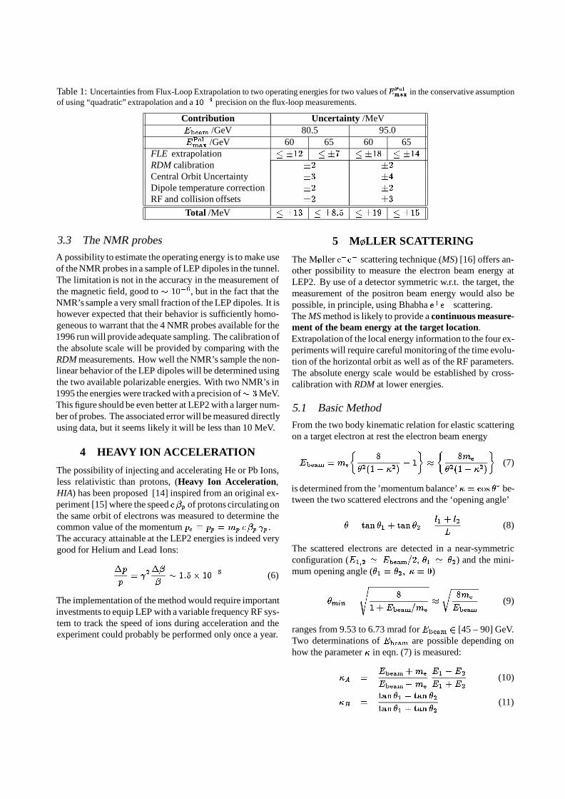
Table 1: Uncertainties from Flux-Loop Extrapolation to two operating energies for two values ofEPol

max in the conservative assumptionof using “quadratic” extrapolation and a 104 precision on the flux-loop measurements.

Contribution Uncertainty /MeVEbeam /GeV 80.5 95.0EPolmax /GeV 60 65 60 65

FLE extrapolation 12 7 18 14RDM calibration 2 2Central Orbit Uncertainty 3 4Dipole temperature correction 2 2RF and collision offsets 2 3

Total /MeV 13 8:5 19 15

3.3 The NMR probes

A possibility to estimate the operating energy is to make useof the NMR probes in a sample of LEP dipoles in the tunnel.The limitation is not in the accuracy in the measurement ofthe magnetic field, good to 106, but in the fact that theNMR’s sample a very small fraction of the LEP dipoles. It ishowever expected that their behavior is sufficiently homo-geneous to warrant that the 4 NMR probes available for the1996 run will provide adequate sampling. The calibration ofthe absolute scale will be provided by comparing with theRDM measurements. How well the NMR’s sample the non-linear behavior of the LEP dipoles will be determined usingthe two available polarizable energies. With two NMR’s in1995 the energies were tracked with a precision of 3MeV.This figure should be even better at LEP2 with a larger num-ber of probes. The associated error will be measured directlyusing data, but it seems likely it will be less than 10 MeV.

4 HEAVY ION ACCELERATION

The possibility of injecting and accelerating He or Pb Ions,less relativistic than protons, (Heavy Ion Acceleration,HIA) has been proposed [14] inspired from an original ex-periment [15] where the speed c p of protons circulating onthe same orbit of electrons was measured to determine thecommon value of the momentum pe pp = mp c p p.The accuracy attainable at the LEP2 energies is indeed verygood for Helium and Lead Ions:

p

p= 2

1:5 105 (6)

The implementation of the method would require importantinvestments to equip LEP with a variable frequency RF sys-tem to track the speed of ions during acceleration and theexperiment could probably be performed only once a year.

5 MLLER SCATTERING

The Mller ee scattering technique (MS) [16] offers an-other possibility to measure the electron beam energy atLEP2. By use of a detector symmetric w.r.t. the target, themeasurement of the positron beam energy would also bepossible, in principle, using Bhabha e+e scattering.The MS method is likely to provide a continuous measure-ment of the beam energy at the target location.Extrapolation of the local energy information to the four ex-periments will require careful monitoring of the time evolu-tion of the horizontal orbit as well as of the RF parameters.The absolute energy scale would be established by cross-calibration with RDM at lower energies.

5.1 Basic Method

From the two body kinematic relation for elastic scatteringon a target electron at rest the electron beam energy

Ebeam = me

8

2(1 2) 1

8me

2(1 2)

(7)

is determined from the ’momentum balance’ = cos be-tween the two scattered electrons and the ‘opening angle’

= tan 1 + tan 2 =l1 + l2

L(8)

The scattered electrons are detected in a near-symmetricconfiguration (E1;2 ' Ebeam=2, 1 ' 2) and the mini-mum opening angle (1 = 2; = 0)

min =

s8

1 + Ebeam=me

r

8me

Ebeam

(9)

ranges from 9.53 to 6.73 mrad for Ebeam 2 [45 – 90] GeV.Two determinations of Ebeam are possible depending onhow the parameter in eqn. (7) is measured:

A =Ebeam+me

Ebeamme

E1 E2

E1 +E2

(10)

B =tan 1 tan 2

tan 1 + tan 2(11)

L

Hydrogen Gas Jet (GJT)

Recoil Proton Tracker

Silicon Microstrip Detector (SMD)

Electromagnetic Calorimeter (ECAL)

LEP beam

Scattered electronθ

θ

1

2

E

E

1

2

Figure 3: Schematics for the Mller detector.

The proposed detector is shown schematically in fig. 3.It consists of the following elements:

A hydrogen Gas Jet Target (GJT) similar to that useddin the UA6 experiment [17]. The bound electrons ofthe hydrogen atoms serve as target.

A position-sensitive Silicon Micro-strip Detector(SMD) with full azimuthal acceptance and a 2 to 10mrad polar angular acceptance.

A high resolution Electro-Magnetic Calorimeter(ECAL) with a similar angular coverage.

A small silicon micro-strip detector in vacuum, closeto the GJT, to detect recoil protons from elastic e-pscattering (Recoil Proton Tracker, RPT).

MethodA for the determnation of the parameter (10) usesboth the SMD and the ECAL but is independent of the beamposition, while method B (11) uses only the SMD and re-quires the beam position to be known.The precision on the quantities , A, B is, from eqn. (7):

Ebeam

Ebeam

= 2

+ 2 m ()2 (12)

where m = + is the measured A or B .From eqn. (12) 1 MeV precision on Ebeam 100 GeV re-quires knowing to 5106. The respective tolerances onL (30 m) and l (20 cm for = min) are 75 m and 1 m.These figures are very tight but not impossible (sec. 5.4).

5.2 Statistical Accuracy

The 2 mrad minimum scattering angle intercepted by thedetector corresponds to an accepted Mller cross sectionsof 15:5 b. With a luminosity on the target electrons of4 1031cm2sec1 [16] the Mller event rate is

rM = 620 Hz (2:2 106 events=hour): (13)

The statistical accuracy estimated from a Monte Carlo sim-ulation is typically 2 MeV for a sample of 106 events at 90GeV, which can be collected in about 30 min. The statisticalerror after a measuring time tm is then:

Estat0 ' 1:4 MeV hr1=2p

tm(14)

' 2 MeV in 30 min data taking:

In the case of Bhabha e+e the scattering cross section isabout 1/4 of that for Mller scattering and the statistical er-ror two times larger. The statistical error is thus sufficientlysmall compared to the goal of 1–2 MeV overall accuracy.

5.3 Simulation of Systematic Effects

A Monte Carlo simulation was performed taking into ac-count radiative corrections, Fermi motion [18] and ECALresolution together with realistic assumptions for the elec-tron beam energy spread, size and angular divergence atEbeam = 90GeV [19]. The effect of each individualcontri-bution was studied with the parameters collected in table 2.The systematic bias due to individual contributions as wellas the overall systematic shift for both methods A and B aresummarized in table 3. For method A the most importantsystematic shifts are due to ECAL resolution and Fermi mo-tion, whereas for method B the finite beam size effect dom-inates.

Table 2: Mller Scattering - Parameters for the model of the de-tector and LEP2 electron beam used for Monte Carlo simulationsof SystematicEffects.

L (GJT–SMD) m 30SMD acceptance mrad 2.00 - 6.00ECAL acceptance mrad 1.67 - 6.33ECAL resolution % E=E = 3:37=E1=4

Beam size mm x = 1:54 y = 0:54

Divergence rad x0 = 28:5 y0 = 5:0

Energy spread MeV 125 at Ebeam =90 GeV

5.4 Elastic e-p Scattering to monitor the Target-Detector distance

The position and size (a few mm) of the gas jet are notstable. It is proposed to monitor continuously the meanvalue of L by detecting and analyzing elastic e-p scatteringevents. The recoil proton is detected, in coincidence withthe scattered electron, in the Recoil Proton Tracker (RPT) asmall silicon strip detector in vacuum, built into the supportof the GJT. A similar arrangement was used in the UA6experiment [17].The cross section for ep scattering is 46 b for electronsdetected between 2 and 7 mrad. If the azimuthal accep-tance is 16 %, the accepted cross section is 7:4 b, or 74events/second with a luminosity of 1031 cm2sec1. In a1 hour of data collection 2:7 105 events will be recordedand the mean longitudinal target position determined witha statistical accuracy of 10 m. This is about an orderof magnitude better than the tolerance of 75 m in L

required for 1 MeV precision on Ebeam.A 2 MeV statistical error is obtainable in 30 minutesdata taking time at 90 GeV. Detailed simulations anticipatea2 MeV intrinsic systematic error when cross calibratingwith the resonant depolarization. Systematic errors fromthe extrapolation to the IP’s of Ebeam measured at the GasTarget location remain to be investigated.

Table 3: Mller Scattering - Systematic shifts of the energy measurement for Ebeam=50 and 90 GeV.

Contribution Systematic Energy Shifts /MeVEbeam /GeV 50 90

Method EA EB EA EB

Radiative effects 0.1 0.2 0.2 0.2 -0.4 0.7 -0.4 0.7Fermi motion -1.1 0.7 -1.1 0.7 -2.0 1.3 -2.0 1.3Beam size 0.2 0.1 -2.0 0.2 0.4 0.4 -8.1 0.4Beam divergence 0.1 0.1 -0.7 0.2 0.8 0.4 -2.1 0.4ECAL resolution -2.9 0.2 0.2 0.2 -7.2 0.4 0.7 0.4

All effects /MeV -8.9 0.8 -6.3 0.8 -9.4 1.5 -16.7 1.5

6 CONCLUSIONS

The problematics of beam energy measurement in conjunc-tion with the experimentation at LEP2 has been addressed.

Use of the flux-loop up to magnetic fields correspondingto 100 GeV beam energy would provide a calibration of thenon-linearity of each octant.A reasonable set of NMR probes (one per octant) would pro-vide a very precise (106) and continuous measurement ofthe local magnetic field, on-line with the operation.Future experience with regular Flux-loopmeasurements andtheir comparison with in-situ NMR probes should reduce toabout 10 MeV the above conservative estimates.This method makes use of existing technologies and re-quires little additional equipment (NMR).

Polarization at 60 GeV is shown to be sufficient to de-rive the beam energy at the W pair threshold within therequired accuracy (eqn. 1). Polarization at 65 GeV wouldprovide a 15 MeV (or better) precision over the whole LEP2energy range.

The Mller Scattering allows for continuous on–line en-ergy measurements over time intervals of about 30 minwith a 2 MeV intrinsic accuracy when cross calibratedwith the resonant depolarization.Further investigation is needed to evaluate the systematic er-rors from extrapolating the local beam energy informationat the target to the four IP’s. Accurate and continuous saw–toothing monitoring will certainly be needed.Its implementation requires important implications for themachine. A reconfiguration of the magnetic structure in theLSS of interest would be needed to provide adequate spac-ing between target and detector. The method also involvesthe construction, installation and operation of a Gas Targetwhose technical realization is estimated to be of the orderof at least 18 months [20].

The Heavy Ion Acceleration method would provide avery high precision, but its implementation would also re-quire important machine modifications at the RF level.Costs, manpower and time estimates are likely not to be jus-tified by the limited exploitation of the method.

7 ACKNOWLEDGMENTS

Fruitful contributions during the several meetings of theWorking Group from E. Brambilla, F. Cavallari, G. Coignet,Z. Feng, C. Hawkes, A. Hofmann, W. Kubischta, E. Martin,P. Puzo, F. Tecker, G. Valenti, B. Vuaridel and J. Wenningerare gratefully acknowledged.

8 REFERENCES

[1] The LEP Polarization Team, Z. Phys. C 66, 45–62 (1995).

[2] LEP2 Workshop, Physics/Machine Interface WG4,Yellow Report in publication.

[3] M. Placidi, Proc. Vth LEP Performance Workshop, Cha-monix, January 1995.

[4] R. Assmann et al., CERN SL/94-08 (AP), March 1994.

[5] J. M. Jowett, Contribution to the WG4/Energy CalibrationSubgroup.

[6] M. Boge, Contribution to the Discussion Day on LEP Oper-ation at 70 GeV, October 1995.

[7] J.M. Jowett, J. Wenninger, J. Yamartino, CERN SL/Note 95-46 (OP), April 1995.

[8] E. Keil, CERN SL/95-75 (AP), July 1995.

[9] A. Blondel, M. Koratzinos, Memorandum to the EnergyWorking Group, June 1995.

[10] Memorandum of the Energy Working Group, July 1995.

[11] The LEP Energy Working Group, Report in preparation.

[12] K. Henrichsen, private communication (this Workshop).

[13] A. Blondel, Contribution to the WG4/Energy CalibrationSubgroup.

[14] D. Plane, Contribution to the WG4/Energy Calibration Sub-group.

[15] A. Hofmann, T. Risselada, LEP Note 383, 1982.

[16] P. Galumian et al., NIM A327 (1993) 269-276.

[17] J.Antille et al., Phys. Lett. B194 (1987) 568.

[18] L.G. Levchuk et al., CEBAF TN 93-059, Aug. 1993.

[19] D. Brandt, CERN LEP200 Note 93-08, Dec. 1993.

[20] W. Kubischta, private communication.

WATER COOLING

A. Scaramelli, CERN, Geneva, Switzerland

1 HOW THE COOLING SYSTEMWORKS

The LEP's main components, magnet, RF, and vacuumpipe, are cooled using demineralized water which ispumped into the LEP tunnel after passing through heatexchangers. The primary water is cooled in coolingtowers installed on the surface.The LEP machine is divided in eight octants. The water isdistributed by mean of pipelines DN 250: the supply andthe return line, forming a closed circuit. The coolingsystem serves vacuum chambers, magnets, collimatorsand RF.Every machine component is cooled by a dedicatedsystem. In general, the demineralized water passesthrough a valve, a strainer and a flow-fix to regulate theflow rate independently from the internal friction lossesand then into the magnet through a rubber hose. Comingfrom the magnet, the water reaches the return pipe (seeFig. 1)

P2

Magnet

Rubber hose

DN 250Ball valves

Flow FixStrainer

P1

P4

P3

Figure 1: Cooling water course in a machine’scomponent

The magnets’ layout changes frequently, following themachine physics requirements. This can producevariations in the difference of pressure inlet-outlet of eachcooled element depending on its position in the tunnel.The flow rate must be kept constant in the elements andthe flow-fix has to compensate for the possible differencein ∆p.The problem can also be solved in a classical and simpleway by designing an appropriate diaphragm for eachelement. In a diaphragm, the relation between the flowrate and ∆P is linear. When a magnet is moved, thediaphragm should be replaced in order to avoid any flowrate variation.

The "Flow-Fix" approach solves this problem in adifferent way, avoiding the need to design an ad hocdevice.

2 WHAT IS A FLOW FIXThe flow-fix was designed to maintain the flow rateconstant with a large range of pressure variation, thefunction is shown in Fig. 2.

0 1 2 3 4 5 6 7 8 9 10 11 12

Inlet pressure to flow limiting valve

Nom

inal

flow

rat

e (

l/min

)

+/- 5%

Operation range

Figure 2: Flow-rate versus head loss curve.

A few series of flow-fix were produced for the threemachine components: vacuum chamber, collimators andmagnets. A total number of 1208 flow-fix were installed.In the following table, the number and the characteristicsof the flow-fix are shown.

Machineelement

Flow rate(l/min)

Number ofFlow Fix

Vacuum 120 200Magnet 6.0

10.612.013.419.023.225.227.029.531.535.543.845.846.248.450.4

16101242084090122402302036668208

Collimator 15.040.0

4020

3 PROBLEMS AND SOLUTIONSTo match the energy transition from phase LEP 100 toLEP 200, the demineralized water flow rates required bythe various users have to increase by a factor 2 whencompared to the LEP 100 rates. The consequence is thatthe flow-fix designed for the LEP 100 rates, and in placesince 1988, have to be replaced. Following a call fortenders, Messrs. Instrum were awarded the contract tosupply the 1200 needed flow-fixes. These new deviceswere fitted in the first two octants (8.1 and 8.7) at Point 8in 1994.Flow regulation instability problems were encounteredwhen they were commissioned. A test bunch wasdeveloped, simulating the operating conditions of theflow-fixes, to understand the reason for suchmisfunctions.The diagram in Fig. 3 shows the pressure variation (P2) atthe outlet of a flow-fix. This measurement, recorded overa minute, shows a maximum amplitude of 1.2 bar.

Figure 3: Pressure variation (P2) at the outlet of aflow-fix (1st flow-fix production).

The results of all these tests have made it possible toproduce prototypes without any presence of instabilityand to draw the manufacturer's attention to a new designof the FF drawing up a schedule for alterations to thewhole serie, still under the contract guarantee.

1. At the manufacturer's expense:• modifying the defective equipment in

accordance with CERN's specifications.• producing a test-piece for each

production serie to be tested at CERN.

P1 = Flow Fix inlet pressure

P2 = Flow Fix outlet pressure

Figure 4: Pressure variation (P2) at the outlet of aflow-fix (new flow-fix production).

2. Following CERN's approval, the production may start.The prototypes were successfully tested in earlyDecember 1995, as shown in Fig. 4. The pressure stabilityP2 may be compared to that of Fig. 3 in the same testconditions.It was thus possible to start production in January and thedelivery schedule has been drawn up in accordance withthe firm's production capacity and the LEP shut-downplanning (see the following table).

Planning

456 FF sent to the supplier

Back to CERN modified

Test at bench

Installation (replacement)

Second serie sent to the supplier

Back to CERN

Test at bench

Installation octants 4 and 6

15/12/’95

15/01/’96

15/01 - 08/02

08/02 - 15/02

15/02

15/03

15/03 - 08/04

08/04 - 15/04

4 OTHER STEPSThe decision was taken to check all the modified flow-fixes on the test rig, prior to installation. In addition othersteps have been taken to improve the hydraulic system ofthe octants:

1. Pressure sensors have been fitted on each magnet 1/2cell and will make it possible to measure the flow ratein operation. It should also be noted that this data willfacilitate the proper monitoring of the mechanicalbealth of the flow-fixes in future. Such measurementsall along the octants will also make it possible tooptimise the operating parameters of the pumps(pressure, flow).

2. The hydraulic systems at both the main manifolds andthe distribution systems inside the magnets, havecomplex physical characteristics. At many points, it ispossible to bleed in a efficient way the air from thesystem. Automatic bleeds on each octant have nowbeen installed, thus making it possible to reduce therisk of hammer phenomena effect.

3. The filters upstream of each flow-fix will be checked.4. All the components that could be a possible cause of

water hammer have been examined and some itemshave been changed, e.g. the opening times of theisolating valves of the octant pumps have beensignificantly increased as to avoid any secondaryeffect.

P1 = Flow Fix inlet pressure

P2 = Flow Fix outlet pressure

∆p = ~ 1.2 barWWWWW

To conclude, such improvements should solve theproblems we have been discussing. Nevertheless, we notethat these flow-fixes valves are devices operating infatigue and becoming fragile owing to friction in theirinternal components. A possible alternative solutionwould be to replace these dynamic components by fixedflow rate calibrations (diaphragms) accepting all theconcomitant advantages and drawbacks.

POWER DISSIPATED BY THE BEAM OR BY THE HIGHER ORDERMODES (HOM) IN VACUUM COMPONENTS

E. Haebel1, N. Hilleret2, J.M. Jimenez2 and R. Valbuena3

CERN SL-RF1, LHC-VAC2, EST-ESI3

ABSTRACT

The upgrade of LEP performances (higher energy andintensity) will submit various components of the LEP to ahigher thermal load due to beam losses (synchrotronradiation, beam induced electromagnetic losses) and tothe HOM losses coming out from the super conductingcavities and propagating along the beam pipe. Toevaluate the exact magnitude of these losses and theirinfluence on the cryogenic and vacuum performance ofthe LEP machine, several vacuum components wereequipped with thermocouples in order to measure thetemperature increase in the presence of beam.

Three types of measurements were done : The firstconcerns standard bellows and consists in measuring thetemperature variation of the mobile RF contacts inside thebellows. The second permits the evaluation of the heatload on unshielded bellows in standard straight sections.The third aims to determine the power radiated in formsof HOM by super conducting accelerating modules and totest a new prototype of HOM absorber.

The first results show a negligible beam inducedheating on standard unshielded bellows in straightsections which contrasts with the more or less pronouncedheating observed on shielded bellows. First results alsoclearly show the strong influence of HOM radiated by theaccelerating modules and an evaluation of the emittedHOM power will be given.

INTRODUCTION

With the increase of LEP intensity and energy, variouscomponents of the LEP will be submitted to a higherthermal load induced by the synchrotron radiation, thebeam induced electromagnetic losses and the HOM lossesinduced in the super conducting cavities and propagatingalong the beam pipe. To evaluate the exact magnitude ofthese losses and their influence on the cryogenic andvacuum performance of the LEP machine, several vacuumcomponents were equipped with thermocouples in orderto measure the temperature increase in the presence ofbeam. The main objective of these measurements were tomeasure the effect of the power dissipated on the bellows(shielded and unshielded) and to test the efficiency (HOMabsorption level, outgasing rate, particulate

contamination, cooling system,...) of an inter-moduleprototype equipped with ferrite absorbers to absorb theHOM coming out from the accelerating modules.

1. DESCRIPTION AND POSITION OFTHE SENSORS

1.1. Standard shielded bellows

Two bellows were modified in order to insert athermocouple between two RF contact fingers inside thebellows. These bellows were placed in a bending sectionin LEP Point 6 and in a straight section in LEP Point 1.

1.2. Unshielded bellows

Five bellows were equipped with a thermocouple inorder to measure the external temperature in the middle ofthe bellows. All the bellows were thermally insulated tomaximise the temperature increase. The first bellows wereplaced in Point 4 far from any module. This measurementwill give us a reference of the temperature increase due tothe beam without the contribution of the HOMdissipation. Two bellows were placed near one module inPoint 2 and 6 and an other one between two modules inPoint 6. The last thermocouple was mounted on a largebellows next to the enlarged vacuum chamber to compareits dissipation respect to the others.

1.3. New prototype of HOM absorber

It is well known that a non-negligible quantity ofHOM which have a frequency higher than 2.3 GHz cancome outside the accelerating modules and propagatealong the vacuum pipes. These HOM generated inside theaccelerating module dissipate their energy in all thecomponents situated in the poximity of the sourceincluding the others accelerating modules. In the worstcase, this travelling wave can interact with the wavesinside the others modules and produce strong dissipation.Since this dissipation may not be acceptable inside thesuper conducting elements of the module, it was decidedto put these absorbers between the modules - in anintermodule pumping station - to stop the propagation ofthe HOM wave. Two inter-modules pumping stationswere equipped with the ferrite absorbers and placed indifferent position in LEP. The first one was placed in

Point 4 far from any module to measure the powerdissipated by the beam without any contribution of theHOM. The second one was placed at 5.70m from amodule in Point 8 to collect the HOM coming out fromthe accelerating module. The inter-module can be cooleddown with circulating water. 4 thermocouples were placedin the inter-module : 2 inside in contact with the copperbar in which are brazed the ferrite absorbers and one atboth ends of the inter-module.

2. EXPERIMENTAL RESULTS

The data are collected every two minutes and stored ina day-day file with the format : Time-Total beam current-Energy-Temperature. The equilibrium temperaturewithout beam can be easily subtracted from the measuredtemperature to obtain the temperature increase.

2.1. Standard shielded bellows

The measurements done with the two bellows placedin LEP show strong differences in the temperatureincrease. As example, for a total beam current of 7 mA atan energy of 44 GeV, the temperature increase was about75ºC for the bellows placed in Point 6 and 5ºC for the oneplaced in Point 1. This result tend to prove that thetemperature increase depend on the quality of theelectrical contact between the fingers.

2.2. Unshielded bellows

The temperature increase measured on the bellowsplaced on a large cylindrical chamber is similar to thetemperature increase of the reference bellows in Point 4.Beam power losses do not induce significant temperatureincrease on these bellows.

2.2.1. Calibration of the sensors

The bellows were calibrated in-situ to have therelation between the power dissipated and the temperatureincrease for each bellows. The results of the calibrationare given below :

_TRA43(no module) = 7.3 x PRA43(no module)_TRA27(one module) = 6.4 x PRA27(one module)_TRA67(one module) = 7.6 x PRA67(one module)_TRA67(two modules) = 11.4 x PRA67(two modules)

2.2.2. Relations between the sensors

The data collected from August to November show alinear dependence between the temperature increasemeasured in the bellows placed near modules with respectto the temperature increase of the reference (Point 4).

_TRA27(one module) = 1.89 x _TRA43(no module)_TRA67(one module) = 2.05 x _TRA43(no module)

_TRA67(two modules) = 4.32 x _TRA43(no module)

2.2.3. Estimation of the contribution of theHOM to the total power dissipated

From the two previous matrixes, we can extract therelations between the total power dissipated in the bellowswith respect to the power dissipated only by the beam(synchrotron radiation and beam induced electromagneticlosses) as deduced from RA43 measurements :

PRA27(one module)=2.16 x Pbeam lossesPRA67(one module)=2.00 x Pbeam lossesPRA67(two modules) = 2.77 x Pbeam lossesPHOM RA27(one module) = 1.16 x Pbeam lossesPHOM RA67(one module) = 1.00 x Pbeam lossesPHOM RA67(two modules) = 1.77 x Pbeam losses

PHOM RA27(one module) = 54 % Total powerdeposited

PHOM RA67(one module) =50 % Total powerdeposited

PHOM RA67(two modules) =64 % Total powerdeposited

Our results give also the following ratio :

P(HOM-Type 1 RA27)/P(HOM-Type 5 RA67)=1.16

P(HOM-two modules)/P(HOM-one module)=1.78

The power dissipated is higher in Point 2 than in Point6 and this can be easily explained by the higher efficiencyof the HOM coupler mounted in the modules of Point 6(type 5). We also observed that the power dissipatedbetween two modules is 78 % higher than the onedissipated near one module.

The power dissipated in the bellows can be plottedversus the total beam current and diagram 1 and 2 showthe curves for the bellows placed between two modulesfor two different beam energy. The power deposited donot exceed 4W for a beam current up to 7 mA at 44 GeV.For the same beam current, the power deposited in thebellows far from any cavity (RA43) is very low about0.9W. The comparison of the two diagrams show that thepower dissipated increases with the beam energy. But thecoefficient of the fit equation can not be easily explain.These results show that we should not expect strongproblem of heating of the circular DN100 bellows withthe increase of LEP energy.

y = 0,03 x2 + 0,30 xR2 = 0,94

0,0

0,5

1,0

1,5

2,0

2,5

3,0

3,5

4,0

0 2 4 6 8 Total beam current (mA)

Diagram 1 : Quadratic dependance of the powerdeposited on the bellows respect to the total beam current

at 44GeV.

y = 0,15 x2 + 0,18 xR2 = 0,95

0,0

0,5

1,0

1,5

2,0

2,5

3,0

0,0 1,0 2,0 3,0 4,0 Total beam current (mA)

Diagram 2 : Quadratic dependance of the powerdeposited on the bellows respect to the total beam current

at 65GeV.

2.3. New prototype of HOM absorber

The two thermocouples inserted at the centre of twodifferent copper ferrite supports of the inter-module in RA87 give the same value proving the good reproducibilityof the measurements. This way of measuring thetemperature inside a vacuum component give satisfactoryresults since we do not have problems of thermal contacts.

Diagram 3 shows that the temperature increase ishigher in RA 87 next to a module, than in RA 43 far fromany module. For a total beam current close to 4 mA, thetemperature increase - without water cooling - at thecentre of a ferrite support is about 135 °C in RA 87 and100 °C in RA 43.

The measurements show a direct proportionalitybetween the temperature increase in RA 87 and that in RA43 : _T(RA87) = 1.48 _T(RA43). A quadraticdependence of temperature versus beam intensity is alsoevident (see diagram 4). But the coefficient of the fitequation were not still understood.

To reduce the temperature increase of the ferriteabsorbers for current higher than 4 mA, the copper barssupporting the ferrite can be cooled down with circulatingwater. The test of the efficiency of the cooling systemgive very good results since a flow of about 1 l/min give atemperature increase of the copper bar lower than 20 °Cinstead of 120 °C expected without cooling (see diagram5).

0

20

40

60

80

100

120

140

0

1

2

3

4

5

6

7

T (inside the intermodule) - RA 43T (inside the intermodule) - RA 87

Total beam current

Diagram 3 : Difference of the temperature increase ofthe ferrite absorbers placed near a module (RA87) and far

from any module(RA43).

3E

”. E25”. EW

E ES.

- an”:

- EHE

- Dam" -

ENE -

EH.

- can“ - an”: - H

EM“

- n55“

- HEM

: - D

EE - a

n“:

2.

..

;

3:

33

“.

.53

ES. 2

..

.;

3

:3

3“

.

.53 E2.

9”.a

y = 2,2 x2 + 0,2 xR2 = 0,993

y = 7,0 x2 + 5,2 xR2 = 0,995

0

20

40

60

80

100

120

0,0 1,0 2,0 3,0 4,0 Total beam current (mA)

T (RA 87) near one RF module

T (RA 43) no module

Diagram 4 : Quadratic dependance of the temperatureincrease respect to the total beam current.

0

10

20

30

40

50

60

70

80

90

100

0

1

2

3

4

5

6

7

8 T(RA 43) without water cooling

T(RA 87) with water cooling

Total beam current

Diagram 5 : Effect of the water cooling on thetemperature increase of the ferrite absorbers.

3. ESTIMATION OF THE POWERDISSIPATED IN THE FERRITE

ABSORBERS

With water cooling, we can assume that the ends of thecopper bars remain at a constant temperature. Then, thepower dissipated in the absorbers can be easily extracted

from the increase of 20ºC measured in the middle of thecopper bar. Some calculations give a total power close to450 Watts. But, some measurements done in the Lab showthat the temperature of the water used for the coolingincreases of 3ºC for a power dissipated of 150 Watts. Ifwe take into account this correction, the total powerdissipated is now close to 300 Watts. The followingequation give the details of the contribution of the beamand of the HOM dissipation to the total power measured :

Initial conditions :

E = 65 GeVI = 4 mAPRA43=Pbeam losses (placed far from any

module)PRA87=P(beam losses+HOM losses)

Results :

_TRA87=1.5 x _TRA43

so P(beam losses + HOM losses)= 1.5 x Pbeam losses

_TRA87-with water cooling = 14 ºC

then P(beam losses + HOM losses)= 300 Watts

Finally :

PRA43=Pbeam losses=200 Watts

PRA87=PHOM - RA87 + Pbeam losses

so PHOM - RA87 = 100 Watts

In fact, if we want to consider the total HOM poweremitted by a module, we have first to multiply by two thepower measured since this power is emitted in bothdirections ; and secondly, we have to correct the value ofthe measured power from the absorption due to thecomponents placed between the emitting module and theferrite absorbers. This can not be easily done.

We did not observe any problem of gas desorptionfrom the ferrite. The outgasing due to the thermal cyclesoccurring with beams, is comparable to that of a stainlesssteel tube. Concerning possible particulate contaminationfrom the ferrite, a test has been made prior to installation:an inter-module equipped with ferrite does not releasemore dust than a standard one. The effect on particulatecontamination due to material fatigue because of thethermal cycling during operation is not known yet,however with water cooling the _Ts remain small.

4. CONCLUSIONS

The measurements done on the bellows show that weshould not expect strong problems on the DN100unshielded bellows with the increase of LEP energy. Infact, the power deposited is very small, about 3 Watts for4 mA at 65 GeV. But more extended measurements willstart after the 95/96 shutdown to try to measure the HOMemission and absorption profile in a straight section with

3E

”.

E

25

”.

E

WE

ES.

-I

IJ

II

IH

II

IH

II

IW

I

DD

._

._

.

-u

-¢

-u

¢u

u

.u

up

-

Dam

--

-L

--

L-

--

v-

-+

...........

new

" u u " s

cu

m

accelerating modules (Point 6 and 8). We must also takecare to the fact that the absorption of the bellows stronglyincrease when the bunches length decrease. The previousresults are only relevant for bunches size close to 13 mm.

The good accuracy of the data collected on this kind ofbellows allow some calculations to estimate the HOMpower emitted by the accelerating modules only bymeasuring the external temperature increase of thebellows. The calculations are still going on and thepreliminary results show a good correspondance withrespect to the theoritical calculation of E. Haebel and E.Plawski (LEP 200 Note 94-19).

Concerning shielded bellows, more than 15thermocouples will be inserted between the RF contactfingers of 10 shielded bellows. These bellows will beplaced in different position in LEP to check the magnitudeand the physical origin of the temperature increase in thiskind of bellows.

For the measurements done on modified inter-modules, our results show that this vacuum componentworks well: good HOM absorption, no strong outgasingand no particulate contamination. The next measurementswill be done with an inter-module placed between twomodules in Point 8.

scheme for EPAC'96. This new publication methodrequires special care on the part of authors and morework in the preparation of the final document for theeditorial team. Experience with the pilot scheme hashighlighted the need to give more help to authors with thepreparation of their papers, particularly for the inclusionof graphics and use of fonts. The majority of the timeafter receipt of the postscript files (manuscripts) is spentfixing problems which either prevent the postscript filefrom passing through the software or which result in poorquality in the final document. This paper summarises thedifficulties encountered and suggests improvements in themethods and procedures to be implemented for EPAC'96.

ALIGNMENT UPDATE

M. Hublin, A. Mathieu, J. Schmitt , CERN, Geneva, Switzerland

INTRODUCTIONDuring this shut-down we are aligning about one

hundred elements as part of the energy upgrade; from theend of November 95 to the end of May 96, we are alsoimproving the alignment of the quadrupoles. We wouldlike to thank our colleagues in the group and those fromthe industrial services who help us carry out thesemeasurements and support the database and softwareactivities.

VERTICAL ALIGNMENT OF THEQUADRUPOLES

In December we made a complete levelling of thequadrupoles for the fourth consecutive year and theclosure of the measurements was 3mm.

After calculations using the new smoothing programwritten in J. P. Quesnel’s section, we found about 65quadrupoles at more than 0.4 mm from the polynomialcurve.

The first part of the vertical displacements has alreadybeen made, and later we will move the quadrupoles oneach side of the MQ 799500 (which the settled 2.2 mm in1995). In agreement with the LHC-VA and SL-MSgroups, we are going to realign the quadrupoles anddipoles of this tectonic zone adding blocks under thejacks; so it will be possible to continue moving theelements upwards until to the end of the LEPexploitation.

VERTICAL LINK OF THE LOW BETAQUADRUPOLES

This year it is planned to install hydrostatic vessels atIP4 and IP6 and to update the installation at IP2; the newscheme consists of 5 vessels, 4 of them are linkedtogether in order to know the slope and tilt of the girder.The fifth vessel and one installed on the ground furtherback are linked to the symmetric elements to record theposition of the low beta girders on each side of theexperiment on line continuously.

This large project is led by W. Coosemans andinvolves personnel from the EST-ESM, SL-CO and SL-MS groups.

HORIZONTAL ALIGNMENT OF THEQUADRUPOLES

The radial smoothing

We measured 8.5 km during the 1993-1994 shutdownand after the calculations 31 quadrupoles were moved bydistances from 0.3 mm to 1.7 mm.

In 1994-1995, the quadrupoles in another 12 km weremeasured and the new smoothing program showed that84 of them had to move by distances from 0.3 to 1 mm.

Measurements are in progress from IP5 to IP7 in orderto finish the horizontal realignment of the whole of LEP.

CROSSING THROUGH THEEXPERIMENTS

In 1994/5 optical measurements linking the two sidesof the IP were made in IP6 and IP8. Similarmeasurements have just been completed in IP2 and IP4.These measurements are necessary to improve thehorizontal positions in the low beta regions and to alignthe masks placed on the superconducting quadrupoles andexperimental vacuum chambers.

DISCUSSION: GENERAL PERFORMANCE ISSUES

Gianluigi ArduiniSL Division

1 WHAT DO THE USERS THINK OF BIFACILITIES ?

Logging of the measured beam parameters should beimproved and extended (e.g. to include tune spectra) toallow an easier and complete off-line analysis of beamparameters recorded during operation and machinedevelopment sessions.

BEUV calibrations over the years confirm that theaccuracy in the measurement of the beam size is of a fewpercent. The large errors in the emittance values are dueto the discrepancy existing between the calculated opticsstored in the data base (MAD Twiss files) and the actualmachine optics. β beating, RF asymmetries, beam-beameffects are the major responsibles for the deviations ofthe optics from MAD predictions. BOM 1000 turnmeasurements in the presence of a certain RFdistribution and with separated beams should provide areference for the measured optics. The deviations fromthe unperturbed optics due to different RF voltagedistributions could be measured and the beam-beameffects in collision could be calculated from luminositydata and then added as corrections.

2 WHAT IMPROVEMENTS AREPLANNED BY BI ?

Up to now only a laboratory calibration was availablefor the streak camera. The calibration using the bunchlength measurement provided by the experiments withtwo colliding beams would be the first test in situ. Thisshould be performed at 45 GeV and high Qs to verify theresponse to short bunches and should take place duringthe 1996 Z0 run (a few days long). No energydependance of the calibration is expected and correctionfactors to take into account different beam sizes areavailable.

An independent method of measuring the bunchlength has been proposed by L. Vos. It relies on themeasurement of the signal produced by a single bunchon two pairs of button electrodes adequately chosen andinstalled in an existing pick-up. The bunch length wouldbe determined from the accurate measurement of therelative spectral power at two frequencies (2 and 8 GHz)and from the estimated transfer impedance of the systemelectrode + cable. The above method can in principle beused at any energy.

The new proposed BOM calibration with injection ofone bunch, of current variable in steps of 10 µA, will be

performed once or twice per year. The reduction of thefull scale of the DC current monitor to 500 µA, requiredfor the calibration, should be applied only during thisprocedure.

3 NEW UTILITIES FOR BEAM-BEAMOPTIMIZATION

At the present time the origin of the QS0 movementas a function of the beam energy is not clear. A possiblecause could be the heating of the magnet supports due tothe temperature rise of the current bus bars. Nothingcould be inferred in this respect from the readings of thetemperature gauges at the QS0. A feedback tocompensate for orbit drifts due to QS0 movements isconsidered as necessary. The easiest implementation ofthis feedback foresees the correction of the vertical orbitdrift by means of the vertical QS0 correctors driven bythe readings of the hydrostatic levelling system.

The accuracy of the measurement of the beam-beamkick, θbb, should be better than 5 µrad in order toimplement a feedback able to stabilize the separation toits optimum value within 0.5 µm. The accuracy in θbb

depends on the stability of the beam position readingprovided by the pick-ups used for the measurement(PU.QS0 and PU.QS4 left and right). This stability isdifferent from an interaction point to another and at thepresent time would allow an accuracy of 1-2 µm.

4 ENERGY MEASUREMENTPOSSIBILITIES AT LEP 2

Vertical orbit errors (π bumps) become spintransparent at some well-defined values of the beamenergy, in that case higher levels of polarization areachievable. These optimum values depend on thevertical phase advance per cell and are 60.6 GeV and 91GeV for 60o and 90o, respectively.

5 WATER COOLINGThe new flow-fix prototypes have been tested up to

pressures of 12 bar, that is above the expected maximumpressure of 11 bar. Filter maintenance is foreseen tominimize the pressure drop in the cooling circuit.

For the 1996 run the temperature of the cooling waterat the exit of the heat exchangers will be regulated insuch a way to keep constant the average between theinput and output temperatures.

6 TEMPERATURE MEASUREMENTS ONTHE BELLOWS

Concerns have been expressed about the possiblity ofparticulate contamination as a consequence of thermalstresses that the ferrite absorbers could undergo. In orderto minimize this risk the absorbers were water cooledthus reducing the temperature excursion below 20 oC.

General Performance IssuesSummary

Roger Bailey, SL Division, CERN, Geneva, Switzerland

1 INTRODUCTIONTopics presented during the General Performancesession are for the purposes of the summary grouped intothree categories;• appreciation of and improvements foreseen for beam

instrumentation• new utilities for beam-beam optimization and plans

for energy measurement at LEP2• hardware issues

2 BEAM INSTRUMENTATION

2.1 What do the users think ?

The two important activities that make extensive use ofbeam instrumentation are of course operations andmachine development.

Operations is mostly concerned with using a tried andtested subset of instruments (BOM, BEUV, BCT, BCE,luminosity monitors and Q-meter) and in general thelevel of satisfaction is rather high. The point was madethat much has been done this year to allow these heavily-used beam diagnostics to work with bunch trains.Suggested areas for further improvement for routineoperation are with BOM (gain jumps in the widebands,missing pickups, speed), BEUV (realistic opticsfunctions on the on-line database to allow bettercalibration) and the new Q-meter (only partialfunctionality available, reliability of interface). Moregenerally, a significant improvement could be made byincorporating on-line diagnostics into the user interfaces,and by more comprehensive and more reliable datalogging.

As well as using the above facilities, machinedevelopment also needs to make use of more ‘exotic’instruments (BEXE, wire scanner, streak camera, beamloss monitors) and here the level of satisfaction is muchlower. It is generally felt that these instruments are notbeing exploited to anywhere near their full potential. Thecomment was also made that because of the diversenature of the logged data, post-analysis of MD is verytime consuming.

2.2 What improvements are planned ?

Of course, improvements are foreseen, in particular forthe following instruments;• BOM• streak camera• BCT lifetime measurements• beam-beam display• new Q-meter• BEXE• BEUVFor this effort to produce the best results, an activecollaboration with the users is essential. Furthermore insome cases beam time is needed, notably for calibrationof the BOM (needs dedicated machine time) and forcross calibration of the streak camera (needs severalhours of Z0 running).

3 NEW UTILITIES

3.1 Collision offset scans

Optimization of the vertical beam overlap is important tomaximise machine performance. This is achieved byscanning the beams across each other, which can causebeam blow-up, backgrounds and invariably a drop inluminosity for the duration of the scan, and for thesereasons the scanning time should be kept to a minimum.Up to now the parameter measured during the scan hasbeen the luminosity itself, which has resulted in a sound,automatic procedure but which is rather slow. During thehigh energy runs late in 1995, scans using a newobservable, the beam-beam deflection angle based onclosed orbit interpolations to the IP, have producedimpressive results. They are fast and accurate, andshould prove to be an important improvement as LEPmoves to higher energies, where the scan time willnecessarily increase for the same precision onluminosity. This method may also open the way forfeedback systems which can work on all four interactionpoints simultaneously.

3.2 QS0 movements

Movements of the QS0 magnets, which now appear toarise from thermal effects, have a serious impact on thevertical orbit stability, which is particularly importantduring the squeeze and in physics coasts. While animproved correction algorithm has helped during 1995,

new measurement systems now open up the possibilityof some kind of feedback system to automaticallycorrect for the movements. It is possible to installfeedback on the girder itself, but this would beexpensive. A software solution is also possible but thiscould lead to complications when settings are reloadedfrom backup. The preferred solution is to use the QS0position measurements to generate a signal that is fedback directly into the vertical corrector(s) next to theQS0, and this suggestion will be pursued.

3.3 Energy measurement at LEP2

In the LEP2 era, the uncertainty on the beam energy isrequired to be < 15MeV. The technique of resonantdepolarisation used up to now around the Z0 energy isknown to be good to the 1MeV level, but polarisationlevels fall with increasing energy and it is unlikely thatsufficient levels will be found at the highest energies. Itis therefore proposed to use the flux loop measurementsto extrapolate the beam energy from the highest energywhere resonant polarisation is possible. If this is 60GeV,the precision at 80GeV is expected to be between 10-15MeV, while a measured beam energy at 65GeV willensure that errors of <15MeV will be possible up to95GeV. Experience in 1996 with the NMR equipmentnow installed in 4 points of LEP could well reduce thequoted errors.

4 HARDWARE ISSUES

4.1 Water cooling

A critical element in the cooling system is the flow-fixinstalled to regulate the water flow as the pressurevaries. Three systems are equipped; magnets(952),vacuum(200) and collimators(60). It has been found thatinstabilities in the flow rate induce a lot of movement inthe flow-fix, which in the absence of O-rings andlubricants has exposed mechanical weaknesses. This hasresulted in many failures. During 1995 modified designswere successfully tested, and all the flow-fix will bereplaced, with installation complete by mid-April.Furthermore, steps will be taken to stabilise the waterpressure by installing air purging equipment and anti-hammer devices, and by an increased maintenanceprogram on the filters. Finally, as a last resort in theevent of continuing problems, design of a completelydifferent system using diaphragms will start this year.

4.2 Temperature measurements amd HOMabsorption

The main objective of these measurements was toestimate the power dissipated by the beam and by theHOM losses induced in the superconducting cavities,and their propogation along the beam pipe. Severalcomponents in different places in LEP were equipped

with thermocouples, and two intermodules with ferriteabsorbers were installed to check absorption of the HOMpower.

First results show negligible beam induced heating onstandard unshielded bellows, with little change seen alsoon the bellows of a large chamber. However,measurements from shielded bellows show strongdifferences; in one case a temperature difference of1000C was measured for a total beam current of 7mA at44GeV, while another case showed 300C. These studieswill continue with more bellows equipped for 1996.

First results also show clear evidence of HOM heatingnear the RF in point 8, and the HOM power has beenestimated to be 100W. The ferrite proves to be a goodabsorber of the HOM, but the question was raised if thisis the right way to go. These studies will also continue in1996, with a ferrite absorber installed between two RFmodules in point 8.

4.3 Alignment

A full levelling in the vertical plane will be made duringthe 95/96 shutdown; this is the 4th successive year thatthis has been done. The particular problem centred atMQ799500 continues to evolve, with a further 2mm fallcompared to last year. In all 65 quadrupoles have beenfound to be at >0.4mm from the polynominal fit, andwill be realigned.

Radial measurement takes more time; about 8.5km weredone in 93/94, with a further 12km in 94/95. Theremaining 6km will be completed during the 95/96shutdown. An improved smoothing algorithm is nowavailable, which applies to both planes. This will betested on 1 octant during 95/96, and if successful will beapplied to the whole ring in 96/97, taking some 6 monthsto complete. Alignment through the 4 experimentsshould be completed before the 96 startup.

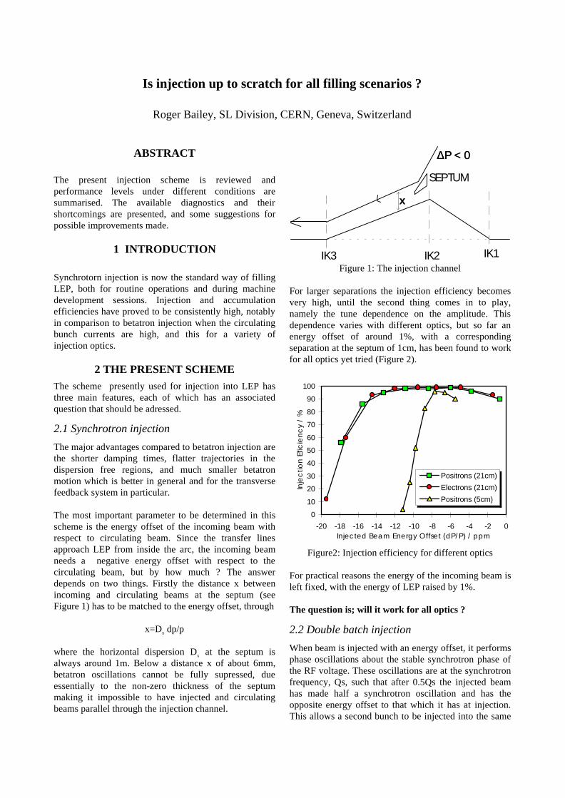
Is injection up to scratch for all filling scenarios ?


ABSTRACT

The present injection scheme is reviewed andperformance levels under different conditions aresummarised. The available diagnostics and theirshortcomings are presented, and some suggestions forpossible improvements made.

1 INTRODUCTION

Synchrotorn injection is now the standard way of fillingLEP, both for routine operations and during machinedevelopment sessions. Injection and accumulationefficiencies have proved to be consistently high, notablyin comparison to betatron injection when the circulatingbunch currents are high, and this for a variety ofinjection optics.

2 THE PRESENT SCHEMEThe scheme presently used for injection into LEP hasthree main features, each of which has an associatedquestion that should be adressed.

2.1 Synchrotron injection

The major advantages compared to betatron injection arethe shorter damping times, flatter trajectories in thedispersion free regions, and much smaller betatronmotion which is better in general and for the transversefeedback system in particular.

The most important parameter to be determined in thisscheme is the energy offset of the incoming beam withrespect to circulating beam. Since the transfer linesapproach LEP from inside the arc, the incoming beamneeds a negative energy offset with respect to thecirculating beam, but by how much ? The answerdepends on two things. Firstly the distance x betweenincoming and circulating beams at the septum (seeFigure 1) has to be matched to the energy offset, through

x=Dx dp/p

where the horizontal dispersion Dx at the septum isalways around 1m. Below a distance x of about 6mm,betatron oscillations cannot be fully supressed, dueessentially to the non-zero thickness of the septummaking it impossible to have injected and circulatingbeams parallel through the injection channel.

IK3 IK2 IK1

SEPTUM

x

∆Ρ < 0∆Ρ < 0

Figure 1: The injection channel

For larger separations the injection efficiency becomesvery high, until the second thing comes in to play,namely the tune dependence on the amplitude. Thisdependence varies with different optics, but so far anenergy offset of around 1%, with a correspondingseparation at the septum of 1cm, has been found to workfor all optics yet tried (Figure 2).

0

10

20

30

40

50

60

70

80

90

100

-20 -18 -16 -14 -12 -10 -8 -6 -4 -2 0Injected Beam Energy Offset (dP/P) / ppm

Inje

ctio

n E

ficie

nc

y /

%

Positrons (21cm)

Electrons (21cm)

Positrons (5cm)

Figure2: Injection efficiency for different optics

For practical reasons the energy of the incoming beam isleft fixed, with the energy of LEP raised by 1%.

The question is; will it work for all optics ?

2.2 Double batch injection

When beam is injected with an energy offset, it performsphase oscillations about the stable synchrotron phase ofthe RF voltage. These oscillations are at the synchrotronfrequency, Qs, such that after 0.5Qs the injected beamhas made half a synchrotron oscillation and has theopposite energy offset to that which it has at injection.This allows a second bunch to be injected into the same

bucket, with little or no perturbation to the circulatingbeam (Figure 3).

Φ

Φ

E

E

Turn = N ; Injection 1

Turn = N + 0.5/Qs ; Injection 2

RF-Bucket

Circulating Beam

Circulating Beam

Figure3: Double batch injection

The tricky thing here is the synchronisation between SPSand LEP, which has to take into account severalconstraints. For example the SPS extraction kickerrepetition rate has to be at least 149 µs, corresponding toa minimum of 6.75 SPS turns, or 1.75 LEP turns,between extractions. At the other extreme, from thepoint of view of synchrotron radiation in the SPS, it isbest to extract the high energy beam as quickly as

possible. On the LEP side, the number of LEP turnsbetween injections into the same bucket has to matchreasonably well with the Qs, so that the circulating beamis not affected. Also it is best not to leave beamcirculating too long before the second injection comesinto the same bucket, because of filamentation of thecirculating beam.

The scheme used consists of non-equidistant bunches inthe SPS, arranged into 2 families, and extracted in aparticular order with the advantage that the referencebunch in the SPS is the last to be extracted from thismachine. Implementation of this scheme has involvedchanging the harmonic number in the SPS, from 4616 to4620, by physical deformation of the 100MHz cavities.The scheme also introduces more complexity for theCPS, since this machine now needs to re-phase betweeninjection of each of the two batches. The fullsynchronisation scheme is shown in Figure 4.

Here it can be seen that there are 6 LEP turns betweeninjections into the same bucket, which matches well witha Qs of .08. This parameter can be increased in jumps of7, because after 7 LEP turns, which corresponds to 27SPS turns, the SPS and LEP are back in syncronisation.The choice of i in 6+i*7 depends on the desired Qs, asshown in figure 5. With the options shown, there isclearly a problem for Qs between .14 and .16. For thesevalues one would need longer between injections, withthe problems already mentioned then perhaps cominginto play. There are in any case particular problems witha Qs of .143, since this corresponds to exactly 7 LEPturns and so would not work for any value of i in theabove.

The question is; will it work for all Qs ?

1 3/4 4 1/4 1 3/4 1 3/4 4 1/4 1 3/42 3/4

6 + (i * 7) Turns

18 1/4 +2* (i * 7) LEP Turns = 1.55ms +2*(i*7) LEP Turns

LEP

Turns

17/28 10/28h 21/28h 14/28h 3/28h 24/28h 7/28h 0SPS Bucket

LEP Bucket 1 4 3 2 1 4 2 3

6 + (i * 7) Turns

Figure 4: The SPS-LEP synchronisation scheme

9V » iv”? Jva Vfififi’

%% 000 d%%%% '9'» 00000 $V“%

‘Qfifififififil « A..

0

0.5

1

0.07 0.08 0.09 0.1 0.11 0.12 0.13 0.14 0.15 0.16Qs

-Co

s(P

hi)

8 Turns

15 Turns

22 Turns

29 Turns

36 Turns

43 TurnsOOps!

Safe Minimum

Figure 5: Cos(Phi) of first batch as a function of Qs for different delays between injections

A point not to be missed with this scheme is that only2 lepton cycles are needed in the SPS. This frees timein the SPS supercycle for parasytic machinedevelopment, which has proved very valuablethroughout the year, with some 40*12 hour sessionsused in the shadow of SPS physics operation.

2.3 22 Gev injection energy

After several tests and some hardware changes in theSPS to allow extraction at the higher energy, thisvalue has been used successfully over the last 4 weekperiod of 1995, with no adverse effects seen.Furthermore, the expected gain of 10% inaccumulated current has been clearly demonstrated.For details and the answer to the following question,see presentation 2_02.

The question is; what limits the energy of theinjected beam ?

3 PERFORMANCE LEVELS INDIFFERENT MODES

In all cases studied, synchrotron injection yieldshigher efficiencies than betatron injection, particularlyinto a 'full' machine. This has been shown during aseries of MD experiments in 1994 and 1995, andoperationally in 1995. Some examples to make thepoint are given.

Figure 6 shows the positron injection efficiency as afunction of circulating electron bunch current, duringPretzel filling for both synchrotron and betatroninjection. While both schemes are over 80% efficientduring the first part of the process, betatron injectionefficiency falls sharply with counter-rotating bunchcurrents in excess of 100 uA. 4 on 4 efficiencies withsynchrotron injection are also shown.

Figure 7 shows the accumulation efficiency of onebeam as a function of circulating current, for bothsynchrotron and betatron injection into the detunedoptics. Also shown are the efficiencies withsynchrotron injection into the physics optics, whereessentially no reduction in efficiency is found.

0

10

20

30

40

50

60

70

80

90

100

0 50 100 150 200 250 300 350

Electron Bunch Current /uA

8x8 Betatron Inj

8x8 Synchrotron Inj

4x4 Synchrotron Inj

Figure 6: Positron injection efficiency vs circulatingelectron current in different modes

50

55

60

65

70

75

80

85

90

95

100

0 50 100 150 200 250 300 350 400 450 500

Average Bunch Current /

Betatron (21cm Optics)Synchrotron Injection (21cm Optics)Synchrotron Injection (5cm Optics)

Figure 7: Positron accumulation efficiencies withbetatron and synchrotron injection

For double batch injection, no direct measurementshave been made, for reasons that will be mentioned insection 4. However this mode has been usedoperationally throughout 1995, and the SPS and LEPmeasurement databases allow an estimate ofperformance to be extracted. Selecting a typical fill,3012, the bunch intensities in the SPS/LEP transferline can be found, which can then be converted intothe current per minute available to a LEP bunch. Byusing the LEP data, the intensity rise during fillingcan be used to find the current per minute actuallyaccumulated into a single bunch. Comparing thesetwo values yields an accumulation efficiency ofaround 80%, which is furthermore constant throughoutthe whole filling process. This corresponds to a totalfilling rate of around 1mA per minute, or a totalfilling time of under 10 minutes when things areoptimum.

4 DIAGNOSTICS, UTILITIES ANDSUGGESTED IMPROVEMENTS

While not really diagnostics, it should be said that theBeam Current Equaliser has proved to be a geatsuccess, allowing for each beam 1, 2, 3, or 4 trains of1, 2, 3, or 4 bunchlets to be injected as required. Thisflexibility has proved particularly powerful duringmachine development studies on differentconfigurations of bunch trains.

Otherwise the diagnostic most used is the slope of theBCT display! If it was clear that the machine wouldbe filled in something like 20mins, injectionefficiency was regarded as fine. There are features onthe BCT display to show the injection andaccumulation efficiencies, which are calculated fromthe bunch currents in the transfer line and thecirculating bunch currents after some turns (injectionefficiency) and a few hundred ms (accumulationefficiency). However, neither of these displays arecorrect with double batch injection, where the sameLEP bunch receives 2 transfer line bunches; theresults are wrong by about a factor 2. It would beextremely useful to make the necessary modificationsto have a correct online measure of the injection andaccumulation efficiencies for double batch injection.

If it was felt that the injection was not good enough,the most common approach was to check the end ofthe transfer line and the position of the incomingbeam on the luminescent screens.

More advanced procedures are available. Bycomparing the measured trajectory with the closedorbit, changes to the end of the transfer line (verticalplane), or to the IKP3 and the septum voltages

(horizontal plane), can be computed and this has oftenbeen used to optimise the injection trajectory.Utilities for measurement and correction of theinjection trajectory should be pushed into wideroperational use, with upgraded facilities ifappropriate. For example new pickups at the ends ofthe injection lines into LEP would improve thecorrection, leading to automatic correctionpossibilities.

By following the turn by turn evolution of the positionof the injected beam, a knowledge of the dispersion atthe injection point allows any injection phase error tobe deduced. For example with a Qs of .085, the beamshould have zero energy error and hence zero positionerror after 3 turns, if the injection phase is correct.Utilites to compute these kind of corrections arecoming, but for now are not used routinely by thecrews.

5 CONCLUSIONSynchrotron injection has proved to be a very efficientmethod of filling LEP in several modes. During 1995,double batch injection has been used throughoutroutine operation, with accumulation efficienciesaround the 80% level. For any new optics and anynew choice of Qs, the points raised such be given dueconsideration. There is room for improvement in theutilities available to the operators to measure andoptimise injection efficiencies, so that non-specialistscan maintain the impressive performances attainable.

How High can we push the Injection Energy of LEP ?

G. de Rijk, CERN, Geneva, Switzerland

ABSTRACTDuring 1995 the injection energy of LEP was

increased from 20 GeV to 22 GeV, with a correspondingincrease in the maximum bunch currents that can beaccumulated. The results from the commissioning of SPSand LEP at the new energy are presented together withthe prospects for, and limitations in the SPS to, furtherincreases of the LEP injection energy.

1 COMMISSIONING OF THE 22 GEVLEP INJECTION

1.1 LEP bunch currents

The single bunch current limit in LEP, during normaloperational conditions with as fractional tunes(Qh,Qv,Qs) = (0.28, 0.22, 0.085), is limited by thevertical Transverse Mode Coupling Instability (TMCI).The threshold current due to this instability is :

Ith = 2πQsEf 0

eΣβk(σs)Where Qs is the synchrotron tune, E the beam energy, f0the revolution frequency, β the vertical beta function at atransverse impedance with a loss factor k. The loss factork is a function of that specific impedance and the bunchlength σs. Accordingly, the maximum bunch currentshould be a linear function of the injection beam energy.Since its' commissioning in 1989, injection into LEP hasalways been done at a beam energy of 20 GeV. During amachine development session on 19th September 1995for the first time it was tried to inject electrons into LEPat 22 GeV [1]. As a first step the maximum single bunchcurrent for e- at 20 GeV was measured to be 515 mA withQs=0.083. The two machines, SPS and LEP, were thentuned to 22 GeV. At this energy, and the same Qs, themaximum single bunch current for e- was 575 mA, nicelyconfirming the 10% gain which was expected. In figure 1a current vs. time curve of this machine developmentsession can be seen. During the last period of 1995, so-called LEP 1.4, injection was routinely done at 22 GeVwithout seeing any adverse effects.

1.2 SPS 22 GeV operation.

The commissioning of 22 GeV lepton acceleration cyclesin the SPS was already started 3 years ago. At severaloccasions an e- beam was accelerated up to 22 GeVsuccessfully. The setting up of the SPS for acceleration ofe+ and e- beam to 22 GeV in September '95 was thusvery smooth. Some points needed nevertheless someattention to assure a correct extraction from the SPS andinjection in LEP:.

• The generation of the SPS and LEP timing pulses forpower supplies, kickers and beam observation.

• The SPS RF fast timing pulses.• The old (NODAL) SPS extraction and transfer line

software.Operation of the SPS with 22 GeV lepton cycles provedto be as straightforward as with 20 GeV cycles. Thestronger synchrotron radiation did not cause any increasein spark rate in the electro-static septa used for the protonextraction.

2 LIMITATIONS IN THE SPS RING

2.1 RF voltage limitations

A summary of the available RF voltage in the SPScan be found in table 1.

cavity type cavitiesV/cav(MV)

V total(MV)

200MHz SW 20 0.7 14352 MHz SC 4 7 28100 MHz SW 1 1 1All 43

Table 1 Available RF voltage for leptons in the SPS.

The required RF voltage for lepton acceleration in theSPS can be found in table 2.

Momentum(GeV)

V(MV)

20 2422 3523 4224 50

Table 2 Required RF voltage for leptons in the SPS.

The comparison between presently available and requiredRF voltage indicates that the maximum possiblemomentum for leptons in the SPS is 23 GeV. To updatethis to 24 GeV a new 352 MHz SC RF cavity is needed.This would also imply a significant extension of thecryogenic plant, used to cool the super conducting RFcavities in the SPS.

2.2 Limitations on the SPS main magnetic cycle

In the main magnetic cycle for the SPS (main bendingmagnets and quadrupoles) the lepton cycles are spaced by1.2 s. At the end of each lepton cycle the magnets aremagnetised with a current corresponding to 23.5 GeV.

Hence, a maximum beam momentum below 23.5 GeVhas no repercussions on the cycle lengths nor on themagnetic history. In the available time interval a 24 GeVlepton cycle can probably still fit in.

2.3 Limitations due to the synchrotron radiation

The criterion for the acceptable radiation dose, receivedby the magnets coils due to the synchrotron radiation isgiven in the LEP design report [2]. The dose induced bythe synchrotron radiation should not exceed the doseinduced by the protons, being 106 rad/year. The dose onthe inside of the coils as a function of energy can be foundin table 3 [2].

Energy (GeV) Dose(rad/yr)

20 6.6x104

22 2.0x105

23 4.6x105

24 1.0x106

Table 3 The yearly radiation dose due to the synchrotronradiation on the inside of the SPS magnet coils [2].

The assumption in the design report was that the beampipe would shield the coils from a large part of theradiation. This is not the case at the flanges whereradiation can escape and illuminate distinct parts of themagnets. The problem was solved by introducing specialLead and Tungsten shielding pieces into the bellows [3].It was done such as to get a similar shielding effect asfrom the un-perturbed beam pipe. With these precautionsone can conclude that the system was designed to be stillOK at 23 GeV. The radiation dose does reach values toonear to the limit when the beam momentum reaches 24GeV.

3 LIMITATIONS IN THE SPS -LEPBEAM TRANSFER LINES

3.1 Magnet limitations

All magnets are dimensioned such that the limits areabove 25 GeV. The limit for the cooling circuits of themagnets is situated around 28 GeV.

3.2 Power convertor limitations

E(GeV)

PCname

Iops(A)

Imax(A)

limitorigin

23 IQFD1211 118 120 PC24 IMSA1822 588 600 DCCT

IDFD1211 120 120 PCIMSA1221 586 600 DCCT

Table 4 Current limitations on transfer line powerconvertors

In table 4 the limits on the power convertors are listed.From this we may conclude that 23 GeV can be donewithout any modifications. To reach 25 GeV some smallmodifications are needed on some power convertors.

3.3 Kicker magnet limitations

The kicker magnet power generators already underwentan update from 20 GeV to 22 GeV. A further update of5% to run at 23 GeV is relatively easy. No additionalhardware installation is needed for this. A 10 % update to24 GeV is still possible but will need more effort. At 23GeV it is equally possible to run at the same kick settingsas 22 GeV but to adapt the angle of the beam at thebegin/end of the transfer line.

4 RECOMMENDATIONS

4.1 The possibilities

Using the maximum RF voltage available the SPScan deliver lepton beams of 23 GeV to LEP without anyadditional investments or developments. Updating theSPS for lepton beams of 24 GeV requires the installationof an additional 352 MHz SC cavity which also means anextension of the installed cryogenic plant in BA4. Smalladjustments on several power convertors and kicker powergenerators would also be needed. A more seriouslimitation is the deposited radiation dose on the magnetcoils by the synchrotron radiation of the beam. At 24GeV this dose is at the limit of what is acceptable.

4.1 A safe strategy

When we want to take into account the operationalreliability of the SPS and the RF requirements we shouldlook at the repercussions of RF cavity trips in the SPS.This information can be found in table 5. One shouldthereby remind that the 4 super conducting RF cavities areinstalled into 2 cryostats. Hence, in case of cryogenicproblems on one cryostat 2 cavities will be out of order.

Energy(GeV)

possible# of SCtripped

possible# of cryostatproblems

possible# of SWCtripped

20 2 1 2022 1 0 1023 0 0 2

Table 4 RF trips in the SPS. Operational possibilities:The maximum number of non functioning cavities whichwill not inhibit the acceleration of the beam.

From table 5 we can read that the operation of the SPS at23 GeV is very much at the limit and induces the risk of alower efficiency due to a too marginal RF poweravailable. Even at 22 GeV we risk to loose a week ofoperation in the case of a cryogenic problem on one of thecryostats. Hence, it would be more reasonable to continue

to run the SPS lepton cycles at 22 GeV. Meanwhile afallback solution with 20 GeV lepton cycles shouldalways be kept available such that with a delay of half aday a switch-back to 20 GeV will be possible.

REFERENCES[1] PERC summary notes MD 19-9-95 on 22 GeV

injection into LEP, R. Bailey, P. Collier , R.Giachino, L Norman

[2] LEP design report, vol I, The LEP Injector Chain,CERN /SPS/83-26

[3] Shielding the SPS against synchrotron radiation,B.de Raad, CERN /SL/90-119(DI)

0

0.1

0.2

0.3

0.4

0.5

0.6

0.7

7:17

:29

9:23

:05

11:0

4:49

11:2

0:41

11:3

2:45

11:4

4:45

11:5

6:49

Time

Sin

gle

Bun

ch C

urre

nt /

mA

22 GeV, High Qs20 GeV 22 GeV

Maximum Accumulated Intensity in a Single Bunch for Injection at 20 GeV, 22 GeV and with High Qs

Figure 1 Single bunch e- beam current vs. time for the 22 GeV injection MD session

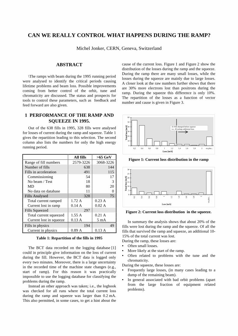
CAN WE REALLY CONTROL WHAT HAPPENS DURING THE RAMP?

Michel Jonker, CERN, Geneva, Switzerland

ABSTRACT

\The ramps with beam during the 1995 running periodwere analysed to identify the critical periods causinglifetime problems and beam loss. Possible improvementscoming from better control of the orbit, tune andchromaticity are discussed. The status and prospects fortools to control these parameters, such as feedback andfeed forward are also given.

1 PERFORMANCE OF THE RAMP ANDSQUEEZE IN 1995.

Out of the 638 fills in 1995, 328 fills were analysedfor losses of current during the ramp and squeeze. Table 1gives the repartition leading to this selection. The secondcolumn also lists the numbers for only the high energyrunning period.

All fills >65 GeVRange of fill numbers 2579-3226 3068-3226Number of fills 638 144Fills in acceleration 491 115

Commissioning 54 17No beam / Test 18 3MD 80 20No data on database 11 0

Fills Analysed 328 75Total current ramped 1.72 A 0.23 A Current lost in ramp 0.14 A 0.02 A

Fills Squeezed 297Total current squeezed 1.55 A 0.21 A Current lost in squeeze 0.13 A 5 mA

Fills in physics 194 49Current in physics 0.89 A 0.13 A

Table 1: Repartition of the fills in 1995

The BCT data recorded on the logging database [1]could in principle give information on the loss of currentduring the fill. However, the BCT data is logged onlyevery two minutes. Moreover, there is a large uncertaintyin the recorded time of the machine state changes (e.g.,start of ramp). For this reason it was practicallyimpossible to use the logging database for classifying theproblems during the ramp.

Instead an other approach was taken; i.e., the logbookwas checked for all runs where the total current lossduring the ramp and squeeze was larger than 0.2 mA.This also permitted, in some cases, to get a hint about the

cause of the current loss. Figure 1 and Figure 2 show thedistribution of the losses during the ramp and the squeeze.During the ramp there are many small losses, while thelosses during the squeeze are mainly due to large losses.A closer look at the raw numbers further shows that thereare 30% more electrons lost than positrons during theramp. During the squeeze this difference is only 10%.The repartition of the losses as a function of vectornumber and cause is given in Figure 3.

0

10

20

30

40

50

60

0,2 0,4 0,6 0,8 1 1,2 1,4 1,6 1,8 2 ou plus...

Loss [mA]

Tot

al lo

ss [m

A]

31 Fills dumped before squeeze i.e., 30 mAmp additional loss.

Figure 1: Current loss distribution in the ramp

0

5

10

15

20

25

30

0,2

0,4

0,6

0,8 1

1,2

1,4

1,6

1,8 2

ou p

lus.

..

Loss [mA]

Tot

al lo

ss [m

A]

Figure 2: Current loss distribution in the squeeze.

In summary the analysis shows that about 20% of thefills were lost during the ramp and the squeeze. Of all thefills that survived the ramp and squeeze, an additional 10-15% of the total current was lost.During the ramp, these losses are:• Often small losses.• More likely at the start of the ramp.• Often related to problems with the tune and the

chromaticity.During the squeeze, these losses are:• Frequently large losses, (in many cases leading to a

dump of the remaining beam).• In general associated with bad orbit problems (apart

from the large fraction of equipment relatedproblems).

flflflmflfl_fifl

"|—l:|—|:l—I:|—|:|—|: l—lflfl I—I |—|

Current loss during ramps

0

10

20

30

40

50

BE

FO

RE

Sta

rt

V1

7

V0-

20

V20

-60

V60

-100

V1

00

-20

0

V2

05

un

kno

wn

Cur

rent

Los

s [m

A]

Current loss during ramps

0

10

20

30

40

50

be

fore

V2

05

-23

8

V2

20

V2

30

V2

38

afte

r

Cur

rent

Los

s [m

A]

Current loss during squeeze

0

10

20

30

40

50

60

70

un

kno

wn

orb

it

tun

e

Qs

tfb rf

scrf

gvc

gvc/

op

pc/

op zl

cryo

Cur

rent

Los

s [m

A]

Current loss during squeeze

0

10

20

30

40

50

slop

pyso

ft

un

kno

wn

orbi

t

tune rf

rfsc

gvc/

op

pc/o

p

mai

nben

ds zl

zlsp

ark

db

Cur

rent

Los

s [m

A]

Figure 3: Repartition of the losses during the ramp and squeeze.

2 DO WE REALLY KNOW WHATHAPPENS DURING THE RAMP.

In the previous section we have seen that the controlof machine parameters is important to minimise the lossesduring the ramp and the squeeze. Tune and chromaticityare important to control during the start of the ramp.During the squeeze orbit drifts also become important.This section discusses how each of these three machineparameters can be controlled during the ramp andsqueeze.

ORBIT

The orbit during the ramp and squeeze, is normallycorrected by interrupting the ramp and squeeze severaltimes (breakpoints). At each breakpoint the orbit ismeasured and corrected. This is rather a time consumingtask, which is only done to commission the ramp for anew optic. Once the optics is commissioned, the orbit isonly corrected at injection, between the ramp and thesqueeze and at the end of the squeeze. The orbitcorrections are then incorporated in the correctorfunctions (gradual out or with constant strength).

This implies that we are usually blind to what happensduring the ramp and the squeeze, and that we are not sureif a given orbit correction is properly interpolated duringthe ramp and squeeze. This last point is particularly ofimportance for the squeeze where the optics is changing.

Only occasionally, when a bad orbit is expected duringthe ramp, an additional break point is set and the orbit iscorrected.

An option that allows the orbit measurement system totake consecutive measurements during the ramp wasdiscussed several times in Chamonix [2]. The optionactually has been implemented and works up to somelevel of convenience. During one (68 GeV) run, themulti-orbit option was used to measure the orbit evolutionduring the ramp, during the squeeze and during thesecond ramp.

The analysis of this measurement is presented here.Figure 4 shows the growth of the orbit relative to the startof the ramp, the squeeze and the second ramp; i.e., therms of the orbit relative to the reference orbit taken at thestart is given. Figure 7 displays the same data for theelectron-positron difference orbit and clearly shows thepoor adaptation of the separator functions (or optics)during the squeeze

These figures show that the orbit distortions can besignificant. The rms changes rapidly at the start of theramp approaching and for some cases passing the level of1 mm2. Note that the usual orbits typically have an rms of0.8 (horizontal) and 0.6 (vertical). A small increase of therms does not necessarily mean that the orbit gets worse. Aplot of the absolute numbers of the electron-positrondifference orbit shows that the rms is even slightlyimproving at the end of the squeeze.

. m fl fl fi fl fl fl _H mmflmmm

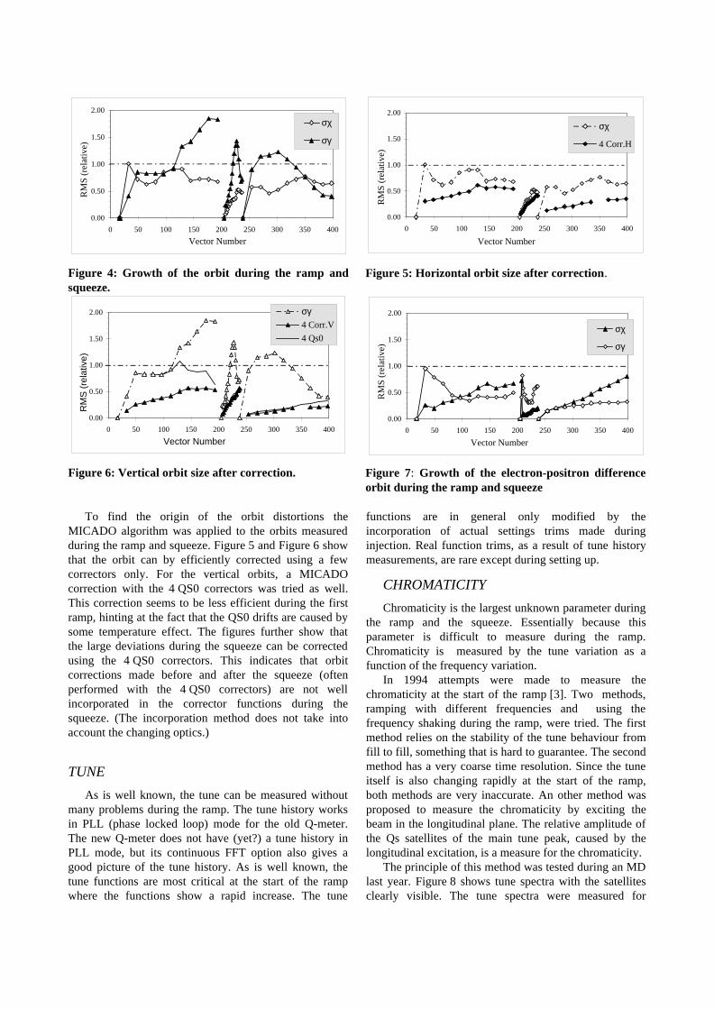
0.00

0.50

1.00

1.50

2.00

0 50 100 150 200 250 300 350 400

Vector Number

RM

S (

rela

tive)

σχ

σγ

Figure 4: Growth of the orbit during the ramp andsqueeze.

0.00

0.50

1.00

1.50

2.00

0 50 100 150 200 250 300 350 400

Vector Number

RM

S (

rela

tive)

σγ4 Corr.V

4 Qs0

Figure 6: Vertical orbit size after correction.

0.00

0.50

1.00

1.50

2.00

0 50 100 150 200 250 300 350 400

Vector Number

RM

S (

rela

tive)

σχ

4 Corr.H

Figure 5: Horizontal orbit size after correction.

0.00

0.50

1.00

1.50

2.00

0 50 100 150 200 250 300 350 400

Vector Number

RM

S (

rela

tive)

σχ

σγ

Figure 7: Growth of the electron-positron differenceorbit during the ramp and squeeze

To find the origin of the orbit distortions theMICADO algorithm was applied to the orbits measuredduring the ramp and squeeze. Figure 5 and Figure 6 showthat the orbit can by efficiently corrected using a fewcorrectors only. For the vertical orbits, a MICADOcorrection with the 4 QS0 correctors was tried as well.This correction seems to be less efficient during the firstramp, hinting at the fact that the QS0 drifts are caused bysome temperature effect. The figures further show thatthe large deviations during the squeeze can be correctedusing the 4 QS0 correctors. This indicates that orbitcorrections made before and after the squeeze (oftenperformed with the 4 QS0 correctors) are not wellincorporated in the corrector functions during thesqueeze. (The incorporation method does not take intoaccount the changing optics.)

TUNE

As is well known, the tune can be measured withoutmany problems during the ramp. The tune history worksin PLL (phase locked loop) mode for the old Q-meter.The new Q-meter does not have (yet?) a tune history inPLL mode, but its continuous FFT option also gives agood picture of the tune history. As is well known, thetune functions are most critical at the start of the rampwhere the functions show a rapid increase. The tune

functions are in general only modified by theincorporation of actual settings trims made duringinjection. Real function trims, as a result of tune historymeasurements, are rare except during setting up.

CHROMATICITY

Chromaticity is the largest unknown parameter duringthe ramp and the squeeze. Essentially because thisparameter is difficult to measure during the ramp.Chromaticity is measured by the tune variation as afunction of the frequency variation.

In 1994 attempts were made to measure thechromaticity at the start of the ramp [3]. Two methods,ramping with different frequencies and using thefrequency shaking during the ramp, were tried. The firstmethod relies on the stability of the tune behaviour fromfill to fill, something that is hard to guarantee. The secondmethod has a very coarse time resolution. Since the tuneitself is also changing rapidly at the start of the ramp,both methods are very inaccurate. An other method wasproposed to measure the chromaticity by exciting thebeam in the longitudinal plane. The relative amplitude ofthe Qs satellites of the main tune peak, caused by thelongitudinal excitation, is a measure for the chromaticity.

The principle of this method was tested during an MDlast year. Figure 8 shows tune spectra with the satellitesclearly visible. The tune spectra were measured for

different values of the horizontal chromaticity. Figure 9shows the dependence of the amplitude ratio as a functionof the chromaticity trim. This MD has shown that theprinciple works. However, to convert this to a validprocedure for measuring the chromaticity during theramp, requires more work and MD studies.

.00

.02

.04

.06

.08

.10

0.1

91

7

0.1

94

2

0.1

96

6

0.1

99

1

0.2

65

5

0.2

68

0.2

70

4

0.3

61

0.3

63

5

0.3

65

9

Qh

Am

plitu

de

Q' trim=0

Q'trim=2

Q'trim=4

Figure 8: Tune spectra for various chromaticity trims.Note that this figure only shows the principal modeand the two Qs satellites.

Amplitude Ratio (m- + m+) / m0

0

0.5

1

1.5

2

-1 0 1 2 3 4 5Qh'trim

Pea

k ra

tio

Figure 9: Amplitude ratio as a function of thechromaticity trim.

Additional tools are required to collect raw dataduring the ramp, and to extract the chromaticity from thisdata using a sliding FFT window. The amplitude ratiomay further depend on the tune value itself, specifically ifstrong resonance's are present. Since the tune is varyingrapidly during the ramp, a careful calibration is requiredof this method. This calibration should also take intoaccount the dependency on the tune.

This method may probably evolve someday into amethod of measuring the chromaticity during the ramp.However, it will probably be a delicate procedure and nota tool for everyday usage.

3 DO WE HAVE THE TOOLS TOCONTROL WHAT HAPPENS DURING

THE RAMP.In this section we will discuss the options to improve

the control of the three critical machine parameters duringthe ramp. Essentially there are two general ways tocontrol these parameters: feed-back or feed-forward.

Orbit

A first improving of the orbit control during thesqueeze should come from a proper incorporationstrategy for the 4 QS0 corrections. If such a strategy takesinto account the changing optics during the squeeze, mostof the orbit distortions during the squeeze will disappear.A similar remark holds for the ZL functions which, asindicated by the difference orbit, are not well adapted tothe changing optics during the squeeze.

The multi-orbit option of the bom system couldprovide an effective feed-forward system. The orbitdistortions measured during a ramp or squeeze can becorrected and incorporated into the functions for the nextramp. This will be particularly useful to improve the turnaround time while commissioning the ramp for a newoptics.

At present there is still some effort required to makesuch a system to work. The acquisition of the multi-orbitsystem works, but has some disadvantage. After theacquisition of a multi-orbit, there is more than one minuterequired to process the raw data. During this time theorbit system is unavailable. If the orbit at the end of theramp or squeeze is causing lifetime problems, such adelay will probably not be appreciated. A possibleimprovement can be made if the last orbit is extractedwith higher priority and be made available for correction.

Further work is needed to provide a tool whichanalysis the data from the multi-orbit. The tool shoulddetect if all bom stations responded properly (in the datapresented above, one station had to be excluded since itsdata did not make any sense). The individual orbitsshould be corrected with some correction strategy. Aconcise result display should provide the operator withenough information to decide whether the corrections areto be incorporated into the orbit functions or not.

If orbit distortions are due to mechanical movementsof the supra quads, as suggested by the success of the 4QS0 corrections, one might think of using a directfeedback system. Such a feedback system is alreadyconsidered to be used during physics mode [4]. Thisfeedback will use the data from a hydrostatic levelmeasurement and act on the QS0 correctors. To use thesame feedback during the ramp and squeeze will be moretricky. In the first place, the QS0 correctors are executinga ramp function and cannot be trimmed. A solution wouldbe to use a trim-daq. The second complication is that theenergy and optics are changing during the ramp and

squeeze. The feedback system should be aware of thisand adapt its gain accordingly.

Tune

Tune is probably the best controlled parameter duringthe ramp. Tune-history data can be displayed and fedforward into the tune functions for the next ramp. At themoment this procedure goes entirely by hand. Convertingthe tune-history data to a function trim can be confusing.A modification of the tune-history display, that allows theoperator to extract the tune function trim from the tunedata would be appreciated.

There exists also a feedback mechanism for the tune(tune-lock option on the old Q-meter). This mechanismworks particularly well with lower beam currents. Sincetune control is less critical at lower intensities, it isusually not used in these cases. At higher intensitieswhere tune control becomes more critical, this systemperforms less well. The presence of higher order modes inthe tune spectrum can confuse the PLL of the Q-meter. Insuch a case the feedback can easily lock onto the wrongtune value. The new Q-meter, if provided with a correctpeak tracking algorithm in continuous FFT mode, shouldbe able to perform better.

Chromaticity

Although we have no direct way to control thechromaticity during the ramp, there is an option to makethis parameter less critical. Transverse feedback (TFB) ina resistive mode can be used to suppress coherentoscillations of the beam. With the additional dampingprovided by the TFB system, one can afford to run themachine with a lower chromaticity making the machineless critical to this parameter during the ramp.

TFB was used during most of the time in 1995.Although no comparative data is available, the generalimpression is that chromaticity has been less of a problemwith the usage of TFB.

4 ANY OTHER IDEAS TO MAKE LIFEEASIER ?

Apart from striving to better control the machineparameters that affect the stability during the ramp, onecould also operate the machine in a way that avoids someof these problems. Some of these idea’s are:• Ramp faster At present, the LEP energy ramp goes at 1/8 of the

original design speed. The advantage of rampingfaster would be that less time is spend with the tune(and chromaticity) near dangerous resonance’s ; i.e.,the machine will have changed its characteristicsbefore the instabilities grow out of hand. On the otherhand, ramping faster may have effects on the tune andthe chromaticity itself. Eddy currents caused by the

changing magnetic field create higher order magneticmoments. Part of this effect is normally corrected bythe correc mechanism.

An MD was done this year where the machine wasramped at only one quarter of the design speed (i.e.,twice the regular speed). No particular problems wereobserved during this MD [5].

• Ramp less As has been show before, the start of the ramp is more

critical. Injecting at higher energy would avoid someof the problems causing losses at the start of the ramp.Prospects for injecting at higher energy are discussedin an other session of this workshop [6].

• Squeeze less To avoid problems related to the changing (and badly

matched) optics during the squeeze one could injectinto an optics with a lower β*. Such an optic couldmake the squeeze shorter and, if better matched, lesscritical. This topic is discussed in a special session inthis workshop [7].

REFERENCES

[1] R.Billen, The evolution of the LEP logging database.

Presented at the International Conference onAccelerator and Large Experimental Physics ControlSystems. - ICALEPCS '95, -Chicago, IL, USA,30 Oct-3 Nov 1995

[2] H.Schmickler, Applications for the 1000-Turn OrbitAcquisition, in J.Poole (Ed.) Proceedings of the ThirdWorkshop on LEP performance, Chamonix France,January 10-16 1993, CERN SL/93-19(DI) (1993),pp. 217-218.

- M.Lamont, Orbit Feedback, in J.Poole (Ed.)Proceedings of the Fourth Workshop on LEPperformance, Chamonix France, January 17-21 1994,CERN SL/94-06(DI) (1994), pp. 103-105.

[3] M.Jonker, Problems at the Start of High IntensityRamps, in J.Poole (Ed.) Proceedings of the FifthWorkshop on LEP performance, Chamonix France,January 15-19 1995, CERN SL/95-08(DI) (1995),pp. 79-81.

[4] J.Wenninger, New utilities for beam-beamoptimisation, Presentation 1.03, these proceedings.

[5] P.Collier and G.Roy, Removal off the LEP RampRate Limitation, SL-MD Note 195, Dec. 1995.

[6] G.de Rijk, How High Can We Push the InjectionEnergy of LEP?, Presentation 2.02, these proceedings.

[7] G.Roy, Is Injection and Ramping with the SqueezedOptic the Answer to Life the Universe and Every-thing?, Presentation 2.04, these proceedings.

IS “INJECTION AND RAMPING WITH SQUEEZED OPTICS” THEANSWER TO LIFE, THE UNIVERSE AND EVERYTHING?

Ghislain ROYSL Division

Abstract

The adoption of Synchrotron Injection last year has madeit possible to investigate “injection and ramping withsqueezed optics”1 instead of the normal detuned optics.Forty-two good arguments, from time saving and avoidingpathological behaviours of magnet excitations to numerol-ogy, all in favor of the use of a single optics from injection tophysics are presented. Results from MD are detailed and po-tential drawbacks and limitations of this operating schemeare discussed with a proposal for a timely implementationof this Answer in 1996.

1 INTRODUCTION

Synchrotron injection[2, 4] has been used extensively atLEP since the last period of the 1994 run. Besides its manyadvantages[3] it has opened the possibility of injecting di-rectly into the squeezed optics with

y= 5 cm, thereby

suppressing the Squeeze segment for LEP operation. Thishas been tested in machine development sessions in 1994and 1995 and the first section gives a review of the results.Then some details of the main arguments in favor of injec-tion into squeezed optics are presented. Finally some poten-tial problems are outlined.

2 MD RESULTS

The first machine development session on synchrotron in-jection into squeezed optics[5] was done at the end of 1994right after synchrotron injection was put in daily opera-tion. The MD showed that, contrary to betatron injectioninto squeezed optics where injection was difficult and ac-cumulation impossible[7], it is possible to inject into thesqueezed optics using synchrotron injection. A single beamof positrons was used, no radiation was seen in the experi-ments and the injection efficiency was measured as a func-tion of the energy offset (fig. 1). The same maximum bunchcurrent was accumulated in the squeezed and the detunedoptics showing no single beam intensity limitation specificto injection on squeezed optics.

A second MD in October 1995 was used to inject andramp two beams[9]. It was discovered that the QS2 mag-nets are the horizontal aperture limits of LEP at injectionfor both the detuned and squeezed optics when all collima-tors are retracted. Collimators were closed to a safe position

1Note that this string is exactly forty-two characters long includingspaces.

0

10

20

30

40

50

60

70

80

90

100

-20-18-16-14-12-10 -8 -6 -4 -2 0Injection Efficiency [%]

Injected Beam Energy Offset [ppm]

e+

e-

21cm 5cm

Figure 1: Injection efficiency into an empty LEP as a func-tion of the momentum deviation of the injected beam. Thetwo curves correspond to the nominal detuned optics (

y=

21 cm) and the squeezed optics (y= 5 cm). The betatron

injection on squeezed optics is shown at p

p= 0 and its

efficiency was around 20%10%

and this procedure was used for the rest of the year. We ac-cumulated reasonable currents with no attempt to probe thetwo-beam intensity limit and ramped the beams to 45.6 GeV.Transverse feedback was off, longitudinal feedback was onand we found no particular problem to ramp 1.6 mA (44with 200 A per bunch) and without losses.

The third MD[10] in November 1995 was intended toprobe the two-beam intensity limit. It was difficult to tunethe injection for electrons and positrons at the same time.An energy difference of about 0.3% or 66 MeV between thetwo beams extracted from the SPS could be the cause of this.This could not be quickly fixed from the SPS side and wedecided to change the program of the MD. One beam wasramped at double the nominal speed with squeezed optics.The beam arrived at 45 GeV with no losses.

Overall the MD’s on Injection and Ramping withSqueezed Optics have been remarkably smooth. Injectionis clean and the ramp is at least as easy as with the detunedoptics. The only outstanding item is the two-beam currentlimit which could not be tested because of poor injectionwith two beams.

3 ADVANTAGES

The advantages of “Injection and Ramping with SqueezedOptics” are numerous and the author has identified forty-twovalid arguments. Most of them can be classified under thefour headings below.

3.1 Saving Time

As was pointed out by P. Collier[8] the time taken in theRamp and Squeeze will nearly triple for LEP2. The currentstrategy was adopted to meet energy scan requirements andincludes the following steps: Ramp from 22 GeV to about44 GeV, Squeeze then Ramp to final energy.

The time taken in the ramp itself is mostly controlled bythe Timex parameter which allows one to slow-down theramp with respect to the design ramp speed. Timex 8 hasbeen used so far and it would take about 2.5 cups2 to rampwithout stop to 90 GeV.

For comparison it takes about half a cup to go through thetwenty eight vectors of the Squeeze segment. Settings gen-eration takes one-half to one cup depending on the databaseconditions. At the end of each segment optical corrections(orbits, tunes...) must be done by the crew and this can takeanywhere from one-eighth to four cups.

With the present scheme and Timex 8 it would take aboutfive cups, or close to 40 minutes to take the beams frominjection to preparing physics at 90 GeV. Injection andRamping with Squeezed Optics would not only suppress theSqueeze but also two of the three optics correction steps andat least one settings generation. In the same conditions itwould then take about two cups to ramp the beams, a sav-ing of close to 25 minutes.

This time saving would clearly be very beneficial to mini-mize the turn-around time between physics fills and therebycontribute to the overall efficiency of LEP. Remember thatunless we are beam-beam limited the luminosity decay willbe faster for LEP2 and therefore we expect to have morefills per day than we had for LEP1 physics. Another ef-fect clearly seen during the high-energy run in 1995 is theshorter time constant of the heating and cooling of the ma-chine. Since the stability and reproducibility of LEP isclearly linked to the temperature stability it is very impor-tant that we minimise the time between physics fills.

Doubling the ramp speed with Timex 4 would save alsosome time in the Ramp itself. It has been successfullytried[10] in conjunction with Injection and Ramping withSqueezed Optics. We propose to start LEP in 1996 withTimex 4 and investigate a further reduction during the year.Note also that any reduction of Timex gives even more in-centive to suppress the Squeeze segment in the above timeaccounting.

2The Collier Unit at Percolator is convenient for control room pur-poses. 1 cup 7 min 42 sec.

3.2 Ease of Operation

Details on the behaviour of LEP during the Ramp is reportedat this workshop [12]. The Ramp can be somewhat hard tocontrol in the first thirty vectors or so. It is usually a verysmooth process at higher energy.

The incorporation of trims at low energy in the Rampfunctions is relatively easy since the only changing param-eter is the energy. Improvements have been proposed[12]for controlling the tunes and chromaticities. For orbit con-trol we incorporate the trims into the functions such that theyare propagated at constant strength. Further improvementsof orbit control are also envisaged.

Funny how just when you think life can’t possiblyget any worse it suddenly does.

Marvin [1]

The propagation of corrections during the Squeeze ismuch harder since we must take into account the change ofoptics. An optics is clearly defined and matched for a fewpoints only (

y= 21, 14, 11, 9, 8, 7, 6 and 5 cm). Between

these points a linear interpolation is done and the optics ismismatched; the tunes and chromaticities may change andthe Bunch Train bumps are not closed as can be seen on theBEUV with the beams “stepping” through the Squeeze. Or-bit and optics corrections can only be done at these matchedpoints. Matching more points would merely reduce the step-size and the magnitude of the effects. With more bunch cur-rent required for LEP2 the beams may become more sensi-tive to tune and/or chromaticity excursions.

The propagation of orbit corrections across the Squeezeis a problem: we try and correct the orbit in the Rampand Squeeze with as few correctors as possible, resulting insome non-local correction. We also use preferentially thecorrectors close to the QS0 magnets since we know thesemagnets are the most sensitive (thermal drifts...)[12, 13].The change of optics in the even insertions is most pro-nounced at the final doublet. It is therefore expected thatthe orbit can degrade significantly at the end of the Squeezewith the risk of current loss. The beam losses being oftenunequal for the two beams or among bunches of a train thestability of the following physics fill can be jeopardised.

From an operational point of view the suppression ofthe Squeeze segment is desirable. More effort could thenbe placed on tuning the machine at injection and beforephysics.

3.3 Ease of Matching

The preparation of a new optics usually starts with the op-timization of the physics optics. As part of the process wecheck that detuning is possible down to

y= 21 cm. We

never had to reject an optics for failing to detune but we of-ten have to play some tricks such as using the quadrupolesin the RF sections to help with the Low-Beta optics (LOBS)or changing the value of

xat injection. In 1995 it was not

possible to detune IP4 and IP8 to y= 21 cm while keep-

ing x= 2:5 m so we used 2.0 m instead. This situation,

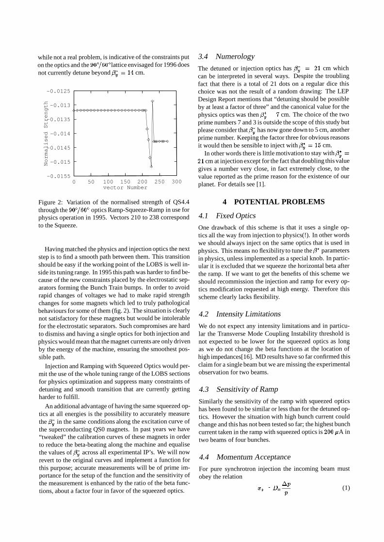
while not a real problem, is indicative of the constraints puton the optics and the 90=60lattice envisaged for 1996 doesnot currently detune beyond

y= 14 cm.

-0.0155

-0.015

-0.0145

-0.014

-0.0135

-0.013

-0.0125

0 50 100 150 200 250 300

Normalised Strength

vector Number

Figure 2: Variation of the normalised strength of QS4.4through the 90=60 optics Ramp-Squeeze-Ramp in use forphysics operation in 1995. Vectors 210 to 238 correspondto the Squeeze.

Having matched the physics and injection optics the nextstep is to find a smooth path between them. This transitionshould be easy if the working point of the LOBS is well in-side its tuning range. In 1995 this path was harder to find be-cause of the new constraints placed by the electrostatic sep-arators forming the Bunch Train bumps. In order to avoidrapid changes of voltages we had to make rapid strengthchanges for some magnets which led to truly pathologicalbehaviours for some of them (fig. 2). The situation is clearlynot satisfactory for these magnets but would be intolerablefor the electrostatic separators. Such compromises are hardto dismiss and having a single optics for both injection andphysics would mean that the magnet currents are only drivenby the energy of the machine, ensuring the smoothest pos-sible path.

Injection and Ramping with Squeezed Optics would per-mit the use of the whole tuning range of the LOBS sectionsfor physics optimization and suppress many constraints ofdetuning and smooth transition that are currently gettingharder to fulfill.

An additional advantage of having the same squeezed op-tics at all energies is the possibility to accurately measurethe

yin the same conditions along the excitation curve of

the superconducting QS0 magnets. In past years we have“tweaked” the calibration curves of these magnets in orderto reduce the beta-beating along the machine and equalisethe values of

yacross all experimental IP’s. We will now

revert to the original curves and implement a function forthis purpose; accurate measurements will be of prime im-portance for the setup of the function and the sensitivity ofthe measurement is enhanced by the ratio of the beta func-tions, about a factor four in favor of the squeezed optics.

3.4 Numerology

The detuned or injection optics has y= 21 cm which

can be interpreted in several ways. Despite the troublingfact that there is a total of 21 dots on a regular dice thischoice was not the result of a random drawing: The LEPDesign Report mentions that “detuning should be possibleby at least a factor of three” and the canonical value for thephysics optics was then

y= 7 cm. The choice of the two

prime numbers 7 and 3 is outside the scope of this study butplease consider that

yhas now gone down to 5 cm, another

prime number. Keeping the factor three for obvious reasonsit would then be sensible to inject with

y= 15 cm.

In other words there is little motivation to stay withy=

21 cm at injection except for the fact that doubling this valuegives a number very close, in fact extremely close, to thevalue reported as the prime reason for the existence of ourplanet. For details see [1].

4 POTENTIAL PROBLEMS

4.1 Fixed Optics

One drawback of this scheme is that it uses a single op-tics all the way from injection to physics(!). In other wordswe should always inject on the same optics that is used inphysics. This means no flexibility to tune the parametersin physics, unless implemented as a special knob. In partic-ular it is excluded that we squeeze the horizontal beta afterthe ramp. If we want to get the benefits of this scheme weshould recommission the injection and ramp for every op-tics modification requested at high energy. Therefore thisscheme clearly lacks flexibility.

4.2 Intensity Limitations

We do not expect any intensity limitations and in particu-lar the Transverse Mode Coupling Instability threshold isnot expected to be lower for the squeezed optics as longas we do not change the beta functions at the location ofhigh impedances[16]. MD results have so far confirmed thisclaim for a single beam but we are missing the experimentalobservation for two beams.

4.3 Sensitivity of Ramp

Similarly the sensitivity of the ramp with squeezed opticshas been found to be similar or less than for the detuned op-tics. However the situation with high bunch current couldchange and this has not been tested so far; the highest bunchcurrent taken in the ramp with squeezed optics is 200 A intwo beams of four bunches.

4.4 Momentum Acceptance

For pure synchrotron injection the incoming beam mustobey the relation

xs = Dx

p

p(1)

<>

where Dx is the horizontal dispersion at the septum, fixedby the optics, xs is the separation between the injected andcirculating beam, severely limited by the septum thickness,and p=p is the difference between the injected beam en-ergy and the circulating beam energy. Only the last parame-ter can be varied easily. Obviously it is not enough to injectthe particles into the machine but they have to be stable afterinjection. The damping in synchrotron phase space is of theorder of a few hundred turns but the particles will be lost ina few turns if they come close to an integer resonance.

The momentum acceptance is estimated from the evolu-tion of the tunes as a function of the energy deviation. Thechromatic effects will severely limit this momentum accep-tance. The sextupoles can be arranged to control the chro-maticity and at the same time minimise the higher order ef-fects; however the lower

ythe more important these chro-

matic effects get, with a correlated reduction of the dynamicacceptance. If the required energy offset from equation 1falls outside of the dynamic acceptance then synchrotron in-jection is impossible.

The horizontal dispersion also appears in equation 1 withconsequences for the low emittance lattices foreseen forLEP2. A stronger focusing (x = 108 or 135) gives asmaller natural horizontal emittance but also less dispersionin the arcs where the injection septum is located. The re-duction is of the order of 30% for the 108 lattice comparedto the usual 90. Therefore for the same separation at theseptum an increase of the momentum deviation by the sameamount is required.

Therefore, if we assume the same momentum ac-ceptance for the optics used in MD (90=60) and the108=60physics optics foreseen for 1996, it is clear fromfigure 1 that we cannot inject into squeezed optics for the108=60lattice. Possible solutions to this problem include:

Increase the dynamic acceptance using different exci-tation patterns of the sextupoles. Using the full flexi-bilityof the power converter layout already gives someresult. Recabling of the different families might beconsidered. The use of octupoles is also being consid-ered.

Increase the horizontal dispersion at the septum us-ing a controlled mismatch of the dispersion suppres-sors. A dispersion wave will propagate and its effectsshould be studied. The dispersion function can also bemanipulated locally provided the quadrupoles in thisregion are fitted with independent power supplies.

Combine synchrotron and betatron injection. Somebenefits of synchrotron injection will be lost however.This is certainly the case for the part of the 5 cm curveof figure 1 for p=p > :6% and clearly the effi-ciency is less already. The mechanism for this effi-ciency drop is not known and should be studied.

This is currently the largest problem encountered with In-jection and Ramping with Squeezed Optics. Solutions arebeing studied and it is possible that this could be solved be-fore the 1996 startup.

Other observations with the 108=60and108=90detuned lattices this year report some diffi-culties in tuning the injection for both electrons andpositrons at the same time. This has been observed on thesqueezed 90=60optics as well and is not totally explainedat this time.

5 CONCLUSION

Several machine development sessions have shown that theinjection on squeezed optics is possible at LEP. No intensitylimitations have been seen nor are they expected from thismode of operation. The advantages listed all contribute toa streamlined mode of operation of LEP at higher energies;the fact that some matching constraints can be alleviated isalso of considerable interest since it has been shown at thisworkshop [14, 15] that the LEP2 optics still has potentialproblems.

However experience with high-tune lattices this year hasrevealed injection problems. Also the lack of optics flex-ibility when different options for high energy operationsare still considered is not in favor of this scheme. Themain drawback is the reduced momentum acceptance of thesqueezed optics although this was not a problem for the90=60optics. High tune lattices are more likely to sufferfrom this.

Therefore it is not recommended to switch to Injectionand Ramping with Squeezed Optics for the 1996 startup.But there is no reason to keep

y= 21 cm at injec-

tion. In fact we will certainly not be able to ramp an op-tics with

y= 21 cm to 90 GeV for the parasitic beam-

beam tune shift would be too high[16]. The operational108=60optics for 1996 should have

yas low as possi-

ble and a dynamic acceptance sufficient to accommodate anincoming beam with p=p = 1:3% which corresponds top=p = 0:95% for the 90=60lattice which gave an in-jection efficiency of about 50%. The energy difference be-tween the electron and positron extraction in the SPS shouldbe fixed at the LEP startup. We hope to be able to fully im-plement Injection and Ramping with Squeezed Optics laterin 1996.

The major difference between something thatcannot possibly go wrong and something thatmight go wrong is that when something that can-not possibly go wrong goes wrong it turns out tobe impossible to get at or repair.

Marvin, [1]

6 REFERENCES

[1] D.N. Adams, “The Hitchiker’s Guide to the Galaxy”, avail-able in good bookstores.

[2] P. Collier, “Synchrotron Injection”, Proceedings of the FifthWorkshop on LEP Performance, Chamonix, January 13-18,1995

[3] R. Bailey, “Is injection up to scratch for all filling scenar-ios?”, Presentation 2.01 in these proceedings.

[4] P. Collier and H. Schmickler, SL-MD Note 132, October1994.

[5] P. Collier and G. Roy, SL-MD Note 165, January 1995.

[6] P. Collier, SL-MD Note 152, November 1994.

[7] J.P. Koutchouk, private communication.

[8] P. Collier, presentation at the Mini-Chamonix Workshop,11th October 1995, Ferney-Voltaire.

[9] P. Collier and G. Roy, SL-MD Note 191, October 1995.

[10] P. Collier and G. Roy, SL-MD Note 195, December 1995.

[11] K. Hubner et al., LEP Commissioning Note 20, November1989.

[12] M. Jonker, “Can we really control what happens during theramp?”, Presentation 2.03 in these proceedings.

[13] J. Wenninger, “New utilities for beam-beam optimisation”,Presentation 1.03 in these proceedings.

[14] F. Ruggiero, “Estimation of the dynamic aperture for variousoptics and tunes”, Presentation 3.08 in these proceedings.

[15] J. Jowett, “108/90 optics”, Presentation 3.03 in these pro-ceedings.

[16] D. Brandt, private communication

Can we finally stop talking about crossing synchro betatron resonances duringthe ramp?

H. Schmickler, CERN, Geneva, Switzerland

Abstract

We will probably never stop talking about SBR’s, but af-ter this presentation we might be tempted to cross the reso-nance 2qs = qv with high intensity beams during the ramp.Evidence from an MD experiment and systematic measure-ments on the strength of the resonance as a function of thebeam energy will be reported.

1 MOTIVATION

The single bunch intensity in LEP is limited by the Trans-verse Mode Coupling Instability (TMCI). In order toachieve highest possible bunch currents a high synchrotrontune qs is needed. At one moment during the energy rampthe high synchrotron tune has to be lowered and hence thebeams will cross amongst others the synchro betatron reso-nance 2qs = qv. At 20 GeV beam energy this resonance hasfound to be very strong resulting in beam blowup and inten-sity losses. So many ramping schemes have been proposedand discussed in previous Chamonix workshops that during1995 an experimental program was carried out in order tofind at which beam energy this resonance can safely beencrossed.

2 A SCIENTIFIC APPROACH

2.1 Machine Experiments

During machine studies in 1993 and 1994 the strength ofthe vertical synchro betatron resonances has been found todepend mainly on the following machine parameters:

mean residual vertical dispersion< Dy >

chromaticity

bunch intensity

In order to answer the question of this presentation the en-ergy dependence of the vertical SBR had to determined ex-perimentally. For this each of the above parameters had tobe kept constant while the energy of the beams was varied.

The followingexperiment was carried out: 200A bunchcurrent was accumulated into a single positron bunch. Bymeans of closed orbit corrections< Dy > was adjusted toabout 10 cm and the horizontal and vertical chromaticitieswere set to +2 units.

The strength of the vertical SBR was measured by socalled tune scans. During this measurement procedure the

vertical tune is slowly varied and the vertical emittance ismeasured with the UV telescope BEUV. Every 2 secondsthe tunes are changed and the UV telescope is read out at2 Hz yielding 4 measurement points per tune setting. 400data points can be accumulated in about 12 minutes machinetime. Fig. 1 shows as example the data obtained at 45.6 GeVbeam energy.

Figure 1: Measurement example of a tune scan. The verti-cal beam size is measured as a function of the vertical tune.In the top diagram the data is presented as a function ofthe vertical tune divided by the synchrotron tune. VerticalSBRs show up at integer values in x. In the bottom tracethe same data is displayed as a function of the differencebetween the horizontal and vertical tune normalized to thesynchrotron tune. In this form the coupling resonance andits synchrotron side bands show up at integer x-values.

vert

- be

am s

ize

ve

rt.

beam

Siz

e

1.8

1.6 1,4

1,2

0.8

0.6

0.4

0.2

1,8

1.6

1,4

1.2

0,8

0,6

0.4

0.2

incoh.qv/qs

—O.8 —O.4 O 0.4 0.8 1.2 1‘6 2 2.4 2,8 incoh,(qh—qv)/qs

SBR—MD 05—10—95, Beam energy 45.60 GeV

2.2 Results on the Energy Dependence

Figure 2: Beam blow up as measured on the vertical SBR2qs = qv at 28.5 GeV beam energy. The solid curve is a res-onance curve fit to the data.

Figure 3: Beam blow up as measured on the vertical SBR2qs = qv at 45.6 GeV beam energy. The solid curve is a res-onance curve fit to the data.

The 200 A bunch was ramped from 20 GeV to the follow-ing beam energies: 28.5 GeV, 37.1 GeV and 45.6 GeV. Ateach energy the orbit was corrected towards the reference

orbit measured at 20 GeV. This way the residual vertical dis-persion< Dy >was controlled and reproduced with valuesbetween 7 and 11 cm. The chromaticities were adjusted ineach case to +2 units. The data points just around the verti-cal SBR 2qs = qv were extracted and a resonance curve wasfitted to the data.

Fig. 2 shows the result at 28.5 GeV beam energy and fig. 3the corresponding curve at 45.6 GeV beam energy.

The data obtained at the four beam energies is summa-rized in fig. 4. The top graph shows the measured emittanceblowup calculated as the square of the measured blowup inbeam size and the bottom graph shows the width of the res-onance (in units of tune). Although the errors are quite largeone has to conclude that the strength of this SBR grows withenergy. In total one would have to conclude that mountingin beam energy would not help crossing the vertical SBR2qs = qv safely.

Figure 4: Emittance blowup at the vertical SBR 2qs = qv asa function of beam energy (top diagram) and width of thisresonance (bottom diagram)

3 A PRAGMATIC APPROACH

The above interpretation for the crossing of the vertical SBR2qs = qv is in contrast to the operational experience. Athigher beam energies this resonance does not reduce thebeam life time. In order to quantify this fact the followingexperiment was carried out:

500 A bunch currents were accumulated into 4 electronand positron bunches yielding a total of 4 mA beam current.The full bunch train separation bumps were applied to themachine. In order to allow for some margin in daily opera-tion the orbit was corrected very poorly with an rms of 1.5

vert

- be

am

Siz

e

: SBR—MD 0 5 — 1 0 — 9 5 , Beam ene rgy 28.50 GeV

emittance blowup 3-7 _ resonance width 1.810—3

0,4 —

|

8 2.12 2.16 2.2 2.24 2.28

inconqv/qs

| | 2 2.04 2.0

emitt

ance

bla

wup

AM

EN

-P

LD

CD

VO

GL

OO

O

+

_\

b e a m ene rgy

vert

- be

am

Siz

e

3,6 3.2 2.8 2.4 : SBR—MD 0 5 — 1 0 — 9 5 , Beam ene rgy 45.60 GeV

1,6 1.2 0.8 0,4

e 'ttance blowup 8-0 _ r so once width 3.010—3

a)

reso

nanc

e w

idth

(10—

3)

07

||Ill|||ll|||ll|||Ill||IllIllllllllllllllllllllll

_\

b e a m ene rgy

1 . 5 .7 .8 1.9 2 2 , 1 2.2 2.3 2.4-

inconqv/qs

mm in the vertical plane. The chromaticities very adjustedto +1.5 units.

Under these conditions the SBR 2qs = qv was crossedslowly resulting in a 60 % beam current loss. The condi-tions very reestablished and the experiment repeated. Againbeam current was lost. In both cases the individual bunchcurrents were lost down to levels when coherent oscillationsat eigenfrequencies of the the quadrupolar m = 1 modesbecome visible in the transverse spectra (about 200 A) perbunch.

Again the bunch currents were restored and the beamsramped to 35 GeV. The orbit was corrected towards the 20GeV reference and the SBR 2qs = qv was again crossedslowly. At this beam energy the crossing resulted only in ablowup of the vertical beam size (as expected from the pre-vious chapter), but the lifetimes of the bunches were hardlylowered.

4 CONCLUSIONS

The strength of the vertical SBR 2qs = qv has been found ex-perimentally to increase with beam energy in LEP. The emit-tance blowup due this resonance as well as the width of theresonance grow with energy. This is of no consequence forthe safe crossing of the resonance with high intensity beamsduring energy ramping. Even with a poor orbit correctionand with 500 A bunches in both beams the SBR 2qs = qvcould be crossed safely at 35 GeV beam energy.

But the energy dependence of the resonance has to be keptin mind. If the trend continues up to 90 GeV beam energythis could depending on the workingpoint become a limitingfactor for the vertical beam emittances in collision.

Injection Energy : Injection and Ramping Issues Session Discussion

2.01 Is injection up to scratch for all filling scenarios ?

During the discussion it was mentioned by A. Burnsthat the problem of the injection efficiency display forthe BCT can be fixed for the double batch injection in1996.

In the fall of 1996 one additional pickup at the end ofthe TI transfer lines will be available. A feedback canthen be implemented for the steering of the lines.

2.02 How high can we push the injection energy ofLEP ?

In the discussion it was mentioned that the lepton radi-ation cannot be separated from the huge radiation dueto the protons.

A suggestion to install LEP copper cavities in the SPSto be able to increase the injection energy was rejectedby the RF group.

2.03 Can we really control what happens during theramp ?

It was made clear by members of the BI group thatpost-mortem systems to analyze beam losses are notand will never be available.

In the discussion not everybody was convinced that theexponential start of the ramp is really smooth enoughto deal with high bunch currents in a fast ramp.

The advantage of a fast start of the ramp is of coursethat one can leave the “dirty” low energy region morequickly. Hopefully the feedbacks can handle thebeams during such a start.

2.04 Is injection and ramping with the squeezed opticsthe answer to life the universe and everything ?

In the discussion it became clear that one can gainabout 0.2% inE=E for the momentum aperture withanother chromaticity correction scheme.

2.05 Can we finally stop talking about crossingsynchro-betatron resonances during the ramp ?

During the discussion it was mentioned that at highbunch currents the behavior of the beams may be dom-inated by coherent effects for which the studies of theincoherent synchro-betatron resonance may not be rel-evant at all.

SUMMARY: INJECTION AND RAMPING ISSUES

Paul Collier, SL Division

ABSTRACT

The papers presented during the session on injection andramping issues fell into three main categories; the currentinjection scheme into LEP, the possibilities for changing themachine parameters at injection and issues related toramping and squeezing. For the mechanics of injection adescription was given of the present scheme includingsynchrotron injection and the use of double batch injection,both made operational in 1995. The performance andlimitations of this scheme were also discussed. Two paperswere presented on the possibilities for changing the machineparameters at injection. One discussed the feasibility ofreducing the β*

v at injection, while the other looked at thepossibilities of further increases to the LEP injection energy.In the section on ramping two papers were presented lookingat parameter control during the ramping and squeezingprocess and the (potential) problems with crossing synchro-betatron resonances during ramping.

1 THE MECHANICS OF INJECTION WITHTHE PRESENT SCHEME

1.1 Synchrotron Injection

During 1995 exclusive use was made of synchrotroninjection to accumulate beams in LEP. This has proved verysuccessful and apparently allows high injection efficienciesfor all foreseen bunch schemes (4x4, pretzel and bunchtrains). The advantage of synchrotron injection is that itresults in flatter trajectories in the straight sections of LEPand twice the damping rate for injection oscillations. Thefact that the injection oscillations are now at a very lowfrequency has also permitted the introduction of the doublebatch injection scheme, described below.

For synchrotron injection the injected beam can besteered parallel to the circulating beam if the followingrelation is satisfied:

x D PPx= ∆

Where x is the distance between the injected andcirculating beam at the septum and Dx is the horizontaldispersion. The minimum value of x is determined by thethickness of the septum, together with a safety margin. InLEP it is about 6 mm. For the present 90/60 optics, thedispersion at the septum is about 1 m. This allows injectionusing a minimum ∆P/P of 0.6%. In practice a value ofabout 1% was found to be necessary for good injection. For

high focusing lattices the dispersion is smaller and therequired minimum value of ∆P/P increases. For the 108/60lattice a minimum ∆P/P of about 1% is needed and the likelyoperational value is close to 1.4%. This could lead toproblems with the dynamic acceptance of LEP. For the90/60 optics at injection the momentum acceptance isadequate, but becomes much smaller as the β*

v is reduced. Inorder to avoid potential problems in the future it isrecommended that the dynamic acceptance becomes anobject which is checked and optimised during the matchingphase of the optics at injection. In addition schemes couldbe investigated to increase the dispersion at the injectionpoint. This scheme could involve the use of individuallypowered quadrupoles to produce a dispersion bump, or amis-match of the optics in the dispersion supressors toproduce a dispersion wave. Both schemes have advantagesand disadvantages. The first would produce as perturbationto the dispersion only in the injection zone, but could becostly. The second would cost no money, but would producea dispersion wave in all arcs of the machine and might provedifficult to arrange such that the change in Dx is the same atboth injection points.

1.2 Double Batch Injection

If two injections are made into LEP, spaced by half asynchrotron oscillation, or any odd multiple thereof, then thesecond injection can be made without disturbing the first.This “double batch” scheme was put into operation in 1995and works well. The main advantage for this scheme comesfor the injector chain. As the PS complex can only deliver 8bunches (of positrons) in one supercycle, the whole of theinjection into LEP can be performed using one positron andone electron cycle. This frees beam time in the PS and SPSfor other uses. During the year this time was usedextensively in the SPS for MD studies with electrons,protons and heavy ions. A total of 42 days MD time wasgained. Similar gains in the PS were made. With theincreased activity preparing for the LHC the ability to usethis time for machine studies will become even moreimportant in the future.

For LEP the only problem with the double batch schemeis that the time between successive injections into a LEPbunch becomes a function of the Qs in use in LEP. To allowthe cog-wheeling to work, this delay can only be changed inmultiples of 7 LEP turns, the smallest number whichcorresponds to an exact number of SPS turns (28). As aresult there is a ‘hole’ in the double batch scheme for certainvalues of Qs. This is centred around the region where Qs =0.1428. Here, one complete synchrotron oscillation takes

exactly 7 turns. A delay corresponding to an odd multiple of3.5 turns can therefore never be generated.

The size of the hole in Qs depends on the constraints seton the length of time the complete extraction from the SPS isallowed to take. This is due to synchrotron radiation in theSPS ring. If the limit for the time needed for extraction istaken as 10 ms, then the forbidden region stretches from Qs =0.141 to Qs = 0.151.

6.3 Performance of the Present System

Statistics data from the physics periods during 1995indicates that the efficiency of injection into LEP has beengood, at around 80% of the beam available from the SPS.This corresponds to an accumulation rate of 1mA/min for thetotal current. Although good, there are still some minorproblems. These are principally related to adjusting theinjection to optimise injection efficiency. It was noted thatinjection optimisation is still an ‘expert’ action and was notdone often enough during operations. Two suggestions weremade to improve the situation:

• Resurrection of the injection efficiency measurementon the BCT displays, which stopped working with the arrivalof bunch trains. This allows easy diagnosis of when aproblem with injection exists.

• By adding two pickups at the end of the injection linesa feedback system can be implemented to keep the positionand angle of the beam at the septum constant. Drifts in theinjection lines accounted for most of the injection relatedproblems last year. These pickups will be installed during1996.

It should be noted that the ultimate injection rate intoLEP is now clearly limited by the amount of beam that canbe injected into the SPS, not by the production of beam inthe PS.

2 THE β*

V AT INJECTIONThe use of synchrotron injection has opened up the

possibility of injection into squeezed optics. MD’s havebeen performed in 1994 and 1995 and shown that injectioninto squeezed optics works and there is no noticeablereduction in the single beam intensity limits. In addition twobeams were successfully accumulated and ramped with noloss. The use of the physics optics for injection bringsseveral advantages including:• Easier and faster operation• Relaxing of matching constraints with no need to detunethe optics• Avoiding strange quadrupole excitation functions duringthe squeeze.

Although full advantage comes with the use of the sameoptics for injection and physics, they still apply to a certainextent, if the β*

v is set to some intermediate value forinjection.

The studies have, however, highlighted that thedifference in energy of the electrons and the positrons

leaving the SPS is significant. It has been measured to beabout 0.4% during the year. It is recommended that theenergy of the two beams is adjusted to the same value in theSPS.

As studies have not yet been done with two beams athigh energy and no attempt has been made with lowemittance lattices, the use of the fully squeezed optics forinjection can not be recommended. This should be the goalfor 1997. In the meantime injection with an intermediatevalue of β*

v can be used operationally for 1996. A value inthe range 10-15 cm is suggested.

3 INCREASING THE LEP INJECTIONENERGY (FURTHER)

In 1995 the injection energy of LEP was increased from20 to 22 GeV. This gave the expected 10% increase in thesingle bunch current limit. Further increases are possible forthe SPS and would presumably result in a correspondingincrease in the bunch current limits in LEP. 23 GeV is justpossible with no modification to the SPS hardware, 24 GeVcould be done, but would be expensive as additional RFcavities and cryogenics would be required.

However, the SPS at energies above 22 GeV would havevery little safety margin for the RF system. All availablevolts would be needed to accelerate the beam to theextraction energy. It is felt that the 5% gain in bunch currentthat increasing the injection energy to 23 GeV would bring,is not yet worth it as any RF problems in the SPS woulddirectly affect the overall efficiency of LEP.

During the presentation on increasing the SPS energy, itwas noted that already, at 22 GeV, the margin is quite small.The SPS is equipped with 4 super-conducting RF cavities,organised into 2 bi-modules. To still reach 22 GeV only onecavity can be out of operation A cryogenic problem wouldinvolve the loss of 2 cavities and 22 GeV could no longer bereached. For this reason is was stated that the option ofreturning to 20 GeV should be kept.

This is similar to the situation in the SPS, at 20 GeV, afew years ago, when only one bi-module was installed.During this period there was never any suggestion ofinjecting into LEP at 18 GeV. It is therefore suggested thatLEP is set-up assuming only 22 GeV injection exists.

If a major problem caused the loss of a bi-module in theSPS, then 20 GeV could be resurrected. Generating the 20GeV settings for LEP is a minor part of the effort required tochange the injection energy (about 2 hours manipulations onthe LEP operations database). In any case LEP would be offfor 1-2 days as the 20 GeV cycles in the SPS would have tobe re-established, and a complete re-commissioning ofinjection and ramping in LEP performed.

4 CONTROLLING PARAMETERS DURINGRAMPING AND SQUEEZING

From the statistics of operation in physics last year somesuprising figures came out.

• 45% of attempts to go into physics never arrived.• Some beam loss occurred in 40% of ramps. Usually

involving a small amount of beam, at the start of the ramp.• Losses occurred in 20% of squeezes. Here the

tendency was to loose a large fraction of the beam at the endof the squeeze.

The analysis indicated that the main preventable cause(excluding equipment problems) of beam loss during theramp was the tune and chromaticity. For the squeeze theparameter causing the beam loss was usually the verticalclosed orbit. The conclusion was that better tune and orbitcontrol were necessary for the ramp and squeeze. Thiscontrol could take the form of feed forward (correct for thenext attempt), or feedback (correct immediately).

The presentation continued with the presently availablecontrol systems. It was noted that for both tune and orbit amechanism for feed forward has existed for some time. Inthe case of tune, this is used operationally, but at present isdifficult to use as the tune history measurement cannot besynchronised with the end points of the ramp. In addition anauto-trim facility to calculate the necessary trim is lacking inthe SloppySoft control system. In the case of the orbit thefeed forward system it is hardly ever used.

In addition a feedback system for the betatron tunes hasbeen available for many years. The Q-loop was usedsuccessfully in operations up to 1992. This fell out of favourbecause of the problem, at the time, with side peaks on thetune spectrum causing the system to loose lock. An attemptshould be made to put it back into operation for 1996 mustbe made. For the orbit, it was noted that the major causes ofproblems with the orbit can be traced to the verticalmovement of the QS0 quadrupoles. A feedback system onthe position of these elements, using the hydrostaticmeasuring system and the correctors next to the quadrupoles,would essentially remove the problem of beam loss duringthe squeeze.

5 RAMPING FASTERUsing the present scheme of injecting at 22 GeV,

ramping to 44 GeV, squeezing and then ramping to the finalenergy, it will take 17.5 minutes to reach 80 GeV - evenwithout stopping. The present ramp rate of 67.5 MeV/s is1/8th of the original LEP design. Doubling the ramp rate to125 MeV/s should give 30 hours extra physics during anormal LEP year (based on 200 physics fills). It is thereforedesirable to ramp faster.

During an MD in 1995 ramping at twice the present ratewas attempted. No significant problems could be foundalthough the dynamic corrections for the main quadrupolesobviously changed. Increasing the rate beyond that might bemore problematic as the dynamic multipole components inthe main bends increase rapidly with increasing ramp rate.In any case increasing the ramp rate follows a law ofdiminishing returns, in that the time saved with eachdoubling of the rate is halved. For 1996 ramping with twicethe present rate is recommended.

6 THE VERY LAST WORD ON CROSSINGSYNCHRO-BETATRON RESONANCES

DURING THE RAMPTo get high bunch currents for LEP at high energies, the

scheme using high values of Qs is the most promising.During the energy ramping the Qs will eventually have todrop. It is likely, with the present working point in LEP, thatthe beam will have to cross Qv = 2Qs somewhere during theramp.

The strength of synchro-betatron resonances depends onmany parameters and has been studied extensively duringmachine development periods in LEP. The strength of theresonances has been found to increase with beam current anddispersion. Most suprisingly the beam blow-up due to Qv =2Qs appears to increase with beam energy. However duringthe ramping process temporary blow-up of the beams is notimportant, providing that it does not lead to bad lifetime orbeam loss. At injection energy, crossing the resonance Qv =2Qs slowly has been shown to cause a major loss of beam.The same experiment at 35 GeV caused a large verticalbeam blow-up, but no loss of beam or reduction in lifetime.As both experiments were performed under similarconditions, which match the likely conditions during theramp (high bunch currents, poor vertical orbit), theconclusion is clear: cross Qv = 2Qs just above 35 GeV andstop talking about it for ramping.

7 CONCLUSIONSSeveral clear points/areas for study came out of the

injection and ramping issues session:

7.1 Injection

• Stay with double batch synchrotron injection, it works well• Avoid values of Qs in the range 0.141<Qs<0.151• Investigate increasing the Dx at the injection points.• Make the dynamic acceptance at injection part of theoptics checklist and try and increase it where possible.• Inject into an intermediate value of β*

v in the range 10-15cm. Continue studying injection into fully squeezed optics.• Stay with an injection energy of 22 GeV, keep the optionof injecting at 23 GeV in reserve.• Forget 20 GeV injection, until circumstances dictate its use

7.2 Ramping/Squeezing

• Make more use of the available tools for tune controlduring ramping.• Improve the utilities for feed forward of tune and orbittrims for the next attempt.• Implement a feedback system on the vertical position ofQS0 quadrupoles based on the hydrostatic measurementsystem, feeding back into the adjacent corrector magnets.• Ramp Faster.• Stop worrying about crossing synchro-betatron resonancesduring the ramp.

Bunch intensity limitations I: What do we expect?

Albert Hofmann, SL Division

Abstract

In 1995 injection at 22 GeV was made possible which in-creased the threshold of instabilities by about 10%. On theother hand the impedance of LEP has become larger due tothe installation of superconducting cavities and their neces-sary infrastructure. Coupled bunch instabilities are weak inLEP for equidistant bunches due to the large spacing. How-ever, in bunch train operation the field induced by the firstbunch is felt by the other bunches of the same train resultingin some vertical oscillation. A longitudinal single bunch ef-fect has been observed which manifests itself by satellites ofthe dipole and quadrupole mode frequencies and by a cur-rent limit. It is not completely understood but can be curedby lengthening the bunch with wiggler magnets. Among thetransverse effects the head-tail instability appears for posi-tive and negative chromaticities leaving only a small rangeof Q0 for stable operation. The transverse mode couplinginstability TMCI determines the maximum bunch current.Working with high synchrotron tuneQs and relatively longbunches gives the highest threshold for this effect. Synchro-betatron resonances of low order have to be avoided at injec-tion but they can be crossed at higher energy during ramp-ing.

1 COUPLED BUNCH INSTABILITIES

In operation of LEP with 4 or 8 equidistant bunches coupledbunch instabilities are weak in LEP due to the large bunchspacing. Some appearing residual oscillations can easily bedamped by the feedback systems. For the bunch trains, how-ever, the bunch distances within one train are smaller. Thiscan lead to an open loop instability in which a small oscil-lation of the first bunch leads to larger oscillation ampli-tudes of the later bunches without any actions back to thefirst bunch. In contrast to the exponential growth obtainedfor equidistant bunches the growth of the later bunches in atrain follows only a power law and can be stabilized at finiteamplitudes by the radiation damping. This effect appearsmainly in the transverse plane for trains with 3 or 4 bunchesand can in some cases lead to amplitudes sufficiently largethat beam loss occurs. For future operation with only 2bunches per train the oscillation of the second bunch is basi-cally smaller. However, it can still represent a problem forthe planed higher bunch current. The transverse feedbacksystem can help to provide stability. A detailed descriptionof this instability is given in [1]

2 LONGITUDINAL SINGLE BUNCHINSTABILITY

In the past a longitudinal single bunch effect has beenobserved for short bunches. With increasing current thequadrupole mode appears on the spectrum analyzer at aboutthe same intensity at which turbulent bunch lengtheningstarts. At a somewhat higher bunch current this quadrupoleand the dipole mode develop satellites and shortly after theintensity saturates. For a bunch length of about 8 mm ob-tained with the damping wigglers alone this bunch intensitylimit is around 0.55 mA. The mechanism of this effect isnot completely understood. However, the limitation can beremoved by lengthening the bunches with the polarizationwigglers and has not been observed under this conditioneven at Ib=0.95 mA.

3 SYNCHROBETATRON RESONANCES

At injection energy vertical and, to lesser importance,horizontal synchrobetatron resonances Qy = nQs up ton = 3 can lead to particle losses at high currents citemy-ers. They are mainly driven by residual dispersion at thecavities. Since these resonances should be avoided thechoice of betatron tunes becomes much restricted. Thefact that the coherent betatron tunes and the incoherentsynchrotron tunes depend on the bunch current makes thesituation worse. Furthermore, to increase the thresholdof the transverse mode coupling instability a large Qs ischosen and the head-tail mode with tuneQy Qs is strongand depends on current leaving little room in the tune di-agram. During energy ramping all the current dependenttunes change again and the synchrotron tune has to bereduced due to limited RF-voltage. Fortunately, most of thesynchrobetatron resonances can be crossed at sufficientlyhigh energies.

4 HEAD-TAIL INSTABILITIES

The combined motion in betatron and synchrotron phasespace lead to an exchange of particles between head andtail of a bunch. A field induced by the head in a transverseimpedance can excite oscillation of the tail. During the ex-change between the particles at the head and tail a finitechromaticityQ0 = dQ=(dp=p) changes the phase of the os-cillation which can be such as to make a continuation of theexcitation possible. For a machine operating like LEP abovetransition energy a positive chromaticity provides stability

of this simple head-tail mode. However, there are highermodes of less importance which become unstable in thiscase. At high bunch currents in LEP there is a small rangeof stability of 0 Q0

1. It is difficult to keep bothchromaticities of electrons and positrons within this rangeduring injection and the first part of energy ramping. Sincethe lowest head-tail mode contains a center-of-mass motionit can be damped by the transverse feed-back system. Thismakes it possible to extend the chromaticity range to nega-tive values [3].

5 TRANSVERSE MODE COUPLINGINSTABILITY, TMCI

For a high bunch current or a large transverse impedancethe force exerted by the head on the tail can be sufficientlystrong as to modify the head-tail modes and to change theirfrequencies. Two such modes can couple together leadingto an instability even at vanishing chromaticity. The thresh-old of this Transverse Mode Coupling Instability TMCI in-creases with largerQs and, for the LEP impedance, also forlarger bunch length. As a consequence the best results areobtained with a high RF-voltage and with the polarizationand damping wigglers at maximum fields. A comparison ofthe TMCI for different optics is given in [4] and a detaileddescription can be found in [5]

The threshold of the TMCI can be obtained with the ap-proximate equation

Ith =!0EQs

eP

k?(s)(1)

Here, !0 is the revolution frequency, E the beam energy, the value of the lattice function at the impedances and k?the transverse mode loss factor which can be obtained froman integral of the transverse impedance and the bunch modespectrum which depends of the bunch length s.

To estimate this instability the impedance of the differ-ent components in LEP has been computed and the trans-verse mode loss factor k? evaluated as a function of bunchlength s [6, 7]. A linear fit has been made for the latter inthe range of typical bunch length 10 mm s 20 mmand used to calculate the threshold currents [5]. The situa-tions in 1993 and end of 1995 are shown together with somemeasurements in Figs. 1 and 2. The impedance seem to beoverestimated for 1993 but is nearly correct for 1995. Thiscould mean that the increase between the two dates is under-estimated which could have implications for the estimatesmade for future years. This should be clarified. For the timebeing we estimate the increase for June 1996 which is plot-ted in Fig. 3.

6 MAXIMUM BUNCH CURRENT IN THEPRESENCE OF THE OTHER BEAM

The encounter of an electron bunch with the positronbunches at locations of beam separations can lead to aninteraction involving the impedance as well as direct fields.

It has been shown that this can reduce the threshold ofthe TMCI [8]. For the case of 4 4 bunches having 4encounters with vertical separation the estimated reductionis about 12 %. For the 8 8 bunch operation with pretzelsthere are 8 encounters with horizontal separation at loca-tions having dispersion and the 4 encounters with vorticalseparation. The estimated reduction is about 22 %. Finally,four trains of 2 bunches have 12 encounters with verticalseparation. Assuming the effect goes about with the squareroot of encounters we estimate a reduction of 20 % for thiscase.

7 ESTIMATES OF THE INTENSITYLIMITS

We have also to estimate the instabilities for the differentlattices. The 1080/600-lattice has a lower momentum com-paction factor and a slightly larger value for y in thearcs. Both differences reduce the threshold resulting in areduction of about compared to the 900/600-lattice. For the1080/900-lattice the average y in the arcs is smaller lead-ing to a smaller reduction. With this we can estimate theexpected performance in 1996 which is tabulated in [9].

8 REFERENCES

[1] B. Zotter, “Beam Break Up; is there any ?”; Contribution 209to this workshop.

[2] S. Myers, “Experimental Observation of Synchro-betatronResonances in LEP”; Proceedings of the Fourth Workshop onLEP Performance, ed. J. Poole, CERN SL/94-06, p. 225.

[3] M. Jonker, “ Transverse Feedback for Bunch Trains”; Pro-ceedings of the Fifth Workshop on LEP Performance, ed. J.Poole, CERN SL/95-08, p. 53.

[4] D. Brandt and A. Hofmann’ “ Does a highQs Raise the Max-imum Intensity to be Accumulated in LEP ?”; Proceedingsof the Fourth Workshop on LEP Performance, ed. J. Poole,CERN SL/94-06, p. 149.

[5] K. Cornelis, “TMCI and What to Do About it ?”; Contribution208 to this workshop.

[6] B. Zotter, Private communication.

[7] G. Sabbi, Simulation of Single-Bunch Collective Effects inLEP by Linear Expansion of the Distribution Moments”;CERN SL/95-25.

[8] K. Cornelis, The Influence of the Beam-beam Interaction onHead-tail Modes”; Proceedings of the Fourth Workshop onLEP Performance, ed. J. Poole, CERN SL/94-06 p. 185.

[9] A. Hofmann’ “How Many Bunches Would We Like to Runwith for LEP2 ?”; Contribution 402 to this workshop.

0.0

0.2

0.4

0.6

0.8

1.0

1.2

1.4

0.00 0.02 0.04 0.06 0.08 0.10 0.12 0.14 0.16 0.18 0.20

100 200 300 400 600 VRFMV

...........................................................................................................................................................................................................................................................................................................................................................................................................................................................................................................................................

IthmA

Qs

900-lattice; = 0:000186

0.00

0.01

0.02

0.03

0.04

0.05

0.06

.............

.............

.............

.............

.............

.............

.............

.............

.............

.............

..........................

..........................

..........................

..........................

..........................

......

s

m

s

Ith

Figure 1: TMC-thresholds and s vs. Qs in 1993 for 640Cu-cavity cells at = 40:6m, 1 s.c. cavity module at = 51:3m, 2800 shielded bellows at = 84:4m, 260 cir-cular bellows at = 40:6m, 85 unshielded 103 mm bel-lows at =51.3m. The DW and PW are at 1 T givingE=E=0.00182; E=20 Gev.

0.0

0.2

0.4

0.6

0.8

1.0

1.2

1.4

0.00 0.02 0.04 0.06 0.08 0.10 0.12 0.14 0.16 0.18 0.20

100 200 300 400 600 VRFMV

..........................................................................................................................................................................................................................................................................................................................................................................................................................................................................................................................................

IthmA

Qs

900-lattice; = 0:000186

0.00

0.01

0.02

0.03

0.04

0.05

0.06

.............

.............

.............

.............

.............

.............

.............

.............

.............

.............

.............

..........................

..........................

..........................

..........................

............. .......

s

m

s

Ith

Figure 2: TMC-thresholds ands vs. Qs in Nov. 1995 for640 Cu-cavity cells at = 40:6m, 16 s.c. cavity modules at = 51:3m, 2668 shielded bellows at = 84:4m, 288 circ.bellows at = 40:6m, 131 unshielded 103 mm bellows at =51.3m, 1 pair of synchr. rad. masks at = 320m. TheDW and PW are at 1 T giving E=E=0.00185; E=22 Gev.The point was not limited by TMC but by SBR.

0.0

0.2

0.4

0.6

0.8

1.0

1.2

1.4

0.00 0.02 0.04 0.06 0.08 0.10 0.12 0.14 0.16 0.18 0.20

100 200 300 400 600 VRFMV

.................................................................................................................................................................................................................................................................................................................................................................................................................................................................................................................................

.............

.............

.............

.............

.............

.............

.............

.............

.............

.............

.............

.............

.............

.............

.............

.............

.............

.............

.............

.............

........Nov. 95

June 96

IthmA

Qs

900-lattice; = 0:000186

Ith

Figure 3: Estimated TMC-thresholds vs. Qs in Nov. 95and June 96 for 640 Cu-cavity cells = 40:6m, 16, or 36s.c. cavity modules at = 51:3m, 2668 shielded bellowsat = 84:4m, 288 circ. bellows at = 40:6m, 131 or194 unshielded 103mm bellows, 1 or 4 pairs of synchr. rad.masks at = 320m. The DW and PW are at 1 T givingE=E=0.00185, E=22 Gev.

Bunch intensity limitation II: How do measurements with bunch trains look ?

Malika MeddahiSL Division

Abstract

A complete review of the intensity limits at injection is givenfor the bunch train scheme with 2, 3 and 4 bunches per train.The data from dedicated experiments as well as from oneyear of operational experience is compiled and discussed.Possible limits for the various bunch train configurations aregiven and the dependence of these limits on the parame-ters such as bunch spacing, bump amplitudes and numberof bunches is shown. Finally an estimate for the possiblelimits is attempted.

1 INTRODUCTION

The bunch train scheme with head-on collisions [1] was pro-posed in 1994, tested in 1994 [2], [3] and put into operationin 1995. One of the goal of 1995 was to prove that similarbunch currents as for 4 bunch or Pretzel operation could beaccumulated during machine developments [4].Results from machine developments at 20 GeV are dis-cussed. Effects of the bump amplitudes, bunch spacing,number of bunch per train were studied. Finally an estimateof the possible intensity limit is given.

2 SINGLE BEAM LIMIT WITH ANDWITHOUT BUNCH TRAIN BUMPS

During 1995, in dedicated machine developments, the inten-sity limits for single beam of electrons and positrons withand without bunch train bumps were studied. Most of thepresented results are input from one particular experimentwhich was dedicated to injection studies [4]. The advan-tage being that all sets of data are comparable as the settingup of the machine was the same. Other results have beencompiled from a set of machine developments where partof it were on injection studies. Some data have also beenextracted from normal LEP operation.

2.1 Flat machine

During one dedicated experiment [4], the single beamlimit in the flat machine, i.e without any bunch train bump,was established. The experimental conditions were thefollowing:the longitudinal feedback was on, the transverse feedbackwas off, all the wigglers (polarization, damping and emit-tance wigglers) were on at their maximum values. The

injection used was still the 20 GeV synchrotron injection.At a synchrotron tune (Qs) of 0.098, the maximum singlebeam intensity was found to be 610 A, limited by trans-verse mode coupling instabilities (TMCI).Last year, the TMCI single beam limit was measured forthe same synchrotron tune and found to be 630 A [3].In 1993, for the same synchrotron tune, the TMCI limitwas 680 A for a single beam [5].We can conclude that for a comparable synchrotron tune,the single beam limit is lower than last year and about 10% lower than in 1993.Extensive studies of the changes in the LEP impedance[6, 7] show that the increase of the impedance from 1993to 1995 is in the order of 8 % , which is in good agreementwith the measured reduction of the single beam intensitylimit.

During the operational year of 1995, the injection energywas increased from 20 GeV to 22 GeV and this proved anintensity gain of about 10 % , as expected [8].

2.2 Forming trains

Without any bunch train bumps, and with the same syn-chrotron tune as previouslyused (0.098), trains were formedin order to study their effects on the single beam limit [4].This experiment was first done with positrons and then withelectrons. One train of two bunches was formed with the useof bunches a and c, separated by 174 rf .The results for the positron intensity are :Ia = 530 AIc = 500 AFor the electron beam:Ia = 590 AIc = 500 AIn both cases, it was clearly observed that when the bunchintensity reached 500 A , bunch c started to lose intensityeach time bunch a was injected. This was the real limita-tion in accumulating more intensity and no real cure couldbe found during the experiments.The intensity accumulated into the first bunch of the trainwas close to the single beam limit. However, due to the de-scribed injection problems, the intensity accumulated in thesecond bunch was lower by about 10-15 % than the singlebeam limit.

2.3 Effects of bunch train bumps

Using one train of two bunches of positrons, the bunchtrain bumps were switched on in the even pits only. Accu-mulation into the bunches a and c gave (in parenthesis arethe results without bunch train bumps for comparison)Ia = 515 A (530 A)Ic = 495 A (500 A)We conclude that the effect of the bunch train bumps onthe single beam limit is very small.

In another experiment, this time done with a single bunchsingle beam (not comparable with the previously describedexperiment) the bunch train bumps were switched on in allpoints and it was observed that the single beam limit waslowered by a few percent (at most 10 %).

3 LIMIT WITH TWO BEAMS WITHONE TRAIN IN EACH BEAM

One experiment was dedicated to compare the obtained ac-tual results with the results obtained in machine develop-ment last year [3].We further wanted to test whether differences are observedbetween collisions in 4 and 8, compared to collisions in 2and 6.

3.1 Collisions in IP2 and IP6 compared to IP4and IP8

We used positron train one (a,c) and electron train two (a,c)which are colliding in IP2 and IP6 [4]. The separation was100 % of the nominal values in the even pits (there wereno bumps in the odd pits). The synchrotron tune was still0.098. The accumulation into bunches a and c gaveIa = 500 AIc = 400 AThere were no problems injecting positrons but it wasmuch more difficult to inject the electrons (c was againsuffering from the injection of bunch a).To probe the interaction points 4 and 8, we injected intopositron train one (a,c) and electron train 4 (a,c). The bunchtrain bump amplitudes were left at 100 % of the nominalbump amplitude.The intensities reached were finally:Ia = 510 AIc = 430 AThe results of the accumulated intensities show that thereis practically no difference between the configuration withcollisions in points 2 and 6 and the second scheme withcollisions in points 4 and 8.

Last year, with a higher synchrotron tune (0.113), the con-figuration with collisions in IP4 and IP8 gaveIa = 570 AIc = 480 ADifferences between the intensities of this year and last year

can be explained by the higher synchrotron tune used lastyear.

3.2 Effect of the bunch spacing

We wanted to investigate how does injecting (a,b) comparewith injecting (a,c). A quick attempt was made to accumu-late bunches (a,b) of positron train one and electron traintwo. Without any optimization, the accumulation gave:Ia = 450 AIc = 400 ANo injection problems were observed with the abovecurrent and it seemed significantly easier to reach 400-450A than with the previous configuration. A total intensityof 6.9 mA DC, which gave about 455 A /bunch forpositrons and 365 A /bunch of electrons was reached.The injection was limited by losses on the bunches notinjected. This can be seen in Fig. 1 where the intensityof positron bunches a and b are shown for the first trainas a function of time. Each step corresponds to injectionand it can be observed that when one bunch is filled, theother loses intensity. The threshold where this occurs isslightly higher than when bunches a and c are injected. Thismight come from the fact that the bunch c previously usedhas a smaller separation at the crossing points in the odd pits.

Figure 1: Intensity of bunches a and b of first train ofpositrons

It has also to be reminded that the Bunch Train schemehad been optimized for trains of 4 bunches. As a result, abunch spacing of 87 rf was chosen to accommodate up to4 bunches per train. This is clearly not a good choice fortrains of 2-3 bunches [9].

mull ... mmJIm:m_p_m

mm + Wynmyn)

D199]

HIEJI I I I I I 111.1 311.1 111.1 111.1 511.1 711.1

“and! flu 11:! flat data

4 LIMIT WITH TWO BEAMS WITHFOUR TRAINS IN EACH BEAM

4.1 Bunch trains

During a dedicated experiment, two beams of four trains oftwo bunches were injected [4]. The synchrotron tune was0.098, there was no transverse feedback and the polarizationwigglers were switched on. Accumulation into bunches aand b of each train gave an average energy of:for positrons: < I > = 452 A /bunchfor electrons: < I > = 365 A /bunchThe maximum intensity reached in the positron bunches was495 A. The injection was again limited by losses on thebunches not injected. These results were obtained duringone single attempt.

4.2 Comparison with Pretzel

As a comparison, the best results obtained with the Pretzelscheme [10] wasfor positrons: < I > = 440 A /bunchfor electrons: < I > = 387 A /bunchThis was obtained with a synchrotron tune of 0.097, thetransverse feedback was switched on and there were nopolarization wigglers.The above intensities were extracted from the data base.

We conclude that the first attempt with bunch trains wassimilar to record Pretzel intensity, under similar conditions.

4.3 Two beams, four trains of three bunches

No dedicated experiments to study intensity limitationswere done this year with trains of three bunches. Therecorded values are in this case the operational data whichwere achieved during normal operation of the machine. Ithas to be pointed out that in this case, the intensity was de-liberately limited for background consideration. Up to 350A /bunch have been accumulated during September 1995[11].

4.4 Two beams, four trains of four bunches

Again the available data are from operation during themonth of June 1995 where about 250 A /bunch were ac-cumulated [12].

5 BUNCH TRAIN BUMP AMPLITUDE

Last year it was shown that for one train of two bunchesagainst one train of two bunches, 60 % of the bump ampli-tude gave the same maximum intensity as for 100 % [4].This year, no dedicated experiments were done at injectionto study the effects of the bunch train bumps as a function ofthe intensity. A quick attempt was however done [4], withtwo beams, one train of two bunches and a reduction to 80 %of the bump amplitude had no effect on the intensity. We didnot try to reduce the bumps further, due to time constraints.

We can however conclude that for trains of 2 bunches, theeffect of reducing the bunch train bump amplitude is veryminor, if any.It was also observed that if bunches (a,c) are used, c is lim-ited due to encounters in the odd points, and if (a,b) are used,b is limited due to encounters in the even points. Theseobservations were confirmed during dedicated experimentswhere the beam lifetime was studied as a function of thebump amplitude [13, 14].

6 EXTRAPOLATION AND ESTIMATEFOR FOUR TRAINS OF TWO

BUNCHES

If one considers the possible gains due to the 22 GeV injec-tion, a synchrotron tune of 0.12, the use of the transversefeedback and the polarization wigglers, and one assumesthat the LEP impedance has not drastically increased, injec-tion and accumulation of about 550 to 650 A /bunch canbe expected.

7 CONCLUSIONS

High intensity experiments showed that the singlebeam limit is going down every year. From 1993 to1995 the single beam limit decreased by about 10% ,which is about the increase of the LEP impedance.

The effect of the bunch train bumps on the single beamlimit was found to be relatively small.

No significant difference from a configuration withcollisions in point 4 and 8 versus collisions in point 2and 6 has been observed. The intensity reached werefound to be slightly lower than those found in the ma-chine developments in November 1994. However aslightly higher synchrotron tune was used at this time.

A configuration with bunches a and b seemed more fa-vorable for the filling than bunches a and c. It can beexpected that for a bunch spacing optimized for a twobunch operation, the intensity limit can be pushed fur-ther.With the gain due to the 22 GeV injection, a syn-chrotron tune of 0.12, an optimized bunch spacing, andthe use of the transverse feedback as well as the po-larization wigglers, the bunch intensity can be pushedwell above 500 A, for trains of two bunches.

8 REFERENCES

[1] W. Herr; Bunch trains without a crossing angle; Proceedingsof the fourth workshop on LEP performance, CERN SL/94-06 (1994) 323.

[2] W. Herr; First experience with bunch trains in LEP; Pro-ceedings of the fifth workshop on LEP performance, CERNSL/95-08 (DI) (1995).

[3] M. Meddahi; Bunch train separation and intensity limits; Pro-ceedings of the fifth workshop on LEP performance, CERNSL/95-08 (DI) (1995).

[4] K. Cornelis, W. Herr, M. Lamont, M. Meddahi, J. Poole,A. Spinks and J. Wenninger; Tests on maximum intensity withBunch Trains for different configurations; SL-MD Note 185

[5] D. Brandt; Does a high Qs raise the maximum intensity to beaccumulated in LEP?; Proceedings of the fourth workshop onLEP performance, CERN SL/94-06 (DI) (1994).

[6] K. Cornelis; TMCI and what to do about it?; These proceed-ings.

[7] D. Brandt; Just how are we going to get the beam currents wewant for LEP2 into the machine? ; These proceedings.

[8] P. Collier, Private communication

[9] W. Herr; Bunch trains at high energy; These proceedings.

[10] L. Arnaudon, P. Collier, K. Cornelis, M. Jonker, J. Jowett,R. Olsen, and E. Peschardt; Removal of the pretzel intensitylimit; SL-MD Note 150

[11] Summary notes of the 57th meeting of the SL performancecommittee held on Wednesday 6 September, 1995;

[12] Summary notes of the 54th meeting of the SL performancecommittee held on Wednesday 21 June, 1995;

[13] E. Keil, M. Meddahi, J. Poole; Measurement of the lifetimeagainst amplitude of vertical bumps for bunch trains in pit8.;SL-MD Note 178

[14] W. Herr, E. Keil, G. Roy; Measurement of the lifetimeagainst amplitude of verticalbumps for bunch trains.; SL-MDNote 174

TMCI AND WHAT TO DO ABOUT IT

K. Cornelis

ABSTRACT

The single bunch current in LEP is limited by thevertical TMC instability. Lattices with differenthorizontal focusing give different equilibrium bunchlengths and hence, different values for the verticalTMCI. The evolution of the impedance balance in LEPis discussed and compared with measurements.

1 THE BASIC FORMULAThe single bunch current in LEP is limited by the

vertical transverse mode coupling instability (TMCI).The threshold for the transverse mode couplinginstability can be expressed by the following formula :

IQ Ef

e kths

s

=⊥∑

2πβ σ( )

Qs is the synchrotron tune, E the energy of the beam,f the revolution frequency, e the elementary charge, k thetransverse loss factor accounting for the verticalimpedance of the different structures in the machine andβ the vertical beta-function at these structures. Thisformula shows the different parameters one can act on inorder to increase the threshold.

In 1995 the injection energy (E) was raised from 20GeV to 22 GeV, resulting in the expected increase of10% of the threshold.

A higher Qs will also raise the threshold, but hereone has to take into account the fact that the bunch willshorten, resulting in higher loss factors. For a bunchlength above 7 mm there is however a net gain byincreasing Qs (1). One should also try to keep the betafunction as low as possible in the high impedancestructures.

2 THE EVOLUTION OF THETRANSVERSE IMPEDANCE

In Figure 1 the loss factors (Σβk) for differentelements are shown for bunch lengths between 8mm and20 mm and this for the 1993 configuration. The upperline is the total sum (SUM). The main contributions tothe total impedance are coming from the Cu-cavities(Cu) and the shielded bellows (SBA) in the arcs. Thevertical separators (sep), the third largest on the list,account only for 5%. In figure 2 the same picture isshown for the 1996 configuration. The additional

impedance is mainly due to the increased number ofsuper conducting cavities (S.C.) (36 modules) and theirassociated bellows (valve bel).

sigma s (mm)

Y

0

50000

100000

150000

200000

250000

0 2 4 6 8 10 12 14 16 18 20

Cu

S.C

sep

SBA

Bel L

Bel S

Bel 200

Bel 250

SRM

SUM

Figure 1 : Total loss factors for different elements(multiplied by β in V/pC) as function of bunch length(cm) for the 1993 layout and optics.

sigma s (mm)

Y

0

50000

100000

150000

200000

250000

300000

0 2 4 6 8 10 12 14 16 18 20

Cu

S.C

sep

SBA

Bel L

Bel S

Bel 200

valve bel

SRM

SUM

Figure 2 : Total loss factors for different elements(multiplied by β in V/pC) as function of bunch length(cm) for the 1996 layout (36 SC-modules).

In table 1 a summary is given of the evolution of theloss factors for a 10 mm long bunch. The impedance isgradually increasing with the number of superconducting cavities and their associated pumping valve

bellows (Valve bel). In 1997 one quarter of the Cu-cavities will be taken out so that the total loss factor willbe reduced again with respect to the end of 1996.

Using the simple formula in paragraph one, thebunch current limits were calculated as function of Qsusing the impedance balance in 1993 and 1995. Thecalculation fits pretty well with measured data (figure 3).The 1993 data are at 20 GeV and the 1995 data at 22GeV.

Cu S.C sep SBA Bel L Bel S Valve bel. SRM SUM

93 117780 838 12774 105399 3721 3274 276 0 242657

95 117780 13412 15434 87820 6886 4794 5711 2208 254160

96 117780 30177 15434 87820 6886 4794 13532 4416 278746

96(2) 117780 36883 15434 87820 6886 4794 13532 4416 285452

97 88335 50295 15434 87820 6886 4794 14277 4416 270164

Table 1 : evolution of the loss factors (Σβk) for differentelements from 1993 to 1997.

Cu : copper cavitiesS.C. : super conducting cavitiessep : vertical separatorsSBA : shielded bellows in the arcsBel L : unshielded bellows large diameterBel S : unshielded bellows small diameterValve bel : Pump valve bellowsSRM : synchrotron radiation masks.SUM : total sum

Qs

Y

0.4

0.5

0.6

0.7

0.8

0.9

1

1.1

1.2

1.3

0 0.05 0.1 0.15 0.2

Int 1993

Int 1995

meas.

meas.

Ith

Figure 3 : Calculated intensity limit as function of Qs for1993 and 1995. The crosses are measured data in 1995and the triangles data from 1993.

3 TMCI AND OPTICSThe simple formula for calculating the TMCI

thresholds (paragraph one) depends in two ways on theoptics. The first correlation is straightforward : theamplitude of the beta function at the impedance. Thesecond correlation slips into the formula via the bunchlength. The loss factors depend on the bunch length

(figure 1 and 2), which in its turn depends on themomentum compaction. The stronger the horizontalfocusing, the shorter the bunch for the same momentumspread.

Using a 90o phase advance in the vertical plane instead of 60o, reduces the average β in the shieldedbellows such that a 10% increase in the threshold can beexpected. This was indeed verified during an MD withthe 108/90o lattice.

In the squeezed optics (calculated for the 1996 layoutbut with the 1995 optics) the threshold is smaller thanfor the unsqueezed (figure 4). This comes from the factthat the average vertical β is increased in the superconducting cavities.

Qs

I thr

esh.

0.4

0.5

0.6

0.7

0.8

0.9

1

1.1

0 0.05 0.1 0.15 0.2

21cm

5 cm

Figure 4 : the bunch current limit (mA) as function ofQs for the squeezed and unsqueezed optics.

The 108o phase advance in the horizontal plane givesa shorter bunch length than the 90o lattice. This results ina 5% reduction of the instability threshold for the sameQs.

4 SUMMARY

90 degrees 108 degrees1993 1.000 mA1995 0.930 mA 0.850 mA1996 0.840 mA 0.800 mA1996 (end) 0.820 mA 0.780 mA1997 0.866 mA 0.824 mA

Table 2 : overview of the single bunch current limitsusing the predicted impedance evolution. In 1997 25%of Cu-cavities will be removed.

In table 2 an overview is given for the single bunchintensity limits at 22 GeV for past and futureconfigurations. For this calculations two conditions were

imposed. The first is that the Qs is limited at 0.15. Anexperiment with injection at high Qs revealed problemswith synchro-betatron resonances at a Qs> 0.15. Perhapsthis limitation can be overcome in the future by choosinga better working point, for the time being it is consideredas a practical limit in the calculations. The secondcondition is that the bunch length should be bigger than8 mm. We know from past experience that below thisbunch length a lot of naughty things start to happen (1).

5 REFERENCES(1) K. Cornelis, How can we get 1mA per Bunch at 20GeV, Chamonix proceedings 1995, 1995.

Beam Breakup - is there any?

Bruno ZotterSL Division

Abstract

Multi-bunch beam breakup, a well-known phenomenon inLinacs, has been observed in LEP when operated with bunchtrains. For higher bunch currents, the later bunches ineach train oscillate transversely with large amplitudes. Thiscould explain the fact that bunch currents are much morelimited in trains of 3 or more bunches. The oscillationsare driven by transverse wake fields, the strongest comingfrom the copper RF cavities with large impedances. The ef-fect of the SC cavities is much weaker, and even separatingthe orbits at their location, needed to avoid parasitic colli-sions in bunch trains, does not change the oscillation am-plitudes significantly. Small oscillations of the first bunch,which enhance the oscillations of the later ones, could becaused by constantly changing HOM frequencies due tolow-frequency, mechanical oscillations of the SC cavities(“microphonics”).

1 BEAM BREAKUP IN LINACS

Beam break-up is a well-known phenomenon in linacs, re-ferring to the resonant excitation of transverse oscillationsof a group of particles by a preceding one, oscillating with(nearly) the same frequency. Two types of BBU are com-monly distinguished: Single-bunch beam break-up (”SBBU”): the tail parti-

cles of a bunch are driven by those in front. This is similar toTMCI (transverse mode coupling instability), but in Linacs- without synchrotron motion which brings large amplitudeparticles periodically from the back to the front - there isno continuous growth, the bunches are only deformed intoa banana shape. This may cause particle loss, but at leastincreases the emittance. Multi-bunch beam break-up (”MBBU”) occurs in

bunch trains and may lead to large oscillations and/or par-ticle loss in later bunches. Known for over 30 years, it wasa major problem of the large Stanford Linear Accelerator(SLAC) in the mid 60-ies.

1.1 How to fight BBU

In the SLAC Linac, BBU was overcome by changing thewhole RF structure from a ”constant impedance” to a ”con-stant gradient” type [1]. Each consecutive cell of a sectionof the disk-loaded structure has a slightly smaller beam holein the iris, and hence a higher impedance, such that the RFpower fed from one end of a structure leads to the same (ac-celerating) field gradient. Also the outer radii of the cells

Figure 1: Phase space motion of Third Bunch, Equal bunchcurrents 0.45 mA

have to be made correspondingly smaller in order to keepthe fundamental frequency constant.

For linear colliders, where trains of up to 100 quite strongbunches are foreseen, e.g. in NLC or JLC, the iris radii musteven be varied with a Gaussian distribution(”detuned struc-ture”) to keep the long-range wake-field sufficiently low [2].In addition, each cell should be damped by holes or couplersconnected to resistive loads. To avoid SBBU, a rather largeenergy gradient over each bunch must be used to enhance”BNS-damping”.

2 BBU IN CIRCULAR ACCELERATORSAND STORAGE RINGS

During the early days of commissioning of the SppS col-lider, a very fast loss of bunch current was observed - lessthan one revolution period - and was explained as SBBUwhen injecting too short, strong bunches [3]. However, tomy knowledge, MBBU had never been seen before in circu-lar accelerators or storage rings. Bunch trains are used reg-ularly in CESR, but there injection is at operating energy,the effect is much weaker and no BBU has been reported.

An essential difference between linacs and circular accel-erators is the fact that in the latter bunches pass many timesthrough the same structures - many millions of times in thecase of storage rings. Therefore even very small wake fieldkicks can lead to large deflections and current loss.

If the kicks are periodic, i.e. exactly the same at each pas-

/ //// %% \

/ , ( / ———

— — ‘ — 1

\\ \ \ \ § \ \\

Figure 2: Phase space motion of Third Bunch, UnequalCurrents 0.45, 0.425, 0.40 mA

sage, they can be compared with the effect of misalignedmagnets and will - after a transient oscillation damped bysynchrotron radiation - only change the closed orbit. How-ever, if the kicks vary - as may be caused by wake fieldschanging faster than radiation damping - they will producean algebraic growth of the amplitudes of the later bunches:linear for the second, quadratic for the third, cubic for thefourth etc.

yk(t) yk(0) t1

The MBBU in bunch trains in storage rings differs essen-tially from known instabilities with exponential growth,such as TMCI or the coupled bunch instabilities caused byvery long-range, multi-turn wakes. Its basic theory was de-veloped at CERN over the last years [4, 5], mainly withthe help of visitors to the SL/AP group: Hiromi Okamoto,Robert Gluckstern, Guang-xiao Li [6, 7], and first resultswere reported already in previous Chamonix meetings.

2.1 Theoretical results

The main effects of transverse wake fields driven by the pre-vious bunches in a train, proportional to the product of thecurrent in the exciting bunch and the wake potential at thedistance between the bunches, are:

1) slightlydifferent closed orbits for each bunch in a train;2) oscillation amplitudes initially growing with a power

law, but limited by exponential radiation damping. Never-theless, the maximum amplitudes of later bunches may ex-ceed the available aperture, and then these bunches can getscraped. The amplitude growth can be reduced by break-ing the resonance between oscillating bunches. Several ap-proaches were investigated, e.g. frequency detuning by oc-tupoles or with RF quads. A much simpler method wasfound by storingsufficiently different currents in each bunchof a train. This changes their (coherent) betatron frequenciesby detuning due to short-range wake fields. Fig.1 shows themotion of the third bunch in phase space for 3 equal bunchesin LEP, Fig.2 the same with small differences between the

Figure 3: LEP Cu-Cavity Wake Potential near Bunch B

bunch currents. However, unequal bunch currents may notalways be desirable for physics.

3 BBU IN LEP BUNCH TRAINS

In LEP, MBBU is mainly driven by transverse wake fieldsin the RF copper cavities, which remain quite strong evenat large distances. The LEP SC cavities have much weakerwakes, mainly due to their larger beam holes, hence their ef-fect is small - even when the orbits are separated at their lo-cations. In principle it is possible to compute the long-rangewake potentials even quite far behind a cavity (Fig.3). How-ever, they are a superpositionof rapidly oscillating wakes ofmany higher order modes with incommensurable frequen-cies, and thus their values depend critically on the precisedimensions of a cavity (or cell). These dimensions are notthe same in all 600 cavity cells due to fabrication tolerances,and furthermore will vary with temperature and tuner posi-tions. Hence only an upper limit for the kick can be esti-mated from the computed wakes, while its real value mightbe considerably lower. The algebraic amplitude growth isreduced by one power if the first bunch of a train does notoscillate but only has an offset w.r.t. the electrical axis ofthe cavities. This is almost always the case due to closedorbit deformations and/or cavity misalignment. However,it was observed that also the first bunch oscillates contin-uously in LEP, possibly due to low-frequency, mechanicaloscillations (”microphonics”) of the SC cavities, which leadto slow changes of the wake potential - but still faster thanthe weak radiation damping at injection - and thereby candrive oscillations.

Kick Strength 2 0.010 Damping = 6000 Turns

PHASE SPACE THIRD BUNCH

F a e - 2 ‘ 1 2 ' ; I i i / : A ‘ “‘3 \

‘

é\

1

72' ,x \

My M( W 3t t t QENQKK

\\ \\ / / v x \ ‘ \ \ \V‘ \ / ‘ .4 / j //

\\,-\‘ is,”

/ fl, \\ x

t / H 4 " t

Sc

al

ed

W

ak

e

Po

te

nt

ia

l

W (

3)

Sc

al

e

Fa

ct

or

52

V

/p

Cm

Wake Potentials ABC19.1:LEP—5CELLCUCAVITY MROT= 1, SIG= 2.000 cm, DDZ= 4.000 mm, DDR= 4.000 mm

0 . 6 _ - - - - I l l ' - |

_ 52' 0.4 - < | _

_ M

—0.4 _—

—0.6 - - - - ' - 73 73.5 74 74.5 75

Distance from Bunch Head s (In)

Cpu Time Used: 3.107E+03(s) 11/09/94 12.27.28

3.1 MD Results

In 1995, two MD runs (23.8. and 12.9.) were dedicated tothe study of BBU in LEP with bunch trains, in particular tothe measurement of the oscillations of individual bunchesand their dependence on orbit separation [8]. The frequen-cies and amplitudes of 3 (later 2) positronbunches in 4 trainswere measured using several instruments which were oper-ated by specialists:

a) BEUV - burst mode/mountain range (R.Jung)b) Wide-band PUs -1000 turns (G.Morpurgo)c) BEX - o.k. for oscillations (E.Rossa)d) HOMs in SC cavities (J.Uythoven)

The main goals of the experiments were to1) measure the oscillationamplitudes of different bunches

in a train at high bunch currents;2) measure effects of orbit separation in SC cavities;3) measure effect of transverse feedback (E.Peschardt);4) vary the phase between RF stations (E.Peschardt).

Table 1: Vertical Amplitudes (BEUV)

Bunch No Current Sep. ON Sep. OFF(mA) (2:55) (5.08)

A 0.315 0.2 mm 0.8 mmB 0.310 2.0 mm 4.0 mmC 0.309 0.6 mm 1.5 mm

ratio B/A 10 5ratio C/A 3 1.9

With 3 bunches per train, up to 360 A per bunch couldbe reached. The oscillation amplitude of the first bunch (A)was small but finite, always below 1 mm. (see Table 1, notethat the excitations of bunch A were quite different proba-bly since the measurements were taken several hours apart).The oscillation amplitudes of bunch B - at 87 RF or about75 m distance - were much bigger (up to 4 mm), while Theamplitude of bunch C - at twice the distance - was some-what smaller (1.5 mm). This could be explained if the wakesof bunch A and bunch B happen to interfere destructively,but more likely the large-amplitude oscillation of bunch Bleads to sufficiently large frequency detuning that the reso-nant buildup of the oscillation of bunch C was disturbed.

With only 2 bunches per train, higher bunch currentscould be reached (540 A per bunch). However, the secondbunch - in position C - still had considerably larger oscilla-tion amplitudes, about 3 to 5 times that of the first one. Thiscould explain the large background observed with bunchtrains of high currents (see Tables 2 and 3).

Since the separator voltage could not be changed contin-uously with beam in LEP, we measured at 3 fixed levels: off- half - full separation. In the first MD, only the separatorsnear the SC cavities in I2 and I6 were powered, in the secondone all of them in order to avoid spurious dispersion. The

Table 2: Vertical Amplitudes (PU)

Bunch No Current Sep. ON Sep. OFFmA arbitrary units

A 0.5 0.025 0.015C 0.5 0.091 0.086

ratio C/A 3.64 5.73

oscillation amplitudes of all bunches did NOT change sig-nificantly when the separator voltage was applied, i.e. for asubstantial vertical displacement of the orbits inside the SCcavities.

Table 3: Vertical Amplitudes (BEX)

Bunch No Current Sep. ON Sep. OFFmA arbitrary units

A 0.5 0.034 0.023C 0.5 0.092 0.086

ratio C/A 2.71 3.74

Transverse feedback did reduce the oscillation ampli-tudes, but the amplitudes of bunch B remained over 1 mm.A phase-shift of 30 degrees between the RF stationshad no strong effect. Longitudinal bunch motion occurred,probably due to loss of Landau damping, and longitudinalfeedback was needed to keep the bunches stable. Synchro-betatron resonances were difficult to avoid with such a largenumber of bunches, with slightly different tunes which splitinto a number of sidebands at higher current levels.

4 CONCLUSIONS

Multi-bunchBeam Breakup (MBBU) occurs at injection en-ergy in LEP when operated with bunch trains at large bunchcurrents. The oscillation amplitudes of the later buncheswere found to be considerably larger than those of the firstone. This effect may limit the maximum current in the laterbunches - and hence luminosity. Also the first bunch oscil-lates continuously, although with smaller amplitude, whichcould be caused by relatively slow, mechanical oscillations(“microphonics”) of the SC cavities.

A vertical orbit shift inside the SC cavities, obtained byapplication of the separator voltage near I2 and I6, did notchange the amplitude ratios between bunches significantly.Transverse feedback did reduce the amplitudes, but they stillremained quite large. Longitudinal feedback was requiredto keep the bunches stable, and synchro-betatron resonanceswere difficult to avoid at higher currents due to the splittingof oscillation frequencies into several sidebands.

5 REFERENCES

[1] R. Neal, W. Panofsky, Science 152 (1966) p.206

[2] J. Wang, E. Nelson, SLAC Pub 6142 (1993)

[3] D. Brandt, J. Gareyte, Proc. First EPAC Rome (1988) p.690

[4] C. Bovet et al, CERN Divisional Report SL/94-95

[5] B. Zotter, CERN Divisional Report SL/95-86

[6] H. Okamoto, CERN Divisional Report SL/94-75

[7] R. Gluckstern et al, Phys.Rev.E, vol.52 (1995) p.1026

[8] D. Brandt et al, LEP -MD Note 181 (1995)

Just how are we going to get the beam currentswe want for LEP2 into the machine ?

Daniel BrandtSL Division

Abstract

Starting from the limits expected from the RF specialists,the maximum intensities likely to be available in 1996 arepresented. Special emphasis is given to the description ofthe different operation scenarios under consideration. Foreach of these, the maximum intensity, the optimal numberof bunches per beam and the corresponding scheme to ac-cumulate these intensities are discussed.

1 INTRODUCTION

The operation of LEP in 1996 is likely to strongly dependon RF considerations since the number of SC modules willbe more than doubled (from 16 to 44 modules). As a conse-quence, it becomes very difficult to make any prediction asfar as the performance of the machine is concerned. For thisreason, before tackling the problem of how to get high in-tensities in the machine, one has to first define the imposedRF boundary conditions and the corresponding maximumintensities to be expected. The knowledge of the total RFvoltage defines the operation energy for 1996, whereas theavailable RF power yields the maximum intensity to be ac-cumulated per beam. As far as the single bunch intensityis concerned, different scenarios accounting for the exper-tise accumulated with the new RF system as a function ofthe operation time are presented. The best suited scheme toaccumulate these intensities as well as the optimum numberof bunches for each scenario are also discussed. Finally, thestatus of the new transverse reactive feedback is briefly re-ported.

2 RF LIMITS FOR 1996

It should be rather clear that the operation of the machine in1996 will mainly depend on both the availabilityand the per-formance of the new SC cavities. The installationof the newSC modules will take place in two distinct steps, namely afirst batch of 20 modules (total 36) for May 96 followed by8 additional modules in September (total 44). The corre-sponding RF voltage and power can thus be estimated, pro-vided the following basic assumptions are verified:

The gradient achieved with the Nb-Cu modules is6 MV/m.

The gradient for the Nb modules is 5 MV/m.

Units SC cavities MV

4 Nb 16 136

32 Nb-Cu 128 1306

Cu 300

Total 144 1742

Table 1: Expected maximum RF voltage for May 96

300 MV will be available from the conventional Cucavities.

The problem of the higher order modes losses below2 GHz (modes trapped in the cavities or in the conesof the modules) is solved with the replacement of thecables of the HOM couplers (it has however to be re-membered that 10 modules presently in the machinewill still be equipped with the old cables).

It is assumed that the higher order modes above 2 GHz(escaping in the vacuum chamber) will not cause anyintensity limitation below what can be envisaged fromthe RF power point of view. It should be clearly statedthat this point has to be carefully studied as soon ashigh intensities will be available in 1996.

2.1 Expected RF voltage for 1996

The maximum RF voltage to be expected for May 96 is pre-sented in Table 1. The corresponding value for September96 are illustrated in Table 2.

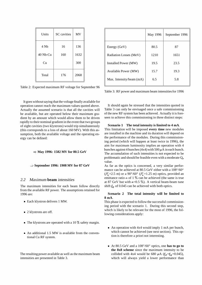
Units SC cavities MV

4 Nb 16 136

40 Nb-Cu 160 1632

Cu 300

Total 176 2068

Table 2: Expected maximum RF voltage for September 96

It goes without saying that the voltage finally available foroperation cannot reach the maximum values quoted above.Actually the assumed scenario is that all the cavities willbe available, but are operated below their maximum gra-dient by an amount which would allow them to be drivenrapidly to their nominal gradient in the event that two groupsof eight cavities (two klystrons) would trip simultaneously(this corresponds to a loss of about 160 MV). With this as-sumption, both the available voltage and the operating en-ergy can be defined:

)May 1996: 1582 MV for 80.5 GeV

) September 1996: 1908 MV for 87 GeV

2.2 Maximum beam intensities

The maximum intensities for each beam follow directlyfrom the available RF power. The assumptions retained for1996 are:

Each klystron delivers 1 MW.

2 klystrons are off.

The klystrons are operated with a 10% safety margin.

An additional 1.5 MW is available from the conven-tional Cu RF system.

The resulting power available as well as the maximum beamintensities are presented in Table 3.

May 1996 September 1996

Energy (GeV) 80.5 87

Radiation Losses (MeV) 1210 1651

Installed Power (MW) 19.5 23.5

Available Power (MW) 15.7 19.3

Max. Intensity/beam (mA) 6.5 5.8

Table 3: RF power and maximum beam intensities for 1996

It should again be stressed that the intensities quoted inTable 3 can only be envisaged once a safe commissioningof the new RF system has been achieved. Actually it is fore-seen to achieve this commissioning in three distinct steps:

Scenario 1 The total intensity is limited to 4 mA.This limitation will be imposed every time new modulesare installed in the machine and its duration will depend onthe performance of the modules. During this commission-ing period (which will happen at least twice in 1996), theaim for maximum luminosity implies an operation with 4bunches against 4 bunches (4x4) with 500A in each bunch.The accumulation of such intensities is not expected to beproblematic and should be feasible even with a moderate Qs

value.As far as the optics is concerned, a very similar perfor-mance can be achieved at 80.5 GeV either with a 108/60

(x

=2.5 m) or a 90/60 (x

=1.25 m) optics, provided anemittance ratio of 1 % can be achieved (the same is trueat 87 GeV but with =0.5 %). A vertical beam-beam tuneshift y of 0.045 can be achieved with both optics.

Scenario 2 The total intensity will be limited to8 mA.This phase is expected to follow the successful commission-ing period with the scenario 1. During this second step,which is likely to be relevant for the most of 1996, the fol-lowing considerations apply:

An operation with 4x4 would imply 1 mA per bunch,which cannot be achieved (see next section). This op-tion is therefore a priori not interesting.

At 80.5 GeV and a 108/60 optics, one has to go tothe 8x8 scheme since the maximum intensity to becollided with 4x4 would be 680 A (x=y=0.045),which will always yield a lower performance than

May 1996 September 1996

Limit for 4 x 4 (mA) 1.625 1.45

Limit for 8 x 8 (mA) 0.810 0.725

Limit for 12 x 12 (mA) 0.540 0.483

8 x 8 better than 0.660 0.600limit for 12 x 12 (mA)

Table 4: Maximum bunch intensities from an RF point ofview

8 x 500 A. However, this feature does not apply tothe 90/60 optics where the condition x=y cannotbe reached below 1 mA/bunch.

At 87 GeV, both 4x4 and 8x8 could be envisaged.However, to achieve a performance comparable to8 x 500 A , one has to accumulate above 710 A inthe 4x4 case, which is already a fairly high intensity.

For this scenario, the choice of the optics is not crucial.However, aiming at maintaining the y at its maximumvalue during the whole run (at the beam-beam limit)would then clearly favor a 108/60 optics with

x=

1.25 m.

Scenario 3 The total RF power is availableIn this case, the aim is to accumulate record intensities. Forthe time being, the only reasonable scheme to accumulatevery high intensities is the high Qs scheme (see next sec-tion).The maximum bunch intensities allowed by the RF as afunction of the number of bunches per beam are illustratedin Table 4. As can be seen from it, operating the machinewith 8 bunches per beam emerges as the best candidate. Asa matter of fact, with 8 x 600 A per beam, one exceedsthe performance which could be achieved with either 4 or12 bunches per beam. Having in mind that this scenario israther unlikely for the initial period at 80.5 GeV, it followsthat, here again, a 108/60 optics with a

xof 1.25 m is

the best candidate for maintaining the machine at the verti-cal beam-beam limit during the whole run.

3 ACCUMULATION SCHEME ANDIMPEDANCE

As already mentioned, the best solution to achieve highbunch intensities is the high Qs scheme which has been suc-cessfully tested in 1995 [1]. Contemplating this scheme for

90/60 108/60

(A) (A)

May 1996Qs = 0.15/0.12 785 / 620 735 / 585

September 1996Qs = 0.15 / 0.12 765 / 605 720 / 570

Table 5: Maximum bunch intensities from an impedancepoint of view

standard operation implies to have the following tools avail-able:

Availability of the injection at 22 GeV (or even higherif possible).

Availability of both the damping and the polarizationwigglers to lengthen the bunches,

Precise knowledge of the bunch length (e.g. from thestreak camera).

Availability of both longitudinal and transverse feed-backs.

Remember that for Qs > 0.15, a new accumulationstrategy would be required (to avoid resonances).

To estimate the maximum intensities one can expects froman impedance point of view, one has to remember that thethresholds for 1996 will be lower than those presented in [1].This is mainly due to the increase of the total impedanceof the machine linked to the installation of the SC modules(actually, a slight increase of the average beta functions inthe RF sections will also contribute to an increase of theimpedance).A detailed review of the LEP impedance budget has beenworked out [2] which enables us to predict that the thresh-olds will be lowered by about 6.5 % for May 96 and a fur-ther reduction of 2.5% for September. It thus follows that,starting from the results obtained in 95 [1], taking into ac-count the increase of impedance and finally adding a 10%reduction for the effect of the second beam, one ends up withthe maximum intensities presented in Table 5. These resultsclearly illustrate the need to work with a high Qs value, es-pecially for the conditions of scenario 3. They also show

that intensities of the order of 800 A/bunch will only bewithin range after part of the conventional Cu system willhave been removed from the machine.

4 TRANSVERSE REACTIVE FEEDBACKSYSTEM

One of the conclusion of the presentation given at the Cha-monix workshop last year was that a second oscillator wasrequired in order to damp (stabilize) the m=-1 mode [3]. Animpressive amount of both theoretical and simulation workhas been achieved in 1995 with the major outcome that anew mode of operation has been proposed. Instead of work-ing in an attractive mode (the oscillator couples to the modem=0 and attracts it), the oscillator is now set-up to work inrepulsive mode [4]. In simulation, this new approach provedto be much more flexible than in the attractive mode (con-straints on required accuracy are relaxed). On top of this,the request for a second oscillator becomes only necessaryat intensities well above what could be presently consideredfor the LEP operation.The dedicated experiment which had been scheduled for theend of 1995 unfortunately failed due to hardware difficultieswith the conventional feedback system. It was therefore notpossible to test the new system. There is however good hopethat the first experimental results will become available dur-ing the few MD periods scheduled in 1996.

5 CONCLUSIONS

The original goal of this presentation was to explain howhigh intensitiescould be accumulated in LEP in 1996. How-ever, when considering the RF limits, it rapidly became ap-parent that the RF constraints were likely to limit the singlebunch intensity at about 500 A/bunch for most of the year(in 4 or 8 bunches per beam). Under these conditions, themain issue became to first establish both the energies andthe most likely scenarios for operating the machine in 1996.For each of these scenarios, the bunch intensities, the opti-mum number of bunches and the most favorable optics havebeen presented. The main features of this approach can besummarized as follows:

In 1996, the total intensity circulating in the machineis likely to be limited at 4 respectively at 8 mA for themajor part of the year. Under these conditions, the op-timal performance is achieved with 500 Aper bunch(4 x 4 or 8 x 8). To accumulate such intensities is notexpected to be a problem.

Even with all the RF power available, an operationwith either 4 x 4 or 12 x 12 is not very attractive. Apartfor the period where the total intensity is limited at4 mA (4x4), the optimum solution is to operate the ma-chine with 8 bunches per beam.

The best suited scheme to safely accumulate high in-tensities is the high Qs scheme. The required Qs val-ues have already been achieved in MDs and it has beendemonstrated that the available wigglers are sufficientfor producing long enough bunches.

In all cases considered, a vertical beam-beam tuneshift y of 0.045 can be achieved. In order to main-tain this value during the whole run, the emittance-ratio will have to be varied as a function of time. A108/60 optics with a

xof 1.25 m ensures a wide

range of flexibility for varying . Furthermore, anearly move to such a strong focusing optics allowsgaining useful experience with an optics which is any-how required above 90 GeV.

The review of the impedance budget shows that the in-stallation of the SC modules has a non negligible im-pact on the maximum intensities to be accumulated.As a consequence, with a Qs of about 0.15 it will notbe possible to accumulate intensities of the order of800 A/bunch as long as some of the conventional Cucavities are not removed from the machine.

6 REFERENCES

[1] D. Brandt et al.; High bunch current;CERN SL-MD Note 197(1995).

[2] A. Hofmann; Bunch intensity limitations I: What do we ex-pect?; These proceedings.

[3] D. Brandt; What is new on the (transverse) feedback front?;Proceedings of the fifth workshop on LEP performance,CERN SL/95-08 (DI) (1995).

[4] E. Perevedentsev; CERN report to be published.

INJECTION ENERGY: ACCUMULATING HIGH INTENSITIESDISCUSSION

Michel Jonker, CERN, Geneva, Switzerland

Session 2.06 A.Hoffman

E.Keil: In your figures on TMC thresholds you havespecified more CU-RF cavities (640) than actuallyinstalled in LEP.A.Hoffman: Yes, but the effect is small. It alsocompensates for some of the impedances that have beenleft out like the 1GHz cavity for the LFB.

E.Keil: The value of Qs=0.15 you have chosen fallsright in the whole of the double batch injection.A.Hoffman: One can also use a slightly higher valueof Qs=0.16.

H.Burkhard: The best results for the maximumcurrent may depend on other machine parameters. Anegative value of chromaticity gives better results.

Session 2.07 M.Meddahi

K.H.Kissler: Do you have any idea why the electronssaturate at lower values than the positrons?M.Meddahi: We have no answer. The same effect is alsoobserved with the 108/60 optics.S.Myers: P.Collier gave an indication last year that it iscoming from the lower intensity in the SPS. In the SPS itis more difficult to correct the orbit of the electrons due tothe directional sensitivity of the BOM system.P.Collier: The electrons have a different energy offsetwhich could also explain part of the effect.K.Cornelis: This effects exist since the beginning and isnot related to bunch trains. Although with pretzels thesituation was reversed.E.Keil: Is there a graph that shows the injectionefficiency as a function of the energy offset?P.Collier: This has been measured only for the positrons.R.Giachino: There is also a tune split which makes adifference.S.Myers: But even if we put the tunes at the mostfavorable place for the electrons, they still accumulateless well than the positrons.

Session 2.08 K.Cornelis

J.Gareyte: The success of the feedback depends on theeffort you put into it.

K.Cornelis: If you need three specialists and a Russianinterpreter it will not work.J.Gareyte: Provided you have the right hardware itshould work.S.Myers: At LEP only a small amount of effort has beenput in so far. At SLAC there has been a whole week ofdedicated MD to commission the feedback. Thedifference is maybe coming from the Qs which is toohigh for the reactive feedback to work. On the other hand,there has been no real push to make it work since wecould not collide these currents anyway.K.Cornelis: I disagree. Several MD's and simulationsshow that the reactive feedback does not work.S.Myers: Perevedensev has recently shown with a laterversion of his program that reactive feedback shouldwork. The question is what is the difference between PEPand LEP?K.Cornelis: Qs and impedance: The TMC also dependson the coupling strengths between the two modes. Hencenot only on Qs but also on the impedance.S.Myers: In PEP the growth rate was 5 turns. In LEP weneed for the reactive feedback higher Q shifts, equivalentto more turns (~2). The feedback system has never beenused at its maximum gain.B.Zotter: How does it depend on impedance?K.Cornelis: The Beta functions at the impedance's areimportant.G.Roy: We should make an effort to minimize the Betafunctions in the CU-RF cavities where the impedance ishigh.J.Jowett: The Beta value in the cavities depends on theposition. From where did you get these values?K.Cornelis: From the output in MAD, which gives thebeta values at the center of the cavities.

Session 2.09 B.Zotter

K.Cornelis: How does the Multi Bunch Beam BreakUp(MBBBU) explain the different tunes of the first and thesecond bunch?B.Zotter: You get tune splits when you have two coupledoscillators. (K.C: even if the coupling is in one direction?!?) With the coupling you will get additional lines in thespectra. The difference in the amplitudes of the motion ofthe two bunches also gives a partial explanation.S.Myers: How do you get different kicks each turn toexcite bunch A?

B.Zotter: Microphonics. The microphonics in the RFcavities have a 10 msec period. This leads to slowlongitudinal motions and instabilities.S.Myers: The best would be to measure the transferfunction: Excite bunch A and measure the effect onbunch B and C.B.Zotter: The measurement was done, but the results arenot yet extracted from the raw data.D.Boussard: Why should a changing frequency due tomicrophonics produce different kicks each turn. Could itcome from Higher Order Modes? Have you tried to damponly bunch A with the transverse feedback and measurebunch B and C?B.Zotter: This has not been measured. The main purposeof the MD was to see if the effect was there.S.Myers: You should drive the longitudinal instabilitiesto test K.Cornelis theory.K.Cornelis: We have to understand the origin of the tunesplit.

Session 2.10 D.Brandt

J.Jowett: You do not need a knob to spill the coupling.Experience last year has shown this.S.Myers: TMCI has been measured from 1993 to 1995and was discussed three times this morning. We see thatthe maximum bunch intensity is getting less and less. Weshould find the source of the missing impedance's. Thecandidates are the cavities and the separators.D.Brandt: K.Cornelis made an MD last year to look forunknown impedance's.D.Boussard: You have not included the limit from theHOM couplers. I remind you that there are still 10modules of the old type. These HOM couplers cannot bereplaced for the time being.S.Myers: What is the power capability of these couplers?D.Boussard: 600 KWatt per cavity.F.Richard: Can you translate these beam currents inluminosity's?D.Brandt: This will be discussed tomorrow inJ.Gareyte's session.K.H.Kissler: Your preferred Qs is in the 0.15 hole of thedouble batch injection.S.Myers: We will use 0.16D.Brandt: But we should then pay more attention tocrossing resonance's.K.H.Kissler: In case the double batch injection is notworking, do we have to maintain the 4 lepton cycles inthe SPS?K.Cornelis: No way.P.Collier: The whole in the double batch efficiency plotsis around Qs=0.14 and comes from the magic SPS-LEPnumber which is 7 turns. This makes double batchimpossible when the Qs oscillations are a multiple of 7turns.

B.Zotter: An other advantage of a high Qs is that the SC-RF always runs at a high voltage.W.Kalbreier: Is it possible to reduce the impedance ofthese pumping T's?D.Brandt: The addition of these pumping T's wherediscovered only last Thursday. They have escaped theattention.?(AT-VA): The K-factor of these T's are the same asother T's already installed.B.Zotter: I believed we would remove 16 CU-RF units.This will compensate for the additional impedance.A.Verdier: There are other things missing from thebalance. The change of elliptical vacuum chambers toround chambers in high beta regions.K.Cornelis: We are not always aware of the details inLEP. Other things which are new are the ferrite's forwhich the effects are not known. What we need is somekind of impedance police as we used to have before.Someone who will look after these things.

Summary: Accumulating High Intensities

Werner Herr, CERN, SL Division

1 INTRODUCTION

When LEP is operated at high energies above 80 GeV perbeam, it allows to collide much higher bunch intensities be-fore the beam-beam limit is reached. An essential questionis therefore whether intensities large enough can be accu-mulated and accelerated to eventually reach this limit andto provide the highest possible luminosities. The purposeof this session was therefore to identify the possible limita-tions, compare with the measurements, find the means to in-crease the intensity limits and to define the scenarios for theaccumulation of these high intensities within the boundaryconditions imposed by the RF and the equipment.

2 WHAT ARE THE MAIN LIMITATIONSFOR HIGH INTENSITIES ?

Several mechanisms are responsible for intensity limitationsobserved at LEP at injection energy [1]. The most importantones are:

Coupled bunch instabilities

Multi bunch beam breakup

Single bunch longitudinal instabilities

Synchro betatron resonances

Head-tail instabilities

Transverse mode coupling instability

Coupled bunch instabilities are frequently observed and canbe transverse and longitudinal. They are mostly driventhrough RF cavities and the usual cures are feedback sys-tems. A special case of a coupled bunch instability is theso-called beam break up which was observed in linear col-liders but requires special attentionwhen LEP is run with thebunch train scheme where bunches follow each other closelyand can interact via short range wakefields.

A longitudinal instability of single bunches can be ob-served at LEP for short, intense bunches [2]. The longitu-dinal motion is unstable and the threshold current can onlybe increased by lengthening the bunches with wigglers. Thesynchro betatron resonances observed in LEP [3] are mainly

driven by a residual dispersion in the RF cavities. The work-ing point has to be chosen such as to avoid these resonancesat injection where they are most dangerous. These reso-nances can limit the value for the synchrotron tune Qs whichcan be used at injection.

Another set of instabilities are head-tail instabilitieswhere the head and the tail of a bunch are coupled via wakefields. These types of instabilities are usually cured with aproper setting of the chromaticity and with feedback sys-tems.

The most fundamental and most important limitation atLEP is the Transverse Mode Coupling Instability (TMCI).The frequency of the modes are changed as a function of theintensity through wake fields and, at a threshold current, thefrequencies of previously separated modes become equaland the modes couple together, resulting in a fast instability.Because of its importance the TMCI was treated in detail inthis session.

3 IS THERE A BEAM BREAK UP WITHBUNCH TRAINS ?

Closely spaced bunches can be the source of the so-calledbeam break up instability: transverse wake fields excited byearlier bunches of a train can drive the later bunches into os-cillations with growing amplitudes [5]. This is in particulartrue since in the LEP bunch train scheme a vertical offsetin the some of the superconducting RF cavities cannot beavoided. The theory predicts a growth rate with a certainpower of the time rather than exponential:

yk(t) / yk(0) tk1

where k is the sequence number of the bunch in the train andy(t) the oscillation amplitude. The second bunch of the trainwould therefore grow linearly with time, the third quadrat-ically and so on.

In machine experiments it was indeed observed that laterbunches in a train have much larger oscillations than the firstbunch which seems to indicate the presence of beam breakup.

A detailed analysis showed that the second bunch in atrain has the strongest oscillation while the oscillation of thethird bunch was slightly smaller (measurement done withthree bunches per train). Another important observationwasthat the amplitude and strength of this oscillation seems in-dependent of the offset in the superconducting RF cavities.

The transverse feedback was successfully used to keep theamplitude of the oscillation small. A small oscillation of thefirst bunch is always present and may be driven by micro-phonics in the RF system [6].

4 TMCI AND INTENSITY THRESHOLD

One of the most important limitations at LEP is the Trans-verse Mode Coupling Instability(TMCI) [7]. The frequencyof the modes are changed as a function of the intensitythrough wake fields and, at the threshold current, the fre-quencies of previously separated modes become equal andthe modes couple together, resulting in a fast instability.

4.1 Basic formula

The threshold intensity where this coupling occurs can bewritten as:

Ith =2 Qs E f0

e

P kT (s)

where Qs is the synchrotron tune, E the injection energy,kT (s) is the transverse mode loss factor and the -function at the source of the impedance. The transversemode loss factor is a convolution between the impedanceand the bunch spectrum, therefore its dependence on thebunch length s. The revolution frequency f0 is of course aconstant in this formula.

In order to increase this threshold intensityone would liketo work with the highest possible injection energy, large syn-chrotron tunes and a small mode loss factor, which impliesa small impedance and long bunches.

4.2 Impedance budget

It has been found that the single bunch intensity has de-creased since 1993 by more than 10 % and part of this de-crease can be attributed to the increased impedance: since1993 superconducting cavities have been added to the ma-chine as well as 8 additional separators for the bunch trainscheme, together with all necessary bellows etc. This ac-counts for approximately 8 % of the losses. In the next fewyears additional cavities will be mounted in LEP and theircontribution becomes more and more important. It is ex-pected that only the removal of the Cu cavities (at least par-tially) can assure a small enough impedance to accumulatethe required intensities.

4.3 Higher E and Qs

In 1995 the injection energy into LEP was raised from 20to 22 GeV and the expected gain of 10 % in the thresholdintensity was immediately observed. A further increase to23 GeV is possible but not recommended since it would beto close to the acceptable limits of the SPS.

Since the intensity threshold is proportional to Qs, onewould like to operate with a Qs as high as possible. In adedicated experiment in 1995 a single bunch intensity of

0.96 mA was achieved with a Qs of 0.164. A too large syn-chrotron tune could however make it hard to avoid differentresonances and the recommended value is around 0.15.

4.4 Effect of optics

It is proposed to run LEP with a low emittance optics and thepresent candidates have phase advances per cell of 900/600,1080/600 and 1080/900. Since the betatron function at thesource of the impedance is an important quantity, and sincethe bunch length depends on the horizontal phase advance,one expects differences between the three proposed lattices.The best candidates are 1080/600 and 1080/900 where thelatter has a slightly more favourable betatron function in thearcs.

4.5 Expectations

Assuming a proposed scenario with an injection energy of22 GeV, a Qs = 0.15 and a maximum bunch length of 8mm one can expect a threshold intensity for a single buncharound 0.80 - 0.84 for 1996 at 80.5 GeV and between 0.74- 0.78 in 1997 due to the increased impedance of additionalsuperconducting cavities.

5 RESULTS FROM RECENTMEASUREMENTS

In a detailed report the results obtained in measurements onthe maximum intensity with bunch trains [4] were shown.The reduction of the single bunch current between 1993 and1995 was confirmed in these measurements to be around 10%.

When trains were formed for a single beam it was possibleto inject an intensity into the first bunch which was close tothe single bunch limit. However, the second bunch alwayssuffered from the injection into the first one and this eventu-ally limited the achievable intensity in the second bunch toa value between 10 and 15 % lower than in the first bunch.The effect of the amplitudes of the bunch train bumps on themaximum intensity was studied and found to be small.

The maximum intensity with two beams was studied intwo steps: in the first step, bunches were injected such as toonly collide in selected collision points and no differencesbetween the four experimental points were found. In thesecond part four trains of two bunches each were injectedwhich is the proposed scheme for LEP 2. Although limitedtime was available, the intensities reached on that first andsingle attempt were:

e+: Imean = 452 A/bunch

e: Imean = 365 A/bunch

The synchrotron tune was 0.098 and the polarization wig-glers were on, no transverse feedback system was used. In-jection problems were encountered again with the trailingbunches which eventually limited their maximum intensity.

In some occasions it was possible to inject up to 498 Ainto the first bunch but the losses on the second bunch werestronger.

A comparison with the previously achieved record inten-sities with the pretzel scheme:

e+: Imean = 440 A/bunch

e: Imean = 387 A/bunch

under very similar conditions, i.e. Qs = 0.097, no polariza-tion wigglers but feedback system on, shows that practicallyidentical intensities could be accumulated immediately. Allabove numbers are taken from the measurement data base.

It is expected that with the proposed synchrotron tune, 22GeV injection and an optimized bunch spacing, these inten-sities can be pushed well above 500 A.

6 HOW DO WE GET THE CURRENTSWE WANT ?

In the last part of the session it was discussed which shouldbe the scenarios to obtain the required beam currents [8].

6.1 RF boundary conditions

The maximum available voltage from the RF system willbe limited to 1582 MV in May 1996 and to 1908 MV inSeptember 1996, allowing for a beam energy of 80.5 GeV inMay and 87.0 GeV in September. It is important to note thatthe maximum beam intensity will be 6.5 mA in May and 5.8mA in September.

6.2 Scenarios for running

Depending on further restrictions several scenarios havebeen discussed and proposed. In the first scenario it is as-sumed that for a fraction of the time the total intensitywill belimited to 4 mA. This implies running with only 4 bunchesper beam to get the best performance and 500A per bunch.This should be achieved easily.

In the second step it is assumed that for part of the yearLEP will be restricted to a total intensity of less than 8 mA.Since running LEP with 1 mA per bunch is not realistic, thiscurrent would be distributed into 8 bunches per beam, mostlikely with 4 trains of 2 bunches. It should be pointed outthat at 87 GeV running LEP with 4 bunches per beam is onlybetter that with 8 bunches if the current per bunch can behigher than 710 A.

In the final scenario the total RF power is available andthe record intensities are expected. The high Qs schemeis the only reasonable scheme to achieve these intensitiesand for a standard operation further requirements were pre-sented: availability of 22 GeV injection, damping and po-larization wigglers to lengthen the bunches, reliable bunchlength measurement, and both, longitudinal and transversefeedback systems. With the expected single bunch intensi-ties and empirically applying a scaling for the presence of

the second beam it is expected to achieve bunch intensitiesbetween 580 and 620 A in May and between 570 and 605A in September 1996. This shows again the importance todecrease the LEP impedance by a reduction of the numberof Cu RF cavities, if possible to zero.

7 TRANSVERSE REACTIVE FEEDBACKSYSTEM

Finally the progress on the transverse reactive feedback sys-tem was reported. The theoretical and simulation work hasprogressed in 1995 and in particular the new approach withrepulsive modes is very promising. The machine experi-ments were obstructed by hardware problems in 1995 andthe hope was expressed that sufficient time will be availableto further explore this instrument which has the potential toallow for very high intensities.

8 REFERENCES

[1] A. Hofmann; Bunch Intensity Limitations I: What do we ex-pect ?; These proceedings.

[2] D. Brandt et al; Experimental observations of instabilities inthe frequency domain at LEP; Proceedings EPAC 1992.

[3] H. Schmickler; Can we stop talking about crossing synchrobetatron resonances ?; These proceedings.

[4] M. Meddahi; Bunch Intensity Limitations II: How do mea-surements with bunch trains look like ?; These proceedings.

[5] B. Zotter; Beam Break Up - is there any ?; These proceedings.

[6] J. Tuckmantel; Performance of RF cavities; These proceed-ings.

[7] K. Cornelis; TMCI and what to do about it ?; These proceed-ings.

[8] D. Brandt; How do we get the beam currents we want forLEP2 into the machine ?; These proceedings.

Optics for physics and for LEP2

A. VerdierSL Division

Abstract

At 90GeV with bunch currents below 1mA, the horizon-tal beam-beam limit can only be reached with an horizontalemittance much smaller than that associated with the presentLEP lattice. However the vertical beam-beam limit, whichis the only important one for the luminosity, can be reachedprovided a small emittance ratio is achieved. In this contextit will be shown to what extend a low-emittance lattice is at-tractive for a high luminosity at 90GeV (a small emittancealso leads to less background in the experiments).

The compatibility with Pretzels operation will be dis-cussed, as well as some hardware implications.

A comparison between two optics : 90/60 and 108/60 willbe done in the frame of bunch-train operation.

1 INTRODUCTION

Now LEP enters high energy operation, it is important tounderstand to what extend low-emittance lattices are useful.This is why the basis for the luminosity optimisation and itsconsequence on the choice of a lattice is recalled first. Onthis basis a comparison between lattices proposed for LEP2is done.

The implications of the non-linear chromaticity correc-tion on high energy operation will be discussed. Outcomeof the discussions held during the workshop are included.

As LEP2 will work presumably with bunch-trains, the ef-fects due to the parasitic beam-beam crossings will be com-pared for two tentative 96 optics.

2 LUMINOSITY OPTIMISATION.

In order to have a complete view of the problem, let’s startfrom basic concepts used to describe particles collision. Theprobability of interaction of a given particle is proportionalto the density of particles it encounters and to the interac-tion probability. In fact the relevant density is the numberof particles encountered by unit of surface. The probabilityof an interaction is then given by the product, which is di-mensionless, of its so called cross-section with the density.In our case, the density of particles encountered per unit oftime by a particle in a given bunch is proportional to its col-lision frequency fc with the counter rotating bunches andthe density N2g2(x; y) of the latter. N2 is the bunch pop-ulation and g2(x; y) is the distribution function normalisedto unity. In order to obtain the event production rate in thebunch collisions, this product has to be integrated over the

distribution of particles in the given bunch, i.e. :

dNevent

dt=

Z +1

1

dx

Z +1

1

dyeventN1g1(x; y)N2g2(x; y)fc:

As the event cross-section event does not depend on theposition variables, the event production rate is eventuallyequal to the product of the event cross-section with some-thing which depends only on the machine parameters andis called the luminosity : L. It is simply given by the dou-ble integral over x and y of the product of the distributionfunctions.

For the LEP case, even with the beam-beam interac-tion, the central part of the beam has been observed to beGaussian-like. The non Gaussian tails of the distributioncontain less than one per-mil of the intensity [1]. The dis-tribution function is of the form 1

2yxexp( x2

x2

y2

y2).

The luminosity is then given by [2] :

L =N1N2fc

2q2x;1 + 2x;1

q2y;1 + 2y;2

If the two beams have equal sizes, this reduces to :

L =N2fc

4xy(1)

In order to examine the effect of the shape of the distributionon the luminosity, the double integral has been computed fortwo other simple distributions. The parabolic distributionfunction is :

g(x; y) = f(x)f(y)

with :

f(x) =3

4l

1

xl

2;l < x < +l

The luminosity associated with this distribution is givenby an expression which differs from (1) only by a factor50/3=16.666... instead of 4 = 12:566::: in the denomi-nator. For a quartic distribution with :

f(x) =15

16l

1

xl

22;l < x < +l

this factor becomes 73=52 = 13:720::, i.e. at 9% of thatof the Gaussian distribution. Of course these distributionsare not realistic for an electron machine but the similarity ofthe coefficient in the formulae shows that the shape of any

bell-shaped distribution function has little effect on the lu-minosity. Therefore formula (1) will be used in the subse-quent analysis. More important : the strategy to maximisethe luminosity will not depend on the shape of the distribu-tion at all.

The factors entering the luminosity formula are indepen-dent of each other to a certain extend. For instance the col-lision frequency fc can be increased by an increase of thenumber of bunches. This can be done with special schemeslike Pretzels or bunch-train. However these schemes setphase constraints on the insertion optics which reduce theirflexibility.

In any case, the largest luminosity will be obtained by de-creasing the beam sizes as much as possible. The limit inthis direction is set by the beam-beam interaction since thefield created by a bunch passage goes with the inverse of thebeam size. The strength of this interaction is measured withthe beam-beam tune-shift parameter which is nothing butthe tune-shift due to the linear part of the non-linear beam-beam lens. For a particle encountering a beam with a Gaus-sian transverse distribution at a place where the-functionstake the values x

and y, this parameter is given in each

oscillation plane by [4]:

x =Nrex

2 x(x + y)y =

Nrey

2 y(x + y)(2)

where re is the classical radius of the electron and therelativistic energy factor. The expression Nre

2 is equal to

1.39472109m for half a milliampere at 45.6GeV in LEP.These formulae are computed with the first order tune-shiftformula of Courant and Snyder [5], and hence do not givethe actual tune-shifts if their values are too large. The over-estimate is already for 10% a -value of 0.016. An exhaus-tive discussion of these effects are discussed in reference [6].Any computation related with so called “weak-strong” ef-fects can be done with MAD which contains a “beam-beam”element. These tune-shift parameters do not have anythingmagic, they just give a measure of the beam-beam interac-tion and their maximum values come only from the past ex-perience.

It is clear that these parameters increase with decreas-ing beam sizes. It has been observed that, for any machineup to now, their value is limited to about 0.06 per cross-ing [3]. Although they do not describes the physics asso-ciated with the beam-beam interaction, which is dominatedby non-linearities, it seems to be a quite good “invariant”of the phenomenon which imposes a limit to the intensitywhich can be collided in a given machine.

Let’s do now some algebra to eliminate the beam sizes asmuch as we can in the luminosity formula. In LEP we workwith flat beams, so we isolate terms like x

yin the equations.

If we do this in the expression of y, and replace the productxy in equation (1), we obtain :

L =Nfc y

2rey

1 +

y

x

(3)

This formula is exact. We have only assumed that we canwrite the r.m.s. beam sizes :

x;y =px;yEx;y:

where Ex;y stands for the emittances. Numerically the LEPluminosity is given by :

L(cm2s1) 2:1673 1029kbib(mA)E(GeV )y

y

This formula is actually used in the control system to com-pute y from the luminosity measurement, y

having beenmeasured. The luminosity does not depend on x if x >>y. Nevertheless x must be smaller than say 0.05 in LEP(the upper limit on up to now). It can be written as :

x =Nre

2 Ex

1 +

y

x

1:41

Ex(nm)

90

p(Gev=c)ib(mA)

(4)For a given phase advance in the arc cells and without wig-gler, the horizontal emittance scales with p2, so that xscales with p3 at constant current. It is easy to see that, athigh energy, the maximum beam-beam tune-shift can onlybe reached with a large bunch current and a small emittance,i.e. a large horizontal phase advance per cell. This was theinitial argument to propose such phase advances for LEP2[7]. In fact, as said above, for our case of flat beams, the onlyimportant parameter is y. x and y are simply related by[8] :

y = x

sExy

Eyx

(5)

obtained merely from the ratio of the ’s given in (2). Thisexpression is exact. It is fundamental to determines how tomaximise the luminosity with the machine parameters forany given linear optics for the flat beam case. Once we havemade y

as small (this is thoroughly discussed in [8]) andy as large as we can, the only free parameters are x

andEy. The vertical emittance is limited by our ability to correctthe vertical closed orbit distortion, the machine couplingandthe vertical dispersion at the IP’s. The minimum value ofx is limited by the background due to the large value of

x in QS1 and the non-linear horizontal chromaticity cor-rection. Up to now a value down to 1.2m is possible, thelower limit imposed by the non-linear chromaticity is un-known. The latter imposes also that the horizontal phase ad-vance between QS1 and the first SF sextupole in the arc bewell different from =4 + k=2 for a 90 horizontal phaseadvance. This is an additional constraint on the insertionoptics. For the 108 lattice, this constraint does not exist.However the present sextupole circuits cannot be used andhave to be re-cabled.

It was argued in the present workshop that the blow-updue to the beam-beam interaction is not included in theabove considerations. The vertical blow-up does not haveto be considered as the vertical emittance is adjusted empiri-cally to obtain the maximum of y. Whether this blow-up is

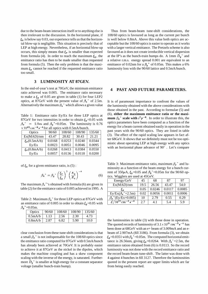
due to the beam-beam interaction itself or to anything else isthen irrelevant to the discussion. In the horizontal plane, ifx is below say 0.03, our experience tells us that the horizon-tal blow-up is negligible. This situation is precisely that ofLEP at high energy. Nevertheless, if an horizontal blow-upoccurs, this simply means that x is smaller than expectedfrom formula (4). In order to reach the maximum y , theemittance ratio has then to be made smaller than requestedfrom formula (5). Then the only problem is that the maxi-mum y cannot be reached if the requested emittance ratiotoo small.

3 LUMINOSITY AT 87GEV.

In the end-of-year’s test at 70GeV, the minimum emittanceratio achieved was 0.005. The emittance ratio necessaryto make a y of 0.05 are given in table (1) for four LEP2optics, at 87GeV with the present value of x

of 2.5m.Alternatively the maximum x

which allows a given value

Table 1: Emittance ratio Ey/Ex for three LEP optics at87GeV for two intensities in order to obtain y=0.05 withx = 2:5m and y

=0.05m. The luminosity is 0.761032cm2s1for all optics with 0.5mA/bunch.

Optics 90/60 108/60 108/90 135/60Ex(MAD)/nm 43.47 28.82 30.43 21.21x(0.5mA/b) 0.0168 0.0253 0.0240 0.0344

Ey/Ex 0.0023 0.0051 0.0046 0.0095x(0.8mA/b) 0.0268 0.0413 0.0384 0.0550

Ey/Ex 0.0057 0.0136 0.0118 0.0200

of y for a given emittance ratio, is (5) :

x = y

x

y

2Ey

Ex

1

(6)

The maximum x’s obtained with formula (6) are given in

table (2) for the emittance ratio of 0.005 achieved in 1995. A

Table 2: Maximum x for three LEP optics at 87GeV with

an emittance ratio of 0.005 in order to obtain y=0.05 withy=0.05m.

Optics 90/60 108/60 108/90 135/600.5mA/b 1.13 2.56 2.30 4.730.8mA/b 2.87 6.82 5.90 10.0

clear conclusion from these tune-shift considerations is thata small x

is not indispensable for the 108/60 optics sincethe emittance ratio computed for 87GeV with 0.5mA/bunchhas already been achieved at 70GeV. It is probably easierto achieve it at 87GeV as the nickel in the dipoles, whichmakes the machine coupling and has a skew componentscaling with the inverse of the energy, is saturated. Further-more Dy

is smaller at high energy for a constant separatorvoltage (smaller bunch-train bump).

Thus from beam-beam tune-shift considerations, the108/60 optics is favoured as long as the current per bunchis well below 0.8mA. Above this value both optics are ac-ceptable but the 108/60 optics is easier to operate as it workswith a larger vertical emittance. The Pretzels scheme is alsofavoured as it does not create irreducible vertical dispersionat the IP’s as the bunch-train bumps do. A 1mm Dy

anda relative r.m.s. energy spread 0.001 are equivalent to anemittance of 0.02nm for a y

of 0.05m. This makes a 6%luminosity loss with the 90/60 lattice and 0.5mA/bunch.

4 PAST AND FUTURE PARAMETERS.

It is of paramount importance to confront the values ofthe luminosity obtained with the above considerations withthose obtained in the past. According to formulae (5) and(6), either the maximum emittance ratio or the maxi-mum x

scale with i2p6. In order to illustrate this, theoptics parameters have been computed as a function of theenergy for a beam current obtained easily in operation in thepast years with the 90/60 optics. They are listed in table(3). The effect of the rapid scaling law appears in fact af-ter 68GeV. It shows that we definitely must not be too opti-mistic about operating LEP at high energy with any opticswith an horizontal phase advance of 90 . Let’s compare

Table 3: Maximum emittance ratio, maximum x and lu-

minosity as a function of the beam energy for a bunch cur-rent of 350A, y=0.05 and y

=0.05m for the 90/60 op-tics. Wigglers are used at 45GeV.

Energy/GeV 45 68 87 97Ex(MAD)/nm 19.5 26.56 43.47 54.0

x 0.05 0.0246 0.0117 0.0085Ey/Ex(x

=2.5m) 0.02 0.0056 0.0011 0.0006x(Ey/Ex=0.005) 10 2.79 0.55 0.29

L=1031cm1s2 2.7 4.1 5.4 5.9

the luminosities in table (3) with those done in operation.The quoted records of luminosity of 3.11031cm2s1 hasbeen done at 68GeV with an e+ beam of 3.009mA and an e-beam of 2.907mA (fill 3186). From formula (3), we obtainy=0.0351 withy

=0.05m. The computed horizontal emit-tance is 26.56nm, giving x=0.0264. With x

=2.5m, theemittance ration obtained from (6) is 0.0113. So the recordluminosity was not done with the record emittance ratio andthe record beam-beam tune-shift . The latter was done with4 against 4 bunches in fill 3127. Therefore the luminositiesquoted in the present report are upper limits which are farfrom being easily reached.

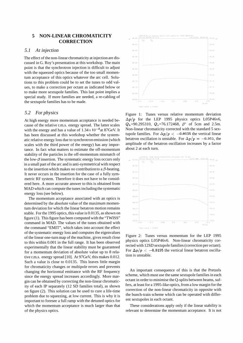
5 NON-LINEAR CHROMATICITYCORRECTION

5.1 At injection

The effect of the non-linear chromaticity at injection are dis-cussed in G. Roy’s presentation at this workshop. The mainpoint is that the synchrotron injection is difficult to adjustwith the squeezed optics because of the too small momen-tum acceptance of this optics whatever the arc cell. Solu-tions to this problem could be to set the tunes to odd val-ues, to make a correction per octant as indicated below orto make more sextupole families. This last point implies aspecial study. If more families are needed, a re-cabling ofthe sextupole families has to be made.

5.2 For physics

At high energy more momentum acceptance is needed be-cause of the relative r.m.s. energy spread. The latter scaleswith the energy and has a value of 1.34103at 87GeV. Ithas been discussed at this workshop whether the system-atic relative energy loss due to synchrotron emission (whichscales with the third power of the energy) has any impor-tance. In fact what matters to estimate the off-momentumstability of the particles is the off-momentum mismatch ofthe low- insertion. The systematic energy loss occurs onlyin a small part of the arc and is anti-symmetrical with respectto the insertion which makes no contribution to a -beating.It never occurs in the insertion for the case of a fully sym-metric RF system. Therefore it does not have to be consid-ered here. A more accurate answer to this is obtained fromMAD which can compute the tunes including the systematicenergy loss (see below).

The momentum acceptance associated with an optics isdetermined by the absolute value of the maximum momen-tum deviation for which the linear betatron motion remainsstable. For the 1995 optics, this value is 0.0135, as shown onfigure (1). This figure has been computed with the “TWISS”command in MAD. The values of the tunes obtained withthe command “EMIT”, which takes into account the effectof the systematic energy loss and computes the eigenvaluesof the linear one-turn map of the machine, gives result closeto this within 0.001 in the full range. It has been observedexperimentally that the linear stability must be guaranteedfor a momentum deviation of absolute value up to 8 rela-tive r.m.s. energy spread [10]. At 97GeV, this makes 0.012.Such a value is close to 0.0135. This leaves little marginfor chromaticity changes or multipole errors and preventschanging the horizontal emittance with the RF frequencysince the energy spread increases accordingly. More mar-gin can be obtained by correcting the non-linear chromatic-ity of each IP separately (12 SD families total), as shownon figure (2). This solution can be used to cure a life-timeproblem due to squeezing, at low current. This is why it isimportant to foresee a full ramp with the detuned optics forwhich the momentum acceptance is much larger than thatof the physics optics.

Figure 1: Tunes versus relative momentum deviationp=p for the LEP 1995 physics optics L05P46v6,Qh=90.295310, Qv=76.172468, of 5cm and 2.5m.Non-linear chromaticity corrected with the standard 5 sex-tupole families. For p=p < 0:0135 the vertical linearbetatron oscillation is unstable. For p=p = 0:015, theamplitude of the betatron oscillation increases by a factorabout 2 at each turn.

Figure 2: Tunes versus momentum for the LEP 1995physics optics L05P46v6. Non-linear chromaticity cor-rected with 12SD sextupole families (correction per octant).For p=p < 0:0195 the vertical linear betatron oscilla-tion is unstable.

An important consequence of this is that the Pretzelsscheme, which must use the same sextupole families in eachoctant in order to minimise the Q-splits between beams, suf-fers, at least for a 1995-like optics, from a low margin for thecorrection of the non-linear chromaticity in opposite withthe bunch-train scheme which can be operated with differ-ent sextupoles in each octant.

These considerations apply only if the linear stability isrelevant to determine the momentum acceptance. It is not

L O 5 P 4 6 V 6 , y e t a n o t h e r b u n c h t r a i n 0 0 0 0 5 f o r 1 9 9 5 o p e r a t I ' o n H P / U X v e r s I o n 8 . 1 7 / 9 1 3 / 1 2 / 9 5 0 8 . 5 0 . 0 6

I I I I I 9 0 . 5 0 I I I I I 7 6 . 5 0

_ Qx Qy 7

90 .45 — 2 7 6 . 4 5

90 .40 — 2 7 6 . 4 0

9 0 . 3 5 — 2 7 6 . 3 5

9 0 . 3 0 — m 7 7 6 . 3 0 ___d_,_,

9 0 . 2 5 — 2 7 6 . 2 5

9 0 . 2 0 — 2 7 6 . 2 0

9 0 . 1 5 — m * 7 6 . 1 5

9 0 . 1 0 — 7 7 6 . 1 0

9 0 . 0 5 — 7 7 6 . 0 5

9 0 . 0 0 - I I I - I - I - I I 7 6 . 0 0 — . O 1 5 — . O 1 0 — . 0 0 5 0 . 0 . 0 0 5 . 0 1 0 . 0 1 5

(55/n

T a b l e n a m e = T U N E S

L O 5 P 4 6 V 6 , 1 9 9 5 o p t i c s . c h r o m a t i c i t y c o r r e c t e d w i t h 1 2 S D HP/UX version 5 .17/9 10 /01 /95 15.01.45 . I I . I I 90.50 I . I . I 76.50

Qx Qy 7

90 45 I , 76 45

90 40 — — 76 4o

90 35— — 76 35

90 3o — \ \ - 7 6 3o _ A .

90 25 — — 76 25

90 20 — — 76 20

90 15 — — 76 15

90 1 o - — 76 10

90 05 — — 76 05

90.00 _ I I I I . I I I I I I _ 76.00 —,o15 —.o1o —.005 0.0 .005 .010 .015

(SE/poo

T a b l e n a m e = T U N E S

Table 4: Effect of the parasitic bunch crossings for to two possible optics for 1996. The computation of these effects hasto be done to assess the validity of any optics proposed for bunch-train operation. For both optics : 4trains of 2 bunchesseparated by 150RF x

=2.5m, y=0.05m, e = 1:4103 E=90GeV, y=0.045, Ib=0.5mA, separators at maximum.

MAD 108/60 90/60Max. D

y (even IP’s)/mm 1.26 1.33Max. Dy (machine)/mm 55.6 52.2

Dy (rms)/mm 22.7 21.2x, y at 90 GeV/nm 30.8, 0.055 46.4, 0.052

Train and orbit9x, y from Maximum y/nm 30.0 , 0.17 46.0, 0.11y (all parasitic collisions) -0.0070 -0.0072Max. x (single head-on) 0.023 0.015x (all parasitic collisions) 0.0018 0.0018

Qx-spread 0.0010 0.0092Qy-spread 0.00045 0.00032Qx’-spread 0.0265 0.0191Qy’-spread 0.0406 0.1286

Max. y-sep. (even pits)/m 1.90 1.85Max. y-cross. angle (even pits)/mrad 0.090 0.080

CM E-shift (even pits)/MeV 0 0

obvious that this is the case at very high energy where thesingle particle stability is determined by the phenomenon ofRadiative Beta-Synchrotron Coupling [11]. At large ampli-tudes, the particles passing in the quadrupole fields emit anon-negligible amount of photons, which changes their en-ergy. This makes a coupling mechanism between the beta-tron amplitudes and the synchrotron one. In any case it iseasy to distinguish which phenomenon makes the life-timeproblem if any, using the detuned optics which has a largermomentum acceptance. If the latter is responsible, this canbe studied by reducing the momentum acceptance by meansof the sextupole families.

6 OPTICS COMPARISON.

Runningwith bunch-trains implies that the effects due to theparasitic bunch crossings are under control. In order to es-timate their importance, computer programs has been madeby Eberhard(orbit9) and Chris(train). These programs com-pute the closed orbit distortions due to the parasitic cross-ings as well as the perturbations of tunes and chromaticities.“orbit9” does it to the first order and computes the optimisa-tion of the offsets at the collision points and the associatedluminosity loss for all bunches. “train” computes self con-sistent closed orbits for all bunches but does not do the op-timisation of the offsets. It uses second order transfer mapsbetween collisions, computed by MAD and provides alsothe CM energy shift and the frequencies of the beam-beammodes.

An example of the quantities examined for the compari-son of optics proposed for LEP operation is shown in table4. The most serious effect is probably the crossing angle

due to the parasitic beam-beam interactions. In fact LEPwas run at 45.6 and 70GeV with a crossing angle almostequal to that given in this table. The tune and chromatic-ity spread are negligible. The offsets in the even pits can becorrected exactly with the vernier separators for the case oftwo bunches per train. Their value is given here to have anorder of magnitude of the miscrossing which appears whenthe bunch currents decrease in the course of a physics run,starting from a situation where the offset has been correctedat high current. This table can be used for a further com-parison for an energy of 90GeV and a current of 0.5mA perbunch.

7 CONCLUSION

The good results obtained at 68GeV must not make us forgetthat the parameters needed to reach a high performance athigh energy are not easy to reach. The main point is the fastdecrease with energy of the requested emittance ratio whichscale as/ i2p6 This can be partly overcome by a decreaseof x

, at the price of a more complicated horizontal non-linear chromaticity correction and eventually a re-cabling ofthe sextupole circuits. Low-emittance lattices are the bestcandidates to help in this direction. However, doing twicethe average luminosity done in the LEP1.5 run at the end of1995 requires already some operation skill to reach at thesame time a large y and a large intensity per bunch withthe bunch-trains scheme on.

The Pretzels scheme has the drawback of a critical non-linear chromaticity correction at very high energy.

BEAM-BEAM EFFECTS AS A FUNCTION OF THE TUNES

E. Keil, CERN, Geneva, Switzerland

Abstract

The coherent beam-beam modes at high energy are pre-sented for the beam-beam limited case, i.e. with beam-beamtune shift parameters of the order of 0.045. The effects ofodd and even integral parts of the tunes are discussed. Re-sults of beam-beam simulations by J. Poole et al. are pre-sented.

1 INTRODUCTION

In this contribution, I apply the accelerator physics of linearcoherent beam-beam modes [1] to LEP operated close to thebeam-beam limit at 87 GeV. Unless stated otherwise, I usethe numerical parameters shown in Tab. 1.

Table 1: Numerical ParametersHorizontal emittance x 28 nmVertical emittance y 1.12 nmEmittance ratio 4 %Bunch current I 0.896 mAx in even pits 1.25 my in even pits 0.05 mx in odd pits 25 my in odd pits 30 mFull vertical separation y in odd pits 9.44 mm

The horizontal and vertical beam-beam tune shift param-eters x and y are given by the following expression:

z =Nrez

2 (x + y)z(1)

Here z may be eitherx for the horizontal or y for the verticalplane; re is the classical electron radius, is the usual rela-tivistic factor, and z is the rms beam radius at the head-oncollision point in the z-plane. Since I assume in Tab. 1 thatx=y is equal to x=y, x and y are equal, and it sufficesto adjust the bunch populationN such that x = y = 0:045

are obtained at 87 GeV. The important physical parametersfor coherent beam-beam modes are x and y, and the phaseadvances x and y between the collision points.

The beam-beam collisions do not excite linear couplingbetween horizontal and vertical motion if the beams are up-right ellipses at the collision points, and if the product of theseparations x y vanishes at all collision points. I assume

this to be the case and study the linear beam-beam modes ei-ther in the horizontal or in the vertical plane, wherever theseparated tune shifts are larger.

Figure 1: Growth rate per turn jj 1 for a 2 + 2 = 4

machine with errors vs. vertical tunes Qy

of the e beams.The tune range is 0 Q

y 2 in the left, and 2 Q

y 4

in the right graph.

2 PERIODICITY WITH TUNE

If only the head-on collisions in the even pits are taken intoaccount, and the parasitic collisions in the odd pits and atthe bunch train collision points are neglected, the stabilityof the beam-beam modes is the same as that of two bunchesin each beam colliding in four equidistant collision points,and the stability pattern repeats itself every 2 units. In thenotation of [1], this case is called 2 + 2 = 4. A compar-ison of the mode patterns for two tune ranges is shown inFig. 1. The two abscissas are the vertical tunesQ+ and Q

of the positron and electron beams, assumed to be indepen-dent for the purposes of this calculation, although they maydiffer by at most a small fraction of a unit in practice. Plot-ting the mode pattern in this way makes it easy to identifythe type of resonance, which occur when one or the otherof the tunes Q or when their sum Q+ + Q take certainvalues. The ordinate is the growth rate of the most unstablebeam-beam mode per turn, given by jj1 where jj is thelargest absolute eigenvalue. The left graph of Fig. 1 showsthe tune interval 0 Q 2, the right graph the tune in-terval 2 Q 4. I attribute any small differences in thegrowth rates to numerical inaccuracies. I assume the largeerrors onI=I, = and=2, discussed in Chapter 3.

Resonances below all integral and half-integral values of ei-therQ+ orQ, and resonances below integral values of thesum Q+ + Q can be seen.

Figure 2: Growth rate per turn jj 1 for a 4 + 4 4

machine with errors vs. vertical tuneQy

and bunch currentI of the e beams. The tune range is 0 Q

y 4 in the

left, and 4 Qy 8 in the right graph.

If in addition to the head-on collisions in the even pits theparasitic collisions in the odd pits are also included, the sta-bility pattern repeats itself every 4 units of tune. In the no-tation of [1], this case is called 4 + 4 4. A comparisonof the growth rates is shown in Fig. 2. The abscissa point-ing to the right is the tune Q of both beams, in the range0 Q 4 in the left graph and in the range 4 Q 8

in the right graph. The abscissa pointing to the left is thebunch current in the range 0 I 0:9 mA. The abscissacan also be taken as the beam-beam tune shift parameter inthe range 0 0:045. The large errors onI=I, =

and =2 are assumed. Resonances with growth rates in-creasing about linearly with I and starting at all integral andhalf-integral values of Q can be seen. Small differences be-tween the two graphs are caused by numerical inaccuracies.Fig. 2 shows that the periodicity two is very pronounced,leading to differences in the behaviour above even and oddtunes similar to those in 2 + 2 = 4 machines.

If the parasitic collisions of four bunch trains are in-cluded, the stability pattern is outside the scope of [1], butrepeats itself every 4 units.

3 EFFECTS OF RANDOM ERRORS

Perfect machines in which all bunch populations, all -functions at the collision points, and all phase advancesthrough the arcs are identical have rather few unstable beam-beam modes. As an example, the growth rate in a perfect2 + 2 = 4 machine is shown in Fig. 3. Beam-beam reso-nances occur only when one of the two tunes Q, or theirsumQ++Q is below an even number. The growth rates onthe resonances correspond to e-folding times of about twoturns or less.

Machines with random errors have more resonances than

Figure 3: Growth rate per turn jj1 for a perfect 2+2 = 4

machine vs. vertical tunes Qy

of the e beams

perfect machines, and therefore avoiding error-driven res-onances is more difficult. I include random errors on thebunch current by I=I = 0:1 and 0.3, the -functions atthe collision points by = = 0:1 and 0.3, and on thephase advances by =2 = 0:01 and 0.03. The rangesare chosen such that typical values of these errors in LEPfall between the lower and higher value. All results are av-eraged over ten seeds. This works because the positions oferror-driven resonances are independent of the seed whiletheir widths vary.



of the e beams with bunchcurrent errors I=I = 0:1 in the left and I=I = 0:3 inthe right graph.

3.1 2 + 2 = 4 Machines with Bunch CurrentErrors

Fig. 4 shows the beam-beam resonances in a 2 + 2 = 4

machine with errors on the bunch current. New resonancesappear when one of the tunes is below any integer. Theirwidths and growth rates increase with the current error.

0 4 B X1:0.03 iXiXiXiX 20/01/96 17.24 hp

0 4 B X1:0.03 ixixixix 20/01/961725 hp

‘ """ 1111111111“ |\\

........................ _. .......... 1‘

I‘? 'I'?’

1111111 1'1 .. _- 4 ‘ g “ : ..-.‘ ‘é‘.‘o‘ ...‘ : : - - - . . .1. ...: o....:q.‘.

OO

9

........................................ 4, 1711:1111

v11

, - .‘.‘:.:.‘.-

: 1 1 11111111111/IIII/1/I1

.'....._- . 4 . . :

2 B X1:0.045 XXXX 20/01/9614.15 hp

1111’ ' 111 m

o 2 B x1:o.045 ><><><>< 21/01/96 09.44 hp

1111 111 In,

1 11111111111111 : 11111111111M~11

11111 11111111 1

1111:1111 mm 111111111 11111111111111 .309»

‘11

0 2 B X1:01045 XXXX21/O1/96 0945 hp



of the e beams with -function current errors= = 0:1 in the left and= =

0:3 in the right graph.

3.2 2 + 2 = 4 Machines with -Beating

Fig. 5 shows the beam-beam resonances in a 2+2 = 4 ma-chine with errors on the -functions. In addition to the reso-nances already present in a perfect machine and in a machinewith bunch current errors, new resonances appear when oneof the tunes is below any half- integer, and when the sum ofthe two tunes is below any integer. Their widths and growthrates increase with the -function error.



of the e beams with phaseadvance errors =2 = 0:01 in the left and =2 =

0:03 in the right graph.

3.3 2 + 2 = 4 Machines with Phase Errors

Fig. 6 shows the beam-beam resonances in a 2+2 = 4 ma-chine with errors on the phase advances in the arcs. No newresonances appear in addition to those already present in amachine with -function errors. Their widths and growthrates increase with the phase advance error.



of the e beams with smallerrors in the left and large errors in the right graph.

3.4 2 + 2 = 4 Machines with all Three Errors

Fig. 7 shows the combined effect of all three kinds of error ina 2+2 = 4 machine for the full period of two units of tune.The width and growth rate on the error-driven resonancesare larger for the larger set of errors.



of the e beams with largeerrors above an even tune in the left and above an odd tunein the right graph.

Fig. 8 shows a comparison between the resonances in aunit of tune above an even and an odd value for the largeset of errors. Above an even tune, the most dangerous reso-nance is the error-driven sum resonance Q++Q below aninteger. Above an odd tune, the most dangerous resonanceis the sum resonance Q+ + Q below an even integer al-ready present in a perfect machine. There is a factor of aboutthree between the maximum growth rates.

Fig. 9 shows a comparison between the resonances in halfa unit of tune above an even and an odd value, i.e. at frac-tional tune values close to those used in LEP, for the largeerrors. The abscissa pointing to the right is the commonvertical tune Q

yof the two beams, and the abscissa point-

I I I“

I

( l .

I‘“ «I

III III ‘~

”I’

I. I,

"I“ III! I‘I‘I‘IIIII IIIIIII I I I O IIIIIIIIIIIIIIIIIIIIIIII‘I‘I'I'IWIWIIMW O II’IIIW IIIIIII“ IIIIIII IIIIIIIm' III, («I -_ 0 III" IIIIIII’ ‘I‘inwwIIlllnII/I/III

.6 IIIIIIIIIIIIIIIIIIIIIIIII II I III IIIIIIIIIIIIIIIIIIIIIIII II I III III III

1»: _. “‘ ,,,,,,,,,,,,, III III * I“‘I‘I‘I‘.. »»»»»»»»»» II III 'I IIIIIIII'III‘mlnII/I WEII "IIII' ”“IIIIIIIIIIIII III"... IIIIIII III” I “I III” IIIIIIIIIIIII I "I

"1"""'"::::::::::;..:... III III...

E ‘ m‘fl“

III IIII IIIII o

2 B XI:0.045 ><><><>< 2I/OI/96 I025 hp 0

2 B XI70IO45 XXXX 2 I / O I / 9 6 I 0 2 5 hp

m“ III“; - I I I

II” III

0 2 8 X I : 0 0 4 5 XXXX2I / O I / 9 6 I I I 2 hp

III

~.I_‘:_'_':I“~~-»..I_I

: ’1‘: . “Ina

XIa’II'I‘IfiIAII‘I‘IIII III III I; I

3 IIII‘I‘II‘I‘II‘IIIIIII IIII IIIIIIIIIIIII ’1 ”II“‘\““““I“““ I III IIIIIIIIII IIIIIIIIIIIIIIII 1 «I III I I IIIIIII IIIII IIIII'II'II'I'II “II\“II“IIIII III” III III IIIIIIII

IIII‘II‘IIII I“ I

I 2 B XI70IO45 X X X X 2 I / O I / 9 6 I I , I 4 h p



and bunch current I of thee beams with large errors above even tune in the left andabove odd tunes in the right graph.

ing to the left is the bunch current I, and also the beam-beam tune shift parameter in the range 0 0:045.The error driven resonance starts at the half-integral tune forsmall I, and moves towards lower fractional parts ofQ

yas

I increases. This movement is more pronounced above oddtunes. At the maximum bunch current I and the maximumbeam-beam tune shift = 0:045, the lower edge of the stop-band is at qy 0:29 for an even tune, and at qy 0:22 foran odd tune. The growth rate corresponds to an e-foldingtime of about seven turns, while the transverse damping timedue to synchrotron radiation at 87 GeV corresponds to about100 turns.

3.5 Summary for 2+2=4 Machines

The beam-beam modes in 2 + 2 = 4 machines are pe-riodic in the tunes Q with period two. Errors on thebunch current, the -functions at the collision points andthe phase advances through the arcs cause beam-beam res-onances when one of the tunes falls below any integral orhalf-integral tune, and when the sum of the tunes of the twobeams in the same plane falls below an integer. The widthsand growth rates of all resonances increase with increas-ing x and y, and the widths and growth rates of the error-driven resonances increase with the errors. With increas-ing x and y, the half-integral resonances move towardssmaller fractional tunes and may get close to typical LEPworking points. For this reason, working points above eventunes are better than working points above odd tunes.

4 4+4 4 MACHINES

For the study of 4 + 4 4 machines, I assume head-oncollisions in the even pits and vertically separated beams inthe odd pits. The beam-beam tune shifts for two beams witha full separation y in the odd pits are given by:

x =Nrex

2 y2y =

Nrey

2 y2(2)

Before LEP was modified for bunch trains, the ratio x=ywas about 25, and therefore the ratio of the separated beam-beam tune shifts was x=y 25. This explains why Italked about horizontal modes at Chamonix 1992 [2]. Sincethe modification of the odd pits for bunch trains, the ratiox=y 1, and the ratio x=y 1. Therefore, the hor-izontal and vertical beam-beam modes are very similar.

In a 4 + 4 4 machine with errors, the beam-beam res-onances occur at the same tunes as in a 2 + 2 = 4 machinewith errors. Therefore, I do not repeat the discussion of theeffects of errors in the tune plane.

Figure 10: Growth rate per turn jj 1 for a 4 + 4 4


of the e beams with largeerrors above even tune in the left and above odd tunes in theright graph.

Fig. 10 compares the results for the beam-beam reso-nances in half a unit of tune above an even and odd value, i.e.at fractional tune values close to those used in LEP whichhas the same abscissas and ordinate as Fig. 9. Comparingthe two figures shows that the half-integral resonance movestowards lower fractional tunes in the 4 + 4 4 machineeven more rapidly than in the 2 + 2 = 4 machine. At themaximum bunch current I and the maximum beam-beamtune shift = 0:045, the lower edge of the stopband is atqy 0:27 for an even tune, and at qy 0:19 for an oddtune. The growth rate in the 4 + 4 4 machines is about50 % higher than that in the 2 + 2 = 4 machine, and corre-sponds to an e-folding time of about four turns.

5 BEAM-BEAM SIMULATIONS

Jean-Francois Perrin did the beam-beam simulations de-scribed here with the program of Myers [3]. The simula-tions assume that the two beams collide head-on in the evenpits, while they are vertically separated in the odd pits. Thehorizontal emittances are 42.6 nm in the 90/60 configura-tion, and 28 nm in the 108/60 and the 108/90 configuration.The configurations are labelled by the horizontal/verticalphase advance in the arcs in degrees. The emittance ratiois = 1 %. The bunch currents are adjusted such thaty = 0:045 is reached at 87 GeV. In all configurations, it

"I II; "’I’I’o/I / i N w,” I"! M m! I

"W 7"?!) v, W?

I

w. "1» t

T‘u.......‘

'9‘: 39:».

away”

. ..........

.....

............

........

‘ ......

............

..

............

...........

............

..........‘.

. ............

........

0 ..«....«

..‘...:‘....

v .

8

¢.“.¢‘¢¢.‘.v¢. 1“»..v .‘

. ......

...........

..........

............

...._......

.....

............

............

... ‘

............

..d,...........

.

............

............

.

. . . ....

.......<......

........

......

...,........

.........

....... .

............

..... ‘

....... ..

............

...... ‘

O

on...¢.¢ . ¢.¢‘...v

¢..‘..‘¢¢“.‘

. ..........

.4............

.........

- .¢¢.¢¢.¢v¢¢‘¢‘¢“‘¢‘.¢‘.¢‘.‘v¢“¢‘v ‘

..........

... .... . ..

............

..

............

,.......... .

....... ...

. ,

.... ......

.... ..... .

........ .

.

... .....,

............

........... .

. ,

v............

............

......

.¢.«y....‘..‘.¢

.¢.‘¢¢.¢‘.¢¢.¢v¢ y

.. .........

............

..........

. ..........

............

........

............

............

....... (

............

............

.......

............

......... ..

...... .

fiM

fifi

fi .

’ ‘..:¢«.«.. ««:¢««»:~. ‘ 4

4

........

........

........

«.....

.

V ‘

«.«««...««.«««..«

«« .I‘

. « .«.««.«.

N

-

- -

.... .....

........

U

..... .....

........ ...

.... ....

. ,

““” ”‘_~,““‘,“ ,A.

. ............

.....:.....:

....‘..:. . ‘

“””””“”~“” ,

‘ . .M§fi

§fia:géw

4»««»««~«~«~A V‘

...

... ........

..........

m¢..¢.. ....‘.:.‘

¢.,:v....‘

.:.‘...¢

..¢.....

........

........

‘¢...‘.¢ 'A

‘.::::“‘.::::

‘:::::’:::::

::.:::::::::

::::‘:::“

............

............

_.

'

c¢¢¢¢¢§¢¢¢v§¢¢¢v¢v

‘ ¢¢¢.‘.o¢¢‘.o“¢.¢.¢p¢

«

............

............

..

«.««-«««««.«4‘V

............

............

............

........<......

.

............

............

.. V

............

..... .....

.. ‘ . .

2 3

4 5

‘5‘ “‘35...“ ........

\

..........

.......

.

- .

‘ .

. ......

..,.........

.. ,

............

...... ~

...<............

..‘

............

... ‘

............

...

............

..... ‘

............

....

.

............

.......‘y

.

.

............

......

.

...

............

...... (

.... ......

............

. ‘

¢.‘¢¢ ......

............

. ,

,

......

‘........¢..‘.‘.

‘...‘y

......

. ......

............

.. ‘

a ' ‘ “ ' “ ‘ M

a‘ \

‘ fefi

e‘v: 1

~

0 .. .

. xv”: .5:‘.::

‘ -

.l

»

. 4 .~« .. . .....

. .. .......

A

.......

............

....... ‘

.

...... ...

..........

. ........

‘

. .........

. ......

...... .....

....‘

.......

............

...........

,

........

............

............

.‘

.....

............

............

. ,

..... ......

...... .....

........ ‘

..... ....

............

...........

‘

‘ . ‘ : X MM

‘ »

. ..........

............

.... ,

............

............

.. ‘

............

............

...

. . . . . ..v‘».

:‘a ‘..v

. . . .

. . . . .

. .

‘,:::.‘:

‘:..

.......

«p 4.... .».¢‘ ....

‘.

Km 1 w » , N00rv

0.1 O

X\ 0 0 - 3 * X , X , X , X 21/01/961 14 ‘ 8 h

9

‘h ...........

........ «”4;

(‘.¢‘¢¢¢¢¢v¢¢¢.‘.¢‘.“¢“‘

............

............

..¢

« ......:....

..,:~.~:...

‘zn‘xgrg‘gx’fiw

o .......

..............

... ... ,

‘ .....

.. ..........

.«.« «. ‘

............

...........

.... o

............

..........<

....... ‘

............

............

... a

0 “.¢‘ ¢.¢v“¢“v¢.“‘p¢“‘¢‘¢ ’

v

8 “‘¢ ‘G‘.“‘¢‘ ,‘&

¢¢G“

. ...

v............

..... ‘

.. ......<

_........... ‘

‘

............

......

. ...‘,.....

........,‘

............

... ..‘

.

.«......~ .. ..

. ‘

. ,.........

......

. ............

...

............

....

O

‘x f ? ” v

. 6

. . .‘ ..‘.¢

..¢.

.... ......

..... ‘

~

........

. ....... ‘

. ...........

.««.~.‘ ‘

. ............

......«... ‘

‘

,

............

.. .........

.. ‘

~

............

............

... ‘

............

............

...

. ............

............

....‘ A

O ‘gfiggxg¢:::“€v::fir‘«

». '

4

. ..:»....,.%..;::«

“..:‘:~.o

-

'

. ‘ . .“.‘.“

..‘v“.“.‘.c

“.¢¢‘¢.‘

‘

...‘....¢.¢......

¢............

¢‘...‘ ‘

“‘G‘.“‘G‘G‘.““‘.‘fi“‘.“‘.¢“.“¢

‘ I

¢«.¢c‘¢¢¢‘.¢¢¢«¢¢.¢‘..‘.¢.¢...‘.

J \

~

0 :5

‘ v‘v¢v"¢vu¢«v¢‘¢«v¢v¢‘¢¢‘v¢v¢‘o

'

«.¢...¢...¢

..¢¢« “

‘

¢

¢ ¢

- ‘

‘

.¢.¢¢¢¢¢¢¢¢.¢¢¢¢¢O\‘¢

... . .....

........ ..

..... .....

... \

v‘“‘”««~”«»«

w... ......

............

..........,.

:.... ‘

u “””””“”-4

... .... ..

............

..........,.

:. .....

»,_”””“””‘«”,‘.

.. ........

............

......... ..

.......

‘. ”‘“‘~”‘“ ”é,“

... .......

.. ......

........:...

............

.

O a.«......

«.:.~..»<

.Mfiggfifi

gfigggfifid

g «mmmmmmwu

'

c“¢‘.“.¢‘v“‘.‘v¢v

‘ “G...

fi‘fi¢v¢‘¢‘¢v¢¢vi¢

““““‘

““““

“

‘¢‘¢. ‘é"‘v“.§“p“ ‘

..... ......

........ ‘.

...... .......

.....<...v_

8 ¢‘.

¢‘ ‘ .¢v¢‘¢“‘¢‘¢¢ .¢‘v‘ ‘

. .....

............

..< ....v..

..«. ‘.¢¢¢¢o.¢«‘a ....¢..

1

O 2 O 3

0A 4 O 5

............

.......~ ......

¢.: ‘

- -

-

............

....«-”ow” ‘ ‘

:

... ......,.

......,.....

...»‘ ‘

_

... ........

.....< .....

..... .

_

. ..........

.‘.«, ..........

...

¥

.. .........

..«............

...;

. . ..........,.

............

. .

. ......

............

.......‘

5

.....,......

............

‘

..........‘.

..‘........

.

. ...<,.....

............

....

‘ .

.v............

...........‘

_

- ...........

.......«. ‘ ‘

_

............

...........

_

,

.. .........

....«....‘

.. ......

........ .

............

....

............

....‘.

0

¢ fivfi“““fi“.‘

. . ..........

....

.

............

...4

. v........

. a........... ‘

............

..« ‘

...‘........

.... ‘

............

.......

.

............

........

«6..........

.«... ‘ ~

............

....

M. . M

.

............

............

..... I

............

............

..... ‘

............

............

....

4B X \ 0 0 3 9 X

’ X , X , X Z W / O l / 96 M . 5 0 h p

is assumed that x = 1:25 m in the even pits. Because ofthe different horizontal emittances in the different configu-rations, the absolute luminosities are also different.

The results of the beam-beam simulations are shown inFig. 11 for the 90/60 configuration, in Fig. 12 for the 108/60configuration, and in Fig. 13 for the 108/90 configuration.The abscissa in the left graph and the abscissa pointing to theright in the right graph of all three figures is the horizontaltune. The ordinate in the left graph and the abscissa pointingto the left in the right graph of all three figures is the verticaltune. The size of the boxes in the left graph and the ordinatein the right graph of all three figures shows the luminosityL in units of the luminosity L0 achieved in the absence ofany beam blow-up.

Figure 11: Scaled luminosity for the 90/60 configuration vs.tunes 90:1 Qx 90:4 and 76:1 Qy 76:4.

Figure 12: Scaled luminosity for the 108/60 configurationvs. tune 102:1 Qx 102:4 and 76:1 Qy 76:4.

Figure 13: Scaled luminosity for the 108/90 configurationvs. tune 103:1 Qx 103:4 and 97:1 Qy 97:4.

The highest ratio L=L0 0:525 is achieved in the 90/60configuration. The best ratio L=L0 0:42 in the 108/60configuration is about 20 % lower. It is not surprising thatthe good working points are similar in the 90/60 and the108/60 configurations, with fractional tunes qx 0:35

and qy 0:2, rather close to the tunes actually used inLEP operation. The best ratio L=L0 0:38 in the 108/90configuration is still lower than in the 108/60 configura-tion. This configuration differs from the other two by thefact that horizontal and vertical tunes are above odd values.The working regions are different, one with fractional tunesqx 0:1 : : :0:15 and qy 0:35 : : :0:4, the other withqx 0:35 : : :0:4 and qy 0:2 : : :0:25. The reader shouldnotice that in both working regions one or the other of thefractional tunes approaches the half-integer, where coherentbeam-beam resonances exist.

6 CONCLUSIONS

Coherent beam-beam modes cause resonances in LEP withrealistic errors I=I, =, and =2 when the tune Qof one beam is below integers and half integers, and whenthe sum of the tunes of the two beams in the same plane isbelow an integer. With increasing beam-beam tune shifts ,the resonances move from the half integers to smaller valuesof the tunes, and get close to typical working points in LEP.Since the beam-beam effects caused by the head-on beam-beam collisions are much stronger than those caused by theseparated beam-beam collisions in the odd pits, the reso-nances are periodic inQwith period two. These resonancesare worse above oddQ than above even Q. The growth rateon the error-driven half-integral resonances are much fasterthan the transverse damping rates. Beam-beam simulationsfor three LEP configurations show that the scaled luminosityL=L0 is highest in the 90/60 configuration, 20 % lower inthe 108/60 configuration, and a further 10 % lower in the108/90 configuration. The last configuration differs fromthe other two by the odd tunes.

7 REFERENCES

[1] K. Hirata and E. Keil, ‘Linear Beam-Beam Resonancesdue toCoherent Dipole Motion’,CERN SL/95-117 (AP) (1995).

[2] E. Keil, ‘Horizontal Coherent Beam-Beam Modes in LEP’,CERN SL/92-29 (DI) (1992) 373.

[3] S. Myers, ‘Review of Beam-Beam Simulations’, LectureNotes in Physics 247 (Springer, Berlin 1986) 176.

7 6 . 3 5

76 .25

7 8 . 1 5

BBEAM Tune Scan (90"/so"1cu1ce. 87 06V)

76 .2 7 6 1 5 90.1 76.1 BBEAM Tune Scon(90"/50”1cu1ce.87 GeV)

7 5 . 4

7 6 . 3 5

76 .25

7 8 . 1 5

‘102.1

D D D D D D D U D D , D D D D D D D D D D

D D D D D D D D D ~ H D D D D D D D D D

; D D D D D D D D D D

D D D D D D D D D D . D D D D D D D D D D D D D D D D D D D D EDDDDDDQDD

@Dflmflm E 1 1 0 2 , 1 5 1 0 2 . 2 1 0 2 . 2 5 1 0 2 . 3 02.35 1 0

BEEAM Tune Scan (108760" 10c. a7 Gav) 02. 76.1

EEEAM Tune Scan (1os°/eo°1omce.a7 Gav)

9 7 . 3 5

9 7 . 2 5

9 7 . 1 5

‘10

D E E D D D - , D D D E D D D E E D

. D D D D D D D D D D * D D D D D D D D D D ’ D D D D D D D D D D i m fl fl fl fl fl m m u u

1 1 1 1 1 3 .1 1 0 3 , 1 5 1 0 3 . 2 1 0 3 . 2 5 1 0 3 . 3 1 0 3 . 3 5 1 0

BEEAM Tune Scan (108790" 10c. 57 (36V) EEEAM Tune Scan (105790" 10c. a7 Gav)

LEP Optics with (x; y) = (108; 90)

J.M.. Jowett, CERN, Geneva, Switzerland

Abstract

An optics with phase advances of (x; y) = (108; 90)in the arc cells has a number of advantages over one with(x; y) = (108; 60). In particular its dynamic apertureis larger and the single-bunch current limit is higher. Thereasons for these differences are now well understood. Ex-periments on an optics with odd integer parts of the tunesconfirmed these expectations. A preliminary version of anew optics with even integer parts of the tunes is presentedand shown to have a good horizontal dynamic aperture.With further work it may meet most other criteria for an op-erational LEP2 optics.

1 MOTIVATION

The maximum operating energy of LEP will be determinedby the available dynamic aperture. It has been shown pre-viously [1] that the (90; 60) optics used in physics forthe last two years has a barely adequate horizontal dynamicaperture for energies above 90 GeV. The (108; 60) op-tics, despite the advantage of a lower horizontal emittance,is similarly—but even more severely—limited. It has beenshown recently [2] that a (108; 90) optics is horizontallylimited at a larger value by a different physical effect.

Another significant advantage of any optics with a verti-cal phase advance y = 90 per arc cell is a higher thresh-old for transverse mode-coupling instability than an opticswith y = 60.

On the other hand, there are some well-known disadvan-tages of this choice: it is expected to be harder to correctthe vertical orbit and the polarization level is expected tobe lower. Indeed these were the principal reasons for ourswitch to (90; 60) for LEP1 here in 1993. The reducedpolarization would reduce the maximum energy where wecan do energy calibration [9].

The sextupoles in arcs would need to be re-cabled at anyswitch to a (108; 90) optics.

1.1 Understanding Dynamic Aperture Plots

In this talk, as well as in [3, 4], a number of dynamic aper-ture plots will be shown. I would like to pause here to re-call [1] what they mean. Ideally, these plots should show the6 dimensions of particle phase space but present graphicaldisplays are limited to 2, 3 or 4 dimensions. When limitedto three dimensions, it is most natural to take the three ac-tion variables, I = (I1; I2; I3) ' (Ix; Iy; It) of the modesof linear oscillation around the closed orbit and suppress

the phases. Here the approximate equality applies in the fa-miliar case where the first two modes can be approximatelyidentified with horizontal and vertical “betatron” motion andthe third with “synchrotron” oscillations. Most of the time,we track with fixed initial phases = (0; 0; 3=2)and, mostof the time, this is justifiable. Sometimes, however, it is im-portant also to average over the phase of the third mode inorder to evaluate the momentum acceptance.

By convention, the plots are made, not in terms of theactions themselves, but the square roots of closely relatedquantities (Ax; Ay; At) = (2I1; 2I2; 2 I3). In terms ofthese, we can say that:

103pAx=m is the maximum amplitude of

horizontal betatron oscillations, expressed inmm, at a place where x = 1m. (Similarly forAy)p

At=% is the maximum amplitude of energyoscillation (expressed in %).

Thus, the physical horizontal displacement of a particlefrom the closed orbit is given by the expression:

x 'pxAx cos (2Qxs=C + x(s) + x)

+Dx

pAt cos (2Qss=C + t(s) + t) (1)

(These simplifications are not strictly correct unless the ringis uncoupled, flat, etc. The proper description in terms ofthe projections of eigenmodes of linear oscillation aroundclosed orbit is always used in the calculations. Strictlyspeaking, we give amplitude variables for modes 1, 2 and3.)

Most of our dynamic aperture plots (e.g., Figure 1) showtwo surfaces. The more irregular one is the dynamic aper-ture surface itself obtained by tracking particles with radia-tion damping until they are either lost or it is sure that theystarted in the basin of attraction of the closed orbit (this isour computational definition of the dynamic aperture). Theellipsoidal surface represents the beam-stay-clear, taken asan indication of a comfortably adequate dynamic aperture.In the

pAx direction this ellipsoid corresponds to 10 of

the beam distribution corresponding to the horizontal emit-tance, x. In the

pAy direction, it corresponds to 10 of

a beam distribution in which the vertical emittance is artifi-cially set to y = x=2 (thus covering the extreme case ofmaximal betatron coupling). In the

pAt direction it corre-

sponds to 7 of the energy distribution in the beam, enoughfor adequate quantum lifetime. This projection of the dy-

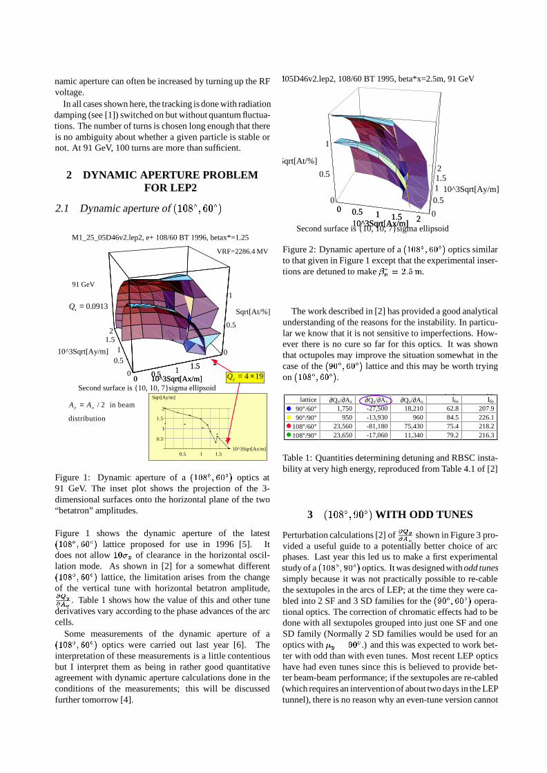
namic aperture can often be increased by turning up the RFvoltage.

In all cases shown here, the tracking is done with radiationdamping (see [1]) switched on but without quantum fluctua-tions. The number of turns is chosen long enough that thereis no ambiguity about whether a given particle is stable ornot. At 91 GeV, 100 turns are more than sufficient.

2 DYNAMIC APERTURE PROBLEMFOR LEP2

2.1 Dynamic aperture of (108; 60)

q

M1_25_05D46v2.lep2, e+ 108/60 BT 1996, betax*=1.25

00.5 1 1.5 2

10^3Sqrt[Ax/m]0

0.5

11.52

10^3Sqrt[Ay/m] 0

0.5

1

Sqrt[At/%]

00.5 1 1.5 2

10^3Sqrt[Ax/m]Second surface is 10, 10, 7sigma ellipsoid

91 GeV

VRF=2286.4 MV

0.5 1 1.510^3Sqrt[Ax/m]

0.5

1

1.5

2

Sqrt[Ay/m]

Qs = 0 0913.

A Ay x= / 2 in beam

distribution

Qy = ×4 19

Figure 1: Dynamic aperture of a (108; 60) optics at91 GeV. The inset plot shows the projection of the 3-dimensional surfaces onto the horizontal plane of the two“betatron” amplitudes.

Figure 1 shows the dynamic aperture of the latest(108; 60) lattice proposed for use in 1996 [5]. Itdoes not allow 10x of clearance in the horizontal oscil-lation mode. As shown in [2] for a somewhat different(108; 60) lattice, the limitation arises from the changeof the vertical tune with horizontal betatron amplitude,@Qy

@Ax

. Table 1 shows how the value of this and other tunederivatives vary according to the phase advances of the arccells.

Some measurements of the dynamic aperture of a(108; 60) optics were carried out last year [6]. Theinterpretation of these measurements is a little contentiousbut I interpret them as being in rather good quantitativeagreement with dynamic aperture calculations done in theconditions of the measurements; this will be discussedfurther tomorrow [4].

M05D46v2.lep2, 108/60 BT 1995, beta*x=2.5m, 91 GeV

0 0.5 1 1.5 210^3Sqrt[Ax/m]0

0.5

11.52

10^3Sqrt[Ay/m]0

0.5

1

Sqrt[At/%]

0 0.5 1 1.5 210^3Sqrt[Ax/m]Second surface is 10, 10, 7sigma ellipsoid

Figure 2: Dynamic aperture of a (108; 60) optics similarto that given in Figure 1 except that the experimental inser-tions are detuned to make x = 2:5m.

The work described in [2] has provided a good analyticalunderstanding of the reasons for the instability. In particu-lar we know that it is not sensitive to imperfections. How-ever there is no cure so far for this optics. It was shownthat octupoles may improve the situation somewhat in thecase of the (90; 60) lattice and this may be worth tryingon (108; 60).

lattice ∂Qx/∂Ax ∂Qy/∂Ax ∂Qy/∂Ay I6x I6y

90°/60° 1,750 -27,500 18,210 62.8 207.990°/90° 950 -13,930 960 84.5 226.1

108°/60° 23,560 -81,180 75,430 75.4 218.2108°/90° 23,650 -17,060 11,340 79.2 216.3

(depend on lowβ)

Table 1: Quantities determining detuning and RBSC insta-bility at very high energy, reproduced from Table 4.1 of [2]

3 (108; 90) WITH ODD TUNES

Perturbation calculations [2] of @Qy

@Ax

shown in Figure 3 pro-vided a useful guide to a potentially better choice of arcphases. Last year this led us to make a first experimentalstudy of a (108; 90) optics. It was designed with odd tunessimply because it was not practically possible to re-cablethe sextupoles in the arcs of LEP; at the time they were ca-bled into 2 SF and 3 SD families for the (90; 60) opera-tional optics. The correction of chromatic effects had to bedone with all sextupoles grouped into just one SF and oneSD family (Normally 2 SD families would be used for anoptics with y = 90.) and this was expected to work bet-ter with odd than with even tunes. Most recent LEP opticshave had even tunes since this is believed to provide bet-ter beam-beam performance; if the sextupoles are re-cabled(which requires an interventionof about two days in the LEPtunnel), there is no reason why an even-tune version cannot

also be developed (see Section 6).Figure 2 shows a new 3-dimensional scan of the dy-

namic aperture of this optics, confirming the results of [2].The horizontal dynamic aperture is considerably larger thanshown in Figure 1 in accordance with the reduced value of@Qy

@Ax

indicated in Table 1. The horizontal dynamic apertureis in fact limited by another physical effect, the RadiativeBeta-Synchrotron Coupling (RBSC) instability, describedin [1].

A comparison of the quantities I6x and I6y (see Table 1)that characterise this instability shows that the (108; 90)optics is not significantly better or worse than the others.

It is true, however, that reducing the value of x will en-hance this instability because of the additional radiation inthe quadrupoles of the interaction region. Figure 1 was com-puted for an optics with x = 1:25m while Figure 4 wasdone for x = 2:5m. It has been pointed out that the com-parison between the two made in my talk was somewhat un-fair. To remedy this, I now include the dynamic aperture ofthe (108; 60) optics with x = 2:5m as Figure 2.1 Whilethe situation is a little better for x = 2:5m, it can still onlybe described as marginal.

I would like to direct your attention to Figure 8 of [2]which shows how the addition of imperfections affects thedynamic aperture of various lattices. It should be noted thatthe dynamic aperture of the (108; 90) case is diminishedsomewhat by imperfections while that of (108; 60) is not.This can be understood on the basis of the physical effectswhich determine the stability limit. Detuning with ampli-tude is not significantly changed while a perfect lattice lim-ited by RBSC is more vulnerable to the imperfection-drivenresonances which appear at large amplitudes.

3.1 MD on (108; 90) in 1995

In 1995 we had two MD sessions with the odd-tune optics:

15/9/95, fill 1989.00 The beam circulated immediatelyand we measured single-bunch instability limit (see Sec-tion 4). We ramped 4 e+ bunches of 0.1 mA to 45.6 GeVwith no losses.

7/10/95, fill 3062.00 Continuingfrom the previous MD,we squeezed to y = 9 cm and measured dynamic apertureusing the injection kicker, with and without the emittancewigglers. Afterwards, we squeezed to y = 5 cm and mea-sured dynamic aperture again.

It proved to be possible to correct the closed orbit toyRMS = 0:35mm. Following this a transverse polariza-tion of 10 % was measured without further optimisation ofbeam conditions. At the end we lost the beam by switch-ing on damping wigglers (this was expected in view of thelimited momentum acceptance).

1This is by no means justice for all optics since the (108; 90) opticsin Figure 4 was tracked with a very asymmetric RF voltage distributionwhile the (108; 60) optics in Figures 1 and 2 were privileged with per-fect symmetry.

J M J tt (108° 90°) ti LEP P f W k h Ch i 16/1/96 P 6

12

µ y / o

1 90

2 108

:

:

µ

µx

x

=

=

o

o

∂∂Q

Ay

x

Perturbationcalculations usingHori-Depritalgorithmimplented inMathematica(Y. Alexahin,CERN-SL-95-110(AP).

∂∂Q

Ay

x µ y = 60o

µ x / o

∂∂Q

Ay

x

(units of 1000)

(units of 1000)

Figure 3: How the choice of arc-cell phase advance can af-fect the critical derivative of the vertical tune with horizon-tal amplitude. The colour-coding of the dots (if you can seeit) serves to guide the eye and is defined in Table 1. Thisfigure is also reproduced from Figures 6 and 7 of [2].

(108° 90°) i f k h Ch i 16/1/96 8

108/90 optics 1995, Y05E46, 91GeV, odd tunes, stan

01

2

3

4

10^3Sqrt[Ax/m]

0

1

2

10^3Sqrt[Ay/m]

0

0.5

1

1.5

Sqrt[At/%]

01

2

3

4

10^3Sqrt[Ax/m]

Second surface is 10, 10, 7sigma ellipsoid

0.5 1 1.5 2 2.5 310^3Sqrt[Ax/m]

0.5

1

1.5

2

2.5

Sqrt[Ay/m]

VRF=2464 MV

91 GeV

RBSC

Figure 4: Dynamic aperture of the 1995 (108; 90) opticswith odd tunes at 91 GeV. Otherwise this figure is analogousto Figure 1.

SD-

_ 5 | : | - _

—lSD"

The RMS vertical dispersion was measured to beDyRMS = 5 cm.

The dynamic aperture measurements were found to be ingood agreement with tracking for the conditions of the ex-periment. By including the effect of imperfections it waspossible to model the experiment in detail (see [2], to be re-viewed tomorrow in [4].

4 SINGLE-BUNCH INTENSITY

A higher vertical phase advance reduces the average valueof y in the arcs. As discussed in other talks [7, 8] there isa theoretical expectation that this reduces the effect of thetransverse impedance of bellows joining vacuum chambersections. Since these are give a major contribution to the to-tal transverse impedance, we can expect to raise the thresh-old for the transverse mode-coupling instability (TMCI) bychanging from a lattice with y = 60 to one with y =90. Figures given in Table 4.2 of [2] indicate that the im-provement expected should be of the order of 12 %.

In the first MD, we saw that the single-bunch current waslimited at Ib = 505A in conditions (damping wiggler fieldB+DW = 1:02T, polarization wigglers off andQs ' 0:085 )where it had been limited at Ib = 430A in the (108; 60)optics. The instability limiting the current had the classichallmarks of TMCI.

The tune-shiftswith current were also measured in the ex-periment [2].

The increased TMCI threshold will increase luminosityatLEP2 provided that the two-beam current is not otherwiselimited (e.g., by parasitic beam-beam effects at injection). Itis worth mentioning that, when some of the copper RF cav-ities are removed, the factor by which we will gain by mov-ing to a higher vertical phase advances will increase as thebellows account for a larger fraction of the total transverseimpedance.

5 POLARIZATION

Polarization at energies up to about 65 GeV is desirable forenergy calibration by extrapolation to 90 GeV [9].

So far there have been no measurements of polarizationabove 46 GeV or so on any lattice. Still, theoretical under-standing is now good enough for quantitative prediction. Itconsists essentially of linear depolarization theory for latticemodelling supplemented by sideband theory for additionaldepolarization due to synchrotron sideband resonances andenergy spread. The polarization levels attainable withy =90 are expected to be lower than with y = 60. This ispartly due to the difficulty of correcting vertical orbit to suf-ficient level when pickups are spaced at intervals of 90.

The reduced level of polarization is the biggest disadvan-tage of a (108; 90) optics. Despite all this, there are somegrounds for hope, namely:

Success with the vertical orbit in MD (yRMS =0:35mm).

Measurement of 10% polarization in MD on(108; 90).

Unexploited potential to improve the polarization byspin harmonic compensation, etc.

So far there have been no measurements of polarization on(108; 60) to make a comparison.

50 60 70 80 90

E/GeV

0

5

10

15

20P / %

Polarization at Z= 10%

50 60 70 80 90E/GeV

0

0.1

0.2 Optimum Qs for maximum P

50 60 70 80 900

5

10

15

20P / %

Polarization at Z= 20%

E/GeV

Optimistic prediction

?

Figure 5: Extrapolations of measured polarization valuemeasured at 45 GeV to higher energy using the sidebandtheory to account for the effect of the increasing energyspread in the beam. At the same time, the synchrotron tuneis adjusted as a function of energy in order to minimise de-polarization effects, as shown in the small plot at top right.The upper left plot shows an extrapolation based on ourmeasured value P = 10% at 45.6 GeV while the lower plotpresents an extrapolation from an optimisticP = 20%.

6 NEW (108; 90) OPTICS WITH EVENTUNES

As mentioned in Section 3 and shown in [10], even integerparts of the tunes are favoured for beam-beam reasons. A(108; 90) optics with [Qx] = 102 and [Qx] = 96 is underdevelopment. This part of my talk describes some prelimi-nary results, on this new optics.

To allow a better chromatic correction the sextupoleshave been re-cabled (within MAD) into two SF and twoSD families (as they were back in 1992, otherwise the lay-out is for 1996). The matching started from the (108; 60)optics proposed for 1996 [5] and many of the insertions

are identical. The present version needs some minor im-provements (particularly to the dispersion suppressors) andchecks need to be made that it meets all constraints now im-posed on an operational optics, is not too sensitive to imper-fections and so on. However, because of its similarities tothe (108; 60) optics, one can say that it is basically bunch-train compatible2.

At the time of speaking, little effort has been made to im-prove the chromatic behaviour of this optics so the momen-tum acceptance is poor as indicated in Figure 6.

q Not yet well corrected ...

102.2

102.22

102.24

102.26

102.28

102.3

102.32

102.34

102.36

102.38

-0.008 -0.006 -0.004 -0.002 0 0.002 0.004 0.006 0.008

96.09

96.1

96.11

96.12

96.13

96.14

96.15

96.16

96.17

96.18

96.19

QxQy

Preliminary

Figure 6: Tune variation as a function of a fixed momen-tum deviation for non-radiating particles in a machine withno RF system. Although it is only roughly related to thephysics of the problem, this is enough to show that the mo-mentum acceptance of this optics needs to be improved.

The dynamic aperture of this preliminary optics is shownin Figure 7. Although the momentum acceptance looksgood here, this is due to the fact that all particles start offwith the same synchrotron phase in the tracking. An av-eraging over synchrotron phase—for which there was notenough time before this workshop—will reduce the aperturefor synchrotron oscillations. However note that exactly thesame tracking methodology was applied in all the cases re-ported in this talk so all other cases would suffer some re-duction.

The main point of showing such a preliminary result is toshow that it is possible to maintain the improvement in hor-izontal dynamic aperture in a (108; 90) optics with eventunes. Whether this optics can be developed further into aworkable solution for the highest operating energies of LEPremains to be demonstrated.

2When a final version is developed we will need to check non-localside-effects of bunch train bumps and parasitic encounters, such as howthe vertical dispersion adds up at the IPs, etc.

108/90 preliminary Qx=102,Qy=96, e+ betax*=2.5m, 9

0 1 2 3

10^3Sqrt[Ax/m]0

12

34

10^3Sqrt[Ay/m]0

0.5

1

1.5

2

Sqrt[At/%]

0 1 2 3

10^3Sqrt[Ax/m]Second surface is 10, 10, 7sigma ellipsoid

Figure 7: Dynamic aperture of a preliminary (108; 90)optics with even tunes and x = 2:5m at 91 GeV. See im-portant comments in the text concerning the momentum ac-ceptance. For this tracking, the RF voltage distributionwasmoderately asymmetric.

7 CONCLUSIONS

At present it seems that a (108; 90) optics with even orodd tunes is the strongest candidate for use at the highestLEP2 energies. It is probably the best candidate to over-come the limitationof LEP energy by dynamic aperture, i.e.,this may be the only way to get to LEP’s top energy. Or theremay be no way.

Other advantages accruing to this choice of optics includehigher single-bunch current which will help luminosity. Themain drawback is the reduced expectation for polarization.

First indications are that an even-tune version of a(108; 90) optics is feasible. The preliminary version ofa physics optics has good horizontal dynamic aperture al-though some reduction should be expected from imperfec-tions. Moreover the horizontal dynamic aperture will besensitive to the RF voltage available (because of RBSC in-stability). Its optical performance and detailed suitability(check-list) remain to be checked.

Although it should be possible to match to x = 1:25m,this may reduce dynamic aperture (extra radiation in low-quads may enhance the RBSC).

So far, in my opinion, experiments have failed to showthat tracking results are pessimistic. I.e., we must take dy-namic predictions seriously (see also [4])!

Acknowledgements This talk has drawn heavily on thework of Y. Alexahin [2]. Recent dynamic aperture calcula-tions have been carried out very efficiently with the help ofnew software developed with S. Tredwell.

8 REFERENCES

[1] J.M. Jowett, “Dynamic Aperture for LEP: Physics and Cal-culations”, in J. Poole (Ed.), Proceedings of the Fourth Work-

shop on LEP Performance, Chamonix, January 1994, CERNSL/94-06 (DI) (1994).

[2] Y. Alexahin, “Improving the dynamic aperture of LEP2”,CERN–SL–95–110 (AP) 1995.

[3] J.M. Jowett, “Problems expected from RF asymmetries”, thisworkshop.

[4] F. Ruggiero, “Dynamic Aperture”, this workshop.

[5] M. Meddahi, private communication.

[6] C. Arimatea, D. Brandt, A. Hofmann, G. von Holtey, R. Jung,M. Lamont, M. Meddahi, G. Morpurgo, F. Ruggiero, SL-MDNote 199 (1995).

[7] A. Hofmann, “Bunch Intensity Limitations”, this workshop.

[8] K. Cornelis, “TMCI and what to do about it”, this workshop.

[9] M. Placidi, “Energy measurement possibilities for LEP2”,this workshop.

[10] E. Keil, “Beam-beam effects as a function of the tunes”, thisworkshop.

CAN WE CORRECT THE SOLENOID COUPLING BETTER THAN IN1995?

Ghislain ROYSL Division

Abstract

Although coupling measurements have consistently givengood results in 1995 there has been some suspicion about a”coupling mystery” at 45 GeV. I review and compare exper-imental and simulation results for the different correctionsused in 1995. Alternate schemes and hardware changeshave been proposed which are described and evaluated.

1 INTRODUCTION

The compensation of the coupling introducedby experimen-tal solenoids in LEP is required in order to avoid beam blow-up and a tilt of the transverse planes of motion which bothcould reduce the luminosity. I first review the principle ofthis compensation then describe the methods used in prac-tice in 1995 with a discussion of the experimental results.The third section reviews the improvements under study for1996.

2 SOLENOIDS AND COUPLINGCOMPENSATION

2.1 Effect of solenoids

A solenoid can be described as a constant longitudinal mag-netic field that couples the two transverse planes of motion,resulting in a tilt of the transverse planes along the acceler-ator and a blow-up of the vertical beam size.

According to the treatment of coupling in perturbationtheory[1, 2, 3] the coupling vector is defined as

C = i

4

Bsl

(B)

sy

x

sxy

!(1)

where Bsl is the solenoid integrated field and (B) is themagnetic rigidity proportional to the beam energy. Havingconstant solenoidal fields in LEP the scaling with the in-verse of the beam energy ensures that the coupling effectsget weaker as we go to higher energies for LEP2. The lastterm in equation 1 is a geometric term related to the beamparameters at the interaction point (IP).

2.2 Emittance ratio

The effect of coupling on vertical emittance can be de-scribed by the emittance ratio as a function of the modulus

of the coupling vector:

y

x=

jCj

2

2jCj

2

2+ 0:5

(2)

where is the separation between the fractional parts of thetunes. At LEP we generally have 0:1.

The integrated fields of the four LEP solenoids are givenin table 1 together with the emittance ratio contribution ofeach solenoid with no compensation, for different energiesand different values of .

2.3 Local effects

The coupling of the transverse planes of motion producesalso a local tilt of the axes of the beam ellipsoid which canbe seen in the physical x y plane. This tilt is opposite forthe two beams at the IP and quickly reduces the luminosityin the case of flat beams as we have in LEP. Coupling in thex0 y plane produces a local blow-up of the beam in thevertical plane as well. Other coupling components do notaffect the vertical beam size at the IP.

2.4 Principles of compensation

The LEP design report[4, 3] recommends using four pairsof antisymmetrically powered tilted quadrupoles in the in-sertions and close to the solenoids in order to satisfy equa-tions 3 below, which represent the cancellation of the effectof the coupling vector at the IP calculated over one side ofan insertion (first two equations), while taking care not tointroduce other coupling components (last two equations):

Xj

(1

2

pxyKsl)j sin(x y)j +

1

2jCj = 0

Xj

(1

2

pxyKsl)j sin(x + y)j +

1

2jC+j = 0 (3)

Xj

(1

2

pxyKsl)j cos(x y)j = 0

Xj

(1

2

pxyKsl)j cos(x + y)j = 0

It is possible to reduce the number of pairs to less thanfour but this requires some phase relations to be held for allforeseeable optics for LEP. This option of “magic phases”

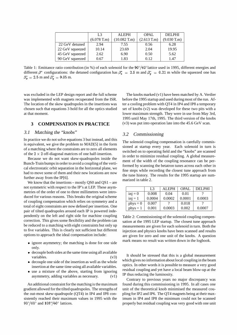
L3 ALEPH OPAL DELPHI(6.078 T.m) (10.082 T.m) (2.613 T.m) (9.030 T.m)

22 GeV detuned 2.94 7.55 0.56 6.2822 GeV squeezed 10.14 23.69 2.04 19.9545 GeV squeezed 2.62 6.90 0.50 5.6290 GeV squeezed 0.67 1.83 0.12 1.47

Table 1: Emittance ratio contribution (in %) of each solenoid for the 90=60lattice used in 1995, different energies anddifferent configurations: the detuned configuration has x = 2:5 m and y = 0:21 m while the squeezed one hasx = 2:5 m and y = 0:05 m.

was excluded in the LEP design report and the full schemewas implemented with magnets recuperated from the ISR.The location of the skew quadrupoles in the insertions waschosen such that equations 3 hold for all the optics studiedat that moment.

3 COMPENSATION IN PRACTICE

3.1 Matching the “knobs”

In practice we do not solve equations 3 but instead, and thisis equivalent, we give the problem to MAD[5] in the formof a matching where the constraints are to zero all elementsof the 2 2 off-diagonal matrices of one half-insertion.

Because we do not want skew-quadrupoles inside theBunch-Train bumps in order to avoid a coupling of the verti-cal electrostatic orbit separation in the horizontal plane, wehad to move some of them and their new locations are nowfurther away from the IP[6].

We know that the insertions – mostly QS0 and QS1 – arenot symmetric with respect to the IP’s at LEP. These asym-metries of the order of one to three millimetres were intro-duced for various reasons. This breaks the original schemeof coupling compensation which relies on symmetry and atotal of eight constraints are now defined per insertion. Onepair of tilted quadrupoles around each IP is powered inde-pendently on the left and right side for machine couplingcorrection. This gives some flexibility and the problem canbe reduced to a matching with eight constraints but only upto five variables. This is clearly not sufficient but differentoptions to approach the ideal compensation include:

ignore asymmetry; the matching is done for one sideonly.

decouple both sides at the same time using all availablevariables. (v3)

decouple one side of the insertion as well as the wholeinsertion at the same time using all available variables.

use a mixture of the above, starting from ignoringasymmetry, adding variables as necessary. (v1)

An additional constraint for the matching is the maximumgradient allowed for the tilted quadrupoles. The strengths ofthe out-most skew-quadrupole (QT4) in IP4 and IP8 con-sistently reached their maximum values in 1995 with the90=60 and 108=60 lattices.

The knobs marked (v1) have been matched by A. Verdierbefore the 1995 startup and used during most of the run. Af-ter a cooling problem with QT4 in IP4 and IP8 a temporaryset of knobs (v2) was developed for these two pits with alower maximum strength. They were in use from May 3rd,1995 until May 17th, 1995. The third version of the knobs(v3) was put into operation late into the 45.6 GeV scan.

3.2 Commissioning

The solenoid coupling compensation is carefully commis-sioned at startup every year. Each solenoid in turn isswitched on to operating field and the “knobs” are scannedin order to minimize residual coupling. A global measure-ment of the width of the coupling resonance can be per-formed by scanning the betatron tunes across each other infine steps while recording the closest tune approach fromthe tune history. The results for the 1995 startup are sum-marized in table 2.

L3 ALEPH OPAL DELPHIinj = 0 0.008 0.04 0.01 ?inj = 1 0.0004 0.0002 0.0001 0.0003phys = 0 0.007 ? 0.018 ?phys = 1 0.001 0.0003 0.002 0.0007

Table 2: Commissioning of the solenoid coupling compen-sation at the 1995 LEP startup. The closest tune approachmeasurements are given for each solenoid in turn. Both theinjection and physics knobs have been scanned and resultsare given for zero and one unit of the knobs. A questionmark means no result was written down in the logbook.

It should be stressed that this is a global measurementwhich gives no informationabout local coupling in the beamoptics. In other words it is possible to measure a very goodresidual coupling and yet have a local beam blow-up at theIP thus reducing the luminosity.

Contrary to previous years no major discrepancy wasfound during this commissioning in 1995. In all cases oneunit of the theoretical knob minimised the measured cou-pling for IP2 and IP6. The QT4 magnets being at their max-imum in IP4 and IP8 the minimum could not be scannedproperly but residual coupling was very good with one unit

of the calculated knob. An initial discrepancy in the OPALcompensation was quickly traced to a database problemwhich left one of the tilted pair of quadrupoles with morecurrent than requested.

In previous years some 20% discrepancy was not uncom-mon and in 1994 a minus sign had to be introduced forthe ALEPH compensation which was most probably dueto a skew quadrupole with crossed leads; however severalchecks of magnet polarities showed a correct wiring and thereversal of the ALEPH solenoidal field should be excluded.

For the commissioningof the (v2) knobs we had only timeto check that the global compensation as measured with theclosest tune approach was the same with the (v2) knobs inIP4 and IP8 as it was with the (v1) knobs; the measurementgave Q = 0:0025 in both cases and is considered to be agood value.

3.3 An experiment...

In a machine development session[8] while LEP was be-ing optimized to reach the highest possible beam-beam tuneshift it was observed that both the beam sizes as seen on theBEUV and the luminositywere sensitive to orbit correctionsand the coupling compensation scheme. Best results wereobtained with version (v3) of the knobs in pits 2 and 4. Inpit 4 the direction of improving compensation was limitedin range by the maximum strength of QT4. The trim historyof this fill reveals that a “sanity check” took place at aboutthe same time these observations were made. This opera-tion allows one to resynchronize the machine and the con-trol database; clearly we are not now in a position to knowexactly the currents in the tilted quadrupoles during this ex-periment. However similar observations were made in sub-sequent physics fills.

This experiment raised a question about the difference be-tween the two sets of knobs. They are evaluated below butthe following explanation can be proposed already. It hasbeen observed that very small distortions of the vertical or-bit, of the order of 200 m peak-to-peak, are sufficient tomake a dent of the order of 10% in the optimised luminos-ity at LEP. Such an orbit could be generated by a change ofintegrated strength Ks 3: 103 m1 at a place with ahorizontal orbit excursion of x = 2:7 mm. The change ofstrength corresponds to the maximum difference betweenthe (v1) and (v3) knobs and happens at QT2 around IP4.While a 2:7 mm horizontal orbit excursion seems large itcannot be excluded so this mechanism is a possible candi-date for the observed behaviour. A significant change in thevertical orbit can also dramatically change the dispersion atthe IP’s which in turn strongly influences the luminosity.

3.4 High energy observations

Other observations at energies above 46 GeV during thelast period of the 1995 run report excellent beam sizes andemittance ratios down to about 0.5%[7]. Residual couplingmeasurements in these conditions consistently gave Q =

0:0002 for the closest tune approach.

4 EVALUATION OF COMPENSATION

In order to evaluate the knobs used in operation in 1995 thefollowing comparison is based on the 90=60 physics op-tics 45.6 GeV with emittance wigglers at 0.84 T.m and witha total RF voltage of 240 MV. The observables are the ver-tical emittance as can be seen on the BEUV and the beamsizes at the IP which influence directly the luminosity. Notethat the beam sizes quoted include the usual emittance con-tribution( =

p), the local coupling contributionand the

dispersion contribution where applicable. The beam tilt isnot easily observed and I have ignored it in this evaluation.

4.1 Emittance and beam sizes

Results for LEP without vertical Bunch-Train bumps aresummarised in table 3 below.

For L3 and OPAL the solenoids can be well compensatedwith the first set of knobs with no emittance blowup andlocal beam size contribution at the IP below 0:5 m. ForALEPH and DELPHI the missing QT4 strength is charac-terised by a limited emittance blow-up but a larger beam sizecontributionat the IP which indicates that the local couplingis not well compensated.

The second set of knobs (v2), implemented for ALEPHand DELPHI only, are even worse to that respect. This is notabnormal since they were matched with a lower maximumstrength for QT4. They give very good global correctionwith no emittance blowup – and this explains the unchangedclosest tune approach after they were introduced – but a verysignificant beam size contribution at IP4 and IP8.

The third set of knobs, which has clearly helped reducingbeam emittances in LEP, shows here the worst vertical beamsizes in all four pits coming mainly from emittance blowup.It also leads to higher beam size contributions than the (v1)set in all four experiments.

The conclusions of this knob evaluation is that the (v1)set of knobs is clearly the best for coupling compensationin 1995. Also it has become clear that machine observa-tions, such as emittance blowup and closest tune approachmeasurements, look only at the global aspect of the couplingcorrection while one should also worry about a good localdecoupling at the IP to ensure small beam sizes and no tiltof the beams which would cause a loss of luminosity.

4.2 Effect of Bunch-Train bumps

After exciting the Bunch-Train collision bumps to maxi-mum amplitude in the even pits and to the optimized val-ues of 80/100/80/100% in the odd pits the same evaluationof the three sets of knobs is shown in table 4.

The vertical emittance is here dominated by the verticaldispersion generated by the Bunch Train bumps. Some in-crease of the vertical beam sizes coming from local couplingcan also be seen, especially for L3 with the (v3) knob andDELPHI for (v2).

In conclusion the solenoid compensation knobs, despitethe shortcomings shown in the previous section, are not

L3 sol. (v1) (v2) (v3)x [nm.rad] 35.3 35.4 35.4y [nm.rad] 0.04 < 5: 106 0.034y [m] 3.3 0.026 2.14

ALEPH sol. (v1) (v2) (v3)x [nm.rad] 34.0 35.4 35.4 35.3y [nm.rad] 1.60 0.01 0.006 0.02y [m] 11.7 1.51 0.46 1.30

OPAL sol. (v1) (v2) (v3)x [nm.rad] 35.3 35.4 35.4y [nm.rad] 0.11 < 5: 106 0.0008y [m] 3.2 0.45 3.12

DELPHI sol. (v1) (v2) (v3)x [nm.rad] 34.0 35.4 35.4 35.3y [nm.rad] 1.57 1: 105 1: 105 0.045y [m] 11.1 1.00 4.18 2.37

all four sol. (v1) (v1/v2) (v3)x [nm.rad] 32.1 35.4 35.5 35.4y [nm.rad] 3.73 1:4 104 1:0 104 0.022y [m] 22. 1.5 4.1 2.0y [m] 19.2 0.6 1.2 1.6

Table 3: Effect of solenoid compensation for LEP physicsoptics in 1995 without Bunch-Train bumps. The first col-umn gives the effect of the solenoid alone. The last threecolumns give the effect of the solenoid plus the compensa-tion for three different compensation schemes. y is givenat the IP where the solenoid is excited. The bottom partgives the combined effect of the four solenoids and their re-spective compensations; the last two lines correspond to themaximum of the vertical beam sizes in all four IP’s and theaverage of the four.

likely to have significantly affected the beam sizes duringthe 1995 run. The compensation is however marginal andactions should be taken to improve the situation in 1996.

5 POSSIBLE IMPROVEMENTS

5.1 Higher gradients

It appears from previous sections that the most importantimprovement to the coupling compensation would be to in-crease the maximum gradients for QT4 in IP4 and IP8 tothe level needed for a proper compensation. The missingstrength has been calculated, based on the preliminary 1996108=60 lattice and represents 11% of the maximum in IP4and 9% in IP8. A request has been made to the magnet groupto try and obtain this added strength from the existing mag-nets. These magnets, recuperated from the ISR machine,are likely to have design margins which will allow this up-grade. Whether the power converters will be able to deliverthe added power is being studied.

The same calculation based on the preliminary 90=60

lattice for 1996 shows that we need close to 70% added

L3 sol. (v1) (v2) (v3)x [nm.rad] 35.1 35.2 35.2y [nm.rad] 0.17 0.094 0.16y [m] 4.89 3.39 4.19

ALEPH sol. (v1) (v2) (v3)x [nm.rad] 33.9 35.1 35.0 35.1y [nm.rad] 1.53 0.088 0.088 0.085y [m] 11.5 2.67 2.24 2.32

OPAL sol. (v1) (v2) (v3)x [nm.rad] 35.1 35.1 35.1y [nm.rad] 0.26 0.093 0.095y [m] 5.0 3.50 3.49

DELPHI sol. (v1) (v2) (v3)x [nm.rad] 33.8 35.1 35.1 35.1y [nm.rad] 1.45 0.090 0.089 0.106y [m] 10.9 2.37 4.67 2.96

all four sol. (v1) (v1/v2) (v3)x [nm.rad] 32.1 35.1 35.1 35.2y [nm.rad] 3.56 0.087 0.086 0.090y [m] 22.0 3.5 4.6 3.7y [m] 19.2 2.9 3.4 3.1

Table 4: Effect of solenoid compensation for LEP physicsoptics in 1995 with Bunch-Train bumps at 100% in evenpits and 100/80/100/80% in odd pits. The column layout isthe same as that of table 3. For comparison, the contributionof the Bunch Train bumps alone gives x = 35:1 nm:rad,y = 0:092 nm:rad, y = 3:47 m and y = 2:81 m.

strength on QT4 in IP4 and IP8 in this configuration. Thisis quite surprising since the two optics have very similar in-sertion design. A comparison with the 1995 situation showsthat the IP4 optics was the least favourable for solenoid com-pensation; yet it was used as the starting point to rematch IP4and IP8 for 1996. From past experience it is likely that wecan bring the 90=60 lattice situation very close to that ofthe 108=60 lattice by appropriate matching. A modifica-tion to LEP which has been requested for linear optics flexi-bility might prove very helpful here: the quadrupoles of theRF section forming two FODO cells will be equipped withindependent power supplies in IP4. This will make it possi-ble to locally change the phase advance without introducingbeating in the RF sections.

5.2 Symmetric layout

In order to reduce the beta-beating induced by the left/rightasymmetries of the QS0 and QS1 layout we match the lin-ear optics of the insertions left and right separately. We haveseen that this technique is now also used for coupling knobs.A request has been placed to the magnet group to try and re-cover the original layout as much as possible. The follow-ing evaluation is based on the current layout with existingasymmetries and compares three ways of doing the match-ing in the presence of asymmetries. For this evaluation we

have assumed that the strength needed for QT4 in IP4 andIP8 is available.

The first method, labelled Sym. in table 5 has perfect an-tisymmetry of the QT excitations around the IP. The secondmethod, L/R, uses a matching of the left and right side ofthe insertionat the same time using eight constraints and fivevariables. The last method, L/global, uses a matching of theleft side and of the whole insertion at the same time.

L3 Sym. L/R L/globalx [nm.rad] 35.4 35.4 35.4y [nm.rad] < 5: 106 id. id.y [m] 0.006 0.011 0.021

ALEPH Sym. L/R L/globalx [nm.rad] 35.4 35.4 35.4y [nm.rad] 1: 105 8: 105 < 5: 106

y [m] 0.033 0.093 0.024

OPAL Sym. L/R L/globalx [nm.rad] 35.4 35.4 35.4y [nm.rad] < 5: 106 id. id.y [m] 0.002 0.006 0.011

DELPHI Sym. L/R L/globalx [nm.rad] 35.3 35.3 35.4y [nm.rad] < 5: 106 id. id.y [m] 0.005 0.007 0.005

Table 5: Evaluation of different strategies for solenoid com-pensation in the presence of layout asymmetries.

This evaluation shows that the matching strategy has littleinfluence on the coupling compensation provided we haveenough strength for the skew-quadrupoles. The effect of thelayout asymmetries is not clearly visible; the Sym. knobsgiving even the best results. Therefore the layout asymme-tries are not the source of the problem for coupling com-pensation. The coupling knobs should be matched assumingperfect antisymmetry of the skew-quadrupole excitations in1996.

5.3 Coupled matching

At KEK, where TRISTAN runs at energies close to 30 GeVand experimental solenoids have fields equivalent to thoseinstalled at LEP, it has been found critical to match thesolenoid compensation to the linear lattice design[9].

The solenoids and the compensating tilted quadrupolesintroduce a mismatch of the linear optics which shows as abeta-beating along the machine. This was quite strong forTRISTAN and good results have been achieved with match-ing directly the coupled 4 4 matrix. The case of LEP isnot as critical since we run at much higher energies. E. Keilhas shown[10] that a beating of the order of 3% is present at45 GeV if one decouples the solenoids ignoring linear op-tics changes. This can be reduced to essentially zero withcoupled-matching and changes of skew-quadrupole excita-tions of the order of K

K 5: 103, or 0:3A at maximum

gradient.In a study of the solenoid model[11], A. Verdier has

shown that small changes in the model[12] can easily entailchanges of up to a few percents in the skew-quadrupole ex-citations. Considering that the changes above are within theerrors of the solenoid model at hand, A. Verdier concludedthat the induced beating is unavoidable. Note that this beat-ing is expected to be reduced significantly as we go to higherenergy.

However injection into LEP is done at 22 GeV which isbelow the operating energy of TRISTAN. The question ofthe beating at injection is therefore valid especially if oneconsiders injecting on squeezed optics where the geomet-rical factor of equation 1 enhances the effect. As far as Iknow this has not been studied but should be checked be-fore the 1996 startup. We should also explore the possibil-ity of using the coupled matching technique to “steer” thelinear optics matching to a good working point for couplingcompensation[13].

6 CONCLUSION

Despite the good coupling measurements using the clos-est tune approach method in 1995 we have shown that thecoupling compensation was not optimized. Mostly affectedwere IP4 and IP8 where the QT4 skew-quadrupoles are lo-cated in a place in phase such that the necessary gradientfor efficient decoupling is above the maximum availablefor the magnets. This lead to a difficult balancing betweendecoupling at the IP, which ensures no local beam blowupor tilt, and global decoupling which ensures no emittanceblowup. However it was shown that the vertical dispersionfrom the Bunch Train bumps actually dominate the emit-tance and beam sizes such that these coupling compensationshortcomings are not likely to have been a major problem in1995.

However we clearly have to find a solution for this miss-ing strength of the QT4 magnets in IP4 and IP8. An upgradeof the maximum gradient, involving magnets and powerconverters, has been requested and is being studied. Thesituation can certainly be improved also with a careful re-matching of these insertions.

Provided we can get this maximum gradient it has beenshown that, with the current level of layout asymmetries, wecan and should use antisymmetric knobs. The layout of theinsertions will be modified during the shutdown in order tobring them as close as possible to the original symmetric lay-out for linear optics matching purposes.

The coupled matching used in KEK is not needed at LEPat high energy. However it might prove useful at injectionenergy, especially in view of injection on squeezed optics.

7 REFERENCES

[1] G. Guignard, “The general theory of all sum and differenceresonances in a three dimensional magnetic field in a syn-chrotron”, CERN 76-06, 1976

[2] G. Guignard, “A general treatment of resonances in acceler-ators”, CERN 78-11, 1978

[3] J.P. Koutchouk, “Betatron coupling for LEP V13”,LEP Note 480, December 1983.

[4] LEP Design Report, Vol. II, CERN-LEP/84-01

[5] H. Grote and F.C. Iselin, “The MAD Program, User’s Refer-ence Manual”, CERN-SL 90-13 (AP), March 1995 (Rev 4).

[6] J. Poole, “The Implications of Running with Bunch Trains”,in Proceedings of the Fifth Workshop on LEP Performance,Chamonix, January 13-18, 1995.

[7] H. Burkhardt, “Performance in Physics”, Presentation 4.06in these proceedings.

[8] K. Cornelis et al., “Removal of the beam-beam tune shiftlimit for bunch trains”, SL-MD Note 190, October 1995

[9] S. Kamada, Particle and Fields ’91 (Vancouver 1991), 1055.

[10] E. Keil, “Solenoids, beta-beating and perfect matching”, SL-MD Note 75, December 1992.

[11] A. Verdier, “Improvement of the solenoid description in theLEP model”, SL/Note 93-33 (AP), March 1993.

[12] J.P. Koutchouk, F. Ruggiero and A. Verdier, “An op-tics model for the LEP solenoids”, SL/Note 92-33 (AP),June 1992.

[13] A. Verdier, private communication.

Problems Expected From RF Asymmetries

J.M. Jowett, CERN, Geneva, Switzerland

Abstract

Asymmetries of the RF voltage distribution have more sig-nificant effects as the energy of LEP is increased. Potentialproblems include differences between beams (tune splits,residual horizontal separation at the IPs, etc.), requiringsuitable corrections. Some operational experience with RFasymmetry has been gained at 65 GeV. Some additional ex-perimental studies are reported.

1 RADIATION, ORBIT AND BEAMPARAMETERS

LEP2 will be unique1 among e+e colliders in the strengthof the radiation effects that interact with the distribution ofthe RF voltage. Some of the basic physics of this was dis-cussed in previous workshops in this series, e.g., in [4, 5]and others have examined particular aspects [6].

At LEP2 we must recognise that the RF cavities are justas much a part of the optics as the quadrupoles: neglect-ing them in optical calculations is no longer admissible.Adequate theory and computational methods exist but areperhaps not applied often enough by enough people. Thisis because of the familiarity and efficacy of the traditionalCourant-Snyder formalism which has served us so well forso long. Howevere a unifying method for all linear op-tics calculations can be based on the elementary notions ofthe closed orbit and the eigenvectors of linearised motionaround it [1], thus avoiding any use of dispersion functionsin the calculation of the beam emittance. In essence, this isthe method now used in MAD commands such as EMIT,TWISS3, ENVELOPE, ... At high energy in LEP, theuse of pre-radiating commands like TWISS, OPTICS,BMPM, ... may be misleading, especially where disper-sion functions are involved in calculations. There have beenfairly few opportunities for detailed tests of the theory so farand we have recently gone some way towards putting thatright. In LEP’s brief run at 65–70 GeV at the end of last yearwe had our first taste of significant energy sawtoothing andRF asymmetry effects.

In this talk I shall review only information that has re-cently come to light on the effects of RF asymmetries.The results of earlier theoretical studies can be found else-where [2, 3].

1Except perhaps for TRISTAN

2 HORIZONTAL ORBIT WITHRADIATION

Let us briefly review the differences between the horizontalclosed orbits of electrons and positrons that can arise even inan ideal ring. Discussions of this effect go back (at least) tothe 1970’s and various laboratory reports by several authors.I will not attempt to give precise references here since thereare probably others that I don’t know about.

It is well known that the energy/momentum deviationsof e+e closed orbits are equal and opposite at each pointin ring (if we neglect the very small effect of the localenergy deviations on the radiation from the closed orbit).In terms of the fractional momentum deviations on theclosed orbit, (s), related to the momentums by p(s) =p0 (1 + (s)), the periodic solutionsof the appropriate dif-ferential equations satisfy:

8s 2 [0; C); +(s) = (s): (1)

A naıve idea based on a misconception of the “proton” dis-persion function is that the horizontal component of theclosed orbit is given by

x(s)?= Dx(s)

(s)

?=) x+(s)

?= x(s); (2)

An extra term, to which attention was drawn in [8], actuallybreaks this anti-symmetry of the closed orbit. Let us sketchwhere this effect comes from.

Neglecting chromatic terms, the horizontal closed orbitof either beam is a periodic solution of a Hill equation

x00(s) +K(s)x(s) = G(s)(s); x(s +C) = x(s);

(3)whereG(s) = eBy(s)=p0 is the local bending strength. Wecan look for a periodic solution by writing

x(s) = Dx(s)(s) = xB(s) (4)

where, again, xB(s) must be periodic on the circumference,C. At the same level of approximation, the equation defin-ing the “dispersion function” Dx(s) is

D00x(s) +K(s)Dx(s) = G(s); Dx(s + C) = Dx(s)

(5)and can be combined with (3) to give

x00B(s)+K(s)xB(s) = 2D0x(s)

0(s)Dx(s)

00(s) (6)

The first term on the right-hand side contains a part thatchanges sign for electrons and positrons:

0

(s) =@H

@zt

1 + G(s)x(s)

p0

1 + (s)

2

c1bx(s); y(s); s

2(7)

where we have used notations defined in [5]. In particularthe first term on the right-hand side of (7) is the Hamiltoniandescription of the effect of the RF cavities.

Hence the anti-symmetry of the electron-positron closedorbits is broken:

x+B(s) + xB(s) 6= 0 =) x+(s) + x(s) 6= 0 (8)

In practice, the operational orbit correction proceeds asif (8) were an equality: the average orbit of the electronand positron beams is corrected, assuming constant energyaround the ring so that the ideal orbit should vanish. Thesize of the Bassetti term, xB will be a limit to how well theclosed orbit can be corrected. However it should not be re-garded as a “noise” term: it has a well-determined coherentbehaviour which may interfere more subtly with the orbitcorrection.

Should this turn out to affect the quality of operationalorbit correction, a solution can be envisaged. First we notethat correction of a single-beam orbit can be done in princi-ple if a reference sawtooth orbit for the ideal ring is avail-able. Even with two beams in the ring, separate orbit infor-mation is available for each of them from LEP’s BOM sys-tem. So, we could correct each beam in separate calculationand intelligentlycombine the two resulting of sets correctorsettings. Of course the feasibility of this would depend onthe quality of BOM readings for the individual beams!

The ideal sawtooth orbit required for this procedure canbe constructed by running MAD with a description of theRF voltage configuration (and the rest of the machine state)at the moment the orbit is measured.

It happens that, in the course of analysing the measure-ments described in Section 3.1 I have already written a littleprogram that converts data from the RF voltage logging intoa MAD description. However it will need to be integratedinto orbit measurement and correction packages.

I strongly recommend that a MAD process should run inbackground and update the ideal sawtooth orbits (and theoptical functions) whenever the RF distribution changes.This scheme would do away with the much-deprecated fixed“Twiss” file serving as a description of the optics to the con-trol system.

3 EXPERIENCE WITH LEP 1.5

We can take some comfort in the fact that the run at 65–70 GeV at the end of 1995 gave us some of the worst RFasymmetry we are likely to see in LEP. This is because of thehistory of superconducting cavity installation and the per-formance of the various sets of cavities installed at the time.The final LEP2 installation will be more symmetric.

Significant tune-splits (especially in the vertical plane)were expected and measured in operation. It proved pos-sible to correct the worst of the tune-splits by using tiltedsextupoles where the beams were vertically separated insidethe bunch train bumps around the odd points. This workedacceptably (as did the previous pretzel sextupole scheme) ina semi-empirical fashion. To know how much tune-split toexpect it would be better to take account of the actual RFdistribution. The MAD process proposed above could helpwith this too.

It seems fair to say that the tune-splits posed no insur-mountable problems in operation even with quite high val-ues of the beam-beam parameter.

Another effect that may or may not be related to RF asym-metry is that of unwanted horizontal separations at the IPs.Since bunch trains were adopted we lack the means to cor-rect directly.

In the pretzel scheme, these arose from imperfect closureof the long-range pretzel bumps and could be removed bymeasuring them and applying a calculated correction usingthe gaps of the pretzel separators and trim separators.

In bunch train operation at 45 GeV separations of up to0.05 mm were seen [9]. At 65 GeV, these were much re-duced, possibly because of the reduction of the bunch trainbumps to 20 % at that energy. There is no quantitative phys-ical explanation for such separations at present.

A campaign of Monte-Carlo simulations of imperfect ma-chines [3] showed that RF trips and bunch train bumps donot in themselves create horizontal separations at the IPs.The same method of simulation applied to pretzel operationat 45 GeV reproduced separations typical of what was ob-served (about 0.1 mm).

3.1 MD on RF asymmetry at 65 GeV

RFconfig1

RFconfig3

RFconfig5

RFconfig7

VR

F.L

2

VR

F.R

2

VR

F.L

4

VR

F.R

4

VR

F.L

6

VR

F.R

6

VR

F.L

8

VR

F.R

8

0

100

200

300

VRF / MV

Figure 1: RF voltage distributions created in the experi-ment. The bars show the relative magnitudes of the voltagesto the left and right of each IP. These have been constructedfrom the RF logging database.

RUN# 320600 "LEP 65 GeV RF configuration 1"COMMENT WB Gain 7 DATE "18/12/95" "18/12/95"TIMEFILNAME orbit_06-54-07 TIME "12.20.21" "12.20.21"DATE 24/11/95 xav yav xrms yrms GAMTR 74.6303 74.6306TIME 06:54:07 Global -0.00684 -0.01925 0.603687 0.53 ALFA 0.00018 0.0001795 dQ(e+e-)OPTICS l05p46_v6 Measured tunes XIY 1.0421 0.776399 0.265701ENERGY 65.00 e+ e- dQ(e+e-) XIX 0.957654 0.941598 0.016056

BUNCH# 0 Qy 0.2133 0.1933 0.02 QY 76.2017 76.1841 0.0176LEP_MODE adjust Qx 0.2769 0.2722 0.0047 QX 90.2921 90.287 0.0051BEAM_CURRENT 844.780029 DELTA 0 0REVOLUTION# 0 TYPE "OPTICS" "OPTICS"TURN# 0 ORIGIN "MAD 8.17/3 HP/UX"

PARTICLE 2

PUNAME XP XE YP YE (YP+YE)/2 dY (XP+XE)/2 dX xp(MAD) xe(MAD) (xp+xe)/2 dx(MAD) dX-dx(MAD)

IP1 FALSE FALSE FALSE FALSE FALSE FALSE FALSE FALSE -0.0015994 -0.0145 -0.0080497 0.0129006 FALSE

PU.QL1B.R1 -0.346 -0.476 -4.016 5.01 0.497 -9.026 -0.411 0.13 0.023048 0.0135145 0.01828125 0.0095335 0.1204665

PU.QL2B.R1 -0.48 -0.68 -3.16 3.662 0.251 -6.822 -0.58 0.20 0.0315364 0.0209815 0.02625895 0.0105549 0.1894451

PU.QL4B.R1 0.012 -0.074 -4.298 4.712 0.207 -9.01 -0.031 0.09 0.00998787 0.0210377 0.015512785 -0.01104983 0.09704983

PU.QL5.R1 1.478 1.254 0.436 -0.296 0.07 0.732 1.366 0.22 0.0107757 0.0433536 0.02706465 -0.0325779 0.2565779

PU.QL6.R1 0.318 0.298 6.686 -7.018 -0.166 13.704 0.308 0.02 -0.00173231 0.0140678 0.006167745 -0.01580011 0.03580011

PU.QL7.R1 0.226 0.314 2.432 -1.968 0.232 4.4 0.27 -0.09 -0.0219869 -0.00177632 -0.01188161 -0.02021058 -0.06778942

PU.QL8.R1 -0.464 -0.346 0.432 0.398 0.415 0.034 -0.405 -0.12 -0.0200602 -0.0121486 -0.0161044 -0.0079116 -0.1100884

PU.QL9.R1 -0.944 -0.652 0.102 -0.03 0.036 0.132 -0.798 -0.29 -0.0413223 -0.0377335 -0.0395279 -0.0035888 -0.2884112

PU.QL10.R1 -0.878 -0.674 -0.296 -0.684 -0.49 0.388 -0.776 -0.20 -0.0287916 -0.0318804 -0.030336 0.0030888 -0.2070888

PU.QL11.R1 -1.442 -1.072 -0.066 -0.222 -0.144 0.156 -1.257 -0.37 -0.0485595 -0.0626174 -0.05558845 0.0140579 -0.3840579

PU.QL12.R1 -1.046 -0.866 0.37 0.3 0.335 0.07 -0.956 -0.18 -0.0226143 -0.0399754 -0.03129485 0.0173611 -0.1973611

PU.QL14.R1 -0.456 -0.548 0.556 0.904 0.73 -0.348 -0.502 0.09 0.073795 -0.0701413 0.00182685 0.1439363 -0.0519363

PU.QL15.R1 0.6 -0.086 0.118 0.28 0.199 -0.162 0.257 0.69 0.284228 -0.186806 0.048711 0.471034 0.214966

PU.QL16.R1 0.696 0.318 -0.658 -0.394 -0.526 -0.264 0.507 0.38 0.157596 -0.100057 0.0287695 0.257653 0.120347

PU.QL17.R1 0.468 -0.254 0.022 -0.038 -0.008 0.06 0.107 0.72 0.27384 -0.184169 0.0448355 0.458009 0.263991

-2

-1

0

1

2

y(e+

)-y(

e-)

[mm

]

MEASURED ORBIT COMPUTED ORBIT

Measured vertical difference orbit

Figure 2: Comparison of measured and computed e+e tune splits for the first RF configuration used in the MD. The

vertical difference orbit is also shown. The measured and predicted tunes splits for this configuration are in good agreement.Like all the orbits shown in this talk, values are shown only at the BPMs, rather as they would be seen experimentally.

PU.QL18.R1 0.48 0.266 0.054 -0.386 -0.166 0.44 0.373 0.21 0.130437 -0.107048 0.0116945 0.237485 -0.023485

PU.QD20.R1 0.822 0.856 -0.3 -0.782 -0.541 0.482 0.839 -0.03 0.0763379 -0.120554 -0.02210805 0.1968919 -0.2308919

PU.QD22.R1 0.204 0.248 0.872 0.79 0.831 0.082 0.226 -0.04 0.0585855 -0.085902 -0.01365825 0.1444875 -0.1884875

PU.QD24.R1 0.276 0.142 -1.058 -0.678 -0.868 -0.38 0.209 0.13 0.0451542 -0.00579294 0.01968063 0.05094714 0.08305286

PU.QD26.R1 1.042 1.016 -0.67 -0.23 -0.45 -0.44 1.029 0.03 0.0119287 0.0105242 0.01122645 0.0014045 0.0245955

PU.QD28.R1 0.054 0.256 -0.468 -0.482 -0.475 0.014 0.155 -0.20 -0.0104201 -0.0338028 -0.02211145 0.0233827 -0.2253827

PU.QD30.R1 -0.45 -0.294 0.498 0.016 0.257 0.482 -0.372 -0.16 -0.0112741 -0.0160423 -0.0136582 0.0047682 -0.1607682

PU.QD32.R1 0 0.006 0.606 0.128 0.367 0.478 0.003 -0.01 -0.0230045 0.0623619 0.0196787 -0.0853664 0.0793664

PU.QD34.R1 -0.022 0.09 0.362 0.346 0.354 0.016 0.034 -0.11 -0.0562288 0.0786803 0.01122575 -0.1349091 0.0229091

PU.QD36.R1 FALSE FALSE FALSE FALSE FALSE FALSE FALSE FALSE -0.0785816 0.0343534 -0.0221141 -0.112935 FALSE

PU.QD38.R1 0.322 0.584 0.38 0.818 0.599 -0.438 0.453 -0.26 -0.0794425 0.0521326 -0.01365495 -0.1315751 -0.1304249

PU.QD40.R1 0.39 0.54 0.166 0.112 0.139 0.054 0.465 -0.15 -0.091153 0.130541 0.019694 -0.221694 0.071694

PU.QD42.R1 -0.332 -0.062 -0.982 -1.6 -1.291 0.618 -0.197 -0.27 -0.124371 0.146818 0.0112235 -0.271189 0.001189

PU.QD44.R1 -0.186 0.266 0.686 0.212 0.449 0.474 0.04 -0.45 -0.146762 0.102473 -0.0221445 -0.249235 -0.202765

PU.QD46.R1 0.16 0.63 0.534 0.554 0.544 -0.02 0.395 -0.47 -0.147597 0.120339 -0.013629 -0.267936 -0.202064

PU.QD48.R1 -0.204 0.078 0.924 1.372 1.148 -0.448 -0.063 -0.28 -0.159283 0.198759 0.019738 -0.358042 0.076042

PU.QD48.L2 -0.468 -0.082 0.772 1.224 0.998 -0.452 -0.275 -0.39 -0.192546 0.214896 0.011175 -0.407442 0.021442

PU.QD46.L2 -0.366 0.258 -0.62 -0.64 -0.63 0.02 -0.054 -0.62 -0.214905 0.170623 -0.022141 -0.385528 -0.238472

PU.QD44.L2 0.04 0.576 -0.334 -0.876 -0.605 0.542 0.308 -0.54 -0.215745 0.188604 -0.0135705 -0.404349 -0.131651

PU.QD42.L2 -0.29 0.098 0.032 -0.422 -0.195 0.454 -0.096 -0.39 -0.227488 0.266921 0.0197165 -0.494409 0.106409

PU.QD40.L2 -0.232 0.238 -0.162 -0.172 -0.167 0.01 0.003 -0.47 -0.260646 0.283042 0.011198 -0.543688 0.073688

PU.QD38.L2 -0.036 0.68 -0.148 0.306 0.079 -0.454 0.322 -0.72 -0.283027 0.238769 -0.022129 -0.521796 -0.194204

PU.QD36.L2 -0.206 0.442 -0.28 0.17 -0.055 -0.45 0.118 -0.65 -0.284026 0.256756 -0.013635 -0.540782 -0.107218

PU.QD34.L2 0.57 1.136 -0.394 -0.442 -0.418 0.048 0.853 -0.57 -0.295578 0.335202 0.019812 -0.63078 0.06478

PU.QD32.L2 0.702 1.39 0.574 0.09 0.332 0.484 1.046 -0.69 -0.32869 0.351182 0.011246 -0.679872 -0.008128

PU.QD30.L2 -0.016 0.836 0.876 0.392 0.634 0.484 0.41 -0.85 -0.351341 0.306714 -0.0223135 -0.658055 -0.193945

PU.QD28.L2 -0.014 0.782 0.502 0.39 0.446 0.112 0.384 -0.80 -0.352141 0.325078 -0.0135315 -0.677219 -0.118781

PU.QD26.L2 0.284 1.02 -0.648 -0.196 -0.422 -0.452 0.652 -0.74 -0.363603 0.403582 0.0199895 -0.767185 0.031185

PU.QD24.L2 0.012 0.822 -0.19 0.228 0.019 -0.418 0.417 -0.81 -0.396993 0.419053 0.01103 -0.816046 0.006046

-10

-5

0

5

10

dX=x

(e+)

-x(e

-) [m

m ] Measured horizontal difference orbit

-10

-5

0

5

10

dx(M

AD

)=x(

e+)-

x(e-

) [m

m ]

Computed horizontal difference orbit

-1

-0.5

0

0.5

1

dX-d

x(M

AD

) [m

m ]

Difference between measured and computed horizontal difference orbits

Figure 3: Comparison of measured and computed horizontal e+e difference orbit for the first RF configuration used inthe MD. The horizontal difference orbit is in good agreement with prediction.

PU.QD22.L2 -0.704 0.326 -0.426 -0.486 -0.456 0.06 -0.189 -1.03 -0.419423 0.374891 -0.022266 -0.794314 -0.235686

PU.QD20.L2 -0.728 0.2 -0.304 -0.816 -0.56 0.512 -0.264 -0.93 -0.420204 0.393533 -0.0133355 -0.813737 -0.114263

PU.QS18.L2 -0.118 0.684 0.218 -0.252 -0.017 0.47 0.283 -0.80 -0.43198 0.471629 0.0198245 -0.903609 0.101609

PU.QS17.L2 FALSE FALSE FALSE FALSE FALSE FALSE FALSE FALSE -0.818482 0.917182 0.04935 -1.735664 FALSE

PU.QS16.L2 0.244 1.094 0.052 0.302 0.177 -0.25 0.669 -0.85 -0.433774 0.483319 0.0247725 -0.917093 0.067093

PU.QS15.L2 0.392 1.734 -0.002 0.208 0.103 -0.21 1.063 -1.34 -0.703628 0.758415 0.0273935 -1.462043 0.120043

PU.QS14.L2 -0.532 0.07 0.336 0.772 0.554 -0.436 -0.231 -0.60 -0.232815 0.225679 -0.003568 -0.458494 -0.143506

PU.QS12.L2 -1.478 -1.346 -0.82 -0.748 -0.784 -0.072 -1.412 -0.13 -0.0145782 -0.0224071 -0.01849265 0.0078289 -0.1398289

PU.QS11.L2 -1.654 -1.648 0.196 0.122 0.159 0.074 -1.651 -0.01 0.00547415 -0.0327779 -0.013651875 0.03825205 -0.04425205

PU.QS10.L2 0.262 0.164 1.006 0.62 0.813 0.386 0.213 0.10 0.00801653 0.0121144 0.010065465 -0.00409787 0.10209787

PU.QS9.L2 0.052 -0.246 0.888 0.75 0.819 0.138 -0.097 0.30 0.0195206 0.0640658 0.0417932 -0.0445452 0.3425452

PU.QS8.L2 -0.77 -0.742 1.046 1.044 1.045 0.002 -0.756 -0.03 -0.00021659 0.0157757 0.007779558 -0.01599229 -0.012007715

PU.QS7.L2 -1.254 -1.04 -0.414 -0.302 -0.358 -0.112 -1.147 -0.21 -0.0175606 -0.0068143 -0.01218745 -0.0107463 -0.2032537

PU.QS6.L2 0.116 -0.038 2.43 5.154 3.792 -2.724 0.039 0.15 -0.00857491 -0.0202069 -0.014390905 0.01163199 0.14236801

PU.QS5.L2 0.196 0.498 -2.612 1.7 -0.456 -4.312 0.347 -0.30 -0.00943567 -0.0578907 -0.033663185 0.04845503 -0.35045503

PU.QS4.L2 -0.216 -0.24 -5.958 6.852 0.447 -12.81 -0.228 0.02 0.00525865 -0.020292 -0.007516675 0.02555065 -0.00155065

PU.QS2.L2 -0.068 -0.278 -1.402 -0.126 -0.764 -1.276 -0.173 0.21 0.0247565 -0.00442387 0.010166315 0.02918037 0.18081963

PU.QS1A.L2 0.14 -0.102 -0.802 0.008 -0.397 -0.81 0.019 0.24 0.0256384 -0.00341586 0.01111127 0.02905426 0.21294574

PU.QS0.L2 -0.084 -0.102 0.016 -0.582 -0.283 0.598 -0.093 0.02 0.0105497 0.00162102 0.00608536 0.00892868 0.00907132

IP2 FALSE FALSE FALSE FALSE FALSE FALSE FALSE FALSE 0.00370343 0.0104643 0.007083865 -0.00676087 FALSE

PU.QS0.R2 0.2 0.188 0.162 0.104 0.133 0.058 0.194 0.01 0.000637924 0.029987 0.015312462 -0.02934908 0.041349076

PU.QS1A.R2 0.898 1.074 -1.446 -0.276 -0.861 -1.17 0.986 -0.18 -0.00103584 0.072917 0.03594058 -0.07395284 -0.10204716

PU.QS2.R2 0.446 0.67 -1.882 -0.284 -1.083 -1.598 0.558 -0.22 -0.00139596 0.0704176 0.03451082 -0.07181356 -0.15218644

PU.QS4.R2 0.42 0.504 -6.378 6.358 -0.01 -12.736 0.462 -0.08 -0.00710086 0.0151122 0.00400567 -0.02221306 -0.06178694

PU.QS5.R2 -0.116 -0.23 -1.668 2.512 0.422 -4.18 -0.173 0.11 -0.0204164 -0.0263626 -0.0233895 0.0059462 0.1080538

PU.QS6.R2 -0.68 -0.722 0.13 2.536 1.333 -2.406 -0.701 0.04 -0.00715408 -0.024216 -0.01568504 0.01706192 0.02493808

PU.QS7.R2 0.926 0.83 0.014 0.082 0.048 -0.068 0.878 0.10 -0.00249024 -0.0498664 -0.02617832 0.04737616 0.04862384

PU.QS8.R2 -0.088 -0.14 -0.877 -0.791 -0.834 -0.086 -0.114 0.05 0.00554816 -0.0007401 0.002404032 0.006288257 0.045711743

PU.QS9.R2 FALSE FALSE FALSE FALSE FALSE FALSE FALSE FALSE 0.0226371 0.0549937 0.0388154 -0.0323566 FALSE

-0.1

-0.08

-0.06

-0.04

-0.02

0

0.02

0.04

0.06

0.08

(x(e

+)+x

(e-))

/2 [m

m ]

Computed horizontal average orbit (Bassetti effect in ideal ring)

Figure 4: The non-zero average horizontal orbit (“Bassetti effect”) in an ideal machine, calculated for the same case asFigures 2 and 3.

At the end of last year we carried out one MD study oncontrolled variations of the RF asymmetry (fill 3206.00 on24/11/95). The conditions created were not according toplan (hardware problems, loss of time and only 4 hours ofuseful time in the end). However the MD was carried out at65 GeV with separated beams, each containing 4 bunches of0.1 mA each. We created the 8 different RF voltage distribu-tions shown in Figure 1. We did not manage to measure theeffect of the RF voltage distribution on dynamic aperture.

The main purpose of the MD was to test our ability to pre-dict the effects of RF asymmetries on optics and orbits. Asnoted above, there have been very few opportunitiesto makesuch tests.

Figures 2–3 show a comparison of the measured and com-puted horizontal difference orbits for the first of the RF con-figurations. The agreement is very good but deterioratessomewhat later in the sequence of orbits (not shown here),probably because of other drifts in the machine. Figure 4shows the calculated average orbit of e+e, which is non-zero, as predicted from (8). In this case the effect was smallenough that it did not have any effect on the orbit correction.

Figure 5 shows a comparison of measured tune-splits andthose computed on a perfect machine with MAD using theset of 8 RF voltage distributions. Again, the agreement isvery good at the start of the experiment but gets a littleworseas time goes on, probably due to other changes in the ma-chine. However at each change of RF distribution, the in-crements in tune-split follow theory rather well.

These measurements do not support any suggestion thatthe calculations of the orbit and optical changes due to RF

Computed and measured tune-splits

-0.02

-0.01

0

0.01

0.02

0.03

0.04

0.05

RF

conf

ig1

RF

conf

ig2

RF

conf

ig3

RF

conf

ig4

RF

conf

ig5

RF

conf

ig6

RF

conf

ig7

RF

conf

ig8

dQ(e

+e-

)

dQx(e+e-)(MAD)dQx(e+e-)(meas)dQy(e+e-)(MAD)dQx(e+e-)(meas)

Figure 5: Comparison of measured tune-splits and thosecomputed on a perfect machine

"108/90 preliminary Qy=96 "108/90 preliminary Qx=102 Qy=96DATE "14/01/96" DATE "14/01/96" "14/01/96"TIME "13.39.09" VRF.L2 294 TIME "13.39.09" "12.49.36"GAMTR 26/03/00 VRF.R2 294 GAMTR 86.9566 87.1662ALFA 00:00:11 Global VRF.L4 260 ALFA 0.0001323 0.00013162 dQ(eXIY ############## VRF.R4 260 XIY -0.263555 6.17069 -6.4XIX -2.53 VRF.L6 294 XIX -2.52523 6.82915 -9.3

QY 96.1649 VRF.R6 294 QY 96.1649 96.1704 -0QX 102.345 VRF.L8 385 QX 102.345 102.368 -0CIRCUM 26658.87208 VRF.R8 455 CIRCUM 26658.87 26658.872DELTA 0 DELTA 0 0TYPE "OPTICS" VRFtot 2536 TYPE "OPTICS" 8.17/3 HP/UX"

ORIGIN "MAD

PUNAME xp(MAD) xe(MAD) (xp+xe)/2 dx(MAD)

IP1 0.0715145 -0.0286027 0.0214559 0.1001172

PU.QL1B.R1 0.184457 -0.0492563 0.06760035 0.2337133

PU.QL2B.R1 0.236907 -0.0615225 0.08769225 0.2984295

PU.QL4B.R1 -0.0143245 0.0147544 0.00021495 -0.0290789

PU.QL5.R1 -0.143631 0.0650462 -0.0392924 -0.2086772

PU.QL6.R1 -0.107711 0.0395468 -0.0340821 -0.1472578

PU.QL7.R1 -0.245738 0.0733674 -0.0861853 -0.3191054

PU.QL8.R1 -0.158827 0.0418462 -0.0584904 -0.2006732

PU.QL9.R1 -0.262568 0.0597318 -0.1014181 -0.3222998

PU.QL10.R1 -0.15521 0.0300606 -0.0625747 -0.1852706

PU.QL11.R1 -0.231806 0.0351409 -0.09833255 -0.2669469

PU.QL12.R1 -0.0990752 0.000794455 -0.049140373 -0.0998697

PU.QL14.R1 0.246736 -0.269494 -0.011379 0.51623

PU.QL15.R1 0.881452 -0.867633 0.0069095 1.749085

PU.QL16.R1 0.43519 -0.438572 -0.001691 0.873762

PU.QL17.R1 0.624113 -0.688036 -0.0319615 1.312149

PU.QL18.R1 0.213279 -0.298358 -0.0425395 0.511637

PU.QD20.R1 0.122582 -0.242921 -0.0601695 0.365503

PU.QD22.R1 0.233316 -0.258431 -0.0125575 0.491747

PU.QD24.R1 0.0866736 -0.136718 -0.0250222 0.2233916

PU.QD26.R1 -0.0620323 -0.0715561 -0.0667942 0.0095238

PU.QD28.R1 0.0878988 -0.142609 -0.0273551 0.2305078

PU.QD30.R1 0.0591297 -0.0781227 -0.0094965 0.1372524

PU.QD32.R1 -0.158471 0.0387025 -0.05988425 -0.1971735

PU.QD34.R1 -0.0802503 -0.0133077 -0.046779 -0.0669426

PU.QD36.R1 0.00389156 -0.0127867 -0.00444757 0.0166783

PU.QD38.R1 -0.212301 0.124277 -0.044012 -0.336578

PU.QD40.R1 -0.250551 0.123783 -0.063384 -0.374334

PU.QD42.R1 -0.0958557 0.0723007 -0.0117775 -0.1681564

PU.QD44.R1 -0.235843 0.190466 -0.0226885 -0.426309

PU.QD46.R1 -0.385929 0.256042 -0.0649435 -0.641971

PU.QD48.R1 -0.240382 0.182085 -0.0291485 -0.422467

PU.QD48.L2 -0.269186 0.246232 -0.011477 -0.515418

PU.QD46.L2 -0.483225 0.364401 -0.059412 -0.847626

PU.QD44.L2 -0.401466 0.315075 -0.0431955 -0.716541

PU.QD42.L2 -0.320049 0.314397 -0.002826 -0.634446

PU.QD40.L2 -0.540211 0.449639 -0.045286 -0.98985

PU.QD38.L2 -0.578306 0.448448 -0.064929 -1.026754

PU.QD36.L2 -0.41964 0.398642 -0.010499 -0.818282

PU.QD34.L2 -0.557333 0.518321 -0.019506 -1.075654

PU.QD32.L2 -0.709233 0.584213 -0.06251 -1.293446

PU.QD30.L2 -0.567183 0.50796 -0.0296115 -1.075143

PU.QD28.L2 -0.596898 0.570394 -0.013252 -1.167292

6 6 6 5 65

COMPUTED ORBIT

-6

-4

-2

0

2

4

6

dx(M

AD

)=x(

e+)-

x(e-

) [m

m

]

Computed horizontal difference orbit

0 2

-0.15

-0.1

-0.05

0

0.05

0.1

0.15

0.2

(x(e

+)+x

(e-))

/2 [m

m ]

Computed horizontal average orbit (Bassetti effect in ideal ring)

RF voltage distribution

050

100150200250300350400450500

VRF.L2 VRF.L4 VRF.L6 VRF.L8

VR

F /

MV

Figure 6: Computed horizontal difference and average orbits and tunes in a perfect machine at 91 GeV. The inset bar chartshows the RF voltage distribution used in the calculation.

asymmetries are defective.

4 HORIZONTAL ORBIT AT 91 GEV

4.1 Average orbit effect

In the previous section we saw that the non-zero average or-bit was practically negligible at 65 GeV. One might ask howmuch worse it gets at 91 GeV. Figure 6 is an example of anideal ring with some dispersion mis-match in the optics (ac-tually the preliminary (108; 90) optics discussed in [10].The figure also shows the computed tune-splits, which re-main significant.

In this case, the amplitude of the average orbit approaches0.2 mm in a few places in the ring. This is perhaps justenough that it may begin to interfere with attempts to cor-rect the orbit very well. But I don’t think it is anything tolose much sleep over.

4.2 Separation at the IPs

As we saw in 1993–94, luminosity can be substantially re-duced by any residual horizontal separation at the IPs and itis vital to have the means to correct it down to a fraction ofthe beam size.

-0.08

-0.06

-0.04

-0.02

0

0.02

0.04

0.06

0.08

PU

.QS

10.L

2

PU

.QS

9.L2

PU

.QS

8.L2

PU

.QS

7.L2

PU

.QS

6.L2

PU

.QS

5.L2

PU

.QS

4.L2

PU

.QS

3.L2

PU

.QS

1A.L

2

PU

.QS

0.L2

IP2

PU

.QS

0.R

2

PU

.QS

1A.R

2

PU

.QS

3.R

2

PU

.QS

4.R

2

PU

.QS

5.R

2

PU

.QS

6.R

2

PU

.QS

7.R

2

PU

.QS

8.R

2

PU

.QS

9.R

2

PU

.QS

10.R

2

xp-x

e / m

m

Figure 7: Horizontal separation shown at the pickups in aninteraction region for the same case shown in Figure 6.

Figure 7 shows the separation in a typical interaction re-gion (for a perfect machine with a dispersion mismatch).The separations seem to be always small at the IPs. Therethe horizontal difference orbit is dominated by the symmet-ric part of the separation Dx because of a small residualdispersion function (with no opposite-sign component).

4.3 Imperfect machines

As mentioned earlier, a campaign of simulations [3] includ-ing random errors was carried out in late 1993 to early 1995.Ensembles of 30 machines were created with typical errorsin most elements. The simulation included the orbit correc-tion process (but not solenoid coupling or its compensation).

Simulations of 4-bunch flat orbit or bunch-train schemesfor imperfect LEP2s showed that the separations remainsmall (< 0:01mm. This suggested that there will be noneed for additional horizontal separators in such schemes at

45 GeV or 90 GeV. The same simulation method applied tothe pretzel scheme reproduced typical separations (0.1 mm)measured at the IPs in 1994.

These simulations included effects of localised RF tripsand these did not change the horizontal separations at theIPs either.

These results remain in contradiction with [9]. So far no-one has offered an explanation.

Future work on these topics should update the simulationsto the latest configurations of RF, bunch trains, various op-tics, betatron coupling and its compensation, misalignmentsof more elements (RF?) and so on. A different line of cal-culation might try to explain the measured separations interms of more side effects of bunch trains. In either case,this amounts to a great deal of detailed work.

5 DYNAMIC APERTURE

5.1 RF trips

Not surprisingly, after what we have already seen, the dy-namic aperture can change with RF asymmetry and thereis a risk of losing one or other beam. In some cases thiscan dramatically change the nature of the dynamic aperturelimit, e.g., when enough voltage is available a given latticemay be limited by the effects of resonances. An RF trip maymean that the limiting mechanism changes to the RBSC in-stability, changing the shape of the dynamic aperture qual-itatively. These effects require further study.

5.2 Electron-positron differences

Figure 8 shows that the two beams can even have a slightlydifferent dynamic aperture. In this particular case, the dif-ference is probably mainly due to the tune-split, amountingto the shift of a resonance in action space. So far I have notfound any cases with more substantial differences betweenthe beams. Nevertheless this topic is worth further investi-gation.

6 CONCLUSIONS

Tune-splits will continue to be a fact of life and the meansfor their adjustment should continue to be available. Witha view to running at high beam-beam parameter at high en-ergy, we should consider whether anything can be done to-wards automatic tune-split correction when an RF unit trips.

The “Bassetti effect” is not quite negligible for pur-poses of average orbit correction at highest energies. Itwould be well worthwhile making some improvements toorbit-correction technique, including the replacement of the“Twiss file” in the control system as outlined above. Theorbit separations themselves are actually dominated by thenon-Bassetti part.

Horizontal separation at the IPs is still not expected withflat orbits or bunch-train bumps. However there is presentlyno explanation of measurements at 45 GeV in bunch trainoperation; some possibilities remain to be investigated in

J M J tt RF t i LEP P f W k h Ch i 16/1/96 P 1L2 R2 L4 R4 L6 R6 L8 R8 octants

VRFtotal=1760.

0

50

100

150

200

250

300

VRF / MV

10^3Sqrt[Ay/m]10^3Sqrt[Ay/m]

Dev 90/60 for 1996, 80 GeV e+, Qs=0.122

0

2

410^3Sqrt[Ax/m]

0

1

2

00.5

1

1.5

2

Sqrt[At/%]

0

1

2

00.5

1

1.5

2

Sqrt[At/%]

Dev 90/60 for 1996, 80 GeV e-, Qs=0.122

01

23

410^3Sqrt[Ax/m]

0

1

2 10^3Sqrt[Ay/m]

00.5

1

1.5

2

Sqrt[At/%]

0

1

2 10^3Sqrt[Ay/m]

00.5

1

1.5

2

Sqrt[At/%]

Positrons

Electrons

Difference isprobably mainlydue to tune-split:shift of aresonance inaction space.

Figure 8: Dynamic aperture of electrons and positrons inthe same machine.

simulations. The pretzel scheme has the capability for com-pensation built-in.

The dynamic aperture may change with RF asymmetryand be different between the two beams. This is yet anotherreason to make sure that the beams have ample dynamicaperture at high energy.

In practice, the global voltage control system will be es-sential to maintain as much RF symmetry as possible. Itwill always be useful–in more ways than are apparent at firstglance—to have RF voltage in reserve!

7 REFERENCES

[1] A.W. Chao, “Evaluation of beam distribution parameters in anelectron storage ring”, J. Appl. Phys. 50(2), 1979

[2] J.M. Jowett, “Effect of an RF Trip in a Perfect LEP2”, CERNLEP2 Note 94–17 (1994).

[3] J.M. Jowett, presentations to the Bunch Train Study and LEP2Studies Working Groups, 1993–95.

[4] J.M. Jowett, “The 8-bunch Pretzel Scheme”, in J. Poole(Ed.), “Proceedings of the Second Workshop on LEP Perfor-mance”, Chamonix, January 19–25, 1992, CERN SL/92-29(DI) (1992) 347.

[5] J.M. Jowett, “Dynamic Aperture for LEP: Physics and Cal-culations”, in J. Poole (Ed.), Proceedings of the Fourth Work-shop on LEP Performance, Chamonix, January 1994, CERNSL/94-06 (DI) (1994).

[6] H. Schmickler, “Implications of Energy Sawtooth on Opera-tion”, same Proceedings as [5], 421.

[7] . Chao, “Evaluation of beam distribution parameters in anelectron storage ring”J. Appl. Phys., 50(2) (1979) 595-8.

[8] M. Bassetti, “Effects due to the discontinuous replacement ofradiated energy in an electron storage ring”, Proc. 11th Inter-national conference on high-energy accelerators, Geneva, 7-11 July 1980, Birkhauser, Basel, (1980) 650.

[9] M. Lamont, “Horizontal miscrossings”, SL-MD Note 194(1995).

[10] J.M. Jowett, “LEP Optics with (x; y) = (108; 90)”,this workshop.

High Energy: Optics IssuesDiscussion

1 DISCUSSION

1.1 Optics for physics and considerations,A.Verdier

If one were to reduce x below 1 m., would thebackground still be acceptable, in particular, wouldthe aperture at QS1 be large enough? There wassome debate and it was concluded that this should bechecked. The general consensus, however, was that1.0 m. would seem to be the practical limit.

1.2 Beam-Beam effects as a function of thetunes, E.Keil

The tunes shown are those given by the magnets.

The results of the simulations hold for tunes modulo 4.

There was an extended and inconclusive discussionabout relative versus absolute luminosity, which valuethe beam-beam tune shift was fixed at in the simula-tions, whether to set the beta and coupling ratio smallerrequired and allow beam-beam to compensate etc.

1.3 108/90 Optics, J.Jowett

The demanded energy aperture is the usual 7. Therewas a inconclusive discussion on whether the 1/4turn energy sawtooth should be superimposed on thisvalue. It was agreed that this could be simulated withMAD and explored in MD. One could also explore theproblem by varyingQ00.

The chromaticity correction is quadrant by quadrantbecause the insertions differ from each other.

One could let the vertical emittance be as small as youlike and let beam-beam do the rest.

Anharmonicity: one loses particles because of verticaltune variation with horizontal betatron amplitude.

Although the non-linear chromaticity for 108/90 ispoor the dynamic aperture looks good. Surprise wasexpressed that the poor Q=(p=p) behaviour wasnot reflected in the dynamic aperture. It was claimedthat the dynamic aperture (energy) was given by theRF voltage. The discussion was to be continued.

It was suggested that 90/60 should be kept alive for po-larization at higher energies. It was pointed out that,perhaps, the requisite 15 MeV accuracy could be ob-tained from polarization at 45 GeV followed by a fluxloop at higher energies.

The possibility of polarization at 60 GeV with 108/90was viewed with skepticism.

Correction of Q00 at low energy would help syn-chrotron injection.

It was noted that the dynamic aperture simulations for108/60 where very worrying, and that more data frommachine development was urgently required.

1.4 Can we correct the solenoid coupling betterthan in 1995? G.Roy

Given that insertion asymmetries in the layout are im-portant, one should force the layout to be symmetric.This apparently has already been requested.

Would it be possible to choose an optical configurationthat avoids pushing the skew quadrupoles to their max-imum? This is clearly a question of phase ...

It was pointed out that the skew quadrupoles werefrom the ISR. It was possible, therefore, that they wereover-designed. One should check whether in fact theycould be pushed further.

The strength of the sidebands of the main coupling res-onances at 22 GeV should be reduced if at all possible.These could well cause a problem at high intensity.

1.5 Expected problems from RF asymmetries,J.Jowett

Simulations on the effects of missing RF units wereshown in the talk.

The Bassetti effect of some 50 m is small comparedwith a typical r.m.s. of 500 m. However, it was feltthat the effect could possibly drive resonances becauseof its harmonic content.

Are the bunch train sextupoles strong enough at90 GeV? The answer was a qualified yes, the powerconverters will stay unipolar with a basis introduced.

Summary: High Energy Optics Issues

Daniel BrandtSL Division

Abstract

This paper presents a summary of the talks given in the 3rdsession dedicated to the optics issues at high energy.

1 INTRODUCTION

This session dedicated to the optics issues at high energywas very interesting and initiated some animated discus-sions.It was first demonstrated that the extremely small emittanceratio observed in the runs at 65-68 GeV could be explainedin terms of coupling compensation. As a consequence ofthis improvement, it has been shown that, contrary to ourprevious expectations, an operation of LEP at the beam-beam limit should be considered as feasible by now. Thisnew possibilityhowever implies to completely re-define ourstrategy for operating the machine.The need for an optics with strong focusing being estab-lished already for quite some time, the question whether op-tics with odd tunes are acceptable in terms of beam-beameffects has been addressed. In addition to that, a new op-tics with 108 phase advance in the horizontal plane and90 in the vertical one has been proposed. Finally, the dif-ferent effects related with energy sawtooth and RF asym-metries which have to be kept under control at high energyhave been reviewed.

2 SOLENOID COUPLINGCOMPENSATION

The solenoids have a constant magnetic field which cou-ples the motion of the particles in the transverse planes. Thiscoupling is compensated locally with 4 families of skewquadrupoles (QTs). However, only one of these families hasan independent left-right powering. It goes without sayingthat this local compensation implies that it should have ab-solutely no effect outside of the insertions.The problem emerged in 1995 with the constraints relatedto the bunch train scheme: on one hand, the QTs had tobe located outside of the bunch train bumps, on the otherhand, there was almost no available free space outside dueto the presence of the new SC cavities. This thus impliedthat the positions of the QTs were fixed by considerationscompletely independent of the coupling compensation. Asa result, the correction around IP2 and IP6 turned out to befeasible, whereas that around IP4 and IP8 showed that about

10% strength was missing for the QT4 family. Fortunately,the effect of this missing strength could be simulated and hasbeen found small enough to be acceptable. However, sincethe solenoids have a constant field, it follows that the effectof the missing strength decreases with energy. This mainlyexplains the different emittance ratios observed between 45and 68 GeV (although the reduction was stronger than ex-pected).Another important outcome of the presentation was cer-tainly the effect of the asymmetric insertions, which provedto be a real problem. As a matter of fact, the layout on theleft of the experiments is not always exactly the same thanthat on the right. Since only one of the QTs family has an in-dependent left-right powering, it could be shown, that an ap-parent good couplingcompensation yielded a blow-up of thebeam at the interaction point. Consequently, an almost per-fect compensation in terms of coupling was thus synonymof a rather poor luminosity. This problem is well understoodby now and formal requests to have insertions as symmet-rical as possible have been formulated.An illustration of the sensitivity of the compensation on thebetatron phase advance has been highlighted by a compari-son between the compensation for the 108/60 optics andthat of the 90/60 optics. In both cases the compensationextends between the quadrupoles QS0 and QS8. Althoughboth optics have the same optical design between QS0 andQS6, the missing strength resultingon QT4 is about 10% forthe 108/60 whereas it reaches about 70% for the 90/60

optics.Finally, it has been proposed to include the QT quadrupolesas parameters in the matching of the optics (coupled match-ing). This procedure, which is standard in some other lab-oratories, is not felt to be essential for matching optics forhigh energy. However, its potential use when consideringinjection directly on a squeezed optics has been underlined.

3 OPTICS FOR PHYSICS AND

CONSIDERATIONS

The runs at 65 and 68 GeV have shown that emittance ra-tios as small as 0.5% could indeed be achieved. With suchlow values, it becomes possible to envisage an operation forLEP where the beam-beam limit would not only be reachedat the start of the fill, but could actually be maintained dur-ing the whole run. Such a mode of operation, which had notbe considered so far, would imply to completely modify our

philosophy of operation.As a matter of fact, as long as LEP was operated at 45 GeV,the goal was to correct the emittance ratio as well as possi-ble such as to get the highest possible beam-beam tune shifty. With the presently achieved, the initial y might bemuch too high so that one will have to vary some param-eters in order to maintain it at the desired value during therun. The possible parameters to be varied follow from therelation presented in [1], namely:

y = x

sy

x

x

y

In practice, the following rules apply:

y

results directly from optics and chromaticity con-siderations.

x is mainly defined from the accumulated intensity.

According to the above relation, it is then possible to:

1. Keep at its minimum value and vary x

. This pro-cedure is not easy, since it requires a dedicated op-tics matching for each modification. Furthermore, thelower limits for

xare around 1 m, that is not far from

the actual values.

2. Fix x

and vary (lower limits are not known yet).

The second solution appears to be the easiest one, especiallywhen considering that one will have to increase at the be-ginning of the fill (e.g. make it worse), which should notbe too difficult. However, whatever the solution retained, itturns out that for a 90/60 optics this strategy could onlywork up to about 80 GeV (hard limits on

xor ). It thus

follows that above 80 GeV, one has to:

1. Accumulate higher intensities (increase x).

2. Move to optics with smaller horizontal emittances.

The comparison between different optics has shown that anoptics with 108 phase advance in the horizontal plane isa very good candidate for the whole range between 87 and97 GeV.It was also recalled that since the layout of IP2/IP6 is dif-ferent from that of IP4/IP8, the correction of the non-linearchromaticity requires a quadrant by quadrant correctionscheme. As far as the side effects of the bunch train bumpsare concerned, they have been found small and tolerableboth for the 90/60 and the 108/60 optics.

4 BEAM-BEAM EFFECTS AS AFUNCTION OF THE TUNES

The presentation was divided into two distinct parts, namelythe coherent beam-beam effects and the incoherent ones.

4.1 Coherent effects

Simulation results for the resonances driven by the coher-ent beam-beam modes in LEP have been presented. Thesimulations include errors on the bunch intensity, the beta-beating and the phase errors. The main features can be sum-marized as follows:

Strong resonances are present when the tune of onebeam is below the integer or the half-integer. Actuallythe same conclusion applies when the sum of the tunesis below an integer.

The width of the resonances increases with intensity. Working points just above even tunes are much bet-

ter than above odd tunes. However, with the strongdamping prevailing at high energies, an odd tuneshould a priori not be excluded provided it offers someother significant advantages.

4.2 Incoherent beam-beam effects

The simulation results can be summarized as follows:

The working point presently used for the 90/60 op-tics is convenient and corresponds to optimal perfor-mance.

The working point selected for the 108/60 optics(above even integer) is also expected to yield a goodperformance.

The working point retained so far for the 108/90

optics (above odd integer) is predicted to result in arather poor performance. An improved performanceshould be reached when the tune is near the half inte-ger (which is bad from a coherent beam-beam point ofview).

5 108/90 OPTICS

The main issue of this presentation is that simulation re-sults indicate that the dynamic aperture of the 108/60 op-tics would be insufficient around 90 GeV. For this reason,it is proposed to consider a 108/90 optics whose dynamicaperture should be much larger [2]. Actually, the potentialof a 108/90 optics has already been discussed on differentoccasions [3, 4] but mainly from a collective effect point ofview.The main features of this optics are:

Improved dynamic aperture. Higher single bunch intensity limit (average beta func-

tion in the arcs is smaller). Closed orbit correction is more difficult (90 phase ad-

vance in the vertical plane) which is likely to imply alower level of polarization.

5.1 Status of the 108/90 optics

Y. Alexahin [5] developed an optics with odd tunes whichhas been tested successfully in MD. However a solutionwith odd tunes is not felt to be optimum from a beam-beam

point of view (see previous section). On top of this, it re-mains to be demonstrated that this configuration is compati-ble with the bunch train scheme. More recently, J. Jowett [2]worked out a solutionwith even tunes which is still very pre-liminary. This solution has to be further developed in orderto be tested in MD during 1996.

5.2 Dynamic aperture around 90 GeV

Simulations indicate that the dynamic aperture of the108/60 optics at 91 GeV (x=30.3 nm) is insufficient [2].An experiment at 65 GeV with an artificially blown-up hor-izontal emittance (x 39 nm) did not show any problemwith the beam lifetime [6].Actually, these two statements are not necessarily in contra-diction if one considers the following arguments:

The simulation assumes an unrealistic emittance ratio of 50 % whereas the high energy runs have shownthat it was rather of the order of 0.5%. Consequently,the volume occupied by the beam in the experimentdoes not reach the critical region identified by the sim-ulation.

The simulation considers the case of full coupling. Inthis particular condition, it is usually assumed that thehorizontal emittance is decreased to compensate forthe huge increase in the vertical plane. This is nottaken into account in the simulation. Including thiseffect would again bring the required aperture awayfrom the critical region.

As long as the horizontal beam-beam tune shift x re-mains smaller than the beam-beam limit, it looks likethe requirement for an aperture of at least 10 x isnot justified. This has been experimentally shown byI. Reichel [7] in a fill with maximum vertical beam-beam tune shift (y around 0.05) where the collimatorscould be closed at 8 x without any effect on the beamlifetime.

Despite of these arguments, it remains that the possibil-ity of an insufficient aperture has to be taken seriously. Ithas therefore been decided that additional MDs with in-creased emittances will be performed with the 108/60 op-tics both at 80.5 and 87 GeV. For the same reason, work onthe 108/90 optics has to be actively pursued such as to beable to carefully test this new optics in MDs during 1996.

6 EXPECTED PROBLEMS FROM RFASYMMETRIES

It was recalled that above 90 GeV, the radiation losses willbe larger than 2 GeV. The effects related with the energysawtooth become really important and have to be studiedcarefully. The fact that the RF distribution around the ma-chine is asymmetric will significantly increase the potentialproblems such as:

The tune splits, which cannot be avoided, will defini-tively have to be corrected with the help of dedicated

sextupoles. The Bassetti effect [8], which accounts for the fact

that, at any azimuthal position along the machine, thehorizontal displacement of the electron beam is not ex-actly the opposite of that of the positrons, might haveto be taken account. Although this effect is expectedto be small, it might have to be included in the futurealgorithms developed for closed orbit correction.

The RF asymmetries could also be responsible for ahorizontal separation at the interaction points. How-ever, simulations have shown that this effect should benegligible at high energy.

It has also been mentioned that RF asymmetries havean influence on the dynamic aperture. Actually, thelatter could even be slightly different for the electronsand the positrons.

The global voltage control, whose task is to automati-cally optimize the symmetry of the RF distributionwillbe an essential ingredient to maintain the above men-tioned problems to a minimum level.

7 CONCLUSIONS

The optics issues at high energy have been reviewed. Theemittance ratio observed at 65 and 68 GeV allows us to hopefor an operation of LEP at the vertical beam-beam limit evenat high energy. Above 80 GeV, a strong focusing optics isrequired and an optics with 108 phase advance in the hori-zontal plane seems to be the best candidate. As far as thechoice for the vertical phase advance is concerned, somework remains to be done to check whether a 108/60 of-fers enough dynamic aperture or whether one has to moveto a 108/90 optics. Independently of the optics retained,beam-beam considerations clearly favor the choice of eventunes. Finally, the importance of both the energy sawtoothand the RF asymmetries have been highlighted. Althoughpotentially dangerous, the general feeling is that these ef-fects should remain small and are well under control.

8 REFERENCES

[1] A. Verdier; Optics for physics and considerations;These proceedings.

[2] J. Jowett; 108/90 optics;These proceedings

[3] D. Brandt; Review of the LEP2 Performance;CERN LEP2 Note 94-20 (1994).

[4] Y. Alexahin et al.; Low Emittance Lattice for LEP;CERN SL/95-32 (AP) (1995).

[5] Y. Alexahin; Improving the Dynamic Aperture of LEP2;CERN SL/95-110 (AP) (1995).

[6] C. Arimatea et al.; Dynamic Aperture with the 108/60 op-tics; CERN SL-MD Note 199 (1995).

[7] I. Reichel; The loss monitors at high energy;These proceedings

[8] J. Jowett; Expected problems from RF asymmetries;These proceedings.

LEP2 parameters and performance

J. GareyteSL Division

Abstract

Parameters for LEP2 operation at 80.5 GeV in summer1996, at 87 GeV in fall 1996 and at 97 GeV in 1998 are ex-amined, taking into account experience gained during the65 to 68 GeV operation in 1995. Performance can be op-timized for a wide range of total beam currents allowed bythe RF system at different stages of its commissioning usingthe possibility of operating with either 4, 6 or 8 bunches perbeam. Initital luminosities reach the 1032cm2s1 range atmaximum beam current.

1 INTRODUCTION

The operational experience gained in 1995 during theLEP1.5 run as well as the results of Machine Developmentsessions confirmed the most optimistic scenario envisagedpreviously for LEP2. The 108=60 lattice seems to behaveas expected and provides the small horizontal emittancesrequired. Operation with bunch trains has been mastered,and a beam-beam parameter of the order of 0.04 has beenreached with 2 bunches per train. Very small vertical emit-tances have been achieved, with a ratio = Ey=Ex as lowas 0:5%. Finally by operating with high values of Qs it hasbeen possible to raise the single bunch current to about 1mA.

The superconducting RF system has become a reality. Itslimitations and ways to gradually overcome them have beenmore clearly identified. Until the full system is installed andcommissioned, it will be necessary to start operating witha low beam current in order to reduce the risk of damag-ing critical elements, and then gradually increase it towardsmaximum values. In this situation, it will be shown howother parameters of the machine can be chosen to constantlyoptimize the physics output.

2 RF LIMITATIONS ASSUMED

We suppose that RF cavities are installed according to theschedule published towards the end of 1996. Each klystronfeeding 8 cavities should deliver 1 MW after full commis-sioning in 1998. However during the initial phase, and inparticular in 1996, we can count only on 0.8 MW/klystron.As usual we assume that 2 klystrons can be OFF at any time.

With these assumptions Table 1 gives for each energyconsidered the RF power available and the maximum totalbeam current allowed.

Furthermore we assume that the total beam current will

be limited to 4 mA at the beginning of each physics period,and that it will increase gradually to reach 8 mA at the end.It is not guaranteed that the maximum beam current of Table1 can be reached at all in 1996.

Date July 1996 Oct. 1996 July 1998Energy GeV 80.5 87 97RF power MW 13 16 32Itot:MAX mA 10.7 9.7 12.5

Table 1: RF limits

3 BEAM PHYSICS CONSIDERATIONS

The luminosity is given by:

L =

2erey

kb Ib y; (1)

where is the relativistic factor, e the electron charge, rethe classical electron radius, and

ythe value of the vertical

betatron function at the collision point. All parameters inbracket are fixed for a given energy and LEP configuration.The variable parameters are the number of bunches kb, thebunch current Ib and the vertical beam-beam parameter ywhich is given by

y = x

sExyxEy

(2)

Here Ex and Ey are the horizontal and vertical emit-tances,

xis the value of the horizontal betatron function

at the collision point, and x is the horizontal beam-beamparameter, which is given by

x =

re

2 ef

IbEx

; (3)

where f is the revolution frequency.After years of optimization a maximum beam-beam pa-

rameter of 0.045 has been reached in LEP1. Due to a muchfaster synchrotron damping, it should be much easier toachieve regular operation with this value in LEP2.

For a given bunch current one can increase y by reducingEx, which is obtained as a result of a stronger horizontalfocusing in the arcs, by reducing

xand by minimisingEy.

Reducing x

can be done at the expense of increasing themaximum betatron function in the quadrupoles close to the

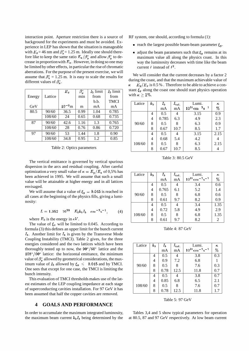
interaction point. Aperture restriction there is a source ofbackground for the experiments and must be avoided. Ex-perience in LEP has shown that the situation is manageablewith Ex= 46 nm and

x= 1.25 m. Ideally one should there-

fore like to keep the same ratio Ex=

xand allow

xto de-

crease in proportionwithEx. However, in doing so one maybe limited by other effects, in particular the rise of chromaticaberrations. For the purpose of the present exercise, we willassume that

x= 1.25 m. It is easy to scale the results for

different values of x

.

Ex x

Ib limit Ib limitEnergy Lattice min from from

b.b. TMCIGeV 109m m mA mA80.5 90/60 36.5 0.99 1.04 0.785

108/60 24 0.65 0.68 0.735

87 90/60 42.6 1.16 1.3 0.765108/60 28 0.76 0.86 0.720

97 90/60 53 1.44 1.8 0.90108/60 34.8 0.95 1.2 0.85

Table 2: Optics parameters

The vertical emittance is governed by vertical spuriousdispersion in the arcs and residual coupling. After carefuloptimization a very small value of = Ey=Ex of 0,5% hasbeen achieved in 1995. We will assume that such a smallvalue will be attainable at higher energy and in all latticesenvisaged.

We will assume that a value of y = 0:045 is reached inall cases at the beginning of the physics fills, giving a lumi-nosity:

L = 1:952 1023 E0kbIb cm

2s1; (4)

where E0 is the energy in eV .The value of x will be limited to 0.045. According to

formula (3) this defines an upper limit for the bunch currentIb. Another limit for Ib is given by the Transverse ModeCoupling Instability (TMCI). Table 2 gives, for the threeenergies considered and the two lattices which have beenthoroughly tested up to now, the 90=60 lattice and the108=60 lattice: the horizontal emittance, the minimumvalue of

xallowed by geometrical considerations, the max-

imum value of Ib allowed by x 0:045 and by TMCI.One sees that except for one case, the TMCI is limiting thebunch intensity.

This evaluation of TMCI thresholds makes use of the lat-est estimates of the LEP coupling impedance at each stageof superconducting cavities installation. For 97 GeV it hasbeen assumed that half the copper cavities are removed.

4 GOALS AND PERFORMANCE

In order to accumulate the maximum integrated luminosity,the maximum beam current kbIb being determined by the

RF system, one should, according to formula (1):

reach the largest possible beam-beam parameter y.

adjust the beam parameters such that y remains at itsmaximum value all along the physics coast. In thisway the luminosity decreases with time like the beamcurrent I instead of I2.

We will consider that the current decreases by a factor 2during the coast, and that the maximum achievable value of = Ey=Ex is 0.5 % . Therefore to be able to achieve a con-stant y along the coast one should start physics operationwith 2%.

Latice kb Ib Itot: Lumi. mA mA 1031cm2s1 %

4 0.5 4 3.15 0.94 0.785 6.3 4.9 2.3

90/60 8 0.5 8 6.3 0.98 0.67 10.7 8.5 1.74 0.5 4 3.15 2.154 0.68 5.4 4.2 4

108/60 8 0.5 8 6.3 2.158 0.67 10.7 8.5 4

Table 3: 80.5 GeV


4 0.5 4 3.4 0.64 0.765 6.1 5.2 1.4

90/60 8 0.5 8 6.8 0.68 0.61 9.7 8.2 0.94 0.5 4 3.4 1.354 0.72 5.8 4.9 2.9

108/60 8 0.5 8 6.8 1.358 0.61 9.7 8.2 2

Table 4: 87 GeV


4 0.5 4 3.8 0.34 0.9 7.2 6.8 1

90/60 8 0.5 8 7.6 0.38 0.78 12.5 11.8 0.74 0.5 4 3.8 0.74 0.85 6.8 6.5 2.1

108/60 8 0.5 8 7.6 0.78 0.78 12.5 11.8 1.7

Table 5: 97 GeV

Tables 3,4 and 5 show typical parameters for operationat 80.5, 87 and 97 GeV respectively. At low beam current

luminosity is maximum when the machine operates with 4bunches per beam. When the total beam current allowed bythe RF reaches 8 times the maximum current per bunch, wehave to increase the number of bunches, going to 6 and then8 bunches per beam. In this way, we can reach in all casesa beam-beam parameter y = 0.045 with reasonable valuesof the parameter , as can be deduced from the values givenin the tables.

Comparison of parameters for the two lattices envisagedshow the interest of the 108=60 lattice over the now wellproven 90=60 lattice: the value of which is necessaryto reach y = 0.045 is significantly larger in the first one.Using the 90=60 lattice one may be able to reach the sameinitial luminosity as with the 108=60 but certainly not tomaintain y = 0:045 all along the physics coast.

5 CONCLUSION

This analysis shows the interest of switching to the108=60 lattice as soon as possible during the first op-eration period of 1996. It holds the promise of a largerintegrated luminosity already at 80.5 GeV (and is somewhatless demanding in RF voltage to reach this crucial value ofthe energy ). Moreover learning how to master operationwith this lattice will be invaluable for the runs at higherenergy for which it becomes a necessity.

Bunch trains at high energy

Werner Herr, CERN, SL Division

Abstract

A possible scenario for operating LEP2 with bunch trainsis presented and the consequences of the higher energyon the parameters are discussed. In particular the numberof bunches and their spacing are optimized and possiblechanges to the layout of the separators in the interaction re-gions are mentioned. The effect of the energy sawtooth andpossible RF trips on the closure of the bunch train bumpsare discussed.

1 WHAT IS DIFFERENT AT LEP 2 ?

When LEP is operated at higher energies, i.e. above 80 GeVper beam, this implies certain differences to LEP at Z0 en-ergy. Such differences which have consequences for thebunch train scheme [1, 2, 3] are:

Smaller amplitudes of the separation bumps.

Higher bunch intensities in collision.

Fewer bunches per train (less than 4).

Energy sawtooth and RF asymmetries.

Some of these have immediate consequences for the bunchtrain scheme, e.g. smaller bumps or number of bunches pertrain, or have indirect effects such as the energy sawtoothor a very asymmetric RF structure caused by trips of cavityunits.

In the following these consequences are discussed andpossible counter measures are proposed. In particular a dif-ferent bunch spacing optimized for LEP 2 energies is pre-sented and possible modifications to the layout of the sep-aration scheme are discussed which now become possiblefor this new mode of operation.

The main assumptions for all calculations are that the LEPenergy is 87 GeV and the nominal layout for the RF cavi-ties and separators is used unless stated otherwise. Further Ihave assumed a low emittance lattice, i.e. a phase advanceof 1080 in the horizontal plane. Constraints for the bunchspacing come from the longitudinal feedback system, whichat the time of the calculations required a bunch spacing tobe a multiple of 6 RF [4].

2 WHAT ARE THE CONSEQUENCES ?

2.1 Smaller bump amplitudes

An immediate consequence of the higher energy is the re-duction of the bunch train separation bumps if the layout ofthe separators or their strengths is unchanged: the bump am-plitudesscale with the beam energy E as 1/E. As an example

9550. 9600. 9650. 9700. 9750. 9800. 9850. 9900. 9950.s (m)

E / p 0 c = 0 .Table name = TWISS

Vertical separation in even pitHP/UX version 8.14/7 21/11/95 17.09.38

0.0

.001

.002

.003

.004

.005

.006

.007

.008

.009

.010

Figure 1: Present vertical bunch train bump in even points. Solidline is for 45.6 GeV (OLD), dashed line for 87 GeV (NEW)

6150. 6250. 6350. 6450. 6550. 6650.s (m)


Vertical separation in odd pitHP/UX version 8.14/7 21/11/95 17.08.12

-.0150

-.0125

-.0100

-.0075

-.0050

-.0025

0.0

.0025

.0050

.0075

.0100

Figure 2: Present vertical bunch train bump in odd points. Solidline is for 45.6 GeV (OLD), dashed line for 87 GeV (NEW)

the separation bumps for 45.6 (OLD) and 87 GeV (NEW)for the even and odd pits are shown in Figs. 1 and 2. As aconsequence the separation of the two beams at the parasiticcollision points is also scaled by 1/E.

W N E O L D

2.2 Scaling of side effects

Both, reduced separation and bump amplitudes have conse-quences for all the side effects of the bunch train scheme.The most important are beam-beam effects, vertical dis-persion and coupling. Although the coupling due to thesolenoids is not a direct consequence of the bunch trainbumps and is not affected by their reduction, it is of crucialimportance for the performance and has a clear energy de-pendence.

Beam-beam tune shifts For sufficiently well separatedbeams the tune shift from a parasitic encounter can be ap-proximated by [5]:

/

N

y2 E/ N E

where N is the intensity per bunch and y the vertical sep-aration. Although the beam-beam tune shift scales as 1/E,its dependence on the separation is strong (/ 1/y2) and re-sults in a tune shift which increases with energy. Further wehope for higher bunch intensities and must therefore expecta larger parasitic tune shift. It is believed, that the strongerdamping at higher energies helps to allow for this highertune shift but it should be tried to minimize it as much aspossible. At LEP 2 we shall operate with fewer bunches,i.e. most likely with 2 bunches per train and a possible max-imum of 3 bunches per train, therefore we can optimize thebunch spacing to reduce the overall beam-beam tune shiftto an acceptable value. This is discussed in a later section.

Beam-beam induced orbit effects Another importanteffect of the parasitic beam-beam interactions is their effecton the closed orbit of the particles. The coherent beam-beamkick can change the closed orbit of the bunches [5, 6] andfurthermore, the closed orbit can be different for the indi-vidual bunches of a train. This beam-beam kick scales ap-proximately as:

y0

/

N

y E/ const:

Although the beam-beam kick increases proportional to thedecreasing bunch separation, the stiffer beam at the higherenergy makes this effect to be practically energy indepen-dent. It is again possible to minimize this effect furtherby a better (i.e. more separation) bunch spacing and fewerbunches. The case of two bunches per train is a special casewhere the two bunches of a train can be collided head-onat the interaction point by a proper adjustment of the sepa-rators at the collision points provided the bunch intensitiesare not too different. This is a consequence of the symme-try which causes the first bunch of a train to have the op-posite displacement as the last bunch of the correspondingtrain from the opposing beam [7]. This clearly favours anoperation of LEP with two bunches per train.

Vertical dispersion The residual vertical dispersion isa direct consequence of the vertical bump and therefore allrelevant parameters scale as the bump amplitudes, i.e. en-ergy:

Dmax

; Drms

; D

/ y /

1

E

All effects are therefore smaller at higher energies and a de-tailed estimate is given in another session of this workshop[8]. All associated side effects such as e.g. energy offset atcollision point, vertical emittance increase and excitation ofresonances are therefore reduced.

Coupling (solenoids) In 1995 the vertical emittancewas strongly affected by not fully compensated couplingfrom the solenoid magnets of the experiments [9]. Thiswas a source of limitation for the luminosity performancein 1995 with bunch trains. Since the fields of the solenoidsremain constant, their effect is expected to decrease with in-creasing energy / 1/E. Such a behaviour has already beenobserved in the run at 65 GeV in October 1995 where thevertical beam emittance was significantly reduced comparedto 45.6 GeV.

3 WHAT IS A GOOD BUNCH SPACING ?

With four bunches per train the choice of the bunch spac-ing was very limited and constraints from the RF equipmentled to a spacing of 87 RF [10]. For less than four bunchesper train the choice of the spacing is less limited and can toa much larger extend be chosen from beam dynamics con-siderations rather than technical boundary conditions. TheFigs. 3 and 4 show each one half of the bunch train bumpin the even (Fig. 3) and odd points (Fig. 4). The verticallines indicate the positions of the parasitic beam-beam en-counters assuming the old bunch spacing of 87 RF . It be-

Figure 3: Present vertical separation in even points, vertical linesindicate parasitic collision points (87 RF spacing)

comes clear from these figures that the bunch spacing couldnot be substantially changed for four bunches per train andhave good separation at all parasitic encounters. For fewerbunches per train, in particular if only two bunches are de-sired, it is possible to optimize the bunch spacing to min-

S e p o r o fi o fl w h h ‘ o c u ‘ v e r fi c o ‘ s e p o r o fi o n s c h e fl d e 1 P 4

BLMWCW S p O C 1 fl g 8 7 7 \ R F

6 4 7 77>

‘ 1 1 ‘ ‘ 1 7 1 6 0 7 1 4 0 7 1 2 0

\ N P U T C b

‘ 1 ‘ 7 1 0 0 7 8 0 7 5 0 7 4 0 7 2 0

d x s t o r w c e f r o r Y W ‘ p ( N d )

Figure 4: Present vertical separation in odd points, vertical linesindicate parasitic collision points (87 RF spacing)

imize the side effects. The constraints from the RF sys-tem (longitudinal feedback system requires a multiple of 6RF as the spacing) and the BOM system for closed orbitmeasurements have to be taken into account, however. Thecrossover of the two orbits near the odd points (Fig. 4) mustalso be avoided.

3.1 Two bunches in one train

It is possible to choose a spacing which minimizes the para-sitic beam-beam effects. This is illustrated in Fig. 5, wherethe integrated parasitic beam-beam tune shift for each bunchin a train is plotted for the horizontal and vertical planes. For

Figure 5: Integrated parasitic beam-beam tune shift as functionof bunch spacing, 2 bunches per train

the ideal bunch spacing the tune shifts assume a minimumfor both planes and all bunches of a train. For two bunchesper train there is no difference between the two bunches dueto the symmetry and they have the same tune shifts providedthe bunch intensities are not too different. The assumptionsfor this calculation are:

Optics with phase advance: 1080/600.

Energy is 87 GeV.

Full bump is on.

Intensity per bunch 0.5 mA, all bunches equal.

Emittances: x = 30 nm, y = 0.33 nm(corresponds to = 0.045 in collision).

The calculations were done with two independent programsand gave consistent results.

From Fig. 5 one can determine that a spacing between115 and 160 RF would be a good choice with a minimumaround 124 RF . Together with the constraints describedabove the recommended spacings1 are 126 and 132 RF .The absolute minimum in the horizontal beam-beam tuneshift visible in Fig. 5 corresponds to a bunch spacing wherethe parasitic collision point is at the maximum of the sepa-ration (cf. Fig. 3).

3.2 Three bunches in one train

Although three bunches per train are not the most desirablescenario for bunch trains at LEP2, a similar study has beenmade and the results are shown in Fig. 6. For three bunchesin a train not all bunches experience the same beam-beameffects, even for identical bunches. Two classes can be dis-tinguished (i.e. the head and tail bunch in one class and thecentral bunch in the second) and therefore the horizontal andvertical integrated tune shift is plotted for both classes. Thebest spacing corresponds now to a minimum of the enve-lope of all curves in the figure. The assumptions made are

Figure 6: Integrated parasitic beam-beam tune shift as functionof bunch spacing, 3 bunches per train

the same as in the two bunch case. With the above con-straints, this minimum can be identified around a spacing of126 RF , identical to one of the values found for two bunchoperation.

1In the discussion session the boundary condition for the longitudinalfeedback system was modified and the new recommended spacing alsocompatible with the BOM system is 118RF .

S e p o r o fi c h w‘wth \ c c u \ V e r t ' w c o ‘ s e p o r o fi o h s c h e m e H33

A 7

E 1 2 j B U h c h S p O C I h g 8 7 AR; v 7 .77

8 8 7 O 7 6 + a O L)

(D 4 >

O

, 4 ’ — _ _ 7 - — — » " " — ‘ \ \

6 7 % 7 8 7

7 1 2 7

7 ‘ w \ w w w \ w w w \ w \ w \ w \ w \ w

7 7 6 0 7 7 4 0 7 ’ 1 2 0 7 ’ 1 0 0 7 8 0 7 .60 7 4 0 7 2 0

d x s t O h c e f r o m \ p ( m ) \ N P U T o r b "

A N ) 9e (é Toto‘ t u h e s h ‘ w f t f o r d f f f e r e h t b u h c h SDOC‘H'Tg ( 2 b u h c h e s ) C $ 1 4 7 7C U) G) 7 C

3 1 2 7 7—:

E 7

‘ 1 0 7

8 7 o o

7 o o

o 6 7 o

7 0 ° . o

o 4 7

7 . -

2 7 0 .

7 o

O x x x x ‘ W O O 7 2 0 1 4 0 7 8 0 2 0 1 5 0 ' O

B u h c h s p o c x h g ( \ o r ’ h b d o i r f )

2 0

Toto‘ t u h e s h ‘ w f t f o r d f f f e r e h t b u h c h SDOC‘H'Tg ( 3 b u h c h e s )

7 . - 7 I

: o I

: I

7 - O

: I o o

: . -

7 I

j o 7 I 7 - a ' - - I 7 o 7 - . .

\ x \ x x \ x x \ x x \ x x \ x x \ x

1 2 1 7 5 1 2 0 1 2 4 1 2 8 1 3 2 1 3 5 B u h c h s p o c x h g ( \ o r ’ h

‘ 1 4 o b d o i r f )

3.3 Higher order modes

The higher order modes excited by the passing bunches inthe superconducting cavities have to be coupled out to avoidproblems. The contributions from the bunches in a train canadd together and the higher order mode losses can becometoo large to be acceptable. For certain values of the bunchspacing, the fields can add coherently or suppress each other.As an indication, Figs. 7 and 8 show the higher order modeenhancement factor [11] as a function of the bunch spac-ing for 2 and 3 bunches per train for the chosen values ofthe spacing of 126 and 132 RF . Both values are very

Figure 7: Higher order modes (HOM) enhancement factor for 2bunches spaced by 132 RF

Figure 8: Higher order modes (HOM) enhancement factor for 3bunches spaced by 126 RF

favourable for the higher order mode suppression, howeverthe assumed frequency may vary between individual cavi-ties and a precise prediction is difficult.

4 CAN WE IMPROVE THE LAYOUT OFTHE SEPARATION BUMPS ?

Having reduced the number of bunches it may now be pos-sible to find a modification to the bunch train separation lay-out which is more favourable, i.e. creates smaller residualvertical dispersion and possibly allows for a larger bump.

One particular aspect discussed earlier was the increase ofthe separation at the central collisionpoint in the even pointsduring injection and ramping. A second suggestion was toshorten the bumps in the odd points to avoid unnecessaryseparation and orbit excursions.

4.1 Possible new layout in odd pits

The inspection of Figs. 2 and 4 shows a large excursion ofthe separation bump in the odd points. From Fig. 4 it can beseen that this part of the bump was necessary to accommo-date the parasitic encounter of the fourth bunch. After thefourth bunch was abandoned, there is no need for this partof the bump and it was studied how this large distortion canbe avoided.

A possible new layout is shown in Fig. 9. For this schemethe two separators at the outer ends of the bump were movedtowards the interaction point near the crossing of the originalbump with the central closed orbit. The contribution from

6150. 6250. 6350. 6450. 6550. 6650.s (m)


Vertical separation in odd pitHP/UX version 8.14/7 21/11/95 17.06.08

-.0150

-.0125

-.0100

-.0075

-.0050

-.0025

0.0

.0025

.0050

.0075

.0100

Figure 9: Possible new layout for separation bump in odd points

the odd points to the residual dispersion is reduced by ap-proximately 35% and a possible advantage for the reliabilityof the separators is expected (less synchrotron radiation withsmaller bumps). However, with the present optics in the oddpoints, the required strengths on the separators in their newpositions is larger than what can be presently achieved. Fur-ther studies with a modified optics are required before a de-cision can be made to move the separators.

4.2 Possible new layout in even pits

Independent of the number of bunches and their spacing itis possible to increase the separation at the central collisionpoints if additional separators are installed. In the presentscheme the two bumps on each side are established with 6separators to ensure sufficient separation and a head on col-lision at the interaction point (Fig. 10). During injection,ramping and preparation a symmetric bump is superimposedwith a subset of four of these separators (dashed lines in Fig.10). These four separators therefore serve for both types ofbumps and are not independent: a larger injection bump im-plies a larger bunch train bump and vice versa. In particu-lar the maximum achievable amplitudes are limited by the

R e d u c fi o fl f a c t o r ( f o r H e ‘ d G d t T O m ) , 6 5 9 M H Z , G . D o m e

Q: i 5 7 S p o c i fl g : 1 3 2 . W O V S ‘ S fl g t h S 33 , 8 * B u m c h E S : 2 . ‘3 i C , o ,

L: 7 Q 7 j i

b 7 (D m 1

1 1 1 1 1 1 1 1 1 1 1 1 1 1 1 2 9 1 3 0 1 3 1 1 3 2 1 3 3 ' 1 3 4 . 1 3 5

B u fl c h d 1 s t o r ’ 1 c e 1 n A R ;

R e d u c fi o fl f a c t o r ( f o r H e ‘ d G d t T O m ) , 6 5 9 M H Z , G . D o m e

Q: 5 S p O C W W g : 1 2 6 . W O V S ‘ S fl g t h S 33 8 B u m c h E S : 3 . ‘3 C o

L: Q j

b (D m

ASA A A A «1 2 7 . . B u fl c h c h s t o m c e 1 n A R ;

2 9

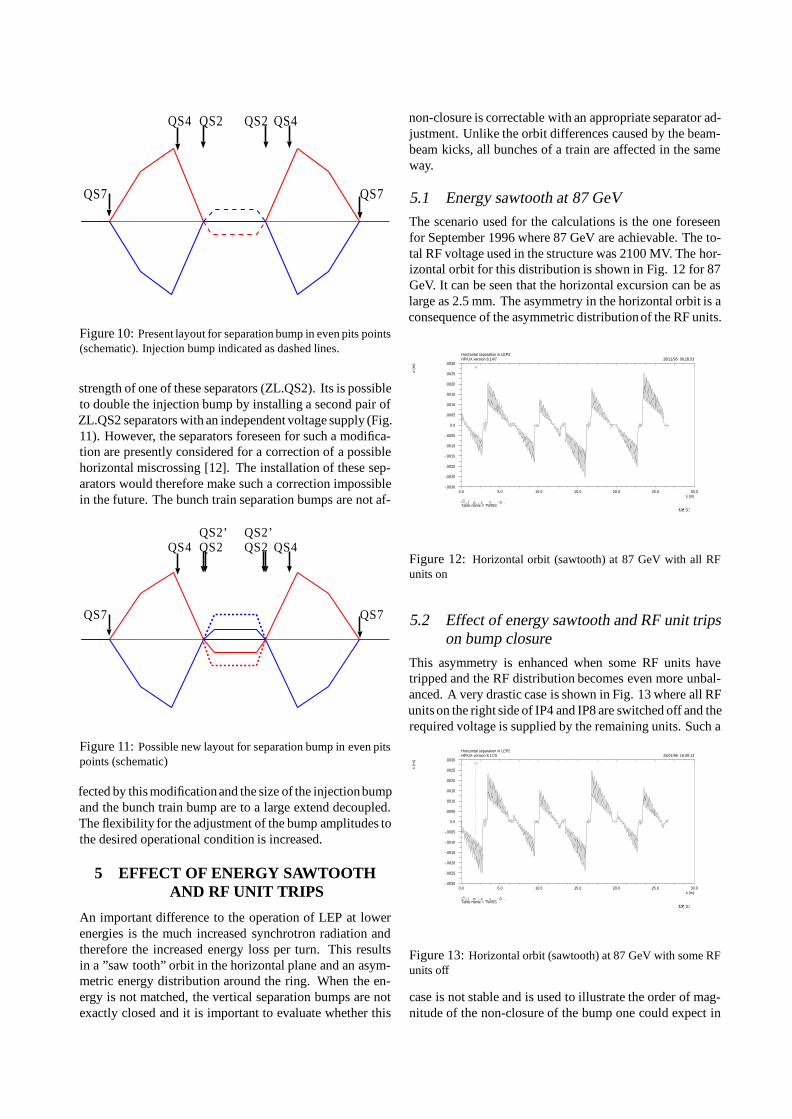
QS4 QS2

QS7 QS7

QS2 QS4

Figure 10: Present layout for separation bump in even pits points(schematic). Injection bump indicated as dashed lines.

strength of one of these separators (ZL.QS2). Its is possibleto double the injection bump by installing a second pair ofZL.QS2 separators with an independent voltage supply (Fig.11). However, the separators foreseen for such a modifica-tion are presently considered for a correction of a possiblehorizontal miscrossing [12]. The installation of these sep-arators would therefore make such a correction impossiblein the future. The bunch train separation bumps are not af-

QS4 QS2

QS7 QS7

QS2 QS4QS2’ QS2’

Figure 11: Possible new layout for separation bump in even pitspoints (schematic)

fected by this modificationand the size of the injectionbumpand the bunch train bump are to a large extend decoupled.The flexibility for the adjustment of the bump amplitudes tothe desired operational condition is increased.

5 EFFECT OF ENERGY SAWTOOTHAND RF UNIT TRIPS

An important difference to the operation of LEP at lowerenergies is the much increased synchrotron radiation andtherefore the increased energy loss per turn. This resultsin a ”saw tooth” orbit in the horizontal plane and an asym-metric energy distribution around the ring. When the en-ergy is not matched, the vertical separation bumps are notexactly closed and it is important to evaluate whether this

non-closure is correctable with an appropriate separator ad-justment. Unlike the orbit differences caused by the beam-beam kicks, all bunches of a train are affected in the sameway.

5.1 Energy sawtooth at 87 GeV

The scenario used for the calculations is the one foreseenfor September 1996 where 87 GeV are achievable. The to-tal RF voltage used in the structure was 2100 MV. The hor-izontal orbit for this distribution is shown in Fig. 12 for 87GeV. It can be seen that the horizontal excursion can be aslarge as 2.5 mm. The asymmetry in the horizontal orbit is aconsequence of the asymmetric distributionof the RF units.

0.0 5.0 10.0 15.0 20.0 25.0 30.0s (m)


∗10∗∗( 3)

Horizontal separation in LEP2HP/UX version 8.14/7 28/11/95 09.28.53

-.0030

-.0025

-.0020

-.0015

-.0010

-.0005

0.0

.0005

.0010

.0015

.0020

.0025

.0030

x (m

)

Figure 12: Horizontal orbit (sawtooth) at 87 GeV with all RFunits on

5.2 Effect of energy sawtooth and RF unit tripson bump closure

This asymmetry is enhanced when some RF units havetripped and the RF distribution becomes even more unbal-anced. A very drastic case is shown in Fig. 13 where all RFunits on the right side of IP4 and IP8 are switched off and therequired voltage is supplied by the remaining units. Such a

0.0 5.0 10.0 15.0 20.0 25.0 30.0s (m)


∗10∗∗( 3)

Horizontal separation in LEP2HP/UX version 8.17/3 25/01/96 16.09.13

-.0030

-.0025

-.0020

-.0015

-.0010

-.0005

0.0

.0005

.0010

.0015

.0020

.0025

.0030

x (m

)

Figure 13: Horizontal orbit (sawtooth) at 87 GeV with some RFunits off

case is not stable and is used to illustrate the order of mag-nitude of the non-closure of the bump one could expect in

the worst case. Another possible scenario with significanteffect on the bump closure is the loss of one cavity inside abunch train bump.

To evaluate this non-closure I have calculated the closedorbits in the presence of the bunch train bumps for the 4 fol-lowing RF scenarios:

RF scenarios:O: NO RF, i.e. no sawtoothA: All RF o.k., 87 GeV, 1978 MVB: All RF right of IP4 and IP8 offC: All RF inside a bump off (IP6)

Table 1: Vertical separation at interaction points for differ-ent RF configurations

SeparationCase: IP2 IP4 IP6 IP8

(m) (m) (m) (m)

0 0.0 0.0 0.0 0.0

A +0.1 +0.2 -0.3 -0.1

B -4.6 -4.9 -4.8 -5.6

C +2.8 +2.0 +1.6 +2.9

The results of this calculation are shown in Table 1. With-out any RF, i.e. without a sawtooth, the bump is obviouslycompletely closed and for the nominal RF structure (A) thenon-closure is in the order of a few tenth of a micron. Forthe very drastic cases (B + C) the non-closure can be as largeas 5 - 6 micron, still small enough to be easily correctedwith the separators. For more realistic scenarios for RF tripsand losses, the resulting separation of the two beams is evensmaller.

6 EXPERIENCE AND EXPECTATIONS

In 1995 LEP was run with bunch trains and some experi-ence was gained. The first attempts with four bunches pertrain proved the principle but did not allow to reach thehighest luminosities with good lifetimes. This was there-fore abandoned quickly and for the rest of the year LEP wasoperated with 4 trains of 3 bunches each. Towards the endof the run, the luminosities reached were equal to the bestachieved with the pretzel in 1994 although with higher cur-rents per beam: a best luminosity of 2.3 1031 cm2

s1

was achieved at 45.6 GeV with a total current around 7 - 8mA. This corresponds to a beam-beam tune shift of

0.03, significantly lower that in 1994. In a dedicated ma-chine experiment where LEP was operated only with twobunches per train a much higher beam-beam tune shift wasrestored ( = 0.042 - 0.045) and it is believed that the lower

tune shift was at least partiallycaused by the non-central col-lisions which are unavoidable in all cases with more thantwo bunches per train.

A single run with bunch trains at 68 GeV gave the recordluminosity of 3.1 - 3.4 10

31cm

2s1 with a tune shift

around 0.035. This was achieved with very little optimiza-tion and it is expected that equivalent tune shifts can bereached above 80 GeV. Running LEP 2 with 4 trains of 2bunches and hoping for a bunch intensity around 500 Aper bunch [13, 14], we expect a peak luminosity around 7.0 10

31cm

2s1 with a tune shift around 0.045.

7 ARE BUNCH TRAINS COMPATIBLEWITH OTHER SCHEMES ?

An important question is the compatibility of the bunchtrain scheme with alternative schemes such as 4 equidis-tant bunches per beam which would be the preferred sce-nario when the total intensity is limited by RF considera-tions. Such a scheme was indeed used for most of the LEPoperation at 65 and 68 GeV and its success indicate verylittle problems. To completely restore the old situation (i.e.before pretzel or bunch trains) the separators next to the evenpoints have to be re-conditioned (polarity change) and twoseparators in all odd pits have to be moved to their origi-nal positions. However, the successful running at 65 and 68GeV and in particular the small vertical emittances achievedindicate that such a modification is not necessary. In partic-ular since the effect of the bumps get smaller with increasingenergy.

Alternative schemes with 6 bunches per train (either with2 trains of 3 bunches or with unequally loaded trains) or 2trains of 2 bunches are proposed and will be studied sepa-rately. These schemes require no modification to the hard-ware. Some of these schemes have the nice feature that thebumps in the odd points become unnecessary and can beswitched off.

8 CONCLUSION

A study on possible modifications to the bunch train schemeto optimize it for LEP2 energies can be summarized as fol-lows:

Smaller amplitudes of the separation bumps are notavoidable and the side effects have to be evaluatedfor the new cases.

A modified bunch spacing can minimize the side effectsand a spacing of 118 RF is recommended forTwo bunches per train.

A modification to the separator layout is possible andcould improve the scheme but has implications of thepossibility for a steering of the horizontal miscrossing.

The effect of the energy sawtooth and RF asymmetrieson the bump closure was evaluated and found acceptable.

The bunch train scheme is compatible with an operationof four equidistant bunches and the desired luminositycan be achieved.

9 REFERENCES

[1] W. Herr; Bunch trains without a crossing angle;Proceedings of the fourth workshop on LEP performance,CERN SL/94-06 (1994) 323.

[2] C. Bovet et al; Final report of the 1994 bunch train studygroup CERN/94-95 (1994).

[3] W. Herr; Fist experience with Bunch trains ;Proceedings of the fifth workshop on LEP performance,CERN SL/95-0x (1995) xxx.

[4] E. Peschardt, Private communication.

[5] E. Keil; Side effects of beam-beam crossings in bunch trainswith head-on collisions CERN/94-76 (1994).

[6] W. Herr; Coherent dipole oscillations and orbit effects in-duced by long range beam-beam interactions in the LHC;CERN/SL/91-34 (AP) and LHC Note 165.

[7] W. Herr, 19th meeting of the Bunch Train Study Group, 1994.

[8] A. Verdier; Proceedings of this workshop.

[9] G. Roy; Proceedings of this workshop.

[10] W. Herr and E. Peschardt, 14th meeting of the Bunch TrainStudy Group, 1994.

[11] G. Dome, 10th meeting of the Bunch Train Study Group,1993.

[12] J. Jowett; Proceedings of this workshop.

[13] M. Meddahi; Proceedings of this workshop.

[14] D. Brandt; Proceedings of this workshop.

Dynamic Aperture for LEP 2 with Various Optics and Tunes

Francesco RuggieroSL Division

Abstract

We present latest simulation results and discuss dynamicaperture measurements performed in 1995 on various LEP 2optics. After recalling the protocol proposed for these mea-surements and the outcome of several related MD’s, wecompare the 90=60, the 108=60 and the 108=90 lat-tices and try to draw some conclusion for the performanceof LEP above 90 GeV.

1 INTRODUCTION

As discussed in Refs. [1], the measured aperture until theend of 1993 was nearly a half of the dynamic aperture pre-dicted by tracking and most likely due to a physical obstaclein the beam pipe. After November 1993 both Q-meter andsingle-kick measurements gave larger results and, in partic-ular, during an experiment at 45.6 GeV with damping andemittance wigglers turned on to simulate LEP 2 conditions,horizontal measurements using the injection kicker IK3Ewere in excellent agreement with MAD simulations for the90=60 squeezed optics g05p46. The measured horizon-tal aperture, corresponding to a kicker voltage of 6 kV for abunch current loss of 15%, was Ameas

x= 2:2103

pm to

be compared to AMADx

2:4103p

m with wigglers offand toAMAD

x 2:2103pm with wigglers on. It should

be mentioned that there is some discrepancy between thehorizontal emittance computed by MAD with wigglers onand the predictionsof the program WIGWAM, which makesuse of a better interpolation algorithm to evaluate radiationintegrals. Therefore MAD tracking results with wigglers onmay have to be taken with some care. Also the dynamicaperture for electrons and positrons, having different tunes,can be significantly different and a more systematic trackingcampaign is still required.

The single-kick method is now preferred over the methodbased on resonant excitation by the Q-metre, since it givesmore reproducible results. The analysis of these results isparticularly simple for a kicker voltage corresponding to abunch current loss of 50%, since in this case the dynamicaperture is given by the product of the kick angle by thesquare root of the betatron function at the kicker centre: it isindependent of the beam emittance, but an additional mea-surement by the 1000-turn technique is required in case ofsignificant beta-beating. Although a ‘pencil beam’ wouldbe better suited for a systematic exploration of the stabilityregion in the six-dimensional phase space, for practical rea-sons a ‘fat beam’ with emittance and damping wigglers at

their maximum level is recommended during dynamic aper-ture measurements. The reason is that usually the betatronphase of the kicks is never varied, since we always use thesame kicker, nor do we explore different momentum devia-tions of the bunch. Therefore the results obtained with wig-glers on are more conservative and reliable; they can be con-sidered as a survival test under conditions as close as possi-ble to LEP 2 conditions. Moreover, it is much easier to findthe kicker voltage corresponding to 50% current loss usinga fat beam rather than a pencil beam.

In the next two sections, we discuss the results of sev-eral related MD’s at 45.6 and at 65 GeV, respectively, wherethe dynamic aperture was measured or inferred for the108=60 and the 108=90 optics. Recent tracking resultsare presented in the last section, together with some perspec-tive for the performance of LEP above 90 GeV.

2 MEASUREMENTS AT 45.6 GEV

2.1 Dynamic aperture for the 108=60 optics

The measurements at 45.6 GeV on the 108=60 squeezedoptics e05r46 are discussed in Ref. [2]. After commission-ing the ramp and squeeze, the aperture was first measuredon a positron beam withQx = :276, Qy = :172, Q0

x= 3:8

and Q0

y= 2:9. The damping and emittance wigglers were

switched on at their maximum value and the measured emit-tances were "x = 20 nm, "y = 1 nm. For a voltage of 3 kVon the injection kicker IKP3, where x = 115m, the bunchcurrent was reduced by 50% (down to 28 A). Therefore,using the kicker calibration

x0 = 0:073mradkV

20 GeVE

;

the corresponding kick angle was x0 = 0:096 mrad andthe dynamic aperture for positronsAe

+

x= x0

px = 1:0

103p

m. This measured value is considerably smaller thanthe value obtained by tracking (without wigglers), namelyAMADx

= 1:65103p

m. It should be mentioned that thekicker timing was first set to an old ’92 value of 76:6s (rec-ommended in the standard protocol) and then to the correct’95 value of 64:7 s.

The positron beam was dumped and the aperture mea-surement was then repeated with electrons, having Qx =

:272, Qy = :159 and Q0

x= Q0

y= 3:8. Always with

wigglers on, this time the 50% bunch current loss occurredfor a voltage of 4:25 kV on the injection kicker IK3E (thebunch current being reduced from 120 down to 59A). The

corresponding kick angle was x0 = 0:136 mrad and thedynamic aperture for electrons Ae

x= 1:5 103

pm, in

fairly close agreement with tracking predictions.

2.2 Dynamic aperture for the 108=90 optics

The measurements at 45.6 GeV on the 108=90 optics arediscussed in Ref. [3]. An electron beam was kicked with thekicker IK3E, wherex = 126m, under different conditions:the resulting bunch current losses are reported in Fig. 1.

∆I

I

b

b

Vkick

[kV]

1

23

Figure 1: Relative bunch current loss vs. IK3E kicker volt-age under different conditions for the 108=90 optics at45.6 GeV (from Ref. [3]): 1)

y= 9 cm and no wig-

glers, 2) y= 9 cm and emittance plus damping wigglers

switched on, 3) y= 5 cm and no wigglers.

With wigglers switched off, the losses reached about 40%for a kicker voltage of 6:6 kV when

y= 9 cm and for

a kicker voltage of 6:2 kV when y= 5 cm. The corre-

sponding dynamic aperture was therefore Ameasx

= (2:22:4) 103

pm, in agreement at the 10% level with the

simulation value AMADx

= 2:5 103p

m. When damp-ing and emittance wigglers were switched on, with

y=

9 cm, significant losses appeared already at a kicker volt-age around 4:2 kV (see curve 2 in Fig. 1): the correspond-ing emittance and relative energy spread were "x = 24 nmand = 1:4 103, respectively. With wigglers on andy= 5 cm, the electron beam had a poor lifetime. This can

be partly explained by the limited energy acceptance of thesqueezed optics y05e46, of about 8 103, without sex-tupole re-cabling.

The observed losses for the 9 cm optics with wigglers off(see curve 1 in Fig. 1) show a local maximum for a kickervoltage around 4:6 kV. This has been tentatively associatedwith particle trapping in the third order resonance and sub-sequent escape to larger amplitudes due to quantum fluctu-ations [3]. However, accepting such a mechanism as a pos-sible explanation, the conclusion would be that the effectivehorizontal beam size is bigger than the nominal x and theusual 10 criterion adopted for the required dynamic aper-ture (at the beam–beam limit) should then be revised.

3 MEASUREMENTS AT 65 GEV

3.1 Increasing the beam emittance with the108

=60 optics

The measurements at 65 GeV on the 108=60 optics arediscussed in Ref. [4]: there was no time to kick the beam,but the dynamic aperture was estimated by increasing thehorizontal emittance using the wigglers and then changingthe damping partition numbers by a reduction of the RF fre-quency.

A single positron beam (with Ib 100 A) was firstramped to 45:6 GeV, then squeezed to

y= 5 cm and

ramped up to 65 GeV. The emittance measured at the BEUVwithout wigglers was "BEUV

x= 26 nm (while the nominal

value is "nomx

= 16 nm). With the emittance wigglers attheir maximum value (0:84 Tm), the measured emittancebecame "BEUV

x= 35 nm (while the value computed by

WIGWAM is "nomx

= 31 nm). At this point the RF fre-quency was reduced by 50 Hz, corresponding to a partitionnumber Jx = 0:76 and to an emittance "nom

x= 39 nm:

the measured emittance became "BEUVx

= 45 nm and thebeam lifetime was still very good. The vertical emittance re-mained around "BEUV

y= 0:5 nm. A further reduction of the

RF frequency by 50 Hz led to an emittance "BEUVx

= 62 nmaccompanied by poor beam lifetime. The (BEUV) emit-tance corresponding to a beam lifetime still around 40 hourswas estimated to 55 nm. Meanwhile the horizontal beta-tron function was measured by the 1000-turn technique andthe corresponding beta-beating at the BEUV was found tobe 14%.

Before discussing the conclusions that can be drawn fromthese measurements, it is worth mentioning that the hori-zontal emittance computed by MAD after the first 50 Hzreduction of RF frequency (with emittance wigglers on) is"MADx

= 43 nm instead of the WIGWAM value of 39 nm.The emittance computed by MAD after the second 50 Hzstep is "MAD

x= 69 nm, i.e., even larger than the value mea-

sured by the BEUV. This results correspond to a wigglerstrength adjusted in MAD such as to reproduce the nomi-nal WIGWAM emittance of 31 nm before the first frequencystep (however, the MAD value of Jx is 1:117 instead of 1).

The simulation results corresponding to MD conditionsafter the first 50 Hz reduction of RF frequency are shownin Figs. 2 and 3: the (10; 10; 7) beam ellipsoid refersto the nominal horizontal emittance "x = 39 nm and tothe measured vertical emittance "y = 0:5 nm. Thethree-dimensional plot in Fig. 2 indicates that the avail-able dynamic aperture is not sufficient to accommodate the(10; 10; 7) beam ellipsoid. This is even more clear fromthe two-dimensional cut shown in Fig. 3, where the beamellipse crosses the dynamic aperture in the (Ax; Ay) planeat Ax = 1:75 103

pm. Since the measured beam life-

time under these condition was still very good, one couldbe tempted to conclude that the simulation results must bewrong.

To be fair, let us trust the BEUV and assume that a beam

e05r46 65GeV MD condition Ex=39nm,Ey=0.5nm

0 0.5

1

1.5

2

10ˆ3Sqrt[Ax/m]

0

0.5

1

1.5

10ˆ3Sqrt[Ay/m]

0

0.2

0.4

0.6

0.8

Sqrt[At/%]

0 0.5

1

1.5

2

10ˆ3Sqrt[Ax/m]

Second surface is 10, 10, 7sigma ellipsoid

Figure 2: Dynamic aperture computed by MAD trackingfor the 108=60 optics e05r46 using MD conditions at65 GeV (VRF = 601 MV): three-dimensional plot andbeam ellipsoid corresponding to "x = 39 nm and "y =

0:5 nm. The x and y-axis denote normalised apertures (butthe symbolsAx andAy appearing in the figure labels are thesquare of those discussed in the text), while the vertical axiscan be identified with the relative energy deviationp=p inper cent.

0.5 1 1.5 2 10ˆ3Sqrt[Ax/m]

0.5

1

1.5

Sqrt[Ay/m]

Figure 3: Dynamic aperture in the (Ax; Ay) plane for theoptics e05r46 at 65 GeV: two-dimensional cut of picture inFig. 2 for p = 0. The dashed line corresponds to the(10; 10) beam ellipse with "x = 39 nm and "y = 0:5 nm.

with horizontal emittance "BEUVx

= 55 nm (i.e., almosttwice the nominal emittance at 91 GeV) had still a lifetimeof 40 hours. The point is, however, that a single beam has agood lifetime provided the available aperture is about 7 inall three planes (remember that the 10 criterion applies tobeams in collision) and this sets the following lower bound

on the measured horizontal dynamic aperture:

Ameasx

7q"BEUVx

' 1:65 103p

m:

Therefore the experiment with the 108=60 optics at65 GeV is compatible with MAD predictions.

3.2 Negative chromaticity tests

The LEP dynamic aperture scales roughly as the inverse ofthe sextupole strengths. A straightforward way to increasethe aperture is thus to weaken the chromaticity correction,working with transverse feedback and negative chromatici-ties. A first test with a low intensity beam (Ib = 20 A) us-ing the 108=60 squeezed optics at 65 GeV showed that,in the absence of feedback, the chromaticities could be low-ered down toQ0

x= 27 and Q0

y= 26 before having life-

time problems.With the 90=60 squeezed optics still at 65 GeV, two

beams were put in collision (at a beam-beam tune shiftbb 0:03) with the vertical feedback on (the horizontalfeedback did not work properly). Then the vertical chro-maticity was progressively lowered and for Q0

y= 7 the

beams were lost, probably because of an RF trip. We re-peated the test with two separated beams (Ib = 250 A),stopping the ramp at 45:6 GeV. The vertical chromaticitycould be reduced down to Q0

y= 15 with good lifetime,

but the beams were lost when the vertical feedback wasswitched off. During a final test with colliding beams at45:6 GeV (with a beam-beam tune shift bb 0:027) thechromaticity could be lowered down to Q0

y= 10 with

15 hours beam lifetime and vertical feedback on.

4 TRACKING RESULTS AT 91 GEV

At LEP 2 energies, the dynamic aperture of the 108=90

optics y05e46 (with odd tunes Qx = 103:268, Qx =

97:193) is mainly limited by Radiative Beta-SynchrotronCoupling [5]. As shown in Figs. 4 and 5 it is largely suffi-cient in the (Ax; Ay) plane, but is marginal in the (Ay; At =

p=p) plane.On the contrary, the main problem of the 108=60 op-

tics is the large cross-anharmonicity @Qy=@Ax, leading toan insufficient dynamic aperture in the (Ax; Ay) plane. Thisis shown in Fig. 6, where the aperture is normalised to thebeam dimensions at 90 GeV. This plot has been obtained bya modified version of MAD (available as rgomad in thedirectory hpariel:/users/rgo/rgomad) with newfeatures such as the automatic search and optimisation ofdynamic aperture.

A comparison of the dynamic aperture in the (Ax; Ay)

plane for different optics at 91 GeV, including also the effectof quadrupole misalignments and closed orbit, is shown inFig.7.

4.1 Perspectives

The dynamic aperture of low-emittance lattices has beenmeasured for the first time in 1995: the agreement with

0.5 1 1.5 2 2.5 3 10ˆ3Sqrt[Ax/m]

0.5

1

1.5

2

2.5

Sqrt[Ay/m]

Figure 4: Dynamic aperture in the (Ax; Ay) plane for the108=90 optics y05e46 at 91 GeV: VRF = 2464MV,Qs =

0:106 and (10; 10) beam ellipse corresponding to "y =

"x=2.

0.5 1 1.5 2 10ˆ3Sqrt[Ay/m]

0.5

1

1.5

Sqrt[At]/%

Figure 5: Dynamic aperture in the (Ay; At = p=p) planefor the 108=90 optics y05e46 at 91 GeV: same conditionsas in Fig. 4.

MAD predictions at 45:5GeV is at the 10% level, althoughwith the 108=60 lattice the aperture for positronswas con-siderably lower than that for electrons (possibly as a con-sequence of the kicker timing), while the 108=90 latticewith

y= 5 cm had poor lifetime with wigglers on. The

measurements at 65 GeV with the 108=60 lattice are com-patible with MAD predictions.

Above 90 GeV, the aperture is marginal for the 108=90

lattice and probably insufficient for 108=60 lattice. How-ever:

octupoles can be used to improve the aperture of the108=60 lattice and larger values ofQy are beneficialto that of the 90=60 lattice [3].

further improvements for all lattices (at the 10 15%level) are possible by means of a reliable transversefeedback system, working at negative chromaticitiesQ0 15.

new tools, namely post-processing of MAD tracking

0.0 2. 4. 6. 8. 10. 12. 14. 16. 18. 20.DYNAPX

Table name = SPECIAL

DYNAP WITH RADIATION DAMPING: DELTAP=0, Ey=Ex/2C05R46 (108/60): E=90 GeV, Vrf=2280 MV, Qs=0.1, Ex=31 nmHP/UX version 8.18/0 27/01/96 20.28.47

0.0

2.

4.

6.

8.

10.

12.

14.

16.

18.

20.

DY

NA

PY

Figure 6: Dynamic aperture in the (Ax; Ay) plane for the108=60 optics c05r46 at 90 GeV: the scale on the two axesis the number of beam ’s.

data and rgomad, are now available for more system-atic studies and for a pragmatic approach to the optimi-sation of the LEP dynamic aperture.

5 ACKNOWLEDGEMENTS

I would like to thank J. Jowett and S. Tredwell for theirtracking results, shown in Figs. 2, 3, 4 and 5.

6 REFERENCES

[1] F. Ruggiero, in Proceedings of the Fourth Workshop on LEPPerformance,Chamonix, 1994, Ed. J. Poole, CERN SL/94-06(DI), pp. 73–90 (1994) and Proceedingsof the Fifth Workshopon LEP Performance, Chamonix, 1995, Ed. J. Poole, CERNSL/95-08 (DI), pp. 164–166 (1995).

[2] D. Brandt, A. Hofmann, G. von Holtey, M. Lamont, M. Med-dahi, G. Roy, ‘Ramp, squeeze and collide with the 108=60

lattice for bunch train operation’, SL-MD Note 189 (1995).

[3] Y. Alexahin, ‘Improving the dynamic aperture of LEP2’,CERN SL-95-110 (AP) (1995).

[4] C. Arimatea, D. Brandt, A. Hofmann, G. von Holtey, R. Yung,M. Lamont, M. Meddahi, G. Morpurgo and F. Ruggiero, ‘Dy-namic aperture with the 108=60’, SL-MD Note 199 (1995).

[5] J. Jowett, in Proceedingsof the Fourth Workshopon LEP Per-formance, Chamonix, 1994, Ed. J. Poole, CERN SL/94-06(DI), pp. 47–71 (1994).

HX

Figure 7: Dynamic aperture in the (Ax; Ay) plane at 91 GeV for different optics (from Ref. [3]). The solid lines refer tothe perfect machines withVRF = 2500MV, the dotted lines are the 10 ellipses and the dashed lines represent the averageaperture over many seeds (dots) for quadrupole misalignments, closed orbit correction and VRF = 2237 MV.

muBD—ED muQD—BD

The Loss Monitors At High Energy

I. Reichel, RWTH Aachen, Aachen, Germany

Abstract

Results obtained with the loss monitors during the 1995 runwill be presented. During the high energy run problems dueto the increase of synchrotron radiation were encountered.At the moment it is still studied how this problems can besolved. The outcome of this studies will influence future ap-plications of the loss monitors. Possible applications liketail scans and fast detection of major beam losses will bediscussed.

1 THE LOSS MONITORS

1.1 How they work

During the ’95 run almost 100 beam loss monitors were in-stalled in LEP. Most of them are located at collimators closeto the experiments. In addition some collimators aroundIP5 are also equipped with loss monitors. These loss moni-tors are either close to COLH.IP5 (horizontal aperture limit)or COLV.QL9.R5 (dedicated vertical tail scan collimator).Those two collimators are also equipped with scintillators.

Usually the loss monitors are placed such that they aremainly sensitive to only one particle type and that the sen-sitivity is the same for both jaws of the collimator. Figure 1shows schematically the layout around COLH.IP5.

beam loss monitorsbox containing

vacuum chamber

collimator jaw

scintillator

Figure 1: The horizontal aperture limiter with its loss mon-itors and scintillators (schematic).

The loss monitors are the same as the ones used for HERAat DESY [1]. They consist of two PIN diodes sensitive toionising particles. A single high-energetic photon rarelyproduces a signal in both diodes.

Only a coincidence from both diodes is counted as a sig-nal. The background due to photons was low during the45 GeV runs because there were not many photons of suffi-cient energy to produce a signal even in a single diode. Withhigher energies the critical energy of the synchrotron radia-tion increases and therefore more photons create signals inthe diodes resulting in a high background for some moni-tors. Obviously the lead shielding, which has a thickness of5 mm, is not sufficient for higher energies. The optimumthickness of the shielding will be studied and implementedbefore the start-up.

1.2 Results from ’95

Due to technical problems the data from the loss monitorswere only logged during a few fills at 45 GeV and some at65/68 GeV. The data are still under study in order to find outabout the capabilities of the system [2].

Figure 2 shows data taken duringa whole physics fill froma loss monitor located close to the horizontal aperture limit(COLH.IP5).

0255075

100125150175200

0 500

020406080

100120140

249.18 260 270.82

fillin

g

adju

stph

ysic

s

time since beginning of fill (minutes)

time since beginning of fill (minutes)

phys

ics

adju

st

coun

trat

e (H

z)co

untr

ate

(Hz)

collimatorto physicssettings

off-momentum collimators in

R&

S

adju

st

Figure 2: Loss rate measured at the horizontal aperture lim-iter (COLH.IP5) during a physics fill.

The loss rate is given as count rate from the loss moni-tor. This monitor is very sensitive and a calibration usingthe BCT showed that at 45 GeV a count is obtained for ev-ery third to fourth particle lost at that collimator.

Before the collimators are set to physics settings the lossrate is very low. At the time when the collimators are movedfrom the ramp&squeeze settings to physics a rise in the lossrate can be seen. The sharp rise happens at the time, whenthe aperture limiters are moved in by about 2:5x.

Shortly afterwards the other collimators are also movedcloser to the beam. Some of the losses occur now at othercollimators like the off-momentum collimators leading toa decrease of the rate seen at the aperture limit COLH.IP5.The same behaviour was also observed with the scintillatorsinstalled close to that collimator.

During physics the loss rate tends to go down while thecurrent decreases. Jumps are usually due to orbit correc-tions. During the adjust phase at the end of the fill

y-

adjustments took place and there were some RF-trips whichcould explain the higher loss rate.

From the data we conclude that the loss monitors at thehorizontal aperture limit are not plagued by background dueto synchrotron radiation but measure real particle losses atthat collimator. Some other loss monitors however suffer se-vere background from synchrotron radiation. This is mainlythe case for those located close to the collimators at theQS15 quadrupoles which are located inside the bending re-gion. An example of one of those monitors is shown inFig. 3.

0

2

4

6

8

7400 7600 7800 8000

0

2

4

6

8

7410 7420 7430 7440

R&

S

fillin

g

phys

ics

adju

st

adju

st

time (minutes)

time (minutes)

coun

trat

e (k

Hz)

coun

trat

e (k

Hz)

1st ramp squeeze

2nd ramp

Figure 3: Loss rates measured at COLH.QS15.L2 during aphysics fill at 45 GeV. The measured rate is mainly back-ground due to synchrotron radiation.

The measured loss rate increases strongly during the endof the first ramp and during the whole second ramp. Thisleads us to the conclusion that the signal is dominated bysynchrotron radiation.

1.3 Loss Monitors and Scintillators

Unfortunately for most of the ’95 run there was no onlinedisplay of the loss monitors available in the control room.At the aperture limits there are also scintillators installed forwhich an online display exists which was used frequentlyby the operators to adjust the working point and as an earlywarning for changing conditions. We therefore think that anonline display of the loss monitors is useful.

The scintillators were also used in tail scans to check theloss monitors for saturation effects1. It could be shown thatboth instruments are linear over several orders of magnitudewith respect to each other (see Fig. 4).

10

1

10

10

10

-1

2

3

1 10 10 10 102 3 4

external jaw

internal jaw

counts/s in PIN diode

scin

tilla

tor

(bac

kgro

und

subt

ract

ed)

Figure 4: Comparison of the loss rates measured with ascintillator and a loss monitor installed close to each other(see Fig. 1). The data of a few tail scans during one fill wasused for this plot.

At the lower end of the curve both instruments are at thelimit of their resolution. The resolution of the loss monitorscan be improved by using longer integration times (at themoment 1s). At the upper end the curve for measurementsusing the external jaw of the collimator tends to be slightlyhigher than those done with the internal jaw. We assume thatthis is due to insufficient alignment of the loss monitor. Asthe surface of this instrument is only 1 cm2 it is very sen-sitive to even small displacements with respect to the beamwhich we noticed already during earlier measurements 2.

1The loss monitors are already corrected for known saturation effects2The difference in sensitivity for both jaws was about a factor 40.

Checking the position of the loss monitor showed that it was misplacedby about 4 cm with respect to the centre of the vacuum chamber.

#:

77

77

7

:7

7,

,

7:

77

,,

7

:7

7,

,

7:

77

,,

7

:7

7,

,

W

. W

W oouvooo

m m

a

wn

“.

..

-

o m

H

“n

et-u

. “

- a

H

‘ n

o“

o

n

o ‘

\ \ \ H H ‘

0 O

O -

O

0

\ \ \ H H ‘

2 TAIL SCANS

2.1 How They Are Done

During the ’95 run the main application of the loss mon-itors were the tail scans. These are done in the followingway: One jaw of a collimator is moved closer to the beamin steps of typically 0.1 mm (at the collimators used for thescans x 1 mm and y 0:3 mm respectively). At eachstep the loss rate is measured with the loss monitors installedclose to the collimator. In addition also the rate from thescintillators is measured but due to a lower update rate weobtain data from the scintillatoronly for every third to fourthstep.

Usually scans are done with both jaws to become inde-pendent of the orbit position. The plots shown here fromtail scans are corrected for orbit deviations, i.e. the collima-tor position is transformed such that it corresponds to thedistance between the centre of the beam and the collimatorjaw.

During MDs the loss monitors were calibrated againstlifetime as calculated from beam currents measured usingthe BCT. This calibration allows to convert the measuredcount rates to loss rates in units of inverse beam lifetimes.To compare the results with simulations we would also needan absolute measurement of the emittance.

2.2 Horizontal Plane

A result for horizontal tails scans is given in Fig. 5.

collimator position (mm)

inve

rse

lifet

ime

(1/h

)

10

10

10

10

10

10

-6

-5

-4

-3

-2

-1

1

0 2 4 6 8 10 12 14 16 18 20

1

10

10

10

10

10

10

2

3

4

5

6

150µA bunch current

500µA bunch current

Figure 5: Horizontal tail scans with different bunch cur-rents. Both measurements were done during physics, i.e.with colliding beams at 65 GeV.

In all horizontal tail scans (at 45 GeV and 65/68 GeV)we observed tails corresponding to lifetimes between 100and 1000 hours. The far tails did not vary much with ma-chine parameters (e.g. chromaticity). In addition they are

about the same for separated and colliding beams. We as-sume that they are mainly produced by scattering of particleswith thermal photons. This will soon be studied in simula-tions.

At around 6 the collimator reaches the Gaussian coreof the beam. This leads to a very steep rise of the loss rate.With a bunch current of 500 A we observed a rise far-ther away from the beam. As the measured emittance wasroughly the same as for the lower bunch current and the lossrate rises somewhat slower we tend to think that this is notyet the Gaussian core 3.

This measurement showed us that even with such highbunch currents there is still plenty of space in the machine.In the horizontal plane we could close the collimator by 30%and in the vertical plane by 40 % without affecting the life-time. These results might also be useful for an estimate ofthe dynamic aperture.

During the 45 GeV run systematic measurements weredone to study the influence of various machine parameterson the tails. It was also tried to check how well the collima-tors protect each other. Figure 6 shows the result of one ofthese measurements.


inve

rse

lifet

ime

(1/h

)

10

10

10

10

10

10

10

-7

-6

-5

-4

-3

-2

-1

1

10

0 2 4 6 8 10 12 14 16 18

10-1

1

10

102

103

104

105

106

107

COLH.QS1B.L4 at 8σ

1σ = 1mm

Figure 6: Effect of an (artificial) aperture limit atCOLH.QS1B.L4 on the tails measured at COLH.IP5. Thelower curve is the one measured after COLH.QS1B.L4was moved in to 8 , the upper curve was measured before.

We first did a scan with all collimators at ramp&squeezesettings (upper curve). Then COLH.QS1B.L4 was closedto 8 and the tail scan was repeated (lower curve). Far out(> 12) the tails did not change from which we concludethat these particles are not in an equilibrium state but ratherlocally ’produced’.

3The measurement was done parasitically at the beginning of a physicsfill with excellent luminosity and the collimator scan was stopped early toexclude any risk of beam loss.

M'l

Between 8 and 12 the measured loss rate was reducedby up to a factor five due to the artificial aperture limit.

2.3 Vertical Plane

At 45 GeV systematic studies of the vertical tails havebeen done [3]. At higher energies the measurements wereplagued by synchrotron radiation. A typical result for thepositron beam from the 65 GeV-run is shown in Fig. 7. Theelectron monitor at the same collimator had very high back-ground for both jaws due to synchrotron radiation from thearc.


inve

rse

lifet

ime

(1/h

)

-6

-5

-4

-3

-2

-1

10

10

10

10

10

10

1

0 2 4 6 8 10 12 14 16 18 20

1

10

10

10

10

10

10

2

3

4

5

6

0 20 40 60 80 100 120 140collimator position (σ, approx.)

lifet

ime

(h)

aperture limit

top jaw

bottom jaw

Figure 7: Vertical tail scan showing the problems due tosynchrotron radiation for the positron monitor.

In contrary to the horizontal plane we can not use the aper-ture limit in the vertical plane for tail scans because it is lo-cated in the arcs (close to QD30) where it receives too highsynchrotron radiation rates. Instead we use the dedicatedcollimator COLV.QL9.R5. The setting of the aperture limitin physics corresponds to about 7.4 mm at this collimatorand is indicated in the plot by a dashed line.

If we use the bottom jaw of the collimator the results seemto be sensible. However if we use the top jaw, we measuredfar too high loss rates which were of the order of 10 hoursalready when the collimator was still in the ’shadow’ of theaperture limit. Only when reaching the Gaussian core wemeasured sensible loss rates, but lifetimes of that order ofmagnitude can be measured better directly from the beamcurrents. Measurements showed that synchrotron radiationcoming from the bunch train bump in QL5 hits the uppercollimator jaw and is scattered back into the loss monitorand produces the high background rates [4].

At the moment we are still working on a cure for that. Wewill probably put a thicker lead shielding around the lossmonitors and/or move them to a slightly different position

with respect to the collimator in order to avoid the problemswith the synchrotron radiation.

2.4 Results

The tail scans are a useful tool to study the outer parts of thebeam profile. They are fast (a scan takes less than 2 minutes)and can be done during physics without problems. There-fore they can be used to check e.g. if there are problems withthe aperture.

The software makes it possible to close the collimatorsstepwise while observing the loss rate at each step and hav-ing an ’emergency button’ which moves the collimator backto the pre-scan position at once [5].

3 CONCLUSION

During the ’95 run the loss monitors were mainly used forthe tail scans. As the scintillators were frequently used inoperation we hope to achieve the same with the loss moni-tors as soon as an online display becomes available.

It is not possible right now to be sure of further applica-tions because until now we have not much experience withthe loss monitors and an off-line analysis of the logged fillsis still under study.

At the moment some loss monitors are still plagued bysynchrotron radiation but we hope to solve that problem be-fore the start-up.

4 REFERENCES

[1] W. Bialowons et al.: Electron Beam Loss Monitors for HERA,Proceedingsof the Fourth European Particle AcceleratorCon-ference, London 1994.

[2] Thesestudies are done by Thomas Spickermannwho also pro-vided Figures 2 and 3.

[3] H. Burkhardt: Beam Lifetime and Beam-Beam Tails inLEP, Proceedings of the Seventh Advanced Beam Dynam-ics Workshop on Beam-Beam Issues for Multibunch, High-Luminosity Circular Colliders, Dubna 1995, to be published.

[4] The layout of the bunch train bump in the odd pits can be seenin Fig. 2 of W. Herr: Bunch Train Bumps at High Energy,these proceedings. In our case (IP5) the polarity is reversed.

[5] The software for the tail scans was written by Jean-JacquesGras. He also modified it according to our requests.

f

N

. . . . . . . ' 9 ‘ . . 0 .0 .

o ., . . . . . . . o o q . o ¢ c o .

SUMMARY OF SESSION 3B – HIGH ENERGY: PERFORMANCE ISSUES

E. Keil, CERN, Geneva, Switzerland

Abstract

This summary covers the talks given in Session 3B of theSixth LEP Performance Workshop, which was devoted toperformance issues at high energy. The four talks describedthe loss monitors, the bunch train schemes for LEP, the dy-namic aperture, and performance predictions.

1 INTRODUCTION

In the session, four talks were presented which I shall sum-marize in the followingorder: I. Reichel [1]: ‘The loss mon-itors at high energy’ in Chapter 2. W. Herr [2]: ‘Bunch trainsat high energy’ in Chapter 3. F. Ruggiero [3]: ‘Estimate ofthe dynamic aperture with various optics and tunes’ in Chap-ter 4 J. Gareyte [4]: ‘Parameters and performance’ in Chap-ter 5. Chapter 6 contains my own conclusions.

2 LOSS MONITORS

The loss monitors are shown in Fig. 1 of [1]. They consistof PIN diodes, installed on top of the vacuum chamber nextto the collimators. They are supposed to be sensitive to e+

and e, and insensitive to photons. However, it turned outthat they are still too sensitive to vertical synchrotron radi-ation fans caused by the bunch train bumps. Modificationsare foreseen. Once the loss monitors are calibrated againsta beam lifetime measurement with the beam current trans-former, they allow measuring very small loss rates, corre-sponding to lifetimes 103 h, and observing beam tails faroutside the Gaussian beam distribution.

The loss monitors have a fast response, and can be usedduring colliding-beam physics runs. It would be interestingto use them to measure the aperture needed by the beams andto relate these observations to the dynamic aperture stud-ies described in Chapter 4 in future. In an experiment at65 GeV, with the two beams colliding at bunch currentsI = 0:5 mA, the apertures of the horizontal aperture colli-mator and of the vertical collimator equipped for tail scanscould be reduced by 30 % without a lifetime reduction.

3 BUNCH TRAINS

The bunch train scheme with head-on collisions in the evenpits and vertical separation at the parasitic collision pointthere and in the odd pits was proposed by Herr at Chamonix1994 [5]. First tests with one bunch train in each beam, col-liding in Pits 2 and 6, were carried out in November 1994and described by Herr at Chamonix 1995 [6]. The complete

scheme with head-on collisions in all four even pits wasready by the time of the 1995 LEP startup. It allowed a proofof principle for bunch trains with up to 4 bunches/train, ata bunch spacing s = 87RF, determined by parameters ofthe longitudinal feedback system.

3.1 Experience in 1995

The most important parameters achieved in 1995 are listedin Tab. 1. Trains with k = 4 bunches were quickly aban-doned. The figures for trains with k = 3 bunches are typ-ical for LEP operation. The figures for trains with k = 2bunches at 45.6 GeV were obtained in a single machine de-velopment session, those at 68 GeV in the only high-energyphysics run with bunch trains in November 1995.

Table 1: Achieved bunch train parameters in 1995: numberof bunches in a train k, total current of both beams I, lumi-nosityL, vertical beam-beam tune shift parameter y . Notethat 1 (bs)1 = 1030cm2s1.

E/GeV k I/mA L/(bs)1 y45.6 445.6 3 7–8 23 0.0345.6 2 3.5 16 0.042–0.04568.0 2 5.5 31 0.036

3.2 What is different in LEP2?

The limits on the total RF power and on the total beam cur-rent in LEP2, discussed in Chapter 5, and the discouragingexperience with trains of four bunches make it unlikely thatLEP2 will ever be operated with more than three bunches.Hence, it becomes possible to reconsider the bunch spac-ing. If the LEP2 insertions and the electro-static separatorexcitations are held constant when the LEP beam energy isincreased from 45.6 GeV to about 90 GeV, the bump am-plitudes y / 1=E become smaller, and the separated beam-beam tune shifts / I=Ey2 become larger. The orbitaleffects, caused by the higher synchrotron radiation losses inLEP2 and usually called energy sawtooth [7], may also haveconsequences on the bunch trains.

3.3 Trains with k = 2 Bunches

The separated horizontal beam-beam tune shift x, summedover all parasitic collision points, has a broad minimum

around 126 : : :132 RF, while the separated vertical beam-beam tune shift y also summed over all parasitic collisionpoints, is a slowly rising function in this range. Duringdiscussions, it was found that it should be possible to op-erate the longitudinal feedback system at a bunch spacings = 118 RF [8], and that this spacing is also favourablefor the wide-band beam position monitors close to the evenpits [9]. Should it after all be possible to tune the longitudi-nal feedback cavities to exactly three times the frequency ofthe RF accelerating system, then the bunch spacing will be-come s = 120 RF [8]. Provided that the buch current dif-ferences are small, and given the symmetries of LEP2, trainswith two bunches have the unique feature that head-on col-lisions can be achieved for both bunches by vertical vernieradjustment, and that therefore the CM energy error vanishes.The upper limit on the inequality of the bunch currents stillhas to be calculated. The smaller ratio = y=x, achievedin the high-energy runs in November 1995 and suggestedin the performance estimates in Chapter 5, makes setting-up and vernier adjustments more difficult.

3.4 Trains with k = 3 Bunches

For trains with three bunches, there are two sums for theseparated beam-beam tune shifts, one for the head and tailbunches, and another one for the central bunch. They bothhave a broad minimum at a bunch spacing s = 126 RF,which is sufficiently close to the recommended figure(s) fortrains of two bunches, s = 118 RF or s = 120 RF notto propose yet another value. Contrary to trains with twobunches, vertical offsets at the IP y=y 1=2 and the con-comitant CM energy errors are unavoidable. Both effectsare enhanced by the smaller ratio = y=x, assumed inChapter 5.

3.5 Effects of Energy Sawtooth

The energy sawtooth describes the fact that the electrons andpositrons gain energy in the RF systems and lose energy inthe arcs in opposite patterns. If the electrons and positronshave opposite energy offsets of e+ and e in the pits, theelectrostatic bumps are not closed any longer, and verticalorbit differences between electrons and positrons propagatearound LEP, in particular to the head-on collision points inthe even pits. This effect was present when LEP was op-erated with two RF stations at 45.6 GeV, and the energiesof electrons and positrons were different in the odd pits.InLEP2, it is enhanced by the higher energy and RF unit trips,and reduced by the fact that there are four RF stations insteadof two. The offsets found in computer simulation with thenominal LEP2 RF system are of the order of a fraction ofm, those found with one or two RF units tripped are abouta m, both must be corrected by vernier adjustments.

3.6 Open Questions

The vertical electro-static separator bumps are longer thanneeded for trains of two bunches. In the odd pits, they ex-

tend over about 3/4 instead of the 1/4 vertical betatron wave-lengths needed, and contribute unnecessarily to the verticaldispersion and emittance. Thus the question arises whethershorter bumps are feasible. We know already that shorten-ing the bumps in the odd pits by only moving electro-staticseparators and leaving the optical configuration unchangedwould require doubling the deflection in the separators.

The bunch current which was injected into LEP has al-ways been smaller with two beams and bunch trains thanwith single beams [10]. Thus the question arises whetherthis difference can be reduced by a larger separation at22 GeV. Horizontal offsets between the two beams at theeven pits of the order of a few tens of m have been ob-served with bunch trains in 1995. Thus the questions comesup whether horizontal vernier adjustment is needed. Severalseparators are available which could be used either for in-creasing the vertical separation at injection or for cancellingthe horizontal separation at collision energy in the even pits,but not for both.

4 DYNAMIC APERTURE

4.1 Measured vs. Computed Dynamic Aperture

The dynamic aperture is the volume in 6D phase space –centred around the origin – where the beam particles per-form stable betatron and synchrotron oscillations indefi-nitely. The first question which arises in this context is: Howlarge is the dynamic aperture? In LEP, it can be observedby kicking the beam and observing the surviving fractionas a function of the kick amplitude. It can also be com-puted by tracking programs. Recent developments in track-ing programs include an automated search for the dynamicaperture, and clever post-processing of the tracking results.Agreement within10 % between observation and simulationat 45 GeV was reported, giving some degree of confidencethat the dynamic aperture in LEP2 can be predicted reliably.

4.2 Dynamic Aperture vs. Emittance

The second question which arises in the context of the dy-namic aperture is: How much dynamic aperture is neededfor colliding beams with given nominal emittances or rmsradii? The traditional requirements are: 10x, 10y, and7e. These multiplying factors can be experimentally ver-ified by increasing x and/or y and/or e, or by reducingeither the dynamic aperture or the physical aperture, and ob-serving the lifetime. The beam radii x, y, and e are notas independent as might be desirable for the measurements.Reducing the dynamic aperture is not easy. However, re-ducing the physical aperture with collimators in straightfor-ward, and has already been done, as described in Chapter 2.

4.3 Dynamic Aperture vs. Lattice at 91 GeV

The simulated dynamic aperture of the 108/60 configura-tion, shown in Fig. 6 of [3], is not large enough for op-eration at 91 GeV. The limit is reached when the verti-

cal tune Qy reaches the nearest lower integer due to thecross-anharmonicity @Qy=@Ax. The cut of the dynamicaperture of the 108/90 configuration demonstrates that thedynamic apertuure is marginal for operation at 91 GeV.The limit is reached when the vertical tune Qy reaches thenearest lower integer due to the second-order chromaticity@2Q=@(dp=p)2. Note that this configuration has odd tuneswhich may not be desirable because of coherent beam-beammodes [11]. In the comparison between the 108/60 and108/90configurations it should be borne in mind that the for-mer has x = 1:25 m in the even pits, while the latter hasx = 2:5 m there, and that configurations with higher xtend to have a larger dynamic aperture. The dynamic aper-ture of the 90/60 configuration, presented at Chamonix in1994 and shown in Fig. 8.14 of [12], is “just barely adequatein the horizontal plane” at 90 GeV.

4.4 Outlook for Dynamic Aperture

Starting with the bad things, we do not have a LEP2 latticewith enough dynamic aperture for operation much beyond87 GeV. Although we do understand that different mecha-nisms limit the dynamic aperture in different configurations,we do not have specific methods to fight these mechanisms.We do not have dedicated dynamic aperture kickers and as-sociated software which allow quick measurements of thedynamic aperture routinely. Among the better things aregood agreement between observed and simulated dynamicapertures, fair confidence in the criteria on the relation be-tween the beam radii and the dynamic aperture, and recentprogress in the simulation tools. Since the dynamic aper-ture is limited by effects due to the sextupoles needed forthe chromaticity correction, we should study how quicklythe dynamic aperture increases with y > 5 cm.

5 PARAMETERS AND PERFORMANCE

5.1 Lessons from 1995

We have learned in 1995 that much larger single beam cur-rents than those used in routine operation are possible. Abunch current of 1 mA was reached by operating LEP witha synchrotron tuneQs = 0:17. For our performance predic-tions, we use predicted thresholds for the transverse modecoupling instability, which are based on the superconduct-ing cavity installation schedule and Qs = 0:15 [13]. Wehave the choice between two lattices, the 90/60 configura-tion used in 1995 operation and the 108/60 configuration de-velopped in MD. We assume that the bunch trains are opti-mised for two bunches, as discussed in Chapter 3. We alsoexploit fully the small ratio = y=x 0:5% achieved.

5.2 RF Limitations

For the performance estimates to be given below, it is as-sumed that the RF power/klystron increases from 0.8 MWduringcommissioning to 1 MW after cleaning of the system,

and that it should still be possible to operate LEP at the en-ergy foreseen with 2 klystrons OFF. These assumptions leadto the parameters in Tab. 2.

Table 2: RF Limitations for LEP2

Date Jul 96 Oct 96 Jul 98Energy/GeV 80.5 87 97Power/MW 13 16 32Total current/mA 10.7 9.7 12.5

Further, we assume that the total beam current in bothbeams starts at 4 mA, increases to 8 mA when enough ex-perience has been gained running at the lower current, andfinally reached the figures shown in Tab. 2.

5.3 Arguments

The following arguments enter in the performance esti-mates. We assume horizontal emittances x = 42:6 nm forthe 90/60 configuration and x = 28 nm for the 108/60 con-figuration at 87 GeV. At this stage we do not invoke chang-ing the horizontal and longitudinal emittance by changingthe horizontal and longitudinal damping partition numbersJx and Je 3 Jx. We adjust the bunch current I suchthat we reach the limit given by the transverse mode cou-pling instability at 22 GeV [13] and the RF limitations de-scribed above, whichever is smaller. We finally adjust theratio of the beam emittances = y=xto reach y = 0:045,trying to stay in the range 0:5 % 2 : : :4 %. We ob-serve that the lower limit on imposes an upper limit onx at the head-on collision points, and that the synchrotronradiation background from the QS0-QS1 doublet imposesan upper limit on the horizontal beam divergence x=x atthe head-on collision points, and hence a lower limit on xthere. We propose to reduce during the coast by a factorof about two in order to keep the beams at the beam-beamlimit y = 0:045, and thus to achieve L / I down to halfthe bunch current at the beginning of the coast.

5.4 Performance at 87 GeV

Using the above arguments, we estimate the LEP perfor-mance at 80.5, 87 and 98 GeV. Tab. 3 shows the results at87 GeV as an example.

5.5 Discussion of Performance

If we start operating LEP at 87 GeV with the 90/60 config-uration while the limit of 4 mA on the total current is in ef-fect, it is best to use four bunches, and we get the peak lu-minosity shown in the first line of Tab. 3. Once the limiton the total current is lifted, we can go to the bunch cur-rent limit imposed by the transverse mode coupling insta-bility, and achieve the peak luminosity shown in the secondline. At larger beam currents, we switch from four to eightbunches, and for 8 mA achieve the peak luminosity shown

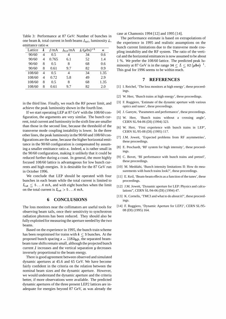
Table 3: Performance at 87 GeV: Number of bunches inone beam k, total current in both beams Itot, luminosityL,emittance ratio

Lattice k I/mA Itot/mA L/(bs)1

90/60 4 0.5 4 34 0.690/60 4 0.765 6.1 52 1.490/60 8 0.5 8 68 0.690/60 8 0.61 9.7 82 0.9

108/60 4 0.5 4 34 1.35108/60 4 0.72 5.8 49 2.9108/60 8 0.5 8 68 1.35108/60 8 0.61 9.7 82 2.0

in the third line. Finally, we reach the RF power limit, andachieve the peak luminosity shown in the fourth line.

If we start operating LEP at 87 GeV with the 108/60 con-figuration, the arguments are very similar. The bunch cur-rent, total current and luminosity in the sixth line are smallerthan those in the second line, because the threshold of thetransverse mode coupling instability is lower. In the threeother lines, the peak luminosity in the 90/60 and 108/60con-figurations are the same, because the higher horizontal emit-tance in the 90/60 configuration is compensated by assum-ing a smaller emittance ratio . Indeed, is rather small inthe 90/60 configuration, making it unlikely that it could bereduced further during a coast. In general, the more highlyfocused 108/60 lattice is advantageous for low bunch cur-rents and high energies. It is desirable for the 87 GeV runin October 1996.

We conclude that LEP should be operated with fourbunches in each beam while the total current is limited toItot 5 : : :6 mA, and with eight bunches when the limiton the total current is Itot > 5 : : :6 mA.

6 CONCLUSIONS

The loss monitors near the collimators are useful tools forobserving beam tails, once their sensitivity to synchrotronradiation photons has been reduced. They should also befully exploited for measuring the aperture needed by the twobeams.

Based on the experience in 1995, the bunch train schemehas been reoptimised for trains with k 3 bunches. At theproposed bunch spacing s = 118RF, the separated beam-beam tune shifts remain small, although the projected bunchcurrent I increases and the vertical separation y decreasesinversely proportional to the beam energy.

There is good agreement between observed and simulateddynamic apertures at 45.6 and 65 GeV. We have becomefairly confident in the criteria on the relation between thenominal beam sizes and the dynamic aperture. However,we would understand the dynamic aperture and the criteriabetter, if more observations were available. The predicteddynamic apertures of the three present LEP2 lattices are in-adequate for energies beyond 87 GeV, as was already the

case at Chamonix 1994 [12] and 1995 [14].The performance estimate is based on extrapolations of

the experience in 1995 and realistic assumptions on thebunch current limitations due to the transverse mode cou-pling instability and the RF system. The ratio of the verti-cal and the horizontal emittances is now assumed to be about1 %. We prefer the 108/60 lattice. The predicted peak lu-minosity at 87 GeV is in the range 34 L 82 (bs)1.This goal for 1996 seems to be within reach.

7 REFERENCES

[1] I. Reichel, ‘The loss monitors at high energy’, these proceed-ings.

[2] W. Herr, ‘Bunch trains at high energy’, these proceedings.

[3] F. Ruggiero, ‘Estimate of the dynamic aperture with variousoptics and tunes’, these proceedings.

[4] J. Gareyte, ‘Parameters and performance’, these proceedings.

[5] W. Herr, ‘Bunch trains without a crossing angle’,CERN SL/94-06 (DI) (1994) 323.

[6] W. Herr, ‘First experience with bunch trains in LEP’,CERN SL/95-08 (DI) (1995) 117.

[7] J.M. Jowett, ‘Expected problems from RF asymmetries’,these proceedings.

[8] E. Peschardt, ‘RF system for high intensity’, these proceed-ings.

[9] C. Bovet, ‘BI performance with bunch trains and pretzel’,these proceedings.

[10] M. Meddahi, ‘Bunch intensity limitations II: How do mea-surements with bunch trains look?’, these proceedings.

[11] E. Keil, ‘Beam-beam effects as a function of the tunes’, theseproceedings.

[12] J.M. Jowett, ‘Dynamic aperture for LEP: Physics and calcu-lations”, CERN SL/94-06 (DI) (1994) 47.

[13] K. Cornelis, ‘TMCI and what to do about it?’, these proceed-ings.

[14] F. Ruggiero, ‘Dynamic Aperture for LEP2’, CERN SL/95-08 (DI) (1995) 164.

How Many Bunches Would we Like to Run with for LEP2 ?

Albert Hofmann, SL Division

Abstract

To find the optimum number of bunches the luminosity iscalculated for the three lattices having the phase advances900/600, 1080/600 and 1080/900 per cell and for the twobeam energies 80.5 and 87 GeV foreseen for 1996. Asboundary condition a maximum beam-beam tune shift of0.045 and a minimum emittance ratio of 0.5% were as-sumed. Furthermore the bunch current limitation by thetransverse mode coupling instability TMCI was taken intoaccount. There is also a limit of the total current imposedby the RF-system which must be considered. For each casea bunch number of 4 or 8 per beam has been tried to seewhich results in the highest luminosity. Within the errors ofthis estimate the 8 bunch operation with the pretzel and thebunch train scheme give the same luminosity. At 80.5 GeV4 bunch operation has a slight advantage if the total currentis limited to 4 mA. However, for the other cases 8 bunchesare better and the 1080-lattices are easier to operate. At 87GeV 8 bunches and high horizontal phase advance are ad-vantageous.

1 INTRODUCTION

The beam-beam tune shifts for flat beams are given by

x =reIb

x

2ef0 2x=

reIb

2ef0 Ex

; y =reIb

y

2ef0 xy;

(1)with Ib = bunch current, is the lattice function and therms beam size in the interaction point and Ex the horizontalemittance. We assume that these tune shifts are limited to0.045

x 0:045 ; y 0:045: (2)

The luminosity is given by

L =kI2

b

4e2f0xy; (3)

with k being the number of bunches per beam.To save space in the tables we give here the luminos-

ity in engineering units: am2s1. The unit ‘am’ is Atto-meter, 1 am =1018m. The luminosity unit is therefore:

1 am2s1 = 1036m2s1 = 1032cm2s1.

2 LATTICE PROPERTIES AND BUNCHCURRENT LIMITATIONS

We consider the three lattices with horizontal/vertical phaseadvances 900/600, 1080/600 and 1080/900 per cell and cal-

Lattice 900/600 1080/600 1080/900

Ex nm 36.5 23.7 23.7Ib (x=0:045) mA 1.04 0.68 0.68hyiarc m 88 88 71

Table 1: Emittance Ex, Ib reaching x=0.045 and averagey in the arcs at E = 80.5 GeV

Lattice 900/600 1080/600 1080/900

Ex nm 42.6 27.7 27.7Ib (x=0:045) mA 1.54 0.86 0.86hyiarc m 88 88 71

Table 2: Emittance Ex, Ib reaching x=0.045 and averagey in the arcs at E = 87 GeV

culate the emittances, the bunch currents for which the hor-izontal beam-beam tune shift reaches the imposed limit andthe average vertical beta function in the arcs. This is donefor the energies E = 80.5 GeV to be used in summer 1996and E = 87 GeV foreseen for the later part of this year. Theresults are shown in tables 1 and 2. Each of the different op-tics has two possible values for the horizontal beta functionin the interaction point

x= 1.25 m and

x= 2.5 m. For the

vertical beta function at the interaction points we take in allcases

y= 0.05 m.

To obtain the maximum bunch current we refer to the cal-culation of the TMCI threshold carried out in a previous pre-sentation [1]. The single beam TMCI threshold was esti-mated to be Ib = 0.87 mA for the 900/600-lattice, withQs =0.15 and for the impedance of all the components which arein LEP in summer 1996. Later in the year there will be mores.c. cavities installed but the effect on the impedance is notvery large. It will be neglected and the same impedance isused for the whole year as far as this investigation is con-cerned. With two beams this current will be reduced byabout 12% due to the 4 separated encounters leading to Ib= 0.77 mA [2]. For 4 trains of 2 bunches there are 12 sep-arated encounters. Assuming the reduction is proportionalto the square root of the number of encounters we get a re-duction of about 20% giving Ib = 0.7 mA. The pretzel hassome of the encounters at finite dispersion which gives alarger reduction of about 22% giving Ib =0.68 mA. The dif-ference in Ib between bunch train and pretzel for 8 bunchesis much smaller than the uncertainty of this estimation andwe take the same value for both. We will later also con-sider 12 bunches having 20 separated encounters for which

Lattice 900/600 1080/600 1080/900

Ib (44) mA 0.77 0.71 0.75Ib (88) mA 0.70 0.63 0.68Ib (1212) mA 0.64 0.59 0.62

Table 3: Single bunch current limitation by TMCI

we get with this method a reduction of 27% leading to Ib= 0.64 mA. The lattices with a horizontal phase advance of1080 have a smaller momentum compaction which leads toa lower threshold [3] Furthermore, the 1080/600-lattice hasa larger vertical beta function in the arcs which enhances theeffect of the shielded bellows. Taking both effects into ac-count we find a reduction of 7% compared to the 900/600-optics. The 1080/900-lattice has a smaller beta function inthe arcs giving a corresponding reduction of 2%. Consider-ing all these factors we obtain the values for the bunch cur-rents listed in table 3.

3 CALCULATIONS OF LUMINOSITY

To calculate the luminosity for the boundary conditions out-lined in the previous section we compare first the bunch cur-rent determined by the total current given by the RF-systemwith the one given by the TMCI and take the smaller one.Then we check if the horizontal tune shift does not exceedthe imposed limit of 0.045. Now we reduce the coupling un-til the vertical beam-beam is reached or until we reach theminimum emittance ratio of 0.005. This procedure is car-ried out for all lattices and bunch numbers.

4 RESULTS

We start with the lower energy E = 80,5 GeV and take alimit of the total current given by the RF-system of 4 mAwhich can probably be increased soon to 8 mA and later to13 mA. The results are listed in tables 4 and 5. The causeof the bunch current limitation is indicated either by theallowed total current, the horizontal beam-beam tune shiftlimit or the TMCI threshold. The value of the couplingwhich reaches the vertical beam-beam limit is calculatedand printed in bold if it is larger than the assumed limit of0.005. The luminosity is given in am2s1=1032cm2s1,(1 am = 1 Atto-meter =1018m). Its largest value is printedin bold.

For the higher energy of 87 GeV to be used in 1996 thelattice parameters are listed in table 2. The total current is as-sumed to reach 8 mA after some initial operation at a lowercurrent. The values of bunch current, coupling and luminos-ity are listed in table 6.

Operating LEP with 12 bunches per beam could be inter-esting in cases of 8 bunches for which the current per bunchis limited by the beam-beam tune shift or the TMCI thresh-old and not by the total current. The most likely candidateis the last line listed in table 5. We investigate this case for8 and 12 bunches and present it in table 7. The bunch cur-rent is now limited by the total current of 13 mA to Ib = 0.54

Optics Ib LmA lim. am2s1

x

(m) 1.25 2.5 1.25 2.590=60

4 4 0.5 tot. 0.009 0.005 0.31 0.308 8 0.25 tot. 0.002 0.001 0.21 0.15108=60

4 4 0.5 tot. 0.022 0.011 0.31 0.318 8 0.25 tot. 0.005 0.003 0.31 0.23108=90

4 4 0.5 tot. 0.022 0.011 0.31 0.318 8 0.25 tot. 0.005 0.003 0.31 0.23

Table 4: Currents, coupling and luminosity for E = 80.5GeV, Itot 4 mA


x

(m) 1.25 2.5 1.25 2.590=60

4 4 0.77 TMC 0.022 0.011 0.48 0.488 8 0.70 TMC 0.018 0.009 0.88 0.15108=60

4 4 0.68 x 0.040 0.020 0.43 0.438 8 0.63 TMC 0.035 0.017 0.79 0.79108=90

4 4 0.68 x 0.040 0.020 0.43 0.438 8 0.68 TMC 0.040 0.020 0.86 0.86

Table 5: Currents, coupling and luminosity for E = 80.5GeV, Itot 13 mA

mA. This results in a smaller luminosity.

5 DISCUSSION

The tables 4 to 7 give the conditions at the beginning of arun. As the bunch current decays one tries to reduce the cou-pling in order to minimize the reduction of luminosity. Sincethe minimum coupling was assumed to be = 0.005 it will


x

(m) 1.25 2.5 1.25 2.590=60

4 4 0.77 TMC 0.016 0.008 0.52 0.528 8 0.5 tot. 0.007 0.004 0.68 0.51108=60

4 4 0.71 TMC 0.032 0.016 0.48 0.488 8 0.5 tot. 0.016 0.008 0.68 0.68108=90

4 4 0.75 TMC 0.036 0.018 0.51 0.518 8 0.5 tot. 0.016 0.008 0.68 0.68

Table 6: Currents, coupling and luminosity forE = 87 GeV,Itot 8 mA


x

(m) 1.25 2.5 1.25 2.5108=90

8 8 0.68 TMC 0.040 0.020 0.86 0.8612 12 0.54 tot. 0.026 0.013 0.68 0.68

Table 7: Currents, coupling and luminosity for E = 80.5GeV, Itot 13 mA using 8 or 12 bunches per beam

be difficult to follow the mentioned procedure if the initialcoupling is already small. For this reason one prefers caseswhich have a somewhat larger initial coupling.

Starting with the lower energy of 80.5 GeV and 4 mA to-tal current we find that one operates best with a 1080-latticeand 4 bunches. As the total current limitation is increased 8bunch operation gives a better performance. The 900=600-optics gives the best performance followed closely by the108

0=900-lattice and then by the 1080=600-lattice. The dif-ference in luminosities between the different optics is lessthan 12%.

At the higher energy of 87 GeV and a total current of 8mA operation with 4 bunches gives less luminosity. For 8bunch operation the 900=600-lattice has low coupling andgives less luminosity for the larger

x. Both 108

0-latticesgive the same performance since the bunch current is deter-mined by the total current.

Operation with 12 bunches per beam gives less luminos-ity in the energy range considered. There might be casesfor which 6 bunches could give slightly better performance.Although it is possible to use this bunch number it involvesanother operation mode which has to be optimized. This ishardly worthwhile for the marginal luminosity gain.

The 1080=900-lattice gives as much or more luminositythan the 108

0=600-optics due to the difference in averagevertical beta function in the arcs. However, a gain is onlyachieved in the cases being not dominated by the total cur-rent limitation. For the choice between these lattices otherarguments like dynamic aperture and polarization are prob-ably more important.

6 REFERENCES

[1] A. Hofmann’ “Bunch Intensity Limitations I: What do we Ex-pect ?”; Contribution 206 to this workshop.

[2] K. Cornelis, The Influence of the Beam-beam Interaction onHead-tail Modes”; Proceedings of the Fourth Workshop onLEP Performance, ed. J. Poole, CERN SL/94-06 p. 185.

[3] D. Brandt and A. Hofmann’ “ Does a highQs Raise the Max-imum Intensity to be Accumulated in LEP ?”; Proceedingsof the Fourth Workshop on LEP Performance, ed. J. Poole,CERN SL/94-06, p. 149.

Review of bunch train running (1995) and Pretzel running (1994)


ABSTRACT

The general performance of the machine is summarisedfor each of the two modes of running. Operationalefficiencies and major difficulties are compared. Areasfor possible improvement are presented.

1 INTRODUCTIONDuring most of 1994, LEP was operated with an 8-bunchper beam Pretzel scheme, accumulating over 60 pb-1 ofluminosity at the Z0 peak. Through 1995, differentvariants of bunch train schemes were used, with bestresults during a prolonged period with 4 trains of 3bunches per beam, when an intergrated luminosity ofabout 40 pb-1 was accumulated during a scan in energyaround the Z0 resonance. These running periods arecompared. The high energy run at the end of 1995 is alsomentioned.

2 COMPARISON OF STATISTICSA comparison of the overall statistics between the yearsis given in Table 1. The data from 1995 have been splitinto three. Firstly the runs at high energies, for so-calledLEP1.4, are separated out. Secondly, data taken duringthe energy scan are also separated out since during thistime operational conditions were not changed and so thisprovides fair comparison with 1994 running. Finally thewhole of LEP1 running during 1995 is shown forcompleteness. From these statistics there are good, badand other things to note.

PHASE 1994 1995Lep1

1995scan

1995Lep1.4

access 2 2 1 5

down-time 10 14 13 14

failed fills 11 18 12 21

filling 15 13 14 21

physics 59 47 50 39

calibration 3 6 10 0

% dump/lost 77/23 71/29 74/26 33/67

200 fill 150 fill 100 fill 50 fill

Table 1: Basic statistics for 1994 and 1995

2.1 The Good ...

The good thing to note is that during LEP1 running in1995 the filling time for physics coasts was actuallybetter than in 1994, and that for 50% higher totalcurrent. While good, this is not exactly a fair comparisonbecause in 1995 several new things were introduced thathelped the injection rate. Notable among these were thefollowing;• use of polarisation wigglers• use of transverse feedback• use of synchrotron injection• introduction of the Beam Current Equaliser• better optimisation of the SPSAs discussed in detail in session 2, filling the machine inany mode is not a limitation to performance.

2.2 The Bad ...

The first bad thing to note for 1995 is that trains of 4 arevery hard to handle. This is reflected in the much longertime spent on filling that did not result in a physics coastduring the first phase of LEP1 running, when trains of 4were tried and eventually abandoned. While filling wasalready difficult, selective bunches of the trains were lostduring the ramp or the squeeze, almost certainly due totune and chromaticity differences between bunchlets.This often resulted in the surviving beams beingdumped, and the fills that did make it into physics wereoften with very uneven bunch currents and physicsconditions were with the problems that this brings.

The second bad thing for 1995 was the down-time,which was consistently significantly higher than in 1994.A look at the fault statistics shows that this increase isdominated by LEP RF, so no surprises there given all theactivity with superconducting units. The other bigcontribution to 1995 down-time came from breakdownsin the SPS (extraction septum feedthrough). In otherwords bunch train running did not contribute to thisincease.

The third bad thing for 1995 was the number of fills lost,compared to 1994. A look at these statistics shows thatthe increase is dominated by ZL sparks, which for themost part were due to problems encountered with bunchtrain separators in point 3. Coasts lost due to RF tripsalso showed a notable rise, which again is no surprisewith so many new and untried elements in the machine.

2.3 ... and the Future

While not directly related to bunch trains or Pretzel, thefigures for LEP 1.4 show that everything was worseduring this period, with an overall efficiency for physicsdown to 39% and a big jump in the number of fills lost,almost exclusively due to RF trips.

3 COMPARISON OF PERFORMANCEIn both schemes, the single bunch current accumulatedoperationally was around 350 uA, giving a total currentof 5.6mA for Pretzel and 8mA for bunch trains of 3bunchlets. The beam-beam tune shifts routinely acheivedfor Pretzel and trains of 3 were .04 and .025respectively. This resulted in similar luminosityperformance with the two schemes.

However there is strong evidence to suggest that theabove numbers are not hard limits. Using transversefeedback, synchrotron injection, a higher Qs and morePretzel separation, bunches of 450uA were accumulatedduring machine development on the Pretzel scheme.There is even room for further improvement here, sincethe polarisation wigglers were not used in thisexperiment.

With 2 bunches per train, and with a modified bunchspacing and lower bunch trains bumps, a beam-beamtune shift of .042 was acheived during bunch train MD.Also with 2 bunches per train, bunch currents of over400uA were accumulated during a different experiment.

Putting these together would suggest that Pretzel and abunch train scheme based on 2 bunches per train arecomparable in terms of bunch current, tune shift andhence luminoisty.

4 DOMINANT PROBLEMS

4.1 Pretzel

With high luminosity Pretzel running, the machineperformance was very sensitive to the vertical orbit anddrifts thereof, and to the settings of the vertical separatorvernier settings. Differences between e+ and e- added tothe difficulties. Perhaps as a result of these things, beamblow-up and backgrounds were a frequent problem inphysics. These could be controlled by fine adjustment ofthe chromaticites in physics, and would have been easierto handle had the transverse feedback been available.

4.2 Bunch trains with 3 bunchlets

During bunch train running, a high rate of sparks on thevertical separators in points 3 and 4 meant that thesehad to be run with asymmetric voltages on the positiveand negative plates.

Again differences between e+ and e- made life difficult,although now these differences appear also betweenbunches of the same beam. These effects disappear withtrains of two.

The bunch train bumps gave radiation problems atinjection, particularly in ALEPH and DELPHI, wherecollimators had to be used to project the experimentsduring filling. In physics the bunch train bumps alsogave background difficulties, this time predominatly inL3 and OPAL. Reduction of the electrostatic bumptogether with the superposition of magnetic bumps, toensure that the amplitude at the QS4 remained under10mm, went a long way to solving this problem.

5 CONCLUSIONTrains of 4 proved very difficult operationally. Withtrains of 3 the overall statistics were very close to thoseof 1994, with the machine spending 60% of thescheduled physics time either in stable physicsconditions or in energy calibration. The only realdifference was an increase in the number of fills lost,with a significant contribution from sparking of thebunch train separators.

While overall performance in terms of luminosty wasvery similar with the two schemes, the operational limitscame from different sources. In Pretzel the total currentwas limited to a little over 5mA, but a high beam-beamtune shift ensured luminosities of over 2 1031 cm-2 s-1 . Inbunch trains with 3 bunches per train it proved difficultto increase the tune shift above .025, but the currentfrom the extra bunches provided luminositiescomparable with the Pretzel scheme. Removal of thetune shift limit with bunch trains appears only possiblewith 2 bunches per train, thereby losing the potential ofgoing to very high total currents with this scheme.

The comment was also made that operations found themachine very sensitive with the Pretzel scheme, but thatthis was probably connected to the high performancesachieved for the circulating current. It remains to be seenif the bunch train scheme is more stable when regularhigh peformance levels are seen.

The bunch train bumps gave rise to radiation problems atinjection and background problems in physics. Botheffects however could be minimised, and the latter willin any case improve as we move to higher energies.

SEPARATOR PERFORMANCE WITH BUNCH TRAINS AND PRETZEL

Brennan Goddard, CERN, Geneva, Switzerland

ABSTRACT

The introduction of Bunch Trains required someimportant changes to the separation system in LEP, withthe addition of the eight ZL7 separators, the‘decommissioning’ of the ZX and ZXT separators, andnew methods of control. An important operationaldifference with Bunch Trains was the need to power allseparators during physics; previously with Pretzel the ZLseparators in the even IP were only powered withrelatively low voltages for vernier adjustment. Theoperational consequences of the move from Pretzel toBunch Trains are discussed in regard to hardwareinstallations, overall system flexibility, controls, vernieradjustments and beam induced sparks. In addition, theeffects of the 70 GeV run are briefly reviewed, andradiation related observations with Bunch Trains aredescribed.

1 INTRODUCTIONReliable operation of the separator system is vital for

the realisation of maximum luminosity in LEP. A singlespark in a separator can result in the total loss of thestored beams, either through severe orbit distortions or abeam-dump triggered by radiation in the experimentaldetectors. The presence of beam in the machine has beenshown to increase the number of sparks observed,depending on many parameters including the machineoperating conditions and the position of the separators.

The LEP separator system has undergone severaltransformations since the start of LEP operation in 1989.The first major alteration was completed for operation in1993, with the installation of a set of eight horizontalseparators for the Pretzel scheme [1, 2]. For 1995,another major change was made, with the installation of

eight new vertical separators for Bunch Trains [3, 4].The two schemes, Pretzel and Bunch Trains, involvedthe use of different sets of separators, different modes ofoperation, and different machine conditions. Theschemes can be compared in terms of the performance ofthe separator system as a whole.

This paper outlines the separator hardwarerequirements for the two schemes, Pretzel and BunchTrains, and examines the performance of the overallseparator system in each case. The performance issuesconsidered are system flexibility, controls, hardwarecomplexity and reliability, and beam-induced breakdown(sparking). The performance of the Bunch Train systemduring the “high-energy” run at the end of 1995 isdiscussed, and progress made toward the development ofimproved insulating materials is briefly outlined.

2 SEPARATOR SYSTEMS

2.1 The Pretzel Separation System

The Pretzel separation system was added on to theexisting vertical separation layout [5], and wasessentially different at all levels: hardware, low-levelelectronics, controls and application programs. ThePretzel separators were further subdivided into twoseparate sets: the eight horizontal (ZX) separators usedto create the Pretzel separation in mid-arc, and the twoZXT (trim) separators which were necessary to correctthe horizontal miscrossings at the experimental (even)interaction points (IP).

With Pretzel, a total of 42 separators were needed, 24of them operated at high voltage during physics. Thelayout of the Pretzel separators in an even IP and an oddIP is shown schematically in figure 1.

EVENIP

ZL4 ZL2 ZL2 ZL4ZX11 ZX11

ZL4 ZL1ZL1 ZL4ZXT

(IP1 &IP5)ODD

IP

Figure 1. Schematic diagram of the separator layout with Pretzel, for the case of an even IP and an odd IP.

E9

ea

EVENIP

ZL4 ZL2 ZL2 ZL4

ZL8 ZL1ZL1 ZL8

ODDIP

ZL7 ZL7

Figure 2. Schematic diagram of the separator layout with Bunch Trains, for the case of an even IP and an odd IP.

2.2 The Bunch Train Separation System

The conversion of the separation system to allowoperation with Bunch Trains involved the addition ofeight new vertical (ZL) separators, and the displacementof eight existing ZL. The original system, designed foruse with the simple ‘4×4’ scheme, became part of thesystem for Bunch Trains, whilst the use of the ZX andZXT separators was discontinued. The opportunity wastaken to rationalise the separator electronics and controlsinto a more homogeneous structure.

As a result of the operating constraints inherent toBunch Trains, a significant amount of separatorequipment became redundant; for example theSynchronous Discharge switch could no longer be usedto collide the beams, and the dedicated vertical verniersystem could not be used to optimise the collisions.

With Bunch Trains, a total of 40 separators areneeded, and all 40 operate at high voltage duringphysics. The layout of the Bunch Train separators in aneven IP and an odd IP is shown schematically in figure2.

3 FLEXIBILITYThe operation of the separation system is also subject

to several constraints which are imposed by the hardwareconfiguration or performance. These constraints differedbetween the Pretzel and Bunch Train systems, and aregiven below. In addition, the advantages in flexibilityinherent in the equipment for each scheme are discussed.

3.1 Constraints with Pretzel

• In the installed positions near the arcs, the ZXseparators would only work with positive highvoltage. If negative high voltage was used,unacceptably high spark rates were observed withbeam [6].

• The ZX separators were unipolar, i.e. had only onehigh voltage electrode. Since this high voltage had tobe positive, the field direction was fixed, and no

reversal was possible without breaking the vacuumand physically rotating the separator.

• The ZX separators were recuperated from the SPS‘PPbar’ project, and were very different in design tothe ZL separators, Consequently, spares and reserveswere more difficult to assure.

3.2 Constraints with Bunch Trains

• No horizontal vernier adjustment is possible tocorrect any horizontal miscrossings at the IP. Recentmeasurements and analyses suggest that thesemiscrossings were present at 45 GeV energies, butnot at 65 - 68 GeV [7].

• Because the separators remain powered in physics,the beams have to be brought into collision bydischarging the separator electrodes through theinternal resistance of the high voltage generator. Thecircuit has a time constant of the order of 30 seconds,so that several minutes are required to reduce thevoltages to the required levels.

• The repeated sparking in the ZL8 separators in IP3meant that these units had to be operated with thenegative voltage switched off. This limited the BunchTrain bump amplitude somewhat (although 93% ofthe nominal field was eventually obtained byreducing the inter electrode gap). Sparking in theZL4 separators in IP2 and IP6 also lead to areduction in the Bunch Train bump amplitude inthese IP to 70% of the nominal value.

3.3 Advantages with Pretzel

• The horizontal vernier, to adjust miscrossings at theIP, was virtually for ‘free’, requiring just the extratwo ZXT to be installed in IP1 and IP5. The vernieradjustment was made possible by using the motorisedelectrodes of the ZX separators to adjust the fields inthe separators.

• The vertical vernier system was dedicated, in that aset of separate vernier generators were used. Thus, asmaller vernier step could be achieved if necessary.

• The beams could be brought into collision in a fewseconds using the fast synchronous discharge switch.

3.4 Advantages with Bunch Trains

• The ZL separators are all bipolar, and if necessarythe field direction can be reversed without breakingthe vacuum (although this does of course entail areconditioning of the separator over a period of atleast five days). This possibility proved useful in the1994/1995 shutdown where several polarity changeswere necessary.

• The system uses only ZL separators, so that sparesand reserves are standard, and the tanks are generallyinterchangeable.

4 CONTROLSThe original vertical separator control system [8] was

comprehensive, specified prior to commissioning andstable over the first few years of operation. The systemused G-64 type equipment controllers with softwarewritten in Pascal under Flex, XENIX PCs as interfaces tothe global accelerator network (Token Ring) andapplication software running on Apollo.

For the usual reasons concerned with time, moneyand manpower, ad-hoc solutions had to be adopted forthe Pretzel extensions [9]. This made the controlstructure of the overall separator configuration verydisparate: e.g. the ZX Pretzel separators re-used old SPStype electronics, with a VME system running OS-9 asprocess controller, and no proper application software;the ZX Trim Pretzel separators used ‘off the shelf’equipment controllers, industrial PCs running LynxOS,and a dedicated application software using the TSToolkit developed in the SL/BT group [10].

The advent of Bunch Trains imposed numerouschanges in the control electronics and at all levels of thecontrol software of the separators. It was also used as anoccasion to move towards a more homogeneous controlof these systems. The details of the LEP separatorcontrols from 1995 are described in [11]; however themain features are as follows:• The high level control is all made via a single

application programme, “SloppySoft”.• The interface to the global accelerator network is

made using process control PCs all running theSL/CO recommended LynxOS.

• Connection to the equipment controllers is madeusing the MIL-1553 fieldbus.

• The equipment controllers for the generators are allstandard G64 type (except for a small number of SPStype modules which are used on the new ZL7separators in the even IP, e.g. for spark counters).

Obviously, these improvements to the controlssystem could have been made with the Pretzel system,

had the same effort and resources been devoted to theproblem. Equally obviously, it is unlikely that theseresources would have been made available for 1995, orindeed in the near future, without the urgency of theBunch Train project.

Finally, it is also important to point out that, althougha return to Pretzel would necessitate several changes tothe control system, the present homogeneity andstructure would be at least retained, and even improvedwhere possible.

5 OPERATIONAL HARDWAREThe description of the operational hardware can be

subdivided into two parts; first the quantity andcomplexity of hardware which has to be maintained asoperational, and second the manner in which thishardware is actually used in operation. In the followingthese considerations are evaluated for the two separationschemes.

5.1 Quantity and complexity of the hardware

The major separator hardware items required tooperate the Pretzel and Bunch Train schemes are shownin table 1.

Equipment Pretzel Bunch Train

ZL Separator 32 40ZX Separator 10160kV generator 38 3635kV generator 8Synchro switch 4Vernier commutator 103M cooling stations 16 24

Table 1. Amount of operational separator hardwarerequired with Pretzel and Bunch Train schemes.

From this table, the amount of operational hardwarerequired for the Bunch Train scheme is less than that forPretzel: in fact if one considers that the total number ofseparators is two fewer with Bunch Trains, the onlyinstance where the amount of hardware increases is thenumber of 3M cooling stations, which are required tocirculate cooling liquid inside the electrodes of theseparators in the even IP.

What is probably even more important for theoperational reliability is the reduction in the complexityof the overall separator system. The vertical vernieradjustment with Pretzel was accomplished using thesynchronous discharge (synchro) switch, the verniercommutators and the separate 35kV generators.Although this system brought the beams very rapidlyinto collision, and allowed very fine adjustment of thevertical offsets, the complexity of the arrangement was

such that it was a common source of faults (section 6).The synchro switches in particular required frequentmaintenance and recalibration.

5.2 Mode of operation of the hardware

With Pretzel, the beams were brought into collisionin the even IP by rapid discharge of the ZL separatorvoltages using the synchro switch. These 16 separatorswere then powered with low voltages (<15 kV) using thevernier generators and main generators of the samepolarity, in order to allow bi-directional vernieradjustment of the beam collisions. The main Pretzelseparators remained powered at high voltage, so that atotal of 24 separators were needed with high field(>10 kV/cm) during physics.

With Bunch Trains, all six separators in the even IPmust remain powered during physics, in order to providethe separation of the bunches in a train at the parasiticencounters whilst colliding the two bunches at the IP.This means that the beams have to be brought intocollision slowly, and furthermore that a total of 40separators are needed at high field during physics.

As will be discussed in section 7, this difference inthe number of separators required in physics has someconsequences on the number of sparks that are to beexpected.

6 FAULTSThe number of equipment faults for the years 1994

and 1995 were loosely classified as a function of the sub-system (e.g. controls, generators etc.). As the effect of aparticular fault, in terms of hours lost of machine time,can vary dramatically depending on many othercircumstances, and is difficult to estimate, the basis forcomparison was taken as the number of faults whichcaused an interruption in operation, and whichnecessitated an intervention by an equipment specialist.These numbers are shown in table 2.

Sub-system 1994 Pretzel 1995 Bunch Trains

Controls 12 7Vernier switch 8Generator 6 4Synchro switch 4DAC card 3 2

Total 33 13

Table 2. Number of faults occurring during operationwith Pretzel and Bunch Train separation systems.

The main conclusion is that the system wassignificantly more reliable with Bunch Trains, ascompared to Pretzel, despite the many changes whichwere made. The streamlining of the controls systemdescribed earlier had a large effect, as did the disuse ofthe synchro switch and dedicated vernier system.Excluding the controls system, the actual number ofhardware faults dropped from 21 with Pretzel in 1994 tosix with Bunch Trains in 1995.

7 BEAM INDUCED SPARKSThe susceptibility of high voltage devices to beam

induced sparking is well known both in LEP and the SPS[12]. There are several ways to reduce sparking, the mostobvious (and effective) being to switch off theequipment concerned. With Pretzel, 18 separators wereeffectively ‘off’ during physics conditions, with 24separators in use. With Bunch Trains, all 40 ZLseparators are used, which means that more sparks canbe expected for the overall system, even if the spark rateper unit remains unchanged.

The number of beam induced sparks occurring in1994 and 1995 was analysed as a function of theseparation scheme (Pretzel or Bunch Trains), the type ofseparator (ZX or ZL), the machine mode (physics andcalibration, or filling, acceleration and adjust), and thenumber of sparks which caused a lost fill (beam loss ofgreater than 20%). The results are shown in table 3.

Year Scheme Separator LEP mode Total sparks Fills lost

1994 Pretzel ZX fill., acc. or adj. 180 01994 Pretzel ZX phys. or calib. 263 11994 Pretzel ZL fill., acc. or adj. 51 (n/a)1994 Pretzel ZL phys. or calib. 6 3

AAAAAAAA

AAAAAAAA

AAAAAAAA

AAAAAAAA

AAAAAAAA

AAAAAAAAAAAAAA

AAAAAAAA

AAAAAAAA

AAAAAAAA

AAAAAAAA

AAAAAAAAAAA

AAAAAAAA

AAAAAAAA

AAAAAAAA

AAAAAAAA

AAAAAAAAAAA

AAAAAAAA

AAAAAAAA

AAAAAAAA

AAAAAAAA

AAAAAAAAAAAAAA

AAAAAAAA

AAAAAAAA

AAAAAAAA

AAAAAAAA

AAAAAAAAAAAAAAAA

AAAAAAAA

AAAAAAAA

AAAAAAAA

AAAAAAAA

AA

1994 B.Train ZL fill., acc. or adj. 13 31994 B.Train ZL phys. or calib. 8 21995 B.Train ZL fill., acc. or adj. 33 201995 B.Train ZL phys. or calib. 28 10

Table 3. Spark statistics with Pretzel and Bunch Trains from 1994 and 1995, for different separators and LEPmachine modes.

The conclusions which can be drawn from table 3,together with some explanations about particular figures,are given in the following sub-sections.

7.1 ZX11L sparking in IP4 with Pretzel

At first glance, the very large number of sparksoccurring in the ZX separators with Pretzel indicates amajor performance problem. The sparks were definitelybeam induced, and were affected by collimator positionsand beam current [13]; the other important point is thatthe sparks were (virtually) never associated with beamloss in the machine. However, all sparks were in fact ona single separator, ZX11.L4. In 1992, this unit had beenmodified to allow spark measurements on the groundelectrode; for 1994 operation this modification had beenremoved, to leave the separator (ostensibly) in itsoriginal state. Since the unit is still installed in LEP, it isimpossible to say whether there could still be a hardwareproblem with this particular unit.

As already mentioned, the ZX separators with Pretzelwere constrained to operation with positive voltage only,since with negative voltage and circulating beam, thespark rate was so high as to render normal operationimpossible.

7.2 ZL sparking with Pretzel

As can be seen from table 3, the number of fills inphysics with Pretzel which were lost due to a spark inthe ZL separators could almost be termed negligible.The fact that, with Pretzel, only 16 of the ZL separatorswere used in physics obviously reduced the number ofsparks. In contrast, a higher number of sparks were seenat 20 GeV and before the beams were brought intocollision; a possible explanation is that filling times werelonger with Pretzel. Unfortunately no data is availableon the number of fills lost under these conditions.

7.3 ZL4R sparking in IP4 with Bunch Trains

During the final tests in the 1994/1995 shutdown, theseparator ZL4R.IP4 exhibited a rather poor performancewith positive polarity, which was on the limit foracceptance. Due to time constraints and the workloadalready imposed by the Bunch Train programme, thedecision was made to leave the separator in the machinefor 1995, but to change it if necessary during the firsttechnical stop. At the start of the year, six sparksoccurred in this separator, at which point the ratio ofpositive to negative voltage was altered to reduce thevoltage on the suspect electrode. This manipulationworked, and the separator was operated in this way forthe remainder of the year. It has now been removed fromthe machine and replaced with another unit.

7.4 ZL8 sparking in IP3 with Bunch Trains

At the start of the Bunch Train tests in 1994, andduring the commissioning period in 1995, a problememerged with repeated sparking on the ZL8 separators inIP3 [14], 21 of the 61 sparks observed during 1995 wereon these two separators, and 12 of the 21 sparks seenduring the Bunch Train test period at the end of 1994.The sparking had the following features:• All sparks occurred at 45 GeV.• All sparks were on the ZL8 units, never ZL1.• All sparks were in IP3, never in IP7.• IP3 and IP7 were optically identical.• Sparks happened with single e+ or e- beams.• Sparks were often associated with beam loss.

The search for the cause of this sparking lead to thediscovery of an aperture restriction in IP3 caused by amisaligned vacuum chamber; however, removal of theaperture limitation did not stop the sparking. Studieswith scintillators to try and locate the cause of thesparking proved inconclusive. Finally, it was found thatthe sparking was cured by operating the separators withpositive high voltage only: the threshold negativevoltage for sparking was between 10 kV and 30 kV. Theseparators were operated for the remainder of the year ata total positive voltage of 166 kV, instead of the nominal114 kV each of positive and negative voltage; the inter-electrode gap could be reduced from 100 mm to 78 mm,to give 93% of the nominal field, without sparking.

7.5 ZL4 sparking in IP2,6 with Bunch Trains

From June 1995 onwards a series of sparks wereobserved in the ZL4 separators to the left and right ofIP2 and IP6. A total of 16 sparks were recorded, andthese sparks were generally associated with partial orcomplete beam loss. Almost all sparks occurred duringthe ‘adjust’ machine mode. The investigation of possiblecauses proved inconclusive, however nearly all sparksseemed to occur at moments when the separator voltagewas being changed.

The situation was substantially improved by reducingthe amplitude of the Bunch Train bumps in these IP to70% of the nominal value: subsequently only four sparkswere seen on these separators over the final seven weeksof LEP operation in 1995.

8 RESULTS FROM HIGH ENERGY RUN

8.1 Separator sparking

The increase in LEP energy at the end of 1995 wasan important test for the performance of the separators.The critical photon energy of the synchrotron radiation(SR) scales with the third power of the beam energy, sothat at 65 - 68 GeV the SR from the LEP arcs has a

critical energy of around 230 keV, as compared to some70 keV at a beam energy of 45 GeV. The concern hasalways existed that at LEP2 the very high energy SRphotons could lead to serious problems with separatorsparks. In the event, only one spark occurred during theoperation at 65 - 68 GeV, and this did not cause anybeamloss. During this period, the separators in the evenIP were generally operated at 20% of the nominal fields;however, all separators in the odd IP were powerednormally. This result is considered encouraging.

8.2 Radiation dose measurements

Following a suggestion from TIS/RP, the radiationdose at every ZL separator in LEP was measured duringthe high energy run, using ‘passive’ Alanine samples.These were placed on the upper surface of the separatorflange, in the direction of the IP. At the end of the run,the samples were removed and the radiation doseanalysed. The results were somewhat surprising. A dosein excess of 107 rads was delivered to the samples on theZL8 separators in IP3 and IP7, and 106 rads on the ZL4separators in IP2 and IP6. The doses measured for allseparators in the machine are shown in figure 3; another

striking feature is the localised nature of the peak doseson certain separators only.

The origin of the radiation is not known. Possiblesources are SR from the Bunch Train bumps, from thepolarisation wigglers (in IP3 and IP7) or losses oncollimators (in IP2 and IP6). The correlation with thesystematic sparking problems seen in IP3 and IP2, IP6earlier in 1995 (at 45 GeV) is also evident, althoughthere are several puzzling aspects: why are there nosparks on the ZL8 separators in IP7, and why was noradiation dose measured on the ZL4.R2 separator?

In order to try to establish where this radiation iscoming from, and if it really is the cause of the sparkingseen in these separators, the dose measurements need tobe continued and expanded in 1996. A method ofquantifying the radiation flux on a particular separatorwould be extremely useful, as other parameters (BunchTrain bump, wiggler current, orbit, collimator positionsetc.) could be varied to locate the source. A possibilitywould be an adaptation of the beam loss monitorsalready installed in LEP [15], or the installation ofscintillator detectors at strategic points.

0

50000

100000

150000

200000

ZL

8_

L1

ZL

1_

L1

ZL

1_

R1

ZL

8_

R1

ZL

7_

L2

ZL

4_

L2

ZL

2_

L2

ZL

2_

R2

ZL

4_

R2

ZL

7_

R2

ZL

8_

L3

ZL

1_

L3

ZL

1_

R3

ZL

8_

R3

ZL

7_

L4

ZL

4_

L4

ZL

2_

L4

ZL

2_

R4

ZL

4_

R4

ZL

7_

R4

ZL

8_

L5

ZL

1_

L5

ZL

1_

R5

ZL

8_

R5

ZL

7_

L6

ZL

4_

L6

ZL

2_

L6

ZL

2_

R6

ZL

4_

R6

ZL

7_

R6

ZL

8_

L7

ZL

1_

L7

ZL

1_

R7

ZL

8_

R7

ZL

7_

L8

ZL

4_

L8

ZL

2_

L8

ZL

2_

R8

ZL

4_

R8

ZL

7_

R8

Dos

e in

gra

y (J

/kg,

100

rad

)

IP1 IP7IP6IP5IP4IP3IP2 IP8

Figure 1. Radiation doses measured at the ZL separators, during the high energy run in 1995.

9 DEVELOPMENT OF PROTOTYPEINSULATORS

A research and development programme has beenunder way for well over a year aimed at producingprototype insulators which could reduce separatorsparking in LEP. The project has demonstrated that ionimplantation and ion assisted deposition onto the surfaceof conventional alumina ceramics can alter the highvoltage properties of the insulator. Hold off voltages canbe increased, conditioning times reduced, and most

importantly, the spark rate of a surface under exposure toUV radiation and e- bombardment can be reduced bymore than an order of magnitude. The aim for 1996 is toapply this technology to full scale insulator assemblies,test the behaviour in the laboratory at CERN, and installtwo separators equipped with the prototypes into LEP intime for the start-up. These separators will be locatednext to the existing ZL8 separators in IP3, and it will bepossible to switch between the conventional andprototype units with a minimum of intervention. Theunits will be tested in operation to evaluate the efficacyof the prototypes.

10 CONCLUSIONSReliable performance of the LEP separator system isimportant for both Pretzel and Bunch Train schemes.Comparison of the system flexibility, hardwarecomplexity and reliability, and separator sparkingindicates that the Bunch Train system is preferable:• The overall system is more flexible due to the

uniformity of the installed hardware and controls;• Although no horizontal vernier capability exists with

Bunch Trains, none appears to be necessary atenergies above 45 GeV, and if it is necessary, thehardware exists and can be recuperated;

• The amount and complexity of the hardware isreduced, which has had a very positive impact on thereliability;

• The number of fills lost because of sparks hasincreased; however with Bunch Trains most of thesesparks (43 out of a total of 61 in 1995) were due tosystematic problems which were subsequentlyovercome;

• The results of the 65 - 68 GeV run at the end of theyear were encouraging, with only one separatorspark;

• The measurements of radiation doses at 68 GeVshowed that very high radiation fluxes were presenton certain separators. Moreover, these were generallythe units that had shown systematic sparking earlierin the year. A thorough follow up of these results isnecessary in 1996.

11 ACKNOWLEDGEMENTSThe work described in this paper is the result of the

combined efforts of many people within the SL/MS/ES,SL/MS/TC, SL/BT/EC and SL/OP teams: in particularBruno Balhan, Jean-Paul Deluen and Willi Kalbreier.The radiation measurements were made possible byFlorence Pirotte and colleagues, from TIS/RP.

REFERENCES[1] J.M.Jowett et al., Preparations for High-Luminosity

LEP, Proceedings of EPAC’90, Nice, Vol. I, pp.403-405, 1990.

[2] W. Kalbreier et al., The Pretzel Separation Schemein LEP, HEACC’92, Hamburg, International Journalof Modern Physics A (Proceedings supplement) 2A,Vol. I, pp. 401-404, 1993.

[3] C.Bovet et al., Final Report of the 1994 Bunch TrainStudy Group, CERN SL/94-95 (AP), 1994.

[4] B.Balhan et al., Modification of the LEPElectrostatic Separator Systems for Operation withBunch Trains, PAC’95, Dallas, CERN SL/95-45(BT), 1995.

[5] W.Kalbreier et al., Commissioning and OperatingExperience with the Electrostatic Beam SeparationSystem of the LEP e+ e- Collider, Proceedings ofthe second European Particle AcceleratorConference, Nice, Vol. I, pp. 815-817, 1990.

[6] W.Kalbreier and B.Goddard, Radiation TriggeredBreakdown Phenomena in High Energy e+ e-Colliders, IEEE Trans. On Electrical Insulation,Vol. 28 No. 4, pp. 444-453, 1993.

[7] M.Lamont, Horizontal Miscrossings, CERN SL-MDNote 194, 1995.

[8] V.Mertens et al., Surveillance and Diagnostic Toolsfor the LEP Beam Separation System, Proc.European Particle Accelerator Conference, Nice,France, June 12 - 16, 1990, Vol. 1, pp. 851 - 853.

[9] V.Mertens, Controls for Pretzel Separators, Proc.Second Workshop on LEP Performance, Chamonix,France, January 19 - 25, 1992, p. 273, CERN SL/92-29 (DI).

[10]V.Mertens et al., A Simple Generic Software ToolKit for Distributed Controls Applications, Proc.International Conference on Accelerators and LargeExperimental Physics Control Systems, Berlin,Germany, October 18 - 22, 1993, Nucl. Inst. Meth.A352(1994)427, CERN SL/93-49 (BT).

[11]A.K.Brignet et al., The Evolution of the LEPSeparator controls in the wake of the Bunch TrainProject, CERN SL/Note 95-47 (BT), 1995.

[12]N.Garrel et al., Performance Limitations in HighVoltage Devices in the LEP Electron PositronCollider and its SPS Injector, Le Vide: Science,technique et applications, 275, pp. 386-397, 1995.

[13]B.Goddard et al., Horizontal collimator influence on45GeV performance of the special TAZ ZXseparators in 1993, CERN SL-MD Note 114, 1994.

[14]G.Arduini et al., Studies of ZL8 separator sparkingin LEP IP3, CERN SL-MD Note 179, 1995.

[15] I.Reichel, this Workshop.

BI PERFORMANCE WITH BUNCH TRAINS AND PRETZEL

Claude Bovet, CERN, Geneva, Switzerland

INTRODUCTIONMost instruments have been able to cope with the

introduction of the four additional bunches of the Pretzelscheme, except the 32 BPMs near mi-arc and the BEXEdetectors for which the signal multiplexing had to beredone. With bunch trains (B.T.) many instruments wereunprepared to gate on individual bunches and lots ofmodifications have been proposed in 1994 [1] andrealized since, some are still in the pipeline. Here is astatus report on the performance of different instruments.

BUNCH CURRENT TRANSFORMERS(BCT)

For pretzel operation BCTs were acquired in parallelthrough 16 independent electronic channels which limitedthe accuracy of the bunch to bunch calibration to about 2-

3 %. The relative precision (typically 90×10-6 in 1994)allowed measurement of individual bunch lifetimes.

Lecroy oscilloscopes with 8-bit fast sampling havebeen used in order to separate bunches in trains. Theresult was excellent for bunch to bunch normalisation,since all measurements went made through the samechannel. But relative precision of single bunch

measurements (typically 500×10-6) is insufficient forsingle bunch lifetimes.

In the course of 1996 a new acquisition system will beimplemented which uses BOSC-type 16-bit acquisitionchannels and should have the advantages of bothpreceding systems so that BCTs should perform well, inthe future, with either type of LEP filling [2].

BOM NBThe additional bunch crossings introduced at mid-arc

by the Pretzel scheme rule out the measurements madewith the 16 BPMs at QD48 and the measurements madewith the 16 BPMs at QD46 are valid only for one of thebeams (the one going toward the mid-arc crossing).

With B.T. a number of BPMs located from Q5 to Q9can measure only the beam incoming toward the IP [3]and therefore do not deliver a complete information onthe closed orbit [4]. In order to suppress thisinconvenience in the even straight sections it has beendecided to convert four BPMs on each side of even IPs,from NB to WB electronics. This conversion will beeffective in 1997.

BOM WBThis system suffered no limitations with the addition

of the four Pretzel bunches.In order to cope with the B.T. mode an external

triggering [5] has been introduced in 1995, in order toenable the measurement of all individual bunches. Sincethe WB signal detection needs a clean interval of ±40 ns,a BPM cannot work in the vicinity of a bunch crossing(±6 m). This condition was excluding the measurementsat the 8 QL4 with trains of 3 bunches separated by 87λRF.

In the future, when 32 more BPMs will be equippedwith WB electronics in the even straight sections, thenumber of those put out of service, in function of thebunch separation, is shown in fig. 1.

TUNE METERSA new generation of tune meters is now available at

LEP and they provide a full functionality for bothschemes. With bunch trains, the BPMs used for thevertical tune measurements would not work with a bunchseparation lying in the interval 140 to 170 λRF. The

shaker used for bunch excitation has a rise time of 2 µsfor high power and of 300 ns for low power excitationwhich makes it impossible, resp. difficult to exciteindividual bunches in a train. On the observation side,when the two couplers are used instead of the normalbuttons in order to enhance the sensitivity needed toobserve π and σ-modes, for example, there is somecrosstalk between bunches in a train, due to the limitedcable bandwidth.

SYNCHROTRON RADIATIONTELESCOPES (BEUV)

In the normal mode of TV observation (20 msintegration) the measured beam sizes stemm from asuperposition of all bunch images, including beamoscillations and sytematic closed orbit differences. Thislatter effect exists with bunch trains and can lead to someblow-up of the measured emittances.

When the information is read in the burst mode, theuse of the new microchannel plate amplifiers (MCP)allows the separation of bunches even within trains.

50 100 150 200 250 300

Distance between bunches [RF periods]

0

4

8

12

16

20

Nb PU off

QS7 (4,8)

QS6 (2,6)

QS6 (4,8)

QS5 (2,6)

QS5 (4,8)

QL4 (1,3,5,7)

QS4 (2,4,6,8)

QS3 (2,4,6,8)

QL2 (1,3,5,7)

QL1 (1,3,5,7)

PU off

Fig. 1 BPMs out of service with trains of two bunches, versus bunch separation

X- RAY MONITORS (BEXE)BEXE detectors allow turn by turn observation of

vertical bunch sizes. In order to gate on a given bunch ina train, pulsing of the detector bias voltage has beenintroduced which has a minor drawback of spoiling 3 to 4of the 64 channels. BEXE detectors are being displacedfrom QL12 to QL8 in order to remain exposed to thesame level of syncrotron radiation doses at LEP2. Thereis no indication that Pretzel or BT closed orbits shouldcreate any problem.

STREAK CAMERANow that a new card has been developed to trigger the

camera at any moment in the cycle with a jitter of lessthan 4 ps, any configuration of bunches can beprogrammed to appear on the live display available atPCR.

LUMINOSITY DETECTORSThe acquisition system of the 8 pairs of Bhabha

detectors has been adapted to allow parallel data takingfor trains with up to four bunches and has been verymuch used for luminosity scans during 1995. In theupgrade of the system necessary to cope with the higherbackground to signal ratio at LEP2, this facility will be

preserved so that there is no limitation of use of thisdetector in either configuration.

POLARIMETERSThe main difficulties encountered during polarimeter

runs in 1995 come from synchrotron radiation producedby the B.T. vertical separation bump at IP1. The mirrorwith a multilayer dielectric coating which deflects thelaser beam to meet with the electron beam has beendamaged by s.r. during 1995 and will be replaced, for thefuture, with a more stable all metallic mirror [6]. Theproblem encountered with outgassing of the supportingstructure should be solved by suppressing its nickel oxydecoating [6]. But it remains sure that this mirror system ismore vulnerable to s.r. swept in the vertical plane with theB.T. separation bump than to s.r. stemming from thePretzel orbit.

BEAM LOSS MONITORS (BLM)The use of certain monitors has been limited through

the strong synchrotron radiation produced in the verticalseparation bumps. This inconvenience should be curedwith an additional shielding of the diodes (4 cm instead ofthe present 5 mm) which will be installed during thepresent shut-down.

Table 1. Remaining limitations in the use of beam instruments

Instrument Pretzel Bunch TrainBCT none noneBOM NB 8 × 4 BPM missing in mid-arc 4 × (2 to 3 BPM) missing in odd straight sectionsBOM WB none according to bunch separationTune-meter none no individual bunch excitation

some coupling in bunch observationBEUV none bunch size is influenced by closed orbitsBEXE none small limitations due to bias pulsingStreak camera none noneLuminosity det. none nonePolarimeters none mirror for laser beam is heated by s.r.BLM no experience use limited by synchrotron radiation

REFERENCES

[1] C. Bovet, ed. LEP Beam Instrumentation with shortBunch Trains, SL/Note 94-65 (BI), August 1994.

[2] A. Burns, H. Schmickler, Private Communication.[3] C. Bovet, Another BOM Improvement for Bunch

Trains, SL-Note 95-109 (BI), October 1995.[4] M. Meddahi, Effects of missing monitors with bunch

trains on the orbit correction, SL/Note 95-48 (AP),May 1995.

[5] C. Bovet, What can be gained with a special Gating ofthe Wide Band BOM Electronics,SL-Note 94-99 (BI), November 1994.

[6] B. Dehning, Private Communication.

Performance in Physics

H.Burkhardt, CERN, Geneva, Switzerland

Abstract

The performance achieved in terms of luminosityand beam-beam tune shift is compared for Pretzel and bunch train run-ning. Limitations at physics energy in background and life-time are also compared based on experience in operation andanalysis of logged data.

1 REMARKS ON THE COMPARISON

The quantitative comparison is based on two data sets, rep-resenting each about two to three month of running:

Pretzel 1994: Final Pretzel operation fills 2300 to 2436(19/8 to 16/10). This data represents well tuned, ma-ture Pretzel operation, based on initial experience from1992, major Pretzel operation in 1993 and optimiza-tion in 1994.

Bunch Trains 1995: Stable conditionsover a compara-ble time period were only available for 4x3+4x3 run-ning. All fills (2816-3042 from 25/7 to 4/10) in thisbunch train configuration are used. We were still onthe learning curve (for example modification of cou-pling compensation resulting in improved luminosityperformance from the 24/9 on). There was also the ad-ditional complication of the energy scan.

The transverse feedback has been used systematically in op-eration from the 28/8/95 (fill 2939) on. The transverse feed-back was turned on in both planes at injection and generallyleft on for physics. This would have allowed to reduce thehigh chromaticities (Q’ about 10 in both planes) but was notexploited.It is very unlikely that we will need more than 4x2+4x2bunches for LEP2. Bunch train performance with 4x2+4x2bunches has been studied in machine development and gavemuch better vertical tune shifts (y=0.042 rather than 0.03 orless observed with 4x3+4x3). For the extrapolation of back-ground to LEP2 we should note that the bunch train bumpamplitude will decrease with energy.

2 BACKGROUND

For LEP1, currents per bunch were mainly limited inphysics by experimental requirements: Not more than a fewper cent of the luminosity was lost due to background. Thishas not changed between Pretzel and bunch train opera-tion. To take an example in the bunch train running in 1995:Beam currents were increased in week 35 (fill 2955, to 8.7

mA total or about 360A at injection and 8.4 mA total or350A in collision). There were no particular operationalproblems to reach these currents. Beam lifetimes in col-lisions were good. Experiments reported about increaseddead time and probability for detector trips and asked tocome back to previous levels implying to keep currents be-low 8 mA total or 330 A per bunch.In both cases, Pretzel and bunch train running, problemswere more due to occasional background spikes or stormsrather than to high continuous background levels.Particular to bunch trains is the sharp increase of back-ground from synchrotron radiation for bump amplitudesabove 10 mm [1], as can bee seen in figure 1. Bunch train

0 5 10 15100

10 1

10 2

103

104

bump amplitude at QS4 (mm)

phot

ons/

BX

•mA

ALEPH 'bgd1' DELPHI 'bgd1'

MC ALEPHMC DELPHIMC OPAL

Figure 1: Synchrotron radiation background photon flux asfunction of the bunch train bump amplitude in quadrupoleQS4. Lines are from Monte Carlo Simulation and dots frommeasurements.

bumps had to be reduced (to 70 % of the maximum volt-age) in points 2 and 6 to run at acceptable background lev-els and collimators were set vertically tighter than in 1994(12.5/25 for "x= 40 nm, = 0.1 in 1995 or 6% tighter inthe vertical plane than the 12/25 for "x=45 nm settingsused in 1994). The rise of background with bump ampli-tude depends also on (vertical) emittance, orbit and colli-mator settings (COLV.QS1, COLZ.QS2). It is likely that thebackground spikes in bunch train operation were connectedwith the fact that we operated very close to the sharp rise ofbackgrounds with bunch train bump amplitudes near 10mm.The bunch train bump amplitude can decrease with energywithout increase in the residual beam-beam tune shift. This

should decrease the probability for background spikes fromthis source at higher energies in LEP.

3 COMPARISON OF LUMINOSITY,TUNE SHIFT, CURRENTS AND

LIFETIME

The logged luminosity information from physics operationwas averaged over time intervals of 15 minutes and aver-aged over the four experiments. The result for the two se-lected running periods is shown as histogram in figure 2.The average luminosity of the 4x3+4x3 bunch train running

1994, fills 2300-2436 (last Pretzel), <L>= 11.7•1030 cm-2s-1 1995, fills 2816-3042 (all 4•3+4•3), <L>= 11.1•1030 cm-2s-1

Luminosity in 1030 cm-2 sec-1

0

50

100

150

0 5 10 15 20 25

1995 1994

Ent

ries

1994

0

50

150

200

Entries 1995

Figure 2: Histogram of luminosities recorded in Pretzel andbunch train running. Every entry represents the average lu-minosity of the four experiments over 15 minutes.

is nearly equal to the last and best Pretzel performance.The currents per bunch are shown in figure figure 3.Currents per bunch were very similar in both cases. A cleardifference exists in lifetimes. As described also in last yearsChamonix, lifetime problems were observed with the e+

beam in Pretzel operation [2].An average beam lifetime below 10 hours over a 15 minuteinterval implies significant extra losses. Whenever this hap-pened, the bunch current in the opposite beam was added tofigure 3 as filled histogram. The fraction of bunch currentswith lifetime problems normalized to all currents is shown infigure 4. The probability for lifetime problems remains lowexcept for the e+ beam in the case of Pretzel operation: ForPretzel operation, currents per bunch were simultaneouslylimited by background and positron beam-lifetime. Beamlifetimes in Pretzel operation were very sensitive to tune.Figures 5 and 6 show the vertical beam-beam tune shift pa-rameter y as function of bunch current. The beam-beamtune shift parameter in 4x3+4x3 bunch train operation is

0

100

200

300

0

50

100

150

200

0 0.1 0.2 0.3 0.4 0.5

Pretzel 1994

Bunch Trains 4•3+4•3 1995

<ie+> = 0.212 mA <ie-> = 0.221 mA

<ie+> = 0.209 mA <ie-> = 0.192 mA

Bunch Current in mA

τ < 10 h

τ < 10 h

e+

e-

e+

e-

Ent

ries

Figure 3: Comparison of currents per bunch in Pretzel run-ning (top) and bunch train operation (bottom).

0

10

20

30

40

50

0

10

20

30

40

0 0.1 0.2 0.3 0.4 0.5

Pro

babi

lity

for

lifet

ime

belo

w 1

0 ho

urs

in %

Bunch Current in mA

Pretzel 1994

Bunch Trains 4•3+4•3 1995

e+

e-

e+e-

Figure 4: Measured probability for the lifetime to drop be-low 10 hours as function of the bunch currents.

about 30 % lower than in the final Pretzel operation. Asa result, the luminosity of Pretzel and bunch train opera-tion was about equal in spite of the increase in number ofbunches from 8+8 in Pretzel to 12+12 with bunch trains.The main reason for the lower beam-beam tune shift param-eter in 4x3+4x3 operation are probably differences in ver-tical separation between colliding bunchlets. Beam-beamtune shift parameters comparable to Pretzel operation werereached in a machine development session with 4x2+4x2bunches [3].

4 LEP 1.5 PHYSICS OPERATION

After a technical stop in October ’95 for the installationof additional superconducting RF units, the beam energywas raised for the first time in LEP significantly above Z-energies (Eb 45 GeV) to beam energies of 65 to 68 GeV.

0

0.02

0.04

0 0.2 0.4

NFILL.GE.2300.AND.NFILL.LE.2436 94 Pretzel

κ=1% ξy=0.04

Bunch current in mA

vert

ical

tune

shi

ft pa

ram

eter

ξy < ξy > = 0.034

Figure 5: y dependence on current in final Pretzel oper-ation. The expected behaviour for an emittance ratio of=1% and a maximum y=0.04 is also shown.

0

0.02

0.04

0 0.2 0.4

NFILL.GE.2816.AND.NFILL.LE.3042LEP1 95 4*3+4*3

κ=1% ξy=0.04

Bunch current in mA

vert

ical

tune

shi

ft pa

ram

eter

ξy

< ξy > = 0.023 or ~ 70 % of Pretzel

Figure 6: y dependence for bunch train operation with4x3+4x3 bunches.

RF requirements were to keep total currents initially at 2-3mA and later to allow for a maximum of 4 mA total. Oper-ation was with full bunch train bumps in the odd points andbumps ramped down to 20% in the even collision points.One fill (3126 on the 9/11/95) had bumps on (to 60/60/40/60%) in the even points and another fill (3186 on the 22/11/95)bumps on and 4x2+4x2 bunches. No particular problemswere observed. The beam-beam tune shift as function ofbunch currents for the first fill with a total current of 4 mA

and a beam energy of 65 GeV is shown in figures 7. This

0

0.02

0.04

0 0.2 0.4Bunch current in mA

vert

ical

tune

shi

ft pa

ram

eter

ξ y

H.BurkhardtFill 3127 Eb=65 GeV 9-11-95

κ =

0.5

%

Figure 7: y dependence on bunch current observed at abeam energy of 65 GeV. The data is shown as dots and theexpected behaviour for an emittance ratio =0.5% and amaximum y=0.045 as line.

fill 3127, gave the best peak luminosities in the history ofLEP reaching 2.61031cm2s1 and record tune shifts up toy 0.05. Tail scans, done parasitically during physics op-eration in this coast showed that collimators could be closedto 9 or 30% closer than physics settings in the horizontalplane and by about 40% in the vertical plane without signif-icantly increased loss rates or lifetime problems [4].

5 SUMMARY

For LEP2 it is likely, that we can run in good physics condi-tions with currents well above 500A/bunch. Performanceboth in physics and injection will be important.The average performance of the new 4x3+4x3 bunch trainoperation was about equal to the final Pretzel performance.Given a maximum allowed current in physics (from RF),it will be important to run with the highest possible tuneshift y . Pretzel tune shifts were about 30% higher thanfor bunch trains with 4x3+4x3 bunches in regular operation.Higher tune shifts were reached in machine development for4x2+4x2 bunches.Both in Pretzel and bunch trains 4x3+4x3 at LEP1, currentsper bunch were limited by the experimental requirements toabout 330A (background spikes, storms). For Pretzel, thelimitation was both in background and positron beam life-time.Beam lifetimes in Pretzel operation were very sensitive totune.The background problems with bunch train operation wererelated to the size of the vertical separation bump (sharp in-

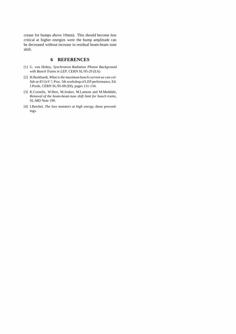
crease for bumps above 10mm). This should become lesscritical at higher energies were the bump amplitude canbe decreased without increase in residual beam-beam tuneshift.

6 REFERENCES

[1] G. von Holtey, Synchrotron Radiation Photon Backgroundwith Bunch Trains in LEP, CERN SL/95-29 (EA)

[2] H.Burkhardt, What is the maximum bunch currentwe can col-lide at 45 GeV ?, Proc. 5th workshop of LEP performance, Ed.J.Poole, CERN SL/95-08 (DI), pages 131-134.

[3] K.Cornelis, W.Herr, M.Jonker, M.Lamont and M.Meddahi,Removal of the beam-beam tune shift limit for bunch trains,SL-MD Note 190.

[4] I.Reichel, The loss monitors at high energy, these proceed-ings.

Discussion: Bunch Trains vs. Pretzel

H.Burkhardt, CERN, Geneva, Switzerland

It was remarked that the Q’ correction is less flexible inthe Pretzel scheme.Pretzel operation was more sensitive to small tune changes.It was suggested this was only due to the higher beam-beamtune shifts. From the operation side it was argued that life-time problems with Pretzel were a more general feature anddifficult to handle even in cases were the tune shift was arti-ficially lowered, for example by exciting strongly the emit-tance wiggler. It was speculated that resonances were moreexcited in Pretzel operation and non gaussian tails more sig-nificant.Dynamic aperture could become a serious limitation forLEP2. It was claimed, that the dynamic aperture is not re-duced in the Pretzel scheme.It was remarked that there were quite some problems in Tris-tan with RF trips, probably induced by synchrotron radia-tion. It was asked if this could also be important for LEPand if there would be differences in Pretzel or bunch trainoperation in this context. In both cases the orbit can be zeroin the cavities and moreover they are protected by collima-tors.Tune splits were observed in both schemes for different rea-sons. At LEP1.5 tune splits were mainly a consequenceof asymmetric RF but did not cause problems in operation.Tune shifts and lifetimes were excellent.

SUMMARY: PRETZEL VS BUNCH TRAINS

K. Cornelis

1 NUMBER OF BUNCHES

The number of bunches one would like to collide, inorder to optimise the luminosity, depends strongly on theintensity limit per bunch and on the total current limit.The first limit is given by the threshold for coherentinstabilities, the second is imposed by limitations in thesuper conducting cavities. The bunch current limitdepends on the optics used and three different optics wereconsidered : 90/60 degrees, 108/60 degrees and 108/90degrees. All calculations were done with a vertical beam-beam tune shift of 0.045. For a total beam current of 4mAa 4x4 scheme gives the best luminosity. For a total beamcurrent of 8 mA and higher (results were shown forcurrents up to 13 mA) an 8x8 scheme is preferable. A12x12 scheme does not give any advantage in all theconsidered cases.

2 BUNCH TRAINS AND PRETZEL SEENBY OPERATIONS

A comparison from the 1994 pretzel run with the 1995bunch train run shows that the efficiency in 1994 wasslightly higher than in 1995 (67% against 64%).However, it should be mentioned that in 1994 the pretzeloperation was already well established, whereas thebunch train operation had only just started and was stillon a learning curve.

Problems encountered with the pretzel operation werethe following :

-Intensity limit at injection (0.45 mA/bunch)

-Tune and chromaticity differences between electronsand positrons

-Horizontal tails in physics.

- A very sensitive machine in physics but high beam-beam tune shifts (0.04)

For the bunch train operation the following problemswere mentioned :

-Horizontal orbit difference between electrons andpositrons at injection.

-ZL sparks killing the beam

-Tune and chromaticity splits.

-Radiation at injection.

-Tighter collimator settings in physics to avoidradiation (but this gave no lifetime problems)

- Lower beam-beam tune shift (0.03), but veryreproducible and less sensitive.

3 THE SEPARATORS

In a third presentation a comparison was given of theseparator behaviour in both schemes. For the pretzelscheme 42 separators are in use at injection and 24 inphysics. For the bunch train scheme 40 separators areused at injection and 40 in physics. The fault rate on theseparators in 1995 (bunch trains) was lower than in 1994(pretzel).

For the bunch train operation all the separators are thesame and interchangeable, which is not the case inpretzel.

Thanks to the bunch train project, the separatorcontrols and software has been standardised andupgraded.

The spark rate in both schemes is comparable, but inthe case of pretzel a spark does not necessarily kill thebeam.

The main advantage of the bunch train scheme is thefact that the hardware is installed. Going back to thepretzel scheme would mean a substantial effort from theBT group.

4 BEAM INSTRUMENTATION

For most of the beam instrumentation the bunch trainscheme is more difficult. The shorter distance betweenthe different bunches in a train asks for a larger bandwidth than the original design. However, in most of thecases this problems were solved. For the BCT, tunemeter, BEXE, streak camera and luminosity counters, theindividual bunches can be resolved. For the BOM thenumber of blind pick up’s in the even straight sectionscan be reduced to a minimum by choosing the rightbunch spacing.A specific problem is the outgasing of the polarimetermirror which, with the bunch train bump on, is heated bysynchrotron light.

5 PERFORMANCE IN PHYSICS

In both pretzel and bunch train operation, the amount ofbunch current which could be collided was limited bybackground requirements. A specific problem for thebunch trains was the photon background coming fromQS4. Reducing the bunch train bump and using tightercollimator settings solved this problem.The average luminosities over two stable periods, one in1994 (pretzel) and one in 1995 (bunch trains) giveroughly the same results ( 11.7 1030 cm-2s-1 for pretzelagainst 11.1 1030cm-2s-1). This comparison has to be takenwith care since the bunch train operation during thisperiod was with 4x3 against 4x3 bunches. The averagebeam-beam tune shift during the same periods was 0.034for pretzel, peaking at .045. For the bunch trains theaverage beam-beam tune shift was 0.023 peaked at 0.03.However, an MD with 4x2 against 4x2 gave a beam-beam tune shift of 0.042 for bunch trains.

OPERATIONAL REQUIREMENTS

Gianluigi ArduiniSL Division

ABSTRACT

On the basis of the experience gained in running LEPwith an increasing number of superconducting RF unitsunder global voltage control, the operational requests onthe RF control software to be used in the control roomfor the LEP 2 phase are discussed. The maximumattainable beam energies, taking into account theconsequences of a trip of one or several RF units onquantum lifetime, are also presented.

1 ’95 OPERATIONAL EXPERIENCEThree aspects charcterizing 1995 LEP operation are

considered relevant for analyzing the operationalexperience as regards the RF control from the PrevessinControl Room (PCR):• the increase in the number of RF units and in

particular the larger and larger use ofsuperconducting (SC) units. Being the RF voltageprovided by a SC unit more than twice that availablefrom a conventional copper unit, any instability andin particular any RF trip has an evident impact on thebeam. In some cases, particularly at high energy,when the reserve of the total RF voltage is smaller,an RF trip may result in a partial or complete beamloss. During the 1995 LEP 1 phase 27% of beamlosses were due to an RF trip while in the LEP 1.5phase this percentage increased up to 90%. Thefrequent occurrence of RF problems determined amassive use of programs for the diagnosis and thecontrol of the RF units.

• the routine use of the Global Voltage Control (GVC)software in operation. This program was designed inorder to provide a tool for the operator to keep adesired total voltage and in minimizing RFasymmetries during ramp and in physics.

• the Energy Scan for the precise determination of themass and the width of the Z0 line. This required acomplete and reliable logging of the RF parameters.

Essentially four main functionalities of the RFcontrol system are of interest for operations andtherefore were made available in PCR: RF faultdiagnostics, RF switch on, GVC and RF logging. Theirperformances in the 1995 run are discussed below.

1.1 RF fault diagnostics

Fast RF fault diagnostics programs providing concisereports on the status of the RF hardware are essential torapidly recover normal operation conditions. Thelocalization of the faulty unit and the detection of thefault are necessary to determine which actions theoperator must take to restart the unit and, in case ofmajor problems, to provide the RF expert with all theinformation required for an effective intervention. Thealarm and RF surveillance screens are the first referencefor the operator when abnormal beam parameters, thatcan be attributed to a change in the RF voltagedistribution, are observed. These screens already providea concise indication of the faulty unit, the origin of theRF trip (RF or power converter interlocks) and the statusof the RF unit. During the 1995 run no alarm wasgenerated in case of a SC unit trip, furthermore therefreshing rate of the RF surveillance screen data wasrelatively slow (approximately once every 1-2 minutes).

Once detected the fault, it was often necessary todetermine the interlock status of the RF unit beforeproceeding to restart it. While a summary of the RF andHV interlock status of any number of Cu units wasavailable on Apollo under the operational environment(SloppySoft), a X-terminal expert program had to beused to have a similar report for the SC units. Being anexpert program the latter lacked of a user-friendlyinterface and it was difficult to consult because itprovided an interlock report only for one unit at a timeand too many details for operational use.

1.2 RF switch on

RF switch on was often hampered by communicationproblems linked to the GPIB bus. Switch on with beamwas definitely more problematic for SC units, because ofthe major complexity of the tuning procedure, ascompared to Cu units. This procedure used the beamcurrent as an input parameter to determine the optimumtuning power. Tuning of the SC cavities was thenachieved by thermal expansion of Ni bars (cooled by Hegas flow) rigidly connected to the extremities of thecavities and heated with coils. The unit switch onprocedure took about 10 minutes (approximately equalto the time required to ramp from 44 GeV to 65 GeV) ascompared to about 1 minute for Cu units. The switch onprogram was not protected against beam current readingerrors, only a protection against overheating of the

tuning bars existed. These errors sometimes resulted inheating the tuning bars above the optimum value andtherefore in a delay of the switch on by a few tens ofminutes (the time taken by the tuning bar to cool down).

A program to switch on any number of units wasavailable in PCR under SloppySoft, nevertheless theswitch on status was not updated automatically but onlyon request. This feature proved to be of particularinterest for the SC units because of the long switch ontime as compared to Cu units. For this reason a X-terminal program, providing a continuous update of theswitch on status for the SC units and generally used bythe RF expert to control the RF units, was madeavailable by the RF group as a temporary fix to theabove problem. The considerations expressed in section1.1 about expert programs equally apply to this case.

1.3 Global Voltage Control

The Global Voltage Control program wassuccessfully used since the beginning of the 1995 run tocontrol the distribution of the RF voltage among the RFunits during the ramp.

The following problems were observed duringoperation:• unpredictable results were often observed when

trimming the synchrotron tune Qs: in some cases thetotal voltage did not change, in some others (when amismatch was found between the required totalvoltage and the effective voltage) an unrelevant Qs

trim (1x10-6) was used to re-estabilish the total RFvoltage. The operator was often left with the choiceof disabling GVC and setting the RF voltage of theindividual units or to change the total RF voltage inthe GVC control program, with the result that norecord was left of the trim done.

• in a few cases the voltages of some RF units werefound out of tolerance (even higher than themaximum RF voltage settings) as compared to therequired settings;

• the absence of a “set vector” option during the LEP1.5 phase, when the injection energy was raised from20 GeV to 22 GeV, required the generation of the RFsettings for 20 GeV (vector 0) and then the ramp to22 GeV (vector 17).

The above problems, but in particular the lack of auser-friendly interface, are probably at the origin of thelimited use of GVC in physics. At least 4 applicationsshould be used to control the system and to producedisplays, such as those showing the RF level of each unitor the RF voltage in the sectors left and right of eachinteraction point.

The operator could not specify the symmetry type hewanted to run the machine because this condition washard-coded in the program. The symmetry type is animportant parameter in the optimization of the

performance of the machine, not only during the ramp,but in particular during physics.

During the LEP 1.5 phase frequent changes in the RFconfiguration were required in the quest for stableoperation and in order to cope with the evolution of theperformances of the individual units. In this respectediting and reloading the Current Data Set (the filecontaining, among other parameters, the maximum RFlevels) required the use of two different applications anda lengthy procedure because of the absence of a graphicuser interface (e.g. an input window).

1.4 RF data logging

RF data logging during the Energy Scan was oftenaffected by the communication problems alreadymentioned. As a result of that the logging of the RFvoltages was discontinuous and required the constantintervention of the operator to reset communications.The absence, in the frame of the RF control software, ofa dedicated application to check and resetcommunications with the RF units, further increased thenumber of applications required to run the RF hardware.

2 1996 RF SCENARIODuring 1996 the number of SC units will further

increase in two steps. The number of units and themaximum available total voltage foreseen in these twophases are listed in Tables 1 and 2, respectively. Theequivalence 1 SC unit = 2 SC modules = 8 SC cavitiesshould be kept in mind in the following.

Number of units Max.RF voltage[MV]

Cu cavities 120 292SC Cu/Nb cavities 128 1280SC Nb cavities 4 (12) 34 (102)Maximum total RF voltage [MV] 1606 (1674)Table 1: Installed RF cavities and maximum availableRF voltage by week 22 (end of May). According to theRF installation plans the installation of 2 solid Nbmodules (273.2 and 273.3) is not assured [1].

Number of units Max.RF voltage[MV]

Cu cavities 120 292SC Cu/Nb cavities 160 1600SC Nb cavities 16 136Maximum total RF voltage [MV] 2028Table 2: Installed RF cavities and maximum availableRF voltage by week 40 (end of September) [2].

The maximum RF voltages listed in Table 3(corresponding to those used in operation in 1995) havebeen assumed for the individual units. These are slightlyconservative values for the Cu units, in fact conditioning

of these cavities is foreseen during the shutdown and animprovement of their maximum performances (by a fewMV/unit) is expected [2].

Unit type Max. RF voltage [MV]Cu units (even numbers) 38Cu units (odd numbers) 35SC Cu/Nb units 80SC Nb units 68Table 3: Maximum RF voltage per unit assumed in thecalculation of the total available RF voltage in Tables 1and 2.

An estimate of the maximum beam energiesachievable in 1996 with the expected total RF voltageslisted in Tables 1 and 2 is presented in Table 4 for the108o/60o optics (αp = 1.38251 x 10-4). The reduction inthe maximum achievable energy resulting by theconsideration of a reserve in the RF voltage (in order toface the RF trip of one or two units) is also shown. Thequantum lifetime drop in occasion of a SC unit trip is infact so important (several order of magnitude) and theswitch on procedure and GVC response time (about 1 s)too slow that running without reserve would inevitablybring to loose the beam in case of a RF trip.

Maximum beam energy [GeV]no reserve 1 klystron trip 2 klystron trip

June 83.8 (84.7) 82.7 (83.6) 81.6 (82.5)October 88.9 88.0 87.1

Table 4: Estimated maximum beam energy as a functionof the reserve allocated for RF trips. In brackets arepresented the values expected in case also the SC Nbmodules 273.2 and 273.3 are installed by week 22.

The maximum beam energy that allows a quantumlifetime larger than 100 hours has been assumed as acriterion in compiling Table 4. The beam lifetime incollision is mainly dominated by beam-beamBremsstrahlung (about 10 hours at LEP 2 [3]) thereforethe above criterion is relatively conservative.Furthermore, Sands formula [4], that has been used inthe above calculations, provides more pessimisticestimates of the quantum lifetime as compared to otherformulas [5].

The maximum energies achievable with the 90o/60o

optics (αp = 1.90985 x 10-4) are about 0.4-0.5 GeV lowerthan the corresponding ones listed in Table 4 for the108o/60o optics.

The voltage induced by the beam in a tuned SCcavity at high currents is not negligible (about -60MV/tripped unit for a beam DC current of 8 mA [6]),nevertheless the cavities are rapidly detuned in theoccurrence of a RF trip. Few tens of milliseconds aresufficient to detune the cavity by magnetostrictive actionon the tuning bars and to reduce by one order of

magnitude the impedance of the cavity seen by the beamand therefore the induced voltage. The further reductionin the quantum lifetime resulting from the negativeinduced voltage is therefore limited to the detuning timeand it should not result in relevant beam losses.

3 OPERATIONAL REQUIREMENTSAs can be seen from Tables 1 and 2 the number of

SC units will double by the end of May 1996 and willtriplicate by the end of September 1996. A reliable anduser-friendly RF control software is therefore mandatory.In formulating the operational requirements it seemsreasonable to classify them in two sets, according towhat is considered their degree of urgency.

3.1 Improvement of the existing RF controlhardware and software

The highest priority should be given to the solutionof the communication problems because this wouldalready have a beneficial effect on the speed and theeffectivness of the switch on procedure, as well as on thereliability of the RF data logging.

The reliability and the versatility of the existing RFcontrol software in the operational environment(SloppySoft) should be improved with the aim ofminimizing the number of existing applications.

The possibility of checking and resettingcommunications should be made available underSloppySoft as before.

Alarms for every unit should be displayed in the PCRalarm screen and a faster update of the RF surveillancescreen should be attained (update every 20 s should befeasible [7]). A more extensive use of colours shouldhelp in reducing the number of listed items (e.g., theMain Circuit Breaker status and the high voltage levelcould be presented in a single column, the same could befor the voltage loop status and the RF level) and shouldhelp the operator in the detection of the fault.

A HV and RF interlock summary should be availablein SloppySoft for all the RF units.

The reliability and the speed of the switch onprocedure should be improved, in particular protectionagainst heating of the tuning bars above the optimumtemperature should be implemented.

GVC reliability with respect to the points mentionedin section 1.3 should be enhanced. All the optionsforeseen for this applications should be implemented: theoperator should have the possibility to choose among thedifferent symmetry conditions and the auto-switch-onprocedure with beam should be implemented [8].Tripped units could be therefore automatically restartedafter an automatic check of the fault type and switchingon RF units during the ramp should be also feasible.

RF problems during the ramp could occur because ofRF trips or vacuum problems on power couplers [9]. In

that case stopping the ramp and restarting the trippedunits could be a safe measure, taking into account thatthe switch on time for a SC unit is comparable with thetime required to ramp from 22 GeV to 80 GeV withoutstopping. Therefore a ‘stop of ramp’ option should beprovided in GVC (it could be even automatic in case ofRF trip).

A ‘set vector’ option should allow more flexibility inchanging the injection energy [10].

The possibility of taking into account the RF voltagesof units that are on but not ramped proved to be usefulalready during the 1995 run and it would be important inchoosing the ramp strategy and in the policy of keepingone or two units as a reserve of RF voltage in physics.

3.2 Dedicated application for the RF control inPCR

The degree of complexity of the RF hardwarecertainly justify the implementation of a dedicatedapplication for the RF control under SloppySoft, such asthose already existing for the separator and collimatorcontrol. This application should include:• fault diagnostics, switch on program and

communication manager for all the RF units,longitudinal and transverse feedback;

• user-friendly GVC manager permitting to select theabove mentioned options (symmetry type, rampstrategy, vector number, ramp stop....) and to easilyedit and reload the Current Data Set;

• displays: schematic synopsis with use of colours toindicate the status of a component and to interrogateeasily the system (clicking on the displayedcomponent), bar histograms displaying the RFvoltage of each unit and the RF voltage in the sectors(these last two applications already exist);

• other diagnostics tools such as bunch display andbucket scan.

4 CONCLUSIONS1995 operational experience with the RF control

system has been characterized by the successful use ofthe Global Voltage Control during the ramp. Majorconcerns came from the unreliability of thecommunications with the hardware, the insufficient faultdiagnostics for the SC units and the lack of flexibility ofGVC to allow its efficient use in physics. The increase inthe number of SC units in 1996 should allow theattainment of the maximum energies of 81.6 GeV by thebeginning of June and of 87.1 GeV by the beginning ofOctober, with an adequate reserve of RF voltage, for the108o/60o optics. In reason of the increased complexityand extension of the RF hardware, the improvement ofthe weak points above mentioned is mandatory for thestart-up. The creation of a dedicated application for theRF control with its own fixed displays seems also

justified once solved the more urgent problems aboveunderlined.

ACKNOWLEDGMENTSI would like to thank all the collegues of the LEP

operation team for providing me with the results of theirexperience in operating the RF hardware from PCR andfor their suggestions about the possible improvements. Iam indebted to L. Arnaudon, D. Boussard, E. Ciapala, G.Geschonke and J. Sladen for the explanations concerningthe RF hardware and controls, as well as the installationplans for 1996.

REFERENCES[1] J. Montes, H. Schuhback, ‘LEP - Planning de

travaux pendant le SHUTDOWN du 27NOVEMBRE 1995 au 16 JUIN 1996’, 10th

November 1995, Annexe 15.

[2] G. Geschonke, private communications.

[3] H. Burkhardt, ‘Beam-Beam Tuneshift, Emittanceand Lifetime’, Proceedings of the Fourth Workshopon LEP Performance, J. Poole ed., CERN SL/94-06(DI), Geneva, 1994, pp. 413-419.

[4] M. Sands, SLAC-121 (1970).

[5] F. Ruggiero, CERN SL/93-05 (AP).

[6] D. Boussard, ‘70 GeV Run - RF Considerations’,transparencies presented at the ‘Discussion Day onLEP Operation at 70 GeV’, Ferney Voltaire, 11th

October 1995.

[7] E. Ciapala, private communication.

[8] E. Ciapala, ‘How Can We Survive the 1995 RFAsymmetries ?’, Proceedings of the Fifth Workshopon LEP Performance, J. Poole ed., CERN SL/95-08(DI), Geneva, 1995, pp. 140-145.

[9] G. Geschonke, 'RF Constraints', Proceedings of theFifth Workshop on LEP Performance, J. Poole ed.,CERN SL/95-08 (DI), Geneva, 1995, pp. 195-197.

[10]G. de Rijk, ‘How high we can push the injectionenergy of LEP ?’, these Proceedings.

PRODUCTION OF CAVITIES AND MODULES

Karl-Martin Schirm, CERN, Geneva, Switzerland

ABSTRACT

For the LEP energy upgrade 180 superconducting Nb/Cucavities have been produced so far by European industryand by CERN. Some adjustment of the initial productionrecipe was required for overcoming difficulties related tothe copper surface preparation before coating.Furthermore, discontinuities in the production sequenceor in equipment maintenance sometimes resulted in lowcavity performance. We have addressed both issues bystatistical evaluation of production and performance datacombined with Nb layer optical inspection. The coatingacceptance rate and the average cavity performance arenow significantly improved. Cavity repair andperformance recovery was successfully applied indifferent cases.

1 INTRODUCTIONSixty-five superconducting 350 MHz cavities, series

produced by three different European companies, havebeen successfully operated at their nominal field gradientof 6 MV/m in a first physics run of LEP at 65 GeV.Hence, five years after the initial technology transfer toindustry, the CERN developed Nb/Cu thin film approachhas successfully proven its potential for the followingLEP energy upgrade steps. However, especially the firstyears of production have been marked by somedifficulties closely related to the very demandingmanufacturing and assembly steps. The cavity acceptancerate in the vertical RF reception test was clearly too lowfor respecting the time schedule for module delivery.Defective Nb layers often had to be chemically removedand the bare cavities returned to the manufacturer for anew coating causing delay and additional costs. Theinvestigation of those cavity failures had to be intensifiedin a close collaboration between CERN and the industrystaff for getting the cavity production off the planningcritical path.

2 ACCEPTANCE TESTINGCavities delivered from the manufacturer are

acceptance tested at CERN before further assembly stepscan be considered. Contractually fixed acceptance criteriainclude a quality factor Q(E) of at least 3.4*109 (4.5K) inthe vertical RF test. This value, based on the results ofcavities from the CERN development series, wasgenerally considered as ambitious. Cavities failing in thatrespect are suffering from losses in the active layer,mostly in form of local defects. These can be detected by

the temperature mapping method [1] where a temperaturesignal on the outer surface exceeding the backgroundvalue by more than 100 mK is counted as “hot-spot”. Astatistical evaluation of the “hot-spot” locations [2] inrejected cavities allowed us to identify differentproduction steps as relevant in the defect build-updepending on the manufacturer concerned. However, themain difficulty consisted in understanding the lossprocesses causing these “hot-spots”. Therefore we haveincluded a visual inspection of the Nb layer by means of avideo camera robot [2] in the cavity rejectionformalism.Video images of defects are stored in aninspection database allowing a systematic classificationand also providing defect reports to the companies. Some350 m2 cavity/cryounit inner surface have been inspectedso far including one cavity with excellent performancefor comparison.

3 DEFECTSThe major result of video surface analysis in Nb/Cu

350 MHz cavities is the possibility of classifying allrelevant “hot-spots” in two defect types.

3.1 The interface defect

By far most of the “hot-spots” measured on cavitiesduring the RF test are caused by a non-uniform interfacecomposition. The characteristic feature is a reducedthermal contact between the active Nb layer and thecopper bulk by the presence of copper oxides at theinterface and/or reduced layer sticking. This is clearlyrelated to failures in the chemical polish - water rinsing -drying of the copper surface before coating.

Fig. 1a: Lack of coating adherence due to the presenceof a copper oxide at the Nb/Cu interface

1fi-a3 :11.

’171L82' 5/12/1994 : 353—4 CHUITT

Gfiflflfi . 116.68 S

A hystheretical Q(E) curve can give a first indicationfor a starting peel-off. Figure 1a shows a typical examplefor an interface defect taken after the manual removal ofthe detached Nb. Defective zones can heat-up under RFpower and are destroyed by sometimes eruptive meltingas seen by scanning electron microscope (SEM) on asample cut-out from a whole cavity (fig. 1b).

Fig. 1b: Interface defect analyzed by SEM

Detached areas are typically in the order of somesquare millimeters which seems to be few compared tothe 5.5 m2 inner surface. But this peel-off is sufficient forfully spoiling the cavity performance and the onlypossible cure is the chemical removal of the Nb followedby a new coating.

3.2 The surface defect

Fig. 2a: Surface defect consisting of particles andrecristalized Nb.

The situation is somewhat different if the defect consistsof foreign particles sitting on a correctly grown Nb layer.This can happen if some contamination is introduced intothe cavity during final rinsing, assembly, testing oroperation. The contaminant is then heated up by the RFfield. It can sink into the surface if the meltingtemperature of Nb is locally reached. Particles bound that

way are not easily removable and they typically lead to“quenching” at a certain field gradient. Figure 2a shows asurface defect in a cavity that was quenching at 5 MV/m.The surrounding Nb surface has recristalized aftermelting.

3.3 Cavity repair and performance recovery

Both types of defects can also occur after moduleassembly and during operation leading to a performancedrop and the non-functioning of the cryounit concerned.There is clearly a need for cavity repair and maintenance.It was shown at CERN in three cases, that it is possible todo a Cu chemistry and new coating in an assembled unit,meaning the cavity with He tank around. But this methodis somewhat risky and time consuming. It should only beapplied if parts of the Nb are peeled-off. Surface defects(3.2) can be treated by grinding the defect under videocontrol, trying to remove the particles and to flatten thesurface zone. High pressure water rinsing is appliedafterwards for cleaning. Using that method we havesuccessfully treated the defect shown in fig. 2a [2] andmore recently one unit of a module that was quenching at4.5 MV/m in the string test just before installation inLEP. Both cavities were recovered to full performance.

4 IMPROVING THE ACCEPTANCERATE

It is clear by now that the chemical and mechanicalcomposition of the copper surface before coating is thecritical property for the coating success rate. Increasing itis only possible by analyzing in the very detail everyproduction step that could play a role in the creation ofdefects. Unfortunately we can not precisely define thephysical surface properties that we need nor can wemeasure anything in that respect during the productionsequence. So we have to trace back from an observeddefect in the Nb layer in the acceptance test to its originin the fabrication. Rapidly identifying and correcting thefaulty procedure means less cavities produced in serieswith the same defect. A very close collaboration betweenpeople in the companies and at CERN and the soundknowledge of the various production steps is mandatory.Without going into any details it is to mention that mostlyinstallations and maintenance items, for the chemistryplants but also for the bake and sputtering set-up wasconcerned. The ultra-pure water quality was sometimesdoubted, clean-room subjects discussed, changingoperators in the production often introduced additionalfaults. We have improved the production recipe by fine-tuning bake-out and sputter parameters [3], enhanced thecopper electropolishing and added more chemical polishcycles for a decreased probability of liquid retention inmaterial pits [4] and introduced systematic cleaning of thechemical plant by recirculating sulfamic acid after eachtreatment. For summing up the result of the continous

effort we show in fig. 3a the evolution of the first Nblayer acceptance rate as an indicator for the throughput inthe cavity production.

92 93 94 950%

10%

20%

30%

40%

50%

60%

70%

80%

90%

100%

92 93 94 95

Year of Production

First Coating Acceptance RatesData 31/12/95

Figure 3a: First Nb coating acceptance rates in theseries production of the three companies

In 1995 we have reached a level of first coatingacceptance of almost 70%. This value is sufficiently highfor fullfilling the production planning. However, it is amean value over one year for three companies and all ofthem have seen periods during that year when their cavityacceptance rate dropped back to 0% due to deviatingfabrication processes.

Increasing the cavity throughput was the main issue ofthe improvements mentioned, but this effort was alsohighly beneficial for the cavity performance. Cavities arenow in general accepted with Q-factors around 20%better than the acceptance threshold value, most of themstill show a reasonable Q at 8 MV/m. The development ofthese numbers during the production is illustrated infigure 3b.

3.00

3.10

3.20

3.30

3.40

3.50

3.60

3.70

3.80

3.90

4.00

4.10

4.20

4.30

4.40

4.50

4.60

4.70

4.80

4.90

9394

950

1

2

3

4

5

6

7

8

9

10

Acc

epte

d C

aviti

es

Q(6MV/m)*10 9

Q-factor distribution

93

94

95

QAV = 4.04

QAV = 3.92QAV = 3.72

4.5K

Figure 3b: Distribution of the Q-factor acceptance valuesat 6 MV/m and 4.5K.

We can see in the distribution of 1994 a transition of theacceptance maxima near 3.4*109 to a new maxima around4.3*109. This trend was confirmed in 1995 when very fewcavities had to be accepted with values close to thethreshold.

5 CONCLUSIONThe industrie production of LEP2 350 MHz cavities inNb/Cu technology has improved to a high level of cavityacceptance rate and performance. The availability ofenough statistics on production and testing data but alsowell adapted analysis methods have refined ourunderstanding of technology specific defects. Even moreis it now a matter of quick and close interaction betweenthe acceptance testing at CERN and the people in industryto stabilize these results until the last cavity will beproduced in 1997 [5]. Key issues for the ongoingproduction are the installations maintenance and acontinous production sequence. The performancerecovery methods that we have developed are promisingand should be further improved.

REFERENCES[1] H. Piel and R. Romijn; CERN/EF/RF 80-3; 13 June

1980[2] K.M. Schirm et al.; Proceedings of the 7th workshop

on RF Superconductivity, Gif-sur-Yvette, France,17-20 Oct. 95; p.702/717

[3] E. Chiaveri et al.; Proceedings of the 15th PAC,Dallas 1- 4 May 1995

[4] S. Calatroni et al., Proceedings of the 6th workshopon RF Superconductivity, Newport News, Virginia,USA, 4-8 Oct. 93; p.702/717

[5] E. Chiaveri; this workshop

1 I

ll

-I

ll

s

III. I

!

Il

l-

un

mo

—

llllllu ml!

Il

fli

ii

ifl

flv

"

““

“‘

>

Performance of Cavities

J. TückmantelCERN, SL-RF

on behalf of the sc. cavity community

Abstract

LEP2 superconducting cavity modules produced by

industry now show typically performances in the

acceptance tests superior to specifications. The recent LEP

run up to 70 GeV has demonstrated these capabilities.

Nevertheless, one should be aware that the cavity

potential cannot always be fully exploited. We will

discuss the limiting mechanisms here and present possible

remedies, improvements or bypasses. Of concern are

effects due to the grouping of 8 cavities to one klystron,

tolerances in the coupling strength and field flatness,

externally induced and ponderomotive cavity oscillations

under strong beam loading, power coupler and cavity

processing and higher order mode power constraints.

1. INTRODUCTION

During the last run of LEP in 1995 the 16 installed

superconducting cavity modules (64 cavities) were

challenged - with full support of the warm copper RF

system - to keep two beams of 70 GeV on orbit, asking

for the flawless operation of all those modules. This

feasibility has been demonstrated for two (short) coasts.

Only a trivial problem independent of the installed

modules made one pair of modules unavailable, thus

taking the possibility of a 70 GeV beam. However, for

the still possible beam energy of 68 GeV, many 'standard'

coasts were operated to full satisfaction of the physicists.

This demonstration has only been possible due to the

solution of different problems showing up in '95 or

before. Some of those are still not yet completely

resolved but solutions are under preparation.

2. MAIN COUPLERS

The power couplers for the sc. cavities [1] have been

plagued by multipacting (MP), which could be processed

away with long time RF application but which reappeared

soon after during normal operation again. This problem

seems to be solved now applying several improvements

(for more details see [2]).

2.1. Geometrical changes

Theoretical MP calculations [3][4][5] and the location

of arcing marks showed that the electrons impinge only

on the outer surface of the coaxial line (one-side MP),

especially on the cooled 'extension', the outer coaxial

conductor connecting the (cold) cavity port to the (warm)

upper part of the coupler.

Another strong level was detected in the 'choke' of the

variable coupler [6]. Since time was short, the latter level

was suppressed directly in abandoning the variable coupler

and thus the choke. Evidently this has consequences for

the problem of field flatness (see later).

Fig. 1 : The adjustable coupler

50 Ω

75 Ω

Fig. 2 Section of 50 and 75 Ω couplerwith a (sketched) typical MP-track

—

‘

III III :

II

I

III

ma

r

I.

.\

\\

'.

\\

\\

\\

..

.

F

u I

m

.«

x

x.

..

\

l\

\

.n

..

".

fl,

.,

.\

\

M

r l

m

_

WV

/

: .

..

..

..

..

.

15

..

..

.V

n ..

..

.

‘1

3.

..

.-

x...

Another geometrical change of the coupler wasapplied: reduction of the inner diameter of the antennachanging the line impedance Z from 50 to 75 Ω.

The electrons move only in the outer region (fig. 2)and this modification of the geometry does not change thecoaxial field there, provided the RF-voltage is scaledcorrespondingly. Practically this means that we will havethe same MP levels but they will appear at transmittedpowers scaled with Z, now 50% higher, thus shifting atleast one dangerous level out of the operational range.Further reduction of the antenna diameter is hardlypossible due to overheating (more RF-current on lesssection) and mechanical weakness.

2.2. Modifications of the 'extensions'

To fight the MP in the extensions, one step consistedin improvements of the surface quality to reduce thesecondary electron emission coefficient in depositing thethin Copper layer by either pulsed electro deposition orsputtering [7]. To avoid welding and brazing 'seen' by theRF, extensions are manufactured as a monolithic piece[8]. These improvements reduced the processing times andincreased the period till MP reappeared, but did notsuppress it permanently.

2.3. Improvements of the 'ceramic windows

During these tests the hypothesis that condensed gasesare the culprit 'destroying' any clean or processed (cold)surface after a short time became increasingly probable.Since also heating of the ceramic window was observed athigher RF powers, it could be possible that the windowdesorbed gases that were captured again by the coldsurfaces. To adapt the window to the more stringentenvironment of cold sc. cavities, it was improved in thefollowing way [9][2]• Brazing with complete penetration• Kovar Ferrules machined and welded under pressure• More homogeneous Ti coating• Cu-plating of Ferrules• Improved air cooling

These modifications proved efficient and no moreoverheating of windows was observed, reducing in parallelthe quantity of 'available' gases in the coupler.

2.4. DC bias voltage

The complete suppression of MP was finally achievedin adding a bias voltage of about 2.5 kV which perturbsthe resonant electron orbits sufficiently up to the foreseenmaximum power of 200 kW. On the other hand oneshould not believe that a new coupler could simply beoperated to full power in applying the DC bias voltagewhich was demonstrated in an experiment where arcingdeveloped under such a condition. This confirms the firmrule, that each coupler has to be pre-processed without

bias up to its maximum design power before it can beoperated safely with DC bias voltage.

The DC bias voltage has to be brought onto theantenna as well as the RF, which technically needs acapacitor resisting these combined fields without breakdown. A 'do-it-yourself' capacitor was constructed in ahurry that allowed a fast and successful test of the DCbias idea. This capacitor did not always live long and wasmodified, finally resisting these constraints. However, tobe on the safe side, a known and proven construction [10](from the SPS tetrode amplifiers at 200 MHz) was adaptedto this application - especially annular modes have to beavoided - and works to full satisfaction.

During the last runs of LEP in '95, all power couplerswere operated with DC bias and no MP problemsappeared.

2.5. Bake-out of couplers in situ

Tests with basically warm extensions on a test standwhich could be cooled artificially by liquid nitrogen atdifferent locations finally confirmed the hypothesis ofcondensed gases, of which water seems to be the mostperturbing one, without any doubt [11]. Thereforecouplers, which are pre-processed with RF but have to beexposed to (humid) air at least during mounting in theclean room - were baked for about 24 h in situ on theevacuated cavity, reducing the RF processing timessignificantly, which is very important for a smoothcontinuation of production.

3. HIGHER ORDER MODES

3.1. General considerations

Due to cavity manufacturing tolerances, one has nowell defined phase relation from bunch to bunch for thehigher order modes and we have to be prepared for theworst case, a resonant build-up. Therefore, the fields ofthese modes have to be attenuated sufficiently betweensubsequent bunch(-train)s. Measurements [12] have shownthat the bunchlets in a train do not add up fields for thestrongest HOMs but one can roughly add powers, thus theworst case is not realised here.

3.2. The three frequency ranges

There exist 3 frequency ranges: Up to about 1 GHzmodes are confined in the superconducting parts of thecavity and the only attenuation is given by the HOMcouplers (the power coupler might contribute slightly)designed for this purpose and doing their job as expected.

Up to about 2 GHz, modes can leak out of thecavities, thus 'touching' the normal conducting inter-cavity bellows and cones at both ends of the module, butare still confined in the module. The losses will partly be

dumped as heat in the bellows and cones, a fractionending finally in the liquid Helium (LHe), which one triesto avoid. The loaded Q for this mechanism was estimatedto be in the order of 106 [13]. Measurements oftemperature increase on the bellows and cones do notshow worrying increases for the beam currents realisednow [14]. The HOM couplers - basically not designed forthis frequency range - still seem to do a good job. The'hook coupler' on all Nb/Cu cavities shows even betterperformance than the older coupler (type 1) on the 30degree modules.

Worst case power estimates [13] for both ranges,assuming the resonant case for the dominant (TM011zero-mode) and adding power for the other modes, yieldabout 540 W/coupler for cavities equipped with the type 5(hook-) coupler and 730 W/cavity for the bulk Nbmodules with coupler type 1 (having less coupling, thusallowing a stronger resonant build-up with finally morepower to be extracted).

Finally, above about 2 GHz modes can leak into theLEP beam pipe which seems to take place sincemeasurements of the cavity spectra do not showsignificant RF power in this frequency range [15].

3.2. Modes above 2 GHz

Calculations with ABCI [16] - the program waschecked with known results at lower frequencies - predict[17] [18] a significant RF power stripped off the beamabove 2 GHz, a part of which might end up in the LHe.This power shows strong dependence on the bunch lengthin this frequency range.

To examine this question experimentally and get thecapability to attenuate these modes outside the modules,an RF ferrite absorber was developed [19] and incorporatedinto a vacuum pumping manifold. Bench measurementsshowed at least 95% power absorption at 3, 4 and 5 GHz[20].

The direct beam image current loss was estimated for8 bunches of 0.5 mA to be 120 W. Temperaturemeasurements [21] on an absorber away from moduleswhere no HOM should propagate, indicated 200 W whichis in reasonable agreement. Additionally for a string of 4modules under the same conditions about 1100 W HOMlosses were calculated. One would therefore expect about550 W leaking out at each end, however, only about100 W were detected.

This seems to show that the RF power stripped off thebeam is smaller than expected for the estimated bunchlength, but lets on the other hand the uneasy impressionthat we have not completely understood thesemechanisms.

3.3. RF power transport through the vacuum tank

Another serious problem was the transport of the RFpower (below 2 GHz) from the coupler in the insulationvacuum to the outside world. The first way chosen was a

single cable when the announced total beam current wasabout 6 mA. Subsequent increases in announced beamcurrents (power is proportional to the square of the bunchcharge) and safety margin lead to the use of two parallelcables (with RF power splitter) cooled by a dedicated Hegas circuit [22].

25 Ω

50 Ω

25 Ω

RF window (cold)

open air

insul. vac.

connectors andvac. tight feed-through

2 cooled cables

'RF-Tee'

Fig. 3a: RF transport by 2 cooled cables (sketch)

Tests up to 175 W per cable (available power limit at640 MHz) worked. Lacking a better solution withpressing installation schedule, ten modules were equippedthis way and installed in LEP.

However, problems in type N and '7/16' connectors invacuum at 150-200 W observed in parallel (not only invery rare incidents) did not give entire confidence in thisdesign for high power. Furthermore, the dedicated He gascircuit and the clamping of the cable - the cable insulationwas partly removed - carried other technical risks and werework intensive and are difficult to handle in case of futurerepair.

3.4. The rigid coaxial line

. HOM coupler

25 Ω

25 Ω

50 Ω 50 Ω

insul. vac.

open air

'rigid line'

RF window (warm)

RF window (cold)

RF contacts(sliding)

'RF-Tee'

connectors in air !!!!

Fig. 3b: RF transport by rigid line (sketch)

Fortunately, the changes of the cryostat form theolder 30 degree design to the 45 degree design [23] (tomake room for LHC above LEP) applied for all industryNb/Cu modules, was used to place the ports for the cablesexactly above the HOM couplers themselves in case of apossible improvement.

This option was exploited [24], placing the powerdivider with its connectors outside the cryostats in air.

The RF transport from coupler to the coaxial feed-through is realised by a rigid coaxial line with sliding RFcontacts (which have not to be vacuum tight) at bothends, compensating the thermal contraction during cooldown and allowing an easy mounting without alignmentproblems.

Tests were done up to about 900 W at 640 MHz(resonant loop) without problems. Also the latestmodules, now all equipped with these rigid lines, did notshow any problems during the 70/68 GeV run (admittedwith only relatively low currents compared to the peakexpectations). However, one should not forget thatactually 10 modules with cooled cables are installed inLEP.

3.5. Semi-rigid cables for bulk Nb modules

A still unsolved problem due the increasing beamcurrent exists for the same task for the older bulk Nb (andtwo CERN produced Nb/Cu prototype modules with 30degree geometry). Here ports are not situated above thecouplers - thus excluding a reasonable construction of arigid line - and connectors are foreseen on a dome close toone end of each (one-cavity-) unit. In this case we have touse cables and the power of one HOM coupler has to betransported from one end of the unit to the other.

A first modification will be made in adding two smallholes in the 'main girder' of the unit, roughly above theHOM coupler concerned, foreseen with a feed-through,thus reducing the length of cable considerably. As cableswe intend to use semi rigid lines made by industry (usede.g. for aeroplane radar) with Si02 filling and vacuumtight connectors, thus thermal conductivity from thecentre wire - having the highest current density - to theouter conductor is sufficient to avoid overheating of thiswire. To circumvent the problem of connectors, the one atthe warm end will be situated in the air (thus no moreproblems) as part of the feed-through and the cold end willbe fixed during mounting without connector directly ontothe power splitter. To remove the created RF heating, wehave to add a He-gas cooling circuit, but since the outerconductor is not a braid but a (semi-) rigid tube,longitudinal thermal conductivity is better and only veryfew clamps are necessary. Studies are under way but itseems impossible that such modules equipped with thesecables will be installed till mid '96.

4. CAVITY PERFORMANCE

4.1. Eight cavities with one generator

One high-efficiency 1 MW klystron supplies 8cavities (supplying 80 MV to the beam) and therefore noindividual cavity deviation can be compensated bygenerator control.

To reduce the impedance presented by the high Qcavities to the beam, an RF-feedback system (sketch infig. 4) was tested with success [25]. It reduces also anyperturbation to the beam caused by instabilities in (oneof) the 8 cavities supplied by this klystron.

RF sum

driverklystron

(+)

(-)

Fig. 4 The RF feed back set-up with 8 cavities and one generator

fl f \ / \flH 1” \ fl f “v E I1 Ix I1 I’ ‘I Ix I1 Ix '

\ J \ / \ / \ J \ J V \ / \ /

fl fl / N / K H / 1 I1 Ix I’

\J \ J v \ /

[Na/N _‘| Ix I1 Ix ' \ J V \ / \ /

fl ‘ fl fl f ‘ fl 1” VGA“ 1 Ian/”V3.” I1 Ix I1 I’ ‘I Ix I1 Ix ' I1 Ix I1 I’

\ J \ / \ / \ / \ J V \ / \ / \ J \ / \ / \ J

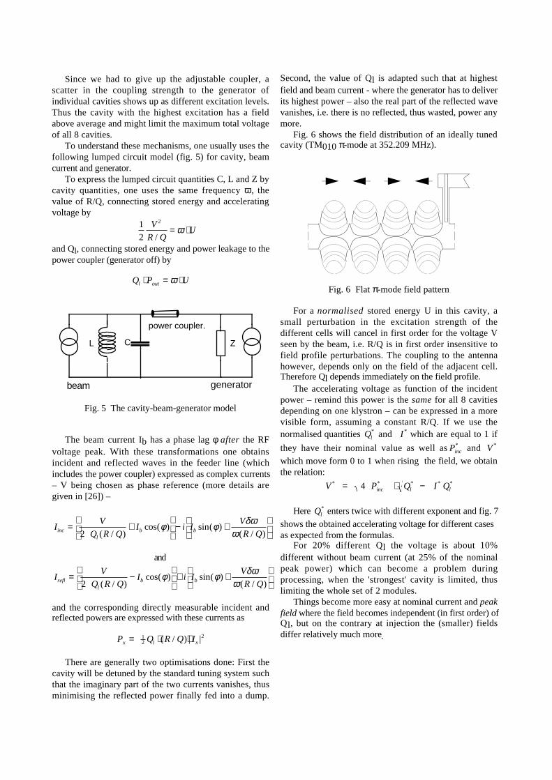
Since we had to give up the adjustable coupler, ascatter in the coupling strength to the generator ofindividual cavities shows up as different excitation levels.Thus the cavity with the highest excitation has a fieldabove average and might limit the maximum total voltageof all 8 cavities.

To understand these mechanisms, one usually uses thefollowing lumped circuit model (fig. 5) for cavity, beamcurrent and generator.

To express the lumped circuit quantities C, L and Z bycavity quantities, one uses the same frequency ω, thevalue of R/Q, connecting stored energy and acceleratingvoltage by

12

V 2

R / Q= ω ⋅U

and Ql, connecting stored energy and power leakage to thepower coupler (generator off) by

Ql ⋅ Pout = ω ⋅U

L C

power coupler.

Z

beam generator

Fig. 5 The cavity-beam-generator model

The beam current Ib has a phase lag φ after the RFvoltage peak. With these transformations one obtainsincident and reflected waves in the feeder line (whichincludes the power coupler) expressed as complex currents– V being chosen as phase reference (more details aregiven in [26]) –

Iinc = V

2 Ql (R / Q)+ Ib cos(φ )

− i Ib sin(φ ) + Vδω

ω (R / Q)

and

Irefl = V

2 Ql (R / Q)− Ib cos(φ )

+ i Ib sin(φ ) + Vδω

ω (R / Q)

and the corresponding directly measurable incident andreflected powers are expressed with these currents as

Px = 12 Ql ⋅ (R / Q)⋅| Ix |2

There are generally two optimisations done: First thecavity will be detuned by the standard tuning system suchthat the imaginary part of the two currents vanishes, thusminimising the reflected power finally fed into a dump.

Second, the value of Ql is adapted such that at highestfield and beam current - where the generator has to deliverits highest power – also the real part of the reflected wavevanishes, i.e. there is no reflected, thus wasted, power anymore.

Fig. 6 shows the field distribution of an ideally tunedcavity (TM010 π-mode at 352.209 MHz).

Fig. 6 Flat π-mode field pattern

For a normalised stored energy U in this cavity, asmall perturbation in the excitation strength of thedifferent cells will cancel in first order for the voltage Vseen by the beam, i.e. R/Q is in first order insensitive tofield profile perturbations. The coupling to the antennahowever, depends only on the field of the adjacent cell.Therefore Ql depends immediately on the field profile.

The accelerating voltage as function of the incidentpower – remind this power is the same for all 8 cavitiesdepending on one klystron – can be expressed in a morevisible form, assuming a constant R/Q. If we use thenormalised quantities Ql

* and I* which are equal to 1 if

they have their nominal value as well as Pinc* and V *

which move form 0 to 1 when rising the field, we obtainthe relation:

V * = 4 Pinc* ⋅ Ql

* − I* Ql*

Here Ql* enters twice with different exponent and fig. 7

shows the obtained accelerating voltage for different casesas expected from the formulas.

For 20% different Ql the voltage is about 10%different without beam current (at 25% of the nominalpeak power) which can become a problem duringprocessing, when the 'strongest' cavity is limited, thuslimiting the whole set of 2 modules.

Things become more easy at nominal current and peakfield where the field becomes independent (in first order) ofQl, but on the contrary at injection the (smaller) fieldsdiffer relatively much more.

g

J — F

Fig. 7 Normalised field as function of normalisedincident power for 3 different Ql

* conditions: 80%, 100%

and 120% nominal value. The left batch shows thesituation without beam current, the highest curvecorresponds to 120% nominal Ql

* . The centre batch

corresponds to half, the right batch to full nominal beamcurrent (precisely I cos(φ ) ). The higher curve below

cross-over belongs to the 80% nominal Ql* , becoming the

lower one above cross-over.

4.2. Field profile checks in the tunnel

We have observed scatter in the coupling strength andthe main culprit is in fact (there are possible othercontributions) considered the field profile. Industry tunesraw copper cavities better than 5% deviation in field fromthe average value before sputtering the Nb layer, however,during sputtering, handling and heat treatments the profilemight change in a certain measure. Since a precise fieldprofile measurement would probably spoil the ultra cleancavity, we cannot do this routinely. A few spot-checksshowed field profiles not far away but also not perfectly inthe original range after sputtering and mounting. We havealso observed in LEP one cavity 'sticking' considerablyout in field compared to its 7 brothers .

To confirm the behaviour of the cavities installed inLEP, we cannot do a direct measurement (needs todismount the main coupler). Instead, we have observed theexcitation of the 3 other pass band modes of the TM010family compared to the accelerating one (generator off,numerical correction of tune dependent effects). For aperfect cavity those modes should in first order not beexcited at all, for a good real cavity a few per cent of theaccelerating mode are acceptable. All installed cavitieshave been checked in this way and most of them in facthad only a few per cent excitation. However, there were afew candidates with 7-10 % and one cavity had even 12%,exactly the one (C16 in fig. 8) already known for its over-excitation.To correct this excitation, a λ/4-RF transformer was builtas modified wave guide and tested [27]. It worked asexpected up to the highest power levels and brought thiscavity 'in line' again. This λ/4-RF transformer is certainlytoo expensive to equip all cavities with it, but as

demonstrated in extreme and annoying cases, correctionsare possible.

12

3

C9

C11

C13

C15

0

0.05

0 .1

Fig. 8: Excitation of fundamental pass band modescompared to accelerating mode for 8 cavities (at 233)

4.3. Ponderomotive cavity oscillations

When operating modules with increased beam currents,several cavities started to show strong oscillations of thecavity field amplitude that were in phase with oscillationsof the cavity RF-phase-signal. This suggested aponderomotive oscillation (PO) (e.g. [28][29]), inprinciple known but not clearly observed on the LEP sc.cavities before for reasons shown later.

In fact, when 'filling' a cavity with a RF field, thisfield creates 'radiation pressure' on the cavity walls. Incontrast what one might deduce naively from the image of'RF-photons' hitting the cavity wall, this pressure may bepositive and negative[30]: Applying the 'right hand rule'of the Lorentz force, one sees that for the magnetic surfaceRF field and its induced shielding current an outside forceon this current and thus also on the wall is produced.Since magnetic field and shielding current are bothproportional to the RF-field, this force is proportional tothe square of the excitation. For the electric field theinduced surface charges are attracted by the electric field,thus creating a force pulling the wall inside, againproportional to the square of the excitation. Since RFfields in cavities have distinct regions where magnetic andothers where electric fields dominate, the cavity wall isbent correspondingly inside or outside.

Unfortunately this does not create a cancellation of theinduced cavity detuning, but always a decrease ofresonance frequency. This can be understood from alumped circuit resonator: Increase of the magnetic volumemeans a larger inductance with lower frequency, decreaseof the electric volume means increasing the capacitor

fl / x / f /

[LEI

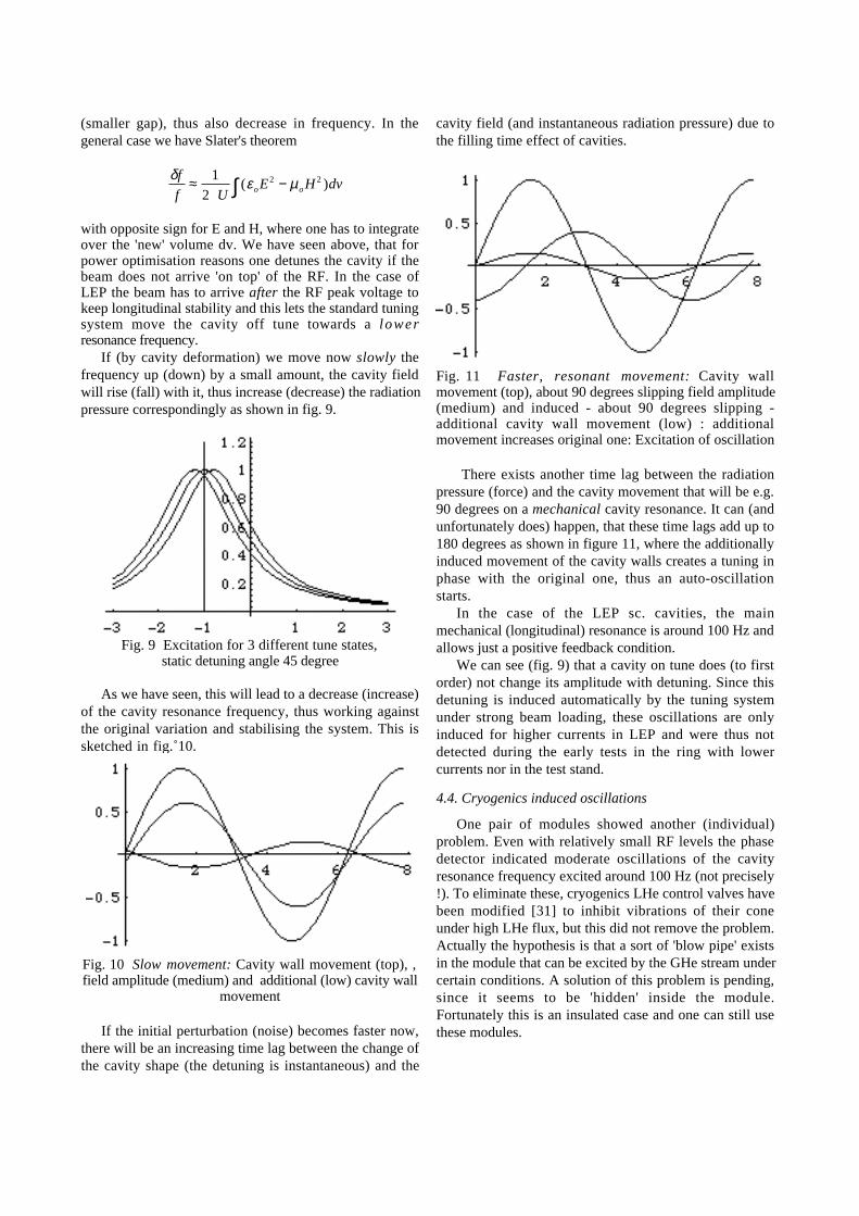
(smaller gap), thus also decrease in frequency. In thegeneral case we have Slater's theorem

δf

f≈ 1

2 U(εoE2 − µo∫ H 2 )dv

with opposite sign for E and H, where one has to integrateover the 'new' volume dv. We have seen above, that forpower optimisation reasons one detunes the cavity if thebeam does not arrive 'on top' of the RF. In the case ofLEP the beam has to arrive after the RF peak voltage tokeep longitudinal stability and this lets the standard tuningsystem move the cavity off tune towards a lowerresonance frequency.

If (by cavity deformation) we move now slowly thefrequency up (down) by a small amount, the cavity fieldwill rise (fall) with it, thus increase (decrease) the radiationpressure correspondingly as shown in fig. 9.

Fig. 9 Excitation for 3 different tune states,static detuning angle 45 degree

As we have seen, this will lead to a decrease (increase)of the cavity resonance frequency, thus working againstthe original variation and stabilising the system. This issketched in fig. 10.

Fig. 10 Slow movement: Cavity wall movement (top), ,field amplitude (medium) and additional (low) cavity wall

movement

If the initial perturbation (noise) becomes faster now,there will be an increasing time lag between the change ofthe cavity shape (the detuning is instantaneous) and the

cavity field (and instantaneous radiation pressure) due tothe filling time effect of cavities.

Fig. 11 Faster, resonant movement: Cavity wallmovement (top), about 90 degrees slipping field amplitude(medium) and induced - about 90 degrees slipping -additional cavity wall movement (low) : additionalmovement increases original one: Excitation of oscillation

There exists another time lag between the radiationpressure (force) and the cavity movement that will be e.g.90 degrees on a mechanical cavity resonance. It can (andunfortunately does) happen, that these time lags add up to180 degrees as shown in figure 11, where the additionallyinduced movement of the cavity walls creates a tuning inphase with the original one, thus an auto-oscillationstarts.

In the case of the LEP sc. cavities, the mainmechanical (longitudinal) resonance is around 100 Hz andallows just a positive feedback condition.

We can see (fig. 9) that a cavity on tune does (to firstorder) not change its amplitude with detuning. Since thisdetuning is induced automatically by the tuning systemunder strong beam loading, these oscillations are onlyinduced for higher currents in LEP and were thus notdetected during the early tests in the ring with lowercurrents nor in the test stand.

4.4. Cryogenics induced oscillations

One pair of modules showed another (individual)problem. Even with relatively small RF levels the phasedetector indicated moderate oscillations of the cavityresonance frequency excited around 100 Hz (not precisely!). To eliminate these, cryogenics LHe control valves havebeen modified [31] to inhibit vibrations of their coneunder high LHe flux, but this did not remove the problem.Actually the hypothesis is that a sort of 'blow pipe' existsin the module that can be excited by the GHe stream undercertain conditions. A solution of this problem is pending,since it seems to be 'hidden' inside the module.Fortunately this is an insulated case and one can still usethese modules.

L

4.5. Fighting the ponderomotive oscillations

The external constraints (production from sheet metal,350 MHz, about 4 cells, 5-6 MV/m, up to 14 mA beamcurrent) nearly automatically lead to a design sensitive forPO. Therefore it is nearly impossible and would be linkedto terrible constraints in other areas to build a cavityintrinsically free from this effect (and most of the cavitiesexist already). Therefore we have to fight it by externalmeans.

One possibility would be external mechanicalattenuation. Measurements [32] have shown that the'natural' attenuation of the system has mechanical Q-values of 10-20. A more detailed analysis [33] showed thateven much stronger attenuation will not guarantee cavitiesfree from these oscillations up to the highest field.

Fig. 12 shows the growth rates of a cavity withmechanical Q=20 for different tuning angles. One deducesthat at 2 MV/m there is no positive growth rate, but at 6MV/m for nearly all negative tuning angles - indirectlyforced by the arrival of the beam after the RF peak voltage

- instabilities are excited. The only region remainingstable is close to 'on tune', as already proposed by [34],but asking for higher RF reflections (see later)

-1.00E+02

-5.00E+01

0.00E+00

5.00E+01

1.00E+02

1.50E+02

- 9 0 - 4 0 1 0 6 0

2 MV/m

4 MV/m

6 MV/m

Fig. 12 Ponderomotive growth rates [1/s] as function ofthe detuning angle for a mechanical Q=20 for different

fields

feed—forwardfilter

Imag

Mechanicaltransferfunctionof cavity

G'Transfer FunctionAmplitude -> Tune X

Gxp

Tuningloopfilter

SelectiveFilter

av

∆φ

GxaStandard tuning loop

Feed forward

Parallel loop

x = δω/σ

Fig. 13 Tests to suppress the ponderomotive oscillation

It was tried [32] to fight the oscillations by electronicmeans in the tuner control loop (see fig. 13). One cannotsimply increase the loop gain since other oscillations willbe excited, but one possibility is a dedicated filter tuned tothe PO excitation frequency with high gain amplificationparallel to the normal filter (feed back). Anotherpossibility is to measure the amplitude set-value and itsvariations and 'guess' with the known (?) transferfunctions the reaction of the cavity, counteracting inadvance (feed forward)

Both methods have been tried, but both showed thesame problems. It was possible to suppress the PO undercertain conditions, but often other oscillations wereexcited and in any case the setting of the parameters wasso critical, that one can not count on a reliable operationof about 250 cavities in the ring.

Therefore the only reliable way is to run the cavities'on tune'. We will look for the price in the next section.To realise such a tuning system is more complicated thanthe standard one (e.g. one would need a beam RF signalcorrect in amplitude and phase) and it was tried toapproximate the 'on tune behaviour' with the existing tunesystem. This was done in setting a fixed detuning angle,thus the cavity was not exactly on tune at lower field(where things are much less critical, see fig. 12), butapproach sufficiently the 'on tune state' at high field toavoid PO.

The 68/70 GeV run was mastered in this way and POhave not been a problem during all coasts. However, oneshould keep in mind that the currents in LEP in thisperiod were significantly lower than the later expectedpeak currents and we will have a look for this case now.

4.6. Running cavities on tune

We have seen in section 4.1. the expression for theincident and reflected currents and corresponding powers. Ifwe run on tune, the imaginary part of the current cannotbe made to zero but we have forced δω=0 and the incidentpower increases by the corresponding amount (the real partof the current remains unchanged)

δP = 12

Ql (R / Q) (Ib sin(φ ))2

The maximum current (in theory power limited) isabout 14 mA and at top energy and field, the synchronousphase angle (measured here from peak RF to beam arrival)is about 30 degree. With our standard values Ql=2 106

and (R/Q)=232 Ω (circuit Ω !!), the additional power isabout 10 kW while the beam power is 125 kW, thus we'waste' 8% of the energy.

At injection things look worse since with the samecurrent the synchronous phase angle is about 90 degree,thus the 'wasted' power is 45 kW.

Fortunately at this moment the beam needs only a fewkW (20-22 GeV) and the klystron can still deliver the totalpower. Concerning the power bill one should consider thatthe injection phase is much shorter than the coast.

This looks quite reasonable, however, there remainsone hidden problem once the peak currents announced arereached. For optimised settings we have no more reflectedpower at peak field and nominal beam current. If we stay'on tune', we add about 10% of reflected power in thefeeder line, including the power coupler. This does notseem much, but 10% power corresponds to 32% involtage and the corresponding standing wave has peakvalues of 132% in voltage or 174% in equivalent power !!

For the main coupler - the MP runs at the peakvoltage region - this means that the level shifted out ofthe operational range by the decision to use a 75 Ωcoupler is in the range again and couplers have to beprocessed 'across' this level. There exists one possibilityaround this problem, however, additional hardware has tobe built.

4.7. Reducing the power coupler load on tune

We have seen the model to describe a cavity with beamand generator in fig. 5. This leads to the following idea:

powercoupler

X

beam generator

reactiveload

Fig. 14: Adding a reactive load between generator and power coupler to compensate overloading

If one adds the very small reactive load X betweengenerator and power coupler we have two degrees offreedom: We can run the cavity alone with beam loadingcompensation, thus seen downstream along the maincoupler, the loading of the latter is minimised. WithoutX, evidently the PO could restart again, but tuning X suchthat cavity and X together form a tuned resonator, eachchange of the cavity frequency does not change theamplitude in first order, thus PO will not start out of thenoise.

Evidently, to use this method literally, we have toadapt X to the different states of beam current, cavity fieldand phase angle during injection, ramping (and coast).This would require a relatively expensive construction.

To avoid this financial problem, there exists the 'poorman's solution': adapt a fixed (and less expensive) reactiveload to the worst case, which does not cancel completelyeverywhere but reduces overloading of the coupler. Ananalysis of the different cases can be found in [26] and one

=¢$ / $%=

sees that this load is not necessary as long as one remainssomewhat below the announced peak beam currents.

Fig. 15 shows a sketch how such a reactive load mightbe realised.

react. load

from klystron

Fig. 15 Realisation of a small reactive load

5. CONCLUSIONS

The power coupler problems can be considered solved,provided one keeps the established production, processingand operations methods. In parallel also the ceramicwindow was modified so that over-heating was notobserved any more.

The abandon of the adjustable version of the powercoupler has taken the possibility to adjust for field profilescatter, but a tested λ/4 transformer exists to compensatefor the few (only one till today) extreme cases.

Concerning higher order modes, up to about 2 GHzHOM couplers 'do their job', even above the specifiedfrequency range. HOM coupler quenches have not clearlybeen observed any more. There have been very few'incidents' [35] during the high current (HERA) run, butthese did definitely not drive the coupler really hot. Thereare no indications of excessive heating of bellows andcones in the modules up to today's beam currents.

Above 2 GHz the power expected from calculationswas not found, which leaves a question-mark, but thereexists a tested design of an absorber capable to annihilatethese modes if this proves to be necessary in the future.

The problem of RF transport for the HOMs throughthe insulation vacuum has been solved conclusively forthe 45 degree Nb/Cu industry cavities with the use of therigid coaxial line. However, one should not forget that 10modules with cooled cables exist in the ring which are notguaranteed (but might still work, depending on the HOMexcitation) for the announced peak beam currents.

The same task has not yet been completely solved forthe 30 degree modules. Studies to use semi-rigid cables areunder way.

Concerning the cavities and modules, they have beenworking reliably. Two cases of degradation have beenobserved. One could already be recovered by high powerpulsed processing in the ring [36]. For the second onethere was not enough time (and hardware not immediatelyavailable) to try the same method.

The problem of 8 cavities with one generator can becircumvented with the λ/4 transformer for extreme casesand we have to live with the smaller variations. Theponderomotive oscillations have been safely suppressed in

running close to tune. Finally, the cryogenic inducedoscillations still persist.

The 68/70 GeV run has demonstrated that the cavitiesand couplers fulfil the expectations and the Mega-Voltscan be delivered. A trivial problem independent of themodules limited the voltage corresponding to 68 GeV, butat this beam energy many stable coasts showed also thereliability of the system.

6. REFERENCES

[1] E. Haebel et al., Proc. 3rd Workshop on RFSuperconductivity, Ed. K. Sheppard, ANL-PHY-88-1.

[2] J.Tückmantel et al., "Improvements to Power Couplersfor the LEP2 Superconducting Cavities", Proceedings of'95 PAC, Dallas, Texas, 1995.

[3] J.P. Budlinger et A. Laisne, NIM 61 (1968), 253-259 (inFrench).

[4] J. Tückmantel, Proc. CERN Main Coupler Workshop, Oct1992, Editor C. Wyss.

[5] E. Somersalo et al, TESLA report 94-14.[6] E. Haebel, Part. Accel., Vol. 40, P 155[7] C. Benvenuti et al, CERN LEP2 Note 94-21.[8] G. Bachy , priv. comm.[9] H.P. Kindermann, priv. comm.[10] H.P. Kindermann, R. Maleyran, CERN SPS/88-1 (ARF).[11] E.Haebel, priv. comm.[12]O. Brunner, CERN SL/MD Note 130[13] E.Haebel, priv. comm.[14] O. Brunner and G. Geschonke, Proc. of LEP Performance

Workshop, Chamonix 1995[15] O. Brunner, priv. comm.[16] Y.H. Chin CERN/LEP/TH 88-3 (1983)[17] R. Baskaran and E.Haebel, "Estimation of the Power

Deposited in Different Frequency Ranges for the LEP SCCavity Module", LEP2 Note 93-01 (1993)

[18] E.Haebel and E Plawski, "Influence of the beam bunchlength on the HOM power deposition in the sc LEPcavities", LEP2 Note 94-19 (1994)

[19] M. Jimenez, priv. comm[20] E.Haebel, priv. comm.[21] M. Jimenez, this workshop[22] M. Barranco-Luque et al, priv. comm.[23] G. Cavallari et al., "Status Report on Sc. RF cavities at

CERN", Proc. 5th Workshop on RF Sc, 19-23 Aug. '91,Editor D. Proch, DESY

[24] D. Boussard, priv. comm.[25] E. Peschard, this workshop[26] J. Tückmantel, CERN-SL-note 95-100 (RF)[27] H.P. Kindermann, priv. comm.[28] M. M. Karliner, V. E. Shapiro and I. A. Shekhtman:

"Instability in the walls of a cavity due toponderomotive forces of the electromagnetic field", Sov.Phys. Tech. Phys, Vol 11 (1967)

[29] P.H. Ceperley: "Ponderomotive oscillations in asuperconducting helical resonator", IEEE Trans. on Nucl.Sci., Vol. 19, no 2 (1972), p217ff

[30] E. Haebel and J. Tückmantel, unpublished[31] Ph. Gayet, priv. comm.[32] D. Boussard, P. Brown and J. Tückmantel:

"Electroacoustic instabil i t ies in the LEP2superconducting cavities", CERN-SL 95-81 RF

[33] J. Tückmantel, CERN-SL-note 95-119 (RF)[34] D. Boussard, priv. comm.[35] G. Geschonke, priv. comm.[36] J. Uythoven, priv. comm.

fW/NfW/qfi

L\ \ J \ / AKJ/kj

RF System for High Intensity

Ernst PeschardtSL Division

Abstract

When LEP is fully equipped with 272 SC cavities theimpedance at the fundamental RF frequency is very high,135 G½ compared to 10.2 G½ for 120 copper cavitiesonly. For high intensity beams this can provoke beaminstabilities at injection energy when the beam inducedvoltage is high compared to the generator voltage and athigh energy when the stable phase angle approaches 90°.This instability can be cured with an RF feedback system(fast control of the amplitude and phase of the vector sumof eight cavities) which reduces the shunt impedance seenby the beam. This feedback system also helps againstcavity voltage oscillations caused by electromagneticexcitation of mechanical resonances. However klystrontrips are more likely with this feedback so a procedure forreliable switch-on with high beam currents should beestablished.

For LEP2 the frequency of the longitudinal feedbacksystem will be changed so that the system can be used fora bunch spacing which is a multiple of six RFwavelengths if it is possible to tune the resonantfrequency of the cavities down to 997.9 MHz; if not abunch spacing of 118 RF wavelengths will be used.

1 INTRODUCTIONWhen LEP is fully equipped with 272 super-

conducting cavities the impedance at the fundamental RFfrequency is very high, about 135 G½ compared to10.2 G½ for LEP1 with 120 room-temperature cavities.At the same time the beam current will be high, up to14 mA d.c. Problems with beam stability due to staticbeam loading are therefore foreseen.

Basically the cavity impedance at the fundamental RFfrequency provokes two different instabilities [1]:

1. The first Robinson instability which is intensityindependent causes longitudinal dipole oscillations.

2. The second Robinson instability which is beamcurrent dependent. When the stability limit is reachedlongitudinal focusing is lost for the dipole mode.

2. THE FIRST ROBINSON INSTABILITYAccording to Robinson a beam is stable with an RF

system if the real part of the cavity impedance is agrowing function of energy. This means that above

transition energy the cavities should be tuned to belowthe RF frequency.

What is important for the evaluation of this instabilityis the difference in impedance at the lower and uppersynchrotron sideband (Figure 1).

Frequency

fRF

+fs

-fs

Figure 1: Robinson stability above transition. Theimpedance at the synchrotron sidebands is highest for theparticles with the highest energy.

In LEP this instability is weak for two oppositereasons:• For the coupled copper cavity assemblies theresonance width is large compared to the revolutionfrequency so that detuning does not change significantlythe sum of the impedances at the lower and uppersynchrotron sidebands (Figure 2).

Frequency deviation [kHz]

0.00

5.00

10.00

15.00

20.00

25.00

-80 -60 -40 -20 0 20 40 60

Figure 2: Impedance curve for a copper coupled cavityassembly. The vertical lines show revolution frequencyharmonics.

In fact an experiment was done in 1991 and it wasfound that the low intensity dipole oscillation amplitudewas independent of tuning angle from -30 to +30° [2].• On the contrary, for the SC cavities the resonancewidth is very narrow compared to the synchrotronfrequency. This means that the resistance at the twosynchrotron sidebands is not changed significantly bydetuning (Figure 3).

Deviation from resonance [Hz]

0.00

100.00

200.00

300.00

400.00

500.00

-1000 -500 0 500 1000

-f +fs s

Figure 3: Real part of the impedance for an SC cavity

with a loaded Q of 2 × 106.

Quantitatively the friction term which causesRobinson damping is given by:

α =

2πfs IDC (ZR− − ZR

+ )2VRF cosϕ s

where fs is the synchrotron frequency, IDC the DC beam

current, (ZR− − ZR

+ ) the difference of the real part of thecavity impedance at the lower and upper synchrotron

sideband, VRF the peak RF voltage and ϕ s the stablephase angle.

Typical parameters at injection energy duringoperation in autumn 1995 were:

fs = 950 Hz

IDC = 6 mA

VRF = 170 MV

ϕ s = 170°For a rather large detuning of let us say 30° (50 Hz)

the difference in Re(Z) at the synchrotron sidebands is0.83 M½ for one cavity or about 50 M½ for the 60 SCcavities which have been installed in LEP until now.

The damping rate (or excitation rate if the detuning ispositive) is then

α = 5. 3 s -1

which is comparable to the longitudinal synchrotron

radiation damping rate of about 10 s-1.

For LEP2 version 4 the number of cavities will haveincreased to 272. For the same Qs on the 108° lattice the

damping rate is 27 s-1.

3 THE SECOND ROBINSONINSTABILITY

The limit for the second Robinson instability is givenby:

Y sin(2φz ) = 2cos ϕB

where Y is the relative beam loading (Y = IB/I0), ϕB is

the stable phase angle and ϕ Z the detuning angle whichautomatically increases with the beam loading when thetuning system keeps the phase between the generatorcurrent and the total cavity voltage constant (Figure 4).

IB

ϕ s

VB

VT

VG

ϕz

Figure 4: Vector diagram showing the relationshipbetween beam and generator voltages.

Expressed with words, this limit is reached when thebeam loading is so high that the generator voltage is inopposite phase to the beam current. Longitudinalfocusing is then lost for the dipole mode and the bunchwill grow exponentially until current losses re-establishstability [3].

For LEP1 this instability has never been a problem.The impedance of the copper cavities is relatively lowand the beam current moderate (Figure 5). For 10 mAand 170 MV the relative beam loading is about 1.2, farbelow the minimum stability limit of 2.

rk

ull

Detuning Angle [deg.]

0.00

1.00

2.00

3.00

4.00

5.00

-90 -45 0 45 90

Vb/V

Unstable

"Unstable"

Detuning curve

LEP 1

Figure 5: Robinson stability limits above transition andthe detuning curve for a stable phase angle of 180°. For apositive detuning angle LEP is only potentially unstable.

For LEP2.4 with 272 SC cavities the relative beamloading can be higher than 10 at injection with the

present Qs. At high energy where ϕB is close to 90° thestability limit is also reached for the SC cavities when thepower absorbed by the beam is so high that the cavity is amatched load for the generator. At 90 GeV and 2200 MVthis happens when the beam current is about 12 mA if the

loaded Q of the cavities is 2 × 106.

The threshold for this instability can be raised in fourdifferent ways:

1. By cavity detuning. This turns the vector for thebeam induced current back to an angle it would otherwisehave reached at a lower current. However, this costsgenerator power because then the generator current is notin phase with the total voltage. The extra power requiredis inversely proportional to the cosine of the detuningangle.

2. With a high Qs scheme. This requires high RFvoltage at injection so the relative beam loadingdecreases and reaches only a value of 2.5 at injectionwith 10 mA DC beam current and 1050 MV RF (Qs =0.18 on the 108° lattice) but the system is still potentiallyunstable.

3. By switching on RF units at an intermediateenergy. This decreases the impedance at injection underthe condition that the unused cavities are detuned.However, this procedure should be avoided because it istime consuming and there is a risk that the complicatedswitch-on procedure aborts with an error message.

4. With a vector sum feedback system. This decreasesthe impedance seen by the beam by a factor which isequal to the loop gain. Such a system is being developedfor LEP.

4 VECTOR SUM FEEDBACK

4.1 System description

In LEP one klystron drives eight cavities. This meansthat the vector sum for eight cavities has to beconstructed (Figure 6).

The correct amplitude of each signal is obtained bycancelling differences in antenna calibrations and cableattenuation with a well defined fixed attenuator at eachinput.

The correct phase is obtained by measuring therelative phase of each of the antenna signals andcompensating differences with short cables of welldefined electrical lengths.

The signal at the output of the second combiner isthen a true picture of the voltage seen by the beam.

The filter has been inserted in order to avoidexcitation of other modes than the ¹ mode.

The vector sum signal is compared to an RF referencesignal in a combiner and the error signal drives theklystron through the driver amplifier. In fact, the systemtries to keep the total cavity voltage equal to the generatorvoltage in amplitude and phase by adding a vector whichcancels the beam induced voltage (Figure 4).

The amplitude of the generator voltage is controlledwith the modulator which is connected to the globalvoltage system.

Σ

Σ

Σ

C 1

C 2

C 3

C 4

C 5

C 6

C 7

C 8

K

Global voltage control

φ

RF ref. in

Phaseloop

Power/current feedback

Mod.

Figure 6: Simplified block diagram of the vector sumfeedback system.

When the system is setup the phase shifter is adjustedfor maximum stability, i.e. the total phase shift in theloop has to be 180° plus an integer number of RFwavelengths.

|

A :‘

—\_

|

I 82

8

H fl???

Even then stability can be a problem. The cavityphase can practically vary by ± 90° and the klystronphase shift varies by about 60° from minimum tomaximum current. With additional uncontrollable phasevariations the usual 135° stability criterion is thereforeeasily exceeded. A klystron phase loop which keeps thephase at the output of the circulator constant with respectto the feedback error signal has therefore been added.This means that the vector sum feedback has less phasevariations to compensate. This loop has been made slowin order to avoid conflicts with the vector sum feedbackloop.

A second slow loop has been added. This varies theklystron current as function of output power. This loopkeeps the klystron collector dissipation below about700 kW and acts as an energy saver by keeping theklystron current low when the required output power islow.

4.2 Advantages of the system

The gain of the vector sum feedback loop has beenadjusted to 26 dB when the klystron current is about 10 Abut it varies linearly with the klystron current. It islimited by the precision with which the vector sum can beconstructed. The cavity impedance seen by the beam isthen decreased by the same factor. This should besufficient to ensure that the second Robinson stabilitylimit is exceeded.

Other advantages of the system are:1. Voltage loss caused by a trip of another unit is

prevented [4]. When the total RF voltage suddenlydecreases the change of the stable phase angle causes animmediate voltage loss which is not compensated beforethe voltage loop reacts (Figure 7). For scalar feedbackthis takes about 100 ms, for vector sum feedback lessthan 1 ms.

I B I

I

T

Gsϕ

Figure 7: Vector diagram illustrating voltage loss in anSC RF unit when a klystron in another unit trips.

2. Cavity voltage and phase oscillations caused byelectromagnetic excitation of mechanical resonances arenot seen by the beam. However, the voltage loss causedby these oscillations is not prevented because theoscillation frequencies are different from cavity to cavity.

3. The feedback system compensates for offsets in thetuning system. An offset is often added on purpose inorder to prevent ponderomotive oscillations [5]. Withoutthe vector sum feedback this offset has to becompensated by changing the unit phase.

4. The over-voltage caused by a beam loss iscompensated. If the operating conditions are such that thecavity is a matched load for the generator and the beam issuddenly lost or dumped, the cavity acts as an opencircuit and the voltage in the cavity will double. This isdetected by the feedback system which then decreases thedrive level.

4.3 Disadvantages of the system

With vector sum feedback klystron trips are morelikely because the RF unit is much more sensitive toamplitude or phase variations in the low power partcaused by for example microphonics in the electronics.Any disturbance is multiplied by the loop gain.

In addition fault-finding is difficult. If a unit tripsfrequently it is difficult to find out if it is due to theklystron, the low power electronics, a cavity or a badcontact in a connector. Therefore the system will bemade such that it is easy to change from vector sumfeedback to scalar sum feedback. If this is done for only afew units beam stability is still preserved The importanceof this matter should be underlined because in phase 2.4of LEP, 36 SC RF units will be in operation.

5 SWITCH-ON PROCEDURES

5.1 Without beam

The procedure for switching on an RF unit withoutbeam is well established and can be thoroughly testedduring cavity conditioning. To avoid conflicts betweenthe klystron phase loop and the vector sum feedback thelatter will not be switched on before the klystron phaseloop has stabilised the phase at the output of the klystronand the cavities are tuned. Nevertheless, because of thecomplicated switch-on procedure continuous running ofthe RF units is preferable (Figure 8).

5.2 With beam

With high beam current the switch-on is not so easybecause it is possible that the cavities tune on the beam-induced voltage instead of the generator voltage. This canhappen due to noise or because the antenna acts as a pick-up and sees a beam signal which is relatively highcompared to the cavity voltage when the cavity is farfrom tune [6].

The beam current reading is now available in the RFcontrol system. This is used to adjust the klystron outputpower to a value which almost guarantees that thecavities tune on the generator voltage.

Due to the slow thermal tuning system it can happenthat seven of the eight cavities are tuned. For the lastcavity high power is still required for a modest field. Thismeans that the field in the cavities already tuned can berather high, 5 to 6 MV/m, and the total field of the unitnot very well controlled. For this reason the globalvoltage control is set to be inactive until all the cavitiesare in tune.

At injection where the stable phase angle is close to180° it is also important that the unit phase is correct.With less than 90° phase difference between generatorvoltage and beam induced voltage the beam pumpspower into the cavity. This power is reflected back to thegenerator through the power coupler and with non-idealdirectional couplers in the waveguide it can generatesignals which disturb the tuning system.

6 THE LONGITUDINAL FEEDBACKSYSTEM

Usually a longitudinal feedback system works at afrequency which is an harmonic of the RF frequency.This is not the case for the LEP feedback system.Development cost and time was significantly reducedbecause DESY generously supplied four 1 GHz cavitieswith a tuning range of -2.4 to +1.3 MHz. Within thisrange the harmonic number was chosen to be a multipleof 360 and as close as possible to 1 GHz. The frequencyis then:

fFB =

24787

fRF = 999. 95 MHz

This means that the system can only work with bunchtrains if the bunch spacing is 87 RF wavelength or amultiple thereof.

In order to optimise the bunch spacing with respect tobeam separation and BOM operation it is planned tochange the feedback frequency for LEP2. The largestflexibility is obtained for:

fFB =

176

fRF = 997. 926 MHz

The system can then be used for a bunch spacingwhich is a multiple of six RF wavelengths. This impliesmodifications to the low power electronics, especially thefrequency generation system. In addition, in order to keepthe cavities a multiple number of half wavelengths fromthe IPs they have to be moved 2.04 cm towards IP6.

A disadvantage of this solution is that the harmonicnumber is not a multiple of eight but only of four

(88740). This means that the system cannot be used foreight equidistant bunch trains, a mode of operation whichwas used occasionally last year in order to accumulatehigh current in one beam.

A second and more serious disadvantage is that now itis very difficult to tune the cavities down to 997.9 MHzbecause fixed tuners were inserted in the cavities whenthey were modified for bunch train operation. The extratuners made it easier to decrease the Q of the cavities [7].

There is, however, another solution. If the feedbackfrequency is left unchanged and a certain phasedifference between bunch a and b is tolerated it ispossible to find a bunch spacing within an acceptablerange for which the phase error is small. A good choice is118 RF wavelengths. The distance between bunch a and bis then 335.0115 wavelengths at the feedback frequencyand the phase difference between bunch a and b 4.1°which is fully acceptable. For the beam observationsystem and the beam separation in the bunch train bumpsa distance of 118 RF wavelengths is also a good choice.

7 ACKNOWLEDGEMENTThanks are due to A. Butterworth and E. Ciapala who

wrote the flow chart of the switch-on procedure.

8 REFERENCES[1] K.W. Robinson, "Stability of beams in Radio

frequency systems", CEAL-1010, Feb. 1964.

[2] E. Peschardt, "Observation of Longitudinal BunchOscillations" Proc. of the second workshop on LEPperformance, Chamonix, Jan. 1992, pp 215-17.

[3] D. Boussard, "Design of a ring RF system", Proc. ofthe fourth general accelerator physics course, Jülich,pp 294-322.

[4] D. Boussard, "Transparencies from discussion dayon LEP operation at 70 GeV", Ferney Voltaire, Oct.1995.

[5] J. Tückmantel, "Performance of cavities", Proc. ofthis workshop.

[6] D. Boussard, Private Communication.

[7] E. Peschardt, "Longitudinal Feedback for BunchTrains" Proc. of the fifth workshop on LEP performance,

Chamonix, Jan. 1995, pp 57-58.

Exit witherror message

Wait 5 seconds

Check PC output

Set tuner setpoints OPERATION

Switch-on vector sum feedback, klystroncurrent/power loop and GVC

<45 kV

Start

Exit on succesful completion

ReadGroup number, Status output destinationBeam current, Tuning power parameters

Estimate tuning power required

Check driver amplisNot ON

Set appropriate (estimated) current for tuning power

Set RF switch ON

Ramp to tuning power using klystron current, set MS tuner ACTIVE

Max current (10A) exceeded

RF ON?

>180 iterations

Check tuning, |phase error| < 15°

Ramp to switch-on voltage (15 MV) using klystron current

RF ON?

RF ON?



No


Yes


No

No


Yes


No Exit witherror message

Update status

Reset temperature and tuner drive interlocksSet MS tuner INACTIVE, set RF switch OFFReset function generator, set nominal RF phaseSet drive level control and klystron loops remoteSet vector sum feedback OFFSet RF ramp rate, set modulator voltage (2.3 V)Set minimum klystron current, select current loopReset RF switch

Initialise

RF ON?

Figure 8: Flow chart of the switch-on procedure for an SC RF unit with vector sum feedback.

No

D

D

LEP2 UPGRADES AND PLANNING: CAVITIES

Enrico Chiaveri, CERN, Geneva, Switzerland

ABSTRACT

The status of sc cavity production by the threecompanies will be presented, as well as that of ancillaryequipment such as higher-order mode and power couplers.At present 180 bare cavities have passed the intermediateRF test and 40 cryomodules have been accepted.Retrofitting of these, which consists of the installation ofcouplers (HOM and PC), started at the beginning of 1995and has already been completed for 24 modules. Futureplanning, taking into account the completion of “PhaseIII”, implementation of “Phase IV” and retrofitting of allindustrial cryomodules will be presented.

1 INDUSTRIAL PRODUCTIONDuring 1995 the industrial production of sc cavities

and modules in the three firms ANSALDO, CERCA andSIEMENS (now ACCEL) continues, keeping to theplanned schedule. As far as the bare cavities are concerned,particularly for the Nb coating procedure, the companiesmanaged to increase the success rate of first coating to70%, which has to be taken as a good level consideringthe very demanding fabrication procedure. (180 cavitiespassed the RF test.) This was possible thanks to the veryclose collaboration between CERN and the firms.Systematic T-mapping measurement for all bare cavitiesin the vertical cryostat test (not required contractually) and[1] computer control optical bench gave us enoughinformation on Nb coating failure to help industry, duringthe fabrication sequence, to correct any errors in thesequence in good time.

Cryomodule final assembly under clean roomconditions is now very well mastered. Last year 40cryomodules were received as expected and 39 of thempassed the RF acceptance test. One of the major problemswhich we are faced with this year is the decision bySiemens to close the activity in the present place,including sc cavity production. A solution was found bycreating a new company (ACCEL) and keeping thepersonnel who are essential to the sc cavity contract. Thisdifficult period could be overcome by keeping “in situ”the CERN expert in order to assure, during the transitionperiod, the required rate of production.

2 RETROFITTING OF SC MODULESAT CERN

During 1994 we were faced with a major technicalproblem on the RF ancillary equipment, particularly withregard to the power coupler [2]. At present this problemhas been solved but at that time in order to avoidsuspending production CERN agreed with the three firmsto receive, for final RF testing, the sc modules notequipped with HOM and power coupler. This implied thatCERN would be in charge of the final mounting ofcouplers. this operation was called initially retrofitting asit was applied on modules having already been equippedby the firms with bad (variable) couplers. At CERN ateam has been set up who are able to recover all industrialsc modules after the RF test. Retrofitting consists of thefollowing sequence: • opening the cryostats of the module and removing the

superisolation• installing the module in the clean room• assembly of the power coupler and its extension

(double-walled tube), HOM on the cavities• closing the cryostats of the module.

These procedures require very well-trained and wellmanaged personnel, particularly for the clean roomassembly, in order to avoid contamination which couldspoil RF performance. During 1995 24 sc modules wererecovered in this way and only one unit was limited to4.5 MV/m. The sc module containing the limited unithad to be disassembled, an optical inspection made and thedamaged region of the NB layer ground, rinsed with high-purity water followed by the RF test and final assembly,the complete procedure taking only six weeks! This gaveus an idea of the time that would be necessary in thefuture for recovering an sc module from the LEP tunnel ifnecessary.

At present power coupler production is carrying on ata very high rate — four couplers per week, including RFconditioning, with most of the work being done atCERN. As far as higher-order mode couplers areconcerned, a contract was placed with a company(INGOVI-SICN) and the present rate of production is 16HOM/month. In Figure 1 can be seen the future planningfor the RF ancillary equipment, including some spareparts, until the end of the project.

1995 1996 1997 1998

PLANNING HIGH ORDER MODES AND POWER COUPLERS

248

424

520

HOM

JUNE

96

192

299

PC

Figure 1

180

248

CAVITIES

40

54

62

MODULES

24

RETROFITTING

1995 1996 1997 1998

PLANNING DELIVERY AND RETROFITTING OF MODULES

48

62

OCTOBER

AUGUST

Figure 2

\\ \\ \\ \\ \

3 PRESENT STATUS ANDPLANNING

In December 1995 the Finance Committee agreed tonegotiate with the three firms for a contractual option for32 cavities (eight sc modules, two ACCEL, two CERCAand four ANSALDO). At present with this option on theLEP2 project we have to consider three different phases:Phase II, consisting of 168 Nb/Cu cavities (42 scmodules), Phase III consisting of 48 Nb/Cu cavities (12sc modules) and Phase IV consisting of 32 Nb/Cucavities (eight sc modules) for a total of 248 Nb/Cucavities (62 sc modules). Considering the present rate ofproduction, the whole project could be concluded by theend of 1997. In order to achieve this target, CERN has tocontinue to do the retrofitting for all 62 sc modules andmust keep the “in-house” production for the powercouplers. This schedule is summed up in Figure 2.

4 CONCLUSIONSAt three companies (ANSALDO, CERCA, ACCEL)

the series production of Nb/Cu cavities and sc modules isproceeding successfully. In the future 32 more cavitiesmust be produced according to a Finance Committeedecision of December 1995 which gives us a total of 248Nb/Cu cavities (62 sc modules). Our goal is to havefinally in the tunnel at the 1997/98 shutdown a total of68 sc modules (62 regular Nb/Cu industry production,two Nb/Cu partly produced by CERN and four Nb sheetmodules).

REFERENCES[1] K. Schirm, This Workshop.[2] D. Boussard, Proc. 5th Workshop on LEP

Performance, Chamonix 1995, pp.190-4 [CERNSL/95-08 (DI)].

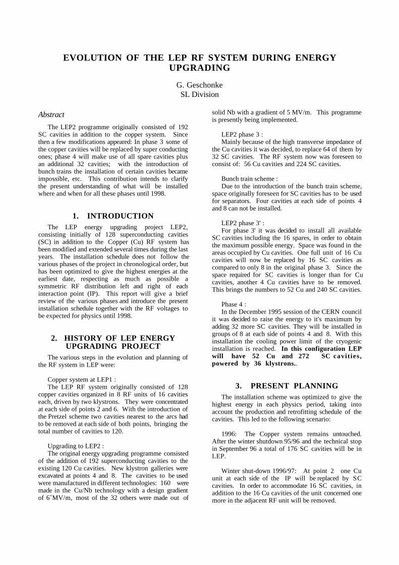
EVOLUTION OF THE LEP RF SYSTEM DURING ENERGYUPGRADING

G. GeschonkeSL Division

Abstract

The LEP2 programme originally consisted of 192SC cavities in addition to the copper system. Sincethen a few modifications appeared: In phase 3 some ofthe copper cavities will be replaced by super conductingones; phase 4 will make use of all spare cavities plusan additional 32 cavities; with the introduction ofbunch trains the installation of certain cavities becameimpossible, etc. This contribution intends to clarifythe present understanding of what will be installedwhere and when for all these phases until 1998.

1. INTRODUCTIONThe LEP energy upgrading project LEP2,

consisting initially of 128 superconducting cavities(SC) in addition to the Copper (Cu) RF system hasbeen modified and extended several times during the lastyears. The installation schedule does not follow thevarious phases of the project in chronological order, buthas been optimized to give the highest energies at theearliest date, respecting as much as possible asymmetric RF distribution left and right of eachinteraction point (IP). This report will give a briefreview of the various phases and introduce the presentinstallation schedule together with the RF voltages tobe expected for physics until 1998.

2. HISTORY OF LEP ENERGYUPGRADING PROJECT

The various steps in the evolution and planning ofthe RF system in LEP were:

Copper system at LEP1 :The LEP RF system originally consisted of 128

copper cavities organized in 8 RF units of 16 cavitieseach, driven by two klystrons. They were concentratedat each side of points 2 and 6. With the introduction ofthe Pretzel scheme two cavities nearest to the arcs hadto be removed at each side of both points, bringing thetotal number of cavities to 120.

Upgrading to LEP2 :The original energy upgrading programme consisted

of the addition of 192 superconducting cavities to theexisting 120 Cu cavities. New klystron galleries wereexcavated at points 4 and 8. The cavities to be usedwere manufactured in different technologies: 160 weremade in the Cu/Nb technology with a design gradientof 6 MV/m, most of the 32 others were made out of

solid Nb with a gradient of 5 MV/m. This programmeis presently being implemented.

LEP2 phase 3 :Mainly because of the high transverse impedance of

the Cu cavities it was decided, to replace 64 of them by32 SC cavities. The RF system now was foreseen toconsist of: 56 Cu cavities and 224 SC cavities.

Bunch train scheme :Due to the introduction of the bunch train scheme,

space originally foreseen for SC cavities has to be usedfor separators. Four cavities at each side of points 4and 8 can not be installed.

LEP2 phase 3' :For phase 3' it was decided to install all available

SC cavities including the 16 spares, in order to obtainthe maximum possible energy. Space was found in theareas occupied by Cu cavities. One full unit of 16 Cucavities will now be replaced by 16 SC cavities ascompared to only 8 in the original phase 3. Since thespace required for SC cavities is longer than for Cucavities, another 4 Cu cavities have to be removed.This brings the numbers to 52 Cu and 240 SC cavities.

Phase 4 :In the December 1995 session of the CERN council

it was decided to raise the energy to it's maximum byadding 32 more SC cavities. They will be installed ingroups of 8 at each side of points 4 and 8. With thisinstallation the cooling power limit of the cryogenicinstallation is reached. In this configuration LEPwill have 52 Cu and 272 SC cavit ies ,powered by 36 klystrons..

3. PRESENT PLANNINGThe installation scheme was optimized to give the

highest energy in each physics period, taking intoaccount the production and retrofitting schedule of thecavities. This led to the following scenario:

1996: The Copper system remains untouched.After the winter shutdown 95/96 and the technical stopin September 96 a total of 176 SC cavities will be inLEP.

Winter shut-down 1996/97: At point 2 one Cuunit at each side of the IP will be replaced by SCcavities. In order to accommodate 16 SC cavities, inaddition to the 16 Cu cavities of the unit concerned onemore in the adjacent RF unit will be removed.

Points 4 and point 8 will be equipped with 8additional SC cavities on each side.

Winter shut-down 1997/98:At point 6 one Cu unit at each side of the IP will

be replaced by SC cavities. In order to accommodate16 SC cavities, 16 Cu cavities plus an additional onein the adjacent unit will be removed.

The configurations with corresponding voltagesafter the various installation campaigns are given intables 1 to 4. In these tables the first line gives the RFunit numbers, the ones marked in bold are the oneswhich will be modified or equipped with SC cavities inthe previous shut-down. In the second row the voltagesof each unit are given in MV. These are the voltagesthat will be lost due to an RF trip. The third rowshows the RF voltages at each side of the interactionpoints and the total for each point. The voltages given

are the maximum achievable, if all cavities run at theirdesign gradient.

4. OPEN QUESTIONSDuring the meeting in Chamonix it became clear,

that the present schedule implies different latticesduring 1997 running in points 2 and 6, because coppercavities have been replaced at IP2 and not at IP6. Thisquestion requires further study and might lead to earlierremoval of the Cu cavities in point 6 without,however, being able to replace them with SC cavities.

In table 2 it is assumed, that during the Septembertechnical stop 12 additional Nb cavities will beinstalled in units 273.1 and 273.2. It is not clear yet,if this is possible, most likely only 8 can be installedfor scheduling reasons.

Jun.96231 Cu 232 Cu 2 3 3 . 1 233.2 IP 2 273.1 273.2 272 Cu 271 Cu

3 5 4 0 8 0 8 0 3 4 4 0 3 52 3 5 3 4 4 1 0 9

431.2 4 3 2 . 1 4 3 2 . 2 433.1 433.2 IP 4 473.1 473.2 4 7 2 . 1 4 7 2 . 2 471.18 0 8 0 8 0 8 0

1 6 0 3 2 0 1 6 0

631 Cu 632 Cu 633.1 633.2 IP 6 673.1 673.2 672 Cu 671 Cu3 5 4 0 8 0 8 0 8 0 8 0 4 0 3 5

2 3 5 4 7 0 2 3 5

831.2 8 3 2 . 1 8 3 2 . 2 8 3 3 . 1 833.2 IP 8 8 7 3 . 1 8 7 3 . 2 872.1 872.2 871.18 0 8 0 4 0 8 0 4 0 8 0 8 0

2 0 0 4 8 0 2 8 0

t o t a l = 1 6 1 4 MV

Table 1: Configuration after the winter shutdown 1995/96

Sep.96231 Cu 232 Cu 233.1 233.2 IP 2 2 7 3 . 1 2 7 3 . 2 272 Cu 271 Cu

3 5 4 0 8 0 8 0 6 8 6 8 4 0 3 5

2 3 5 4 4 6 2 1 1

431.2 432.1 432.2 4 3 3 . 1 4 3 3 . 2 IP 4 4 7 3 . 1 4 7 3 . 2 472.1 472.2 471.18 0 8 0 4 0 8 0 8 0 4 0 8 0 8 0

2 8 0 5 6 0 2 8 0

631 Cu 632 Cu 633.1 633.2 IP 6 673.1 673.2 672 Cu 671 Cu3 5 4 0 8 0 8 0 8 0 8 0 4 0 3 5

2 3 5 4 7 0 2 3 5

831.2 832.1 832.2 8 3 3 . 1 8 3 3 . 2 IP 8 873.1 873.2 872.1 872.2 871.18 0 8 0 4 0 8 0 8 0 4 0 8 0 8 0

2 8 0 5 6 0 2 8 0

t o t a l = 2 0 3 6 MV

Table 2: Configuration after the 1996 September technical stop

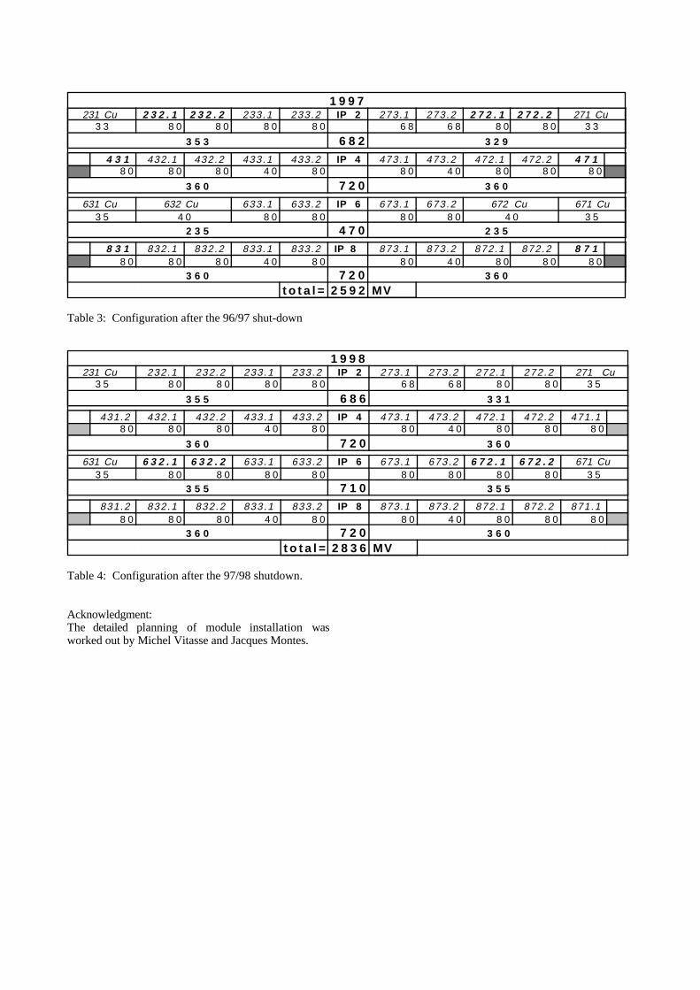
1 9 9 7231 Cu 2 3 2 . 1 2 3 2 . 2 233.1 233.2 IP 2 273.1 273.2 2 7 2 . 1 2 7 2 . 2 271 Cu

3 3 8 0 8 0 8 0 8 0 6 8 6 8 8 0 8 0 3 3

3 5 3 6 8 2 3 2 9

4 3 1 432.1 432.2 433.1 433.2 IP 4 473.1 473.2 472.1 472.2 4 7 18 0 8 0 8 0 4 0 8 0 8 0 4 0 8 0 8 0 8 0

3 6 0 7 2 0 3 6 0

631 Cu 632 Cu 633.1 633.2 IP 6 673.1 673.2 672 Cu 671 Cu3 5 4 0 8 0 8 0 8 0 8 0 4 0 3 5

2 3 5 4 7 0 2 3 5

8 3 1 832.1 832.2 833.1 833.2 IP 8 873.1 873.2 872.1 872.2 8 7 18 0 8 0 8 0 4 0 8 0 8 0 4 0 8 0 8 0 8 0

3 6 0 7 2 0 3 6 0

t o t a l = 2 5 9 2 MV

Table 3: Configuration after the 96/97 shut-down

1 9 9 8231 Cu 232.1 232.2 233.1 233.2 IP 2 273.1 273.2 272.1 272.2 271 Cu

3 5 8 0 8 0 8 0 8 0 6 8 6 8 8 0 8 0 3 5

3 5 5 6 8 6 3 3 1

431.2 432.1 432.2 433.1 433.2 IP 4 473.1 473.2 472.1 472.2 471.18 0 8 0 8 0 4 0 8 0 8 0 4 0 8 0 8 0 8 0

3 6 0 7 2 0 3 6 0

631 Cu 6 3 2 . 1 6 3 2 . 2 633.1 633.2 IP 6 673.1 673.2 6 7 2 . 1 6 7 2 . 2 671 Cu3 5 8 0 8 0 8 0 8 0 8 0 8 0 8 0 8 0 3 5

3 5 5 7 1 0 3 5 5

831.2 832.1 832.2 833.1 833.2 IP 8 873.1 873.2 872.1 872.2 871.18 0 8 0 8 0 4 0 8 0 8 0 4 0 8 0 8 0 8 0

3 6 0 7 2 0 3 6 0

t o t a l = 2 8 3 6 MV

Table 4: Configuration after the 97/98 shutdown.

Acknowledgment:The detailed planning of module installation wasworked out by Michel Vitasse and Jacques Montes.

Discussion: Performance of RF

Jan Uythoven

1 Operational requirements

E. Ciapala gave a general comment: Most of theproblems mentioned in the talk are well known to theRF-group and improvements will be made before '96operation starts (GPIB handler, VME chassis software,Global Voltage Control). The user interface can beimproved, but one has to know what is desired.

M. Lamont, S. Myers: It was concluded that it might be agood idea to stop the ramp after the trip of (some) RFunits during the ramp, if it is clear that otherwise thebeam would be lost because of insufficient RF-volts. Athigh beam energies the beam loss during a stop/start ofthe ramp will probably be limited.

M. Jonker: Any changes of the total RF-volts made withthe Global Voltage Control should also be known toSloppy Soft. At the moment these two systems workindependently. This can cause problems, e.g. if Qs-trimsare being made with Sloppy Soft, after the RF volts havebeen changed with the GVC.

D. Boussard: The total voltages quoted for May andSeptember '96 are both slightly optimistic.

2 Production of cavities

S. Myers: Can the defects as presented in the talk alsooccur with already installed modules in LEP?K. Schirm: The in '95 installed modules have a very goodquality coating, but dust particles could fall on the cavitywall and cause damage after being burned by the RF.D. Boussard: It has happened that a cavity whichperformed well in the string did not reach the 6 MV/m inthe tunnel.J. Uythoven: After degradation of performance of modulesin LEP high power processing has recovered normaloperation.

L. Foa: Is it possible to reach higher cavity fields than thenominal 6 MV/m with the experience gained so far?K. Schirm: It seems we can not go much higher.

S. Myers: Why is the coating only 1.5 µm thick?W. Weingarten: This is the result of calculations, a testwith a 0.5 µm layer showed a degradation of performance.

3 Performance of cavities

P. Darriulat: What is limiting the accelerating field at6 MV/m during normal operation?J. Tückmantel: There is no fundamental reason; for themoment this is the set limit.D. Boussard: At the moment we use an average field of6 MV/m as a set limit, this means that some of thecavities can be running at 7 MV/m. It is not expected thatthe cavities can run much higher.

P. Darriulat: Can we go to a lower temperature to increasethe accelerating field?J. Tückmantel: It is not foreseen to go lower, alsobecause of safety reason. It is now too late to change.

F. Ruggiero: Is it possible that the power which ismeasured at the ferrite absorbers (> 2 GHz) is lower thanexpected because one is measuring at the wrong place?B. Zotter: The power depends critically on the bunchprofile, which is not well known.

4 RF System for high intensity

C. Wyss: By how much is the klystron efficiency reducedwith the vector sum feedback system?E. Peschardt: A few percent, up to 10 %.

6 LEP2 upgrades and planning: RF system

J. Jowett: Is all the information on the installation of thecavities included in the LEP database?C. Wyss: Should be all right, MAD files are createdautomatically.

J. Poole: After the copper cavities have been taken out,when are the magnets going to be moved?G. Geschonke: The magnets will be moved at the sametime as the cavities are taken out.

B. Zotter: How many copper cavities will finally stay in?G. Geschonke: 52.

D. Brandt: The planning to move some of the coppercavities out of LEP in the '96/'97 shut-down and some inthe '97/'98 shut-down is not good for the LEP opticsbecause of the resulting different magnet schemes inpoints 2 and 6. It will be better to move the magnets inboth points at the same time.

SUMMING-UP SESSION:PERFORMANCE OF RF

Daniel Boussard, CERN, Geneva, Switzerland

ABSTRACT

After the successful run of last November, the futuresteps of the LEP2 project, including Phase IV, can beplanned with reasonable confidence. The performance andlimitations of the superconducting cavities are brieflyreviewed together with the modifications necessary to theRF system for LEP2 operation.

1 INTRODUCTIONChamonix 96 is the first workshop in the series where

superconducting RF in LEP is a reality. After thesuccessful run in October-November 95 at energies of 65,68 and 70 GeV, we have gained confidence for the futuresteps of the project, from both the technical and theplanning points of view. It is recalled here that the nextmilestones of the project are as follows:

• 80.5 GeV run in July/August 96• 87 GeV run in October 96• Completion of Phase IV, now approved during the97-98 shutdown.It is interesting to have a quick look at the predictions

(or rather the educated guesses!) presented at the lastworkshop in January 95. Although the details of cavityand module fabrication turned out to be different from theprospects of last January, the planning of installation ofmodules in LEP was remarkably accurate: 14 modules inNovember 95 achieved, 32 planned for June 96. Even theextrapolated curve of 95 fits with the installation of thelast Phase IV modules foreseen during the 97-98shutdown.

This shows not only good luck in preparing the 1995guesses, but also that production and installation ofsuperconducting cavity modules is a mature activity, wellorganized in the firms and at CERN, and for which fairlyreliable schedules can be established.

The extension of LEP2 up to an energy of about97 GeV (called Phase IV) is an approved project as oflast December. In its final form there will be in total 68modules (272 cavities) installed in LEP. They will all beof the standard Nb/Cu type, except four bulk Nb modulesinstalled in Point 2 of LEP. This set-up makes full useof all cryogenic power available and all cavities andmodules produced. There will be no complete sparemodule on the surface available for replacing a faulty onein LEP; only a few additional cavities will be kept readyto refurbish (in about six weeks) a module taken out ofLEP.

The completion of the LEP2 Phase IV programme isforeseen during the 97-98 shutdown, in accordance withthe production schedule in the firms, and with thecapability of the CERN team to complete the modulesafter delivery. It goes without saying that the presentwell-trained teams must be kept until the end of theproject, as well as all equipment needed for constructionand testing.

2 CAVITIESThe choice of Nb/Cu technology, which at the

beginning of the project was the subject of controversialdiscussions turned out to be a success. UndoubtedlyNb/Cu is a difficult technology, requiring more criticalsteps than bulk Nb (sputtering) and great care in thepreparation of the interface between copper and niobium.However this technology is now well under control, asdemonstrated by a predictable average production rate.Although a 100% success rate in the cavity coating isprobably a dream, the average values obtained over theyears showed a remarkable increase up to the present 70%.As important is the quality factor Q0 at the design field(6 MV/m) which increased from year to year as a result ofbetter controlled procedures. In the framework of theLEP2 project, 1700 m2 of copper surface have alreadybeen coated with niobium. This impressive number mustbe compared to the size of a typical defect (1 mm2), lethalfor the Nb coating, in order to evaluate both the difficultyof the project and the present achievements.

There has been tremendous progress made on the RFcouplers in the last year. Complete suppression ofmultipactor in the coupler coaxial line with d.c. biasrescued the project by making vacuum outbursts in thecouplers disappear completely during operation.Conditioning of the couplers (without d.c. bias) appearedvery different in a warm test stand as compared to a coldcavity. This has been understood, and was due to theenhanced secondary emission coefficient of cold surfacescovered with adsorbed gases. The main source is the warmRF window, heated by the RF field during couplerconditioning on a cold cavity. A new procedure has beenimplemented, where the RF window is baked at 200°Cprior to cavity cooldown and the coupler surface is notcooled before conditioning is completed. The gain inconditioning time has been spectacular (one order ofmagnitude). Now the production of couplers (assembledand conditioned at CERN) is on average four couplers perweek, including conditioning.

Experiments are continuing to evaluate the limitperformance of the LEP2 RF couplers. At present300 kW of CW power have been transmitted throughwarm couplers; on a cold cavity an equivalent couplerpower of 250 kW has been achieved. These results areimportant for LEP2, because of the need of a significantsafety margin above the nominal 125 kW per coupler tocope with microphonics and imbalance between cavities.The ongoing R&D on RF couplers is also of greatinterest for all high-intensity applications of sc cavities,in particular for the LHC RF system.

It seems that we have a good solution for the HOMs.There has been no indication of a HOM quench during sccavity operation with beam (admittedly with moderatebeam currents). It should not be forgotten, however, thatthere are still ten modules in LEP with old HOM cablesof limited power capability and one bulk Nb module withold HOM feedthroughs. It is not possible to modify thesemodules in the near future without putting in jeopardy theLEP2 Phase IV installation schedule. As a consequenceHOM power coming out of these modules will have to bewatched carefully as the beam intensity is raised. Thethree bulk Nb modules to be installed must be equippedwith semi-rigid, vacuum-tight cables, which unfortunatelyhave very long delivery times. Therefore, it is foreseenthat two Nb modules will be installed in LEP only inSeptember 96.

The RF ferrite absorbers installed in LEP (one close tothe sc modules, one far away) gave the first experimetnalevidence of HOM power radiated outside the sc modules.Investigations should continue in this direction to betterunderstand where HOM power is finally dissipated. Inparticular more precise temperature measurements of theintercavity bellows (inside a module) would be desirable.

An interesting academic problem (Lorentz forcedetuning, ponderomotive oscillations) has turned into aserious limitation of the LEP2 sc cavities, imposingadditional constraints on their operation. The effectappears because of cavity detuning (to optimize powertransfer to the beam) and the presence of mechanicalresonances of the cavity vessel. The latter are verydifficult to remove, and the only practical choice is todetune the cavities to less than optimum. The price to payis more power from the klystron (at most 10 kW moreper cavity) and higher fields in the coupler (which,however, could be reduced by an outside reactive load).

Running cavities with non-optimum detuning requiresvector sum feedback to ensure proper cavity phasing withrespect to the reference RF voltage and the beam. Such afeedback system will also suppress the effect of externallydriven mechanical oscillations (usually coming from thecryogenic system).

With fixed RF couplers the dispersion in Qext amongthe eight cavities driven by one klystron results in animbalance of cavity fields. The large Qext errors (whichwere shown to be related to distortions of the field flatnessof the cavity) can be corrected by an external λ/4

transformer, as demonstrated experimentally on aninstalled LEP2 cavity.

It remains, however, that in order to reach an averagefield of 6 MV/m over the eight cavities of a klystron,some of them will be pushed higher (say by 10 to 15%).This shows that it is not realistic now to envisage anoperating field significantly higher than the present6 MV/m . In fact LEP2 is the only machine where theoperating average accelerating field is so close to themaximum achieved in the laboratory.

3 RF SYSTEMFrom the point of view of RF, LEP2 is a high-

intensity machine, contrary to LEP1. The difference doesnot come from the modest increase in beam currents, butfrom the large change (more than one order of magnitude)of impedance at the RF frequency. This raises the issue ofbeam stability (2nd Robinson limit) which becomescritical at injection (at low RF voltage) and at high energy(when almost all RF power is transferred to the beam). Inthis high beam loading regime, it has been observed thatdifferent RF units become coupled via the beam,sometimes leading to a catastrophic loss of RF volts.Also switching on an RF unit with beam may beproblematic because of the large beam induced voltages inthe tuning circuits of the individual cavities.

An RF feedback, working on the vector sum of alleight cavities driven by a single klystron is certainly themost appropriate solution to high beam loadingproblems. RF feedback circuits have been successfullyimplemented on modules installed in LEP. This ishowever an added complication which will require moreefforts for complete understanding of the behaviour of RFunits. Fault finding is obviously more difficult in a closedloop system; RF trips are certainly more likely becausethe loop gain amplifies any spurious transient in thesystem and switching on with beam will require a morecomplete procedure. Obviously the control of such asystem is not mature yet; we are still in a phase oflearning how to make the best use of the system and it isnot surprising that easy-to-use facilities from the maincontrol room are not available now. The operations crewshould realise that we do not have well proven proceduresand that it will take some time to implement them into auser-friendly software. The importance of the GlobalVoltage Control has been stressed again, especially inview of keeping the symmetry of the RF distribution.

In spring 96, nine new klystrons will have to beinstalled, debugged, tested and put into operation. This isa considerable effort for a small team of specialists, andone cannot exclude weaknesses in the power system at theJune 1996 start-up. It is known already that the junctionbetween magic T and its 300 kW load is a weak point,which last year led to the burning of a circulator.Solutions are now being tested and hopefully could beimplemented before June 96 on LEP.

To minimize the risks of faults (klystron trips andpossible equipment damage) we decided to deliberately runthe RF system at low power at the beginning of the run..The corresponding maximum beam intensity was set(somewhat arbitrarily) to 4 mA total until we haveenough safety margin to reach the specified energy.

The same strategy was used during the 65-70 GeV runand proved successful. During the 80.5 GeV run, nofallback position at a lower energy will be allowed in caseof major RF failures, which must therefore be avoided byrunning the system very cautiously.

4 FEEDBACKSLongitudinal and transverse beam feedbacks are crucial

for the operation of LEP, although there is no clearevidence of exponentially growing multibunchinstabilities. In this respect, parasitic excitation ofbunches (due to noise?) certainly plays an important role,and it would be desirable to chase possible sources(including the RF system). Microphonics in cavities havebeen quoted as the source of transverse excitation of thefirst bunch in a train, but without any quantitativeestimate.

The longitudinal feedback has been modified to copewith bunch trains, by increasing the bandwidth of the1 GHz cavities. In doing so the centre frequency haschanged, making the choice of bunch spacing morelimited. Despite the fact that an approximate solution hasbeen found, work should continue to bring the cavitycentre frequency closer to its original value, thuspermitting any bunch spacing multiple of 6λRF.

Simulations have shown the interest of the so-called“Russian” feedback against TMCI. A better understandingat the RF engineer level of this quite unusual feedbackprinciple would certainly help bring this clever idea closerto an operational system.

PROCEEDINGS OF THE SIXTH - CERN Document Server

Documents

Transcript of PROCEEDINGS OF THE SIXTH - CERN Document Server