Experimental Investigations on the Influence of thePhotocathode Laser Pulse Parameters on the Electron

Bunch Quality in an RF - Photoelectron Source

Dissertationzur Erlangung des Doktorgrades

des Departments Physikder Universität Hamburg

vorgelegt vonMarc Hänelaus Cottbus

Hamburg2010

Gutachter der Dissertation: Prof. Dr. rer. nat. Shaukat KhanProf. Dr. rer. nat. Jörg Roßbach

Gutachter der Disputation: Prof. Dr. rer. nat. Shaukat KhanPD Dr. rer. nat. Bernhard Schmidt

Datum der Disputation: 22. Juni 2010

Vorsitzender des Prüfungsausschusses: Dr. rer. nat. Georg Steinbrück

Vorsitzender des Promotionsausschusses: Prof. Dr. rer. nat. Jochen Bartels

Leiterin des Departments Physik: Prof. Dr. rer. nat. Daniela Pfannkuche

Dekan der Fakultät für Mathematik,Informatik und Naturwissenschaften: Prof. Dr. rer. nat. Heinrich Graener

KurzdarstellungFreie Elektronen Laser die nach dem SASE Prinzip arbeiten, wie der European XFEL,benötigen Elektronenpakete mit Spitzenstromstärken von mehreren Kiloampère und ge-ringer transversaler Emittanz. Während die hohen Spitzenströme durch longitudinaleKomprimierung der Elektronenpakete erreicht werden kann, muss die transversale Emit-tanz bereits an der Elektronenquelle Werte von weniger als 1 mmmrad aufweisen. DieEntwicklung von Elektronenquellen, welche diese Spezifikationen erfüllen, ist die Aufgabedes Photoinjektor Teststandes bei DESY in Zeuthen (PITZ).Kern eines Photoinjektors ist die Elektronenkanone in welcher die Elektronenpakete er-zeugt werden und die erste Beschleunigung stattfindet. Die Extraktion der Elektronenvon der Katode erfolgt mittels des äußeren lichtelektrischen Effekts, wofür ein Lasersys-tem benötigt wird, welches speziellen Anforderungen genügen muss. Im ersten Teil dieserArbeit wird untersucht, ob das Lasersystem und die Laserstrahlführung diese Spezifikatio-nen erfüllen. Im zweiten Teil der Arbeit wird anhand von Simulationen und Experimentenuntersucht, welchen Einfluß die zeitlichen und räumlichen Eigenschaften der Laserpulseauf die Qualität der damit erzeugten Elektronenpakete haben. Diese Einflussnahme istmöglich, da die Reaktionszeit der Cs2Te Katode klein ist im Vergleich zur Dauer derLaserpulse. Davon ausgehend werden Verbesserungsvorschläge und Toleranzen definiert.

AbstractFree Electron Lasers based on the SASE principle like the European XFEL require elec-tron bunches having peak currents of several kiloamperes as well as very low transverseemittance. While high peak currents can be generated using longitudinal bunch compres-sion techniques, the transverse emittance must have values as low as 1 mmmrad alreadyat the source. The development of electron sources fulfilling these demanding specifica-tions is the goal of the Photo Injector Test Facility (PITZ) in DESY, Zeuthen site.The key component of a photoinjector is the electron gun cavity where the electronsbunches are generated and immediately accelerated. The extraction of the electrons isbased on the photoelectric effect of the cathode which requires a laser system having spe-cial capabilities. In the first part of the thesis, measurements are presented which wereperformed to investigate whether the laser and the laser transport system fulfill theserequirements. The second part of the thesis is dedicated to simulations as well as experi-mental studies on the impact of the temporal and spatial parameters of the laser pulseson the electron bunch quality. This influence is possible because the response time ofthe Cs2Te photocathode is short compared to the laser pulse duration. Based on theseinvestigations, suggestions for improvements are given and tolerances for the laser pulseproperties are defined.

For my family, Jana and SontjeThank you for being part of my life

Contents

1 Introduction 2

2 PITZ - an overview 72.1 Electron bunch acceleration and focusing . . . . . . . . . . . . . . . . . . . 72.2 Electron bunch diagnostics . . . . . . . . . . . . . . . . . . . . . . . . . . . 9

2.2.1 Charge . . . . . . . . . . . . . . . . . . . . . . . . . . . . . . . . . . 92.2.2 Transverse shape and position . . . . . . . . . . . . . . . . . . . . . 92.2.3 Longitudinal phase space distribution and its projections . . . . . . 102.2.4 Transverse phase space distribution . . . . . . . . . . . . . . . . . . 11

3 Laser system and laser pulse diagnostics 123.1 Requirements for the laser system . . . . . . . . . . . . . . . . . . . . . . . 123.2 The laser systems used at PITZ . . . . . . . . . . . . . . . . . . . . . . . . 13

3.2.1 The laser oscillator . . . . . . . . . . . . . . . . . . . . . . . . . . . 143.2.2 The laser pulse shaper . . . . . . . . . . . . . . . . . . . . . . . . . 153.2.3 The regenerative amplifier . . . . . . . . . . . . . . . . . . . . . . . 173.2.4 Double-pass and booster amplifier . . . . . . . . . . . . . . . . . . . 173.2.5 The optical sampling system (OSS) . . . . . . . . . . . . . . . . . . 18

3.3 The laser beamline . . . . . . . . . . . . . . . . . . . . . . . . . . . . . . . 203.3.1 Imaging on the Beam Shaping Aperture . . . . . . . . . . . . . . . 203.3.2 Imaging onto the photocathode . . . . . . . . . . . . . . . . . . . . 21

3.4 Laser pulse diagnostics . . . . . . . . . . . . . . . . . . . . . . . . . . . . . 233.4.1 Temporal laser pulse shape . . . . . . . . . . . . . . . . . . . . . . . 243.4.2 Transverse laser pulse shape . . . . . . . . . . . . . . . . . . . . . . 293.4.3 Laser pulse energy . . . . . . . . . . . . . . . . . . . . . . . . . . . 313.4.4 Laser pulse position . . . . . . . . . . . . . . . . . . . . . . . . . . . 323.4.5 High-speed camera . . . . . . . . . . . . . . . . . . . . . . . . . . . 333.4.6 Diagnostics setup . . . . . . . . . . . . . . . . . . . . . . . . . . . . 34

3.5 Summary . . . . . . . . . . . . . . . . . . . . . . . . . . . . . . . . . . . . 36

4 Measurement of laser pulse properties 374.1 Comparison between the Optical Sampling System and the FESCA200

streak camera . . . . . . . . . . . . . . . . . . . . . . . . . . . . . . . . . . 374.2 Invariance of the temporal laser profile upon transport through the laser

beamline . . . . . . . . . . . . . . . . . . . . . . . . . . . . . . . . . . . . . 394.3 Invariance of the temporal laser pulse shape along the laser pulse train . . 404.4 Spatial dependence of the temporal laser shape . . . . . . . . . . . . . . . 404.5 Investigation of thermal lensing . . . . . . . . . . . . . . . . . . . . . . . . 424.6 The beam size at the vacuum mirror . . . . . . . . . . . . . . . . . . . . . 47

5 The electron emission process 495.1 Photoemission in Cs2Te . . . . . . . . . . . . . . . . . . . . . . . . . . . . 505.2 Field-enhanced emission . . . . . . . . . . . . . . . . . . . . . . . . . . . . 525.3 Mirror charge and space charge-limited emission . . . . . . . . . . . . . . . 545.4 Summary . . . . . . . . . . . . . . . . . . . . . . . . . . . . . . . . . . . . 55

6 Electron beam dynamics 576.1 Phase space representation of the electron beam . . . . . . . . . . . . . . . 576.2 Sources of transverse emittance . . . . . . . . . . . . . . . . . . . . . . . . 59

6.2.1 Cathode emittance . . . . . . . . . . . . . . . . . . . . . . . . . . . 596.2.2 RF induced emittance . . . . . . . . . . . . . . . . . . . . . . . . . 606.2.3 Space charge-induced emittance . . . . . . . . . . . . . . . . . . . . 61

6.3 Transverse emittance compensation and the invariant envelope . . . . . . . 626.4 The longitudinal phase space . . . . . . . . . . . . . . . . . . . . . . . . . . 66

7 Influence of the laser pulse parameters on the electron beam properties 697.1 General considerations . . . . . . . . . . . . . . . . . . . . . . . . . . . . . 707.2 The optimized laser pulse properties . . . . . . . . . . . . . . . . . . . . . 737.3 Influence of the laser pulse duration . . . . . . . . . . . . . . . . . . . . . . 757.4 Influence of laser pulse rise and fall times . . . . . . . . . . . . . . . . . . . 797.5 Influence of modulations on the flat-top . . . . . . . . . . . . . . . . . . . . 837.6 Modulations of the momentum distribution caused by distortions on the

laser pulse . . . . . . . . . . . . . . . . . . . . . . . . . . . . . . . . . . . . 887.7 Transverse laser spot size on the cathode . . . . . . . . . . . . . . . . . . . 927.8 Transverse laser pulse shape . . . . . . . . . . . . . . . . . . . . . . . . . . 94

8 Summary and outlook 102

A The transverse laser pulse shape near the image plane 105

B Signal decay under UV light exposure at Jai M10SX cameras 108

C Technical drawings of the laser vacuum mirror 110

D Error sources during the measurement of the transverse phase spacedistribution 112

E Electron beam dynamics at low bunch charge 118

Acronyms

ADC Analog-Digital-ConverterBBO β-BaB2O4, beta-Barium BorateLBO LiB3O5, Lithium triborateNd:YLF Nd3+:YLiF4, Neodymium doped Yttrium Lithium FluorideYb:KGW Yb3+:KGd(WO4)2, Ytterbium doped Potassium Gadolinium TungstateYb:YAG Yb3+:Y3Al5O12 , Ytterbium doped Yttrium Aluminium Garnetcw continuous waveBSA Beam Shaping ApertureOSS Optical Sampling SystemDFG Difference Frequency GenerationFROG Frequency Resolved Optical GatingSHG Second Harmonic GenerationGRENOUILLE Grating Eliminated No-nonsense Observation of Ultrafast Incident

Laser Light E-fieldsTG Transient Grating

1

Chapter 1

Introduction

One of the most important tools in natural science research is light. It is used to illu-minate objects, investigate materials by measuring their response to light exposure or tointentionally modify matter.In the early 20th century Albert Einstein proposed the principle of Light Amplification byStimulated Emission of Radiation (LASER). It was based on the rate equations of photonabsorption as well as spontaneous and stimulated emission [Eins]. Desirable properties ofthe light produced by the proposed sources led to continuous efforts until the year 1960,when Maiman et al. realized the first laser system based on ruby [Maim]. Shortly after-wards, the first nonlinear optical effect (frequency doubling in quartz) could be observedin 1961, thanks to the high intensity of the laser light [Fran]. Ever since, the frontiersof the available laser pulse properties were pushed forward. Nowadays, it is possible togenerate light pulses with durations of less than one hundred attoseconds using state-of-the-art laser systems [Goul]. The available wavelengths range from the infrared up tothe soft x-ray region. However, hard x-ray radiation is not yet accessible by conventionallaser systems.In the meantime, an alternative way of generating coherent short light pulses emerged. Itis based on the idea, that the radiating electrons do not necessarily need to be bound to anucleus as it is the case for conventional lasers. Instead, the electrons are emitted from asource and accelerated to ultra-relativistic velocities. Subsequently, they pass a magneticstructure with an periodic magnetic field perpendicular to the moving direction of theelectrons1, called undulator (shown in figure 1.1). Due to the Lorentz force, the electronsmove on a sinusoidal trajectory and start to emit electromagnetic radiation in the forwarddirection. This process is called undulator radiation and the emitted wavelength is givenby [FEL]

1The distance between two pole faces having the same direction of the magnetic field is called undu-lator period.

2

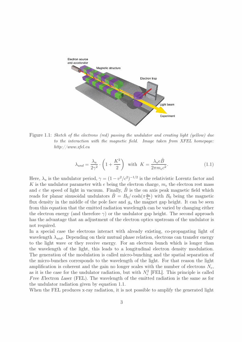
Figure 1.1: Sketch of the electrons (red) passing the undulator and creating light (yellow) dueto the interaction with the magnetic field. Image taken from XFEL homepage:http://www.xfel.eu

λund =λu

2γ2·(

1 +K2

2

)with K =

λueB̃

2πmec2. (1.1)

Here, λu is the undulator period, γ = (1− v2/c2)−1/2 is the relativistic Lorentz factor andK is the undulator parameter with e being the electron charge, me the electron rest massand c the speed of light in vacuum. Finally, B̃ is the on axis peak magnetic field whichreads for planar sinusoidal undulators B̃ = B0/ cosh(π gu

λu) with B0 being the magnetic

flux density in the middle of the pole face and gu the magnet gap height. It can be seenfrom this equation that the emitted radiation wavelength can be varied by changing eitherthe electron energy (and therefore γ) or the undulator gap height. The second approachhas the advantage that an adjustment of the electron optics upstream of the undulator isnot required.In a special case the electrons interact with already existing, co-propagating light ofwavelength λund. Depending on their mutual phase relation, electrons can transfer energyto the light wave or they receive energy. For an electron bunch which is longer thanthe wavelength of the light, this leads to a longitudinal electron density modulation.The generation of the modulation is called micro-bunching and the spatial separation ofthe micro-bunches corresponds to the wavelength of the light. For that reason the lightamplification is coherent and the gain no longer scales with the number of electrons Ne,as it is the case for the undulator radiation, but with N2

e [FEL]. This principle is calledF ree E lectron Laser (FEL). The wavelength of the emitted radiation is the same as forthe undulator radiation given by equation 1.1.When the FEL produces x-ray radiation, it is not possible to amplify the generated light

3

in an optical resonator, because the required optical elements, particularly mirrors withhigh reflectivity, are not available. Hence, the light must be amplified in a single passthrough the undulator. In this case the generation of the light can be subdivided into threesteps [FEL]. At start-up, the light is created from shot noise. Afterwards, the electronsresonantly interact with the light leading to an exponential increase of the light intensity.Finally the FEL amplification process saturates. The onset of saturation is the optimumoperating point of an FEL. After traveling through the undulator, electron bunches aresent to a beam dump and the light can be delivered to the experimental stations (seefigure 1.1). This process of light generation is called Self-Amplified Spontaneous Emission(SASE). The SASE light pulses possess very special properties such as pulse durations inthe femtosecond range, high intensities and a high degree of transverse coherence [FEL,Sald02]. The smallest wavelength demonstrated so far is 0.15 nm [SLAC] while peakbrilliances larger than 1029 photons

s mrad2 mm2 0.1%BW [FLASH] for the fundamental wavelength wereobtained at FLASH. Future FELs like the XFEL will provide light pulses of even higherquality (see table 1.1).To achieve these properties, the requirements on the electron bunch quality are verydemanding. The minimum achievable wavelength, for example, is proportional to thegeometric transverse emittance ε (see chapter 6.1 for the definition of ε) and the energyspread ΔE of the electron bunch [Ros01]

λmin∼= 18πε

ΔE

E·√

γIA

Ip

1 + K2

K2. (1.2)

In this equation, E is the mean energy of the electron bunch, Ip is the peak current andIA = 17 kA is the Alfvén current. The minimum achievable wavelength scales inverselyproportional to the peak current. Conversely, a higher peak current, meaning a largercharge density, causes an increase of the transverse space charge forces and thus a growthof the transverse emittance, which is disadvantageous in terms of low λmin. These con-siderations show, that a proper choice of the electron bunch properties is influenced bymany interdependencies.Another parameter which characterizes the performance of an FEL is the required undu-lator length to achieve gain saturation which occurs at approximately twenty times thepower gain length Lg [FEL]. The latter one is defined as the length needed to amplifythe radiation power by a factor of e. According to [Ferr02], this length is proportional to

Lg ∝ εn · γ3/2

K · √2Ip(1 + K2/2). (1.3)

A reduction of the gain length is an important cost saver since it determines the requiredundulator length. Therefore, it is preferential to have electron bunches with a low trans-verse emittance. In table 1.1, the operating parameters are summarized for the currently

4

Parameter FLASH (run 2007-2009) European XFELElectron bunch properties

bunch charge 1 nC 1 nCenergy at undulator 1 GeV 17.5 GeVpeak current 1-2 kA 5 kArequired transv. norm.emittance at undulator 2.0 mmmrad (proj.) 1.4 mmmrad (slice)

Undulator propertiestotal undulator length 30 m 165 mundulator period λund 27.3 mm 35.6 mmundulator gap gund 12 mm 10 mmpeak magnetic field 0.47 T 1.0 T

FEL radiation propertieswavelength range 6.8 - 47 nm down to 0.1 nmpulse duration 10 - 70 fs 100 fspeak power 1 - 5 GW 20 GWpeak brilliancein photons

smm2 mrad2 0.1%BW 1029 − 1030 5.0 · 1033

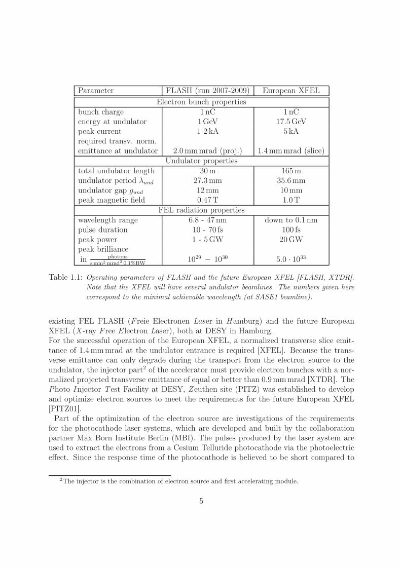
Table 1.1: Operating parameters of FLASH and the future European XFEL [FLASH, XTDR].Note that the XFEL will have several undulator beamlines. The numbers given herecorrespond to the minimal achievable wavelength (at SASE1 beamline).

existing FEL FLASH (F reie Electronen Laser in H amburg) and the future EuropeanXFEL (X -ray F ree E lectron Laser), both at DESY in Hamburg.For the successful operation of the European XFEL, a normalized transverse slice emit-tance of 1.4 mmmrad at the undulator entrance is required [XFEL]. Because the trans-verse emittance can only degrade during the transport from the electron source to theundulator, the injector part2 of the accelerator must provide electron bunches with a nor-malized projected transverse emittance of equal or better than 0.9 mmmrad [XTDR]. ThePhoto I njector T est Facility at DESY, Z euthen site (PITZ) was established to developand optimize electron sources to meet the requirements for the future European XFEL[PITZ01].

Part of the optimization of the electron source are investigations of the requirementsfor the photocathode laser systems, which are developed and built by the collaborationpartner Max Born Institute Berlin (MBI). The pulses produced by the laser system areused to extract the electrons from a Cesium Telluride photocathode via the photoelectriceffect. Since the response time of the photocathode is believed to be short compared to

2The injector is the combination of electron source and first accelerating module.

5

the laser pulse duration [Suber], the temporal laser pulse profile has a direct impact onthe longitudinal electron bunch properties. The same is true for the transverse shape ofthe laser pulses, which is translated to the initial transverse charge density distributionof the electron bunch.In this work, the relations between the photocathode laser pulse parameters and the re-sulting electron bunch properties are investigated experimentally. After an introductionto the PITZ setup, the laser system, the laser transport system (laser beamline) andthe available laser pulse diagnostics are presented. This is followed in chapter 4 by theexperimental characterization of the emitted laser pulses as well as the laser beam trans-port system. Since a large part of the transverse emittance budget originates from thegeneration of the electron bunch, the process of electron emission from a photocathodeis introduced in detail in chapter 5. This is followed in chapter 6 by the presentationof the beam dynamics which takes place after the emission.In chapter 7, the relationsbetween laser pulse parameters and the electron bunch properties will be investigated bysimulations and compared with measurements.

6

Chapter 2

PITZ - an overview

The Photoinjector Test Facility at DESY in Zeuthen (PITZ) is a test bench for thedevelopment and optimization of photo-injector components which are planned to beinstalled at FLASH and the future European XFEL. The main goal is to produce electronbunches with 1 nC charge having a normalized projected transverse emittance of not morethan εn = 0.9 mm·mrad at the injector output. All major components which have aninfluence on the transverse emittance like the gun cavity or the laser system as well asthe available diagnostics are continuously improved and investigated.In the following sub-chapters, the machine setup which has been used for the experimentalinvestigations is introduced. At first, the sub-components associated with the accelerationof the electron bunches will be described. These are the electron gun and the boostercavity together with the solenoid magnets which are used for focusing and compensationof the space charge induced emittance growth. Secondly, the available electron bunchdiagnostics will be summarized.

2.1 Electron bunch acceleration and focusingAt PITZ, two accelerating RF cavities are used, both operated at a frequency of 1.3 GHz(L-band). The electron gun cavity is a 1.6-cell copper cavity, which has a field balance1

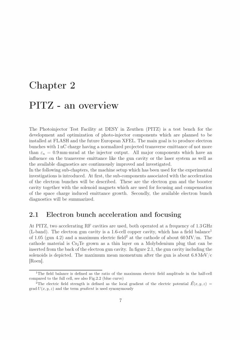
of 1.05 (gun 4.2) and a maximum electric field2 at the cathode of about 60 MV/m. Thecathode material is Cs2Te grown as a thin layer on a Molybdenium plug that can beinserted from the back of the electron gun cavity. In figure 2.1, the gun cavity including thesolenoids is depicted. The maximum mean momentum after the gun is about 6.8 MeV/c[Roen].

1The field balance is defined as the ratio of the maximum electric field amplitude in the half-cellcompared to the full cell, see also Fig.2.2 (blue curve)

2The electric field strength is defined as the local gradient of the electric potential �E(x, y, z) =grad U(x, y, z) and the term gradient is used synonymously

7

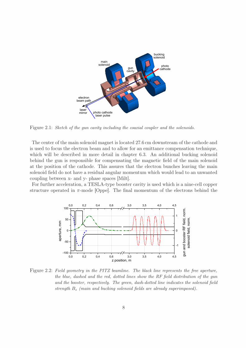
Figure 2.1: Sketch of the gun cavity including the coaxial coupler and the solenoids.

The center of the main solenoid magnet is located 27.6 cm downstream of the cathode andis used to focus the electron beam and to allow for an emittance compensation technique,which will be described in more detail in chapter 6.3. An additional bucking solenoidbehind the gun is responsible for compensating the magnetic field of the main solenoidat the position of the cathode. This assures that the electron bunches leaving the mainsolenoid field do not have a residual angular momentum which would lead to an unwantedcoupling between x- and y- phase spaces [Milt].For further acceleration, a TESLA-type booster cavity is used which is a nine-cell copper

structure operated in π-mode [Oppe]. The final momentum of the electrons behind the

Figure 2.2: Field geometry in the PITZ beamline. The black line represents the free aperture,the blue, dashed and the red, dotted lines show the RF field distribution of the gunand the booster, respectively. The green, dash-dotted line indicates the solenoid fieldstrength Bz (main and bucking solenoid fields are already superimposed).

8

booster cavity can be up to 14.7 MeV/c. The distribution of the electric and magneticfields are shown in figure 2.2, where the field plots are normalized to unity. Typicalrun conditions are 60 MV/m as the maximal RF field amplitude on the photocathode,14 MV/m as the maximum booster gradient and a peak solenoid strength of 230 mT.

2.2 Electron bunch diagnosticsThe electron bunches can be characterized in many ways: their charge, the transverseshape and position, the momentum distribution, the longitudinal bunch profile, the longi-tudinal phase space distribution and finally the transverse phase space distributions in x-and y-direction. The following sub-chapters provide an overview of the techniques usedat PITZ for measuring these properties.

2.2.1 Charge

Two different devices are available for measuring the charge of the electron bunches.Firstly, Integrating Current Transformers (ICTs, produced and calibrated by Bergoz[Berg]) are used. These devices can be viewed as coils around the beam pipe. Elec-tron bunches passing such a coil induce a voltage in the windings. Integrating that signalwith an oscilloscope and taking into account the calibration factor of 0.8 C/Vs allows tocompute the bunch charge. This device is appropriate for the measurement of chargelevels larger than 100 pC and is specially suited for the 1 nC regime.For smaller charges, the Faraday cup (FC) is used, which acts as a charge collector whenit is inserted in the beam path. The charge flow, i.e. the current, is observed with anoscilloscope and the total charge can be determined by integrating the signal and scalingit with a calibration factor of 0.02 C/Vs. There is no principle limitation to small chargelevels when using a Faraday cup, but the advantage of an ICT is the non-destructivemeasurement.

2.2.2 Transverse shape and position

The transverse charge distribution as well as the position of the beam can be measuredusing a view screen together with a camera. At PITZ, screens coated with Cerium dopedYAG3 powder are used which produce broadband light in the visible spectrum. Thelight intensity is proportional to the number of the electrons and scales with their en-ergy [Spes01]. Another type of screen utilizes optical transition radiation (OTR screens)which occurs when high-energy electrons cross the boundary of two materials having dif-ferent indices of refraction.To further detect the absolute position of the electron beam along the beamline, five

3YAG = Yttrium Aluminium Garnet

9

button-type beam position monitors (BPM) are installed at different locations. Further-more, wire scanners (WS) are employed, where a thin wire is moved transversely throughthe electron beam. Electrons hitting the wire create showers of gamma quanta whichgenerate light in scintillator plates. The light is detected using photomultiplier tubes(PMT). The integrated PMT-signals vs. wire position yield the projection of the beamshape perpendicular to the wire’s moving direction in x and y.

2.2.3 Longitudinal phase space distribution and its projections

The momentum distribution of the electron bunches can be measured using spectrometerdipole magnets. The radius of the deflection curve of a single electron depends on its mo-mentum via r(p) = p

B·e , where r is the radius, p the particle momentum, B the magneticfield and e is the elementary charge. Therefore, the beam momentum distribution can beobserved on a screen after the dipole and together with the magnetic field these imagesallow to compute the mean momentum as well as the momentum spread.The first spectrometer dipole is placed behind the electron gun cavity to measure thebeam properties in the low-energy section. This dipole has a nominal deflection angle of60 degrees and is able to measure beam momenta of up to 8.8 MeV/c, which is sufficientsince the maximum of the beam momentum from the gun operated at 60 MV/m is approx.6.95 MeV/c [Roen].The second dipole is located after the booster cavity. It is a 180 degrees dipole that wasdesigned to measure momenta of up to 40 MeV/c which is needed for future upgrades ofthe machine. This dipole also serves as part of a setup to measure the transverse sliceemittance [Ivan02].The resolution of both systems depends on the initial beam parameters, particularly onthe quality of the focusing. Under standard conditions, the momentum resolution of thelow-energy dispersive arm is about 6 keV/c and that of the high-energy dispersive arm isabout 8 keV/c [Roen]. A third dipole is situated at the end of the beamline, but will notbe discussed here, because it was not used for the measurements.To measure the longitudinal bunch profile, two screen stations in the straight section(before and after the booster) are equipped with Čerenkov-radiators (Silica Aerogel) andOTR-screens. The electron bunches passing those radiators create a light pulse whosetemporal intensity distribution corresponds to the longitudinal electron bunch distribu-tion. The generated light distribution is imaged onto a streak camera and can be measuredwith a temporal resolution of the whole system of about 4 ps [Roen] (the streak cameraitself has a temporal resolution of about 2 ps).Finally, these radiators can be inserted in the dispersive sections where the electrons aresorted after their momenta. The generated light distribution is transported and imagedonto the entrance slit of a streak camera. The streak camera adds temporal informationto the momentum distribution resulting in the longitudinal phase space distribution in{t,pz}-space.

10

2.2.4 Transverse phase space distribution

The transverse emittance of an electron bunch corresponds to the area of the electronbeam’s transverse phase space distribution. At PITZ, the transverse emittance is mea-sured using the single-slit scan technique [Stay]. For this purpose, three EMSY4 - stationsare installed at different locations in the beamline. Each of these stations contains a YAG-screen for the observation of the electron beam size as well as slits in the horizontal andvertical direction having openings of 10 μm and 50μm. Moving the slits into the beampath causes all electrons which are not inside the slit acceptance to be scattered by thetungsten bulk material. The transmitted parts of the beam are called beamlets and due totheir small charge the space charge forces can be neglected. These beamlets are observedon a screen (see figure 2.3) and their intrinsic divergence can be determined from theirbeam size perpendicular to the slit orientation divided by the drift length between slitand screen.In addition, taking into account the slit position and the divergence of the whole beamletfor each measurement point during the scan, one is able to reconstruct the transversetrace space5. This allows to compute the transverse emittance according to Equation 6.7.The transverse emittance measurement setup was designed to have a systematic error ofless than 10 % for a broad range of electron beam parameters.More information about the transverse phase space and the measurement of the transverseemittance can be found in chapter 6.1 and in [Stay].

Figure 2.3: Illustration of the slit scan technique. Only a tiny fraction of the original electronbunch can pass the slit and is recorded by a screen further downstream.

4EMSY = Emittance Measurement SYstem5While the coordinates of the transverse phase space are x and px, the transverse trace space has x

and x′ = px/pz as coordinates.

11

Chapter 3

Laser system and laser pulse diagnostics

In this chapter the laser system at PITZ which was developed and built by the Max BornInstitute Berlin (MBI) will be described at first. Afterwards, the laser transport to thephotocathode is introduced and finally the available laser pulse diagnostics in the laserhut as well as in the accelerator tunnel is presented.

3.1 Requirements for the laser systemThe laser system must be able to produce a variable number of laser pulses arranged intrains. The pulse spacing within the trains is 1 μs, while the trains have a repetitionrate of 10 Hz with 800 pulses per train at maximum. Since the European XFEL willincorporate superconducting accelerator technology, the acceleration of this large numberof electron bunches is possible. The laser pulses must have a wavelength around 261 nm(see chapter 5.1) to efficiently extract electrons from the photocathode material (Cs2Te)and the number of photons must be sufficient to reach a charge level of at least 1 nC.Because the electron bunch properties strongly depend on the temporal shape of the laserpulse, the optimum conditions of about 20 ps long (FWHM1) flat-top profile and rise andfall times as short as possible must be carefully fulfilled. The transverse shape should bea circular flat-top which is not generated in the laser system but in the laser beamline bycutting the magnified beam leaving only the central part using a circular aperture. Theenergy loss can be up to 80 % in this case which puts even higher demands on the initiallaser pulse energy. The reasons for these requirements will be given in section 6.2.Another important issue is the timing stability of the laser system. The total rms2 timingjitter between the RF in the gun cavity and the laser pulses must be better than 200 fs[XTDR]. The reason for this stringent requirement is the dependence of the electron bunchproperties, like mean momentum and momentum spread, on the RF phase at emission.

1FWHM = Full Width at Half Maximum2rms = root mean square

12

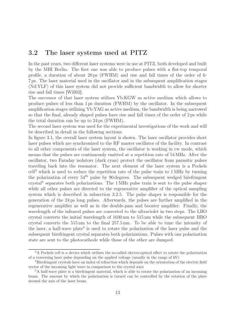
3.2 The laser systems used at PITZIn the past years, two different laser systems were in use at PITZ, both developed and builtby the MBI Berlin. The first one was able to produce pulses with a flat-top temporalprofile, a duration of about 20 ps (FWHM) and rise and fall times of the order of 6-7 ps. The laser material used in the oscillator and in the subsequent amplification stages(Nd:YLF) of this laser system did not provide sufficient bandwidth to allow for shorterrise and fall times [Will02].The successor of that laser system utilizes Yb:KGW as active medium which allows toproduce pulses of less than 1 ps duration (FWHM) by the oscillator. In the subsequentamplification stages utilizing Yb:YAG as active medium, the bandwidth is being narrowedso that the final, already shaped pulses have rise and fall times of the order of 2 ps whilethe total duration can be up to 24 ps (FWHM).The second laser system was used for the experimental investigations of the work and willbe described in detail in the following sections.In figure 3.1, the overall laser system layout is shown. The laser oscillator provides shortlaser pulses which are synchronized to the RF master oscillator of the facility. In contrastto all other components of the laser system, the oscillator is working in cw mode, whichmeans that the pulses are continuously emitted at a repetition rate of 54 MHz. After theoscillator, two Faraday isolators (dark cyan) protect the oscillator from parasitic pulsestraveling back into the resonator. The next element of the laser system is a Pockelscell3 which is used to reduce the repetition rate of the pulse train to 1 MHz by turningthe polarization of every 54th pulse by 90 degrees. The subsequent wedged birefringentcrystal4 separates both polarizations. The 1 MHz pulse train is sent to the pulse shaperwhile all other pulses are directed to the regenerative amplifier of the optical samplingsystem which is described in subsection 3.2.5. The pulse shaper is responsible for thegeneration of the 24 ps long pulses. Afterwards, the pulses are further amplified in theregenerative amplifier as well as in the double-pass and booster amplifier. Finally, thewavelength of the infrared pulses are converted to the ultraviolet in two steps. The LBOcrystal converts the initial wavelength of 1030 nm to 515 nm while the subsequent BBOcrystal converts the 515 nm to the final 257.5 nm. To be able to tune the intensity ofthe laser, a half-wave plate5 is used to rotate the polarization of the laser pulse and thesubsequent birefringent crystal separates both polarizations. Pulses with one polarizationstate are sent to the photocathode while those of the other are dumped.

3A Pockels cell is a device which utilizes the so-called electro-optical effect to rotate the polarizationof a traversing laser pulse depending on the applied voltage (usually in the range of kV)

4Birefringent crystals have an index of refraction which depends on the orientation of the electric fieldvector of the incoming light wave in comparison to the crystal axes

5A half-wave plate is a birefringent material, which is able to rotate the polarization of an incomingbeam. The amount by which the polarization is turned can be controlled by the rotation of the platearound the axis of the laser beam.

13

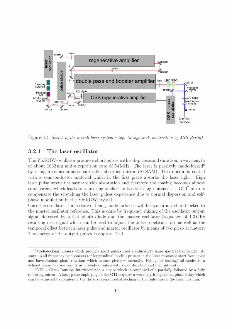
Figure 3.1: Sketch of the overall laser system setup. (design and construction by MBI Berlin)

3.2.1 The laser oscillator

The Yb:KGW-oscillator produces short pulses with sub-picosecond duration, a wavelengthof about 1032 nm and a repetition rate of 54 MHz. The laser is passively mode-locked6

by using a semiconductor saturable absorber mirror (SESAM). This mirror is coatedwith a semiconductor material which in the first place absorbs the laser light. Highlaser pulse intensities saturate this absorption and therefore the coating becomes almosttransparent, which leads to a favoring of short pulses with high intensities. GTI7 mirrorscompensate the stretching the laser pulses experience due to normal dispersion and self-phase modulation in the Yb:KGW crystal.Once the oscillator is in a state of being mode-locked it will be synchronized and locked tothe master oscillator reference. This is done by frequency mixing of the oscillator outputsignal detected by a fast photo diode and the master oscillator frequency of 1.3 GHzresulting in a signal which can be used to adjust the pulse repetition rate as well as thetemporal offset between laser pulse and master oscillator by means of two piezo actuators.The energy of the output pulses is approx. 2 nJ.

6Mode-locking: Lasers which produce short pulses need a sufficiently large spectral bandwidth. Atstart-up all frequency components (or longitudinal modes) present in the laser resonator start from noiseand have random phase relations which in sum give low intensity. Fixing (or locking) all modes to adefined phase relation results in individual pulses with short duration and high intensity.

7GTI = Gires-Tournois Interferometer, a device which is composed of a partially followed by a fullyreflecting mirror. A laser pulse impinging on the GTI acquires a wavelength-dependent phase delay whichcan be adjusted to counteract the dispersion-induced stretching of the pulse inside the laser medium.

14

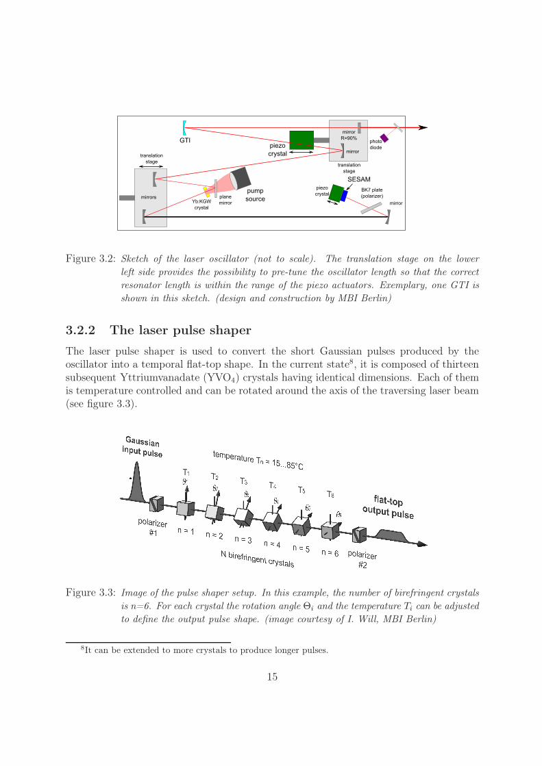
Figure 3.2: Sketch of the laser oscillator (not to scale). The translation stage on the lowerleft side provides the possibility to pre-tune the oscillator length so that the correctresonator length is within the range of the piezo actuators. Exemplary, one GTI isshown in this sketch. (design and construction by MBI Berlin)

3.2.2 The laser pulse shaper

The laser pulse shaper is used to convert the short Gaussian pulses produced by theoscillator into a temporal flat-top shape. In the current state8, it is composed of thirteensubsequent Yttriumvanadate (YVO4) crystals having identical dimensions. Each of themis temperature controlled and can be rotated around the axis of the traversing laser beam(see figure 3.3).

Figure 3.3: Image of the pulse shaper setup. In this example, the number of birefringent crystalsis n=6. For each crystal the rotation angle Θi and the temperature Ti can be adjustedto define the output pulse shape. (image courtesy of I. Will, MBI Berlin)

8It can be extended to more crystals to produce longer pulses.

15

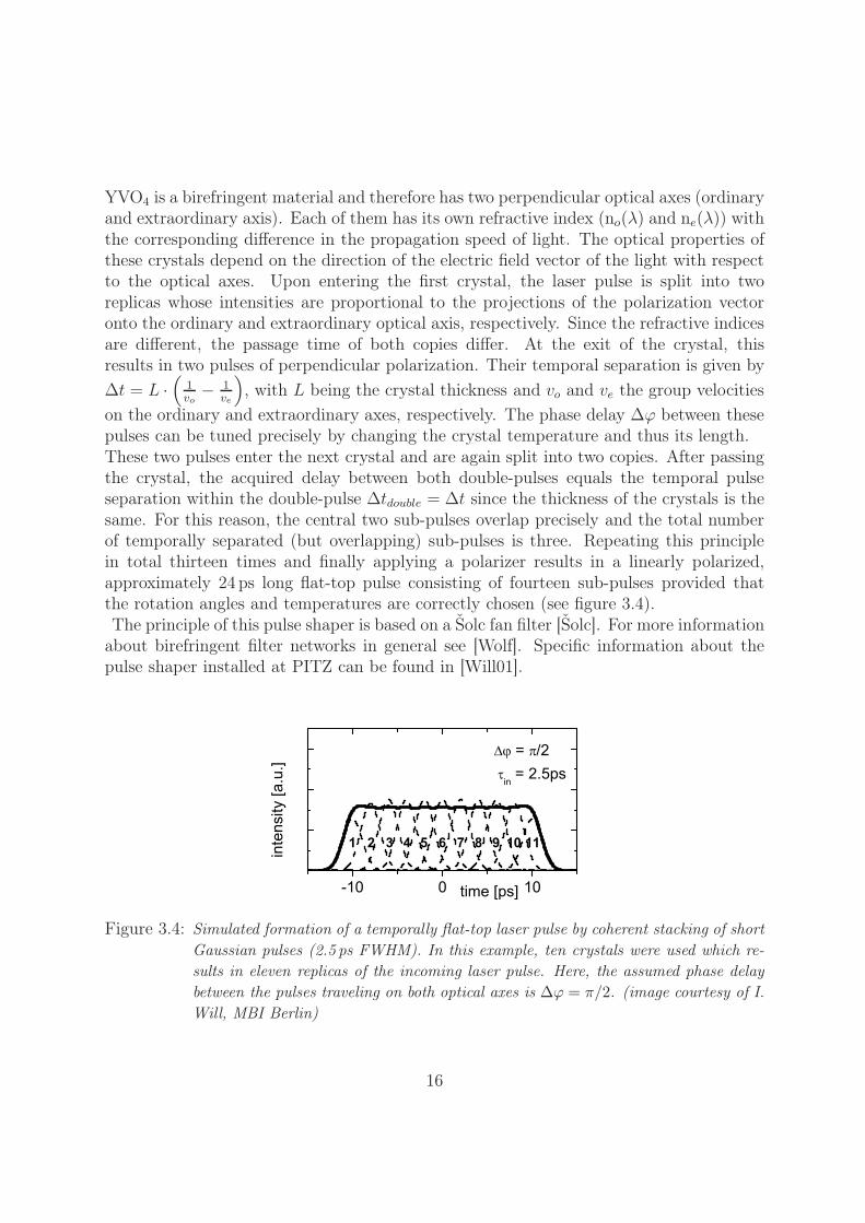
YVO4 is a birefringent material and therefore has two perpendicular optical axes (ordinaryand extraordinary axis). Each of them has its own refractive index (no(λ) and ne(λ)) withthe corresponding difference in the propagation speed of light. The optical properties ofthese crystals depend on the direction of the electric field vector of the light with respectto the optical axes. Upon entering the first crystal, the laser pulse is split into tworeplicas whose intensities are proportional to the projections of the polarization vectoronto the ordinary and extraordinary optical axis, respectively. Since the refractive indicesare different, the passage time of both copies differ. At the exit of the crystal, thisresults in two pulses of perpendicular polarization. Their temporal separation is given byΔt = L ·

(1vo

− 1ve

), with L being the crystal thickness and vo and ve the group velocities

on the ordinary and extraordinary axes, respectively. The phase delay Δϕ between thesepulses can be tuned precisely by changing the crystal temperature and thus its length.These two pulses enter the next crystal and are again split into two copies. After passingthe crystal, the acquired delay between both double-pulses equals the temporal pulseseparation within the double-pulse Δtdouble = Δt since the thickness of the crystals is thesame. For this reason, the central two sub-pulses overlap precisely and the total numberof temporally separated (but overlapping) sub-pulses is three. Repeating this principlein total thirteen times and finally applying a polarizer results in a linearly polarized,approximately 24 ps long flat-top pulse consisting of fourteen sub-pulses provided thatthe rotation angles and temperatures are correctly chosen (see figure 3.4).The principle of this pulse shaper is based on a Šolc fan filter [Šolc]. For more information

about birefringent filter networks in general see [Wolf]. Specific information about thepulse shaper installed at PITZ can be found in [Will01].

Figure 3.4: Simulated formation of a temporally flat-top laser pulse by coherent stacking of shortGaussian pulses (2.5 ps FWHM). In this example, ten crystals were used which re-sults in eleven replicas of the incoming laser pulse. Here, the assumed phase delaybetween the pulses traveling on both optical axes is Δϕ = π/2. (image courtesy of I.Will, MBI Berlin)

16

By completely removing the pulse shaper, the laser system can produce UV output pulseswith a Gaussian temporal shape having a duration of approx. 2 ps (FWHM).

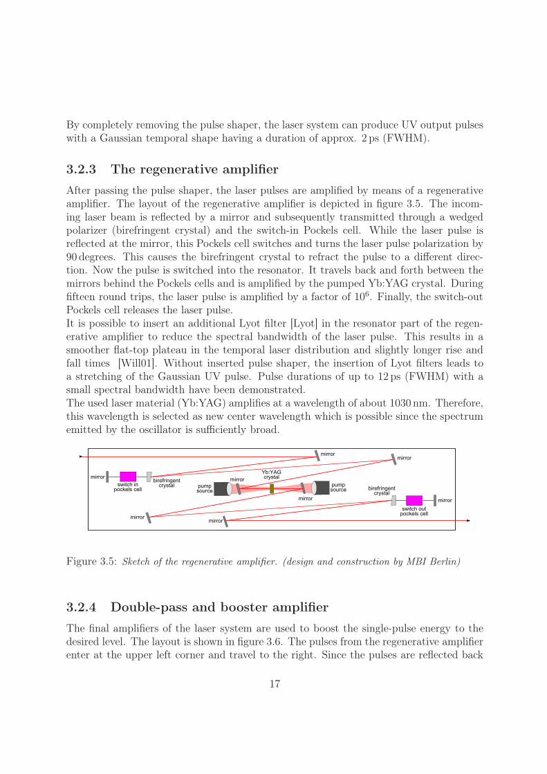
3.2.3 The regenerative amplifier

After passing the pulse shaper, the laser pulses are amplified by means of a regenerativeamplifier. The layout of the regenerative amplifier is depicted in figure 3.5. The incom-ing laser beam is reflected by a mirror and subsequently transmitted through a wedgedpolarizer (birefringent crystal) and the switch-in Pockels cell. While the laser pulse isreflected at the mirror, this Pockels cell switches and turns the laser pulse polarization by90 degrees. This causes the birefringent crystal to refract the pulse to a different direc-tion. Now the pulse is switched into the resonator. It travels back and forth between themirrors behind the Pockels cells and is amplified by the pumped Yb:YAG crystal. Duringfifteen round trips, the laser pulse is amplified by a factor of 106. Finally, the switch-outPockels cell releases the laser pulse.It is possible to insert an additional Lyot filter [Lyot] in the resonator part of the regen-erative amplifier to reduce the spectral bandwidth of the laser pulse. This results in asmoother flat-top plateau in the temporal laser distribution and slightly longer rise andfall times [Will01]. Without inserted pulse shaper, the insertion of Lyot filters leads toa stretching of the Gaussian UV pulse. Pulse durations of up to 12 ps (FWHM) with asmall spectral bandwidth have been demonstrated.The used laser material (Yb:YAG) amplifies at a wavelength of about 1030 nm. Therefore,this wavelength is selected as new center wavelength which is possible since the spectrumemitted by the oscillator is sufficiently broad.

Figure 3.5: Sketch of the regenerative amplifier. (design and construction by MBI Berlin)

3.2.4 Double-pass and booster amplifier

The final amplifiers of the laser system are used to boost the single-pulse energy to thedesired level. The layout is shown in figure 3.6. The pulses from the regenerative amplifierenter at the upper left corner and travel to the right. Since the pulses are reflected back

17

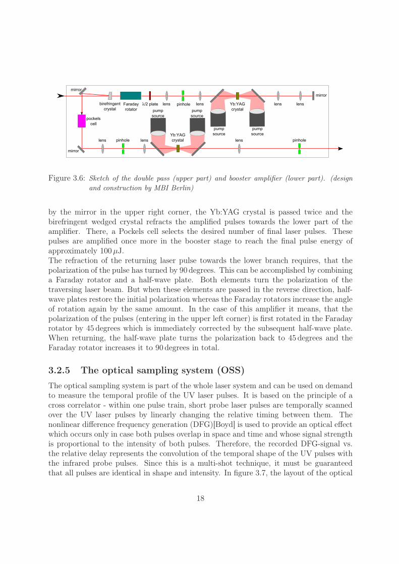
Figure 3.6: Sketch of the double pass (upper part) and booster amplifier (lower part). (designand construction by MBI Berlin)

by the mirror in the upper right corner, the Yb:YAG crystal is passed twice and thebirefringent wedged crystal refracts the amplified pulses towards the lower part of theamplifier. There, a Pockels cell selects the desired number of final laser pulses. Thesepulses are amplified once more in the booster stage to reach the final pulse energy ofapproximately 100μJ.The refraction of the returning laser pulse towards the lower branch requires, that thepolarization of the pulse has turned by 90 degrees. This can be accomplished by combininga Faraday rotator and a half-wave plate. Both elements turn the polarization of thetraversing laser beam. But when these elements are passed in the reverse direction, half-wave plates restore the initial polarization whereas the Faraday rotators increase the angleof rotation again by the same amount. In the case of this amplifier it means, that thepolarization of the pulses (entering in the upper left corner) is first rotated in the Faradayrotator by 45 degrees which is immediately corrected by the subsequent half-wave plate.When returning, the half-wave plate turns the polarization back to 45 degrees and theFaraday rotator increases it to 90 degrees in total.

3.2.5 The optical sampling system (OSS)

The optical sampling system is part of the whole laser system and can be used on demandto measure the temporal profile of the UV laser pulses. It is based on the principle of across correlator - within one pulse train, short probe laser pulses are temporally scannedover the UV laser pulses by linearly changing the relative timing between them. Thenonlinear difference frequency generation (DFG)[Boyd] is used to provide an optical effectwhich occurs only in case both pulses overlap in space and time and whose signal strengthis proportional to the intensity of both pulses. Therefore, the recorded DFG-signal vs.the relative delay represents the convolution of the temporal shape of the UV pulses withthe infrared probe pulses. Since this is a multi-shot technique, it must be guaranteedthat all pulses are identical in shape and intensity. In figure 3.7, the layout of the optical

18

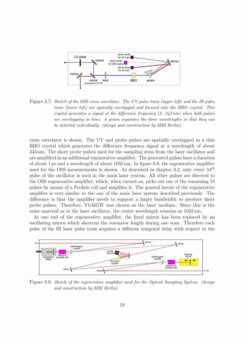
Figure 3.7: Sketch of the OSS cross correlator. The UV pulse train (upper left) and the IR pulsetrain (lower left) are spatially overlapped and focused into the BBO crystal. Thiscrystal generates a signal at the difference frequency (λ=343 nm) when both pulsesare overlapping in time. A prism separates the three wavelengths so that they canbe detected individually. (design and construction by MBI Berlin)

cross correlator is shown. The UV and probe pulses are spatially overlapped in a thinBBO crystal which generates the difference frequency signal at a wavelength of about343 nm. The short probe pulses used for the sampling stem from the laser oscillator andare amplified in an additional regenerative amplifier. The generated pulses have a durationof about 1 ps and a wavelength of about 1032 nm. In figure 3.8, the regenerative amplifierused for the OSS measurements is shown. As described in chapter 3.2, only every 54th

pulse of the oscillator is used in the main laser system. All other pulses are directed tothe OSS regenerative amplifier, which, when turned on, picks out one of the remaining 53pulses by means of a Pockels cell and amplifies it. The general layout of the regenerativeamplifier is very similar to the one of the main laser system described previously. Thedifference is that the amplifier needs to support a larger bandwidth to produce shortprobe pulses. Therefore, Yb:KGW was chosen as the laser medium. Since this is thesame material as in the laser oscillator, the center wavelength remains at 1032 nm.

At one end of the regenerative amplifier, the fixed mirror has been replaced by anoscillating mirror which shortens the resonator length during one scan. Therefore eachpulse of the IR laser pulse train acquires a different temporal delay with respect to the

Figure 3.8: Sketch of the regenerative amplifier used for the Optical Sampling System. (designand construction by MBI Berlin)

19

pulses of the UV train. After one scan the original position of the oscillating mirror isrestored. The translation stage on the left hand side in figure 3.8 allows a pre-adjustmentof the resonator length to provide a temporal overlap of the IR and UV pulses within thescan range.

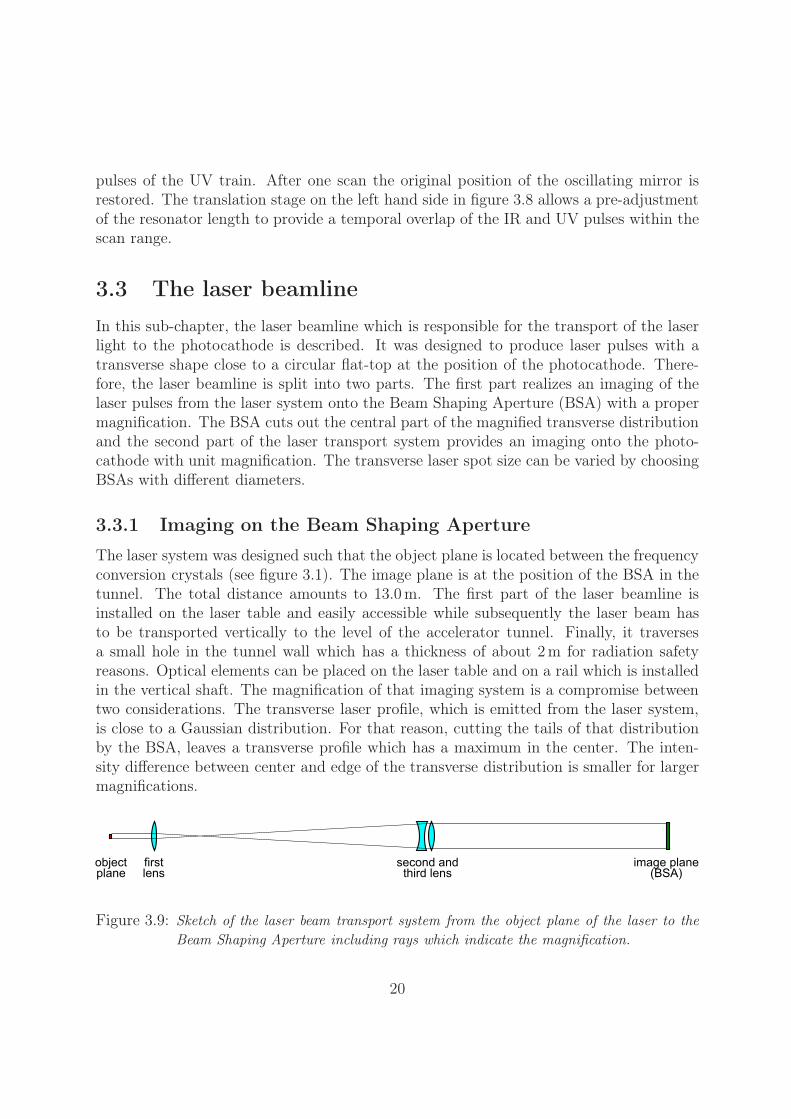
3.3 The laser beamlineIn this sub-chapter, the laser beamline which is responsible for the transport of the laserlight to the photocathode is described. It was designed to produce laser pulses with atransverse shape close to a circular flat-top at the position of the photocathode. There-fore, the laser beamline is split into two parts. The first part realizes an imaging of thelaser pulses from the laser system onto the Beam Shaping Aperture (BSA) with a propermagnification. The BSA cuts out the central part of the magnified transverse distributionand the second part of the laser transport system provides an imaging onto the photo-cathode with unit magnification. The transverse laser spot size can be varied by choosingBSAs with different diameters.

3.3.1 Imaging on the Beam Shaping Aperture

The laser system was designed such that the object plane is located between the frequencyconversion crystals (see figure 3.1). The image plane is at the position of the BSA in thetunnel. The total distance amounts to 13.0 m. The first part of the laser beamline isinstalled on the laser table and easily accessible while subsequently the laser beam hasto be transported vertically to the level of the accelerator tunnel. Finally, it traversesa small hole in the tunnel wall which has a thickness of about 2 m for radiation safetyreasons. Optical elements can be placed on the laser table and on a rail which is installedin the vertical shaft. The magnification of that imaging system is a compromise betweentwo considerations. The transverse laser profile, which is emitted from the laser system,is close to a Gaussian distribution. For that reason, cutting the tails of that distributionby the BSA, leaves a transverse profile which has a maximum in the center. The inten-sity difference between center and edge of the transverse distribution is smaller for largermagnifications.

Figure 3.9: Sketch of the laser beam transport system from the object plane of the laser to theBeam Shaping Aperture including rays which indicate the magnification.

20

On the other hand, a large magnification means that more laser pulse energy is lost atthe BSA.The initial beam size at the object plane was measured to be xrms = 107 μm and yrms =95μm (measured as rms-value of small cuts through the center of the transverse distribu-tion). The reason for the asymmetry is the different angular acceptance of the frequencyconversion process in the BBO crystal for both planes9.As a compromise between all given constraints, it was decided to use a Kepler-like tele-scope consisting of three lenses. The last two lenses are combined to produce an elementof arbitrary focal length [Hafer](see figure 3.9). The overall magnification for this setupis about 6.5.

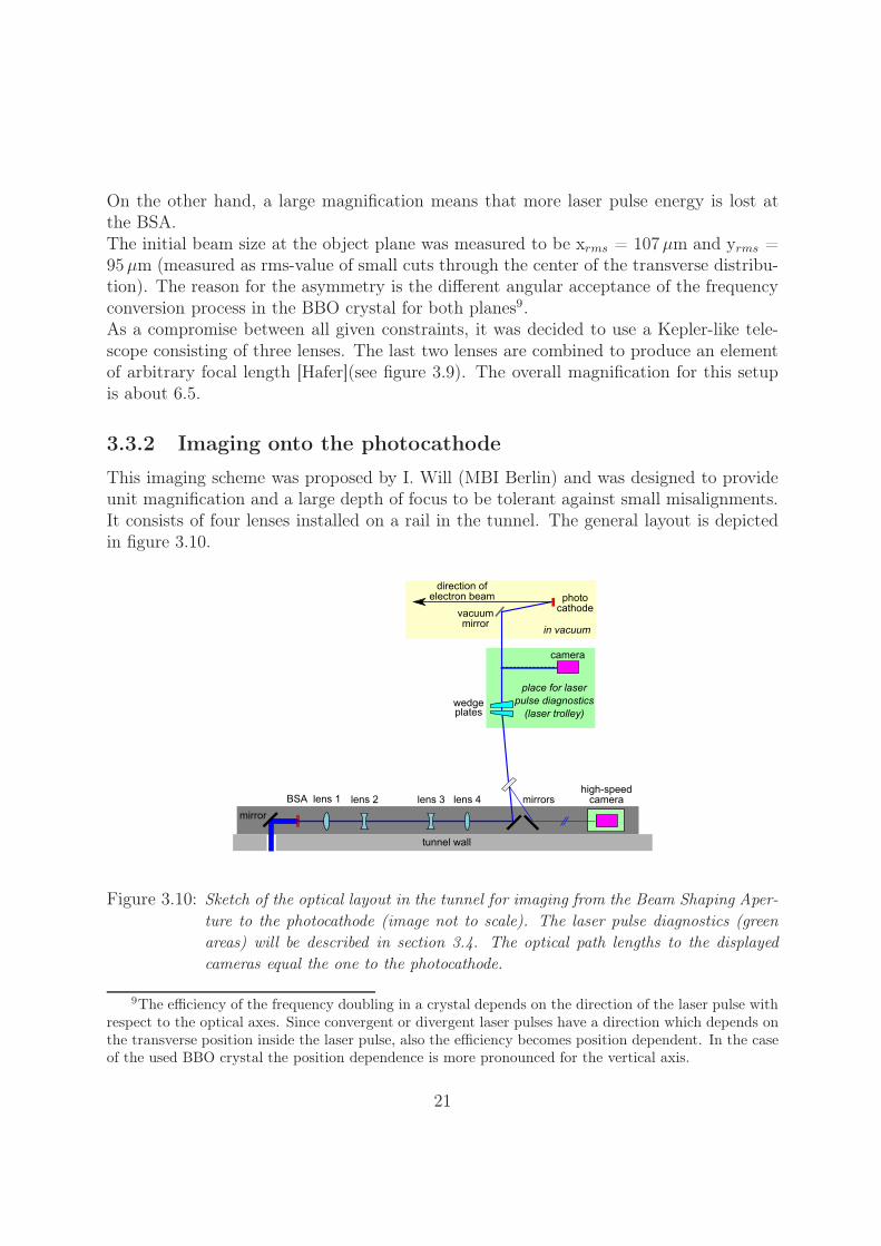
3.3.2 Imaging onto the photocathode

This imaging scheme was proposed by I. Will (MBI Berlin) and was designed to provideunit magnification and a large depth of focus to be tolerant against small misalignments.It consists of four lenses installed on a rail in the tunnel. The general layout is depictedin figure 3.10.

Figure 3.10: Sketch of the optical layout in the tunnel for imaging from the Beam Shaping Aper-ture to the photocathode (image not to scale). The laser pulse diagnostics (greenareas) will be described in section 3.4. The optical path lengths to the displayedcameras equal the one to the photocathode.

9The efficiency of the frequency doubling in a crystal depends on the direction of the laser pulse withrespect to the optical axes. Since convergent or divergent laser pulses have a direction which depends onthe transverse position inside the laser pulse, also the efficiency becomes position dependent. In the caseof the used BBO crystal the position dependence is more pronounced for the vertical axis.

21

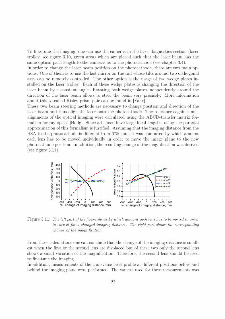
To fine-tune the imaging, one can use the cameras in the laser diagnostics section (lasertrolley, see figure 3.10, green area) which are placed such that the laser beam has thesame optical path length to the cameras as to the photocathode (see chapter 3.4).In order to change the laser beam position on the photocathode, there are two main op-tions. One of them is to use the last mirror on the rail whose tilts around two orthogonalaxes can be remotely controlled. The other option is the usage of two wedge plates in-stalled on the laser trolley. Each of these wedge plates is changing the direction of thelaser beam by a constant angle. Rotating both wedge plates independently around thedirection of the laser beam allows to steer the beam very precisely. More informationabout this so-called Risley prism pair can be found in [Yang].These two beam steering methods are necessary to change position and direction of thelaser beam and thus align the laser onto the photocathode. The tolerances against mis-alignments of the optical imaging were calculated using the ABCD-transfer matrix for-malism for ray optics [Hodg]. Since all lenses have large focal lengths, using the paraxialapproximation of this formalism is justified. Assuming that the imaging distance from theBSA to the photocathode is different from 6750 mm, it was computed by which amounteach lens has to be moved individually in order to move the image plane to the newphotocathode position. In addition, the resulting change of the magnification was derived(see figure 3.11).

Figure 3.11: The left part of the figure shows by which amount each lens has to be moved in orderto correct for a changed imaging distance. The right part shows the correspondingchange of the magnification.

From these calculations one can conclude that the change of the imaging distance is small-est when the first or the second lens are displaced but of these two only the second lensshows a small variation of the magnification. Therefore, the second lens should be usedto fine-tune the imaging.In addition, measurements of the transverse laser profile at different positions before andbehind the imaging plane were performed. The camera used for these measurements was

22

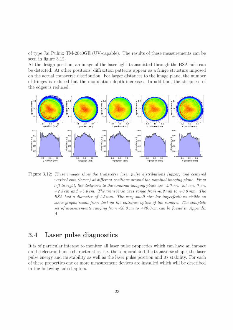
of type Jai Pulnix TM-2040GE (UV-capable). The results of these measurements can beseen in figure 3.12.At the design position, an image of the laser light transmitted through the BSA hole canbe detected. At other positions, diffraction patterns appear as a fringe structure imposedon the actual transverse distribution. For larger distances to the image plane, the numberof fringes is reduced but the modulation depth increases. In addition, the steepness ofthe edges is reduced.

Figure 3.12: These images show the transverse laser pulse distributions (upper) and centeredvertical cuts (lower) at different positions around the nominal imaging plane. Fromleft to right, the distances to the nominal imaging plane are -5.0 cm, -2.5 cm, 0 cm,+2.5 cm and +5.0 cm. The transverse axes range from -0.9mm to +0.9mm. TheBSA had a diameter of 1.5mm. The very small circular imperfections visible onsome graphs result from dust on the entrance optics of the camera. The completeset of measurements ranging from -20.0 cm to +20.0 cm can be found in AppendixA.

3.4 Laser pulse diagnosticsIt is of particular interest to monitor all laser pulse properties which can have an impacton the electron bunch characteristics, i.e. the temporal and the transverse shape, the laserpulse energy and its stability as well as the laser pulse position and its stability. For eachof these properties one or more measurement devices are installed which will be describedin the following sub-chapters.

23

3.4.1 Temporal laser pulse shape

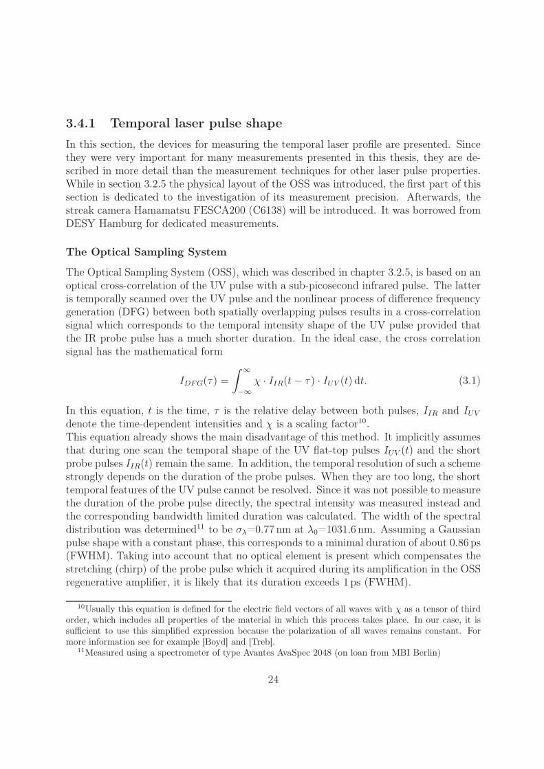
In this section, the devices for measuring the temporal laser profile are presented. Sincethey were very important for many measurements presented in this thesis, they are de-scribed in more detail than the measurement techniques for other laser pulse properties.While in section 3.2.5 the physical layout of the OSS was introduced, the first part of thissection is dedicated to the investigation of its measurement precision. Afterwards, thestreak camera Hamamatsu FESCA200 (C6138) will be introduced. It was borrowed fromDESY Hamburg for dedicated measurements.

The Optical Sampling System

The Optical Sampling System (OSS), which was described in chapter 3.2.5, is based on anoptical cross-correlation of the UV pulse with a sub-picosecond infrared pulse. The latteris temporally scanned over the UV pulse and the nonlinear process of difference frequencygeneration (DFG) between both spatially overlapping pulses results in a cross-correlationsignal which corresponds to the temporal intensity shape of the UV pulse provided thatthe IR probe pulse has a much shorter duration. In the ideal case, the cross correlationsignal has the mathematical form

IDFG(τ) =

∫ ∞

−∞χ · IIR(t − τ) · IUV (t) dt. (3.1)

In this equation, t is the time, τ is the relative delay between both pulses, IIR and IUV

denote the time-dependent intensities and χ is a scaling factor10.This equation already shows the main disadvantage of this method. It implicitly assumesthat during one scan the temporal shape of the UV flat-top pulses IUV (t) and the shortprobe pulses IIR(t) remain the same. In addition, the temporal resolution of such a schemestrongly depends on the duration of the probe pulses. When they are too long, the shorttemporal features of the UV pulse cannot be resolved. Since it was not possible to measurethe duration of the probe pulse directly, the spectral intensity was measured instead andthe corresponding bandwidth limited duration was calculated. The width of the spectraldistribution was determined11 to be σλ=0.77 nm at λ0=1031.6 nm. Assuming a Gaussianpulse shape with a constant phase, this corresponds to a minimal duration of about 0.86 ps(FWHM). Taking into account that no optical element is present which compensates thestretching (chirp) of the probe pulse which it acquired during its amplification in the OSSregenerative amplifier, it is likely that its duration exceeds 1 ps (FWHM).

10Usually this equation is defined for the electric field vectors of all waves with χ as a tensor of thirdorder, which includes all properties of the material in which this process takes place. In our case, it issufficient to use this simplified expression because the polarization of all waves remains constant. Formore information see for example [Boyd] and [Treb].

11Measured using a spectrometer of type Avantes AvaSpec 2048 (on loan from MBI Berlin)

24

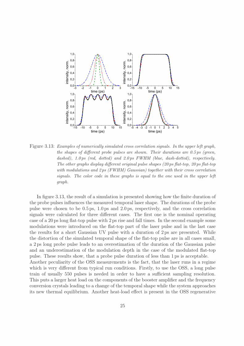
Figure 3.13: Examples of numerically simulated cross correlation signals. In the upper left graph,the shapes of different probe pulses are shown. Their durations are 0.5 ps (green,dashed), 1.0 ps (red, dotted) and 2.0 ps FWHM (blue, dash-dotted), respectively.The other graphs display different original pulse shapes (20 ps flat-top, 20 ps flat-topwith modulations and 2 ps (FWHM) Gaussian) together with their cross correlationsignals. The color code in these graphs is equal to the one used in the upper leftgraph.

In figure 3.13, the result of a simulation is presented showing how the finite duration ofthe probe pulses influences the measured temporal laser shape. The durations of the probepulse were chosen to be 0.5 ps, 1.0 ps and 2.0 ps, respectively, and the cross correlationsignals were calculated for three different cases. The first one is the nominal operatingcase of a 20 ps long flat-top pulse with 2 ps rise and fall times. In the second example somemodulations were introduced on the flat-top part of the laser pulse and in the last casethe results for a short Gaussian UV pulse with a duration of 2 ps are presented. Whilethe distortion of the simulated temporal shape of the flat-top pulse are in all cases small,a 2 ps long probe pulse leads to an overestimation of the duration of the Gaussian pulseand an underestimation of the modulation depth in the case of the modulated flat-toppulse. These results show, that a probe pulse duration of less than 1 ps is acceptable.Another peculiarity of the OSS measurements is the fact, that the laser runs in a regimewhich is very different from typical run conditions. Firstly, to use the OSS, a long pulsetrain of usually 550 pulses is needed in order to have a sufficient sampling resolution.This puts a larger heat load on the components of the booster amplifier and the frequencyconversion crystals leading to a change of the temporal shape while the system approachesits new thermal equilibrium. Another heat-load effect is present in the OSS regenerative

25

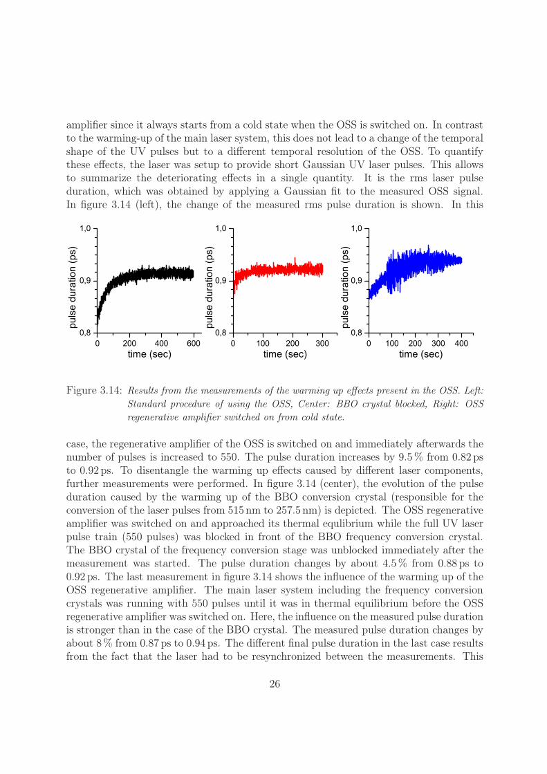
amplifier since it always starts from a cold state when the OSS is switched on. In contrastto the warming-up of the main laser system, this does not lead to a change of the temporalshape of the UV pulses but to a different temporal resolution of the OSS. To quantifythese effects, the laser was setup to provide short Gaussian UV laser pulses. This allowsto summarize the deteriorating effects in a single quantity. It is the rms laser pulseduration, which was obtained by applying a Gaussian fit to the measured OSS signal.In figure 3.14 (left), the change of the measured rms pulse duration is shown. In this

Figure 3.14: Results from the measurements of the warming up effects present in the OSS. Left:Standard procedure of using the OSS, Center: BBO crystal blocked, Right: OSSregenerative amplifier switched on from cold state.

case, the regenerative amplifier of the OSS is switched on and immediately afterwards thenumber of pulses is increased to 550. The pulse duration increases by 9.5 % from 0.82 psto 0.92 ps. To disentangle the warming up effects caused by different laser components,further measurements were performed. In figure 3.14 (center), the evolution of the pulseduration caused by the warming up of the BBO conversion crystal (responsible for theconversion of the laser pulses from 515 nm to 257.5 nm) is depicted. The OSS regenerativeamplifier was switched on and approached its thermal equlibrium while the full UV laserpulse train (550 pulses) was blocked in front of the BBO frequency conversion crystal.The BBO crystal of the frequency conversion stage was unblocked immediately after themeasurement was started. The pulse duration changes by about 4.5 % from 0.88 ps to0.92 ps. The last measurement in figure 3.14 shows the influence of the warming up of theOSS regenerative amplifier. The main laser system including the frequency conversioncrystals was running with 550 pulses until it was in thermal equilibrium before the OSSregenerative amplifier was switched on. Here, the influence on the measured pulse durationis stronger than in the case of the BBO crystal. The measured pulse duration changes byabout 8 % from 0.87 ps to 0.94 ps. The different final pulse duration in the last case resultsfrom the fact that the laser had to be resynchronized between the measurements. This

26

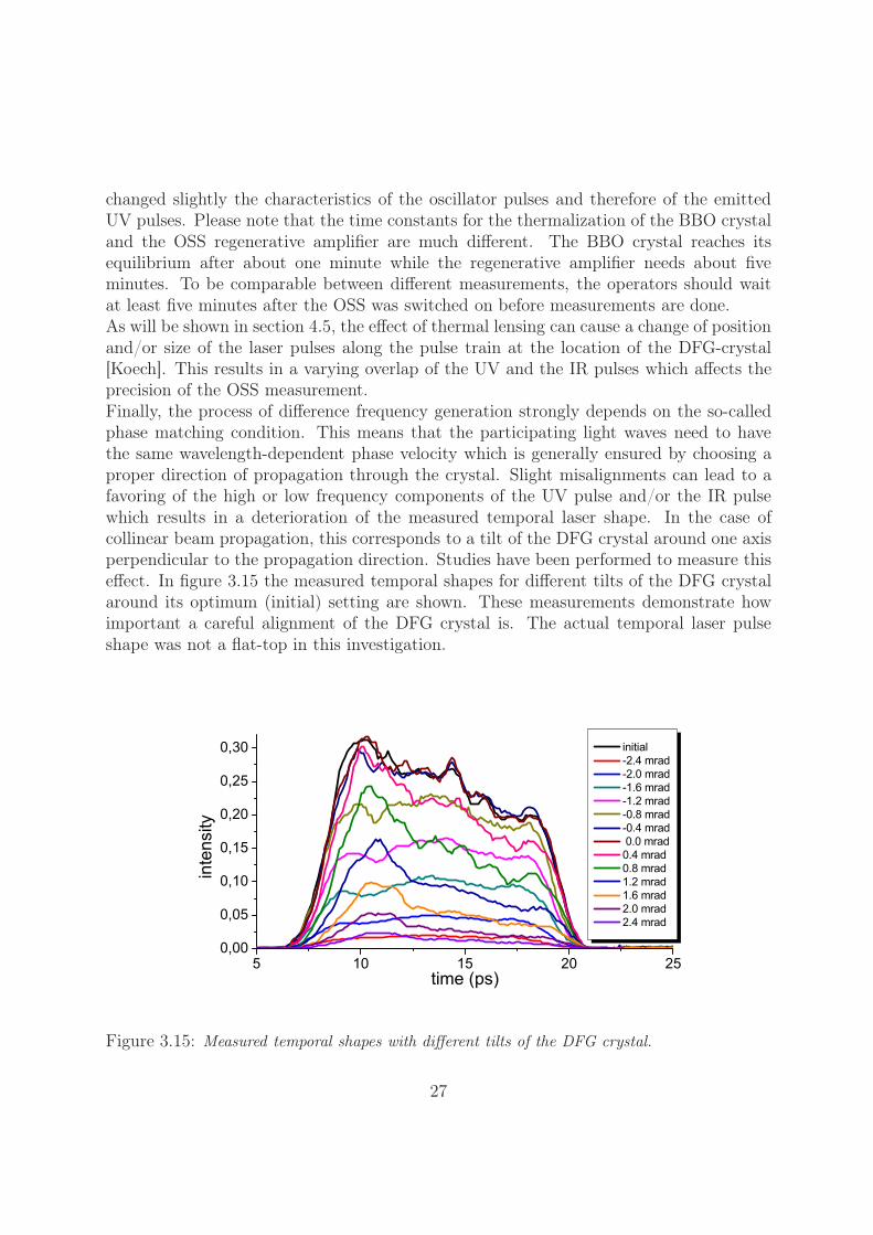
changed slightly the characteristics of the oscillator pulses and therefore of the emittedUV pulses. Please note that the time constants for the thermalization of the BBO crystaland the OSS regenerative amplifier are much different. The BBO crystal reaches itsequilibrium after about one minute while the regenerative amplifier needs about fiveminutes. To be comparable between different measurements, the operators should waitat least five minutes after the OSS was switched on before measurements are done.As will be shown in section 4.5, the effect of thermal lensing can cause a change of positionand/or size of the laser pulses along the pulse train at the location of the DFG-crystal[Koech]. This results in a varying overlap of the UV and the IR pulses which affects theprecision of the OSS measurement.Finally, the process of difference frequency generation strongly depends on the so-calledphase matching condition. This means that the participating light waves need to havethe same wavelength-dependent phase velocity which is generally ensured by choosing aproper direction of propagation through the crystal. Slight misalignments can lead to afavoring of the high or low frequency components of the UV pulse and/or the IR pulsewhich results in a deterioration of the measured temporal laser shape. In the case ofcollinear beam propagation, this corresponds to a tilt of the DFG crystal around one axisperpendicular to the propagation direction. Studies have been performed to measure thiseffect. In figure 3.15 the measured temporal shapes for different tilts of the DFG crystalaround its optimum (initial) setting are shown. These measurements demonstrate howimportant a careful alignment of the DFG crystal is. The actual temporal laser pulseshape was not a flat-top in this investigation.

Figure 3.15: Measured temporal shapes with different tilts of the DFG crystal.

27

It must be mentioned, that the Optical Sampling System is the only way to measure thetemporal laser pulse profile with a relatively high precision (temporally and in intensity)at the given wavelength and laser pulse energy. The streak camera, which is introducednext, has a comparable temporal precision but the intensity resolution is rather low.FROG techniques [Treb] cannot be used because second order processes as they are usedfor SHG FROG or GRENOUILLE are not possible at the required wavelength and thelimited intensity of the UV pulses does not allow to use third-order nonlinear processeslike in TG FROGs.

The streak camera Hamamatsu FESCA200

To have an independent measurement of the temporal laser profile, studies have been per-formed using a streak camera with an appropriate temporal resolution. The HamamatsuFESCA200 [Hama01] is the only streak camera offering sub-picosecond resolution in theUV. According to [Tomiz], the temporal resolution was measured to be about 800 fs at awavelength of 262 nm.

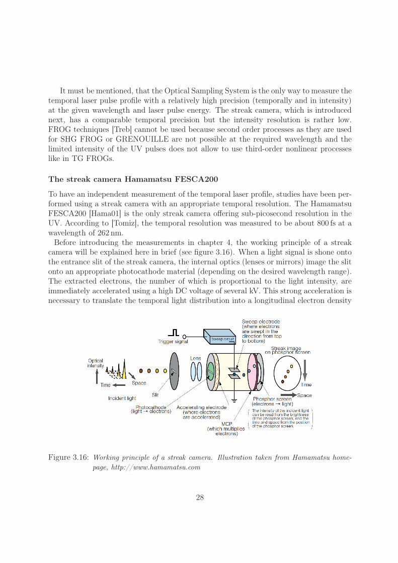
Before introducing the measurements in chapter 4, the working principle of a streakcamera will be explained here in brief (see figure 3.16). When a light signal is shone ontothe entrance slit of the streak camera, the internal optics (lenses or mirrors) image the slitonto an appropriate photocathode material (depending on the desired wavelength range).The extracted electrons, the number of which is proportional to the light intensity, areimmediately accelerated using a high DC voltage of several kV. This strong acceleration isnecessary to translate the temporal light distribution into a longitudinal electron density

Figure 3.16: Working principle of a streak camera. Illustration taken from Hamamatsu home-page, http://www.hamamatsu.com

28

distribution before the repulsion of the electrons can deteriorate this process and there-fore reduce the temporal resolution. In the next step, the electron bunch crosses a rapidlychanging electric field perpendicular to the electron direction. During this voltage sweep,the amount of deflection that one electron experiences depends linearly on its longitudinalposition in the bunch. Thus, the temporal distribution of the electron bunch is convertedinto a transverse distribution. In the next step, the electron bunch density (i.e. signalstrength) is increased by means of a microchannel plate12 (MCP). Behind the MCP, theelectrons hit a fluorescent screen. Its light distribution is finally imaged onto a CCD13

camera and can be read out by a personal computer.The high temporal resolution of this device is accompanied by the drawback that thedynamic range of the FESCA200 is only 1:40 [Hama02]. In addition, this streak camerahas an ultra-high sensitivity (single-photon detection is possible) which requires a verystrong attenuation of the laser pulses. This leads to the fact that the measured temporallaser shapes are obtained by photon counting which reduces the intensity resolution.

3.4.2 Transverse laser pulse shape

Another important laser pulse property is the transverse shape of the laser pulses im-pinging on the photocathode. In the PITZ tunnel, two different measurement systemsare installed. The first system consists of cameras which are mounted on the laser trol-ley. Beam splitters can be moved into the laser path reflecting the laser light towardsthe cameras, which are positioned such that the laser pulses experience the same opticalpath lengths to the cameras as to the photocathode. Therefore, they are called virtualcathodes (VC). The laser light illuminates directly the CCD chip. The cameras are syn-chronized to the machine master clock and the transverse laser shape can be measuredand processed using an appropriate video software [Weis]. In the run periods before 2007,analog cameras of type JAI M10SX14 were used primarily but showed many disadvan-tages. Firstly, the CCD chips were protected by a cover glass, which is not speciallysuited to transmit UV light. Instead it produced fluorescence light which appears as anadditional background to the actual signal15 (halo around the laser spot in left image offigure 3.17). Moreover, these cameras were equipped with micro lenses which focus thelight onto the active area of each pixel16. The micro lenses tend to become opaque forUV light (visible light was not affected), since they are made of polymer materials whosechemical bonds are broken under UV light exposure (photo fragmentation). This caused

12A microchannel plate is a two-dimensional array of tiny tubes (or channels) each acting as anindividual electron multiplier by secondary electron emission. Therefore, a MCP combines the sensitivityof a photomultiplier tube (PMT) with spatial resolution.

13CCD = Charge Coupled Device14These cameras have a resolution of 782 x 582 pixels and a pixel size of 8.3 μm x 8.3 μm.15A study of the fluorescence can be found in Appendix B.16This is usually only about 30% of the actual chip size

29

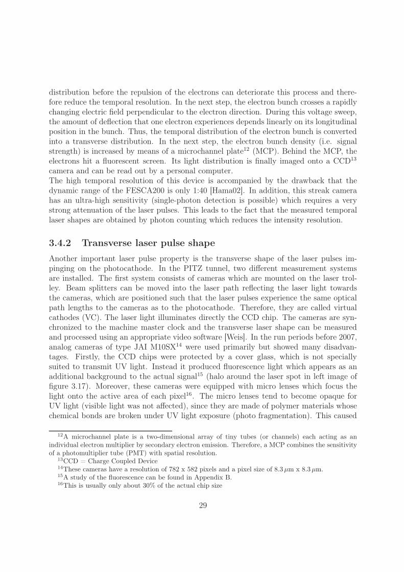
a rapid and inhomogeneous change of the sensitivity across the CCD chip distorting themeasurement of the transverse profile.For these reasons, another type of camera was installed which is UV capable (JAI Pul-nix TM1405-GE OP21-1UV). This camera does not have micro-lenses and the glass coverplate is replaced by a plate made of quartz. In addition, the camera has a higher resolutionof 1392 x 1040 pixels and a pixel size of only 4.65 μm x 4.65μm. No position-dependentdegradation of the sensitivity has been observed even after several months of use. Otheradvantages are that the connection to the control system is done via lossless GigabitEthernet connection and the dynamic range is 1:4096 (12 bit) in contrast to the analogcamera having 1:256 (8 bit). In figure 3.17, examples are displayed which demonstratethe difference in quality of images taken by both camera types.Finally, one peculiarity of both camera types must be mentioned. Since the laser light

is coherent and the thin protection cover plates have no anti-reflective coating, position-dependent interference patterns can occur which add to the actual transverse shape. Forthese reasons, it is planned to use cameras without micro lenses and without any coverplate. To protect the CCD chip, a custom made window made of anti-reflectively coatedfused silica will be mounted instead. First measurements with such kind of cameras havebeen done already (see measurement of depth of focus, Appendix A).

Figure 3.17: Left: image taken with JAI M10SX, right: image taken with JAI Pulnix TM1405-GE OP21-1UV

30

3.4.3 Laser pulse energy

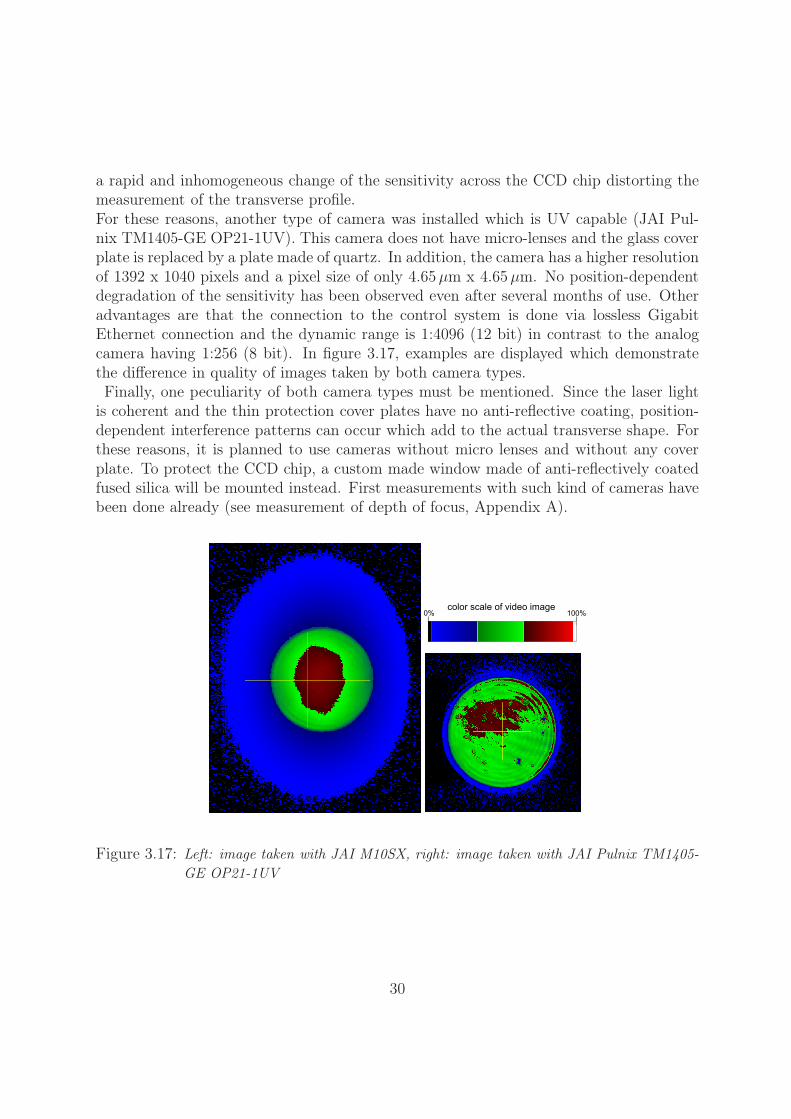
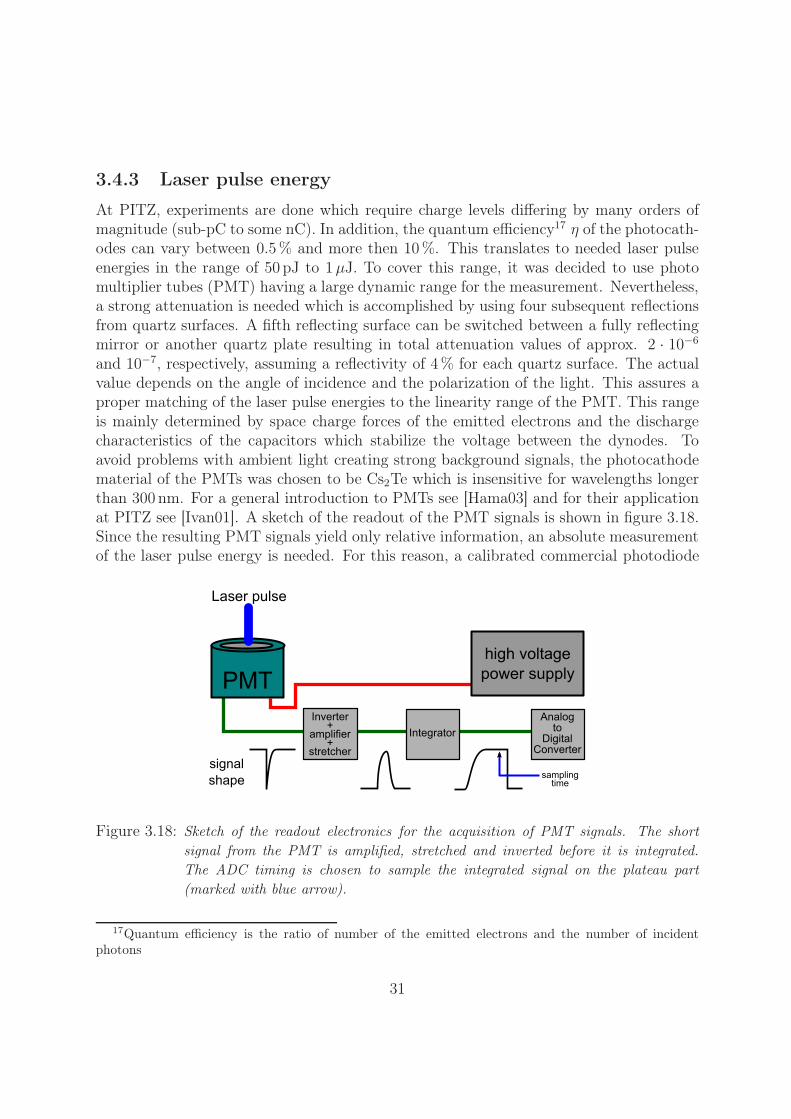
At PITZ, experiments are done which require charge levels differing by many orders ofmagnitude (sub-pC to some nC). In addition, the quantum efficiency17 η of the photocath-odes can vary between 0.5 % and more then 10 %. This translates to needed laser pulseenergies in the range of 50 pJ to 1μJ. To cover this range, it was decided to use photomultiplier tubes (PMT) having a large dynamic range for the measurement. Nevertheless,a strong attenuation is needed which is accomplished by using four subsequent reflectionsfrom quartz surfaces. A fifth reflecting surface can be switched between a fully reflectingmirror or another quartz plate resulting in total attenuation values of approx. 2 · 10−6

and 10−7, respectively, assuming a reflectivity of 4 % for each quartz surface. The actualvalue depends on the angle of incidence and the polarization of the light. This assures aproper matching of the laser pulse energies to the linearity range of the PMT. This rangeis mainly determined by space charge forces of the emitted electrons and the dischargecharacteristics of the capacitors which stabilize the voltage between the dynodes. Toavoid problems with ambient light creating strong background signals, the photocathodematerial of the PMTs was chosen to be Cs2Te which is insensitive for wavelengths longerthan 300 nm. For a general introduction to PMTs see [Hama03] and for their applicationat PITZ see [Ivan01]. A sketch of the readout of the PMT signals is shown in figure 3.18.Since the resulting PMT signals yield only relative information, an absolute measurementof the laser pulse energy is needed. For this reason, a calibrated commercial photodiode

Figure 3.18: Sketch of the readout electronics for the acquisition of PMT signals. The shortsignal from the PMT is amplified, stretched and inverted before it is integrated.The ADC timing is chosen to sample the integrated signal on the plateau part(marked with blue arrow).

17Quantum efficiency is the ratio of number of the emitted electrons and the number of incidentphotons

31

(Ophir NOVA II with photodiode PD10-pJ SH) was installed in the laser trolley. Anattenuated part of the laser pulse can be directed to the photodiode by means of movablemirrors. The diode is capable of measuring single-pulse energies in the range of 50 pJ to200 nJ.While the PMT can measure the energy of all pulses, the photodiode is only capable tomeasure one single pulse per train. The reason is that the maximum pulse repetition rateof the photodiode is 12 kHz which is less than the required 1 MHz.

3.4.4 Laser pulse position

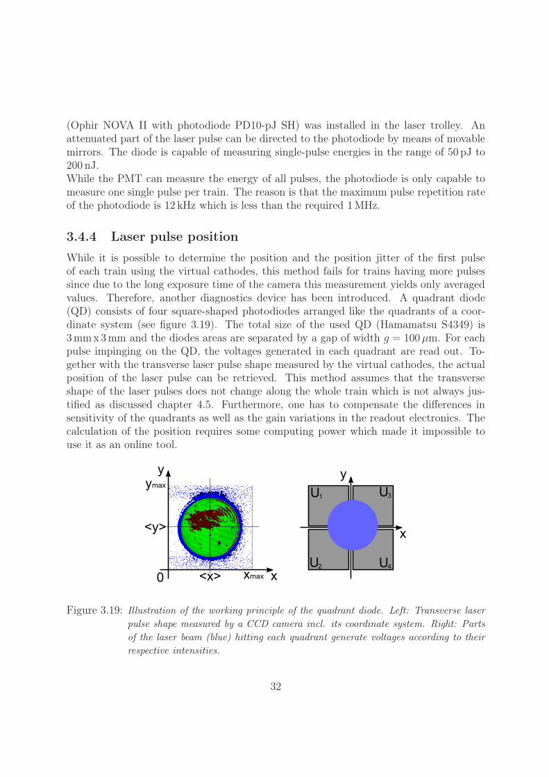
While it is possible to determine the position and the position jitter of the first pulseof each train using the virtual cathodes, this method fails for trains having more pulsessince due to the long exposure time of the camera this measurement yields only averagedvalues. Therefore, another diagnostics device has been introduced. A quadrant diode(QD) consists of four square-shaped photodiodes arranged like the quadrants of a coor-dinate system (see figure 3.19). The total size of the used QD (Hamamatsu S4349) is3 mmx3 mm and the diodes areas are separated by a gap of width g = 100 μm. For eachpulse impinging on the QD, the voltages generated in each quadrant are read out. To-gether with the transverse laser pulse shape measured by the virtual cathodes, the actualposition of the laser pulse can be retrieved. This method assumes that the transverseshape of the laser pulses does not change along the whole train which is not always jus-tified as discussed chapter 4.5. Furthermore, one has to compensate the differences insensitivity of the quadrants as well as the gain variations in the readout electronics. Thecalculation of the position requires some computing power which made it impossible touse it as an online tool.

Figure 3.19: Illustration of the working principle of the quadrant diode. Left: Transverse laserpulse shape measured by a CCD camera incl. its coordinate system. Right: Partsof the laser beam (blue) hitting each quadrant generate voltages according to theirrespective intensities.

32

In figure 3.19 the working principle of the position retrieval algorithm is shown. The laserpulse impinging on the QD, generates voltages in each quadrant (U1...U4). The ratios

RQDx =

(U3 + U4) − (U1 + U2)

U1 + U2 + U3 + U4

and RQDy =

(U1 + U3) − (U2 + U4)

U1 + U2 + U3 + U4

(3.2)

give information about the horizontal and vertical position, respectively. When the laserbeam is exactly in the center of the QD, both ratios are zero. To relate RQD

x and RQDy

to real positions, they must be compared to the corresponding ratios obtained from thetransverse laser profile measured by a CCD camera. With xmax and ymax being the totalnumber of pixels of the CCD chip in x- and y-direction, respectively, p(x, y) the pixelvalue at position (x, y) and g the gap width of the QD, the ratio for x-coordinate reads

RCCDx (xi, yi) =

⎛⎜⎜⎜⎜⎝

ymax∑y=0

y/∈[yi− g

2;yi+

g2

]

xi− g2∑

x=0

p(x, y)

⎞⎟⎟⎟⎟⎠ −

⎛⎜⎜⎜⎜⎝

ymax∑y=0

y/∈[yi− g

2;yi+

g2

]

xmax∑x=xi+

g2

p(x, y)

⎞⎟⎟⎟⎟⎠

ymax∑y=0

y/∈[yi− g

2;yi+

g2

]

xmax∑x=0

x/∈[xi− g

2;xi+

g2

]p(x, y)

. (3.3)

In this formula, it is assumed that the center of the quadrant diode is located at the(camera-) pixel-coordinates (xi, yi). Using this together with the corresponding equationfor RCCD

y (xi, yi), it is possible to retrieve the real pixel-coordinates of the laser spot onthe QD by finding xi and yi for which

RQDx = RCCD

x (xi, yi) and RQDy = RCCD

y (xi, yi) (3.4)

is true. Finally, the positions are obtained by scaling xlaseri and ylaser

i with the pixel sizeof the used CCD camera. For this reason, the accuracy of the position retrieval is limitedto these pixel dimensions.For more information about the quadrant diode used at PITZ see [Ivan01].

3.4.5 High-speed camera

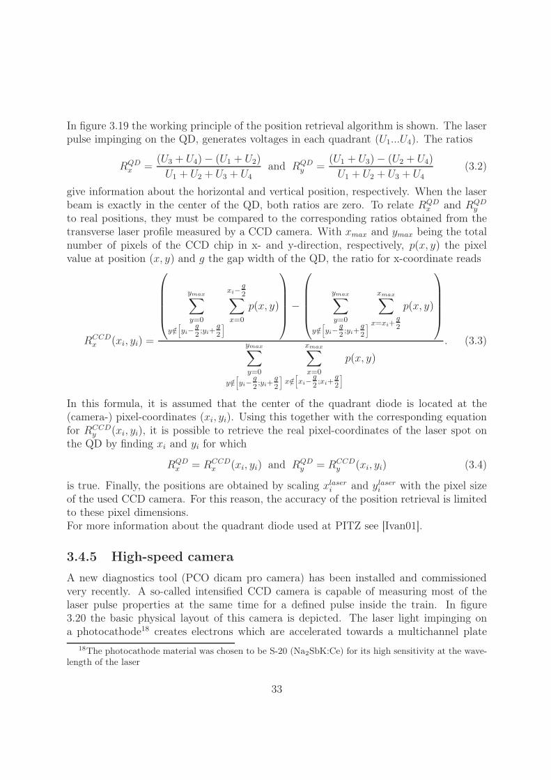
A new diagnostics tool (PCO dicam pro camera) has been installed and commissionedvery recently. A so-called intensified CCD camera is capable of measuring most of thelaser pulse properties at the same time for a defined pulse inside the train. In figure3.20 the basic physical layout of this camera is depicted. The laser light impinging ona photocathode18 creates electrons which are accelerated towards a multichannel plate

18The photocathode material was chosen to be S-20 (Na2SbK:Ce) for its high sensitivity at the wave-length of the laser

33

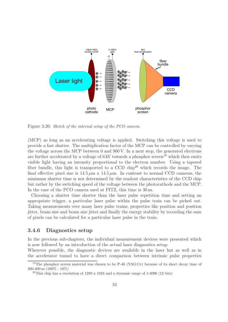
Figure 3.20: Sketch of the internal setup of the PCO camera.

(MCP) as long as an accelerating voltage is applied. Switching this voltage is used toprovide a fast shutter. The multiplication factor of the MCP can be controlled by varyingthe voltage across the MCP between 0 and 900 V. In a next step, the generated electronsare further accelerated by a voltage of 6 kV towards a phosphor screen19 which then emitsvisible light having an intensity proportional to the electron number. Using a taperedfiber bundle, this light is transported to a CCD chip20 which records the image. Thefinal effective pixel size is 14.5μm x 14.5μm. In contrast to normal CCD cameras, theminimum shutter time is not determined by the readout characteristics of the CCD chipbut rather by the switching speed of the voltage between the photocathode and the MCP.In the case of the PCO camera used at PITZ, this time is 30 ns.

Choosing a shutter time shorter than the laser pulse repetition time and setting anappropriate trigger, a particular laser pulse within the pulse train can be picked out.Taking measurements over many laser pulse trains, properties like position and positionjitter, beam size and beam size jitter and finally the energy stability by recording the sumof pixels can be calculated for a particular laser pulse in the train.

3.4.6 Diagnostics setup

In the previous sub-chapters, the individual measurement devices were presented whichis now followed by an introduction of the actual laser diagnostics setup.Wherever possible, the diagnostic devices are available in the laser hut as well as inthe accelerator tunnel to have a direct comparison between intrinsic pulse properties

19The phosphor screen material was chosen to be P-46 (YAG:Ce) because of its short decay time of200-400 ns (100% - 10%)

20This chip has a resolution of 1280 x 1024 and a dynamic range of 1:4096 (12 bits)

34

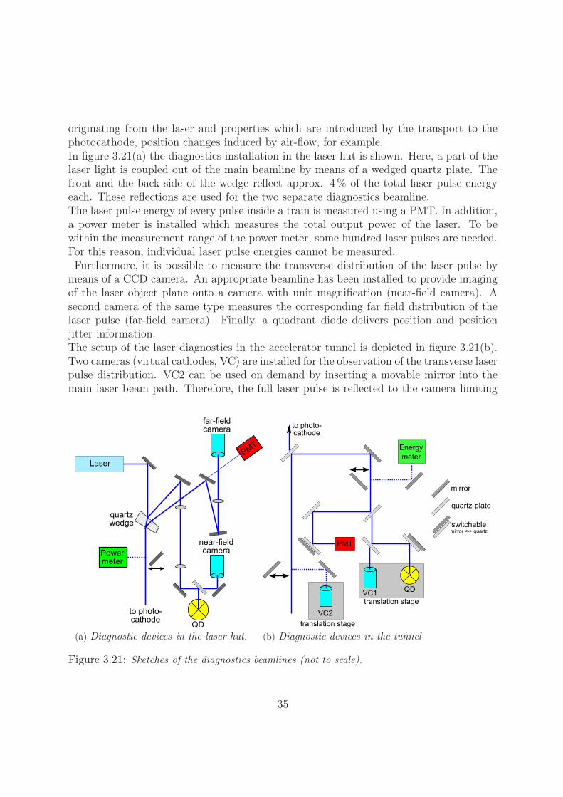
originating from the laser and properties which are introduced by the transport to thephotocathode, position changes induced by air-flow, for example.In figure 3.21(a) the diagnostics installation in the laser hut is shown. Here, a part of thelaser light is coupled out of the main beamline by means of a wedged quartz plate. Thefront and the back side of the wedge reflect approx. 4 % of the total laser pulse energyeach. These reflections are used for the two separate diagnostics beamline.The laser pulse energy of every pulse inside a train is measured using a PMT. In addition,a power meter is installed which measures the total output power of the laser. To bewithin the measurement range of the power meter, some hundred laser pulses are needed.For this reason, individual laser pulse energies cannot be measured.Furthermore, it is possible to measure the transverse distribution of the laser pulse by

means of a CCD camera. An appropriate beamline has been installed to provide imagingof the laser object plane onto a camera with unit magnification (near-field camera). Asecond camera of the same type measures the corresponding far field distribution of thelaser pulse (far-field camera). Finally, a quadrant diode delivers position and positionjitter information.The setup of the laser diagnostics in the accelerator tunnel is depicted in figure 3.21(b).Two cameras (virtual cathodes, VC) are installed for the observation of the transverse laserpulse distribution. VC2 can be used on demand by inserting a movable mirror into themain laser beam path. Therefore, the full laser pulse is reflected to the camera limiting

(a) Diagnostic devices in the laser hut. (b) Diagnostic devices in the tunnel

Figure 3.21: Sketches of the diagnostics beamlines (not to scale).

35

its use to the low-intensity regime. In contrast, VC1 is illuminated by the permanentreflection from a fixed quartz-plate (see figure 3.21(b), top left). Since the reflectioncoefficient is of the order of a few percent, this camera is used in the high laser intensityregime only. A PMT and a quadrant diode are used to measure the energy and theposition of the laser pulses. To yield an absolute information about the laser pulse energy,a calibrated, commercially available photo diode can be used on demand by inserting amirror. The complex combinations of reflections from mirrors and quartz-plates shownin figure 3.21(b) is necessary to match the laser pulse energy to the measurement rangesof the diagnostic devices. Finally, it is possible to change the position of the laser spoton the cameras and the quadrant diode without changing the position of the laser on thephotocathode by means of translation stages.At last, the high-speed camera, introduced in subsection 3.4.5, is also installed in theaccelerator tunnel but not shown in figure 3.21. It is placed at an image plane positionbehind the last mirror of the optics beamline in the tunnel, see figure 3.10.

3.5 SummaryIn this chapter, the laser, the laser beamline and the available laser pulse diagnostics wereintroduced. The installed diagnostics allows to observe all relevant laser pulse properties,i.e. the laser pulse energy, the temporal and transverse shape as well as the position.Recording the pulse energy and position is possible for each pulse within a train usinga photomultiplier tube and a quadrant diode. For the measurement of the temporalshape using the OSS some hundred pulses are needed, whereas the transverse shape isusually measured for the first pulse in a train only using CCD cameras. Finally, thehigh-speed camera allows to do dedicated investigations on a chosen pulse within a trainusing an appropriate trigger and a shutter time shorter than the temporal spacing of thelaser pulses. This shows that plenty of information about the laser pulses generating theelectron bunches is gathered but a full characterization of each pulse within a train is notyet possible.In the next chapter, dedicated measurements will be presented to characterize the laserand the laser beamline using the diagnostic tools that were introduced here.

36

Chapter 4

Measurement of laser pulse properties

In this chapter, dedicated measurements will be presented which were performed to char-acterize the laser and the laser beamline. These are firstly, a comparative study of the tem-poral shape measured by the Optical Sampling System and the Hamamatsu FESCA200streak camera. Secondly, the streak camera was used to study the influence of the com-plete laser beamline up to the photocathode on the temporal laser pulse shape. For thispurpose, the streak camera measurements took place in the tunnel at the (virtual) positionof the photocathode and immediately afterwards in the laser hut. The next investigationcompared the temporal laser shapes of different pulses within the laser pulse train. Af-terwards, measurements are presented which investigate the dependence of the temporallaser profile on the transverse position. While in the fifth part the effect of thermal lensingin the laser system is studied under various conditions, the topic of the final section isthe laser spot size at the position of the inner vacuum mirror (see figure 3.10). At thisposition, the laser beamline has the strongest space restrictions. In addition, since thereis no imaging plane, diffraction patterns occur which increase the total beam span. Incase parts of these diffraction patterns are clipped one would expect a deterioration ofthe laser spot transverse distribution at the position of the photocathode. In

4.1 Comparison between the Optical Sampling Systemand the FESCA200 streak camera

In this sub-chapter, investigations of the precision of the Optical Sampling System willbe presented which require another, completely independent measurement system. Forthis purpose, the streak camera Hamamatsu FESCA200 [Hama01] was used. At the laserwavelength of about 260 nm, this streak camera has a resolution of approx. 800 fs [Tomiz]which is comparable to the resolution of the Optical Sampling System. The advantageof the FESCA200 streak camera over the Optical Sampling System is its single-shotmeasurement capability. On the other hand, the measurements obtained with the streak

37

Figure 4.1: Comparison between single shot measurements (left) and averaged data (right) usinga Hamamatsu FESCA200 streak camera.

camera have a low signal-to-noise ratio (see chapter 3.4.1). While many other streakcameras overcome this problem by applying the so-called synchroscan technique, i.e. asynchronized overlap of many single shots by the streak camera, this is not possible withthe FESCA200. The reason is, that the voltage needed for the transverse deflection ofthe electrons is swept linearly, whereas the synchroscan technique requires a sinusoidalvoltage modulation. The internal trigger jitter for the linear voltage ramp amounts toabout 20 ps [Hama01]. Thus, the averaging cannot be done automatically by the streakcamera, but is left to the post-processing stage. As an example, figure 4.1 shows fiveindividual measurements and the resulting averaged signal.

Figure 4.2: Comparison between FESCA200 (black) and OSS (red) measurements for a 12 ps(FWHM) almost flat top pulse and a 2 ps (FWHM) Gaussian pulse, respectively.Note, that the displayed streak camera measurements were obtained by averagingfive individual measurements.

Because of the low signal-to-noise ratio of single-shot streak camera measurements, alltemporal profiles presented hereafter show the average of five individual measurements.To compare the results obtained with the Optical Sampling System and the streak camera,

38

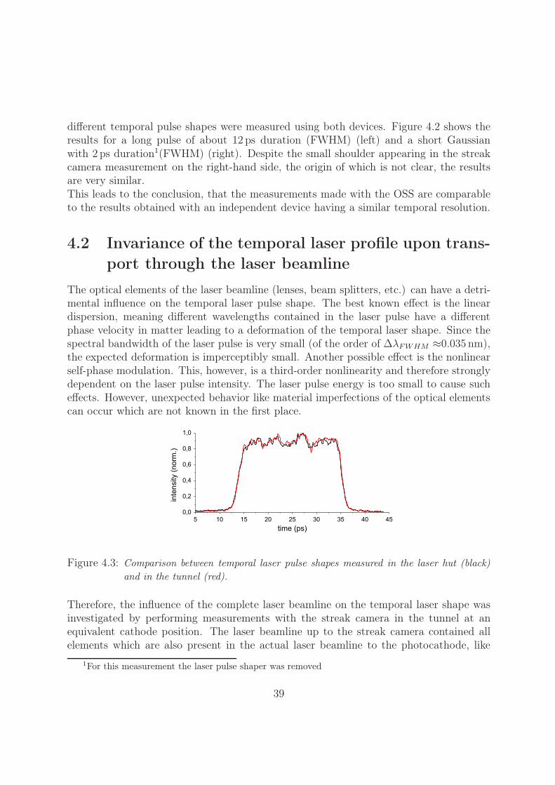
different temporal pulse shapes were measured using both devices. Figure 4.2 shows theresults for a long pulse of about 12 ps duration (FWHM) (left) and a short Gaussianwith 2 ps duration1(FWHM) (right). Despite the small shoulder appearing in the streakcamera measurement on the right-hand side, the origin of which is not clear, the resultsare very similar.This leads to the conclusion, that the measurements made with the OSS are comparableto the results obtained with an independent device having a similar temporal resolution.

4.2 Invariance of the temporal laser profile upon trans-port through the laser beamline

The optical elements of the laser beamline (lenses, beam splitters, etc.) can have a detri-mental influence on the temporal laser pulse shape. The best known effect is the lineardispersion, meaning different wavelengths contained in the laser pulse have a differentphase velocity in matter leading to a deformation of the temporal laser shape. Since thespectral bandwidth of the laser pulse is very small (of the order of ΔλFWHM ≈0.035 nm),the expected deformation is imperceptibly small. Another possible effect is the nonlinearself-phase modulation. This, however, is a third-order nonlinearity and therefore stronglydependent on the laser pulse intensity. The laser pulse energy is too small to cause sucheffects. However, unexpected behavior like material imperfections of the optical elementscan occur which are not known in the first place.

Figure 4.3: Comparison between temporal laser pulse shapes measured in the laser hut (black)and in the tunnel (red).

Therefore, the influence of the complete laser beamline on the temporal laser shape wasinvestigated by performing measurements with the streak camera in the tunnel at anequivalent cathode position. The laser beamline up to the streak camera contained allelements which are also present in the actual laser beamline to the photocathode, like

1For this measurement the laser pulse shaper was removed

39

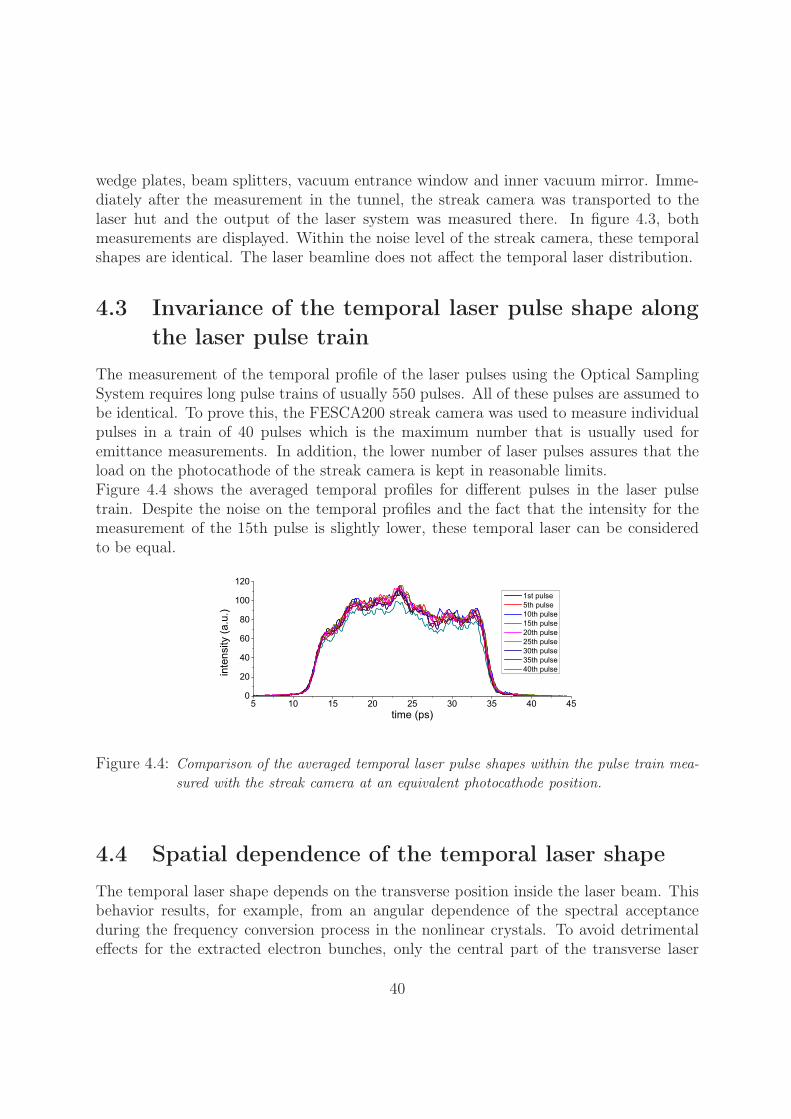
wedge plates, beam splitters, vacuum entrance window and inner vacuum mirror. Imme-diately after the measurement in the tunnel, the streak camera was transported to thelaser hut and the output of the laser system was measured there. In figure 4.3, bothmeasurements are displayed. Within the noise level of the streak camera, these temporalshapes are identical. The laser beamline does not affect the temporal laser distribution.

4.3 Invariance of the temporal laser pulse shape alongthe laser pulse train

The measurement of the temporal profile of the laser pulses using the Optical SamplingSystem requires long pulse trains of usually 550 pulses. All of these pulses are assumed tobe identical. To prove this, the FESCA200 streak camera was used to measure individualpulses in a train of 40 pulses which is the maximum number that is usually used foremittance measurements. In addition, the lower number of laser pulses assures that theload on the photocathode of the streak camera is kept in reasonable limits.Figure 4.4 shows the averaged temporal profiles for different pulses in the laser pulsetrain. Despite the noise on the temporal profiles and the fact that the intensity for themeasurement of the 15th pulse is slightly lower, these temporal laser can be consideredto be equal.

Figure 4.4: Comparison of the averaged temporal laser pulse shapes within the pulse train mea-sured with the streak camera at an equivalent photocathode position.

4.4 Spatial dependence of the temporal laser shapeThe temporal laser shape depends on the transverse position inside the laser beam. Thisbehavior results, for example, from an angular dependence of the spectral acceptanceduring the frequency conversion process in the nonlinear crystals. To avoid detrimentaleffects for the extracted electron bunches, only the central part of the transverse laser

40

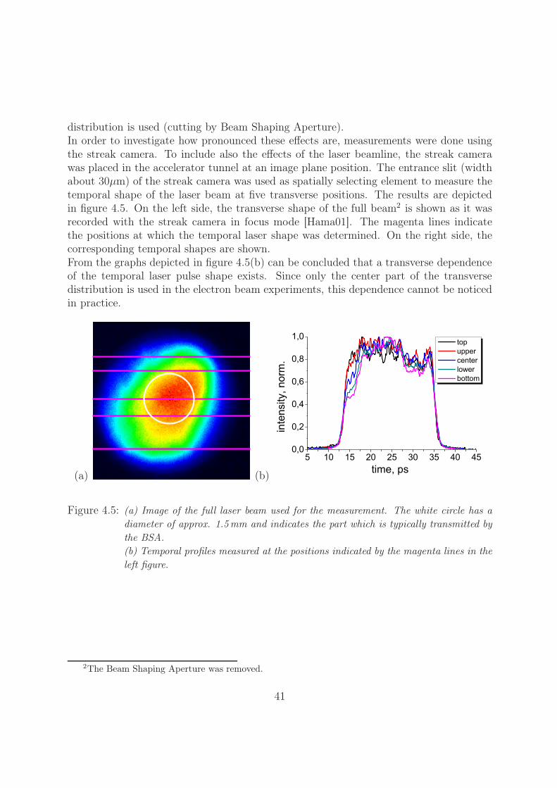
distribution is used (cutting by Beam Shaping Aperture).In order to investigate how pronounced these effects are, measurements were done usingthe streak camera. To include also the effects of the laser beamline, the streak camerawas placed in the accelerator tunnel at an image plane position. The entrance slit (widthabout 30μm) of the streak camera was used as spatially selecting element to measure thetemporal shape of the laser beam at five transverse positions. The results are depictedin figure 4.5. On the left side, the transverse shape of the full beam2 is shown as it wasrecorded with the streak camera in focus mode [Hama01]. The magenta lines indicatethe positions at which the temporal laser shape was determined. On the right side, thecorresponding temporal shapes are shown.From the graphs depicted in figure 4.5(b) can be concluded that a transverse dependenceof the temporal laser pulse shape exists. Since only the center part of the transversedistribution is used in the electron beam experiments, this dependence cannot be noticedin practice.

(a) (b)

Figure 4.5: (a) Image of the full laser beam used for the measurement. The white circle has adiameter of approx. 1.5mm and indicates the part which is typically transmitted bythe BSA.(b) Temporal profiles measured at the positions indicated by the magenta lines in theleft figure.

2The Beam Shaping Aperture was removed.

41

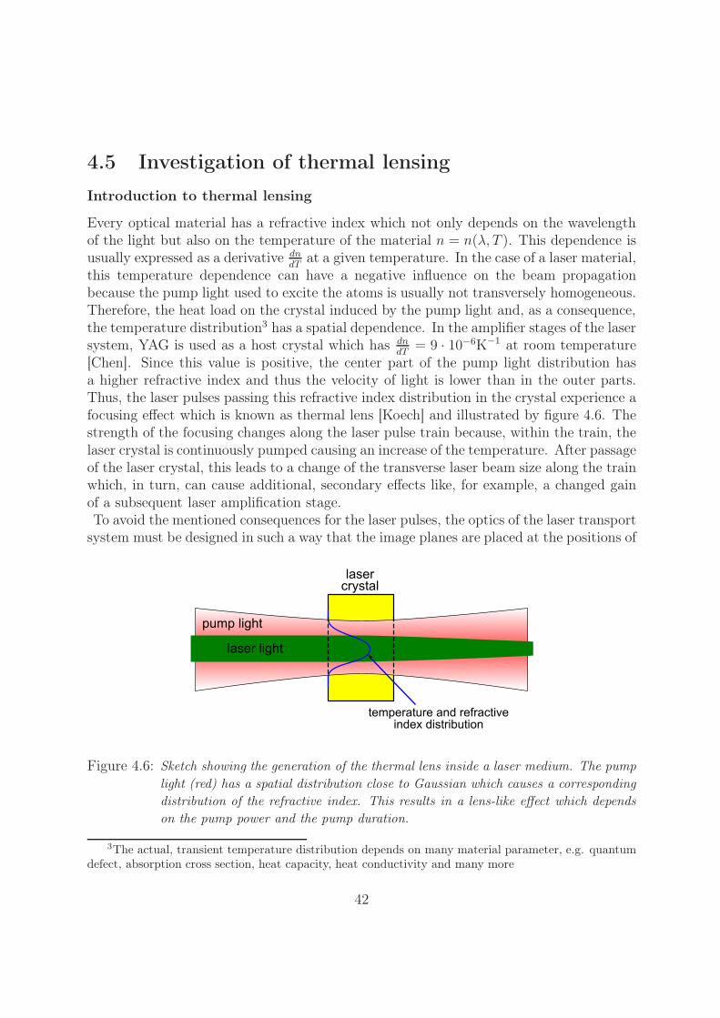
4.5 Investigation of thermal lensingIntroduction to thermal lensing

Every optical material has a refractive index which not only depends on the wavelengthof the light but also on the temperature of the material n = n(λ, T ). This dependence isusually expressed as a derivative dn

dTat a given temperature. In the case of a laser material,

this temperature dependence can have a negative influence on the beam propagationbecause the pump light used to excite the atoms is usually not transversely homogeneous.Therefore, the heat load on the crystal induced by the pump light and, as a consequence,the temperature distribution3 has a spatial dependence. In the amplifier stages of the lasersystem, YAG is used as a host crystal which has dn

dT= 9 · 10−6K−1 at room temperature

[Chen]. Since this value is positive, the center part of the pump light distribution hasa higher refractive index and thus the velocity of light is lower than in the outer parts.Thus, the laser pulses passing this refractive index distribution in the crystal experience afocusing effect which is known as thermal lens [Koech] and illustrated by figure 4.6. Thestrength of the focusing changes along the laser pulse train because, within the train, thelaser crystal is continuously pumped causing an increase of the temperature. After passageof the laser crystal, this leads to a change of the transverse laser beam size along the trainwhich, in turn, can cause additional, secondary effects like, for example, a changed gainof a subsequent laser amplification stage.To avoid the mentioned consequences for the laser pulses, the optics of the laser transport

system must be designed in such a way that the image planes are placed at the positions of

Figure 4.6: Sketch showing the generation of the thermal lens inside a laser medium. The pumplight (red) has a spatial distribution close to Gaussian which causes a correspondingdistribution of the refractive index. This results in a lens-like effect which dependson the pump power and the pump duration.

3The actual, transient temperature distribution depends on many material parameter, e.g. quantumdefect, absorption cross section, heat capacity, heat conductivity and many more

42

the potential thermal lenses. In addition, the imaging from the laser to the Beam ShapingAperture as well as the subsequent imaging on the photocathode must be carefully aligned.If this condition is fulfilled, the change of the beams divergence by the thermal lens doesnot affect the beam size in the next image plane. Thus, the laser pulse properties remainconstant along the train. Even though the alignment of the laser beamline was donevery carefully, a remaining impact of the thermal lens on the laser pulse properties at theposition of the photocathode cannot be excluded.

Measurement setup

To quantify the thermal lensing effect, the PCO camera was placed at a position at whichthe optical path length to the photocathode and the PCO camera were identical. Duringthe measurements, the PCO camera recorded images of the transverse laser profile (tenprofiles for every tenth pulse in a pulse train of 850 pulses). These images were usedto extract the laser beam position, size and intensity4 and the corresponding variationswhich are shown in the graphs of figures 4.7 and 4.8 as rms error bars. In addition,the photo-multiplier tube (PMT) in the laser hut was used to measure the laser pulseenergies emitted from the laser system. The PMT signals were sampled using a fastADC. Its sampling frequency was 1 MHz which allowed to measure the energy of everypulse within the train. Since the sampling of the ADC was triggered to begin before theemission of the laser pulse train started, the first pulse appears at channel no. 699. Here,100 measurements were taken to retrieve the average and jitter values. The error barsappear as gray band in the figures because the point density is too large to resolve themindividually.One specialty of the laser beamline must be mentioned. To spatially clean the laserpulses and thus remove imperfections from the transverse distribution, an iris of variablediameter is placed on the laser table (not at an image position). This iris as well as theBeam Shaping Aperture in the tunnel are distorting the measurements of the thermallensing because they are cutting large parts of the distribution. In reality, this can havepositive and negative effects, for example a movement of the beam before the BeamShaping Aperture will only result in a small change of the center of gravity of the transversedistribution but at the same time the total transmitted laser energy can vary significantly.

Measurements and results

In order to analyze the influence of the mentioned laser beamline elements, the followingsequence of the measurements was chosen. At first, the nominal measurement setup wasused, meaning the Beam Shaping Aperture of 1.5 mm diameter was inserted and the irisin the laser hut was closed to get a good transverse profile. In the second measurement,the BSA was removed and in the subsequent, third measurement, also the iris in the laser

4Measured as sum of pixels

43

hut was fully opened. Finally, the pump light intensity of the last amplification stage andtherefore the heat load on the laser crystals was reduced to see the change of the ther-mal lensing. This was done by decreasing the current of the pumping diodes from 24 A(nominal value) to 18 A. These measurements were performed in the short-pulse mode(the pulse shaper was removed) and the laser pulse duration was about 2.5 ps (FWHM).For the last measurement, the pulse shaper was inserted again and a 24 ps flat-top profilewas produced to see the thermal lensing effect under low-emittance measurement condi-tions.In figure 4.7(a), the results for the first measurement (with BSA and closed iris) are shown.The center position of the laser beam did not change significantly, the same is true forthe beam sizes which change only by about 10μm. The laser intensity, however, droppedto about 40 % from the first pulse towards the end of the laser pulse train.Figure 4.7(b) shows the results with the BSA being removed. In this case, the positiondoes not change significantly but the beam size increases by about 15 % along the trainwhile the intensity drops to 60 %. This result is in agreement with the first measurementbecause inserting the BSA masks the effect of the increasing beam size but the drop inintensity is more severe.In figure 4.7(c), the results are depicted for the case of an open iris. Now the laserbeamline does not clip the laser pulse transversely (vignetting). The complete laser pulseenergy emitted by the laser is transported to the PCO camera. This can be seen bycomparing the measured intensities of the laser hut PMT and the sum of pixels from thePCO camera.The laser pulse position does not change significantly but the beam size decreases byabout 5 % in x-direction and about 10 % in y-direction. This means that the effect ofthermal lensing is still present.The last graph of figure 4.7 shows the results for the pumping diode current of the boosteramplifier changed from 24 A to 18 A. The currents of the pumping diodes for the double-pass amplifier, the regenerative amplifier and the oscillator remained unchanged. This wasdone to reduce the heatload on the crystal and therefore the thermal lens effect. However,the change of the pumping current resulted in a rising slope of the laser pulse energy alongthe laser pulse train. This had to be compensated by adjusting the timing characteristicsof the pump diodes of the double-pass amplifier such that the pumping of the laser crystalstarts 100μs earlier. From figure 4.7(d) it becomes evident that the consequent increaseof the heat load on the laser crystal of the double-pass amplifier counteracts the reductionof the heat load on the booster amplifier. The beam size in x-direction increases by 19 %and in y-direction by 7 % while the laser intensity along the train drops by 23 %.These results show that the thermal lens effect is present in the booster as well as inthe double-pass amplifier. It cannot be reduced by simply decreasing the pumping diodeoutput power of one of the final amplifier stages.

44

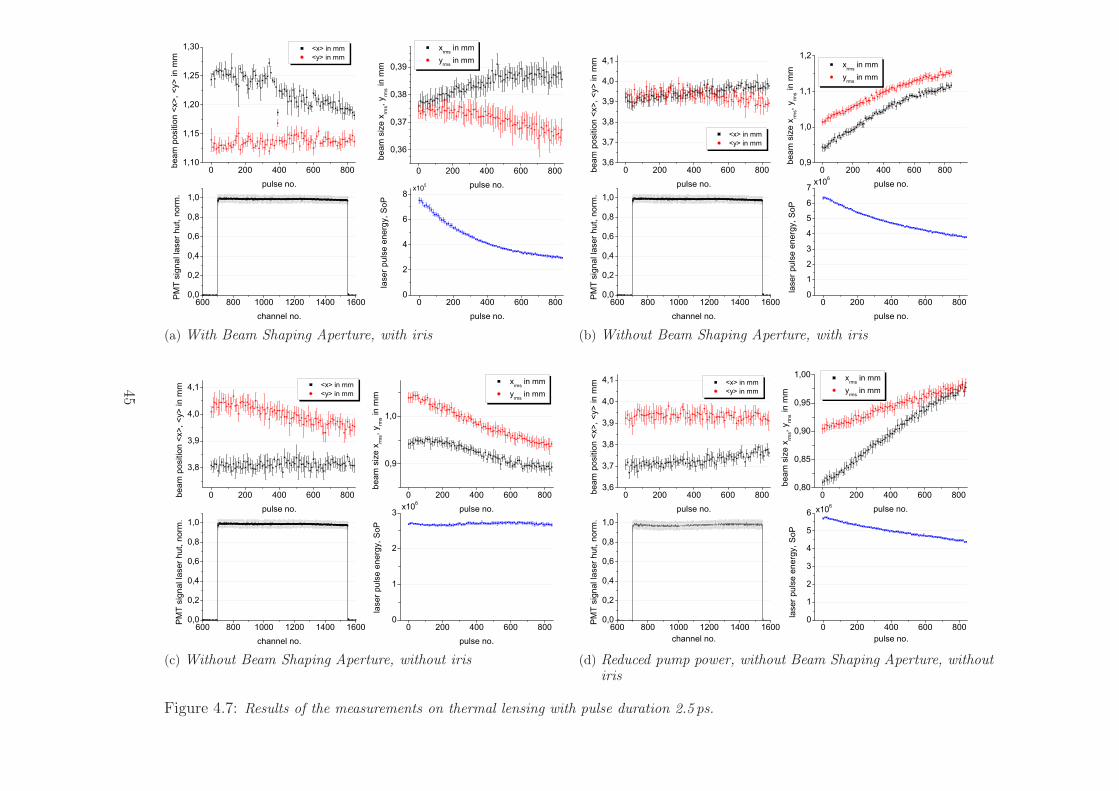
(a) With Beam Shaping Aperture, with iris (b) Without Beam Shaping Aperture, with iris

(c) Without Beam Shaping Aperture, without iris (d) Reduced pump power, without Beam Shaping Aperture, withoutiris

Figure 4.7: Results of the measurements on thermal lensing with pulse duration 2.5 ps.

45

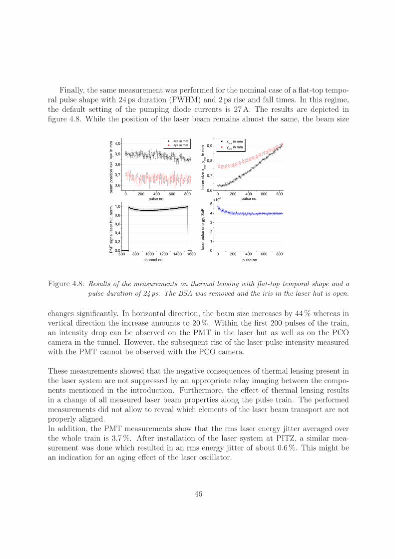
Finally, the same measurement was performed for the nominal case of a flat-top tempo-ral pulse shape with 24 ps duration (FWHM) and 2 ps rise and fall times. In this regime,the default setting of the pumping diode currents is 27 A. The results are depicted infigure 4.8. While the position of the laser beam remains almost the same, the beam size

Figure 4.8: Results of the measurements on thermal lensing with flat-top temporal shape and apulse duration of 24 ps. The BSA was removed and the iris in the laser hut is open.

changes significantly. In horizontal direction, the beam size increases by 44 % whereas invertical direction the increase amounts to 20 %. Within the first 200 pulses of the train,an intensity drop can be observed on the PMT in the laser hut as well as on the PCOcamera in the tunnel. However, the subsequent rise of the laser pulse intensity measuredwith the PMT cannot be observed with the PCO camera.

These measurements showed that the negative consequences of thermal lensing present inthe laser system are not suppressed by an appropriate relay imaging between the compo-nents mentioned in the introduction. Furthermore, the effect of thermal lensing resultsin a change of all measured laser beam properties along the pulse train. The performedmeasurements did not allow to reveal which elements of the laser beam transport are notproperly aligned.In addition, the PMT measurements show that the rms laser energy jitter averaged overthe whole train is 3.7 %. After installation of the laser system at PITZ, a similar mea-surement was done which resulted in an rms energy jitter of about 0.6 %. This might bean indication for an aging effect of the laser oscillator.

46

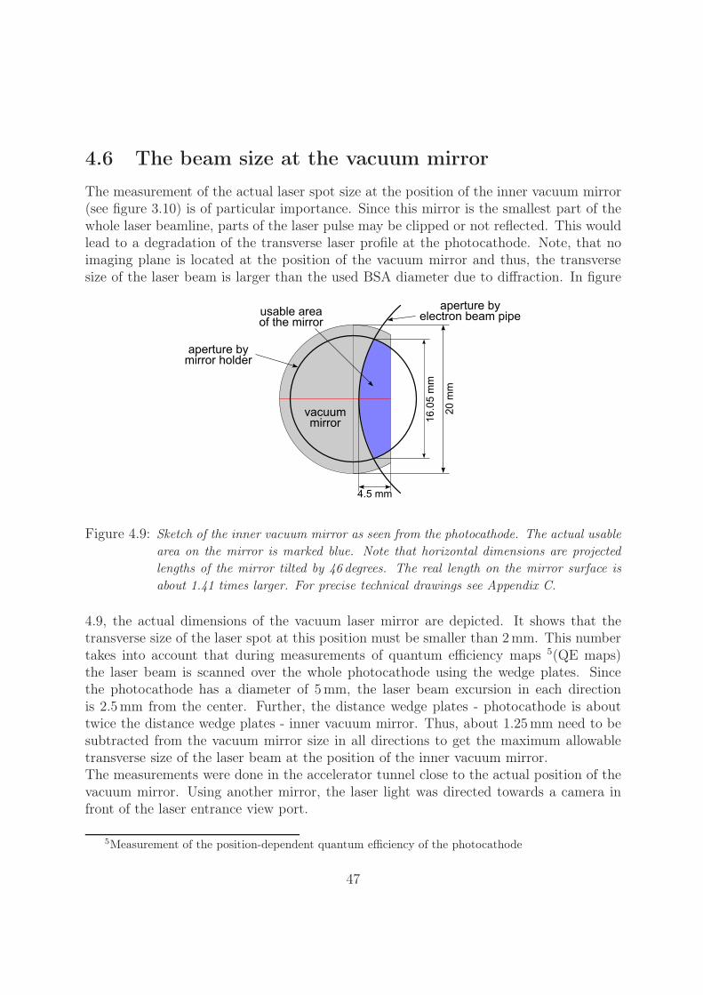
4.6 The beam size at the vacuum mirrorThe measurement of the actual laser spot size at the position of the inner vacuum mirror(see figure 3.10) is of particular importance. Since this mirror is the smallest part of thewhole laser beamline, parts of the laser pulse may be clipped or not reflected. This wouldlead to a degradation of the transverse laser profile at the photocathode. Note, that noimaging plane is located at the position of the vacuum mirror and thus, the transversesize of the laser beam is larger than the used BSA diameter due to diffraction. In figure

Figure 4.9: Sketch of the inner vacuum mirror as seen from the photocathode. The actual usablearea on the mirror is marked blue. Note that horizontal dimensions are projectedlengths of the mirror tilted by 46 degrees. The real length on the mirror surface isabout 1.41 times larger. For precise technical drawings see Appendix C.

4.9, the actual dimensions of the vacuum laser mirror are depicted. It shows that thetransverse size of the laser spot at this position must be smaller than 2 mm. This numbertakes into account that during measurements of quantum efficiency maps 5(QE maps)the laser beam is scanned over the whole photocathode using the wedge plates. Sincethe photocathode has a diameter of 5 mm, the laser beam excursion in each directionis 2.5 mm from the center. Further, the distance wedge plates - photocathode is abouttwice the distance wedge plates - inner vacuum mirror. Thus, about 1.25 mm need to besubtracted from the vacuum mirror size in all directions to get the maximum allowabletransverse size of the laser beam at the position of the inner vacuum mirror.The measurements were done in the accelerator tunnel close to the actual position of thevacuum mirror. Using another mirror, the laser light was directed towards a camera infront of the laser entrance view port.

5Measurement of the position-dependent quantum efficiency of the photocathode

47

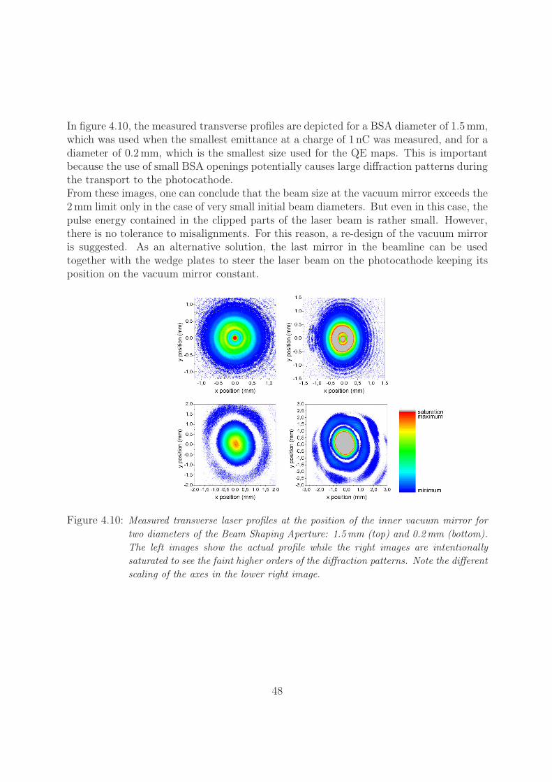
In figure 4.10, the measured transverse profiles are depicted for a BSA diameter of 1.5 mm,which was used when the smallest emittance at a charge of 1 nC was measured, and for adiameter of 0.2 mm, which is the smallest size used for the QE maps. This is importantbecause the use of small BSA openings potentially causes large diffraction patterns duringthe transport to the photocathode.From these images, one can conclude that the beam size at the vacuum mirror exceeds the2 mm limit only in the case of very small initial beam diameters. But even in this case, thepulse energy contained in the clipped parts of the laser beam is rather small. However,there is no tolerance to misalignments. For this reason, a re-design of the vacuum mirroris suggested. As an alternative solution, the last mirror in the beamline can be usedtogether with the wedge plates to steer the laser beam on the photocathode keeping itsposition on the vacuum mirror constant.

Figure 4.10: Measured transverse laser profiles at the position of the inner vacuum mirror fortwo diameters of the Beam Shaping Aperture: 1.5mm (top) and 0.2mm (bottom).The left images show the actual profile while the right images are intentionallysaturated to see the faint higher orders of the diffraction patterns. Note the differentscaling of the axes in the lower right image.

48

Chapter 5

The electron emission process

The main part of the emittance of an electron bunch is generated during the emissionprocess. For this reason, the aspects associated with the emission are introduced in thischapter.Three emission mechanisms are relevant for the electron bunch production in accelerators.These are the field emission, the thermionic emission and the photoemission.Field emission occurs when a material is exposed to a very strong electric field which causesa lowering of the potential barrier at the surface of the material and thus an increasedprobability of quantum mechanical tunneling of the electrons. In RF photoinjectors, thisprocess leads only to an unwanted current contribution (dark current). Therefore it is notfurther discussed. For more information on this topic see [Han].A second process of charge production is the thermionic emission. It is based on theheating of the cathode material until a sufficiently large part of the high-energy tail ofthe electron density distribution inside the material exceeds the surface potential barrier.These high-energy electrons can escape into the vacuum and produce the electron beamupon acceleration. This emission process is used for example at SCSS, Japan [SCSS], orat MaxLAB, Sweden [MAXlab]. A review on thermionic emission can be found in [Modi].The third process of charge production, which is also used at PITZ, is the photoemission.Upon light illumination, electrons inside the material are excited to energy levels whichare appropriate to overcome the surface potential barrier and are therefore emitted. Thisprocess is possible in metals (e.g. copper) and semiconductors (e.g. GaAs or Cs2Te). Theelectron bunch production using photoemission has proven to provide beams of highestquality so far. The main reason is the possibility to influence the electron bunch propertiesby changing the transverse and temporal parameters of the laser pulse which is used forthe extraction. The choice of the photocathode material is influenced by several param-eters, for example the quantum efficiency, cathode lifetime, robustness to poor vacuumconditions and the efforts associated with the development of a proper laser system. For

49

PITZ, the best compromise between the given constraints is Cesium Telluride1.The following sub-chapters are dedicated to the physics of the photoemission of Cs2Te.Firstly, the emission process is described in detail. This is followed by the presentation ofissues arising from two facts: The space charge fields, which are generated by the bunchitself, are not negligible during the emission and secondly, the emission can be enhancedby a strong electric field at the cathode surface.

5.1 Photoemission in Cs2TeAccording to Spicer [Spic], the photoemission can be described by a three-step model:

1. Excitation of an electron inside the material by absorption of a photon

2. Migration of the electron towards the surface

3. Electron emission across the surface potential barrier

The absorption takes place in the Cs2Te-layer which has a thickness of 20-30 nm [Lede01]and is deposited on a Molybdenum plug. Since the photon absorption length is less than20 nm, most of the photons promote electrons to the conduction band. These electronsmove randomly inside the photocathode layer. Since the electron density in the conductionband of the semiconductor is very low, the probability of collisions between electrons islittle. Therefore, the electron escape length can be of the order of μm allowing almostall electrons to escape [Han]. In addition, the movement towards the surface can besupported by an external electric field.The time the electrons need to travel to the surface defines the photocathode responsetime. Due to the small absorption length, the photoelectrons are excited close to thesurface. Therefore, one would expect the response time to be very short. Dedicatedmeasurements do not exist but estimates range from 0.5 ps to less than 2 ps, which wasjustified by experimental observations.To obtain a better insight into the photoemission process, the band structure of Cs2Te asmeasured by Powell et al.[Pow] is depicted in figure 5.1. The excitation of electrons fromthe valence band to the conduction band requires photon energies of at least Ephoton =3.3 eV which is equal to the band gap. The density of states at the initial and final energylevel is very low in this case making the transition very inefficient. Furthermore, theseelectrons could not escape into the vacuum because they need to overcome the surfacepotential barrier. This energy difference from the lower conduction-band edge to the

1Another widely used photocathode material is copper. Its advantage is the resistance against poorvacuum condition which makes the handling easy, but the disadvantage is the low quantum efficiencyof the order of 10−5 − 10−4. GaAs can provide electron bunches with a very low cathode emittance(see chapter 6.2.1) but requires vacuum pressures in the range of 10−11 − 10−12 mbar which cannot bemaintained in RF gun cavities.

50

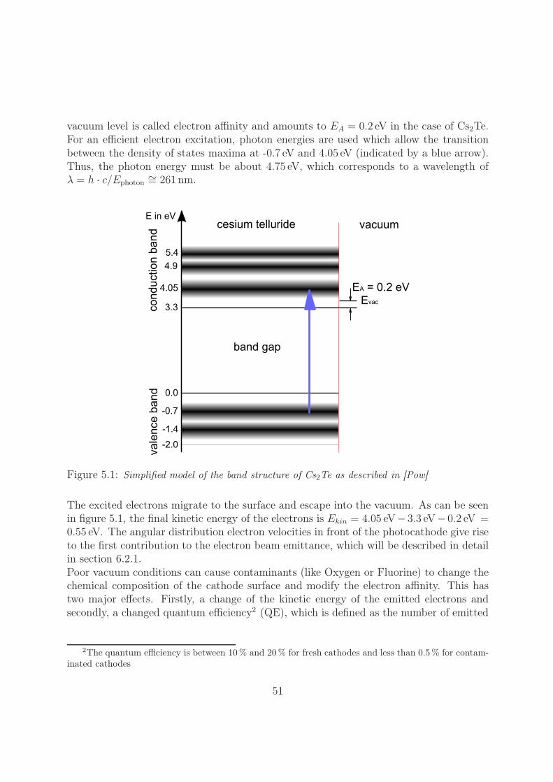
vacuum level is called electron affinity and amounts to EA = 0.2 eV in the case of Cs2Te.For an efficient electron excitation, photon energies are used which allow the transitionbetween the density of states maxima at -0.7 eV and 4.05 eV (indicated by a blue arrow).Thus, the photon energy must be about 4.75 eV, which corresponds to a wavelength ofλ = h · c/Ephoton

∼= 261nm.

Figure 5.1: Simplified model of the band structure of Cs2Te as described in [Pow]

The excited electrons migrate to the surface and escape into the vacuum. As can be seenin figure 5.1, the final kinetic energy of the electrons is Ekin = 4.05 eV− 3.3 eV− 0.2 eV =0.55 eV. The angular distribution electron velocities in front of the photocathode give riseto the first contribution to the electron beam emittance, which will be described in detailin section 6.2.1.Poor vacuum conditions can cause contaminants (like Oxygen or Fluorine) to change thechemical composition of the cathode surface and modify the electron affinity. This hastwo major effects. Firstly, a change of the kinetic energy of the emitted electrons andsecondly, a changed quantum efficiency2 (QE), which is defined as the number of emitted

2The quantum efficiency is between 10 % and 20 % for fresh cathodes and less than 0.5 % for contam-inated cathodes

51

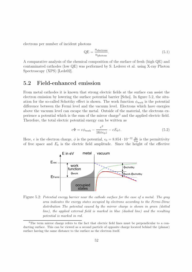
electrons per number of incident photons

QE =nelectrons

nphotons. (5.1)

A comparative analysis of the chemical composition of the surface of fresh (high QE) andcontaminated cathodes (low QE) was performed by S. Lederer et al. using X-ray PhotonSpectroscopy (XPS) [Lede02].

5.2 Field-enhanced emissionFrom metal cathodes it is known that strong electric fields at the surface can assist theelectron emission by lowering the surface potential barrier [Scho]. In figure 5.2, the situ-ation for the so-called Schottky effect is shown. The work function φwork is the potentialdifference between the Fermi level and the vacuum level. Electrons which have energiesabove the vacuum level can escape the metal. Outside of the material, the electrons ex-perience a potential which is the sum of the mirror charge3 and the applied electric field.Therefore, the total electric potential energy can be written as

eΦ = eφwork − e2

16πε0z− eE0z. (5.2)

Here, e is the electron charge, φ is the potential, ε0 = 8.854 · 10−12 AsVm is the permittivity

of free space and E0 is the electric field amplitude. Since the height of the effective

Figure 5.2: Potential energy barrier near the cathode surface for the case of a metal. The grayarea indicates the energy states occupied by electrons according to the Fermi-Diracdistribution The potential caused by the mirror charge is shown in green (dottedline), the applied external field is marked in blue (dashed line) and the resultingpotential is marked in red.

3The term mirror charge refers to the fact that electric field lines must be perpendicular to a con-ducting surface. This can be viewed as a second particle of opposite charge located behind the (planar)surface having the same distance to the surface as the electron itself.

52

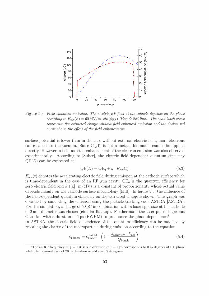
Figure 5.3: Field-enhanced emission. The electric RF field at the cathode depends on the phaseaccording to Eacc(φ) = 60MV/m ·sin(φRF) (blue dotted line). The solid black curverepresents the extracted charge without field-enhanced emission and the dashed redcurve shows the effect of the field enhancement.

surface potential is lower than in the case without external electric field, more electronscan escape into the vacuum. Since Cs2Te is not a metal, this model cannot be applieddirectly. However, a field-assisted enhancement of the electron emission was also observedexperimentally. According to [Suber], the electric field-dependent quantum efficiencyQE(E) can be expressed as

QE(E) = QE0 + k · Eacc(t). (5.3)

Eacc(t) denotes the accelerating electric field during emission at the cathode surface whichis time-dependent in the case of an RF gun cavity, QE0 is the quantum efficiency forzero electric field and k ([k]=m/MV) is a constant of proportionality whose actual valuedepends mainly on the cathode surface morphology [Milt]. In figure 5.3, the influence ofthe field-dependent quantum efficiency on the extracted charge is shown. This graph wasobtained by simulating the emission using the particle tracking code ASTRA [ASTRA].For this simulation, a charge of 50 pC in combination with a laser spot size at the cathodeof 2 mm diameter was chosen (circular flat-top). Furthermore, the laser pulse shape wasGaussian with a duration of 1 ps (FWHM) to pronounce the phase dependence4.In ASTRA, the electric field dependence of the quantum efficiency can be modeled byrescaling the charge of the macroparticle during emission according to the equation

Qmacro = Qinitialmacro ·

(1 +

kSchottky · Eacc

Qbunch

). (5.4)

4For an RF frequency of f = 1.3 GHz a duration of t = 1 ps corresponds to 0.47 degrees of RF phasewhile the nominal case of 20 ps duration would span 9.4 degrees

53

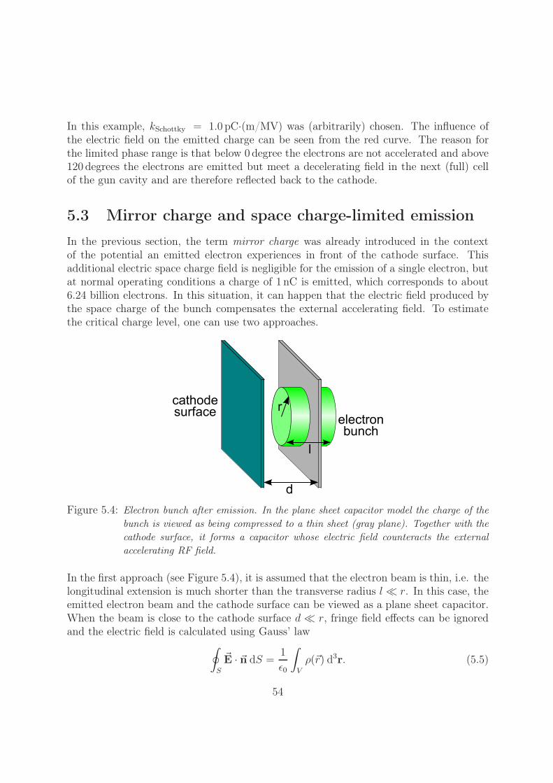
In this example, kSchottky = 1.0pC·(m/MV) was (arbitrarily) chosen. The influence ofthe electric field on the emitted charge can be seen from the red curve. The reason forthe limited phase range is that below 0 degree the electrons are not accelerated and above120 degrees the electrons are emitted but meet a decelerating field in the next (full) cellof the gun cavity and are therefore reflected back to the cathode.

5.3 Mirror charge and space charge-limited emissionIn the previous section, the term mirror charge was already introduced in the contextof the potential an emitted electron experiences in front of the cathode surface. Thisadditional electric space charge field is negligible for the emission of a single electron, butat normal operating conditions a charge of 1 nC is emitted, which corresponds to about6.24 billion electrons. In this situation, it can happen that the electric field produced bythe space charge of the bunch compensates the external accelerating field. To estimatethe critical charge level, one can use two approaches.

Figure 5.4: Electron bunch after emission. In the plane sheet capacitor model the charge of thebunch is viewed as being compressed to a thin sheet (gray plane). Together with thecathode surface, it forms a capacitor whose electric field counteracts the externalaccelerating RF field.

In the first approach (see Figure 5.4), it is assumed that the electron beam is thin, i.e. thelongitudinal extension is much shorter than the transverse radius l � r. In this case, theemitted electron beam and the cathode surface can be viewed as a plane sheet capacitor.When the beam is close to the cathode surface d � r, fringe field effects can be ignoredand the electric field is calculated using Gauss’ law∮

S

�E · �n dS =1

ε0

∫V

ρ(�r) d3r. (5.5)

54

In this equation, �E is the electric field vector, �n is the surface normal vector and S is thesurface of the volume V which encloses the charge density ρ(�r). By integrating over thecylinder’s surface one obtains

Ez =σ

ε0. (5.6)

Here, σ is the surface charge density of the thin bunch. For Ez = Eacc(t), the externalelectric field is fully compensated and no electron will be accelerated from the cathodesurface. For circular flat-top electron bunch of radius r, the maximum extractable chargeQmax can be estimated as

Qmax = π · r2ε0 · Eacc(t). (5.7)

The second approach derives the space charge limit by assuming a constant currentstreaming from the cathode. The limit is expressed in terms of a maximum currentdensity which causes, due to space charge forces, the field at the cathode to drop to zero.This is well known as the Child-Langmuir law [Reis]

J =4

9· ε0

√2e

me· φ3/2

d2. (5.8)

Here, me is the electron rest mass, φ is the potential difference between the cathode surfaceand a point at distance d. Please note that in the sheet capacitor model, the maximumextractable charge is proportional to the potential φ while in the Child-Langmuir law itscales with φ3/2.Since the electron bunch is neither a flat sheet nor a constant current, both models canonly give an estimate at which charge level space charge forces start to distort the emission.Typical parameters are a bunch duration of 20 ps (flat-top) which corresponds to about6 mm length, an electron bunch radius of 0.75 mm and a maximum electric field amplitudeon the cathode of 60 MV/m. For an RF emission phase of 40 deg, the plane sheet capacitormodel predicts a maximum extractable charge of about QPSC

max=600 pC whereas the Child-Langmuir law gives about QCL

max=250 pC. In practice, it can be observed that with thisparameter combination the space charge effects start to distort the emission at a bunchcharge of about 1 nC while it is possible to extract up to about 1.5 nC.

5.4 SummaryIn this chapter, the process of photoemission was introduced. It was shown that theelectron yield, i.e. the bunch charge, depends not only on the number of incident photonsbut also on the strength of the applied electric field amplitude. In addition, the emittedcharge itself causes an electric field which diminishes the external electric field at thecathode and therefore counteracts the field-enhanced emission. It sets a limit to themaximal extractable charge.

55

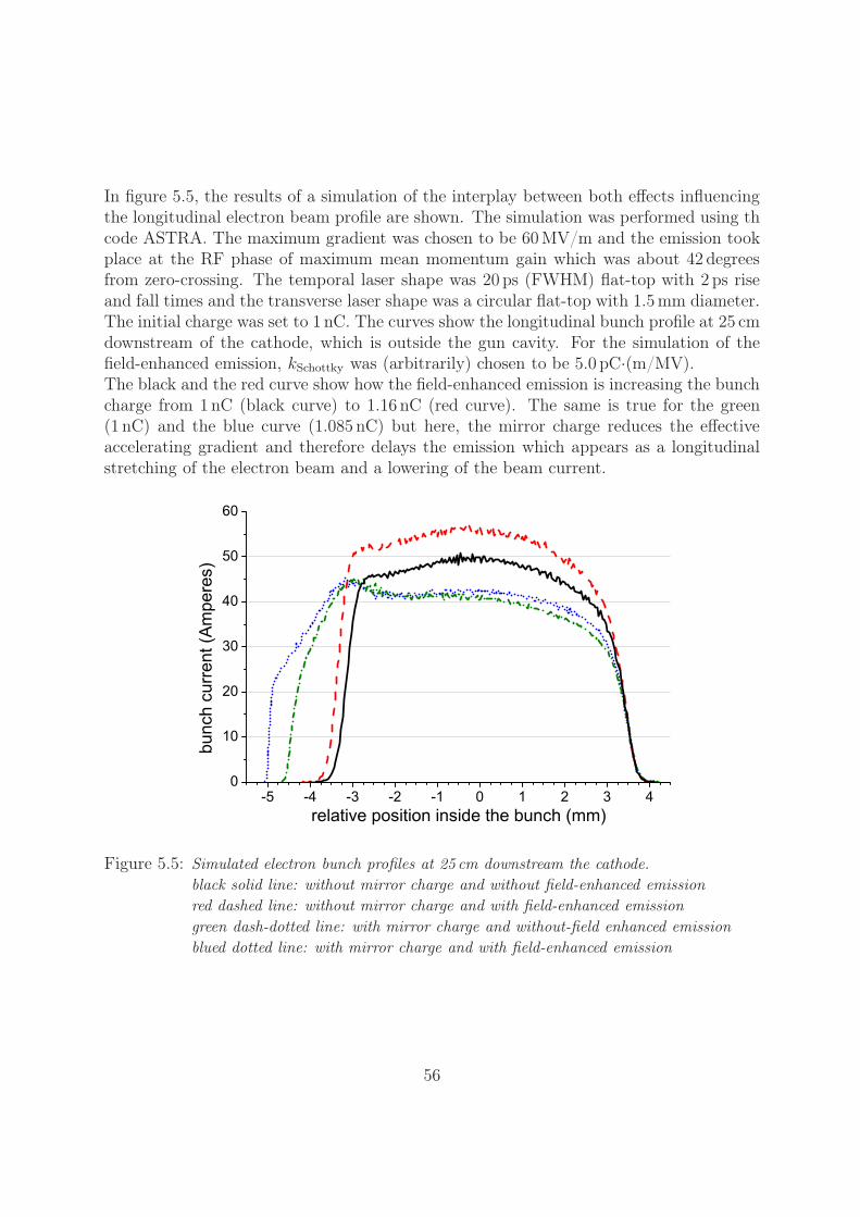
In figure 5.5, the results of a simulation of the interplay between both effects influencingthe longitudinal electron beam profile are shown. The simulation was performed using thcode ASTRA. The maximum gradient was chosen to be 60 MV/m and the emission tookplace at the RF phase of maximum mean momentum gain which was about 42 degreesfrom zero-crossing. The temporal laser shape was 20 ps (FWHM) flat-top with 2 ps riseand fall times and the transverse laser shape was a circular flat-top with 1.5 mm diameter.The initial charge was set to 1 nC. The curves show the longitudinal bunch profile at 25 cmdownstream of the cathode, which is outside the gun cavity. For the simulation of thefield-enhanced emission, kSchottky was (arbitrarily) chosen to be 5.0 pC·(m/MV).The black and the red curve show how the field-enhanced emission is increasing the bunchcharge from 1 nC (black curve) to 1.16 nC (red curve). The same is true for the green(1 nC) and the blue curve (1.085 nC) but here, the mirror charge reduces the effectiveaccelerating gradient and therefore delays the emission which appears as a longitudinalstretching of the electron beam and a lowering of the beam current.

Figure 5.5: Simulated electron bunch profiles at 25 cm downstream the cathode.black solid line: without mirror charge and without field-enhanced emissionred dashed line: without mirror charge and with field-enhanced emissiongreen dash-dotted line: with mirror charge and without-field enhanced emissionblued dotted line: with mirror charge and with field-enhanced emission

56

Chapter 6

Electron beam dynamics

This chapter is dedicated to a detailed description of the fundamental electron beam dy-namics in a so-called split injector setup. This term refers to injector layouts which consistof a short electron gun cavity, a subsequent solenoid magnet for emittance compensationin the drift space towards the next accelerating structure [Sera]. The sources and the evo-lution of the transverse emittance along the electron beamline are presented together witha description of the concept of the invariant envelope, which helps to optimize the setupfor lowest transverse emittance. This is followed by an introduction to the longitudinalphase space dynamics.

6.1 Phase space representation of the electron beamThe state of one single particle can be fully described by the definition of its coordinate inthe six-dimensional phase space composed of the particle’s position �r and its momentum�p

u = u(�r, �p) = (x, px, y, py, z, pz)T . (6.1)

During the transport along the accelerator, this particle experiences forces arising fromelectric and magnetic fields. Electric fields are mainly used to accelerate particles, whilemagnetic fields steer and focus the beam. The action of the these fields on the particlemotion can be described by the Lorentz force equation

�F =d�p

dt= q ·

(�E + �v × �B

). (6.2)

In this formula, �F is the force, q is the charge of the particle, �E and �B are the electricand the magnetic field strengths, respectively, and �v is the particle velocity.An ensemble of particles such as an electron bunch is better described by its six-dimensionalphase space density f6(�r, �p) according to

dN = f6(�r, �p)dV6. (6.3)

57

In this equation, dN is the number of particles in the infinitesimally small six-dimensionalhyper volume dV6. Alternatively, one can use dQ = ρ6(�r, �p) dV6 with ρ being the chargedensity and dQ the charge contained in dV6. If the coupling between the three differentplanes can be ignored, the complexity of this six dimensional representation can be reducedby defining three two-dimensional subspaces according to the three spatial directions.These are the longitudinal phase space density f2(z, pz) and the two transverse phasespace densities f2(x, px) and f2(y, py). The reduced phase space densities are, e.g. for thehorizontal coordinate, defined by

f2(x, px) =

∫ ∫ ∫ ∫f6(�r, �p) dy dpy dz dpz. (6.4)

In an accelerator, the longitudinal momentum of the particles is orders of magnitudelarger than the transverse momenta. Therefore, it is justified to use the paraxial approxi-mation in connection with the divergence angles x′ = px/pz and y′ = py/pz instead of thetransverse momenta. The new density distributions f2(x, x′) and f2(y, y′) are called tracespace distributions.The transverse rms emittance εrms of a bunch is defined as the rms area it occupies intrace space. For the {x,x′}-trace space, the expression for εx,rms reads

εx,rms =

√〈x2〉 〈x′2〉 − 〈xx′〉2 , [εx,rms] = m · rad. (6.5)

The angular brackets indicate the central second order moments of the enclosed quantities.Assuming x̄ = 0 and x̄′ = 0, they are defined as

⟨x2

⟩=

1∫ ∫f2(x, x′) dx dx′ ·

∫ ∫f2(x, x′) · x2 dx dx′,

⟨x′2⟩ =

1∫ ∫f2(x, x′) dx dx′ ·

∫ ∫f2(x, x′) · x′2 dx dx′, (6.6)

〈xx′〉 =1∫ ∫

f2(x, x′) dx dx′ ·∫ ∫

f2(x, x′) · xx′ dx dx′.

From the definitions of x′ and y′ follows that the divergence and hence the emittancescales inversely proportional to the longitudinal beam momentum pz. By normalizing theemittances, it is possible to compare beams of different momenta

εx,rms,norm = βγ ·√

〈x2〉 〈x′2〉 − 〈xx′〉2. (6.7)

Since all transverse emittance values given in this work follow this definition, the sub-scripts rms and norm are omitted from now on.In addition to the definitions already given, the quantities transverse emittance and trans-verse phase/trace space distribution can be defined also for thin slices perpendicular to

58

the z-axis. The resulting transverse slice emittance and slice phase/trace space are im-portant for the concept of emittance compensation described in chapter 6.3. Since thephase space of the whole bunch is a result of the projection of all slice phase spaces ontoone plane, the emittance defined in equation 6.5 is also called projected emittance.

Liouville’s theorem

Liouville’s theorem states that in a conservative field in which the forces can be derivedfrom a potential the six-dimensional volume of the phase space remains constant [Leje].One consequence of this theorem is that the emittance of a particle ensemble is constant.This invariance of the emittance is a key issue in the description of the particle beammotion in accelerators. Unfortunately, this theorem is not applicable for the descriptionof electron bunches in an injector setup. The reason is that at low beam energies, typicalfor injectors, the influence of the space charge forces is very strong. Since it is impossibleto define a potential and thus an Hamiltonian for space charge forces, Liouville’s theoremcannot be applied.In addition, this theorem is valid for the six-dimensional phase space volume. In thecase of coupling between the longitudinal and transverse subspaces, the six-dimensionalphase space volume might remain unchanged, but not necessarily its projections to thetwo-dimensional phase spaces (equation 6.4) whose volume is usually measured.

6.2 Sources of transverse emittanceThere are three main contributions to the total transverse emittance. Firstly, there isthe emittance arising from disordered movement of the electrons as they escape from thecathode surface (cathode emittance1). The second contribution comes from the pondero-motive RF focusing forces while the third reason for emittance growth is the occurrencespace charge forces. In the following sections, these contributions will be introduced.

6.2.1 Cathode emittance

As shown in chapter 5.1, the electrons emitted from the photocathode have random direc-tions independent of their position on the cathode. Therefore, the thermal emittance hasno x-x′ correlation and equation 6.7 reduces to εcath = βγ ·√〈x2〉 〈x′2〉 = βγ · xrmsx

′rms =

xrmspx,rms/(m0c). While xrms is defined by the transverse laser spot size, px,rms needsfurther consideration. Following the arguments in [Floet], the momentum of an emittedelectron is mainly defined by the electron affinity of the material. Firstly, the electron

1The term thermal emittance is also frequently used even though it originally refers to the cathodeemittance of thermionic emitters.

59

affinity influences the final kinetic energy and secondly, the momentum inside the ma-terial must have a sufficiently large component in the direction of the surface normal toovercome the surface potential barrier. Otherwise, the particle is reflected back into thebulk. This sets a limit for the maximum angle the particle momentum can have withrespect to the surface normal. This angle can be calculated as

ϕmax = arccos

√EA

Einsidekin

. (6.8)

Following the calculation of px,rms in [Floet], the cathode emittance reads

εcath = xrms ·√

2Eoutsidekin

m0c2· 1√

3·√

2 + cos3 ϕmax − 3 cosϕmax

2 · (1 − cos ϕmax). (6.9)

Here Eoutsidekin is the kinetic energy of the electron inside the material reduced by the

electron affinity. Typical values for Cs2Te are Einsidekin = 0.75 eV and EA = 0.2 eV and for

the laser beam size at the cathode xrms = 0.375mm. For this parameter combination,the cathode emittance amounts to 0.25 mmmrad.One can further simplify equation 6.9 by allowing the particles to be emitted into the fullhalf-sphere in front of the cathode (ϕmax=90 degrees)2

εcath = xrms ·√

2Eoutsidekin

3m0c2. (6.10)

Using this approximation, the cathode emittance for the above parameter combination isεcath=0.32 mmmrad.

6.2.2 RF induced emittance

The z-component of the time-dependent electric field along the symmetry axis of the guncavity can be expressed as

Ez(z, t) = Ez(z) · cos(2πf · t + φ0). (6.11)

In this equation, Ez(z) is the time-independent, on-axis field distribution which is deter-mined by the cavity’s geometry, f is the RF frequency (about 1.3 GHz at PITZ) and φ0

is an initial phase offset.

2The simulation code ASTRA which was used throughout this thesis uses this approximation tosimulate the cathode emittance.

60

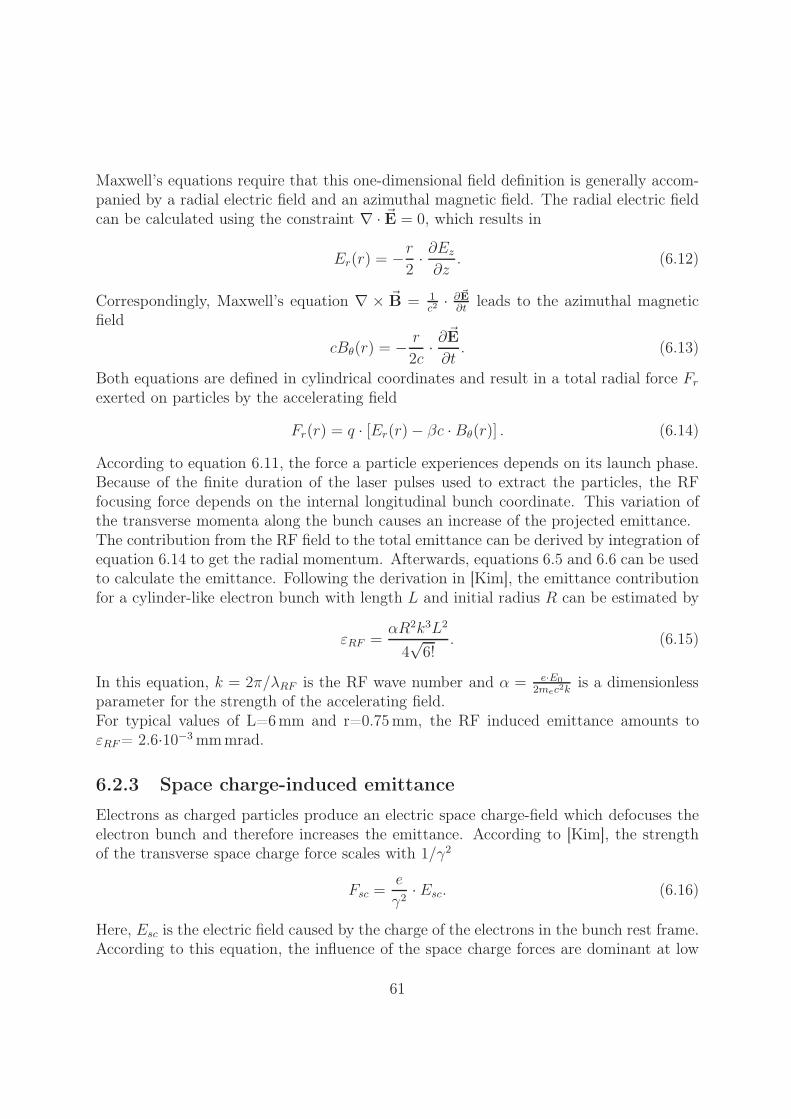
Maxwell’s equations require that this one-dimensional field definition is generally accom-panied by a radial electric field and an azimuthal magnetic field. The radial electric fieldcan be calculated using the constraint ∇ · �E = 0, which results in

Er(r) = −r

2· ∂Ez

∂z. (6.12)

Correspondingly, Maxwell’s equation ∇ × �B = 1c2

· ∂�E∂t

leads to the azimuthal magneticfield

cBθ(r) = − r

2c· ∂�E

∂t. (6.13)

Both equations are defined in cylindrical coordinates and result in a total radial force Fr

exerted on particles by the accelerating field

Fr(r) = q · [Er(r) − βc · Bθ(r)] . (6.14)

According to equation 6.11, the force a particle experiences depends on its launch phase.Because of the finite duration of the laser pulses used to extract the particles, the RFfocusing force depends on the internal longitudinal bunch coordinate. This variation ofthe transverse momenta along the bunch causes an increase of the projected emittance.The contribution from the RF field to the total emittance can be derived by integration ofequation 6.14 to get the radial momentum. Afterwards, equations 6.5 and 6.6 can be usedto calculate the emittance. Following the derivation in [Kim], the emittance contributionfor a cylinder-like electron bunch with length L and initial radius R can be estimated by

εRF =αR2k3L2

4√

6!. (6.15)

In this equation, k = 2π/λRF is the RF wave number and α = e·E0

2mec2kis a dimensionless

parameter for the strength of the accelerating field.For typical values of L=6 mm and r=0.75 mm, the RF induced emittance amounts toεRF = 2.6·10−3 mmmrad.

6.2.3 Space charge-induced emittance

Electrons as charged particles produce an electric space charge-field which defocuses theelectron bunch and therefore increases the emittance. According to [Kim], the strengthof the transverse space charge force scales with 1/γ2

Fsc =e

γ2· Esc. (6.16)

Here, Esc is the electric field caused by the charge of the electrons in the bunch rest frame.According to this equation, the influence of the space charge forces are dominant at low

61

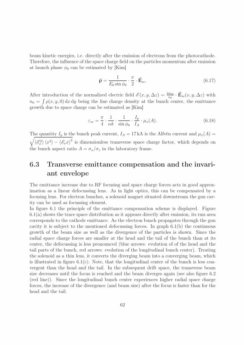
beam kinetic energies, i.e. directly after the emission of electrons from the photocathode.Therefore, the influence of the space charge field on the particles momentum after emissionat launch phase φ0 can be estimated by [Kim]

�p =1

E0 sin φ0· π

2· �Esc. (6.17)

After introduction of the normalized electric field E (x, y, Δz) = 4πε0n0

· �Esc(x, y, Δz) withn0 =

∫ρ(x, y, 0) dx dy being the line charge density at the bunch center, the emittance

growth due to space charge can be estimated as [Kim]

εsc =π

4· 1

αk· 1

sin φ0· Ip

IA· μx(A). (6.18)

The quantity Ip is the bunch peak current, IA = 17 kA is the Alfvén current and μx(A) =√〈E 2

x 〉 〈x2〉 − 〈Exx〉2 is dimensionless transverse space charge factor, which depends onthe bunch aspect ratio A = σx/σz in the laboratory frame.

6.3 Transverse emittance compensation and the invari-ant envelope

The emittance increase due to RF focusing and space charge forces acts in good approx-imation as a linear defocussing lens. As in light optics, this can be compensated by afocusing lens. For electron bunches, a solenoid magnet situated downstream the gun cav-ity can be used as focussing element.In figure 6.1 the principle of the emittance compensation scheme is displayed. Figure6.1(a) shows the trace space distribution as it appears directly after emission, its rms areacorresponds to the cathode emittance. As the electron bunch propagates through the guncavity it is subject to the mentioned defocussing forces. In graph 6.1(b) the continuousgrowth of the beam size as well as the divergence of the particles is shown. Since theradial space charge forces are smaller at the head and the tail of the bunch than at itscenter, the defocussing is less pronounced (blue arrows: evolution of of the head and thetail parts of the bunch, red arrows: evolution of the longitudinal bunch center). Treatingthe solenoid as a thin lens, it converts the diverging beam into a converging beam, whichis illustrated in figure 6.1(c). Note, that the longitudinal center of the bunch is less con-vergent than the head and the tail. In the subsequent drift space, the transverse beamsize decreases until the focus is reached and the beam diverges again (see also figure 6.2(red line)). Since the longitudinal bunch center experiences higher radial space chargeforces, the increase of the divergence (and beam size) after the focus is faster than for thehead and the tail.

62

(a) Cathode emittance in tracespace.

(b) Space charge forces defocusthe bunch.

(c) The solenoid acts as a thinlens.

(d) The trace space distribu-tion evolves into a emit-tance minimum.

Figure 6.1: Emittance compensation process. The longitudinal bunch center which experienceshigher radial space charge forces is indicated by a red area while the bunch’s headand tail are displayed in blue.

Eventually, this leads to an alignment of the trace space angles of all longitudinal partsof the bunch and thus to an emittance minimum depicted in figure 6.1(d).To avoid a further emittance increase, the electron bunch must be accelerated very quickly(scaling of the space charge forces with 1/γ2). Conditions for the optimum accelerationcan be found using the invariant envelope approach [Sera].Before the invariant envelope is discussed, it must be stressed that the emittance com-pensation scheme only takes into account linear defocussing forces Fr(r) ∝ r. NonlinearRF- or space charge forces cannot be compensated and lead to an increase of the totalemittance.Since these nonlinear forces predominantly occur at the transverse edges of the electronbeam, they tend to increase the rms trace space area and therefore the emittance eventhough the charge contained in these regions is low. For this reason, the emittance mightbe given using a cut of the transverse trace space distribution at a certain trace space

63

Figure 6.2: Simulated model case for the transverse emittance (black) and transverse rms beamsize (red) evolution along the electron beamline for the cases with (solid line) andwithout booster (dashed line). The inset shows the same graph which is scaled to seethe whole emittance curve.

intensity level [Stay].Furthermore, since different longitudinal parts of the electron beam are launched at

different RF phases of the gun cavity, a correlation between longitudinal position andmomentum exists. For this reason, the projected emittance typically shows two minimain the case of an optimized setup (see figure 6.2), each representing the optimum overlapof head-and-center and center-and-tail slice trace space distributions [Kras01].

The invariant envelope

The evolution of an electron bunch along the beamline can be described in the paraxialapproximation by the envelope equation [Carl, Sera]

σ′′ + σ′γ′

γ+ σ

Ω2γ′2

γ2=

κs

σγ3+

ε2n

σ3γ2. (6.19)

This model can be applied when the longitudinal momentum spread of the bunch is smallso that the longitudinal slices do not mix. Here, σ = σ(ζ) is the rms beam size of alongitudinal slice as a function of the internal bunch coordinate ζ = z − vt, γ is therelativistic factor and the primes at each variable indicate the derivative with respect toz. The beam perveance is denoted with κs = Ip/2IA (Ip is the peak current and IA theAlfvén current) and εn indicates the normalized rms slice emittance.Equation 6.19 describes in a general way the evolution of the beam size of longitudinalslices under the influence of a defocussing space charge (first term on the r.h.s.) and the

64

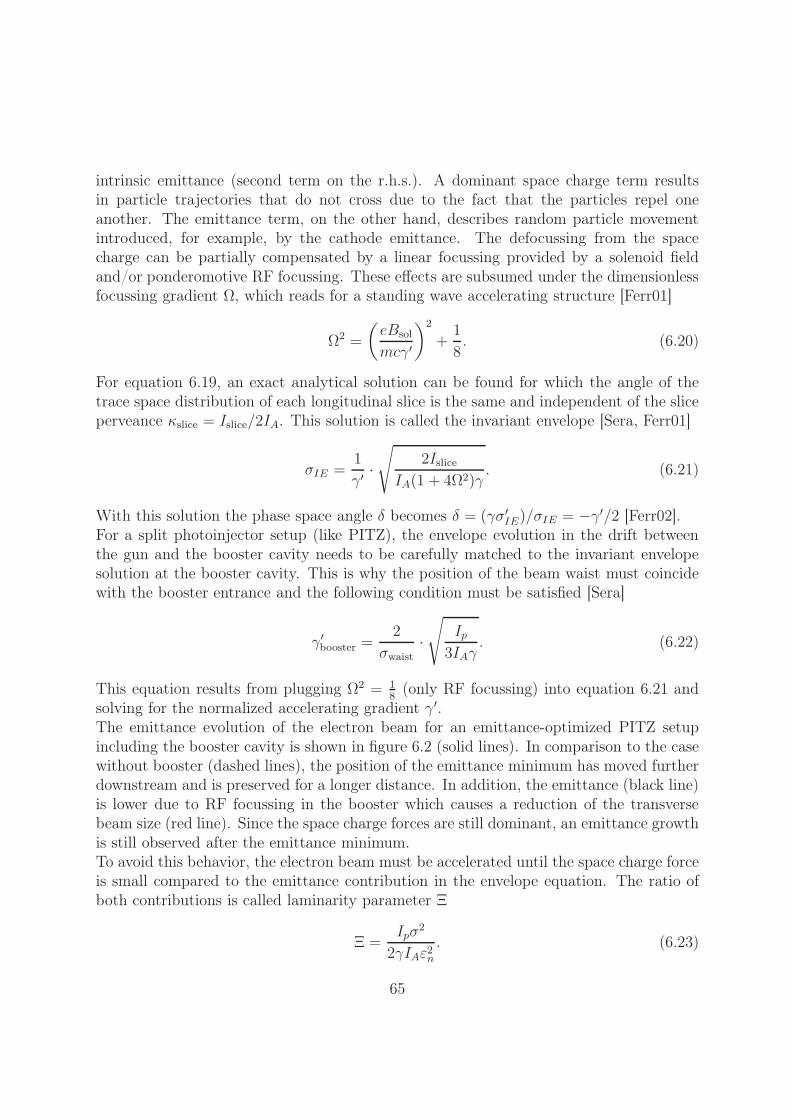
intrinsic emittance (second term on the r.h.s.). A dominant space charge term resultsin particle trajectories that do not cross due to the fact that the particles repel oneanother. The emittance term, on the other hand, describes random particle movementintroduced, for example, by the cathode emittance. The defocussing from the spacecharge can be partially compensated by a linear focussing provided by a solenoid fieldand/or ponderomotive RF focussing. These effects are subsumed under the dimensionlessfocussing gradient Ω, which reads for a standing wave accelerating structure [Ferr01]

Ω2 =

(eBsol

mcγ′

)2

+1

8. (6.20)

For equation 6.19, an exact analytical solution can be found for which the angle of thetrace space distribution of each longitudinal slice is the same and independent of the sliceperveance κslice = Islice/2IA. This solution is called the invariant envelope [Sera, Ferr01]

σIE =1

γ′ ·√

2Islice

IA(1 + 4Ω2)γ. (6.21)

With this solution the phase space angle δ becomes δ = (γσ′IE)/σIE = −γ′/2 [Ferr02].

For a split photoinjector setup (like PITZ), the envelope evolution in the drift betweenthe gun and the booster cavity needs to be carefully matched to the invariant envelopesolution at the booster cavity. This is why the position of the beam waist must coincidewith the booster entrance and the following condition must be satisfied [Sera]

γ′booster =

2

σwaist·√

Ip

3IAγ. (6.22)

This equation results from plugging Ω2 = 18

(only RF focussing) into equation 6.21 andsolving for the normalized accelerating gradient γ′.The emittance evolution of the electron beam for an emittance-optimized PITZ setupincluding the booster cavity is shown in figure 6.2 (solid lines). In comparison to the casewithout booster (dashed lines), the position of the emittance minimum has moved furtherdownstream and is preserved for a longer distance. In addition, the emittance (black line)is lower due to RF focussing in the booster which causes a reduction of the transversebeam size (red line). Since the space charge forces are still dominant, an emittance growthis still observed after the emittance minimum.To avoid this behavior, the electron beam must be accelerated until the space charge forceis small compared to the emittance contribution in the envelope equation. The ratio ofboth contributions is called laminarity parameter Ξ

Ξ =Ipσ

2

2γIAε2n

. (6.23)

65

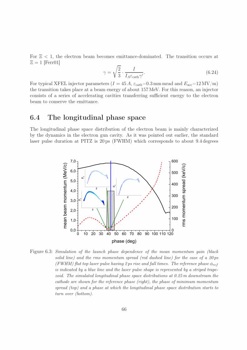
For Ξ < 1, the electron beam becomes emittance-dominated. The transition occurs atΞ = 1 [Ferr01]

γ =

√2

3· I

IAεcathγ′ . (6.24)

For typical XFEL injector parameters (I = 45 A, εcath=0.3 mmmrad and Eacc=12 MV/m)the transition takes place at a beam energy of about 157 MeV. For this reason, an injectorconsists of a series of accelerating cavities transferring sufficient energy to the electronbeam to conserve the emittance.

6.4 The longitudinal phase spaceThe longitudinal phase space distribution of the electron beam is mainly characterizedby the dynamics in the electron gun cavity. As it was pointed out earlier, the standardlaser pulse duration at PITZ is 20 ps (FWHM) which corresponds to about 9.4 degrees

Figure 6.3: Simulation of the launch phase dependence of the mean momentum gain (blacksolid line) and the rms momentum spread (red dashed line) for the case of a 20 ps(FWHM) flat top laser pulse having 2 ps rise and fall times. The reference phase φref

is indicated by a blue line and the laser pulse shape is represented by a striped trape-zoid. The simulated longitudinal phase space distributions at 0.25m downstream thecathode are shown for the reference phase (right), the phase of minimum momentumspread (top) and a phase at which the longitudinal phase space distribution starts toturn over (bottom).

66

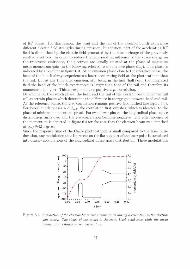
of RF phase. For this reason, the head and the tail of the electron bunch experiencedifferent electric field strengths during emission. In addition, part of the accelerating RFfield is diminished by the electric field generated by the mirror charge of the previouslyemitted electrons. In order to reduce the deteriorating influence of the space charge onthe transverse emittance, the electrons are usually emitted at the phase of maximummean momentum gain (in the following referred to as reference phase φref). This phase isindicated by a blue line in figure 6.3. At an emission phase close to the reference phase, thehead of the bunch always experiences a lower accelerating field at the photocathode thanthe tail. But at any time after emission, still being in the first (half) cell, the integratedfield the head of the bunch experienced is larger than that of the tail and therefore itsmomentum is higher. This corresponds to a positive z-pz-correlation.Depending on the launch phase, the head and the tail of the electron beam enter the fullcell at certain phases which determine the difference in energy gain between head and tail.At the reference phase, the z-pz-correlation remains positive (red dashed line figure 6.3).For lower launch phases φ < φref , the correlation first vanishes, which is identical to thephase of minimum momentum spread. For even lower phases, the longitudinal phase spacedistribution turns over and the z-pz-correlation becomes negative. The z-dependence ofthe momentum is depicted in figure 6.4 for the case that the electron beam was launchedat φref

∼=42 degrees.Since the response time of the Cs2Te photocathode is small compared to the laser pulseduration, any modulation that is present on the flat top part of the laser pulse is translatedinto density modulations of the longitudinal phase space distribution. These modulations

Figure 6.4: Simulation of the electron beam mean momentum during acceleration in the electrongun cavity. The shape of the cavity is shown in black solid lines while the meanmomentum is drawn as red dashed line.

67

are also visible in the projections of the longitudinal phase space distribution onto thetemporal and momentum axes provided that the z-pz-correlation allows to resolve them.These effects are presented in the section 7.6.

68

Chapter 7

Influence of the laser pulse parameterson the electron beam properties

This chapter is dedicated to the presentation of the fundamental relations between laserpulse parameters and electron beam properties. Firstly, some general considerations willbe presented including an explanation of why the default temporal laser profile was chosento be a 20 ps (FWHM) flat-top with rise and fall times of 2 ps. Afterwards, the simulatedoptimum set of parameters (solenoid field strength, laser spot size on the photocathode,gun phase and booster phase) to obtain lowest transverse emittance will be discussed. Inthe subsequent sub-chapters, detailed simulations are presented which show how devia-tions from the optimum laser pulse shape act on the electron bunch properties. Thesesimulations are accompanied by electron beam measurements.Unless stated otherwise, all simulations were done for the PITZ setup described in chapter2.1 using standard operating conditions summarized in table 7.1. The transverse emit-tance was evaluated at the position of the first Emittance Measurement System (EMSY1)which is located 5.74 m downstream of the photocathode. At this position, the measure-ments of the transverse emittance are performed.

Machine parameter Valuemax. electric field gun 60 MV/mmax. electric field booster 14 MV/mnominal bunch charge 1 nCEinitial

kin for calculation of εcath 0.55 eV

Table 7.1: Summary of the standard operation conditions used in simulations and experimentunless stated otherwise.

69

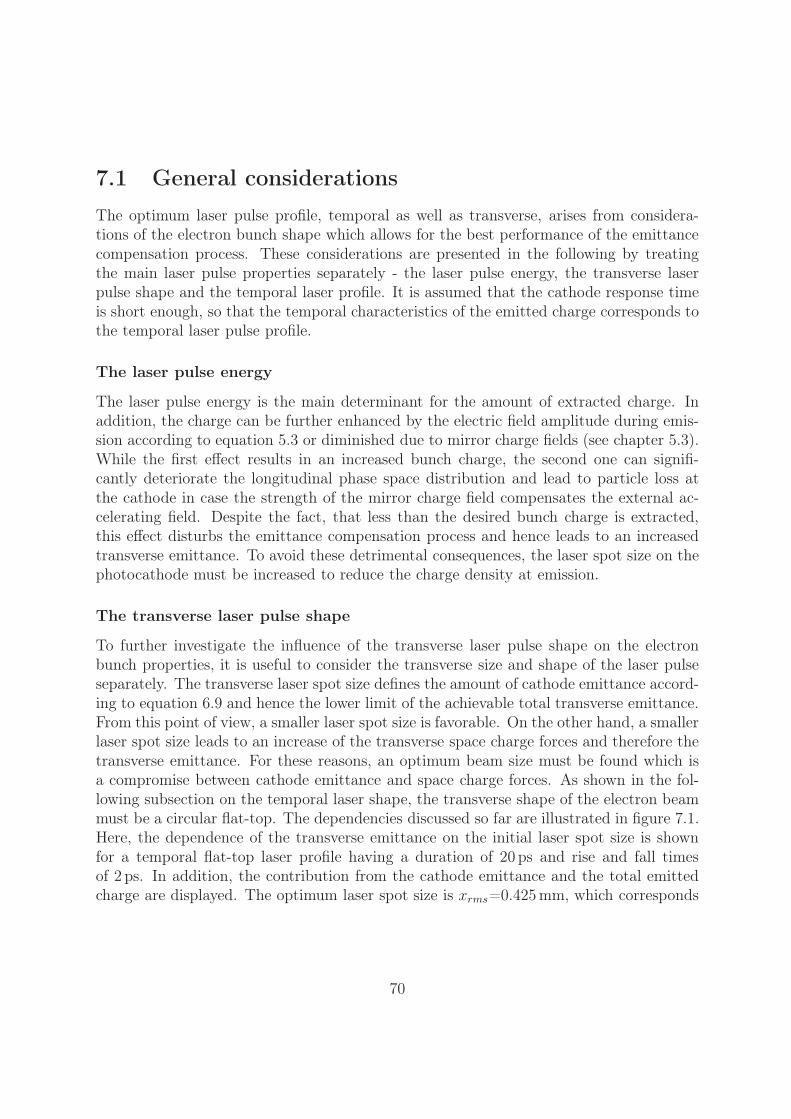
7.1 General considerationsThe optimum laser pulse profile, temporal as well as transverse, arises from considera-tions of the electron bunch shape which allows for the best performance of the emittancecompensation process. These considerations are presented in the following by treatingthe main laser pulse properties separately - the laser pulse energy, the transverse laserpulse shape and the temporal laser profile. It is assumed that the cathode response timeis short enough, so that the temporal characteristics of the emitted charge corresponds tothe temporal laser pulse profile.

The laser pulse energy

The laser pulse energy is the main determinant for the amount of extracted charge. Inaddition, the charge can be further enhanced by the electric field amplitude during emis-sion according to equation 5.3 or diminished due to mirror charge fields (see chapter 5.3).While the first effect results in an increased bunch charge, the second one can signifi-cantly deteriorate the longitudinal phase space distribution and lead to particle loss atthe cathode in case the strength of the mirror charge field compensates the external ac-celerating field. Despite the fact, that less than the desired bunch charge is extracted,this effect disturbs the emittance compensation process and hence leads to an increasedtransverse emittance. To avoid these detrimental consequences, the laser spot size on thephotocathode must be increased to reduce the charge density at emission.

The transverse laser pulse shape

To further investigate the influence of the transverse laser pulse shape on the electronbunch properties, it is useful to consider the transverse size and shape of the laser pulseseparately. The transverse laser spot size defines the amount of cathode emittance accord-ing to equation 6.9 and hence the lower limit of the achievable total transverse emittance.From this point of view, a smaller laser spot size is favorable. On the other hand, a smallerlaser spot size leads to an increase of the transverse space charge forces and therefore thetransverse emittance. For these reasons, an optimum beam size must be found which isa compromise between cathode emittance and space charge forces. As shown in the fol-lowing subsection on the temporal laser shape, the transverse shape of the electron beammust be a circular flat-top. The dependencies discussed so far are illustrated in figure 7.1.Here, the dependence of the transverse emittance on the initial laser spot size is shownfor a temporal flat-top laser profile having a duration of 20 ps and rise and fall timesof 2 ps. In addition, the contribution from the cathode emittance and the total emittedcharge are displayed. The optimum laser spot size is xrms=0.425 mm, which corresponds

70

Figure 7.1: Transverse emittance versus the transverse laser spot size. Displayed are the simu-lated total transverse emittance at 5.74 downstream of the photocathode (black solidline), the cathode emittance (red dashed line) and the emitted charge (blue dottedline)

to a diameter of 1.7 mm1. For laser spot sizes smaller than xrms=0.37 mm, the emissionbecomes space charge dominated and a fraction of the extracted charge cannot leave thecathode. For laser spot sizes larger than xrms=0.45 mm the cathode emittance starts todominate the total transverse emittance.

The temporal laser pulse shape

In chapter 6.3, it was shown that the emittance compensation process can counteract lin-ear transverse defocussing forces. For this reason, it must be ensured that the transversespace charge forces are linear: Fr(r) ∝ r. This is true for a cylindrical electron beam ofradius R and an infinite longitudinal extension having a homogeneous charge density ρ.In this case, the defocussing force experienced by an electron at distance r < R from thecylinder center is Fr(r) = eρ

2ε0· r which can be simply obtained by applying Gauss’ law.

Since the actual electron bunch is not infinitely long, the transverse space charge forcesat the head and the tail are smaller than in the center. The required temporal laser pulseshape according to these considerations is a flat-top with short rise and fall times.The optimal duration of the laser pulse is again a compromise between several consider-ations. To reduce the strength of the transverse space charge fields, a longer laser pulseduration is preferential. On the other hand, FEL operation requires large electron bunch

1For a transverse flat-top profile, the relation between rms size xrms or yrms and diameter d isd = 4 · x/yrms.

71

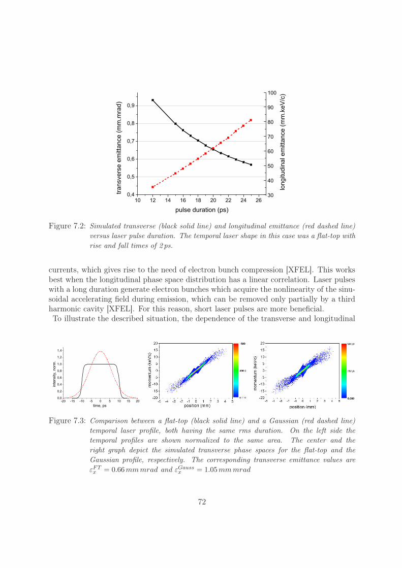
Figure 7.2: Simulated transverse (black solid line) and longitudinal emittance (red dashed line)versus laser pulse duration. The temporal laser shape in this case was a flat-top withrise and fall times of 2 ps.

currents, which gives rise to the need of electron bunch compression [XFEL]. This worksbest when the longitudinal phase space distribution has a linear correlation. Laser pulseswith a long duration generate electron bunches which acquire the nonlinearity of the sinu-soidal accelerating field during emission, which can be removed only partially by a thirdharmonic cavity [XFEL]. For this reason, short laser pulses are more beneficial.To illustrate the described situation, the dependence of the transverse and longitudinal

Figure 7.3: Comparison between a flat-top (black solid line) and a Gaussian (red dashed line)temporal laser profile, both having the same rms duration. On the left side thetemporal profiles are shown normalized to the same area. The center and theright graph depict the simulated transverse phase spaces for the flat-top and theGaussian profile, respectively. The corresponding transverse emittance values areεFTx = 0.66mm mrad and εGauss

x = 1.05mm mrad

72

emittance values on the laser pulse duration are depicted in figure 7.2. The given numberswere obtained by an numerical optimization of the machine parameters for lowest trans-verse emittance. No constraint was given to the longitudinal emittance. As a compromise,a pulse duration of 20 ps FWHM was chosen [XFEL].In order to demonstrate the benefits of an homogeneous charge distribution, figure 7.3shows two simulated transverse phase space distributions. The first was obtained for aflat-top temporal profile of 20 ps (FWHM) and 2 ps rise and fall times, while for the sec-ond one a temporally Gaussian shape was used. Both temporal profiles have the samerms duration which results in a FWHM duration of 13.6 ps for the Gaussian shape. Thedistributions were obtained from an optimization of the machine parameters. The goalwas to minimize the transverse emittance at the location of EMSY1 at 5.74 m downstreamof the photocathode.The temporal laser pulse shape described so far, also known as beer can shape, displaysthe optimum in case that changes of the temporal and the transverse characteristics ofthe laser pulses can be performed solely independently. Without this constraint, whichwas not yet possible to overcome with conventional laser systems, an electron bunch hav-ing a homogeneous charge density bounded by a three dimensional ellipsoid shows betterperformance. As shown in [Limb], this shape exhibits linear space charge forces in alldirection making it the optimal shape for the emittance compensation process. Further-more, this shape remains ellipsoidal under the influence of linear external forces and theinternal linear space charge forces. It has been demonstrated by simulations that theinitial cathode emittance can be fully recovered. In addition, the linearity of the longitu-dinal phase space results in the fact that a bunch compression, as it is needed in FELs,is easier to achieve [Limb].So far, no laser system is capable of producing ellipsoidal laser pulses, but another ap-proach has emerged. As described in [Luit], one can use instead a very short laser pulse(usually of the order of tens of femtoseconds) to extract the electrons from the cathodesurface. Due to the strong space charge fields this so-called pancake-shaped electron bunchself-evolves into an ellipsoid. This principle was proven experimentally [Musu, Mood] buthas one major limitation. Since the laser pulses are very short, the mirror charge field afterextraction is very large. To stay below the threshold of space charge limited extraction,this scheme can only be applied to low-charge electron bunches.

7.2 The optimized laser pulse propertiesThe aforementioned considerations led to a temporal laser pulse shape of a flat-top with20 ps (FWHM) duration and rise and fall times as short as possible. The laser systememployed at PITZ is capable of producing such laser pulses with rise and fall times of about2 ps. For this temporal profile and a transverse circular flat-top shape, an optimization ofthe machine parameters was performed to elaborate a baseline for further investigations on

73

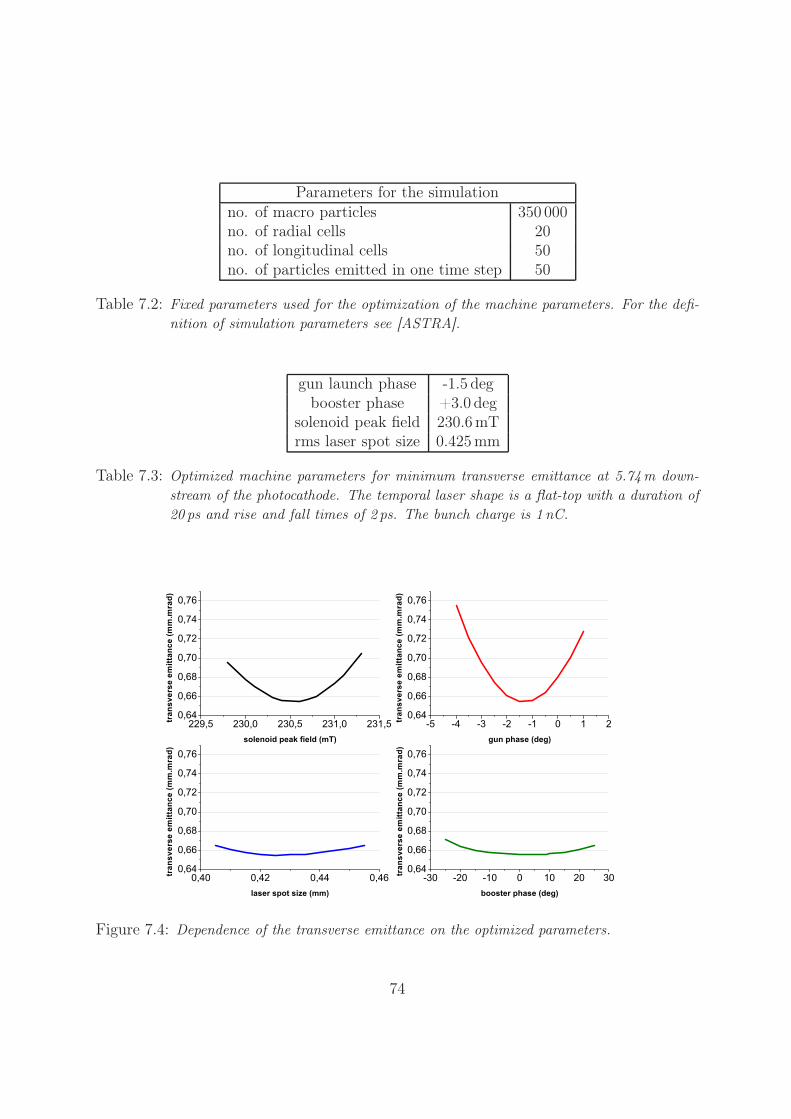
Parameters for the simulationno. of macro particles 350 000no. of radial cells 20no. of longitudinal cells 50no. of particles emitted in one time step 50

Table 7.2: Fixed parameters used for the optimization of the machine parameters. For the defi-nition of simulation parameters see [ASTRA].

gun launch phase -1.5 degbooster phase +3.0 deg

solenoid peak field 230.6 mTrms laser spot size 0.425 mm

Table 7.3: Optimized machine parameters for minimum transverse emittance at 5.74m down-stream of the photocathode. The temporal laser shape is a flat-top with a duration of20 ps and rise and fall times of 2 ps. The bunch charge is 1 nC.

Figure 7.4: Dependence of the transverse emittance on the optimized parameters.

74

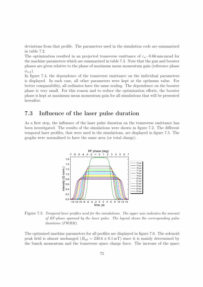
deviations from that profile. The parameters used in the simulation code are summarizedin table 7.2.The optimization resulted in an projected transverse emittance of εn=0.66 mmmrad forthe machine parameters which are summarized in table 7.3. Note that the gun and boosterphases are given relative to the phase of maximum mean momentum gain (reference phaseφref).In figure 7.4, the dependence of the transverse emittance on the individual parametersis displayed. In each case, all other parameters were kept at the optimum value. Forbetter comparability, all ordinates have the same scaling. The dependence on the boosterphase is very small. For this reason and to reduce the optimization efforts, the boosterphase is kept at maximum mean momentum gain for all simulations that will be presentedhereafter.

7.3 Influence of the laser pulse durationAs a first step, the influence of the laser pulse duration on the transverse emittance hasbeen investigated. The results of the simulations were shown in figure 7.2. The differenttemporal laser profiles, that were used in the simulations, are displayed in figure 7.5. Thegraphs were normalized to have the same area (or total charge).

Figure 7.5: Temporal laser profiles used for the simulations. The upper axis indicates the amountof RF-phase spanned by the laser pulse. The legend shows the corresponding pulsedurations (FWHM).

The optimized machine parameters for all profiles are displayed in figure 7.6. The solenoidpeak field is almost unchanged (Bsol = 230.6 ± 0.1mT) since it is mainly determined bythe bunch momentum and the transverse space charge force. The increase of the space

75

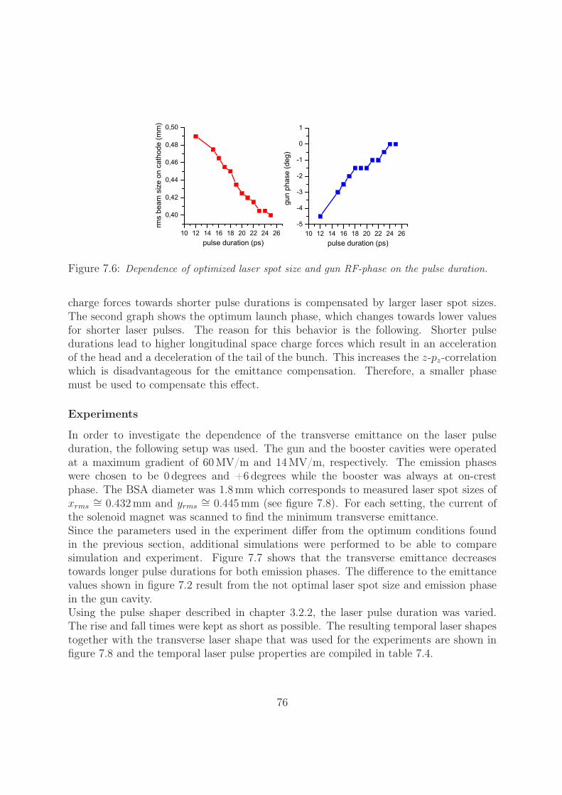
Figure 7.6: Dependence of optimized laser spot size and gun RF-phase on the pulse duration.

charge forces towards shorter pulse durations is compensated by larger laser spot sizes.The second graph shows the optimum launch phase, which changes towards lower valuesfor shorter laser pulses. The reason for this behavior is the following. Shorter pulsedurations lead to higher longitudinal space charge forces which result in an accelerationof the head and a deceleration of the tail of the bunch. This increases the z-pz-correlationwhich is disadvantageous for the emittance compensation. Therefore, a smaller phasemust be used to compensate this effect.

Experiments

In order to investigate the dependence of the transverse emittance on the laser pulseduration, the following setup was used. The gun and the booster cavities were operatedat a maximum gradient of 60 MV/m and 14 MV/m, respectively. The emission phaseswere chosen to be 0 degrees and +6 degrees while the booster was always at on-crestphase. The BSA diameter was 1.8 mm which corresponds to measured laser spot sizes ofxrms

∼= 0.432mm and yrms∼= 0.445mm (see figure 7.8). For each setting, the current of

the solenoid magnet was scanned to find the minimum transverse emittance.Since the parameters used in the experiment differ from the optimum conditions foundin the previous section, additional simulations were performed to be able to comparesimulation and experiment. Figure 7.7 shows that the transverse emittance decreasestowards longer pulse durations for both emission phases. The difference to the emittancevalues shown in figure 7.2 result from the not optimal laser spot size and emission phasein the gun cavity.Using the pulse shaper described in chapter 3.2.2, the laser pulse duration was varied.The rise and fall times were kept as short as possible. The resulting temporal laser shapestogether with the transverse laser shape that was used for the experiments are shown infigure 7.8 and the temporal laser pulse properties are compiled in table 7.4.

76

Figure 7.7: Simulated dependence of the transverse emittance on the laser pulse duration forthe specific experimental conditions and a gun launch phase of 0 degrees (black solidline) and +6 degrees off-crest (red dashed line).

(a) (b) (c)

(d) (e) (f)

Figure 7.8: Temporal laser shapes (a)-(e) and the transverse laser shape (f) used in the exper-iments. The BSA had a diameter of 1.8mm. While the peaks in the transverseprofile were caused by diffraction originating from dust particles on the CCD chip,the faint horizontal stripes were caused by interference of the laser pulse in the coverplate of the CCD.

77

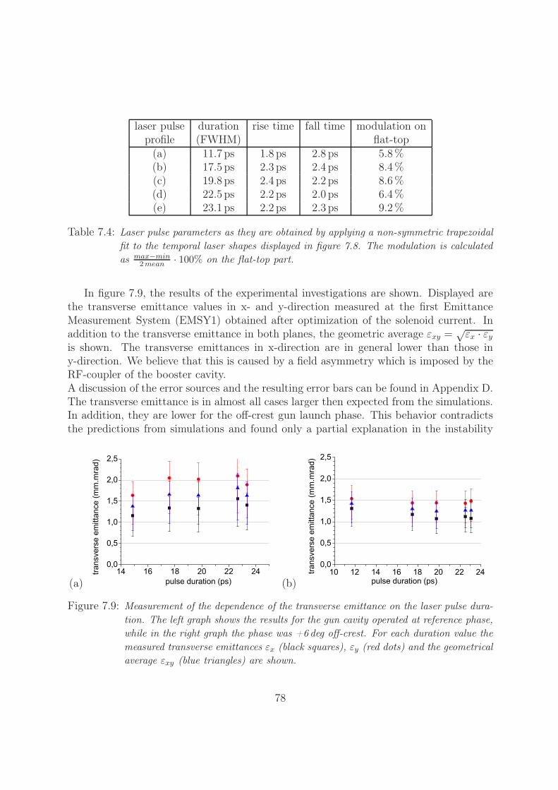
laser pulse duration rise time fall time modulation onprofile (FWHM) flat-top

(a) 11.7 ps 1.8 ps 2.8 ps 5.8 %(b) 17.5 ps 2.3 ps 2.4 ps 8.4 %(c) 19.8 ps 2.4 ps 2.2 ps 8.6 %(d) 22.5 ps 2.2 ps 2.0 ps 6.4 %(e) 23.1 ps 2.2 ps 2.3 ps 9.2 %

Table 7.4: Laser pulse parameters as they are obtained by applying a non-symmetric trapezoidalfit to the temporal laser shapes displayed in figure 7.8. The modulation is calculatedas max−min

2 mean · 100% on the flat-top part.

In figure 7.9, the results of the experimental investigations are shown. Displayed arethe transverse emittance values in x- and y-direction measured at the first EmittanceMeasurement System (EMSY1) obtained after optimization of the solenoid current. Inaddition to the transverse emittance in both planes, the geometric average εxy =

√εx · εy

is shown. The transverse emittances in x-direction are in general lower than those iny-direction. We believe that this is caused by a field asymmetry which is imposed by theRF-coupler of the booster cavity.A discussion of the error sources and the resulting error bars can be found in Appendix D.The transverse emittance is in almost all cases larger then expected from the simulations.In addition, they are lower for the off-crest gun launch phase. This behavior contradictsthe predictions from simulations and found only a partial explanation in the instability

(a) (b)

Figure 7.9: Measurement of the dependence of the transverse emittance on the laser pulse dura-tion. The left graph shows the results for the gun cavity operated at reference phase,while in the right graph the phase was +6 deg off-crest. For each duration value themeasured transverse emittances εx (black squares), εy (red dots) and the geometricalaverage εxy (blue triangles) are shown.

78

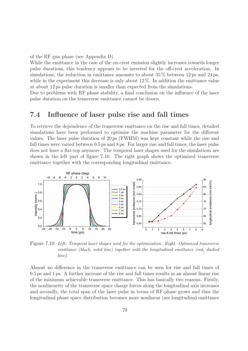
of the RF gun phase (see Appendix D).While the emittance in the case of the on-crest emission slightly increases towards longerpulse durations, this tendency appears to be inverted for the off-crest acceleration. Insimulations, the reduction in emittance amounts to about 35 % between 12 ps and 24 ps,while in the experiment this decrease is only about 12 %. In addition the emittance valueat about 12 ps pulse duration is smaller than expected from the simulations.Due to problems with RF phase stability, a final conclusion on the influence of the laserpulse duration on the transverse emittance cannot be drawn.

7.4 Influence of laser pulse rise and fall timesTo retrieve the dependence of the transverse emittance on the rise and fall times, detailedsimulations have been performed to optimize the machine parameter for the differentvalues. The laser pulse duration of 20 ps (FWHM) was kept constant while the rise andfall times were varied between 0.5 ps and 8 ps. For larger rise and fall times, the laser pulsedoes not have a flat-top anymore. The temporal laser shapes used for the simulations areshown in the left part of figure 7.10. The right graph shows the optimized transverseemittance together with the corresponding longitudinal emittance.

Figure 7.10: Left: Temporal laser shapes used for the optimization. Right: Optimized transverseemittance (black, solid line) together with the longitudinal emittance (red, dashedline).

Almost no difference in the transverse emittance can be seen for rise and fall times of0.5 ps and 1 ps. A further increase of the rise and fall times results in an almost linear riseof the minimum achievable transverse emittance. This has basically two reasons. Firstly,the nonlinearity of the transverse space charge forces along the longitudinal axis increasesand secondly, the total span of the laser pulse in terms of RF-phase grows and thus thelongitudinal phase space distribution becomes more nonlinear (see longitudinal emittance

79

Figure 7.11: Dependence of optimized parameters on the rise and fall times.

in figure 7.10). These two reasons reduce the efficiency of the emittance compensation.The dependence of the optimized parameters on the rise and fall times are depicted infigure 7.11. For longer rise and fall times the preferred solenoid current decreases becausethe reduced average bunch current requires less focussing strength. Further, the increasedbunch length allows for smaller transverse laser spot sizes. The variations in the gun phaseof φ = −1.0 ± 0.5degrees is not significant.

Experiments

During the experiments, the Beam Shaping Aperture was chosen to have a diameter of1.5 mm, which corresponds to a laser spot size of xrms = yrms = 0.375mm for a perfect cir-cular flat-top. The measured laser spot sizes were xrms

∼= 0.365mm and yrms∼= 0.368mm

(see figure 7.13). The gun launch phase was +6 degrees off-crest and the magnetic fieldstrength of the solenoid was optimized experimentally. The results of the simulationsreflecting the specific experimental conditions are depicted in figure 7.12.The linear increase of the transverse emittance for longer rise and fall times which wasfound earlier is only true for the case of on-crest acceleration, whereas for the case of+6 degrees gun launch phase, the transverse emittance is slightly smaller for 2 ps rise andfall times, but remains constant for all other cases at about 1.33 mmmrad. Besides thisfinding, the transverse emittance for +6 degrees gun phase is in general larger than forthe on-crest case.The experimentally used temporal laser shapes are shown in figure 7.13. For some values

of the rise and fall times, the transverse emittance was measured several times. In thesecases, only one measured temporal profiles is shown even though, the temporal shapeswere recorded each time. The laser pulse parameters for all measurements are compiled intable 7.5. In figure 7.14, the experimentally measured transverse emittance values are dis-played. The main results are, that the transverse emittances are almost constant withinthe error bars but about 0.2 mmmrad lower than expected from the simulations. The

80

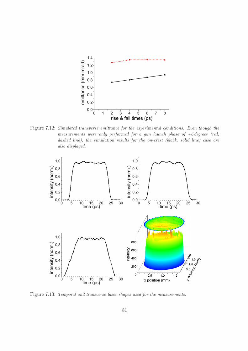
Figure 7.12: Simulated transverse emittance for the experimental conditions. Even though themeasurements were only performed for a gun launch phase of +6 degrees (red,dashed line), the simulation results for the on-crest (black, solid line) case arealso displayed.

Figure 7.13: Temporal and transverse laser shapes used for the measurements.

81

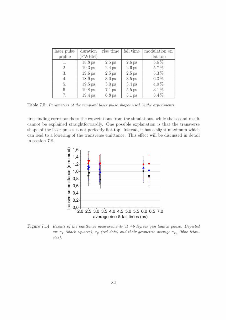
laser pulse duration rise time fall time modulation onprofile (FWHM) flat-top

1. 18.8 ps 2.5 ps 2.6 ps 5.6 %2. 19.3 ps 2.4 ps 2.6 ps 5.7 %3. 19.6 ps 2.5 ps 2.5 ps 5.3 %4. 18.9 ps 3.0 ps 3.5 ps 6.3 %5. 19.5 ps 3.0 ps 3.4 ps 4.9 %6. 19.8 ps 7.1 ps 5.5 ps 3.1 %7. 19.4 ps 6.8 ps 5.1 ps 3.4 %

Table 7.5: Parameters of the temporal laser pulse shapes used in the experiments.

first finding corresponds to the expectations from the simulations, while the second resultcannot be explained straightforwardly. One possible explanation is that the transverseshape of the laser pulses is not perfectly flat-top. Instead, it has a slight maximum whichcan lead to a lowering of the transverse emittance. This effect will be discussed in detailin section 7.8.

Figure 7.14: Results of the emittance measurements at +6 degrees gun launch phase. Depictedare εx (black squares), εy (red dots) and their geometric average εxy (blue trian-gles).

82

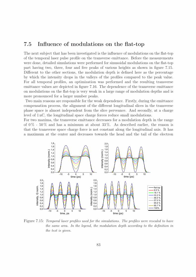
7.5 Influence of modulations on the flat-topThe next subject that has been investigated is the influence of modulations on the flat-topof the temporal laser pulse profile on the transverse emittance. Before the measurementswere done, detailed simulations were performed for sinusoidal modulations on the flat-toppart having two, three, four and five peaks of various heights as shown in figure 7.15.Different to the other sections, the modulation depth is defined here as the percentageby which the intensity drops in the valleys of the profiles compared to the peak value.For all temporal profiles, an optimization was performed and the resulting transverseemittance values are depicted in figure 7.16. The dependence of the transverse emittanceon modulations on the flat-top is very weak in a large range of modulation depths and ismore pronounced for a larger number peaks.Two main reasons are responsible for the weak dependence. Firstly, during the emittance

compensation process, the alignment of the different longitudinal slices in the transversephase space is almost independent from the slice perveance. And secondly, at a chargelevel of 1 nC, the longitudinal space charge forces reduce small modulations.For two maxima, the transverse emittance decreases for a modulation depth in the rangeof 0 % - 50 % and has a minimum at about 33 %. As described earlier, the reason isthat the transverse space charge force is not constant along the longitudinal axis. It hasa maximum at the center and decreases towards the head and the tail of the electron

Figure 7.15: Temporal laser profiles used for the simulations. The profiles were rescaled to havethe same area. In the legend, the modulation depth according to the definition inthe text is given.

83

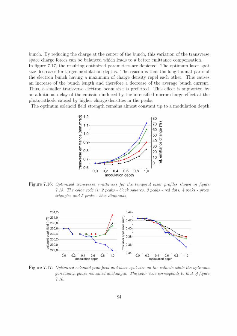
bunch. By reducing the charge at the center of the bunch, this variation of the transversespace charge forces can be balanced which leads to a better emittance compensation.In figure 7.17, the resulting optimized parameters are depicted. The optimum laser spotsize decreases for larger modulation depths. The reason is that the longitudinal parts ofthe electron bunch having a maximum of charge density repel each other. This causesan increase of the bunch length and therefore a decrease of the average bunch current.Thus, a smaller transverse electron beam size is preferred. This effect is supported byan additional delay of the emission induced by the intensified mirror charge effect at thephotocathode caused by higher charge densities in the peaks.The optimum solenoid field strength remains almost constant up to a modulation depth

Figure 7.16: Optimized transverse emittances for the temporal laser profiles shown in figure7.15. The color code is: 2 peaks - black squares, 3 peaks - red dots, 4 peaks - greentriangles and 5 peaks - blue diamonds.

Figure 7.17: Optimized solenoid peak field and laser spot size on the cathode while the optimumgun launch phase remained unchanged. The color code corresponds to that of figure7.16.

84

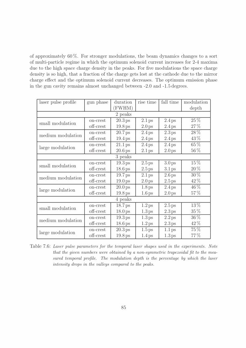
of approximately 60 %. For stronger modulations, the beam dynamics changes to a sortof multi-particle regime in which the optimum solenoid current increases for 2-4 maximadue to the high space charge density in the peaks. For five modulations the space chargedensity is so high, that a fraction of the charge gets lost at the cathode due to the mirrorcharge effect and the optimum solenoid current decreases. The optimum emission phasein the gun cavity remains almost unchanged between -2.0 and -1.5 degrees.

laser pulse profile gun phase duration rise time fall time modulation(FWHM) depth2 peaks

small modulation on-crest 20.3 ps 2.1 ps 2.4 ps 25 %off-crest 19.8 ps 2.0 ps 2.4 ps 27 %

medium modulation on-crest 20.7 ps 2.4 ps 2.3 ps 28 %off-crest 19.4 ps 2.4 ps 2.4 ps 43 %

large modulation on-crest 21.1 ps 2.4 ps 2.4 ps 65 %off-crest 20.6 ps 2.1 ps 2.0 ps 56 %

3 peaks

small modulation on-crest 19.3 ps 2.5 ps 3.0 ps 15 %off-crest 18.6 ps 2.5 ps 3.1 ps 20 %

medium modulation on-crest 19.7 ps 2.1 ps 2.6 ps 30 %off-crest 19.0 ps 2.0 ps 2.5 ps 42 %

large modulation on-crest 20.0 ps 1.8 ps 2.4 ps 46 %off-crest 19.8 ps 1.6 ps 2.0 ps 57 %

4 peaks

small modulation on-crest 18.7 ps 1.2 ps 2.5 ps 13 %off-crest 18.0 ps 1.3 ps 2.3 ps 35 %

medium modulation on-crest 19.3 ps 1.3 ps 2.2 ps 36 %off-crest 18.6 ps 1.2 ps 2.3 ps 42 %

large modulation on-crest 20.3 ps 1.5 ps 1.1 ps 75 %off-crest 19.8 ps 1.4 ps 1.3 ps 77 %

Table 7.6: Laser pulse parameters for the temporal laser shapes used in the experiments. Notethat the given numbers were obtained by a non-symmetric trapezoidal fit to the mea-sured temporal profile. The modulation depth is the percentage by which the laserintensity drops in the valleys compared to the peaks.

85

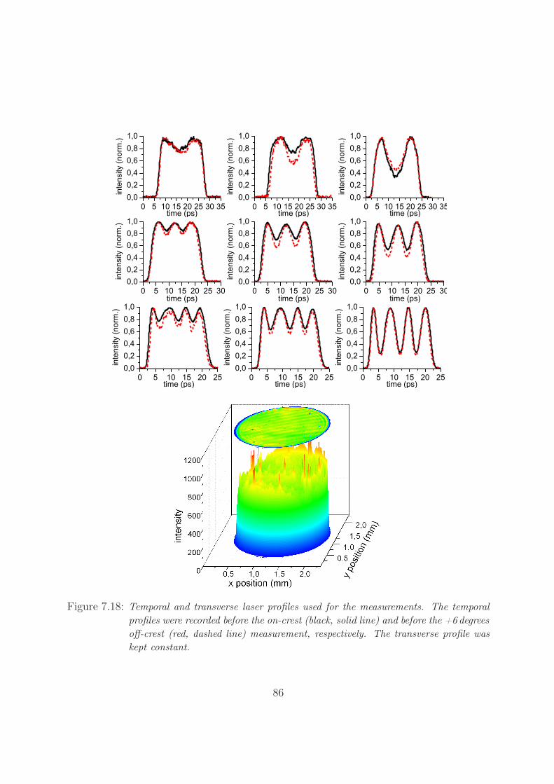
Figure 7.18: Temporal and transverse laser profiles used for the measurements. The temporalprofiles were recorded before the on-crest (black, solid line) and before the +6 degreesoff-crest (red, dashed line) measurement, respectively. The transverse profile waskept constant.

86

Experiments

The temporal laser shapes generated using the pulse shaper are shown in figure 7.18.Depicted are the measurements obtained before the on-crest and before the off-crest mea-surements of the transverse emittance. The slight differences are due to the warming-upeffect of the Optical Sampling System (see section 3.4.1).The experimental results together with the simulations of the experimental conditions aredepicted in figure 7.19. The obtained transverse emittance values do not show a tendencyto increase for larger modulation depths2. The increase of the transverse emittance ex-pected from the simulations is very small and within the error bars of the measurement.Besides the differences in the absolute numbers obtained by simulations and experimentwhich was already discussed before, these measurements demonstrate that the influence ofmodulations on the flat-top part of the laser pulses is currently too small to be detected.

Figure 7.19: Experimental results together with simulations. Left: Results for the gun cavityoperated on-crest, right: gun cavity operated +6 degrees off-crest. The lines showthe simulation results for two peaks (black, solid line), three peaks (red, dashedline) and four peaks (blue, dash-dotted line). The dots represent the measurementresults using the same color code. Depicted are εx (squares), εy (circles) and εxy

(diamonds). For better visibility the error bars for εx and εy are omitted.

The fact that longitudinal space charge forces can reduce the modulations in the longi-tudinal phase space distribution is not valid anymore for low charges. For this reason,modulations which are imprinted in the longitudinal electron bunch density during emis-sion caused by a modulation of the laser pulse temporal profile remain. In the case of aproper tilt of the longitudinal phase space distribution, this modulation also occurs in themomentum distribution of the electron bunch. This momentum modulation can give rise

2Please note, that in the simulated experiment of the 2-peak case no minimum of the transverseemittance can be found as it was the case for a fully optimized setup (see figure 7.16).

87

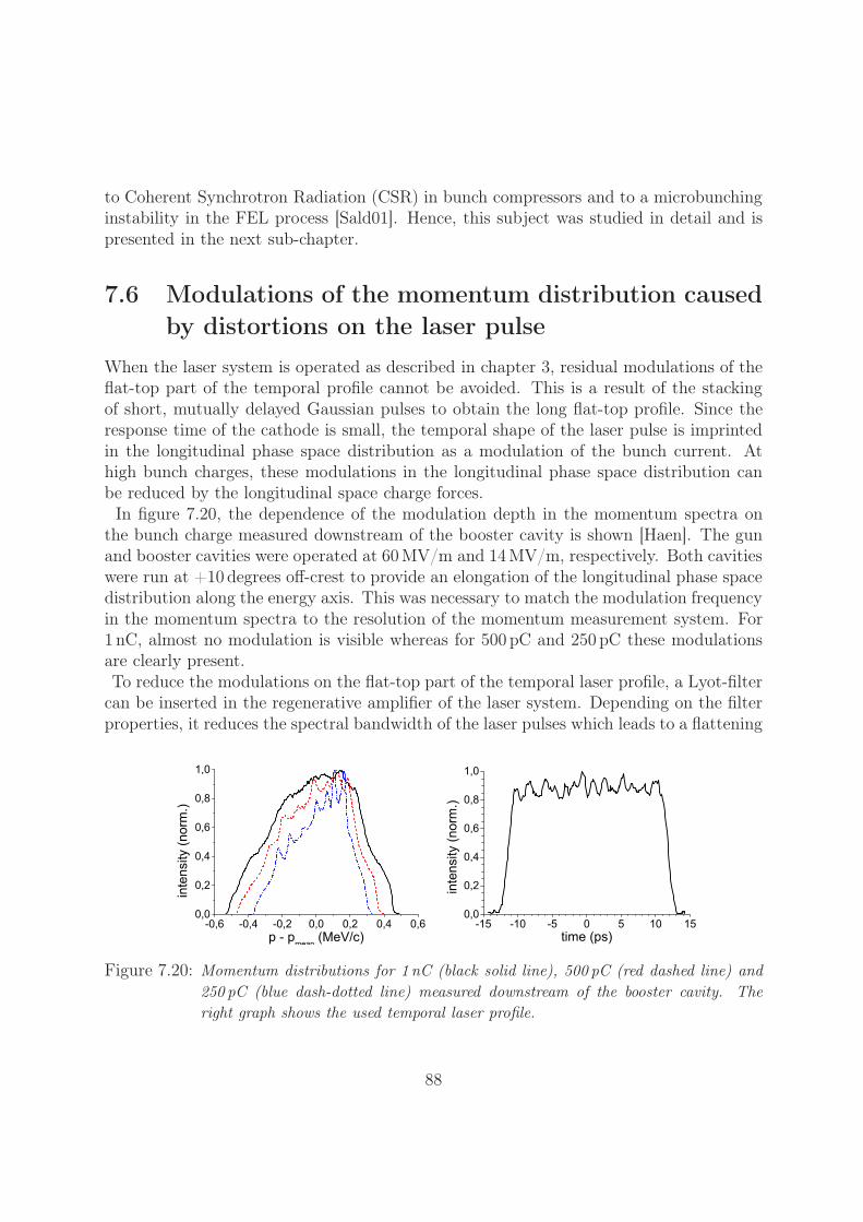
to Coherent Synchrotron Radiation (CSR) in bunch compressors and to a microbunchinginstability in the FEL process [Sald01]. Hence, this subject was studied in detail and ispresented in the next sub-chapter.

7.6 Modulations of the momentum distribution causedby distortions on the laser pulse

When the laser system is operated as described in chapter 3, residual modulations of theflat-top part of the temporal profile cannot be avoided. This is a result of the stackingof short, mutually delayed Gaussian pulses to obtain the long flat-top profile. Since theresponse time of the cathode is small, the temporal shape of the laser pulse is imprintedin the longitudinal phase space distribution as a modulation of the bunch current. Athigh bunch charges, these modulations in the longitudinal phase space distribution canbe reduced by the longitudinal space charge forces.In figure 7.20, the dependence of the modulation depth in the momentum spectra on

the bunch charge measured downstream of the booster cavity is shown [Haen]. The gunand booster cavities were operated at 60 MV/m and 14 MV/m, respectively. Both cavitieswere run at +10 degrees off-crest to provide an elongation of the longitudinal phase spacedistribution along the energy axis. This was necessary to match the modulation frequencyin the momentum spectra to the resolution of the momentum measurement system. For1 nC, almost no modulation is visible whereas for 500 pC and 250 pC these modulationsare clearly present.To reduce the modulations on the flat-top part of the temporal laser profile, a Lyot-filter

can be inserted in the regenerative amplifier of the laser system. Depending on the filterproperties, it reduces the spectral bandwidth of the laser pulses which leads to a flattening

Figure 7.20: Momentum distributions for 1 nC (black solid line), 500 pC (red dashed line) and250 pC (blue dash-dotted line) measured downstream of the booster cavity. Theright graph shows the used temporal laser profile.

88

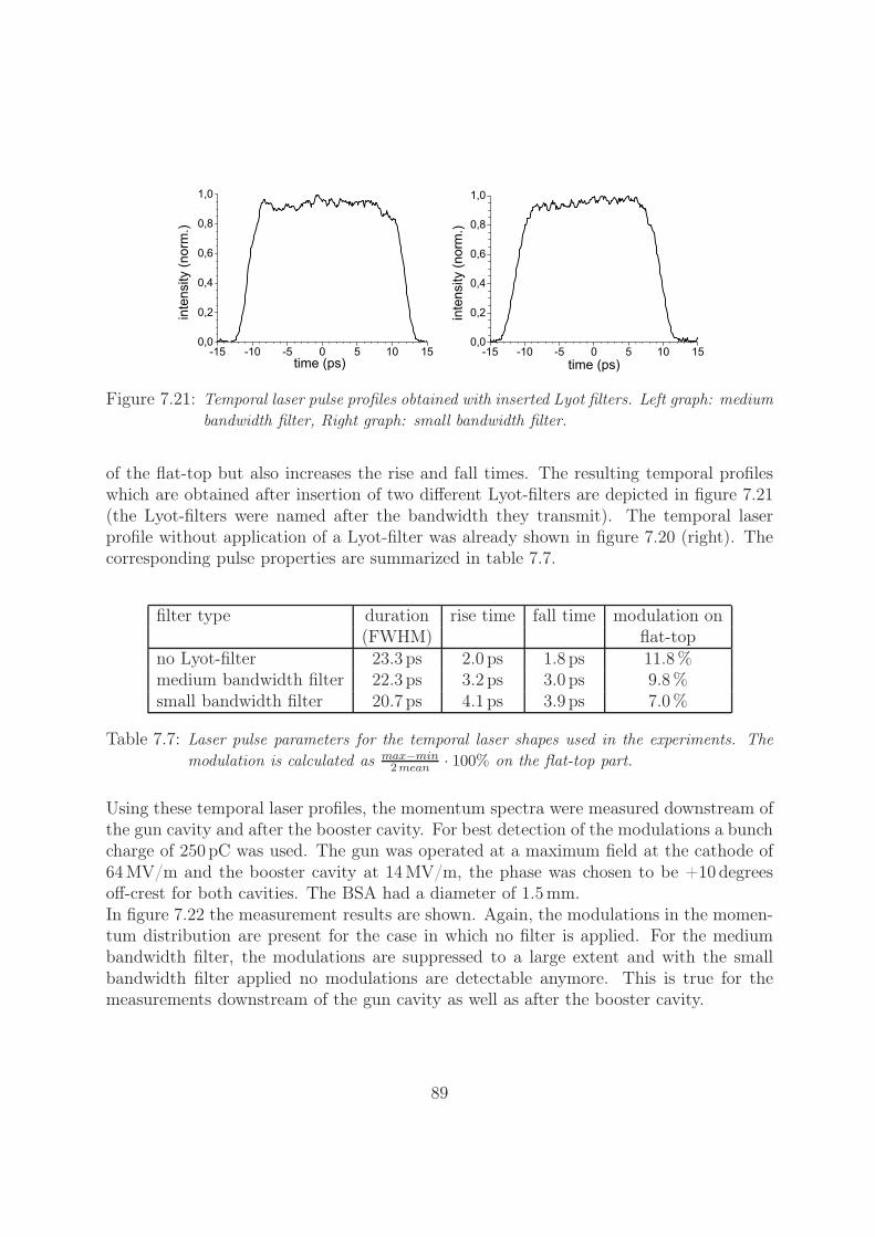
Figure 7.21: Temporal laser pulse profiles obtained with inserted Lyot filters. Left graph: mediumbandwidth filter, Right graph: small bandwidth filter.

of the flat-top but also increases the rise and fall times. The resulting temporal profileswhich are obtained after insertion of two different Lyot-filters are depicted in figure 7.21(the Lyot-filters were named after the bandwidth they transmit). The temporal laserprofile without application of a Lyot-filter was already shown in figure 7.20 (right). Thecorresponding pulse properties are summarized in table 7.7.

filter type duration rise time fall time modulation on(FWHM) flat-top

no Lyot-filter 23.3 ps 2.0 ps 1.8 ps 11.8 %medium bandwidth filter 22.3 ps 3.2 ps 3.0 ps 9.8 %small bandwidth filter 20.7 ps 4.1 ps 3.9 ps 7.0 %

Table 7.7: Laser pulse parameters for the temporal laser shapes used in the experiments. Themodulation is calculated as max−min

2 mean · 100% on the flat-top part.

Using these temporal laser profiles, the momentum spectra were measured downstream ofthe gun cavity and after the booster cavity. For best detection of the modulations a bunchcharge of 250 pC was used. The gun was operated at a maximum field at the cathode of64 MV/m and the booster cavity at 14 MV/m, the phase was chosen to be +10 degreesoff-crest for both cavities. The BSA had a diameter of 1.5 mm.In figure 7.22 the measurement results are shown. Again, the modulations in the momen-tum distribution are present for the case in which no filter is applied. For the mediumbandwidth filter, the modulations are suppressed to a large extent and with the smallbandwidth filter applied no modulations are detectable anymore. This is true for themeasurements downstream of the gun cavity as well as after the booster cavity.

89

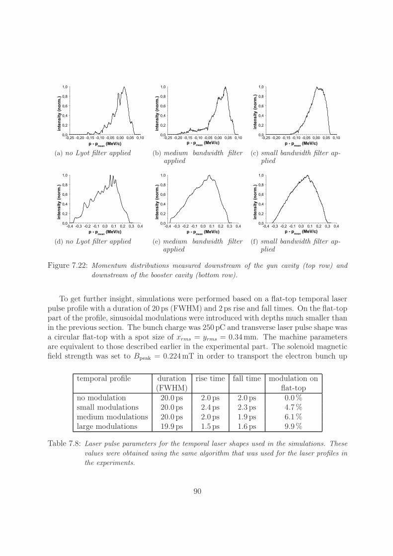
(a) no Lyot filter applied (b) medium bandwidth filterapplied

(c) small bandwidth filter ap-plied

(d) no Lyot filter applied (e) medium bandwidth filterapplied

(f) small bandwidth filter ap-plied

Figure 7.22: Momentum distributions measured downstream of the gun cavity (top row) anddownstream of the booster cavity (bottom row).

To get further insight, simulations were performed based on a flat-top temporal laserpulse profile with a duration of 20 ps (FWHM) and 2 ps rise and fall times. On the flat-toppart of the profile, sinusoidal modulations were introduced with depths much smaller thanin the previous section. The bunch charge was 250 pC and transverse laser pulse shape wasa circular flat-top with a spot size of xrms = yrms = 0.34mm. The machine parametersare equivalent to those described earlier in the experimental part. The solenoid magneticfield strength was set to Bpeak = 0.224mT in order to transport the electron bunch up

temporal profile duration rise time fall time modulation on(FWHM) flat-top

no modulation 20.0 ps 2.0 ps 2.0 ps 0.0 %small modulations 20.0 ps 2.4 ps 2.3 ps 4.7 %medium modulations 20.0 ps 2.0 ps 1.9 ps 6.1 %large modulations 19.9 ps 1.5 ps 1.6 ps 9.9 %

Table 7.8: Laser pulse parameters for the temporal laser shapes used in the simulations. Thesevalues were obtained using the same algorithm that was used for the laser profiles inthe experiments.

90

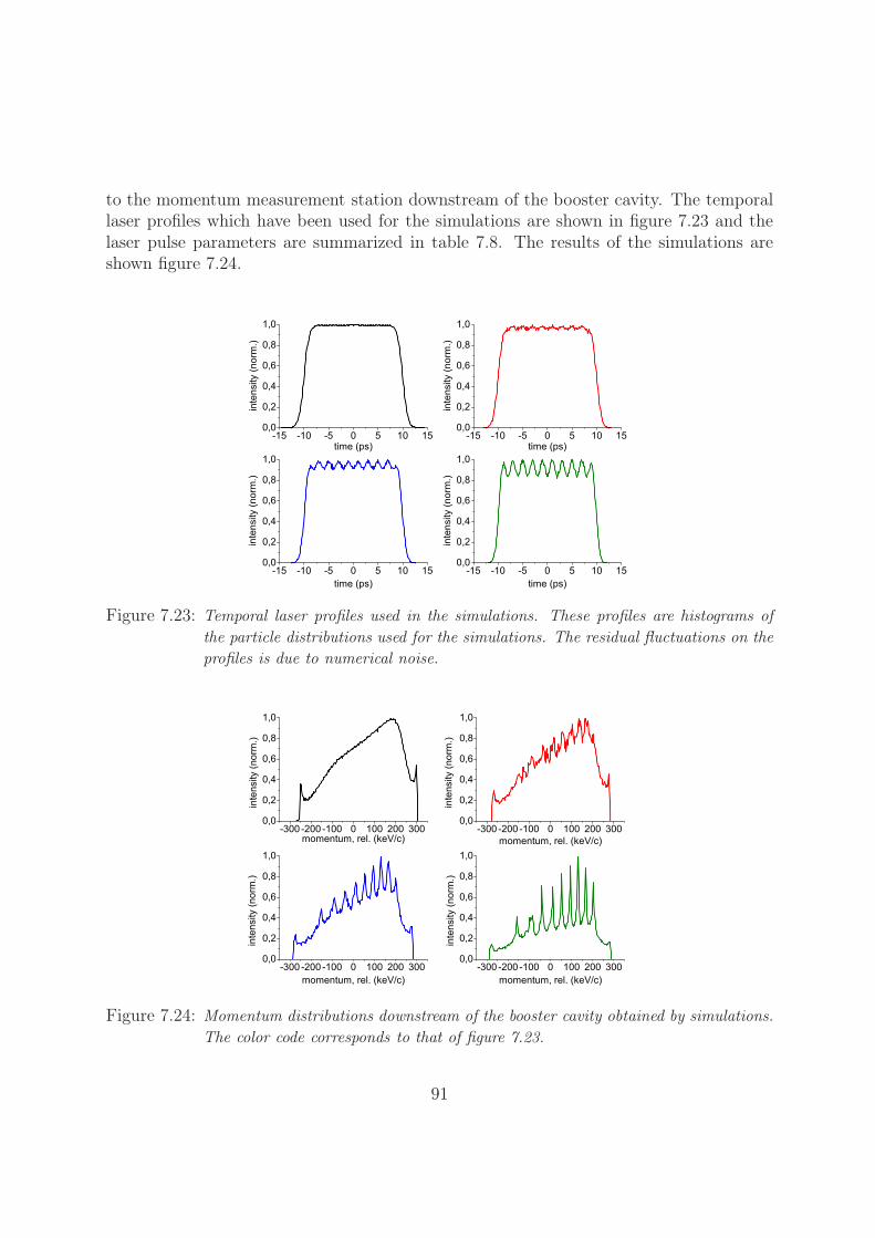
to the momentum measurement station downstream of the booster cavity. The temporallaser profiles which have been used for the simulations are shown in figure 7.23 and thelaser pulse parameters are summarized in table 7.8. The results of the simulations areshown figure 7.24.

Figure 7.23: Temporal laser profiles used in the simulations. These profiles are histograms ofthe particle distributions used for the simulations. The residual fluctuations on theprofiles is due to numerical noise.

Figure 7.24: Momentum distributions downstream of the booster cavity obtained by simulations.The color code corresponds to that of figure 7.23.

91

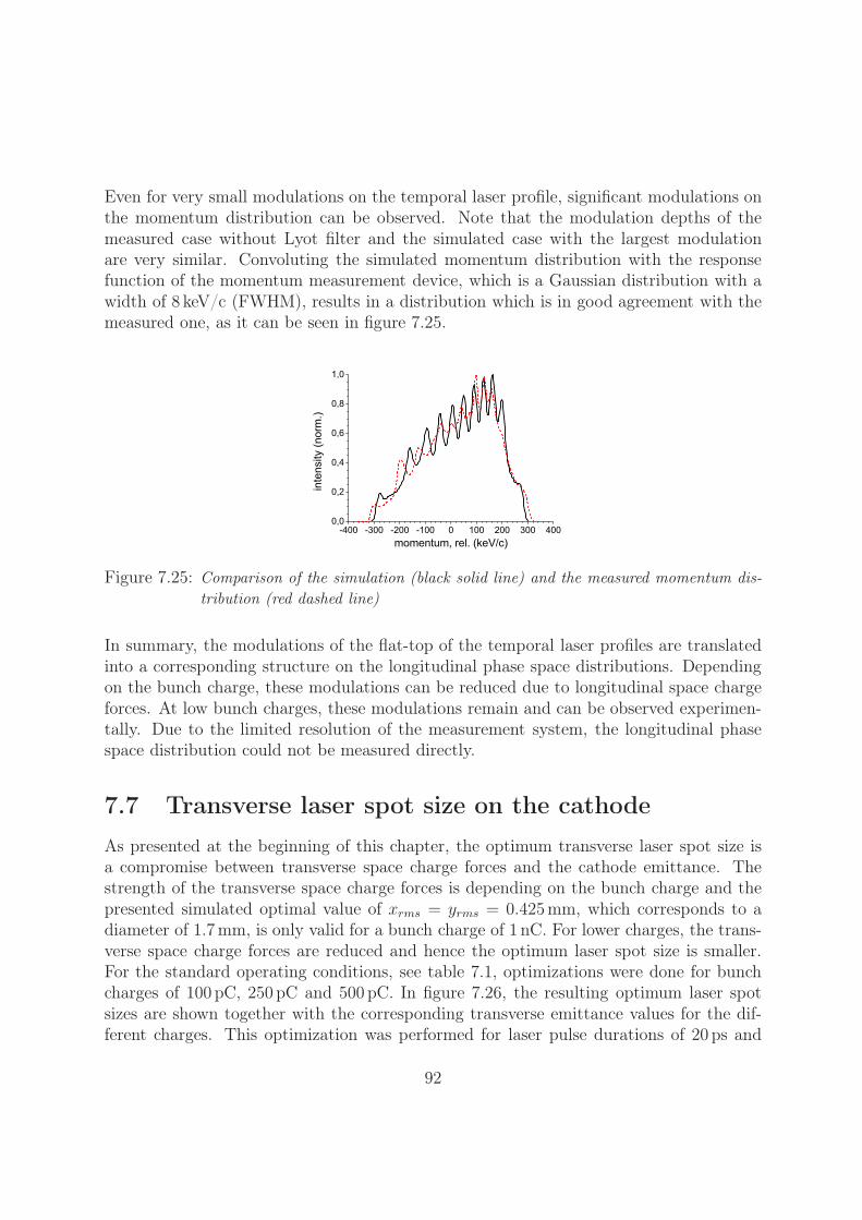
Even for very small modulations on the temporal laser profile, significant modulations onthe momentum distribution can be observed. Note that the modulation depths of themeasured case without Lyot filter and the simulated case with the largest modulationare very similar. Convoluting the simulated momentum distribution with the responsefunction of the momentum measurement device, which is a Gaussian distribution with awidth of 8 keV/c (FWHM), results in a distribution which is in good agreement with themeasured one, as it can be seen in figure 7.25.

Figure 7.25: Comparison of the simulation (black solid line) and the measured momentum dis-tribution (red dashed line)

In summary, the modulations of the flat-top of the temporal laser profiles are translatedinto a corresponding structure on the longitudinal phase space distributions. Dependingon the bunch charge, these modulations can be reduced due to longitudinal space chargeforces. At low bunch charges, these modulations remain and can be observed experimen-tally. Due to the limited resolution of the measurement system, the longitudinal phasespace distribution could not be measured directly.

7.7 Transverse laser spot size on the cathodeAs presented at the beginning of this chapter, the optimum transverse laser spot size isa compromise between transverse space charge forces and the cathode emittance. Thestrength of the transverse space charge forces is depending on the bunch charge and thepresented simulated optimal value of xrms = yrms = 0.425mm, which corresponds to adiameter of 1.7 mm, is only valid for a bunch charge of 1 nC. For lower charges, the trans-verse space charge forces are reduced and hence the optimum laser spot size is smaller.For the standard operating conditions, see table 7.1, optimizations were done for bunchcharges of 100 pC, 250 pC and 500 pC. In figure 7.26, the resulting optimum laser spotsizes are shown together with the corresponding transverse emittance values for the dif-ferent charges. This optimization was performed for laser pulse durations of 20 ps and

92

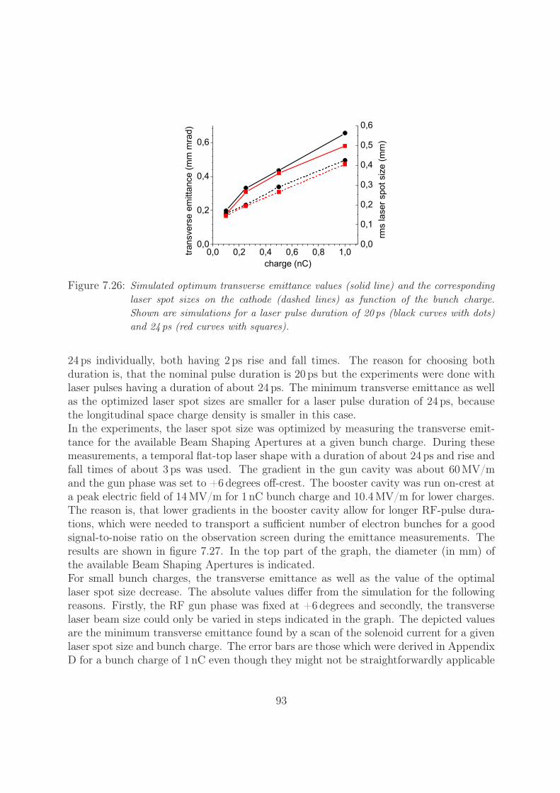
Figure 7.26: Simulated optimum transverse emittance values (solid line) and the correspondinglaser spot sizes on the cathode (dashed lines) as function of the bunch charge.Shown are simulations for a laser pulse duration of 20 ps (black curves with dots)and 24 ps (red curves with squares).

24 ps individually, both having 2 ps rise and fall times. The reason for choosing bothduration is, that the nominal pulse duration is 20 ps but the experiments were done withlaser pulses having a duration of about 24 ps. The minimum transverse emittance as wellas the optimized laser spot sizes are smaller for a laser pulse duration of 24 ps, becausethe longitudinal space charge density is smaller in this case.In the experiments, the laser spot size was optimized by measuring the transverse emit-tance for the available Beam Shaping Apertures at a given bunch charge. During thesemeasurements, a temporal flat-top laser shape with a duration of about 24 ps and rise andfall times of about 3 ps was used. The gradient in the gun cavity was about 60 MV/mand the gun phase was set to +6 degrees off-crest. The booster cavity was run on-crest ata peak electric field of 14 MV/m for 1 nC bunch charge and 10.4 MV/m for lower charges.The reason is, that lower gradients in the booster cavity allow for longer RF-pulse dura-tions, which were needed to transport a sufficient number of electron bunches for a goodsignal-to-noise ratio on the observation screen during the emittance measurements. Theresults are shown in figure 7.27. In the top part of the graph, the diameter (in mm) ofthe available Beam Shaping Apertures is indicated.For small bunch charges, the transverse emittance as well as the value of the optimallaser spot size decrease. The absolute values differ from the simulation for the followingreasons. Firstly, the RF gun phase was fixed at +6 degrees and secondly, the transverselaser beam size could only be varied in steps indicated in the graph. The depicted valuesare the minimum transverse emittance found by a scan of the solenoid current for a givenlaser spot size and bunch charge. The error bars are those which were derived in AppendixD for a bunch charge of 1 nC even though they might not be straightforwardly applicable

93

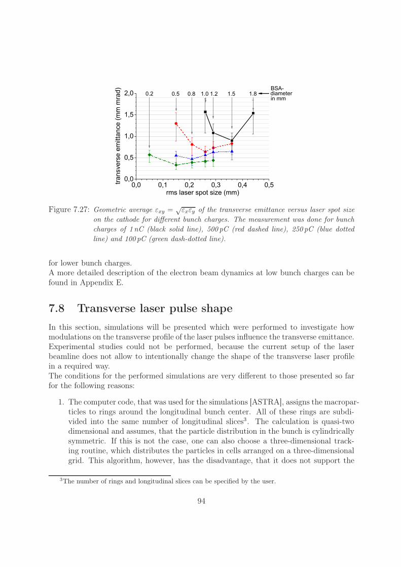
Figure 7.27: Geometric average εxy = √εxεy of the transverse emittance versus laser spot size

on the cathode for different bunch charges. The measurement was done for bunchcharges of 1 nC (black solid line), 500 pC (red dashed line), 250 pC (blue dottedline) and 100 pC (green dash-dotted line).

for lower bunch charges.A more detailed description of the electron beam dynamics at low bunch charges can befound in Appendix E.

7.8 Transverse laser pulse shapeIn this section, simulations will be presented which were performed to investigate howmodulations on the transverse profile of the laser pulses influence the transverse emittance.Experimental studies could not be performed, because the current setup of the laserbeamline does not allow to intentionally change the shape of the transverse laser profilein a required way.The conditions for the performed simulations are very different to those presented so farfor the following reasons:

1. The computer code, that was used for the simulations [ASTRA], assigns the macropar-ticles to rings around the longitudinal bunch center. All of these rings are subdi-vided into the same number of longitudinal slices3. The calculation is quasi-twodimensional and assumes, that the particle distribution in the bunch is cylindricallysymmetric. If this is not the case, one can also choose a three-dimensional track-ing routine, which distributes the particles in cells arranged on a three-dimensionalgrid. This algorithm, however, has the disadvantage, that it does not support the

3The number of rings and longitudinal slices can be specified by the user.

94

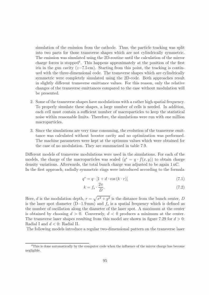
simulation of the emission from the cathode. Thus, the particle tracking was splitinto two parts for those transverse shapes which are not cylindrically symmetric.The emission was simulated using the 2D-routine until the calculation of the mirrorcharge forces is stopped4. This happens approximately at the position of the firstiris in the gun cavity (z=7.5 cm). Starting from this point, the tracking is contin-ued with the three-dimensional code. The transverse shapes which are cylindricallysymmetric were completely simulated using the 2D-code. Both approaches resultin slightly different transverse emittance values. For this reason, only the relativechanges of the transverse emittances compared to the case without modulation willbe presented.

2. Some of the transverse shapes have modulations with a rather high spatial frequency.To properly simulate these shapes, a large number of cells is needed. In addition,each cell must contain a sufficient number of macroparticles to keep the statisticalnoise within reasonable limits. Therefore, the simulations were run with one millionmacroparticles.

3. Since the simulations are very time consuming, the evolution of the transverse emit-tance was calculated without booster cavity and no optimization was performed.The machine parameters were kept at the optimum values which were obtained forthe case of no modulation. They are summarized in table 7.9.

Different models of transverse modulations were used in the simulations. For each of themodels, the charge of the macroparticles was scaled (q∗ = q · f(x, y)) to obtain chargedensity variations. Afterwards, the total bunch charge was adjusted to be again 1 nC.In the first approach, radially symmetric rings were introduced according to the formula

q∗ = q · [1 + d · cos (k · r)] (7.1)

k = fs · 2π

D. (7.2)

Here, d is the modulation depth, r =√

x2 + y2 is the distance from the bunch center, Dis the laser spot diameter (D=1.9 mm) and fs is a spatial frequency which is defined asthe number of oscillation along the diameter of the laser spot. A maximum at the centeris obtained by choosing d > 0. Conversely, d < 0 produces a minimum at the center.The transverse laser shapes resulting from this model are shown in figure 7.29 for d > 0:Radial I and d < 0: Radial II.The following models introduce a regular two-dimensional pattern on the transverse laser

4This is done automatically by the computer code when the influence of the mirror charge has becomenegligible.

95

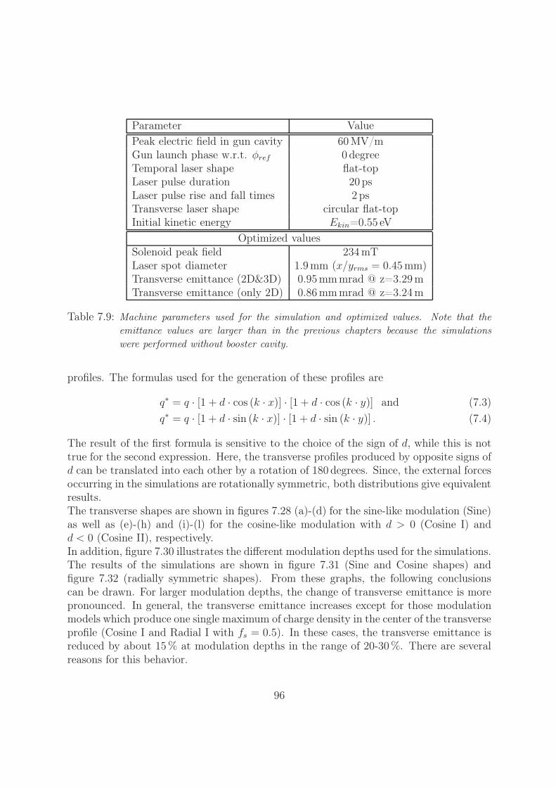
Parameter ValuePeak electric field in gun cavity 60 MV/mGun launch phase w.r.t. φref 0 degreeTemporal laser shape flat-topLaser pulse duration 20 psLaser pulse rise and fall times 2 psTransverse laser shape circular flat-topInitial kinetic energy Ekin=0.55 eV

Optimized valuesSolenoid peak field 234 mTLaser spot diameter 1.9 mm (x/yrms = 0.45mm)Transverse emittance (2D&3D) 0.95 mmmrad @ z=3.29 mTransverse emittance (only 2D) 0.86 mmmrad @ z=3.24 m

Table 7.9: Machine parameters used for the simulation and optimized values. Note that theemittance values are larger than in the previous chapters because the simulationswere performed without booster cavity.

profiles. The formulas used for the generation of these profiles are

q∗ = q · [1 + d · cos (k · x)] · [1 + d · cos (k · y)] and (7.3)q∗ = q · [1 + d · sin (k · x)] · [1 + d · sin (k · y)] . (7.4)

The result of the first formula is sensitive to the choice of the sign of d, while this is nottrue for the second expression. Here, the transverse profiles produced by opposite signs ofd can be translated into each other by a rotation of 180 degrees. Since, the external forcesoccurring in the simulations are rotationally symmetric, both distributions give equivalentresults.The transverse shapes are shown in figures 7.28 (a)-(d) for the sine-like modulation (Sine)as well as (e)-(h) and (i)-(l) for the cosine-like modulation with d > 0 (Cosine I) andd < 0 (Cosine II), respectively.In addition, figure 7.30 illustrates the different modulation depths used for the simulations.The results of the simulations are shown in figure 7.31 (Sine and Cosine shapes) andfigure 7.32 (radially symmetric shapes). From these graphs, the following conclusionscan be drawn. For larger modulation depths, the change of transverse emittance is morepronounced. In general, the transverse emittance increases except for those modulationmodels which produce one single maximum of charge density in the center of the transverseprofile (Cosine I and Radial I with fs = 0.5). In these cases, the transverse emittance isreduced by about 15 % at modulation depths in the range of 20-30 %. There are severalreasons for this behavior.

96

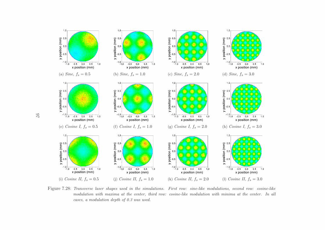
(a) Sine, fs = 0.5 (b) Sine, fs = 1.0 (c) Sine, fs = 2.0 (d) Sine, fs = 3.0

(e) Cosine I, fs = 0.5 (f) Cosine I, fs = 1.0 (g) Cosine I, fs = 2.0 (h) Cosine I, fs = 3.0

(i) Cosine II, fs = 0.5 (j) Cosine II, fs = 1.0 (k) Cosine II, fs = 2.0 (l) Cosine II, fs = 3.0

Figure 7.28: Transverse laser shapes used in the simulations. First row: sine-like modulations, second row: cosine-likemodulation with maxima at the center, third row: cosine-like modulation with minima at the center. In allcases, a modulation depth of 0.3 was used.

97

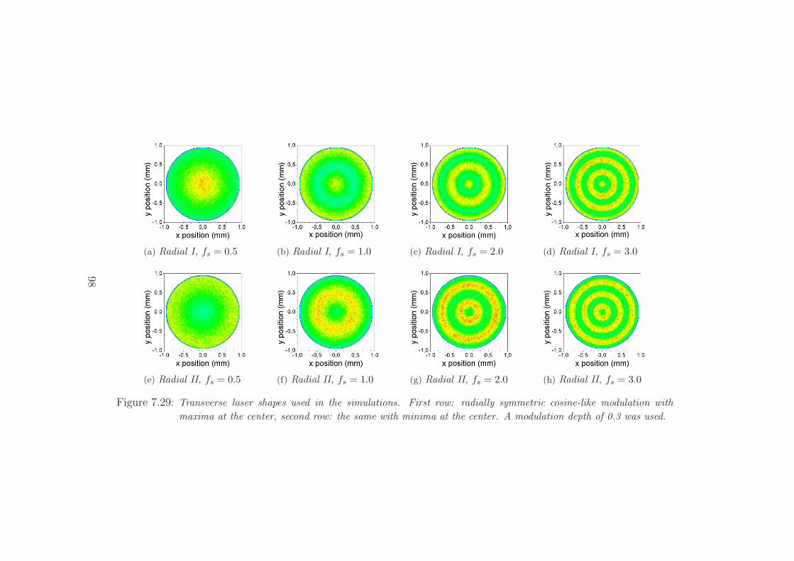
(a) Radial I, fs = 0.5 (b) Radial I, fs = 1.0 (c) Radial I, fs = 2.0 (d) Radial I, fs = 3.0

(e) Radial II, fs = 0.5 (f) Radial II, fs = 1.0 (g) Radial II, fs = 2.0 (h) Radial II, fs = 3.0

Figure 7.29: Transverse laser shapes used in the simulations. First row: radially symmetric cosine-like modulation withmaxima at the center, second row: the same with minima at the center. A modulation depth of 0.3 was used.

98

t](a) d = -0.05 (b) d = -0.1 (c) d = -0.2

(d) d = -0.3 (e) d = -0.5

Figure 7.30: Modulation depths that were used in the simulations. As an example the cosine-likemodulation with fs=0.5 was chosen.

Firstly, the transverse shapes with a maximum in charge density at the center corre-spond to smaller transverse laser spot size. This reduces the contribution of the cathodeemittance. Secondly, even though the maximum at the center imposes nonlinearities inthe transverse space charge forces, this - usually detrimental effect - is compensated bythe fact that more charge is located close to the bunch center and therefore, the rmstransverse emittance becomes smaller. Furthermore, towards larger modulation frequen-cies, the increase in transverse emittance becomes less pronounced. This is an effect ofthe transverse space charge forces which tend to reduce the high-frequency modulations.Furthermore, the emittance increase becomes almost equal for similar transverse shapes(the sine/cosine-shapes on one hand as well as the radially symmetric shapes on the otherhand) at high modulation frequencies. And finally, the highest value of transverse emit-tance increase can be observed for transverse shapes which are deviating most from thecylindically symmetric shapes and/or in which the maxima of the charge density distri-bution are located away from the center.

99

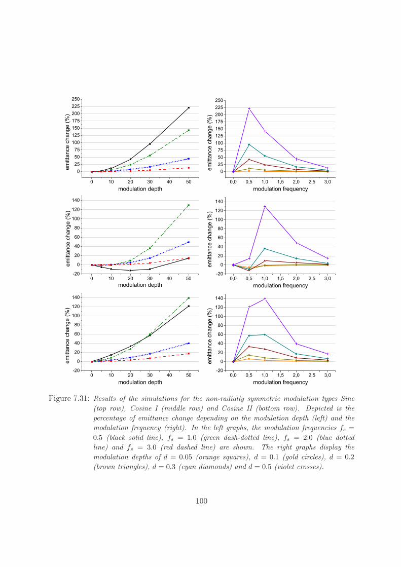
Figure 7.31: Results of the simulations for the non-radially symmetric modulation types Sine(top row), Cosine I (middle row) and Cosine II (bottom row). Depicted is thepercentage of emittance change depending on the modulation depth (left) and themodulation frequency (right). In the left graphs, the modulation frequencies fs =0.5 (black solid line), fs = 1.0 (green dash-dotted line), fs = 2.0 (blue dottedline) and fs = 3.0 (red dashed line) are shown. The right graphs display themodulation depths of d = 0.05 (orange squares), d = 0.1 (gold circles), d = 0.2(brown triangles), d = 0.3 (cyan diamonds) and d = 0.5 (violet crosses).

100

Figure 7.32: Results of the simulations for the radially symmetric modulation types Radial I (toprow) and Radial II (bottom row). The graphs and color codes correspond to thoseof figure 7.31.

In summary, the increase of the transverse emittance is most sensitive to transverseshapes in which the center of gravity of the charge density distribution is not the geometriccenter of the bunch. Furthermore, transverse shapes should be avoided in which the chargedensity has maxima away from the bunch center.The presently used scheme of cutting a Gaussian transverse laser distribution by a hardedged circular hole has proven to be beneficial over the perfect flat-top shape. And finally,the diffraction patterns shown in figure 3.12, which occur when the photocathode is notexactly placed in the image plane, have a spatial frequency which is too high to causea significant increase of the transverse emittance. On the other hand, the fact that thegeometric center of the transverse laser shape does not coincide with the center of gravityis much more severe.

101

Chapter 8

Summary and outlook

The successful operation of Free Electron Lasers such as FLASH in Hamburg and espe-cially the future European XFEL require electron sources which are capable of producingelectron bunches of very high quality. One of the key components of the electron bunchproduction is the photocathode laser system since it allows to influence the electron bunchproperties by adjusting the temporal and spatial characteristics of the laser pulses usedto extract the photoelectrons. For this reason, the first part of the thesis was dedicatedto a thorough investigation of the laser system which is currently installed at PITZ (builtby MBI Berlin) including the laser beam transport system. The results are briefly sum-marized as follows:

• The temporal laser shapes measured with the Optical Sampling System are ingood agreement with the measurements using an independent device (streak cam-era Hamamatsu FESCA200) having a comparable temporal resolution. It was alsoshown that this level of precision requires the Optical Sampling System to be ad-justed very accurately (see chapter 3.4.1).

• The influence of the laser beam transport system on the temporal laser shape isnegligible.

• Within a train of 40 pulses, no difference between the temporal shapes of the laserpulses could be detected.

• A dependence of the temporal laser profile on the transverse position in the pulsewas found. Since only the center part of the whole beam is transmitted through theBeam Shaping Aperture, the remaining variation is small.

• The laser material which is used in the current laser system shows the effect of ther-mal lensing. This effect can be reduced by proper imaging of the laser pulses in thelaser system itself as well as in the laser beam transport system to the photocathode.Even though strong efforts were made to provide optimum imaging conditions, it

102

was found that the effect of thermal lensing still causes a change of the laser pulseproperties along the pulse trains. Operation with long laser pulse trains in whicheach laser pulse has the same properties appears to be impossible with the currentsetup. On the other hand, this did not compromise the measurement of transverseemittance since it requires only short pulse trains with less than forty pulses.

• Finally, the importance of accurate alignment of the laser pulses on the inner vacuumwas demonstrated.

In the second part of the thesis, the influence on the laser pulse parameters on the electronbunch properties was investigated. This is of great importance, since the results definewhich laser pulse properties are the most critical and therefore give a baseline for futurephotocathode laser developments. The findings were:

• Simulations showed that the transverse emittance should decrease for longer laserpulse durations while the longitudinal emittance increases. Experimentally, thisbehavior could be observed only in the case of an RF emission phase of +6 degreeswhereas for on-crest acceleration the transverse emittance increased. The reason forthis behavior is not yet fully clear but there is evidence that the observed low RFphase stability had a strong impact on the measurement results.

• Optimizing the machine parameters to get minimal transverse emittance for laserpulses with different rise and fall times led to the result, that for rise and fall timeslarger than 1 ps the increase of the transverse emittance is almost linear. On theother hand, the simulation of the specific measurement conditions resulted in analmost constant transverse emittance which was also found experimentally.

• The influence of modulations on the flat-top part of the laser pulses was investigated.Simulations show that the increase of the transverse emittance is less than 10 % fora modulation depth of less than 40 % for up to five peaks. Because of the large errorin the measurement of the transverse emittance due to th RF phase instabilities,these small changes could not be identified in the measured values.

• In case of small bunch charges, modulations on the temporal flat-top of the laserpulse which are translated into modulations on the longitudinal phase space distri-bution during emission cannot be reduced by longitudinal space charge forces. Thesemodulations remain during transport of the electron beam and can be detected asmodulation of the momentum distribution. This could be confirmed experimentally.

• The tendency that for low bunch charges the optimum transverse emittance andthe corresponding transverse laser spot size decrease was found in simulations andconfirmed experimentally. For example, at a bunch charge of 1 nC the minimumtransverse emittance was measured to be ε1nC

xy =0.9 mmmrad using a laser spot size

103

of x/yrms=0.36 mmmrad while at 250 pC the minimum was found to be ε250pCxy =

0.47 mmmrad for a laser spot size of x/yrms=0.21 mmmrad. The given values wereobtained without applying a charge cut.

• Detailed simulations were performed to investigate the dependence of modulations ofthe transverse laser profile on the transverse emittance. It was found that a singlemaximum of the charge density at the center of the transverse laser distributionwhich naturally occurs in the current laser beamline setup, can result in a reductionof the transverse emittance of up to 15 %. Higher modulation frequencies causeless increase in transverse emittance and hence the diffraction patterns which occurwhen the photocathode is not exactly in the image plane are not causing a significantincrease of the transverse emittance. This is valid only when the geometric centerand center of gravity of the transverse laser pulse shape are identical.

Outlook

The next step is to repeat the measurements of the transverse emittance with an im-proved RF phase stability in the gun cavity. This would allow to decide which tolerancesin the photocathode laser pulse properties are acceptable for the operation of ax X-rayfree electron laser such as the future European XFEL.Furthermore, measuring the transverse emittance with additional experimental techniquesleads to a better understanding of the underlying processes. At the moment, several newtechniques are under development at PITZ, e.g. tomographic reconstruction of the trans-verse phase spaces as well as slice emittance measurement methods.In the mid-term future, it is planned to install a transverse deflecting cavity in the PITZbeamline. Together with a dispersive section, the longitudinal phase space can be mea-sured with a much higher precision than possible so far. This new tool would allow to geta better insight into the longitudinal electron beam dynamics at low bunch charges.

104

Appendix A

The transverse laser pulse shape nearthe image plane

The following images show the transverse profiles of the laser beam at different distancesbefore and behind the imaging plane (denoted as nominal position which should actuallybe the photocathode). The transverse distribution at the imaging plane shows the sharpedges from the beam shaping aperture as well as the cut transverse Gaussian distributionfrom the laser which is slightly shifted to the lower left edge in this case. The changeof the transverse distributions before and behind the imaging plane are symmetric andthe expected diffraction patterns are clearly visible as rings around the center. For largerdistances from the imaging plane the number of the rings decreases and the modulationdepth becomes large also in the center.Note, that the scaling of the color code is different for each image. The speckles whichare visible on some of these images result from dust on the cover glass of the camera. Theused Beam Shaping Aperture had a diameter of 1.5 mm. This laser spot size was chosenbecause it was used during the measurements of the lowest transverse emittance. Thehorizontal and vertical axes range from -1.2 mm to +1.2 mm.

105

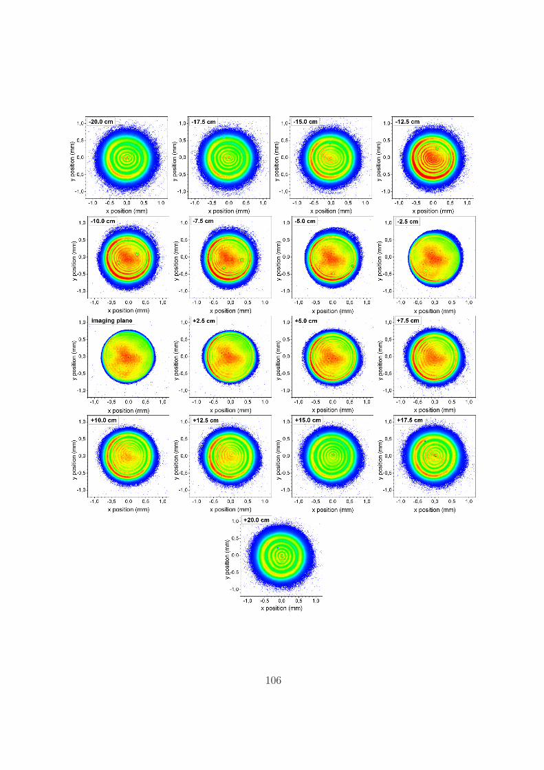
106

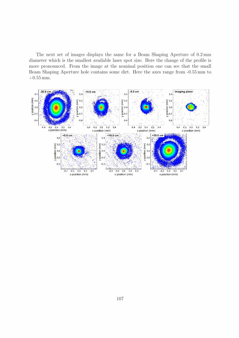
The next set of images displays the same for a Beam Shaping Aperture of 0.2 mmdiameter which is the smallest available laser spot size. Here the change of the profile ismore pronounced. From the image at the nominal position one can see that the smallBeam Shaping Aperture hole contains some dirt. Here the axes range from -0.55 mm to+0.55 mm.

107

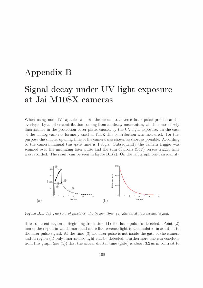
Appendix B

Signal decay under UV light exposureat Jai M10SX cameras

When using non UV-capable cameras the actual transverse laser pulse profile can beoverlayed by another contribution coming from an decay mechanism, which is most likelyfluorescence in the protection cover plate, caused by the UV light exposure. In the caseof the analog cameras formerly used at PITZ this contribution was measured. For thispurpose the shutter opening time of the camera was chosen as short as possible. Accordingto the camera manual this gate time is 1.03μs. Subsequently the camera trigger wasscanned over the impinging laser pulse and the sum of pixels (SoP) versus trigger timewas recorded. The result can be seen in figure B.1(a). On the left graph one can identify

(a) (b)

Figure B.1: (a) The sum of pixels vs. the trigger time, (b) Extracted fluorescence signal.

three different regions. Beginning from time (1) the laser pulse is detected. Point (2)marks the region in which more and more fluorescence light is accumulated in addition tothe laser pulse signal. At the time (3) the laser pulse is not inside the gate of the cameraand in region (4) only fluorescence light can be detected. Furthermore one can concludefrom this graph (see (5)) that the actual shutter time (gate) is about 3.2μs in contrast to

108

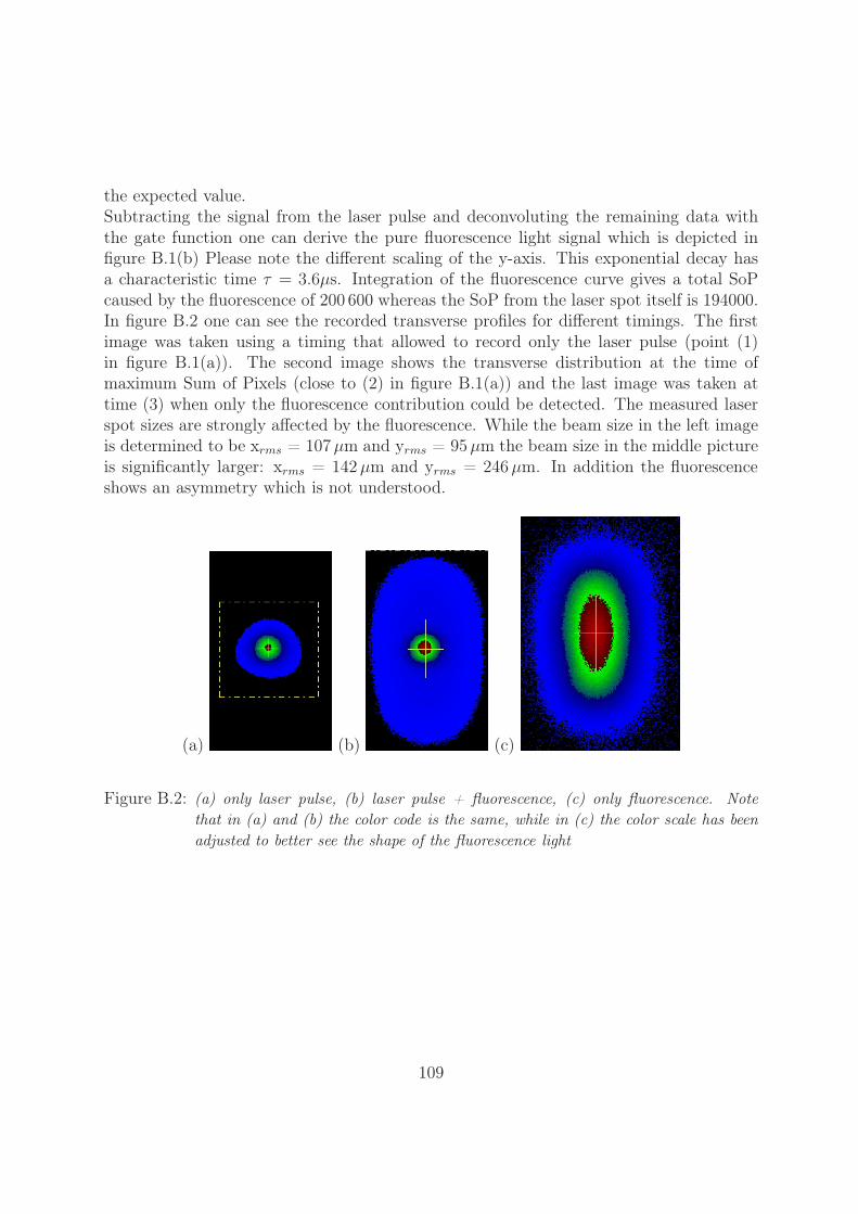
the expected value.Subtracting the signal from the laser pulse and deconvoluting the remaining data withthe gate function one can derive the pure fluorescence light signal which is depicted infigure B.1(b) Please note the different scaling of the y-axis. This exponential decay hasa characteristic time τ = 3.6μs. Integration of the fluorescence curve gives a total SoPcaused by the fluorescence of 200 600 whereas the SoP from the laser spot itself is 194000.In figure B.2 one can see the recorded transverse profiles for different timings. The firstimage was taken using a timing that allowed to record only the laser pulse (point (1)in figure B.1(a)). The second image shows the transverse distribution at the time ofmaximum Sum of Pixels (close to (2) in figure B.1(a)) and the last image was taken attime (3) when only the fluorescence contribution could be detected. The measured laserspot sizes are strongly affected by the fluorescence. While the beam size in the left imageis determined to be xrms = 107 μm and yrms = 95μm the beam size in the middle pictureis significantly larger: xrms = 142 μm and yrms = 246 μm. In addition the fluorescenceshows an asymmetry which is not understood.

(a) (b) (c)

Figure B.2: (a) only laser pulse, (b) laser pulse + fluorescence, (c) only fluorescence. Notethat in (a) and (b) the color code is the same, while in (c) the color scale has beenadjusted to better see the shape of the fluorescence light

109

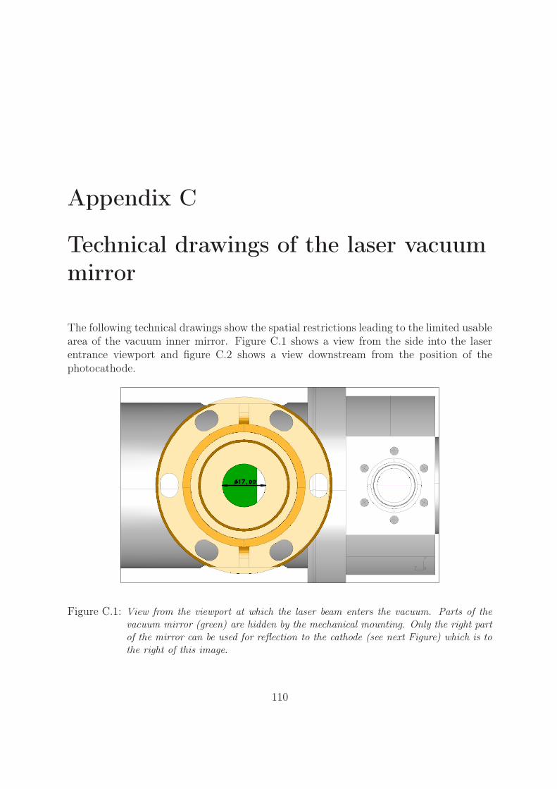
Appendix C

Technical drawings of the laser vacuummirror

The following technical drawings show the spatial restrictions leading to the limited usablearea of the vacuum inner mirror. Figure C.1 shows a view from the side into the laserentrance viewport and figure C.2 shows a view downstream from the position of thephotocathode.

Figure C.1: View from the viewport at which the laser beam enters the vacuum. Parts of thevacuum mirror (green) are hidden by the mechanical mounting. Only the right partof the mirror can be used for reflection to the cathode (see next Figure) which is tothe right of this image.

110

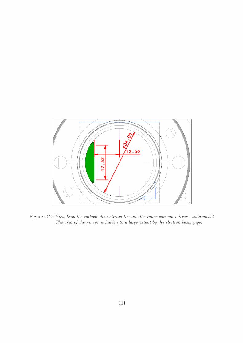
Figure C.2: View from the cathode downstream towards the inner vacuum mirror - solid model.The area of the mirror is hidden to a large extent by the electron beam pipe.

111

Appendix D

Error sources during the measurementof the transverse phase spacedistribution

This appendix summarizes the error sources which occurred during the measurement ofthe transverse emittance. These errors define the error bars that are shown in the graphscontaining the measurement results.

Measurement procedure

During the measurement of the transverse emittance using the slit scan technique severalerror sources lead to an uncertainty of the measurement result. These are, for example:

• Uncertainty of the determination of the bunch mean momentum which is needed tocalculate the relativistic scaling factor βγ in equation 6.7.

• Uncertainties associated with the measurement of transverse electron bunch distri-bution which is needed for the determination of the transverse sizes of the wholeelectron bunch as well as those of the beamlets, see chapter 2.2.4:

– Granularity of the observation screen material (usually YAG powder).

– Resolution of the camera used to record the image of the observation screen.

– Dynamic range of the camera.

– Quality of the optical imaging system between screen and camera.

• Precision of the slit machining and its positioning in the beamline.

These and other error sources have been investigated in detail in [Stay, PITZ02]. It wasshown that the systematic error is less than 10 % in a wide range of machine parameters.

112

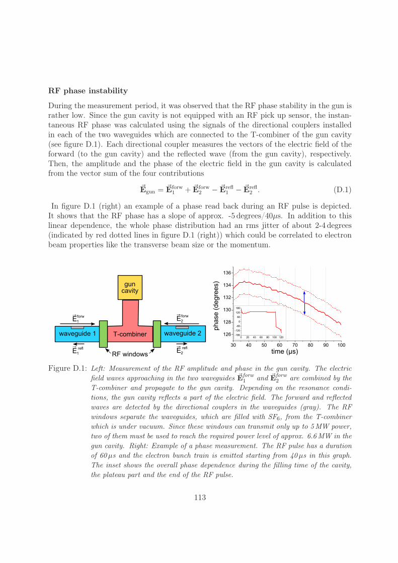
RF phase instability

During the measurement period, it was observed that the RF phase stability in the gun israther low. Since the gun cavity is not equipped with an RF pick up sensor, the instan-taneous RF phase was calculated using the signals of the directional couplers installedin each of the two waveguides which are connected to the T-combiner of the gun cavity(see figure D.1). Each directional coupler measures the vectors of the electric field of theforward (to the gun cavity) and the reflected wave (from the gun cavity), respectively.Then, the amplitude and the phase of the electric field in the gun cavity is calculatedfrom the vector sum of the four contributions

�Egun = �Eforw1 + �Eforw

2 − �Erefl1 − �Erefl

2 . (D.1)

In figure D.1 (right) an example of a phase read back during an RF pulse is depicted.It shows that the RF phase has a slope of approx. -5 degrees/40μs. In addition to thislinear dependence, the whole phase distribution had an rms jitter of about 2-4 degrees(indicated by red dotted lines in figure D.1 (right)) which could be correlated to electronbeam properties like the transverse beam size or the momentum.

Figure D.1: Left: Measurement of the RF amplitude and phase in the gun cavity. The electricfield waves approaching in the two waveguides �Eforw

1 and �Eforw2 are combined by the

T-combiner and propagate to the gun cavity. Depending on the resonance condi-tions, the gun cavity reflects a part of the electric field. The forward and reflectedwaves are detected by the directional couplers in the waveguides (gray). The RFwindows separate the waveguides, which are filled with SF6, from the T-combinerwhich is under vacuum. Since these windows can transmit only up to 5MW power,two of them must be used to reach the required power level of approx. 6.6MW in thegun cavity. Right: Example of a phase measurement. The RF pulse has a durationof 60 μs and the electron bunch train is emitted starting from 40μs in this graph.The inset shows the overall phase dependence during the filling time of the cavity,the plateau part and the end of the RF pulse.

113

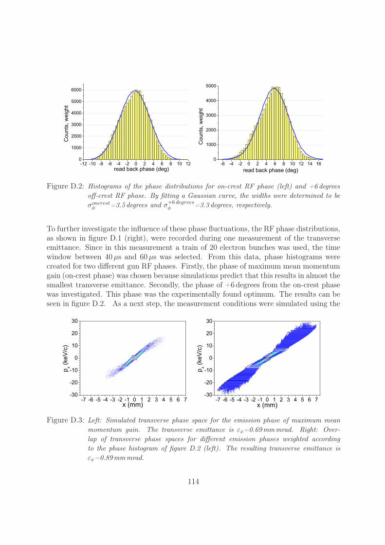
Figure D.2: Histograms of the phase distributions for on-crest RF phase (left) and +6 degreesoff-crest RF phase. By fitting a Gaussian curve, the widths were determined to beσoncrest

φ =3.5 degrees and σ+6 degreesφ =3.3 degrees, respectively.

To further investigate the influence of these phase fluctuations, the RF phase distributions,as shown in figure D.1 (right), were recorded during one measurement of the transverseemittance. Since in this measurement a train of 20 electron bunches was used, the timewindow between 40μs and 60μs was selected. From this data, phase histograms werecreated for two different gun RF phases. Firstly, the phase of maximum mean momentumgain (on-crest phase) was chosen because simulations predict that this results in almost thesmallest transverse emittance. Secondly, the phase of +6 degrees from the on-crest phasewas investigated. This phase was the experimentally found optimum. The results can beseen in figure D.2. As a next step, the measurement conditions were simulated using the

Figure D.3: Left: Simulated transverse phase space for the emission phase of maximum meanmomentum gain. The transverse emittance is εx=0.69mmmrad. Right: Over-lap of transverse phase spaces for different emission phases weighted accordingto the phase histogram of figure D.2 (left). The resulting transverse emittance isεx=0.89mmmrad.

114

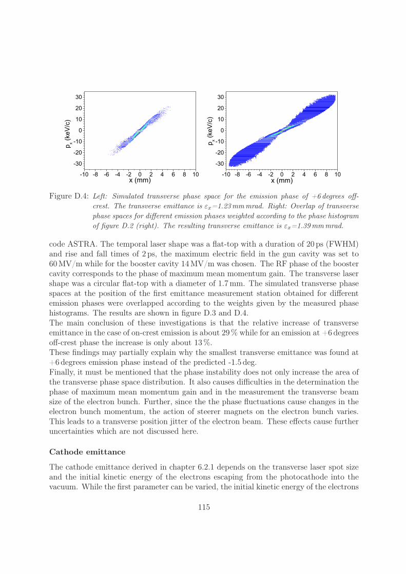
Figure D.4: Left: Simulated transverse phase space for the emission phase of +6 degrees off-crest. The transverse emittance is εx=1.23mmmrad. Right: Overlap of transversephase spaces for different emission phases weighted according to the phase histogramof figure D.2 (right). The resulting transverse emittance is εx=1.39mmmrad.

code ASTRA. The temporal laser shape was a flat-top with a duration of 20 ps (FWHM)and rise and fall times of 2 ps, the maximum electric field in the gun cavity was set to60 MV/m while for the booster cavity 14 MV/m was chosen. The RF phase of the boostercavity corresponds to the phase of maximum mean momentum gain. The transverse lasershape was a circular flat-top with a diameter of 1.7 mm. The simulated transverse phasespaces at the position of the first emittance measurement station obtained for differentemission phases were overlapped according to the weights given by the measured phasehistograms. The results are shown in figure D.3 and D.4.The main conclusion of these investigations is that the relative increase of transverseemittance in the case of on-crest emission is about 29 % while for an emission at +6 degreesoff-crest phase the increase is only about 13 %.These findings may partially explain why the smallest transverse emittance was found at+6 degrees emission phase instead of the predicted -1.5 deg.Finally, it must be mentioned that the phase instability does not only increase the area ofthe transverse phase space distribution. It also causes difficulties in the determination thephase of maximum mean momentum gain and in the measurement the transverse beamsize of the electron bunch. Further, since the the phase fluctuations cause changes in theelectron bunch momentum, the action of steerer magnets on the electron bunch varies.This leads to a transverse position jitter of the electron beam. These effects cause furtheruncertainties which are not discussed here.

Cathode emittance

The cathode emittance derived in chapter 6.2.1 depends on the transverse laser spot sizeand the initial kinetic energy of the electrons escaping from the photocathode into thevacuum. While the first parameter can be varied, the initial kinetic energy of the electrons

115

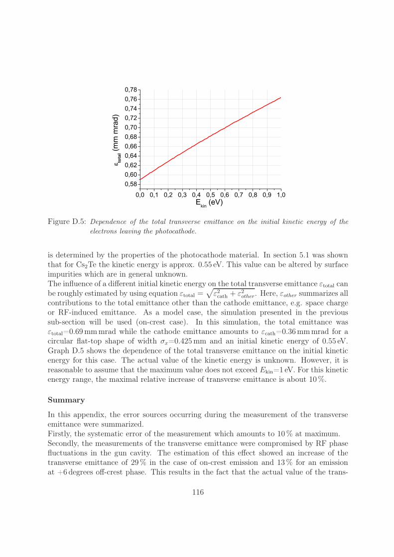
Figure D.5: Dependence of the total transverse emittance on the initial kinetic energy of theelectrons leaving the photocathode.

is determined by the properties of the photocathode material. In section 5.1 was shownthat for Cs2Te the kinetic energy is approx. 0.55 eV. This value can be altered by surfaceimpurities which are in general unknown.The influence of a different initial kinetic energy on the total transverse emittance εtotal canbe roughly estimated by using equation εtotal =

√ε2cath + ε2

other. Here, εother summarizes allcontributions to the total emittance other than the cathode emittance, e.g. space chargeor RF-induced emittance. As a model case, the simulation presented in the previoussub-section will be used (on-crest case). In this simulation, the total emittance wasεtotal=0.69 mmmrad while the cathode emittance amounts to εcath=0.36 mmmrad for acircular flat-top shape of width σx=0.425 mm and an initial kinetic energy of 0.55 eV.Graph D.5 shows the dependence of the total transverse emittance on the initial kineticenergy for this case. The actual value of the kinetic energy is unknown. However, it isreasonable to assume that the maximum value does not exceed Ekin=1 eV. For this kineticenergy range, the maximal relative increase of transverse emittance is about 10 %.

Summary

In this appendix, the error sources occurring during the measurement of the transverseemittance were summarized.Firstly, the systematic error of the measurement which amounts to 10 % at maximum.Secondly, the measurements of the transverse emittance were compromised by RF phasefluctuations in the gun cavity. The estimation of this effect showed an increase of thetransverse emittance of 29 % in the case of on-crest emission and 13 % for an emissionat +6 degrees off-crest phase. This results in the fact that the actual value of the trans-

116

verse emittance is lower than the measured one by about 22 % and 12 % for the on-crestand off-crest phase respectively. The last uncertainty could originate from the unknownamount of cathode emittance. It was estimated that an initial kinetic energy of the emit-ted electrons of 1 eV instead of 0.55 eV used in the simulations leads to an increase of thetotal transverse emittance of 10 %. This means that the actual value is about 9.5 % lowerthan the measured value.While the first and the third error source can increase and decrease the measured emit-tance compared to the simulated one, the phase instability can only increase the measuredemittance. For this reason, the error bars are +19.5 %/-41.5 % and +19.5 %/-31.5 % forthe on-crest and +6 degrees off-crest measurements, respectively.

117

Appendix E

Electron beam dynamics at low bunchcharge

While the main subject of this thesis was the investigation of the dependence of theelectron bunch properties on the laser pulse parameters at a charge level of 1 nC, thischapter is dedicated to a brief overview of the electron beam dynamics at low chargeof some tens of pC. The differences in the longitudinal and transverse electron beamdynamics will be discussed separately.

Longitudinal dynamics

At high charge densities1, the longitudinal dynamics of the electron bunch is mainly de-termined by three factors. Firstly, the instantaneous RF field at which each longitudinalslice is emitted defines its energy gain while being accelerated in the gun cavity. Sec-ondly, the longitudinal space charge forces will cause an acceleration of the head and adeceleration of the tail part of the electron bunch. And finally, the mirror charge effect atthe cathode influences the longitudinal dynamics at emission. In the low charge densitycase the second and third contributions are negligible. This behavior was simulated andis shown in figure E.1. For these simulations a maximal electric field in the gun cavityof 60 MV/m was chosen, the emission took place at phase of maximum mean momentumgain, the transverse laser shape was a circular flat-top of 1.7 mm diameter and the tem-poral laser shape was a flat-top with a duration of 20 ps (FWHM) and 2 ps rise and falltimes.In addition to the mentioned effects, high space charge forces cause an increase of the

slice energy spread. This is in general accompanied by a reduction of modulations in thelongitudinal phase space introduced by modulations in the laser pulse temporal profile

1Note that here the differences in charge density are discussed rather than the total bunch chargesince the charge density mainly determines the electron bunch dynamics.

118

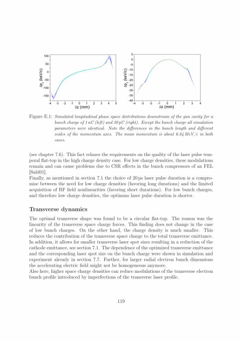
Figure E.1: Simulated longitudinal phase space distributions downstream of the gun cavity for abunch charge of 1 nC (left) and 20 pC (right). Except the bunch charge all simulationparameters were identical. Note the differences in the bunch length and differentscales of the momentum axes. The mean momentum is about 6.84MeV/c in bothcases.

(see chapter 7.6). This fact relaxes the requirements on the quality of the laser pulse tem-poral flat-top in the high charge density case. For low charge densities, these modulationsremain and can cause problems due to CSR effects in the bunch compressors of an FEL[Sald01].Finally, as mentioned in section 7.1 the choice of 20 ps laser pulse duration is a compro-mise between the need for low charge densities (favoring long durations) and the limitedacquisition of RF field nonlinearities (favoring short durations). For low bunch charges,and therefore low charge densities, the optimum laser pulse duration is shorter.

Transverse dynamics

The optimal transverse shape was found to be a circular flat-top. The reason was thelinearity of the transverse space charge forces. This finding does not change in the caseof low bunch charges. On the other hand, the charge density is much smaller. Thisreduces the contribution of the transverse space charge to the total transverse emittance.In addition, it allows for smaller transverse laser spot sizes resulting in a reduction of thecathode emittance, see section 7.1. The dependence of the optimized transverse emittanceand the corresponding laser spot size on the bunch charge were shown in simulation andexperiment already in section 7.7. Further, for larger radial electron bunch dimensionsthe accelerating electric field might not be homogeneous anymore.Also here, higher space charge densities can reduce modulations of the transverse electronbunch profile introduced by imperfections of the transverse laser profile.

119

Bibliography

[ASTRA] http://www.desy.de/˜mpyflo

[Berg] http://www.bergoz.com , ICT-178-2-XXX-X

[Boyd] Robert W. Boyd, Nonlinear Optics, Second edition, Elsevier 2000

[Carl] B.E. Carlsten and D.T. Palmer Enhanced emittance compensation in a high-frequency RF photoinjector using RF radial focusing, NIM A, 425, 37-50, 1999

[Chen] S. Chénais et al., Diode-pumped Yb:GGG laser: comparison with Yb:YAG,Optical Materials 22 99-106, 2003

[Eins] A. Einstein, Zur Theorie der Strahlung, Mitteilungen der PhysikalischenGesellschaft Zürich. Nr. 18, 1916

[FEL] P. Schmüser, M. Dohlus, J. Roßbach, Ultraviolet and Soft X-Ray Free-Electron Lasers: Introduction to Physical Principles, Experimental Results, Techno-logical Challenges, Springer Berlin Heidelberg, 2008

[Ferr01] M. Ferrario et al., Recent advances and novel ideas for high brightnesselectron beam production based on photo-injectors, The Physics and Application ofHigh Brightness Electron Beams, World Scientific Publishing Co. Pte. Ltd., 2003

[Ferr02] M. Ferrario, Emittance Compensation in High Brightness RF Photoinjectors:an introduction with some application, talk at CASA seminar, Jefferson Lab, 2003

[FLASH] W. Ackermann et al., Operation of a free-electron laser from the extremeultraviolet to the water window, Nature Photonics, Vol. 1, 336-342, 2007

[Floet] K. Flöttmann, Note on the thermal emittance of electrons emitted by CesiumTelluride photo cathodes, TESLA-FEL internal note 97-01, 1997

[Fran] P.A. Franken et al., Generation of optical harmonics, PRL 7, No. 4, 118-119,1961

120

[Goul] E. Goulielmakis et al., Single-Cycle Nonlinear Optics, Science 320, 1614,2008

[Haen] M. Hänel et al., Electron Bunch Momentum Distribution Modulations atPITZ, Proc. of FEL09, FEL 2009, Liverpool, UK

[Hafer] H. Haferkorn, Optik, 4th edition, WILEY-VCH, 2003

[Hama01] Homepage of Hamamatsu Photonics,http://sales.hamamatsu.com/de/produkte/system-division/ultra-fast/streak-systems/part-c6138.php

[Hama02] Homepage of Hamamatsu Photonics,http://sales.hamamatsu.com/assets/pdf/hpspdf/Guidetostreak.pdf

[Hama03] Homepage of Hamamatsu Photonics,http://sales.hamamatsu.com/assets/applications/ETD/pmt_handbook/pmt_handbook_complete.pdf

[Han] J.-H. Han, Dynamics of Electron Beam and Dark Current in Photocathode RFGunsPhD thesis at PITZ, 2005

[Hodg] Norman Hodgson and Horst Weber, Optical Resonators, Fundamentals -Advanced Concepts - Applications, Springer Berlin, 1997

[Ivan01] Y. Ivanisenko, Photo Injector Cathode Laser Beam Intensity and PositionMonitoring SystemMaster thesis at PITZ, 2007

[Ivan02] Y. Ivanisenko, Slice Emittance Measurement Using an Energy Chirped Beamin a Dispersive Section at PITZ, Proc. of FEL 2008, Gyeongju, South Korea, 2008

[Kim] K.-J. Kim, RF and Space-charge Effects in Laser-driven RF Electron Guns, NIMA 275, 201-218, 1989

[Koech] W. Koechner, Solid-State Laser Engineering, Sixth Revised and Updated Edi-tion, Springer, 2006

[Kras01] M. Krasilnikov, private communication

[Kras02] M. Krasilnikov, Photo injector optimization: PITZ-1.7 experience, Talk atthe PITZ collaboration meeting, December 2009, Zeuthen

[Lede01] S. Lederer, private communication

121

[Lede02] S. Lederer et al., XPS Studies of Cs2Te Photocathodes, Proc. of FEL 2007,Novosibirsk, Russia, 2007

[Leje] C. Lejeune and J. Aubert, Emittance and Brightness: Definitions and Mea-surements, Advances in Electronics and Electron Physics, Supplement 13A, AcademicPress Inc., 1980

[Limb] C. Limborg-Deprey, P.R. Bolton, Optimum electron distributions or spacecharge dominated beams in photoinjectors, NIM A, 557, 106-116, 2006

[Luit] O.J. Luiten et al., How to Realize Uniform Three-Dimensional Ellipsoidal Elec-tron Bunches, Phys. Rev. Letters 93, No. 9, 2004

[Lyot] B. Lyot, Optical apparatus with wide field using interference of polarized light,C. R. Acad. Sci. (Paris) 197, 1593, 1933

[Maim] T.H. Maiman, Stimulated optical radiation in ruby, Nature, 187, 493-494, 1960

[MAXlab] B. Anderberg et al., The design of a 3 GHz thermionic RF-gun and energyfilter for MAX-lab, NIM A 491, 307-313, 2002

[Milt] V. Miltchev, Investigations on the transverse phase space at a photo injector forminimized emittance,PhD thesis at PITZ, 2006

[Modi] A. Modinos, Theory of thermionic emission, Surface Science 115, 469-400, 1982

[Mood] J.T. Moody et al., Longitudinal phase space characterization of he blow-outregime of rf photoinjector operation, PRST AB 12, 070704, 2009

[Musu] P. Musumeci et al., Experimental Generation and Characterization of Uni-formly Filled Ellipsoidal Beam Distribution, Proc. of EPAC08, Genoa, Italy, 2008

[Oppe] A. Oppelt et al., Status and first results from the upgraded PITZ facility,Proc. of FEL 2005, Stanford, USA, 2005

[PITZ01] F. Stephan et al., Photo Injector Test Facility under Construction at DESYZeuthen, Proc. of FEL 2000, Durham, North Carolina, USA, 2000

[PITZ02] F. Stephan et al., Detailed characterization of electron sources yielding firstdemonstration of European X-ray Free-Electron Laser beam quality, PRST AB 13,020704, 2010

[Pow] R. A. Powell et al., Photoemission studies of Cesium Telluride, Phys. Rev. B8, 3987-3995, 1973

122

[Reis] M. Reiser, Theory and design of charged particle beams, Wiley Series in BeamPhysics and Accelerator Technology, 1994

[Roen] J. Rönsch, Investigations on the longitudinal phase space at a photo injector,PhD thesis at PITZ, 2009

[Ros01] , J. Rossbach et al., Fundamental limitations of an X-ray FEL operation dueto quantum fluctuations of undulator radiation, NIM A 393, 152-156, 1997

[Sald01] E.L. Saldin et al., Longitudinal space charge-driven microbunching instabilityin the TESLA Test Facility linac, NIM A 528, 355-359, 2004

[Sald02] E.L. Saldin et al., The physics of free electron lasers, Springer, 2000

[Scho] W. Schottky, Über die kalte und warme Elektronenentladungen, Zeitschrift fürPhysik A, 14 1 63-106, 1923

[SCSS] K. Togawa et al., CeB6 electron gun for the soft X-ray FEL project at SPring-8, NIM A 528, 312-315, 2004

[Sera] L. Serafini and J.B. Rosenzweig, Envelope analysis of intense relativisticquasilaminar beams in rf photoinjectors: A theory of emittance compensation, Phys.Rev. E, 55, 6, 7565-7590, 1997

[SLAC] B. McNeil, First light from hard X-ray laser, Nature Photonics, Vol. 3, 375-377,2009

[Šolc] Ivan Šolc, Birefringent Chain Filter, J. Opt. Soc. Am., 55, 17, 1965

[Spes01] R. Spesyvtsev, Transverse Beam Size Measurement Systems at Photo InjectorTest Facility in ZeuthenMaster thesis at PITZ, 2007

[Spic] W. E. Spicer, Photoemissive, Photoconductive, and Optical Absorption Studiesof Alkali-Antimony Compounds, Phys. Rev. 112, 114-122, 1958

[Stay] L. Staykov, Characterization of the transverse phase space at the photo-injectortest facility in DESY, Zeuthen sitePhD thesis at PITZ, 2008

[Suber] G. Suberlucq, Development and Production of Photo Cathodes for the CLICTest Facility, Proc. of FEL 1996, Rome, Italy, 1996

[Tomiz] Hiromitsu Tomizawa (Spring8), private communication

123

[Treb] R. Trebino, Frequency resolved optical gating, the measurement of ultrashortlaser pulses, Kluwer Academic publishers, Boston, Dordrecht, London, 2002

[Weis] S. Weisse et al., Tine Video System: Proceedings on Redesign, Proc. ofICALEPCS 2009, Kobe, Japan, 2009

[Will01] I. Will, G. Klemz, Generation of flat-top picosecond pulses by coherent pulsestacking in a multicrystal birefringent filter, Optics Express 16, 19, 2008

[Will02] I. Will, G. Koss, I. Templin, The upgraded photocathode laser of the TESLATest Facility, NIM A 541 467-477, 2005

[Wolf] Emil Wolf (editor), Progress in Optics, Volume IX, North Holland PublishingCompany, Amsterdam, London, 1971

[XFEL] M. Ferrario et al., Conceptual Design of the XFEL Photoinjector, 2001

[XTDR] M. Altarelli et al., The European X-Ray Free-Electron Laser - Technicaldesign report, July 2007

[Yang] Yaguang Yang, Analytic Solution of Free Space Optical Beam Steering UsingRisley Prisms, J. Lightwave Technol. 26, 3576-3583, 2008

124

Acknowledgements

I would like to express my thankfulness to many people who contributed morally andscientifically to the success of this thesis:

Prof. Shaukat Khan, Prof. Jörg Roßbach, Dr. Frank Stephan, Dr. Jürgen Bährand Dr. Mikhail Krasilnikov for thoroughly proof-reading my thesis and giving me usefulcomments and advice.

All the colleagues at PITZ who were always willing to discuss different topics relatedto the presented work, especially Dr. Juliane Rönsch-Schulenburg and my office matesYevgeniy Ivanisenko, Grigorii Vashchenko and Dr. Marek Otevrel.

Furthermore, the presented results of the electron beam measurements might fit ona few pages but they required many weeks of measurements. These measurements weredone on shift by the members of the PITZ group who I want to express my gratitude.

Dr. Guido Klemz for ginving me insight into the specialties of the laser system atPITZ and the long discussions about laser physics in general.

Dr. Siegfried Schreiber who always was a source of motivation and for his supportduring the measurements of the laser pulse properties.

All mechanical and electronic engineers, programmers and technical staff at DESYwho supported me during the commissioning of new components: Hartmut Lüdecke, Ger-ald Koss, Jochen Bienge, Mario Pohl, Jörg Schultze, Bagrat Petrossyan, Stefan Weisseand others.

Most of all, I would like to thank my family Jana and Sontje Könnemann who sup-ported me during the long time of creating this thesis.

Thank you all !

125