Proceedings of the Second International

Conference on Symbolic Computation and

Cryptography

Carlos Cid and Jean-Charles Faugere (Eds.)

23 – 25 June 2010,Royal Holloway, University of London, Egham, UK

Programme Chairs

Carlos Cid Royal Holloway, University of London, UKJean-Charles Faugere UPMC-INRIA, France

Programme Committee

Daniel Bernstein University of Illinois at Chicago, USAOlivier Billet Orange Labs, FranceClaude Carlet University of Paris 8, FrancePierre-Alain Fouque ENS - Paris, FranceJoachim von zur Gathen Universitat Paderborn, GermanyPierrick Gaudry CNRS, FranceJaime Gutierrez University of Cantabria, SpainAntoine Joux Universite de Versailles Saint-Quentin-en-Yvelines, FranceMartin Kreuzer Universitat Passau, GermanyDongdai Lin Institute of Software of Chinese Academy of Sciences, ChinaAlexander May Ruhr-Universitat Bochum, GermanyAyoub Otmani GREYC-Ensicaen & University of Caen & INRIA, FranceLudovic Perret LIP6-UPMC Univ Paris 6 & INRIA, FranceIgor Shparlinski Macquarie University, AustraliaBoaz Tsaban Bar-Ilan University, IsraelMaria Isabel Gonzalez Vasco Universidad Rey Juan Carlos, Spain

Algebraic attacks using SAT-solvers 7Martin Kreuzer and Philipp Jovanovic

Cold Boot Key Recovery using Polynomial System Solving with Noise 19

Martin Albrecht and Carlos Cid

Practical Key Recovery Attacks On Two McEliece Variants 27Valerie Gauthier Umana and Gregor Leander

Algebraic Cryptanalysis of Compact McEliece’s Variants - Toward a Complexity Anal-ysis 45

Jean-Charles Faugere, Ayoub Otmani, Ludovic Perret and Jean-Pierre Tillich

A variant of the F4 algorithm 57

Vanessa Vitse and Antoine Joux

Improved Agreeing-Gluing Algorithm 73Igor Semaev

WXL: Widemann-XL Algorithm for Solving Polynomial equations over GF(2) 89Wael Mohamed, Jintai Ding, Thorsten Kleinjung, Stanislav Bulygin and Johannes Buchmann

Analysis of the MQQ public key cryptosystem 101Rune Odegard, Ludovic Perret, Jean-Charles Faugere and Danilo Gligoroski

Multivariate Quasigroups Defined by T-functions 117Simona Samardziska, Smile Markovski and Danilo Gligoroski

Lattice Polly Cracker Signature 129

Emmanuela Orsini and Carlo Traverso

A public key exchange using semidirect products of groups 137Maggie Habeeb, Delaram Kahrobaei and Vladimir Shpilrain

On lower bounds for Information Set Decoding over Fq 143Robert Niebuhr, Pierre-Louis Cayrel, Stanislav Bulygin and Johannes Buchmann

On homogeneous polynomial decomposition 159

Jaime Gutierrez and Paula Bustillo

An Efficient Method for Deciding Polynomial Equivalence Classes 163Tianze Wang and Dongdai Lin

Algebraic techniques for number fields 183Jean-Francois Biasse, Michael J. Jacobson Jr and Alan K. Silvester

Implicit Factoring with Shared Most Significant and Middle Bits 197Jean-Charles Faugere, Raphael Marinier and Guenael Renault

On the Immunity of Boolean Functions Against Probabilistic Algebraic Attacks 203Meicheng Liu and Dongdai Lin

4

A Family of Weak Keys in HFE (and the Corresponding Practical Key-Recovery)209Charles Bouillaguet, Pierre-Alain Fouque, Antoine Joux and Joana Treger

A Multivariate Signature Scheme with a Partially Cyclic Public Key 229Albrecht Petzoldt, Stanislav Bulygin and Johannes Buchmann

Multivariate Trapdoor Functions Based on Multivariate Left Quasigroups and LeftPolynomial Quasigroups 237

Smile Markovski, Simona Samardziska, Danilo Gligoroski and Svein.J. Knapskog

6

Algebraic Attacks Using SAT-Solvers

Philipp Jovanovic and Martin Kreuzer

Fakultat fur Informatik und MathematikUniversitat Passau

D-94030 Passau, Germany

Abstract. Algebraic attacks lead to the task of solving polynomial sys-tems over F2. We study recent suggestions of using SAT-solvers for thistask. In particular, we develop several strategies for converting the poly-nomial system to a set of CNF clauses. This generalizes the approachin [4]. Moreover, we provide a novel way of transforming a system over F2eto a (larger) system over F2. Finally, the efficiency of these methods isexamined using standard examples such as CTC, DES, and Small ScaleAES.

Key words: algebraic cryptanalysis, SAT solver, AES, polynomial systemsolving

1 Introduction

The basic idea of algebraic cryptanalysis is to convert the problem of breaking acypher to the problem of solving a system of polynomial equations over a finitefield, usually a field of characteristic 2. A large number of different approacheshas been developed to tackle such polynomial systems (for an overview, see [12]).

In this note we examine a recent suggestion, namely to convert the system toa set of propositional logic clauses and then to use a SAT-solver. In [8] this wassuccessfully applied to attack 6 rounds of DES. The first study of efficient meth-ods for converting boolean polynomial systems to CNF clauses was presentedin [4] where the following procedure was suggested:

(1) Linearise the system by introducing a new indeterminate for each term inthe support of one of the polynomials.

(2) Having written a polynomial as a sum of indeterminates, introduce newindeterminates to cut it after a certain number of terms. (This number iscalled the cutting number.)

(3) Convert the reduced sums into their logical equivalents using a XOR-CNFconversion.

Later this study was extended slightly in [5], [3], and [17] but the procedurewas basically unaltered. Our main topic, discussed in Section 2 of this paper,is to examine different conversion strategies, i.e. different ways to convert thepolynomial system into a satisfiability problem. The crucial point is that the

7

linearisation phase (1) usually produces way too many new indeterminates. Ourgoal will be to substitute not single terms, but term combinations, in order tosave indeterminates and clauses in the CNF output.

For certain cryptosystems such as AES (see [9]) or its small scale variants(see [6]), the polynomial systems arising from an algebraic attack are naturallydefined over a finite extension field F2e of F2, for instance over F16 or F256. Whileit is clear that one can convert a polynomial system over F2e to a polynomialsystem over F2 by introducing additional indeterminates, it is less clear whatthe best way is to do this such that the resulting system over F2 allows a goodconversion to a SAT problem. An initial discussion of this question is containedin [2]. Although the algorithm we present in Section 3 is related to the one giventhere, our method seems to be easier to implement and to allow treatment oflarger examples.

In the last section we report on some experiments and timings using thefirst author’s implementation of our strategies in the ApCoCoA system (see [1]).By looking at the Courtois Toy Cipher (CTC), the Data Encryption Standard(DES), and Small Scale AES, we show that a suitably chosen conversion strategycan save a substantial amount of logical variables and clauses in the CNF output.The typical savings are in the order of 10% of the necessary logical variables andup to 25% in the size of the set of clauses. The main benefit is then a significantspeed-up of the SAT-solvers which are applied to these sets of clauses. Here thegain can easily be half of the execution time or even more. We shall also see thata straightforward Grobner basis approach to solving polynomial systems over F2is slower by several orders of magnitude.

This paper is based on the first author’s thesis [11]. Unless explicitly notedotherwise, we adhere to the definitions and notation of [13] and [14].

2 Converting Boolean Polynomials to CNF Clauses

In this section we let F2 be the field with two elements and f ∈ F2[x1, . . . , xn]a polynomial. Usually f will be a boolean polynomial, i.e. all terms in thesupport of f will be squarefree, but this is not an essential hypothesis. LetM = {X1, . . . , Xn} be a set of boolean variables (atomic formulas), and let Mbe the set of all (propositional) logical formulas that can be constructed fromthem, i.e. all formulas involving the operations ¬, ∧, and ∨.

The following definition describes the relation between the zeros of a poly-nomial and the evaluation of a logical formula.

Definition 1. Let f ∈ F2[x1, . . . , xn] be a polynomial. A logical formula F ∈ Mis called a logical representation of f if ϕa(F ) = f(a1, . . . , an) + 1 for everya = (a1, . . . , an) ∈ Fn2 . Here ϕa denotes the boolean value of F at the tuple ofboolean values a where 1 = true and 0 = false.

The main effect of this definition is that boolean tuples at which F is satisfiedcorrespond uniquely to zeros of f in Fn2 . The following two lemmas contain usefulbuilding blocks for conversion strategies.

8

Lemma 2. Let f ∈ F2[x1, . . . , xn] be a polynomial, let F ∈ M be a logical rep-resentation of f , let y be a further indeterminate, and let Y be a further booleanvariable. Then G = (¬F ⇔ Y ) is a logical representation of the polynomialg = f + y.

Proof. Let a = (a1, . . . , an, b) ∈ Fn+12 . We distinguish two cases.

(1) If b = 1 then g(a) = f(a) + 1 = ϕa(F ). Since ϕb(Y ) = 1, we get ϕa(¬F ⇔Y ) = ϕa(¬F ) = ϕa(F ) + 1.

(2) If b = 0 then g(a) = f(a) = ϕa(F ) + 1 and ϕb(Y ) = 0 implies ϕa(¬F ⇐⇒Y ) = ϕa(F ).

In both cases we find ϕa(¬F ⇐⇒ Y ) = g(a) + 1, as claimed. ut

The preceding lemma is the work horse for the standard conversion algorithm.The next result extends it in a useful way.

Lemma 3. Let f ∈ F2[x1, . . . , xn, y] be a polynomial of the form f = `1 · · · `s+ywhere 1 ≤ s ≤ n and `i ∈ {xi, xi + 1} for i = 1, . . . , s. We define formulasLi = Xi if `i = xi and Li = ¬Xi if `i = xi + 1. Then

F = (¬Y ∨ L1) ∧ . . . ∧ (¬Y ∨ Ls) ∧ (Y ∨ ¬L1 ∨ . . . ∨ ¬Ls)

is a logical representation of f . Notice that F is in conjunctive normal form(CNF) and has s+ 1 clauses.

Proof. Let a = (a1, . . . , an, b) ∈ Fn+12 We will show ϕa(F ) = f(a) + 1 by in-

duction on s. In the case s = 1 we have f = x1 + y + c where c ∈ {0, 1} andF = (¬Y ∨L1)∧ (Y ∨¬L1) where L1 = X1 if c = 0 and L1 = ¬X1 if c = 1. Theclaim ϕa(F ) = f(a) + 1 follows easily with the help of a truth table.

Now we prove the inductive step, assuming that the claim has been shownfor s− 1 factors `i, i.e. for f

′ = `1 · · · `s−1 and the corresponding formula F ′. Tobegin with, we assume that `s = xs and distinguish two sub-cases.

(1) If as = 0, we have ϕa(F ) = ϕa(¬Y ∨L1)∧ . . .∧ (¬Y ∨Ls−1)∧¬Y = ϕb(¬Y )and f(a) = b. This shows ϕa(F ) = f(a) + 1.

(2) If as = 1, we have f(a) = f ′(a). Using ϕa(Ls) = 1, we obtain

ϕa(F ) = ϕa(¬Y ∨L1)∧ . . .∧ (¬Y ∨Ls−1)∧ (Y ∨¬L1∨ . . .∨¬Ls−1) = ϕa(F′)

Hence the inductive hypothesis yields ϕa(F ) = ϕa(F′) = f ′(a)+1 = f(a)+1.

In the case `s = xs + 1, the proof proceeds in exactly the same way. ut

Based on these lemmas, we can define three elementary strategies for con-verting systems of (quadratic) polynomials over F2 into linear systems and a setof CNF clauses.

Definition 4. Let f ∈ F2[x1, . . . , xn] be a polynomial.

9

(1) For each non-linear term t in the support of f , introduce a new indetermi-nate y and a new boolean variable Y . Substitute y for t in f and append theclauses corresponding to t+y in Lemma 3 to the set of clauses. This is calledthe standard strategy (SS).

(2) Assuming deg(f) = 2, try to find combinations xixj+xi in the support of f .Introduce a new indeterminate y and a new boolean variable Y . Replacexixj+xi in f by y and append the clauses corresponding to xi(xj+1)+y inLemma 3 to the set of clauses. This is called the linear partner strategy(LPS).

(3) Assuming deg(f) = 2, try to find combinations xixj + xi + xj + 1 in thesupport of f . Introduce a new indeterminate y and a new boolean variable Y .Replace xixj + xi + xj + 1 in f by y and append the clauses correspondingto (xi + 1)(xj + 1) + y in Lemma 3 to the set of clauses. This is called thedouble partner strategy (DPS).

Let compare the effect of these strategies in a simple example.

Example 5. Consider the polynomial f = x1x2 + x1x3 + x2x3 + x1 + x2 + 1 inF2[x1, x2, x3]. The following table lists the number of additional logical variables(#v) and clauses (#c) each strategy produces during the conversion of thispolynomial to a set of CNF clauses.

strategy SS LPS DPS# v 4 3 3# c 25 17 13

Even better results can be achieved for quadratic and cubic terms by applyingthe following two propositions.

Proposition 6 (Quadratic Partner Substitution).Let f = xixj + xixk + y ∈ F2[x1, . . . , xn, y] be a polynomial such that i, j, k arepairwise distinct. Then

F = (Xi ∨ ¬Y ) ∧ (Xj ∨Xk ∨ ¬Y ) ∧ (¬Xj ∨ ¬Xk ∨ ¬Y ) ∧(¬Xi ∨ ¬Xj ∨Xk ∨ Y ) ∧ (¬Xi ∨Xj ∨ ¬Xk ∨ Y )

is a logical representation of f .

Proof. Using a truth table it is easy to check that the polynomial g = xixj +xixk ∈ F2[x1, . . . , xn] has the logical representation

G = (¬Xi ∨ ¬Xj ∨Xk) ∧ (¬Xi ∨Xj ∨ ¬Xk)

Now Lemma 2 implies that the formula F = ¬G ⇔ Y represents f , and afterapplying some simplifying equivalences we get the claimed formula. ut

It is straightforward to formulate a conversion strategy, called the quadraticpartner strategy (QPS), for polynomials of degree two based on this propo-sition. Let us see how this strategy performs in the setting of Example 5.

10

Example 7. Let f = x1x2 + x1x3 + x2x3 + x1 + x2 + 1 ∈ F2[x1, x2, x3]. ThenQPS introduces 2 new logical variables and produces 16 additional clauses. Al-though the number of clauses is higher than for DPS, the lower number of newindeterminates is usually more important and provides superior timings.

For cubic terms, e.g. the ones appearing in the equations representing DES,the following substitutions can be used.

Proposition 8 (Cubic Partner Substitution).Let f = xixjxk + xixjxl + y ∈ F2[x1, . . . , xn, y], where i, j, k, l are pairwisedistinct. Then

F = (Xi ∨ ¬Y ) ∧ (Xj ∨ ¬Y ) ∧ (Xk ∨Xl ∨ ¬Y ) ∧ (¬Xk ∨ ¬Xl ∨ ¬Y ) ∧(¬Xi ∨ ¬Xj ∨ ¬Xk ∨Xl ∨ Y ) ∧ (¬Xi ∨ ¬Xj ∨ ¬Xk ∨ ¬Xl ∨ Y )

is a logical representation for f .

Proof. Using a truth table it is easy to check that the polynomial g = xixjxk +xixjxl ∈ F2[x1, . . . , xn] has the logical representation

G = (¬Xi ∨ ¬Xj ∨ ¬Xk ∨Xl) ∧ (¬Xi ∨ ¬Xj ∨Xk ∨ ¬Xl)

Now Lemma 2 yields the representation F = ¬G⇔ Y for f , and straightforwardsimplification produces the desired result. ut

By inserting this substitution method into the conversion algorithm, we getthe cubic partner strategy (CPS). In Section 4 we shall see the savings inclauses, indeterminates, and execution time one can achieve by applying thisstrategy to DES. For cubic terms, it is also possible to pair them if they havejust one indeterminate in common. However, this strategy apparently does notresult in useful speed-ups and is omitted.

To end this section, we combine the choice of a substitution strategy withthe other steps of the conversion algorithm and spell out the version which weimplemented and used for the applications and timings in Section 4.

Proposition 9 (Boolean Polynomial System Conversion).Let f1, . . . , fm ∈ F2[x1, . . . , xn], and let ` ≥ 3 be the desired cutting number.Consider the following sequence of instructions.

C1. Let G = ∅. Perform the following steps C2-C5 for i = 1, . . . ,m.C2. Repeat the following step C3 until no polynomial g can be found anymore.C3. Find a subset of Supp(fi) which defines a polynomial g of the type required by

the chosen conversion strategy. Introduce a new indeterminate yj, replace fiby fi − g + yj, and append g + yj to G.

C4. Perform the following step C5 until #Supp(fi) ≤ `. Then append fi to G.C5. If #Supp(fi) > ` then introduce a new indeterminate yj, let g be the sum of

the first `− 1 terms of fi, replace fi by fi − g+ yj, and append g+ yj to G.

11

C6. For each polynomial in G, compute a logical representation in CNF. Returnthe set of all clauses K of all these logical representations.

This is an algorithm which computes (in polynomial time) a set of CNF clauses Ksuch that the boolean tuples satisfying K are in 1-1 correspondence with the so-lutions of the polynomial system f1 = · · · = fm = 0.

Proof. It is clear that steps C2-C3 correspond to the linearisation part (1) ofthe procedure given in the introduction, and that steps C4-C5 are an explicitversion of the cutting part (2) of that procedure. Moreover, step C6 is basedon Lemma 2, Lemma 3, Prop. 6, or Prop. 8 for the polynomials g + yj fromstep C3, and on the standard XOR-CNF conversion for the linear polynomialsfrom steps C4-C5. The claim follows easily from these observations. ut

3 Converting Char 2 Polynomials to Boolean Polynomials

In the following we let e > 0, and we suppose that we are given polynomialsf1, . . . , fm ∈ F2e [x1, . . . , xn]. Our goal is to use SAT-solvers to solve the systemf1(x1, . . . , xn) = · · · = fm(x1, . . . , xn) = 0 over the field F2e . For this purpose werepresent the field F2e in the form F2e ∼= F2[x]/〈g〉 with an irreducible, unitarypolynomial g of degree e.

Notice that every element a of F2e has a unique representation a = a1 +a2x+ a3x

2 + · · ·+ aexe−1 with ai ∈ {0, 1}. Here x denotes the residue class of x

in F2e . Let ε be the homomorphism of F2-algebras

ε : (F2[x]/〈g〉)[x1, . . . , xn] −→ (F2[x]/〈g〉)[y1, . . . , yen]

given by xi 7→ y(i−1)e+1 + y(i−1)e+2 · x+ · · ·+ yie · xe−1 for i = 1, . . . , n.

Proposition 10 (Base Field Transformation).In the above setting, consider the following sequence of instructions.

F1. Perform the following steps F2-F5 for i = 1, . . . ,m.F2. For each term t ∈ Supp(fi) compute a representative t′′ for ε(t) using the fol-

lowing steps F3-F4. Recombine the results to get a representative for ε(fi).F3. Apply the substitutions xj 7→ y(j−1)e+1 + y(j−1)e+2 · x+ · · ·+ yje · xe−1 and

get a polynomial t′.F4. Compute t′′ = NRQ∪{g}(t′). Here Q = {y2k − yk | k = 1, . . . , ne} is the set

of field equations of F2 and the normal remainder NR is computed by theDivision Algorithm (see [13], Sect. 1.6).

F5. Write ε(fi) = hi1 + hi2x+ · · ·+ hiexe−1 with hij ∈ F2[y1, . . . , yne].

F6. Return the set H = {hij}.

This is an algorithm which computes a set of polynomials H in F2[y1, . . . , yen]such that the F2-rational common zeros of H correspond 1-1 to the F2e-rationalsolutions of f1 = · · · = fm = 0.

12

Proof. Using the isomorphism F2e ∼= F2[x]/〈g〉 we represent the elements of F2euniquely as polynomials of degree ≤ e − 1 in the indeterminate x. Let a =(a1, . . . , an) ∈ Fn2e be a solution of the system f1 = · · · = fm = 0. For k =1, . . . , n, we write ak = ck1 + ck2x+ · · ·+ ckex

e−1 with ck` ∈ {0, 1}.By the definition of ε, we see that (c11, . . . , cne) is a common zero of the poly-

nomials {ε(f1), . . . , ε(fm)}. Since {1, x, . . . , xe−1} is a basis of the F2[y1, . . . , yne]-module F2[x][y1, . . . , yne], the tuple (c11, . . . , c1e) is actually a common zero ofall coefficient polynomials hij of each ε(fi).

In the same way it follows that, conversely, every common zero (c11, . . . , cne) ∈Fne2 of H yields a solution (a1, . . . , an) of the given polynomial system over F2evia ak = ck1 + ck2x+ · · ·+ ckex

e−1. ut

In the computations below we used the representations F16 = F2[x]/〈x4 +x+ 1〉 for Small Scale AES and F256 = F2[x]/〈x8 + x4 + x3 + x+ 1〉 for the fullAES. They correspond to the specifications in [6] and [9], respectively.

4 Applications and Timings

In this section we report on some experiments with the new conversion strategiesand compare them to the standard strategy. Moreover, we compare some of thetimings we obtained to the straightforward Grobner basis approach. For thecryptosystems under consideration, we used the ApCoCoA implementations byJ. Limbeck (see [15]).

As in [4], the output of the conversion algorithms are files in the DIMACSformat which is used by most SAT-solvers. The only exception is the systemCryptoMiniSat which uses a certain XOR-CNF file format (see [17]). The con-version algorithm generally used the cutting number 4 (exceptions are indicated).The timings were obtained by running MiniSat 2.1 (see [10]) resp. the XOR ex-tension of CryptoMiniSat (see [16]) on a 2.66 GHz Quadcore Xeon PC with 8GB RAM. The timings for the conversion of the polynomial system to a set ofCNF clauses were ignored, since the conversion was not implemented efficientlyand should be seen as a preprocessing step. Finally, we note that the timingsrepresent averages of 20 runs of the SAT solvers, for each of which we haverandomly permuted the set of input clauses. The reason for this procedure isthat SAT solvers are randomized algorithms which rely heavily on heuristicalmethods.

4.1 The Courtois Toy Cipher (CTC)

This artificial cryptosystem was described in [7]. Its complexity is configurable.We denote the system having n encryption rounds and b parallel S-boxes byCTC(n,b). In the following table we collect the savings in logical variables (#v)and clauses (#c) we obtain by using different conversion strategies. The S-boxeswere modelled using the full set of 14 equations each.

13

system (#vSS ,#cSS) (#vLPS ,#cLPS) (#vDPS ,#cDPS) (#vQPS ,#cQPS)CTC(3,3) (361, 2250) (352, 1908) (334, 1796) (352, 2246)CTC(4,4) (617, 4017) (601, 3409) (569, 3153) (617, 3953)CTC(5,5) (956, 6266) (931, 5316) (881, 4916) (956, 6116)CTC(6,6) (1369, 8989) (1333, 7621) (1261, 7045) (1369, 8845)

Thus the LPS and QPS conversions do not appear to provide substantialimprovements over the standard strategy, but DPS reduces the input for theSAT-solver by about 8% variables and 22% clauses. Let us see whether thisresults in a meaningful speed-up. To get significant execution times with MiniSat,we consider the system CTC(6,6). We restrict ourselves to the optimized numberof 7 equations per S-box, i.e. we are solving a system of 612 equations in 468indeterminates over F2, and we use MiniSat (time tM in seconds) and the XORversion of CryptoMiniSat (time tC in seconds).

strategy # v # c tM tCSS 937 5065 27.5 39.3LPS 865 4417 19.0 33.9DPS 793 3841 24.3 43.5QPS 937 5065 25.4 34.5

Thus LPS resulted in a 31% speed-up of MiniSat and in a 14% speed-upof CryptoMiniSat. The reduction by 15% variables and 24% clauses using DPSprovided a 12% speed-up of MiniSat and no speed-up of CryptoMiniSat. Al-though QPS did not save any logical variables or clauses, it speeded up MiniSatby 8% and CryptoMiniSat by 12%. By combining these methods with otheroptimizations, significantly larger CTC examples can be solved.

4.2 The Data Encryption Standard (DES)

Next we examine the application of SAT-solvers to DES. By DES-n we denotethe system of equations resulting from an algebraic attack at n rounds of DES.To model the S-boxes, we used optimized sets of 10 or 11 equations that we com-puted via the technique explained in [12]. Since the S-box equations are mostlycomposed of terms of degree 3, we compare SS conversion to CPS conversion.The optimal cutting number for SS turned out to be 4 or 5 in most cases.

In the following table we provide the number of polynomial indeterminates(#i), the number of polynomial equations (#e), the number of logical variables(#v) and clauses (#c) resulting from the SS and the CPS conversion, togetherwith some timings of MiniSat (tM,S and tM,CPS), as well as the XOR version ofCryptoMiniSat (tC). (The timings are in seconds, except where indicated.)

system #i #e (#vSS ,#cSS) (#vCPS ,#cCPS) tM,SS tC tM,CPS

DES-3 400 550 (5114, 34075) (4583, 30175) 0.06 0.36 0.06DES-4 512 712 (6797, 45428) (6089, 40228) 390 179 310DES-5 624 874 (8480, 56775) (6205, 71361) 33h 96h 4.8h

14

From this table we see that, for DES-3 and DES-4, the CPS reduces thenumber of logical variables and clauses by about 11% each. For instance, forDES-4 this results in a 21% speed-up of MiniSat. In the case of DES-5 we usedcutting length 6 for CPS and achieved a 27% reduction in the number of logicalvariables and an 85% speed-up.

4.3 Small Scale AES and Full AES

Let us briefly recall the arguments of possible configurations of the Small ScaleAES cryptosystem presented in [6]. By AES(n,r,c,e) we denote the system suchthat

– n ∈ {1, . . . , 10} is the number of encryption rounds,– r ∈ {1, 2, 4} is the number of rows in the rectangular input arrangement,– c ∈ {1, 2, 4} is the number of columns in the rectangular input arrangement,– e ∈ {4, 8} is the bit size of a word.

The word size e indicates the field F2e over which the equations are defined,i.e. e = 4 corresponds to F16 and e = 8 to F256. By choosing the parametersr = 4, c = 4 and w = 8 one gets a block size of 4 · 4 · 8 = 128 bits, and SmallScale AES becomes AES.

For the cutting number in the following tables, we used the number 4, sincethis turned out to be generally the best choice. Let us begin with a table whichshows the savings in logical variables and clauses one can achieve by using theQPS conversion method instead of the standard strategy. Notice that AES yieldslinear polynomials or homogeneous polynomials of degree 2. Thus QPS is theonly conversion strategy suitable for minimalizing the number of logical variablesand clauses.

In the following table we list the number of indeterminates (#i) and equations(#e) of the original polynomial system, as well as the number of logical variablesand clauses of its CNF conversion using the standard strategy (#vSS ,#cSS) andthe QPS conversion (#vQPS ,#cQPS).

AES(n,r,c,w) #i #e (#vSS ,#cSS) ( #vQPS ,#cQPS)AES(9,1,1,4) 592 1184 (2905, 17769) (2617, 16905)AES(4,2,1,4) 544 1088 (3134, 20123) (2878, 19355)AES(2,2,2,4) 512 1024 (2663, 17611) (2471, 17035)AES(3,1,1,8) 832 1664 (11970, 83509) (11010, 78469)AES(1,2,2,8) 1152 2304 (14125, 101249) (13165, 96209)AES(2,2,2,8) 2048 4096 (32530, 236669) (30610, 226589)AES(1,4,4,8) 4352 8704 (52697, 383849) (49497, 367049)

Although the QPS conversion reduces the logical indeterminates in the CNFoutput by only about 6-8% and the clauses by an even meagerer 4-5%, we willsee that the speed-up for MiniSat can be substantial, e.g. about 27% for oneround of full AES.

15

Our last table provides some timings for MiniSat with respect to the SSconversion set of clauses (tM,SS), with respect to the QPS conversion set ofclauses (tM,QPS), and of the XOR version of CryptoMiniSat (tC).

AES(n,r,c,w) tM,SS tC tM,QPS

AES(9,1,1,4) 0.08 0.02 0.07AES(4,2,1,4) 1.31 0.58 0.50AES(2,2,2,4) 0.83 0.62 0.71AES(3,1,1,8) 73.6 114 55.7AES(1,2,2,8) 112 131 61.7AES(2,2,2,8) (7079) 73h (6767)AES(1,4,4,8) 5072 15h 3690

Thus the QPS conversion usually yields a sizeable speed-up. Notice that,for small and medium size examples, also the XOR version of CryptoMiniSatprovides competitive timings. The timings for AES(2,2,2,8) are based on cuttinglengths 5 and 3, respectively, since these choices turned out to be significantlyfaster. The timings also depend on the chosen plaintext-ciphertext pairs. Abovewe give typical timings. In extreme cases the gain resulting from our strategiescan be striking. For instance, for one plaintext-ciphertext pair in AES(3,1,1,8)we measured 222 sec. for the SS strategy and 0.86 sec. for the QPS strategy.

When we compare these timings to the Grobner basis approach in [15], wesee that SAT-solvers are vastly superior. Of the preceding 7 examples, only thefirst two finish without exceeding the 8 GB RAM limit. They take 596 sec. and5381 sec. respectively, compared to fractions of a second for the SAT-solvers.

Finally, we note that the timings seem to depend on the cutting number ina rather subtle and unpredictable way. For instance, the best timing for onefull round of AES was obtained by using the QPS conversion and a cuttingnumber of 6. In this case, MiniSat was able to solve that huge set of clausesin 716 seconds, i.e. in less than 12 minutes. Clearly, the use of SAT-solvers incryptanalysis opens up a wealth of new possibilities.

Acknowledgements. The authors are indebted to Jan Limbeck for the possibil-ity of using his implementations of various cryptosystems in ApCoCoA (see [15])and for useful advice. They also thank Stefan Schuster for valuable discussionsand help with the implementations underlying Sect. 4.

References

1. ApCoCoA team: ApCoCoA: Applied Computations in Commutative Algebra.Available at http://www.apcocoa.org

2. Bard, G.: On the rapid solution of systems of polynomial equations over low-degree extension fields of GF(2) via SAT-solvers. In: 8th Central European Conf.on Cryptography (2008)

3. Bard, G.: Algebraic Cryptanalysis. Springer Verlag (2009)

16

4. Bard, G., Courtois, N., Jefferson, C.: Efficient methods for conversion and solutionof sparse systems of low-degree multivariate polynomials over GF(2) via SAT-solvers. Cryptology ePrint Archive 2007(24) (2007)

5. Chen, B.: Strategies on algebraic attacks using SAT solvers. In: 9th Int. Conf. forYoung Computer Scientists. IEEE Press (2008)

6. Cid, C., Murphy, S., Robshaw, M.: Small scale variants of the AES. In: Fast Soft-ware Encryption: 12th International Workshop. pp. 145–162. Springer Verlag, Hei-delberg (2005)

7. Courtois, N.: How fast can be algebraic attacks on block ciphers. In: Bi-ham, E., Handschuh, H., Lucks, S., Rijmen, V. (eds.) Symmetric Cryp-tography – Dagstuhl 2007. Dagstuhl Sem. Proc., vol. 7021. Available athttp://drops.dagstuhl.de/opus/volltexte/2007/1013

8. Courtois, N., Bard, G.: Algebraic cryptanalysis of the data encryption standard.In: Galbraith, S. (ed.) IMA International Conference on Cryptography and CodingTheory. LNCS, vol. 4887, pp. 152–169. Springer Verlag (2007)

9. Daemen, J., Rijmen, V.: The Design of Rijndael. AES – The Advanced EncryptionStandard. Springer Verlag, Berlin (2002)

10. Een, N., Sorensen, N.: Minisat. Available at http://minisat.se11. Jovanovic, P.: Losen polynomieller Gleichungssysteme uber F2 mit Hilfe von SAT-

Solvern. Universitat Passau (2010)12. Kreuzer, M.: Algebraic attacks galore! Groups - Complexity - Cryptology 1, 231–

259 (2009)13. Kreuzer, M., Robbiano, L.: Computational Commutative Algebra 1. Springer Ver-

lag, Heidelberg (2000)14. Kreuzer, M., Robbiano, L.: Computational Commutative Algebra 2. Springer Ver-

lag, Heidelberg (2005)15. Limbeck, J.: Implementation und Optimierung algebraischer Angriffe. Diploma

thesis, Universitat Passau (2008)16. Soos, M., Nohl, K., Castelluccia, C.: CryptoMiniSat. Available at

http://planete.inrialpes.fr/∼soos/17. Soos, M., Nohl, K., Castelluccia, C.: Extending SAT solvers to cryptographic prob-

lems. In: Kullmann, O. (ed.) Theory and Applications of Satisfiability Testing –SAT 2009. LNCS, vol. 5584. Springer Verlag (2009)

17

18

Cold Boot Key Recovery using PolynomialSystem Solving with Noise

Martin Albrecht? and Carlos Cid

Information Security Group,Royal Holloway, University of London

Egham, Surrey TW20 0EX, United Kingdom{M.R.Albrecht,carlos.cid}@rhul.ac.uk

1 Introduction

In [8] a method for extracting cryptographic key material from DRAM used inmodern computers was proposed; the technique was called Cold Boot attacks. Inthe case of block ciphers, such as the AES and DES, simple algorithms were alsoproposed in [8] to recover the cryptographic key from the observed set of roundsubkeys in memory (computed via the cipher key schedule operation), whichwere however subject to errors (due to memory bits decay). In this work wepropose methods for key recovery for other ciphers used in Full Disk Encryption(FDE) products. We demonstrate the viability of our method using the block-cipher Serpent, which has a much more complex key schedule than AES. Ouralgorithms are also based on closest code word decoding methods, however applya novel method for solving a set of non-linear algebraic equations with noisebased on Integer Programming. This method should have further applicationsin cryptology, and is likely to be of independent interest.

2 Cold Boot Attacks

Cold Boot attacks were proposed in [8]. The method is based on the fact thatDRAM may retain large part of its content for several seconds after removing itspower, with gradual loss over that period. Furthermore, the time of retention canbe potentially increased by reducing the temperature of memory. Thus contraryto common belief, data may persist in memory for several minutes after removalof power, subject to slow decay. As a result, data in DRAM can be used to recoverpotentially sensitive data, such as cryptographic keys, passwords, etc. A typi-cal application is to defeat the security provided by disk encryption programs,such as Truecrypt [10]. In this case, cryptographic key material is maintainedin memory, for transparent encryption and decryption of data. One could applythe method from [8] to obtain the computer’s memory image, potentially extractthe encryption key and then recover encrypted data.

? This author was supported by the Royal Holloway Valerie Myerscough Scholarship.

19

The Cold Boot attack has thus three stages: (a) the attacker physically removesthe computer’s memory, potentially applying cooling techniques to reduce thememory bits decay, to obtain the memory image; (b) locate cryptographic keymaterial and other sensitive information in the memory image; and (c) recoverthe original cryptographic key. We refer the reader to [8, 9] for discussion onstages (a) and (b). In this work we concentrate on stage (c).

A few algorithms were proposed in [8] to tackle stage (c), which requires one torecover the original key based on the observed key material, probably subject toerrors (the extent of which will depend on the properties of the memory, lapsedtime from removal of power, and temperature of memory). In the case of blockciphers, the key material extracted from memory is very likely to be a set ofround subkeys, which are the result of the cipher’s key schedule operation. Thusthe key schedule can be seen as an error-correcting code, and the problem ofrecovering the original key can be essentially described as a decoding problem.

The paper [8] contains methods for the AES and DES block ciphers. For DES,recovering the original 56-bit key is equivalent to decoding a repetition code.Textbook methods are used in [8] to recover the encryption key from the closestcode word (i.e. valid key schedule). The AES key schedule is not as simple asDES, but still contains a large amount of linearity (which has also been exploitedin recent related-key attacks, e.g. [3]). Another feature is that the original en-cryption key is used as the initial whitening subkey, and thus should be presentin the key schedule. The method proposed in [8] for recovering the key for theAES-128 divides this initial subkey in four subsets of 32 bits, and uses 24 bitsof the second subkey as redundancy. These small sets are then decoded in orderof likelihood, combined and the resulting candidate keys are checked against thefull schedule. The idea can be easily extended to the AES with 192- and 256-bit keys. The authors of [8] model the memory decay as a binary asymmetricchannel, and recover an AES key up to error rates of δ0 = 0.30, δ1 = 0.001 (seenotation below).

Other block ciphers are not considered in [8]. For instance, Serpent [2], formerlyan AES candidate, is also found in popular FDE products (e.g. Truecrypt [10]).The cipher presents much more complex key schedule operations (with morenon-linearity) than DES and AES. Another feature is that the original encryp-tion key does not explictly appear in the expanded key schedule material (butrather has its bits non-linearly combined to derive the several round subkeys).These two facts led to the belief that these ciphers are not susceptible to theattacks in [8], and could be inherently more secure against Cold Boot attacks.In this work, we demonstrate that one can also recover the encryption key forthe Serpent cipher. We expect that our methods can also be applied to otherpopular ciphers1.

1 In the full version of this paper we also consider the block cipher Twofish, for whichwe apply different, dedicated techniques.

20

3 The Cold Boot Problem

We define the Cold Boot problem as follows. Consider an efficiently computablevectorial Boolean function KS : Fn2 → FN2 where N > n and two real numbers0 ≤ δ0, δ1 ≤ 1. Let K = KS(k) be the image for some k ∈ Fn2 , and Ki be thei-th bit of K. Now given K, compute K ′ = (K ′0,K

′1, . . . ,K

′N−1) ∈ FN2 according

to the following probability distribution:

Pr[K ′i = 0 | Ki = 0] = 1− δ1 , P r[K ′i = 1 | Ki = 0] = δ1,P r[K ′i = 1 | Ki = 1] = 1− δ0 , P r[K ′i = 0 | Ki = 1] = δ0.

Thus we can consider such a K ′ as the output of KS for some k ∈ Fn2 exceptthat K ′ is noisy. It follows that a bit K ′i = 0 of K ′ is correct with probability

Pr[Ki = 0 | K ′i = 0] =Pr[K ′i = 0|Ki = 0]Pr[Ki = 0]

Pr[K ′i = 0]=

(1− δ1)

(1− δ1 + δ0).

Likewise, a bit K ′i = 1 of K ′ is correct with probability (1−δ0)(1−δ0+δ1) . We denote

these values by ∆0 and ∆1 respectively.

Now assume we are given the function KS and a vector K ′ ∈ FN2 obtainedby the process described above. Furthermore, we are also given an efficientlycomputable control function E : Fn2 → {True, False} which returns True orFalse for a given candidate k. The task is to recover k such that E(k) returnsTrue. For example, E could use the encryption of some data to check whetherthe key k recovered is the original key.

In the context of this work, we can consider the function KS as the key scheduleoperation of a block cipher with n-bit keys. The vector K is the result of thekey schedule expansion for a key k, and the noisy vector K ′ is obtained fromK due to the process of memory bit decay. We note that in this case, anothergoal of the adversary could be recovering K rather than k (that is, the expandedkey rather than the original encryption key), as with the round subkeys onecould implement the encryption/decryption algorithm. In most cases, one shouldbe able to efficiently recover the encryption key k from the expanded key K.However it could be conceivable that for a particular cipher with a highly non-linear key schedule, the problems are not equivalent.

Finally, we note that the Cold Boot problem is equivalent to decoding (poten-tially non-linear) binary codes with biased noise.

4 Solving Systems of Algebraic Equations with Noise

In this section we propose a method for solving systems of multivariate algebraicequations with noise. We use the method to implement a Cold Boot attackagainst ciphers with key schedule with a higher degree of non-linearity, such asSerpent.

21

4.1 Max-PoSSo

Polynomial system solving (PoSSo) is the problem of finding a solution to asystem of polynomial equations over some field F. We consider the set F ={f0, . . . , fm−1}, where each fi ∈ F[x0, . . . , xn−1]. A solution to F is any pointx ∈ Fn such that ∀f ∈ F , we have f(x) = 0. Note that we restrict ourselves tosolutions in the base field in the context of this work.

We can define a family of “Max-PoSSo” problems, analogous to the well-knownMax-SAT family of problems. In fact, these problems can be reduced to theirSAT equivalents. However, the modelling as polynomial systems seems morenatural in our context. Thus let Max-PoSSo denote the problem of finding anyx ∈ Fn that satisfies the maximum number of polynomials in F . Likewise, byPartial Max-PoSSo we denote the problem of returning a point x ∈ Fn such thatfor two sets of polynomials H and S in F[x0, . . . , xn−1], we have f(x) = 0 forall f ∈ H, and the number of polynomials f ∈ S with f(x) = 0 is maximised.Max-PoSSo is Partial Max-PoSSo with H = ∅.

Finally, by Partial Weighted Max-PoSSo we denote the problem of returning apoint x ∈ Fn such that ∀f ∈ H : f(x) = 0 and

∑f∈S C(f, x) is minimised, where

C : f ∈ S, x ∈ Fn → R≥0 is a cost function which returns 0 if f(x) = 0 and somevalue v > 0 if f(x) 6= 0. Partial Max-PoSSo is Partial Weighted Max-PoSSowhere C(f, x) returns 1 if f(x) 6= 0 for all f . We can consider the Cold Bootproblem as a Partial Weighted Max-PoSSo problem over F2.

Let FK be an equation system corresponding to KS such that the only pairs(k,K) that satisfy FK are any k ∈ Fn2 and K = K(k). In our task however,we need to consider FK with k and K ′. Assume that for each noisy output bitK ′i there is some fi ∈ FK of the form gi + K ′i, where gi is some polynomial.Furthermore assume that these are the only polynomials involving the outputbits (FK can always be brought into this form) and denote the set of thesepolynomials S. Denote the set of all remaining polynomials in FK as H, anddefine the cost function C as a function which returns

11−∆0

for K ′i = 0, f(x) 6= 0,1

1−∆1for K ′i = 1, f(x) 6= 0,

0 otherwise.

Finally, let FE be an equation system that is only satisfiable for k ∈ Fn2 forwhich E returns True. This will usually be an equation system for one or moreencryptions. Add the polynomials in FE to H. Then H,S, C define a PartialWeighted Max-PoSSo problem. Any optimal solution x to this problem is acandidate solution for the Cold Boot problem.

In order to solve Max-PoSSo problems, we can reduce them to Max-SAT prob-lems. However, in this work we consider a different approach which appears tobetter capture the algebraic structure of the underlying problems.

22

4.2 Mixed Integer Programming

Integer optimisation deals with the problem of minimising (or maximising) afunction in several variables subject to linear equality and inequality constraintsand integrality restrictions on some of or all the variables. A linear mixed integerprogramming problem (MIP) is defined as a problem of the form

minx{cTx|Ax ≤ b, x ∈ Zk × Rl},

where c is an n-vector (n = k + l), b is an m-vector and A is an m× n-matrix.This means that we minimise the linear function cTx (the inner product of cand x) subject to linear equality and inequality constraints given by A and b.Additionally k ≥ 0 variables are restricted to integer values while l ≥ 0 variablesare real-valued. The set S of all x ∈ Zk × Rl that satisfy the linear constraintsAx ≤ b, that is

S = {x ∈ Zk × Rl | Ax ≤ b},is called the feasible set. If S = ∅ the problem is infeasible. Any x ∈ S thatminimises cTx is an optimal solution.

We can convert the PoSSo problem over F2 to a mixed integer programmingproblem using the Integer Adapted Standard Conversion described in [4].

Furthermore we can convert a Partial Weighted Max-PoSSo problem into aMixed Integer Programming problem as follows. Convert each f ∈ H to lin-ear constraints as in [4]. For each fi ∈ S add some new binary slack variable eito fi and convert the resulting polynomial as before. The objective function weminimise is

∑ciei, where ci is the value of C(f, x) for some x such that f(x) 6= 0.

Any optimal solution x ∈ S will be an optimal solution to the Partial WeightedMax-PoSSo problem.

We note that this approach is essentially the non-linear generalisation of decod-ing random linear codes with linear programming [6].

5 Cold Boot Key Recovery

We have applied the method discussed above to implement a Cold Boot keyrecovery attack against AES and Serpent. We refer the reader to [5, 2] for thedetails of the corresponding key schedule operations. We will focus on the 128-bitversions of the two ciphers.

For each instance of the problem, we performed our experiments with between40−100 randomly generated keys. In the experiments we usually did not considerthe full key schedule but rather a reduced number of rounds in order to improvethe running time of our algorithms. We also did not include equations for Eexplicitly. Finally, we also considered at times an “aggressive” modelling, wherewe set δ1 = 0 instead of δ1 = 0.001. In this case all values K ′i = 1 are consideredcorrect (since ∆1 = 1), and as a result all corresponding equations are promotedto the set H.

23

5.1 Experimental Results

In the Appendix we give running times and success rates for key recovery usingthe Serpent key schedule up to δ0 = 0.30. We also give running times andsuccess rates for the AES up to δ0 = 0.40 (in order to compare our approachwith that in [8], where error rates up to δ0 = 0.30 were considered). We notethat in the case of the AES, a success rate lower than 100% may still allow asuccessful key recovery since the algorithm can be run on later segments of thekey schedule if it fails for the first few rounds.

Acknowledgements

We would like to thank Stefan Heinz, Timo Berthold and Ambros Gleixner fromthe SCIP team for optimising our parameters and helpful discussions. We wouldalso like to thank an anonymous referee for helpful comments.

References

1. Tobias Achterberg. Constraint Integer Programming. PhD thesis, TU Berlin 2007.http://scip.zib.de

2. E. Biham, R.J. Anderson, and L.R. Knudsen. Serpent: A New Block CipherProposal. In S. Vaudenay, editor, Fast Software Encryption 1998, volume 1372 ofLNCS, pages 222–238. Springer–Verlag, 1998.

3. Alex Biryukov, Dmitry Khovratovich and Ivica Nikolic. Distinguisher and Related-Key Attack on the Full AES-256. Advances in Cryptology - CRYPTO 2009, LNCS5677, 231–249, Springer Verlag 2009.

4. Julia Borghoff, Lars R. Knudsen and Mathias Stolpe. Bivium as a Mixed-IntegerLinear Programming Problem. Cryptography and Coding – 12th IMA InternationalConference, LNCS 5921, 133–152, Springer Verlag 2009.

5. J. Daemen and V. Rijmen. The Design of Rijndael. Springer–Verlag, 2002.6. Jon Feldman. Decoding Error-Correcting Codes via Linear Programming. PhD

thesis, Massachusetts Institute of Technology 2003.7. Gurobi Optimization, Inc, http://gurobi.com.8. J. Alex Halderman, Seth D. Schoen, Nadia Heninger, William Clarkson,

William Paul, Joseph A. Calandrino and Ariel J. Feldman, Jacob Appelbaum andEdward W. Felten. Lest We Remember: Cold Boot Attacks on Encryption Keys.USENIX Security Symposium, 45–60, USENIX Association 2009.

9. Nadia Heninger and Hovav Shacham. Reconstructing RSA Private Keys fromRandom Key Bits. Cryptology ePrint Archive, Report 2008/510, 2008.

10. TrueCrypt Project, http://www.truecrypt.org/.

24

A Experimental Results

Running times for the MIP solvers Gurobi [7] and SCIP [1] are given below.For SCIP the tuning parameters were adapted to meet our problem2; no suchoptimisation was performed for Gurobi. Column “a” denotes either aggressive(“+”) or normal (“–”) modelling. The column “cutoff t” denotes the time wemaximally allowed the solver to run until we interrupted it. The column r givesthe success rate.

Gurobi

N δ0 a #cores cutoff t r max t

3 0.15 – 24 ∞ 100% 17956.4s3 0.15 – 2 240.0s 25% 240.0s

3 0.30 + 24 3600.0s 25% 3600.0s

3 0.35 + 24 28800.0s 30% 28800.0s

SCIP

3 0.15 + 1 3600.0s 65% 1209.0s

4 0.30 + 1 7200.0s 47% 7200.0s

4 0.35 + 1 10800.0s 45% 10800.0s

4 0.40 + 1 14400.0s 52% 14400.0s5 0.40 + 1 14400.0s 45% 14400.0s

Table 1. AES considering N rounds of key schedule output

Gurobi

N δ0 a #cores cutoff t r Max t

8 0.05 – 2 60.0s 50% 16.22s12 0.05 – 2 60.0s 85% 60.00s

8 0.15 – 24 600.0s 20% 103.17s12 0.15 – 24 600.0s 55% 600.00s

12 0.30 + 24 7200.0s 20% 7200.00s

SCIP

12 0.15 + 1 600.0s 32% 597.37s16 0.15 + 1 3600.0s 48% 369.55s20 0.15 + 1 3600.0s 29% 689.18s

16 0.30 + 1 3600.0s 55% 3600.00s20 0.30 + 1 7200.0s 57% 7200.00s

Table 2. Serpent considering 32 ·N bits of key schedule output

2 branching/relpscost/maxreliable = 1, branching/relpscost/inititer = 1,separating/cmir/maxroundsroot = 0

25

26

Practical Key Recovery Attacks On Two McEliece Variants

Valerie Gauthier Umana and Gregor Leander

Department of MathematicsTechnical University of Denmark

Denmark{v.g.umana, g.leander}@dtu.mat.dk

Abstract. The McEliece cryptosystem is a promising alternative to conventional public key encryptionsystems like RSA and ECC. In particular, it is supposed to resist even attackers equipped with quantumcomputers. Moreover, the encryption process requires only simple binary operations making it a goodcandidate for low cost devices like RFID tags. However, McEliece’s original scheme has the drawbackthat the keys are very large. Two promising variants have been proposed to overcome this disadvantage.The first one is due to Berger et al. presented at AFRICACRYPT 2009 and the second is due to Barretoand Misoczki presented at SAC 2009. In this paper we first present a general attack framework andapply it to both schemes subsequently. Our framework allows us to recover the private key for mostparameters proposed by the authors of both schemes within at most a few days on a single PC.1

Keywords. public key cryptography, McEliece cryptosystem, coding theory, post-quantum cryptogra-phy

1 Introduction

Today, many strong, and standardized, public key encryption schemes are available. The mostpopular ones are based on either the hardness of factoring or of computing discrete logarithms invarious groups. These systems provide an excellent and preferable choice in many applications, theirsecurity is well understood and efficient (and side-channel resistant) implementations are available.

However, there is still a strong need for alternative systems. There are at least two importantreasons for this. First, RSA and most of the discrete log based cryptosystems would break downas soon as quantum computers of an appropriate size could be built (see [11]). Thus, it is desirableto have algorithms at hand that would (supposedly) resist even attackers equipped with quantumcomputers. The second reason is that most of the standard schemes are too costly to be implementedin very constrained devices like RFID tags or sensor networks. This issue becomes even moreimportant when looking at the future IT landscape where it is anticipated that those tiny computerdevices will be virtually everywhere [13].

One well-known alternative public encryption scheme that, to today’s knowledge, would resistquantum computers is the McEliece crypto scheme [9]. It is based on the hardness of decodingrandom (looking) linear codes. Another advantage is that for encryption only elementary binaryoperations are needed and one might therefore hope that McEliece is suitable for constrained devices(see also [5] for recent results in this direction). However, the original McEliece scheme has a seriousdrawback, namely the public and the secret keys are orders of magnitude larger compared to RSAand ECC.

One very reasonable approach is therefore to modify McEliece’s original scheme in such a waythat it remains secure while the key size is reduced. A lot of papers already followed that line of

1 Note that, in [6] Faugere et.al. present independent analysis of the same two schemes with better running timescompared to our attacks.

27

research (see for example [10,7,1]), but so far no satisfying answer has been found. Two promisingrecent schemes in this direction are a McEliece variant based on quasi-cyclic alternant codes byBerger et al. [3] and a variant based on quasi-dyadic matrices by Barreto and Misoczki [2]. As wewill explain below both papers follow a very similar approach to find suitable codes. The reductionin the key size of both schemes is impressive and thus, those schemes seemed to be very promisingalternatives when compared to RSA and ECC.

In this paper, however, we show that many of the parameter choices for both schemes can bebroken. For some of them the secret key can be computed, given the public one, within less thana minute for the first variant and within a few hours for the second scheme. While there remainsome parameter choices that we cannot attack efficiently, it seems that further analysis is neededbefore those schemes should be used.

Our attack is based on a general framework that makes use of (linear) redundancy in subfieldsubcodes of generalized Reed Solomon Codes. We anticipate therefore that any variant that reducesthe key size by introducing redundancy in such (or related) codes might be affected by our attackas well.

We describe the two variants in Section 3 briefly, giving only the details relevant for our attack(for more details we refer the reader to the papers [3,2]). In Section 4 we outline the generalframework of the attack and finally apply this framework to both schemes (cf. Section 5 and 6).

2 Notation

Let r,m be integers and q = 2r. We denote by Fq the finite field with q elements and by Fqm itsextension of degree m. In most of the cases we will consider the case m = 2 and we stick to thisuntil otherwise stated. For an element x ∈ Fq2 we denote its conjugate xq by x.

Given an Fq basis 1, ω of Fq2 we denote by ψ : Fq2 → F2q the vector space isomorphism such

that ψ(x) = ψ(x0 + ωx1) =(x1x0

). Note that, without loss of generality, we can choose θ such that

ψ(x) =( φ(x)φ(θx)

)where φ(x) = x+ x with x = xq. Note that we have the identity

φ(x) = φ(x). (1)

A fact that we will use at several instances later is that given a = φ(αx) and b = φ(βx) for someα, β, x ∈ Fq2 we can recover x as linear combination of a and b (as long as α, β form an Fq basis ofFq2). More precisely it holds that

x =α

βα+ βαb+

β

βα+ βαa (2)

Adopting the notation from coding theory, all vectors in the papers are row vectors and vectorsare right multiplied by matrices. The i.th component of a vector x is denote by x(i). Due to spacelimitations, we do not recall the basis concepts of coding theory on which McEliece and the twovariants are based on. They are not needed for our attack anyway. Instead we refer the reader to [8]for more background on coding theory and in particular on subfield subcodes of Generalized ReedSolomon codes.

28

3 Two McEliece Variants

We are going to introduce briefly the two McEliece variants [3,2] that we analyzed. For this, wedenote by xi, ci two sets of elements in Fq2 of size n. Furthermore let t be an integer. Both variantshave a secret key parity check matrix of the form:

(secret key) H =

φ(c0) φ(c1) . . . φ(cn−1)φ(θc0) φ(θc1) . . . φ(θcn−1)

......

...

φ(c0xt−10 ) φ(c1x

t−11 ) . . . φ(cn−1x

t−1n−1)

φ(θc0xt−10 ) φ(θc1x

t−11 ) . . . φ(θcn−1x

t−1n−1)

=

sk0...

sk2t−1

(3)

Thus, both schemes are based on subfield subcodes of Generalized Reed Solomon codes (see [8] formore background on those codes). Note that Goppa codes, the basic building block for the originalMcEliece encryption scheme are a particular kind of subfield subcodes of Generalized Reed Solomoncodes. To simplify the notation later we denote by ski the i.th row of H.

The public key in both variants is

(public key) P = SH, (4)

where S is a secret invertible 2t × 2t matrix. Actually, in both schemes P is defined to be thesystematic form of H, which leads to a special choice of S. As we do not make use of this fact forthe attacks one might as well consider S as a random invertible matrix.

In both cases, without loss of generality c0 and x0 can be supposed to be 1. In fact, given thatthe public key H is not uniquely defined, we can always include the corresponding divisions neededfor this normalization into the matrix S.

The main difference between the two proposals is the choice of the constants ci and the pointsxi. In order to reduce the keysize, both of the public as well as of the secret key, those 2n valuesare not chosen independently, but in a highly structured way.

Both schemes use random block-shortening of very large private codes (exploiting the NP-completeness of distinguishing punctured codes [14]) and the subfield subcode construction (toresist the classical attack of Sidelnikov and Shestakov, see [12]). In [3,2] the authors analyze thesecurity of their schemes and demonstrate that none of the known attack can be applied. Theyalso prove that the decoding of an arbitrary quasi-cyclic (reps. an arbitrary quasi-dyadic) code isNP-complete.

For the subfield subcode construction, both schemes allow in principle any subfield to be used.However the most interesting case in terms of key size and performance is the case when the subfieldis of index 2 (i.e. m = 2) and we focus on this case only.

Both schemes use a block based description of the secret codes. They take b blocks of ` columnsand t rows. The subfield subcode operation will transform each block into a 2t × ` matrix andthe secret parity check matrix H is the concatenation of the b blocks. Thus, one obtains a code oflength `b.

Note that when we describe the variants, our notation will differ from the one in [3,2]. This isan inconvenience necessary in order to unify the description of our attack on both variants.

29

3.1 The Quasi-Cyclic Variant

Berger et al. propose [3] to use quasi-cyclic alternant codes over a small non-binary field. Let α bea primitive element of Fqm and β ∈ Fqm an element of order ` (those are public values). The secretkey consists of b different values yj and aj in Fqm where b is small, i.e. b ≤ 15 for the proposedparameters. The constants ci and points xi are then defined by

c`j+i := βisaj and x`j+i := βiyj (5)

for all 0 ≤ i ≤ ` − 1 and 0 ≤ j ≤ b − 1. Here 1 ≤ s ≤ ` − 1 is a secret value. Table 1 lists theparameters proposed in [3]. Note that in [3] cyclic shifts (modulo `) of the columns are applied.This does not change the structure of the matrix (since β has order `) and that is why we can omitthis from our analysis.

Table 1. Parameters proposed in [3] and the running time/complexity of our attacks. The attacks were carried ona PC with an Intel Core2 Duo with 2.2 GHz and 3 GB memory running MAGMA version V2.15 − 12. Times areaveraged over 100 runs.

q qm ` t b Public key Assumed Complexity (log2) Av. running time (sec) Av. running time (sec)size (bits) security attack Section 5.1 attack Section 5.2 attack Appendix B

I 51 100 9 8160 80 74.9 – –II 51 100 10 9792 90 75.1 – –III 28 216 51 100 12 13056 100 75.3 – –IV 51 100 15 20400 120 75.6 – –

V 75 112 6 6750 80 – – 47VI 210 220 93 126 6 8370 90 87.3 62 –VII 93 108 8 14880 100 86.0 75 –

3.2 The Quasi-Dyadic Variant

Misoczki and Barreto propose [2] to use binary Goppa codes in dyadic form. They consider (quasi)dyadic Cauchy matrices as the parity check matrix for their code. However, it is well known thatCauchy matrices define generalized Reed Solomon codes in field of characteristic 2 [2] and thus,up to a multiplication by an invertible matrix which we consider to be incorporated in the secretmatrix S, the scheme has a parity check matrix of the form (3).

Again, the only detail to be described here is how the constants ci and points xi are chosen.First we choose ` = t a power of two. Next, choose v = [Fqm : F2] = mr elements in Fqm :y0, y1, y2, y4, · · · , y2v . For each j =

∑vk=0 jk2

k such that jk ∈ {0, 1} (i.e. the binary representationof j) we define

yj =v∑

k=0

jky2k + (WH(j) + 1)y0 (6)

for 0 ≤ j ≤ #Fqm−1 and WH(j) is the Hamming weight of j. Moreover, choose b different elementski with 0 ≤ i ≤ #Fqm − 1, b different elements ai ∈ Fqm and define

x`i+j := yki⊕j and c`i+j := ai (7)

30

for all 0 ≤ j ≤ `−1 and 0 ≤ i ≤ b−1. This choice implies the following identity. For j =∑u−1

f=0 jf2f ,where u = log2(`) it holds that

x`i+j =

u−1∑

f=0

jfx`i+2f + (WH(j) + 1)xli. (8)

Note that in [2] dyadic permutations are applied. However, this does not change the structure ofthe matrix and that is why we can omit this from our analysis.

Table 2 lists the parameters proposed in [2, Table 5].

Table 2. Sample parameters from [2] along with the complexity of our attack. Running time was measured on a PCwith an Intel Core2 Duo with 2.2 GHz and 3 GB memory running MAGMA version V2.15− 12.

q qm ` t b public key size assumed security complexity of the attack (log2) estimated running time(h)

128 128 4 4096 80 43.7 36128 128 5 6144 112 43.8 41

28 216 128 128 6 8192 128 44.0 47256 256 5 12288 192 44.8 107256 256 6 16384 256 44.9 125

4 General Framework of the Attack

The starting observation for our analysis and attacks is the following interpretation of the entriesin the public key P .

Proposition 1. Let H be the 2t × n parity check matrix defined as in Equation (3). MultiplyingH by a 2t× 2t matrix S we obtain a 2t× n matrix P of the form

P = SH =

φ(c0g0(x0)) φ(c1g0(x1)) . . . φ(cn−1g0(xn−1))φ(c0g1(x0)) φ(c1g1(x1)) . . . φ(cn−1g1(xn−1))

......

...φ(c0g2t−1(x0)) φ(c1g2t−1(x1)) . . . φ(cn−1g2t−1(xn−1))

where gi are polynomials with coefficients in Fq2 of degree less than t. Moreover, if S is bijectivethe polynomials gi form an Fq basis of all polynomials of degree at most t− 1.

The proof of this proposition can be found in Appendix A.This observation allows us to carry some of the spirit of the attack of Sidelnikov and Shestakov

(see [12]) on McEliece variants based on Reed-Solomon codes over to the subfield subcode case.The basic idea is that multiplying the public key P by a vector results (roughly speaking) in theevaluation of a polynomial at the secret points xi. More precisely the following holds.

Proposition 2. Continuing the notation from above, multiplying the public parity check matrix Pwith a vector γ ∈ F2t

q results in

γP = (φ(c0gγ(x0)), . . . , φ(cn−1gγ(xn−1))) (9)

where gγ(x) =∑2t−1

i=0 γigi(x).

31

Table 3. The relation among the values γ, gγ and γP . The polynomials gi are defined in Proposition 1

γ A vector in F2tq

gγ The polynomial defined by gγ(x) =∑2t−1i=0 γigi(x).

γP A vector in Fnq whose entries are given by φ(cigγ(xi)).

As the values γ, gγ and γP are extensively used below we summarize their relation in Table 3.Thus, if we would have the possibility to control the polynomial gγ (even though we do not

know the polynomials gi) then γP reveals, hopefully, useful information on the secret key. Whilein general, controlling gγ seems difficult, it becomes feasible in the case where the secret points xiand the constants ci are not chosen independently, but rather fulfil (linear) relations. The attackprocedure can be split into three phases.

Isolate: The first step of the attack consists in choosing polynomials gγ that we want to use in theattack. The main obstacle here is that we have to choose gγ such that the redundancy allows usto efficiently recover the corresponding γ. As we will see later, it is usually not possible to isolatea single polynomial gγ but rather to isolate a vector space of polynomials (or, equivalently, ofvectors γ) of sufficiently small dimension.

Collect: After the choice of a set of polynomials and the recovery of the corresponding vectors γ, thenext step of the attack consists in evaluating those polynomials at the secret points xi. In thelight of Proposition 2 this is simply done by multiplying the vectors γ with the public paritycheck matrix P .

Solve: Given the information collected in the second step of the attack, we now have to extract thesecret key, i.e. the values xi and ci. This corresponds to solving a system of equations. Dependingon the type of collected information this is done simply by solving linear equations, by firstguessing parts of the key and then verifying by solving linear equations, or by solving non-linearequations with the help of Grobner basis techniques. The advantage of the first two possibilitiesis that one can easily determine the running time in general while this is not true for the lastone. However, the use of Grobner basis techniques allows us to attack specific parameters veryefficiently.

4.1 The Isolate Phase and the Collect Phase in Detail

The redundancy in the choice of the points xi and the constants ci will allow us to identify sets ofpolynomials or more precisely vector spaces of polynomials. In this section we elaborate a bit moreon this on a general level. Assume that we are able to identify a subspace Γ ⊆ F2t

q such that foreach γ ∈ Γ we know that gγ is of the form

gγ = α1xd1 + α2x

d2 + · · ·+ αrxdr

for some αi ∈ Fq2 and di < t. Equation (9) states that multiplying γ with the public key yields

γP = (φ(c0gγ(x0)), . . . , φ(cn−1gγ(xn−1))) .

Using the assumed form of gγ , and writing αi = αi,1 + αi,2θ with αi,1, αi,2 ∈ Fq, we can rewriteφ(cgγ(x)) as

φ(cgγ(x)) = φ(c(α1xd1 + α1x

d1 + . . . αrxdr))

= α1,1φ(cxd1) + α1,2φ(θcxd1) + · · ·+ αr,1φ(cxdr) + αr,2φ(θcxdr).

32

Recalling that we denote by ski the i.th row of the secret key (cf. Equation 3), we conclude that

γP = α1,1 sk2d1 +α1,2 sk2d1+1 +α2,1 sk2d2 +α2,2 sk2d2+1 + · · ·+ αr,2 sk2dr+1 .

Now, if the dimension of Γ is 2r this implies that there is a one to one correspondence between theelements γ ∈ Γ and the coefficient vector (α1, . . . , αr). Stated differently, there exists an invertible2r × 2r matrix M such that for a basis γ1, . . . , γ2r of Γ we have

γ1...γ2r

P = M

sk2d1...

sk2dr+1

, (10)

where we now know all the values on the left side of the equation. This has to be compared to theinitial problem (cf Equation 4) we are facing when trying to recover the secret key given the publicone, where S is an invertible 2t× 2t matrix. In this sense, the first step of the attack allows us tobreak the initial problem into (eventually much) smaller subproblems. Depending on the size of r(which will vary between 1 and log2 t in the actual attacks) and the specific exponents di involved,this approach will allow us to efficiently reconstruct the secret key.

Note that we are actually not really interested in the matrix M , but rather in the values xi andci. Therefore, a description of the result of the isolate and collect phase that is often more usefulfor actually solving for those unknowns is given by

M−1

γ1...γ2r

P =

sk2d1...

sk2dr+1

. (11)

The advantage of this description is that the equations are considerably simpler (in particular linearin the entries of M−1) as we will see when attacking specific parameters.

5 Applying the Framework to the Quasi-Cyclic Variant

In the following we show how the framework described above applies to the McEliece variant from[3] defined in Section 3.1. In particular we are going to make use of Equation (5). Recall that β isan element of order ` in Fq2 . If ` is a divisor of q − 1, such an element is in the subfield Fq. This isthe case for all the parameters in Table 1 except the parameter set V . We first focus on this case,the case that β is not in the subfield is considered in Appendix B. Section 5.1 describes an attackthat works for parameters I-IV,VI and VII. Furthermore, for parameters VI and VII we describeattacks that allow us to recover the secret key within a few seconds in Section 5.2.

Note that in any case the secret value s (cf. Equation (5)) can be recovered very efficientlybefore applying the actual attacks, and we therefore assume it to be known from now on. However,due to space limitations and the fact that s is small anyway, we do not explain the details forrecovering s.

5.1 The case β ∈ Fq (parameters I-IV,VI and VII)

In this part we describe an attack that works essentially whenever β is in the subfield. The attackhas a complexity of roughly q6× (ndb)(4nd + b)2(log2 q

2)3 (where nd = blog2(t− `)c) which is lower

33

than the best attacks known so far. Moreover, the attack is a key recovery attack, thus running theattack once allows an attacker to efficiently decrypt any ciphertext. However, these attacks are farfrom being practical (cf. Table 1 for actual values).

In the attack we apply the general framework twice. The first part will reduce the number ofpossible constants ci to q6 values. In the second part, for each of those possibilities, we try to findthe points xi by solving an over defined system of linear equations. This system will be solvable forthe correct constants and in this case reveal the secret points xi.

Recovering the Constants cj

Isolate: We start by considering the simplest possible candidate for gγ , namely gγ(x) = 1. The tasknow is to compute the corresponding vector γ. Multiplying the desired vector γ with the public keyP we expect (cf. Equation (9)) to obtain the following

γP = (φ(c0gγ(x0)), . . . , φ(cn−1gγ(xn−1))) = (φ(c0), φ(c1), . . . , φ(cn−1)).

Now, taking Equation (5) into account, this becomes

γP =(φ(a0), φ(βsa0), φ(β2sa0), . . . , φ(β(`−1)sa0),

φ(a1), φ(βsa1), φ(β2sa1), . . . , φ(β(`−1)sa1),...

...

φ(ab−1), φ(βsab−1), φ(β2sab−1), . . . , φ(β(`−1)sab−1)).

Since β is in the subfield we have φ(βx) = βφ(x) for any x ∈ Fq2 . Using this identity we see that γcorresponding to the constant polynomial gγ fulfils

γP = φ(a0)v0 + φ(a1)v1 + · · ·+ φ(ab−1)vb−1

wherevi = (0, . . . , 0︸ ︷︷ ︸

i`

, 1, βs, β2s, . . . , β(`−1)s, 0, . . . 0︸ ︷︷ ︸((b−1)−i)`

) for 0 ≤ i ≤ b− 1.

In other words, the γ we are looking for is such that γP is contained in the space U spanned byv0 up to vb−1, i.e. γP ∈ U = 〈v0, . . . , vb−1〉. Thus to compute candidates for γ we have to computea basis for the space Γ0 = {γ | γP ∈ U}. We computed this space for many randomly generatedpublic keys and observed the following.

Experimental Observation 1 The dimension of the space Γ0 is always 4.

We do not prove this, but the next lemma explains why the dimension is at least 4.

Lemma 1. Let γ be a vector such that gγ(x) = α0 + α1x`. Then γ ∈ Γ0.

Proof. To show that γ is in Γ0 we have to show that γP is a linear combination of the vectors vi. Tosee this, it suffices to note that gγ(βx) = α0 +α1(βx)` = α0 +α1x

` = gγ(x) as β` = 1. As the pointsxi fulfil Equation (5) we conclude γP = φ(a0gγ(y0))v0 +φ(a1gγ(y1))v1 + · · ·+φ(ab−1gγ(yb−1))vb−1.

utAs, due to Observation 1, dim(Γ0) = 4 we conclude that

{gγ | γ ∈ Γ0} = {α0 + α1x` | α0, α1 ∈ Fq2}.

34

Collect Phase: Denote by γ1, . . . , γ4 a basis of the four dimensional space Γ0. Referring to Equation(11) we get

M−1

γ1γ2γ3γ4

P =

sk0

sk1

sk2`

sk2`+1

. (12)

for an (unknown) 4× 4 matrix M−1 with coefficients in Fq.

Solve Phase: We denote the entries of M−1 by (βij). The i.th component of the first two rows ofEquation (12) can be rewritten as

β00(γ1P )(i) + β01(γ2P )(i) + β02(γ3P )(i) + β03(γ4P )(i) = sk(i)0 = φ(ci) = ci + ci

β10(γ1P )(i) + β11(γ2P )(i) + β12(γ3P )(i) + β13(γ4P )(i) = sk(i)1 = φ(θci) = θci + θci.

Dividing the second equation by θ and adding the two implies

δ0(γ1P )(i) + δ1(γ2P )(i) + δ2(γ3P )(i) + δ3(γ4P )(i) =

(θ

θ+ 1

)ci, (13)

where

δi =

(β0i +

β1i

θ

)∈ Fq2 .

Assume without loss of generality that c0 = 1. Then, for each possible choice of δ0, δ1 and δ2 wecan compute δ3 (using c0 = 1) and subsequently candidates for all constants ci. We conclude thatthere are (q2)3 possible choices for the constants ci (and thus in particular for the b constantsa0 = c0, . . . , ab−1 = c(b−1)`). We will have to repeat the following step for each of those choices.

Recovering Points xi Given one out of the q6 possible guesses for the constants ci we now explainhow to recover the secret values xi by solving an (over defined) system of linear equations. Most ofthe procedure is very similar to what was done to (partially) recover the constants.

Isolate Here we make use of polynomials gγ = xd for d ≤ t − 1. The case gγ = 1 is thus a specialcase d = 0. Following the same computations as above, we see that for the vector γ correspondingto gγ = 1 it holds that γP ∈ Ud where

Ud = 〈v(d)0, . . . , v(d)b−1〉 (14)

andv(d)i = (0, . . . , 0︸ ︷︷ ︸

i`

, 1, βs+d, β2(s+d), . . . , β(`−1)(s+d), 0, . . . 0︸ ︷︷ ︸((b−1)−i)`

) for 0 ≤ i ≤ b− 1.

As before we define Γd = {γ | γP ∈ Ud}, and, based on many randomly generated public keys westate the following.

Experimental Observation 2 For d ≤ t− ` the dimension of the space Γd is always 4.

35

Similar as above, the next lemma, which can be proven similar as Lemma 1, explains why thedimension of Γd is at least 4.

Lemma 2. Let γ be a vector such that gγ(x) = α0xd + α1x

d+`. Then γ ∈ Γd.

As, due to Observation 2, dim(Γd) = 4 we conclude that

{gγ | γ ∈ Γd} = {α0xd + α1x

d+` | α0, α1 ∈ Fq2}.

Collect Phase: Denote by γ(d)1, . . . γ(d)4 a basis of the four dimensional space Γd. Referring toEquation (11) we get

M−1d

γ(d)1γ(d)2γ(d)3γ(d)4

P =

sk2d

sk2d+1

sk2(`+d)

sk2(`+d)+1

for an (unknown) 4×4 matrix M−1d with coefficients in Fq from which we learn (similar to Equation(13))

(θθ

+ 1)cix

di = δ(d)0(γ(d)1P )(i) + δ(d)1(γ(d)2P )(i) + δ(d)2(γ(d)3P )(i) + δ(d)3(γ(d)4P )(i) (15)

for unknowns δ(d)i ∈ Fq2 (and unknowns xi). How to solve such a system? Here, the freedom ofchoice in d allows us to choose 1 ≤ d ≤ t − ` as a power of two. In this case, Equations (15)become linear in the bits of xi when viewed as binary equations for a fixed guess for ci. Let ndbe the number of possible choices for d, i.e. nd = blog2(t − `)c. We get a linear system with(log2 q

2)(4nd + b) unknowns (4nd for the unknowns δ(d)i and b unknowns for the points x`j = yj)and (log2 q

2)ndb equations (log2 q2 equation for each d and each component i = j`). Thus whenever

b > 4 and nd ≥ 2 (i.e. t ≥ 4) this system is likely to be over defined and thus reveals the secretvalues xi. We verified the behavior of the system and observed the following.

Experimental Observation 3 Only for the right guess for the constants ci the system is solvable.When we fix wlog x0 = 1, for the right constants there is a unique solution for the values xi.

As there are q6 possibilities for the constants and it takes roughly (ndb)(4nd+b)2(log2 q2)3 binary

operations to solve the system, the overall running time of this attack is q6×(ndb)(4nd+b)2(log2 q

2)3.For the concrete parameters the attack complexity is summarized in Table 1.

5.2 Practical Attacks for parameter sets VI and VII

In this part we describe how, using Grobner basis techniques, we can recover the secret key for theparameter sets VI and VII of Table 1 within a few seconds on a standard PC. The attack resemblesin large parts the attack described above. The main difference in the solve phase is that we are notgoing to guess the constants to get linear equations for the points, but instead solve a non-linearsystem with the help of Grobner basis techniques.

36

Isolate: Again, we make use of polynomials gγ = xd but this time with the restriction t− ` ≤ d < `.To recover the corresponding vectors γ we make use of the space Ud defined by Equation (14). Now,with the given restriction on d it turns out that the situation, from an attacker’s point of view, isnicer as for Γd = {γ | γP ∈ Ud}, we obtain

Experimental Observation 4 For t− ` ≤ d < ` the dimension of the space Γd is always 2.

Thus, we isolated the polynomials g(x) = αdxd in this case. In other words

{gγ | γ ∈ Γd} = {αxd | α ∈ Fq2}.The reason why we did not get the second term, i.e. xd+` in this case, is that the degree of gγ isbounded by t− 1 and d+ ` exceeds this bound.

Collect Phase: Denote by γ(d)1, γ(d)2 a basis of the two dimensional space Γd. Referring to Equation(11) we get

M−1d

(γ(d)1γ(d)2

)P =

(sk2d

sk2d+1

),

for an (unknown) 2× 2 matrix M−1d with coefficients in Fq.

Solve Phase: We denote the entries of M−1d by (βij). The i.th component of the first row can berewritten as

β00(γ(d)1P )(i) + β01(γ(d)2P )(i) = cixdi + cixdi (16)

Again, we can assume x0 = c0 = 1. This (for i = 0) reveals β00(γ(d)1P )(0) + β01(γ(d)2P )(0) = 0 and

thus β01 =β00(γ(d)1P )(0)

(γ(d)2P )(0). Substituting back into Equation (16) we get

β00

((γ(d)1P )(i) +

(γ(d)1P )(0)

(γ(d)2P )(0)(γ(d)2P )(i)

)= cix

di + cixdi .

For parameter sets VI and VII we successfully solved this set of equations within seconds on astandard PC using MAGMA [4]. For parameters VI, d ranges from 33 to 92 and for parameters VIIfrom 15 to 92. Thus in both cases we can expect to get a highly overdefined system. This allows us

to treat ci and xdi as independent variables, speeding up the task of computing the Grobner basisby a large factor. The average running times are summarized in Table 1.

This attack does not immediately apply to parameters I to IV as here the range of d fulfillingt−` ≤ d < ` is too small (namely d ∈ {49, 50}) which does not result in sufficiently many equations.However, we anticipate that using Grobner basis techniques might speed up the attack for thoseparameters as well.

6 Applying the Framework to the Dyadic Variant

In this section we introduce, in a very similar way as we did in Section 5.1, how to apply the generalframework of the attack to the McEliece variant introduced in [2] and described in Section 3.2. Foru = log2 t the attack to be described a complexity of roughly q2 × (log2 q

2)3(u2 + 3u+ b)2u(u+ b)binary operations, which for the parameters given in [2] means that we can recover the secret keywithin at most a few days with a standard PC (cf. Table 1 for actual values).

37

Recovering Constants cj

Isolate phase: As before we consider gγ(x) = 1 and we want to compute the corresponding vectorγ. From Equation (9) we have that

γP = (φ(c0gγ(x0)), . . . , φ(cn−1gγ(xn−1))) = (φ(c0), φ(c1), . . . , φ(cn−1)).

Now, taking Equation (7) into account, this becomes

γP = (φ(a0), φ(a0), φ(a0) . . . , φ(a0),

φ(a1), φ(a1), φ(a1) . . . , φ(a1),

......

φ(ab−1), φ(ab−1), φ(ab−1) . . . , φ(ab−1)) .

We see that γ corresponding to the constant polynomial gγ fulfils

γP = φ(a0)v0 + φ(a1)v1 + · · ·+ φ(ab−1)vb−1

wherevi = (0, . . . , 0︸ ︷︷ ︸

i`

, 1, 1, 1, . . . , 1, 0, . . . 0︸ ︷︷ ︸((b−1)−i)`

) for 0 ≤ i ≤ b− 1.

Let U be the space spanned by v0 up to vb−1. The γ that we are looking for is such that

γP ∈ U = 〈v0, . . . , vb−1〉.Thus in order to find γ we have to compute a basis for the space Γ0 = {γ | γP ∈ U}. We did

this for many randomly generated public keys and observe the following.

Experimental Observation 5 The dimension of the space Γ0 is always 2.

The next lemma shows, why the dimension is at least 2.

Lemma 3. Let γ be a vector such that gγ(x) = α0. Then γ ∈ Γ0.

Note that dimΓ0 = 2 is actually the best case we can hope for within our framework.

Collect Phase: Denote by γ1, γ2 a basis of the two dimensional space Γ0. Referring to Equation(11) we get

M−1(γ1γ2

)P =

(sk0

sk1

)(17)

for an (unknown) 2× 2 matrix M−1 with coefficients in Fq.

Solve Phase: We denote the entries of M−1 by (βij). We get(β00 β01β10 β11

)(γ1γ2

)P =

(φ(c0), φ(c1), · · · , φ(cb−1)φ(θc0), φ(θc1), · · · , φ(θcb−1)

).

Assuming wlog that c0 = 1, we can compute β01 as a function of β00 and β11 as a function ofβ10. Then guessing β00 and β10 allows us to recover all the constants. We conclude that there areq2 possible choices for the b constants a0, . . . , ab−1. We will have to repeat the following step foreach of those choices.

38

Recovering Points xi Assuming that we know the constants ci we explain how to recover thesecret values xi by solving an (over-defined) system of linear equations. If the set of constants thatwe have chosen in the previous step is not the correct one, the system will not be solvable.

Isolate: We start by considering gγ(x) = x, and multiply the desired vector γ with the public keyP . We expect (cf. Equation (9)) to obtain the following:

γP = (φ(c0gγ(x0)), . . . , φ(cn−1gγ(xn−1)))

thenγP = (φ(a0x0), φ(a0x1), . . . , φ(a0x`−1),

φ(a1x`), φ(a1x`+1), . . . , φ(a1x2`−1),...

......

φ(ab−1x(b−1)`), φ(ab−1x(b−1)`+1), . . . , φ(ab−1xb`−1)).

(18)

Recalling Equation (8) we see that the vector γ we are looking for fulfils

(γP )(`i+j) =u−1∑

f=0

jf (γP )(`i+2f ) + (1 +WH(j))(γP )(`i) ∀ 0 ≤ i < b, 0 ≤ j < ` (19)

where j =∑u−1

f=0 jf2f is the binary representation of j. Denoting Γ1 = {γ ∈ F2tq | γ fulfils (19)} we

got the following observation by randomly generating many keys.

Experimental Observation 6 The dimension of the space Γ1 is always u+ 1.

Clearly, the dimension is at least u + 1 as we are actually only checking if gγ is F2 affine and

therefore if γ is such that gγ(x) = α0 + α1x+ α2x2 + · · ·+ αux

2u−1then γ ∈ Γ1.

Collect Phase: A straight-forward application of Equation (10) would lead to a linear system thatbecomes only over-defined for a large number of blocks. Thus, in order to avoid this we modify thecollect phase as follows. Let γ ∈ Γ1 be given. We have

γP = (φ(a0gγ(x0)), φ(a0gγ(x1)), . . . , φ(a0gγ(xl−1)),

φ(a1gγ(x`)), φ(a1gγ(x`+1)), . . . , φ(a1gγ(x2`−1)), . . . )

where gγ is an F2 affine polynomial. Making use of the identity

x0 + xi = x` + x`+i ∀ 0 ≤ i < `

allows us to compute µ(i)γ = φ(a0(gγ(x0 + xi) + g(0))) and ν

(i)γ = φ(a1(gγ(x0 + xi) + g(0))). As

we assume we know the constants a0 and a1, given µ(i)γ and ν

(i)γ we can recover (cf. Equation (2))

z(i)γ = gγ(x0 + xi) + g(0) (as long as (a0, a1) is an Fq basis of Fq2). Next, by solving a system of

linear equations, we compute a γ′ such that

z(i)γ′ = θz(i)γ .

39

It turns out that the corresponding polynomial gγ′ is unique up to adding constants, i.e. gγ′ = θgγ+c.Summarizing our findings so far we get

γP = (φ(a0gγ(x0)), φ(a0gγ(x1)), . . . , φ(ab−1gγ(xn−1)))

γ′P = (φ(θa0gγ(x0) + a0c), φ(θa0gγ(x1) + a0c), . . . , φ(θab−1gγ(xn−1) + ab−1c)).

This, again using Equation (2), allows us to compute

δ = (a0gγ(x0), a0gγ(x1), . . . , ab−1gγ(xn−1)) + (a0c′, a0c′, . . . , ab−1c

′) + (a0c′′, a0c′′, . . . , ab−1c

′′)

for (unknown) constants c′, c′′. Repeating this procedure for different elements γ ∈ Γ1 will eventuallyresult in δ1, . . . , δu+2 that span a space of dimension u+2. The data we collected can thus be writtenas

δ1...

δu+2

= M

(a0, a0, . . . , ab−1)(a0, a0, . . . , ab−1)

(a0x0, a0x1, . . . , ab−1xn−1)...

...

(a0x2u−1

0 , a0x2u−1

1 , . . . , ab−1x2u−1

n−1 )

(20)

for an invertible (u+ 2)× (u+ 2) matrix M .

Solve Phase: Multiplying Equation (20) by M−1 yields equations that, when viewed as binaryequations, are linear in the entries of M−1 and the values xi (as we assume the ai to be known).The first two rows of M are determined by the (known) values of the constants ai. Thus we are leftwith Nu = log2(q

2)(u(u+ 2) + (u+ b)) unknowns, i.e. the remaining u(u+ 2) entries of M−1 andthe u+ b points

x0, x1, x2, x4, . . . , x2u−1 , x`, x2`, x3`, . . . x(b−1)`

(all other points are given as linear combinations of those). The number of equations is Ne =log2(q

2)(u + b) × u. In particular, whenever b ≥ 4 and u ≥ 4, i.e. t ≥ 24, we get more equationsthan unknowns and can hope for a unique solution. We implemented the attack and observed thefollowing.

Experimental Observation 7 Only for the right guess for the constants ci the system is solvable.In this case the constants x0 and x1 could be chosen as arbitrary non-zero elements in Fq2.

As there are q2 possibilities for the constants and it takes roughly (NeN2u) binary operations

to solve the system, the overall running time of this attack is q2 × (log2 q2)3(u2 + 3u+ b)2u(u+ b)

binary operations. In Table 2 we computed the complexity of the attack for the sample parametersgiven in [2, Table 5].

Acknowledgement

We like to thank the authors of [3] for providing us a sample implementation of their cipher. Wealso like to thank Søren Thomsen and Tom Høholdt for fruitful discussions.

40

References

1. M. Baldi and F. Chiaraluce. Cryptanalysis of a new instance of McEliece cryptosystem based on QC-LDPCCodes. IEEE International Symposium on Information Theory, pages 2591–2595, 2007.

2. Paulo S. L. M. Barreto and Rafael Misoczki. Compact McEliece Keys from Goppa Codes. In Proceedings ofthe 16th International Workshop on Selected Areas in Cryptography, SAC 2009, volume 5867 of Lecture Notes inComputer Science. Springer-Verlag, 2009.

3. Thierry P. Berger, Pierre-Louis Cayrel, Philippe Gaborit, and Ayoub Otmani. Reducing Key Length of theMcEliece Cryptosystem. In Bart Preneel, editor, AFRICACRYPT, volume 5580 of Lecture Notes in ComputerScience, pages 77–97. Springer, 2009.

4. Wieb Bosma, John J. Cannon, and Catherine Playoust. The Magma Algebra System I: The User Language. J.Symb. Comput., 24(3/4):235–265, 1997.

5. Thomas Eisenbarth, Tim Guneysu, Stefan Heyse, and Christof Paar. Microeliece: Mceliece for embedded devices.In Christophe Clavier and Kris Gaj, editors, CHES, volume 5747 of Lecture Notes in Computer Science, pages49–64. Springer, 2009.

6. J.-C. Faugere, A. Otmani, L. Perret, and J.-P. Tillich. Algebraic cryptanalysis of McEliece variants with compactkeys. In Proceedings of EUROCRYPT 2010, LNCS. Springer, 2010. to appear.

7. P. Gaborit. Shorter keys for code based cryptography. International Workshop on Coding and Cryptography,Bergen, Norway, 2005.

8. F. J. MacWilliams and N. J. Sloane. The theory of error-correcting codes. North Holland, Amsterdam, 1977.9. Robert .J. McEliece. A public key cryptosystem based on alegbraic coding theory. DSN progress report, 42-

44:114–116, 1978.10. C. Monico, J. Rosenthal, and A. Shokrollahi. Using low density parity check codes in the McEliece cryptosystem.

IEEE International Symposium on Information Theory, page 215, 2000.11. Peter W. Shor. Algorithms for quantum computation: Discrete logarithms and factoring. In IEEE Symposium

on Foundations of Computer Science, pages 124–134, 1994.12. V. M. Sidelnikov and S. O. Shestakov. On cryptosystem based on gerenalized reed-solomon codes. Discrete

Mathematics, 4(3):57–63, 1992.13. Mark Weiser. The computer for the 21st century. Scientific American, Special Issue on Communications,

Computers, and Networks September, September 1991.14. C. Wieschebrink. Two NP-complete problems in coding theory with an application in code based cryptography.

IEEE International Symposium on Information Theory, pages 1733–1737, 2006.

A Proof of Proposition 1

Proof. For the proof it is enough to consider the effect of multiplying a vector s ∈ Ftq by H. Forconvenience we label the coordinates of s as

s = (α0, β0, α1, β1, . . . , αt−1, βt−1)

We compute

sH = s

φ(θc0) . . . φ(θcn−1)φ(c0) . . . φ(cn−1)

......

φ(θc0xt−10 ) . . . φ(θcn−1x

t−1n−1)

φ(c0xt−10 ) . . . φ(cn−1x

t−1n−1)

=

(t−1∑

i=0

αiφ(θc0xi0) +

t−1∑

i=0

βiφ(c0xi0), . . . ,

t−1∑

i=0

αiφ(θcn−1xin−1) +t−1∑

i=0

βiφ(cn−1xin−1)

)

=

(φ(c0

t−1∑

i=0

(θαi + βi)xi0), . . . , φ(cn−1

t−1∑

i=0

(θαi + βi)xin−1)

)

= (φ(c0g(x0)), . . . , φ(cn−1g(xn−1)))

41

where g(x) =∑t−1

i=0(θαi + βi)xi. ut

B A practical attack for parameter set V

Recall that β is an element of order ` in Fq2 . Attacks for the case that β is actually in the subfieldFq are discussed in Section 5. In the case that β is not in the subfield things are a little differentand we focus on this case here.

Isolate Phase: Assume that again we would like to isolate the polynomial gγ(x) = xd. Multiplyingthe vector γ with the public key P yields

γP =(φ(a0y0), φ(βs+da0y0), φ(β2(s+d)a0y0) . . . , φ(β(`−1)(s+d)a0y0),

φ(a1y1), φ(βs+da1y1), φ(β2(s+d)a1y1) . . . , φ(β(`−1)(s+d)a1y1),...

...

φ(ab−1yb−1), φ(βs+dab−1yb−1), . . . , φ(β(`−1)(s+d)ab−1yb−1)).

However, as β is not in the subfield we cannot continue as before. Instead (γP )(0) and (γP )(1)

allow to recover a0y0 by means of (γP )(0) = φ(a0y0) and (γP )(1) = φ(βs+da0y0) using Equation(2), which reveals a0y0 as

a0y0 =(γP )(0)βs+d + (γP )(1)

βs+d + 1.

The same argument reveals ajyj using (γP )(j`) and (γP )(j`+1). Therefore, when looking for γcorresponding to xd we can solve for all γ such that γP fulfils

(γP )(j`+i) = φ

(βi(s+d)

(γP )(j`)βs+d + (γP )(j`+1)

βs+d + 1

)(21)

for 0 ≤ j < b and 0 ≤ i < `. We denote by Γd the space of all possible solutions, i.e.

Γd = {γ | γP fulfils Equation (21) }

Experimental Observation 8 The dimension of Γd is in {4, 6, 8}.We next explain those dimensions.

Lemma 4. {gγ | γ ∈ Γd} contains all polynomials

α0xd + αd+`1 + α2x

r + α4xr+`

of degree at most t− 1 where r = q(d+ s)− s mod `.

Proof. For this we first claim that any polynomial fulfilling either g(βx) = βdg(x) or βsg(βx) =

βd+sg(x) is in the set. The first condition is obvious and the second follows from the fact that inthis case (using Equation (1))

φ(βsg(βx)) = φ(βd+sg(x)) = φ(βd+sg(x))

42

andφ(g(x)) = φ(g(x)).

If g(x) is a monomial g(x) = xr we get

g(βx) = βrg(x)

Thus, to fulfil the second equations r has to fulfil.

r = q(d+ s)− s mod `

ut

Clearly, the smaller the dimension of Γd is, the better the attack. We pick only those d suchthat dimΓd = 4 (avoiding the exponents d+ ` and r + `). The condition for this is

t− ` ≤ d ≤ ` and r − ` ≤ d ≤ `

and βd+s /∈ Fq. In this case{gγ | γ ∈ Γd} = {α0x

d + α1xr}

where r = q(d+s)−s mod `. For parameter set V, we ran through all possible values s and verifiedthat in any case the number of suitable exponents d is at least 8.

Collect Phase: The collect phase, too, is different in this case. Denote by γ(d)1, γ(d)2 two linearlyindependent elements in Γd. Define

gγ(d)1 = α0xd + α1x

r

andgγ(d)2 = α′0x

d + α′1xr.

We have

(γ(d)1P )(i`) = φ(aig(yi))

= φ(ai(α0ydi + α1y

ri ))

= φ(aiα0ydi + aiα1yri )

and

(γ(d)1P )(i`+1) = φ(aiβsg(βyi)) = φ(aiβ

s(α0βdydi + α1β

ryri ))

= φ(βs+daiα0ydi + βs+raiα1yri ))

= φ(βs+d(aiα0ydi + aiα1yri ))

where we made use of the identity βs+r = βs+d. Thus, given (γ(d)1P )(i`) and (γ(d)1P )(i`+1) allowsus to compute

ηi = aiα0ydi + aiα1yri

and similarlyη′i = aiα

′0ydi + aiα′1y

ri .

43

We obtain vectors η, η′ ∈ Fbq2 such that

(ηη′

)=

(α0 α1

α′0 α′1

)(a0y

d0 , a1y

d1 , . . . , ab−1y

db−1

a0yr0, a1yr1, . . . , ab−1y

rb−1

)

Stated differently, there exist elements β0, β1, β2, β3 such that

(β0 β1β2 β3

)(ηη′

)=

(a0y

d0 , a1y

d1 , . . . , ab−1y

db−1

a0yr0, a1yr1, . . . , ab−1y

rb−1

). (22)

Solve Phase: We only consider the first row of Equation (22). In other words

β0η(i) + β1η

′(i) = aiydi .

Again, we assume wlog that a0 = y0 = 1 and this allows us to represent β1 in terms of the unknownβ0. Thus, we finally get equations

β0η(i) +

(β0η

(0) + 1

η′0

)η′(i) = aiy

di .

Using the computer algebra package MAGMA this system of equations can be solved very quicklyon a standard PC. We give the running time in Table 1.

44

Algebraic Cryptanalysis of Compact McEliece’s Variants –Toward a Complexity Analysis

Jean-Charles Faugère1, Ayoub Otmani2,3, Ludovic Perret1, and Jean-Pierre Tillich2

1 SALSA Project - INRIA (Centre Paris-Rocquencourt)UPMC, Univ Paris 06 - CNRS, UMR 7606, LIP6

104, avenue du Président Kennedy 75016 Paris, Francejean-charles.faugere@inria.fr, ludovic.perret@lip6.fr

2 SECRET Project - INRIA RocquencourtDomaine de Voluceau, B.P. 105 78153 Le Chesnay Cedex - Franceayoub.otmani@inria.fr, jean-pierre.tillich@inria.fr

3 GREYC - Université de Caen - EnsicaenBoulevard Maréchal Juin, 14050 Caen Cedex, France.

Abstract. A new algebraic approach to investigate the security of the McEliece cryptosystem has beenproposed by Faugère-Otmani-Perret-Tillich in Eurocrypt 2010. This paper is an extension of this work.The McEliece’s scheme relies on the use of error-correcting codes. It has been proved that the privatekey of the cryptosystem satisfies a system of bi-homogeneous polynomial equations. This propertyis due to the particular class of codes considered which are alternant codes. These highly structuredalgebraic equations allowed to mount an efficient key-recovery attack against two recent variants of theMcEliece cryptosystems that aim at reducing public key sizes by using quasi-cyclic or quasi-dyadicstructures. Thanks to a very recent development due to Faugère-Safey el Din-Spaenlehauer on thesolving of bihomogeneous bilinear systems, we can estimate the complexity of the FOPT algebraicattack. This is a first step toward providing a concrete criterion for evaluating the security of futurecompact McEliece variants.

Keywords : public-key cryptography, McEliece cryptosystem, algebraic cryptanalysis, F5, bi-linearsystems,.

1 Introduction

One of the main goals of the public-key cryptography is the design of secure encryption schemes by ex-hibiting one-way trapdoor functions. This requires the identification of supposedly hard computationalproblems. Although many hard problems exist and are proposed as a foundation for public-key primitives,those effectively used are essentially classical problems coming from number theory: integer factorization(e.g. in RSA) and discrete logarithm (e.g. in Diffie-Hellman key-exchange). However, the lack of diversityin public key cryptography is a major concern in the field of information security. This situation wouldworsen if ever quantum computers appear because schemes that are based on these classical number theoryproblems would become totally insecure.Consequently, the task of identifying alternative hard problems that are not based on number theory onesconstitutes a major issue in the modern public-key cryptography. Among those problems, the intractabilityof decoding a random linear code [7] seems to offer the most promising solution thanks to McEliece whofirst proposed in [24] a public-key cryptosystem based on irreducible binary Goppa codes. The class ofGoppa codes represents one of the most important example of linear codes having an efficient decodingalgorithm [8, 27]. The resulting cryptosystem has then very fast encryption and decryption functions [10].A binary Goppa code is defined by a polynomial g(z) of degree r ≥ 1 with coefficients in some extensionF2m of degree m > 1 over F2, and a n-tuple L = (x1, . . . ,xn) of distinct elements in F2m with n≤ 2m. Thetrapdoor of the McEliece public-key scheme consists of the randomly picked g(z) with L which togetherprovide all the information to decode efficiently. The public key is a randomly picked generator matrix

45

of the chosen Goppa code. A ciphertext is obtained by multiplying a plaintext with the public generatormatrix and adding a random error vector of prescribed Hamming weight. The receiver decrypts the messagethanks to the decoding algorithm that can be derived from the secrets.

After more than thirty years now, the McEliece cryptosystem still belongs to the very few public key cryp-tosystems which remain unbroken. Its security relies upon two assumptions: the intractability of decodingrandom linear codes [7], and the difficulty of recovering the private key or an equivalent one. The problemof decoding an unstructured code is a long-standing problem whose most effective algorithms [20, 21, 29,12, 9] have an exponential time complexity. On the other hand no significant breakthrough has been ob-served during the past years regarding the problem of recovering the private key. Indeed, although someweak keys have been identified in [22], the only known key-recovery attack is the exhaustive search ofthe secret polynomial Γ (z) of the Goppa code, and applying the Support Splitting Algorithm (SSA) [28]to check whether the Goppa code candidate is permutation-equivalent to the code defined by the publicgenerator matrix.

Despite its impressive resistance against a variety of attacks and its fast encryption and decryption, McEliececryptosystem has not stood up to RSA for practical applications. This is most likely due to the large sizeof the public key which is between several hundred thousand and several million bits. To overcome thislimitation, a trend had been initiated in order to decrease the key size by focusing on very structured codes.For instance, quasi-cyclic code like in [19], or quasi-cyclic codes defined by sparse matrices (also calledLDPC codes) [1]. Both schemes were broken in [26]. It should be noted that the attacks have no impacton the security of the McEliece cryptosystem since both proposals did not use the binary Goppa codes ofthe McEliece cryptosystem. These works were then followed by two independent proposals [6, 25] thatare based on the same kind of idea of using quasi-cyclic [6] or quasi-dyadic structure [25]. These twoapproaches were also broken in [18] where for the first time an algebraic attack is introduced against theMcEliece cryptosystem.

Algebraic cryptanalysis is a general framework that permits to assess the security of theoretically all cryp-tographic schemes. So far, such type of attacks has been applied successfully against several multivariateschemes and stream ciphers. The basic principle of this cryptanalysis is to associate to a cryptographicprimitive a set of algebraic equations. The system of equations is constructed in such a way to have a corre-spondence between the solutions of this system, and a secret information of the cryptographic primitive (forinstance the secret key of an encryption scheme). In the case of the McEliece cryptosystem, the algebraicsystem that has to be solved has the following very specific structure:

McEk,n,r(X,Y) ={

gi,0Y0X j0 + · · ·+gi,n−1Yn−1X j

n−1 = 0∣∣∣ i ∈ {0, . . . ,k−1}, j ∈ {0, . . . ,r−1}

}(1)

where the unknowns are the Xi’s and the Yi’s and the gi, j’s are known coefficients with 0≤ i≤ k−1, 0≤ j≤n−1 that belong to a certain field Fq with q = 2s. We look for solutions of this system in a certain extension

field Fqm . Here k is an integer which is at least equal to n− rm. By denoting X def= (X0, . . . ,Xn−1) and

Y def= (Y0, . . . ,Yn−1) we will refer to such an algebraic system by McEk,n,r(X,Y). This algebraic approach

as long as the codes that are considered are alternant codes. It is important to note that a Goppa code canalso be seen as a particular alternant code. However, it is not clear whether an algebraic attack can bemounted efficiently against the original McEliece cryptosystem because the total number of equations isrk, the number of unknowns 2n and the maximum degree r−1 of the equations can be extremely high (e.g.n = 1024 and r−1 = 49).

But in the case of the tweaked McEliece schemes [6, 25], it turns out that is possible to make use of thisstructure in order to reduce considerably the number of unknowns in the algebraic system. This is becauseof the type of codes that are considered: quasi-cyclic alternant codes in [6] and quasi-dyadic Goppa codesin [25]. In particular, it induces an imbalance between the X and Y variables. Moreover, it was possibleto solve efficiently the algebraic system thanks to a dedicated Gröbner bases techniques. Finally, it wasalso observed experimentally in [18] but not formally proved that the complexity of the attack is mainlydetermined by the number of remaining variables in the block Y.

The motivation of this paper is to revisit the FOPT algebraic attack [18] in view of the recent results on bi-linear systems [16]. This permits to make more precise the dependency between the security of a McEliece

46

(and its variants) and the properties of the algebraic system (1). This is a first step toward providing aconcrete criterion for evaluating the security of future compact McEliece variants.

Organisation of the paper. After this introduction, the paper is organized as follows. We briefly recall theMcEliece cryptosystem in the next section. In Section 3, we recall how we can derive the algebraic system(1). We emphasize that these parts are similar to the ones in [18]. Section 4 is the core of the paper. Weexplain how we can extract a suitable (i.e. affine bi-linear) system from McEk,n,r(X,Y). We then recallnew results on the complexity of solving generic affine bi-linear systems, which permit to obtain a roughestimate of the complexity of the FOPT attack. Finally, in Section 6, we compare our theoretical boundwith the practical results obtained in [18].

2 McEliece Public-Key Cryptosystem

We recall here how the McEliece public-key cryptosystem is defined.

Secret key: the triplet (S,Gs,P) of matrices defined over a finite field Fq over q elements, with q being apower of two, that is q = 2s. Gs is a full rank matrix of size k× n, with k < n, S is of size k× k and isinvertible, and P is permutation matrix of size n× n. Moreover Gs defines a code (which is the set of allpossible uGs with u ranging over Fk

q) which has a decoding algorithm which can correct in polynomial timea set of errors of weight at most t. This means that it can recover in polynomial time u from the knowledgeof uGs + e for all possible e ∈ Fn

q of Hamming weight at most t.

Public key: the matrix product G = SGsP.

Encryption: A plaintext u ∈ Fkq is encrypted by choosing a random vector e in Fn

q of weight at most t. Thecorresponding ciphertext is c = uG+ e.

Decryption: c′ = cP−1 is computed from the ciphertext c. Notice that c′ = (uSGsP+e)P−1 = uSGs +eP−1

and that eP−1 is of Hamming weight at most t. Therefore the aforementioned decoding algorithm canrecover in polynomial time uS. This vector is multiplied by S−1 to obtain the plaintext u.This describes the general scheme suggested by McEliece. From now on, we say that G is the publicgenerator matrix and the vector space C spanned by its rows is the public code i.e. C

def={

uG | u ∈ Fkq}

.What is generally referred to as the McEliece cryptosystem is this scheme together with a particular choiceof the code, which consists in taking a binary Goppa code. This class of codes belongs to a more generalclass of codes, namely the alternant code family ([23, Chap. 12, p. 365]). The main feature of this last classof codes is the fact that they can be decoded in polynomial time.

3 McEliece’s Algebraic System

In this part, we explain more precisely how we construct the algebraic system described in (1). As explainedin the previous section, the McEliece cryptosystem relies on Goppa codes which belong to the class ofalternant codes and inherit from this an efficient decoding algorithm. It is convenient to describe suchcodes through a parity-check matrix. This is an r×n matrix H defined – over an extension Fqm of the fieldwhere the code is constructed – as follows:

{uGs | u ∈ Fkq}= {c ∈ Fn

q | HcT = 0}. (2)

r satisfies in this case the condition r ≥ n−km . For alternant codes, there exists a parity-check matrix with a

very special form related to Vandermonde matrices. More precisely there exist two vectors x=(x0, . . . ,xn−1)and y = (y0, . . . ,yn−1) in Fn

qm such that V r(x,y) is a parity-check matrix, with

V r(x,y)def=

y0 · · · yn−1y0x0 · · · yn−1xn−1...

...y0xr−1

0 · · · yn−1xr−1n−1

. (3)

We use the following notation in what follows.

47

Definition 1. The alternant code Ar(x,y) of order r over Fq associated to x = (x0, . . . ,xn−1) where the xi’sare different elements of Fqm and y = (y0, . . . ,yn−1) where the yi’s are nonzero elements of Fqm is definedby Ar(x,y) = {c ∈ Fn

q | V r(x,y)cT = 0}.It should be noted that the public code in the McEliece scheme is also an alternant code. We denote hereby the public code, the set of vectors of the form

{uG | u ∈ Fkq}= {cSGsP | c ∈ Fk

q}.

This is simple consequence of the fact that the set {uSGsP | u ∈ Fkq} is obtained from the secret code

{uGs | u ∈ Fkq} by permuting coordinates in it with the help of P, since multiplying by an invertible matrix

S of size k×k leaves the code globally invariant. The key feature of an alternant code is the following fact.

Fact 1. There exists a polynomial time algorithm decoding an alternant code once a parity-check matrixH of the form H =V r(x,y) is given.

In other words, it is possible to break the McEliece scheme once we can find x∗ and y∗ in Fnqm such that

{xG | x ∈ Fnq}= {y ∈ Fn

q | V r(x∗,y∗)yT = 0}. (4)

From the knowledge of this matrix V r(x∗,y∗), it is possible to decode the public code, that is to sayto recover u from uG+ e. Finding such a matrix clearly amounts to find a matrix V r(x∗,y∗) such thatV r(x∗,y∗)GT = 0. Let X0, . . . ,Xn−1 and Y0, . . . ,Yn−1 be 2n variables corresponding to the x∗i s and y∗i respec-tively. We see that finding such values is equivalent to solve the following system:

{gi,0Y0X j

0 + · · ·+gi,n−1Yn−1X jn−1 = 0

∣∣∣ i ∈ {0, . . . ,k−1}, j ∈ {0, . . . ,r−1}}

(5)

where the gi, j’s are the entries of the known matrix G with 0≤ i≤ k−1 and 0≤ j ≤ r−1.The cryptosystems proposed in [6, 25] follow the McEliece scheme [24] with the additional goal to designa public-key cryptosystem with very small key sizes. They both require to identify alternant codes havinga property that allows matrices to be represented by very few rows. In the case of [6] circulant matrices arechosen whereas the scheme [25] focuses on dyadic matrices. These two families have in common the factthe matrices are completely described from the first row. The public generator matrix G in these schemes isa block matrix where each block is circulant in [6] and dyadic in [25]. The algebraic approach previouslydescribed leaded to a key-recovery in nearly all the parameters proposed in both schemes [18]. The crucialpoint that makes the attack possible is due to the very particular structure of the matrices and their blockform describing the public alternant codes. This permits to drastically reduce the number of variables inMcEk,n,r(X,Y).

4 On Solving McEk,n,r(X,Y)

Thanks to a very recent development [16] on the solving of bi-linear systems, we can revisit the strategyused in [18] to solve McEk,n,r(X,Y). As we will see, this permits to evaluate the complexity of computinga Gröbner bases of McEk,n,r(X,Y) for compact variants of McEliece such as [6, 25]. Before that, we recallbasic facts about the complexity of computing Gröbner bases [11, 13–15].

4.1 General Complexity of Gröbner Bases

The complexity of computing such bases depends on the so-called degree of regularity, which can beroughly viewed as the maximal degree of the polynomials appearing during the computation. This degreeof regularity, denoted Dreg in what follows, is the key parameter. Indeed, the cost of computing a Gröbnerbasis is polynomial in the degree of regularity Dreg. Precisely, the complexity is:

O

((N +Dreg

Dreg

)ω), (6)

48

which basically correspond to the complexity of reducing a matrix of size(N+Dreg

Dreg

)(2<ω ≤ 3 is the “linear

algebra constant”, and N the number of variables of the system). The behavior of the degree of regularityDreg is well understood for random (i.e. regular and semi-regular) systems [2, 4, 3, 5].

Proposition 1. The degree of regularity of a square regular quadratic system in X is bounded by:

1+nX , (7)

where nX is the number of variables in the set of variables X. Consequently, the maximal degree occurringin the computation of a DRL Gröbner basis (Degree Reverse Lexicographical order see [13]) is boundedby the same bound (7).

On the contrary, as soon as the system has some kind of structure as for McEk,n,r(X,Y), this degree ismuch more difficult to predict in general. Typically, It is readily seen that McEk,n,r(X,Y) has a very specificstructure, it is bi-homogeneous (i.e. product of two homogeneous polynomials with distinct variables).

4.2 Extracting a Bi-Affine System from McEk,n,r(X,Y)

As explained, McEk,n,r(X,Y) is highly structured. It is very sparse as the only monomials occurring in thesystem are of the form YiX

ji , with 0 ≤ i ≤ k− 1 and 0 ≤ j ≤ r− 1. It can also be noticed that each block

of k equations is bi-homogeneous, i.e. homogeneous if the variables of X (resp. Y) are considered alone.More precisely, we shall say that f ∈ Fqm [X,Y] is bi-homogeneous of bi-degree (d1,d2) if:

∀α,µ ∈ Fqm , f (αX,µY) = αd1 µd2 f (X,µY).

Note that the equations occurring in McEk,n,r(X,Y) are of bi-degree ( j,1), with j,0≤ j ≤ r−1.We briefly recall now the strategy followed in [18] to solve McEk,n,r(X,Y). The first fundamental remarkis that there are k linear equations in the n variables of the block Y in McEk,n,r(X,Y). This implies thatall the variables of the block Y can be expressed in terms of nY ′ ≥ n− k variables. From now on, we willalways assume that the variables of the block Y′ only refer to these nY ′ free variables. The first step is thento rewrite the system (1) only in function of the variables of X and Y′, i.e., the variables of Y \Y′ aresubstituted by linear combinations involving only variables of Y′.In the particular cases of [6, 25], the quasi-cyclic and dyadic structures provide additional linear equationsin the variables of X and Y′ which can be also used to rewrite/clean the system. In the sequel, we denoteby McEk,n,r(X′,Y′) the system obtained from McEk,n,r(X,Y) by removing all the linear equations in X andY.This system McEk,n,r(X′,Y′) being naturally overdetermined, we can “safely” remove some equations. In[6, 25], the system McEk,n,r(X′,Y′) is always defined over a field of characteristic two. It makes sensethen to consider the set of equations of McEk,n,r(X′,Y′) whose degree in the variables of X′ is a powerof 2, i.e. equations of bi-degree (2 j,1). We obtain in this way a sub-system of McEk,n,r(X′,Y′), denotedBiMcEk,n,r(X′,Y′), having nX ′ and nY ′ variables and at most k · log2(r) equations. This system is a “quasi"bi-linear system over Fm

2 as McEk,n,r(X′,Y′) viewed over F2 is bi-linear. Note that some constant terms canoccur in McEk,n,r(X′,Y′), so the system is more precisely affine bi-linear.

Proposition 2. Let BiMcEk,n,r(X′,Y′) ⊂ Fqm [X′,Y′] be the system from McEk,n,r(X′,Y′) by consideringonly the equations of bi-degree (2 j,1). This system has nX ′ + nY ′ variables, at most k · log2(r) equationsand is affine bi-linear.

4.3 On the Complexity of Solving Affine Bi-Linear Systems

Whilst the complexity of solving general bi-homogenous system is not known, the situation is different forbi-affine (resp. bi-linear) systems. In particular, the theoretical complexity is well mastered, and there is anow a dedicated algorithm for such systems [16]. As already explained, our equations are “quasi" bi-linearas we are working with equations of bi-degree (1,2 j) over a field of characteristic 2. The results presentedin [16] can be then extended with a slight adaptation to the context.

49

A first important result of [16] is that F5 [15] algorithm is already optimal for “generic" (random) affinebi-linear systems, i.e. all reductions to zero are removed by the F5 criterion. Another fundamental result isthat the degree of regularity of a square generic affine bi-linear system is much smaller than the degree ofregularity of a generic system. It has been proved [16] that:

Proposition 3. The degree of regularity of a square generic affine bi-linear system in X’ and Y’ is boundedby:

1+min(nX ′ ,nY ′), (8)

where nX ′ and nY ′ are the number of variables in the blocks X′ and Y′ respectively. Consequently, themaximal degree occurring in the computation of a DRL Gröbner basis is also bounded by (8).

Remark 1. This bound is sharp for a generic square affine bi-linear system and is much better than theusual Macaulay’s bound (7) for a similar quadratic system (that is to say a system of nX ′ + nY ′ quadraticequations in nX ′ +nY ′ variables):

1+min(nX ′ ,nY ′)� 1+nX ′ +nY ′

Since BiMcEk,n,r(X′,Y′) is a bilinear system it is reasonable to derive a bound for this system from theprevious result:

Proposition 4. Let BiMcEk,n,r(X′,Y′) be as defined below. The maximum degree reached when computinga Gröbner basis of BiMcEk,n,r(X′,Y′) is smaller that:

1+min(nX ′ ,nY ′).

Remark 2. Note that the bound is not tight at all. In our situation the affine bi-linear systems are overdeter-mined whilst [16] only considered systems with at most as many variables than the number of equations.

Finally, it appears [16] that the matrices occurring during the matrix version of F5 can be made di-vided into smaller matrices thanks to the bi-linear structure. Let dim(Rd1,d2) =

(d1+nX ′d1

)(d2+nY ′d2

). More

precisely, the matrices occurring at degree D during the matrix F5 on a bi-linear systems are of size:(dim(Rd1,d2)− [td1

1 td22 ]HS(t1, t2)

)× dim(Rd1,d2) for all (d1,d2) such that d1 + d2 = D,1 ≤ d1,d2 ≤ D− 1,

where the notation [td11 td2

2 ]HS(t1, t2) stands for the coefficient of the term td11 td2

2 in the Hilbert bi-serieHS(t1, t2) defined in the appendix.As pointed out, these results hold for a bi-linear system. For an affine bi-linear, this can be considered as agood (i.e. first order) approximation. The idea is that we have to “bi-homogenize" the affine bi-linear systemwhich corresponds to add some columns. We can then estimate the space/time complexity of computing aGröbner basis of BiMcEk,n,r(X′,Y′).

Proposition 5. Let D = min(nX ′ + 1,nY ′ + 1). The time complexity of computing a DRL-Gröbner basisGDRL of BiMcEk,n,r(X′,Y′) is bounded from above by:

∑

d1 +d2 = D1≤ d1 ,d2 ≤ D−1

(dim(Rd1,d2)− [td1

1 td22 ]HS(t1, t2)

)ωdim(Rd1,d2)

, with ω,1≤ ω ≤ 2.

The space complexity is bounded by: ∑

d1 +d2 = D1≤ d1 ,d2 ≤ D−1

(dim(Rd1,d2)− [td1

1 td22 ]HS(t1, t2)

)dim(Rd1,d2)

,

It is worth to mention that, for the cryptosystems considered in [18], the number of free variables nY ′ inY′ can be rather small (typically 1 or 2 for some challenges). We have then a theoretical explanation ofthe practical efficiency observed in [18]. In addition, we have a concrete criteria to evaluate the security

50

of future compact McEliece’s variants, namely the minimum of the number of variables nX ′ and nY ′ in theblocks X′ and Y′ respectively should be sufficiently “big". This will be further discussed in the last section.To conclude this section, we mention that the goal of the attack is compute the variety (i.e. set of solutions)V associated to McEk,n,r(X′,Y′). As soon as we have a DRL-Gröbner basis GDRL of BiMcEk,n,r(X′,Y′), thevariety can be obtained in O

((#V )ω) thanks to a change of ordering algorithm [17]. We have to be sure

that the variety V has few solutions. In particular, we have to remove parasite solutions (correspondingto Xi = X j or to Yj = 0). A classical way to do that is to introduce new variables ui j and vi and add toMcEk,n,r(X′,Y′) equations of the form: ui j · (Xi−X j)+ 1 = and vi ·Yi + 1 = 0. In practice, we have notadded all theses equations; but only few of them (namely 4 or 5). The reason is that we do not want to addtoo many new variables. These equations and variables can be added to BiMcEk,n,r(X′,Y′) whilst keepingthe affine bi-linear structure. To do so, we have to add the vi to the block X′, and the variables ui j to theblock Y′. So, as we add only few new variables, the complexity of solving BiMcEk,n,r(X′,Y′) with thesenew constraints is essentially similar to Proposition 5.

5 Application to Key Recovery Attacks of Compact McEliece Variants

The algebraic approach as described in Section 3 had been applied in [18] to two variants of the McEliececryptosystem [6, 25]. These two systems propose code-based public-key cryptosystems with compact keysby using structured matrices. The BCGO cryptosystem in [6] relies on quasi-cyclic alternant codes whereasthe MB cryptosystem in [25] uses quasi-dyadic Goppa codes. The most important fact is that the introduc-tion of structured matrices induces linear relations between the xi’s and the y j’s defining the secret code.We briefly recall how they are built and we refer the reader to [18] for more details.In both schemes, the public code C is defined over a field Fq = F2s which is considered as a subfield of Fqm

for a certain integer m.The length n and the dimension k of C are always of the form n = n0` and k = k0`where ` divides qm−1 and n0 and k0 are integers such that k < n < qm. We now give the additional linearequations that link the xi’s and the yi’s in order to describe how the codes are obtained.

BCGO Scheme. Let α be a primitive element of Fqm . Let ` and N0 be such that qm− 1 = N0` and let

β be an element of Fqm of order `, that is to say β def= αN0 . The public code is an alternant code Ar(x,y)

such that rm = n− k = (n0 − k0)` and where x = (x0, . . . ,xn−1) and y = (y0, . . . ,yn−1) satisfy for anyb ∈ {0, . . . ,n0−1} and for any j ∈ {0, . . . , `−1} the following linear equations [18]:

xb`+ j = xb`β j

yb`+ j = yb`β je(9)

where e is an integer secretly picked in {0, . . . , `− 1}. We are able to simplify the description of the sys-tem McEk,n,r(X,Y) by setting up the unknown Xb for xb` and the unknown Yb for yb`. We obtain thefollowing algebraic system in which we assume that e is known:

Proposition 6 ([18]). Let G = (gi, j) be the k× n public generator matrix with k = k0` and n = n0`. Forany 0≤ w≤ r−1 and any 0≤ i≤ k−1, the unknowns X0, . . . ,Xn0−1 and Y0, . . . ,Yn0−1 should satisfy:

n0−1

∑b=0

g′i,b,wYbXwb = 0 where g′i,b,w

def=

`−1

∑j=0

gi,b`+ jβ j(e+w). (10)

Furthermore, one Xi can be set to any arbitrary value (say X0 = 0) as well as one Yi can be set to anyarbitrary nonzero value (say Y0 = 1). Finally, The system (10) has (n0 − 1) unknowns Yi and (n0 − 1)unknowns Xi. It has k0 linear equations involving only the Yi’s and (r− 1)k/` = (r− 1)k0 polynomialequations involving the monomials YiXw

i with w> 0.

We have then:

Corollary 1. The system (10) has nY ′ = n0− k0−1 free variables in the Yb’s.

51

MB Scheme. The public code defined by the (public) generator matrix G can be seen as an alternant codeA`(x,y) (that is to say r = `) where for any 0≤ b≤ n0−1 and 0≤ i≤ `−1, we have the following linearequations [18]:

yb`+i = yb`

xb`+i = xb`+∑log2(`−1)j=0 η j(i)(x2 j + x0)

(11)

where ∑log2(`−1)j=0 η j(i)2 j with η j(i) ∈ {0,1} is the binary decomposition of i. This description enables to

simplify the unknowns involved in McEk,n,r(X,Y) to Yb`, Xb` with b ∈ {0, . . . ,n0−1} and to the unknownsX2 j with j ∈ {0, . . . , log2(`−1)}We then obtain the following algebraic system:

Proposition 7 ([18]). Let G = (gi, j) be the k× n public generator matrix with k = k0` and n = n0`. Forany w, i such that 0≤ w≤ `−1 and 0≤ i≤ k−1, we have:

n0−1

∑b=0

Yb`

`−1

∑j=0

gi,b`+ j

(Xb`+

log2(`−1)

∑j=0

η j( j)(X2 j +X0)

)w

= 0 (12)

Furthermore, two Xi’s can be set to any (different) arbitrary values (say X0 = 0 and X1 = 1) as well as oneYi can be set to any arbitrary nonzero value (say Y0 = 1). Finally, The system (12) has n0−1 unknowns Yiand n0−2+ log2(`) unknowns Xi. Furthermore, it has n0−m linear equations involving only the Yi’s, and(`−1)`(n0−m) polynomial equations involving the monomials YiXw

i with w> 0.

It holds then:

Corollary 2. The system (12) has nY ′ = m−1 free variables in the Yb’s.

6 Comparison of Theoretical complexity with Experimental Results

In the table below, we present the experimental results obtained in [18] for BCGO and MB schemes. Forthe sack of comparaison, we include a bound on theoretical complexity of computing a Gröbner bases ofBiMcEk,n,r(X′,Y′):

Ttheo ≈

∑

d1 +d2 = D1≤ d1 ,d2 ≤ D−1

(dim(Rd1,d2)− [td1

1 td22 ]HS(t1, t2)

)dim(Rd1,d2)

, (13)

as obtained in Section 4. Regarding the linear algebra, this is a bit optimistic. However, as already pointedour, we have been also rather pessimistic regarding others parameters. For instance, we are not using the factthat the systems are overdetermined, and we have also only considered a sub-system of McEk,n,r(X′,Y′).All in all, this bound permits a give a reasonable picture of the hardness of solving BiMcEk,n,r(X′,Y′).It is of course not sufficient to set parameters, but sufficient to discard many weak compact variants ofMcEliece.

52

Table 1. Cryptanalysis results for [6] (m = 2)

Challenge q ` n0 nY ′ Security [6] nX ′ Equations Time (Operations, Memory) Ttheo

A16 28 51 9 3 80 8 510 0.06 sec (218.9 op, 115 Meg) 217

B16 28 51 10 3 90 9 612 0.03 sec (217.1 op, 116 Meg) 218

C16 28 51 12 3 100 11 816 0.05 sec (216.2 op, 116 Meg) 220

D16 28 51 15 4 120 14 1275 0.02 sec (214.7 op, 113 Meg) 226

A20 210 75 6 2 80 5 337 0.05 sec (215.8 op, 115 Meg) 210

B20 210 93 6 2 90 5 418 0.05 sec (217.1 op, 115 Meg) 210

C20 210 93 8 2 110 7 697 0.02 sec (214.5 op, 115 Meg) 211

QC600 28 255 15 3 600 14 6820 0.08 sec (216.6 op, 116 Meg) 221

Table 2. Cryptanalysis results for [25].

Challenge q nY ′ ` n0 Security nX ′ Equations Time (Operations, Memory) Ttheo

Table 2 22 7 64 56 128 59 193,584 1,776.3 sec (234.2 op, 360 Meg) 265

Table 2 24 3 64 32 128 36 112,924 0.50 sec (222.1 op, 118 Meg) 229

Table 2 28 1 64 12 128 16 40,330 0.03 sec (216.7 op, 35 Meg) 28

Table 3 28 1 64 10 102 14 32,264 0.03 sec (215.9 op, 113 Meg) 28

Table 3 28 1 128 6 136 11 65,028 0.02 sec (215.4 op, 113 Meg) 27

Table 3 28 1 256 4 168 10 130,562 0.11 sec (219.2 op, 113 Meg) 27

Table 5 28 1 128 4 80 9 32,514 0.06 sec (217.7 op, 35 Meg) 26

Table 5 28 1 128 5 112 10 48,771 0.02 sec (214.5 op, 35 Meg) 27

Table 5 28 1 128 6 128 11 65,028 0.01 sec (216.6 op, 35 Meg) 27

Table 5 28 1 256 5 192 11 195,843 0.05 sec (217.5 op, 35 Meg) 27

Table 5 28 1 256 6 256 12 261,124 0.06 sec (217.8 op, 35 Meg) 27

Dyadic256 24 3 128 32 256 37 455,196 7.1 sec (226.1 op, 131 Meg) 229

Dyadic512 28 1 512 6 512 13 1,046,532 0.15 sec (219.7 op, 38 Meg) 28

We briefly discussed of the theoretical complexity obtained for the first row of the second column. Asexplained, we have used the formula (13). We have computed the coefficient [td1

1 td22 ]HS(t1, t2) by using the

explicit formula of HS(t1, t2) provided in the appendix using the explicit values of nX ′ = 59 and nY ′=7,and assuming that the system is square; in that case the degree of regularity is 8. For this parameter, thesub-system BiMcEk,n,r(X′,Y′) has actually 288 equations (of degree 2,3 and 5). Hence, it is interesting tocompute [2, 4, 3, 5] the degree of regularity of a semi-regular system of the same size: we found a regularityof 11 leading to a cost of 285.2 for the Gröbner basis computation (using (6), with ω = 2). It is expected thata new results of the degree of regularity of generic overdetermined bi-linear systems would lead to tighterbounds.As a conclusion, one can see that the theoretical bound (13) provides a reasonable explanation regardingthe efficiency of the attack presented in [18]. In particular, it is important to remark that the hardness of theattack seems related to d = min(n′X ,n

′Y ). The complexity of the attack clearly increases with this quantity.

For the design of future compact variants of McEliece, this d should be then not too small. Regarding thecurrent state of the art, it is difficult to provide an exact value. Very roughly speaking, BiMcEk,n,r(X′,Y′)can be considered as hard as solving a random (overdetermined) algebraic system with d = min(nX ′ ,nY ′)equations over a big field. With this in mind, we can say that any system with d ≤ 20 should be within thescope of an algebraic attack.Note that another phenomena, which remains to be treated, can occur. In the particular case of binary dyadiccodes, the Gröbner basis of BiMcEk,n,r(X′,Y′) can be easily computed, but the variety associated is too big.This is due to the fact that the Gröbner basis is “trivial" (reduced to one equation) and not provides thenenough information. This is typically due to the fact that we have used only a sub-set of the equations

(of

53

bi-degree (2 j,1)). So, the open question is how we can use cleverly all the equations of McEk,n,r(X′,Y′) in

the binary case.

References

1. M. Baldi and G. F. Chiaraluce. Cryptanalysis of a new instance of McEliece cryptosystem based on QC-LDPCcodes. In IEEE International Symposium on Information Theory, pages 2591–2595, Nice, France, March 2007.

2. Magali Bardet. Étude des systèmes algébriques surdéterminés. Applications aux codes correcteurs et à la cryp-tographie. PhD thesis, Université de Paris VI, 2004.

3. Magali Bardet, Jean-Charles Faugère, and Bruno Salvy. Complexity study of Gröbner basis computation. Techni-cal report, INRIA, 2002. http://www.inria.fr/rrrt/rr-5049.html.

4. Magali Bardet, Jean-Charles Faugère, and Bruno Salvy. On the complexity of Gröbner basis computation of semi-regular overdetermined algebraic equations. In Proc. International Conference on Polynomial System Solving(ICPSS), pages 71–75, 2004.

5. Magali Bardet, Jean-Charles Faugère, Bruno Salvy, and Bo-Yin Yang. Asymptotic behaviour of the degree ofregularity of semi-regular polynomial systems. In Proc. of MEGA 2005, Eighth International Symposium onEffective Methods in Algebraic Geometry, 2005.

6. T. P. Berger, P.L. Cayrel, P. Gaborit, and A. Otmani. Reducing key length of the McEliece cryptosystem.In Bart Preneel, editor, Progress in Cryptology - Second International Conference on Cryptology in Africa(AFRICACRYPT 2009), volume 5580 of Lecture Notes in Computer Science, pages 77–97, Gammarth, Tunisia,June 21-25 2009.

7. E. Berlekamp, R. McEliece, and H. van Tilborg. On the inherent intractability of certain coding problems. Infor-mation Theory, IEEE Transactions on, 24(3):384–386, May 1978.

8. E. R. Berlekamp. Factoring polynomials over finite fields. In E. R. Berlekamp, editor, Algebraic Coding Theory,chapter 6. McGraw-Hill, 1968.

9. D. J. Bernstein, T. Lange, and C. Peters. Attacking and defending the McEliece cryptosystem. In PQCrypto,volume 5299 of LNCS, pages 31–46, 2008.

10. B. Biswas and N. Sendrier. McEliece cryptosystem implementation: Theory and practice. In PQCrypto, volume5299 of LNCS, pages 47–62, 2008.

11. Bruno Buchberger. Ein Algorithmus zum Auffinden der Basiselemente des Restklassenringes nach einemnulldimensionalen Polynomideal. PhD thesis, University of Innsbruck, 1965.

12. A. Canteaut and F. Chabaud. A new algorithm for finding minimum-weight words in a linear code: Applicationto McEliece’s cryptosystem and to narrow-sense BCH codes of length 511. IEEE Transactions on InformationTheory, 44(1):367–378, 1998.

13. D. A. Cox, J. B. Little, and D. O’Shea. Ideals, Varieties, and algorithms: an Introduction to Computational Al-gebraic Geometry and Commutative Algebra. Undergraduate Texts in Mathematics, Springer-Verlag, New York.,2001.

14. J.-C. Faugère. A new efficient algorithm for computing gröbner bases (f4). Journal of Pure and Applied Algebra,139(1-3):61–88, 1999.

15. J.-C. Faugère. A new efficient algorithm for computing gröbner bases without reduction to zero : F5. In ISSAC’02,pages 75–83. ACM press, 2002.

16. Jean-Charles Faugère, Mohab Safey El Din, and Pierre-Jean Spaenlehauer. Gröbner bases of bihomogeneousideals generated by polynomials of bidegree (1,1): Algorithms and complexity. CoRR, abs/1001.4004, 2010.

17. Jean-Charles Faugère, Patrizia M. Gianni, Daniel Lazard, and Teo Mora. Efficient computation of zero-dimensional gröbner bases by change of ordering. J. Symb. Comput., 16(4):329–344, 1993.

18. Jean-Charles Faugère, Ayoub Otmani, Ludovic Perret, and Jean-Pierre Tillich. Algebraic cryptanalysis ofMcEliece variants with compact keys. In Proceedings of Eurocrypt 2010. Springer Verlag, 2010. to appear.

19. P. Gaborit. Shorter keys for code based cryptography. In Proceedings of the 2005 International Workshop onCoding and Cryptography (WCC 2005), pages 81–91, Bergen, Norway, March 2005.

20. P. J. Lee and E. F. Brickell. An observation on the security of McEliece’s public-key cryptosystem. In Advances inCryptology - EUROCRYPT’88, volume 330/1988 of Lecture Notes in Computer Science, pages 275–280. Springer,1988.

21. J. S. Leon. A probabilistic algorithm for computing minimum weights of large error-correcting codes. IEEETransactions on Information Theory, 34(5):1354–1359, 1988.

22. P. Loidreau and N. Sendrier. Weak keys in the mceliece public-key cryptosystem. IEEE Transactions on Informa-tion Theory, 47(3):1207–1211, 2001.

23. F. J. MacWilliams and N. J. A. Sloane. The Theory of Error-Correcting Codes. North–Holland, Amsterdam, fifthedition, 1986.

54

24. R. J. McEliece. A Public-Key System Based on Algebraic Coding Theory, pages 114–116. Jet Propulsion Lab,1978. DSN Progress Report 44.

25. R. Misoczki and P. S. L. M. Barreto. Compact McEliece keys from Goppa codes. In Selected Areas in Cryptogra-phy (SAC 2009), Calgary, Canada, August 13-14 2009.

26. A. Otmani, J.P. Tillich, and L. Dallot. Cryptanalysis of McEliece cryptosystem based on quasi-cyclic ldpc codes. InProceedings of First International Conference on Symbolic Computation and Cryptography, pages 69–81, Beijing,China, April 28-30 2008. LMIB Beihang University.

27. N. Patterson. The algebraic decoding of Goppa codes. IEEE Transactions on Information Theory, 21(2):203–207,1975.

28. N. Sendrier. Finding the permutation between equivalent linear codes: The support splitting algorithm. IEEETransactions on Information Theory, 46(4):1193–1203, 2000.

29. J. Stern. A method for finding codewords of small weight. In G. D. Cohen and J. Wolfmann, editors, CodingTheory and Applications, volume 388 of Lecture Notes in Computer Science, pages 106–113. Springer, 1988.

A Hilbert Bi-Series

We say that an ideal is bihomogeneous if there exists a set of bihomogeneous generators. The vector spaceof bihomogeneous polynomials of bi-degree (α,β ) in a polynomial ring R will be denoted by Rα,β . If Iis a bihomogeneous ideal, then Iα,β will denote the vector space I∩Rα,β .

Definition 2 ([16]). Let I be a bihomogeneous ideal of R. The Hilbert bi-series is defined by

HSI (t1, t2) = ∑(α,β )∈N2

dim(Rα,β/Iα,β )tα1 tβ

2 .

For bi-regular bilinear systems, [16] provide an explicit form of the bi-series.

Theorem 2. Let f1, . . . , fm ∈ R be a bi-regular bilinear sequence, with m≤ nX ′ +nY ′ . Then

HSIm(t1, t2) =(1− t1t2)m +NnX ′+1(t1, t2)+NnY ′+1(t1, t2)

(1− t1)nX ′+1(1− t2)nY ′+1 ,

where

Nn(t1, t2) = t1t2(1− t2)nm−n

∑=1

(1− t1t2)m−n−`[

1− (1− t1)`n

∑k=1

tn−k1

(`+n− k−1

n− k

)].

55

56

A variant of the F4 algorithm

Antoine Joux1,2 and Vanessa Vitse2

1 Direction Generale de l’Armement (DGA)2 Universite de Versailles Saint-Quentin, Laboratoire PRISM, 45 av. des Etats-Unis, 78035 Versailles cedex, France

antoine.joux@m4x.org vanessa.vitse@prism.uvsq.fr

Abstract. Algebraic cryptanalysis usually requires to find solutions of several similar polynomial sys-tems. A standard tool to solve this problem consists of computing the Grobner bases of the correspond-ing ideals, and Faugere’s F4 and F5 are two well-known algorithms for this task. In this paper, we adaptthe “Grobner trace” method of Traverso to the context of the F4 algorithm. The resulting variant ofF4 is well suited to algebraic attacks of cryptosystems since it is designed to compute Grobner basesof a set of polynomial systems having the same shape. It is faster than F4 as it avoids all reductions tozero, but preserves its simplicity and its computation efficiency, thus competing with F5.

Key words: Grobner basis, Grobner trace, F4, F5, multivariate cryptography, algebraic cryptanalysis

1 Introduction

The goal of algebraic cryptanalysis is to break cryptosystems by using mathematical tools coming fromsymbolic computation and modern algebra. More precisely, an algebraic attack can be decomposed in twosteps: first the cryptosystem and its specifics have to be converted into a set of multivariate polynomialequations, then the solutions of the obtained polynomial system have to be computed. The security of acryptographic primitive thus strongly relies on the difficulty of solving the associated polynomial system.These attacks have been proven to be very efficient for both public key or symmetric cryptosystems andstream ciphers (see [2] for a thorough introduction to the subject).

In this article, we focus on the polynomial system solving part. It is well known that this problem is verydifficult (NP-hard in general). However, for many instances coming from algebraic attacks, the resolutionis easier than in the worst-case scenario. Grobner bases, first introduced in [6], are a fundamental tool fortackling this problem. Historically, one can distinguish two families of Grobner basis computation algorithms:the first one consists of developments of Buchberger’s original algorithm [8, 14, 15, 19], while the second canbe traced back to the theory of elimination and resultants and relies on Gaussian elimination of Macaulaymatrices [10, 24–26]. Which algorithm to use depends on the shape and properties of the cryptosystem andits underlying polynomial system (base field, degrees of the polynomials, number of variables, symmetries...).

Faugere’s F4 algorithm [14] combines ideas from both families. It is probably the most efficient installationof Buchberger’s original algorithm, and uses Gaussian elimination to speed up the time-consuming step of“critical pair” reductions. It set new records in Grobner basis computation when it was published a decadeago, and its implementation in Magma [5] is still considered as a major reference today. However, F4 sharesthe main drawback of Buchberger’s algorithm, namely, it spends a lot of time computing useless reductions.This issue was addressed by Faugere’s next algorithm, F5 [15], which first rose to fame with the cryptanalysisof the HFE Challenge [16]. Since then, it has been successfully used to break several other cryptosystems(e.g. [4, 17]), increasing considerably the popularity of algebraic attacks. It is often considered as the mostefficient algorithm for computing Grobner bases over finite fields and its remarkable performances are forthe main part attributable to the use of an elaborate criterion. Indeed, the F5 criterion allows to skipmuch more unnecessary critical pairs than the classical Buchberger’s criteria [7]; actually it eliminates a

57

priori all reductions to zero under the mild assumption that the system forms a semi-regular sequence[3]. Nevertheless, this comes at the price of degraded performances in the reduction step: the polynomialsconsidered in the course of the F5 algorithm are “top-reduced”, but their tails are left almost unreducedbecause many reductions are forbidden for “signature” compatibility conditions.

In many instances of algebraic attacks, one has to compute Grobner bases for numerous polynomialsystems that have the same shape, and whose coefficients are either random or depend on a relativelysmall number of parameters. In this context, one should use specifically-devised algorithms that take thisinformation into account. A first idea would be to compute a parametric or comprehensive Grobner basis [30];its specializations yield the Grobner bases of all the ideals in a parametric polynomial system. However, forthe instances arising in cryptanalysis, the computational cost of a comprehensive Grobner basis is prohibitive.Another method was proposed by Traverso in the context of modular computations of rational Grobner bases[29]: by storing the trace of an initial execution of the Buchberger algorithm, one can greatly increase thespeed of almost all subsequent computations. Surprisingly, it seems that this approach was never applied tocryptanalysis until now.

We present in this paper how a similar method allows to avoid all reductions to zero in the F4 algorithmafter an initial precomputation. A list of relevant critical pairs is extracted from a first F4 execution, and isused for all following computations; the precomputation overhead is largely compensated by the efficiencyof the F4 reduction step, yielding theoretically better performances than F5. This algorithm is by natureprobabilistic: the precomputed list is in general not valid for all the subsequent systems. One of the maincontribution of this article is to give a complete analysis of this F4 variant and to estimate its probability offailure, which is usually very small.

The paper is organized as follows. After recalling the basic structure of Buchberger-type algorithms, weexplain in section 2 how to adapt it to the context of several systems of the same shape. We then givedetailed pseudo-code of our variant of F4, which consists of the two routines F4Precomp and F4Remake, forthe first precomputation and the subsequent iterations respectively. In section 3, we recall the mathematicalframe for the otherwise imprecise notion of “similar looking systems” and derive probability estimates forthe correctness of our algorithm, depending on the type of the system and the size of the base field. Wealso compare the complexities of our variant and of F5, and explain when it is better to use our algorithm.The last section is devoted to applications: the first example is the index calculus method of [20] and is atypical case where our algorithm outperforms F4 and F5. We then show how it fits into the hybrid approachof [4] and consider the example of the cryptanalysis of the UOV signature scheme [22]. The next exampleis provided by the Kipnis-Shamir attack on the MinRank problem: we compare our results to those of [17].Finally, we evaluate the performances of our F4 variant on the classical Katsura benchmarks.

We would like to mention that the Grobner trace method has already been applied to Faugere’s algorithmsfor the decoding of binary cyclic codes [1]; however, the analysis therein was limited to this very specificcase, and no implementation details nor probability estimates were given. This idea was then independentlyrediscovered in our previous article [20], where it was applied to the discrete log problem on elliptic curves.

2 The F4 variant

2.1 Description of the algorithm

We begin by recalling the standard characterization of Grobner bases:

Theorem 1 ([8]) A family G = {g1, . . . , gs} in K[X1, . . . , Xn] is a Grobner basis if and only if for all1 ≤ i < j ≤ s, the remainder of S(gi, gj) on division by G is zero, where S(gi, gj) is the S-polynomial of gi

and gj: S(gi, gj) =LM(gi) ∨ LM(gj)

LT (gi)gi −

LM(gi) ∨ LM(gj)

LT (gj)gj.

58

It is straightforward to adapt this result into the Buchberger’s algorithm [8], which outputs a Grobner basisof an ideal I = 〈f1, . . . , fr〉: one computes iteratively the remainder by G of every possible S-polynomialsand appends this remainder to G whenever it is different from zero. In the following, we will rather workwith critical pairs instead of S-polynomials: the critical pair of two polynomials f1 and f2 is defined as thetuple (lcm, u1, f1, u2, f2) where lcm = LM(f1) ∨ LM(f2) and ui = lcm

LM(fi).

The reduction of critical pairs is by far the biggest time-consuming part of the Buchberger’s algorithm.The main idea of Faugere’s F4 algorithm is to use linear algebra to simultaneously reduce a large number ofpairs. At each iteration step, a Macaulay-style matrix is constructed, whose columns correspond to monomialsand rows to polynomials. This matrix contains the products (uifi) coming from the selected critical pairs(classically, all pairs with the lowest total degree lcm, but other selection strategies are possible) and also allpolynomials involved in their reductions, which are determined during the preprocessing phase. By computingthe reduced row echelon form of this matrix, we obtain the reduced S-polynomials of all pairs considered.This algorithm, combined with an efficient implementation of linear algebra, yields very good results.

As mentioned in the introduction, F4 has the drawback of computing many useless reductions to zero,even when the classical criteria of Buchberger [7] are taken into account. But when one has to computeseveral Grobner bases of similar polynomial systems, it is possible to avoid, in most cases, all reductions tozero by means of a precomputation on the first system. Here is the outline of our F4 variant:

1. For precomputation purposes, run a standard F4 algorithm on the first system, with the followingmodifications:– At each iteration, store the list of all polynomial multiples (ui, fi) coming from the critical pairs.– During the row echelon computing phase, reductions to zero correspond to linear dependency relations

between the rows of the matrix; for each such relation, remove a multiple (ui, fi) from the stored list.2. For each subsequent system, run a F4 computation with the following modifications:

– Do not maintain nor update a queue of untreated pairs.– At each iteration, instead of selecting pairs from the queue, pick directly from the previously stored

list all the relevant multiples (ui, fi).

2.2 Pseudo-code

We now give the detailed pseudo-code of the F4Precomp algorithm which performs the precomputation, andof the F4Remake algorithm which is used for the subsequent systems.

The precomputation

Given a family of polynomials {f1, . . . , fr}, the F4Precomp algorithm computes for each iteration stepof the classical F4 algorithm, the list of polynomial multiples that will be used by F4Remake on subsequentcomputations. This algorithm follows very closely [14], with the following additional features:

– A list L of lists of couples is introduced; at the end of the i-th main iteration, L[i] contains the desired listof polynomial multiples for that step. Each polynomial multiple is represented by a couple (m,n), wherem is a monomial and n is the index of the polynomial in a global list G (this list G will be progressivelyreconstructed by F4Remake). In the same way, a list Ltmp is used to temporary store these couples.

– Instead of just computing the reduced row echelon form M ′ of the matrix M , we also compute anauxiliary matrix A such that AM = M ′. If reductions to zero occur, then the bottom part of M ′ isnull and the corresponding bottom part of A gives the linear dependencies between the rows of M . Thisinformation is exploited in lines 23 to 29, in order to remove from the temporary list Ltmp the uselessmultiples before copy in L[step]. Actually, only the bottom-left part A′ of A is of interest: it contains thelinear dependencies between the rows of M coming from the critical pairs, modulo those coming from thepreprocessing. It is clear that with each dependency relation, one polynomial multiple can be removed,but some care must be taken in this choice. To do so, the row echelon form A of A′ is then computed and

59

the polynomial multiples corresponding to the pivots of A are removed. Among the remaining polynomialmultiples, those whose leading monomial is now unique can also be removed.

Apart from these modifications, the pseudo-code is basically the F4 algorithm with Gebauer and Mollerinstallation of the BuchBerger’s criteria (Update subroutine) [19]. The only notable change concerns theimplementation of the Simplify procedure: instead of searching through all the former matrices and theirrow echelon forms for the adequate simplification as in [14], we introduce an array TabSimplify whichcontains for each polynomial f in the basis a list of couple of the form (m, g) ∈ T ×K[X], meaning that theproduct mf can be simplified into the more reduced polynomial g. This array is updated after the reducedrow echelon form is computed (lines 13 to 18 of Postprocessing).

Alg. 1 F4Precomp

Input : f1, . . . , fr ∈ K[X]Output : a list of lists of couples (m,n) ∈ T × N1. G← [ ], Gmin ← ∅, P ← ∅, TabSimplify ← [ ], L← [ ]2. for i = 1 to r do3. G[i]← fi4. TabSimplify[i]← [(1, fi)]5. Update(fi)6. step = 17. while P 6= ∅ do8. Psel ← Sel(P )9. F ← [ ], LM(F )← ∅, T (F )← ∅, L[step]← [ ], Ltmp ← [ ]

10. for all pair = (lcm, t1, g1, t2, g2) ∈ Psel do11. for k = 1 to 2 do12. ind← index(gk, G)13. if (tk, ind) /∈ Ltmp then14. Append(Ltmp, (tk, ind))15. f ← Simplify(tk, ind)16. Append(F, f)17. LM(F )← LM(F ) ∪ {LM(f)}18. T (F )← T (F ) ∪ {m ∈ T : m monomial of f}19. Preprocessing(F, T (F ), LM(F ))20. M ← matrix whose rows are the polynomials in F21. (M ′|A)← ReducedRowEchelonForm(M |I#F ) (⇒ AM = M ′)22. rank ← Postprocessing(M ′, LM(F ))23. if rank < #F then24. A′ ← A[rank + 1..#F ][1..#Ltmp]25. A← ReducedRowEchelonForm(A′)26. C ← {c ∈ {1, . . . ,#Ltmp} : c is not a column number of a pivot in A}27. for j ∈ C do28. if ∃k ∈ C such that k 6= j and LM(F [k]) = LM(F [j]) then29. Append(L[step], Ltmp[j])30. step← step + 131. return L

In the pseudo-code, some variables are supposed to be global: G, a list of polynomials that forms a basisof 〈f1, . . . , fr〉; Gmin, a set of polynomials which is the minimalized version of G; TabSimplify, an arrayof lists of couples used for the simplification of polynomials multiples; P , a queue of yet untreated criticalpairs. The function Sel on line 8 is a selection function, whose expression depends on the chosen strategy;usually, selecting all pairs of lowest total degree lcm (normal strategy) yields the best performances. Thenotation index(g,G) stands for the integer i such that G[i] = g, and the function pair(f1, f2) outputs thecritical pair (lcm, u1, f1, u2, f2). Finally, ReducedRowEchelonForm computes as expected the reduced row

60

echelon form of its input matrix. We stress that great care should be taken in the implementation of thislast function since almost all the execution time of the algorithm is spent in it. Note that the test on line 15in Update is only necessary during the initialisation phase of F4Precomp (line 5).

Alg. 2 Update

Input : f ∈ K[X]1. for all pair = (lcm, t1, g1, t2, g2) ∈ P do2. if (LM(f) ∨ LM(g1) divides strictly lcm) AND (LM(f) ∨ LM(g2) divides strictly lcm) then3. P ← P \ {pair}4. P0 ← ∅, P1 ← ∅, P2 ← ∅5. for all g ∈ Gmin do6. if LM(f) ∧ LM(g) = 1 then7. P0 ← P0 ∪ pair(f, g)8. else9. P1 ← P1 ∪ pair(f, g)

10. for all pair = (lcm, t1, g1, t2, g2) ∈ P1 do11. P1 ← P1 \ {pair}12. if @pair′ = (lcm′, t′1, g

′1, t′2, g′2) ∈ P0 ∪ P1 ∪ P2 such that lcm′|lcm then

13. P2 ← P2 ∪ {pair}14. P ← P ∪ P2

15. if @g ∈ Gmin such that LM(g)|LM(f) then16. for all g ∈ Gmin do17. if LM(f)|LM(g) then18. Gmin ← Gmin \ {g}19. Gmin ← Gmin ∪ {f}

Alg. 3 Preprocessing

Input : F, T (F ), LM(F )1. Done← LM(F )2. while T (F ) 6= Done do3. m← max(T (F ) \Done)4. Done← Done ∪ {m}5. for all g ∈ Gmin do6. if LM(g)|m then

7. g′ ← Simplify(

mLM(g)

, index(g,G))

8. Append(F, g′)9. LM(F )← LM(F ) ∪ {m}

10. T (F )← T (F ) ∪ {m′ ∈ T : m′ monomial of g′}11. break

Alg. 4 Simplify

Input : t ∈ T, ind ∈ NOutput : p ∈ K[X]1. for (m, f) ∈ TabSimplify[ind] (from last to first) do2. if m = t then3. return f4. else5. if m|t then6. Append

(TabSimplify[ind],

(m, t

mf))

7. return tmf

61

Alg. 5 Postprocessing

Input : a matrix M in reduced row echelon form with #F lines and an ordered set of monomials LM(F )Output : the rank of the matrix M1. for i = 1 to #F do2. f ←M [i]3. if f = 0 then4. break5. if LM(f) /∈ LM(F ) then6. Append(G, f)7. Update(f)8. TabSimplify[#G]← [(1, f)]9. else

10. for g ∈ Gmin do11. ind← index(g,G)12. if LM(g)|LM(f) then13. for j = 1 to #TabSimplify[ind] do

14. if TabSimplify[ind][j] =(

LM(f)LM(g)

, .)then

15. TabSimplify[ind][j] =(

LM(f)LM(g)

, f)

16. break17. if j > #TabSimplify[ind] then

18. Append(TabSimplify[ind],

(LM(f)LM(g)

, f))

19. return i− 1

F4Remake

The F4Remake algorithm uses the same routines Simplify, Preprocessing and Postprocessing. Sinceit no longer uses critical pairs, the subroutine Update can be greatly simplified and is replaced by Update2.

Alg. 6 F4Remake

Input : f1, . . . , fr ∈ K[X], a list L of lists of couples (m,n) ∈ T × NOutput : Gmin, the reduced minimal Grobner basis of f1, . . . , fr1. G← [ ], Gmin ← ∅, TabSimplify ← [ ]2. for i = 1 to r do3. G[i]← fi4. TabSimplify[i]← [(1, fi)]5. Update2(fi)6. for step = 1 to #L do7. F ← [ ], LM(F )← ∅, T (F )← ∅8. for all (m,n) ∈ L[step] do9. if n > #G then

10. computation fails ! exit11. f ← Simplify(m,n), Append(F, f)12. LM(F )← LM(F ) ∪ {LM(f)}13. T (F )← T (F ) ∪ {m ∈ T : m monomial of f}14. Preprocessing(F, T (F ), LM(F ))15. M ← matrix whose rows are the polynomials in F16. M ′ ← ReducedRowEchelonForm(M)17. Postprocessing(M ′, LM(F ))18. return InterReduce(Gmin)

62

Alg. 7 Update2

Input : f ∈ K[X]1. if @g ∈ Gmin such that LM(g)|LM(f) then2. for all g ∈ Gmin do3. if LM(f)|LM(g) then4. Gmin ← Gmin \ {g}5. Gmin ← Gmin ∪ {f}

2.3 Further developments

The above pseudo-code of F4Remake does not check the correctness of the computation, except for the basicverification of line 10. More tests could be easily included: for instance, it is possible to store during theprecomputation the leading monomials of the generators created at each step, and check in F4Remake ifthe new generators have the correct LM . In case of a failed computation, proper error handling would berecommended, e.g. either by restarting or resuming the computation with the standard F4. At the end of theexecution, a last check would be to verify whether the result (which is always a basis of the ideal) is indeed aGrobner basis. This can be quite expensive, but is usually unnecessary: indeed, the output is always correctif the sets of leading monomials of the bases returned by F4Remake and F4Precomp coincide, assuming thatthe precomputation behaved generically (see section 3). Anyway, when the ideal is zero-dimensional with asmall degree (as is often the case in the context of algebraic attacks), a verification is almost immediate.

It is also possible to store during precomputation all the relevant polynomial multiples appearing in thematrices M , instead of only those arising from the critical pairs. This increases considerably the size ofF4Precomp’s output, but allows to skip the preprocessing phase in F4Remake. However, the gain providedby this optimization is relatively minor, since the cost of the preprocessing is usually small compared to thecomputation of the reduced row echelon form.

A different approach is outlined in [1]: instead of recording the information about relevant polynomialsin a file, the precomputation directly outputs a program (in the C language) containing the instructions forthe subsequent computations. Clearly, this code generating technique is much more complicated, but shouldbe faster even when the compilation time of the output program is taken into account.

3 Analysis of the algorithm and complexity

3.1 Similar systems

Our algorithm is designed to be applied on many systems of the “same shape”. If {f1, . . . , fr} and {f ′1, . . . , f ′r}are two similarly-looking polynomial systems, we want to estimate the probability that our algorithm com-putes the Grobner basis of the second system, the precomputation having been done with the first system.This requires some more precise definitions.

Definition 2 A generic polynomial F of degree d in n variables X1, . . . , Xn is a polynomial with coefficients

in K[{Yi1,...,in}i1+...+in≤d] of the form F =∑

i1+...+in≤dYi1,...,inX

i11 . . . Xin

n .

A generic polynomial is thus a polynomial in which each coefficient is a distinct variable. Such polynomialsare interesting to study because a system of random polynomials f1, . . . , fr (i.e. such that each coefficient

63

is random) of total degree d1, . . . , dr respectively, is expected to behave like the corresponding system ofgeneric polynomials.

Let F1, . . . , Fr be a system of generic polynomials. If we consider Fi as an element of K(Y )[X], we cancompute the Grobner basis of this system with the F4 algorithm, at least theoretically (in practice, therational fraction coefficients will likely become extremely large). Now let f1, . . . , fr be a random systemwith deg(fi) = deg(Fi). We say that f1, . . . , fr behaves generically if we encounter the same number ofiterations as with F1, . . . , Fr during the computation of its Grobner basis using F4, and if the same numberof new polynomials with the same leading monomials are generated at each step of the algorithm. We willnow translate this condition algebraically. Assume that the system f1, . . . , fr behaves generically until the(i − 1)-th step; this implies in particular that the critical pairs involved at step i for both systems aresimilar, in the following sense: (lcm, u1, p1, u2, p2) is similar to (lcm′, u′1, p

′1, u′2, p′2) if LM(p1) = LM(p′1) and

LM(p2) = LM(p′2) (so that ui = u′i and lcm = lcm′).

Let Mg be the matrix of polynomial multiples constructed by F4 at step i for the generic system, andM be the one for f1, . . . , fr. It is possible that after the preprocessing M is smaller than Mg, but forthe purpose of our discussion, we may assume that the missing polynomial multiples are added to M ; thecorresponding rows will have no effect whatsoever later in the algorithm. Thus the k-th rows of M and Mg,seen as polynomials, have identical leading monomial; we note s the number of distinct leading monomials inM (or Mg). If we compute the reduced row echelon form of Mg, up to a well-chosen permutation of columnswe obtain

Mg =

(Irank A

0 0

)

Using the same transformations on M with adapted coefficients, we obtain a matrix

M =

Is C0 B

A′

0 0

where B is a square matrix of size rank−s. Then the system f1, . . . , fr behaves generically at step i if andonly if this matrix B is invertible. Finally, we obtain that the system behaves generically during the courseof the F4 algorithm if at each step, the corresponding matrix B is invertible.

Heuristically, since the system is random, we will assume that these matrices B are random. This hypoth-esis will allow us to give estimates for the probability that a system behaves generically, using the followingeasy lemma:

Lemma 3 Let M = (mij) ∈ Mn(Fq) be a random square matrix, i.e. such that the coefficients mij arechosen randomly, independently and uniformly in Fq. Then M is invertible with probability

∏ni=1(1 − q−i).

This probability is greater than the limit c(q) =∏∞i=1(1− q−i).

When q is large, c(q) is very close to 1− 1/q and has the explicit lower bound c(q) ≥(q − 1

q

) qq−1

.

Since a system behaves generically if and only if all the matrices B are invertible, we obtain the probabilitythat our F4 variant works successfully:

Theorem 4 The algorithm F4Remake outputs a Grobner basis of a random system f1, . . . , fr ∈ Fq[X] witha probability that is heuristically greater than c(q)nstep , assuming that the precomputation has been done withF4Precomp in nstep steps, for a system f01 , . . . , f

0r ∈ Fq[X] that behaves generically.

For a system of generic polynomials, it is known that the number of steps nstep during the execution ofF4 (for a degree-graded monomial order) is at most equal to the degree of regularity dreg of the homogenized

64

system, which is smaller than the Macaulay bound∑ri=1(degFi − 1) + 1 [24]; this bound is sharp when the

system is underdetermined. Since c(q) converges to 1 when q goes to infinity, for a fixed degree of regularitythe probability of success of our algorithm will be very close to 1 when the base field Fq is sufficiently large.

In practice, it is rather uncommon to deal with completely random polynomials. For many applications,the involved polynomial systems actually depend on a small number of random parameters, hence a moregeneral framework would be the following:

Definition 5 Let F1, . . . , Fr be polynomials in K[Y1, . . . , Y`][X]. We call the image of the map

K` → K[X]r, y = (y1, . . . , y`) 7→ (F1(y), . . . , Fr(y))

a parametric family (or family for short) of systems. We call the system (F1, . . . , Fr) the generic parametricsystem of the family.

A system of generic polynomials is of course a special case of a generic parametric system. As above,the F4Remake algorithm will give correct results for systems f1, . . . , fr in a family that behave like itsassociated generic parametric system. The probability that this happens is difficult to estimate since itobviously depends on the family considered, but is usually better than for systems of generic polynomials.An important class of examples is when the highest degree homogeneous part of the Fi has coefficients in K(instead of K[Y1, . . . , Y`]). Then all systems of this parametric family behave generically until the first fall ofdegree occurs. As a consequence, the probability of success of our algorithm can be quite good even whenthe base field is relatively small, see section 4.2 for an example.

3.2 Change of characteristic

Another application of our algorithm is the computation of Grobner bases of “random” polynomial systemsover a large field, using a precomputation done over a small finite field. Even for a single system f1, . . . , frin Fp[X], it is sometimes more advantageous to precompute the Grobner basis of a system f ′1, . . . , f

′r with

deg fi = deg f ′i in Fp′ [X] for a small prime p′, and then use F4Remake on the initial system, than to directlycompute the Grobner basis with F4. The estimated probabilities derived in section 3.1 do not directly applyto this situation, but a similar analysis can be done.

We recall that for every prime number p, there exists a well-defined reduction map Q[X]→ Fp[X], whichsends a polynomial P to P = cP mod p, where c ∈ Q is such that cP belongs to Z[X] and is primitive(i.e. the gcd of its coefficients is one). Let I = 〈f1, . . . , fr〉 be an ideal of Q[X], and let I = 〈f1, . . . , fr〉 bethe corresponding ideal in Fp[X]; we note {g1, . . . , gs} the minimal reduced Grobner basis of I. Accordingto [12], we say that p is a “lucky” prime if {g1, . . . , gs} is the minimal reduced Grobner basis of I, and“unlucky” otherwise. There is a weaker, more useful notion (adapted from [27]) of “F4 unlucky prime” or“weak unlucky prime”: a prime number p is called so if the computation of the Grobner bases of I andI with F4 differs. By doing the same analysis as in section 3.1, we can show that p is weakly unlucky ifand only if one of the above-defined matrices B is not invertible. As before, these matrices can heuristicallybe considered as random and thus we obtain that the probability that a prime p is not weakly unlucky, isbounded from below by c(p)nstep . So, if we want to compute the Grobner basis of a system f1, . . . , fr ∈ Fp[X]where p is a large prime, we can lift this system to Q[X] and then reduce it to f ′1, . . . , f

′r ∈ Fp′ [X] where p′

is a small prime number. Then we execute F4Precomp on the latter system and use the precomputation onthe initial system with F4Remake. This will produce the correct result if p and p′ are not weakly unlucky,thus p′, while small enough so that the precomputation takes the least time possible, must be large enoughso that the probability c(p′)nstep is sufficiently close to 1.

65

In practice, this last approach should be used whenever possible. If one has to compute several Grobnerbases over a large field Fq of systems of the same parametric family, the precomputation should not be doneover Fq, but rather over a smaller field. We will adopt this strategy in almost all the applications presentedin section 4.

3.3 Precomputation correctness

The output of F4Precomp is correct if the first system behaves generically; we have seen that this occurswith a good probability c(q)nstep . We will now consider what can happen when the precomputation is notcorrect, and how to detect it. We can, at least theoretically, run F4Remake on the generic system; followingTraverso’s analysis [29] two cases are then possible:

1. This would produce an error. Then F4Remake will fail for most subsequent systems, so this situation canbe easily detected after very few executions (the probability of no detection is very low: rough estimateshave been given in [29] for the different characteristic case). More precisely, as soon as an error occurswith F4Remake, one has to determine whether the precomputation was incorrect or the current systemdoes not behave generically. This can be done by looking at the course of the algorithm: if at some stepF4Remake computes more new generators than F4Precomp, or generators with higher leading monomials,then we know at once that it is the precomputation which is incorrect.

2. The computation would succeed but the resulting output is not a Grobner basis. This situation, whileunlikely, is more difficult to detect: one has to check that the outputs of F4Remake on the first executionsare indeed Grobner bases. If there is a system for which this is not true, then the precomputation isincorrect.

Alternatively, one can run F4Precomp on several systems and check that the outputs coincide. If it is not thecase, one should obviously select the most common output; the probability that a majority of precomputationsis similarly incorrect is extremely low. Of course, if c(q)nstep is sufficiently close to 1, then the probability ofan incorrect precomputation is low enough not to have to worry about these considerations.

3.4 Complexity

Generally, it is difficult to obtain good estimates for the complexity of Grobner basis computation algorithms,especially of those based on Buchberger’s approach. However, we can give a broad upper bound of thecomplexity of F4Remake, by observing that it can be reduced to the computation of the row echelon form ofa D-Macaulay matrix of the homogenized system, whose useless rows would have been removed. In the caseof generic systems, D is equal to the degree of regularity dreg of the homogenized system. Thus we have anupper-bound for the complexity of our algorithm:

Proposition 6 The number of field operations performed by F4Remake on a system of random polynomialsover K[X1, . . . , Xn] is bounded by

O

((dreg + n

n

)ω)

where dreg is the degree of regularity of the homogenized system and ω is the constant of matrix multiplication.

Since there is no reduction to zero as well with F5 (under the assumption that the system is semi-regular),the same reasoning applies and gives the same upper-bound, cf [3]. However, we emphasize that theseestimates are not really sharp and do not reflect the difference in performances between the two algorithms.Indeed, F4Remake has two main advantages over F5: the polynomials it generates are fully reduced, and itavoids the incremental structure of F5. More precisely, the F5 criterion relies on the use of a signature or

66

label for each polynomial, and we have already mentioned in the introduction that signature compatibilityconditions prohibit some reductions; therefore, the polynomials generated by F5 are not completely reduced,or are even redundant [13]. This incurs either more costly reductions later in the algorithm or a larger numberof critical pairs. Secondly, the incremental nature of F5 implies that the information provided by the lastsystem polynomials cannot be used to speed up the first stages of the computation.

Thus, our F4 variant should be used preferentially as soon as several Grobner bases have to be computedand the base field is large enough for this family of systems. Nevertheless, the F5 algorithm remains irre-placeable when the Grobner basis of only one system has to be computed, when the base field is too small(in particular over F2) or when the systems are so large that a precomputation would not be realisable.

4 Applications

In all applications, the variant F4Remake is compared with an implementation of F4 which uses the sameprimitives and structures (in language C), and also with the proprietary software Magma (V2.15-15) whoseimplementation is probably the best publicly available for the considered finite fields. Unless otherwisespecified, all tests are performed on a 2.6 GHz Intel Core 2 Duo processor and times are given in seconds.

4.1 Index calculus

An index calculus method has been recently proposed in [11, 18] for the resolution of discrete logarithm onE(Fqn) where E is an elliptic curve defined over a small degree extension field. In order to find “relations”,they make use of Semaev’s idea [28] which allows to convert the relation search into the resolution of amultivariate polynomial system. A variation of this approach is given in [20], where relations with a slightlydifferent form are considered: it has the advantage of leading to overdetermined systems and is thus fasterin practical cases. We focus on the resolution of the polynomial systems arising from this last attack inthe special case of E(Fp5) where p is a prime number. The polynomial systems in this example fit into theframework of parametric families: the coefficients polynomially depend on the x-coordinate of a randompoint R ∈ E(Fp5) (and also of the equation of the curve E). Our algorithm is particularly relevant for thisexample because of the large number of relations to collect, leading to an average of 4!p2 systems to solve.Moreover, p is large in all applications so the probability of success of our F4 variant is extremely good.

We cite directly the results from [20], where the F4Remake algorithm has first been introduced. Thesystems to solve are composed of 5 equations defined over Fp of total degree 8 in 4 variables. DegrevlexGrobner bases of the corresponding ideals over several prime fields of size 8, 16, 25 and 32 bits are computed.The probabilities of failure are estimated under the assumption that the systems are random, and knowingthat the computation takes 29 steps.

size of p est. failure probability F4Precomp F4Remake F4 F4 Magma

8 bits 0.11 8.963 2.844 5.903 9.660

16 bits 4.4× 10−4 (19.07) 3.990 9.758 9.870

25 bits 2.4× 10−6 (32.98) 4.942 16.77 118.8

32 bits 5.8× 10−9 (44.33) 8.444 24.56 1046

Fig. 1. Experimental results on E(Fp5)

67

As explained in section 3.2, it is sufficient to execute the precomputation on the smaller field to get alist of polynomial multiples that works for the other cases; the timings of F4Precomp over the fields of size16, 25 and 32 bits are thus just indicative. The above figures show that the precomputation overhead islargely compensated as soon as there are more than two subsequent computations. Note that it would havebeen hazardous to execute F4Precomp on a smaller field as the probability of failure increases rapidly. It ismentioned in [20] that the systems have also been solved with a personal implementation of F5, and thatthe size of the Grobner basis it computes at the last step before minimalization is surprisingly large (17249labeled polynomials against no more than 2789 polynomials for both versions of F4). As a consequence, thetimings of F5 obtained for these systems are much worse than those of F4 or its variants. This shows clearlythat on this example, it is much more efficient to apply our algorithm rather than F5.

4.2 Hybrid approach

The hybrid approach proposed in [4] relies on a trade-off between exhaustive search and Grobner basiscomputation. The basic idea is that when one wants to find a solution of a given system f1, . . . , fr ∈K[X1, . . . , Xn], it is sometimes faster to try to guess a small number of variables X1, . . . , Xk. For eachpossible k-tuple (x1, . . . , xk), one computes the Grobner basis of the corresponding specialized systemf1(x1, . . . , xk), . . . , fr(x1, . . . , xk) ∈ K[Xk+1, . . . , Xn] until a solution is found; the advantage is that thespecialized systems are much simpler to solve than the initial one.

The hybrid approach is thus a typical case when many systems of the same shape have to be solvedand fits perfectly into the framework of parametric families we have described in section 3.1. However, thismethod is most useful when the search space is reasonably small, which implies in particular that the sizeof the base field cannot be too large, so one should be wary of the probability of success before applying ourF4 variant to this context.

As an example, we consider the cryptanalysis of the Unbalanced Oil and Vinegar system (UOV, [22]),described in [4]. Briefly, the attack can be reduced to the resolution of a system of n quadratic equationsin n variables over a finite field K; for the recommended set of parameters, n = 16 and K = F16. Althoughthe base field is quite small, our F4 variant has rather good results in this cryptanalysis: this is due to thefact that the quadratic part of the evaluated polynomials fi(x1, . . . , xk) ∈ K[Xk+1, . . . , Xn] does not dependon the values of the specialized variables X1, . . . , Xk, and hence all the systems behave generically until thefirst fall of degree. For instance, for k = 3 the computation with F4 takes 6 steps, and no fall of degreeoccurs before the penultimate step, so a heuristic estimation of the probability of success is c(16)2 ' 0.87.To check this estimate we have performed an exhaustive exploration of the search space F3

16 using F4Remake.The actual probability of success is 80.859%, which is satisfying but somewhat smaller than estimated. Thedifference can be readily explained by the fact that the systems are not completely random.

4.3 MinRank

We briefly recall the MinRank problem: given m + 1 matrices M0,M1, . . . ,Mm ∈ Mn(K) and a positive

integer r, is there a m-tuple (α1, . . . , αm) ∈ Km such that Rank

(m∑

i=1

αiMi −M0

)≤ r.

We focus on the challenge A proposed in [9]: K = F65521;m = 10;n = 6; r = 3. The Kipnis-Shamir’sattack converts instances of the MinRank problem into quadratic multivariate polynomial systems [23]. Forthe set of parameters from challenge A, we thus have to solve systems of 18 quadratic equations in 20variables, and since they are underdetermined, we can specialize two variables without loss of generality.These systems can be solve either directly or with the hybrid approach [17]; in the first case, our F4 variantwill be relevant only if one wants to break several different instances of the MinRank problem.

68

Experiments with F4 and our variant show that, either for the full systems or the systems with onespecialized variable, the matrices involved at different steps are quite large (up to 39138 × 22968) andrelatively sparse (less than 5% non-zero entries). With both types of systems, a lot of reductions to zerooccurs; for example, we have observed that for the full system at the 8th step, 17442 critical pairs among17739 reduce to zero. This makes it clear that the classic F4 algorithm is not well suited for these specificsystems.

It is difficult to compare our timings with those given in [17] using F5: besides the fact that the experimentswere executed on different computers, the linear algebra used in Faugere’s FGb implementation of F5 (whosesource code is not public) seems to be highly optimized, even more so than in Magma’s implementation ofF4. On this point, our own implementation is clearly not competitive: for example, at the 7th step forthe full system, Magma’s F4 reduces a 26723 × 20223 matrix in 28.95 sec, whereas at the same step ourimplementation reduces a slightly smaller matrix of size 25918×19392 in 81.52 sec. Despite these limitations,we have obtained timings comparable with those of [17], listed in the table below. This means that with amore elaborate implementation of linear algebra, our F4 variant would probably be the most efficient forthese systems.

F5 F4Remake F4 F4 Magma

full system 30.0 27.87 320.2 116.6

1 specialized variable 1.85 2.605 9.654 3.560

Fig. 2. Experimental results on MinRank

Computations were executed on a Xeon bi-processor 3.2 GHz for F5. The results of F4Remake have been obtained aftera precomputation over F257 of 4682 sec for the full system and 113 sec for the system with one variable specialized.

4.4 Katsura benchmarks

To illustrate the approach presented in section 3.2, we have applied our algorithm to the computation of theGrobner bases of the Katsura11 and Katsura12 systems [21], over two prime fields of size 16 and 32 bits.As already explained, the idea is to run a precomputation on a small prime field before executing F4Remake

over a large field (actually, for Katsura12 the first prime p = 251 we chose was weakly unlucky). The timingsshow that for both systems, the speed gain on 32 bits compensates the precomputation overhead, contrarilyto the 16 bits case.

8 bits 16 bits 32 bits

Precomputation F4Remake F4 F4 Magma F4Remake F4 F4 Magma

Katsura11 27.83 9.050 31.83 19.00 15.50 60.93 84.1

Katsura12 202.5 52.66 215.4 143.3 111.4 578.8 > 5h

Fig. 3. Experimental results on Katsura11 and Katsura12

As a side note, we observed that surprisingly, the matrices created by F4 are quite smaller in our versionthan in Magma (e.g. 15393×19368 versus 20162×24137 at step 12 of Katsura12); of course, both version stillfind the same new polynomials at each step. This phenomenon was already present in the previous systems,

69

but not in such a proportion. This seems to indicate that our implementation of the Simplify subroutine ismuch more efficient.

5 Conclusion

We have presented in this article a variant of the F4 algorithm that provides a very efficient probabilisticmethod for computing Grobner bases; it is especially designed for the case where many similar polynomialsystems have to be solved. We have given a precise analysis of this context, estimated the probability ofsuccess, and evaluated both theoretically and experimentally the performances of our algorithm, showingthat it is well adapted for algebraic attacks on cryptosystems.

Since Faugere’s F5 algorithm is considered as the most efficient tool for computing Grobner bases, we havetried as much as possible to compare its performances with our F4 variant. Clearly, F5 remains irreplaceablewhen the Grobner basis of only one system has to be computed or when the base field is too small, inparticular over F2. However, our method should be used preferentially as soon as several Grobner baseshave to be computed and the base field is large enough for the considered family of systems. The obtainedtimings support in part this claim, indicating that with a more elaborate implementation of linear algebraour algorithm would outperform F5 in most cases.

Acknowledgements: The authors would like to thank Jean-Charles Faugere for pointing out existingprevious works, and Daniel Lazard for his helpful remarks.

References

1. D. Augot, M. Bardet, and J.-C. Faugere. On the decoding of binary cyclic codes with the Newton identities. J.Symbolic Comput., 44(12):1608–1625, 2009.

2. G. Bard. Algebraic Cryptanalysis. Springer-Verlag, New York, first edition, 2009.3. M. Bardet, J.-C. Faugere, B. Salvy, and B.-Y. Yang. Asymptotic behaviour of the degree of regularity of semi-

regular polynomial systems. Presented at MEGA’05, Eighth International Symposium on Effective Methods inAlgebraic Geometry, 2005.

4. L. Bettale, J.-C. Faugere, and L. Perret. Hybrid approach for solving multivariate systems over finite fields.Journal of Mathematical Cryptology, pages 177–197, 2009.

5. W. Bosma, J. J. Cannon, and C. Playoust. The Magma algebra system I: The user language. J. Symb. Comput.,24(3/4):235–265, 1997.

6. B. Buchberger. Ein Algorithmus zum Auffinden der Basiselemente des Restklassenringes nach einem nulldimen-sionalen Polynomideal. PhD thesis, University of Innsbruck, Austria, 1965.

7. B. Buchberger. A criterion for detecting unnecessary reductions in the construction of Grobner bases. In E. W.Ng, editor, Proc. of the EUROSAM 79, volume 72 of Lecture Notes in Computer Science, pages 3–21. Copyright:Springer, Berlin - Heidelberg - New York, 1979.

8. B. Buchberger. Grobner bases: An algorithmic method in polynomial ideal theory. In N. Bose, editor, Multi-dimensional systems theory, Progress, directions and open problems, Math. Appl. 16, pages 184–232. D. ReidelPubl. Co., 1985.

9. N. Courtois. Efficient zero-knowledge authentication based on a linear algebra problem MinRank. In Advancesin Cryptology – ASIACRYPT 2001, pages 402–421. Springer, 2001.

10. N. Courtois, A. Klimov, J. Patarin, and A. Shamir. Efficient algorithms for solving overdefined systems ofmultivariate polynomial equations. In Advances in Cryptology – EUROCRYPT 2000, pages 392–407. Springer,2000.

11. C. Diem. On the discrete logarithm problem in elliptic curves. Preprint, available at: http://www.math.

uni-leipzig.de/~diem/preprints/dlp-ell-curves.pdf, 2009.12. G. L. Ebert. Some comments on the modular approach to Grobner-bases. SIGSAM Bull., 17(2):28–32, 1983.

70

13. C. Eder and J. Perry. F5C: a variant of Faugere’s F5 algorithm with reduced Grobner bases. arXiv/0906.2967,2009.

14. J.-C. Faugere. A new efficient algorithm for computing Grobner bases (F4). Journal of Pure and Applied Algebra,139(1-3):61–88, June 1999.

15. J.-C. Faugere. A new efficient algorithm for computing Grobner bases without reduction to zero (F5). InProceedings of ISSAC 2002, New York, 2002. ACM.

16. J.-C. Faugere and A. Joux. Algebraic cryptanalysis of hidden field equation (HFE) cryptosystems using Grobnerbases. In CRYPTO, pages 44–60, 2003.

17. J.-C. Faugere, F. Levy-Dit-Vehel, and L. Perret. Cryptanalysis of MinRank. In Advances in Cryptology –CRYPTO 2008, pages 280–296, Berlin, Heidelberg, 2008. Springer-Verlag.

18. P. Gaudry. Index calculus for abelian varieties of small dimension and the elliptic curve discrete logarithmproblem. J. Symbolic Computation, 2008. doi:10.1016/j.jsc.2008.08.005.

19. R. Gebauer and H. M. Moller. On an installation of Buchberger’s algorithm. J. Symbolic Comput., 6(2-3):275–286,1988.

20. A. Joux and V. Vitse. Elliptic curve discrete logarithm problem over small degree extension fields. Applicationto the static Diffie–Hellman problem on E(Fq5). Cryptology ePrint Archive, Report 2010/157, 2010.

21. S. Katsura, W. Fukuda, S. Inawashiro, N. M. Fujiki, and R. Gebauer. Distribution of effective field in the Isingspin glass of the ±J model at T = 0. Cell Biochem. Biophys., 11(1):309–319, 1987.

22. A. Kipnis, J. Patarin, and L. Goubin. Unbalanced Oil and Vinegar signature schemes. In Advances in Cryptology– EUROCRYPT’99, pages 206–222. Springer, 1999.

23. A. Kipnis and A. Shamir. Cryptanalysis of the HFE public key cryptosystem by relinearization. In Advances inCryptology – CRYPTO’ 99, pages 19–30. Springer Berlin, Heidelberg, 1999.

24. D. Lazard. Grobner bases, Gaussian elimination and resolution of systems of algebraic equations. In Computeralgebra (London, 1983), volume 162 of Lecture Notes in Comput. Sci., pages 146–156. Springer, Berlin, 1983.

25. F. Macaulay. Some formulae in elimination. Proceedings of London Mathematical Society, pages 3–38, 1902.26. M. S. E. Mohamed, W. S. A. E. Mohamed, J. Ding, and J. Buchmann. MXL2: Solving polynomial equations

over GF (2) using an improved mutant strategy. In PQCrypto, pages 203–215. Springer, 2008.27. T. Sasaki and T. Takeshima. A modular method for Grobner-basis construction over Q and solving system of

algebraic equations. J. Inf. Process., 12(4):371–379, 1989.28. I. Semaev. Summation polynomials and the discrete logarithm problem on elliptic curves. Cryptology ePrint

Archive, Report 2004/031, 2004.29. C. Traverso. Grobner trace algorithms. In Symbolic and algebraic computation (Rome, 1988), volume 358 of

Lecture Notes in Comput. Sci., pages 125–138. Springer, Berlin, 1989.30. V. Weispfenning. Comprehensive Grobner bases. J. Symbolic Comput., 14(1):1–29, 1992.

71

72

Improved Agreeing-Gluing Algorithm

Igor Semaev

Department of Informatics, University of Bergen, Norwayigor@ii.uib.no

Abstract. A system of algebraic equations over a finite field is called sparse if each equa-tion depends on a low number of variables. Finding efficiently solutions to the system isan underlying hard problem in the cryptanalysis of modern ciphers. In this paper a deter-ministic Improved Agreeing-Gluing Algorithm is introduced. The expected running time ofthe new Algorithm on uniformly random instances of the problem is rigorously estimated.The estimate is at present the best theoretical bound on the complexity of solving averageinstances of the problem. In particular, this is a significant improvement over those in ourearlier papers [15, 17]. In sparse Boolean equations a gap between the worst case and the av-erage time complexity of the problem has significantly increased. Also we formulate AverageTime Complexity Conjecture. If proved that will have far-reaching consequences in the fieldof cryptanalysis and in computing in general.

1 Introduction

1.1 The problem and motivation

Let (q, l, n,m) be a quadruple of natural numbers, where q is a prime power. Then Fq denotes afinite field with q elements and X = {x1, x2, . . . , xn} is a set of variables from Fq. By Xi, 1 ≤ i ≤ mwe denote subsets of X of size li ≤ l. The system of equations

f1(X1) = 0, . . . , fm(Xm) = 0 (1)

is considered, where fi are polynomials over Fq and they only depend on variablesXi. Such equationsare called l-sparse. A solution to (1) over Fq is an assignment in Fq to variables X that satisfies allequations (1). That is a vector of length n over Fq provided the variables X are ordered. The maingoal is to find all solutions over Fq. A deterministic Improved Agreeing-Gluing (IAG) Algorithmis suggested. This is presented by two variations. The expected complexity of one variation isrigorously estimated assuming uniform distribution on the problem instances; see Section 1.2. Theresults provide a significant improvement over earlier average time complexity estimates [15, 17].

The approach, which exploits the sparsity of equations and doesn’t depend on their algebraicdegree, was studied in [21, 13, 15, 17]. These are guess-and-determine algorithms. In sparse equationsthe number of guesses on a big enough variable set Y and the time to produce them is much lowerthan q|Y | due to the Search Algorithm; see Section 8. Previously, no preference was made on whichvariables to guess. We now argue that guessing values of some particular variables leads to betterasymptotic complexity bounds.

The article was motivated by applications in cryptanalysis. Modern ciphers are product, themappings they implement are compositions of not so many functions in a low number of variables.The similar is true for asymmetric ciphers. Intermediate variables are introduced to simplify equa-tions, describing the cipher, and to get a system of sparse equations. For a more general type of

73

sparse equations, Multiple Right Hand Side linear equations describing in particular AES; see [14].An efficient solution of the equations breaks the cipher.

Let Y be an ordered string of variables and a be an Fq-vector of the same length. We say thata is a vector in variables Y , or Y -vector, if the entries of a may be assigned to the variables Y , forinstance, in case of fixation.

1.2 Probabilistic model

We look for the set of all solutions to (1) over Fq, so we only consider for fi polynomials of degree atmost q − 1 in each variable. Obviously, the equation fi(Xi) = 0 is determined by the pair (Xi, Vi),where Vi is the set of Xi-vectors, where fi is zero. Given q, n, m, and l1, . . . , lm ≤ l, uniformdistribution on instances is assumed. As any particular information on equations is beforehandassumed unknown, this looks the most fair probabilistic model to compute expected complexities.The uniformity means

1. the equations in (1) are independently generated. Each equation fi(Xi) = 0 is determined by2. the subset Xi of size li taken uniformly at random from the set of all possible li-subsets of X,

that is with the probability(nli

)−1,3. and the polynomial fi taken uniformly at random and independently of Xi from the set of all

polynomials of degree ≤ q−1 in each of variables Xi. In other words, with the equal probability

q−qli

.

Running time of any deterministic solving algorithm is a random variable under that model. Weassume that m/n tends to d ≥ 1 as q and l are fixed and n tends to infinity.

Table 1. Algorithms’ running time: q = 2 and m = n.

l 3 4 5 6

the worst case, [10] 1.324n 1.474n 1.569n 1.637n

Gluing1, expectation, [15] 1.262n 1.355n 1.425n 1.479n

Gluing2, expectation, [15] 1.238n 1.326n 1.393n 1.446n

Agreeing-Gluing, expectation, [17] 1.113n 1.205n 1.276n 1.334n

r 2 3 3 4Weak Improved Agreeing-Gluing, expectation 1.029n 1.107n 1.182n 1.239n

.

2 Previous Ideas and the New Approach

One earlier method [15] is based on subsequent computing solutions Uk to the equation subsystems:f1(X1) = 0, . . . , fk(Xk) = 0 for k = 1, . . . ,m. Gluing procedure extends instances Uk to instancesUk+1 by walking throughout a search tree. In the end, all system solutions are Um. The runningtime is determined by the maximal of |Uk|. Gluing2 is a time-memory trade-off variation of the basisGluing1 Algorithm. See Table 1 for their running time expectation in case of n Boolean equationsin n variables and a variety of l. Any instance of (1) may be encoded by a CNF formula with theclause length of at most k = dlog2 qe l and in dlog2 qen Boolean variables. Therefore worst case

74

complexity bounds in [10] for k-SAT are also worst case bounds for equations (1). In Boolean casethey are shown in the first line of Table 1.

In Agreeing-Gluing Algorithm [17] we only extend those intermediate solutions from Uk that donot contradict with the rest of the equations fk+1(Xk+1) = 0, . . . , fm(Xm) = 0. That makes lots ofsearch tree branches cut and implies a better average time complexity.

Let Zr denote variables that occur in at least r equations (1). The new method has two variations.In the Strong IAG Algorithm the largest r, where Zr is not empty, is taken. Then Zr-vectors thatdo not contradict any of (1) are generated by the Search Algorithm; see Section 8. We denote themWr. For each a ∈Wr the variables Zr are substituted by the entries of a. New l-sparse equations ina smaller variable set X \Zr are to solve. One then recursively computes Wr−1, . . . ,W2. All systemsolutions are then easy to deduce; see Lemma 2 below.

In the Weak IAG Algorithm r is a parameter. The vectors Wr are generated by the SearchAlgorithm. The variables Zr are substituted by the entries of a ∈Wr. New equations, in case r ≥ 3,are encoded by a CNF formula and local search algorithm [6] is applied to find all solutions. Inthis paper we study only the case li = l. Two last lines in Table 1 show expected complexity ofthe Weak IAG Algorithm and the optimal value of r. The expected complexity of the Strong IAGAlgorithm is not presented in this article. The Agreeing-Gluing Algorithm [17] is a particular caseof the present method for r = 1.

3 Trivially unsolvable equations

The probability that a randomly chosen equation in l variables is solvable over Fq, i.e., admits at

least one solution over Fq, is 1 − (1 − 1q )q

l

. So the probability the equation system (1) is trivially

unsolvable( at least one of the equations has no solutions over Fq) is 1 −[1− (1− 1

q )ql]m

. This

value tends to 1 as l and q are fixed and m = dn tends to infinity. It is very easy to recognize,with some average complexity R, a trivially unsolvable equation system. However, for small d thatonly gives a negligible contribution to the average complexity estimate while it is exponential. LetQ denote average complexity of a deterministic algorithm on all instances of (1). Let Q1 denoteaverage complexity of the algorithm on the instances of (1) which are not trivially unsolvable, i.e.,each equation has at least one solution over Fq. In both cases uniform distribution is assumed. Bythe conditional expectation formula,

Q =

[1− (1− 1

q)ql

]dnQ1 +

(1−

[1− (1− 1

q)ql

]dn)R.

Therefore, Q1 <[1− (1− 1

q )ql]−dn

Q. For q = 2 and d = 1 that will affect the bound at l = 3:

in case of the Weak IAG Algorithm, Q1 becomes bounded by 1.033n. For all other l the influenceis negligible: estimates for Q and Q1 are almost identical. For larger d = 1 + δ the contributionis larger, but Q becomes sub-exponential fast. So Q1 remains bounded by a very low exponentialfunction at least for low δ. In fact, we believe that Q1 becomes sub-exponential too, though it isnot proved here.

75

4 Average time complexity conjecture

The problem of solving (1) is NP-hard as it is polynomially equivalent to k-SAT problem fork = dlog2 qe l and dlog2 qen variables. A drastic improvement over last few years in average timecomplexity of solving (1) might indicate

There exists an algorithm whose expected time complexity on uniformly random instances(1) is sub-exponential in n as q and l are fixed, m ≥ n while n tends to infinity.

We call this statement Average Time Complexity Conjecture. If proved that will have far-reachingconsequences in the field of cryptanalysis and in computing in general. Previously, for quadraticsemi-regular Boolean equation systems it was shown that Grobner basis algorithm is of sub-exponential complexity provided n = o(m); see [1]. The present conjecture claims that is truefor average sparse equation systems regardless their regularity and algebraic degree, and for anym ≥ n.

5 Related Methods

Grobner basis algorithm was designed to work with general algebraic equation systems over anyground field; see [3, 12, 8, 9]. It may be used to solving them. The running time is bounded by a value

proportional to(n+DD

)ωground field operations, where ω is the exponent in matrix multiplication

complexity. The parameter D, called regularity degree, is only computed for semi-regular equationsas they are defined in [2]. Theoretical complexity of the Grobner basis algorithms as F4 or F5on general polynomial equation systems remains unknown. It is also unknown whether an averageequation system behaves semi-regularly, though this seems plausible [2].

The estimate simplifies to(nD

)ωfor any Boolean equations [2]. In case of l-sparse Boolean

equation systems each polynomial in (1) admits at most 2l monomials. Let l be fixed while n = mtending to infinity. Then each row in Macaulay matrices has bounded number of nonzero terms.Wiedemann algorithm [19] may likely be used to do the linear algebra step. We then put ω = 2.Also let m = n. The regularity degree for semi-regular Boolean equations in case n = m wasestimated as D ∼ αdn, where αd depends on the equations maximal algebraic degree d. So thatα2 = 0.09, α3 = 0.15, α4 = 0.2 and so on; see [1]. By estimating the binomial coefficient, thecomplexity is then 22H(αd)n up to a polynomial factor, where H(α) is the binary entropy function.One can see that only for quadratic semi-regular polynomials the running time is lower than 2n,brute force complexity, and equal to 1.832n bit operations. The best heuristic bound is then of order1.724n [20], where the method was combined with variable guessing.

In contrast to [1, 2, 20], when it comes to average equation systems, our estimates are rigorousmathematical statements and very low exponential functions themselves even in non quadratic case;see Table 1. Table 2 presents extended data on IAG algorithm behavior. It shows cl for a largervariety of l ≤ 19, where the expected complexity of the IAG Algorithm(computed at r = 2) is cnlfor Boolean l-sparse equations. That compares favorably with the above estimates by Grobner basisalgorithms.

Sparse equations may be encoded by a CNF formula and solved with a SAT-solving software.The asymptotical complexity of modern SAT-solvers, as MiniSat [16], is unknown, though they maybe fast in practice [5] for relatively low parameters.

76

Table 2. IAG Algorithm(r = 2) base constant cl, q = 2 and m = n

l 3 4 5 6 7 8 9 10 11 12 13 14 15 16 17 18 19

cl 1.029 1.118 1.191 1.252 1.304 1.347 1.385 1.418 1.448 1.474 1.497 1.518 1.538 1.555 1.571 1.586 1.600

6 Notation, Basic Lemma and Example

Let Y ⊆ X be a subset of variables and a be a Y -vector. Assume fi(Xi) = 0 is one of the equations,where Vi is the set of its local solutions in variables Xi. Let Xi * Y and b ∈ Vi agree(have thesame values) with a on common variables Xi ∩ Y . Then Vi(a) denotes the projections of such bto variables Xi \ Y . In other words, Vi(a) are solutions in variables Xi \ Y to fi(Xi) = 0 afterthe Y get substituted by a. If Xi ⊆ Y and the projection of a to Xi does not appear in Vi, thenwe write Vi(a) = ∅. Otherwise, Vi(a) 6= ∅. It is obvious that Vi(a) = ∅ iff the fixation of Y byconstants a contradicts the equation fi(Xi) = 0. The following statement is the basement for theIAG Algorithm complexity analysis in Section 10.

Lemma 1. Let W be the set of Y -vectors that contradict none of equations (1). Assume thatX1, X2, . . . , Xm are fixed and polynomials f1, f2, . . . , fm are taken uniformly at random as in Section1.2. Then the expectation of |W | is given by

Ef1,...,fm |W | = q|Y |m∏

i=1

(1− (1− 1

q)q|Xi\Y |

).

Proof. Let a be a Y -vector. We compute Pr(a ∈ W ), the probability that a contradicts non offi(Xi) = 0. As fi are independent,

Pr(a ∈W ) =m∏

i=1

Pr(Vi(a) 6= ∅).

One sees Pr(Vi(a) = ∅) = (1− 1q )q|Xi\Y |

and this value doesn’t depend on a. So

Ef1,...,fm |W | =∑

a

Pr(a ∈W ) = q|Y |Pr(a ∈W ) = q|Y |m∏

i=1

(1− (1− 1

q)q|Xi\Y |

).

That proves the Lemma. ut

According to Section 1.2, X1, X2, . . . , Xm are random subsets in X. Therefore the full expecta-tion of |W | is given by

E|W | = EX1,...,Xm(Ef1,...,fm |W |) = EX1,...,Xm

(q|Y |

m∏

i=1

(1− (1− 1

q)q|Xi\Y |

))(2)

by Lemma 3 below. This expectation is estimated in Section 10 for Y = Zr(k), the set of variablesthat appear in at least r ≥ 1 of X1, . . . , Xk, where all li = l. Therefore, Y = Zr(k) is here a random

77

variable too. The final estimate is (14). Its maximum in k upper bounds the first stage expectedcomplexity of the Weak IAG Algorithm asymptotically. The second stage complexity is similarlyestimated in Section 11.

We have Zr(r) ⊆ Zr(r + 1) ⊆ . . . ⊆ Zr(m) = Zr. Let Wr(k) be the set of Zr(k)-vectors a suchthat Vi(a) 6= ∅ for all i = 1, . . . ,m. The Search Algorithm, in Sections 7 and 8, extends instancesWr(k) to Wr(k + 1). Its output is Wr = Wr(m). Three cases should be studied separately.

Case r = 1. Then Um = W1, all system solutions in variables X1 ∪ . . . ∪Xm. Extending W1(k) toW1(k + 1) by walking over a search tree is the Agreeing-Gluing Algorithm [17].

Case r = 2. Remark that variables in different Xi \ Z2 are pairwise different.

Lemma 2. Let Xi1 , Xi2 , . . . , Xis be all variable sets such that Xij * Z2. After reordering of vari-ables it holds that

Um =⋃

a∈W2

{a} × Vi1(a)× Vi2(a) . . .× Vis(a). (3)

Example Let the system of three Boolean equations be given:

x1 x2 x30 0 11 0 01 1 11 0 1

,

x3 x4 x50 0 01 0 11 1 10 0 1

,

x5 x6 x70 0 00 1 11 1 01 0 1

.

Then Z2(2) = {x3} and Z2(3) = {x3, x5} and the directed products (3) are:

x3 x5 x1 x2 x4 x6 x70 0 1 0 × 0 × 0 0

1 10 1 1 0 × 0 × 1 0

0 11 1 0 0 × 0 × 1 0

1 1 1 0 11 0

.

So 16 solutions to the system are represented by three strings of length 2, that is by 0, 0, and 0, 1,and 1, 1 related to variables x3, x5.

Case r ≥ 3. The Search Algorithm returns some a ∈Wr. The variables Zr are substituted by theentries of a. The problem is represented in a conjunctive normal form (CNF) with the clause lengthof at most k = dlog2 qe l and in n1 = dlog2 qe |X \ Zr| Boolean variables. Local search algorithm,described in [6], is used to find all solutions. In worst case, that takes O(N(2− 2

k+1 )n1) bit operationsto find N solutions.

7 Weak IAG Algorithm

We define a rooted search tree. The tree has at most m + 1 levels numbered 0, 1, . . . ,m. The rootat level 0 is labeled by ∅. Vertices at level k are labeled by vectors Wr(k) 6= ∅ or ∅ if Zr(k) = ∅.

78

Let a be a level k vertex. It is connected to a level k + 1 vertex b whenever a is a sub-vector of b.Remark that Zr(k) ⊆ Zr(k + 1). We now describe the Algorithm.

Stage 1( Search Algorithm) It starts at the root. Let the Algorithm be at a level k vertex awhich is extended to b with a projection of Vk+1(a) to variables Zr(k + 1) \ Zr(k). If b doesnot contradict to any of the equations , then b is a level k + 1 vertex. The Algorithm walks tothat. Otherwise, another projection is taken to extend a. If all the projections are exhausted,the Algorithm backtracks to level k − 1. This stage output is Wr = Wr(m).

Stage 2 Let the Algorithm achieve a vertex a ∈Wr. If r = 1, then a is a system solution. If r = 2,then the system solutions are deduced with (3). If r ≥ 3, a system of l-sparse equations invariables X \Zr after substituting Zr by constants a is solved with local search. If no vertex atlevel m is hit , then the system has no solution.

Fig. 1. The search tree.

Theorem 1. 1. If r < 3, then the algorithm running time is O (m∑i |Wr(i)|) operations with

vectors over Fq of length at most n.

2. If r ≥ 3, then the running time is O(m∑i |Wr(i)|+ |Wr| cn−|Zr|

)operations, where c = (2 −

2ldlog2 qe+1 )dlog2 qe.

The values |Wr(k)| are random under the probabilistic model. They depend on the sets X1, . . . , Xm

and the polynomials f1, . . . , fm. In Section 10 we estimate the maximal of their expectations byusing Lemma 1. The expectation of |Wr| cn−|Zr| is estimated in Section 11. For a range of r theestimates are computed with an optimization software like MAPLE. One then finds r such that therunning time expectation is minimal. Remark that the computation does not depend on n.

The search tree for the example system is presented in Fig. 1, where r = 2. Level 2 vertices arelabeled by W2(2) = {(0), (1)}, vectors in variables Z2(2) = {x3}. The vertices at level 3 are labeledby W2(3) = {(0, 0), (0, 1), (1, 1)}, vectors in variables Z2(3) = {x3, x5}.

79

8 General Search Algorithm

Given Y ⊆ X, the Algorithm finds all Y -vectors over Fq that do not contradict any of equations(1). A subset sequence Y1 ⊆ Y2 ⊆ . . . ⊆ Ys = Y is taken. That defines a search tree. The root islabeled by ∅, the vertices at level 1 ≤ k ≤ s are labeled by Yk-vectors that do not contradict anyof (1). We denote them W (k). Vertices a and b at subsequent levels are connected if a is a sub-vector of b. The algorithm walks with backtracking throughout the tree by constructing instancesW (k). The running time is proportional to |W (1)|q|Y2\Y1|+|W (2)|q|Y3\Y2|+. . .+|W (s−1)|q|Ys\Ys−1|

operations. A sequence of subsets that minimizes the running time may be taken. In IAG Algorithmsthe sequence is Zr(r) ⊆ Zr(r + 1) ⊆ . . . ⊆ Zr(m) = Zr. In practice, one may find that a Yk-vectora contradicts the whole system (1) but not only each of the equations taken separately. One thenruns the Agreeing Algorithm [14, 18] after the variables Yk get substituted by constants a. Even ifno contradiction is found, one may learn values of some new variables. That improves the methodefficiency. However such a variation seems difficult to evaluate.

9 Tools

In this Section we collect miscellaneous auxiliary statements. Let η = η(x, y) be any variable thatdepends on two independent discrete random variables x and y. Then Ey η denotes the expectationof η, where y is generated to its initial distribution. So Ey η is a function in x.

Lemma 3. [17] For the full expectation of η = η(x, y) we have

Ex,y η = Ex(Ey(η)).

Random Allocations Theory studies random allocations of particles(balls) into boxes, see [11].Let k complexes of particles be independently and uniformly allocated into n boxes, li ≤ n particlesat the i-th allocation. This means that at the i-th allocation any li boxes are occupied with theequal probability

(nli

)−1. This is how variable sets X1, . . . , Xm are generated according to Section1.2. Let ν1, . . . , νn be the string of box frequencies, that is νi is the number of particles in the i-thbox. Let A = A(ν1, . . . , νn) be any event depending on the frequencies νi. Let also Pr(A| l1, . . . , lk)denote the probability of the event A under the allocation by complexes of l1, . . . , lk particles.

Lemma 4.

Pr(A| l1, . . . , lk) ≤ Pr(A| 1, . . . , 1)∏ki=1 (1− 1/n) . . . (1− (li − 1)/n)

,

where Pr(A| 1, . . . , 1) is the probability of A under condition that L = l1 + . . . + lk particles areallocated one after the other, i.e., L of 1’s are in the expression Pr(A| 1, . . . , 1).

Proof. Let L particles be independently and uniformly allocated into n boxes one after the other.Let B denote the event that the first l1 particles were allocated into different boxes, the following l2were allocated into different boxes etc, until the last lk particles were allocated into different boxes.In other words, the event B occurs if the particles are allocated by complexes of size l1, l2, . . . , lk.Then Pr(B) =

∏ki=1 (1− 1/n) . . . (1− (li − 1)/n) as the particles were allocated independently. By

the complete probability formula we get

Pr(A| 1, . . . , 1) = Pr(B) Pr(A| B) + Pr(B) Pr(A| B)

≥ Pr(B) Pr(A| B) = Pr(B) Pr(A| l1, . . . , lk)

as Pr(A|B) = Pr(A| l1, . . . , lk). That proves the Lemma. ut

80

Let fn(z) =∑∞k=0 an,k z

k, where real an,k ≥ 0, be an analytic function for any natural n.

Lemma 5. For any real z0 > 0

an,k ≤fn(z0)

zk0.

Proof. The expansion of fn has only nonnegative coefficients, so an,k zk0 ≤ fn(z0). ut

To minimize the estimate one may take a positive root z0 to

∂(n ln f(z)− k ln z)

∂z= 0

if there exist any. In case there is only one root, the Lemma estimate is proportional to the mainterm of the asymptotic expansion for an,k with saddle point method as n and k tend to infinity; see[4]. Lemma 5 estimate is then asymptotically close to the real value of an,k. We use this observationin Lemmas 6, 7 and 11.

Let µr = µr(t, n) be the number of boxes with just r particle after uniform allocation of t

particles one after the other into n boxes. Let E (xµr11 . . . x

µrss ) be the expectation of the random

variable xµr11 . . . x

µrss , where x1, . . . , xs are any variables. By definition,

E (xµr11 . . . x

µrss ) =

∑

k1,...,ks

Pr(µr1 = k1, . . . ,µrs = ks) xk11 . . . xkss .

Theorem 2 in Chapter 2, Section 1 of [11] states

∞∑

t=0

nt zt

t!E (x

µr11 . . . x

µrss ) =

(ez +

zr1

r1!(x1 − 1) + . . .+

zrs

rs!(xs − 1)

)n. (4)

In particular, we get

∞∑

t=0

nt zt

t!E (x

µ00 . . . x

µr−1

r−1 ) =

(ez + (x0 − 1) + . . .+

zr−1

(r − 1)!(xr−1 − 1)

)n.

We there put x0 = . . . = xr−1 = 0 and get

(ez − 1− z . . .− zr−1

(r − 1)!

)n=∞∑

t=nr

ntzt

t!Pr(µ0 = 0, . . . ,µr−1 = 0)

as Pr(µ0 = 0, . . . ,µr−1 = 0) = 0 for t < nr. Let g(z) = ez − 1− z . . .− zr−1

(r−1)! .

Lemma 6. Let r ≥ 1. For any natural number t ≥ nr

Pr(µ0(t, n) = 0, . . . ,µr−1(t, n) = 0) ≤ gn(z0) t!

zt0 nt,

where z0 is the only nonnegative root of the equation nz(ez−1−z...− zr−2

(r−2)!

)

ez−1−z...− zr−1

(r−1)!

= t.

81

Proof. Let t > nr. The equation has the only positive solution z0. The statement is true by Lemma

5. Let t = nr, then z0 = 0. One sees that gn(z0) t!xt0 n

t is defined at z0 = 0 and equal to (n r)!(r!)n nn r . On

the other hand, one directly computes

Pr(µ0(nr, n) = 0, . . . ,µr−1(nr, n) = 0) =(nr)!

(r!)n nnr.

The statement is true for any t ≥ nr. That proves the Lemma. ut

It follows from (4) that

∞∑

t=0

nt zt

t!E (x

µ11 . . . x

µr−1

r−1 ) =

(ez + z(x1 − 1) + . . .+

zr−1

(r − 1)!(xr−1 − 1)

)n. (5)

Substitute xi = xi for i = 1, . . . , r − 1. Then

∞∑

t=0

nt zt

t!E (xµ1+2µ2+...+(r−1)µr−1)

=

[ez −

(z + . . .+

zr−1

(r − 1)!

)+

(zx+ . . .+

(zx)r−1

(r − 1)!

)]n.

We have

E (xµ1+2µ2+...+(r−1)µr−1) =t∑

k=0

xkPr (µ1 + 2µ2 + . . .+ (r − 1)µr−1 = k)

because Pr (µ1 + 2µ2 + . . .+ (r− 1)µr−1 = k) = 0 if k > t. We again denote zx by x and get fromthe last two identities that

∑

t≥k

nt zt−k xk

t!Pr (µ1 + 2µ2 + . . .+ (r − 1)µr−1 = k)

=

[ez −

(z + . . .+

zr−1

(r − 1)!

)+

(x+ . . .+

xr−1

(r − 1)!

)]n.

We now put z = 0. Therefore,

(1 + x+ . . .+

xr−1

(r − 1)!

)n=

(r−1)n∑

t=0

nt xt

t!Pr (µ1 + 2µ2 + . . .+ (r − 1)µr−1 = t).

We remark that the probability is zero if t > (r − 1)n. Let h(x) = 1 + x . . .+ xr−1

(r−1)! .

Lemma 7. Let r ≥ 1. For any natural number t such that (r − 1)n ≥ t ≥ 0 we have

Pr (µ1 + 2µ2 + . . .+ (r − 1)µr−1 = t) ≤ hn(x0)

xt0

t!

nt,

where x0 is the only nonnegative root (including ∞) of the equation nx(1+x+...+ xr−2

(r−2)!

)

1+x+...+ xr−1

(r−1)!

= t.

82

Proof. Let (r − 1)n > t > 0. The equation has the only positive solution x0. The estimate is trueby Lemma 5. Let t = 0, then x0 = 0 and the Lemma is true as both the sides of the inequality are1. Let t = (r − 1)n, then x0 = ∞. The right hand side of the inequality is defined at x0 = ∞ andequal to t!

((r−1)!)n nt . On the other hand,

Pr (µ1 + 2µ2 + . . .+ (r − 1)µr−1 = t) = Pr (µr−1(t, n) = n) =t!

((r − 1)!)n nt.

That proves the Lemma. utLemma 8. For every integer number k ≥ 0 it holds that

kke−k ≤ k! ≤ kke−k√

2π(k + 1).

10 Complexity Estimate. Stage 1

Let li = l for all i = 1, . . . ,m. We now estimate the expectation of |Wr(k)|. Its maximum in k willbe estimated with (14). The following is an implication of Lemma 1 and formula (2).

E|Wr(k)| = EX1,...,Xm

(q|Zr(k)|

m∏

i=1

(1− (1− 1

q)q|Xi\Zr(k)|

)). (6)

According to the probabilistic model, X1, . . . , Xm are uniformly allocated into the whole variableset X of size n. So we use the language of particle allocation into n boxes from now. In particular,Zr(k) is the set of boxes with at least r particles after uniform allocation by k complexes of size l.We split the product in (6):

E|Wr(k)| = EX1,...,Xm

q|Zr(k)|

k∏

i=1

(1− (1− 1

q)q|Xi\Zr(k)|

) m∏

j=k+1

(1− (1− 1

q)q|Xj\Zr(k)|

) .

We say the event A = A(U, t1, . . . , tk) occurs if Zr(k) = U and |Xi \ U | = ti, where i = 1, . . . , k.With the conditional expectation formula we get

E|Wr(k)| =∑

U

∑

t1,...,tk

q|U |k∏

i=1

(1− (1− 1

q)qti

)E(A) Pr(A), (7)

where U runs over all subsets of X and 0 ≤ ti ≤ l and we denoted

E(A) = EX1,...,Xm

m∏

j=k+1

(1− (1− 1

q)q|Xj\Zr(k)|

)∣∣∣∣∣∣A

.

We now estimate the probability of the event A. Let |U | = u.

Lemma 9. Let L = lk and T = t1 + . . .+ tk. Then

Pr(A) ≤(un

)L−T (n−un

)TP1(L− T, u) P2(T, n− u)

∏ki=1

(lti

)∏l−1i=1 (1− i

n )k,

83

where

P1(L− T, u) = Pr(µ0(L− T, u) = 0, . . . ,µr−1(L− T, u) = 0),

P2(T, n− u) = Pr(µ1(T, n− u) + 2µ2(T, n− u) + . . .+ (r − 1)µr−1(T, n− u) = T ).

Proof. Assume 0 < u < n, otherwise the statement is easy with Lemma 4. We say the event Boccurs if |Xi \ U | = ti for i = 1, . . . , k. Then Pr(A) = Pr(B)Pr(A|B).

Pr(B) =k∏

i=1

Pr(|Xi \ U | = ti) =k∏

i=1

(ul−ti)(n−uti

)(nl

) =

=k∏

i=1

(l

ti

) (un

)l−ti (n− un

)ti (1− 1u ) . . . (1− l−ti−1

u )(1− 1n−u ) . . . (1− ti−1

n−u )

(1− 1n ) . . . (1− l−1

n )

=

(un

)L−T (n−un

)T ∏ki=1

(lti

)∏ki=1 (1− 1

u ) . . . (1− l−ti−1u )

∏ki=1 (1− 1

n−u ) . . . (1− ti−1n−u )

∏l−1i=1 (1− i

n )k.

The event A|B occurs if and only if the following two events A1 and A2 occur simultaneously.First, the complexes of l − t1, . . . , l − tk particles are allocated into |U | = u boxes, where each boxis occupied by at least r particles. Second, the complexes of t1, . . . , tk particles are allocated into|X \U | = n−u boxes, where each box is occupied by at most r−1 particles. These are independentevents. Therefore Pr(A|B) = Pr(A1)Pr(A2).

Let µ′s(t1, . . . , tk, n) be the number of boxes with exactly s particles after k uniform allocationsinto n boxes by complexes of t1, . . . , tk particles. The event A1 occurs if and only if µ′i(l− t1, . . . , l−tk, u) = 0 for i = 0, . . . , r − 1. The event A2 occurs if and only if µ′i(t1, . . . , tk, n− u) = 0 for i ≥ r.The latter is equivalent to

µ′1(t1, . . . , tk, n− u) + 2µ′2(t1, . . . , tk, n− u) + . . .+ (r − 1)µ′r−1(t1, . . . , tk, n− u) = T.

By Lemma 4,

Pr(A1) ≤ P1(L− T, u)∏ki=1 (1− 1

u ) . . . (1− l−ti−1u )

and

Pr(A2) ≤ P2(T, n− u)∏ki=1 (1− 1

n−u ) . . . (1− ti−1n−u )

So Pr(A) = Pr(B)Pr(A|B) =

= Pr(B)Pr(A1)Pr(A2) ≤(un

)L−T (n−un

)TP1(L− T, u) P2(T, n− u)

∏ki=1

(lti

)∏l−1i=1 (1− i

n )k.

That proves the Lemma. utLemma 10. E(A) = E(u), where

E(u) =m∏

j=k+1

EXj

(1− (1− 1

q)q|Xj\U|

)

only depends on the size u of the set U .

84

Proof. For any X1, . . . , Xk, where A occurs, we have

EXk+1,...,Xm

m∏

j=k+1

(1− (1− 1

q)q|Xj\Zr(k)|

)∣∣∣∣∣∣A

=

m∏

j=k+1

EXj

(1− (1− 1

q)q|Xj\U|

).

as Xk+1, . . . , Xm are independent. That doesn’t depend on X1, . . . , Xk. By Lemma 3, E(A) =EX1,...,Xk(EXk+1,...,Xm(. . .

∣∣A)) = E(u). The value depends on the size of the set U and not on theset itself. That proves the Lemma. ut

From (7) by Lemma 10, we get

E|Wr(k)| =n∑

u=0

(n

u

)qu E(u)

∑

t1,...,tk

k∏

i=1

(1− (1− 1

q)qti

)Pr(A) (8)

as Pr(A) only depends on u, t1, . . . , tk. From (8) by Lemma 9,

E|Wr(k)| ≤ 1∏l−1i=1(1− i

n )k

n∑

u=0

(n

u

)qu E(u) (9)

×L∑

T=0

CT

(un

)L−T (n− un

)TP1(L− T, u) P2(T, n− u),

where CT =∑t1+...+tk=T

∏ki=1

(lti

) (1− (1− 1

q )qti). Let f(z) =

∑lt=0

(lt

) (1− (1− 1

q )qt)zt. It is

obvious that fk(z) =∑lkT=0 CT z

T and

Lemma 11. For every 0 ≤ T ≤ l k we have CT ≤ fk(z0)

zT0, where z0 is the only nonnegative

root(including ∞ for T = lk) to the equation k

∑lt=1 t (lt)

(1−(1− 1

q )qt)zt

∑lt=0 (lt)(1−(1− 1

q )qt) zt

= T.

We now estimate E(u). Let u = βn, then

EXi(1− (1− 1

q)q|Xi\U|

) = 1−l∑

t=0

(ul−t)(n−ut

)(nl

) (1− 1

q)qt

= 1−l∑

t=0

(βnl−t)(n−βnt

)(nl

) (1− 1

q)qt

.

By taking limn→∞, we get

Lemma 12. Let |U | = βn, where 0 ≤ β ≤ 1 as n tends to ∞, then

EXi(1− (1− 1

q)q|Xi\U|

) = F (β) +O(1

n),

where F (β) = 1−∑lt=0

(lt

)βl−t(1− β)t(1− 1

q )qt

and O( 1n ) is uniformly bounded in β.

Lemmas 10 and 12 imply E(u) ≤ (F (β) + ε)m−k, where ε is any positive number and n is bigenough. Let L = αn and T = γn. So m−k

n = mn − α

l . As mn tends to d, then

E(u) ≤ (F (β) + ε)(d−αl )n (10)

85

for any positive ε as n tends to∞. By Lemma 6, P1(L−T, u) ≤ gu(x0) (L−T )!

xL−T0 uL−T, where x0 is the only

nonnegative root of the equation βx(ex−1−x...− xr−2

(r−2)!

)

ex−1−x...− xr−1

(r−1)!

= α− γ. Therefore, by estimating (L− T )!

with Lemma 8, we get

P1(L− T, u) ≤[gβ(x0)

xα−γ0

(α− γβe

)α−γ+ ε

]n, (11)

for any positive ε and big enough n. By Lemma 7, P2(T, n− u) ≤ hn−u(y0) T !

yT0 (n−u)T . Therefore,

P2(T, n− u) ≤[h1−β(y0)

yγ0

(γ

(1− β)e

)γ+ ε

]n, (12)

for any positive ε and all big n, where y0 is a nonnegative root to (1− β)y(1+y+...+ yr−2

(r−2)!

)

1+y+...+ yr−1

(r−1)!

= γ. By

Lemma 11,

CT ≤(fαl (z0)

zγ0

)n, (13)

where z0 is the only nonnegative root to αl

∑lt=1 t (

lt)(1−(1− 1

q )qt)zt

∑lt=0 (lt) (1−(1− 1

q )qt) zt

= γ. We remark that for any

positive ε bounds (11), (12), (13) and (10) are true simultaneously for all big enough n. Therefore,

E|Wr(k)| ≤ (n+ 1)(lm+ 1)∏l−1i=1 (1− i

n )mmax

[qβ f

αl (z0) gβ(x0) h1−β(v0) (α− γ)α−γ γγ

ββ (1− β)1−β (z0v0)γ xα−γ0 eαF (β)d−

αl + ε

]n,

for any positive ε and big enough n, where Lemma 8 was used to bound the binomial coefficient(nu

). Therefore,

E|Wr(k)| ≤[max

(qβ f

αl (z0) gβ(x0) h1−β(y0) (α− γ)α−γ γγ

ββ (1− β)1−β (z0y0)γ xα−γ0 eαF (β)d−

αl

)+ ε

]n(14)

for any positive ε and big enough n. The maximum is over 0 ≤ β ≤ 1 and 0 ≤ γ ≤ α. We remark thatthe parameters α, β, γ should satisfy rβ ≤ α− γ and (r− 1)(1−β) ≤ γ, otherwise P1(L−T, u) = 0or P2(T, n − u) = 0. The complexity of the first stage is upper bounded by the maximum of (14)over 0 ≤ α ≤ dl. For any q, l, d, r one computes a maximum of (14) main term, which is a realvalued function in three real variables α, β, γ under some restrictions. That may be done with anadvanced optimization package like MAPLE.

11 Complexity Estimate. Stage 2

Let r ≥ 3. Let Wr = Wr(m) and Zr = Zr(m). Let X1, . . . , Xm be fixed and f1, . . . , fm randomlygenerated. Then one proves that Ef1,...,fm

(|Wr|cn−|Zr|

)is the expected complexity to compute all

solutions, where c is defined in Theorem 1. Similarly to (6),

E(|Wr|cn−|Zr|

)= EX1,...,Xm

(q|Zr|cn−|Zr|

m∏

i=1

(1− (1− 1

q)q|Xi\Zr|

)).

86

Let L = lm. Similarly to (9),

E(|Wr| cn−|Zr|

)≤ 1∏l−1i=1(1− i

n )m

n∑

u=0

(n

u

)qucn−u

×L∑

T=0

CT

(un

)L−T (n− un

)TP1(L− T, u) P2(T, n− u),

where CT =∑t1+...+tm=T

∏mi=1

(lti

) (1− (1− 1

q )qti)

. Therefore,

E(|Wr| cn−|Zr|

)≤[

max

(qβc1−β fd(z0) gβ(x0) h1−β(y0) (dl − γ)dl−γ γγ

ββ (1− β)1−β (z0y0)γ xdl−γ0 edl

)+ ε

]n(15)

for any positive ε and big enough n. The maximum is over 0 ≤ β ≤ 1 and 0 ≤ γ ≤ dl. Weremark that the parameters α, β, γ should satisfy rβ ≤ dl − γ and (r − 1)(1 − β) ≤ γ, otherwiseP1(L− T, u) = 0 or P2(T, n− u) = 0.

References

1. M. Bardet, J.-C.Faugere, and B. Salvy, Complexity of Grobner basis computation for semi-regular overde-termined sequences over F2 with solutions in F2, Research report RR–5049, INRIA, 2003.

2. M. Bardet, J-C. Faugere, B. Salvy and B-Y. Yang, Asymptotic Behaviour of the Degree of Regularity ofSemi-Regular Polynomial Systems, in MEGA 2005, 15 pages.

3. B. Buchberger, Theoretical Basis for the Reduction of Polynomials to Canonical Forms, SIGSAM Bull.39(1976), 19-24.

4. E.T. Copson, Asymptotic expansions, Cambridge University Press, 1965.5. N. T. Courtois and G. V. Bard, Algebraic Cryptanalysis of the Data Encryption Standard, Crypt. ePrint

Arch., report 2006/402.6. E. Dantsin, A. Goerdt, E. A. Hirsch, R. Kannan, J. M. Kleinberg, C. H. Papadimitriou, P. Raghavan,

U. Schning,A deterministic (2− 2/(k + 1))n algorithm for k-SAT based on local search. Theor. Comput.Sci. 289(2002), pp.69–83.

7. N. Een, N. Sorensson, MiniSat home page, http://minisat.se/8. J.-C. Faugere, A new efficient algorithm for computing Grbner bases (F4), Journal of Pure and Applied

Algebra, vol. 139 (1999), pp. 61-88.9. J.-C. Faugere, A new efficient algorithm for computing Grobner bases without reduction to zero (F5), in

ISSAC 2002, pp. 75 – 83, ACM Press, 2002.10. K. Iwama, Worst-Case Upper Bounds for kSAT, The Bulletin of the EATCS, vol. 82(2004), pp. 61–71.11. V. Kolchin, A. Sevast’yanov, and V. Chistyakov, Random allocations, John Wiley & Sons, 1978.12. D. Lazard, Grobner-bases, Gaussian elimination and resolution of systems of algebraic equations, in

EUROCAL 1983, pp. 146–156.13. H. Raddum, Solving non-linear sparse equation systems over GF (2) using graphs, University of Bergen,

preprint, 2004.14. H. Raddum, I. Semaev, Solving Multiple Right Hand Sides linear equations, Des. Codes Cryptogr.,

vol.49 (2008), pp.147–160.15. I. Semaev, On solving sparse algebraic equations over finite fields, Des. Codes Cryptogr., vol. 49 (2008),

pp.47–60.16. N. Een, N. Sorensson, MiniSat home page, http://minisat.se/17. I. Semaev, Sparse algebraic equations over finite fields, SIAM J. on Comp., vol. 39(2009), pp. 388-409.

87

18. I. Semaev, Sparse Boolean equations and circuit lattices, Des. Codes Cryptogr.(2010), to appear.19. D. H. Wiedemann, Solving sparse linear equations over finite fields, IEEE Trans. Information Theory,

vol. 32(1986), pp. 54–62.20. B.-Y. Yang, J-M. Chen, and N.Courtois, On asymptotic security estimates in XL and Grobner bases-

related algebraic cryptanalysis, LNCS 3269, pp. 401–413, Springer-Verlag, 2004.21. A. Zakrevskij, I. Vasilkova,Reducing large systems of Boolean equations,4th Int.Workshop on Boolean

Problems, Freiberg University, September, 21–22, 2000.

88

PWXL: A Parallel Wiedemann-XL Algorithmfor Solving Polynomial Equations over GF(2)

Wael Said Abdelmageed Mohamed1, Jintai Ding2, Thorsten Kleinjung3,Stanislav Bulygin4, and Johannes Buchmann1

1 TU Darmstadt, FB InformatikHochschulstrasse 10, 64289 Darmstadt, Germany

{wael,buchmann}@cdc.informatik.tu-darmstadt.de2 Department of Mathematical Sciences, University of Cincinnati, OH 45220, USA

jintai.ding@uc.edu3 EPFL IC LACAL, Station 14, CH-1015 Lausanne, Switzerland

thorsten.kleinjung@epfl.ch4 Center for Advanced Security Research Darmstadt (CASED)

Stanislav.Bulygin@cased.de

Abstract. The XL algorithm is an algorithm for solving systems ofmultivariate polynomial equations over finite fields. XL expands the ini-tial system by multiplying it with monomials below a certain degree.XL then linearizes the expanded system and solves the linear system byGaussian elimination. Since the linear systems that have to be solved aresparse, the Wiedemann algorithm can be applied to reduce the high timeand space complexity of Gaussian elimination. The main contribution ofthis paper is to show how PWXL, a combination of XL and a parallelWiedemann solver, further reduces the time and space cost. When usingn processors, the running time is divided by n and the linear system isdistributed over memory of the n processors without the need to storein one place at any time of the computation. By using PWXL, we areable to solve an HFE system of univariate degree 4352 with 34 equationsin 34 variables in almost 13 days using 16 processors, which was neverdone before by any known algebraic solver.

1 Introduction

In this paper we are interested in solving systems of multivariate quadraticpolynomial equations over the field GF(2). This problem is called ”MQ-problem”and NP-complete [1]. In cryptography, constructing a system of multivariatepolynomial equations that defines the secret of a cryptographic primitive andthen solving this system to recover that secret information is called algebraiccryptanalysis (attack). These attacks are applicable to a variety of ciphers, blockciphers like AES and Serpent [2], stream ciphers like Toycrypt [3] and E0 [4],and asymmetric cryptosystems like HFE [5]. Moreover, recently it has been usedto attack linear RFID Authentication Protocols [6].

Hidden Field Equations (HFE) is a class of asymmetric algorithms that areused for encryption or signatures. The security of this scheme is not proved while

89

2 W.S.A. Mohamed, J. Ding, T. Kleinjung, S. Bulygin, and J. Buchmann

this security is related to the problem of solving a system of multivariate polyno-mial equations over finite fields. In the extended version of [7], Patarin proposedtwo explicit quadratic HFE challenge signature schemes. The first challenge,HFE(d=96, n=80), is a scheme that gives signatures of length 80 bits using asecrete polynomial of degree 96 over GF(2). The second challenge, HFE(d=4352,n=144), gives signatures of length 144 bits. The hidden polynomial has a degree4352 over GF(16) with 36 variables and 4 of the 36 equations are not givenpublic. In [5], Faugere and Joux proposed a theoretical attack with a good com-plexity as well as a very practical method for breaking the first HFE challenge.While Courtois claims the complexity of 263 on HFE challenge 2 [8].

The XL algorithm, which stands for eXtended Linearization, was proposedin [9] as a simple and powerful algorithm for solving overdetermined systems ofpolynomial equations. The general strategy of XL can be viewed as a combinationof bounded degree Grobner basis and linearization [10]. The main idea of thisalgorithm is to produce from each original polynomial equation a large numberof higher degree polynomial equations by multiplying the original polynomialwith all possible monomials up to some bounded degree, then XL linearizes theextended system and solves it using Gaussian elimination.

Indeed, the Macaulay matrix of the linearized extended system has rows rep-resenting multiples of original polynomials and columns representing monomialsup to a given degree. The number of non-zero elements in each row is boundedby the maximum number of monomials that appear in one original polynomial.Therefore, the whole matrix tends to be sparse. In this case, using Gaussianelimination for the linear algebra step increases the density of the matrix due tothe fill-in property. Solving such matrix by F4 [11] and/or XL makes the linearalgebra very costly in terms of memory and time. For example, F4 algorithmthat is implemented in Magma was not able to solve a dense random systemwith 32 variables in 32 quadratic equations on a server that has 128GB memory.

On the other hand, sparse linear algebra was successfully used in integer fac-torization specially the use of block Wiedemann over GF(2) in the number fieldsieve method to factor the RSA-768 number [12]. This leads to the importanceof using the Wiedemann algorithm as a solver instead of Gaussian elimination.Other reasons for using Wiedemann are that when XL extends the system to acertain high degree the resulting system is very sparse and the systems that areinitially produced from cryptosystems are very large and sparse, Wiedemann isfaster than Gaussian elimination for sparse systems.

In this paper, we represent an algorithm that uses the block Wiedemannalgorithm over GF(2) as a solver instead of Gaussian elimination in the XLalgorithm, we call it WXL. This idea was used over GF(256) with a scalarversion of Wiedemann in [13]. We present an experimental comparison withMagma’s implementation of the F4 algorithm, MXL3 [14], an efficient algorithmfor computing Grobner basis, and WXL. Our experiments are based on randominstances of the MQ-problem and some HFE cryptosystems that demonstratethe effect of using such solver. We show that a parallel version of WXL, we callit PWXL, is able to solve an instance of the HFE systems of univariate degree

90

WXL 3

4352, the same degree as challenge 2, that are generated directly over GF(2)with 34 quadratic equations in 34 variables while Magma’s F4 and MXL3 cannot solve any of such systems with more than 31 variables using the same serverwith 128GB memory.

This paper is organized as follows. In section 2, we give an overview of theWiedemann algorithm. We then present the WXL algorithm in section 3. In sec-tion 4, we introduce experimental results on HFE systems and random systems.A discussion for PWXL is presented in section 5. Finally we conclude the paperin section 6.

2 The Wiedemann Algorithm

In 1986 Wiedemann introduced an algorithm to solve a linear system and com-pute the determinant of a black box matrix over a finite field [15]. Wiedemann’sapproach uses the fact that the minimal polynomial of a matrix generates theKrylov sequences of the matrix and their projections. In other words, when asquare matrix is repeatedly applied to a vector, the resulting sequence is linearrecursive. In 1994 Coppersmith introduced a block version of Wiedemann’s al-gorithm over GF(2) [16]. By using projections of a block of vectors instead of asingle vector it is possible to do the parallelization of the matrix times vectorproducts.

The computation of the minimal generating matrix polynomial of the blockWiedemann sequence is an important task. Several algorithms have been in-troduced to deal with this task. Coppersmith uses a multivariate generaliza-tion of the Berlekamp-Massey algorithm, Kaltofen solves a homogeneous blockToeplitz system and Villard proposes the using of Fast Power Hermite-Padesolver (FPHPS) algorithm of Backermann and Labahn [17]. While EmmanuelThome [18] presents an algorithm, adapted from the divide-and-conquer ap-proach that yielded the HGCD (half-gcd) algorithm and the PRSDC (polyno-mial reminder sequence by divide-and-conquer) algorithm.

Consider the system Ax = b over a finite field GF(q), with A a non-singular,sparse n×n matrix. The approach used by Wiedemann is to start from a vectorb and to compute the Krylov sequence {uAib}2n−1

i=0 , for any row vector u ∈GF (q)1×n. This sequence is linearly generated since the set of all theses vectorshas dimension ≤ n , so there exists a non-trivial linear dependency relationbetween the first n+1 vectors of this sequence. Moreover, this sequence provides aminimal recurrence polynomial FA,bu (λ) that can be computed using Berlekamp-Massey algorithm. Wiedemann proved that for random vectors u and b withhigh probability FA,bu (λ) = FA(λ), where FA is the minimum polynomial of thematrix A.

Let FA,bu (λ) = c0 + c1λ+ c2λ2 + ...+ cdλ

d, c0, c1, .., cd ∈ GF(q), and c0 = 1.The vectors of the Krylov sequence satisfy the linear equation FA,b(A)b = 0.Hence c0b+ c1Ab+ c2A

2b+ ...+ cdAdb = 0, rearranging we obtain b = −A(c1b+

c2Ab + ... + cdAd−1b). If we define x = −(c1b + c2Ab + ... + cdA

d−1b) then x isa solution of Ax = b. For the case that c0 = 0, A is singular, then we have

91

4 W.S.A. Mohamed, J. Ding, T. Kleinjung, S. Bulygin, and J. Buchmann

c1Ab+c2A2b+ ...+cdA

d−1b = 0 or A(c1b+c2Ab+ ...+cdAd−1b) = 0. So, we can

either find a solution of Ax = b or a non-trivial element in the kernel ker(A)of A. The block Wiedemann algorithm is presented in algorithm 1.

Algorithm 1 bWiedemann

1: Inputs2: A ∈ GF (2)N×N

3: Output4: w 6= 0 such that Aw = 0.5: Begin6: Pick up random matrices X ∈ GF (2)m,N , Y ∈ GF (2)N,n. Let Z = AY7: Let δl = dN/me and δr = bN/nc. Compute ai = XAiY, i = 0, . . . , δl + δr − 1.8: Compute a generating vector polynomial g(λ) = clλ

l + cl+1λl+1 + · · · + cdλ

d ∈GF (2)n[λ] of degree at most δr for the sequence {XAiY }, where l ≥ 0, d ≤ δr ,cl 6= 0.

9: Compute w ← clY + cl+1AY + · · ·+ cdAd−lY ;

(with high probability w 6= 0 and Al+1w = 0)10: Compute the first k such that Akw = 0;11: If k ≥ 1 then w = Ak−1w else w = 012: End

3 WXL: The Wiedemann XL Algorithm

As XL the WXL algorithm starts with linearizing the original system of poly-nomial equations to construct an equivalent Macaulay matrix of the system atstarting degree D = 2. This is achieved by replacing each monomial by a newvariable. If the constructed Macaulay matrix is not undetermined then we canapply Wiedemann to try to solve, otherwise like XL extends the system to thenext higher degree D + 1 and we repeat the linearization. In the case that wefound a determined or overdetermined matrix then we try to solve it by extract-ing a square sub-matrix from the extended system at that degree. If there is asolution, we must check whether such a solution for the linearized system is alsoa solution to the original quadratic system or not. If this solution is satisfiable tothe original system then terminate and return the solution, otherwise we may trysome other square sub-matrix to be solved again until some limit. After tryingup to some limit and there is no solution then extend the system and linearizeagain. Algorithm 2 describes the WXL algorithm.

The main critical point of WXL is to choose a number of polynomials in orderto construct a square Macaulay matrix of the system at a certain degree thatcan generate as small number of solution as possible for the linearized system.We use a heuristic argument from [13] that if we pick rows at random underthe constraint that we have enough equations at each level, then usually wehave a linearly independent set. This is exactly what we mean by the function

92

WXL 5

Algorithm 2 WXL

1: Inputs2: P : set of m quadratic polynomials.3: Limit: number of maximum trails.4: Output5: Solution: A solution of P=0.6: Variables7: Macaulay: a matrix whose entries are the coefficients of a system of multivariate

polynomial equations in graded lex order.8: Macaulay

sq : a square submatrix.

9: P : set of all polynomials that are included in the system.10: D: the highest degree of P .11: solved: a flag to indicate whether the system is solved or not.12: attempt: a counter for the number of trails.13: Wsolution: set of solutions generated by Wiedemann for the linearized system.14: Begin15: Initialization(){Macaulay, Solution, Wsolution ← ∅, solved ← false, P ← P , D ← 2 }

16: repeat17: Macaulay ← Linearize(P )18: if nRows(Macaulay) ≥ nCols(Macaulay) then19: attempt ← 120: repeat21: Macaulay

sq ← Make square(Macaulay)22: Wsolution ← Wiedemann(Macaulay

sq )23: if Wsolution 6= ∅ then24: (solved,Solution) ← Check solution(P , Wsolution)25: if solved then26: Return (Solution)27: end if28: end if29: attempt ← attempt+ 130: until (attempt ≥ Limit)31: end if32: D ← D + 133: P ← P ∪ Extend(P , D )34: until (solved)35: End

93

6 W.S.A. Mohamed, J. Ding, T. Kleinjung, S. Bulygin, and J. Buchmann

Make square(Macaulay) in the WXL algorithm. In all experiments of HFE anddense random systems, WXL always solves using only the first square sub-matrixat a certain degree D. While for some supper sparse random systems, it needsto select more than one such square sub-matrix.

In the WXL algorithm, by Extend(P , D ) we mean, multiply each polynomialby a monomial of degree D−2. Wiedemann(Macaulay

sq ) applies the block Wiede-mann algorithm to a square Macaulay matrix as it is described in algorithm1.

4 Experimental Results

In this section we present experimental results and compare the performance ofWXL with Magma’s implementation of F4 and MXL3. We are interested in solv-ing systems of multivariate quadratic polynomial equations when the number ofequations is the same as the number of unknowns. We use some instances ofdense random systems generated by Courtois [19] and some HFE systems gen-erated by the code of John Baena. All the dense random systems have multiplesolutions except for the instance with 24 variables has a unique solution. Thecentral map for the HFE scheme is not necessarily a bijection, therefore we mayfind more than one solution to such systems.

The complexity of solving systems of dense multivariate quadratic polynomialequations depends on the number of variables in each system. Therefore, thecomplexity of solving different systems with the same number of variables moreor less will be the same. In this framework, the results given in this section are foran instance for each system. All the experiments are done on a Sun X4440 server,with four ”Quad-Core AMD OpteronTMProcessor 8356” CPUs and 128GB ofmain memory. Each CPU is running at 2.3 GHz. In these experiments we useonly one out of the 16 cores.

We used Magma version (V2.16-1) unless stated. The WXL algorithm weimplemented uses block Wiedemann solver written by Thorsten Kleinjung whichuses 64 bit word block Wiedemann and returns 64 solutions. It also uses MSLGDC(Matrix Sequences Linear Generator by Divide-and Conquer) algorithm for com-puting linear generator in subquadratic computation [18]. All experimental datafor MXL3 are done by Mohamed Saied Emam Mohamed, the first author of [14].

Tables 1 and 2 show results for HFE systems of univariate degree 4352 thatare generated directly over GF(2) and results for dense random systems, respec-tively. The first column ”Sys” denotes the number of variables and the numberof equations for each system. The highest degree of the elements of the systemcan reach is denoted by ”D”. The used memory in Megabytes and the executiontime in seconds is represented by ”Mem” and ”Time” respectively.

In both tables, we can see that WXL always outperforms F4 in terms ofmemory, our implementation of WXL is not optimized yet. Therefore Magma’sF4 version (V2.16-1) is faster than WXL. Magma’s F4 is using a fast, improved ,and updated linear algebra. For older versions, table 3 shows that WXL is fasterand uses less memory than F4 version (V2.13-10).

94

WXL 7

Table 1. Performance of WXL among F4 and MXL3 for HFE(4352, Sys)

SysF4 MXL3 WXL

D Mem Time D Mem Time D Mem Time

24 6 3557 274 6 390 352 6 436 788

25 6 7561 310 6 607 800 6 524 1321

26 6 11910 629 6 1208 1463 6 814 2324

27 6 17722 1293 6 2437 3880 6 920 4074

28 6 22086 2976 6 4844 10735 6 1057 7348

29 6 32370 6811 6 9626 19802 6 1619 11925

30 6 95086 61257 6 15050 33818 7 9167 394800

31 6 115,875 98,797 6 23,168 94,280 7 19,909 439,925

Table 2. Performance of WXL among F4 and MXL3 for dense random systems

SysF4 MXL3 WXL

D Mem Time D Mem Time D Mem Time

24 6 3558 235 6 392 341 6 514 800

25 6 7561 457 6 698 704 6 578 1290

26 6 11926 957 6 1207 1429 6 749 2413

27 6 17717 2187 6 2315 2853 6 1052 4516

28 6 22088 4096 6 4836 7982 6 1403 7159

29 6 32392 7701 6 9375 18796 6 1797 11312

0.1

1

10

100

1000

10000

100000

1e+06

10 15 20 25 30 35

Mem

ory

(MB

)

Sys

Performance of WXL for HFE(4352, Sys)

F4MXL3WXL

Fig. 1. Performance of WXL among F4 and MXL3 for HFE(4352, 10-31)

95

8 W.S.A. Mohamed, J. Ding, T. Kleinjung, S. Bulygin, and J. Buchmann

Table 3. Performance of WXL versus F4v2.13−10

SysF4v2.13−10 WXL

D Mem Time D Mem Time

24 6 3071 855 6 514 800

25 6 5128 1341 6 578 1290

26 6 8431 3325 6 749 2413

27 6 13312 6431 6 1052 4516

28 6 20433 13810 6 1403 7159

29 6 30044 25631 6 1797 11312

Table 4. Matrix dimensions for MXL3, F4, and WXL

Sys MXL3 F4 WXL

24 57183×57171 207150×78637 190051×190051

25 66631×76414 248795×109046 245506×245506

26 88513×102246 298673×148885 313912×313912

27 123938×140344 354294×198007 397594×397594

28 201636×197051 420773×261160 499178×499178

29 279288×281192 499258×340290 621616×621616

WXL also outperforms MXL3 in terms of memory for systems with numberof variables greater than 24 and for systems with 28-29 variables, WXL is fasterand consumes less memory than MXL3. Starting from 30 variables WXL is worsein terms of time against MXL3 this because WXL solves at degree 7 while MXL3

solves at degree 6. Figure 1 shows a comparison among F4, MXL3, and WXL interms of memory for HFE systems that have a number of variables 10-31.

In table 4, we compare the matrix dimensions with MXL3, F4, and WXL. Itis obvious that WXL has the biggest matrix dimensions because WXL did nothave an optimized selection strategy for extending polynomials which is the keyfor MXL3 and F4.

We realized that MXL3 is better than WXL in both memory and time forsystems that have number of variables less than 25. The main reason for that isMXL3 has an optimized selection strategy that makes the systems solved with avery small matrix dimensions compared to WXL. While WXL is better only inmemory but not in time for systems that have number of variables greater than24. For systems that have a number of variables 28 and 29, WXL is better inboth time and memory. MXL3 uses mutants that make some systems solved atlower degree than WXL. This is the reason that WXL takes a lot of time in theinstances that have 30 and 31 variables.

5 PWXL: A Parallelization of WXL

In this section we discuss the parallelized version of the WXL algorithm and thepromising results that can be obtained from it. Obviously, the last version of

96

WXL 9

Magma’s implementation of F4 is faster than WXL. One way to improve WXLis to use more than one processor based on the advantage that the Wiedemannalgorithm is applicable to be parallelized while F4 is not easy to be parallelized.

There are several implementations of the block Wiedemann algorithm. Wetest WLSS2 [20] and Kleinjung’s code that is used to factor RSA-768 num-ber [12]. The latter is more efficient than WLSS2. Therefore we focus only on itto be the solver for our PWXL algorithm. Kleinjung’s code is implemented in Cand parallelized by MPI (Message Passing Interface).

It consists of five separated programs that communicate by means of files.Each program is corresponding to a step in algorithm 1. We add to these fiveprograms another two. The first one is for preprocessing that is responsible forextending the original system up to a certain degree, select a square matrixfrom the extended system, then convert the square matrix to the proper formatthat is accepted by the first program in Kleinjung’s code. The second programis responsible for checking the solution that is generated from Wiedemann andreturns it such that it is also a solution for the original system otherwise itreturns a no solution message.

A big advantage of PWXL is the fact that the linear systems can be generatedin a distributed fashion. Since we know what the initial system is and what theeffect of the multiplication by monomials is, we can generate the parts of thesystem on the respective nodes without the need to store the full linear systemin one place at any time.

The experimental server for these experiments is a SUN X4440, with four”Six-Core AMD OpteronTMProcessor 8435” CPUs running at 2.6 GHz each, 24Cores in total and 64 GB System memory. The reasons for not to use the sameserver as in section 4 are: there is no more free cores in this server and we haveonly a license for Magma at it.

The run time of Wiedemann depends on the number P of processors, butin a more complex way. Basically there are local computations and there is acommunication between processors. The later depends on the topology of thenetwork; a torus topology of P = P1 × P2 processors with P1 ≈ P2 seems to bea good choice.

In table 5, we compare the performance of the PWXL algorithm in time using1, 2, 4, 8, 16 processors to HFE systems with univariate degree 4352 for 24-33equations in 24-33 variables. The time measured in seconds except for biggersystems it is in hours (H) or days (D).

In [14], the authors noticed that when MXL3 and F4 tried to solve a 32 vari-able system, both solvers were unable to extend the system to degree 7 becauseof memory. While PWXL solves systems starting from number of variable equalto 30 at degree 7. Also, PWXL can successfully solve an instance of HFE(4352,34) in 13.17 days using 16 processors.

97

10 W.S.A. Mohamed, J. Ding, T. Kleinjung, S. Bulygin, and J. Buchmann

Table 5. Experimental Results for PWXL

Sys 1P 2P 4P 8P 16P

24 730 408 214 143 96

25 1295 762 438 288 158

26 2398 1306 721 553 245

27 4456 2422 1397 751 464

28 7686 3921 2874 1602 889

29 13790 8004 4325 2715 1945

30 4.62D 3.26D 2.45D 22.30H 15.4H

31 12.33D 6.41D 4.07D 2.88D 22.03H

32 16.70D 11.72D 6.13D 4.93D 1.73D

33 32.79D 20.27D 11.46D 7.93D 3.18D

6 Conclusion and Future Work

In this paper, we represent the WXL algorithm for solving multivariate quadraticpolynomial systems over GF(2) that is based on the block Wiedemann algorithminstead of Gaussian elimination as a solver. Experimentally, WXL is better thanMagma’s F4, which is known to be the best available implementation of F4,in terms of memory for HFE and dense random systems. Moreover, by usingPWXL, a parallelized version of WXL, we are able to solve systems with highernumber of variables that aren’t solved by other solvers.

We are interested in solving instances of random and HFE systems of uni-variate degree 4352 which is the same degree of the HFE challenge 2. Fromexperimental point of view, we can conclude that HFE systems of univariatedegree 4352 over GF(2) have the same complexity of random systems within thenumber of variables from 10 to 34.

We plan to use more processors in order to push PWXL to solve systems withmore number of variables taking into account the number of processors versus thenumber of variables. We also intend to use some ideas from structured Gaussianelimination to minimize the matrix dimensions and at the same time keep thesparsity not changed as possible.

The PWXL implementation is applicable only for systems that can be solvedat a degree where the number of polynomials is greater than or equal to thenumber of monomials. So we intend to use the concept of mutant to solve suchshortage. The mixing between MXL3 and PWXL is a promising tool that canimprove the field of algebraic cryptanalysis.

Acknowledgment

We would like to thank John Baena for supporting us with his code of generatingHFE systems.

98

WXL 11

References

1. Garey, M.R., Johnson, D.S.: Computers and Intractability; A Guide to the Theoryof NP-Completeness. W. H. Freeman and Co., New York, NY, USA (1990)

2. Courtois, N.T., Pieprzyk, J.: Cryptanalysis of Block Ciphers with OverdefinedSystems of Equations. In: ASIACRYPT 2002. Volume 2501 of Lecture Notes inComputer Science., Queenstown, New Zealand, Springer-Verlag, Berlin (2002) 267–287

3. Courtois, N.T.: Higher Order Correlation Attacks, XL Algorithm and Cryptanal-ysis of Toyocrypt. In: proceding of 5th International Conference on InformationSecurity and Cryptology (ICISC). Volume 2587 of Lecture Notes in ComputerScience., Seoul, Korea, Springer-Verlag (2002) 182–199

4. Armknecht, F., Krause, M.: Algebraic Attacks on Combiners with Memory. In:CRYPTO. Volume 2729 of Lecture Notes in Computer Science., Santa Barbara,California, USA, Springer (2003) 162–175

5. Faugere, J.C., Joux, A.: Algebraic Cryptanalysis of Hidden Field Equation (HFE)Cryptosystems Using Grobner Bases. In: Advances in Cryptology - CRYPTO 2003,23rd Annual International Cryptology Conference Proceedings, Springer (2003)44–60

6. Deursen, T., Radomirovic, S.: Algebraic Attacks on RFID Protocols. In: WISTP’09: Proceedings of the 3rd IFIP WG 11.2 International Workshop on InformationSecurity Theory and Practice. Smart Devices, Pervasive Systems, and UbiquitousNetworks, Brussels, Belgium, Springer-Verlag (2009) 38–51

7. Patarin, J.: Hidden Fields Equations (HFE) and Isomorphisms of Polynomials(IP): two new families of Asymmetric Algorithms. In: Proceeding of InternationalConference on the Theory and Application of Cryptographic Techniques Advancesin Cryptology- Eurocrypt. Volume 1070 of Lecture Notes in Computer Science.,Saragossa, Spain, Springer (1996) 33–48

8. Courtois, N.T.: Algebraic Attacks over GF(2k), Application to HFE Challenge2 and Sflash-v2. In: Public Key Cryptography (PKC 2004), 7th InternationalWorkshop on Theory and Practice in Public Key Cryptography. Volume 2947 ofLecture Notes in Computer Science., Springer (2004) 201–217

9. Courtois, N.T., Klimov, A., Patarin, J., Shamir, A.: Efficient Algorithms forSolving Overdefined Systems of Multivariate Polynomial Equations. In: EURO-CRYPT 2000. Volume 1807 of Lecture Notes in Computer Science., Bruges, Bel-gium, Springer (2000) 392–407

10. Ars, G., Faugere, J.C., Imai, H., Kawazoe, M., Sugita, M.: Comparison betweenXL and Grobner Basis Algorithms. In: ASIACRYPT 2004. Volume 3329 of Lec-ture Notes in Computer Science., Jeju Island, Korea, Springer Berlin / Heidelberg(2004) 338–353

11. Faugere, J.C.: A New Efficient Algorithm for Computing Grobner Bases (F4).Pure and Applied Algebra 139 (1999) 61–88

12. Kleinjung, T., Aoki, K., Franke, J., Lenstra, A., Thom, E., Bos, J., Gaudry, P.,Kruppa, A., Montgomery, P., Osvik, D.A., te Riele, H., Timofeev, A., Zimmer-mann, P.: Factorization of a 768-bit RSA Modulus. Cryptology ePrint Archive,Report 2010/006 (2010) http://eprint.iacr.org/.

13. Yang, B.Y., Chen, O.C.H., Bernstein, D.J., Chen, J.M.: Analysis of QUAD. In: FastSoftware Encryption: 14th International Workshop, (FSE 2007). Lecture Notes inComputer Science, Luxembourg, Luxembourg, Springer-Verlag (2007) 290–308

99

12 W.S.A. Mohamed, J. Ding, T. Kleinjung, S. Bulygin, and J. Buchmann

14. Mohamed, M.S.E., Cabarcas, D., Ding, J., Buchmann, J., Bulygin, S.: MXL3:An Efficient Algorithm for Computing Grobner Bases of Zero-dimensional Ideals.In: Proceedings of The 12th international Conference on Information Security andCryptology, (ICISC 2009). Lecture Notes in Computer Science, Springer-Verlag,Berlin (2009)

15. Wiedemann, D.H.: Solving Sparse Linear Equations over Finite Fields. IEEETrans. Inf. Theor. 32 (1986) 54–62

16. Coppersmith, D.: Solving Homogeneous Linear Equations Over GF(2) via BlockWiedemann Algorithm. Math. Comput. 62 (1994) 333–350

17. Turner, W.J.: A Block Wiedemann Rank Algorithm. In: ISSAC ’06: Proceedingsof the 2006 international symposium on Symbolic and algebraic computation, NewYork, NY, USA, ACM (2006) 332–339

18. Thome, E.: Subquadratic Computation of Vector Generating Polynomials andImprovement of the Block Wiedemann Algorithm. J. Symb. Comput. 33 (2002)757–775

19. Courtois, N.T.: Experimental Algebraic Cryptanalysis of Block Ciphers.http://www.cryptosystem.net/aes/toyciphers.html (2007)

20. Kaltofen, E., Lobo, A.: Distributed Matrix-Free Solution of Large Sparse LinearSystems over Finite Fields. Algorithmica 24 (1997) 331–348

100

Analysis of the MQQ Public Key Cryptosystem

Rune Ødegard1 ?, Ludovic Perret2, Jean-Charles Faugere2, and DaniloGligoroski3

1 Centre for Quantifiable Quality of Service in Communication Systems at theNorwegian University of Science and Technology in Trondheim, Norway.

rune.odegard@q2s.ntnu.no2 Institut National de Recherche en Informatique et en Automatique, Solving

ALgebraic Systems and Applications ProjectLaboratoire d’Informatique de Paris 6, Universite Pierre et Marie Curie, France

ludovic.perret@lip6.frJean-Charles.Faugere@grobner.org

3 Department of Telematics at the Norwegian University of Science and Technologyin Trondheim, Norwaydanilog@item.ntnu.no

Abstract. MQQ is a multivariate cryptosystem based on multivariatequadratic quasigroups and the Dobbertin transformation [18]. The cryp-tosystem was broken both by Grobner bases computation and MutantXL[27]. The complexity of Grobner bases computation is exponential in thedegree of regularity, which is the maximum degree of polynomials oc-curring during the computation. The authors of [27] observed that thedegree of regularity for solving the MQQ system is bounded from aboveby a small constant. In this paper we go one step further in the analysisof MQQ. We explain why the degree of regularity for the MQQ system isbounded. The main result of this paper is how the complexity of solvingthe MQQ system is the minimum complexity of solving just one quasi-group block and solving the Dobbertin transformation. Furthermore, weshow that the degree of regularity for solving the Dobbertin transfor-mation is bounded from above by the same constant as the bound onthe MQQ system. We then investigate the strength of a tweaked MQQsystem where the input to the Dobbertin transformation is replaced withrandom linear equations. We find that the degree of regularity for thistweaked system varies both in the size of the quasigroups and the numberof variables. We conclude that if a suitable replacement for the Dobbertintransformation is found, MQQ can possibly be made strong enough toresist pure Grobner attack for correct choices of quasigroups size andnumber of variables.

Keywords: multivariate cryptography, Grobner bases , public-key, mul-tivariate quadratic quasigroups, algebraic cryptanalysis

? Rune Steinsmo Ødegard was visiting the SALSA team at LIP6 during the researchof this paper.

101

2 Ødegard, Perret, Faugere and Gligoroski

1 Introduction

Multivariate cryptography comprises all the cryptographic schemes that use mul-tivariate polynomials. At first glance, many aspects of such systems are temptingfor cryptographers. Basing schemes on the hard problem of solving a system ofmultivariate equations is very appealing for multiple reasons. Most importantly,generic algorithms to solve this problem are exponential in the worst case, andsolving random system of algebraic equations is also known to be difficult (i.e.exponential) in the average case. Moreover, no quantum algorithm allowing tosolve non linear equations exists. Finally, multivariate schemes usually requirecomputations with rather small integers leading to rather efficient smart-cardimplementations (see for example [7]).

The use of polynomial systems in cryptography dates back to the mid eightieswith the design of Matsumoto and Imai [26], later followed by numerous otherproposals. Two excellent surveys on the current state of proposals for multivari-ate asymettric cryptosystems has been made by Wolf and Prenel [34] and Billetand Ding [6]. Basicly the current proposals can be classified into four main cate-gories, some of which combine features from several categories: Matsumoto-Imailike schemes [29,31], Oil and Vinegar like schemes [30,21], Stepwise TriangularSchemes [32,19] and Polly Cracker Schemes [12]. In addition Gligoroski et al.has proposed a fifth class of trapdoor functions based on multivariate quadraticquasigroups [18].

Unfortunately, it appears that most multivariate public-key schemes sufferfrom obvious to less obvious weaknesses. This is evident in [6] where a niceoverview of the cryptanalysis techniques in multivariate asymmetric cryptogra-phy is given. Some attacks are specific attacks which focus on one particularvariation and breaks it due to specific properties. One example of this is theattack of Kipnis and Shamir against Oil and Vinegar [22]. However most attacksuse general purpose algorithms that solve multivariate system of equations. Asmentioned, algorithms for solving random system of equations are known to beexponential in the avarage case. However in the case of multivariate public-keyschemes the designer has to embed some kind of trapdoor function to enableefficient decryption and signing. To acheive this the public-key equations areconstructed from a highly structured system of equations. Although the struc-ture is hidden, it can be exploited for instance via differential or Grobner basedtechniques.

Grobner basis [9] is a well established and general method for solving poly-nomial systems of equations. The complexity of Grobner bases computation isexponential in the degree of regularity, which is the maximum degree of poly-nomials occurring during the computation [4]. The first published attack onmultivariate public-key cryptosystems using Grobner basis is the attack by Pa-terin on the Matsumoto-Imai scheme [28]. In the paper Patarin explains exactlywhy Grobner bases is able solve the system. The key remark is that there existsbilinear equations relating the input and the output of the system [6]. This lowdegree relation between the input and the output means that only polynomials

102

Analysis of the MQQ Public Key Cryptosystem 3

of low degree will occur during the computation of Grobner bases. As a resultthe complexity of solving the system is bounded in this low degree.

Another multivariate cryptosystem that has fallen short for Grobner basescryptanalysis is the MQQ public key block cipher [18]. The cipher was solvedboth by Grobner bases and MutantXL independently in [27]. However [27] didnot theoretically explain why the algebraic systems of MQQ are easy to solve inpractice. In this paper we explain exactly why the MQQ cryptosystem is suscep-tible to algebraic cryptanalysis. This is of course interesting from a cryptanalysisperspective, but also from a design perspective. If we want to construct strongmultivariate cryptographic schemes we must understand why the weak schemeshave been broken.

1.1 Organisation of the paper

This paper is organized as follows. In Section 2 we give an introduction to multi-variate quadratic quasigroups. After that we describe the MQQ public key cryp-tosystem. In Section 3 we give a short introduction to the theory of Grobnerbasis and recall the theoretical complexity of computing such bases. The com-plexity of computing Grobner bases is exponential in the degree of regularity,which is the maximal degree of the polynomials occurring during computation.In Section 4 we show that the degree of regularity of MQQ systems is boundedfrom above by a small constant. We then explain this behavior thanks to theshape of the inner system. In Section 5 we further elaborate on the weaknesses ofthe MQQ system, and investigate if some tweaks can make the system stronger.Finally, Section 6 concludes the paper.

2 Description of MQQ public key cryptosystem

In this section we give a description of the multivariate quadratic quasigrouppublic key cryptosystem [18]. The system is based on previous work by Glig-oroski and Markovski who introduced the use of quasigroup string processing incryptography [24,25].

2.1 Multivariate quadratic quasigroups

We first introduce the key building block namely multivariate quadratic quasi-groups. For a detailed introduction to quasigroups in general we refer the inter-ested reader to [33].

Definition 1 A quasigroup is a set Q together with a binary operation ∗ suchthat for all a, b ∈ Q the equations ` ∗ a = b and a ∗ r = b have unique solutions `and r in Q. A quasigroup is said to be of order n if there are n elements in theset Q.

103

4 Ødegard, Perret, Faugere and Gligoroski

Let (Q, ∗) be a quasigroup of order 2d, and β be a bijection from the quasigroupto the set of binary strings of length d, i.e

β : Q→ Zd2a 7→ (x1, . . . , xd)

(1)

Given such a bijection we can naturally define a vector valued Boolean function

∗vv : Zd2 × Zd2 → Zd2(β(a), β(b)) 7→ β(a ∗ b) (2)

Now let β(a ∗ b) = (x1, . . . , xd) ∗vv (xd+1, . . . , x2d) = (z1, . . . , zd). Note that eachzi can be regarded as a 2d-ary Boolean function zi = fi(x1, . . . , x2d), where eachfi : Zd2 → Z2 is determined by ∗. This gives us the following lemma [18].

Lemma 1 For every quasigroup (Q, ∗) of order 2d and for each bijection β :Q → Zd2 there is a unique vector valued Boolean function ∗vv and d uniquelydetermined 2d-ary Boolean functions f1, f2, . . . , fd such that for each a, b, c ∈ Q:

a ∗ b = cm

(x1, . . . , xd) ∗vv (xd+1, . . . , x2d) = (f1(x1, . . . , x2d), . . . , fd(x1, . . . , x2d)).(3)

This leads to the following definition for multivariate quadratic quasigroups.

Definition 2 ([18]) Let (Q, ∗) be a quasigroup of order 2d, and let f1, . . . , fd bethe uniquely determined Boolean functions under some bijection β. We say thatthe quasigroup is multivariate quadratic quasigroup (MQQ) of type Quadd−kLink(under β) if exactly d − k of the corresponding polynomials fi are of degree 2and k of them are of degree 1, where 0 ≤ k ≤ d.

Gligoroski et al. mention [18] that quadratic terms might cancel each other.By this we mean that some linear transformation of (fi)1≤i≤n might result inpolynomials where the number of linear polynomials is larger than k, while thenumber of quadratic polynomials is less than d− k. Later Chen et al. [10] haveshown that this is more common than previously expected. In their paper theygeneralizes the definition of MQQ above to a family which is invariant by lineartransformations in Z2[x1, . . . , x2d].

Definition 3 Let (Q, ∗) be a quasigroup of order 2d, and let f1, . . . , fd be theunique Boolean functions under some bijection β. We say that the quasigroup isa multivariate quadratic quasigroup (MQQ) of strict type Quadd−kLink (underβ), denoted by Quadsd−kLin

sk, if there are at most d−k quadratic polynomials in

(fi)1≤i≤d whose linear combination do not result in a linear form.

Chen et al. also improves Theorem 2 from [18] which gives a sufficient conditionfor a quasigroup to be MQQ. We restate this theorem below.

104

Analysis of the MQQ Public Key Cryptosystem 5

Theorem 1 Let A1 = [fij ]d×d and A2 = [gij ]d×d be two d×d matrices of linearBoolean expressions with respect to x1, . . . , xd and xd+1, . . . , x2d respectively. Letc be a binary column vector of d elements. If det(A1) = det(A2) = 1 and

A1 ·(xd+1, . . . , x2d)T+(x1, . . . , xd)

T = A2 ·(x1, . . . , xd)T+(xd+1, . . . , x2s)T , (4)

then the vector valued Boolean operation

(x1, . . . , xd)∗vv (xd+1, . . . , x2d) = B1A1 ·(xd+1, . . . , x2d)T +B2 ·(x1, . . . , xd)T +c

(5)defines a quasigroup (Q, ∗) of order 2d which is MQQ for any non-singularBoolean matrices B1 and B2

In addition Chen et al. proved [10] that no MQQ as in Theorem 1 can be ofstrict type QuadsdLin

s0. This result uncovered a possible weakness in [18] since

the proposed scheme is using 6 quasigroups of type Quad5Lin0.Notice that the vector valued Boolean function defining the MQQ in Theorem

1 have no terms of the form xixj with i, j ≤ d or i, j > d. This means that if weset the first or the last half of the variables to a constant, we end up with onlylinear terms in the MQQ. It is still an open question if there exists MQQ thatare not as in Theorem 1.

The MQQs used in this paper has been produced using the algorithm pro-vided in Appendix A. The algorithm is based on the paper [10], and producesMQQs that are more suitable for encryption since they are guaranteed to be ofstrict type Quadsd−kLin

sk.

2.2 Dobbertin bijection

In addition to MQQs, the public key cryptosystem [18] also uses a bijectionintroduced by Dobbertin in [13]. Dobbertin proved that the following function,in addition to being multivariate quadratic, is a bijection in Z22r+1 .

Dr : Z22r+1 → Z22r+1

x 7→ x2r+1+1 + x3 + x

(6)

2.3 Public key cryptosystem based on MQQ

We are now ready to describe the public key cryptosystem presented by Glig-oroski et al. in [18]. Let N = nd be the desired number of variables (x1, . . . , xN ),and let {∗1vv, . . . , ∗kvv} be a collection of MQQs of size 2d represented as 2d-aryvector valued Boolean functions. The public key is constructed as follows.

Algorithm MQQ public key construction.1. Set X = [x1, . . . , xN ]T . Randomly generate a N ×N non-singular Boolean

matrix S, and compute X←S ·X.2. Construct an n-tuple I = {i1, . . . , in}, where ij ∈ {1, . . . , k}. The tuple I

will decide which MQQ, ∗ijvv, to use at each point of the quasigroup trans-formation.

105

6 Ødegard, Perret, Faugere and Gligoroski

3. Represent X as a collection of vectors of length d, X = [X1, . . . , Xn]T .

Compute Y = [Y1, . . . , Yn]T where Y1 = X1, Y2 = X1 ∗i1vv X2, and Yj =

Xj ∗ijvv Xj+1 for j = 1, . . . , n.4. Set Z to be the vector of all the linear terms of Y1, . . . , Yj . Here Y1 will be

all linear terms, while each Yj has between 1 and k linear terms dependingon the type Quadsd−kLin

sk of MQQ used. Transform Z with one or more

Dobbertin bijections of appropriate size. For example if Z is of size 27 wecan use one Dobbertin bijection of dimension 27, three of dimension 9, orany other combination adding up to 27. W ←Dob(Z).

5. Replace the linear terms of Y = [Y1, . . . , Yn]T with the terms in W. Ran-

domly generate a N × N non-singular Boolean matrix T, and computeY←T ·Y

6. return the public key Y. The private key is S,T, {∗1vv, . . . , ∗kvv} and I.

3 Grobner basis cryptanalysis

In recent years Grobner bases has been used as a tool to mount efficient algebraiccryptanalysis [6] In particular, Grobner bases has been used to attack MQQ [27].In this paper we go one step further by explaining the weakness found in [27]. Inaddition we investigate the possibility of constructing stronger MQQ systems.

3.1 Short introduction to Grobner bases

This section introduces the concept of Grobner bases. We refer to [11] for basicdefinitions, and a more detailed description of the concepts.

Let K be a field and K[x1, . . . , xn] the polynomial ring over K in the vari-ables x1, . . . , xn. Recall that a monomial in a collection of variables is a productxα = xα1

1 · · ·xαnn where αi ≥ 0. Let > be an admissible monomial order on

k[x1, . . . , xn]. The most common example of monomial order is the lexicograph-ical order where xα > xβ if in the difference α − β ∈ Zn the leftmost nonzeroentry is positive. Another frequently encountered order is the graded reverse lex-icographical order where xα > xβ iff

∑i αi >

∑i βi or

∑i αi =

∑i βi and in the

difference α−β ∈ Zn the rightmost nonzero entry is negative. For different ordersGrobner bases has specific theoretical property and different practical behaviors.Given a monomial order > the leading term of a polynomial f =

∑α cαx

α, de-noted LT>(f), is the product cαx

α where xα is the largest monomial appearingin f in the ordering >.

Definition 4 ([11]) Fix a monomial order > on k[x1, . . . , xn], and let I ⊂k[x1, . . . , xn] be an ideal. A Grobner basis for I (with respect to >) is a finitecollection of polynomials G = {g1, . . . , gt} ⊂ I with the property that for everynonzero f ∈ I, LT>(f) is divisible by LT>(gi) for some i.

Let

f1(x1, . . . , xn) = · · · = fm(x1, . . . , xn) = 0 (7)

106

Analysis of the MQQ Public Key Cryptosystem 7

by a system ofm polynomials in n unknowns over the field K.The set of solutionsin K, which is the algebraic variety, is defined as

V = {(z1, . . . , zn) ∈ k|fi(z1, . . . , zn) = 0∀1 ≤ i ≤ n} (8)

In our case we are interested in the solutions of the MQQ system, which isdefined over Z2.

Proposition 1 ([16]) Let G be a Grobner bases of [f1, . . . , fm, x21−x1, . . . , x2n−

xn]. It holds that:

1. V = ∅ (no solution) iff G = [1].2. V has exactly one solution iff G = [x1 − a1, . . . , xn − an] where ai ∈ Z2.

Then (a1, . . . , an) is the solution in Z2 of the algebraic system.

From the proposition we learn that in order to solve a system over Z2 we shouldadd the field equations x2i = xi for i = 1, . . . , n. This means that we have tocompute a Grobner bases of m + n polynomials and n variables. This is quitehelpful, since the more equations you have, the more able you are to computeGrobner bases [16].

3.2 Complexity of computing Grobner bases

Historically the concept of Grobner bases, together with an algorithm for com-puting them, was introduced by Bruno Buchberger in his PhD-thesis [9]. Buch-berger’s algorithm is implemented in many computer algebra systems. However,in the last decade, more efficient algorithms for computing Grobner bases havebeen proposed. Most notable are Jean-Charles Faugere’s F4[14] and F5 [15] algo-rithms. In this paper we have used the magma [23] 2.16-1 implementation of theF4 algorithm on a 4 core Intel Xeon 2.93GHz computer with 128GB of memory.

The complexity of computing a Grobner basis of an ideal I depends on themaximal degree of the polynomials appearing during the computation. Thisdegree, called degree of regularity, is the key parameter for understanding thecomplexity of Grobner basis computations [4]. Indeed, the complexity of thecomputation is polynomial in the degree of regularity Dreg, more precisely thecomplexity is:

O(NωDreg), (9)

which basically correspond to the complexity of reducing a matrix of size NDreg .Here 2 < ω ≤ 3 is the “linear algebra constant”, and N the number of variablesof the system. Note that Dreg is also a function of N , where the relation betweenDreg and N depends on the specific system of equations. This relation is wellunderstood for regular (and semi-regular) systems of equations [1,4,2,5]. On thecontrary, as soon as the system has some kind of structure, this degree is muchmore difficult to predict. In some particular cases, it is however possible to boundthe degree of regularity (see the works done on HFE [16,20]). But it is a hardtask in general.

107

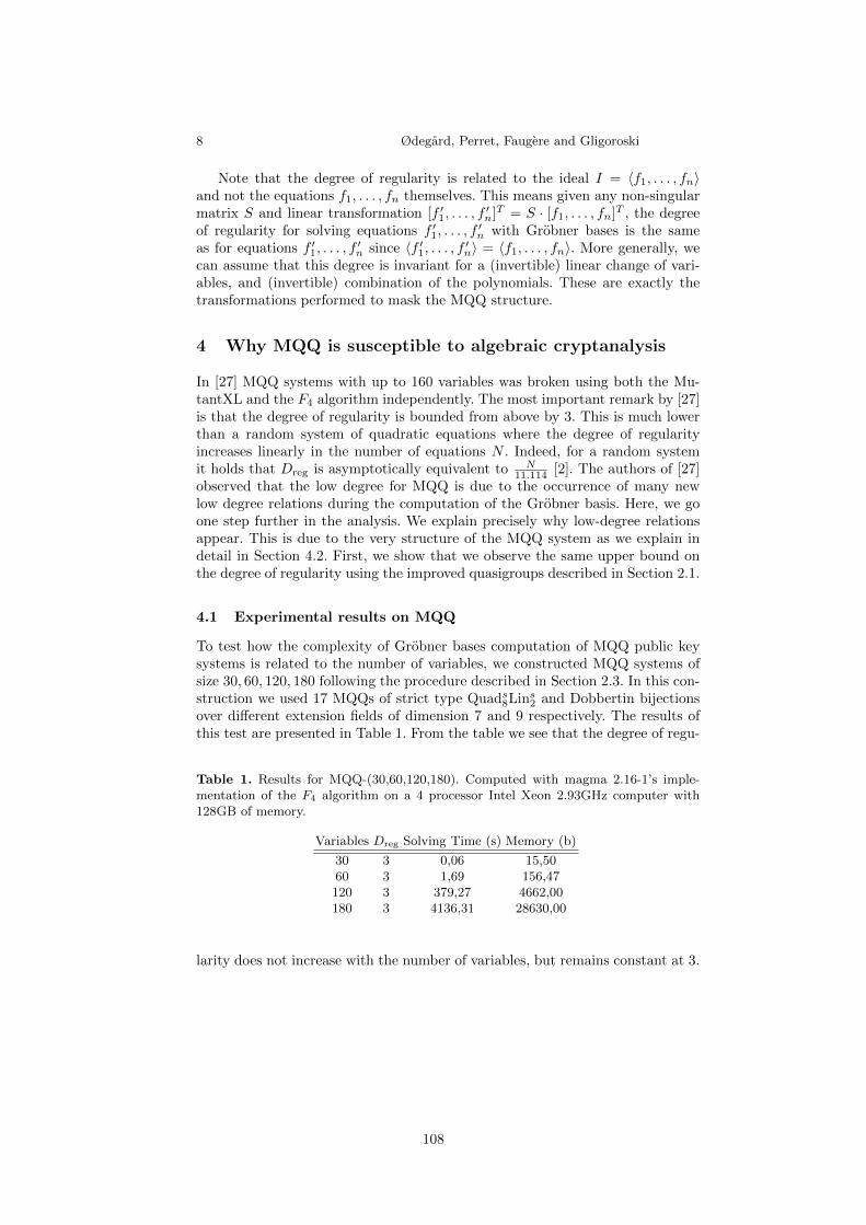
8 Ødegard, Perret, Faugere and Gligoroski

Note that the degree of regularity is related to the ideal I = 〈f1, . . . , fn〉and not the equations f1, . . . , fn themselves. This means given any non-singularmatrix S and linear transformation [f ′1, . . . , f

′n]T = S · [f1, . . . , fn]T , the degree

of regularity for solving equations f ′1, . . . , f′n with Grobner bases is the same

as for equations f ′1, . . . , f′n since 〈f ′1, . . . , f ′n〉 = 〈f1, . . . , fn〉. More generally, we

can assume that this degree is invariant for a (invertible) linear change of vari-ables, and (invertible) combination of the polynomials. These are exactly thetransformations performed to mask the MQQ structure.

4 Why MQQ is susceptible to algebraic cryptanalysis

In [27] MQQ systems with up to 160 variables was broken using both the Mu-tantXL and the F4 algorithm independently. The most important remark by [27]is that the degree of regularity is bounded from above by 3. This is much lowerthan a random system of quadratic equations where the degree of regularityincreases linearly in the number of equations N . Indeed, for a random systemit holds that Dreg is asymptotically equivalent to N

11.114 [2]. The authors of [27]observed that the low degree for MQQ is due to the occurrence of many newlow degree relations during the computation of the Grobner basis. Here, we goone step further in the analysis. We explain precisely why low-degree relationsappear. This is due to the very structure of the MQQ system as we explain indetail in Section 4.2. First, we show that we observe the same upper bound onthe degree of regularity using the improved quasigroups described in Section 2.1.

4.1 Experimental results on MQQ

To test how the complexity of Grobner bases computation of MQQ public keysystems is related to the number of variables, we constructed MQQ systems ofsize 30, 60, 120, 180 following the procedure described in Section 2.3. In this con-struction we used 17 MQQs of strict type Quads8Lin

s2 and Dobbertin bijections

over different extension fields of dimension 7 and 9 respectively. The results ofthis test are presented in Table 1. From the table we see that the degree of regu-

Table 1. Results for MQQ-(30,60,120,180). Computed with magma 2.16-1’s imple-mentation of the F4 algorithm on a 4 processor Intel Xeon 2.93GHz computer with128GB of memory.

Variables Dreg Solving Time (s) Memory (b)

30 3 0,06 15,5060 3 1,69 156,47120 3 379,27 4662,00180 3 4136,31 28630,00

larity does not increase with the number of variables, but remains constant at 3.

108

Analysis of the MQQ Public Key Cryptosystem 9

Once again, this is not the behaviour of a random system of equations for whichthe degree of regularity is asymptotically linear in the number of variables. Weexplain the reason of such difference in the next section.

4.2 Shape of the MQQ system

This non-random behavior can be explained by considering the shape of the“unmasked” MQQ system. By unmasked we mean the MQQ system withoutthe linear transformation S and T . The maximal degree of the polynomialsoccurring in the computation of a Grobner basis is invariant under the lineartransformation S and T as explained in Section 3.2. In Figure 1 we show whatvariables appear in each equation for an unmasked MQQ system of 60 variables.The staircase shape comes from the cascading use of quasigroups, while thethree blocks of equations at the bottom are from Dobbertin bijection of size 7. A

Fig. 1. Shape of 60 variable MQQ public key system without the use of S and T trans-formation. Black means that the corresponding variables is used in the equation. Thesystem was constructed with 4 MQQs of type Quads

8Lins2, one MQQ of type Quads

7Lins3,

and 3 Dobbertin bijections defined over 3 different extension fields of dimension 7.

random multivariate system would use all 60 variables in all equations. For theMQQ system in this example only 1

3 of the variables are used in each quasigroupand about 2

3 is used in each block of Dobbertin transformation.Now assume the Grobner basis algorithm somewhere during the calculation

has found the solution for one of the quasigroup blocks Yj = Xj ∗ijvv Xj+1. Dueto the cascading structure of the MQQ system the variables of Xj are used in

109

10 Ødegard, Perret, Faugere and Gligoroski

the block Yj−1 = Xj−1 ∗ij−1vv Xj and the variables of Xj+1 are used in the block.

Yj+1 = Xj+1 ∗ij+1vv Xj+2. Remember from Section 2.1 that if we set the first or

the last half of the variables of an MQQ to constant all equations becomes linear.This means that if we have solved the block Yj , the equations of the blocks Yj−1

and Yj+1 becomes linear. The blocks Yj−1 and Yj+1 can then be solved easily.This gives us solution for the variables Xj−1 and Xj+2, which again makes theequations in the blocks Yj−2 and Yj+2 linear. Continuing like this we have rapidlysolved the whole system.

Similarly, assume the Grobner basis has solved the Dobbertin blocks at somestep. This gives us the solution to all the variables in X1 which makes the firstquasigroup block Y1 = X1 ∗i1vvX2 linear. Solving this gives us the first half of theequations of the block Y2 and so on. This means that the solution of the wholeMQQ system is reduced to either solving just one block of quasigroup equations,or solving the Dobbertin transformation. The security of solving the MQQ sys-tem is therefore the minimum complexity of solving Dobbertin transformationand one MQQ block.

5 Further analysis of MQQ

Using the knowledge from Section 4.2 we investigate if it is possible to strengthenthe MQQ system. To do this we have to determine the weakest part of the system;the Dobbertin transformation or the quasigroup transformation.

5.1 The Dobbertin transformation

Recall that the Dobbertin transformation is a bijection over Z2r+12 defined by

the function Dr(x) = x2r+1+1 + x3 + x. For any r we can view this function as

2r + 1 Boolean functions in 2r + 1 variables. In Table 2 our experimental re-sults on the degree of regularity for solving this system of equations is listed forvarious r. From the table we see that the degree of regularity for the Dobbertintransformation seems to be bounded from above by 3. This means Dobbertin’stransformation is not “random” and can be easily solved by Grobner bases com-putation. In addition we learn that tweaking the MQQ system by increasing thesize of the extension field, over which the transformation is defined, will have noeffect on strengthening the system.

Proving mathematically (if true) that the degree of regularity for Dr(x) isconstant at 3 for all r is difficult. We can however give show that the degree ofregularity is low for all practical r. Let K = Fq be a field of q elements, and letL be an extension of degree n over K. Recall that an HFE polynomial f is alow-degree polynomial over L with the following shape:

f(x) =∑

0≤i,j≤nqi+qj≤d

ai,jxqi+qj +

∑

0≤k≤nqk≤d

bkxqk + c, (10)

110

Analysis of the MQQ Public Key Cryptosystem 11

Table 2. The observed degree of regularity, Dreg, for the Dobbertin bijection overZ2r+12 for r = 2, . . . , 22 when computed with magma 2.16-1’s implementation of the F4

algorithm on a 4 processor Intel Xeon 2.93GHz computer with 128GB of memory

r Dreg r Dreg r Dreg

2 3 9 3 16 33 3 10 3 17 34 3 11 3 18 35 3 12 3 19 36 3 13 3 20 37 3 14 3 21 38 3 15 3 22 3

where ai,j , bk and c all lie in L. The maximum degree d of the polynomial hasto be chosen such that factorization over L is efficient [8]. Setting q = 2 andn = 2r + 1 we notice that the Dobbertin transformation is actually an HFEpolynomial, Dr(x) = x2

r+1+20 + x21+20 + x2

0

. This is very helpfull since a lot ofwork has been done on the degree of regularity for Grobner basis compuation ofHFE polynomials [16,8]. Faugere and Joux showed that the degree of regularityfor Grobner bases computation of an HFE polynomial of degree d is boundedfrom above by log2(d) [16,17]. For the Dobbertin transformation this means thedegree of regularity is bounded from above by r + 1.

However, since the coefficients of the Dobbertin transformation all lie inGF (2), we can give an even tighter bound on the degree of regularity. Similar tothe weak-key polynomials in [8] the Dobbertin transformation commutes with

the Frobenius automorphism and its iterates Fi(x) : x 7→ x2i

for 0 ≤ i ≤ n.

Dr ◦ Fi(x) = Fi ◦Dr(x) (11)

From the equations we see that when Dr(x) = 0 we have Fi ◦ Dr(x) = 0.This means for each i we can add the n equations over GF (2) correspondingto the equation Dr ◦ Fi(x) = 0 over GF (2n) to the ideal. However, many ofthese equations are similar. Actually, we have that Fi and Fj are similar if andonly if gcd(i, n) = gcd(j, n) [8]. Worst case scenario is when n is prime. TheFrobenius automorphism then gives us 2n equations in n variables. From [3] wehave the following formula for the degree of regularity for a random system ofmultivariate equations over GF (2) when the number of equationsm is a multipleof the number of variables n. For m = n(N + o(1)) with N > 1/4 the degree ofregularity is

Dreg

n=

1

2−N +

1

2

√2N2 − 10N − 1 + 2(n+ 2)

√N(N + 2) + o(1) (12)

Setting N = 2 we get Dreg = − 32 + 1

2

√−13 + 16

√2 · n ≈ 0.051404 · n. This

is the upper bound for a random multivariate system with the same numberof equations and variables as the Dobbertin transformation. This provides us agood indication that the degree of regularity for Dobbertin (which is not random

111

12 Ødegard, Perret, Faugere and Gligoroski

at all) should be small, as observed in the experiments, and even smaller than aregular HFE polynomial.

5.2 The quasigroup transformation

To get an idea how strong the quasigroup transformation is, we decided to runsome experiments where we replaced the input to the Dobbertin transformationwith random linear equations. This means that solving the Dobbertin block willno longer make all the equations in the quasigroup transformation linear. Theresult of our experiment on this special MQQ system where the linear equationsare perfectly masked is listed in Table 3. From the table it appears that boththe quasigroup size and the number of variables have an effect on the degreeof regularity. This tells us that if we replace Dobbertin transformation witha stronger function, the MQQ system can possibly be made strong enough toresist pure Grobner attack for correct choices of quasigroups size and number ofvariables.

Table 3. Effects of quasigroup size and the Dobbertin transformation on the observeddegree of regularity for Grobner bases computations of 60 variable MQQ systems.Dreg is the observed degree of regularity of normal MQQ systems, while D∗

reg is theobserved degree of regularity for the same system where the input to Dobbertin hasbeen replaced with random linear equations.

Variables Quasigroup size Quasigroups type Dobbertin Dreg D∗reg

3025 4 Quads

3Lins2 and 1 Quads

2Lins3 7,9 3 3

210 2 Quads8Lin

s2 7,7 3 4

4025 5 Quads

3Lins2 and 2 Quads

2Lins3 7,7,7 3 4

210 3 Quads8Lin

s2 7,9 3 4

220 1 Quads17Lin

s3 7,7,9 3 4

5025 9 Quads

3Lins2 7,7,9 3 3

210 4 Quads8Lin

s2 9,9 3 4

6025 11 Quads

3Lins2 9,9,9 3 3

210 4 Quads8Lin

s2 and 1 Quads

7Lins3 7,7,7 3 5

220 1 Quads18Lin

s2 and 1 Quads

17Lins3 7,9,9 3 5

6 Conclusion

We have confirmed the results of [27] showing that the degree of regularity forMQQ systems are bounded from above by a small constant, and therefore MQQsystems in large number of variables can easily be broken with Grobner basescryptanalysis. The main result of this paper is our explanation of the underlyingreason for this bound on the degree of regularity. We explained this by showinghow the complexity of solving MQQ systems with Grobner bases is equal tothe minimum of the complexity of solving the Dobbertin transformation and

112

Analysis of the MQQ Public Key Cryptosystem 13

the complexity of solving one MQQ block. Furthermore, our experimental datashowed that the degree of regularity for solving the Dobbertin transformationis bounded from above by 3, the same as the bound on the MQQ system. It isnatural to conclude that the Dobbertin transformation is a serious weakness inthe MQQ system.

We also showed that if the Dobbertin transformation is replaced with anideal function, which perfectly hides the linear parts of the system, the degreeof regularity varies in the size of the quasigroups and the number of variables.We conclude that if a suitable replacement for the Dobbertin transformation isfound, MQQ can possibly be made strong enough to resist pure Grobner attackfor correct choices of quasigroups size and number of variables.

References

1. Magali Bardet. Etude des systemes algebriques surdetermines. Applications auxcodes correcteurs et a la cryptographie. PhD thesis, Universite de Paris VI, 2004.

2. Magali Bardet, Jean-Charles Faugere, and Bruno Salvy. Complexity study ofGrobner basis computation. Technical report, INRIA, 2002. http://www.inria.

fr/rrrt/rr-5049.html.3. Magali Bardet, Jean-Charles Faugere, and Bruno Salvy. Complexity of Grobner

basis computation for semi-regular overdetermined sequences over F2 with solu-tions in F2. Technical report, Institut national de recherche en informatique et enautomatique, 2003.

4. Magali Bardet, Jean-Charles Faugere, and Bruno Salvy. On the complexity ofGrobner basis computation of semi-regular overdetermined algebraic equations.In Proc. International Conference on Polynomial System Solving (ICPSS), pages71–75, 2004.

5. Magali Bardet, Jean-Charles Faugere, Bruno Salvy, and Bo-Yin Yang. Asymptoticbehaviour of the degree of regularity of semi-regular polynomial systems. In Proc.of MEGA 2005, Eighth International Symposium on Effective Methods in AlgebraicGeometry, 2005.

6. Olivier Billet and Jintai Ding. Overview of cryptanalysis techniques in multivariatepublic key cryptography. In Massimiliano Sala, Teo Mora, Ludovic Perret, ShojiroSakata, and Carlo Traverso, editors, Grobner bases, coding and cryptography, pages263–283. Springer Verlag, 2009.

7. Andrey Bogdanov, Thomas Eisenbarth, Andy Rupp, and Christopher Wolf. Time-Area Optimized Public-Key Engines: MQ -Cryptosystems as Replacement for El-liptic Curves? In Cryptographic Hardware and Embedded Systems (CHES), volume5154, pages 145–61. Lecture Notes in Computer Science, 2008.

8. Charles Bouillaguet, Pierre-Alain Fouque, Antoine Joux, and Joana Treger. A fam-ily of weak keys in hfe (and the corresponding practical key-recovery). CryptologyePrint Archive, Report 2009/619, 2009.

9. Bruno Buchberger. Ein Algorithmus zum Auffinden der Basiselemente des Restk-lassenringes nach einem nulldimensionalen Polynomideal. PhD thesis, Leopold-Franzens University, 1965.

10. Yanling Chen, Svein Johan Knapskog, and Danilo Gligoroski. MultivariateQuadratic Quasigroups (MQQ): Construction, Bounds and Complexity. Submittedto ISIT 2010, 2010.

113

14 Ødegard, Perret, Faugere and Gligoroski

11. David Cox, John Little, and Donal O’Shea. Using Algebraix Geometry. Springer,2005.

12. Francoise Levy dit Vehel, Maria Grazia Marinari, Ludovic Perret, and CarloTraverso. A survey on polly cracker system. In Massimiliano Sala, Teo Mora,Ludovic Perret, Shojiro Sakata, and Carlo Traverso, editors, Grobner bases, codingand cryptography, pages 263–283. Springer Verlag, 2009.

13. Hans Dobbertin. One-to-one highly nonlinear power functions on GF(2n). Appl.Algebra Eng. Commun. Comput., 9(2):139–152, 1998.

14. Jean-Charles Faugere. A new efficient algorithm for computing Grobner bases(F4). Journal of Pure and Applied Algebra, 139(1-3):61–88, June 1999.

15. Jean-Charles Faugere. A new efficient algorithm for computing Grobner baseswithout reduction to zero (F5). In Proceedings of the 2002 International Symposiumon Symbolic and Algebraic Computation, New York, 2002. ACM.

16. Jean-Charles Faugere and Antoine Joux. Algebraic cryptanalysis of Hidden FieldEquation (HFE) cryptosystems using Grobner bases. In Dan Boneh, editor,Advances in Cryptology - CRYPTO 2003, volume 2729 of LNCS, pages 44–60.Springer, 2003.

17. Pierre-Alain Fouque, Gilles Macario-Rat, and Jacques Stern. Key recovery onhidden monomial multivariate schemes. In Nigel P. Smart, editor, EUROCRYPT,volume 4965 of Lecture Notes in Computer Science, pages 19–30. Springer, 2008.

18. Danilo Gligoroski, Smile Markovski, and Svein Johan Knapskog. Multivariatequadratic trapdoor functions based on multivariate quadratic quasigroups. InMATH’08: Proceedings of the American Conference on Applied Mathematics, pages44–49, Stevens Point, Wisconsin, USA, 2008. World Scientific and EngineeringAcademy and Society (WSEAS).

19. Louis Goubin, Nicolas T. Courtois, and Schlumbergersema Cp. Cryptanalysis ofthe ttm cryptosystem. In Advances of Cryptology, Asiacrypt2000, pages 44–57.Springer, 2000.

20. Louis Granboulan, Antoine Joux, and Jacques Stern. Inverting HFE is quasipoly-nomial. In CRYPTO, pages 345–356, 2006.

21. Aviad Kipnis, Hamarpe St. Har Hotzvim, Jacques Patarin, and Louis Goubin.Unbalanced oil and vinegar signature schemes. In In Advances in Cryptology EU-ROCRYPT 1999, pages 206–222. Springer, 1999.

22. Aviad Kipnis and Adi Shamir. Cryptanalysis of the oil & vinegar signature scheme.In CRYPTO ’98: Proceedings of the 18th Annual International Cryptology Con-ference on Advances in Cryptology, pages 257–266, London, UK, 1998. Springer-Verlag.

23. MAGMA. High performance software for algebra, nuber theory, and geometry —a large commercial software package. http://magma.maths.usyd.edu.au.

24. Smile Markovski. Quasigroup string processing and applications in cryptography.In Proc. 1-st Inter. Conf. Mathematics and Informatics for industry MII 2003,1416 April, Thessaloniki, 278290, page 278290, 2003.

25. Smile Markovski, Danilo Gligoroski, and Verica Bakeva. Quasigroup string pro-cessing. In Part 1, Contributions, Sec. Math. Tech. Sci., MANU, XX, pages 1–2,1999.

26. Tsutomu Matsumoto and Hideki Imai. Public quadratic polynomial-tuples forefficient signature-verification and message-encryption. In Advances in Cryptology– EUROCRYPT 1988, volume 330 of LNCS, pages 419–453. Springer–Verlag, 1988.

27. Mohamed Saied Mohamed, Jintai Ding, Johannes Buchmann, and Fabian Werner.Algebraic attack on the MQQ public key cryptosystem. In CANS ’09: Proceedings

114

Analysis of the MQQ Public Key Cryptosystem 15

of the 8th International Conference on Cryptology and Network Security, pages392–401, Berlin, Heidelberg, 2009. Springer-Verlag.

28. Jacques Patarin. Cryptanalysis of the matsumoto and imai public key scheme ofeurocrypt’88. In Lecture Notes in Computer Science, pages 248–261, 1995.

29. Jacques Patarin. Hidden field equations (hfe) and isomorphisms of polynomials(ip): two new families of asymmetric algorithms. In EUROCRYPT, pages 33–48.Springer-Verlag, 1996.

30. Jacques Patarin. The oil & vinegar signature scheme, 1997.31. Jacques Patarin, Louis Goubin, and Nicolas Courtois. C ∗−+ and hm: Variations

around two schemes of t.matsumoto and h.imai. In Advances in Cryptology -Asiacrypt’98, volume 1514, pages 35–49. Springer, 1998.

32. Adi Shamir. Efficient signature schemes based on birational permutations. InCRYPTO ’93: Proceedings of the 13th annual international cryptology conferenceon Advances in cryptology, pages 1–12, New York, NY, USA, 1994. Springer-VerlagNew York, Inc.

33. J. D. H. Smith. An introduction to quasigroups and their representations. Chapman& Hall/CRC, 2007.

34. Christopher Wolf and Bart Preneel. Taxonomy of public key schemes based on theproblem of multivariate quadratic equations. Cryptology ePrint Archive, Report2005/077, 2005.

A Algorithm for generating random MQQ

In this section we present the pseudo-code for how the MQQs used in this paperhave been generated. The code was implemented in magma.

Algorithm MQQ algorithm1. n ←{size of quasigroup}2. L ←{number of linear terms}3. if L ≤ 24. then Q = n5. else Q = n− L6. CorrectDeg ←True7. while CorrectDeg8. do A1 ←IdentityMatrix(n) (∗ The identity matrix of size n ∗)9. X1 ←[x1, . . . , xn]

T

10. X2 ←[xn+1, . . . , x2n]T

11. for i ←1 to Q12. do for j ←i+ 1 to n13. do for k ←i+ 1 to (n)14. r ∈R {0, 1} (∗ random element from the set

{0,1} ∗)15. A1(i,j) = A1(i,j) + r ∗X1k16. B ←RandomNonSingularBooleanMatrix(n) (∗ Random non singular

Boolean matrix of size n ∗)17. C ←RandomBooleanVector(n) (∗ Random Boolean vector of size

n ∗)

115

16 Ødegard, Perret, Faugere and Gligoroski

18. A1 ←B ∗A119. X1 ←B ∗X1 + C20. L1 ←RandomNonSingularBooleanMatrix(n) (∗ Random non singu-

lar Boolean matrix of size n ∗)21. L2 ←RandomNonSingularBooleanMatrix(n) (∗ Random non singu-

lar Boolean matrix of size n ∗)22. A1 ←LinTrans(A1, L1) (∗ Lineary transform the indeterminates of

A1 according to L1 ∗)23. X1 ←LinTrans(X1, L1) (∗ Lineary transform the indeterminates of

X1 according to L1 ∗)24. X2 ←LinTrans(X2, L2) (∗ Lineary transform the indeterminates of

X2 according to L2 ∗)25. MQQ ←A1 ∗X2 +X126. GBMQQ ←Grobner(MQQ,2) (∗ The truncated Grobnerbasis of de-

gree 2 under graded reverse lexicographical ordering. ∗)27. Deg ←{number of linear terms in GBMQQ}28. if Deg= L29. then CorrectDeg ←False30. return GBMQQ

116

Multivariate Quasigroups Defined by T-functions

S. Samardziska1, S. Markovski1, D. Gligoroski2

1 Institute of Informatics, Faculty of Sciences, “Ss Cyril and Methodius” University,Skopje, Republic of Macedonia, {simona,smile}@ii.edu.mk

2 Faculty for Informatics, Institute of Telematics, Norwegian University of Scienceand Technology, Trondheim, Norway, danilog@item.ntnu.no

Abstract. In this paper we investigate quasigroups represented as vec-tor valued Boolean functions in their polynomial ANF form. We proposean effective general deterministic procedure for construction of multi-variate quasigroups of arbitrary order and degree. It offers solution tosome open problems regarding the production of Multivariate QuadraticQuasigroups (MQQ) used in the MQQ PKC scheme, of orders higherthan 25 and of desired type, as well as finding a lower bound on thenumber of MQQs. Even more, it provides deeper insight into the struc-ture of the MQQs and enables a different classification concerning theircomplexity. For this, we use T-functions, and make a complete charac-terization of the T-functions that define permutations and quasigroups.

Keywords: Multivariate Quasigroup, Multivariate Quadratic Quasigroup,T-function

1 Introduction

Using quasigroups for cryptographic purposes is an idea present in the sci-entific public for several decades and is becoming more exploited and popularevery day. Here we are interested in quasigroups represented as vector valuedBoolean functions (v.v.b.f.) in their polynomial ANF form, and the problem offinding a procedure for constructing quasigroups of any order and degree. Suchprocedure would be especially suitable for creation of Multivariate QuadraticQuasigroups (MQQ) that are the basis of the public key cryptsystem proposedby Gligoroski at al. [2] in 2007, as an attempt to overcome the weaknesses ofthe previously proposed MQ schemes. Although the encryption/decryption partof MQQ was broken by Mohamed et al. [4] in 2008, by removing 1/4 of thepublic key equations the scheme can still be used for digital signatures, keepingits ultra-fast performances for signing and verifications.

In this paper we propose an effective general deterministic procedure forconstruction of multivariate quasigroups of arbitrary order and degree. It offerssolution to the open problems of producing quasigroups of orders higher than 25,mentioned in [2]. Also, it provides deeper insight into the structure of the MQQsand enables a different classification concerning the complexity of the MQQs,with great security implications.

Our procedure uses T-functions defined by Klimov and Shamir [3].

117

2

We will not distinguish between the elements x ∈ Z2w and their binaryrepresentation (xw , xw−1, . . . , x1) ∈ Zw

2 . If f : (Zw2 )m → (Zw

2 )l and x is a m-coordinate vector of w-bit words, let xj

i denote the i-th bit of the j-th component

of x, and let f(x)ji denote the i-th bit of the component j of f(x).

Definition 1. Let f : (Zw2 )m → (Zw

2 )l. f is called T-function, if for every x ∈(Zw

2 )m, the k-th bit of the j-th component, f(x)jk, depends only on the rightmost

k bits of each component of x, for every j ∈ {1, . . . , m}.

Proposition 1. [3] The Boolean functions: complement, “and”, “exclusive or”,and “or”, and the operations: negation, addition, subtraction and multiplicationover Zw

2 are all T-functions.

Note that left shift is a T-function (since it is equivalent to multiplication bya power of 2), but right shift and circular rotations are not. Also, compositionof two T-functions is again a T-function, and thus every sequence of T-functionsapplied to x ∈ (Zw

2 )m is also a T-function.

2 T-functions that define permutations and quasigroups

Klimov and Shamir [3] proposed sufficient, but not necessary, conditions fora T-function to be a permutation or a quasigroup.

Here we provide sufficient and necessary conditions, and make a completecharacterization of the T-functions that define permutations and quasigroups.

Let w ≥ r ≥ 1, and let f : Zw2 → Zr

2 be a vector valued Boolean function. fcan be represented as an r-tuple of Boolean functions f = (f (r), f (r−1), . . . , f (1)),where f (s) : Zw

2 → Z2, s = 1, . . . , r, and f (s)(x) is the s-th bit of f(x). TheBoolean function f (s)(xw, . . . , x1) can be represented by its Algebraic NormalForm (ANF) as a polynomial in w variables x1, . . . , xw of the form

f (s)(xw , . . . , x1) =⊕

j=(jw ,...,j1)∈Zw2

ajxjww . . . xj2

2 xj11 ,

where aj ∈ Z2, x0 is an empty string and x1 = x. The algebraic degree of aBoolean function f is the number of variables in the longest term of the ANFform of f . Generally, higher degree means more applicable Boolean function forcryptography.

It can be verified that the ANF form of a T-function f : Zw2 → Zw

2 , isf = (f (w), f (w−1), . . . , f (1)), where, for every s = 1, . . . , w,

f (s)(xw , . . . , x1) =⊕

j=(js,...,j1)∈Zs2

ajxjss . . . xj1

1 .

Lemma 1. Let p = (p(w), p(w−1), . . . , p(1)) be a T-function that is a permutationon Zw

2 . Then, for every m = 1, . . . , w, the projection p|m = (p(m), p(m−1), . . . , p(1))is a permutation on Zm

2 .

118

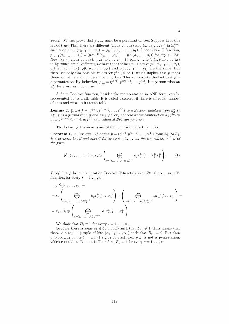
3

Proof. We first prove that p|w−1 must be a permutation too. Suppose that this

is not true. Then there are different (xw−1, . . . , x1) and (yw−1, . . . , y1) in Zw−12

such that p|w−1(xw−1, . . . , x1) = p|w−1(yw−1, . . . , y1). Since p is a T-function,

p|w−1(aw−1, . . . , a1) = (p(w−1)(aw, . . . , a1), . . . , p(1)(aw, . . . , a1)) for any a ∈ Zw

2 .Now, for (0, xw−1, . . . , x1), (1, xw−1, . . . , x1), (0, yw−1, . . . , y1), (1, yw−1, . . . , y1)in Zw

2 which are all different, we have that the last w−1 bits of p(0, xw−1, . . . , x1),p(1, xw−1, . . . , x1), p(0, yw−1, . . . , y1) and p(1, yw−1, . . . , y1) are the same. Butthere are only two possible values for p(w), 0 or 1, which implies that p mapsthese four different numbers into only two. This contradicts the fact that p isa permutation. By induction, p|m = (p(m), p(m−1), . . . , p(1)) is a permutation onZm

2 for every m = 1, . . . , w.

A finite Boolean function, besides the representation in ANF form, can berepresented by its truth table. It is called balanced, if there is an equal numberof ones and zeros in its truth table.

Lemma 2. [1]Let f = (f (w), f (w−1), . . . , f (1)) be a Boolean function from Zw2 to

Zw2 . f is a permutation if and only if every nonzero linear combination awf (w) ⊕

aw−1f(w−1) ⊕ · · · ⊕ a1f

(1) is a balanced Boolean function.

The following Theorem is one of the main results in this paper.

Theorem 1. A Boolean T-function p = (p(w), p(w−1), . . . , p(1)) from Zw2 to Zw

2

is a permutation if and only if for every s = 1, . . . , w, the component p(s) is ofthe form

p(s)(xw , . . . , x1) = xs ⊕

⎛⎝ ⊕

j=(js−1,...,j1)∈Zs−12

ajxjs−1

s−1 . . . xj22 xj1

1

⎞⎠ , (1)

Proof. Let p be a permutation Boolean T-function over Zw2 . Since p is a T-

function, for every s = 1, . . . , w,

p(s)(xw , . . . , x1) =

= xs

⎛⎝ ⊕

j=(js−1,...,j1)∈Zs−12

bjxjs−1

s−1 . . . xj11

⎞⎠ ⊕

⎛⎝ ⊕

j=(js−1,...,j1)∈Zs−12

ajxjs−1

s−1 . . . xj11

⎞⎠ =

= xs · Bs ⊕

⎛⎝ ⊕

j=(js−1,...,j1)∈Zs−12

ajxjs−1

s−1 . . . xj11

⎞⎠ .

We show that Bs ≡ 1 for every s = 1, . . . , w.Suppose there is some s1 ∈ {1, . . . , w} such that Bs1 �≡ 1. This means that

there is a (s1 − 1)-tuple of bits (αs1−1, . . . , α1) such that Bs1 = 0. But thenp|s1

(0, αs1−1, . . . , α1) = p|s1(1, αs1−1, . . . , α0), i.e., p|s1

is not a permutation,which contradicts Lemma 1. Therefore, Bs ≡ 1 for every s = 1, . . . , w.

119

4

Conversely, let p be a Boolean function of the form (1).Let awp(w) ⊕ aw−1p

(w−1) ⊕ · · ·⊕ a1p(1) be an arbitrary nonzero linear combi-

nation of the coordinates of p, and let m be the highest index such that am = 1.Then

awp(w)⊕aw−1p(w−1)⊕· · ·⊕a1p

(1) = xm⊕

⎛⎝ ⊕

j=(jm−1,...,j1)∈Zm−12

βjxjm−1

m−1 . . . xj11

⎞⎠ .

For each variation of the bits xw, . . . , xm+1, xm−1, . . . , x1, the bit xm can be 0or 1, so the last sum, for exactly half of the elements of Zw

2 is 0 and for the otherhalf it is 1. Therefore, awp(w) ⊕ aw−1p

(w−1) ⊕ · · · ⊕ a1p(1) is balanced, so from

Lemma 2, we get that p is a permutation.

Now that we have characterized the permutation T-functions, the propertiesof the Boolean functions that define quasigroups, are quite clear.

Theorem 2. A Boolean T-function q : (Zw2 )2 → Zw

2 , defines a quasigroup if andonly if it is of the form q = (q(w), q(w−1), . . . , q(1)) where for every s = 1, . . . , w,and (x, y) = (xw, . . . , x1; yw, . . . , y1),

q(s)(x, y) = xs ⊕ ys ⊕

⎛⎜⎜⎜⎝

⊕

j = (js−1, .., j1)∈ Zs−12

k = (ks−1, .., k1)∈ Zs−12

bjkxjs−1

s−1 . . . xj11 y

ks−1

s−1 . . . yk11

⎞⎟⎟⎟⎠ . (2)

Proof. Let q be a function in the given form. It is enough to show that for agiven a = (aw−1, . . . , a0) ∈ Zw

2 , q(x, a) and q(a, y) are permutations.

q(x, a) = (q(w−1)(x, a), q(w−2)(x, a), . . . , q(0)(x, a))

and for every s = 0, . . . , w − 1,

q(s)(x, a) = xs ⊕ as ⊕

⎛⎜⎜⎜⎝

⊕

j = (js−1, .., j0)∈ Zs2

k = (ks−1, .., k0)∈ Zs2

bjkxjs−1

s−1 . . . xj11 xj0

0 aks−1

s−1 . . . ak11 ak0

0

⎞⎟⎟⎟⎠ .

From Theorem 1 the last is a permutation. Similarly, we prove that q(a, y) is apermutation as well.

Conversely, let q define a quasigroup. Then, for every a ∈ Zw2 , q(x, a) and

q(a, y) are permutations. Again, from Theorem 1 the coefficient of xs in q(s)(x, a)is identically equal to 1, and the bit xs does not affect the rest of the sum. Thesame holds for the coefficient of ys in q(s)(a, y), i.e. it is identically equal to 1,and ys does not affect the rest of the sum. This is only possible if q(s)(x, y) is ofthe form (2).

120

5

All quasigroups that are T-functions are very structured. In general, theyhave the required classical properties for application in cryptography, like non-commutativity, nonassociativity, nonidempotency, nonlinearity and so on. Still,cryptoprimitives using them can be attacked quite easy, for example, usingHensel lifting.

Nevertheless, because of their simple shape, huge number and clear prop-erties, they can be used as a base for fast creation of quasigroups with solidcryptographic properties.

In [7], Wu proves that affine transformations of the components or of thevariable of a Boolean permutation, produce new Boolean permutations. Theycan be used to efficiently mix the bits of a Boolean permutation.

We say that a quasigroup is a Boolean quasigroup if it is defined as vectorvalued Boolean function. The results of Wu can be applied on Boolean quasi-groups, too. The proof that it is possible, basically reduces to considering one ofthe quasigroup variables as a parameter. Then, clearly, we have a permutationin the other variable. From the definition of quasigroups, since the new functionsare permutations, we have the sufficient condition for obtaining a quasigroup.

Proposition 2. Let q = (q(w), q(w−1), . . . , q(1)) be a Boolean quasigroup overZw

2 , let D = (dij) be a w × w binary matrix and let c = (cw, . . . , c1) ∈ Zw2 . Then

qD ⊕ c is a Boolean quasigroup if and only if D is nonsingular.

Proposition 3. Let q = (q(w), q(w−1), . . . , q(1)) be a Boolean quasigroup overZw

2 , let D1 = (d1ij) and D2 = (d2

ij) be w × w binary matrices and let c1 =

(c1w, . . . , c1

1), c2 = (c2w, . . . , c2

1) ∈ Zw2 . Then q(xD1 ⊕ c1, yD2 ⊕ c2) is a Boolean

quasigroup if and only if D1 and D2 are nonsingular.

Note that the transformations in the last two propositions are actually iso-topies.

3 Construction of Boolean quasigroups of various degreesand orders

The established form (2) of the T-functions that are quasigroups from theprevious section, is quite easy for manipulation. But, for creation of special typesof quasigroups we will rewrite it in an equivalent matrix form, very suitable forimplementation.

Theorem 3. Let x = (xw , . . . , x1) and y = (yw, . . . , y1) be variables over Zw2 .

Then every T-function that is a quasigroup can be written as a vector valuedBoolean function in a unique form

q(xw, . . . , x1, yw, . . . , y1) = A1 · (xw , . . . , x1)T + A2 · (yw, . . . , y1)

T + bT , (3)

where A1 = [fij ]w×w and A2 = [gij ]w×w are upper triangular matrices ofBoolean expressions, such that:

121

6

– for every i = 1, . . . , w, fii = 1 and gii = 1,– for every i = 1, . . . , w − 1, fiw = fiw(y1), and giw are constants,– for all i, j, i < j < w, fij can depend only on the variables xw−j , . . . , x1,

yw−j+1, . . . , y1 and gij can depend only on xw−j , . . . , x1, yw−j, . . . , y1,– the vector b = (bw, . . . , b1) is a Boolean constant vector.

Proof. We show that (3) and (2) are equivalent forms of a T-function that is aquasigroup. From (3), q is of the form q = (q(w), q(w−1), . . . , q(1)) where for everys = 1, . . . , w, and (x, y) = (xw, . . . , x1; yw, . . . , y1),

q(s)(x, y) = (0, . . . , 0, 1, fw−s+1,w−s+2, . . . , fw−s+1,w) · (xw , . . . , x1)T +

+ (0, . . . , 0, 1, gw−s+1,w−s+2, . . . , gw−s+1,w) · (yw, . . . , y1)T + bs =

= xs ⊕ fw−s+1,w−s+2(xs−2, . . . , x1, ys−1, . . . , y1)xs−1 ⊕⊕ fw−s+1,w−s+3(xs−3, . . . , x1, ys−2, . . . , y1)xs−2 ⊕

...

⊕ fw−s+1,w−1(x1, y2, y1)x2 ⊕ fw−s+1,w(y1)x1 ⊕⊕ ys ⊕ gw−s+1,w−s+2(xs−2, . . . , x1, ys−2, . . . , y1)ys−1 ⊕⊕ gw−s+1,w−s+3(xs−3, . . . , x1, ys−3, . . . , y1)ys−2 ⊕

...

⊕ gw−s+1,w−1(x1, y1)y2 ⊕ gw−s+1,wy1 ⊕ bs =

= xs ⊕ xs−1 ·

⎛⎜⎜⎜⎝

⊕

j = (js−2, .., j1)∈ Zs−22

k = (ks−1, .., k1)∈ Zs−12

β(s−1)jk x

js−2

s−2 . . . xj11 y

ks−1

s−1 . . . yk11

⎞⎟⎟⎟⎠ ⊕

...

⊕ x2 ·

⎛⎜⎜⎜⎝

⊕

j1 ∈ Z2

k = (k2, k1)∈ Z22

β(2)jk xj1

1 yk22 yk1

1

⎞⎟⎟⎟⎠ ⊕ x1 ·

⎛⎝ ⊕

k1 ∈ Z2

β(1)k yk1

1

⎞⎠ ⊕

⊕ ys ⊕ ys−1 ·

⎛⎜⎜⎜⎝

⊕

j = (js−2, .., j1)∈ Zs−22

k = (ks−2, .., k1)∈ Zs−22

γ(s−1)jk x

js−2

s−2 . . . xj11 y

ks−2

s−2 . . . yk11

⎞⎟⎟⎟⎠ ⊕

...

⊕ y2 ·

⎛⎝ ⊕

j1 ∈ Z2, k1 ∈ Z2

γ(2)jk xj1

1 yk11

⎞⎠ ⊕ y1 · γ(1) ⊕ bs,

which is equivalent to (2).

122

7

Using (3) (or (2)) one can create a quasigroup that is a T-function of arbi-trary degree, by restricting the degrees of fij and gij . It also allows constructionof a quasigroup of arbitrary order 2w. This characteristic, together with the var-ious types of isotopic transformations given, is especially suitable for creation ofMQQs.

As the authors of [2] noted in the paper, the randomized algorithm for gener-ating MQQs given there was able to produce only quasigroups of low orders (atmost 25). That is why the authors proposed the creation of MQQs of higher or-der as an open problem. Another important issue mentioned, was distinguishingthe different types of MQQs, and finding a way of producing only quasigroupsof the desired type. Finally, finding their number, or lower bound was also posedas open research question regarding the security of the algorithm.

Here, we propose an effective general algorithm, that gives answers to thesequestions, but also goes deeper into the structure of the MQQs and enables adifferent classification, with great security implications.

Definition 2. A quasigroup (Q, ∗) of order 2w is called Multivariate QuadraticQuasigroup (MQQ) of type Quadw−kLink if exactly w − k of the polynomialsq(i) are of degree 2 (i.e., are quadratic) and k of them are of degree 1 (i.e., arelinear), where 0 ≤ k < w.

The general form of a MQQ of order 2w that is a T-function, follows directlyfrom the general case.

Corollary 1. The vector valued Boolean function q(xw, . . . , x1, yw, . . . , y1) overZw

2 defines a quasigroup that is a multivariate quadratic quasigroup and a T-function if and only if it can be written in the form (3) where fij and gij arelinear Boolean expressions.

We will call these quasigroups Triangular Multivariate Quadratic Quasi-groups (T-MQQ).

Proposition 4. With suitably chosen matrices A1 and A2 of linear Booleanexpressions, using the form (3), one can produce a T-MQQ of arbitrary typeQuadw−kLink, for k = 1, . . . , w, but never of type QuadwLin0.

Proof. In (3), q(s) is of the form

q(s)(x, y) = (0, . . . , 0, 1, fw−s+1,w−s+2, . . . , fw−s+1,w) · (xw , . . . , x1)T +

+ (0, . . . , 0, 1, gw−s+1,w−s+2, . . . , gw−s+1,w) · (yw, . . . , y1)T + bs.

So, if we choose fw−s+1,j and gw−s+1,j, j = w − s+1, . . . , w, to be constants (0sand 1s), than q(s) will be a linear polynomial. In this manner we can produce asmany linear coordinates of q as we want. Note that the structure of a T-functionimplies that q(1) is always linear, hence a T-MQQ of type QuadwLin0 can notbe constructed.

The type of linear Boolean expressions that are present as elements in thematrices A1 and A2, in (3), determines the complexity of the produced T-MQQ

123

8

q = (q(w), q(w−1), . . . , q(1)) in the sense of the different quadratic monomialsthat will occur in the functions q(s), 1 ≤ s ≤ w. Using similar strategy as in theprevious proposition, we have the following one.

Proposition 5. With suitably chosen matrices A1 and A2 of linear Boolean ex-pressions, using the form (3), one can produce T-MQQ q = (q(w), q(w−1), . . . , q(1))with the following structure of q(s):

– the only quadratic monomials that appear are of type xixj (yiyj),– q(s) contains quadratic monomials only of type xixj and yiyj,– q(s) contains quadratic monomials only of type xixj and xiyj (yiyj and xiyj),– q(s) contains quadratic monomials of type xixj, xiyj and yiyj (i.e., of all

types).

The implication of this proposition is that there is a way to mix all the variablesxw, . . . , x1, yw, . . . , y1 and increase the complexity of the MQQ. We should notethat some of the MQ-based cryptsystems that have been broken ([2], [5]) usemultivariate quadratic polynomials that don’t mix all the variables, which canimpair the security of the system.

Nevertheless, sometimes one needs to trade-off between security and effi-ciency. Quasigroup based cryptsystems use bijective transformations that includethe quasigroup operation in one direction (encryption), and some parastrophicoperation in the opposite direction (decryption). Generally, finding the paras-trophic operation is a time consuming procedure, especially for quasigroups ofhigher order. The next proposition gives a special form of a MQQ of arbitraryorder that does not mix all the variables, but whose left parastrophe can beeasily found. (The case for the right parastrophe is analogous.)

Proposition 6. Let A1 = [fij ]w×w and A2 = [gij ]w×w be upper triangularmatrices of linear Boolean expressions, such that:

– for every i = 1, . . . , w, fii = 1 and gii = 1,– for every i = 1, . . . , w − 1, fiw and giw are constants,– for all i < j < w, fij and gij can depend only on xw−j , . . . , x1,– the vector b = (bw, . . . , b1) is a Boolean constant vector.

Then,

q(xw, . . . , x1, yw, . . . , y1) = A1 · (xw , . . . , x1)T + A2 · (yw, . . . , y1)

T + bT ,

is a quasigroup with left parastrophe q\

q\(xw , . . . , x1, yw, . . . , y1) = A−12 · ((yw , . . . , y1)

T − A1 · (xw, . . . , x1)T − bT ).

Proof. Clearly, q is a T-MQQ. Since A2 is upper triangular A−12 exists, and

since A1 and A2 depend only on the xj variables, one can verify that

q(xw , . . . , x1, q\(xw, . . . , x1, yw, . . . , y1)) = (yw, . . . , y1)T , and,

q\(xw , . . . , x1, q(xw, . . . , x1, yw, . . . , y1)) = (yw, . . . , y1)T ,

i.e., q\ is the left parastrophe of q.

124

9

Now, using Proposition 2 and Proposition 3 we can perform isotopic trans-formations to a T-MQQ and obtain a general MQQ.

Proposition 7. Let q be a T-MQQ of order 2w as defined in Corollary 1. LetD,D1,D2 be w × w nonsingular Boolean matrices, and let c, c1, c2 be Booleanvectors of dimension w. Then

q∗(xw , . . . , x1, yw, . . . , y1) = q((xw , . . . , x1) ·D1 +c1, (yw, . . . , y1) ·D2 +c2) ·D+c

defines a MQQ.

Proposition 7 provides a way for construction of MQQs that are suitable for usein an MQ-based cryptsystems. Their strength for application in a variant of thescheme [2] is being studied by the authors at the moment.

Example 1. We give an example of a T-MQQ of order 25 obtained using (3).Then using Proposition 7 we construct a general MQQ of order 25.

Let A1, A2 be 5 × 5 matrices given by

A1 =

⎡⎢⎢⎢⎢⎣

1 x1 ⊕ x2 ⊕ x3 ⊕ y2 ⊕ y4 x2 ⊕ y3 y1 1 ⊕ y1

0 1 1 ⊕ x1 ⊕ y1 ⊕ y2 x1 ⊕ y1 00 0 1 1 ⊕ x1 ⊕ y2 y1

0 0 0 1 1 ⊕ y1

0 0 0 0 1

⎤⎥⎥⎥⎥⎦

,

A2 =

⎡⎢⎢⎢⎢⎣

1 x3 ⊕ y2 ⊕ y3 y2 x1 00 1 1 ⊕ x1 ⊕ y2 x1 ⊕ y1 10 0 1 1 ⊕ y1 10 0 0 1 00 0 0 0 1

⎤⎥⎥⎥⎥⎦

,

and let b = (1, 0, 1, 1, 1). Then,

q(x5, . . . , x1, y5, . . . , y1) = A1 · (x5, . . . , x1)T + A2 · (y5, . . . , y1)

T + bT =

=

⎡⎢⎢⎢⎢⎢⎢⎢⎢⎢⎢⎣

1 ⊕ x1 ⊕ x2x3 ⊕ x1x4 ⊕ x2x4 ⊕ x3x4 ⊕ x5 ⊕ x1y1 ⊕ x2y1 ⊕ x1y2⊕⊕x4y2 ⊕ x3y3 ⊕ y2y3 ⊕ x3y4 ⊕ x4y4 ⊕ y2y4 ⊕ y3y4 ⊕ y5

x1x2 ⊕ x3 ⊕ x1x3 ⊕ x4 ⊕ y1 ⊕ x2y1 ⊕ x3y1 ⊕ x1y2 ⊕ x3y2 ⊕ y1y2⊕⊕y3 ⊕ x1y3 ⊕ y2y3 ⊕ y4

1 ⊕ x2 ⊕ x1x2 ⊕ x3 ⊕ y1 ⊕ x1y1 ⊕ y2 ⊕ x2y2 ⊕ y1y2 ⊕ y3

1 ⊕ x1 ⊕ x2 ⊕ x1y1 ⊕ y2

1 ⊕ x1 ⊕ y1

⎤⎥⎥⎥⎥⎥⎥⎥⎥⎥⎥⎦

is a T-MQQ. Now, let

D1 =

⎡⎢⎢⎢⎢⎣

0 0 0 1 10 0 1 1 11 1 1 0 10 0 1 0 11 0 1 1 0

⎤⎥⎥⎥⎥⎦

, D2 =

⎡⎢⎢⎢⎢⎣

1 0 0 0 01 0 0 1 00 0 1 0 11 0 1 1 01 1 0 1 0

⎤⎥⎥⎥⎥⎦

, D =

⎡⎢⎢⎢⎢⎣

1 1 0 1 01 1 1 0 01 1 1 1 11 1 1 1 00 1 0 0 0

⎤⎥⎥⎥⎥⎦

,

125

10

and c1 = (0, 0, 1, 0, 1), c2 = (0, 0, 1, 1, 1) and c = (1, 0, 0, 1, 1). Then

q∗(x5, . . . , x1, y5, . . . , y1) =

= q((x5, . . . , x1) · D1 + c1, (y5, . . . , y1) · D2 + c2) · D + c =

=

⎡⎢⎢⎢⎢⎢⎢⎢⎢⎢⎢⎢⎢⎢⎢⎢⎢⎢⎢⎢⎢⎣

x3 ⊕ x1x4 ⊕ x2x4 ⊕ x1y1 ⊕ x3y1 ⊕ x5y1 ⊕ x1y2 ⊕ x2y2 ⊕ x5y2⊕⊕y1y2 ⊕ y3 ⊕ x2y3 ⊕ x3y3 ⊕ x4y3 ⊕ y1y3 ⊕ y4 ⊕ x3y4 ⊕ y5

x2 ⊕ x4 ⊕ x1x4 ⊕ x2x4 ⊕ x5 ⊕ x1y1 ⊕ x3y1 ⊕ x5y1 ⊕ x1y2 ⊕ x2y2⊕⊕x5y2 ⊕ y1y2 ⊕ x2y3 ⊕ x3y3 ⊕ x4y3 ⊕ y1y3 ⊕ y4 ⊕ x3y4 ⊕ y5

1 ⊕ x2 ⊕ x1x2 ⊕ x1x3 ⊕ x4 ⊕ x1x4 ⊕ x5 ⊕ x1y1 ⊕ x2y1 ⊕ x3y1⊕⊕x5y1 ⊕ y2 ⊕ x2y2 ⊕ x3y2 ⊕ x5y2 ⊕ x1y3 ⊕ y2y3 ⊕ x1y4

1 ⊕ x2 ⊕ x1x2 ⊕ x3 ⊕ x1x3 ⊕ x4 ⊕ x1x4 ⊕ x2x4 ⊕ x1x5 ⊕ x2y1⊕⊕x3y2 ⊕ x4y2 ⊕ x5y2 ⊕ y3 ⊕ x1y3 ⊕ x2y3 ⊕ x3y3 ⊕ x4y3⊕

⊕y1y3 ⊕ y2y3 ⊕ y4 ⊕ x1y4 ⊕ x3y4 ⊕ y1y4 ⊕ y5

x1 ⊕ x2 ⊕ x3 ⊕ x1x4 ⊕ x5 ⊕ x1x5 ⊕ x2y1 ⊕ x3y1 ⊕ x4y1 ⊕ x5y1⊕⊕x1y2 ⊕ x4y2 ⊕ x5y2 ⊕ y1y2 ⊕ y4 ⊕ y1y4

⎤⎥⎥⎥⎥⎥⎥⎥⎥⎥⎥⎥⎥⎥⎥⎥⎥⎥⎥⎥⎥⎦

is a MQQ of order 25.

At the end we give an estimate of the lower bound of different MQQs of order2w, that comes as a consequence of the discussion above.

Proposition 8. There are exactly 2w+∑w−1

j=1 j(4w−4j−1) T-MQQs of order 2w.

Proof. For each fij there are exactly 22(w−j+1) choices, and for each gij exactly

22(w−j)+1 choices. This means that there are 2∑w

j=2 2(w−j+1)(j−1) different ma-trices A1 and 2

∑wj=2[2(w−j)+1](j−1) different matrices A2. The vector b can be

chosen in 2w ways. Altogether, the number of different T-MQQs of order 2w is

exactly 2w+∑w−1

j=1 j(4w−4j−1).

The number of T-MQQs for the first few values of w is given in Table 1.

w 2 3 4 5 6 8 9 10 12 14 15 16

T-MQQs 25 216 238 275 2131 2316 2453 2625 21090 21743 22150 22616

Table 1. T-MQQs of order 2w

This number can be regarded as a lower bound for general MQQs of order2w. Even though it is clear that the number of MQQs that can be created usingProposition 7 is much bigger, the claim itself does not specify it. Still, it providesan estimate of the number of different constructions of MQQs. Since there arearound 0.28·2w2

different nonsingular matrices, the total number of constructions

is around 0.283 · 23w2+4w+∑w−1

j=1 j(4w−4j−1).

126

11

References

1. C. Adams and S. Tavares,The Structured Design of Cryptographically Good S-Boxes,Journal of Cryptology (1990) 3, pp.27–41

2. D. Gligoroski, S. Markovski, and S.J. Knapskog, Multivariate quadratic trapdoorfunctions based on multivariate quadratic quasigroups, American Conference on Ap-plied Mathematics; Harvard, March 2008, USA.

3. A. Klimov and A. Shamir, A New Class of Invertible Mappings, In B.S. KaliskiJr. and C .K. Koc and C. Paar, editor, 4th Workshop on Cryptographic Hardwareand Embedded Systems (CHES), volume , pages 471–484. Springer-Verlag, LectureNotes in Computer Science, August 2002.

4. M. S. E. Mohamed, J. Ding, J. Buchmann and F. Werner Algebraic Attack onthe MQQ Public Key Cryptsystem, Lecture Notes in Computer Science, Volume5888/2009, pp. 392-401

5. A. Kipnis, J. Patarin, and L. Goubin, Unbalanced Oil and Vinegar signatureschemes, Advances in Cryptology, EUROCRYPT 1999, LNCS Vol. 1592, pp. 206–222, 1999.

6. S. Samardziska, Polynomial n-ary quasigroups of order pw, Masters’ thesis, PMF -Skopje, 2009, http://sites.google.com/site/samardziska/publications/pubs/mastersSamardziska.pdf

7. C. K. Wu and V. Varadharajan, Public key cryptsystems based on Boolean permu-tations and their applications, International journal of computer mathematics 2000,vol. 74, no2, pp. 167-184

127

128

Lattice Polly Cracker Signature (abstract)

Emmanuela Orsini, Carlo Traverso

Dipartimento di Matematica, Universita di Pisa.?

1 Introduction

Lattice Polly Cracker (LPC) is a lattice cryptosystem using lattice Grobnerbases. The cryptosystem uses two lattices, algebraically isomorphic but not iso-metric. The public lattice L has a Grobner basis that is hard to compute, andthe private lattice L′ has a Grobner basis that is simple to compute. The iso-morphism constitutes the trapdoor information.

A message m, chosen in a subset M ⊆ Zn is encrypted adding to it anelement of the public lattice L, and is decrypted computing the normal form ofthe message modulo the Grobner basis of L′.

In this paper we give further analysis linking normal form with respect to asuitable Grobner basis to the approximate Closest Vector Problem. This analysisallows to give a test to estimate the security of an instance of LPC.

We define moreover a signature protocol using LPC; this uses a protocol sim-ilar to other lattice signature protocols, the signer being identified by her abilityto solve an approximate CVP challenge. LPC instances to use for signaturesare different from LPC instances to use for encryption, but their constructionfollows the same scheme.

This LPC signature scheme, like other lattice signature protocols, is not zero-knowledge, and is subject to the learning attack of Nguyen-Regev[6], but allows aperturbation procedure (different from the NTRU perturbation procedure) thatmakes this attack impossible.

2 Lattice Grobner bases and CVP

Let L ⊆ Zn be an integer lattice and k a field. Let X = (x1, . . . , xn). Thenk[X] is isomorphic to the monoid algebra k[Nn]. Any element γ ∈ Zn can berepresented as a pair (α, β) of elements of Nn such that α− β = γ, and the pair(α, β) is unique if they are chosen minimally, i.e. αiβi = 0.

To each γ ∈ L we associate the binomial Xγ = Xα−Xβ (the map is injectiveunless k has characteristic 2) and the ideal generated by {Xγ | γ ∈ L} is theideal IL associated to L (remark that L is uniquely determined by IL even incharacteristic 2).

Given a term-ordering (a total ordering of Zn that is compatible with thegroup law, and such that 0 is the minimum of Nn) the reduced Grobner basis GL

? Research performed with the contribute MIUR in the project “Algebra commutativa,computazionale e combinatorica”, PRIN 2007

129

of IL is defined. Since IL is a binomial ideal every element of GL is a binomialXα −Xβ and αiβi = 0, hence GL can be identified with a subset of the latticeand defined purely in lattice terms.

We will restrict ourselves to lattices of full rank (i.e. lattices of rank n in Zn)although most results are valid more in general (or easy to generalize).

Given a Grobner basis G of a lattice L, one can compute the normal formNF (x) = NFG(x) of every element x ∈ Zn. We have (NF (x) = NF (y)) ⇔((x − y) ∈ L). Remark that NF (x) is the smallest such element in Nn, withthe comparison done in term-ordering. If the term-ordering is degree-compatiblethis is also the (possibly non unique) minimal element in l1 norm, hence theproblem solved is NP -hard; this is just an additional proof that finding theGrobner basis (with respect to a degree-compatible term-ordering) is NP -hard.For other orderings this is not true, for example, for Lex odering finding theGrobner basis (of a full-rank lattice) is equivalent to finding the Hermite normalform ([2, 3]).

Given a polynomial ideal and its Grobner basis, the set S of monomials thatare in normal form is called the staircase. We call core of the staircase a rectanglecontained in the staircase, and bounding box a minimal rectangle containing thestaircase (it exists if the ideal is zero-dimensional). More explicitly, a core andthe bounding box are defined by two sequences, ci for the core and bi for thebounding box, and given α = (a1, . . . , an) such that ai < ci then α ∈ S, and ifα ∈ S then ai < bi for all i. The bi are identified from the reduced Grobner basisG since G contains a polynomial whose leading term is xbii , and the ci can bechecked since the defining condition is equivalent to state that

∏xci−1i is in S.

The core, even if it is maximal, is not unique, but this does not really matter,we are just interested to have staircases containing a core of specified form; thebounding box instead is unique.

In the case of lattices, since the determinant d of a lattice L is equal to thenumber of elements of Zn/L, and this in turn is the cardinality of the staircase,we have

∏ci ≤ d ≤

∏bi.

The bounding box limits the size of NF (x) for every x ∈ L, hence a smallbounding box means that we can solve the CVP with a good approximation formost vectors.

More on lattice Grobner bases can be found in [3, 1, 2].

3 Block lattices and their Grobner bases

We consider a lattice L ⊆ Zn of rank n, and a sequence of integers 0 = m0 <m1 < · · · < mk = n. Define ni = mi −mi−1. Define Li = L ∩ (0n−mi ⊕ Zmi).Each Li is a sublattice of L of dimension mi and Li ⊆ Li+1. Define d0 = 1 anddi = detLi/di−1

A basis of Li can be extended to a basis of Li+1, so eventually we have abasis of L that, repesented as rows of a matrix, and (adding the new vectorsat the top) constitutes a block matrix with zero blocks ovder the diagonal; theblocks on the diagonal have determinant dk, . . . , d1.

130

We call such a structure a block lattice. Of course, any lattice, given the mi,has a corresponding block lattice structure, we will restrict our interest to blocklattices in with the di have some restricted form, for example all the ni and allthe di are the same, or vary in some restricted form.

If we choose a block ordering compatible with the block structure (the vari-ables in different blocks compare lexicographically, smaller index being larger),then the Grobner basis can be computed from the Grobner basis of the diag-onal blocks. Using DegRevLex in the blocks it is easy to obtain “manageable”Grobner bases (bases with “few” elements and a large core or a small boundingbox). Normal form with respect of such bases can be used to provide a goodapproximation to a closest vector problem; one hence expects that finding sucha Grobner basis is a hard problem.

4 Block Lattice Polly Cracker

Lattice cryposystems have usually a common pattern. There is a set M ⊆ Znand a lattice L ⊆ Zn such that M is injectively mapped to Zn/L. There is someform of trapdoor information that allows to compute the normal form modulo L,i.e. given an element c = m+ l ∈M + L with m ∈M and l in a suitable subsetH ⊆ L, then m can be recovered. A message is either an element m ∈M or anelement h ∈ H, and its encryption is m+h (the element that is not the messagebeing chosen at random). Recovering the message is done computing the normalform, and this is only presumed possible through the trapdoor information. Forexample GGH, NTRU and McEliece fit in this pattern.

Lattice Polly Cracker is a cryptosystem that exploits normal form modulo alattice Grobner basis.

While the basic idea is simple, its implementation is harder; recovering asuitable Grobner basis (moderate cardinality and core sufficiently large) can bedone for block lattices, but such lattices are special, and it is easy to discover theirstructure through the Hermite Normal Form; in particular they have very shortvectors (those of the smaller blocks). Hence one defines two lattices, L ⊆ Zn andL′ ⊆ Zn that are algebraically isomorphic: there is an isomorphism φ : Zn → Zn(an unimodular matrix) such that φ(L) = L′. L ⊆ Zn is the public lattice,M ⊆ Zn is the message set, and L′ is a block lattice with a staircase having acore that contains φ(M). Given a lattice L ⊆ Zn whose determinant d factorssuitably (e.g. d = 2N ) one can exhibit a block lattice L′ ⊆ Zn algebraicallyisomorphic to L and with a good staircase (with a suitable core); but it is hardto build one that brings a given set M of messages into the staircase of L′. Whileit is relatively simple to build L′ and the map φ, and recovering the lattice L aposteriori.

The details of the construction are given in [3], together with heuristic con-siderations on the difficulty of recovering the shortest block of the private lattice,that has a basis composed of elements of L : d = {m ∈ Zn | dm ∈ L}, d beingthe determinant of the smallest block. These elements are conjecturally shortvectors of L : d.

131

The security of the public lattice is connected with the length of the shortestvector of the lattice: hence estimating it is important.

We can easily find short vectors in the private lattice: the smallest blocksare composed of short vectors. The map from the private lattice to the publiclattice is not of course an isometry, but we expect nonetheless that the image ofthe smaller blocks contains vectors significantly short.

Given the private key of a LPC instance one can hence compute the shortervector of the image of some of the smaller blocks, and this allows to estimate howgood the instance is, comparing to an estimate of the shorter vector computedthrough the Gaussian heuristics.This can also be used to estimate the heuristicprocedures to define a random LPC instance. It turns out that the procedureoutlined in [3] produces public lattices with remarkably large shortest vector.Typically, a random LPC instance of dimension 200 has gaussian estimate 64,and the shortest vector has length from 200 to 500. One of dimension 400 hasgaussian estimate 91 and shortest vector length from 900 to 9000.

5 LPC signature (LPCS)

Lattice signatures are usually defined through a path similar to lattice encryp-tion, and is substantially an authentication protocol. The public key is given bya lattice L ⊆ Zn and two subsets M and C of Zn; M represents a commitmentto find an element m ∈ M equivalent modulo L to a challenge c ∈ C. Theidentification challenge can only be satisfied knowing a trapdoor information.The signature variant implies to respond to a challenge that is a hash of thedocument to sign.

Signing through LPC requires a setting similar to the LPC encryption, witha public lattice L, a private lattice L′ and a trapdoor isomorphism φ : Zn → Znsending L to L′, but now M is a subset containing the inverse image φ−1(S)of the staircase of L′. To simplify the setting, we build L, φ and M such thatM ⊇ φ−1(B), where B is the bounding box.

With procedures similar to those outlined in [3] we show how to build suitablekeys. The steps of this construction are the following:

1. Choose the set M of commitments in the form [0, (r − 1)]n.

2. Choose the sizes ni of the diagonal blocks and the determinants di; for eachi choose randomly a matrix ni × ni having suitably small bounding box.These will be the diagonal blocks of the block matrix defining the privatelattice L′. Through these blocks, the staircase S of L′ is determined. Let Bbe the bounding box.

3. Fill randomly the rest of the block diagonal matrix.

4. Choose the isomorphism φ−1 from Zn in the private to the public coordi-nates, such that φ−1(B) ⊆M .

5. Check that the public lattice has smallest vector sufficiently large to ensurethe desired level of security.

132

Of course the choice of the parameters has to be made in such a way thatthe construction is possible and that finding a suitable lattice is reasonablyfast. Moreover one can also restrict some choices to get some desirable features(for example, choose the random off-diagonal blocks in a way that ensures withhigh probability a sufficiently rich group structure of Zn/L. This can be testedcomputing the Smith normal form of the lattice).

These steps are the same that are needed to build a LPC instance, but withsome significant differences: in LPC we need to consider the core, instead ofthe bounding box, the inclusion is reversed, and the isomorphism is built inthe opposite direction; this has as consequence that it is more difficult to buildinstances with large shortest vector, although it is still easy to build instanceswith shortest vector with size larger than the Gaussian heuristics.

6 Suggested parameters and procedures

In this section we make explicit choices of the parameters outlined above. Slightlydifferent choices have been attempted,

With these parameters we are able to build easily instances of LPCS that webelieve to be practically secure, although further experience is needed to backthis belief.

As for LPC, the key is concealing suitably the smallest block. But whilein LPC one has constraints on the map from the public coordinates and theprivate coordinates (to ensure that the message box is sent inside the core of thestaircase) in LPCS one needs to constrain the map from the private coordinatesto the public coordinates, to ensure that the bounding box falls inside of thechallenge set.

This is a substantial difference, since recovering a basis of the smallest blockmeans recovering small vectors in a private lattice through their image in thepublic space, that is known, and here we have a constraint on the map, insteadof a constraint on the inverse. As a consequence, the public coordinates of thebasis of the smallest block of the private lattice are much shorter than than thecoordinates of the other basis elements, and this might make retrieving themeasier.

Hence to conceal them, ensuring that they are larger than the gaussian heuris-tic bound for the public lattice requires a richer bag of tricks, and explaining allof them in a short space is rather challenging. We will try to do our best at leastshowing them,

The first trick is the construction of the private lattice. We choose the blocks,giving special care to the smallest block, that is chosen with special properties.

First, we want that the group Z/L is as rich as possible, with many subgroupsand as far from cyclic as possible, and with a decomposition into a sum ofirreducible cyclic groups as non-unique as possible. This is best obtained with agroup whose order is a power of 2, hence all the blocks will have determinant apower of 2.

133

The smallest block will need to be a bit more special than the other blocks,since it is the target of the attacks. and has to be protected. We choose thisblock of dimension 6, with determinant 1024, bounding box sides between 3 and6, and bounding box volume at most 4096. The other blocks will have dimension4, determinant 4096, bounding box sides at most 15 and bounding box volumeat most 8192. Finding such blocks by random search is relatively easy.

To complete the private lattice, we have to fill the blocks off the diagonal. Wedo this randomly, but to ensure that Z/L is far from cyclic, we put the conditionthat a suitable number (default 24) of entries to the right of every diagonal blockare multiple of a power of 2 (default 8).

As commitment set M we choose the cube [0, 20]n; and we want to find anisomorphism (a unimodular matrix X = xi,j) sending the bounding box into M .To simplify, we choose X with non-negative entries. This means that if B is thevector defining the bounding box, BM should be a vector with entries ≤ 20. Wepose further bounds that make the construction of a unimodular matrix easier:if i ≤ j and i ≤ n − 6 then xi,i = 1 and xi,j = 0. Moreover we require thatfor every j < n − 6 at least one xi,j 6= 0 with i ≥ n − 6 (this means that everycoodinate mixes with the smallest block, and the last 6 rows have at least oneout of 6 elements non zero).

We have checked that these choices ensure that the coordinates of a basis ofthe smallest block do not have unusually small length, being invariably largerthan the predicion of the Gaussian heuristics.

We have not yet experimented enough to conclude that finding the smallestblock is hard from the public lattice.

In http://posso.dm.unipi.it/crypto/LPCS there are a few challenges. Weare able to build LPCS instances lattices of dimension n with determinant 23n

(hence the public key, in Hermite normal form, has 3n2 bits) and signatures withM = (0, 20)n (hence the signature has 4.3n bits). We expect LPCS to be at leastas secure as other lattice signature schemes with the same lattice dimension.

7 Learning attacks to LPCS and how to avoid them

Like other lattice signature schemes that share the signing mechanism, LPCSis not zero-knowledge. Although slightly different from the signature schemesconsidered in [6], the parallelogram learning attack appears to be possible onLPCS in its basic form. The parallelogram is no longer complete (the completeparallelogram is the image of the bounding box, and the staircase is only a subsetof small density) but identifying the cone generated by the signatures the mapφ−1 may be recovered.

We have not attempted the learning attack, but we have tried a remedy. Wehave the commitment set M , the staircase S and φ−1(S) ⊆M . We also have theGrobner basis G′ of L′ and we can compute G = φ−1(G′). If m ∈ M satisfiesthe commitment, and m′ = m + g or m′ = m − g is such that m′ ∈ M we canreplace m with m′. This can be repeated, and usually allows to find an elementoutside of the cone on the staircase image.

134

Remark however that multiple signatures of the same message represent indifferent ways the same element, hence leak a short lattice element. This meansthat the same document should never be signed twice. And allowing movingsignatures has as a consequence that the private key is larger (at least twice aslarge) and the signing procedure is slower.

This has however a different positive side: the experience shows, not un-expectedly, that almost every signature falls inside a smaller box than M , forexample [0, 18]n, especially if we allow to move the signature as above, or if wecan modify the document to sign. Reducing thus the commitment set of courseincreases the difficulty of signature forgery.

References

1. AM. Bigatti, R. LaScala, L. Robbiano, Computing Toric Ideals. J. Symb.Comp.27(1999), pp. 351–365.

2. M. Caboara, F. Caruso, C. Traverso. Grobner Bases in Public Key Cryptography.,Proc. ISSAC ’08, ACM (2008), pp. 315–323.

3. M. Caboara, F. Caruso, C. Traverso. Lattice Polly Cracker cryptosystems, accepted,J. Symb. Comp., 2010, currently available at http://posso.dm.unipi.it/crypto

4. O. Goldreich, S. Goldwasser, and S. Halevi. Public-key Cryptosystems from LatticeReduction Problems. In CRYPTO ’97, LNCS 1294, 112–131, 1997.

5. P. Nguyen. Cryptanalysis of the Goldreich-Goldwasser-Halevi cryptosystem fromCrypto ’97. in Crypto’99, LNCS 1666 288–304, 1999.

6. P. Q. Nguyen, O. Regev Learning a Parallelepiped: Cryptanalysis of GGH andNTRU Signatures. J. Cryptol., 22:139–160, 2009.

135

136

A public key exchange using semidirect prod-ucts of groups

M. Habeeb, D. Kahrobaei and V. Shpilrain

1. Key Exchange Protocol

Recall the definition of a semidirect product:Let H,Q be two groups, and let φ : Q→ Aut(H) be a homomorphism. Then thesemidirect product of H and Q is Γ = HoφQ = {(h, q) : h ∈ H, q ∈ Q} where thegroup operation is given by

(h, q)(h′, q′) = (hφ(q)(h′), qq′).

Let now A and B be groups, (b, a) ∈ B × A, and n ∈ N. We require B tobe an abelian group, with the additional condition that its automorphism group,Aut(B), must contain a sufficiently large abelian subgroup. In our key exchangeprotocol, A,B,Aut(B), (b, a), and n are public information.

Bob begins by choosing an embedding φ : A → Aut(B), which he keepssecret. He then computes

x = (b, a)n = (bφ(a)(b)φ(a2)(b) · · ·φ(an−1)(b), an) ∈ B oφ A.Bob then sends x to Alice.

Alice also chooses an embedding ψ : A → Aut(B), which she keeps secret,and computes

y = (b, a)n = (bψ(a)(b)ψ(a2)(b) · · ·ψ(an−1)(b), an) ∈ B oψ A.Alice sends y to Bob.

Bob can find the element

ψ(a)(b)ψ(a2)(b) · · ·ψ(an−1)(b) ∈ Bby multiplying the first coordinate of y by b−1, while Alice can find the element

φ(a)(b)φ(a2)(b) · · ·φ(an−1)(b) ∈ B

137

2 M. Habeeb, D. Kahrobaei and V. Shpilrain

by multiplying the first coordinate of x by b−1. Denote φ(a) by φa and ψ(a) by ψa.

Bob can now compute

n−1∏

i=1

φai(ψa(b)ψa2(b) · · ·ψan−1(b)) =n−1∏

i=1

φia(ψa(b)ψ2a(b) · · ·ψn−1a (b))

=

n−1∏

i=1

φia ◦ ψa(b)φia ◦ ψ2a(b) · · ·φia ◦ ψn−1a (b).

Similarly, Alice can compute

n−1∏

i=1

ψai(φa(b)φa2(b) · · ·φan−1(b)) =n−1∏

i=1

ψia(φa(b)φ2a(b) · · ·φn−1a (b))

=

n−1∏

i=1

ψia ◦ φa(b)ψia ◦ φ2a(b) · · ·ψia ◦ φn−1a (b)).

If in addition to B being abelian, we require that φa and ψa commute inAut(B), then we have the following equality:

n−1∏

i=1

φai(ψa(b)ψa2(b) · · ·ψan−1(b)) =n−1∏

i=1

φia(ψa(b)ψ2a(b) · · ·ψn−1a (b))

=n−1∏

i=1

φia ◦ ψa(b)φia ◦ ψ2a(b) · · ·φia ◦ ψn−1a (b)

=

n−1∏

i=1

ψa ◦ φia(b)ψ2a ◦ φia(b) · · ·ψn−1a ◦ φia(b)

=

n−1∏

j=1

ψja ◦ φa(b)ψja ◦ φ2a(b) · · ·ψja ◦ φn−1a (b)

If we denote this element by k, then k is computable by both Bob and Alice asshown above, giving them a shared key. The security of this protocol relies onthe difficulty of recovering the homomorphisms φ and ψ from (b, a) ∈ B × A, x,and y. The most obvious way for an adversary to find the shared secret key is todetermine either the homomorphism φ or ψ based on the public information. Sinceboth x and y are public, an adversary can easily compute

ψ(a)(b)ψ(a2)(b) · · ·ψ(an−1)(b) ∈ Band

φ(a)(b)φ(a2)(b) · · ·φ(an−1)(b) ∈ B.

138

A public key exchange using semidirect products of groups 3

If the adversary determines φ, then he knows φa ∈ Aut(B) and can compute

n−1∏

i=1

φia(ψa(b)ψ2a(b) · · ·ψn−1a (b)) =

n−1∏

i=1

φia ◦ ψa(b)φia ◦ ψ2a(b) · · ·φia ◦ ψn−1a (b))

which is the shared key, k. Similarly, if the adversary determines ψ, he can alsofind the shared secret key.

2. Proposed Platform Group

The group B can be an additive abelian p-group of order pm with the addi-tional property that pb = 0 for every b ∈ B, where p is approximately 105.Then B may be considered an m-dimensional vector space over Z/pZ = Fp. Un-der these conditions the group of automorphisms of B is GLm(Fp). The order ofGLm(Fp) is (pm − 1)(pm − p) · · · (pm − pm−1). Since we require a homomorphismφ : A → Aut(B), the order of φ(a) must divide the order of a. We know thatAut(B) has an element of order p, and so to ensure that we can find a non-trivialhomomorphism φ, we require that the group A also be a p group of order pl. Now|B oφ A| = pm+l, and so 1 < n < pm+l. For security purposes, we require n to besufficiently large.

If we require B and A to be as above, the homomorphisms φa and ψa havematrix representations J and K respectively, and the element b and the sharedkey k can be represented as column vectors.

We would like to ensure that it is easy to find homomorphisms φa, ψa thatcommute. We begin by choosing an arbitrary matrix M ∈ GLm(Fp) and a natural

number s with s = bm2c, which are made public. Bob chooses an automorphism

of the form H =

(Q 00 I

)and Alice chooses an automorphism of the form S =

(I 00 R

), where Q,R are s×s block matrices and I is the (m−s)×(m−s) identity

matrix. The matrices H and S are kept secret. Bob and Alice select the matrices

J = PB(MHM−1) =t′∑

i=1

ciMHiM−1

and

K = PA(MSM−1) =t∑

i=1

diMSiM−1

respectively, where ci, di ∈ Fp are randomly selected coefficients. We would like toadd the additional requirement that the matrices J and K do not have an ”‘easy”’form, such as diagonal, upper triangular or lower triangular matrices, although the

139

4 M. Habeeb, D. Kahrobaei and V. Shpilrain

probability of this occurring is negligible. The matrices J and K commute, andcan be used as φa and ψa. Now computing the shared key takes the form

n−1∑

i=1

J i(K · b+K2 · b+ · · ·Kn−1 · b) =n−1∑

i=1

(J iK · b+ J iK2 · b+ · · ·+ J iKn−1 · b)

= (J + J2 + · · ·+ Jn−1)(K · b+K2 · b+ · · ·+Kn−1 · b)= k

or

n−1∑

i=1

Ki(J · b+ J2 · b+ · · · Jn−1 · b) =n−1∑

i=1

(KiJ · b+KiJ2 · b+ · · ·KiJn−1 · b)

= (K +K2 + · · ·+Kn−1)(J · b+ J2 · b+ · · ·+ Jn−1 · b)= k

Finding the matrix K from the public information b and

K · b+K2 · b+ · · ·+Kn−1 · b = g

is equivalent to solving the matrix equation

(K +K2 + · · ·+Kn−1) · b = g. (2.1)

Similarly, from the public information we may find J by solving the equation

(J + J2 + · · ·+ Jn−1)b = h. (2.2)

We may write these matrix equations as a system of m polynomial equations inthe entries of K (or J). The search problem for polynomial equations over finitefields has been well studied and is known to be NP-hard [1]. By adding b to bothsides of (2.1), which is public to the attacker, equation (2.1) becomes

(I +K +K2 + · · ·+Kn−1) · b = g + b,

which is equivalent to

(I −Kn) · b = (I −K) · (g + b).

Although this simplifies equation (2.1) it does not simplify the problem at handsince we will still have a matrix equation, which can still be written as a systemof non-linear equations over a finite field. We also note that if the matrices Jand K are of a simple form (diagonal, upper or lower triangular) then this equa-tion becomes easier to solve, but the probability of this occuring is neglible. Thecryptosystem is secure against eigenvalue attacks as the matrices J and K areunknown.

140

A public key exchange using semidirect products of groups 5

References[1] G. V. Bard. Algebraic Cryptanalysis (Springer-Verlag, 2009) 1-392

M. HabeebCUNY Graduate Center, City University of New Yorke-mail: MHabeeb@GC.Cuny.edu

D. KahrobaeiCUNY Graduate Center, City University of New Yorke-mail: DKahrobaei@GC.Cuny.edu

V. ShpilrainThe City College of New York and CUNY Graduate Centere-mail: shpil@groups.sci.ccny.cuny.edu

141

142

On lower bounds for Information Set Decodingover Fq

Robert Niebuhr1, Pierre-Louis Cayrel2, Stanislav Bulygin2, and JohannesBuchmann1,2

1 Technische Universitat DarmstadtFachbereich Informatik

Kryptographie und Computeralgebra,Hochschulstraße 1064289 Darmstadt

Germany{rniebuhr, buchmann}@cdc.informatik.tu-darmstadt.de

2 CASED – Center for Advanced Security Research Darmstadt,Mornewegstrasse, 32

64293 DarmstadtGermany

{pierre-louis.cayrel, stanislav.bulygin}@cased.de

Abstract. Code-based cryptosystems are promising candidates for post-quantum cryptography. The increasing number of cryptographic schemesthat are based on codes over fields different from F2 requires an analy-sis of their security. Information Set Decoding (ISD) is one of the mostimportant generic attacks against code-based cryptosystems. We givelower bounds for ISD over Fq, thereby anticipating future software andhardware improvements. Our results allow to compute conservative pa-rameters for cryptographic applications.

Key words: Information Set Decoding, lower bounds, codes, post quan-tum, cryptography.

Introduction

Error-correcting codes have been applied in cryptography for at least threedecades since R. J. McEliece published his paper in 1978 [10]. It has receivedmuch attention as it is a promising candidate for post-quantum cryptography.McEliece used the class of binary Goppa codes for his construction, and mostother schemes published since then have also been using binary codes.However, in recent years, many new proposals use codes over larger fields Fq,mostly in an attempt to reduce the size of the public and private keys. Twoexamples that received a lot of attention are quasi-cyclic codes [3] by Berger atal., and quasi-dyadic codes [11] (Misoczki-Barreto). The security, however, is notas well understand for q-ary codes as for binary ones: Faugere et al. [7] publishedan attack which broke these two cryptosystems for several sets of parameters.

143

This makes it important to analyze the complexity of attacks against code-basedcryptosystems over larger fields Fq.

The two most important types of attacks against code-based cryptosystems arestructural attacks and decoding attacks. Structural attacks exploit structuralweaknesses in the construction, and often they attempt to recover the private key.Decoding attacks are used to decode a given cipher text. In this paper, we willnot consider structural attacks, since they are restricted to certain constructionsor classes of codes. Information Set Decoding (ISD) is one of the most importantgeneric decoding attacks, and it is the most efficient against many schemes.

Previous work

Over the years, there have been many improvements and generalizations of thisattack, e.g. Lee-Brickell [9], Stern [14], Canteaut-Chabaud [6], Bernstein et al. [5].Recently, two papers – Finiasz-Sendrier [8] and Peters [12] – studied this algo-rithm. The former provides lower bounds for the complexity of the ISD algorithmover F2, the latter describes how to generalize Stern’s and Lee-Brickell’s algo-rithms to Fq.

Our contribution

In this paper, we propose and prove lower bounds for the complexity of ISDalgorithms over Fq. Our analysis gives an improvement of the efficiency of theISD algorithm compared to Peters’ analysis [12] and generalizes the lower boundsproposed by Finiasz and Sendrier in [8]. In addition to that, we show how to usethe structure of Fq to increase the algorithm efficiency and compare our lowerbounds with the ISD algorithm described by Peters. The details of the proof aregiven in the Appendix.

Organization of the paper

In Section 1, we start with a review of coding theory and cryptography over Fq.The subsequent Section 2 presents the Information Set Decoding algorithm weare analyzing and states the lower bounds result. In Section 3, we apply theselower bounds to concrete parameters and compare the results with the mostrecent algorithm. We conclude in Section 4.

1 Review

1.1 Coding theory over Fq

In general, a linear code C is a k-dimensional subspace of an n-dimensional vectorspace over a finite field Fq, where k and n are positive integers with k ≤ n, and qis a prime power. The error-correcting capability of such a code equals (d−1)/2,

144

and it is the maximum number of errors that can be decoded. By (n, k, t), wedenote a code that can efficiently decode t ≤ (d− 1)/2 errors. The co-dimensionr of this code is defined by r = n− k.

Definition 1 (Hamming weight). The (Hamming) weight wt(x) of a vectorx is the number of its non-zero entries.

Definition 2 (Minimum distance). The (Hamming) distance d(x, y) betweentwo codewords x, y ∈ C is defined as the (Hamming) weight of x− y. The mini-mum weight d of a code C is defined as the minimum distance between any twodifferent codewords, or equivalently as the minimum weight over all non-zerocodewords:

d := minx,y∈Cx 6=y

d(x, y) = minc∈Cc6=0

wt(c).

A linear code of length n, dimension k and minimum distance d is called an[n, k, d]-code.

Definition 3 (Generator and Parity Check Matrix). Let C be a linearcode over Fq. A generator matrix G of C is a matrix whose rows form a basis ofC:

C = {xG : x ∈ Fkq}.A parity check matrix H of C is defined by

C = {x ∈ Fnq : HxT = 0}

and generates the dual space of C. For a given parity check matrix H and anyvector e, we call s the syndrome of e with sT := HeT .

Remark 1. Two generator matrices generate equivalent codes if one is obtainedfrom the other by a linear transformation or permutation. Therefore, we canwrite any generator matrix G in systematic form G = [Ik|R], which allowsa more compact representation. If C is generated by G = [Ik|R], then a paritycheck matrix for C is H = [−RT |In−k] (up to permutation, H can be transformedso that the identity submatrix is on the left hand side).

The problems which cryptographic applications rely upon can have differentnumbers of solutions. For example, public key encryption schemes usually haveexactly one solution, while digital signatures often have more than one possiblesolution. The uniqueness of solutions can be expressed by the Gilbert-Varshamov(GV) bound:

Definition 4 (q-ary Gilbert-Varshamov bound). Let C be an (n, k, t) codeover Fq, and let r := n− k. The q-ary GV bound is the smallest integer t0 suchthat

t0∑

i=0

(n

i

)(q − 1)i ≥ qr.

145

For large values of n, the last term dominates the sum, so the condition is oftenapproximated by (

n

t0

)(q − 1)t0 ≥ qr.

If the number of errors that have to be corrected is smaller than the GV bound,then there is at most one solution. Otherwise, there can be several solutions.

1.2 The syndrome decoding problem and the McEliece PKC

Problem 1. Given a matrix H and a vector s, both over Fq, and a non-negativeinteger t; find a vector x ∈ Fnq of weight t such that HxT = sT .

This problem was proved to be NP-complete in 1978 [4], but only for binarycodes. In 1994, A. Barg proved that this result holds for codes over all finitefields ([1, in russian] and [2, Theorem 4.1].

Many code-based cryptographic schemes are based on the hardness of syndromedecoding. Among these are the McEliece cryptosystem and the CFS signaturescheme. The latter, however, is unsuitable for q-ary codes, since it requires codeswith a high density (ratio of the number of codewords to the cipher space size),and the density rapidly decreases with increasing field size q. We will thereforebriefly describe the McEliece cryptosystem and show how it can be attacked bysolving the syndrome decoding problem.

The McEliece PKC The McEliece public-key encryption scheme was pre-sented by R. McEliece in 1978 ([10]). The original scheme uses binary Goppacodes, for which it remains unbroken, but the scheme can be used with any classof codes for which an efficient decoding algorithm is known.

Let G be a generator matrix for a linear (n, k, t)-code over Fq, DG a correspond-ing decoding algorithm. Let P be a n×n random permutation matrix and S ank× k invertible matrix over Fq. These form the private key, while (G, t) is made

public, where G = SGP .

Encryption: Represent the plaintext as a vector m of length k over Fq, choosea q-ary random error vector e of weight at most t, and compute the ciphertext

c = mG+ e.

Decryption: Compute

c = cP−1 = mSG+ eP−1.

As P is a permutation matrix, eP−1 has the same weight as e. Therefore, DGcorrects these errors:

mSG = DG(c)

146

Let J ⊆ {1, . . . , n} be a set such that G·J is invertible, then we can compute theplaintext

m = mSG ·G−1·J · S−1.

Attacking the McEliece PKC Many variants of the McEliece encryptionscheme have been proposed, often in an attempt to reduce the size of the publickey. In most cases, these variants differ in which class of codes they use. Many ofthese variants have been broken, since a structural weakness had been found, butthe original scheme using binary Goppa codes remains secure to date. For mostparameters, ISD-like attacks are the most efficient attacks against the McEliecescheme (an exception is the CFS signature scheme, where a Generalized Birthdayattack due to Bleichenbacher is more efficient).

2 Lower bounds for Information Set Decoding over Fq

The algorithm we describe here recovers a q-ary error vector. It is a generaliza-tion of [8] to codes over Fq. We first describe how to modify the algorithm towork over Fq, then we show how to use the field structure to increase efficiencyby a factor of

√q − 1.

In each step, we randomly re-arrange the columns of the parity check matrix Hand transform it into the form

H =

(In−k−l H1

0 H2

), (1)

where In−k−l is the identity matrix of size (n− k− l). Usually, the columns arechosen adaptively to guarantee the success of this step. Although this approachcould bias the following steps, it has not shown any influence in practice. Thevariables l and p (see next step) are algorithm parameters optimized for eachattack.

The error vector we are looking for has p errors in the column set correspondingto H1 and H2, and the remaining (t− p) errors in the first (n− k − l) columns.We first check all possible error patterns of p errors in the last k + l columnssuch that the weighted sum S of those p columns equals the syndrome s in thelast l rows. We do this by searching for collisions between the two sets L1 andL2 defined as

L1 = {H2eT : e ∈W1} (2)

L2 = {s2 −H2eT : e ∈W2}, (3)

where W1 ⊆ Wk+l;bp/2c;q and W2 ⊆ Wk+l;dp/2e;q are given to the algorithm,and Wk+l;p;q is the set of all q-ary words of length k + l and weight p. Writing

147

e = [e′|e1 + e2] and s = [s1|s2] with s2 of length l, this means we search forvectors e1 and e2 of weight bp/2c and dp/2e, respectively, such that

H2 · [e1 + e2]T = sT2 .

If this succeeds, we compute the difference S − s; if this does not have weightt− p, the algorithm restarts. Otherwise, the non-zero entries correspond to theremaining t− p errors:

HeT =

(In−k−l H1

0 H2

)(e′

e1 + e2

)

=

(In−k−l · e′T +H1 · (e1 + e2)T

H2 · (e1 + e2)T

)

=

(In−k−l · e′T

0

)+ S

!=

(sT1sT2

)

Therefore, we have

In−k−l · e′T = sT1 −H1 · (e1 + e2)T ,

revealing the remaining columns of e.

Using the field structure We can use the field structure of Fq to increase thealgorithm efficiency. Note that for all vectors e such that HeT = sT , there areq − 1 pairwise different vectors e′ such that He′T = asT for some a ∈ Fq\{0},namely e′ = ae. Clearly, if we find such an e′, we can calculate e which solvesthe syndrome decoding problem. We can modify the algorithm to allow it to findthese vectors e′ as well, thereby increasing the fraction of error vectors that are(implicitly) tested in each iteration by a factor of q − 1 (see the Appendix for adetailed description).Since this fraction is calculated using |W1| · |W2|, we can also keep the fractionconstant and decrease the size of the sets Wi by a factor of

√q − 1 each. As

the work factor in each iteration of the algorithm is linear in |W1| + |W2|, thisincreases the algorithm efficiency by a factor of

√q − 1.

A simple way to decrease the size of the sets Wi is to redefine them as follows.For any vector a over Fq, let us denote its first non-zero entry by a(0) ∈ Fq\{0},and let

W ′1 ⊆ {e ∈ Wk+l;bp/2c;q : e(0) = 1} (4)

L′1 ={

(H2eT )((H2e

T )(0))−1 : e ∈W ′1}

(5)

L′2 ={

(s2 −H2eT )((s2 −H2e

T )(0))−1 : e ∈W2

}. (6)

148

Remark 2. Note that even though the calculation of each vector is more costlydue to the final division by the leading coefficient, this is by far offset by thesmaller number of vectors that need to be calculated.

The algorithm thus works as follows:

Algorithm 1 Information Set Decoding over FqParameters:

– Code parameters: Integers n, r = n− k and t, and a finite field Fq

– Algorithm parameters: Two integers p > 0 and l > 0, and two sets W1 ⊆ {e ∈Wk+l;bp/2c;q : e(0) = 1} and W2 ⊆ Wk+l;dp/2e;q

Remark: The function hl(x) returns the last l bits of the vector x ∈ Fnq . The variables

y := (HeT1 )(0) and z := (s−HeT2 )(0) are notational shortcuts.

Input: Matrix H0 ∈ Fr×nq and a vector s0 ∈ Fr

q

Repeat (MAIN LOOP)P ← random n× n permutation matrix(H,U)← PGElim(H0P ) //partial Gauss elimination as in (1)s← s0U

T

for all e1 ∈W1

i← hl(HeT1 /y) (ISD 1)write(e1, i) //store e in some data structure at index i

for all e2 ∈W2

i← hl((sT2 −HeT2 )/z) (ISD 2)

S ← read(i) //extract the elements stored at index ifor all e1 ∈ S

if wt(sT −H(e1 + e2)T ) = t− p (ISD 3)return (P, e1z/y + e2), (SUCCESS)

Proposition 1. If(nt

)(q − 1)t < qr (single solution), or if

(nt

)(q − 1)t ≥ qr

(multiple solutions) and(rt−p)(kp

)(q − 1)t � qr, a lower bound for the expected

cost (in binary operations) of the algorithm is

WFqISD(n, r, t, p, q) = minp

1√q − 1

· 2lmin((nt

)(q − 1)t, qr

)

λq(r−lt−p)(k+lp

)(q − 1)t

·√(

k + l

p

)(q − 1)p

with l = logq

(Kqλq

√(kp

)(q − 1)p−1 · ln(q)/2

)and λq = 1− exp(−1) ≈ 0.63.

An exception is p = 0 where we cannot gain a factor of√q − 1, hence

WFqISD(n, r, t, 0, q) =

(nt

)(rt

)

If(nt

)(q − 1)t ≥ qr and

(rt−p)(kp

)(q − 1)t ≥ qr, the expected cost is

149

WFqISD ≈ minp

2lqr/2√(r−lt−p)(q − 1)t−p

with l ≈ logq

(Kt−p

qr/2√( rt−p)(q−1)t−p

· ln(q)/2

).

Remark 3. The variable Kq represents the number of operations required tocheck the condition (ISD 3). A realistic value for Kq is Kq = 2t, which will beused for the parameters in Section 3.

Remark 4. In the algorithm described above, all computations are done overFq, so the complexity also depends on the implementation of q-ary arithmetic.A naıve implementation yields an additional factor of log2(q) for addition andlog2

2(q) for multiplication. There are several techniques to improve this, e.g. bylifting to Z[x] (for large q) or by precomputing exp and log tables (for small q).Especially for small q, this allows to make q-ary arithmetic nearly as fast asbinary, so in order to gain conservative estimates, we will neglect this factor.

Remark 5. The total work factor is the product of the number of iterations bythe work factor per iteration. In practice, the latter is essentially the sum of amatrix multiplication (with the permutation matrix), the Gaussian elimination,and the search for collisions between L′1 and L′2. Compared with the binarycase, the Gaussian elimination is slower in the q-ary case, because every row hasto be divided by the pivot entry. However, since the matrix multiplication andthe Gaussian elimination are much faster than the collision search, we do notallocate any cost to them.

3 Results

In [12], the author shows how to extend Lee-Brickell’s and Stern’s algorithms tocodes over Fq. The website [13] lists the work factor of this algorithm againstseveral parameters. We use the same parameters and compare these results withour lower bound.

150

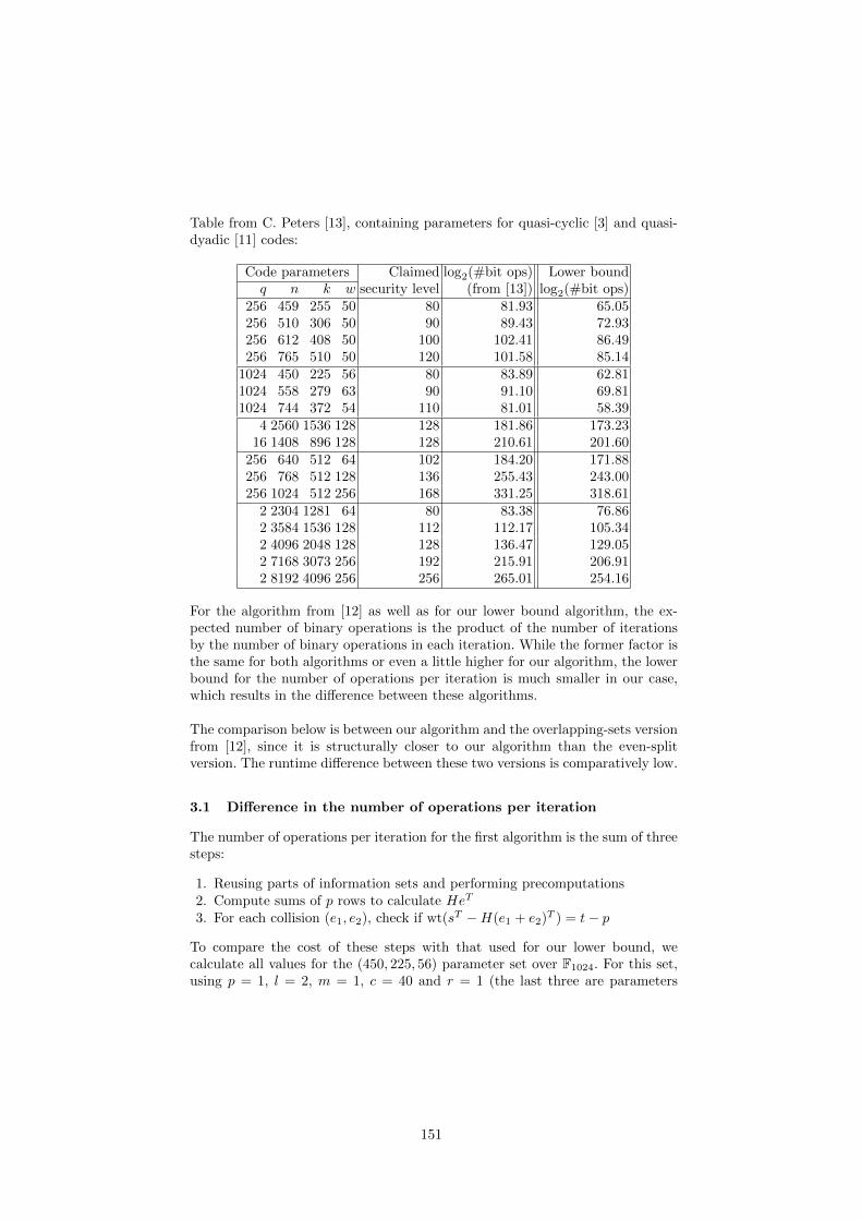
Table from C. Peters [13], containing parameters for quasi-cyclic [3] and quasi-dyadic [11] codes:

Code parameters Claimed log2(#bit ops) Lower boundq n k w security level (from [13]) log2(#bit ops)

256 459 255 50 80 81.93 65.05256 510 306 50 90 89.43 72.93256 612 408 50 100 102.41 86.49256 765 510 50 120 101.58 85.14

1024 450 225 56 80 83.89 62.811024 558 279 63 90 91.10 69.811024 744 372 54 110 81.01 58.39

4 2560 1536 128 128 181.86 173.2316 1408 896 128 128 210.61 201.60

256 640 512 64 102 184.20 171.88256 768 512 128 136 255.43 243.00256 1024 512 256 168 331.25 318.61

2 2304 1281 64 80 83.38 76.862 3584 1536 128 112 112.17 105.342 4096 2048 128 128 136.47 129.052 7168 3073 256 192 215.91 206.912 8192 4096 256 256 265.01 254.16

For the algorithm from [12] as well as for our lower bound algorithm, the ex-pected number of binary operations is the product of the number of iterationsby the number of binary operations in each iteration. While the former factor isthe same for both algorithms or even a little higher for our algorithm, the lowerbound for the number of operations per iteration is much smaller in our case,which results in the difference between these algorithms.

The comparison below is between our algorithm and the overlapping-sets versionfrom [12], since it is structurally closer to our algorithm than the even-splitversion. The runtime difference between these two versions is comparatively low.

3.1 Difference in the number of operations per iteration

The number of operations per iteration for the first algorithm is the sum of threesteps:

1. Reusing parts of information sets and performing precomputations2. Compute sums of p rows to calculate HeT

3. For each collision (e1, e2), check if wt(sT −H(e1 + e2)T ) = t− p

To compare the cost of these steps with that used for our lower bound, wecalculate all values for the (450, 225, 56) parameter set over F1024. For this set,using p = 1, l = 2, m = 1, c = 40 and r = 1 (the last three are parameters

151

specific for the first algorithm), we calculate a total cost of the first algorithmof 276.6, which consists of 252 iterations of 224.6 operations each3.

Precomputations The cost of the first step is given in [12] as

(n− 1)

((k − 1)

(1− 1

qr

)+ (qr − r)

)c

r,

where c and r are algorithm parameters (i.e. r is not the co-dimension of thecode). For these parameters, this amounts to 224.4 operations, so it is the mostexpensive step.Our algorithm does not use precomputation, so we allocate no cost.

Compute sums of p rows to calculate HeT The cost of this step for thefirst algorithm is

((k − p+ 1) + (N +N ′)(q − 1)p) l.

The parameters N and N ′ are the sizes of the sets and correspond to W1 andW2. For the parameters given above, this step adds 219.3 operations.

Our algorithm allocates to this step a cost of

l|W ′1|+ l|W2| = 2l

√(k + l

p

)(q − 1)p−1.

We make this optimistic assumption4 for the cost of a matrix-vector multiplica-tion to anticipate further software and hardware improvements for this operation.The result is 26 operations in this case.

Check collisions The first algorithm allocates a cost of

q

q − 1(w − 2p)2p

(1 +

q − 2

q − 1

)NN ′(q − 1)2p

ql

to this step. For our set of parameters, this equals 222.4 operations.

In our algorithm, we expect the number of collisions to be

λq|W ′1| · |W2|ql

=λq(k+lp

)(q − 1)p−1

ql.

The cost Kq to check each collision is taken to be Kq = 2t. Since the expectednumber of collisions per iteration is very small, the expected cost per iteration

3 The difference between this value and the one listed in the Table results from thefact the the latter were optimized with p ≥ 2, while p = 1 turns out to be better.

4 From the cryptanalyst’s point of view.

152

is < 1.

Some of the assumptions above may seem fairly optimistic. However, we findthat necessary since we want to establish conservative lower bounds.

4 Conclusion and Outlook

In this paper, we have presented and proved lower bounds for Information SetDecoding algorithms over Fq. Part of the result is a modification of the algo-rithms from [8] which allows to increase the efficiency of the algorithm by afactor of

√q − 1.

It can be seen from the table in Section 3 that over F2 the efficiency of concretealgorithms is not far from the lower bound, while over larger fields the gap iswider. We propose to further investigate improvements over Fq to decrease thesize of this gap.

Also, in some situations an attacker has partial knowledge of the error vector. Forexample, in the FSB hash function it is known that the solution e (of HeT = sT )is a regular word, that means that each block of size n/t has weight 1. It shouldbe analyzed how partial knowledge of the solution can increase the efficiency ofattacks in order to better estimate the security of cryptographic schemes.

References

[1] Barg, A.: Some New NP-Complete Coding Problems. In: Probl. Peredachi Inf.30 (1994), S. 23–28. – (in Russian)

[2] Barg, A.: Complexity Issues in Coding Theory. In: Electronic Colloquium onComputational Complexity (ECCC) 4 (1997), Nr. 46

[3] Berger, T. P. ; Cayrel, P.-L. ; Gaborit, P. ; Otmani, A.: Reducing Key Lengthof the McEliece Cryptosystem. In: AFRICACRYPT Bd. 5580, Springer, 2009(Lecture Notes in Computer Science), S. 77–97

[4] Berlekamp, E. ; McEliece, R. ; Tilborg, H. van: On the inherent intractabilityof certain coding problems. In: IEEE Trans. Inform. Theory 24 (1978), Nr. 3, S.384–386

[5] Bernstein, D. J. ; Lange, T. ; Peters, C.: Attacking and defending the McEliececryptosystem. In: PQCrypto ’08: Proceedings of the 2nd International Workshop onPost-Quantum Cryptography. Berlin, Heidelberg : Springer-Verlag, 2008. – ISBN978–3–540–88402–6, S. 31–46

[6] Canteaut, A. ; Chabaud, F.: A New Algorithm for Finding Minimum-WeightWords in a Linear Code: Application to McEliece’s Cryptosystem and to Narrow-Sense BCH Codes of Length 511. In: IEEE Transactions on Information Theory44 (1998), Nr. 1, S. 367–378

[7] Faugere, J.-C. ; Otmani, A. ; Perret, L. ; Tillich, J.-P.: Algebraic Cryptanalysisof McEliece Variants with Compact Keys. 2009. – (preprint)

153

[8] Finiasz, M. ; Sendrier, N.: Security Bounds for the Design of Code-based Cryptosystems. In: Advances in Cryptology – Asiacrypt’2009, 2009. –http://eprint.iacr.org/2009/414.pdf

[9] Lee, P.J. ; Brickell, E.F.: An observation on the security of McEliece’s public-keycryptosystem. In: EUROCRYPT ’88, Lect. Notes in CS, 1988, S. 275–280

[10] McEliece, R.J.: A Public-key cryptosystem based on algebraic coding theory.In: DNS Progress Report (1978), S. 114–116

[11] Misoczki, R. ; Barreto, P. S. L. M.: Compact McEliece Keys from GoppaCodes. In: Selected Areas in Cryptography, 16th Annual International Workshop,SAC 2009 Bd. 5867, Springer, 2009 (Lecture Notes in Computer Science)

[12] Peters, C.: Information-set decoding for linear codes over Fq. Cryptology ePrintArchive, Report 2009/589, 2009. – http://eprint.iacr.org/

[13] Peters, C.: Iteration and operation count for information-set decoding over Fq.Jan 2010. – http://www.win.tue.nl/∼cpeters/isdfq.html

[14] Stern, J.: A method for finding codewords of small weight. In: Proc. of CodingTheory and Applications, 1989, S. 106–113

A Proof of Proposition 1

Except for the additional factor of 1/√q − 1, the proof is similar to that in [8].

We will use the same approach and focus on the differences. As above, let y(0)denote the first non-zero entry of vector y ∈ Fnq \{0}.

A.1 Efficiency improvement using the field structure of Fq

The step of the algorithm that can be made more efficient using the fieldstructure of Fq is the search for a pair (e1, e2) such that e1 ∈ Wk+l;bp/2c;q,e2 ∈ Wk+l;dp/2e;q and

HeT1 = sT2 −HeT2 ,where Wk+l;p;q is the set of all q-ary words of length k + l and weight p.

Let W ′1, W2, L′1 and L′2 be defined as in (4)-(6). First note that for any pair(e1, e2) and all non-zero values y ∈ Fq, we have

HeT1 = sT2 −HeT2 ⇔ (HeT1 )y−1 = (sT2 −HeT2 )y−1.

Instead of HeT1 and sT2 − HeT2 , we can store (HeT1 )(HeT1 (0))−1 in L′1 and(sT2 −HeT2 )((sT2 −HeT2 )(0))−1 in L′2, respectively. The list L′1, however, wouldcontain every entry exactly (q− 1) times, since for every y ∈ Fq\{0}, e1 and ye1yield the same entry. Therefore, we can generate the first list using only vectorse1 whose first non-zero entry is 1.

To see that there is exactly one collision between L′1 and L′2 for every solutionof the problem, let (e1, e2) be a pair found by our algorithm. Let y = HeT1 (0)and z = (sT −HeT2 )(0). Then we have

(HeT1 )y−1 = (sT −HeT2 )z−1,

154

and therefore (e1zy−1, e2) is a solution to the problem.

Conversely, let (e1, e2) be a solution to the problem, i.e. HeT1 + HeT2 = sT2 . Wewant to show that there exists a collision between L′1 and L′2 which correspondsto this solution. Let y = HeT1 (0) and z = (sT2 −HeT2 )(0). Since HeT1 = sT2 −HeT2 ,we have

(HeT1 )y−1 = (sT2 −HeT2 )z−1. (7)

As we did not limit the set W2, the right hand side of equation (7) belongs to L′2.

Let x = e1(0). The first non-zero entry of e′1 = e1x−1 is 1, so it was used to

calculate one member of L′1. As He′T1 (0) = (H(e1x−1)T )(0) = yx−1,

(He′T1 )((He′T1 )(0))−1 = (H(e1x−1)T )(yx−1)−1 = (HeT1 )y−1.

Therefore, the left hand side of equation (7) belongs to L′1.Since z = y, this collision between L′1 and L′2 corresponds to the solution (e1, e2).

Obviously, this improvement can only be applied if p > 0, i.e. if there actuallyis a search for collisions. If p = 0, we are simply trying to find a permutationwhich shifts all error positions into the first r positions of s, so the runtime isthe inverse of the probability P0 of this event with P0 =

(rt

)/(nt

). For the rest of

this section we assume p > 0.

A.2 Cost of the algorithm

In most cases, the value of t will be smaller than the GV bound, and we expectthe algorithm to require many iterations. In that case, in one iteration of ourMain Loop, we expect to test a fraction λq(z) = 1−exp(zq) of vectors inWk+l;p;q,where

zq =|W ′1| · |W2|(

k+lp

)(q − 1)p−1

. (8)

The success probability of each pair (e1, e2) is the number of pairs matching thesyndrome in the last l rows, divided by the total number of possible values ofHe with e ∈ Wk+l;p;q. Depending on the code parameters, the latter is eithergiven by the number of error patterns or by the number of syndromes:

Pq =λq(zq)

(r−lt−p)(q − 1)t−p

min((nt

)(q − 1)t, qr

) .

The success probability in one iteration of Main Loop is hence:

Pp;q(l) = 1− (1− Pq)(k+lp )(q−1)p

≈ 1− exp(−Pq ·(k + l

p

)(q − 1)p)

= 1− exp

(− λq(zq)Np;q(l)

),

155

where

Np;q(l) =min

((nt

)(q − 1)t, qr

)(r−lt−p)(k+lp

)(q − 1)t

.

For small Pp;q(l), the cost of the algorithm can be calculated approximately as

Np;q(l)

λq(zq)·(l|W ′1|+ l|W2|+Kq

λq(zq)(k+lp

)(q − 1)p−1

ql

),

which is the approximate number of iterations times the number of operationsper iteration.Kq is the expected cost to perform the check wt(sT−H(e1+e2)T ) =t− p.

It is easy to see that we minimize this formula by choosing |W ′1| = |W2|,

Np;q(l) ·(

2l|W ′1|λq(zq)

+Kq

(k+lp

)(q − 1)p−1

ql

).

Using (8), we get

Np;q(l) ·(

2l

√zq

λq(zq)

√(k + l

p

)(q − 1)p−1 +Kq

(k+lp

)(q − 1)p−1

ql

).

Analytically, the optimal value for zq is z ≈ 1.25, but zq = 1 is very close tooptimal. Hence we choose zq = 1, set λq = λq(1) = 1− e−1 and use (8),

Np;q(l)

√(k + l

p

)(q − 1)p−1

2

λq·

l +

Kqλq2·

√(k+lp

)(q − 1)p−1

ql

.

The optimal value for l can be approximated by l = logq

(Kqλq

√(k+lp

)(q − 1)p−1 · ln(q)/2

).

In practice, we use l ≈ logq

(Kqλq

√(kp

)(q − 1)p−1 · ln(q)/2

). For small values of

q, the factor (ln(q)/2) can be neglected. Hence the cost is

1√q − 1

· 2lmin((nt

)(q − 1)t, qr

)

λq(r−lt−p)(k+lp

)(q − 1)t

·√(

k + l

p

)(q − 1)p.

Minimizing over p gives the result.

Now consider the case where(rt−p)(kp

)(q−1)t ≥ qr. Then the Main Loop is likely

to succeed after a single iteration. This corresponds to the birthday algorithmdescribed in [8]:

WFBA ≈2√P·(l +

K0

2√P2l

).

156

We can apply this result here, since it does not depend on the field size, but onlyon the success probability. In the q-ary case this formula becomes

WFqBA ≈2√P·(l +

K0

2√Pql

).

Easy analysis shows that the optimal value for l is

l = logq

(ln(q)K0

2√P

).

Applying this in our case with Kt−p instead of K0 (since K0 is the cost of thethird step in the algorithm of [8], which is Kt−p when applied in the case ofISD), using

P = Pq ≈(r−lt−p)(q − 1)t−p

qr,

and minimizing over p yields the lower bound result:

WFqISD ≈2lqr/2√(

r−lt−p)(q − 1)t−p

with l ≈ logq

(Kt−p

qr/2√(r−lt−p)(q−1)t−p

· ln(q)/2

).

157

158

On homogeneous polynomial decomposition

Paula Bustillo and Jaime Gutierrez1

Universidad de Cantabria, Santander, Spain

Extended Abstract

In [9], the authors proposed a new cryptosystem called 2R-scheme inspired by theC∗-cryptosystem, see [7]. In a 2R-scheme the space of plain texts and ciphertextsis IFmq , where IFq is a finite field of q elements. The secret key items are three affinebijections r, s, t : IFmq −→ IFmq and two applications φ, ψ : IFmq −→ IFmq given bym quadratic equations over IFq. The public key is the polynomial representationof the application t ◦ ψ ◦ s ◦ φ ◦ r : IFmq −→ IFmq . This representation consists ofm polynomials of degree 4.

The above applications φ and ψ are chosen among easily invertible ones inorder to make decryption easy. For all proposed easily invertible applications atthat time, the one-round schemes were broken, i.e., the analogous cryptosystemswith secret key s ◦ φ ◦ r. Therefore, the security of 2R-schemes was based onthe difficulty of decomposing a list of m polynomials in IK[x] = IK[x1, . . . , xm],where IK is an arbitrary field. The paper [10] proposed efficient attacks that makethe system insecure if m or m − 1 polynomials in the list are given. Inspiredby these ideas, in [1], the authors presented and algorithm that given a listf = (f1, . . . , fu) of u homogeneous polynomials of degree 4 in m variables, findslists g = (g1, . . . , gu) and h = (h1, . . . , hm) of homogeneous polynomials ofdegree 2 in m variables such that fi = gi(h1, . . . , hm) for all i ∈ {1, . . . , u},under some favourable circumstances. The algorithm was extended in [3] to alist of polynomials f of arbitrary degree n = r · s. There is an improvement ofthe algorithm in [2], together with an algorithm for a list f of polynomials ofdegrees r1, . . . , ru respectively such that s > 1 divides all degrees.

Computation of intermediate IK-algebras and(r, s)-decompositions

We aim here at finding the relation among the concept of (r, s)-decomposition ofhomogeneous polynomials proposed in [1] and the computation of intermediateIK-algebras and intermediate fields We shall start by the definition of (r, s)-decomposable polynomials:

Definition 1. Let f = (f1, . . . , fu) ∈ IK[x]u be a list of homogeneous polyno-mials of degree n = rs. We say that f is (r, s)-decomposable if there exist alist g = (g1, . . . , gu) ∈ IK[x]u of homogeneous polynomials of degree r and alist h = (h1, . . . , hm) ∈ IK[x]m of homogeneous polynomials of degree s suchthat fi = gi(h1, . . . , hm), written f = g ◦ h. The tuple (g,h) is called an (r, s)-decomposition of f .

159

If A is a regular matrix, then g ◦ h = g ◦ A−1 ◦ A ◦ h. To avoid this am-biguity, two decompositions (g,h) and (g′,h′) of a polynomial are defined to

be equivalent if there exists a regular matrix A such that h′T = AhT . Bythis equivalence relation, we guarantee that two non-equivalent decompositionsprovide two different intermediate IK-algebras.

It is easy to see that f has an (r, s)-decomposition (g,h) if and only if IK[f ] ⊂IK[h]. Moreover, this relation is bijective:

Proposition 1. Non-equivalent (r, s)-decompositions of a list of polynomialsf = (f1, . . . , fu) correspond bijectively to IK-algebras in IK[f ] ⊂ IK[x] generatedby m homogeneous polynomials of degree s.

This bijective relation does not extend to a bijective relation among the (r, s)-decompositions of f and the proper fields in IK(f) ⊂ IK(x) generated by a list hof homogeneous polynomials of degree s in general.

The algoritm of Faugere and Perret only finds an (r, s)-decomposition of f iff has only one non-equivalent decomposicion, i.e., it only finds a decompositionwhen there is exactly one intermediate IK-algebra (field) in IK[f ] ⊂ IK[x] (inIK(f) ⊂ IK(x)) generated by m homogeneous polynomials of degree s.

The dimension of (r, s)-decomposable polynomials

In [5], the dimension of the decomposable univariate polynomials over an alge-braically closed field is counted, and in [4], the author counts the dimension ofthe so called uni-multivariate decomposable polynomials, see [6], over an alge-braically closed field. Here, we try counting the dimension of (r, s)-decomposablepolynomials in m variables over an algebraically closed field.

From now on, IK will denote an algebraically closed field. Let Pm,n = {f ∈IK[x] : f is homogeneous of degree n} be the vector space of homogeneous poly-nomials of degree n in m variables of dimension am,n =

(m+n−1

n

)

By arranging the monomials of degree n in m variables with respect to thelexicographical order >lex, m(1) = xn1 ,m(2) = xn−1

1 x2, . . . ,m(am,n) = xnm, wecan identify a polynomial in Pm,n sorted with respect to the lexicographicalorder with a tuple in IKam,n , thus identifiying Pm,n with the affine space IKam,n .

For n = rs, we have the composition map

γm,n,r : Pm,r × Pm,sm −→ Pm,n(g, h1, . . . , hm) 7→ g(h1, . . . , hm)

Clearly, the set Dm,n,r of (r, s)-decomposable polynomials of degree n isIm γm,n,r. The map γm,n,r can be identified with a polynomial map

Γm,n,r : IKam,r × (IKam,s)m −→ IKam,n

that sends the coefficients of g, h1, . . . , hm to the coefficients of g(h1, . . . , hm).This map identifies Dm,n,r with Decm,n,r = Im Γm,n,r. We aim at finding thedimension of the Zariski closure of Decm,n,r, Decm,n,r.

A straightforward way to compute the dimension is to combine a suitablenormalization in (r, s)-decomponsitions with the following theorem:

160

Theorem 1. ([8]) Let X,Y be algebraic sets over IK. If f : X −→ Y is adominating polynomial map, i.e., such that Y = f(X), then there exists an opensubset U in Y such that f−1(y) has dimension dimX − dimY for all y ∈ U .

As a consequence, if the map Γm,n,r|X : X −→ Decm,n,r is dominatingand such that all polynomials in Decm,n,r \ C have a finite number of (r, s)-decompositions, for a closed set C 6= Decm,n,r, then dimDecm,n,r = dimX.

It is clear that for X = IKam,r+m·am,s the hypothesis are not satisfied: when-ever a polynomial f has the (r, s)-decomposition f = g ◦ h, we can decomposef as f = (g ◦A−1) ◦ (A ◦ h) for every A ∈ GLm(IK).

Assume that f = g(h1, . . . , hm) is an (r, s)-decomposition of f where h1, . . . , hmare linearly independent. Then, the vector space generated by h1, . . . , hm is alsogenerated by m homogeneous polynomials h′1, . . . , h

′m of degree s such that each

polynomial is monic with respect to the lexicographical order, lm(h′1) >lex>lex. . . >lex lm(h′m), and coefflm(hi)

(hj) = 0 for i 6= j, where lm(t) denotes the lead-

ing monomial of the polynomial t and coeffm(t) is the coefficient of the monomialm in the polynomial t. Then, for h′ = (h′1, . . . , h

′m), there exists an homogenous

polynomial g′ in m variables of degree r such that f = g′ ◦ h′.Let V (i1, . . . , im) be the set of vector spaces generated by m polynomials

h1, . . . , hm, where i1 < i2 < · · · < im, each hj is monic with leading coefficientm(ij), and coefflm(hj)

(hi) = 0 if i 6= j:

i1 i2 imh1 → 0 1 · · · 0 · · · · · · 0 · · ·h2 → 0 0 0 1 · · · · · · 0 · · ·

0 0 0 0 · · · · · · 0 · · ·hm → 0 0 0 0 0 0 1 · · ·

Each vector space in V (i1, . . . , im) can be determined by m · (am,s − m)

coefficients in IK at most, thus identifying V (i1, . . . , im) with IKm·(am,s−m).

Let V = ∪1≤i1<i2<...<im≤am,sV (i1, . . . , im) and V be the algebraic set corre-

sponding to V by the identification between Pm,s and IKam,s . Then, Decm,n,r =

Im Γm,n,r(IKam,r × V ). Clearly, dimDecm,n,r = dim Im Γ (IKam,r × V ) ≤ am,r +

m·(am,s−m). Therefore, if it could be proven that dim Im Γ (IKam,r × V (1, 2, . . . ,m)) =am,r +m · (am,s −m), then dimDecm,n,r = am,r +m · (am,s −m).

For (2, 2)-decompositions in two variables it can be proven that dimDec2,4,2 =3 + 2(3− 2) = 5 by using Grobner basis computations.

Counting the dimension of decomposable lists of homogeneous polynomialsof the same degree is completely analogous. Let Decm,n,r,u be the set of lists fof u homogeneous polynomials in IK[x] of degree n that are (r, s)-decomposable,and let

Γm,n,r,u : (IKam,r )u × V −→ Decm,n,r,ube the function that maps the coefficients of the normalized tuple (g,h) to thecoefficients of g ◦ h. If the above normalization were the good one, then thedimension of Decm,n,r,u would be dim((IKam,r )u×V ) = u ·am,r+m · (am,s−m).

161

References

1. Faugere, J.-C., Perret, L.: Cryptanalysis of 2R− schemes. Advances in cryptology—CRYPTO 2006. Lecture Notes in Comput. Sci. 4117 (2006) 357–372

2. Faugere, J.-C., Perret, L.: High order derivatives and decomposition of multivari-ate polynomials. ISSAC ’09: Proceedings of the 2009 international symposium onSymbolic and algebraic computation (2009) 207–214

3. Faugere, J.-C., Perret, L.: An efficient algorithm for decomposing multivariate poly-nomials and its applications to cryptography. Journal of Symbolic Computation 44(2009) 1676–1689

4. von zur Gathen, J.: Counting decomposable multivariate polynomials. TechnicalReport arXiv:0811.4726 (2008)

5. von zur Gathen, J.: The number of decomposable univariate polynomials. ISSAC’09: Proceedings of the 2009 international symposium on Symbolic and algebraiccomputation (2009) 359–366

6. von zur Gathen, J., Gutierrez, J. Rubio, R.: Multivariate polynomial decomposition.Applicable Algebra in Engineering, Communication and Computing 14, (2003) 11–31,

7. Matsumoto, T., Imai, H.: Public quadratic polynomial-tuples for efficient signature-verification and message-encryption. Advances in cryptology—EUROCRYPT ’88.Lecture Notes in Comput. Sci. 330 (1988) 419–453

8. Mumford, D.: The red book of varieties and schemes. Lecture Notes in Mathematics1358, Springer-Verlag (1988)

9. Patarin, J., Goubin, L.: Asymmetric Cryptography wiht S-Boxes. Proceedings ofICICS’97, Lecture Notes in Comput. Sci. 1334 (1997) 369–380

10. Ye, D., Dai, Z., Lam, K.-Y.: Decomposing attacks on asymmetric cryptographybased on mapping compositions. Journal of Cryptology. The Journal of the Inter-national Association for Cryptologic Research 14, (2001) 137–150

162

An Efficient Method for Deciding PolynomialEquivalence Classes

Tianze Wang1,2 and Dongdai Lin1

1 SKLOIS, Institute of Software, Chinese Academy of Sciences, Beijing 100190, China2 Graduate University of Chinese Academy of Sciences, Beijing 100149, China

wtziscas@hotmail.com, ddlin@is.iscas.ac.cn

Abstract. The enumeration of isomorphism of polynomials (IP) prob-lem is first introduced in [1], which consists of counting the number ofsolutions for an instance of IP problem and counting the number of dif-ferent equivalence classes. In this paper we give a method to find all thepolynomial equivalence classes under the IP with one secret problem forthe cases of even characteristic ground field except F2. We fist identifya rough classification according to matrix equivalence relation then ineach matrix equivalence class we get finer classification according to thelinearly equivalence relation. The given method is much more effectivethan exhaustive search algorithm and feasible for small n and q.

Keywords: Enumerative Problem, Isomorphism of Polynomials, Equiv-alence Class, Equivalent Keys

1 Introduction

Multivariate public key schemes dates back to the mid eighties with the design ofMI scheme [2], from then on there are many papers on this direction. The securityis based on the problem of solving system of nonlinear multivariate equationsover a finite field which was proven to be NP-hard [3]. Since multivariate publickey cryptography is proposed as the alternative to RSA cryptosystem and thereis no quantum algorithms for that hard problem, it is of our interest.

In multivariate public key schemes it is usual to hide an easily inverted multi-variate polynomial system a by composing two invertible affine transformations,say S and T , then the resulting polynomial system b = T ◦ a ◦ S is random-looking. And this is highly related to another hard and fundamental problem,namely the isomorphism of polynomials (IP) problem. The IP problem is recov-ering the secret transformations S and T given a and b.

Recently Lin et. al. introduced the corresponding enumerative problem ofIP problem in [1]. This problem has two meanings: one is to identify the num-ber of solutions of IP problem, which is equivalent to compute the number ofequivalent keys for a fixed system of polynomials as the central function of onescheme. As we know, the isomorphism of polynomials can induce an equivalencerelation, hence we can get a partition of all polynomial systems according to thisequivalence relation. Thus the other meaning is to identify all the equivalence

163

2

classes. Obviously not all system of nonlinear equations are hard to solve, andintuitively we think that the polynomial systems in the equivalence class con-taining some easy instance are also easily solved. Therefore we should avoid touse those instances.

Related works. The overwhelming majority of previous works are dedicatedto find a solution of instances of IP with two secrets and IP with one secretproblems, however they all neglect to consider the problem of identifying thenumber of the solutions of that problem which is related to the equivalent keysfor a fixed central function and finding all equivalence classes.

In [4], the authors for the first time considered the equivalent keys of somemultivariate public key schemes, such as C∗, HFE and oil-vinegar schemes. Andthey introduced some sustaining transformations, in which the “Big sustainer”and “Frobenius sustainer” are used to analyze the SFLASH [5, 6] and subfieldvariant of HFE schemes [7]. However they did not consider the general case,that is they did not connect the problem of equivalent key with the polynomialisomorphism problem which is a fundamental hard problem in MPKC.

In [1], the authors introduced a new tool, namely finite geometry, to studythe enumerative problem of IP. And they gave some lower-bounds of the numberof IP classes. Then they applied this new tool on an generalized MPKC scheme,i.e. “MI-like” shceme, they got the conclusion that there are many “MI-like”instances in HFE schemes which are insecure.

Our results. As we know, there is no algorithm for identifying all linearlyequivalence classes from the set of all multivariate homogeneous quadratic poly-nomial systems. The interests of the researchers are of IP problem. But in thispaper, we focus on the enumerative problem of equivalence classes and we willshow how to find the complete classification of polynomials according to the clas-sification by friendly mapping Ψ1. We give an heuristic algorithm to determinethe number of equivalence classes under the problem of IP with one secret. Thismethod that underlies the algorithms takes advantage the invariant propertiesof the “diagonal” polynomials under the actions of linear transformations.

We first define a equivalence relation, i.e. matrix equivalence, which is thenecessary condition of linearly equivalence. Thus we get the rough classificationaccording to the matrix equivalence relation. Then based on the rough classifi-cation and the stabilizer computed already we can get the finer classes, i.e. thelinearly equivalence classes. Empirically the orders of the stabilizers are much lessthan the order of general linear group. Thus the efficiency of the given algorithmis higher than exhaustive search algorithm.

Organization of this paper. In section 2 we will move on to the basicingredients that explain our techniques to solve the enumeration of IP problem.Then, in section 3, we give the two implications of enumerative problem. Insection 4, we give the mathematic principle and the algorithms for counting thenumber of equivalence classes under IP with one secret problem. And In section5, we present an example to illustrate our method and analyze the results.

164

3

2 Preliminaries

In this section, we remind the definition of the IP problem first given by J.Patarin[8] and the univariate representation of a polynomial system [9] which is crucialto our method. Then we recall the definition of friendly mapping introduced in[1] and some basic properties.

2.1 Isomorphism of Polynomials

By Fq we denote a finite field with q elements and by Fq[x] = Fq[x1, . . . , xn] thepolynomial ring in the indeterminates x = x1, . . . , xn over Fq where n > 1.Let u > 1 be an integer and A,B ∈ Fq[x]

u such that all polynomials inA = (a1(x), . . . , au(x)) and B = (b1(x), . . . , bu(x)) are of total degree 2. Thenwe say A and B are isomorphic if there are two invertible affine transforma-tions T = (TL, TC) ∈ GLu(Fq) × Fuq , S = (SL, SC) ∈ GLnFq × Fnq satisfying(b1(x), . . . , bu(x)) = (a1(xSL+SC), . . . , au(xSL+SC))·TL+TC , i.e. B = T ◦A◦S.

The IP problem can be stated as follows: given isomorphic A,B ∈ Fq[x]u asabove, find an isomorphism (T, S) from A to B. More precisely, this problem isalso known as IP with two secrets (IP2S). There is another problem called IPwith one secret (IP1S) in which we only consider the action of S and the degreesof polynomials in A and B may be greater than 2.

There are some variants according to the following parameters: the first oneis that S and T are affine or linear; the second is that the polynomials in Aand B are homogeneous or not; the third is that the number of indeterminatesn equals to the number of polynomials u or not. These factors have influenceon the difficulty of the IP problem to some degree. Note that the IP problemconcerned in this paper is the linear, homogeneous and n = u variant.

2.2 Univariate Representations

Isomorphism between Fqn and Fnq . Take g(x) ∈ Fq[x] to be an irreduciblepolynomial of degree n, then Fqn ∼ Fq[x]/g(x). It is well known that Fqn asvector space over Fq and Fnq are isomorphic. Let φ be the standard Fq− linearisomorphism between Fqn and Fnq given by

φ(α0 + α1x+ · · ·+ αn−1xn−1) = (α1, α1, · · · , αn−1)

Using this map we can “lift” the quadratic polynomial system and linear trans-formation onto the extension field Fqn .

Quadratic polynomial systems. We denote all systems of n homogeneousquadratic polynomials in n indeterminates over the ground field Fq by P. LetP ∈ P, then the univariate representation of P , P = φ−1 ◦P ◦ φ, is of the form:

P (X) =

n−1∑

i=0

i∑

j=0

αijXqi+qj

165

4

for some αij ∈ Fqn , if q > 2. We note that for q = 2 the correspondence dosenot hold.

This correspond was first given by Kipnis and Shamir in [9]. Then we use Pto denote the corresponding univariate polynomials in P.

Linear transformations. Let L be a linear transformation of Fq-vectorspace Fnq , then L = φ−1 ◦ L ◦ φ is of the form:

L(X) =

n−1∑

i=0

αiXqi

where αi ∈ Fqn .Then we denote the set of all invertible linear transformations over Fq by

L and its corresponding univariate representation set by L. In the sequel, weconsider the IP problem over the extension field Fqn using their univariate rep-resentations.

2.3 Friendly Mapping

In [1], Lin et. al. introduced the definition of friendly mapping which is the bridgeconnecting the univariate polynomial over the extension field Fqn and the matrixover Fqn while converting the operation of composition of polynomials to thecongruence transformation of matrices. Note that the composition of polynomialsmentioned above means the composition of an univariate representation of ahomogeneous quadratic polynomials system and an univariate representation ofa linear transformation over the ground field Fq. Generally speaking, for thecomposition of any two univariate polynomials the friendly mapping does nothave the property. And the definition of friendly mapping is given as follow:

Definition 1. Let Mn×n(Fqn) be the set of all n × n matrices over Fqn . Amapping Ψ from P to Mn×n(Fqn) is called friendly mapping if for every

L ∈ L and P ∈ P, Ψ(P ◦ L) = LΨ(P )L′, where “′” means the transpose of amatrix and L is a matrix associated with L over extension field Fqn as follow

L =

a0 aqn−1 · · · aqn−1

1

a1 aq0 · · · aqn−1

2...

.... . .

...

an−1 aqn−2 · · · aq

n−1

0

n×n

The authors of [1] gave a candidate of friendly mapping. For any P =∑n−1i=0

∑ij=0 aijX

qi+qj ∈ P, define Ψ1 : P →Mn×n(Fqn) as

Ψ1(P ) =

2a00 a10 · · · an−1,0

a10 2a11 · · · an−1,1

......

. . ....

an−1,0 an−1,1 · · · 2an−1,n−1

.

166

5

Sometimes, we also call Ψ1(P ) the matrix associated with P or associated matrixto P . And easily to check that for P1, P2 ∈ P, Ψ1(P1 + P2) = Ψ1(P1) + Ψ1(P2).

3 Enumerative problem of polynomial isomorphism

The enumerative problem of polynomial isomorphism is first brought in [1]. Itactually consists of two different problems which have close connections to eachother. One is counting the number of equivalent keys for a fixed central function,i.e. the number of solutions of IP problem. The other is counting the number ofdifferent schemes, i.e. the number of equivalence classes since isomorphism is anequivalence relation.

3.1 Enumeration of equivalent keys

We suppose that F1 and F2 are two central functions and isomorphic, then theIP problem for this instance is that find two invertible affine transformations(T, S) s.t. F2 = T ◦ F1 ◦ S. The goal is identify one pair(T, S), but the numberof solutions of the instance is out of consideration. Here we will claim that theuniqueness of the solution is not always ture, that is there may exist more thanone solution, say (T1, S1) and (T2, S2), i.e.

F2 = T1 ◦ F1 ◦ S1 = T2 ◦ F1 ◦ S2

If we use F1 as the central function of one scheme, then the effect of the twosecret keys (T1, S1) and (T2, S2) are the same, that is they will generate the samepublic key, i.e. F2. Hence we call (T1, S1) and (T2, S2) the equivalent keys forF1. Therefore the number of solutions of IP problem is highly related to the realnumber of different secret keys for a fix central function.

From the equation above we have that

F1 = (T−11 ◦ T2) ◦ F1 ◦ (S2 ◦ S−1

1 )

We use Solution(F2, F1) to denote the solution of the instance of IP problem,i.e. {(T, S) ∈ (GLu(Fq)×Fuq )×(GLn(Fq)×Fnq )|F2 = T ◦F1◦S}. If F1 and F2 areisomorphic, then it is easy to check that |Solution(F2, F1)| = |Solution(F1, F1)|.And Solution(F2, F1) = {(T ◦ U, V ◦ S)|(U, V ) ∈ Solution(F1, F1)} provided(T, S) ∈ Solution(F2, F1).

The number of equivalent keys for isomorphic polynomials are the same,that is in one equivalence class, whichever polynomial you choose as the thecentral function, the number of equivalent keys is the same. And as above, foran equivalence class, we only need to identify the number of solutions of thisinstance of IP problem: F1 = T ′ ◦ F1 ◦ S′, i.e. |Solution(F1, F1)|.

167

6

3.2 Enumeration of equivalence classes

Since the isomorphism of polynomials is an equivalence relation, then this re-lation induces a partition of all homogeneous quadratic polynomials. The enu-meration of equivalence classes is to identify the exact number of equivalenceclasses.

This number corresponds to the number of different schemes, since if we picktwo polynomial systems from one equivalence class as the central functions, thenwe can always get the same public keys by delicate choices of the secret keys.That is if we pick two isomorphic systems of polynomials , say F1 and F2, asthe central functions and F2 = T ◦F1 ◦S. If we arbitrarily choose (T ′, S′) as thesecret key for F2, then we can choose (T ′ ◦ T, S ◦ S′) as the secret key for F1,which makes the public keys equal, i.e.

T ′ ◦ F2 ◦ S′ = T ′ ◦ (T ◦ F1 ◦ S) ◦ S′ = (T ′ ◦ T ) ◦ F1 ◦ (S ◦ S′)

Note that the formulation above is for IP2S problem, and there are the cor-responding problems for IP1S problem. In the next section, we will give sometechniques for identifying the exact number of equivalence classes for IP1S prob-lem over even characteristic ground field Fq with exception Fq = F2.

4 Decide the polynomial equivalence classes

In this section, we will introduce some techniques to identify all the polynomialequivalence classes. Let Fq be a finite field of characteristic 2, n be an integerand P be the set of all homogeneous quadratic polynomial systems, i.e.

P =

p1(x1, . . . , xn). . .pn(x1, . . . , xn)

|pi(x1, . . . , xn)is a homogeneous

quadratic polynomial inFq[x1, . . . , xn]

In order to classify the set P, we firstly “lift” all the polynomials systems andlinear transformations over the ground field Fq onto the extension field Fqn . Bythe standard isomorphism φ : Fqn → Fnq , we “lift” P from Fnq onto Fqn which

is φ−1 ◦ P ◦ φ, in which the polynomial has the form∑n−1i=0

∑i−1j=0 aijX

qi+qj ∈Fqn [X], where aij ∈ Fqn . In the sequel, we denote the set of polynomials overthe extension field Fqn by P for simplicity. Note that here we deal with the casethat Ch(Fq) = 2 and q > 2.

Because we consider the problem of IP1S, for simplicity, as in [1], we havethe following definition.

Definition 2. Let P1(X) =∑n−1i=0

∑i−1j=1 aijX

qi+qj , P2(X) =∑n−1i=0

∑i−1j=1 bijX

qi+qj ∈P. We say that P1 and P2 are linearly equivalent if and only if there existsL(X) =

∑n−1i=0 aiX

qi ∈ L such that P1(L(X)) = P2(X) for all X ∈ Fqn .

168

7

4.1 An important observation

As we know the elements inP is nothing but a linearly combination of monomialsof the form Xqi+qj ∈ Fqn [X]. By the definition of friendly mapping Ψ1, we know

that Ψ1 maps monomials Xqi+qj for i 6= j and X2qi to triangular and diagonalentries of its associated matrix. Thus we can roughly classify the monomialsXqi+qj into two sorts, one is Xqi+qj for i 6= j and the other is X2qi . Accordingto corollary 4 of [1] monomials from the two sorts are not linearly isomorphic.

Therefore we suppose T = {Xqi+qj |0 ≤ i < j ≤ n − 1} and D = {X2qi |0 ≤i ≤ n − 1}. From the definition of friendly mapping it follows that Ψ1 mapsmonomials in T (resp. D) to the triangular(resp. diagonal) part of the associatedmatrix, thus we call the monomials in T (resp. D) the triangular(resp. diagonal)monomial simply. And we use nT (resp. nD) to denote the cardinality of T (resp.D). It is obvious that nT = 1

2n(n− 1) and nD = n.

We suppose

F = {n−1∑

i=0

i−1∑

j=0

aijXqi+qj ∈ Fqn [X]|aij can not be zero at the same time}

and

G = {n−1∑

i=0

aiX2qi ∈ Fqn [X]|ai can not be zero at the same time}

The set F(resp. G) is the linear combination of the monomials in T (resp. D)without the zero polynomial and we may call the polynomial in F(resp. G)triangular(resp. diagonal) polynomial simply. We use nF (resp. nG) to denote the

cardinality of F(resp. G) and it is easy to compute that nF = (qn)12n(n−1) − 1

and nG = (qn)n − 1. And there is another class of polynomials which are thelinear combination of monomial in T and D, i.e.

M = {f + g|f ∈ F , g ∈ G} = F + G

we may call the polynomial in M mixed polynomial. Similarly using nM todenote the cardinality ofM, thus nM = nFnG . Therefor we can roughly classifyP into four disjoint sets, that is, {0},F ,G andM where 0 is the zero polynomial,i.e.

P = {0} ∪ F ∪ G ∪M

And easy to get that nP = 1 + nF + nG + nM = q12n

2(n+1). Now we give theimportant observation.

Lemma 1. For any polynomial g ∈ G, to which the polynomials linearly equiv-alent are still in G.

169

8

Proof: suppose g =n−1∑i=0

giX2qi and the invertible linear transformation l ∈ L is

n−1∑i=0

aiXqi , thus

g ◦ l = (n−1∑

i=0

gil2qi)

=

n−1∑

i=0

gi(

n−1∑

j=0

ajXqj )2q

i

=n−1∑

i=0

n−1∑

j=0

gia2qi

j X2qi+j

Thus g ◦ l is a linear combination of monomials in D, that is, g ◦ l ∈ G. utThis lemma implies that we can consider the classification of G separately.

Theorem 1. Let h1 and h2 be two polynomials in P. If they are linearly iso-morphic then Ψ1(h1) and Ψ1(h2) are congruent.

Proof: h1 and h2 are linearly isomorphic if and only if there exists a lineartransformation l ∈ L, s.t. h1 ◦ l = h2. By the definition of Ψ1 it follows thatΨ1(h2) = Ψ1(h1 ◦ l) = lΨ1(h1)l′, thus Ψ1(h1) and Ψ(h2) are congruent. Here l isthe matrix corresponding to linear transformation l. ut

Remark 1: The inverse of the theorem is not right in general;Remark 2: If we divide hi into the triangular part and diagonal part, say

hi = fi + gi where fi ∈ F ∪ {0} and gi ∈ G ∪ {0} for i = 1, 2, as Ψ1(hi) =Ψ1(fi + gi) = Ψ1(fi) + Ψ1(gi) = Ψ1(fi) for i = 1, 2, then that Ψ1(h1) and Ψ(h2)are congruent is equivalent to that Ψ1(f1) and Ψ(f2) are congruent. This leadsto the following concept.

Definition 3. For any h1, h2 ∈ P, h1 and h2 are called matrix isomorphic ifΨ1(h1) and Ψ1(h2) are congruent.

By the definition 3 and theorem 1 we can say that matrix isomorphism isnecessary condition of linearly isomorphism.

Lemma 2. For any h1, h2 ∈ P, Ψ1(h1) and Ψ1(h2) are congruent if and onlyif there exists an invertible linear transformation l ∈ L s.t. h1 ◦ l = h2 + g forsome g ∈ G ∪ {0}.Proof: (sufficiency) Ψ1(h2) = Ψ1(h2)+Ψ1(g) = Ψ1(h2+g) = Ψ1(h1◦l) = lΨ1(h1)l′,thus Ψ1(h1) and Ψ1(h2) are congruent.

(necessity) Because Ψ1(h1) and Ψ1(h2) are congruent, there exists an invert-

ible linear transformation, say l ∈ L, s.t. lΨ1(h1)l′ = Ψ1(h2). Thus Ψ1(h1 ◦ l) =Ψ1(h2), i.e. Ψ1(h1 ◦ l)+Ψ1(h2) = Ψ1(h1 ◦ l+h2) = O, where O is the zero matrix.Therefore h1 ◦ l+h2 must be in G ∪{0} by the definition of Ψ1, thus we supposeg = h1 ◦ l + h2, i.e. h1 ◦ l = h2 + g for some g ∈ G ∪ {0}. Then the lemma isshown. ut

170

9

Lemma 3. Matrix isomorphism defined in definition 3 is an equivalence rela-tion.

Proof:

1. (reflexivity) for any polynomial h ∈ P, h and h are matrix isomorphic by X;2. (symmetry) for h1, h2 ∈ P and h1 is matrix isomorphic to h2, i.e. there

exists an invertible linear transformation l ∈ L s.t. h1 ◦ l = h2 + g for someg ∈ G ∪{0}. By invertibility of l it follows that h2 ◦ l−1 = (h1 ◦ l+ g) ◦ l−1 =h1 ◦ l ◦ l−1 + g ◦ l−1 = h1 + g ◦ l−1. By lemma 1 g ◦ l−1 is still in G ∪ {0}.Thus h2 is also matrix isomorphic to h2;

3. (transitivity) for h1, h2, h3 ∈ P, if h1 is matrix isomorphic to h2 and h2 ismatrix isomorphic to h3, i.e. there exist two invertible linear transformationsl1, l2 ∈ L s.t. h1 ◦ l1 = h2+ g1 and h2 ◦ l2 = h3+ g2 for some g1, g2 ∈ G ∪{0}.Then h1 ◦ l1 ◦ l2 = (h2 + g1) ◦ l2 = h2 ◦ l2 + g1 ◦ l2 = h3 + g2 + g1 ◦ l2, it isobvious that g2 + g1 ◦ l2 is in G ∪ {0}. utFrom lemma 3 we know that matrix isomorphic is also an equivalence relation

and a necessary condition of linearly isomorphism. Thus it is straightforward tohave the idea that we can classify P using the matrix isomorphism, then in eachequivalence class using linearly isomorphism we can make a finer classification.

4.2 The main technique

In this subsection we give the principle to classify each matrix equivalence classusing the linearly isomorphism equivalence relation.

By the property of friendly mapping which is shown in the remark 2 oftheorem 1 it follows that Ψ1(P/(G∪{0})) = Ψ1(F), thus using matrix equivalencerelation that we classify P/(G∪{0}) is equivalent to classify F . We suppose thatF =

⋃mFi=1 Fi and Fi∩Fj = φ for i 6= j. Thus {F1, . . . ,FmF } is a partition of F ,

i.e. a partition of P/(G ∪ {0}), where mF is the number of matrix equivalenceclasses. P/(G ∪ {0}) =

⋃mFi=1(Fi + G ∪ {0}) where Fi + G ∪ {0} = {f + g|f ∈

Fi, g ∈ G ∪ {0}}.However how to get the partition is not the focal point of this paper, we focus

on that based on this rough classification of P how to get the finer partitionunder linearly isomorphic equivalence relation, that is how to classify the setFi + G ∪ {0}. Next we will introduce the main technique.

Theorem 2. If f1 ∈ Fi and f2 ∈ Fj with i 6= j, then for any g1, g2 ∈ G ∪ {0},f1 + g1 can not be linearly isomorphic to f2 + g2.

Proof: For contradiction we suppose that f1+g1 is linearly isomorphic to f2+g2by invertible linear transformation l ∈ L, i.e. (f1 + g1) ◦ l = f2 + g2, thusf1 ◦ l = f2 + (g1 ◦ l + g2). From lemma 1 it follows that (g1 ◦ l + g2) is still inG ∪{0}, thus f1 and f2 are matrix isomorphic which means they are in the samematrix equivalence class. That is contradiction to the condition that f1 ∈ Fi andf2 ∈ Fj with i 6= j. The theorem is shown. ut

Remark: The theorem indicates that polynomials from different matrixequivalence classes can not be linearly isomorphic.

171

10

Theorem 3. If f1 and f2 are in the same matrix equivalence class, say Fi,then for any g ∈ G ∪ {0}, the linearly equivalence class of f2 + g, i.e. the set{(f2 + g) ◦ l|l ∈ L}, must contain f1 + g′ for some g′ ∈ G ∪ {0}.

Proof: As f1 and f2 are matrix isomorphic, there exists a invertible linear trans-formation l ∈ L s.t. f2 ◦ l = f1 + g1 for some g1 ∈ G ∪ {0}. Thus (f2 + g) ◦ l =f2 ◦ l+ g ◦ l = f1 + (g1 + g ◦ l). By lemma 1 (g1 + g ◦ l) is in G ∪ {0}, we denote(g1 + g ◦ l) by g′. Therefore (f2 + g) ◦ l = f1 + g′ for some g′ ∈ G ∪ {0}. ut

The theorem shown above indicates that if we choose an arbitrary elementfi ∈ Fi as the representative of Fi, then every linearly equivalence class of anyelement in Fi contains a polynomial of the form fi+ g for some g ∈ G ∪{0}. Wecan consider fi + g as the representative of its linearly equivalence class. Thus

Fi + G ∪ {0} =mFi⋃

j=1

fi + gj

where fi + gj is the linearly equivalence class containing fi + gj , i.e. fi + gj ={(fi + gj) ◦ l|l ∈ L}and mFi is the number of linearly equivalence classes inFi + G ∪ {0}. If we want to determine mFi , the number of linearly equivalenceclasses in Fi + G ∪ {0}, we have to identify the exact number of all linearlyequivalence classes of fi + g for any g ∈ G ∪ {0}, that is we have to determinefor different g1, g2 ∈ G ∪ {0}, if fi + g1 and fi + g2 represent the same class.

Therefore we don’t directly compute the number of linearly equivalenceclasses in each matrix equivalence class, instead we try to count how manyclasses the diagonal polynomials are classified into. The latter problem is mucheasier.

For simplicity we use the notation Stab(Ψ1(fi)) to denote the set of invertible

linear transformations l ∈ L s.t. lΨ1(fi)l′ = Ψ1(fi), i.e.

Stab(Ψ1(fi)) = {l ∈ L|lΨ1(fi)l′ = Ψ1(fi)}= {l ∈ L|Ψ1(fi ◦ l) = Ψ1(fi)}= {l ∈ L|fi ◦ l = fi + g for some g ∈ G ∪ {0}}

and use the similar notation Stab(fi) to denote {l ∈ L|fi ◦ l = fi}.

Theorem 4. If h ∈ P, then

(i) Stab(Ψ1(h)) ≤ L;(ii) Stab(h) ≤ L;(iii) Stab(h) ≤ Stab(Ψ1(h)).

Proof: (i) We suppose l1, l2 ∈ Stab(Ψ1(h)), i.e. h ◦ l1 = h+ g1 and h ◦ l2 = h+ g2for some g1, g2 ∈ G ∪ {0}. Then h ◦ (l1 ◦ l−1

2 ) = (h ◦ l1) ◦ l−12 = (h+ g1) ◦ l−1

2 =h ◦ l−1

2 + g1 ◦ l−12 = h + g2 ◦ l−1

2 + g1 ◦ l−12 = h + (g1 + g2) ◦ l−1

2 . By lemma 1(g1 + g2) ◦ l−1

2 is in G ∪ {0}, thus l1 ◦ l−12 is also in Stab(Ψ1(h)) which means

Stab(Ψ1(h)) forms a group with respect to the usual composition of mappings.

172

11

(ii) The proof is immediate.(iii) By (i) and (ii) it is sufficient to show that Stab(h) ⊆ Stab(Ψ1(h)) which isobvious. ut

Thus to achieve the goal of determining the exact number of linear equiv-alence classes of Fi + G ∪ {0}, for a given g ∈ G ∪ {0} we have to determinehow many g′ ∈ G ∪ {0} s.t. fi + g′ are in the linearly equivalence class contain-ing fi + g, that is equivalent to determine how many fi + g represent the samelinearly equivalence class.

Corollary 1. If fi is a representative of matrix equivalence class Fi and g ∈G ∪ {0}, then Stab(fi + g) ≤ Stab(Ψ1(fi)).

Proof: By theorem 4 (i) and (ii), Stab(Ψ1(fi)) ≤ L and Stab(fi + g) ≤ L.Thus it is sufficient to show that Stab(fi + g) ⊆ Stab(Ψ1(fi)). For any elementl ∈ Stab(fi + g), we have that (fi + g) ◦ l = fi + g. Thus fi ◦ l = fi + (g + g ◦ l).By lemma 1 g + g ◦ l is in G ∪ {0} which means l is in Stab(Ψ1(fi)). Then thecorollary is shown. ut

Theorem 5. If fi is a representative of matrix equivalence class Fi, then fora given g′ ∈ G ∪ {0}, the cardinality of {g ∈ G ∪ {0}|fi + g = fi + g′} is[Stab(Ψ1(fi)) : Stab(fi + g′)] = |Stab(Ψ1(fi))|/|Stab(fi + g′)|.

Proof: By corollary 1 Stab(fi+ g′) ≤ Stab(Ψ1(fi)). We suppose that l1, l2 are inthe same right coset of Stab(Ψ1(fi)) modulo Stab(fi + g′), that is, there exista linear transformation l ∈ Stab(fi + g′) s.t. l1 = l ◦ l2. Then (fi + g′) ◦ l1 =(fi + g′) ◦ (l ◦ l2) = (fi + g′) ◦ l2. And the triangular parts of (fi + g′) ◦ l1and (fi + g′) ◦ l2 are the same, namely fi. Thus the diagonal parts must equal,which means linear transformations in the same coset will “generate” the samediagonal polynomial. Then by Lagrange Theorem we can get the conclusion. ut

4.3 The algorithms

In this subsection we give two algorithms to identify the number of matrix equiv-alence classes and linearly equivalence classes of P according to the techniquegiven in the previous subsection.

Algorithm 1: Identify all matrix equivalence classes

Input: FOutput: R,C = {F1,F2, . . . ,FmF } and S1: R← φ,C ← φ, S ← φ,B ← F2: while not IsEmpty(B) do3: f = Random(B)4: R← R ∪ {f};Ftemp ← {f};Stemp ← φ5: for l ∈ L do6: h′ = f ◦ l7: if TriangularPart(h′) = f then

173

12

8: Stemp ← Stemp ∪ {l}9: else Ftemp ← Ftemp ∪ {TriangularPart(h′)}10: end if11: end for12: C ← C ∪ {Ftemp};S ← S ∪ {Stemp}13: B ← B\Ftemp14: end while15: return (R,C, S)

In algorithm 1, F is the set of triangular polynomials as given in subsection4.1. R contains the representatives of Fi(1 ≤ i ≤ mF ), i.e. fi, C contains allmatrix equivalence classes and S contains the stabilizer of Ψ1(fi). It is easy to seethat algorithm 1 is actually exhaustive search in F . Obviously, in this way, wenot only get the number of matrix equivalence classes, but also get exact everymatrix equivalence class i.e. C and the matrix stabilizer for every representativei.e. S.

By corollary 1, we know that if |Stab(Ψ1(fi))| = 1, then for any g ∈ G ∪ {0},|Stab(Ψ1(fi+ g))| = 1. Thus we can omit the process for searching the stabilizerof fi + g. For the fi with |Stab(Ψ1(fi))| > 1, we have the following algorithm toidentify the number of linearly equivalence classes in Fi + G ∪ {0}.

Algorithm 2: Classify each matrix equivalence class using our techniques

Input: fi, Si,G ∪ {0}Output: R,C = {G1, G2, . . . , GmFi

} and S1: R← φ,C ← φ, S ← φ,B ← G ∪ {0}2: while not IsEmpty(B) do3: g = Random(B)4: R← R ∪ {g};Gtemp ← {g};Stemp ← φ5: for l ∈ Si do6: h′ = (fi + g) ◦ l7: if h′ = fi + g then8: Stemp ← Stemp ∪ {l}9: else Gtemp ← Gtemp ∪ {h′ − fi}10: end if11: end for12: C ← C ∪ {Gtemp};S ← S ∪ {Stemp}13: B ← B\Gtemp14: end while15: return (R,C, S)

In algorithm 2, based on the output of algorithm 1 we identify the numberof linearly equivalence classes in each matrix equivalence class. The notions are

174

13

as in algorithm 1. And since we have identified the set Stab(Ψ1(fi)), when wetry to identify the stabilizer of fi + g for some g ∈ G ∪ {0} we can only checkthe linear transformations in Stab(Ψ1(fi)). Empirically |Stab(Ψ1(fi))| is far lessthan |L|, thus the efficiency is higher than the exhaustive search algorithm.

Argument for the efficiencyFrom the proof of lemma 7 in [1] we get this theorem

Theorem 6. For any a ∈ F ∗qn and 0 ≤ j < i ≤ n− 1,

|Stab(Ψ1(aXqi+qj ))| = |Stab(Ψ1(X

qi−j+1))| = |{cX|cqi−j+1 = 1}|

except i− j = n2 .

Proof: The theorem follow easily from that for i− j = n2 ,

Stab(Ψ1(aXqi+qj )) = Stab(Ψ1(X

qi+qj ))

andStab(Ψ1(X

qi+qj )) = Xq−j ◦ Stab(Ψ1(Xqi−j+1)) ◦Xqi

utAnd we know that for Xqk+1 = 1 has only one solution in Fqn if and only ifn

gcd(k,n) is odd. Thus we suppose n = 2sn0 and n0 is not divisible by 2. Then for

those k = 2sl where 1 ≤ l ≤ n0−1, Xqk+1 = 1 has only one solution, i.e. X = 1.Therefore by theorem 6, for monomials of the form aXqi+qj where a ∈ F ∗

qn

and 0 ≤ j < i ≤ n− 1 s.t. ngcd(i−j,n) = 1, the order of matrix stabilizer is 1. By

remark 2 of theorem 1 we know that for any polynomial h = f + g where f isa monomial discussed above and g ∈ G{0}, |Stab(Ψ1(h))| = 1. And the number

of these kinds of polynomials is 12 (n0 − 1)n(qn − 1)qn

2

, which means using the

algorithms given in this paper we need not check at least 12 (n0 − 1)n(qn − 1)qn

2

polynomials.

5 Experiments and Analysis

In this Section, we will give an example to show how to use our technique tofind all the polynomial isomorphism classes. In this example, we will restrict ourpolynomial to be over finite field F4.

Let P be the set of all homogeneous quadratic polynomial systems over F4

with 3 variables and 3 polynomials, that is

P =

f1(x1, x2, x3)f2(x1, x2, x3)f3(x1, x2, x3)

|fi(x1, x2, x3) ∈ F4[x1, x2, x3]

is homogeneous and quadratic

Following our convention, we ”lift” P from F 34 onto extension field F43 by the

standard isomorphism φ : F43 → F 34 . In φ

−1 ◦P ◦ φ, the univariate polynomial

175

14

has the form∑2i=0

∑ij=0 aijX

4i+4j . Then we use the notation P to denote the

set {∑2i=0

∑ij=0 aijX

4i+4j ∈ F43 [X]}.Using the technique introduced in last section, we can divide P into four

parts which are

F = {aX40+41 + bX40+42 + cX41+42 ∈ F43 [X]|a, b, c can not be zero at the same time}= {aX5 + bX17 + cX20 ∈ F43 [X]|a, b, c can not be zero at the same time}

G = {aX2·40 + bX2·41 + cX2·42 ∈ F43 [X]|a, b, c can not be zero at the same time}= {aX2 + bX8 + cX32 ∈ F43 [X]|a, b, c can not be zero at the same time}M = {f + g|f ∈ F , g ∈ G} = F + G and {0}.

It is obvious that nF = nG = (43)3 − 1 and nM = (49 − 1)(49 − 1). Thus

the cardinality of P is nF + nF + nF + 1 = 418 = 236. What we will do is todetermine the number of linearly equivalence classes of the 236 polynomials inP. And it is known that |GL3(F4)| = 181440.

5.1 Experiment results

Now we show the results of the example:Step 1 Classify P using matrix equivalence relation.

As we know polynomials in G∪{0} can not be linearly equivalent to polynomialsin F andM. And the polynomials in G ∪ {0} are all in one matrix equivalenceclass. Therefore in the first step actually we classify P/(G ∪ {0}), i.e. F ∪M,using matrix equivalence relation. For Ψ1(F) = Ψ1(F), actually we classify F .

Experiment results show that F is divided into 43 matrix equivalence classes,suppose that

F = A1

21⋃

i=1

Bi21⋃

j=1

Cj

where |Stab(Ψ1(A1))| = 1, |Stab(Ψ1(Bi))| = 48 and |Stab(Ψ1(Cj))| = 2880 for1 ≤ i, j ≤ 21. Note that the notation Stab(Ψ1(A1)) denote Stab(Ψ1(h)) for anypolynomial h ∈ A1 and it is the same for Stab(Ψ1(Bi)) and Stab(Ψ1(Cj)).

By theorem 4 (i) we know that

|A1| = |GL3(F4)|/|Stab(Ψ1(A1))| = 181440/1 = 181440

|Bi| = |GL3(F4)|/|Stab(Ψ1(Bi))| = 181440/48 = 3780

|Cj | = |GL3(F4)|/|Stab(Ψ1(Cj))| = 181440/2880 = 63

for 1 ≤ i, j ≤ 21. And we can compute that

|A1|+21∑

i=0

|Bi|+21∑

j=0

|Cj |

= 1× 181440 + 21× 3780 + 21× 63 = 262143 = 49 − 1

= |F|

176

15

Step 2 Classify {A1 + G ∪ {0}} using linearly equivalence relation.By the analysis in previous section and |Stab(Ψ1(A1))| = 1 we know that for anypolynomial in {A1 + G ∪ {0}}, say h = f + g with f ∈ A1 and g ∈ {G ∪ {0}},|Stab(h)| = 1. Thus every element in {A1 + G ∪ {0}} is in different linearlyequivalence class which has exact 181440 polynomials, which means {A1 + G ∪{0}} is divided into 49 linearly equivalence classes.

Step 3 Classify {Bi + G ∪ {0}} for 1 ≤ i ≤ 21 using linearly equivalencerelation.It is easy to compute that the cardinality of {Bi + G ∪ {0}} is |Bi| × |G ∪ {0}| =3780× 49 for 1 ≤ i ≤ 21.

Experiment results show that {Bi + G ∪ {0}} is divided into 6742 linearlyequivalence classes, which are in four sorts. There are 160 linearly equivalenceclasses in the first sort and the order of polynomial stabilizer of the elements inany of these classes is 4. In the second sort, there is only one linearly equivalenceclass whose polynomial stabilizer has 3 elements. In the third sort, there are2320 linearly equivalence classes and any class has polynomial stabilizer withorder 2. At last in the forth sort, there are 4261 linearly equivalence classes andthe polynomial stabilizer of each class has only one element, i.e. the identicaltransformation X. Thus we can suppose that

{Bi + G ∪ {0}} =160⋃

j1=1

B(1)i,j1

⋃B

(2)i,1

2320⋃

j3=1

B(3)i,j3

4261⋃

j4=1

B(4)i,j4

for 1 ≤ i ≤ 21. We easily get that

1. |B(1)i,j1| = 181440/4 for 1 ≤ j1 ≤ 160;

2. |B(2)i,1 | = 181440/3;

3. |B(3)i,j3| = 181440/2 for 1 ≤ j3 ≤ 2320;

4. |B(4)i,j4| = 181440/1 for 1 ≤ j4 ≤ 4261;

Thus the number of polynomials in the 6742 linearly equivalence classes is

160× 181440

4+ 1× 181440

3+ 2320× 181440

2+ 4261× 181440 = 3780× 49

which means

|{Bi + G ∪ {0}}| =160∑

j1=1

|B(1)i,j1|+ |B(2)

i,1 |+2320∑

j3=1

|B(3)i,j3|+

4261∑

j4=1

|B(4)i,j4|

Step 4 Classify {Cj + G ∪ {0}} for 1 ≤ j ≤ 21 using linearly equivalencerelation.It is easy to compute that the cardinality of {Cj + G ∪ {0}} is |Cj | × |G ∪ {0}| =63× 49 for 1 ≤ j ≤ 21.

Experiment results show that {Cj + G ∪ {0}} is divided into 274 linearlyequivalence classes, which are in ten sorts. In the equation below we use the

177

16

notation C(k) to denote the equivalence classes in the kth sort:

{Cj + G ∪ {0}} =⋃C

(1)j,1

⋃C

(2)j,1

30⋃

i3=1

C(3)j,i3

⋃C

(4)j,1

53⋃

i5=1

C(5)j,i5

20⋃

i6=1

C(6)j,i6

20⋃

i7=1

C(7)j,i7

5⋃

i8=1

C(8)j,i8

120⋃

i9=1

C(9)j,i9

23⋃

i10=1

C(10)j,i10

and

1. |C(1)j,1 | = 181440/480;

2. |C(2)j,1 | = 181440/288;

3. |C(3)j,i3| = 181440/96 for 1 ≤ i3 ≤ 30;

4. |C(4)j,1 | = 181440/60;

5. |C(5)j,i5| = 181440/48 for 1 ≤ i5 ≤ 53;

6. |C(6)j,i6| = 181440/10 for 1 ≤ i6 ≤ 20;

7. |C(7)j,i7| = 181440/6 for 1 ≤ i7 ≤ 20;

8. |C(8)j,i8| = 181440/4 for 1 ≤ i8 ≤ 5;

9. |C(9)j,i9| = 181440/2 for 1 ≤ i9 ≤ 120;

10. |C(10)j,i10| = 181440 for 1 ≤ i10 ≤ 23;

Thus the number of polynomials in the 274 linearly equivalence classes is

181440× (1

480+

1

288+

30

96+

1

60+

53

48+

20

10+

20

6+

5

4+

120

2+

23

1) = 63× 49

which means

|{Cj + G ∪ {0}}| = |C(1)j,1 |+ |C

(2)j,1 |+

30∑

i3=1

|C(3)j,i3|+ |C(4)

j,1 |+53∑

i5=1

|C(5)j,i5|+

20∑

i6=1

|C(6)j,i6|

+20∑

i7=1

|C(7)j,i7|+

5∑

i8=1

|C(8)j,i8|+

120∑

i9=1

|C(9)j,i9|+

23∑

i10=1

|C(10)j,i10|

Step 5 Classify G ∪ {0} using linearly equivalence relation.Experiments show that G ∪ {0} is divided into 44 linearly equivalence classeswhich are in four sorts:

G ∪ {0} = G(1)1

21⋃

i=1

G(2)i

21⋃

j=1

G(3)j

⋃{0}

and

1. |G(1)1 | = 181440;

2. |G(2)i | = 181440/48 for 1 ≤ i ≤ 21;

178

17

3. |G(3)j | = 181440/2880 for 1 ≤ j ≤ 21;

Thus the number of polynomials in the 44 linearly equivalence classes is

1× 181440 + 21× 181440

48+ 21× 181440

2880+ 1× 1 = 49

which means

|G ∪ {0}| = |G(1)1 |+

21∑

i=1

|G(2)i |+

21∑

j=1

|G(3)j |+ |{0}|

Therefore P is divided into

49 + 21× 6742 + 21× 274 + 43 + 1 = 409524

different linearly equivalence classes.

Table 1. Classification of P

A1 + G ∪ {0} Bi + G ∪ {0} Ci + G ∪ {0} G ∪ {0}Cardinality 181440× 49 3780× 49 63× 49 49

No. of classes 49 6742 274 44

|Stab(Ψ1(f))| 1 48 2880 181440

In the above table the index i is between 1 and 21.

Table 2. Classification of Bi + G ∪ {0}(1 ≤ i ≤ 21)

B(1)i,j1

B(2)i,1 B

(3)i,j3

B(4)i,j4

No. of classes 160 1 2320 4261

|Stab(f)| 4 3 2 1

No. of g 12 16 24 48

No. of polys 45360 60480 90720 181440

5.2 Brief analysis of the results

We analyze the complexity of this example briefly as the argument for thatthe algorithms given in this paper is much more effective than the exhaustivesearch algorithm. The exhaustive search algorithm is straightforward, that iswe randomly pick a polynomial from P and let l run though all the invertibletransformations, then we get one linearly equivalence class and remove it fromP. We repeat this process until all polynomials in P are considered.

179

18

Table 3. Classification of Cj + G ∪ {0}(1 ≤ j ≤ 21)

C(1)j,1 C

(2)j,1 C

(3)j,i3

C(4)j,1 C

(5)j,i5

No. of classes 1 1 30 1 53

|Stab(f)| 480 288 96 60 48

No. of g 6 10 30 48 60

No. of polys 378 630 1890 3024 3780

C(6)j,i6

C(7)j,i7

C(8)j,i8

C(9)j,i9

C(10)j,i10

No. of classes 20 20 5 120 23

|Stab(f)| 10 6 4 2 1

No. of g 288 480 720 1440 2880

No. of polys 18144 30240 45360 90720 181440

From the experiment results we know that there are totally 409524 differentlinearly equivalence classes and |GL3(F4)| = 181440 which is the number ofall invertible linear transformations, thus for the exhaustive search algorithmwe have to do 409524 × 181440 ≈ 236 operations. We note that one operationinvolves composition and comparison of two polynomials.

Then let us consider the algorithms given in this paper. In the first step,using algorithm 1, it is also exhaustive search algorithm, however, in this stepwe just consider the matrix equivalence classes, thus according to the result ofstep 1 we know that we have done 44× 181440 ≈ 223 operations. By theoreticalanalysis in step 2 we do nothing. In step 3, by algorithm 2 and result of step1, we need 21 × 6742 × 48 ≈ 223 operations. In step 4, the process is similarto that in step 3, we need 21 × 274 × 2880 ≈ 224 operations. In the last step,it uses exhaustive search algorithm which needs 44 × 181440 ≈ 223 operationsby its result. Therefore the total operations needed for the algorithms are 223 +223 + 224 + 223 ≈ 225.3 which is less than 226. By analysis above we get thatthe algorithms given in this paper are much more effective than the exhaustivesearch algorithm for this example.

There are some improvements in the algorithms given in this paper comparedwith the naive exhaustive search algorithm. In step 1 we use algorithm 1 whichis actually an exhaustive search algorithm, but it is in the set of triangularpolynomials, i.e. F as opposed to P. For nF ¿ nP, it is more feasible. And thetheoretical analyses in step 2 save us the most time. In step 3 and 4, we usealgorithm 2 in which the cycle for l is in a subgroup as opposed to all invertiblelinear transformations. Thus the two step are more effective. In the last step,similar to step 1, the exhaustive search is in G ∪{0} which is more feasible whenq and n is small.

6 Conclusion

In this article, we present an efficient method to decide the exact number ofequivalence classes in the case of IP1S problem for even characteristic ground

180

19

field except F2. This algorithm is far more efficient than the exhaustive searchmethod. However the efficiency of the algorithm is not totally understood. Moreresearch will be needed.

References

1. Dongdai Lin, Jean-Charles Faugere, Ludovic Perret, and Tianze Wang. On enumer-ation of polynomial equivalence classes and their application to mpkc. manuscript,2009.

2. T. Matsumoto and H. Imai. Public Quadratic Polynomial-tuples for efficientsignature-verification and message-encryption. In Eurocrypt, volume 88, pages 419–453. Springer.

3. A.S. Fraenkel and Y. Yesha. Complexity of solving algebraic equations. InformationProcessing Letters, 10(4-5):178–179, 1980.

4. C. Wolf and B. Preneel. Large superfluous keys in multivariate quadratic asymmetricsystems. Proceedings of Public Key Cryptography-PKC 2005, 3386:275–287.

5. V. Dubois, P.A. Fouque, and J. Stern. Cryptanalysis of sflash with slightly modifiedparameters. Lecture Notes in Computer Science, 4515:264, 2007.

6. V. Dubois, P. Fouque, A. Shamir, and J. Stern. Practical cryptanalysis of SFLASH.LECTURE NOTES IN COMPUTER SCIENCE, 4622:1, 2007.

7. C. Bouillaguet, P.A. Fouque, A. Joux, and J. Treger. A Family of Weak Keys inHFE (and the Corresponding Practical Key-Recovery).

8. J. Patarin. Hidden fields equations (HFE) and isomorphisms of polynomials (IP):Two new families of asymmetric algorithms. Lecture Notes in Computer Science,1070:33–48, 1996.

9. A. Kipnis and A. Shamir. Cryptanalysis of the HFE public key cryptosystem byrelinearization. Lecture Notes in Computer Science, pages 19–30, 1999.

181

182

Algebraic techniques for number fieldcomputations (extended abstract)

Jean-Francois Biasse1, Michael J. Jacobson, Jr.2?, and Alan K. Silvester3

1 Ecole Polytechnique, 91128 Palaiseau, Francebiasse@lix.polytechnique.fr

2 Department of Computer Science, University of Calgary2500 University Drive NW, Calgary, Alberta, Canada T2N 1N4

jacobs@cpsc.ucalgary.ca3 Department of Mathematics and Statistics, University of Calgary

2500 University Drive NW, Calgary, Alberta, Canada T2N 1N4aksilves@math.ucalgary.ca

Abstract. We present improvements to the computations related toquadratic number fields and their application to cryptology.

1 Introduction

Quadratic number fields were proposed as a setting for public-key cryptosystemsin the late 1980s by Buchmann and Williams [4, 5]. Their security relies onthe hardness of the discrete logarithm problem in the imaginary case and theinfrastructure discrete logarithm problem in the real case. The complexity ofthe algorithms for solving these problems is bounded by L(1/2, O(1)) where thesubexponential function is defined as

L(α, β) = eβ log |∆|α log log |∆|1−α ,

where ∆ is the discriminant of the order we are working with. This complexityis asymptotically slower than the one for factoring which reduces to the problemof computing the class number, and although the discrete logarithm problem inthe Jacobian of elliptic curves remains exponential, there is no known reductionbetween this problem and the discrete logarithm problems in number fields either[14]. Therefore, studying the hardness of the discrete logarithm problem and ofthe principality testing problem on number fields is of cryptographic interestsince they provide alternative cryptosystems whose security is unrelated to thosecurrently being used.

Following the recommendations for securely choosing discriminants for use inquadratic field cryptography of [10] for the imaginary case and of [13] for the realcase, we restricited our study to the case of prime discriminants. Indeed, in bothimaginary and real cases, it usually suffices to use prime discriminants, as thisforces the class number h∆ to be odd. In the imaginary case, one then relies on

? The second author is supported in part by NSERC of Canada.

183

the Cohen-Lenstra heuristics [9] to guarantee that the class number is not smoothwith high probability. In the real case, one uses the Cohen-Lenstra heuristics toguarantee that the class number is very small (and that the infrastructure istherefore large) with high probability. This restriction also prevents ourselvesagainst the attacks described by Castagnos and Laguillaumie in the imaginarycase [7] and by Castagnos, Joux, Laguillaumie and Nguyen in the real case [6]which are designed for discriminants of the form ∆ = ±np2.

In this paper, we describe improvements to the algorithms for computing thegroup structure of the ideal class group Cl(O∆) of the maximal orderO∆, solvinginstances of the discrete logarithm problem in Cl(O∆), computing the regulatorof O∆ when ∆ > 0 and solving the infrastructure discrete logarithm problem.After a brief description of the necessary background concerning number fields,we describe the last improvements affecting the linear algebra phase. We beginwith a dedicated Gaussian elimination strategy to reduce the dimensions of therelation matrix M . Then, we provide numerical data about an implementationof a new algorithm for computing the Hermite Normal Form of M and thusdeduce the group structure of Cl(O∆). We also describe a new algorithm for theregulator computation, and finally we show the impact of a new algorithm dueto Vollmer [23] for solving instances of the discrete logarithm problem in Cl(∆).

Note that most of this paper is not new material. Section 3 is taken from [1],and Section 4 from [2]. Vollmer’s algorithm described in Section 5 for computingthe HNF was already used in [1], but it had not been compared with the existingHNF algorithm. Section 6 is taken from [3]. The security estimates given inSection 7 were not described before.

2 Number fields

Let K = Q(√∆) be the quadratic field of discriminant ∆, where ∆ is a non-zero

integer congruent to 0 or 1 modulo 4 with ∆ or ∆/4 square-free. The integralclosure of Z in K, called the maximal order, is denoted by O∆. An ideal can berepresented by the two dimensional Z-module

a = s

[aZ+

b+√∆

2Z

],

where a, b, s ∈ Z and 4a | b2−∆. The integers a and s are unique, and b is definedmodulo 2a. The norm of a is given by N (a) = as2. Ideals can be multiplied usingGauss’ composition formulas for integral binary quadratic forms. Ideal normrespects this operation. The prime ideals of O∆ have the form pZ+(bp+

√∆)/2Z

where p is a prime that is split or inert in K, i.e., the Kronecker symbol (∆/p) 6=−1. As O∆ is a Dedekind domain, every ideal can be factored uniquely as aproduct of prime ideals. We define the ideal class group as Cl(∆) := I∆/P∆,where I∆ is the set of invertible ideals, and P∆ is the set of principal ideals ofO∆. This way, given two ideals a and b we have

[a] = [b] ∈ Cl(∆)⇐⇒ ∃α ∈ K b = (α)a.

184

Cl(∆) is a finite group of cardinality h∆. To create M , we use sieving basedtechniques to find relations of the form

(α) = pe11 . . . penn ,

where α ∈ K, and the pi are the prime ideals belonging to the set B of primeideals of norm bounded by a certain bound B. Every time such a relation isfound, we add the vector [e1, . . . , en] as a row of M . The most efficient way todo this is to use an adapation of the multiple polynomial quadratic sieve dueto Jacobson [11], which was improved by Biasse [1] who used the large primevariants. Under the generalized Riemann hypothesis (GRH), if B ≥ 6 log2 |∆|,the lattice Λ generated by all the possible relations satisfies

Cl(∆) ' Zn/Λ.

A linear algebra phase consisting in the computation of the Smith Normal Form(SNF) of M yields the group structure of Cl(∆).

The units of O∆ form a multiplicative group

U∆ ' µ∆ × {ε∆} (real) or U∆ ' µ∆ (imaginary),

where µ∆ are the roots of unity, and ε∆ is the fundamental unit. In the realcase, we compute the regulator R∆ := log |ε∆| by finding kernel vectors of Mduring the linear algebra phase. Then, we give them as input to an algorithmdue to Maurer [16] along with the generators αi, i ≤ n of the relations. Forcryptographic applications, we focus on solving the discrete logarithm problem(infrastructure DLP in the real case). Given two ideals a and b such that thereexists x ∈ Z with [b] = [a]x ∈ Cl(∆), we aim at finding x and log |α| mod R∆where b = (α)ax. In imaginary fields (∆ < 0), α is trivial, and we only computex.

3 Structured Gaussian elimination

Before applying the linear algebra algorithms we mentioned, we perform a Gaus-sian elimination step to reduce the dimensions of M . The main drawback of thisstrategy is that the density and the size of the coefficients of the matrix increaseafter each recombination of rows. We used a graph-based elimination strategyfirst described by Cavallar [8] for factorization, and then adapted by Biasse [1] tothe context of number fields. Given a column involving N rows, this algorithmfinds an optimal recombination strategy between the rows with respect to a costfunction

C(r) :=∑

1≤|ei|≤8

1 + 100∑

|ej |>8

|ej |,

where r = [e1, . . . , en] is a row. This cost function penalizes rows with largeentries and high density. The first step of the algorithm is to build the completegraph G having N edges, and whose vertices (i, j) are weighted by the cost of the

185

recombination involving the rows i and j according to C. Then, we compute theminimum spanning tree T of G. Finally, we recombine the rows starting fromthose corresponding to the leaves of T and finishing with its root. At the end, weverify that the resulting matrix Mred has full rank with Linbox rank function.If not, we add more rows and repeat the process.

To illustrate the impact of this structured Gaussian elimination strategy overthe naive Gaussian elimination, we monitored in Table 1 the evolution of thedimensions of the matrix, the average Hamming weight of its rows, the extremalvalues of its coefficients and the time taken for computing its HNF in the caseof a relation matrix corresponding to ∆ = 4(1060 + 3). We kept track of thesevalues after all i-way merges for some values of i between 5 and 170. The originaldimensions of the matrix were 2000× 1700, and the timings were obtained on a2.4 Ghz Opteron with 32GB of memory.

Table 1. Comparative table of elimination strategies

Naive Gauss

i Row Nb Col Nb Average weight max coeff min coeff HNF time

5 1189 1067 27.9 14 -17 357.910 921 799 49.3 22 -19 184.830 757 635 112.7 51 -50 106.650 718 596 160.1 81 -91 93.770 699 577 186.3 116 -104 85.690 684 562 205.5 137 -90 79.0

125 664 542 249.0 140 -146 73.8160 655 533 282.4 167 -155 72.0170 654 532 286.4 167 -155 222.4

With dedicated elimination strategy

i Row Nb Col Nb Average weight max coeff min coeff HNF time

5 1200 1078 26.8 13 -12 368.010 928 806 42.6 20 -15 187.230 746 624 82.5 33 -27 100.850 702 580 107.6 64 -37 84.370 672 550 136.6 304 -676 73.490 656 534 157.6 1278 -1088 67.5

125 637 515 187.1 3360 -2942 63.4160 619 497 214.6 5324 -3560 56.9170 615 493 247.1 36761280 -22009088 192.6

Table 1 shows that the use of our elimination strategy led to a matrix withsmaller dimension (493 rows with our method, 533 with the naive elimination)and lower density (the average weight of its rows is of 214 with our method and282 with the naive elimination). These differences result in an improvement of

186

the time taken by the HNF computation: 56.9 with our method against 72.0with the naive Gaussian elimination.

4 Regulator computation

To solve the infrastructure discrete logarithm problem, we first need to computean approximation of the regulator. For this purpose, we used an improved ver-sion of Vollmer’s system solving based algorithm [24] described by Biasse andJacobson [2]. In order to find elements of the kernel, the algorithm creates extrarelations ri, 0 ≤ i ≤ k for some small integer k (in our experiments, we alwayshave k ≤ 10). Then, we solve the k linear systems XiM = ri using the functioncertSolveRedLong from the IML library [22]. We augment M by adding the rias extra rows, and augment the vectors Xi with k − 1 zero coefficients and −1at index n+ i, yielding

M ′ :=

M

ri

, X ′i :=

(Xi 0 . . . 0 −1 0 . . . 0

).

The X ′i are kernel vectors of M ′, which can be used along with the vector vcontaining the real parts of the relations, to compute a multiple of the regulatorwith Maurer’s algorithm [17, Sec 12.1]. As shown in Vollmer [24], this multiple isequal to the regulator with high probability. In [2], it is shown that this method isfaster than the one requiring a kernel basis because it only requires the solutionto a few linear systems, and it can be adapted in such a way that the linearsystem involves Mred.

To illustrate the impact of this algorithm, we used the relation matrix ob-tained in the base case for discriminants of the form 4(10n+ 3) for n between 40and 70. The timings are obtained on a 2.4GHz Opteron with 16GB of memory.In Table 2, the timings corresponding to our system solving approach are taken

Table 2. Comparative table of regulator computation time

n Kernel Computation System Solving

40 15.0 6.245 18.0 8.350 38.0 20.055 257.0 49.060 286.0 103.065 5009.0 336.070 10030.0 643.0

with seven kernel vectors. However, in most cases only two or three vectors are

187

required to compute the regulator. As most of the time taken by our approachis spent on system solving, we see that computing fewer kernel vectors wouldresult in an improvement of the timings, at the risk of obtaining a multiple ofthe regulator.

5 Class group computation

The class group structure is obtained with the diagonal coefficients of the SNFof M . Unfortunatelly, even after the Gaussian elimination, the dimensions ofMred are too large to allow a direct SNF computation. We thus have to computethe Hermite normal form (HNF) H of M first, and then to find the SNF of theessential part of H. A matrix H is said to be in HNF if with ∀j < i : 0 ≤ hij < hiiand ∀j > i : hij = 0. For the imaginary case, we can use an algorithm due toVollmer [25] which requires solutions to linear systems. For each i ≤ n, we definetwo matrices

Mi =

a1,1 . . . am,1

......

a1,i . . . am,i

and ei =

0

...

0

1

.

For each i, let hi be the minimal denominator of a rational solution of the systemMix = ei solved using the function MinCertifiedSol of IML [22]. We haveh∆ =

∏i hi, and an extra computation involving modular reductions yields the

essential part of the HNF of M . In most cases only a limited number of systemsare to be soved. In the real case, we used a modular HNF algorithm [20]. Itneeds a multiple of h∆ in input. To compute this multiple, we took the GCDof the determinants h1 and h2 of two n × n submatrices of M . We used thedeterminant function of Linbox for this purpose, which is why we refer to thisstrategy as NTL/Linbox in the following. Several implementations of an HNFalgorithm are available today. In this section, we compare the most efficient ones:Magma, Sage, Kash, Pari to the methods we used in our computations. We usedMagma V2.11-2 whereas a new algorithm is used since V.2.14. According to thedevelopers’ webpage, this algorithm should be more efficient on random densematrices than the one we used, but we were not able to have it run on the sameplateform. Sage Version 4.1.1, which is open-source, has an HNF algorithm basedon the heuristic idea of Micciancio and Warinschi [18], which was analyzed andimplemented By Pernet and Stein [21]. We used Kash Version 4 and Pari-2.3.5whose HNF algorithm is due to Batut. Note here that Kash and Pari’s algorithmprovide the unimodular transformation matrix corresponding to the operationson the rows resulting in the HNF of the relation matrix. This step is not necessaryfor the ideal class group computation and can be time consuming.

188

Algorithm 1 Essential part of the HNF

Input: ∆, relation matrix A ∈ Zm×n of full rank and h∗ such that h∗ ≤ h < 2h∗.Output: The essential part of the HNF of A.h← 1 , i← n , l← 1.while h < h∗ do

Compute the minimal denominator hi of a solution −→vi of Ai · x = ei.h← h · hi.i← i− 1, l← l + 1.

end whileLet U be the l×m matrix whose rows are the −→vi for i ≤ l and H = (hij) be the l× lsubmatrix of UA containing its last l rows.for 2 ≤ i ≤ l dohij ← hij mod hii for all j > i.

end forreturn H.

We also assessed the performances of Vollmer’s algorithm on a single node,and on a several nodes. We noted between brackets the minimum number ofnodes that is required to obtain the best performances in the parallelized version.

Table 3. Comparative timings of the HNF algorithms in the imaginary case

size |B| algorithm HNF time stdev

130 320

Pari 16,64 9,01Kash 3,4 0,5Sage 5,6 0,68

Magma 0,98 0,12NTL/Linbox 2,37 0,34

Vollmer 2,2 1,04Vollmer Par (6) 0,61 0,05

150 400

Pari 30,56 4,09Kash 13,09 2,57Sage 12,69 8,06

Magma 3,63 0,91NTL/Linbox 6,61 0,74

Vollmer 7,12 3,54Vollmer Par (7) 1,62 0,11

160 450

Pari 54.41 25.55Kash 19,57 6,25Sage 19,96 5,26

Magma 5,55 2,25NTL/Linbox 8,67 2,39

Vollmer 8,02 2,62Vollmer Par (6) 1,91 0,38

189

In Table 3, we compared the time for computing the HNF of a relation matrixcorresponding to negative discriminants of size ranging between 130 and 160 bits.For each discriminant size, we drew five random fundamental discriminants andcomputed a relation matrix on a 2.4 GHz Opteron with 8GB of memory. Unlikefor the other benchmarks, we did not draw random prime discriminants becauseVollmer’s algorithm tends to be faster when working with relation matrices cor-responding to cyclic ideal class groups. We notice that the best performanceson a single are still optainded by Magma, but that the parallelized version ofVollmer’s algorithm allows a significant speed-up if several nodes are availablefor this computation. This opens the way to fully parallelized algorithms sincethe relation collection phase is trivially parallelizable on as many nodes as wewant.

6 DLP solving

For solving the discrete logarithm problem, we implemented an algorithm dueto Vollmer [23] which also involves system solving. Given two ideals a and bsuch that b = ax for some integer x, it consists of finding two extra relationsra : (αa) = a ∗ pe11 . . . penn and rb : (αb) = b ∗ pf1

1 . . . pfnn and extending the factorbase with two extra elements: B′ = B ∪ {a, b}. The extra relations are obtainedby multiplying a and b by random power products of primes in B and sievingwith the resulting ideal. Then, we construct the matrix

A′ :=

A (0)

rb

ra

1

0

,

and solve the system XA′ = (0, . . . , 0, 1). The last coordinate of X necessarilyequals −x. For each system, we used certSolveRedLong from the IML library[22]. It appeared that it was faster than both kernel computation and HNFcomputation. Testing the principality of an ideal I and finding α such that(α) = I can be done by finding a power product satisfying I =

∏i peii . Then,

we need to solve the system XM = b where b = [e1, . . . , en]. If this system hasa solution, then I is principal and its generator is α =

∏i α

xii where the αi

are the generators of the relations used for constructing M and the xi are thecoefficients of X. An algorithm of Maurer [16] computes log |α| mod R∆ givenR∆, (αi)i≤n and X.

To study the impact of Vollmer’s algorithm for solving the discrete logarithmproblem without computing the structure of Cl(∆), we provided numerical datain Table 4 for discriminants of size between 140 and 220 bits. The timings, givenin CPU seconds, are averages of three different random prime discriminants,obtained with 2.4 GHz Opterons with 8GB or memory. We denote by “DL”the discrete logarithm computation using Vollmer’s method and by “CL” the

190

Table 4. Comparison between class group computation and Vollmer’s Algorithm

Size Strategy |B| Sieving Elimination Linear algebra Total

140CL 200 2.66 0.63 1.79 5.08DL 200 2.57 0.44 0.8 3.81

160CL 300 11.77 1.04 8.20 21.01DL 350 10.17 0.73 2.75 13.65

180CL 400 17.47 0.98 12.83 31.28DL 500 15.00 1.40 4.93 21.33

200CL 800 158.27 7.82 81.84 247.93DL 1000 126.61 9.9 21.45 157.96

220CL 1500 619.99 20.99 457.45 1098.43DL 1700 567.56 27.77 86.38 681.71

class group computation. We list the optimal factor base size for each algorithmand discriminant size (obtained via additional numerical experiments), the timefor each of the main parts of the algorithm, and the total time. In all cases weallowed two large primes and took enough relations to ensure that Mred havefull rank. Our results show that using Vollmer’s algorithm for computing discretelogarithms is faster than the approach of [12] that also requires the class group.

7 Security estimates

As the relation collection clearly influences the overall time of the algorithm, weclassified the quadratic discriminants with respect to the difficulty to create therelation matrix. During the sieving phase, we essentially test the smoothness ofideals with respect to B. This boils down to testing the smoothness of norms withrespect to primes p such that there is a p ∈ B satisfying N (p) = p. Therefore, the

hardest discriminants will be those satisfying(∆p

)= −1 for the small primes.

When we choose discriminants at random, we cannot control this property, andwe thus observe a high standard deviation in the performances of the DLPalgorithms at a fixed discriminant size. To provide security estimates, we wantto choose our instances of the discrete logarithm problem amongst the easiestones, and ensure that the performances of the algorithm for solving the DLP areregular. In our experiments, we studied the performances of Vollmer’s algorithmfor solving the discrete logarithm problem on imaginary discriminants of threeclasses.

1. The easy discrimiants, satisfying(∆p

)= 1 for p = 2, 3, 5, 7, 11.

2. The intermediate discriminants, satisfying(∆p

)= −1 for p = 2, 3, 5, 7, 11

and(∆p

)= 1 for p = 13, 17, 19, 23, 31.

3. The hard discrinants, satisfying satisfying(∆p

)= −1 for p ≤ 31.

191

In Table 5, we randomly drew 10 negative prime discriminants of size 170,190 and 210 bits for each class of discriminant, and computed the time to solvean instance of the DLP. We used a 2,4 GHz Opteron with 32GB of memory andcounted the time in CPU seconds.

Table 5. Comparative table of DLP time for ∆ < 0

Easy Intermediate Hard

Size Average Stdev Average Stdev Average Stdev

170 22.1 4.7 65.5 18.7 103.0 26.5

190 70.3 13.3 162.7 25.5 224.8 32.26

210 257.7 26.0 655.7 99.7 885.5 152.1

We observe in Table 5 that the time taken to solve the discrete logarithmproblem corroborates the hypothesis we made on the difficulty of solving thediscrete logarithm problem on the classes of discriminants we described. For oursecurity estimates, we will take random discriminants belonging to the easy class,unlike in [3], where we took random discriminants and thus observed timings withlarge standard deviations. The rest of the methodology remains the same. Wefirst provide timings allowing ourselves to decide if the run time of our algorithmfollows the proven complexity O(L|∆|[1/2, 3

√2/4 + o(1)], or the heuristic one

O(L|∆|[1/2, 1 + o(1)]). Then, we give the discriminant size required to providean equivalent level of security as the RSA moduli recommended by NIST [19]. Weassume that the run time of factoring algorithms follow the heuristic complexityof the generalized number field sieve LN [1/3, 3

√64/9 + o(1)], and follow the

approach of Hamdy and Moller [10] who used the equation

LN1 [e, c]

LN2 [e, c]=t1t2, (1)

to compute the run time t2 on input size N2, knowing the run time t1 on in-put size N1. To date, the largest RSA number factored is RSA-768, a 768 bitinteger [15]. It is estimated in [15] that the total computation required 2000 2.2GHz AMD Opteron years. As our computations were performed on a differentarchitecture, we follow Hamdy and Moller and use the MIPS-year measurementto provide an architecture-neutral measurement. In this case, assuming that a2.2 GHz AMD Opteron runs at 4400 MIPS, we estimate that this computationtook 8.8 × 106 MIPS-years. Using this estimate in conjunction with (1) yieldsthe estimated running times to factor RSA moduli of the sizes recommended byNIST given in Table 6, where we focus on the three classes of discriminants andcompare them to random discriminants.

The results of our experiments for the imaginary case are given in Table 7,and for the real case in Table 8. They were obtained on 2.4 GHz Xeon with2GB of memory. For each bit length of ∆, denoted by “size(∆),” we list the

192

Table 6. Security Parameter Estimates

RSA ∆ < 0 (rnd.) ∆ < 0 (easy) ∆ < 0 (int.) ∆ < 0 (hard) Est. time (MIPS-years)

768 640 661 640 631 8.80× 106

1024 798 821 798 788 1.07× 1010

2048 1348 1378 1349 1337 1.25× 1019

3072 1827 1860 1827 1813 4.74× 1025

7680 3598 3643 3599 3579 1.06× 1045

15360 5971 6028 5972 5948 1.01× 1065

RSA ∆ > 0 (rnd.) ∆ > 0 (easy) ∆ > 0 (int.) ∆ > 0 (hard) Est. time (MIPS-years)

768 634 638 632 629 8.80× 106

1024 792 796 789 786 1.07× 1010

2048 1341 1346 1337 1334 1.25× 1019

3072 1818 1824 1814 1810 4.74× 1025

7680 3586 3594 3580 3575 1.06× 1045

15360 5957 5966 5949 5942 1.01× 1065

average time in seconds required to solve an instance of the appropriate discretelogarithm problem (t∆) and standard deviation (std). For each size, we solved10 instances of both problems. In both cases, we concluded that the run timedwas in O(L|∆|[1/2, 1 + o(1)]).

References

1. J-F. Biasse, Improvements in the computation of ideal class groups of imaginaryquadratic number fields, To appear in Advances in Mathematics of Communica-tions.

2. J-F. Biasse and M. J. Jacobson, Jr., Practical improvements to class group andregulator computation of real quadratic fields, 2010, To appear in ANTS 9.

3. J-F. Biasse, M. J. Jacobson, Jr., and A. K. Silverster, Security estimates forquadratic field based cryptosystems, 2010, To appear in ACISP 2010.

4. J. Buchmann and H. C. Williams, A key-exchange system based on imaginaryquadratic fields, Journal of Cryptology 1 (1988), 107–118.

5. , A key-exchange system based on real quadratic fields, CRYPTO ’89, Lec-ture Notes in Computer Science, vol. 435, 1989, pp. 335–343.

6. G. Castagnos, A. Joux, F. Laguillaumie, and P. Q. Nguyen, Factoring pq2 withquadratic forms: Nice cryptanalyses, ASIACRYPT ’09: Proceedings of the 15thannual international conference on the theory and applications of cryptology andinformation security (Berlin, Heidelberg), Lecture Notes in Computer Science, vol.5912, Springer-Verlag, 2009, pp. 469–486.

7. G. Castagnos and F. Laguillaumie, On the security of cryptosystems with quadraticdecryption: The nicest cryptanalysis, EUROCRYPT ’09: Proceedings of the 28thannual international conference on Advances in Cryptology (Berlin, Heidelberg),Lecture Notes in Computer Science, vol. 5479, Springer-Verlag, 2009, pp. 260–277.

8. S. Cavallar, Strategies in filtering in the number field sieve, ANTS-IV: Proceedingsof the 4th International Symposium on Algorithmic Number Theory, Lecture Notein Computer Science, vol. 1838, Springer-Verlag, 2000, pp. 209–232.

193

Table 7. Average run times for the discrete logarithm problem in Cl∆, ∆ < 0

size(∆) t∆ (sec) std L|∆|[1/2,√

2]/t∆ L|∆|[1/2, 1]/t∆140 3.73 0.61 2.33× 1012 3.78× 108

142 4.75 0.86 2.37× 1012 3.57× 108

144 4.92 0.92 2.97× 1012 4.14× 108

146 5.21 0.64 3.62× 1012 4.68× 108

148 5.92 0.69 4.10× 1012 4.93× 108

150 6.36 1.47 4.92× 1012 5.49× 108

152 6.65 0.89 6.05× 1012 6.26× 108

154 8.20 1.27 6.30× 1012 6.06× 108

156 10.68 4.11 6.20× 1012 5.55× 108

158 10.36 2.23 8.18× 1012 6.81× 108

160 12.11 2.51 8.95× 1012 6.93× 108

162 18.03 3.64 7.67× 1012 5.53× 108

164 22.78 8.03 7.74× 1012 5.20× 108

166 21.23 4.84 10.58× 1012 6.62× 108

168 26.59 8.32 10.75× 1012 6.27× 108

170 29.15 8.15 12.45× 1012 6.77× 108

172 32.24 6.78 14.28× 1012 7.24× 108

174 49.71 18.65 11.74× 1012 5.55× 108

176 52.08 12.57 14.18× 1012 6.26× 108

178 51.99 9.79 17.96× 1012 7.40× 108

180 75.10 18.75 15.70× 1012 6.04× 108

182 73.34 4.76 2.02× 1013 7.29× 108

184 80.66 14.19 2.32× 1013 7.81× 108

186 79.69 16.25 2.96× 1013 9.30× 108

188 93.73 11.09 3.16× 1013 9.30× 108

190 100.89 13.93 3.69× 1013 10.15× 108

192 117.18 14.71 3.98× 1013 10.26× 108

194 133.77 16.43 4.37× 1013 10.54× 108

196 167.70 21.11 4.37× 1013 9.86× 108

198 162.21 13.59 5.65× 1013 11.94× 108

200 195.29 24.69 5.87× 1013 11.61× 108

202 291.58 27.96 4.90× 1013 9.10× 108

204 292.70 42.55 6.09× 1013 10.59× 108

206 335.39 39.38 6.63× 1013 10.80× 108

208 360.00 51.24 7.69× 1013 11.75× 108

210 396.10 82.10 8.69× 1013 12.46× 108

212 448.85 72.62 9.53× 1013 12.82× 108

214 535.67 123.40 9.92× 1013 12.52× 108

216 595.56 109.94 11.07× 1013 13.12× 108

218 641.99 89.52 12.73× 1013 14.16× 108

220 829.98 151.75 12.19× 1013 12.74× 108

230 1564.74 226.924 18.60× 1013 14.27× 108

240 1564.74 226.924 52.48× 1013 29.71× 108

250 5552.59 953.788 40.94× 1013 17.20× 108

194

Table 8. Average run times for the infrastructure discrete logarithm problem.

size(∆) t∆ (sec) std L|∆|[1/2,√

2]/t∆ L|∆|[1/2, 1]/t∆140 3.66 3.00 2.38× 1012 3.86× 108

142 9.33 0.85 1.21× 1012 1.82× 108

144 10.49 1.00 1.39× 1012 1.94× 108

146 10.78 0.92 1.75× 1012 2.26× 108

148 10.21 1.32 2.38× 1012 2.86× 108

150 11.14 1.70 2.81× 1012 3.13× 108

152 12.29 1.39 3.27× 1012 3.39× 108

154 11.11 0.97 4.65× 1012 4.47× 108

156 14.58 2.59 4.54× 1012 4.06× 108

158 15.46 2.35 5.48× 1012 4.56× 108

160 15.72 2.21 6.89× 1012 5.34× 108

162 29.48 6.72 4.69× 1012 3.38× 108

164 31.71 3.49 5.56× 1012 3.73× 108

166 33.82 4.54 6.64× 1012 4.15× 108

168 37.61 4.95 7.60× 1012 4.43× 108

170 40.06 5.43 9.06× 1012 4.92× 108

172 42.63 5.80 10.80× 1012 5.48× 108

174 47.45 8.81 12.30× 1012 5.82× 108

176 50.73 8.92 14.56× 1012 6.43× 108

178 55.09 14.07 16.95× 1012 6.99× 108

180 65.12 25.86 18.11× 1012 6.97× 108

182 218.06 23.48 6.82× 1012 2.45× 108

184 204.61 18.27 9.16× 1012 3.08× 108

186 222.69 21.26 10.59× 1012 3.33× 108

188 220.46 22.92 13.45× 1012 3.95× 108

190 221.67 24.60 16.80× 1012 4.62× 108

192 232.10 27.68 2.01× 1013 5.18× 108

194 239.50 29.81 2.44× 1013 5.89× 108

196 307.33 38.90 2.38× 1013 5.38× 108

198 298.28 55.29 3.07× 1013 6.49× 108

200 337.96 73.80 3.39× 1013 6.71× 108

202 791.08 113.13 1.80× 1013 3.35× 108

204 888.10 95.55 2.01× 1013 3.49× 108

206 900.51 61.40 2.47× 1013 4.02× 108

208 871.15 80.96 3.17× 1013 4.85× 108

210 948.95 114.40 3.63× 1013 5.20× 108

212 1021.10 79.65 4.19× 1013 5.63× 108

214 1091.83 160.53 4.86× 1013 6.14× 108

216 1110.52 146.59 5.93× 1013 7.03× 108

218 1250.34 194.58 6.53× 1013 7.27× 108

220 1415.05 237.89 7.15× 1013 7.47× 108

230 4196.60 812.71 6.93× 1013 5.32× 108

240 6409.90 1097.76 12.81× 1013 7.25× 108

250 16253.60 2653.25 13.98× 1013 5.87× 108

195

9. H. Cohen and H. W. Lenstra, Jr., Heuristics on class groups of number fields,Number Theory, Lecture notes in Math., vol. 1068, Springer-Verlag, New York,1983, pp. 33–62.

10. S. Hamdy and B. Moller, Security of cryptosystems based on class groups of imagi-nary quadratic orders, Advances in Cryptology - ASIACRYPT 2000, Lecture Notesin Computer Science, vol. 1976, 2000, pp. 234–247.

11. M. J. Jacobson, Jr., Subexponential class group computation in quadratic orders,Ph.D. thesis, Technische Universitt Darmstadt, Darmstadt, Germany, 1999.

12. , Computing discrete logarithms in quadratic orders, Journal of Cryptology13 (2000), 473–492.

13. M. J. Jacobson, Jr., R. Scheidler, and H. C. Williams, The efficiency and securityof a real quadratic field based key exchange protocol, Public-Key Cryptography andComputational Number Theory (Warsaw, Poland), de Gruyter, 2001, pp. 89–112.

14. M. J. Jacobson, Jr. and H. C. Williams, Solving the Pell equation, CMS Books inMathematics, Springer-Verlag, 2009, ISBN 978-0-387-84922-5.

15. T. Kleinjung, K. Aoki, J. Franke, A. K. Lenstra, E. Thome, J. W. Bos, P. Gaudry,A. Kruppa, P. L. Montgomery, D. A. Osvik, H. te Riele, A. Timofeev, and P. Zim-merman, Factorization of a 768-bit RSA modulus, Eprint archive no. 2010/006,2010.

16. M. Maurer, Regulator approximation and fundamental unit computation for realquadratic orders, Ph.D. thesis, Technische Universitt Darmstadt, Darmstadt, Ger-many, 1999.

17. , Regulator approximation and fundamental unit computation for real-quadratic orders, Ph.D. thesis, Technische Universitat Darmstadt, Darmstadt, Ger-many, 2000.

18. D. Micciancio and B. Warinschi, A linear space algorithm for computing the hermitenormal form, ISSAC ’01: Proceedings of the 2001 international symposium onSymbolic and algebraic computation (New York, NY, USA), ACM, 2001, pp. 231–236.

19. National Institute of Standards and Technology (NIST), Recommendation forkey management - part 1: General (revised), NIST Special Publication 800-57, March, 2007, See: http://csrc.nist.gov/groups/ST/toolkit/documents/

SP800-57Part1_3-8-07.pdf.20. R. Kannan P. Domich and L. Trotter, Hermite normal form computation using

modulo determinant arithmetic, Math. Oper. Research 12 (1987), 50–59.21. C. Pernet and W. Stein, Fast computation of hermite normal forms of random

integer matrices, Journal of Number Theory In Press, Corrected Proof (2010),–.

22. A. Storjohann, Iml, http://www.cs.uwaterloo.ca/∼astorjoh/iml.html.23. U. Vollmer, Asymptotically fast discrete logarithms in quadratic number fields, Al-

gorithmic Number Theory — ANTS-IV, Lecture Notes in Computer Science, vol.1838, 2000, pp. 581–594.

24. , An accelerated Buchmann algorithm for regulator computation in realquadratic fields, Algorithmic Number Theory — ANTS-V, Lecture Notes in Com-puter Science, vol. 2369, 2002, pp. 148–162.

25. Ulrich Vollmer, A note on the Hermite basis computation of large integer matrices,International Symposium on Symbolic and Algebraic Computation, ISSAC ’03(J. Rafael Sendra, ed.), ACM Press, 2003, pp. 255–257.

196

Implicit Factoring with Shared Most Significant and Middle Bits

Jean-Charles Faugère, Raphaël Marinier, and Guénaël Renault

UPMC, Université Paris 06, LIP6INRIA, Centre Paris-Rocquencourt, SALSA Project-team

CNRS, UMR 7606, LIP64, place Jussieu

75252 Paris, Cedex 5, Francejean-charles.faugere@inria.fr, raphael.marinier@polytechnique.edu,

guenael.renault@lip6.fr

Keywords: implicit factorization, lattices, RSA

The corresponding paper version of this extended abstract is accepted for PKC2010 [3]

The problem of factoring integers given additional information about their factors has been stud-ied since 1985. In [6], Rivest and Shamir showed that N = pq of bit-size n and with balanced factors(log2(p) ≈ log2(q) ≈ n

2 ) can be factored in polynomial time as soon as we have access to an oracle thatreturns the n

3 most significant bits (MSBs) of p. Beyond its theoretical interest, the motivation behind thisis mostly of cryptographic nature. In fact, during an attack of an RSA-encrypted exchange, the cryptan-alyst may have access to additional information beyond the RSA public parameters (e,N), that may begained for instance through side-channel attacks revealing some of the bits of the secret factors. Besides,some variations of the RSA Cryptosystem purposely leak some of the secret bits (for instance, [8]). In1996, Rivest and Shamir’s results were improved in [2] by Coppersmith applying lattice-based methodsto the problem of finding small integer roots of bivariate integer polynomials (the now so-called Copper-smith’s method). It requires only half of the most significant bits of p to be known to the cryptanalyst(that is n

4 ).

In PKC 2009, May and Ritzenhofen [5] significantly reduced the power of the oracle. Given an RSAmodulus N1 = p1q1, they allow the oracle to output a new and different RSA modulus N2 = p2q2 such thatp1 and p2 share at least t least significant bits (LSBs). Note that the additional information here is onlyimplicit: the attacker does not know the actual value of the t least significant bits of the pi’s, he only knowsthat p1 and p2 share them. In the rest of the paper, we will refer to this problem as the problem of implicitfactoring. When q1 and q2 are α-bit primes, May and Ritzenhofen’s lattice-based method rigorously findsin quadratic time the factorization of N1 and N2 when t ≥ 2α + 3. Besides, their technique heuristicallygeneralizes to k−1 oracle queries that give access to k different RSA moduli Ni = piqi with all the pi’ssharing t least significant bits. With k−1 queries the bound on t improves to: t ≥ k

k−1 α . Note that theseresults are of interest for unbalanced RSA moduli: for instance, if N1 = p1q1, N2 = p2q2 are 1000-bitRSA moduli and the qi’s are 200-bit primes, knowing that p1 and p2 share at least 403 least significantbits out of 800 is enough to factorize N1 and N2 in polynomial time. Note also that the method absolutelyrequires that the shared bits be the least significant ones. They finally apply their method to factorize kn-bit balanced RSA moduli Ni = piqi under some conditions and with an additional exhaustive search of2

n4 .

Very recently, in [7], Sarkar and Maitra applied Coppersmith and Gröbner-basis techniques on theproblem of implicit factoring, and improved heuristically the bounds in some of the cases. Contrary to

197

[5], their method applies when either (or both) LSBs or MSBs of p1, p2 are shared (or when bits in themiddle are shared). Namely, in the case of shared LSBs they obtain better theoretical bounds on t than[5] as soon as α ≥ 0.266n. Besides, their experiments often perform better than their theoretical bounds,and they improve in practice the bound on t of [5] when α ≥ 0.21n. Note finally that their bounds arevery similar in the two cases of shared MSBs and shared LSBs. Readers interested in getting their precisebounds may refer to their paper [7].

Unfortunately, Sarkar and Maitra’s method is heuristic even in the case of two RSA moduli, and doesnot generalize to k≥ 3 RSA moduli. In fact, when the pi’s share MSBs and/or LSBs, their method consistsin building a polynomial f1 in three variables, whose roots are (q2 +1,q1,

p1−p22γ ), where γ is the number

of shared LSBs between p1 and p2. That is, p1−p22γ represents the part of p1− p2 where the shared bits

do not cancel out. To find the integer roots of f1, they use the Coppersmith-like technique of [4] whichconsists in computing two (or more) new polynomials f2, f3, . . . sharing the same roots as f1. If the varietydefined by f1, f2, f3, . . . is 0-dimensional, then the roots can be easily recovered computing resultants orGröbner basis. However, with an input polynomial with more than two variables, the method is heuristic:there is no guarantee for the polynomials f1, f2, f3, . . . to define a 0-dimensional variety. We reproducedthe results of Sarkar and Maitra and we observed that f1, f2, f3, . . . almost never defined a 0-dimensionalvariety. They observed however that it was possible to recover the roots of the polynomials directly bylooking at the coefficients of the polynomials in the Gröbner basis of the ideal generated by the fi’s, evenwhen the ideal was of positive dimension. The assumption on which their work relies is that it will alwaysbe possible. For instance, in the case of shared MSBs between p1 and p2, they found in their experimentsthat the Gröbner basis contained a polynomial multiple of x− q2

q1y−1 whose coefficients lead immediately

to the factorization of N1 and N2. They support their assumption by experimental data: in most cases theirexperiments perform better than their theoretical bounds. It seems nevertheless that their assumption isnot fully understood.

Our contribution consists of a novel and rigorous lattice-based method that address the implicit fac-toring problem when p1 and p2 share most significant bits. That is, we obtained an analog of May andRitzenhofen’s results for shared MSBs, and our method is rigorous contrary to the work of Sarkar andMaitra in [7]. Namely, let N1 = p1q1 and N2 = p2q2 be two RSA moduli of same bit-size n. If q1,q2are α-bit primes and p1, p2 share t most significant bits, our method provably factorizes N1 and N2 assoon as t ≥ 2α +3 (which is the same as the bound on t for least significant bits in [5]). This is the firstrigorous bound on t when p1 and p2 share most significant bits. From this method, we deduce a newheuristic lattice-based for the case when p1 and p2 share t bits in the middle. Moreover, contrary to [7],these methods heuristically generalize to an arbitrary number k of RSA moduli and do not depend on theposition of the shared bits in the middle, allowing us to factorize k RSA moduli as soon as t ≥ k

k−1 α +6(resp. t ≥ 2k

k−1 α +7) most significant bits (resp. bits in the middle) are shared between the pi’s (more pre-cise bounds are stated later in this paper). A summary of the comparison of our method with the methodsin [5] and [7] can be found in table 1.

Let’s give the main idea of our method with 2 RSA moduli in the case of shared MSB’s. Consider thelattice L spanned by the row vectors v1 and v2 of the following matrix:

(K 0 N20 K −N1

)where K = b2n−t+ 1

2 c

Consider also the following vector in L:

v0 = q1v1 +q2v2 = (q1K,q2K,q1q2(p2− p1))

The key observation is that the t shared significant bits of p1 and p2 cancel out in the algebraic relationq1N2− q2N1 = q1q2(p2− p1). Furthermore, we choose K in order to force the coefficients of a shortest

198

Table 1: Comparison of our results against the results of [5] and [7]

k (numberof RSAmoduli)

May, Ritzenhofen’sResults [5]

Sarkar, Maitra’s Results [7] Our results

k = 2

When p1, p2 sharet LSBs: rigor-ous bound oft ≥ 2α + 3 using2-dimensionallattices of Z2.

When p1, p2 share either t LSBs orMSBs: heuristic bound better than t ≥2α + 3 when α ≥ 0.266n, and experi-mentally better when α ≥ 0.21n. In thecase of t shared bits in the middle, bet-ter bound than t ≥ 4α+7 but dependingon the position of the shared bits. Using46-dimensional lattices of Z46

When p1, p2 share t MSBs: rig-orous bound of t ≥ 2α+3 using2-dimensional lattices of Z3. Inthe case of t bits shared in themiddle: heuristic bound of t ≥4α +7 using 3-dimensional lat-tices of Z3.

k ≥ 3

When the pi’sall share t LSBs:heuristic bound oft ≥ k

k−1 α usingk-dimensionallattices of Zk.

Cannot be directly applied.

When the pi’s all share tMSBs (resp. bits in the mid-dle): heuristic bound of t ≥

kk−1 α + δk (resp. t ≥ 2k

k−1 α +δk), with δk ≤ 6 (resp. ≤ 7) andusing k-dimensional ( k(k+1)

2 -

dimensional) lattices of Zk(k+1)

2 .

vector of L on the basis (v1,v2) to be of the order of 2α ≈ q1 ≈ q2. We proved a result stating that v0 isindeed a shortest vector of L (thus N1 and N2 can be factored in polynomial time) as soon as t ≥ 2α +3.Besides, we generalized this construction to an arbitrary number of k RSA moduli such that a small vectorof the lattice harnesses the same algebraic relation, and to shared middle bits. However, the generalizedconstructions in both cases become heuristic: we use the Gaussian heuristic to find a condition on t forthis vector to be a shortest of the lattice. More precisely, we obtained the following results

Theorem 1. Let N1 = p1q1,N2 = p2q2 be two n-bit RSA moduli, where the qi’s are α-bit primes andthe pi’s are primes that share t most significant bits. If t ≥ 2α + 3, then N1 and N2 can be factored inquadratic time in n.

Let C (k,s,B) be the time to find a shortest vector of a k-dimensional lattice of Zs given by B-bit basisvectors. We have the following generalization and application which are stated under Gaussian heuris-tic (we assume that if ±v0 is a vector of a d-dimensional lattice L with norm smaller than

√d

2πe Vol(L)1d

then it is a shortest vector of L):

Theorem 2. Let N1 = p1q1, . . . ,Nk = pkqk be k n-bit RSA moduli, with the qi’s being α-bit primes, andthe pi’s being primes that all share t most significant bits. The Ni’s can be factored in time C (k, k(k+1)

2 ,n),as soon as

t ≥ kk−1

α +1+k

2(k−1)

(2+

log2(k)k

+ log2(πe))

Theorem 3. Let N1 = p1q1, . . . ,Nk = pkqk be k n-bit RSA moduli, where the qi’s are α-bit primes andthe pi’s are primes that all share t bits from the position t1 to t2 = t1 + t. The Ni’s can be factored in timeC ( k(k+1)

2 , k(k+1)2 ,n), as soon as

t ≥ 2α +2

k−1α +

k+12(k−1)

log2(2πe)

199

We support these results by experimental facts. In order to check the validity of Gaussian heuristic inour case and the quality of our bounds on t, we implemented the methods on Magma 2.15 [1].The MSB case. We generated many random 1024-bit RSA moduli, for various values of α and t. Weobserved that the results were similar for other values of n. In the case where k = 2, we used the La-grange reduction to find with certainty a shortest vector of the lattice, and for 3 ≤ k ≤ 40 we comparedSchnorr-Euchner’s algorithm (that provably outputs a shortest vector of the lattice) with LLL (that givesan exponential approximation of a shortest vector). We used only LLL for k = 80.We conducted experiments for k = 2,3,10,40 and 80, and for several values for α . In the rigorous casek = 2, we observed that the attack consistently goes one bit further with 100% success rate than ourbound in Theorem 1. In all our experiments concerning the heuristic cases k ≥ 3, we observed that wehad 100% success rate (thus, Gaussian heuristic was always true in our case) when t was within thebound of Theorem 2. That means that the assumption concerning the Gaussion heuristic was always truein our experiments. Moreover, we were often able to go a few bits (up to 3) beyond the theoretical boundon t. When the success rate was not 100% (that is, beyond our experimental bounds on t), we foundthat Gaussian heuristic was not true in a very limited number of the cases (less than 3%). Finally, upto dimension 80, LLL was always sufficient to find v0 when t was within the bound of Theorem 2, andSchnorr-Euchner’s algorithm allowed us to go one bit further than LLL in dimension 40.The middle bits case. Contrary to the case of shared MSBs, Gaussian heuristic may fail when we applyour method with shared bits in the middle since there may exist some exceptional shortest vectors whichdoes not correspond to the solution of our problem. When k = 2 the phenomenon of exceptional shortvectors rarely appeared when t was within the bound of Theorem 3 (less than 1% of failure and did notdepend on the position of the bits, moreover, we were generally allowed to go 2 or 3 bits further with90% of success). When k ≥ 3 it was not still the case. When Schnorr-Euchner’s algorithm did not returnv0, we tried to find it in a reduced basis computed by LLL. Our experiments showed that for the samesize of problems the rate of success is approximately 80% when t was within the bound of Theorem 3and allowed us to go one or two bits further with success rate ≈50%.Efficiency comparisons. Additionally, we show in Table 2 the lowest value of t with 100% success rateand the running-time of LLL and Schnorr-Euchner’s algorithm for several values of k (k RSA moduliwith pi’s factors sharing t MSBs). For each k, we show the worst running-time we encountered whenrunning 10 tests on an Intel Xeon E5420 at 2.5Ghz. We see that all individual tests completed in less than1 second for 2≤ k ≤ 20. We used Schnorr-Euchner’s algorithm up to k = 60 where it took at most 6200seconds. LLL completes under one minute for 20≤ k ≤ 40 and in less than 30 minutes for 40≤ k ≤ 80.

Applications of implicit factoring have not yet been extensively studied, and we believe that theywill develop. The introduction of [5] gives some ideas for possible applications. They include destructiveapplications with malicious manipulation of public key generators, as well as possibly constructive ones.Indeed, our work shows that when t ≥ 2α+3, it is as hard to factorize N1 = p1q1, as generating N2 = p2q2with p2 sharing t most significant bits with p1. This problem could form the basis of a cryptographicprimitive.

References

1. Wieb Bosma, John Cannon, and Catherine Playoust. The Magma algebra system I: The user language. J. SymbolicComput., 24(3-4):235–265, 1997. Computational algebra and number theory (London, 1993).

2. Don Coppersmith. Finding a small root of a bivariate integer equation; factoring with high bits known. In Ueli M.Maurer, editor, EUROCRYPT, volume 1070 of Lecture Notes in Computer Science, pages 178–189. Springer,1996.

200

Table 2: Running time of LLL and Schnorr-Euchner’s algorithm, and bound on t as k grows. (Shared MSBs withα = 300 and n = 1024)

300

350

400

450

500

550

600

650

0 10 20 30 40 50 60 70 80100

101

102

103

104

t (nu

mbe

r of M

SBs s

hare

d am

ong

the

p i’s

)

latti

ce re

duct

ion

time

(in se

cond

s)

k (number of RSA moduli)

t

Schnorr-Euchner

LLL

3. Jean-Charles Faugère, Raphaël Marinier, and Guénaël Renault. Implicit factoring with shared most significantand middle bits. In P.Q. Nguyen and D. Poincheval, editors, PKC, volume 6056 of Lecture Notes in ComputerScience, pages 70–87. Springer-Verlag, 2010.

4. Ellen Jochemsz and Alexander May. A strategy for finding roots of multivariate polynomials with new applica-tions in attacking rsa variants. In Xuejia Lai and Kefei Chen, editors, ASIACRYPT, volume 4284 of Lecture Notesin Computer Science, pages 267–282. Springer, 2006.

5. Alexander May and Maike Ritzenhofen. Implicit factoring: On polynomial time factoring given only an implicithint. In Stanislaw Jarecki and Gene Tsudik, editors, Public Key Cryptography, volume 5443 of Lecture Notes inComputer Science, pages 1–14. Springer, 2009.

6. Ronald L. Rivest and Adi Shamir. Efficient factoring based on partial information. In Franz Pichler, editor,EUROCRYPT, volume 219 of Lecture Notes in Computer Science, pages 31–34. Springer, 1985.

7. Santanu Sarkar and Subhamoy Maitra. Further Results on Implicit Factoring in Polynomial Time. Advances inMathematics of Communications, 3(2):205–217, 2009.

8. Scott A. Vanstone and Robert J. Zuccherato. Short rsa keys and their generation. J. Cryptology, 8(2):101–114,1995.

201

202

On the Immunity of Boolean functions AgainstProbabilistic Algebraic Attacks ?

(Extended Abstract)

Meicheng Liu1,2 and Dongdai Lin1

1 The State Key Laboratory of Information Security, Institute of Software, ChineseAcademy of Sciences, Beijing 100190, China

2 Graduate University of Chinese Academy of Sciences, Beijing 100049, Chinameicheng.liu@gmail.com, ddlin@is.iscas.ac.cn

Abstract. In this paper, we study the immunity of Boolean functionsagainst probabilistic algebraic attacks and its relations with other crypto-graphic properties. To measure the ability of Boolean functions resistantto probabilistic algebraic attacks, we introduce the notions of distance toalgebraic immunity and k-error algebraic immunity, and then present thebounds of distance to algebraic immunity. Besides, new relations betweenhigh order nonlinearity and algebraic immunity are obtained.

1 Introduction

Algebraic attacks, which use cleverly over-defined systems of multi-variable non-linear equations to recover the secret key, have been regarded as a great threatagainst stream ciphers based on LFSR. A new cryptographic property known asalgebraic immunity(AI), used to scale the ability of Boolean functions to resistalgebraic attacks, is proposed for Boolean functions. There are a large number ofliteratures investigating algebraic immunity but few referring to the immunityof Boolean functions against probabilistic algebraic attacks. As long ago as 2003,Courtois and Meier[2] described the probabilistic scenario of algebraic attacks:

S4. There exists a nonzero function g of low degree such that gf is equal toa function of low degree with probability 1− ε.

Later, Braeken and Preneel[1] generalized S4 to the two scenarios S4a and S4b:S4a. There exists a nonzero function g of low degree such that gf = g on 0f

with probability 1− ε, where 0f = {x|f(x) = 0}.S4b. There exists a nonzero function g of low degree such that gf = 0 on 1f

with probability 1− ε, where 1f = {x|f(x) = 1}.Recently, Pometun [4] introduced the notion of the high order partial nonlin-

earity as a measure of the ability of Boolean functions resistant to probabilisticalgebraic attacks, and obtained several properties of the high order partial non-linearity especially for balanced functions.

? This work was supported by the National Natural Science Foundation of China underGrants 10971246 and 60970152.

203

2 M. Liu, D. Lin

Definition 1 [4, Definition 9] The partial nonlinearity of the r-th order of theBoolean function f is given by

nlpr(f) = minc∈F2,1≤deg(g)≤r

2n Pr[g 6= f |f = c].

In this paper, we further research the immunity of Boolean functions againstprobabilistic algebraic attacks. First, we unify the two scenarios S4a and S4binto one scenario, and then study the validity of probabilistic algebraic attacks.Furthermore, we introduce the notions of distance to algebraic immunity (similarto but different to high order partial nonlinearity) and k-error algebraic immu-nity, and present the relations among distance to algebraic immunity, k-erroralgebraic immunity, algebraic immunity and high order nonlinearity.

2 Preliminary

Let F2 be the binary field. An n-variable Boolean function is a mapping from Fn2into F2. Denote the set of all n-variable Boolean functions by Bn. An n-variableBoolean function can be uniquely represented as a truth table of length 2n,

f = [f(0, 0, · · · , 0), f(1, 0, · · · , 0), · · · , f(1, 1, · · · , 1)].

The number of ones in the truth table of f is called the Hamming weight of f ,denoted by wt(f). If wt(f) = 2n−1, then f is called balanced. The number ofx ∈ Fn2 at which f(x) 6= g(x) is called the Hamming distance between f and g ,denoted by d(f, g). It’s well known that d(f, g) = wt(f + g).

An n-variable Boolean function can also be uniquely represented as a mul-tivariate polynomial over F2: f(x) =

∑c∈Fn

2acx

c, ac ∈ F2, called algebraic

normal form (ANF). The algebraic degree of f , denoted by deg(f), is defined asmax{wt(c)|ac 6= 0}.

The minimum distance between f and Boolean functions with degree atmost r is called r-th order nonlinearity of f , denoted by nlr(f). That is nlr(f) =mindeg(g)≤r d(f, g). It is called nonlinearity, denoted by nl(f), if r = 1.

3 Probabilistic Algebraic Attacks

Let f, g, h be n-variable Boolean functions, g 6= 0 and h of low degrees. As-sume that f, g, h satisfy the scenario S4, i.e., Pr[gf = h] ≈ 1. Denote A ={x|g(x)f(x) = h(x)}, B = {x|h(x)f(x) = h(x)}. If c ∈ A, i.e., g(c)f(c) = h(c),then h(c)f(c) = g(c)f2(c) = g(c)f(c) = h(c), and x ∈ B. Therefore, A ⊂B. Then

Pr[gf = h] = Pr[x ∈ A] ≤ Pr[x ∈ B] = Pr[hf = h].

Hence

maxhf ′=0

Pr[f + 1 = f ′] ≥ Pr[h(f + 1) = 0] = Pr[hf = h] ≥ Pr[gf = h] ≈ 1,

204

On the Immunity of Boolean functions 3

i.e., f + 1 is equal to some Boolean function admitting h as an annihilator withprobability ≈ 1.

Similarly to S4, if there is a Boolean function g of low degree such that Pr[gf =0] ≈ 1, then probabilistic algebraic attacks are available. In this scenario, f isequal to some Boolean function admitting g as an annihilator with probabil-ity ≈ 1.

The two above scenarios can be reduced into one scenario that f is equal tosome Boolean function of low algebraic immunity with probability ≈ 1. So, S4aand S4b can be concluded into the scenario:

S4′. There exists a nonzero function f ′ of low algebraic immunity such that f = f ′

with probability 1− ε.

3.1 Validity of Probabilistic Algebraic Attacks

Without loss of generality, we suppose that f coincides with S4b. Let p =Pr[g(x) = 0|x ∈ 1f ] and p0 = Pr[g(x) = 0]. Now we consider the differenceδf (g) = p− p0. If δf (g) ≈ 0, then solving the equation systems of g(x) = 0(x ∈1f ) is almost equivalent to solve the equation systems of g(x) = 0, and thereforeit is unavailable to applying probabilistic algebraic attacks. Hence, probabilisticalgebraic attacks make necessary that δf (g) 6≈ 0. The value δf (g) reflects thevalidity of probabilistic algebraic attacks on f using the function g. The smallerδf (g) is, the worst probabilistic algebraic attacks behave; but not vice versa.

Theorem 1 Let f be an n-variable balanced Boolean function. Then

maxdeg(g)≤r

|δf (g)| = 2n−1 − nlr(f)

2n.

If nlr(f) is close to 2n−1, then max |δf (g)| is close to 0. And if nlr(f) is closeto 0, then max |δf (g)| is close to 1

2 . This means that if the function f is balancedand of high r-th order nonlinearity, then f is also robust against r-th orderprobabilistic algebraic attacks to some extent.

4 Distance to Algebraic Immunity

In this section, we consider the set of n-variable Boolean functions with algebraicimmunity ≤ r, and discuss the minimum distance between a Boolean functionand that set.

Definition 2 [3] The algebraic immunity of a function f , denoted by AI(f),isdefined as

AI(f) = min{deg(g)|gf = 0 or g(f + 1) = 0, g 6= 0}.

Denote by AIr = {f ∈ Bn|AI(f) ≤ r} the set of n-variable Boolean func-tions with algebraic immunity ≤ r. By convention AI0 = {0, 1}.

205

4 M. Liu, D. Lin

Proposition 1 Let r ≥ 1. Then AIr = {gh+ c|g, h ∈ Bn, c ∈ F2, 1 ≤ deg(g) ≤r}.

It is significant to study the setAIr, since its complementary set Bn\AIr con-tains all the functions with algebraic immunity ≥ r + 1. Then we introduce thenotion of distance to algebraic immunity.

Definition 3 The minimum distance between the Boolean function f and theset AIr is called the distance to algebraic immunity r, denoted by dair(f), i.e.,

dair(f) = d(f,AIr) = minf ′∈AIr

d(f, f ′). (1)

Proposition 2 dair(f) = min1≤deg(g)≤r

{d(gf, 0),d(gf, g)}.

The distance to algebraic immunity is similar to but not the same as thepartial nonlinearity. For balanced f we have nlpr(f) = 2 dair(f) while for theunbalanced case nlpr(f) is always not an integer.

5 k-error Algebraic Immunity

Now, we consider the minimum algebraic immunity of the new functions afterchanging some values in the truth table of f . First, we introduce the notion ofk-error algebraic immunity.

Definition 4 Let k ≥ 0 be an integer and f ∈ Bn. The k-error algebraic im-munity of the function f is defined as

AIk(f) = minwt(h)≤k

{AI(f + h)}.

It’s well known that k-error algebraic immunity generalizes the notion ofalgebraic immunity. For small k, Boolean functions should have high k-erroralgebraic immunity.

By Definition 3 and Definition 4, we have the following result.

Corollary 1 Let f ∈ Bn. Then dair(f) = min{k|AIk(f) ≤ r}.

By Corollary 1, any function f has dair(f)-error algebraic immunity atmost r, and has (dair(f)− 1)-error algebraic immunity greater than r.

6 Bounds of Distance to Algebraic Immunity

Theorem 2 Let f ∈ Bn and wtmin(f) = min{wt(f),wt(f + 1)}. Then

dair(f) ≤ wtmin(f)−r∑

i=0

(n

i

)+ 1.

206

On the Immunity of Boolean functions 5

Corollary 2 Let n > 1 be an odd integer and f ∈ Bn. Then dain−12

(f) ≤ 1 and

AI1(f) ≤ n−12 .

Braeken and Preneel [1] proved that dair(f) ≤ 2n−r−1. In [4], Pometunobserved that dair(f) ≤ 1

2 nlr(f) for balanced f .

Theorem 3 Let f ∈ Bn and wtmax(f) = max{wt(f),wt(f + 1)}. Then

dair(f) ≥ 2n−r−1 +1

2nlr(f)− 1

2wtmax(f).

For large r, the bound of Theorem 3 may be negative. However, we only needconsider small r in practice. By Theorem 3, we state that balanced functions isoptimal among the functions of the same r-th order nonlinearity. This coincideswith the viewpoint that balance is a very important property in cryptography forBoolean functions. For balanced f , if nlr(f) is close to 2n−1, then dair(f) is closeto 2n−r−1. This means that if the balanced function f has high r-th order non-linearity, then f also has high dair(f). Again, it states that a balanced functionof high r-th order nonlinearity can avoid the scenario S4′ to some extent.

From Theorem 3, we derive the lower bound of dair(f) for Boolean functionswith a designated k-th order nonlinearity, and obtain some results as byproductson the relations between k-th order nonlinearity and algebraic immunity.

Corollary 3 Let f ∈ Bn, 1 ≤ r ≤ k. If nlk(f) > wtmax(f)−2n−k, then dair(f) >2n−k−1(2k−r − 1) and AI(f) > k.

Corollary 4 Let f ∈ Bn. If AI(f) ≤ k, then nlk(f) ≤ wtmax(f)− 2n−k.

Acknowledgement

The authors thank the anonymous referees for their valuable comments on thispaper.

References

1. A. Braeken and B. Preneel. Probabilistic algebraic attacks. In 10th IMA interna-tional conference on cryptography and coding, 2005, number 3796 in Lecture Notesin Computer Science, pages 290–303. Springer-Verlag, 2005.

2. N. Courtois, W. Meier. Algebraic attacks on stream ciphers with linear feed-back. Advances in Cryptology-EUROCRYPT 2003, LNCS 2656. Berlin, Heidel-berg: Springer, 2003, 345–359.

3. W. Meier, E. Pasalic, C. Carlet. Algebraic attacks and decomposition of Booleanfunctions. Advances in Cryptology-EUROCRYPT 2004, LNCS 3027. Berlin, Hei-delberg: Springer, 2004: 474–491.

4. S. Pometun. Study of Probabilistic Scenarios of Algebraic Attacks on Stream Ci-phers. Journal of Automation and Information Sciences. 2009, 41(2): 67–80.

207

208

A Family of Weak Keys in HFE(and the Corresponding Practical Key-Recovery)

Charles Bouillaguet1,Pierre-Alain Fouque1, Antoine Joux2,3, and Joana Treger2,4

1 Ecole Normale Supérieure{charles.bouillaguet, pierre-alain.fouque}@ens.fr

2 Université de Versailles-Saint Quentin3 DGA

antoine.joux@m4x.org4 ANSSI

joana.treger@ssi.gouv.fr

Abstract. The HFE (Hidden Field Equations) cryptosystem is one of the most inter-esting public-key multivariate scheme. It has been proposed more than 10 years ago byPatarin and seems to withstand the attacks that break many other multivariate schemes,since only subexponential ones have been proposed. The public key is a system of quadraticequations in many variables. These equations are generated from the composition of thesecret elements: two linear mappings and a polynomial of small degree over an extensionfield. In this paper we show that there exist weak keys in HFE when the coefficients ofthe internal polynomial are defined in the ground field. In this case, we reduce the secretkey recovery problem to an instance of the Isomorphism of Polynomials (IP) problembetween the equations of the public key and themselves. Even though for schemes such asSFLASH or C∗ the hardness of key-recovery relies on the hardness of the IP problem, thisis normally not the case for HFE, since the internal polynomial is kept secret. However,when a weak key is used, we show how to recover all the components of the secret key inpractical time, given a solution to an instance of the IP problem. This breaks in particulara variant of HFE proposed by Patarin to reduce the size of the public key and called the“subfield variant”. Recovering the secret key takes a few minutes.Key words: Cryptanalysis, multivariate cryptography, HFE, weak keys, Gröbner Bases.

1 Introduction

Multivariate cryptography is interesting from several points of view. First of all, it is based on ahard problem, namely solving system of multivariate equations, for which there only exist genericalgorithms whose complexity is exponential in the worst case. Then, it has been proposed asan alternative to the RSA cryptosystem since there is no quantum algorithms for this problem.Finally, it is also appealing since the public operation does not require computations with largeintegers, and no crypto-processor is needed.

The HFE cryptosystem has been proposed in 1996 by Patarin in [28] in order to avoid hisattack on the Matsumoto-Imai cryptosystem [23, 27]. This last scheme has also been called C∗

and basically hides the power function X 7→ X1+qθ

in an extension field of degree n over Fq,using two secret linear bijections S and T . In order to invert it, it suffices to remark that thispower function, as the RSA power function, can be easily inverted provided 1 + qθ is invertiblemodulo qn − 1. In [28], Patarin proposed to change the internal known monomial into a secretpolynomial f of small degree. The legitimate user can still easily invert the public key since sheknows S and T , and can invert the small degree polynomial using the Berlekamp algorithm forinstance.

209

1.1 Related Works

From the adversary point of view, the action of S and T transforms the secret internal polynomialinto a very sparse univariate polynomial of very high degree, as shown for instance by Kipnisand Shamir in [22].

A possible decryption attack would consist in inverting or factorizing this polynomial. How-ever, there are no efficient algorithms to perform these tasks (an attempt can be found in [35]),and merely deciding the existence of roots is in fact NP-complete (cf. [22]).

HFE belongs to the category of public-key cryptosystems based on the hardness of com-puting a functional decomposition: given the composition of two functions f and g, can oneidentify the two components? Other examples include C∗, SFLASH [30], FAPKC [36], 2R [32]and McEliece [24]. With the exception of the latter, the former have all been broken becausecomputing a functional decomposition was not as hard as expected. In the context of HFE,computing such a decomposition is related to decomposing the univariate representation of thepublic key, in order to recover the secret internal polynomial f as well as polynomial representa-tions of S and T . Computing polynomial decompositions is a simple and natural mathematicalproblem which has a long history, going back to the works of Ritt and Ore in 1922 and 1930respectively [34, 26]. Today, polynomial decomposition algorithms exist for some classes of poly-nomials over finite fields [37, 38], but no such algorithm is applicable to HFE. One step of theattack presented in this article amounts to computing a polynomial decomposition, and makesuse of Gröbner bases.

The complexity of existing attacks, which all amount to solving systems of quadratic equa-tions, depends on the degree d of the secret internal polynomial. When this degree is fixed, theircomplexity is polynomial in the security parameter n, although the exponent can be ridiculouslylarge. In order for decryption to be polynomial, d must grow at most polynomially in n, and inthat case the attacks are no longer polynomial. We consider this setting to be the most naturalone to compare the asymptotic complexity of these attacks.

A simple decryption attack against HFE consists, given a ciphertext, in trying to solve theequations given by the public key. In 2003, Faugère and Joux experimentally showed that theHFE equations are not random systems of multivariate equations, because computing a Gröbnerbasis for these equations is much easier than the corresponding problem with random quadraticequations [16]. This allowed a custom implementation of the F5 algorithm [15] to break the firstHFE challenge, for which the public key has 80 quadratic equations in 80 unknowns over F2.Later, Granboulan et al. [20] showed that specific algebraic properties of the HFE equationsmake the complexity of inverting HFE subexponential, in O

(exp

(log2 n

)).

In general, the hardness of recovering the secret key of HFE from the public key is unrelatedto the Isomorphism of Polynomials (IP) problem [28], unless the internal polynomial is madepublic. A key recovery attack in the usual case where this polynomial is secret was presentedin [22] and turns the problem of recovering T into an instance of the MinRank problem, thedecisional version of which is NP-Complete [6]. Solving this instance of MinRank can be done bysolving an overdetermined system of about n2 quadratic equations in about n · log d variables.The complexity of solving these equations is subexponential in O

(exp

(log3 n

)). This is too high

to be practical, even for parameters corresponding to the HFE challenge that was broken.

These results show that HFE is not as robust as expected. However, can we consider HFEreally broken? Is it still a viable alternative to RSA?

The cryptographic community often perceives HFE as broken, because of the practical at-tacks on some instances, and vastly lost both trust and interest in it. We would like to arguethat the situation of HFE is slightly more complex. The complexity of some Gröbner basisalgorithms, like F5 [15] is better understood [1] and allows to estimate the complexity of thedecryption attacks, which remains relatively high for general instances. Moreover, standard

2

210

modifications – such as removing some equations from the public key– destroy the algebraicstructure presented by public key and that was exploited by Gröbner basis algorithms. HFEwith Removed public equations is often called HFE−, and suitable for a signature scheme. Noattack faster than exhaustive search are known against HFE−. In particular, the second HFEcryptanalytic challenge, with removed public equations, is currently far from being broken. Fur-thermore, it is suggested in [11] (based on experimentations) that the subexponential behaviorof the Gröbner basis computation is mostly due to the fact that the computations are performedover F2, and that over odd-characteristic fields, computing a Gröbner basis of the public-keyis no longer subexponential, but plainly exponential. This would mean that even when HFE isused for encryption, there are non-broken parameters.

All in all, HFE is comparatively in better shape than the SFLASH signature scheme forwhich polynomial time algorithms are known both to invert [13, 12] and to recover equivalentsecret keys [18]. These attacks against SFLASH exploit the fact that multiplication matricescommute in some way with the internal monomial1. Then, it is possible to recover conjugatesof the multiplications by the secret matrix S using simple linear algebra on the differential ofthe public key [18]. However, for general HFE, the multiplications no longer commute with thesecret polynomial. Another issue is that we also need to recover the internal secret polynomial.

1.2 Our Results

In this paper, we consider the key recovery problem on a class of weak keys for HFE. As opposedto the decryption attack of Faugère and Joux [16], we recover an equivalent representation ofthe secret key that subsequently allows to inverse the trapdoor with the same complexity asthe legitimate user. The weak instances we attack are defined by using an internal polynomialwith coefficients in the ground field and not in the extension field as it was originally specified,or instances that are reducible to these specific ones (by considering equivalent transformationsS and T , see section 3.1). Some instances belonging to this category were proposed by Patarinhimself in [29] (an extended version of [28]) with the aim of reducing the size of the HFE publickey (the so-called “subfield” variant). However, notice that the family of weak keys described heredoes not reduce to this subfield variant, and choosing the coefficients of the secret polynomialin the base field can seem rather natural. While in general, the hardness of the key-recoverydoes not depend on the hardness of the IP problem, we show that key recovery can be reducedto an instance of the IP problem, and that the solutions of this problem allow us to efficientlyrecover all the secret elements (or equivalent data). The latest IP algorithms allows to solvethe instances in practice for realistic parameters set. To mount our attack, as in the SFLASHcase [12], we try to find a commutation property to gain information about the secret key. Inour attack, since multiplications no longer commute, we instead use the Frobenius map.

Coming back to the subfield variant, other schemes, including UOV [21] for instance, alsohave subfield variants, and the default in the design of an older version of SFLASH (v1) was tochoose the secrets in a subfield. These schemes, or their subfield variants have all been broken:SFLASH v1 was attacked by Gilbert and Minier in [19], and subfield-UOV was shown to beinsecure as well [4]. Although SFLASH and HFE share a similar structure, the Gilbert-Minierattack against SFLASH v1 cannot be applied to subfield-HFE, since it is based on Patarin’sattack against C∗. Because this latter attack has no equivalent for HFE, there is no knownattack against the subfield variant of HFE.

As mentioned above, the complexity of nearly all existing attacks depends on the degree ofthe internal secret polynomial. Even the most concrete and realistic threat, namely computinga Gröbner basis of the public-key, will become irrealistic if this degree is chosen high enough (a

1 SFLASH is based on C∗ and has a single internal monomial.

3

211

drawback is that decryption then becomes slower). A nice feature of the attack presented in thispaper is that its asymptotic complexity is only marginally affected by the degree of the internalpolynomial. As such, it be applied in practice to HFE instances on which existing attacks wouldbe completely intractable. We also argue that under standard conjectures on the complexityof Gröbner basis computation, it is possible to establish that the complexity of our remainspolynomial when the degree of the internal polynomial grows polynomially with n.

1.3 Organization of the Paper

Section 2 gathers some mathematical results, as well as basics on the HFE cryptosystem. Insubsection 2.3, we give known results on the problem of finding isomorphisms of polynomials,that we need to mount our attack. Then, we describe our attack on the specific instances ofHFE mentioned before in section 4. Finally, in section 5, to illustrate the attack, we show thatwe can break in practice a wide range of realistic parameters, including the ones proposed byPatarin for the “subfield” variant.

2 About HFE

2.1 Mathematical Background

Extension Fields and Vector Spaces. Let K be the finite field with q elements and L anextension of K of degree n > 1. L is isomorphic to Kn via an application ϕ. Hence, any applicationA defined over L can be seen as an application over Kn and conversely (just consider ϕ−1◦A◦ϕ).Recall that any application over L is a polynomial of L[X].

The Frobenius Map. The application F : X 7→ Xq over L is called the Frobenius map. It isan automorphism of L that fixes any element of K. As a consequence, F can also be seen as amatrix F ∈ GLn (K). A polynomial P ∈ L[X] commutes with F if and only if its coefficients arein K.

Linear Polynomials. Let M be an endomorphism of Kn. It can be represented by a matrixover Kn, but also as a polynomial over L. Such K-linear (or “additive”) polynomials only havemonomials of degree qi, for 0 ≤ i ≤ n− 1. In the sequel, we will always identify a n× n matrixover K with its polynomial representation over L. The set of matrices commuting with F overMn(K) is the K-vector space of dimension n generated by

(F0,F, . . . ,Fn−1

). We will also need

the following lemma:

Lemma 1. Let M ∈ GLn (K) be an invertible matrix. If its polynomial representation hascoefficients over K, then it is also the case for its inverse.

Proof. If the polynomial representation of M has coefficients in K, then M commutes withF. This implies that M−1 also commutes with F, which in turn implies that the polynomialrepresentation of M−1 has coefficients in K. ⊓⊔

2.2 Hidden Field Equations

The HFE scheme was designed in [28] by Patarin. Notice that specific variations of HFE doexist, but we will focus on the basic HFE scheme. Let us briefly recall its mechanism.

4

212

Let K = Fq be the field with q elements. The HFE secret key is made up of an extension Lof degree n over K, a low-degree polynomial f over L, and two invertible affine mappings S andT over Kn. The secret polynomial f has the following particular shape:

f(X) =∑

0≤i,j≤n

qi+qj≤d

ai,jXqi+qj

+∑

0≤k≤n

qk≤d

bkXqk

+ c, (1)

with the ai,j , the bk and c lying in L. Polynomials with the same shape as f are called HFEpolynomials2. Because decryption requires to invert f , the maximum degree of f , denoted byd, has to be chosen so that the factorization of f over L is efficient. All known algorithms forfactorizing over finite fields are at least quadratic in the degree of the polynomial, which restrictsd to values smaller than about 216. It also makes sense to consider degree bounds of the formd = 2 · qD, because in equation (1), we may then consider the sum over values of i and j smallerthan D. Because the iterates of the Frobenius are K-linear, then f , seen as a transformation ofKn, can be represented represented by a vector of n quadratic polynomials in n variables overK. This property extends to the public key of the basic HFE scheme, defined by PK = T ◦ ◦S.

2.3 Known Algorithms for Finding Isomorphisms of Polynomials

In this section we briefly list the known techniques to solve the Isomorphism of Polynomials(IP) problem. This problem was first introduced in [28], and its hardness underlies for instancethe hardness of the key-recovery of the C∗ scheme. As already mentionned, the security of HFEdoes not rely in general on the hardness of this problem, but in the case of the attack on specificinstances presented in this paper, we reduce the recovery of the private key to solving an instanceof the IP problem, which happens to be tractable in some cases (e.g. the “subfield” case, seesection 5).

Recall that finding a polynomial isomorphism between two vectors of multivariate polyno-mials a and b means finding two invertible matrices U and V in GLn(Fq), as well as two vectorsc and d in Fq

n such that:

b (x) = V (a (U · x+ c)) + d (2)

It has been proved that the IP problem is not NP-hard, unless the polynomial hierarchycollapses [17]. On the other hand, IP has been shown to be as hard as Graph-Isomorphism [33],for which no polynomial algorithms are known.

The first non-trivial algorithm for IP, known as the “To and Fro” technique, is due to Courtoiset al. [33]. In its primitive form, this algorithm assumes the ability to inverse the polynomialsystems, and has therefore an exponential complexity. A theoretical, birthday-based version ofthis algorithm is claimed to solve the problem in time and space O

(qn/2

)if c = d = 0.

In [17], Faugère and Perret present a new technique for solving IP when c = d = 0. The ideais to model the problem as an algebraic system of equations and solve it by means of Gröbnerbases [5, 8]. This technique has the advantage over the previous one that it is deterministic andalways succeeds. On the down side, its complexity is hard to predict. In practice, it turns outto be efficient for instances of IP where the coefficients of all the monomials of all degree of aand b are randomly chosen in Fq. For random instances of IP, the practical complexity of [17]has empirically been observed to be O

(n9).

2 They were also studied much earlier in a completely different context by Dembowski and Ostrom [9],so they are sometimes referred to as D–O polynomials in the literature.

5

213

More recently, a faster algorithm dealing with the same class of instances (c = d = 0)provably achieves an expected complexity of O

(n6)

on random instances [3]. This means thatsolving such random instances is feasible in practice for n = 128 or n = 256, which are thehighest values encountered in practical HFE settings.

No polynomial algorithm is known when c 6= 0 or d 6= 0, or when a and b are homogeneous,and these are the most recurring settings in multivariate cryptography. However, it was alsoshown in [3] that it is possible to solve these hard instances without first guessing c and d.This enables a birthday-based algorithm to deal in practice with these hard instances in timen3.5 · qn/2.

3 A Specific Family of HFE Secret Polynomials

3.1 A commutation property for some HFE Secret Polynomials

To begin with, let us consider the à la C∗ case, where the secret polynomial f over L is justa monomial a · Xqi+qj

, a ∈ L. Then the public key PK = T ◦ f ◦ S can also be written asT ′ ◦Xqi+qj ◦ S, by “absorbing” the multiplication by the constant a into T . As a consequence,without loss of generality, we can suppose that a ∈ K (or even that a = 1, but a ∈ K suffices forour purpose).

This secret monomial has some special commutation properties, which were used in [12,13] to perform attacks on SFLASH. More precisely, composing it on the right hand size bymultiplications Mx by an element x is equivalent to composing it on the left hand size byMxqi+qj . Another property, not used in [12, 13], is that it also commutes with the Frobeniusmap F and its iterates.

When we consider a more general HFE secret polynomial, the two commutation properties nolonger hold. However, if we restrict the HFE polynomials to have their coefficients in K, we losethe first property but the commutation with the Frobenius map still remains. Such instances canbe represented by figure 1. Notice that if the coefficients of the HFE secret polynomial f can allbe written as the product of the same element u of L with an element of K, then by consideringan equivalent transformation T made up of the original T and the multiplication by this factoru, we can suppose that f has coefficients in K too. This is the same as for the monomial caseexplained above. The same goes if we can modify the transformation S by composing it witha multiplication by an element m over L, in such a way that the remaining polynomial f hascoefficients in K. In fact, this is all about equivalent secret keys [39]. Finally, the commutationproperty with the Frobenius can be exploited for instances of the type:

f(X) =∑

0≤i,j≤n

qi+qj≤d

u · ai,j ·mqi+qj ·Xqi+qj

+∑

0≤k≤n

qk≤d

u · bk ·mqk ·Xqk

+ u · c, (3)

with ai,j , bk, c ∈ K, u ∈ L, and m ∈ L.

Fig. 1. PK = T ◦ f ◦ S. The broken arrow indicates that f has coefficients in K.

6

214

Our key-recovery attack described in Section 4 exploits this second commutation propertyand could also apply to monomial instances of HFE, but this is not the point of this paper,as it has already been efficiently done [12, 13, 18]. Notice that legitimate users could easilycheck whether the internal polynomial of their secret keys belongs to the family verifying thiscommutation property, but we do not detail this fact here. In the next subsection, we givebounds on the number of HFE secret polynomials belonging to the family described.

3.2 An Estimation of the Cardinal of this Family

Let us study the cardinal of the family highlighted in section 3.1. Recall that we consider HFEpolynomials with coefficients in K, but also polynomials that can be written Mδ ◦ f ′ ◦Mλ, wheref ′ has coefficients in K, Mδ (respectively Mλ) is the multiplication by δ ∈ L \ K (respectivelyλ ∈ L \ K).

Amongst this set of polynomials defined by Mδ ◦ f ′ ◦Mλ, there are some instances for whichf ′ commutes with multiplication applications. We already mentionned the case where f ′ is amonomial, but actually, such a commutative property may arise when f ′ is made up of twoterms or sometimes more. Let us detail this point. We can write:

f ′ ◦Mλ(X) =∑

i,j

ai,j · (λ ·X)qi+qj

+∑

i

bi · (λ ·X)qi

+ c

=∑

i,j

ai,j · λqi+qj ·Xqi+qj

+∑

i

bi · λqi ·Xqi

+ c; (4)

Mδ ◦ f ′(X) =∑

i,j

ai,j · δ ·Xqi+qj

+∑

i

bi · δ ·Xqi

+ δ · c. (5)

When K = F2 and c = 0, or K 6= F2 and f ′ is homogeneous, we can sometimes have an equalitybetween the two right-hand sides of equations (4) and (5) above. Let us consider these instancesand suppose we have such an equality. As a result, we have some conditions on δ and λ. Moreprecisely, we see that for a commutation property with multiplications to exist, the conditions,when consistents, often force λ and δ to live in a strict subfield of L, which turns out to be mostprobably K as soon as f ′ has more than two terms. These are very specific instances, but haveto be considered if we want to evaluate the number of HFE secret keys which belong to thefamily described in subsection 3.1. We have:

Proposition 2. The number of HFE secret polynomials belonging to the family considered inthis paper is lower-bounded by:

i) (q(D+1)(D+2)

2 − 1) · qD+2 · (qn − q), when K 6= F2,

ii) (qD(D+1)

2 − 1) · qD+3 · (qn − q), when K = F2,

corresponding to O(qD2+n

), and upper-bounded by:

i)((q

(D+1)(D+2)2 − 1) · qD+2 − (D+1)(D+2)

2 · (q − 1))

· (qn − q)2 + (D+1)(D+2)2 · (q−1) · (qn − q),

when K 6= F2,

ii)((q

D(D+1)2 − 1) · qD+2 − (D+1)(D+2)

2 · (q − 1))

· (qn − q)2 + (D+1)(D+2)2 · (q − 1) · (qn − q),

when K = F2,

which corresponds to O(qD2+2n

).

7

215

Proof. An HFE polynomial has (D+1)(D+2)2 + (D + 1) + 1 = D(D+5)

2 + 3 terms when K 6= F2,(D+1)(D+2)

2 − (D + 1) + (D + 2) + 1 = (D+1)(D+2)2 + 2 when K = F2. We have:

1. K has q elements. The number of HFE polynomials with coefficients in K 6= F2 is qD(D+5)

2 +3

(q(D+1)(D+2)

2 +2 when K = F2). We however focus on polynomials over K, which are non-linear

over K. This gives (q(D+1)(D+2)

2 − 1) · qD+2 polynomials when K 6= F2, (q(D+1)(D+2)

2 −(D+1) −1) · qD+3 = (q

D(D+1)2 − 1) · qD+3 otherwise.

2. The number of elements belonging to L\K is qn −q. Hence, the number of HFE polynomialsthat can be written as a polynomials with coefficients in K (a polynomial of point 1.),composed on the left by a mulitplication Mλ, for λ ∈ L \ K, is:

(q(D+1)(D+2)

2 − 1) · qD+2 · (qn − q), when K 6= F2,

(qD(D+1)

2 − 1) · qD+3 · (qn − q), when K = F2.

This corresponds to the lower bound of the proposition.

Now, to evaluate the exact number of polynomials belonging to our family, we should evaluatethe number of polynomials that can be written as in point 2, composed on the right by amultiplication by an element of L\K. However, we saw that some polynomials have the propertythat composing them by a multiplication on the left is equivalent to composing them by anothermultiplication on the right. We thus have to be carefull not to count such poynomial twice.Amongst these polynomials, only monomials have this property for sure. The number of K-

quadratic monomials over L with coefficients in K is (D+1)(D+2)2 · (q − 1) or (D(D+1)

2 ) · (q − 1),whether K = F2 or not. This allows to establish the upper-bound of the proposition:

((q

(D+1)(D+2)2 − 1) · qD+2 − (D + 1)(D + 2)

2· (q − 1)

)· (qn − q)2

+(D + 1)(D + 2)

2· (q − 1) · (qn − q), when K 6= F2,

((q

D(D+1)2 − 1) · qD+2 − (D + 1)(D + 2)

2· (q − 1)

)· (qn − q)2

+(D + 1)(D + 2)

2· (q − 1) · (qn − q), when K = F2.

⊓⊔

We show in this paper that for all HFE secret polynomials with coefficients in K (or moreprecisely, the family described by equation (3) and number in proposition 2), the security infact relies on the hardness of the IP problem. Moreover, in the cases where this IP problem canbe solved (see subsection 2.3), then we can also recover an efficient secret key (maybe differentfrom the original one) in practical time.

4 The Attack

The attack being quite complex, let us give an overview. A pseudo-code of the attack is givenin fig. 2. First, we show that the representation of L can be supposed public. Then, as alreadymentioned in Section 3.1, we use the commutation of the Frobenius map with the secret poly-nomials considered, which propagates to the public key PK. This key property allows us torecover applications closely related to S and T . An interpolation of PK combined with these

8

216

applications then gives us a polynomial over K from which we recover f or an equivalent low-degree polynomial by computing a functional decomposition. In any case, we obtain the originalsecret key or a different one that allows us to decrypt as efficiently as the secret key owner. Allthese assertions are detailed and justified in this section.

Fig. 2 Pseudo-code of the attack

Require: An HFE public key PK, generated by (T, f , S) such that f ∈ K[X].Ensure: An equivalent secret key: (T ′, f ′, S′), with deg f ′ ≤ deg f .1: // section 4.22: repeat

3: Let (U, V ) be a (random) solution to the IP problem: U ◦ PK = PK ◦ V .4: until U and F are similar5: // section 4.36: for all i0 in [1; n − 1] prime with n do

7: Let k = i0−1 mod n.

8: Compute eS, eT such that F = eS ◦ V k ◦ eS−1 = eT −1 ◦ Uk ◦ eT .9: // section 4.4

10: Interpolate g = eT −1 ◦ PK ◦ eS−1.11: if g has coefficients in K then

12: // section 4.513: Compute F1, F2 and f2, such that g ◦ F1 = F −1

2 ◦ f2.

14: return“

eT · F −12 , f2, F

−11 · eS

”

15: end if

16: end for

4.1 Equivalent Secret Keys : Irrelevance of Hiding the Extension

It is shown in [39] that there are many equivalent keys in HFE. As a consequence, one canassume S and T to be linear bijections (as opposed to affine), and arbitrarily choose their valueon one point. Indeed, it is possible to compensate changes in S and T by changes in f . In therestricted setting where f is assumed to have coefficients in the base field K (instead of theextension field L), this is no longer possible, because there is not enough freedom if we want tokeep f ∈ K[X].

However, what holds in general and still holds for our family of secret keys is that the assump-tion of keeping the representation ϕ of L secret is not necessary. This was already mentionedin the original paper [28], and as a matter of fact, the specifications of both Quartz [31] andSFLASH make the description of the extension public. In any case, it is possible to generatethe same public key from the same secret polynomial, while fixing an arbitrary correspondencebetween L and Kn. It simply requires slight modifications on S and T :

Proposition 3. Let SK = (T, f , S, ϕ) be an HFE secret key. Then for any choice of an iso-morphism ϕ′ between L and Kn, there exist two affine bijections S′ and T ′ such that SK′ =(T ′, f , S′, ϕ′) is equivalent to SK (i.e., generates the same public key).

Proof. If ϕ′ denotes another isomorphism between L and Kn, then φ = ϕ′ ◦ ϕ−1 is a K-linearinvertible application such that ϕ′ = φ◦ϕ. Using the correspondence ϕ′, the composition T ′◦f◦S′

is also equal to PK, where T ′ = φ ◦ T and S′ = S ◦ φ−1. ⊓⊔

9

217

Thus, the assumption of keeping L secret does not have an influence on the security of HFE.Would the extension be secret, one could just arbitrarily fix its own and be guaranteed thatan equivalent secret key exists. As a consequence, throughout the sequel, we assume that thedescription of L is public.

4.2 A Useful Property of HFE Secret Polynomials Lying in K[X]

Recall from Section 2.1 that because f has coefficients in K, then it commutes with F:

f ◦ F(X) = F ◦ f(X) (6)

Patarin left as an open problem whether this property has security implications or not. Weshall demonstrate that it does indeed. Most importantly, this property is detectable on thepublic-key.

Proposition 4. There exists non-trivial polynomial isomorphisms between the public key anditself. More precisely, the invertible mapping ψ defined below transforms a matrix M that com-mutes with f into a solution of the polynomial automorphism of the public-key:

ψ : M 7→(T ·M−1 · T−1, S−1 ·M · S

)

As a consequence, ψ(F ), . . . , ψ(Fn−1

)are non-trivial isomorphisms between PK and itself.

Proof. Let M be a matrix such that f ◦M = M ◦ f . Then we get:

PK ◦ (S−1 ◦M ◦ S) = T ◦ f ◦ S ◦ S−1 ◦M ◦ S= T ◦M ◦ f ◦ S= (T ◦M ◦ T−1) ◦ PK

⇔ PK = (T ◦M ◦ T−1)−1 ◦ PK ◦ (S−1 ◦M ◦ S)

Then, because of (6), ψ(F ), . . . , ψ(Fn−1

)are automorphisms of the public key. ⊓⊔

Remark 1. The existence of other solutions besides those mentioned in proposition 4 is extremelyunlikely. Indeed, this would imply the existence of other linear applications commuting with the(non-linear) internal polynomial. However, besides the monomial instances, where multiplicationmatrices commute in some sense with f , we are not aware of instances that would verify such aproperty. Thus, if we consider a particular solution of the problem of retrieving an automorphismof the public-key, we can assume that it is ψ

(F i0), for some unknown power i0.

Hardness of the IP Problem. We discussed algorithms for solving the IP problem in sub-section 2.3. In our setting, the conditions for which the polynomial-time IP algorithms areapplicable are:

i) The secret transformations S and T are linear (as opposed to affine).ii) The bk coefficients of (1) are not all zero.iii) The c coefficient of (1) is non-zero.

The first condition can only be satisfied if choosing linear S and T was a deliberate decision(otherwise it will only happen with negligible probability). There are good reasons of doing so:first it reduces a bit the size of the private key. Second, in general, because of the existence ofequivalent keys, it can be assumed that S and T are linear. However, we emphasize that this lastfact is no longer true if the internal polynomial f is chosen in K[X] instead of L[X] (section 4.1).

10

218

A sequence of bad design decisions could still lead to the combination of a restricted f and linearS and T .

The second condition will always be satisfied with high probability, and the third will besatisfied with probability 1/q. It must be noted that if c = 0 in (1), then the public-key sendszero to zero, which might not be desirable.

In the case where S and T are affine, the situation is much more painful, and breaking theIP instance in practice requires a workload of q′n/2 if the coefficients of S live in Fq′ . In the caseof the “subfield variant” though, since q′ = 2 and n is small enough, breaking the IP instancesis still tractable (see section 5).

4.3 Retrieving “nearly S” and “nearly T ” Applications

Let us assume that we have found an automorphism (U, V ) = ψ(Fi0)

of the public-key, forsome unknown integer i0 in the interval [1;n− 1]. The whole point of the attack is to “extract”enough information about S and T from this automorphism. For this purpose, the value of i0has to be known, and it is required that i0 and n be relatively prime. This latter condition canbe easily checked for: Fi and Fj are similar if and only if gcd(i, n) = gcd(j, n). Therefore, i0 isrelatively prime with n if U and F are similar. If it turns out not to be the case, we take another automorphism of PK, until it passes the test. Since there are φ(n) values of i0 that areprime with n, we expect to check n/φ(n) = O (log log n) candidates.

To find out the actual value of i0, we simply guess its value, and check whether the remainingsteps of the attack are carried out successfully. Fortunately, there is a way to discard bad guessessystematically before the most computationally expensive step of the attack, as we will explainin section 4.4.

With the preceding notations, we have the following result:

Proposition 5. Let (U, V ) = ψ(Fi0), with gcd(i0, n) = 1. Let k be such that k · i0 = 1 mod n.

i) There exist S, T in GLn (K) such that F = S ◦ V k ◦ S−1 and F = T−1 ◦ Uk ◦ T .

ii) Both S · S−1 and T · T−1 commute with F.

Proof. i) We know that U and V are both similar to Fi0 . Thus Uk and V k are both similarto Fi0·k = F1 mod n = F.

ii) Let us consider the case of S (something similar holds for T ). We have:

F = S ◦ V k ◦ S−1

= S ◦ S−1 ◦ Fi0·k ◦ S ◦ S−1

= S ◦ S−1 ◦ F ◦ S ◦ S−1

And thus F ◦ S ◦ S−1 = S ◦ S−1 ◦ F. ⊓⊔In practice, S and T can be found very efficiently through linear algebra, given that i0 is known.Note that for now, this proposition cannot be used to test whether our current guess for i0 iscorrect, since we do not know S.

4.4 Building an Equivalent Secret Key

The information about S (resp. T ) contained in S (resp. T ) can be used to cancel the action of

S and T on the public key. It follows from proposition 5 (see also section 2) that F1 = S · S−1

and F2 = T−1 · T are linear combinations over K of powers of F. We immediately obtain that:

T−1 ◦ PK ◦ S−1 = F−12 ◦ T−1 ◦ T ◦ f ◦ S ◦ S−1 ◦ F−1

1

= F−12 ◦ f ◦ F−1

1 . (7)

11

219

We therefore define:

g = T−1 ◦ PK ◦ S−1 mod(Xqn −X

)

Because the HFE polynomials are stable by left and right composition by additive polynomi-als and by reduction modulo Xqn −X, the “peeled off” polynomial g is still an HFE polynomial.Thus g has O

(n2)

coefficients, and that they can be uniquely determined in polynomial timeby interpolation (this was noted in [22]. Note that there would not be a unique solution if wedid not perform the modular reduction of g). By doing so, we obtain an equivalent secret key,

namely(T ,g, S

).

By itself, this equivalent key is not particularly useful, since the degree of g is typically qn,and we are therefore still facing our initial task of factorizing a sparse polynomial of very highdegree. However, g has a very important property which brings us one step closer to the originalsecret-key:

Proposition 6. The coefficients of g are in K (and not in L).

Proof. By hypothesis, the coefficients of f are in K. From proposition 5, we have that thecoefficients of the polynomial representation of F1 and F2 are in K, then, so are those of thepolynomial representations of F1

−1 and F2−1 (by lemma 1). ⊓⊔

The result of proposition 6 is illustrated in figure 3. This figure also helps remembering howthe applications introduced so far intervene.

Fig. 3: PK = T ◦ f ◦ S = T ◦ g ◦ S. Broken arrows stand for applications with coefficients in K.

This proposition can be used to verify if our guess for i0 was right. Indeed, if g is foundnot to be in K[X], then the guess was wrong. We are aware that the fact that g ∈ K[X] doesnot rigorously prove that we have found the right value of i0. However, it does not matter, asg ∈ K[X] is sufficient for the subsequent step to work.

4.5 Recovering a Low-Degree Equivalent Secret Key

To be useful, an equivalent secret key must have an internal polynomial of low degree. We nowshow how to obtain one, by actually computing the decomposition given by equation (7) ofSection 4.4. This is in fact a much easier problem than computing the equivalent decompositionon the original public key, because we deal with applications whose coefficients belong to K.They are then left invariant by the Frobenius (hence by F1 and F2), which implies that theproblem of finding the decomposition reduces to finding a solution of an overdefined system of

12

220

quadratic equations. This system can be solved in practical time by computing a Gröbner basis,as we now show. To this end, we introduce the following notations:

F1(X) =

n−1∑

k=0

xkXqk

F−11 (X) =

n−1∑

k=0

ykXqk

F2(X) =n−1∑

k=0

zkXqk

F−12 (X) =

n−1∑

k=0

tkXqk

g(X) =∑

qi+qj<qn

aijXqi+qj

+

n−1∑

i=0

biXqi

+ c

f2(X) =∑

qi+qj≤d

eijXqi+qj

+∑

qi≤d

fiXqi

+ g

Then, we consider the following polynomial equation, also represented by figue 4.5, obtainedby composing both sides of equation (7) of Section 4.4 with F1:

g ◦ F1 = F−12 ◦ f2. (8)

Fig. 4: g = F−12 ◦ f ◦ F−1

1 . Broken arrows stand for applications with unknown coefficients.

The left-hand side becomes:

g ◦ F1 =∑

aij

(n−1∑

k=0

xkXqk

)qi+qj

+∑

bi

(n−1∑

k=0

xkXqk

)qi

+ c

=∑

i,j,k,l

aij · xk · xl ·Xqi+k+ql+j

+∑

i,k

bi · xk ·Xqi+k

+ c

We obtain a polynomial whose coefficients are quadratic in the coefficients of F1. Now, letus compute the right-hand side:

F−12 ◦ f2 =

n−1∑

k=0

tk

∑

qi+qj≤d

eijXqi+qj

+∑

qi≤d

fiXqi

+ g

qk

=∑

i,j,k

tk · eij ·Xqi+k+qj+k

+∑

i,k

tk · fi ·Xqi+k

+ g ·∑

k

tk

We again obtain a polynomial whose coefficients are quadratic in the coefficients of bothf2 and F−1

2 . Reducing both sides modulo Xqn − X and identifying coefficient-wise the two

13

221

sides of equation (8) yields a system of O(n2)

quadratic equations in O(n+D2

)unknowns.

However, these equations admit many parasitic solutions (for example, F1 = f2 = 0). To avoidthese, we also encode the fact that F1 and F2 are invertible. We describe how we encode theinvertibility of F1, as this is similar for F2. We start from the equation: F1 ◦ F−1

1 (X) = X:because the coefficients of the left-hand side are quadratic in the xk’s and yk’s, we obtain nquadratic equations by reducing the LHS modulo Xqn − X and equating the coefficients onboth sides of the equation. Note that this also introduce in all 2n additional unknowns (n forthe coefficients of F−1

1 and n for the coefficients of F2).All in all, assuming that the degree of f is d = 2qD, this yields n(n+ 3)/2 + 1 equations in

4n + D(D + 5)/2 + 4 variables, not counting eventual field equations (one per variable). Theexistence of at least one solution is guaranteed, because of equation (7) of Section 4.4, as longas we picked the right power of the Frobenius matrix in section 4.2. In fact, even though wejust need one, we know that many solutions exist: for instance because the Frobenius commuteswith everything in equation (8), we can take a particular solution, compose both F−1

2 and F1

with the Frobenius, and obtain a new solution.It turns out that these equations can be solved efficiently, even though the number of variables

is higher than what is usually tractable, because it is very overdetermined: we have O(n2)

equations in O(n+D2

)variables, and D has to be small for decryption to be efficient (i.e.,

D = O (log n)). In this setting, computing a Gröbner basis turns out to be feasible in practice.

Conjecture 1. The Gröbner basis of a system of random quadratic equations with the samenumber of variable and polynomials as our equations can be computed by manipulating poly-nomials of degree at most 8. Thus, it can be computed in time at most O

(n24)

by the F4 or F5

algorithms [14, 15]. This is true if D is fixed, or even if grows polynomially with log n.

Justification of the Conjecture. We argue that the complexity of computing a Gröbnerbasis of our equations is fact polynomial under realistic assumptions, although in the generalcase the algorithms involved in the computation are simply or doubly exponential.

The usual strategy to solve such an overdefined system of equations is to compute a Gröbnerbasis for the graded reverse lexicographic order, since it is easier, and then to convert it to aGröbner basis for the lexicographic order. Let us recall that the complexity of all known Gröbnerbases algorithms depends on the degree of regularity of the system [7, 1]. This corresponds to themaximal degree of polynomials manipulated during a Gröbner basis computation. If dreg is thedegree of regularity of an ideal I ⊂ k[x1, . . . , xm], then the complexity of computing a Gröbnerbasis of I using the F5 algorithm [15] is upper-bounded by:

O((

n+ dreg

dreg

)ω)= O

(nω·dreg

)

where ω is the linear algebra constant (between 2 and 3). In general, it is a difficult problem toknow a priori the degree of regularity, although lower-bounds were shown in the context of theanalysis of the XL algorithm [10].

To upper-bound the complexity of our Gröbner-basis computation, we use an existing approx-imation of the degree of regularity that applies to regular and semi-regular system of equations(i.e., in which the equations are “as independent as possible”. For a formal definition, see [1]).It is conjectured that the proportion of semi-regular systems goes to 1 when n goes to +∞.Therefore, we will assume that for large n a random system is almost surely semi-regular (whichis to some extent a worst-case assumption, as it usually means that our system is not easierto solve than the others). The coefficients of the Hilbert series associated with the ideal gen-erated by a semi-regular sequence coincide with those of the series expansion of the function

14

222

f(z) =(1 − z2

)m/(1− z)n, up to the degree of regularity. The degree of regularity is the small-

est degree d such that the coefficient of degree d in the series expansion of f(z) is not strictlypositive. This property enables an explicit computation of the degree of regularity for givenvalues of m and n.

Furthermore, Bardet et al. [1] give asymptotic developments of the expression of the degreeof regularity in the case of α · n equations in n variables, where α is a constant greater than 1.While this result is not directly applicable to our case (because we have about αn2 equations),we use it to derive a heuristic expression of the degree of regularity for systems of α · n2.

When there are α · n semi-regular quadratic equations in n variables, [1] gives:

dreg = n

(α− 1

2−√α(α− 1)

)− a1

2(α(α− 1))16

n13 −

(2 − 2α− 1

4√α(α− 1)

)+ O

(1/n1/3

),

with a1 ≈ −2.33811. (9)

While we are well-aware that it is not theoretically justified (because equation (9) is es-tablished for a constant α), we now set α = βn, and express dreg as a function of β. Thisyields

dreg =1

8β− a1

2β1/3− 3

2+ O (1/n) . (10)

This heuristic result can be empirically checked to be rather precise, for various values of βand n, as shown in fig. 5(a). When n grows to infinity, it seems that the degree of regularityconverges to a constant, an approximation of which is given by (10). We now apply this resultto our setting:

1. Consider that D is fixed. Then when n becomes big, we have β = 1/32. Equation (10) thenyields dreg = 7 for large n (actually computing it using the Hilbert series gives a value of 8for big n). Computing the Gröbner basis can thus be achieved with complexity O

(n8ω).

2. Consider that the degree of f grows polynomially with n, which means that D = O (log n).

In that case we have β = 1/32 + O(

log nn

), and equation (10) still yields dreg ≈ 7 for large

n.

This shows that even in the more general setting the computation of the Gröbner basisshould be polynomial, and the degree of the polynomials should not increase beyond a giventhreshold. Fig. 5(b) shows the degree of regularity of systems having the same parameters asthose considered in the attack.

Comments and Practical Results. While the result conjectured above means that com-puting the polynomial decomposition we are dealing with should be polynomial, some remarksare in order. First, our equations are not random, not to mention semi-regular. This followsfrom the fact that they admit many solution, while a random overdetermined system has nosolutions with overwhelming probability. Next, our experiments (for various values of n and D)indicate that a Gröbner basis can be computed by manipulating polynomials of degree at most3, leading to an empirical complexity of O

(n9). Our equations are thus easier to solve than

random systems with the same parameters.

Once the equations are solved, we recover an equivalent secret-key(T · F−1

2 , f2, F−11 · S

),

which allows us to decrypt with the same time complexity as the legitimate user, since f2 hasessentially the same degree as f .

15

223

0

20

40

60

80

100

120

140

0 100 200 300 400 500

Deg

ree

of R

egul

arity

n

Degree of Regularity of Semi-Generic Systems With β n2 Equations in n Unknowns

β=2-8

β=2-7

β=2-6

β=2-5

β=2-4

heuristic estimateexact value

(a) Comparison between the heuristic estimate and the actual values of the degree of regularity forα · n2 quadratic equations in n unknowns.

0

10

20

30

40

50

0 100 200 300 400 500

Deg

ree

of R

egul

arity

n

Degree of Regularity of Semi-Regular Systems Corresponding to the Attack

D=log(n)D=5*log(n)

D=10D=20

(b) Degree of regularity of semi-generic systems of n(n + 3)/2 + 1 quadratic equations in 4n + D(D +5)/2 + 4 variables.

16

224

5 Applications and Experiments

We programmed the HFE key-generation and encryption, as well as the attack, in the MAGMA [2]computer-algebra system. We do not claim that our implementation is efficient, nor reflects whatkind of performances can be obtained in encryption. All the experiments were run on one coreof an Intel 2.3Ghz Xeon “Nehalem” computer with 74 Gbyte of RAM. We tested our attack onseveral sets of parameters described below. We forged the solution of the IP instance from theknowledge of the secret S and T . The actual timings are given in figure 5.

Weak Keys. We first tested the attack on realistically-sized weak keys, corresponding toparameters set A,B and C. The chosen parameters allows the encryption or signature of 256, 134and 97 bits respectively. We choose the degree of the internal polynomial very conservatively(i.e., much higher than what was proposed for the HFE challenges, and high enough to makedecryption painfully slow). To make the IP part of the attack feasible, we choose the secretbijections S and T to be linear (as opposed to affine). Then solving the IP instance is a matterof seconds with the techniques presented in [3]. We emphasize that none of the existing attackcan be close to practical on parameter sets A and B.

Patarin’s “Subfield” Variant of HFE. In order to reduce the size of the public key, Patarinsuggested in [29] a “subfield” variant of HFE, in which the coefficients of the quadratic equationsof PK live in a subfield k of K. If K = F256 and k = F2, this reduces the size of the publickey by a factor of 8. To achieve this, the coefficients of S and T , the coefficients of the definingpolynomial of the extension field L, and the coefficients of the internal polynomial f have to bechosen in k (instead of K or L for the latter). S and T will be affine, so the polynomial-time IPalgorithms do not apply in this case.

In order for the reduction of the public key size to be effective, K has to be relatively bigand k relatively small. The former implies that D cannot be very huge, otherwise decryptionis impractical, while the latter means little entropy in the internal polynomial. This opens apossible way of attack, consisting in guessing f and then solving the IP problem to recover Sand T . We shall compare the attack presented in this paper with this simple one.

Patarin’s “concrete proposal” is parameter set D in fig. 5. For practical decryption, we haveto choose D = 2 (yielding an internal polynomial of degree at most 131072), and decryptioncan take at most 4 minutes on our machine. The internal polynomial has at most 10 terms withcoefficients in F2. The simple “guess-f -then-IP” key recovery attack therefore needs to solve 210

affine IP instances for which q = 2 and n = 29. Such instances are in fact tractable even witholder techniques (though no one ever noticed it), for instance using the “to-and-fro” algorithmof [33]. In that case, the “guess-then-IP” attack has a workload of 268. With the new attackpresented in this paper, and the more advanced IP techniques described in [3], solving the IPinstance takes about one second, and our attack takes less than one minute.

To show that the “subfield” variant is broken beyond repair, we show that it is possible toattack in practice parameters twice as big as the concrete proposal. This is parameter set E.The internal polynomial now has 21 terms, so the simple attack requires breaking 221 affineinstances of the IP problem with q = 2 and n = 59. According to [3], breaking one of theseinstance should take about one month using inexpensive hardware, with a workload of about259. The “guess-then-IP” attack is here clearly impractical with a complexity of 280. Our attackrequires one month to break the IP instance, plus about 4 hours for the remaining steps.

17

225

Parameter set A B C D E

block size (bits) 256 134 97 232 236

q 256 4 2 256 16

N 32 67 97 29 59

deg f 131072 131072 128 131072 131072

coefficients of f in F256 F4 F2 F2 F2

S and T linear linear linear affine affine

coefficients of S, T in F256 F4 F2 F2 F2

Terms in f 10 54 29 10 21

size of PK (bits) 143’616 314’364 461’138 13’485 107’970

IP polynomial ≈ 1s ≈ 5 weeks

Interpolation of g (once) 79s 30 min 140 min 51s 23min

Gröbner 7h 1 day 1 week 45s 3h

Variables / Equations 136 / 593 322/4947 423/10028 124 / 494 253 / 1889

Memory required 2.1Gbyte 45Gbyte 180Gbyte 350Mbyte 13.9Gbyte

Order Change 15s 30 min 4h 0s 30s

Fig. 5: Timings for the Attack

6 Conclusion

In this paper, we considered a special family of HFE instances, where the internal secret poly-nomial is defined over the base field K instead of the extension field L. We show that, in thatcase, there are non-trivial isomorphisms of polynomials between the corresponding public keyand itself. Interestingly, finding such an isomorphism suffices to completely recover (in practicaltime) a secret-key that allows fast decryption.

References

1. Bardet, M., Faugère, J.C., Salvy, B., Yang, B.Y.: Asymptotic Behaviour of the Degree of Regularityof Semi-Regular Polynomial Systems. In: MEGA’05. (2005) Eighth International Symposium onEffective Methods in Algebraic Geometry, Porto Conte, Alghero, Sardinia (Italy), May 27th – June1st.

2. Bosma, W., Cannon, J.J., Playoust, C.: The Magma Algebra System I: The User Language. J.Symb. Comput. 24(3/4) (1997) 235–265

3. Bouillaguet, C., Faugère, J.C., Fouque, P.A., Pérret, L.: Isomorphism of Polynomials : New Results(October 2010) unpublished manuscript. Available at: http://www.di.ens.fr/~bouillaguet/pub/ip.pdf.

4. Braeken, A., Wolf, C., Preneel, B.: A Study of the Security of Unbalanced Oil and Vinegar SignatureSchemes. In Menezes, A., ed.: CT-RSA. Volume 3376 of Lecture Notes in Computer Science.,Springer (2005) 29–43

5. Buchberger, B.: Ein Algorithmus zum Auffinden der Basiselemente des Restklassenringes nacheinem nulldimensionalen Polynomideal. PhD thesis, University of Innsbruck (1965)

6. Buss, J.F., Frandsen, G.S., Shallit, J.: The Computational Complexity of Some Problems of LinearAlgebra. J. Comput. Syst. Sci. 58(3) (1999) 572–596

7. Cox, D.A., Little, J., O’Shea, D.: Ideals, Varieties, and Algorithms: An Introduction to Computa-tional Algebraic Geometry and Commutative Algebra, 3/e (Undergraduate Texts in Mathematics).Springer-Verlag New York, Inc., Secaucus, NJ, USA (2007)

8. Cox, D.A., Little, J.B., O’Shea, D.: Ideals, Varieties and Algorithms. Springer (2005)9. Dembowski, P., Ostrom, T.G.: Planes of Order n with Collineation Groups of Order n2. Mathe-

matische Zeitschrift 103(3) (1968) 239–258

18

226

10. Diem, C.: The xl-algorithm and a conjecture from commutative algebra. In Lee, P.J., ed.: ASI-ACRYPT. Volume 3329 of Lecture Notes in Computer Science., Springer (2004) 323–337

11. Ding, J., Schmidt, D., Werner, F.: Algebraic Attack on HFE Revisited. In Wu, T.C., Lei, C.L.,Rijmen, V., Lee, D.T., eds.: ISC. Volume 5222 of Lecture Notes in Computer Science., Springer(2008) 215–227

12. Dubois, V., Fouque, P.A., Shamir, A., Stern, J.: Practical Cryptanalysis of SFLASH. In: CRYPTO.Volume 4622., Springer (2007) 1–12

13. Dubois, V., Fouque, P.A., Stern, J.: Cryptanalysis of SFLASH with Slightly Modified Parameters.In: EUROCRYPT. Volume 4515., Springer (2007) 264–275

14. Faugère, J.C.: A new efficient algorithm for computing Gröbner bases (F4). Journal of Pure andApplied Algebra 139(1-3) (June 1999) 61–88

15. Faugère, J.C.: A New Efficient Algorithm for Computing Gröbner Bases Without Reduction to Zero(F5). In: ISSAC ’02: Proceedings of the 2002 International Symposium on Symbolic and AlgebraicComputation, New York, NY, USA, ACM (2002) 75–83

16. Faugère, J.C., Joux, A.: Algebraic Cryptanalysis of Hidden Field Equation (HFE) CryptosystemsUsing Gröbner Bases. In Boneh, D., ed.: CRYPTO. Volume 2729 of Lecture Notes in ComputerScience., Springer (2003) 44–60

17. Faugère, J.C., Perret, L.: Polynomial Equivalence Problems: Algorithmic and Theoretical Aspects.In Vaudenay, S., ed.: EUROCRYPT. Volume 4004 of Lecture Notes in Computer Science., Springer(2006) 30–47

18. Fouque, P.A., Macario-Rat, G., Stern, J.: Key Recovery on Hidden Monomial Multivariate Schemes.In Smart, N.P., ed.: EUROCRYPT. Volume 4965 of Lecture Notes in Computer Science., Springer(2008) 19–30

19. Gilbert, H., Minier, M.: Cryptanalysis of SFLASH. In Knudsen, L.R., ed.: EUROCRYPT. Volume2332 of Lecture Notes in Computer Science., Springer (2002) 288–298

20. Granboulan, L., Joux, A., Stern, J.: Inverting HFE Is Quasipolynomial. In Dwork, C., ed.:CRYPTO. Volume 4117 of Lecture Notes in Computer Science., Springer (2006) 345–356

21. Kipnis, A., Patarin, J., Goubin, L.: Unbalanced Oil and Vinegar Signature Schemes. In: EURO-CRYPT. (1999) 206–222

22. Kipnis, A., Shamir, A.: Cryptanalysis of the HFE Public Key Cryptosystem by Relinearization. InWiener, M.J., ed.: CRYPTO. Volume 1666 of Lecture Notes in Computer Science., Springer (1999)19–30

23. Matsumoto, T., Imai, H.: Public Quadratic Polynominal-Tuples for Efficient Signature-Verificationand Message-Encryption. In: EUROCRYPT. (1988) 419–453

24. McEliece, R.: A Public-Key Cryptosystem Based on Algebraic Coding Theory (1978) DSN ProgressReport 42-44.

25. Naccache, D., ed.: Topics in Cryptology - CT-RSA 2001, The Cryptographer’s Track at RSAConference 2001, San Francisco, CA, USA, April 8-12, 2001, Proceedings. In Naccache, D., ed.:CT-RSA. Volume 2020 of Lecture Notes in Computer Science., Springer (2001)

26. Ore, O.: Contributions to The Theory of Finite Fields. Transactions A. M. S. 36 (1934) 243–27427. Patarin, J.: Cryptoanalysis of the Matsumoto and Imai Public Key Scheme of Eurocrypt’88. In

Coppersmith, D., ed.: CRYPTO. Volume 963 of Lecture Notes in Computer Science., Springer(1995) 248–261

28. Patarin, J.: Hidden fields equations (hfe) and isomorphisms of polynomials (ip): Two new familiesof asymmetric algorithms. In: EUROCRYPT. (1996) 33–48

29. Patarin, J.: Hidden Fields Equations (HFE) and Isomorphisms of Polynomials (IP): Two NewFamilies of Asymmetric Algorithms. In: EUROCRYPT. (1996) 33–48 Etended version available onhttp://www.minrank.org/hfe.pdf.

30. Patarin, J., Courtois, N., Goubin, L.: Flash, a fast multivariate signature algorithm. [25] 298–30731. Patarin, J., Courtois, N., Goubin, L.: QUARTZ, 128-Bit Long Digital Signatures. [25] 282–29732. Patarin, J., Goubin, L.: Asymmetric cryptography with s-boxes. In Han, Y., Okamoto, T., Qing,

S., eds.: ICICS. Volume 1334 of Lecture Notes in Computer Science., Springer (1997) 369–38033. Patarin, J., Goubin, L., Courtois, N.: Improved Algorithms for Isomorphisms of Polynomials. In:

EUROCRYPT. (1998) 184–20034. Ritt, J.F.: Prime and Composite Polynomials. American M. S. Trans. 23 (1922) 51–66

19

227

35. Sidorenko, A.V., Gabidulin, E.M.: The Weak Keys For HFE. In: 7th International Symposium onCommunication Theory and Applications. (2003) 239–244

36. Tao, R.J., Chen, S.H.: Two varieties of finite automaton public key cryptosystem and digitalsignatures. Journal of computer science and technology 1(1) (1986) 9–18

37. von zur Gathen, J.: Functional Decomposition of Polynomials: The Tame Case. J. Symb. Comput.9(3) (1990) 281–299

38. von zur Gathen, J.: Functional Decomposition of Polynomials: The Wild Case. J. Symb. Comput.10(5) (1990) 437–452

39. Wolf, C., Preneel, B.: Large Superfluous Keys in Multivariate Quadratic Asymmetric Systems. InVaudenay, S., ed.: Public Key Cryptography. Volume 3386 of Lecture Notes in Computer Science.,Springer (2005) 275–287

20

228

A Multivariate Signature Scheme with a Partially CyclicPublic Key

Albrecht Petzoldt1, Stanislav Bulygin2, and Johannes Buchmann1,2

1 Technische Universitat Darmstadt, Department of Computer ScienceHochschulstraße 10, 64289 Darmstadt, Germany

{apetzoldt,buchmann}@cdc.informatik.tu-darmstadt.de2 Center for Advanced Security Research Darmstadt - CASED

Mornewegstraße 32, 64293 Darmstadt, Germany{johannes.buchmann,Stanislav.Bulygin}@cased.de

Abstract. Multivariate public key cryptography is one of the main approaches to guaranteethe security of communication in the post-quantum world. Due to its high efficiency andmodest computational requirements, multivariate cryptography seems especially appropriatefor signature schemes on low cost devices. However, multivariate schemes are not yet muchused, mainly because of the large size of the public key. In this paper we present a newidea to reduce the public key size of multivariate cryptosystems by proposing a multivariatesignature scheme with a partially cyclic public key. The scheme is based on the UOV-Schemeof Kipnis and Patarin, but reduces the size of the public key by up to 83 %.

Keywords: Multivariate Cryptography, UOV Signature Scheme, reduced key size

1 Introduction

When quantum computers arrive, cryptosystems based on numbertheoretic problems such as fac-toring or discrete logarithms will become insecure. So, to guarantee the security of communicationin the post-quantum world, alternatives to classical public key schemes are needed. Besides lattice-,code and hash-based cryptosystems, Multivariate public key cryptography [BB08], [DG06] is oneof the main approaches to achieve this goal. Since it requires only modest computational re-sources, multivariate schemes seem to be appropriate for the use on low cost devices. However,these schemes are not yet widely used, mainly because the large size of their public and privatekeys.

The basic idea behind multivariate cryptography is to choose a system Q of m quadraticpolynomials in n variables which can be easily inverted (central map). After that one chooses twoaffine invertible maps S and T to hide the structure of the central map. The public key of thecryptosystem is the composed map P = S ◦ Q ◦ T which is difficult to invert. The private keyconsists of S, Q and T and therefore allows to invert P.

In the last years, a lot of work was done to find ways how to reduce the key size of multivariateschemes. One way to achieve this is by choosing the coefficients of the private maps out of smallerfields (e.g. GF (16) instead of GF (256)). However, this increases the signature length [CC08].Another way to reduce the size of the private key is by using sparse central polynomials, whichis done for example in the TTS schemes of Yang and Chen [YC05]. While these attempts mainlylook for ways to reduce the size of the private key, we are concentrating on the public key. Inthis paper we present a new idea to reduce the public key size of multivariate schemes. The mainidea behind our scheme is to choose the coefficients of the private key in such a way that thecorresponding public key gets a compact structure.

As we find, by this strategy it is not possible to create a scheme with a completely cyclic key,but we can achieve that a major part of the public key will be cyclic. So, we will have MP = (B|C),where B is a partially circulant matrix obtained from a vector b and C is a matrix with no apparent

229

structure. Thus we have to store only the vector b and the matrix C, which reduces the size of thepublic key by up to 83 %. Furthermore, the number of multiplications needed in the verificationprocess can be reduced by 41 %.

The rest of the paper is organized as follows:In Section 2 we describe the Oil and Vinegar (OV) Signature Scheme, which is the basis of ournew scheme and look at certain properties of its public key. A detailed description of our newscheme can be found in Section 3 . In Section 4 we give a security analysis of our scheme. Section5 gives example parameters and compares the scheme to other multivariate schemes of the UOVfamily, and Section 6 concludes the paper with future research questions.

2 The (Unbalanced) Oil and Vinegar Signature Scheme

One way to create easily invertible multivariate quadratic systems is the principle of Oil and Vine-gar, which was first proposed by J. Patarin in [Pa97].

Let K be a finite field (e.g. K = GF (28)). Let o and v be two integers and set n = o + v.Patarin suggested to choose o = v. After this original scheme was broken by Kipnis and Shamirin [KS98], it was recommended in [KP99] to choose v > o (Unbalanced Oil and Vinegar (UOV)).In this section we describe the more general approach UOV.We set V = {1, . . . , v} and O = {v+ 1, . . . , n}. Of the n variables x1, . . . , xn we call x1, . . . , xv theVinegar variables and xv+1, . . . , xn Oil variables. We define o quadratic polynomialsqk(x) = qk(x1, . . . , xn) by

qk(x) =∑

i∈V, j∈Oα(k)ij xixj +

∑

i,j∈V, i≤jβ(k)ij xixj +

∑

i∈V ∪Oγ(k)i xi + η(k) (1 ≤ k ≤ o)

Note that Oil and Vinegar variables are not fully mixed, just like oil and vinegar in a salad dressing.

The map Q = (q1(x), . . . , qo(x)) can be easily inverted. First, we choose the values of the vVinegar variables x1, . . . , xv at random. Therefore we get a system of o linear equations in the ovariables xv+1, . . . , xn which can be solved by Gaussian Elimination. (If the system does not havea solution, choose other values of x1, . . . , xv and try again).

To hide the structure of Q in the public key one concatenates it with a linear invertible mapT . So, the public key of the UOV scheme is given as

P = Q ◦ T (1)

Remark 1: In opposite to other multivariate schemes the second affine map S is not needed forthe security of UOV. So it can be dropped.

2.1 Properties of the public key

The public key P of the UOV scheme consitsts of o quadratic polynomials in n variables.

P = (p(1), . . . , p(o))

=

n∑

i=1

n∑

j=i

p(1)ij xixj +

n∑

i=1

p(1)i xi + p

(1)0 , . . . ,

n∑

i=1

n∑

j=i

p(o)ij xixj +

n∑

i=1

p(o)i xi + p

(o)0

(2)

After having chosen a monomial ordering (e.g. graded lexicographical ordering), we can write down

the public coefficients into an o× (n+1)·(n+2)2 -matrix MP .

230

MP =

p(1)11 p

(1)12 . . . p

(1)nn p

(1)1 . . . p

(1)n p

(1)0

......

p(o)11 p

(o)12 . . . p

(o)nn p

(o)1 . . . p

(o)n p

(o)0

=

π11 . . . π1d

......

πm1 . . . πmd

, (3)

where d = (n+1)·(n+2)2 is the number of columns in MP . For the UOV scheme, the public key is

given asP = Q ◦ T ,

with a linear invertible map T and the central map Q (as defined in the previous subsection).

Due to equation (1), we get the following equations for the coefficients of the quadratic termsof the public key:

p(r)ij =

n∑

k=1

n∑

l=k

αijkl · q(r)kl =

v∑

k=1

n∑

l=k

αijkl · q(r)kl (1 ≤ i ≤ j ≤ n, r = 1, . . . , o) (4)

with

αijkl =

{tki · tli (i = j)tki · tlj + tkj · tli otherwise

(5)

Note that the right hand side of equation (4) only contains coefficients of the quadratic terms ofQ and coefficients of T and is linear in the former ones. The second ”=” in equation (4) is due tothe fact, that all the qij (i, j ∈ O) are zero.

3 The Scheme

3.1 Construction

We denote s := v·(v+1)2 + o · v. For i = 1, . . . , o we define two s-vectors v

(i)P = (p

(i)kl |1 ≤ k ≤ v, k ≤

l ≤ n) and v(i)Q = (q

(i)kl | 1 ≤ k ≤ v, k ≤ l ≤ n) containing the first quadratic coefficients of the

public and private polynomials with respect to the graded lexicographical ordering.

Note that the vector v(i)Q contains all the nonzero quadratic coefficients of the i-th central

polynomial.Additionally, we define an s× s matrix A containing the coefficients of the equations (4):

A =(αijkl

)(1 ≤ k ≤ v, k ≤ l ≤ n for the rows, 1 ≤ i ≤ v, i ≤ j ≤ n for the columns), i.e.

A =

α1111 α

1211 . . . α

vn11

α1112 α

1212 . . . α

vn12

......

α11vn α

12vn . . . α

vnvn

. (6)

Therefore we have (for each i = 1, . . . o):

v(i)P = v

(i)Q ·A. (7)

We can use the equations (7) to create a UOV-like scheme with much smaller public key.To build our new scheme, we assign the coefficients of T some random elements of K. Therefore,

the entries of the matrix A can be computed by equation (5).

Thus equation (7) yields a linear relation between the vectors v(i)P and v

(i)Q .

To use this relation properly, we need the matrix A to be invertible. Assuming A being invert-ible, we can prove the following theorem:

Theorem: For every ` ≤ v·(v+1)2 + o · v, b = (b1, . . . , b`) ∈R K` and invertible affine map

T = (MT , cT ) : Kn → Kn there exist two quadratic maps P,Q : Kn → Ko such that

231

1. Q is a UOV map2. we have P = Q ◦ T as a composition of mappings and the entries of the matrix MP fulfill

πij = b(j−i mod `)+1 (1 ≤ i ≤ o, 1 ≤ j ≤ `) (8)

Remark 2: To justify the assumption of A being invertible, we carried out a number of ex-periments. For different values of o and v we created 1000 matrices A each time and tested, howmany of them were invertible. Table 1 shows the results. As the table shows, the condition of A

(28,o,v) (2,4) (5,10) (10,20) (15,30) (20,40)

% invertible 99.3 99.6 99.7 99.5 99.4

Table 1. Percentage of the matrices A being invertible

being invertible is nearly always complied.

Remark 3: When choosing ` < v·(v+1)2 + o · v, one has to define the vectors v

(i)P and v

(i)Q and

the matrix A in a slightly different way. We leave out the details here.

3.2 Description of the Scheme

Key Generation

1. For ` ≤ v·(v+1)2 + o · v choose a vector b = (b1, . . . , b`) ∈R K`.

2. Choose a linear map T = (MT , cT ) at random. If MT is not invertible, choose again.3. Compute for T the corresponding matrix A (using equations (4) and (5)). If A is not invertible,

go back to step 2.4. For i = 1, . . . , o set

v(i)P = Si−1(b)

where Si(b) is the circular right shift of the vector b by i positions.

5. Solve for i = 1, . . . , o the linear systems given by equation (7) to get the vectors v(i)Q and

therewith the quadratic coefficients of the central polynomials.6. Choose the coefficients of the linear terms of the private polynomials at random.7. Compute the public key as P = Q ◦ T .

The public key of the scheme consists of the vector b and the last (n+1)·(n+2)2 − ` columns of MP .

The private key consists of the maps Q and T .

Signature generation and verification The signature generation and verification works asin the case of the UOV Scheme. To sign a message with a hash value h ∈ Ko, one computesrecursively y = Q−1(h) and z = T −1(y). The signature of the message is z ∈ Kn. (Here Q−1(h)means finding one preimage of h ∈ Ko under Q, which we get by choosing the vinegar variablesat random and solving the linear system for the oil variables.)To verify the signature, one computes w = P(z). If w = h holds, the signature is accepted, other-wise rejected.

The size of the public key is ` + o ·(

(n+1)·(n+2)2 − `

)= o · (n+1)·(n+2)

2 − (o − 1) · ` field elements,

the size of the private key is o ·(v·(v+1)

2 + o · v + n+ 1)

+ n · (n+ 1) field elements.

232

4 Security

In this part of the paper we analyse the security of our scheme. To do this, we consider the effectsof the special structure of our public key under known attacks.

Direct attacks [BB08]: When attacking our scheme directly, one has to solve an underdeter-mined system of quadratic equations. So, before applying an algorithm like XL or a Groebnerbasis algorithm, one has to guess at at least v of the variables. We analysed the effects of thisguessing on our public key and found, that a major part of the cyclic structure gets lost. Thefollowing experiments show, that the F4-algorithm (as implemented in MAGMA) is not able touse the remaining structure in the key and can not solve the system faster than a UOV schemewith the same parameters.

(28, o, v) (11,22) (12,24) (13,26) (14,28)

UOV 6.2 m 0.9 h 6.8 h 47.1 h

cyclicUOV 6.1 m 0.9 h 6.8 h 47.0 h

Table 2. Direct attacks with MAGMA’S F4-algorithm

UOV-Reconciliation [BB08]: In this attack one tries to find an equivalent private key by a basischange of the variables. To find such a change of basis, one has to solve a several overdeterminedsystems of multivariate quadratic equations which can be derived easily from the public key. Wefound that during the algebraic part of this attack much of the cyclic structure of the public keygets lost such that the resulting systems are very similar to those we looked at for direct attacks.Our experiments showed, that MAGMA can not solve the resulting systems faster than thoseobtained from a UOV scheme.

(28, o, v) (10,20) (11,22) (12,24) (13, 26) (14,28)

UOV 55 s 390 s 3142 s 24316 s 173524 s

cyclicUOV 54 s 388 s 3144 s 24298 s 173352 s

Table 3. Running time of the Reconciliation attack

Rank attacks [GC00]: In this paragraph we compare the behavior of Rank attacks against thestandard UOV and our scheme. For different values of o and v we created 100 instances of bothschemes and computed the matrices Pi (i = 1, . . . , o) representing the homogenous quadratic partsof the public polynomials. For every instance we formed 100 linear combinations H of the matricesPi. We found that for both schemes nearly all of them were full rank and none had rank less thann− 2 (see Table 4). So, it seems that Rank attacks are hardly applicable.

UOV Attack [KP99]: The goal of this attack is to find the preimage of the oil subspace O ={x ∈ Kn : x1 = · · · = xv = 0} under the affine invertible transformation T . To achieve this, oneforms random linear combinations of the matrices Pi, multiplies them with the inverse of one ofthe Pi and looks for invertible subspaces of these matrices. For each pair (o, v) in the table wecreated 100 instances of both schemes. Then we attacked these instances by the UOV-attack tofind out the number of trials we need to find a basis of T −1(O). Table 5 shows the results.

233

(28, o, v, n) (8,16,24) (10,20,30) (12,24,36) (16,32,48) (20,40,60)

UOV Rank(H)n 9965 9963 9962 9966 9965

n-1 35 37 38 34 35n-2 0 0 0 0 0

cyclicUOV Rank(H)n 9964 9957 9959 9964 9958

n-1 0 0 0 0 0n-2 36 43 41 36 42

Table 4. Behavior of Rank attacks against our scheme

(28,o,v) (5,7) (8,11) (12, 15) (15, 18)

UOV 1734 531768 852738 1183621

cyclicUOV 1728 532614 847362 1146382

Table 5. Average number of trials in the UOV-attack

5 Example Parameters

Considering the above security analysis (especially the results of our experiments with rank at-tacks) and the fact, that a UOV scheme with o = 24, v = 48 is considered to be secure, we propose(for K = GF (256)) the parameters o = 25, v = 50.Table 6 shows a comparison of the standard UOV scheme [KP99], the Rainbow signature scheme[DS05], [PB10] and our scheme.

public key private key hashsize signaturesize (kB) size(kB) (bit) size (bit)

UOV(44,48) 63.3 56.3 192 576Rainbow(17,13,13) 25.7 19.1 208 344cyclicUOV(25,50) 12.3 66.3 200 600

Table 6. Comparison of different UOV-based signature schemes

Besides the considerable reduction of the public key size, the number of multiplications needed inthe verification process is decreased by about 41 %.This can be seen as follows: To evaluate an arbitrary public key, for every quadratic term twoK-multiplications are needed. Together with the n multiplications for the linear terms, one needsn · (n+ 2) multiplications for each polynomial. Hence, to evaluate the whole public key, one needs

o · n · (n+ 2) K −multiplications (9)

When evaluating our partially cyclic public key, some of the multiplications can be used severaltimes (For example, b1 × x1 appears in every of the o public polynomials.) Thus, we do not haveto carry out all the multiplications one by one. A close analysis shows, that by using this strategywe can reduce the number of multiplications needed in the verification process to

o · n · (n+ 2)−(n · (n− 1)

2− o · (o− 1)

2

), (10)

which, for o = 25 and v = 50, leads to a reduction of 41 %.

234

6 Conclusion and Future Work

We think that our proposal is an interesting idea how to reduce the public key size of multivariateschemes. Our preliminary security analysis seems to show that known attacks against UOV donot break our scheme. However, there remains a lot of work to be done. Some points we want toaddress in the future are

1. Completion of the security analysis of the present scheme (e.g. decomposition of polynomials)2. Use of a pseudorandom matrix B3. Extension of the idea to the Rainbow signature scheme [DS05]

7 Acknowledgements

We thank Jintai Ding, Christopher Wolf and Enrico Thomae for helpful comments and fruitfuldiscussions.

References

[BB08] Bernstein, D.J., Buchmann, J., Dahmen, E. (Eds.): Post-Quantum Cryptography. Chapter Mul-tivariate Cryptography. Springer, Heidelberg (2009)

[CC08] Chen, A.I.-T., Chen, C.-H. O., Chen, M.-S., Cheng, C.M., and Yang, B.-Y.: Practical-Sized In-stances for Multivariate PKCs: Rainbow, TTS and `IC- Derivatives. In: LNCS 5299 pp. 95–108,Springer Heidelberg (2008)

[DG06] Ding, J., Gower, J. E., Schmidt, D.: Multivariate Public Key Cryptosystems. Springer, Heidelberg(2006)

[DS05] Ding J., Schmidt D.: Rainbow, a new multivariate polynomial signature scheme. In Ioannidis, J.,Keromytis, A.D., Yung, M. (eds.) ACNS 2005. LNCS vol. 3531, pp. 164–175 Springer, Heidelberg(2005)

[DY08] Ding, J., Yang, B.-Y., Chen, C.-H. O., Chen, M.-S., and Cheng, C.M.: New Differential-AlgebraicAttacks and Reparametrization of Rainbow. In: LNCS 5037, pp.242–257, Springer, Heidelberg(2005)

[GC00] Goubin, L. and Courtois, N.T.: Cryptanalysis of the TTM cryptosystem. In Advances in Cryp-tology ASIACRYPT 2000, LNCS vol. 1976 , pp. 44–57. Tatsuaki Okamoto, ed., Springer (2000).

[KP99] Kipnis, A., Patarin, L., Goubin, L.: Unbalanced Oil and Vinegar Schemes. In: Stern, J. (ed.)EUROCRYPT 1999. LNCS vol. 1592, pp. 206–222 Springer, Heidelberg (1999)

[KS98] Kipnis, A., Shamir, A.: Cryptanalysis of the Oil and Vinegar Signature scheme. In: Krawzyck,H. (ed.) CRYPTO 1998, LNCS vol. 1462, pp. 257–266 Springer, Heidelberg (1998)

[Pa97] Patarin, J,: The oil and vinegar signature scheme, presented at the Dagstuhl Workshop on Cryp-tography (September 97)

[PB10] Petzoldt, A., Bulygin, S., Buchmann, J.: Selecting Parameters for the Rainbow Signature Scheme.To appear in: Proceedings of PQCrypto’10

[YC05] Yang, B.-Y., Chen J.-M.: Building secure tame like multivariate public-key cryptosystems: Thenew TTS. In: Boyd, C., Gonzales Nieto, J.M. (eds.) ACISP 2005. LNCS vol. 3574, pp. 518-531.Springer, Heidelberg (2005)

235

236

Multivariate Trapdoor Functions Based on

Multivariate Left Quasigroups and LeftPolynomial Quasigroups

S. Markovski1, S. Samardziska1, D. Gligoroski2, S.J. Knapskog3

1 Institute of Informatics, Faculty of Sciences, “Ss Cyril and Methodius” University,Skopje, Republic of Macedonia, {smile,simona}@ii.edu.mk

2 Faculty for Informatics, Institute of Telematics, NTNU, Trondheim, Norway,danilog@item.ntnu.no

3 Centre for Quantifiable Quality of Service in Communication Systems,NTNU, Trondheim, Norway, Svein.J.Knapskog@Q2S.ntnu.no

Abstract. A new class of multivariate quadratic trapdoor functions,MQQ, was defined elsewhere. The trapdoor functions were generatedby quasigroup string transformations based on a class of quasigroupscalled multivariate quadratic quasigroups. The scheme was broken usingGrobner basis attacks and it can be used now only as a signature scheme.In order to prevent Grobner basis attacks, in this paper we propose amodification of the previous scheme by mixing two types of multivariatefunctions. We have defined a family of s bit PKCs, for each s ≥ 104. Fors = 160 the public key produces 160-bit ciphertext by using 80 quadraticpolynomials in 160 Boolean variables over GF (2) and 10 polynomials in20 variables over the ring Z256. All polynomials are obtained by leftquasigroups. Using some mathematics, we conclude that our PKCs areinfeasible on brute force and on nowadays known Grobner bases attacks.

Key words: Public Key Cryptosystem, Left Quasigroup, Left Polyno-mial Quasigroup, Left Quasigroup String Transformation, MultivariateQuadratic Left Quasigroup

1 Introduction

The seminal paper of Diffie and Helman [2], where for the first time the publickey paradigm was defined, has completely changed the way how we perceive thecontemporary cryptography, and has influenced many areas of our modern infor-mation society. Nowadays ever growing e-commerce, e-banking, e-government,e-voting, etc. cannot be imagined without public key cryptsystems. There is aconstant need for faster, more flexible and more secure public key designs. Forexample, the current e-voting systems would significantly gain on practicabilityand usability if the public key algorithms that they usually use (RSA [12] orElliptic Curves Cryptography [7, 8]) would run faster (in the range of hundredsto thousand times faster).

Matsumoto and Imai [5] in 1985 defined the first multivariate quadratic (MQ)scheme, and up to 2005 three other types of MQ schemes were defined. All of

237

2

these schemes were broken using different kinds of attacks. An excellent surveyarticle for these four schemes is written by Wolf and Preneel [15].

Here we propose a new algorithm, called LQLP, that is aimed to overwhelmthe weaknesses of the fifth MQ scheme, the MQQ algorithm, proposed by Glig-oroski, Markovski and Knapskog in 2007 [3]. MQQ, which means multivariatequadratic quasigroup, was defined by using this new type of quasigroups. Theyallowed symbolic computations by quasigroups to be performed, and they wereused for construction of multivariate quadratic polynomials as trapdoor func-tions. The MQQ algorithm, that is very fast in hardware as well as in software,was broken by Mohamed et al. in 2008 [9] and now can only be used for signatureschemes.

The successful attacks on MQQ using Grobner bases (or attacks of similarkinds) gave us the idea to produce a hybrid type of polynomials for trapdoorfunctions that are based on multivariate polynomials. For that purpose we usepolynomials over the field GF (2) and polynomials over the ring Z256 with thesame set of Boolean variables. These polynomials are constructed using left mul-tivariate quasigroups and left polynomial quasigroups. As much as we know,there have not been any applications of left quasigroups in cryptography (atleast for symbolic computations) so far. Here we show how left quasigroups canbe used for defining suitable trapdoor functions and we use them to define anew public key algorithm LQLP-s, where s is a positive integer denoting the bitlength of the messages. Here we define the LQLP-160 in details, and we showhow LQLP-128 and even LQLP-104 can be defined. We discuss that brute forceand Grobner bases attacks on LQLP-{104,128,160} are infeasible.

In section 2 we give a brief introduction to left quasigroups and to quasigroupstring transformations, and we define new classes of Multivariate Quadratic LeftQuasigroups (MQLQ) and Left Polynomial Quasigroups (LPQ). In section 3 wedescribe in details our PKC LQLP-160, based on MQLQs and LPQs. In Section4 some mathematical properties of the system are considered. The operatingcharacteristics are considered in Section 5, and the security aspects in Section6. Conclusions are given in Section 7.

2 Left quasigroups

In this section we define left quasigroups, left quasigroup string transformations,presentation of the left quasigroups as vector valued Boolean functions and aconstruction of MQLQs and LPQs.

Definition 1. A left quasigroup (Q, ∗) is a groupoid, i.e., a nonempty set Qendowed with a binary operation ∗ : Q × Q → Q, satisfying the law

(∀u, v ∈ Q)(∃! x ∈ Q) u ∗ x = v. (1)

It follows from (1) that for each a, b ∈ Q there is a unique x ∈ Q such thata∗x = b. Also, the left cancellation law a∗x = a∗y =⇒ x = y holds. The uniquesolution of the equation a∗x = b is denoted by x = a\∗ b and then \∗ is a binaryoperation on Q called a parastrophe (or adjoint operation) of ∗. The groupoid

238

3

(Q, \∗) is a left quasigroup too, since the element x = a∗ b is the unique solutionof the equation a \∗ x = b. In fact, the algebra (Q, ∗, \∗) satisfies the identities

x \∗ (x ∗ y) = y, x ∗ (x \∗ y) = y. (2)

Conversely, if the identities (2) hold true on (Q, ∗, \∗), then (Q, ∗) is a left quasi-group and \∗ is its parastrophe.

Left quasigroup string transformations. Consider an alphabet (i.e., a finiteset) Q, and denote by Q+ the set of all nonempty words (i.e., finite strings)formed by the elements of Q. In this paper, depending on the context, we willuse two notifications for the elements of Q+: a1a2 . . . an and (a1, a2, . . . , an),where ai ∈ Q. Let ∗ be a left quasigroup operation on the set Q. For each l ∈ Qwe define two functions el,∗, dl,∗ : Q+ → Q+ as follows.

Definition 2. Let ai ∈ Q, M = a1a2 . . . an. Thenel,∗(M) = b1b2 . . . bn ⇐⇒ b1 = l ∗ a1, b2 = b1 ∗ a2, . . . , bn = bn−1 ∗ an,dl,∗(M) = c1c2 . . . cn ⇐⇒ c1 = l ∗ a1, c2 = a1 ∗ a2, . . . , cn = an−1 ∗ an,

i.e., bi+1 = bi ∗ ai+1 and ci+1 = ai ∗ ai+1 for each i = 0, 1, . . . , n − 1, whereb0 = a0 = l.

The functions el,∗ and dl,∗ are called respectively e–transformation and d–transformation of Q+ based on the operation ∗ with leader l.

Theorem 1. If (Q, ∗) is a left quasigroup, then el,∗ and dl,\∗ are mutuallyinverse permutations of Q+, i.e., dl,\∗(el,∗(M)) = M = el,∗(dl,\∗(M)) for eachleader l ∈ Q and for every string M ∈ Q+.

Left quasigroups as vector valued Boolean functions. We will use thepresentation of finite left quasigroups (Q, ∗) of order 2d by vector valued Booleanfunctions, where we take Q = {0, 1, . . . , 2d − 1} and we identify the elements ofQ by their d-bit binary presentations. Now, the binary operation ∗ on Q can beviewed as a vector valued operation ∗vv : {0, 1}2d → {0, 1}d defined as:

a ∗ b = c ⇐⇒ ∗vv(x1, x2, . . . , xd, y1, y2, . . . , yd) = (z1, z2, . . . , zd),where x1 . . . xd, y1 . . . yd, z1 . . . zd are binary presentations of a, b, c.

Each zi depends of the bits x1, x2, . . . , xd, y1, y2, . . . , yd and is uniquely de-termined by them. So, each zi can be viewed as a 2d-ary Boolean functionzi = fi(x1, x2, . . . , xd, y1, y2, . . . , yd), where fi : {0, 1}2d → {0, 1} strictly de-pends on and is uniquely determined by ∗. Thus, we have the following.

Lemma 1. For every left quasigroup (Q, ∗) of order 2d there is a uniquely de-termined v.v.b.f. ∗vv and there are uniquely determined 2d-ary Boolean functionsf1, . . . , fd such that for each a, b, c ∈ Q

a ∗ b = c ⇐⇒ ∗vv(x1, . . . , xd, y1, . . . , yd) == (f1(x1, . . . , xd, y1, . . . , yd), . . . , fd(x1, . . . , xd, y1, . . . , yd)).

Recall that each k-ary Boolean function f(x1, . . . , xk) can be presented in aunique way by its algebraic normal form (ANF), and we will not make differencebetween f and its ANF. We write f(x1, . . . , xk) when we consider the argumentsof a polynomial f to be the indeterminate variables x1, x2, . . . , xk of its ANF.The ANFs of the Boolean functions fi give us information about the complexityof the left quasigroup (Q, ∗) via the degrees of the polynomials fi. Here we

239

4

are interested in left quasigroups that have Boolean functions of degree 2. If,furthermore, they can be used for symbolic computations, such left quasigroupsare said to be MQLQ (multivariate quadratic left quasigroups).

A construction of MQLQ. Here we present a construction of MQLQ thatwill be used in the sequel. Let x1, . . . , x2d be Boolean variables, d > 1. LetA1 = [fij ]d×d and A2 = [gij ]d×d be two d × d nonsingular matrices of linearBoolean expressions, such that the functions fij and gij depend on the variablesx1, . . . , xd. Let D = [dij ]d×d be nonsingular Boolean matrix and let c = [ci]d×1

be a Boolean vector. Then the following theorem holds.

Theorem 2. The vector valued operation

∗vv(x1, . . . , x2d) = D · (A1 · (xd+1, . . . , x2d)T + A2 · (x1, . . . , xd)

T + cT ) (3)

defines a left quasigroup (Q, ∗) of order 2d that is MQLQ, where Q = {0, 1, . . .. . . , 2d − 1}. The parastrophe \∗ of ∗ is defined by

\∗ vv(x1, . . . , x2d) = A1−1 · (D−1 · (xd+1, . . . , x2d)

T −A2 · (x1, . . . , xd)T −cT ).

Theorem 2 implies an easy construction of MQLQs. One only needs a suitableconstruction of the nonsingular matrices of linear Boolean expressions A1 =[fij ]d×d and A2 = [gij ]d×d. A simple way to construct that kind of matrices isby the following MQLQalgorithm.

MQLQalgorithm

Input: Integer d > 1.

1. Generate uniformly at random d(d − 1) affine Boolean expressions denoted asf1,2, f1,3, . . . , f1,d, f2,3, f2,4, . . . , f2,d, . . . , fd−2,d−1, fd−2,d, fd−1,d,g1,2, g1,3, . . . , g1,d, g2,3, g2,4, . . . , g2,d, . . . , gd−2,d−1, gd−2,d, gd−1,d;

2. Define the terms ai,j of a d × d-matrix A1[ai,j ] as follows:i > j =⇒ ai,j = 0, ai,i = 1, i < j =⇒ ai,j = fi,j ;

3. Define the terms bi,j of a d × d-matrix A2[bi,j ] as follows:i > j =⇒ bi,j = 0, bi,i = 1, i < j =⇒ bi,j = gi,j ;

Output: A pair of d × d matrices A1 and A2 .

Left polynomial quasigroups. Let P (x, y) be a bivariate polynomial over aring (R, +, ·). Define an operation ∗ on R by a ∗ b = P (a, b). If (R, ∗) is a leftquasigroup, then we say that P is a left polynomial quasigroup. In the sequelwe are interested only of left polynomial quasigroups on the ring (Z2n , +, ·).

By a result of Rivest [13] we have the following simple criterion for a poly-nomial to be a left polynomial quasigroup.

Proposition 1. A bivariate polynomial P (x, y) over the ring (Z2n , +, ·) is aleft polynomial quasigroup if and only if the univariate polynomials P (0, y) andP (1, y) are permutations.

In the same paper Rivest gives a necessary and sufficient conditions a noncon-stant polynomial P (x) = a0+a1x+a2x

2+· · ·+akxk ∈ Z2n [x] to be a permutationpolynomial: a1 is odd, a2 + a4 + a6 + . . . is even and a3 + a5 + a7 + . . . is even.

A bivariate polynomial P (x, y) is of degree d if d = m + n is the maximalnumber such that P contains a member axmyn, a = 0. We say that P is linear,quadratic, ternary, quarterly if d = 1, 2, 3, 4, respectively. Here we are interestedup to quarterly polynomials.

240

5

Theorem 3. Over the ring (Z2n , +, ·) there are 23n−1, 26n−3, 210n−5, 215n−3

bivariate linear, quadratic, ternary and quarterly polynomials, respectively, thatdefine left polynomial quasigroups.

Since different polynomials can define the same polynomial function, fromthe results given in [14], it can be shown that the following theorem holds.

Theorem 4. Over the ring (Z2n , +, ·), there are at least 210n−15, 215n−25

bivariate ternary and quarterly left polynomial quasigroups.

For n = 4 there are at least 225, 235, and for n = 8 there are at least 265, 295

bivariate ternary and quarterly left polynomial quasigroups, respectively.The left quasigroup (Z2n , ∗) defined by a left polynomial quasigroup P (x, y)

as a ∗ b = P (a, b), for each a, b ∈ Z2n , has its parastrophe \∗. It follows from thenext theorem that that parastrophe is left polynomial quasigroup as well.

Theorem 5. Let P (x, y) be a left polynomial quasigroup over Z2n . Then thereis a left polynomial quasigroup P\(x, y) such that

P\(x, P (x, y)) = y = P (x, P\(x, y)).

The polynomial P\ over Z2n has, in general, very high degree, and it isimpractical for effective computations. A much more effective way to computethe unknown x from the equation P (a, x) = b, where a, b ∈ Z2n are fixed, is byusing the method of Hensel lifting [4]. It consists of finding the bits of the binarypresentation of the unknown x by iteratively solving the equation P (a, x) = bin the rings Z2 (the first bit can be found), Z22 (the second bit can be found),. . . , Z2n (the n-th bit can be found). Generally, it can happen the first bit tohave two possible values (the bits 0 and 1), the second bit to have two possiblevalues , and so on, i.e., in the process of finding the solution a branching canappear. For the case of permutation polynomials we have the following result.

Theorem 6. Let P (x) = a0 + a1x + a2x2 + · · · + adx

d be a permutation poly-nomial over Z2n , and let b ∈ Z2n . Then, the equation P (x) = b over Z2n canbe solved using Hensel lifting in exactly n steps without any branching, i.e., thei-th bit of the unique solution x is unambiguously determined in the i-th step.

3 Description of the algorithm LQLP-160

For our cryptsystem LQLP-160 we use the MLQLPolyQ algorithm, definedby two auxiliary algorithms MQLQequations and LPolyQequations. We alsoneed another two auxiliary algorithms InverseMQLQ and InverseLPolyQ forthe decryption phase. These algorithms are given below.

MQLQequations

Input: 80 affine Boolean functions f1, f2, . . . , f80

such that each fi depends on 160 Boolean variables x1, x2, . . . , x160.

1. Represent a vector x = (f1, . . . , f80) of affine Bool. functions of variablesx1, . . . , x160 as a string x = X1 . . . X16 of vectors Xi of dimension 5;

2. Generate at random 16 left quasigroups of order 25, (Q, ∗1), . . . , (Q, ∗16)by using the MQLQalgorithm;

241

6

3. Transform by using d-transformations the string x = X1 . . . X16 into the stringy = Y1 . . . Y16, where Yi are vectors of dimension 5, as follows:Take a random vector L ∈ {0, 1}5 as leader and put

Y1 = L ∗1 X1, Y2 = X1 ∗2 X2, Y3 = X2 ∗3 X3, . . . , Y16 = X15 ∗16 X16;4. Generate uniformly at random a nonsingular 80 × 80 Boolean matrix S80 and

represent the string y = Y1Y2 . . . Y16 as a vector y = (y1, y2, . . . , y80);5. Compute S80 · yT = (p1, p2, . . . , p80);

Output: 80 MQ polynomials pi(x1, x2, . . . , x160) over the field GF (2).

InverseMQLQ

Input: A vector b of 80 bits b = (b1, b2, . . . , b80).

1. Compute S−180 · bT = (y1, y2, . . . , y80) = y;

2. Represent the vector y as a string y = Y1 . . . Y16 of vectors Yi of dimension 5;3. Transform by using e-transformations the string y = Y1 . . . Y16 into the string

f ′ = F ′1 . . . F ′

16, where F ′i are vectors of bits of dimension 5, as follows:

F ′1 = L \∗1 Y1, F ′

2 = F ′1 \∗2 Y2, F ′

3 = F ′2 \∗3 Y3, . . . , F ′

16 = F ′15 \∗16 Y16, ;

Output: 80 bits f ′1, . . . , f

′80, where F ′

i = (f ′5i−4, . . . , f

′5i) for i = 1, . . . , 16.

LPolyQequations

Input: 20 byte variables C1, C2, . . . , C10, D1, D2, . . . , D10 such thateach Ci and each Di depends on Boolean variables x1, x2, . . . , x160.

1. Choose uniformly at random 3 nonsingular 10 × 10 matrices S′10, S′′

10

and S′′′10 over the ring Z256;

2. Choose randomly a constant vector const = (const1, . . . , const20) ∈ Z20256;

3. Compute

[S′

10 OS′′

10 S′′′10

]· (C1, . . . , C10, D1, . . . , D10)

T + constT =

= (C′1, . . . , C

′10, D

′1, . . . , D

′10);

4. Choose uniformly at random a sequence of 10 left polynomial quasigroupsof degree 3 P1(x, y), P2(x, y), . . . , P10(x, y) ∈ Z256[x, y] ;

5. Denote by (q′1, q

′2, . . . , q

′10) the vector (P1(C

′1, D

′1), . . . , P10(C

′10, D

′10));

6. Choose uniformly at random a nonsingular 10 × 10 matrix S10 over the

ring Z256 and compute S10 · (q′1, q

′2, . . . , q

′10)

T = (q1, q2, . . . , q10);

Output: 10 multivariate polynomials qi(C1, C2, . . . , C10, D1, D2, . . . , D10)over the ring Z256.

InverseLPolyQ

Input: 20 bytes B1, . . . , B10, C1, . . . , C10.

1. Compute S−110 · (B1, B2, . . . , B10)

T = (B′1, . . . , B

′10);

2. Compute S′10 · (C1, . . . , C10)

T + (const1, . . . , const10)T = (C′

1, . . . , C′10);

3. Denote by Pi\(x, y) the parastrophe of Pi(x, y), i = 1, 2, . . . , 10;4. Denote by (D′

1, . . . , D′10) the vector (P1\(C

′1, B

′1), . . . , P10\(C′

10, B′10));

5. Compute (D1, . . . , Dk) =

S′′′−110 · ((D′

1, . . . , D′10)

T − (const11, . . . , const20)T − S′′

10 · (C1, . . . , C10)T );

Output: 10 bytes D1, . . . , D10.

MLQLPolyQ

Input: 160 Boolean variables x1, x2, . . . x160.

1. Generate uniformly at random a nonsingular 160 × 160 Boolean matrix S;2. Denote by (f1, f2, . . . , f160) the vector S · (x1, x2, . . . , x160)

T ;3. Compute MQLQequations(f1, f2, . . . , f80) =

(p1(x1, . . . , x160), p2(x1, . . . , x160), . . . , p80(x1, . . . , x160));

242

7

4. Choose randomly two nonsingular 80 × 80 Boolean matrices SL and SR;5. Compute SL · (f1, f2, . . . , f80)

T = (y1, y2, . . . , y80) andSR · (f81, f82, . . . , f160)

T = (y81, y82, . . . , y160) ;6. Construct a vector of 10 bytes (C1, . . . , C10) as

C1 = y1||y2|| . . . ||y8, C2 = y9||y10|| . . . ||y16, . . . , C10 = y73||y74|| . . . ||y80;7. Construct a vector of 10 bytes (D1, . . . , D10) as

D1 = y81||y82|| . . . ||y88, D2 = y89|| . . . ||y96, . . . , D10 = y153||y154|| . . . ||y160;8. Compute LPolyQequations(C1, . . . , C10, D1, . . . , D10) =

= (q1(C1, . . . , C10, D1, . . . , D10), . . . , q10(C1, . . . , C10, D1, . . . , D10));

Output: 80 MQ polynomials pi(x1, x2, . . . , x160) over GF (2)and 10 multivariate polynomials qi(C1, . . . , C10, D1, . . . , D10) over Z256.

Creation of a private and a public key. Let x = (x1, x2, . . . , x160) be avector of 160 Boolean variables. The creation of the public and the private keyis obtained by application of the MLQLPolyQ algorithm.

The public key consists of 80 equations over GF (2), 10 equations over Z256,

and a 160 × 160 matrix A = S′S, where S′ =

[SL OO SR

]. The 90 equations are

as follows:

b1 = p1(x1, x2, . . . , x160), . . . , b80 = p80(x1, x2, . . . , x160),B1 = q1(C1, . . . , C10, D1, . . . , D10), . . . , B10 = q10(C1, . . . , C10, D1, . . . , D10).

(4)

Note that, for given bi and Bj , (4) is a system of 90 equations with 160Boolean unknowns x1, . . . , x160. Namely, as defined, Ci and Di are functions ofy1, y2, . . . , y160, and each yi is a function of x1, x2, . . . , x160 as well.

The private key consists of the following tuple: (S, S80, SL, SR, S10, S′10, S

′′10,

S′′′10, ∗1, . . . , ∗16, L, const, P1(x, y), . . . , P10(x, y) , where S, S80, SL, SR are non-

singular Boolean matrices of dimensions 160 × 160, 80 × 80, 80 × 80, 80 × 80,respectively, while S10, S′

10, S′′10, S′′′

10 are nonsingular matrices of dimension10 × 10 over Z256, ∗1, . . . , ∗16 are left quasigroup operations of order 25, L ∈{0, 1}5, const ∈ Z20

256 and Pi(x, y) ∈ Z256[x, y] are polynomial quasigroups.The flowchart of the creation of the public key is presented in Figures 1.

Encryption. The encryption is performed by using the matrix A and thesystem of equations (4). To encrypt a message M = m1m2 . . . m160 consist-ing of 160 bits mi, we first evaluate the polynomials p1, p2, . . . , p80 and weget 80 bits b1, b2, . . . , b80, where bi = pi(m1, m2, . . . , m160). Next we computeA · (m1, m2, . . . , m160)

T = (m′1, m

′2, . . . , m

′160) and we form 20 bytes C1, . . . , C10,

D1, . . . , D10 as C1 = m′1||m′

2|| . . . ||m′8, . . . , C10 = m′

73||m′74|| . . . ||m′

80, D1 =m′

81||m′82|| . . . ‖|m′

88, . . . , D10 = m′153||m′

154|| . . . ||m′160. Then we evaluate the

polynomials q1, q2, . . . , q10 and we get 10 bytes B1, B2, . . . , B10, where Bi =qi(C1, . . . , C10, D1, . . . , D10).

The ciphertext is an 160 bits string b1 . . . b80||B1|| . . . ||B10.The flowchart of the encryption is presented in Figure 2.

Decryption and Signature Generation. Let us have a ciphertext b1b2 . . . b160,where bi are bits. The decryption procedure is as follows.1. Compute (f ′

1, f′2, . . . , f

′80) = InverseMQLQ(b1, b2, . . . , b80);

243

8

Fig. 1. Creation of the public key.

Fig. 2. Encryption.

2. Construct a vector of 10 bytes (B1, . . . , B10), as B1 = b81||b82|| . . . ||b88,B2 = b89||b90|| . . . ||b96, . . . , B10 = b153||b154|| . . . ||b160;

3. Compute (y1, . . . , y80) = SL · (f ′1, f

′2, . . . , f

′80)

T ;

4. Construct a vector of 10 bytes (C1, . . . , C10) as C1 = y1|| . . . ||y8, . . . , C10 =y73|| . . . ||y80;

5. Compute (D1, . . . , D10) = InverseLPolyQ(C1, . . . , C10, B1, . . . , B10);

6. Represent the string of bytes D1||D2|| . . . ||D10 as a string of bits y81 . . . y160;

7. Compute (f ′81, f

′82, . . . , f

′160) = S−1

R · (y81, y82, . . . , y160)T ;

8. Compute (x1, x2, . . . , x160) = S−1 · (f ′1, f

′2, . . . , f

′160)

T ;

9. The obtained string x1x2 . . . x160 of 160 bits is the plaintext.

The flowchart of the decryption is presented in Figure 3.

244

9

Fig. 3. Decryption.

Using the private key, the signature of a message M is performed in a stan-dard way, i.e., we first apply a 160 bit hash function H on the message M andthen we apply the decryption procedure on the string H(M).

4 Some mathematical properties of the algorithm

We consider some mathematical properties of LQLP-160. Let denote by E, D :{0, 1}160 → {0, 1}160 the encryption (E) and the decryption (D) function. Thesefunctions make use of the properties of the left quasigroups, in the sense thatthey have adjoint operations that satisfy the identities (2). From that, and fromTheorem 1, the next theorem follows.

Theorem 7. The functions E and D are permutations on the set {0, 1}160.

One very important consequence of Theorem 7 is the next one, that followsfrom the fact that the function D is a bijection.

Theorem 8. Let b1, . . . , b80 be given bits and let B1, . . . , B10 be given bytes.Then the system of equations (4) has unique solution (x1, . . . , x160) ∈ {0, 1}160.

Next, we discuss the system of equations (4). It consists of 80 equations

b1 = p1(x1, x2, . . . , x160), . . . , b80 = p80(x1, x2, . . . , x160), (5)

over the field GF (2), and 10 equations

B1 = q1(C1, . . . , C10, D1, . . . , D10), . . . , B10 = q10(C1, . . . , C10, D1, . . . , D10),(6)

over the ring (Z256, +, ·). Here, bi are given bits and Bj are given bytes.From the equations (6) we can extract 80 equations with Boolean variables

yi as it is shown below.

245

10

In the system (6) we replace each Ci by 27y8i−7 + · · ·+22y8i−2 +2y8i−1 + y8i

and each Di by 27y80+8i−7 + · · · + 2y80+8i−1 + y80+8i, for i = 1, . . . , 10. Afterrearrangement, the polynomials qj for j = 1, 2, . . . , 10, can be expressed as

qj = 27qj,7 + 26qj,6 + 25qj,5 + 24qj,4 + 23qj,3 + 22qj,2 + 2qj,1 + qj,0, (7)

where qj,i are multivariate polynomials on Z256(+, ·) with variables y1, . . . , y160

and with coefficients 0 or 1.

Proposition 2. The polynomials qj,0, qj,1, . . . , qj,7 in (7) are uniquely deter-mined.

Let denote by q⊕j,i the polynomial over (Z2, ⊕, ·) obtained from the polynomial

qj,i over (Z256, +, ·) by replacing all occurrences of the operation + by ⊕.Next, let denote by tj,7tj,6tj,5tj,4tj,3tj,2tj,1tj,0 the binary representation of qj ,

where tj,i are Boolean variables. We are going to represent the bits tj,i buy usingthe bits q⊕

j,i and some additional Boolean variables.For the binary representation tj,0,7tj,0,6tj,0,5tj,0,4tj,0,3tj,0,2tj,0,1tj,0,0 of qj,0,

where tj,0,r are Boolean variables, we have

tj,0 = tj,0,0 = q⊕j,0 (8)

and then qj can be represented as

qj = 27(qj,7 + tj,0,7) + . . . 22(qj,2 + tj,0,2) + 2(qj,1 + tj,0,1) + q⊕j,0. (9)

Now, let denote by tj,1,7tj,1,6tj,1,5tj,1,4tj,1,3tj,1,2tj,1,1tj,1,0 the binary repre-sentation of qj,1 + tj,0,1, where tj,1,r are Boolean variables. Then we have that

tj,1 = tj,1,0 = q⊕j,1 ⊕ tj,0,1 (10)

and qj can be represented as

qj = 27(qj,7+tj,0,7+tj,1,7)+· · ·+22(qj,2+tj,0,2+tj,1,2)+2(q⊕j,1⊕tj,0,1)+q⊕

j,0. (11)

In the same way we have

tj,2 = tj,2,0 = q⊕j,2 ⊕ tj,0,2 ⊕ tj,1,2 (12)

and qj can be represented as

qj = 27(qj,7+tj,0,7+tj,1,7+tj,2,7)+· · ·+22(q⊕j,2⊕tj,0,1⊕tj,1,2)+2(q⊕

j,1⊕tj,0,1)+q⊕j,0,

(13)where tj,2,7tj,2,6 . . . tj,1,1tj,1,0 is the binary representation of qj,2 + tj,0,2 + tj,1,2.

Finally, continuing in the same manner of indexing the variables of type t,after 8 steps we have that

qj = 27(qj,7 ⊕ tj,0,7 ⊕ . . . tj,6,7)+ · · ·+22(q⊕j,2 ⊕ tj,0,1 ⊕ tj,1,2)+2(q⊕

j,1 ⊕ tj,0,1)+q⊕j,0,

(14)and

tj,3 = tj,3,0 = q⊕j,3 ⊕ tj,0,3 ⊕ tj,1,3 ⊕ tj,2,3,

tj,4 = tj,4,0 = q⊕j,4 ⊕ tj,0,4 ⊕ tj,1,4 ⊕ tj,2,4 ⊕ tj,3,4,

tj,5 = tj,5,0 = q⊕j,5 ⊕ tj,0,5 ⊕ tj,1,5 ⊕ tj,2,5 ⊕ tj,3,5 ⊕ tj,4,5,

tj,6 = tj,6,0 = q⊕j,6 ⊕ tj,0,6 ⊕ tj,1,6 ⊕ tj,2,6 ⊕ tj,3,6 ⊕ tj,4,6 ⊕ tj,5,6,

tj,7 = tj,7,0 = q⊕j,7 ⊕ tj,0,7 ⊕ tj,1,7 ⊕ tj,2,7 ⊕ tj,3,7 ⊕ tj,4,7 ⊕ tj,5,7 ⊕ tj,6,7.

(15)

We have the following lemma.

246

11

Lemma 2. Let denote the binary representation of the bytes Bj by bj,7bj,6bj,5

bj,4bj,3bj,2bj,1bj,0 for j = 1, 2, . . . , 10. Then any solution (y′1, y

′2, . . . , y

′160) ∈

{0, 1}160 of the system of 10 equations (6) over the ring (Z256, +, ·) is also asolution of the following system of 80 equations over the field (Z2, ⊕, ·), wherey = (y1, y2, . . . , y160)

b1,0 = q⊕1,0(y), b1,1 = q⊕

1,1(y) ⊕ u1,1, . . . , b1,7 = q⊕1,7(y) ⊕ u1,7,

b2,0 = q⊕2,0(y), b2,1 = q⊕

2,1(y) ⊕ u2,1, . . . , b2,7 = q⊕2,7(y) ⊕ u2,7,

. . . . . . . . . . . . . . . . . . . . . . . . . . . . . . . . . . . . . . . . . . . . . . . . . . . . . . . . . . . . . . . . . .b10,0 = q⊕

10,0(y), b10,1 = q⊕10,1(y) ⊕ u10,1, . . . , b10,7 = q⊕

10,7(y) ⊕ u10,7,

(16)

for suitable choice of the Boolean variables ui,j (i = 1, 2, . . . , 10, j = 0, 1, 2, . . . , 7).

We have taken the symbols yi in (16) to represent Boolean variables. In ouralgorithms we have in fact that yi are linear Boolean expressions with variablesx1, x2, . . . , x160, i.e., yi = yi(x1, x2, . . . , x160). After replacing the variables yi

by its linear expressions yi(x1, x2, . . . , x160), from (16) we obtain the followingsystem of 80 equations on the field Z2(⊕, ·), where x = (x1, x2, . . . , x160)

b1,0 = s1,0(x), b1,1 = s1,1(x) ⊕ u1,1, . . . , b1,7 = s1,7(x) ⊕ u1,7,b2,0 = s2,0(x), b2,1 = s2,1(x) ⊕ u2,1, . . . , b2,7 = s2,7(x) ⊕ u2,7,. . . . . . . . . . . . . . . . . . . . . . . . . . . . . . . . . . . . . . . . . . . . . . . . . . . . . . . . . . . . . . . . . .b10,0 = s10,0(x), b10,1 = s10,1(x) ⊕ u10,1, . . . , b10,7 = s10,7(x) ⊕ u10,7,

(17)

where sj,i(x1, x2, . . . , x160) = q⊕j,i(y1(x), y2(x), . . . , y160(x)).

From Lemma 2 we have the following theorem.

Theorem 9. Let the system of 10 equations (6) on the ring (Z256, +, ·) dependon the variables x1, x2, . . . , x160. Then any solution x′

1, x′2, . . . , x

′160 ∈ {0, 1}160

of (6) gives a solution (x′1, x

′2, . . . , x

′160, u

′1,1, u

′1,2, . . . , u

′10,7) ∈ {0, 1}230 of (17),

for suitably chosen bits u′j,i for the unknowns uj,i.

Theorem 10. There is only one solution (x′1, x

′2, . . . , x

′160, u

′1,1, u

′1,2, . . . , u

′10,7) ∈

{0, 1}230 of the system of 160 equations with 230 Boolean variables, obtained byjoining the systems (5) and (17), such that (x′

1, x′2, . . . , x

′160) ∈ {0, 1}160 is a

solution of the system of equations (4).

5 Operating characteristics of LQLP-160

In this section we will discuss the size of the private and the public key as wellas the number of operations per byte for encryption and decryption.

The size of the public and the private key. For a message block of 160bits the memory needed for the 80 multivariate quadratic equations over GF (2)is 80(1 +

(1601

)+

(1602

)) = 1030480 bits, or less than 126 Kbytes. For the 10

equations over Z256 we need 10(1 +(201

)+

(202

)+

(203

)) = 13510 bytes, or less

than 14 Kbytes. For the matrix A we need less than 4 Kbytes. Altogether, thepublic key can be stored in 143 Kbytes.

247

12

The private key consists of the Boolean matrices S, S80, SL, SR, of the ma-trices of bytes S10, S

′10, S

′′10, S

′′′10, of a bit vector L and of a byte vector const,

that can be stored in less than 5.9 Kbytes. Each of the 16 MQLQs requires 0.01Kbytes. Finally, for the polynomials Pi(x, y) ∈ Z256[x, y] of degree 3, we need0.1 Kbytes. Altogether, the public key can be stored in 6 Kbytes.

Number of operations for encryption and decryption. We assume thatAND, XOR, addition and multiplication over Z256 are executed in one cycle.

A rough non-optimized estimate of the number of operations for the encryp-tion can be summarized in two formulas for the evaluation of the MQ polynomialsover GF (2) and polynomial of degree 3 over Z256, respectively. Thus, 3078400bit operations are needed for 80 MQ polynomials and 50600 byte operations areneeded for 10 polynomials over Z256.

In the decryption procedure we have 3 matrix-vector multiplications of di-mension 80 in bits (36660 bit operations), one matrix-vector multiplication ofdimension 160 (51400 bit operations), 4 matrix-vector multiplications with 3subtractions of dimension 10 in bytes (790 byte operations). For 16 left quasi-groups we have 14732 bit operations, and for 10 Hensel liftings in the polynomialsPi(x, y) we have 12780 bit operations.

A very rough non-optimized estimate of the cycles per encrypted/decryptedbyte on 8, 32 and 64-bit architectures is given in Table 1.

Cycles per encrypted byte Cycles per decrypted byteArch=8-bit Arch=32-bit Arch=64-bit Arch=8-bit Arch=32-bit Arch=64-bit

21770 5443 2722 761 191 96

Table 1. Non-optimized estimate of cycles per encrypted/decrypted byte

Parallelization. We do not consider here the problem of parallelization ofour algorithms. Still, we note that many of the computations can be made inparallel. All of the evaluations of the polynomials pi, i = 1, 2, . . . , 80, and ofthe polynomials Pi, i = 1, 2, . . . , 10, as well as the left quasigroups ∗i, i =1, 2, . . . , 16, can be done in parallel, since they can be realized independently.Also, that can be done for the matrix computations, an for some other actions,too. In parallel implementations, the estimates of Table 1 will be significantlysmaller.

6 Security analysis of the algorithm

We will address several security aspects of LQLP-160. From the first two sub-sections we conclude that the brute force attack is computationally infeasible.In the fourth subsection we show that a Grobner bases attack has a complex-ity higher than 280. Some other kinds of attacks are briefly mentioned in thesubsequent subsections.

The size of the pool of MQLQ quasigroups and of LPQ. The MQLQsof order 25, as constructed in Section 2 by the MQLQalgorithm, are build from

248

13

two 5×5-matrices A1 and A2, each one containing 10 affine Boolean expressionswith variables x1, x2, x3, x4, x5. Since there are 26 = 64 such affine Booleanexpressions, there are 2120 different constructions of pairs of such matrices. Also,we need an 5 × 5 nonsingular Boolean matrix D and a vector c ∈ {0, 1}5. Sincearound 28% of randomly generated Boolean matrices are nonsingular, there areapproximately 0.28 · 252

= 223 matrices D. So, there are 21202232524 = 2152

different constructions of 16 left quasigroups of order 25. Clearly, not all of themmay define different left quasigroups. Anyhow, the pool of left quasigroups oforder 25, defined by MQQalgorithm, is a huge one. (Note that the number ofleft quasigroups of order 25 is 32!32.)

By Theorem 4 there are at least 210n−15 ternary left polynomial quasigroupsover the ring Z2n . So, 10 left polynomial ternary quasigroups over the ring Z28

can be chosen in 2650 different ways.

Decomposition of the public matrix A. The public key contains a Boolean

160 × 160 matrix A, obtained as a product of the block matrix S′ =

[SL OO SR

]

and the matrix S, i.e., A = S′S. SL and SR are Boolean 80 × 80 matrices,while S is a nonsingular Boolean 160× 160 matrix. An attack can be performedif the matrices S and S′ are known. We show that, given the matrix A, it iscomputationally infeasible to find the matrices S and S′. Namely, the followingproperty holds.

Proposition 3. Let A be a given nonsingular Boolean 160 × 160 matrix, andlet X, Y and Z be unknown nonsingular Boolean matrices, such that X and Yare of dimension 80 × 80, while Z is of dimension 160 × 160. Then the matrix

equation

[X OO Y

]·Z = A has as many solutions as there are pairs of nonsingular

Boolean 80 × 80 matrices, i.e., approximately (0.28 · 2802

)2 > 212796 solutions.

Grobner bases attack. In order to prevent our PKC from Grobner bases at-tack we use different types of polynomial equations. For starting an attack, onehas to transform the polynomials over the ring Z256 into multivariate polynomi-als over the field GF (2). A way of how a transformation can be done is shown inSection 4, where a system of 160 multivariate polynomials with 230 variables isobtained. So, the system has 270 different solutions, and by Theorem 10 exactlyone of them gives the plaintext. Since the complexity of finding a solution of asystem of 160 multivariate (at least quadratic) equations with 160 unknowns inGF (2) is much larger than 210, we conclude that a Grobner bases attack on ourPKC of this type has a complexity at least 280.

An attacker can form a much simpler system of 90 multivariate polynomialequations in GF (2) with 160 unknowns as follows. Take the 80 polynomials from(5) and only the following 10 polynomials

b1,0 = q⊕1,0(y), b2,0 = q⊕

2,0(y), . . . , b10,0 = q⊕10,0(y),

from (16), where a new variable ui,j is not involved. Anyhow, 270 solutions, i.e.,application of Grobner bases is needed again.

249

14

An attacker may try to develop a system in GF (2) directly from the system(6) by using the fact that x+y = x⊕y+2xy, where x, y are bits, + is operation inZ256 and ⊕ is operation in Z2. In that case the attacker will obtain 80 equationsin 160 variables on GF (2) of degree at least 13. One equation will consist inaverage of 260 terms. As much as we know, the system of 160 equations in 160variables of degree at least 13 of this kind, cannot be solved by Grobner bases.

Since the XL [1] procedure for solving MQ polynomials [6] is equivalent toGrobner bases attack, our PKC is resistent for XL attacks too.

Isomorphism of polynomials and MinRank attacks. The isomorphismof polynomials with one secret introduced by Patarin [10] can be briefly formu-lated as follows. For two multivariate mappings P, P ′ : {0, 1}n → {0, 1}n given bytheir polynomials (P1(x1, . . . , xn), . . . , Pn(x1, . . . , xn)) and (P ′

1(x1, . . . , xn), . . . ,P ′

n(x1, . . . , xn)) find (if any) an invertible affine mapping S : {0, 1}n → {0, 1}n

such that P ′ = S ◦ P , where the operation ◦ is composition of mappings. Us-ing isomorphism of polynomials, Peret in 2005 [11] showed that the scheme ofPatarin is not secure. We cannot see how this attack can be realized on our PKC,especially since the inner polynomials are not known, so the attack cannot bemount.

The MinRank problem is as follows. Given a sequence of matrices (M1, . . . ,Mn) over some field and an integer r < n, find a linear combination of thematrices such that Rank(

∑ni=1 λiMi) ≤ r. The MinRank attacks consists of

representation of a given public key of n polynomials Pi(x1, . . . , xn) in the formPi(x1, . . . , xn) = xT Mix, where Mi are n × n matrices in a field. If the privatekey is constructed by polynomials P ′

i (x1, . . . , xn) such that they can be describedas P ′

i (x1, . . . , xn) = xT Aix, and if the minimal rank r of Ai is much smallerthan n, then there are effective algorithms for finding linear combination ofthe matrices Mi such that Rank(

∑ni=1 λiMi) ≤ r. The information for those

linear combinations can be used for breaking the system. We cannot see howthese attacks can be realized on our PKC, having in mind that the obtainedsystem of equations contains polynomials of degree at least 3. On the otherhand, the MQLQs can be chosen such that the minimal ranks of their quadraticpolynomial, when represented in matrix form, is at least 8.

7 Conclusion

By using left quasigroups that allow symbolic computations we have designeda PKC LQLP-160, in details. The design of LQLP-160 can be easily modifiedfor LQLP-s, s ≥ 104, in such a way to be still resistent against brute forceand Grobner bases attacks. What we need is to keep the 10 polynomial equa-tions (6) while reducing the number of polynomial equations (5). Some techni-cal slight modifications of the algorithms MLQLPolyQ, MQLQequations andLPolyQequations should be made, as well. Thus, for LQLP-128 we have toseparate the 128 binary variables xi into two groups: x1, . . . , x48 (for build-ing MQLQs) and x49, . . . , x128 (for building LPQs). Then, for example, we can

250

15

modify the line 6. of MLQLPolyQ algorithm by using 48 variables as follows:“Construct a vector of 10 bytes (C1, . . . , C10) as C1 = y1|| . . . ||y8, . . . , C6 =y41|| . . . ||y48, C7 = y13|| . . . ||y20, C8 = y21|| . . . ||y28, C9 = y29|| . . . ||y36, C10 =y37|| . . . ||y44.” Also, the matrix SL is of dimension 48×48, while SR is still of di-mension 80×80, and the matrix S80 has to be replaced by a matrix S48. Insteadof 16 MQLQ of order 25 we can use 8 MQLQ of order 26, and so on.

We have taken s ≥ 104 since 104 bits are still enough a secure LQLP algo-rithm to be constructed, by using 24 bit variables only for building MQLQs.

We have succeeded to construct a PKC with a moderate speed, comparableto today’s standard PKCs. Its advantages are the lower number of bits variables,i.e., the length of the messages, and the possibility to be realized in parallel. Theparallelization can make our PKC much faster in hardware implementations.

References

1. N. Courtois, A. Klimov, J. Patarin, and A. Shamir: Efficient Algorithms for SolvingOverdefined Systems of Multivariate Polynomial Equations, in B. Preenel, editor,Advances in Cryptology–Eurocrypt 2000, LNCS 1807/2000, Springer, pp. 392–407.

2. W. Diffie and M. Hellman: New Directions in Cryptography, IEEE Trans. Inform.Theory, Vol IT-22, No 6, (1976), 644–654.

3. D. Gligoroski, S. Markovski, and S.J. Knapskog: Multivariate quadratic trapdoorfunctions based on multivariate quadratic quasigroups, American Conference on Ap-plied Mathematics; Harvard, March 2008, USA.

4. E. Kaltofen: Sparse Hensel Lifting, EUROCAL’85, European Conf. Comput. Alge-bra Proc. Vol. 2, 1985, pp. 4–17.

5. Imai, H. and Matsumoto T.: Algebraic methods for constructing asymmetric cryp-tosysytems, in Proceedings of 3rd Intern. Conf. AAECC-3, Grenoble, France, July15-19, 1985, J. Calmet ed., LNCS 29/1985, Springer, pp. 108–119.

6. A. Kipnis, A. Shamir: Cryptanalysis of the HFE public key cryptosystem, In Ad-vances in Cryptology, CRYPTO 1999, LNCS 1666/1999, Springer, pp. 19–30.

7. N. Koblitz: Elliptic curve cryptosystems, in Mathematics of Computation 48, (1987),pp. 203–209.

8. V. Miller: Use of elliptic curves in cryptography, CRYPTO 85, 1985.9. M. S. E. Mohamed, J. Ding, J. Buchmann and F. Werner Algebraic Attack on the

MQQ Public Key Cryptosystem, LNCS 5888/2009, Springer, pp. 392–401.10. J. Patarin: Hidden Field Equations (HFE) and Isomorphisms of Polynomials (IP):

two new families of asymmetric algorithms, in Advances in Cryptology, EURO-CRYPT 1996, LNCS 1070/1996, Springer, pp. 33–48.

11. L. Peret: A Fast Cryptanalysis of the Isomorphism of Polynomials with One SecretProblem, EUROCRYPT 2005, LNCS 3494, Springer, pp. 354-370, 2005.

12. R. Rivest, A. Shamir and L. Adleman: A Method for Obtaining Digital Signaturesand Public Key Cryptosystems, Comm. ACM, Vol 21, No 2, (1978), pp. 120–126.

13. Ronald L. Rivest: Permutation polynomials modulo 2w, Finite Fields and TheirApplications 7, (2001) pp. 287–292

14. S. Samardziska: Polynomial quasigroups of order pw, Masters’ thesis, Skopje, 2009.http://sites.google.com/site/samardziska

15. C. Wolf and B. Preneel: Taxonomy of Public Key Schemes based on the problemof Multivariate Quadratic equations, Cryptology ePrint Archive, Report 2005/077,2005.

251