Proceedings of Papers - ICEST 2021 Conference

52nd INTERNATIONAL SCIENTIFIC CONFERENCE

ON INFORMATION, COMMUNICATION AND

ENERGY SYSTEMS AND TECHNOLOGIES

(ICEST 2017)

Niš, Serbia, June 28-30, 2017

P r o c e e d i n g s o f P a p e r s

ISSN: 2603-3259 Issue: 1

University of Niš,

Faculty of Electronic Engineering,

Serbia

University St. Kliment Ohridski,

Faculty of Technical Sciences,

Bitola, Macedonia

Technical University of Sofia,

Faculty of Telecommunications,

Bulgaria

N

B S

52nd INTERNATIONAL SCIENTIFIC CONFERENCE ON INFORMATION,

COMMUNICATION AND ENERGY SYSTEMS AND TECHNOLOGIES

Proceedings of Papers

Published by Publishing House, Technical University of Sofia

N

B S

ICEST 2017 – 52nd INTERNATIONAL SCIENTIFIC CONFERENCE ON

INFORMATION, COMMUNICATION AND ENERGY SYSTEMS AND

TECHNOLOGIES

Niš, Serbia, June 28 - 30, 2017


Issue: 1

ISSN: 2603-3259 (Print)

ISSN: 2603-3267 (Online)

Number of copies printed: 30

Printed by: Publishing House, Technical University of Sofia, 2017

All rights reserved. This book, or parts thereof, may not be reproduced in any form or by

any means, electronic, or mechanical, including photocopying or any information storage

and the retrieval system not known or to be invented, without written permission from the

Publisher.

ICEST 2017 - LII INTERNATIONAL SCIENTIFIC CONFERENCE ON

INFORMATION, COMMUNICATION AND ENERGY SYSTEMS AND

TECHNOLOGIES, Serbia, Niš, June 28 - 30, 2017


Editors: Prof. Dr. Bratislav D. Milovanović

Prof. Dr. Nebojša S. Dončov

Prof. Dr. Zoran Ž. Stanković

Dr. Biljana P. Stošić

Technical Support: Dr. Biljana P. Stošić

Publishing of this edition has been financially supported by

Ministry of Education, Science and Technological Development of Republic of Serbia

Dear Colleagues,

The LII International Scientific Conference on Information, Communication and Energy Systems and Technologies - ICEST 2017 was held from June 28 to 30, 2017, at the Faculty of Electronic Engineering, University of Niš, Serbia. The Conference is, for the sixteenth time, jointly organized by the Faculty of Electronic Engineering, Niš, Serbia; the Faculty of Telecommunications, Sofia, Bulgaria, and by the Faculty of Technical Sciences, Bitola, Macedonia. This is the sixth time that this big Balkan event takes place in Niš.

As to the earlier ICEST Conferences, many authors from institutions all over the Europe submitted their papers. This year, 105 papers have been accepted for oral (42 papers) or poster (63 papers) presentation.

After the Conference opening one plenary lecture “Niš - The Town of Advanced Technologies” was given by Prof. Dr. Goran S. Đorđević, assistant mayor of the City of Niš for the field of science and advanced technology.

I hope that all participants had taken opportunities not only to exchange their knowledge, experiences and ideas but also to make contacts and establish further collaboration.

I hope that we will meet again at the next ICEST Conference.

On the behalf of the Technical Program Committee,

Prof. Dr. Bratislav Milovanović ICEST 2017 Conference Chair

organized by

University of Niš, Faculty of Electronic Engineering, Serbia

Technical University of Sofia, Faculty of Telecommunications, Bulgaria

University "St. Kliment Ohridski", Bitola, Faculty of Technical Sciences Macedonia

under auspices of

Serbian Ministry of Education, Science and Technological Development

in cooperation with

Innovation Centre of Advanced Technologies (ICAT)

Academy of Engineering Sciences of Serbia

Serbia and Montenegro IEEE Section

ETRAN Society

TECHNICAL PROGRAM COMMITTEE Chair:

B. Milovanović Singidunum University, Belgrade, Serbia

Vice-chairs:

K. Dimitrov Technical University of Sofia, Bulgaria

C. Mitrovski University “St.Kliment Ohridski”, Bitola, Macedonia

Members:

N. Acevski University “St. Kliment Ohridski”, Bitola, Macedonia

I. Atanasov Technical University of Sofia, Bulgaria

M. Atanasovski University “St. Kliment Ohridski”, Bitola, Macedonia

A. Bekiarski Technical University of Sofia, Bulgaria

W. Bock University of Ottawa, Canada

O. Boumbarov Technical University of Sofia, Bulgaria

V. Češelkoska University “St. Kliment Ohridski”, Bitola, Macedonia

D. Denić University of Niš, Serbia

V. Demirev Technical University of Sofia, Bulgaria

R. Dinov Technical University of Sofia, Bulgaria

D. Dimitrov Technical University of Sofia, Bulgaria

T. Dimovski University “St. Kliment Ohridski”, Bitola, Macedonia

D. Dobrev Technical University of Sofia, Bulgaria

I. Dochev Technical University of Sofia, Bulgaria

B. Dokić University of Banja Luka, Bosnia and Herzegovina

N. Dončov University of Niš, Serbia

G. S. Djordjević University of Niš, Serbia

T. Eftimov Plovdiv University “Paisii Hilendarski”, Bulgaria

V. Georgieva Technical University of Sofia, Bulgaria

G. Iliev Technical University of Sofia, Bulgaria

I. Iliev Technical University of Sofia, Bulgaria

M. Ivković University of Novi Sad, Serbia

D. Janković University of Niš, Serbia

A. Jevremović Singidunum University, Belgrade, Serbia

I. Jolevski University “St. Kliment Ohridski” Bitola, Macedonia

L. Jordanova Technical University of Sofia, Bulgaria

Z. Jovanović University of Niš, Serbia

M. Kostov University “St. Kliment Ohridski” Bitola, Macedonia

R. Kountchev Technical University of Sofia, Bulgaria

M. Lutovac Singidunum University, Serbia

J. Makal Tech. University of Byalistok, Poland

D. Mančić University of Niš, Serbia

G. Marinova Technical University of Sofia, Bulgaria

V. Marković University of Niš, Serbia

A. Markovski Un. “St. Kl. Ohridski”, Bitola, Macedonia

M. Milanova Univ. of Arkansas at Little Rock, USA

Z. Milivojević College of Applied Technical Sciences, Niš, Serbia

I. Milentijević University of Niš, Serbia

R. Miletiev Technical University of Sofia, Bulgaria

T. Mitsev Technical University of Sofia, Bulgaria

S. Mirchev Technical University of Sofia, Bulgaria

P. Mitrevski University “St. Kliment Ohridski”, Bitola, Macedonia

K. Nakamatsu University of Hyogo, Japan

I. Nedelkovski University “St. Kliment Ohridski”, Bitola, Macedonia

T. Nikolov Technical University of Sofia, Bulgaria

B. Nikolova Technical University of Sofia, Bulgaria

Z. Nikolova Technical University of Sofia, Bulgaria

D. Pantić University of Niš, Serbia

E. Pencheva Technical University of Sofia, Bulgaria

M. Petkovski University “St. Kliment Ohridski”, Bitola, Macedonia

P. Petković University of Niš, Serbia

S. Pleshkova Technical University of Sofia, Bulgaria

V. Poulkov Technical University of Sofia, Bulgaria

V. Radoičić University of Belgrade, Serbia

P.M. Radevska University “St. Kliment Ohridski”, Bitola, Macedonia

L. Raikovska Technical University of Sofia, Bulgaria

P. Spalević Faculty of Tehnical Sciences, K. Mitrovica, Serbia

R. Stanković University of Niš, Serbia

Z. Stanković University of Niš, Serbia

B. Stefanovski University “St. Kliment Ohridski”, Bitola, Macedonia

D. Stojanović University of Niš, Serbia

M. Stojčev University of Niš, Serbia

L. Stoimenov University of Niš, Serbia

G. Stoyanov Technical University of Sofia, Bulgaria

B. Stošić University of Niš, Serbia

G. Todorov St. Cyril and St. Methodius University of Veliko Tarnovo, Bulgaria

M. Todorova St. Cyril and St. Methodius University of Veliko Tarnovo, Bulgaria

Lj. Trpezanovski University “St. Kliment Ohridski”, Bitola, Macedonia

B. Tsankov Technical University of Sofia, Bulgaria

A. Tsenov Technical University of Sofia, Bulgaria

M. Veinović Singidunum University, Belgrade, Serbia

B. Veselić University of Niš, Serbia

I. Uzunov Technical University of Sofia, Bulgaria

S. Valtchev NOVA-University, Lisbon, Portugal

L. Zieleznik Brookes University of Oxford, UK

CONFERENCE ORGANIZING COMMITTEE Chair:

N. Dončov University of Niš, Serbia

International coordinators:

K.Dimitrov Technical University of Sofia, Bulgaria

C. Mitrovski University “St. Kliment Ohridski", Bitola, Macedonia


University of Niš, Serbia

A. Atanasković University of Niš, Serbia

T. Dimitrijević University of Niš, Serbia

D. Janković University of Niš, Serbia

J. Joković University of Niš, Serbia

V. Jović University of Niš, Serbia

D. Mančić University of Niš, Serbia

N. Maleš-Ilić University of Niš, Serbia

Z. Marinković University of Niš, Serbia

V. Marković University of Niš, Serbia

M. Milijić University of Niš, Serbia

O. Pronić-Rančić University of Niš, Serbia



B. Veselić University of Niš, Serbia

Technical University of Sofia, Bulgaria

B. Bonev Technical University of Sofia, Bulgaria

R. Goleva Technical University of Sofia, Bulgaria

K. Kassev Technical University of Sofia, Bulgaria

B. Kehayov Technical University of Sofia, Bulgaria

D. Kireva Technical University of Sofia, Bulgaria

Ts. Mitsev Technical University of Sofia, Bulgaria

M. Nenova Technical University of Sofia, Bulgaria

N. Neshov Technical University of Sofia, Bulgaria

K. Nikolova Technical University of Sofia, Bulgaria

P. Petkov Technical University of Sofia, Bulgaria

K. Stoyanova Technical University of Sofia, Bulgaria

M. Stoyanova Technical University of Sofia, Bulgaria

M. Vasileva Technical University of Sofia, Bulgaria

University “St. Kliment Ohridski”, Bitola, Macedonia

B. Arapinovski University “St. Kliment Ohridski”, Bitola, Macedonia

T. Dimovski University “St. Kliment Ohridski”, Bitola, Macedonia

N. Mojsovska University “St. Kliment Ohridski”, Bitola, Macedonia

J. Pargovski University “St. Kliment Ohridski”, Bitola, Macedonia

M. Spirovski University “St. Kliment Ohridski”, Bitola, Macedonia

CONFERENCE EXECUTIVE COMMITTEE

Conference Chair:

B. Milovanović Singidunum University, Belgrade, Serbia

Conference Technical Editor:


Conference Secretary


Technical support:

Z. Đorđević University of Niš, Serbia

M. Kostić Innovation Centre of Advanced Technologies, Niš, Serbia

V. Djordjević Innovation Centre of Advanced Technologies, Niš, Serbia

Conference Marketing Design Team:


I. Milovanović Singidunum University, Belgrade, Serbia

CONFERENCE SECRETARIAT

Address:

ICEST 2017 Conference

University of Niš

Faculty of Electronic Engineering

Aleksandra Medvedeva 14

18000 Niš, Serbia

phone: +381 18 529 105, 529 302, 529 303

fax: +381 18 588 399

e-mail: [email protected]

CONFERENCE INTERNET SITE

For further information, please visit the Conference Internet Site: http://www.icestconf.org

LIST OF ICEST 2017 REVIEWERS Prof. Dr. Nikola Acevski University “Ss. Cyril and Methodius”, Bitola, Macedonia Prof. Dr. Goce Arsov University “Ss. Cyril and Methodius”, Macedonia Dr. Aleksandar Atanasković University of Niš, Serbia Prof. Dr. Ivaylo Atanasov Technical University of Sofia, Bulgaria Prof. Dr. Dejan Ćirić University of Niš, Serbia Prof. Dr. Dragan Denić University of Niš, Serbia Dr. Tijana Dimitrijević University of Niš, Serbia Prof. Dr. Dimitar Dimitrov University “Ss. Cyril and Methodius”, Bitola, Macedonia Prof. Dr. Kalin Dimitrov Technical University of Sofia, Bulgaria Prof. Dr. Rangel Dinov Technical University of Sofia, Bulgaria Prof. Dr. Ivo Dochev Technical University of Sofia, Bulgaria Prof. Dr. Nebojša Dončov University of Niš, Serbia Prof. Dr. Ivo Draganov Technical University of Sofia, Bulgaria Prof. Dr. Goran Lj. Đorđević University of Niš, Serbia Prof. Dr. Sandra Đošić University of Niš, Serbia Mr. Predrag Eferica University of Niš, Serbia Veska Georgieva Technical University of Sofia, Bulgaria Prof. Dr. Georgi Iliev Technical University of Sofia, Bulgaria Dr. Ilija Jolevski University "St.Kliment Ohridski", Bitola, Macedonia

Dr. Jugoslav Joković University of Niš, Serbia Prof. Dr. Goran Jovanović University of Niš, Serbia Prof. Dr. Zoran Jovanović University of Niš, Serbia Prof. Dr. Zivko Kokolanski University “Ss. Cyril and Methodius”, Bitola, Macedonia Prof. Dr. Mitko Kostov University “Ss. Cyril and Methodius”, Bitola, Macedonia Prof. Dr. Roumen Kountchev Technical University of Sofia, Bulgaria Prof. Dr. Miroslav Lutovac Singidunum University, Belgrade, Serbia Prof. Dr. Nataša Maleš-Ilić University of Niš, Serbia Prof. Dr. Dragan Mančić University of Niš, Serbia Prof. Dr. Violeta Manevska University "St.Kliment Ohridski",Bitola, Macedonia Doc. Dr. Zlatica Marinković University of Niš, Serbia Prof. Dr. Aleksandar Markovski University "St.Kliment Ohridski", Bitola, Macedonia Prof. Dr. Vera Marković University of Niš, Serbia Rosen Miletiev Technical University of Sofia, Bulgaria Prof. Dr. Dejan Milić University of Niš, Serbia Dr. Marija Milijić University of Niš, Serbia Zoran Milivojević College of Applied Technical Sciences, Niš, Serbia Prof. Dr. Bratislav Milovanović Singidunum University, Belgrade, Serbia Prof. Dr. Nenad Milošević University of Niš, Serbia

Prof. Dr. Seferin Mirtchev Technical University of Sofia, Bulgaria Prof. Dr. Pece Mitrevski University "St.Kliment Ohridski", Bitola, Macedonia Prof. Dr. Cvetko Mitrovski University "St.Kliment Ohridski", Bitola, Macedonia Prof. Dr. Boyanka Nikolova Technical University of Sofia, Bulgaria Mr. Goran Nikolić University of Niš, Serbia Prof. Dr. Tatjana Nikolić University of Niš, Serbia Dr. Aleksandra Panajotović University of Niš, Serbia Prof. Dr. Vesna Paunović University of Niš, Serbia Prof. Dr. Roberto Pašić University "St.Kliment Ohridski", Bitola, Macedonia Prof. Dr. Evelina Pencheva Technical University of Sofia, Bulgaria Prof. Dr. Branislav Petrović University of Niš, Serbia Prof. Dr. Bratislav Predić University of Niš, Serbia Prof. Dr. Olivera Pronić-Rančić University of Niš, Serbia Prof. Dr. Milena Stanković University of Niš, Serbia Prof. Dr. Zoran Stanković University of Niš, Serbia

Prof. Dr. Vladimir Stanković University of Niš, Serbia Prof. Dr. Mile Stankovski University “Ss. Cyril and Methodius”, Bitola, Macedonia Prof. Dr. Radomir Stanković University of Niš, Serbia Dr. Jovan Stefanovski JP Strezevo, Bitola, Macedonia Prof. Dr. Blagoja Stevanovski University “Ss. Cyril and Methodius”, Bitola, Macedonia Prof. Dr. Leonid Stoimenov University of Niš, Serbia Prof. Dr. Dragan Stojanović University of Niš, Serbia Prof. Dr. Mirjana Stojanović University of Belgrade, Serbia Prof. Dr. Georgy Stoyanov Technical University of Sofia, Bulgaria Dr. Biljana Stošić University of Niš, Serbia Prof. Dr. Ljupčo Trpezanovski University "St.Kliment Ohridski"- Bitola, Macedonia Prof. Dr. Aleksandar Tsenov Technical University of Sofia, Bulgaria Prof. Dr. Ivan Uzunov Technical University of Sofia, Bulgaria Prof. Dr. Mladen Veinović Singidunum University, Belgrade, Serbia Prof. Dr. Boban Veselić University of Niš, Serbia

I

TABLE OF CONTENTS

ORAL SESSIONS

TELECOMMUNICATION SYSTEMS AND TECHNOLOGIES

1A.1 Stability of Lidar Inversion in the Case of Multilayer Atmospheric Aerosol Distribution ....................... 5 Tsvetan Mitsev Technical University of Sofia, Bulgaria

1A.2 A Signal Envelop Criterion for Passive Voice Quality Analyzing .............................................................. 9 Angel Garabitov and Aleksandar Tsenov Technical University of Sofia, Bulgaria

1A.3 A Comparative Factor Evaluation of Downlink Resource Allocation Algorithms in Indoor Communication Environments ....................................................................................................... 13

Viktor Stoynov and Zlatka Valkova-Jarvis Technical University of Sofia, Bulgaria

1A.4 Energy and One to Minimum Eigenvalue Spectrum Sensing Algorithm ................................................ 17 Amir Eslami and Gunes Karabulut Kurt Istanbul Technical University, Turkey

1A.5 Load Balance Algorithm Suitability: A New Paradigm on Self-Organized Networking ........................ 21 Fall Hachim, Ouadoudi Zytoune and Yahyai Mohamed Ibn Tofail University, Morocco

1A.6 Contention Resolution using Signal Tones for Wireless Sensor Networks .......................................... 25 Milica Jovanović, Igor Stojanović, Sandra Djošić and Goran Lj. Djordjević University of Niš, Serbia

SIGNAL PROCESSING

1B.1 Closed-form Design of New Class of Selective CIC FIR Filter Functions .............................................. 31 Biljana Stošić and Vlastimir Pavlović University of Niš, Serbia

1B.2 Wideband Speech Signal Coding with the Implementation of Modified BTC Algorithm...................... 36 Stefan Tomić, Zoran Perić and Jelena Nikolić University of Niš, Serbia

1B.3 Medical Condition Assessment of Patients with Disabilities Based on Daily Activity Analysis ......... 40 Ivo Draganov, Pavel Dinev, Darko Brodić* and Ognian Boumbarov Technical University of Sofia, Bulgaria *University of Belgrade, Serbia

1B.4 Feature Extraction and Classification Using Minimal Curvature of 3D Mesh for Automatic Crater Detection ......................................................................................................................... 44

Nicole Christoff Technical University of Sofia, Bulgaria and Aix-Marseille Université, France

1B.5 Content-Based Images Retrieval with Discrete Wavelet Transform ....................................................... 48 Mitko Kostov, Elena Kotevska, Metodija Atanasovski and Gordana Janevska St. Kliment Ohridski University, Bitola, Macedonia

1B.6 Medical Images Watermarking using Complex Hadamard Transform ................................................... 52 Rumen Mironov and Stoyan Kushlev Technical University of Sofia, Bulgaria

ELECTRONICS AND CONTROL SYSTEMS

4A.1 Energy Efficiency of Wireless Sensor Networks ...................................................................................... 59 Tatjana Nikolić, Goran Nikolić, Mile Stojčev, Branislav Petrović and Goran Jovanović University of Niš, Serbia

II

4A.2 Mathematical Model of I2C Communication Based on Logics ................................................................ 63 Pavel Hubenov Technical University of Gabrovo, Bulgaria

4A.3 Analysis and Design of Ultra Low Voltage Converter .............................................................................. 67 Kaloyan Mihaylov, Juli Zlatev and Rumen Arnaudov Technical University of Sofia, Bulgaria

4A.4 Lambert W Function Application to Time-Delay Automatic Control Systems ....................................... 71 Radmila Gerov and Zoran Jovanović* School of Agriculture with a student’s dormitory Rajko Bosnić, Negotin, Serbia *University of Niš, Serbia

4A.5 Sampled-Data Sliding Mode Control Design of Single-Link Flexible Joint Robotic Manipulator ........ 75 Abid Raza, Rameez Khan and Fahad Mumtaz Malik National University of Science and Technology, Islamabad, Pakistan

4A.6 Guidance and Control System for Platoon of Autonomous Mobile Robots .......................................... 79 Vesna Antoska-Knights, Zoran Gacovski* and Stojce Deskovski** Faculty of Technol. and Technic. Sciences, Veles, Macedonia *European University, Skopje, Macedonia **Technical Faculty, Bitola, Macedonia

RADIO COMMUNICATIONS, MICROWAVES AND ANTENNAS

5A.1 Evaluation of Variances in Infrared Thermography of a Human Face During the Mental Workload ........................................................................................................................................... 85

Kalin Dimitrov, Stanyo Kolev, Hristo Hristov and Viktor Mihaylov Technical University of Sofia, Bulgaria

5A.2 Miniaturized Hairpin Defected Ground Structure Filter Design .............................................................. 89 Marin Nedelchev and Alexander Kolev Technical University of Sofia, Bulgaria

5A.3 A Comparison of Techniques for Characterizing Varied Microstrip Lines ........................................... 93 Biljana Stošić and Zlata Cvetković University of Niš, Serbia

5A.4 Improving Shielding Effectiveness of a Rectangular Metallic Enclosure with Aperture by Using Printed Dog-bone Dipole Structure ............................................................................ 97

Nataša Nešić, Bratislav Milovanović*, Nebojša Dončov**, Vanja Mandrić-Radivojević*** and Slavko Rupčić*** College of Applied Technical Sciences Niš, Serbia *Singidunum University, Belgrade, Serbia **University of Niš, Serbia ***Communications Faculty of Electrical Engineering, Osijek, Croatia

5A.5 Measurement of the Shielding Effectiveness of Passive Cable Television Elements ........................ 101 Péter Prukner, István Drotár, Máté Liszi and Szilvia Nagy Széchenyi István University, Győr, Hungary

5A.6 On Wavelet Based Modeling of EMC Test Chambers – Economic Prediction of the Refined Expansion Coefficients ......................................................................................................... 105

Máté Liszi, István Drotár, Péter Prukner and Szilvia Nagy Széchenyi István University, Győr, Hungary

5A.7 Study of a Bandwidth of Symmetrical Microstrip Antennas .................................................................. 109 Marija Milijić, Aleksandar Nešić* and Bratislav Milovanović** University of Niš, Serbia *IMTEL Communications AD, Belgrade, Serbia **Singidunum University, Belgrade, Serbia

5A.8 X-pol Antenna for ISM Applications Optimized through the Design of Experiment Theory .............. 113 Kliment Angelov and Kalina Kalinovska Technical University of Sofia, Bulgaria

III

COMPUTER SCIENCE AND INTERNET TECHNOLOGIES I

4B.1 Enumeration of Bent Boolean Functions Using GPU with CUDA......................................................... 119 Miloš Radmanović and Radomir Stanković University of Niš, Serbia

4B.2 Leveled Binary Trees and Integer Sequences Generation .................................................................... 123 Adrijan Božinovski University American College Skopje, Macedonia

4B.3 Analysis of Classification Algorithms for using in Vertical Retrieval Systems ................................... 127 Nemanja Popović and Suzana Stojković University of Niš, Serbia

4B.4 CSPlag: A Source Code Plagiarism Detection Using Syntax Trees and Intermediate Language .............................................................................................................................. 131

Darko Puflović, Milena Frtunić Gligorijević and Leonid Stoimenov University of Niš, Serbia

4B.5 Software Tool for Planning and Monitoring of Provided Medical Services ......................................... 135 Marija Veljanovski, Aleksandar Veljanovski, Aleksandar Milenković and Dragan Janković University of Niš, Serbia

4B.6 Statistical Analysis of Dice CAPTCHA Usability ..................................................................................... 139 Darko Brodić*, Alessia Amelio** and Ivo Draganov*** *University of Belgrade, Serbia, **University of Calabria, Rende, Italy ***Technical University of Sofia, Bulgaria

4B.7 Tool for Interactive and Automatic Composition of Business Processes ........................................... 143 Alexandra Koleva and Aleksandar Dimov Sofia University “St. Kliment Ohridski”, Bulgaria

4B.8 Analysis and Justification of Indicators for Quality Assessment of Data Centers ............................. 147 Rosen Radkov Technical University of Varna, Bulgaria

COMPUTER SCIENCE AND INTERNET TECHNOLOGIES II

5B.1 Analysis and Mining of Big Spatio-temporal Data .................................................................................. 153 Aleksandra Stojnev and Dragan Stojanović University of Niš, Serbia

5B.2 Ontology and Reasoning on Device Connectivity .................................................................................. 157 Evelina Pencheva, Ivaylo Atanasov, Anastas Nikolov and Rozalina Dimova* Technical University of Sofia, Bulgaria *Technical University of Varna, Bulgaria

5B.3 An Approach to Design Interfaces for Trust, Security and Load Management in Mobile Edge Computing ............................................................................................................................ 161

Evelina Pencheva, Ivaylo Atanasov, Pencho Kolev* and Miroslav Slavov* Technical University of Sofia, Bulgaria *Technical University of Gabrovo, Bulgaria

5B.4 E-commerce Development with Respect to its Security Issues and Solutions: A Literature Review .................................................................................................................................... 165

Javed Shaikh, Sachin Babar and Georgi Iliev Technical University of Sofia, Bulgaria

5B.5 An Approach of Network Protection Against DDoS Attacks ................................................................. 169 Ivan Georgiev and Kamelia Nikolova Technical University of Sofia, Bulgaria

5B.6 Review of Modern Virtual Reality HMD Devices and Development Tools ............................................ 173 Aleksandar Jovanović and Aleksandar Milosavljević University of Niš, Serbia

IV

5B.7 Computer Application for Simple Sustainability Assessment .............................................................. 178 Aleksandar Veljanovski, Vladimir Radojević* and Vladimir Stanković University of Niš, Serbia *Univerity of Belgrade, Serbia

5B.8 Optimized Port Allocation Algorithm for Deflection Router with Minimal Buffering .......................... 182 Igor Stojanović, Milica Jovanović, Sandra Djošić and Goran Lj. Djordjević University of Niš, Serbia

POSTER SESSIONS

Poster I – RADIO COMMUNICATIONS, MICROWAVES AND ANTENNAS

2A.1 Development of Low-Power Wireless Sensor Network for Improving the Energy Efficiency in Buildings ................................................................................................................. 191

Zoran Marinov and Aleksandar Markoski St. Kliment Ohridski University, Bitola, Macedonia

2A.2 Thermal Impact on a Human’s Head Tissues During a Long Call via Cell Phone ............................... 195 Petia Dimitrova, Nikolay Valkov, Dimitar Mitkov, Viktor Stoyanov and Svetlin Antonov Technical University of Sofia, Bulgaria

2A.3 Reception of DVB-T Signals: Peculiarities and Problems ..................................................................... 199 Oleg Panagiev Technical University of Sofia, Bulgaria

2A.4 Methodology for Calculation of the Outage Probability of a Free-Space Optical Communication System in the Presence of Atmospheric Turbulence ................................... 203

Yordan Kovachev and Tsvetan Mitsev Technical University of Sofia, Bulgaria

2A.5 Symmetry in Quasi-static Analysis of Transmission Lines by Using Strong FEM Formulation ....... 207 Žaklina Mančić and Vladimir Petrović* University of Niš, Serbia *Robert Bosch, GmbH, Germany

2A.6 Estimation of the EM Wave Phase Delay in the Ionosphere Using Neural Model ............................... 211 Zoran Stanković, Ivan Milovanović, Nebojša Dončov, Maja Sarevska and Bratislav Milovanović

2A.7 RF Power Amplifier Linearization by Even-order Nonlinear Baseband Signals ................................. 216 Aleksandra Đorić, Nataša Maleš-Ilić* and Aleksandar Atanasković* Innovation Centre of Advanced Technologies, Niš, Serbia *University of Niš, Serbia

2A.8 One Possibility to Increase the Scope for Radar Module HB100 and Fields of Application .............. 221 Peter Petkov, Rosen Vitanov and Ivaylo Nachev Technical University of Sofia, Bulgaria

2A.9 Circular Patch Antenna with Arced Slots Analyzed by Cylindrical TLM Solver .................................. 224 Tijana Dimitrijević, Jugoslav Joković and Nebojša Dončov University of Niš, Serbia

2A.10 The Influence of LoS and Shadowing Components on Outage Probability of Energy Harvesting DF Relay System ....................................................................................................... 228

Aleksandra Cvetković and Vesna Blagojević* University of Niš, Serbia * University of Belgrade, Serbia

Poster II - INFORMATION AND COMMUNICATION TECHNOLOGIES

2B.1 The q-Exponential Functions and Orthogonal Polynomials as the Special Motzkin Paths ............... 235 Predrag Rajković, Sladjana Marinković and Miomir Stanković* University of Niš, Serbia *Mathematical institute SASA, Belgrade, Serbia.

V

2B.2 Outage Probability Performance of Hybrid RF/FSO System with SSC Receiver ................................ 241 Milica Petković and Goran T. Djordjević University of Niš, Serbia

2B.3 Outage Probability of Cooperative Multi-hop Multiuser Relaying Networks ....................................... 245 Nikola Sekulović, Aleksandra Panajotović*, Aleksandra M. Cvetković* and Daniela Milović* College of Applied Technical Sciences, Niš, Serbia *University of Niš, Serbia

2B.4 On the Capacity Analysis of Digital Communications over Generalized Fading Channels with Blockage ............................................................................................................................................. 249

Jelena Anastasov, Aleksandra M. Cvetković, Daniela Milović and Dejan Milić University of Niš, Serbia

2B.5 The use of Secure Wireless Sensor Networks to Control and Protect Critical Infrastructure .......... 253 Milan Stanojević, Petar Spalević*, Ivan Milovanović and Saša Stanojčić** University Singidunum, Belgrade, Serbia Faculty of Engeneering, Kosovska Mitrovica, Serbia **High Technical School of Telecommunication, Belgrade, Serbia

2B.6 A New Performance Determination of IEEE 802.11a 54 Mbps Open Laboratory Links ...................... 257 José Pacheco de Carvalho, Cláudia Pacheco, Hugo Veiga and António Reis* University of Beira Interior, Covilhã, Portugal * University of Beira Interior, Covilhã, Portugal and University of Aveiro, Portugal

2B.7 A Study on the Human Inner Ear Preparedas a Multidisciplinary Approach: Telecommunications and Power Engineering ........................................................................................ 261

Kalpit Bakal and Pushkar Vaidya* Tata Lockheed Martin Aerostructures Ltd., Telangana, India *University of Mumbai, India

2B.8 The Performace Evaluation of GMSAT Video Watermarking against Geometric Attacks .................. 265 Zoran Veličković, Zoran Milivojević and Marko Veličković College of Applied Technical Sciences, Niš, Serbia

2B.9 Comunication Protocols for IoT Devices ................................................................................................ 269 Neven Nikolov Technical University of Sofia, Bulgaria

2B.10 Dangerous Weather Warning Algorithm in VANET ................................................................................ 273 Tsvetan Marinov, Maria Nenova and Georgi Iliev Technical University of Sofia, Bulgaria

2B.11 Software Implementation of the Computer-Aided Design Platform Online-CADCOM in Cloud Environment ................................................................................................................................ 277

Ognyan Chikov and Galia Marinova Technical University of Sofia, Bulgaria

2B.12 Schema on Read Modeling Approach Implementation in Big Data Analytics in Traffic .................... 283 Slađana Janković, Snežana Mladenović, Stefan Zdravković and Ana Uzelac University of Belgrade, Serbia

2B.13 Analisys of Urban Spaces in Barcelona Using Georeferenced Twitter Data ....................................... 287 Nikola Džaković, Nikola Dinkić, Jugoslav Joković and Leonid Stoimenov University of Niš, Serbia

2B.14 Macrodiversity Reception Level Crossing Rate in the Presence of Mixed Nakagami-m and Rician Multipath Fading ..................................................................................................................... 291

Ivica Marjanović, Danijel Đošić, Ivan Đurić, Dejan Milić, Marijana Milenković and Mihajlo Stefanović University of Niš, Serbia

Poster III - SIGNAL PROCESSING

2C.1 The Influence of Babble Noise on Subjective Speech Intelligibility in a Room with High Reverberation Time ........................................................................................................................... 297

Violeta Stojanović, Zoran Milivojević and Zoran Veličković College of Applied Technical Sciences, Niš, Serbia

VI

2C.2 The Influence of Industrial Noise on the Performance of Speech Intelligibility Serbian Sentence Matrix Test ................................................................................................................... 301

Zoran Milivojević, Dijana Kostić and Darko Brodić* College of Applied Technical Sciences, Niš, Serbia *University of Belgrade,Serbia

2C.3 Application of the Image Processing and Analysis in the Quantification of the Parahippocampal Region Synaptophysin Immunoreactivity ..................................................... 305

Ivan Jovanović, Slađana Ugrenović and Aleksandra Jovanović University of Niš, Serbia

2C.4 An Advanced Method for Chilli Plant Disease Detection Using Image Processing ............................ 309 Dipak Patil, Swapnil Kurkute, Pallavi Sonar and Svetlin Antonov* Sandip Institute of Engineering & Management, Nashik, India *Technical University of Sofia, Bulgaria

2C.5 Segmentation of Spleen with Pathology from Abdominal MRI ............................................................. 314 Antoniya D. Mihaylova Technical University of Sofia, Bulgaria

Poster IV - ENERGY SYSTEMS AND EFFICIENCY, ENGINEERING EDUCATION

3A.1 Harmonic Models of Some Nonlinear Low Voltage Electric Devices and Their Applications ........... 321 Ivan Anastasijević and Lidija Korunović University of Niš, Serbia

3A.2 A Photovoltaic Battery System for Reducing Peak Power of Industrial Customers Demand ........... 325 Nikola Stevanović, Aleksandar Janjić* and Zoran Stajić* Research and Development Centre “ALFATEC”, Niš, Serbia *University of Niš, Serbia

3A.3 Optimization of Energy Storage Capacity in an Islanded Microgrid ..................................................... 329 Vassil Guliashki and Galia Marinova* Institute of Information and Communication Technologies – BAS, Sofia, Bulgaria *Technical University of Sofia, Bulgaria

3A.4 Internet of Things in Power Distribution Networks – State of the Art .................................................. 333 Aleksandar Janjić, Lazar Velimirović*, Jelena Velimirović* and Željko Džunić** University of Niš, Serbia *Mathematical Institute of the Serbian Academy of Sciences and Arts, Belgrade, Serbia **Junis,University of Niš, Serbia

3A.5 Self and Mutual Impedances of Power Transmission Lines ................................................................. 337 Miodrag Stojanović, Dragan Tasić, Nenad Cvetković and Dejan Jovanović University of Niš, Serbia

3A.6 Algorithmic Application for Calculation of Chopping Currents and High Transient over-Voltages for a New Vacuum Interrupter .......................................................................................... 341

Shaker Gatan Riga Technical University, Latvia

3A.7 Analysis of Parameters and Time Sequences for full Operation Mode of Vacuum Interrupter for Medium Voltage Power Plants ......................................................................................... 345


3A.8 Integrated Education Platform for PI Controllers Tuning of the Electrical Drives .............................. 350 Bojan Banković, Milutin Petronijević, Nebojša Mitrović, Vojkan Kostić and Filip Filipović University of Niš, Serbia

3A.9 Affordable Virtual Laboratory for Remote Control of Variable Speed Drives ..................................... 354 Filip Filipović, Milutin Petronijević, Nebojša Mitrović and Bojan Banković University of Niš, Serbia

3A.10 Studying the Process of Analogue and Digital Modulation ................................................................... 358 Stanio Kolev, Veska Georgieva, Lyubomir Laskov and Kalin Dimitrov Technical University of Sofia, Bulgaria

VII

3A.11 Сreating Laboratory Models for Auto Backup Power ............................................................................ 362 Ginko Georgiev, Silvija Letskovska, Kamen Seimenliyski and Pavlik Rahnev* Burgas Free University, Bulgaria *Technical College, Burgas, Bulgaria

3A.12 Laboratory Classes for Saved Emissions of Greenhouse Gases ......................................................... 366 Silviya Letskovska, Kamen Seymenliyski, Ginko Georgiev and Pavlik Rahnev* Burgas Free University, Bulgaria *Technical College, Burgas, Bulgaria

3A.13 Spectrum Analysis of Analog Signals in MATLAB Environment .......................................................... 370 Lyubomir Laskov, Veska Georgieva and Stanio Kolev Technical University of Sofia, Bulgaria

3A.14 Spectrum Analysis of Digital Signals in MATLAB Environment ........................................................... 374 Lyubomir Laskov, Veska Georgieva and Stanio Kolev Technical University of Sofia, Bulgaria

Poster V - CONTROL SYSTEMS

3B.1 Certification and Authorisation for Placing in Service of Control-Command and Signalling Subsystems in Bulgaria .......................................................................................................... 381

Denitsa Kireva-Mihova and Kalin Mirchev* Technical University of Sofia, Bulgaria *Tinsa Ltd., Sofia, Bulgaria

3B.2 The Role of the Human Factor in the Control of Highly Important Automated Objects ..................... 385 Zoya Hubenova, Peter Getsov and Georgi Sotirov Space Research and Technology Institute–BAS, Sofia, Bulgaria

3B.3 Application of a PLC Controller for Control of Forces and Torques in Real Time .............................. 389 Desislava Mihaylova and Svilen Stoyanov Technical University of Varna, Bulgaria

3B.4 System for Flight Control and Technical Condition of Unmanned Aeral System ............................... 393 Krume Andreev, Ivo Dochev and Rumen Arnaudov Technical University of Sofia, Bulgaria

3B.5 Integrated Navigation and 9DoF Inertial System for Automotive Applications ................................... 397 Rosen Miletiev, Emil Iontchev*, Petar Kapanakov and Rumen Yordanov Technical University of Sofia, Bulgaria *Higher School of Transport “T. Kableshkov”, Sofia, Bulgaria

3B.6 Identification Method for Objects by High Order Models in Closed Loop ........................................... 401 Jordan Badev, Angel Lichev and Georgi Terziyski University of Food Technologies, Plovdiv, Bulgaria

3B.7 A New Method for Parallel Operation Units by Synchronized Instrument Transformers Associated with Switchboards ......................................................................................... 405


3B.8 Artificial Neural Network for Identification of Multicomponent Mixtures of Tea ................................. 409 Mariyana Sestrimska, Tanya Titova and Veselin Nachev University of Food Technologies, Plovdiv, Bulgaria

Poster VI – ELECTRONICS, MEASUREMENT SCIENCE AND TECHNOLOGY

3C.1 Design of Integrated Switching-Mode Amplifier on CMOS 0.35 µm Process ...................................... 415 Tihomir Brusev, Georgi Kunov and Elissaveta Gadjeva Technical University of Sofia, Bulgaria

3C.2 Efficiency Investigation of BUCK DC-DC Converter with ZVS Using SPICE ....................................... 419 Georgi Kunov, Tihomir Brusev and Elissaveta Gadjeva Technical University of Sofia, Bulgaria

VIII

3C.3 Direct Integrating Converter Realized as Strain Gauge Bridge with Frequency Deviation and Low Power Supply .............................................................................................................................. 423

Svilen Stoyanov and Desislava Mihaylova Technical University of Varna, Bulgaria

3C.4 A Bidirectional Series Resonant DC-DC Converter with Improved Characteristics ........................... 427 Aleksandar Vuchev, Nikolay Bankov and Angel Lichev University of Food Technologies, Plovdiv, Bulgaria

3C.5 Design and Realization of a HB LLC Resonant Converter with Synchronous Rectification ............. 431 Zoran Živanović and Vladimir Smiljaković IMTEL Communications AD, Belgrade, Serbia

3C.6 Modeling of the Optimal Trajectory Control System of Constant Frequency Series Resonant Converter ..................................................................................................................................................... 435

Nikolay Bankov and Aleksandar Vuchev University of Food Technologies, Plovdiv, Bulgaria,

3C.7 An Overview of Power Supplies with Constant Output Power and their Common Design Method ......................................................................................................................................................... 439

Nikolay Madzharov Technical University of Gabrovo, Bulgaria

3C.8 A Short Survey on Wireless Interfaces in Embedded Systems ............................................................ 443 Valentina Rankovska and Stanimir Rankovski Technical University of Gabrovo, Bulgaria

3C.9 Wireless System for Battery Cell Voltage Monitoring ............................................................................ 447 Dimiter Badarov, Georgy Mihov and Racho Ivanov Technical University of Sofia, Bulgaria

3C.10 Arduino-based Wireless Sensor Nodes ................................................................................................... 451 Milen Todorov, Boyanka Nikolova, Georgi Nikolov and Milena Terzieva Technical University of Sofia, Bulgaria

3C.11 A Cost-Effective Linearization System used for Resolution and Accuracy Increase of an Angular Position Encoder ......................................................................................................................... 455 Jelena Jovanović and Dragan Denić University of Niš, Serbia

3C.12 Correction of Systematic Errors in Odometry Model for Position Determination of Mobile Tracked Robot ............................................................................................................................................ 460 Sladjana Djurašević and Alenka Milovanović University of Kragujevac, Serbia

ORAL SESSIONS

Session 1A:

TELECOMMUNICATION SYSTEMS AND

TECHNOLOGIES

5

Stability of Lidar Inversion in the Case of Multilayer Atmospheric Aerosol Distribution

Tsvetan Mitsev

Abstract – In this paper a technique for inverting the lidar equation that does not require additional (non-lidar) data and can be used when the lidar response contains extrema (in the case of stratified atmosphere) is proposed. A numerical experiment shows that the relative error of the inversion profile of the extinction coefficient is comparable to that due to noise fluctuations in the model profile of range-normalized lidar signal.

Keywords – Lidar, Atmosphere, Atmospheric aerosol, Solving lidar equation, Lidar sounding of the atmosphere.

I. INTRODUCTION

There are various methods for remote sensing of the Earth's surface and its atmosphere. An important place among them occupy laser locational methods [1]. Light detection and ranging (lidar) systems are being successfully applied for the analysis of parameters of the atmosphere. Often lidar is used in combination with other methods to investigate atmospheric aerosol properties [2, 3]. This is because atmospheric aerosol seriously affects Earth's climate. The basis of the use of lidar is the processing of lidar data. Improving old methods for processing lidar data and development of new methods is an ongoing process.

In [4] the main methods for solving single-scattering elastic lidar equation are presented. Algorithms for retrieving atmospheric parameters and constituents from elastic lidar signals are shown in [5, 6]. They allow direct retrieval of the extinction coefficient profile from the lidar signals. In [7] Kovalev presents algorithms for extraction of the extinction-coefficient profile from the elastic-lidar signal. The author discusses specific scenarios for profiling vertical aerosol loading.

Algorithms for retrieving atmospheric parameters and constituents from elastic lidar signals are shown in [5, 6]. They allow direct retrieval of the extinction coefficient profile from the lidar signals. In [7] Kovalev presents algorithms for extraction of the extinction-coefficient profile from the elastic-lidar signal. The author discusses specific scenarios for profiling vertical aerosol loading.

This work is a continuation of our work [8]. We propose a new approach to determining α(zm) (the point at which we pre-known the extinction coefficient value and from which we start solving the lidar equation) with the aid of lidar data. The basic idea consists in using the entire convex portion of the S-function around one of its maximum (or, alternatively, its concave portion around a minimum). This ensures a sufficient

stability of the solution for α(zm) with respect to ΔS(zi), i.e. the S-function of raw lidar data. Once α(zm) is found, we employ the Klett’s algorithm to recover the entire α(zi) profile without imposing any constraints on its shape.

II. MATHEMATICAL MODELING AND SOLUTION

OF THE PROBLEM

The study of the atmosphere by lidar sounding requires knowledge of the physics of the interaction of the optical radiation with the material content of the atmosphere. Depending on the size of the particles basically two types of scattering are defined. Both of them are known as elastic interaction of light with scattering particles. When the particles are very small compared to the wavelength of the light we have Rayleigh scattering. To describe interaction of light with particles whose sizes are similar to or larger than the wavelength of the light Mie scattering is used.

Elastic scattering is the most common interaction used in lidar systems. For most wavelengths of the laser radiation used in lidars, molecular scattering is negligible in comparison to the aerosol. In these cases, the range-dependent backscatter and extinction coefficients can be considered as functions only of the aerosols. In this case, in the absence of multiple scattering and monochromatic (laser) radiation, output single scattering elastic lidar equation is brought out. It plays a major role in the study of atmospheric aerosol content (natural and industrial).

A number of methods for the inversion of single scattering elastic lidar equation have been developed and improved. Each one of these approaches require the use of prior information or adoption of physically justified assumptions. Thus reaching the lidar inversion.

One of the first proposed methods for solving lidar equation, used today, is slope method. For its use it is assumed homogeneous atmosphere, i.e. volume extinction and backscatter coefficients are accepted constant along the entire sounding path. This method is very convenient to calculate the average value of the extinction coefficient.

In relatively clean atmosphere can be applied close boundary solution. This method works in the forward direction, suggesting independent measurement or prior knowledge of the extinction coefficient at the start of the measurement range.

Another approach to inversion is the optical depth solution. In this method, it is necessary independent non-lidar measurement of total optical depth of lidar measurement range. By determination of the transmission term in the lidar equation it is possible calibration of the lidar system.

The most widely used method for inverting elastic lidar returns today is the backward inversion method. In this

Tsvetan Mitsev is with the Faculty of Telecommunications atTechnical University of Sofia, 8 Kl. Ohridski Blvd, Sofia 1000,Bulgaria, E-mail: [email protected]

6

method the extinction coefficient at the far boundary is assumed to be known. The signal is inverted backward, toward the instrument. This method is part of our overall recovery algorithm of the extinction coefficient profile. Below will present its improvement.

The basic form of the single scattering elastic lidar equation, describing a monostatic monochromatic lidar is [4], [9]:

z

zdzzAzS0

2exp , (1)

where S(z) is the range-normalized signal, A is the instrumentation constant, α and β are the volume extinction and backscatter coefficients.

Finding the solution of the lidar inverse problem is an inherently incorrect problem in the sense that the solution is not unique and is unstable. It is a common practice to assume

a power law relationship between β and α KC . Then the solution of (1) with respect to α (K = 1) can be written in the form [8, 9]:

....,,2,1,0,

2

ni

zzSz

zS

zSz

i

mjj

m

m

ii

(2)

where zm is a specific distance at the far end of the sounding trace and δz is the data sampling interval. The lidar inversion solution is stabilized if one chooses the backward procedure of Klett [9, 10]. This requires the determination of the boundary value of α(zm) which cannot be obtained directly from the experimental data. Knowing the correct α(zm) is important since in practice it is the most significant source of errors. Ferguson, further, employed an iteration scheme to determine α(zm) whose initial value is chosen from visibility data and Mulders showed a procedure requiring much less computing time. Evans utilized an appropriate calibration of the lidar system in conjunction with a simple modification of Klett’s method. Yee developed a technique for inversion of the lidar equation that permits objective incorporation of prior information (made available by an alternative means) for the extinction function and of additional information encoded in the lidar data.

We will now derive the formulas for the point zm where the S-function has a minimum (Fig. 1a).

First, we approximate α(z) (Fig. 1b) in the vicinity of point zm by a second order polynomial:

212

210 ,,, zzzzaaa m . (3)

For the coefficients a0 and a1 we can write

0,0 10 aza m (4)

a

z

z2

zm

z1

S(z)

ξ

Δz2

0

-Δz1

S(zm)

S(z2)

S(z1)

z

z2

zm

z1

(zm)

(z)

b

Fig. 1. General view of the portion of the S-function used (a) and the corresponding α(z) portion (b)

Using the above assumptions and substitutions, we can

reduce (1) to:

.2exp

,2exp

0

0

00

mz

dACA

dAS

(5)

Differentiating the above expression, and taking into

account that 00 mzSS and 020 2a , we

arrive at:

mza 21 2 (6)

We then substitute (3) in (5) and make use of (4) and (6) to obtain an analytical approximation of the S-function in the interval 21 , zz ( 11 zzz m and mzzz 22 ):

7

.3

12exp

2

32

22

22

20

azz

azzAS

mm

mm

(7)

In order to determine α(zm) based on lidar data for S(z), we substitute ξ in (7) by 0, – Δz1 and Δz2, successively, and form the ratios:

yxxx

xx

yx

S

zS

3

222exp

210

2

11

(8)

ykxkkx

x

ykkx

S

zS

322

222

3

222exp

210

(9)

where 312112 ,, zayzzxzzk m .

Since zm, z1, z2, S(z1), S(z2), and, therefore, σ1 and σ2, can be determined using the lidar data S(zi) (after an appropriate smoothing of the latter), the set of equations (8) and (9) gives us the possibility to calculate α(zm) and a2. The way of defining σ1 and σ2, makes it obvious that is only sufficient to have the values of the S-function in relative units, and that the value of A0 (respectively C) is of no significance.

The choice Δz1 = Δz2 = Δz allows us to reduce set (8), (9) to a single transcendental equation. Based on the lidar-registered S-function, it is also possible to determine α(zm) by choosing the points z1 and z2 (Fig. 1) unilaterally with respect to zm. A further possibility is to assume σ1 = σ2 = σ, calculate

12 zzk , and then use (8) and (9) to find x, respectively

α(zm).

III. NUMERICAL EXPERIMENT AND RESULTS

We will now apply the technique developed to recover the profile α(z) in the case of a multilayer distribution of the atmospheric aerosol. We will use a model profile with optical thickness τ = 0,909 and define the values of the profile αmod(z) at 51 points zi (i = 0, 1, … , 50) with δz = 0,01 km. We then calculate the respective S-function in relative units:

.

,exp

0mod0

1mod1modmod

zzS

zzzzzSi

jjjii

(10)

0 10 20 30 40 50 i

km-1

mod,i

2,5

2,0

1,5

1,0

0,5

i

Fig. 2. Comparison between the inversion profile α(z) and the model profile αmod(z)

We then proceed to find zm, respectively S(zm), using the abscissa values of the S(zi) minimum. If zzm is not an

integer, we discretize the S-function again, but keep the δz value such that zm coincides with the abscissa of one of the S(z) samples. Further, we determine the respective pairs 5,4,3,. qzqzS m . Having calculated σ1,q, σ2,q, we

determine xq and, respectively, zqxz qmq . . The next

step is to find the averaged with respect to q value of α(zm). The latter is then substituted in algorithm (2). Finally, using the entire arrays of “lidar-registered”data S(zi), we recover the profile α(zi) within the ranges [z0, zn].

Fig. 2 presents a comparison of the recovered profile α(zi) with the model profile αmod(zi). The curves illustrate the satisfactory accuracy and stability of the overall recovery of the α(zi) profile.

%

20

10

-10

ε

εS

-10 0 10 %

Fig. 3. Sensitivity of α(zm) to noise fluctuations in S(zm)

8

We carried out a numerical experiment. It demonstrated that the method proposed does not amplify the noise variations mmS zSzS of the input data, i.e,

Smm zz (Fig. 3).

IV. CONCLUSION

We describe a procedure for approximate solution of the lidar equation. It is based on using lidar data to determine the extinction coefficient at a point where the S-function has a minimum. The solution is not constrained by the type of aerosol stratification investigated. The technique is tested by means of a numerical experiment on model profiles αmod(z). The solutions thus obtained satisfy the requirements of atmospheric remote sensing investigations.

REFERENCES

[1] Claus Weitkamp (editor), Lidar: Range-Resolved Optical Remote Sensing of the Atmosphere, Springer Series in Optical Sciences, Springer Verlag, New York, 2005.

[2] C. Tsamalis, A. Chedin, J. Pelon, and V. Capelle, “The Seasonal Vertical Distribution of the Saharan Air Layer and Its Modulation by the Wind”, Atms. Chem. Phys., vol. 13, 2013, pp. 11235-11257.

[3] A. Chauvigne, K. Sellegri, M. Hervo, N. Montoux, P. Freville, and P. Goloub, “Comparison of the Aerosol Optical Properties and Size Distribution Retrieved by Sun Photometer with in Situ Measurements at Midlatitude”, Atmos. Meas. Tech., vol. 9, 2016, pp. 4569-4585.

[4] V. Hey, and D. Joshua, A Novel Lidar Ceilometer, Design, Implementation and Characterisation (Theory of Lidar), Springer, 2015, pp. 23-41.

[5] F. Masci, “Algorithms for the Inversion of Lidar Signals: Rayleigh-Mie Measurements in the Stratosphere”, Annali di Geofisika, vol. 42, no. 1, pp. 71-83, February 1999.

[6] I. S. Stachlewska, and C. Ritter, “On Retrieval of Lidar Extinction Profiles Using Two-Stream and Raman Techniques”, Atmos. Chem. Phys., vol. 10, no. 6, 2010, pp. 2813–2824.

[7] V. A. Kovalev, Solutions in LIDAR Profiling of the Atmosphere, John Wiley & Sons, 2015, pp. 1-77.

[8] Ts. Mitsev, “Lidar Inversion in the Case of Multilayer Aerosol Distribution”, COMITE 2017, Burno, Czesh Republic, April 19-21, 2017.

[9] D. Klett, “Stable Analytical Inversion Solution for Processing Lidar Returns”, Appl. Opt., vol. 20, 1981, pp. 211-220.

[10] D. Klett, “Lidar Inversion with Variable Backscatter/Extinction Ratios”, Appl. Opt., vol. 24, 1985, pp. 1638-1643.

9

A Signal Envelop Criterion for Passive Voice Quality Analyzing

Angel Garabitov1 and Aleksandar Tsenov2

Abstract – The paper is discussing problems connected with tools to non-intrusively evaluate VoIP quality by signal waveform analysis. The aim of this paper is to present new models for objective, nonintrusive, prediction of voice quality for IP networks and to illustrate their application to voice quality monitoring control in VoIP networks. The method detects impairments of quality of audio for human perception. It enables to see the quality of VoIP connection at a glance and warns when quality deteriorates. This gives the option to troubleshoot VoIP network before users are affected by VoIP specific connection problems (echo, noise or breaks in the conversation). The signal waveform envelope distortion is reviewed; practical questions of its numerical implementation are discussed. Several examples of how the criterion can be used are given.

Keywords – VoIP quality, Signal waveform analysis.

I. INTRODUCTION

For low speed WAN links that are not well-provisioned to serve voice traffic, problems such as delay, jitter, and loss become even more pronounced. In this particular network environment, the following factors can contribute to poor voice quality:

• Large data packets sent before voice packets introduce long delays.

• Variable-length data packets sent before voice packets make delays unpredictable, resulting in jitter.

• Narrow bandwidth makes the 40-byte combined RTP, UDP, and IP header of a 20-byte VoIP packet especially wasteful.

• Narrow bandwidth causes severe delay and loss because the link frequently is congested.

• Many popular QoS techniques that serve data traffic very well, such as WFQ and RED, are ineffective for voice applications:

Unlike the elastic data traffic that adapts to available bandwidth, voice quality becomes unacceptable after too many drops and too much delay. Perfect sound quality (QoS) in telecommunications systems depends on absence or insignificant influence of impairments affecting encoding, transmission, and amplification. To implement QoS on a network requires the configuration of QoS features that provide better and more predictable network service by supporting bandwidth allocation, improving loss

characteristics, avoiding and managing network congestion, metering network traffic, or setting traffic flow priorities across the network. There are many solutions for QoS assessing. At first stage the software detects impairments and at the second stage uses proprietary algorithms to convert them into MOS score prediction according to ITU-T P.800 standard.

Recently, objective speech quality assessment has become a very active research area. This is an attempt to circumvent the limitations of subjective testing by simulating the opinions of human testers algorithmically. There are two distinct approaches to objective testing: intrusive and non-intrusive.

Intrusive speech quality estimation techniques compare the test (i.e., network distorted) speech signal, as reconstructed by the decoder, to the reference, input speech, basing their estimation on the measured amount of distortion. ITU-T

On the other hand, non-intrusive schemes assess the quality of the distorted signal in the absence of the reference signal. This approach is effective in environments where the reference speech signal is not accessible. P.563 is the new ITU-T Recommendation for non-intrusive evaluation speech quality in narrowband telephony applications [3]. Intrusive models are more reliable than the nonintrusive ones as the former have access to a reference speech signal to compare the distorted speech signal with.

However, the afore-mentioned models are compute-intensive as they base their results on the time and/or frequency domain analysis of the speech signal under test. They also require the test call to be recorded for a considerable duration before it can be analyzed. Hence, they are not suitable for real-time and continuous monitoring of speech quality.

II. WAVEFORM ENVELOPE DISTORTION

CRITERION

The delayed packet may come late or may not come at all, in case it is lost. QoS (Quality of Service) considerations for voice are relatively tolerant towards packet loss, as compared to text. Besides, voice smoothing mechanism regulates it so that you don’t feel the bump. When a packet is delayed, you will hear the voice later than you should. If the delay is not big and is constant, your conversation can be acceptable. Unfortunately, the delay is not always constant, and varies depending on some technical factors. This variation in delay is called jitter, which causes damage to voice quality. Damages in quality sound reflects on the sound signals and can be seen in signal waveform envelop.

The paper is discussing problems connected with tools to non-intrusively evaluate VoIP quality by waveform analysis. The method detects impairments of quality of audio for

1Angel Garabitov is with the Faculty of German Engineering andBusiness Administration at Technical University of Sofia, 8 Kl.Ohridski Blvd, Sofia 1000, Bulgaria, E-mail: [email protected]

2Aleksandar Tsenovis with the Faculty of German Engineeringand Business Administration at Technical University of Sofia, 8 Kl.Ohridski Blvd, Sofia 1000, Bulgaria, E-mail:[email protected]

10

human perception. It enables to see the quality of VoIP connection at a glance and warns when quality deteriorates. This gives the option to troubleshoot your VoIP network even before users are affected by VoIP specific connection problems (echo, noise or breaks in the conversation).

The mechanics behind human voice production are unique and in many ways quantifiable. Understanding human speech and its perceived properties are an important factor when it comes to the development and engineering of communications equipment. Speech is made up from a number of different types of sound which include voiced sound, unvoiced and plosive. All of these sounds are influenced by the person's sinuses and nasal cavities and all make up what we understand as normal human speech. Some basic sounds in the English language and their sonogram are shown in Fig.1.

Fig. 1. Vowel and consonants sounds

Reference are voiced Bill Shephard, coordinator of the Syndicate examinations in English as a foreign language at the University of Cambridge. All referenced samples have continuous and smooth signal envelopes [10].

III. SOUND SAMPLES ENVELOPE ANALYZING

A. Basics Envelop Curve Smoothness Analyses

After comparing the number of significant deviations from the smoothness with an average conversation can assess the quality of a call. The idea is to apply voice quality prediction model to achieve optimum end-to-end voice quality.

A smooth function or a continuously differentiable function is a function that has a continuous derivative on the entire definition set.

It is possible to make analogy with the physical movement and signal envelope. The first derivative or rate of change of envelope’s amplitude will be analogous to the speed of the physical object. The second derivative or the velocity change rate will be the acceleration.

Any sudden change in speed and acceleration are a reflection of a hard or soft impact.

In the signal envelope, each sharp jump on the first or the second derivative speaks of distortion of the smoothness of the shape, and hence of the possibility that it may be due to interruption or jitter.

The sound attack front may be due to some of the specificity of the speech. Another simple way of describing the attack phase, consists in estimating the amplitude

difference between the beginning and the end of the attack phase. Another description of the attack phase is related to its average slope.

The number of jumps above a certain value can definitely be interpreted as a disturbance and disruption of the speech intelligibility.

The quality of a telecommunication voice service is largely influenced by the quality of the transmission system. Nevertheless, the analysis, synthesis and prediction of quality should take into account its multidimensional aspects.

After comparing the number of significant deviations from the smoothness with an average conversation can assess the quality of a call. The idea is to apply voice quality prediction model to achieve optimum end-to-end voice quality.

B. Envelope Extraction Using the Signal

The envelope extraction is based on two alternate strategies: either based on a filtering of the signal, or on a decomposition into frames via a spectrogram computation.

Fig. 2. Envelop extraction process

The envelope of the signal is a feature that was built on the

characteristic points of the signal, for example, on the extremes. Each (discrete or continuous) signal are local extremes: the local maxima and local minima. As a result, it is possible to build two envelopes: the lower envelope constructed by local minimum points, and the upper envelope constructed by local maximum points. This example shows how to extract the signal envelope using the signal.

The waveform envelope distortion is reviewed. In normal telephone signal amplitude has no abrupt changes and the curve of the waveform envelope is smooth. Large jumps occur in case of problems such as jitter lost packets, and so on. Jumps in the value of the first derivative defined numerically is an indication of a problem. The proposed method is based on analysis of the smoothness of the waveform envelope by numerically determining the first derivative. The phone sound usually has enormous volumes and is easily affected by noises. Furthermore, for reasons of the complex and highly non-stationary nature of phone sound signals, they should be segmented into components for the first step of automatic analysis and classification. To obtain proper information, signal is divided into small portions – which are processed independently. After exhausting the entire length of the processed signal received items of jumps in the differential are added together. In value of the amount compared with the averages can assess the quality of the conversation.

Different segments of filter length equal to 300 to obtain a smoother shape.

11

Here is an example of audio file with its envelope and corresponding first derivative:

Fig. 3. Envelop and corresponding first derivative of vowel [au]

C. Experimental Environment

We compare the output (out signal) with an input (in signal). The algorithm must include monitoring and measurement (or calculation) the basic parameters of the language.

Fig. 4. Experimental environment

D. The Input Test Signal is Sawtooth 1kHz

Envelop and histogram of the signal without defects is shown in Fig. 5.

Fig. 5. Sample without defect

The range of values is 10-5. The histogram of local extrema shows only one great value due to first jump of the signal in moment on start.

E. Output Test Signal - Sawtooth 1kHz with Defects

We set standards and stepwise parameter degradation network to affect the sound quality - from RTP (protocol for the transmission of sound) using Linux “tc” command. The result is judged what kind of degradation of network parameters (delay, loss, jitter) as it affects most intelligibility.

Fig. 6. Settings of experimental environment

Test signal with defects Increase the filter length to 300 to obtain a smoother shape.

Fig. 7. Sample size 300 and 100 Histogram of first derivative Values: [7 14 6 12 9 1 0 0 0

2]. The range of values is 10-3. Second derivative Values: [13 9 4 5 2 2 12 3 0 2]. The range of values is 10-5. After comparing the number of significant deviations from the smoothness with an average conversation can assess the quality of a call.

Fig. 8. Histograms and local extremums for sample size 300 and 100

The histogram of local extrema shows many great values.

12

IV. PROPOSED ALGORITHM

The derivative of function ( )f t must be defined for all t .

( ) ( )( )

f t h f tf t

h

(1)

2

)()(2)(h

httfhtff

(2)

Formula (2) is a variation of the numerical differentiation

formula using three adjacent values. It results in a smoother and more accurate value of the first derivative.

In general terms, the method of the algorithm is as follows. 1) Located the signal extremes. They must be sought

between every two consecutive sign changes. 2) Build two envelopes signal: lower and upper. Obtain

the analytic signal. Extract the envelope, which is the magnitude (modulus) of the analytic signal. Plot the envelope along with the original signal.

3) Determine whether a function is continuous by numerically differential. Finde first derivative of upper part (1) or (2).

4) Finding the absolute value of the first derivative function and find the peaks.

5) Finding all local extremums. 6) Building a histogram 7) Comparing the result with Network performance

objectives for IP-based services - Y.1541 (12/11) 8) Assessing the quality of a call

V. VOIP AND QOS. IS THE SIGNAL ACCEPTABLE?

For enterprise VoIP to compete successfully with the Plain Old Telephone System, the voice quality should be at least equal to analog phones or better. Audio quality was a significant concern in the earliest implementations of VoIP, when the technology was fairly new.

Audio calls will thus be subject to high levels of jitter, degrading the quality of conversations. If the QoS settings are correct and network traffic is at its usual levels, there should not be any significant problem with intelligibility. The sound quality of VoIP calls drops dramatically when UDP packets are not received in a timely fashion, if packets are lost or reordered.

QoS may be measured in a number of different ways, several of which are detailed in various IETF standards for RTP such as RFC 3550 and RFC 3611. The QoS usual common monitoring program monitors the quality of a network connection by looking at "quality of service" parameters like VoIP jitter, packet loss, packet delay variation, duplicate packets and other readings.

Several telephony phenomena, further exacerbated by VoIP processing, affect the character of voice conversations without really affecting sound quality at all. These phenomena include end-to-end and round-trip network delay, delay variance (jitter), and echo. Intelligibility is directly impacted by noise or other types of distortion.

The clarity of a voice signal or voice channel has been measured subjectively according to ITU-T Recommendation P.800 resulting in a mean opinion score (MOS).

It is very difficult to separate the quantification of voice quality (the evaluation or measurement of noise and distortion) from the subjective experience of the human talker and listener. Voice quality can really only be judged relative to the situation being assessed and the human experience of it [8].

VI. CONCLUSIONS AND FUTURE WORK

The problem of real-time quality estimation of VoIP is of significant interest. This paper has shown an approach for solving this problem by employing the envelope of the signal. One of the main objectives of this research was to estimate the effect of fragmentation on speech quality. This is due to the fact that the analytical algorithms do not model the effect of fragmentation on speech quality [8] [9]. Hence, the effect of fragmentation can be mapped only by conducting suitably designed formal subjective tests.

The focus of the current research has been on estimating the effect of all VoIP traffic parameters that affect the listening quality of a telephone call in combine. A future objective would be to derive a neural network model for conversational quality estimation of a call. Conversational quality suffers due to increase in the end-to-end delay of a call. Clearly, the next objective would be to estimate the particular effect of VoIP traffic parameters and their impact on the signal quality.

VII. ACKNOWLEDGEMENT

Research, the results of which are presented in this publication are funded by internal competition, TU-Sofia 2017, CONTRACT 172ПД0010-07 for a research project to help PhD

REFERENCES

[1] U. Black, Voice Over IP, Upper Saddle River, New Jersey: Prentice Hall PTR, 2000.

[2] A. Cray, Voice Over IP: Hear's How, 1998. [3] ITU-T Recommendation P.563. [4] T-REC-Y.1541 IPDV [5] P.800: Methods for Subjective Determination of Transmission

Quality - ITU -T Recommendation P.800 [6] ITU-T Rec. G.1020 [7] S. Pennock, "Accuracy of the Perceptual Evaluation of Speech

Quality (Pesq) Algorithm", Measurement of Speech and Audio Quality in Networks (MESAQIN), 2002.

[8] L. F. Sun, Е. C. Ifeachor, "Subjective and Objective Speech Quality Evaluation Under Bursty Losses", Measurement of Speech and Audio Quality in Networks (MESAQIN), 2002.

[9] S. Moller, Assessment and Prediction of Speech Quality in Telecommunications, Kluwer Academic Publishers, Boston/Dordrecht/London, 2000, 116-117.

[10] A Linguistic Feature Representation of the Speech Waveform http://www.mit.edu/~mitter/SKM_theses/93_9_Eide_PhD.pdf

13

A Comparative Factor Evaluation of Downlink Resource Allocation Algorithms in

Indoor Communication Environments Viktor Stoynov1 and Zlatka Valkova-Jarvis2

Abstract – In this paper a new comparative factor (CF) is developed and used to compare several classic downlink resource allocation algorithms(RAAs) in indoor wireless environments, simulated by means of the Realistic Indoor Environment Generator (RIEG). The CF components’ values are analysed for five different downlink RAAs studied across different numbers of users.

Keywords – Resource allocation algorithms; Small cells; Indoor communication environment; Comparative factor.

I. INTRODUCTION

As a result of urbanisation, a large percentage of current mobile traffic takes place in indoor environments, where many obstacles impact signal propagation and thereby deteriorate the users’ Quality of Service (QoS). Today's consumers are interested not only inthe variety and availability of services, but also in coverage and data rates. A consistent, predictable, trouble-freeindoor environment would contribute to ensuring an adequate QoS for users.

Small cells are an inexpensive and elegant approach to improving wireless indoor coverage, due to their flexible distribution and low transmission power. The throughput of an item of user equipment (UE) is affected by many factors, including the distance from the serving transmitter, the availability of a multipath environment, applied multiple antenna techniques, as well as resource allocation algorithms (RAAs). RAAs for wireless communication has been an active research area in recent years, due tothe rapidly-increasingdemands on data rates which has led to a large growth in traffic [1]. Many publicationshave compared different resource allocation scheduling algorithms in heterogeneous networks, comprising macro- and small-cells. However, the comparison has beenmainly in terms of average UE throughput and “fairness”. Thus the number of outages and the throughput of cell-edge usershavenot beenconsidered. Another flaw in the studies so far relates to the simulations themselvesand it is that the network models and chosen simulation parameters are insufficiently realistic [1], [2].

Since each algorithm for the distribution of available resources has pros and cons, the intelligent solution logically involves the development of a mixed scheduler design. The proportional fair algorithm, often regarded as the

optimalchoice, strikes a balance between system fairness and throughput. Acombination of proportional fair and maximum throughput algorithms may maximise system throughput with guaranteed fairness for users [3], [4].

In order to provide an excellent indoor QoS in line with users’ needs, telecommunication service providers need to apply RAAs that ensure a high average user throughput (particularly for cell-edge users), good fairness with regard to radio resource distribution, and lack of outages. The balance between the aboveparameters is highly important in indoor environments (offices, shopping centres, markets, et al), since the traffic demands are higher and the signal propagation is deteriorated. In this work we develop and introduce a CF that comprises the above-mentioned performance parameters and use it to compare five resource allocation algorithms in several indoor scenarios. Thus a particular RAA can be recommended depending on the number of the users and femtocells.

Experimental results are carried out by the Vienna LTE-Advanced (LTE-A) system level simulator [5]. Since femtocells are oftendeployed in anetwork by clients they are usually spread in an uncontrolled manner, which does not help the efficient performance of the network. An adequate location of the femtocells in line with the specifics of the indoor environment, as well as usage of appropriate downlink resource allocation algorithms,will contribute to a better coverage and data rate for the users, thus improving the QoS.

The paper is organised as follows: Section II describes the downlink resource allocation algorithms. Section III presents the system model of the indoor environment and introduces the comparative factor. Section IV discusses the system level simulation results, and Section V concludes the paper.

II. DOWNLINK RESOURCE

ALLOCATIONALGORITHMS

The scheduling RAAs can be summarised into two types, each following a different strategy: channel-independent scheduling (CIS) and channel-dependent scheduling (CDS).

The CISstrategy can never providean optimalsolution in a wireless network, due to the lack of information about the channel conditions. On the other hand, the CDS strategy isbased on optimal algorithms and can thus achieve a better performance by allocating resources, since it has information about the channel quality.

A. Channel-Independent Scheduling Strategies

The CIS strategywas first introduced in wired networks and is based on the assumption of time-invariant and error-free

1Viktor Stoynov is with the Faculty of Telecommunications atTechnical University of Sofia, 8 Kl. Ohridski Blvd, Sofia 1000,Bulgaria, E-mail: [email protected]

2Zlatka Valkova-Jarvis is with the Faculty of Telecommunicationsat Technical University of Sofia, 8 Kl. Ohridski Blvd, Sofia 1000,Bulgaria. E-mail: [email protected]

14

transmission media. Since this is unrealistic for LTE networks, it is typically used in combination with the CDS strategy to improve system performance. In this publication two algorithms based on the CIS strategy are discussed: Round Robin (RR) and Resource Fair (RF).

The RRalgorithm allocates resources to each UE, without taking into account the channel quality or data rate.

At first, UEsare queued at random, with each new UE joining the end of the queue. All available resources are assigned to the first UE in the queue, any unused resources then becoming available for the next UE and so on untilthe queue does not contain any UEs requesting resources.

The RF algorithm distributes resources equally among all UEs, with the goal of achieving the maximum total rate for all UEs while simultaneouslyensuring fairnessin regard to the number of resource blocks allocated toeach UE.

B. Channel-Dependent Scheduling Strategies

The CDS strategy allocates resources via optimal algorithms in respect to the channel conditions. In this paper, three CDS strategy-based algorithms are investigated – Maximum Throughput (MT), Proportional Fair (PF) andBest Channel Quality Indicator(CQI).

The MT algorithm achieves maximum throughput thanks to the multiuser diversity of the system. Primarily, UEs’ reports about channel quality indicators are considered in order to identify the data rate of a sub-channel for the UEs. Thus UEscan be ranked as having good or bad channel quality, resourcesaccordingly being allocated to users so that each one achieves the highest possible throughput in their identified sub-channel on the basis of the signal-to-noise ratio (SNR). The aim of the MT algorithm is only to maximise the throughput and it attains this by assigning the resources in an unfair manner.

Fairness is improvedwhen the PF algorithm is appliedand the average throughput is preserved, i.e. efficiency is retained. A priority function is calculated as a ratio of the instantaneous to average throughput and is used to prioritise the UEs. The highest priority user is allocated resources, thereafter the priority function is re-calculated and another UE get the highest rank. The algorithm repeats until either all UEs’ needs are satisfied or the resources are exhausted.

The idea behind the Best CQI algorithm is to assign resources to the UE with the best radio-link environment. In order to calculate the CQI, UEs and the base station (BS) exchange signals. In the downlink direction, the BS transmits reference signals to the UEs. These downlink pilots help the UEs to calculate the CQI, which is fedback to the BS to identify the best CQI. The higher the value of the CQI, the better the quality of the channel.

III. SYSTEM MODEL

A. Indoor Wireless Network Layout

To compare the performance of different resource allocation strategies a realistic indoor environment comprising different

numbers of small cells (femtocells) and users is employed. Simulationsare conducted in indoor design, using the wall layout method namedRealistic Indoor Environment Generator (RIEG) [6]. The RIEG method distributes rectangles, thus modelling a floorplan with many rooms and corridors. The arrangement of the walls is characterised by two basic parameters – wall density λ and wall attenuation ω. The wall density defines the length of the wallspersquare meter while the wall attenuation defines the impact of the walls on signal propagation. The simulations are performed in a Region of Interest (RoI) with a set area η. When η is multipliedby the wall density λ, the total length of walls Lsum will be obtained:

sumL . (1)

When the RoIarea increases, the total length of walls will increase too, aiming to satisfy the required constant wall density λ.

The system model of the investigated indoor wireless network provides a random deployment of femtocellsequipped with omnidirectional antennae and employing the Closed Loop Spatial Multiplexing (CLSM) transmission mode. The lack of interference from BSs is assumed.

The indoor network environment layout is shown in Fig. 1. The dots represent UEs,whilethe circlesdenote femtocells (transmitters). The model excludes the possibility of a UE or a transmitter beinglocated exactly in a wall.

Fig. 1. Indoor wireless network environment layout based on the

RIEG wall layout method

B. The Comparative Factor

Different scheduling RAAs can be better evaluated whena summative integrated assessment is applied. Its value will provide both general information about the usefulness of the competing algorithms and specific information about the level of particular performance parameters. Thus it will be possible to select the best RAA for use in an indoor environment.

In this work we propose a CF, which is a generalised metric,and simultaneously takes into account four

15

differentindoor performance parameters – normalised average user throughput, normalised average cell-edge user throughput, fairness and outage ratio:

4321 FFFFF . (2)

To ensure a meaningful value of the CF, all four parameters are constituted to take values from 0 to 1. Hence, the CF will range from -1 to 3.

Normalised Average User Throughput (F1): The UE data rate depends on the quality of the channel

numerically identified by the Signal-to-Interference ratio (SIR).Hence, a wide range of SIR received by the UEs results in highuser throughput diversity. The impact of network topologies on users’ throughput performance can be better comprehended when the average user throughput Tavg is considered:

N

TT

N

kk

avg

1 , (3)

where Tk is the throughput of kth user, and N is the number of users.

In order to transform (3) into a dimensionlessratio, theaverage user throughput Tavg is normalised againstan experimentally obtained reference user throughput TR. Experiments to deliver TR are carried out for an indoor layout with only one femtocell,a free-of-walls RoI, and the corresponding number of users. As a result, the normalised average user throughput (F1) parameter isas follows:

R

avg

T

TF 1 . (4)

F1ranges from 0 to 1, and its best value is 1 when the average user throughput is equal to the reference user throughput. The worst case (F1 = 0) occurs when obstacles are so numerous that the users’ throughput becomes zero.

Normalised Average Cell-edge User Throughput (F2): At the edge of the cell the signal is weakest and inter-cell

interference further degrades the overall network performance and in particular reduces the user throughput. Therefore, to achieve all-over network coverage for mobile users and to avoid call-drops during cell handover it is imperative to maintain a minimum throughput at the edge of the cell. The averagecell edge-user throughput Tavg_edge is defined asthe 5th percentile of the UE throughput empirical cumulative distribution function (ECDF).

By analogy to F1, the cell-edge user throughput is normalised againstthe reference throughput of cell-edge users TR_edge, experimentally delivered as the reference user throughput TR. Hence, the normalised average cell-edge user throughput F2, is as follows:

R_edge

avg_edge

T

TF 2 . (5)

Since the reference throughputs are used to determine the maximum value of throughputs, like F1, F2 also rangesfrom 0 to 1and has its best value equal to 1.

Fairness (F3): UEs expect to receive bandwidth fairly, thus improving the

QoS. Hence, fairness is an attribute of the resource sharing and allocation techniques. The consequence of an unfair resource allocation between different UEs may lead toresource starvation, resource wastage or redundant allocation.

The parameter fairness F3 attains its maximum value of 1 when resources are distributed equally, regardless of the needs of individual users. It is defined as:

N

kk

N

kk

TN

T

F

1

2

2

13 . (6)

Outage ratio (F4): The outage ratio represents the ratio of the number of users

with outages Nout to the total number of users N:

N

NF out4 . (7)

Clearly, the best value of F4 is achieved when there are no users with outages (F4=0), while the worst (F4=1) occurs when all users have outages.

The CF can be consideredas a way of analysing the overall QoS. The CF increases due to an increase in throughput or user fairness and a decrease in the number of outages. This results in better overall performance for the users.

IV. SYSTEM-LEVEL SIMULATIONS AND ANALYSIS OF THE RESULTS

A. Simulation Setup

The experiments were carried out using different numbers of users (10, 20, 30, and 100) and a constant number of 5 femtocells. Each of the 100 conducted simulations took placewitha different location of the femtocells.The RIEG wall layout was used to model a comparatively realistic floor plan. No particular traffic model and user throughput requirements were considered. The aim was for every UE to maximise its throughput. The numerical values of the simulation parameters are given in Table I.

TABLE I SIMULATION PARAMETERS

Parameter Value Frequency 2.14 GHz Bandwidth 20 MHz

Number of resource blocks (RB) 100 Transmission mode CLSM

Femtocell transmitter power 1 W Number of users 10 - 100

Number of femtocells 5 Number of simulations 100

Simulation time 0.1 s Wall density 0.2 m-2

Wall attenuation 10 dB Simulation area size (RoI) 20m x 20m Reference area size (RoI) 8m x 10m

16

B. Experimental Results Analysis

The maximum values of the CF for the five scheduling RAAsand for different numbers of users are shown in Fig. 2. The RR, PF and RF algorithms providea good coverage according to the corresponding CF values. The PF algorithm shows best performance,despitethe number of users and achievesa balance between the CF componentsand hencethe best QoS.

The RF and RR algorithms achieve monotonically smooth curves due to their excellent fairness. The increased number of UEs and the reducing amount of the available resources per user affect the performance of the MT and Best CQI algorithmsto the greatest extent. The increased number of cell-edge users leads to a significant reduction in the value of the CF, when throughput maximisation is desired. The maximum of the CF for each scheduling RAA is achieved in the best location of the femtocell for the corresponding number of users.

Fig. 2. Maximum Comparative Factor as a function of

the number of users

The values of the four indoor performance parameters of the CF for different numbers of users is depicted in Fig. 3.

The MT and the Best CQI RAAs contribute most to accomplishing an excellent normalised average throughput (F1). The parameter F2, which refers to the cell-edge users’QoS, shows that it is poor and that outages are often observed. The PF RAA behaves similarly to the RF and RR algorithmsin respect to the parameters F1, F3 and F4.

A clearly-defined goal of next-generation networks is to provide an excellent level of mobile services to users located at the periphery of the cell. The RF and RR algorithms based on the channel-independent strategyare easier to implement and control due to the lack of channel information. For this reason, they are often preferred over thePF RAA.

V. CONCLUSION

In this paper a Comparative Factor comprising four performance parameters has been proposed to compare five

scheduling RAAs. The experiments conducted demonstrate that the PF algorithm achieves the maximum values of the CF for any number of users, thus providing the best QoS. The contribution of each component of the CF for the assessment of the most often-used RAAs is experimentally evaluated. Future work may focus on the investigation of scenarios when specific traffic models are also considered. The CF can be used not only for comparison of scheduling RAAs but also for different issues that affect the users’ QoS.

Fig. 3. Comparative Factor components for different number of users

ACKNOWLEDGEMENT

This work was supported by the Scientific Project No. 162ПД0011-07 of Technical University of Sofia.

REFERENCES

[1] D. Singh, and P. Singh, “Radio Resource Scheduling in 3GPP LTE: A Review”, International Journal of Engineering Trends and Technology, vol. 4, no. 6, June 2013, pp. 2405-2411.

[2] R. Trivedi, and M. Patel, "Comparison of Different Scheduling Algorithm for LTE", International Journal of Emerging Technology and Advanced Engineering, vol. 4, no. 5, May 2014, pp. 334-339.

[3] B. Nsiri, M. Nasreddine, and M. Ammar, "Modeling and Performance Evaluation of Scheduling Algorithms for Downlink LTE cellular Network", The 10th International Conf. on Wireless and Mobile Communications (ICWMC), 2014, pp. 60-64.

[4] R. Subramanian et al., “Performance Comparison of Packet Sche-duling Algorithms in LTE-A Hetnets”, The 22nd Asia-Pacific Conf. on Communications (APCC2016), 2016, pp.185-190.

[5] M. Rupp, S. Schwarz, and M. Taranetz, The Vienna LTE Advanced Simulators: Up and Downlink, Link and System Level Simulation, 1st ed., ser. Signals and Communication Technology, Springer Singapore, 2016.

[6] V. Stoynov, and Z. Valkova-Jarvis, “The Impact of Abstract-Modelled Wall Layouts on User Throughput in Wireless Indoor Environments”, First International Balkan Conf. on Communications and Networking, Tirana, Albania, May 31-June 2, 2017.

17

Energy and One to Minimum Eigenvalue Spectrum Sensing Algorithm

Amir Eslami1 and Gunes Karabulut Kurt2

Abstract –Covariance based spectrum sensing methods of cognitive radio technology are known for their non-reliance property to signal and noise power. Using Tracy-Widom distribution of minimum eigenvalue, energy and one to minimum eigenvalue spectrum algorithm is proposed. Unlike energy detection,the performance of the proposed approach does not rely on noise power. Limiting distribution approach to minimum eigenvalue causes the detection algorithm to perform much better in lower SNR ranges. Our proposed method performs better not only in low SNR range but also in low smoothing factors when compared to well known maximum to minimum eigenvaluemethod. The performance improvement is evaluated analytically and compared with other well known algorithms in a wide SNR range and different smoothing factors.

Keywords –Spectrum sensing, Cognitive radio technology, Maximum to minimum eigenvalue method, Energy detection, Energy and one to minimum eigenvalue method.

I. INTRODUCTION

IEEE 802.22 wireless regional area networks are designed to operate over the vacant TV band for broadband access to Wi-Fi devices by using cognitive radio (CR) technology. One the key factors in CR technology is spectrum sensing and reliably detecting the status of the spectrum band being sensed. Researchers have been trying to find new sensing algorithms or to determine ways to increase the performance and reliability of existing methods. There are a wide array of sensing algorithms in the literature including energy detection (ED) [3], [5], matched filter, wavelet based spectrum sensing, cyclostationary based and covariance based detection methods [2]. Each method has its own requirements for the detection process, for instance, the cyclic frequency of primary user is needed for cyclostationary method, waveform information is needed for matched filter method and the noise variance is needed for ED method where the noise uncertainty effects its performance significantly [1]. In this paper by using a limiting approach to the minimum eigenvalue of covariance matrix, we introduce a new method of energy and one to minimum eigenvalue (EOME), inheriting both energy detection and one to minimum eigenvalue effects at once without reliance to any information about the primary user’s signal or the noise power. Tracy-Widom distribution of minimum eigenvalue gives EOME a much higher performance in low SNR ranges. There is a method in literature named energy to minimum eigenvalue method (EME) with decision fraction, similar to our proposed method that uses asymptotic approach to the minimum eigenvalue [2], [4], and [9]. EME method has

discussed in Section III and it has a much lower performance compared to EOME and maximum to minimum eigenvalue (MME) methods as shown in literature [2], [9] and Section IV of this letter. Rest of the letter is organized as follows. In Section II, system background of cognitive radio systems and in Section III, a brief overview of MME and EME methods are provided. In Section IV, the EOME method is introduced. In Section V, numerical and simulation results are given followed by concluding remarks in Section VI.

II. SYSTEM BACKGROUND

Assuming that we are interested in sensing a frequency band with central frequency of fc and W bandwidth, received signals are effected by noise, small and large scale fading effects [2] which can be modeled by different distributions in literature. We assume that additive white Gaussian noise (AWGN) shown as ηc(t) in this paper, is stationary process satisfying E[ηc(t)]=0 and E[ηc(t),ηc(t+τ)]=0 for any τ≠0 with variance . The procedure of detection in cognitive radio systems is a binary hypothesis process. In the case that the channel is being used by primary user, H1 hypothesis is selected whenever the channel is in idle status, hypothesis H0 is selected. These two hypotheses for discrete signals which are being sampled with the rate of fs, compatible with the Nyquist sampling theorem can be shown as follows[2]:

),()()()(:

),()(:

1

0

nnXnhnYH

nnYH

(1)

where Y(n) is the signal received by detector, X(n) is the signal used by primary user and h(n) is the channel response from source signal to detector. Smoothing factor is used to make time diversity in covariance based spectrum sensing methods by using consecutive signal samples in detection process. Smoothing factor is shown as L in this paper and its effect on received signal samples shown below [2]:

.)1(),...,1(),()(ˆ TLnYnYnYnY (2)

In case of hypothesis H0, where there is no signal sent over the frequency band, the received signal samples with L smoothing factor can be modeled as follows:

.)1(),...,1(),()(ˆ TLnnnn (3)

Statistical covariance matrices of any matrix like can be defined as:

)(ˆ)(ˆ)(ˆ nYnYEnR T

Y . (4)

Amir Eslamiand Gunes Karabulut Kurt are with the Faculty ofElectrical and Electronics Engineering at Istanbul TechnicalUniversity, Istanbul, Turkey, E-mails: eslami15, [email protected]

18

III. BRIEF OVERVIEW OF MME AND EME

METHODS

Maximum to minimum eigenvalue is based on the ratio of the maximum eigenvalue to the minimum eigenvalue of the covariance matrix of the received signal. This ratio is then compared to a pre-calculated threshold. If the fraction is larger than the threshold, busy status is concluded and idle is decided otherwise [4]. When the channel is in idle status and no primary user is using the sensed spectrum band, (n) is equal to covariance matrix of the noise matrix [10].

NL

Ln

T nnN

NR2

1ˆ )(ˆ)(ˆ

1)( . (5)

It is shown in the literature that converges to

Tracy-Widom distribution of order 1 if noise is real and order 2 if noise is complex. emax is the maximum eigenvalue, Z(N), β and Ω are defined as follows:

)()( ˆ2NR

NNZ

, (6)

,12

LN (7)

.1

1

11

3

1

LNLN (8)

Considering N large enough, asymptotic approach in the literature shows that the minimum eigenvalue of (N) is

equal to √ √ )2.

Using the asymptotic value of minimum eigenvalue shown as emin and Tracy-Widom distribution of emax, probability of false alarm in MME detection method can be written as follows [2], [10].

,1|

2

10min

max

LN

FHe

ePPfa

(9)

where

2

1

)()1(

2

LN

NPQ

N fa . (10)

Energy to minimum eigenvalue (EME) method is based on the fraction of average energy to asymptotic value of minimum eigenvalue. If the fraction is greater than a pre-defined threshold, method decides busy and idle status is decided otherwise. The probability of false alarm in this case is obtained as:

)|)((

|)(

0

22

0min

HLNN

tEP

He

tEPPfa

N

NLNQ

2

2

. (11)

The expression of can be calculated using (11) as:

.2)(

2

1

LN

NNPQ fa

(12)

IV. ENERGY AND ONE TO MINIMUM EIGENVALUE

SPECTRUM SENSING METHOD

It is shown in the literature that minimum eigenvalue can be modeled with a Tracy-Widom distribution. By considering

number of samples, N, large enough, converges to

Tracy-Widom of order 1 if noise is real and order 2 if noise is complex [6], [8]. emin is minimum eigenvalue, Z(N) is the same as equations 6. Ψ and υ are defined as:

2)( LN , (13)

3

1

11)(

NLNL . (14)

Then, the probability of false alarm of one to minimum eigenvalue (OME) can be defined as:

0min0min

|1|1

HePHe

PPfa

. (15)

By using limiting the distribution of minimum eigenvalue theorem and assuming noise as real, (15) can be written as:

)()(1

2

2

NZN

PNZN

PPfa

)(/ 2

NZNP

2

1

/NF . (16)

So we obtain:

19

)(112 faPF

N. (17)

Here,θ can be calculated as:

))(( 1

12

faPF

N. (18)

In the case of complex noise, the order of Tracy-Widom distribution in the (16) is 2. From equation (18), it is obvious that threshold of OME relies on noise power. Probability of thenormalized energy of received signals, E(N), be bigger than a threshold named ϕunder hypothesis H0 can be shown as [1], [3]:

0|)( HNEPPfa . (19)

Assuming signal samples large enough and using central limit theorem, probability density function of E(N) under hypothesis H0, becomes a normal distribution with mean equal

to and variance equal to . So, probability of false alarm

can be calculated as follows:

04

2

4

2

|/2/2

)(H

NN

NEPPfa

NQ

/2 4

2

, (20)

where, ϕ can be calculated as [3]:

N

PQ fa )(21

12 . (21)

Considering that the values of normalized energy, ϕ and one to minimum eigenvalue are always positive, and combining equations (15) and (19), we can obtain:

0

min

|)(1

HNEe

PPfa

0

min

|)(

He

NEP , (22)

whereλcan be calculated as:

N

PQ

PF

N fa

fa

)(21

)(

1

11

. (23)

By simplifying λ, threshold of EOME method can be evaluated as:

))((

)(21

1

1

fa

fa

PF

PQNN. (21)

EOME sensing method is given in algorithm 1. The complexity of covariance based spectrum methods

stem from the computational of covariance matrix, and eigenvalue decomposition of the covariance matrix. For covariance matrix computations, LN multiplications and L(N-1) additions are needed [2]. For eigenvalue decomposition, fast SVD symmetric algorithm [7] can be used with O L2logL) multiplications and additions which makes the total computational complexity equal to LN + O(L2logL).

V. NUMERICAL RESULTS AND DISCUSSION

The performance of proposed spectrum sensing algorithm is evaluated with the help of numerical results obtained using MATLAB software simulations and compared with very well-known methods. All simulations are using modulated random primary user signals and i.i.d. Gaussian distributed noise samples are used. It is assumed that channel is slow fading and doesn't change during the sampling period. Pfa is chosen as 0.1, 103 signal samples are used and the stopping criterion is set at 104 iterations.

First we have plotted the probability of detection of EOME method vs. SNR passing through Gaussian channel in figure 1 compared with EME and MME methods with smoothing factors of 4 and 16 and ED method without and with noise uncertainty 0.5dB. ED has a good performance but highly reliable to accuracy of noise power measurement in a way that with an only 0.5dB uncertainty in noise power estimation, performance of ED decrease in a high range that makes this method unusable in practice. Algorithm 1. Energy and one to minimum eigenvalue spectrum sensing method. Input: λ, Pfa, L Output: Di 1: Xn = received signal samples, n=1,2,3,…,N 2: Create matrix using L consecutive samples 3: Calculate the eigenvalues of covariance matrix 4: Calculate normalized energy of received signals, E(N) 5: Find the minimum eigenvalue, emin

6: ζ =

7: if ζ<λ 8: Di H0 9: else 10: Di H1

11: return Di 12: end for EME has a much lower performance compared to other mentioned blind methods such as MME and EOME because of using asymptotic value of minimum eigenvalue in EME threshold measurement. In smoothing factor of 4, EOME method performs better compared to MME in all SNR ranges. Higher smoothing factors increase the performance of covariance based spectrum sensing methods with the cost of

20

higher computational complexity as shown in section IV. In high smoothing factors, MME has a better performance in SNRs higher than -11dB but in lower SNRs, EOME performs so much better than MME method passing through Gaussian channel.

Figure 2 shows the effect of smoothing factors between 4 and 16 on MME and EOME in different SNRs equal to -6dB, -10 dB and -14dB passing through Gaussian channel. In high SNR ranges, as mentioned earlier, both MME and EOME methods performs good in all smoothing factors. In -10dB for example, both methods performs almost like each other. In low SNRs such as -14dB, EOME performs much higher than MME method in the specified smoothing factors but in SNRs near to -10dB, performance of EOME is better in smoothing factors lower than 5.

VI. CONCLUSION

We introduced EOME, a blind sensing algorithmperformance of doesn't rely on any information about primary signal or noise power, by jointly using Tracy-Widom distribution of minimum eigenvalue and energy detection effects at once. Limiting distribution approach to minimum eigenvalue has made EOME perform better when compared to MME and EME methods in low SNR ranges. For devices with processing shortage, EOME performs better with low smoothing factors causing reduced computational complexity which helps making its implementation possible in practice. We also suggested to use fast SVD symmetric algorithm to have a faster process compared to classical methods. This paper provides findings to detail the effects of using limiting distribution of minimum eigenvalue combined with energy detection in covariance based spectrum sensing approaches, addressing a guideline towards optimal solutions to fulfill fundamental sensing requirements of IEEE802.22 WRAN.

REFERENCES

[1] A. Eslami, and S. Karamzadeh,"Proposal and Analysis of a New Spectrum Sensing Algorithm for Cognitive Radio Driven Hospitals", International Journal of Applied Mathematics, Electronics and Computers, vol. 4, pp. 48-51, 2016.

[2] Y. H. Zeng, Y. C. Liang, "Eigenvalue-based Spectrum Sensing Algorithms for Cognitive Radio", IEEE Transactions on Communications, vol. 57, pp. 1784-1793, 2009.

[3] Z.Ye, G.Memik, and J.Grosspietsch, "Energy Detection using Estimated Noise Variance for Spectrum Sensing in Cognitive Radio Networks", Wireless Communications and Networking Conference 2008.

[4] N. Pillay, and H. J. Xu, "Blind Eigenvalue-based Spectrum Sensing for Cognitive Radio Networks", IET Communications, vol. 6, no. 11, pp. 1388-1396, July 2012.

[5] M. Lopez-Benitez, F. Casadevall, "Improved Energy Detection Spectrum Sensing for Cognitive Radio", IET Commun., vol. 6, no. 8, pp. 785-796, May 2012.

[6] O. N. Feldheim, and S. Sodin. "A Universality Result for the Smallest Eigenvalues of Certain Sample Covariance Matrices", Geometric and Functional Analysis, vol. 20, no. 1, pp. 88-123, 2010.

[7] W. Xu, and Q. Sanzheng, "A Fast Symmetric SVD Algorithm for Square Hankel Matrices", Linear Algebra and its Applications 428, no. 2-3, pp. 550-563, 2008.

[8] F. Penna, R. Garello, and M. Spirito, "Cooperative Spectrum Sensing Based on the Limiting Eigenvalue Ratio Distribution in Wishart Matrices", IEEE Commun. Lett., vol. 13, no. 7, pp. 507-509, July 2009.

[9] A. Eslami, and S. Karamzadeh, "Double Threshold Maximum to Minimum Eigen-value Spectrum Sensing Proposal and Performance Analysis", 2016 National Conference on Electrical, Electronics and Biomedical Engineering (ELECO), pp. 646-649, 2016.

[10] C.B.A. Wael, N. Armi, and B.P. Rohman,"Spectrum Sensing for low SNR Environment using Maximum-Minimum Eigenvalue (MME) Detection", 2016 International Seminar on Intelligent Technology and Its Applications (ISITIA), pp. 435-438, 2016.

Fig. 1. Simulation results for EOME, EME, MME, all with L=4 and 16 and ED with 0 and 0.5 dB noise uncertainty sensing methods

Fig. 2. Simulation results for EOME and MME sensing methods with different smoothing factors in SNRs equal to -6dB, -10dB and -14dB

21

Load Balance Algorithm Suitability: A New Paradigm on Self-Organized Networking

Fall Hachim1, Ouadoudy Zytoune2 and Yahyai Mohamed1

Abstract – Spatio-temporal variation in traffic demand makes the cellular technologies suffer from load imbalance problem. The diversity of propositions handling this issue demonstrates their partial contribution to network performances. This paper presents Algorithm Suitability theory, which optimizes permanently system metrics. Based on software-defined networking and lexicographic optimality, it improves both energy and spectral efficiency.

Keywords – Algorithm, Cell State, Load Balance, Radio Resource Distribution, Software-Defined Networking, Suitability.

I. INTRODUCTION

In a given wireless cellular network site, power and bandwidth budget are physically limited resources. Until the creation of 4G network technologies, the design of radio protocols was motivated by spectral efficiency (SE) due to the rising number of emerging high data rate wireless applications [1]. Meanwhile, energy efficiency (EE) has become, more and more, central concernsfor network operators in the rendezvous of effectiveness and green society. However, optimizing both SE and EE do not always coincide and may even conflict sometimes [2]. With the random behavior of mobile users, spatio-temporal variation in traffic demand causes a non-uniformly load distribution among cells and,leverages negatively the SE and EE performances. Third Generation Partnership Project (3GPP) provided load balancing (LB) operation through its self-organized network (SON) functionality [3]. As soon as the standard LB schemehas been published, it has been demonstrated that its original formulation could be optimized in term of SE and EE.In the light of scientific literature, several solutions have been proposed. Therefore, authors in [4] approach the phenomenon in the side of user Quality of Service (QoS) constraints. Differing from this study, authors of [5] introduce an EE scaling factor as a criterion for target cell selection in LB procedure. An interference-aware LB solver is studied in [6] where an optimal solution guarantees a low level of inter-cell interference (ICI), which leverages edge user throughputs. While in [6], a network state (ICI) is considered, authors in [7] advocate a cell-reselection-based LB scheme where they demonstrate an effectiveness in an environment with lot of small-size data packet services, which is a frequent scenario with the diffusion of smart phones.

By analyzing this non-exhaustive literature review, we realize that LB algorithms suffer mainly from these drawbacks: first, their diversity demonstrates their partial contribution in network performances. The consequence is a non-permanently optimized system. Second, their formulation uses combinatorial optimization approaches, which are often complex. Given that they are distributed among base stations (BS) that have limited capacity, they cause high power consumption and delay degradation. Third, the actual design principle is hardware oriented and is not in adequacy with next generation mobile cellular network requirements. Therein, scalability will be an important performance metric indicator [8].

To counter the limitations cited above, algorithm suitability (AS) is proposed as an interesting alternative. The concept tries to optimize permanently the network performance by benefiting from all advantages provided by different solvers. We define therefore what we call spectro-energy efficiency (SEE), which represents the number of bits received by a mobile per combined energy and frequency unit. A multi-objective function of EE and SE is formulated using scalarization method. By using information uploaded by BSs, a SDN (Software-Defined Networking) controller supervises in real time fashion the network state. Then, with a lexicographic optimality criterion, it maximizes the objective function by ascribing the resolution of two wireless LTE radio interface operations (LB and radio resource distribution (RRD)) to predefined optimizers.

After presenting the system model and problem formulation in Section II, the resolution through a lexicographic optimality criterion is described in Section III while Section IV discuss the obtained results before we conclude in Section V.

II. SYSTEM MODEL AND PROBLEM FORMULATION

Consider a wireless cellular deployment and a set B of neighbor BSs. Let be the available bandwidth atevery BS b. The access mode to LTE radio interface is based on Orthogonal Frequency Division Multiple Access (OFDMA). Every user k in the set K of mobiles turns a random number of services (VoIP, Streaming Video, Online gaming, etc…). The bandwidth is shared in a set N of physical resource block (PRB). The resource allocation is submitted to relation (1), where , , represents an assignment parameter taking 1 when the PRB is allocated to the mobile k on its service s and 0 otherwise.

∑ , , . (1)

The bandwidth usage ratio is defined in Eq. (2) as:

∑ , , . (2)

1Fall Hachim and Yahyai Mohamed are with the department ofmathematics at Ibn Tofail University, Morocco, E-mail:[email protected].

2Ouadoudi Zytoune is with the National School of Managementand Trading at Ibn Tofail University, Morocco.

22

According to [9], when70% 100%, the cell is heavily loaded, while 100characterizes anoverloaded cell. Load Balance is recommendedand, a mobile user k is attached to only one BS b in the context of Eq. (3):

∑ , 1(3).

Let denotes a subset in and represents the cell edge mobile users. At cell edge regions, the throughput of users suffer from SINR (signal to interference plus noise ratio) denoted , and defined by Eq. (4):

,, ,

∑ ′, ′, . (4)

, and , denote respectively the power seen by the mobile kand the channel gain from BS b. is the Additive White Gaussian Noise (AWGN). The maximum available rate on a given PRB n for a mobile user k is given in Eq. (5) and, for a minimum rate , , on its service s, the required QoS follows relation (6):

, 1 , ) (5)

∑ , , , , (6)

For energy characterization, the power seen by a mobile k from BS b is the sum of total powers received in every PRB n:

∑ ∑ , (7)

is the overall power budget available at the BS. The SE is defined as the number of bits received by a mobile per unit bandwidth and the global SE of a BS b is as seen in Eq. (8):

(8)

where ∑ .

The EE represents the number of bits received by a mobile per unit energy as seen in Eq. (9): (9)

SE and EE are increasing function of bandwidth and power respectively and, their optimization may present two conflicting objectives [1]. LB Algorithms, which are based on Qos constraints [4], optimize the SE as the throughput requirement (constraint 6) relies on an efficient use of bandwidth. As far as that goes, the solvers taking into account the SINR [6], walks on the same way because a low level of ICI means a good rate while the energy-aware LB solver [5] relies on power mode of target BS. Without being a LB scheme, resource efficiency presented in [1] makes a combination of conflicting objectives as shown in Eq. (10). However, this scheme consider a perfect channel state information, i.e. without taking into account SINR phenomenon.

Max (10)

s.t. (1), (6), (7)

Eq. (10) is a summation of two parameters with different dimensions ((bit/Hz) and (bit/joule)). However, it could be interesting if we introduce the following parameters:

, 11

. 12

Interestingly Eqs. (11) and (12), measure the number of bit per unit energy and bandwidth (bit/(Hz*joule)). Thus, let SEE be a single parameter representing both SE and EE as seen in objective function represented by Eq. (13):

Max 13

s.t. (1), (6), (7)

An EE maximizer only use as bandwidth as possible [1]. Then, the denominator of first term in Eq. (11), increases and decreases the first term of Eq. (13), the same reasoning can be done for the second term in Eq. (13). In the following, we present a way to counter these drawbacks.

III. SPC-BASED LEXICOGRAPHIC OPTIMALITY OF

ALGORITHM SUITABILITY

We define the average SINR of cell edge users for a BS b as:

∑ , (14)

At frame (i), Eqs. (2) and (14) give the matching information in the processes of predicting the network state at frame (i+1). Lexicographic optimality is an optimization approach where several objectives, in competition, are classified according to a specified order of importance [10]. It can be formulated as follow:

,

min.∈ Ω

∗

∗

.

.

.

.∗

(15)

with ∗ ∗ and ∗ the better solution found by optimizing the objective function. Ωis the set of feasible solutions.

Using this above mathematical theory, we propose the following LB scheme by considering these hypotheses:

State 1 : 70% , normal network operation State 2: 70% 100% , the cell is heavily

loaded State 3: 100%, the cell is overloaded.

23

For SINR phenomenon and for a user , the SINR , must verify:

, , (16) where is the minimum required signal level for guaranteeing 1% BLER (bloc error rate) [11].We assume that when , the ICI starts to destroy transmission, mainly for edge users governed by a BS b.

Load balancing means transferring some cell edge users from a heavily or over loaded cell to a slightly loaded neighboring one. Thus, technically speaking, all LB algorithms have same objectives [3]. However, they differ from mathematical formulations, triggering parameters, cell performance metric considerations, etc…. Consider the LB algorithm treated in [6], it worries about interference level and provide good performance by reducing the ICI at cell edge regions. Likewise, for balancing load, the energy mode of potential target cells can be considered as in [5]. Therefore, there is a network state dimension in the formulation of algorithms. Then, the first objective function ( in our lexicographic order represents the network state. This first criterion is submitted as a constraint in the second, where the performances of algorithms are evaluated and represent the second objective function ( ). Algorithms differ also by the complexity of mathematical approach . Therefore, we can resume algorithm suitability as follow: In a given cell state, which algorithm offers more performances with less complexity (SPC).

ALGORITHM I describes the proposed solver, which is aimed at simplicity because the LB and the RRD solvers are already complex (Table I). At every TTI (time transmission interval), the BS forwards the cell state about load and ICI in line 2 (the two considered network state parameters in this paper. As the system is open, any other implementation can be done). Given that the SDN controller is a high sever capacity, it analyzes all the cell states, chooses the matching algorithms, performs the related calculation and, forwards the plane to the BS that executes instructions (line 4 to 12).

IV. RESULTS AND DISCUSSIONS

The performances of LB algorithmsare evaluated through call blocking rate, load balance index and fifth percentile throughput. However, in the aim to keep faithful to the paper requirements, we assess EE and SE behaviors only of Algorithm suitability in comparison with some reference algorithms (TABLE I).

Abbreviations:

CR-LB: Cell Reselection-based Load Balancing algorithm [7]

IA-LBA: Interference-Aware Load Balancing Algorithm [6]

EE-LB: Energy Efficiency Load Balancing [5]

PSO: Particle Swarm Optimization RRD algorithm [12]

: Fair-Weighted Fair-Queening interference based radio resource scheduling [11].

QA-EERS: Qos-Aware Energy Efficiency Resource Scheduling [13].

O: Oriented

SSPE: Small Size data Packet Environment.

ICI: Inter-Cell Interference

ESM: Energy Saving Mode

EE: Energy Efficiency

ALGORITHM I ALGORITHM SUITABILITY LOAD BALANCING

Fig. 1. Spectral Efficiency vs. Transmission Power with 3.8

MSC=QPSK 2/3 [Schoenen 14]

1. FOR each BS b ∈ B and at every frame i

2. CALCULATE and using (2) and (14)

3. END FOR 4. IF 70% 100%

AND 5. FIND an EE-oriented LB scheme and

a SE-oriented RRD one by resolving (15) among algorithms in TABLE I

6. END IF 7. IF 70% 100%

AND 8. FIND an ICI-oriented LB scheme and

an EE-oriented RRD one by resolving (15) among algorithms in TABLE I

9. END IF 10. IF 100% 11. TURN an ICI-oriented LB scheme and

a Load-oriented RRD one by resolving (15) among algorithms in TABLE I

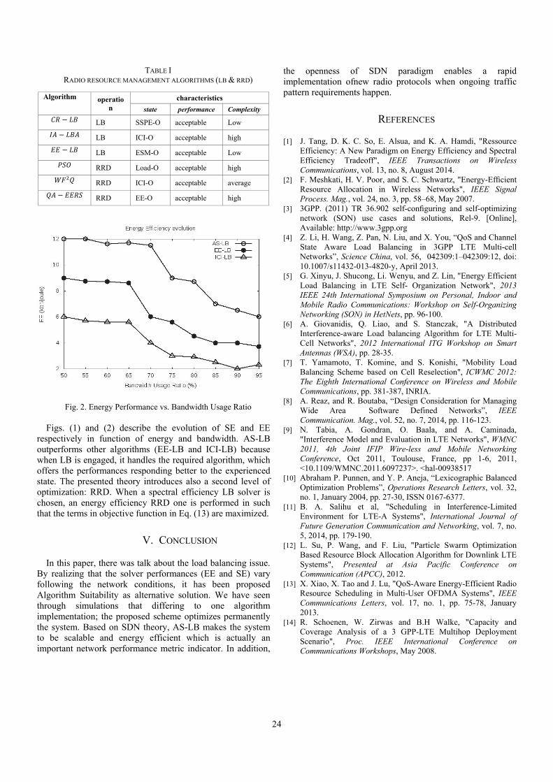
24

TABLE I RADIO RESOURCE MANAGEMENT ALGORITHMS (LB & RRD)

Algorithm operation

characteristics

state performance Complexity

LB SSPE-O acceptable Low

LB ICI-O acceptable high

LB ESM-O acceptable Low

RRD Load-O acceptable high

RRD ICI-O acceptable average

RRD EE-O acceptable high

Fig. 2. Energy Performance vs. Bandwidth Usage Ratio

Figs. (1) and (2) describe the evolution of SE and EE respectively in function of energy and bandwidth. AS-LB outperforms other algorithms (EE-LB and ICI-LB) because when LB is engaged, it handles the required algorithm, which offers the performances responding better to the experienced state. The presented theory introduces also a second level of optimization: RRD. When a spectral efficiency LB solver is chosen, an energy efficiency RRD one is performed in such that the terms in objective function in Eq. (13) are maximized.

V. CONCLUSION

In this paper, there was talk about the load balancing issue. By realizing that the solver performances (EE and SE) vary following the network conditions, it has been proposed Algorithm Suitability as alternative solution. We have seen through simulations that differing to one algorithm implementation; the proposed scheme optimizes permanently the system. Based on SDN theory, AS-LB makes the system to be scalable and energy efficient which is actually an important network performance metric indicator. In addition,

the openness of SDN paradigm enables a rapid implementation ofnew radio protocols when ongoing traffic pattern requirements happen.

REFERENCES

[1] J. Tang, D. K. C. So, E. Alsua, and K. A. Hamdi, "Ressource Efficiency: A New Paradigm on Energy Efficiency and Spectral Efficiency Tradeoff", IEEE Transactions on Wireless Communications, vol. 13, no. 8, August 2014.

[2] F. Meshkati, H. V. Poor, and S. C. Schwartz, "Energy-Efficient Resource Allocation in Wireless Networks", IEEE Signal Process. Mag., vol. 24, no. 3, pp. 58–68, May 2007.

[3] 3GPP. (2011) TR 36.902 self-configuring and self-optimizing network (SON) use cases and solutions, Rel-9. [Online], Available: http://www.3gpp.org

[4] Z. Li, H. Wang, Z. Pan, N. Liu, and X. You, “QoS and Channel State Aware Load Balancing in 3GPP LTE Multi-cell Networks”, Science China, vol. 56, 042309:1–042309:12, doi: 10.1007/s11432-013-4820-y, April 2013.

[5] G. Xinyu, J. Shucong, Li. Wenyu, and Z. Lin, "Energy Efficient Load Balancing in LTE Self- Organization Network", 2013 IEEE 24th International Symposium on Personal, Indoor and Mobile Radio Communications: Workshop on Self-Organizing Networking (SON) in HetNets, pp. 96-100.

[6] A. Giovanidis, Q. Liao, and S. Stanczak, "A Distributed Interference-aware Load balancing Algorithm for LTE Multi-Cell Networks", 2012 International ITG Workshop on Smart Antennas (WSA), pp. 28-35.

[7] T. Yamamoto, T. Komine, and S. Konishi, "Mobility Load Balancing Scheme based on Cell Reselection", ICWMC 2012: The Eighth International Conference on Wireless and Mobile Communications, pp. 381-387, INRIA.

[8] A. Reaz, and R. Boutaba, “Design Consideration for Managing Wide Area Software Defined Networks”, IEEE Communication. Mag., vol. 52, no. 7, 2014, pp. 116-123.

[9] N. Tabia, A. Gondran, O. Baala, and A. Caminada, "Interference Model and Evaluation in LTE Networks", WMNC 2011, 4th Joint IFIP Wire-less and Mobile Networking Conference, Oct 2011, Toulouse, France, pp 1-6, 2011, <10.1109/WMNC.2011.6097237>. <hal-00938517

[10] Abraham P. Punnen, and Y. P. Aneja, “Lexicographic Balanced Optimization Problems”, Operations Research Letters, vol. 32, no. 1, January 2004, pp. 27-30, ISSN 0167-6377.

[11] B. A. Salihu et al, "Scheduling in Interference-Limited Environment for LTE-A Systems", International Journal of Future Generation Communication and Networking, vol. 7, no. 5, 2014, pp. 179-190.

[12] L. Su, P. Wang, and F. Liu, "Particle Swarm Optimization Based Resource Block Allocation Algorithm for Downlink LTE Systems", Presented at Asia Pacific Conference on Communication (APCC), 2012.

[13] X. Xiao, X. Tao and J. Lu, "QoS-Aware Energy-Efficient Radio Resource Scheduling in Multi-User OFDMA Systems", IEEE Communications Letters, vol. 17, no. 1, pp. 75-78, January 2013.

[14] R. Schoenen, W. Zirwas and B.H Walke, "Capacity and Coverage Analysis of a 3 GPP-LTE Multihop Deployment Scenario", Proc. IEEE International Conference on Communications Workshops, May 2008.

25

Contention Resolution using Signal Tones for Wireless Sensor Networks

Milica Jovanovic1, Igor Stojanovic1, Sandra Djosic1 and Goran Lj. Djordjevic1

Abstract – This paper deals with contention resolution using signal tones for Wireless Sensor Networks (WSNs). We give an overview of existing contention resolution mechanisms, and describe briefly representative protocols by stating their essential behavior and emphasizing their strengths and weaknesses.

Keywords – Wireless sensor networks, Energy efficiency,

Medium access control, Contention resolution.

I. INTRODUCTION

A wireless sensor network (WSN) consists of a number of autonomous sensor nodes, composed of sensors, a low-power radio transceiver, small amount of memory and processing capability as well as limited battery power supply [1]. The primary objective in WSN design is maximizing node/network lifetime, leaving the other performance metrics as secondary objectives. Since the communication of sensor nodes is more energy consuming than their computation, it is a primary concern to minimize communication while achieving the desired network operation.

MAC protocol defines how and when nodes may access the shared medium in order to transmit their data and tries to ensure that no collisions occur. The collisions can be resolved in two ways: statically, by assigning each node exclusive time slot and dynamically, by adding a contention period at the beginning of each data transfer period. During the contention period nodes contend for medium access by employing a suitable contention resolution mechanism (CRM). Only the node that wins the contention is allowed to transmit its message, while others go back to sleep until the next active period. There are two primarily sources of energy overhead associated with contention-based MAC protocols: 1) contention overhead, and 2) collision overhead. The contention overhead is a consequence of additional energy consumption during the contention period, which may involve energy for transmitting control packets, as well as the energy for carrier transmission and carrier sensing. The collision overhead is a consequence of data packet collisions that are not prevented by the CRM. In general, there is a trade-off: the more energy spent on contention resolution, the less energy will be lost due to collisions, and vice versa.

There are two main problems that lowers the networks energy efficiency and throughput: hidden terminal problem and exposed terminal problem. The hidden terminal problem causes collisions and the exposed terminal problem lowers the data throughput.

CRM based on carrier sense multiple access (CSMA) protocol is often chosen due to its simplicity, low contention overhead and scalability [2]. With this scheme, sensor node randomly selects the moment of time in which it will starts with transmission, it senses the channel and withdraws if the channel is busy; or transmits the carrier signal otherwise. However, CSMA is susceptible to hidden- and exposed terminal problems, which lowers its energy efficiency and throughput. In order to combat the hidden terminal problem, a mechanism known as RTS/CTS handshake is widely used in wireless networks [3]. With RTS/CTS, signal tones are replaced with RTS and CTS control packets. Although the use of RTS/CTS mechanism avoids most of the data collisions, it is particularly unsuitable for WSNs because of high overhead due to control packets exchange [4]. Hence, the RTS/CTS is out of scope of this paper.

A class of CRMs based on exchanging unmodulated or modulated signals of short duration on the carrier frequency (so called tones) between the nodes offers a promising solution for collision-free communication with low contention overhead [5]-[7]. All of them provides the collision-freedom in a single-hop environment. In a multi-hop environment, the hidden-terminal problem may occur. To overcome this problem, several MAC protocols are proposed [8], [9]. Among others, a BCD-like contention resolution algorithm with tone-based signaling is proposed, which provides collision-free communication [10], [11].

In this paper, we give a survey of the tone-based CRM s for WSN. Section II explains the hidden- and exposed terminal problem end gives the overview of the existing tone-based CRMs and emphasizes their distinct features related to WSNs. Section III introduces TONE CRM, specifically developed for WSNs, which successfully eliminates hidden and exposed terminal problems.

II. CONTENTION RESOLUTION USING SIGNAL

TONES

The main requirements for the wireless networks are energy efficiency and throughput, which are mainly affected by the limited range of the radio transceiver. There are two problems characteristic for wireless medium: hidden and exposed terminal problem.

The hidden terminal problem occurs when two or more nodes, not visible to each other (due to limited transmission range, presence of obstacles, etc.) intend to send their messages to the same receiver during a given active period. The energy consumed during the transmission and reception of collided data messages is wasted, and additional energy is required for the retransmission, which lowers the energy efficiency of the network.

1Authors are with the Faculty of Electronic Engineering atUniversity of Nis, Aleksandra Medvedeva 14, 18000 Nis, Serbia, e-mail: milica.jovanovic, igor.stojanovic, sandra.djosic,goran.lj. [email protected]

26

The exposed terminal problem occurs when a node withdraws due to the ongoing transmission from one of its neighbors, although its transmission wouldn’t collide with the ongoing. This causes unnecessary delay, thus lowering the throughput of the network.

The signal tone is a radio signal of limited duration that carries no information. It is used for binary indication of transmitter’s state. There are several ways the MAC protocols can use signal tone: in form of a busy tone, jamming signal and binary-countdown (BCD) procedure.

A. Busy Tone

MAC protocols based on a busy tone uses two frequency channels: data channel and control channel. The busy tone is transmitted on the control channel by receiver, during the reception of the data on the data channel. In this way, by transmitting the busy tone node prevents its neighbors to initiate new transmission which would cause collisions. Although the use of the busy tone efficiently eliminates collisions, the increased energy consumption due to the long tones and increased price and consumption of the radio transceiver makes it unsuitable for use in WSNs. There are several existing MAC protocols that use busy tone.

BTMA protocol is designed for single-hop networks with central base station [5]. Base station transmits the busy tone in case that the carrier is detected on the data channel. The sensor node that has packet to transmit firstly senses the control channel and transmits only if the busy tone is not sensed, otherwise retreats for an arbitrary period of time. Although it eliminates the hidden terminal problem in single-hop networks, BTMA cannot deal with the hidden and exposed terminal problem in multi-hop networks.

RI-BTMA also uses separate control channel [12]. Sensor node that has packet to transmit firstly senses the control channel. In case that the busy tone is not sensed, node transmits the RTS packet containing the recipients address on the data channel, and waits the recipient’s response in form of a busy tone on the control channel. The recipient that detects its address on the data channel transmits the busy tone until the end of the data reception. In the absence of the busy tone, the transmitter retreats for an arbitrary period of time. In this manner the busy tone acts as the reservation ton and CTS packet, in which way it deals with the hidden terminal problem.

DBTMA protocol is a distributed solution intended for the ad hoc networks [13]. This protocol uses two busy tones on two separate channels: the receive busy tone, transmitted by receiver during data reception, and the transmit busy tone, transmitted by transmitter during transmission of the RTS packet. The node that has message to send first senses both control channels. In case that at least one channel is occupied, it retreats and tries later; otherwise, it initializes the procedure by sending the RTS packet on the data channel, together with the transmit busy tone on the control channel. After that, the transmitter stops sending the transmit busy tone and waits for the receive busy tone. Potential receiver that senses the transmit busy tone starts transmission of the receive tone, until the period intended for reception of the whole data packet.

The transmitter sends its data packet after it senses the receive busy tone. In this manner DBTMA successfully eliminates hidden and exposed terminal problem, with the cost of the additional hardware and additional delay due to generation and detection of the additional busy tone on the second control channel.

B. Jamming Signal

The jamming signal is used by the nodes during contention for the channel access [6]. All the nodes that have message to send simultaneously start to transmit the jamming signal of a different length. After that, they sense the channel. If the medium is still occupied, the node lost contention and retreats. In this manner, the node with the longest jamming signal is the winner and starts with the data transmission.

Black-Burst protocol is designed for the single-hop networks. It divides nodes in to two groups: nodes with the high and with the low priority [6]. The jamming signal is used by the nodes with the high priority: the node with message to send senses the channel and, in case it’s free, begins to transmit the jamming signal. Duration of the jamming signal is set by each node individually and corresponds to its delay in the network. After the transmission ends, the node samples channel ad retreats in case it’s busy. In this case, the winner is always the node with the longest jamming signal, i.e. the highest delay. The nodes in the group with the low priority uses regular CSMA/CA contention mechanism in case there are no nodes with the high priority interested in transmission.

Priority MAC protocol within the ad-hoc networks implements priorities similarly to the Black-Burst [7]. In the network that offers K different classes of services, each class is assigned different duration of the jamming signal, proportional to its priority. This provides the node with the highest priority to be the winner, since it has the longest jamming signal.

C. The Binary-Countdown, BCD

BCD-based MAC protocols for wireless networks implement arbitration concept from the CAN busses (Controller Area Network). CAN bus for the wired networks implements bit-dominant arbitration [14]. The node priority is coded with the unique binary sequence. The CAN arbitration concept provides the access to the medium to the node with the highest (or the lowest) binary sequence. The arbitration functions as follows: the percipient nodes sends synchronously their binary sequences bit by bit in fixed time moments. The logical one (or zero) is coded using dominant signal and the logical zero (or one) using recessive signal. In case there is at least one dominant signal transmitted, the resulting signal on the communication line will be dominant. The resulting signal is recessive only if all the transmitted signals are recessive. The nodes that have sent the dominant signal continues with the contention, all the others retreat.

In the wireless networks that implement BCD algorithm, the CAN arbitration is implemented in the following manner: the dominant bit is implemented as signal tone of certain duration, and the recessive as the absence of the signal tone.

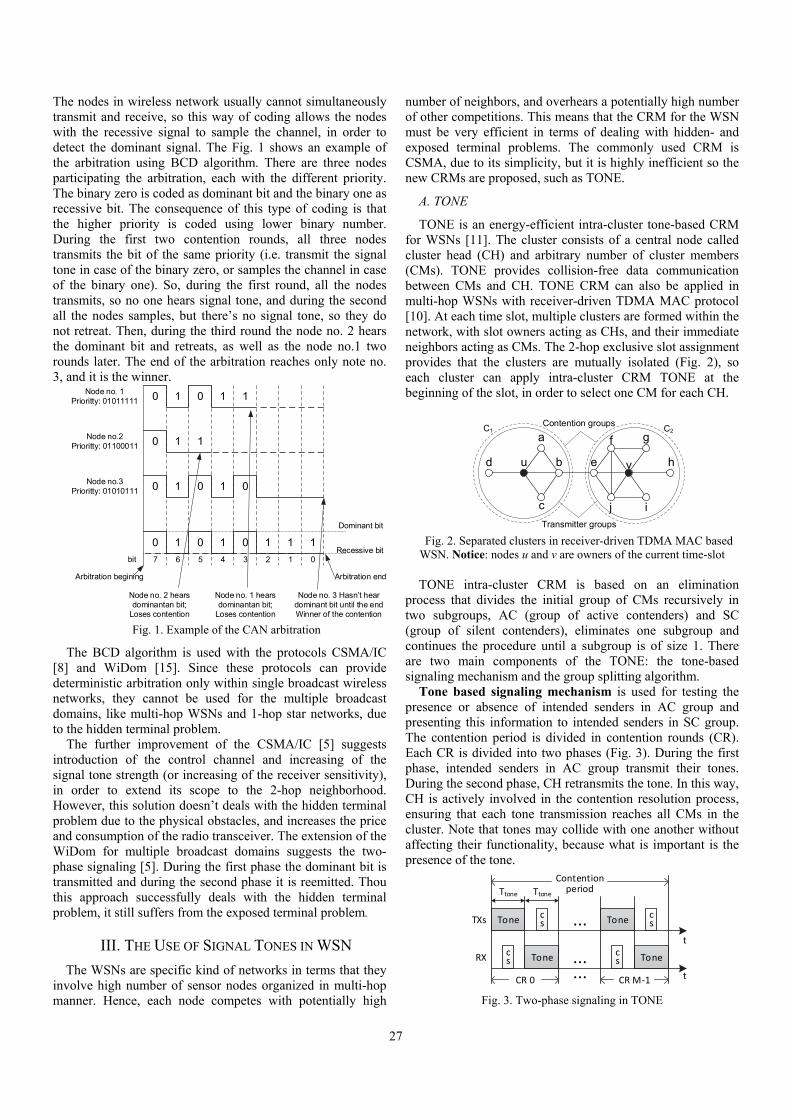
27

The nodes in wireless network usually cannot simultaneously transmit and receive, so this way of coding allows the nodes with the recessive signal to sample the channel, in order to detect the dominant signal. The Fig. 1 shows an example of the arbitration using BCD algorithm. There are three nodes participating the arbitration, each with the different priority. The binary zero is coded as dominant bit and the binary one as recessive bit. The consequence of this type of coding is that the higher priority is coded using lower binary number. During the first two contention rounds, all three nodes transmits the bit of the same priority (i.e. transmit the signal tone in case of the binary zero, or samples the channel in case of the binary one). So, during the first round, all the nodes transmits, so no one hears signal tone, and during the second all the nodes samples, but there’s no signal tone, so they do not retreat. Then, during the third round the node no. 2 hears the dominant bit and retreats, as well as the node no.1 two rounds later. The end of the arbitration reaches only note no. 3, and it is the winner.

10 1 1

11

1 1

11 1 1 1

0

0

0 0 0

000

Node no. 1Prioritty: 01011111

Node no.2Prioritty: 01100011

Node no.3Prioritty: 01010111

Arbitration begining

Recessive bit

Dominant bit

Node no. 2 hears dominantan bit;

Loses contention

Node no. 1 hears dominantan bit;

Loses contention

Node no. 3 Hasn’t hear dominant bit until the end Winner of the contention

Arbitration end

bit 01234567

Fig. 1. Example of the CAN arbitration

The BCD algorithm is used with the protocols CSMA/IC [8] and WiDom [15]. Since these protocols can provide deterministic arbitration only within single broadcast wireless networks, they cannot be used for the multiple broadcast domains, like multi-hop WSNs and 1-hop star networks, due to the hidden terminal problem.

The further improvement of the CSMA/IC [5] suggests introduction of the control channel and increasing of the signal tone strength (or increasing of the receiver sensitivity), in order to extend its scope to the 2-hop neighborhood. However, this solution doesn’t deals with the hidden terminal problem due to the physical obstacles, and increases the price and consumption of the radio transceiver. The extension of the WiDom for multiple broadcast domains suggests the two-phase signaling [5]. During the first phase the dominant bit is transmitted and during the second phase it is reemitted. Thou this approach successfully deals with the hidden terminal problem, it still suffers from the exposed terminal problem.

III. THE USE OF SIGNAL TONES IN WSN

The WSNs are specific kind of networks in terms that they involve high number of sensor nodes organized in multi-hop manner. Hence, each node competes with potentially high

number of neighbors, and overhears a potentially high number of other competitions. This means that the CRM for the WSN must be very efficient in terms of dealing with hidden- and exposed terminal problems. The commonly used CRM is CSMA, due to its simplicity, but it is highly inefficient so the new CRMs are proposed, such as TONE.

A. TONE

TONE is an energy-efficient intra-cluster tone-based CRM for WSNs [11]. The cluster consists of a central node called cluster head (CH) and arbitrary number of cluster members (CMs). TONE provides collision-free data communication between CMs and CH. TONE CRM can also be applied in multi-hop WSNs with receiver-driven TDMA MAC protocol [10]. At each time slot, multiple clusters are formed within the network, with slot owners acting as CHs, and their immediate neighbors acting as CMs. The 2-hop exclusive slot assignment provides that the clusters are mutually isolated (Fig. 2), so each cluster can apply intra-cluster CRM TONE at the beginning of the slot, in order to select one CM for each CH.

Contention groups

Transmitter groups

d u

a

c

b ve

f g

h

ij

C2C1

Fig. 2. Separated clusters in receiver-driven TDMA MAC based

WSN. Notice: nodes u and v are owners of the current time-slot TONE intra-cluster CRM is based on an elimination

process that divides the initial group of CMs recursively in two subgroups, AC (group of active contenders) and SC (group of silent contenders), eliminates one subgroup and continues the procedure until a subgroup is of size 1. There are two main components of the TONE: the tone-based signaling mechanism and the group splitting algorithm.

Tone based signaling mechanism is used for testing the presence or absence of intended senders in AC group and presenting this information to intended senders in SC group. The contention period is divided in contention rounds (CR). Each CR is divided into two phases (Fig. 3). During the first phase, intended senders in AC group transmit their tones. During the second phase, CH retransmits the tone. In this way, CH is actively involved in the contention resolution process, ensuring that each tone transmission reaches all CMs in the cluster. Note that tones may collide with one another without affecting their functionality, because what is important is the presence of the tone.

Tonecs

Tonecs

Tonecs

Tonecs

TXs

RX

Ttone Ttone

...t

t

...

Contentionperiod

CR 0 CR M‐1...

Fig. 3. Two-phase signaling in TONE

28

Two phase operation of tone-based signaling mechanism is crucial for avoiding both hidden- and exposed terminals in TONE. Hidden terminals are avoided because all the intended senders are merged into single contention group by means of CH node that acts as a tone repeater. Exposed terminals are avoided since clusters are isolated, so there no simultaneously active potential senders from different clusters.

The group splitting algorithm determinates how a group of non-eliminated contenders is partitioned into AC and SC group at the beginning of each CR. It is performed locally by each non-eliminated intended sender, and it does not require any communication among nodes.

TONE uses novel group-splitting mechanism, based on BCD, which aim to minimize the size of the AC group at each CR. By lowering the size of the AC group, TONE decreases the number of tone transmissions, thereby improving the energy efficiency.

If c is the size of the current contention group and the r is the number of the remained contention rounds, TONE computes the size of the AC group as in Eq. (1):

1 2

2

r

r

if cg

c else

(1)

Using the concept of contention interval, the proposed group splitting mechanism does not need to explicitly determine which nodes belong to which subgroup. Knowing its own competition number, the boundary values of contention interval, and the size of AC group, every contending node can individually determine to which subgroup it belongs.

By eliminating hidden- and exposed terminal problem, TONE CRM improves energy efficiency and throughput, while providing collision-free data communication in multi-hop WSN.

IV. CONCLUSION In this paper we presented the overview of the contention

resolution mechanisms that use signal tones employed in current MAC protocols for WSNs. The use of signal tones can certainly simplify contention resolution and lower the energy consumption. There are several efficient solutions that use signal tones in centralized wireless networks. However, due to hidden- end exposed terminal problems, generalization of these schemes to multi-hop networks is not always possible, or comes with the cost of increased protocol complexity. We identified the TONE protocol as the most promising contention resolution mechanism based on signal tones for the use in multi-hop WSNs. When integrated in receiver-driven TDMA MAC, the TONE provides collision-free data communication. Design of an efficient signal tone-based contention resolution mechanism for other categories of MAC protocols (e.g. MAC with common active period) is still an open problem, since so far there are no defined communication standards for WSNs based on signal tones.

ACKNOWLEDGEMENT This work was supported by the Serbian Ministry of

Science and Technological Development, project No. TR – 32009 - "Low-Power Reconfigurable Fault-Tolerant Platforms".

REFERENCES

[1] F. Akyildiz, W. Su, Y. Sankarasubramaniam, and E. Cayirci, Wireless sensor networks: A survey”, Computer Networks, vol. 38, no. 3, pp. 393-422, 2002.

[2] Anadbabu, Siddaraju, and R. Guru, “Energy Efficiency Mechanism in Wireless Sensor Networks: A Survey”, International Journal of Computer Applications, vol. 139, no. 14, pp. 27-33, 2016,

[3] B. Mamalis, D. Gavalas, C. Konstantopolous, and G. Pantziou, “Clustering in Wireless Sensor Networks” in Y. Zhang, L. T. Yang, J. Chen (Ed.): “RFID and Sensor Networks: Architectures, Protocols, Security, and Integrations”, pp. 323-353, Boca Raton: CRC Press, 2010.

[4] B. Priya, and S. Solai Manohar, “Lifetime Enhancement of Cluster Based Wireless Sensor Network through Energy Efficient MAC Protocol”, Circuits and Systems, vol. 7, no. 9, pp. 2296-2308, 2016.

[5] H. Jiang, W. Zhuang, X. Shen, A. Abdrabou, and P. Wang, “Differentiated services for wireless mesh backbone”, IEEE Communications Magazine; vol. 44, no. 7, pp. 113-119, 2006.

[6] J. L. Sobrinho, and A. S. Krishnakumar, “Quality-of-service in ad hoc carrier sense multiple access wireless networks”, IEEE Journal on Selected Areas in Communications, vol. 17, no. 8, pp. 1353–1368. 1999.

[7] J-P. Sheu, C-H. Liu, S-L Wu, and Y-C. Tseng, “A Priority MAC Protocol to Support Real-time Traffic in Ad Hoc Networks”, Wireless Networks, vol. 10, no. 1, pp. 61–69, 2004.

[8] C. You, H. S. Hassanein, and H. Yeh, "CSMA/IC: a new paradigm for medium access control in wireless LANs and ad hoc wireless networks", International Journal of Wireless and Mobile computing, vol. 1, no. 3/4, pp. 211-228, 2006.

[9] N. Pereira, B. Andersson, E. Tovar, and A. Rowe, „Static-Priority Scheduling over Wireless Networks with Multiple Broadcast Domains”, in Proc. of the 28th IEEE International Real-Time Systems Symposium (RTSS’07), pp. 447-458, 2007.

[10] M. D. Jovanovic, and G. Lj. Djordjevic, “Contention Resolution Mechanism for Receiver-Driven TDMA-Based Wireless Sensor Networks”, Facta Universitatis, Series: Automatic Control and Robotics, vol. 12, no. 1, pp. 53-73, 2013.

[11] M. D. Jovanovic, I. Z. Stojanovic, S. M. Djosic, and G. Lj. Djordjevic, „Intra-Cluster Tone-Based Contention Resolution Mechanism for Wireless Sensor Networks”, Computers and Electrical Engineering, Elsevier, vol. 56, pp. 485-497, November 2016

[12] W. Song, H. Jiang, W. Zhuang, and X. Shen, “Resource management for QoS support in cellular/WLAN interworking”, IEEE Network, vol. 19, no. 5, pp. 12–18, 2005.

[13] Z.J. Haas, and J. Deng, “Dual busy tone multiple access (DBTMA)-a multiple access control scheme for ad hoc networks”, IEEE Transactions on Communications, vol. 50, no. 6, pp. 975-985, 2002.

[14] R.I. Davis, A. Burns, R.J. Bril, and J.J. Lukkien, "Controller Area Network (CAN) schedulability analysis: Refuted, Revisited and Revised", Real-Time Systems, vol. 35, no. 3, pp. 239-272, 2007.

[15] N. Pereira, B. Andersson, and E. Tovar, "WiDom: A Dominance Protocol for Wireless Medium Access", IEEE Transactions on Industrial Informatics, vol. 3, no. 2, pp. 120-130, May 2007.

Session 1B:

SIGNAL PROCESSING

31

Closed-form Design of New Class of Selective CIC FIR Filter Functions

Biljana P. Stošić, Vlastimir D. Pavlović

Abstract — This paper deals with design of new CIC (Cascaded-Integrator-Comb) FIR (finite impulse response) filter functions. Closed-form expressions of new class of selective CIC filter functions by introducing spreading of the delays in the CIC filter comb stages are firstly presented here. Then, the authors are focused on the analysis of the proposed CIC filters in comparison with existing classical CIC structures and some recent results reported in the literature. The novel cascaded-filter architecture has valuable benefits: higher insertion loss in stopband, smaller impulse response coefficient values, and better characteristic in passband region compared with classical CIC filters.

Keywords — Digital filters, CIC FIR filters, Multiplierless design, Linear phase, Selective filters, Compensator filter.

I. INTRODUCTION CIC (Cascaded-Integrator-Comb) FIR (finite impulse response) filters introduced by Eugene B. Hogenauer [1], more than three decades ago, are becoming increasingly popular due to their compact integration with modern communication systems, their multiplier free design, etc. Various improvements of classical CIC filters have been reported in the last decade [2]-[10]. However, further improvement is still an issue, e.g. design of new CIC FIR filter functions, improvement of large passband droop which is undesirable in many applications because the original signal can be destroyed, increasing of attenuation in the stopband region, etc.

A CIC filter is cascade connection of simple integrator and comb filter stages. Design of a novel class of selective CIC filter functions based on the classical CIC filters, by spreading the delays in the CIC filter comb stages, is recently shown in the literature [6]-[10]. In [6], and [8]-[10], novel CIC filter functions in the explicit compact form, as well as their frequency responses and performance improvements over the classical CIC filters, are presented. The novel designed class gives higher insertion losses in the stopband region, and higher selectivity. The paper [8] provides graphs which can be used to design a novel class of selective CIC filters given specification which is suggested in [6]. They are very useful for the designers who will be able to do selection of the design parameters of the novel filter functions that they need for the particular design task.

In this paper, the new modified CIC FIR filter functions which preserve the CIC filter simplicity avoiding the multipliers are designed. The novel filter functions are given

Biljana P. Stošič and Vlastimir D. Pavlović are with the University of Niš, Faculty of Electronic Engineering, Aleksandra Medvedeva 14, 18000 Niš, Serbia, E-mail: [email protected]

in recursive and non-recursive forms. The performance analysis in more detail through a few examples is done. It starts by a detailed analysis of frequency response characteristics. A comparative study of the performances is made with that of well-known classical CIC filters in graphical and tabular forms, as well as with some recent improvements of classical CIC filters given recently in the litearture [6]-[10]. Comparisons are for the same level of constant group delay. Also, some parameters of the novel class CIC filter functions (i.e. passband cut-off frequency and minimum attenuation in stopband) and their dependence on free parameters are given. The results illustrate the superiority of the suggested novel CIC filter functions and show that they can be a good alternative instead of classical CIC filters.

II. CLASSICAL CIC FILTER FUNCTIONS The z -domain expression for the classical CIC FIR filter

function with normalized amplitude response characteristic is

KzNHzKNH ),(),,( , (1)

1

01

1

)1(

1),(

N

r

rN

zNzN

zzNH , (2)

where N is the decimation factor, and K is the number of CIC sections [1].

The frequency response of CIC FIR filter function presented in exponential form is

KNKjj

N

NeezKNH

)2/(sin

)2/(sin),,( 2/)1( . (3)

The magnitude response characteristic is defined as the magnitude of the complex filter frequency response given in (3). The phase response characteristic of the proposed new modified CIC FIR filter functions is defined as the phase angle of the complex filter frequency response given in (3), and has the form

22/)1( ),,( KNKN , ,...2 ,1 ,0 (4)

A filter has a linear phase and therefore a constant group delay defined as

2/)1( /),,( ),,( KNdKNdKN . (5)

III. DESIGN FORMS OF NOVEL CLASS OF CIC FIR

FILTER FUNCTIONS

A. Non-Recursive and Recursive Forms of Novel Filter Class

The novel filter class is designed as cascade of four non-identical CIC FIR filter sections ),2( zNH , ),1( zNH ,

),1( zNH and ),2( zNH which are repeated L times.

A recursive form of a novel class of CIC FIR filter functions is given as

32

LNN

LNN

zN

z

zN

z

zN

z

zN

zzLKNH

)1()2(

1

)1()1(

1

)1()1(

1

)1()2(

1),,,(

1

)2(

1

)1(

1

)1(

1

)2(

and LK 4 . (6) The proposed filter function has normalized amplitude response characteristics.

The filter function of a designed novel class of CIC FIR filter functions can be written in non-recursive form as

3 2

0 0 0

( 1)1

00 0

1 1 1( , , , )

2 1 1

1 1( , ) (7)

2 ( , , )

LN N N

r r r

r r r

LN KN

r r

r r

H N K L z z z zN N N

z h N r zN H N K L

where ),,(0 LKNH is the normalized constant for the unit

magnitude response at 0f , where parameter LK 4 , and

),( rNh represent the coefficients of the impulse response.

B. Impulse Response Coefficients

Vector h is the vector of impulse response coefficients, defined as

),(),1,(...,),1,(),0,(),,( MNhMNhNhNhLKN h (8)

where total number of elements is 1)1( KNM . The

coefficients satisfy the following symmetry condition, ),(),( rMNhrNh . The impulse response coefficients of

the classical CIC filters can be also found in [5]. The non-recursive implementation of classical CIC filter

functions, ),,( zKNH , obtained for odd value of free integer

parameter 7N and 4K , is observed here in the form of Eq. (7). The normalized constant is 2401. The vector of the impulse response coefficient is

1 4, 10, 20, 35,

56, 84, 116, 149, 180, 206, 224, 231, 224,

206, 180, 149, 116, 84, 56, 35, 20, 10, 4, 1,

)4,7(CICh (9)

The non-recursive forms of novel class of CIC filter functions, ),,,( zLKNH , obtained for even value of integer parameter

7N and 4K (obtained for 1L ), satisfied Eq. (7). The constant is 2160)1,4,7(0 H . The vector h of impulse

response coefficients is 1,4,10,20,35,55,79,106,134,160,181,195,200,

(7,4,1)195,181,160,134,106,79,55,35,20,10,4,1

h (10)

Notice that the proposed linear phase FIR filter functions in non-recursive form have shown obvious symmetry of coefficients. The normalized constants for proposed filter class are smaller than those of classical CIC FIR filters. Also, impulse response coefficients of proposed filter class have smaller values in comparison to those of classical CIC filters.

C. Frequency Responses

Frequency response of designed FIR filter functions is easily obtained by evaluating the filter function in the z -plane at the

sample points defined by setting jez , where f 2 is

angular frequency in radians per second. Using Euler’s identity, frequency response characteristic can be written in exponential form as

( 1) /2 sin (( 2) / 2)( , , , )

( 2) sin ( / 2)

sin (( 1) / 2) sin (( 1) / 2) sin (( 2) / 2)

( 1) sin ( / 2) ( 1) sin ( / 2) ( 2) sin ( / 2)

Lj j K N

L

NH N K L z e e

N

N N N

N N N

and LK 4 . (11) The magnitude response characteristic of the proposed filter

functions, ),,,( jeLKNH , is defined as the magnitude of

the complex filter frequency response ),,,( jezLKNH .

The linear phase response characteristic of the proposed novel class of the modified CIC FIR filter functions is

22/)1( ),,,( KNLKN , ,...2 ,1 ,0 , and

LK 4 . (12) A novel class of the modified CIC FIR filter functions has a

the constant group delay response characteristic expressed as ( , , , ) ( 1) / 2N K L N K and LK 4 . (13)

D. Zero-Plots for Filter Functions

The locations of zeros in z -plane along with their multiplicities for the classical CIC and the proposed class of CIC filter functions are shown in Fig. 1. They are shown for case of 8N , and 2L .

-1 -0.5 0 0.5 1

-1

-0.5

0

0.5

1

8

8

8

8

8

8

Real Part

Imag

ina

ry P

art

(a) Classical CIC filter

-1 -0.5 0 0.5 1

-1

-0.5

0

0.5

1

2

2

2

4

4 2

2

2

2

2

2

2

2

2

2

2

2

2

2

4

2

Real Part

Imag

inar

y P

art

(b) Novel filter class, 2L

Fig. 1. Locations and multiplicities of filter function zeros in z -plane for 8N , and 8K cascades

Note that the comb stages of the classical CIC filters

produce N zeros, equally spaced around the unit-circle, and the integrator stages produce single poles canceling the zeros at 1z . Finally, the classical CIC filter function has 1N

different zeros being a thN root of unity and located at Nrj

r ez /2 , 1,...,2,1 Nr . The total number of zeros is

( 1)N K . Note that the classical CIC filters have all

multiple zeros with maximum multiplicity equal to the number of cascades K , which is not the case in the proposed solutions. The zeros of the proposed filter class are more evenly distributed with their multiplicities therefore reduced as can be seen in Fig. 1b.

E. Selection of the Design Parameters

The choice of free integer parameters N and L is done in the same way as for CIC filters, there are the same restrictions

33

on the group delay response. The parameter K can take different integer values, LK 4 .

The attenuation in the stopband region is closely related to the parameter L . By increasing L for the constant value of N , the higher stopband attenuation is achieved. The constant group delay is equal for the classical CIC filters (Eq. (1)) and the novel modified CIC filter functions (Eq. (6)). The constant group delays for different values of parameters N , L and LK 4 are given in Table I.

TABLE I GROUP DELAY FOR 11,...,6,5N , 3,2,1L AND 4K L

N 5 6 7 8 9 10 11 12

][s

1L 8 10 12 14 16 18 20 22

2L 16 20 24 28 32 36 40 44

3L 24 30 36 42 48 54 60 66

IV. DESIGN EXAMPLE AND COMPARISONS OF

NOVEL CIC FIR FILTER FUNCTIONS In order to validate theoretical design, a test example is

designed for different filter parameters.

A. Frequency Responses of new CIC Filter Functions Compared with Classical CIC Filters

Like classical CIC filters, new designed CIC FIR filter functions have significant passband droop, which is usually intolerable in many cases, what can be seen in Fig. 2. Hence, it is of great interest to get a flat passband in some way, i.e. by connecting an additional filter (so-called CIC compensator) in cascade with the CIC decimator.

Passband droop compensation is done by use of a multiplerless FIR filter with one free parameter b presented in [3, 4]

2( ) 1N N NG z B A z z , (14)

where )2(2 bB is a scaling factor ensuring unitary gain

at the digital frequency zero, and

222bA . The

compensator is connected in the cascade with the suggested filter functions.

TABLE II CUT-OFF FREQUENCIES IN PASSBAND AND STOPBAND, CONSTANT GROUP

DELAY AND STOPBAND ATTENUATION OF CLASSICAL CIC FILTER FOR

4,8K AND 8N

K cpf max ]dB[ csf min ]dB[

4 0.00881 0.28 0.1008 51.1894

8 0.00623 0.28 0.1008 102.3788

In order to illustrate clearly the achieved improvements of the new class, the normalized magnitude response characteristics in dB of the new class and classical CIC filters are summarized in Fig. 2. It can be concluded that achieved passband droop compensation is similar for both values of parameter 1, 2L .

TABLE III CUT-OFF FREQUENCIES IN PASSBAND AND STOPBAND, CONSTANT GROUP

DELAY AND STOPBAND ATTENUATION OF PROPOSED CLASS OF CIC

FILTER FOR 4,8K , 1, 2L , 8N AND max ( ) 0.28dBcpf

Filter type L K cpf csf min ]dB[

no added droop- compensation filter

1 4 0.00864 0.09716 60.8814

2 8 0.00611 0.09717 121.7628

added droop-compensation filter with

1b

1 4 0.01505 0.09753 60.8812

2 8 0.00763 0.09717 121.7626

0 0.05 0.1 0.15 0.2 0.25 0.3 0.35 0.4 0.45 0.50

20

40

60

80

100

120

140

160

180

200

Frequency, fA

ttena

utio

n [d

B]

New CIC filter functions L=1New CIC filter functions L=1 with included droop-compensation filterClassical CIC filters K=4New CIC filter functions L=2New CIC filter functions L=2 with included droop-compensation filterClassical CIC filters K=8

K=8

K=4

(a) Whole frequency range

0 0.005 0.01 0.015 0.02 0.0250

0.5

1

1.5

2

2.5

3

3.5

4

4.5

5

Frequency, f

Atte

naut

ion

[dB

]

New CIC filter functions L=1New CIC filter functions L=1 with included droop-compensation filterClassical CIC filters K=4New CIC filter functions L=2New CIC filter functions L=2 with included droop-compensation filterClassical CIC filters K=8

K=8

K=4

(b) Passband detail

Fig. 2. Magnitude response characteristics in dB of proposed class of CIC FIR filter functions and those functions with included droop-compensation filter for 8N , different values of parameter 1L

and 2L , and 1b

In Tables II and III, parameter values of both the classical CIC filter function ),,( zKNH , given in Eq. (1), and the novel

CIC filter functions ),,,( zLKNH , given in Eq. (6), are

presented respectively. They are obtained for chosen parameter values 8N and 4,8K obtained for

1, 2L . The given parameters are: passband and stopband

cut-off frequencies, cpf and csf , maximum attenuation in the

passband, max [dB] and miminum attenuation in the

stopband region, min ]dB[ . The filter functions are designed

for the same number of cascaded sections with the difference that the CIC filters have an identical section in all cascades, and the designed novel class has a cascade-connected different CIC filter sections. Also, they have the same level of constant group delay, as well as number of delay elements, but the novel designed filter functions give higher insertion losses in stopband, as well as it has higher selectivity.

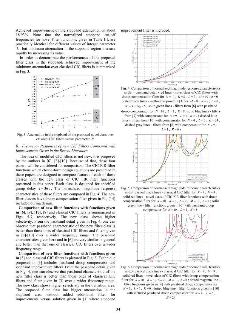
34

Achieved improvement of the stopband attenuation is about 18.93%. Note that the normalized stopband cut-off frequencies for novel filter functions, given in Table III, are practically identical for different values of integer parameter L , but minimum attenuation in the stopband region increase rapidly by increasing its value.

In order to demonstrate the performances of the proposed filter class in the stopband, achieved improvement of the minimum attenuation over classical CIC filters is summarized in Fig. 3.

Fig. 3. Attenuation in the stopband of the proposed novel class over

classical CIC filters versus parameter N

B. Frequency Responses of new CIC Filters Compared with Improvements Given in the Recent Literature

The idea of modified CIC filters is not new, it is proposed by the authors in [6], [8]-[10]. Because of that, these four papers will be considered for comparison. The CIC FIR filter functions which closed-form design equations are presented in these papers are designed to compare feature of each of those classes with the new class of CIC FIR filter functions presented in this paper. Each class is designed for specified group delay 36 s . The normalized magnitude response

characteristics of these filters are compared in Fig. 4. The new filter classes have droop-compensation filter given in Eq. (14) included during design.

Comparison of new filter functions with functions given in [6], [9], [10], [8] and clasical CIC filters is summarized in Figs. 5-7, respectively. The new class shows higher selectivity. From the passband detail given in Fig. 4, one can observe that passband characteristic of the new filter class is better than those ones of classical CIC filters and filters given in [8]-[10] over a wider frequency range. The passband characteristics given here and in [6] are very similar in general and better than that one of classical CIC filters over a wider frequency range.

Comparison of new filter functions with functions given in [3] and classical CIC filters is pictured in Fig. 8. Technique proposed in [3] includes passband droop compensator and stopband improvement filters. From the passband detail given in Fig. 4, one can observe that passband characteristic of the new filter class is better than those ones of classical CIC filters and filter given in [3] over a wider frequency range. The new class shows higher selectivity in the transition area. The proposed filter class has bigger attenuation in the stopband area without added additional filter for improvements versus solution given in [3] where stopband

improvement filter is included.

0 0.001 0.002 0.003 0.004 0.005 0.006 0.007 0.008 0.009 0.010

0.05

0.1

0.15

0.2

0.25

0.3

0.35

0.4

0.45

0.5

Frequency, f

Atte

naut

ion

[dB

]

Filter functions AEU [6]Filter functions JCSC [9]Filter functions IETE JR [10]Filter functions IEEE SP [8]New CIC filter functionsFilter functions DSP [3]

Fig. 4. Comparison of normalized magnitude response characteristics

in dB - passband detail (red lines - novel class of CIC filters with droop-compensation filter for 10N , 8K , 2L , 10M , 0b ; dotted black lines - method proposed in [3] for 9M , 9K , 0b ,

1 4N , 2 5N ; solid green lines - filters from [6] with passband

droop compensator for 10N , 1L , 8K ; solid blue lines - filters from [9] with compensator for 9N , 1L , 9K ; dashed blue

lines - filters from [10] with compensator for 4N , 3L , 24K ; dashed gray lines - filters from [8] with compensator for 9N ,

1L , 9K )

0.02 0.04 0.06 0.08 0.1 0.12 0.14 0.16 0.18 0.20

20

40

60

80

100

120

140

160

180

200

X: 0.1002Y: 136.8

Frequency, f

Atte

naut

ion

[dB

]

X: 0.1602Y: 116.1

X: 0.1056Y: 165.6

Filter functions AEU [6]New CIC filter functionsClassical CIC filters


in dB (dashed black lines - classical CIC filter for 9K , 9N ; solid red lines - novel class of CIC FIR filter functions with droop-compensation filter for 10N , 8K , 2L , 10M , 0b ; solid

green line - filter functions given in [6] with passband droop compensator for 10N , 1L , 8K

0 0.02 0.04 0.06 0.08 0.1 0.12 0.14 0.16 0.18 0.20

50

100

150

200

250

X: 0.1041Y: 181.6

Frequency, f

Atte

naut

ion

[dB

]

X: 0.1526Y: 217.6

X: 0.0997Y: 136.8

X: 0.1595Y: 116.1

Filter functions JCSC [9]

New CIC filter functions

Classical CIC filters

Filter functions IETE JR [10]


in dB (dashed black lines - classical CIC filter for 9K , 9N ; solid red lines - novel class of CIC filters with droop-compensation

filter for 10N , 8K , 2L , 10M , 0b ; dotted magenta line - filter functions given in [9] with passband droop compensator for

9N , 1L , 9K ; dotted blue line - filter functions given in [10] with included passband droop compensator for 4N , 3L ,

24K

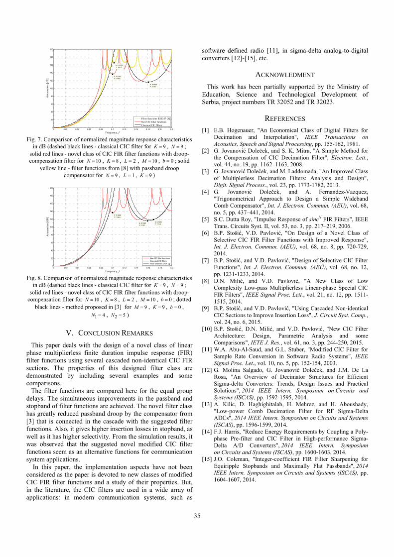
35

0 0.02 0.04 0.06 0.08 0.1 0.12 0.14 0.16 0.18 0.20

20

40

60

80

100

120

140

160

180

200

X: 0.1029Y: 165.7

Frequency, f

Atte

naut

ion

[dB

]

X: 0.1002Y: 136.8

X: 0.1609Y: 116.1

Filter functions IEEE SP [8]New CIC filter functionsClassical CIC filters


in dB (dashed black lines - classical CIC filter for 9K , 9N ; solid red lines - novel class of CIC FIR filter functions with droop-compensation filter for 10N , 8K , 2L , 10M , 0b ; solid

yellow line - filter functions from [8] with passband droop compensator for 9N , 1L , 9K )

0 0.02 0.04 0.06 0.08 0.1 0.12 0.14 0.16 0.18 0.20

20

40

60

80

100

120

140

160

180

200

X: 0.0999Y: 136.8

Frequency, f

Atte

naut

ion

[dB

]

X: 0.1689Y: 119.4X: 0.1592

Y: 116.1

New CIC filter functions

Classical CIC filtersFilter functions DSP [3]


in dB (dashed black lines - classical CIC filter for 9K , 9N ; solid red lines - novel class of CIC FIR filter functions with droop-

compensation filter for 10N , 8K , 2L , 10M , 0b ; dotted black lines - method proposed in [3] for 9M , 9K , 0b ,

1 4N , 2 5N )

V. CONCLUSION REMARKS

This paper deals with the design of a novel class of linear phase multiplierless finite duration impulse response (FIR) filter functions using several cascaded non-identical CIC FIR sections. The properties of this designed filter class are demonstrated by including several examples and some comparisons.

The filter functions are compared here for the equal group delays. The simultaneous improvements in the passband and stopband of filter functions are achieved. The novel filter class has greatly reduced passband droop by the compensator from [3] that is connected in the cascade with the suggested filter functions. Also, it gives higher insertion losses in stopband, as well as it has higher selectivity. From the simulation results, it was observed that the suggested novel modified CIC filter functions seem as an alternative functions for communication system applications.

In this paper, the implementation aspects have not been considered as the paper is devoted to new classes of modified CIC FIR filter functions and a study of their properties. But, in the literature, the CIC filters are used in a wide array of applications: in modern communication systems, such as

software defined radio [11], in sigma-delta analog-to-digital converters [12]-[15], etc.

ACKNOWLEDMENT

This work has been partially supported by the Ministry of Education, Science and Technological Development of Serbia, project numbers TR 32052 and TR 32023.

REFERENCES

[1] E.B. Hogenauer, "An Economical Class of Digital Filters for Decimation and Interpolation", IEEE Transactions on Acoustics, Speech and Signal Processing, pp. 155-162, 1981.

[2] G. Jovanović Doleček, and S. K. Mitra, "A Simple Method for the Compensation of CIC Decimation Filter", Electron. Lett., vol. 44, no. 19, pp. 1162–1163, 2008.

[3] G. Jovanović Doleček, and M. Laddomada, "An Improved Class of Multiplerless Decimation Filters: Analysis and Design", Digit. Signal Process., vol. 23, pp. 1773-1782, 2013.

[4] G. Jovanović Doleček, and A. Fernandez-Vazquez, "Trigonometrical Approach to Design a Simple Wideband Comb Compensator", Int. J. Electron. Commun. (AEU), vol. 68, no. 5, pp. 437–441, 2014.

[5] S.C. Dutta Roy, "Impulse Response of sincN FIR Filters", IEEE Trans. Circuits Syst. II, vol. 53, no. 3, pp. 217–219, 2006.

[6] B.P. Stošić, V.D. Pavlović, "On Design of a Novel Class of Selective CIC FIR Filter Functions with Improved Response", Int. J. Electron. Commun. (AEU), vol. 68, no. 8, pp. 720-729, 2014.

[7] B.P. Stošić, and V.D. Pavlović, "Design of Selective CIC Filter Functions", Int. J. Electron. Commun. (AEÜ), vol. 68, no. 12, pp. 1231-1233, 2014.

[8] D.N. Milić, and V.D. Pavlović, "A New Class of Low Complexity Low-pass Multiplierless Linear-phase Special CIC FIR Filters", IEEE Signal Proc. Lett., vol. 21, no. 12, pp. 1511-1515, 2014.

[9] B.P. Stošić, and V.D. Pavlović, "Using Cascaded Non-identical CIC Sections to Improve Insertion Loss", J. Circuit Syst. Comp., vol. 24, no. 6, 2015.

[10] B.P. Stošić, D.N. Milić, and V.D. Pavlović, "New CIC Filter Architecture: Design, Parametric Analysis and some Comparisons", IETE J. Res., vol. 61, no. 3, pp. 244-250, 2015.

[11] W.A. Abu-Al-Saud, and G.L. Stuber, "Modified CIC Filter for Sample Rate Conversion in Software Radio Systems", IEEE Signal Proc. Let., vol. 10, no. 5, pp. 152-154, 2003.

[12] G. Molina Salgado, G. Jovanović Doleček, and J.M. De La Rosa, "An Overview of Decimator Structures for Efficient Sigma-delta Converters: Trends, Design Issues and Practical Solutions", 2014 IEEE Intern. Symposium on Circuits and Systems (ISCAS), pp. 1592-1595, 2014.

[13] A. Kilic, D. Haghighitalab, H. Mehrez, and H. Aboushady, "Low-power Comb Decimation Filter for RF Sigma-Delta ADCs", 2014 IEEE Intern. Symposium on Circuits and Systems (ISCAS), pp. 1596-1599, 2014.

[14] F.J. Harris, "Reduce Energy Requirements by Coupling a Poly-phase Pre-filter and CIC Filter in High-performance Sigma-Delta A/D Converters", 2014 IEEE Intern. Symposium on Circuits and Systems (ISCAS), pp. 1600-1603, 2014.

[15] J.O. Coleman, "Integer-coefficient FIR Filter Sharpening for Equiripple Stopbands and Maximally Flat Passbands", 2014 IEEE Intern. Symposium on Circuits and Systems (ISCAS), pp. 1604-1607, 2014.

36

Wideband Speech Signal Coding with the Implementation of Modified BTC Algorithm

Stefan Tomić1 Zoran Perić2 and Jelena Nikolić3

Abstract – This paper presents a modified Block Truncation Coding (BTC) algorithm and its application in wideband speech signal coding. Since the original BTC algorithm is designed for application in black and white image coding, it is modified to a great extent, while preserving the basic principles. The modified algorithm exploits the common characteristics of the speech signal and images, while the dominant modifications are implemented in the area of signal quantization. The algorithm is applied to real input speech signals and the results are very impressive, indicating a wide applicability of our proposal.

Keywords – Adaptive coding, Algorithm, BTC, Speech signal coding, Quantization.

I. INTRODUCTION

Speech signal is one of the most important signals in nature, which digital form we meet every day. From the time of just using landline telephones, we came to an area where voice can easily be transmitted through the internet, almost instantaneously, while having a great variety of methods to do so. As modern telecommunication networks deal with a great amount of data daily, it is highly important that they use optimal amount of storage space and transmission bandwidth. This makes signal compression highly important in every telecommunications system which handles speech signals [1], [2]. Properly compressed speech signals need to comply with certain quality standards, while demand an optimal storage space. Quality is determined by the compression algorithm applied and the chosen bit rate [1], [2]. Efficient usage of available bit rate is crucial for obtaining high quality output signal, which can be easier to store and send through communication system. This gives a great importance to the research in the field of signal compression, as technologies constantly evolve and new challenges are faced.

Due to the great number of researches on this topic, there are a lot of speech signal coding algorithms in the literature. As multimedia data transmission plays important part in modern signal processing, we can find some similar coding techniques applied in audio and video signal coding. This has inspired the authors to consider implementing image coding algorithm in speech signal coding. The application of an image coding algorithm in speech signal coding represents a novelty and by applying certain modifications to the original

Block Truncation Coding (BTC) algorithm [3], we obtain a novel speech signal coding algorithm. The original BTC algorithm is based on the input signal decomposition into non-overlapping blocks of input signal samples (frames) [3]. Along with the input signal samples, the algorithm uses the mean value and standard deviation, as statistical parameters of the input signal frame in the coding process. As these parameters are also required for decoding, they also need to be transmitted through the channel. In this case, mean value and standard deviation are representing the side information, which provides higher quality of the output signal, but also increase the bit rate. Since the side information is added per frame, the amount of side information depends on the frame size. The basic BTC algorithm implements uniform quantization, while in this paper we choose more robust quantizers, suitable for wideband speech signal coding.

It has been shown in [4] that the BTC algorithm can be successfully applied in narrowband speech signal coding. Also, the similar approach has been utilized in [5], where the modified BTC algorithm has been applied in audio signal coding. Unlike in [4] and [5], in this paper we introduce the usage of sub-frames for higher adaptation of the algorithm to the statistics of the wideband speech signal. In addition, we implement changes in the quantization process, which we describe in Section 2. The modified algorithm is applied in coding of wideband speech signal, with sampling frequency of 16 KHz. The rest of the paper is organized as follows. Section 2 describes the modified BTC algorithm design. The performance analysis of the algorithm is presented in Section 3, while Section 4 is dedicated to conclusions.

II. MODIFIED BTC ALGORITHM

As mentioned, the original BTC algorithm is developed for black and white image compression [3]. It is based on decomposing the input signal into frames, which are processed individually. For each frame, the mean value and standard deviation are calculated and used in the quantization process. This gives us three variables in total, the input signal samples, and the two aforementioned statistical parameters which describe the frame. The basic BTC algorithm implements three uniform quantizers, with the total bit rate of 2 bits per sample [3]. This is possible due to the algorithm design and the fact that black and white image pixel value is defined in the interval from 0 to 255. As wideband speech signal sample amplitude can have unpredictable value, we implement more robust quantization methods, while applying higher bit rates. Additionally, we narrow the range of the input signal samples, by subtracting the mean value of the subframe from each subframe sample. In such a way,

1Stefan Tomić is with the Faculty of Electronic Engineering at University of Niš, Aleksandra Medvedeva 14, 18000 Niš, Serbia, E-mail: [email protected]

2Zoran Perić is with the Faculty of Electronic Engineering at University of Niš, Aleksandra Medvedeva 14, 18000 Niš, Serbia

3Jelena Nikolić is with the Faculty of Electronic Engineering at University of Niš, Aleksandra Medvedeva 14, 18000 Niš, Serbia

37

Fig. 1. Modified BTC algorithm: encoder (above) and decoder (bellow)

difference signal frame is formed, which is more suitable for coding, due to its lower amplitude dynamics. In difference to the original algorithm, in the modified BTC algorithm, each input signal frame is divided into subframes.

Unlike with the original BTC algorithm [3], we design three different quantizers to be applied to different variables of the input signal. Fig. 1 presents the block diagram of our modified BTC algorithm, where quantizers are denoted by Encoder 1-3 and Decoder 1-3. Difference signal defined by the frame length of Mf samples for L number of subframes, each containing Msf samples is calculated as:

( ) ( ) ( ) LjMixxd sfjsf

mj

ijsf

i ,...,2,1,,...,2,1,ˆ ==−= , (1) where xi

(j) denotes the ith input signal sample, of the jth subframe, while ( )jsf

mx is the quantized mean value of the jth subframe. Mean value is calculated for each subframe and it is quantized by applying the quasilogarithmic µ law quantizer [6], denoted by Encoder 1 and Decoder 1. The thus defined difference signal frame is brought to the input of Encoder 3, along with the standard deviation of the frame. Standard deviation is calculated for each frame and it is quantized with the application of the log-uniform quantizer [7] denoted by Encoder 2 and Decoder 2. Standard deviation of the frame is used in adaptive quantization of the subframes that the frame consists of, which outputs adaptive difference signal subframe denoted as ( )jasf

id . The outputs of the three defined encoders denoted by I, J and K are sent through the channel as binary information. The received information needs to be reconstructed into usable form, which represents the original input signal. Decoded output signal sample is obtained by adding the quantized mean value of the subframe to the adaptive difference signal subframe samples:

( ) ( ) ( )LjMidxy sf

jasfi

jsfm

ji ,...,2,1,,...,2,1,ˆˆ ==+= . (2)

This procedure is performed for all subframes of the input signal, which gives us the reconstructed signal. As we have the original input signal and its reconstructed form, we can inspect the objective quality of the output signal. For this purpose, we use a well-known measure, named signal to quantization noise ratio (SQNR) [1], [2], [8], [9]. SQNR is calculated for a certain bit rate used. As our algorithm implements frames and subframes, the total bit rate is influenced by the frame and subframe size and the bit rate used in individual quantizers. Accordingly, the total bit rate used in the modified BTC algorithm is defined by:

fsf M

rMrrR 21

3 ++= , (3)

where r3 denote the bit rate used for quantization of the difference signal frame, r1 and r2 represent the bit rates used for quantizing the mean value and standard deviation, respectively, while Msf and Mf denote the number of samples which subframes and frames contain, respectively.

Along with the changes in the algorithm design, our algorithm implements significant modifications in the quantization process. Quantization is a significant step in obtaining a digital representation of the signal, and it has high impact on the output signal quality. Quantizer can be defined as a series of encoder and decoder [9]. It performs mapping of the unknown input signal amplitudes, into the group of allowed signal amplitudes. For defining a quantizer one need to determine the support region of the quantizer, which is defined by the minimum and maximum support region thresholds as [xmin, xmax]. Depending on the quantizer type

38

and implemented bit rate, the decision thresholds which divide the support region are chosen. Based on which decision threshold is defined, the input speech signal sample is mapped to the corresponding representative. In the quantization design process, speech signal can be successfully modelled with a memoryless Laplacian source, with the mean value equal to zero, as it is assumed in this paper. Laplacian source of variance σ2 and mean value equal to zero is defined by [1], [2], [9]:

−=

σσ

2exp

2

1)(2

xxp . (4)

As above mentioned, the modified BTC algorithm implements three different quantizers, where each of them is dedicated to a certain input signal parameter. The input signal is divided into frames, while each frame is divided into subframes. Mean value is calculated for each subframe, while the standard deviation is calculated just for the main frames. As standard deviation does not change as fast as the mean value, we can use the standard deviation of the main frame to perform the adaptive quantization of the subframe and reduce the bit rate.

Mean value of the subframe is quantized with the application of quasilogarithmic quantizer, that is the logarithmic quantizer defined with the µ compression law. This quantizer performs signal compression by applying a compressor function defined by [6], [9]:

( ) ( ) ( ) ,,sgn1ln1ln max

max

max xxxx

xxxc ≤

+

+= µ

µµ (5)

where µ represents the compression factor. We implemented a compression factor equal to 255, to ensure robustness in wider area of possible subframe mean values. The bit rate used for mean value of the subframe amounts to 5, so that the side information added for the mean amounts to 5 bits per subframe. The designed quantizer implements optimal support limit, determined for the quasilogarithmic quantizer with 32 quantization levels designed for the Laplacian source of unit variance.

Unlike the mean value, the standard deviation is calculated just for main frames as it assumed that it will properly correspond to each subframe in the main frame. Standard deviation of the input signal frame is quantized with the application of the log-uniform quantizer, constructed for Ng quantization levels and for the support region [20 log σmin, 20 log σmax] [7]:

( ) ( )( ) ( ) lumin10 Δ

212log20ˆˆlog20 −

+==kj

kj σσσ , (6)

where k=1,…, Ng, while a single quant width is defined by:

gN

= min

max10

lu

log20Δ

σσ

. (7)

For quantizing standard deviation of the frame, we have designed a log-uniform quantizer with 16 representational levels, which use 4 bits per input signal frame. The support region of this quantizer is given by the range of [-20dB, 20dB].

The third variable in the designed algorithm is difference signal frame, which carries the most important information about the input signal. Difference signal is quantized by applying forward adaptive quasilogarithmic quantizer, designed for smaller value of compression factor. We chose compression factor equal to 80, as we are aware of the fact that a smaller value is a proper choice for adaptive quantization. Quantization is performed in two phases. Firstly, we obtain the fixed represents of the difference signal frame, by applying compression function defined by Eq. (5). Fixed represents are multiplied by the quantized value of standard deviation, which gives us adaptive represents of the difference signal frame.

III. EXPERIMENTAL RESULTS AND ANALYSES

This section describes the implementation of the designed algorithm in real wideband speech signal coding and its objective performance evaluation. When applying quantization, we introduce an irreversible error for each input signal sample. These errors can be summed up into a mean squared error, which form a measure called signal distortion. In the case of using real input signal defined by:

∑ −=

=S

nyx nnS

D1

2)(1 , (8)

where xn and yn represent the original and quantized input signal samples, respectively, while S represents the total number of the input signal samples. Signal distortion determines the objective quality measure used in this paper, named SQNR, defined by [9]:

=

D

2

10log10]dB[SQNR σ . (9)

Input signals used in the experiments are male and female speech signals, sampled at 16 KHz. Table I presents the experimental results of implementing the modified BTC algorithm to a male speech signal, sampled at 16 KHz. Frame size is equal to 320 samples, while subframe size varies in the range from 5 to 320 samples. As we buffer 320 samples, of the input speech signal sampled at 16 kHz, this introduce delay of 0.02 seconds into the speech signal transmission process. In the case when frame and subframe have the same size, we practically do not implement subframe in the algorithm. This special case is presented to show the benefits of including subframes. Additionally, we compare the results with Pulse Code Modulation (PCM) [6], a widely implemented coding standard, typically used for comparison. In this case, PCM is designed for a fixed bit rate, equal to 7 bits per sample, as it does not implement frames and subframes, so we do not introduce the side information.

39

By observing Table I, one can notice that the modified BTC algorithm provides gain in SQNR for all observed parameters, when compared to PCM. In the case when the subframes are not implemented, this gain amounts to around 4.5 dB. To analyze the influence of subframes, we can observe the case when subframe size is equal to 10 samples. In this case bit rate is increased for 0.5 bits per sample. As it is known that one additional bit increases the SQNR for approximately 6 dB [9], increase of 0.5 bits per sample, should increase the SQNR for around 3 dB. By comparing the values from the Table I, we see that the SQNR of the modified BTC algorithm is increased for around 4.4 dB. This means that we obtain the gain in SQNR of around 1.4 dB, just by implementing subframes into the algorithm. By applying the same logic to the PCM, and estimating its SQNR for 7.51 bits per sample, we can conclude that the modified BTC algorithm provides gain in SQNR of around 5.9 dB, for the case of subframe size is equal to 10 samples: 37.05dB - (28.13 dB+3 dB).

TABLE I SQNR OBTAINED FOR MALE SPEECH SIGNAL

Frame size

Subframe size

Bit rate SQNRBTC [dB]

SQNRPCM [dB]

320 5 8.0125 39.7409 28.13 320 10 7.5125 37.0506 28.13 320 20 7.2625 34.5204 28.13 320 40 7.1375 33.2855 28.13 320 320 7.0281 32.666 28.13

TABLE II SQNR OBTAINED FOR FEMALE SPEECH SIGNAL

Frame size

Subframe size

Bit rate SQNRBTC [dB]

SQNRPCM [dB]

320 5 8.0125 41.2025 29.60 320 10 7.5125 38.2895 29.60 320 20 7.2625 35.4304 29.60 320 40 7.1375 33.8531 29.60 320 320 7.0281 33.2202 29.60

Table II presents the performance of the modified BTC algorithm and PCM, when both are applied to female speech signal, sampled at 16 KHz. By applying the same principles as for Table I, the modified BTC algorithm without implementing the subframes provides gain in SQNR of around 3.6 dB, compared to PCM. When we implement subframes, consisting of 10 input signal samples, the practical gain in SQNR amounts to around 5.7 dB, compared to the PCM, for the same bit rate equal to 7.51 bits per sample. Again, to analyze the influence of the subframes, we compare the performance of the modified BTC algorithm, when we do not implement subframes, to the case when subframe consists of 10 input signal samples. By comparing the results of the modified BTC algorithm with and without implementing subframes, we conclude that when applied to the female speech signal, implementation of subframes provides gain in SQNR equal to 2 dB.

IV. CONCLUSION

In this paper, we have presented the modified BTC algorithm and its application in wideband speech signal coding. The basic principles of the original black and white image coding algorithm has been preserved, while the main modifications have been performed in the quantization process. Additionally, we have introduced the implementation of subframes, which, as shown, improve objective output signal quality, while do not significantly increase the complexity of the algorithm. By applying the algorithm in real wideband speech signal coding, we have shown that the modified BTC algorithm provides gain in SQNR ranging from 3.6 up to 5.9 dB, when compared to PCM. Furthermore, by introducing the subframes, the gain in SQNR increase in the range from 1.4 to 2 dB, while complexity of the algorithm does not significantly increase. By observing the numerical results, we can conclude that the proposed modified BTC algorithm can be successfully applied in wideband speech signal coding. The proposed algorithm use simple quantization techniques, while providing high quality output speech signal. This leaves a great space for possible improvements, which are left to the future research.

ACKNOWLEDGEMENT

This work is supported by Serbian Ministry of Education, Science and Technologic Development (Project TR 32035).

REFERENCES

[1] W.C. Chu, Speech Coding Algorithms: Foundation and Evolution of Standardized Coders, New Jersey, John Wiley & Sons, pp. 143-183, 2003.

[2] L. Hanzo, C. Somerville, and J. Woodard, Voice and Audio Compression for Wireless Communications, London, John Wiley & Sons, Chapter 1, pp. 1-28, 2007.

[3] E.J. Delp, and O.R. Mithcell, “Image Compression using Block Bruncation Coding”, IEEE Trans. Commun., vol. 27 no. 9, pp. 1335-1342, 1979, doi: 10.1109/tcom.1979.1094560

[4] Z. Perić, S. Tomić, and M. Tančić, “High Quality Speech Signal Coding with the Application of BTC Algorithm”, TELSIKS'15, Conference Proceedings, pp. 23-26, Niš, Serbia, 2015.

[5] S. Tomic, Z. Peric, and J. Nikolic, “Modified BTC Algorithm for Audio Signal Coding”, Advances in Electrical and Computer Engineering, vol. 16, no. 4, pp. 31-38, 2016.

[6] ITU-T, Recommendation G.711, “Pulse Code Modulation (PCM) of Voice Frequencies”, International Telecommunication Union, 1972.

[7] J. Nikolić, and Z. Perić, “Lloyd-Max’s Algorithm Implementation in Speech Coding Algorithm Based on Forward Adaptive Technique”, Informatica, vol. 19, no. 2, pp. 255-270, 2008.

[8] A. Kondoz, Digital Speech: Coding for Low Bit Rate Communication Systems, John Wiley & Sons, Ch. 2–3, pp. 5-55, 2004.

[9] N.S. Jayant, and P. Noll, Digital Coding of Waveforms, New Jersey, Prentice Hall, Chapter 5, pp. 221-251, 1984.

40

Medical Condition Assessment of Patients with Disabilities Based on Daily Activity Analysis

Ivo Draganov1, Pavel Dinev1, Darko Brodić2, Ognian Boumbarov1

Abstract – In this paper is presented a general approach for the medical condition assessment of patients with disabilities. It is based on daily activity analysis using common accelerometer sensors carried by the monitored person while at home without medical personnel present. Six types of activities are being investigated using the k-NN classifier after initial pre-processing of the raw input data followed by additional reduction in dimension and thus recognition time. Promising results are obtained which could bring useful statistics for the progress of the medical state of the observed individual over prolonged time.

Keywords – Human activity recognition, Accelerometer, k-NN, patient, Motor disabilities.

I. INTRODUCTION

Human activity recognition based on data obtained by wearable sensors has been investigated for numerous years now [1]. It has various applications such as monitoring the performance of sportsman, medical observation of patients during active treatment and rehabilitation mainly during the presence of medical personnel, warfare activities evaluation and analysis and many others. In the recent years the use of low-cost sensors, primarily accelerometers embedded in smartphones, become popular for general use among wider groups of users [2]. With the increase of the amount of individuals suffering from different disabilities who don’t need permanent support by nursing staff it becomes a need to have distant monitoring of their daily activity accomplishments. Thus, it is possible to evaluate the evolution of their condition for prolonged time and possibly take proper measures in the future for enhancing their way of life.

Multiclass hardware-friendly support vector machine (SVM) was used by Anguita et al. [3] for the classification of human activities. They incorporated inertial sensors from a smartphone inside the proposed system with the idea to reduce power consumption by using fixed-point arithmetic. The average precision with this modified multi-class SVM is 89.23%, very close to the 89.95% precision of the classical one got at the same experimental setup.

Another more accurate but instruction non-sparing multiclass SVM is tested in [4] by the same team where 96.67% precision is reported. There a new database is suggested to the public containing data from static and

dynamic activities implemented for periods from 12 to 15 sec. Volunteers in a group of 30 people performed standing, sitting, laying down, walking, walking downstairs and upstairs. Totally, 2947 patterns were produced and used within the tested recognition engine.

Su et al. [5] presented an extensive classification of the particular components of the most common activity recognition systems using smartphone sensors. They presented 11 kinds of sensors forming 5 groups of 39 activities. The experimental setups met in literature are split to number of subjects (single and multi), sensor amount (single and multi), sensor location (7 types), and location of activity (2 types). The recognition features may be generated from values in time-domain and in frequency-domain. The classifiers are seen as base-level ones including decision tree, decision table, k-NN, HMM, SVM, etc. and meta-level classifiers – with voting, stacking, cascading, etc.

Lara and Labrador [6] looked through most of the productive methods for human activities recognition (HAR). All of them have been reported as successful in the following everyday use: ambulation, transportation, phone usage, fitness, and military. They generalized the overall structure of a HAR system starting from the input signal being location data, physiological signals, acceleration signals, and environmental signals. From all of them features are formed separated as structural and statistical. After learning and inference recognition models are created and then the actual recognition takes place. The complete HAR systems, e.g. Ermes, eWatch, Tapia, etc. assure accuracy from 71% to 98%. Single recognition engines are also classified in relation to their precision varying in the interval 77-99%.

Hierarchical Hidden Markov Models (H-HMM) is the foundation of a HAR system proposed by Lee and Cho in [7]. For additional enhancement of the recognition rate the authors divide into a cascade style the input data to activity and action. A set of actions processed by HMMs in probabilistic fashion and forming a weighted decision as an output leads to the final activity recognition. Most accurately is recognized the standing, close to 100%, followed by running with close to 95% and ascending – 85%, and then walking and descending – with less than 80%. Other activities have been also evaluated with the tendency of better performance for the H-HHM over artificial neural networks (ANNs) only for the descending activities.

Bayat et al. [8] also developed their own HAR system. Subjects from 29 to 33 years of age performed running, slow walk, fast-walk, aerobic dancing, walking stairs-up, and stairs-down. With 79573 data samples gathered the researchers tried the following classifiers which produced accuracy of: Multilayer Perceptron – 89.5%, SVM – 88.8%Random Forest – 87.6%, LMT – 85.9%, Simple Logistic – 85.4%, Logit Boost – 82.5% when the smartphone is held in hand.

1Ivo Draganov, Pavel Dinev and Ognian Boumbarov are with the Faculty of Telecommunications, Technical University of Sofia, 8 Kl.Ohridski Blvd, Sofia 1000, Bulgaria, E-mail: [email protected],[email protected], [email protected]

2Darko Brodić is with the University of Belgrade, TechnicalFaculty in Bor, V.J. 12, 19210 Bor, Serbia, E-mail: [email protected]

41

Unsupervised learning is used in the work of Know et al. [9] for recognizing human activities when their number is previously undetermined. It turned out that Gaussian mixture method copes with the problem when this number is firstly known while hierarchical clustering (DBSCAN) is more than 90% accurate without that prior knowledge using Calinski–Harabasz index. They processed walking, running, sitting, standing, and lying down. The normal mutual information (NMI) is 0.8670 for the k-means clustering, 1.000 for the GMM and 0.9092 for the HIER approach. The proposed approach is expected to produce efficient results also for greater number of activities.

Relatively different approach was undertaken by Duong et al. [9] where they argue about the efficient duration and hierarchical modeling when recognizing human activities that inherent hierarchical structures are also beneficial to the process. Coxian distribution is found useful when building Coxian Hidden semi-Markov Model (CxHSMM) for the complex temporal dependencies. It possesses several advantages among others the multinomial or exponential family distributions, proper density in nonnegative distributions, easier parameterization, and thus faster computational execution with the opportunity for closed-form estimation solutions. Hierarchical and duration extensions of the HMM are then combined into Switching Hidden Semi-Markov Model (SHSMM). Classification accuracy achieved in one of the experimental setups was 88.24% for HMM and 94.12% – for CxHSMM while the number of activities was k = 4. The Early Detection Rate (EDR) in same time was 9.12 against 8.35 respectively.

Weiss and Lockhart [10] suggest the use of personal and impersonal (universal) models for human activity recognition. While the personal ones are adapted to each user independently the universal is considered applicable to every new user’s behavior processed by the system. Both models were applied over a dataset consisting of the following actions: walk, jog, stair, sit, stand, and lie with 9291records from 59 users. The following classifiers were used during testing: decision trees, Random Forest, instance-based learning, neural networks (Multilayer Perceptron), rule induction, Naïve Bayes, Voting Feature Intervals, and Logistic Regression. The highest accuracy was achieved for the multilayer perceptron with 98.7% for the personal method and only 75.9% for the impersonal. For the separate activities jogging was found most frequently with 99.8% and 95.2% respectively. Within the confusion matrices the walk has highest rank with a level of 2480 for impersonal and 3359 for the personal approach. The results clearly show that the personal method is much more accurate even with shorter input records rather than seeking a generalized model from the users.

In Section II description is given for the most common types of accelerometers used in practice and the compared classification algorithms with the applied technique employing reduction of dimensionality for faster execution during our study, in Section III – quantitative representation and analysis of some experimental results, and then in Section IV a conclusion is made.

II. DESCRIPTION OF SENSORS AND PROPOSED

ALGORITHM

A. Types of Accelerometers The most common types of accelerometers applicable in

various devices include: Piezoelectric accelerometer with charge output – it is

based on the piezo-effect most often working with a quartz crystal which forms a connection with an object weighting preliminary known mass; the last is pushed by the outer acceleration and leads to charge flowing through the crystal which later is measured and gives indication of the inertial processes;

Piezoelectric accelerometer with voltage output – its working principle is analogous to the above described kind but additional electronic circuit transforms the generated charge to a voltage;

Resistive accelerometers – a metal plate changes its electrical resistance in function of its deformation under the influence of the measured acceleration from the outside environment. Typically 4 plates are connected in a Vin’s bridge for more accurate measurements;

Piezo-resistive accelerometer – analogous in working principle to the resistive one but the deformable material is made of semiconductor material which assures higher sensitivity during measurement;

Capacitive accelerometer – a flat capacitor changes its capacitance when an inner plane under the outer influence moves between its plates and shows the acceleration;

Optical accelerometer – optic fiber changes its properties under deformation and in particular its optical conductivity and when connected in a system of interference filters where a narrow spectral band is selected the ratio between the inducted and reflected light exhibits the acceleration;

Thermo accelerometer – more rarely used, consisting of a heater and a thermo couple in a sealed environment; when stationary the sensor is in thermo steady state but when moving at variable speed the inside air moves making the inner ambience thermo unstable and the thermo couple registers the change by producing particular voltage which then is converted in acceleration units.

B. Proposed Algorithm

In order to have smaller execution time for the recognition

of a particular activity here a splitting of the raw input data is suggested by direction – x, y, and z for the cumulative acceleration returned by the sensor.

The algorithm follows the next general steps: 1. Loading of files with the full database with all

labels’ set, training data and labels for them. 2. Separate vectors are obtained for the x, y and z axes. 3. All vectors are normalized in the range [-1, 1].

42

4. In the input of the classifier, in this case k-NN, a matrix is submitted containing the vectors for all three axes.

5. After classification the true positives, true negatives, false positives and false negatives are found.

6. Step 4 and 5 are repeated for separately passed x, y and z vectors.

The prototype of the function of the classifier contains its initializing parameters: class=knnclassify(sample,train,group,nv,'cosine','random') where class is the parameter which presents the group where the respective sample belongs, sample – matrix with rows that need to be classified into groups and contains the same number of columns as train, train – matrix used for training of the algorithm with the same number of columns as sample, group – label (index) of the training vectors, nv – number of vectors used for training, ‘cosine’ – parameter which defines the type of distance used for measuring in feature space, ‘random’ – defines the rule on which the selection of how a particular sample is being classified.

The k-NN classifier relies on the next three main steps: 1. Initializing of the list according to the training set of

vectors. 2. Testing vectors for classification are assigned by

minimal distance of cosine type:

)')('(

'1

tytysxsx

tysxstd , (1)

where xs and yt are the vectors between which the distance is calculated, x’

s and y’t are their transposed form respectively.

3. Applying the rule on which the behavior of the classifier is determined – a value of ‘random’ is selected which is a main type with random break point.

Additional features that may be employed in the process are [1]:

n

i

iyn

y

1

1 , (2)

which is the arithmetic mean found by the n components yi of the input vector over one dimension;

n

iiy

nYRMS

1

21)( , (3)

and the root mean square (RMS) for the same set;

n

i

yiyny

1

21

1 , (4)

where σy is the standard deviation which could also be used in its quadratic form , that is the variance:

n

i

yiyny

1

21

12 . (5)

The mean absolute deviation (MAD) is another measure that can be included in the process:

n

i

yiyn

YMAD

11

1)( (6)

or the energy derived from the Fourier Transform coefficients Fi (i – the number of the current component) of Y:

n

n

iiF

YEnergy

1

2

)( . (7)

III. EXPERIMENTAL RESULTS

In the presented experimentation the public database WISDM is used [12]. It consists of 29 subjects performing 6 types of activities carrying a smartphone in their trousers with the sensor. Sampling period is 50 ms (sampling frequency - 20 Hz). The total number of samples are 1098204, where 38.6% of them represent walking, running – 31.2%, walking up-stairs – 11.2%, walking down-stairs – 9.1%, sitting – 5.5%, standing – 4.4%. The data format for storage is [user], [activity], [timestamp], [x-acceleration], [y-acceleration], [z-acceleration].

All the testing is done on IBM®PC® compatible computer with Intel i7-2670QM CPU running at 2.8 GHz and 6 GB of RAM on MS® Windows® 7 Ultimate OS within Matlab® 2013a platform.

The results are presented in Table 1.

TABLE I HUMAN ACTIVITY RECOGNITION ACCURACY BY THE K-NN

CLASSIFIER FOR THE FULL DATA SET AND SEGMENTED OVER

DIMENSIONS

Activity and

results

Number of correctly classified vectors over the dimension(s) used for the feature

[x,y,z] x y z

Running 1102 1822 3418 3418

Walking 927 2407 0 0

Up-stairs 381 0 0 0

Down-stairs

119 0 0 0

Sitting 133 0 0 0

Standing 0 0 0 0

Time, s 0,5963 0,2805 0.2667 0.2763

Accuracy, %

24,21 38,44 31,12 31,12

The achieved efficiency of the tested algorithm is measured

by the accuracy [6]:

FNFPTNTP

TNTPAccuracy

, (8)

which can be supplemented also by the following parameters:

FPTP

TPecision

Pr , (9)

FNTP

TPcall

Re , (10)

recallecision

callecisionmeasureF

Pr

Re.Pr.2 , (11)

43

where TP are the True Postivies, TN – True Negatives, FP- False Positives, and FN – False Negatives.

Total number of the input samples is 10983. When working with all 3 dimensions for the feature vectors the amount of wrongly classified ones is 8437, for the x-dimension – 6754, for the y - 7565, and for z - 7565.

Graphically, the results among different activities are given in Fig. 1.

Fig. 1. Recognition rate by type of activity

It appears that for the walking activity the x direction and for the running – the y or z (equally) are preferable to select for realization of initial stage of recognition (fast preliminary search) among all records from the database. This initial pass (round) may play a filtering role for considerable amount of feature vectors to be eliminated from furhter steps in a HAR system during further stages for refined search. Execution time reduction is 3.43 for each of these cases in comparison to the full feature set comprising of the three dimensions. This approach could be really effective in a parallel computation system where different dimensions are processed in a separate thread and even possibly each kind of activity is searched independently inside the records by independent processing unit. In such a multi-branch implementation some particular activites may be looked for simultaneously over more than one dimension, e.g. running – over x and y.

Further investigation should pose attention to the use of combinations of two directions, which additionally may reduce the number of undiscovered activities inside prolonged recordings at earlier stages, additionally speeding-up the whole recognition process.

IV. CONCLUSION

In this paper was presented a study about the possibilities of application of low-cost inertial sensors built-in smartphones for medical condition assessment of patients with disabilities based on their daily activity. The experimental results show that separable representation of feature vectors over the principal dimensions of x, y and z could reduce the execution time of recognizing particular activities of the individual. Since each activity has predominant exhibition over certain direction which gives non-uniform distribution for the base coordinate axes one or two appropriate components may be employed. It allows faster searching among patient’s database

records on a prolonged time bases (daily, weekly, monthly, etc.) for establishing detailed statistic of his / her motor performance in comparison to the use of the full fetaures’ values. In turn, this process provides shorter terms for prescribing proper measures by the medical personnel, possibly even in semi-autonomous mode. Further examination of more activities and combining 2 principal dimensions or one arbitrary direction for them during searching is to be accomplished.

ACKNOWLEDGEMENT

This work was supported by the National Scientific Fund at the Ministry of Education and Science, Republic of Bulgaria, within the project DFNI I02/1 "Intelligent man-machine interface for assistive medical systems in improving the independent living of motor disabled users".

REFERENCES

[1] O. Lara, and M. Labrador, "A Survey on Human Activity Recognition Using Wearable Sensors", IEEE Communications Surveys and Tutorials, vol. 15, no. 3, pp. 1192-1209, 2013.

[2] A. Khan, Y. Lee, S. Lee, and T. Kim, "Human Activity Recognition via an Accelerometer-Enabled-Smartphone Using Kernel Discriminant Analysis", 2010 5th International Conference on Future Information Technology (FutureTech), pp. 1-6, 2010.

[3] D. Anguita, A. Ghio, L. Oneto, X. Parra, and J. Reyes-Ortiz, "Human Activity Recognition on Smartphones Using a Multiclass Hardware-Friendly Support Vector Machine", International Workshop on Ambient Assisted Living, Springer Berlin Heidelberg, pp. 216-223, 2012.

[4] D. Anguita, A. Ghio, L. Oneto, X. Parra, and J. Reyes-Ortiz, "A Public Domain Dataset for Human Activity Recognition Using Smartphones", ESANN, 2013.

[5] X. Su, H. Tong, and P. Ji, "Activity Recognition with Smartphone Sensors", Tsinghua Science and Technology, vol. 19, no. 3, pp. 235-249, 2014.

[6] M. Labrador, and O. Lara, Human Activity Recognition: Using Wearable Sensors and Smartphones, CRC Press, 2013.

[7] Y.-S. Lee, and S.-B. Cho, "Activity Recognition Using Hierarchical Hidden Markov Models on a Smartphone with 3D Accelerometer", International Conference on Hybrid Artificial Intelligence Systems, Springer Berlin Heidelberg, pp. 460-467, 2011.

[8] A. Bayat, M. Pomlun, and D. Tran, "A study on Human Activity Recognition Using Accelerometer Data From Smartphones", Procedia Computer Science, vol. 34, pp. 450-457, 2014.

[9] Y. Kwon, K. Kang, and C. Bae, "Unsupervised Learning for Human Activity Recognition Using Smartphone Sensors", Expert Systems with Applications, vol. 41, no. 14, pp. 6067-6074, 2014.

[10] T. Duong, D. Phung, H. Bui, and S. Venkatesh, "Efficient Duration and Hierarchical Modeling for Human Activity Recognition", Artificial Intelligence, vol. 173, no. 7-8, pp. 830-856, 2009.

[11] G. Weiss, and J. Lockhart, "The Impact of Personalization on Smartphone-Based Activity Recognition", AAAI Workshop on Activity Context Representation: Techniques and Languages, pp. 98-104, 2012.

[12] http://www.cis.fordham.edu/wisdm/dataset.php

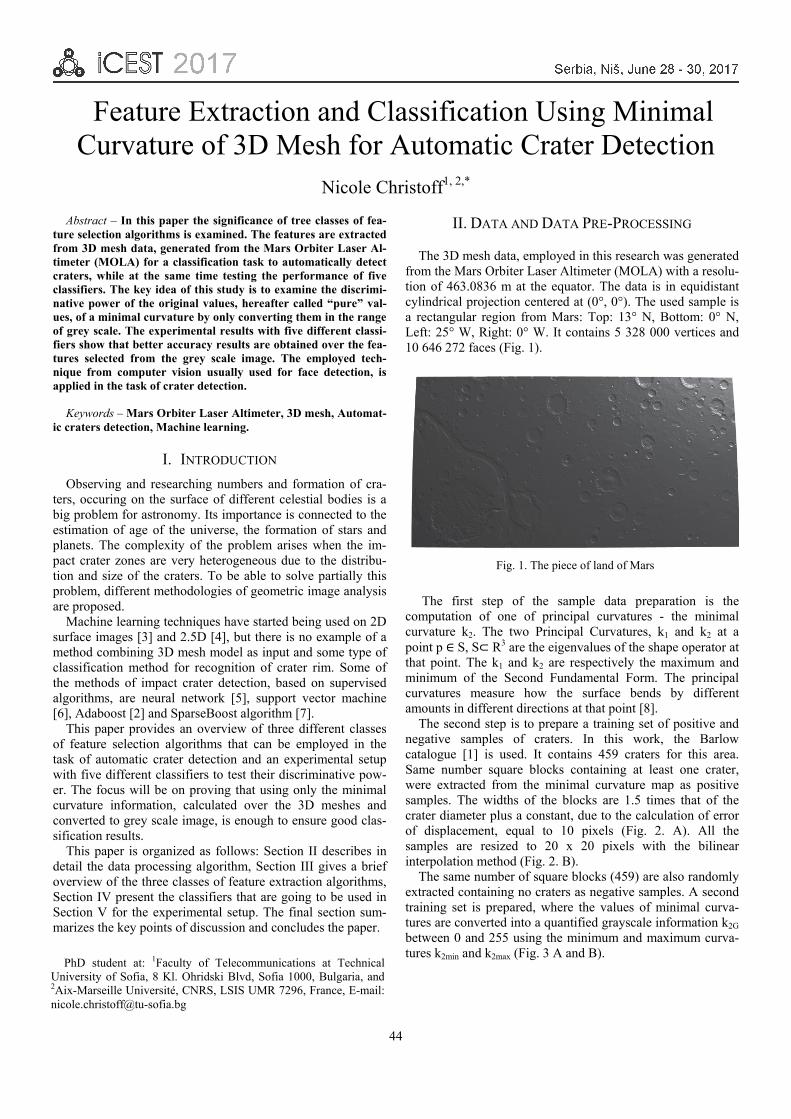
44

Feature Extraction and Classification Using Minimal Curvature of 3D Mesh for Automatic Crater Detection

Nicole Christoff1, 2,*

Abstract – In this paper the significance of tree classes of fea-ture selection algorithms is examined. The features are extracted from 3D mesh data, generated from the Mars Orbiter Laser Al-timeter (MOLA) for a classification task to automatically detect craters, while at the same time testing the performance of five classifiers. The key idea of this study is to examine the discrimi-native power of the original values, hereafter called “pure” val-ues, of a minimal curvature by only converting them in the range of grey scale. The experimental results with five different classi-fiers show that better accuracy results are obtained over the fea-tures selected from the grey scale image. The employed tech-nique from computer vision usually used for face detection, is applied in the task of crater detection.

Keywords – Mars Orbiter Laser Altimeter, 3D mesh, Automat-ic craters detection, Machine learning.

I. INTRODUCTION

Observing and researching numbers and formation of cra-ters, occuring on the surface of different celestial bodies is a big problem for astronomy. Its importance is connected to the estimation of age of the universe, the formation of stars and planets. The complexity of the problem arises when the im-pact crater zones are very heterogeneous due to the distribu-tion and size of the craters. To be able to solve partially this problem, different methodologies of geometric image analysis are proposed.

Machine learning techniques have started being used on 2D surface images [3] and 2.5D [4], but there is no example of a method combining 3D mesh model as input and some type of classification method for recognition of crater rim. Some of the methods of impact crater detection, based on supervised algorithms, are neural network [5], support vector machine [6], Adaboost [2] and SparseBoost algorithm [7].

This paper provides an overview of three different classes of feature selection algorithms that can be employed in the task of automatic crater detection and an experimental setup with five different classifiers to test their discriminative pow-er. The focus will be on proving that using only the minimal curvature information, calculated over the 3D meshes and converted to grey scale image, is enough to ensure good clas-sification results.

This paper is organized as follows: Section II describes in detail the data processing algorithm, Section III gives a brief overview of the three classes of feature extraction algorithms, Section IV present the classifiers that are going to be used in Section V for the experimental setup. The final section sum-marizes the key points of discussion and concludes the paper.

II. DATA AND DATA PRE-PROCESSING

The 3D mesh data, employed in this research was generated from the Mars Orbiter Laser Altimeter (MOLA) with a resolu-tion of 463.0836 m at the equator. The data is in equidistant cylindrical projection centered at (0°, 0°). The used sample is a rectangular region from Mars: Top: 13° N, Bottom: 0° N, Left: 25° W, Right: 0° W. It contains 5 328 000 vertices and 10 646 272 faces (Fig. 1).

The first step of the sample data preparation is the computation of one of principal curvatures - the minimal curvature k2. The two Principal Curvatures, k1 and k2 at a point p ∈ S, S⊂ R3 are the eigenvalues of the shape operator at that point. The k1 and k2 are respectively the maximum and minimum of the Second Fundamental Form. The principal curvatures measure how the surface bends by different amounts in different directions at that point [8].

The second step is to prepare a training set of positive and negative samples of craters. In this work, the Barlow catalogue [1] is used. It contains 459 craters for this area. Same number square blocks containing at least one crater, were extracted from the minimal curvature map as positive samples. The widths of the blocks are 1.5 times that of the crater diameter plus a constant, due to the calculation of error of displacement, equal to 10 pixels (Fig. 2. A). All the samples are resized to 20 x 20 pixels with the bilinear interpolation method (Fig. 2. B).

The same number of square blocks (459) are also randomly extracted containing no craters as negative samples. A second training set is prepared, where the values of minimal curva-tures are converted into a quantified grayscale information k2G between 0 and 255 using the minimum and maximum curva-tures k2min and k2max (Fig. 3 A and B).

PhD student at: 1Faculty of Telecommunications at TechnicalUniversity of Sofia, 8 Kl. Ohridski Blvd, Sofia 1000, Bulgaria, and2Aix-Marseille Université, CNRS, LSIS UMR 7296, France, E-mail:[email protected]

Fig. 1. The piece of land of Mars

45

III. FEATURE EXTRACTION

Tree classes of features are calculated to train and test dif-ferent classifiers: Local Binary Pattern operator (LBP), Haar-like and Scaled Haar-like feature. The LBP and Haar are an example of a typical computer vision computation pipeline for face recognition, used for dimension reduction preprocessing steps.

A. LBP Cascade Classifier

The Local Binary Pattern operator (LBP) was first intro-duced by [9] for byte adaptation of a previous study done by [10] and is a powerful texture descriptor. Texture is defined as a function of spatial variations in the pixel intensity of an im-age. The idea behind this operator is that common features, such as edges, lines, point, can be represented by a value in a particular numerical scale. As a result, 2124 features for each resized sample are obtained.

B. Haar-Like Cascade Classifier

Haar-like features are attributes extracted from Region of Interest (ROI) used in pattern recognition. The utilization of these features instead of handling gray or color level of the pixels directly was proposed in [11]. First, the pixel values inside the black area are added together; then the values in the white area are summed. Only eight types of square masks are used to extract feature, as seen in Fig. 4. Then the total value of the white area is subtracted from the total value of the black area. This result is used to categorize sub-regions. A total of 2048 features are obtained for each resized sample.

The weak classifiers become strong classifiers when ar-ranged in Haar-like cascade. They are able to detect structures despite illumination, color or scale variation. This method is one of the most popular techniques for face detection, firstly described by Viola and Jones [12].

C. Scaled Haar-like Feature

It is a variant of Haar-like feature. This feature is proposed by [2], which use the fact that large craters are usually deeper than small ones, and this means most of the Haar-like feature values of the large craters are larger than those of small ones. The scaled Haar-like feature is computed by division of the Haar-like feature value with a coefficient of the resolution of the sample to adjust the Haar-like features for large craters and small craters to the same scale. The number of scaled Haar-like features for all resized sample is the same as that of Haar-like features.

IV. TRAINING DIFFERENT CLASSIFIERS

Five popular classifiers are used in this study.

A. K-Nearest Neighbours Algorithm (KNN)

Feature extraction is performed on raw data prior to apply-ing KNN algorithm on the transformed data in feature space. A commonly used distance metric for continuous va-riables is Euclidean distance. Cosine similarity is very effi-cient to evaluate, especially for sparse vectors, as only the non-zero dimensions need to be considered.

B. Support Vector Machine (SVM)

SVM is a classier with good generalization power that uses the features extracted by the descriptor. SVM works basically by finding an optimal hyper plane that best separates the two classes. Kernel functions can be used with SVM in order to enable the classifier to deal with non-linearly separable classes. These functions modify the feature space trying to

Fig. 2. Positive sample "pure": (A) Window with size equal to 1.5

times diameter of the crater plus constant equal to 10 px, (B) The same sample, resampled to 20x20 pixels

Fig. 4. Eight type of masks are used for Haar-like feature extraction

Fig. 3. Positive sample in grey scale: (A) Window with size equal to

1.5 times diameter of the crater plus constant equal to 10 pixels, (B) The same sample, resampled to 20x20 pixels

46

transform it into a linear separable problem. Several types of kernel functions are commonly used: uniform (linear), Gaus-sian (Radial Basis Function (RBF)) [13], quadratic [14] and cosine.

C. Decision Tree

Decision Trees are a non-parametric supervised learning method used for classification and regression. The goal is to create a model in the form of a tree structure. It breaks down a dataset into smaller and smaller subsets while at the same time an associated decision tree is incrementally developed. The final result is a tree with decision nodes and leaf nodes. A decision node has two or more branches. The leaf node represents a classification or decision [15].

D. AdaBoost

Boosted Trees incrementally builds an ensemble by training each new instance to emphasize the training instances pre-viously mis-modeled. A typical example is AdaBoost. It is an approach to machine learning based on the idea of creating a highly accurate prediction rule by combining many relatively weak and inaccurate rules.

E. Bagged Tree

Bagging decision trees, an ensemble method, builds mul-tiple decision trees by repeatedly resampling training data with replacement, and voting the trees for a consensus predic-tion.

V. RESULTS

For the tests the k-fold cross validation procedure is ap-plied. 918 total samples of 918 are divided into 10 groups of equal size. Five different classifiers are trained each using 9 groups, holding out each of the groups. For each of the four classifiers, the group left out is tested. The 10 test results are averaged. All samples get to be used for both training and testing. The result is unbiased and with minimum variance.

The number of true positive detections is represented with TP (CR - detected craters, which are real craters and NCR – zones, with no craters), FP represents the number of false pos-itive detections (CR – detected craters are not actual craters and NCR – detected no crater zones are not actual no craters zones), FN represents the number of false negative detections (CR – un-detected real craters and NCR – undetected negative samples) and TN represents the number of true negative de-tections (CR – for positive samples and NCR – for no crater zones). The best scenario is obtaining larger TP CR and TP NCR and smaller FP (CR and NCR). There are 459 positive and same number (459) negative samples. The best detection rate, for original values of minimal curvature, using SVM with qua-dratic kernel function respectively TP CR: 418, FN CR: 42, TP NCR: 427 and FN NCR: 31. A good TP CR results are obtained using SVM (Gaussian), but the number of FP CR increase two times (see Table I).

TABLE I CONFUSION MATRIX FOR DIFFERENT CLASSIFIERS UNDER "PURE"

10 fold cross validation

ACTUAL

PREDICTED TP CR

TN CR

FN CR

FP NCR

TP NCR

TN NCR

FN NCR

FP CR

KNN

Euc

lide

an

1 130 330 373 85 3 63 397 449 9 5 33 427 458 0 7 25 435 457 1 9 18 442 458 0 11 14 446 458 0

Cos

ine

1 188 272 369 89 3 265 195 446 12 5 262 198 454 4 7 249 221 455 3 9 245 215 456 2 11 236 224 456 2

SVM

Linear 420 40 413 45 Quadratic 418 42 427 31

Cubic 401 59 431 27 Gaussian 426 34 382 76

Decision tree 345 115 374 84 Ensemble classifiers

AdaBoost 407 53 429 29 Bagged tree 402 58 406 52

TABLE II CONFUSION MATRIX FOR DIFFERENT CLASSIFIERS UNDER "GRAY"

10 fold cross validation

ACTUAL

PREDICTED TP CR

TN CR

FN CR

FP NCR

TP NCR

TN NCR

FN NCR

FP CR

KNN

Euc

lide

an

1 230 230 413 45 3 229 231 439 19 5 221 239 443 15 7 216 244 443 15 9 213 247 447 11 11 209 251 445 13

Cos

ine

1 275 185 391 67 3 375 85 453 5 5 389 71 450 8 7 389 71 451 7 9 394 66 451 7 11 395 65 449 9

SVM

Linear 427 33 420 38 Quadratic 452 8 442 16

Cubic 455 5 440 18 Gaussian 454 6 452 6

Decision tree 403 57 417 41

Ensemble classifiers

AdaBoost 428 32 251 207 Bagged tree 458 2 445 13

47

Using greyscale values of minimal curvature, better de-tection rate is obtained using SVM with Gaussian kernel func-tion respectively TP CR: 454, FN CR: 6, TP NCR: 452 and FN NCR: 6. The best TP CR (458) is resulted, which is one of the challenges in astrophysics, using Bagged tree, but the number of FP CR increase two times (13) (see Table II). In Fig. 5 is presented a comparative study with obtained accuracy results. The bins, colored in blue represent results for k2G “grey” training set and with green – k2 “pure” training set. Best accuracy detection rate for “pure” values of minimal curvature, we obtain using Bagged trees - 98.4%. For the greyscale values of k2, best accuracy of 92.0% is obtained with SVM, using quadratic kernel function (Fig. 5).

VI. CONCLUSION AND FUTURE WORK

In this paper, we have presented tree different methods for feature extraction from grey level image of minimal curvature, extracted from 3D mesh data, generated from the MOLA. We presented an overview of the ensemble of classifiers used to automatically detect craters on the surface of Mars. Thanks to the experimental results, we can conclude that the best per-forming classifier for crater detection is Bagged tree if we pass from RGB to grey scale image representation.

As future work, we plan to test those features on other types of calculated curvatures. Another step is to add the neural network back propagation of error classifier to the experimen-tal setup.

ACKNOWLEDGEMENT

This paper was supported by Contract No 162ПД0033-07 of Technical University-Sofia, Research Sector. Research project: «Segmentation and modeling of geometrical characte-ristics of 3D objects» - 2016.

REFERENCES

[1] N.G. Barlow, "Crater Size-Frequency Distributions and a Re-vised Martian Relative Chronology", Icarus, vol. 75, no. 2, pp. 285-305, 1988.

[2] K. Di, W. Li, Z. Yue, Y. Sun, and Y. Lui, "A Machine Learning Approach to Crater Detection From Topographic Data", Advances in Space Research, vol. 54, no. 11, pp. 2419-2429, 2014.

[3] T.F. Stepinski, W. Ding, and R. Vilalta, “Detecting Impact Craters in Planetary Images Using Machine Learning”, pp. 146-159, 2012.

[4] G.T. Vamshi, T.R. Martha, and K.V. Kumar, “An Object-Based Classification Method for Automatic Detection of Lunar Impact Craters From Topographic Data”, Advances in Space Research, vol. 57, pp. 1978-1988, 2016.

[5] J.R. Kim, J.Muller, S. van Gasselt, J.G. Morley, and G. Neu-kum, “Automated Crater Detection, a New Tool for Mars Car-tography and Chronology”, Photogramm. Eng. Remote Sens., vol. 71, no. 10, pp. 1205-1217, 2005.

[6] P.G. Wetzler, R. Honda, B. Enke, W.J. Merline, C.R. Chapman, and M.C. Burl, “Learning to Detect Small Impact Craters”, Proceedings 7th IEEE WACV/MOTION, pp. 178-184, 2005.

[7] Y. Wang, G. Yang, and L. Guo, “A Novel Sparse Boosting Method for Crater Detection in the High Resolution Planetary Image”, Advances in Space Research, vol. 56, no. 5, pp. 982-991, 2015.

[8] M.P. Do Carmo, Differential Geometry of Curves and Surfaces, pp. 2-30, 1976.

[9] T. Ojala, M. Pietikainen, and D. Harwood, "Performance Evalu-ation of Texture Measures with Classification Based on Kull-back Discrimination of Distributions", International Conference on Pattern Recognition, pp. 582-585, 1994.

[10] L. Wang, and D. He, "Texture Classification Using Texture Spectrum", Pattern Recognition, vol. 23, no. 8, pp. 905-910, 1990.

[11] P. Viola, and M. Jones, "Rapid Object Detection Using a Boosted Cascade of Simple Features", IEEE Computer Society Conference on Computer Vision and Pattern Recognition, pp. 511-518, 2001.

[12] P. Viola, and M. Jones, "Robust Real-time Face Detection", International Journal of Computer Vision, vol. 57, pp. 137-154, 2004.

[13] C.W. Hsu, C.C. Chang, and C.J. Lin., A Practical Guide to Support Vector Classification, 2016.

[14] W.S. Cleveland, and S.J. Devlin. "Locally Weighted Regression: An Approach to Regression Analysis by Local Fitting", Journal of the American Statistical Association, vol. 83, pp. 596-610, 1988.

[15] http://www.cs.princeton.edu/courses/archive/spr07/cos424/pape rs /mitchell-dectrees.pdf

Fig. 5. Accuracy

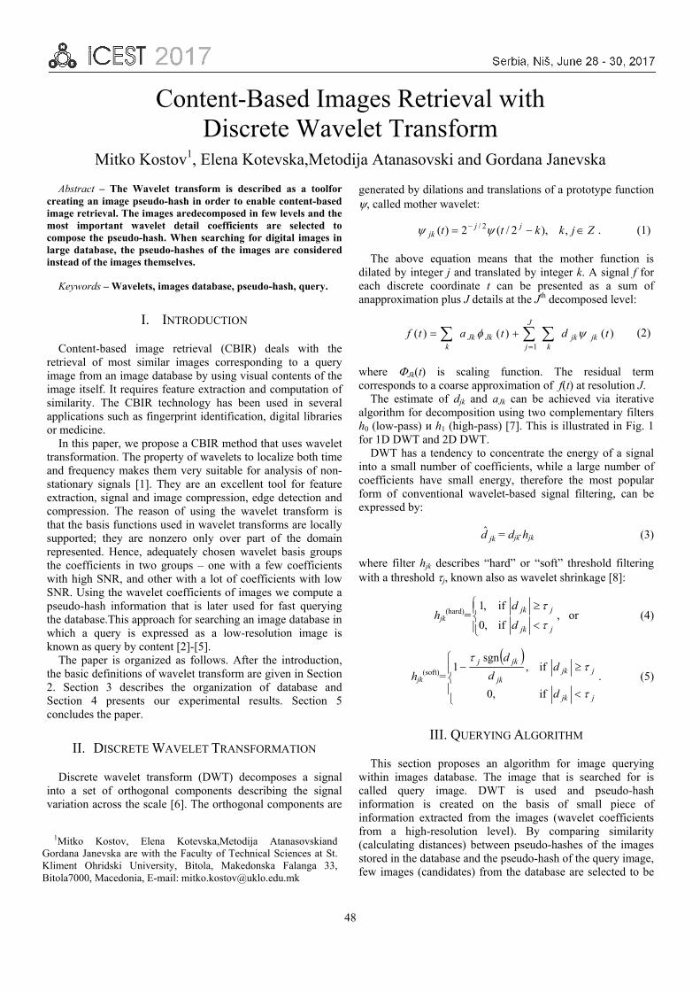
48

Content-Based Images Retrieval with Discrete Wavelet Transform

Mitko Kostov1, Elena Kotevska,Metodija Atanasovski and Gordana Janevska

Abstract – The Wavelet transform is described as a toolfor creating an image pseudo-hash in order to enable content-based image retrieval. The images aredecomposed in few levels and the most important wavelet detail coefficients are selected to compose the pseudo-hash. When searching for digital images in large database, the pseudo-hashes of the images are considered instead of the images themselves.

Keywords – Wavelets, images database, pseudo-hash, query.

I. INTRODUCTION

Content-based image retrieval (CBIR) deals with the retrieval of most similar images corresponding to a query image from an image database by using visual contents of the image itself. It requires feature extraction and computation of similarity. The CBIR technology has been used in several applications such as fingerprint identification, digital libraries or medicine.

In this paper, we propose a CBIR method that uses wavelet transformation. The property of wavelets to localize both time and frequency makes them very suitable for analysis of non-stationary signals [1]. They are an excellent tool for feature extraction, signal and image compression, edge detection and compression. The reason of using the wavelet transform is that the basis functions used in wavelet transforms are locally supported; they are nonzero only over part of the domain represented. Hence, adequately chosen wavelet basis groups the coefficients in two groups – one with a few coefficients with high SNR, and other with a lot of coefficients with low SNR. Using the wavelet coefficients of images we compute a pseudo-hash information that is later used for fast querying the database.This approach for searching an image database in which a query is expressed as a low-resolution image is known as query by content [2]-[5].

The paper is organized as follows. After the introduction, the basic definitions of wavelet transform are given in Section 2. Section 3 describes the organization of database and Section 4 presents our experimental results. Section 5 concludes the paper.

II. DISCRETE WAVELET TRANSFORMATION

Discrete wavelet transform (DWT) decomposes a signal into a set of orthogonal components describing the signal variation across the scale [6]. The orthogonal components are

generated by dilations and translations of a prototype function , called mother wavelet:

Zjkktt jjjk ,),2/(2)( 2/ . (1)

The above equation means that the mother function is dilated by integer j and translated by integer k. A signal f for each discrete coordinate t can be presented as a sum of anapproximation plus J details at the Jth decomposed level:

J

j kjkjk

kJkJk tdtatf

1

)()()( (2)

where Jk(t) is scaling function. The residual term corresponds to a coarse approximation of f(t) at resolution J.

The estimate of djk and аJk can be achieved via iterative algorithm for decomposition using two complementary filters h0 (low-pass) и h1 (high-pass) [7]. This is illustrated in Fig. 1 for 1D DWT and 2D DWT.

DWT has a tendency to concentrate the energy of a signal into a small number of coefficients, while a large number of coefficients have small energy, therefore the most popular form of conventional wavelet-based signal filtering, can be expressed by:

jkd = djkhjk (3)

where filter hjk describes “hard” or “soft” threshold filtering with a threshold j, known also as wavelet shrinkage [8]:

hjk(hard)=

jjk

jjk

d

d

if,0

if,1, or (4)

hjk(soft)=

jjk

jjkjk

jkj

d

dd

d

if,0

if,sgn

1. (5)

III. QUERYING ALGORITHM

This section proposes an algorithm for image querying within images database. The image that is searched for is called query image. DWT is used and pseudo-hash information is created on the basis of small piece of information extracted from the images (wavelet coefficients from a high-resolution level). By comparing similarity (calculating distances) between pseudo-hashes of the images stored in the database and the pseudo-hash of the query image, few images (candidates) from the database are selected to be

1Mitko Kostov, Elena Kotevska,Metodija AtanasovskiandGordana Janevska are with the Faculty of Technical Sciences at St.Kliment Ohridski University, Bitola, Makedonska Falanga 33,Bitola7000, Macedonia, E-mail: [email protected]

49

considered visually if some of them correspond to the image-query.

In order to calculate the pseudo-hash information for an RGB image, the following procedure is applied.

1) RGB image A is converted to A1 in YCbCr colour space, where Y is the luminance (intensity) component and Cb (blue chrominance) and Cr (red chrominance) are the blue-difference and red-difference chroma components, respectively;

2) The wavelet transform at level (j) is applied over the Y component of the image A1and three subimages with same resolution are obtained from the horizontal, vertical and diagonal detail coefficients, D(j,h), D(j,v) , D(j,d), respectively;

3) The three subimages D(j,h), D(j,v) , D(j,d)are summed up in one super-subimage D(k), that contains all the horizontal, vertical and diagonal detail coefficients;

4) The super-subimage D(k) is filtered by usinghard-threshold filtering given by (4) in order to keep only the most important coefficients D1

(j); 5)Positions (xi, yi) of the coefficients D1

(j) make up the pseudo-hash information for an image (the values of the coefficients are not important).

A database that keeps pseudohash information for theimages contains three relations according to their schemas given in Fig. 2.

In the relation tbl_image, the attribute id_image is theprimary key. This relation contains description of the images: name, description and location (if the images are picture filesin the file system).

The relation tbl_hash contains pseudohashinformation for each image in the database. The primary key is the attribute id, while the attributeid_imageis foreign key that takes its

values from the primarykey of the relation tbl_image. The plusminus attribute contains information for the sign of the wavelet coefficients.

The relation tbl_query contains the pseudo-hash calculated from the query image by applying the same algorithm as for the other images.

A list of candidateimages can be obtained by measuring the silimilarity between pseudo-hashesof the images in the database and the pseudo-hash of the query-image expressed as following

jijiji yyxx

M, 22

1

(5)

where (xi, yi) are coordinates of wavelet coefficient of images stored in the database, while (xj, yj) are coordinates of wavelet coefficient of the query image. It is not necessary the wavelet coefficients of candidate images to overlap the wavelet coefficients of query image.The influence of overlapping over non-overlapping coefficients can be controlled through the parameter . Choosing to be close to zero, the influence of overlapping coefficients over non-overlapping coefficients is bigger, and vice versa. Images with bigger value for the similarity M are likely to correspond to the query image.

The proposed algorithm is given in Fig. 3.

IV. EXPERIMENTAL RESULTS

Тhis Section presents the results obtained by experiments performed. Pseudo-hash information obtained from 1000 images by using the proposed algorithm from Setion 3 are stored in a Microsoft Access database with schema given in Fig. 2. Some of these images are shown in Fig. 4. The database contains data for a lot of similar images with people, animals, landscapes, objects, etc. The database does not contain the images themselves; the images are picture files in the file system.

The haar wavelet transform in three levels is applied over the Y components of the YCbCr converted images. The horizontal, vertical and diagonal detail coefficients from the

H02

H1 2f =a0,k

d1,k

a1,k

H02

H1 2d2,k

a2,k

.

.

.

H02

H1 2dJ,k

aJ,k

aJ-1

(a)

(b)

Fig. 1. Discrete wavelet transform tree for (a) 1D DWT, (b) 2D DWT

tbl_image

id_image : integername : textdescription : textlocation : text

tbl_hash

id : integerid_image : integerx_coord : integery_coord : integerplusminus : yes/no

tbl_query

id : integerx_coord : integery_coord : integerplusminus : yes/no

Fig. 2. Relation schemas in the images database

50

third level are summed up and the most important 5% pixels are kept – the pseudohash.

Next, the images shown in Figs. 5a, 5b, 5c and 6a, 6b, 6c are used as query-images.They are image id 87 and its versions id 1088, id 1089, and image id 501 and its versions id 1501, id 1503. The resolutionsof all the query images are 256x384. The most important third level wavelet coefficients of the three images are shown in Figs. 5d, 5e, 5f, and 6d, 6e, 6f, respectively. Their resolutions are 48x32, which means that only a few coefficients were taken into consideration for the calculation of the pseudo-hash.

The database already contains pseudo-hash information for the imageswith id 87 and id 501 in the table tbl_hash. Next step is estimating the similarity between pseudo-hashes of the images in the database and the pseudo-hash of the query-image by using (5). The parameter has value 0.1. A simple SQL SELECT statement used to process pseudohashes is:

SELECT Sum(1/(Sqr(([tblQuery].[xcoord]-[tblHash].[xcoord])^2+([tblQuery].[ycoord]-[tblHash].[ycoord])^2)+0.1)) AS M, tblHash.idimage

FROM tblQuery, tblHash GROUP BY tblHash.idimage ORDER BY Sum(1/(Sqr(([tblQuery].[xcoord]-

[tblHash].[xcoord])^2+([tblQuery].[ycoord]-[tblHash].[ycoord])^2)+0.1)) DESC;

The results of calculated similarities between the query

imagesand the images in the database are shown in the Tables I and II. It can be seen that the images with id 87 and id 501 have the highest similarity.

Query Image

DWT

Wavelet thresholdingDB

SQL query

RGB YCbCr

Pseudo-hash (coefficients coordinates)

Calculating similarity M

Fig. 3. Block diagram of the proposed algorithm

Fig. 4. Part of images database with 1000 images

(c) (f)

Fig. 5. (а) Query image id 87; (b) Query image id 1088; (c) Query image id 1089; (d-e-f) The most important wavelet coefficients at

level 3 of images with id 87, 1088, 1089

(b) (e)

(a) (d)

50 100 150 200 250

50

100

150

200

250

300

350

10 20 30

5

10

15

20

25

30

35

40

45

50 100 150 200 250

50

100

150

200

250

300

350

10 20 30

5

10

15

20

25

30

35

40

45

50 100 150 200 250

50

100

150

200

250

300

350

10 20 30

5

10

15

20

25

30

35

40

45

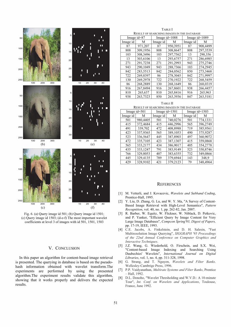
51

V. CONCLUSION

In this paper an algorithm for content-based image retrieval is presented. The querying in database is based on the pseudo-hash information obtained with wavelet transform.The experiments are performed by using the presented algorithm.The experiment results validate this algorithm, showing that it works properly and delivers the expected results.

REFERENCES

[1] M. Vetterli, and J. Kovacevic, Wavelets and Subband Coding, Prentice-Hall, 1995.

[2] Y. Liu, D. Zhang, G. Lu, and W. Y. Ma, "A Survey of Content-Based Image Retrieval with High-Level Semantics", Pattern Recognition, vol. 40, no. 1, pp. 262-82, Jan. 2007.

[3] R. Barber, W. Equitz, W. Flickner, W. Niblack, D. Petkovic, and P. Yanker, "Efficient Query by Image Content for Very Large Image Databases", Compcon Spring'93, Digest of Papers, pp. 17-19, IEEE, 1993.

[4] C.E. Jacobs, A. Finkelstein, and D. H. Salesin, "Fast Multiresolution Image Querying", SIGGRAPH '95 Proceedings of the 22nd Annual Conference on Computer Graphics and Interactive Techniques.

[5] J.Z. Wang, G. Wiederhold, O. Firschein, and S.X. Wei, "Content-based Image Indexing and Searching Using Daubechies' Wavelets", International Journal on Digital Libraries, vol. 1, no. 4, pp. 311-328, 1998.

[6] G. Strang, and T. Nguyen, Wavelets and Filter Banks. Wellesley-Cambrige Press, 1996.

[7] P.P. Vaidyanathan, Multirate Systems and Filter Banks, Prentice – Hall, 1992.

[8] D.L. Donoho, "Wavelet Thresholding and W.V.D.: A 10-minute Tour", Int. Conf. on Wavelets and Applications, Toulouse, France, June 1992.

(a) (d)

(b) (e)

(c) (f)

Fig. 6. (а) Query image id 501; (b) Query image id 1501; (c) Query image id 1503; (d-e-f) The most important wavelet

coefficients at level 3 of images with id 501, 1501, 1503

TABLE II RESULT OF SEARCHING IMAGES IN THE DATABASE

Image id=501 Image id=1501 Image id=1503 Image id M Image id M Image id M

501 980,4405 501 740,0276 501 774,1331415 372,4684 415 446,2996 565 396,2749491 339,702 472 408,8988 719 385,9561423 337,9365 565 389,1053 490 375,9287523 336,5647 445 387,8903 497 360,9072472 335,7105 423 387,1307 415 359,0868565 333,2177 434 386,9017 405 354,2778435 333,1247 791 383,9149 523 350,8746766 329,8053 407 383,6355 732 349,0866445 329,4135 789 379,6944 143 348,9 429 328,9102 421 379,2123 79 348,4964

TABLE I RESULT OF SEARCHING IMAGES IN THE DATABASE

Image id=87 Image id=1088 Image id=1089 Image id M Image id M Image id M

87 971,207 87 950,3951 87 908,4499808 309,1956 808 308,8647 808 297,3539103 308,3496 103 297,7562 13 290,356 13 303,6106 13 293,6757 271 286,6985271 291,7238 271 291,2993 943 275,2746943 290,1049 943 288,7366 103 274,2945842 283,5513 842 284,0562 850 273,3468722 269,8397 86 278,3045 842 271,9997130 269,2978 722 270,1922 722 268,545986 268,2889 130 268,1649 86 268,0319916 267,8494 916 267,8601 938 266,4457810 265,637 810 265,8416 916 265,963 938 263,7323 850 263,3936 847 263,5181

100 200 300

50

100

150

200

250

10 20 30 40

5

10

15

20

25

30

100 200 300

50

100

150

200

250

10 20 30 40

5

10

15

20

25

30

100 200 300

50

100

150

200

250

10 20 30 40

5

10

15

20

25

30

52

Medical Images Watermarking using Complex Hadamard Transform

Rumen P. Mironov1, Stoyan Kushlev2

Abstract – An algorithm for digital watermarking of medical

images using complex Hadamard transform is presented. The developed algorithm allow high detection of unauthorized access or attacks on the included watermark. The obtained experimental results for some attacks over the test medical images are made on the base of mean-squared error and signal to noise ratio of the reconstructed images.

Keywords – Medical Image Watermarking, Complex

Hadamard Transform, Orthogonal Transforms.

I. INTRODUCTION

Recent technological advances in Computer Science and Telecommunications introduced a radical change in the modern health care sector, including: medical imaging facilities, Picture Archiving and Communications System (PACS), Hospital Information Systems (HIS), information management systems in hospitals which forms the information technology infrastructure for a hospital based on the DICOM (Digital Imaging and Communication in Medicine) standard. These services are introducing new practices for the doctors as well as for the patients by enabling remote access, transmission, and interpretation of the medical images for diagnosis purposes [1], [2], [3].

Digital watermarking has various attractive properties to complement the existing security measures that can offer better protection for various multimedia applications [4]. The applicability of digital watermarking in medical imaging is studied in [5] and a further justification of the watermarking considering the security requirements in teleradiology is discussed in [2].

The new medical information systems required medical images to be protected from unauthorized modification, destruction or quality degradation of visual information. The other problem is a copyright protection of disseminated medical information over Internet. In this regard three main objectives of watermarking in the medical image applications: data hiding, integrity control, and authenticity are outlined in [5], which can provide the required security of medical images.

Every system for watermarking can be characterized with invisibility of the watermark, security of the watermark, robustness of the watermark and the ability for reversible

watermarking. The importance of each depends on the application and how it is used [6], and [7]. For the needs of medicine the main watermarking characteristics are:

Invisibility of the watermark – the embedded watermark should be invisible without reducing the quality of the original images;

Security of the watermark – secrecy to unauthorized persons of the information for the embedded watermark;

Robustness and fragility of the watermark – robust watermarking is resistant to possible attacks such as image processing and on the other hand fragile watermarks will allow high detection of unauthorized access or attacks on the watermark;

Reversibility of the watermark – removing of the embedded watermark should not reduce the quality of the original images.

Based on processing domain, watermark techniques can be separated as watermarking in spatial domain, watermarking in frequency domain and watermarking in phase domain of the input signal. According to the way of watermark preprocessing, discern two groups of methods: the first one is when the watermark is transformed in the domain of the input image and the second one is when the watermark is not transformed in the domain of the input image. Another classification is based upon the transparency of the watermark into the input images - the watermark is transparent or non- transparent.

Watermarking in spatial domain allow easy realization of the algorithms for watermarking. The disadvantage of using the spatial domain is that the watermarks have low efficiency and robustness. Using frequency and phase domain allow watermarks whit high transparency and robustness. Using transformations on the watermarks themselves assures high security agents unauthorized attacks.

The best way to test the watermark robustness is by simulating of unauthorized attacks. Unauthorized attacks are attacks against the integrity of the watermark. The most command attacks are unauthorized removal, adding or detection of watermark. The removal and adding of watermarks are active attacks while the detections of watermarks are passive attacks.

An outline of the medical image watermarking field that uses various techniques to embed watermark data and utilize various functions to detect tampered regions is given below in the paper [8].

In the present work an algorithm for digital watermarking of medical images using complex Hadamard transform is described. The developed algorithm allow high detection of unauthorized access or attacks on the included watermark. The obtained experimental results for some simulated attacks

1Rumen P. Mironov is with the Faculty of Telecommunications,Technical University of Sofia, Boul. Kl. Ohridsky 8, Sofia 1000,Bulgaria. E-mail: [email protected]

2Stoyan Kushlev is with the Faculty of Telecommunications,Technical University of Sofia, Boul. Kl. Ohridsky, 8, Sofia 1000,Bulgaria. E-mail: [email protected]

53

over the test medical images are made on the base of mean-squared error and signal to noise ratio of the reconstructed images. The robustness of the watermark against some attacks are tested with the post processing of watermarked images by adding of Salt and Pepper noise, Gaussian noise, filtration whit median filters and average filters.

II. MATHEMATICAL DESCRIPTION

The common results and properties, obtained from the one dimensional Complex Hadamard Transform, described in [9], can be generalized for two-dimensional Complex Hadamard Transform. In this case the 2D signals (images) can be represented by the input matrix [X] with the size NxN. The result is a spatial spectrum matrix [Y] with the same size. The corresponding equations for the forward and the inverse 2D CHT are:

][][1

][][

2 NN

NN

CHYCHN

X

CHXCHY

(1)

The Hadamard transformation is simple for implementation transformation, there for it is used for compression and watermarking of information. The proposed complex Hadamard transform matrix has the advantages of having similar structure as the well know real Hadamard matrix. The complex Hadamard matrix consists of only four values 1; -1; j; -j. The properties of complex Hadamard transform matrices and its applications in digital image processing are described in detail in [9], [10].

The developed algorithm for embedding of watermark is made in the following steps: Step 1: Preparation of the image – the image is

prepared for embedding using the forward complex Hadamard transformation.

Step 2: Embedding the watermark into the image – the embedding process of the watermark is based upon modifying the phase of the spectrum coefficients.

Step 3: Reconstruction of the image – the reconstruction of the image is done using the reverse complex Hadamard transformation.

The extraction of the watermark is made by the following steps: Step 1: Preparation of the watermark image – same as

in the embedding the image is prepared using the forward complex Hadamard transformation.

Step 2: Preparation of the non-watermarked image –for the extraction of the watermark in the decoder a non-watermark copy of the image is used. The non watermark image is prepared using the forward complex Hadamard transformation.

Step 3: Extracting the watermark from the image. Step 4: Reconstruction of the extracted watermark –

the reconstruction of the extracted watermark is done using the reverse complex Hadamard transformation.

Step 5: Estimating if the acquired watermark is valid – estimates if there were attacks agents the integrity of the watermark.


For the analyses of efficiency of the developed algorithm for watermarking of medical images three test images, shown in Fig. 1 (a), (b), (c), with size 512x512 and 256 gray levels are used.

These images are transformed by the 2D CHT with kernel

32x32. By this way the input image is divided on 256 sub-images with size 32x32, the input watermark (letter K) is embedded into the phase spectrum of some sub-images and the algorithm is simulated by the developed MATLAB program.

Fig. 1. (b) Input X-ray test image “Spine 2”

Fig. 1. (a) Input X-ray test image “Spine 1”

Fig. 1. (c) Input X-ray test image “Spine 3”

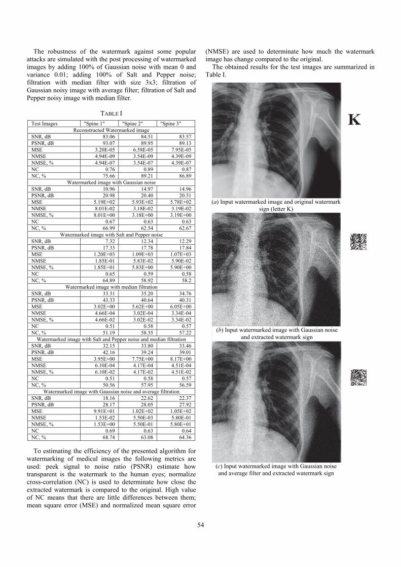
54

The robustness of the watermark against some popular attacks are simulated with the post processing of watermarked images by adding 100% of Gaussian noise with mean 0 and variance 0.01; adding 100% of Salt and Pepper noise; filtration with median filter with size 3x3; filtration of Gaussian noisy image with average filter; filtration of Salt and Pepper noisy image with median filter.

TABLE I

To estimating the efficiency of the presented algorithm for watermarking of medical images the following metrics are used: peek signal to noise ratio (PSNR) estimate how transparent is the watermark to the human eyes; normalize cross-correlation (NC) is used to determinate how close the extracted watermark is compared to the original. High value of NC means that there are little differences between them; mean square error (MSE) and normalized mean square error

(NMSE) are used to determinate how much the watermark image has change compared to the original.

The obtained results for the test images are summarized in Table I.

Test Images "Spine 1" "Spine 2" "Spine 3" Reconstructed Watermarked image

SNR, dB 83.06 84.51 83.57 PSNR, dB 93.07 89.95 89.13 MSE 3.20E-05 6.58E-05 7.95E-05 NMSE 4.94E-09 3.54E-09 4.39E-09 NMSE, % 4.94E-07 3.54E-07 4.39E-07 NC 0.76 0.89 0.87 NC, % 75.66 89.21 86.89

Watermarked image with Gaussian noise SNR, dB 10.96 14.97 14.96 PSNR, dB 20.98 20.40 20.51 MSE 5.19E+02 5.93E+02 5.78E+02 NMSE 8.01E-02 3.18E-02 3.19E-02 NMSE, % 8.01E+00 3.18E+00 3.19E+00 NC 0.67 0.63 0.63 NC, % 66.99 62.54 62.67

Watermarked image with Salt and Pepper noise SNR, dB 7.32 12.34 12.29 PSNR, dB 17.33 17.78 17.84 MSE 1.20E+03 1.09E+03 1.07E+03 NMSE 1.85E-01 5.83E-02 5.90E-02 NMSE, % 1.85E+01 5.83E+00 5.90E+00 NC 0.65 0.59 0.58 NC, % 64.89 58.92 58.2

Watermarked image with median filtration SNR, dB 33.31 35.20 34.76 PSNR, dB 43.33 40.64 40.31 MSE 3.02E+00 5.62E+00 6.05E+00 NMSE 4.66E-04 3.02E-04 3.34E-04 NMSE, % 4.66E-02 3.02E-02 3.34E-02 NC 0.51 0.58 0.57 NC, % 51.19 58.35 57.22

Watermarked image with Salt and Pepper noise and median filtration SNR, dB 32.15 33.80 33.46 PSNR, dB 42.16 39.24 39.01 MSE 3.95E+00 7.75E+00 8.17E+00 NMSE 6.10E-04 4.17E-04 4.51E-04 NMSE, % 6.10E-02 4.17E-02 4.51E-02 NC 0.51 0.58 0.57 NC, % 50.56 57.95 56.59

Watermarked image with Gaussian noise and average filtration SNR, dB 18.16 22.62 22.37 PSNR, dB 28.17 28.05 27.92 MSE 9.91E+01 1.02E+02 1.05E+02 NMSE 1.53E-02 5.50E-03 5.80E-01 NMSE, % 1.53E+00 5.50E-01 5.80E+01 NC 0.69 0.63 0.64 NC, % 68.74 63.08 64.36

(a) Input watermarked image and original watermark sign (letter K)

(b) Input watermarked image with Gaussian noise and extracted watermark sign

(c) Input watermarked image with Gaussian noise and average filter and extracted watermark sign

55

Fig. 2. Results for watermarked image "Spine 2" with different post processing attacks

In Fig. 2 (a)-(f) the visual results for watermarked image "Spine 2" with different post processing attacks are shown. On the right corner of each image is shown the extracted watermark.

IV. CONCLUSION

An algorithm for digital watermarking of medical images using complex Hadamard transform is presented. The obtained experimental results for some attacks over the test medical images are made on the base of mean-squared error and signal to noise ratio of the reconstructed images. They show that the developed algorithm allows high detection of unauthorized access or attacks on the included watermark. On the other hand the embedded watermark is practically invisible for the doctors and retains largely the information in the original images. All this leads to the conclusion that the developed algorithm for watermarking can be used successfully for watermark protection of medical data.

V. ACKNOWLEDGEMENT

The author thanks the National Fund for Scientific Research of the Bulgarian Ministry of Education and Science for the financial support by the contract I-02/1.

VI. REFERENCES

[1] P. Koushik, G. Ghosh, and M. Bhattacharya, "Biomedical Image Watermarking in Wavelet Domain for Data Integrity Using Bit Majority Algorithm and Multiple Copies of Hidden Information", American Journal of Biomedical Engineering, 2012, vol. 2, no. 2, pp. 29-37.

[2] H. Nyeem, W. Boles, and C. Boyd, "A Review of Medical Image Watermarking Requirements for Teleradiology", Journal Digital Imaging, 2013, vol. 26, pp. 326-343.

[3] L. Siau-Chuin, and J. M. Zain, "Reversible Medical Image Watermarking for Tamper Detection and Recovery", 3rd IEEE International Conference on Computer Science and Information Technology, 2010, vol. 5, pp. 417-420.

[4] I. Cox, M. Miller, J. Bloom, J. Fridrich, and T. Kalker, Digital Watermarking and Steganography, 2nd Edition, Elsevier, Burlington, 2007.

[5] G. Coatrieux, H. Maitre, B. Sankur, Y. Rolland, and R. Collorec, "Relevance of Watermarking in Medical Imaging", IEEE EMBS International Conference on Information Technology Applications in Biomedicine, 2000, pp. 250–255.

[6] W.K. Pratt, Digital Image Processing, 4th Ed., John Wiley & Sons. Inc., Hoboken, New Jersey, 2007.

[7] R.C. Gonzalez, and R.E. Woods. Digital Image Processing, Third Ed., Pearson Education Inc., 2008.

[8] A. Ustubioglu, and G. Ulutas, "A New Medical Image Watermarking Technique with Finer Tamper Localization", Journal of Digital Imaging, Springer International Publishing, 2017, pp.1-17.

[9] R. Mironov, and R. Kountchev, "Analysis of Complex Hadamard Transform Properties", XLI International Scientific Conference on Information, Communication and Energy Systems and Technologies, ICEST 2006, 26 June - 1 July, Sofia, Bulgaria, 2006, pp.173-176.

[10] B. Falkowski, and S. Rahardja, "Complex Hadamard Transforms: Properties, Relations and Architecture", IEICE Trans. Fundamentals, vol. E87-A, no. 8, August 2004.

(d) Input watermarked image with median filter and extracted watermark sign

(e) Input watermarked image with 100% salt and pepper noise and extracted watermark sign

(f) Input watermarked image with 100% salt and pepper noise and median filter and extracted

watermark sign

Session 4A:

ELECTRONICS AND CONTROL SYSTEMS

59

Energy Efficiency of Wireless Sensor Networks T. R. Nikolić, G. S. Nikolić, M. K. Stojčev, B. D. Petrović, G. S. Jovanović*

Abstract – Wireless sensor network includes a large number of simple sensor nodes that consist of sensor, microcontroller and transceiver block. Sensor nodes usually operate with non-rechargeable batteries so that the power consumption becomes a very important issue in the development of these networks. The main goal of this paper is to reduce power consumption of sensor nodes and extend the lifetime of batteries. The total power consumption of a sensor node is evaluated in real application conditions by using information from datasheets for all its blocks. Simulation results show that power-gating technique is superior in respect to power-saving, especially in the case when lower duty-cycling is implemented.

Keywords – Wireless sensor networks, Energy efficiency, Power-saving, Power-gating.

I. INTRODUCTION

Low-power wireless system is constituent of many contemporary applications. It includes a number of wireless sensor nodes that collect information from external environment with sensors, then process the information, and communicate with other neighboring nodes in the network. Such system has to operate for an extended period of time with only a limited power source available, and is usually constrained to a limited size (i.e. small battery could be used) [1]. For most situations the use of rechargeable batteries is not a realistic option. For instance, buried nodes used in wireless underground sensor networks and nodes embedded inside the walls of buildings, in the roads, or in the internal structures of a bridge, typically cannot employ rechargeable batteries [2]. Therefore, the main goal is to extend as much as possible the lifetime of non-rechargeable batteries.

Two design areas can be exploited in order to increase the lifetime of a battery: networking protocols and power management. The focus of this work is on the specific power management techniques. They provide an efficient energy solution for wireless sensor network (WSN) nodes that are powered by non-rechargeable batteries.

We identified two power management aspects that allow a significant extension of the battery lifetime [2]:

1) The conventional power-saving approach is based on setting the standby pin (sometimes called shutdown or power save). The majority of the blocks in a WSN node have some sort of standby pin. However, such control cannot effectively switch off all the internal circuitries of the module. The quiescent current for the power-saving mode is small but still higher than 1 μA.

T. R. Nikolić, G. S. Nikolić, M. K. Stojčev, B. D. Petrović, G. S. Jovanović, are with the Faculty of Electronic Engineering, Niš, Serbia.

2) The power-gating technique is based on the introduction of an electronic switch between an electronic module or chip and the power-supply line. It can be applied in WSNs as a way to save energy for both active and sleep modes of a device [3]. Therefore, it is possible to temporarily shut down blocks of circuitries that are not in use. For instance, while the sensor node is taking measurements usually, the radio transceiver is not required and it can be turned off.

By using power-saving, the module can quickly return to normal operation as soon as the standby pin returns to disabled mode. The main disadvantage of the power-gating technique is the delay caused by completely turning off/on a device (can be as high as 1 s). However, if this delay is not so critical for a given WSN application, a significant energy reduction can be achieved by means of power-gating.

In this paper we estimate the energy consumption of the wireless sensor node in real application conditions by using information from datasheets for all its building blocks (microcontroller, sensor and transceiver), for both mentioned power management techniques. Next to that, we show in what cases it is justified to use power-gating technique in order to extend the lifetime of batteries.

The rest of the paper is organized as follows. Section two considers energy consumption of a wireless sensor node and techniques for its reduction. Section 3 gives brief description of activities of sensor node in real applications. Experimental results are presented in Section 4. Concluding remarks are given in Section 5.

II. STRUCTURE OF SENSOR NODE FROM ENERGY

CONSUMPTION POINT OF VIEW

A low-power wireless system comprises a number of wireless sensor nodes, and each node consists of several functional blocks. The Fig. 1 shows a simple architecture of a typical wireless sensor node which is used in many applications. In our current design, the energy source is a battery (energy harvesting unit can be used in future design). The power management unit generates the required supply voltages and handles power allocation of all functional blocks within node. The sensor block collects information about the conditions in the environment and generates data which is processed by a microcontroller. The transceiver block sends/receives data to/from the access point or neighboring wireless sensor nodes. In addition, the microcontroller handles with switching on/off the various functional blocks, processes the sensed data, and drives the transceiver.

60

Fig. 1. Block diagram of a low-power wireless sensor node

The three main ways in which wireless sensor node consumes energy are sensing, communication and data processing. For each unit of useful work it performs, the node consumes different amount of energy. In a low-power wireless sensor node shown in Figure 1, all the functional blocks must be carefully specified and designed to minimize the total system power. In terms of consumption of sensor node, we consider a processor, a sensing module, and a radio transceiver. These blocks can be in active or inactive (sleep) state. Therefore, for one beacon period, TBP, we define the time interval during which the sensor node is active as TON, and the time interval during which the sensor node is inactive (sleep) as TOFF.

At the beginning, in order to estimate energy consumption, we consider the following scenario. The sensor node periodically wakes up, performs some processing (10% of time TON), takes measurements (50% of time TON), sends/receives data to/from the neighboring node (30% of time TON), performs more processing (10% of time TON), and finally sleeps again (time TOFF). In such node we apply two power management techniques: a) the power-saving technique, that is, the use of standby/sleep pins already available at the sensing and radio modules, and b) the power-gating technique, implemented externally. It is assumed that the power source (e.g., batteries) is directly connected to the devices, that is, no additional loss due the existence of a voltage regulator or DC-DC converter. Table 1 shows the values for the power consumed in each task/state that are based on off-the shelf analog switches and modules used in wireless sensor nodes [2].

TABLE 1 POWER PROFILE FOR A WSN NODE

Microcontroller Sensor Transceiver Active (regular operation)

5 mW 30 mW 350 mW

Inactive (power saving) 2 W 5 W 20 W

Inactive (power gating) 2 W 1 W 1 W

Researches show that even at low radio on-time operation (radio on-time, or duty-cycle, is approximately 1-2%) the energy needed for communication is about an order of magnitude more expensive that all other operations combined [4]. From Table 1 we can conclude that the wireless transceiver consumes the highest power in active and inactive

(power saving) state in respect to the other blocks. In inactive state with applying power gating technique the power consumption of the transceiver block is significantly reduced.

During simulation, we consider and compare three cases:

1) Active mode – all constituents of the sensor node are active during the time interval TON, while during the time interval TOFF they switch to power-saving mode;

2) Power-saving mode – each constituent of the sensor node is active during part of TON, only, when it is addressed, and after that enters into power-saving mode for the rest of TON and TOFF;

3) Power-gating mode – each constituent of the sensor node is active during part of TON, only, when it is addressed, and after that enters into power-gating mode for the rest of TON and TOFF.

Total energy consumption is calculated as the sum of energy consumption in the active state and the idle (sleep) state, taking into account all the blocks of the sensor node

sleepidletranscmcusensleepidleactivetotal EEEEEEE // (1)

Simulation results shown in Figure 2 present the total energy consumption levels for one year period in respect to different application duty cycles (expressed as number of measurements per day), for three mentioned cases. The total energy consumption per year for the power-saving mode is calculated as the sum of the active and the inactive (power-saving) values. For the power-gating mode, similarly, it is the sum of active and the inactive (power-gating) values. For calculation of energy consumption per year, the values for the consumed power, presented in Table 1, are used.

102

103

104

105

102

103

104

105

106

Time period between adjacent activations of the sensor node [s]

Ene

rgy

cons

umpt

ion

per

year

[J]

Power-saving mode

Active mode

Power-gating mode

Fig. 2. Total energy consumption for three cases

As can be seen from Fig. 2, energy consumption is reduced by applying both power management techniques. Power-gating technique is superior with respect to power-saving technique when the number of sensor node activations is reduced. In general, for all three cases, as the duty cycle decreases the energy consumption decreases, too. For example, in the case of power-gating mode, when

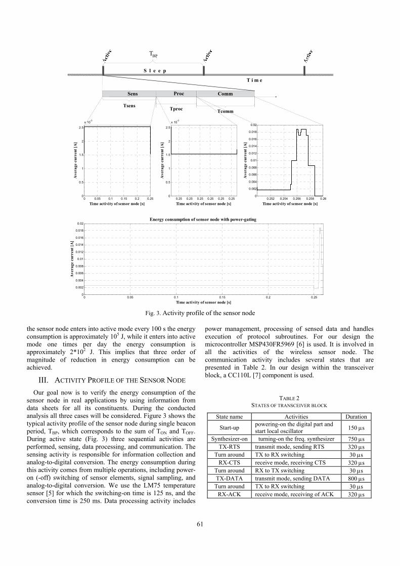
61

Sens Proc

iBPT

Comm

TsensTproc Tcomm

S l e e p

T i m e

0 0.05 0.1 0.15 0.2 0.250

0.002

0.004

0.006

0.008

0.01

0.012

0.014

0.016

0.018

0.02Energy consumption of sensor node with power-gating

Time activity of sensor node [s]

Ave

rage

cur

rent

[A

]

0 0.05 0.1 0.15 0.2 0.250

0.5

1

1.5

2

2.5

x 10-3


Ave

rage

cur

rent

[A

]

0.25 0.25 0.25 0.25 0.25 0.250

0.5

1

1.5

2

2.5

x 10-3


Ave

rage

cur

rent

[A

]

0.252 0.254 0.256 0.258 0.260

0.002

0.004

0.006

0.008

0.01

0.012

0.014

0.016

0.018

0.02


Ave

rage

cur

rent

[A

]

Fig. 3. Activity profile of the sensor node

the sensor node enters into active mode every 100 s the energy consumption is approximately 105 J, while it enters into active mode one times per day the energy consumption is approximately 2*102 J. This implies that three order of magnitude of reduction in energy consumption can be achieved.

III. ACTIVITY PROFILE OF THE SENSOR NODE

Our goal now is to verify the energy consumption of the sensor node in real applications by using information from data sheets for all its constituents. During the conducted analysis all three cases will be considered. Figure 3 shows the typical activity profile of the sensor node during single beacon period, TBP, which corresponds to the sum of TON and TOFF. During active state (Fig. 3) three sequential activities are performed, sensing, data processing, and communication. The sensing activity is responsible for information collection and analog-to-digital conversion. The energy consumption during this activity comes from multiple operations, including power-on (-off) switching of sensor elements, signal sampling, and analog-to-digital conversion. We use the LM75 temperature sensor [5] for which the switching-on time is 125 ns, and the conversion time is 250 ms. Data processing activity includes

power management, processing of sensed data and handles execution of protocol subroutines. For our design the microcontroller MSP430FR5969 [6] is used. It is involved in all the activities of the wireless sensor node. The communication activity includes several states that are presented in Table 2. In our design within the transceiver block, a CC110L [7] component is used.

TABLE 2 STATES OF TRANSCEIVER BLOCK

State name Activities Duration

Start-up powering-on the digital part and start local oscillator 150 s

Synthesizer-on turning-on the freq. synthesizer 750 s TX-RTS transmit mode, sending RTS 320 s

Turn around TX to RX switching 30 s RX-CTS receive mode, receiving CTS 320 s

Turn around RX to TX switching 30 s TX-DATA transmit mode, sending DATA 800 s

Turn around TX to RX switching 30 s RX-ACK receive mode, receiving of ACK 320 s

62

In order to achieve reduction in energy consumption in a sensor node operation, in our design with data from datasheets, we propose using two techniques, power-saving and power-gating. Power-saving approach is based on using standby pin for switching on/off the sensor node architecture between active and sleep state. In this case, the average current at a given supply voltage (power consumption) in sleep state corresponds to value from datasheet for each block of the sensor node. Power-gating approach uses load switches for switching on/off the sensor element and the transceiver block with the aim to switch-off the leakage currents of inactive elements. As load switch TPS22908 [8] is used. In this case, the quiescent current for this load switch is used as average current in sleep state.

IV. EXPERIMENTAL RESULTS

In order to verify our proposal, we have conducted an analysis for all three mentioned cases. The simulation is carried out by using Matlab tool. With aim to calculate the energy consumption for all constituents of the sensor node, individually, data from the datasheets relating to the average current are used. The supply voltage of 3V is used. The total energy consumption is calculated for one year period in respect to different measurement frequency. Simulation results in Matlab tool, for active, power-saving and power-gating mode, are presented in Fig. 4.

102

103

104

105

101

102

103

104

105

106

Time period between adjacent activations of the sensor node [s]

Ene

rgy

cons

umpt

ion

per

year

[J]

Power-saving mode

Active mode

Power-gating mode

Fig. 4. Total energy consumption in real conditions

By analyzing Fig. 4 we can conclude the following:

1) In general, for both power-saving and power-gating technique, as the time period between two measurements increases the energy consumption decreases, but this reduction is more pronounced in power-gating. For example, in the case of power-gating mode, when the sensor node performs measurement every 100 s the energy consumption is approximately 800 J, while for measurements one times per day the energy consumption is approximately 50 J. This implies that the reduction of 16 times can be achieved.

2) Power-gating technique is superior with respect to the power-saving technique, for any period of measurement. For example, when the sensor node is activated at every 103 s, the

energy consumption is approximately 100 J when power-gating is implemented, and 500 J for power-saving, while for active mode is about 1.7*105 J.

V. CONCLUSION

Nowadays, WSNs are widely used in many applications due to number of advantages such as reduced cost and flexibility. However, energy consumption in wireless sensor nodes with non-rechargeable batteries is very important issue. In this paper we have presented two energy efficient techniques that can be used in order to extend the lifetime of batteries. For both techniques we have estimated the energy consumption of all building blocks of the wireless sensor node. With aim to show a justification of utilization of the power gating technique in real applications we have conducted analysis by using information from datasheets. Simulation results show that the energy consumption of the sensor node is significantly decreased when power-gating technique is implemented (one order of magnitude in regard to power-saving). The obtained results provide the sensor node designer to make a correct choice which relate to the power management technique and selection of beacon time.

ACKNOWLEDGEMENT

This work was supported by the Serbian Ministry of Education and Science, Project No TR-32009 – "Low power reconfigurable fault-tolerant platforms".

REFERENCES

[1] A. Burdett, "Ultra-Low-Power Wireless Systems: Energy-Efficient Radios for the Internet of Things", IEEE Solid-State Circuits Magazine, vol. 7, no. 2, Spring 2015, pp. 18-28.

[2] A. Silva, M. Liu, and M. Moghaddam, "Power-Management Techniques for Wireless Sensor Networks and Similar Low-Power Communication Devices Based on Nonrechargeable Batteries", Journal of Computer Networks and Communic., 2012, Art. ID 757291, 10 pages.

[3] M.A. Pasha, S. Derrien, and O. Sentieys, "Toward Ultra Lowpower Hardware Specialization of a Wireless Sensor Network Node", IEEE 13th International Multitopic Conference (INMIC’09), pp. 1-6, Islamabad, Pakistan, December 2009.

[4] S. Aggarwal, and R. Rani, "A Review of Fault Detection Techniques for Wireless Sensor Networks", International Journal of Computer Science Issues (IJCSI), July 2013, vol. 10, issue 4, no. 1, pp. 127-138.

[5] Maxim Integrated, Datasheet for Digital Temperature Sensor and Thermal Watchdog with 2-Wire Interface, available at https://datasheets.maximintegrated.com/en/ds/LM75.pdf, (accessed March 2017)

[6] Texas Instruments, datasheets for MSP430™ ultra-low-power Microcontrollers, http://www.ti.com, (accessed March 2017)

[7] Texas Instruments, datasheet for Value Line Transceiver CC110L, available at http://www.ti.com/product/cc110L, (accessed March 2017)

[8] Texas Instruments, Low Ron Load Switch, http://www.ti.com/lit/ds/symlink/tps22908.pdf

63

Fig. 2. SDA line, message structure

Fig. 1. Communication via SDA and SCL lines

Development of I2C Communication Based on Logics

Pavel Hubenov

Abstract - The fundamental purpose of this article is to demonstrate how to develop logic gates based driver for communication between two different hardware devices via I2C bus. Once the driver is assembled should be used among peripheral devices captured on this bus. The scope here is high level messages based on designed modules. Avoided is description of low level design which is fundamental for all blocks. Accordingly, the specification of the system, master and slave devices could be different quantity but synchronized. Requirements to the master devices are higher because of its functionality. The example presents driver to communicate with EEPROM memory 24C02. Analysis of researched results [1].

Keywords - Logic gates, I2C, EEPROM, CPLD.

I. INTRODUCTION

Inter-Integrated Circuit (shorted as I2C), pronounced I-squared-C, also called TWI, two wire interface, is a multi-master, multi-slave, single-ended, serial computer bus. Differentiating from other buses this one is for onboard communication.

According to the speed there are several types of the bus from original 100kHz till reach 5MHz ultra-fast mode. Its application is spread outwards of computer boards. Small projects which include just a minor functional processor are equipped with outside located sensors, switches, memories and etc., communicated via this bus. As a requirement of the developed driver is accepted original 100kHz clock frequency because of the wider usage [2].

There are two lines ensured the communication itself – SDA, serial data and SCL, serial clock, Fig. 1. First one provides messages which contained strongly defined structured data. The second one guarantees the clock which is responsible for synchronization of the provided data. The driver development is based on strongly recommended structured messages for I2C bus, Fig. 2.

Properly communication demands to be realized messages with strongly recommended structured data, Fig. 2. According to the example using eeprom memory 24C02 and its specification, there are two different modes – read and write. The Low Significant Bit statement of the DEVICE ADDRESS message, LSB, defines which mode is selected – to write, if it is high level, or to read – low level. Next 3 bits set hardware adjusted address of the device. Most Significant bits “1010”

are hard cored default starting statements of the message, Fig. 2a.

When this message is sent on the I2C bus, a slave device, which has same hardware adjusted address on own pinouts, will receive and process the contained data. Then it will response with very short pulse as an acknowledge bit, ACK, which has to be detected by the master device within SCL is low levelled. After this bit is processed by the master device, it sends the second message, containing the address of the desired byte in the memory, Fig. 2b. An acknowledge bit is followed to enable the master device’s last message providing the byte which should be saved, Fig. 2c.

All three messages have to be synchronized referred to serial clock line, SCL. Basically, every transition occurred on SDA line – raised and falling edge of the messages has to be triggered when SCL line is low levelled.

Other case, when “Read” mode is desired, to read the current written memory cell is necessary to run first message from Fig. 2a with high level of the low significant bit, LSB. Then after the acknowledge bit, the memory sent a response which master device can process [3].

Pavel Hubenov is PhD student at Technical University ofGabrovo, 5300 Gabrovo, 4 Hadji Dimitar street, Bulgaria, E-mail: [email protected].

64

Fig. 3. Block schematic of the driver

Fig. 4. Block schematic of the 1-byte multiplexer

Fig. 5. Comparator of two 1-byte messages

II. DEVELOPMENT MODEL OF THE BASIC MODULES

The block schematic is presented in Fig. 3. A multiplexer MUX provides all input data to the inputs of a comparator, which routes it to the inputs of the shift register with parallel inputs and serial output, PISO. Control Module enables the shift register sending and the whole 8 bits word loaded on the multiplexer inputs, is transmitted sequentially on the SDA bus outwards to the memory. Pulses from this bus are delivered via internal feedback bus FBIn to Control Module which pass them through shift register with serial inputs and parallel outputs, SIPO, to the Comparator. Different pinout is used, as an input, externally connected outside the integrated circuit to SDA bus, for monitoring the acknowledge signal from the memory, called external feedback FBEx. If both compared messages by the comparator are different an error occurred. If not, Control Module waits for the low level of the acknowledge signal, via FBEx and if so, select next channel of the multiplexer and the same execution is following [4].

A. Multiplexer

Multiplexer, MUX, module is a tripled 8 bits’ multiplexer with adjacent data inputs, address inputs and 8 bits output. The number of the inputs depends on the desired functionality. Presented one in Fig. 4 is based on 8 multiplexers with 3 inputs each [5].

The number of the inputs of each multiplexer, NMUXin, is in function of the number of messages, NMESS, to be loaded:

NMUXin = NMESS. (1)

According to the specification of the memory device, there is a mode of sequential reading with more than 3 words. After that is defined the number of the common addresses inputs, NMUXadd:

NMUXin = 2 NMUXadd. (2)

The number of the used multiplexers, NMUX, depends on the number of the bits, NMESSbits, of each message, i.e. its length:

NMUX = NMESSbits. (3)

As per the Fig. 2, to load mentioned three 1-byte messages simultaneously, the multiplexer needs 3x1 byte inputs. In this case, first message has to be load to inputs labeled as DA7-DA0(Data Address). Second one, to inputs WD7-WD0(Word Data) and third one to D7-D0(Data). Another approach is using one 1-byte input, and dynamically changed data which transition should be in the meantime between the last bit of the message and approximately at the same time or around the acknowledge, ACK, received bit. Disadvantage is rescued synchronization and complicated extra module to ensure this delay.

B. Comparator

Basically, this module compares both 8 bits messages – input and output one of both shift registers, Fig. 5. They have to be absolutely the same transferred via internal feedback, FBIn or external feedback FBEx. Otherwise, there is an internal problem for the environment itself, or external one over the hardware connections, if FBEx has failed. In both cases, Control Module should stop processing and generate warning on Y. It decides which feedback to be used.

To develop this module is necessary to be defined inputs for compared words, NCOMPin:

NCOMPin= NMESSbits. (4)

This module is peripheral, for verification only, connected to multiplexer – shift register bus.

65

Fig. 7. Shift register with parallel inputs and serial output

Fig. 6. Shift register with parallel inputs and serial output

Fig. 8. SDA and SCL synchronization

C. Shift Register with Parallel Inputs and Serial Outputs

Register with parallel inputs and serial output, PISO, provides messages in pulse sequence, based on D-latches synthesis, Fig. 6. It is a standard register. The input numbers, NPISOin, are as follow:

NPISOin= NCOMPin. (5)

When is designed this module, should be taken into account whether it has to be able to memorize the message or not.

If it captures all P7 - P0 statements internally, and within message sending, input statements are enabled to be changed, the internal triggers have to be reset after the last bit is sent and before acknowledge bit negative pulse is expired.

D. Shift Register with Serial Input and Parallel Outputs

Register with serial input and parallel outputs, SIPO, provides messages from pulse sequence to 1-byte parallel statements, based on D-latches synthesis. Used is a standard register schematic, with serial input and parallel outputs, Fig. 7. The number of outputs, NSIPOout, is in function of number of messages length:

NSIPOout= NCOMPin. (6)

E. Control Module

This module is responsible to process the exact input clock frequency, to provide it reduced to different modules, ensures synchronization among all of them, manage enabling or disabling their functions. Based on the requirement for fSCL=100 kHz, the input counter has to divide fundamental frequency, fCLK, n times, Fig. 8, as follow:

n=TSCL/TCLK, (7)

where n is the difference in times. Since SDA and SCL pulses are shifted to 90 degrees, the shifter sub-module has to ensure

a delay for accurate transition of SDA exactly when SCL is in the middle of its low level. The delay time m is as follow:

m=n/4, [ pulses of TCLK ], (8)

T0SCL= T0SDA+ m, (9)

where, T0SCL and T0SDA are starting zero times in the very beginning.

Another feature of Control Module is ACK bit detection. For that purpose, a special sub-module is designed based on a counter which observes the signal via feedback, currently selected one. Reaching the last bit, a counter enables the input of a latch which has to be triggered by the acknowledge bit. The triggered output runs next operation.

III. CONCLUSION

The main purpose of the article is to present how is assembled a driver for communication dedicated to I2C bus and realized using logic gates functions. The scope of the designed block schematic is high levelled relationship among the blocks, because it is mostly byte level but a bit level. How they communicate onboard and their behavior with peripheral devices. The strategy is defined according to the complexity of the project. In the current case, algorithm and modules which process it, covered basic communications between the driver and outside located memory. A stress test has been run and upgrade options are arisen.

The developed schematic ensures sending of structured frames according to I2C communications messages. It could be used with different peripherals with minimum changes if necessary.

An advantage to develop a driver like this is the upgrade option. All of the mentioned equations are messages based on, which is fundamental for more complexity communication bus if is necessary. This approach allows to be implemented between two hardware devices on one board, which communicate over upgraded to two bytes’ messages bus for example, i.e. acknowledge bit confirms after 2 received bytes.

66

Customized in this way limits it to be applicable within, between or among, only a group of devices with upgraded modules but not standards. This upgrade is not a benefit which is deserved to be achieved at any cost. Another upgrade option is frequency incrementation. Both should lead to faster and bigger volume of data transfer, but for customized needs. Realized communication on this test example is referenced on fSCL=100 kHz, but easy recalculating to fSCL=2 MHz (this is the maximum allowed frequency as per equations (7), (8) and (9), if fCLK=8 MHz) and testing, provide successfully data transfer result from Comparator Module. In this case is used internal feedback to check if bytes are properly transferred and accepted. And for customized needs this method is more successful than the first one [6].

Intentionally low-level design and development of every module is avoided in the description, because using standard units like registers and multiplexers is recommended. Mostly, an extra functionality could be added, but it is referred to Boolean algebra rules and logic synthesis, which could be added as extra schematics to someone of the standards [7].

For realization of the driver is used complex programmable logic device. This environment is based on

logic gates functions synthesis and allows low level designing enough.

REFERENCES

[1] E. Karbab, D. Djenouri, S. Boulkaboul, and A. Bagula, “Car Park Management with Networked Wireless Sensors and Active RFID”, Electro Information Technology EIT, 2015; 9

[2] T. Kuphaldt, Lessons in Electric Circuits, 4th edition, pp. 433-470, 2007;7

[3] Philips Semiconductors, “Application Note I2C Bus”, AN10216-01, I2C manual, pp. 11-50, 2003;5

[4] A. Maini, „Digital Electronics - Principles, Devices and Applications”, John Wiley & Sons Ltd, pp. 69-115, pp.269-298, Chichester, England, 2007; 2

[5] A. Aleksandrov, G. Goranov, and P. Hubenov, “Mathematical Model of Control System of Drilling Machine”, ICEST, Ohrid, 2016;3

[6] J. Oberg, W. Hu, A. Irturk, M. Tiwari, T. Sherwood, and R. Kastner, “Information Flow Isolation in I2C and USB” , Design Automation Conference DAC, 2011;8

[7] S. Lee, “Advanced Digital Logic Design”, Nelson, 1120 Birchmount Road, Toronto, Ontario, pp. 6-148, 2006;6

67

Analysis and Design of Ultra Low Voltage Converter Kaloyan Mihaylov1, Juli Zlatev2, Rumen Arnaudov3

Abstract – Micropower energy harvesting often requires transformation of the voltage from the primary source to somewhat higher output voltage for powering low power sensor modules. Ultra low voltage converter construction and details about the working principle are presented in this paper. Key moments in the design of such converters are the transformer and the switching transistor(s). Details are given on usage of different types of some transistors and transformers, minimum required voltage levels and later some additional directions for further work are described.

Keywords – Ultra low voltage, Converter, Energy harvesting, Sensors, Power supply.

I. INTRODUCTION

Powering sensors and sensor networks often is assisted by harvesting the required energy. Conversion and condition of this energy is mandatory, most of the times from ultra low voltage to somewhat higher voltage. Step up transformers often work with voltages below 0.5 V and power levels in the milliwatt range. They’re usually Meissner/Armstrong self oscillating transformers [1]. Some of these converters have starting voltage of about 10 mV [2]. The voltage and power levels on the secondary (or output) winding strongly affect the type and the properties of the switching element not only in the light of efficiency. They also define the operating point levels for the switch. To ensure startup of the converter a “normally on” device is required. Normally on devices are the junction field effect transistors (JFET) since they conduct current with zero gate voltage. Other problems arise including preservation of the transformer self oscillations, efficiency, output voltage. The conducted research strives to summarize the above mentioned problems and to give solution to each one.

II. CONSTRUCTION OF SELF-OSCILLATING

CONVERTER WITH JFET SWITCH

Fundamental role in the construction of ultra low voltage self-oscillating step-up converter plays the switching element. Problems caused by the low voltage include:

- non-linear working region of the transistor;

- very small driving currents/voltages (according to the switch type);

- power loss in the transistor; The JFET transistor comes as the first option for a

switching element in the design of ultra low voltage converters. Their “normally on” state allow current flowing through the primary of the transformer, hence magnetizing currents and induced voltage in the secondary (load) winding. This way an oscillation process can begin allowing the further work of the device. Main drawback of the JFET transistor is the channel resistance which leads to:

- low efficiency (the channel resistance of the common (non-specialized) JFETs is in the order of tens of ohms);

- low efficiency of the transformation caused by DC flow. The primary winding usually has very low ohmic resistance and inductive reactance;

To a certain degree these problems may be solved: - using several transistors in parallel; - increasing the primary’s windings and thus effectively

increasing the inductive reactance.

Fig. 1. Schematic of self-oscillating step-up transformer In Fig. 1 the basic schematic of self-oscillating transformer

is shown. Since the transformer windings are in phase, the current flowing in the primary coil doesn’t turn on the transistor (it is “on” with zero gate voltage). The oscillation process started in the LC tank circuit (composed of the secondary winding of the transformer and the C1 capacitor) switches off the transistor Q1 (the network R3, Q1, R1 and D1) in the negative half-cycle allowing a positive feedback.

The diode D1 ensures no forward current flow through the Q1’s gate (which would otherwise act as a diode to ground). The resistor R1 limits the gate current flowing back from the gate (remember that despite field driven, the JFET’s gate is non-isolated and there is current flow) and may have value of tens of kiloohms. The resistor R2 ties the gate to ground preventing operating point shift.

1Kaloyan Mihaylov, PhD student, is with the Faculty ofTelecommunications at Technical University of Sofia, 8 Kl.Ohridski Blvd, Sofia 1000, Bulgaria, E-mail:[email protected]

2Juli Zlatev, PhD student, is with the Faculty ofTelecommunications at Technical University of Sofia, 8 Kl.Ohridski Blvd, Sofia 1000, Bulgaria, E-mail: [email protected]

3Prof. Dr. Rumen Arnaudov is with the Faculty ofTelecommunications at Technical University of Sofia, 8 Kl.Ohridski Blvd, Sofia 1000, Bulgaria. E-mail: [email protected]

68

In Fig. 2 the voltage curve at the transistor’s drain is shown (channel 1, blue line), as well as the secondary voltage with respect to ground (channel 2, red line). The current drawn by the source can be easily distinguished (channel 1 voltage drop).

Fig. 2. Channel 1 – input voltage (500 ), Channel 2 (red line) – gate voltage

The current flowing through the primary coil is measured

across 10 Ω resistor. It can be seen in Fig. 3 (channel 1, blue line). Despite the JFET’s high channel resistance it is good to ensure short rise and fall times in order to maximize efficiency and to minimize switching losses.

Fig. 3. Channel 1 (blue line) is the current measured across 10 resistor. Channel 2 (red curve) is the gate voltage

III. EXPERIMENTS WITH SEVERAL JFET

TRANSISTORS IN PARALLEL

For the purpose of the measurements several BF256B transistors were used. The power supply voltage is 150 mV.

The transistor gates are connected according to the schematic in Fig. 1. A 10 Ω resistor is put between the diode D1 and each of the gates. The diode D1 is 1N5819 and was

found to increase the output voltage (compared to a schematic without the diode).

In Fig. 4 the waveform of the output voltage can be seen (channel 1, blue line). The measured peak output voltage for four (4) transistors in parallel is 4 V. The effective supply current is 1.2 mA.

The measured values for the peak output voltage versus the number of the parallel transistors are given in Table 3.

TABLE I SECONDARY PEAK VOLTAGE AND PRIMARY CURRENT VERSUS THE

TRANSISTORS USED IN PARALLEL

Number of transistors

Peak output voltage [ ]

Primary current [ ]

4 4 1.2 3 3 1 2 2.86 0.8 1 0.8 0.8

The increased number of the switches leads to decreased

(overall) channel resistance. From Table 3 the current increase can be seen for setups with more transistors.

IV. EXAMINATION OF THE MINIMUM START-UP

VOLTAGE FOR DIFFERENT TYPES OF

TRANSISTORS

Increased number of transistors was just shown to increase the output voltage. Another key point of the ultra low voltage converters follows to be examined. Important property of the step-up converter is the minimum startup voltage (or the minimum working voltage). In this chapter several types of JFET transistors were used to obtain the lowest working voltage. The results are shown in Table 4.

TABLE II MINIMUM STARTUP VOLTAGE FOR STEP UP CONVERTER WITHOUT LOAD

Transistor 2SK168 80 500 0.9 BF256B 120 550 0.8 2SK161 50 (120) 400 (1600) 0.4 (0.5) 2SK193 50 (120) 400 (1500) 0.4 (0.55) 2SK192A 70 (120) 500 (2100) 0.7 (0.67)

The transformer used for the examined minimum startup

(input) voltages in table 4 has ratio 3:300, realized with ferrite E cores Kaschke E16/5, material K2006, AL value 1050. For some of the transistors secondary measurement with higher input voltage is given in parenthesis. One may remark the decreased consumption with 2SK192A for higher input voltage. The input current increases slowly together with increasing the input voltage up to about 100 mV. After passing the 100 mV input voltage level the current slowly drops. The effect owes to the better turn off of the transistor. The higher output voltage has greater amplitude (both negative and positive) which leads to fully turned off transistor.

69

V. EXPERIMENTING WITH DIFFERENT

TRANSFORMERS

So far the changes and the observation of the schematic concerned the switching element. More information can be acquired with different types of transformers. 3 market available transformers produced by Coilcraft and one custom made transformer were tested. The properties of the transformers are shown in Table 3.

TABLE III CHARACTERISTICS OF THE TRANSFORMERS

Part number

Ratio L

primary

L1 DCR Ω

L2 DCR Ω

SFR (kHz)

253P 1:20 25 0.2 72 580 123Q 1:50 12.5 0.085 200 360 752S 1:100 7.5 0.085 340 230

The custom made transformer (10:300 K.) has turns ratio of 10:300, ferrite core Kaschke E16/5, material K2006, AL value 1050 without air gap.

The effective input voltage, load (if any) and the peak output voltage are given in Table 4.

TABLE IV INPUT AND OUTPUT VOLTAGES FOR THE DIFFERENT TRANSFORMERS

Transformer

Transistor

(Ω)

[mV]

752S 2SK193 L12 80 - 1200 752S 2SK193 L12 500 10000 220 752S 2SK161 Y406 130 - 1680 752S 2SK161 Y406 680 10000 144 752S BF256B 230 - 1120 752S BF256B 2000 10000 108 752S 2SK192A 120 - 720 752S 2SK192A 970 10000 100 123Q 2SK193 L12 90 - 1580 123Q 2SK193 L12 300 10000 116 123Q 2SK161Y406 150 - 2240 123Q 2SK161Y406 500 10000 100 253P 2SK193 L12 180 - 2680 253P 2SK193 L12 300 10000 170 253P 2SK161 Y406 300 - 3400 253P 2SK161 Y406 670 10000 208

10:300 K. 2SK193 L12 60 - 1200 10:300 K. 2SK193 L12 170 10000 120 10:300 K. 2SK161 Y406 90 - 2000 10:300 K. 2SK161 Y406 250 10000 120 Measurements with BF256B were conducted only for

single transformer and it was later rejected because the high required input voltage.

VI. REDUCING THE CHANNEL RESISTANCE USING A

MOSFET SWITCH

The reason for combining several switching elements in parallel is the high channel resistance of the JFET transistor. MOSFET transistor could be introduced to the schematic in order to optimize the working parameters such as primary current. The JFET switch should always exists in order to ensure the device startup and possibly further oscillations.

Attention should be paid when choosing the MOSFET. Most of these transistors have high gate voltage (up to few volts for the power transistors). The secondary negative voltage should satisfy the NJFET requirements, also the secondary positive voltage should match the working parameters of the chosen NMOSFET.

In Fig. 4 is shown possible test setup including both transistors. R1 is used for current measurements. R3 is output load.

Fig. 4. Schematic of self-oscillating transformer with JFET and MOSFET switching transistors in parallel

Two MOSFETs utilizing low gate voltage were found

suitable for the schematic shown above. One of them is CETSEMI CEM8208 which drain current versus the gate voltage is shown in Fig. 5. It can be seen that voltages above 0.5 V can satisfy the requirements of the ultra low voltage converter (depending on the used transformer).

Another transistor conforming to the above mentioned requirements for low gate voltage is IRLML6344. Its channel resistance versus the gate voltage is shown in table 5.

The MOSFET’s gate is directly connected to the secondary coil without any passive element (for reference the NJFET is connected via rectifier). This is to ensure that the MOSFET will conduct current from the lowest possible output voltage. It should be kept in mind that the secondary winding positive and negative voltage shouldn’t exceed the maximal gate values as noted in the supplier’s datasheet.

70

Fig. 5. Drain current versus the gate voltage for CETSEMI

CEM8208

TABLE V IRLML6344 VS

0 - 0.7 310kΩ

0.1 - 0.8 ~60kΩ

0.2 - 0.9 1.65kΩ

0.3 - 1 171Ω

0.4 18MΩ 1.1 18.2Ω

0.5 7.2MΩ 1.2 3.5Ω

0.6 2MΩ 1.3 <1Ω

VII. FURTHER IMPROVEMENTS

The analysis stressed on the use of the switching elements and the transformer. However it can be seen that there is a lot of space for further improvements. Some of them include:

- Utilization of charge pump in order to fully load up the transformer (including both the positive and the negative half cycles).

- Use of synchronous rectifier to increase efficiency and minimize/exclude the voltage drop in the output stage [3].

- Precise (and efficient) output voltage regulation. Since these types of generators are often used for trickle

charge or to charge a super-capacitor (the energy is stored for long time and consumed in short cycles by whatever device is connected to the output) it could happen so that the storage element is overcharged. This may be solved using shunt regulator. However with a view to overall efficiency best is to shut down the generator while it isn’t needed. This may be done with a switch to the input of the generator.

VIII. CONCLUSION

The conducted research gives detailed information on: - The type of the switching transistor; - The operating conditions of the generator under load; - The parameters of the converter with different

transformers; - Details on keeping the oscillations; - Input and output voltage. The low input voltage often forces the working point to the

non-linear region of the transistor (see the comments for table 2) which will worsen the working parameters. The schematic was improved in several ways.

First the NJFET switch was selected so as to ensure minimum startup voltage.

Second, the JFET’s channel resistance problem is solved involving several transistors working in parallel.

Since the second option doesn’t give best results, additional proposition for including a MOSFET switch in parallel with the JFET is made.

Third, different types of transformers were used to reveal an important fact, precisely, the transformer’s primary winding in these converters often has very low inductive reactance. Ensuring high primary to secondary ratios will force the engineer to make compromise between the primary’s inductance versus the turns ratio. The higher the primary’s inductance, the higher the efficiency.

Last but not least, the conducted experiments give information on building cheap, simple and reliable ultra low voltage converter.

The conducted research gives details on the usage of ultra low voltage step up converters for use with low power electronics, sensor modules and etc. It provides useful information on some key moments in the design process.

REFERENCES

[1] S. Adami, V. Marian, N. Degrenne, C. Vollaire, B. Allard, and F. Costa, "Self-Powered Ultra-low Power DC-DC Converter for RF Energy Harvesting", Faible Tension Faible Consommation, 2012, DOI: 10.1109/FTFC.2012.6231746.

[2] P. Woias, M. Islam, S. Heller, and R. Roth, "A Low-Voltage Boost Converter Using a Forward Converter with Integrated Meissner Oscillator", Journal of Physics Conference, Series 476, 2013, DOI: 10.1088/1742-6596/476/1/012081.

[3] H. Yu, H. Wu, Y. Wen, and L. Ping, "An Ultra-low Input Voltage DC-DC Boost Converter for Micro-Energy Harvesting System", 2nd International Conference on Information Science and Engineering (ICISE), 2010, DOI: 10.1109/ICISE.2010.5691809.

[4] J. Damaschke, "Design of a Low-Input-Voltage Converter for Thermoelectric Generator", APEC '96. Conference Proceedings, 1996, DOI: 10.1109/APEC.1996.500539.

71

Lambert W Function Application to Time-Delay Automatic Control Systems

Radmila Gerov1 and Zoran Jovanović2

Abstract – The paper presents the design of the P (proportional) controller for integral time-delay systems by employing a pole placement method. By determining the set-point conditions on the selection of the dominant poles and the amplification coefficient of the controllers, systems stability in the absence of perturbations is guaranteed.

Keywords – P controller, Integral Time Delay Systems, Lambert W function, Pole placement.

I. INTRODUCTION

There are numerous reasons for a delay in dynamic systems: the delay of the material, signal, sensor responses… The systems functioning are not only affected by the current values of their variables (states), but also by their previous values, which is why they are difficult to maintain [1].

During system design, the quality of the transitory mode and system functioning in a static mode need to be taken into account. The Lyapunov-Krasovskii approach is usually used for analyzing the stability of time-delay systems (TDS) [2], but also other traditional approaches, which are extremely difficult to apply, can be used: the Routh-Hurwitz criterion, the Nyquist plot [3], as well as numerous other methods common in literature.

The control of TDS, especially in industry, is carried out by a proportional–integral–derivative controller (PID) [4], proportional-integral controller (PI) [5], the Smith predictor [6] and its modified versions... The desired systems functioning can be realized only with carefully selected controller parameters, where various techniques are used; a pole placement [7], parameter optimization, optimal criteria, as well as the application of Lambert W function (LWF) [8].

By using the pole placement approach, the paper analyzed the maintenance of the integral first-order time-delay system (FOTDS) and the astatic first-order time-delay system with a proportional controller (P). The sufficient conditions for the selection of the amplification of the controllers and dominant poles were established by using LWF [9]. The response received by simulation was obtained for different values of the desired poles, and it was shown that the sufficient conditions were accurately determined. LambertW_DDE Toolbox [10] was used for calculations.

The analysis and the obtained results were classified into V parts. In the II section, LWF was introduced; in the III part,

the way of projecting P by using LWF was explained, and the criteria for the selection of the amplification coefficient of P and dominant poles were provided, too. In the subsection A, FOTDS results were shown, while the subsection B displayed IFORDS results. The response of the control systems functioning under parameter P was presented in section IV; in the V part, the conclusion with a suggestion for further analysis was outlined.

II. LAMBERT W FUNCTION

Lambert W function W(z) is an equation solution

( )( ) , ,W zW z e z z C= Î (1)

where C is a set of complex numbers. W(z) has an infinite number of solutions and an infinite number of branches Wk(z) where kϵ(-¥ ,¥ ). If zϵR, where R is a set of real numbers, only two branches Wk(z) have real solutions (1) and, only if z>0, then there is one solution W0(z); for -1/e<z<0, there are two solutions W0(z) and W-1(z), Fig. 1.

Fig. 1. A graph of function Wk(z)=z for zϵR, kϵ(-1,0)

The range of branches Wk(z) and the conditions for the

convergence into C, and various numerical methods for solving problems (1), were explained in [9]. For solving a scalar and matrix shape (1), Maple and Mathlab can be used.

III. DETERMINING PARAMETER P OF THE

CONTROLLER

Let the transfer functions be: a FOTDS object Gp(s) (2), an IFOTDS object Gip(s) (3), P regulator Gc(s) (4), where Km are amplification coefficient of the FOTDS and IFOTDS, Tm their time constants, h time delay and Kp the amplification of P controller.

1Radmila Gerov is with School of Agriculture with a student’sdormitory Rajko Bosnić, Bukovo bb, 19300 Negotin, Serbia, E-mail: [email protected] 2Zoran Jovanović is with Faculty of Electronic Engineering,University of Nis, Aleksandra Medvedeva 14, 18000 Niš, Serbia,E-mail: [email protected]

72

( ) .1

hsmp

m

KG s e

T s-=

+ (2)

( ) .( 1)

hsmip

m

KG s e

s T s-=

+ (3)

( )

( ) .( )c p

U sG s K

E s= = (4)

y(t), u(t), e(t) and r(t) denote the output of the coupled

system with the negative feedback of the unit, which has Gc(s)Gp(s) or Gc(s)Gip(s) in the direct branch, control signal as a passage into the object Gp(s) or Gip(s) and concurrently as an output from the P controller Gc(s), input signal into Gc(s), a reference signal, and their Laplace transforms Y(s), U(s), E(s) and R(s), where:

( ) ( ) ( ),E s R s Y s= - (5)

then the closed-loop transfer with the regulator:

//

/

( ) ( )( )( ) .

( ) 1 ( ) ( )c p ip

p ipc p ip

G s G sY sT s

R s G s G s= =

+ (6)

A. Determining P parameter for the FOTDS model

By replacing (2) and (4) in (6) the equation below is obtained:

( )( ) .

( ) 1

hsm p

p hsm m p

K K eY sT s

R s T s K K e

-

-= =+ +

(7)

A characteristic system equation (8)

1 0,hsm m pT s K K e-+ + = (8)

has an infinite number of solutions. Translating it into a domain of time, a first-order DDE (9) for r(t)=0 is obtained.

( ) 1( ) ( ) 0.m p

m m

K Kdy ty t y t h

dt T T+ + - = (9)

Using simple mathematical operations, (8) is translated into

a LWF shape (10), wherefrom (11) is obtained for the purpose of determining poles of the systems.

1( )1

( ) .m m

hh s

m pT T

m m

K K hh s e e

T T

+

+ =- (10)

1 1( ) .m

hm p T

k km m

K K hs W e

h T T= - - (11)

The selection of the desired poles, in the infinite spectrum of poles, is reduced to the selection of the dominant poles (the

closest to the imaginary axis from the complex plane), and it cannot be arbitrary, but the target poles need to meet certain criteria. If λk is a solution of (11), then λk=Reλk+iImλk. In order for the system to be stable, a condition Reλk<0 must be satisfied; and it was established in [8] and [9] that the dominant poles are obtained by solving (11) only if kϵ(-1,0). If it is (12) then [9] is (13)

( ) ( ) , ,m

hm p T

k km

K K hW e W z i z x iy

Tx h- = = + = + (12)

( cos sin ),x ex x h h h= - ( cos sin ).y ex h h x h= + (13)

Considering that m

hm p T

m

K K hz e R

T=- Î , it follows that

( cos sin ) 0y ex h h x h= + = , where: 0 cot .h x h h= =-

It is, from LWF characteristics, inferred that the solution (11), and thereby the stability of the system, taking into consideration that h>0, Km>0, Tm>0, is dependent on a number of factors: for z>0, it can be said that:

a) z>(h/Tm)exp(h/Tm),W0(z)>h/Tm, Reλ0>0 system is unstable

b) 0<z<(h/Tm)exp(h/Tm), 0<W0(z)<h/Tm, Reλ0<0, Imλ0=0, Kp<0

for z<0, it follows that Kp>0 and: c) -1/e<z<0, -1<W0(z)<0, -1<ξ<0, η=0,

-1/h-1/Tm<Reλ0<-1/Tm, Imλ0=0 d) –π/2<z<-1/e, -1+i0<W0(z)<0+i1.5708, ξ<0, η≠0 -1/h-1/Tm<Reλ0<-1/Tm, 0<Imλ0<i1.5708 e) - π <z <–π/2, 0+i1.5708<W0(z)<0.5008+i1.8369, ξ >0, η≠0, -1/Tm<Reλ0<-1/Tm+0.5008/h, Imλ0≠0

from the criterion e) what clearly ensues is that Reλ0<0, if and only if 1/Tm>0.5008/h for each W0(z), or if ξ<h/Tm which further implies that W0(z)<h/Tm+iη, where η must fulfill –ηcotη=ξ, which is also a sufficient condition for the stability in this range. From (13) z=x is obtained, wherefrom critical Kp is received, which has the system oscillating in a constant amplitude with its own oscillation frequency. From the above it can be said that: if -1/e<z<0, the system is asymptotically stable and closed and where criteria (12) are valid.

1 1 10 , ,m

h

Tmp o

m m m

TK e

ehK h T Tl

-

< < - - < <- (12)

for –π/2<z<-1/e, the conditions are (13)

1.

,2

1 1 1,

5708

m m

h h

T Tm mp

m m

om m

T Te K e

ehK hK

h T

i

T h

p

l

- -

< <

- - < <- +

(13)

in which case the conditions of the range stability - π <z <–π/2 are already given.

During the P controller projection, the sufficient conditions for the selection of Kp and λ are (12), (13) and the conditions are shown in e).

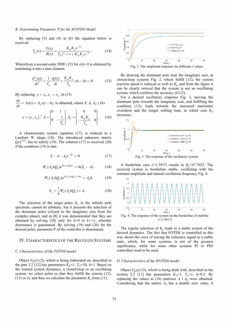
73

B. Determining Parameter P for the IFOTDS Model

By replacing (3) and (4) in (6) the equation below is received

2

( )( ) ,

( )

hsm p

ip hsm m p

K K eY sT s

R s T s s K K e

-

-= =+ +

(14)

Wherefrom a second-order DDE (15) for r(t)=0 is obtained by translating it into a time domain.

2

2

( ) 1 ( )( ) 0.m p

m m

K Kd y t dy ty t h

T dt Tdt+ + - = (15)

By replacing 1 2 1 ,,y x x x = = in (15)

( ) ( ),d

dxAx t A x t h

dt= + - is obtained, where X, A, Ad (16)

( )1 2

0 00 1

, , , .10 0

Tm pd

m m

K Kx x x A A

T T

æ öæ ö ÷÷ çç ÷÷ çç ÷÷ çç ÷÷= = =çç ÷÷ çç ÷÷- -ç ÷ç ÷ ÷ç÷ç ÷çè ø è ø

(16)

A characteristic system equation (17), is reduced to a

Lambert W shape (18). The introduced unknown matrix QϵC2x2, has to satisfy (19). The solution (17) is received (20) if the condition (19) is met.

0.hS

dS A A e-- - = (17)

( )( ) ( ).k d kW A hQ

k d k kW A hQ e h S A= - (18)

( ( ) )( ) .k d kW A hQ Ah

k d k dW A hQ e A h+ = (19)

1

( ) .k k d kS W A hQ Ah

= + (20)

The selection of the target poles Sk, in the infinite pole

spectrum, cannot be arbitrary, but it presents the selection of the dominant poles (closest to the imaginary axis from the complex plane); and in [8] it was demonstrated that they are obtained by solving (20) only for k=0 or k=±1, whereby dominance is guaranteed. By solving (19) and (20) for the desired poles, parameter P of the controller is determined.

IV. CHARACTERISTICS OF THE RECEIVED SYSTEMS

C. Characteristics of the FOTDS model

Object Gp(s) (2), which is being elaborated on, described in the part 3.2 [12] has parameters Km=1, Tm=30, h=1. Based on the wanted system dynamics, a closed-loop or an oscillating system, we select poles so that they fulfill the criteria (12), (13) or e), and then we calculate the parameter Kp from (11).

Fig. 2. The amplitude response for different λ values

By drawing the dominant pole near the imaginary axis, at

closed-loop systems Fig. 2, which fulfill (12), the system reaction speed is reduced as well as Kp, and from the figure it can be clearly noticed that the system is not an oscillating system, which confirms the accuracy of (12).

For a desired oscillatory response Fig. 3, moving the dominant pole towards the imaginary axis, and fulfilling the condition (13), leads towards the increased maximum overshoot and the longer settling time, in which case Kp increases.

Fig. 3. The response of the oscillatory system

A borderline case λ=1.5917i results in Kp=47.7625. The

received system is borderline stable, oscillating with the constant amplitude and natural oscillation frequency Fig. 4.

Fig. 4. The response of the system on the borderline of stability

λ=1.5917i The regular selection of Kp leads to a stable system of the

desired dynamics. The fact that FOTDS is controlled in this way shows the error of tracing the reference signal in a stable state, which, for some systems, is not of the greatest significance, while for some other systems PI or PID controllers need to be used.

D. Characteristics of the IFOTDS model

Object Gip(s) (3), which is being dealt with, described in the section 2.2 [11] has parameters Km=1, Tm=1, h=0.5. By replacing the values in (16) matrices A i Ad were obtained. Considering that the matrix Ad has a double zero value, it

74

ensues that the matrix AdhQ, for any value Q, will assume the following shape:

21 22

0 0,dA hQ

m m

æ ö÷ç ÷=ç ÷ç ÷çè ø

Therefore, a distinctive value AdhQ is equal to zero, which is why because of the characteristics of LWF [9], Wk(0)=0 for k=0, Wk(0)=-¥ for k≠0, a traditional procedure of making use of identical branches k1=k2 cannot be applied, but rather hybrid branches k1≠ k2 are used in this case. By determining that k2=0 and k1ϵ(-¥ ,¥ ) the following is obtained:

1

1 2

2

22 1( ) 0

( ) ,0 (0)

k

k k dk

W mW A hQ V V

W-

æ ö÷ç ÷ç= ÷ç ÷ç ÷è ø

where V is a distinctive vector of the matrix AdhQ. The desired dynamics of the system is established by selecting the dominant poles, whereby solving (19) and (20), Kp is received.

A system without a controller Kp=1, Fig. 7 displays the settling time of 15.5s, 45% of overshoot, and GM=6.64 dB PM=29.3 deg, Fig. 8.

Fig. 7. An overshoot response of the system for various Kp values

Fig. 8. A frequency response of the open-loop system

By moving a pole onto the left side of the complex plane,

which reduces Kp, what is received are the overshoot and the settling time thus, if the projection for PM of around 60 degrees is performed, Kp=0.4, the settling time of 10.2 and the overshoot smaller than 9%, will be obtained Fig. 7.

By moving the pole towards the imaginary axis from the complex plane, the oscillation of the system is increased, an increased overshoot and the longer settling time are obtained. For Kp=1.6, Fig. 7, the overshoot is 76% and the settling time is 39 s.

It is quite clear that due to the first-order IFODTS astatism the system’s steady state error equals zero, unlike in FOTDS.

V. CONCLUSION

P controller designed with LWF can be used for controlling the FOTDS and IFOTDS, if the systems are affected by minor perturbation, or if the steady state error of the system in the presence of perturbation does not greatly affect the functioning of the system. Otherwise, PI or PID should be used.

In the future, what can be explored is the effect of the perturbation on this kind of controlled system, as well as the projection of PI and PID controllers for the IFOTDS by using the Lambert W method, and the projection of PID controllers for the FOTDS.

ACKNOWLEDGMENT

This paper was realized as a part of the projects III 43007 and TR 35005, funded by the Ministry of Education, Science and Technological Development of the Republic of Serbia.

REFERENCES

[1] M.R. Stojić, Sistemi automatskog upravljanja, Niš, Srbija, Elektronski fakultet u Nišu, 2004.

[2] V. Kharitonov, Time-delay systems - Lyapunov functionals and matrices, Control Engineering, Birkhaeuser, Boston, MA, 2013.

[3] R.C. Dorf, and R.H. Bishop, Modern Control System, 12th ed, Prentice Hall, 2011.

[4] G.J. Silva, A. Datta, and S.P. Bhattacharyya, PID Controllers for Time-Delay Systems, Control Engineering, Birkhaüser, Boston, 2005.

[5] G.J. Silva, A. Datta, and S.P. Bhattacharyya, "PI Stabilization on First-Order System with Time Delay", Automatica, vol. 37, pp. 2025-2031, 2001.

[6] O.J. Smith, "A Controller to Overcome Dead Time", ISA Journal, vol. 6, no. 2, pp. 28-33, 1959.

[7] K.J. Åström, and T. Hägglund, PID Controllers: Theory, Design, and Tuning, Research Triangle Park, North Carolina, Instrument Society of America, 1995.

[8] S. Yi, P. W. Nelson, and A.G. Ulsoy, Timedelay Systems: Analysis and Control Using the Lambert W Function, World Scientific, 2010.

[9] R.M. Corless, G.H. Gonnet, D. E.G. Hare, D. J. Jeffrey, and D.E. Knuth, "On the Lambert W Function", Advances in Computational Mathematics, vol. 5, pp. 329-359, 1996.

[10] S. Yi, P.W. Nelson, and A.G. Ulsoy, "The Lambert W Function Approach to Time Delay Systems and the LambertW_DDE Toolbox", 10th IFAC Workshop on Time Delay Systems, the International Federation of Automatic Control, North Eastern University, Boston, USA, 2012.

[11] A. Visioli, and Q. C. Zhong, Control of Integral Processes with Dead Time, Springer/Verlag, London, 2011.

[12] S. Skogestad, "Simple Analytic Rules for Model Reduction and PID Controller Tuning", Journal of Process Control, vol. 13, 2003.

75

Sampled-Data Sliding Mode Control Design of Single-Link Flexible Joint Robotic Manipulator

Abid Raza1, Rameez Khan2, Fahad Mumtaz Malik3

Abstract – In this paper, we have designed a sampled data control law for the single-link flexible joint robotic manipulator using two different approaches. First, we have designed the sampled-data sliding mode control (SMC) based on the continuous time system. In the second approach, we have obtained the approximate discrete model of the system and then designed discrete sliding mode control based on this approximate system. Simulation results have been obtained and a performance comparison has been presented for both techniques.

Keywords – Sampled-data control, Sliding mode control, Robotic manipulator.

I. INTRODUCTION

Robotic manipulators are widely being used in industry are highly nonlinear systems which often suffer from unmodeled dynamics and uncertainties. Recently control engineers have designed controllers for flexible joint robots but it is still very less as compared to the rigid robots. However, in many applications, the robotic manipulators have some flexible joints as well. At the same time, the flexibility of joints may limits the performance and robustness of the controllers designed for robots or may lead to instability [1]. Also, the flexibility of joints can be considered a step for the flexible robot link [2] so to by studying the flexible joint manipulator can lead us to the flexible link which helps to have link lighter in weight that ultimately results in fast robotic motions. If the flexibility of joint is modeled by the spring, dynamic model of flexible joints can be obtained. Some advantages of flexible joints robotic manipulators over rigid manipulators are less control effort, fast motion, light weight and smaller dimension [3]-[6].

To design sliding mode controller for the flexible joint manipulator, state variables of each joint, velocities, acceleration and jerks of the link must be known [5]. Since last two decades, dynamic modeling and non-linear control of robotic manipulators (flexible) is the area of research which received notable consideration. To design a control topology that is efficient and robust, the first and fundamental step is to develop an accurate dynamic model of a flexible joint robot. In industrial and space applications, we need the controller that can reduce the disturbance effects and can cope with modeling

uncertainties. For flexible joints, a robust controller should be designed for the stabilization or tracking purpose that has negligible link vibration.

For this purpose, different techniques have been suggested for last two decades. For example, linear quadratic regulation (LQR) control technique is widely used for such control [7], another technique which is vastly used is adaptive output feedback controller based on a back stepping [8]-[10]. In the case of nonlinear control, feedback linearization is the most renowned technique that is used for robotic manipulators [11]. The integral control technique described in [12] and [13], robust control that uses PD control and H∞ control, PD fuzzy and optimal control and sliding mode control [14]. In [15], an adaptive second order terminal sliding mode controller for robotic manipulators is proposed.

Almost all the research for control of robotic manipulators is carried out in the continuous time domain. However, due to the increasing availability of microprocessor hardware, control algorithms are now usually implemented in digital controllers. In this paper, we have focused on sampled data sliding mode control, as SMC is nonlinear control and is more robust as compared to most of the conventional control techniques.

In this paper, we have focused on the stabilization of flexible joint robotic manipulator in discrete time domain. Sliding mode control is designed using sampled data control techniques and their comparison is carried out on the basis of simulation results. This paper is divided into five sections. In section 2 dynamic modeling of single link flexible joint robot is discussed. In section 3, sliding mode controller is designed that would stabilize the robotic manipulator. In section 4 sampled data control techniques are discussed. Using these techniques SMC is designed for the system, simulation results are presented to show the comparison of sampled data control techniques. Section 5 discusses the conclusion on the basis of these simulation results.

II. DYNAMIC-MODELLING OF FLEXIBLE JOINT SINGLE-LINK ROBOTIC MANIPULATOR

In this work, we have focused upon the flexible joint single link robotic manipulator. The dynamic model of single-link robotic manipulator with the flexible joints is derived using the Euler-Lagrange equations and is given by [16], [17]

Fig. 1 shows the model of single link flexible joint robotic manipulator [18]. are the link positions, describes the link inertia whereas is the actuator inertia, the nominal load is denoted by , represents the joint stiffness and input torque is denoted by .

1Abid Raza is with the Department of Electrical Engineering at College of Electrical and Mechanical Engineering, National University of Science and Technology, Islamabad, Pakistan, E-mail: [email protected]

2Rameez Khan is with the Department of Electrical Engineering at College of Electrical and Mechanical Engineering, National University of Science and Technology, Islamabad, Pakistan

3Fahad Mumtaz Malik is with the Department of Electrical Engineering at College of Electrical and Mechanical Engineering, National University of Science and Technology, Islamabad, Pakistan

76

Fig. 1. Model of a single-link, flexible joint manipulator

Using this dynamic model state space model of this robotic

manipulator is derived. State space model of manipulator is given by

where the constants are given by and the input torque is .

we have designed a sliding mode controller using this state space model for the stabilization of this system in next section.

III. STABILIZATION USING SAMPLED DATA SMC BASED ON EMULATION

Sampled-data control refers to the control of a continuous system with discrete controller. There are two main techniques for sampled data control [19] [20].

• Emulation design • Approximate discrete model based control design

Emulation design is considered as a simpler method to design a controller for sampled-data systems. In terms of system stability and performance, it is also considered as inferior design technique as compared to other methods. In designing controller by this technique sampling is completely overlooked. The continuous controller is discretized, in next step implementation is done using sample and hold devices.

Fig. 2 shows the block diagram of steps that are followed during the emulation design. In this technique of control design, the control law derived for the continuous time system is discretized. The classical sliding mode control suffers from chattering. Chattering is a severe problem especially in the mechanical system because it causes wear and tear in the system. There are different methods developed to reduce chattering. A well-known method is the replacement of the

Fig. 2. Emulation design

discontinuous signum function with the saturation function [17]. In this method, the real sliding is replaced with the sliding in a small vicinity of the discontinuous surface. The chattering issue can be overcome if we use saturation function instead of signum function. Consider the sliding surface

(3)

The following control law has been proposed for the stabilization of the single link flexible joint robotic manipulator.

where

(4)

0 2 4 6 8 10 12 14 16 18 20-2

-1.5

-1

-0.5

0

0.5

1

1.5

2

Time(Seconds)

Sta

tes

Stabilization

x1x2x3x4

Fig. 3. States Stabilization using Sampled Data SMC based on Emulation

In Fig. 3, state stabilization based on Emulation design is shown. These simulation results are generated by using MATLAB/SIMULINK. State is the position of the link and we can see this state stabilizes to the origin within 12 sec. All other states also stabilize to the origin within a certain time. This shows that we have designed efficient control law using emulation that stabilizes all the system states.

IV. STABILIZATION USING SAMPLED DATA SMC BASED ON APPROXIMATE DISCRETE MODEL

DESIGN

In approximate discrete model based control design technique, the controller is designed by using the approximate discrete model of the plant in discrete time domain. For non-linear systems, exact modeling of the system is almost impossible so approximate discrete model of the plant is used to design a controller for nonlinear systems. Then, this discrete controller is implemented using sample-and-hold devices. In this paper, we have discussed the controller design for sampled data control.

Fig. 4. SMC based on approximate discrete model

77

Fig. 4 shows the block diagram of steps that are followed during the sampled data control using approximate discrete model. Using this technique SMC is designed in this section. The discretization is done using Euler forward difference method. The Euler model approximation is

State space model of manipulator (1) is

Using the approximate discrete model of the manipulator we will design SMC that will stabilize the system. The approximate discrete model is given by

Consider the following sliding surface

To stabilize it globally using Sliding mode control law

where

The constants are .

0 2 4 6 8 10 12 14 16 18 20-10

-5

0

5

10

Time(Seconds)

Sta

tes

Stabilization

x1x2x3x4

Fig. 5. States Stabilization using sampled data SMC based on approximate discrete model

In Fig. 5, state stabilization based on SMC (approximate

discrete model) is shown. These simulations are generated by using MATLAB SIMULINK. State is the position of the link and we can see this state stabilizes to the origin within 4

seconds. All other states also stabilize to origin approximately within four seconds. This shows that SMC designed using approximate discrete model is more efficient as compared to the previous technique and it also stabilizes all the system states.

V. COMPARISON OF APPROXIMATE DISCRETE MODEL AND EMULATION DESIGN SMC

In this section, a comparison of both sampled-data control techniques is presented. The simulation is done using MATLAB/SIMULINK for the implementation of the controller on robotic manipulator. The results of the comparison of both techniques are shown in Fig. 6.

In simulation results, stabilization of Single link flexible joint robotic manipulator using SMC based on emulation design and SMC based on approximate discrete model are compared. It is obvious that stabilization of states using approximate discrete model is quicker than that of SMC based on emulation design. In the case of SMC based on emulation design, there are oscillations of states before settling down to the origin. Also, time taken to stabilize using emulation design is more than that of approximate discrete model design. Results of SMC based on approximate discrete model stabilize the states quickly which shows SMC based on approximate discrete model is better stabilization approach for single link robotic manipulator than that of SMC based on emulation design.

VI. CONCLUSION

In this paper, SMC feedback control for single-link flexible joint robotic manipulator system is discussed. Two approaches for the design of sampled data sliding mode control are studied and simulation results are presented. It is clear that the SMC based on approximate discrete model is better as it stabilizes the states in less time for the same parametric values of the system. Moreover, by using SMC based on approximate discrete model the region of attraction is increased as compared to emulation design. The main outcome of Sampled Data SMC is the robustness. It (SMC based on approximate discrete model) is more robust against disturbance to conventional techniques used for robotic manipulator control (feedback linearization). SMC based on approximate discrete model has the insensitivity to parameter variations to a larger extent (greater region of attraction), fast dynamic responses and better disturbance rejection which is required for the smooth motions of the robotic manipulator.

Now sampled data control is becoming popular than the continuous time. The sampled data controls that are derived and simulated can be further extended to sampled data observer. The states can be estimated with the help of an observer so we do not need to have sensors on all states. This work can also be extended for the n-link flexible joint robotic manipulator. Based on this work, a robust controller can also be designed for the tracking problem for the robotic manipulator.

78

0 2 4 6 8 10 12 14 16 18 20-1

-0.5

0

0.5

1

Time(Seconds)

Sta

te x

1

Stabilization

SMC based on CT SystemSMC based on ADTE System

(a)

0 2 4 6 8 10 12 14 16 18 20-1.5

-1

-0.5

0

0.5

Time(Seconds)

Sta

te x

2

Stabilization


(b)

0 2 4 6 8 10 12 14 16 18 20-3

-2

-1

0

1

Time(Seconds)

Sta

te x

3

Stabilization


(c)

0 2 4 6 8 10 12 14 16 18 20-10

-5

0

5

10

Time(Seconds)

Sta

te x

4

Stabilization


(d)

Fig. 6. Estimated States Comparison of approximate discrete model, Emulation SMC: (a) State X1 stabilization, (b) State X2 stabilization,

(c) State X3 stabilization, (d) State X4 stabilization

REFERENCES [1] L.M. Sweet, and M.C. Good, "Redefinition of the Robot Motion

Control Problem: Effects of Plant Dynamics, Drive System Constraints, and User Requirements", 23rd IEEE Conf. on Decision and Control, pp. 724-732, Las Vegas, Nev, USA, 1984.

[2] H. Asada, Z.D. Ma, and H. Tokumaru, "Inverse Dynamics of Flexible Robot Arms. MODELING and Computation for Trajectory Control", Journal of Dynamic Systems, Measurement and Control, vol. 112, no. 2, pp. 177-185, 1990.

[3] M.C. Chien, and A.C. Huang, "Adaptive Control for Flexible-Joint Electrically Driven Robot with Time-Varying Uncertainties", IEEE Transactions on Industrial Electronics, vol. 54, no. 2, pp. 1032-1038, 2007.

[4] N. Lechevin, and P. Sicard, "Observer Design for Flexible Joint Manipulators with Parameter Uncertainties", IEEE International Conference on Robotics and Automation (ICRA'97), vol. 3, pp. 2547-2552, Albuquerque, NM, USA, April 1997.

[5] P. Tomei, "An Observer for Flexible Joint Robots", IEEE Transactions on Automatic Control, vol. 35, no. 6, pp. 739-743, 1990.

[6] I. Hassanzadeh, H. Kharrati, and J.-R. Bonab, "Model Following Adaptive Control for a Robot with Flexible Joints", IEEE Canadian Conference on Electrical and Computer Engineering (CCECE'08), pp. 1467-1472, Niagara Falls, Canada, May 2008.

[7] M.A. Ahmad, "Vibration and Input Tracking Control of Flexible Manipulator Using LQR with Non-Collocated PID Controller", 2nd UKSIM European Symposium on Computer Modelling and Simulation, pp. 40-45, September 2008.

[8] W. Yim, "Adaptive Control of a Flexible Joint Manipulator", IEEE International Conference on Robotics and Automation (ICRA'01), pp. 3441-3446, May 2001.

[9] J.H. Oh, and J.S. Lee, "Control of Flexible Joint Robot System by Backstepping Design Approach", IEEE International Conference on Robotics and Automation (ICRA'97), vol. 4, pp. 3435-3440, April 1997.

[10] F. Ghorbel, J.Y. Hung, and M.W. Spong, "Adaptive Control of Flexible-Joint Manipulators", IEEE Control Systems Magazine, vol. 9, no. 7, pp. 9-13, 1989.

[11] S. Moberg, and S. Hanssen, "On Feedback Linearization for Robust Tracking Control of Flexible Joint Robots", 17th IFACWorld Congress Seoul, Korea, July 2008.

[12] L.C. Lin, and K. Yuan, "Control of Flexible Joint Robots via External Linearization Approach", Journal of Robotic Systems, vol. 7, no. 1, pp. 1-22, 2007.

[13] M.W. Spong, K. Khorasani, and P.V. Kokotovic, "An Integral Manifold Approach to the Feedback Control of Flexible Joint Robots", IEEE Journal of Robotics and Automation, vol. 3, no. 4, pp. 291-300, 1987.

[14] J. S. Yeon, and J. H. Park, "Practical Robust Control for Flexible Joint Robot Manipulators", IEEE International Conference on Robotics and Automation (ICRA'08), pp. 3377-3382, May 2008.

[15] S. Mondal, and C. Mahanta, "Adaptive Second Order Terminal Sliding Mode Controller for Robotic Manipulators", Journal of the Franklin Institute, vol. 351, no. 4, 2014, pp. 2356-2377.

[16] APA H. K. Khalil, Nonlinear Systems, 3rd Edition (prentice Hall), 2002.

[17] M.W. Spong, and M. Vidyasagar, Robot Dynamics and Control, John Wiley & Sons, New York, NY, USA, 2006.

[18] M. Moez Belhaouane, M. Faiez Ghariani, "Improved Results on Robust Stability Analysis and Stabilization for a Class of Uncertain Nonlinear Systems", Mathematical Problems in Engineering, vol. 2010 (2010), Article ID 724563.

[19] D.S. Laila, "Design and Analysis of Nonlinear Sampled Data Control Systems", PhD Dissertation-Department of Electrical and Electronics Engineering, the University of Melbourne, April 2003.

[20] F. Mumtaz, "Sampled Data Control Based on Discrete Time equivalent Models", PhD Dissertation-Department of Electrical Engineering, NUST College of Electrical and Mechanical Engineering, Pakistan 2009.

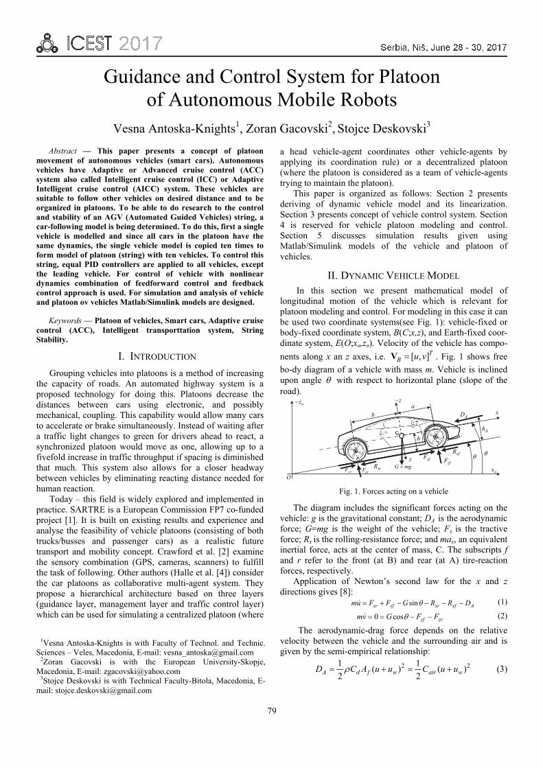
79

Guidance and Control System for Platoon of Autonomous Mobile Robots

Vesna Antoska-Knights1, Zoran Gacovski2, Stojce Deskovski3

Abstract — This paper presents a concept of platoon

movement of autonomous vehicles (smart cars). Autonomous vehicles have Adaptive or Advanced cruise control (ACC) system also called Intelligent cruise control (ICC) or Adaptive Intelligent cruise control (AICC) system. These vehicles are suitable to follow other vehicles on desired distance and to be organized in platoons. To be able to do research to the control and stability of an AGV (Automated Guided Vehicles) string, a car-following model is being determined. To do this, first a single vehicle is modelled and since all cars in the platoon have the same dynamics, the single vehicle model is copied ten times to form model of platoon (string) with ten vehicles. To control this string, equal PID controllers are applied to all vehicles, except the leading vehicle. For control of vehicle with nonlinear dynamics combination of feedforward control and feedback control approach is used. For simulation and analysis of vehicle and platoon ov vehicles Matlab/Simulink models are designed.

Keywords — Platoon of vehicles, Smart cars, Adaptive cruise control (ACC), Intelligent transporttation system, String Stability.

I. INTRODUCTION

Grouping vehicles into platoons is a method of increasing the capacity of roads. An automated highway system is a proposed technology for doing this. Platoons decrease the distances between cars using electronic, and possibly mechanical, coupling. This capability would allow many cars to accelerate or brake simultaneously. Instead of waiting after a traffic light changes to green for drivers ahead to react, a synchronized platoon would move as one, allowing up to a fivefold increase in traffic throughput if spacing is diminished that much. This system also allows for a closer headway between vehicles by eliminating reacting distance needed for human reaction.

Today – this field is widely explored and implemented in practice. SARTRE is a European Commission FP7 co-funded project [1]. It is built on existing results and experience and analyse the feasibility of vehicle platoons (consisting of both trucks/busses and passenger cars) as a realistic future transport and mobility concept. Crawford et al. [2] examine the sensory combination (GPS, cameras, scanners) to fulfill the task of following. Other authors (Halle et al. [4]) consider the car platoons as collaborative multi-agent system. They propose a hierarchical architecture based on three layers (guidance layer, management layer and traffic control layer) which can be used for simulating a centralized platoon (where

a head vehicle-agent coordinates other vehicle-agents by applying its coordination rule) or a decentralized platoon (where the platoon is considered as a team of vehicle-agents trying to maintain the platoon). This paper is organized as follows: Section 2 presents deriving of dynamic vehicle model and its linearization. Section 3 presents concept of vehicle control system. Section 4 is reserved for vehicle platoon modeling and control. Section 5 discusses simulation results given using Matlab/Simulink models of the vehicle and platoon of vehicles.

II. DYNAMIC VEHICLE MODEL In this section we present mathematical model of

longitudinal motion of the vehicle which is relevant for platoon modeling and control. For modeling in this case it can be used two coordinate systems(see Fig. 1): vehicle-fixed or body-fixed coordinate system, B(C;x,z), and Earth-fixed coor-dinate system, E(O;xo,zo). Velocity of the vehicle has compo-

nents along x an z axes, i.e. [ , ]TB u vV . Fig. 1 shows free

bo-dy diagram of a vehicle with mass m. Vehicle is inclined upon angle with respect to horizontal plane (slope of the road).

z

ab

G mgxrF

xfR

zrF

z

x

ox

oz

xrRxfF

zfF

Ah

h

O

AD

Fig. 1. Forces acting on a vehicle

The diagram includes the significant forces acting on the vehicle: g is the gravitational constant; DA is the aerodynamic force; G=mg is the weight of the vehicle; Fx is the tractive force; Rx is the rolling-resistance force; and max, an equivalent inertial force, acts at the center of mass, C. The subscripts f and r refer to the front (at B) and rear (at A) tire-reaction forces, respectively.

Application of Newton’s second law for the x and z directions gives [8]:

sinxr xf xr xf Amu F F G R R D

(1)

0 cos zf zrmv G F F (2)

The aerodynamic-drag force depends on the relative velocity between the vehicle and the surrounding air and is given by the semi-empirical relationship:

2 21 1( ) ( )

2 2A d f w air wD C A u u C u u

(3)

1Vesna Antoska-Knights is with Faculty of Technol. and Technic.Sciences – Veles, Macedonia, E-mail: [email protected] 2Zoran Gacovski is with the European University-Skopje,Macedonia, E-mail: [email protected] 3Stojce Deskovski is with Technical Faculty-Bitola, Macedonia, E-mail: [email protected]

80

where ρ is the air density (= 1.202 kg/m3 at an altitude of 200 m), Cd is the drag coefficient, Af is the frontal area of the vehicle, u is the vehicle-forward velocity, and uw is the wind velocity (i.e.,positive for a headwind and negative for a tail-wind). The drag coefficient for vehicles ranges from about 0.2 (i.e., streamlined passenger vehicles with underbody cover) to 1.5 (i.e., trucks); 0.4 is a typical value for passenger cars [8].

The rolling resistance arises due to the work of deforma-tion on the tire and the road surface, and it is roughly proportional to the normal force on the tire:

( ) cosx xf xr r zf zr rR R R f F F f mg (4)

where fr is the rolling-resistance coefficient in the range of about 0.01 to 0.4, with 0.015 as a typical value for passenger vehicles.

For farther consideration we use equation (1). Equation (1) is nonlinear in the forward velocity, ( )u t but otherwise is

a simple dynamic system: it only has one state variable. So, what are the main challenges incruise-control design problems? The difficulties arise mainly from two factors: (1) plant uncertainty due to change of vehicle weight, and (2) external disturbances due to road grade. Thus, a good cruise-control algorithm must work well under these uncertainties.

Equation (1), using (3) and (4) can be rewritten: 21

sin cos ( )2x r air wmu F mg f mg C u u

(5)

where air r dC A C is a constant.

Equation (5) is used for creation of nonlinear Simulink model of the vehicle in the platoon.

For analysis of the dynamics and stability of the vehicle and string stability of the platoon we need a linearized model of the vehicle. In vector-matrix form the linearized system gets form [3]:

0 1 0 0

1 1 10 x

x xF d

u uK m m m

. (6)

III. VEHICLE CONTROL SYSTEM

In cases when the real vehicle is with nonlinear dynamics (in our case equation (5) for longitudinal dynamics) it is very useful to implement combination of feed-forward control and feedback control approach, presented on Fig. 3.

The feed-forward control is formed on the inverse model of the object and on the generator of nominal trajectories

which generates the desired trajectory )(tox . This desired

trajectory is based on the previously prepared data or from the process of operation of the system based on the measured data. For realization of this trajectory it is necessary that regulator in feedback is present, which will generate the needed control )(tu for elimination of the error of the

trajectory of the object from the desired trajectory. This provides stabilisation of the control process of the object.

The sum control u(t) of the moving object from Fig. 3, when the linear regulator is formed by the matrix K(t), is given with the following relation:

( ) ( ) ( ) ( ) ( ) ( ) ( ) ( )[ ( ) ( )]o o o ot t t t t t t t t t u u u u K x u K x x (7)

The syntesis of the control law given by equation (7) is performed in two steps. In the first step the nominal control

)(tou is determined under assumption of ideal conditions i.e.

when no disturbances are present.

)(tu)(tox )(tu )(tx

)(tx

)(tx

)(tou)(tox

Fig. 2. Concept of feed-forward and feedback control system

of nonlinear object

According to the described concept (Fig. 2), the control laws for vehicles can be developed. In this paper feed-forward control is determined based on (6) for nominal tractive force which present nominal control.

Feedback controller, which provides stabilization of the object around the nominal trajectory, can be designed using linearized model. Under assumption that the dynamic behavior of the object with respect to the nominal trajectory is linear, as described with (6), for the control )(tu , we can

apply methods for synthesis developed for linear systems: PID controller design, Linear Quadratic Regulator (LQR), methods for pole placement, adaptive optimal control etc.[3].

In this paper PID control design approach is used and PID feedback controller is obtained based on linear model of the vehicle derived above with parameters determined using numerical values. For simulation and testing of vehicle dynamics and vehicle control system Simulink model is developed which is shown in Fig. 3.

Module reference inputs, generate reference acceleration ao, velocity vo, and position xo, similar like the leader of the platoon. These signals go to the PID controller where are processed according to:

( ) ( ) ( )Ix p o o D o

Ku F K x x x x K v v

s

(8)

where , , andp I DK K K are proportional, integral and derivati-

ve gains of the controller, a, v and x are real acceleration, velocity and position of the vehicle.

Fig. 3. Simulink diagram for the vehicle control

Module Nominal control, Fig. 3, consists of equation (6), and module Vehicle dynamics, which is based on full nonlinear model, equation (5). Simulink model in Fig. 3 can be used for open loop, and closed loop simulation of the controlled vehicle.

81

IV. CONTROL OF A PLATOON OF VEHICLES Platooning requires another level of control beyond

individual vehicles. Two fundamentally different approaches to platooning have been suggested: (1) point-following control, in which each vehicle is assigned a particular moving slot on the highway and maintains that position [5]; and (2) vehicle-following control, in which each vehicle in the platoon regulates its position relative to the vehicle in front of it based on information about the lead vehicle motion [6] and locally measured variables (i.e., its own motion and headway to the vehicle in front). In this paper we discuss the vehicle-following control approach, which is the focus of most current research and development work in the area [8].

4v 3v 2v 1v Lv

Lxoz

1 1Ldx x x

4x3x

1x2x

2 1 2dx x x 3 2 3dx x x 4 3 4dx x x

2 2Ll x x 3 3Ll x x

4 4Ll x x

1 1Ll x x

O

Lz

Lx

ox

L4a La1a2a3a

Fig. 4. Configuration of platoon with 5 vehicles

Movement of the vehicles we observe in the inertial (or absolute) coordinate system ( ; , )o oG O x y which is fixed to the

road with origin in the starting point, O (Fig. 4). Positions, ix ,

velocities, i iv x , and accelerations, i ia v , ,1,2,3,4i L ,

measured with respect to ( ; , )o oG O x y , are absolute quantities.

Coordinate system ( ; , )L LL L x y , see Fig. 4, is fixed to the

vehicle-leader with origin in the center of its mass. Relative position, velocity and acceleration of the vehicles with respect to ( ; , )L LL L x y are denoted as: i L il x x , ri L iv v v ,

,ri L ia a a 1,2,3,4i respectively. Distances between

vehicles are denoted as 1 , ,1, 2,3, 4i i idx x x i L , and

relative velocities and accelerations of the vehicles with respect to vehicle in front of them are respectively:

1 1

1 1

,

, ,1,2,3,4.i i i i i

i i i i i

dv v v x x

da a a x x i L

Based on Fig. 3, and mathematical model of individual vehicle together with its own control system - Matlab/-Simulink model of the platoon of 10 vehicles is developed. The main Simulink diagram of this model is shown in Fig. 5. In this model each vehicle gets information about acceleration, velocity and position of the previous vehicle, and also gets the same information about vehicle-leader.

Using vehicle model (5), if 0 and 0wV , we can find

acceleration of the vehicle in this form:

20

1 1( ),

2x r air x x xu a F f mg C u F F Fm

(9)

Substituting (8) in (9) we can find acceleration written for i-th vehicle:

1 1

21 0

1[ ( ) ( )

1( ) )],

2

Iii pi i i i i i i

Di i i x r air i

Ka K x x hd x x hd

m s

K v v F f mg C u

(10)

where ihd is constant distance between i-1-th and i-th

vehicles. Deriving (9a) we can get jerk which act on the i-th vehicle ( 0 and x rF f mg are constant), and using relations:

i ix v , (11)

i iv a , (12)

we can find:

1 1 11

[ ( ) ( ) ( ) ].oi Ii i i i pi i i Di i i air ia K x x hd K v v K a a C u a

m (13)

Equations (11), (12) and (13) represent linear state space model of the i-th vehicle in the platoon. Variables

1 1 1, , andi i i ix v a a in equation (13) are input variables for

the i-th vehicle and they are position, velocity and acceleration of the previous, or i-1-th, vehicle. Equations (11)-(13) can be used for generation state space model of string of several vehicles. This model is useful for stability analysis of the string using techniques of linear control theory. Here we form model for string of three vehicles: vehicle-leader, and two vehicles-followers. Outputs of the vehicle-leader generate input variables, , , andL L Lx v a ,

for the first vehicle in the string. Other two vehicles are described with equations obtained from (11-13) if we put i=1,2, and for i=1i-1=L (L-index for vehicle – leader).

For a platoon of vehicles, beside individual vehicle stability, is defined string stability of the platoon [8, 9]. If the preceding vehicle is accelerating or decelerating, then the spacing error could be nonzero; we must ensure that the spacing error attenuates as it propagates along the string of vehicles because it propagates upstream toward last vehicle. Linear model of the string of three vehicles (vehicle- leader and two vehicles-followers) in vector-matrix form is given with equation (14) and (15):

1 1

2 2

1 1

2 211 1

1 1

2 222 2 2 2

1 1

0 0 1 0 0 0

0 0 1 1 0 0

0 0 0 0 1 0

0 0 0 0 0 1

0 0 0

0

0 0 0

0 0 0

0 0 0

0 0 0

oD airI P

oD airI P P D

I P

x x

dx dx

v v

v vK C uK Ka am m ma aK C uK K K K

m m m m m

K K

m

1

211

2

0 0

0 0

0 0

0 0

0

0 0 0 0

L

L

ILD

I

xhd

vhdKaK

mm m

K

m

(14)

If we select for outputs distance between vehicles, 2dx ,

and velocities 1v and 2v , we can form output vector,

2 1 2[ ]Tdx v vy , as:

2

1

2

0 1 0 0 0 0 0 0 0

0 0 1 0 0 0 0 0 0

0 0 0 1 0 0 0 0 0

L

L

L

dx x

v v

v a

y x (15)

Stability analysis of the individual vehicle and platoon of vehicles can be made in Matlab using their linear models and compute poles of the system or find gain and phase margins with help of Nyquist plot. For example, for string of two vehicles-followers, using model (14) and parameters, we can find eigenvalues or poles, p1,…, p6 :

82

-1.2690 ,-1.2690, -0.5306, -0.5306, -0.0149, -0.0149 which are real and negative, and system is stable. These results are given for parameters of the vehicles and PID controllers given in Section V.

V. SIMULATION RESULTS We have simulated a platoon with 10 vehicles. Fig. 5 presents basic SIMULINK block diagram for the platoon model. All vehicles are the same with parameters. Parameters used in simulations are: m=1000 kg mass of the vehicles, =1.2 kg/m3 - air density, Af =1.2 m2 - frontal area of the vehicle, Cd=0.5; % drag koeficient, fr =0.01 - rolling resistance coeficient, g=9.81 - gravity acceleration, Cair= 0.5*Cd*Af*o=0.234 - constant, cos 73.6roll rF f mg

- rolling resistance force, u=20 m/s - velocity of the vehicles. Desired distances among vehicles are dxi0=50 m, Parameters of PID controllers are: KPi=700, KIi=10, and KDi=1800. Vehicle-Leader generates acceleration, velocity and position which are shown in the pictures below.

Fig. 5. Matlab/Simulink model of the platoon of 10 vehicles

Fig. 6 shows velocity profile of the vehicle leader and responses of vehicles – followers. Fig. 7 shows distance errors between vehicles for the same inputs. Fig. 8 shows positions of the vehicles in the platoon when each vehicle gets information for acceleration, velocity and position only for previous vehicle.

0 10 20 30 40 50 60 70 80 90 10018

20

22

24

26

28

t [s]

Veh

icle

vel

ociti

es,

vi [

m/s

]

Absolute vehicle velocities

Vehicle-Leader

Vehicle 9

Fig. 6. Trapezoidal change of vehicle-leader velocity and

responses of vehicles in the platoon

In this situation errors in positions between vehicles are smaller. It is known in the literature that information for vehicle-leader movement and inter-vehicle communication influence to better control and string stability of the platoon.

VI. CONCLUSIONS AND FUTURE WORK In this paper we have developed a nonlinear and linearized

model of the longitudinal motion of the vehicle. Feedforward control and feedback PID control approach is applied to design vehicle controller. Using this vehicle model with its

0 20 40 60 80 100-1

-0.5

0

0.5

1

1.5

2

t [s]

Dis

tanc

e er

rors

bet

wee

n ve

hicl

es,[

m]

Distance errors between vehicles

Vehicle 9

Vehicle 1

Fig. 7. Distance errors between vehicles

0 10 20 30 40 50-500

0

500

1000

t [s]

Veh

icle

pos

ition

s, x

i [m

]

Absolute vehicle positions

Vehicle 1

Vehicle 9

Vehicle - Leader

Fig. 8. Positions of the vehicles

designated control system model of platoon with ten vehicles is developed. In this model vehicles can get information for acceleration, velocity and position for previous vehicle and for movement of the vehicle –leader. String stability of the platoon is discussed and transfer function of the string useful for stability analysis is presented. Based on the developed models Matlab/Simulink models are created which can be used for simulation and performance analysis of the vehicle dynamics and platoon’s control system. In future work, we plan to develop more accurate models of the vehicles and platoons. We plan to design and test different then PID control laws, for example LQR and Fuzzy logic control. Realization using different sensors and wireless communication among vehicles will be our interest in future.

REFERENCES [1] E. Chan, P. Gilhead, P. Jelinek, and P.Krejčí, "SARTRE

Cooperative Control of Fully Automated Platoon Vehicles", 18th World Congress on Intelligent Transport Systems, USA, 2011.

[2] S.A. Crawford, "Performance Evaluations of Sensor Combinations for Mobile Platoon Control", Univ. of Calgary, Rep. 20213, 2005.

[3] G.F. Franklin, J.D. Powell, and A. Emami-Naeini; Feedback Control of Dynamic Systems, fourth edition, 2002.

[4] B.A. Güvenç, and E. Kural, "Adaptive Cruise Control Simulator. A Low-Cost Multiple-driver in the-loop Simulator", Istanbul Technical University, 2006.

[5] S. Halle, and B. Chaib-Draa, "A Collaborative Driving System Based on Multi Agent Modelling and Simulations", Transportation Research Part C: Emerging Technologies, pp. 320-345.

[6] S. Sheikholeslam, and CA. Desoer, "Longitudinal Control of a Platoon of Vehicles. I: Linear Model", Institute of Transportation Studies, University of California at Berkeley, 1989.

[7] J. Zhong, "PID Controller Tuning: A Short Tutorial", Mechanical Engineering, Purdue University, 2006.

[8] A. Galip Ulsoy, H. Peng, and M. Cakmakcı, Automotive Control Systems, Cambridge University Press, 2012.

[9] C.-Y. Liang, and H. Peng, "String Stability Analysis of Adaptive Cruise Controlled Vehicles", http://www-personal.umich. edu/~hpeng/JSME 2000.pdf.

Session 5A:

RADIO COMMUNICATIONS, MICROWAVES

AND ANTENNAS

85

Evaluation of Variances in Infrared Thermography of a Human Face During the Mental Workload

Kalin Dimitrov1, Stanyo Kolev2, Hristo Hristov3 and Viktor Mihaylov4

Abstract – The aim of this study was to explore the relationships between the temperatures of different areas of a person's face in mental workload (MWL). Correlations between points and areas and assessments have been sought and made of the averages and variances during the experiment with a group of people. The brains of these people were initially at rest, and then were loaded with arithmetic calculations.

Keywords – Infrared thermography, Facial thermal image,

Nasal skin temperature, Radiometry.

I. INTRODUCTION

In the present day, push-button calculators and computers are commonly used and play a crucial role in our lives. This will undoubtedly increase in the future as programs become more sophisticated and the speed of machines increase and their size and price decrease. Unfortunately, this has led to a reliance on the calculator even for simple calculations: the student automatically reaches for his/her calculator as soon as he/she sees an addition or multiplication question which has to be done.

The dependency on calculators, in lieu of the natural mental skills of humans, could lead to a loss of intellectual dignity. As calculators get more and more sophisticated they can do more and more complicated jobs: drawing graphs, solving equations and differentiating and integrating. Ultimately, all mathematical processes which the mind is capable of, could be done with the calculator. This demonstrates that we do not practice only mathematics which the calculator cannot do but that we practice mathematics for its ability to develop the mind [1-5].

The innate ability of humans to solve mathematical problems without regard to applications is a time-honored method to keep one’s mind stimulated [6-9]. One becomes more familiar with how numbers interact. If someone can't add and subtract without the help of a calculator, it can certainly reflect poorly on him. It is the fact that calculators are most useful in a setting that requires either things that are essentially impossible for humans to compute at any reasonable speed or for calculations with rather large numbers. For two digit addition, not using a calculator should

actually be faster, given that you have learned the techniques well.

The increasing of mental workload, which is caused by using the appropriate choice of arithmetical tasks, is suitable for the estimation of changes of human body processes [10-14]. Here we will study temperature fields changing on the human face [15]. In our research group, we have studied ideas to evaluate and estimate correlations using facial thermal imaging as measured by infrared thermography [16,17].

Thermal image techniques have been widely used in industry for detecting the faults online of operating components or systems [18-24]. Furthermore, the technology can also be extended for personal identification recognition [25]. Here we investigate how the distribution of blood flow in superficial blood vessels causes the changes of the local skin temperature. This is readily apparent in the human face where the layer of flesh is very thin [26,27]. The human face and body emit both the mid and far infrared (8-12μm) bands [24]. Therefore, mid and far infrared thermal cameras can sense the temperature distributions in the face at a distance to produce thermal images.

The advantage of using skin temperature is that, unlike the measurement of electrophysiological indicators, the method obviates the need to attach sensors, hence it is possible to measure the mental workload by using low-bound and non-contact methods. However, this method uses time series data and is a relative evaluation based on the comparison of resting and task loading, thus providing feedback of the results of the analysis is time consuming.

II. THEORY

Any object with temperature higher than absolute zero degree (-273oC) will emit electromagnetic radiation spontaneously [21]. This is known as natural or thermal radiation. By definition, all incident radiation will be absorbed by a black body in a continuous spectrum according to Planck [28].

Many methods are based on the extraction of the forehead and nose temperature for performing the evaluation and estimation [29]. However, this approach does not consider the correlation between different points/areas. The proposed study enables parts or areas of temperature change other than the nose to be captured.

This presents the possibility of accurate evaluation and estimation at levels that are more sensitive than the conventional methods.

In general, physiological indices are often used as an indication of autonomic nerve activity derived from indicators such as the heart rate, respiration, blood pressure, myoelectric properties, and electroencephalogram (EEG) measurements [30].

1Kalin Dimitrov is with the Faculty of Telecommunications atTechnical University of Sofia, 8 Kl. Ohridski Blvd, Sofia 1000,Bulgaria, E-mail: [email protected].

2Stanyo Kolev is with the Faculty of Telecommunications atTechnical University of Sofia, 8 Kl. Ohridski Blvd, Sofia 1000,Bugaria, E-mail: [email protected].

3Hristo Hristov, E-mail: [email protected] 4Viktor Mihaylov is with the Faculty of Telecommunications at

Technical University of Sofia, 8 Kl. Ohridski Blvd, Sofia 1000,Bugaria, E-mail: [email protected]

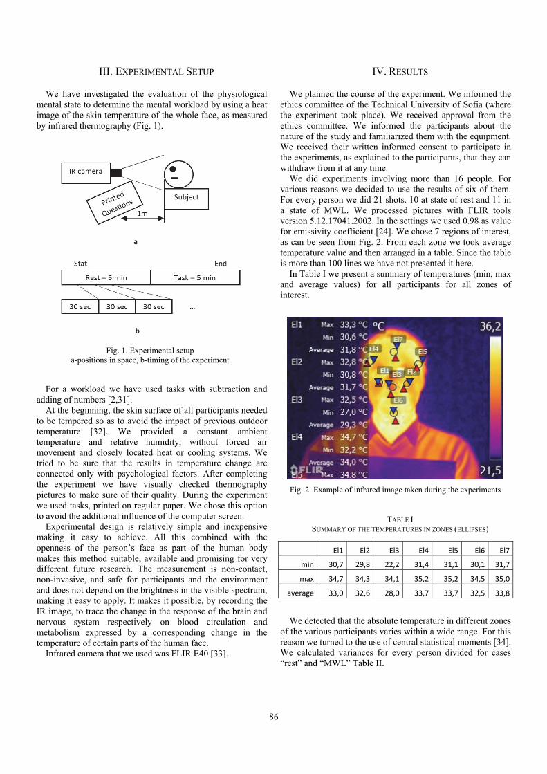
86

III. EXPERIMENTAL SETUP

We have investigated the evaluation of the physiological mental state to determine the mental workload by using a heat image of the skin temperature of the whole face, as measured by infrared thermography (Fig. 1).

For a workload we have used tasks with subtraction and

adding of numbers [2,31]. At the beginning, the skin surface of all participants needed

to be tempered so as to avoid the impact of previous outdoor temperature [32]. We provided a constant ambient temperature and relative humidity, without forced air movement and closely located heat or cooling systems. We tried to be sure that the results in temperature change are connected only with psychological factors. After completing the experiment we have visually checked thermography pictures to make sure of their quality. During the experiment we used tasks, printed on regular paper. We chose this option to avoid the additional influence of the computer screen.

Experimental design is relatively simple and inexpensive making it easy to achieve. All this combined with the openness of the person’s face as part of the human body makes this method suitable, available and promising for very different future research. The measurement is non-contact, non-invasive, and safe for participants and the environment and does not depend on the brightness in the visible spectrum, making it easy to apply. It makes it possible, by recording the IR image, to trace the change in the response of the brain and nervous system respectively on blood circulation and metabolism expressed by a corresponding change in the temperature of certain parts of the human face.

Infrared camera that we used was FLIR E40 [33].

IV. RESULTS

We planned the course of the experiment. We informed the ethics committee of the Technical University of Sofia (where the experiment took place). We received approval from the ethics committee. We informed the participants about the nature of the study and familiarized them with the equipment. We received their written informed consent to participate in the experiments, as explained to the participants, that they can withdraw from it at any time.

We did experiments involving more than 16 people. For various reasons we decided to use the results of six of them. For every person we did 21 shots. 10 at state of rest and 11 in a state of MWL. We processed pictures with FLIR tools version 5.12.17041.2002. In the settings we used 0.98 as value for emissivity coefficient [24]. We chose 7 regions of interest, as can be seen from Fig. 2. From each zone we took average temperature value and then arranged in a table. Since the table is more than 100 lines we have not presented it here.

In Table I we present a summary of temperatures (min, max and average values) for all participants for all zones of interest.

TABLE I SUMMARY OF THE TEMPERATURES IN ZONES (ELLIPSES)

El1 El2 El3 El4 El5 El6 El7

min 30,7 29,8 22,2 31,4 31,1 30,1 31,7

max 34,7 34,3 34,1 35,2 35,2 34,5 35,0

average 33,0 32,6 28,0 33,7 33,7 32,5 33,8

We detected that the absolute temperature in different zones of the various participants varies within a wide range. For this reason we turned to the use of central statistical moments [34]. We calculated variances for every person divided for cases “rest” and “MWL” Table II.

Fig. 1. Experimental setup a-positions in space, b-timing of the experiment

Fig. 2. Example of infrared image taken during the experiments

87

TABLE II VARIANCES

person El1 El2 El3 El4 El5 El6 El7

rest 1 0,008 0,041 0,473 0,009 0,039 0,044 0,007

mwl 1 0,016 0,037 0,138 0,060 0,027 0,052 0,007

rest 2 0,020 0,043 0,255 0,035 0,026 0,023 0,022

mwl 2 0,016 0,089 0,121 0,054 0,369 0,014 0,016

rest 3 0,144 0,314 0,662 0,390 0,063 0,103 0,035

mwl 3 0,071 0,073 3,527 0,197 0,071 0,149 0,036

rest 4 0,294 0,312 0,637 0,094 0,092 0,325 0,056

mwl 4 0,084 0,109 0,134 0,081 0,038 0,053 0,044

rest 5 0,187 0,078 0,326 0,076 0,072 0,007 0,025

mwl 5 0,046 0,047 0,522 0,040 0,038 0,086 0,010

rest 6 0,172 0,127 0,134 0,431 0,171 0,389 0,048

mwl 6 0,112 0,193 0,129 0,401 0,173 0,385 0,020

We subtracted the values of variance in the case “MWL” of the values in the “rest”. We puted this values in Table III.

TABLE III SUBTRACTED VARIANCES – (CASE REST MINUS CASE MWL)

prsn El1 El2 El3 El4 El5 El6 El7

1 ‐0,007 0,004 0,335 ‐0,051 0,012 ‐0,009 0,000

2 0,004 ‐0,046 0,135 ‐0,019 ‐0,342 0,009 0,007

3 0,073 0,241 ‐2,865 0,193 ‐0,008 ‐0,046 ‐0,001

4 0,210 0,203 0,503 0,013 0,054 0,273 0,012

5 0,140 0,031 ‐0,196 0,035 0,034 ‐0,079 0,015

6 0,060 ‐0,066 0,006 0,030 ‐0,002 0,004 0,028

We noticed that only areas El1 and El7 are indicative. Finally, we calculated the correlation between the different zones for all measurements (Table IV).

V. CONCLUSION

This study shows that the IR shooting of changing the surface temperature of the skin of certain areas of the human face allows registration of the change in brain activity. The results show that based on this idea, studies could be made on the influence of various external factors on the brain activity and accordingly, the reaction of the human body, since the change in mental processes gives rise to a change in the temperature of the facial tissues. The method could be involved in creating models for assessing or predicting the response of the body to the change of the environment, change of the health status and the change of various psychological factors giving rise to different types of stress. It could also be applied in reliable mechanisms for assessing the impact of

different thought processes on the mind and hence the physiological responses of the human body.

TABLE IV CORRELATION BETWEEN ZONES

El1‐El2 El1‐El3 El1‐El4 El1‐El5 El1‐El6 El1‐El7

0,9 0,7 0,7 0,4 0,9 0,9

El2‐El3 El2‐El4 El2‐El5 El2‐El6 El2‐El7

0,7 0,5 0,3 0,8 0,9

El3‐El4 El3‐El5 El3‐El6 El3‐El7

0,4 0,3 0,7 0,8

El4‐El5 El4‐El6 El4‐El7 El5‐El6 El5‐El7 El6‐El7

1,0 1,0 0,6 0,9 0,4 0,9

REFERENCES

[1] E. Bojorges-valdez, J.C. Echeverría, and O. Yanez-Suarez, “Evaluation of the Continuous Detection of Mental Calculation Episodes as a BCI Control Input”, Elsevier, Computers in Biology and Medicine, vol. 64, pp. 155-162, 2015.

[2] S. Caviola, G. Gerotto, and I.C. Mammarella, “Computer-based Training for Improving Mental Calculation in Third and Fifth-Graders”, Elsevier, Acta Psychologica, vol. 171, pp. 118-127, 2016.

[3] M.W. Scerbo, R.C. Britt, and D. Stefanidis, “Differences in Mental Workload Between Traditional and Single-Incision Laparoscopic Procedures Measured with a Secondary Task”, Elsevier, The American Journal of Surgery, vol. 213, pp. 244-248, 2017.

[4] T. Heine, G. Lenis, P. Reichensperger, T. Beran, O. Doessel, and B. Deml, “Electrocardiographic Features for the Measurement of Drivers' Mental Workload”, Elsevier, Applied Ergonomics, vol. 61, pp. 31-43, 2017.

[5] K. Mandrick, V. Peysakhovich, F. Rémy, E. Lepron, and M. Causse, “Neural and Psychophysiological Correlates of Human Performance Under Stress and High Mental Workload”, Elsevier, Biological Psychology, vol. 121, pp. 62-73, 2016.

[6] Z. Visnovcova, M. Mestanik, M. Gala, A. Mestanikova, and I. Tonhajzerova, “The Complexity of Electrodermal Activity is Altered in Mental Cognitive Stressors”, Elsevier, Computers in Biology and Medicine, vol. 79, pp. 123-129, 2016.

[7] F. Chen, Z. Hu, X. Zhao, R. Wang, Z. Yang, X. Wang, and X. Tang, “Neural Correlates of Serial Abacus Mental Calculation in Children: A Functional MRI Study”, Elsevier, Neuroscience Letters, vol. 403, pp. 46-51, 2006.

[8] X. Li, Y. Zhanga, L. Feng, and Q. Meng, “Early Event-Related Potentials Changes During Simple Mental Calculation in Chinese Older Adults With Mild Cognitive Impairment: A Case–Control Study”, Elsevier, Neuroscience Letters, vol. 475, pp. 29-32, 2010.

[9] K. Kasahara, S. Tanaka, T. Hanakawa, A. Senoo, and M. Honda, “Lateralization of Activity in the Parietal Cortex Predicts the Effectiveness of Bilateral Transcranial Direct Current Stimulation on Performance of a Mental Calculation

88

Task”, Elsevier, Neuroscience Letters, vol. 545, pp. 86-90, 2013.

[10] K. Ueda, E. C. Brown, K. Kojima, C. Juhasz, and E. Asano, “Mapping Mental Calculation Systems with Electrocorticography”, Elsevier, Clinical Neurophysiology, vol. 126, pp. 39-46, 2015.

[11] K. A. Herborn, J. L. Graves, P. Jerem, N. P. Evans, R. Nager, D. J. Mccafferty, and D. E.F. Mckeegan, “Skin Temperature Reveals the Intensity of Acute Stress”, Eelsevier, Physiology & Behavior, vol. 152, pp. 225-230, 2015.

[12] M. S.B. Guaranha, G.M. De Araujo Filho, K. Lin, L.M. F.F. Guilhoto, L.O. S.F. Caboclo, and E. M.T. Yacubian, “Prognosis of Juvenile Myoclonic Epilepsy is Related to Endophenotypes”, Elsevier, Seizure, vol. 20, pp. 42-48, 2011.

[13] F. Bousefsaf, C. Maaoui, and A. Pruski, “Remote Detection of Mental Workload Changes Using Cardiac Parameters Assessed with a Low-cost Webcam”, Elsevier, Computers in Biology and Medicine, vol. 53, pp. 154-163, 2014.

[14] A. Marinescu, S. Sharples, A.C. Ritchie, T.S. López, M. Mcdowell, and H. Morvan, “Exploring the Relationship Between Mental Workload, Variation in Performance and Physiological Parameters”, Ifac-papers Online, vol. 49-19, pp. 591-596, 2016.

[15] E. Salazar-López, E. Domínguez, V. Juárez Ramos, J. de la Fuente, A. Meins, O. Iborra, G. Gálvez, M.A. Rodríguez-Artacho, and E. Gómez-Milán, “The Mental and Subjective Skin: Emotion, Empathy, Feelings and Thermography”, Elsevier, Consciousness and Cognition, vol. 34, pp.149-162, 2015.

[16] K. Dimitrov, "Infrared Investigation on the Thermal Field in the Case of Influence of Low Frequency Magnetic Signals on Live Tissue", ICEST 2016, pp. 37-40, 2016.

[17] K. Dimitrov, S. Kolev, I. Andonova, and T. Mitsev, "Infrared Investigation on the Thermal Field of the Human Face During the EEG Session", ICEST 2016, pp. 479-482, 2016.

[18] A. Szentkuti, H. S. Kavanagh, and S. Grazio, “Infrared Thermography and Image Analysis for Biomedical Use”, Periodicum Biologorum, vol. 113, no. 4, pp. 385-392, 2011.

[19] J. Serup, G. B. E. Jemec, G. L. Grove, Handbook of Non-Invasive Methods and the Skin, Second Edition, CRC Press, 2006.

[20] B. Jones, “A Reappraisal of the Use of Infrared Thermal Image Analysis in Medicine”, IEEE Trans. Med. Imaging, vol. 17, no. 6, pp.1019-27, 1998.

[21] F. Ring, A. Jung, J. Żuber, Infrared Imaging, IOP, 2015.

[22] S. Nudelman, Nuclear Medicine, Ultrasonics, and Thermography, Springer Science & Business Media, 2013.

[23] M. Diakides, J. D. Bronzino, and D. R. Peterson, Medical Infrared Imaging: Principles and Practices, CRC Press, 2012.

[24] Y. Houdas, and E. F. J. Ring, Human Body Temperature: Its Measurement and Regulation, Springer Science & Business Media, 2013.

[25] C.D. Katsis, N. Katertsidis, G. Ganiatsas, and D.I. Fotiadis, "Toward Emotion Recognition in Car-Racing Drivers: A Biosignal Processing Approach", IEEE Transactions on Systems Man and Cybernetics Part A Systems and Humans, vol. 38, no. 3, pp. 502-512, 2008.

[26] R. Fuksis, M. Greitans, O. Nikisins, and M. Pudzs, “Infrared Imaging System for Analysis of Blood Vessel Structure”, Electronics and Electrical Engineering, no. 1(97), pp. 45-48, 2010.

[27] A. E.R. Young , T.J. Germon, N.J. Barnett , A.R. Manara and R. J. Nelson, “Behaviour of Near-Infrared Light in the Adult Human Head: Implications for Clinical Near Infrared Spectroscopy”, British Journal of Anaesthesia, vol. 84, no. 1, pp. 38-42, 2000.

[28] P. Childs, et. all, Practical Temperature Measurement. Butterworth Heinemann, Elsevier, 2001.

[29] I. Fernández-Cuevas, J.C. Bouzas Marins, J.A. Lastras, P. M.G. Carmona, S.P. Cano, M.Á. García-Concepción, and M. Sillero-Quintana, “Classification of Factors Influencing the Use of Infrared Thermography in Humans: A Review”, Infrared Physics & Technology, Elsevier, vol. 71, pp. 28-55, 2015.

[30] F. Al-shargie, T.B. Tang, N. Badruddin, and M. Kiguchi, "Simultaneous Measurement of EEG-fNIRS in Classifying and Localizing Brain Activation to Mental Stress", 2015 IEEE International Conference on Signal and Image Processing Applications (ICSIPA), IEEE Conference Publications, pp. 282-286, 2015.

[31] H. Bin Mahpop, P. A/P Sivasubramaniam, “Addition of Whole Numbers with Regrouping Using the “Soroban”, Elsevier, Procedia Social and Behavioral Sciences, vol. 8, pp. 50-56, 2010.

[32] K. Ammer, “The Glamorgan Protocol for Recording and Evaluation of Thermal Images of the Human Body”, Thermology International, vol. 18, no. 4, pp. 125-129, 2008.

[33] http://www.flir.com/cs/emea/en/view/?id=41372 - FLIR Systems, Inc. (last visit - 04.2017)

[34] H.C. Taneja, Advanced Engineering Mathematics, I.K. International Pvt Ltd, 2007.

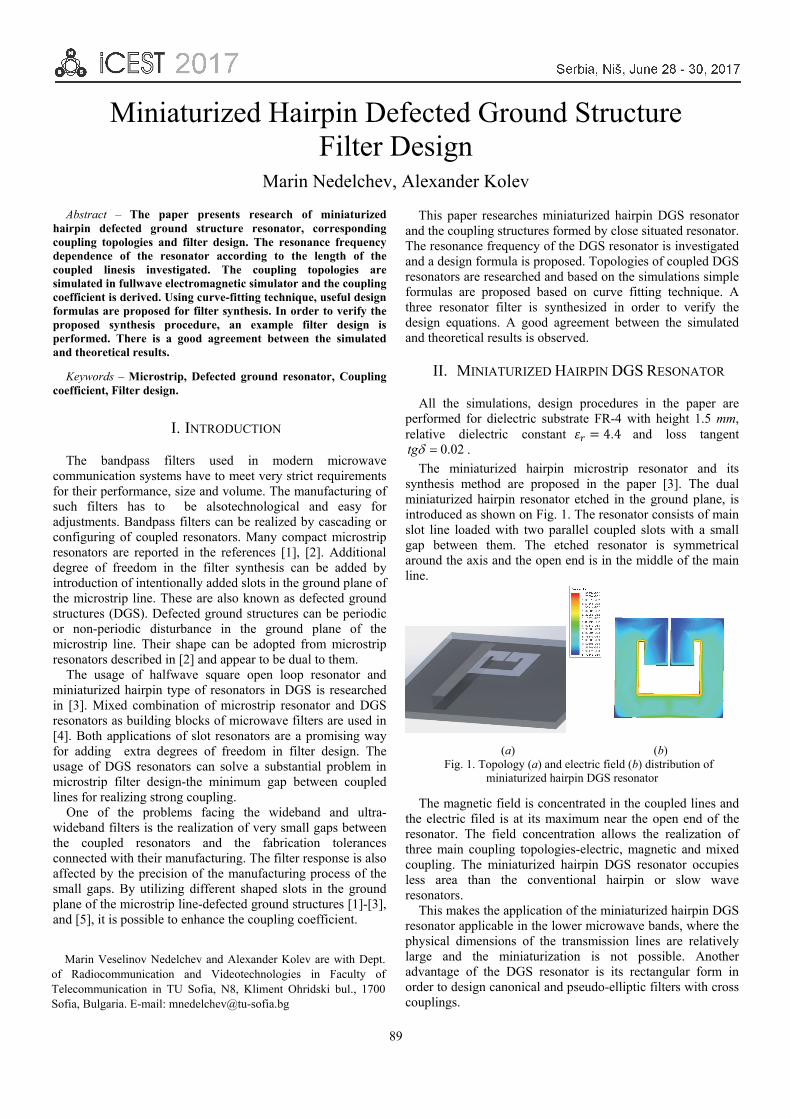
89

Miniaturized Hairpin Defected Ground Structure Filter Design

Marin Nedelchev, Alexander Kolev

Abstract – The paper presents research of miniaturized hairpin defected ground structure resonator, corresponding coupling topologies and filter design. The resonance frequency dependence of the resonator according to the length of the coupled linesis investigated. The coupling topologies are simulated in fullwave electromagnetic simulator and the coupling coefficient is derived. Using curve-fitting technique, useful design formulas are proposed for filter synthesis. In order to verify the proposed synthesis procedure, an example filter design is performed. There is a good agreement between the simulated and theoretical results.

Keywords – Microstrip, Defected ground resonator, Coupling coefficient, Filter design.

I. INTRODUCTION

The bandpass filters used in modern microwave communication systems have to meet very strict requirements for their performance, size and volume. The manufacturing of such filters has to be alsotechnological and easy for adjustments. Bandpass filters can be realized by cascading or configuring of coupled resonators. Many compact microstrip resonators are reported in the references [1], [2]. Additional degree of freedom in the filter synthesis can be added by introduction of intentionally added slots in the ground plane of the microstrip line. These are also known as defected ground structures (DGS). Defected ground structures can be periodic or non-periodic disturbance in the ground plane of the microstrip line. Their shape can be adopted from microstrip resonators described in [2] and appear to be dual to them.

The usage of halfwave square open loop resonator and miniaturized hairpin type of resonators in DGS is researched in [3]. Mixed combination of microstrip resonator and DGS resonators as building blocks of microwave filters are used in [4]. Both applications of slot resonators are a promising way for adding extra degrees of freedom in filter design. The usage of DGS resonators can solve a substantial problem in microstrip filter design-the minimum gap between coupled lines for realizing strong coupling.

One of the problems facing the wideband and ultra-wideband filters is the realization of very small gaps between the coupled resonators and the fabrication tolerances connected with their manufacturing. The filter response is also affected by the precision of the manufacturing process of the small gaps. By utilizing different shaped slots in the ground plane of the microstrip line-defected ground structures [1]-[3], and [5], it is possible to enhance the coupling coefficient.

This paper researches miniaturized hairpin DGS resonator and the coupling structures formed by close situated resonator. The resonance frequency of the DGS resonator is investigated and a design formula is proposed. Topologies of coupled DGS resonators are researched and based on the simulations simple formulas are proposed based on curve fitting technique. A three resonator filter is synthesized in order to verify the design equations. A good agreement between the simulated and theoretical results is observed.

II. MINIATURIZED HAIRPIN DGS RESONATOR

All the simulations, design procedures in the paper are performed for dielectric substrate FR-4 with height 1.5 mm, relative dielectric constant 4.4 and loss tangent

02.0tg .

The miniaturized hairpin microstrip resonator and its synthesis method are proposed in the paper [3]. The dual miniaturized hairpin resonator etched in the ground plane, is introduced as shown on Fig. 1. The resonator consists of main slot line loaded with two parallel coupled slots with a small gap between them. The etched resonator is symmetrical around the axis and the open end is in the middle of the main line.

(a) (b) Fig. 1. Topology (a) and electric field (b) distribution of

miniaturized hairpin DGS resonator

The magnetic field is concentrated in the coupled lines and the electric filed is at its maximum near the open end of the resonator. The field concentration allows the realization of three main coupling topologies-electric, magnetic and mixed coupling. The miniaturized hairpin DGS resonator occupies less area than the conventional hairpin or slow wave resonators.

This makes the application of the miniaturized hairpin DGS resonator applicable in the lower microwave bands, where the physical dimensions of the transmission lines are relatively large and the miniaturization is not possible. Another advantage of the DGS resonator is its rectangular form in order to design canonical and pseudo-elliptic filters with cross couplings.

Marin Veselinov Nedelchev and Alexander Kolev are with Dept. of Radiocommunication and Videotechnologies in Faculty of Telecommunication in TU Sofia, N8, Kliment Ohridski bul., 1700 Sofia, Bulgaria. E-mail: [email protected]

90

The coupled slot lines can be used for control of the resonant frequency of the resonator. The dimensions of the resonator tuned to central frequency 0 2.4f GHz are shown

on Fig. 1a. The main slot has the width of 50Ω microstrip line 2.8w mm . Using electromagnetic simulation the resonance

frequency is obtained. Fig. 2 shows the dependence of the first resonant frequency to the length of the parallel coupled lines p.

Fig. 2. Dependence of the resonance frequency of the length of the

coupled lines

Following the results from the simulations, the resonance frequency of the DGS resonator is easily tuned by adding or removing of metal to the ground plane. The dependence is almost linear. Using curve fitting a useful design expression is derived for the length of the coupled arms:

00.9858 [GHz]103.8 ,[ ]fp e mm (1)

The accuracy of Eq.1 compared to the electromagnetic simulations is better than 2.5 % and prevents errors caused by wrong read of the graphic results shown on Fig. 2.

III. COUPLING COEFFICIENTS AND EXTERNAL

QUALITY FACTOR SIMULATIONS

The coupling coefficient for synchronously tuned resonators can be calculated easily by finding the eigenfrequencies associated with the coupling between a pair of coupled resonators of even ( evenf ) and odd ( oddf ) mode

[2], when the coupled resonators are overcoupled:

2 2

2 2even odd

even odd

f fk

f f

. (2)

A full wave EM simulator based on the Finite element method (FEM) is used to identify the resonance frequencies in the response [2].

The coupling topologies used to realize the coupling coefficients are shown on Fig. 3. The miniaturized hairpin slot resonators shown on Fig. 3 are dual to the miniaturized hairpin resonator and the electromagnetic field is inversely distributed in it. The maximum value of the magnetic field is in the connection point of the coupled lines with the main

transmission line and the maximum value of the electric field is in the center of the main slot line. There are three main types of coupling typologies - electric, magnetic and mixed. In Fig. 3a is shown electric coupling, where the electric field has a maximum and dominates over the magnetic field. In this way the sign of the coupling coefficient is negative and can be used for cross coupled filters.

(a) (b)

(b) (d)

Fig. 3. Coupling topologies of miniaturized hairpin DGS resonators: (a) electric, (b) magnetic, (c) mixed,

and (d) external quality factor

Fig. 3b shows the magnetic coupling, where the magnetic field is predominant over the electric field. The sign of the coupling coefficient is positive.

An important part of the synthesis of microstrip filters is to determine the gap between the coupled resonators according to the value of the coupling coefficient found from the approximation. There are three main approaches to find out the space between the resonators - analytic formulas [2], approximate formulas from curve-fitting [4] and extraction from EM simulations using the method described in [2], and [3].

Using full-wave EM simulations of the coupling structures, which are very weekly coupled to 50 microstrip feed line,

the coupling coefficients are extracted using Eq. (2).

Fig. 4. (a) Dependence of the coupling coefficient for electric

coupling

91

Fig. 4. (b) Dependence of the coupling coefficient for magnetic coupling

Fig. 4 (c) Dependence of the coupling coefficient for mixed coupling

Fig. 4 a-c shows the coupling coefficient for all three types of coupling in dependence of the gap between the resonators s.

The dependence of the coupling coefficient for electrical coupling is exponential with respect to the spacing between the resonators. Using curve fitting method, for the design purposes it is derived the following dependence.

For electric coupling and electric coupling coefficient Me: eM

e es 26.4088.6 (3)

For magnetic coupling and magnetic coupling coefficient Mm:

mMm es 45.1826.12 (4)

And for mixed coupling and electric coupling coefficient Mmix:

mixMmix es 73.2805.13 (5)

Using Eq.(3)-(5) it is easy to compute the spacing between the coupled lines. The main constraint for the equations is

0.2,3s mm and their accuracy toward the simulations is

better than 5 %.

The position of the input/output lines is defined by the external quality factor. The external quality factor is realized by a 50 microstrip line on the top layer of the substrate,

shown on Fig. 3(d).

Fig. 5. Dependence of the external coupling to the position of the input/output microstrip line

The external quality factor is very sensitive to close placement of the microstrip line. The input/output microstrip line influences on the resonance frequency of the slot resonator and shifts it to lower values. This effect have to be compensated in the filter design by reduction of the coupled lines in the middle of input/output resonators. As the input/output line is on the top layer, it can overlap the resonator or can be placed aside it.

IV. BANDPASS FILTER SYNTHESIS AND

SIMULATIONS

In order to verify the proposed topologies of coupled resonators and formulas for coupling coefficients a three resonator Chebyshev filter is designed. Therefore the required coupling coefficients have to be computed using standard technique described in [2]

, 11

n nn n

FBWM

g g

, (6)

where FBW is the fractional bandwidth and ng , 0,1, 2,3n

are the values of the element of the lowpass filter prototype. There are various sources of precomputed values for the

elements for different pass band ripple. The current design is for center frequency 0 2400f MHz , bandwidth

200f MHz and return loss in the passband 20RL dB .

The values for the coupling coefficients are

12 23 0.086M M and the external quality factor is

25.98eQ . The corresponding gaps are 12 23 1.13s s mm

and overlapping between the input/output line and the resonator is 1.25d mm .

The filter is simulated in fullwave EM simulator and the results are shown on Fig.6. The passband losses are -3 dB and the maximum return loss in the pass band is -13.26 dB.

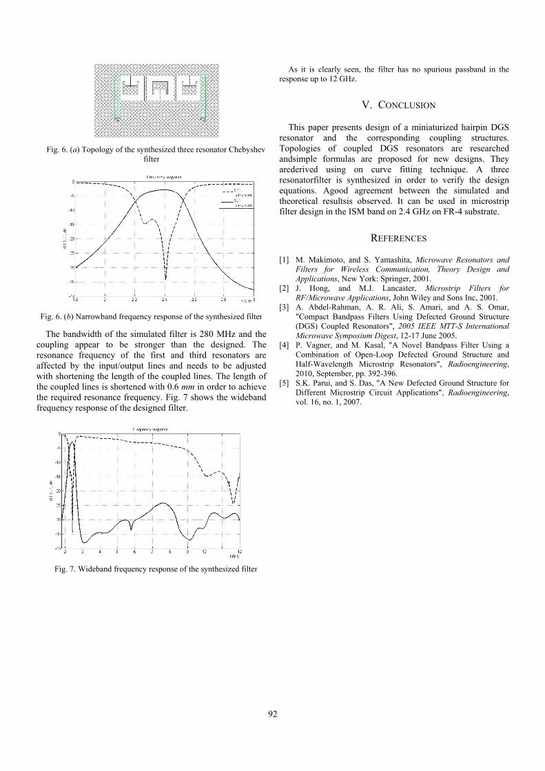
F

Fig

Tcouresoaffewiththe the freq

Fig. 6. (a) Topo

g. 6. (b) Narrow

The bandwidthupling appearonance frequeected by the h shortening tcoupled linesrequired reso

quency respon

Fig. 7. Wideb

ology of the synfi

wband frequency

h of the simur to be stroency of the input/output the length of ts is shortened onance frequennse of the desi

band frequency

nthesized three rilter

y response of th

ulated filter is onger than th

first and thilines and neethe coupled liwith 0.6 mm ncy. Fig. 7 shgned filter.

response of the

resonator Cheby

he synthesized

280 MHz anhe designed. ird resonatoreds to be adjines. The lengin order to ac

hows the wide

e synthesized fi

92

yshev

filter

nd the The

s are usted

gth of hieve eband

lter

Asrespo

ThresonTopoandsarederesonequatheorfilter

[1]FA

[2]R

[3]

[4]

[5]

s it is clearly sonse up to 12 G

his paper presnator and ologies of csimple formuerived usingnatorfilter is ations. Agoodretical resultsr design in the

M. Makimoto,Filters for WApplications, NJ. Hong, anRF/MicrowaveA. Abdel-Rahm"Compact Ban(DGS) CoupleMicrowave SymP. Vagner, andCombination oHalf-Waveleng2010, SeptembS.K. Parui, andDifferent Micrvol. 16, no. 1, 2

seen, the filter GHz.

V. CON

sents design othe corresp

coupled DGSulas are propg on curve

synthesized d agreement sis observed. e ISM band on

REFER

and S. YamaWireless CommNew York: Sprind M.J. Lane Applications, Jman, A. R. A

ndpass Filters Ud Resonators",

mposium Digestd M. Kasal, "Aof Open-Loop gth Microstrip er, pp. 392-396

d S. Das, "A Nrostrip Circuit 2007.

r has no spurio

NCLUSION

of a miniaturionding coupS resonators

posed for newfitting tech

in order to vbetween thIt can be us

n 2.4 GHz on

RENCES

ashita, Microwamunication, Thnger, 2001.

ncaster, MicroJohn Wiley and

Ali, S. Amari, Using Defected, 2005 IEEE Mt, 12-17 June 20A Novel Bandp

Defected GroResonators",

6. New Defected G

Applications",

ous passband in

ized hairpin Dpling structu are researcw designs. Thnique. A tverify the dee simulated sed in microFR-4 substrat

ave Resonatorsheory Design

ostrip Filters d Sons Inc, 200

and A. S. Od Ground Stru

MTT-S Internati005. pass Filter Usiound Structure

Radioenginee

Ground Structur, Radioenginee

n the

DGS ures. ched They three esign

and strip te.

s and and

for 1.

Omar, ucture ional

ing a and

ering,

re for ering,

93

A Comparison of Techniques for Characterizing Varied Microstrip Lines

Biljana P. Stošić, Zlata Cvetković

Abstract — The varied microstrip taper is fully characterized in frequency-domain. A comparison of different techniques for the line characterization is done. The accuracy of the used methods is studied using analysis of linearly tapered microstrip line. Results of numerical simulations compared with the analytical solutions have shown good agreement.

Keywords — Transmission line, Microstrip line, Linearly tapered line, Characterization.

I. INTRODUCTION

Tapered microstrip lines play an important role in microwave engineering. This nonuniform transmission lines have been extensively used in many applications, e.g., in impedance matching [1], pulse shaping [2, 3], couplers [4], [5], antennas [6], and filters [7]. Namely, impedance matching is an important aspect in the design of microwave and millimeter wave circuitry since impedance mismatches may severely deteriorate the overall performance of electronic systems.

The tapered transmission line performs matching of different impedances, i.e. a physical transition between parts of circuit with different impedances. The taper profile can be chosen in many ways. By changing the type of taper, one can obtain different passband characteristics. Several taper profiles may be considered: linear, exponential, triangular, logarithmic, and so on. In this paper, lineraly tapered microstrip line is characterized. Three analysis methods are used and compared here: (1) analytical equations based on the transmission line theory, (2) numerical simulations in Advanced Design System (ADS), (3) numerical simulations obtained by applying the wave digital filter theory.

Analytical method for analyzing tapered transmission lines has been introduced in [8-14]. This method is based on transmission line theory. Here, the method is applied to characterize microstrip taper designed on low-loss substrate.

Wave digital filter theory and its application in modeling and analyzing microstrip circuits of different geometries is explained in details in many papers [15, 16]. The calculating of the wave transfer matrix polynomials for the wave digital networks (WDNs) at hand is discussed in [15]. Here, modification of the existing approach is done in order to find frequency response in WDN which represents model of circuit with different port impedances.

Biljana P. Stošić and Zlata Cvetković are with the University of Niš, Faculty of Electronic Engineering, Aleksandra Medvedeva 14, 18000 Niš, Serbia, E-mails: [email protected]; [email protected]

II. TAPERED TRANSMISSION LINE

The aim of the analysis given here is matching impedance

0Z to the impedance LZ . A general circuit with included

tapered line of length L is shown in Fig. 1. In the global model, a taper is fed with a voltage source of amplitude E and internal impedance 0Z , and is terminated with an

impedance LZ .

Fig. 1. A circuit with tapered line

In this paper, the terms „linear” refer to the geometrical profile of the tapered line along its length. Line width as a function of the distance z for linearly tapered line is

max minmin( )

w ww z w z

L

, 0 z L , (1)

where min (0)w w represents minimum and max ( )w w L

maximum width of tapered line.

III. ANALYSIS TECHNIQUES

The methods are applied here to linearly tapered microstrip line. The line is characterized in the frequency domain. Comparison of the analysis results of all three methods explained in the text below is done on case of this line. (1) Starting up with the transmission line theory, the analytcal equations for linear taper are developed. Taper can be treated as lossless transmission line. One can consider an infinitely small portion of uniform line which can be regarded as a two-port circuit with distributed series impedance ( , )Z z and

distributed shunt admittance ( , )Y z . Without loss of

generality, the series impedance is made of a resistance R'dz and an inductance L'dz, where R' is the resistance per unit length and L is the inductance per unit length. The shunt admittance is made up of a parallel resistance (of admittance G'dz) and a capacitance C'dz, where G' is the conductance per unit length and C is the capacitance per unit length. Elementary circuit theory shows that the differential equations of transmission line are [5-7]

94

( , )( , ) ( , )

dV zZ z I z

dz

, (3)

( , )( , ) ( , )

dI zY z V z

dz

, (4)

where ( , ) ( , ) ( , )Z z R z j L z represents the impedance

per-unit-length, ( , ) ( , ) ( , )Y z G z j C z represents the

admittance per-unit-length, and is the angular frequency in radians/second.

Classic transmission line theory states that the characteristic impedance 0Z of a transmission line can be derived from a

knowledge of the resistance R , inductance L , conductance G , and capacitance C per unit length of the transmission line from the expression

0( , )

( , )

Z zZ

Y z

. (5)

The propagation constant is

( , ) ( , )Z z Y z . (6)

Consider a lossless and linearly varied single transmission line with the distributed primary parameters 0( ) (1 )L z L m z ,

0( ) / (1 )C z C m z ,

( ) ( ) 0R z G z ,

where 0( / 1) /Lm Z Z L .

The differential equations for voltage and current are

2

22

( , ) ( )( ) 0

1

d V z m dV zV z

m z dzdz

,

and

2

22

( , ) ( )( ) 0

1

d I z m dI zI z

m z dzdz

,

where 2 2( , ) ( , ) ( / ) effrZ z Y z c .

The solutions of these equations, i.e. the voltage and current distributions across the line, are obtained as

1 1 2 1( ) (1 ) ( (1 ) / ) ( (1 ) / )V z m z K J mz m K Y mz m ,

and

1 0 2 00

( ) ( (1 ) / ) ( (1 ) / )j

I z K J mz m K Y mz mZ

,

respectively. 1K and 2K are constants found from the

boundary conditions ( 0)V z E ,

and 0( ) / ( ) (1 )LV z L I z L Z Z mL .

Bessel functions of the first kind are denoted by ( )nJ z , and

Bessel function of the second kind by ( )nY z . Index n shows

their order. If some expressions are assigned as 1 ( 0) /u u z m and

2 ( ) (1 ) /u u z L mL m , then constants are

1 1 2 0 2

11 1 1 2 1 2 1 1

0 2 1 1 1 1 0 2

( ) ( )

( ) ( ) ( ) ( )

( ) ( ) ( ) ( )

K Y u j Y u E

J u Y u J u Y u

j J u Y u J u Y u

and

2 1 2 0 2

11 1 1 2 1 2 1 1

0 2 1 1 1 1 0 2

( ) ( )

( ) ( ) ( ) ( )

( ) ( ) ( ) ( )

K J u j J u E

J u Y u J u Y u

j J u Y u J u Y u

Input impedance of the line is ( 0) / ( 0)inZ V z I z ,

and the reflection coefficient is 0 0( ) / ( )in in inZ Z Z Z .

This method can be easily implemented in the MATLAB

environment. MATLAB functions besselj and bessely are employed to find the response. besselj(nu,Z) computes the Bessel function of the first kind, for each element of the array Z . bessely(nu,Z) computes the Bessel function of the second kind. The order nu need not be an integer, but must be real.

(2) Numerical simulations of the line is done in Advanced Design System (ADS) by schematic shown in Fig. 2a. In ADS, component Microstrip Width Taper (MTAPER) is used for representing varied line. The frequency-domain analytical model is a microstrip line macro-model developed by Agilent. The taper is constructed from a series of straight microstrip sections of various widths that are cascaded together. The microstrip line model is the MLIN model. The number of sections is frequency dependent. Dispersion, conductor loss, and dielectric loss effects are included in the microstrip model. Fig. 2b shows layout of tapered line which is designed on low-loss Ultralam substrate.

MTAPERTaper7

L=19.05 mmW2=5080 umW1=2075.2 umSubst="MSub1"

TermTerm1

Z=50 OhmNum=1

TermTerm2

Z=25 OhmNum=2

S_ParamSP1

Step=0.01 GHzStop=14 GHzStart=2 GHz

S-PARAMETERS

MSUBMSub1

Rough=0 milTanD=0.0022T=0.017018 mmHu=3.9e+034 milCond=5.8E+07Mur=1Er=2.6H=762 um

MSub

(а)

95

(b)

Fig. 2. (a) ADS schematic of varied taper,

(b) Layout of varied taper in ADS

(3) Numerical simulations is done by applying the wave digital filter theory. In Fig. 3, profile of the linear taper as a function of the longitudinal distance is shown. In order to characterized the line that has length L , the wave digital approach can be applied if the line is approximated with several segments of different widths and equal lengts. Line width ( )w z is a function of distance along line, where z is

distance from the 0Z side of the line [15, 16]. A good

approximation is achieved if the line width is determined at the half of the segment. In other words, for this taper, one can write for the width of the ith subsection

( )2

beginendbegin i i

i iw w

w z w

, 1, 2,...,i N . (2)

Here, endiw and begin

iw denote the line width at the beginning

and the end, respectively, calculated from Eq. (1). N is the total number of subsections in which the entire transmission line is breaked, and it can be chosen arbitrarily. A very simple algorithm for direct calculation of polynomial coefficients of rational functions 21S and 11S ,

developed in z-domain, is described in [15]. In that paper, one case of circuit consisting of two cascadede linear tapers which forms circuit with equal port impedances is consider. In order to find response of the circuit which port impedances differs one from another, the equations given there are modified. When determine the 21S parameter in wave digital model,

one have to take care of ratio 0 / LZ Z , and should calculate

new value of parameter 21S as 21 0 / LS Z Z .

)(zw0Z LZ

)(zZc Fig. 3. Linearly tapered line and

its approximation for wave digital approach

IV. ANALYZED EXAMPLE CIRCUIT

The accuracy of the used methods is studied using analysis of linearly tapered microstrip line. The aim of the analyzed circuit is matching impedance 0 50Z to the impedance

25LZ . The microstrip line is designed for an Ultralam

substrate and considered to be lossless. The parameters are: minimum line width min 599.44 w m at 0Z side of the

line, maximum line width max 5080 w m at LZ side of the

line, line length 19.05 L mm , relative dielectric constant of substrate 2.6r and substrate high 762 h m .

Scaterring parameters of the linearly varied taper obtained by use of different methods are pictured in Figs. 4-6. They show responses both simulated in MATLAB by proposed approaches and obtained in ADS simulator.

In the case of WDNs, results are obtained in 0.056753 s. If the taper is analyzed directly by using analytical equations, much more simulation time is required, 20.439872 s.

Results of numerical simulations compared with the analytical solutions have shown good agreement.

2 4 6 8 10 12 14

x 109

0

0.2

0.4

0.6

0.8

1

1.2

X: 2.017e+009Y: 0.2682

X: 5.369e+009Y: 0.03818

X: 7.996e+009Y: 0.07926

X: 1.079e+010Y: 0.01969

X: 3.999e+009Y: 0.1149

Fig. 4. Reflection coefficient vs. frequency (Method (1))

4 6 8 10 122 14

0.2

0.4

0.6

0.8

1.0

0.0

1.2

freq, GHz

mag

(S(1

,1))

m1

m2 m3 m4m5

mag

(S(2

,1))

m1freq=mag(S(1,1))=0.250

2.050GHzm2freq=mag(S(1,1))=0.074

4.030GHz

m3freq=mag(S(1,1))=0.075

6.020GHz

m4freq=mag(S(1,1))=0.069

8.010GHz

m5freq=mag(S(1,1))=0.012

9.670GHz

Fig. 5. Reflection and transmission coefficients vs.

frequency (Method (2))

96

2 4 6 8 10 12 140

0.2

0.4

0.6

0.8

1

1.2

10 segments

X: 2.037Y: 0.2532

f [GHz]

Ultralam 2000

|S21

|

|S11

|

X: 3.995Y: 0.07958

X: 5.979Y: 0.07196

X: 8.016Y: 0.07045

X: 12.01Y: 0.05571X: 9.789

Y: 0.007542

Fig. 6. Reflection and transmission coefficients vs.

frequency (Method (3))

V. CONCLUSION REMARKS

A modification of the wave digital approach is proposed, whose aim is to enlarge types of microstrip structures that can be modeled into WDNs. Types of structures that can be analyzed through the ideas proposed in the paper [15] are those with different port impedances.

The S parameters are important in microwave design because they are easier to measure and work with at high frequencies. The proposed approach is implemented on a processor Intel(R) Core(TM) i5-3470 CPU @ 3.2 GHz . The analysis of wave digital networks is a very efficient, because there is no high memory request and a very short time is needed for response calculation in the frequency domain directly (a few seconds or even less). This approach provides the faster structure simulation versus complex and time consuming 3D models.

A comparison of different techniques (numerical and analytical solutions) for characterizing the linear taper is done. The advantages and disadvantages of the used techniques are demonstrated by one example and some comparisons (frequency response and estimated time). The computer simulated results obtained by WDNs and analytical equations are compared to those simulations obtained in ADS (simulation based on circuit-level (Circuit-level) and electromagnetic 2.5D MoM simulation (Momentum)). One can observe that results obtained by described approach have good agreement with ADS data in whole frequency band.

ACKNOWLEDGMENT

This work has been partially supported by the Ministry of Education, Science and Technological Development of Serbia, project number TR 32052.

REFERENCES

[1] R.E. Colin, Foundations for Microwave Engineering, McGraw-Hill, New York, 1996.

[2] W.-K. Chen, The Circuits and Filters Handbook, CRC Press, 1995.

[3] E. Afshari, H.S. Bhat, A. Hajimiri, J.E. Marsden, "Extremely Wideband Signal Shaping Using One- and Two-Dimensional Nonuniform Nonlinear Transmission Lines", J. Appl. Phys., vol. 99, Mar. 2006.

[4] F. Hosseini, M. K.-A. Hosseini, M. Yazdani, "Novel Compact Branchline Coupler Using Non-uniform Transmission Line", AsiaPacific Microw. Conf., pp. 1577-1580, 2009.

[5] P. Salem, C. Wu, M. C. E. Yagoub, "Non-uniform Tapered Ultra Wideband Directional Coupler Design and Modern Ultra Wideband Balun Integration", Proc. AsiaPacific Conf., 2006-Dec.

[6] N.H. Younan, B.L. Cox, C.D. Taylor, W.D. Rather, "An Exponentially Tapered Transmission Line Antenna", IEEE Trans. Electromagn. Compat., vol. 36, no. 1, pp. 141-144, Feb. 1994.

[7] L.A. Hayden, V. K. Tripathi, "Nonuniformly Coupled Microstrip Filters for Analog Signal Processing", IEEE Trans. Microw. Theory Tech., vol. 39, no. 1, pp. 47-53, Jan. 1991.

[8] K. Lu, "An Efficient Method for Analysis of Arbitrary Nonuniform Transmission Lines", IEEE Transactions on Microwave Theory and Techniques, vol. 45, no. 1, January, 1997, pp. 9-14.

[9] C.L. Edwards, M. Lee Edwards, S. Cheng, R. Stilwell and C.C. Davis, "A Simplified Analytic CAD Model for Linearly Tapered Microstrip Lines", IEEE MTT-S Digest, 2003, pp. 2101-2104.

[10] C.L. Edwards, M. Lee Edwards, S. Cheng, R.K. Stilwell and C. C. Davis, "A Simplified Analytic CAD Model for Linearly Tapered Microstrip Lines Including Losses", IEEE Transactions on Microwave Theory and Techniques, vol. 52, no. 3, March, 2004, pp. 823-829.

[11] D. Jovanović and Z. Cvetković, "Analysis of Lossless Linearly Tapered Transmission Line", ETRAN 2015 Conference, Serbia, Silver Lake, June 8-11, 2015, pp. MT1.8.

[12] M. Khalaj-Amirhosseini, "Analysis of Coupled or Single Nonuniform Transmission Lines Using Step-by-Step Numerical Integration", Progress In Electromagnetics Research, PIER 58, pp. 187-198, 2006.

[13] M.H. Eghlidi, K. Mehrany and B. Rashidian, "Analytical Approach for Analysis of Nonuniform Lossy/Lossless Transmission Lines and Tapered Microstrips", IEEE Transactions on Microwave Theory and Techniques, vol. 54, no. 12, pp. 4122-4129, Dec. 2006.

[14] S. M.H. Javadzadeh, Z. Mardy, K. Mehrany, F. Farzaneh and M. Fardmanesh, "Fast and Efficient Analysis of Transmission Lines With Arbitrary Nonuniformities of Sub-Wavelength Scale," in IEEE Transactions on Microwave Theory and Techniques, vol. 60, no. 8, pp. 2378-2384, Aug. 2012.

[15] B.P. Stošić, and M.V. Gmitrović, "Implementation of Wave Digital Model in Analysis of Arbitrary Nonuniform Transmission Lines", Microwave and Optical Technology Letters, vol. 49, no. 9, pp. 2150-2153, 2007.

[16] M. Gmitrović, B. Stošić, A. Đorđević, "Modeling of 1D Structures by using Wave Digital Elements", L Conference on ETRAN, Belgrade, Serbia and Montenegro, June 6-8, 2006, vol. II, pp. 317-320.

97

Improving Shielding Effectiveness of a Rectangular Metallic Enclosure with Aperture by Using Printed

Dog-bone Dipole Structure Nataša Nešić1, Bratislav Milovanović2, Nebojša Dončov3,

Vanja Mandrić-Radivojević4 and Slavko Rupčić4

Abstract – In this paper, theelectromagneticshielding results of both numerical and experimental models of an enclosure with a printed dog-bone dipole antenna inside are considered. This printed structure is placed inside the enclosure in order to improve the protective function of the enclosure. The impact of this structure on values of shielding effectiveness of the enclosure is analyzed, especially at the first resonance of the enclosure. In order to obtain the optimal results, the printed structure position inside the enclosure is changed in three parallel positions.

Keywords – Aperture,Enclosure, Shielding effectiveness, Dog-

bone dipole structure, Monopole antenna, TLM wire method.

I. INTRODUCTION

At resonant frequencies, the shielding metal enclosure can indicatevery low or even negative values of the shielding effectiveness (SE) [1]. Consequently, the resonant frequencies of the enclosure can be critical since they might compromise the useful frequency range in which electromagnetic (EM) shielding is provided. Therefore, several techniques were implemented to improve the shielding properties. For instance, in [2] an extra aperture as a matched load instead of a shorted waveguide was proposed by using TLM (Transmission Line Matrix) method. Paper [3] combined MoM and FEM methods for EM field distribution to determine the effect of the aperture size of a loaded enclosure with PCB(s) inside. Also, SE can be improved by using conductive foam, or absorbers [4], [5]. Furthermore, the composite materials based on nanotechnology [6], metamaterial structure [7] and a frequency-selective surface [8] can be employed as damping techniques.The enclosure can be coated with composite material or can be made of that material [9].

More related to this work, in [10] a simple strategy was

proposed to suppress the first resonance in a metal enclosureby putting small antenna elements with loaded resistance.It was shown that placing a small dipole or loop antenna structure on the enclosure wall opposite to the enclosure aperture can improve the enclosure SE. The effective length of this printed structure was chosento match the enclosure’s first resonant frequency. Numerical study, based on this research, was carried out in [11], to further investigate this strategy.

In this paper, the impact of the printed dipole dog-bone antenna inserted in the shielding metal enclosure with a rectangular aperture is consideredboth numerically and experimentally from the viewpoint of the shielding effectiveness of enclosure. The dog-bone antenna structure, with the dimensions designed to influence the first enclosure resonance, is printed on an epoxy substrate which is placed inside the enclosure in three positions parallel to the aperture wall. Numerical and experimental SE results of the enclosure are obtained by using a receiving-monopole antenna.

II. NUMERICAL TLM WIRE MODEL

Anumerical modeling technique,called the TLM method [12], is employed in this paper. The TLM method has been enhanced with a number of different compact models to allow an efficient modelling of EM important features [12]-[14]. For modelling an antenna inside enclosure whose purpose is to measure the EM field level and distribution, the compact wire model is the most appropriate. It is based on wire segment incorporated into the Symmetrical Condensed Node (SCN). The SCN with wire segment is running in z-direction is shown in Fig. 1. The impedances of additional wire network link and short-circuit stub lines depend on used space and time-step discretization, and also on per-unit length wire capacitance and inductance [14]. Two-way coupling between signal in the z-directed wire circuit and external EM field described by pulses in transmission line network of SCN (marked bold in Fig. 1) is achieved through points A and B. In considered case,the wire is connected to the ground via resistor R. The induced current on the wire, due to external EM field, generates voltage on the resistor R, loaded at wire base, allowsmeasuringthe level of EM field.

The considered metal enclosure is shown in Fig. 2. It is rectangular, with internal dimensions of (300x400x200) mm3 and an aperture of dimensions (50 x 10) mm2 is positioned symmetrically around the center on the frontal wall. Material from which the enclosure is made of is copper. Thickness of the enclosure walls is t = 2 mm, while the frequency range of

1Nataša Nešićis with the College of Applied Technical SciencesNiš, Aleksandra Medvedeva 20, Niš 18000,Serbia, E-mail: [email protected]

2Bratislav Milovanović is with the University of Singidunum,Danijelova 32, Belgrade 11000, Serbia, E-mail: [email protected]

3Nebojša Dončov is with the Faculty of Electronic Engineering inNiš, University of Niš, Aleksandra Medvedeva 14, Niš 18000, Republic of Serbia,E-mail: [email protected]

4Vanja Mandrić-Radivojević and Slavko Rupčićare with Department of Communications Faculty of Electrical EngineeringOsijek 31000, Croatia, E-mails: [email protected], [email protected]

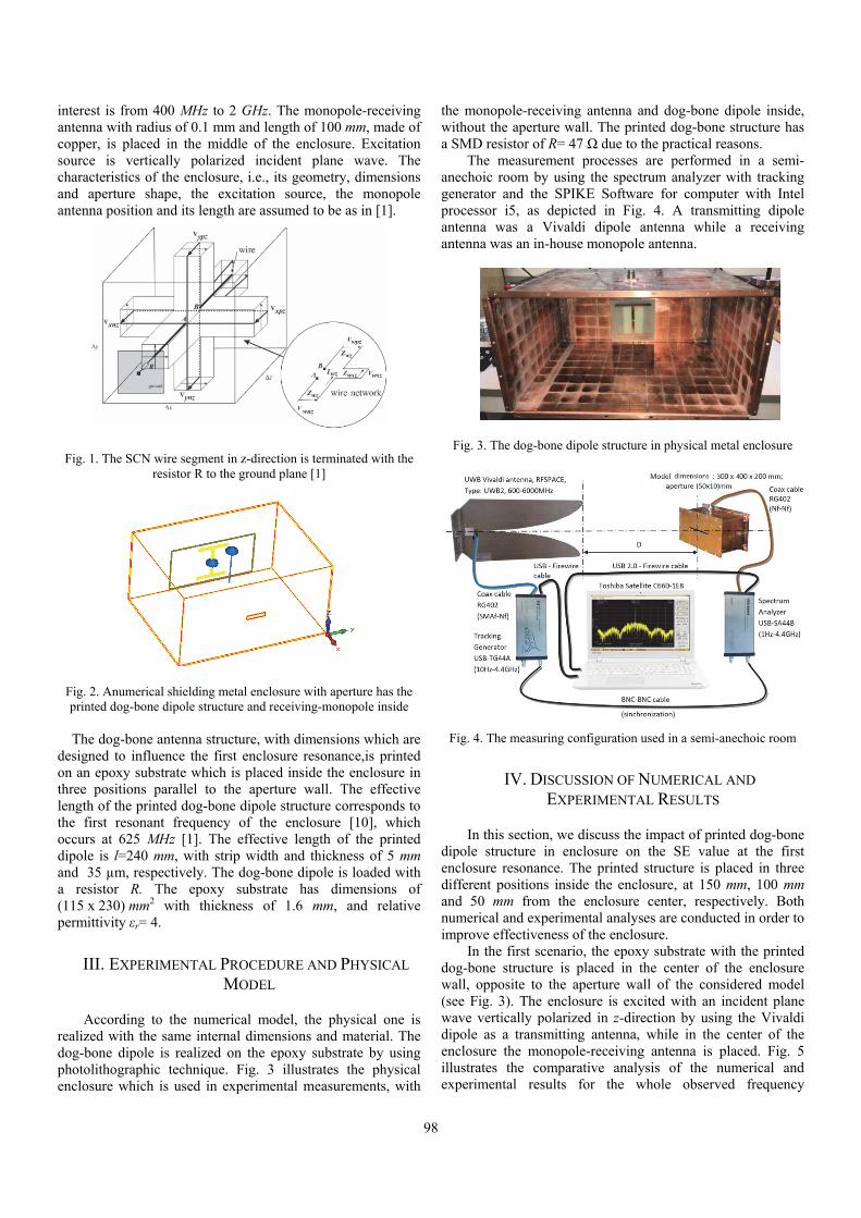
98

interest is from 400 MHz to 2 GHz. The monopole-receiving antenna with radius of 0.1 mm and length of 100 mm, made of copper, is placed in the middle of the enclosure. Excitation source is vertically polarized incident plane wave. The characteristics of the enclosure, i.e., its geometry, dimensions and aperture shape, the excitation source, the monopole antenna position and its length are assumed to be as in [1].

Fig. 1. The SCN wire segment in z-direction is terminated with the resistor R to the ground plane [1]

Fig. 2. Anumerical shielding metal enclosure with aperture has the printed dog-bone dipole structure and receiving-monopole inside The dog-bone antenna structure, with dimensions which are

designed to influence the first enclosure resonance,is printed on an epoxy substrate which is placed inside the enclosure in three positions parallel to the aperture wall. The effective length of the printed dog-bone dipole structure corresponds to the first resonant frequency of the enclosure [10], which occurs at 625 MHz [1]. The effective length of the printed dipole is l=240 mm, with strip width and thickness of 5 mm and 35 µm, respectively. The dog-bone dipole is loaded with a resistor R. The epoxy substrate has dimensions of (115 x 230) mm2 with thickness of 1.6 mm, and relative permittivity εr= 4.

III. EXPERIMENTAL PROCEDURE AND PHYSICAL

MODEL

According to the numerical model, the physical one is realized with the same internal dimensions and material. The dog-bone dipole is realized on the epoxy substrate by using photolithographic technique. Fig. 3 illustrates the physical enclosure which is used in experimental measurements, with

the monopole-receiving antenna and dog-bone dipole inside, without the aperture wall. The printed dog-bone structure has a SMD resistor of R= 47 Ω due to the practical reasons.

The measurement processes are performed in a semi-anechoic room by using the spectrum analyzer with tracking generator and the SPIKE Software for computer with Intel processor i5, as depicted in Fig. 4. A transmitting dipole antenna was a Vivaldi dipole antenna while a receiving antenna was an in-house monopole antenna.

Fig. 3. The dog-bone dipole structure in physical metal enclosure

Fig. 4. The measuring configuration used in a semi-anechoic room

IV. DISCUSSION OF NUMERICAL AND

EXPERIMENTAL RESULTS

In this section, we discuss the impact of printed dog-bone dipole structure in enclosure on the SE value at the first enclosure resonance. The printed structure is placed in three different positions inside the enclosure, at 150 mm, 100 mm and 50 mm from the enclosure center, respectively. Both numerical and experimental analyses are conducted in order to improve effectiveness of the enclosure.

In the first scenario, the epoxy substrate with the printed dog-bone structure is placed in the center of the enclosure wall, opposite to the aperture wall of the considered model (see Fig. 3). The enclosure is excited with an incident plane wave vertically polarized in z-direction by using the Vivaldi dipole as a transmitting antenna, while in the center of the enclosure the monopole-receiving antenna is placed. Fig. 5 illustrates the comparative analysis of the numerical and experimental results for the whole observed frequency

99

range.The numerical curves results are labelled as Empty_sim for the empty enclosure, Monopole_sim for the enclosure with monopole-receivingantenna and Dog-bonefr1_150mm for the case with dog-bone on the wall opposite to the aperture wall, in presence of the receiving-monopole in the center. The experimental analyses are labelled: Monopole_meas for the case with receiving in-house monopole, Dog-bone fr1_150mm_measis related to receiving in-house monopole and the printed dog-bone structure,as presented in Fig. 3. It can be observed that both simulated and measured results have a very good match. A narrow frequency range, from 400 MHz to 800 MHz, is shown in Fig. 6 since it is important for observing the SE values occurred at the first resonance of the enclosure. It is evident that the monopole-receiving antenna inside enclosure creates some perturbation. Consequently, the position of the first resonance is shifted toward the lower frequencies in comparison to the empty enclosure, which is analyzed in detail in [1]. It can be observed that the SE results for the first resonance is higher for about 20 dB in comparison to the empty enclosure. In Table I, the SE values at the first resonant frequencies are provided for all considered cases.

TABLE I THE SE VALUES AT THE FIRST ENCLOSURE RESONANCE

Dog-bone structure

fr1_sim [MHz]

fr1_meas [MHz]

SE_sim[MHz] SE_meas [dB]

fr1_150mm 582.025 575.923 26.11 22.99 fr1_100mm 578.631 559.894 25.74 27.87 fr1_50mm 523.286 536.091 35.92 29.35 Empty 624.365 - -2.22 - Monopole 583.045 582.632 24.41 20.99

Fig. 5. The SE of enclosure with a printed dog-bone structure placed at 150mm from the enclosure center and with receiving monopole. The second scenario is conducted for the numerical model

with the same printed dog-bone structure which is now shifted 50 mm from the internal enclosure wall toward the enclosure center. In other words, the dog-bone structure is placed 100 mm from the center of enclosure to the wall which is opposite to the aperture wall. Fig. 7 illustrates the numerical SE curves obtained for Dog-bone fr1_100mm and Monopole_sim are quite similar. For the experimentally

measured results, the SE measured curve for the second dog-bone scenario is shifted toward lower frequencies, at the first resonant frequency, in comparison to the Monopole_meas and the first dog-bone scenario. Also, the SE values at the first resonance and around resonance increase in contrast to the resonance of the empty enclosure.

Fig. 6.The frequency range around the first resonant frequency for scenario as in Fig. 5

Fig. 7. The first resonance SE peaks for the second dog-bone scenario, enclosure with monopole antenna and the empty enclosure.

In the third scenario, we put the printed dog-bone dipole at

position of 50 mm from the enclosure centermrc4. In Fig. 8 it can be observed that the third dog-bone dipole gives the most significant improvement in comparison to other two scenarios.

Fig. 9 gives the measured SE characteristics for the three dog-bone dipole scenarios. Table I shows the values of the first resonant frequencies and the amplitudes for all three scenarios. It is clear that the third scenario has the most prominent suppression. The improvement in the suppression of the SE amplitude at the resonance is significant, (35.92-(-2.22)) dB = 38.14 dB for Dog-bone fr1_50 compared to the empty enclosure, and the level of (35.92-24.41) dB = 11.51 dB for Dog-bone fr1_50 compared to the enclosure with monopole. It should be noted that these data are given for numerical analysis. In addition, the measurements related to dog-bone structure are consistent with the corresponding numerical analyzes and, according to

400 600 800 1000 1200 1400 1600 1800 2000

0

20

40

60

80

100

120

SE

(d

B)

Frequency (MHz)

Dogbone fr1_150_sim Monopole_sim Dogbone fr1_150_meas Empty_sim Monopole_meas

400 500 600 700 800

0

20

40

60

80

SE

(dB

)

Frequency (MHz)

Dogbone fr1_150_sim Monopole_sim Dogbone fr1_150_meas Empty_sim Monopole_meas

400 500 600 700 800

0

20

40

60

80

SE

(dB

)

Frequency (MHz)

Dog-bone fr1_100_sim Dog-bone fr1_100_meas Monopole_sim Monopole_meas Empty_sim

100

the perturbation theory, this is expected impact of the body placed into the resonator.

Fig. 8. The first resonance SE peaks for the third dog-bone scenario,

enclosure with monopole antenna and the empty enclosure.

Fig. 9. The measured first resonance SE peaks for the three dog-bone scenarios in the enclosure.

V. CONCLUSION

To increase the SE level of the shielding enclosure, especially at the first resonance frequency, a printed dog-bone structure, with dimensions which are designed to influence the first enclosure’s resonance, is put inside the enclosure.It has been shown that this structure may improve the SE around 30dB. Also, there might be a resonance frequency shift of around 90MHz.Further research can be related to finding the appropriate printed dipole structure with dimensions and shape which can be adequate for suppressing the first three enclosure resonances.Also, we will analyze the case for another receiving antennawhich creates less perturbation of EM field distribution inside an enclosure,e.g. a dipole antenna [1].

ACKNOWLEDGEMENT

This work has been partially supported by the Ministry for Education, Science and Technological Development of

Serbia; projectnumberTR32052, by the EUROWEB+ project and by the COST IC 1407 Action.

REFERENCES

[1] N.J. Nešić, and N.S. Dončov, "Shielding Effectiveness Estimation by using Monopole-receiving Antenna and Comparison with Dipole Antenna", Frequenz DeGruyter, no. 5-6, DOI 10.1515/freq-2015-0203, pp. 1-11, 2016.

[2] M. Bahadorzadeh, and A.A. Lotfi-Neyestanak, "A Novel and Efficient Technique for Improving Shielding Effectiveness of a rectangular Enclosure using Optimized Aperture Load", Elektronika ir Elektrotechnika, vol. 18, no. 10, pp. 89-92, 2012.

[3] S. Yenikaya, and G. Yenikaya, "Electromagnetic Coupling Analysis of Signal throught Aperture Perforated in a Loaded Shielding Enclosure Using Hybrid MoM/FEM", Int. Journal of Basic & Applied Sciences IJBAS-IJENS, vol. 11, no. 6, pp. 81-86, 2011.

[4] R. Kumar, S.R. Dhakate, P. Saini, and R.B. Mathur, "Improved Electromagnetic Interference Shielding Effectiveness of Light Weight Carbon Foam by Ferrocene Accumulation", The Roy. Soc. of Chem. 2013: RSC Advances, vol. 3, pp. 4145-4153, 2013.

[5] X. Luo, and D.D. Chung, "Electromagnetic Interference Shielding Using Continuous Carbon-Fiber Carbon-Matrix and Polymer-Matrix Composites", Elsevier Science:Composites: Part B , vol. 30, p. 227-231, 1999.

[6] T.K. Gupta, B.P. Singh, R.B. Mathur, and S.R. Dhakate, "Multi-Walled Carbon Nanotube–Graphene–Polyaniline Multiphase Nanocomposite with Superior Electromagnetic Shielding Effectiveness", The Royal Society of Chemistry 2014: Nanoscale, vol. 6, p. 842-851, 2014.

[7] F. Costa, S. Genovesi, A. Monorchio, and G. Manara, "A Circuit-based Model for the Interpretation of Perfect Metamaterial Absorbers", IEEE Trans. on Antennas and Propagation, vol. 63, no. 3, pp. 1201 - 1209, 2013.

[8] B.A. Munk, Frequency Selective Surfaces Theory and Design, New York: John Wiley and Sons, Inc., 2000.

[9] A. Ameli, P.U. Jung, and C.B. Park, "Electrical Properties and Electromagnetic Interference Shielding Effectiveness of Polypropylene/Carbon Fiber Composite Foams", Elsevier: Carbon, vol. 60, pp. 379-391, 2013.

[10] J. Paul, S. Greedy, H. Wakatsuchi, and C. Christopoulos, "Measurements and Simulations of Enclosure Damping Using Loaded Antenna Elements", 10th Int. Symp. on EMC, pp. 676–679, York, 2011.

[11] T. Cvetković, Numerical Characterization of Shielding Effectiveness of an Enclosure with Apertures Based on Coupling with the Wire Structures (in Serbian), Niš: Doctoral disertation, Faculty of Electonic Engineering, 2015, pp. 107-119.

[12] C. Christopoulos, The Transmission-Line Modelling (TLM) Method, New Jersey: IEEE Press in assoc. with Oxford University Press, Piscataway, 1995.

[13] A.J. Wlodarczyk, V. Trenkić, R. Scaramuzza, and C. Christopoulos, "A Fully Integrated Multiconductor Model for TLM", IEEE Trans. of MTT, vol. 46, no. 12, pp. 2431-2437, 1998.

[14] V. Trenkić, A.J. Wlodarczyk, and R. Scaramuzza, "A Modelling of Coupling between Transient Electromagnetic Field and Complex Wire Structures", Int. Journal of Num. Modelling, vol. 12, no. 4, pp. 257-273, 1999.

400 500 600 700 800

0

20

40

60

80

SE

(d

B)

Frequency (MHz)

Dog-bone fr1_50_sim Dog-bone fr1_50_meas Monopole_sim Monopole_meas Empty_sim

400 500 600 700 800 900

20

30

40

50

60

70

SE

(d

B)

Frequency (MHz)

Dog-bone fr1_50mm Dog-bone fr1_100mm Dog-bone fr1_150mm

101

Measurement of the Shielding Effectiveness of Passive Cable Television Elements

Péter Prukner1, István Drotár1, Máté Liszi1, Szilvia Nagy2

Abstract – The frequencies that are available due to the digital switchover of the terrestrial television broadcasting overlap with the frequencies used in cable television systems. Theoretically the two systems are independent of each other, but in practice, in case of not sufficient shielding, the cable television signals can disturb or can be disturbed by the signals from the over the air frequency bands. The main objective of the study was to find out about the shielding effectiveness of various cables and taps. During the measurements we also investigated how the measured results change in the case of broken cables, damaged multitaps and not properly secured closings using the specifications and directions of the 50083-2 EMC standard as a guideline.

Keywords – EMC, Digital dividend, Digital switchover CATV, Shielding effectiveness.

I. INTRODUCTION

A. Digital Dividend Switchover from analogue to digital television broadcasting

resulted in a significant difference in the spectrum usage. The introduction of the DVB-T system caused the decrease of the channel need and resulted in an increase of the quality of the programmes, compared to the former, analogue systems. The frequency bands unused by the new system is called digital dividend [1].

Due to the advanced compressing and coding methods (H.264/MPEG-4 AVC, HEVC/ITU-T H.265) as well as the transport techniques applied in the present networks, a broadcasting system needs smaller and smaller part of the spectrum, moreover, further decrease can be achieved by new base band coding and multiplexing methods. Thus, we can conclude that the final size of the digital dividend can not be determined yet. It is clear, however, that these new frequency bands can be used for other purposes and technologies, and the most effective usage would be a harmonized one, i.e., if all the countries would have the same allocation.

As the bandwidth demand of the mobile telecommunication increases rapidly, the question arose, whether the whole former television band is necessary for DVB-T broadcasting. Due to the favorable wave propagation properties and the LTE technology, the 800 MHz band is more useful for mobile purposes [2-6], thus the EU regulations adapted quickly: CEPT developed a mobile allocation plan to band 790-

862 MHz. During World Radiocommunication Conference, WRC 2007, the decision was made that allows the alternative use of the frequency band, and in its footnote 5.316A part of the countries intended to allocate the band for mobile communications as well.

According to the calculations, the two services (mobile and TV) could not work beside each other without distraction [4,5], thus the only solution was to empty the band first, before the mobile providers could start to use it. The channel allocation of the band is given in decision ECC/DEC/(09)03.

B. CATV Frequency Bands In case of cable television (CATV) networks, spectrum

allocation is different from that of the terrestrial or satellite broadcasting, due to the fact that the network communication takes place on shielded network that is isolated from its environment, thus the complete available frequency domain belongs practically to the service provider. Fig. 1 shows the frequency allocation valid from 2014.

Fig. 1. Frequency allocation of CATV systems from 2014

C. Noise in Coaxial Networks A CATV system has significantly better signal to noise

ratio than the terrestrial or satellite broadcasting [7], due to its shielding. The shielding can suppress the disturbing signals and noise from over-the-air waves, thus modulations with higher number of states can be applied. This is the main reason why the shielding of the CATV networks is an essential task.

In case of coaxial networks both radiated and conducted waves can cause disturbance. The aim of this work is to focus on radiated noise. In case of radiated disturbance, the waves propagating over-the-air enter the coaxial network either through the cables or though the equipments on the network [8,9]. The reason of this undesired coupling can be multiple, like damaged or broken shielding, connector error, poor quality parts, faulty building of the network, or such large

1IstvánDrotár, Péter Prukner and Máté Liszi are with the RadioFrequency Test Laboratory of the Széchenyi István University,Egyetem tér 1., H-9026 Győr, Hungary [email protected], [email protected], [email protected].

2Szilvia Nagy is with the Department of Telecommunications atSzéchenyi István University, Egyetem tér 1., H-9126 Győr, Hungary,[email protected]

Analogue TVDVB‐C

EuroDocsis2.0, 3.0LTE distortion

102

external noise that the shielding can not filter it. Decreasing the noise can be carried by determining the reason and the then either mending it or supressing by other means, like applying more effective or extra shielding. The parameter determining how much the cable or equipment is protected from the noise sources is called shielding effectiveness (SE). Measurements of the SE of active or passive CATV network elements can be carried out according to EN 50083-2 [10].

D. The Goal of the Measurements Looking at the CATV frequency bands, we can conclude

that over-the-air band DD1 overlaps with the upper part of the CATV frequency domain. In free space the mobile providers have the license for the frequency band, and the CATV systems are theoretically independent of the over-the-air frequency domains, however, in reality over-the air signals can penetrate into coaxial networks, thud CATV service providers had to develop methods for overcoming the problems of this noise source already. The aim of this study is to determine the disturbances caused by mobile channels in CATV network passive elements.

The examined units were coaxial cables of types RG 6, RG 11, QR540, by two different manufacturers, one multitap and two line splitters. IT was also necessary to simulate other elements, like damaged or broken cable, not properly closed multitap, damaged splitter, or soaked splitter.

II. METHOD OF MEASUREMENT

A. EN 50083-2

European standard EN 50083-2 [10] determines the radiation and immunity properties of transmission, receiving, processing and broadcasting of signals from video, audio and interactive systems. In the newer, 2012 version the new EMC environment arisen by the DD1 mobile channel is also taken into account, thus the measurement methods are developed considering the 790-862 MHz LTE systems. The standard gives the shielding effectiveness limits of passive elements between 5 MHz and 3.5 GHz both for analogue and digital signals.

Point 5.5 of the standard determines 3 measurement methods for shielding effectiveness of passive devices, of which one can be applied for our frequency band: the method of absorption measuring clamp. The main problem of the method that is designed for emission, and the standard does not give immunity measurement setups. The limits corresponding to this measurement are to be found in Table 1. In the band DD1 the limit for a Class A device is 75 dB.

TABLE 1 LIMITS OF SHIELDING EFFECTIVENESS OF PASSIVE ELEMENTS WITHIN

THE NOMINAL FREQUENCY BANDS

Frequency domain MHz

Limit dB

Class A Class B

5 – 30 85 75

30 – 300 85 75

300 – 470 80 75

470 – 1000 a) 75 65

950 b) – 3500 55 50

a) For equipments with upper band limit 1000 MHz. b) For equipments with lower band limit 950 MHz.

According to Note 2 of the standard, the calculation for

disturbances up to 120 dB(µV/m) is the following. At 800 MHz the coupling coefficient is approximately 25 dB, SE 75 dB, thus the remaining undesired signal level is still 20 dB(µV). The standard also mentions in Note 3 that in the band large fields are also possible, thus Class B devices can not be used.

The standard does not specify the measurement techniques or setups for cable immunity, the absorbing clamp setup can not be modified for the purposes specialized by the service providers, thus we have developed a new method based on Note 2 of point 5.5 of the standard.

B. Measuring Shielding Effectiveness

According to Note 2 of point 5.5 of standard EN 50083-2 [10] the undesired signal level can be calculated as

120 dB(μV/m) – 25 dB – 75 dB = 20 dB(uV/m), (1)

i.e.,

Edisturbing − acoupling − SE = Eundesired, (2) where Edisturbing is the field intensity of the disturbing signal [dB(μV/m)], acoupling the coupling constant at 800 MHz [dB], SE the shielding effectiveness and Eundesired the field intensity of the undesired signal in the channel.

If SE is expressed from formula (2) we arrive at

SE = Edisturbing − acoupling − Eundesired, (3) thus if we know the level of the disturbing signal over-the-air at the passive element and the undesired signal inside the passive device, and the coupling constant, the shielding effectiveness can be determined. It is easy to see that if the level of the disturbing signal is increased, the field intensity of the undesired signal increases simultaneously, thus the field intensity determined by the service provider can be applied in this measurement setup, and the result can be deducted to the limits of the standard.

103

C. Measurement Setup

We generated 10 V/m field intensity at the measuring table using an antenna 4 m apart from the position of the equipment under test (EUT). All the passive elements had F-type connectors and 75 Ω impedance.

After determining the path attenuation and the field homogenity a Python programme was used to control and carry out the measurements in the 792-862 MHz band.

In the frequency domain 790 to 862 MHz the signal path loss of the measuring equipments is 9,87 dB.

Fig. 2. Measurement setup for shielding effectiveness measurement

Standard IEC 61000-4-3 “Electromagnetic immunity tests

of radiated radiofrequency fields” [11] determines the method of measuring field homogeneity, which is summarized in Fig. 3. It is essential to have homogeneous field on the whole geometry of the EUT.

During the measurement the largest deviation was 0,2 V/m which is acceptable.

Fig. 3. Measurement setup for field homogeneity test according to standard IEC 61000-4-3

III. MEASUREMENT AND RESULTS

A. Shielding Effectiveness of Coaxial Cables

According to our measurements the shielding effectiveness values of cables from the two manufacturers and of the three studied types are different, as the technologies of the production are different. As an example, in Fig. 4. SE vs frequency functions of two cables of type RG6 can be seen. The two subfigures mean two different service providers and the different colours cover different geometrical, shielding and impedance matching conditions as mentioned in the caption.

Fig. 4. Shielding effectiveness of RG6 cables of two different

service providers. Line colours belong to the following conditions. Green: cable on table, horizontal position, matched terminator,

unshielded; orange: cable on table, horizontal, matched terminator, shielded; blue: vertical position, matched terminator. The straight,

thick, dark red line gives the limit of the class A devices according to EN 50083-2

According to the measurements we can conclude, that the

cables – except for one case – satisfy the limits given in the standard, moreover, in most cases the shielding effectiveness is much better than necessary. Applying multiple shielding can improve the results.

B. Shielding Effectiveness of Multitaps and Line Splitters

Measuring multitaps or line splitters are carried out with a reference cable. In both cases the equipments were tested with different termination conditions, i.e., with proper, matched terminators, with one or more loose terminator, and with open outputs. Also other damages, like soaking are modelled. As an example, the results of a multitap can be seen in Fig. 5, and measurements of a splitter is given in Fig. 6.

Spectrum Analyser

Field intensity meter

Field intensity probe

Fully Anechoic ChamberGenerator Amplifier

Tested area

Probe Optical cable

Antenna

104

Fig. 5. Shielding effectiveness of a multitap. Red line gives the SE of the reference cable, blue line the SE of the multitap with properly closed outputs, purple with one access gate open, cyan with all the access ports open, orange with loosely closed access

gates and black with all the outputs loosely terminated. Green line is the limit for class A devices according to standard EN

50083-2

Fig. 6. Shielding effectiveness of a splitter. Red line gives the SE of the reference cable, cyan line the SE of the splitter with

properly closed outputs, orange with loosely closed outputs and black with the splitter soaked, but all the outputs properly

terminated. Green line is the limit for class A devices according to standard EN 50083-2

It can be seen, that all the devices met the conditions of the standard, if the connections were properly closed.

From the measurements we have concluded that in case of properly assembled CATV network provides sufficient shielding against the disturbances from the new DD1 bands. However, a broken shielding or a loosely connected cable or terminator can cause significant increase in the noise level of the network. Thus, it is essential to select cables of proper quality, and to assemble the network properly with the designated torque, and to apply the terminators everywhere.

IV. CONCLUSION

To summarize, we can state that in case of a well-built CATV network the risk of such disturbances which causes such a high noise level that the network management needs to intervene is very low. In case of poor materials or assembly, high noise can arise, and intervention of the service manager can be necessary. Intervention would mean carrying out such steps as decreasing the number of states of the modulation e.g. from 256 QAM to 64 QAM, thus decreasing the data rate.

The significance of the studied problem is increasing as the frequency domains occupied by mobile services tend to penetrate deeper and deeper under 900 MHz, moreover within a couple of years the second digital dividend band will also be available for mobile service providers (under 700 MHz), and the 450 MHz band also needs to be carefully studied.

As it is important for both the CATV and the mobile network providers to operate disturbance-free, their common interest is to develop their systems so, that the other party’s services would be able to run properly. The regulations should also ensure the cooperation of these services.

ACKNOWLEDGEMENT

Supported by the ÚNKP-16-4 New National Excellence Programme of the Ministry of Human Capacities of Hungary.

REFERENCES

[1] Digital Dividend - Insights for Spectrum Decisions, ITU, August 2012.

[2] H. R. Karimi, M. Fenton, G. Lapierre, and E. Fournier, "European Harmonized Technical Conditions and Band Plans for Broadband Wireless Access in the 790-862 MHz Digital Dividend Spectrum", IEEE Symposium on New Frontiers in Dynamic Spectrum (2010 DySPAN), Singapore, 6-9 April 2010.

[3] D. Setiawan, D. Gunawan, and D. Sirat, "Interference Analysis of Guard Band and Geographical Separation Between DVB-T and E-UTRA in Digital Dividend UHF Band", IEEE- International Conference on Instrumentation, Communications, Information Technology, and Biomedical Engineering (ICICI-BME), Bandung, 23-25 November 2009.

[4] W. Wang, B. Wang, Z. Lv, W. Huang, and Y. Zhang, "Analysis of Interference From Digital Terrestrial Television Broadcast to LTE TDD in Digital Dividend Spectrum", 2nd IEEE International Conference on Network Infrastructure and Digital Content, Beijing, 24-26 September 2010.

[5] J. Ribadeneira-Ramírez, G. Martínez, D. Gómez-Barquero, and N. Cardona, "Interference Analysis Between Digital Terrestrial Television (DTT) and 4G LTE Mobile Networks in the Digital Dividend Bands", IEEE Transactions on Broadcasting, vol. 62, pp. 24-34, 2016.

[6] B. Modlic, G. Sisul, and M. Cvitkovic, "Digital Dividend -Opportunities for New Mobile Services", International Symposium ELMAR '09, Zadar, 28-30 September 2009.

[7] R. P.C. Wolters, "Characteristics of Upstream Channel Noise in CATV-Networks", IEEE Transactions on Broadcasting, vol. 42, pp. 328-332, 1996.

[8] Y. Hayashi, Y. Kayano, T. Mizuki, H. Sone, and H. Inoue, "Contact Conditions in Connectors that Cause Common Mode Radiation", IEICE Transactions on Electronics, vol. E94, pp. 1369-1374, 2011.

[9] J. Putz, "Future Challenges in CATV Broadcasting (A jövő kihívásai a kábeltelevíziózásban, in Hungarian)", Infocommunications Journal, vol. LX, pp. 9-14, 2005.

[10] EN 50093-2 Cable Netvorks of Television Sigals, Audio Signals and Interactive Services, (MSZ EN 50093-2, Televíziójelek, hangjelek és interaktív szolgáltatások kábelhálózatai, MSZT, 2012).

[11] EN 61000-4-3 Electromagnetic Compatibility (EMC), (MSZ EN 61000-4-3 Elektromágneses összeférhetőség (EMC), MSZT, 2006).

105

On Wavelet Based Modeling of EMC Test Chambers – Economic Prediction of the Refined Expansion

Coefficients Máté Liszi1, István Drotár1, Péter Prukner1 and Szilvia Nagy2

Abstract – Electromagnetic compatibility (EMC) is a key issue in the present smart world, and most of EMC standards require measurement in either fully anechoic chambers or semi anechoic chambers or reverberation chambers. In order to give a sufficiently precise approximation on the measurement uncertainty, it is important to know, i.e., to measure and to model the electromagnetic field distribution inside the chamber around the device under test and the test antenna.

A one dimensional simplified model is presented for electromagnetic field distribution modelling with a straightforward possibility to extend to higher dimensions. Wavelets are ideal tools for modelling such environments, where the length scale of the obstacles vary, like the test chambers with different sizes of devices under test.

Keywords – EMC, Fully Anechoic Chamber, Semi Anechoic

Chamber, Wavelet, Electromagnetic field modelling.

I. INTRODUCTION

The measurement uncertainty of emission conformity or antenna measurements in fully anechoic chambers (FAC) with 3 m measurement distances is higher, compared to the chambers allowing 10 m measurement distance or to the open area test site (OATS). To understand the phenomenon and the reasons of this effect, simulation methods provide great help. Results computed from simulations can be the key in finding solutions for reducing measurement uncertainty.

The most commonly used tools for modelling anechoic chambers are the finite element method [1], beam-tracing [2], finite differences [3,4], circuital methods [5] or the method of moments [6]. In case of the often-changing devices under test which have various sizes, a model where the adaptivity is a built-in feature can be advantageous. Wavelet based differential equation solver can provide adaptivity [7,8,9]: if the solution is not precise enough, new resolution levels can be added to the already existing solutions thus improving the result.

In the following considerations, after a short introduction to wavelet theory, and wavelet-based differential equation solving methods in Section II, a more detailed summary of a very economic prediction of the finer resolution wavelet coefficients is presented in Section III. The prediction is based

on the Ritz variation principle. A one-dimensional model system is built to demonstrate the applicability of the method. As a last step, the conclusions are drawn in Section IV.

II. WAVELET BASED MODELLING OF

ELECTROMAGNETIC FIELDS

Wavelet analysis is an effective tool for data analysis, however it can be used for solving differential equations, too [7]. In wavelet analysis and wavelet based function synthesis the space of the functions is divided to subspaces corresponding to different resolution levels, or different detailedness of the function. The key point of wavelet theory that each of these resolution level has the same shaped basis function set, i.e., the wavelets, which arise from one common mother wavelet ψ0 by simply shifting and shrinking or stretching, thus the mth resolution level basis function at the shift position k can be given as ψmk(x)= 2m/2ψ0( 2

−mx – k ). There exists another type of basis function family; the

scaling functions expand sub-spaces of the whole function space that include all the resolution levels up to a given refinement index m. Scaling function arise similarly to wavelets: the mth resolution level basis function at shift index position k can be written as ϕmk(x)= 2m/2ϕ0( 2

−mx – k ), where ϕ0 is the mother scaling function.

This duality means that any function, like a component of the electromagnetic field, can be expressed both ways, either with only scaling functions – in this case very high resolution level is needed for the whole spatial domain if the function contains fine details at some spots –, with only wavelets – in this case infinitely rough resolution level wavelets might also be necessary –, or in a mixed expansion – starting from a moderately rough resolution level set of scaling functions and adding refinements to only those domains where the function includes finer details.

Both the wavelets and the scaling functions can be generalized to higher dimensions, in those cases the indices are composite resolution level and shift indices, and the variable is also a multi-dimensional variable.

In order to find the possible standing waves and their

frequencies, a wave equation

01

2

2

2

2

Ftv

F (1)

has to be solved for the coupled electric and magnetic fields. Here the 3-dimensional field function F can mean either magnetic (H ) or electric (E ), both having 3 spatial and one

1Máté LISZI, István DROTÁR, Péter PRUKNER, SzéchenyiIstván University, Radio Frequency Test Laboratory, Egyetem tér 1,Győr, Hungary, H-9026. E-mail: [email protected],[email protected], [email protected]. Web: http://rf.sze.hu

2Szilvia NAGY, Széchenyi István University, Department ofTelecommunications, Egyetem tér 1, Győr, Hungary, H-9026E-mail: [email protected]

106

temporal variable. Temporal dimension is usually treated with one of the finite differences methods in the wavelet solver techniques, thus resulting in a simple elliptic equation with a source or an eigenvalue equation

02 SF (2)

where the notation S can cover either the source as a function of the space variables at the given time step, or an eigenvalue. An mth resolution level wavelet approximation of the field leads to either a pure scaling function expansion, i.e., to

,)( k

mkmkm rcrF (3)

or to a combination of a rough level scaling function expansion refined with as many wavelet resolution levels as necessary

.)(1

0

00

m

mn knknk

kkmkm

m rdrcrF (4)

Using these expansions the differential equations can be straightforwardly transformed into matrix equations: the solution vectors of these matrix equations consist of the wavelet and scaling function expansion coefficients cnk and dnk. Although the matrix equation is simple compared to the differential equation, its solution still has a high computational demand, especially in case of eigenvalue equations. Moreover, in positions, where the solution should be a smooth function, the expansion coefficients dnk are zero, thus calculating them is unnecessary.

III. PREDICTING HIGHER RESOLUTION LEVEL

COEFFICIENTS

If an mth resolution level approximation of the eigenvector solution is already given, naturally arises the question whether it is possible to predict the finer resolution coefficients from the solution in a more economic way than solving the differential equation itself at a higher resolution level. Knowing the approximate next level coefficients can have the following advantages: a) they can be used to determine, whether a wavelet with a given shift index has to be included into the more precise calculation, b) they can be used for calculating the error of the already existing solution, c) they can be used as a last refinement step.

Adding just one wavelet with a variable coefficient δmk to the already existing solution F[m], as

mkmk

mpredm FF 1 (5)

and applying the Ritz variation principle to the thus arising eigenvalue leads to the approximate coefficient

,122

2

12][][

R

WS

R

WS mm

mk (6)

where the W and R are calculated the same way as the matrix elements in the discretization of the differential equation [8]: W contains only the new wavelet, whereas R both the new wavelet and the already used ones. S[m] is the eigenvalue corresponding to the eigenvector F[m], which is to be refined.

The resulting predicted coefficients δmk approximate the real coefficients very well. In a 1-dimensional model system consisting of a large air-filled space, a thinner absorber layer and a metallic wall on both sides, we calculated the exact, eigenvector coefficients as well as the predicted ones and plotted the results in Fig. 1. In the plot the expansion coefficients of the eigenfunction with 4 nodes is plotted at two resolution levels. Clearly, the approximation is getting better, as the starting solution is improving with the resolution as it can be seen in Fig. 2.

Seeing the success of the prediction method we have applied it to an already predicted starting coefficient set, i.e., we applied the variation principle to coefficient Δmk of

mkmkkmkm

mpredm FF

11121 . (7)

Fig. 1. Coefficients of the eigenfunctions of mode with N=4 nodes (dmk , green line), of the first prediction (δmk , red dashed line) and the second prediction (Δmk , black dotted line) for resolution levels m=2

and m=4. The shift index k is scaled so that the position of the coefficients would meet the beginning of the support of wavelet ψmk

in the real space. Arbitrary units. The space of the chamber in the given dimension is 10 units (−5 to 5), the permittivity of the 1 unit

thick covering absorbent layer is set to 3, whereas the metallic wall is modelled with permittivity10000 at spatial positions below −6 and above 6 units. Daubechies wavelets and scaling functions with 6

coefficients were used in the calculations

107

The resulting formula is very similar to (6)

,122

2

12][][

p

ppm

p

ppm

mkR

WS

R

WS (6)

only the matrix elements Wp and Rp, as well as the eigenvalue S[m]p contains not only wavelets from F[m-1], but the ones with the 1st predicted coefficients, too. The second predicted coefficients can be seen in Fig. 1, too, in black dotted lines.

These second predicted coefficients are significantly worse than the first prediction; they tend to oscillate around the real values. This property manifest also in the functions arising from the calculated coefficients. In Fig. 3 these functions are given at two resolution levels; Already at the 4th resolution the functions with the predicted and the eigenvector coefficients are indistinguishable. Their difference is given in Fig 4 for better visibility.

A rather simple averaging method can make the second predicted coefficients better [10].

IV. CONCLUSION

An early stage one-dimensional forerunner of a wavelet based solver for the standing waves appearing in EMC test chambers like FACs or SACs are presented in the paper. As

Fig. 3. Approximations of the eigenfunctions with N=0 and N=4 nodes, at scaling function resolution levels m=2 and m=4.

Arbitrary units. The model is the same as in Fig. 1. The black lines are the same as the first and third applied resolution level eigenfunctions in Fig. 2 (red line and blue line), the other two lines are predicting the next resolution level results (green and

cyan in Fig. 2)

Fig. 2. Wavelet expansion eigenfunctions E(x) for increasing resolution levels in case of the basic mode standing wave (N=0) and the four-node mode (N=4). Arbitrary units. The model is the same as in Fig. 1. Notation m covers the last applied wavelet resolution

level, thus the overall resolution is m+1

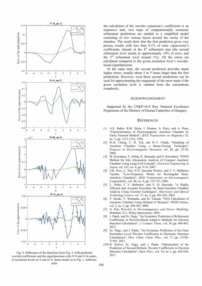
108

the calculation of the wavelet expansion’s coefficients is an expensive task, two steps of computationally economic refinement predictions are studied in a simplified model consisting of two various layers around the cavity of the chamber. The result show that the first prediction gives very precise results with less than 0.1% of error eigenvector’s coefficients, already at the 4th refinement step (the second refinement level results in approximately 10% of error, and the 3rd refinement level around 1%). All the errors are calculated compared to the given resolution level’s wavelet-based eigenfunctions.

At the same time, the second prediction provides much higher errors, usually about 3 to 5 times larger than the first predictions. However, even these second predictions can be used for approximating the magnitude of the error made if the given resolution level is omitted from the calculations completely.

ACKNOWLEDGEMENT

Supported by the ÚNKP-16-4 New National Excellence Programme of the Ministry of Human Capacities of Hungary.

REFERENCES

[1] A.E. Baker, R.M. Sitzia, I. Preston, A. Puzo, and A. Pons, "Characterisation of Electromagnetic Anechoic Chamber by Finite Element Method", IEEE Transactions on Magnetics 32, no. 3, pp. 1513-1516, 1996.

[2] B.-K. Chung, C. H. Teh, and H.-T. Chuah, "Modeling of Anechoic Chamber Using a Beam-Tracing Technique", Progress In Electromagnetics Research, vol. 49, pp. 23-38, 2004.

[3] M. Kawabata, Y. Ishida, K. Shimada, and N. Kuwabara, "FDTD Method for Site Attenuation Analysis of Compact Anechoic Chamber Using Large-Cell Concept", Electrical Engineering in Japan, vol. 162, no. 4, pp. 9-16, 2007.

[4] I.M. Prez, L. Nuo, F.D. Quesada Pereira, and J. V. Balbastre Tejedor, "Low-Frequency Model for Rectangular Semi-Anechoic Chambers", IEEE Transactions on Electromagnetic Compatibility, vol. 48, no. 4, pp. 725-733, 2006.

[5] L. Nuño, J. V. Balbastre, and F. D. Quesada, "A Highly Efficient and Accurate Procedure for Semi-Anechoic Chamber Analysis Using Circuital Techniques", Microwave and Optical Technology Letters, vol. 37, no. 4, pp. 263-265, 2003.

[6] T. Sasaki, Y. Watanabe, and M. Tokuda, "NSA Calculation of Anechoic Chamber Using Method of Moment", PIERS Online, vol. 2, no. 2, pp. 200-205, 2006.

[7] G. Pan, Wavelets in Electromagnetics and Device Modeling, Hoboken, N.J., Wiley-Interscience, 2003.

[8] J. Pipek, and Sz. Nagy, "An Economic Prediction of Refinement Coefficients in Wavelet-Based Adaptive Methods for Electron Structure Calculations", J. Comput. Chem., vol. 34, pp. 460-465, 2013.

[9] Sz. Nagy, and J. Pipek, "An Economic Prediction of the Finer Resolution Level Wavelet Coefficients in Electronic Structure Calculations", Phys. Chem. Chem. Phys., vol. 17, pp. 31558-31565, 2015.

[10] B. Szióvá, Sz. Nagy, and J. Pipek, "Optimization of the Prediction of Second Refined, Wavelet Coefficients in Electron Structure Calculation", Open Phys., vol. 14, no 1, pp. 643-650, 2017.

Fig. 4. Difference of the functions from Fig. 3, with predicted wavelet coefficients and the eigenfunctions with N=0 and N=4 nodes, at resolution levels m=2 and m=4. Same model as in Fig. 1. Arbitrary

units

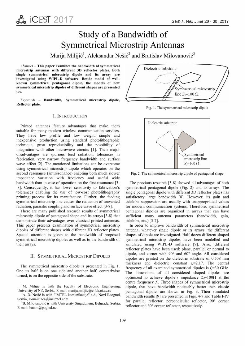
109

Study of a Bandwidth of Symmetrical Microstrip Antennas

Marija Milijić1, Aleksandar Nešić2 and Bratislav Milovanović3

Abstract – This paper examines the bandwidth of symmetrical microstrip antennas with different 3D reflector plates. Both single symmetrical microstrip dipole and its array are investigated using WIPL-D software. Beside model of well-known symmetrical pentagonal dipole, the models of new symmetrical microstrip dipoles of different shapes are presented too.

Keywords – Bandwidth, Symmetrical microstrip dipole, Reflector plate.

I. INTRODUCTION

Printed antennas feature advantages that make them suitable for many modern wireless communication services. They have low profile and low weight, simple and inexpensive production using standard photolithographic technique, great reproducibility and the possibility of integration with other microwave circuits [1]. Their major disadvantages are spurious feed radiation, tolerances in fabrication, very narrow frequency bandwidth and surface wave effect [2]. The mentioned limitations can be overcome using symmetrical microstrip dipole which operates on the second resonance (antiresonance) enabling both much slower impedance variation with frequency and useful wide bandwidth than in case of operation on the first resonance [3- 8]. Consequently, it has lower sensitivity to fabrication’s tolerances enabling the use of low-cost photolithography printing process for its manufacture. Further, the feeding symmetrical microstrip line causes the reduction of unwanted radiation, parasitic coupling and surface wave effect [3-8].

There are many published research results of symmetrical microstrip dipole of pentagonal shape and its arrays [3-8] that demonstrate their advantages over classical printed antennas. This paper presents examination of symmetrical microstrip dipoles of different shapes with different 3D reflector plates. Special attention is given to the bandwidth of proposed symmetrical microstrip dipoles as well as to the bandwidth of their arrays.

II. SYMMETRICAL MICROSTRIP DIPOLES

The symmetrical microstrip dipole is presented in Fig. 1. One its half is on one side and another half, contrariwise turned, is on the opposite side of the substrate.

Fig. 1. The symmetrical microstrip dipole

Fig. 2. The symmetrical microstrip dipole of pentagonal shape

The previous research [3-8] showed all advantages of both symmetrical pentagonal dipole (Fig. 2) and its arrays. The single pentagonal dipole with different 3D reflector plates has satisfactory large bandwidth [8]. However, its gain and sidelobe suppression are usually with unappropriated values for modern communication systems. Therefore, symmetrical pentagonal dipoles are organized in arrays that can have sufficient many antenna parameters (bandwidth, gain, sidelobe, etc.) [3-7].

In order to improve bandwidth of symmetrical microstrip antenna, whatever single dipole or its arrays, the different shapes of dipole are investigated. Half-dozen different shaped symmetrical microstrip dipoles have been modelled and simulated using WIPL-D software [9]. Also, different reflector plates have been used: plane, parallel or normal to dipole, and corner with 90° and 60° angle. All considered dipoles are printed on the dielectric substrate of 0.508 mm thickness end dielectric constant εr=2.17. The central frequency of all examined symmetrical dipoles is fc=30 GHz. The dimensions of all considered shaped dipoles are optimized to achieve dipole’s impedance Zd=100Ω at the centre frequency fc. Three shapes of symmetrical microstrip dipole, that have bandwidth noticeably better then classic pentagonal dipole, are shown in Fig. 3. Their simulated bandwidth results [9] are presented in Figs. 4-7 and Table I-IV for parallel reflector, perpendicular reflector, 90° corner reflector and 60° corner reflector, respectively.

1M. Milijić is with the Faculty of Electronic Engineering,University of Niš, Serbia, E-mail: [email protected]

2A. D. Nešić is with "IMTEL-komunikacije" a.d., Novi Beograd,Serbia, E-mail: [email protected]

3B. Milovanović is with University Singidunum, Belgrade, Serbia,E-mail: [email protected]

110

(a)

(b)

(c)

Fig. 3. The symmetrical microstrip dipole of (a) Shape 1, (b) Shape 2, and (c) Shape 3

Fig. 4. VSWR parameter of symmetrical dipoles with parallel

reflector

TABLE I FREQUENCY RANGE OF SYMMETRICAL DIPOLES WITH PARALLEL

REFLECTOR WHERE VSWR<2

Shape f [GHz] f [%] Classical pentagonal 25-32.4 24.6 Shape 2 25-36.9 39.66 Shape 3 25.1-38.1 43.33

For every considered reflector only three best simulation

results are presented. Firstly, VSWR parameters of symmetrical dipoles with parallel reflector at distance λ0/4=2.5 mm (λ0 is wavelength in vacuum at fc=30 GHz) are presented in Fig. 4 and in Table I. It can be noticed that symmetrical microstrip dipoles of shape 2 and shape 3 have significantly greater bandwidth where their VSWR<2 then classical symmetrical pentagonal dipole. Furthermore, Fig. 5 and Table II show the simulation results of symmetrical dipoles with perpendicular reflector at distance λ0/4=2.5 mm from dipole. There are only simulation results for bandwidth of symmetrical dipoles of shape 1-3 that are all better than simulation results for bandwidth of symmetrical pentagonal dipole (27.33 % of central frequency).

Fig. 5. VSWR parameter of symmetrical dipoles with perpendicular

reflector

TABLE II FREQUENCY RANGE OF SYMMETRICAL DIPOLES WITH

PERPENDICULAR REFLECTOR WHERE VSWR<2

Shape f [GHz] f [%] Shape 1 25.2-33.6 28 Shape 2 23.8-39.6 52.67 Shape 3 25.1-40.5 51.33

Moreover, Fig. 6-7 and Table III-IV present the simulated VSWR parameters of symmetrical dipoles in corner reflectors whose apex is at distance λ0/2=5 mm from dipole. Feeding lines for dipoles penetrate the junction of two reflector plates through holes with diameter of 2.3 mm so the influence of the metallic plates on the microstrip lines is minimized. Obviously, the dipoles in corner reflectors have smaller frequency range where their VSWR<2 then dipoles with plane reflector plate (parallel or normal to dipole). Although, the symmetrical dipoles of shape 1-3 have better wideband characteristics then symmetrical pentagonal dipole in case of reflector with 90° angle. Symmetrical pentagonal dipole’s bandwidth is 13% of central frequency. When dipoles are examined in corner reflector with 60° angle, only symmetrical dipoles of shape 2-3 have greater bandwidth then classical symmetrical pentagonal dipole. The gain of all considered dipoles is 6-7 dBi.

111

Fig. 6. VSWR parameter of symmetrical dipoles in corner reflector

with 90° angle

TABLE III FREQUENCY RANGE OF SYMMETRICAL DIPOLES IN CORNER

REFLECTOR WITH 90° ANGLE WHERE VSWR<2

Shape f [GHz] f [%] Shape 1 26.6-31.9 17.67 Shape 2 21.6-32.5 36.33 Shape 3 21.3-32.5 37.33

Fig. 7. VSWR parameter of symmetrical dipoles in corner reflector

with 60° angle

TABLE IV FREQUENCY RANGE OF SYMMETRICAL DIPOLES IN CORNER

REFLECTOR WITH 60° ANGLE WHERE VSWR<2

Shape f [GHz] f [%] Classical pentagonal 25.8-31.6 19.33 Shape 2 25-33.7 29 Shape 3 25.4-34.2 29.33

Fig. 8. Antenna array with cosecant squared-shaped radiation pattern

III. ANTENNA ARRAY WITH COSECANT SQUARE

SHAPED RADIATION BEAM

The antenna array of four radiating elements, feeding network and bal-un are printed on the same dielectric substrate with dielectric constant εr=2.17 and thickness of 0.508 mm. The array is positioned in corner reflector with angle of 60° and with apex at distance λ0/2 (at the centre frequency fc=30 GHz) from centres of radiating elements (Fig. 8). Three antenna arrays have been modelled whose radiating elements are symmetrical printed dipoles of pentagonal shape, shape 2 and shape 3 (Fig. 2 and Fig. 3). The dipoles are axially placed, decreasing their mutual impedance, at the distance d=0.8λ0=8 mm (at fc=30 GHz). Orchard Elliot's and genetic algorithm methods have been applied for synthesizing the antenna array. The normalized amplitude for dipoles i=1,4 are u1=0.4038, u2=0.567, u3=1 and u4=0.725 while phase shifts are φ1=0°, φ2=14°, φ3=0° and φ4=-36° [10].

The feeding network is also the symmetrical microstrip structure (Fig. 8). After the coaxial connector there is a beginning part of feeding network BAL-UN for transition from conventional microstrip to symmetrical microstrip structure (Fig. 8). Characteristics and dimensions of the λ/4 transformers in symmetrical microstrip technique have been calculated using TEM analysis. Using values u1, u2, u3 and u4

for dielectric substrate of 0.508 mm thickness, 2.17 relative dielectric permittivity, 41 MS/m conductivity of metal, insignificantly small values of loss tangent and conductor thickness, the width Wk, k=1,2,3,4,A,B (Fig. 8) of λ/4 impedance transformers have been obtained (W1=0.49 mm, W2=1 mm, W3=1.02 mm, W4=0.53 mm, WA=1.29 mm, WB=1.89 mm). The phase shifts are adjusted by setting the lengths of dipoles’ feeding microstrip lines of 100Ω. The feeding line for the second dipole, whose phase shift is 14°, is 0.4 mm shorter than feeding line for the first dipole with phase shift of 0°. Similarly, the feeding line associated with the fourth dipole with phase shift of -36° is 1.04 mm longer than feeding line of the third dipole with phase shift of 0°. Lastly, the feeding network was developed and verified using WIPL-D Microwave Pro software [9].

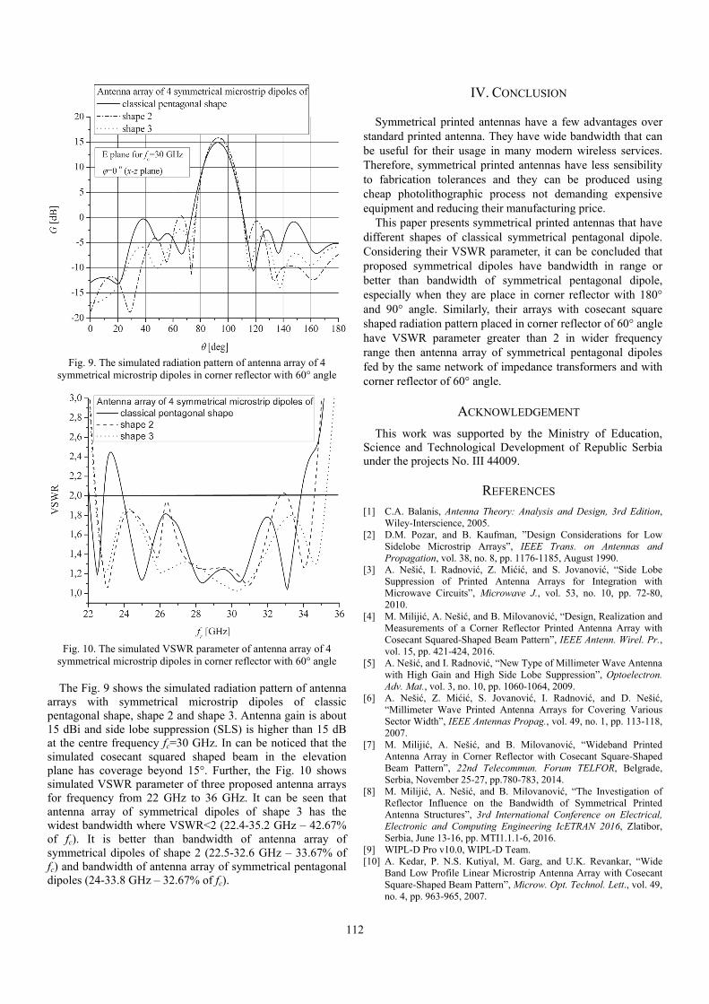
112

Fig. 9. The simulated radiation pattern of antenna array of 4 symmetrical microstrip dipoles in corner reflector with 60° angle

Fig. 10. The simulated VSWR parameter of antenna array of 4 symmetrical microstrip dipoles in corner reflector with 60° angle The Fig. 9 shows the simulated radiation pattern of antenna

arrays with symmetrical microstrip dipoles of classic pentagonal shape, shape 2 and shape 3. Antenna gain is about 15 dBi and side lobe suppression (SLS) is higher than 15 dB at the centre frequency fc=30 GHz. In can be noticed that the simulated cosecant squared shaped beam in the elevation plane has coverage beyond 15°. Further, the Fig. 10 shows simulated VSWR parameter of three proposed antenna arrays for frequency from 22 GHz to 36 GHz. It can be seen that antenna array of symmetrical dipoles of shape 3 has the widest bandwidth where VSWR<2 (22.4-35.2 GHz – 42.67% of fc). It is better than bandwidth of antenna array of symmetrical dipoles of shape 2 (22.5-32.6 GHz – 33.67% of fc) and bandwidth of antenna array of symmetrical pentagonal dipoles (24-33.8 GHz – 32.67% of fc).

IV. CONCLUSION

Symmetrical printed antennas have a few advantages over standard printed antenna. They have wide bandwidth that can be useful for their usage in many modern wireless services. Therefore, symmetrical printed antennas have less sensibility to fabrication tolerances and they can be produced using cheap photolithographic process not demanding expensive equipment and reducing their manufacturing price.

This paper presents symmetrical printed antennas that have different shapes of classical symmetrical pentagonal dipole. Considering their VSWR parameter, it can be concluded that proposed symmetrical dipoles have bandwidth in range or better than bandwidth of symmetrical pentagonal dipole, especially when they are place in corner reflector with 180° and 90° angle. Similarly, their arrays with cosecant square shaped radiation pattern placed in corner reflector of 60° angle have VSWR parameter greater than 2 in wider frequency range then antenna array of symmetrical pentagonal dipoles fed by the same network of impedance transformers and with corner reflector of 60° angle.

ACKNOWLEDGEMENT

This work was supported by the Ministry of Education, Science and Technological Development of Republic Serbia under the projects No. III 44009.

REFERENCES [1] C.A. Balanis, Antenna Theory: Analysis and Design, 3rd Edition,

Wiley-Interscience, 2005. [2] D.M. Pozar, and B. Kaufman, ”Design Considerations for Low

Sidelobe Microstrip Arrays”, IEEE Trans. on Antennas and Propagation, vol. 38, no. 8, pp. 1176-1185, August 1990.

[3] A. Nešić, I. Radnović, Z. Mićić, and S. Jovanović, “Side Lobe Suppression of Printed Antenna Arrays for Integration with Microwave Circuits”, Microwave J., vol. 53, no. 10, pp. 72-80, 2010.

[4] M. Milijić, A. Nešić, and B. Milovanović, “Design, Realization and Measurements of a Corner Reflector Printed Antenna Array with Cosecant Squared-Shaped Beam Pattern”, IEEE Antenn. Wirel. Pr., vol. 15, pp. 421-424, 2016.

[5] A. Nešić, and I. Radnović, “New Type of Millimeter Wave Antenna with High Gain and High Side Lobe Suppression”, Optoelectron. Adv. Mat., vol. 3, no. 10, pp. 1060-1064, 2009.

[6] A. Nešić, Z. Mićić, S. Jovanović, I. Radnović, and D. Nešić, “Millimeter Wave Printed Antenna Arrays for Covering Various Sector Width”, IEEE Antennas Propag., vol. 49, no. 1, pp. 113-118, 2007.

[7] M. Milijić, A. Nešić, and B. Milovanović, “Wideband Printed Antenna Array in Corner Reflector with Cosecant Square-Shaped Beam Pattern”, 22nd Telecommun. Forum TELFOR, Belgrade, Serbia, November 25-27, pp.780-783, 2014.

[8] M. Milijić, A. Nešić, and B. Milovanović, “The Investigation of Reflector Influence on the Bandwidth of Symmetrical Printed Antenna Structures”, 3rd International Conference on Electrical, Electronic and Computing Engineering IcETRAN 2016, Zlatibor, Serbia, June 13-16, pp. MTI1.1.1-6, 2016.

[9] WIPL-D Pro v10.0, WIPL-D Team. [10] A. Kedar, P. N.S. Kutiyal, M. Garg, and U.K. Revankar, “Wide

Band Low Profile Linear Microstrip Antenna Array with Cosecant Square-Shaped Beam Pattern”, Microw. Opt. Technol. Lett., vol. 49, no. 4, pp. 963-965, 2007.

113

X-pol Antenna for ISM Applications Optimized Through the Design of Experiment Theory

Kliment Angelov1 and Kalina Kalinovska2

Abstract – In this study an optimization of X-pol antenna with reflector dimensions has been described. The goal is achieved using design of experiment theory for antenna suitable for use in 433MHz ISM band. This type of antenna is applicable on order to guarantee better communication in the available ICM bands, where the electromagnetic frequency resource is constantly take busier with more, even M2M, short or permanent in time data transfers.

Keywords – X-pol Antenna, Design of Experiment, Antenna Parameters Optimization, ISM band applications.

I. INTRODUCTION

Nowadays, the communications, alongside with the mobility, are the two largest components of the progress of mankind. Transmission of huge amount of data for daily activity has entered deep into the life of every modern man. Sometimes the stream is continues data with high speed of around amount of Terabits per second. Other cases are when a very short digital messages are transmitted. In some specific cases mobility is needed when information is being transfered. In these cases, inevitably free electromagnetic waves as a carrier of information has been used [1], [2]. This leads to continuous increasing the load of the spectrum, which is not an unlimited resource. From this perspective, any moves for optimization the wireless transmission of information are of significant benefit.

The antenna plays a huge role for the realization of every wireless communication. In many cases they are complex technical solutions that are designed to implement specific characteristics. However, in some other applications sometimes is impossible to use complex antennas due to restrictions in size, weight, cost and the like. Some examples of similar aspects are the cases in the Industrial, Scientific and Medical (ISM) bands systems for access control, remote control and Radio Frequency Identification (RFID). The list expands with the attractive from today's perspective Smart Systems and other. A good example is the Machine To Machine (M2M) communications. M2M type remote communication uses a simple radiating elements. Optimization can be done for stationary antennas of these systems too. Such optimization can be done for better coverage. This will lead to a reliable communication link, to

less need for retransmission of information, and so to that the ISM bands are going to be less overloaded.

In this article has been viewed the possibility of using X-pol antenna with reflector to achieve better radio coverage of a given area. The antenna optimization, used in the research, is based on the theory of design of experiment to achieve the best possible case and analysis of its other parameters and characteristics.

II. DESCRIPTION OF THE PROBLEM

A. The X-pol Antenna Conception

In the idea to realize the X-pol antenna with reflector is the concept of forming a loop antenna [3], [4] in the form of the outer contour of the letter 'X'. On Fig. 1 is shown the structure of a planar developed frame of the antenna. Mainly two parameters define the shape - the length l of the arm and its angle of divergence α.

Fig. 1. Structure of a planar radiating loop element of X-pol antenna

The geometric variables largely defined the electromagnetic behaviour of the frame, respectively impedance match to standard 50Ω and the radiation pattern.

1Kliment Angelov is with the Faculty of Telecommunications atTechnical University of Sofia, 8 Kl. Ohridski Blvd, Sofia 1000, Bulgaria, E-mail: [email protected]

2Kalina Kalinovska is with the Faculty of Telecommunications atTechnical University of Sofia, 8 Kl. Ohridski Blvd, Sofia 1000, Bulgaria. E-mail: [email protected]

114

In order to achieve directivity in a half-sphere, behind the active element a screen is added. Fig. 2 shows a three-dimensional appearance of such X-pol antenna with reflector.

Fig. 2. 3D view of X-pol antenna with reflector

B. Optimization of the X-pol Antenna Geomery

Optimization of the geometry of the X-pol antenna at a particular input arm length l and an angle of divergence α can be done by using the theory of the planned experiment. This theory gives the opportunity to make a model of considered parameter behaviour in relationship to changes of several factors. In this case is necessary to conduct full factorial experiment type 32, in which two factors are varied on three levels. In the specific task these factors are the arm length l and an angle of divergence α. It is appropriate the parameter to be the antenna matching represented by a standing wave ratio (SWR). Based on the data generated in nine attempts in a planned experiment type 32 the analytical dependence of the parameter in the factor field has the form [5]:

2

222

2

111

211222110

..

....

xbxb

xxbxbxbbY

In the upper equation Y is a parameter for impedance match or standing wave ratio - SWR and x1 and x2 are the two factors, in this case they are respectively the length l and the angle α. The coefficients b are defined according the laws:

9

1

2

1

9

1

200 .

3

1.

9

5

j i jjijjj yxyxb

9

1

..6

1

jjji yxb

9

1

2

1

....4

1

jjkjij

iik yxxb

9

1

9

1

22

1 3

1..

2

1

j jjjij

iii yyxb

III. RESULTS

With the preliminary study were selected levels of variation of the two factors for the antenna that works in ISM band frequency 433,92 MHz. In this frequency band a number of systems for remote control are in use, like remote opening of garage doors or barriers, signals for alarm activation/deactivation etc. Specific values for these geometric indicators and the levels of their variations for this experiment are given in Table I.

TABLE I BASE FACTOR LEVELS

Level of variation

Factor

x1 x2

+1 88 mm 38˚

0 85 mm 35˚

–1 82 mm 32˚

In Table II are listed data readings of the parameter Y for the nine attempts with different levels of varying factors.

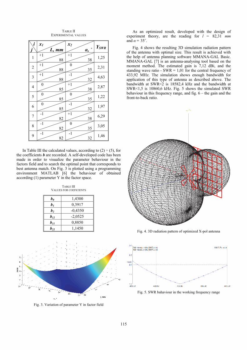
115

TABLE II EXPERIMENTAL VALUES

i j

x1

L, mm x2

α, ˚ YSWR

1 +1

88 +1

38 1,25

2 +1

88 0

35 2,31

3 +1

88 -1

32 4,63

4 0

85 +1

38 2,87

5 0

85 0

35 1,22

6 0

85 -1

32 1,97

7 -1

82 +1

38 6,29

8 -1

82 0

35 3,05

9 -1

82 -1

32 1,46

In Table III the calculated values, according to (2) ÷ (5), for the coefficients b are recorded. A self-developed code has been made in order to visualize the parameter behaviour in the factors field and to search the optimal point that corresponds to best antenna match. On Fig. 3 is plotted using a programming environment MATLAB [6] the behaviour of obtained according (1) parameter Y in the factor space.

TABLE III VALUES FOR COEFICIENTS

b0 1,4300

b1 0,3917

b2 -0,4350

b12 -2,0525

b11 0,8850

b22 1,1450

Fig. 3. Variation of parameter Y in factor field

As an optimized result, developed with the design of experiment theory, are the reading for l = 82,31 mm and α = 35˚.

Fig. 4 shows the resulting 3D simulation radiation pattern of the antenna with optimal size. This result is achieved with the help of antenna planning software MMANA-GAL Basic. MMANA-GAL [7] is an antenna-analysing tool based on the moment method. The estimated gain is 7,12 dBi, and the standing wave ratio - SWR = 1,01 for the central frequency of 433,92 MHz. The simulation shows enough bandwidth for application of this type of antenna as described above. The bandwidth at SWR<2 is 18582,4 kHz and the bandwidth at SWR<1,5 is 10860,6 kHz. Fig. 5 shows the simulated SWR behaviour in this frequency range, and fig. 6 – the gain and the front-to-back ratio.

Fig. 4. 3D radiation pattern of optimized X-pol antenna

Fig. 5. SWR bahaviour in the working frequency range

116

Fig. 6. Gain and Front-to-back ratio behaviour in the working frequency range

Fig. 5 shows an example for practical use of proposed antenna in case of remote control of garage door. In this case the antenna is oriented in direction of the eventual arriving vehicles and makes the data transfer in this area more reliable. That tends to better transmitting, less data resending and decreasing the noise level for other communication units in this area, that are using the same frequency.

Fig. 5. Practical application of X-pol antenna with reflector

IV. CONCLUSION

Based on the experimental results the following conclusions can be made:

X-pol antenna with reflector consequence of the impedance match optimization achieved extremely good value;

The resultant directivity can help in improving wireless communication in ISM frequency bands;

It is appropriate to seek ways to reduce the size of the antenna, which can be accomplished using fractal design of the elements;

REFERENCES

[1] H. Suzin, Radio Wave Propagation for Telecommunication Applications, Springer-Verlag Berlin Heidelberg, 2005.

[2] M. Schwartz, Mobile Wireless Communications, Cambridge University Press, 2005.

[3] R.C. Jonson, Antenna Engineering Handbook, 3-rd ed., McGraw Hill, 1993.

[4] R.E. Collin, Antennas and Radiowave Propagation, McGraw-Hill, 1985.

[5] I.N. Vuchkov, and L.N. Bojadjieva, Quality Improvement with Design of Experiments. A response Surface Approach, Kluwer Academic Publishers, Dordrecht, Netherland, 2001.

[6] MATLAB IMAGE PROCESSING TOOLBOX. User's Guide, "The Math - Works Inc.", 2000, www.mathworks.com.

[7] И.В. Гончаренко, "Антенны КВ и УКВ. Часть I. Компьютерное моделирование MMANA", Издательское предприятие РадиоСофт, Журнал «РАДИО», Москва, 2004.

Session 4B:

COMPUTER SCIENCE AND INTERNET

TECHNOLOGIES I

119

Enumeration of Bent Boolean Functions Using GPU with CUDA

Miloš Radmanović1 and Radomir S. Stanković2

Abstract – Bent functions are special type of cryptographic Boolean functions. These functions make very small subset of the total number of bent functions, especially for large number of variables. Therefore, the only possible method for complete enumeration of bent function is obtained by using the exhaustive search of all possible functions. Testing of bentness across all possible functions, even for small numbers of variables, requires a lot of processing time. Thus, this paper proposes a parallel algorithm for enumeration of bent functions using GPU with CUDA. The algorithm is based on the usage of fast spectral transform calculations and certain restrictions that should be satisfied by bent functions in the spectral Reed-Muller domain. Experimental results showed that the proposed GPU-based algorithm can efficiently enumerate the bent functions of 6 to 10 variables.

Keywords – Cryptography, Boolean function, Bent function, Enumeration, GPU, CUDA.

I. INTRODUCTION

Bent Boolean functions are functions with maximum nonlinearity. They ensure the cryptographic effectiveness and they can resist to various cryptanalysis attacks. Furthermore, they are also applied in many other areas such as coding theory, logic synthesis, and digital telecommunications [1]. Bent functions have specific properties and characterizations. The most common characterization for Boolean bent functions is the equal absolute values of all coefficients of their Walsh spectra [1]. They exist only for the even number of variables. There is no precise definition of the structure of bent functions. In general, it is unknown the complete enumeration and classification of them [2].

Finding the complete set of bent functions for a given number of inputs is an open problem and known are the lower and upper bounds in terms of the number of inputs [1]. There is no a formal method for enumeration, generalization, construction, or classification of all bent functions for the given number of inputs. Thus, during recent years, it has been developed a large number of methods for enumeration, construction, and etc., of particular bent functions that have specific characterizations [2]. However, specific bent functions are very rare and they make very small subset of the total number of bent functions, especially for large number of variables.

Therefore, the only possible method for the complete enumeration of bent function is obtained by using the

exhaustive search of all possible functions. Testing of bentness across all possible functions, even for small numbers of variables, requires a lot of processing time. Consequently, the number of n-variable Boolean bent functions is known only for n≤8. The general number of bent functions is an open problem. Note that, the number of Bent functions increases rapidly with increasing n. It is known that, there are 8 bent functions in two variables, 896 bent functions in four variables, 5.425.430.528 bent functions in 6 variables [3], and 99.270.589.265.934.370.305.785.861.242.880 bent functions in 8 variables [4].

There are two types of methods for enumerations of Boolean bent functions, primary and secondary. The primary methods are based on the direct enumeration in Boolean domain [5]. The secondary methods are based on algebraic normal form or enumeration in Reed-Muller domain [4], [6], [7]. Almost all secondary methods used property that all bent functions of n variables have algebraic degree at most n/2. The amount of computations for enumerations of bent functions extremely increases, especially in the case of functions with large number of variables. For example, secondary method described in [4], for complete enumeration of bent functions on 8 variables has been used approximately 50 PCs running for 3 months.

The secondary methods for enumerations of bent functions in Reed-Muller domain can be very CPU time consuming and processing time is often the limiting parameter for practical applications. In [8], it is shown that there is significant benefit by using a reconfigurable SRC-6 computer to enumerate bent Boolean functions for cryptographic applications. Further, in [9], it is shown that the speed at which bent functions can be enumerated was improved using the circular pipeline implemented on FPGA.

The efficiency of using parallel multi-core CPU technique for random generation of bent function in Reed-Muller domain is analyzed in [10]. The GPUs are also an attractive target for parallel computations because of its high performance and low cost. Recent generations of GPUs have become programmable, enabling the use of GPUs for general purpose computations. The efficiency of using parallel GPU technique for random generation of bent function in Reed-Muller domain is analyzed in [11], where it is reported significant execution speedup on a GPU with 8 multiprocessors and 384 cores. Therefore, in this paper we proposed a parallel algorithm for enumeration of bent functions using GPU platform. The method is based on the usage of certain restrictions that should be satisfied by bent functions in the spectral Reed-Muller domain. The proposed method uses computation of the fast Reed-Muller transform and the computation of the fast Walsh transform.

For experiments, we developed two independent implementations, a single-core implementation using C++ and a GPU-based implementation using CUDA framework. Experimental results show that the proposed parallel algorithm using GPU platform offers computational speedups

1Miloš Radmanović is with the Faculty of Electronic Engineering,Aleksandra Medvedeva 14, 18000 Niš, Serbia, E-mail:[email protected]

2Radomir S. Stanković is with the Faculty of ElectronicEngineering, Aleksandra Medvedeva 14, 18000 Niš, Serbia, E-mail:[email protected]

120

for hundreds times over performing the same algorithms on CPUs. As the Boolean function size increases, the number of bentness tests extremely increases. For this reason it is experimented with Boolean functions of the small sizes with computations restriction.

II. PRELIMINARIES

The Reed-Muller (RM) spectral transform represents an important operator for obtaining AND-EXOR expressions of Boolean functions. The RM transform matrix of order n, denoted by )(nR , is defined recursively as [12]:

11

01)1( ),1()(

1RRnR

n

i. (1)

For the bentness test, it is needed the inverse RM spectral transform. Since the RM transform matrix )(nR is a self-

inverse matrix over GF(2), the forward and inverse RM transform are equal.

The Walsh spectral transform matrix of order n in the Hadamard ordering, denoted by )(nW , is defined as [12]:

11

11)1( ),1()(

1WWnW

n

i. (2)

The spectrum of a Boolean function f given by truth vector

TnfffF )12()1(),0( ,, is computed as [12]:

FnTS f )( , (3)

where T(n) is any of the matrices R(n), and W(n), with computations performed in GF(2) for the RM transform, and in the set of integer numbers for the Walsh transform. The recursive definition of R(n), and W(n) is the fundamental for the definition of the fast RM and fast Walsh spectral transform algorithm [12], similar to the fast Fourier transform (FFT) algorithm. Figure 1 shows the “butterfly” operations for R(1), and W(1) [12]. The fast spectral transform algorithm reduces computational complexity of a spectral transform

from )2( 2nO to )2log2( 2nnO [12].

The computation of the fast spectral transform algorithm consists of the repeated application of the same “butterfly” operations.

A Boolean function ),...,,( 21 nxxxf in )1,1( encoding is

called bent if all elements of the Walsh spectrum vector WfS ,

have the same absolute value 2/2n [1].

For example, for a bent function of four variables ),,,( 4321 xxxxf , given by

TF 11,0,1,0,0,1,0,0,1,0,1,1,1,1,1, , the Walsh spectrum with

(1,-1) encoding can be computed as FWS Wf )4(, , where

result is: TWfS ,-4,4,4,-4,-4,4,-4,4,-4,-4,4,44,-4,-4,-4-, and

all elements have the same absolute value 4. The Reed-Muller form of a Boolean function f, also called

AND-EXOR expression, can be computed from the RM spectrum vector RMfS , [12]:

RMfn SnXxxxf ,21 )(),,,( (4)

where

in

ixnX 1)(

1 (5)

and where addition and multiplication are modulo 2. For example, for a bent function of four variables

),,,( 4321 xxxxf , from previous example, the RM spectrum

with (1,-1) encoding can be computed as FRMS RMf )4(, ,

where result is: TRMfS 00,0,0,0,0,0,1,0,0,1,1,0,0,0,0,, . The

elements of vector )(nX are ,,,,,,1[)4( 4224334 xxxxxxxX

.],,,,,,,,, 4321321421214313141143232Txxxxxxxxxxxxxxxxxxxxxxxxx

The corresponding RM form is: 41321 xxxxf . The algebraic degree of a product term in a RM form is the

number of variables in that term. The algebraic degree of a RM form )deg( f is the number of variables in the product

term with the maximum algebraic degree. Algebraic degree )deg( f of a bent function ),...,,( 21 nxxxf

is at most 2/n for 2n [2]. Note that the bent function from the previous example can

be characterized by the upper bound of the algebraic degree of the RM form: 2/42)1),,,(deg( 41324321 xxxxxxxxf .

III. ENUMERATION OF BENT FUNCTIONS IN REED-MULLER DOMAIN

The algorithm for enumeration of bent functions in the Reed-Muller domain takes as its input only the number of function variables. Since the algebraic degree of an n-variable bent function is less or equal to n/2, the number of non-zero elements of RM spectrum vector is limited and their positions in the RM spectrum vector are restricted.

For example, for a bent function of four variables ),,,( 4321 xxxxf , elements of the vector )(nX are

,,,,,,,,,,,,1[)4( 43131411432324224334 xxxxxxxxxxxxxxxxxxxxX Txxxxxxxxxxxx ],,, 432132142121 , where the number of variables

in a product term is less or equal to 2. For this reason the following positions in the RM spectrum vector are restricted for non-zero elements and other positions are always zero:

TRMfS 0-,0,-,0,0,-,-,0,-,-, -,-,-,-,-,, , There are 11 of 16

Fig. 1. The elementary “butterfly” operations for R(1), and W(1)

121

positions in the RM spectrum vector of bent functions available for non-zero elements.

Therefore, we define the restricted RM spectrum of a bent function ),,,( 4321 xxxxf denoted by vector

(4),(3),(2),(1),(0),[ ,,,,,, RMfRMfRMfRMfRMfRMf SSSSSSR T

RMfRMfRMfRMfRMfRMf SSSSSS (12)](10),(9),(8),(6),(5), ,,,,,,

It should be noticed that elements of the restricted RM spectrum have the number of ones in the binary representation of the RM spectrum vector index less or equal to 2. Thus, the number of elements of the restricted RM spectrum is 11.

The size of the restricted RM spectrum of n-variable bent

function is

2/

0

n

i i

n.

For example, the size of the restricted RM spectrum in relation to the size of RM spectrum for bent functions with 8 variables is 163 out of 256, and with 10 variables is 638 out of 1024

Starting from this observation, the search space is defined by the size of the restricted RM spectrum, where elements of

spectrum takes values from T00,0,...,0, to T11,1,...,1, . For example, the size of search space for bent functions with 8

variables is 1632 , and with 10 variables is 6382 . An outline of the algorithm for the enumeration of bent

functions in Reed-Muller domain is given as Algorithm 1. Algorithm 1 1: Set the number of function variables n and set the

counter of bent functions to 0. 2: Calculate the size of the restricted RM spectrum. 3: Generate vector IND of the RM spectrum vector indices

for translations from the restricted RM spectrum to the RM spectrum.

4: Execute for loop where elements of the restricted RM spectrum take values from 0,0,…,0,0 to 1,1,…,1,1.

4: Translate the restricted RM spectrum to the RM spectrum by using vector IND.

5: Compute the truth-vector from the RM spectrum by using the Fast RM transform.

6: Do )1,1( encoding of the truth-vector.

7: Compute the first, second, and last element of the Walsh spectrum from truth-vector using rows of the Walsh spectral transform matrix [11], and test if the element has the absolute

value 2/2n . If the bentness test is sucessful, increase the counter of bent functions and go to the step 4.

8: Compute all elements of the Walsh spectrum from truth-vector by using the Fast Walsh transform, and test if all

elements have the absolute value 2/2n . If the bentness test is sucessful, increase the counter of bent functions and go to the step 4.

9: Obtain the number of bent functions by reading the counter value.

IV. GPU-BASED ALGORITHM FOR ENUMERATION

OF BENT FUNCTIONS

For GPU architectures, the model of parallel processing is based on a large number of processor cores with the ability to directly address into a shared GPU RAM memory. This organization of computations allows to have a large number of threads performing the same operations on different data simultaneously [13]. Enumeration of bent function in the Reed-Muller domain uses computations of the fast Reed-Muller transform and the fast Walsh transform. Running FFT-like algorithms on a GPU platform can give a better performance compared to a singlecore CPU or a multicore CPU platform. FFT-like algorithms applied on small vectors can be more efficient performed on the CPU compared to GPU [13]. If on the other hand, there is the need to perform large amount of FFT-like algorithms applied on small vectors with minimal moves to/from the GPU, then the GPU-based algorithm is the optimal choice.

Thus, in this paper we proposed GPU-based algorithm for enumeration of bent functions in the RM domain. Details of algorithm are given as Algorithm 2.

Algorithm 2 1: Set the number of function variables n and set the

counter of bent functions to 0. 2: Calculate the size of restricted RM spectrum. 3: Generate vector IND of RM spectrum vector indices for

translations from the restricted RM spectrum to the RM spectrum.

4: Alloc GPU memmory and copy data stored in CPU memory to the GPU memory.

5: Split the loop into multiple loops according to maximal number of GPU threads (determined by the GPU hardware) where elements of the restricted RM spectrum take values from 0,0,…,0,0 to 1,1,…,1,1.

6: Use threads id and the number of splits to work out which loop iterations of the restricted RM spectrum to perform.

7: Translate the restricted RM spectrum to the RM spectrum using vector IND.

8: Computae of the truth-vector from the RM spectrum by using the Fast RM transform.

9: Do )1,1( encoding of the truth-vector.

10: Compute the first, second, and last element of the Wlash spectrum from the truth-vector using rows of the Walsh spectral transform matrix [11], and test if the element has the

absolute value 2/2n . If the bentness test is sucessful, increase the counter of bent functions and go to the step 6.

8: Compute of the all elements of the Walsh spectrum from the truth-vector using fast Walsh transform, and test if all

elements have the absolute value 2/2n . If the bentness test is sucessful, increase the counter of bent functions and go to the step 6.

9: Copy data stored in the GPU memory back to the CPU memory.

10: Obtain the number of bent functions by reading the counter value.

122

Note that steps 2 to 8 of the Algorithm 2 are executed on GPU and the number of actual threads that are simultaneously active in hardware depends on the used GPU. For example, with NVidia GTX560Ti GPU, the maximal number of threads is 65535*1024=67107840, and the maximal number of simultaneously active threads is 384 (determined by number of cores).

V. EXPERIMENTAL RESULTS

CUDA framework gives to program developers a direct access to the virtual instruction set and memory of the parallel computational elements in NVidia GPUs. For this reason, it is developed a referent single-core CPU C++ and CUDA implementation on GPU platform of the algorithm for enumeration of bent function. The single-core CPU implementation is performed on an Intel i7 CPU at 3.66 GHz. The CUDA implementations on GPU platform is performed on NVidia GeForce GTX-560Ti on 900 MHz with 1 GB DDR5 4 GHz RAM (8 multiprocessors and 384 cores).

Table 1 shows computation performance of the algorithm for enumeration of bent function using referent single-core CPU C++ and the GPU-based implementations. The presented values are computational times for 1 million bentness tests of functions. From data in Table 1, it can be seen that on GPU platform, for all the computations, CUDA implementation of the algorithm significantly reduces computation times when compared to the CPU implementation. Note that for the largest Boolean functions, experiments were not performed, due to very long CPU computation time.

TABLE I COMPUTATION PERFORMANCE OF ALGORITHM FOR ENUMERATION

OF BENT FUNCTIONS USING C++ AND CUDA IMPLEMENTATIONS

Num. of function variables

Computation time for 1 million bentness tests [s]

CPU i7-3.66 GPU GTX-560Ti 6 0.498 0.009 8 1.778 0.017

10 7.566 0.041

VI. CONCLUSION

This paper proposes an algorithm for enumeration of bent functions based on the exhaustive search of all possible functions in the Reed-Muller domain by using GPU and CUDA. The ultimate goal is to exceed the computation performance for finding the total number of bent functions, since the computation time for the enumeration is exponential in the number of variables in the function. The proposed implementation exploits the parallel mapping of exhaustive search algorithm for the enumeration of bent functions in Reed-Muller domain by performing the same operations over

different data simultaneously which is a good match to GPU hardware.

The experimental results confirm that the application of the proposed GPU-based algorithm leads to significant computational speedups. It is also confirmed that this implementation could be especially efficient for functions with large number of variables. From the results, it is also evident that CUDA framework can be efficiently used in implementation of the proposed GPU-based algorithm.

Future work will be directed towards the extension of the proposed technique to the enumerations various other classes of Boolean functions.

ACKNOWLEDGEMENTS

The research reported in this paper is partly supported by the Ministry of Education and Science of Serbia, projects ON174026 (2011-2017) and III44006 (2011-2017).

REFERENCES

[1] S. Mesnager, Bent Functions: Fundamentals and Results, Springer International Publishing, 2016.

[2] N. Tokareva, Bent Functions, Results and Applications to Cryptography, Academic Press, 2015.

[3] T. Sasao, J. Butler, and M. Thornton, Progress in Applications of Boolean Functions, Morgan and Claypool Publishers, 2010.

[4] P. Langevin, and G. Leander, “Counting All Bent Functions in Dimension Eight 99270589265934370305785861242880”, Designs, Codes and Cryptography, vol. 59, pp. 193-201, 2011.

[5] N. Tokareva, "On the Number of Bent Functions From Iterative Constructions: Lower Bounds and Hypotheses", Advances in Math. of Communications, vol. 5, no. 4, pp. 609-621, 2011.

[6] Q. Meng, M. Yang, H. Zhang, and J. Cui, “A Novel Algorithm Enumerating Bent Functions”, Discrete Math., vol. 308, no. 23, pp. 5576-5584, 2008.

[7] N. Kolomeets, “Enumeration of the Bent Functions of Least Deviation From a Quadratic Bent Function”, Journal of Applied and Industrial Mathematics, vol. 6, no. 3, pp. 1990-4797, 2012.

[8] J. Shafer, S. Schneider, J. Butler, and P. Stanica, “Enumeration of Bent Boolean Functions by Reconfigurable Computer”, 18th IEEE Annual International Symposium on Field-Programmable Custom Computing Machines, pp. 265-272, Charlotte, NC, USA, 2010.

[9] S. Schneider, and J. Butler, “Bent Function Enumeration by a Circular Pipeline Implemented on an FPGA”, Proc. 12th Int. Workshop on Boolean Problems (IWSBP2016), pp. 159-166, Freiberg, Germany, 2016.

[10] M. Radmanović, and R. Stanković, “Random Generation of Bent Functions on Multicore CPU Platform”, Int. Sci. Conf. on Inf. Communication and Energy Systems and Technologies (ICEST 2016), pp. 239-242, Ohrid, Macedonia, 2016.

[11] M. Radmanović, “Efficient Random Generation of Bent Functions using GPU Platform”, 12th Int. Workshop on Boolean Problems (IWSBP2016), pp. 167-173, Freiberg, Germany, 2016.

[12] M.A. Thornton, R. Drechsler, and D.M. Miller, Spectral Techniques in VLSI CAD, Springer, 2001.

[13] D.A. Yuen, L. Wang, X. Chi, L. Johnsson, W. Ge, and S. Yaolin, GPU Solutions to Multi-scale Problems in Science and Engineering, Springer Science & Business Media, 2013.

123

Leveled Binary Trees and Integer Sequences Generation Adrijan Božinovski

Abstract – This paper introduces a data structure called a leveled binary tree, as a a generalization of both the complete and full binary tree. It is shown how inserting nodes in a leveled binary tree, while maintaining a preference for a single direction (either strictly left or strictly right) makes the number of single-direction edges in the binary tree increase according to certain regularities. These regularities are formalized using mathematical formulae, which are presented and proved, and it is shown how they produce specific integer sequences which can be expanded to infinity.

Keywords – Leveled binary tree, Single-direction edges, Minimum, Maximum, Integer sequence, Online Encyclopedia of Integer Sequences.

I. INTRODUCTION

Trees are fundamental concepts in computer science, and are frequently used to keep track of ancestors or descendants, sports tournaments, organizational charts of large corporations and so on [1]. Trees are one of the basic data structures used in combinatorial algorithms [2], search techniques (e.g. [3, 4]), and game playing [5]. This paper also points out the use of binary trees for generating integer sequences, which are important in information forensics [6], cryptography [7], and security [8].

A binary tree is a data structure made up of nodes, in which each node contains an information part and links, also called edges, to two other such nodes, called the node’s left and right child nodes, respectively. A node can be null as well, in which case it contains no information. A recursive definition of a binary tree is that it is a structure with a finite set of nodes, which either contains no nodes or contains a root node and binary trees as its left and right child nodes [9].

Binary trees have been shown to be very useful in mathematics and computer science and as such have been extensively studied. Several variations of the binary tree structure have been conceived, such as binary search trees, red-black trees [9], AVL trees [10], B-trees [11], and so on. Binary trees are often used as auxiliary data structures in other research endeavors, both practical (e.g., [12,13]) and theoretical (e.g., [14,15]), but occasionally are the subject of the research itself (e.g., [16]).

In this paper, a new variation of binary trees, called leveled binary trees, will be introduced. It will be shown how particular integer sequences can be generated using them, which will be presented and the formulae for their generation will be proved. These integer sequences have been included into the Online Encyclopedia of Integer Sequences.

II. LEVELED BINARY TREES

A leveled binary tree is a binary tree in which nodes are inserted in a breadth-first fashion. In other words, insertion of a node increases the height of the tree only when the tree is full, i.e., when all of the positions at the last level have already been occupied. Fig. 1 shows examples of leveled binary trees with numbers of nodes n = [1,9].

a) b) c)

d) e) f)

g) h) i)

Fig. 1. Examples of leveled binary trees for n = [1,9]

In a leveled binary tree, nodes can be inserted arbitrarily, as long as the leveled structure is preserved, in a sense that no new level is inserted until all the possible positions in the last level have been occupied. This is a generalization of the complete binary tree structure, where nodes in the last level are always placed as far left as possible [17]. Also, if a leveled binary tree has n = 2k - 1 nodes, where k 0 is an integer, it is a full binary tree [18]. Examples of full binary trees are shown in Fig. 1a, 1c and 1g, having 1, 3 and 7 nodes respectively. In this paper, the root is treated as being placed on level 0.

III. MINIMUM NUMBER OF SINGLE-DIRECTION

EDGES IN A LEVELED BINARY TREE

A. Motivation and Formula

During the course of research, a question appeared about the regularity by which the minimum number of left edges appear in a leveled binary tree with progressively increasing values of n. Specifically, a question arose about how to obtain a formula which would produce the minimum numbers of left edges in leveled binary trees with n nodes.

Adrijan Božinovski is with the School of Computer Science andInformation Technology at University American College Skopje,1000 Skopje, Macedonia, E-mail: [email protected]

124

Initially, this problem was solved algorithmically, and the formula was extracted subsequently. The formula is presented in equation (1).

amin(n) = 2h-1 - 1 + (n - 3·2h-1 + 1) · H(n - 3·2h-1 + 1) (1)

where h = log2n and represents the height of the leveled binary tree, and H() is the Heaviside step function.

The following section provides a proof of this formula. For the sake of simplicity, the proof will concern the minimum number of left edges in a leveled binary tree with a given number of nodes n. The same formula may be used for the minimum number of right edges in a leveled binary tree, whereas the proof is analogous.

B. Proof of the Formula

Building a leveled binary tree is done in such a way that nodes are inserted only on a single level, until it is completely filled, i.e., inserting nodes in a new level is possible only when all levels up to the new one have been filled completely. Thus, the nature of the leveled binary tree guarantees that its level is always h = log2n.

If a leveled binary tree has n = 2k - 1 nodes, it is a full tree. Since the number of edges in any tree is 1 less than the number of its nodes, a full binary tree contains 2k - 2 edges. Since there is an equal number of left and right edges in a full binary tree, 2k-1 - 1 edges in a full binary tree are strictly left (and also strictly right).

If a leveled binary tree has n 2k - 1 nodes, it is not a full tree. However, since a new level is inserted in a leveled binary tree only after the previous one has been fully populated, it is only the last level which shows that the leveled binary tree is not full – the sub-tree consisting of the root and all the levels up the last is a full binary tree. In other words, the tree of level h = log2n is not full, but its sub-tree of level h - 1 is full. This means that there are at least 2h-1 - 1 left edges in any leveled binary tree.

The maximum number of nodes in the last level of a leveled binary tree is 2h – when this number of nodes is reached, the leveled tree becomes a full tree. In order to keep the number of left edges to a minimum, only right child nodes would be inserted in the last level as much as possible. The number of possible right child nodes that can be inserted in the last level is 2h/2 = 2h-1 – after this many right child nodes are inserted, there is no more room for right child nodes in the last level, so the next node to be inserted would have to be a left child node, thus forcing the increase of the number of left edges in the leveled binary tree. As an example, the leveled binary tree in Fig. 1e has the minimum possible number of left edges, but the next node to be inserted in the last level has to be a left child node, as shown in Fig. 1f, so the number of left edges in the tree must increase.

In order for the number of left edges to be forced to increase, the number of nodes in the leveled binary tree must be greater than the number of nodes in all levels before the last plus half of all possible nodes in the last level. Thus, in order for the number of left edges to be forced to increase, it is necessary that n > 2h - 1 + 2h-1, so n > 3·2h-1 + 1, thus n - 3·2h-1 + 1 > 0. Using the Heaviside step function, it can be said that

if H(n - 3·2h-1 + 1) = 1 the minimum number of left edges in a leveled binary tree increases, whereas if H(n - 3·2h-1 + 1) = 0 the minimum number of left edges in a leveled binary tree stays 2h-1 - 1.

The amount by which the minimum number of left edges increases in a leveled binary tree is the same amount required for the minimum number of left edges to increase. This means that the minimum number of left edges in a leveled binary tree will be 2h-1 - 1 + n - 3·2h-1 + 1 if n - 3·2h-1 + 1 > 0 and 2h-1 - 1 otherwise. Employing the Heaviside step function notation, the expression 2h-1 - 1 + (n - 3·2h-1 + 1) · H(n - 3·2h-1 + 1) is obtained, which is shown in equation (1).

C. Integer Sequence

Obtaining the results for progressive values of n using this formula gives the following values: 0, 0, 1, 1, 1, 2, 3, 3, 3, 3, 3, 4, 5, 6, 7, 7, 7, 7, 7, 7, 7, 7, 7, 8, 9, 10, 11, 12, 13, 14, 15, 15, 15, 15, 15, 15, 15, 15, 15, 15, 15, 15, 15, 15, 15, 15, 15, 16, 17, 18, 19, 20, 21, 22, 23, 24, 25, 26, 27, 28, 29, 30, 31, 31, 31, 31, 31, 31, 31, 31..., and this sequence can be expanded to infinity. It starts with the value for n = 1, as values for n 0 are disregarded (since there are no binary trees with n 0 nodes). The first nine values of this sequence correspond with the number of left edges in the leveled binary trees of Fig. 1a to 1h. This sequence has been included into the On-Line Encyclopedia of Integer Sequences [19].

IV. MAXIMUM NUMBER OF SINGLE-DIRECTION

EDGES IN A LEVELED BINARY TREE

A. Motivation and Formula

Following the discovery of the integer sequence linked with the minimum number of single-direction edges in a leveled binary tree, curiosity prompted research about the regularity which governs the maximum number of single-direction edges in a leveled binary tree as well. Following the same approach, an algorithm was devised first and the formula was extracted afterwards. The formula is shown in (2).

amax(n) = (n + 2h-1 - 1) · He + (-1)He · (2h - 1) (2)

where, once again, h = log2n and represents the height of the leveled binary tree, and He = H(-n + 3·2h-1 - 1), where, again, H() is the Heaviside step function.

The proof will concern the maximum number of right edges in a leveled binary tree, to enable the use of Fig. 1 again. The formula for the maximum number of left edges in a leveled binary tree is identical and its proof is analogous.

B. Proof of the Formula

Once again, h = log2n is the level of the leveled binary tree, 2h-1 - 1 is the number of single-direction (in this case, strictly right) edges in the full binary sub-tree of level h-1, and 2h is the maximum possible number of nodes in the last level

125

(h) of the leveled binary tree. In it, it is possible to insert strictly right nodes, thus increasing the number of strictly right edges, up to a certain threshold, after which the maximum number of right edges remains unchanged until a next level is reached. The threshold is identical as in the previous formula, except that the increase of the number of right edges in the last level will take place while the threshold is not reached, and afterwards that number will remain unchanged until a next level is reached. Thus, it can be said that the number of right edges in the last level of the leveled binary tree will increase while n < 2h - 1 + 2h-1, i.e., n < 3·2h-1 - 1, or, stated differently, -n + 3·2h-1 - 1 > 0. Stated using the Heaviside step function, the number of strictly right edges will increase as long as H(-n + 3·2h-1 - 1) = 1, and will remain unchanged as long as H(-n + 3·2h-1 - 1) = 0. To shorten the writing, the annotation He = H(-n + 3·2h-1 - 1) is used.

The maximum number of right edges in a leveled binary tree is the number of right edges in the full binary sub-tree plus half of the possible edges in the last level, which equals to 2h-1 - 1 + 2h-1 = 2h - 1. On the other hand, if the last level is not completely filled with right edges, the total number of right edges will equal to the total number of edges in the tree minus the number of left edges in the full binary sub-tree of level h-1, which equals to n - 1 - (2h-1 - 1) = n - 2h-1. In other words, the maximum number of right edges in a leveled binary tree is n - 2h-1 when He = 1 and 2h - 1 when He = 0. Both cases can be included in a single expression when stated as (n + 2h-1 - 1)·He + (-1)He · (2h - 1), which represents equation (2).

C. Integer Sequence

Obtaining the results for progressive values of n using this formula gives the following values: 0, 1, 1, 2, 3, 3, 3, 4, 5, 6, 7, 7, 7, 7, 7, 8, 9, 10, 11, 12, 13, 14, 15, 15, 15, 15, 15, 15, 15, 15, 15, 16, 17, 18, 19, 20, 21, 22, 23, 24, 25, 26, 27, 28, 29, 30, 31, 31, 31, 31, 31, 31, 31, 31, 31, 31, 31, 31, 31, 31, 31, 31, 31, 32, 33, 34, 35, 36, 37, 38..., and this sequence can also be expanded to infinity. It also starts with the value for n = 1, and the first nine values of this sequence correspond with the number of right edges in the leveled binary trees of Fig. 1a to 1h. This sequence has also been included into the On-Line Encyclopedia of Integer Sequences [20].

V. CONCLUSION

In this paper, leveled binary trees are introduced as binary trees in which nodes are inserted in a breadth-first fashion. It is shown that special cases of the leveled binary trees are the complete binary trees and full binary trees. Inserting new nodes in a leveled binary tree while maintaining preference for a single direction, i.e., strictly left or strictly right child nodes, leads to the number of the single-direction edges increasing according to certain regularities. It is shown how the minimum and maximum numbers of single-direction edges in leveled binary trees are obtained according to certain formulae, which are presented and proved. Both formulae produce particular integer sequences which can be expanded

to infinity, and both of those sequences have been included into the Online Encyclopedia of Integer Sequences.

The concept of a leveled binary tree is a novel one, and there are no previous results involving leveled binary trees as such, as far as the author could find. It can therefore be inferred that there is no previous research on this topic, and the hope of the author is that this paper will spark further such research and leveled binary trees will find their place and purpose in science. It can be said that the first such purpose is to be used as a data structure based on which integer sequences can be explained and generated, such as the two integer sequences presented in this paper, and hopefully there will be more.

ACKNOWLEDGEMENT

George Tanev was an MSc student doing his Master's Thesis under the supervision of the author during the work shown in this paper. Thus, he contributed to it, especially to the first of the two sequences presented herein.

REFERENCES

[1] R. Sedgewick, Algorithms in C++, Parts 1-4: Fundamentals, Data Structures, Sorting, Searching, 3rd ed, Addison-Wesley, 1998.

[2] D.L. Kreher, and D.R. Stinson, Combinatorial Algorithms: Generation, Enumeration, and Search, Discrete Mathematics and its Applications (Book 7), CRC Press, 1st Edition, 1998.

[3] G. Brassard, and P. Bratley, Fundamentals of Algorithmics, Prentice Hall of India, 2002.

[4] A. Bozinovski, and S. Bozinovski, "N-Queens Pattern Generation: An Insight into Space Complexity of a Backtracking Algorithm", Proc. 3rd Int. Symp. Information and Communication Technologies, Las Vegas, Nevada, USA, 281-286, 2004.

[5] E. Rich, Artificial Intelligence, McGraw-Hill series in artificial intellilgence, McGraw-Hill Inc., 1983.

[6] I. Suh, and T. C. Headrick, "A Comparative Analysis of the Bootstrap Versus Traditional Statistical Procedures Applied to Digital Analysis Based on Benford’s Law", J. Forensic and Investigative Accounting, vol. 2, no. 2, pp. 144-175, 2010.

[7] J. Buchmann, E. Dahmen, E. Klintsevich, K. Okeya, and C. Vuillaume, "Merkle Signatures with Virtually Unlimited Signature Capacity", Proc. 5th Int. Conf. Applied Cryptography and Network Security, Zhuhai, China, pp. 31-45, 2007.

[8] J. Katz, "Binary Tree Encryption: Constructions and Applications", Information Security and Cryptology (ICISC 2003), vol. 2971, Lecture Notes in Computer Science, pp. 1-11, Springer, 2003.

[9] T.H. Cormen, C.E. Leiserson, R.L. Rivest, and C. Stein, Introduction to Algorithms, 3rd ed., The MIT Press, 2009.

[10] G. M. Adel'son-Vel'skii, and E.M. Landis, "An Algorithm for the Оrganization of Information", Soviet Math. Doklady, vol. 3, pp. 1259-1263, 1962.

[11] R. Bayer, and E. McCreight, "Organization and Maintenance or Large Oriented Indexes", Acta Inform., vol. 3, no. 3, pp. 173-189, 1972.

[12] S. Roch, and M Steel, "Likelihood-Based Tree Reconstruction on a Concatenation of Alignments can be Statistically Inconsistent", Theor. Popul. Biol., vol. 100, pp. 56-62, 2014.

126

[13] Y. Li, M. Xu, H. Zhao, and W. Huang, "Hierarchical Fuzzy Entropy and Improved Support Vector Machine Based Binary Tree Approach for Rolling Bearing Fault Diagnosis", Mech. Mach. Theory, vol. 98, pp. 114-132, 2016.

[14] B. Liu, Y. Shen, X. Chen, Y. Chen, and X. Wang, "A partial binary tree DEA-DA cyclic classification model for decision makers in complex multi-attribute large-group interval-valued intuitionistic fuzzy decision-making problems," Inf. Fusion, vol. 18, pp. 119-130, 2014.

[15] Y. Lee, and J. Lee, "Binary tree optimization using genetic algorithm for multiclass support vector machine," Expert Syst. Appl, vol. 42, no. 8, pp, 3843-3851, 2015.

[16] M. Amani, K.A. Lai, and R.E. Tarjan, "Amortized rotation cost in AVL trees," Inf. Process. Lett., vol. 98, no. 5, pp. 327-330, 2016.

[17] M.T. Goodrich, R. Tamassia, and M.H. Goldwasser, Data Sructures and Algorithms in Java, 6th ed., Wiley, 2014.

[18] E. Horowitz, and S. Sahni, Fundamentals of Data Structures. Computer Science Press, 1983.

[19] A. Božinovski, G. Tanev, Sequence A277267 in the On-Line Encyclopedia of Integer Sequences, 2016, (accessed October 13, 2016) Available from: https://oeis.org/A277267.

[20] A. Božinovski, Sequence A279521 in the On-Line Encyclopedia of Integer Sequences, 2016, (accessed December 23, 2016) Available from: https://oeis.org/A279521.

127

Analysis of Classification Algorithms for using in Vertical Retrieval Systems Nemanja Popović1 and Suzana Stojković2

Abstract – Classification is the most solved and the most used machine learning problem. In a last few decades many classification algorithms have been developed. Because of that, when classification is needed in some problem solving, the best algorithm should always be selected. The problem that is analysed in this paper is choosing classification algorithms that can be used in vertical retrieval system for both document and query classification. We compared SVM, Multinomial Naïve Bayes algorithm, Bernoulli Naïve Bayes algorithm and Random forest. The experiments presented in the paper, show that in the long documents classification SVM and Multinomial Naïve Bayes algorithms have a similar precision (SVM is a little better), but the Multinomial Naive Bayes algorithm correctly classified 93.14% of queries, while SVM only 22.55%.

Keywords – Information retrieval, Vertical retrieval, Text classification, Naïve Bayes classifier, SVM classifier, Random forest.

I. INTRODUCTION

Information retrieval systems (IRS) [1] are the systems the goal of which is to find the documents in the large corpus of the documents that contain information that the user needs. The corpuses that are retrieved increase very fast. For example, in the Web searching, the retrieving corpus consists of all documents on the Web. That is why finding the information that the user needs gets harder and harder.

There are three basic requirements that IRS should satisfy: Response time should be as short as possible. The number of selected documents should not be too

large. Retrieved documents should be relevant to the user

query. To improve all these parameters, vertical search (search on

the given domain) [2] is often used. In the vertical retrieval systems, the documents from the corpus are classified in the set of the domains and the user specifies the query and the domain in which the search should be done. Users of the retrieval systems often are not experts in the domain of its queries, and they cannot specify the domain in the right way. Our idea is to automatically detect the query domain, i.e., to classify the queries on the similar ways as the documents in the corpus. The first step in that process is to choose the classification algorithm that can be applied in both document and query classification.

Classification problem is a very often solved machine learning problem. Its goal is to predict the value of the unknown class attribute based on the set of values of the known attributes. Now, classification is used in many science areas: in medicine (to classify the results of various analyses) in speech recognition, in OCR systems, etc. and, of course, in text classification. Text classification, except for vertical retrieval, is used in spam detecting and in sentiment analysis. Many classification algorithms have been developed and different algorithms are used in different areas: Naïve Bayes algorithm, SVM algorithm, Decision tree, Neural networks, Rule-based algorithm, K-nearest neighbours, Logistic regression, etc. More about classification algorithms can be seen in [3], [4] and [5] and in references therein.

Always when the classification should be applied, the first question is: Which algorithm should be used? Many papers compare the performance of various classification algorithms in different areas and analyse their use for document categorization (see for example [6], [7]). Query classification is more difficult, because a query is a very short text and because many algorithms that perform best in document classification are not applicable in the query classification. That is why many algorithms specialised only for query classification have been developed (see for example [8]-[10] and references therein). Many of these algorithms are applicable on specific domain, many of them are based on feedback of the user. This paper tests standard text classification algorithms with the goal of finding an algorithm applicable both to document and query classifications.

The paper is organised as follows: In Section 2, short description of the IRS is given. Section 3 presents the classification algorithms that are usually used in text classification. Section 4 analyses the performance of different classification methods in classification of big documents and short queries. Section 5 summarises the results of provided experiments and gives some possible directions for the future work.

II. IRS SYSTEMS

Information retrieval system accepts the user queries in the text form, retrieves the corpus of the natural language text documents and returns the list of ranked retrieved documents. To speed up the searching process, IRS creates internal representation of the documents known as inverted index. Inverted index contains data about all terms in the corpus (in which documents the term is appearing, how many times, etc.), i.e., the inverted index is a structure representation of the unstructured corpus. The search for relevant documents is performed in the inverted index, instead in the unstructured large corpus. Simplified scheme of the IRS is given in the

1Nemanja Popović is with the Faculty of Electronic Engineering atUniversity of Niš, Aleksandra Medvedeva 14, 1800 Niš, E-mail:[email protected]

2Suzana Stojković is with the Faculty of Electronic Engineering atUniversity of Niš, Aleksandra Medvedeva 14, 1800 Niš, E-mail:[email protected]

128

Fig.1. In the structure from the Fig. 1, the inverted index is unique

for the whole corpus. In the vertical retrieval systems, the documents are classified into domains, and separate inverted index is created for each domain. Later, searching is done only in one domain. This way the search time is reduced. If the query domain is defined correctly, the returned documents are the most relevant.

III. CLASSIFICATION ALGORITHMS

In the previous section, we mentioned searching in only one domain. This type of IRS system is called IRS system with vertical search and it requires that the classification step should be performed before the search. In this section, we will discuss preparation of data set and different classification algorithms in detail.

Before running algorithms on data set, data set needs to be processed and prepared. The first step in text categorization is transforming documents, which typically are strings of characters, into a representation suitable for the learning algorithm. Information Retrieval research suggests that word stems work well as representation units and that their ordering in a document has minor importance for most classification tasks. This leads to an attribute-value representation of text. Each distinct word corresponds to a feature, with the number of times the word occurs in the document as its value. To avoid large unnecessary feature vectors, words are considered as features only if they are not “stop-words” (like “the”, “or”, etc.) and if they occur in the training data at least N times, where N can be configured. In addition, from Information Retrieval it is known that scaling the dimensions of the feature vector with their inverse document frequency (IDF) improves performance.

Finally, all the documents from the prepared data set can be classified using algorithms that are recommended for text classification. Those algorithms are Naïve Bayes, Support Vector Machines (SVM) and Random forest.

A. Naïve Bayes

Naïve Bayes algorithm is a classification technique based on Bayes Theorem. It assumes that there is no relation between the presence of different features in a class. One example of Naïve Bayes classification is fruit classification. If an object has features such as yellow, long and sweet, we can consider it a banana.

Building a model with Naïve Bayes algorithm is very easy, and it makes it very useful to work with large data sets. Even though Naïve Bayes is very simple, it is known as a very good performing algorithm and can outperform even highly sophisticated classification methods.

There are three types of Naïve Bayes algorithm and we will explain them in detail. They are Gaussian Naïve Bayes, Multinomial Naïve Bayes and Bernoulli Naïve Bayes.

Gaussian Naïve Bayes algorithm is variation of Naïve Bayes algorithm that is specifically used when the features have continuous values. It is assumed that all the features are following a Gaussian distribution. Gaussian distribution is a normal distribution.

Multinomial Naïve Bayes is a Naïve Bayes variation that estimates the conditional probability of a particular word/term/token given a class as the relative frequency of the term t in documents belonging to class c.

teVct

ct

T

TctP )|(

This variation takes into account the number of occurrences of term t in training documents from class c, including multiple occurrences.

Bernoulli Naïve Bayes is a Naïve Bayes variation that generates a Boolean indicator about each term of vocabulary. If a term does not belong to the vocabulary then 0 is generated, if a term belongs then 1 is generated. This variation generates a significantly different model from Multinomial because it does not take into account the number of occurrences of each word and because it takes into account the non-occurring terms within documents. Bernoulli model is known to make many mistakes while classifying long documents because it does not take into account the multiple occurrences of the words.

B. SVM

Support vector machines are based on the Structural Risk Minimization principle ([11], [12]) from the computational learning theory. The idea of structural risk minimization is to find a hypothesis h for which we can guarantee the lowest true error. The true error of h is the probability that h will make an error on an unseen and randomly selected test example. An upper limit can be used to connect the true error of a hypothesis h with the error of h on the training set and the complexity of H (measured by VC-Dimension), the hypothesis space containing h [9]. Support vector machines and the hypothesis h which (approximately) minimises this limit on the true error by effectively and efficiently controlling the VC-Dimension of H.

Fig. 1. IRS structure

129

SVMs are universal learners. In their basic form, SVMs learn linear threshold function. Nevertheless, by a simple “plug-in” of an appropriate kernel function, they can be used to learn polynomial classifiers, radial basic function (RBF) networks and three-layer sigmoid neural nets.

One remarkable property of SVMs is that their ability to learn can be independent of the dimensionality of the feature space. SVMs measure the complexity of hypotheses based on the margin with which they separate the data, not the number of features. This means that we can generalise even in the presence of very many features, if our data is separable with a wide margin from the hypothesis space.

The same margin argument also suggests a heuristic for selecting good parameter settings for the learner (like the kernel width in an RBF network) [9]. The best parameter setting is the one that produces the hypothesis with the lowest VC-Dimension. This allows fully automatic parameter tuning without expensive cross-validation.

C. Random Forest

Decision tree learning is a method for approximating discrete-valued target functions, in which a decision tree represents the learned function. Learned trees can also be re-represented as sets of if-then rules to improve human readability. These learning methods are among the most popular of inductive inference algorithms and have been successfully applied to a broad range of tasks from learning to diagnose medical causes to learning to assess credit risk of loan applicants.

Random forest is a method (firstly defined in [13]) that use sets of decision trees on either random subsets of training data, or splits with randomly generated vectors, and computes the score as a function of these different components. Usually these random vectors are generated from a fixed probability distribution. Because of this, random vectors can be created by either random input selection, or random split selection. In addition, it is possible to create the trees in a lazy way, which is tailored to the particular test instance at hand in the case of random forests.

IV. DOCUMENTS AND QUERY CLASSIFICATION BY

DIFFERENT ALGORITHMS

It appears there is a new problem in testing the system we used: It needs to have the corpus of classified documents and corpus of classified queries and for each pair (<document>,<query>) it should assess the relevance of the document to the query. There are many benchmark corpuses for document classification testing, and some corpuses of documents and queries for testing of information retrieval systems (such as TREC [12]), but there are not known corpuses that can be used in both purposes. Because of that, we created our own corpus containing 1225 documents that are taken from the Wikipedia website, and 100 queries suitable for searching in the document corpus. The documents and queries are classified into 10 classes: architecture, art, biology, chemistry, computer science and informatics,

literature, mathematics, music, philosophy and physics. To verify that the classification method is applicable on

bigger corpuses, we tested all presented algorithms on the standard benchmark corpus of documents Reuters 21578-Apte-90Cat [14]. This corpus contains 15473 documents classified into 91 different classes.

Implementation of classifiers is done using Java programming language. All classification algorithms are used from Weka 3.6.6 library. Classification model is created by using StringToWordVector filter from Weka. This filter is used to get 1000 words from each document. IDFTransform and TDTransform are turned on and stop list was used to filter out all stop words from documents. After this filter is applied, classifications are performed on the transformed corpus.

We conducted the experiments on a HP ZBook 15, the basic parameters of which are shown in Table I.

TABLE I EXPERIMENTAL SYSTEM PERFORMANCES

CPU Intel® Core™ i7-4900MQ CPU @ 2.80GHz RAM 16GB OS Windows 8.1 Enterprise

GPU NVIDIA Quadro K2100M

The results of the document classification from the Wikipedia corpus are shown in the Table II. This table contains number and percentage of correctly classified instances and time needed for model creation. All values are average values calculated after running algorithms 10 times.

TABLE II CLASSIFICATION PERFORMANCES ON WIKIPEDIA CORPUS

Number/percentage correctly classified

Time for model creation (s)

Random Forest 1141 / 93.2% 9.05s Naïve Bayes Multinomial

1178 / 96.1% 0.04s

Bernoulli Naïve Bayes

1120 / 91.4% 2.45s

SVM 1161 / 94.8% 2.4s

As it can be seen from Table II, the best results are achieved by using Naïve Bayes Multinomial algorithm. The number/percentage of correctly classified documents with Naïve Bayes Multinomial algorithm is 1178/96.1% that is better than SVM algorithm is used (1164/94.8%). The time required for model creation is also showing that best choice is Naïve Bayes Multinomial, as the time of 0.04s is much shorter than SVM with 2.4s.

All algorithms are applied on classification of documents from the “Reuters 21578-Apte-90Cat” corpus. Results of these experiments are shown in Table III.

130

TABLE III CLASSIFICATION PERFORMANCES ON REUTERS 21578 CORPUS


Time for model creation (s)

Random Forest

2502 / 62.1769% 2716.38

Naïve Bayes Multinomial

2867 / 71.25% 3.27

Bernoulli Naïve Bayes

2647 / 65.78% 56.32

SVM 2923 / 72.64% 87.57

From Table III we can see that SVM has slightly better results than Naïve Bayes Multinomial, but it is around 26 times slower. Because SVM and Naïve Bayes Multinomial have similar number of correctly classified documents, but Naïve Bayes Multinomial algorithm is much faster, this makes Naïve Bayes Multinomial algorithm a better choice for vertical IR system.

Results of executing classification algorithms on the search query corpus are given in Table IV. The results from Table IV show that the most applicable algorithm in query classification is Naïve Bayes Multinomial algorithm.

TABLE IV CLASSIFICATION PERFORMANCES ON SEARCH QUERY CORPUS


Random Forest 12/11.77% Naïve Bayes Multinomial 95/93.14%

Bernoulli Naïve Bayes 18/17.65% SVM 23/22.55%

A comparative review of the correctly classified documents by all algorithms on all three corpuses is shown in the Fig 2.

V. CONCLUSION

After looking into the results of Random Forest, Naïve Bayes Multinomial, Bernoulli Naïve Bayes and SVM that

were compared on two different corpuses of documents, we can clearly see that Naïve Bayes Multinomial and SVM algorithms which have the best results in terms of the number of correctly classified documents. Naïve Bayes Multinomial shows a better time for model creation and for running classification. However, based on the best results in the query classification, the Naïve Bayes Multinomial is the best solution for the vertical retrieval systems.

For future work, the system can be improved by using different classification methods for document and query classification. In that case, for query classification some specialised algorithm for query classification or for short text classification (such as LSA [16], Bag of concepts [17] etc.) can be applied.

REFERENCES

[1] C.D. Manning, P. Raghavan, and H. Schutze, An Introduction to Information Retrieval, Cambridge University Press, Cambridge, England, 2009.

[2] B. John, The Search: How Google and its Rivals Rewrote the Rules of Business and Transformed Our Culture. New York: Portfolio, 2005.

[3] R.O. Duda, P.E. Hart, and D.G. Stork, Pattern Classification, Second edition, Wieley Interscience, 2000.

[4] J. Han, and M. Kamber, Data Mining: Concepts and Techniques, Second edition, Elsevier, 2006.

[5] P.-N. Tan, M. Steinbach, and V. Kumar, Introduction to Data Mining, Addison Wesley, 2006.

[6] A. Mahinovs, and A. Tiwari, “Text Classification Method Review”, Decision Engineering Report Series, Edited by Rajkumar Roy and David Baxter, Cranfield University, 2005.

[7] Y.H. Li, and K. Jain, “Classification of Text Documents”, The Computer Journal, vol. 41, no. 8, pp. 537-546, 1998.

[8] D.-T. Le, and R. Bernardi, “Query Classification Using Topic Models and Support Vector Machine”, 2012 Student Research Workshop, pp. 19-24, Jeju, Republic of Korea, 2012.

[9] M. Alemzadeh, F. Karray, and R. Khoury, “Query Classification using Wikipedia's Category Graph”, Journal of Emerging Technologies in Web Intelligence, vol. 4, no. 3, pp. 207-220, 2012.

[10] C. Xia, and X. Wang, “Graph-Based Web Query Classification”, 12th Web Information System and Application Conference, pp. 241-244, 2015.

[11] C. Cortes, and V. Vapnik, “Support-Vector Networks”, Machine Learning, vol. 20, pp. 273-297, November 1995.

[12] V.N. Vapnik, The Nature of Statistical Learning Theory, Springer, New York, 1995.

[13] T.K. Ho, “Random Decision Forest”, 3rd International Conference on Document Analysis and Recognition, Montreal, QC, pp. 278-282,1995.

[14] Reuters-21578 Text Categorization Collection available at http://kdd.ics.uci.edu/databases/reuters21578/reuters21578.html (last access 14.3.2017)

[15] TREC Retrieval Conference, available on http://trec.nist.gov/ (lass access 14.3.2017)

[16] S.T. Dumais, ""Latent Semantic Analysis", Annual Review of Information Science and Technology, 2005.

[17] M. Sahlgren, and R. Cöster. “Using Bag-of-Concepts to Improve the Performance of Support Vector Machines in Text Categorization”, 20th Intern. Conf. on the Computational Linguistics, Article no. 487, Geneva, Switzerland, 2004.

Fig. 2. Comparison of classification algorithms on different testing

corpuses RS structure

131

CSPlag: A Source Code Plagiarism Detection Using Syntax Trees and Intermediate Language

Darko Puflović1, Milena Frtunić Gligorijević2 and Leonid Stoimenov3

Abstract – Different techniques can be used to detect plagiarism in the source code. However, they do not always give good results, especially when the code is deliberately altered to disguise the copied parts from different sources. This paper describes an approach that uses the syntax and semantic analysis of the code to perform the necessary pre-processing steps, and then compare the obtained abstract syntax trees and intermediate language code to determine the precise amount and the locations of the plagiarized code.

Keywords – Plagiarism detection, Source code, Abstract syntax trees, Intermediate language, n-gram.

I. INTRODUCTION

With increasing quantity of source code and its availability on the internet there is an increasing need for a system that can detect plagiarism inside newly written ones. A number of solutions that can be used to deal with this problem already exist [1]. These systems use various technologies to identify plagiarism inside specific languages or across variety of different ones.

However, these solutions are somewhat outdated and can’t cope with a growing number of features in new and updated versions of programming languages. The majority of compilers these days are open source and provides the tools for syntax and semantic analysis through APIs, so that information obtained through them can provide more detailed and accurate analysis that can assist in the detection of the more complex plagiarism cases.

Syntax and semantic analysis are used to transform syntax trees into more generic representations that are afterwards going to be used to determine similarity between them in combination with the intermediate language code that is obtained by compiling original source. These procedures will be presented on the example of the C# programming language, using .NET Compiler Platform1, but it can also be used on codes written in other programming languages, like Visual Basic.NET, F#, IronPython, IronRuby and other .NET languages. Also, with minor changes, it can be used for other languages that offer a similar set of tools for syntax and

1 .NET Compiler Platform - https://github.com/dotnet/roslyn/

semantic analysis, such as Swift, Kotlin and others. In the next section, an overview of some solutions that are

commonly used to detect plagiarism will be given. Section 3 provides information on the benefits of the proposed approach.

II. RELATED WORK

The problem of plagiarism detection occurs in different areas and forms. Using the code without crediting author is a copyright infringement as well as the use of any other material without author’s permission. Source code plagiarism may appear in academic environments, but also in companies. Different environments and levels of knowledge of programming languages can bring a diversity of methods that can be used to accomplish same task. This makes the problem of detecting different types of plagiarism difficult.

There are a number of solutions that can cope with various types of plagiarism in different ways [2]. Most of the problems that occur during the task of detection are mainly related to the definition of the plagiarism in source code. The different levels at which they can occur carry different criteria by which it is necessary to determine what can be considered plagiarism.

Less knowledge of the language syntax diversity offers fewer ways in which that code can be altered and those alterations often represent smaller challenge to the detection system. With increasing knowledge of the possibilities that language offers, there are growing opportunities to hide intention and to make detection process more difficult. Nevertheless, this is not the only problem, because every task set before the developer has a limited number of solutions. It is hard to determine how much change in code is enough to consider code original.

Most of the plagiarism detection tools are designed to work inside academic environment, mostly due to their primary use in reviewing students’ work.

Existing plagiarism detection tools [1] use variety of techniques to accomplish that task. Some solutions, like Plaggie [3] can detect similarities across files in one programming language, in this case Java. Few other solutions, namely CodeMatch [4], JPlag [5] and MOSS [6] use different approaches to make sense of plagiarism across large number of languages.

Sherlock [7] uses an approach similar to natural language processing. Taking into account all the elements of the syntax, Sherlock can detect, with a great precision, verbatim copies of code. On the other hand, any change in identifier names, comments or order in which operands appear can be misleading for the system.

1Darko Puflović is with the Faculty of Electronic Engineering at University of Niš, Aleksandra Medvedeva 14, Niš, 18000, Serbia, E-mail: [email protected]

2Milena Frtunić Gligorijević is with Faculty of ElectronicEngineering at University of Niš, Aleksandra Medvedeva 14, Niš,18000, Serbia, E-mail: [email protected]

3Leonid Stoimenov is with Faculty of Electronic Engineering atUniversity of Niš, Aleksandra Medvedeva 14, Niš, 18000, Serbia,E-mail: [email protected]

132

CodeMatch combines algorithms to match different types of syntax. Numerous programming languages that are supported by this tool give more options to its users, but also give worse results in few cases when knowledge about specific language is of great importance, like when identifier names are changed.

JPlag is well-known online plagiarism detection tool that takes language structure into consideration. The only modifications that represented the challenge for this tool were due to the change in order of the code parts. Those modifications occur mostly during method extractions.

MOSS is another well-known tool with online access. Detection of the places where plagiarism occurs is one possibility. Large number of programming languages are supported, and that is the reason behind bad results in case of complex transformations of the code that can mislead this tool. Like JPlag, more information about specific programming languages are needed to make better judgment.

Most of these solutions are designed to work with a variety of programming languages and examine similar aspects that appear in all of them. However, this approach doesn’t give the best results in cases when it is necessary to recognize copied parts of code that are deliberately altered to conceal the intention to use someone else’s code with low possibility of being detected.

There are other attempts to utilize different methods from natural language processing [8], even machine learning [9], but all of these methods are lacking deeper understanding of code semantics. On the other hand, having all the information about syntax and semantics in the code, gives all the information needed for analysis of one programming language, but makes that approach hardly usable on source code written in different language.

III. PROPOSED APPROACH

Although the results that we have obtained by using tools described in chapter 2 are good, it is easy to intentionally change source code in order to confuse the tool into thinking that code isn’t plagiarized. Those kinds of changes are easy for human to apply, but hard to spot by an automatic tool. To enable detection of this kind of plagiarism, it is necessary to transform code first into more generic form, and then use comparison methods that have more information about code itself.

.NET Compiler Platform provides access to internal mechanisms of the C# and Visual Basic.NET compilers. In this way, it is possible to access information that compiler use in the translation process of the code into intermediate language and to obtain intermediate language itself for further analysis. Through syntax analysis of the code, it is possible to get information about syntax nodes inside syntax tree, but also the tokens and trivia from the parts of that tree. In most cases, this information is valuable enough for simpler transformations, but more complicated ones require knowledge of semantic code features, like data types, namespaces that contain certain class or list of unused using directives. This information can be provided through semantic APIs, that are part of the compiler. The combination of those

two APIs can provide sufficient information necessary to transform original code into the representation that is more suitable for comparison.

Before the analysis of the code, some pre-processing steps have to take place first. The task of pre-processing is to ensure that the codes have the same representation of similar syntax elements so that further analysis process is not disturbed by these changes.

A. Pre-Processing of the Source Code

Pre-processing steps, that are going to be described below, include loop and if to switch statement transformations, replacement of unary operators with their expended form, and using of full namespace paths for classes and class members. These transformations were chosen because they are commonly used to conceal plagiarized parts of the code.

There are several implementations of loops in C# programming language, but they all have similar role in the source code. The author may deliberately exchange one type of loop for another to mask the copied part of the code. Using syntactic analysis, it is possible to translate all different kinds of loops in while loop. One possible problem, during this transformation is the scope of the variables defined before the loop. This problem can be solved by placing the loop code inside the block syntax. One more problem is transformation of the foreach loop that does not access elements in the same way as the other loops. It is possible, however, to place the current pointer to the element of the collection inside variable and to call MoveNext method in every iteration of the loop.

Another potential problem for detection of the similarity may be the use of switch statements instead of if, else if or else statements. Transformation of switch statement can be problematic due to the possibility of using jump instructions, but it is possible to eliminate these problems and produce the code that works in the same way as before the change.

Using unary operators it is possible to change syntax tree without modifying program output by adding just a few characters to the code. Just one example of these transformations is the use of plus (+) operator before numeric literal. In most cases, source code contains only minus operator when it is necessary to store negative number, but adding plus sign before number doesn’t change the result, but does change syntax of the code. Another transformation that is necessary to do is to change prefix and postfix increment and decrement operators (i++, i--, ++i, --i) in the full form using plus and minus operators, number literal 1 and equals expression (i = i + 1). This transformation does not have to be the result of a deliberate attempt to mask plagiarism, but also different style that author uses to write his code. One more transformation is the replacement of the assignment with operation into full form (i += 10 into i = i + 10). Operations that can be used inside this expression are plus (+), minus (-), divide (/), multiply (*), modulo (%), and (&), or (|), exclusive or (^), left shift (<<) and right shift (>>).

Due to the large number of classes, which sometimes have the same name, the use of different namespaces can alter the program behavior. Using directives allow the usage of shorter namespace names that can appear in the code as substitute for longer ones inside these directives. Newer versions of C#

133

programming language offer the ability to use “using static” directive that allows all static members of the class to be used directly from code, without specifying class name. All these features make programming easier, but also open the door to possibilities for masking copied parts of the code. The transformation that is part of the pre-processing of the code allow replacement of all methods, delegates, properties, fields, events, classes, structures and interfaces into fully qualified names that include alias (global or extern alias) and whole namespace. In the case of using static directive, class members can be replaced with fully qualified name with the class name they belong.

After all identifiers are replaced with fully qualified names, it is possible to remove unnecessary using directives from code. This step is optional since sometimes unnecessary using directives can be valuable for determining if the entire file is a copy.

The list of pre-processing transformations doesn’t end here and contains some steps that mostly deal with literal changes, like replacements of numeric literal values with expression that evaluates the same result (e.g. 40 with 10 + 30) or replacing characters inside string literals with the same Unicode values (e.g. "s" with "\u0073").

B. Similarity Measures

Once the pre-processing transformations are completed,

the task of identifying similarities inside the code can begin. This approach uses 3 different techniques to detect plagiarism:

Comparison of the abstract syntax trees [10, 11] Comparison of the source code text Comparison of the intermediate language

Transformed syntax trees contain information about whole expressions, nodes and trivia. Syntax nodes and trivia consist of too specific information to be used in detection, but they are part of expressions. The task of comparing the similarities has to start from the comparison of the expressions on the same level and depth of syntax tree. By comparing the expressing types and specific information about that type of expression it is possible to dismiss many of those that are not similar in any way. Ones that are potentially similar are used in further analysis by comparing syntax nodes and trivia that they consist of.

Identifier names may be taken into consideration or not during the comparison, which can help to identify intentional changes to cover up copied code. Another problem that has to be addressed is the usage of extract method refactoring that enables expressions to be moved to another method that can be called from the first one. Using syntax information it is easy to find the location of the original expressions and replace values of parameters inside them with original values from the starting method. In this way, it is possible to identify even those cases with great accuracy. Finding a set of subtrees that contains the same information in two syntax trees can be used to display similarity results in different ways. Two of the simplest ones are using the similarity measure in percentage

and by labeling the text representation so the user can see and compare them.

Pre-processed syntax trees can be represented as source code text as well. Using tokenization, that text can be divided that enables the creation of the n-gram models. These models can be further used to calculate probabilities of element occurrence inside the source code. Comparing these probabilities it is possible to conclude what percentage of the code is plagiarized and to show that parts of the code as well. Resolving fully quantified names of identifiers plays crucial role in this step by enabling detection of similar parts of code without a lot of mistakes during the process. Likewise, this reduces the impact of the non-similar parts, because it dramatically increases the number of tokens in the code. Anyway, this comparison provides insight into similarities which are located in different parts of the code which can be useful in cases of extracted methods, when the code is not in the same method in original and plagiarized versions of the code.

A previous method work great on the text representation of the code, but don’t really help identifying similarities in results and are related to the programming language C#. Comparison of the intermediate language allows these two issues to be addressed. Intermediate code (IL) generated from any .NET language can be represented using the similar set of IL instructions. Those instructions are emitted after compiler optimizations that make them even more suitable for analyzing output results of the code. IL instruction consists of the label, instruction and, if there is a need, argument (e.g. IL_0000: ldc.i4.3). Creating n-gram model out of the pair that consists of instruction and argument can be used to detect similar parts of the code and show that similarity in the same way as the previous approaches.

C. Results CSPlag, described in this paper was tested on four pairs of

source codes written for this purpose. Results of these comparisons are shown in Table 1 and will be discussed in the following paragraphs.

TABLE I COMPARISON WITH JPLAG AND MOSS

Tool 1. 2. 3. 4. Expected results 100% 50% 15% 0% JPlag 100% 25.8% 26% NA MOSS 53% NA NA NA CSPlag 100% 43% 11% 4%

The first pair of codes contains identical expressions with

altered identifier names, one extracted method and using few labels and jumps. JPlag proved to be very reliable in this task, but MOSS had troubles, stopping at the first jump without detecting rest of the copied code.

The second pair consists of two different source codes with copied loops that are exchanged in second file into different kind of loop (for loop into while and foreach) and if, else statements are replaced by switch statement in the second

134

file. JPlag recognized some statements but had issues recognizing loop replacements and similarities between if, else statements and their switch substitute. MOSS, on the other hand, didn’t recognize similarity sufficiently large to notify the user about potential plagiarism. Pre-processing techniques that CSPlag use had impact on result which is higher than in the first two systems.

The third pair of codes contains few statements that have the same name but represent calls to different methods and few others that use different name for namespace identifier, but represent the same namespace. In this case JPlag recognizes all method calls, regardless of what namespace they belong, as the same method call. The result reflects the situation by showing slightly higher percent of similarity then there is in the code. MOSS on the other hand gives no results in this case again, because of the altered namespaces in the calls. CSPlag detected these changes and didn’t recognize these pieces of code as similar ones which caused lower similarity.

Finally, last pair consists of different codes and results in all three approaches gave good results on this task.

IV. DISCUSSION AND CONCLUSION

Applying pre-processing to the source code and syntax trees proved to be very successful and of great importance in the overall similarity detection. Some refactoring tools that come preinstalled in development environments can obstruct the task of plagiarism detection. Those tools use syntax and semantic analysis to change original code, so the easiest way to counteract their effect is to use the same techniques to transform code back into original state.

In cases where the developer intentionally changes the parts of the code to cover traces of copied parts, those transformations can provide considerably better similarity results. Similar syntax and semantic information is of great help even in the process of syntax tree comparison, where it is possible to exclude irrelevant information for even better accuracy. In combination with intermediate language comparison, precision of the plagiarism detection can be even more improved and in addition to that, it allows comparison of the codes written in different languages.

On the other hand, transformations are not mandatory and similarity can be obtained even without doing any pre-processing steps. List of pre-processing steps is not limited to

ones described in this paper and it is possible to write new ones that can deal with some other forms of plagiarism that are not the part of the system today.

REFERENCES

[1] V.T. Martins, F. Daniela, H.P. Rangel, and C. Daniela, "Plagiarism Detection, A Tool Survey and Comparison", 3rd Symposium on Languages, Applications and Technologies, Schloss Dagstuhl – Leibniz-Zentrum fuer Informatik, vol. 38, pp. 143-158, 2014.

[2] M. Agrawal, and D.K. Sharma, "A State of Art on Source Code Plagiarism Detection", 2nd International Conference on Next Generation Computing Technologies, pp. 236-241, 2016, doi: 10.1109/NGCT.2016.7877421.

[3] A. Ahtiainen, S. Surakka, and M. Rahikainen, "Plaggie: GNU-Licensed Source Code Plagiarism Detection Engine for Java Exercises", 6th Baltic Sea conference on Computing Education Research: Koli Calling 2006, pp. 141-142, 2006.

[4] P. Modiba, V. Pieterse, and B. Haskins, "Evaluating Plagiarism Detection Software for Introductory Programming Assignments", Computer Science Education Research Conference, pp. 37-46, ACM, 2016.

[5] L. Prechelt, G. Malpohl, and M. Phlippsen, "JPlag: Finding Plagiarisms Among a Set of Programs", Technical report, Fakultat for Informatik, Universitat Karlsruhe, 2000.

[6] S. Schleimer, D.S. Wilkerson, and A. Aiken, "Winnowing: Local Algorithms for Document Fingerprinting", 2003 ACM SIGMOD International Conference on Management of Data (SIGMOD'03), New York, NY, USA, pp. 76-85, 2003.

[7] J. Hage, P. Rademaker, and N. Vugt, "A Comparison of Plagiarism Detection Tools", Utrecht University, Utrecht, Netherlands, pp. 28, 2010.

[8] M. Chilowicz, E. Duris, G. Roussel, "Syntax TREE Fingerprinting: A Foundation for Source Code Similarity Detection", 2009.

[9] M. AlSallal, R. Iqbal, S. Amin, A. James, and V. Palade, "An Integrated Machine Learning Approach for Extrinsic Plagiarism Detection", 9th International Conference on Developments in eSystems Engineering (DeSE), pp. 203-208, Liverpool, United Kingdom, 2016.

[10] H. Kikuchi, T. Goto, M. Wakatsuki, and T. Nishino, "A Source Code Plagiarism Detecting Method Using Sequence Alignment with Abstract Syntax Tree Elements", International Journal of Software Innovation (IJSI), pp. 41-56, 2015.

[11] M. Chilowicz, E. Duris, and G. Roussel, "Syntax Tree Fingerprinting for Source Code Similarity Detection", IEEE 17th International Conference on Program Comprehension, Vancouver, Canada, pp. 243-247, 2009.

135

Software Tool for Planning and Monitoring of Provided Medical Services

Marija Veljanovski, Aleksandar Veljanovski, Aleksandar Milenković and Dragan Janković

Abstract – Business planning and monitoring is a very complex

process for any company or organization. The problem is especially pronounced in the health systems which are exclusively focused on patients and their health state. In addition to planning a sustainable business health institution, it is necessary to consider a plan for providing services and features in the prevention and treatment of diseases, as well as legislation and regulations governing the health care system of the Republic of Serbia. This paper describes the process of creating a plan for the provision of medical services using the implemented application Medis.NET.PlanRada. The problems that may arise in the planning process are also described. The application can be useful when planning medical services for a certain period of time, usually on an annual basis, as well as for monitoring the implementation of the execution plan in primary health care institutions.

Keywords – Planning, Plan execution, Primary health care, Plan realization, Plan monitoring.

I. INTRODUCTION

Planning is a process of forming a suitable model with a desired future and designing appropriate ways to achieve that future. The result of this process is a plan, which is the projection of the desired state, providing steps that help a company reach the previously set goals. This process is especially complicated for large companies and systems such as a country’s health care system.

The health system is one of the most complex systems in a country. Each state has an obligation to take care of, and improve the health status of its population, although the models of functioning are more or less different. According to the World Health Organization, a healthcare system includes a healthcare infrastructure that provides a set of programs and services and provides health care to individuals, families and community [1].

A health system has to ensure health care which is physically, geographically and economically accessible, as well as affordable, integrated and of high-quality. It also needs to ensure the development of healthcare workers, sustainability of funding, decentralization of management and financing, as well as placing patients in the center of the system. Its purpose is to preserve and improve human health by providing efficient modern and traditional health services. At the same time, these should be accessible and acceptable to people [2]. Given the system’s importance and impact on

people’s health and economy, states implement a series of measures for the planning and management of health systems. The aim is to ensure stable financing and a rational and high-quality health care delivery system in order to provide basic health care within available resources.

Due to the complexity of health system, the process of planning its proper functioning is extremely complex. National plans and strategies for the development and improvement of the entire system are adopted at the state level, while each institution plans its operations in accordance with the national strategy. Particular attention has been paid to the quality and efficiency of health care services in order to preserve health, and improve preventive and current diagnostic activities and therapy. For healthcare facilities, the process of planning is more important than its outcome.

The planning process is motivated by the tendency to lower the degree of uncertainty that the future holds and avoid undesirable future situations. Planning would be unnecessary if one could be certain that there would be no unpleasant surprises in the future and that the desired objectives could be accomplished on their own. Having in mind that the degree of abstraction and uncertainty in planning increase with the length of the period in question, planning includes developing both short- and long-term plans. For every plan, a choice is made among several options, together with decisions on how to optimally utilize the limited resources which are at the institution’s disposal.

This paper describes the planning in primary healthcare institutions (health centers, student clinics, and occupational medicine), the objectives and problems that occur during the planning process, as well as the application that helps creating the plan, especially in monitoring its execution. The application itself can be integrated with pre-existing medical information systems. This paper will describe the integration with the existing medical information system MEDIS.NET [2].

II. PLANNING IN PRIMARY HEALTHCARE

INSTITUTIONS

Primary health care is the foundation of the entire healthcare system. This implies that the majority of patients’ health problems and needs are solved at this level with active support of individuals, families and communities. This is done through standard interventions, such as preventive and curative examinations, promotion of health and prevention, early diagnosis, timely treatment and rehabilitation. Primary health care should have a central place and role in the development strategies of health systems and solve at least 80% of all health problems.

Marija Veljanovski, Aleksandar Veljanovski, AleksandarMilenković i Dragan Janković, Faculty of Electronic Engineering,University of Nis, Aleksandra Medvedeva 14, 18000 Nis, Srbija, E-mails: marija.veljanovski, aleksandar.veljanovski,aleksandar.milenkovic, [email protected]

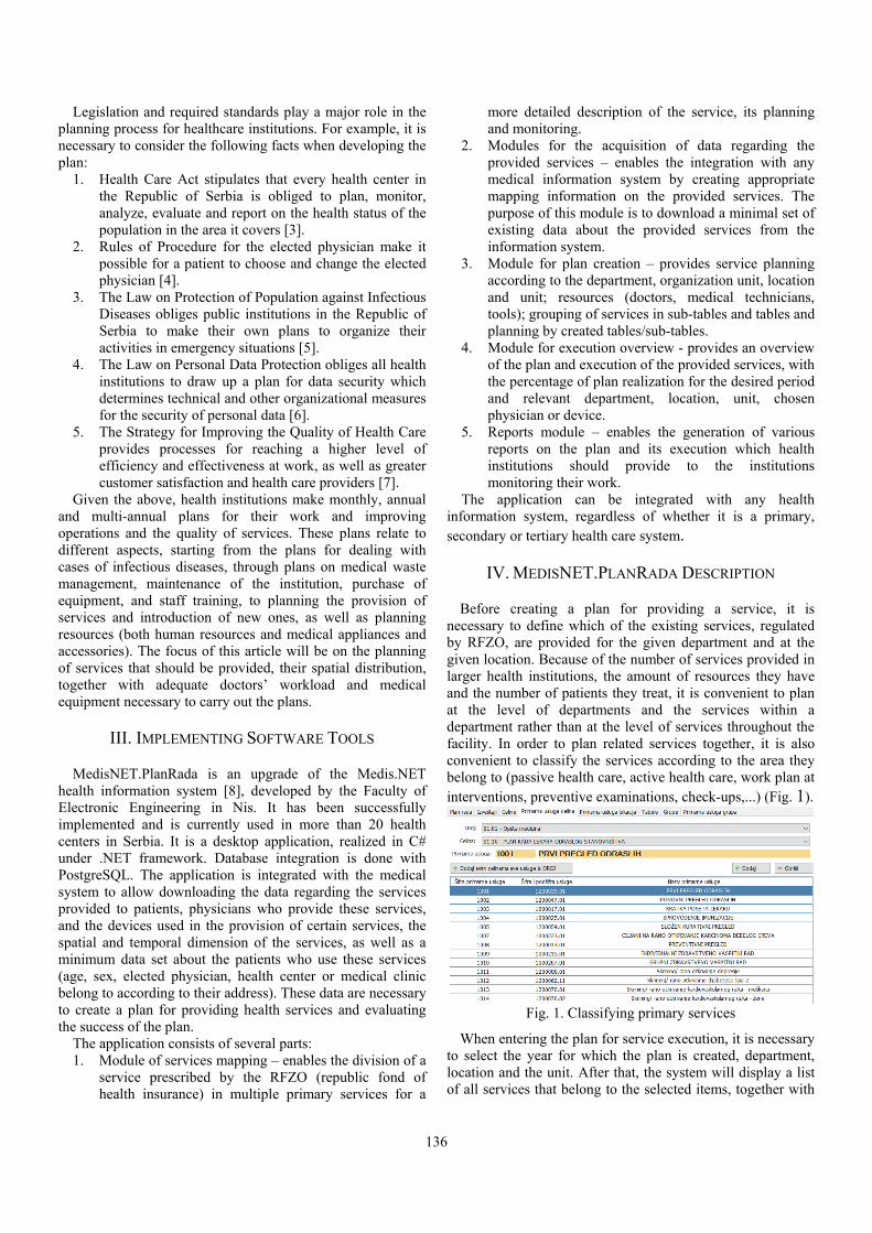
136

Legislation and required standards play a major role in the planning process for healthcare institutions. For example, it is necessary to consider the following facts when developing the plan:

1. Health Care Act stipulates that every health center in the Republic of Serbia is obliged to plan, monitor, analyze, evaluate and report on the health status of the population in the area it covers [3].

2. Rules of Procedure for the elected physician make it possible for a patient to choose and change the elected physician [4].

3. The Law on Protection of Population against Infectious Diseases obliges public institutions in the Republic of Serbia to make their own plans to organize their activities in emergency situations [5].

4. The Law on Personal Data Protection obliges all health institutions to draw up a plan for data security which determines technical and other organizational measures for the security of personal data [6].

5. The Strategy for Improving the Quality of Health Care provides processes for reaching a higher level of efficiency and effectiveness at work, as well as greater customer satisfaction and health care providers [7].

Given the above, health institutions make monthly, annual and multi-annual plans for their work and improving operations and the quality of services. These plans relate to different aspects, starting from the plans for dealing with cases of infectious diseases, through plans on medical waste management, maintenance of the institution, purchase of equipment, and staff training, to planning the provision of services and introduction of new ones, as well as planning resources (both human resources and medical appliances and accessories). The focus of this article will be on the planning of services that should be provided, their spatial distribution, together with adequate doctors’ workload and medical equipment necessary to carry out the plans.

III. IMPLEMENTING SOFTWARE TOOLS

MedisNET.PlanRada is an upgrade of the Medis.NET health information system [8], developed by the Faculty of Electronic Engineering in Nis. It has been successfully implemented and is currently used in more than 20 health centers in Serbia. It is a desktop application, realized in C# under .NET framework. Database integration is done with PostgreSQL. The application is integrated with the medical system to allow downloading the data regarding the services provided to patients, physicians who provide these services, and the devices used in the provision of certain services, the spatial and temporal dimension of the services, as well as a minimum data set about the patients who use these services (age, sex, elected physician, health center or medical clinic belong to according to their address). These data are necessary to create a plan for providing health services and evaluating the success of the plan.

The application consists of several parts: 1. Module of services mapping – enables the division of a

service prescribed by the RFZO (republic fond of health insurance) in multiple primary services for a

more detailed description of the service, its planning and monitoring.

2. Modules for the acquisition of data regarding the provided services – enables the integration with any medical information system by creating appropriate mapping information on the provided services. The purpose of this module is to download a minimal set of existing data about the provided services from the information system.

3. Module for plan creation – provides service planning according to the department, organization unit, location and unit; resources (doctors, medical technicians, tools); grouping of services in sub-tables and tables and planning by created tables/sub-tables.

4. Module for execution overview - provides an overview of the plan and execution of the provided services, with the percentage of plan realization for the desired period and relevant department, location, unit, chosen physician or device.

5. Reports module – enables the generation of various reports on the plan and its execution which health institutions should provide to the institutions monitoring their work.

The application can be integrated with any health information system, regardless of whether it is a primary, secondary or tertiary health care system.

IV. MEDISNET.PLANRADA DESCRIPTION

Before creating a plan for providing a service, it is necessary to define which of the existing services, regulated by RFZO, are provided for the given department and at the given location. Because of the number of services provided in larger health institutions, the amount of resources they have and the number of patients they treat, it is convenient to plan at the level of departments and the services within a department rather than at the level of services throughout the facility. In order to plan related services together, it is also convenient to classify the services according to the area they belong to (passive health care, active health care, work plan at interventions, preventive examinations, check-ups,...) (Fig. 1).

Fig. 1. Classifying primary services

When entering the plan for service execution, it is necessary to select the year for which the plan is created, department, location and the unit. After that, the system will display a list of all services that belong to the selected items, together with

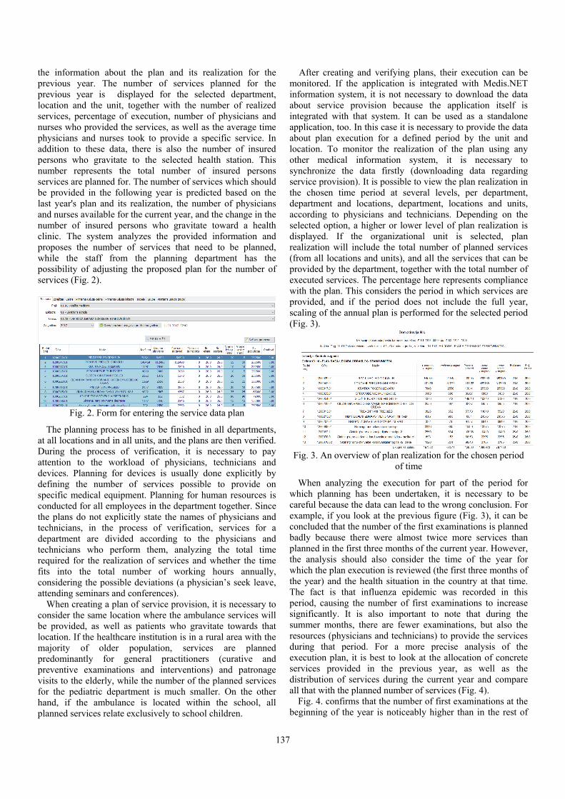
137

the information about the plan and its realization for the previous year. The number of services planned for the previous year is displayed for the selected department, location and the unit, together with the number of realized services, percentage of execution, number of physicians and nurses who provided the services, as well as the average time physicians and nurses took to provide a specific service. In addition to these data, there is also the number of insured persons who gravitate to the selected health station. This number represents the total number of insured persons services are planned for. The number of services which should be provided in the following year is predicted based on the last year's plan and its realization, the number of physicians and nurses available for the current year, and the change in the number of insured persons who gravitate toward a health clinic. The system analyzes the provided information and proposes the number of services that need to be planned, while the staff from the planning department has the possibility of adjusting the proposed plan for the number of services (Fig. 2).

Fig. 2. Form for entering the service data plan

The planning process has to be finished in all departments, at all locations and in all units, and the plans are then verified. During the process of verification, it is necessary to pay attention to the workload of physicians, technicians and devices. Planning for devices is usually done explicitly by defining the number of services possible to provide on specific medical equipment. Planning for human resources is conducted for all employees in the department together. Since the plans do not explicitly state the names of physicians and technicians, in the process of verification, services for a department are divided according to the physicians and technicians who perform them, analyzing the total time required for the realization of services and whether the time fits into the total number of working hours annually, considering the possible deviations (a physician’s seek leave, attending seminars and conferences).

When creating a plan of service provision, it is necessary to consider the same location where the ambulance services will be provided, as well as patients who gravitate towards that location. If the healthcare institution is in a rural area with the majority of older population, services are planned predominantly for general practitioners (curative and preventive examinations and interventions) and patronage visits to the elderly, while the number of the planned services for the pediatric department is much smaller. On the other hand, if the ambulance is located within the school, all planned services relate exclusively to school children.

After creating and verifying plans, their execution can be monitored. If the application is integrated with Medis.NET information system, it is not necessary to download the data about service provision because the application itself is integrated with that system. It can be used as a standalone application, too. In this case it is necessary to provide the data about plan execution for a defined period by the unit and location. To monitor the realization of the plan using any other medical information system, it is necessary to synchronize the data firstly (downloading data regarding service provision). It is possible to view the plan realization in the chosen time period at several levels, per department, department and locations, department, locations and units, according to physicians and technicians. Depending on the selected option, a higher or lower level of plan realization is displayed. If the organizational unit is selected, plan realization will include the total number of planned services (from all locations and units), and all the services that can be provided by the department, together with the total number of executed services. The percentage here represents compliance with the plan. This considers the period in which services are provided, and if the period does not include the full year, scaling of the annual plan is performed for the selected period (Fig. 3).

Fig. 3. An overview of plan realization for the chosen period

of time

When analyzing the execution for part of the period for which planning has been undertaken, it is necessary to be careful because the data can lead to the wrong conclusion. For example, if you look at the previous figure (Fig. 3), it can be concluded that the number of the first examinations is planned badly because there were almost twice more services than planned in the first three months of the current year. However, the analysis should also consider the time of the year for which the plan execution is reviewed (the first three months of the year) and the health situation in the country at that time. The fact is that influenza epidemic was recorded in this period, causing the number of first examinations to increase significantly. It is also important to note that during the summer months, there are fewer examinations, but also the resources (physicians and technicians) to provide the services during that period. For a more precise analysis of the execution plan, it is best to look at the allocation of concrete services provided in the previous year, as well as the distribution of services during the current year and compare all that with the planned number of services (Fig. 4).

Fig. 4. confirms that the number of first examinations at the beginning of the year is noticeably higher than in the rest of

138

the year, and that a similar situation is repeated from year to year. Therefore, this fact is very important for monitoring the realization of the plan. For each of the planned services, there is a correlation with the time of year. For example, a regular check-up of first grade children is carried out from May to the end of August, vaccination is usually done in the spring and fall, an injuries due to falls usually occur during the winter months.

Fig. 4. Service execution

Given all the above, it can be concluded that service monitoring should be done for short periods of time but with great awareness of the connection between the location where the services are provided and the time range for single services. The job is further complicated by the sheer number of services. The described system therefore includes an automatic check of plan realization which singles out only those services whose execution deviates more than a specified percentage (considering the total number of planned services in the current and previous year (or previous years, according to the history data that an institution possess), the distribution of their execution by months, and the degree of deviation that the user defines). The deviation percentage can be defined by the users themselves. Greater deviations require further analysis and possibly the revision of the planned service provision. For example, if the number of first examinations and interventions due to a flu epidemic significantly increases, it is necessary to increase the number of physicians and technicians, reallocate resources from other sites or departments if possible, or make a reorganization plan to reduce the number of other services whose execution is not so critical. If service is not realized according to the plan, this does not necessarily mean that there is an error in the planning process, but may indicate a change of health condition of the population gravitating to that institution.

Another important aspect to the service planning and monitoring their realization is monitoring the workload of physicians and technicians, or devices that provide these services. Due to the constant development and advancement of treatment and prevention, the plan needs to include periods when the staff attend professional training seminars, and are therefore not able to provide the planned services. The number of insured persons who gravitate toward an institution, their age structure are considered when planning physicians and technicians who will be at the site to provide services. Further improvement in the planning can be achieved by analyzing the medical histories of patients in a

certain area in order to select the most qualified physician for the most common diseases in a given area.

V. CONCLUSION

This article describes some of the problems the health institutions face when creating a plan for providing services and monitoring its realization. It describes developed application that supports the entire process of planning and monitoring the execution of the plan with warnings about significant deviations from the plan and appropriate reports. The application enables planning and execution monitoring, as well as the workload of physicians, technicians and devices. The goal is to increase the efficiency and quality of services, and improve the health state of the population. Deviations from the plan are easy to detect. They can represent a change of the population’s health state in a certain area.

The described solution represents the first phase of the application’s implementation for planning services in primary health care. The second phase requires the existence of a database with information of the provided services from a longer period of time (several years) which the system will use to "learn" how services are planned and realized for defined parameters. The system would then be able to precisely generate an execution plan of services for the future, following the migration of the population (based on the change in address), aging, gravitation to institutions, available devices and human resources and their knowledge, as well as new methods and trends in treatment. This gives room for further work on the application’s development and simplification of the medical service planning in primary health care.

REFERENCES

[1] D.E. Evans, A. Tandon, C. J.L. Murray, et al. “The Comparative Efficiency of National Health Systems in Producing Health: An Analysis of 191 Countries”, Geneva, Switzerland, World Health Organization, (Global Programme on Evidence for Health Policy Discussion Paper no. 29), 2000.

[2] A. Milenković, D. Janković, M. Stojković, A. Veljanovski, and P. Rajković, “Software Module for Registering Provided Health Services and Consumed Medications in Infirmary”, TELFOR 2015, Belgrade, Serbia, November 24-26, 2015, 9.12 (870).

[3] Zakon o zdravstvenoj zaštiti. Službeni glasnik RS, Beograd, br.107/2005, 72/2009, 88/2010, 99/2010, 57/2011, 119/2012 i 45/2013.

[4] Pravilnik o načinu i postupku ostvarivanja prava iz obaveznog zdravstvenog osiguranja (“Sl. glasnik RS”, br. 10/2010).

[5] Zakon o zaštiti stanovništva od zaraznih bolesti (“Sl. glasnik RS”, br. 15/2016 od 25, februra 2016.god.).

[6] Zakon o zaštiti podataka o ličnosti (“Sl. glasnik RS”, br. 97/2008, 104/2009 - dr. zakon, 68/2012 - odluka US i 107/2012).

[7] Strategija za stalno unapređenje kvaliteta zdravstvene zaštite i bezbednost pacijenata (“Sl. glasnik RS”, br. 15/2009).

[8] D. Janković, A. Milenković, P. Rajković, T. Stanković, I. Marković, S. Cvetković, D. Vučković, S. Pešić, “Medicinski informacioni sistem MEDIS.NET”, realizator: Elektronski fakultet Niš - Laboratorija za medicinsku informatiku, 2010, http://www.elfak.ni.ac.rs/phptest/new/html/nauka/tehnicka_resenja/resenja/0259.html.

139

Statistical Analysis of Dice CAPTCHA Usability Darko Brodić1, Alessia Amelio2 and Ivo R. Draganov3

Abstract – In this paper the elements of the CAPTCHA usability are analyzed. CAPTCHA, as a time progressive element in computer science, has been under constant interest of ordinary, professional as well as the scientific users of the Internet. The analysis is given based on the usability elements of CAPTCHA which are abbreviated as user-centric approach to the CAPTCHA. To demonstrate it, the specific type of Dice CAPTCHA is used in the experiment. The experiment is conducted on 190 Internet users with different demographic characteristics on laptop and tablet computers. The obtained results are statistically processed. At the end, the results are compared and conclusion of their use is drawn.

Keywords – Artificial intelligence, CAPTCHA, Demographic characteristics, Internet, Response time, Statistical analysis.

I. INTRODUCTION

CAPTCHA (Completely Automated Public Turing test to tell Computers and Humans Apart) is a program representing a challenge-answer to the given test, which is used to realize if the solver is an Internet user (human) or a computer program (computer robot). This process includes the following elements: (i) The computer as a server, which generates the CAPTCHA test, (ii) Internet users or computer program which try to correctly solve the given task, (iii) The computer which evaluates the answer to the CAPTCHA in the format Yes/No (correctly/incorrectly solved). Typically, the CAPTCHA task is accustomed to the humans. Hence, there is a greater possibility that humans will solve this task compared to computer robots abbreviated as bots. Hence, the aim of the CAPTCHA program is to differentiate Internet users from bots [1].

The application of CAPTCHA program is useful in the following areas: (i) Online systems, (ii) The creation of free e-mail accounts, (iii) Online pooling, and (iv) Online system for buying tickets, etc [2].

Still, the CAPTCHA should fulfill certain elements, such as: (i) The solving of CAPTCHA should not rely on the user’s knowledge of certain language, (ii) The solving of CAPTCHA should not depend on the user’s age, (iii) CAPTCHA should make an automatic evaluation of the correctness, (iv) The user’s privacy should not be violated, and (v) It should be easy for Internet users to be solved unlike bots [3].

The related works on CAPTCHA often employ statistical approaches treating their various aspects. They can be partitioned taking into account their properties in the following areas: (i) Security, (ii) Practicality, and (iii) Usability [4].

Security represents the main concern to the CAPTCHA programmers. It represents a central problem of CAPTCHA, but it is not the only one that is of a great importance.

Practicality is connected to the way of creating certain types of CAPTCHA. Again, it has greater concerns of programmers than CAPTCHA users.

The usability represents the main problem related to the use of the CAPTCHA. Accordingly, it especially concerns the CAPTCHA users. Hence, this study is used to uncover the elements of CAPTCHA usability, which represents the main concern of the Internet users. In this way, an objective analysis of a certain type of CAPTCHA can facilitate better understanding the user-centric relation between computer and man, i.e. CAPTCHA and Internet user which will contribute to innovate and improve CAPTCHA elements to be more accustomed to the Internet users unlike bots.

This paper is organized in the following manner. Section II presents the CAPTCHA types. Section III describes the experiment. Section IV gives the results of the experiment and discussed them. Section V draws conclusions and points out the direction of future works.

II. CAPTCHA TYPES

All CAPTCHA types can be divided into five typical groups: (i) Text-based CAPTCHA, (ii) Image-based CAPTCHA, (iii) Audio-based CAPTCHA, (iv) Video-based CAPTCHA and (v) Other types of CAPTCHA [5].

Text-based CAPTCHA asks the Internet users to input exact combination of the given characters. This type of CAPTCHA is the most widespread one. In order to reduce its vulnerability to bot attacks, many distorted elements are incorporated. Unfortunately, the text-based CAPTCHA can be successfully attacked by bot due to the solid OCR (Optical Character Recognition) programs. Fig. 1 shows an example of the text-based CAPTCHA.

Fig. 1. An example of the text-based CAPTCHA Image-based CAPTCHA is considered as one of the most

advanced and safest types of CAPTCHA. It requires from the users to find out a certain image from a list of images and point to it. Due to that, its elements include the image details.

1Darko Brodić is with the Technical Faculty in Bor, University ofBelgrade, Vojske Jugoslavije 12, 19210 Bor, Serbia, E-mail:[email protected]

2Alessia Amelio is with the DIMES, University of CalabriaVia P.Bucci Cube 44, 87036 Rende (CS), Italy, E-mail:[email protected]

3Ivo R. Draganov is with the Faculty of Telecommunications atTechnical University of Sofia, 8 Kl. Ohridski Blvd, Sofia 1000,Bulgaria, E-mail: [email protected]

140

It represents a relatively easy task to be solved by Internet users unlike bots. Fig. 2 illustrates an example of the image-based CAPTCHA.

Fig. 2. An example of image-based CAPTCHA Audio-based CAPTCHA includes an “audio element”

whose purpose is an audio reproduction of characters that the user should have to input in order to solve the CAPTCHA. This type of CAPTCHA is especially designed for the people with disabilities. Unfortunately, the audio-based CAPTCHA is mostly attacked by speech and recognition algorithms in approximately 70% of cases. Fig. 4 illustrates an example of the audio-based CAPTCHA with “audio element” in the top right corner.

Fig. 3. An example of the audio-based CAPTCHA Video-based CAPTCHA contains text information

embedded into the video. Hence, it is a video which includes a passing text given in specific color compared to video background. The user should recognize the given passing text and type it. The modern OCR programs challenge this task, making this CAPTCHA vulnerable to bot attacks. Fig. 4 illustrates an example of the video-based CAPTCHA.

Fig. 4. An example of the video-based CAPTCHA Other types of CAPTCHA represent those CAPTCHAs that

cannot be part of the previous standardization. Fig. 5 illustrates the examples of such types of CAPTCHA.

III. EXPERIMENT

The CAPTCHA experiment is conducted on 190 Internet users. It is divided in two different experiments solving two different Dice CAPTCHAs (Dice 1 and 2). The first experiment is based on Dice CAPTCHAs tested on a community of 90 laptop users aged from 29 to 62 years. The laptop used for the experiment is Lenovo B51 with the

following characteristics: (i) 15.6" wide screen, (ii) CPU Quad-core 2.4 GHz Celeron, (iii) 4 GB of RAM, (iv) 500 GB of internal memory, and (v) Operating system Microsoft Windows 7. The second experiment is based on Dice CAPTCHAs tested on a community of 100 tablet users aged from 28 to 55 years. The tablet used for the experiment is Lenovo IdeaTab A3000 with the following characteristics: (i) 7" wide screen, (ii) CPU Quad-core 1.2 GHz Cortex-A7, (iii) 1 GB of RAM, (iv) 16 GB of internal memory, and (v) Operating system Android.

Fig. 5. An example of other type of CAPTCHA on the Dice CAPTCHA samples (Dice 1 at the top, and Dice 2 at the bottom) All Internet users represent volunteer students, employees,

clerks, teachers and engineers, who signed an online consent form before starting the experiment. Accordingly, they gave their consent to anonymously provide and use their data only for research and study purposes. Each of them was required to solve Dice CAPTCHA, and the response time to find the solution to the CAPTCHA was registered. The users are partitioned taking into account their various demographic factors: (i) Age, (ii) Education level, (iii) Gender. The experimental results are then statistically processed. The obtained results are then compared to evaluate (dis)advantages of using Dice CAPTCHA by the different Internet users’ groups (laptop or tablet).

IV. RESULTS AND DISCUSSION

A. Hypotheses

It is worth noting that the solution time for “ideal” CAPTCHA should not depend on the age, education and gender differentiation. However, if any CAPTCHA can satisfy these elements, then it doesn’t mean that it can be solved quickly and easily. According to previous facts, the following four hypotheses are proposed according to the given demographic characteristics:

Hypothesis 1 (H1) - There exists a statistically significant difference between users’ groups (laptop vs. tablet) in average response time to solve the CAPTCHA.

Hypothesis 2 (H2) - There exists a statistically significant difference between age groups in solving the CAPTCHA,

Hypothesis 3 (H3) - The group of Internet users with higher education will have a faster response time in solving the CAPTCHA,

Hypothesis 4 (H4) - There exists a statistically significant difference between gender groups in solving the CAPTCHA,

141

B. Experimental Results

The first results of the experiment are given in Tables I-II. These tables give a descriptive analysis of the obtained results for 90 laptops’ and 100 tablets’ Internet users concerning CAPTCHA Dice 1 and 2. They are obtained by Kolmogorov-Smirnov test, which test the unknown distribution and check the normality assumption in the analysis of variance [6].

TABLE I ONE-SAMPLE KOLMOGOROV-SMIRNOV TEST FOR LAPTOP USERS

Gender Age Education Dice 1 Dice 2 N 90 90 90 90 90 Mean 1.16 1.70 1.88 7.644 6.514 SD 0.364 0.461 0.329 2.554 2.203 Asymp. Sig. (2-tailed)

0.000 0.000 0.000 0.046 0.003

The most important information represents the measure

Asymp. Sig. (2-tailed). It defines the statistical significance of the analyzed data. Because it is smaller than 0.05, then obtained results are statistically significant. Also, it is worth noting that the average time to solve CAPTCHA Dice 1 is 7.6444, while CAPTCHA Dice 2 is solved in 6.514 seconds by laptop users.

TABLE II ONE-SAMPLE KOLMOGOROV-SMIRNOV TEST FOR TABLET USERS

Gender Age Education Dice 1 Dice 2 N 100 100 100 100 100 Mean 1.59 1.30 1.44 12.090 8.590 SD 0.494 0.461 0.499 5.874 4.360 Asymp. Sig. (2-tailed)

0.000 0.000 0.000 0.005 0.018

From Table II, the measure Asymp. Sig. (2-tailed) is again

lower than reference of 0.05, which determines the statistical significance of the analyzed data. Furthermore, it is worth noting that the average time to solve CAPTCHA Dice 1 is 12.090, while CAPTCHA Dice 2 is solved in 8.590 seconds by tablet users.

From Tables I-II, it is quite clear that exists a statistically significant difference in the response time to solve CAPTCHA Dice1 and Dice 2 between laptop and tablet users’ group. Obviously, Dice CAPTCHA is more convenient to be solved on a laptop than on a tablet computer. It is proved by statistical significant population. Hence, H1 is proved.

C. Statistical Test

The Mann-Whitney U test is a non-parametric test which can be used to (dis)prove a null-hypothesis H0 and a research hypothesis H1. Essentially, this test is used to compare differences between two independent groups N1 and N2. To be used, some pre-assumptions should be valid: (i) Input should be composed of two categorical independent groups N1 and N2, (ii) Output should be ordinal or continuous, (iii) There

should be no correlation between groups N1 and N2, and (iv) The input variables should not be normally distributed. The Mann-Whitney U test considers 3 important measures: (i) p-value, (ii) U value, and (iii) Z value.

The p-value is the first crucial measure of this statistical test. Its value can be interpreted as follows: (i) p<0.05 shows a strong evidence against the null-hypothesis. As a consequence, the null-hypothesis of the test is disproved, while research hypothesis H1 is proved, (ii) p>=0.05 shows a weak evidence against the null-hypothesis of the test. As a consequence, the null-hypothesis of the test is proved, while research hypothesis H1 is disproved. U value is calculated as:

1 11 2 1

( 1) ,

2

n nU n n R

(1)

where U represents the result of the Mann-Whitney U test. Accordingly, n1 is the size of the independent group N1, n2 is the size of the independent group N2, and R1 represents the sum of ranks of group N1. If U value is higher than the critical U value, then the two groups N1 and N2 will have the same score distributions, otherwise the two distributions N1 and N2 will be different in some aspect. Critical value U is important only for small size distributions, where the number of their elements is up to 20. If the group is larger than 20, then U value approaches to normal distribution. In that case, the Z value has importance. It is calculated as:

1 2

1 2 1 2

/ 2 .

( 1) /12

U n nZ

n n n n

(2)

If the absolute value of Z is lower than 1.96, then the two groups N1 and N2 will have the same score distributions, otherwise the two distributions of N1 and N2 will be dissimilar in some way. Accordingly, if Z is lower than 1.96 research hypothesis is disproved, otherwise it is proved.

D. Analysis of the Results and Discussion

The results obtained by statistically processing (Mann-Whitney U test) of experimental data for the age characteristic of the laptop/tablet users are given in Table III.

The first relevant measure, which has to be evaluated is Asymp. Sig. (2-tailed). For laptop users as well as for tablet users concerning CAPTCHA Dice 1 and 2 it is higher than 0.05. Accordingly, this analysis is not statistically significant. Hence, H2 is not proved.

The results obtained by statistically processing (Mann-Whitney U test) experimental data for the education demographic characteristic of the laptop and tablet users are given in Table IV.

Again, the measure Asymp. Sig. (2-tailed) is evaluated the first. For laptop users as well as for tablet users concerning CAPTCHA Dice 1 and 2 it is higher than 0.05. Hence, this analysis is not statistically significant. This leads that H3 is not proved.

142

TABLE III MANN-WHITNEY U TEST (LAPTOP/TABLET USERS) FOR THE AGE

Laptop Age (y/o)

N Mean rank (1/2)

Z Asymp. Sig. (2-tailed)

Dice 1 27/63 90 49.04/43.98 -0.842 0.400 Dice 2 27/63 90 53.48/42.08 -1.899 0.058

Tablet Age (y/o)

N Mean rank (1/2)


Dice 1 70/30 100 48.21/55.83 -1.208 0.227 Dice 2 70.30 100 49.06/53.87 -0.764 0.445

*y-younger, o-older, 1-group 1 (younger), 2-group 2 (older)

TABLE IV MANN-WHITNEY U TEST (LAPTOP/TABLET USERS) FOR THE

EDUCATION

Laptop Educ. (h/s)

N Mean rank (1/2)


Dice 1 79/11 90 44.08/55.73 -1.387 0.165 Dice 2 79/11 90 43.86/57.27 -1.596 0.110

Tablet Educ. (h/s)

N Mean rank (1/2)


Dice 1 44/56 100 53.75/47.95 -0.997 0.319 Dice 2 44/56 100 50.63/50.40 -0.038 0.969

*h-higher, o-secondary, 1-group 1 (higher), 2-group 2 (secondary)

The results obtained by statistically processing (Mann-

Whitney U test) experimental data for the gender demographic characteristic of the laptop and tablet users are given in Table V.

TABLE V MANN-WHITNEY U TEST (LAPTOP/TABLET USERS) FOR THE GENDER

Laptop Gender (m/f)

N Mean rank (1/2)


Dice 1 14/76 90 52.79/44.16 -1.137 0.256 Dice 2 14/76 90 46.61/45.30 -0.173 0.863

Tablet Gender (m/f)

N Mean rank (1/2)


Dice 1 59/41 100 52.47/47.66 -0.820 0.412 Dice 2 59/41 100 48.58/53.27 -0.800 0.424

*m-male, f-female, 1-group 1 (male), 2-group 2 (female)

From Table V the measure Asymp. Sig. (2-tailed) is again

higher than reference value 0.05. Hence, for laptop users as well as for tablet users concerning CAPTCHA Dice 1 and 2 the given analysis is not statistically significant. Accordingly, H4 is not proved.

From the aforementioned, the H1 is only proved, while H2, H3 and H4 are not proved. Because, the postulate of “ideal” CAPTCHA is to be solved in reasonable time (less than 30 sec. [5]), and the solution time should not depend on the age, education and gender differentiation, the Dice CAPTCHA represents a good direction toward creating an “ideal” CAPTCHA. However, it is worth noting that using CAPTCHA on different computer types should also diminish differences between solution time of certain CAPTCHA. In our case, solution time of Dice CAPTCHA between laptop

and tablet users is almost 50% less in favor of laptop users. Taking into account this information, Dice CAPTCHA is more accustomed to the laptop than tablet Internet users. Hence, Dice CAPTHA can be considered only as the first step in right direction toward creating an “ideal” CAPTCHA.

V. CONCLUSION

The paper analyzed the response time of Internet laptop and tablet users in solving the Dice CAPTCHA version 1 and 2. To research the given topic, an experiment was conducted on 190 users. It was divided into two parts: (i) testing of 90 laptop users in solving Dice CAPTCHA 1 and 2, and (ii) testing of 100 tablet users in solving Dice CAPTHA 1 and 2. Then, the obtained results were statistically processed. According to the results, four hypotheses were established, which should be proved or disproved. All hypotheses were closely related to the elements of an “ideal” CAPTCHA. Using statistical tools, a descriptive statistical analysis and the results of Mann-Whitney U test were used for proving and disproving the given hypotheses. At the end, the H1 hypothesis was only proved, while the other ones were rejected. In spite of the obtained result, which represents the main elements of an “ideal” CAPTCHA, due to rather different time in solving Dice CAPTCHA between laptop and tablet users, this type of CAPTCHA cannot be used as an example of “ideal” CAPTCHA. But, because of some overlapping with the characteristics of an “ideal” CAPTCHA, the Dice CAPTCHA is a good start and a right direction toward creating the real “ideal” CAPTCHA.

ACKNOWLEDGEMENT

This study was partially funded by the Grant of the Ministry of Education, Science and Technological Development of the Republic of Serbia, as a part of the project TR33037.

REFERENCES

[1] L. Von Ahn, M. Blum, and J. Langford, “Telling Humans and Computers Apart Automatically”, Communication of ACM, vol. 47, no. 2, pp. 47-60, 2004.

[2] The CAPTCHA test. http://en.wikipedia.org/wiki/CAPTCHA [3] L. von Ahn, M. Blum, N. Hopper, and J. Langford,

“CAPTCHA: Using Hard AI Problems for Security”, Proceedings of Eurocrypt, Warsaw, Poland, pp. 294-311, 2003.

[4] P. Baecher, M. Fischlin, L. Gordon, R. Langenberg, M. Lutzow, and D. Schroder, “CAPTCHAs: The Good, the Bad and the Ugly”, Sicherheit, pp. 353-365, 2010.

[5] D. Brodić, S. Petrovska, M. Jevtić, and Z. N. Milivojević, “The Influence of the CAPTCHA Types to its Solving Times”, Proceeding of 39th MIPRO, Opatija, Croatia, pp. 1274-1277, 2016.

[6] W.J. Conover, Practical Nonparametric Statistical, pp. 428-433, John Wiley & Sons, Inc. New York, 1999.

143

Tool for Interactive and Automatic Composition of Business Processes

Aleksandra Koleva1 and Aleksandar Dimov2

Abstract – Web services provide means for electronic execution of business processes. However, composition of services for this purpose may become a tedious task for non-IT professionals. In this paper we propose an approach to cope with this problem by developing a web-based software tool that is capable to propose to users appropriate services for creation of a business process. Afterwards the tool automatically compose and executes the selected services.

Keywords – Service Oriented Architecture, Service Discovery, Service Selection, Automatic Service Composition, Business Process.

I. INTRODUCTION

Service Oriented Architecture is an architectural concept for development of distributed systems that has matured a lot during the last two decades [4]. It is claimed to enable reusability and straightforward integration of highly complex heterogeneous systems. The building elements and fundamental notion of SOA systems are called services. As stated in [1] service is a broad term that has different meaning depending on its usage context. For example, in computer science, the terms of web-service, e-service and business service have common meaning. In this paper, we will focus on web-services (WS), which are broadly recognized as [12]: Loosely coupled reusable software components that encapsulate discrete functionality and are distributed and programmatically accessible over standard Internet and XML-based protocols. Web services should be considered as software components, accessible by unique URL. Interfaces of such components are described using well-defined protocols, majority of which are XML-based. Web-services are also composable and may be consumed by other services for use in different applications or in execution of business processes [5].

However, currently integration of services is mainly performed by technically aware personnel and general users doesn’t have enough possibilities to create and execute business processes of their own. This paper presents an interactive tool that is capable to both provide recommendations to the users for service composition and

also automatically implement and execute it. For this purpose it provides users with recommendations about services to be included into the composition, this way facilitating the process of their selection. This is based on information about service functionality. Afterwards, it automatically binds the selected services, asks for input data, if needed and finally, executes them.

The rest of the paper is organized as follows: Section 2 briefly presents current state of the art in the area; Section 3 describes some design and implementation details about the tool for interactive automatic composition of business processes and finally Section 4 concludes the paper and points out directions for future research.

II. STATE OF THE ART IN SERVICE COMPOSITION

DISCOVERY AND SELECTION

There exist several research directions that have relation with the work presented here. Among them are service composition, discovery and selection. Two big groups of approaches for service discovery and selection may be distinguished – based on semantic information and the second, based on information about Quality of Service (QoS). It should be noted that concerns finding appropriate service, based on its functionality. On the other hand, QoS approaches, mostly focus on selection among services, when you have several alternatives that fulfill functional requirements. Approaches that use semantic information usually involves tools for automated web service discovery based on some description of the service semantics using a language like OWL-S [6] or analysis of the service WSDL [7]. Service selection, based on QoS use a formal representation of service quality and corresponding models to select the best service that fit user needs [9] or a given composition [10].

As pointed out in the introduction, in order to achieve substantial business value from services it is needed to be able to compose them into bigger units. There exist several classifications [2], [3], and [11] of service composition approaches, which discuss the subject in deep details. However for the purpose of this work we focus on more fundamental service composition classes, which are briefly described below:

Dynamic and static composition – dynamic composition may also be referred as run-time or automatic composition, where respective services are composed automatically during execution of the composite service. In order to achieve this, a number of additional disciplines as artificial intelligence, formal specification and etc. may be involved. Dynamic composition allows for SOA systems to change themselves transparently for the users and adapt to change in the environment and/or requirements.

1Aleksandra Koleva is with the Faculty of Mathematics andInformatics at Sofia University “St. Kliment Ohridski”, 5 James Bourchier Blvd, Sofia 1164, Bulgaria, E-mail: [email protected]

2Alexandar Dimov is with the Faculty of Mathematics andInformatics at Sofia University “St. Kliment Ohridski”, 5 James Bourchier Blvd, Sofia 1164, Bulgaria, and Section of SoftwareTechnologies and Information Systems, Institute of Mathematics and Informatics, Bulgarian Academy of Sciences, Acad. Georgi BonchevStr., Block 8, 1113 Sofia, E-mail: [email protected]

144

Different approaches for dynamic service composition are used. For example, model languages, like UML may be used for high level abstract description of the composition. In the approach, described in [8], Object Constraint Language (OCL) is applied to enable transformation to particular service composition standards like WS-BPEL or OWL-S. Another aspect of dynamic composition is about the method for selection of services that will take part in the composition. It may be based on Quality of Service (QoS), on semantic discovery of services or eventually, on combination of both approaches.

On the other hand static composition deals with design time interconnection of services. It requires advanced users and/or a certain amount of programming efforts in order to be implemented.

Choreography and orchestration – these two composition approaches focus more on behavioral details about role of specific service in the composition. Service orchestration is about organization of a centralized service, which executes as the main business process. It is called orchestrator and acts as an endpoint for the other services that take part into the composition. It also coordinates their execution (Fig. 1).

Service choreography (Fig. 2) is more about distributed management of invocation of services that participate in the composition. This is in contrast with orchestration, where control flow from orchestrator’s perspective is important. Choreography is composition of services, where interactions between multiple services are of prime importance.

Service composition notations – There exist a number of notations to describe service compositions as well as other languages that supplement them. The most commonly used service composition language is called WS-BPEL (Web Services Business Process Execution Language) [13]. It is aimed towards description of service compositions based on XML and WSDL variables, and structured composition representations using standard operators as logical branches, loops and etc. In order to achieve automatic compositions WS-BPEL should be complemented with a corresponding notation, which is machine readable and would enable programmable search and composition of services. One such notation is OWL-S [14], which represents a technology to provide semantic markup for web services. It is aimed towards description of the semantics of services and is based on three main sub-ontologies:

Profile – describes what actually the service will do Process model – describes how the service works and

helps for implementation of processes for service invocation, composition and monitoring.

Grounding – describes how the service can be accessed.

There also exist other semantic notations for services, like WSMO (Web Service Modeling Ontology) [15] and SWSF (Semantic Web Services Framework) [16].

So far in this section, we have reviewed some of general properties of existing approaches for service discovery and composition. Further we will make an overview of the work directly related to ours – these are the existing service composition platforms.

Cloudwork [17] is an integration platform that allows customers to automate tasks between existing web- and cloud-based systems. For example, one cloud automate businesses with ticket support system or synchronize two storage services (like Google Drive with Dropbox).

Elastic.io is an API integration and orchestration platform, which offers simple interface to create and execute multiple web applications directly via the browser. It is appropriate to be used by nonprogrammers, however does not allow free access.

Although not directly aimed at service composition, Wufoo [18] helps users to build online forms, share them and collect data. It is Internet application which automatically builds the database, backend and scripts needed to make collecting and understanding user‘s data easy.

“If This Then That” [19] gives users possibility to connect applications via models and triggers, expressed in the so-called “recipes”. They may be either of type “if recipe”, allowing user to create connection with statement “if this then that”, or “do recipe” enabling simple actions over the web. Users have to activate accounts for the relative connected channels like e-mail address, Dropbox account, google drive etc.

Zapier [20] uses a combination of triggers and activities (or action-reaction rules), called zaps to allow users to define combinations of applications. A drag and drop environment for creation of zaps is provided and the latter may be also scheduled for iterative execution.

Fig. 1. Service orchestration

Fig. 2. Service choreography

Service 1 Service 2

Service n

Service 1

Service 2

Service n

…

Orchestrator service

Compositionendpoint

145

III. TOOL FOR AUTOMATIC SERVICE COMPOSITION

In this section, we present the design and implementation details about our automatic service composition tool. One of the most important tasks is to implement an algorithm, responsible for discovery of appropriate services. Main requirement for our tool is to propose recommendations to users about appropriate services for a composition. This is in order not only to automate the composition process, but also to help them to create their own business processes. For this purpose the tool should first implement service discovery rules. Afterwards, when appropriate services are found, users should select the services, they find most relevant to be included into the composition.

Additionally, one of our main quality requirements is about efficiency and performance of the tool. Simplified service discovery mechanism is implemented in order to enable service discovery and selection, while at the same time keeping efficiency and performance. Services are annotated with the two additional properties: service level and service category.

Service level marks the possible position of services into a composition. We have divided services into three levels: beginning, transition and ending services.

Beginning services – these services may act only as a starting point of a business process. For example, these may be authentication services or services for searching a specific set of items.

Transition services form the core of the business process – these are the services that may be called by a beginning service and they may call another transition service themselves. All transition services are additionally tagged with information about what other service (beginning or transition) may call them. This additional information is stored together with other service metadata.

Ending service – are services that represent the final of a business process and are not supposed to result into call to another service. Ending services are also tagged with information about what other service (beginning or transition) may call them

Service level meta-information is usually set by administrators and sometimes during business process creation, users may also tag a transition service as ending if they want to finish their process.

However, in order for the algorithm for service recommendation to be fully functional, information about service level is not enough. For this purpose we define another

Fig. 3. Flow of activities of the tool for interactive automatic composition of business processes

146

meta-information tag about services, called category. Categories represent simplified description of the semantics of the service. This way, services may be matched by categories and users may select the category of next service in the business process. Afterwards, the tool selects the best service of this category to be included into the composition, based on QoS. These metadata about services are currently implemented into a database that acts as a service registry.

The tool implements interactive user communication, in which the user repeatedly selects which service wants to compose next. First the tool finds and lists to the user all available beginning services. After that based on metadata of the transition and ending services, all of them that may be called afterwards are listed. This is an iterative process, which ends with selection of a final service by the user (Fig. 3).

Composition of the selected services is implemented, following the orchestration approach. User decides to execute the service composition(represented by the “call services” state on Fig. 3), which causes the tool to read and parse the description of each participating service. This results into a web form, with input fields for all required data. The user should provide this data, as it is required by participating services for their execution, by filling the form. Finally the tool implements an orchestration approach that calls all selected services with the data provided by the user.

IV. CONCLUSION

Traditionally, composition of services in order to execute specific business processes required a certain amount of implementation and programming knowledge. However for the development of the IT society, such possibilities should be available for wider range of users with various computer literacy levels. This paper presents a tool that is capable to interactively facilitate users to build a composition of services into a business process. It also provides recommendation for appropriate services, this way facilitating creation of the business process.

This is an ongoing work and further research includes, improvement of the method for adding meta-information to services, as now this requires a significant amount of administrative work to tag all transition and ending services with list of services, allowed to execute them.

ACKNOWLEDGEMENT

Research, presented in this paper was partially supported by the DFNI I02-2/2014 (ДФНИ И02-2/2014) project, funded by the National Science Fund, Ministry of Education and Science in Bulgaria.

REFERENCES

[1] Z. Baida, J. Gordijn, and B. Omelayenko, "A Shared Service Terminology for Online Service Provisioning", 6th International Conference on Electronic Commerce, Delft, The Netherlands, pp. 1-10, 2004.

[2] D. Claro, P. Albers, and J. Hao, "Web Services Composition", Semantic Web Services, Processes and Applications, Springer US, pp. 195-225, 2006.

[3] S. Dustdar, and W. Schreiner, "A Survey on Web Services Composition", International Journal of Web and Grid Services 1.1, pp. 1-30, 2005.

[4] T. Erl, SOA: Principles of Service Design, Pearson Education, Inc., Boston, USA, 2008.

[5] M. Hepp, et all, "Semantic Business Process Management: A Vision Towards Using Semantic Web Services for Business Process Management", IEEE International Conference on e-Business Engineering, pp. 535-540, 2005.

[6] M. Klusch, B. Fries, and K. Sycara, "Automated Semantic Web Service Discovery with OWLS-MX", Fifth International Joint Conference on Autonomous Agents and Multiagent Systems, ACM, 2006.

[7] R. Nayak, and B. Lee, "Web Service Discovery with Additional Semantics and Clustering", IEEE/WIC/ACM International Conference on Web Intelligence, 2007.

[8] B. Orriëns, J. Yang, and M. Papazoglou, "Model Driven Service Composition", International Conference on Service-Oriented Computing, Springer Berlin Heidelberg, 2003.

[9] D. Petrova-Antonova, "A QoS-Aware Approach for Web Service Selection Based on Probability Evaluation", M CC SSI MCCSIS 43, 2011.

[10] D. Petrova-Antonova, and A. Dimov, "A QoS Driven Approach for Probability Evaluation of Web Service Compositions", 6th International Conference on Software and Database Technologies (ICSOFT), pp. 321-326, 2011.

[11] D. Petrova-Antonova, and A. Dimov, "Towards a Taxonomy of Web Service Composition Approaches", Journal of Scalable Computing: Practice and Experience, vol. 12, no. 4, pp. 377-384, 2011.

[12] I. Sommerville, Software Engineering, Addison Wesley, 2010. [13] Web Services Business Process Execution Language Version

2.0, 2007, available at: http://docs.oasis-open.org/wsbpel/2.0/ OS/wsbpel-v2.0-OS.html

[14] OWL-S: Semantic Markup for Web Services, 2014. available at: http://www.w3.org/Submission/OWL-S/

[15] D2v1.4. Web Service Modeling Ontology (WSMO), 2007. available at http://www.wsmo.org/TR/d2/v1.4/

[16] Semantic Web Services Framework SWSF Version 1.0, 2005. Available http://www.daml.org/services/swsf/1.0/

[17] Cloudwork website, available at https://cloudwork.com [18] WooFoo website, available at https://www.wufoo.com/ [19] If this than that website, available at https://ifttt.com/about [20] Zapier website, available at https://zapier.com/

147

Analysis and Justification of Indicators for Quality Assessment of Data Centers

Rosen Radkov

Abstract –The quality of aDataCenter (DC) can be assessed by different criteria. The purpose of this article is to analyse the indicators that can be used to assess the quality of DC from the point of view of the accessibility of the services provided.Based on the analysis is substantiated set of significant indicators for the DC quality. Quantification of the quality is offered using a complex generalizedindicator, which can be used to benchmark between different DC’s and selects an optimal variant for concrete business case.

Keywords –Data center, Quality, Dependability, Availability, Reliability.

I. INTRODUCTION

New IT services like cloud computing are currently reaching a growing number of users. These new trendsare the reason for correspondingly high demands. Servers and data centers must be 100% available around the clock. Down times and interruptions or delays in data transmission must be virtually eliminated.

Which are the indicators for assessing the quality of a Data Center(DC)? How to choose which DC’sIT infrastructure (ITIS) is right for concrete business case?

II. TERMS AND DEFINITIONS

A. Definition Quality

According to Wikipedia, the qualityis an essential attribute of any product or service and plays a crucial role in the function of the economic operators and market relations.

A modern definition of quality derives from Joseph Juran's "fitness for intended use." This means that quality is "meeting or exceeding customer expectations."

Accordingly to that definition, the quality of a DC would be determined by the services provided to consumers and their criteria for satisfaction.

This article will not address issues related to the response time after to a request to the DC, its performance or energy efficiency.

B. Dependability

The quality of a DC can be assessed by different indicators. Commonly used indicator for this purpose in the technics is the concept of dependability. In the most general sense the

dependability is the ability of anobject to retain its essential properties in set modes and in operating conditions [1].

The systematic expositionof the dependability concept includes three parts: the threats to dependability, the attributes of dependability and tools for achieving dependability (Fig. 1) [2].

Fig. 1. The dependability tree

Dependability attributes describe the propertieswhich are required of a system. Dependability threats express the reasons for asystem to cease to perform its function or, in otherwords, the threats to dependability. Dependability means are the methods and techniques enabling the development of adependable system, such as fault prevention, fault tolerance, fault removal, and fault forecasting [3].

Dependability threats are defined as follow: a fault is physical defect, imperfection, or flaw that occurs in some software or hardware component; an error is a deviation from correctness or accuracy in computation, which occurs as a result of a fault; afailure is a transition from correct to incorrect service, and this means that at least some external state of the service deviates from the correct state.

A common feature of the three terms is that they give us a message that somethingwent wrong. The difference is that, in the case of a fault, the problem occurred onthe physical level; in the case of an error, the problem occurred on the computationallevel; in the case of a failure, the problem occurred on a system level [3].

Dependability

Threats

Faults

Errors

Failures

Attributes

Availability

Reliability

Safety

Confidentiality

Integrity

Maintainability

Means

Fault prevention

Fault tolerance

Fault removal

Fault forecasting

Rosen Radkov is a member of the Department of Software and Internet Technologies at Technical University of Varna, 1Studentska Str., Varna9010, Bulgaria, E-mail: [email protected]

148

The DC is a set of interacting components where the dependability of the system is a complex property. The basic attributes of dependability are: availability- readiness of the DC for correct service in any point in time [1], [2]; reliability - continuity of a correct service [1], [2]; safety - the absence of catastrophic consequences for the user(s) and the environment; confidentiality - protection from unauthorized disclosure; integrity - protection against unauthorized modification of information; maintainability - the ability of DC to operate without interruption during processes of repairs, maintenances and modifications;

If t is designated as atime interval in which a DC should be available, then reliability is the probability that DC will work according to its functional specification in period t, and availabilityis the probability that DC is not defective or under repair when it should be used. It can therefore be concluded that the availability is a function of the reliability and maintainability.

Dependability means are the methods and techniques enabling the development ofa dependable system.The means to attain dependability and security can be defined as follow:fault prevention: means to prevent the occurrence or introduction of faults; fault tolerance(FT): means to avoid service failures in the presence of faults; fault removal: means to reduce the number and severity of faults; fault forecasting: means to estimate the present number, the future incidence, and the likely consequences of faults.

C. MTBF and MTTR

These two terms, used in theory of dependability, have a place there. Mean Time Between Failures (MTBF) is defined as the average or expected time between two failures of a component or a system and Mean Time To Recover (MTTR) is the average time to recover a failed module or system. The following equations illustrates the relations of MTBF and MTTR with reliability and availability:

Reliability= (1)

Availability= (2)

Analyzing these formulas we can draw the following conclusions [4]: First: if value of MTBF is higher, the higher the reliability and availability of the system; Second: MTTR affects availability. This means if it takes a long time to recover a system from afailure, the system is going to have a low availability; Third: High availability can be achieved if MTBF is very large compared to MTTR [5], [6], [7].

D. Disaster Tolerance and Disaster Recovery

DC and its ITIS need to become resistant to disasters.After а detailed analysis of the literature it is found that the characteristic „resistant to disaster DC“connects to the following two notions: disaster tolerance (DT) and disaster recovery (DR). The first concept is a characteristic of DC

related to the disaster resilience, i.e. DC continues to carry out its activity, regardless of disaster. The second term is associated with the ability of DC to be recovered in minimal time and with minimal data loss disaster [5].

According to some sources that make analysis and design of ITIS, resistance to disaster (DT) isa system that in its characteristics corresponds to the DT. Other sources consider the recovery issues of ITIS after distress [5]. This leads to an incomplete assessment of the characteristics of ITIS, which are: current situation, the impact of the disaster on the different subsystems and vulnerabilities leading to potential risks.

Therefore, to obtain more accurate and comprehensive description of the sustainability of ITIS disaster stages of planning, construction, research and evaluation, is necessary to use a comprehensive approach. It should consider both concepts - DT and DR, where both should be united in one concept forHighly Reliable Data Centre (HRDC).

E. RPO and RTO

A DC which retains its ability to provide services during disasters and to store the critical data post disaster will noted as Highly Reliable Data Centre (HRDC). In case of a fault on one / some of its components and inconsequence run unavailable, HRDC should be able to resume work for a minimum period of time. A solution that meets the requirements for HRDC is related to the value definition of two parameters: RTO (Recovery Time Objective) and RPO (Recovery Point Objective). The time needed to restore the work of a DC after a disaster (incident) is defined as RTO, while with RPO is being indicated the time interval before the disaster, which the business has accepted as eligible for which data will be lost (Fig.2).

Fig. 2. Graphical representation of RPO and RTO

III. INDICATORS FOR ASSESSMENT OF DCS

In the case of DC design, taking into account the requirements of the customer, an optimal solution must be chosen. These requirements have a direct relation to both the reliability and quality of the DC. But there is no approach to selecting ITIS for DC for a particular business case or to confirm that the existing ITIS is appropriate.

As a result of the analysis and the information presented above, for the assessment of the quality of the DC and the selection of the optimal option, are selected some of indicatorsdiscussed above and additional indicators.

A. Availability

Availability is one of indicators which used to assess DC’s probability that it is operating correctly and is available to

149

perform its function at the certain amount of time. Availability is typically used as ameasure of dependability for systems where shortinterruptions can be tolerated [3].

An availability factorKav defined by the following:

Kav= ∗ 100[%] (3)

Availability of the DC is often specified in terms of downtime and uptime per year. If we use this terms the formula is[8]:

Kav= ∗ 100[%] (4)

Depending on the value obtained, one of availability classes (0 to 6) is assigned to DC (Table I). These classes usually are indicated by number of 9th.

TABLE I AVAILABILITY CLASSES

Availability class Kav, % Number of 9th

Downtime

0 <90 1 90 one 36.5 days/year 2 99 two 3.65 days/year 3 99,9 three 8.76 hours/year 4 99,99 four 52 min/year 5 99,999 five 5 min/year 6 99,9999 six 31 sec/year

Some authors asRohani, etc. [6], [9], classifyavailability as

inherent, achieved and operational. The last of them is most important for us because is a measure of real average availability over a period of time and includes all experienced sources of downtime, such as administrative downtime, logistic downtime, etc [9].

B. RTO

As noted above, the RTO defines the time required for the full recovery of the DC operation after an accident (disaster, incident) reported from the moment of occurrence of the event. If we look at the time axis, the distance between the point where the incident occurs and the RTO point is a time interval during which applications are inaccessible, respectively business processes that are dependent on these applications are totally or partially discontinued. Now has a business processes with requirements this time to be a milliseconds.. Achieving such a break time is not always financially feasible and possible for many businesses in the world, but that does not prevent it from being desired.

On the other hand, any interruption of a business process results in damages that can be directly or indirectly financially assessed. Hence, assuming a calculation of the value of one minute, hour, or other time interval (most often a minute) that the business has determined, any interruption of work can be valued. This value is used as the basis on which the organization will determine the RTO and the IT solution that needs to be built in order to achieve the required RTO.

It is very important to specify that the achievement of a particular RTO is not just a matter of a technical solution.

Recovery time depends on many components. One of the most important and obligatory components is the presence of Disaster Recovery Plan (DRP). The lack of such a plan makes the recovery of work unpredictable over time because the activities that will have to be carried out have yet to be clarified, coordinated with the management and carried out. The activities normally required to be performed when the work is restored are:problem analysis, damage assessment and order of needed equipment; installation of hardware and operating systems; installation of application software; restore data from latest backup; testing the system and troubleshooting and restoring work and announcing the end of the incident.Depending of ITIS of DC, this time can be very different and can be lower if implemented IT solution includes possibility to transfer operations to a spare center (cold, hot or hot.The timing of these activities depends on the competence of the staff and the periodic conduct of the exercises for the execution of the DRP.

The conclusion that can be drawn is that as much as the RTO is less, the price of the IT solution is higher.

C. RPO

As described in previous part,with RPO we denote a point in time before the incident to which the data will be recovered. This means that there will be lost data. The business must define how much data to be lost. An organization typically has information of a different type. Each type of information, during the work process, changes with different dynamics. It is therefore possible to reserve the different types of data in a different way in the same organization. For example, let's compare the change to the following two types of information: files and database in the chain of commercial stores. Even without accurate information, it can be very accurate to assume that loss of documents or change in documents for one hour will be much less significant than the loss of business data for the same time. Depending on the application software used in the latter case, work may not be easily recoverable in the absence of data, which means that such an IT solution must be implemented to prevent data loss.The RPO backup / replication strategy has a direct impact both the RTO size and the cost of the IT solution, i.e. the RPO is less, the higher the value of the IT solution.

Strategies that are used in practice, ranked in descending order of RPO, are: a backup of tape; a backup of a disk array; asynchronous replication of data; synchronous replication of data.If backups are stored in a location different than the backup centre, the RTO will increase with time for logistics.

D. CAPEX

The cost of building a DC is a complex indicator that consists of many components:

- cost of design IT solution (depended from RTO, RPO and Kav);

- cost of hardware and software components of selected IT solution;

- cost of installation and implementation;

150

- cost of premises and engineering installations (not include in this paper).

CAPEX will be quantified using Kcapexaccording Table II.

TABLE II CAPEX CLASSES

Kcapex CAPEX (BGN) 1 >1 000 000 2 500 000 – 1 000 000 3 100 000 - 500 000 4 50 000 – 100 000 5 10 000 – 50 000 6 < 10 000

E. OPEX

Operational costs includes: salaries of IT personal or outsourcing IT services;license fees for system and application software;depreciation charges for of equipment and premises, maintenance of premises and all necessary engineering facilities (rents, electricity, cleaning, etc.). In this paper, these costs will not be taking into consideration.

OPEX will be quantified usingKopexaccording Table III.

TABLE III OPEX CLASSES

Kopex OPEX(BGN) 1 >100 000 2 50 000 – 100 000 3 20 000 - 50 000 4 5 000 – 20 000 5 1 000 – 5 000 6 < 1 000

F. Implementation time

The implementation time is the sum of times for the following activities: logistics - Тlog;operating systems installation – Tos;application software installation– Tapp; installation on premises – Tinst;employee education - Tedu.

Timpl= Tlog+Tos+Tapp+Tinst+Tedu (5)

IV. COMPLEX GENERALIZED INDICATOR

If describe customer requirements as follow:

CR=RTO, RPO, KAV, KCAPEX,KOPEX,, TIMPL,IMPACT (6) whereImpactis a vector that sets the weighting factors

(importance) for each of the indicator. They are determined by the customer and may have one of the following values: 1 - low importance, 2 - medium importance and 3 - high importance.

The known complex arithmetic indicator KCRcan be used for quantification of the CR. KCR is calculating by formula:

ii

iCR dbK

6

1, (7)

wherediare standardized estimates of single

indicatorsxi(RTO, RPO, KAV, KCAPEX,KOPEX,, TIMPL), i.e. 0<[di= iXf ]≤1, and bi- the respective weighting factors.

16

1

iib (8)

The complex indicator KCRprovides an opportunity both for

quantitative assessment of the quality of the DC and for the optimal choice between several variants of DC.

V. CONCLUSION

The quality of a Data Center (DC) can be assessed by different criteria. In this paperwas analyzed the indicators that can be used to assess the quality of DC from the point of view of the accessibility of the services provided. Based on the analysis was substantiated set of significant indicators for the DC quality. Quantification of the quality is offered using a complex generalized indicatorKCR, which can be used to benchmark between different variants of DC and selects an optimal variant for concrete business case.

It was justified that there is a need for the use of a complex approach for assessing the sustainability of a HRDC.

ACKNOWLEDGEMENT

I would like to thank the anonymous reviewers for their valuable feedback.

REFERENCES

[1] Хр. Христов, В. Трифонов, Надеждност и сигурностнакомуникациите. София: Новизнания, pp. 15-25, 2005.

[2] A. Avizienis, J. Laprie, and B. Randell, “Fundamental Concepts of Dependability”, LAAS Rep. no. 01-145, 2014.

[3] E. Dubrova, “Fault-tolerant design”, Fault-Tolerant Des., pp. 1-185, 2013. Закон за защита прибедствия, Държавен вестник, бр. 39, 2011.

[4] Cisco, “Design in Gand Managing High Availability IP Networks”, 2004.

[5] А. Павлов, “Структурный анализ катастрофоустойчивой информационной системы,” СПИИРАН, vol. 8, pp. 128–153, 2009.

[6] H. Rohani, and A.K. Roosta, “Calculating Total System Availability,” Univ. van Amsterdam, 2014.

[7] J. Gray, and D.P. Siewiorek, “High-Availability Computer Systems”, Computer (Long. Beach. Calif), vol. 24, no. 9, pp. 39-48, 1991.

[8] ANSI/BICSI, ANSI/Bicsi 002. 2014. [9] ReliaSoft Corporation, “Availability and the Different Ways

to Calculate It.” [Online]. Available: http://www.weibull.com/hotwire/issue79/relbasics79.htm.

Session 5B:

COMPUTER SCIENCE AND INTERNET

TECHNOLOGIES II

153

Analysis and Mining of Big Spatio-temporal Data Aleksandra Stojnev1 and Dragan Stojanović2

Abstract – Spatio-temporal data analysis and mining has become a critical component of the Big spatial data strategy for most organizations in various domains. The interdisciplinary nature of spatiotemporal data mining means that its techniques must be developed with awareness of the underlying application domains. During the process of data mining, it is important to adjust datasets to the mining task that is being performed, to take into account different temporal and spatial models while mining, and to validate or discard relationships mined from the data. In this paper we give a brief overview of spatio-temporal data analysis and mining process, as well as its demonstration on telecom and OSM data.

Keywords – Big spatio-temporal data, Spatio-temporal data mining, Telecom data.

I. INTRODUCTION

Extensive growth in spatio-temporal data volumes and the rapid development of tools and technologies for managing big data have resulted in emerging of different methods for retrieving non-trivial information and useful knowledge from stored data. The analysis and mining of spatio-temporal data include any formal technique that examines the objects by analyzing their topology, geometric, geographic and temporal characteristics. Recent trends in IT have led to a proliferation of studies whose focus is the areas where mining and analysis of spatial and spatio-temporal data can be of crucial importance [1]. Consequently, as businesses rely on information retrieved by data mining process, a group of disciplines oriented to finding solutions for spatial and spatio-temporal data analysis and mining has emerged. For example, it is beneficial to extract different relations from the volume of communications in given area at specific time, as it can lead to better understanding of human behavior and thus provide valuable information to business analysts. These relations can include identification of popular places in the area, patterns in human movements or correlations between communication volume and popularity of a place or an event [2].

In this paper we introduce one solution for handling big volumes of spatio-temporal data so as to extract specific information. Specifically, with spatially and temporally aggregated telecom data, and data from OpenStreetMap dataset, we manage to identify and visualize popular areas, patterns in human movements and relations between these two. Additionally, we manage to find correlation of popular events and telecom activity.

The paper is organized as follows. The Section II surveys related work in both spatio-temporal data mining, and pattern extraction. Section III gives a brief overview of systems for spatio-temporal data analysis and mining. An example of spatio-temporal mining regarding area of Milan, Italy and November and December, 2013 is presented in Section IV. Section V concludes the paper and outlines direction for further research.

II. RELATED WORK

Specificity of spatio-temporal domain imposes the need for the integration of both spatial and temporal attributes in the process of data analysis, resulting in the development of specialized techniques and algorithms for spatio-temporal data mining. For example, the authors in [3] provide in-depth description of big spatio-temporal modeling and the analysis of data that have form of time-series with numerical values attached. The accent is on combination of interactive visualization techniques and statistical and machine-learning methods. In the same vein, in [4] another research regarding interactive visual analysis and trajectory events exploration regarding spatial, temporal and event aspect is presented.

Authors in [5] presented a framework for pattern detection using historical data and creation of efficient movement index. Furthermore, in [6], Distance-based Bayesian inference Spatial Association Index and Spatio-logical inference for associative analysis, are presented, that can lead to identification of relations between real-world events and model similar events that are described with highly variable values. Spatio-temporal data clustering is presented in [7], defining herd pattern that can describe development of a herd and behavior of animals in it. A large number of papers addresses traffic prediction problem in order to improve navigation, traffic regulation, urban planning and similar. In [8], a framework that can learn in real-time and predict traffic by mapping current state to the trained model is presented and evaluated. Furthermore, in [9], taxi routes are analyzed, and a model for visual query creation is presented.

There are a large number of published studies that deals with literature review and classification of spatio-temporal data analysis and mining techniques [10-12]. One systematic study of different approaches in spatio-temporal data mining regarding desired results is presented in [13]. In all the studies reviewed here, spatio-temporal data mining is recognized as highly important area of development, both for academic and industrial purposes.

III. SYSTEMS FOR ANALYSIS AND MINING OF BIG

SPATIO-TEMPORAL DATA

Big spatio-temporal data mining process includes various preprocessing, analysis and postprocessing steps, as well as a

1Aleksandra Stojnev is with the Faculty of Electronic Engineeringat University of Niš, Aleksandra Medvedeva 14, 18000 Niš, Serbia,E-mail: [email protected]

2Dragan Stojanović is with the Faculty of Electronic Engineeringat University of Niš, Aleksandra Medvedeva 14, 18000 Niš, Serbia,E-mail: [email protected]

154

visualization of the identified results. Preprocessing steps include cleaning, integration, transformation, reduction and data protection. The analysis of big spatio-temporal data includes sorting, organizing or grouping large quantities of spatio-temporal data so as to identify the relevant information and knowledge. The main aim of spatial and spatio-temporal analysis is to detect relationships between objects, taking into account the area in which the entities are located, and their spatial relationships: topology, position and distance information. Different approaches in spatio-temporal data mining process can include multidimensional spatio-temporal data analysis, spatio-temporal characterization and topological relationships discovery, mining topological relationship patterns, spatio-temporal neighborhood and association rules, spatio-temporal classification, clustering, trend detection and prediction, outlier analysis, collocation pattern or episode discovery and discovery of movement and cascading patterns [13]. The knowledge obtained in the process of spatio-temporal data analysis and mining often requires additional processing: simplification, evaluation, visualization and documentation. Furthermore, the newly discovered knowledge can be interpreted and incorporated into existing systems, which could lead to potential conflicts with previously induced knowledge [14]. Important step in spatio-temporal data mining process is the efficient visualization of retrieved information, as it can improve general awareness of the targeted domain. Moreover, a large number of data mining techniques involve interactive analysis, which would not be possible if the data are not visualized properly.

Existing tools and libraries for handling spatial and temporal data are being adapted to meet the requirements of spatio-temporal data domain. Moreover, a vast number of dedicated systems for handling big data are emerging. For the purpose of this research we used Apache Spark1 platform, which is specialized for distributed Big Data processing and analysis, and QGIS2 for visualization of retrieved results.

Apache Spark is a fast and general cluster computing system for large-scale data processing. It provides high-level APIs in Scala, Java, Python, and R, and an optimized engine that supports general computation graphs for data analysis. It also supports a rich set of higher-level tools including Spark SQL for SQL and DataFrames, MLlib for machine learning, GraphX for graph processing, and Spark Streaming for stream processing. MLlib includes various learning algorithms such as classification, regression, clustering, and collaborative filtering, support for feature extraction, transformation, dimensionality reduction, and selection, and utility functions for linear algebra, statistics, data handling, etc.

QGIS is a multiplatform open source application for visualization, editing and analyzing spatial data. It has support for vector and raster data, and can be easily integrated with other GIS open source packages including PostGIS, GRASS GIS, MapServer and others. Functionality of the package can be extended by plugins that can be written in Python or C++.

1 http://spark.apache.org/ 2 http://www.qgis.org

IV. ANALYSIS AND MINING OF BIG OPEN

TELECOM AND OSM DATA

A. Identified Challenges

In order to give an example of spatio-temporal data analysis and mining, we have identified several challenges that can be addressed using data mining techniques. Firstly, we want to identify popular places in one area, using telecom data. Given the fact that telecom interaction level is proportional with the number of individuals using their devices, we can assume that the areas that have the biggest telecom interaction are the ones that contain most popular places. If we create heat map for telecom activity, and overlay it with main tourist, amusement or business attractions, we can identify the most popular locations among them. Secondly, it is important to detect temporal patterns regarding the popularity of a given location. In such manner we can identify variations in telecom activities that are related to location and time of the day or week. Furthermore, it can be beneficial to identify patterns in human movements during the day, or create correlations with the location popularity and time of the day. In that way we can be able to detect what are the areas where traffic congestions are possible. At least, we want to isolate events that can influence crowd movements in order to create correlations between popular events and telecom activities. This analysis will provide an insight how particular events can impact trajectories of people in the area of interest. However, different datasets can have different spatial and temporal aggregation and in order to address identified challenges, an appropriate method for combining them must be found.

B. Open Big Data Sets

For the purposes of this paper, we used both authoritative and VGI data. As an example of the former, Telecom Italia Open Big Data dataset is used [15], while Open Street Map3 (OSM) data are used as an example of the latter.

Among a broad list of initiatives dealing with VGI, OpenStreetMap (OSM) is one of the most promising crowd-sourced projects. The collected spatial data are made publicly available and may thus be used for individual purposes as well. The data themselves are distributed under a license that guarantees freedom of use, but makes it mandatory that all derived data are distributed under the same. For the purpose of this paper, we used part of OSM data often referred to as Points of Interest (POI) data. POI is an object on a map or in a geodataset that occupies a particular point and has tags which describe the feature they represent. List of amenities inside Milan grid area (118,084 records) is retrieved from OSM using OSM plugin for QGIS. Set of POIs tagged with tourist or office tags is extracted from retrieved data.

Telecom Open Big Data is one of the most popular authoritative datasets. The data cover the period of two months (November and December 2013) and the area of Milan and Trent in Italy. Data are divided into several sets

3 https://www.openstreetmap.org/

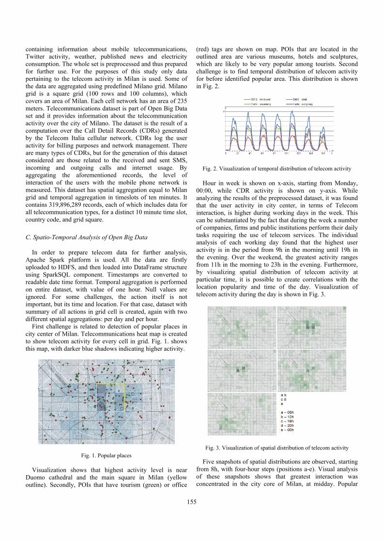
155

containing information about mobile telecommunications, Twitter activity, weather, published news and electricity consumption. The whole set is preprocessed and thus prepared for further use. For the purposes of this study only data pertaining to the telecom activity in Milan is used. Some of the data are aggregated using predefined Milano grid. Milano grid is a square grid (100 rows and 100 columns), which covers an area of Milan. Each cell network has an area of 235 meters. Telecommunications dataset is part of Open Big Data set and it provides information about the telecommunication activity over the city of Milano. The dataset is the result of a computation over the Call Detail Records (CDRs) generated by the Telecom Italia cellular network. CDRs log the user activity for billing purposes and network management. There are many types of CDRs, but for the generation of this dataset considered are those related to the received and sent SMS, incoming and outgoing calls and internet usage. By aggregating the aforementioned records, the level of interaction of the users with the mobile phone network is measured. This dataset has spatial aggregation equal to Milan grid and temporal aggregation in timeslots of ten minutes. It contains 319,896,289 records, each of which includes data for all telecommunication types, for a distinct 10 minute time slot, country code, and grid square.

C. Spatio-Temporal Analysis of Open Big Data

In order to prepare telecom data for further analysis, Apache Spark platform is used. All the data are firstly uploaded to HDFS, and then loaded into DataFrame structure using SparkSQL component. Timestamps are converted to readable date time format. Temporal aggregation is performed on entire dataset, with value of one hour. Null values are ignored. For some challenges, the action itself is not important, but its time and location. For that case, dataset with summary of all actions in grid cell is created, again with two different spatial aggregations: per day and per hour.

First challenge is related to detection of popular places in city center of Milan. Telecommunications heat map is created to show telecom activity for every cell in grid. Fig. 1. shows this map, with darker blue shadows indicating higher activity.

Fig. 1. Popular places Visualization shows that highest activity level is near

Duomo cathedral and the main square in Milan (yellow outline). Secondly, POIs that have tourism (green) or office

(red) tags are shown on map. POIs that are located in the outlined area are various museums, hotels and sculptures, which are likely to be very popular among tourists. Second challenge is to find temporal distribution of telecom activity for before identified popular area. This distribution is shown in Fig. 2.

Fig. 2. Visualization of temporal distribution of telecom activity Hour in week is shown on x-axis, starting from Monday,

00:00, while CDR activity is shown on y-axis. While analyzing the results of the preprocessed dataset, it was found that the user activity in city center, in terms of Telecom interaction, is higher during working days in the week. This can be substantiated by the fact that during the week a number of companies, firms and public institutions perform their daily tasks requiring the use of telecom services. The individual analysis of each working day found that the highest user activity is in the period from 9h in the morning until 19h in the evening. Over the weekend, the greatest activity ranges from 11h in the morning to 23h in the evening. Furthermore, by visualizing spatial distribution of telecom activity at particular time, it is possible to create correlations with the location popularity and time of the day. Visualization of telecom activity during the day is shown in Fig. 3.

Fig. 3. Visualization of spatial distribution of telecom activity

Five snapshots of spatial distributions are observed, starting from 8h, with four-hour steps (positions a-e). Visual analysis of these snapshots shows that greatest interaction was concentrated in the city core of Milan, at midday. Popular

156

events can cause aberrations from normal telecom activity. X Factor finale was held on December, 12, in Milan, more precisely in Mediolanum Forum. Fig. 4. shows visualization of telecom activity distribution in that area, for December, 12.

Fig. 4. Visualization of spatial distribution of telecom activity Presented visualization shows how events can change

human behavioral patterns. Lighter areas are the ones that have higher activity. Namely, increased activity in selected area is consistent with the event itself, as it starts at 20h, and peaks in spatial distribution of telecom interaction align both with location and with time of the event.

V. CONCLUSION

Extraction of useful information and knowledge from large spatio-temporal datasets is not an easy task. The main aim of this research was to create an overview of all stages of spatio-temporal data mining process. Each data mining task, after acquiring of the data, includes preprocessing, processing and postprocessing steps. The most commonly used methods for every stage in spatio-temporal analysis and mining are listed. Furthermore, the demonstration of processing and analysis of authoritative (Telecom Open Big Data) and VGI data (OSM) is presented. As large amounts of data require Big Data technologies, Apache Spark is used for detection of useful information and mobility patterns, regarding temporal and spatial distribution of user activities. Four challenges related to spatio-temporal data mining are identified and addressed, including finding popular places in a city, identifying patterns in temporal and spatial distribution of telecom activity, and detecting correlations between popular events and distribution of telecom interaction. Further work will be focused on integrating different datasets and extracting useful knowledge from combined datasets. The analysis and mining of spatio-temporal data is, and will be the point of strong focus for further improvement. This research provides perfect starting point for extensive research in spatio-temporal mining.

ACKNOWLEDGMENT

This paper has been realized as a part of the project "Studying climate change and its influence on the environment: impacts, adaptation and mitigation" (III 43007) financed by the Ministry of Education, Science and Technological Development of the Republic of Serbia for the period 2011-2017.

REFERENCES

[1] A. Stojnev, and D. Stojanović, "Sparkle – A Framework for Spatial Analysis on Apache Spark Platform", IcETRAN 2016 Conference, Zlatibor, 2016.

[2] A. Stojnev, and D. Stojanović, "Real-time Processing of Big Geospatial Data based on Spark Streaming", SAUM 2016 Conference, Niš, 2016.

[3] N. Andrienko, and G. Andrienko, "A Visual Analytics Framework for Spatio-Temporal Analysis and Modelling", Data Mining and Knowledge Discovery, pp.1-29, 2013.

[4] L. Cibulski, D. Gračanin, A. Diehl, R. Splechtna, M. Elshehaly, C. Delrieux, and K. Matković, "ITEA—Interactive Trajectories and Events Analysis: Exploring Sequences of Spatio-Temporal Events in Movement Data", The Visual Computer, vol. 32, no. 6-8, pp.847-857, 2016.

[5] N. Mamoulis, H. Cao, G. Kollios, M. Hadjieleftheriou, Y. Tao, and D. W. Cheung, “Mining, Indexing, and Querying Historical Spatiotemporal Data”, ACM SIGKDD 2004 Conference, Seattle, WA, USA, 2004.

[6] R.F. Dos Santos, A. Boedihardjo, S. Shah, F. Chen, C. Lu, and N. Ramakrishnan, "The Big Data of Violent Events: Algorithms for Association Analysis Using Spatio-Temporal Storytelling", GeoInformatica, vol. 20, no. 4, pp. 879-921, 2016.

[7] Y. Huang, C. Chen, and P. Dong, “Modeling Herds and Their Evolvements from Trajectory Data”, Geographic Information Science, vol. 5266, pp. 90-105, 2008.

[8] J. Xu, D. Deng, U. Demiryurek, C. Shahabi, and M. van der Schaar, “Mining the Situation: Spatiotemporal Traffic Prediction With Big Data”, Journal of Selected Topics in Signal Processing, vol. 9, no. 4, pp. 702–715, 2015.

[9] N. Ferreira, J. Poco, H. T. Vo, J. Freire, and C. T. Silva, “Visual Exploration of Big Spatio-Temporal Urban Data: A Study of New York City Taxi Trips”, IEEE Trans. Vis. Comput. Graph., vol. 19, no. 12, pp. 2149-2158, 2013.

[10] T. Cheng, J. Haworth, B. Anbaroglu, G. Tanaksaranond, and J. Wang, “Spatiotemporal Data Mining”, Handbook of Regional Science, Eds. Berlin, Heidelberg: Springer Berlin Heidelberg, pp. 1173-1193, 2014.

[11] R.R. Vatsavai, and B. Bhaduri, “Geospatial Analytics for Big Spatiotemporal Data: Algorithms, Applications, and Challenges”, InNSF Workshop on Big Data and Extreme-Scale Computing, Charleston, SC, 2013.

[12] S. Shekhar, Z. Jiang, R.Y. Ali, E. Eftelioglu, X. Tang, V. Gunturi, and X. Zhou, "Spatiotemporal Data Mining: A Computational Perspective", ISPRS International Journal of Geo-Information, vol. 4, no. 4, pp. 2306-2338, 2015.

[13] K.V. Rao, A. Govardhan, and K. V.C. Rao “Spatiotemporal Data Mining: Issues, Tasks And Applications”, International Journal of Computer Science & Engineering Survey, vol. 3, no. 1, pp. 39-52, 2012.

[14] I. Bruha, “Pre- and Post-processing in Machine Learning and Data Mining”, Lecture Notes in Computer Science, pp. 258-266, 2001.

[15] Spazio Dati, “Dandelion API | Semantic Text Analytics as a Service”, Dandelion API, Available: http://www.dandelion.eu. [Accessed: 10-Apr-2017].

157

Ontology and Reasoning on Device Connectivity Evelina Pencheva1, Ivaylo Atanasov1, Anastas Nikolov1, Rozalina Dimova2

Abstract – In this paper, we present an approach to cloud application orchestration. The approach allows detection and resolution of interactions among cloud applications. The approach is based on ontology for IoT device connectivity. It is illustrated for applications which add functionality to basic bearer selection procedure.

Keywords – Connectivity management, Cloud orchestration, Diagnostic and monitoring traps, Ontology, Reasoning.

I. INTRODUCTION

The amount of data generated by connected device increases exponentially with the ubiquitous penetration of Internet of Things (IoT). Cloud computing is a way to alleviate the data problem. It involves delivering data, applications, multimedia and more over the Internet to data centers. Both technologies serve to increase efficiency in different application areas.

Device-to-cloud communication involves an IoT device connecting directly to an Internet cloud application to exchange data and control message traffic. It often uses wireless connections, but can also use cellular technology [1], [2]. Different technologies have different requirements for quality of service (QoS), which complicates the logic for bearer selection. Furthermore, the logic for bearer selection may be based on different policies such as the device location and the requirements for charging.

Cloud connectivity lets an application to obtain remote access to a device. It also potentially supports pushing software updates to the device.

Cloud orchestration is programming that manages the interconnection and interactions among cloud-based applications. To orchestrate cloud applications is to arrange them so they achieve a desired result. A comparative study on existing approached to cloud service orchestration is presented in [3]. In [4], the authors present layer architecture for cloud service orchestration. A decentralized approach to the orchestration of cloud services using multi-agent system is proposed in [5]. In [6], the authors present an autonomic framework for cloud computing orchestration based on virtual machines migrations and heuristics to select hosts to be activated or deactivated when needed. The survey on research related to cloud orchestration shows that works deal with high level architectural aspects and do not provide more details on detecting and resolving of interactions among applications.

In this paper we propose an approach to cloud

application orchestration. The approach allows detection and resolution of interactions among cloud applications. It is illustrated for applications which add functionality to basic bearer selection procedure for IoT devices.

The paper is structured as follows. In Section II, a semantic data related to IoT connectivity management is presented. Section III describes cloud applications which manage device connectivity based on different policies. Possible service interactions and their resolution are discussed in Section IV. The conclusion discusses implementation aspects of the proposed method for service orchestration and highlights its benefits.

II. DEVICE CONNECTIVITY MANAGEMENT

ONTOLOGY

Our research is based on Open Mobile Alliance (OMA) trap mechanism which may be employed by an application to enable the device to capture and report events and other relevant information generated from various components of the device, such as a protocol stack, device drivers, or applications [7]. OMA traps that may be used for connectivity management are geographic trap, received power trap, call drop trap, quality of service (QoS) trap, and data speed trap [8].

In order to send information over the network, any IoT device needs connectivity. A connected device uses a network bearer and can measure its signal strength. A possible sequence of procedures performed by the server running cloud application for connectivity management and wireless device in the context of connectivity management is as follows. The server establishes an observation relationship with the device to acquire periodical or triggered notifications about signal strength of the used bearer. The device sends periodical or triggered notifications about signal strength. Upon dropping of signal strength under application defined threshold, the server queries about used and available network bearers. In case the device senses available unused bearers, the cloud application may initiate bearer selection. Different cloud applications may use different policies for the bearer selection. For example, a cloud application may apply location based policy for bearer selection, while another cloud application may initiate bearer selection procedure whenever an uplink or downlink average data speed reaches an application defined lower or higher threshold value. Fig. 1 shows the ontology related to connectivity management of IoT devices.

In the figure, a bearer change is required for the device when it experiences bad signal whose signal strength is under application defined value. In addition to basic concepts and properties related to basic connectivity management, the figure show concepts and properties related to location based and data speed-based bearer selection. A cloud application may define geographic area in which a preferred bearer has to

1The authors are with the Faculty of Telecommunications atTechnical University of Sofia, 8 Kl. Ohridski Blvd, Sofia 1000, Bulgaria, E-mail: enp, [email protected]

2R. Dimova is with the Faculty of Computing and Automatics at Technical University of Varna, Studentska str, Varna, Bulgaria, E-mail: [email protected]

158

be used. Another cloud application may define thresholds indicating low and high uplink and downlink speeds, and when the data speeds are below/above low/high thresholds the application considers the speed as unacceptable.

Fig. 1. Ontology for connectivity management of IoT devices The proposed ontology may be described by OWL. For

sake of brevity we describe the ontology by description logic. The following concepts express the device state and facts

related to the device connectivity: disconnected – the device is disconnected; connectedb – the device is connected by bearer b; weakSignalb– the device is connected by bearer b, but

the signal strength of b is low; availableb – the bearer b is available. Roles represent actions or notifications about events

related to device connectivity management. connects – device connects to the network; disconnects – the device disconnects from the network; change – the device changes the used bearer; signalDrops – the signal of the used bearer drops; getParameters - the server queries the device about

connectivity parameters; parameters - the device provides the requested

connectivity parameters; changeBearer - the server instructs the device to change

the used bearer. Concepts and roles are used to specify the connectivity

management model (CMM). The Terminology box (TBox) consists of expressions that represent how the device can change its state.

disconnected⊑connects.connectedb (1)

connectedb⊑getParameters.connectedb (2)

connectedb⊑parameters.connectedb⊓availablec (3)

connectedb⊑parameters.connectedb⊓availablec (4)

connectedb⊑(signalDrops⊓getParameters).weakSignalb (5)

weakSignalb⊑parameters.(weakSignalb⊓availablec) (6)

weakSignalb⊓availablec⊑changeBearer.connectedc (7)

weakSignalb⊑parameters.(weakSignalb⊓availablec) (8)

weakSignalb⊓availablec⊑disconnects.disconnected (9)

connectedb⊑disconnects.disconnected (10)

weakSignalb⊑disconnects.disconnected (11) The Assertion box (ABox) contains one statement

presenting the initial state for each device: s0:⊓dDevices

disconnected. To express the fact that each device is in exactly one state

at any moment the following statement is used:

⊤⊑(⊔d1,d2CMM, d1d2(s1⊓s2))⊓(⊔dCMM s) The device state changes by means of actions defined as

action functions. An action function FuncCMM for given state corresponds to the possible transitions in the CMM. For example, the expression FuncCMS(connectedb)= signalDrop disconnect means that, if the device is connected, the received power of the used bearer may drop, the device may disconnect or deregister.

The fact that each device can change the CMM state only by means of certain actions is represented by the following

statement: for all sCMM, and all RFuncCMM (s), s⊑R.s.

III. ADDING FUNCTIONALITY TO DEVICE

CONNECTIVITY

A. Location-Based Bearer Selection

The Location-based Bearer Selection (LBS) application assumes that there is a predefined geographic area in which a preferred bearer is used. The state diagram of service logic for location based bearer selection is shown in Fig.2.

Additional concepts representing facts and roles are defined: inArea – the device is located in the specified area; outOfArea – the device is located out of the specified

area; preferredb – the bearer b is the preferred one in the

specified area; enters – the device enters the specified area; exits – the device exits the specified area; location – the device sends its location; getLocation – the server queries about device’s location. The following trivial axiomis true: outOfArea≡inArea. The refinement of the knowledge base for LBS application

is defined by the following statements. When the device is connected, the application queries about

device location:

Device

Bearer

uses senses

Connected Device

Disconnected Device

Preferred Bearer

defines

supports

isA

Acceptable Speed

Unacceptable Speed

is

is

Available Bearer

UsedBearer

is is

SignalStrength

has

HighSignal

is

is

Connected Weak Signal

is

LowSignal

experiences

DataSpeed

is Provided Speed

provides

connects

disconnects

signalDrops

signalRises

is

may be

decreases increases

OutOfArea

InArea may be

enters

exits

isA

159

LBS⊓connectedb⊑getLocation. connectedb (12) The device responds and the application can determine its

location with respect of the predefined geographic area:

Fig. 2. State diagram of service logic for location-based bearer selection

LBS⊓connectedb⊑location.(connectedb⊓inArea) (13)

LBS⊓connectedb⊑location.(connectedb⊓outOfArea) (14) Based on the device response of the query about

connectivity parameters, the application may determine whether the device uses the preferred bearer, or the preferred bearer is among the available ones in case the device is in the area:

LBS⊓connectedb⊓inArea⊑ parameters.(connectedb⊓inArea⊓preferredb) (15)

LBS⊓connectedb⊓inArea⊑ parameters.(connectedb⊓inArea⊓preferredc⊓availablec)(16)

If the device is in the area and the preferred bearer is not used but available, the application initiates bearer change:

LBS⊓connectedb⊓inArea⊓preferredc⊓availablec⊑ changeBearer.(connectedc⊓inArea⊓preferredc) (17)

The device may enter or exit the area:

LBS⊓connectedb⊓inArea⊑ exits.(connectedb⊓outOfArea) (18)

LBS⊓connectedb⊓outOfArea⊑ enters.(connectedb⊓inArea) (19)

The application logic is summarized by:

LBS⊑ (connectedb⊓inArea⊓preferredc⊓availablec) (20)

B. Data Speed-Based Bearer Selection

Data speed bearer selection (DBS) application uses the data speed trap. The application configures different data speed traps for uplink and downlink. Low speed data traps become active when the average data speed calculated for the given period reaches below the server defined lower threshold value. High speed data traps become active when the average data speed calculated for the given period reaches above this higher threshold value. The application initiates bearer selection whenever the data speed trap goes to active. The knowledge base for this service is extended with new concepts representing unacceptable for the application data speeds and bearer with appropriate data speed, a new role for trap activity and statements for bearer selection logic: speedUnacceptableb – the data speed is beyond the

application defined thresholds; dsTrapFires – any of the data speed traps goes active; appropriateb – the data speed supported by bearer b are

acceptable for the application. The refinement for DBS service is defined by the following

statements. Being connected to bearer b, the device may experience

unacceptable for the application data speeds:

DBS⊓connectedb⊑dsTrapFires.(connectedb⊓ speedUnacceptableb) (21)

If the data speeds are unacceptable, the application queries the device about its connectivity parameters:

DBS⊓connectedb⊓speedUnacceptableb⊑ getParameters.(connectedb⊓speedUnacceptableb) (22)

Based on the device response, the application may determine that there is an available bearer which supports acceptable data speeds and the application initiates bearer change:

DBS⊓connectedb⊓speedUnacceptableb⊑ parameters.(connectedb⊓speedUnacceptableb

⊓availablec⊓appropriatec) (23)

DBS⊓connectedb⊓speedUnacceptableb⊓availablec

⊓appropriatec⊑changeBearer.connectedc (24) Based on the device response, the application may

determine that there is no available bearer which supports acceptable data speeds and the application initiates device disconnect:

DBS⊓connectedb⊓speedUnacceptableb⊑ parameters.(connectedb⊓speedUnacceptableb

⊓availablec⊓appropriatec) (25)

DBS⊓connectedb⊓speedUnacceptableb⊓availablec

⊓appropriatec⊑disconnects.disconnected (26) The following statement summarizes the application logic:

DBS⊑(connectedb⊓speedUnacceptableb⊓ availablec⊓appropriatec). (27)

connected

connected⊓ inArea

signalDop/ getParameters

weak signal

parameters

no

disconnectconnected⊓

inArea⊓preferre

connected⊓ outOfArea

connects

signalDrop/ getParameters

connected

Is thedevice inthe area?

Is the usedbearer the

preferred one?

noIs thepreferred

beareravailable

yes

yes/changeBearer

no

enters/getParameters

*(disconnected)

disconnected

disconnected

location/getParameters

parameters

yes

exits

yes /changeBearer,

getLocation

disconnected

no / disconnect

Is there an available bearer?

signalDrop/ getParameters

enters, exits

connected⊓ outArea

exits

getLocation

160

IV. REASONING ON SERVICE INTERACTION

By the use of OMA Diagnostic and monitoring traps different policies may be used for connectivity management. Further, the bearer selection may depend on available subscriber balance. Real-time information about device provider’s balance may be acquired by means of Policy and Charging Control (PCC) functionality. The PCC concept is designed to enable flow based charging including online credit control and policy control which supports service authorization and quality of service management [9].

When introducing new application, it is important to find out whether the new application is contradictory to existing concepts i.e. whether it satisfies or not the statements in the TBox representing the connectivity management model.

Interaction between LBS and DBS occurs when the device is in the specified area and uses the preferred bearer as to LBS, and the data speeds are unacceptable and the DBS requires a change to a bearer which is available one and supports acceptable data speeds. We formally prove our claim.

Proposition 1: Undesired service interaction occurs on

activation of LBS⊓DBS. Proof: Applying standard reasoning to the knowledge base

we derive the following sequence of device’s state and transitions: As to (1) s0 connect s1: connectedb. As to (12) s1 getLocation s1. As to (13) s1 location s2: connectedb⊓inArea. As to (2) to s2 getParameters s2.

As to (3) s2 parameters s3: connectedb⊓inArea⊓preferredb. As to (21) s3 dsTrapFire s4: connectedb⊓inArea⊓preferredb⊓ speedUnacceptableb. As to (2) s4 getParameters s4. As to (3) s4 parameters s5:connectedb⊓inArea⊓preferredb⊓ speedUnacceptableb ⊓acceptablec⊓availablec.

As to s5 changeBearerc s6: connectedc⊓inArea⊓preferredb. As to (2) s6 getParameters s6. As to (24) s6 parameters s7: connectedc⊓inArea⊓preferredb⊓ availableb which contradicts to (20) as to LBS, namely

(connectedb⊓inArea⊓preferredc⊓availablec). The result shows that when applying both applications to

the same device, statements representing the LBS and DBS do not satisfy the statements in the knowledge base i.e. both applications contradict to each other.

Once detected, service interactions may be resolved by setting priorities. The cloud functionality for service orchestration determines the required behavior in case of service interaction based on application priority. Application with higher priority can override the instructions of application with lower priority.

Let us denote the priority of i service by Pi. Then

LBS⊓CBS⊓PLBS<PCBS⊓connectedb⊓inArea⊓preferredb⊓ speedUnacceptableb⊓acceptablec⊓availablec⊑ changeBearer.connectedb⊓inArea⊓preferredc⊓

availablec⊓speedUnacceptablec (28)

V. CONCLUSION

In this paper we propose an approach to cloud service orchestration. The approach is illustrated for applications which add value to IoT device connectivity management. Each cloud application applies specific policy for the network bearer that has to be used by the device. The approach is based on ontology for device connectivity. The ontology and the application logic may be described by Ontology Web Language (OWL). The service interaction is considered as satisfiability problem and undesired application behavior may be discovered by applying standard reasoning algorithm. There exist a number of ontology editors and frameworks for constructing domain models and knowledge-based applications with ontologies and reasoners to infer logical consequences from a knowledge base.

The proposed method for resolving service interaction using priorities allows dynamic service orchestration.

ACKNOWLEDGEMENT

The research is conducted under the grant of project ДH07/10-2016, funded by National Science Fund, Ministry of Education and Science, Bulgaria.

REFERENCES

[1] J. Zhou, Z. Cao, X. Dong and X. Lin, "Security and privacy in cloud-assisted wireless wearable communications: Challenges, solutions, and future directions," in IEEE Wireless Communications, vol. 22, no. 2, pp. 136-144, 2015.

[2] J. Huang et al., "Modeling and Analysis on Access Control for Device-to-Device Communications in Cellular Network: A Network-Calculus-Based Approach," in IEEE Transactions on Vehicular Technology, vol. 65, no. 3, pp. 1615-1626, 2016.

[3] K. Bousselmi, Z. Brahmi and M. M. Gammoudi, "Cloud Services Orchestration: A Comparative Study of Existing Approaches," 2014 28th International Conference on Advanced Information Networking and Applications Workshops, Victoria, BC, 2014, pp. 410-416.

[4] P. Jain, A. Datt, A. Goel and S.C. Gupta, "Cloud service orchestration based architecture of OpenStack Nova and Swift," 2016 International Conference on Advances in Computing, Communications and Informatics (ICACCI), Jaipur, 2016, pp. 2453-2459.

[5] Z. Brahmi and J. Ben Ali, "Cooperative agents-based decentralized framework for cloud services orchestration," 2015 6th International Conference on Information Systems and Economic Intelligence (SIIE), Hammamet, 2015, pp. 46-51.

[6] R. Weingärtner, G.B. Bräscher and C.B. Westphall, "A Distributed Autonomic Management Framework for Cloud Computing Orchestration," 2016 IEEE World Congress on Services (SERVICES), San Francisco, CA, 2016, pp. 9-17.

[7] Open Mobile Alliance, Diagnostics and Monitoring Management Object. OMA-TS-DiagMonTrapMO-V1_0-20090414-C, 2009

[8] Open Mobile Alliance, Diagnostics and Monitoring Trap Events Specifications,”OMA-TS-DiagMonTrapEvents-V1_2-20131008-A, 2013

[9] 3GPP Technical Specification Group Services and System Aspects; Policy and charging control architecture, Release 13, v13.7.0, 2016.

161

An Approach to Design Interfaces for Trust, Security and Load Management in Mobile Edge Computing Evelina Pencheva1, Ivaylo Atanasov1, Pencho Kolev2, Miroslav Slavov2

Abstract – Mobile Edge Computing (MEC) is an emerging technology aimed to increase network flexibility and to reduce time to market for new services. It brings the cloud capabilities in radio access network. In this paper, we present an approach to design core MEC Web Services for trust and security management, and for load level management. The proposed Web Services allows MEC application registration, discovery of available services and registered applications, and signing service agreement for service usage, as well as control on internal load management.

Keywords – Mobile Edge Computing, Infrastructure Services, Web Services, Service Oriented Architecture, Authentication

I. INTRODUCTION

Mobile communications evolve continuously in order to meet the requirements for low latency, increase of traffic volumes, higher data rates and reliable connectivity. Mobile Edge Computing (MEC) is an emerging technology aimed to meet these requirements [1]. It exploits a combination of virtualization, cloud capabilities and coordination techniques which interact with each other in Radio Access Network (RAN). Virtualization of RAN functions is a way to solve some of the main challenges network operators face in deployment of new services, for example excessive time to market, increasing cost of energy, security and reliability.

MEC applications may contribute to increasing of user experience and efficient utilization of network resources [2]. MEC provides real-time network data such as radio conditions, network statistics, etc, for authorized applications to offer context-related services that can differentiate end user experience. MEC use cases and deployment options are presented in [5]. For reasons of performance, cost and scalability, MEC may be deployed at the radio node, at an aggregation point, or at the edge of the core network. MEC A state-of-the-art research efforts and challenges on MEC domain are in presented in [6].

As to [7], in order to enable the development of viable MEC ecosystem, it is important to develop Application Programming Interfaces (APIs) that are simple as possible and are directly answering the needs of applications. To the extent this is possible, MEC needs to reuse existing APIs that fulfill the requirements.

MEC-service platform provides three types of middleware

services: infrastructure services, radio network information services and traffic offload function [8]. Infrastructure services are used by applications for communications, service discovery and integration. Communication between MEC services and applications is based on Service-oriented Architecture (SOA). The applications access MEC services and other applications hosted on the same MEC platform through Web Services Application Programming Interfaces. Discovery and integration services provide visibility of services available on the MEC platform and enables flexible application deployment. Applications may discover service status, locate its end points and publish their own end point for usage of other applications. The access to MEC services is secured (authenticated and authorized).

Radio network information services provide authorized applications with low level real-time radio and network information related to users and cells. The traffic offload function prioritizes traffic and routes the selected, policy- based, user-data stream to and from applications that are authorized to receive the data.

The security of Web Services and the XML based communications is of great importance to the overall security of distributed systems. Furthermore, in order to facilitate interoperability, the security mechanisms should preferably be based on established standards. In [9], the authors evaluate the importance of XML Signature and XML Encryption for WS-Security. A review of Web Service security research in the field of cloud security is provided in [10]. While a lot of research is done on Web Service cryptography and digital signatures, there is a lack of works related to integrity of SOA-based systems.

In this paper, we present an approach to design infrastructure MEC Web Services for trust, security and load management. The proposed MEC Web Services allow application registration, discovery of available MEC services and registered applications, signing service agreement for MEC service usage, as well as control on internal load management.

The paper is structured as follows. Section II presents the description of MEC Web Service that may be used for application authentication and registration, discovery of available MEC services and registered applications. Section III describes Web Service interfaces. Section IV presents in brief interfaces of MEC Web Service for internal load management. The conclusion summarizes the contributions.

II. DESCRIPTION OF APPLICATION REGISTRATION

WEB SERVICE

Generic requirements to MEC platform include management of the application lifecycle, provisioning of application environment which supports verification of

1The authors are with the Faculty of Telecommunications atTechnical University of Sofia, 8 Kl. Ohridski Blvd, Sofia 1000,Bulgaria, E-mail: enp, [email protected]

1The authors are with the Faculty of Electrotechnica andElectronika at Technical University of Gabrovo 4 Hadji Dimitar,Gabrovo 5300, Bulgaria, E-mail: [email protected];miroslav)[email protected]

162

application authenticity and integrity, as well as application mobility.

The complete cycle for using MEC application consists of three phases:

1. Authentication. Before using MEC services, the Application needs to be authenticated by the MEC service platform which prevents from unauthorized access. The authentication may be mutual e.g. the Application also authenticates the MEC platform,

2. Service selection. Once authenticated, the application selects service/application to be used. To ensure non-repudiation, the MEC service platform can request a signing of a service agreement before allowing the service/application to be used.

3. Service use. Only after authentication, service selection and signing the service agreement have been done, the application can start using the actual service/application.

Apart from providing security, the authentication and service selection process allows MEC service platform provider to determine access right profiles for different applications. The amount of permissions can be made on the level of trust awarded to the application.

Fig.1 illustrates the sequence diagram for application authentication and MEC service discovery, selection and signing of service agreement.

The procedure for initial access is as follows. 1. At initial contact, the Application requests authentication

by invoking authenticate operation. As the Application may support different authentication mechanisms, it provides as parameters the application identifier and list of the supported authentication mechanisms. The authentication mechanisms may be supported by cryptographic processes to provide confidentiality, and by digital signatures to ensure integrity. The inclusion of cryptographic processes and digital signatures in the authentication procedure depends on the type of selected authentication method. In some cases strong authentication may need to be enforced by the MEC platform to prevent misuse of resources.

2. The authentication between the Application and MEC platform is based on challenge-handshake authentication protocol. The Application and the MEC platform share a secret key. The MEC platform chooses an authentication method based on the capabilities of the Application. The MEC platform generates a challenge and based on the shared secret key computes a token and expected result. It responses to the Application with the chosen authentication method, the challenge and token.

3. The Application carries out a computation that resembles the generation of the token and the result at the MEC platform. If the calculated token is equal to the received one, the Application considers the MEC platform as authenticated. The Application invokes register operation and sends locally calculated result. The Application may send also some details that describe itself and may be used by other applications.

4. The MEC platform verifies whether the received result matches to the locally calculated one and if so, it sends

to the Application response for successful authentication and registration. If it does not, authentication fails.

5. When the MEC platform and the Application have successfully authenticated each other, the Application can request the list of existing MEC services by invoking listWebServices operation.

6. The MEC platform returns a list of existing Web Services with information about service ID and whether the respective Web Service is currently available or unavailable.

Fig. 1. Application authentication and MEC service discovery,

selection and signing of service agreement

7. In order to discover the desired service, the Application may invoke discoverService operation which request more details about particular Web Service.

8. The MEC platform responses with a description of the Web Service.

9. The Application selects the Web Service by invoking selectService operation.

10. The MEC service requests that the Application confirms the intention to use the service by signing a service agreement. The signing of service agreement is to ensure nonrepudiation i.e. to prevent the Application from denying it has used the service. The service agreement may be done by digital signature.

11. The application signs the service agreement. Digital signature parameter contains cryptographic message syntax object (as defined in RFC 2630) with content type of signed data.

12. Once the service agreement has been successfully signed, the Application received an initial access to the Web Service and can start using it.

The Application may subscribe for changes in the availability status of MEC service. The Application starts

:Application Logic

:Agreement Web Service

:Authentication :Access

Application Application Registration Web Service

1. authenticateRequest (AppID, Auth. method list)

2. authenticateResponse (Auth. method, challenge, token)

3. registerRequest (auth response, app details)

4. registerResponse

5. listWebServicesRequest

6. listWebServiceResponse (list of available services)

9. selectServiceRequest (service ID)

10. signServiceAgreementRequest(agreement text)

11. signServiceAgreementResponse (digital signature)

12. selectServiceResponse

7.discoverServiceRequest (service ID)

8. discoverServiceResponse (service description)

163

notification with criteria defined. When the availability status of a MEC service changes, a notification message is sent to the Application. When the duration or count for notifications has been completed, the Application is notified.

Fig. 2 shows a sequence diagram for notifications about Web Service availability status.

Fig. 2. Triggered notifications about changes in MEC service

availability status

III. APPLICATION REGISTRATION INTERFACES

Application Registration Web Service provides interfaces for trust and security management. These interfaces support methods for application authentication, service/application, application selection and access to selected service/ application.

The Authentication interface is used for mutual authentication, application registration and deregistration. The authenticate operation is used by the Application to initiate authentication. The register operation is used by the Application to register with the MEC platform in case of successful authentication. The deregister operation is used by the Application to deregister from the MEC platform.

The Access interface is used by the application to obtain the identities of available services and applications and to sign service agreement for usage of selected service/applications. The Application uses listServices operation to request access to the identities of available services. The Application uses listApplications operation to request access to the identities of registered applications. With discoverService or discoverApp-lication operations the Application may receive more details about a particular Web Service or registered application. The Application uses selectService operation or selectApplication operation to select the MEC service or registered application.

The ServiceAgreement interface is used to sign an agreement that allows the Application to use the chosen service/application. It supports signServiceAgreement opera-tion and agreementTerminated operation used to terminate the agreement. Once these contractual details have been agreed, the Application will be allowed to actually use it.

The Application Registration Web Service supports also interfaces that may be used to notify about MEC service or application availability.

The ApplicationStatusNotificationManager interface sets up notifications for the status of applications registered at the MEC platform. The startApplicationNotification operation is used to make available notifications about the registration

status of applications. The stopApplicationNotification operation is used to terminate subscription for the registration status of applications.

The interface to which notifications about application registration status are delivered is ApplicationNotification. It supports applicationNotification operation which notifies about changes in the registration status of an Application and applicationError which informs that notifications are cancelled. The appNotificationEnd operation informs the Application that the notifications have been completed when the duration or count for notifications have been completed.

The ServiceStatusNotificationManager interface sets up notifications for the status of MEC services. The startServiceNotification operation is used to make available notifications about the MEC services status. The stopServiceNotification operation is used to terminate notifications about the MEC service status.

The interface to which notifications about MEC service status are delivered is ServiceNotification. It supports serviceNotification operation which notifies about changes in the availability status of a MEC service and serviceError which informs that notifications are cancelled. The serviceNotificationEnd operation informs the Application that the notifications have been completed when the duration or count for notifications have been completed.

Fig. 3 shows a simplified state diagram for Application registration and access to MEC services and applications.

Fig. 3. Registration and access to MEC services

In ApplicationUnregistered state, the Application is not

registered. If the Application invokes authenticate operation, it provides its identity and supported authentication methods. In MutualAuthentication state, the MEC platform chooses an authentication method to be used, calculates a token and the expected result and challenges the Application. If the Application invokes register operation providing the right authentication response, the MEC framework registers the Application.

In RegisteredApplication state, the Application can request a list with available MEC service and discover a particular service. If the Application invokes selectService operation, the MEC platform initiates signing service agreement. In ServiceAccessing state, if the Application signs the service

Application Unregistered

Mutual Authentication

Registered Application

authenticate

register

successful authentication

authentication failed

listServices discoverService

selectService

Service Accessing

signServiceAgreement

Access Granted

listServices discoverService listApplications discoverApplication

selectServiceselectApplication

:Application Logic

:Notification Web Service

:Service Notification

:Notification Application

Application Application Registration Web Service

1. startServiceNotificationRequest

2. startServiceNotificationResponse

3. serviceNotificationRequest (service ID, status)

4. serviceNotificationResponse

Service status changes

5. serviceNotificationEndRequest

6. serviceNotificationEndResponse

forward

forward

164

agreement, the MEC platform grants the service access. In AccessGranted state, the Application can request access to another MEC service or registered application. Before granting the access, the MEC platform requests signing service agreement.

IV. LOAD MANAGEMENT WEB SERVICE

The Load Management Web Service allows the MEC platform to monitor and control the Application load according to a load management policy. The load management policy identifies rules for load management that the MEC platform needs to follow.

The AppLoadManager interface provides the following operations. The startLoadNotification operation is used by the MEC platform to subscribe for notifications about Application load level changes. The stopLoadNotification operation is used to terminate subscription for notifications about Applica-tion load level changes. The holdNotification operation is used by the MEC platform to hold temporary notifications from the Application. The MEC platform uses restoreNotification operation to request the Application to restore sending notifications. The appLoadStatisctics operation is used by the MEC platform to send to the Application statistics about its load level. The appLoadStatError operation is used by the MEC platform to inform the Application that load statistics can not be sent due to error.

The Load Manager interface provides the following operations. The Application uses reportLoad operation to report changes in its load level. The getAppLoadStatistics operation is used by the Application to request from the MEC platform load statistics report.

Fig. 4 shows a state diagram representing the MEC platform view of the Application and internal load levels.

Fig. 4. Application and MEC platform load level states

V. CONCLUSION

Mobile Edge Computing provides the ability to run IT based servers at the network edge, applying the concepts of cloud computing. A variety of new value added services can be provided with the integration of applications and radio network equipment. These services are oriented to improvement of

quality of experience for mobile users, to enablement of disruptive Internet of Things services, to optimization of radio network performance, etc.

In this paper we propose an approach to design Infrastructure Web Services for MEC. Using the proposed MEC Web Services, applications can access MEC services and other applications hosted on the same MEC platform through Web Services Application Programming Interfaces. Trust and security management functionality provides applications with secured access to MEC service, visibility of available MEC services and other registered applications, thus enabling flexible application deployment. Applications may discover MEC service status as well as the status of other registered applications.

The proposed MEC infrastructure Web Services allow the network operator to manage the life cycle of the applications: deploy, start, stop and un-deploy more efficiently.

ACKNOWLEDGEMENT

The research is conducted under the grant of project ДH07/10-2016, funded by National Science Fund, Ministry of Education and Science, Bulgaria.

REFERENCES

[1] Y. Chen, and L. Ruchenbusch, "Mobile Edge Computing: Brings the Value Back to Networks", IEEE Software Defined Networks, Newsletter, March 2016, Available at: http://sdn.ieee.org/newsletter/march-2016/mobile-edge-computing-bring-the-values-back-to-networks

[2] R. Roman, J. Lopez, and M. Mambo, "Mobile Edge Computing, Fog et al.: A Survey and Analysis of Security Threats and Challenges", Future Generation Computer Systems, 2016, Available at: https://arxiv.org/pdf/1602.00484.pdf

[3] M. T. Beck, S. Feld, C. Linnhhoff-Popien, and U. Pützschler, "Mobile Edge Computing", Informatik-Spektrum, vol. 39, issue 2, pp. 108-114, 2016.

[4] D. Sarria, D. Park, M. Jo, "Recovery for Overloaded Mobile Edge Computing", Future Generation Computer Systems, 2016, http://dx.doi.org/10.10.2016/j.future.2016.06.024

[5] M. Beck, M. Werner, S. Feld, and T. Schimper, "Mobile Edge Computing: A Taxonomy", 2014, The Sixth International Conference on Advances in Future Internet, IARIA, Available at:http://citeseerx.ist.psu.edu/viewdoc/download?doi=10.1.1.670.9418&rep=rep1&type=pdf

[6] A. Ahmed, and E. Ahmed, "A Survey on Mobile Edge Computing", 10th IEEE International Conference on Intelligent Systems and Control (ISCO 2016), 2016, pp. 1-8.

[7] ETSI GS MEC 003, Mobile Edge Computing (MEC); Framework and Reference Architecture, v1.1.1, 2016.

[8] ETSI GS MEC 002 Mobile Edge Computing (MEC); Technical Requirements, v1.1.1, 2016.

[9] N.A. Nordbotten, "XML and Web Services Security Standards," in IEEE Communications Surveys & Tutorials, vol. 11, no. 3, pp. 4-21, 3rd Quarter 2009.

[10] C.P. Cheong, C. Chatwin, and R. Young, "A New Secure Token for Enhancing Web Service Security," 2011 IEEE International Conference on Computer Science and Automation Engineering, Shanghai, 2011, pp. 45-48.

MEC platform normal load

MEC platform overloaded

internal overload detection

Application normal load

Application overloaded

Application severely

overloaded

internal loadchange

detection

loadLevel “0” “1”




holdNotifications

holdNotifications

holdNotifications

reportLoad reportLoad

reportLoad restore Notifications

restore Notifications

restore Notifications

165

E-commerce Development with Respect to its Security Issues and Solutions: A Literature Review

Javed R.Shaikh1 ,Sachin D.Babar 2 And Georgi Iliev3

Abstract - In today's era of the digital world, we cannot

imagine a single day without the use of Internet. Along with the use of internet Electronic commerce (E-commerce) business is growing extremely fast and getting much more in use, compared with other businesses. There are many reasons why maximum customers are using online shopping, some of the reasons are, it is low-cost, real-time, interactive, personalized, cross domain. Due to the use of E-commerce customers can get the real experience in the virtual world. In E-commerce development, the question of security and trust always has been in doubt. The customer's interest for adaptation of E-commerce is mainly dependent on three factors which are customer's attitude towards online transaction systems, security and the last is trust in the reliability of online product suppliers. Personal information security is major concerns for customers and merchants dealing with E-commerce. As the popularity of E-commerce increases so the threats grow. From the development of the concept of E-commerce many security issues are related to it. In this paper a literature review of E-commerce development is considered with respect to its security issues and available solutions. This paper also has a summary of different issues faced by E-commerce systems.

Keywords - E-commerce, Security of E-commerce network, Privacy, Trust, Security solutions.

I. INTRODUCTION

In the 21st century electronic payments are becoming an important part of our everyday life. For Most of the people, it is hard to imagine a single day where they do not make a use of credit/debit cards in a physical store or to perform some mode of online payments or for money transfer over the internet.

Nowadays doing electronic business on the Internet is already an easy task. With the increase of E-commerce use, cheating and snooping is also increasing. To develop the E-commerce, security and privacy are two main issues over the internet [1]. The Internet does not offer much security required for it. Stealing data is undetectable in most cases. Some operating systems offer little or no security against virus or malicious software, which means that users cannot even trust the information displayed on their own screens. At the same time, user awareness for security risks is very less.

We almost trust on E-commerce system without consideration for how they work [2].

The study realized that there are some methods used within E-commerce that contribute trust and security, but still there are many security and trust issues, which need better solutions in order to have a secure and trustworthy E-commerce system. A large number of E-commerce application such as stock trading, banking, shopping, and gaming rely on the security strengths of SSL/TLS protocols [3].

According to the survey, which took place in the United States between educators and practitioner, was about the security issues in E-commerce. The survey's result showed that most of educators and practitioners were worried about their online payment and personal information because of the lack of trust regarding the security issues within the E-commerce [4]. In order to increase E-commerce business, it is very important to gain the trust of customers by continuously reviewing and resolving all new security issues related to it [5]. Below Fig.1 shows the basic E-commerce chain involved during online business.

Fig. 1. E-commerce chain

II. BACKGROUND OF E-COMMERCE

All commercial activities conducted through the Internet are collectively referred to as E-commerce [6]. The year 1990 comes up directly in people's mind when they think of E-commerce because it was a time when E-commerce had a good development. According to Dykert et. al.[7] the E-commerce's starts in earlier than the 1990s. According to authors E-commerce had a strong connection with the Internet, and the E-commerce start goes back with the Internet's establishment that started with a military research project during the 1970s. According to author one of the reasons why E-commerce had its successes at the beginning of the 1990s was World Wide Web which was introduced in 1992 [4].Amazon was one of the first E-commerce businesses to establish a secure market [8].

1Javed R.Shaikh is with the Faculty of Telecommunications atTechnical University of Sofia, 8 Kl. Ohridski Blvd, Sofia 1000, Bulgaria, E-mail: [email protected]

2Sachin D.Babar is with the STES Sinhgad Institute of Technology, Lonavala, Pune.

3Georgi Iliev is with the Faculty of Telecommunications atTechnical University of Sofia, 8 Kl. Ohridski Blvd, Sofia 1000, Bulgaria. E-mail: [email protected]

166

III. E-COMMERCE SECURITY ISSUES

In the internet age, E-commerce is a special and critical system for the commercial transaction activity. At present, the information security of electronic commerce is not optimistic [9]. E-commerce security issue should be concerned especially. There are many factors that are important within E-commerce, which should be improved [6]. But considering time constraint we have chosen to focus on security and trust within E-commerce. Before using E-commerce system we need to address different issues of a system and its major components to ensure its availability, survivability and safety and privacy of data [4]. As mentioned, security is a major concern for E-commerce sites and consumers alike. E-commerce security is generally a part of an information security and is applied to the factors such as computer security, data security and other factors of information security.

Consumer privacy is becoming the most publicized security issue replacing theft and fraud as top concerns in E-commerce. The DOS and DDOS attacks demonstrated that business sites did not maintain adequate security protection and intrusion detection measures. Some of the sites did not detect the compromise, which occurred months before the DDOS attacks [10].Therefore, with the industry best security practices, E-commerce applications are secured with different layers of protection, as per the risk level of the application [11]. Generally, E-commerce security has three types of security fronts [12].

1. Client side Security Issues 2. Server-side Security Issues 3. Transaction Security Issues

A. Client Side Security Issues

From the user's point of view, client-side security is typically important and the major concern. In client-side security the use of computer security technologies, such as proper user authentication and authorization, access control, and anti-virus protection is common. The data analysis on common online banks in [13] shows that the client side security protection for online banking does need improvement. Most banks use single cipher security system which is vulnerable to virus and cyber-attacks. Client side safety protection is the weakest part of online banking service providers [14].

B. Server-side Security Issues

The second important issue is server side security issue. It requires proper client authentication and authorization reliability and availability. It should also take care of the non-repudiation of origin, sender anonymity audit trail, and accountability. Table 1 enlists various security features along with its description.

TABLE 1 SECURITY FEATURES OF E-COMMERCE

C. Transaction Security Issues

Transaction side security issue is also important. It needs various and better security services such as data authentication, access control, data confidentiality, data integrity and non-repudiation. Transaction security is critical to bolstering consumer confidence in a particular E-commerce site. There are a number of defenses for transaction security such as encryption and switched network topologies. Encryption techniques such as secret-key, public-key and digital signatures are the most common method of ensuring transaction privacy, confidentiality and securely. But the common weakness of these techniques is that they depend on the security of the endpoint systems.

Transaction security depends on the organization's ability to ensure privacy, authenticity, integrity, availability and the blocking of unwanted intrusions [10]. There are many phases of E-commerce transaction and each phase has different security measures [15].

IV. TYPES OF E-COMMERCE SECURITY THREATS

The standard client-server model has three components: the server system, the network and the client system [10].At each side, there are some threats. Protection against these threats is also very important to grow E-commerce business. Fig.2 shows classification of different threats associated with E-commerce.

Fig. 2. Types of security threats

A. Denial of Services (DOS)

DOS is the type of attack where it removes information altogether and deletes information from a transmission or file. The distributed denials of Service Attacks (DDOS) scripts are

Security features DescriptionAuthorization Allows you to manipulate data

Authentication Allows you to have access to your account

Encryption Deals with hiding of informationAuditing Keeps a record of operations

Integrity Provides prevention against unauthorized data manipulation

Non-repudiation Prevention against any one party from reneging on an agreement

167

common, easiest and effective to implement attack out of all attacks available on the WEB.

Spamming: Spamming consist of sending unsolicited commercial emails to individuals, Hacker targets one computer or network, by E-mail bombing and sends thousands of email messages to it.

Viruses: Viruses are nothing but the specially designed programs to perform unwanted events. It is software that attaches itself to another program and can cause damage when the host program is activated. Viruses are the most publicized threat to client systems.

B. Unauthorized Access

Illegal access to systems, applications or data is unauthorized access. It is clarified into two types.

Passive unauthorized access: listening to the communications channel to find secrets of processes.

Active unauthorized access: Modifying system or data Message stream modification.

C. Theft and Fraud

Fraud occurs when the stolen data is used or modified. Theft of software or data occurs by doing illegally copying from company‘s servers. It includes copying credit or debit card details of other users and using them for illegal purchases for selfishness.

V. SECURITY APPROACHES AT VARIOUS LEVELS

E-commerce security strategies deal with two issues: one is protecting the integrity of the business network and its internal systems and second is accomplishing transaction security between the customer and the business. The main tool businesses use to protect their internal network is the firewall [10]. In general, in E-commerce security front end servers must be protected against unauthorized access, back end systems must be protected to ensure privacy, confidentiality, and integrity of data and the corporate network must be protected against intrusion. Following are the different security approaches at various Levels in E-commerce [1] [16].

A. Application System Level

At application level security features such as confidentiality, integrity, availability, Non-repudiation and anonymity are taken into consideration by various means of encryption techniques, digital signature etc.

B. Security Protocol Level

There are mainly two protocols associated with security of E-commerce at the protocol level.

1) Secure Socket Layer (SSL): It is a protocol layer which exists between the connection oriented layer (TCP/IP) and application layer (HTTP). TCP provide the end to end reliable service which is used by the SSL. TCP established a secure communication between client and the server using encryption and digital signature [14]. 2) Secure Electronic Transaction (SET): Secure Electronic Transaction is communication protocol standard and an encryption and security specification protocol for securing credit card transactions in open network called the Internet during E-commerce transactions. SET also provides privacy and protection to ensure the authenticity of the electronic transaction.

C. Security Authentication Level

To maintain security at authentication level different techniques are utilized such as the use of message digest, digital signature and use of different encryption and decryption standards.

Message Digest: It is useful to find whether message which is sent by the sender is modified or not. The message digest is a hashing function of all the bits of the message in which comparison of sender's and recipient message digest take place to detect the error.

Digital Signature: To remove the problem of public key encryption, we use a digital signature for authentication. Before sending data content in the form of a message, the sender encrypts message content with her own private key (digital signature), which authenticate the sender because in network no one has anyone's private key.

D. Encryption Technology Level

Encryption technology provides secure communication over unsecured networks. Encryption technique encodes the plain text in to unreadable form (cipher text) which helps to protect the data from being viewed by unauthorized person.

Symmetric Key Encryption: It is also known as private key encryption. In this case same key is used for the encryption and decryption.

Asymmetric Key Encryption: It is also called public key encryption. In asymmetric key cryptography, we use two keys, one for encryption method and another key for decryption method. One key is Public and second one is private.

VI. AVAILABLE SECURITY TOOLS IN E–COMMERCE

Different security tools such as Firewal, Public key Infrastructure (PKI), Encryption software, Digital certificates, Digital signature, Biometrics, Password etc. are available in the market to protect the E-commerce business [17].

The Pretty good Privacy (PGP) is also available to take care of E-commerce.PGP provides confidentiality and authentication service that can be used for electronic mail and

168

file storage applications. PGP has grown explosively and is now widely used. The actual operation of PGP consists of five services: authentication, confidentiality, compression, e-mail compatibility, and segmentation. Three main reasons responsible for the growth of PGP are mentioned below [18].

It is based on the algorithm that has survived extensive public review and is considered extremely secure.

It has a wide range of applicability It was not developed by, nor is it controlled by, any

governmental or standards organization.

VII. SECURITY VULNERABILITIES IN E-COMMERCE

There are many points of failure, or vulnerabilities, in an E-commerce environment. Even in a simplified E-commerce scenario, a single user contacts a single website, and then gives his credit card and address information for shipping a purchase, many potential security vulnerabilities exist. Indeed, even in this simple scenario, there are a number of systems and networks involved. Each has some security issues [19].

When a consumer makes an online purchase, the merchant's web server usually catches the order's personal information in an archive of recent orders. This archive contains everything necessary for credit-card fraud. Accordingly, an E-commerce merchant's first security priority should be to keep the web servers' archives of recent orders behind the firewall, not on the front-end web servers. The merchant's back-end and database need to have strong security provisions. A site's servers can weaken the company's internal network. This is not easily remedied, because the web servers need administrative connections to the internal network, but web server software tends to have buggy security. Here, the cost of failure is very high, with potential theft of customer’s identities or corporate data.

VIII. CONCLUSION

E-commerce security is the protection of E-commerce assets from unauthorized access, use, alteration, or destruction. Dimensions of E-commerce security are Integrity, No repudiation, Authenticity, Confidentiality, and Availability. This paper highlights the existing E-commerce security threats, its security issue and related techniques applied in E-commerce security field along with the major challenges. We have also discussed the security vulnerabilities present in the E-commerce business. At present, the firewall technology, data encryption technology, and information hiding technology are widely used in electronic commerce information system security. So many years passed from the development of E-commerce but still it has some security issues associated with it. Reliable solution to available security issues is very important to grow E-commerce business. In addition, we should strength the legal system, management system and credit system [20]. We can improve the transaction security using advanced cryptographic standards.

REFERENCES

[1] K. Ahmed, and Md. S. Alam, “E-Commerce Security Through ECC”, International Conference on Information Security & Privacy, Nagpur, India, 2015.

[2] Issues of Security and Privacy in Electronic Commerce. www.cs.virginia.edu.

[3] M. Lal Das, and N. Samdaria, “On the Security of SSLTLS-Enabled Applications”, Elsevier, 2014.

[4] A. Haidari, and K. Paktiani, “A Study About Trust and Security Within E-Commerce”, University of Gothenburg, Sweden, 2011.

[5] M.I. Ladan, “E-commerce Security Issues”, Internatinal Conference on Future Internet of Things and Cloud, 2014.

[6] S.-T. Lai, F.-Y. Leu, and W. C.-C. Chu, ”A Multi-Layer Secure Prevention Scheme for Improving E-commerce Security”, Eighth International Conference on Innovative Mobile and Internet Services in Ubiquitous Computing, IEEE, 2014.

[7] L. Dykert, et. al, “E-Business-för Tillväxt Och Lönsamhet”, Lund, Studentlitteratur, 2002.

[8] T.A. Kraft, R. Kakar, ”E-commerce Security”, Proc. CONISAR, Washington DC, 2009.

[9] J. Xuehui, “Research on the Security of Electronic Commerce Based on Computer Network”, Fourth International Conference on Intelligent Systems Design and Engineering Applications, IEEE, 2013.

[10] R.C. Marchany, and J.G. Tront, “E-commerce Security Issues”, 35th Hawaii International Conference on System Sciences, 2002.

[11] A.C. Perera, K. Kesavan, and S.V. Bannakkotuwa, “E-Commerce (WEB) Application Security: Defense Against Reconnaissance”, IEEE International Conference on Computer and Information Technology, 2016.

[12] S.M. Reza Farshchi, F. Gharib, and R. Ziyaee, “Study of Security Issues on Traditional and New Generation of E-commerce Model”, International Conference on Software and Computer Applications IPCSIT, vol. 9, IACSIT Press, Singapore, 2011.

[13] S.M. Reza Farshchi, F. Gharib, and R. Ziyaee, "Study of Security Issues on Traditional and New Generation of E-commerce Model”, International Conference on Software and Computer Applications, 2011.

[14] W3C Working Group Note, “Web services architecture”, http://www.w3c.org/TR/ws-arch, 2004.

[15] S. Yasin, K. Haseeb, and R. J. Qureshi, “Cryptography Based E-commerce Security: A Review”, IJCSI International Journal of Computer Science Issues, vol. 9, issue 2, no. 1, March 2012.

[16] A. Chaudhary, K. Ahmad, and M. A. Rizvi, “E-commerce Security Through Asymmetric Key Algorithm”, Fourth International Conference on Communication Systems and Network Technologies, IEEE, 2014.

[17] M. Niranjanamurthy, D. R. Dharmendra Chahar, “The Study of E-Commerce Security Issues and Solutions”, International Journal of Advanced Research in Computer and Communication Engineering, vol. 2, Issue 7, July 2013.

[18] Dr. Nada M. A. Al-Slamy, “E-Commerce Security”, IJCSNS International Journal of Computer Science and Network Security, vol. 8, no. 5, May 2008.

[19] IBM, Microsoft, Verisign,“WS-Security pecification 1.0”, 2002, http://www.ibm.com/developerworks/library/wssecure.

[20] F. Zhu, and G. Li, “Study on Security of Electronic Commerce Information System”, IEEE, 2011.

169

An Approach of Network Protection Against DDoS Attacks

Ivan Georgiev1 and Kamelia Nikolova2

Abstract – An approach of network protection against Distributes Denial of Services (DDoS) attacks is proposed. The research is focused on attacks targeting network resources. Radware attack mitigation solution called DefensePro is used and configured in order to protect the network resource of a data center. The efficiency of the proposed network protection is verified experimentally.

Keywords – Distributed Denial of Service, Attacks, Network resources, Data center.

I. INTRODUCTION

Since the first denial of service (DoS) attack in 1974, Distributed DoS (DDoS) attacks have remained among the most significant and damaging cyber attacks. They receive much attention in last two decades [1]-[9] and play an important role when designing network topology. Both DoS and DDoS attacks are a major threat to the operation of websites, applications and servers, but the problem of DDoS is more complex and difficult to be solved due to two main reasons [6]. Firstly, DDoS attack uses more than one network node and more than one network connectivity thus each victim regardless as well be secured can become inactive. Secondly, the use of seemingly legitimate traffic complicates the response because it is difficult to identify and block the attack without compromising the legitimate users.

The problem with DDoS attacks is even more relevant in data centers where multiple organizations host their servers providing different functions and services. As data centers are the most popular location for Software Defined Networks / Network Functions Virtualization (SDN/NFV), proper planning of the network and the use of specialized hardware/software to prevent DDoS attacks are required [3][7][8]. Building a working system to stop malicious attacks includes not only its design but also an analysis of the functionality and effectiveness [5]. A number of possible approaches to implement network protection are proposed and described in the literature [1]-[9]. More than a hundred of publications on DDoS attacks and defense approaches published in last fifteen years are reviewed and discussed in [1][2]. A conceptual framework was also presented in [1], where change point detection of packet inter-arrival time was used to detect different forms of DDoS attack in the cloud. A broad classification of various DDoS attacks, DDoS defensive architectures, such as source-end, victim-end and intermediate architectures, as well as various detection and mitigation mechanisms such as statistical based, soft-computing based,

knowledge based and data mining based approaches are presented and analysed in [2].

In real time networks, it is not possible to fulfil all the requirements for DDoS detection and various performance parameters must be taken into account and need to be carefully balanced against each other. Thus, there is no universal solution how to protect and secure the network.

The main aim of this paper is to propose an approach to protect a Data Center Network against DDoS attacks targeting network resources. After a carefully analysis of the possible solutions, a hardware firewall is selected and configured. Some experiments are conducted, verifying the performance of the applied solution.

This paper is organized into 6 sections. In Section II the different types of DDoS attacks targeting network resources are considered. Possible software and hardware solutions to prevent network resources against DDoS attacks, together with their position in the network topology are analysed in Section III. An approach of network protection is proposed in Section IV, while the conducted experiments and analysis are given in Section V. Concluding remarks are presented in Section VI.

II. TYPES OF DDOS ATTACKS TARGETING

NETWORK RESOURCES

There exist a number of classification of various DDoS attacks in [2][5][6]. They can be classified by [2] attack rate (continuous, or variable rate), by impact on service availability (disruptive, or degrading the services) and by exploited vulnerability through which an attacker launches attack on the victim (bandwidth, or resource depletion).

Attacks targeting network resources aim to deplete the entire victim’s bandwidth by using a large amount of illegitimate traffic. This type of attacks, often called “network flood” is very simple to be implemented. They can be realized as UDP (User Datagram Protocol) flood, ICMP (Internet Control Message Protocol) flood, IGMP (Internet Group Management Protocol) flood, amplification attacks, connection-oriented attacks, connectionless attacks and reflective attacks [6].

The UDP flood attack is based on sending a large amount of UDP datagrams from potentially falsified IP (Internet protocol) addresses to random server-victim’s port [8]. The server receiving this traffic tries to find application that listen on this port and to respond with ICMP Destination Unreachable message in case of no such application. Thus, the server becomes enable to process every request due to bandwidth consuming. UDP flood considered as a volumetric attack is measured in Mbps (bandwidth) and PPS (packets per second). The ICMP flood attack is also a volumetric attack [6]

The authors are with the Faculty of Telecommunications atTechnical University of Sofia, 8 Kl. Ohridski Blvd, Sofia 1000, Bulgaria, E-mails: [email protected] and [email protected]

170

which can use every ICMP message type (ping request is commonly used). Once enough ICMP traffic is sent to a target server, the server becomes overwhelmed from attempting to process every request, resulting in a denial-of-service. The operating principle of IGMP flood attack [6] is similar to above mentioned attacks, but includes a large number of IGMP messages resulting in denial-of-service conditions. The amplification attack uses the discrepancy between requests and responses in communication. Smurf attacks (ICMP amplification) and Fraggle attacks (UDP amplification) are typical representatives, as well as DNS amplification.

The connection-oriented attack requires to establish a connection prior to initiate DDoS attacks. As a result the server and application resources are depleted. TCP (Transmission Control Protocol)- or HTTP (Hypertext Transfer Protocol)-based attacks are typical examples. TCP SYN flood attack is the most popular one. Although the connectionless attacks (for example UDP floods and ICMP floods) does not require to establish a connection they affect network resources causing denial of service before the malicious packets can even reach the server. The attack can be classify as reflective when the attacker makes use of a potentially legitimate third party to send his or her attack traffic, ultimately concealing his or her own identity [6].

III. PROTECTION METHODS AGAINST DDOS

ATTACKS

DDoS attacks are even more devastating in data centers. Considering the fact that in these facilities various type of equipment is collocated, providing a number of different services, DDoS attacks are frequent issues. All types of attacks, described above, could be observed at the data center’s network, and they vary in target, volume and duration. The no-volumetric ones affect only the targeted IP address or service. The incoming traffic of massive DDoS attacks, however, physically overloads the links from the Internet to the international routers of the data center. This is the worst case scenario, because the targeted client as well as the other customers begin suffering packet loss. In this case, the issue must be immediately addressed by network administrators in order to stop the traffic and disengage the international bandwidth.

Considering current network design, the following actions could be performed:

access control list (ACL) filtration - ACL is a way to affect the malicious traffic by traffic inspection based on predefined rules. Nevertheless the various functions for traffic filtering, based on direction, IP addresses, TCP/UDP transport and ports, ACLs could be more appropriate for DoS, rather than DDoS attacks. The network devices’ filtration principle is based on packet processing according to the configured ACLs. This function is done by the device central processing unit (CPU) and if attack with volume of several Gb/s has to be processed, this may cause CPU overload and even device failure. This is the reason, ACLs not to be used for defense mechanism against DDoS.

Blackhole (null-route) - The blackhole function is another way of dealing with malicious traffic. It’s just a routing table entry, which is propagated to the Internet Service Provider (ISP), in this way instructing their router to send the traffic towards “null-route” or in other words - to drop it. Because it’s simple and effective, this is the way to stop ingress volumetric DDoS attacks. In this way, the malicious traffic do not reach the data center’s network and do not cause international links overflow. And yet, this method has its disadvantages – null-route creation stops all the incoming traffic towards the attacked IP address. Even if there is legitimate traffics towards the victim IP address, it would be discarded and again denial of service is caused.

By the analysis made so far regarding the network design and ways of dealing with DDoS, it turns out that services offered by data centers need dedicated system for protection against such threats. DefensePro [10], a Radware product, is an Intrusion Prevention System (IPS) device for defense against DDoS attacks, which provides business continuity of ISPs by dealing with present and emerging network-based attacks. The system inspects in real time the incoming traffic for potential threats and if such is detected it gets discarded. Choosing this device is based on the fact that despite the traditional IPS systems, DefensePro has the ability of detecting network and system resources abuse, malware spread, authentication intrusion and identity theft [10]. The existing features, providing full protection against traditional vulnerability-based attacks, known worms, trojans, bots and SSL-based attacks make it exclusively suitable for DDoS mitigation. Furthermore, behaviour-based, automatically generated in real-time signatures allow “zero-minute” attack detection such as: network and application flood, HTTP flood, malware, website hacking, brute force attacks, etc. DefensePro system consists of the following components [10]:

DefensePro device – the term device refers to the physical platform, used for traffic filtration;

Management interface – APSolute Vision – physical device, which provides functions for configuration, monitoring and reporting;

Rаdwаre security update service – web platform providing periodic or emergency signature updates. In this way, the system can address new-come security threats such as worms, trojans, bots and application vulnerabilities.

There are two ways to implement the IPS in a production network [10]:

Typical deployment - as a transparent device for entire international traffic. DefensePro is placed between data center’s ISP and the international routers, in this way protecting all the devices behind it against ingress attacks.

Out-of-path deployment - as a device deployed out-of-path for the incoming traffic, which also provides full mitigation capabilities. In this way the IP ranges that should be protected against DDoS are routed through the device, where the traffic is cleansed and returned back to the core network.

For this contribution out-of-path deployment is chosen, due to the following reasons:

The typical deployment is more suitable for new

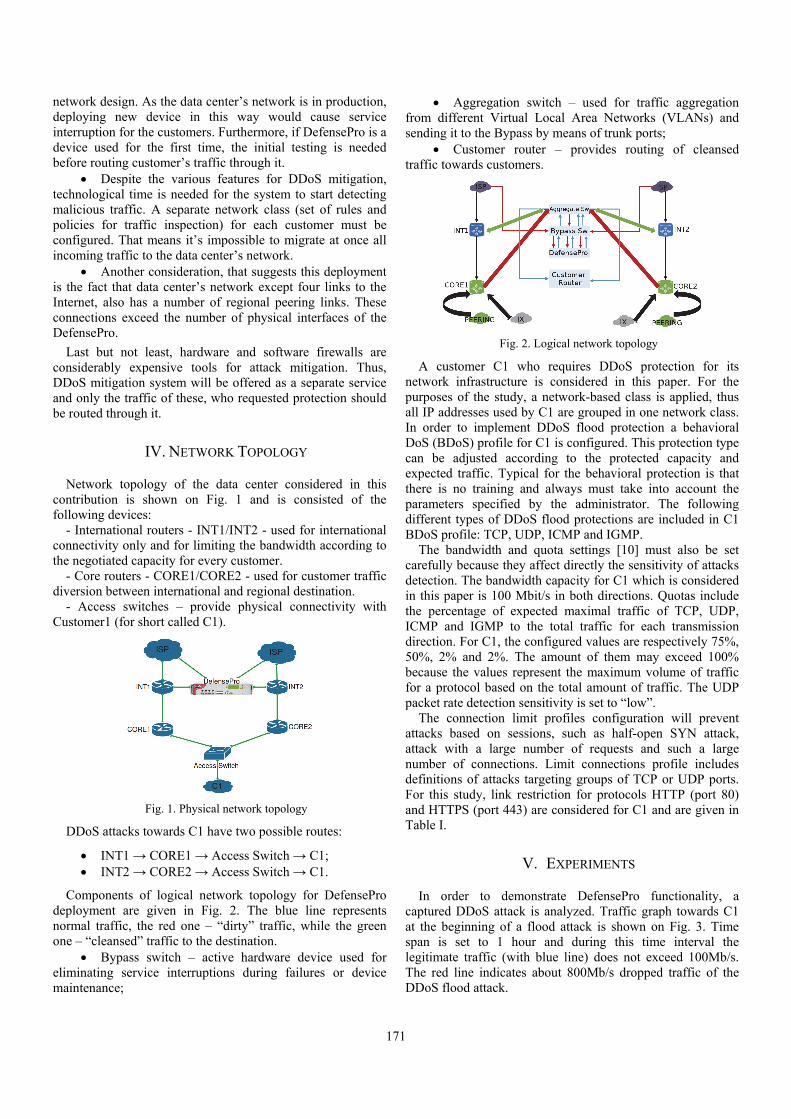
171

network design. As the data center’s network is in production, deploying new device in this way would cause service interruption for the customers. Furthermore, if DefensePro is a device used for the first time, the initial testing is needed before routing customer’s traffic through it.

Despite the various features for DDoS mitigation, technological time is needed for the system to start detecting malicious traffic. A separate network class (set of rules and policies for traffic inspection) for each customer must be configured. That means it’s impossible to migrate at once all incoming traffic to the data center’s network.

Another consideration, that suggests this deployment is the fact that data center’s network except four links to the Internet, also has a number of regional peering links. These connections exceed the number of physical interfaces of the DefensePro.

Last but not least, hardware and software firewalls are considerably expensive tools for attack mitigation. Thus, DDoS mitigation system will be offered as a separate service and only the traffic of these, who requested protection should be routed through it.

IV. NETWORK TOPOLOGY

Network topology of the data center considered in this contribution is shown on Fig. 1 and is consisted of the following devices:

- International routers - INT1/INT2 - used for international connectivity only and for limiting the bandwidth according to the negotiated capacity for every customer.

- Core routers - CORE1/CORE2 - used for customer traffic diversion between international and regional destination.

- Access switches – provide physical connectivity with Customer1 (for short called C1).

Fig. 1. Physical network topology

DDoS attacks towards C1 have two possible routes:

INT1 → CORE1 → Access Switch → C1; INT2 → CORE2 → Access Switch → C1.

Components of logical network topology for DefensePro deployment are given in Fig. 2. The blue line represents normal traffic, the red one – “dirty” traffic, while the green one – “cleansed” traffic to the destination.

Bypass switch – active hardware device used for eliminating service interruptions during failures or device maintenance;

Aggregation switch – used for traffic aggregation from different Virtual Local Area Networks (VLANs) and sending it to the Bypass by means of trunk ports;

Customer router – provides routing of cleansed traffic towards customers.

Fig. 2. Logical network topology

A customer C1 who requires DDoS protection for its network infrastructure is considered in this paper. For the purposes of the study, a network-based class is applied, thus all IP addresses used by C1 are grouped in one network class. In order to implement DDoS flood protection a behavioral DoS (BDoS) profile for C1 is configured. This protection type can be adjusted according to the protected capacity and expected traffic. Typical for the behavioral protection is that there is no training and always must take into account the parameters specified by the administrator. The following different types of DDoS flood protections are included in C1 BDoS profile: TCP, UDP, ICMP and IGMP.

The bandwidth and quota settings [10] must also be set carefully because they affect directly the sensitivity of attacks detection. The bandwidth capacity for C1 which is considered in this paper is 100 Mbit/s in both directions. Quotas include the percentage of expected maximal traffic of TCP, UDP, ICMP and IGMP to the total traffic for each transmission direction. For C1, the configured values are respectively 75%, 50%, 2% and 2%. The amount of them may exceed 100% because the values represent the maximum volume of traffic for a protocol based on the total amount of traffic. The UDP packet rate detection sensitivity is set to “low”.

The connection limit profiles configuration will prevent attacks based on sessions, such as half-open SYN attack, attack with a large number of requests and such a large number of connections. Limit connections profile includes definitions of attacks targeting groups of TCP or UDP ports. For this study, link restriction for protocols HTTP (port 80) and HTTPS (port 443) are considered for C1 and are given in Table I.

V. EXPERIMENTS

In order to demonstrate DefensePro functionality, a captured DDoS attack is analyzed. Traffic graph towards C1 at the beginning of a flood attack is shown on Fig. 3. Time span is set to 1 hour and during this time interval the legitimate traffic (with blue line) does not exceed 100Mb/s. The red line indicates about 800Mb/s dropped traffic of the DDoS flood attack.

172

TABLE I CONNECTION LIMIT PROTECTION FOR CUSTOMER1

Name TCP

port 80 UDP port

80 TCP

port 443 UDP port

443 Application HTTP HTTP HTTPs HTTPs Protocol TCP UDP TCP UDP Number of connections

100 100 100 100

Tracking type

Source Count

Source Count

Source Count

Source Count

Action Mode Drop Drop Drop Drop Risk Medium Medium Medium Medium Suspend Action

Source IP Source IP Source IP Source IP

Fig. 3. Input traffic to Customer1 at the beginning of the attack

The whole attack is given on Fig. 4 where it can be seen that the flood traffic reaches 8 Gb/s.

Fig. 4. Input traffic to Customer1 during attack

Such volume of flood attack would overflow Internet capacity of C1 if there is a lack of DDoS mitigation system and would cause denial-of-service condition. Furthermore, inbound volumetric traffic would cause Internet connectivity problems for most of customers of the data center. Using mitigating capabilities of DefensePro, only the malicious traffic is dropped and the legitimate one is unaffected, in this way providing business continuity. The traffic of the physical port of C1 captured by means of Cacti software [11] is given on Fig. 5.

Fig. 5. Traffic on Customer 1 physical port

As it could be seen during the DDoS attack, only a slight traffic increase is observed (blue line), which proves that the system has successfully mitigated the DDoS attack. Detailed report on the detected DDoS attack is prepared by DefensePro system, but because of the paper limit is not given here.

VI. CONCLUSION

An approach of network protection against DDoS flood attacks targeting network resources was proposed. An IPS DefensePro “out-of-path deployment” system was implemented and configured. Following the results obtained from experiments the main conclusion is that the proposed design is working properly and can successfully protect the network topology so considered. Keep in mind that the real time network protection has a number of aspects that must be carefully analyzed and taken into account, the ideal solution does not exist and thus the DDoS protection remains the hottest research area.

ACKNOWLEDGEMENT

The research is conducted under the grant of project DH07/10-2016, funded by National Science Fund, Ministry of Education and Science, Bulgaria.

REFERENCES

[1] O. Osanaiye, K.R. Choo, and M. Dlodlo, “Distributed Denial of Service (DDoS) Resilience in Cloud: Review and Conceptual Cloud DDoS Mitigation Framework”, Journal of Network and Computer Applications, vol. 67, pp. 147-165, May 2016.

[2] K. Prasad, A. Reddy, and K. Rao, “DoS and DDoS Attacks: Defense, Detection and Traceback Mechanisms - A Survey”, Global Journal of Computer Science and Technology: (E) Network, Web & Security, vol. 14, no. 7, Ver. 1.0, pp. 15-32, 2014.

[3] B. Wang, Y. Zheng, W. Lou, and Y.T. Hou, “DDoS Attack Protection in the Era of Cloud Computing and Software-Defined Networking”, Computer Networks, vol. 81, pp. 308-319, 2015.

[4] I. Nunes, F. Schardong, and A. Schaeffer-Filho, “BDI2DoS: An Application Using Collaborating BDI Agents to Combat DDoS Attacks”, Journal of Network and Computer Applications, vol. 84, pp. 14-24, 2017.

[5] D. Anstee, P. Bowen, C.F. Chui, and G. Sockrider, Worldwide Infrastructure Security Report, Arbor Networks Special Report, Vol. XII, Arbor Networks, 2017. (www.arbornetworks.com)

[6] Radware, DDoS Handbook, 2015. [7] A. Shameli-Sendi, M. Pourzandi, M. Fekih-Ahmed, and M.

Cheriet, “Taxonomy of Distributed Denial of Service Mitigation Approaches for Cloud Computing”, Journal of Network and Computer Applications, vol. 58, pp. 165-179, 2015.

[8] P. Dzurenda, Z. Martinasek, and L. Malina, “Network Protection Against DDoS Attacks”, Intern. Journal of Advances in Telecommunications, Electrotechnics, Signals and Systems, vol. 4, no. 1, pp. 8-14, 2015.

[9] W. Zhou, W. Jia, S. Wen, Y. Xiang, and W. Zhou, “Detection and Defense of Application-Layer DDoS Attacks in Backbone Web Traffic”, Future Generation Computer Systems, vol. 38, pp. 36-46, 2014.

[10] Radware, DefensePro User Guide, January 2016. [11] I. Berry, T. Roman, L. Adams, J.P. Pasnak, J. Conner, R.

Scheck, and A. Braun, The Cacti Manual, The Cacti Group, 2017.

173

Review of Modern Virtual Reality HMD Devices and Development Tools

Aleksandar Jovanović1 and Aleksandar Milosavljević2

Abstract - The paper describes the development of virtual reality with an emphasis on HMD devices and tools for application development. Firstly, we will describe popular VR HMD devices for PC, mobiles, and consoles. Secondly, we will describethe developmentenvironmentfor native, multi-platform and web applications. Next, through the development of VR software application, we will introduce best practices for VR development and user experience standards.

Keywords - Virtual reality, HMD, Software development, Game engine.

I. INTRODUCTION

In the mind of most people idea of virtual reality is connected with imaginary worlds from sci-fi movies or novels.By definition from 1993virtual realityis: “Virtual reality refers to immersive, interactive, multi-sensory, viewer-centered, three-dimensional computer-generated environments and the combination of technologies required to build these environments” [1].The first example of virtual reality appeared in 1938with a device for watching stereoscopic image. However, the first stereoscopic device which brought attention to the public was a View-Master from 1939. Today, thestereoscopic device represents afundamental pattern for making low-budget VR HMDdevices. The first concept for a modern HMD (head-mounted display)device that has attracted attention was the Ultimate display from 1965. The concept is made by Ivan Sutherland, whose idea was to develop a device that will use acomputer-generatedgraphic for creating interactive worlds. Duringthat periodthe term VR was not yet known, computers were in the early stage of development and the forerunners of VR devices operated using cameras[2]. The first VR device which used computer hardware and object creation in real time appears in 1968 called Sword of Damocles. Creators of this device were Ivan Sutherland and his student Bob Sproull.During the 90's there were unsuccessful attempts of VR devices like an iGlasses, Nintendo Virtual Boy, Cybermaxx, and VFX-1[3].

The first modern VR device was created in 2012 from young engineer and first CEO of company Oculus VR, Palmer Luckey. In August 2012, Oculus VRlaunches Kickstarter campaign about cutting edge technology called Oculus Rift. A social network company Facebook acquired Oculus VR for 2 billion dollars with avision that VR will be the next big thing after mobile phones[4].

The goal of the paper is to showcase thepotential of VR technologies. The paper will provide information regarding modern VR devices and software development techniques and tools. After, it will introduce an important concept for VR software development which includes best practices and standard for high-quality VR experience. High-quality VR experience is essential for building next generation product. Also, there is a demand on the market for VR developers and experts in HMD technologies like Oculus Rift and Google Cardboard. Regarding the concept proposed in this paper current and future developers will have abrief overview of the current state of technologies and knowledge to overcome beginning steps in VR developer carriers. The paper is organized in the following way. Firstly,we will describe modern VR HMD devices like Oculus Rift, Gear VR, Google Cardboard and HTC Vive. Secondly, we will describe VR application development for PC, mobile, and web-based solutions. Also, compareHMD devices for theVR application development.Thirdly, we will describe VR applicationGhost Hunt. At the end, we will introduce best practices and user experience standard for VR development.

II. VR HMD DEVICES

The presence of the modern generation of virtual reality starts from 2012and until now VR dedicated companies and industry leaders developed their own HMD devices and software development environments. HMD is a type of computer display device that is worn on the head or is built in as part of a helmet. The most popular VR HMD devices for smartphones,PC,and game consoles areGoogle Cardboard, Oculus Rift, Playstation VR, HTC Vive, Samsung Gear VR, Avegant Glyph, and Razer OSVR.

There are three types of VR devices [5]. The first type is Mobile VR which includes aportable device for asmartphone like Google Cardboard and Samsung Gear VR. This is the more intuitive approach for users because there is no need for PC device, additional settings, and cables for activating theapplication on the smartphone. The second type is astandalone device for PC desktop devices like Oculus Rift and HTC Vive. Unlike a first type, they are more optimized and provide abetter experience from performance and graphic rendering perspective. The third type is VR for game consoles like Playstation VR.

The basis for all of modern VR devices are lenses, adisplay for watching stereoscopic pictures and inertial measurement unit (IMU). The lens is coming with different characteristic, for example, Oculus Rift has two lenses A and B. The difference is thedistancebetween the lens anddisplay device. The information isdisplayed on the screen using the graphic processing unit (GPU). The GPU allows devices to operate

1Aleksandar Jovanović is with the Faculty of ElectronicEngineering atUniversity of Niš, Aleksandra Medvedeva 14, 18000Niš, Serbia, E-mail: [email protected]

2Aleksandar Milosavljević is with the Faculty of ElectronicEngineering atUniversity of Niš, Aleksandra Medvedeva 14, 18000Niš, Serbia, E-mail: [email protected]

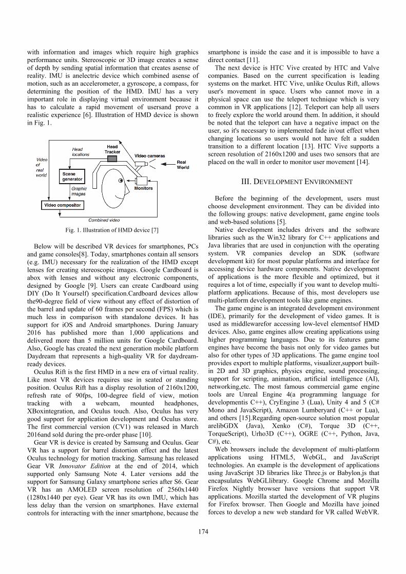
withperfof drealmotdeteimphas realin F

Band(e.glensabodesiDIYthe9the mucsupp201deliAlsDayread

OLikposrefrtracXBgooThe201

GVR OcuGeasuppsuppVR (128lesscon

h informationformance unitdepth by sendlity. IMU is ation, such as aermining the portant role in

to calculatelistic experienFig. 1.

Below will be d game consolg. IMU) necesses for creatin

ox with lenseigned by Goo

Y (Do It You90-degree fielbarrel and up

ch less in coport for iOS 6 has publi

ivered more to, Google hasydream that rdy devices. Oculus Rift is e most VR ition. Oculus

resh rate of cking with oxintegration,

od support fore first comme6and sold dur

Gear VR is deR has a suppoulus technologar VR Innovported only port for Sams

R has an AM80x1440 per s delay than ntrols for intera

Fig

n and imagests. Stereoscop

ding spatial inanelectric devan accelerome

position of n displaying e a rapid monce [6]. Illustr

described VRes[8]. Today, ssary for the ng stereoscopies and withouogle [9]. Use

urself) specificld of view wipdate of 60 fraomparison wand Android

ished more than 5 millios created the nrepresents a h

the first HMDdevices requiRift has a di90fps, 100-d

a webc, and Oculusr application ercial version ring the pre-orvice is created

ort for barrel gy for motion vator EditionSamsung No

sung Galaxy sMOLED screye). Gear Vthe version oacting with th

g. 1. Illustration

s which requpic or 3D imaformation thavice which coeter, a gyrosco

the HMD. virtual enviroovement of ration of HMD

R devices for smartphones realization ofic images. Gout any electr

ers can createcation.Cardbothout any effeames per seco

with standalond smartphone

than 1,000 on units for Gnext generatiohigh-quality V

D in a new erires use in sisplay resolutidegree field am, mount

s touch. Alsodevelopment (CV1) was

rder phase [10d by Samsungdistortion efftracking. Sam

n at the endote 4. Later smartphone seeen resolutio

VR has its ownon smartphonhe inner smartp

of HMD devic

uire high graage creates a at creates asenombined asenope, a compasIMU has a

onment becauusersand proD device is sh

smartphonescontain all se

f the HMD eoogle Cardboaronic compone Cardboard oard devices fect of distortiond (FPS) whne devices. Is. During Janapplications

Google Cardbon mobile platVR for daydr

a of virtual reseated or stanion of 2160xof view, m

ted headph, Oculus has and Oculus

released in M0]. g and Oculus. ffect and the msung has reld of 2014, w

versions adderies after S6. on of 2560xn IMU, which

nes. Have extphone, becaus

ce [7]

174

aphics sense

nse of nse of ss, for

very use it ove a hown

, PCs ensors xcept ard is nents, using allow ion of ich is t has nuary

and board. tform ream-

eality. nding 1200,

motion hones,

very store.

March

Gear latest eased which d the Gear

x1440 h has ternal se the

smardirec

Thcompsysteuser'physcommto frebe nuser,chantransscreeplace

Bechoothe fand w

NalibraJavasystedeveacceof arequplatfmult

Th(IDEuseddevichighenginalso provin 2suppnetwtoolsdeveMonand arelibTorqC#),

WapplitechnusingencaFirefapplifor Fforce

rtphone is insct contact [11]he next devicpanies. Basedems on the ma's movement sical space camon in VR apeely explore t

noted that the , so it's necess

nging locationsition to a difen resolution ed on the wall

III. D

efore the beose developmfollowing grouweb-based solative develop

aries such as tlibraries that

em. VR coelopment kit) ssing device

applications isires a lot of ti

form applicatiti-platform devhe game enginE), primarily d as middlewaces. Also, gamer programmnes have becofor other type

vides export toD and 3D gr

port for scriptworking,etc. Ts are Unrealelopmentis C+no and JavaScothers [15].RbGDX (Jav

queScript), Uretc.

Web browsers ications usinnologies. An g JavaScript 3

apsulates Webfox Nightly ications. MozFirefox browses to develop

side the case ]. ce is HTC Vivd on the cuarket. HTC V

in space. Uan use the telpplications [1the world arouteleport can

sary to implemns so users wfferent locatioof 2160x1200l in order to m

DEVELOPME

eginning of tent environmups: native delutions [5]. pment includthe Win32 libt are used in ompanies defor most popuhardware coms the more fime, especiallyions. Becausevelopment toone is an integrfor the devel

arefor accessinme engines all

ming languageome the basises of 3D applo multiple platraphics, physting, animatio

The most faml Engine 4(a++), CryEngincript), Amazoegarding open

va), Xenko rho3D (C++)

include the dng HTML5example is th3D libraries lbGLlibrary. Gbrowser hav

zilla started thser. Then Goa new web st

and it is imp

ve created byurrent specificVive, unlike OUsers who caleport techniq12]. Teleport und them. In ahave a negatimented fade iwould not haon [13]. HTC0 and uses tw

monitor user m

ENT ENVIRON

the developmment. They can

evelopment, g

des drivers abrary for C++conjunction wevelop an ular platformsmponents. Naflexible and y if you want e of this, mools like game rated developmlopment of vng low-level low creating aes. Due to is not only forlications. The tforms, visualsics engine, son, artificial

mous commerca programmine 3 (Lua), Uon Lumberyarn-source solut

(C#), Torq), OGRE (C+

development , WebGL,

he developmeike Three.js oGoogle Chro

ve versions the developmeoogle and Motandard for VR

possible to ha

y HTC and Vcation is lea

Oculus Rift, allannot move que which iscan help all uaddition, it shive impact onin/out effect wave felt a sudC Vive supporwo sensors thatmovement [14]

NMENT

ment, users mn be dividedgame engine t

and the softw+ applications with the opera

SDK (softws and interfaceative developmoptimized, buto develop m

st developersengines. ment environm

video games. elementsof Happlications uts features g

r video gamesgame engine izer,support bsound processintelligence (cial game enng language

Unity 4 and 5rd (C++ or Ltion most popque 3D (C++, Python, J

of multi-platfand JavaSc

ent of applicator Babylon.js ome and Mothat support

ent of VR pluozilla have joR called Web

ave a

Valve ading lows in a very

users hould n the when dden rts a t are ].

must into

tools

ware and

ating ware e for ment ut it

multi-s use

ment It is

HMD using game s but tool

built-sing, (AI),

ngine for

(C# Lua), pular C++, Java,

form cript tions that

ozilla VR

ugins oined bVR.

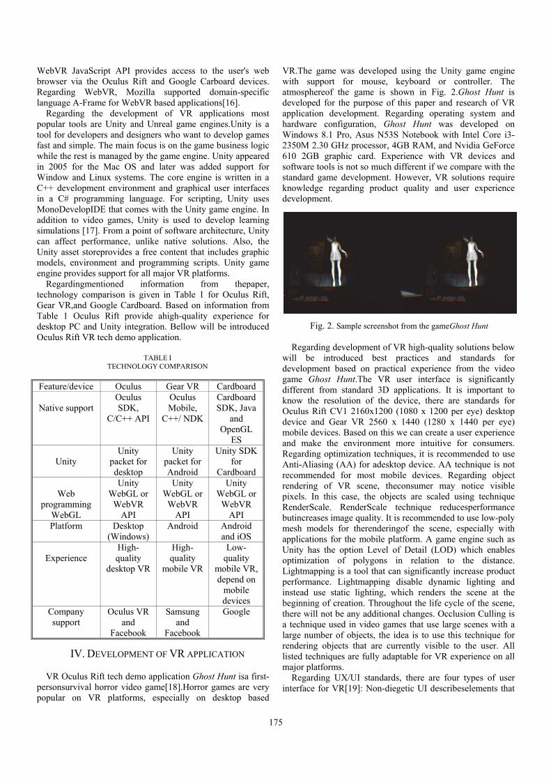
175

WebVR JavaScript API provides access to the user's web browser via the Oculus Rift and Google Carboard devices. Regarding WebVR, Mozilla supported domain-specific language A-Frame for WebVR based applications[16].

Regarding the development of VR applications most popular tools are Unity and Unreal game engines.Unity is a tool for developers and designers who want to develop games fast and simple. The main focus is on the game business logic while the rest is managed by the game engine. Unity appeared in 2005 for the Mac OS and later was added support for Window and Linux systems. The core engine is written in a C++ development environment and graphical user interfaces in a C# programming language. For scripting, Unity uses MonoDevelopIDE that comes with the Unity game engine. In addition to video games, Unity is used to develop learning simulations [17]. From a point of software architecture, Unity can affect performance, unlike native solutions. Also, the Unity asset storeprovides a free content that includes graphic models, environment and programming scripts. Unity game engine provides support for all major VR platforms.

Regardingmentioned information from thepaper, technology comparison is given in Table 1 for Oculus Rift, Gear VR,and Google Cardboard. Based on information from Table 1 Oculus Rift provide ahigh-quality experience for desktop PC and Unity integration. Bellow will be introduced Oculus Rift VR tech demo application.

TABLE I TECHNOLOGY COMPARISON

IV. DEVELOPMENT OF VR APPLICATION

VR Oculus Rift tech demo application Ghost Hunt isa first-personsurvival horror video game[18].Horror games are very popular on VR platforms, especially on desktop based

VR.The game was developed using the Unity game engine with support for mouse, keyboard or controller. The atmosphereof the game is shown in Fig. 2.Ghost Hunt is developed for the purpose of this paper and research of VR application development. Regarding operating system and hardware configuration, Ghost Hunt was developed on Windows 8.1 Pro, Asus N53S Notebook with Intel Core i3-2350M 2.30 GHz processor, 4GB RAM, and Nvidia GeForce 610 2GB graphic card. Experience with VR devices and software tools is not so much different if we compare with the standard game development. However, VR solutions require knowledge regarding product quality and user experience development.

Regarding development of VR high-quality solutions below will be introduced best practices and standards for development based on practical experience from the video game Ghost Hunt.The VR user interface is significantly different from standard 3D applications. It is important to know the resolution of the device, there are standards for Oculus Rift CV1 2160x1200 (1080 x 1200 per eye) desktop device and Gear VR 2560 x 1440 (1280 x 1440 per eye) mobile devices. Based on this we can create a user experience and make the environment more intuitive for consumers. Regarding optimization techniques, it is recommended to use Anti-Aliasing (AA) for adesktop device. AA technique is not recommended for most mobile devices. Regarding object rendering of VR scene, theconsumer may notice visible pixels. In this case, the objects are scaled using technique RenderScale. RenderScale technique reducesperformance butincreases image quality. It is recommended to use low-poly mesh models for therenderingof the scene, especially with applications for the mobile platform. A game engine such as Unity has the option Level of Detail (LOD) which enables optimization of polygons in relation to the distance. Lightmapping is a tool that can significantly increase product performance. Lightmapping disable dynamic lighting and instead use static lighting, which renders the scene at the beginning of creation. Throughout the life cycle of the scene, there will not be any additional changes. Occlusion Culling is a technique used in video games that use large scenes with a large number of objects, the idea is to use this technique for rendering objects that are currently visible to the user. All listed techniques are fully adaptable for VR experience on all major platforms.

Regarding UX/UI standards, there are four types of user interface for VR[19]: Non-diegetic UI describeselements that

Feature/device Oculus Gear VR Cardboard

Native support Oculus SDK,

C/C++ API

Oculus Mobile,

C++/ NDK

Cardboard SDK, Java

and OpenGL

ES

Unity Unity

packet for desktop

Unity packet for Android

Unity SDK for

Cardboard

Web programming

WebGL

Unity WebGL or

WebVR API

Unity WebGL or

WebVR API

Unity WebGL or

WebVR API

Platform Desktop (Windows)

Android Android and iOS

Experience

High-quality

desktop VR

High-quality

mobile VR

Low-quality

mobile VR, depend on

mobile devices

Company support

Oculus VR and

Facebook

Samsung and

Facebook

Google

Fig. 2. Sample screenshot from the gameGhost Hunt

176

do not belong to the virtual world, e.g. HUD (head-up display). This type of UI is poorly used in VR applications, primarily because of user focus. SpatialUIdescribes an element that is part of the VR world. In relation to non-digest, they have aposition that is not accompanied by the user. DiegeticUIdescribes an element that follows some object in the scene. A good example is the energy of the enemy to the scene. MetaUIdescribes the effect on the scene that is not part of the VR world. For example, change of color if theuser loses energy. Diegetic UI elements were used in video game Ghost Hunt. The main character uses diegetic element in a form of a smartphone. Also, smartphone flash effect representsthe meta UIelementon the player screen.

For adapting a standard 3D video game into VR there are a few simple steps from the Unity game engine. For Oculus Rift, the userneeds a special camera rig that moves directly in Unity from Oculus integration package. Also, the userneeds to enable Virtual Reality Supportedcheck box in Player Settings. A similar way is for Cardboard application using the Unity SDK for Cardboard. For HTC Vive, theuser needs to get a Steam account, install the runtime on the development machine, then go into Unity and download the SteamVR camera rig from the asset store and attach it to existing camera. At the end disable all in-game camera in favor of the new VR camera. All listed packages and features are free for download and development.

Because VR is in the early stage of development there is the possibility of error on major operating systems like Windows or Oculus SDK legacy runtime. It is recommended to use the latest version of Oculus SDK. The latest version of Oculus SDK supports game engine integrations for Unity, Unreal, WebVR, native and mobile applications. Before a developer publishes anapplication, the solution should follow best practice for best VR experience defined by Oculus team. After submission, theapplication will be reviewed by Oculus team. For example, if the application has the option to move theposition of the head by y-axis using a mouse or controller,it will be returned for correction.

Regarding the best practices for mobile VR, developers should consider mobile application Cardboard Design Lab. The mobile platform is limited regarding user interaction and a novel approach to increase user experience and interaction is to use haptic devices.

V. CONCLUSION

This paper discussed thedevelopment of VR technology, with a focus on use cases and implementations. Firstly, VR HMD devices were described. Secondly,we describe the development environment for VR, Unity game engine and compare HMD devices. Thirdly, the development of the VR applicationwas described using best practices and UI/UX standards. VR devices and software tools are ready for serious software development. However, software developersshould befamiliar with best practices if they want to achieve high-quality VR experience.

In the future, we can expect that VR moves forward, primarily because of the great interest of the companies and the community of users. Virtual and augmented reality

devices like Oculus Rift, Leap Motion or HoloLens have been increasing popularity among developers. The new interdisciplinary field will be created through theconnection of VR with education, medicine, art,automotive, and architecture. Game engines are becoming increasingly popular, especially because it does not require financial investment and provides a simple interface for operation.

Regarding future research, there is a potential for the use of VR in education, communication and simulation development. VR platform can help in thedevelopment of inclusion, acommunity of users who will be ready to cooperate regardless of their limitations. Future research will focus on use cases that can improve people skills using modern VR technologies.

REFERENCES

[1] C. Cruz-Neira, D.J. Sandin, and T.A. DeFanti, "Surround-Screen Projection-Based Virtual Reality: The Design and Implementation of the CAVE", 20th Annual Conference on Computer Graphics and Interactive Techniques SIGGRAPH'93, pp. 135-142, 1993.

[2] T. Mazuryk, and M. Gervautz, "Virtual Reality History, Applications, Technology and Future", Technical Report TR-186-2-96-06, 1996.

[3] P. Bouvier, F. De Sorbier, P. Chaudeyrac, and V. Biri, "Cross-Benefits Between Virtual Reality and Games", Computer Games Multimedia and Allied Technology Conference, 2008.

[4] E. Guirado Carmen, and G. Castro Carmen, "Crowdfunding as an Open Innovation for Co-Creation", Strategic Approaches to Successful Crowdfunding, 2016.

[5] T. Parisi, “Learning Virtual Reality”, O’Reilly Media, 2015 [6] M. Tawadrous, D. Rojas, B. Kapralos, A. Hogue, and A.

Dubrowski, "The Effects of Stereoscopic 3D on Knowledge Retention Within a Serious Gaming Environment", Multimedia Tools and Applications, March 2016.

[7] R. T. Azuma, "A Survey of Augmented Reality", Teleoperators and Virtual Environments, vol. 6, no. 4, pp. 355-385, August 1997.

[8] “The Best VR Headsets”, online documentation, link: http://www.wareable.com/headgear/the-best-ar-and-vr-headsets, last accessed 14.04.2017.

[9] A. Amer, and P. Peralez, "Affordable Altered Perspectives Making Augmented and Virtual Reality Technology Accessible", Global Humanitarian Technology Conference (GHTC) IEEE, 2014.

[10] D. Sharma, "A Review Paper on Virtual Reality Oculus Rift and Augment Reality", International Journal of Current Research, vol. 8, no. 09, pp. 37941-37945, September 2016.

[11] J. Lee, B. Kim, B. Suh, and E. Koh, "Exploring the Front Touch Interface for Virtual Reality Headsets", 2016 CHI Conference Extended Abstracts on Human Factors in Computing Systems, pp. 2585-2591, 2016.

[12] K. Kim, "Is Virtual Reality (VR) Becoming an Effective Application for the Market Opportunity in Health Care, Manufacturing, and Entertainment Industry?", European Scientific Journal, 2016.

[13] T.J. Dodds, and R.A. Ruddle, "Using Teleporting, Awareness and Multiple Views to Improve Teamwork in Collaborative Virtual Environments", Visualization and Virtual Reality Research Group School of Computing, 2008.

177

[14] M.S. Hasan, and H. Yu, "Innovative Developments in HCI and Future Trends", International Journal of Automation and Computing, vol. 14, no. 1, pp 10-20, December 2016.

[15] B. Cowan, and B. Kapralos, "An Overview of Serious Game Engines and Frameworks", Recent Advances in Technologies for Inclusive Well-Being, vol. 119 of the series Intelligent Systems Reference Library, pp. 15-38, February 2017.

[16] S. Neelakantam, and T. Pant, Learning Web-based Virtual Reality: Build and Deploy Web-based Virtual Reality Technology, Apress, 2017.

[17] C.-W. Yang, T.-H. Lee, C.-L. Huang, and K.-S. Hsu, "Unity 3D Production and Environmental Perception Vehicle Simulation Platform", International Conference on Advanced Materials for Science and Engineering (ICAMSE), 2016.

[18] B. Perro, "Sign of a Threat: The Effects of Warning Systems in Survival Horror Games", COSIGN, 2004.

[19] P. Salomoni, C. Prandi, M. Roccetti, L. Casanova, L. Marchetti, and G. Marfia, "Diegetic user Interfaces for Virtual Environments with HMDs: A User Experience Study with Oculus Rift", Journal on Multimodal User Interfaces, pp. 1-12, January 2017.

178

Computer Application for Simple Sustainability Assessment

Aleksandar Veljanovski1, Vladimir Radojevic2 and Vladimir Stankovic1

Abstract – Sustainable development has a long history that captured a lot in wide and depth both in theory and practice. Many claimed that a corner stone in the building of "sustainable development" had been marked by John Elkington in 1997 with his "Cannibals and forks – the Triple Bottom Line of 21st century business". Increasing importance of "sustainable" even made captured "domain of sustainable" wider and deeper in last 17 years, too. UN Millennium Goals from 2000 and Agenda for Sustainable Development in 2015 engraved permanent landmarks in building of society with sustainable development. Therefore, there are many authors who try to develop methods for sustainability assessment/evaluation. In this paper we describe a computer application that we have developed, which enables simple first level assessment of sustainability.

Keywords – Sustainability, Triple Bottom Line, Assessment, Evaluation, Computer Application.

I. INTRODUCTION

Leading international and global governing bodies of UN, gradually took sustainable 17 goals agenda as it prime outcome for 2030, which started formally as the 7th out of 8 UN Millennium Goals in 2002. It seems to be that under the umbrella of sustainable agenda are similar as previous 7 Millennium goals, and other 10 spanned sustainable goals agenda into more detailed manner. Previously recognized as only one out of seven, now sustainability is one standing out for all 17 goals at global agenda. Therefore, assessment and evaluation of sustainability has become an increasingly important issue. In this paper we will give a brief overview of the term sustainability itself and a review of numerous methods of sustainability assessments, followed by development and presentation of our assessment software application for sustainability measurement.

In 1994, John Elkington coined the term triple bottom line. There was no single eureka moment, but rather synergetic impact of ideas and work on SustainAbility (a think – tank found in 1987), Brundtland report in 1987 with social and economic dimensions of the agenda among other things [1]. In the simplest terms, the Triple Bottom Line (TBL) agenda

focuses on corporations – not just on the economic value that they add, but also on the environmental and social value that they add or destroy [2]. Therefore, sustainability is an intersection and integration of three factors: social, environmental and economic, and is often presented as three circles, as shown in Fig. 1.

Fig. 1. Triple Bottom Line

From 1960 to the present, three great waves of public pressure have shaped the environmental agenda. The roles and responsibilities of governments and the public sector have mutated in response to each of these three waves – and will continue to do so. Although each wave of activism has been followed by a down-wave of falling public concern, each successive wave has significantly expanded the agendas of politics and business [2]. Wave 1 brought an understanding that environmental impacts and natural resource demands have to be limited, resulting in an initial outpouring of environmental legislation. The business response was defensive, focusing on compliance, at best. Wave 2 brought a wider realization that new kinds of production technologies and new kinds of products are needed, culminating in the insight that development processes have to become sustainable – and a sense that business would often have to take the lead. The business response began to be more competitive. Wave 3 focuses on the growing recognition that sustainable development will require profound changes in the governance of corporations and in the whole process of globalization, putting a renewed focus – on government and on civil society. Now, in addition to the compliance and competitive dimensions, the business response will need to focus on market creation.

1Aleksandar Veljanovski and Vladimir Stankovic are with the Faculty of Electronic Engineering at University of Nis, Aleksandra Medvedeva 14, 18000 Nis, Serbia, E-mail: aleksandar.veljanovski,[email protected].

2Vladimir Radojevic is with the Center for Multidisciplinary Studies of Department of Computer Science at University ofBelgrade, Serbia, E-mail: [email protected]

179

Pearce [3] says: "Recognizing that people's actions toward nature and each other are the source of growing damage to the environment and resources needed to meet human needs and ensure survival and development, I PLEDGE to act to the best of my ability to help make the Earth a secure and hospitable home for present and future generations."

Daly [4] questioned: "What is it that is supposed to be sustained in "sustainable" development?" Two broad answers have been given. First, utility should be sustained; that is, the utility of future generations is to be non-declining. The future should be at least as well off as the present in terms of its utility or happiness as experienced by itself. Utility here refers to average per capita utility of members of a generation. Second, physical throughput should be sustained, that is, the entropic physical flow from nature’s sources through the economy and back to nature’s sinks, is to be non-declining.

In the supply chain management domain, lessons about strategic importance of competitiveness brought by sustainability had been implemented by Carter and Rogers [5]

along with the measurements of ranking of sustainable practice by intersection and integration of social, economic and environmental aspects of sustainable supply chain management practise.

Sustainability has definitely become a global agenda; therefore various sustainability assessment methods have been developed. We will describe some of them in the next section.

II. SUSTAINABILITY ASSESSMENT

Vinouh et al. [6] developed a computer-based decision support system for the assessment of the sustainability level of a manufacturing organization. Their system was developed designated as fuzzy-logic-based sustainability evaluation. Decision support system is taking into consideration various factors needed for insuring sustainability. The system calculates the fuzzy logic sustainability index, Euclidean distance, and fuzzy performance importance index. This model should help the companies to analyze various aspects of sustainability within their organization and work toward further improvement of it.

Benedetto and Klemeš [7] improved the Life Cycle Assessment (LCA), a well-known tool for analyzing environmental impacts on a wide perspective with reference to a product system and the related environmental and economic impacts. They stressed a need for a novel approach that complements environmental and financial considerations and introduced a new graphical representation: the Environmental Performance Strategy Map. It allows one to combine the main environmental indicators (footprints) with the additional dimension of cost. Their study defined the Sustainable Environmental Performance Indicator as a single measure for sustainability of a given option. Comparison of different options for strategic decision-making purposes can be enhanced and facilitated by the use of this indicator.

Calderón [8] aimed at presenting a model, in the form of a template and a set of operating instructions, produced by the European Commission for the appraisal of sustainability of projects requesting financial support under the Urban Pilot Projects scheme. The proposed appraisal scheme should

jointly take into consideration the three main components of the sustainability concept, namely economic, social, and environmental, subjectively weighted to produce a single index. Evaluation of a single index was handed over to a panel of external evaluators for them to reach consistent decisions across the European Union (EU).

Munda [9] argued that sustainability assessment needs a set of multi-dimensional indicators and how could such indicators be aggregated. Like in a classical conflictual situation, studied in multi-criteria decision theory, some indicators improve while others deteriorate. For instance, when incomes grow, SO2 might go down while CO2 increases.

Ticehurst et al. [10] explored coastal lakes as ecosystems of significant value generating many ecological, social and economic benefits. Clearly, integration and intersection of ecological, social and economic issues are in the domain of sustainability thought. Like in [9], conflicts, for example between lake users and upstream communities, are present in multi-criteria decision theory. There are many techniques that can be used to integrate the variables involved in such conflicts including system dynamics, meta-modelling and coupled component models, but many of these techniques are too complex for catchment managers to employ on a routine basis. The overall result is the potential to compromise the sustainability of these important ecosystems. In their paper, they present research to address this problem. Development of an integrated model framework based on a Bayesian network (Bn) was presented. Bns are used to assess the sustainability of eight coastal lake-catchment systems, located on the coast of New South Wales (NSW), Australia. Their paper described the potential advantages in the use of Bns and the methods used to develop their frameworks. A case study application for the Cudgen Lake of northern NSW is presented to illustrate the techniques.

Tseng et al. [11] examined sustainable production indicators (SPIs). SPis is a complex concept for which determining multiple qualitative criteria is not trivial. Thus, they developed a generalized quantitative evaluation model, which considers both the interdependence relation between criteria and the fuzziness of subjective perception concurrently. They evaluated the performance of synthetic SPIs by adopting fuzzy measure and analytical network process (ANP) method in a multi-nation original equipment manufacturing firm.

Jayal et al. [12] developed improved models, metrics, scoring methods, predictive models for sustainability evaluation and optimization techniques at the product, process and system levels to achieve sustainability in manufacturing. They used a holistic view, spanning not just the product and the manufacturing processes involved in its fabrication, but also the entire supply chain, including the manufacturing systems across multiple product life-cycles. Their paper presents an overview of recent trends and new concepts in the development of sustainable products, processes and systems with examples focusing on dry, near-dry and cryogenic machining.

Gunasekaran and Spalanzani [13] stated that today it is not enough to be successful in business, it is becoming imperative to safeguard the environment, safety and welfare of those

180

alive today and prepare for those yet to come. Various stakeholders have realized that the future of the earth, and therefore that of future generations, is at stake. They provided classification and critical review of the available SBD literature and developed a framework for SBD and suggest future research directions, along with the tools, techniques and some performance measures and metrics for SBD. Čuček et al. [14] presented an overview of footprints as

defined indicators that can be used to measure sustainability. Many definitions, units of measurement in its single instance of social, economic and environmental dimensions are unclear. Even more, footprints could be composite of two and more individual composites are also assessed. These composite combinations have multi-objective optimization problem for which authors presented several tools for optimizations, calculations, graph based and mathematical programming based.

Bond et al. [15] draw mainly on theoretical papers along with the few case study examples published to date (from England, Western Australia, South Africa and Canada). Their paper outlines what might be considered state-of-the-art sustainability assessment. Such processes must: (i) address sustainability imperatives with positive progress towards sustainability; (ii) establish a workable concept of sustainability in the context of individual decisions/assessments; (iii) adopt formal mechanisms for managing unavoidable trade-offs in an open, participative and accountable manner; (iv) embrace the pluralistic inevitabilities of sustainability assessment; and (v) engender learning throughout. They postulated that sustainability assessment may be at the beginning of a phase of expansion not seen since environmental impact assessment was adopted worldwide.

III. OUR APPROACH

Our basic idea is as follows: there are many questions/indicators, and each of them can be ‘placed’ in only 1 of 7 possible areas, as each question/indicator deals with:

1. Only the economic aspects or 2. Only the environmental aspects or 3. Only the social aspects or 4. Both the economic and environmental aspects or 5. Both the economic and social aspects or 6. Both the environmental and social aspects or 7. All three aspects For example, the question ‘Are the workers motivated?’

regards both the social and economic aspects. Taking care of the workers’ motivation basically belongs to the social aspect, but their motivation directly influences their efficiency, which will increase/decrease the company’s profits. Therefore, this indicator also deals with the economic aspects. It is not easy to properly define which question belongs to which area, therefore experts’ job is to define the questions/indicators for the evaluated entity (firm, company, organization, etc.) and categorize them to one of the seven areas. In such system each of the seven areas is important for the sustainability, not only the center where the three circles intersect. If any of the areas is neglected, it will negatively influence the sustainability.

Since various questions/indicators can be more or less important than other questions/indicators, each can have a proper weight, which is expressed as a positive number – the greater the weight, the greater the importance. When evaluating, each question/indicator can have 5 values, from 1 to 5. Then for each of the 7 areas an average value may be calculated according to Eq. (1). Here n is the number of questions/indicators for that particular area and wi and vi are the proper weights and values for each of them.

n

ii

i

n

ii

w

vwave

1

1 (1)

The obtained average value for each of the areas is a number between 1 and 5. We can convert that number into a proper shade of grey, with 1 being the darkest (black) and 5 being the lightest (white). If we color each of the 7 areas with the proper shade of grey, we can immediately derive interesting conclusions, such as:

1. Which area is the darkest, therefore which aspect is the most important to focus on, in order to increase sustainability.

2. How ‘close’ are all the areas to the color white, which gives a sense of how sustainable the evaluated system is.

In the remainder of this section we will describe the application we have developed. It basically has two parts: manipulation of the questions/indicators and assessment. Clicking the button ‘Manipulate questions/indicators’ selects the first part, which is shown in Fig. 2. The user can enter a new question/indicator or delete an existing one, as well as change the text, weight or area for any of the questions. Clicking the ‘Save’ button saves the changes.

Fig. 2. Manipulating questions/indicators - Changing the area Clicking the ‘Fill a Survey’ button starts the evaluation. For

each of the questions/indicators the user should select a value from 1 to 5, as shown in Fig. 3. After all the questions are answered the user can click the ‘Submit’ button and the application will show the results, as can be seen in Fig. 4. The left part of the window shows the seven colored areas. We can see in the shown case that the economic aspect is great, while work needs to be done on the social and environmental aspects. The most important part in this particular case is the part that deals with both social and environmental aspects, as that area is the darkest. The user can click on any of the seven areas, and the results for that area will be shown in the right

181

part of the window. There we can see the proper questions/indicators for the selected area with their weights and values. The calculated average value is shown at the bottom. Clicking on some other area gives the results for that area.

Fig. 3. Filling the survey

Fig. 4. Results As can be seen, the application is easy to use and gives a

simple sustainability assessment, which may be valuable as a first level evaluation. Another merit of our approach is that it gives a different view, compared to existing models.

In future work we may enrich our model with some more complex evaluations.

IV. CONCLUSION

Previously being only one out of seven goals, sustainability is now standing out for all 17 goals at global agenda. Therefore, sustainability assessment/evaluation has become an increasingly important issue. In this paper we gave a review of several methods of sustainability assessment, and described our simple computer application for first level sustainability assessment. The application is easy to use and gives a different approach, compared to existing models.

ACKNOWLEDGEMENT

The research presented in this paper was supported in part by the Serbian Ministry of Education, Science and Technological Development [TR32012].

REFERENCES

[1] "Report of the World Commission on Environment and Development: Our Common Future", URL: www.un-documents.net/our-common-future.pdf

[2] J. Elkington, "Enter the Triple Bottom Line", The Triple Bottom Line: Does It All Add up?, pp. 1-16, 2004.

[3] D. Pearce, "Do We Understand Sustainable Development?", Building Research & Information, vol. 33, no. 5, pp. 481-483, 2005.

[4] H.E. Daly, "Sustainable Development—Definitions, Principles, Policies", The future of Sustainability, Springer Netherlands, pp. 39-53, 2006.

[5] C.R. Carter, and D.S. Rogers, "A Framework of Sustainable Supply Chain Management: Moving Toward New Theory", International Journal of Physical Distribution & Logistics Management, vol. 38, no. 5, pp. 360-387, 2008.

[6] S. Vinodh, K. Jayakrishna, V. Kumar, and R. Dutta, "Development of Decision Support System for Sustainability Evaluation: A Case Study", Clean Technologies and Environmental Policy, vol. 16, no. 1, pp. 163-174, Jan. 2014.

[7] L. De Benedetto, and J. Klemeš, "The Environmental Performance Strategy Map: an integrated LCA Approach to Support the Strategic Decision-Making Process", Journal of Cleaner Production, vol. 17, no. 10, pp. 900-906, July 2009.

[8] E.J. Calderón, "An Applied Method for the Assessment of Sustainability of Urban Pilot Projects", Environmental Impact Assessment Review, vol. 20, no. 3, pp. 289-298, June 2000.

[9] G. Munda, "Measuring Sustainability": A Multi-Criterion Framework", Environment, Development and Sustainability, vol. 7, no. 1, pp. 117-134, January 2005.

[10] J.L. Ticehurst, L. T.H. Newham, D. Rissik, R.A. Letcher, and A.J. Jakeman, "A Bayesian Network Approach for Assessing the Sustainability of Coastal Lakes in New South Wales, Australia", Environmental Modelling & Software, vol. 22, no. 8, pp. 1129-1139, August 2007.

[11] M.-L. Tseng, L. Divinagracia, and R. Divinagracia, "Evaluating Firm’s Sustainable Production Indicators in Uncertainty", Computers & Industrial Engineering, vol. 57, no. 4, pp. 1393-1403, November 2009.

[12] A.D. Jayal, F. Badurdeen, O.W. Dillon Jr., and I.S. Jawahir, "Sustainable Manufacturing: Modeling and Optimization Challenges at the Product, Process and System Levels", CIRP Journal of Manufacturing Science and Technology, vol. 2, no. 3, pp. 144-152, 2010.

[13] A. Gunasekaran, and A. Spalanzani, "Sustainability of Manufacturing and Services: Investigations for Research and Applications", International Journal of Production Economics, vol. 140, no. 1, pp. 35-47, November 2012.

[14] L. Čuček, J.J. Klemeš, Z. Kravanja, "A Review of Footprint Analysis Tools for Monitoring Impacts on Sustainability", Journal of Cleaner Production, vol. 34, pp. 9-20, October 2012.

[15] A. Bond, A. Morrison-Saunders, J. Pope, "Sustainability assessment: the state of the art", Impact Assessment and Project Appraisal, vol. 30, no. 1, pp. 53-62, Feb. 2012.

182

Optimized Port Allocation Algorithm for Deflection Router with Minimal Buffering

Igor Stojanovic1, Milica Jovanovic2, Sandra Djosic3 and Goran Djordjevic4

Abstract – In this work we present solutions for improving performance of deflection router with minimal buffering. Proposed solutions modify the both, port allocation algorithm and architecture of the baseline deflection router. In the modified architecture, the buffer inject stage is placed at the output, instead of input of the port allocation stage. The optimized algorithm uses prioritized instead of randomized selection while choosing deflected flit for in-router buffering. Evaluations show that the proposed modifications yield an improvement of 11% in network saturation throughput under uniform traffic pattern.

Keywords – Network-On-Chip (NoC), Deflection routing, Side buffering, Multi-core.

I. INTRODUCTION

With the current VLSI technology that supports extensive integration of transistors, the modern System on Chip (SoC) architecture complexity is rapidly growing. Traditional bus-based interconnection fabric faces with many limitations, mostly in term of scalability and bandwidth, which make it inefficient and difficult to meet future hardware demands [1]. A network-on-chip (NoC) has been proposed as an alternative option for on-chip communication system that successfully copes with growing complexity by reducing the both, hardware design effort and time to market [2], [3].

NoC is a communication system that includes a set of routers interconnected in a structured way using point-to-point physical channels (links) [3]. Each router also has additional link to a local processing element (PE), implemented as an IP core, that exchanges data with other IP cores in a NoC. Among many NoC topologies, the 2D mesh NoC has emerged due to its simplicity, regularity, and scalability. The NoC routers traditionally employ wormhole switching technique as the robust technique that successfully handles high traffic loads. In order to avoid deadlocks and achieve better channel utilization, it usually adopts virtual channel flow control mechanism [2]. Beside its superior performance, wormhole switching technique is not cost effective for many SoC

designs because it relays on buffers for temporarily storing flits (elementary units of exchange data) on the paths to its final destination. Buffers take the large silicon area, which reflects to higher end price, and consume significant amount of power.

The growing demand for low-cost, low-power SoC designs made a new branch in the NoC research area – Bufferless Network-on-Chip [6]. In a difference to buffered NoC, bufferless NoC does not incorporate buffers for temporarily flit storage. Because of a lack of buffers, each flit that reached a router in a current network cycle has to leave it in the next cycle. Each flit of a packet is routed independently through the network and any port contention between multiple arriving flits over the same productive port (i.e. port that brings flit closer to its destination) results in misrouting, where one of the flits is directed to desired port (i.e. productive port) and the rest are deflected, i.e. directed to another output ports. By removing the buffers, bufferless NoC significantly reduces power consumption and silicon costs, because of the smaller chip die area. On the other hand, under high traffic load, performance of the bufferless NoC rapidly drops [4]. This performance degradation is caused by the fact that under high traffic load deflections occurs more frequently. Each deflection puts the flit on the nonproductive way that brings it further from the destination. Therefore, the benefits of the bufferless NoC are only applicable under low to medium traffic load.

Many previous works proposes different mechanisms that try to improve bufferless NoC performance under high traffic load. AFC [7] proposes hybrid NoC that can switch between buffered and bufferless NoC, respective to the traffic state, thus trying to combine the benefits of the both, buffered and bufferless NoC. However, switching between the two modes of operation requires substantial time in order to power up the buffers. Therefore, high frequency of switching under intensive load degrades network performance, while rising power consumption. There is also a line of research that cope with high traffic load by incorporating a small, flit-sized buffer (i.e. side buffer) for storing deflected flits in a bufferless NoC router. The idea is to prevent some of deflected flits to make unproductive hop by storing the flit in the side buffer of the current router and give it the chance in the next cycle to allocate productive port. The most prominent bufferless NoC router with a side buffer that is used as a baseline router in many succeeding works is MinBD [9].

In this work, we present solutions for improving performance of the deflection routers with minimal buffering. The proposed solutions modify the both, router architecture and port allocation algorithm. Modified router architecture balances overall traffic load, at the same time improving injection fairness. In the other hand, proposed port allocation algorithm improves allocation strategy of conventional

1Igor Stojanovic is teaching associate at Faculty of ElectronicEngineering, University of Nis, A. Medvedeva 14, 18000 Nis,Serbia, E-mail: [email protected]

2 Milica Jovanovic is teaching assistent at Faculty of ElectronicEngineering, University of Nis, A. Medvedeva 14, 18000 Nis,Serbia, E-mail: [email protected]

3 Sandra Djosic is teaching assistent at Faculty of ElectronicEngineering, University of Nis, A. Medvedeva 14, 18000 Nis,Serbia, E-mail: [email protected]

4 Goran Djordjevc is professor at Faculty of ElectronicEngineering, University of Nis, A. Medvedeva 14, 18000 Nis,Serbia, E-mail: [email protected]

183

deflection routers by prioritizing selection and storing deflected flits that are most likely to be directed to the productive port in the next cycle.

The rest of this paper is organized as follows: Section II gives overview of the bufferless deflection routing. Section III introduces side buffer technique as extension to bufferless deflection routing. The proposed solution is elaborated in the section IV. Section V describes simulation set up, defines and compares measured metrics for the two conventional deflection router architectures and the router with proposed solutions.

II. BUFFERLESS DEFLECTION ROUTING

Deflection routing technique, used in bufferless NoC, requires that all the flits reached a given router in one cycle, must leave it the next cycle. This restriction is due to the fact that bufferless NoC does not include buffer for flit storing, so there is no room for new incoming flits unless the previous flits leave it. In a situation when two or more incoming flits have one productive port (port that brings it closer to its destination), only one flit can be directed to productive port, and the remaining are deflected to non-productive, free ports. The deflection routing can be implemented to any network topology as long as there are routers with the same number of input and output ports. In the 2D mesh topology, which is used in this work, each router has five bidirectional links, where four of them are used for exchanging flits with neighboring routers and the fifth is used by the local IP core for flit inject/eject.

Fig. 1 shows a set of routers connected in the 2D mesh topology.

Fig. 1. 2D Mesh NoC topology

In general, internal bufferless NoC architecture consists of

three main stages: Eject, Inject, and Port Allocation and Switching (PAS) stage (Fig. 2.).

The Eject stage takes one of the locally addressed flits (flit addressed to IP core attached to a current router), if present, and brings it to the local IP core. The Inject stage takes the flit from the local IP core and injects it to the network, if there are free input ports. The PAS stage firstly determines productive ports for each incoming flit by comparing the addresses of the current router and the router of the destination IP core.

Fig. 2. Architecture of baseline deflection router

Then, the PAS stage moves the input flits to the output ports according to the information obtained in previous activity. Note that PAS stage has to resolve situation when multiple input flits content over the same productive output port. The implemented contention resolution strategy significantly influences overall NoC performance. In other words, PAS stage makes the important difference between various bufferless NoC designs.

Among several bufferless NoC router architectures, BLESS [6] and CHIPPER [8] has emerged as baseline routers for many future works. The only difference between BLESS and CHIPPER is in PAS stage. BLESS incorporates 4x4 crossbar switch controlled by the allocator unit. Port allocation is priority based where the highest priority is assigned to the oldest flit in the network. This assures that each flit reach it destination in a finite period of time. Although priority based allocation strategy achieves superior performances, it relays on complex, sequential hardware with high latency. On the other hand, CHIPPER incorporates much simpler PAS stage that is composed of two-stage permutation network with four arbiter blocks. Each arbiter block implements allocator unit and 2x2 crossbar switch. Crossbar switch is configured by the randomly selected flit’s productive ports. This simplification significantly reduces hardware footprint and latency, but with the performances penalty.

III. DEFLECTION ROUTING WITH SIDE BUFFER

Among many prior works that try to compensate bufferless deflection router performance loss, deflection routing with side buffer has emerged as promising solution. Introduced in MinBD [9], this solution attracts wide attention due to its simple, cost-effective extension to the traditional bufferless routers, such as BLESS and CHIPPER. In difference to baseline bufferless routers, it implements small side buffer attached to each router in the network. The idea is to preserve up to one deflected flit in a cycle from being misrouted by storing it temporarily in a side buffer. The flit stays in the current router until the next network cycle when it is given a chance to contend again for a productive output port. By preventing some of deflected flits to be misrouted, side buffer implementation reduces misrouting rate, at the same time improving network performances.

Fig. 3 shows architecture of baseline deflection router with side buffer.

184

Ejec

t

Inje

ct

Bu

ffe

r In

ject

Bu

ffer

Eje

ct

Fig. 3. Architecture of baseline deflection router with side buffer A side buffer is attached to the deflection router via two

additional stages – buffer eject and buffer inject stage. Buffer eject stage randomly takes one of deflected flits at the output port and puts it to the side buffer if it is empty. This flit will be injected to the network in some future network cycle via buffer inject stage. Although it significantly improves network performance, this router architecture reduces injection fairness [4][10]. Preceding the inject stage of a local IP core, buffer inject stage gets higher priority over inject stage thus lowering chance of a local IP core to inject the flits in the network.

IV. OPTIMIZED BUFFERLESS DEFLECTION ROUTER

ARCHITECTURE

In this work we propose solutions that modify the both, router architecture and port allocation algorithm of the traditional bufferless NoC router with side buffer. Fig. 4 shows proposed router architecture.

Fig. 4. Proposed deflection router architecture

As it can be observed, in the proposed router architecture

the buffer inject stage is moved from the input to the output of the PAS stage. This organization raises probability for a local IP core to inject flits in the network, thus balancing overall traffic and improving injection fairness.

Traditional bufferless NoC router with side buffer implements simple allocation algorithm that randomly selects one of the deflected flit for storing in a side buffer. The proposed solution modifies this algorithm by enabling additional options when choosing one of deflected flits for buffering. The modified algorithm includes several activities. At the first, it identifies candidate flits for storing in the side buffer. A candidate flit is any non-locally addressed deflected flit, i.e. any flit that is directed to a non-productive port at the output of PAS stage except those that are addressed to the local IP, but not ejected from the router in the current network cycle. At the second step, the algorithm selects one of

candidate flits (if any) for storing in the side buffer. The highest priority is given to the candidate flit deflected to the output port that is productive for the flit which currently resides in the side buffer. The rationale for such selection criterion is to prevent misrouting of the buffered flit due to the lack of free productive ports. Namely, injection of a deflected flit into the side buffer forces the buffered flit to leave the router. If all its productive ports are occupied, the buffered flit will inevitably be misrouted to an unwanted direction. However, if the selected candidate flit and the buffered flit share the same productive port, the buffered flit can always be productively routed through the port which is freed up after the candidate flit is injected into the side buffer. If more than one candidate flits share productive port with the buffered flit, the priority is given to the candidate flits with two productive ports. Such selection criterion is motivated by the fact that the probability to allocate a productive port for the buffered flit is higher if the flit has two productive ports.

Finally, if none of candidate flits share productive port with the buffered flit, or the side buffer is empty, the algorithm gives priority to candidate flits with two productive ports, also. If there are no such flits, the algorithm reduces to the allocation policy of the baseline bufferless deflection routers with side buffer – i.e., it randomly selects a candidate flit for injecting into the side buffer.

Coupled with the optimized router architecture with side buffer, the proposed algorithm improves buffer utilization by favoring storage of the deflected flits that have the highest probability to get productive output port in the following network cycles. Together with the modified router architecture, proposed solutions also improve overall injection fairness.

V. EVALUATION

In order to evaluate performance of the proposed solutions we use an in-house cycle-accurate NoC simulator developed in SystemC. We have simulated two conventional router architectures: CHIPPER (as a representative of true bufferless deflection router), MinBD (as the baseline deflection router with a side buffer), and the router with a side buffer that implements our architecture and port allocation algorithm. Routers are organized within the 2D mesh network with dimension of 8x8 routers. The simulation is conducted under synthetic traffic with flits addressed in the both uniform and transpose traffic patterns. Flits are generated and injected into the network following a Poisson distribution. In all our simulations, the flit injection rate (i.e. the average inter-arrival time of flits at injection port of each router) is swept from zero to network saturation.

Fig. 5 shows simulation results. Latency numbers presented in these graphs are measured from the time the flit was generated at the source node to the time it arrives at the destination node, including the time the flit spends in the IP core’s queue. As can be observed from these figures, for both traffic patterns, all the router architecture achieve almost the same performance at low traffic load. As the traffic load increases, the flit latency dramatically increases due to the network congestion.

185

(a)

(b)

Fig. 5. Load-latency graphs comparing deflection router architectures (CHIPPER, Baseline deflection router with side buffer

– BDR_SB, Optimized deflection router with side buffer – ODR_SB): (a) Uniform traffic pattern; (b) Transpose traffic pattern

Table 1 compares throughputs (i.e. maximum traffic

accepted by the network measured in flits per node and per clock cycle) of the network based on conventional deflection router architectures with the throughput of the network based on deflection router with side buffer that implements proposed solutions. For each network, throughput is measured under saturation traffic load. As it can be observed, the proposed solutions improve network throughput for 11%, under uniform traffic load, and 12%, under transpose traffic load, compared to baseline bufferless deflection router with side buffer.

TABLE I NOC THROUGHPUT COMPARISON

Traffic pattern CHIPPER

Baseline deflection router

with SB

Optimized deflection router with SB

Uniform 0.242 0.332 0.366 Transpose 0.375 0.40 0.45

VI. CONCLUSION

In this paper we have proposed a modified architecture of minimally-buffered deflection router in which the position of the buffer inject stage is moved from input to the output of the PAS stage. Also, we have proposed a port allocation algorithm for deflection router with side buffer. The proposed algorithm modifies conventional random based buffering of deflected flits by prioritizing the buffering of the deflected flits that are most likely to get productive port in the next network cycle. In conjunction, these two modifications improve overall performances of deflection-routing based network on chip, in terms of misrouting rate, latency and injection fairness. By replacing conventional deflection router with the proposed optimized router, the saturation throughput of 2D mesh network is increased for 11%.

REFERENCES

[1] S. Borkar, “Future of Interconnect Fabric: A Contrarian View”, 12th ACM/IEEE International Workshop on System Level Interconnect Prediction, pp. 1-2, 2010.

[2] W. Dally, W. James, and B. Towles, Principles and Practices of Interconnection Networks, Elsevier, 2004.

[3] F. Gebali, H. Elmiligi, and MW. El-Kharashi, Networks-on-chips: Theory and Practice, Taylor & Francis Group, LLC, 2006.

[4] I. Stojanovic, M. Jovanovic, and G. Djordjevic, “Dual-mode Inter-router Communication Channel for Deflection-routed Networks-on-chip”, Journal of Supercomputing, pp. 2597-2613, 2015.

[5] G. Michelogiannakis, D. Sanchez, W.J. Dally, and C. Kozyrakis, “Evaluating Bufferless Flow Control for On-chip Networks”, Proc. 4th ACM/IEEE International Symposium on Networks-On-Chip, pp. 9-16, 2010.

[6] T. Moscibroda, and O. Mutlu, “A Case for Bufferless Routing in On-Chip Networks”, Proc. 36th International Symposium on Computer Architecture, pp. 196-207, 2009.

[7] S. Jafri, Y. Hong, M. Thottethodi, and T. Vijaykumar, ”Adaptive Flow Control for Robust Performance and Energy”, Proc. 43rd Annual IEEE/ACM International Symposium on Microarchitecture, pp. 433-444, 2010.

[8] C. Fallin, C. Craik, O. Mutlu, “CHIPPER: A Low-complexity Bufferless Deflection Router”, Proc. 17th International Symposium on High Performance Computer Architecture (HPCA), pp. 144-155, 2011.

[9] C. Fallin, G. Nazario, X. Yu, K. Chang, R. Ausavarungnirun, and O. Mutlu, “MinBD: Minimally-Buffered Deflection Routing for Energy-Efficient Interconnect”, Proc. 6th IEEE/ACM International Symposium on Networks on Chip, pp. 1-10, 2012.

[10] I. Stojanovic, and G. Djordjevic, “In-channel Misrouting Suppression Technique for Deflection-Routed Networks on Chip”, FACTA UNIVERSITATIS, Electronics and Energetics, pp. 309-323, 2016.

POSTER SESSIONS

Session PO1:

2A - RADIO COMMUNICATIONS, MICROWAVES AND ANTENNAS

191

Development of Low-Power Wireless Sensor Network for Improving the Energy Efficiency in Buildings

Zoran Marinov1, Aleksandar Markoski2

Abstract –In this paper has been described the development of low-cost and low-powered wireless sensor network, that can be implemented for improving the energy efficiency in buildings. The sensor network uses Low Energy Bluetooth technology for connecting the sensor nodes to the central device. Asa central device and gateway has been used Raspberry Pi 2, and as sensor nodes have been used SimpleLinkSensorTags CC2650 from Texas Instruments.The functionality of the WSN has been demonstrated by logging and comparing measured temperatures, collected from different locations of a building during various times of the day.

Keywords –Wireless Sensor Network, Bluetooth Low Energy, Energy Efficiency of Buildings, SensorTag CC2650, Raspberry Pi.

I. INTRODUCTION

With the rapidly increasing development of smart devices, smart homes, smart building and even smart cities, the request of wireless sensor networks with low energy consumption is enormous. The wireless sensor networks (WSNs) with low energy consumption also should be low cost to produce, and to maintain. WSNs can be constructed using different wireless technologies including: Bluetooth Low Energy [7], ZigBee [11], and 6LoWPAN [3].

One of the areas where the WSNs have been widely used is the Civic engineering, especially with the development of the “smart buildings”. One application of the WSNs would be the monitoring of the air temperature inside and outside the building. Additionally, the collected data will be used for constructing the air conditioning systems of the building.

The Bluetooth Low Energy (BLE) technology has been usedas awireless technology for developing the WSN, characterized with ultra-low energy consumption and low cost. Usually BLE WSNs have been powered by one coin-cell battery than can last for more than a year. The low power consumption allows integration of energy harvesting technology, as solar energy.

The WSN defined in this research, implements few sensor nodes, model SimpleLink©SensorTag CC2650. As a central device is used Raspberry PI 2, that collects the data from the sensor nodes and allows the BLE WSN to connect to different networks and the Internet.

The WSN has been tested in real environment and the results were presented to determine the helpfulness of the system in improving the energy efficiency in buildings.

II. BACKGROUND

A. Wireless Sensor Networks

A wireless sensor network (WSN) combine sensor nodes, central devices and data processing, using wireless technologies and web or mobile applications in order to monitor environmental changes or physical conditions [1]. The sensor node, as a main component of the WSN, is a smart device that contains one or more sensors, processor, memory, power supply, wireless antenna and other additional elements [1]. With the development of the new technologies the cost and energy consumption of the sensor nodes and the other components of the WSNs decrease, while their performances and functionalities have increased.

A WSN can connect from few nodes up to thousands of nodes, depending on the geographic are that needs to be covered and the required accuracy. WSN usually is constructed to do one specific task as flow monitoring, control and automatization of devices in smart buildings, hear rate monitoring and monitoring of the environmental changes, like air temperature, the research subject in this paper.

B. Wireless Technologies used in WSNs

In the sensor industry, there are many differentsensors from different producers that measure all kinds of physical parameters. To have effective integration of these sensors into the wireless networks, these sensors should be standardized. Additionally, standardized data formats and standardized commination protocols are necessary, so sensors from different manufactures can be combined in same WSNs without any prior adjustments.The standardized technologies ensure that one technology will not depend just from one manufacturer, but the whole industry.

The SimpleLink© solutions from Texas Instruments have been designed to simplify the development of the WSNs allowing the sensor nodes to connect through multiple wireless technologies. The SimpleLink©CC2650SensorTag (used as sensor node in the WSN that this paper describes)supports Bluetooth Low Energy, ZigBee and 6LoWPAN as standardized wireless connection technologies [2]. The specifications of each technology are given in Table I.

1Zoran Marinov is currently a postgraduate student at the Facultyof Information and Communications Technologies, St. KlimentOhridski University, Bitola, Macedonia

2Dr. Aleksandar Markoski is full time professor at the Faculty of Information and Communications Technologies, St. KlimentOhridskiUniversity, Bitola, Macedonia

192

TABLE I SPECIFICATIONS OF THE WIRELESS TECHNOLOGIES[3][7][11]

Bluetooth Low Energy

6LoWPAN ZigBee

Max. Nodes per Master

7+ 200+ 200+

Range 100+m 100m 100m Data Transfer

1Mb/s 200kb/s 250kb/s

Peak current consumption

15mA 25mA 30mA

Topology Star/Mesh/ Scatternet

Star/Mesh Star/Mesh

C. Bluetooth Low Power

Bluetooth [8] is global wireless technology that has been built in billions of devices as smartphones, computers, headsets, printers, speakers, and smartwatches. This wireless technology allows exchanging data over short distance using radio waves in the band from 2.4 to 2.485 GHz.

Bluetooth was invented by the telecom company Ericsson in 1994. Bluetooth is managed by the Bluetooth Special Interest Group (SIG), which includes more than 30,000c ompanies in different areas as networking, telecommunication, computing and electronics. Bluetooth SIG supervises the development of the specification, manages the qualification program, and protects the standard. Every manufacturer must meet the required Bluetooth SIG standards to market their devices as a Bluetooth device.

Bluetooth Low Power (BLE) [8], compared to the standard Bluetooth, was projected to offer significantly reduced power consumption and cost, while maintaining same or better characteristics.BLE operates at the same range (2.4–2.4835 GHz) as the standard Bluetooth, but uses a different set of channelsand frequency hopping to neutralize narrowband interference problems. This, allows BLE to send same amount of data in about 3ms compared to 100ms needed for the standard Bluetooth, which saves a lot of energy when the device is powered from a battery.

III. DEVELOPMENT OF BLUETOOTH LOW ENERGY

WIRELESS SENSOR NETWORK

In this research, Bluetooth Low Energy Wireless Sensor Network has been developed to monitors the air temperature at few different locations of a building and the collected data has been stored into a database. The collected data can be used to determine the energy efficiencyof the building, based on the changes of the air temperatures inside the billing compared to the outside temperatures at the same time. In addition, has been created web application that can connect to the database, search the data by date and time and visualize the positions of the sensor nodes and air temperatures with a heat map.

A. Hardware Components

For monitoring the air temperature has been used SensorTag CC 2650, show in Fig. 1, and it will operate under the Bluetooth Low Energy mode that is the default firmware for the sensor nodes. This sensor nodehas ten low power consumption sensors: ambient light sensor, altimeter/pressure sensor, humidity sensor, 9 – axis motion sensor, IR thermophile temperature sensor, magnet sensor and microphone [2].

Fig. 1. Raspberry Pi 2 with the SensorTag CC2650 nodes

As a central device has been used Raspberry Pi 2, presented in Fig. 1, one circuit board computer with a size of a credit card, that comes with 900 MHz quad-core ARM Cortex-A7 CPU, 1 GB RAM, 4 USB 2 ports, 40 GPIO pins, full HDMI video port, Ethernet port, 3.5 mm audio jack and micro SD card slot [6]. And all these come at very low price. Raspberry Pi 2 is presented in Fig 1. The quad-core ARM Cortex-A7 CPU allows full version of GNU Linux or Windows 10 to be installed. The recommended operating system (OS) is Raspbian,even Raspberry Pi 2 is compatible with Ubuntu, Windows 10 IoT Core, OpenELECи RISC OS. In this paper is used the recommend OS, Raspbian.

To enable Bluetooth connection to the Raspberry Pi 2 has been used USB Bluetooth 4.0 Dongle, also shown in Fig. 1, plugged in one of the USB ports.

B. Software Components

First, has to be installed the OS on Raspberry Pi 2, and for that additional hardware is required. This includes monitor, HDMI cable to connect the monitor, USB keyboard and mouse and SD card, which will store all data and the OS. The SD card has to be formatted first, has to be done on a computer that runs Windows, Mac orLinux. Next, the installation file of the OS Raspbian has to be downloaded from the official web site of Raspberry Pi foundation (https://www.raspberrypi.org/downloads/) and copied to the SD card [6]. Once the SD card is inserted into Raspberry Pi and it is turned on, the installation window opens where to be has followed the steps to complete the installation. After the installation of the OS, Raspberry Pi is fully functional.

193

Fig. 2. Node-RED visual editor with the SensorTag nodes added and connected to MySQL node

The next step is to install the Bluetooth dongle and the Bluetooth stack and drivers, which are necessary to be established Bluetooth Low Energy connection between the Raspberry Pi and the sensor nodes. Inthis case, has been used BlueZ 5.39 [8]that can be downloaded and installed with the following commands:

sudomkdirbluez cdbluez sudowgetwww.kernel.org/pub/linux/bluetooth/bluez-5.39.tar.xz sudo unxz bluez-5.39.tar.xz sudo tar xvf bluez-5.39.tar cd bluez-5.39 sudo ./configure—disable-systemd sudo make sudo make install Once the BlueZ has been installed, the following step is to install Node-RED, visual programming tool for wiring together hardware devices, APIs and online services. Node-RED delivers a flow editor that allows wiring together flows with a use of wide range of nodes. Flows can be easily deployed to the runtime with a singleclick.With over 225,000 modules, it is easy to upgrade the range of palette nodes and add new capabilities to Node-RED [4]. The OS Raspbian comes with pre-installed Node-Red, so there is no need for any additional installations. In Fig. 2 is shown the Node-RED visual editor with the sensorTag nodes added and connected to MySQL node. The SenorTag nodes can be simply added to

the work are by pilling from the palette (on the left side). Once the nodes have been added they can be configured on the settings window. Since in this project only the air temperature will be monitor, only the temperature sensor has been enabled.

After the SensorTag nodes have been configured, additional software is required for storing the temperatures, accessing them and presenting for further researching. For this, has been installed LAMP (Linux, Apache, MySQL, PHP) stack. Linux was installed already, and the other servers Apache, MySQL and PHP can be installed with the following commands respectively:

sudo apt-get install apache2 sudo apt-get install php5 libapache2-mod-php5 sudo apt-get install mysql-server php5-mysql Apache is popular web server that can serve web pages

and HTML pages with a use of programing language as PHP (installed previously). MySQL[5] is the most used system for databases owned by Oracle Corporation. There are two types of editions that can be used, Open SourceMySQL community Server andProprietaryEnterprise Server.For the research has been used the open source edition for creating database that will store the measured air temperatures. When MySQL server is installed and the database is created, MySQL node can be added into the workplace of Node-RED and connected with the SensorTag nodes as displayed in Fig. 2. Once the connections are completed all system can be run with a single click on the Deploy button.

194

Fig. 3. Instance of measured air temperatures in a given date and time

IV. TESTING OF THE SYSTEM

To test the entire system, five sensor nodes were placed on different location of a building, 4 inside the building and one outside to monitor the outside temperature. For accessing and visualization of the collected data has been created web application that will connect to the MySQL database with a PHP script [9], search the database by previously entered parameters and display the results on the web page. In addition, after the results are returned, on the page will be displayed a heat-map of the locations of the sensors and the measured temperatures on the given date and time. For the heat-map has been used Leaflet heat map. Leaflet [10] is leading opensource JavaScript library for mobile and web interactive maps. In Fig. 3 has been shown one sample of the result from the testing on a given date.

V. CONCLUSION

In this research paper was presented Bluetooth Low Energy Wireless Sensor Network for improving the energy efficiency of buildings. It has been designed with SensorTag CC2650 nodes and Raspberry Pi 2, and a number of open-source software programs. Based on the research, we can conclud that this system has ultra-low energy consumption and very low cost to implement and maintain. Also, it is compact, customizable, scalable, easy to deploy, and easy to maintain. The application of this system will helpto improve the energy

efficiency and energy management in the buildings. This will provide preservation of the energy resources and economic advance, while in a same time the effectiveness will increase.

REFERENCES

[1] J. Suhonen, M. Kohvakka, V. Kaseva, T. D. Hamalainen, and M. Hannikainen, Low-Power Wireless Sensor Networks, Springer - New York, 2012.

[2] EspenSlette, Multi-Standard CC2650 SensorTag Design Guide, http://www.ti.com/lit/ug/tidu862/tidu862.pdf(Accessed, 2017).

[3] J. Olsson, (Accessed April, 2017), 6LoWPAN Demystified, http://www.ti.com/lit/wp/swry013/swry013.pdf

[4] Node-RED Documentation, https://nodered.org/docs/(Accessed April, 2017).

[5] My SQL 5.7 Reference Manual, https://dev.mysql.com/doc/ (Accessed April, 2017).

[6] Raspberry Pi Hardware Guide, https://www.raspberrypi.org/learning/hardware-guide/ (Accessed April, 2017).

[7] The Bluetooth Special Interest Group (SIG), http://www.bluetooth.com (Accessed April, 2017).

[8] BlueZ, Official Linux Bluetooth Protocol Stack, http://www.bluez.org/(Accessed April, 2017).

[9] The PHP Manual, http://php.net/docs.php(Accessed February, 2017).

[10] Leaflet Guide, http://leafletjs.com/examples.html (Accessed February, 2017).

[11] The ZigBee Alliance, http://www.zigbee.org/ (Accessed March, 2017).

195

Thermal Impact on a Human’s Head Tissues During a Long Call Via Cell Phone

Petia Dimitrova1, Nikolay Valkov2, Dimitar Mitkov3, Viktor Stoyanov4, Svetlin Antonov5

Abstract – The scope of this paper is to determine what is the thermal impact over human head skin, created by a cell phone, while calling over UMTS network. The analysis is twofold: theoretical based on the human anatomy and physiology and the impact of EMF over biological structures and practical conducted via thermo-visual method with infrared camera. Thus the obtained data was from real people in equal conditions, not based on computer simulations. The distance between the infrared camera and observed participant was 1 meter which practically eliminates the interference between the object and the surrounding environment data. The results shows there is no critical heating of the human skin even after 40 minutes of calling This may be explained as a biological mechanism for adaptation in different conditions and biological processes related to it.

Keywords – Thermal impact, Thermography, Human body, Cell phone, EMF, Health, Phone call.

I. INTRODUCTION

As we tend to use mobile phones and numerous other wireless devices more and more intensively in our everyday life, certain concern about potential health effects related to their use is gaining more and more public attention. Despite international and national agencies have established safety guidelines about exposure to radiofrequency (RF) fields, public concern is still rising about potential harmful health effects related to RF field exposure.

In different studies are described different approaches how to find the answer of the question: are the cell phones unhealthy during a call (conversation) and how much time is the safety period for use of this technology to communicate [1-4]. One of the easiest and simple ways to investigate this topic is to use a thermography camera. Its applications are variety in medicine, security, industry etc [5-7]. The use of this technology would lead us to the right answer of the submitted question.

The theoretical analysis is based on the human anatomy and physiology [8]. If the size of some organ or some tissue is commensurate with the electromagnetic wavelength a resonance phenomenon appears. The depth of electromagnetic wave penetration in the material depends on the radio frequency and the properties of the respective tissue. In frequency range over 3 GHz the penetration is weakly and the main part of the wave energy get lose in the skin as heat

treatment in this layer of the body. In frequency around 1 GHz the penetration is about 3 cm in depth and the wave energy could treat some organs as heat source which can deviate the temperature of operating differently of the normal temperature. In this case the heating procedure by the electromagnetic wave is dangerous because in such depth in the human body is very hard to do a self-thermal conditioning even in case the affected part is low blood irrigated.

If the frequency is even lower the wave penetration in the human body would be even deeper. The thermal impact of the electromagnetic wave (the transformation of this kind of energy into heat) is due to some active loss, dielectric loss and other losses.

The released thermal energy rise the temperature in some local part of the biological object. This leads to thermal difference between the neighboring organs and then is spread to the surrounding part of the body. This process of thermal self-regulation is forwarded by the blood circulation. That’s why the parts of low blood circulation are mostly in danger of overheating, especially the eyes [8].

The experimental observation includes a design of the experimental process, selection of the technical equipment, test in standardized environment for all observer people and analysis of the results compared to the theoretical base.

II. METHOD OF EXPERIMENT

The planning of the experiment includes clearing which region of the human head is more and direct affected by the electromagnetic field produced by the cell phone. The region of the human’s head is defined as the plane set by the co-ordinates X0Z (top view of the head is shown on Fig. 1.) which will be the main area of investigation- the profile zone around the human’s ear.

Fig. 1. Schematic representation of the experimental process

The authors are with the Faculty of Telecommunications at theTechnical University of Sofia, 8 Kl. Ohridski Blvd, Sofia 1000,Bulgaria.

1E-mail: [email protected]; 2E-mail: [email protected]; 3E-mail: [email protected]; 4E-mail: [email protected]; 5E-mail: [email protected]

196

The graphical schema of the corpus and antenna location in the experimental telecommunication device (Samsung Galaxy S7) is shown on Fig. 2 [9].

Fig. 2. Front view of the used experimental cell phone (Samsung Galaxy S7) with antenna location

The thermal camera used in this experiment has parameters

which are described in Table I. As it is shown, the temperature range and the thermal sensitivity meet the requirements for human body as an object of measuring.

TABLE I PARAMETERS OF THE INFRARED CAMERA USED IN THE EXPERIMENT

Temperature Range in °F -4°F to 1,202°F

Temperature Range in °C -20°C to 650°C

IR Resolution 160 × 120 pixels

Thermal Sensitivity < 0.07°C

Accuracy ±2°C

Spectral range 7,5 µm – 13 µm

Detector type Uncooled FPA, 160 x 120 pxl

Multi Spectral Dynamic Imaging (MSX)

IR image with enhanced detail presentation

MSX Resolution 320 × 240

For the experimental purpose a conventional cell phone is used. The related parameters of this device are described in Table II [8]. During the phone conversation 3G network connectivity is used. The human holds the cell phone device all the time touching his own auricle. The exception of moments of not holding the device is when catching the thermal snapshots in a constant interval of 4 minutes when experimenting for 40 minutes in total. The reason to investigate for a total period of 40 minutes comes from the experience of the authors who are used to talk by their cell phones for such duration several times per week usually.

TABLE II TECHNICAL SPECIFICATION OF THE USER CELL PHONE

2G GSM GSM850,GSM900, DCS1800, PCS1900

3G TD-SCDMA B34(2010), B39(1880)

3G UMTS B1(2100), B2(1900), B4(AWS), B5(850)

4G FDD LTE

B1(2100), B2(1900), B3(1800), B4(AWS), B5(850), B7(2600), B8(900), B12(700), B18(800), B19(800), B20(800),B29(700), B30(2300)

4G TDD LTE B38(2600), B39(1900), B40(2300), B41(2500)

Wi-Fi 802.11 a/b/g/n/ac 2.4G+5GHz, VHT80 MU-MIMO

Bluetooth Bluetooth v4.2

Bluetooth Profiles

A2DP, AVRCP, DI, HFP, HID, HOGP, HSP, MAP,OPP, PAN, PBAP

Other connectivity GPS, Glonass, NFC

SAR 1.59 W/kg (body) / 1.03 W/kg (head)

At all the time the objects of measurements use the conventional cell phone device only for vocal conversation. None of the other connectivity / functions of the device are allowed (all other technical connections are set to off) to be used, therefore only the circuit including the main antenna is spreading electromagnetic field to the body and to the telecom connectivity point in the range cell.

The experiment is made for 3 objects of measuring in a row. The three people are 21 years old who participated in the experiment; they were healthy with normal blood pressure in the range of 130/80 mm Hg and 75 heart beats per minute. All

197

of them agreed to participate in this study after the warning that it may cause some decay of their health state in physical or mental field.

III. RESULTS AND DISCUSSIONS

The global opinion of the population on the Earth is negative regarding to the impact of the cell phone to the human’s physical health. Usually this opinion is according to rumour and no scientific or enough clear explanation how such conclusion is made. An easier to realize consequence for the human’s body is such health issue as hearing loss due to the loud audio/sound level coming from the phone device speaker when it is such tuned regularly (every day of use in loud adjustment). On other side the electromagnetic field treatment (exposing) and its effect on the human’s body and mind is not so easy to be estimated and explained. Here it comes the need of better understanding the theory and a practical investigation of this problem. In this paper the purpose of the authors is to verify how the electromagnetic field influence the thermal state of human’s head skin and is this treatment leading to a dangerous outcome.

The process of thermography investigation on human’s profile head skin can be represented as a graphical data. Fig. 3 shows the current distribution of the temperature values for τ = 40 min. This picture shows only the thermal data obtained by the investigated object.

Fig. 3. Temperature t [oC] on the head profile plane for Object#2 in current time τ=40 min

The possibilities to report the results after thermographycal

investigation and analysis on human’s profile head skin can be represented as a thermal picture laid on the real picture of the scene. The amount of the thermal coloured parts on the picture depends on the given temperature range for the investigation.

Fig. 4 shows the current distribution of the temperature values for τ = 40 min for the same object, but as thermal data obtained by the investigated object placed as colours distribution over the real picture.

The summarised temperature values measured on the head profile plane (X0Z) are showed on Fig. 5 for period of 40

minutes call regarding to the conditions described in the previous section.

The graphical data summarizing the temperature values deviation (∆t [oC]) between the current time and the beginning moment measured on the head profile plane for 40 minutes of call is shown on Fig. 6.

Fig. 4. Temperature t [oC] on the head profile plane for Object#2 in current time τ=40 min

Fig. 5. Temperature t[oC] on the head profile plane

in the current time τ[min]

Fig. 6. Temperature deviation ∆t [oC] on the head profile plane

in time domain τ [min] In some cases the body temperature over than 37oC is

considered as a state of ill health. In this study the thermal map shows that this marker of illness is partly displayed on

198

the human’s head on the profile plane (X0Z) and it doesn’t affect large zone of the skin. The temperature of 37 oC is passed over only for Object 1, whose initial temperature is higher than the other Objects. This is why the information from the temperature deviation on Fig. 6 is more informative regarding to the impact of the use of the cell phone to the human’s skin temperature. The deviation ∆t for the Object 1 is smaller than 1 degree. On other side, the deviation of the temperature for the Object 2 is higher, but not very much than 1 degree. For Object 3 there is some initial decrease in the temperature compared to its first value and we believe this is due to some psychological reason or specific blood circulation in this head region. The obtained temperature data regarding to the Object 3 shows the same trend of deviation as the previews two, which leads to the idea of coincidence in the biological-thermal reaction between the three representatives.

IV. CONCLUSION

The final conclusion of this scope is that at 2,1 GHz there is very low reflectance from the head skin layer but only about 40% or less of the falling EMW in RF spectrum will penetrate in the underlying tissues beneath the skin of the head. The absorbed EM energy is transformed into thermal and thus it will be diffused in a very short period of time because of the many blood vessels going in and out of the head. Because of that every amount of additional thermal energy induced by RF of mobile phones during call is scattered very quickly. In our opinion this is the reason for having warmer area of the head where the phone is situated (parietal area, near the ear) and the rest of the head remaining cooler.

The time period of 40 minutes in treatment with the electromagnetic field for vocal conversation through the conventional cell phone device is harmless regarding to the results obtained by the thermal-vision investigation.

In future work this problem can be examined closely regarding to the SAR and other conditions and how the electromagnetic field influence the tissues as a volume under the skin surface of the human’s head.

ACKNOWLEDGEMENT

Authors thanks for the support by the Faculty of Telecommunications and the Department of Radio communications and Video technologies in the Technical university of Sofia for the placed IR thermal camera at their disposal for the purpose of this work.

Authors thanks for the support by all the 3 people who participated voluntarily as objects of thermal investigations.

REFERENCES

[1] K. Nikita, and A. Kiourti, Electromagnetic Fields in Biological Systems, New York, CRC Press, 2012.

[2] A. Ahlbom, J. Bridges, and M. Mattsson, Possible Effects of Electromagnetic Fields (EMF) on Human Health, Brussels, European Commission, 2007.

[3] M.A. Macrì, Sr. di Luzio, and S. di Luzio, “Biological Effects of Electromagnetic Fields”, IJIP, vol. 15, no. 2, pp. 95-105, 2002.

[4] M. Cihan, and B. Eker, “Magnetic Field Effects On Quality Of Human Life”, 1st International Conference on Quality of Life, University of Kragujevac, Serbia, pp. 261-266, 2016.

[5] A.D. Usman, W.F. Wan Ahmad, M. Z.A. Ab. Kadir, M. Mokhtar, and A. Rusnani, "Thermographic Analysis of Swiss Albino Mice Exposed to 1.8 GHz GSM Frequency", Progress in Electromagnetics Research Symposium (PIERS 2011), pp. 110-115, Marrakesh, 2011.

[6] A. Bekiarski, S. Pleshkova, and S. Antonov, “Real Time Processing and Database of Medical Thermal Imager”, 6th International Conference on Communications, Electromagnetics and Medical Applications (CEMA’11), pp. 101-106, Sofia, 2011.

[7] A. S.H. Alchalabi, E. Aklilu, A. R. Aziz, and M. A. Khan, "Thermal Effect of Chronic Mobile Phone Radiation Exposure at Frequency 1800 MHz on Adult Sprague-Dawley Rats", South Asian Journal of Experimental Biology, vol. 5, no. 5, pp. 167-173, 2015.

[8] OpenStax College, Anatomy & Physiology. OpenStax College. 19 June 2013.

[9] http://gadgetguideonline.com/s7/galaxy-s7-online-manual/galaxy-s7-layout-and-galaxy-s7-edge-layout/

199

Reception of DVB-T Signals: Peculiarities and Problems Oleg Borisov Panagiev

Abstract – This paper presents the results from the measurements of the influence of the differences in the polarization between Tx and Rx antennas by DVB-T broadcasting. Considered are the cases of directional and omnidirectional antenna for Ricean and Rayleigh channels. Comparisons are made with the standard requirements of ETSI and the experimental results are presented through graphical interpretations.

Keywords – DVB-T, BER, C/N, Ricean and Rayleigh channels.

I. INTRODUCTION

This paper covers an investigation of the influence of the change in polarization of the electromagnetic waves by reception of DVB-T signals with a directional (log-periodic LP-21) and an omnidirectional (monopole) antenna in urban and rural conditions, by which are received direct as well as reflected signals. According to the standard [1] these are the cases of Ricean and Rayleigh channels, whose mathematical descriptions are presented with the distributions of Rice and Rayleigh.

Fig. 1 (right side) shows the case of reception of DVB-T signals in urban conditions, where there are lot of buildings with different emplacement and height. The antennas can be mounted on different sides of the building, different floors or on the roof, whereat part of them will receive directed signal (Gaussian channel) or directed and reflected signals with

directed and undirected antenna (Ricean and Rayleigh channel). In Fig. 1 (left side) is presented the case of reception of DVB-T signals with the use of directional and omnidirectional antennas in rural environment, where the buildings are small and spread [2, 3, 4].

In both cases the reception of signals is implementable with the already aforementioned antennas with vertical and/or horizontal polarization. There are different reasons use reception of broadcasted with vertical polarization signals with antennas installed for horizontal polarization and vice versa.

Furthermore, it is known that in the case of reflections, under certain conditions, the polarizations of the broadcasted signal changes in the place of reception [5]. Also, when the antenna is installed, it is possible that the antenna is not oriented for horizontal or vertical polarization, but has a displacement in left or right in relation to the vector of the electric field. This displacement can range from few degrees to several tens of degrees in the vertical or horizontal plane, whereat signals broadcasted with vertical polarization are received with antenna oriented for reception of signals that have neither horizontal nor vertical polarization. By the suggested methodology for investigation are also considered the reception with one antenna for vertical polarization of local programs and transboundary reception of signals with horizontal polarization (without rotating the antenna), as well as the influence of other radiocommunication systems: LTE, WiMax, DTT, etc. [6, 7, 8].

Oleg B. Panagiev is with the Technical University of Sofia,Bulgaria, E-mail: [email protected]

200

II. MATHEMATICAL RELATIONSHIPS

The reception of DVB-T signals is accompanied with a variety of specifics and difficulties, as essential are the influence of the carrier-to-noise ratio, which is different for the different modulation of the carrier signals, different degrees of the convolution code, as it is also dependent on the type of the connection channel. According to [1], by television reception there are three types of connection channels distinguished:

a) Gaussian channel - characterized with the reception of the broadcasted directed signal from the transmitter, through directed reception antenna. In this case, the mathematical description of the connection channel is presented by Gaussian distribution, respectively AWGN noise.

b) Ricean channel – characterized with a reception, with the use of directed reception antenna, when there are reflected signals. The mathematical description (modeling) of this connection channel is presented by Rice distribution:

N

i

N

iii

txij

ei

txo

ty1 0

2/)]()([)(

, (1)

where: - the first term before the sum represents the line of sight ray; - N is the number of echoes equal to 20; - Θi is the phase shift from scattering of the i’th path; - ρi is the attenuation of the i’th path; - τi is the relative delay of the i’th path.

The Ricean factor K (the ratio of the power of the direct path (the line of sight ray) to the reflected paths) is given as:

N

iio

K1

2/2 (2)

A Ricean factor K = 10 dB has been used in the simulations. In this case:

2/1]

1

210[

N

iio

(3)

c) Rayleigh channel – characterized with receiving via omnidirectional receiver antenna (dipole/monopole) at the presence of reflected signals. The mathematical description is being presented by a Rayleigh distribution:

N

ii

txij

ei

kty1

)()(

, (4)

where 2/1]

1

2/[1

N

ii

k .

In Table 1 are presented the minimal allowed (limit) values of the carrier-to-noise ratio for a non-hierarchical modulation for BER = 2.10-4 after a Viterbi decoding and Quasi Error Free (QEF) receiving after the Read Solomon decoder [1, 9].

The carrier-to-noise ratio that is needed at the place of receiving depends on the Effective Radiated Power (ERP)

TABLE 1 THE MINIMAL ALLOWED (LIMIT) VALUES OF THE C/N

Required C/N for BER = 2x10-4 after Viterbi QEF after Reed-Solomon

Modulation Code rate

Gaussian channel

Ricean channel

Rayleigh channel

16-QAM 1/2 8,8 9,6 11,2 16-QAM 2/3 11,1 11,6 14,2 16-QAM 3/4 12,5 13,0 16,7 16-QAM 5/6 13,5 14,4 19,3 16-QAM 7/8 13,9 15,0 22,8 64-QAM 1/2 14,4 14,7 16,0 64-QAM 2/3 16,5 17,1 19,3 64-QAM 3/4 18,0 18,6 21,7 64-QAM 5/6 19,3 20,0 25,3 64-QAM 7/8 20,1 21,0 27,9

from the transmitter. In many cases though, the maximal ERP is limited by the possible interference with the existing radio transmitters of other signals. Hereof there is a research made on the dependence of BER and the carrier-to-noise ratio from the intensity E of the field at the place of receiving.

The intensity E of the electromagnetic field at the place of the antenna mount is defined/calculated according to the expression [10]:

kGUE dB -6V/m] [dB μ , (5)

where U is the level of the DVB-T signal at the place of the measurement (at the input of the level strength meter); G is the gain by voltage of the antenna (dB); ak .][dB ,

where l is the length of connecting coaxial cable and a is its attenuation for 100m at a given frequency; λ [m] = c/f, and c = 300 000 km/s is the speed of light in vacuum and f is the carrier frequency for the relevant television channel (f≡fc).


On 01.10.2013 in Bulgaria the aerial transmission of television channels was fully switched to DVB-T, and the polarization of the signals from the multiplexes was changed to a vertical. The late analog television transmission used a horizontal polarization and so the antennas were oriented (mounted) for this polarization. Most of the users of this service are still using their antennas with a horizontal polarization. Few years ago, this change aroused my interest to research the characteristics of this type of emitting and receiving a DVB-T signal from different multiplexes – local and remote (Table 2). The measurements were made with pointed antenna with a direct receiving and receiving of reflected signals. Later the research was broadened by conducting the measurements with omnidirectional antenna (monopole). Unfortunately, due to the deactivation (suspension of the transmission) of most multiplexes in the region of Sofia, only the channels 27, 40 and 49 were left. Since the transmitter of ch. 49 is more than 40 kilometers away from the place, where the measurements took place, the intensity E of the electromagnetic field is low. By receiving

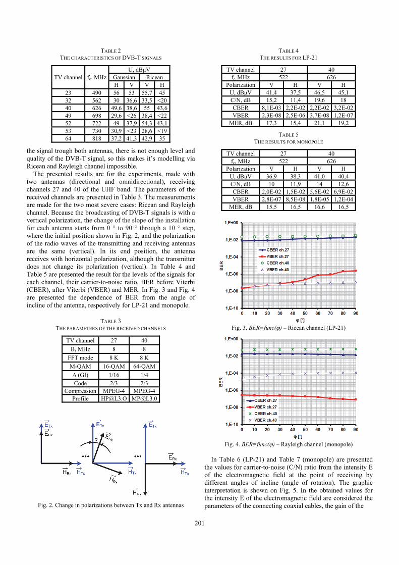
201

TABLE 2 THE CHARACTERISTICS OF DVB-T SIGNALS

TV channel fc, MHz U, dBμV

Gaussian Ricean H V V H

23 490 56 53 55,7 4532 562 30 36,6 33,5 <2040 626 49,6 38,6 55 43,649 698 29,6 <26 38,4 <2252 722 49 37,9 54,3 43,153 730 30,9 <23 28,6 <1964 818 37,2 41,3 42,9 35

the signal trough both antennas, there is not enough level and quality of the DVB-T signal, so this makes it’s modelling via Ricean and Rayleigh channel impossible.

The presented results are for the experiments, made with two antennas (directional and omnidirectional), receiving channels 27 and 40 of the UHF band. The parameters of the received channels are presented in Table 3. The measurements are made for the two most severe cases: Ricean and Rayleigh channel. Because the broadcasting of DVB-T signals is with a vertical polarization, the change of the slope of the installation for each antenna starts from 0 ° to 90 ° through a 10 ° step, where the initial position shown in Fig. 2, and the polarization of the radio waves of the transmitting and receiving antennas are the same (vertical). In its end position, the antenna receives with horizontal polarization, although the transmitter does not change its polarization (vertical). In Table 4 and Table 5 are presented the result for the levels of the signals for each channel, their carrier-to-noise ratio, BER before Viterbi (CBER), after Viterbi (VBER) and MER. In Fig. 3 and Fig. 4 are presented the dependence of BER from the angle of incline of the antenna, respectively for LP-21 and monopole.

TABLE 3 THE PARAMETERS OF THE RECEIVED CHANNELS

TV channel 27 40

B, MHz 8 8

FFT mode 8 K 8 K

M-QAM 16-QAM 64-QAM

Δ (GI) 1/16 1/4 Code 2/3 2/3

Compression MPEG-4 MPEG-4 Profile [email protected] [email protected]

Fig. 2. Change in polarizations between Tx and Rx antennas

TABLE 4 THE RESULTS FOR LP-21

TV channel 27 40fc, MHz 522 626

Polarization V H V HU, dBμV 41,4 37,5 46,5 45,1C/N, dB 15,2 11,4 19,6 18CBER 8,1E-03 2,2E-02 2,2E-02 3,2E-02VBER 2,3E-08 2,5E-06 3,7E-08 1,2E-07

MER, dB 17,3 15,4 21,1 19,2

TABLE 5 THE RESULTS FOR MONOPOLE

TV channel 27 40fc, MHz 522 626

Polarization V H V HU, dBμV 36,9 38,3 41,0 40,4C/N, dB 10 11,9 14 12,6CBER 2,0E-02 1,5E-02 5,6E-02 6,9E-02VBER 2,8E-07 8,5E-08 1,8E-05 1,2E-04

MER, dB 15,5 16,5 16,6 16,5

Fig. 3. BER=func() – Ricean channel (LP-21)

Fig. 4. BER=func() – Rayleigh channel (monopole)

In Table 6 (LP-21) and Table 7 (monopole) are presented

the values for carrier-to-noise (C/N) ratio from the intensity E of the electromagnetic field at the point of receiving by different angles of incline (angle of rotation). The graphic interpretation is shown on Fig. 5. In the obtained values for the intensity E of the electromagnetic field are considered the parameters of the connecting coaxial cables, the gain of the

202

TABLE 6 C/N AND E FOR LP-21

TV channel 27 40 fc, MHz 522 626

Polarization V H V HE, dBμV/m 50,43 46,53 57,18 55,78

C/N, dB 15,2 11,4 19,6 18

TABLE 7 C/N AND E FOR MONOPOLE

TV channel 27 40 fc, MHz 522 626

Polarization V H V HE, dBμV/m 57,96 59,46 63,73 63,13

C/N, dB 10 11,9 14 12,6

antennas, the levels of the signals and the wave length of every channel.

Constellation diagrams are presented in Fig. 6.

Fig. 5. C/N=func(E)

(a) Ricean channel

(b) Rayleigh channel

Fig. 6. Constellations

IV. CONCLUSION

By comparison of the obtained results for the two channels, received with directional and omnidirectional antennas, it is to be seen, that the data presented in table and graphic type allow the following conclusions to be made:

C/N ratio by directional antenna is in the permissible limits according to the standard ETSI (Table 1) for the two television channels with Gaussian and Ricean channels; C/N ratio by omnidirectional antenna is between 4dB and 5dB lower than the values of the standard ETSI (Table 1) for the two television channels with Rayleigh channel; For ch.27, when using a monopole antenna, the levels at horizontal polarization/position are higher than those at vertical because of the shift of the polarization from vertical to horizontal, as a result of the reflection from the buildings; the frequency is lower than this of channel 40 and the lower guard interval 1/16.

REFERENCES

[1] ETSI EN 300 744 V1.4.1 (2001-01), European Standard, Digital Video Broadcasting (DVB); Framing Structure, Channel Coding and Modulation for DTT, ETSI, 2001.

[2] A. Arifuzzaman, M. Saleh, M. Tarique, and R. Islam. “Effects of Filters on DVB-T Receiver Performance under AWGN, Rayleigh and Ricean Fading Channels”, IJCNC, vol. 5, no. 4, pp. 87-101, 2013.

[3] L. Polák, and T. Kratochvil, ”DVB-T/H Digital Television Transmission and its Simulation over Ricean and Rayleigh Fading Channels”, Elektrorevue, vol. 12, no. 6, pp. 74-1-74-7, 2010.

[4] V.P. Kalogirou, T. H.N. Velivasaki, and C.N. Capsalis, “Performance Measurements of a DVB-T System Affected by 5-MHz Generic Adjacent Channel Interference”, Progress in Electromagnetics Research C, vol. 17, pp. 1-15, 2010.

[5] I. Poole, “Antenna Polarisation or Polarization”, www.radio-electronics.com

[6] Annex A: UHF Technical Compatibility Issues, Ægis Systems Limited, 2006.

[7] S. Sadinov, P. Daneva, and P. Kogias, “Description and Simulation of OFDM Reception Process”, Journal of Engineering Science and Technology Review, Kavala, Greece, vol. 7, issue 3, pp. 18-22, 2014.

[8] T. Todorova-Sokolova, “Engineering in Public Administration”, Journal of Multidisciplinary Emgineering Science and Technology (JMEST); vol. 3, no. 5, pp. 4884-4887. Retrieved from http://www.jmest.org/vol-3-issue-5-may-2016/; JMESTN42351607, 2016.

[9] K. Konov, Digital Radio and Television Broadcasting, Dios, S., 2010.

[10] O.B. Panagiev, Handbook for Laboratory Exercises in Radio and Television Systems and Networks, Sofia, Pubishers of Technical University of Sofia, 2010.

203

Methodology for Calculation of the Outage Probability of a Free-Space Optical Communication System in the

Presence of Atmospheric Turbulence Yordan Kovachev1 and Tsvetan Mitsev2

Abstract – In this paper a method for evaluating the outage probability of FSO system using optimal system parameters is provided. It is considered the presence of moderate to strong atmospheric turbulence and random jitter in the direction of laser beam propagation. Closed form expressions for calculating the outage probability are derived.

Keywords – Random jitter, Gamma-gamma distribution, Atmospheric turbulence, Log-normal distribution, Outage probability.

I. INTRODUCTION

The more demanding telecommunication services have become; the more bandwidth they need. This constant need of increasing the channel capacity poses the question of finding new means to transfer data at high bit rates. One fairly new alternative technology is the Free-Space Optical (FSO) communication systems. It is a wireless optical technology, that can transfer information at very high speeds, close to the channel capacity of optical fiber links.

Having such high-speed communication systems, however, raises the question for their availability and respectively their outage probability. There are a lot of research papers regarding the performance of high-speed FSO systems under various conditions such as: strong atmospheric turbulence [1-4], different atmospheric visibility [5] and pointing errors [7-9].

Our previous work [10-11] presents a method for optimizing the laser beam divergence angle θt, so that the FSO system can be reliable under various atmospheric conditions. Using optimal beam divergence also compensates for the fluctuations in the laser beam direction. In this paper we will show a method for evaluation of such FSO system in the presence of atmospheric turbulence.

From here on the paper is structured as follows: II. Calculation of the optimal divergence of a gaussian beam, III. Methodology for calculating the outage probability of FSO in the presence of atmospheric turbulence and IV Conclusion.

II. CALCULATION OF THE OPTIMAL DIVERGENCE

OF A GAUSSIAN BEAM

Fig. 1 shows the basic parameters of a free-space optical system:

Fig. 1. FSO link and system parameters

The transmitter (TA) and the receiver (RA) antennas are aligned. The distribution of the optical radiation intensity I(ρz, z) in the plane z = const depends mainly on the phase and amplitude distribution of the field in the transmitting antenna. We accept equiphase and Gaussian amplitude distribution. The optical power radiated by the laser source is ФL, whereas Фt and Фr are the optical fluxes at TA and RA. Optical power at the entrance of the photodetector is represented with Фpd. I(0, z) is the optical radiation intensity along the axis of the antenna. Diagram width of the receiving antenna is 2θr. The radius of the Gaussian laser beam is represented by ρz and is defined by:

2

,0,

e

zIzI z (1)

Equation (1) is also used to define the divergence θt of the radiation in the far field region. Losses in the transmitter and receiver antenna are denoted with τt and τr, while τa is the transparency of the atmospheric channel.

Radial distribution of the optical radiation intensity in the plane z = const, in which receiving aperture is situated, is shown in Fig. 2.

1Yordan Kovachev is with the Faculty of Telecommunications atTechnical University of Sofia, 8 Kl. Ohridski Blvd, Sofia 1000,Bulgaria, E-mail: [email protected]

2Tsvetan Mitsev is with the Faculty of Telecommunications atTechnical University of Sofia, 8 Kl. Ohridski Blvd, Sofia 1000,Bulgaria. E-mail: [email protected]

204

Fig. 2. Radial distribution of the intensity in a plane z = const for two values of the divergence of the optical radiation θt

The intensity Imin, corresponds to the minimal optical power through RA, respectively the minimal Фpd, for which the FSO system works reliably, with bearable bit error ratio (BER). It also defines the optimal magnitudes of the optical beam divergence angle θt, opt and the corresponding beam radius, ρz,

opt, which allows for maximal angular deviation θmax (and the corresponding linear shifts ρmax) of the optical beam axis from its original direction. These misalignments can be consequence of unstable foundations on which the antennas are mounted, building sway, pointing errors or large scale turbulent eddies.

In order to calculate optimal beam divergence angle and radius, we first need to find the minimal power in the entrance of the photodetector, that allows the FSO system to work reliably (corresponding to reasonable BER). We can calculate Фpd using the expression

2

1

BFbI

B

I

I2

2

I

I2

I

I2

pd

..

..2.4

....

2

1

eRR

ATk

R

CSNR

R

eCSNR

R

eCSNR

(2)

In (2) RI and η(λ0) are the integral sensitivity and the quantum efficiency of the photodetector, CI is the channel capacity. A is a constant of the receiver; RFB is the value of the resistor in the feedback of the preamplifier. The background optical flux ФB is defined by the brightness of the background radiation LλB, the transmission wavelength of the interference filter before the photodetector ΔλF, and the parameters of the receiver; radius of the aperture Rr and its angular width θr.

F2r

2rB,r

2B ..... RL (3)

Signal to noise ratio (SNR) is defined by the BER needed for the particular use case [14]

22erfc

2

1 SNRBER (4)

According to Gaussian beam theory the intensity distribution in the far-field region, in which the receiver is placed is defined by

z

zIzIz2

2

2exp,0, (5)

The optical radiation along the axis of the laser beam is

z.

.z,S,..z,I a

2z

LM0t20

(6)

When ρ = ρmax the optical radiation intensity I = Imin, i.e.

z

zIIz2

2max

min 2exp,0 (7)

From (6) and (7) the equation for ρmax can be derived:

min22

z

Latmax

)1.(.

...2ln

2

1

Iez

(8)

The value of the laser beam radius ρz for which FSO can bare the extreme magnitudes of the linear shifts is

7183,2e,e..

...2

min

Latopt,

Izz

(9)

Imin is calculated by the condition

2rr

constpd

min

.. RI SNR

(10)

Having the expressions (2), (8) and (9), and knowing, that, θt = ρz/z, we can easily derive the expression for optimal beam divergence angle, θt,opt.

205

III. METHODOLOGY FOR CALCULATING THE

OUTAGE PROBABILITY OF FSO IN THE PRESENCE

OF ATMOSPHERIC TURBULENCE

A. Channel Model

It is well known that under turbulent conditions the optical intensity is redistributed. The recent studies in this field widely accept that the optical intensity is modelled with log-normal distribution in the case of weak turbulence [6, 12] and with gamma-gamma distribution, when we want to simulate moderate to strong turbulence in the atmospheric channel.

Having this in mind the intensity distribution under weak turbulence is modelled with:

2

22

σ2

2/σ/lnexp

πσ2

1)(

I

I

I

II

IIf (11)

Where σI is the scintillation index described in the Raytov theory [12] eqn (12) through eqn (18).

Under moderate to strong turbulence, the optical intensity is modelled with the gamma-gamma distribution:

I

I

I

I

IIf

αβ2

)β()α(

αβ2)( βα

12βα

2βα

(12)

Where K is the Bessel function of the second kind and n-th order. α and β are positive parameters:

,1

62.09.01

69.0151.0expβ

,1

56.018.01

49.0expα

1

6

7

5

1222

6

522

1

6

7

5

122

2

dd

d (13)

Where 6/116/722 56.0 ZkCn and ZkRd 4/2 .

Here, k is the optical wave number, λ is the wavelength and 2nC stands for the altitude-dependent index of the refractive

structure parameter and varies from 10-13 m-2/3 for strong turbulence to 10-17 m-2/3 for weak turbulence.

B. Outage Probability

Having the laser beam intensity distribution, we can define the outage probability as:

)(out thIIPP . (14)

In other words, this is the probability that the instantaneous optical intensity falls below a specified threshold. Having in mind that the FSO system is set to work with optimal beam divergence angle, this means that the intensity should not fall below Imin.. Тhe outage probability can be calculated from:

dI

I

I

I

I

IP

I

out

min

0

βα

12βα

2βα

αβ2

)β()α(

αβ2 (15)

By writing the modified Bessel function in terms of the Meijer’s G-function [13:15], we get

dII

IG

I

I

IP

I

out

min

0 2,

2

0,22,0

12βα

2βα

2βα

I

αβ

)β()α(

αβ2

(16)

We derive the closed form expression for (16) using [14] eqn (26):

21

0,22,0

2βα

2βα

2,

2,

2

αβ

)β()α(

αβ2

I

IG

I

IPout

(17)

Equation (17) is the final solution to (15) and can be used to calculate the outage probability of a free-space optical communication system.

IV. CONCLUSION

In this paper we presented a methodology for calculating the outage probability of FSO. The system is using optimal beam divergence angle, which compensates any random jitter presented in the initial laser beam direction. We’ve considered the case where the wireless optical system is working in the presence of moderate to strong atmospheric turbulence. The atmospheric channel was modelled with gamma-gamma distribution. The result of this paper is a closed form expression for calculating the outage probability of free-space optical communication system in the presence of strong turbulence.

206

As a future work we consider performing numerical simulations of the outage probability depending on various parameters like: optical power of the transmitter, distance between transmitter and receiver, channel capacity (CI) and different radius of the receiving aperture. Such study would benefit the evaluation and design of reliable free space optical systems.

REFERENCES

[1] N. A.M. Nor, Z. Ghassemlooy, S. Zvanovec, and M.R. Bhatnagar, “Comparison of Optical and Electrical based Amplifyand-Forward Relay-Assisted FSO Links over Gamma-Gamma Channels”, 10th International Symposium on Communication Systems, Networks and Digital Signal Processing (CSNDSP), 2016.

[2] N. Mishra, and D.S. Kumar, "Outage Analysis of Relay Assisted FSO Systems over K-Distribution Turbulence Channel", International Conference on Electrical, Electronics, and Optimization Techniques (ICEEOT), 2016.

[3] C. Ben Naila, A. Bekkali, K. Wakamori, and M. Matsumoto, “Performance Analysis of CDMA-Based Wireless Services Transmission Over a Turbulent RF-on-FSO Channel”, Journal of Optical Communications and Networking, vol. 3, no. 5, pp. 475-486, 2011.

[4] A. Prokes, “Modelling of Atmospheric turbulence Effect on Terrestrial FSO Link”, Radioengineering, vol. 18, no. 1, April 2009.

[5] I. Kim, and E. Korevaar, "Availability of Free-Space Optics (FSO) in Hybrid FSO/RF Systems", Proc. Optical Wireless Communications IV, SPIE 4530, November 27, 2011.

[6] A. Prokes, and L. Brancik, "Degradation of Free Space Optical Communication Performance Caused by Atmospheric Turbulence", Proc. IEEE, 2nd International Conference on

Advances in Computational Tools for Engineering Applications, pp. 338-341, 2012

[7] B. Pachedjieva, E. Ferdinandov, B. Bonev, and S. Saparev, "Influence of the Transmitters Antenna Mechanical Vibrations on Bit-Error Rate in Ground-to-Ground Free-Space, Laser Communication Systems", E+E, vol. 3-4, pp. 41-44, June 2007.

[8] N. Mohammed, A. El-Wakeel, and M. Aly,”Pointing Error in FSO Link under Different Weather Conditions”, International Journal of Video & Image Processing and Network Security, vol. 12, no. 2, pp. 6-9, 2012.

[9] J. Poliak, P. Pezzei, E. Leitgeb, and O. Wilfert. “Analytical Expression of FSO Link Misalignments Considering Gaussian Beam”, 18th European Conference on Network and Optical Communications and 8th Conference on Optical Cabling and Infrastructures, Graz, Austria, pp. 99-103, 2013.

[10] Y. Kovachev, and Ts. Mitsev, “FSO Availability Depending on the Meteorological Conditions”, 9th International Conference on Communications, Electromagnetism and Medical Applications (CEMA '14), Oct 16, 2014.

[11] Ts. Mitsev, and Y. Kovachev, “Availability of Free-Space Optical Systems Depending on Atmospheric Conditions and System Parameters”, International Journal of Wireless Communications and Networking Technologies, vol. 5, no. 3, April – May 2016.

[12] A. Prokes, “Modelling of Atmospheric Turbulence Effect on Terrestrial FSO Link”, Radioengineering, vol. 18, no. 1, April 2009.

[13] T.A. Tsiftsis, “Performance of Heterodyne Wireless Optical Communication Systems over Gamma-Gamma Atmospheric Turbulence Channels“, Electronics Letters, 28th February 2008, vol. 44, no. 5.

[14] V.S. Adamchik, and O.I. Marichev, “The Algorithm for Calculating Integrals of Hypergeometric Type Functions and its Realization in REDUCE System”, Int. Conf. on Symbolic and Algebraic Computation, Tokyo, Japan, pp. 212-224, 1990.

[15] I.S. Gradshteyn, and I.M. Ryzhik, "Table of Integrals, Series, and Products", Academic Press, New York, 2000, 6th edn.

207

Symmetry in Quasi-Static Analysis of Transmission Lines by Using Strong FEM Formulation

Žaklina Mančić1 and Vladimir Petrović2

Abstract – In the quasi-static analysis of transmission lines, symmetry should be taken into account whenever possible, in order to reduce the number of unknowns and thus the calculation time. In this paper, it is described how to include the symmetry in the calculation of quasi-static lines by using the strong FEM formulation.

Keywords – Quasi-static analysis, Finite element method, Strong FEM formulation, Symmetry, Capacitance per unit length.

I. INTRODUCTION

In recent years, the authors are paying more attention to the strong FEM formulation for analysis of electrostatic problems (Galerkin variant, [1]). While weak FEM formulation is widespread in the literature [2,3] strong FEM formulation can rarely be found and to the authors’ best knowledge, no one is researching its application to electromagnetic problems in the way that will be here briefly exposed, except the authors.

Unlike weak FEM formulation, whose basis functions have

just 0C continuity, strong formulation exploits basis functions that have continuity of both function and its first

derivative on the element boundaries ( 1C continuity). In electrostatics, this fact allows satisfaction of the boundary condition for continuity of the potential V on the boundaries between elements as well as continuity of the normal component of the vector electric displacement field ( nD ) on

the boundary between elements. By using the properties of the strong basis functions in the analysis of the symmetric structures, symmetry can be simply taken into account.

In this paper, it will be shown how to solve problems which include symmetry using strong FEM formulation considering examples of square coaxial line, shielded symmetric stripline and shielded microstrip with conducting strip of the zero thickness on the isotropic substrate. The observed examples can be solved with high accuracy. It will be shown that by taking symmetry into account, the required number of unknowns is significantly reduced while maintaining accuracy, as it could be expected. Also, we will show that in some cases it is necessary to discard some basis functions on certain finite elements in order to satisfy both boundary conditions.

FEM prodecure applied here is described in details in [4-8]. According to the FEM procedure, closed 2D domain is

divided into subdomains, finite elements of rectangular shape. Unknown potential functions of finite elements are approximated as the sum of basis functions with unknown coefficients. These basis functions are polynomials which satisfy both boundary conditions for potential continuity V

( 0C continuity) and vector nD ( 1C continuity). Potential V

is approximated as:

N

=j

jj faV1

. (1)

In this expression ja are unknown coefficients and jf are

basis functions. 2D closed domain is considered, bounded by contours 1C (where is 0V=V ) and 2C (where is

0nn D=D ,

snnn ρ=DD=D 02010 and 0=ρs ). The final system of

equations for analysis of 2D problems is [7]:

N=i,dlDw+dlwVC

=dlwfC+dSwf+dln

fεwa

C

ni

C

i

N

=j C

ij

regS

iSjSj

C

ij

2,...1,

gradεgrad

2

02

1

0

111

(2)

In Galerkin variant is ii f=w . This system of equations is

valid for both strong and weak formulation and ε is relative permittivity. C is the constant.

In the case when applied basis functions automatically (and exactly) satisfy Dirichlet’s condition (for known potential), in the previous equation 0=C should be set for finite elements which have boundary on the conductor. In these elements, the set of basis functions are limited to those which are equal to zero on the conductor surface. Next, additional basis functions which give a constant potential on the conductor surface are added to this set. In the case of node-based functions, these additional basis functions are node-based functions for nodes which are on the conductor. In the case of non node-based basis functions (as in this work), these additional functions are doublets and quadruplets [4] (Figs. 1 and 2). Then, the constant non-zero potential on conductor boundaries is provided by parts of quadruplets and doublets. The corresponding coefficients ja of these

functions are known in advance and in the system of equations all terms of that type are moved to the right-hand side. Now, when the Dirichlet’s boundary condition are automatically satisfied, the system of equations is finally:

N=i,dlDw

=dSwf+dln

fεwa

C

ni

N

=jregS

iSjSj

C

ij

2,...1,

gradεgrad

2

02

11

(3)

1Žaklina Mančić is with the Faculty of Electrical EngineeringUniversity of Niš, Aleksandra Medvedeva Niš 18000, Serbia, E-mail:[email protected]

2Vladimir Petrović is with the Robert Bosch, GmbH, Reutlingen,Germany, E-mail: [email protected]

208

The Neumann boundary condition (known nD ) is applied in

symmetrical cases, when the field is tangential to the symmetry line. In this case n 0D .

II. STRONG BASIS FUNCTIONS AND SYMMETRY

In the case of analyzed 2D problems, strong basis functions are formed as a product of one-dimensional strong basis functions which are proposed in [9].

Two-dimensional strong basis functions consist of quadruplets (Fig. 1), doublets (Fig. 2) and singlets (Fig. 3). There are four types of quadruplets; quadruplets shown in Fig. 1a provide continuity of the potential V on the boundaries between finite elements, whereas quadruplets shown in Fig. 1b and Fig. 1c provide continuity of nxD and nyD ,

respectively, while quadruplet shown in Fig. 1d provides continuity of both nxD and nyD . Quadruplets have four parts.

Fig. 1. Quadruplets for the strong FEM formulation in homogeneous media. They provide continuity (a) of V , (b) of nxD , (c) nyD , and

(d) both nxD and nyD

Fig. 2. Doublets for the strong FEM formulation

Fig. 3. Typical singlet for the strong FEM formulation

The first quadruplet in Fig. 1 can be considered as node-

based basis function. This quadruplet and its parts are used for the implementation (satisfaction) of Dirihlet’s boundary condition. The remaining quadruplets in Fig. 2 and their parts are used for satisfying Neumann boundary condition. They give rise to nD component between the four quadruplet

elements. Where, due to symmetry, is 0nD at boundaries

between the four elements, 1. quadruplet in Fig. 1d and 2. either quadruplet in Fig. 1b or the one in Fig. 1c, depending on the orientation of the symmetry line, are excluded from the set of basis function, as they give rise to nD . In this way, the

symmetry is involved in the system of equations. When the symmetry is taken into account, doublets are excluded from Fig. 2b for the same reason as for quadruplets. Singlets are not excluded from the set because 0nD is always valid on the

boundaries for them.

A. Examples

We analyze examples of square coaxial line with air dielectric, 1=εr (Fig. 4), shielded stripline with air dielectric

and zero strip thickness (Fig. 5), and shielded microstrip line with zero metal thickness (Fig. 6).

In the first example (Fig. 4) symmetry lines are denoted as contour 2 in Fig. 4b. On this contour, the field is tangential and the Neumann boundary condition 0nD is satisfied. On

the contour 1 (on the conductor) the Dirichlet’s boundary condition is satisfied.

(a)

(b) Fig. 4. (a) Square coaxial cable with air ( 1=εr )

and (b) quarter structure

For square coaxial line considered without symmetry, 3/ =ba , for the number of finite elements 288=n , required

number of unknowns in the matrice of the system is 1152=N (Fig. 4a). When the symmetry is taken into

account, Fig. 4b, it is enough to consider just a quarter of the structure, thus the number of elements is 72=n (=288/4) whereas the number of unknowns 288=N . In cases without symetry it is obtained characteristic impedance

Ω=Zc 60.375 , for , 3=n=n yx for the aforementioned

number of finite elements and Ω=Zc 60.505 , for

209

4=n=n yx . In the case when symetry is taken into account,

it is obtained Ω=Zc 60.344 , for 3=n=n yx and

Ω=Zc 60.468 for 4=n=n yx , for the aforementioned

number of finite elements (agreement of these results with benchmark solutions is already shown in [4], for 3/ =ab , benchmark solution is Ω=Zc 60.6109 . In this case some

basis functions on particular finite elements have to be discarded, in order to satisfy adequately boundary conditions (parts of quadruplets or doublets over finite elements denoted using gray color, Fig. 4b). This example has already been discussed in [4], but it is not explained how symmetry should be introduced. The emphasis of the paper [4] is placed on discussion about the convergence of the results for the characteristic impedance depending on the both number of finite elements and the order of the basis function. In previous work [5-8], the comparison of the results obtained for this as well as other similar geometries with the results obtained using different numerical methods is performed, while advantages and disadvantages of the proposed method are highlighted, too. However, the purpose of this paper is to discuss how the symmetry should be implemented to satisfy both boundary conditions. The number of finite elements (mesh density) and the order of basis function are the result of previous research of the authors, obtained by comparing the obtained results with the other methods. The same is valid for the following examples, as the structures we analyze have well-known solutions of the high accuracy.

In the second example (Fig. 5, 5/ =wa , 4/ =wb ) it is also enough to analyze just the quarter of the structure too. Inside the structure is air, 1.=εr

(a)

(b)

(c)

Fig. 5. (a) Shielded stripline with zero-thickness of the conducting strip, and (b) and (c) quarter structure

For observed geometry, software package FEMM [3] gives ΩZ c 94.2789= (for 20 nodes and 26 triangular finite

elements). Some basis functions on particular finite elements have to be discarded, in order to satisfy adequately boundary conditions, too. Such are, for example, parts of quadruplets or doublets over finite elements denoted using gray color in Fig. 5c, which have parts on two contours, so they should satisfy at the same time Dirichlet’s condition on the one edge and Neumann’s boundary condition on the other one. If it is not possible at the same time, they should be discarded from the set. For such configuration without symmetry for

1536=N unknowns and 384=n mesh elements, Ω=Zc 95.91 is obtained for 3=n=n yx order of basis

functions. When symmetry is considered for 596=N of unknowns and 96=n mesh elements, it is obtained

Ω=Zc 94.92 . For the order of basis function 4=n=n yx ,

when the symmetry is taken into consideration (the number of finite elements remains the same and it is 96=n ) the number of unknowns is raising to 1621=N while the characteristic impedance is Ω=Zc 95.808 . This small difference can be

explained by the aforementioned exclusion of some basis functions in the solution with symmetry.

As for the third example, microstrip structures with single-layered and multi-layered isotropic, biisotropic and anisotropic substrate and strip of the finite as well as zero thickness are analyzed in [5-8]. Thus, for example, for microstrip of zero thickness of the conducting strip on istotropic substrate, ( 5/ =ba , 4/ =wb ), Fig. 6a, it is enough to analyze one half of the structure (Fig. 6b).

(a)

(b) Fig. 6. (a) Shielded microstrip, 4/5,/ =wb=wa ,

and (b) half structure

210

Software package FEMM [3] gives 5442.41cZ for 20

nodes and 26 triangular finite elements. For 216=n mesh elements and 864=N unknowns, without symmetry, for the substrate of 9.3=εr it is obtained Ω=Zc 41.7298 . When the

symmetry is taken into consideration and just the half of the configuration is observed, i.e. 108=n finite elements, it is obtained Ω=Zc 41.7615 . If we consider this configuration

with the air medium, 1=εr , for 216=n mesh elements it is

obtained Ω=Z c 95.3860

while if the symmetry is taken into

consideration as in Fig. 7, i.e. if it is considered the half of geometry, 108=n mesh elements and 429=N unknowns, it is obtained

095.9188cZ = Ω . Those small differences

between results obtained with and without symmetry can also be explained by the exclusion of some of basis functions in the symmetry case. In the observed case in Fig. 5a, Fig. 5b and Fig. 6 the order of basis function is 3=n=n yx and there

are 216=n mesh elements. Besides the case of Fig. 5a where it was demonstrated that quarter of the structure is enough to take symmetry into consideration in the case of homogeneous dielectric (air in the observed case), the structure in Fig. 7 demonstrates how to take symmetry into consideration by observing the half of the structure for the same example as in the Fig. 5a.

Fig. 7. Half of structure which represents shielded stripline with air

III. CONCLUSION

As FEM has sparse matrix, it is convenient to take symmetry into account whenever it is possible as the size of the system matrix can be reduced and thus the computing time.

In this paper, it is explained how the symmetry is applied for the strong form of FEM. Because of the special (strong)

basis functions, that automatically satisfy 1C continuity, the

use of symmetry leads to exclusion of some basis function on the edges of the reduced calculation domain. Application of this method is shown in three characteristic examples. Because of the exclusion of some basis functions, small differences in results with and without symmetry was observed. It is shown on the few examples that the influence of symmetry does not significantly affect the accuracy of the results but it increases the computation speed and it significantly decreases the number of unknowns.

. s

ACKNOWLEDGEMENT

This research is supported by Serbian Ministry of Education, Science and Technological Development (Project TR-32052 MNTR).

REFERENCES

[1] J. Jin, The Finite Element Method in Electromagnetics, New York: Wiley, 1993.

[2] Z. Pantić, and R. Mittra, "Quasi TEM-Analysis of Microwave Transmission Lines by the Finite Element Method", IEEE Trans. MTT-34, pp. 1096-1103, 1986.

[3] D. Meeker, FEMM-Finite Method Magnetics, Version 4.2, Oktober 16, 2010, (http://www.femm.info/wiki/HomePage)

[4] Ž.J. Mančić, and V.V. Petrović, "Strong FEM Solution for the Square Coaxial Line", TELSIKS 2009, Niš, Serbia, October 7-9, vol. 2, pp. 343-346, 2009.

[5] Ž.J. Mančić, and V.V. Petrovic, "Strong and Weak FEM Formulations of Higher Order for Quasi-Static Analysis of Shielded Planar Transmission Lines", Microwave and Optical Technology Letters, vol. 53, no. 5, pp. 1114-1119, May 2011.

[6] Ž.J. Mančić, and V.V. Petrovic, "Strong FEM Formulation for Quasi-Static Analysis of Shielded Striplines in Anisotropic Homogeneous Dielectric", Microwave and Optical Technology Letters, vol. 54, no. 4, pp. 1001-1006, April 2012.

[7] Ž.J. Mančić, and V.V. Petrovic, "Analysis of a Square Coaxial Line with Anisotropic Substrates by the Strong FEM Formulation", Facta Universitatis. Series: Electronics and Energetics, pp. 625-636, vol. 28, no. 4, 2015.

[8] Z.J. Mancic, and V.V. Petrovic, "Quasi-Static Analysis of the Square Coaxial Cable with Tellegen Bi-isotropic Substrate by the Strong FEM Formulation", TELSIKS 2013, Niš, Serbia, October 16-19, vol. 2, pp. 513-516, 2013.

[9] V.V. Petrovic, and B.D. Popovic, "Optimal FEM Solutions of One Dimensional EM Problems", Int. J. of Numerical Modelling, vol. 14, no. 1, pp. 49-68, Jan-Feb 2001.

211

Estimation of the Carrier Phase Advance of the EM signal in the Ionosphere Using Neural Model

Zoran Stankovic1, Ivan Milovanovic2, Nebojsa Doncov1, Maja Sarevska3 and Bratislav Milovanovic2

Abstract – An alternative approach to estimate the phase advance of the carrier signal in the ionosphere using artificial neural networks is presented. A neural model was developed based on multilayer perceptron network that, from information about the latitude of the observed receiving terminal and the current point in time during the day, determines the approximate value of the concentration of ions in the ionosphere. This value is then used to estimate a phase advance of the carrier signal, during its propagation through the ionosphere. Current model architecture enables the estimation of the ionospheric carrier phase advance for the spring and autumn periods of the Mediterranean areas.

Keywords – EM propagation, Ionosphere, Neural Networks, Neural Modelling.

I. INTRODUCTION

The ionosphere is a layer of an atmosphere that contains a much higher concentration of free ions than other layers of the atmosphere. Because of this property, it represents such an electromagnetic environment that strongly influences the change in the characteristics of EM waves that pass through it [1-5]. If signals of wireless communication systems are viewed in one part of their path through the ionosphere (typical examples of the satellite communication system signals), then changes in the trajectory of the signal, changes in signal degradation, changes in the frequency of the signals, changes in the phase carrier, and changes In signal polarization [5]. These changes affect the proper operation of the aforementioned wireless systems, and the space-time characterization of these changes can be of great importance for their construction and exploitation. A typical example of the negative impact of signal changes in the ionosphere is the possibility of an error in determining the position of users on the ground using satellite navigation systems (such as the Global Positioning System - GPS) due to a change in signal degradation.

Changing the concentration of free electrons in the ionosphere dominates the change in the characteristics of the signal that extends through the ionosphere [1-5]. Therefore, the knowledge of the distribution of the electron concentration on the signal path propagation through the ionosphere is of vital importance for describing and modeling the change in the characteristics of the signal. The concentration of free

electrons in the ionosphere as well as the distribution of this value at altitude (the elevation profile of the ionosphere) depends on a large number of spatial and temporal parameters, and the most important ones are: the geographical location of the site above which the profile of the ionosphere, the seasons, the time during the day and the intensity of the sun Activities within the 11-year-old Swabian cycle.

In order to describe the functional dependence of a certain signal parameter on the concentration of an electron in the ionosphere, the volume usually represents the amount that represents the total concentration of free electrons on the path of expansion through the ionosphere or shortened TEC (Total Electron Content) [1,5]. Determining the TEC values for the desired geographical locations and the desired weather moments is a rather complex task. One approach is the use of specialized software for modeling height profiles of the ionosphere [5,6]. These software are very expensive and are generally not publicly available. The second approach is to make TEC values read from various tables and complex graphs obtained by measurements on a limited set of geographic locations using interpolation for the desired geographic location [2,6]. This method is painstaking and often imprecise.

An alternative approach to determining the TEC value that can overcome some of the problems of the above-mentioned approaches is the modeling of the spatial-temporal dependence of TEC values using artificial neural networks [7-10] as shown in [11]. There is a developed neuronal model for the prediction of additional time signal delay in the ionosphere for the winter and summer periods.

This paper is a continuation of the conducted research presented in [11]. Using the multilayer perceptron network (MLP) [7-11] which was trained to determine the TEC value during the autumn and spring period, developed a neuronal model for the Ionospheric Carrier Phase Advance.

II. NEURAL MODEL OF THE IONOSPHERIC

CARRIER PHASE ADVANCE

Ionospheric Carrier Phase Advance can be calculated using the formula [5]

][10824.4 5

TECf

(1)

where TEC is the aforementioned electron density along the signal path from the transmitter to the receiver expressed in units of electron/m2, and f is the carrier frequency is expressed in Hz. For the realization of the neural model, the dependence of the TEC value on the latitude and time of the day for the

1Zoran Stankovic and Nebojsa Doncov are with the Faculty ofElectronic Engineering, University of Nis, A. Medvedeva 14, 18000Nis, E-mail: [zoran.stankovic, nebojsa.doncov]@elfak.ni.ac.rs

2Ivan Milovanovic and Bratislav Milovanovic are with theSingidunum University, DLS center Nis, 18000 Nis,[email protected], [email protected]

3Maja Sarevska is with European University - Republic ofMacedonia (EURM), [email protected]

212

Mediterranean region obtained by the measurements in the autumn period during the mean solar activity and the solar flux of 110 (Fig. 1) were taken and measurements in the spring period in low solar activity and solar Flux of 90 (Fig. 2)

Fig. 1. Contour plots of measured TEC data vs. hours and latitude for

autumn (TEC units are in1016 elektron/m2)

Fig. 2. Contour plots of measured TEC data vs. hours and latitude for

spring (TEC units are in1016 elektron/m2)

Fig. 3. Neural model of the ionospheric carrier phase advance over the Mediterranean area

Architecture of the neural model of the ionospheric carrier phase advance over the Mediterranean area (MLP_PA – MLP Phase Advance) is presented in Fig. 3. This model models the dependence of the ionospheric carrier phase advance on the geographic latitude value of the observed site in the Mediterranean region, la, the time of the day, h, and the signal requency, f,

),,(_ fhlaf PAMLP (2)

The MLP_PA model consists of MultiLayer Perceptron (MLP) network that models the dependence of TEC values on

the geographic latitude values of the observed spot in the Mediterranean region and the time of the day

),(_ hlafTEC TECMLP (3)

and is designated in the model by the MLP_TEC block, and from the ionospheric carrier phase advance calculation block which calculates the ionospheric carrier phase advance calculation according to the equation (1) based on the estimated TEC value by the MLP_TEC network and the frequency values.

The MLP_TEC network architecture is given in Figure 4 [11]. If the MLP processing function is provided with y=y(x,W) where, x is the input vector, y is the output vector, and W is the total weight of the neural network [7-9], according to the equation (3) the input vector is x=[la, h]T, while the output output vector will be y=[TEC]. The output of the l-th hidden layer of the MLP can be represented by the vector of the yl dimension Nl 1 where Nl is the number of neurons in the l-th hidden layer, and where i-th element in that vector - yl[i] represents the output i-th neuron of the s-th network layer (s=l+1 also counting the input layer) vi

(s)=vi(l+1),

i.e. stands T)1()1(2

)1(1 ],,,[ l

Nll

l lvvv y . That vector is

)( 1 llll F bywy (4)

where yl-1 is the dimension vector Nl-1 1 and represents the output of the (l-1)-th hidden layer, wl is the matrix of the connection weight between the neurons of the (l-1)-th and l-th hidden layer dimensions Nl Nl-1, while bl Represents the bias vector of the neuron of the l-th hidden layer. In accordance with this notation, y0 represents the output of the input buffer layer, so that y0 = x. Element wl[i,j] weight matrix wl Indicates the weight of the connection between the i-th neuron in the hidden layer (l-1) and j-th neuron in the hidden layer l, i.e. between i-th neuron in the network layer s=l and j-th Neurons in the network layer s=l+1, while element bi

(l)=b[i] Represents the bias value of the i-th neuron in the hidden layer l. Function F represents the activation function of neurons in hidden layers and in the case of MLP_TEC network it is a tanges hyperbolic sigmoidal function

uu

uu

ee

eeuF

)( (5)

All neurons from the last hidden layer H are connected with the neuron of the output layer. The activation function of the neuron in the last layer is linear, and the output of the MLP_TEC network is

HoTEC yw (6)

where wo is the the weight of the connection between the neuron of the H-th hidden layer and he neuron of the output layer with dimensions of 1 NH (Fig. 4). In line with this, the weight of the network looks like this:

HoHW bbwww ,...,,,,..., 11 .

213

The general mark for this defined MLP neural model is MLPH-N1-…-Ni-…-NH where H Represents the total number of hidden layers of the MLP network used, while Ni represents the total number of neurons in the i-th hidden layer. Thus, the MLP2-12-10 designation, denotes a MLP model whose neural network has a total of four neural layers (input, output, and two hidden layers) and has 12 neurons in the first hidden layer and 10 neurons in the second hidden layer.

Fig. 4. Architecture of the MLP_TEC neural network for TEC value

estimation over the Mediterranean area [11]

III. MODELING RESULTS

For realization and training of MLP_PA model MatLab development environment was used. The model was applied to determine the ionospheric carrier phase advance for the autumn and winter period. Training for different periods was carried out for both periods MLPH-N1-…-Ni-…-NH networks where stand H = 2 and 5 Ni 22. In both cases, the Levenberg-Marquartd training method was used with a given training accuracy of 10-4. Each network was tested with an appropriate set of test samples to obtain its generalization characteristics expressed through the largest test error (WCE), the average test error (ATE), and the PPM correlation coefficient value (rPPM) [7-11].

In the autumn period, the MLP_TEC network training and testing assemblies were obtained by reading the values from the graphics in Fig. 1, at the cross-section points of the selected latitude and TEC range. In selecting the latitude value for the training set, a step of 1 in the range [34 41] so the training session had 250 samples. For the test set, a step of 2 in the range [35.5 39.5] was used, so the test set had 100 samples.

As for the spring period, using the same reading algorithm, but now in Fig. 2, training and test sets were obtained that had 233 and 90 samples respectively.

Table 1 and Table 2 show the test results for three MLP_TEC networks of autumn and winter periods respectively, which had the highest correlation coefficient value per test set. For the realization of the MLP_PA model in the autumn period, the network with the highest correlation

coefficient was selected, which is MLP2-5-5 network. According to the same principle for MLP_PA model implementation in the spring period, MLP2-10-6 network was selected. In Fig. 5, a diagram of the dissipation of the MLP2-5-5 network on the test set of the autumn period is shown, while in Fig. 6, a diagram of the dissipation of the MLP2-10-6 network is displayed on the test set of the spring period.

TABLE I TESTING RESULTS FOR THREE MLP MODELS WITH THE HIGHEST rPPM

VALUE (AUTUMN)

MLP model WCE [%] ACE [%] rPPM

MLP2-5-5 15.27 2.87 0.9897 MLP2-6-6 14.68 3.26 0.9868 MLP2-10-5 15.42 3.23 0.9863

TABLE II TESTING RESULTS FOR THREE MLP MODELS WITH THE HIGHEST rPPM

VALUE (SPRING)

MLP model WCE [%] ACE [%] rPPM

MLP2-10-6 16.14 2.87 0.9868 MLP2-5-5 15.58 2.99 0.9862 MLP2-6-6 15.82 3.16 0.9846

Fig. 5. Scattering diagram for MLP2-5-5 model (autumn, test set)

Fig. 6. Scattering diagram for MLP2-10-6 model (spring, test set)

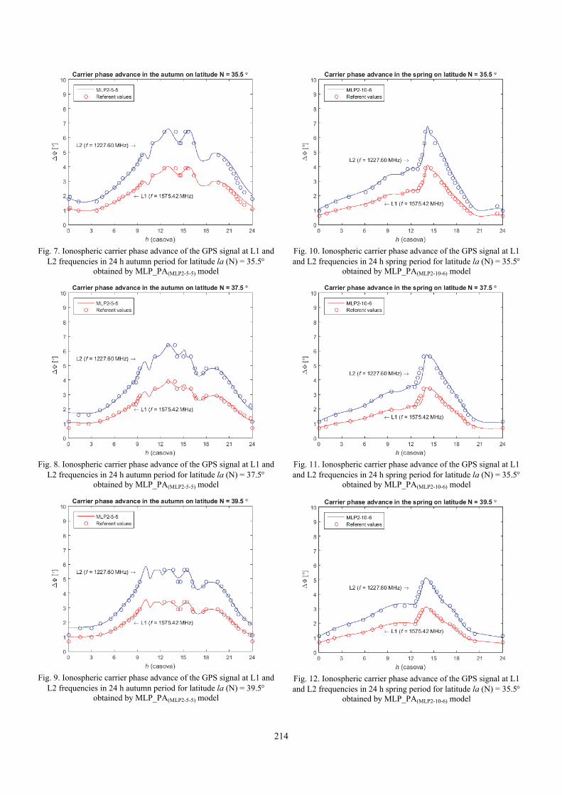
214

Fig. 7. Ionospheric carrier phase advance of the GPS signal at L1 and

L2 frequencies in 24 h autumn period for latitude la (N) = 35.5 obtained by MLP_PA(MLP2-5-5) model





Fig. 10. Ionospheric carrier phase advance of the GPS signal at L1 and L2 frequencies in 24 h spring period for latitude la (N) = 35.5

obtained by MLP_PA(MLP2-10-6) model





215

The MLP_PA model for the autumn period was realized using the trained MLP2-5-5 network and bears the mark MLP_PA(MLP2-5-5), The model for the spring period is labeled MLP_TD(MLP2-10-6) because model MLP2-10-6 of the network was used for its realization. These models are used to simulate ionospheric carrier phase advance GPS of the systems on L1 and L2 frequencies (Fig. 7-12).

Ionospheric carrier phase advance of the GPS signal at L1 and L2 frequencies in 24 h autumn period for latitude la (N) = 35.5, 37.5 and 39.5 obtained by MLP_PA(MLP2-5-5) model are shown in the Fig. 7, 8 and 9. respectively. For each longitude value, this model generated the ionospheric carrier phase advance values for a 6-minute daily period, which means at 241 points. Resaults obtained by the MLP_TD(MLP2-5-

5) model are compared with the reference values obtained by direct application of formula (1) to TEC values read from the graphics in Figure 1, it can be observed that good results are obtained by a neural model with reference values. Figures 10-12 show the values of ionospheric carrier phase advance of the GPS signal at L1 and L2 frequencies in 24 h spring period for latitude la (N) = 35.5, 37.5 and 39.5 obtained by MLP_PA(MLP2-10-6) model. Also, in this case, for each latitude, this model generates signal delay values for a daily period with a resolution of 6 min, which means at 241 points. The results obtained by the neural model were compared with the reference values obtained by reading from Fig. 2. For the spring period, a good values can be made between the obtained results with the reference values.

IV. CONCLUSION

To describe changes in the characteristics of EM waves that extend through the ionosphere, it is vital to determine the concentration of free electrons on the path of expansion through the ionosphere or TEC value. Today, for the determination of TEC values at the desired location, either complex numerical-empirical models for generating profile of the ionosphere are based on specialized software available to a narrow set of users (for example, scientific and military organizations of large countries) for geographical areas that meet their needs, Or empirical data obtained by measurements on a limited number of spatial-temporal locations around the world and which are organized through a large number of tables and graphics. Determining the TEC value by visual reading for the isocontact of the selected graphics and using manual interpolation can take a long time and can be imprecise. It is shown that the modeling of the dependence of TEC values shown in the graphs using multilayer perceptron networks can increase the speed and precision of the procedure for determining the TEC value, and therefore can automate the procedures for determining changes in the TEC

dependent parameters of the EM signal when it passes through the ionosphere.

The presented results of the application of the MLP_PA neural model for determining the ionospheric carrier phase advance for the autumn and spring period of the Mediterranean region confirm the justification of the application of models based on artificial neural networks in the process of characterizing the EM signal extending through the ionosphere. The results also confirm that the neuronal model can be a good alternative to expensive and hardware-challenging numerical models and software to describe the impact of the ionosphere on the EM wave propagation as well as slow and rough calculations based on manual use of TEC graphics.

ACKNOWLEDGEMENT

This paper is supported by the project TR-32052 and TR-32054 of the Ministry of Education in the Republic of Serbia.

REFERENCES

[1] M. Dragović, Antene i prostiranje radio talasa, Beopres, Beograd, 1996.

[2] Maja. S. Mitic, Jonosfera, Astronomski magazin, april, 2002., http://static.astronomija.co.rs/suncsist/ planete/zemlja/jonosfera/jonosfera.htm.

[3] Ž. Stevanović, "Radio-amaterske analogne KT i UKT komunikacije u Srbiji", Radioamater br. 2., 2010.

[4] T. Pratt, C.W. Bostian, J. E.Allnutt, Satellite Communications, John Wiley and Sons, 2003. god.

[5] S. Basu, J. Buchau, F.J. Rich, E.J. Weber, E.C. Field, J.L. Heckscher, P.A. Kossey, E.A. Lewis, B.S. Dandekar, L.F. McNamara, E.W. Cliver, G.H. Millman, J. Aarons, S. Basu, J.A. Klobuchar, S. Basu, M.F. Mendillo, Ionospheric Radio Wave Propagation, Chapter 10, http://www.ngdc.noaa.gov/stp/space-weather/online-publications/miscellaneous/afrl_publications/ handbook_1985/Chptr10.pdf

[6] J.A. Klobuchar and J. Aarons, Numerical Models of Total Electron Content Over Europe and the Mediterranean and Multi-station Scintillation Comparisons, INTERNATIONAL AGARD Agardograph,1973.

[7] S. Haykin, Neural Networks, New York, IEEE, 1994. [8] Q.J. Zhang, and K.C. Gupta, Neural Networks for RF and

Microwave Design, Artech House, 2000. [9] C. Christodoulou, M. Georgiopoulos, Applications of Neural

Networks in Electromagnetics, Artech House, 2001 [10] I. Milovanović, Z. Stanković, M. Agatonović, M. Milijić,

„Efficient Neural Model for Estimation of the Microwave Antenna Noise Temperature“, ICEST 2013 Conference, Ohrid, Macedonia, June 26–29, 2012, pp. 425-428.

[11] Z. Stanković, I. Milovanović, J. Jovanović, N. Dončov, B. Milovanović, “Estimation of the EM Wave Propagation Delay in the Ionosphere using Artificial Neural Networks”, YUINFO 2017 Conference, March 12-15, Kopaonik, Serbia.

216

RF Power Amplifier Linearization by Even-order Nonlinear Baseband Signals

Aleksandra Đorić1, Nataša Maleš-Ilić2 and Aleksandar Atanasković2

Abstract – This paper represents the linearization technique of RF power amplifier that exploits the second- and fourth-order nonlinear signals formed for linearization in a digital baseband domain. The combined second- and fourth-order linearization signals, adequately processed in amplitude and phase, modulate carrier second harmonic which is then injected at the input or output of the amplifier transistor. The effects of the proposed linearization method are evaluated on a single stage power amplifier for simulated QAM digitally modulated signal characterized with frequency spacing between spectral components up to 20 MHz for different input power levels.

Keywords – Linearization, Amplifier, Baseband signal, Second harmonics, Second- and fourth-order nonlinearity.

I. INTRODUCTION

The power amplifiers need to support good linearity and high power efficiency in order to meet requirements of processing high rate non-constant envelope signals. For achieving high power efficiency, the power amplifier should operate around its compression region which distorts the linearity of the output signals; therefore a significant effort has been devoted for development of the linearization techniques for the nonlinear RF and microwave power amplifiers. Different linearization methods for minimizing the nonlinear distortions of the power amplifiers have been proposed [1]-[6]: feedback, feed-forward, predistortion, technique that utilizes the even-order nonlinear signals processed in analogue domain, etc.

In the analysis carried out in [7]-[10] the proposed linearization method applies a digital processing of the baseband signal to generate the linearization signals of the second-order in order to suppress the intermodulation products of the third-order in the nonlinear amplifier. The adequately modified baseband signals formed and processed in the digital domain modulate the second harmonic of the fundamental carrier after they had been appropriately set in amplitude and phase. The linearization effects of the proposed technique have already been analysed for the single stage PA and the Doherty configurations in [8]-[10], as well as for the mixer [11].

The linearization approach presented in this paper extends

the linearization method based on a baseband signal for linearization of the second-order so that the exploitation of the signals for linearization of the second- and fourth- order that modulate the fundamental carrier second harmonics is suggested. The digital linearization signals are generated and processed in amplitude and phase in the baseband. The modulated signals at the second harmonic are then injected at the input of the amplifier transistor together with the fundamental signal or inserted at the transistor output in order to reduce the intermodulation products of the third- and fifth-order. The injected signals for the linearization and the fundamental signal are mixed due to the second order nonlinearity of the transistor generating additional third-order and fifth-order nonlinear products that may suppress the original intermodulation products caused by the transistor nonlinear characteristic.

The effects of the proposed linearization method are estimated on a single stage power amplifier for the QAM signals wherein I and Q components are single tones with frequency spacing of spectrum components from 2 MHz to 20 MHz at different input power levels. The obtained results are compared for two cases: when the second- and fourth-order nonlinear signals for the linearization are inserted only at the input of the amplifier transistor (first case) and when the second- and fourth-order nonlinear signals for the linearization are injected only at the output of the amplifier transistor (second case).

II. ANALYSIS

Theoretical analysis of the linearization approach is based on the current nonlinearity at the transistor output in the amplifier circuit, [7]-[9], which can be represented by a Taylor-series polynomial model [11]-[13].

The digitally modulated signal is characterized by the magnitude c(t), phase ( )tϕ and carrier frequency 0ω , as:

( ) = ( ) cos(ω + φ( ))0= ( ) cos(φ( )) cos(ω ) - ( ) sin(φ( )) sin(ω )0 0= ( cos(ω ) - sin(ω ))0 0

v t c t t tgsc t t t c t t tv I t Q ts (1)

where I and Q are the in-phase and quadrature-phase components of the baseband signal.

The second-order nonlinear signal of the digital signal expressed by equation (1) comprises the DC signal and signal at the second harmonic of the fundamental carrier. The I and Q components of the baseband signal required for the linearization that modulate the carrier second harmonic have the forms ( )22

2 QIIIM −= and IQIMQ 22 = , respectively.

1Aleksandra Đorić is with the Innovation centre of advanced technologies Niš, Serbia, Bulevar Nikole Tesle 61/5, 18000 Niš, Serbia, E-mail: [email protected]

2Nataša Maleš-Ilić and Aleksandar Atanasković are with the Faculty of Electronic Engineering, University of Niš, Serbia, Aleksandra Medvedeva 14, 18000 Niš, Serbia, E-mails: [natasa.males.ilic,aleksandar.atanaskovic]@elfak.ni.ac.rs

217

When the nonlinear system of the fourth-order nonlinearity is driven by the input signal expressed by equation (1), the output signal consists of DC signal, the signal components at the carrier second harmonic as well as the components at carrier fourth harmonic. The in-phase and quadrature-phase components of this fourth-order nonlinear signal at the carrier second harmonic, which is needed for the linearization, have the forms: ( )44

4 QIIMI −= and ( )2224 QIIQIMQ += ,

respectively.

Fig. 1 shows the block diagram of the amplifier with the linearization circuit that forms, processes and directs the carrier second harmonic, modulated by the modified baseband signals of the second- and fourth-order nonlinearities, at the amplifier transistor input and output.

The desired signals for linearization of the second-order, 2IMI and 2IMQ signals, are multiplied by oia for

amplitude tuning and adjusted in phase by oiθ . Also, the

amplitude and phase tuning of the fourth-order nonlinear signals for linearization, 4IMI and 4IMQ , is performed by the coefficients oib and oiϕ . Indexes i and o in subscript are

related to the signals prepared for the injection at the input and output of the amplifier transistor, respectively. The second- and fourth-order signals processed and prepared for the linearization are injected at IQ modulators with carrier frequency 0ω2 -fundamental carrier second harmonic. After that, the modulated signals (denoted as the IM2 and IM4 signals for linearization) are fed through the bandpass filter, which is characterized by the centre frequency of 0ω2 , at the amplifier transistor input together with the fundamental signal, (equation (2)) or at the output of the amplifier transistor, (equation (3)), where ( ) ( )( )tQtIvo 00 ωsinωcos − is the output signal at fundamental frequency.

( ) ( ) ( )[ ]

( ) ( ) ( )[ ]

( ) ( ) ( ) ( )[ ]tQIIQtQIijeib

tIQtQIijeia

tQtIsvtgsv

0ω2sin22

20ω2cos44

2

1

0ω2sin20ω2cos22

2

1θ

0ωsin0ωcos

+−−−

+

+−−−

+

+−=

ϕ (2)

(7)

( ) ( ) ( )[ ]

( ) ( ) ( )[ ]

( ) ( ) ( ) ( )[ ]tQIIQtQIojeob

tIQtQIojeoa

tQtIovtdsv

0ω2sin22

20ω2cos44

2

1

0ω2sin20ω2cos22

2

1θ

0ωsin0ωcos

+−−−

−

+−−−

−

+−=

ϕ (3)

The distorted current observed at the output of the amplifier when the signals for linearization of the second- and fourth-order are inserted at the amplifier transistor input can be expressed by equation (4) if the third-order intermodulation products are concerned and by equation (5) in case of the fifth-order intermodulation products.

( )

( ) ( ) ( )( )tQtIQIdmgovijeia

dmgovsvdmgovsv

mgsvijeiamgsv

ilinIMtdsi

0ωsin0ωcos22

114

1

122

4

321

2

4

3

22

13

3

4

3_3

−+−

+

+++

+−

+=

θ

θ

(4)

( )

( ) ( ) ( )( )tQtIQIdmgijeiaov

mgsvijeiadmgovij

eib

mgsvijeibmgsv

ilinIMtdsi

0ωsin0ωcos222

1222

8

1

322

8

311

4

1

22

15

5

8

5_5

−+−

+

+−

+−

+

+−

+=

θ

θϕ

ϕ

(5)

The equations (6) and (7) represents the amplifier output distorted current of the third- and fifth-order in case when the signals for linearization of the second- and fourth-order are inserted at the amplifier transistor output.

( )

( ) ( ) ( )( )tQtIQIdmgovsvdmgovsv

dmgsvojeoamgsv

olinIMtdsi

0ωsin0ωcos22

122

4

321

2

4

3

114

13

3

4

3_3

−+++

+−

−=

θ

(6)

( )

( ) ( ) ( )( )tQtIQIdmgojeoasv

dmgsvojeobmgsv

olinIMtdsi

0ωsin0ωcos222

2122

8

1

114

15

5

8

5_5

−+−

+

+−

−=

θ

ϕ

(7)

The first term in equations (4) and (6) represents the signal distorted by the cubic term of the amplifier (gm3), which is considered dominant in causing the third-order intermodulation products and spectral regrowth [12], [13]. The mixing products of the fundamental signal and IM2 signals supplied at the transistor input or output are expressed as the second and fifth terms in equation (4) and the second term in equation (6). The third and fourth terms in both equations (i.e., the mixed terms between drain and gate, gm1d2 and gm2d1) produce the drain–source current at IM3 frequencies with opposite phases so that they may be considered to cancel each other partially [13]. According to the previous analysis, it is possible to reduce spectral regrowth caused by the third-order distortion of the fundamental signal by selecting the appropriate amplitude and phase of the IM2 signals which are injected at the input or output of the amplifier transistor. In the approach presented in this paper and [7]-[9] the amplitude and phase of the IM2 signals are set on the optimal values by using DSP.

The first term in equations (5) and (7) expresses the fifth-order intermodulation products of the drain-source current of amplifier transistor. It is formed due to the amplifier nonlinearity of the fifth-order, gm5, when the fundamental

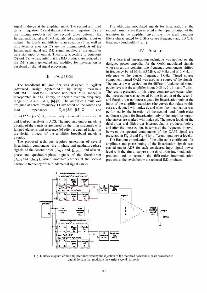
218

signal is driven at the amplifier input. The second and third terms in equation (5) and the second term in equation (7) are the mixing products of the second order between the fundamental signal and IM4 signals fed at amplifier input or output. The fourth and fifth terms in equation (5) as well as third term in equation (7) are the mixing products of the fundamental signal and IM2 signal supplied at the amplifier transistor input or output. Therefore, according to equations (5) and (7), we may infer that the IM5 products are reduced by the IM4 signals generated and modified for linearization in baseband by digital signal processing.

III. PA DESIGN

The broadband RF amplifier was designed in Agilent Advanced Design System-ADS by using Freescale’s MRF281S LDMOSFET whose non-linear MET model is incorporated in ADS library, to operate over the frequency range 0.7 GHz-1.1 GHz, [6]-[8]. The amplifier circuit was designed at central frequency 1 GHz based on the source and load impedances ( )5.5 j15 sZ = + Ω and

( )12.5 j27.5 lZ = + Ω , respectively, obtained by source-pull and load-pull analysis in ADS. The input and output matching circuits of the transistor are based on the filter structures with lumped elements and reference [6] offers a detailed insight in the design process of the amplifier broadband matching circuits.

The proposed technique requires generation of several linearization components: the in-phase and quadrature-phase signals of the second-order ( 2IMI and 2IMQ ), and also in-phase and quadrature-phase signals of the fourth-order ( 4IMI and 4IMQ ), which modulate carriers at the second harmonic frequency of the fundamental signal carrier.

The additional modulated signals for linearization at the second harmonic are then injected at the input or output of the transistor in the amplifier circuit over the ideal bandpass filters characterized by 2 GHz centre frequency and 0.5 GHz frequency bandwidth (Fig. 1).

IV. RESULTS

The described linearization technique was applied on the designed power amplifier for the QAM modulated signals whose spectrum contains two frequency components shifted in frequency by ±1 MHz, ±3 MHz, ±5 MHz and ±10 MHz in reference to the carrier frequency 1 GHz. Timed source component named QAM was used as a source of the signals. The analysis was carried out for different fundamental signal power levels at the amplifier input: 0 dBm, 3 dBm and 7 dBm. The results presented in this paper compare two cases: when the linearization was achieved by the injection of the second- and fourth-order nonlinear signals for linearization only at the input of the amplifier transistor (the curves that relate to this case are denoted with index i), and when the linearization was performed by the insertion of the second- and fourth-order nonlinear signals for linearization only at the amplifier output (the curves are marked with index o). The power levels of the third-order and fifth-order intermodulation products, before and after the linearization, in terms of the frequency interval between the spectral components of the QAM signal are presented in Fig. 3 and Fig. 4 for different input power levels.

The Random optimization of the adjustable coefficients for amplitude and phase tuning of the linearization signals was carried out in ADS for each considered input signal power level with the aim to suppress the third-order intermodulation products and to restrain the fifth-order intermodulation products at the levels below the reduced IM3 products.

Fig. 1. Block diagram of the amplifier linearized by the injection of the modified baseband signals processed in digital domain that modulate the carrier second harmonic

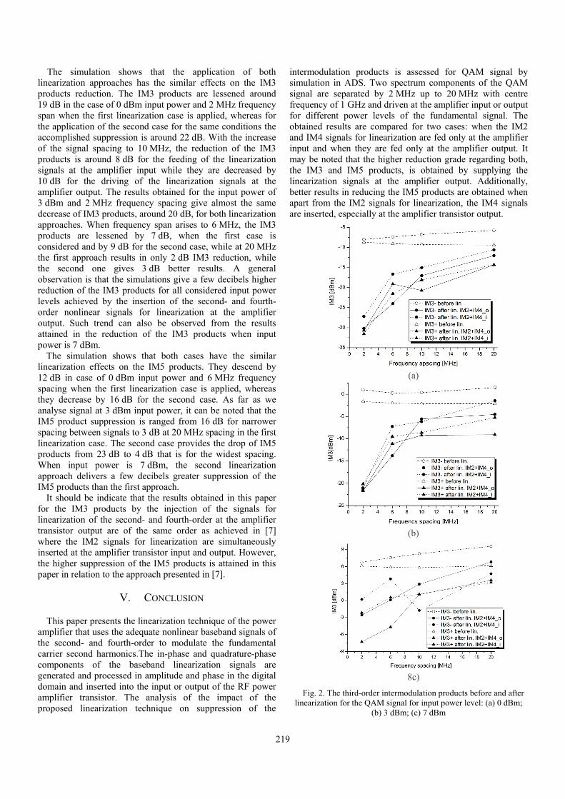
219

The simulation shows that the application of both linearization approaches has the similar effects on the IM3 products reduction. The IM3 products are lessened around 19 dB in the case of 0 dBm input power and 2 MHz frequency span when the first linearization case is applied, whereas for the application of the second case for the same conditions the accomplished suppression is around 22 dB. With the increase of the signal spacing to 10 MHz, the reduction of the IM3 products is around 8 dB for the feeding of the linearization signals at the amplifier input while they are decreased by 10 dB for the driving of the linearization signals at the amplifier output. The results obtained for the input power of 3 dBm and 2 MHz frequency spacing give almost the same decrease of IM3 products, around 20 dB, for both linearization approaches. When frequency span arises to 6 MHz, the IM3 products are lessened by 7 dB, when the first case is considered and by 9 dB for the second case, while at 20 MHz the first approach results in only 2 dB IM3 reduction, while the second one gives 3 dB better results. A general observation is that the simulations give a few decibels higher reduction of the IM3 products for all considered input power levels achieved by the insertion of the second- and fourth-order nonlinear signals for linearization at the amplifier output. Such trend can also be observed from the results attained in the reduction of the IM3 products when input power is 7 dBm.

The simulation shows that both cases have the similar linearization effects on the IM5 products. They descend by 12 dB in case of 0 dBm input power and 6 MHz frequency spacing when the first linearization case is applied, whereas they decrease by 16 dB for the second case. As far as we analyse signal at 3 dBm input power, it can be noted that the IM5 product suppression is ranged from 16 dB for narrower spacing between signals to 3 dB at 20 MHz spacing in the first linearization case. The second case provides the drop of IM5 products from 23 dB to 4 dB that is for the widest spacing. When input power is 7 dBm, the second linearization approach delivers a few decibels greater suppression of the IM5 products than the first approach.

It should be indicate that the results obtained in this paper for the IM3 products by the injection of the signals for linearization of the second- and fourth-order at the amplifier transistor output are of the same order as achieved in [7] where the IM2 signals for linearization are simultaneously inserted at the amplifier transistor input and output. However, the higher suppression of the IM5 products is attained in this paper in relation to the approach presented in [7].

V. CONCLUSION

This paper presents the linearization technique of the power amplifier that uses the adequate nonlinear baseband signals of the second- and fourth-order to modulate the fundamental carrier second harmonics.The in-phase and quadrature-phase components of the baseband linearization signals are generated and processed in amplitude and phase in the digital domain and inserted into the input or output of the RF power amplifier transistor. The analysis of the impact of the proposed linearization technique on suppression of the

intermodulation products is assessed for QAM signal by simulation in ADS. Two spectrum components of the QAM signal are separated by 2 MHz up to 20 MHz with centre frequency of 1 GHz and driven at the amplifier input or output for different power levels of the fundamental signal. The obtained results are compared for two cases: when the IM2 and IM4 signals for linearization are fed only at the amplifier input and when they are fed only at the amplifier output. It may be noted that the higher reduction grade regarding both, the IM3 and IM5 products, is obtained by supplying the linearization signals at the amplifier output. Additionally, better results in reducing the IM5 products are obtained when apart from the IM2 signals for linearization, the IM4 signals are inserted, especially at the amplifier transistor output.

(a)

(b)

8c)

Fig. 2. The third-order intermodulation products before and after linearization for the QAM signal for input power level: (a) 0 dBm;

(b) 3 dBm; (c) 7 dBm

220

(a)

(b)

(c)

Fig. 3. The fifth-order intermodulation products before and after linearization for the QAM signal for input power level: (a) 0 dBm;

(b) 3 dBm; (c) 7 dBm

ACKNOWLEDGEMENT

This work was supported by the Ministry of Education, Science and Technological Development of Republic of Serbia; the project number III-44009.

REFERENCES

[1] P. Kenington, High-Linearity RF Amplifier Design, Artech House, Chapters 4-6, pp. 135-423, 2000.

[2] S. Cripps, RF Power Amplifiers for Wireless Communications, Artech House, Chapter 9, pp. 251-282, 1999.

[3] M.K. Kazimierczuk, RF Power Amplifiers, Wiley, Chapter 9, pp. 321-343, 2008.

[4] N. Mizusawa, and S. Kusunoki, “Third- and Fifth-order Baseband Component Injection for Linearization of the Power Amplifier in a Cellular Phone”, IEEE Transactions on Microwave Theory and Techniques, vol. 53, no. 11, pp. 3327-34, 2005.

[5] N. Males-Ilić, B. Milovanović, and Đ. Budimir, “Effective Linearization Technique for Amplifiers Operating Close to Saturation”, International Journal of RF and Microwave Computer-Aided Engineering, vol. 17, no. 2, pp. 169-78, 2007.

[6] A. Đorić, N. Males-Ilić, A. Atanasković, and B. Milovanović, “Linearization of Broadband Microwave Amplifier”, Serbian Journal of Electrical Engineering, vol. 11, no. 1, pp. 111-120, February 2014.

[7] A. Atanasković, N. Males-Ilić, K. Blau, A. Đorić, and B. Milovanović, “RF PA Linearization using Modified Baseband Signal that Modulates Carrier Second Harmonic”, Microwave Review, Vol. 19, No.2, pp. 119-124, December 2013.

[8] A. Đorić, N. Maleš-Ilić, and A. Atanasković, “RF PA Linearization by Signals Modified in Baseband Digital Domain“, Facta Universitatis, Series: Electronics and Energetics, vol. 30, no. 2, June 2017.

[9] A. Đorić, N. Males-Ilić, A. Atanasković, and V. Marković, “Linearization of Broadband Doherty Amplifier by Baseband Signal that Modulates Second Harmonic”, Eurocon 2017, Ohrid, Macedonia, 6-8 July 2017.

[10] A. Đorić, N. Maleš-Ilić, A. Atanasković, and B. Milovanović, “Mixer Linearization by Modified Baseband Signals”, Sinteza 2016, Belgrade, Serbia, pp. 299-303, 22 April 2016.

[11] J.C. Pedro, and J. Perez, “Accurate Simulation of GaAs MESFET's Intermodulation Distortion using a New Drain-source Current Model”, IEEE Trans. Microw. Theory Techn., vol. 42, pp. 25-33, January 1994.

[12] J.P. Aikio, and T. Rahkonen, “Detailed Distortion Analysis Technique based on Simulated Large-signal Voltage and Current Spectra”, IEEE Trans. Microw. Theory Techn., vol. 53, pp. 3057-3065, 2005.

[13] A. Heiskanen, J. Aikio, and T. Rahkonen, “A 5th Order Volterra Study of a 30W LDMOS Power Amplifier, International Symposium on Circuits and Systems - ISCAS'03, Bangkok, Thailand, vol. 4, pp. 616-619, May 2003.

221

One Possibility to Increase the Scope for Radar Module HB100 and Fields of Application Peter Z. Petkov1, Rosen Vitanov2 and Ivaylo Nachev3

Abstract – This paper presents modification that extends the

range of HB100 radar module. It is a typical example of doppler radar and consists of Dielectric Resonator Oscillator (DRO), microwave mixer and patch antennas. Disadvantage is the low gain stock antennas have and thus become non-functional for use on large areas. An antennas that increase its coverage are proposed in this article, thus extending applications of this radar - to control flight of drones and other unmanned vehicles.

Keywords – Radar, Antenna, Patch antenna, Patch array.

I. INTRODUCTION

In the last years doppler radars fоund a wide application in intelligent systems and devices. Development of new technologies made it possible to minimize weight, dimensions, power consumption and also improve their overall performance. Proposed design replaces the integrated patch antennas of the radar module with a series fed patch array with a higher gain. The antenna of the radar HB-100 has low gain - approximately 1-2dBi, (assumed 1,5dB) at an operating frequency of 10.525GHz [1]. Fig. 1 shows structure of a series fed patch array developed for to achieve larger coverage of the Doppler signal.

Fig. 1. Series fed patch array – simulation model

1Peter Petkov is Associate Professor with the Faculty of

Telecommunications at Technical University of Sofia, 8 Kl. Ohridski Blvd, Sofia 1000, Bulgaria, E-mail: [email protected].

2Rosen Vitanov is PhD student with the Faculty of Telecommunications at Technical University of Sofia, 8 Kl. Ohridski Blvd, Sofia 1000, Bulgaria, E-mail: [email protected]

3Ivaylo Nachev is a student at Faculty of Telecommunications at Technical University of Sofia, 8 Kl. Ohridski Blvd, Sofia 1000, Bulgaria, E-mail: [email protected]

Microstrip antenna array consists of many space separated independent radiating slots – horn, dippol, microstrip lane. Their advantages over traditional antennas are: low cost in serial production, construction resistant to shock and vibration, different types of design, big gain (up to 10 dBi per patch) and other microwave equipment can be integrated in patch array construction [2].

II. SERIES FED PATCH ARRAY DESIGN

An important step when designing patch antenna is to take into account dielectric substance on which patches are made. The employed substrate for the proposed design is Rogers RO 4003 with thickness h=0.508mm and dissipation factor tanδ = 0.00027 [3]. In order to improve the bandwidth and efficiency of antennas, a design method called “suspended substrate” is chosen, where the thickness of the gap between ground plane and antenna is ∆=1mm. In this method we use the equivalent dielectric constant (1.7). Distribution of the elements of the simulated model, as with radars frequency ƒс = 10.525GHz we have wavelength λ = 28.50mm, and λg = 22.6150mm. For calculation of antenna dimensions a straightforward basic algorithm is proposed: Step 1: Calculation of width (W): Width of the Micro strip antenna is given by the equation:

1

2112.2208 1

2 2r

c

ε +c WW = = mm, >

f h

, (1.1)

where c is the speed of the light c=3*108, rε is a dielectric

constant of substrate, cf is radar frequency and h is substrate

thickness. Step 2: Calculation of Effective Length (L): Length of the microstrip radiator is given by:

2 c eff

cL =

f , (1.2)

where cf is radar frequency and effε is effectively dielectric

constant of substrate. Step 3. Calculation of the Length extension (Lext): The actual length is obtained by the equation (accounting for the fringing fields):

0.3 0.264

0.412 0.88250.258 0.8

ext

W

hL h mm

W

h

. (1.3)

222

Step 4: Calculation of the actual length of the Patch (L): The actual length of the patch is given by:

2 12.9650eff extL = L+ L = mm . (1.4)

Determination of effective dielectric permittivity eff :

0.5

1 11 10 1.5886

2 2r r

eff

ε + ε hε = + + = mm

w

. (1.5)

The length of the guided wave:

g

eff

λλ =

. (1.6)

Influence of the gap is taken into account:

1.72r

eqr

ε h+ε = = mm

ε h+

, (1.7)

where rε is a dielectric constant of substrate and is a the

thickness of the gap. The connection between designed antenna and a radar module is established by using SMA connectors with characteristic impedance Z0=50 Ω. To determine the width for micro strip line a method suggested by Wheeler и Schneider [4] is used. By these methods width of the micro strip lines is calculated to be 5.3010 mm. The length of microstrip line is half the wavelength λg/2 and feed line is a quarter of the wavelength λg/4.

To determine the dimensions of the antenna Eqs. (1.1) - (1.6) are used with electromagnetic simulator, a model of the proposed antenna was synthesized using the results from the calculations above. The CAD tool gives the opportunity for fine tune of the design and determination of the actual size of antenna components for given operating frequency. The final results is shown in Fig. 2.

Fig. 2. Distribution of the elements of the simulated model

In Table 1 are presented the values obtained for dimensions of the antenna components.

TABLE 1 VALUES OBTAINED FOR DIMENSIONS OF THE ANTENNA COMPONENTS

W

[mm] L [mm]

w [mm]

Microstrip line [mm]

Feed line [mm]

Calculated 12.2 12.96 5.3 12.4 6.2 After

simulation 13.1 11.0 5.3 12.4 6.2

In Fig. 3 is displayed the return loss of the antenna. Figs. 4a

and 4b display the polar radiation pattern of the designed patch array compared which HB-100 stock antennas. Fig. 5 shows directivity in 3D pattern. In Figs. 5a and 5b, the radiation pattern of proposed array is displayed in Cartesian coordinate system. The gain is 15.14d Bi, which corresponds to 32.65 times amplification. Results of Table 2 show the comparison with integrated manufacturer antennas and designed in this publication.

TABLE 2 COMPARISON WITH INTEGRATED MANUFACTURER ANTENNAS AND

DESIGNED IN THIS PUBLICATION

Gain dBi linear HB 100 antennas 1.5 1.41 Proposed patch array 15.14 32.65

Results show that this design method and using dielectric

substrate RO4003, gain increases significantly and thus increasing the radius of operation /range/ and selectivity of the radar.

Fig. 3. Antenna bandwidth (S11)

223

Fig. 4a. Comparison between patch array and HB100 antennas in azimuth plane

Fig. 4b. Comparison between proposed patch array and HB100 antenna in elevation plane

Fig. 5a. Radiation Pattern azimuth

Fig. 5b. Radiation Pattern elevation

III. CONCLUSION

Modifying HB100 in this article showed multiple increase in its scope and for this purpose a modern method for a patch array desing is used (Table 2). The modified device is fully functionally and may be integrated on real devices.

REFERENCES

[1] HB100 datasheet. https://www.limpkin.fr/public/HB100/HB100_Microwave_Sensor_Module_Datasheet.pdf

[2] R. Bancroft, Microstrip and Printed Antenna Desing, Second Edition, 2009.

[3] Rogers RO4003 specification, https://www.rogerscorp.com/documents/726/acm/RO4000-Laminates---Data-sheet.pdf.

[4] K. Chang, RF and Microwave Wireless Systems, 2000. [5] M. Gachev, Microstrip Schemes, ISBN 978-954-580-298-0.

224

Circular Patch Antenna with Arced Slots Analyzed by the Cylindrical TLM Solver

Jugoslav Joković, Tijana Dimitrijević, and Nebojša Dončov

Abstract – A coax-fed microstrip patch antenna of a circular geometry containing two arc-shaped slots within a radiated patch has been designed using the in-house solver based on the TLM method adjusted to the cylindrical grid. Its performances have been analysed with regards to the classic circular patch antenna. The antenna exhibits a dual-frequency operation, where the upper frequency can be easily controlled by adjustments of the arc–shaped slots dimensions.

Keywords – TLM method, Cylindrical mesh, Circular patch antenna, Dual frequency operation.

I. INTRODUCTION

Microstrip and printed circuit antennas have gained prominence over the past decades as viable and desirable antenna elements and arrays. The interest in these antennas stems directly from advantages such as low profile, low cost, light weight, conformity to surface, mass production, dual-frequency operation possibilities and direct integrability with microwave circuitry. There are some limitations, however, principally in characteristics such as low gain and narrow bandwidth [1,2].

Dual-band antennas have received much attention for application in mobile communications systems and radar applications. Dual-frequency operation can be obtained by using several techniques: multilayer structures, parasitic elements coupled to the main patch, aperture coupled parallel resonators, log-periodic or quasi-log-periodic structures [3,4]. All of these structures might face problems with design and manufacture stages while the overall size is considerably larger than that of the patch. Similarly, stagger-tuned resonators, reactively loaded patches with short pins, varactor diodes or optically controlled pin diodes can also be used to either increase the bandwidth or perform dual frequency operation. However, it might be difficult to accommodate the diodes or pins underneath the patch which has to be small for high frequencies. Likewise, the resonant frequency of a microstrip patch antenna is possible to be tuned by an adjustable air gap between the substrate and the ground plane. Complications that might emerge are: mechanical change of the air-gap height and it is difficult to design an array consisting of a large number of elements, [5].

In addition to all these attempts made to improve the frequency agility of patch antennas, the main demands for applications in mobile communications systems is to obtain a

dual-frequency patch antenna without increasing either its size or height. One of the approaches to achieve dual band operation is to embed a pair of arc-shaped slots close to the radiating edge of a microstrip antenna [6]. Such configuration does not increase the size of the antenna and at the same time provides flexibility in changing the frequency of operation by proper choice of the slots parameters.

Generally, patch antennas can be analyzed either by approximate techniques (the cavity model, the transmission-line model etc.) [1,7] or by numerical full-wave methods. Besides simplification of the problem by using certain assumptions, the approximate techniques cannot be applied to the structures of complex geometry, such as for instance the circular patch containing sectoral or arced slots. Hence, the full-wave methods are inevitable to be used. Among them, the Transmission-Line Matrix (TLM) method is one of the most accurate and versatile [8]. However, commercial software packages that use the TLM method for electromagnetic (EM) field analysis are generally developed in the rectangular coordinate system. In accordance with this, complications emerge: staircase approximation of the circular/cylindrical boundaries and associated numerical errors, limitations of the coaxial feed radius, difficulties with creating the model containing sectoral and arced slots etc. To achieve better conformity of the mesh, which is highly associated with the accuracy of the results, and to overcome limitations of the rectangular TLM approach, the authors of this paper propose usage of the TLM method developed in the orthogonal polar mesh for modelling and analysis of structures of circular/cylindrical geometry [9].

In this paper, in-house solver based on the TLM method adjusted to the cylindrical grid and enhanced with the compact wire model is used as a tool for design and analysis of the single-feed circular patch antenna with two arc-shaped slots. In addition to better accommodation of the cylindrical mesh to the analyzed structure, the efficiency of the cylindrical solver will be compared with the rectangular one, in terms of the number of cells required for simulation and limitations .

II. CYLINDRICAL TLM SOLVER

The TLM method is a time-domain numerical technique used for solving various problems in electromagnetic engineering. It uses the network of interconnected link-lines to model EM field in a propagation space through scattering and connection of voltage pulses [1].

To overcome limitations associated with the TLM algorithm developed in the rectangular coordinate system, which is generally exploit by commercial available software packages, an in-house TLM solver has been realized in a

Authors are with the Faculty of Electrical Engineering, University of Nis, Aleksandra Medvedeva 14, 18000 Nis, Serbia, E-mail: [email protected], [email protected],[email protected]

225

cylindrical coordinate system [9]. The solver generates an orthogonal polar mesh consisting of TLM cells known as hybrid symmetrical condensed nodes (HSCN), given in Fig.1 [10]. The compact wire model [11] has been adjusted to the cylindrical grid and embedded into the solver allowing for modelling of wire elements within the considered structure. It is actually a wire network interposed over the existing network which consists of additional link and stub lines to account for increased capacitance and inductance caused by the wire presence.

The solver enables adequate description of an inhomogeneous media, which in case of patch antennas allows for modelling of a substrate. Likewise, modelling of three types of boundaries has been also enabled: electric wall, magnetic wall and absorbing wall. Since the patch antenna represents an open problem, it is necessary to extend the area to be modelled to take into account fringing field associated with the patch edges. The external boundary is then described as absorbing, while the ground plane and the radiated patch are defined as perfectly conducted boundaries. A coaxial feed attached between the ground plane and the circular patch is used as an excitation, where a voltage source is connected to the coaxial feed through the so-called wire port. Because of the pulses propagation through different material properties, the mesh is requested to be relevantly chosen to maintain a time synchronism.

After determination of the link and stub lines impedances as well as wire nodes impedances, the 3DTLMcyl_cw algorithm goes through the next stages: problem definition and imposing initial conditions, equivalent voltages and currents calculation for each node (EM field components can be calculated as well), scattering procedure for regular and wire nodes, connection procedure for regular and wire nodes, modification of the connection procedure at boundaries, calculation of the current induced in the probe wire (output result) in the time domain, transforming data into the frequency domain, calculation of S parameters or input impedance.

III. RESULTS AND DISCUSSION

To explore an effect of adding the arc-shaped slots to the radiated patch, a coax-fed circular patch antenna has been first analyzed by 3DTLMcyl_cw solvers in cylindrical and rectangular grid (Fig. 2). Fig. 3. illustrates the magnitude of the S11 parameter of the single-feed classic circular patch antenna realized on the FR4 substrate. A radius of the radiated patch equals to 20 mm, and that of a ground plane is 30 mm. A probe feed for excitation is optimized to provide an impedance matching betwwen the antenna and the feed and it equals 7.5 mm. As can be seen, a resonant frequency of the excited TM11 mode is equal to 2.075 GHz, while TM12 mode is excited at 4.24 GHz. A good agreement between results obtained in cylindrical and rectangular solvers is achieved.

When the above CP antenna is modified by inserting two arc-shaped slots, a dual-frequency antenna is obtained. The layout of the dual-band circular patch antenna which includes two arc-shaped slots discussed above is shown in Fig. 4. The circular patch has a diameter of a = 20 mm, and is printed on a FR4 substrate of thickness h = 1.5mm, and relative permittivity ɛr = 4.2. The two arc-shaped slots, having a narrow width w = 1 mm and subtended by an angle Ɵ, are placed close to the boundary of the circular patch with a distance of s = 1 mm. Also, the two arc-shaped slots are centered with respect to the r-axis. A single probe feed for dual-frequency operation is placed along the r-axis with a distance ρ = 7.5 mm away from the patch center. In order to find an optimum location for matching the impedance of the feeding line the parametric analysis using in-house 3DTLMcyl_cw software has been carried out.

Since the circular radiated patch surface is modified by embedding a pair of slots close to the boundary, where the excited patch surface current for the TM11 mode has a minimum value, the resonant frequency f1 will be slightly changed. On the other hand, another resonant mode that is excited in the considered design is the TM12 mode for which the excited patch surface current has a maximum value close to the patch boundary. As a result, the resonant frequency f2 of TM12 mode might be significanly decreased by the introduction of the narrow slots close to the patch edges. This effect is investigated for various angle Ɵ and illustrated in Fig. 5. As can be seen, the first resonant frequency remains almost the same, whereas the second resonant frequency decreases with rising angle Ɵ. The corresponding resonant frequency values and bandwidths, determined from 10dB return loss, for all considered cases are compared in Table I.

To compare efficiency of the 3DTLMcyl_cw solver to the corresponding solver in the rectangular grid, the considered antenna configuration has been also simulated by the rectangular TLM solver. Obtained simulated reflection coefficients for different mesh resolution (1mm, 0.5mm, and 0.66mm) are plotted in Fig. 6. Aparently, the mesh of higher resolution, and consequently greater number of cells, has to be used to reach satisfactory accuracy. Additionally, a wire radius has to be decreased with reducing the cell sizes.

r

z

VrpzVznrVrpφ

Vznφ

Vφpz

Vφpr

Vφnr

Vφnz

Vrnz

Vrnφ

Vzpφ

Vzpr

φ

z

r

φ

Co

r

Co

φ

Co

z

Fig. 1. HSCN cylindrical node

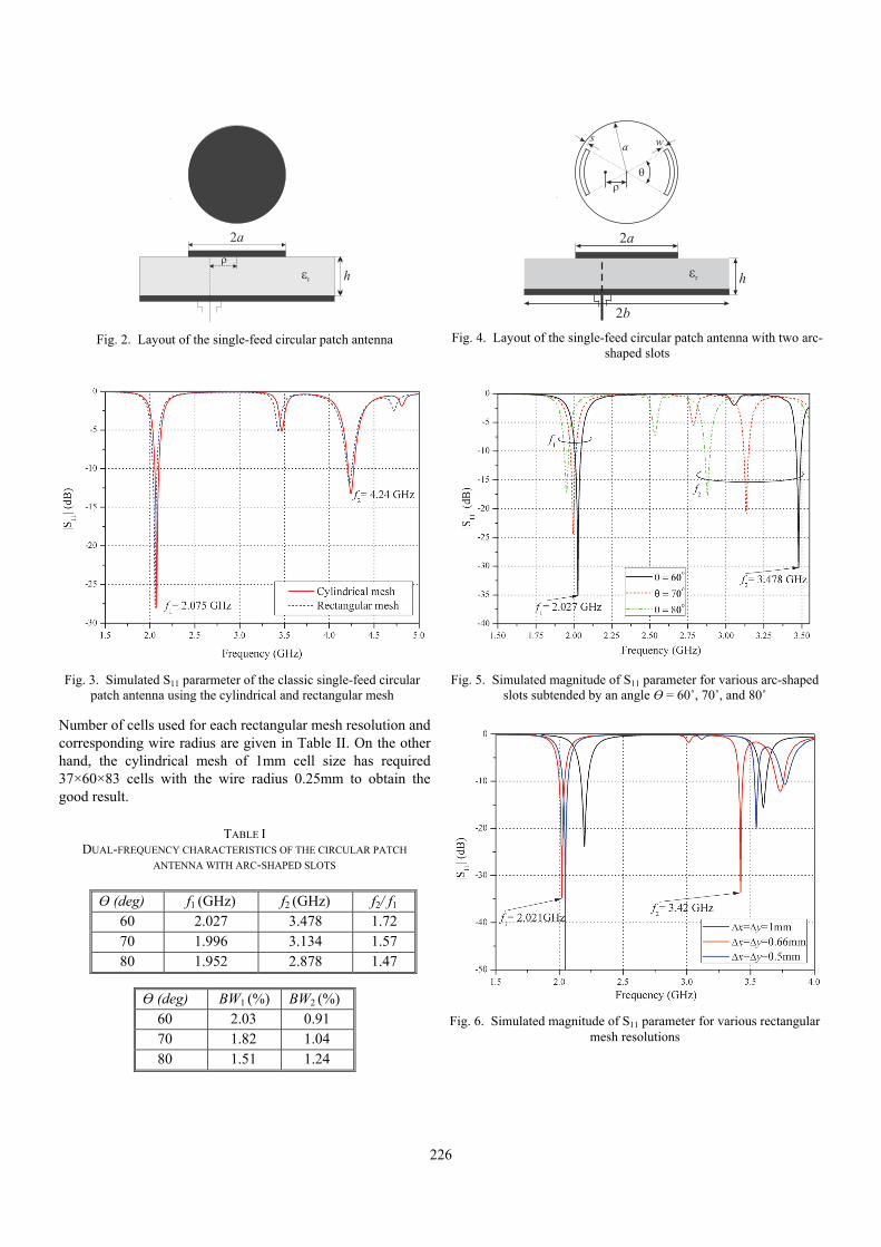
226

Number of cells used for each rectangular mesh resolution and corresponding wire radius are given in Table II. On the other hand, the cylindrical mesh of 1mm cell size has required 37×60×83 cells with the wire radius 0.25mm to obtain the good result.

TABLE I

DUAL-FREQUENCY CHARACTERISTICS OF THE CIRCULAR PATCH

ANTENNA WITH ARC-SHAPED SLOTS

Ɵ (deg) f1 (GHz) f2 (GHz) f2/ f1 60 2.027 3.478 1.72 70 1.996 3.134 1.57 80 1.952 2.878 1.47

Ɵ (deg) BW1 (%) BW2 (%) 60 2.03 0.91 70 1.82 1.04 80 1.51 1.24

Fig. 5. Simulated magnitude of S11 parameter for various arc-shaped slots subtended by an angle Ɵ = 60˚, 70˚, and 80˚

Fig. 6. Simulated magnitude of S11 parameter for various rectangular mesh resolutions

h

2a

r

Fig. 2. Layout of the single-feed circular patch antenna

h

2a

r

ws

2b

a

Fig. 4. Layout of the single-feed circular patch antenna with two arc-shaped slots

Fig. 3. Simulated S11 pararmeter of the classic single-feed circular patch antenna using the cylindrical and rectangular mesh

227

TABLE II COMPARISON OF NUMBER OF CELLS USED IN DIFFERENT MESHES

Cell size

along x, y (mm)

Number of cells

3DTLMrec_cw Wire radius (mm)

0.5 179×179×63 0.15 0.66 149×150×63 0.20 1.0 119×119×63 0.25

IV. CONCLUSION

In this paper, the in house solver based on the TLM method adjusted to the orthogonal polar mesh has been used to design and analyze the circular patch antenna with two arc-shaped slots embedded. Advantages of the used solver compared to the rectangular TLM are found in much easier antenna model building, better conformity of the mesh to the narrow arced slots, less complicated optimization of the coaxial feed position and, particularly, better efficiency due to much smaller number of cells requested for the modelling procedure.

ACKNOWLEDGEMENT

This paper is funded by means of the Ministry of Education and Science of Republic of Serbia within the project numbered III 44009 and III43012.

REFERENCES

[1] C.A. Balanis, Antenna Theory: Analysis and Design, John Wiley & Sons, New York, 2012.

[2] R. Garg, Microstrip Antenna Design Handbook, Artech House, 2001.

[3] J.G. Wu, and X.M. Zhou, "A Design of Miniaturization Dual-Frequency Antenna for GPS and WLAN Application", 2012 International Conference on Microwave and Millimeter Wave Technology (ICMMT), Shenzhen, pp. 1-3, 2012.

[4] S. Maci, and G. BifJi Gentil, "Dual-Frequency Patch Antennas", IEEE Antennas and Propagation Magazine, vol. 39, no. 6, December 1997.

[5] J. Jan, and K. Wong, "Single-Feed Dual-Frequency Circular Microstrip Antenna with an Open-Ring Slot", Microwave Opt. Technol. Lett., vol. 22, pp. 157-160, 1999.

[6] K. Wong, and G. Hsieh, "Dual-Frequency CMA with a Pair of Arc-Shaped Slots", Microwave Opt. Technol. Lett., vol. 19, pp. 410-412, 1998.

[7] D. Guha, and Y. M.M. Antar, Microstrip and Printed Antennas: New Trends, Techniques and Applications, John Wiley & Sons, New York, 2011.

[8] C. Christopoulos, The Transmission-Line Modeling Method: TLM, Institute of Electrical and Electronics Engineers, 1995.

[9] J. Jokovic, T. Dimitrijevic, and N. Doncov, "Efficient Integral Cylindrical Transmission-Line Matrix Modeling of a Coaxially Loaded Probe-Coupled Cavity", IET Microw, Antenna & Propag., vol. 9, no. 8, pp. 788-794, 2015.

[10] R. Scaramuzza, and A.J. Lowery, "Hybrid Symmetrical Condensed Node for the TLM Method", Electron. Lett., vol. 26, no. 23, pp. 1947-1949, 1990.

[11] V. Trenkic, A.J. Wlodarzcyk, and R.A. Scaramuzza, "Modeling of Coupling Between Transient Electromagnetic Field and Complex Wire Structures", Int. J. Numer. Model. Electron. Netw. Devices Fields, vol. 12, no. 4, pp. 257-273, 1999.

228

The Influence of LoS and Shadowing Components on Outage Probability of

Energy Harvesting DF Relay System Aleksandra M. Cvetkovic 1 and Vesna M. Blagojevic2

Abstract – Dual-hop system with simultaneous wireless information and power transfer and decode-and-forward (DF) relay is investigated. The outage probability performance in mixed Rician and shadowing fading channels is determined, for the scenario when relay harvests energy and time-switching (TS) scheme is applied. In addition, the closed-form tight asymptotic outage expression is derived. The impact of energy harvesting ratio, line-of-sight (LoS), shadowing components and fading parameters on outage probability is investigated and discussed.

Keywords – Decode-and-forward relay, Energy harvesting, Outage probability, Rician fading, Time switching scheme.

I. INTRODUCTION

Energy harvesting technique has recently occupied a special place in research area, as an efficient solution for powering wireless communication devices. In contrast to natural energy sources (wind, solar, etc.) which are depended on weather conditions and can not be used indoors, the sources of radio frequency (RF) energy are omnipresent and controllable. Moreover, RF signals are able to simultaneously transfer both information and energy, which is an additional justification for the widely investigated application of this technique [1-4].

Since the receiver is unable to perform energy harvesting and information signal processing at the same time, two concepts of receiver schemes are usually adopted: time switching (TS) and power splitting (PS). In TS-based scheme, one part of time is used to harvest energy at the relay, while the rest of time is dedicated for the decoding and transmission. On the other hand, in the PS-based receiver architecture, one part of received power is utilized for harvesting, while the remaining power is used for signal processing [4].

The simultaneous wireless transfer of information and power is applied in both relay and sensor networks, which are used to expand the signal coverage area providing the same quality of service and improve signal transmission [3-4]. In the scenarios where it is not possible to provide direct communication between transmitter and receiver, relays are used to enable communication between them. In order to improve system performances, it is desirable to provide line-of-sight (LoS) between source and relay node. In [5], the multi-user system over Rician distributed fading channel was studied, considering opportunistically harvesting PS scheme.

Moreover, dual-hop system in mixed Rician and Rayleigh fading scenario with energy harvesting amplify-and-forward (AF) relay and PS scheme was analyzed in [6] and [7]. The impact of LoS path effect on the outage probability is investigated in [6], for the case when only one user destination node exists, while AF multiuser system is considered in [7]. The minimization of outage performances based on power allocation, relay placement and PS for dual-hop decode-and-forward (DF) system over Rician fading channels is analyzed in [8].

In this paper, we analyze dual-hop relaying system, where DF relay is powered by RF energy harvested from source node based on TS scheme. The relay position is determined such that LoS is provided between source and relay nodes, and the first hop is affected by Rician fading. The second hop is influenced by the simultaneous existence of multipath fading and shadowing effects, which are modeled by generalized-K (Gamma-Gamma) distribution due to mathematical tractability [9]. For the considered scenario the outage probability expression is determined in the integral form and various effects of LoS and shadowing components are investigated. Furthermore, the approximative expression is derived in the exact closed-form. Numerical results has been obtained and shown excellent agreement between exact and approximate results in high average signal-to-noise (SNR) on the second hop regime. Monte Carlo simulations are presented to confirm derived analytical expressions.

II. SYSTEM AND CHANNEL MODEL

A. System Model

We consider the DF relay system where direct link between the source and the destination is not available due to obstacles and/or deep fading. In order to establish connection between the destination nodes, the position of the relay is determined such that the LoS between the source and the relay exists. The source transmits information to a destination via DF relay, which also harvest RF energy based on the time-switching scheme. The total communication time slot T is divided into two parts, based on energy harvesting ratio value . In the first time interval T, relay harvests energy, and the remaining time (1−)T is used for information transmission from the source to the relay and from the relay to the destination (this interval is divided into two equal parts) [4].

The source transmits signal x with power PS. If we denote the channel fading gain from the source to the relay by hSR, the received signal at the relay is given with

R S SR Ry P h x n , (1)

1Aleksandra M. Cvetković, is with the Faculty of ElectronicEngineering at University of Nis, Aleksandra Medvedeva 14, 18000Nis, Serbia, E-mail: [email protected]

2Vesna M. Blagojevic is with School of Electrical Engineering, atUniversity of Belgrade, Bulevar kralja Aleksandra 73, 11000Belgrade, Serbia, E-mail: [email protected]

229

where nR is the additive white Gaussian noise (AWGN) at the relay with variance 2

R . As the relay harvests energy during

the time interval T, the harvested energy at the relay is 2

H S SRE P h T , where is the energy conversion

efficiency coefficient. The output relay power is obtained as

22

1R S SRP P h

. (2)

The relay transmits signal xR to the destination, and the channel fading gain form the relay to the transmitter is hRD. The received signal at the destination is given by

D R RD R Dy P h x n . (3)

where nD is AWGN at the destination with variance 2D .

B. Source-Relay Channel

We assume that the position of the relay enables signal propagation with the LoS between the source and the relay. The source sends information to the relay and also enables energy for signal transmission from the relay to the destination. It is assumed that fading over source-relay channel follows Rician distribution [10]. As the signal-to-noise ratio (SNR) is given with

2

2

S SRR

R

P h

, (4)

the probability density function (PDF) of the instantaneous SNR at the relay is [10]

1

0

1 12SR

R

KK

SR SR

K e K Kp e I

(5)

where K denotes the Rician K factor (equal to the ratio of the power of the LoS component to the average power of the

scattered component), 2SR RE is the average SNR at the

relay and I0(x) is the zero-th order modified Bessel function of the first kind [11, Eq. 8.431.1].

The corresponding cumulative distribution function (CDF) is given by [10]

2(1 )1 2 ,

R

SR

KF Q K

(6)

where Q(x) is the first-order Marcum Q-function [10].

C. Relay-Destination Channel

We assumed that the environment from the relay to the destination is such that it can be considered that in addition to fading in the channel, the shadowing effect exists. The phenomenon of multipath fading is modeled by Nakagami

PDF and the variation of the average power (as a result of shadowing effect) follows Gamma PDF [9]. Therefore, the PDF of composite generalized K fading is given by

2

2

12

2

2

m s

RD

m s

s m

m m

m s

hm s RD

m mm s

m mRD

m mp

m m

m mK

(7)

where mm is Nakagami-m multipath fading parameter, ms is

the shadowing parameter, 2RD RDE h is the average SNR

and K(x) is modified Bessel function of the second kind [11, Eq. 8.432.3]. The corresponding CDF is

22,11,3

11, ,0RD

m s

hs mm s RD

m mF G

m mm m

.

(8)

where ,,

rp qm n

s

aG x

b

is Meijer G-function [11, Eq. 9.301].

Finally, using (2), the instantaneous SNR at the destination node, can be determined as

2 2

2

22 2

2

2

1

2.

1

D S SR RDD

RR RD R RD

D

P h h

h c h

(9)

where

2

2

2

1R

D

c

.

III. OUTAGE PERFORMANCE

The outage probability is important performance measure, defined as the probability that the instantaneous equivalent SNR of dual-hop system, falls below a predetermined protection value, th [10]. In the considered DF relay system, the outage probability can be determined as

,out r R th r D th R thP P P , (10)

and also written in the equivalent form

2

2,

d

R

R RRD

th

thout th r RD R th

R

thth R Rh

R

P F P hc

F F pc

(11)

By using the infinite-series representation of I0(.) [11, Eq. 8.447.1], the outage probability can be re-written in the following form

230

20

1

2,11,3

1 e 11

!

1e d

, ,0

R

R

SR

th

iK

out thim s SR SR

K

i m s thR R

s mRD R

K K KP F

m m i

m mG

m mc

(12)

After substituting R tht in (12) and applying binomial

theorem the outage probability is determined as

0 0

1

2

1

2,11,3

0

1 e

1e

!

1e d

, ,0

R

th

SR

SR

K i

out thi jm s SR

i Ki jth

SR

K t

j m s th

s mRD th

iKP F

jm m

K K

i

m mt G t

m mc t

(13)

Unfortunately, we can not find a closed-form analytical solution for the integral in (13). The outage probability given by (13) can be evaluated by numerical integration.

However, for small argument value of Meijer G-function using [12, Eq. 07.34.06.0006.01], and / thy t , the

approximation for the integral (13) can be determined in the exact closed-form. The approximate expression for the outage probability is derived in the following closed-form in the case when mm< ms

1

12

0 0

1e

1

!

1 11 , 2,

th

m s SR

R

m

KKs mm m

out thm m s SR

m iim sth

i jRD

i

thm

SR SR

m m K eP F

m m m

i jm m

jc i

K K KU j j m

(14)

For the case when mm>ms, the approximate outage probability expression is given as

1

12

0 0

1

1

!

1 11 , 2,

th

s m SR

R

s

KKm sm m

out ths m s SR

m iim sth

i jRD

i

ths

SR SR

m m K eP F e

m m m

i jm m

jc i

K K KU j j m

(15)

where U(a,b;z) is the confluent hypergeometric function of the second kind [11, eq. 9.211.4].

IV. NUMERICAL RESULTS

In order to analyze the impact of LoS component and shadowing effects, the numerical results for dual-hop DF harvesting system with applied time-switching scheme are presented in this section. Numerical results are obtained and confirmed by independent Monte-Carlo simulation method. It has been demonstrated that the closed-form approximate expression tightly bounds the exact results.

In Fig. 1. the influence of direct LoS component between source and relay is presented for various values of energy harvesting ratio . For small values of Rician factor K, ratio of the total time dedicated for the energy harvesting, does not significantly affect outage performance if >0.3. With the increase of factor K, the outage probability decreases, and the outage floor appears for large values of K parameter. The value of outage floor strongly depends on energy harvesting ratio. For example, by increasing energy harvesting ratio from 0.3 to 0.5, the outage performance is lower an order of magnitude.

0 2 4 6 8 10 12 14 16 18 2010-6

10-5

10-4

10-3

10-2

10-1

analytical results simulation results

th = 5 dB, = 0.8,

mm = 2.1 , ms = 3.2

Out

age

prob

abili

ty

K [dB]

=0.9

=0.7

=0.5

=0.3

=0.1

SR = 20 dB, RD = 10 dB

Fig. 1. Outage probability versus Rician K factor for various values

of energy harvesting ratio

0.1 0.2 0.3 0.4 0.5 0.6 0.7 0.8 0.910-4

10-3

10-2

10-1

100

RD = 15 dB

RD = 25 dB

RD = 10 dB

analytical results approximation simulation results

th = 5 dB, = 0.8,

mm = 5.1 , ms = 2.2

Out

age

prob

abil

ity

K =10 dB, SR=15 dB

RD = 5 dB

Fig. 2. Outage probability versus energy harvesting ratio for various

values of average SNR of second hop

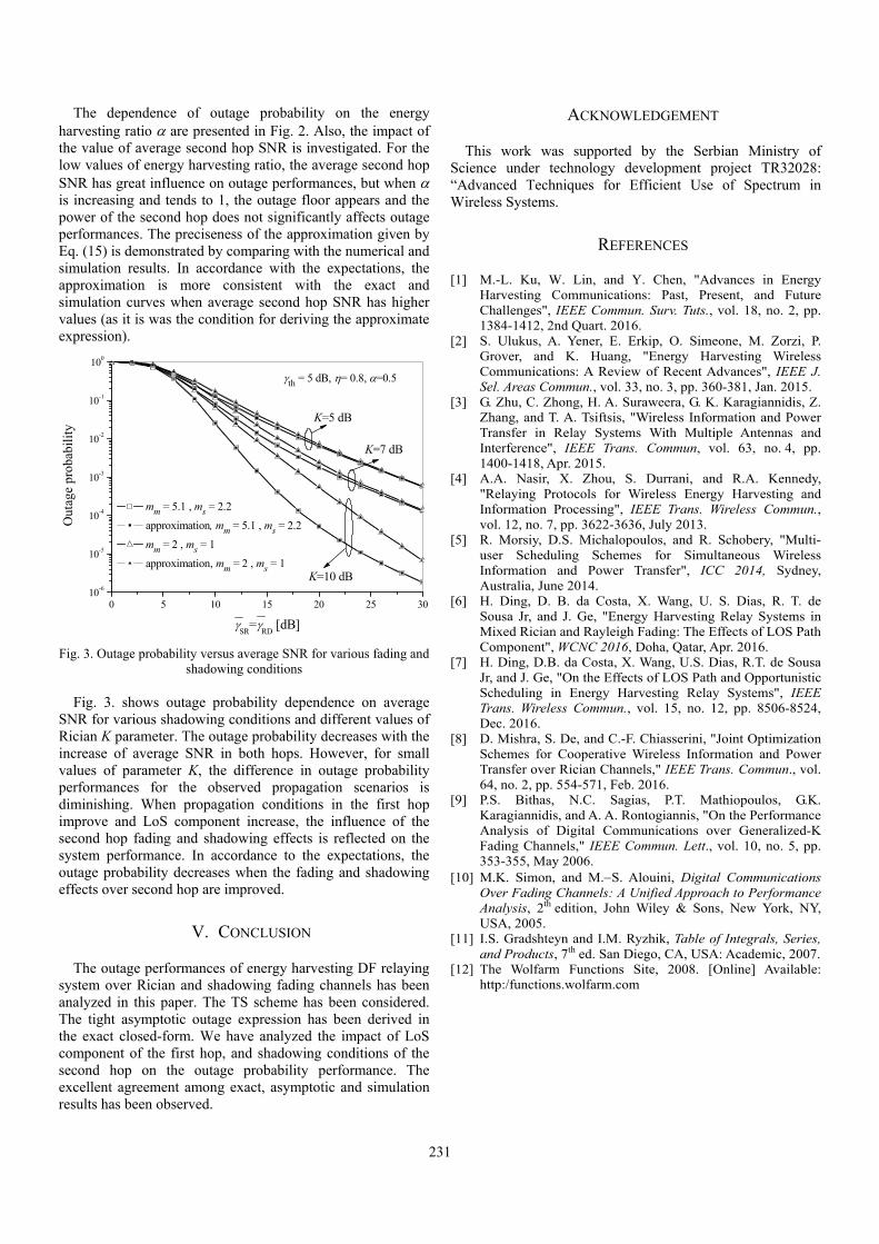
231

The dependence of outage probability on the energy harvesting ratio are presented in Fig. 2. Also, the impact of the value of average second hop SNR is investigated. For the low values of energy harvesting ratio, the average second hop SNR has great influence on outage performances, but when is increasing and tends to 1, the outage floor appears and the power of the second hop does not significantly affects outage performances. The preciseness of the approximation given by Eq. (15) is demonstrated by comparing with the numerical and simulation results. In accordance with the expectations, the approximation is more consistent with the exact and simulation curves when average second hop SNR has higher values (as it is was the condition for deriving the approximate expression).

0 5 10 15 20 25 3010-6

10-5

10-4

10-3

10-2

10-1

100

K=10 dB

K=7 dB

mm = 5.1 , ms = 2.2

approximation, mm = 5.1 , ms = 2.2

mm = 2 , ms = 1

approximation, mm = 2 , ms = 1

Out

age

prob

abil

ity

SR

=RD

[dB]

th = 5 dB, = 0.8, =0.5

K=5 dB

Fig. 3. Outage probability versus average SNR for various fading and

shadowing conditions Fig. 3. shows outage probability dependence on average

SNR for various shadowing conditions and different values of Rician K parameter. The outage probability decreases with the increase of average SNR in both hops. However, for small values of parameter K, the difference in outage probability performances for the observed propagation scenarios is diminishing. When propagation conditions in the first hop improve and LoS component increase, the influence of the second hop fading and shadowing effects is reflected on the system performance. In accordance to the expectations, the outage probability decreases when the fading and shadowing effects over second hop are improved.

V. CONCLUSION

The outage performances of energy harvesting DF relaying system over Rician and shadowing fading channels has been analyzed in this paper. The TS scheme has been considered. The tight asymptotic outage expression has been derived in the exact closed-form. We have analyzed the impact of LoS component of the first hop, and shadowing conditions of the second hop on the outage probability performance. The excellent agreement among exact, asymptotic and simulation results has been observed.

ACKNOWLEDGEMENT

This work was supported by the Serbian Ministry of Science under technology development project TR32028: “Advanced Techniques for Efficient Use of Spectrum in Wireless Systems.

REFERENCES

[1] M.-L. Ku, W. Lin, and Y. Chen, "Advances in Energy Harvesting Communications: Past, Present, and Future Challenges", IEEE Commun. Surv. Tuts., vol. 18, no. 2, pp. 1384-1412, 2nd Quart. 2016.

[2] S. Ulukus, A. Yener, E. Erkip, O. Simeone, M. Zorzi, P. Grover, and K. Huang, "Energy Harvesting Wireless Communications: A Review of Recent Advances", IEEE J. Sel. Areas Commun., vol. 33, no. 3, pp. 360-381, Jan. 2015.

[3] G. Zhu, C. Zhong, H. A. Suraweera, G. K. Karagiannidis, Z. Zhang, and T. A. Tsiftsis, "Wireless Information and Power Transfer in Relay Systems With Multiple Antennas and Interference", IEEE Trans. Commun, vol. 63, no. 4, pp. 1400-1418, Apr. 2015.

[4] A.A. Nasir, X. Zhou, S. Durrani, and R.A. Kennedy, "Relaying Protocols for Wireless Energy Harvesting and Information Processing", IEEE Trans. Wireless Commun., vol. 12, no. 7, pp. 3622-3636, July 2013.

[5] R. Morsiy, D.S. Michalopoulos, and R. Schobery, "Multi-user Scheduling Schemes for Simultaneous Wireless Information and Power Transfer", ICC 2014, Sydney, Australia, June 2014.

[6] H. Ding, D. B. da Costa, X. Wang, U. S. Dias, R. T. de Sousa Jr, and J. Ge, "Energy Harvesting Relay Systems in Mixed Rician and Rayleigh Fading: The Effects of LOS Path Component", WCNC 2016, Doha, Qatar, Apr. 2016.

[7] H. Ding, D.B. da Costa, X. Wang, U.S. Dias, R.T. de Sousa Jr, and J. Ge, "On the Effects of LOS Path and Opportunistic Scheduling in Energy Harvesting Relay Systems", IEEE Trans. Wireless Commun., vol. 15, no. 12, pp. 8506-8524, Dec. 2016.

[8] D. Mishra, S. De, and C.-F. Chiasserini, "Joint Optimization Schemes for Cooperative Wireless Information and Power Transfer over Rician Channels," IEEE Trans. Commun., vol. 64, no. 2, pp. 554-571, Feb. 2016.

[9] P.S. Bithas, N.C. Sagias, P.T. Mathiopoulos, G.K. Karagiannidis, and A. A. Rontogiannis, "On the Performance Analysis of Digital Communications over Generalized-K Fading Channels," IEEE Commun. Lett., vol. 10, no. 5, pp. 353-355, May 2006.

[10] M.K. Simon, and M.S. Alouini, Digital Communications Over Fading Channels: A Unified Approach to Performance Analysis, 2th edition, John Wiley & Sons, New York, NY, USA, 2005.

[11] I.S. Gradshteyn and I.M. Ryzhik, Table of Integrals, Series, and Products, 7th ed. San Diego, CA, USA: Academic, 2007.

[12] The Wolfarm Functions Site, 2008. [Online] Available: http:/functions.wolfarm.com

Session PO2:

2B - INFORMATION AND COMMUNICATION

TECHNOLOGIES

235

The q-Exponential Functions and Orthogonal Polynomials as the Special Motzkin Paths

Predrag Rajković1, Slađana Marinković2, Miomir Stanković3

Abstract – The exponential function, since its introduction, was a subject of a lot of variations, deformations and generaliza-tions. The same happened with different classes of orthogonal polynomials. Here, we wish to emphasize their appearance in some combinatorial problems. The Motzkin paths are a class of positive weighted paths with the appearance in many contexts. We will connect them with the continued fractions, the moments of the functionals and generalizations of the exponential function. Such paths have their interpretations in the computer sciences.

Keywords – Paths, Combinatorics, Exponential functions, Orthogonal Polynomials.

I. INTRODUCTION

The very beginnings of a combinatorial theory of special functions is given in Shapiro’s paper [1] in 1981. and Viennot’s paper [2] in 1983. Nowadays we can note growing interest in this area, a lot of books (G. Andrews [3] and Stanley [4]), papers and thesis were done with this topic (A.T. Benjamin [5] and D. Drake [6]). This method is used in [5] in elementary combinatorial proofs for special numbers identities and combinatorial interpretation of famous Rogers-Ramanujan identities in [7] by D.P. Little and J.A. Sellers. A lot of nice applications for multiple and quasi-orthogonal polynomials, then q-orthogonal polynomials can be found (D. Stanton [8]).

II. ON Q-EXPONENTIAL FUNCTIONS

In the theory of q-calculus (Andrews [3], Stanley [4], Stanton [8] or Rajković-Marinković-Stanković [9]), for a real parameter )1,1(q , we introduce a q-real number qa][ by

..)R .1

1][

aq

qa

a

q (1)

The q-analog of the Pochhammer symbol (q-shifted factorial) is defined by:

,,)1();(,1);(1

1

0

Nkaqqaqak

j

j

k (2)

and

.)();(

);();( R

qqa

qaqa (3)

In the Euler’s works, we can find two analogs of exponential function

),1|(|);(

1

);()(

0

xqxqq

xxe

n n

n

q (4)

).1||0(,);();(

)(0

2

qqxqq

xqxE

n n

n

n

q (5)

Having in mind that

,,!)1()1(lim);(lim1

11N

kkqqqq kk

j

j

qkq (6)

it is valid

.))1((lim))1((lim11

x

qqqqexqExqe

(7)

Fig. 1. The graphics of the small q-exponential function

))1(( xqeq for .1)1.0(0q

Fig. 2. The graphics of the big q-exponential function

))1(( xqEq for .1)1.0(0q

1Predrag Rajković, Faculty of Mechanical Engineering, Univer-sity of Niš, Serbia, Aleksandra Medvedeva 14, Niš, E-mail:[email protected];

2Slađana Marinković, Faculty of Electronic Engineering, Univer-sity of Niš, Serbia, A. Medvedeva 12, Niš; 3Miomir Stanković, Mathematical institute SASA, Belgrade, Serbia.

236

These functions somehow retain some important properties of exponential function, such as, for example,

.1)()( xExe qq (8) We can express

,),())1((0

n

nq xqnExqE

(9)

where

.);(

)1(),( 1

1 0

22

n

k

k

i

i

n

n

n

n

q

q

qq

qqqnE (10)

Hence we have the estimation:

,|),(| 2

n

qqnE (11)

wherefrom, for 0< q, |x| < 1, it is valid

.||1

||1|))1((|2

qx

qxxxqEq

(12)

Exton [10] has defined a generalization of q-exponential function by

).;(!][

);,(0

)1()Exton( CzRz

n

qzqE n

n q

nn

(13)

Floreanini and coauthors [11] have considered the one-parameter family of q-exponential functions of the type

).;();(

);(0

2/)Fl(

2

CzRzqq

qzE n

n n

n

q

(14)

Here, it is true

).();)1((lim )Fl(

1CzezqE z

qq

(15)

These functions are connected by

).;(2;1

);,( )Fl()Exton( CzRzq

qEzqE q

(16)

Again, we notice two well-known particular cases of this family:

.1;)(),0;()( )Fl()Fl(

q

zEzEzEze qqqq (17)

Today, there are a few new deformations and generalizations of the exponential function very useful in various areas of science, such as mechanical statistics, for example in Stanković-Marinković-Rajković [12].

III. BASICS ABOUT CONTINUED FRACTIONS

For two real sequences R=rn and S= sn we can define the continued fraction ),( RSKK like a sequence Kn

with an arbitrary member (Flajolet [13]):

.

3

32

21

10

n

n

n

s

rs

rs

rs

rsK

(18)

The term Kn is the nth convergent of the continued fraction which value is

.lim nnKK

(19)

The expression (1) requires a lot of spacing. That is why the nth convergent is often written in the form

.|

|

|

|

|

|

2

2

1

10

n

nn s

r

s

r

s

rsK (20)

We can simplify nK into the form

,n

nn D

NK (21)

where Nn is nth partial numerator and Dn is nth partial denominator determined by

2121 , nnnnnnnnnn DrDsDNrNsN (22)

with initial values ,,1 001 sNN and .1,0 01 DD

Some authors write

.K 10

i

ii s

rsK

(23)

Example 3. The transformation of a series into its equivalent continued fraction, with the series partial sums being equal to the continued fraction convergents, is due to Euler. The series

0n

ngG is transformed into the continued fraction

,10

i

ii s

rsK

K by the relations:

,1,, 11100 sgrgs (24)

.2,1,11

ng

gs

g

gr

n

nn

n

nn (25)

Example 3. The exponential function ,!0

n

nx

n

xe has

,!n

xd

n

n wherefrom .2,1, nn

xs

n

xr nn

237

Hence xe can be represented by the continued fraction

.

4/1

4/3/1

3/2/1

2/1

1

x

xx

xx

xx

ex

(26)

Applying an equivalence transformation that consists of clearing the fractions this example is simplified to

.

4

33

22

11

1

z

zz

zz

zz

zez

IV. ALPHABET

A letter is a variable which is not non-commutative with others. An alphabet X is a the maximal set of different letters. A word is a linear combination of the letters, i.e. a word is formed from the concatenation U of finitely many letters. A

set of all finite words we define by .*X Hence .,,,,,, 21

*

2121 XuuuXuuuuuuU mmm (27)

The number of words with length is n is nX )(card . The

concatenation U is very similar to the set union, but it is not the same operation. Example 1. For the binary alphabet 1,0B , its norm is

21,0 , and *1,0 is the set of binary words

.,11,01,10,00,1,0,1,0 * (28)

Example 2. The set of all words made via the alphabet cba ,, is

.,,,,,,,,,,,, * bcbbbaacabaacbacba (29)

Example 3. In a genomic sequence, the alphabet is .,,, TCGA

A monoid ,Y is an algebraic structure with a single

associative binary operation and an identity element. A monoid ring ,,Y over R is the set of formal sums

);( YuRsuss uYu

u

(30)

with operations: ,

Yu

uu utsts (31)

).,,,( Rtstsutsts wvuuYu uwv

wv

(32)

Let *

21 Xuuuu m and *

21 Xvvvv n be two words.

The sum of two words is their union and the products are their concatenation: ., *

2121

* XvvvuuuvuXvuvu nm

Hence ,,*X over the set of real numbers R is a monoid

ring. Formal power series extend the usual algebraic operations on polynomials to infinite series of the form

.)(0

n

n

n zfzf (33)

The set of all power series with operations ,],[zC forms

the ring.

It is possible to define a morphism ][: * zCX . We will

deal with it in the next sections. To the infinite alphabet

000 NjjNjjNjj cbaX

. (34)

Flajolet has joined the next nth convergent:

.

11

1

11

1

11

2

211

100

n

nnn

n

b

cab

b

cab

cab

F

(35)

V. MOTZKIN PATHS

Let Mk = (xk, ,yk) (k=0,1,… n) be the points in Oxy plane with yk nonnegative. Then P0 P1…Pn is a Motzkin path if

P0 = (0 ,0), Pn = (xn, ,0), and vector 11 kkk PPu is one of

the next three vectors (up, horizontal and down vector):

,,, OCcOBbOAa (36)

where ).1,1(),0,1(),1,1(),0,0( CBAO (37)

So, a path can be considered like sequence .21 nuuuu The

length of the path is number n and its height is h(u)=max yk. The level steps of path are the vectors b. The area below a path is the sum of the height of the points in the path. The weight )(kw of a vector uk is the number which depends on

its type:

c.uif

b,uifa,uif

c

b

a

kw

k

k

k

y

y

y

k

k

k

,

,

,

)(

1

1

1

(38)

238

In common words, it is a, b or c with the sub-index which is equal to the ordinate of its starting point.

Denote by nΜ the set of all Motzkin paths of length n.

The number nnnM ΜΜ card is the n-th Motzkin

number. Example 3. All Motzkin paths of size .3n That is why .43 M

Fig. 3. All Motzkin paths of size .3n

The Motzkin paths are of the form

.bMcMaMM (39)

Translating the equation above to generating functions, we get ),()(1)( 22 xMxxxMxM (40)

i.e.,

.2

4)1(1)(

2

22

x

xxxxM

(41)

The Motzkin numbers are .323, 127, 51, 21, 9, 4, 2, 1, 1,

The weight w(P) of a path P is the product of the weights of its segments, i.e.

.)()(1

n

k

kwPw (42)

Example 2. The path on the Fig. 4, has the length ,8n the

height ,2h and the weight ,10012110 cabccabaw and

.611211area

Fig. 4. A Motzkin path of size .8n

By convention, the empty path will have weight 1. Let qn be the set of all weighted paths with height at most n. The total weight of qn is denoted by

nT

n TwG

)( . (43)

Some authors use term the generating function for (7) which depends on n and tiles weights. Especially, when weights depends of the same variable, we will get the well-known notion of generating function in mathematics. Theorem 1. (Flajolet [13]) The total weights of all weighted paths of the height n is given by Flajolet’s nth convergent (6).

A Dyck path of length n is a Motzkin path without East steps, i.e. ).1(0 kbk

Example 3. A morphism ][: * zCX defined by

)1()(,0)(),0()( kzqcbjzqa k

kk

j

j

has the generating function

.

11

11

1),(

52

32

12

qzqz

qzqzG

(44)

Hence

).2;();(

),( )(

0

2

zEzqq

qqzG q

n

n n

nFl

(45)

239

Example 4. Let us define the weights

)1()(,0)(),0()( kqcbjza k

kkj (46)

Then we have the generating function

,

1

)(1

)(1

11

1

11

11

1),(

23

2

1

qzqqzq

zq

zqzq

zqqzG

(47)

which satisfies the relation

.),(1

1),(

qzqqzGqzG

(48)

Suppose that ),( qzG can be written in the form

.)(

)(

),(

),(),(

0

0

n

n

n

n

n

n

zqb

zqa

qzB

qzAqzG

Then, the relation (45) gets the form

.

),(

),(1

1

),(

),(

qqzB

qqzAqzqzB

qzA

(49)

Identifying numerators and denominators, we get ).,(),(),(),,(),( 2 qzqqzBqqzBqzBqqzBqzA (50)

From the second relation, we find

),()()(,1)( 1

12

0 qbqqbqqbqb n

n

n

n

n

i.e.,

.)1()1)(1(

)1(),(

2

2

n

nn

n qqq

qqzb

(51)

Finally,

.)2;(

)2;(),(

)Fl(

)Fl(

zE

qzEqzG

q

q

(52)

Example 5. The Rogers–Ramanujan continued fraction has the value:

.)2;(

)2;(

11

11

1),()Fl(

)Fl(

4

3

2 qzE

zE

zqzq

zqzq

qzRRq

q

(53)

Example 6. Let nS be the set of all permutations

nppp ,,, 21 over n elements .,...,1 n A number kp id

displaced if it not equal to k. For any permutation nppp ,,, 21 its distance to the identity permutation as

the sum of the displacements of all elements (Bartschi [14]):

.)(1

n

kkpkD (54)

The number of permutations of total displacement equal to 2d is

.2)(:card),( dDSdnD n (55) These permutations are in correspondence to Motzkin paths whose area is exactly the distance d under consideration. Therefore the problem translates into the problem of counting weighted Motzkin paths of a given area d.

VI. ORTHOGONAL POLYNOMIALS

The orthogonal polynomials are very useful tool in technical sciences. They arose in the 18th century in the study of mechanics, and after that they found applications in others. They appear in numerous mathematical disciplines such as: numerical analysis, approximation theory, differential equa-tions, combinatorics, number theory and statistics . Let m(x) be a positive Borel measure on an interval (a,b) with infinite support and such that all moments

b

a

nn

n xLxdx ],[)( (56)

exist. We take )(x such that .10 In this manner, we

define linear functional L in the linear space of real polynomials P. We can introduce an inner product as follows:

),(][),( PgfgfLgf . (57) which is positive-definite because of the property

).(0),(|||| 2 Pffff (58)

The polynomials Pn(x) defined by

,

1

]det[

1)(

221

121

10

1

0,

nn

n

n

n

jiji

n

xx

xP

(59)

are orthogonal with respect to this inner product, i.e. the following holds:

).(0||||),(0),( nPnmPP nnm (60)

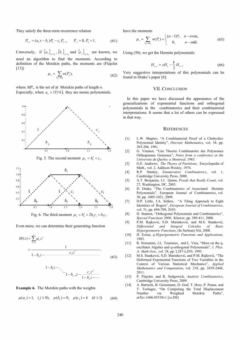
240

They satisfy the three-term recurrence relation

.1,0,)( 0111 PPPcPbxaP kkkkkk (61)

Conversely, if ,0Njja

0Njjb

and 0Njjc

are known, we

need an algorithm to find the moments. According to definition of the Motzkin paths, the moments are (Flajolet [13])

nn MPP

nn Pw ),( (62)

where MPn is the set of al Motzkin paths of length n. Especially, when ,1 kak they are monic polynomials.

Fig. 5. The second moment .1

2

02 cb

Fig. 6. The third moment .2 1110

3

03 cbcbb

Even more, we can determine their generating function

.

11

1

1

1

)(

2

1

1

2

10

0

zb

zczb

zb

zczb

zzM

n

nn

n

n

n

(63)

Example 6. The Motzkin paths with the weights

)1()(,0)(),0(,1)( kkcbja kkj (64)

have the moments

nn MPP

nn n

nnPw

.odd,0

even,,!)!1()( (65)

Using (50), we get the Hermite polynomials:

.2 11 kkk Hk

xHH (66)

Very suggestive interpretations of this polynomials can be found in Drake’s paper [6].

VII. CONCLUSION

In this paper we have discussed the appearance of the generalizations of exponential functions and orthogonal polynomials in the combinatorics and their combinatorial interpretations. It seems that a lot of others can be expressed in that way.

REFERENCES

[1] L.W. Shapiro, “A Combinatorial Proof of a Chebyshev Polynomial Identity”, Discrete Mathematics, vol. 34, pp. 203-206, 1981.

[2] G. Viennot, “Une Theorie Combinatoire des Polynomes Orthogonaux Generaux”, Notes from a conference at the Universite du Quebec a Montreal, 1983.

[3] G.E. Andrews, The Theory of Partitions, Encyclopedia of Math., vol. 2, Addison-Wesley, 1976.

[4] R.P. Stanley, Enumerative Combinatorics, vol. 1, Cambridge University Press, 2000.

[5] A.T. Benjamin, J.J. Quinn, Proofs that Really Count, vol. 27, Washington, DC, 2003.

[6] D. Drake, “The Combinatorics of Associated Hermite Polynomials”, European Journal of Combinatorics, vol. 30, pp. 1005-1021, 2009.

[7] D.P. Little, J.A. Sellers, “A Tiling Approach to Eight Identities of Rogers”, European Journal of Combinatorics, vol. 31, pp. 694-709, 2010.

[8] D. Stanton, “Orthogonal Polynomials and Combinatorics”, Special Functions 2000, Kluwer, pp. 389-411, 2000.

[9] P.M. Rajković, S.D. Marinković, and M.S. Stanković, Differential and Integral Calculus of Basic Hypergeometric Functions, (In Serbian) Niš, 2008.

[10] H. Exton, q-Hypergeometric Functions and Applications, 1983.

[11] R. Noreanini, J.L. Tourneux, and L. Viea, “More on the q-oscillator Algebra and q-orthogonal Polynomials”, I. Phys. A: Math Gen., vol. 28, pp. L287-LZ93, 1995.

[12] M.S. Stanković, S.D. Marinković, and P.M. Rajković, “The Deformed Exponential Functions of Two Variables in the Context of Various Statistical Mechanics”, Applied Mathematics and Computation, vol. 218, pp. 2439-2448, 2011.

[13] P. Flajolet, and R. Sedgewick, Analytic Combinatorics, Cambridge University Press, 2009.

[14] A. Bartschi, B. Geissmann, D. Graf, T. Hruz, P. Penna, and T. Tschager, “On Computing the Total Displacement Number via Weighted Motzkin Paths”, arXiv:1606.05538v1 [cs.DS]

241

Outage Probability Performance of Hybrid RF/FSO System with SSC Receiver Milica Petkovic1 and Goran T. Djordjevic1

Abstract – In this paper, we present the analysis of hybrid radio frequency (RF) / free-space optical (FSO) system. The switch-and-stay (SSC) diversity technique is employed at the receiver. The intensity fluctuations of the optical signal are modelled by Gamma-Gamma distribution, while the RF fink is affected by Rayleigh fading. Novel outage probability expression for hybrid RF/FSO system is derived. The effect of atmospheric turbulence strength and SSC implementation on the hybrid RF/FSO system performance is observed.

Keywords –Atmospheric turbulence, free-space optics (FSO), Gamma-Gamma distribution, outage probability, radio frequency (RF) system, Rayleigh fading, switch-and-stay (SSC) diversity technique.

I. INTRODUCTION

As a license-free and cost-effective modern technique, free-space optical (FSO) system has become a good substitution to traditional wireless radio frequency (RF) systems. The FSO provides high-data rates and wide bandwidth, and represents a good solution for the “last mile” problem [1-3]. Beside an idea to be an alternative, the FSO is also suitable to be a complement technique to the RF systems. The FSO signal transmission represents optical wireless communication between transmitter laser and receiver photodetector via atmospheric channel. Hence, the atmospheric conditions have strong influence on the quality of system performance. Due to variations in atmospheric temperature, pressure and altitude, the random changes in the refractive index occurs, which results in the existence of the atmospheric turbulence [1]. Although many statistical models have been proposed to define the effect of this phenomenon, the Gamma-Gamma distribution is accepted as an optimal model, since it gives a good agreement in experimental and theoretical data in wide range of atmospheric conditions [1-4].

In order to alleviate the optical signal degradation due to atmospheric turbulence, many techniques have been borrowed from RF systems. Firstly, spatial diversity techniques have been considered within FSO systems at the transmitting and/or receiving part [5-8]. The extension of the cover area has been accomplished by applying relying technology within FSO systems [9-11]. Furthermore, the idea of mixed RF/FSO systems, where the first hop is RF link and the second hop represents the FSO signal transmission to overcome a connectivity gap between the backbone and last mile access

networks, has been proposed in [12]. In addition, the hybrid system, which consists from FSO and RF link, was observed in [13-16]. In the hybrid RF/FSO systems, the same data are transmitted over both links simultaneously. The received signals are combined by some of diversity techniques.

In this paper, we analyze the hybrid RF/FSO system, when the switch-and-stay (SSC) diversity technique is applied at the receiver. The well-known Gamma-Gamma distribution is used to model the effect of atmospheric turbulence. The RF channel experiences Rayleigh fading. Novel expression for the outage probability of the system under investigation is derived. Numerical results are presented, which are used to illustrate and observe the effect of atmospheric turbulence strength and SSC implementation on the overall system performance.

The rest of the paper is organized as follows. The system and channel models are presented in Section II. The outage probability analysis is described in Section III. Numerical results and discussions are given in Section IV, while concluding remarks are presented in Section V.

II. SYSTEM AND CHANNEL MODELS

In the hybrid RF/FSO system presented in Fig. 1, the information data are transmitted at the same time via both RF and FSO links, i.e., both FSO and RF links will be simultaneously active. At the receiver, dual branch SSC spatial diversity technique is employed, which is the simplest form of switched diversity. In dual-branch SSC based system, when the instantaneous signal-to-noise ratio (SNR) of the active branch falls below a predetermined switching threshold, T, the receiver switches and stays to the other alternative branch, regardless of whether or not the SNR of the other branch is above or below the threshold [17].

A. FSO Channel Model

In the FSO subsystem, we adopt intensity modulation and

1Milica I. Petkovic and Goran T. Djordjevic are with University ofNis, Faculty of Electronic Engineering, Aleksandra Medvedeva 14,18000 Nis, Serbia, E-mails: [email protected];[email protected]

Fig. 1. System model of hybrid RF/FSO system

242

direct detection (IM/DD) with on/off keying (OOK). It is assumed that the intensity fluctuations of the received optical signal are modeled by Gamma-Gamma distribution, thus the probability density function (PDF) optical signal irradiance, I, is given as [1]

12

22

2 ,If I I K I

(1)

where Γ(.) is the gamma function defined by [18, Eq. (8.310.1)], and K(.) is the -th order modified Bessel function of the second kind defined by [18, Eq. (8.432.2)]. The atmospheric turbulence parameters and are related to the atmospheric conditions. When the plane wave propagation is assumed, the parameters and are defined as [1]

1

2

7/612/5

1

2

5/612/5

0.49exp 1 ,

1 1.11

0.51exp 1 ,

1 0.69

R

R

R

R

(2)

where the Rytov variance 2R is defined as

2 2 7/6 11/61.23 .R nC k L (3)

The wave-number is defined as 2k , where is the

optical wavelength, L is the FSO link length, and 2

nC is the

index of refraction structure parameter, which is used as a metric for the atmospheric turbulence strength.

The instantaneous SNR, FSO, is defined as

1 1

2 2 2 2 2 2

2 2,t t

FSOn n

R P I R P I

(4)

where R denotes the detector responsivity, Pt is the average transmitted optical power, and the

1

2n is the additive white

Gaussian noise (AWGN) variance. The electrical SNR, FSO, is determined as

1 1

2 2 2 22

2 2[ ] ,t t

FSOn n

R P R PI

(5)

since I is normalized for the Gamma-Gamma distributed atmospheric turbulence [ ] 1I .

Based on Eqs. (1), (4) and (5), the PDF of the instantaneous SNR is expressed as

142

4

2 .FSO

FSOFSO

f K

(6)

The cumulative distribution function (CDF) of FSO is determined as

2,11,3

11,

, , 0FSOFSO

F G

(7)

where ,,

m np qG is the Meijer's G-function [18, Eq. (9.301)].

B. RF channel model

The signal transmission via RF link is affected by Rayleigh fading, and the instantaneous SNR, RF, over RF link is defined as

2

2

2,r

RFn

P h

(8)

where h is the signal fading amplitude with 2 1h , where

is mathematical expectation, Pr represents the RF

transmit power, and 2

2n is the AWGN variance.

The average SNR, RF, over RF link is determined as

2 2

22 2

[ ] [ ] .r rRF RF

n n

P Ph

(9)

The PDF of the instantaneous SNR over RF link is expressed as [17]

1exp ,

RFRF RF

f

(10)

while the CDF is

1 exp .RF

RF

F

(11)

, 0 ,

2 , ,

FSO RF

FSO RF

FSO RF

FSO RF FSO RF

FSO RF

FSO RF FSO RF

T TT

T T

ssc

T TT

T T T T

F FF F

F FF

F F F FF F

F F F F

(13)

243

III. OUTAGE PROBABILITY ANALYSIS

The outage probability of the SSC based system is defined as the probability that the instantaneous SNR at SSC output, denoted by SSC, drops below a predetermined outage threshold, denoted by q. For the considered scenario of the hybrid RF/FSO system, the outage probability can be obtained as [17]

,out sscP F q (12)

where sscF q is the CDF of the instantaneous SNR at SSC

output, SSC, defined in Eq. (13) at the bottom of the previous page, and

FSOF and

RFF are the CDFs defined by Eqs.

(7) and (11), respectively.


Numerical results obtained based on the outage probability expression in Eqs. (12) and (13) are presented. The atmospheric turbulence parameters and are determined by Eq. (2). The atmospheric turbulence strength is determined by the index of refraction structure parameter with values

2 156 10nC m-2/3, 2 142 10nC m-2/3 and 2 145 10nC m-2/3 in weak, moderate and strong

turbulence conditions, respectively. Fig. 2 presents the hybrid RF/FSO system outage

probability dependence on the average and electrical SNRs in different atmospheric turbulence conditions. System performs better when the FSO link is affected by weak atmospheric turbulence, i.e., when the index of refraction structure parameter is lower. Beside the hybrid RF/FSO system, the outage probability of the dual branch RF system with SSC receiver is also observed, which is obtained based on Eqs. (12) and (13) considering that

FSO RFF F . It can be

noticed that the hybrid RF/FSO system has better outage probability performance compared to RF system, only when the FSO link is affected by favorable conditions. On the other hand, when the FSO signal transmission suffers from moderate and strong turbulence, dual branch RF system has better performance.

The outage probability dependence on the average and electrical SNRs in weak and strong atmospheric turbulence conditions is presented in Fig. 3, together with the outage probability results of the dual branch SSC based FSO system, which is obtained based on Eqs. (12) and (13) considering that

RF FSO

F F . When the FSO links are affected by weak

atmospheric turbulence, which correspond to clear air terms (sunny days), system with only FSO links has better performance than the hybrid RF/FSO system. When signal transmission environment is influenced by foggy weather conditions, atmospheric turbulence is strong, and the hybrid RF/FSO system has better performance, since the RF link is less dependent on the fog than the FSO link. Since FSO

0 5 10 15 2010-7

10-6

10-5

10-4

10-3

10-2

10-1

100

q=5 dB,L=2000 m

FSO

=RF

=30 dB

FSO

=RF

=15 dB

weak AT conditions moderate AT conditions strong AT conditions

Out

age

prob

abil

ity

T [dB]

Fig. 4. Outage probability versus the switching threshold in various atmospheric turbulence conditions

0 5 10 15 20 25 30 35 4010-6

10-5

10-4

10-3

10-2

10-1

100

RF/FSO hybrid system weak AT conditions strong AT conditions

L=2000 m

T=15 dB

q=4 dB

dual branch FSO system weak AT conditions strong AT conditions

Out

age

prob

abili

ty

FSO

=RF

[dB]

Fig. 3. Outage probability versus FSO=RF for hybrid RF/FSO and dual branch FSO system

0 5 10 15 20 25 30 35 4010-6

10-5

10-4

10-3

10-2

10-1

100

L=2000 m

T=10 dB

q=5 dB

RF/FSO hybrid system weak AT conditions moderate AT conditions strong AT conditions

Out

age

prob

abil

ity

FSO

=RF

[dB]

dual branch RF system

Fig. 2. Outage probability versus FSO=RF for hybrid RF/FSO and dual branch RF system

244

system implementation is easier and less expensive than the RF system implementation, the balance between cost and quality of the transmission can be made to provide optimal system performance.

In Fig. 4, the outage probability in function of the switching threshold is observed, considering different atmospheric turbulence conditions. Both average SNR over RF link and electrical SNR over FSO link take values 15 dB or 30 dB. As it is expected, greater values of SNR lead to the better system performance. The optimal value of the switching threshold can be noticed, when the system has the best performance. This optimal value of the switching threshold is equal to the value of the predetermined outage threshold, i.e., T=q. In this case, the SSC receiver behaves as selection combiner receiver, which selects the channel with greater SNR, leading to the best outage probability performance.

V. CONCLUSION

In this paper, we have presented the outage probability analysis of the hybrid RF/FSO system. The SSC diversity receiver has been employed at the receiver. The FSO link is affected by the Gamma-Gamma distributed atmospheric turbulence, while the RF link is subject to Rayleigh fading. The outage probability expression has been derived. The effect of atmospheric turbulence strength on the system performance has been observed and compared with the performance of dual branch SSC RF and dual branch SSC FSO systems. It has been concluded that hybrid RF/FSO system performs better than the dual branch SSC based RF system only when the FSO link is affected by weak atmospheric conditions. Furthermore, when the weather conditions are good (sunny days), it is more profitable to implement two FSO links than the hybrid RF/FSO system, since the implementation of the FSO link is easy and low-cost. On the other hand, when the optical signal transmission is under the influence of foggy weather conditions, atmospheric turbulence and visibility are strong and harmful, and the hybrid RF/FSO system performs better than the dual branch FSO system.

ACKNOWLEDGEMENT

This work was supported by the Ministry of Education, Science and Technology Development of the Republic of Serbia under Grant TR-32028.

REFERENCES

[1] L.C. Andrews, and R.N. Philips, Laser Beam Propagation through Random Media, 2nd ed., Bellingham, Washington, USA, Spie Press, 2005.

[2] Z. Ghassemlooy, W. Popoola, and S. Rajbhandari, Optical Wireless Communications: System and Channel Modelling with MATLAB, Boca Raton, USA, CRC Press, 2013.

[3] M. A. Khalighi, and M. Uysal, “Survey on Free Space Optical Communication: A Communication Theory Perspective”, IEEE Commun. Surveys Tuts., vol. 16, no. 4, pp. 2231-2258, 2014.

[4] M.A. Al-Habash, L.C. Andrews, and R.L. Phillips, “Mathematical Model for the Irradiance Probability Density Function of a Laser Beam Propagating through Turbulent Media”, Opt. Eng., vol. 40, no. 8, pp. 1554-1562, 2001.

[5] T. A. Tsiftsis, H. G. Sandalidis, G. K. Karagiannidis, and M. Uysal, “Optical Wireless Links with Spatial Diversity over Strong Atmospheric Turbulence Channels”, IEEE Trans. Wireless Commun., vol. 8, no. 2, pp. 951-957, 2009.

[6] E. Bayaki, R. Schober, and R. K. Mallik, “Performance Analysis of MIMO Free-Space Optical Systems in Gamma-Gamma Fading”, IEEE Trans. Commun., vol. 57, no. 11, pp. 3415-3424, 2009.

[7] W. Zixiong, W. Zhong, S. Fu, and C. Lin, “Performance Comparison of Different Modulation Formats over Free-space Optical (FSO) Turbulence Links with Space Diversity Reception Technique”, IEEE Photon. J., vol. 1, no. 6, pp. 277-285, 2009.

[8] H. Moradi, H.H. Refai, and P.G. LoPresti, “Switch-and-stay and Switch-and-examine Dual Diversity for High-speed Free-space Optics Links”, IET Optoelectron., vol. 6, no. 1, pp. 34-42, 2012.

[9] M. Safari, and M. Uysal “Relay-assisted Free-space Optical Communication”, IEEE Trans. Wireless Commun., vol. 7, pp. 5441-5449, 2008.

[10] J.Y. Wang, J.B. Wang, M. Chen, Y. Tang, and Y. Zhang, “Outage Analysis for Relay-aided Free-space Optical Communications over Turbulence Channels with Nonzero Boresight Pointing Errors”, IEEE Photon. J., vol. 6, 7901815, 2014.

[11] G.K. Karagiannidis, T.A. Tsiftsis, and H.G. Sandalidis, “Outage Probability of Relayed Free Space Optical Communication Systems”, Electron. Lett., vol. 42, pp. 994-995, 2006.

[12] E. Lee, J. Park, D. Han, and G. Yoon, “Performance Analysis of the Asymmetric Dual-hop Relay Transmission with Mixed RF/FSO Links”, IEEE Photonic Tech. L., vol. 23, no. 21, pp. 1642-1644, 2011.

[13] N.D. Chatzidiamantis, G.K. Karagiannidis, E.E. Kriezis, and M. Matthaiou, “Diversity Combining in Hybrid RF/FSO Systems with PSK Modulation”, ICC 2011 Conference, pp. 1-6, Kyoto, 2011.

[14] B. He, and R. Schober, “Bit-interleaved Coded Modulation for Hybrid RF/FSO Systems”, IEEE Trans. Commun., vol. 57, no. 12, pp. 3753-3763, 2009.

[15] T. Rakia, H.C. Yang, M.-S. Alouini, and F. Gebali, “Outage Analysis of Practical FSO/RF Hybrid System with Adaptive Combining”, IEEE Commun. Lett., vol. 19, no. 8, pp. 1366-1369, 2015.

[16] M. Usman, H.C. Yang, and M.-S. Alouini, “Practical Switching-based Hybrid FSO/RF Transmission and its Performance Analysis”, IEEE Photon. J., vol. 6, no. 5, pp. 1-13, 2014.

[17] M. K. Simon, and M.-S. Alouni, Digital Communication over Fading Channels, 2nd ed., New York, John Wiley & Sons Inc., 2004.

[18] I.S. Gradshteyn, and I.M. Ryzhik, Table of Integrals, Series, and Products, 6th ed., New York, Academic, 2000.

245

Outage Probability of Cooperative Multi-hop Multiuser Relaying Networks

Nikola Sekulović1, Aleksandra Panajotović2, Aleksandra Cvetković2

and Daniela Milović2

Abstract – The multi-hop amplify-and-forward (AF) relay systems with larger number of mobile users is considered. In order to improve a signal transmission quality in environment with many obstacles, the multi-hop cooperative relays with maximum-ratio-combining (MRC) scheme are implemented. Opportunistic scheme for signal transmission to end users is applied. Outage probability expression for considered system is derived and numerical results are presented and analyzed.

Keywords – Amplify-and-forward relay, Multi-hop, Multiuser, Rayleigh fading.

I. INTRODUCTION

The cooperative relaying technology provides increased coverage area and balanced quality of service for all users. Moreover, applying relays in wireless infrastructure the benefit from the spatial diversity and signal combining techniques can be utilized, leading to a reduction of the fading and shadowing effects. This kind of systems bring greater diversity gain and decreased pathloss. Increasing the number of relays in series results in the pathloss decreasing, while greater number of parallel relays causes increased diversity gain [1].

Many papers consider the multi-hop system with amplify-and-forward (AF) or decode-and-forward (DF) relay protocols without using cooperative diversity [2-4]. In cooperative relaying system, the spatial diversity is based on multiple information signal copies arrived to the destination. The exact symbol error probability (SER) of network with parallel AF nodes which transmit signal only to the destination is derived in [5]. Multi-hop diversity system in which each nod receives signals form all the previous nodes is considered in [6]. The performance analysis of AF and DF relaying diversity is presented for the instantaneous end-to-end signal-to-noise ratio (SNR) using approximation approach. In [7], the relays process and forward the signals to other relays, as well as to the destination, over Rayleigh fading channels. The maximum-ratio-combining (MRC) scheme is applied to the receivers. However, the derived SER is mathematically

difficult to track and performance analysis is complicated. Therefore, the authors in [8] develop an analytical approach for the end-to-end SNR determination of the multi-branch multi-hop system. The analysis in [8] is reduced to the well-known dual-hop system. The MRC technique is applied at both the AF relays and destination in order to combine the signals from the source and previous relays. The average SER expression is presented as a good approximation to the exact simulation results.

In this paper, the multi-hop system discussed in [7-8], is extended to the case when last relay in this network transfers the information signal to a large number of mobile users. In this way, the system exploits the advantages of multi-hop system in the poor non-line-of-sight environment to achieve good signal quality which is then distributed to mobile users. We assume that opportunistic multiuser scheduling scheme is applied in which the mobile user with the strongest channel is selected [9]. The outage probability expression for considered system over Rayleigh fading channels is derived and the impact of number of relays and mobile users are analyzed.

II. SYSTEM MODEL

A multi-hop multiuser wireless relay communication network where a source S (R0) communicates with a

destinations Dk ( 1,k K ) via AF relays Ri ( 1,i L ) is depicted in Fig. 1 (L = 4). Non-line-of-sight environment where direct link between source and relays on one side and destinations on the other side does not exist is explored. Channel gain from the i-th transmission node to the j-th receiving node is denoted as hi,j. Index i = 0 is reserved for the source. We assume that amplitude and phase of channel gains are Rayleigh distributed and uniformly distributed over [0, 2π), correspondingly. For the Rayleigh fading channel exposed to the influence of a zero mean complex additive white Gaussian noise (AWGN), the instantaneous SNR of link between nodes i and j, denoted as γi,j , is modelled as

,

, ,

1exp

i j

i j i j

f

, (1)

with 2 2

, , ,[ ] /i j i j i j siE E h E , where Esi is the

average symbol energy of the i-th transmission node and σ2 is the variance of the noise.

1Nikola Sekulović is with the College of Applied TechnicalSciences, Aleksandra Medvedeva 20, 18000 Nis, Serbia, E-mail: [email protected].

2Aleksandra Panajotović, Aleksandra Cvetković and DanielaMilović are with the Faculty of Electronic Engineering, Departmentof Telecommunications, Aleksandra Medvedeva 14, 18000 Nis,Serbia, E-mails: [email protected], [email protected], [email protected]

246

Fig. 1. Multi-hop multiuser relay network

Time resource T is divided into time slots Δt = T / (L+1)

assigned to the source and each relay. During the time slots, one node acts transmitter and the others act receiver. Namely, data transmission is performed in L+1 steps [8]. The source broadcasts signal to all other relays in the initial (0-th) step.

During the next L steps, let us relate the i-th relay and i-th

transmission step ( 1,i L ). The i-th relay receives signals from the source and previous i-1 relays, combines them using MRC algorithm, amplifies resulting signal and transmits it to the next nodes. The proposed strategy should ensure interference free transmission. Following the described steps, SNR at the first relay and j-th relay can be expressed as [7]

1 0,1A (2)

and

1

,0,

1 ,

, 2,1

jm m j

j jm m m j

AA j L

A

, (3)

respectively. Multi-hop relay system can be approximated with dual-hop relay systems in the way described in details in [8]. The resulting SNR at the last relay, γL, can be obtained using expression equivalent to the result given by [8, Eq. (11)].

The L-th relay serves destination with the best channel condition, i.e. the destination that ensure the most advantageous system performance. As we mentioned, K users are linked to the last relay. We assume that all average SNRs of link between the last relay and destinations are equal

,1 ,2 ,....L L L K m . Opportunistic multiuser

scheduling which assumes that the relay selects the user which channel has the highest instantaneous SNR out of K destinations, ,

1maxm L k

k K

, is adopted. Then, the CDF of

γm is

,

1m L k

K

k

F F

, (4)

where

,

1 expL k

m

F

(5)

Applying the opportunistic protocol in relay-multiuser communication, the equivalent instantaneous end-to-end SNR is defined as [7]

L meq

L m

. (6)

III. OUTAGE PROBABILITY ANALYSIS

In this section, described system is studied in terms of the outage probability which is important and widely accepted system performance indicator. The outage probability is defined as probability that system’s end-to-end SNR falls below a protection value γth, also known as outage threshold, which is determined to satisfy quality of service constraint. The outage probability for considered system can be evaluated as

0

,

0

, 1 2 ,

L

th

L

L

th

eq th r eq th L L L

K

L thr L k L L L

L th

K

L thr L k L L L

L th

F P f d

P f d

P f d I I

(7)

where I1 and I2 are defined in the following way

1

0

th

L L LI f d

, (8)

2 L

th

K

L thr Lk L L L

L th

I P f d

, (9)

with L Lf defined in [8]. Substituting that equation into

(8), we get

,

1 ,1 1

1th

r

r p

NL

r pr p

I e

. (10)

D2

S (=R0)

R1 R2 R3

h0,1 h0,2 h0,3 h0,4

h1,L

h2,3

h1,3

h1,2 RL=4

h2,L

h3,L

D1

DK

.

.

.hL,1

hL,2

hL,K

247

where parameters ,r p and ,r p can be found in [8].

Introducing a change of variables, L thx in (9) and

applying binomial expansion, the integral I2 becomes

20

2

0

1 exp

exp .L

Kk th

k m

thth

m

KI k

k

k f x dxx

(11)

Using PDF of γL and [10, Eq. (3.324.1)], the closed-form expression of integral is obtained

2

2 ,1 1 0 ,

2

1, ,

2 1

1exp 2 ,

rNL Kkth

r pr p k r p m

thth

m r p m r p

K kI

k

kkK

(12)

where Kn(·) denotes the modified Bessel function of the second kind and n-th order [10, Eq. (8.407.1)]. Finally, the outage probability expression for considered AF relay system can be evaluated as the sum of derived expressions (10) and (12).

-10 -8 -6 -4 -2 0 2 4 6 8 1010-5

10-4

10-3

10-2

10-1

100

Out

age

prob

abil

ity

0,L

[dB]

K = 2, m = 15 dB,

th = -5 dB

L = 2 L = 3 L = 4 L = 5

Fig. 2. Outage probability versus average SNR of S-RL link for

different number of relays

We assume that 11 0 / 1L

si i sE E L and that relays are

uniformly distributed between the source and the last relay, so the channel gain between i-th and r-th relay is

2 2

, 0,i r L

r iE h E h

L

(13)

with the path-loss factor μ=3.76 corresponding to the outdoor hotzone model [11]. Numerical results for the outage probability of the system with different number of relays versus average SNR defined for link between the source and

the last relay, i.e. 2 2

0, 0, 0L LE h E , are presented in

Fig. 2. The figure depicts that increasing of relays number leads to the outage probability decreasing. Therefore, deployment of relays in multi-hop multiuser wireless networks is a promising solution for good link quality and high data rate in large areas. But, the gap among the curves reduces with increasing number of relays implying that there is no need to increase number of relays uncontrolled. Also, the influence of L is more evident for lower values of average SNR between the source and the last relay. For higher average SNR values, increasing of number of relays which assist in communication between the source and multiple destinations does not lead to the system performance improvement. Furthermore, it is worth observing that the outage probability curves saturate faster for higher L.

1 2 3 4 5 6 7 810-6

10-5

10-4

10-3

10-2

10-1

100

Out

age

prob

abil

ity

K

L = 3, th = -5 dB,

0,L = 5 dB

m = 0 dB

m = 5 dB

m = 10 dB

m = 15 dB

Fig. 3. Outage probability versus number of users

Examination of the impact of destinations number on the outage probability is carried out through Fig. 3. It can be noticed that the outage probability decreases as K increases. By increasing of K, curves for the outage probability enter saturation. This process becomes faster for higher average SNR between the last relay and destinations. Finally, similar to the conclusion regarding the number of relays made from Fig. 2, the relative gain achieved introducing one more destination decreases with increase of K.

IV. CONCLUSION

In this paper, outage performance for multi-hop multiuser network with the AF relays is analyzed. Analytical expression for outage probability is derived for such system in the Rayleigh fading environment. The effect of users and relays number and average SNR values on the overall system performance is examined. Increasing number of mobile users improves the link quality of the second hop, leading to a better outage probability performance.

248

ACKNOWLEDGEMENT

This work has been funded by Serbian Ministry for Education and Science under the projects TR-32052, III-44006, TR-32051.

REFERENCES

[1] M. Dohler and Y. Li, Cooperative Communications: Hardware, Channel & PHY, United Kingdom, John Wiley & Sons, 2010.

[2] G.K. Karagiannidis, “Performance Bounds of Multihop Wireless Communications with Blind Relays over Generalized Fading Channels”, IEEE Trans. Wireless Commun., vol. 5, no. 3, pp. 498-503, 2006.

[3] C.K. Datsikas, K.P. Peppas, N.C. Sagias, and G.S. Tombras, “Serial Relaying Communications over Generalized-Gamma Fading Channels”, Wirel. Commun. Mob. Com., vol. 12, no. 13, pp. 1191-1202, 2012.

[4] M.O. Hasna, and M.S. Alouini, “Outage Probability of Multihop Transmission over Nakagami Fading Channels”, IEEE Commun. Lett., vol. 7, no. 5, pp. 216-218, 2003.

[5] P.A. Anghel and M. Kaveh, “Exact Symbol Error Probability of a Cooperative Network in a Rayleigh-Fading Environment”, IEEE Trans. Wireless Commun., vol. 3, no. 9, pp. 1416-1421, 2004.

[6] J. Boyer, D.D. Falconer, and H. Yanikomeroglu, “Multihop Diversity in Wireless Relaying Channels”, IEEE Trans. on Commun., vol. 52, no. 10, pp. 1820-1830, 2004.

[7] C. Conne, M. Ju, Z. Yi, H.-K. Song, and I.-M. Kim, “SER Analysis and PDF Derivation for Multi-Hop Amplify-and-Forward Relay Systems”, IEEE Trans. Commun., vol. 58, no. 8, pp. 2413-2424, 2010.

[8] S. Lim, and K. Ko, “Approximation of Multi-hop Relay to Dual-hop Relay and Its Error Performance Analysis”, IEEE Comm. Lett., vol. 21, no. 2, pp. 342-345, 2017.

[9] N. Yang, M. Elkashlan, and J. Yuan, “Outage Probability of Multiuser Relay Networks in Nakagami-m Fading Channels”, IEEE Trans. Veh. Technol., vol. 59, no. 5, pp. 2120-2132, 2010.

[10] I.S. Gradshteyn, and I.M. Ryzhik, Table of Integrals, Series, and Products, San Diego, California, USA, Academic Press, 2007.

[11] “Evolved Universal Terrestrial Radio Access (E-UTRA); further advancements for E-UTRA physical layer aspects,” 3GPP TR 36.814 V9.0.0.

249

On the Capacity Analysis of Digital Communications over Generalized Fading Channels with Blockage

Jelena A. Anastasov, Aleksandra M. Cvetković, Daniela M. Milović and Dejan N. Milić

Abstract – In this paper, ergodic and outage capacity evaluation of wireless communication channel corrupted simultaneously by fading and shadowing phenomena, is given. Namely, capacity analysis over gamma shadowed Weibull fading channel is presented. In addition to ergodic capacity examination, the outage capacity appropriate as a metric of channel with slow signal intensity fluctuations is observed. The case of possible random blockage on the transmission path, taking into consideration both capacity metrics, is also analysed. On the basis of derived analytical expressions, numerical results are shown and influence of various performance parameters on ergodic and outage capacity is checked.

Keywords – Ergodic capacity, Generalized fading channel, Outage capacity, Random blockage.

I. INTRODUCTION

The properties of propagation channels are usually such that the disturbances as fading and shadowing phenomena should be taken in consideration when estimation of performance metric of wireless communication is required [1]. Very often these two nuisances affect the propagation channel simultaneously. Given this fact, there are various fading/shadowing models proposed in literature. As the most suitable for describing shadowing effects is lognormal distribution experimentally gained distribution [1], [2]. Unfortunately, it showed to be inadequate for analytical analysis, so upon short notice it had been replaced by gamma distribution. According to this, the Rayleigh-gamma [2], Nakagami-gamma [3], Weibull-gamma [4] and extended generalized K (EGK) [5] models were proposed, as general composite fading models suitable to determine fading/shadowing deleterious effects.

When the fluctuations of signal intensity, during transmission, are fast i.e. when signal intensity samples are independent at two successive symbols, the ergodic (average) channel capacity is the most appropriate as performance metric. In that case, ergodic capacity determines the maximum data transmission rate over a channel under condition that error probability is arbitrary small. The ergodic capacity of Nakagami-gamma fading channels was analysed in [3], applying different adaptation policies. Analytical derivation of bit error rate (BER) for some binary

modulations, the ergodic capacity and the second order statistics analysis over EGK fading environment was presented in [5]. Authors in [6], in addition to the expression for evaluating ergodic capacity of correlated Rician fading channels influenced by additive white Gaussian noise (AWGN), have determined outage capacity. In the case of quasi-static channels (when the signal fluctuations are slow), the outage capacity is a more suitable metric. Outage capacity is a maximum data transmission rate under a specified outage probability.

An extensive analysis of Weibull-gamma radio-wave propagation was proposed in [7] with brief average capacity examination under various types of transmission policies. Closed-form expressions for the capacity of multiple-input-multiple-output systems at low signal-to-noise ratio (SNR) regime, again over Weibull-gamma fading channels, are offered in [8].

Regarding detailed analysis of signal transmission over radio channel, it is important to observe the consequences of possible obstacles that cross the propagation path. Objects, either stationary or moving, can cause permanently/temporary communication interruption between the transmitter and receiver. The blockage caused by densely located buildings in urban areas was analysed in [9]. In [10], both the average and outage capacity when the transmission path is blocked over generalized EGK fading channels are evaluated.

In this paper, we present the mathematical formulation of ergodic and outage capacity with link blockage when multipath Weibull fading is superimposed on gamma distributed shadowing. According to proposed analysis with linearly described link blockage, numerical results are given. On the basis of analytical as well as numerical results, it is possible to estimate the maximum data error free transmission rate for fixed value of outage probability in the case of wide range of multipath fading and shadowing parameters.

II. ANALYSIS BACKGROUND

We assume that signal experience Weibull-gamma fading. When the signal envelope, R, is Weibull distributed, the corresponding probability density function (pdf) is given by [4]

0,//21exp

/21

2/21

2/

RyRR

yyRp yR

(1)

1Jelena A. Anastasov, Aleksandra M. Cvetković, Daniela M.Milović and Dejan N. Milić are with the University of Niš, Facultyof Electronic Engineering, Aleksandra Medvedeva 14, 18000 Nis,Serbia, E-mails: [email protected],[email protected], [email protected],[email protected]

250

where is the multipath fading severity parameter, denotes the Gamma function [11, eq. (8.3107/1))], and y = E(R2) is the average fading power (E(.) is the expectation ratio). When shadowing effects are present in the propagation channel, y is also random process. For the proposed scenario y is described by gamma pdf as

1 exp / /yp y y y , with being the

shadowing severity parameter and = E(y2). In the propagation channel where fading and shadowing occur simultaneously, the average pdf of the Weibull-gamma random variable can be determined as

0

R R y yp R p R y p y dy

. According to this, and

representing the exponential functions in terms of the Meijer's G functions [12, eqs. (8.4.3.1), (8.4.3.2)], utilizing [13, eq. (2.8.12)] we get [14, eq. (4)]

/21

/2

1/222,00,2

21

1 2 /.

0,1/ , / 2,1/ 2

RR

p R

RH

. (2)

Since the instantaneous SNR per bit is 20/bR E N , with

Eb/N0 being the energy-per-bit to noise spectral density ratio, the corresponding average SNR will be 0/bE N . So,

after some simple algebra, the pdf of the instantaneous SNR becomes

/2 1 /2

1/22,00,2 ,

0,1/ , / 2,1/ 22p H

(3)

with 1 2 / / and

qjj

piinmqp Bb

AazH

,1

,1,, ,

, denoting

the Fox's H function, where p, q, m, n are integers such that 0 m q, 0 n p; ai,bj С; С is the set of complex numbers, and Ai, Bj R+ = (0,), (i = 1,..., p; j = 1,..., q) [13].

III. ERGODIC AND OUTAGE CAPACITY

EVALUATION IN THE PRESENCE OF RANDOM

BLOCKAGE

In this Section, we present analytical expressions of ergodic and outage capacity of Weibull-gamma fading channel and extend the analysis to the scenario with blocked transmission path.

On the basis of definition form of normalized ergodic

capacity as 20

/ log 1ergC B p d

, relaying on

the transformation of log function [12, eq. (8.4.6.5)] into Fox’s H function and applying [13, eq. (2.8.12)], after some

algebra we derived expression for ergodic capacity of Weibull-gamma fading channel in the following way

/2

4,1 1/22,4

2ln 2

/ 2,1/ 2 , 1 / 2,1/ 2

0,1/ , / 2,1/ 2 , / 2,1/ 2 , / 2,1/ 2

ergC

B

H

(4)

with B being the transmission bandwidth. The magnitude Cerg is also called average capacity based on fact that it is obtained by averaging the instantaneous capacity, C= 1log2B , of

an AWGN channel over the pdf of SNR (3). In case of the propagation path is somehow blocked by

obstacle, the evaluation of ergodic capacity under the same statistics assumptions can be performed following

20

log 1ergblockedE

Cp d

B

, (5)

with pE() denoting the pdf of instantaneous SNR when the path is blocked, formulated as [10]

pppp ssE 1 . (6)

Probability ps in (6) is the probability of blockage and (.) is Dirac delta function [15, eq. (14.03.02.0001.01)]. Substituting (6) in (5) and involving (3), integral of the form

0 2 1log dBpI s equals zero utilizing the relation

[15, eq. (14.03.21.0003.01)]. The remaining part of this integral is solved based on the same procedure as in solving (4). So, the expression for evaluating the average capacity of Weibull-gamma fading channel with posibble blockage becomes

(1 )ergblocked erg

s

C Cp

B B . (7)

It is obvious that blockade at transmission path degrades the ergodic channel capacity.

The ergodic capacity is a useful metric when duration of a symbol is much larger than the time when the channel samples are significantly correlated. In the case of quasi-static fading channel, i.e. the slow-varying fading channel, where the instantaneous SNR remains constant over duration of large number of symbols, the more useful metric is outage capacity. The outage capacity, Cout, is defined as the capacity guaranteed for a probability rate (1-r) where

outCCr Pr . (8)

To derive the expression for outage capacity, we relay on the pdf of the intstantaneous SNR. The instantaneous SNR is modeled as a random variable, so as a consequence the instantaneous channel capacity C is a random variable as well. Thus, relaying on (3) and the transformation of variables as

251

12 /

BCC

d

dC

pCp

, we get the target pdf in the

following form

/ 1/2

/

1/22,0 /0,2

ln 2 2

2 1

2 1 .0,1/ , / 2,1/ 2

C B

C C B

C B

p CB

H

(9)

Furthermore, the probability of outage can be estimated as

0

outC

Cr p C dC . (10)

Substituting (9) in (10), making a change of variables as tBC 12 / and utilizing [13, eq. (2.8.17), (2.1.9)] we get the

following closed-form

/2

1/2/2,1

1,3

2

1 1/ ,1/ 22 1 .

0,1/ , / 2,1/ 2 , / 2,1/ 2outC B

r

H

(11)

For the case of possible blockage, the probability of outage can be evaluated as

0

outC

blocked Cblockedr p C dC . (12)

To obtain CpCblocked , one should used transformation

12 /

BC

ECblocked

d

dCp

Cp

. Considering (6) and (3), with

proposed transformation, (12) becomes

/ / /

0

ln 22 2 1 1 2 1 .

outC C B C B C Bblocked s sr p p p dC

B (13)

Relaying on [15, eq. (14.03.21.0001.02)] and regarding primary definition of Heaviside step function [15, eq. (14.03.21.0001.02)], with appropriate change of variables, the first integral in (13) equals ps. To solved the other part of integration in (13) we used the similar procedure as in deriving (7), so the rblocked can be rewritten and evaluated as

1blocked s sr p p r . (14)

Evaluation of channel capacity with the help of analytical results (4), (7), (11), (14), derived in a form of Fox’s H functions, can be performed in Mathematica software package utilizing program given in [10, Appendix].


Fig. 1 shows ergodic and outage capacity dependence on the average SNR for fixed value of probability of outage (r=0.01) and in environments with different fading severity parameter. This figure confirms that the ergodic capacity is the highest attainable channel capacity. In addition, results show that both, ergodic and outage capacity improve with fading parameter increasing (i.e. when better channel conditions occur). Still, the effect of fading severity parameter is more significant for outage than ergodic capacity. For instance, in order to achieve ergodic capacity of 2b/s/Hz, the penalty in average SNR of only 2.3dB can be noticed when fading severity parameter decrease from =4.5 to =1.5, while the penalty in average SNR of even 16dB should be paid to achieve the same value of outage capacity under the similar shifting of fading severity parameter .

0 5 10 15 20 25 300

1

2

3

4

5

6

7

8

9

10

=1.5 =2.5 =3.5 =4.5

Ou

tage

an

d er

god

ic c

apac

ity

[b/s

/Hz]

Average SNR [dB]

=3 r=0.01

Ergodic capacity

Outage capacity

Fig. 1. Ergodic and outage capacity versus the average SNR for different values of fading severity parameter

0 5 10 15 20 25 300

1

2

3

4

5

6

7

8

9

10

ps=0.01

ps=0.1

ps=0.3

ps=0.5

ps=0.7

ps=0.9

Erg

odic

cap

acit

y [b

/s/H

z]

Average SNR [dB]

= =2.5

Fig. 2. Ergodic capacity versus the average SNR for different values of probability of blockage

252

The ergodic capacity of Weibull-gamma fading channel for different values of probability of blockage is presented in Fig. 2. As expected, the best performance i.e. the highest value of ergodic capacity is obtained when there is no blockade between the transmitter and the receiver (ps=0.01 in Fig.). When the probability of blockage increases, the system performance degrades. The system failure occurs in the case of complete path blockade (ps=0.9 in Fig). The effect of possible random blockage on capacity values is the most obvious in the range from medium to large SNR values.

0 1 2 3 4 5 6 7 8 9 100.0

0.1

0.2

0.3

0.4

0.5

0.6

0.7

0.8

0.9

1.0

=20 dB

=2.2, =1.5 =3, =3 =4.2, =4.5

r =

Pr[

C <

Cou

t]

Outage Capacity [b/s/Hz]

=10 dB

Fig. 3. Probability of channel capacity being less than the outage capacity for different fading/shadowing conditions

Fig. 3 presents the probability of the instantaneous channel

capacity being below the outage capacity, r, for different values of fading/shadowing parameters. We can notice that the probability outCCr Pr increases as the channel

fading/shadowing conditions get worse (i.e. as and

decreases), up to 0.8. Beyond this point, r grows faster for lighter fading/shadowing conditions.

V. CONCLUSION

In this paper an analytical framework for evaluating ergodic and outage capacity of randomly blocked Weibull-gamma fading channels have been proposed. Linking outage capacity with probability of outage a new expression has been derived for the case of possible link blockage. The obtained analytical results are applicable in analysing of variety fading/shadowing propagation conditions. The results have illustrated that the effect of random blockage on capacity is more pronounced in the range from medium to large SNR values. In addition, the effect of multipath fading severity showed to be more evident for outage than for ergodic capacity gain. At last, we confirmed that the ergodic capacity is the highest attainable channel capacity.

ACKNOWLEDGEMENT

This work was supported by Ministry of science and technology development of Republic of Serbia (grants III-44006 and TR-32051).

REFERENCES

[1] M.K. Simon, M.S. Alouini, Digital Communications Over Fading Channels: A Unified Approach to Performance Analysis, 2nd edition, John Wiley & Sons, New York, NY, USA, 2005.

[2] P.M. Shankar, “Statistical Models for Fading and Shadowed Fading Channels in Wireless systems: A Pedagogical Perspective”, Wireless Personal Communications, DOI 10.1007/s11277-010-9938-2, 2010.

[3] A. Laurine, M.-S. Alouini, S. Affes, and A. Stephenne, “On the Capacity of Generalized-K Fading Channels”, Global Telecommunications Conference, GLOBECOM 07, IEEE, pp. 3306-3310, 2007.

[4] P.S. Bithas, “Weibull-Gamma Composite Distribution: Alternative Multipath/Shadowing Fading Model”, Elect. Lett., vol. 45, no. 14, pp. 749-751, 2009.

[5] F. Yilmaz, M.–S. Alouini, “A New Simple Model for Composite Fading Channels: Second Order Statistics and Channel Capacity”, 7th International Symposium on Wireless Communication Systems (ISWCS 2010), pp. 676-680, 2010.

[6] S. Furrer, P. Coronel, and D. Dahlhaus, “Simple Ergodic and Outage capacity Expressions for Correlated Diversity Ricean Fading Channels”, IEEE Trans. Wireless Commun., vol. 5, no. 7, pp.1606-1609, 2006.

[7] I.S. Ansari, M.–S. Alouini, “On the Performance Analysis of Digital Communications over Weibull-Gamma Channels”, Vehicular Technology Conference (VTC Spring), DOI: 10.1109/VTCSpring.2015.7145973, 2015.

[8] K. Tiwari, D.S. Saini, and S.V. Bhooshan, “On the Capacity of MIMO Weibull-Gamma Fading Channels in Low SNR Regime”, Jour. of Elect. and Comp. Eng., vol. 2016, article ID 9304597, 8 pages.

[9] J. Choi, “On the Macro Diversity with Multiple BSs to Mitigate Blockage in Millimeter-Wave Communications”, IEEE Commun. Lett., vol. 18, no. 9, pp. 1653-1656, 2014.

[10] J.A. Anastasov, N.N. Zdravković, and G.T. Đorđević, “Outage Capacity Evaluation of Extended Generalized-K Fading Channel in the Presence of Random Blockage”, Jour. of the Frank. Institute, vol. 325, no. 2015, pp. 4610-4623, 2015.

[11] I.S. Gradshteyn, and I.M. Ryzhik, Tables of Integrals, Series, and Products, fifth edition, Academic Press, New York, NY, USA, 1994.

[12] A.P. Prudnikov, Y.A. Brychkov, and O.I. Marichev, Integral and Series: Volume 3, More Special Functions, CRC Press Inc., 1990.

[13] A. Kilbas, M. Saigo, H-Transforms: Theory and Applications, Boca Raton, FL: CRC Press LLC, 2004.

[14] J.A. Anastasov, G.T. Djordjevic, and M.C. Stefanovic, “Outage Probability of Interference-Limited System over Weibull-Gamma Fading Channel”, Elect. Lett., vol. 48, no. 7, pp. 408-410, 2012.

[15] The Wolfram Functions Site, 2008. [Online] Available: http:/functions.wolfram.com

253

Abstract — Critical infrastructures are attractive targets for attack by unauthorized persons with hostile intentions. Wireless sensor networks with modern communications and sensor technology can give the ability to detect unwanted effects. Proper design and structure of this network can provide a high level of protection of critical infrastructure, with a focus on early detection within the monitored zone. This paper will be presented elements of a wireless sensor network and how it can be optimally used in the control, monitoring and protection.

Keywords — Critical infrastructure, Wireless sensor networks, Detection, Security, Scalability.

I. INTRODUCTION

The level of threat to critical infrastructure from attacks of various terrorist, criminal or activist groups in recent years has increased significantly, and therefore they must be adequately secured. The term "critical infrastructure" has not yet received its official definition in Serbia. However positive global consulting practice in this field, we can come to the fact that the term "critical infrastructure" refers to assets and property, which is essential for the everyday functioning of social, economic, political and cultural system of a country [1]. To achieve success in such a demanding enterprise it is necessary that use modern information technology. This technology must be based on modern sensors and sensor systems, with advanced analysis of data obtained from the sensors and their fusion [2]. As a logical choice to solve the problem of this kind of imposed wireless sensor networks (Wireless sensor network - WSN). These networks due to its characteristics: agility, self-organization, scalability, mobility, bidirectional communication, autonomy and large number of various types of sensors stand for an intelligent control system [3]. The objective of this paper is to present the conceptual design of the design of such a control system whose role is to protect critical infrastructure. The work is structured in the following sections: Section 2 briefly explains the elements of WSN and a goal that must be achieved on the basis of user requirements; Chapter 3 presents a method for the realization of solutions, its functions, network elements, problems and

1Milan Stanojević – University Singidunum, 32 Danijelova str., 11000 Belgrade, Serbia, E-mail: [email protected]

2Prof. PhD Petar Spalević – Faculty of engeneering, 7 Kneza Milosa str., 38220 Kosovska Mitrovica, Serbia, E-mail: [email protected]

3Ivan Milovanović, University Singidunum, 32 Danijelova str., 11000 Belgrade, Serbia, E-mail: [email protected]

4Ms. Prof Saša Stanojčić, High Technical School of Telecommunication, 16 Zdravka Čelara str., 11000 Belgrade, Serbia, E-mail: [email protected]

solutions related to safety and the flow of data, along with a brief overview of the problem of energy supply; Chapter 4 briefly points to the essential requirements in the implementation of the proposed solution and conclusion of work.

II. ANALYSIS REQUIRED CHARACTERISTICS OF THE

SYSTEM

A wireless sensor network consists of a large number of small and inexpensive sensor nodes, with minimal computing power and energy consumption. The main objective of the network is to listen, feel, act and send information from their environment to the unit for data collection (Data Sink), which processes them [4]. The system must be autonomous and without the need for excessive maintenance and the presence of technical staff. In order to exercise its primary security feature inevitably imposes a requirement that the system must be secure. Autonomy in the absence of technical personnel opens a lot of opportunities to attack the system, such as tamper breach, physical manipulation and compromising of sensor nodes. To achieve basic functions of the system it is necessary for it to incorporate a single security concept, which consists of a secure communication within the network, mechanism that will give the functional safety during operation and self-protective function. The idea is that the system its basic function defined by three main tasks: (1) to achieve a detection, (2) to achieve the localization and (3) to provide a classification of the object in a monitored area [3][6]. Due to the limited access to the energy supply, energy efficiency of the system must be carefully planned, both in hardware and in software design. This is especially important if one considers that node devices in the network should have the ability to communicate with each other. All mentioned characteristics of the system should be integrated so that they represent a security concept that should guarantee the confidentiality, integrity and availability of wireless sensor networks at any time [5]. Besides the possibility of creating reports and recording events (incidents), the system should allow the user to supervise the activities of the network, configuration and management from a single command center. Only in this way, the network will be secure, flexible and usable to a given situation, to respond at the required conditions.

III. PROPOSAL DESIGN AND NETWORK

ARCHITECTURE

The topology of wireless sensor networks is hierarchically arranged and dynamically self-organized network of equal

The use of Secure Wireless Sensor Networks to Control and Protect Critical Infrastructure

Milan Stanojević1, Petar Spalević2, Ivan Milovanović3, Saša Stanojčić4

254

nodes. They are connected to different types of sensors, which thus form a single sensor node (SN-Sensor Node). These nodes are hierarchically organized into sets or groups of higher levels, called clusters (Cluster) where in within the cluster a single node is selected that will have the role of leader and gateway, so-called cluster head (CH-Cluster Head). It regional connects multiple sensor nodes and acts as a base station, as shown in Fig. 1. Within the cluster, the nodes are not allowed to communicate with each other (peer-to-peer). The aim of such restrictions is the energy efficiency of the network. To improve it is necessary to use the energy-efficient modulation for communication with the sensor nodes and that the nodes can support mode with reduced power consumption [5]. More than one cluster head (CH) is connect to the command center (C), whose function is to collect data from the sensor nodes (SN). Cluster heads have a role to manage and merged the information into the process of data transfer from sensor nodes to the command center [2]-[4].

Fig. 1. The structure of generally system of wireless sensor networks [3]

Sensor nodes can be equipped with a different combination

of sensors displayed in table 1. The purpose of these sensors is detection of people, vehicles and goods, and this is exactly what the system should detect.

TABLE 1 SENSOR TYPES [3]

Sensor type Application AMR Ferromagnetic sensor

Accelerometer Sensor speed and acceleration Singl-PIR Motion sensor Multi-PIR Multiple motion sensor

Longrange-PIR Long range motion sensor Geophone Vibration sensor

GPS Location

A. WSN Hardware

As shown in Fig. 1 wireless sensor networks would be organized in three hierarchical levels: command center, cluster heads and sensor nodes.

Command center (C) collects information from the cluster heads (CH) and displays information to the user using software for the network visualization. The software has the ability to control the sensor network on a basic level. So, using the software we can restart the node, send a message to a certain number of nodes, or perform reprogramming nodes. Each cluster head hardware consists of two parts: (1) built-in mini-PC motherboard (the processor needs to be energy efficient, with a particular RAM and flash memory) and (2) hardware sensor node. The role of Mini-PC board is that maintains a WiFi communications with the command center (C), carried out a preliminary processing of data from sensors and to performs certain tasks on network. The role of the hardware sensor node to communicate with the rest of the sensor nodes in a lower hierarchy

Depending on the shape and properties of the monitored zones in use are several different configurations of sensor nodes. In the housing are located the central module that owns the controller with enough capacity ROM, RAM and flash memory for instructions and data, as well as the radio interface who is compatible with the IEEE 802.15.4 standard in the 2.4 GHz frequency, with 16 different radio channels, with a transfer rate of 250 KB/s and AES encryption. In addition, the central module has the ultra-stable real-time clock (RTC) with maximum 6ppm, voltage regulator and a large range of connectors for connection to sensors [3]. The use of accelerometers inside each enclosure to the sensor node is assumed, and whose role is to register any attempt to open the casing or movement

In the sensor network are implemented four types of sensors. The first type of sensor would be a PIR sensor, who had their three different versions depending on the required characteristics. Sensor versions are: single-PIR with the detection possibility of up to 10 meters, multi-PIR (with more individual PIR sensors with different characteristics) with the possibility of detection of up to 5 meters and long-range-PIR with the detection possibility of up to 50 meters. Usage of the multi-PIR sensor is intended to give information based on which is made assessments of a direction of the object movement, while the use of long-range-PIR sensor is intended to detect an object moving close to the monitored area and every entrance to the zone.

The second type of sensor for detecting is the geophone. Concrete model consists of three sensor capsules that are placed in a waterproof housing, with the aim of detecting vibration in all three axes. The casing is connected to the sensor node over communication and power cable. The ferromagnetic or AMR (anisotropic magneto-resistive) sensors are used for the detection of metal objects. These sensors are used for classification of type of object. Namely because of their energy inefficiency these sensors are used in combination with PIR sensors, where they are included as needed, as shown in Fig. 2 [3].

255

Fig. 2. Using AMR sensors in combination with PIR sensor [3] The last sensor is an accelerometer, which is an integral

part of each sensor node. Its primary purpose is to detect the smallest movements of SN casing. It is used in the physical protection of sensor node from possible unauthorized access.

B. WSN Software

A software architecture of a wireless sensor network consists of: (1) a hierarchical communication structures, (2) security structures, and (3) the algorithm for the detection, localization and classification.

Hierarchical communication structures provide scalability in networks. As shown in Figure 1, the communication between the command center and the cluster heads takes place via a standard TCP/IP protocol through a WiFi network, while the communication in the sensor network based on energy-efficient IEEE 802.15.4 standard. Sensor nodes determined sensor values passed to the cluster head, where is made the previous corrections given values, and then are passed to the command center where they fuse, process, visualize and present to an operator.

There is also a flow of data from the command center to the lower hierarchy device as a configuration instructions, requests for reprogramming of sensor nodes or commands to reset node. All established communications within sensor networks are protected.

Security architecture should provide: (1) security of the communication, and (2) the functional safety of the system. With a communication security is guaranteed a required level of protection for the system operation, while the functional safety guarantee detection of hardware system failure. Although the standard IEEE 802.15.4 offers the possibility of several security options, we do not use them for two main reasons. The first reason is that as additional protection security protocols need to be kept separate from the underlying communication protocol. Therefore, the system is tougher and more resistant to attacks. The second reason is that the security protection provided in the IEEE 802.15.4 standard are not considered safe enough for use in the framework of the proposed scenarios [3].

Conceptual design for communication security system is to integrate all the security features that will be able to detect any violation of the integrity of the system. Communication security is designed in two levels of protection: the level of adaptive frequency hopping (AFS) and the level of security protection. AFS level includes adaptive frequency hopping,

time synchronization, manage the available communication channels and procedures for initiating a joint session between the sensor node and cluster head. The goal of the security protection is to achieve confidentiality, integrity and availability. To protect messages against counterfeiting and manipulation, we keep information with the AES encryption, which is available within the crypto coprocessors existing in all sensor nodes. The encryption process is very fast and energy efficient. The aim is to achieve a system resistance to attacks. As for the communication between the cluster head and the command center, it is realized through standard IEEE 802.11g WiFi, which in the context of its security functions offers WPA2 encryption. It is considered more than enough to protect data in a wireless sensor network.

Crucial to a functioning security of wireless sensor networks is the physical integrity and the integrity of nodes, as well as their sensors. During the constant surveillance of network, we achieve real time detection of current and constant errors, as well as discovering the failure of components. When an error is detected, then they can be managed and therefore achieve more secure state of sensor networks. The reliability of the network is very important in the process of detection of threats. Undetected threat due to the cancellation of a sensor or part of a system, can create holes in a monitored zone. Hence, in system is embedded functional security measures to detect errors in the operation and had taken measures to ensure the proper functioning of the system. Some of the measures which the system periodically performs are: (1) check the integrity of the memory (RAM, ROM, Flash memory), (2) check code entered into the memory with the original code, (3) check the CPU (perform is necessary, due to high energy consumption), (4) check the sensor at the partial or total cancellation and (5) the log read errors in the command center. After the completed check user at the command center could see the validity of the network and to respond if necessary. In cases of cancellation, the first step is the reconfigure network so that adjacent elements in the network take over part of the functions, and if defective device significantly affects the safety, immediately replace the defective device with the correct.

The required characteristics of wireless sensor networks in long-lasting conditions of monitoring are robustness and reliability. Therefore, methods of detection, localization and classification must be easily and effectively implemented in a hierarchical network. In Figure 3. shows the flow of information in the proposed algorithm for the detection, localization and classification [1]. Sensor node is located at the lowest hierarchical level and as such is responsible for data acquisition from sensors. In a wireless sensor network after the first start detection algorithm went into standby mode, while the number of sensor events can reach a significant number. If the number of events grows, this would mean that the object is entered into a monitored zone, however, if the number of events remains small, it would mean that the sensor events causing random noise or other sources (wind, birds, etc.). Also, the activity of each sensor indicating the possible location of the object.

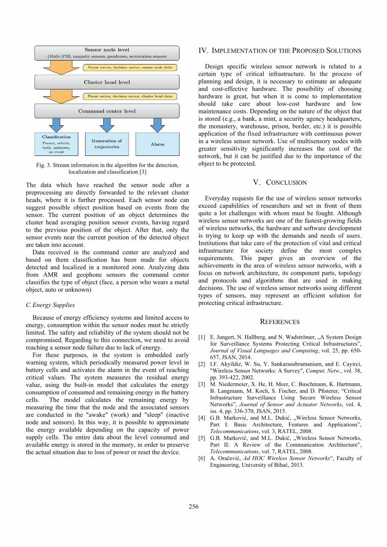
256

Fig. 3. Stream information in the algorithm for the detection, localization and classification [3]

The data which have reached the sensor node after a preprocessing are directly forwarded to the relevant cluster heads, where it is further processed. Each sensor node can suggest possible object position based on events from the sensor. The current position of an object determines the cluster head averaging position sensor events, having regard to the previous position of the object. After that, only the sensor events near the current position of the detected object are taken into account.

Data received in the command center are analyzed and based on them classification has been made for objects detected and localized in a monitored zone. Analyzing data from AMR and geophone sensors the command center classifies the type of object (face, a person who wears a metal object, auto or unknown)

C. Energy Supplies

Because of energy efficiency systems and limited access to energy, consumption within the sensor nodes must be strictly limited. The safety and reliability of the system should not be compromised. Regarding to this connection, we need to avoid reaching a sensor node failure due to lack of energy.

For these purposes, in the system is embedded early warning system, which periodically measured power level in battery cells and activates the alarm in the event of reaching critical values. The system measures the residual energy value, using the built-in model that calculates the energy consumption of consumed and remaining energy in the battery cells. The model calculates the remaining energy by measuring the time that the node and the associated sensors are conducted in the "awake" (work) and "sleep" (inactive node and sensors). In this way, it is possible to approximate the energy available depending on the capacity of power supply cells. The entire data about the level consumed and available energy is stored in the memory, in order to preserve the actual situation due to loss of power or reset the device.

IV. IMPLEMENTATION OF THE PROPOSED SOLUTIONS

Design specific wireless sensor network is related to a certain type of critical infrastructure. In the process of planning and design, it is necessary to estimate an adequate and cost-effective hardware. The possibility of choosing hardware is great, but when it is come to implementation should take care about low-cost hardware and low maintenance costs. Depending on the nature of the object that is stored (e.g., a bank, a mint, a security agency headquarters, the monastery, warehouse, prison, border, etc.) it is possible application of the fixed infrastructure with continuous power in a wireless sensor network. Use of multisensory nodes with greater sensitivity significantly increases the cost of the network, but it can be justified due to the importance of the object to be protected.

V. CONCLUSION

Everyday requests for the use of wireless sensor networks exceed capabilities of researchers and set in front of them quite a lot challenges with whom must be fought. Although wireless sensor networks are one of the fastest-growing fields of wireless networks, the hardware and software development is trying to keep up with the demands and needs of users. Institutions that take care of the protection of vital and critical infrastructure for society define the most complex requirements. This paper gives an overview of the achievements in the area of wireless sensor networks, with a focus on network architecture, its component parts, topology and protocols and algorithms that are used in making decisions. The use of wireless sensor networks using different types of sensors, may represent an efficient solution for protecting critical infrastructure.

REFERENCES

[1] E. Jungert, N. Hallberg, and N. Wadströmer, „A System Design for Surveillance Systems Protecting Critical Infrastructures”, Journal of Visual Languages and Computing, vol. 25, pp. 650-657, JSAN, 2014.

[2] I.F. Akyildiz, W. Su, Y. Sankarasubramaniam, and E. Cayirci, "Wireless Sensor Networks: A Survey", Comput. Netw., vol. 38, pp. 393-422, 2002.

[3] M. Niedermeier, X. He, H. Meer, C. Buschmann, K. Hartmann, B. Langmann, M. Koch, S. Fischer, and D. Pfisterer, “Critical Infrastructure Surveillance Using Secure Wireless Sensor Networks”, Journal of Sensor and Actuator Networks, vol. 4, iss. 4, pp. 336-370, JSAN, 2015.

[4] G.B. Marković, and M.L. Dukić, „Wireless Sensor Networks, Part I: Basic Architecture, Features and Applications”, Telecommunications, vol. 3, RATEL, 2008.

[5] G.B. Marković, and M.L. Dukić, „Wireless Sensor Networks, Part II: A Review of the Communication Architecture”, Telecommunications, vol. 7, RATEL, 2008.

[6] A. Oračević, Ad HOC Wireless Sensor Networks“, Faculty of Engineering, University of Bihać, 2013.

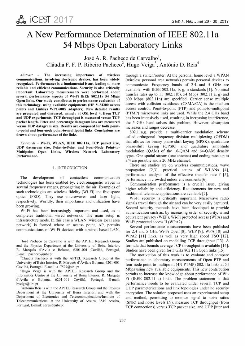
257

A New Performance Determination of IEEE 802.11a 54 Mbps Open Laboratory Links

José A. R. Pacheco de Carvalho1, Cláudia F. F. P. Ribeiro Pacheco2, Hugo Veiga3, António D. Reis4

Abstract – The increasing importance of wireless communications, involving electronic devices, has been widely recognized. Performance is a fundamental issue, leading to more reliable and efficient communications. Security is also critically important. Laboratory measurements were performed about several performance aspects of Wi-Fi IEEE 802.11a 54 Mbps Open links. Our study contributes to performance evaluation of this technology, using available equipments (HP V-M200 access points and Linksys WPC600N adapters). New detailed results are presented and discussed, namely at OSI level 4, from TCP and UDP experiments. TCP throughput is measured versus TCP packet length. Jitter and percentage datagram loss are measured versus UDP datagram size. Results are compared for both point-to-point and four-node point-to-multipoint links. Conclusions are drawn about performance of the links.

Keywords – Wi-Fi, WLAN, IEEE 802.11a, TCP packet size,

UDP datagram size, Point-to-Point and Four-Node Point-to- Multipoint Open Links, Wireless Network Laboratory Performance.

I. INTRODUCTION

The development of contactless communication technologies has been enabled by. electromagnetic waves in several frequency ranges, propagating in the air. Examples of such technologies are wireless fidelity (Wi-Fi) and free space optics (FSO). They use microwaves and laser light, respectively. Worldly, their importance and utilization have been growing.

Wi-Fi has been increasingly important and used, as it completes traditional wired networks. The main setup is infrastructure mode. In this case a WLAN (wireless local area network) is formed where an access point, AP, permits communications of Wi-Fi devices with a wired based LAN,

through a switch/router. At the personal home level a WPAN (wireless personal area network) permits personal devices to communicate. Frequency bands of 2.4 and 5 GHz are available, with IEEE 802.11a, b, g, n standards [1]. Nominal transfer rates up to 11 (802.11b), 54 Mbps (802.11 a, g) and 600 Mbps (802.11n) are specified. Carrier sense multiple access with collision avoidance (CSMA/CA) is the medium access control. Point-to-point (PTP) and point-to-multipoint (PTMP) microwave links are used. While the 2.4 GHz band has been intensively used, resulting in increasing interference, the 5 GHz band solves this problem. However, absorption increases and ranges decrease.

802.11a,g. provide a multi-carrier modulation scheme called orthogonal frequency division multiplexing (OFDM) that allows for binary phase-shift keying (BPSK), quadrature phase-shift keying (QPSK) and quadrature amplitude modulation (QAM) of the 16-QAM and 64-QAM density types. One spatial stream (one antenna) and coding rates up to 3/4 are possible and a 20 MHz channel.

There are studies are on wireless communications, wave propagation [2,3], practical setups of WLANs [4], performance analysis of the effective transfer rate f [5], performance in crowded indoor environments [6].

Communication performance is a crucial issue, giving higher reliability and efficiency. Requirements for new and traditional telematic applications are available [7].

Wi-Fi security is critically important. Microwave radio signals travel through the air and can be very easily captured. Several security methods have been developed to provide authentication such as, by increasing order of security, wired equivalent privacy (WEP), Wi-Fi protected access (WPA) and Wi-Fi protected access II (WPA2). .

Several performance measurements have been published for 2.4 and 5 GHz Wi-Fi Open [8], WEP [9], WPA[10] and WPA2 [11] links, as well as very high speed FSO [12]. Studies are published on modelling TCP throughput [13]. A formula that bounds average TCP throughput is available [14]. Studies have been given for 5 GHz 802.11n Open links [15].

The motivation of this work is to evaluate and compare performance in laboratory measurements of Open PTP and four-node point-to-multipoint (4N-PTMP) 802.11a links at 54 Mbps using new available equipments. This new contribution permits to increase the knowledge about performance of Wi-Fi (IEEE 802.11 a) links. The problem statement is that performance needs to be evaluated under several TCP and UDP parameterizations and link topologies under no security encryption. The solution proposed uses an experimental setup and method, permitting to monitor signal to noise ratios (SNR) and noise levels (N), measure TCP throughput (from TCP connections) versus TCP packet size, and UDP jitter and

1José Pacheco de Carvalho is with the APTEL Research Groupand the Physics Department at the University of Beira Interior,R. Marquês d’Ávila e Bolama, 6201-001 Covilhã, Portugal,E-mail: [email protected]

2Cláudia Pacheco is with the APTEL Research Group at theUniversity of Beira Interior, R. Marquês d’Ávila e Bolama, 6201-001Covilhã, Portugal, E-mail: [email protected]

3Hugo Veiga is with the APTEL Research Group and theInformatics Centre at the University of Beira Interior, R. Marquêsd’Ávila e Bolama, 6201-001 Covilhã, Portugal, E-mail:[email protected]

4António Reis is with the APTEL Research Group and the PhysicsDepartment at the University of Beira Interior, and with theDepartment of Electronics and Telecommunications/Institute ofTelecommunications, at the University of Aveiro, 3810 Aveiro,Portugal, E-mail: [email protected]

258

percentage datagram loss (from UDP communications) versus UDP datagram size.

The rest of the paper is structured as follows: Section II is about the experimental conditions i.e. the measurement setup and procedure. Results and discussion are given in Section III. Conclusions are drawn in Section IV.

II. EXPERIMENTAL DETAILS

Here we have used a HP V-M200 access point [17], with three external dual-band 3x3 MIMO antennas, IEEE 802.11 a/b/g/n, software version 5.4.1.0-01-16481, a 1000-Base-T/100-Base-TX/10-Base-T layer 2 3Com Gigabit switch 16 and a 100-Base-TX/10-Base-T layer 2 Allied Telesis AT-8000S/16 switch [18]. Three PCs were used having a PCMCIA IEEE.802.11 a/b/g/n Linksys WPC600N wireless adapter with three internal antennas [19], to enable 4N-PTMP links to the access point. In every type of experiment, an interference free communication channel was used (ch 36). This was essentially verified through a portable computer, equipped with a Wi-Fi 802.11 a/b/g/n adapter, running Acrylic WiFi software [20]. No encryption was activated in the AP and the wireless adapters of the PCs. The experiments were made under far-field conditions. No power levels above 30 mW (15 dBm) were used, as the wireless equipments were nearby.

A versatile laboratory setup has been planned and implemented for the measurements, as shown in Fig. 1. Up to three wireless links to the AP are possible. At OSI level 4, measurements were made for TCP connections and UDP communications using Iperf software [21]. For a TCP client/server connection (TCP New Reno, RFC 6582, was used), TCP throughput was obtained for a given TCP packet size, varying from 0.25k to 64k bytes. For a UDP client/server communication with a given bandwidth parameter, UDP jitter and percentage loss of datagrams were determined for a given UDP datagram size, varying from 0.25k to 64k bytes.

One PC, with IP 192.168.0.2 was the Iperf server and the others, with IPs 192.168.0.6 and 192.168.0.50, were the Iperf clients (client1 and client2, respectively). Jitter, which is the smooth mean of differences between consecutive transit times, was continuously computed by the server, as specified by the real time protocol RTP, in RFC 1889 [22]. A control PC, with IP 192.168.0.20, was mainly used to control the settings of the AP. Three types of experiments are possible: PTP, using the client1 and the control PC as server; PTMP, using the client1 and the 192.168.0.2 server PC; 4N-PTMP, using simultaneous connections/communications between the two clients and the 192.168.0.2 server PC.

The server and client PCs were HP nx9030 and nx9010 portable computers, respectively. The control PC was an HP nx6110 portable computer. Windows XP Professional was the operating system. The PCs were prepared to enable maximum resources to the present work. Batch command files have been re-written for the new TCP and UDP tests.

The results were obtained in batch mode and written as data files to the client PCs disks. Every PC had a second network adapter, to permit remote control from the official IP University network, via switch.


The wireless network adapters of the PCs were manually configured for a nominal rate of 54 Mbps. No encryption was used. Transmit and receive rates were monitored in the AP during the experiments. They were typically 54 Mbps. For every TCP packet size in the range 0.25k-64k bytes, and for every corresponding UDP datagram size in the same range, data were acquired for Open 4N-PTMP and PTP links at OSI levels 1 (physical layer) and 4 (transport layer) using the setup of Fig. 1. For every TCP packet size an average TCP throughput was calculated from a series of experiments. This value was considered as the bandwidth parameter for every corresponding UDP test, giving average jitter and average percentage datagram loss.

At OSI level 1, signal to noise ratios (SNR, in dB) and noise levels (N, in dBm) were obtained in the AP. Typical values are shown in Fig. 2. The links exhibited good, high, SNR values. The main average TCP and UDP results are summarized in Table I, for Open 4N-PTMP and PTP links. The statistical analysis, including calculations of confidence intervals, was made as in [22]. In Fig. 3 polynomial fits were made (shown as y versus x), using the Excel worksheet, to the TCP throughput data both for both links, where R2 is the coefficient of determination. It gives the goodness of fit. If it is 1.0 it means a perfect fit to data. It was found that, on average, the best TCP throughputs are for PTP links (Table I). There is a very significant degradation to 23% in passing from PTP to 4N-PTMP. This is due to increase of processing requirements for the AP, so as to maintain links between the PCs. Fig. 3 shows that there is a fair increase in TCP throughput with packet size. For small packets there is a large overhead, as there are small amounts of data that are sent in comparison to the protocol components. The role of the frame is very heavy in Wi-Fi. For larger packets, overhead decreases; the amount of sent data overcomes the protocol components.

In Figs. 4-5, the data points representing jitter and percentage datagram loss were joined by smoothed lines. It was found that, on average, the best jitter performance is for PTP links. Let us note a large error bar mainly in the 8k data point of the 4N-PTMP curve (Fig. 4), that needs further investigation. For PTP it can be seen that, for small sized datagrams, jitter is small. There are small delays in sending datagrams. Latency is also small. For larger datagram sizes jitter increases.

Concerning average percentage datagram loss, performances were found on average significantly better for PTP than for 4N-PTMP links (Table I). This is due to increase of processing requirements for the AP, for maintaining links between two PCs. Let us note a large error bar mainly in the 8k data point of the 4N-PTMP curve, that needs further investigation. Fig. 5 generally shows larger percentage datagram losses for small sized datagrams, when the amounts of data to send are small in comparison to the protocol components. There is considerable processing of frame headers and buffer management. For larger datagrams, percentage datagram loss is lower. However, large UDP

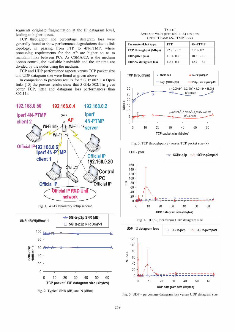
259

segments originate fragmentation at the IP datagram level, leading to higher losses.

TCP throughput and percentage datagram loss were generally found to show performance degradations due to link topology, in passing from PTP to 4N-PTMP, where processing requirements for the AP are higher so as to maintain links between PCs. As CSMA/CA is the medium access control, the available bandwidth and the air time are divided by the nodes using the medium.

TCP and UDP performance aspects versus TCP packet size and UDP datagram size were found as given above.

In comparison to previous results for 5 GHz 802.11n Open links [15] the present results show that 5 GHz 802.11n gives better TCP, jitter and datagram loss performances than 802.11a.

Fig. 1. Wi-Fi laboratory setup scheme

Fig. 2. Typical SNR (dB) and N (dBm)

TABLE I AVERAGE WI-FI (IEEE 802.11.A) RESULTS;

OPEN PTP AND 4N-PTMP LINKS

Parameter/Link type PTP 4N-PTMP

TCP throughput (Mbps) 22.9 +- 0.7 5.2 +- 0.2

UDP-jitter (ms) 4.1 +- 0.6 10.2 +- 0.7

UDP-% datagram loss 1.2 +- 0.1 12.7 +- 8.1

Fig. 3. TCP throughput (y) versus TCP packet size (x)

Fig. 4. UDP - jitter versus UDP datagram size

Fig. 5. UDP – percentage datagram loss versus UDP datagram size

260

IV. CONCLUSION

In the present work a versatile laboratory setup arrangement was devised and implemented, that permitted systematic performance measurements using new available wireless equipments (V-M200 access points from HP and WPC600N adapters from Linksys) for Wi-Fi (IEEE 802.11 a) in 54 Mbps Open PTP and 4N-PTMP links.

Through OSI layer 4, TCP and UDP performances were measured versus TCP packet size and UDP datagram size, respectively. TCP throughput, jitter and percentage datagram loss were measured and compared for Open PTP and 4N-PTMP links. TCP throughput was found to increase with packet size. For PTP jitter, for small sized datagrams, is found small. It increases for larger datagrams. Concerning percentage datagram loss, it was found high for small sized datagrams. For larger datagrams it diminishes. However, large UDP segments originate fragmentation at the IP datagram level, leading to higher losses. In comparison to PTP links, TCP throughput and percentage datagram loss were found to show significant performance degradations for 4N-PTMP links, where the AP experiments higher processing requirements for maintaining links between PCs. The present results show that 5 GHz 802.11n gives better TCP, jitter and datagram loss performances than 802.11a.

Further performance studies are planned using several standards, equipments, topologies, security settings and noise conditions, not only in laboratory but also in outdoor environments involving, mainly, medium range links.

ACKNOWLEDGEMENT

Supports from Universidade da Beira Interior and FCT (Fundação para a Ciência e a Tecnologia)/PEst-OE/FIS/UI0524/2014 (Projecto Estratégico-UI524-2014) are acknowledged.

REFERENCES

[1] Web site http://standards.ieee.org Web site; IEEE 802.11a, 802.11b, 802.11g, 802.11n, 802.11i standards; accessed 10 Jan 2017.

[2] J.W. Mark, and W. Zhuang, Wireless Communications and Networking, Prentice-Hall, Inc., Upper Saddle River, NJ, 2003.

[3] T.S. Rappaport, Wireless Communications Principles and Practice, 2nd ed., Prentice-Hall, Inc., Upper Saddle River, NJ, 2002.

[4] W.R. Bruce III, and R. Gilster, Wireless LANs End to End, Hungry Minds, Inc., NY, 2002.

[5] M. Schwartz, Mobile Wireless Communications, Cambridge University Press, 2005.

[6] N. Sarkar, and K. Sowerby, “High Performance Measurements in the Crowded Office Environment: a Case Study”, ICCT’06-International Conference on Communication Technology, Guilin, China, 27-30 November 2006, pp. 1-4.

[7] E. Monteiro, and F. Boavida, Engineering of Informatics Networks, 4th ed., FCA-Editor of Informatics Ld., Lisbon, 2002.

[8] J. A.R. Pacheco de Carvalho, H. Veiga, P. A.J. Gomes, C.F. Ribeiro Pacheco, N. Marques, and A.D. Reis, “Wi-Fi Point-to-Point Links-Performance Aspects of IEEE 802.11 a,b,g Laboratory Links”, Electronic Engineering and Computing Technology, Series: Lecture Notes in Electrical Engineering, Sio-Iong Ao, Len Gelman, Eds. Netherlands: Springer, 2010, vol. 60, pp. 507-514.

[9] J. A.R. Pacheco de Carvalho, C.F. Ribeiro Pacheco, A. D. Reis, and H. Veiga, “Extended Performance Studies of Wi-Fi IEEE 802.11a, b, g Laboratory WEP Point-to-Multipoint and Point-to-Point Links”, Transactions on Engineering Technologies: World Congress on Engineering 2014, Gi-Chul Yang, Sio-Iong Ao, Len Gelman, Eds. Gordrecht: Springer, 2015, pp. 563-572.

[10] J. A.R. Pacheco de Carvalho, H. Veiga, C.F. Ribeiro Pacheco, and A.D. Reis, “Extended Performance Studies of Wi-Fi IEEE 802.11a, b, g Laboratory WPA Point-to-Multipoint and Point-to-Point Links”, Transactions on Engineering Technologies: Special Volume of the World Congress on Engineering 2013, Gi-Chul Yang, Sio-Iong Ao, Len Gelman, Eds. Gordrecht: Springer, 2014, pp. 455-465.

[11] J. A.R. Pacheco de Carvalho, H. Veiga, C.F. Ribeiro Pacheco, and A. D. Reis, “Performance Evaluation of IEEE 802.11 a, g Laboratory WPA2 Point-to-Multipoint Links”, Lecture Notes in Engineering and Computer Science: Proceedings of the World Congress of Engineering 2014, WCE 2014, 2-4 July 2014, London, U. K., pp. 699-704.

[12] J. A.R. Pacheco de Carvalho, N. Marques, H. Veiga, C. F.F. Ribeiro Pacheco, and A. D. Reis, “Performance Measurements of a 1550 nm Gbps FSO Link at Covilhã City, Portugal”, Applied Electronics 2010 - 15th International Conference, 8-9 September 2010, University of West Bohemia, Pilsen, Czech Republic, pp. 235-239.

[13] J. Padhye, V. Firoiu, D. Towsley, and J. Kurose, "Modeling TCP Throughput: A Simple Model and its Empirical Validation", SIGCOMM Symposium Communications, Architecture and Protocols, August 1998, pp. 304-314.

[14] M. Mathis, J. Semke, and J. Mahdavi, "The Macroscopic Behavior of the TCP Congestion Avoidance Algorithm", ACM SIGCOMM Computer Communication Review, vol. 27, Issue 3, July 1997, pp. 67-82.

[15] J. A.R. Pacheco de Carvalho, H. Veiga, C.F. Ribeiro Pacheco, and A. D. Reis, ”Performance Measurements of Open 5 GHz IEEE 802.11n Laboratory Links”, Lecture Notes in Engineering and Computer Science: Proceedings of the World Congress on Engineering 2016, WCE 2016, 29 June-1 July, 2016, London, U.K., pp. 607-611.

[16] Web site http://www.hp.com; HP V-M200 802.11n access point management and configuration guide; 2010; accessed 3 Jan 2017.

[17] Web site http://www.alliedtelesis.com; AT-8000S/16 level 2 switch technical data; 2009; accessed 10 Dec 2016.

[18] Web site http://www.linksys.com; WPC600N notebook adapter user guide; 2008; accessed 10 Jan 2012.

[19] Acrylic WiFi software; 2016; http://www.acrylicwifi.com; accessed 8 Jan 2017.

[20] Iperf software; 2016; http://iperf.fr; accessed 16 Feb 2017. [21] Network Working Group. “RFC 1889-RTP: A Transport

Protocol for Real Time Applications”, http://www.rfc-archive.org; 1996; accessed 3 Jan 2014.

[22] P.R. Bevington, Data Reduction and Error Analysis for the Physical Sciences, Mc Graw-Hill Book Company, 1969.

261

A Study on the Human Inner Ear Preparedas a Multidisciplinary Approach: Telecommunications and

Power Engineering Kalpit Bakal1, Pushkar Vaidya2

Abstract – In this paper the relation between two different specialities as an interdisciplinary approach to solve a problem in engineering and medical is shown. This study is a good example how to combine fluid dynamics with Power engineering and signal processing as a part of Telecommunications to produce a working model of a biological process. This isan innovative approach to solve such tasks in the real working quarter. In this paper, the biological description of inner ear, simulation model for cochlea, pressure contours on the basilar membrane and the deflection values are shown.This gives us brief idea about how the cochlea works and its interdisciplinary relationship.

Keywords – Telecommunications, Power engineering, Cochlea, Fluid dynamics, Signal processing, Fluent, Mechanical APDL.

I. INTRODUCTION

The purpose of the study is to show the benefits of interdisciplinary approach of fluid dynamics and telecommunications in the field of signal processing. They both show the multidisciplinary point of view being put into practice in cochlea mechanism and the design of human cochlea implants and tuning.

In order to explain the process of design and simulation of the cochlea the geometry and functions of this organ are explained below.

The cochlea is filled with a watery liquid, the perilymph, which moves in response to the vibrations coming from the middle ear via the oval window. As the fluid moves, the cochlea partition (basilar membrane and organ of Corti) moves; thousands ofhair cells sense the motion via their stereocilia, and convert that motion to electrical signals.These signals are communicated via neurotransmitters to many thousands of nerve cells. These primary auditory neurons transform the signals into electrochemical impulses known as action potentials, which travel along the auditory nerve to structures in the brainstem for further processing.

The cochlea originally has the shape like spiral [1]; precisely ‘snail’ as cochlea is Latin for the snail. The main cochlea parts are round window, oval window, the perilymph fluid and Basilar Membrane (BM) as shown in Fig. 1 [2]. The BM is most important element of inner ear as the deformation of BM due to sound pressure waves aftermaths in the motion

of hair cells and the neural signals are generated before delivering it to the brain. The mechanics of the basilar membrane is reason for ear to hear the fine frequency ranges. When the stapes exerts force on the oval window in rhythmic pattern, the perilymph fluid acts as a medium to carry those pressure waves around the BM. Since the stiffness decreases along the length towards apex, it deflects in the particular frequency in the particular region of the length. The deformation due to the travelling waves is proportional to the passive material parameters i.e. elasticity, density and damping properties. The basilar membrane has a detailed frequency map as shown in Fig. 2 [3].

Fig. 1. Cochlea natural geometry representation

Fig. 2. Frequency map for basilar membrane

1Kalpit Bakal is working at Tata Lockheed Martin AerostructuresLtd., Hyderabad, Telangana, India. E-mail: [email protected].

2Pushkar Vaidya is with the University of Mumbai, Kalina,Mumbai, India. E-mail: [email protected]

262

TABLE I

II. GEOMETRICAL AND MATERIAL DESIGN

A. Geometrical and Material Parameters

With initial consideration of cochlea materials and the geometric proportions, original dimensions are considered. The model has been simplified in this work and elements are defined accordingly. The simplification was done since the computational resources were limited. Therefore, instead of

the spiral model a simple box model was designed. The geometry and material properties are as mentioned in the Table I [8].

B. Design Software

The model of cochlea was simplified and designed using SOLIDWORKS. User friendly design features was the primary reason for using the above mentioned software. The simplified model and their dimensions are mentioned in the Figs. 3 and 4 and Table II. The ‘Assembly’ feature was used to design the solid model. The basilar membrane and the outer casing (Fig. 4) were designed separately. Both the components were joined using the ‘Assembly’ operation in SOLIDWORKS.

Fig. 3. Dimension of 2 windows

Fig. 4. Final solid model

TABLE II SOLID MODEL DIMENSIONS

Parts Dimensions(mm) Basilar Membrane 3x0.1x29

Round Window Diameter=0.93 Oval Window Major=1.5, Minor=0.63

Element structure Data

Oval window

Geometric parameters

Major axis(mm) 2.24

Minor axis(mm) 1.4

Thickness(mm) 0.2

Materials parameters

Density(kg/m3) 2.3x103

Elastic modulus (N/m2) 1.71x1010

Round Window


Diameter(mm) 1.2

Thickness(mm) 0.05



Elastic modulus (N/m2) 3.5x105

Basilar Membrane


Base width(mm) 0.1

Apex width(mm) 0.5

Base Thickness(mm) 7.5

Apex Thickness(mm) 2.5

Length(mm) 31.9



Youngs modulus (N/m2)

Base 5x107

Middle 1.5x107

Apex 3x106

263

II. FLUID AND MECHANICAL SIMULATIONS OF

THE MODEL

A. Fluid Simulations

The fluid simulation for the above mentioned model was done in ANSYS FLUENT. The sound wave input at the oval window was given in the form of pressure wave [1]. The simulation was carried out for two frequencies viz. 600 Hz and 12 kHz. The Table III shows the parameters considered for the UDF (User-defined function). UDF is a feature of ANSYS FLUENT in which we can vary the input signal. Here, the input signal is pressure, which is varied as a sinusoid. The number of points to be plotted on the sinusoid mentioned in first column in Table III was decided based on the computation resources available. The graphical representation for the input signal is shown in the Fig. 5. The simulation was carried out using the k-upsilon turbulence model [4], [5]. This model was used since the fluid in our case is incompressible.

TABLE III PARAMETERS OF THE UDF

Fig. 5. Input Signal

After post-processing, the pressure contours were obtained for both the frequencies on the upper as well as lower part of the basilar membrane. As the pressure on the upper surface is higher than the pressure on the lower surface the basilar membrane will bend in the downward direction. This

deforming effect is shown in the section of Mechanical Simulation. Consider Fig. 6 and 7 which shows the cutout of the pressure contour on the basilar membrane for 600Hz. The colour map on the left side of the Figs. 6, 7, 8 and 9 show decreasing value of pressure in the downward direction. The figures show that the upper surface has higher pressure (colour contours) and that is why the basilar membrane will deform downwards.

Fig. 6. Pressure contour on upper surface of BM for 600 Hz

Fig. 7. Pressure contour on lower surface of BMfor 600 Hz

Fig. 8. Pressure contour on upper surface of BM for 12kHz

Frequency 600HZ 12000HZ No. of points for one

sinusoid 9 9

Simulation period 0.1s 0.05s No. of time steps 540 5400 Time-step size 0.000185s 9.529x10-6

No. of iterations\time-step

10 10

Maximum no. of iterations

5400 54000

264

Fig. 9. Pressure contour on lower surface of BM for 12kHz

B. Mechanical Simulation

To observe the deflection and obtain the value of deflection a scaled up model of basilar membrane was designed in ANSYS Mechanical APDL. The dimension was scaled up by a value of 100. The actual size of the cochlea is very small. Of course the results obtained were very small in 10-5micron range. To get a better idea about the numbers related to the results the dimensions were scaled up. The material properties of polyamide-6-titanium dioxide were used for the membrane. The deflection values for this material were approximately the same as that of the original basilar membrane. The pressure values from ANSYS FLUENT on the upper and lower surface of the membrane were taken and averaged out. The force was applied in APDL and the deflection was observed. The maximum deflection for the scaled up model at 600Hz was 0.0053m (Fig. 10) and for 12 kHz was 0.004057m (Fig. 11). This deflection was observed in the area where the basilar membrane is reactive to the respective frequency shown in Fig. 2.

As we can see in the Fig. 2 the frequency range of the cochlea ranges from 200 Hz to 20 kHz. The simulation time for one result took around 40 Hours on an Intel 4th Gen i7 processor. So we decided to cut short to two intermediate frequencies for time saving. We did not have enough processing power while we were actually simulating.

Fig. 10. Deflection for 600 Hz

Fig. 11. Deflection for 12 kHz

III. CONCLUSION

In this paper is shown how the use of two different subjects as fluid dynamics and signal processing help to solve successfullyan interdisciplinary problem related to the both engineering and medicine spheres. Mixing the both lead to better understanding and putting into practice the theory in engineering. The results shows that education and design in multidisciplinary approach leads to solving an engineering problem concerning even to a medical topic. The study of materials was carried out and a suitable material was found out. The simulations were carried to see which part of the membrane reacts to which frequencies and the results almost matched. This is just a start of 3D simulations in this multi-disciplinary approach of fluid mechanics and telecommunications. It is just a crude start in this field which can made smooth further with inclusion of finer grids and animations for the pressure wave on the basilar membrane.

An interdisciplinary approachleads to improved student knowledge and better understanding of the given task.

REFERENCES

[1] S. Antonov, "Hydrodynamic Modeling of the Lymph Transport in Human Cochlea Using CFD Based Software", Journal of Food and Packaging Science, Technique and Technologies 2, pp. 148-153, 2013.

[2] http://www.wikipremed.com/mcat_course_psychology.php?module=2&section=8

[3] http://teddysratlab.blogspot.in/2011/03/and-ears-to-hear.html [4] I. Antonov, R. Velichkova, and S. Antonov, "Differential

Equations for Turbulent Flow", Annual Conference RU & SU, vol. 53, no. Book 1.2, University of Ruse, pp. 119-123, 2014.

[5] S. Antonov, A. Terziev, and S. Bekiarska, "Mathematical Modeling of Sound Wave Propagation Through Endolymph Liquid in the Human Cochlea", Journal of Food and Packaging Science, Technique and Technologies 2, pp. 179-182, 2013.

265

The Performace Evaluation of GMSAT Video Watermarking against Geometric Attacks

Zoran Veličković1, Zoran Milivojević1 and Marko Veličković1

Abstract – In this work, the performance of the algorithm GMSAT protection of original video content in relation to the geometric malicious attacks are determined. The goal of geometric attacks on video is to disable the watermark extraction, thus endangering the copyrights. The paper analyses geometrical attacks realized by the addition of noise, filtering and cropping the parts of the video frames. The GMSAT algorithm showed good resistance to discussed geometric attacks so that it can be recommended for the protection of original video content before exposure on the Internet.

Keywords – Generalized Multistage Arnold Transformation, Watermarking, Geometric attacks.

I. INTRODUCTION

This paper discusses the algorithms for protecting original multimedia content from illegal copying and distribution. In a network environment of modern broadband Internet, protection of multimedia content, especially video, is becoming an indispensable activity of the author prior to publication on the Internet. In 2016, 64% of all Internet transmitted packets related to some form of video traffic [1]. Contemporary online multimedia applications, a special VoIP (Voice over Internet Protocol), VOD (Video on Demand) and video conferencing have contributed to the enormous increase in packet traffic. Adoption of the new standard high-resolution video such as HD, 4K UHD and will only increase the share of video packets in global IP traffic. Required network bandwidth for transmission of 4K video is twice that of HD resolution, that is, nine times higher than the SD resolution. In [1] is presented astonishing assumption that by the end of 2019 the share of the total video packets in IP traffic to increase to 80%.

These data clearly indicate that the exchange of digital multimedia content, especially video, has already become the dominant form of IP traffic. Trends in modern multimedia communication technologies for the researchers set new, previously unknown tasks and challenges [2], [3]. The ubiquitous availability of digital multimedia content, as well as their properties when copying there is no drop in quality, are favored piracy occurs. Copyright protection of digital multimedia content in the aforementioned network conditions is a very complex task [4].

In order to prevent illegal copying and distribution of digital multimedia content on the Internet can be applied standard cryptographic techniques. However, although by standard cryptographic techniques based on PKI (Public Key Infrastructure) are very reliable, they are not adequate for the protection of multimedia content. The main drawback of these techniques is reflected in the necessary decryption before playing multimedia content, which content exposes to security risks. For practical application are more convenient methods which are based on inserting a watermark in the multimedia content [5]-[9]. Methods of protection of multimedia content based on the watermark insertion means the permanent insertion of the multimedia content so that it does not remove during playback. This concept of protection of multimedia content indirectly protects watermark itself from malicious and destructive attacks. In this way, further increases the level of security of protected multimedia content.

The knowledge of the watermark content in some cases can threaten the security of the protected video. Therefore, in this paper it is proposed to use a GMSAT (Generalized MultiStage Arnold Transformation) for encrypting - scrambling of the contents of the watermark [6], [7]. To obtain the original watermark from scrambled, it is developed inverse algorithm IGMSAT. Just knowing all the parameters of IGMSAT it is possible to transform scrambled watermark in the original. Since the algorithm belongs to a class GMSAT invertible chaotic maps it is necessary to know the initial conditions of transformation.

In this article, the insertion of the watermark in scrambled video content reliable algorithm based on a combination of a DWT (Discrete Wavelet Transform), and SVD (Singular Value Decomposition) is applied. Scrambled watermark is embedded into each frame of uncoded video sequences. It should be noted that after the insertion of scrambled watermark, video are coded by H.264 / AVC encoder. Given that, the H.264 / AVC encoder belongs to a class encoder with losses in coding inevitably leads to degradation of video content, and thus the inserted watermark. The influence of the applied encoder on video content and quality of the extracted watermarks are analyzed in previous papers of authors [5]-[8].Also, the prior papers of authors tested the resistance of the used techniques to false tripping of the watermark and lack of knowledge of a set of transformation parameters [6].

This paper especially analyzed malicious attacks which can be classified into geometrical attacks. Because the geometric attacks impact destructively on protected video, the survival of the inserted watermark after these attacks are analyzed. One part of the analysis consists of adding the Gaussian and "salt & pepper" noise, while the second part of the analysis relates to a median filtering, and the tear-off parts of the protected decoded video content.To improve the extracted watermark, advanced corrections algorithm based on a set of

1Zoran Veličković is with College of Applied Technical Sciences,Nis, Serbia, A. Medvedeva 20, 18000 Niš, Serbia, E-mail:[email protected]

1Zoran Milivojević is with College of Applied Technical Sciences,Nis, Serbia, A. Medvedeva 20, 18000 Niš, Serbia, E-mail:[email protected]

1Marko Veličković is with College of Applied Technical Sciences,Nis, Serbia, A. Medvedeva 20, 18000 Niš, Serbia, E-mail:[email protected]

266

extracted variable quality watermarks is used. In this article it is experimentally confirmed the robustness of the proposed algorithm, which includes insertion, extraction and improvement of quality of the watermark to its removal attempts.

The second section presents a mathematical basis of GMSAT, while the third section provides reliable modified algorithms for installation and extraction of the watermark based on DWT and SVD. Fourth section evaluate the proposed algorithm and shows the results of the performed experiments. Based on the analysis results, the robustness of the algorithm on some geometric attacks is verified. In the fifth chapter an appropriate conclusions on the basis of the tests are conducted.

II. GENERALIZED MULTISTAGE ARNOLD

TRANSFORMATION GMSAT

In the prior papers authors are suggested MSAT (MultiStage Arnold Transformation) [7] for scrambling the content of the watermark. The basic idea of this transformation is based on the sequential application of multiple Arnold transformation - stage of the watermark. The transformation parameters of i-th stageai, bi, and the number of sequential iteration ki represent the keys for the encryption, while the period of Arnold transformation stage Ti further demands for the application of inverse MSAT-a. This paper applies GMSAT (Generalized Multistage Arnold Transformation), which allows variations dimensions square watermark Ni in stages [6]. Each stage of a generalized 2D multistage Arnold transformation (i) can be described by the expressions (1) and (2):

11 (1)

, ∈ 1, 2, …

, ∈ 0,1,… , 1 0,1, … , 1 ⊂ (2)

where , i , represent the locations of image pixels, and ai, bi and Ni are parameters of multistage Arnold transformation. Set parameters KeyI which determine a generalized multistage Arnold transformation can be represented by the expression (3):

, , , , , 1,2, … (3)

where Ei represents the i-th stage of the I-th GMSAT stages. When scrambling locations pixels watermark by GMSAT, on the input of the first stage E1 brings the original watermark, and the exit from I-th EI stage gets transformed watermark. When using IGMSAT (Inverse GMSAT) procedure shall be repeated with the same parameters but in reverse order. Scrambled watermark is fed to an inverse algorithm as well as the stages I-th IEI, while the original watermark obtained at the output of the first stage of the inverse algorithm of IE1. Similarly to GMSAT, the output of the previous stage IGMSAT are fed to the following stages of IGMSAT.The capacity of the inserted watermark is equal to 25% of the video frame size.

III. RELIABLE ALGORITHM FOR WATERMARK

INSERTION AND EXTRACTION

In this work, the insertion and extraction of the watermark in the video frame in the SVD domain performs by reliable algorithm. Reliable SVD algorithm solves the problem of false positives watermark which is inherent in standard SVD algorithm. Details of the algorithm for insertion and extraction of encrypted watermark in the DWT-SVD domain [6], [9] are represented by a series of the following steps I and E.

A. Algorithm for Watermark Insertion

Step I1: Decomposition of the frame F by using the second-level DWT transformation:

, (4)

, , ,

, ,

Step I2: SVD decomposition sub-band , k LL2:

⋅ ⋅ . (5)

Step I3: Encrypting the original watermark W' (lower resolution) using a generalized multi-step transformation of Arnold's and the preparation of a watermark W which is inserted into each frame.

_, , , ,

1,2, … . (6)

Step I4: SVD decomposition encrypted watermark W and calculating the principal componentsAwa[8].

∙ ∙ ⋅ ; ∙ . (7)

Step I5: Installation of principal components Awa in a diagonal matrix sub bands by a factor of inserting α:

_ ⋅ . (8)

Step I6:Creating a modified sub-band with embedded watermark:

∙ _ ∙ . (9)

Step I7:Replacing the original sub-band of second frame level by a modified and application of the inverse discrete wavelet transform IDWT2 for obtaining watermarked frame.

, . (10)

B. Algorithm for Watermark Extraction

The process of extracting a watermark W* from a protected video can be done by following the steps E:

Step E1: Decomposition of the original frame F by using the second-level DWT transformation:

, (11) , , ,

, ,

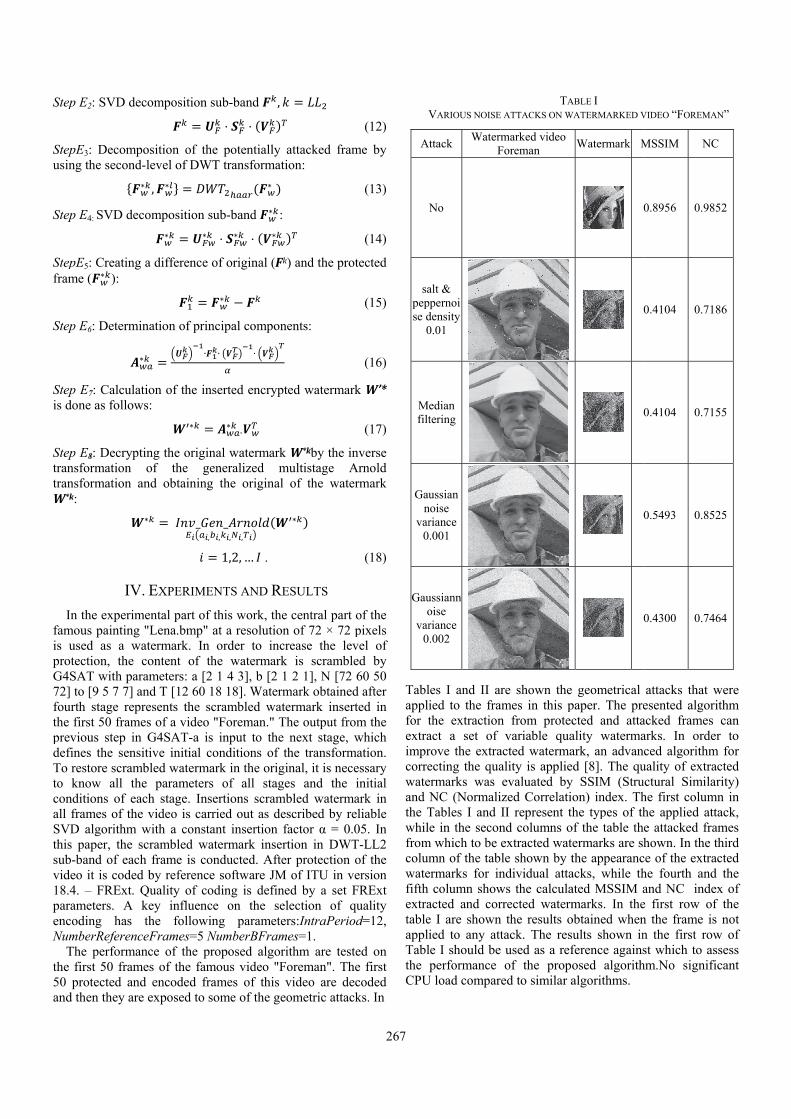
Step

Stepusin

Step

Stepfram

Step

Stepis d

SteptrantranW*k

Infamis uprotG4S72] fourthe prevdefiTo rto conall fSVDthissubvide18.4paraencNum

Tthe 50 and

p E2: SVD dec

pE3: Decompng the second-

∗

p E4: SVD dec

pE5: Creating me ( ∗ ):

p E6: Determin

∗

p E7: Calculatdone as follow

p E8: Decryptnsformation nsformation ak:

IV.

n the experimmous painting used as a watection, the cSAT with parto [9 5 7 7] an

rth stage reprfirst 50 framevious step in ines the sensirestore scrambknow all the

nditions of eacframes of theD algorithm ws paper, the s-band of eacheo it is coded4. – FRExt. Qameters. A koding has mberReferencThe performan

first 50 framprotected and

d then they are

composition s

osition of the-level of DWT

∗ , ∗

composition su

∗ ∗

a difference o

nation of prin

∗ ∙

tion of the insws:

∗

ing the originof the ge

and obtaining

∗ _,

. EXPERIMEN

mental part of t"Lena.bmp" aatermark. In content of thameters: a [2 nd T [12 60 1resents the sces of a video "

G4SAT-a is itive initial cobled watermae parameters ch stage. Inse video is carrwith a constacrambled wat

h frame is cond by referenceQuality of codkey influencethe followineFrames=5 Nnce of the pr

mes of the famd encoded frae exposed to so

sub-band ,

⋅ ⋅

e potentially T transformati

∗

ub-band ∗ :

⋅ ∗ ⋅ ∗

of original (Fk

∗

ncipal compon

∙ ∙

serted encrypt

∙∗

nal watermarkeneralized m

the original

_, , ,

1,2, … .

NTS AND RE

this work, theat a resolutionorder to incr

he watermark1 4 3], b [2 18 18]. Waterm

crambled wate"Foreman." Tinput to the

onditions of tark in the origi

of all stageertions scrambried out as deant insertion ftermark insernducted. Afte

e software JMding is definee on the selng paramete

NumberBFramroposed algori

mous video "Fames of this vome of the ge

attacked framion:

k) and the prot

nents:

ted watermark

k W*kby the inmultistage A

of the water

∗

ESULTS

e central part on of 72 × 72 prease the lev

k is scramble1 2 1], N [72 6mark obtainedermark insert

The output fromnext stage, w

the transformainal, it is necees and the ibled watermascribed by rel

factor α = 0.0rtion in DWTer protection o

M of ITU in veed by a set Flection of qurs:IntraPeriod

mes=1. ithm are testeoreman". Thevideo are decometric attack

267

(12)

me by

(13)

(14)

tected

(15)

(16)

k W’*

(17)

nverse Arnold rmark

(18)

of the pixels vel of ed by 60 50

d after ted in m the which ation. essary initial ark in liable

05. In T-LL2 of the ersion FRExt uality d=12,

ed on e first coded ks. In

V

A

sapepse d

0

Mfilt

Gaun

var0

Gauo

var0

Tablapplifor textraimprcorrewateand the Twhilfromcolumwatefifth extratableappliTablthe CPU

VARIOUS NOISE

ttack Water

F

No

alt & ppernoidensity 0.01

edian tering

ussian noise riance .001

ussiannoise riance .002

les I and II aried to the frathe extractionact a set of rove the extraecting the quaermarks was NC (NormaliTables I and e in the secon

m which to be mn of the tab

ermarks for incolumn show

acted and core I are shownied to any attle I should beperformance

U load compar

TA

E ATTACKS ON W

marked video Foreman

re shown theames in this pn from protec

variable quaacted watermaality is applieevaluated by

ized CorrelatiII represent thnd columns oextracted watle shown by tndividual attaws the calcularrected watermn the results otack. The res

e used as a refof the prop

red to similar a

ABLE I WATERMARKED V

Watermark M

geometrical paper. The prected and attaality watermaark, an advaned [8]. The quy SSIM (Struon) index. Thhe types of th

of the table thtermarks are shthe appearancacks, while thated MSSIM amarks. In the

obtained whensults shown inference againsosed algorithalgorithms.

VIDEO “FOREMA

MSSIM NC

0.8956 0.98

0.4104 0.71

0.4104 0.71

0.5493 0.85

0.4300 0.74

attacks that wesented algoracked frames arks. In ordeced algorithm

uality of extrauctural Similahe first columhe applied atte attacked frahown. In the t

ce of the extrahe fourth andand NC indee first row ofn the frame isn the first rowst which to as

hm.No signifi

AN”

C

52

86

55

25

64

were ithm can

er to m for acted arity) mn in tack, ames third acted d the ex of f the s not w of ssess icant

268

TABLE II VARIOUS CROPPING ATTACKS ON WATERMARKED VIDEO “FOREMAN”

Attack Watermarked video

Foreman Watermark MSSIM NC

Missing 15 pixels from one

side

0.3396 0.6227

Missing 15 pixels from each

sides

0.2478 0.4782

Missing block 15x15 pixels

0.3528 0.6302

Missing 10 pixels, vertical

0.4738 0.7665

Missing 10 pixels, horizontal

0.0892 0.1158

At the beginning it should be noted that due to the rounding

of the applied mathematical transformations and effects coding encoder with losses, it is not possible to extract the watermark with maximum coefficients SSIM and NC. Table I refers to attacks related to the additive noise and filtering, while Table II applies to attacks to remove certain parts of the frame.

The analysis of the results shown in Table I may be seen that the different attacks have different impacts on the quality of the extracted watermark. The applied "salt & pepper" noise ratio (density = 0.01) and the median filter are lowered quality of the extracted watermark to 31.56%, while the effect of the Gaussian noise will lower the quality of the extracted watermarks to 38.67% (variance = 0.001), respectively, 51.99% (variance = 0.002). In Table II are presented the results of geometric attacks based on removing parts of the frames. The proposed algorithm is significantly more resistant to lack of pixels vertically in relation to the lack of pixels horizontally. Cropping decoded frame on the one side

vertically lowers the quality of the extracted video for 62.08% and 72.33% from cropping two sides. Cropping in the center of the frame causes a lowering the quality of 60.6% and 47.1% for the lack of a central vertical. The lack of a central horizontal significantly lowers the quality of the extracted watermark. The proposed algorithm is unresisting to this type of attack because the extracted watermark can not be recognized. In all other considered attacks watermark is detectable and can be successfully extracted from attacked video.

V. CONCLUSION

In this work, the performance of the algorithm to protect video watermark in an attempt geometric malicious attacks are determined. A watermark is inserted in unencoded domain, so it is independent of the compression standards. The content of the watermark is scrambled before insertion in all video frames using GMSAT, while the insertion by reliable algorithms based on DWT and SVD transformations is performed. After protection, video is coded, and in the experimental part of the work has demonstrated resilience of the proposed algorithm on most geometric attacks. The only drawback of this algorithm is expressed in the geometric attack when horizontal area of 10 × 288 pixels is destroyed. This deficiency can be attributed to characteristics SVD transformation. In all other cases the geometric attacks, watermarks were extracted with acceptable quality. The quality of the extracted watermarks measured by SSIM index ranged from 0.2478 to 0.5493, while the NC ranged from 0.4782 to 0.8525. The obtained results are in accordance with a similar algorithms. The presented algorithm showed good resistance in geometric attacks based on adding noise, filtering and cropping, so it can be successfully applied in the protection of original video content on the Internet.

REFERENCES

[1] Cisco White Paper, “Cisco Visual Networking Index: Global Mobile Data Traffic Forecast Update, 2015–2020”, Feb. 2016.

[2] M. Jevtović, and Z. Veličković, Kvalitet usluga digitalnih mreža, Akademska misao, Beograd, 2014.

[3] L. Cai, X. Shen, J.W. Mark, Multimedia Services in Wireless Internet: Modeling and Analysis, John Wiley & Sons, 2009.

[4] R. Ahuja, and S. S. Bedi, “All Aspects of Digital Video Watermarking Under an Umbrella”, I.J. Image, Graphics and Signal Processing, vol. 12, pp. 54-73, 2015.

[5] Z. Veličković, Z. Milivojević, and M. Veličković “The Insertion of the Encrypted Low-Resolution Watermark in the Uncompressed Video”, ICEST 2016, pp. 191-194, Ohrid, 2016.

[6] Z. Veličković, and M. Veličković, “Bezbednost videa žaštićenog vodenim žigom skremblovanim GMSAT algoritmom”, INFOTEH, Jahorina 2017.

[7] Z. Veličković, M. Veličković, Z. Milivojević, “Improved Gray-scale Watermark Encryption Based on Chaotic Maps”, UNITECH 2016, pp. II-145-150, Gabrovo, 2016.

[8] Z. Veličković, Z. Milivojević, M. Veličković, and M. Jevtović, “The Impact of Prediction Structures H.264 Encoder on the Quality of the Extracted Watermark from the Chaos Domain”, ETF Jour. of Electrical Engineering, vol. 22 , pp. 111-121, Podgorica, 2016.

[9] R.M. Ibrahim, N. Kader, and M. Zorkany, “Video Multiple Watermarking Technique Based on Image Interlacing Using DWT”, The Scientific World Journal, Hindawi, vol. 2014.

269

Communication Protocols for IoT Devices Neven Nikolov

Abstract – In this paper is described communication protocols for IoT devices (Embedded Systems ) and difference between them. Here is described the main features of each of them. Here is shown their benefits and disadvantages. In this topic is shown features like security, power consumption, usage and more.

Keywords – Embedded Systems, IoT, Protocol, Cloud

I. INTRODUCTION

There are exists so many standards and protocols for IoT

devices. IoT is used any were, like at in industry, smart homes, military and every were. IoT can read sensors, control motors, machines, relays and everything. IoT devices must communicate between them, and IoT devices must send and collect data to the IoT Server/Cloud. There are exist various IoT protocols. Some of them and most used are described on this article.

II. IOT PROTOCOLS

Higher-level protocols for the Internet of Things (IoT) offer various features that make them suitable for a broad range of applications. IoT protocols have various features and offer different capabilities. Most of these protocols were developed by specific vendors, and these vendors typically promote their own protocol choices.

1. MQTT. This is Message Queuing Telemetry Transport. MQTT is a publish/subscribe messaging protocol designed for lightweight M2M communications Fig. 1. It was originally developed by IBM and is now an open standard. Architecture of MQTT has a client/server model, where every sensor is a client and connects to a server. The server is known as a broker over TCP. MQTT is message oriented, and every message is a discrete chunk of data. Every message is published to an address. That is known as a topic.

Architecture of MQTT has a client/server model, where every sensor is a client and connects to a server. The server is known as a broker over TCP. MQTT is message oriented, and every message is a discrete chunk of data. Every message is published to an address. That is known as a topic.

Clients may subscribe to multiple topics. Every client subscribed to a topic receives every message published to the topic. The MQTT protocol overview is shown on Fig. 2. There is showing Client A, B, C and Broker. For a later time, Client A publishes a value. The broker forwards the message to all subscribed clients.

Neven Nikolov is with the Faculty of Computer Systems and

Technologies at Technical University of Sofia, 8 Kl. Ohridski Blvd, Sofia 1000, Bulgaria, E-mail: [email protected]

Fig. 1. MQTT Publish/ subscribe messaging protocol

The publisher subscriber model allows MQTT clients to

communicate one-to-one, one-to-many and many-to-one. In MQTT topics are hierarchical, like a filing system. Wildcards are allowed when registering a subscription allowing whole hierarchies to be observed by clients.

MQTT supports three quality of service levels. There was “Fire and forget”, “delivered at least once” and “delivered exactly once”. MQTT clients can register a custom “last will and testament” message to be sent by the broker if they disconnect.

Fig. 2. The publisher subscriber model

These messages can be used to signal to subscribers when a

device disconnects. MQTT has support for persistent messages stored on the broker. When publishing messages, clients may request that the broker persists the message. Only the most recent persistent message is stored. When a client subscribes to a topic, any persisted message will be sent to the

270

client. Unlike a message queue, MQTT brokers do not allow persisted messages to back up inside the server.

For security MQTT brokers may require username and password authentication from clients to connect. To ensure privacy, the TCP connection may be encrypted with SSL/TLS.

2. CoAP. This is Constrained Application Protocol. Like HTTP, CoAP is a document transfer protocol Fig. 3. Unlike HTTP, CoAP is designed for the needs of constrained devices.

Fig. 3. CoAP (Constrained Application Protocol)

CoAP packets are much smaller than HTTP TCP flows.

Bitfields and mappings from strings to integers are used extensively to save space. Packets are simple to generate and can be parsed in place without consuming extra RAM in constrained devices. CoAP runs over UDP, not TCP. Clients and servers communicate through connectionless datagrams. Retries and reordering are implemented in the application stack. Removing the need for TCP may allow full IP networking in small microcontrollers. CoAP allows UDP broadcast and multicast to be used for addressing. CoAP follows a client/server model. Clients make requests to servers, servers send back responses. Clients may GET, PUT, POST and DELETE resources. CoAP is designed to interoperate with HTTP and the RESTful web at large through simple proxies Fig. 4.

Fig. 4. CoAP and RESTful

For security CoAP is built on top of UDP not TCP, SSL/TLS are not available to provide security. DTLS, Datagram Transport Layer Security provides the same assurances as TLS but for transfers of data over UDP. Typically, DTLS capable CoAP devices will support RSA and AES or ECC and AES.

3. XMPP. This is Extensible Messaging and Presence Protocol for message-oriented middleware based on XML (Extensible Markup Language). This is open technology for real-time communication, which powers a wide range of applications including instant messaging, presence, multi-party chat, voice and video calls, collaboration, lightweight middleware, content syndication, and generalized routing of XML data Fig. 5.

Fig. 5. XMPP architecture

4. AMQP. This is Advanced Message Queuing protocol. AMQP is open standard application layer protocol for message-oriented middleware. The defining features of AMQP are message orientation, queuing, routing (including point-to-point and publish-and-subscribe), reliability and security. Devices connected to the IoT system have to connect to a kind of centralized hub that allows them to exchange their data with the other devices and backend services. The device that can't be properly connected to the rest of the application ecosystem, is useless from the IoT point of view Fig. 6.

Fig. 6. AMQP

5. HTTP. This is Hypertext Transfer Protocol. HTTP and web sockets are common existing standards, which can

271

be used to deliver XML or JavaScript Object Notation (JSON) in the payload. JSON provides an abstraction layer for Web developers to create a state full Web application with a persistent connection to a Web server. HTTP is the foundation of the client-server model used for the Web. The more secure method to implement HTTP is to include only a client in your IoT device, not a server. In other words, it is safer to build an IoT device that can only initiate connections, not receive. After all, you do not want to allow outside access to your local network. HTTP is defined the GET , POST, PUT, DELETE and more methods.

III. ADVANTAGES AND DISADVANTAGES OF IOT

PROTOCOLS

MQTT, CoAP, XMPP, AMQP and HTTP are useful as IoT protocols, but they have fundamental differences. There are used for connection between IoT device to IoT device, IoT device to Server/Cloud. Each of them is made for specific purpose and they have advantages and disadvantages. IoT protocols are compared in Table 1.

TABLE 1

ADVANTAGES AND DISADVANTAGES IOT PROTOCOLS

Protocol Advantages Disadvantages MQTT

-Good for low battery consumption. -Lightweight API requires minimal processing on a device - Message header can be as small as two bytes. This makes it very bandwidth efficient, ideal for spotty coverage or limited networks -Supports the major IoT message patterns: publish/subscribe and request/reply -MQTT-SN supports topic ID instead of topic name and UDP, ZigBee, Bluetooth and other wireless protocol

- No message queue support (i.e., only the most recent message is stored in a message broker). - No support for such header fields as TTL (time-to-live), reply To and user properties. - It has no section for

message properties.

CoAP

- Has the same strengths as REST except for TCP. - Very fast device-to-device communication in UDP.

-Has the same weaknesses as REST except for quality of service levels. -Offers “confirmable” and “non-confirmable” quality of service. - Supports only request-reply message exchange pattern.

XMPP

- XMPP stands for Extensible Messaging and Presence Protocol - uses the XML text format as its native type, making person-to- person communications natural - runs over TCP, or perhaps over

AMQP

- Support for most message exchange patterns including publish-subscribe, request-reply and message queue. - Support for all classes of service. - Support for detailed header fields such as TTL, replyTo and user properties - Enables portable encoding of messages. - Supports both TCP and UDP.

- Power, processing and memory requirements for a device are relatively high. - Its required header fields are rather long.

HTTP

- Does not require a client library on the device. - Simplifies the architecture if device data loss is acceptable - Provides “lowest common denominator” connectivity, since most devices can use HTTP POST or GET.

- Its header fields are relatively long (if network bandwidth matters) - No support for qualityof service levels. - No support for variedmessage patterns. - The application needsto handle all reliability.

IoT protocols are focused on the application data transfer

and processing. The protocols have their features summarized in Table 2. Several key factors related to infrastructure and deployment are considered separately below.

TABLE 2

FEATURES OF IOT PROTOCOLS

Protocol Architecture Usage Resources TransportMQTT Tree IoT 10Ks/RAM TCP

msging flash CoAP Tree utility 10Ks/RAM UDP

field area flash XMPP Client Server high 10Ks/RAM TCP

Manditory flash AMQP

HTTP Client Server Smart 10Ks/RAM TCP

Energy flash

Protocol Messaging 2G,3G,4G Low Security Power

MQTT Pub/Subsrb Excellent Good Medium CoAP Rqst/Rspnse Excellent Excellent Medium XMPP Pub/Subsrb Excellent Fair High AMQP

HTTP Rqst/Rspnse Excellent Fair Low

272

IV. CONCLUSION

The Internet of Things covers a huge range of industries and use cases that scale from a single constrained device up to massive cross-platform deployments of embedded technologies and cloud systems connecting in real-time. Tying it all together are numerous legacy and emerging communication protocols that allow devices and servers to talk to each other in new, more interconnected ways.

REFERENCES

[1] K. Rowe, Internet of Things Requirements and Protocols, www.embedded-computing.com, February, 21, 2014.

[2] Y. Kwon, Unnderstanding IoT Protocol – Matching your Requirements to the Right Option, www.solace.com, January 25, 2017.

[3] S. Schneider, Understanding the Protocols Behind the Internet of Things, www.beta.electronicdesign.com, Oct. 09, 2013.

[4] R.S. Components, 11 Internet of Things (IoT) Protocols You Need to Know About, www.rs-online.com , April 20, 2015.

[5] T. Jaffey, MQTT and CoAP, IoT Protocols, www.eclipse.org, February 2014.

[6] IoT Stantards and Protocols, www.postcapes.com. [7] B. Kang, and H. Choo, An Experimental Study of a Reliable

IoT Gateway, September 13, 2016. [8] R. Amina, N. Kumara, G. P. Biswasb, R. Iqbalc,V. Changd, A

light Weight Authentication Protocol for IoT- Enabled Devices in Distributed Cloud Computing Environment, November 18, 2016.

[9] L. Atzori, A. Iera, and G. Morabito, The Internet of Things: A Survey, December 10, 2009.

[10] R.F. Fernandes (Jr.), and D. Brandao, Proposal of Receiver Initiated MAC Protocol for WSN in Urban Environment using IoT, December 16, 2016.

[11] M.W. Woo, J.W. Lee, and K.H. Park, A Reliable IoT System for Personal Healthcare Devices, April 12, 2017.

[12] P.P. Ray, A Survey of IoT Cloud Platforms, December 2016.

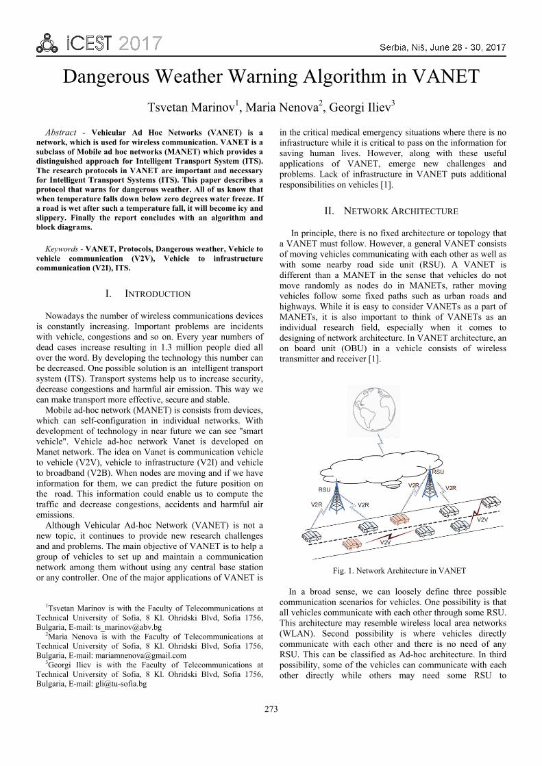
273

Dangerous Weather Warning Algorithm in VANET

Tsvetan Marinov1, Maria Nenova2, Georgi Iliev3

Abstract - Vehicular Ad Hoc Networks (VANET) is a

network, which is used for wireless communication. VANET is a subclass of Mobile ad hoc networks (MANET) which provides a distinguished approach for Intelligent Transport System (ITS). The research protocols in VANET are important and necessary for Intelligent Transport Systems (ITS). This paper describes a protocol that warns for dangerous weather. All of us know that when temperature falls down below zero degrees water freeze. If a road is wet after such a temperature fall, it will become icy and slippery. Finally the report concludes with an algorithm and block diagrams.

Keywords - VANET, Protocols, Dangerous weather, Vehicle to vehicle communication (V2V), Vehicle to infrastructure communication (V2I), ITS.

I. INTRODUCTION

Nowadays the number of wireless communications devices is constantly increasing. Important problems are incidents with vehicle, congestions and so on. Every year numbers of dead cases increase resulting in 1.3 million people died all over the word. By developing the technology this number can be decreased. One possible solution is an intelligent transport system (ITS). Transport systems help us to increase security, decrease congestions and harmful air emission. This way we can make transport more effective, secure and stable.

Mobile ad-hoc network (MANET) is consists from devices, which can self-configuration in individual networks. With development of technology in near future we can see "smart vehicle". Vehicle ad-hoc network Vanet is developed on Manet network. The idea on Vanet is communication vehicle to vehicle (V2V), vehicle to infrastructure (V2I) and vehicle to broadband (V2B). When nodes are moving and if we have information for them, we can predict the future position on the road. This information could enable us to compute the traffic and decrease congestions, accidents and harmful air emissions.

Although Vehicular Ad-hoc Network (VANET) is not a new topic, it continues to provide new research challenges and and problems. The main objective of VANET is to help a group of vehicles to set up and maintain a communication network among them without using any central base station or any controller. One of the major applications of VANET is

1Tsvetan Marinov is with the Faculty of Telecommunications at

Technical University of Sofia, 8 Kl. Ohridski Blvd, Sofia 1756, Bulgaria, E-mail: [email protected]

2Maria Nenova is with the Faculty of Telecommunications at Technical University of Sofia, 8 Kl. Ohridski Blvd, Sofia 1756, Bulgaria, E-mail: [email protected]

3Georgi Iliev is with the Faculty of Telecommunications at Technical University of Sofia, 8 Kl. Ohridski Blvd, Sofia 1756, Bulgaria, E-mail: [email protected]

in the critical medical emergency situations where there is no infrastructure while it is critical to pass on the information for saving human lives. However, along with these useful applications of VANET, emerge new challenges and problems. Lack of infrastructure in VANET puts additional responsibilities on vehicles [1].

II. NETWORK ARCHITECTURE

In principle, there is no fixed architecture or topology that a VANET must follow. However, a general VANET consists of moving vehicles communicating with each other as well as with some nearby road side unit (RSU). A VANET is different than a MANET in the sense that vehicles do not move randomly as nodes do in MANETs, rather moving vehicles follow some fixed paths such as urban roads and highways. While it is easy to consider VANETs as a part of MANETs, it is also important to think of VANETs as an individual research field, especially when it comes to designing of network architecture. In VANET architecture, an on board unit (OBU) in a vehicle consists of wireless transmitter and receiver [1].

Fig. 1. Network Architecture in VANET

In a broad sense, we can loosely define three possible communication scenarios for vehicles. One possibility is that all vehicles communicate with each other through some RSU. This architecture may resemble wireless local area networks (WLAN). Second possibility is where vehicles directly communicate with each other and there is no need of any RSU. This can be classified as Ad-hoc architecture. In third possibility, some of the vehicles can communicate with each other directly while others may need some RSU to

274

communicate. This can be referred as hybrid scenario. Fig. 1 shows these three possibilities.

Communication types in VANETs can be categorized into free types. The category is closely related to VANETs components as described above.

In-vehicle communication, which is more and more necessary and important in VANETs research, refers to the in vehicle domain. In-vehicle communication system can detect a vehicle’s performance and especially driver’s fatigue and drowsiness, which is critical for driver and public safety.

Vehicle-to-vehicle (V2V) communication can provide a data exchange platform for the drivers to share information and warning messages, so as to expand driver assistance.

Vehicle-to-road infrastructure (V2I) communication is another useful research field in VANETs. V2I communication enables real-time traffic/weather updates for drivers and provides environmental sensing and monitoring.

Vehicle-to-broadband cloud (V2B) communication means that vehicles may communicate via wireless broadband mechanisms such as 3G/4G. As the broad band cloud may include more traffic information and monitoring data as well as infotainment, this type of communication will be useful for active driver assistance and vehicle tracking [2].

III. PROTOCOLS IN VANET

In VANET, the routing protocols are classified into five categories: Topology based routing protocol, Position based routing protocol, Cluster based routing protocol, Geo cast routing protocol and Broadcast routing protocol. These protocols are characterized on the basis of area / application where they are most suitable [1].

One of the major challenges in the design of vehicular ad-hoc network is the development of a dynamic routing protocol that can help disseminate the information from one node (vehicle) to another. Routing in VANET is different to the traditional MANET routing because of highly dynamic and ever changing topologies in the former. Few protocols that were earlier designed for MANET environment have been tested on VANET. The challenge however remains as how to reduce delay associated with passing the information from one node to another.

Most of the routing protocols in VANET are closely linked with the topology being used in the network architecture and the performance deviates whenever there is a change in network topology. Routing in VANET can be classified into five major categories namely as:

• Ad-hoc or Topology Driven Protocols • Location Based Routing Protocols • Cluster Based Protocols • Broadcast Protocols • Geocast Protocols

A. Ad-hoc or Topology Driven Routing

In general, VANETs are infrastructure-less networks and many routing protocols devised for prior ad-hoc network such as MANET based on different network topologies may be applied to VANETs with certain modifications. Topology

driven protocols are sub-classified into three categories such as proactive, reactive and hybrid. A number of such protocols were designed to cater the needs of VANET environment [3]-[9], In a proactive protocol, nodes continuously update their routing table with information regarding new routes within the network. This information is passed around to all nodes by sending periodic HELLO packets. This approach, however, creates substantial control overheads. This restricts the use of limited wireless resource such as available bandwidth.

B. Location Based Routing

Another category of protocols that have been shown interest among the researchers are Location or Position Based Routing protocols. In this scheme of protocols information regarding geographic location of vehicles is obtained from different sources like maps, Global Positioning System (GPRS) or even traces of traffic models to help disseminate the information. Quite a few researches like [10]-[13] and have presented a thorough comparison of well known topology based protocols like AODV and DSR in conjunction with Position Based algorithm and the results have shown better and improved performance as compared to using plain topological approach.

C. Cluster Based Routing

In order to reduce the network traffic and routing overheads in VANET, a routing paradigm namely Cluster Based Routing (CBR) is introduced in [14]. The main idea behind CBR is to create a network architecture based on small groups of vehicles called as clusters. In a cluster, one of the vehicles plays the role of a cluster-head as shown in Figure 5. The size of the cluster depends on the design of the routing algorithm which may be based on the number of vehicles in a cluster or the geographical position of the vehicles.

D. Broadcast Routing

Broadcast Routing was one of the traditional routing techniques used in VANET. Primarily broadcast approach is used when the message is needed to be sent to the vehicle that is outside the range. Packets are transmitted using flooding techniques. This ensures delivery of information, but uses extensive resources of bandwidth. As briefed previously, this sort of technique is utilised in many well established routing protocols, especially in the stage of discovering of route to the destination. BROADCOMM and the Nth-Powered P-persistent Broadcast protocol (NPPB) are such well known protocols designed using the broadcasting concept.

E. Geocast Routing

Geocast routing is the classification of routing that deals with dissemination of information in specific area of relevance. Since the early induction of VANET, quite a few

275

approaches of Geocast routing were presented [15]-[20]. Many VANET applications require position dependent multi casting e.g. disseminating hazar dous traffic information to vehicles approaching in the same direction. The key idea behind the Geocast routing is to narrow down the search for next hop to a specific Zone Of Relevance (ZOR). Imagine the possibility of having a mechanis m in which if a car gets involved in an accident, it will automatically report the accident to the approaching vehicles within that zone.

IV. DANGEROUS WEATHER WARNING ALGORITHM

The following paragraph presents the dangerous weather warning algorithm that warns drivers for unsafe road conditions. The algorithm monitors the temperature and rainfall. There are four cases, which are shown in figure 2. Case one is for icy road. Case two is for wet road. The third and fourth cases are for light icy and dry road. If Temp<0Co and rainfall are less then v(constant) we have a light icy road. If Temp<0Co and rainfall are more than v (constant) we have icy road. Analogously if Temp>0Co and rainfall are more than v(constant) have wet road, and for - Temp>0Co and no rainfall, we have safe road. These cases are presented in Fig. 2.

TABLE 1

NOTATIONS

Symbols Significance

previousstate first state for comparative

presentstate value from temperature and rainfall

reportstate state for report

Term time for stop notifications

T time need to stay in a state before starting sending notifications

Rainfall rainfall

Temp measured temperature

Fig. 2. Cases for notification

Fig. 3. Block diagram

We give value to Term and T++. The algorithm works as follows.

Algorithm following temperature and rainfall

Start Initialization (T=0; Term=0; previousstate=0;

presentstate=0; reportstate=0; report=1) While(report==1) Measurment; Create presentstate from "Temp" and "Rainfall" If(previousstate==presentstate) if (T<const1) T++ else reportstate=presenstate; report info for

reportstate; Term=100 else T=0; previousstate= presentstate; if (Term!=0 & reportstate!=0) report info for

reportstate; Term--;

276

V. CONCLUSION

The paper presented VANET network and protocols. Furthermore it considered different types of communications like vehicle to vehicle (V2V), vehicle to infrastructure (V2I) and vehicle to broadband (V2B). We have proposed an algorithm for dangerous weather in VANET. As a result - it improves road safety. Table one reviewed the cases for notification. Figure three shows us the logic of the algorithm with a block diagram. Further research will be necessary. We should consider other algorithms for accidents, road repair and congestions.

REFERENCES

[1] S. ur Rehman, M. Arif Khan, T.A. Zia, and L. Zheng, "Vehicular Ad-Hoc Networks (VANETs) - An Overview and Challenges", Journal of Wireless Networking and Communications, vol. 3, no. 3, pp. 29-38, 2013.

[2] M. Faezipour, M. Nourani, A. Saeed, and S. Addepalli, "Progress and Challenges in Intelligent Vehicle Area Networks", Communications of the ACM, vol. 55, no. 2, pp. 90-100, 2012.

[3] R.B. Soares, and A. A.F. Loureiro, "VCARP: Vehicular Ad-hoc Networks Context-aware Routing Protocol", 2012 IEEE Symposium on Computers and Communications (ISCC), vol. 0, pp. 000 442-000 447, 2012.

[4] C.E. Perkins, and E.M. Royer, "Ad-hoc On-Demand Distance Vector Routing", Second IEEE Workshop on Mobile Computing Systems and Applications, 1999, pp. 90–100.

[5] J. Haerri, F. Filali, and C. Bonnet, "Performance Comparison of AODV and OLSR in VANETs Urban Environments Under Realistic Mobility Patterns", Med-Hoc-Net 2006, 5th Annual Mediterranean Ad Hoc Networking Workshop, June 2006.

[6] B. Li, Y. Liu, and G. Chu, "Improved AODV Routing Protocol for Vehicular Ad hoc Networks", 2010 3rd International Conference on Advanced Computer Theory and Engineering (ICACTE), vol. 4, 2010, pp. V4–337–V4–340.

[7] S. Eichler, F. Dtzer, C. Schwingenschlgl, F. Javier, F. Caro, and J. Eberspcher, "Secure Routing in a Vehicular Ad hoc Network", Proceedings of the 2004 IEEE 60th Vehicular Technology Conference, 2004.

[8] D.B. Johnson, and D.A. Maltz, "Dynamic Source Routing in Ad Hoc Wireless Networks", Mobile Computing, 1996, ch. 5.

[9] M. Zhang, and R.S. Wolff, "A Border Node Based Routing Protocol for Partially Connected Vehicular Ad Hoc Networks",

Journal of Communications, vol. 5, no. 2, pp. 130-143, Feb. 2010.

[10] M. Watfa, Advances in Vehicular Ad-Hoc Networks: Developments and Challenges, ser. Intelligent Transport Systems. IGI Global, 2010.

[11] C. Lochert, H. Hartenstein, J. Tian, H. Fussler, D. Hermann, and M. Mauve, "A Routing Strategy for Vehicular Ad hoc Networks in City Environments", Intelligent Vehicles Symposium, 2003 Proceedings IEEE, 2003, pp. 156-161.

[12] A. Fonseca and T. Vazo, "Applicability of Position-Based Routing for VANET in Highways and Urban Environment", Journal of Network and Computer Applications, vol. 36, no. 3, pp. 961-973, 2013.

[13] G. Liu, B.S. Lee, B.C. Seet, C.H. Foh, K.J. Wong, and K.K. Lee, "A Routing Strategy for Metropolis Vehicular Communications", International Conference on Information Networking (ICOIN), pp. 134-143, 2004.

[14] C. Lin, and M. Gerla, "Adaptive Clustering for Mobile Wireless Networks", IEEE Journal on Selected Areas in Communications, vol. 15, no. 7, pp. 1265-1275, 1997.

[15] M. Kihl, M. L. Sichitiu, and H. P. Joshi, "Design and Evaluation of two Geocast Protocols for Vehicular Ad-hoc Networks", Swedish Governmental Agency for Innovation Systems (Vinnova), 2007.

[16] H. Rahbar, K. Naik, and A. Nayak, "DTSG: Dynamic Time-stable Geocast Routing in Vehicular Ad hoc Networks", 2010 The 9th IFIP Annual Mediterranean Ad Hoc Networking Workshop (Med-Hoc-Net), 2010, pp. 1-7.

[17] Y.B. Ko, and N.H. Vaidya, "Location-Aided Routing (LAR) in Mobile Ad hoc Networks", ACM journal of Wireless Networks, vol. 6, pp. 307-321, 2000.

[18] A.D. Akhtar Husain, and B. Kumar, "A Study of Location Aided Routing (LAR) Protocol for Vehicular Ad hoc Networks in Highway Scenario", International Journal of Information Technology and Web Engineering, vol. 2, no. 2, pp. 118-124, 2010.

[19] S.K. Dhurandher, M.S. Obaidat, D. Bhardwaj, and A. Garg, "GROOV: A Geographic Routing Over Vanets and Its Performance Evaluation", 2012 IEEE Global Communications Conference (GLOBECOM), 2012, pp. 1670-1675.

[20] Y.-B. Wang, T.-Y. Wu, W.-T. Lee, and C.-H. Ke, "A Novel Geographic Routing Strategy over VANET," 2010 IEEE 24th International Conference on Advanced Information Networking and Applications Workshops (WAINA), pp.873-879, 20-23 April 2010.

[21] M. Sivasakthi, and S. Suresh, "Research on Vehicular Ad hoc Networks (VANETs): An Overview", Journal of Applied Sciences and Engineering Research, vol. 2, no. 1, pp. 23-27, 2013.

277

Software Implementation of the Computer-Aided Design Platform Online-CADCOM in Cloud Environment

Ognyan Chikov1 and Galia Marinova2

Abstract – In this paper the software implementation of Online assisted Platform for Computer-aided design in communications (Online-CADCOM) in Cloud environment is described. The platform is presented as multi-tenant Cloud application. Platform and database architecture are discussed as well as platform availability and security. Application lifecycle in Cloud is also described. The role of each aspect is widely discussed and also each potential problem is explained and solutions, applicable for Online-CADCOM and similar cases are proposed.

Keywords — Online-CADCOM, Cloud, Multi-tenant, Platform Architecture, Database, Security, Availability, Lifecycle

I. INTRODUCTION

The developers and suppliers of Computer-aided design (CAD) tools were longtime reticent to direct cloud exposure of their platforms and security reasons were the most widely pointed for this state. Recently some attempts are made to propose online CAD tools on clouds, as the Mentor Graphics SystemVision Cloud platform [13], which proposes only typical models of different electronic and electro-mechanical components and reduced set of Spice-based analysis - frequency and time-domain. Different forms of feedback are provided as blog, chat, comments on designs. The current application of the platform is limited, some advanced options, which are necessary for some oscillator circuits analysis are missing. DesignSoft TinaCloud [14] is a commercial circuit simulator on a Cloud. OrCAD Cloud [15], proposed by Cadence is providing mainly project and design sharing, intelligent pdf files, applications to expand OrCAD Design Suit and documents and discussions on some new concepts.

During the last few years the Laboratory for Computer-Aided Design in Telecommunications in Technical University-Sofia is developing an Online assisted Platform for Computer-aided design in communications (Online-CADCOM), described in [1]. The platform is developed on virtual server and new trends in the area of CAD tools motivated the transfer of Online-CADCOM in a cloud environment. This transfer raises a set of challenges which are considered in details further.

The software realization of Online-CADCOM is implementing Model-View-Controller (MVC) Framework approach for its development as explained in [2]. The platform is built of large number of different content –

resources and connections to studied models and tools, knowledgebase materials, standards and how-to video materials that are used to help students for their study and work process. The most complicated part of the platform is the section with online tools which are classificated based on Daniel-Gajsky Y-model of design levels as explained in [1]. Each tool has separate built in passport with accurate and consistent classification. In terms of implementing this model in software platform that would be hosted on Cloud service, consumptions and prerequisites are taken in order to implement this complicated model. Cloud based web applications have large number of architecture requirements for proper functionallity. The platform is managed by separate system that is developed using the same development approach using MVC Framework [3]. This system is called Content Management System (CMS). Both platforms are operating as one software solution which with the help of CMS represent an online application with riliable method of managing, updating and monitoring. Running software platforms that are built of large number of separate modules requires proper design and scalability of Cloud architecture. Online-CADCOM platform best fits in software as a service (SaaS) model of Cloud applications based on models explained in [4]. Online-CADCOM as a SaaS application provides users of the platform with centralized, network-based access to all platform resources with less overhead than when using an ordinary hosted web application approach. But in order to take advantage of the benefits of making Online-CADCOM as SaaS in Cloud, the platform is providing a level of control over its users data. To earn this trust, one of the highest priorities for Online-CADCOM as SaaS model is creating the platform data architecture that is both robust and secure enough to satisfy tenants or clients who are operating in the platform, and also supply them with effective method for maintaining and administration providing best working times and low latency. The paper considers further the development of Online-CADCOM as a multi-tenant application, the Database partitioning and the availability in Online-CADCOM, the way to achieve a secure multi-tenant cloud application and the application lifestyle in cloud. The application of solutions proposed for the transfer of Online-CADCOM from a virtual server to cloud environment will be useful for any other CAD platform to be transferred to a cloud.

II. ONLINE-CADCOM AS A MULTI-TENANT

CLOUD APPLICATION

Making the platform a multi-tenant application requires to re-design the database architecture of Online-CADCOM [4][5]. The platform is built with SQL Database, a centralized

1Ognyan Chikov is with the Faculty of Telecommunications atTechnical University of Sofia, 8 Kl. Ohridski Blvd, Sofia 1000,Bulgaria, E-mail: [email protected]

2Galia Marinova is with the Faculty of Telecommunications atTechnical University of Sofia, 8 Kl. Ohridski Blvd, Sofia 1000,Bulgaria. E-mail: [email protected]

278

and open-source relational database management system [1]. Furthermore using this approach gives high availability and database „sharding“ to the solution. For making the platform SaaS Cloud based solution, it shold use one of the following database architecture approaches, so all functionalities that are provided initially by using SQL, to continue operating in Cloud as described in[6]:

Table Architecture,

Blob Architecture,

SQL Database Architecture,

SQL Database Architecture on Virtual Machines.

The best approach that is implemented for Online-CADCOM running SQL Database is by using SQL Database Architecture running on Virtual Machines in Cloud [4]. Choosing this approach for Online-CADCOM database is dealing with managing multi-tenant data as explained in [5] which is specific for the platform. There are a lot of Cloud solutions for multi-tenant databases partitioning including shared and isolated approach of tenants databases and containing tables, but choosing this partitioning scheme is based on a couple of considerations affecting the platform and its architecture [4]:

Security Considerations - As Online-CADCOM store sensitive tenant data, users have high expectations about security, so the platform needs to provide strong data safety guarantees. A common misconception holds that only physical isolation can provide an appropriate level of security in the platform. In fact, data stored using a shared database approach can also provide strong data safety, but requires the use of more sophisticated software algorithms.

Tenant Considerations - The number, nature and needs of the tenants that affect content in Online-CADCOM are many and varied. They are using big storage space in the platform and acces to a wide software instances, so separate scheme for each tenant is a good approach, but at the same time data storage requirements may force to move to a shared-database model.

Economical Considerations - Aplications optimized for a shared approach tend to require a larger development effort than applications designed using an isolated approach (because of the relative complexity of developing a shared architecture), resulting in higher initial costs. Since they can support more tenants per server, their ongoing operational costs seems to be lower.

Taking into account the above considerations and also due to Online-CADCOM platform specification which is complicated and built of different categories, content and user-level access, the best one is to use shared databases on Virtual Machine (VM) with separate schemas for every tenant. This approach involves housing multiple tenants in the same database, with each tenant having its own set of tables which are grouped into a schema created specifically for the tenant. Choosing this approach assumes that everything is virtuallized within the Cloud.

When a tenant profile is initially created in the Online-CADCOM platform, the provisioning subsystem algorithm creates a discrete set of tables for the tenant and associates it with the tenant's own virtualized database schema, based on the type of access user level. Below are showed commands that are automatically sent to the virtualized SQL Database when new tenant is created in the platform:

CREATE SCHEMA UserNameSchema AUTHORIZATION

Username Then the platform creates and accesses tables within the tenant's schema using the SchemaName.TableName convention:

CREATE TABLE UserNameSchema.Resumes (UserID

int identity primary key, Resume

nvarchar(MAX))

After the schema is created, it is set as the default schema for the tenant account:

ALTER USER Username WITH DEFAULT_SCHEMA =

UserNameSchema

A tenant account can access tables within its default schema by specifying just the table name, instead of using the SchemaName.TableName convention. This way, a single set of SQL statements can be created for all tenants in platform, which each tenant can use to access its own data:

SELECT * FROM PersonalData

III. ONLINE-CADCOM DATABASE PARTITIONING

Online-CADCOM uses a tenant-base horizontal partitioning as explained in [4] due to the reason that many users would need access in same specific time. This approach is used because sometimes a database can no longer meet baseline performance metrics. This can happen when too many users are trying to access the database concurrently or the size of the database is causing queries and updates to take too long to execute. The simplest way to scale-out a shared database is through horizontal (row-based) partitioning based on tenant IDs. Online-CADCOM as a SaaS with shared database is good for horizontal partitioning because each tenant has its own set of data, so an individual tenant could easily ask to move his data [4]. Different tenants can place radically different demands to the platform so it is important to be planned carefully to avoid simply creating smaller, but still overtaxed, partitions while other partitions are not used.

If the database has problems related to the size of the database, such as the time it takes to perform queries, a tenant-base horizontal partitioning is used to target database size instead, assigning tenants to database servers in such a way as to roughly equalize the amount of data on each one. The partitioning method has significant impact on the platform development. Building support for monitoring into the platform will help to get an accurate view of tenants' usage

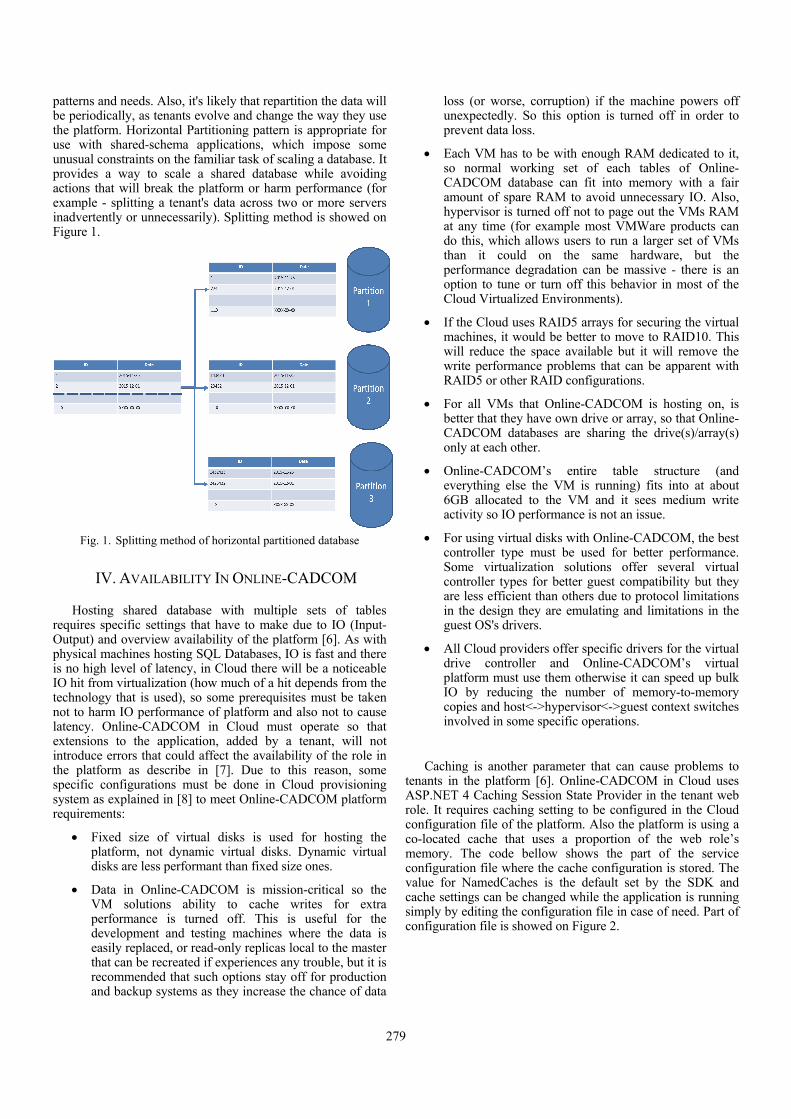
279

patterns and needs. Also, it's likely that repartition the data will be periodically, as tenants evolve and change the way they use the platform. Horizontal Partitioning pattern is appropriate for use with shared-schema applications, which impose some unusual constraints on the familiar task of scaling a database. It provides a way to scale a shared database while avoiding actions that will break the platform or harm performance (for example - splitting a tenant's data across two or more servers inadvertently or unnecessarily). Splitting method is showed on Figure 1.

Fig. 1. Splitting method of horizontal partitioned database

IV. AVAILABILITY IN ONLINE-CADCOM

Hosting shared database with multiple sets of tables requires specific settings that have to make due to IO (Input-Output) and overview availability of the platform [6]. As with physical machines hosting SQL Databases, IO is fast and there is no high level of latency, in Cloud there will be a noticeable IO hit from virtualization (how much of a hit depends from the technology that is used), so some prerequisites must be taken not to harm IO performance of platform and also not to cause latency. Online-CADCOM in Cloud must operate so that extensions to the application, added by a tenant, will not introduce errors that could affect the availability of the role in the platform as describe in [7]. Due to this reason, some specific configurations must be done in Cloud provisioning system as explained in [8] to meet Online-CADCOM platform requirements:

Fixed size of virtual disks is used for hosting the platform, not dynamic virtual disks. Dynamic virtual disks are less performant than fixed size ones.

Data in Online-CADCOM is mission-critical so the VM solutions ability to cache writes for extra performance is turned off. This is useful for the development and testing machines where the data is easily replaced, or read-only replicas local to the master that can be recreated if experiences any trouble, but it is recommended that such options stay off for production and backup systems as they increase the chance of data

loss (or worse, corruption) if the machine powers off unexpectedly. So this option is turned off in order to prevent data loss.

Each VM has to be with enough RAM dedicated to it, so normal working set of each tables of Online-CADCOM database can fit into memory with a fair amount of spare RAM to avoid unnecessary IO. Also, hypervisor is turned off not to page out the VMs RAM at any time (for example most VMWare products can do this, which allows users to run a larger set of VMs than it could on the same hardware, but the performance degradation can be massive - there is an option to tune or turn off this behavior in most of the Cloud Virtualized Environments).

If the Cloud uses RAID5 arrays for securing the virtual machines, it would be better to move to RAID10. This will reduce the space available but it will remove the write performance problems that can be apparent with RAID5 or other RAID configurations.

For all VMs that Online-CADCOM is hosting on, is better that they have own drive or array, so that Online-CADCOM databases are sharing the drive(s)/array(s) only at each other.

Online-CADCOM’s entire table structure (and everything else the VM is running) fits into at about 6GB allocated to the VM and it sees medium write activity so IO performance is not an issue.

For using virtual disks with Online-CADCOM, the best controller type must be used for better performance. Some virtualization solutions offer several virtual controller types for better guest compatibility but they are less efficient than others due to protocol limitations in the design they are emulating and limitations in the guest OS's drivers.

All Cloud providers offer specific drivers for the virtual drive controller and Online-CADCOM’s virtual platform must use them otherwise it can speed up bulk IO by reducing the number of memory-to-memory copies and host<->hypervisor<->guest context switches involved in some specific operations.

Caching is another parameter that can cause problems to tenants in the platform [6]. Online-CADCOM in Cloud uses ASP.NET 4 Caching Session State Provider in the tenant web role. It requires caching setting to be configured in the Cloud configuration file of the platform. Also the platform is using a co-located cache that uses a proportion of the web role’s memory. The code bellow shows the part of the service configuration file where the cache configuration is stored. The value for NamedCaches is the default set by the SDK and cache settings can be changed while the application is running simply by editing the configuration file in case of need. Part of configuration file is showed on Figure 2.

280

Fig. 2. Part of configuration file that shows cache options

Online-CADCOM has built in mechanism for using a delay write pattern when a lot of users are signed in Content Management System (CMS) as method explained in [8][9]. The delayed write pattern is a mechanism that allows code to hand off tasks that may take some time to complete, without need to wait for them to finish - for example upload big video files in Knowledgebase [8][9]. The tasks can executed asynchronously as background processes, while the code that initiated them continues to perform other work or returns control to the users, so a lot of big data files can be processed simultaneously as explained in [9]. The delayed write pattern is particularly useful in the platform because the tasks that must be carried out can run as background processes, and application’s UI (User Interface) is free for other tasks as quickly as possible. It doesn’t mean that the platform cannot return the result of the background process to the user within the current request on the same page without refreshing it. In Clouds background tasks are typically initiated by allowing the UI to hand off the task by sending a message to a storage queue of the platform. Because queues are the natural way to communicate between the roles in a Cloud application, it’s tempting to consider using them for an operation such as saving data collected in the UI of Online-CADCOM. The UI code can write the data to a queue and then continues to serve other users in the platform without need to wait for operations

on the data to be completed. Figure 3 shows the delayed write pattern that Online-CADCOM can use when the platform is hosted in Cloud.

Fig. 3. Delay write pattern algorithm

In this scenario a platform user inserts a file in CMS platform and then submits this file to the platform. The code running in the web role instance puts the file into a message on a queue and returns a “Successful” message to the user as quickly as possible, minimizing the value of time response. One or more tasks in the worker role instances are then responsible for reading the user message that contains the file from the queue and saves it to the cloud storage and then updates the summary statistics. This operation is implemented to avoid any possibility of conflict during uploading files and updating content information and also against latency.

Online-CADCOM is writing directly to storage from the web role process [4][10]. The worker role instances had only one task to do: updating the summary statistics. As using the delayed write pattern implemented in the platform, worker roles must accomplish two tasks: saving the files from user iterations to storage and updating the summary statistics to show information about uploaded files. For best availability it is better that these tasks are separated. New uploaded resources from users is good to be saved to storage as quickly as possible and calculating the summary statistics is not an urgent requirement that is time dependable. The summary statistics can be recalculated at a later time, but file uploading at a later time is not possible. Online-CADCOM can differentiate the level for special and standard users by ensuring that summaries for special users are available more quickly. To scale the tasks separately, the platform uses two separate worker roles as explained in [8]:

A worker role that just updates the statistics by polling a queue for messages containing the identifier of new action sets.

A worker role that just saves new uploaded resources to storage by polling a queue for messages that contain the resource information. The files uploaded in the platform contain headers with information about user, type of file, proper location and etc.

281

V. ONLINE-CADCOM AS A SECURE MULTI-TENANT CLOUD APPLICATION

Online-CADCOM as a SaaS architect cloud based platform has multiple defense levels that complement one another to provide data protection in different ways, under different circumstances available to defense application against both internal and external hacker treats as explained in [4]. This means that Online-CADCOM has security on different levels as showed in [6]. The platform is sensitive because of its data content, so three different levels of security are implemented:

Filtering – platform uses a level between a tenant data source that acts like a sieve, making this level appear to the tenant as its data is the only data in the database.

Permissions – platform uses access control lists (ACLs) to determine who can access data in the application and what this user can do with these resources.

Encryption – every tenant data in the platform is encrypted so in case of threats it remains inaccessible to unauthorized parties even if they have a copy of it.

Online-CADCOM use a trusted database connection that in

case of multi-tenant Cloud application has two methods for security – impersonation and trusted subsystem account [11]. With the impersonation access method, the database is set up to allow individual users to access different tables, views, queries, stored procedures, and other database objects. When an end-user performs an action that directly or indirectly requires a call to a database, the application presents itself to the database as that user, gives access to the user for the purposes of accessing the database. With the trusted subsystem access method, the platform always connects to the database using its own platform process identity, independent of the identity key of the user. The server then grants the application access to the database objects that the application can read or manipulate. This approach makes security management easier, eliminating the need to configure access to database objects on a per-user basis, but it means giving up the ability to secure database objects for individual users and tenants. In Online-CADCOM as SaaS platform, the concept of "users" is a bit more complicated than in traditional hosted web applications as showed in [11], because of the distinction between a tenant and an end user. The tenant is an organization that uses the application to access its own data store, which is logically isolated from data stores belonging to any other tenants. Each tenant grants access to the application to one or more end users, allowing them to access part of the tenant's data using end user accounts controlled by the tenant. So in this case, the platform uses a hybrid approach to data access that combines aspects of both the impersonation and trusted subsystem access methods and gives maximum logical isolation of tenant data without creating an unworkably complex security model. This approach involves creating a database access account for each tenant, and using Access Control Lists (ACLs) to grant each of these tenant accounts access to the database objects the tenant is allowed to use. When an end user performs an action that directly or indirectly requires a call to the platform database, the application uses credentials associated with the tenant account, rather than credentials associated with the end user.

The database server does not know differences between requests originating from different end users associated with the same tenant, and grants all such requests access to the tenant's data. Within the application itself, security code prevents end users from receiving and modifying any data that they are not entitled to access. To secure the database on the table level for example for Knowledgebase, the following automatic command is generated for this table [8]:

GRANT SELECT, UPDATE, INSERT, DELETE ON Knowledgebase FOR User

This adds the user account for “User” to the ACL for the table and this only has to be done once, during the tenant provisioning process because of the hybrid approach to the database access, discussed earlier, that is used in the platform. Any end user accounts created by the tenant will be able to access the table. Online-CADCOM is using also a tenant view filter using SQL views to grant individual tenants access to some of the rows in a given table, while preventing them from accessing other rows:

CREATE VIEW User AS SELECT * FROM Knowledgebase WHERE TenantID =

SUSER_SID()

In addition, Online-CADCOM uses a SAS (Shared Access Signatures) method for the users that can’t be trusted with the storage account key showed in [4] and explained in details in [11]. This is an additional option when exposing the storage account key is not a good option. This approach provides a safe alternative that allows other clients to read, write, and delete data in platform storage account according to the permissions granted, and without need for the account key. This approach is useful when a client tries to access the platform from front-end proxy service. Also this method is created in a platform in order to enable automatic data collaboration with another platform for data sharing or extraction. Figure 4 shows SAS method implemented in Online-CADCOM as a SaaS Cloud platform.

Fig. 4. Shared access signature method (SAS)

First the client browser sends a request to access Online-CADCOM database. Second, the web role sends a request to the gatekeeper worker role for a SAS URL that will enable read only access to platform database. Third, the gatekeeper worker role uses the storage account key to generate the SAS URL and returns it to the worker role. Four, the web role uses

282

the SAS URL when it queries for the platform database it needs to render the web page. Then five, the web role returns the page to the browser.

VI. ONLINE-CADCOM APPLICATION LIFESTYLE

IN CLOUD

The most significant challenges to administrative and management tasks for Online-CADCOM as multi-tenant application when compared to a standard hosted application are concerned with the processes used to back up and restore data [12]. Each tenant’s data is isolated from all others through the use of a shared database with separate tables and storage account for every tenant. It is vital that this isolation is not compromised during the backup and restore process. A tenant must not be able to access a backup that contains other tenants’ data. That is ensured by the database architecture [4]. An automatic backup script is developed in case of database failure or deletion. Also backup of the entire platform can be set from Cloud service platform options as folder backup, partition backup or another user option backup. The code below shows script that is making an SQL backup of the database using PHP language:

<?php include 'config.php'; include 'opendb.php'; $tableName = 'online_cadcom'; $backupFile = 'backup/online_cadcom(date(now)).sql'; $query = "SELECT * INTO OUTFILE '$backupFile' FROM $tableName"; $result = mysql_query($query); include 'closedb.php'; ?> In case of script failure, or losing a connection with the database instance in the cloud, Online-CADCOM has separate method developed script for backing up using the Unix operation system environment with the following command which is scheduled for everyday work:

root@cloud_platform root mysqldump -u root -pPASSWORD --all-databases | gzip > /mnt/disk2

VII. CONCLUSION

Online-CADCOM as a SaaS Cloud based application has to meet high requirements for quality developed process, clean source code and a couple of functions that make the platform compatible with Cloud based technologies. The platform has to be developed using the latest technologies in MVC Framework approach containing rules about proper scale and multi-tenant availability. The solutions proposed in this paper can be used for transfer of other similar platforms from virtual server to cloud. It's especially useful for CAD tools and platforms which will be transferred to cloud.

REFERENCES

[1] G. Marinova, and O. Chikov, "Methodology for Tools Integration in the Online Assisted Platform for Computer-Aided Design in Communications", ICEST 2015, 24-26 June 2015, Sofia, pp. 31-36.

[2] O. Chikov, and G. Marinova, "MVC Framework Approach in the Online assisted platform form Computer-aided Design in Communications – Online-CADCOM", Computer and Communications Engineering, TUS, 2016.

[3] O. Chikov, "Software Development of Content Management System in Online-CADCOM Platform", ICEST 2016, Ohrid, Macedonia.

[4] M.J. Kavis, Architecting the Cloud: Design Decisions for Cloud Computing Service Models (SaaS, PaaS, and IaaS), Wiley, 1 edition 2014.

[5] T. Erl, Cloud Computing: Concepts, Technology & Architecture, Prentice Hall, 2013.

[6] J. Bond, The Enterprise Cloud: Best Practices for Transforming Legacy IT, O'Reilly Media, 1 edition 2015.

[7] P.H. Havewala, Oracle Enterprise Manager Cloud Control 12c: Managing Data Centers Chaos, Packt Publishing, 2012.

[8] D. Schaefer, Cloud-Based Design and Manufacturing (CBDM), Springer 2014.

[9] N.B. Ruparelia, Cloud Computing, The MIT Press, 2013. [10] J. Rhoton, Cloud Computing Explained: Implementation

Handbook for Enterprises, Recursive Press, 2nd edition, 2009. [11] J.W. Rittinghouse, and J.F. Ransome, Cloud Computing

Implementation Management and Security, CRC Press, 2010. [12] Trends in Cloud Computing, CompTIA Research, Fourth

Annual – August 2013. [13] Mentor Graphics, SystemVision Cloud - Free Cloud-Based

Simulation Tool, https://www.systemvision.com/ [14] DesignSoft, TINACloud, 2017,

https://www.tina.com/English/tinacloud/ [15] Cadence OrCAD Capture Cloud, http://www.orcad.com/orcad-

capture-cloud.

283

Schema on Read Modeling Approach Implementation in Big Data Analytics in Traffic

Slađana Janković1, Snežana Mladenović2, Stefan Zdravković3, Ana Uzelac4

Abstract – The exploding growth of unstructured data and overhead of ETL (Extract, Transform and Load) for storing data in RDBMS is the main reason to use schema on read. Schema on read refers to an innovative data analysis strategy in new data-handling tools like Hadoop. With schema on read, you just load your raw, source data into the data store and think about how to parse and interpret later. In the traffic field it is very important to provide an effective sharing of information of public importance. In this research, we apply schema on read modeling approach in order to provide various traffic authorities and other stakeholders with the ability to carry out their own specific Big Data analytics of the source traffic data, without the need to take the source data. The implementation was realized in a case study in road traffic, using Hadoop Distributed File System (HDFS), Apache Hive data warehouse and HiveQL query language.

Keywords – Big Data Analytics, Data Sharing, HDFS, HiveQL.

I. INTRODUCTION

By analyzing signals obtained from machines and sensors, server logs and other new data sources, transport organizations can predict future events and become more proactive. Sensors and other intelligent devices can capture traffic data creating a large, ongoing flow of data. Such data require Big Data management systems for processing and reporting. As a result of the complexity, diversity and stochastic nature of transportation problems, the analytical toolbox required by transportation analyst must be broad. Big Data differs from other technologies is in terms of sophistication analysis it applies. Big Data analytics implies the process of discovering and extracting potentially useful information hidden in huge amounts of data (e.g. discovers unknown patterns and correlations). Big Data analytics uses advanced analytic techniques, such as machine learning, predictive analytics, data mining, text analytics, natural language processing and statistical analysis, against very large, diverse data sets. Data sets can be consisted of different data types such as structured/unstructured, streaming/batch,

with different sizes (from terabytes to zettabytes). Also, while traditional analysis is often designed on the conditions that allow valid statistical inference about the characteristics of a population based on measurements on a small sample, Big Data-style analysis is built on the possibility to learn about systems by observing them in their entirety.

The intelligent transport systems have shown a rapid development over the last 15 years. This development has been accompanied with the need to test the systems that exist in the real world and collect data about their influence. Many previous and on-going transportation projects are not focused on the concept of data sharing and reusage data after the project finishes. The authors in [1] say: “More support services which sharing the data is needed to promote good research results.” In this paper we propose schema on read modeling approach for Big Data analytics in traffic, which may be a modeling approach in the development of the information infrastructure for data sharing in the traffic domain. Schema on read is the revolutionary concept that we do not have to know what we’re going to do with our data before we store it. Data of many types, sizes, shapes and structures can all be thrown into one of the Big Data storage systems. When we access the data, when we query it, then we determine the structure we want to use.

In the second section of this paper an overview of data modeling approaches is given. The third section of the paper is devoted to the description of our Big Data analytics modeling approach. We have implemented our approach in a case study in the traffic domain. In the fourth section of this paper our case study is presented. Finally, the conclusions we reached during the implementation of this modeling approach are given.

II. DATA MODELING APPROACHES OVERVIEW

Relational Database Management Systems (RDBMSs) are widely used for to maintain data received in daily operations. Considering the data modeling of operational databases there are two main models: the Relational and the Entity-Relationship (ER) model. Systems using operational databases are designed to handle a high number of transactions that usually perform changes to the operational data [2]. These systems are called Online Transaction Processing (OLTP) systems.

The evolution of relational databases to decision support databases, referred as Data Warehouses (DWs), occurred with the need to store both operational and historical data, and to analyse that data in complex dashboards and reports. DWs are mainly used for OLAP (Online Analytical Processing) operations. Data modeling in DW consists of defining fact tables with several dimension tables, suggesting star or

1Slađana Janković is with the Faculty of Transport and TrafficEngineering University of Belgrade, Vojvode Stepe 305, Belgrade11000, Serbia, E-mail: [email protected]

2Snežana Mladenović is with the Faculty of Transport and TrafficEngineering University of Belgrade, Vojvode Stepe 305, Belgrade 11000, Serbia, E-mail: [email protected]

3Stefan Zdravković is with the Faculty of Transport and TrafficEngineering University of Belgrade, Vojvode Stepe 305, Belgrade 11000, Serbia, E-mail: [email protected]

4Ana Uzelac is with the Faculty of Transport and TrafficEngineering University of Belgrade, Vojvode Stepe 305, Belgrade 11000, Serbia, E-mail: [email protected]

284

snowflake schema data models [3]. The most common data model used in DW is the OLAP cube, which offers a set of operations to analyze the cube model. Since data is conceptualized as a cube with hierarchical dimensions, its operations have familiar names when manipulating a cube, such as slice, dice, drill and pivot.

The volume of data has been exponentially increasing over the last years, namely due to the simultaneous growth of the number of sources (e.g. users, systems or sensors) that are continuously producing data. Therefore, there is a need to devise new data models and technologies that can handle such Big Data. NoSQL (Not Only SQL) is one of the most popular approaches to deal with this problem. NoSQL databases can be classified in four categories: Key-value stores, (2) Document-oriented databases, (3) Wide-column stores, and (4) Graph databases [4].

A Key-value store represents data as a collection of key-value pairs. Every key consists of a unique alphanumeric identifier that works like an index, and is used to access a corresponding value. Values can be simple text strings or more complex structures like arrays. The Key-value model can be extended to an ordered model whose keys are stored in lexicographical order. The fact of being a simple data model makes Key-value stores ideally suited to retrieve information in a very fast, available and scalable way.

Document-oriented databases were originally created to store traditional documents, like a text file or Microsoft Word document. However, their concept of document goes beyond that, and a document can be any kind of domain object. Documents contain encoded data in a standard format like XML, YAML, JSON or BSON (Binary JSON). Documents contain semi-structured data represented as name-value pairs, which can vary according to the row and can nest other documents. Unlike key-value stores, these systems support secondary indexes and allow fully searching either by keys or by values. Document databases are well suited for storing and managing huge collections of textual documents (e.g. text files or email messages), as well as semi-structured. MongoDB and CouchDB are two most popular Document-oriented database systems.

Wide-column stores (column-oriented databases) represent and manage data as sections of columns. Each section is composed of key-value pairs, where the keys are rows and the values are sets of columns, known as column families. Each row is identified by a primary key and can have column families different from the other rows. Each column of column family consists in a name-value pair. Column families can even be grouped in super column families. Wide-column stores are suited for scenarios like: (1) Distributed data storage; (2) Large-scale and batch-oriented data processing using the famous MapReduce method for tasks like sorting, parsing, querying or conversion and; (3) Exploratory and predictive analytics. Cassandra and Hadoop HBase are two popular frameworks of such data management systems [5].

Graph databases represent data as a network of nodes (representing the domain entities) that are connected by edges (representing the relationships among them) and are characterized by properties expressed as key-value pairs. Graph databases are quite useful when the focus is on

exploring the relationships between data, such as traversing social networks, detecting patterns or infer recommendations. Neo4j and Allegro Graph are two examples of such systems.

Operational, decision support and Big Data approach to data management, from data modeling perspective, DBMSs perspective and data analytics perspective, were observed in Table I.

TABLE I APPROACHES AND PERSPECTIVES OF THE SURVEY

Approach Perspective

Operational Decision Support

Big Data

Data Modeling Perspective

ER, Relational Models

Star Schema, OLAP Cube Models

Key-Value, Document, Wide-Column, Graph

Database Management Systems Perspective

RDBMS DW Big Data-Based Systems

Data Analytics Perspective

OLTP OLAP Batch-oriented processing, Stream-processing, OLTP, Interactive ad-hoc queries

III. SCHEMA ON READ MODELING APPROACH

As we can see in Table I, Big Data analytics can be categorized as follows: (1) Batch-oriented processing; (2) Stream processing; (3) OLTP and; (4) Interactive ad-hoc queries and analysis. Batch-oriented processing is a paradigm where a large volume of data is firstly stored and then analyzed, opposed to the streaming processing where data is continuously arriving in a stream, at a real-time, and is analyzed as soon as possible in order to derive approximate results [6]. We propose schema on read modeling approach for Big Data analytics based on batch-oriented processing.

Schema on write has been the standard for many years in relational databases. Before any data is written in the database, the structure of that data is strictly defined while metadata is stored and tracked. The schema – the columns, rows, tables and relationships are all defined first for the specific purpose that database will serve. Then the data is filled into its pre-defined positions. The data must all be cleansed, transformed and made to fit in that structure before it can be stored.

The emergence of Big Data technologies poses an alternative – a schema on read approach. Schema on read is simple up front: you just write the information to the data store. Unlike schema on write, which requires you to expend time and effort before loading the data, schema on read involves very little delay and you generally store the data at a

285

raw level. In other words, you store what you get from the source systems, as it comes in from those systems, and define the schema at the time of data use (Fig. 1).

Schema on read means you can first write your data and

figure out how you want to organize it later. So why do it that way? As we can see in Table II, the key drivers are flexibility and reuse of raw/atomic data. Exactly these characteristics make schema on read approach appropriate in scenarios of sharing data of public interest. In the next section we present the implementation of this approach to share information of public interest in the field of transport, between the various stakeholders.

TABLE II SCHEMA ON READ MODELING APPROACH

Adv

anta

ges

˗ Gives you massive flexibility over how the data can be consumed.

˗ Your raw/atomic data can be stored for reference and consumption years into the future.

˗ The approach promotes experimentation, since the cost of getting it “wrong” is so low.

˗ Helps to speed the time between data generation and availability.

˗ Gives you flexibility to store unstructured, semi-structured, and/or loosely or unorganized data.

Dis

adva

ntag

es

˗ Since the data is not subjected to ETL (Extract, Transform, Load) and data cleansing processes, nor does it pass through any validation, that data may be riddled with missing or invalid data, duplicates, etc...

˗ The SQL queries tend to be very complex. They take time to write, and time to execute.

˗ Can be “expensive” in terms of computing resources.

˗ The data is not self-documenting (i.e., you cannot look at a schema to figure out what the data are).

IV. CASE STUDY

Our implementation of schema on read modeling approach was realized through a case study of the Big Data analysis of traffic data. We analyzed traffic data from ten locations on the state roads and streets in the town of Novi Sad, Serbia, which the automatic traffic counters generated during the 2015. The Apache Hadoop platform was chosen to store and process the data. Our application of schema on read approach is based on Hadoop Distributed File System (HDFS), Apache Hive™ data warehouse software, and Hive Query Language (HiveQL or just HQL).

HDFS represents a distributed Java-based file system designed to store very large files with streaming data access patterns that run on clusters of commodity hardware. “Very large” in this context means files sizing hundreds of megabytes, gigabytes, or terabytes. HDFS is based on the idea that the most efficient data processing pattern is a write-once, read-many-times pattern. Hadoop moves computing processes to the data on HDFS and not the other way around. Applications that require low-latency access to data, in the tens of milliseconds range, will not work well with HDFS. HDFS is optimized for delivering a high throughput of data, and this may be at the expense of latency. Some common storage formats for Hadoop include: plain text storage (e.g. CSV, TSV, TXT files), sequence files, Avro files, columnar file formats (e.g. Parquet, RC Files, ORC Files).

The Apache Hive™ data warehouse software facilitates reading, writing, and managing large data sets residing in distributed storage using SQL-like query language [7]. Hive provides an SQL dialect, called HiveQL for querying data stored in a Hadoop cluster. Hive translates most queries to MapReduce jobs, thereby exploiting the scalability of Hadoop, while presenting a familiar SQL abstraction. Hive is not designed for online transaction processing. It is commonly used for traditional data warehousing tasks where relatively static data is analyzed, fast response times are not required, and when the data is not changing rapidly. When you write data to a traditional database, the database has total control over the storage. The database is the “gatekeeper.” An important implication of this control is that the database can enforce the schema as data is written. On the contrary, Hive does not have has any control over the integrity of the files used for storage and whether or not their contents are consistent with the table schema. So what if the schema does not match the file contents? Hive does the best it can to read the data. You will get lots of null values if there are not enough fields in each record to match the schema. If some fields are numbers and Hive encounters nonnumeric strings, it will return nulls for those fields. Therefore, Hive can only enforce queries on read. This is called schema on read.

Our solution was implemented through the following phases:

1. To count the traffic at the specified locations, the automatic traffic counters of type QLTC-10C were used. Each counter, during the course of the day, "writes" the data into one text file, so that during one year each counter generates 365/366 files. For each vehicle registered by a counter, one record is created in the text file. Record in the text file

Fig. 1. Schema on read modeling approach

286

contains the following information: index, date and time, direction, lane, vehicle class, vehicle category, vehicle speed and vehicle length. Size of a text file is determined by the volume of traffic in one day at the observed counting place. In our case study, each of the ten counters in 2015 generated 365 files and each text file kept between 4000 and 14000 records.

2. Using the Apache Ambari user interface, on the Hortonworks Sandbox, text files generated by ten automatic traffic counters were uploaded into the HDFS.

3. Based on the structure of uploaded text files the data model for input data was created. According to developed data model, with the help of HiveQL query language, a Traffic Counting Hive database was created.

4. Using HiveQL LOAD DATA INPATH queries the Hive database tables were "filled" with the data from the text files stored on the HDFS (Fig. 2).

5. We have recognized two possible types of the results of

data analysis: indicators of traffic volume and structure and indicators of traffic safety in terms of vehicles speed. HiveQL has the well known powerful technique named Create Table As Select (CTAS). This type of HiveQL queries enable us to quickly derive Hive tables from other tables in order to build powerful schemas for Big Data analysis (Fig. 2). We carried out numerous CTAS and others HiveQL queries on the Hadoop Traffic Counting database resulting in traffic volume indicators and traffic safety indicators.

6. We have created three different “users” of the results of conducted Big Data analysis of traffic data: Windows geo- application (developed in Microsoft Visual Studio 2015 and Visual Basic programming language), Microsoft Excel 2013 workbook and SQL Server 2012 database (Fig. 2). For the geo-application schema on read approach enabled calculating of traffic volume indicators, as predefined attributes of the OpenStreet Maps. For the Excel Workbook this approach enabled the calculation of traffic safety indicators, as attributes of the Bing Maps. For the SQL Server database, this approach enabled the calculation of all traffic indicators according to its relational data model. Access to the Traffic Counting Hadoop database for all three users was enabled with the help of Hortonworks Hive ODBC Driver.

V. CONCLUSION

Schema on read approach can be seen as schema on demand. One area where we see the advantages far outweighing the drawbacks of schema on read strategies is in environments where multiple LOBs (Line of Business) try to hit the same source systems for their own copy of the data. The schema on read approach involves having a data “landing zone” where the raw or atomic data is written out. After getting the data once, all the LOB systems make their schema on read requests against the landing zone. This prevents the source systems from having to deal with all the LOB requests and provides a one-to-many approach of serving up data.

Similar studies, like Hadoop for exploratory analytics and Hadoop as a platform for transforming data or ETL, confirm that there is always a time cost to impose a schema on data. Hadoop provides an important advantage for exploratory BI in a single step from data load to query, which is not available in conventional RDBMS. The data-load-to-query in one step involves: 1. copy data into HDFS with ETL tool; 2. declare the query schema in Hive or Impala, which doesn’t require data copying or re-loading, due to the schema-on-read advantage of Hadoop compared with schema-on-write constraint in RDBMS; 3. explore with SQL queries and launching BI tools for exploratory analytics. In schema on write strategies time cost is paid in the data loading stage. In schema on read strategies, that time cost is paid when we query the data.

ACKNOWLEDGEMENT

This work has been partially supported by the Ministry of Education, Science and Technological Development of the Republic of Serbia under No. 036012. The data generated by automatic traffic counters provided by the company MHM - Project from Novi Sad.

REFERENCES

[1] H. Gellerman, E. Svanberg and Y. Barnard, "Data sharing of transport research data", Transportation Research Procedia, vol. 14, pp. 2227 – 2236, 2016.

[2] D. Sarka, M. Radivojevic and W. Durkin, SQL Server 2016 Developer's Guide, Birmingham, Packt Publishing, 2017.

[3] R. Kimball and M. Ross, The Data Warehouse Toolkit: The Complete Guide to Dimensional Modeling 3rd Edition, Indianapolis, John Wiley & Sons, 2013.

[4] A. Ribeiro, A. Silva and A.R. da Silva, "Data Modeling and Data Analytics: A Survey from a Big Data Perspective", Journal of Software Engineering and Applications, vol. 8, pp. 617-634, 2015.

[5] A. B.M. Moniruzzaman and S.A. Hossain, "NoSQL Database: New Era of Databases for Big data Analytics-Classification, Characteristics and Comparison", International Journal of Database Theory and Application, vol. 6. no. 4, pp. 1-14, 2013.

[6] H. Hu, Y. Wen, T.S. Chua and X. Li, "Toward Scalable Systems for Big Data Analytics: A Technology Tutorial", IEEE Access, vol. 2, pp. 652-687, 2014.

[7] E. Capriolo, D. Wampler and J. Rutherglen, Programming Hive, Sebastopol, O'Reilly Media, 2012.

Fig. 2. Schema on read modeling approach implementation

287

Analyses of Public Spaces in Barcelona using Geo-Referenced Twitter Data

Nikola Džaković1, Nikola Dinkić1, Jugoslav Joković1, Leonid Stoimenov1, Dejan Rančić1

Abstract – This paper concerns the study of user-generated twitter data that could support and improve the understanding of spatial patterns for urban planning and (re)design of open public spaces. The data generated by Twitter social network are analyzed, regardingtemporal and spatial distribution, content classification, language determination and sentiment analyses. The data based on geo-referenced tweets collected in Barcelona, has been preprocessed, filtered and classified by given criteria, by using“Twitter search engine” (TSE) application.

I. INTRODUCTION

Open public spaces are fundamental elementof vibrant, inclusive and smart cities. Represented as active, social, attractive and secure, open public spaces play key role in revitalization of community, it promotes its sense of identity, culture and economic growth. Having methods to properly determine attractiveness of open public spaces has always been a challenge for urbanists, but also an important tool in fields like urban planning, transport, marketing, business, migration and tourism.

The use of Twitter data is very interesting to make analysis of how people use urban open spaces and what is the geographical pattern of their communications. Since the Twitter is a massive platform for online communication within extremely diverse social groups,with data generated by users of this network it is possible to research the spatiotemporal dynamics of location and different aspects of users’ behaviour.Recently, Twitter has gained significant popularity among the social network services. Twitter contains an enormous number of text posts. Lots of users often use Twitter to express feelings or opinions about a variety of subjects. All this information can be obtained from micro-blogging services, as their users post their opinions on many aspects of their life regularly.

Therefore, it is possible to collect text posts of users from different social and interest groups. In this context, Twitter presents interesting challenges. Its short texts (tweets), widespread use of non-standard grammar, spelling and punctuation, as well as slang, abbreviations and neologisms, etc. make syntactic and semantic analysis difficult.Analyzing this kind of content can lead to useful information for fields such as personalized marketing or social profiling. However, analyzing Twitter data comes with its own bag of difficulties. Tweets are small in length, thus ambiguous. The informal style of writing, a distinct usage of orthography, acronymization and a different set of elements like hashtags, user mentions demand a different approach to solve this problem.

The authors are with University of Niš, Faculty of Electronic

Engineering, Aleksandra Medvedeva 14, 18000 Niš, Serbia.

The goal of this paper is to illustrate possibilities of methodologies based on user-generated data that could support and improve the understanding of spatial patterns for urban planning and design of open spaces in urban areas. The case study considered in this paper is a network of open public spaces inBarcelona, representing one of the most attractive and important urban ambient. The method that was used in analysis is the method of mapping users on the social maps (via social networks) based on a new software application Twitter search engine [1]. This Webapplication enables the collection, storage, processing and analysis of data from the social network Twitter. It is the micro-blogging platform that provides a rich collection of real-time commentaries on almost every aspect of life. Data collection is based on the Twitter REST API [2] that allows the collection of tweets in the space defined with geo-referenced points and the given radius. This API provides a wide range of information related to their own tweets and users who post them. In addition to basic information such as text, time, number of retweets, the number of likes and information about the application from which it was posted/sent, as well as the geographical location where the tweet was shared present the basis for the analysis and processing of geospatial data.

II. RELATED WORK

Traditionally, the attractiveness of places hasbeen calculated from survey data, geographical features, and population distribution. For instance, the attractiveness measure of points of interest proposed by Huang et al. [3] considers static factors (e.g., the size of commercial places, the distance to their customers’ homes) and dynamic factors (e.g., restaurants are more attractive at mealtimes). Geo-information is now used on a daily basis - photos can be stored with location information, users on social networks publish their location or require the shortest path to the desired object in the city. Geographic information attached tweets are used primarily as a mechanism for filtering [4]. Geotagging is the case when Twitter users make available their position, so others can see the exact place where the tweet was sent. Information can be analyzed based on location and profile generated by the user.

In his paper [5] Andre S. introduces so called M-Attract, novel methodwhich goal is to assess how much places of interest are attractive, based on trajectory episodes that occur in their surroundings. This section describes the places, sub-regions and region of interest and the trajectory episodes considered by the method.Christoph Breser in his article [6] discussesed about technical solutions for representing archival sources in urban areas. He strive to realise the

inteconwasprobclasassisofttheianatheythatweb

InTwiof tlocaOnedescclasusedor nbe dectheythroexe

T

specHowRESnecspecdataand

Insectplatexplocaspac

Fcitycumsum

TypNumNumNumNumNumNum

erconnectednencerning entitys recorded thblems in thessification of aignments. Thtware applicatir suitability flogue methodytry to accept t arise in the b representation this paper witter, be used the ways is tations of intere of the mocribed in [9]ssify messaged to determinnegative). Thepolar, it goeided if it is a y also apply ough Twittercuting it is ve

III. DAT

The analysis ocified format wever, since ST API isinessary to percific format.Ta to geospati

d this is the firsn order to illtion examinetform of Tw

ploration of tals, visitors aces in Barcelo

Fig. 1 presentsy of Barcelonamulative statimmarized in T

CUMUL

pe of analysis mber of tweetsmber of users mber of retweember of likes mber of applicmber of langu

ess of soury through the he first time. e analogue warchiving, sem

hey use existions from diffor our conceds to the digwhen it comecontext of moons. we describe hoto quantify at

through semanrest, that is gest common ]. V. Pandey

es through twne if the messen if after firses through sepositive or a nsentimental

r social netwery simillar to

TA PROCESS

of geospatial so that geosall informati

n JSON formrform transfo

This process oal data typesst step in this lustrate possibes data comwitter to prothe resulting and tourists ona. s map with alla in period oistic data baable 1.

TAB

LATIVE DATA IN

Alls 120

104ets 202

519cations 45 ages 120

ces, its behlocation wheThere to, th

world mainly miotic systemsting mobile fferent applicaern. Comparingital world ises to solving iodes of practi

ow can socialttractivness ofntic analyze

enerated throuways for semy and C.V.K

wo classifiers. age is neutral

st classifiers mecond classifnegative messanalyzis to mwork, and tone described

SING AND AN

data requirespatial queriesion obtained

mat, before aormation of gof transformats represents tanalysis.

bilities of TSEming from thovide a visuspatial patterwhich have

l georeferencef 13 – 20 Janased on coll

BLE 1 PERIOD 13-20. J

l 0600 412 208 989

0

holders and ere the informhey try to ide

dealing withms, description

technologiesation fields anng and transfes a real chalidentified probice in archive

l networks, suf urban places[7, 8] of data

ugh social netwmantic analy

Krishnakumar First classifie

l or polar (pomessage appeafiers so it casage. In their pmessages gaththe approachd in this paper

NALYSIS

s data to be is can be exec

from the Twany analysis geo-informatiotion of the orihe pre-proces

E applicationhe social netual and sciern, specificalused urban

ed tweets postnuary, 2017, wlected tweets

JANUARY

Geo 16200 3955 720 2894 40 91

288

the mation entify h the

ns and s and nd test erring lenge blems s and

uch as . One a, for work.

yze is Iyer

ers is sitive ars to an be paper hered

h for r.

in the cuted. witter it is

on to iginal ssing,

n, this twork entific ly of open

ted in while s are

Cois pouse. numbmostleasttwee

Twee

MonTuesWedThurFridSatuSundTOT

Sp

hourof thnumbpeak

Fig. 1. Geore

onsidering theossible to see

Fig. 2 and Tmber of tweets

t active on Tht active on Fets.

Fig. 2. Di

DI

ets by days

nday sday dnesday rsday

day rday

day TAL

plitting the Twrs per day, it ihe city life. Th

mber of Tweetk at 9.00-10.0

eferenced tweet13-20. J

e Tweets accoif there are s

Table 2, reprs by days, sh

hursday, postinFriday, when

istribution of al

TAB

ISTRIBUTION OF

All

17791756171918111568168917361206

weets on the is possible to he radial diagrts increases d00 pm, with

ts in Barcelona January

ording to the dsome sensibleresenting statihow that userng 18115 (15%

it was post

l tweets in BCN LE 2 TWEETS BY DAY

l

90 66 90 15 81 92 66 600

time steps whbetter understram in the Figduring the eve8852 Tweets

during week

day of the weee variations inistics in termrs generally w%) tweets, andted 15681 (1

N by days

YS Geo

2157 2096 2358 2962 1863 2403 2361

16200

hich cover thtand some aspg. 3 show howening, reachin, while the u

ek, it n the

ms of were d the 13%)

e 24 pects w the ng a users

wertwe

Trefeis pFor andnighspecabanto visuhou

A

120Porthe andbecUsinthe diffaccothe dive

re the least aceets. To generate erenced Tweeparticularly intr example, betd well distribhttime there acific axes remndoned. Thevexplore dataa

ualized or to ur basis.

Fig.

Analysis of al0 different lartuguese, Frenmost commo

d Catalan withause it highling the total n

selected peferentiating uounts. This aorigin of eac

ersification be

Fig. 5

ctive between

maps shownts between 13teresting toobtween noon anbuted over tharemore differmain active, wvisualization band to chooview the seq

3. Distribution

ll tweets usinanguages [10

nch, Italian, Dan are Spanish

h 16.3% (Fig. ights the use

number of geoeriod, the musers by theanalysis wouldch user and wetween locals

5. Distribution

4.00-5.00 am

n in the Fig3-20 January bserve some dnd 3 p.m., the he city. Otherences: the citwhile other abased on mapsse the range

quence of twe

of all tweets by

ng TSE applic0]: Spanish, anish, Arabic,

h with 44%, E5). The result of tourists f

o-referenced Tmaps could e language d provide mo

would allow grand tourists.

of tweets by lan

m, posting only

. 4, all the have been us

different behav activity iscon

erwise, duringty center and areasare practis allows the vie of hours teets on anhou

y hours

catication detEnglish, Ca

, Russian, of wEnglish with 2t is very particfrom local peTweets collectbe generatedchosen for

ore informatioreater detail i

nguage

289

y 629

geo-sed. It viors. nstant g the some ically iewer to be ur by

tected talan,

which 22.7% cular, eople. ted in d by their

on on in the

Ba

applipostediffeappli“Twmakerest

Fig. 4. Spati

Fig. 6.

ased on dataication detected content ferent applicaications are “itter Web Clie 93.6% of a18 application

ial distribution time interv

Distribution of

a gathered onted that the

for location ations. Fig. “Twitter for Aient” and “I

all tweets postns make only 6

of georeferenceval in day

f tweets by appl

n Twitter forusers of thi

of interest f6 presents

Android”, “TwInstagram” anted for this lo6.4% of total

ed tweets by

lication

r Barcelona, s social netw

from twenty that most u

witter for iPhond they combocation, whiledata.

+

TSE work

two used

one”, bined e the

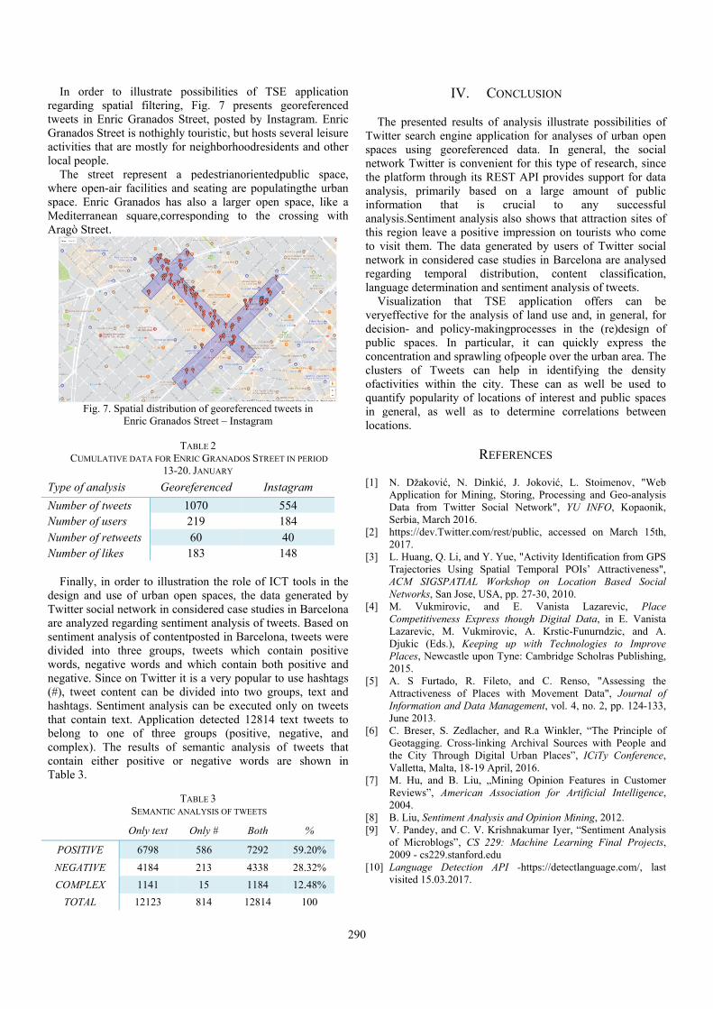
InregatweGraactiloca

TwhespacMedAra

Typ

NumNumNumNum

FdesiTwiare sentdiviworneg(#),hashthatbelocomconTab

PO

NE

CO

n order to arding spatia

eets in Enric Ganados Street iivities that areal people. The street reere open-air fce. Enric Graditerranean s

agò Street.

Fig. 7. SpaE

CUMULATIVE

pe of analysis

mber of tweetsmber of users mber of retweember of likes

Finally, in ordign and use oitter social netanalyzed regatiment analysiided into thrrds, negative

gative. Since o tweet contenhtags. Sentimt contain textong to one

mplex). The rntain either pble 3.

OSITIVE

EGATIVE

OMPLEX

TOTAL

illustrate poal filtering, FGranados Streis nothighly toe mostly for n

epresent a pfacilities and anados has alsquare,corresp

atial distributionEnric Granados

TAB

DATA FOR ENRI

13-20. J

Georef

s 102

ets 61

der to illustratof urban opentwork in consarding sentimis of contentpree groups, twords and w

on Twitter it int can be div

ment analysis ct. Application

of three grresults of sempositive or n

TAB

SEMANTIC ANA

Only text O

6798

4184

1141

12123

ssibilities of Fig. 7 preseeet, posted byouristic, but hneighborhoodr

pedestrianorieseating are polso a larger oponding to t

n of georeferencStreet – Instagr

BLE 2 IC GRANADOS SJANUARY

ferenced

070 19

60 83

tion the role on spaces, the sidered case stent analysis o

posted in Barctweets which

which contain s a very popu

vided into twocan be execut

n detected 128roups (positivmantic analynegative wor

BLE 3 ALYSIS OF TWEET

Only # Bo

586 72

213 43

15 11

814 128

TSE applicents georeferey Instagram. osts several leresidents and

entedpublic sopulatingthe uopen space, lthe crossing

ced tweets in ram

STREET IN PERIOD

Instagram

554 184 40

148

of ICT tools idata generate

tudies in Barcof tweets. Basecelona, tweetsh contain po

both positiveular to use haso groups, texted only on tw814 text tweeve, negative,sis of tweets

rds are show

TS

oth %

92 59.20%

38 28.32%

84 12.48%

814 100

290

cation enced Enric eisure other

space, urban like a

with

D

in the ed by elona ed on were sitive e and shtags xt and weets ets to and

s that wn in

%

%

%

Th

Twitspacnetwthe panalyinforanalythis to vinetwregarlangu

Viverydecispublconcclustofactquanin glocat

[1]

[2]

[3]

[4]

[5]

[6]

[7]

[8][9]

[10]

I

he presented tter search enes using ge

work Twitter iplatform throuysis, primarirmation thaysis.Sentimenregion leave isit them. The

work in considrding tempouage determinisualizationeffective for tsion- and poic spaces. In

centration and ters of Twetivities within

ntify popularitgeneral, as wtions.

N. Džaković,Application foData from TwSerbia, March https://dev.Tw2017. L. Huang, Q. LTrajectories UACM SIGSPANetworks, SanM. VukmiroCompetitiveneLazarevic, MDjukic (Eds.)Places, Newca2015. A. S FurtadoAttractiveness Information anJune 2013. C. Breser, S.Geotagging. Cthe City ThroValletta, MaltaM. Hu, and BReviews”, Am2004. B. Liu, SentimV. Pandey, anof Microblogs2009 - cs229.sLanguage Devisited 15.03.2

IV. CONC

results of anagine applicati

eoreferenced s convenient ugh its REST ly based onat is cru

nt analysis alsa positive impe data genera

dered case stuoral distribunation and senthat TSE the analysis o

olicy-makingpn particular, sprawling ofpets can helpn the city. Tty of location

well as to de

REFER

N. Dinkić, Jor Mining, Storwitter Social N2016.

witter.com/rest/p

Li, and Y. Yue,Using Spatial ATIAL Worksh

n Jose, USA, ppovic, and Eess Express tho

M. Vukmirovic,), Keeping upastle upon Tyne

o, R. Fileto, of Places wi

nd Data Manag

Zedlacher, andCross-linking Aough Digital Ua, 18-19 April, B. Liu, „Mininmerican Associ

ent Analysis annd C. V. Krishns”, CS 229: Mstanford.edu etection API 2017.

CLUSION

alysis illustraion for analysdata. In genfor this type API provides

n a large amucial to o shows that pression on to

ated by users udies in Barceution, contenntiment analys

application of land use anprocesses in t

it can quicpeople over thp in identify

These can as ns of interest aetermine corr

RENCES

J. Joković, L. ring, ProcessinNetwork", YU

public, accesse

, "Activity IdenTemporal POI

hop on Locatp. 27-30, 2010. E. Vanista ough Digital D, A. Krstic-Fu

p with Technoe: Cambridge S

and C. Rensith Movement gement, vol. 4,

d R.a Winkler,Archival SourceUrban Places”, 2016.

ng Opinion Feiation for Art

nd Opinion Minnakumar Iyer, “Machine Learni

-https://detectla

te possibilitieses of urban oneral, the soof research, ss support for mount of puany succesattraction siteourists who cof Twitter so

elona are analynt classificasis of tweets.

offers can nd, in generalthe (re)designckly express he urban area. ying the den

well be useand public sprelations betw

Stoimenov, "ng and Geo-anaU INFO, Kopa

ed on March

ntification from Is’ Attractivention Based S

Lazarevic, PData, in E. Vaunurndzic, and

ologies to ImpScholras Publish

so, "AssessingData", Journano. 2, pp. 124-

, “The Principes with PeopleICiTy Confere

atures in Custotificial Intellige

ning, 2012. “Sentiment Anaing Final Proj

anguage.com/,

es of open ocial since data

ublic ssful es of come ocial ysed tion,

be l, for n of

the The

nsity d to

paces ween

"Web alysis onik,

15th,

GPS ness", Social

Place anista d A. prove hing,

g the al of -133,

le of e and ence,

omer ence,

alysis jects,

last

291

Macrodiversity Reception Level Crossing Rate in the Presence of Mixed Nakagami-m and Rician Multipath

Fading Ivica Marjanović1, Danijel Đošić1, Ivan Đurić1, Dejan Milić1,

Marijana Milenković1 and Mihajlo Stefanović1

Abstract – Macrodiversity (MACD) reception consisting of macrodiversity selection combining (SC) receiver and two microdiversity (MICD) maximal ratio combining (MRC) receivers is considered in this paper. Signal at multiple antennas at the first MRC receiver propagate in non line-of-sight shadowed multipath fading channel and signals at multiple antennas at the second MRC propagate in line-of-sight shadowed multipath fading channel. Signal envelopes of the first MRC receiver are described by using Nakagami-m distribution and signal envelopes at the second MRC receiver are described with Rician distribution. Long term fading is described by using Gamma distribution. Closed form expression for average level crossing rate (LCR) of MACD SC receiver output signal is calculated and the influence of Rician factor and Nakagami-m severity parameter on LCR is analysed and discussed.

Keywords – Macrodiversity, Microdiversity, Nakagami-m fading, Rician fading, Gamma, SC, MRC.

I. INTRODUCTION

Large scale fading and small scale fading degrade outage probability, bit error probability and channel capacity of wireless communication system. MACD structures can be used in cellular mobile radio to reduce long term fading effects and short term fading effects simultaneously [1]-[4]. In this paper MACD reception with SC receiver at macro level and MRC receiver at micro level are studied. MICD MRC receiver combines signal envelopes with two antennas at base station and MACD SC receiver combines signal envelopes average powers with two base stations. Signal at the first base

station operating over Gamma shadowed non line-of-sight short term fading channel and signals at the second MRC receiver operating over line-of-sight short term fading channel and signal envelopes variation at the first MRC receiver is described by using Nakagami-m distribution and signal envelopes variation at the second MRC receiver is modeled by using Rician distribution. The MACD SC receiver reduces Gamma long term fading effects, the first MICD MRC receiver reduces Nakagami-m short term fading effects and the second MACD MRC reception reduces Rician short term fading effects on system performance. Outage probability and bit error probability are performance measures of the first order of wireless communication radio system and average level crossing rate and average fade duration are the second order performance measures of wireless communication system [5]-[8].

There are more works in open technical literature considering LCR of MACD receptions operating over shadowed multipath fading channels. In paper [9], average level crossing rate and average fade duration of MACD system with SC reception at macro level and MRC receptions micro level operating over Gamma shadowed correlated Nakagami-m short term fading are derived as expressions in closed form. The second order statistics of MACD structure consisting of SC MACD reception and MRC micro receptions in the presence of correlated Gamma long term fading and Rician short term fading are studied and evaluated in paper [10]. In the work [11], MACD reception in the presence of small scale κ-µ fading and Gamma large scale fading is considered and average level crossing rate and average fade duration are calculated. Outage probability and bit error probability of MACD system in the presence of Gamma shadowed, Rician fading channel are studied and derived.

In this paper, MACD structure with SC reception at macro level and MRC receiver at micro level where the first MRC receiver operate over non line-of-sight multipath fading channel and the second MRC receiver operating over line-of-sight short term fading channel is considered. Signal at the first MRC receiver experiences Nakagami-m fading and signal at the second MRC receiver subjected to Rician short term fading. Signal envelope average power is described by using correlated Gamma distribution. In this paper, average level crossing rate of SC receiver output signal is calculated as expression in closed form. This expression can be used for calculation of average fade duration of proposed wireless MACD communications system [12]-[16].

1Ivica Marjanović - Faculty of Electrical Engineering at University of Niš, Aleksandra Medvedeva 14, 18000 Niš, Serbia, (e-mail:[email protected]).

1Danijel Đošić - Faculty of Electrical Engineering at University ofNiš, Aleksandra Medvedeva 14, 18000 Niš, Serbia, (e-mail: [email protected]).

1Ivan Đurić - Faculty of Electrical Engineering at University ofNiš, Aleksandra Medvedeva 14, 18000 Niš, Serbia, (e-mail: [email protected]).

1Dejan Milić - Faculty of Electrical Engineering at University ofNiš, Aleksandra Medvedeva 14, 18000 Niš, Serbia, (e-mail: [email protected]).

1Marijana Milenković - Faculty of Electrical Engineering at University of Niš, Aleksandra Medvedeva 14, 18000 Niš, Serbia, (e-mail: [email protected]).

1Mihajlo Stefanović - Faculty of Electrical Engineering at University of Niš, Aleksandra Medvedeva 14, 18000 Niš, Serbia, (e-mail: [email protected]).

292

II. LEVEL CROSSING RATE OF SIGNAL AT

OUTPUTS OF MRC RECEIVERS

Signal envelopes at inputs in the first MRC receiver are denoted with x1 and x2 and at the inputs in the second MRC receiver with y1 and y2. Signal envelopes at outputs of MRC receiver are x and y and at the output of SC receiver signal envelope is denoted with z. Signal x1 and x2 follow Nakagami-m distribution:

2

12 1

1

2, 0, 1, 2.

i

i

m mx

mx i i i

mp x x e x i

m

(1)

where Gaussian noise is equally distributed between branch, squared random variable x can be written as sum of squared variables x1 and x2.

2 2 21 2 .x x x (2)

The first derivative of x is:

1 1 2 2

1.x x x x x

x (3)

The first derivation of Nakagami-m random variable has zero mean Gaussian distribution with variance:

2 1

2 2 2 2 1 .x x mf m

(4)

This x has Gaussian distribution with zero mean and variance:

2 2 2 2 2 2 2 2 21 1 11 22

1.x m m mx f x f f

m m mx

(5)

The join probability density function of x and x is:

2

221.

2x

x

xx x x x

x

p xx p x p x p x e

(6)

The level crossing rate of the first MRC receiver output signal envelope is:

0

.2

xx xx xN dx x p xx p x

(7)

Random variable x fallow χ2 distribution:

2

1

2

4 1

1

2, 0.

2

m mx

mx

mp x x e x

m

(8)

After substituting the expressions for Nx becomes:

2

1

2 1 2

4 1

1

2, 0.

2 2

m mx

mmx

f mN x e x

m

(9)

Squared signal y is:

2 2 21 2 .y y y (10)

The first derivative of y is:

1 1 2 2

1.y y y y y

y (11)

The first derivation of Rician random variable has zero mean Gaussian distribution with variance:

1 2

2 2 2 2 2 .1y y mf

(12)

This random variable y has zero mean Gaussian variance

with variance:

2 2 2 2 .1y mf

(13)

The level crossing rate of the second MRC receiver output signal envelope is:

.2

yy yN p y

(14)

Random variable y fallow χ2 distribution:

2

2

12

2 1

1

2 1

12 222 2

2 12 1

2 2

0 2 1 1

4 1 1 2 14

22

1 12 .

2 ! 2

y

y

iy

i

i

y yp y e I

e e

e yi i

(15)

After substituting the expressions for average level crossing rate becomes:

2

2

1

1

1

2 11 2

2 1 2 1 22

2 1

2 2

0 2 1 1

4 1

2 2

1 12 .

2 ! 2

ym

x

i

i

i

fN e

e

yi i

(16)

Signal envelope powers Ω1 and Ω2 follow correlated Gamma distribution [17]:

1 2

11 2

0

1

1 22

01 1

1 2 1 21 2 1 1 22 1 1 2

0 0

2 1

2 1 1 200 0

11 11 2

1 1

1 2

1 1

1

1 1

1.

! !

cc c

i c

c ci

i c i c

p Ic

ec

ei i c

(17)

293

where c is Gamma shadowing severity parameter, ρ is Gamma correlation coefficient and Ω0 is average power of Ω1 and Ω2. When c goes to infinity shadowed multipath fading channel becomes multipath fading channel. When ρ goes to one, the least signal occurs simultaneously at bout MRC receivers. Diversity gain decreases as correlation coefficient increases.

III. LEVEL CROSSING RATE OF SC RECEIVER

OUTPUT SIGNAL ENVELOPE

Macrodiversity SC receiver selects microdiversity MRC receivers with the highest signal envelope average power at inputs to provide service to mobile user. This, level crossing rate of SC receiver output signal is:

1

1 1 2

2

2 1 2

1 2 1 20 0

2 1 1 2 1 20 0

.

z x

y

N d d N p

d d N p J J

(18)

The integral J1 is [17]:

1

1

1 1

11

1

1 1

2 1 2 4 11 2 1 1

0

2 1

20 1 1 10

1 4 22 2

00 1

2

2 2 2 1 22 20 0

2 1

2 2 1

1 1

!1

11

1

12 .

1 1

m mm

c c

i c

i

i c m j

j j

j

i c m j

fJ m x

m c

i i c i c

mxi c

mxK

(19)

The integral J2 is [17]:

1

1

1

2

2

2 1 1

11

1

2 1

2 11 2

2 12 2 3 2

0 2 1 1

2 1

2 1 1 20 2 20 0

1 2 22

02

02 2

2 2 220

4 1 1 12

2 ! 22 2

1 1

!1 1

11 1

1 2

1

1

i

m i

i

i c

c ci

i c j i

j j

j

i c j

fJ z

i ie

i i cc

mzi c i c

K

1

2

20

22 .

1i

mz

(20)


Level crossing rate of resulting process at output of macrodiversity SC receiver versus of SC receiver output

signal for several values Nakagami-m short term fading severity parameter, Rician k factor and Gamma long term fading severity parameter is shown at Fig. 1.

Fig. 1. Level crossing rate (LCR) depending on the envelope z, when m=c=2, κ=1 and different values of Ω0 and Ω2

Level crossing rate getting wider for higher values of Ω0 and Ω2. Resulting signal has higher influence on level crossing rate for lower values of resulting signal. Level crossing rate decreases as Nakagami-m severity parameter has higher influence on level crossing rate for lower values resulting signal and higher values of Nakagami-m short term fading severity parameter. Level crossing rate increases when Gamma long term fading severity parameter decreases. The influence of Gamma long term fading severity parameter on level crossing rate is higher for lower values of resulting signal for lower values of resulting signal for lower values of Nakagami-m short term fading severity parameter and for higher values of Gamma long term fading severity parameter..

Fig. 2. Level crossing rate (LCR) depending on the envelope z, when

m=c=2, Ω0=1 and different values of κ

Level crossing rate decreases when Rician k factor increases in Fig. 2. Rician k factor has higher influence on level crossing rate for lower values of Rician k factor. Also, Rician k factor has higher influence on level crossing rate for

294

lower values of Nakagami-m short term fading severity parameter and lower values of Gamma long term fading severity parameter

V. CONCLUSION

Macrodiversity system with selection combining receiver at macro level and two maximal ratio combining receiver at micro level signal, at the first MRC receiver operate over non line-of-sight short term fading and signal at the second MRC receiver operate over line-of-sight multipath fading channel is analysed. Nakagami-m distribution is used to describe signal envelope at the first MRC receiver and Rician distribution is used to described signal envelope at the second MRC receiver. Long term fading is described by using correlated Gamma distribution. Macro SC receiver reduces Gamma long term fading effects on system performance the first MRC receiver reduces Nakgami-m short term fading effects on system performance and the second MRC receiver reduces Rician short term fading effects on system performance. In this paper, level crossing rate of SC receiver output signal is calculated as expression closed form. By using this expression, average fade duration of macrodiversity wireless communication system can be calculated. Also, by using derived expression, level crossing rate of macrodiversity system operating over Gamma shadowed, Rayleigh multipath fading channel can be evaluated. The influence of Nakagami-m shape parameter, Rician κ factor and Gamma long term severity parameter on level crossing rate are studied and discussed. Level crossing rate decreases as Nakagami-m shaping parameter increases. When Rician factor or dominant component power increases level crossing rate has lower values. Level crossing rate decreases when Gamma parameter increases and when Gamma parameter goes to infinity, Gamma shadowed multipath fading channel becomes multipath fading channel. When correlation coefficient goes to one macrodiversity system becomes microdiversity system.

REFERENCES

[1] S. Panic, M. Stefanovic, J. Anastasov, and P. Spalevic, Fading and Interference Mitigation in Wireless Communications, CRC Press, New York, 2013.

[2] J. Proakis, Digital Communications, 4nd ed, New York: McGraw-Hill, 2001.

[3] D.B. Djosic, D.M. Stefanovic, and C.M. Stefanovic, “Level Crossing Rate of Macro-Diversity System with Two Micro’diversity SC Receivers over Correlated Gamma Shadowed α-μ Multipath Fading”, IETE Journal of Research, vol. 62, issue 2, 2016, pp. 140-145.

[4] A.V. Marković, Z.H. Perić, D.B. Đošić, M.M. Smilić, and B.S. Jakšić, "Level Crossing Rate of Macrodiversity System over Composite Gamma Shadowed Alpha-kappa-mu Multipath Fading Channel", Facta Universitatis Series: Automatic Control and Robotics, vol. 14, no. 2, 2015, pp. 99-109.

[5] D.S. Krstic, M.C. Stefanovic, and D.A. Aleksic, I. Marjanovic, and G. Petkovic, "Performance of Macrodiversity System with two SC Microdiversity Receivers in the Presence of Rician Fading", Recent Advances in Communications, pp. 162-166.

[6] D. Krstic, S. Suljovic, V. Doljak, M. Stefanovic, E. Leitgeb, and P. Pezzei, "Moment Generating Function of Macrodiversity System with Three Microdiversity MRC Receivers in Gamma Shadowed Nakagami-m Fading Channel", 2016 10th International Symposium on Communication Systems, Networks and Digital Signal Processing (CSNDSP), 2016.

[7] D. Krstic, B. Jaksic, M. Gligorijevic, D. Stefanovic, and M. Stefanovic, "Performance of Diversity System Output Signal in Mobile Cellular System in the Presence of α-μ Short Term Fading and Gamma Long Term Fading", Radioengineering, 2016.

[8] B.S. Jakšić, "Level Crossing Rate of Macrodiversity SC Receiver with two Microdiversity SC Receivers Over Gamma Shadowed Multipath Fading Channel", Facta Universitatis Series: Automatic Control and Robotics, vol. 14, no. 2, 2015, pp. 87-98.

[9] D. Stefanovic, S.R. Panic, and P. Spalevic “Secondorder Statistics of SC Macrodiversity System Operating over Gamma Shadowed Nakagami-m Fading Channels”, AEU - International Journal of Electronics and Communications, vol. 65, no. 5, 2011, pp. 413-418.

[10] N. Sekulovic, and M. Stefanovic, “Performance Analysis of System with Micro- and Macrodiversity Reception in Correlated Gamma Shadowed Rician Fading Channels”, Wireless Personal Communications, vol. 65, no. 1, 2012, pp. 143-156.

[11] S. Panic, D. Stefanovic, I. Petrovic, M. Stefanovic, J. Anastasov, and D. Krstic, “Second Order Statistics of Selection Macro-Diversity System Operating over Gamma Shadowed k -m Fading Channels”, EURASIP J. Wireless Commun. Netw., vol. 2011, no. 1, Oct. 2011, pp. 1-7.

[12] D. Krstic, S. Milosavljevic, B. Milosavljević, S. Suljovic, and M. Stefanovic, "Level Crossing Rate of Macrodiversity in the Presence of Mixed Short Term Fading, Gamma Long Term Fading and Co-channel Interference", International Journal of Communications, vol. 11, 2017, pp 1-7.

[13] D. Krstić, S. Minić, S. Suljović, M. Perić, V. Veličković, and M. Stefanović, "Performance of Macrodiversity System in the Presence of Gamma Long Term Fading and Different Short Term Fading", International Journal of Mathematical Models and Methods in Applied Sciences, vol. 11, 2017, pp. 16-25.

[14] D.S. Krstic, S.G. Minić, S. Milosavljevic, B. Milosavljević, and M. C. Stefanovic, "Macrodiversity Outage Performance in the Presence of Weibull Short Term Fading, Gamma Long Term Fading and α-κ-μ Co-channel Interference", International Journal of Communications, vol. 11, 2017, pp. 14-21.

[15] D. Krstić, R. Gerov, Z. Popović, M. Perić, V. Veličković and M. Stefanović, "Performance of Macrodiversity System with Selection Combining and Three Microdiversity MRC Receivers in the Presence of Various Fading", International Journal of Mathematics and Computers in Simulation, vol. 11, 2017, pp. 14-24.

[16] D.S. Krstić, S. Suljović, M.Č. Stefanović, M.M. Bani Yassein, and D. Aleksić, "Level Crossing Rate of SC Receiver Output Signal in the Presence of Gamma Shadowing and k-μ or Rician Multipath Fading", International Journal of Communications, vol. 9, 2015, pp. 19-27.

[17] I. Gradshteyn, and I. Ryzhik, Tables of Integrals, Series, and products, Academic Press, New York 1994.

Session PO3:

2C - SIGNAL PROCESSING

297

The Influence of Babble Noise on Subjective Speech Intelligibility in a Room with High Reverberation Time

Violeta Stojanović1, Zoran Milivojević2, Zoran Veličković3

Abstract – The first part of this paper describes the experiment which is used for estimation of speech intelligibility depending on room reverberation and superimposed Babble noise. The estimation of the subjective intelligibility is done using MOS test of test sentence application from SMST base. The results are shown both in tables and graphically. The second part of this paper represents the comparative analysis of intelligibility. It also estimated degradation level of speech intelligibility with influence of Babble noise and relation to reverberation effect.

Keywords – Room impulse response (RIR), STI, MOS test, Bablle Noise, Subjective speech intelligibility.

I. INTRODUCTION

Verbal communication is a process of deliberate and, above all, understandable exchange of notions, thoughts and messages between people. For the efficient verbal communication, it is essential to provide good transmission of the speech signal from a speaker to a listener. Noises are one of the factors which affect speech intelligibility. Babble Noise (BN) is on of the best noise for covering the speech. [1]. It represents the acoustic nuisance which originates from N subjects speaking simultaneously end degrades the useful acoustic signal. Degradation measure is shown by SNR relation.

French, Steinberg and Beranek 1947 were the first who highlight the problem of transmission and speech intelligibility [2]. Houtgast and Steeneken in 1980 confirmed an objective method to measure the quality of voice transmission in the room [2] and suggested the acoustic parameters of the Speech Transmission Index, STI [3]. Subjective systems evaluation for transmitting voice using open and closed tests intelligibility, were first performed by Fletcher and Steinberg in 1929 [2], then Egan in 1944, Miller and Nicely in 1955, House in 1965 and Voiers in 1977 etc. Review of tests for evaluating intelligibility of speech was given by Pols in 1991 and Steeneken in 1992.

This paper estimates the Babble Noise impact on subjective speech intelligibility for „Octagon“ room, which is situated at „Queen Mary“ University in London. The experiment is consisted of two stages: a) the analysis of subjective speech intelligibility in a room under the influence of reverberation. [4] and b) the analysis of subjective speech intelligibility in a room under the influence of Babble noise. This experiment is

based on MOS test of speech signal intelligibility from a base Serbian Matrix Sentence Test, SMST [5]. In the first stage of this experiment, the test group of listeners estimated the speech signal intelligibility obtained using the convolution of a clear speech signal out of SMST base and recorded impulse response. The impulse responses refer to the „Octagon“ room at „Queen Mary“ University in London and they were recorded by Centre for Digital Music [6] and they are available at http://c4dm.eecs.qmul.ac.uk/rdr/handle/123456789/10. In the second stage of the experiment, the test group estimated simulated acoustic signal intelligibility of the room with superimposed BN for predefined SNR relations. Two test groups of listeners participated in the experiment. After the analysis of the obtained results from the applied MOS tests, the conclusion about the BN impact on the subjective speech intelligibility in the room.

Work organization is as follows: Section II describes the experiment and the results shown with charts and graphs, Section III shows the results analysis and the Conclusion is in the Section IV.

II. EXPERIMENTS

This paper describes the experiment which estimates BN impact on the subjective speech intelligibility in „Octagon at the Mile End campus of Queen Mary“ at the University in London.

The objective acoustic parameter STI was determined using the impulse of the room in 25 measuring points MP (out of 169) whose positions are shown in Fig. 1. [6] The analysis was carried out using software packages EASERA and Matlab.

Fig. 1. The position of the measuring points in the room

1Violeta Stojanović is with the College of Applied Technical Sciences of Niš, 20. Aleksandra Medvedeva, St, 18000 Niš, Serbia, e-mail: [email protected]

2Zoran Milivojević is with the College of Applied Technical Sciences of Niš, 20. Aleksandra Medvedeva, St, 18000 Niš, Serbia

3.Zoran Veličković is with the College of Applied Technical Sciences of Niš, 20. Aleksandra Medvedeva, St, 18000 Niš, Serbia

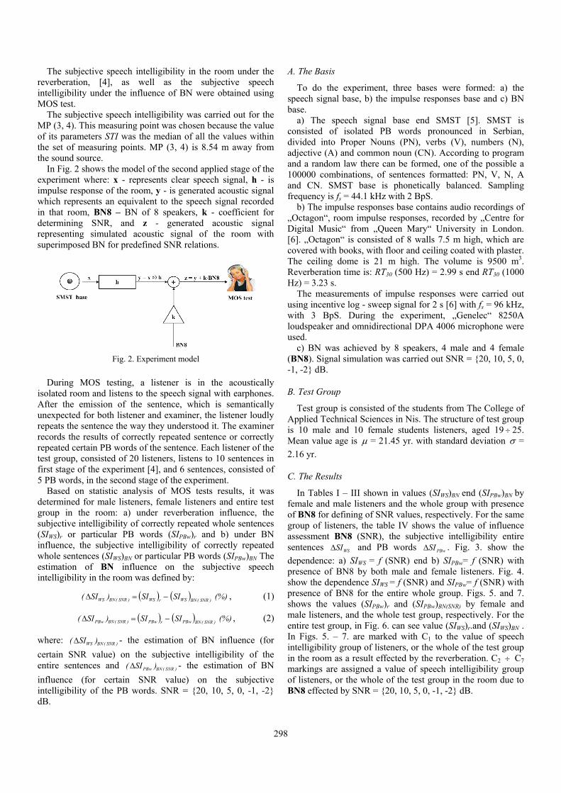
http://c4dm.eecs.qmul.ac.uk/rdr/handle/123456789/10

298

The subjective speech intelligibility in the room under the reverberation, [4], as well as the subjective speech intelligibility under the influence of BN were obtained using MOS test.

The subjective speech intelligibility was carried out for the MP (3, 4). This measuring point was chosen because the value of its parameters STI was the median of all the values within the set of measuring points. MP (3, 4) is 8.54 m away from the sound source.

In Fig. 2 shows the model of the second applied stage of the experiment where: x - represents clear speech signal, h - is impulse response of the room, y - is generated acoustic signal which represents an equivalent to the speech signal recorded in that room, BN8 – BN of 8 speakers, k - coefficient for determining SNR, and z - generated acoustic signal representing simulated acoustic signal of the room with superimposed BN for predefined SNR relations.

Fig. 2. Experiment model

During MOS testing, a listener is in the acoustically isolated room and listens to the speech signal with earphones. After the emission of the sentence, which is semantically unexpected for both listener and examiner, the listener loudly repeats the sentence the way they understood it. The examiner records the results of correctly repeated sentence or correctly repeated certain PB words of the sentence. Each listener of the test group, consisted of 20 listeners, listens to 10 sentences in first stage of the experiment [4], and 6 sentences, consisted of 5 PB words, in the second stage of the experiment.

Based on statistic analysis of MOS tests results, it was determined for male listeners, female listeners and entire test group in the room: a) under reverberation influence, the subjective intelligibility of correctly repeated whole sentences (SIWS)r or particular PB words (SIPBw)r and b) under BN influence, the subjective intelligibility of correctly repeated whole sentences (SIWS)BN or particular PB words (SIPBw)BN The estimation of BN influence on the subjective speech intelligibility in the room was defined by:

( ) ( ) (%)SISI)SI( )SNR(BNWSrWS)SNR(BNWS −=∆ , (1)

( ) ( ) (%)SISI)SI( )SNR(BNPBwrPBw)SNR(BNPBw −=∆ , (2)

where: )SNR(BNWS )SI(∆ - the estimation of BN influence (for certain SNR value) on the subjective intelligibility of the entire sentences and )SNR(BNPBw )SI(∆ - the estimation of BN influence (for certain SNR value) on the subjective intelligibility of the PB words. SNR = 20, 10, 5, 0, -1, -2 dB.

A. The Basis

To do the experiment, three bases were formed: a) the speech signal base, b) the impulse responses base and c) BN base.

a) The speech signal base end SMST [5]. SMST is consisted of isolated PB words pronounced in Serbian, divided into Proper Nouns (PN), verbs (V), numbers (N), adjective (A) and common noun (CN). According to program and a random law there can be formed, one of the possible a 100000 combinations, of sentences formatted: PN, V, N, A and CN. SMST base is phonetically balanced. Sampling frequency is fs = 44.1 kHz with 2 BpS.

b) The impulse responses base contains audio recordings of „Octagon“, room impulse responses, recorded by „Centre for Digital Music“ from „Queen Mary“ University in London. [6]. „Octagon“ is consisted of 8 walls 7.5 m high, which are covered with books, with floor and ceiling coated with plaster. The ceiling dome is 21 m high. The volume is 9500 m3. Reverberation time is: RT30 (500 Hz) = 2.99 s end RT30 (1000 Hz) = 3.23 s.

The measurements of impulse responses were carried out using incentive log - sweep signal for 2 s [6] with fs = 96 kHz, with 3 BpS. During the experiment, „Genelec“ 8250A loudspeaker and omnidirectional DPA 4006 microphone were used.

c) BN was achieved by 8 speakers, 4 male and 4 female (BN8). Signal simulation was carried out SNR = 20, 10, 5, 0, -1, -2 dB.

B. Test Group

Test group is consisted of the students from The College of Applied Technical Sciences in Nis. The structure of test group is 10 male and 10 female students listeners, aged 19 ÷ 25. Mean value age is µ = 21.45 yr. with standard deviation σ = 2.16 yr.

C. The Results

In Tables I – III shown in values (SIWS)BN end (SIPBw)BN by female and male listeners and the whole group with presence of BN8 for defining of SNR values, respectively. For the same group of listeners, the table IV shows the value of influence assessment BN8 (SNR), the subjective intelligibility entire sentences WSSI∆ and PB words PBwSI∆ . Fig. 3. show the dependence: a) SIWS = f (SNR) end b) SIPBw= f (SNR) with presence of BN8 by both male and female listeners. Fig. 4. show the dependence SIWS = f (SNR) and SIPBw= f (SNR) with presence of BN8 for the entire whole group. Figs. 5. and 7. shows the values (SIPBw)r and (SIPBw)BN(SNR) by female and male listeners, and the whole test group, respectively. For the entire test group, in Fig. 6. can see value (SIWS)r.and (SIWS)BN . In Figs. 5. – 7. are marked with C1 to the value of speech intelligibility group of listeners, or the whole of the test group in the room as a result effected by the reverberation. C2 ÷ C7 markings are assigned a value of speech intelligibility group of listeners, or the whole of the test group in the room due to BN8 effected by SNR = 20, 10, 5, 0, -1, -2 dB.

299

TABLE I THE SUBJECTIVE INTELLIGIBILITY OF ENTIRE SENTENCES AND PB

WORDS BY FEMALE LISTENERS WITH PRESENCE OF BN8 FOR DEFINING OF SNR VALUES

SNR (dB) 20 10 5 0 -1 -2 No. WS 3 2 0 0 0 0

No. PBw

PN 7

33

6

24

4

19

2

5

2

3

0

0 V 7 5 6 0 0 0 N 7 3 5 2 1 0 A 6 5 2 1 0 0

CN 6 5 2 0 0 0 (SIWS)BN (%) 30 20 0 0 0 0 (SIPBw)BN(%) 66 48 38 10 6 0

TABLE II THE SUBJECTIVE INTELLIGIBILITY OF ENTIRE SENTENCES AND PB

WORDS BY MALE LISTENERS WITH PRESENCE OF BN8 FOR DEFINING OF SNR VALUES

SNR (dB) 20 10 5 0 -1 -2 No. WS 3 3 1 0 0 0

No. PBw

PN 8

31

4

29

3

19

5

11

0

4

3

6 V 4 6 2 2 1 1 N 7 5 5 3 1 0 A 5 7 5 1 1 0


TABLE III THE SUBJECTIVE INTELLIGIBILITY OF ENTIRE SENTENCES AND PB

WORDS BY WHOLE GROUP WITH PRESENCE OF BN8 FOR DEFINING OF SNR VALUES

SNR (dB) 20 10 5 0 -1 -2 No. WS 6 5 1 0 0 0

No. PBw

PN 15

64

10

51

7

38

7

16

2

7

3

6 V 11 11 8 2 1 1 N 14 8 10 5 2 0 A 11 12 7 2 1 0


TABLE IV THE VALUE OF INFLUENCE ASSESSMENT BN8 (SNR), THE

SUBJECTIVE INTELLIGIBILITY ENTIRE SENTENCES AND PB WORDS FOR FEMALE, MALE AND THE WHOLE GROUP LISTENERS

SNR (dB)

Female listeners

Male listeners

The whole test group

WSSI∆ (%)

PBwSI∆ (%)

WSSI∆ (%)

PBwSI∆(%)

WSSI∆ (%)

PBwSI∆ (%)

20 22 19.6 28 21.2 25 20.4 10 32 37.6 28 25.2 30 33.4 5 52 47.6 48 45.2 50 46.4 0 52 75.6 58 61.2 55 68.4 -1 52 79.6 58 75.2 55 77.4 -2 52 85.6 58 71.2 55 76.4

a)

b)

Fig. 3. Dependence of: a) the entire sentences and b) the BP words, subjective intelligibility of SNR with presence of BN8 by

both male and female listeners

Fig. 4. Dependence of the entire sentences end BP words subjective

intelligibility of SNR with presence of BN8 for the entire whole group listeners

(a)

(b)

Fig 5. The subjective intelligibility of the PB words by: (a) female and (b) male, listeners in the room with presence of BN8

300

III. THE RESULTS ANALYSIS

Based on results shown in the Tables I – IV and in the Figs. 3. - 7. we can draw the following conclusions:

1) the subjective intelligibility of female listeners with the influence of BN8 is: a) the best on SNR = 20 dB, (SIWS)BN = 30 % and (SIPBw)BN = 66 % and b) 0% on SNR = 2105 −− ,,, dB and SNR = -2 dB for the whole sentences and BP words, respectively. The obtained values with the influence of reverberation are: (SIWS)r = 52 % and (SIPBw)r = 85.6 % [4]. Estimated values of the influence of BN8 on the speech intelligibility of female listeners are: BNWS )SI(∆ = 22 % and BNPBw )SI(∆ = 19.6%.

2) a) the subjective intelligibility of male listeners with the influence of BN8 is (SIWS)BN = 30 % and (SIPBw)BN = 62 %) on SNR = 20 dB. The obtained values with the influence of reverberation are: (SIWS)r = 58 % and (SIPBw)r = 83.2 % [4]. The estimated values of the influence of BN on the speech intelligibility of male listeners are: BNWS )SI(∆ = 28 % and

BNPBw )SI(∆ = 21.2%.

Fig. 6. The subjective intelligibility of the sentences by the entire

test group in the room with presence of BN8

Fig. 7. The subjective intelligibility of the PB words by the entire test

group in the room with presence of BN8

b) with the influence of BN8 the male listeners couldn’t understand the whole sentences 100% on SNR = 0, -1, -2 dB. The PB words were least understandable (SIPBw)BN = 8 % on SNR = 1 dB.

3) both female and male listeners, with the influence of BN8, had the same percentage of understanding: a) for the whole sentences on SNR= 20 dB, (SIWS)BN = 30 % (Fig. 3.a) ) and b) for the PB words on SNR= 5 dB, (SIPBw)BN = 38 % (Fig. 3. b) ).

4) the best percentage of understanding of both whole sentences and PB words of the whole test group with the influence of BN, is (SIWS)BN = 30 %) and (SIPBw)BN = 64 %) for SNR = 20 dB (points C2 in the Fig. 6. and 7.). The obtained values with the influence of reverberation are: (SIWS)r = 55 % and (SIPBw)r = 84.4 %, (point C1 in the Fig. 6 and 7.) [4]. The estimated values of BN influence on sentences and PB words intelligibility of the whole test group are BNWS )SI(∆ = 25 % and BNPBw )SI(∆ = 20.4%. The whole test group showed 0 % of understanding of the whole sentences at SNR = 0, -1, -2 dB (points C5, C6, C7 in the Fig. 6.). The least percentage of understanding of the PB words is 6 % at the signal with SNR = -2 dB (point C7 in the Fig.7.).

IV. CONCLUSION

This paper estimated the degradation level of subjective speech intelligibility with influence of Babble noise and relation to reverberation effect in a room with high reverberation time. For the subjective intelligibility of whole sentences, the influence evaluation value results to be within the range: a) for female listeners WSSI∆ = 22 ÷ 52 %, b) for male listeners WSSI∆ = 28 ÷ 58% and c) for the entire test

group WSSI∆ = 25 ÷ 55 %. For the subjective intelligibility of PB words the influence evaluation value results within the range: a) for female listeners PBwSI∆ = 19.6 ÷ 85.6 %, b) for

male listeners PBwSI∆ = 21.2 ÷ 71.28 % and c) for the entire test group PBwSI∆ = 20.4 ÷ 76.4 %.

REFERENCES

[1] N. Krishamurthy, and J. H.L. Hansen, “Babble Noise: Modeling, Analysis and Applications“, IEEE Transactions on Audio,Speech and Language Processing, vol 17, no.7, September 2009.

[2] H. J.M. Steeneken, “On Measuring and Predicting Speech Intelligibility”, Academisch Proefschrift, Soesterberg, 1992.

[3] H. J.M. Steeneken, “Apsyhical Method for measuring Speech Transmission Quality”, J. Acoust. Soc. Am., vol. 19, 1980.

[4] V. Stojanović, Z. Milivojević, and Z. Veličković, “Preciznost procene razumljivosti govora na bazi akustičkog impulsnog odziva”, XVI međunarodni naučno-stručni simpozijum INFOTEH, Jahorina, 2017.

[5] Z. Milivojević, D. Kostić, Z. Veličković, and D. Brodić, “Serbian Sentence Matrix Test for Speech Intelligibility Measurement in Different Reverberant Conditions”, UNITECH, Gabrovo, 2016.

[6] R. Stewart, and M. Sandler, “Database of Omnidirectional and B Format Room Impulse Response”, ICASSP-88, 2010, pp. 165-168.

301

The Influence of Industrial Noise on the Performance of Speech Intelligibility Serbian Sentence Matrix Test

Zoran Milivojević1, Dijana Kostić2, Darko Brodić 3

Abstract – First part of the paper describes the base Serbian Matrix Sentence Test – SMST, which composed of sentence on the Serbian language, with defined syntactically structure. Sentences from the SMST base were used to test the influence of various types of Industrial noise to the performance SMST for SNR = 15 ÷ 10dB, on the people with normal hearing. In the second part of paper are presents experimental results in tabular and graphical format and their analysis. Based on comparative analysis of the results with Babble and Gaussian noise and comparisons with the International Standard IEC 60268-16: 2011 it was shown the conclusion of the intelligibility of speech.

Keywords – Intelligibility of speech, Industrial noise, Matrix

test, MOS test.

I. INTRODUCTION

In the digital communication, testing speech intelligibility has two aims. First is to give an evaluation of hearing disorders and second is the evaluation of speech transmission systems and speech synthesis. In this purpose it has been developed different kinds of tests: a) Logatom [1] and b) Sentences test (Harvard sentences [2], Plomp sentence test [3] and matrix test [4]).

Logatom test are test that use logatom - word without meaning, composed of consonant (C) and vocal (V) [1].

Harvard sentences are a set of standardized sets of words for testing speech [2].

Plomp sentence test is test which use sentences from everyday speech. In this test, semantically structure of sentence is good, but disadvantage of this test is that the examinees can logical guess the word and thus can affect on the test results [3].

Matrix sentence test are test that using defined syntax structure (name, verb, number, adjective and object). The combination of words leads to a large number of possible sentences, and sentence may be illogical in the semantic way. Matrix sentence tests are developed for: Swedish [4], French [5], Spanish [6], i.e.

Following the example of the first matrix test developed for the Swedish language by Hagerman 1982 [4], the authors have formed the base of Serbian Matrix Sentence Test (SMST) [7], for testing performance of speech intelligibility - sentences and words in the Serbian language.

In this paper, experiment was performed with the aim to gave a objective evaluation of performance SMST base in the presence of different types of the Industrial Noise. The experiment is organized in few steps: a) sentences are formed from the SMST base which are superimposed one of the types of industrial noise; b) the signal was degraded for value SNR = -15, -10, -5, -2, 0, 5, 10 dB and c) testing was performed using open MOS test on a test group.

The comparative analysis of the results of experiment with Babble and Gaussian noise and International Standard IEC 60268-16: 2011 leads to the conclusion of the intelligibility of speech.

This paper is organized as follows. In the Section II is a description the SMST base and her phonetically structure. Section III shows experimental results speech intelligibility using sentences from the Serbian MST with the influence of the Industrial noise for different value SNR=10, 5, 0, -2, -5, -10, -15 dB. Section IV represents the conclusion.

II. SERBIAN MATRIX SENTENCE TEST

The SMST base contains 10 name, 10 verb, 10 numbers, 10 adjectives and 10 objects, as it is shown in the Table I [7]. Sentences of the matrix tests have a defined syntax structure, with precise word order: name, verb, number, adjective, object. Combination of the word from the SMST base gives 100000 sentences appropriate for testing performance of intelligibility of speech.

TABLE I

SERBIAN MATRIX SENTENCE TEST

Name Verb Number Adjective Object Slaviša keep eight

hundred expensive books

Tamara buys seventy red apple Gordana has sixteen clean tables Tomislav makes fifteen big houses Jasmina wants ten cheap gloves Miodrag sees nine different ships Marina gives eight yellow chairs Dragoslav sales seven new armchair Miroslav clears six old closet Danica likes five nice flowers

A. Phonetic Structure of the Speech Material

Phonetic structure and occurrence of phonemes, of the speech material base is shown in Fig. 1.

To confirm the validity of phonetic structure and occurrence of phonemes in the SMST base (graphically shown with (-o-)) as a reference, for comparations, are analyzed significant

1Zoran Milivojević, College of Applied Technical Sciences of Niš, Aleksandra Medvedeva 20, 18000 Niš, Serbia, E-mail: [email protected]

2Dijana Kostić, College of Applied Technical Sciences of Niš, Aleksandra Medvedeva 20, 18000 Niš, Serbia, E-mail: [email protected]

3Darko Brodić, University of Belgrade, Technical Faculty in Bor, 112, Vojske Jugoslavije St., 19210 Bor, Serbia, E-mail: [email protected]

302

literary works: the novels "Bridge on the Drina" by Ivo Andrić (--) and "Bakonja fra Brne" Sima Matavulj (-∇-), epics "The Mountain wreath" (-◊-), by Petar Petrović Njegoš and drama “Koštana” (-Δ-), author Bora Stanković.

Fig. 1. Phonemic occurrence phonemes Serbian MST (-ο-), "Bridge

on the Drina" (--),"The Mountain wreath" (-◊-), ″Koštana″(-Δ-), ″Bakonja fra Brne″ (-∇-)

From the Fig. 1 it can be seen that the frequency

occurrence of phonemes SMST base a well follows the occurrence of phonemes in the reference literary works, what leads the conclusion that the SMST base is suitable for testing.

III. EXPERIMENTAL RESULTS AND ANALYSIS

The aim of experiment is to determine the influence of different types of industrial noise on the performance of speech intelligibility SMST base.

A. Experiment

The experiment consists of two parts. In the first part was formed generated signal y. This generated signal is obtained by superposing Industrial noise IN and the speech signal from SMST base x (Fig. 2). Thus obtained signal y=x+k⋅n is change the parameter values SNR in the range from -15÷10 dB.

The second part of the experiment is performing the using MOS test intelligibility on the test group. Testing was implemented in a acoustic ambient suitable for testing, and the examinees are listened reproduced signal y, through the headphones. Examinees would then repeated reproduced signal as they heard and understood, and the examiner are compare answer with the printed sentence on the screen (one of 100000) and note down correct answer to the sentence level and at the level of certain types of words (names, verb, numbers, adjectives and objects). Based on the obtained results it was performed the statistical analysis in order to determine the intelligibility speech. The results were analyzed by percentage in the range of 0 ÷ 100%.

At the end of analysis of results it was performed the comparative analysis of intelligibility of speech in the presence of Idustrial (from this work), Gaussian and Babble noise (the results of [6]). A comparative analysis of intelligibility of speech in the presence Idustrial, Gaussian and Babble noise leads to the conclusion that the best

intelligibility of speech at Idustrial, and the lowest at Babble Noise.

The block diagram of the generated speech signal y is graphically shown on Fig. 2. Speech signal generated from the base SMST is represented by x, and IN represented generated Industrial noise obtained from the base Idustrial noise. Coefficient for determining a parameter value SNR is marked with k .

k

y= x+k IN⋅x

SMST base

IN

Idustrial Noise base

Fig. 2. Block diagram of the generated signal y, formed for testing

intelligibility of performance SMST using MOS test

B. Base

For the purposes of the experiment were formed following bases:

a) SMST base - words spoken in Serbian language, formed at the College of Applied Technical Sciences of Niš,

b) Base of Idustrial noise and c) Test group for MOS test. a) SMST Base From the material of SMST base, by random law, was

obtained speech material base for testing. SMST base was recorded with a appropriate standard equipment. Recorded speech material is remembered in wav format on the hard disk on the computer. Sampling the speech signal is carried out at a frequency fs = 44.1 kHz and 16 bps [8]. After the program selected sentence for the MOS test, the sentence was printed on the screen, and it was visible only to the examiner.

b) Base of Industrial Noise Base of Idustrial noise consists of 4 types (noises are created

from the different tools - Hilti for concrete, Drill for concrete, Drill and Sander), which are superimposed to the sentences selected from the SMST base. Fig. 3 are represent the time characteristics (segment for the duration of 12 ms) and spectral characteristics Idustrial noise for all type of Industrial noise.

c) The Test Group The test group was formed from students of the College of

Applied Technical Science in Nis (14 males and 14 females), aged between 19 ÷ 32.

Testing performance of speech intelligibility was done using open MOS test. The examinee is listened reproduced genereted signal through headphones, after which he/she repeated aloud what he/she thought to heard and understood. The examiner compared answer with the sentence printed on the screen, and recorded the correct answer to the sentence level and at the level type of word (names, verbs, numbers, adjectives and objects).

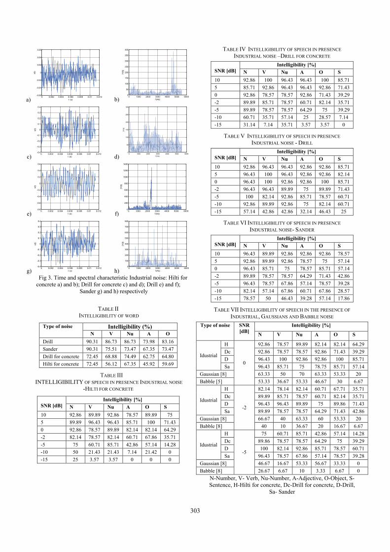
303

a) 0 0.002 0.004 0.006 0.008 0.01 0.012-0.06

-0.04

-0.02

0

0.02

0.04

0.06

t (s)

x(t)

b) 0 1000 2000 3000 4000 5000 60000

50

100

150

200

250

300

350

400

f (Hz)

|Y(f)

|

c) 0 0.002 0.004 0.006 0.008 0.01 0.012-0.4

-0.3

-0.2

-0.1

0

0.1

0.2

0.3

0.4

t (s)

x(t)

d)0 1000 2000 3000 4000 5000 6000

0

50

100

150

200

250

300

f (Hz)

|Y(f)

|

e) 0 0.002 0.004 0.006 0.008 0.01 0.012-0.8

-0.6

-0.4

-0.2

0

0.2

0.4

0.6

t (s)

x(t)

f) 0 1000 2000 3000 4000 5000 60000

200

400

600

800

1000

1200

1400

f (Hz)

|Y(f)

|

g) 0 0.002 0.004 0.006 0.008 0.01 0.012-0.4

-0.3

-0.2

-0.1

0

0.1

0.2

0.3

0.4

t (s)

x(t)

h) 0 1000 2000 3000 4000 5000 60000

100

200

300

400

500

600

700

800

f (Hz)

|Y(f)

|

Fig 3. Time and spectral characteristic Industrial noise: Hilti for

concrete a) and b); Drill for concrete c) and d); Drill e) and f); Sander g) and h) respectively

TABLE II INTELLIGIBILITY OF WORD

Type of noise Intelligibility (%) N V Nu A O

Drill 90.31 86.73 86.73 73.98 83.16 Sander 90.31 75.51 73.47 67.35 73.47 Drill for concrete 72.45 68.88 74.49 62.75 64.80 Hilti for concrete 72.45 56.12 67.35 45.92 59.69

TABLE III INTELLIGIBILITY OF SPEECH IN PRESENCE INDUSTRIAL NOISE

-HILTI FOR CONCRETE

SNR [dB]

Intelligibility [%] N V Nu A O S

10 92.86 89.89 92.86 78.57 89.89 75 5 89.89 96.43 96.43 85.71 100 71.43 0 92.86 78.57 89.89 82.14 82.14 64.29 -2 82.14 78.57 82.14 60.71 67.86 35.71 -5 75 60.71 85.71 42.86 57.14 14.28 -10 50 21.43 21.43 7.14 21.42 0 -15 25 3.57 3.57 0 0 0

TABLE IV INTELLIGIBILITY OF SPEECH IN PRESENCE INDUSTRIAL NOISE –DRILL FOR CONCRETE

SNR [dB]


10 92.86 100 96.43 96.43 100 85.71 5 85.71 92.86 96.43 96.43 92.86 71.43 0 92.86 78.57 78.57 92.86 71.43 39.29 -2 89.89 85.71 78.57 60.71 82.14 35.71 -5 89.89 78.57 78.57 64.29 75 39.29 -10 60.71 35.71 57.14 25 28.57 7.14 -15 31.14 7.14 35.71 3.57 3.57 0

TABLE V INTELLIGIBILITY OF SPEECH IN PRESENCE INDUSTRIAL NOISE - DRILL

SNR [dB]


10 92.86 96.43 96.43 92.86 92.86 85.71 5 96.43 100 96.43 92.86 92.86 82.14 0 96.43 100 92.86 92.86 100 85.71 -2 96.43 96.43 89.89 75 89.89 71.43 -5 100 82.14 92.86 85.71 78.57 60.71 -10 92.86 89.89 92.86 75 82.14 60.71 -15 57.14 42.86 42.86 32.14 46.43 25

TABLE VI INTELLIGIBILITY OF SPEECH IN PRESENCE INDUSTRIAL NOISE- SANDER

SNR [dB]


10 96.43 89.89 92.86 92.86 92.86 78.57 5 92.86 89.89 92.86 78.57 75 57.14 0 96.43 85.71 75 78.57 85.71 57.14 -2 89.89 78.57 78.57 64.29 71.43 42.86 -5 96.43 78.57 67.86 57.14 78.57 39.28 -10 82.14 57.14 67.86 60.71 67.86 28.57 -15 78.57 50 46.43 39.28 57.14 17.86

TABLE VII INTELLIGIBILITY OF SPEECH IN THE PRESENCE OF INDUSTRIAL, GAUSSIANS AND BABBLE NOISE

Type of noise SNR [dB]

Intelligibility [%]

N V Nu A O S

Idustrial

H

0

92.86 78.57 89.89 82.14 82.14 64.29 Dc 92.86 78.57 78.57 92.86 71.43 39.29 D 96.43 100 92.86 92.86 100 85.71 Sa 96.43 85.71 75 78.75 85.71 57.14

Gaussian [8] 63.33 50 70 63.33 53.33 20 Babble [5] 53.33 36.67 53.33 46.67 30 6.67

Idustrial

H

-2

82.14 78.14 82.14 60.71 67.71 35.71 Dc 89.89 85.71 78.57 60.71 82.14 35.71 D 96.43 96.43 89.89 75 89.86 71.43 Sa 89.89 78.57 78.57 64.29 71.43 42.86

Gaussian [8] 66.67 40 63.33 60 53.33 20 Babble [8] 40 10 36.67 20 16.67 6.67

Idustrial

H

-5

75 60.71 85.71 42.86 57.14 14.28 Dc 89.86 78.57 78.57 64.29 75 39.29 D 100 82.14 92.86 85.71 78.57 60.71 Sa 96.43 78.57 67.86 57.14 78.57 39.28

Gaussian [8] 46.67 16.67 53.33 56.67 33.33 0 Babble [8] 26.67 6.67 10 3.33 6.67 0

N-Number, V- Verb, Nu-Number, A-Adjective, O-Object, S- Sentence, H-Hilti for concrete, Dc-Drill for concrete, D-Drill,

Sa- Sander

304

a) -15 -10 -5 0 5 100

20

40

60

80

100

SNR (dB)

Inte

lligi

bilit

y ty

pe o

f wor

d (%

)

Hilti for concreteDrill for concreteDrillSander

b) -15 -10 -5 0 5 100

20

40

60

80

100

SNR (dB)

Inte

lligi

bilit

y ty

pe o

f wor

d (%

)


c) -15 -10 -5 0 5 100

20

40

60

80

100

SNR (dB)

Inte

lligi

bilit

y ty

pe o

f wor

d (%

)


d) -15 -10 -5 0 5 100

20

40

60

80

100

SNR (dB)

Inte

lligi

bilit

y ty

pe o

f wor

d (%

)


e) -15 -10 -5 0 5 100

20

40

60

80

100

SNR (dB)

Inte

lligi

bilit

y ty

pe o

f wor

d (%

)


Fig. 4. Intelligibility of speech for a type of word: a) Name, b) Verb,

c) Number, d)Adjective and e) Object

-15 -10 -5 0 5 100

20

40

60

80

100

SNR (dB)

Inte

lligi

bilit

y of

sen

tenc

es (%

)

Hilti for conDrill for conDrillSander

a)

Name Verb Number Adjective Object0

20

40

60

80

100

Type of word

Inte

lligi

bilit

y (%

)

DrillSanderHilti for concreteDrill for concrete

b)

Fig. 5. Intelligibility of speech for: a) sentences and b) word

C. The Results

Table II÷VI shows the intelligibility of performance SMST with influence of the various types Industrial noise ( Hilti for concrete, Drill for concrete, Drill and Sander) of the entire sentence, as well as types of the words for SNR= -15, -10, -5, -2, 0, 5, 10 dB. Table VII shows the intelligibility of the entire sentence, as well as types of the words in the presence of the Industrial, Gaussian and Babble noise [8] for value of SNR = -5, -2, 0 dB.

D. Analysis the Results

Based on the results shown in Table III÷VI and Fig. 4 it can be concluded that intelligibility of type of word:

a) ’Name’ is best for -5dB for Drill (100%), and the worst for -15dB for Hilti for concrete (25%),

b) ’Verb’ is best for 5 i 0dB for Drill (100%) and the worst for -15 dB for Hilti for concrete (3.57%),

c)’Number’ is best for 10 i 5 dB for Drill and Drill for concrete and 5dB for Hilti for concrete (96.43%), and the worst for -15 dB for Hilti for concrete (3.57%),

d)’Adjective’ is best for 10 i 5dB for Drill for concrete (96.43%) and the worst for -15 dB for Hilti for concrete (0%),

e)’Object’ is best for 10, 5 i 0dB for Drill for concrete, Hilti for concrete and Drill respective (100%), and the worst for -15 dB for Hilti for concrete (0%),

Based on the results shown in Table II and Fig. 5b it can be concluded that intelligibility of word: ’Name’ is the best 90.31% for Drill and Sander and ’Adjective’ the worst for 45.92% for Hilti for concrete.

Based on the results shown in Table III÷VI and Fig. 5a it can be concluded that intelligibility of sentence: is best for 10, 5 i 0dB (85.71%) for Drill and Drill for concrete and the worst for -10 i -15 dB (0%) for Hilti for concrete and -15 dB (0%) Drill for concrete.

By performing comparative analysis with IEC 60268-16: 2011, comes the conclusion that the intelligibility of sentences (0 ÷ 85.71%), and word (3.57 ÷ 100%) is in range from bad to excellent, depending on the value of the SNR.

Analysis the results shown in Table VII, it can be notice, that is intelligibility of speech is significantly better in the presence of Industrial noise than in Gaussian and Babble noise. The best intelligibility of speech is at Idustrial, and the lowest at Babble Noise. This is the expected result when comparing the energy distribution in the spectrum Industrial, Gaussian and Babble noise.

IV. CONCLUSION The aim of the paper is evaluation influence various types of

Industrial noise, for value SNR = -15÷10 dB, on the performance of speech intelligibility SMST. The results of tests are shown that the success of intelligibility of speech goes in range for: a) type of words: Name (25÷100%), Verb (3.57÷100%), Number (3.57÷100%), Adjective (0÷96.43%), Object (0÷100%), b) word (no matter of type) 50.97÷78.06% and c) sentence from 0÷85.71%. Based on the results it can be concluded that Industrial noise does not affect significant to the intelligibility of the speech signal as Gaussian and Babble noise.

REFERENCES [1] IEEE Subcommittee on Subjective Measurements "IEEE

Recommended Practices for Speech Quality Measurements", IEEE Transactions on Audio and Electroacoustics, vol 17, pp. 227-246, 1969.

[2] D. Kostić, Z. Milivojević, V. Stojanović, "The Evaluation of Speech Intelligibility in the Orthodox Church on the Basis of MOS Test Intelligibility Logatom Type CCV", ICEST 2016, Ohrid, Macedonia.

[3] R. Plomp, and A.M. Mimpen,” Improving the Reliability of Testing the Speech Reception Threshold for Sentences”, Audiology, vol. 18, pp. 43–52, 1979.

[4] B. Hagerman, ”Sentences for Testing Speech Intelligibility in Noise”, Scand Audio, vol. 11, pp. 79-87, 1982.

[5] H. Luts et al.,”FIST: A French Sentence Test for Speech Intelligibility in Noise”, International Journal of Audiology, vol. 47, pp. 373-374, 2008.

[6] S. Hochmuth, T. Brand, M. Zokoll, F. Zenker, N. Wardenga, and B. Kollmeier,”A Spanish Matrix Sentence Test for Assessing Speech Reception Thresholds in Noise”, Int. J. Audiol., vol. 51, no. 7, pp. 536-544, 2012.

[7] Z. Milivojević, D. Kostić, Z. Veličković, and D. Brodić, ”Serbian Sentence Matrix Test for Speech Intelligibility Measurement in Different Reverberation Conditions”, UNITEH, Gabrovo, 2016.

[8] Z. Milivojević, D. Kostić, and D. Brodić, ”Performanse razumljivosti Srpskog MST-a u prisustvu akustičkog Gausovog šuma”, INFOTEH, Jahorina, 2017.

305

Application of the Image Processing and Analysis in the Quantification of the Parahippocampal Region

Synaptophysin Immunoreactivity Ivan Jovanović1, Slađana Ugrenović1, Aleksandra Jovanović2

Abstract - The densitometric analysis was performed by ImageJ in order to measure integrated optical density of the synaptophysin labeled parahippocampal region gray and white matter digital images. Obtained data were analyzed by linear regression analysis and revealed significant decrease of the synaptophysin immunoreactivity in the parahippocampal region of the human brain.

Keywords –Parahippocampal region, Synapse, Image

processing and analysis, Densitometry

I. INTRODUCTION

The measurement of medical images often represents crucial method for routine diagnostics, as well as acquiring scientific data. However, with time, development of the more sophisticated medical image acquisition systems caused images to become larger and more complex. This, subsequently required implementation of advanced, time-consuming processing techniques to achieve precise quantification of the structures to be analyzed. Consequently, automation becomes necessity, so that medical specialists could perform simple tasks easily and focus on biomedical issues of the actual problem [1].Level of the automation process to a large degree depends on the types of measurements that are required. Generally, analysis can include measurements of the entire scenes or individual features of the region of the interest, which should be well defined, either by edges or unique brightness, color, texture, or some combination of the latter cited factors [2, 3]. In the majority of the cases some human effort is needed at least to oversee the image processing operations which precede automatic measurement in order to verify that the features of interest are actually extracted from the more complex image. ImageJ represents key powerful tool to process and perform analysis to quantify medical images to aid in the detection of the features of interest [1].

Though significant neuron loss was not observed in the cerebral cortex, some authors consider that the neurobiological basis of the age-related hypofunction of the brain represents synaptic changes [4]. Synaptophysin is the

most abundant synaptic vesicle protein and is therefore often measured in attempts to quantify synapses. It is considered to be a direct measure of the presence of mature synapses [5].

The cortical areas of the parahippocampal region (PR) of the temporal lobe of the brain, are generally accepted to form the system somehow involved in memory processing [6].

Taking into the consideration the fact that the biological underpinnings of the age - related cognitive decline are still unknown, all of these data led us to the assumption that the loss of synapses in the PR during the aging might be important for the disruption of normal memory function. The aim of our research was to, employing image processing and analysis, to assess the dynamics of synaptic density in the PR during the aging process with the quantification of synaptophysin immunoreactivity of the on the digital images of immunohistochemically stained histological slides of this brain area.

II. MATERIAL AND METHODS

The material included the right PR samples of 14 cadavers (10 males and 4 females) that ranged in age from 35 to 80 years. The obtained tissue was routinely histologically processed and further immunohistochemically stained with a monoclonal mouse anti-human synaptophysin antibody (Dako, Code IS776, Clone SY38, Ready – t- Use, EnVision FLEX System).In the immunohistochemically stained sections of each of the 14 evaluated cases, twenty fields of vision were selected by an unbiased method from all layers of the PRs gray matter (GM) and, five fields of vision of the white matter (WM) were selected by the same method and afterwards captured by digital camera (1.3 megapixel resolution) under x 40 lens magnification. The images were captured under the same light and optical conditions, and they contained only PR tissue without blank spaces or artifacts due to the accuracy of the following measurements.

According to Masliah et al. [7], a densitometric analysis was used for the quantification of the synaptophysin immunoreactivity. This analysis includes the evaluation of the brightness of the certain regions, or entire scene of the histological slides via the measurement of integrated optical density (IOD). Optical density is defined in Eq.1:

(1)

where I/I0 is the fraction of the incident light that penetrates through the sample without being absorbed or dispersed. Values of the OD range between 0 and 2.6. Integrated optical density represents the sum of the OD of all analyzed pixels

1Ivan Jovanović is with University of Niš, Faculty of Medicine, Department of Anatomy, Dr. Zoran Đinđić Blvd. 81, 18000 Niš, Serbia, e-mail: [email protected]

1Slađana Ugrenović is with University of Niš, Faculty of Medicine, Department of Anatomy, Dr. Zoran Đinđić Blvd. 81, 18000 Niš, Serbia, E-mail: [email protected]

2Aleksandra Jovanović is with University of Niš, Faculty of Electronic Engineering, Aleksandra Medvedeva 14, 18000 Niš, Serbia, E-mail: [email protected]

306

[3]. Analysis was performed using ImageJ. The system was spatially calibrated with an object micrometer (1:100). The optical density calibration was performed with a Kodak No. 3 calibrated step tablet according to the manual provided on the software’s website (http://rsb.info.nih.gov/ij/docs/examples/calibration/). In order to perform the densitometric analysis, the obtained 24 bit RGB images were split into three 8-bit channels (red, green and blue). The blue channel, on which the synaptophysin positive areas appeared as different shades of gray and the negative areas were light, was used for the analysis (Figs. 1 and 2). This allowed for the influence of neuronal perikarya, glial cells and blood vessels on the results of measurement to be minimized. The IOD of the entire image area was measured for all captured fields of vision in each case, and the obtained values were averaged for the GM and WM, respectively.

The statistical analysis of the obtained densitometric parameter was performed by SPSS (version 16). The correlation between the IOD values and the age of the evaluated cases was established by linear regression analysis. The gender differences were analyzed by Student’s t -test for two independent samples, while the differences between GM and WM IOD were analyzed by paired samples Student’s t-test.

III. RESULTS

A. Histological Analysis

The PR cortex cytoarchitectonic features such as thickness, lamination, neuronal size and shape were well preserved in all of the analyzed cases. The neuropil of PR layers showed two different types of positive reaction. The first characterized by the presence of larger and dark brown stained synaptophysin immunopositive grains and the second which was observed in areas of neuropil that were light brown and with significantly less intense granular immunostaining pattern (Figs. 1 and 2). In younger cases, immunoreactivity of the PR superficial layers was significantly stronger in relation to the deep layers (Fig. 1). In older cases, such differences of the synaptophysin immunoreactivity between the layers of the PR were not observed (Fig. 2). The neuronal perikarya, glial cells and blood vessels were synaptophysin negative (Figs. 1 and 2). The first of the two observed types of the immunopositive reaction predominated in relation to the second one only in the superficial layers of the PR of the younger cases (Fig. 1). In older cases, the frequency of the first type of synaptophysin immunoreactivity significantly decreased in the superficial layers of the PR (Fig. 2). The parahippocampal region WM neuropil was negative and showed a focal presence of the first type of positive reaction. The intensity of the positive reaction of the PRWM insignificantly varied with age.

B. Morphometric Analysis

The results of the densitometric analysis of the evaluated fields of vision of the analyzed cases’ PR are presented in Table I. A linear regression analysis was conducted to evaluate the relationship between the age as a predictor and

the IOD as the outcome variable. This analysis showed that there was a significant decrease of the GM IOD (F(1,12)=6.62, p=0.024) of the analyzed cases with age. Such relationship can be identified by the following model (Eq.2):

IOD = 12.03 x 105 0.037 x Age (2)

which explained 36% (adjusted R square = 0.36) IOD variance and represented large effect size. The IOD of the WM did not significantly change with age (p>0.05).Significant gender differences were not observed in terms of the age and IOD (p > 0.05). The IOD of the GM was significantly higher than the same parameters of the white matter (t = 14.44, df = 13, p<0.001). These differences indirectly additionally confirmed the positivity of immunohistochemical reaction.

From the above described results of the histological and densitometric analysis, it can be concluded that synaptophysin immunoreactivity decreases in the PR with age.

TABLE I

RESULTS OF THE DENSITOMETRIC ANALYSIS OF ALL 14 ANALYZED

CASES

Case Age Gender IODGM (x 105)

IODWM (x 105)

1 35 Male 8.689 6.225

2 37 Male 10.687 6.895

3 42 Female 10.948 6.968

4 42 Male 11.656 7.573

5 43 Male 11.588 8.290

6 55 Male 9.304 7.072

7 56 Male 10.043 7.024

8 57 Female 9.938 6.963

9 61 Male 9.505 6.734

10 61 Male 9.879 6.861

11 77 Female 8.889 6.872

12 78 Male 8.731 6.860

13 78 Male 9.849 6.880

14 80 Female 8.829 7.003

IV. DISCUSSION

Though significant neuron loss was not observed in the cerebral cortex, some authors considered that the neurobiological basis of the age-related cognitive decline represent synaptic changes, predominantly in the hippocampus and prefrontal cortex [4, 8].

According to Honer et al. [9], specific presynaptic proteins such as synaptic vesicle protein synaptophysin are very important for cognitive reserve in the healthy elderly, and the loss of this protein correlates with antemortem cognitive dysfunction. Researchers analyzed the immunoreactivity of this protein in different cortical regions. Synaptophysin

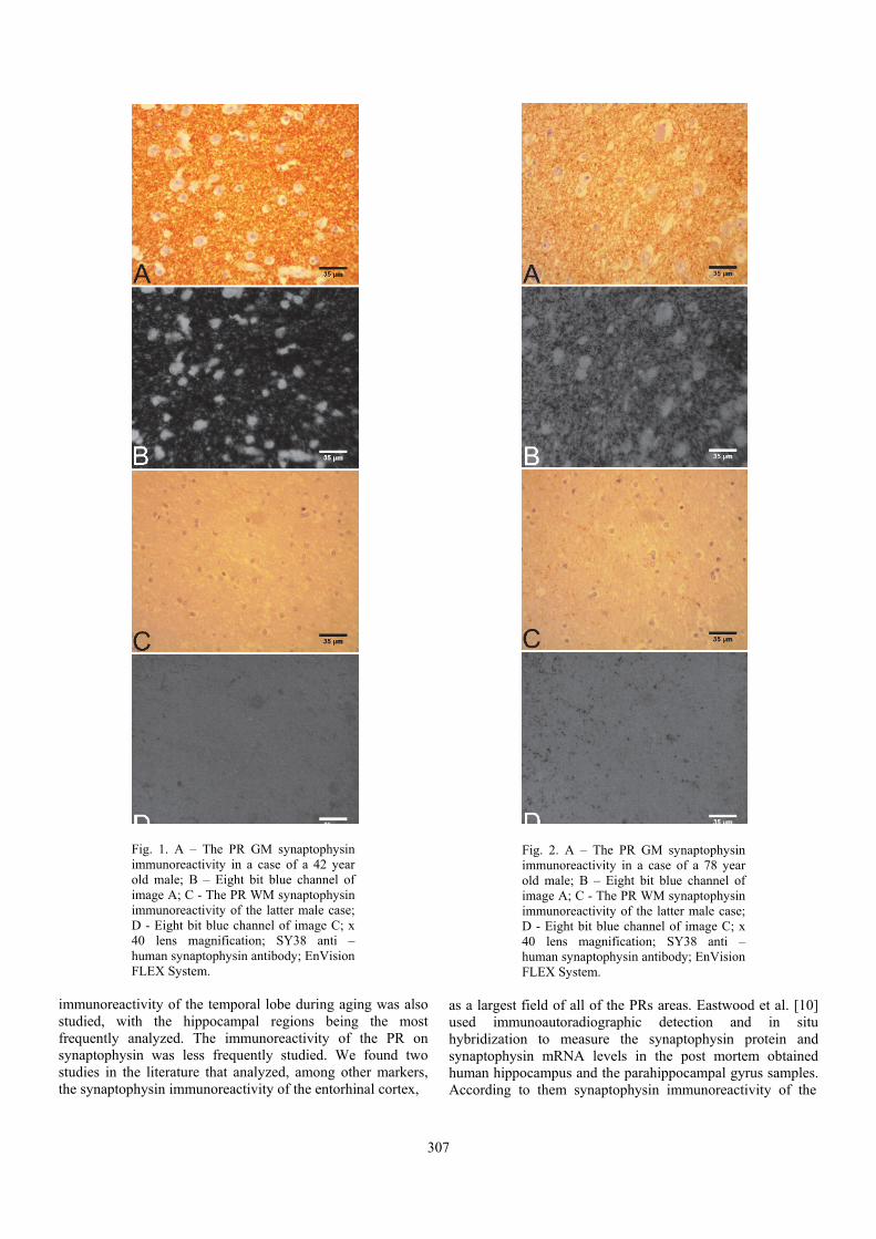
307

Fig. 1. A – The PR GM synaptophysin immunoreactivity in a case of a 42 year old male; B – Eight bit blue channel of image A; C - The PR WM synaptophysin immunoreactivity of the latter male case; D - Eight bit blue channel of image C; x 40 lens magnification; SY38 anti – human synaptophysin antibody; EnVision FLEX System.

immunoreactivity of the temporal lobe during aging was also studied, with the hippocampal regions being the most frequently analyzed. The immunoreactivity of the PR on synaptophysin was less frequently studied. We found two studies in the literature that analyzed, among other markers, the synaptophysin immunoreactivity of the entorhinal cortex,

Fig. 2. A – The PR GM synaptophysin immunoreactivity in a case of a 78 year old male; B – Eight bit blue channel of image A; C - The PR WM synaptophysin immunoreactivity of the latter male case; D - Eight bit blue channel of image C; x 40 lens magnification; SY38 anti – human synaptophysin antibody; EnVision FLEX System.

as a largest field of all of the PRs areas. Eastwood et al. [10] used immunoautoradiographic detection and in situ hybridization to measure the synaptophysin protein and synaptophysin mRNA levels in the post mortem obtained human hippocampus and the parahippocampal gyrus samples. According to them synaptophysin immunoreactivity of the

308

elderly’s group was insignificantly higher than the same of the adult group, which is in opposition to our results. The second study by Stranahan et al. [11] used fluorescence labeling for synaptophysin and established its reduced immunoreactivity around the reelin labeled cells in layer II of the lateral entorhinal cortex of the cognitively impaired aged rats. Nevertheless, the latter cited changes were not detected in the aged cognitively unimpaired animals. However, according to Masliah et al. [7], opposite to our study, methods applied in the latter cited studies have limitations. A major restriction of the studies such as Eastwood et al. [10] which use immunochemical quantification of synapse-associated proteins in brain homogenates is that this method cannot identify the distribution of the synapses in the cortical laminae. The electron microscopic method, used in the study by Stranahan et al. [11], requires well-preserved tissue, which in the case of human tissue usually requires a brain biopsy, and the size of the examined area is very small. Application of the image processing and subsequent densitometric analysis during our research enabled quick and thorough quantification of the synaptophysin immunoreactivity in all layers of the PR cortex. Opposite to the latter studies [10, 11], we detected gradual decrease of the synaptophysin immunoreactivity in this brain region, which could point to the conclusion that the density of the synaptic vesicles, and hence neuronal synapses decrease with advanced age in this region of the brain.

V. CONCLUSIONS

Finally, according to all above cited and the results of our study, it can be concluded that decreased synaptophysin immunoreactivity probably reflects the age-related loss of synapses in this region of the brain, which has potentially deleterious effects for normal memory processing in the elderly. Image processing and analysis of the immunohistochemically labeled PR histological slides enables measuring of the OD of the synaptophysin immunoreactivity and represents rapid, practical and reliable method for quantification of the density of the synaptic vesicles in all of the cortical laminae of this brain region.

ACKNOWLEDGEMENT

Contract grant sponsor: Ministry of Science and Technological Development of Republic of Serbia; Contract grant number: 175092.

REFERENCES

[1] J. Broeke, J. M.M. Pérez, and J. Pascau, Image Processing with ImageJ, Birmingham, Packt Publishing, 2015.

[2] J.C. Russ, and R.T. Dehoff, Practical Stereology, New York, Plenum Press, 2000.

[3] J.C. Russ, The Image Processing Handbook, Taylor & Francis, New York, 2007.

[4] H. Nakamura, S. Kobayashi, Y. Ohashi, and S. Ando, “Age-Changes of Brain Synapses and Synaptic Plasticity in Response to an Enriched Environment”, J. Neurosci. Res., vol. 56, pp. 307-315, 1999.

[5] R. Clare, V.G. King, M. Wirenfeldt, and H.V. Vinters, “Synapse Loss in Dementias”, J. Neurosci. Res., vol. 88, no. 10, pp. 2083-2090, 2010.

[6] R. Insausti, A.M. Insausti, M.T. Sobreviela, A. Salinas, Martinez-J. M. Penuela, “Human Medial Temporal Lobe in Aging: Anatomical Basis of Memory Preservation”, Microsc. Res. Tech., vol. 43, pp. 8-15, 1998.

[7] E. Masliah, R.D. Terry, M. Alford, and R. DeTeresa, “Quantitative Immunohistochemistry of Synaptophysin in Human Neocortex: An Alternative Method to Estimate Density of Presynaptic Terminals in Paraffin Sections”, J. Histochem. Cytochem., vol. 38, pp. 837-844, 1990.

[8] J.H. Morrison, M.G. Baxter, “The Ageing Cortical Synapse: Hallmarks and Implications for Cognitive Decline”, Nat. Rev. Neurosci., vol. 13, pp. 240-250, 2012.

[9] W.G. Honer, A.M. Barr, K. Sawada, A.E. Thornton, M.C. Morris, S.E. Leurgans, J.A. Schneider, and D.A. Bennett, “Cognitive Reserve, Presynaptic Proteins and Dementia in the Elderly”, Transl. Psychiatry., vol. 2, pp. e114, 2012.

[10] S.L. Eastwood, C.S. Weickert, M.J. Webster, M.M. Herman, J.E. Kleinman, and P.J. Harrison, “Synaptophysin Protein and mRNA Expression in the Human Hippocampal Formation from Birth to Old Age”, Hippocampus., vol. 16, pp. 645-654, 2006.

[11] A.M. Stranahan, R.P. Haberman, and M. Gallagher, “Cognitive Decline is Associated with Reduced Reelin Expression in the Entorhinal Cortex of Aged Rats”, Cereb Cortex., vol. 21, pp. 392-400, 2011.

309

An Advanced Method for Chilli Plant Disease Detection Using Image Processing

Dipak P. Patil1, Swapnil R. Kurkute2, Pallavi S. Sonar3, Svetlin I. Antonov4

Abstract – This Paper presents the methods for effective detection of the diseases for enhancing the product quality of plants. Recent studies have confirmed that average production crops in India is reducing because of disease occurred in fully developed plants. We have considered Chilli plants for our study. Producing Chilli is a daunting task as the plant is exposed to the attacks from various micro-organisms and bacterial diseases and pests. The symptoms of the attacks are usually distinguished through the leaves, stems or fruit inspection. Leaf features inspection methodology is used for early detection of chilli disease. Leaf image is captured and processed to determine the health status of each plant. Currently the chemicals are applied to the plants periodically without considering the requirement of each plant. This technique will ensure that the chemicals only applied when the plants are detected to be effected with the diseases. The image processing techniques are used to perform samples chilli disease images. The plant chilli disease detection through leaf image and data processing techniques is very useful and inexpensive system especially for assisting farmers in monitoring the big plantation area.

Keywords – Chilli disease, Leaf image, Image Processing.

I. INTRODUCTION

Plant disease is one of the crucial causes that reduces quantity and degrades quality of product. The ability of disease diagnosis in earlier stage is then very important task in order to be able to timely cure and control such disease for decreasing dissatisfactory products. Chilli is included in the main horticultural commodities. At certain times, it becomes a very high demand in the market because supply is limited. Business chilli indeed belongs in the high-risk plants. Therefore, strategies and technical knowledge and the field became an important matter to be mastered. The systematic and structured should be developing so that it will use by operators to increase the overall production. Many farmers refused to cultivate chilli in the rainy season due to the increase of chilli disease to become high risk for the quality control and productivity. Fig. 1 illustrates the samples of plant chilli disease.

In general, there are two types of factors which can bring death and destruction to chilli plants; living (biotic) and nonliving (a biotic) agents. Living agent’s including insects, bacteria, fungi and viruses. Nonliving agents include extremes of temperature, excess moisture, poor light,

insufficient nutrients, and poor soil pH and air pollutants. Diseased plants can exhibit a variety of symptoms and making diagnosis was extremely difficult. Common symptoms are includes abnormal leaf growth, color distortion, stunted growth, shriveled and damaged pods. Although pests & diseases can cause considerable yield losses or bring death to the plants and it’s also was directly affect to human health. However, crop losses can be minimized, and specific treatments can be tailored to combat specific pathogens if plant diseases are correctly diagnosed and identified early. These need-based treatments also translate to economic and environmental gains.

The remaining paper is organized as below. Section II describes the related work. Detail methodology along with all steps for implementation is elaborated in Section III. An algorithm is presented in Section IV. Results are depicted in Section V and finally conclusions are drawn in Section VI.

II. RELATED WORK

The basic techniques and algorithms that can be used for acquiring, processing and extracting useful information from digital images is elaborated in [1]. Particular emphasis is placed on covering methods used for image sampling and quantization, image transforms, image enhancement and restoration, image encoding, image analysis and pattern recognition. In [2], the sigmoid activation function is used in neural networks with an exponential function that computes nonlinear decision boundaries. This technique acquiesce decision surfaces which approach the Bayes optimal under certain conditions. Another method based on Probabilistic Neural Net-work (PNN) with image and data processing

1Dipak P.Patil, 2Swapnil R.Kurkute and 3Pallavi S.Sonar are withthe Sandip Institute of Engineering & Management, Nashik, India,1E-mail: [email protected], 2E-mail:[email protected], 3E-mail: [email protected]

4Svetlin I.Antonov is with the Faculty of Telecommunications atthe Technical University of Sofia, Bulgaria, E-mail:[email protected]

Fig. 1. Samples of plant chilli disease

310

techniques to implement general purpose automated leaf recognition for plant classification is suggested in [3]. Class-based” image based recognition and rendering with varying illumination can also be an alternative approach suggested where a single input image of an object, and a sample of images with varying illumination conditions of other objects of the same general class, re-render the input image to imulate new illumination conditions [4]. In color constant indexing is a simple method proposed in [5], where objects can be recognized on the basis of their color only. Since the ratios of color RGB triples form nearby locations are insensitive to the changes. Suggested algorithms and mathematical computations are also proven very useful in analysis [6-7]. A novel shape recognition method based on radial basis probabilistic neural network (RBPNN) is presented [8]. This method uses orthogonal least square algorithm (OLSA) to train the RBPNN and the recursive OLSA is adopted to optimize the structure of the RBPNN.

An idea to overcome the problem of face images taken in different lighting condition by combining the robust illumination normalization, local binary pattern texture descriptor and principal component analysis is considered. Here an image is a known face image when Euclidean distance between a test image and training images is minimum. And if this distance is not attained, it is an unknown face image [9].

In [10-11] authors have presented ideas regarding early detection of chilli disease through leaf features inspection. Leaf image is captured and processed to determine the health status of each plant. Finally conclude that the chemicals only applied when the plants are detected to be effected with the diseases. The image processing techniques are used to perform hundreds of chilli disease images. The plant chilli disease detection through leaf image and data processing techniques is very useful and inexpensive system especially for assisting farmers in monitoring the big plantation area.

III. METHODOLOGY

Chilli which is the fruit of capsicum family plant is almost a delicacy in Asian menu. This fruit has a high local demand and can fetch a very handsome economic yield. An attack by disease-causing organisms generates a complex immune response in a plant, resulting in the production of disease-specific proteins involved in plant defense and in limiting the spread of infection. Louse also produce proteins and toxins to facilitate their infection, before disease symptoms appear

such as the leaf color will change. These leaf colors play vital role in the development of plant disease detection. Image processing is traditionally concerned with preprocessing operations such as Fourier filtering, edge detection and morphological operations. Computer vision extends the image processing paradigm to include understanding of scene content and object classification [1]. Therefore, this paper demonstrates the use of image processing techniques to detect the plant chilli disease through leaf image.

A. System Overview

The system consists of two major parts (refer to Fig. 2) such as the digital camera and the LABVIEW software tools to build Graphical User Interface (GUI). The first part of the project is to take image photos of chilli leaf. Picture need to be taken in a group of chilli leaf. MATLAB is the software chosen to perform image processing on the captured image photos. Image processing of an image photo requires numerous standard procedures and steps to be able to identify and recognize the color in an image photo. It has step-by-step procedure showing the image processing of an image photo which the user only needs a few clicks on the GUI itself. Fig. 2 illustrates the block diagram system [1].

B. Image Acquisition

It is another important step in which the images of chilli fruit are taken. Total 20 image samples of chilli fruit are gathered. This image set was further classified into four types which are fully affected, moderately affected, partially affected and the healthy which is normal. Images are taken from the digital camera having high resolution and keeping specific distance between digital camera and chilli fruit. The sample image is shown below.

Fig. 2. Chilli Plant disease detection system block diagram

Fig. 3. Healthy Image of Chilli [13]

311

C. Preprocessing

In this process different operation like filtering, intensifying the image and removing unwanted noise from an image are involved. Median filtering method that replaces the value of pixel by the median of gray level in the neighborhood of that pixel:

f(x,y)=mediang(s,t)

The original value of pixel is included in computation of the median .these filter are quite popular because certain type of random noise ,they provide excellent noise reduction capabilities, with considerably less blurring than linear smoothing filter of similar size.

The image sample is now intensified and converted into binary image. While converting image contrast and brightness of the image keeping with respect to specific value for obtain better results. Preprocessing is done to improve the quality of the acquire image.

D. Segmentation

The aim of segmentation is to subdivide an image into number of regions. The regions obtained correspond to the physical parts or objects of a scene (3-D) represented by the image (2-D). In general, autonomous segmentation is one of the most difficult tasks in digital image processing. The color image segmentation is more complex to process than gray image segmentation, because at the time of processing image, the color and result could be altered. Color image segmentation involves detection of edges or regions by deterministic or stochastic labeling procedure, based on information from intensity and/or spatial information. That wise we first convert RGB image into gray scale image. Thresholding is used to extract an object from its background by assigning an intensity value T (threshold) for each pixel such that each pixel is either classified as an object point or a background point. In band separating we observe three separate color band images. Then we apply masking process for color image segmentation.

E. Feature Extraction

In this step image is observed in different pixel value. According to Pixel values, number of spot and area of each spot or blobs observed. We extract the desired features from the sample image for the analysis of pathogenic affected region of the chilli fruit. Size, Shape, Volume, Color and Texture are the main features that separate diseased chilli from the normal chilli. Color is one of the most important

parameter in feature extraction process. Depending upon this parameter of feature extraction we define or identify the quality of an image. Other important parameters are size, shape and volume. The cost is indirectly depends upon the size. But it is more complex if shape and size of the chilli is irregular. The shape is subjective type parameter which is based on human view. It is also indirectly affected to the cost. The most important parameter of feature extraction is texture. Texture can play an important role in color image segmentation process.

F. Color Feature Extraction

There are four color models namely RGB, HIS, CMY, YIQ. We used RGB color model for analysis. The RGB model is commonly used color model, in which each sensor captures the intensity of the light in the respectively red (R), green (G) or blue (B) bands. In an RGB model basically Red, Green and Blue component of the image sample is extracted. We also extract the total count of red, green and blue pixels in the chilli fruit. We also extract the total count of pixels occupied by entire chilli, which gives the total area of chilli. After texture feature extraction Process is done [14].

G. Converting color from RGB to HSI

Given an image in RGB color format, H component of each RGB pixel is obtained using the equation,

H=Ө if B≤G

360- Ө if B >G With

Ө = Cosˉ Ө 1/2[(R-G)+(R-B)] [(R-G)2(R-B)(G-B)]1/2]

The saturation component is given by , S=1-3÷(R+G+B)[min (R,G,B)].

Finally the intensity component is given by, I= ⅓(R+G+B).

It is assumed that RGB values have been normalized to the range [0,1]and that angle is measured with respect to the red axis of the HIS space can be normalized to the range [0,1] by dividing by 3600. The other two HIS component already in the range if the given RGB values are in the interval [0,1].

H. Converting color from HSI to RGB

Given values of HSI in the interval [0,1].the applicable equation depends on the values of H. There are three sectors of interest ,corresponding to the 1200 interval in the separation of primaries .We begin by multiply 3600 which returns the hue to it’s original range of [00,3600]. RG sector (00 ≤H <120): When H is in this sector, the RGB component is given by the equations

B=I(1-S) R=I[ 1+ S cos H÷ cos(600-H)]

And G=1-(R+B).

GB sector (1200 ≤ H < 2400): If the given value of H is in the sector, we first substract 1200

from it: H=H-1200

Fig. 4. Diseased Image of Chili [13]

312

Then RGB component are R=I(1-S)

G=I[1+S cos H ÷cos(600-H)] And

B=1-(R+G). BR sector (2400 ≤ H ≤ 3600): finally if H is in this range, we subsrtact 2400 from it:

H= H - 2400

Then the RGB components are G=I( 1- S )

B=I[1+S cos H ÷ cos (600 - H)] And

R=1-(G+B).

I. Texture Features Extraction

In texture Feature Extraction important parameter considers. Important texture features like correlation, homogeneity, entropy and contrast are extracted along with color features. For this we use Gray Level Co-occurrence Matrix. The gray co-occurrence matrix function creates a gray level co-occurrence matrix by calculating how frequently a pixel with the particular intensity value i occurs in a specified spatial relationship to a pixel with value j. Gray Level Co-occurrence Matrix was proposed by Haralick. GLCM is a texture description method is not much so difficult, which is based on the repeated occurrence of some gray-level configuration in the texture [14-17].

J. Classification

Percentage of affected area is the key parameter for calculation. Major classification is into partially affected, moderately affected, severely affected and the rest which are normal affected. For classification we cluster the affected area i.e spot on chilli and depending upon their size and number. We classify the input images to disease chilli and normal chilli [13, 15].

IV. ALGORITHM

Following equation is used to calculate the percentage of the affected, i.e. % healthy area of chilli = (healthy area of chilli / total area of chilli) * 100 where, Healthy area = Number of Green pixels in chilli fruit. Total area = total size of chilli fruit % affected area = 100 – % healthy area of chilli.

A. Algorithm

1. Accept the input image. 2. Change the RGB image into to the HSV model. 3. Show the H, S, V bands. 4. Apply threshold on HSV bands. 5. Arrange the relevant binary mask. 6. Apply mask on HSV bands to obtain segmented image. 7. Analyze each spot for its color, size and texture feature. 8. Calculate the features based on the color, size and texture.

9. Compare the input feature value with predefine value and decide the grade. 10. Classify the input chilli image into disease chilli and normal chilli and display the results.

B. Experimental Samples

The photo image prepared as experiment sample for this research paper have some fixed details. Both of the healthy and diseased leaf samples were used for the experimental purpose of this system. For better result, the leaves sample should be in good condition and sharp. See Fig 5.and Fig 6. Throughout the photo capturing section, the distance of the camera and the leaf was adjustable in order to get a clear shot of leaf pattern. The input photo image is a JPG image file and the size of resolution is 3872 x 2592 pixels.

a=imread('A(1).JPG'); A=imresize(a, [800 536]);

The imread function is read image from graphics file. The imresize function is to returns an image of the size specified by [m-rows n-cols]. Images are resized for easier image processing [5], [11] MALTAB and LABVIEW software are used for the simulation purpose, LABVIEW is an advance software [12] used for the simulation and GUI formation.

V. RESULTS AND DISCUSSION

For the implementation and experimentation we have taken seven samples of chilli plants with some healthy leaf sample around five and some diseased leaf samples around 2 and tested using implemented system. The system can be tested with image of 800x536 pixels. The method implemented in this research paper is effective and fastest method in detection of plant chilli disease. The overall result was about 80% which is satisfying and is considered as a successful project.

Fig. 5. Healthy of plant Chilli

Fig. 6. Diseases on Chilli plant

313

TABLE 1 THE PLANT CHILI HEALTHY AND RISKY RESULT

Sample Green

Yellow Cyan Green Healthy/Disease

1 0.000 0.000 4.259 Healthy 2 0.014 0.007 22.916 Healthy 3 0.190 18.519 0.000 Healthy 4 0.033 11.1999 0.060 Healthy 5 4.022 3.234 0.639 Risky 6 1.107 24.883 14.29 Risky 7 1.825 0.001 17.16 Risky

VI. CONCLUSION

This Paper presents the methods for effective detection of the diseases for enhancing the product quality of plants. DIP is used to Chilli Plant Disease Detection. The GUI design using LABVIEW and MATLAB software gives result as either risky or Healthy condition of plant. In this paper image processing for image and color recognition techniques are used for the detection. The method used in this paper is effective and fastest method in detection of plant chilli disease. It is also conclude that this method is one of the best methods among others for early detection of plant chilli disease through leaf inspection

REFERENCES

[1] R.C. Gonzalez, R.E. Woods, and S.L. Eddins, Digital Image Processing Using MATLAB, Prentice Hall, 2004.

[2] D.F. Specht, "Probabilistic Neural Networks for Classification Mapping, or Associative Memory", IEEE International Conference on Neural Networks, vol. 1, 1988.

[3] B.C. Heymans, J.P. Onema, and J.O. Kuti, "A Neural Network for Opuntia Leaf-form Recognition", IEEE International Joint Conference on Neural Networks, 1991.

[4] A. Shashua, and T. Riplin-Raviv, “The Quotient Image: Class-Based Re-Rendering and Recognition with Varying Illuminations”, IEEE Trans., Pattern Analysis and Machine Intelligence, vol. 23, pp. 129-13, 2001.

[5] B. Funt, and G. Finlayson, “Color Constant Color Indexing”, IEEE Trans. on Pattern Analysis and Image Processing, vol. 17, pp. 522-529,1995.

[6] J.-X. Du, X.-F. Wang, and G.-J. Zhang, “Leaf Shape Based Plant Species Recognition”, Applied Mathematics and Computation, vol. 185, 2007.

[7] J.A. Hartigan, and M.A.Wong, "Algorithm AS 136: A K-Means Clustering Algorithm", Journal of the Royal Statistical Society, Series C (Applied Statistics), vol. 28, no. 1, 1979.

[8] J. Du, D. Huang, X. Wang, and X. Gu, “Shape Recognition Based on Radial Basis Probabilistic Neural Network and Application to Plant Species Identification”, 2005 International Symposium of Neural Networks, ser. LNCS 3497, Springer, 2005.

[9] D.P. Patil1, P.S. Sonar, and S.I. Antonov “Face Recognition using LBP and PCA under Different under Different Lighting Condition”, ICEST 2016, Ohrid, Macedonia, June 2016.

[10] Z. Bin Husin, A. H. Bin Abdul Aziz, A. Y. Bin Md Shakaff, and R. B.S. Mohamed Farook, “Plant Chili Disease Detection using the RGB Color Model”, Research Notes in Information Science (RNIS), vol. 13, doi:10.4156/rnis.vol13.16, May 2013.

[11] Z. Bin Husin, A. Bin Abdul Aziz, A. Y. Bin Md Shakaff, and R. B.S.Mohamed Farook, “Feasibility Study on Plant Chilli Disease Detection Using Image Processing Techniques”, 2012 Third International Conference on Intelligent Systems, Modelling and Simulation (ISMS), 2012.

[12] S. R. Kurkute, K. P. Arbuj, C. R. Dargude, and K. D. Dholi, “Laboratory Virtual Instrument Engineering Workbench (LABVIEW)”, International Journal of Modern Embedded System (IJMES), vol. 5, no. 1, pp. 17-20, February, 2017.

[13] S. Joshi, G. Jamadar, S. Nachan, and R. R. Itkalkar, “Chilli Disease Detection”, International Journal of Advances in Science Engineering and Technology, vol. 3, no. 2, April-2015.

[14] J.L. González-Pérez, M.C. Espino-Gudiño, J. Gudiño-Bazaldúa, J.L. Rojas-Rentería, V. Rodríguez Hernández, and V.M. Castaño, “Color Image Segmentation using Perceptual Spaces Through Applets for Determining and Preventing Diseases in Chili Peppers”, African Journal of Biotechnology, vol. 12, no. 7, pp. 679-688, 13 February, 2013.

[15] J.A. Kodagali, and S Balaji, “Computer Vision and Image Analysis based Techniques for Automatic Characterization of Fruits”, International Journal of Computer Applications, vol. 50, no. 6, July 2012.

[16] S.R. Dubey, P. Dixit, N. Singh, and J.P. Gupta, “Infected Fruit Part Detection using K-Means Clustering Segmentation Technique”, International Journal of Artificial Intelligence and Interactive Multimedia, vol. 2, no. 2, 2013.

[17] E. Saldana, and R. Siche, “Computer Vision Applied to the Inspection and Quality Control of Fruits and Vegetables”, Campinas, vol. 16, no. 4, pp. 254-272, 2013.

Fig.7. Plant Chilli Classification Result

314

Segmentation of Spleen with Pathology from Abdominal MRI

Antoniya Mihaylova

Abstract – The analysis of the medical images is very important for the future diagnosis of the specialists, but is often not an easy task and is time-consuming. In this paper is proposed a semi-automated method for segmentation of abdominal organ and its pathological formation. The segmentation method that is used is based on the “Active Contours Without Edges” by Chan and Vese, that ignores edges completely [1]. The advantages of the algorithm are in the fast speed results and the ability to extract not only the organ, but also untypical formations, if there are some. After the segmentation it is easier to make some measurement of the organ and its pathology.

Keywords – Fast segmentation of spleen in MRI with pathology, Tumour segmentation.

I. INTRODUCTION

The manual segmentation of the medical images is often time-consuming and requires the withdrawal of the attention of the specialist in medical imaging diagnostic. To improve this process is necessary to design and develop computer-aided diagnosis (CAD) tools for medical images. An interesting and challenging task in this area is the segmentation of spleen MRI, segmentation of pathological formations in the spleen and measurements of the organ and the formations for better diagnosis for future medical manipulations or surgery. The human spleen is the largest lymphoid organ in the body and its form and position is variable for each person. Because of the partial volume effect, the gray level of the spleen and grayscale similarity of the adjacent abdominal fat, spleen segmentation has always been a problem [3]. All of these make the segmentation of this organ not very easy task. Segmentation is a key preliminary step in many medical applications such as planning and follow-up procedures, here modeling patients’ organs is helpful for both visualization and quantitative measurements [13]. The size of the spleen is giving important information for the health of the human.

The MR diagnostic is often a preferred technique for observation of the abdominal anatomy. MR imaging has been shown to enable accurate volumetric assessment of solid organs in humans [4]. By MRI contrast between the different soft tissues of the body is much greater than those by computed tomography (CT). This makes it especially useful for ontological (cancer) imaging.

There are already a lot of methods for segmentation of abdominal organs, but most of them are for CT not for MR images. In a previous work (paper [8]) is made a classification of these various methods. According it there are three main

classes of methods: gray level based, structure based and texture based. The method we use: “Active Contours Without Edges” by Chan and Vese is part of the gray level based methods. Gray level is the most obvious feature of image [5]. These method as all have their advantages and disadvantages, but the algorithm in this paper is combining the best steps to improve the gray level based method and achieve high accuracy and robustness.

II. GRAY LEVEL BASED SEGMENTATION

A. Active Contour Segmentation

The segmentation based on active contour model of Chan and Vese is a gray level based method and is a special case of the Mumford–Shah function. Active contours, or snakes, are computer-generated curves that move within images to find object boundaries. Its 3D version is often known as deformable models or activesurfaces in literature [14].

We consider ƒ to be the given grayscale image on a domain Ω to be segmented. Mumford and Shah approximate the image ƒ by a piecewise-smooth function u as the solution of the minimization problem. Compared to the piecewise constant Mumford - Shah model, the key differences with the Chan - Vese model are an additional term penalizing the enclosed area and a further simplification that u is allowed to have only two values,

(1)

where C is the boundary of a closed set and c1, c2 are the values of u respectively inside and outside of C [1]. By the method of Chan – Vese the purpose is to find among all u of this from the one that best approximates ƒ,

(2)

There are four terms; the first one penalizes the length, the second one – the enclosed area of C to control its size. The third and fourth are penalizing non-compliance between pricewise constant model u and input image ƒ. By fnding a local minimizer of this problem, a segmentation is obtained as the best two-phase piecewise constant approximation u of the image ƒ [1]. For the minimizer is needed minimalization over all set boundaries C. This is accomplished by applying the level set technique introduced by Osher and Sethian [1,9], where is used a level set function φ for a circle of radius r. The Dirac function δ, which is the gradient of the Heaviside function, penalizes long boundaries between the regions [6].

Antoniya Mihaylova is with the Faculty of Telecommunications at Technical University of Sofia, 8 Kl. Ohridski Blvd, Sofia 1000, Bulgaria

315

B. Other Methods

There are a lot of other gray level based methods, but most of them are too old, although they have already shown their potential. Such methods are Region Growing, Deformable models, Graph cuts, Clustering based, Threshold based, Level set, etc. The Region growing method is one of the most popular and studied methods for segmentation. It is also often very effective, but has of course its drawbacks. Most of them are related with the evaluation of the gray level of the target. The problem began when there is a big similarity between the target’s gray level and the backgrounds’ gray level.

III. ALGORITHM FOR SEGMENTATION OF SPLEEN WITH PATHOLOGY IN MRI

The Algorithm can be separated in two parts: Segmentation of the spleen and Segmentation of the tumor. The steps in the both parts are similar and are presented in Fig. 1. The second block in the diagram in Fig. 1 is with interrupted line because it is done only in the first part of the segmentation approach. In the first part we are starting with loading the original MRI of spleen with pathology. Then follows a preprocessing step, consist of contrast enhancement using CLAHE and filtration based on Homomorphic wavelet. The filter is chosen motivating of a previous investigation presented in paper [15].

Fig. 1. Algorithm for MRI splenic tumor segmentation

After this we have to choose the specific parameters for the

segmentation based on “Active contour without edges”. These are four parameters: mask – Initial rectanguler or polygonal ROI at which the evolution of the segmentation begins; n – Maximum number of iterations to perform in evolution of the segmentation; R – Radius of the location in pixels; Alpha – 'Smooth Factor' – Degree of smoothness or regularity of the boundaries of the segmented regions;

The region of interest (ROI) is chosen as close to the object as it is possible. Higher values of n are used if the initial contour position (specified by the region boundaries in mask) is far from the desired object boundaries. R is chosen according to the quality of the processed images and the visibility of the desired organ for segmentation. The preferred values for R are between 1 and 20. The lower values are used by good quality images, where the resolution is big and so is the processing time shorter. Alfa is set between 1 and 10. Higher values of Alpha produce smoother region boundaries but can also smooth out finer details. Lower values produce more irregularities (less smoothing) in the region boundaries, but allow finer details to be captured [1]. With the specified parameters is made the segmentation using the method described in the previous section. As a result we become an image with contoured spleen and a black and white image of the segmented organ.

The second part consists of almost the same steps as by the first one. The difference is that there is no preprocessing step, because we use an image that is already processed and segmented once before.

IV. EXPERIMENTS AND ANALYSIS

The experiments with the proposed algorithm are made with 20 MRI abdominal images with spleen pathology in different stages. Two of them are chosen to represent the results of the experiments. The image in Fig. 2 is showing the original images from an examination of spleen pathology in early and advanced stage. Image (a) is in coronal plane and image (b) is in axial plane and represents the abdominal area in different weights: T2 for image A and T1 for images B-D. The experiments have shown that the results are better by image A in T2, so this image is used for the visualization in this paper. The size of image (a) on Fig.2 is 512x512 pixels and the size of image (b A) is 453x340 pixels. Both of them are in JPEG format. The experiments are made by computer simulation in MATLAB, version 8.1 environment by using of IMAGE PROCESSING TOOLBOXES.

Fig. 2. Image (a) is a Case courtesy of Dr David Preston,

Radiopaedia.org, rID: 23771. (b) is an original complex MRI. A: In T2-weighted image, a well-circumscribed tumor (arrow) in the

spleen; B-D: In T1 contrast-enhancement dynamic study The obtained images in Fig. 3 are segmentation results from the image in Fig. 2 (a) with the proposed algorithm in the previous section with the following parameters: n = 100, R = 8 and Alpha = 1. The image is in coronal plane and the visibility of the spleen is hard, because of the adjacent organs, fat and ribs. However there are very good segmentation results.

316

Fig. 3. Images (a and c) represent the contour of the segmented spleen and tumor. Images (b and d) are binary images of the

segments

The results from the experiment with the image in Fig. 2 (b) are shown in Fig. 4. The segmentation parameters are set to: n = 30, R = 10 and Alpha = 1. The obtained images are showing very good smoothed and solid contour of the spleen and its pathological formation.

Fig. 4. Images (a and c) represent the contour of the segmented spleen and tumor. Images (b and d) are binary images of the

segments

Beyond the visualization results, there is also a comparison of our method with another gray level based method – Region Growing. An example with the obtained images after Region Growing segmentation of the image in axial plane is shown in Fig. 5. The tests have shown that the Region Growing method is wares by segmenting the splenic tumor, because it consists of parts with very big intensity difference and as a result not the whole tumor is segmented. Also the segmentation of the whole organ is not very good, because some adjacent formations are also contoured and the original form is distorted.

Fig. 5. Images (a) represents the contour of the segmented spleen with use of threshold for max. intensity difference 0.27 and (b)

represents the contour of the segmented tumor with use of threshold for max. intensity difference 0.05. Images (b and d) are images of

the segments

For the comparison is also used the Dice similarity coefficient between the result images of the methods and the ground true (manual segmentation). The Dice Similarity difference is calculated based on the formula below:

(3)

where Smanual and is the binary segment from the manual segmentation and Smethod is the binary segment from the used method. The obtained average values for all experiment images are presented in Table 1. The Table shows that the proposed method has the highest coefficient by both the spleen and the tumor. Also heir is made the conclusion that the pre-processing step as the filtration of the images is very important for the final segmentation results.

TABLE I ACCURACY OF SEGMENTATION METHODS FOR THE SPLEEN AND THE

TUMOR BASED ON DICE SIMILARITY DIFFERENCE

Segmentation method with used

images

Spleen Dice

coefficient (%)

Tumor Dice

coefficient (%)

Active contour without edges with filtered images

91.65 90.54

Active contour without edges with unfiltered images

74.29 86.58

Region Growing with filtered images

85.66 60.38

For evaluation of the splenic malformation some measurements are made and a comparison with a segmented abdominal MRI of a healthy persons. This images are taken from a study of health in Pomerania (East Germany) (Fig. 6).

(a) (a)

(a)

(b)

(c) (d)

(b)

(c) (d)

(b)

(c) (d)

317

Fig. 6. Images (a) represent the contour of the segmented healthy spleen. Image (b) is a binary image of the segment

For this part of the experiment the images were resized to the size of the images from the study, because they were originally very small (256x176 pixels). In Fig. 7 is shown the absolute difference between a segmented healthy spleen and a segmented unhealthy spleen. It is obvious that the sick one is much bigger. The size of the normal spleen is calculated with the Euclidian distance and for the visualized images in this paper is 49.35x60.83 pixels. Measurements are made in its brightest and its highest part. The size for the abnormal spleen is 71.49x106.43 pixels. The size of the splenic tumor is 49.04x52.08 pixels.

Fig. 7. Image (a) is the segment of the healthy spleen; image (b) is the segment of the sick spleen and image (c) shows the absolute

similarity difference

V. CONCLUSION

In this paper is presented a semi-automated segmentation approach for splenic tumor based on “Active contours without edges” by Chan and Vese method. The experiments show that the robustness and the accuracy of it are very high. The Dice coefficient for the spleen segmentation is 91.65% and for the splenic tumor – 90.54%. As future work we are planning to develop the method to segment a whole sequence of MRI abdominal images with pathological formations, calculate the volume of the spleen and the tumor and make an algorithm for evaluation of the spleen abnormality and human health.

ACKNOWLEDGEMENT

The paper was supported by the PhD Students Research Project “Algorithms for automatic segmentation of large-scale medical image data”, NIS 162 PD0001-07/2016.

REFERENCES

[1] P. Getreuer, Chan and Vese Segmentation, IPOL 2012-08-08, Yale University.

[2] A. Behrad, and H. Masoumi, “Automatic Spleen Segmentation in MRI Images using a Combined Neural Network and Recursive Watershed Transform”, IEEE 10th Symposium on neural network applications in Electrical Engineering, Faculty of Electrical Engineering, University of Belgrade, Serbia, September 2010.

[3] H. Jiang, Z. Ma, B. Zhang, and Y. Zhang, “A Spleen Segmentation Method Based on PCAISO”, Software College, Northeastern University, Shenyang, Liaoning, China.

[4] S. W. Farraher, H. Jara, K. J. Chang, A. Hou, and J. A. Soto, „Liver and Spleen Volumetry with Quantitative MR Imaging and Dual-Space Clustering Segmentation“, Radiology, vol. 237, no. 1, pp. 322-328, October 2005.

[5] S. Luo, X. Li, and J. Li, “Review on the Methods of Automatic Liver Segmentation from Abdominal Images“, Journal of Computer and Communications, vol. 2, pp. 1-7, Published Online January 2014.

[6] V. Gergieva, and S. Ermakov, “GUI for CT Image Segmentation via Active Contours“, 4th International IEEE Black Sea Conference on Communication and Networking, 6-9 June 2016, Varna, Bulgaria.

[7] T. Chan, L. Vese, “Active Contours Without Edges”, IEEE Transactions on Image Processing, vol. 10, no. 2, pp. 266-276, 2001.

[8] A. Mihaylova, and V. Georgieva, “A Brief Survey of Segmentation Techniques applayd in MRI and CT”, 11th International Conf. on Communications, Electromagnetism and Medical Applications (CEMA’16), Athens, Greece, 2016.

[9] S. Osher, and J. A. Sethian, “Fronts Propagating with Curvature-Dependent Speed: Algorithms Based on Hamilton-Jacobi Formulations", Journal of Computational Physics, vol. 79, no. 1, pp. 12-49, 1988, http://dx.doi.org/10.1016/0021-9991(88)90002-2

[10] K. Hegenscheid, J. P. Kühn, H. Völzke, R. Biffar, N. Hosten, and R. Puls, “Whole-Body Magnetic Resonance Imaging of Healthy Volunteers: Pilot Study Results from the Population-Based SHIP Study", Rapid Communication, vol. 181, no. 8, pp. 748-759, 2009.

[11] H. Volzke, and all, “Cohort Profile: The Study of Health in Pomerania”, International Journal of Epidemiology, vol. 40, pp. 294-307, 2011.

[12] Z. Wang, A. C. Bovik, H. R. Sheikh, and E. P. Simoncelli, "Image Qualifty Assessment: From Error Visibility to Structural Similarity", IEEE Transactions on Image Processing, vol. 13, no. 4, pp. 600-612, April 2004.

[13] R. Gauriau, R. Ardon, D. Lesage, and I. Blochy, “Multiple Template Deformation. Application to Abdominal Organ Segmentation”, International Symposium on Biomedical Imaging ISBI'15, pp. 359-362.

[14] C. Xu, and J. L. Prince, “Active Contours, Deformable Models, and Gradient Vector Flow”.

(a) (b)

(a) (b) (c)

http://www.iacl.ece.jhu.edu/~chenyang/

Session PO4:

3A - ENERGY SYSTEMS AND EFFICIENCY, ENGINEERING EDUCATION

321

Harmonic Models of Some Nonlinear Low Voltage Electric Devices and Their Applications

Ivan Anastasijević1 and Lidija Korunović2

Abstract – In this paper the short overview of harmonic load models of some electric nonlinear lowvoltage devices is presented. Differently from the majority of the references based on aggregate models, this paper deals with the literature related to load models of the individual lowvoltage electric devices. The paper specifies advantages and disadvantages of the models, their applications, as well as future applications and need for new model development.

Keywords – Harmonic load model, Nonlinear devices, Lowvoltage devices.

I. INTRODUCTION

Nowadays, the application of electric devices with nonlinear characteristics has increases. This is the consequence of the rapid development of electronics and semiconductor switching components. Their price decreases, the reliability and quality are good enough, so the manufacturers of electric appliancesuse themmassively. Many devices which were controlled by the mechanical control units, such as washing machine controllers, nowadays use electronic control units with a lot of semiconductor switches. The application of different power converters is also rising.

The most important consequences of the enlarged use of nonlinear devices and loads are deterioration of power quality and the increase of higher harmonics of the current injected intothe electric grid. Since the grid is designed to operate with sinusoidal current and voltage, the presence of higher harmonics in the network leads to numerous problems. The characteristic problems are: increased power losses, equipment overheating, error of electric meters, motor vibration, resonance, interference with communication systems, etc. [1]. One of the major problems in distribution networks caused by higher current harmonics is equipment overload. Therefore, it is very important to take into consideration the influence of the current distortion in terms of exploitation and planning of distribution systems.

Nonlinear devices that are commonly used are diverse. The most common nonlinear devices are: lighting sources (for example compact fluorescent lamps - CFLs), computers, laptops, air conditioners, television sets, battery chargers, electric vehicles, drive controlled induction motors. Thus, nonlinear low voltage electric devices are the components of each load sector: residential, commercial and industrial [2].

If it is necessary to perform any kind of electric power network analysis, the load model of aggregate load on higher

voltage levels, or aggregate load and/or load model of individual electric devicesin distribution networks, should be known. One of the greatest problems of load modelling in distribution networks is the modelling of electric devices in particularload sector,and thereafter describing formulation of aggregate load models ([3] and [4]).

Aggregate load models in distribution networks are often based on the so called ZIP model.For examplethey provide overall power demandof household or overall power demand of household group. Such models can be used for demand-side management (DSM) and smart grid studies [3]. Nevertheless, data from the papers that deal withZIP model cannot be used for harmonic flow analysis. For that kind of network analysis there is a need to use load models which take into account the existence of higher harmonicsin the current of devices or aggregate loads.

The scope of this paper is to givethe short overview of load models representing some most frequently used groups lowvoltage nonlinear devices that consider the existence of higher harmonic in devices’ currents. Classification of the models is presented in the paper, and despite other published papers, critical analysis of the models is performed and models’ nowadays and future applications are listed.

II. CLASSIFICATION OF THE MODELS

The classification of load models in general, used in different analyses of power networks,can be made by applied approach [5]:

• Component-based approach; • Measurement-based approach.

Component-based load models are based on bottom-up modelling approach. Modelling starts from the lowest voltage level of the power grid (lowvoltage devices, i.e.load components) in order to build the aggregate model for theconsidered voltage level. The aggregate lowvoltage load model represents a group of the lowvoltage devices. Then, the modelling of the load on higher voltage level is based on aggregate load models on the previous voltage level. The levels of the grid can be divided on: device level (the aggregate load model of the group of devices is derived from this level), user level (the aggregate load model of the group of users is derived from this level), user group level (e.g. commercial, residential group; the aggregate user group load model is derived from this level), lowvoltage grid level, medium voltage distribution level and high voltage transmission level [3].

Measurement-based approach represents load modelling on a specific buses, i.e.grid level (for example individual user or user group level) based on measurements in the grid. According to the results of measurements on higher level of

1Ivan Anastasijević is with the Faculty of Electronic Engineering at University of Niš, 14 Aleksandra Medvedeva, Niš 18000, Serbia, E-mail: [email protected].

2Lidija Korunović is with the Faculty of Electronic Engineering at University of Niš, 14 Aleksandra Medvedeva, Niš 18000, Serbia.

322

the grid, lower grid level can be modelled. For example, from the measurements performed in transformer substation load model of the individual users (supplied from this substation) can be derived [3]. It is also possible to create a model in the opposite direction- from measurements of the individual users the aggregate load model can be derived to represent the load model of the user group or the load of whole lowvoltage grid.

Mentioned load modelling approaches are usually used for the researches and analyses of transmission and distribution networks. In these applications the households, for example, are represented with the aggregate load models. Electric lowvoltage devices are not analysed individually, but these are essential parts of the equivalent household load model.

Since the number of electric devices using electronic switching components increases, analysis of the power flow and harmonic flow in lowvoltage networks becomes more important.It is necessary to develop harmonic load models of individual electric lowvoltage devices, which can be used in harmonic power flow and power quality analysis of lowvoltage distribution networks.

Harmonic load models of lowvoltage electric devices, developed by now, are categorized in this paper as:

• Analytical models; • Measurement-based models.

III. ANALYTICAL MODELS

Analytical models of mentioned devices are usually based on equivalent electric circuits of these devices. Then, according to the equivalent electric circuit, harmonic load models are derived analytically.

The model of fluorescent lamp load is given in [5]. The corresponding equivalent electric circuit is shown in Fig. 1.

Fig. 1. Equivalent circuit of the fluorescent lamp

The load model is in the form of exponential static load

model characteristics:

fv p

O

p

OO F

FVVPP

= , (1)

fv q

O

q

OO F

FVVQQ

= . (2)

The assumption made in this model is: connected load voltage and frequency dependence on voltage and frequency can be modelled by exponential functions. The model of the fluorescent lamp is obtained according to the equations of real

and reactive power of the lamp itself and its ballast. These equations are based on the current of the fluorescent lamp, comprising the presence of higher harmonic currents. The approximation of the hysteresis phenomenon of the fluorescent lamp is applied.Characteristic parameters of load model (pv, pf, qv, qf) are calculated for the lamps with and without shunt capacitor and presented in Table I [5]. The parameters of static load model characteristics are compared with the valuesobtained by measurements, and the results are also given in Table I.

TABLE I COMPARED VALUES OF FLUORESCENT LAMP LOAD

CHARACTERISTIC PARAMETERS

Case Parameter Calculated values

Measured values

Without capacitor

pv 1.8329 1.7 to 2 pf -0.9804 -1.0 qv 2.7843 3.0 qf -0.9722 -2.8

With capacitor

pv 1.8329 1.7 to 2 pf -0.9804 -1.0 to 1.0 qv 4.5 5.0 qf -5.1 -5.53

The model of Switch-Mode Power Supply (SMPS) load is

given in [6]. Modern electronic equipment connected to lowvoltage grid (computers, laptops, TV sets, etc.) are referred to as SMPS load. The equivalent electric circuit of the SMPS load is shown in Fig. 2.

Fig. 2. Equivalent circuit of the SMPS load

The most important parameters of SMPS load are:Rsmps– the

sum of all resistances in SMPS conduction path, and Lsmps – the sum of all inductances in SMPS conduction path (Fig. 2). The reqrepresents the equivalent load resistance. According to these parameters, the load model is obtained. Magnitudes and phase angles of current higher harmonics are calculated according to presented SMPS load model and given in [6]. The approximation applied insome calculations is that the impedance of lines/conductors connecting loads to the point of common coupling is negligible.Moreover, the results with different system impedance values are obtained and the comparison of the results is presented.

Analytical models of single-phase and three-phase adjustable speed drives, SASDs and ASDs, respectively, are presented in [7]. This comprehensive research also presents simulation results for: different drive controls - U/f open and closed-loop, field oriented control and direct torque control; different rms supply voltages; sinusoidal and non-sinusoidal

323

supply voltage conditions; and four general types of mechanical loads - constant torque, linear torque, quadratic torque and constant mechanical power. Effect of dc link filter components and system impedance on ASD characteristics is also described in [7]. The measures of current distortion: individual and total harmonic distortion, are presented in the paper.

The main advantage of analytical models is that they are often represented with simple equivalent circuits, and that the model is derived by analytical equations. The disadvantages of these models are the facts that: it is very difficult to acquire all data of device components,inadequate data can yield wrong resultsand some approximations in circuit representation are usually adopted (for example hysteresis of the ballast of fluorescent lamp is simplified or not considered).

IV. MEASUREMENT-BASED MODELS

The form of measurement-based electric load models of the nonlinear lowvoltage devicesare similar to measurement-based models used in transmission and distribution grids. The major difference is that measurements are not performedat different buses of the grid, butatelectric device connections, and they refer to a single, individual device.

One representative paper that describes measurement-based approach applied to the low voltage devices is [8]. In this reference the results of laboratory experiments performed on closed-loop speed controlled DC and AC electric drives are presented. The measurements of higher harmonic currents for different rms supply voltages and for different types of motor loads, are performed. The mathematic polynomial expressions that describe relationships between the voltage and total and individual harmonic distortions of current are presented for examined drives. It is found that the increase of the voltage causes the increase of harmonic distortion, with the reaching of saturation zone at the higher bound of the voltage range.

According to some otheravailable literature, the individual device model is derived by different advanced methods (stochastic, numerical). The principle which can be used in such methods is presented in [9]. It enables to calculate the magnitude and phase angle of the specific higher harmonic of current. Although the paper focuses on aggregate model at user level (household level) the used method can be applied on measurements of individual lowvoltage electric devices. Therefore, the model of certain device can be derived in the same way as in [9]. According to this reference, it will be necessary to know the model that represents the variation of harmonic emission of concerned type of device during the day (qualitative specification of the model) and distribution functionsfor magnitude and phase angle of the considered harmonics for each hour (quantification of the models). Afterwards, the model can be applied in performance simulation of the group of devices that belongs to the same type. As emphasized in the paper, the model can be extended in future by taking into account the influence of different days of the week and seasonson load class behaviour (or electric device usage).In combination with daily variations, better qualitative specification of the model will be obtained.The

on/off operation of the specific devices can also be used in combination with measurement-based approach. These functions can be obtained from researches and surveys of the device users that analyseusers’ habits, lifestyle, etc. The on/off functions canbe derived fromthe procedure given in [10].

When measurements are available in some characteristic points of the lowvoltage networks (for example point of common coupling), it is possible to identify which loads are turned on according to the measured real power and harmonic spectrum of the current [11]. It is important to mention that proposed method in [11] does not require measurements performed on any individual device.

The main advantage of the models based on measurements is that they are obtained by real measurement results, and they represent them well. A drawback of some of the presented measurement-based models is their complexity. Moreover, there are distribution functions, on/off functions and usage time functions of the devices, which may affect the accuracy of the model if they are not properly chosen. For accurate modes numerous measurements with precise equipment are needed.

V. APPLICATIONS OF THE LOAD MODELS

Application of the load model of lowvoltage electric device can be different and it depends on the model itself – its form and the parameters, as well as on the data used for modelling. There are numerous possible applications ofharmonic load models:

• harmonic power flow analysis, • network protection and fault analysis, • analysis of resonance phenomenon in the

networks, • planning and design of the networks, • analysis of networks with distributed energy

sources, • smart grid issues, etc.

This Section discusses the main characteristics of models described in this paper and opportunities for their applications. The load model of fluorescent lamp, proposed in [5], includes the presence of higher harmonics in total load current, but only static load characteristics and their parameters are obtained as the result of the model. Therefore, this model cannot be used for any harmonic analysis. This model can be applied in power system exploitation and planning, analysis of the system stability, or other types of analyses which include static load characteristics (characteristics of real and reactive power).

The load model of SMPS load is given in[6]. Magnitudes and phase angles of higher harmonic currents are calculated according to this model. The applications of the model are in power quality and especially in harmonic analysis. Despite this, the proposed SMPS load model can also be used for representation of aggregate SMPS loads and calculation of their real and reactive power demands.

In [7], individual and total harmonic distortions of SASDs and ADSs currents are presented. Besides, the angles of harmonic currents can be calculated from current waveforms

324

obtained by simulations. Therefore, the models from [7] can be used for harmonic analysis of low voltage networks and for power flow analysis after real and reactive power calculation.

The measurement-based modelsfrom [8] are shown the trends of the influence of voltage change on current harmonic spectra that are not revealed by the usage of analytical models. The results of the paper can be applied as the basis for electric drive modelling and for harmonic power flow analysis.

Measurement-based model introduced in [9], takes into account the higher harmonics of the current (3rd and 5th current harmonicsare given in the paper). Aggregated model of the certain type of devices can be obtained by applying this method to the measurements which included single, individual devices of the same type. This resulting model can be applied in harmonic analysis of the lowvoltage network which includes modelling of current higher harmonic injections into the grid.

The on/off functions of electric devices, related to measurement-based models ([10], [11]), can be applied inthe identification of connected load from the results of the measurements. This enablesthe decomposition of the aggregate load (for example measured at the point of common coupling), so the load of the individual electric device can be specified.

VI. CONCLUSION

Despite many references that deals with aggregate load models used in the transmission and distribution systems, there are relatively small number of papers that consider the load models of individual low voltage electric devices. This paper makes an overview of representative papers regarding lowvoltage devices.It is emphasized that the models can be classified in two categories: analytical and measurement-based. The former can be represented with simple equivalent circuits, and derived by analytical methodsthat are their main advantages. The disadvantages of these models are that they usually have some approximations in circuit representation of the device and frequent lack of circuit data. The advantage of measurement-based models is that they are modelled on the bases of real measurement results and the main drawback is that numerous measurements are needed.

The main characteristics of models described in the paper are listed, and their possible applications are mentioned: harmonic and power quality analysis of low voltage network, power flow calculation and decomposition of the aggregate load. Furthermore, other possible, future applications are listed in the paper like: network protection and fault analysis, analysis of resonance phenomenon, planning and design of the network, smart grid issues and analysis of networks with distributed energy sources.

Although there are numerous nonlinear electric devices used in lowvoltage networks, the harmonic load models are

not investigated for all of them.For example, battery and electric vehicle chargers are becoming more significant lowvoltage electricity consumers, especially in smart grids. Thus, developing their models is of importance for including them in future lowvoltage grid analyses in order to obtain more accurate results.

ACKNOWLEDGEMENT

This paper is a part of the research done within the projects III44004 and III44006 at the University of Niš, Faculty of Electronic Engineering and was supported by the Ministry of Education, Science and Technological Development of the Republic of Serbia.

REFERENCES

[1] R. C. Dugan, M. M. McGranaghan, S. Santoso, and H. W. Beaty, Electrical Power System Quality, New York, McGraw-Hill, 2002.

[2] 566 Working Group C4.605, Modelling and Aggregation of Loads in Flexible Power Networks, Final Report, Paris, CIGRE, 2014.

[3] A. J. Collin, G. Tsagarakis, A. E. Kiprakis, and S. McLaughlin, “Development of Low-Voltage Load Models for the Residential Load Sector”, IEEE Trans., Power Systems, vol. 29, no. 5, pp. 2180-2188, 2014.

[4] G. Tsagarakis, A. J. Collin, A. E. Kiprakis, “Modelling the Electrical Loads of UK Residential Energy Users”, 47th UPEC 2012, pp. 1-6, London, United Kingdom, 2012.

[5] O.M. Fahmy, A.S. Attia, M. A.L. Badr, “A Novel Analytical Model for Electrical Loads Comprising Static and Dynamic Components”, Electric Power Systems Research, vol. 77, no. 10, pp. 1249-1256, 2007.

[6] A.J. Collin, C.E. Cresswell, and S.Ž. Djokić, “Harmonic Cancellation of Modern Switch-mode Power Supply Load”, 14th ICHQP 2010, pp. 1-9, Bergamo, Italy, 2010.

[7] C. Cresswell, Steady State Load Models for Power System Analysis, PhD thesis, The University of Edinburgh, 2009.

[8] M.Petronijević, L. Korunović, and I. Anastasijević, "Analysis of Current Harmonics in DC and AC Drives", 10th MedPower 2016 Conference, pp. 1-6, Belgrade, Serbia, 2016.

[9] A.M. Blanco, A. Grevener, S. Müller, J. Meyer, and P. Schegner: “Stochastic Harmonic Load Model of Residential Users Based on Measurements”, PowerTech2015 Conference, pp. 1-6, Eindhoven, Netherlands, 2015.

[10] D. Salles, C. Jiang, W. Xu, W. Freitas, and H. E. Mazin, “Assessing the Collective Harmonic Impact of Modern Residential Loads—Part I: Methodology”, IEEE Trans., Power Delivery, vol. 27, no. 4, pp. 1937-1946, 2012.

[11] S. Đorđević, M. Dimitrijević, and V. Litovski: “A Non-intrusive Identificationof Home Appliances Using Active Powerand Harmonic Current”, FactaUniversitatis, Series: Electronics and Energetics, vol. 30, no. 2, pp. 199-208, 2017.

http://reference.elfak.ni.ac.rs/index.php?action=reference;sa=list



325

A Photovoltaic Battery System for Reducing Peak Power of Industrial Customers Demand

Nikola Stevanović1, Aleksandar Janjić2 and Zoran Stajić3

Abstract – An algorithm for calculating savings in electrical energy costs for industrial customers, using photovoltaic battery system and determination of dimensions of that system are presented in this paper. Photovoltaic battery system was applied within demand side management (DSM) program for shaving power peak. Algorithm was tested by real daily diagram of demand (one of industrial customers in Serbia) and its results were presented.

Keywords – Industrial customer, Photovoltaic battery system,

Demand side management, Peak shaving.

I. INTRODUCTION

Environmental protection requirements and limited reserve of fossil fuels have led to expansion of renewable energy sources (RES) [1]. RES, including wind, solar and their hybrid systems, have become attractive options of providing energy, offering many benefits such as low cost, no pollutant emission, energy security, easy accessibility and reduction of fossil fuel consumption [2]. The increase in installed capacity of RES has a positive effect on the demand side management (DSM). The DSM can be defined as a program or activities organized by the concessionaire, that allow the control of consumer load, which affect the amount of time and energy used by consumer [3].

Solar energy is the most available type of renewable energy. The photovoltaic systems which convert solar energy into electricity are widespread due to universal availability of solar energy. In recent years, application of photovoltaic systems has spread to industrial sector. They are used in demand control management program in order to increase the energy efficiency of the plant. Increase of energy efficiency leads to the reduction of electricity consumption from the grid and the achievement of significant savings.

In this paper the emphasis is placed on brute force algorithm that calculates savings achieved by application of photovoltaic battery system for industry sector and determines its dimensions for different new power peaks. This algorithm was used in industrial sector because industrial customers pay for peak power that they have used in a period of one month along with electrical energy bill. The cost of power peak in

some cases may be a third of total bill for used electrical energy per month. Therefore, it is very important to perform the cut of peak power. Presented solution for peak power reduction uses photovoltaic battery system. The system was shown in the Fig. 1. Battery bank is being charged from photovoltaic array. Battery energy supplying is managed by charger controller. Battery is being discharged through inverter which converts DC to AC and supplies consumer with power peak period.

Fig. 1. Photovoltaic battery system for demand control

II. THEORETICAL BACKGROUND

DSM is the process of scheduling the loads to reduce the electrical energy consumption and/or the maximum demand [4]. There are many methods of DSM which can be followed by an industry, such as peak shaving, load shifting and valley filling.

Peak shaving is a technique that is used to reduce electrical power consumption during periods of maximum demand on the power utility. Cutting or reducing the duration of the peak can be reached by direct load control, by shutdown of consumer equipment, by diesel generator or by photovoltaic battery system.

Photovoltaic systems directly convert energy of the Sun into electricity. Electricity conversation is performed in photovoltaic cells. Photovoltaic cells are connected in serial and in parallel to make photovoltaic panel. Photovoltaic panels are connected in series to obtain the desired increase in DC voltage, such as 12V, 24V, or 48V. Series connected panels create photovoltaic array. Then, energy produced in photovoltaic array is stored in battery bank. Battery bank consists of serial and parallel connected batteries. Battery consists of serial connected accumulators. The number of serial connected accumulators depends of desired voltage of battery. It can be 24V for two serial connected accumulators or 48V for four serial connected accumulators. Electrical current from photovoltaic array is regulated by charger controller which prevents the voltage level from exceeding the maximum value from charging batteries. Then the customer is supplied with the electrical energy stored in battery bank through inverter in the period of power peak. Meanwhile,

1Nikola Stevanović is with Research and Development Centre “ALFATEC”, Bulevar Nikole Tesle 63/5, 18000 Niš, Serbia, E-mail: [email protected]

2Aleksandar Janjić is with Faculty of Electronic Engineering, University of Niš, Aleksandra Medvedeva 14, 18000 Niš, Serbia, E-mail: [email protected]

3Zoran Stajić is with Faculty of Electronic Engineering, University of Niš, Aleksandra Medvedeva 14, 18000 Niš, Serbia, E-mail: [email protected]

326

power peak is being reduced, due to change of the main energy source.

It is necessary to determine the parameters of photovoltaic battery system according to desired value of new power peak. In order to do so it is necessary to select type, power and the price of photovoltaic panel, type, capacity and price of accumulator, cost of inverter and cost of the rest of used equipment. The number of panels and accumulators can be determined by following equations.

First it is necessary to calculate the daily need for energy (Qd) that should supply customer in order to reduce power peak. This is presented by Eq. 1.

s

d UEQ = , (1)

where E is the energy needed for reducing the power peak and Us is the battery voltage which depends on the value of E. If the reducing energy is lower than 10 kWh, the battery voltage should be 24V, otherwise it should be 48V

The next step is calculating of the real accumulator capacity (Kn), presented by Eq. 2. This is important because battery must supply the customer during cloudy days when there is no energy production and possibility of charging battery bank.

adn NQK ⋅= , (2)

where Na is the number of autonomy days when battery is only being discharged without the possibility of recharging. One of the most important parameters for accumulator is depth of discharging (Tz) which limits the discharge of accumulator and determines the minimal value of real accumulator’s capacity (K), presented in Eq. 3.

z

n

TK

K = (3)

The next step calculation of the daily need for charging (Ql) in Ah (ampere hour) taking into account accumulator charging efficiency (η) (because there are loses in accumulator contacts) and the number of days needed for fully recover of battery bank (Ne). This is given by Eq. 4.

+⋅=

e

ndl N

KQQ

η1 (4)

Then the value of Ql in Ah should be converted to the value in Wh (watt hour) - QlWH, presented in Eq. 5.

sllWH UQQ ⋅= (5)

The number of panels (Np) is calculated by dividing daily need for charging in Wh by average daily electricity production from the photovoltaic system (Kd), determined by calculating in photovoltaic geographical information system (PVGIS) for one panel. This is presented in Eq. 6.

d

lWHp K

QN = (6)

The number of accumulators (NAC) is calculated by dividing minimum capacity of real accumulator by the capacity of one accumulator (AC) – Eq. 7.

ACKN AC = (7)

The number of panels and accumulators is very important for calculating of photovoltaic battery system installation cost (CPS). The installation cost includes costs of photovoltaic panel (Cp), accumulator (Ca), inverter (Ci) and rest of equipment in photovoltaic battery system (Co) and it is presented by Eq. 8.

10001000

3 PPACoPPACiCaNacCpNpCPS ⋅+⋅+⋅⋅+⋅= (8)

where PPA is power of photovoltaic array. The total cost for period of 20 years for industrial customer that uses photovoltaic battery system is calculated by Eq. 9.

( ) CPSCPSPDCPSTCPS +⋅+⋅⋅= 151530240 (9)

where DCPS is daily cost for industrial customer with presence of photovoltaic system, P15PS is new power peak and C15 is power peak cost. The total cost for period of 20 years for industrial customer that does not use photovoltaic battery system is calculated by Eq. 10.

( )151530240 CPDCTC ⋅+⋅⋅= (10)

where DC is daily cost for industrial customer and P15 is value of power peak.

III. ALGORITHM AND DISCUSSION

A. Algorithm

The algorithm which is used to determine savings and dimensions of system is shown in the Fig. 2. It is necessary to make an assumption that daily diagram of industrial consumer is almost constant. Algorithm starts with input of all data, including: Ce - cost of electrical energy (€), C15 - cost of power peak (€), Na - number of autonomy days, Tz - depth of discharging, η - accumulator charging efficiency (%), Ne - number of recover days, Kd - average daily electricity production from the photovoltaic system (PVS) (Wh), Ca - cost of accumulator (€), Cp - cost of panel (€), AC - capacity of accumulator (Ah), Co - cost of the rest equipment in PVS (€), Pp – power of panel (W), Ci - cost of inverter (€) and n -number of new power peaks.

Step No. 1: input daily diagram of demand P(j) for industrial customer.

Step No. 2: input the first value for new power peak (Pc). Step No. 3: calculating the total cost of demand (TC) for

period of 20 years without using PVS. It is being done by calculating hourly cost (HC) summed for a period of one day (DC). Then daily cost is used in Eq. 10. for calculation of total cost of demand (TC).

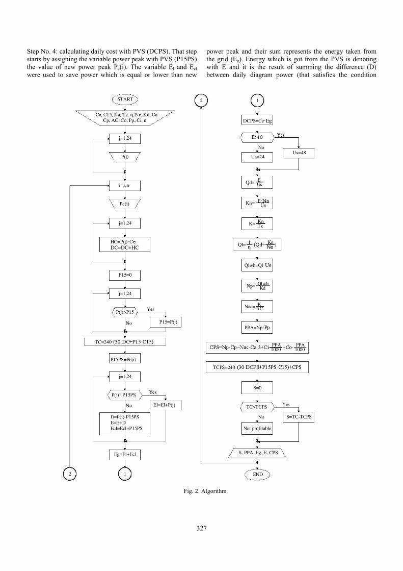
327

Step No. 4: calculating daily cost with PVS (DCPS). That step starts by assigning the variable power peak with PVS (P15PS) the value of new power peak Pc(i). The variable El and Ecl were used to save power which is equal or lower than new

power peak and their sum represents the energy taken from the grid (Eg). Energy which is got from the PVS is denoting with E and it is the result of summing the difference (D) between daily diagram power (that satisfies the condition

Fig. 2. Algorithm

328

P(j)≥P15PS) and power peak. Finally, for this step, energy from the grid is multiplied by the cost of electrical energy and makes daily cost with PVS (DCPS).

Step No. 5: calculating the dimension of PVS (number of panels and accumulators). They are calculated by using Eqs. 1–7. Number of panels is multiplied by panel power representing the dimension of photovoltaic array (PPA).

Step No. 6: calculating the total cost with PVS (TCPS) for period of 20 years. First, it is necessary to calculate the cost of PVS (CPS) using Eq. 8. Then, in order to determine TCPS the cost of PVS should be summed with the cost of energy usage for period of 20 years.

Step No. 7: determining the savings (S) by calculating the difference between total cost without PVS and total cost with PVS. Finally, outputs of this algorithm are savings, dimension of photovoltaic array, energy from grid, energy from PVS and cost of PVS.

Number of new power peaks determines how many times steps 2-7 should be repeated.

B. Testing

Algorithm presented in previous topic was tested using program package MATLAB. The daily diagram of demand used in this paper is taken from one industrial customer in Serbia. It is approximated and shown in the Fig. 3.

Fig. 3. Daily diagram of industrial customer

That daily diagram has four potential new power peaks.

The input data necessary for calculating savings, dimension of photovoltaic array, electrical energy from grid and electrical energy from PVS are: Ce=0.2€, C15=10€, Na=2 days, Tz=0.5, η=0.9%, Ne=10 days, Kd=800W, Ca=250€, Cp=220€, AC=200Ah, Co=30€, Pp=250W, Ci=150€ and n=4. Results for each new power peak are shown in table I.

The selection of most favorable solution is being made after getting results, according to investment capabilities and size of the area predicted for installation of the system.

TABLE I RESULTS FOR EACH NEW POWER PEAK

Pc (kW) S (€)

PPA (W)

CPS (€)

Eg (kWh)

E (kWh)

50 83542 15208 22058 740 40 40 142697 30486 44503 700 80 30 237008 61042 89392 620 160 20 384053 114515 167947 482 300

IV. CONCLUSION

The algorithm for calculating savings in electrical bill for industrial customers with the presence of photovoltaic battery system was analyzed in this paper. This algorithm can be applied in different daily diagrams of demand, whereby benefits of the presence of photovoltaic battery system can be more or less significant, in dependence on the value of power peak.

With current electrical energy price, significant savings by using photovoltaic system are obtained. The price of electrical energy from grid will increase and the price of the photovoltaic equipment will be lower, so these applications will be used for all greater savings. In addition, application of photovoltaic system reduces the pollution and reduces the demand for nonrenewable sources.

In future investigation accent can be put on optimization methods for costs minimization for industrial customers.

ACKNOWLEDGEMENT

The paper is a part of the research done within the project III 44006, supported by Ministry of Education, Science and Technological Development of the Republic of Serbia within the framework of technological development.

REFERENCES

[1] D. Kotur, and Ž. Đurić, “Optimal Spatial and Temporal Demand Side Management in a Power System Comprising Renewable Energy Sources”, Renewable Energy, vol. 108, 2017, pp. 533-547.

[2] Z. Wu, H. Tazvinga, and X. Xia, “Demand Side Management of Photovoltaic-Battery Hybrid System”, Applied Energy, vol. 148, 2015, pp. 294-304.

[3] M. N. Q. Macedo, J. J. M. Galo, L. A. L. Aldeida, and A. C. C. Lima, ”Opportunities and Challenges of DSM in Smart Grid Enviroment”, Conference ENERGY 2013, pp. 156-160, Lisbon, Portugal, March 2013.

[4] M. M. Eissa, “Demand Side Management Program Evaluation Based on Industrial and Commercial Field Data”, Conference MEPCON 10, pp. 15-19, Cairo, Egypt, December 2010.

329

Optimization of Energy Storage Capacity in an Islanded Microgrid Vassil Guliashki1 and Galia Marinova2

Abstract – This paper considers one part of the islanded microgrid design - the optimization of energy storage capacity. GridLab-D open source simulation tool is used for simulation of the microgrid elements. Matlab environment is used to run an optimization solver. The product GridMat is used as an interface tool between Matlab and GridLab-D. Eight different scenarios are tested. For each of them an economic scheduling optimization problem on the considered microgrid is formulated and solved by means of three optimizations methods. The obtained results are discussed and some conclusions are drawn.

Keywords – Microgrids, GridLab-D, GridMat, Matlab, Energy scheduling optimization.

I. INTRODUCTION

A microgrid is a low-voltage distribution system, integrating distributed energy resources (DERs) or renewable energy sources (RES) and controllable loads, which can be used/controlled in either islanded or grid-connected mode. In this paper an islanded microgrid is studied. DERs make the microgrid more secure and reliable in cases of disasters, such as earthquake, which might cause a long time power outage in electrical power grid. On the other hand the microgrid should be robust in controlling supply, demand, voltage, and frequency. The DERs production plan can be evaluated by using meteorological forecasts. In this case the use of energy storage (battery bank) can help in meeting the hourly production plan, providing the additional necessary energy to cover the peak load demand [2]. The capacity of the energy storage is limited and for the time when DERs cannot generate enough energy an independent from the main grid energy source, such like diesel generator is necessary.

Proper selection and optimal sizing of the energy storage is an important task in design of microgrids. The optimal battery bank capacity will allow a minimization of the fuel consumption by the diesel generator and reducing the harmful impact on the environment. At the same time the costs for the end user can be essentially reduced. To optimize the energy storage size eight scenarios with different battery bank capacity are considered. The corresponding optimization problems are based on an economic model for battery bank and diesel generator scheduling, similar to the model presented in [12,13]. The experimental microgrid setup includes a photovoltaic system, a wind turbine, a diesel generator and three houses. The considered microgrid

operates in an island mode, i.e. its point of common coupling (PCC) is disconnected from the main grid. To formulate an optimization task the exact amount of power demand and power supply for the next 24 hours period should be known. This is a heavy requirement, especially in real world applications. For example, there could appear great fluctuations in the wind generators output. The solar radiation forecasts could also be inexact and could vary essentially. For this reason the energy, generated by the diesel generator should include a reserve rate (see [5, 6]) and the forecasted data for the renewable energy resources (wind turbine and photovoltaic system), as well as for the loads (houses) should be taken adding a safe margin for each microgrid element.

The open source GridLab-D (see [3]) is used to simulate all the elements of the microgrid. The software product GridMat (see [1]) is used as an interface tool between Matlab (see [4]) and GridLab-D. Climate data, available on the official website of GridLab-D, are used for the simulations. The optimization problem is solved by using the Matlab optimization toolbox.

II. THE EXPERIMENTAL MICROGRID

The microgrid studied in this work operates with a three-phase medium voltage alternating current (AC) transmission system in an Island mode (disconnected from the Network). A diesel generator is considered in order to supply, together with the RES, the energy necessary to cover the loads. Two type of RES are considered connected in the Microgrid: 1) a photovoltaic system composed by an inverter and a group of solar panels, and 2) a wind turbine. A group of batteries (energy storage system) is also interconnected to the microgrid through a DC/AC bi-directional inverter. The use of optimal battery bank schedule makes the microgrid under study a smart microgrid, since it ensures the balance between the loads and the energy produced by the RES, and allows the minimization of fuel consumption by the diesel generator. The system configuration of the microgrid is presented on Fig. 1.

Fig. 1. Microgrid system configuration

The microgrid with all its components is shown on Fig 2.

1Vassil Guliashki is with the Institute of Information andCommunication Technologies – BAS, “Acad. G. Bonchev” Str. Bl.2, 1113 Sofia, Bulgaria, E-mail: [email protected]

2Galia Marinova is with the Faculty of Telecommunications atTechnical University of Sofia, 8 Kl. Ohridski Blvd, Sofia 1000,Bulgaria, E-mail: [email protected]

330

III. ECONOMIC SCHEDULING OPTIMIZATION MODEL

It this study the behavior of the RES has been simulated from historical climate data of a particular geographical position: Seattle (USA); The data for solar radiation and wind speed, as well for the houses energy consumption are real data for a given winter day. They are taken as a forecasted data.

Fig. 2. The experimental microgrid

In [5] are given energy safety margins necessary to cover the uncertainty of the forecasted data. Taking into account these margin values, in the created optimization model are assumed the following values: Wind turbine: (30%) ; Photovoltaic: (37%); Houses: (+25%); Diesel generator: (+20%). Having available correct forecasted data for the RES production and houses consumption one day before for the next day, it is possible to optimize the microgrid behavior for a whole year, solving one day ahead the correspondent scheduling optimization problem for the next day.

The time interval being analysed (one day and one night) is divided by 24 time steps, each with 1 hour length. The balance power PB of the studied microgrid should satisfy the following equations (see [6]):

PRES + PB = PL (1) PB = PBat_d + PDG , (2)

where PRES is the output power of renewable energy sources, PB is the balance power, PBat_d is the power from discharging the battery system, PDG is the output of the diesel generator, and PL is the microgrid load, equal to houses consumption energy plus battery system charging energy. The parameters and the decision variables used are presented in Table 1.

TABLE 1 PARAMETERS Parameter Description

CC OM RC FC EC CRF SFF

Capital cost for interval of one hour Operation maintenance for one hour Replacement cost (of the battery) Fuel cost for interval of one hour Emission cost for interval of one hour Capital recovery factor for one hour Sinking fund factor for one hour

Taking into account that the photovoltaic area, the wind turbine capacity, as well as the house energy consumption cannot be subject to optimization since their schedules are independent, the objective function includes the balance power:

min F =

)()()(

)()()()().(

24

1

24

1

24

1

tCCtRCtOM

tECtFCtOMtCCPC

Invt

BatBat

DGDGDGt

DGt

Btt

(3)

where PBt is the balance power for hour t and Ct is the cost of this power. In Ct are included the deprecations costs of each microgrid energy generation element (unit), of operational costs of individual units, of the fuel cost (for the fuel consumed by the diesel generator), and of emission cost. Calculating F only the hours, when the diesel generator operates and when the battery system is charging/discharging are taken into account. In [9, 10] are given formulas for calculating the correspondent annual values. Hence the one hour capital cost of microgrid units, which do not need a replacement during the project life time, such like diesel generator and inverter, is calculated as follows:

CCDG = 5475

y) ,.CRF(iCcapDG , (4)

Assuming, that the diesel generator is used average 15 hours in a 24 h period, the denominator is: 5475 = 15 365;

1

y)(1

y).(1

y),CRF(

i

iii (5)

Here CcapDG. is the capital cost (US$), y is the project life time, and i is the annual interest rate [11]:

f

fii

1

' (6)

where: i’ is the loan interest (%), and f is the annual inflation rate (%).

The one hour operation maintenance cost is:

y.5475

)1.( DGCcap

OM (7)

for the diesel generator, and

y.6570

)1.( BatCcap

OM (8)

for the battery, where: λ is the reliability of correspondent unit. Assuming, that the battery bank is used average 18 hours

in a 24 h period (i.e. 365 18 = 6570 hours annually), the one hour battery bank replacement cost is:

6570

),(SFF. repBat yiCrepRC (9)

where: Crep is the replacement cost of battery bank, and SFF is the sinking fund factor, which is calculated as follows [11]:

1

y)(1

SFF

i

i (10)

The one hour fuel cost of diesel generator for hour t is: FC = Cf.G(t)

where: Cf is the fuel cost per liter, and G(t) is the hourly consumption of diesel generator [7, 8, 9, 10] as follows: G(t) = (0,246PDG(t) + 0,08415.PR) (11)

331

where: PDG(t) is the diesel power at time t, and PR is the rated power of the diesel generator.

The hourly emission cost (CO2 emission) is:

EC(t) = )(.0187,01000

)(..tP

tPEEDG

DGcff (12)

where: Ef is the emission function (kg/kWh), and Ecf is the emission cost factor ($/ton)

The necessary economic data are given in Table 2:

TABLE 2 THE ECONOMIC DATA Interest rate i’ (%) 3 Inflation rate (%) 1,6 Inverter life time (years) 20 Battery life time (years) 10 Reliability of inverter (%) 0,98 Reliability of battery (%) 0,98 Reliability of diesel (%) 0,9 Cost of diesel generator (US$/KW) 500 Cost of battery bank (US$/KWh) 200 Cost of inverter (US$/KW) 1000 Fuel cost (Cf) (US$/l) 0,75 Emission function (kg/kWh) 0,34 Emission cost factor (US$/ton) 55

Detailed data about the microgrid components are given

in [13]. The data in Table 2 are taken from [9], only the fuel cost value is taken from [10]. Other parameters to be defined are the energy amount for charging and discharging: Pbt_max, and the maximal battery bank capacity Ebt_max. Since PR = 38, hence CcapDG = 19000 $. In [6] is stated, that the high speed (3600 r/min), air-cooled diesel can be used for about 20 000 h. Hence the project life time y in formulas (5), (7) and (8) is: y = 3,653 years. The annual interest rate i = 0,53846154. Hence CRF(i, y) = 0,67926. CCDG = 2,3573 $/h. OMDG = 0,095 $/h. SFF = 0,141. CcapInv = 10000 $. The inverter one hour capital cost is: CCInv = 0.0761 $/h.

To evaluate the optimal energy storage eight scenarios with different battery bank capacity and the same other parameters are tested. The battery bank capacity data are presented in Table 3.

TABLE 3 THE BATTERY BANK DATA

Ebt_max

[kWh] Pbt_max

[kW] CrepBat

[$] OMBat [$/h]

RCBat [$/h]

1 10 1 2000 0,00167 0,0429 2 25 2,5 5000 0,00417 0,1072 3 50 5 10000 0,00833 0,2143 4 100 10 20000 0,01667 0,4286 5 150 15 30000 0,02501 0,6429 6 200 20 40000 0,03334 0,8572 7 250 25 50000 0,04168 1,0716 8 500 50 100000 0,08335 2,1431

The constraints concerning the diesel generator are: 0,3.PR ≤ PDG(t) ≤ PR (13) Taking into account the modified values from [5], the

following constraint is obtained:

otherwise.0

.25,1.7,0.63,0

).7,0.63,0.25,1.(2,1

)(_

_

LdBatWTPV

dBatWTPVL

DG PPPPif

PPPP

tP (14)

The constraints concerning the battery system are:

Pbt_max PBat(t) + Pbt_max (15) SOCmin SOC(i) SOCmax (16)

24

1

;24,...,1;0)(t

Bat ttP (17)

where: PL(t) is the power absorbed by the houses during the hour "t" [kW]; PPV(t) is the power delivered by photovoltaic panels during the hour "t" [kW]; PWT(i) is the power delivered by wind turbine during the hour "t" [kW]; PBat_d(t) is the power delivered by the battery block (discharging) during the hour "t" [kW]. Pbt_max is the maximum power that the battery system can deliver/absorb [kW]; SOC(t) is the State Of Charge of the battery during the hour "t" [%] SOCmin = lower limit for the State Of Charge of the battery [%] SOCmax = upper limit for the State Of Charge of the battery [%].

Finally taking into account the energy balance of the microgrid (see equations (1)-(2)), the last constraint obtained is:

PBat(t) + PDG(t) PH(t) PPV(t) PWT(t) , t = 1,...,24; (18) where PH(t) is the house consumption energy. The energy PBat(t) is considered positive when the battery is discharging and negative when is charging. Therefore, the equation (15) represents the power limit, which can be delivered or absorbed by the inverter tie to the battery system; the system cannot supply or absorb a power more than the Pbt_max.

The SOC of the battery represents the amount of energy stored in the battery system. Therefore, the equation (16) means that, for each time step, the SOC must be included between a minimum and a maximum value depending by the system used to storage the energy and agree with physical limit of maximum SOC of 100%. In this case, the minimum and maximum level of SOC are fixed to 20% and 100% respectively.

The SOC depends on the value of PBat(t) for each time step; the relation between these variables is shown below:

SOC(t) = SOC(t1) tE

tP

bt

Bat .)(

max_

(19)

where: t is the time step [h], SOC(0) = Initial charge of the battery (it is an input value of the problem). In this optimization problem, the initial value of the SOC is fixed to 50% from Ebt_max. At the begin of the optimization, the battery system is charged to the half of its full charge.

The constraint, shown in equation (17), is used in order to get, at the end of the 24h period, the same value of SOC like at the begin of the period.

IV. TEST RESULTS

The simulations with GridLab-D give the results about the consumption of the houses, the production of the solar panels and wind turbine.

The minimization of (3) subject to (13)-(19) requires 48 variables: PBat(t) and PDG(t), t=1,…,24; To solve this

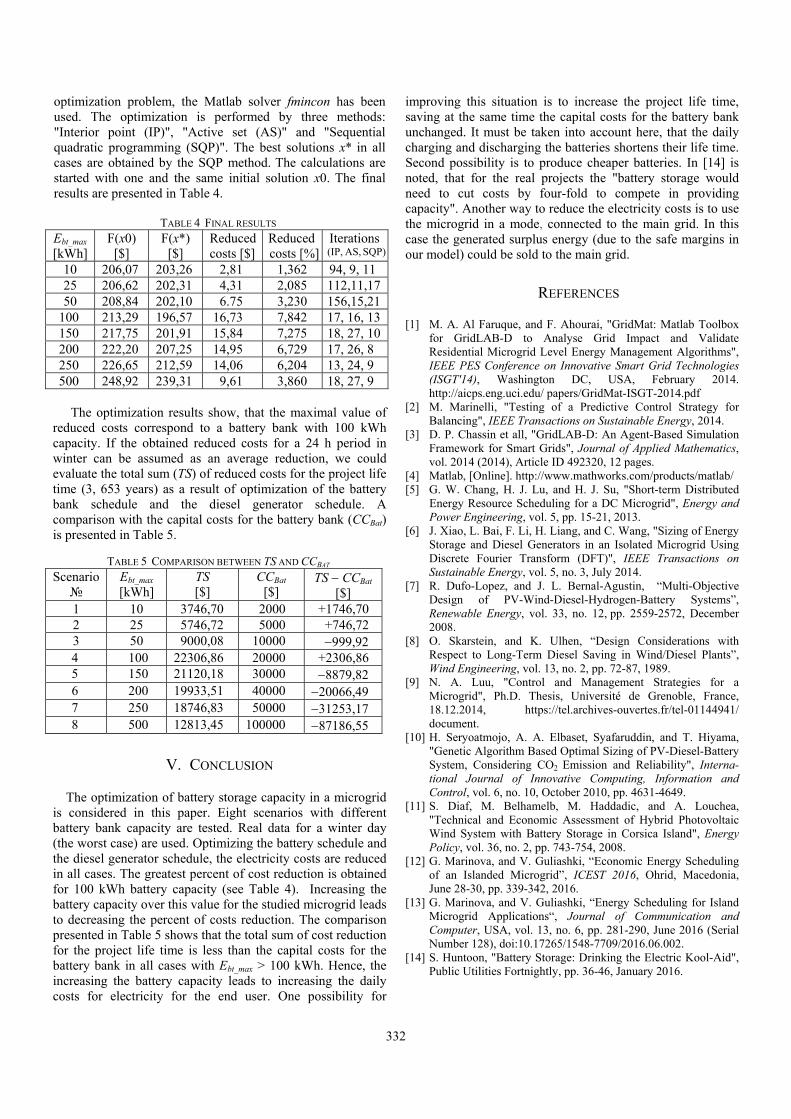
332

optimization problem, the Matlab solver fmincon has been used. The optimization is performed by three methods: "Interior point (IP)", "Active set (AS)" and "Sequential quadratic programming (SQP)". The best solutions x* in all cases are obtained by the SQP method. The calculations are started with one and the same initial solution x0. The final results are presented in Table 4.

TABLE 4 FINAL RESULTS

Ebt_max

[kWh] F(x0) [$]

F(x*) [$]

Reduced costs [$]

Reduced costs [%]

Iterations (IP, AS, SQP)

10 206,07 203,26 2,81 1,362 94, 9, 11 25 206,62 202,31 4,31 2,085 112,11,17 50 208,84 202,10 6.75 3,230 156,15,21

100 213,29 196,57 16,73 7,842 17, 16, 13 150 217,75 201,91 15,84 7,275 18, 27, 10 200 222,20 207,25 14,95 6,729 17, 26, 8 250 226,65 212,59 14,06 6,204 13, 24, 9 500 248,92 239,31 9,61 3,860 18, 27, 9

The optimization results show, that the maximal value of

reduced costs correspond to a battery bank with 100 kWh capacity. If the obtained reduced costs for a 24 h period in winter can be assumed as an average reduction, we could evaluate the total sum (TS) of reduced costs for the project life time (3, 653 years) as a result of optimization of the battery bank schedule and the diesel generator schedule. A comparison with the capital costs for the battery bank (CCBat) is presented in Table 5.

TABLE 5 COMPARISON BETWEEN TS AND CCBAT Scenario

Ebt_max

[kWh] TS [$]

CCBat [$]

TS CCBat [$]

1 10 3746,70 2000 +1746,70 2 25 5746,72 5000 +746,72 3 50 9000,08 10000 999,92 4 100 22306,86 20000 +2306,86 5 150 21120,18 30000 8879,82 6 200 19933,51 40000 20066,49 7 250 18746,83 50000 31253,17 8 500 12813,45 100000 87186,55

V. CONCLUSION

The optimization of battery storage capacity in a microgrid is considered in this paper. Eight scenarios with different battery bank capacity are tested. Real data for a winter day (the worst case) are used. Optimizing the battery schedule and the diesel generator schedule, the electricity costs are reduced in all cases. The greatest percent of cost reduction is obtained for 100 kWh battery capacity (see Table 4). Increasing the battery capacity over this value for the studied microgrid leads to decreasing the percent of costs reduction. The comparison presented in Table 5 shows that the total sum of cost reduction for the project life time is less than the capital costs for the battery bank in all cases with Ebt_max > 100 kWh. Hence, the increasing the battery capacity leads to increasing the daily costs for electricity for the end user. One possibility for

improving this situation is to increase the project life time, saving at the same time the capital costs for the battery bank unchanged. It must be taken into account here, that the daily charging and discharging the batteries shortens their life time. Second possibility is to produce cheaper batteries. In [14] is noted, that for the real projects the "battery storage would need to cut costs by four-fold to compete in providing capacity". Another way to reduce the electricity costs is to use the microgrid in a mode, connected to the main grid. In this case the generated surplus energy (due to the safe margins in our model) could be sold to the main grid.

REFERENCES

[1] M. A. Al Faruque, and F. Ahourai, "GridMat: Matlab Toolbox for GridLAB-D to Analyse Grid Impact and Validate Residential Microgrid Level Energy Management Algorithms", IEEE PES Conference on Innovative Smart Grid Technologies (ISGT'14), Washington DC, USA, February 2014. http://aicps.eng.uci.edu/ papers/GridMat-ISGT-2014.pdf

[2] M. Marinelli, "Testing of a Predictive Control Strategy for Balancing", IEEE Transactions on Sustainable Energy, 2014.

[3] D. P. Chassin et all, "GridLAB-D: An Agent-Based Simulation Framework for Smart Grids", Journal of Applied Mathematics, vol. 2014 (2014), Article ID 492320, 12 pages.

[4] Matlab, [Online]. http://www.mathworks.com/products/matlab/ [5] G. W. Chang, H. J. Lu, and H. J. Su, "Short-term Distributed

Energy Resource Scheduling for a DC Microgrid", Energy and Power Engineering, vol. 5, pp. 15-21, 2013.

[6] J. Xiao, L. Bai, F. Li, H. Liang, and C. Wang, "Sizing of Energy Storage and Diesel Generators in an Isolated Microgrid Using Discrete Fourier Transform (DFT)", IEEE Transactions on Sustainable Energy, vol. 5, no. 3, July 2014.

[7] R. Dufo-Lopez, and J. L. Bernal-Agustin, “Multi-Objective Design of PV-Wind-Diesel-Hydrogen-Battery Systems”, Renewable Energy, vol. 33, no. 12, pp. 2559-2572, December 2008.

[8] O. Skarstein, and K. Ulhen, “Design Considerations with Respect to Long-Term Diesel Saving in Wind/Diesel Plants”, Wind Engineering, vol. 13, no. 2, pp. 72-87, 1989.

[9] N. A. Luu, "Control and Management Strategies for a Microgrid", Ph.D. Thesis, Université de Grenoble, France, 18.12.2014, https://tel.archives-ouvertes.fr/tel-01144941/ document.

[10] H. Seryoatmojo, A. A. Elbaset, Syafaruddin, and T. Hiyama, "Genetic Algorithm Based Optimal Sizing of PV-Diesel-Battery System, Considering CO2 Emission and Reliability", Interna-tional Journal of Innovative Computing, Information and Control, vol. 6, no. 10, October 2010, pp. 4631-4649.

[11] S. Diaf, M. Belhamelb, M. Haddadic, and A. Louchea, "Technical and Economic Assessment of Hybrid Photovoltaic Wind System with Battery Storage in Corsica Island", Energy Policy, vol. 36, no. 2, pp. 743-754, 2008.

[12] G. Marinova, and V. Guliashki, “Economic Energy Scheduling of an Islanded Microgrid”, ICEST 2016, Ohrid, Macedonia, June 28-30, pp. 339-342, 2016.

[13] G. Marinova, and V. Guliashki, “Energy Scheduling for Island Microgrid Applications“, Journal of Communication and Computer, USA, vol. 13, no. 6, pp. 281-290, June 2016 (Serial Number 128), doi:10.17265/1548-7709/2016.06.002.

[14] S. Huntoon, "Battery Storage: Drinking the Electric Kool-Aid", Public Utilities Fortnightly, pp. 36-46, January 2016.

333

Internet of Things in Power Distribution Networks – State of the Art

Aleksandar Janjić1, Lazar Velimirović2, Jelena Velimirović2 and Željko Džunić3

Abstract –This paper analyzes the most prominent smart grid functionsfrom the Internet of Things implementation perspective. A Smart MV/LV substation is proposed as a solution that will handle intelligent operations, such as real-time monitoring, control, and system management, in a successful manner. However, these great benefits come at a price. With rapidly-evolving Internet of Thingsnetwork, maintaining cyber privacy and security will present a great challenge in the future and solutions to efficiently overcome these weaknesses should be further investigated and developed.

Keywords – Cyber security, Internet of Things, Smart grid, Substation automation.

I. INTRODUCTION

Smart technologies are significantly influencing the way people live and work today. Objects used daily such as smart phones and smart home appliances are connected to the Internet via intelligent technologies and are able to provide us with large amounts of data on our habits and lifestyles. There are many products and services on energy consumption that citizens may use to make more informed and efficient decisions on problems that matter to them. Technology has already altered our behavior – how we live andwhat we do, for example, the use of social media, mobile apps and open data can help us to reduce energy use.

Nowadays Internet of Things (IoT) applications allow smart energy management and its optimization at all stages: utility operations are improved, power grids are more efficient and resilient, and stakeholders can use these data to allocate resources appropriately, avoid energy waste, and make right decisions on energy usage and generation

IoT empowers consumers (residential, commercial or industrial) by providing control signals and/or financial incentives to adjust their use of demand side resources at strategic times. Energy consumption at the device level can now be tracked through the IoT platforms, and end users can also use these data for processes such as when is the best time to start or shut down a machine, reduce its use at peak hours, waste less energy and, by doing so, reduce their own energy bills.

Concerning the power distribution network, the process of automation and remote control historically started from high voltages and transformer substations of large installed power. The large portion of installed capacities in the medium voltage (MV) and low voltage (LV) distribution network remained without proper monitoring, control, and outside the usual SCADA utility systems. Fast development of information and communication technologies (ICT) lead to the conception of “intelligent transformer substation“, and its integration in the smart grid environment.

Considering that smart grid is a large and complex system of interconnected devices that use different protocols for communication between themselves, it is vulnerable to cyber attacks and IT threats. Some security concerns, among others, are customers’ security, number of interconnected devices/connectivity and software threats.

II. SMART DISTRIBUTION SUBSTATION

Due to the increasing penetration of dispersed generation, there is a need to increase the intelligence of the components in the MV and LV voltage networks. The increase in sensibility of devices for the quality of voltage and the increasing number of power quality related problems are the reason to look for more functionality in the MV/LV station. The power flows in LV and MV distribution grids will increase their fluctuation as well. To manage these fluctuations while maintaining power quality and reliability, several prototypes of Smart MV/LV substation has been designed [1–5]. These prototypes were focused on particular distribution network problems, like the harmonic voltages, resonance, and peak load reduction.

In general, intelligent components are needed to: Get information and influence the power and voltage

profile

Increase the immunity against power quality problems, such as harmonics, voltage dips, flicker

Reduce the unavailability (minutes of interruption)

Create microgrids which will be able to work autonomously to increase the reliability as needed

Enable the usage of condition based maintenance. A Smart MV/LV substation is built to handle these items.

The smart substation concept enables more reliable, more efficient, real-time monitoring and control of the facility nodes installed in the substation. Smart devices can be added to traditional substation devices to perform intelligent functions and provide ubiquitous IT techniques for monitoring, control and management of the system. Similarly to smart homes, each device in the substation is considered as an object and is assigned a unique IP address, transmitting its

1Aleksandar Janjić is with the Faculty of Electronic Engineering atUniversity of Niš, 14Aleksandra Medvedeva, Niš 18000, Serbia, E-mail: [email protected]

2Lazar Velimirović is with Mathematical Institute of the SerbianAcademy of Sciences and Arts, 36 KnezaMihaila, Belgrade 11001,Serbia, E-mail:[email protected]

2Jelena Velimirović is with Mathematical Institute of the SerbianAcademy of Sciences and Arts, 36 KnezaMihaila, Belgrade 11001,Serbia, E-mail:[email protected]

3Željko Džunić is with Junis,University of Niš, 2 Univerzitetskitrg, Niš 18000, Serbia, E-mail: [email protected]

334

status and receiving control commands from the utility authorized operator via the Internet.

The main functions of the smart substation are summarized as follows:

Intelligent analysis for alarm processing, bad data processing, etc.

Intelligent control for auto-restoration, remedial or predictive action, and emergency state estimation

Intelligent maintenance and management

Intelligent physical safety

Interconnection and application with Geographic Information System (GIS).

The solution presented in [6] relies on anenergymanagement sensors combining monitoring of electrical energy consumption, power quality analysis, and management of electrical energy use in a single powerful internet connected device. With Ethernet or WiFi connectivity and built in web server, sensors can be quickly and easily deployed in any energy management scenario.

Micro RTU Hardware platform is based on ARM platform making the device functional. Micro RTU is designed with two processors: Cortex M4F real time processor with 8 MB of external RAM, serving inputs and outputs in the real time, and Cortex A9 processor with Linux operating system. Its role is to serve the communication interface and data storage.

Central control application performs the periodic polling of remote units in the set of selected transformer substations. Measured values are placed in the RAM of each individual unit. Modbus masters embedded in the central control unit read the Modbus slaves in the remote units, by the TCP protocol through the Virtual Private Network (VPN) formed by the 3G network.

The system requires sophisticated security mechanisms and it is important to note that once performed security evaluation is of a temporary validity only because we face everyday advances regarding the methods for cryptanalysis of cryptographic algorithms. Accordingly, monitoring of security and security re-evaluations of the cryptographic techniques appear as a top-priority issue in the security critical ICT infrastructures.

III. DEMAND SIDE MANAGEMENT

The basis of the new smart grid is a trend that reinvents the functioning mode of electric utilities companies - Demand Side Management (DSM). DSM represents the interface between the utility company and smart devices that consume power with the aim of reducing peaks in power grid demand, minimizing power losses in the grid, and increasing the use of unrealized energy savings during low demand periods. In this way, DSM covers energy efficiency and demand response domains for customers. IoT based management platforms, in other words, deploying energy management measures units at the point of consumption, are a prerequisite for the successful implementation of DSM applications. Electricity customers have at their disposal a variety of

options such as rebates, stimulus funds, incentives, with theaim to cash savings for both participants: utilities and their customers.The general architecture of DSM is presented in Fig. 1 [7].

Fig. 1. Basic architecture of DSM Three basic layers can be recognized: a) Cloud and

Services – central part of the architecture that collects data from different sources, providing tools and technologies for mass data storage and data processing. b)Utility – this layer collects information from different parts of the power generation supply chains (production, transmission, and distribution) and forwards them to the cloud (data related to the level of current and future production and consumption, the price of electricity, and other information that may affect the DR relation). c) Consumers (smart home, smart buildings, industry) – each consumer represents a node in a complex microgrid. Nodes are equipped with so-called sink or hub that collects information from all smart devices for that node and which has a data storage capacity, local data processing and communication capability to devices outside the node.

Coordination of the huge number of IoT devices which are distributed over the entire platform and acquisition of the necessary data in economically viable manner are some of the major challenges for the implementation of DSM. Taking into account that the DSM applications rely on the IoT architecture, the challenges facing the IoT are also projected on the success of DSM

IV. DEMAND RESPONSE

Demand Response (DR) is usually defined as the change in electric usage by end-use customers from their normal consumption patterns in response to changes in the price of electricity over time, or to incentive payments designed to induce lower electricity use at times of high wholesale market prices, or when system reliability is jeopardized. In order to achieve this feature, data about the current consumption of multiple sites during an event should be consolidated in real time through the IoT platform, so the consumer (or the third-party aggregator) can gauge the performance of the entire portfolio almost instantaneously.

The system enables the aggregator to collect customer demand flexibility and provide access to the market. For this purpose, with the development of new features, the aggregator will study which customers can provide profitable DR,

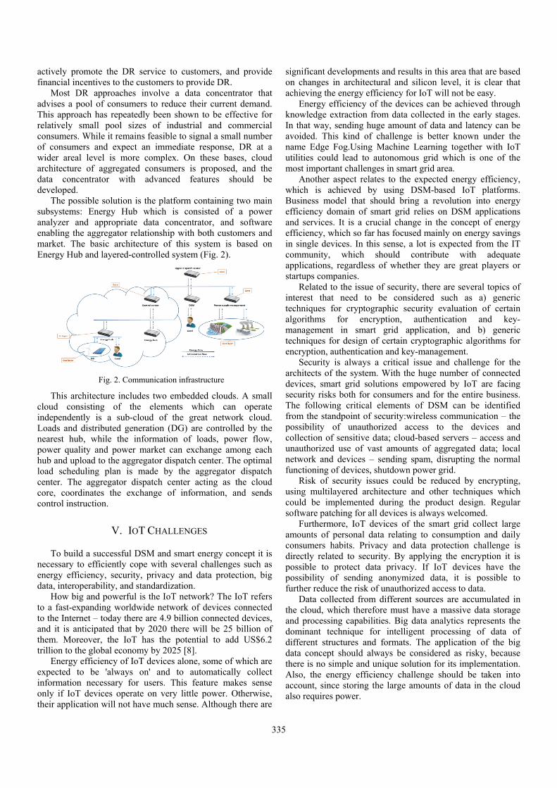
335

actively promote the DR service to customers, and provide financial incentives to the customers to provide DR.

Most DR approaches involve a data concentrator that advises a pool of consumers to reduce their current demand. This approach has repeatedly been shown to be effective for relatively small pool sizes of industrial and commercial consumers. While it remains feasible to signal a small number of consumers and expect an immediate response, DR at a wider areal level is more complex. On these bases, cloud architecture of aggregated consumers is proposed, and the data concentrator with advanced features should be developed.

The possible solution is the platform containing two main subsystems: Energy Hub which is consisted of a power analyzer and appropriate data concentrator, and software enabling the aggregator relationship with both customers and market. The basic architecture of this system is based on Energy Hub and layered-controlled system (Fig. 2).

Fig. 2. Communication infrastructure

This architecture includes two embedded clouds. A small cloud consisting of the elements which can operate independently is a sub-cloud of the great network cloud. Loads and distributed generation (DG) are controlled by the nearest hub, while the information of loads, power flow, power quality and power market can exchange among each hub and upload to the aggregator dispatch center. The optimal load scheduling plan is made by the aggregator dispatch center. The aggregator dispatch center acting as the cloud core, coordinates the exchange of information, and sends control instruction.

V. IOT CHALLENGES

To build a successful DSM and smart energy concept it is necessary to efficiently cope with several challenges such as energy efficiency, security, privacy and data protection, big data, interoperability, and standardization.

How big and powerful is the IoT network? The IoT refers to a fast-expanding worldwide network of devices connected to the Internet – today there are 4.9 billion connected devices, and it is anticipated that by 2020 there will be 25 billion of them. Moreover, the IoT has the potential to add US$6.2 trillion to the global economy by 2025 [8].

Energy efficiency of IoT devices alone, some of which are expected to be 'always on' and to automatically collect information necessary for users. This feature makes sense only if IoT devices operate on very little power. Otherwise, their application will not have much sense. Although there are

significant developments and results in this area that are based on changes in architectural and silicon level, it is clear that achieving the energy efficiency for IoT will not be easy.

Energy efficiency of the devices can be achieved through knowledge extraction from data collected in the early stages. In that way, sending huge amount of data and latency can be avoided. This kind of challenge is better known under the name Edge Fog.Using Machine Learning together with IoT utilities could lead to autonomous grid which is one of the most important challenges in smart grid area.

Another aspect relates to the expected energy efficiency, which is achieved by using DSM-based IoT platforms. Business model that should bring a revolution into energy efficiency domain of smart grid relies on DSM applications and services. It is a crucial change in the concept of energy efficiency, which so far has focused mainly on energy savings in single devices. In this sense, a lot is expected from the IT community, which should contribute with adequate applications, regardless of whether they are great players or startups companies.

Related to the issue of security, there are several topics of interest that need to be considered such as a) generic techniques for cryptographic security evaluation of certain algorithms for encryption, authentication and key-management in smart grid application, and b) generic techniques for design of certain cryptographic algorithms for encryption, authentication and key-management.

Security is always a critical issue and challenge for the architects of the system. With the huge number of connected devices, smart grid solutions empowered by IoT are facing security risks both for consumers and for the entire business. The following critical elements of DSM can be identified from the standpoint of security:wireless communication – the possibility of unauthorized access to the devices and collection of sensitive data; cloud-based servers – access and unauthorized use of vast amounts of aggregated data; local network and devices – sending spam, disrupting the normal functioning of devices, shutdown power grid.

Risk of security issues could be reduced by encrypting, using multilayered architecture and other techniques which could be implemented during the product design. Regular software patching for all devices is always welcomed.

Furthermore, IoT devices of the smart grid collect large amounts of personal data relating to consumption and daily consumers habits. Privacy and data protection challenge is directly related to security. By applying the encryption it is possible to protect data privacy. If IoT devices have the possibility of sending anonymized data, it is possible to further reduce the risk of unauthorized access to data.

Data collected from different sources are accumulated in the cloud, which therefore must have a massive data storage and processing capabilities. Big data analytics represents the dominant technique for intelligent processing of data of different structures and formats. The application of the big data concept should always be considered as risky, because there is no simple and unique solution for its implementation. Also, the energy efficiency challenge should be taken into account, since storing the large amounts of data in the cloud also requires power.

336

The complex architecture of DSM requires communication of an enormous number of devices (M2M – Machine to machine communication). In such an environment, the choice of suitable protocols may directly affect the success of DSM implementation. The complex communication requires adding advanced features which automatically affects the price increase and performance reduction. In the last couple of years, many institutions, such as industry consortia (IEEE, Zigbee Alliance, etc.), standardization bodies, and also some of the leading companies and startups have jointly defined protocols necessary for the advancement of IoT [9].

Their work is mainly focused on adapting IP protocol (6LoWPAN, COAP, and RPL) to enable further expansion of web architecture to the lowest level sensors as well as the development of so-called lightweight protocols, necessary for the interoperability of all devices in the cloud (MQTT, LWM2M, etc.). Nevertheless, interoperability between different vendors, especially those that control different parts of vertical market, remains one of the greatest challenges and roadblocks of further mass deployment of IoT and solutions that are based on it.

Standardization has a key role in removing the technical barriers and ensuring interoperability and reliability. In Europe, standardization of smart metering, as a key component of smart grid, is in the hands of main European Standard Development Organizations (SDOs). Each SDO has responsibility for specific standards: ETSI M2M for inter-device communications, CENELEC (European Committee for Electrotechnical Standardization) for the next generation of electricity meters, and CEN (European Committee for Standardization) for the next generation of non-electricity meters. The following list presents some of general smart metering standards:ETSI TC M2M [10], DLMS/COSEM, M-Bus (“Meter-Bus”), IEEE 802.15.4, ZigBee and ISA 100.11a, PLC – HEMS, IEEE P1905.1.

Complete list of communication and data exchange standards for smart metering in Europe is available in [11].

Efforts towards smart grid standardization are presentworldwide,for example IEEE P2030 [12], ANSI [13], US NIST [14] and IETF [15].

VI. CONCLUSION

The increasing granularity of telemetry in MV and LV networks greatly increases the level of information available to energy intensive industries and utilities. This data must be collected and integrated into existing utility and market operations. This information must also be clearly communicated to customers. There is no doubt that the IoT technology has the potential to be a crucial part of the response of many challenges facing the grid.

More efficient, secure and reliable operation of distribution system can be achieved with the smart substation implementation. The monitoring and control system communicating via Internet with various sensors inside the distribution station and with consumer appliances and sensors is the heart of the Smart MV/LV substation. IT prototype hardware, functions and communication interfaces on an embedded platform based on micro RTU offers the required functionality for the flexible distribution network.

The IoT in power distribution networks is very alike to the problem of auto piloted car: the technology is ready and capable to operate the grid, but even a small anomaly can lead to a disaster. Smart grid architecture and appropriate ICT system have to be carefully designed, in respect of all network stakeholders, and the choice between totally decentralized and centralized system should result in the compromise between them.

ACKNOWLEDGEMENT

This work was supported by the Ministry of Education, Science and Technological Development of the Republic of Serbia through Mathematical Institute SASA under Grant III 44006and Grant III 42006.

REFERENCES

[1] K. Hak-Man, L. Jong-Joo, and K. Dong-Joo, "A Platform for Smart Substation", Future Generation Communication and Networking (FGCN 2007), IEEE, vol. 1, 2007, pp. 579-582.

[2] J. Kester et al., "A Smart MV/LV-Station that Improves Power Quality, Reliability and Substation Load Profile", 20th Intern. Conference and Exhibition on Electricity Distribution - Part 1 (CIRED 2009), Prague, Czech Republic, 8-11 June, 2009.

[3] J. Heckel, "Smart Substation and Feeder Automation for a Smart Distribution Grid", 20th Intern. Conference and Exhibition on Electricity Distribution - Part 1 (CIRED 2009), Prague, Czech Republic, 8-11 June, 2009.

[4] H. Spack et al., "Intelligent Transformer Substations in Modern Medium Voltage Networks as Part of “Smart Grid", 7th Mediterranean Conf. and Exhibition on Power Generation, Transmission, Distribution and Energy Conversion, Agia Napa, Cyprus, Paper No. MED10/240, 7-10 November, 2010.

[5] J. Backes, "The Riesling Project - Pilot Project for Innovative Hardware and Software Solutions for Smart Grid Requirements", 22nd International Conference on Electricity Distribution, Stockholm, Sweden, 10-13 June, 2013.

[6] A. Janjic et al., "Realization of Smart MV/LV Substation through the Concept of Micro RTU", 10th Mediterranean Confer. on Power Generation, Transmission, Distribution and Energy Conversion, Belgrade, Serbia, 6-9 November, 2016.

[7] D. Xu Li, W. He, and S. Li, "Internet of Things in Industries: A Survey", IEEE Transactions on Industrial Informatics, vol. 10, no. 4, pp. 2233-2243, 2014.

[8] J. Anyika, et al., Disruptive Technologies: Advances that will Transform Life, Business, and the Global Economy, vol. 180, San Francisco, CA: McKinsey Global Institute, 2013.

[9] J. Francois, "Internet of Things in Energy Efficiency: The Internet of Things", Ubiquity Symposium, Ubiquity, vol. 2016, February 2016.

[10] TSI TC M2M, TR 102 691, Machine-to-Machine Communications (M2M); Smart Metering Use Cases, 2010.

[11] Z. Fan et al., "Smart Grid Communications: Overview of Research Challenges, Solutions, and Standardization Activities", IEEE Communications Surveys & Tutorials, vol. 15, no. 1, pp. 21-38, First Quarter 2013.

[12] EEE P2030, http://grouper.ieee.org/groups/scc21/2030/2030 index.html, 2010. [87] ANSI, http://webstore.ansi.org/, 2010.

[13] ANSI, http://webstore.ansi.org/, 2010 [14] X. Hong, P. Wang, J. Kong, Q. Zheng, and J. Liu, “Effective

Probabilistic Approach Protecting Sensor Traffic”, IEEE MILCOM, 2005.

[15] F. Baker and D. Meyer, “Internet Protocols for the Smart Grid”, ETF Internet Draft, Apr. 2011.

337

Self and Mutual Impedances of Power Cables Miodrag S. Stojanovic1, Dragan D. Tasic1, Nenad N. Cvetkovic1,

Dejan B. Jovanovic1and Dragan D. Vuckovic1

Abstract –The review of relations for determining self and mutual impedances of power cables is given in the paper. Afterwards, the accuracy of presented relations is tested. The problems of single-core cables with metal sheets earthed at both or one end, with or without cross-bonding are discussed in more details.

Keywords – Power cables, Circulation current, cross-bonding

I. INTRODUCTION

During the realization and exploitation of power transmission lines, it is of great importance to know values of serial self and mutual impedances of cables. It is well known that serial self impedances of the conductors and metal sheets can be determined as a sum of internal and external impedance values. The relations for determining internal impedance of the conductor with circular cross-section are proposed long time ago. During the time, increasing value of transmitted energy resulted in enlarging conductor cross-sections (3000 mm2), as well as in improving constructing solutions for cable realization. In these cases, it is not possible to apply above mentioned, previously proposed relations. On the other hand, main problem in determining external self and mutual impedance is taking into account earth as the return current path. The expressions for determining ground return path impedance for known current frequency are known for almost one century. Those relations are not easy to apply for engineering purposes, since they include calculation of modified Bessel function of complex variable and numerical solving of definite integrals. In order to avoid such difficulties, a large number of simplified engineering relations has been developed. They are often applied without knowledge about their accuracy or about assumptions and neglectings under which these relations are evaluated. A review of relations for calculating self and mutual cable impedances is given in the paper. On one example, the accuracy of presented relations has been tested. The problems of single-core cables with metal sheets placed in the ground, earthed at both or one end, with or without cross-bonding are especially discussed.

II. THEORETICAL BACKGROUND

A. Expressions for Three-Phase Transmission Line

The three single-core cables which form three-phase transmission line are observed, Fig. 1. The cables are laid in flat formation, which is usual for high voltage cables. Phase conductors are marked with 1, 2, and 3, while their metal

sheets are labeled with 4, 5, and 6. Having in mind the mentioned marking of phase conductors and metal sheets, the following matrix equation can be formed:

6

5

4

3

2

1

666564636261

565554535251

464544434241

363534333231

262524232221

161514131211

6

5

4

3

2

1

/

/

/

/

/

/

I

I

I

I

I

I

zzzzzz

zzzzzz

zzzzzz

zzzzzz

zzzzzz

zzzzzz

xU

xU

xU

xU

xU

xU

.(1)

Fig. 1.Three single-core cables laid in a flat formation

Relation (1) has general form and can be applied for arbitrary position of the cables. With iiz , i=1,2,3, self

impedances per unit length of the loops conductor-return ground path are labeled, while iiz , i=4,5,6 denote self

impedances per unit length of the loops metal sheet-return ground path. Also, jiij zz , ji , denote corresponding

mutual impedances per unit length, while x is coordinate along the cable route. Obviously, for cables from Fig. 1 it is

332211 zzz and 665544 zzz . The radial density

distribution of the current flowing through metal sheets depends on the currents flowing through phase cable and currents having closing path outside metal sheets. For taking into account this influence, instead of (1), expression (2), formed for loops cable-metal sheet and metal sheet-return ground [1], is used:

63

52

41

3

2

1

66656463

56555452

46454441

3633

2522

1411

6

5

4

63

52

41

00

00

00

0000

0000

0000

/

/

/

/)(

/)(

/)(

II

II

II

I

I

I

zzzz

zzzz

zzzz

zz

zz

zz

xU

xU

xU

xUU

xUU

xUU

llll

llll

llll

ll

ll

ll

(2)

where it is

euizpslll zzzzzz 332211 ,

zseizeslll zzzzzz 665544 ,

lmllllll zzzzzzz 633652254114 , 1245 zl zz ,

and 1346 zl zz , 2356 zl zz .

Previous relation is formed for cables with metal sheets, but without armature. The same procedure can be applied for the cables with armature and results in more complex relation for

1M.S. Stojanovic, D.D. Tasic, N.N. Cvetkovic, D.B. Jovanovic and D.D. Vuckovic are with Faculty of Electronic Engineering,University of Nis, A. Medvedeva 14, 18000 Nis, Serbia, E-mails: [miodrag.stojanovic, dragan.tasic, nenad.cvetkovic, dejan.jovanovic, dragan.vuckovic]@elfak.ni.ac.rs

338

determining matrix elements of dimension 9x9. In previous expressions, zps is internal impedance per unit length of the cable, ziz is insulation impedance per unit length, zeu is internal impedance per unit length of the metal sheet with internal return path, zes is internal impedance per unit length of internal impedance of metal sheet with external return path, zlm is mutual impedance per unit length of the loops cable-metal sheet and metal sheet-return ground path, zzs is self impedance of the ground, while 125445 zll zzz , 136446 zll zzz

and 236556 zll zzz are mutual impedances per unit length

of the ground. For system from Fig. 1 it is 5645 ll zz . After

simple transformations, expression (2) can be reduced to the form (1) where it is

.

;

;

;

;

;2

235335622665563223

134334611664463113

124224511554452112

633652254114

665544

332211

z

z

z

lmzseizes

zseizes

zseizeslmeuizps

zzzzzzzzz

zzzzzzzzz

zzzzzzzzz

zzzzzzzzzz

zzzzzz

zzzzzzzzzz

(3)

Since expression (2) can be transformed into form (1), expression (1) can be assumed as general.

B. Internal Impedance of Conductor and Metal Sheet

The resistance per unit length of the cable conductor for DC current versus temperature can be determined as

))20(1(' '0 RR , (4)

where '0R labels the resistance of the cable conductors for DC

current at 20°C [2], is temperature coefficient of the resistance, whileis conductors’ temperature. For AC current, there are skin and proximity effects, causing the resistance increasing. For determining AC resistance, in [2] the following relation is used,

)1( ps yyRR . (5)

In (5) ys is coefficient which models skin effect influence, while yp value models influence of the proximity effect. From complex form of Maxwell’s equations system, the following expression for internal impedance per unit length of the conductor cable with circular cross-section of radius cr can

be derived:

)2(

)2(

2

212/3

1

12/30

12/3

cc

cc

c

cin

rjJ

rjJ

r

jz

. (6)

In (6), J0 labels Bessel function of the first kind of zero order, while J1 is Bessel function of the first kind of order one. With

c the penetration depth is labeled:

2

c , (7)

where is angular frequency,is magnetic permeability and is specific resistivity of the conductor. Since

penetration depth at frequency 50 Hz is about 9,35 mm, for cross-sections between 25 mm2 and 2500 mm2 it is 0,3<rc/c<3. Using the first three terms of series expansion of Bessel function, the simplified relation is obtained:

823

11

4

2j

r

rz

c

c

cin

. (8)

For interval 0,3</c<3 the following relations provide error less than 3%:

4

4

8,0192 s

ss

x

xy

,

'109,15 4

R

kfx s

s . (9)

Previous expressions were used until 2014. godine in IEC 60287-1-1, for xs≤2,8. The increase of power results in enlarging the cable cross-section with strongly present skin effect. In order to neutralize skin effect, various solutions (conductors made of lacquered wires, or isolating conductors’ segments) are applied. For calculating these types of cables, in [3] new values of the coefficients for existing expressions are given. For conductors with circular cross-section, for xs≤2,8, relation (9) is recommended. For other interval it is

8,3,733,0354,0

8,38,2,0563,00177,0136,0 2

sss

ssss

xxy

xxxy.(10)

Using previous expressions, the error is less than 0,6% in complete interval. For cables with segment conductors, in IEC60287-1-1, published in 2014, relations (10) are accepted and coefficients values cp and cb are given.

Proximity effects are modeled in standard IEC60287-1-1 with expression

.109,15

,

27.08,0192

18,1312,0

8,0192

4

4

4

22

4

4

R

kfx

x

xa

d

a

d

x

xy

pp

p

p

cc

b

pp

(11)

Internal reactance of the conductor, i.e. internal inductance, can be determined from imaginary part of the expression (6).

Relation (8) provides calculation of internal inductivity with accuracy better than 3% for rp/c≤1,3 (cross section about 460 mm2 at 50 Hz). In [4], for rp/c≤2 the following expression is proposed:

4

26

11

8 c

cin

rl

, (12)

and for rc/c>2 (cross-section larger than 1000 mm2 at 50 Hz):

32

64

32

8 c

c

c

cin rr

l

. (13)

Internal impedance of cylindrical conductor of circular cross-section can be determined as

339

)()()()(

)()()()(

2 1111

1001

urJurNurJurN

urJurNurJurN

r

uz

iooi

iooi

o

cin

. (14)

It can also be applied for calculate the metal sheet impedance when the return path is trough the armature (labelled as zes in (3)). In [5] the following approximation is proposed:

)(2))(coth(

2 oiiioc

o

cin rrr

rrmr

mz

.(15)

Internal impedance of cyilindrical conductor with internal return path can be determined from expression:

)()()()(

)()()()(

2 1111

0101

urJurNurJurN

urNurJurJurN

r

uz

iooi

ioio

iin

. (16)

Applying (24), metal sheet impedance labeled with zes in (3) can be determined. Since the thickness of metal sheet is very small, the non-uniform current distribution in metal sheet can be neglected. Consequently, the resistance of metal sheet can be determined as DC resistance. Insulation impedance in (3) can be determined from expression:

in

ouiz r

rjz ln

20

, (17)

where rou and rin are outer and insulation radius, respectively Expression (25) can be used to determine ziz in (3), adopting that rou is inner radius of metal sheet, rei, while rin is radius of the conductor rc. Also, equation (3) can be applied to determine zeiz, where rou is cable radius, while rin is external radius of metal sheet reo. Mutual impedance of the loops conductor-metal sheet and metal sheet-return ground path zlm is determined as:

)()()()(

1

11112 urJurNurJurNrr

zeoeieieoeieo

clm

. (18)

C. External mutual and self impedances

Ther procedure for calculation of external impedances needs to include soil characteristic, as a part of return current path. Basics for determining values of impedance per unigt length of the conductors placed above the ground or in the ground are given in [6] and [7]. Carson’s relations from [7] are little bit simpler, but they are formed for a conductor above ground, since the approach from [6] provides possibility for analysis of the conductors placed in the ground. The expressions are formed for lineical infinitely long conductor and infinitely deep ground. The expressions for calculating external self and mutual impedances are also given in [5]. They have different form from the ones in [6], but essentially the expressions are identical. Those expressions are:

0

222

22

000

)cos(1

2

)2()(2

dRem

hmKmRKj

z

mmh

mmm

, (19)

and

0

22)(

22

000

)cos(1

2

)()(2

dxem

DmKdmKj

z

mnhmh

mn

, (20)

In previous expressions 0K labels the modified Bessel

function of the second kind of zero order, R radius of the

conductor or cable, while zjm 0 is complex

propagation constant of EM waves through the ground ( zzz j , where z is dielectric permittivity of the

ground). If non-uniform current distribution in metal sheets is

considered, expressions (1) -(2) in combination with (3) are applied, where R is cable radius in expression for zsz , while

12zz , 13zz and 23zz in (3) are determined from expression

(20). Dimension d, D, hm and hn can be noticed from Fig. 2. (1 denotes ground and 2 denotes air).

hm

d

z

x

hm

m

n

hn

1

2

Fig. 2. Two cables in the ground

Integral in (19) and (20) can not be solved in closed form and it is necessary to apply numerical integration. For this reason, there are many published papers with proposed procedures for approximate solution of (19) and (20). Very often, Carson’s relation [7] has been applied with integral that is a little bit simpler for approximate numerical solving than the one from [6] (expressions (19) and (20)). Namely Ammetani proved that Pollaczek expression [7] can be reduced to Carson’s expression [6] by substituting

22)( mnhmhe with ||)( nhmhe in (8), which provided possibility for using Carson’s expression for determining impedance of the conductor placed in the ground. Using Carson’s’ expression also results in simpler approximation which includes complex depth of return path. Expressions for external impedance proposed by Carson include impedance for ideal conducting ground and corrective factors R and

X :

)2

ln2

( 0mm

m

mmm

smm X

r

hjRz

, and (21)

340

)ln2

( 0mn

mn

mnmn

smn X

d

DjRz

. (22)

After some numerical procedures for determining approximate value of external self and mutual impedance (in details presented in [7]), it is obtained:

m

esmm r

Djz ln

2800

and mn

esmn d

Djz ln

2800

.(23)

In (23) it is

ff

eDe

658

1054 4

6159315,0

. (24)

The relation for determining self impedance, that includes complex return path (i.e. complex depth p=1/m) is given in [9] as:

m

mm R

phjz

)(2ln

20

. (25)

Neglecting conductor’s height above the ground h and imaginary part of z , expression (25) can be reduced to [10],

m

emm R

DjZ ln

2800

, f

De

762,711 (26)

Very accurate approximation for external self and mutual impedance is given in [5]

mmm hmRmj

z3

45,0

2ln

20 , (27)

)(3

25,0

2ln

20

nmmn

mn hhmdmj

z . (28)

For zzzz j from (27)-(28), it is

R

Djz e

mm ln28

00

,mn

emn d

Djz ln

2800

,(29)

where it is

ff

eDe

87160,658

2

0

. (30)

III. NUMERICAL RESULTS

The 400 kV power cable of Milliken type with cross-section 2500 mm2 with isolated cupper conductors is observed. Metal sheets are made of aluminum of cross-section 500 mm2. Three single-core cables are placed in a flat formation at the depth 1m, with mutual distance between axis of 0.3 m. The conductor temperature is 90oC, while metal sheet temperature value is assumed as 70oC.

In Table 3, results for internal impedances of metal sheets,

obtained in two different ways, are presented. The first group of results is obtained using Bessel functions in expression (3) (complete model). The second group is calculated using simplified relations (29)-(30). Impedances in (3) are calculated by numerical integration of Pollaczek relations

(19)-(20). In both cases, the same value of conductor internal impedance is used.

TABLE I SELF AND MUTUAL IMPEDANCE OF THE 400 KV CABLE (2500 mm2)

IN A FLAT FORMATION

Impedance Complete model Simplified model z11 [/km] 0,060066+j0,661113 0,0599476+j0,661171 z44 [/km] 0,1177101+j0,600938 0,117266+j0,601210 z41 [/km] 0,0494655+j0,601135 0,0493480+j0,601210 z12 [/km] 0,0494646+j0,505118 0,0493480+j0,505152 z13 [/km] 0,0494646+j0,461566 0,0493480+j0,461601

IV. CONCLUSION

The review of the relations for determining self and mutual impedances of the cable is given in the paper. Afterwards, the accuracy of presented relations is tested. The problems of single-core cables with metal sheets earthed at both or one end, with or without cross-bonding are especially discussed. Considering the presented results, it is obvious that simplified relation can be applied, since the maximal error, which exists in results for mutual resistance, is less than 0,3%.

REFERENCES

[1] H. W. Dommel, Electromagnetic Transients Program Theory Book (EMTP Theory Book), Portland: Bonneville Power Administration, 1986.

[2] IEC Std. 60228, "Conductors of Insulated Cables", 2004. [3] CIGRE Working Group B1.03, "Large Cross-Sections and

Composite Screens Design”, June 2005. [4] H. Schunk, Stromverdrängung, UTB, Dr. Alfred Hüthig Verlag,

1975. [5] L.M. Wedepohl, and D.J. Wilcox, "Transit Analysis of

Underground Power-Transmission Systems", Proc. IEE, 120, pp. 253-260, 1973.

[6] J.R. Carlson, "Wave Propagation in Overhead Wires with Ground Return", Bell System Journal, vol. 5, pp. 539-554, 1926.

[7] F. Pollaczek, "Über das Feld einer unendlichen langen wechselstromdurchflossenen Einfachleitung", E.N.T., vol. 3, pp. 339-360, 1926.

[8] A. Ametani, Y. Miyamoto, T. Asada, Y. Baba, N. Nagaoka, I. Lafaia, J. Mahseredjian, and K. Tanabe, “A Study on High-Frequency Wave Propagation along Overhead Conductors by Earth-Return Admittance/Impedance and Numerical Electromagnetic Analysis”, International Conference on Power Systems Transients (IPST2015), Cavtat, Croatia, June 15-18, 2015, https://goo.gl/HVohBt.

[9] C. Gary, "Approche Complete de la Propagation Multifilaire en Haute Fréquence par Utilisation des Matrices Complexes" (Complete Approach to Multiconductor Propagation at High Frequency with Complex Matrices), EdF Bulletin de la Direction des Etudes et Recherches, Série B, no. 3/4, pp. 5-20, 1976.

[10] A. Deri, G. Tevan, A. Semlyen, and A. Castanheira, "The Complex Ground Return Plane, a Simplified Model for Homogeneous and Multy-Layer Earth Return", IEEE Trans. on Power Apparatus and Systems, vol. PAS 100, no.8, pp. 3686-3693, August 1981.

Areseintesustcurrswitatog

TtimevoltElecdepapp

KLTTMA

Ccurrall Eacwhibe convoltandproc

Bhavof has dchocon[10]

2.1 pracvolt

T

oscipara

S12/1

AlgoCurre

Abstract - Sinearchers demerrupters by utainable againrents and trantches are stillggle ways, thusThis paper pre for a static tage switchingctronics and Lending on C

plications.

Keywords - CaT thyrsitor

ATLAB/Simulin

Circuit breakerents may exof the prima

ch type of circich must be thapplied with

nsiderations otage transient

d high frequecessing switchBoth of hyb

ve been offerehigh speed mediverting switcopping currenntact conducts].

II. AN

The vacuumctical transientage switching

The analysis illatory circuameter , desig

Shaker J. Gatan1, Riga LV-104

orithmients an

nce many yeamonstrate the

using of a renst of an arcingnsient over voltl constructings have been doesents the seqswitching proc

g technique. LLC are desigrow-bar and

lculating choprs, Sequencnk.

I. INTRO

ers using difxhibitdifferent ary functionalcuit breaker hahoroughly undh correctly d

of arcing currts, multiple rency which ching time. brid applicatioed a smooth pechanical contching, itsan ex

nt. In hybrid s large curren

NALYSING D

m interrupter ints problems g process

shows that uit can be degned ŋ, or its

n is with Riga48, Latvia, E-ma

ic Appnd High

V

ars up to dadevelopment

efractory mateg currents andtages. The conv

g in the sameominated yet. quence of thecess for applSince DESY gned for RFsnubber circ

pping currentsces of s

ODUCTION

fferent mediacharacteristic

l requirementas a unique sederstood befodesigning anrents, choppire-ignitions, vcalculate for

on and dampprocess switchtact with powxcellent perfoswitchsystem

nt with lowlo

DAMPING CI

involves veryin power sy

the effect escribed in treciprocal ʎ,

a Technical Unail: Shaker.gata

plicatioh TranVacuum

Medium V

S

ate now, mot of the vacerials “Alloys”d both of chopventional desig

e classical step

switching prlication of me

& Behlke PF systems, bascuit for prote

s, Damping ciswitching t

a for interrucs with respets of the bre

et of characterore the breakend confidenceing currents, voltage escal

full load du

ping circuit thhes which con

wer semicondurmance in lim

m, the mechasses, [1], [2],

IRCUIT

y large numbystem of me

of damping terms of a swhich is the

niversity, [email protected]

341

on for Cnsient om Inte

Voltage Switch

haker J. Gata

st of cuum ” for pping gning ps of

rocess edium Power ically

ection

rcuit, times,

upting ect to eaker. ristics r can e by over

lation uring

heory nsists uctors miting anical , and

er of dium

an single

ratio

of th

Thiscurvmaneffor

Non pL - iC - pR - e

(Li s

1Ls

FromindudamSo th(3) as ab

Whehypethis the i

nesielam

Calculover-Verrupte

hing System

an

he resistance t

/

R R

Z L C

s fact permitsves for differeny practical prrt as one expa

Normally our aparallel RLC cndicative loadparallel parasievaluating res

2

(0))

V

L s

22

11

p

ss

T T

m Eq. (3) expructor of any

mping. We notehat a family ofor different vbscissa. This

Fig. 1.

ere η =0.5 , therbolic functiocondition , foinductor curre

ationoVoltageer

o the surge im

s the construnt values of ηoblems can be

and by using aanalysis for thircuit as followd of stator winite`s capacitoristance that ca

2

11

p

sT T

ress in dimenparallel RLC

e that the onlyof generalizedvalues of η whas been done

Generalized plo

he sine functioon . We mightollowing the sent in parallel

of Chopes for a

mpedance of th

uction of genη , from whice extracted wia table of loghe switching wing;

nding coils; rs; an be damping

sionless from C circuit, wity parameter ind curves can bwith dimension

e in Fig. 1.

ot of inverse tra

on changes frot have developsame argumenl RLC circuit

pping a New

he circuit i.e;

(1)

eralized damch the solutionith about the sarithms. process basic

g oscillating.

(2)

(3)

the current inth any degrenvolved is η. be drawn fromnless quantity

ansform

om a circular ped the curvent .By calculaunder condit

mping ns to same

cally

n the e of

m Eq. , t` ,

to a s for ating tions

of aHowspeccircR =ThereprVo =labelook 2.2 techfirstas pmod

Tbetwthyrthyrmodcurrresi

F

Vof figu

a subsidence twever to gaincific example

cuit in which = 105 Ω , L =5 ese values areresents the equ=13.8√2 KV Selled η=2 in Fking for.

Parallel swhnique R circut peak value oparallel applicde [1]

The flexible rween to eleristors. Flexibrsitors as a codels. It proporents after thistance circuit

Fig. 2. /di dt

III.

Vacuum interr/di dt and d

ure which d

transient, but n familiarity e where the in

the componeH, C = 2·10-8

e typical of uuivalent loss rSo. Zo = √L/C

Fig. 3 gives the

witching techuit will be d

of chopping cuation with two

rates for tranements such ble /du dt anontrol techniqos to make

he time of io

and /du dt aand th

SWITCHING

rupter involve/du dt conver

describes the

have a far wwith these c

nductor currenents have the

F. unloaded tranresistance. Sup

C = 5·104 Ω , ηe shape of the

hnique: the rediminished theurrent , if we co electrodes –

nsition of duas electropl

nd /di dt [6]ques are presa diverting onization by

alignment betwhyristor

G TRANSITIO

es by switchinrsion. An Exptest circuit

wider applicatcurves, considnt is requiredfollowing va

nsformer, wheppose η = 2. The cur current we ar

esistor applice amplitude oconnect this ci– parallel oper

/u dt and dlates and se-[9] for the sented in Simof the chopusing a dam

ween electroplat

ON RATES

ng transition periment synt

an arc of a

342

tion . der a

d in a alues:

ere R

rve re

cation of the ircuit ration

/di dt et of set of

mulink pping

mping

tes

rates thetic a few

thoucontinter

CThe voltapossmodand Chilthe currecalcu

/du

d

Thshor150msparto thbreaThe withtest twenwithare s

usand amperetact “synthetrrupter. urrent commucircuit subseq

age across thsible to causedel which anal

the recoverylds and Greenmathematical

ent zero and ulate the post/ dt were calcu

ss r/ I /tdi dt

Fig. 3. A S

Fig. 4. Transi

he vacuum swrt fixed gap; mm). The caprks over , at whe gap. The

akdown voltagTRV frequen

h L1. The rangwere; Iss = 1.

nty nine shotsh several test summarized in

es is drawn btic prototype

utation is typquent applies

he gap. by adje the switch lyzes events d

y period afternwood [8]. Twl model: a post arc time

t arc current aulated accordi

Synthetic experiof a vac

ition process d

witch under tethe gap sele

pacitor C1 iswhich time C1

fixed gap age ( ~ 15KV)ncy is adjustedges of values c0KA, 2.0KA,

s were made twere for eachn Table I.

between a pe” with a s

pically achievea fast-rising tjusting circuito re-ignite.

during the comrwards has bwo time periocommutating

e. The model and transitionsing to followi

iment for fast cocuum arc

/di dt and du

est VS has itsected was in s charged unt1 delivers an oassures a rea. /dI dt is cod by C2 (<<Cchosen during, 3.0KA, 4.0Kto calculate dh ramp down

air of separasealed vac

ed within 20transient recoit parameters

A mathemammutation pe

been proposedods are define

period priohas been use

s time /di dtng formula

(4)

ommutation

/ dt for TRV

s contacts opethe range (

til the gap ofoscillatory curasonably consontrolled by

C1) as it resong the course oKA & 5.0KA.

/di dt and dutime; the re

ating uum

us . very it is

atical eriod d by ed in r to

ed to and

en at 100-f VS rrent stant L1.

nates f the The /u dt

sults

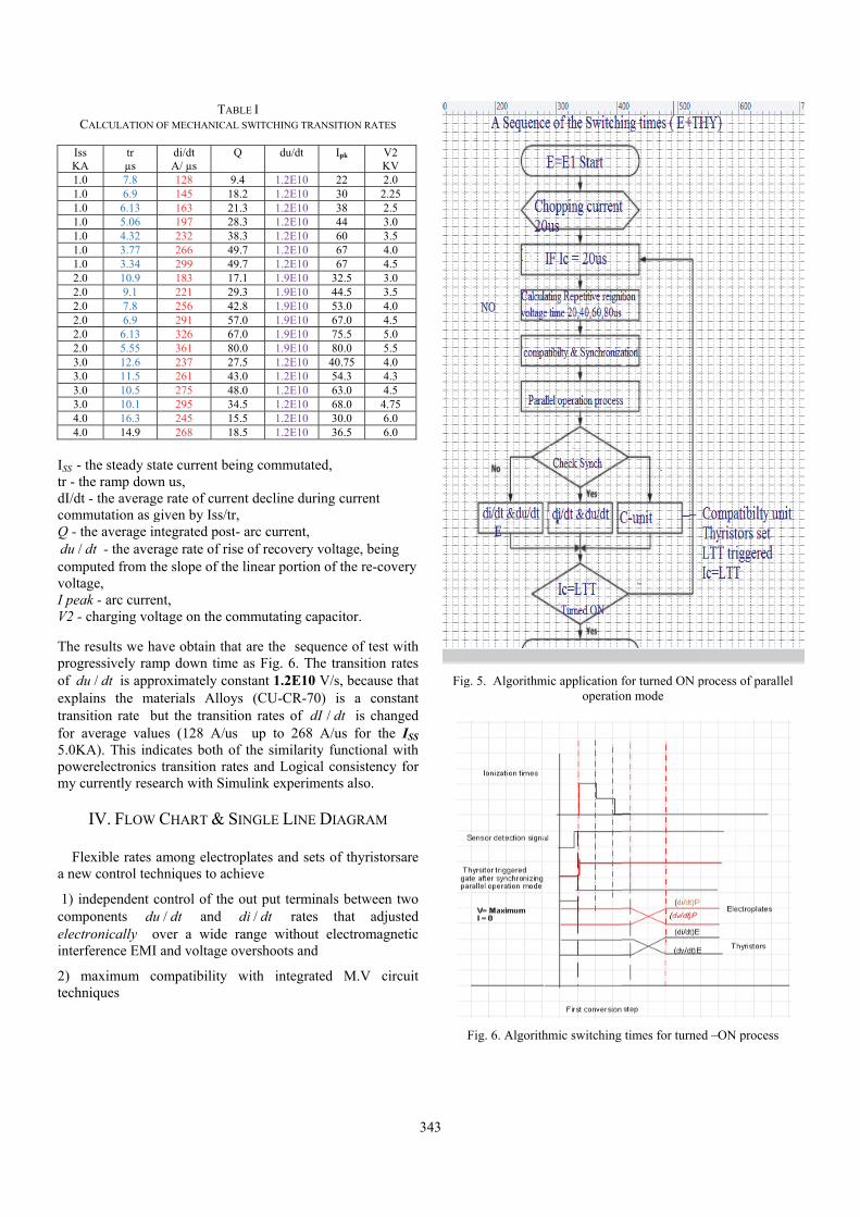
IK1111111222222333344

ISS -tr - dI/dcomQ - ducomvoltI peV2 -

Theprogof dexptranfor 5.0Kpowmy

Fa ne

1) comelecinte

2) tech

CALCULATION

ss KA

tr µs

.0 7.8

.0 6.9

.0 6.13

.0 5.06

.0 4.32

.0 3.77

.0 3.34 2.0 10.9 2.0 9.1 2.0 7.8 2.0 6.9 2.0 6.13 2.0 5.55 3.0 12.6 3.0 11.5 3.0 10.5 3.0 10.1 4.0 16.3 4.0 14.9

- the steady stthe ramp dow

dt - the averagmmutation as g

the average in/ dt - the aver

mputed from thtage, eak - arc curre- charging vol

e results we hgressively ram

/du dt is apprplains the mansition rate b

average valuKA). This ind

werelectronicscurrently rese

IV. FLOW

Flexible rates ew control tec

independent cmponents ductronically oerference EMI

maximum chniques

TAB

OF MECHANICAL

di/dt A/ µs 128 9145 1163 2197 2232 3266 4299 4183 1221 2256 4291 5326 6361 8237 2261 4275 4295 3245 1268 1

tate current bewn us, ge rate of curregiven by Iss/trntegrated postrage rate of rishe slope of the

ent, ltage on the co

ave obtain thamp down timeroximately coaterials Alloybut the transitues (128 A/usdicates both os transition ratearch with Sim

CHART & S

among electrochniques to ach

control of the/u dt and

over a wide I and voltage o

compatibility

BLE I L SWITCHING TR

Q du/dt

9.4 1.2E10 8.2 1.2E10 1.3 1.2E10 8.3 1.2E10 8.3 1.2E10 9.7 1.2E10 9.7 1.2E10 7.1 1.9E10 9.3 1.9E10 2.8 1.9E10 7.0 1.9E10 7.0 1.9E10 0.0 1.9E10 7.5 1.2E10 3.0 1.2E10 8.0 1.2E10 4.5 1.2E10 5.5 1.2E10 8.5 1.2E10

eing commuta

ent decline dur, t- arc current, se of recoverye linear portio

ommutating c

at are the seqe as Fig. 6. T

onstant 1.2E10ys (CU-CR-7tion rates of ds up to 268

of the similarites and Logic

mulink experim

SINGLE LINE

oplates and sehieve

e out put term/di dt rate

range withouovershoots an

with integra

RANSITION RATE

Ipk VK

22 230 2.38 244 360 367 467 4

32.5 344.5 353.0 467.0 475.5 580.0 5

40.75 454.3 463.0 468.0 4.30.0 636.5 6

ted,

uring current

y voltage, beinon of the re-co

capacitor.

quence of test The transition 0 V/s, because70) is a con

/dI dt is cha8 A/us for thity functional cal consistencments also.

E DIAGRAM

ets of thyristo

minals betweenes that adjuut electromagd

ated M.V ci

343

ES

V2 KV

.0 25 .5 .0 .5

4.0 4.5

.0

.5 4.0 4.5

.0

.5 4.0 4.3 4.5

75 6.0 6.0

ng overy

with rates

e that nstant anged he ISS

with cy for

orsare

n two usted

gnetic

ircuit

Figg. 5. Algorithm

Fig. 6. Algorith

mic application foperatio

hmic switching

for turned ON pon mode

times for turne

process of paral

ed –ON process

llel

s

F

Fig

[1]

Fig. 7. Algorith

g. 8. A single linof vacuum

1. The statswitchinprocess

2. Many recurrent value foM.V syn

3. Further determincapacita

4. The thedissipatethe static

S. Gatan, “Interrupters f2016, Lodz un

hmic switching

ne diagram of am interrupter for

IV. CON

tic capacitors ng process – unit function.

esearching papwill not incre

or most full lonchronous mo

measuremenne the maximance. eory of rectied energy thoc switching pr

REFER

“Synchronizingfor Medium Vniversity of Tec

g times for turne

a compact desigr medium voltag

CLUSIONS

are always inInherited ca

. piers indicateease more thaoad operation

otors. nt shall be

mum values of

ifying chopporough the resrocess.

RENCES

g Switching TVoltage”, IEEE,

chnology Lodz-

ed – OFF proce

gn of a new propge switching

nteractive witapacitors for

that the chopat 5A – first n with all typ

implementedf discharged

ping currents sistor will be

Times of Va, 19-20th Septe-Poland.

344

ess

posal

h the each

pping peak es of

d for static

and offer

acuum ember

[2]

[3]

[4]

[5]

[6]

[7]

[8]

[9]

[10]

[11]

[12]

[13]

[14]

[15]

[16]

[17]

M. Murano,Okazaki, “CurCircuit BreakSystems, vol. PF.A. Holmes,vacuum Arcs”New York, JanA.N. GreenwoBreaker on NAIEEE, vol. 79E.J. Tuohy,Magnetizing paper No. F77Feb. 1977. High PowerTechnology. Solutions in TS.E. Childs, aZero Current Vacuum Arc.S.E. Childs,Interruption inps-8, pp. 289-2S. Park, and Method for InIndustry AppliW. Merz, andVoltage VacuInternational (IPMHVC), ppZ. Jian, J. ZhAnalysis and Don Electro-maXuebao/Trans26, no. 8, pp. A. H.E. Say"Modeling thDynamic CirUniversity Po1999-168-172K.Y. Ahn, andSpeed CircuitCam (J)", PEngineers, ParJ. Lou, Q.-M"Dynamic Chthe Fast ElecDianji Gongcno. 6, pp. 23-2T. Genji, O. Speed CurrenSystem”, IEE1428-1435, 19D. Hui, Z.K. W10.5KV/1.5KAApplied SuperG. Coqueny, Device for Raon Railway Co1-7, 2005.

S. Yanabu, Hrrent Chopping

kers”, IEEE TPAS-96, pp. 14

“An Empirica”, paper C 740n. 1974. ood, “The EffeNetworks and9, part III, pp. 5

and J.PanekCurrents: par

7 096-1, IEEE

r Directed–ligThe Basis fo

Transmission Syand A.N. Gree Passage Duripp. 181-188, IEand A.N. G

n Diffuse Mod294, Dec.1980.T.M. Jahns, “

nsulated Gate ications, vol. 39d M. Grims, “

uum Tube ProPower Modula

p. 308-311, 201huang,C . WangDesign of a Higagnetic Repulsisactions of Chi1-5,·August 20

yed, R. W.P. he Opening Mrcuit Breaker ower Engineer

2. d S.H. Kim, "Mt Breaker MecProceedings ofrt C, pp. 663-67

M. Li, Q.-S. Sharacteristics Sictromagnetic Rheng Xuebao/P

29, 2005. Nakamura, M.

nt Limiting CirEE Trans. on P994. Wang, J.Y. ZhaA HTS Fault Crconductivity, vR. Lallemand,

ailway and Distronditions 1000

H. Ohashi, H.g Phenomena oTrans. on Pow

3-149, 1977. al Study of Cu088-1, IEEE PE

ect of Current Cd Transformers545-555, 1960. k, "Choppingrt I; Single Ph

PES Winter M

ght–Triggered or Advanced Pystems – SIEMEenwood, “Evening the Rapid EEE-1983.

Greenwood, “Ade”, IEEE Tran. “Flexible du/dtPower Switche9, no. 3, May 20“Fast Openingtection Applicator and High 12. g, J. Wu, and Lgh Speed Mechion Mechanismina Electrotech11. Ker Kennar,

Mode of a FaDrive(C)", P

ring Conferenc

Modeling and Achanism with aof the Institu72, 2001.

Sun, W.-D. Liuimulation and

Repulsion MechProceedings of

Isozaki,et al, rcuit Breaker

Power System,

ang, et al, “ DeCurrent Limiterol. 16, no. 2, ppG. Josse, et a

ribution NetwoA-25KV-50Hz

. Ishizuka, anof Medium Vower Apparatus

urrent ChoppinES Winter Mee

Chopping in Cis, part II”, Tr

g of Transfohase TransformMeeting, New Y

Thyrsitor vPower ElectroENS. nts Associated

Commutation

A Model for ns. Plasma Sci,

t and di/dt Coes”, IEEE Tran003 (0093-9994

g Switch for Hcation”, 2012 IVoltage Confer

L. Liu, “Simulhanical Contact m”, Diangong Jhnical Society,

A. M.S. Atmast Acting EleProceeding of ce, Leicester,

Analysis of a Hia Spring –Actute of Mecha

u, and J.-L. QOptimal Desig

hanism", Zhongf the CSEE, vol

”400V Class for Electric Pvol. 9, no. 3

velpoment and r”, IEEE Transp. 687-690, 200al, "Current Limrk Design and T(c)", EPE 2005

d T. oltage

and

ng by eting,

ircuit Trans.

ormer mers", York,

valve onics,

with of a

DC. , vol.

ontrol n. on 4). High-IEEE rence

ation Base Jishu

vol.

madj, ectro-f the

UK,

igh –uated nical

Qian, gn of gguo l. 25,

High ower , pp.

Test s. on

06. miter Tests 5, pp.

f

AAlthby uintearcibut switconcbe sem

TevalVD4"forgenetran

KCalc

Sthevinteintethe undconpowswicircvolt

Tchabreaswiutilibothrateadddesc

S12/1

AnfullOp

Abstract – Parahough most ofusing a refracterrupter for thing current, c

the directiontching systemcepts of what

create a miconductors swThis paper adluates switchin4/ABB Vacuur maximum serators 6.6KV/nsformers, rati

Keywords - Pculating chopp

Since many yevacuum circueracting amonerrupter must

general spderstood befonfidence.Morewer electronictching system

cuits for damtages or other

This paper racteristics anaker to genetching systemizing vacuum h of switchines for any idition the insicribed as follo1. Time of2. Time of3. Time of4. The valu5. Multiple

Shaker J. Gatan1, Riga LV-104

nalysisperation

ameters of a vf researchers tory materials he sake of sushopping curren of create p

m are very nehappens insidhomogenous witches for pro

ddresses the deng processingum type 6.6Kswitching tim

V/8MW each haing 6.6KV/1250

Parameters oping currents,

I. INTRO

ears up to datuit breaker ng the charabe scientifica

pecification re the breake

eover the swics offers manm when jointmping choppir facilities [1]-focuses on

nd load specifierate preciselym - electropl

interrupters hng surge, arcininterval timeside electroplatowings: f arcing currenf chopping curf prestrike tranue of restrikese re-ignitions

n is with Riga48, Latvia, E-ma

s of Parn Mod

V

vacuum interrand industries“alloys” electr

stainable mateentsand disrupparameters foecessary. For

de vacuum switswitching p

omising futureescription of a

g times for thrKV/1500A/20Kes 2.7ms". T

ave been conne0KVA in refine

of switching Sequences of s

ODUCTION

te now, we arby classical

acteristics insally analysisawhich muster can be apitching procesny modern bts together byng current a-[16].

the undersfication relativy parameterslates includinhave been viewng currents ans (microsecotes some cha

nt rrent nsient over - vs over voltage

a Technical Unail: Shaker.gata

rametede of VVoltage

Sh

rupter are esses are involvingroplates for vaerials against ptive over volor medium vo

offering thetch itself that process withie technology. all parameteree circuit brea

KV/40KV-IEC6Three synchroected to three pery power plan

processing tswitching proc

re still construdesign, but

side each vacs a high valut be thoroupplied with sss associated enefits as a y using a snuand transient

standing of veto vacuum cs [1]-[12]. Cng some dewed as eliminnd high frequnds’ process

aracteristics ca

voltages s

niversity, [email protected]

345

ers andVacuume Poweaker J. Ga

ential. g only acuum

both ltages, oltage

e new could in a

s and akers,

60-071 onous power nt.

times, cess.

ucting t the cuum

ues of ughly safety

with static ubber over

both circuit Circuit evices nating uency s). In an be

Inassocconnsyncprochighelect

Siinteressenproca conif thewoul

J

Jo

therm(1.37most

1

nesielam

d Timem Interer Planatan

6. Time of v7. Non-sust

n general, theciated with on

nects the switcchronous motoesses for inst

voltage captrostatics char

I

ince the vacurrupter, some ntial for underess. The namntradiction [2ere is an arcld be metal va

2( ) kAT e

62 10J oule heating mionic work7·10-23 J/K ). t metals.

1. Time of ArAccordingwas clasionizationjoule heaswitching

Ionizati Acceler The tota

Harris a

Fig. 1. Catho

e Sequerrupternts

voltage escalatained disrupti

e above chanly vacuum swchgear with poors ,there are atance hysterespacitive insiderged) feedback

I. SWITCHIN

uum arc is thknowledge o

rstanding the e vacuum arc] “If there is

c there is no apor arc inside

kT 6 2( / )A m

as thermioni

k function, The constant

rcing Currentg to the Harrisified “the

n process in aating to a cprocess”;

ion zone ration zone al above proceapproximately

ode cell geometrin Harri

ences r for M

ation & frequeive discharge

aracteristics awitchgear itselower distributalso many nesis currents, ee each transk to the interru

NG PROCESS

he key elemenof its structureoperation of v

c is really incoa vacuum thevacuum”. A e vacuum elec

ic emission, K is BoltzA is approxim

t s model and cpositive ionan Anode placathode plate

essing time wy (20-250 µs)

ry and potentias model

for Medium

encies voltages

are not invollf alone, but wtion transformegative interaceddy currents former (Paraupter process.

S

nt in the vace and behaviovacuum switcorrect, indeedere is no arc , more exact n

ctroplate.

where Ø is mann’s consmatively 6·10

classification s initiated fate and genere surface du

as measured b[15] .

l distribution

m

lving when ms or ctive and

asites

uum or is hing , it’s and

name

(1)

the stant 5 for

who from rates uring

by

346

2. Time of Chopping Current

Current chopping refers to the prospective over voltage events which can result with certain types of inductive load (power transformer) due to the premature suppression of the power frequency current before normal current zero in the vacuum interrupter .

The term multiple re-ignitions refers to the series of alternate re-ignitions and high frequency (typical several hundred KHz)interruptions usually resulting in an increasing train of voltage peaks; this overall phenomena is usually defined as voltage escalation [3]-[4].

If the high frequency accompanying re-ignitions and voltage escalation in one phase couple into other two phases, the process of virtual current chopping can occur [6]. Virtual current chopping involves the load current in the other two phases being forced to zero by superimposed high –frequency reignition coupled current. It is important to appreciate that while current chopping and voltage escalation can occur in a single –phase circuit, virtual current chopping is specifically a 3-phase characteristic : the effects of normal current chopping, multiple reignition and over voltage escalation in one phase can generate surge over voltages in the second and third phases. 3. Time of Prestrike Transient Over-Voltages

Pre-striking of the breaker in picking up a transformer load is somewhat similar to the multiple re-ignition event which occurs on opening a breaker [7]. A high frequency current governed by the circuit parameters flows. However pre-striking transient over voltages is less severe than multiple re-ignitions occurring during load- dropping, first because the contact gap at the first prestrike is very small and second because the contact gap is rapidly decreasing rather than increasing with respect of time. 4. The Restrikes over Voltages

Restrike overvoltage due to the multiple re-ignition of circuit breaker when a switching interrupter process is initiated before current zero. 5. Multiple Re-ignitions

Multiple repeated ignitions means an over voltage magnitude is a straightforward concept: as the amplitude of any overvoltage increases, the probability of breakdown in vacuum, or breakdown of solid insulation increases. Consequently, over voltage magnitude must be considered Transient voltage rate-of –rise is important because very fast rising transients can cause the over voltage to be non-uniformly distributed the transformer windings. For example, a voltage transient with 0.2 µs rise time may result in 80% to100% of a voltage surge appearing across the first coil of the above each transformer for multi-coil windings, turns of the first coilcould be 6 time higher if the transient was slow rising for each 0.2 µs impulses. Consequently this magnitude is well below of the transformer windings could damage the inter-trun insulation of the fist coil of the winding.

An important factor to consider is that, even if the non-uniform voltage distribution in a winding does not actually

result in a failure of the inter-turn insulation, respectively , the fast-rising transients can gradually degrade insulation to the possible point of failure over long period of time - many years over age for power transformers.

The multiple re-ignition phenomena can cause winding insulation to be subjected to fast – transients more frequently with vacuum switchgear (several times per switching event) than with other types of switchgears. It is therefore, important t determine those applications where fast transients could be cause problems, and to take appropriate measures to control the voltage rate-of-rise for this application.

6. Repeated High Frequencies Inside Interrupter a) The first of these is 50 Hz. b) The second frequency is the normal frequency load transient recovery voltage, normally in the range from (500 Hz to 5 KHz).This normal recovery voltage frequency is governed by the effective inductance of the load and capacitance from load terminal to ground; this capacitance may have three components - terminal bushing to ground capacitors, cable capacitors, and a surge capacitors if one is provide at the load the sequence time feedback to the circuit will in the range of between (100 us – 250 us). c) The third frequency is that due to high frequency re-ignitions. Note that in all systems,irrespective of what type of breaker is used, high frequency currents are caused to flow whenever the breaker reignites of prestrikes. The value of frequency is determined by the effective capacitance at the load and the effective inductance of the cable between breaker and load When a re-ignition, restrike, or prestrike transient over voltages occur in the circuit switching device, the collapse of a voltage surge into cable –load system This surge is reflected at the load terminal , returns to the source- breaker end of the system, and travels back and forth along the cable many times until attenuated by losses. The frequency of the current is related to the travel/return frequency of reflected surges propagated back and forth along cable; the frequency is directly proportional to cable length, modified by resistive and reflective attenuation losses. Typical values of high frequency of high frequency vary in the range over 2 MHz for 100 m/length of cable given 0.2 us rise-of-time, to over 50 KHz for 5000 m/length of cable with almost between (12-25 µsec rise-of-time) non valuable.

III. CHOPPING CURRENTS CALCULATION

The process of current chopping is the premature suppression of 50 Hz or 60 Hz circuit current before normal current zero due to instability of the arcs in a vacuum interrupter [6]-[7]. Although the current in the vacuum interrupter can chop to zero almost instantaneously (fraction of a microsecond), the current in the load inductance - 3ph coils in the power transformer cannot attain zero value instantaneously. Time is required for magnetic energy to be transferred from the inductance “transform inductance loads”, and for the magnetic field associated with stored energy to collapse.

Weffesidegive

levereprimpchofirst

V

whe

Acc

When currentective load inde capacitance en by Ic√(1-γ

el and √ Lb/Cs

resents circuitpulse, especialop overvoltaget peak of chop

Fig. 2. C

T C LOADV I Z ere:

TV – Voltage

CI – Current

LOADZ – Load

U – OperatingUr – Rated vUd – InsulatioUp – Rated lius withstand l

Fig.

Fig. 4. F

cording to the

VM

t chop occurductance is trto produce tγ) Lb/Cs wher

s ionization ot losses generlly ions loss e [5]-[6]. Forpping current.

Capacitive cond

D

transient,

t chop, First p

d impedance,

g voltage of involtage – maxion level - Ratghtning impulevel of IEEE

. 3. Chopping c

First peak value

Eq. (1) above

= 0.5 A·300ax = VRMS+ Vt

rs, the enerransferred to tthe so called re CI called

of medium volrate joule heatand very sign

r determine th

densers surge ph

eak value,

nductance loadimum RMS – ed power freq

ulse withstand .

urrent character

e of transient ov

e ;

0 Ω = 1500 Vt = 1.5+7.5= 9

rgy stored inthe available chop overvo

d chopping cu

ltage impedanting and lighnificant in limhe actual valu

henomena

d - KV, KV,

quency RMSlevel – KV, 1

ristics

ver voltage

V 9 KV

347

n the load-ltage, urrent

nce; γ htning miting ue of

(2)

-KV, 1.2/50

Thisfirst N: B

0.5A0.7A0.750.8A0.9A1A2A3A5A6A

10A11A12A

So, fchopdisru

0.5A0.7A0.750.8A0.9A1A2A3A5A6A10A11A12A13A

Anaof IC

is a first calpeak value of

B the rating of

Ud = 20 KV

FIRST

Ic UMAX A 9KV A 9.3KV 5A 9.45KVA 9.6KV A 9.9KV

10.2KV13.2KV16.2KV22.2KV25.2KV

A 37.2KVA 40.2KVA 43.2KV

from the tablepping current cuptive over vo

SECOND

Ic A 10.2KVA 11.4KV5A 11.7KVA 12KV A 12.6KV

13.2KV19.2KV25.2KV37.2KV43.2KV

A 67.2KVA 73.2KVA 79.2KVA 85.2KV

alysis the secC at 3A or 5

THIRD

Ic UM0.5A 10.20.7A 11.40.75A 11.70.8A 12K0.9A 12.61A 13.22A 19.23A 25.25A 37.26A 43.210A 67.211A 73.212A 79.213A 85.2

lculation whif transient ovethe synchrono

U= 6.Ur=7.2 KV

V- Maximum w

TAB

TABLE CALCULA

Ud 20KV 20KV 20KV 20KV 20KV 20KV 20KV 20KV 20KV 20KV

20KV 20KV 20KV

I that we cancannot be exc

oltages.

TABL

D TABLE CALCUL

Ud V 20KV V 20KV V 20KV

20KV V 20KV V 20KV V 20KV V 20KV V 20KV V 20KV V 20KV V 20KV V 20KV V 20KV

cond table in5A of choppi

TABL

D TABLE CALCUL

MAX Ud2KV 20KV4KV 20KV7KV 20KVKV 20KV6KV 20KV2KV 20KV2KV 20KV2KV 20KV2KV 20KV2KV 20KV2KV 20KV2KV 20KV2KV 20KV2KV 20KV

ch is acceptaer voltage ous is Follow6 KV – RMS-KV withstand leve

BLE I ATION AT Z = 30

Max RatAcceptableAcceptableAcceptableAcceptableAcceptableAcceptableAcceptableAcceptableAcceptableNot Accept

NDD- DisrNDD- DisrNDD-Disru

n assume the mceed above 6A

LE II LATION AT Z = 5

Max RAcceptablAcceptablAcceptablAcceptablAcceptablAcceptablAcceptablCritical NDD-DisrNDD-DisrNDD-DisrNDD-DisrNDD-DisrNDD-Disr

ndicates thating current.

LE III LATION AT Z = 6

d Max V AcceptabV AcceptabV AcceptabV AcceptabV AcceptabV AcceptabV AcceptabV Critical V NDD-DiV NDD-DiV NDD-DiV NDD-DiV NDD-DiV NDD-Di

able value for

wings

el of Insulatio

000 Ω

ted level e IEC standarde IEC standarde IEC standarde IEC standarde IEC standarde IEC standarde IEC standarde IEC standarde IEC standardtable

ruptive ruptive uptive

maximum valuA for the reaso

5000 Ω

Rated level le IEC standard le IEC standard le IEC standard le IEC standard le IEC standard le IEC standard le IEC standard

ruptive ruptive ruptive ruptive ruptive ruptive

t a critical va

000 Ω

Rated level ble IEC standardble IEC standardble IEC standardble IEC standardble IEC standardble IEC standardble IEC standard

sruptive sruptive sruptive sruptive sruptive sruptive

r the

n

ue of on of

alue

or numtranthe equabophyleng

T

systtranverydireup posTheassoof candagreinte

5.1 largof mThecircdesiresi

ThicurvmaneffoNorparaL - C - R -

IV. SWITC

EMTP whichothers such

merical tools nsients in indu

high frequeuipment are dove and induysical dimensgths ,all these

Fig. 5.

The Fig. 5 reptem when swnsient voltage y high frequenection of the vin a negative itive at just ab

ese two high fociated with thcurrent. Noticed the negative ee with the neerrupted.

V. AN

Damping unige number of pmedium voltage analysis showcuit can be digned η, or istance to the s

/

R R

Z L C

s fact permitves for differny practical prort as one exparmally our anallel RLC circIndicative loaparallel parasevaluating res

CHING TRAN

h is called eleas SIMUL

that allow fustrial as wellency charactedepend on strauctances also sions, equipmcan be repres

Calculating tim

presents TRV witching off p

approximatency sub trans

voltage – Leftloop of curr

bout 480 µs tifrequency trahe current choe that the negadirection of th

egative polarit

NALYSING D

it: the vacuumpractical transge switching pws that the effdescribed in its reciprocalsurge impedan

ts the construent values of roblems can band in using a

nalysis for thecuit as followinad of stator wisite`s capacitosistance that c

NSIENT CAL

ectromagnetic LINK/MATLAfor depth stul as utility poweristics of thay capacitanc

and they inment layout, sented as follo

me of TRV & R

& Re-ignitionpower transforly (350µs - 4ients both goi

t side. The secent that changime scale indiansients and thop and the immative polarity he two high frty of the last c

DAMPING C

m interrupter isients problemprocess . fect of dampinterms of a

l ʎ, which isnce of the circ

uction of genf η, from whicbe extracted wa table logarit

e switching prng; nding coils; rs – see the in

can be dampin

LCULATION

transient proAB are excudies of switcwer systems. he power syces that mentin turn depen

materials, ows [17];

Re ignitions

ns computed irmer load tha450 µs) and sing in the negcond transientges the polaricates in the fihe voltage loomediate re ignof the voltagerequency transcycle of the cu

CIRCUIT

involved on ams in power sy

ng in an oscillsingle param

s the ratio ocuit

(

neralized damch the solutio

with about the thms. rocess basical

ntroduction; ng oscillating.

348

ogram ellent ching Since ystem ioned

nd on cable

in the at the shows gative t ends ity to igure. op are nition e loop sients urrent

a very ystem

latory meter, of the

(3)

mping ons to same

lly on

1Ls

Fromindudampthat for dabsc

Whypethis the ina suHowspeccircuR =

TrepreVo =labellook

5technfirst as pamod

Ffrequchargbegingenetranscons

22

11

p

ss

T T

m Eq. (4) exprctor of any ping. We nota family of ge

different valueissa. This has

Fig. 6

Where η =0.5, terbolic functiocondition, folnductor curren

ubsidence tranwever to gain

ific example uit in which th105 Ω , L =5 H

These values aesents the =13.8√2 KV Slled η = 2 in

king for .

5.2 Parallel snique R circupeakvalue of

arallel applicae .

Further pointuency f(o) waged–parasitismn to decrease

erates choppinsition processsidered.

2/ pT Tte

ress in dimensparallel RLC

te that the onleneralized cures of η with s been done in

6. Generalized p

the sine function. We might llowing the snt in parallel Rnsient, but h

n familiarity wwhere the in

he componentsH, C = 2·10-8 Fare typical of

equivalent So. Zo = √L/CFig. 5 gives t

switching tecuit will be dimf chopping curation with two

t has also tas measured. Tm are almost din the same t

ng currents, sing rate of

sionless from

C circuit, witly parameter rves can be drdimensionless

n Fig. 6.

plot of inverse t

ion changes frhave develop

same argumenRLC circuit unhave a far wwith these cuductor currens have the follF. unloaded tran

loss resisC = 5·104 Ω, the shape of t

chnique: the reminished the rrent , if we c

o electrodes –

to be considThe electrostatdepleted in thtime of first pmoreover the

/du dt or d

the current in

th any degreeinvolved is ηrawn from Eqs quantity - t`

transform

rom a circularped the curvesnt. By calculander condition

wider applicaurves, consid

nt is required lowing values

nsformer, whestance. Suppη = 2. The c

the current we

esistor applicaamplitude of

connect thiscirparallel opera

der, namely tic charges –s

he a mount curpeak value we formula of

/di dt have to

(4)

n the e of η. So q. (4) ` , as

r to a s for ating ns of tion.

der a in a

s:

ere R pose urve e are

ation f the rcuit ation

the static rrent

which f the o be

1.

2.

3. C4. T5.

6.

[1]

[2]

[3]

[4]

Fig. 7. Dam

The ionizatibetween (20 uThe real factodepends on tranging from

Chopping currTransient overWe are still classified the because matlaevery single physical phenThe theory opower electroswitching prosystem [16]-[

M.T. GlinkoMitigation ofABB ElectricJ.M. Lafferty1980, p. 229. M. Mrano, TOkawa, ”Volby vacuum SSystems, vol. T. Itoh, T. Escalation inThe Vacuum Systems, vol.

mping resistors

VI. CON

on electroplaus –250 us), reor for switchithe values d(700 us - 150

rent times (40r-voltages (45

need furtherinteraction a

ab /Simulink step for instan

nomena. of the snubbeonic applicat

ocess in the fie18].

REF

owski, “Predicf Switching Trc System Techny, “Vacuum Arc

T. Fujii, H. Nltage EscalationSwitches”, IEEEPAS-93, pp. 26Murai, T. Oh

n the SwitchingContactor”, IEEPAS-91, pp. 18

withsnubberthy

NCLUSION

ates zone wespectively. ing transition

/du dt and d00 us) for VD40 us - 800 us)0 us - 480 us r modern tecmong processdoes not invonce the ioniza

er electronic ions offer meld of medium

FERENCES

ction, Modelinransients in Vanology Institute,cs. Theory and

Nishikawa, S. n in interruptin

EE Trans on Po64-271,1994 hkura, and T.g of The Motor

EEE Trans. on P897-1903, 1972

yristors circuit

will be eval

rating interr/di dt that wi

4. ). - 500 us).

chnology toolsing time precolve for calculation time or

circuit and more reliable m voltage switc

ng, Simulationacuum Switchg, Raleigh, NC.Application”, W

Nishikawa, anng Inductive Cower Apparatu

Yakami, “Vr Control Circu

Power Apparatu2.

349

luated

rupter ill be

ls for cisely lating other

other static ching

n and gears”,

Wiley,

nd M. Current us and

oltage uit by us and

[5]

[6]

[7]

[8]

[9]

[10]

[11]

[12]

[13]

[14]

[15]

[16]

[17]

[18]

J. Panek, anAssociated wCircuitd”, IEEPAS-94, pp. 13M. Mrano, S.“Current ChopBreakers”, IEEPAS -96, pp. 1F.A. Holmes Vacuum Arcs“New York, JanA.N. GreenwoThe ApplicatioPower Appara1971. Y. Murai, T.Motor from Swon Power App1974. A.N. GreenwoBreakers on Nvol. 79, Part IIE.J. Tuohy,Magnetising Cpaper No. F77E.W. Buss, ConsiderationsMeeting ConfeK. Yokkura, Ohahi, “MultCircuit BreakeIEEE PES SumIEEE CommitRotating MachAtlanta GeorgiL.P. Harris,Operation”, 8t

Electrical in 1978. S.J. Gatan, “Interrupters foIEEE 2016 LoW. hard MeApproach foApplication”, High Voltage CS.E. Childs, Associated wCommunicatio

nd K.G. Fehrith Virtual Cu

EE Trans. on P317-1325, 1975. Yanabu, H. Opping PhenomEE Trans. on P143-149, 1977. , “An Empiric“, Paper C74 0n. 1974. ood, D.R. Kurtzon of Vacuum Catus and System

Nitta, T. Takwitching Surge aratus and Sys

ood, “The EffNetwork and TraII, pp. 545-555,

and J. PaneCurrents: part , IEEE PES Wi

R.C. Dugans for Mining erence Record, S. Masuda, H

tiple Restrikinger on Motor Insmmer Meeting, Mttee Report, “Ihines”, paper Nia 1981. “A Mathema

th InternationaVacuum Interr

“Synchronizingor Medium Vodz University, P

ertz, and M. or High-Volta2012 IEEE IntConference (IPA.N. Greenw

with Zero curron of a Vacuum

rle, “Over Vourrent Choppinower Apparatu5. Ohashi, H. Ish

mena of MediuPower Apparatu

al Study of Cu088-1, IEEE PE

z, and I.C. SofiCircuit Breakerms, vol. PAS-

kami, and T. Iby Vacuum Swtems, vol. PAS

fect Current Cansformers, part 1960. ek, “Chopping

I: Single-Phainter, New Yorkn, and P.C.

Operations”, paper 31-A, pp. Nishikawa, Mg Voltage Effsulation”, PapeMinnesota, 198Impulse Voltag

No. 81WM 182-

atical Model l Symposium o

rupters, Albuqu

g Switching Toltage-SwitchbPoland. Grimes, “Fast

age Vacuum ternational Pow

PMHVC), pp. 30wood, and J.S.

rent Passage m Arc”, IEEE 19

oltage Phenomng in Three Pus and Systems,

hizuka, T. Okaum Voltage Cius and Systems,

urrent ChoppinES Winter Mee

ianek , “A Guidrs” , IEEE Tran90, pp. 1589-1

Itoh, “Protectiowitch”, IEEE Tr-93, pp. 1472-1

Chopping in Cit II”, Trans. AIE

g of Transfoase Transformk, Feb. 1977.

Lyons, “SpIEEE IAS An

p. 796-775, 197M. Okawa, anfect in a Vacer No. 80SM 6980. ge Strength of5, IEEEPES wi

of Cathode on Discharges uerque, NM, U

Times of Vacboards` Techniq

t Opening SwTube Prote

wer Modulator08-311, 2012. . Sulivan, “EvDuring the R

983.

mena, Phase , vol.

azaki, ircuit , vol.

ng by eting,

de to ns. on 1597,

on of Trans. 1477,

ircuit EEE,

ormer mere”,

pecial nnual 7.

nd H. cuum 97-3,

f AC inter,

Spot and

USA,

cuum ques,

witch ction r and

vents Rapid

350

Integrated Education Platform for PI Controllers Tuning of the Electrical Drives

Bojan Bankovic1, Milutin Petronijevic1, Nebojsa Mitrovic1, Vojkan Kostic1 and Filip Filipovic1

Abstract – The Proportional Integral (PI) controller is the most common part of a control algorithm for electric drives. It gives an acceptable and satisfactory results in the wide range of the electrical drive applications and therefore represents an important part of the teaching process in the engineering sciences. Integrated Education Platform for controllers tuning using graphic user interface in dSPACE ControlDesk environment. Analytical Magnitude Optimum Criterion is used for controllers tuning in the case of the Rotor Field Oriented (RFO) control algorithm. This platform is implemented with dSPACE DS1103 control board and evaluated through laboratory experiments.

Keywords – Integrated education platform, Controllers tuning, Rotor field oriented control algorithm.

I. INTRODUCTION

Experimental approach in students teaching is important part of education. It is a link between theory and practice, preparing them for real engineering jobs, where they will design, build, implement and test real hardware. Development of power electronics, low-cost microcontrollers and microprocessors such as DSP, FPGA and others enabled modernization of the laboratory environments. This new education environment with a possibility of integration software tools and real time control of experiments have been primary part of many laboratories. On this way a risk of short circuits, device and equipment damages or students injuries is minimize.

In the field of the electrical drives control PI controllers are most common choice since they have a simple structure and offer a satisfactory performance over a wide range of operations. The widely use of PI controllers lie on their effectiveness and efficiency, simple implementation and low costs. The PI controller as a type of PID controllers is often applied in the control algorithm of the induction motor drive, among the various control schemes proposed in literature [1]. In electrical drives control a classical multi loop structure is used with appropriate controller in it. The controlled variables are position, speed, current, voltage and torque.

Magnitude Optimum Criterion method is used to design and tune PI controller gains. The efficiency of the tuning depends on the accuracy of the proposed mathematical model according to the actual operating conditions of the electrical drive [1], [2].

The aim of this paper is to present students a platform for the evaluation of system behavior due to different controller parameters tuning in the high-performance drive with RFO control method, based on Matlab/Simulink environment and the dSPACE system through ControlDesk graphic user interface. Practical application of the analytical approach for controllers tuning is analyzed.

II. MATHEMATICAL MODEL FOR RFO

The aim of the high performance drives is good static and dynamic characteristic during the control of the electromechanical variables such as speed, torque and position. The RFO algorithm is a torque-rotor flux decoupled control. A flux phasor is oriented to the rotor flux field orientation, and control method is based on a closed loop structure. The stator currents of the induction motor are separated into flux and torque producing components by using dq coordinate transformation. The torque current component lies in the q axis, while the flux component is on the d axis. The basic equations for RFO control will be presented in the d-q synchronous coordinate system:

qssdqdr

r

mdssdssds iL

dt

d

L

L

dt

diLiru

(1)

dssdqdr

r

mdq

qssqssqs iL

dt

d

L

L

dt

diLiru

(2)

dt

dTiL dr

rdrdsm

(3)

drrdqdsm TiL (4)

rs

m

LL

L2

1 (5)

where: subscripts s and r are corresponding to the stator and the rotor variables, ud, uq, id, iq, ψd, ψq are d-q components of the voltage, current and flux, r, L and Lm are the resistance, self-inductance and magnetizing inductance, is leakage coefficient and Tr is rotor time constant. The speed ω represent the rotor angular speed of the induction motor while ωdq represent the rotation speed of the reference coordinate system.

In order to align the synchronous speed rotating reference frame with the rotor flux it is necessary to know the module and position of the rotor flux space vector. Therefore, the rotor flux position estimator is composed using stator current

1Bojan Bankovic is with the Faculty of Electronic Engineering atUniversity of Nis, Aleksandra Medvedeva 14, Nis 18000, Serbia,E-mail: [email protected]

351

components and motor parameters. The slip speed is calculated from Eq. (6):

qsdr

m

rslip i

L

T 1

(6)

Assuming that the alignment of the q-d axis is performed in a way that the rdr and 0qr , the electromagnetic

torque for induction motor is given with Eq. (7):

qsdrr

me i

L

LpT

2

3 (7)

where: Te, Tm, J and p are electromagnetic torque, external mechanical torque, inertia and number of poles. Based on the Eq. (6) and Eq. (7) the torque is linearly proportional with slip frequency.

Detailed mathematical model of RFO is well-known and can be found in [3], [4]. Basic scheme, shown in Fig. 1. introduces multi-rate digital control system with SVPWM and inner current loop and outer speed loop. In Fig. 1. the main objective of the decoupling circuit is to achieve decoupled control of the motor flux and torque. Eq. (1) and Eq. (2) show that there is no decoupled control between the d-q components of voltages and currents. To achieve decoupled control, it is necessary to introduce appropriate decoupling elements with Eq. (8) and Eq. (9):

qssdqdr

r

mdecds iL

dt

d

L

Lu

_ (8)

dssdqdrr

mdqdecqs iL

L

Lu _ (9)

where are uds_dec, uqs_dec compensation parts which must be added in a decoupling circuit.

Fig. 1. Block diagram of RFO control method

III. TUNING THE CONTROLLERS PARAMETERS

The determination process for an optimal values of controller parameters starts from the selection of appropriate method for their calculation. There are a variety of methods based on theoretical analysis but our focus will be on controller tuning using the magnitude optimum criterion. This criterion can be applied to the current and speed control loop through the technical and symmetrical optimum methods. Motor and inverter specification for controller parameters calculation are given in the Table I.

TABLE I MOTOR AND INVERTER PARAMETERS

Induction motor IM1 parameters Nominal power Pn 1500 W Nominal speed nn 2860 o/min

Number of pole pairs p 1 Nominal stator voltage Usphase 230 V

Stator resistance rs 5.45 Ω Stator Inductance dissipation Lls 11.8 mH

Rotor resistance rr 3.18 Ω Rotor inductance dissipation Llr 11.8 mH

Magnetizing inductance Lm 441.3 mH Total inertia J 0.0035 kgm2

Inverter Danfoss VLT5003 Nominal voltage UVLT,n 3x(380‐440) VAC Rated input current IL,n 3.8 A

Rated output current IVLT,n 4.1 A Switching frequency TPWM 5 kHz

A. Tuning Current Controller

The analysis of the current and speed control loops is done in the frequency domain. Technical optimum as analytical method for calculation the controller parameters is used. The main objective of the method is to maintain the amplitude of the closed loop frequency response equal to unity 1jWCL . The transfer function of the closed loop in

general form is given with Eq. (10):

n

n

mm

CLsasasaa

sbsbsbbsW

22

110

22

110 (10)

where mn . For forcing 1jWCL in the widest

possible frequency range ji ba for ),0)(,0(;, mjniji

given in the [1], [2]. The technical optimum is especially suitable for the transfer function of the close loop with two-degree polynomial function in the denominator. The transfer function of the current close loop needs to be reduced in the form of the Eq. (11).

2

21

10

0

sasaa

asWCL

(11)

The current control loop with controller is shown on Fig. 2.

Fig. 2. Current control loop

352

To reduce transfer function in the form of the Eq. (11) the zero Ti of the controller need to be determine in a such a way that pole zero cancellation between dominant time constant of the object sssi RLT and controller’s zero Ti is achieved.

In the case of the current control loop after moving the block of the A/D signal conversion from feedback path in direct path and for Ti=TS1 the open loop and close loop transfer functions are given in Eq. (12) and Eq. (13).

sei

p

sx

sxOL K

sTsT

Ks

i

isW

1

1 (12)

eiisp

sp

sx

sxCL

TTssTKK

KKs

i

isW

2

(13)

Using one equivalent time constant Te=Tc+Tin+Tad=0.3 ms.

and applying the rule described in [1] 2021 2 aaa , where are

spKKa 0 , iTa 1 , ieTTa 2 , the proportional gain is

es

ip TK

TK

2 and

ss R

K1

. Finally, the close loop transfer

function is given with Eq. (14):

e

CL sTsW

21

1

. (14)

B. Tuning Speed Controller

The transfer function of the close loop is the third degree polynomial function therefore the symmetrical optimum method is applied. The speed control loop is shown in Fig. 3.

Fig. 3. Cascade speed control loop with incorporated current loop

The symmetrical optimum is detailed described in the [1], [5]. The transfer function of the speed close loop needs to be reduced in the form of the Eq. (15).

3

32

21

10

110

sasasaa

saasWCL

(15)

Moving the block of the A/D signal conversion in the direct

path and using time constant msTTTT adicce 6.211' the

transfer functions are given in Eq. (16) and Eq. (17).

sJL

Lp

sTsT

sTKssW r

r

m

e

pOL

1

2

3

1

11'

(16)

mbembmapmap

mapCL

KTTsKTsKTsKKK

KsTKsW

'32

1

(17)

The determination of the controller parameters the system

of the equations are used: 2021 2 aaa , 31

22 2 aaa , where are

map KKa 0 , map KTKa 1 , mbKTa 2 mbeKTTa '3 .

Solving the system of equations lead to proportional gain

rm

rp pLT

JLK

3

4 and '4 eTT .

IV. EXPERIMENTAL VERIFICATION CONTROLLER

TUNING

The experimental system, shown in Fig. 4 comprises three main parts: the frequency converter with three-phase induction motor IM1, the control system and the measuring and acquisition system. Frequency converter Danfoss VLT 5003 is modified with a special IPC control card developed in order to build an open architecture for the rapid control prototyping of control algorithms [6], [7], [8]. Motor is loaded with coupled induction motor IM2, which is controlled with Danfoss frequency converter FC302. The control system is based on the dSPACE DS1103 Controller Board connected to host computer with Matlab/Simulink. Two main components of this software are Real Time Interface (RTI) which is the implementation software and ControlDesk which is the experimentation software.

Fig. 4. Main parts of the experimental system.

The ControlDesk allows users to control and monitor the real-time operation of the experiment using virtual instruments and building a control window [9]. Experiments are guided with ControlDesk virtual control panel shown in Fig. 5. Results are monitored via virtual instruments, and besides, graphics can be copied directly into the prepared template for laboratory reports. Signals from the sensors and encoders are connected to the DS1103 connection panel and then processed in Matlab. The photo of complete test setup is shown in Fig. 6.

Fig. 5. Control panel for controller parameters tuning

353

Fig. 6. Photo of experimental electric motor drive system

V. RESULTS OF CONTROLLERS TUNING

Setting the current controller is done according to the values of the parameters Kpi_dig=46.6203 and Kii_dig=1.09. The induction motor is magnetizing with the nominal current value isd=2.182 A. Fig. 7.1 shows the magnetizing process of the induction motor and Fig. 7.2 stator currents which are DC because the motors shaft does not rotate. The dynamic response examination of the system is performed with the rectangular reference isq amplitude of ±1A. On the Fig. 7.3 the current isq response is given in relation to the reference, while the stator current ia and ib are given in Fig. 7.4.

Fig. 7. Flux and torque currents response and phase currents

Setting the speed controller is done according to the values of the parameters Kpw_dig=0.621821 and Kww_dig=0.07772. Testing the speed controller is performed with rectangular reference amplitude of ±10 rad/s and the period of 1 s. In Fig. 8.1 and Fig. 8.2 a speed response over the rectangular reference is given. There is overshoot in the response characteristic for the symmetrical optimum method which is in the case of the step reference signal about 43%. The torque current isq and the stator currents ia and ib are given on Fig. 8.3 and Fig. 8.4.

Fig. 8. Speed response, torque current and phase currents

VI. CONCLUSION

Integrated Education Platform has a great benefit in education purpose. It represents the connection between the theory and practical application of the acquired knowledge. By working in small groups, students can apply knowledge in the controller parameters setting on the real drive. They can analyse applied analytical or engineering methods, compare them and draw conclusions based on the system's dynamic and static behaviour. Their conclusions may be submitted in a report form for further review.

REFERENCES

[1] K.G. Papadopoulos, “PID Controller Tuning Using the Magnitude Optimum”, Springer International Publishing, Switzerland 2015.

[2] W.J. Umland, and M. Safiuddin, “Magnitude and Symmetric Optimum Criterion for the Design of Linear Control Systems: What is it and How Does it Compare with the Others? “, IEEE Trans. Ind. Appl., vol. 26, no. 3, pp. 489-497, 1990.

[3] R.D. Lorenz, T.A. Lipo, and D.W. Novotny, "Motion Control with Induction Motors", Proceedings of the IEEE, vol. 82, no. 8, 1994, pp. 1215-1240, doi: 10.1109/5.301685.

[4] B. Ozpineci, and L.M. Tolbert, “Simulink Implementation of Induction Machine Model - A modular Approach”, IEEE Int. Conf. Electric Machine and Drives, vol. 2, 2003, pp. 728-734, doi: 10.1109/IEMDC.2003.1210317.

[5] A. L.S. Barbosa, G.A. Junior, and P.R. Barros, "Symmetrical Optimum Based PI Control Redesign", Anais do XX Congresso Brasileiro de Automática, Belo Horizonte, MG, 20 a 24 de Setembro, pp. 1143-1149, 2014.

[6] Simulink Coder User Guide, MathWorks, Massachusetts. www.mathworks.com/help/pdf_doc/rtw/rtw_ug.pdf

[7] DS1103 PPC Controller Board, RTI Reference, Release 2013-A, dSPACE GmBH, May 2013, www.dspace.com

[8] D. Harcog, and K. Jezernik, “Rapid Control Prototyping Using Matlab/Simulink and DSP-based Motor Controller,” Int. J. Eng. Educ., vol. 21, no. 4, pp. 596-605, 2003, doi=10.1.1.157.8053.

[9] O. Versèle, G. Deblecker, and J. Bury, “Implementation of Advanced Control Schemes Using dSPACE Material for Teaching Induction Motor Drives”, International Journal of Electrical Engineering Education, vol. 47, pp. 151-167, April 2010, doi: 10.7227/IJEEE.47.2.5

1 2

3 4

1 2

3 4

354

Affordable Virtual Laboratory for Remote Control of Variable Speed Drives

Filip Filipović1, Milutin Petronijević2, Nebojša Mitrović3 and Bojan Banković4

Abstract – Designing an affordable virtual laboratory for control system stability simulation and remote experimentation with variable speed drives is the focus of this paper. Centre of the laboratory is Raspberry Pi that serves the purpose of web server, Modbus master and communicates with Arduino Due which is used for data acquisition through various affordable sensors.

Keywords – Raspberry Pi, Arduino, Python, internet of things

I. INTRODUCTION

Modern laboratories for electrical engineer education often have constrains not in the lack of equipment for basic experiments, but in the lack of time each student has the equipment on its disposal for experimentation. On the other hand, traditional teaching of subjects such as control theory or electrical machines involves pictures, graphs and formulas. Possibility of doing experiments on the laboratory equipment and observing the results in real time without actually being in the laboratory can be a valuable addition for both aforementioned cases. Leveraging ideas present in the internet of things concept, but inverting usual structure that involves many sensors and less users is foundation for the base idea “The possibility of remotely conducting or observing created experiments using low-cost hardware and analysing results, all within current access level”. Users of the laboratory have accounts and different access levels controlled by the administrator, which can be modified to include experiment observation, stability simulation, experiment setup or any combination of the previous.

II. MATERIALS AND METHODS

Computing power of widely accessible hardware has increased to the point of which web servers, data acquisition systems and even fully functional computers can be bought for a price just over 40 € (price of Raspberry Pi 3 model B). Very popular as an experimentation platform, Raspberry Pi can be seen as a web server of virtual laboratory [1], an

assistant in control education [2], [3] and [4] or in various monitoring systems [5] and those are just some of the examples. In order to maintain low cost of the laboratory, cheap open source hardware was used (Raspberry Pi and Arduino Due), and all used libraries are free of charge for both individual and commercial application. Structure of the system is shown in Fig. 1.

Fig. 1. Overview of the virtual laboratory Existing variable frequency drive, Altivar 71 [6] was used

for virtual laboratory, only preconfigured to accept speed reference via Modbus RTU communication protocol. Problem of communication instability with software based Universal Asynchronous Receiver Transmitter (UART), on Raspberry Pi’s General-Purpose Input Output (GPIO) pins, was solved by processor frequency throttling that led to stable communication. Bidirectional real-time communication is achieved with crossbar.io software library [7] that uses Web Application Messaging Protocol (WAMP), a WebSocket subprotocol. Its Router is paired with Django framework [8] to achieve user administration, security and page organization of web-based laboratory.

Since faster sampling rates were desirable (as low as 10 µs) 32-bit SAM3X8E ARM Cortex-M3 CPU based Arduino Due was chosen instead of Arduino Uno. It uses 5 of its 12-bit analog inputs (pins A0 to A4) to accept the signal from any sensor, as long as the signal voltage is in range 0 – 3,3 V. It is configured to record any number of points per channel (up to 40000 total) and then transmit them back. There is a trigger option, where users can define if they want a trigger, will it be on rising or falling edge, what value, and lastly how many

1Filip Filipović is with the Faculty of Electronic Engineering, University of Niš, 14 Aleksandra Medvedeva, 18000 Niš, Serbia, E-mail: [email protected]

2Milutin Petronijević is with the Faculty of ElectronicEngineering, University of Niš, 14 Aleksandra Medvedeva, 18000Niš, Serbia, E-mail: [email protected]

3Nebojša Mitrović is with the Faculty of Electronic Engineering, University of Niš, 14 Aleksandra Medvedeva, 18000 Niš, Serbia, E-mail: [email protected]

4Bojan Banković is with the Faculty of Electronic Engineering, University of Niš, 14 Aleksandra Medvedeva, 18000 Niš, Serbia, E-mail: [email protected]

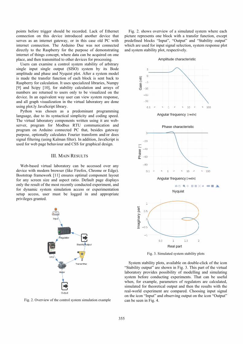
355

points before trigger should be recorded. Lack of Ethernet connection on this device introduced another device that serves as an internet gateway, or in this case old PC with internet connection. The Arduino Due was not connected directly to the Raspberry for the purpose of demonstrating internet of things concept, where data can be acquired on one place, and then transmitted to other devices for processing.

Users can examine a control system stability of arbitrary single input single output (SISO) system by its Bode amplitude and phase and Nyquist plot. After a system model is made the transfer function of each block is sent back to Raspberry for calculation. It uses specialized libraries, Numpy [9] and Scipy [10], for stability calculation and arrays of numbers are returned to users only to be visualized on the device. In an equivalent way user can view system response, and all graph visualization in the virtual laboratory are done using plot.ly JavaScript library.

Python was chosen as a predominant programming language, due to its syntactical simplicity and coding speed. The virtual laboratory components written using it are web-server, program for Modbus RTU communication and program on Arduino connected PC that, besides gateway purpose, optionally calculates Fourier transform and/or does signal filtering (using Kalman filter). In addition, JavaScript is used for web page behaviour and CSS for graphical design.

III. MAIN RESULTS

Web-based virtual laboratory can be accessed over any device with modern browser (like Firefox, Chrome or Edge). Bootstrap framework [11] ensures optimal component layout for any screen size and aspect ratio. Default page displays only the result of the most recently conducted experiment, and for dynamic system simulation access or experimentation setup access, user must be logged in and appropriate privileges granted.

Fig. 2. Overview of the control system simulation example

Fig. 2. shows overview of a simulated system where each picture represents one block with a transfer function, except predefined blocks “Input”, “Output” and “Stability output” which are used for input signal selection, system response plot and system stability plot, respectively.

Fig. 3. Simulated system stability plots

System stability plots, available on double-click of the icon “Stability output” are shown in Fig. 3. This part of the virtual laboratory provides possibility of modelling and simulating system before conducting experiments. That can be useful when, for example, parameters of regulators are calculated, simulated for theoretical output and then the results with the real-world experiment are compared. Choosing input signal on the icon “Input” and observing output on the icon “Output” can be seen in Fig. 4.

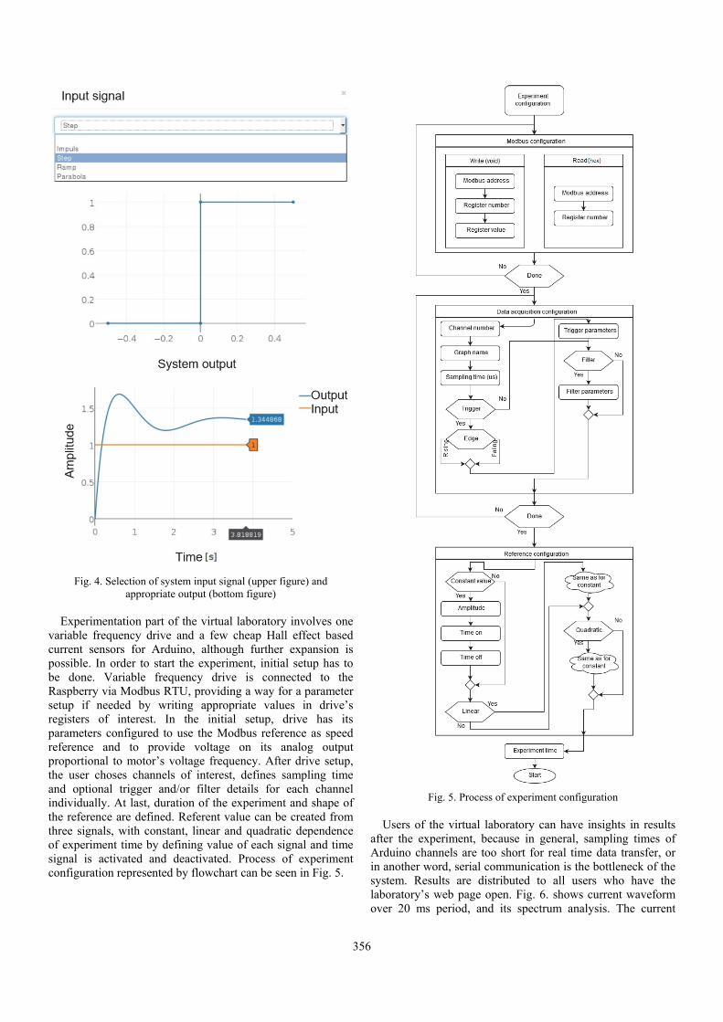
356

Fig. 4. Selection of system input signal (upper figure) and appropriate output (bottom figure)

Experimentation part of the virtual laboratory involves one

variable frequency drive and a few cheap Hall effect based current sensors for Arduino, although further expansion is possible. In order to start the experiment, initial setup has to be done. Variable frequency drive is connected to the Raspberry via Modbus RTU, providing a way for a parameter setup if needed by writing appropriate values in drive’s registers of interest. In the initial setup, drive has its parameters configured to use the Modbus reference as speed reference and to provide voltage on its analog output proportional to motor’s voltage frequency. After drive setup, the user choses channels of interest, defines sampling time and optional trigger and/or filter details for each channel individually. At last, duration of the experiment and shape of the reference are defined. Referent value can be created from three signals, with constant, linear and quadratic dependence of experiment time by defining value of each signal and time signal is activated and deactivated. Process of experiment configuration represented by flowchart can be seen in Fig. 5.

Fig. 5. Process of experiment configuration

Users of the virtual laboratory can have insights in results after the experiment, because in general, sampling times of Arduino channels are too short for real time data transfer, or in another word, serial communication is the bottleneck of the system. Results are distributed to all users who have the laboratory’s web page open. Fig. 6. shows current waveform over 20 ms period, and its spectrum analysis. The current

357

waveform represents noise present during acquisition while no current passes through the current sensor. Although it might seem as a large amplitude of noise, the current sensor has rated current of 30 A, and noise of up to 0,3 A represents 1 % of rated current error, and manufacturer defines this error to be 1,5 % at 25 °C for used current sensor ACS712 [12].

Fig. 6. Waveform of recorded current (raw and filtered) and spectral analysis of filtered current

There is also a possibility of viewing live-stream video of

the experiment using a USB camera attached to the used PC, but its usefulness can be a subject of discussion. For stream functioning, YouTube streaming service is used, and embedded inside the laboratory’s web-page. This enables recording of experiment’s video besides graphs, but this video has unpredictable lag, from 10 to 20 seconds, which makes it difficult to connect exact moments in the conducted experiment on video and graphs.

The WAMP lacks disconnect fall-back procedures and that requires from the user to manually refresh the web page after internet connection problems. Although experiments now have defined running time given on their setup, if later virtual laboratory expansions include real time commands over the internet, this could mean a time period of lost control over system when proper internet connection is not established. In that case, further safety procedures must be taken for ensuring equipment safe operation. Modern browsers are required for establishing WAMP connection (browser like Internet Explorer 9 and earlier versions do not satisfy this requirement) but this is not a problem for common users.

IV. CONCLUSION

Conducting experiments on the real equipment over the internet can be beneficial for students in a way that they can test newly formed knowledge without paying attention to motor wiring, frequency converters and measurement equipment. Laboratories can be more accessible to all students, and live experiments can even be conducted during teaching classes. Their realization is not too expensive, and in this case, added hardware parts for virtual laboratory realization (Raspberry Pi and Arduino with sensors) represent the cheapest part (with combined price just over 80 €).

Laboratory precision of the measured data is not primary concern, and if greater precision or faster sampling times are required, it can be achieved using dedicated microcontroller boards or cards for data acquisition or by using sensors of greater quality. The laboratory itself can be a subject of experimentation, whether with improving existing software or hardware.

Does this mean that traditional approach with laboratory experimentation is obsolete? No, because this type of laboratories can provide easier access to endpoints of experiment (initial parameter setup and results), but not to physical creation of experiment. Physical setup of some experiment is part of the education. This type of laboratories can be a supplement to an engineer’s practical education but not its central part.

REFERENCES

[1] J. Bermúdez-Ortega, et al., "Remote Web-based Control Laboratory for Mobile Devices based on EJsS, Raspberry Pi and Node.js", IFAC-PapersOnLine, vol. 48, no. 29, pp. 158-163, 2015.

[2] J. Sobota, et al., "Raspberry Pi and Arduino Boards in Control Education", IFAC Proceedings, vol. 46, no. 17, pp. 7-12, 2013.

[3] P. Reguera, et al., "A Low-cost Open Source Hardware in Control Education. Case Study: Arduino-Feedback MS-150", IFAC-PapersOnLine, vol. 48, no. 29, pp. 117-122, 2015.

[4] P. Jamieson, and J. Herdtner, "More Missing the Boat—Arduino, Raspberry Pi, and Small Prototyping Boards and Engineering Education Needs Them", 2015 IEEE Frontiers in Education Conference (FIE), 2015.

[5] S. Ferdoush, and X. Li, "Wireless Sensor Network System Design using Raspberry Pi and Arduino for Environmental Monitoring Applications", Procedia Computer Science, vol. 34, pp. 103-110, 2014.

[6] "Variable Speed Drives - Altivar 71 | Schneider Electric", Schneider-electric.com, 2017. [Online]. Available: http://www.schneider-electric.com/en/product-range/1155-altivar-71/. [Accessed: 01- Apr- 2017].

[7] "Crossbar.io", Crossbar.io, 2017. [Online]. Available: http://crossbar.io. [Accessed: 01- Apr- 2017].

[8] "The Web framework for perfectionists with deadlines | Django", Djangoproject.com, 2017. [Online]. Available: https://www.djangoproject.com/. [Accessed: 03- Apr- 2017].

[9] "NumPy — NumPy", Numpy.org, 2017. [Online]. Available: http://www.numpy.org/. [Accessed: 03- Apr- 2017].

[10] "SciPy.org — SciPy.org", Scipy.org, 2017. [Online]. Available: https://www.scipy.org/. [Accessed: 03- Apr- 2017].

[11] Mark Otto, "Bootstrap · The world's most popular mobile-first and responsive front-end framework.", Getbootstrap.com, 2017. [Online]. Available: http://getbootstrap.com/. [Accessed: 10- Apr- 2017].

[12] Allegromicro.com, 2017. [Online]. Available: http://www.allegromicro.com/~/media/Files/Datasheets/ACS712-Datasheet.ashx. [Accessed: 11- Apr- 2017].

358

Studying the Process of Analogue and Digital Modulation Stanio Kolev1, Veska Georgieva2, Lyubomir Laskov3 and Kalin Dimitrov4

Abstract – The study of communication systems is largely based on signals and systems theory. An important objective in modulation is to produce a signal whose frequency range is suitable for transmission over the communication channel to be used. This paper presents an approach for studying the process of the main types of modulations of low and higher order. By using of computer simulations in MATLAB environment different types of modulation can be deep analyzed. It can be used for educational purposes in engineering education.

Keywords – Analog and digital modulation, signal and systems, signal processing, MATLAB.

I. INTRODUCTION

The modulation is a very important part of telecommunications. Practically every transmitter and receiver has a modulator and demodulator. That is why it is extremely important and should be taught in the course "Signals and Systems", which is fundamental for Telecommunications, Computer Systems and Technology, Electronic Engineering and Technology and others. Interesting is the fact that the principle of modulation is borrows from the music. The definition of modulation is that it is a process in which a low-frequency signal is used to control any parameter of another RF signal. One of the main objectives of modulation is by high-frequency signal to carry information long distances. Digital modulation, called manipulations is characterized by the fact, that the signal level changes with a jump as the control signal is digital and takes a value of 0 or 1. There are various types of manipulations of the carrier wave. The change of the symbol of the digital information stream leads to a change of state of one or two parameters of the carrier wave [1-3]. Symbol is 1bit or group of bits that are transported from the 1 position of the carrier wave. The binary signal from the base band is converted into radio signals in the frequency band of the communication channel, that is, by the analog signal to transmit digital information on a specific physical environment of communication. There are three main types of modulations in both analogue and digital form: ASK, FSK and PSK [6, 7]. Each stroke of the manipulation of the carrier signal in the three types of modulation are called

symbol, and transmitted to 1bit information and parameters such as amplitude A, frequency f, and phase φ can accept only values that correspond to '0' or '1'. There modulations with 4 8,16,32,64,128 and more conditions corresponding to 2n (for example, 25 = 32), where n is the number of bits which are transmitted [4,8].

The main criteria for evaluation of modulation are: - Efficient using of bandwidth of the communication

channel. It is characterized by a coefficient of utilization of channels (Bit / s / Hz). Normalized speed.

- Minimum required S / N ratio for unerringly reception. - Resistance to selectively collapse of parts of the frequency

range (fading). We propose to use the program code in MATLAB

environment for deep investigations of this process. So, during the exercises, the students will have the possibility to analyze the different types of modulations. They will be able to change the parameters of the generated signals and analyze their influence on the modulated signal. The obtained results can be presented as graphics in the time and the frequency domain.

II. PROBLEM FORMULATION

The process of analog modulation can be described as follows. Let the high-frequency signal has the form [5]:

)0cos(00 tAtS (1)

Modulating signal is mono harmonic:

)cos( tAmtmS (2)

Amplitude modulated signal is:

)0cos()cos(.1(0

ttmAtamS (3)

where m = Am / Ao is the ratio of the modulation. This coefficient takes values between 0 and 1, and in

practice often used values between 0.3 and 0.5. By m>1 is obtained pre-modulation process. The coefficient of modulation can be determined practically by measured by maximum and minimum values of the amplitude of the carrier signal, using the following formula:

minmax

minmaxAA

AAm

(4)

When the initial phases are not taken into account, which does not diminish the validity of the expression, we can obtain for amplitude modulated signal[9]:

tmA

tmA

tAtamS )0cos(2

0)0cos(2

0)0cos(0 (5)

This expression shows the composition of the spectrum. The digital modulation is most used in the modern

communications systems, so they will be discussed a little more detailed than the analog. Digital modulation (or

1Stanio Kolev is with the Faculty of Telecommunications atTechnical University of Sofia, 8 Kl. Ohridski Blvd, Sofia 1000,Bulgaria, E-mail: [email protected]

2Veska Georgieva is with the Faculty of Telecommunications atTechnical University of Sofia, 8 Kl. Ohridski Blvd, Sofia 1000,Bulgaria, E-mail: [email protected]

3Lyubomir Laskov is with the Faculty of Telecommunications atTechnical University of Sofia, 8 Kl. Ohridski Blvd, Sofia 1000,Bulgaria, E-mail: [email protected]

4 Kalin Dimitrov is with the Faculty of Telecommunications atTechnical University of Sofia, 8 Kl. Ohridski Blvd, Sofia 1000,Bulgaria, E-mail: [email protected]

359

manipulation) is a method for converting a digital BBS signal into a high-frequency analog modulated signal, which is suitable for transmission in the communication channels through stepped change (SK, Shift Keying) of the amplitude, frequency and / or phase of the carrier signal (ASK, FSK, PSK). In most cases this modulation works by the most efficient using of the spectrum (The maximum transmitted bits at 1 Hz). An important parameter is the BR (Band Rate): BR = Rb/BWSK, where BWSK is the bandwidth of the modulated digital signal. In general, however, these signals require less bandwidth and therefore additional treatments for narrowing the spectrum are needed (for example filtration). The latter, however, leads to undesirable effects parasitic AM modulation and ISI.

Fig. 1. Basic block diagram of modulation

The modulated signal (PBS, Pass-Band Signal) is obtained by non-linear mixing of a signal in a main band with a carrier signal (at high frequencies it is most common analog harmonic signal:

. )2cos()( c fctCmtC (6)

The modulation is divided into analog and digital (manipulation) depending on the type of BBS signal. The information from the BBS can be obtained by each of the three main parameters of the carrier signal amplitude Cm, fc frequency or phase φc.

The simplest type of PSK modulation is BPSK, in which the bits "0" and "1" are transmitted with two phase states of the carrier signal in 180 and 0 degrees, respectively.

Fig. 2. BPSK modulation

Doubling of the transmission rate of the manipulated signal (and the necessary bandwidth) is obtained by QPSK (Quadrature PSK) modulation, where the bits are transmitted in pairs (00, 01, 10, 11) with a 4 phase states of the carrier 90 degrees, which is shown in fig.3. In order to avoid unwanted jumps 180 degrees (eg. in the transmission

of a group of bits 0010), where there are parasitic AM modulations using OQPSK modulation with displacement of the odd and even bits of 45 degrees.

Fig. 3. QPSK (Quadrature PSK) modulation

III. EXPERIMENTAL PART

To obtain an analog amplitude modulated signal, the ‘ammod’ function (x, Fc, Fs) can be used. Initially, students can set the following basic parameters: modulation signal x, sampling frequency Fs and carrier frequency Fc. The amplitude and frequency of the modulation signal can be changed. Alternatively, a multichannel signal matrix can be used, where each column of the matrix represents one channel. The vector y represents the modulated signal. In Fig.4 are shown the input signal x(t) and the modulated signal y(t) in time domain, when the index of modulation is m = 0.5 and frequencies of input and carrier signals are fi = 10 kHz and f0 = 500 kHz respectively.

Fig. 4. An example of analog amplitude modulation In Fig. 5 is shown an example of amplitude modulated

signal, which is obtained by the use of a high frequency modulating signal (fi = 25 kHz).

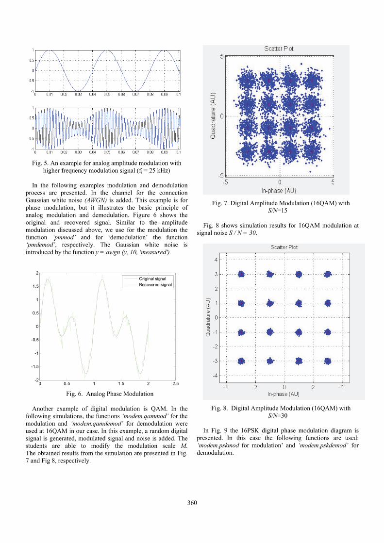
360

Fig. 5. An example for analog amplitude modulation with

higher frequency modulation signal (fi = 25 kHz)

In the following examples modulation and demodulation process are presented. In the channel for the connection Gaussian white noise (AWGN) is added. This example is for phase modulation, but it illustrates the basic principle of analog modulation and demodulation. Figure 6 shows the original and recovered signal. Similar to the amplitude modulation discussed above, we use for the modulation the function ‘pmmod’ and for ‘demodulation’ the function ‘pmdemod’, respectively. The Gaussian white noise is introduced by the function y = awgn (y, 10, 'measured').

0 0.5 1 1.5 2 2.5-2

-1.5

-1

-0.5

0

0.5

1

1.5

2

Original signalRecovered signal

Fig. 6. Analog Phase Modulation

Another example of digital modulation is QAM. In the

following simulations, the functions ‘modem.qammod’ for the modulation and ‘modem.qamdemod’ for demodulation were used at 16QAM in our case. In this example, a random digital signal is generated, modulated signal and noise is added. The students are able to modify the modulation scale M. The obtained results from the simulation are presented in Fig. 7 and Fig 8, respectively.

Fig. 7. Digital Amplitude Modulation (16QAM) with S/N=15

Fig. 8 shows simulation results for 16QAM modulation at

signal noise S / N = 30.

Fig. 8. Digital Amplitude Modulation (16QAM) with S/N=30

In Fig. 9 the 16PSK digital phase modulation diagram is

presented. In this case the following functions are used: ‘modem.pskmod for modulation’ and ‘modem.pskdemod’ for demodulation.

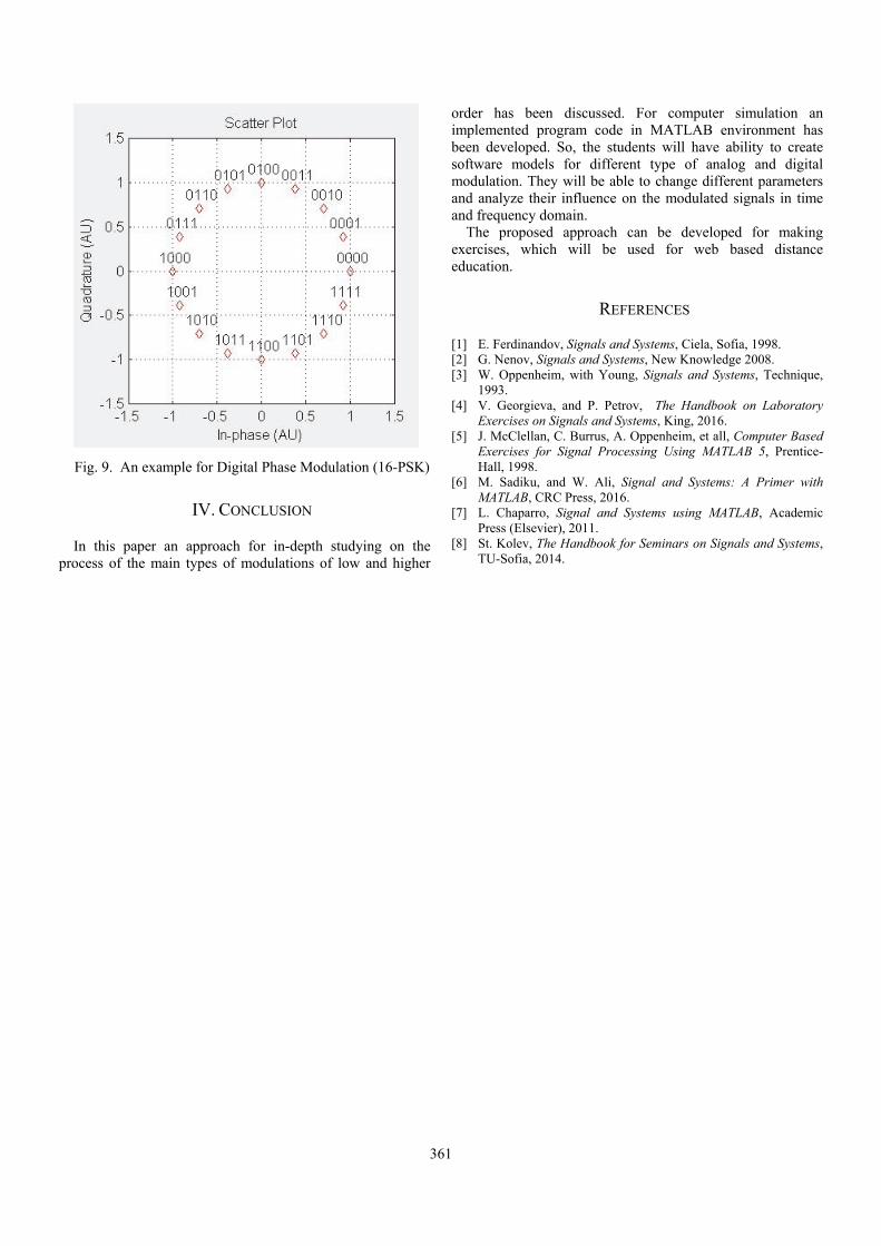
361

Fig. 9. An example for Digital Phase Modulation (16-PSK)

IV. CONCLUSION

In this paper an approach for in-depth studying on the process of the main types of modulations of low and higher

order has been discussed. For computer simulation an implemented program code in MATLAB environment has been developed. So, the students will have ability to create software models for different type of analog and digital modulation. They will be able to change different parameters and analyze their influence on the modulated signals in time and frequency domain.

The proposed approach can be developed for making exercises, which will be used for web based distance education.

REFERENCES

[1] E. Ferdinandov, Signals and Systems, Ciela, Sofia, 1998. [2] G. Nenov, Signals and Systems, New Knowledge 2008. [3] W. Oppenheim, with Young, Signals and Systems, Technique,

1993. [4] V. Georgieva, and P. Petrov, The Handbook on Laboratory

Exercises on Signals and Systems, King, 2016. [5] J. McClellan, C. Burrus, A. Oppenheim, et all, Computer Based

Exercises for Signal Processing Using MATLAB 5, Prentice-Hall, 1998.

[6] M. Sadiku, and W. Ali, Signal and Systems: A Primer with MATLAB, CRC Press, 2016.

[7] L. Chaparro, Signal and Systems using MATLAB, Academic Press (Elsevier), 2011.

[8] St. Kolev, The Handbook for Seminars on Signals and Systems, TU-Sofia, 2014.

362

Сreating Laboratory Models for Auto Backup Power Ginko Georgiev, Silviya Letskovska, Kamen Seymenliyski and Pavlik Rahnev

Abstract –This article is presented the design and implementation of a laboratory model of the panel automatic start of reserve (AVR). The model manages switching switches from primary to backup power.

Keywords – Panel AVR, Backup power, Relay time, Frequency

inverter.

I. INTRODUCTION

The electrical supply system for industrial enterprises (ESSIE) is a set of devices used for generating, transferring and distributing electricity. The purpose of ESSIE is to supply electrical consumers.

The main schemes for ESSIE are: external and internal schemes, industrial units distribution networks for low voltage.

The type of the scheme depends on: the size and type of enterprise; the category of the electrical consumers; the amount of power consumption; the location of the enterprise and the type of electrical consumers.

The requirements for the schemes are to be: dependable; flexible and adaptable (to different modes of work); economical; with high quality power (voltage); convenient and safe to operate with; with the possibility of expansion and development.

By provision of electricity the electricity consumers are divided into four categories - null, first, second and third.

The null category is reserved for those electricity consumers, where an electrical blackout could threaten the life and health of people, cause a threat to national security, cause property damage, cause disruption of complex technological processes, disturbance of vital economic facilities, communication systems and TV.

First category consumers are those, in which power failure leads to considerable material losses, poor mass production and the disruption of a complex technological process. The second category of consumers are those in which the power outage creates a halt in mass production, a downtime for workers, facilities and industrial transport and also disrupts the normal living conditions for a large number of people. The third category of consumers are all the consumers who do not fall in the previous categories [1, 3, 6].

The electrical power supply can be performed:

Fig. 1. Electrical power supply

By getting power from one power source, for consumers "2" and "3" category – (Fig. 1);

By getting power from two power sources - circuit ARA (Automatic Reserve Activation) to consumers of "0" and "1" category (Fig. 2).

Fig. 2. Electricalcircuit with two power sources Automation in power supply systems of industrial

enterprises is being realized with different technical solutions. Among them are the so called automatic reconnection devices (AR); automatic current and frequency discharge devices (ACD, AFD) and devices for automatic switching to backup power and equipment (ABP).The automatic start of the backup power reserve (ABP) is implemented through different technical approaches. The circuit solutions for the realization of ABP are very diverse, and so is their physical performance. The choice of a particular solution depends on the idea of the designers, the requirements from the investors and the existing element base.An ABP panel is a panel that provides an automatic start of the Reserve or automatically switches to backup power. It comes down to electrical installations, which must provide unobstructed continuous operation of electrical equipment in hospitals, airports, mines, factories with continuous uninterrupted work cycles, gas stations, anywhere, where an electrical power supply outage would endanger the lives of people, would cause mass production accidents or loss of materials and data [1, 2].

1Ginko Georgiev - Burgas Free University, San Stefano 62, 8000Burgas, Bulgaria, E-mail: [email protected]

1Silvija Letskovska - Burgas Free University, San Stefano 62,8000 Burgas, Bulgaria, E-mail: [email protected]

1Kamen Seimenliyski –Burgas Free University, San Stefano 62,8000 Burgas, Bulgaria, E-mail: [email protected]

2Pavlik Rahnev – Technical College, As. Zlatarov University, Y. Yakimov 1, Burgas 8010, Bulgaria, E-mail: [email protected]

POWER SOURSE

SWITCH

AIR WIRE

MDS 6-20 KV

MAIN DISTRIBUTIONSUBSTATION

POWER SOURSE

MDS

ARS(AUTOMATIC RESERVE ACTIVATION)

6-20 KV

363

Fig. 3. (a) Block and one-line diagram of the panel This is done by building a bridge, connecting the currently

used electrical network to another one, independent of the first network or by connecting to a backup generator of electricity. Namely the connection between the two networks or between the network and the generator is achieved via a panel ABP.

The ABP is a system of circuit breakers and an electronic component, which monitors the status of the network using predefined data and if necessary restores power by switching to the reserve power supply in case of an emergency power outage or a shutdown caused by a mistake.

If a network doesn’t have a built ABP board, then one is designed and built individually for each network. There may be full backup or part backup. The full backup can power the whole site.

The part backup supplies only the important components and excludes some of the non-vital consumers.

This can be done manually or automatically by changing the program settings of the ABP board.

For example, in the case of a gas station voltage outage, the fuel dispensers, the cash register area and the alarm installation would continue to work, everything else which is unnecessary - coffee machines, storage lighting would not be powered by the ABP panel.

As another example, in a hospital, the operating room would obviously have to work with full equipment.

Upon restoration of the operating voltage, the ABP panel should work in reverse order and shut off the backup power

reserve as to prevent a circuit overload or machinery and equipment shutdown.

The ABP panel must have monitoring systems including an ammeter, a voltmeter, LED status indication and a microprocessor to control the workflow of all systems in the device.

The ABP panel must have a mechanical and electrical interlock, which prevents shifting and simultaneous electrical supply from both sources and must provide an automatic start and stop in case of power outage or restoration.

The ABP panel designs and physical implementations are as diverse as the objects to which they apply.

II. DESIGN AND IMPLEMENTATION OF A LAB

MODEL OF THE ABP PANEL

A. Scheme Implementation Modern training of students in the engineering and science

fields requires the use of models and installations intended for gaining practical skills.

As a result of that, a lab model of the ABP panel has been created for students studying in specialties Engineering and Electric Supply.The model aims to control circuit breakers - switching from primary to backup power [4, 5, 7].

For the creation of the lab model, a “TEPO” type panel has been used - size 60/66 cm.

Tbeen

F

the

B

EoutaHHrese

Tconvolt

Tin actipass

Tpan

T

ownT

The followingn mounted in Frequency inPower supplPLC LOGOPhase monitoTime relay „Relay „Р” – Automatic ci/shutdown/; Automatic c1P; Terminal bloConductors f

Fig. 3a showsscheme realiz

B. Principle of

Established laage from 20

H in the main erve power suThe designed ntrol panel oftage and time.

The minimal vcase of a divates and stased.

There are sevnel:

External voltand LOGO!Voltage 24Velements in tVoltage 220V

The frequencyn. The working a

Relay proteoutage activastate to OFF

g electronic cthe panel:

nverter - SIEMy 220V/24V -! SIEMENS; oring relay – R

„ВР 1”, ”ВР2”1 piece; ircuit breaker

circuit breaker

ocks; for conductivi

Fig. 3. (b) Sch

s an arrangemzation.

f Operation of

aboratory settkV circuit brscheme and

upply from a dpanel is linkef the genera. voltage and thecline in thearts working

veral power

tage 220V forPOWER;

V DC from LOthe panel V, received fr

y inverter uses

algorithm is asction ROCONates circuit br;

components a

MENS MICRO- LOGO! SIEM

RM4TG20 Sc” – 2 pieces;

with a fault r

rs NOARK25

ity.

heme realization

mentof the pan

f the ABP Pan

ting simulatereaker, shuts turns on circu

diesel generatoed to a diesetor two vari

he starting time voltage theafter a certai

sources in th

r supplying a F

OGO!POWER

rom the generas 220V, as fo

s follows: N RFI 421

reaker СН SF1

and materials

OMASTER 42MENS POWE

chneiderelectr

registration mo

5A, 16А 3P и

n

nel. Fig. 3b s

nel

es primary poff circuit bruit breaker Hor. l generator. Iables are fix

me are adjustede diesel genein time period

he terminal b

Frequency Inv

R for supplyin

ator. or DC 24V us

in case of p1 and it chang

364

have

20; ER;

ric;

odule

и 40А

shows

power reaker

HH on

In the xated:

d, i.e. erator d has

block

verter

ng the

ses its

power ges its

C.

Inwas

Circuit breakgives signal toterminal А1 (to circuit breaTime Relay 2LOGO!; After the consends a signalQ1 triggers thfor the time 1+24V to termQ4 sends 220Q4 sends 220signal to motturns off); Time relay Вof LOGO! anThe frequencyIf everything receives at L1input I2, whilvoltage 220VQ2 receives ato relay Р; Relay Р turngenerator is tucircuit; Input I3 is awdoesn’t receivtime period olamp 4 lights Experimenta

n the setting carried out:

Sending a source. Grshows the p

Fig. 4. Green

Disconnectionactivation of frequency regdelay period activation of supply is resto

ker SF1 throuo terminal 48,(+24V voltageaker SF1 on te2 after activat

ntroller receivl to outputs Qhe coil of the 1 with a delay

minal 15 to the 0V to lamp 5; 0V to terminaltor movement

ВР 1 sends signd to DIN of fry inverter staris okay with

1,L2,L3 normle it opens Q2

V; a signal from I

ns on lamp 3urned on norm

waiting signalve normal vo

of 10 secs. In tup ”NOT RU

al Results

presented ab

220 V powerreen indicatorpresence of a

n indicator 1 “M

n from the f an alarm. Rgulator reads starts, whichthe diesel en

ored in the me

ugh block A, while it relaye from the panerminal 25); tion sends sig

es a signal th1 и Q4; relay for the

y of 0” sec aphase monito

l 46 (terminalt of main circu

gnal simultanerequency regurts diesel accethe diesel gen

mal voltage and2. The output

I2 , after whic

, which showmally and supp

l, which it wioltage from ththat case a sig

UNING” and a

ove the follo

r supply fromr 1 on the pamain power s

MAIN POWER P

main power

Red indicator „0”. In this

h aims to prengine, in caseeantime (Fig.

larm terminay for the time nel model is g

gnal to input I

hrough input I

time period rand sends a sioring relay ;

l 46 sends a 2uit breaker НН

eously to inpuulator; leration; nerator, then Pd sends a sign

is with opera

ch it sends a si

ws that the diplies the elect

ll receive if Rhe generator gnal is sent toalso lamp 7.

owing experim

m the main poanel lights upupply (Fig. 4)

RESENTED”

supply with 2 lights up. moment the

event unnecese the main po5).

l 26 2 to

given

I4 of

I4, it

relay ignal

220V Н, it

ut I3

PM4 nal to ating

ignal

iesel trical

RM4 in a

o Q3,

ment

ower p. It ).

the The time

ssary ower

Fig. 5. Re

The frequencstarts up. This imitated finduction mo

Fi

F

After reachinmotor has recapacitors, ithas activated3 lights up, light indicato(Fig. 8).

ed indicator 2-a

cy inverter is he light indicatfrom the comotor”(Fig. 6).

ig. 6. DIESEL A

Fig. 7. ”DIESEL

ng a certain roeached its maxt has reachedd its circuit brthe measured

or shows the

alarm “NO MAI turned on and

tor is still redmbination “fre

ACCELERATI

ACCELERATIO

otation frequeximum becausd its nominal vreaker. The grd voltage is 2still missing m

N POWER”

d the diesel en. The diesel enequency inve

ION

ON”

ency, the induse of the connvoltage 230 Vreen light indi230 V and thmain power su

365

ngine ngine rter -

uction nected V and icator

he red upply

Thinstaknowand automon tfuncpowerelayRecokV sto a usag

[1]H

[2]E

[3]I

[4]

[5]

[6]

[7]

Fig. 8

With restoratgenerator stogradual coolin

he proposed allation that wledge and sk

managementmatization.Ththe stages oftioning of ther supply in cy protection ononnection) devside, activatiobackup powe

ge and restorat

I. Boldea, andHandbook 2nd I.V. ZhezheleElektroenergies1986. A. Fyodorov, Industrial, SofiSchneider ElecTechnical catalSchneider EleTechnical catalVl. Kluchev, T1987. Schneider Eleавтоматизация

8. System is pow

tion of the mps after a ceng of the diese

III. CO

lab setting grants stude

kills in the elet of electricahey create thef the processe electrical ncase of an emn 20 kV side,vice, turning

on of an emerer supply, wortion of the ma

REFER

d S.A. Nasar, ed., 2002.

enko, V. Bozhs in Industria

N. Vassilev, ia, Technique 1ctric Bulgaria, log, 2014. ectric Bulgarialog, 2014. Teorija na elec

ectric Bulgariaя, 2014.

wered by back-

main power sertain time peel generator is

ONCLUSION

is a very ents the oppectric supply fal networks e working alg. They get f

network whenmergency black

verification ooff main circu

rgency diesel rk during backin power supp

RENCES

The Induction

hko, M.L. Rl Plants, Kiev

and S. Side979. Apparatus fo

a, Electrical

ctrozadvijvanet

, Ръководство

-up supply

supply the dieriod, by whis being imitate

useful electportunity to field - monitoand partly torithm depenfamiliar withn there is a mkout - turningof AR (Automuit breaker onengine, switckup power suply.

n Machines De

Rabinovich, Quv: Vishcha Sch

erov, Electricit

or medium vol

installation g

to, Sofia, Tech

о за решения

iesel ch a ed.

trical gain

oring their

nding h the main g off matic n 0,4 hing

upply

esign

uality hool,

ty of

ltage,

guide,

hnica,

я по

366

Laboratory Classes for Saved Emissions of Greenhouse Gases

Silviya Letskovska, Kamen Seymenliyski, Ginko Georgiev and Pavlik Rahnev

Abstract – In this article a web based laboratory for the production of green energy is presented. The laboratory equipped with meteorological system. The laboratory site is created with the ability to receive and display information in real time. This includes not only the weather characteristics and generated electricity but also saved emissions of greenhouse gases.

Keywords – Teaching laboratory, Meteorological system,

Electricity, Emissions of greenhouse gases.

I. INTRODUCTION

In the beginning of 2010 already act lots of international agreements, which charge most of the countries with national indicative goals to reduce the greenhouse gas (GHG) with concrete values. The final goal of the world forces is to oppose the global heat with reaching of the determined concentration of the greenhouse gas in the atmosphere and stabilizing of this proportion for possible longer period of time.

The Kyoto Protocol determines the six GHG emissions with the increased concentration in the atmosphere accelerate global warming. The targets apply to the four greenhouse gases carbon dioxide (CO2), methane (CH4), nitrous oxide (N2O), sulfur hexafluoride (SF6), and two groups of gases, hydrofluorocarbons (HFCs) and perfluorocarbons (PFCs) as well as sulfur dioxide (SO2). The six GHG are translated into CO2 equivalents in determining reductions in emissions. For comparison of the different GHG their different force to accelerate the global warming Intergovernmental Panel on Climate Change (IPCC, 2007) create index called „global warming potential” (GIP).

The Protocol defines three "flexibility mechanisms" that can be used by Annex I Parties in meeting their emission limitation commitments. The three mechanisms are: Clean Development Mechanism (CDM), Joint implementation (JI) and International Emissions Trading (IET). They help investment in new technologies, ecology equipment and modernization of the energy sector. Clean Development Mechanism (CDM) is pointed to countries accepted the concrete commitments for reducing GHG emissions. Often the project under CDM is connected with activities for installation of renewable energy sources.

Increasing the use of the renewable sources in global scale is on the way for decreasing the consequences of the problem.

In Bulgaria, sector “Energy” the biggest part of GHG emissions has burning processes for the production energy – 68% of the emission total in the sector. During 2010 this observed the increasing of the GHG emissions with 2159.4 Gg CO2 - equivalents compared with 2009. European Emissions Trading scheme trade is Mechanism for limitation the volume of the GHG emissions. The system allows to trade which guaranties that the common emissions are kept under the limited value. The energy, generated from photovoltaics could be accepted as ecology pure. The building of Burgas Free University has its own PV – system.

That is way it can be certified with “white certificate”. This document ratified reducing of the energy consumption, which is reached by enterprises (energy producer, suppliers or distributers) in the energy market. In conception with direct connected conception for emission trade, this certificate must guaranty that the common goal for energy economic is reached. The emission factors are coefficients, which determine the quantity of emission for unit activity.

Examples for such factors are: quantity carbon dioxide emitted per MWh in consumption of petroleum fuels [tCO2/MW fuel], in consumption of electrical energy [tCO2/MW electrical energy], or consumption of thermal energy [t CO2/MW heat]. The “standard” emission factors, determined by IPCC, cover all emission of CO2, caused by electricity consumption – burning of fuels for electrical energy, thermal energy, for cooling. They are based on the carbon content of each fuel type, on the base of which determines the emission of greenhouse gases. Carbon dioxide is the most important greenhouse gas [1-4].

II. WEB BASED LABORATORY FOR PRODUCTION

GREEN ENERGY FOR EDUCATION

For the needs of the educational process in Burgas Free University (BFU) the system for production of green energy is built. The idea is the students to receive necessary knowledge and skills in the area of the technologies used in renewable energetic. Important moment in their education is the possibility for estimation to assess whether technology used allows the reduction of harmful emissions. The system has possibility to investigate the dependence - pollution panels - work efficiency - emissions safe.

The base elements of the system are: 16 polycrystalline PV - panels with 3800 Wp power for

electrical energy production; 6 polycrystalline PV-panels with 1100 Wp for

experimental investigations, related to providing energy for domestic hot water;

1Silvija Letskovska - Burgas Free University, San Stefano 62, 8000 Burgas, Bulgaria, E-mail: [email protected]

1Kamen Seimenliyski – Burgas Free University, San Stefano 62, 8000 Burgas, Bulgaria, E-mail: [email protected]

1Ginko Georgiev - Burgas Free University, San Stefano 62, 8000Burgas, Bulgaria, E-mail: [email protected]

2Pavlik Rahnev – Technical College, As. Zlatarov University, Y. Yakimov 1, Burgas 8010, Bulgaria, E-mail: [email protected]

367

Inverter – type IBC Serve Master 3300 MV; PV input 450 VDC, max 2×10 A; 100-350 VDC MPP; Output 230 VAC, 50 Hz, Class I, 3300 W/3600 W, 15,5 Amax.

The system is completed with meteorology station – BFU

METEO – the system for monitoring parameters of sun radiation, the ambient temperature and wind speed, which gives possibility to receive and store data for parameters from the sensors, as well as the produced electrical energy for every 5 minutes [5].

The system consist with: power supply - 12V DC, 1А; module for data storage Fronius Datalogger Web; module for sensors connections Fronius Sensor Box; sensor for wind speed Fronius Wind speed Sensor; sensor for sun radiation.

For goal a more effective processing and analyzing of the data received from the system the software package “Meteo” is developed with the next software applications.

A. Created Software Applications QMeteoLogger

The program QMeteoLogger is created, which periodically

reads the status of the sensors and write the data in one or more data base. For this purpose Access и MySQL are used. It is the main instrument for data recording. The program opens the window from which the initial data from meteorological station are presented.

Fig. 1. Main algorithm QmeteoLogger

The program calculates and the saved emissions are introduced into two databases. Using of two databases has a goal storage of the information the problem with one of them.

Fig. 1 shows the algorithm of created program. The first block realizes connection the data logger to

QMeteoLogger. For this purpose data conversion program from a text in a format suitable for database - creates tables with columns time/value. This is realized with the second block. The third unit records in databases.

The whole scheme/algorithm repeats periodically for five minutes.

With the help of this program realized connection with data logger, and for this purpose there is transformation of data for the program from the text to format suitable for database – creation of tables with columns – time/value. The data are rerecorded and the algorithm repeats periodically in five minutes.

The connection with the local Access BD is done with the use of Open Database Connectivity (ODBC) driver and OLE DB interface for JET storage (standard for ОС WINDOWS).

The main database is on a local MySQL server in Burgas free university, the reserve is a local Access database. It exists and third Microsoft Server database to removed Azure server [7]. B. Created Software Applications Meteo.Logger. AccessViewer and Meteo.Logger. MySQLViewer

With the help of this program the access is performed to the

archived values in the database and allows outputting values of the parameters from the meteorological system in the same program and in Excel file.

The program displays and graphics for the observed parameters for determinate periods of time. It is possible and writing of data in Access database.

Fig. 2. Main algorithm of Meteo.Logger.AccessViewer and

Meteo.Logger. MySQLViewer

The link is added for taking of the reserve copy of Access database. The difference between AccessViewer and MySQLViewer is only on the type of the opened database.

Fig. 2 shows the algorithm of Meteo.Logger.AccessViewer and Meteo.Logger.MySQLViewer.

The description of the algorithm includes: Creating of new database using already existing. Every

open period of time can be recorded as a new Access database;

Download current sensor data

processData

Access Database

MySQL Database

Azure Database

5 minute delay

Save to databases

User Choice

User Timecpan Choice

Download Access database backup from Goodle Drive

Database

Open

User Choice

Generate Chart

Save to Excel file

Save to new

Access database

Save Chart to Excel file

Save Chart to

JPEG

368

Opening of database. The process of opening is done using of Open Database Connectivity (ODBC) driver and OLE DB interface for JET storage. The opened Access tables are stored in the operation memory. This allows their fast and following manipulation before to be written in database. For MySQLViewer is used MySQL driver;

Display period database. The period is loaded into memory and then displayed in tabular form. After this process the data can be recorded in a new database or Excel file recording of period in Excel file. The additional possibility is to add of graphics in Excel file;

Recording of period in new database. This allows creating of several smaller working databases from one bigger. It is possible to be used for other purposes for treatment of the received information;

Withdrawal of the last reserved copy of the Access database from Google Drive. This function allows for every one with the help of Access Viewer to draw the last reserved copy of database;

Output out the graphic for the chosen period. The possibility is created to picture the changes of the parameters for years, months, days. From the table the graphic is generated which is chosen in giving of the command for imagination of the period.

Output complex graphic. There is possibility for creation of complex graphic for chosen periods of time and data table.

C. Creating the Program for Determination and Visualization of the Saved GHG Emissions

Determination of the saved emissions of CO2 in production

of electrical energy using alternative source makes using of an equation:

2/1000pr iE Q f kgCO (1)

where: Qpr – saved electrical energy from renewable energy

source (PV-panels (kW/h); fi – etalon value of the coefficient of the ecology

equivalent of energy sources and energy g CO2/kWh). For electrical energy for CO2 fi = 683 g CO2/kWh [2].

Fig. 3. Web services for meteorological data

On the base of data for the emissions in production of electrical energy from thermal centrals using local lignite coils empiric dependences are done and the etalon values are

determined as follows: fi = 0,0007 g NOx/kWh, and for sulfur dioxide - fi = 0,0035 g SO2/kWh.

For the possibilities to be determined and visualized saved emissions in the time of producing of electrical energy from renewable source the web services were created for meteorological data (Fig. 3).

The server software is written in Service Stack (software package for the C #) and executed on the server of BSU.

The characteristics of the server are: computer ACPI x64-based PC; Operating System Microsoft Windows Server 2012 R2 Datacenter; Internet Explorer 11.0.9600.17416 (IE 11.0.14); 4096 MB system memory. It exists and second MySQL database for removed server.

The written services read database end return specified in the application scope and type of data.

This includes archival and current data from the sensors and data for saved emissions.

In the fact of the lack of open port to the server (lack of direct access to the server) the tunneling service ngrok (ready product accessed in the Internet), which automatically fall if there is present one.

In Fig. 4 archival data for production of electrical energy from PV panels from 04.04.2017 are shown.

D. Creating of Mobile Application for Real Time Data Visualization MeteoRealtimeApp

For the goal of increasing for receiving of information the

application was developed, which derives data in real time from the sensors using FTP server for mediator. Data are in text format. The application is presented for Windows, Linux и Android. Meteo - server read data from meteorological system and suspends them in FTP server. The program reads text data from FTP server, decodes and visualizes.

E. Creating of Web Site of Meteorological Station in Burgas Free University

The web site with the help of ASP.NET packet for web

page and C# for part of the server component is done (Fig. 5) [8].

ASP.NET packet is in accesses for students free of charge via portal Dreemspark.

With this package get the data from the meteorological station stored in a database located in a server of Microsoft.

These data are sent to the graphical interface of the site. To create a site used Bootstrap - software for styling sites

based on HTML/CSS. The site is available at http://bsmeteo.azurewebsites.net/index.aspx.

Web page supports the following functions:

Displays current data on air temperature, wind speed, sun radiation and the production of electricity;

Displays current data on emissions saved the carbon dioxide, sulfur dioxide and nitrogen oxides in the production of electricity with photovoltaic plant.

369

Fig. 4. Data saved emissions and graphic for the production of electricity from photovoltaic panels

Fig. 5. The web site of meteostation

F. Practical Results As a result of introducing in exploitation of the created

program application, creating database received from sensors of the system for production of electrical energy. This database is used in laboratory classes for analyzing the influence of sun radiation onto electricity production and reducing emissions. Using the dependence (1) it could be calculated and visualized saved greenhouse gas emissions. There is a work for introduction of new installations for renewable energy, which will lead to further emission reductions.

III. CONCLUSION

Created software applications for receiving, processing, visualization and archiving of data received from the meteorological station of BFU, as well as calculating and visualization of the saved emissions of greenhouse gases in the work of the PV plant are one good possibility for using modern information technologies in the educational process. The created site weather station gives possibility anyone to have an information in real time not only for meteorological characteristics and energy production and for saved greenhouse gas emissions. The mobile application is a good possibility in real time to give necessary information.

REFERENCES

[1] Kyoto Protocol to the Framework Convention of the United Nations Climate Change, Ministry of Environment and Water, Bulgaria, Prom. SG. 68 of 19.08.2005

[2] Regulation 18/12.11.2004 Еnergy performance of the sites, Ministry of Energy and Energy Resources, Bulgaria.

[3] http://www.rensmart.com/Information/Library/101006-guidelines-ghg-conversion-factors.pdf

[4] S. Letskovska, and K. Seymenliyski, Monitoring System for Evaluation Solar Energy Potential, Burgas Free University, 2014, vol. ХХХ, pp. 208-214.

[5] Peder Vejsig Pedersen, Solar Energy and Urban Pedersen, 2002. [6] Programmer's Heaven C# School Book, 2006. [7] C# Succinctly, 2012.

370

Spectrum Analysis of Analog Signals in MATLAB Environment

Lyubomir Laskov1, Veska Georgieva2 and Stanio Kolev3

Abstract – This paper presents an approach for studying the spectrum analysis of analog signals with various shape forms, by using trigonometric and complex forms of Fourier transformation. An algorithm and its implementation in MATLAB environment have been developed. The implemented software allows studying the spectrum of different analog signals and the influence of signals parameters on its spectrum. The presented approach can be used in engineering education for studying this process.

Keywords – Communication, signal and systems, signal processing, spectrum analyses, detection and identifying of signals, computer simulation, MATLAB.

I. INTRODUCTION

The spectrum analysis of the signals is a basic part in the theory of the telecommunications. It allows each periodic signal to be presented as sum of an infinite number of sinusoidal signals with different amplitudes and initial phase offsets. The spectrum analysis allows to make a deeper study of the signal (distribution of the amplitudes, power, phase shifts, etc.). It also simplifies the understanding and interpretation of the effects of various time-domain operations. The spectrum analysis is widely used in filtration, recognition of signals and noise, restrictions of bandwidth, etc.

The spectrum analysis is studied in the course "Signals and Systems" at the undergraduate course in specialties "Telecommunications", "Computer and Software Engineering" and "Electronics" at Technical University of Sofia. During the seminar exercises the students will have the opportunity to study the spectrum of different periodic and aperiodic analog signals and analyze the amplitude spectrum and phase spectrum of the signals. They will be able to change the signal parameters and analyze their influence on the signal in time and frequency domain.

In order to be able to generate signals with maximum number of different shape forms and to change as much as possible signal parameters, it is proposed to use a program code in the MATLAB environment [1]. The choice of MATLAB over other software products and programming languages is due to the wide range of built-in functions that

will facilitate students, as there is no need to create all these functions from scratch [2]. Writing source code in MATLAB is preferable to the MATLAB Simulink because of the additional features that provide students with ability to change signals in a way that MATLAB Simulink does not provide [3]-[5]. Writing the source code also leads to the requirement that the students will understand the functions describing the calculation of the signal spectrum.


The main tasks to be solved in the spectrum analysis of signals are associated with the variety of signals as types (periodic and aperiodic) and shapes (sinusoidal, rectangular, triangular, sawtooth, Gaussian, etc.), as well as with the usage of the different forms of the Fourier transformation.

Let S(t) is an aperiodic analogue signal, it has the following CFT (Complex Fourier Transformation), given in Eq.1 [6]:

( ) ( ) j tS j S t e dt

(1)

where S(jω) is the Fourier Spectral Density. In general case, it’s a complex function, described with Eq.2 [6]. ( )( ) Re[ ( )] Im[ ( )] ( ) jS j S j j S j S j e (2)

where |S(jω)| is the Amplitude Fourier Spectrum, φ(ω) is Phase Fourier Spectrum

Let S(t) is a periodical analogue signal, the complex form of the Fourier series is described as following [7]:

0( ) jn tnS t C e

(3)

where

0

2

2

1( )

T

jn tn

T

C S t e dtT

(4)

The short trigonometric form of the Fourier series is given with [8]:

00

1

( ) cos( )2 n n

n

aS t A n t

, (5)

where

2 2n n nA a b , (6)

nn

n

barctg

a . (7)

where An is the Amplitude Spectrum, φn is Phase Spectrum. In the Eq. (5) a0 is the constant component of the signal. In the Eq. (6) and (7) with an and bn are labeled the amplitudes of the cosinusoidal and sinusoidal components of the full trigonometric form of the Fourier transformation respectively.

1Lyubomir Laskov is with the Faculty of Telecommunications atTechnical University of Sofia, 8 Kl. Ohridski Blvd, Sofia 1000, Bulgaria, E-mail: [email protected]

2Veska Georgieva is with the Faculty of Telecommunications atTechnical University of Sofia, 8 Kl. Ohridski Blvd, Sofia 1000, Bulgaria, E-mail: [email protected]


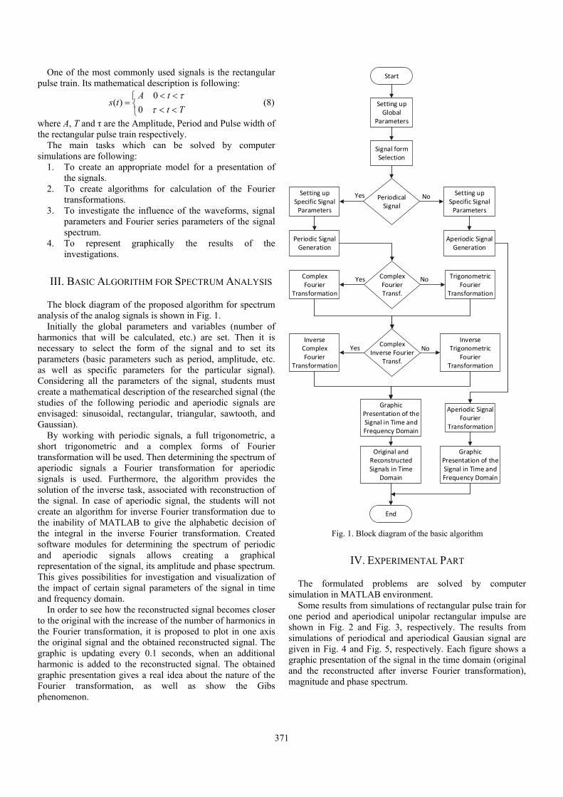
371

One of the most commonly used signals is the rectangular pulse train. Its mathematical description is following:

0

( )0

A ts t

t T

(8)

where A, T and τ are the Amplitude, Period and Pulse width of the rectangular pulse train respectively.

The main tasks which can be solved by computer simulations are following:

1. To create an appropriate model for a presentation of the signals.

2. To create algorithms for calculation of the Fourier transformations.

3. To investigate the influence of the waveforms, signal parameters and Fourier series parameters of the signal spectrum.

4. To represent graphically the results of the investigations.

III. BASIC ALGORITHM FOR SPECTRUM ANALYSIS

The block diagram of the proposed algorithm for spectrum analysis of the analog signals is shown in Fig. 1.

Initially the global parameters and variables (number of harmonics that will be calculated, etc.) are set. Then it is necessary to select the form of the signal and to set its parameters (basic parameters such as period, amplitude, etc. as well as specific parameters for the particular signal). Considering all the parameters of the signal, students must create a mathematical description of the researched signal (the studies of the following periodic and aperiodic signals are envisaged: sinusoidal, rectangular, triangular, sawtooth, and Gaussian).

By working with periodic signals, a full trigonometric, a short trigonometric and a complex forms of Fourier transformation will be used. Then determining the spectrum of aperiodic signals a Fourier transformation for aperiodic signals is used. Furthermore, the algorithm provides the solution of the inverse task, associated with reconstruction of the signal. In case of aperiodic signal, the students will not create an algorithm for inverse Fourier transformation due to the inability of MATLAB to give the alphabetic decision of the integral in the inverse Fourier transformation. Created software modules for determining the spectrum of periodic and aperiodic signals allows creating a graphical representation of the signal, its amplitude and phase spectrum. This gives possibilities for investigation and visualization of the impact of certain signal parameters of the signal in time and frequency domain.

In order to see how the reconstructed signal becomes closer to the original with the increase of the number of harmonics in the Fourier transformation, it is proposed to plot in one axis the original signal and the obtained reconstructed signal. The graphic is updating every 0.1 seconds, when an additional harmonic is added to the reconstructed signal. The obtained graphic presentation gives a real idea about the nature of the Fourier transformation, as well as show the Gibs phenomenon.

Start

Setting up Specific Signal

Parameters

Complex Fourier Transf.

YesComplex Fourier

Transformation

No Trigonometric Fourier

Transformation

Complex Inverse Fourier

Transf.

Inverse Complex Fourier

Transformation

No

End

Periodical Signal

Yes

Aperiodic Signal Generation

Aperiodic Signal Fourier

Transformation

No

Setting up Global

Parameters

Signal form Selection

Periodic Signal Generation


Parameters

Graphic Presentation of the Signal in Time and Frequency Domain


Original and Reconstructed Signals in Time

Domain

YesInverse

Trigonometric Fourier

Transformation

Fig. 1. Block diagram of the basic algorithm

IV. EXPERIMENTAL PART

The formulated problems are solved by computer simulation in MATLAB environment.

Some results from simulations of rectangular pulse train for one period and aperiodical unipolar rectangular impulse are shown in Fig. 2 and Fig. 3, respectively. The results from simulations of periodical and aperiodical Gausian signal are given in Fig. 4 and Fig. 5, respectively. Each figure shows a graphic presentation of the signal in the time domain (original and the reconstructed after inverse Fourier transformation), magnitude and phase spectrum.

372

Fig. 2. Rectangular pulse train for one period and its spectrum

Fig. 3. Aperiodic rectangular pulse and its spectrum

Fig. 4. Gaussian pulse train for one period and its spectrum

Fig. 5. Aperiodic Gaussian pulse and its spectrum

373

In Figs. 6-8 are shown the original and the reconstructed signal in three different stages of reconstruction (represented as a sum of sinusoids with the appropriate amplitude, frequency and initial phase offset). The mathematical description of the reconstructed signals shown on Fig. 6 and Fig. 7 are given in Eq. 9 and Eq. 10 respectively. The mathematical description of the original signal is given in Eq. (8). On each subsequent step (usually by 0,1 seconds) the next harmonic is added to the current state of the reconstructed signal. This continually changing figure shows how with the increase of the number of harmonics that are summed, the reconstructed signal becomes closer to the original.

0

1 0 1( ) cos( )2

0.5 0.637.cos(2 -1.571)

aS t A t

t

(9)

Fig. 6. The original and reconstructed signal by 1 harmonic

Fig. 7. The original and reconstructed signal by 7 harmonics

7001

( ) cos( ) 0.52

0.637.cos(2 -1.571) 0.212.cos(3 -1.571)

0.127.cos(5 -1.571) 0.091.cos(7 -1.571)

n nn

aS t A n t

t t

t t

(10)

Fig. 8. The original and reconstructed signal by 50 harmonics

V. CONCLUSION

In this paper an approach for studying on spectrum of periodic and aperiodic analog signals has been proposed. An algorithm and its implementation in MATLAB environment have been developed. The algorithm provides the solution of the inverse task, associated with reconstruction of the signal.The students can create software models of signals with different forms. They will be able to change the signal parameters and analyze their influence on the signal in time and frequency domain.


REFERENCES

[1] MATLAB, User’s Guide, www.mathwork.com [2] L. Chaparro, Signal and Systems using MATLAB, Academic

Press (Elsevier), 2011. [3] S. Karris, Signal and Systems with MATLAB; Computing and

Simulink; Modeling, Fifth edition, Orchard Publications, 2012. [4] V. Georgieva, S. Lishkov, and D. Dimitrov, "Spectrum Signal

Analysis in MATLAB Environment", ICEST 2005, pp. 738-740, Nish, Serbia and Montenegro, 2005.

[5] В. Георгиева, П. Петров, Сигнали и Системи - ръководство за лабораторни упражнения, Кинг, 2016.

[6] Е. Фердинандов, Сигнали и системи, Сиела, София, 1999. [7] S. Donevska, and B. Donevsky, Advanced Engineering

Mathematics, TU-Sofia, Sofia, 2014. [8] Г. Ненов, Сигнали и Системи, Нови знания, София, 2008.

374

Spectrum Analysis of Digital Signals in MATLAB Environment

Lyubomir Laskov1, Veska Georgieva2 and Stanio Kolev3

Abstract – This paper presents an approach for studying the spectrum analysis of discrete signals with different shape forms, by using Discrete Fourier transformation and Fast Fourier transformation. An algorithm and its implementation in MATLAB environment have been proposed. So by using implemented program code the influence of signals parameters on their spectrum can be deep analyzed. The paper can be used in engineering education for studying this process.

Keywords – Digital signal processing, Spectrum analyses, Computer simulation, MATLAB.

I. INTRODUCTION

The spectrum analysis is widely used in filtration, recognition of signals and noise, restrictions of bandwidth, etc. The development of digital electronics leads to the necessity of creating the equivalent of classical decomposition in Fourier series. In its simple form the Discrete Fourier Transform (DFT) is rarely used because of its computational complexity. A variety of methods to accelerate the computing process of DFT have been proposed, which generalized name is Fast Fourier Transform (FFT) [1].

Some of the commonly used methods for FFT are: time splitting, frequency splitting, Goertzel’s algorithm (by linear filtration), Chirp-z transformation (by using cross correlation), real fast conversion etc. [1].

In the time splitting algorithm the input sequence is divided into one (or two) odd sequences and one (or two) even sequences. This process continues recursively until a plurality of sequences of 2 (or 4) samples each is achieved. Subsequently a 2-point (or a 4-point) operation butterfly have been repeatedly applied. After completing of the calculations at the output the harmonics are obtained. The two-point basic operation is applied when the length of the input string is up to 512 samples. Since the input sequences is longer the performance and the efficiency decreases.

Unlike time-splitting algorithm, in which the harmonics are obtained sequentially, at the frequency-splitting algorithm, the obtained harmonics at the output are divided into a set of even and odd sequences. After completing of the calculations the obtained sequences need to be reordered. In this algorithm the input signal is divided into 2 (or 4) consecutive parts, each of

which is subjected to a basic operation of two (or four) point butterfly. The subsequent separation of the two (or four) sequences to another two (or four) sequences and applying the basic operations continues to be applied recursively, until reaching a sequences of 2 (or 4) samples each. A base operation is applied on these sequences, after which they are fed to the exit as reordered results. The selection of two-point or four-point base operation is analogous as in the case with the time-division algorithm.

The Goertzel’s algorithm is used when only parts of the signal's harmonics will be analyzed. The principle of operation of this algorithm is the separation of the individual harmonics by linear filtering of the input signal. The main advantage of the algorithm is that the number of input samples does not affect the computational complexity [2].

By Chirp-z transformation method an existing methods for fast calculation of cross correlation functions are used. For this purpose, the input sequence will be preliminary modified, and then by fast cross-correlation algorithm will be processed. The result is subjected to further processing in order to obtain a DFT [3].

In cases when the input signals are real, it is possible to obtain a further acceleration of the calculation in the time-splitting and frequency-splitting algorithms. This is done by splitting the actual signal on two signals containing odd and even samples of the original signal. The obtained subsequences are presented as a real and imaginary part of a new signal, which is twice shorter than the original.

The DFT and FFT are studied in the course "Signals and Systems" at the undergraduate course in specialties "Telecommunications", "Computer and Software Engineering" and "Electronics" in Technical University of Sofia. In the labs the students will have the possibility to analyze the magnitude and phase spectrum of discrete signals. They will be able to change the signal parameters and analyze their influence on the signals in time and frequency domain. The students will be able to create the source code, which can generate signals with different form and different parameters, based on their mathematical models. The MATLAB environment has a definite advantage over other software products and other programming languages, because of built-in functions [4], [5]. This would considerably facilitate students in their work.


The main tasks to be solved by spectrum analysis of the signals are the variety of signals as types (periodic and aperiodic) and shapes (sinusoidal, rectangular, triangular, sawtooth, Gaussian, etc.). This paper presents an approach for studying the spectrum analysis of discrete signals with

1Lyubomir Laskov is with the Faculty of Telecommunications atTechnical University of Sofia, 8 Kl. Ohridski Blvd, Sofia 1000,Bulgaria, E-mail: [email protected]

2Veska Georgieva is with the Faculty of Telecommunications atTechnical University of Sofia, 8 Kl. Ohridski Blvd, Sofia 1000,Bulgaria, E-mail: [email protected]


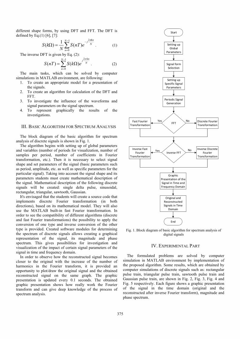
375

different shape forms, by using DFT and FFT. The DFT is defined by Eq.(1) [6], [7]:

1

0

2

)(1

)(N

n

N

knj

enTSN

kS

. (1)

The inverse DFT is given by Eq. (2):

21

0

( ) ( )knN j

N

n

S nT S k e

. (2)

The main tasks, which can be solved by computer simulations in MATLAB environment, are following:

1. To create an appropriate model for a presentation of the signals.

2. To create an algorithm for calculation of the DFT and FFT.

3. To investigate the influence of the waveforms and signal parameters on the signal spectrum.

4. To represent graphically the results of the investigations.

III. BASIC ALGORITHM FOR SPECTRUM ANALYSIS

The block diagram of the basic algorithm for spectrum analysis of discrete signals is shown in Fig. 1.

The algorithm begins with setting up of global parameters and variables (number of periods for visualization, number of samples per period, number of coefficients in Fourier transformation, etc.). Then it is necessary to select signal shape and set parameters of the signal (basic parameters such as period, amplitude, etc. as well as specific parameters for the particular signal). Taking into account the signal shape and its parameters students must create mathematical description of the signal. Mathematical description of the following discrete signals will be created: single delta pulse, sinusoidal, rectangular, triangular, sawtooth, Gaussian.

It's envisaged that the students will create a source code that implements discrete Fourier transformation (in both directions), based on its mathematical model. They will also use the MATLAB built-in fast Fourier transformation. In order to see the compatibility of different algorithms (discrete and fast Fourier transformations) the possibility to apply the conversion of one type and inverse conversion of the other type is provided. Created software modules for determining the spectrum of discrete signals allows creating a graphical representation of the signal, its magnitude and phase spectrum. This gives possibilities for investigation and visualization of the impact of certain signal parameters of the signal in time and frequency domain.

In order to observe how the reconstructed signal becomes closer to the original with the increase of the number of harmonics in the Fourier transform, it is provided an opportunity to plot/draw the original signal and the obtained reconstructed signal on the same graph. The graphic presentation is updated every 0.1 seconds. The obtained graphic presentation shows how really work the Fourier transform and can give deep knowledge of the process of spectrum analysis.

Start


Parameters

FFTYesFast Fourier

Transformation

No Discrete Fourier Transformation

Inverse FFTInverse Fast

Fourier Transformation

No

End

Setting up Global

Parameters

Signal form Selection

Periodic Signal Generation


Original and Reconstructed Signals in Time

Domain

YesInverse Discrete

Fourier Transformation

Fig. 1. Block diagram of basic algorithm for spectrum analysis of digital signals

IV. EXPERIMENTAL PART

The formulated problems are solved by computer simulation in MATLAB environment by implementation of the proposed algorithm. Some results, which are obtained by computer simulations of discrete signals such as: rectangular pulse train, triangular pulse train, sawtooth pulse train and Gaussian pulse train, are shown in Fig. 2, Fig. 3, Fig. 4 and Fig. 5 respectively. Each figure shows a graphic presentation of the signal in the time domain (original and the reconstructed after inverse Fourier transform), magnitude and phase spectrum.

376

Fig. 2. Rectangular pulse train for two periods and its spectrum

Fig. 3. Triangle pulse train for two periods and its spectrum

Fig. 4. Gaussian pulse train for two periods and its spectrum

Fig. 5. Sawtooth pulse train for two periods and its spectrum

377

In Figs. 6-8 are shown the original and the reconstructed signal in three different stages of reconstruction (represented as a sum of sinusoids with the appropriate magnitude, frequency and initial phase offset). On each subsequent step, the next harmonic is added to the current state of the reconstructed signal. This continually changing graphic presentation shows how with the increase of the number of harmonics that are summed, the reconstructed signal becomes closer to the original.

Fig. 6. The original and reconstructed signals by 1 harmonic

Fig. 7. The original and reconstructed signals by 6 harmonics

Fig. 8. The original and reconstructed signals by 50 harmonics

V. CONCLUSION

In this paper an approach for in-depth studying on DFT and FFT has been proposed. An algorithm and corresponding program code in MATLAB environment have been developed. The students will have ability to create software models for discrete signals with different shape forms. They will be able to change the signal parameters and analyze their influence on the signal in time and frequency domain. The proposed algorithm provides the solution of the inverse task, associated with reconstruction of the discrete signal and its graphic presentation.


REFERENCES

[1] V. Ingle, and J. Proakis, Digital Signal Processing Using MATLAB v4, PWS Publishing Company, 1997.

[2] Н. А. Галанина, Д. Д. Дмитриев, Д. И. Ахметзянов, Алгоритм Герцеля для Спектрального Анализа Сигналов, Программные системы и вычислительные методы, No. 4(5), 2013.

[3] O. Alkishriwo, The Discrete Linear Chirp Transform Algorithm and Its Applications, Ph.D. Thesis, University of Pittsburgh, 2013.

[4] L. Chaparro, Signal and Systems using MATLAB, Academic Press (Elsevier), 2011.

[5] S. Karris, Signal and Systems with MATLAB; Computing and Simulink; Modeling, Fifth edition, Orchard Publications, 2012

[6] S. Donevska, and B. Donevsky, Advanced Engineering Mathematics, TU-Sofia, Sofia, 2014

[7] M. Sadiku, and W. Ali, Signal and Systems: A Primer with MATLAB, CRC Press, 2016.

Session PO5:

3B - CONTROL SYSTEMS

381

Certification and Authorisation for Placing in Service of Control-Command and Signalling Subsystems in Bulgaria

Denitsa Kireva-Mihova1 and Kalin Mirchev2

Abstract – The purpose of this article is to review the state-of-play of the verification, assessment and authorisation processes and procedures for the railway structural subsystems CCS (ERTMS) in Bulgaria. Based on a study, the most important issues and discrepancies are highlighted, discussed and provided as outcomes of this review.

Keywords – Railway system, CCS, TSI, Authorisation for

Placing in Service.

I. INTRODUCTION

The European Railway Traffic Management System (ERTMS) is emerging as a global standard for railway signalling regarding train control. It aims at replacing the different national train control and command systems in Europe. ERTMS comprises of the European Train Control System (ETCS), the Global System for Mobile communications - Railway (GSM-R), Traffic Management Systems and operating rules. The technical specifications for ETCS and GSM-R are published in the Control Command and Signalling (CCS) Technical Specification for Interoperability (TSI) [4]. GSM-R provides voice communication for the railways and provides data communication for ETCS.

The specifications for ERTMS at the time being are stable. The European Union Agency for Railways (EUAR or ‘the Agency’) operates an ERTMS Change Control Management of the ERTMS technical requirements to ensure the stability of the specification. It should be noted that testing, certification and authorisation remains a top issue for the smooth deployment of ERTMS.

The term used for Authorisation for Placing in Service (APIS) of a railway structural subsystem changes across the different railway legislation within the European Union (EU). The last definition in force is given by [2] and Table I below.

Looking into the EU legislation (before and following the adoption of the 4th railway package and including TSI CCS [4]) on interoperability and safety and into the EU related recommendations, the following assessment and authorisation entities can be identified:

1) Notified Body (NoBo) 2) Designated Body (DeBo) 3) In-house accredited body 4) Assessment Body, also stated as Risk Assessment

Body (RasBo) 5) Independent Safety Assessor (ISA) (only for CCS

subsystems)

6) Assessment bodies required by the other EU rules relevant for a subsystem to be placed into service (or into the market)

7) Accredited laboratories 8) National Safety Authority (NSA)

TABLE I AUTHORISATION IN ACCORDANCE WITH THE EU RAILWAY

LEGISLATION

Source of legislation Term Definition from the source of

legislation

Directive 2016/797/EU

Authorisation for placing in service of

fixed subsystems

Placing in service means all the operations by which a subsystem is put into its operational service

Authorisation for placing on the market of mobile subsystems

Placing on the market means the first making available on the

Union's market of an interoperability constituent,

subsystem or vehicle ready to function in its design operating

state

Vehicle authorisation for placing on the

market

Here, a role is also taken by the EUAR in the context of the

pre-authorisation of ERTMS track-side projects. In particular, according to the Article 19 of the Directive 2016/797/EU [2], the Agency performs some checks to ensure that the technical solutions envisaged are fully compliant with the relevant TSIs and are therefore fully interoperable. The scope of the aforementioned checks with regards to NoBo tasks is not defined and the risk to have a double check cannot be avoided in full.

II. OVERVIEW OF THE APIS PROCESS WITHIN THE EUROPEAN COUNTRIES

This study shows that the APIS process varies across European countries. Expansion of the study process included Italy, Denmark, France, Poland and Bulgaria.

One common identified issue is the lack of unequivocal definition for new/upgraded/renewed subsystems with clear criteria. A related problem is the identification of the body which decides on the type of the subsystem (new, upgraded or renewed). Italy indicates that this is the Applicant for APIS. In Denmark this could be the NSA, the infrastructure manager and the railway operator but the decision for starting a new APIS procedure is made by the NSA. In Poland the infrastructure manager and the Applicant for APIS are the responsible bodies.

There are no applicable national rules for placing in service of CCS subsystem in Poland and Bulgaria while in Denmark and Italy these exist. This necessitates unification of rules.

There are differences in testing procedures with respect to the role of the NSA. In Bulgaria the NSA participates in the

1Denitsa Kireva is with the Faculty of Telecommunications at Technical University of Sofia, 8 Kl. Ohridski Blvd, Sofia 1000, Bulgaria, E-mail: [email protected]

2Kalin Mirchev is with Tinsa Ltd., 3A Nikolay Haytov Str., Sofia 1113, Bulgaria, E-mail: [email protected]

382

process as a control body involved in the organisation of the process while in the other countries the NSAs do not play a part.

The other common issue is how to proceed with testing a new CCS trackside (Baseline 3) if a certified/authorised vehicle (or at least an on-board CCS, Baseline 3) is not available.

In particular, NoBos have underlined the following priorities:

• Necessity to harmonise the verification/assessment processes put in practice for interoperability assessment developing a common understanding of such processes by the NoBos;

• Not all functions from the System Requirements Specification [6] are implemented and the impact on the integration into a subsystem and also train to track integration is not specified, thus leading NoBos to misunderstandings during assessments;

• Identification of the scope and roles for the different conformity assessment bodies involved in an authorisation process for subsystems, avoiding duplication of work among them;

• Management of specific issues related to an EC verification and conformity assessment like: 1) Management of Subset-076 results from the accredited laboratories (in particular in connection with their approval within the certification process and management of deviations); 2) Management of deviations, restrictions or conditions for use during the assessment/verification tasks and within an authorisation; 3) Practical use of the Recommendations For Use (RFU) to improve their legal validity in order to have common and standardised format for NoBo deliverables.

• The definition of agreed and harmonised approaches to the assessment, especially in case of railway corridors is required.

As feedback from NSAs, the three main problematic areas are:

• Heritage from the past: Some NSAs are confronted with the complexities of managing situations created in the past.

• Work in progress: Some NSAs, when applying correctly the process specified in Directive 2008/57/EC, encounter problems related to the quality of products (not fully compliant with the TSIs) because of several instances of non-conformity of products.

• Planning for the future: Principally, NSAs want to be deeply involved in the whole process leading to authorisation. In some cases NSAs also offer on a ‘voluntary basis’, at the choice of the applicant, a solution whereby the NSA is more involved during the project, with the delivery of intermediate ‘authorisations’ at certain steps of the development/installation.

III. OVERVIEW OF THE VERIFICATION AND ASSESSMENT FRAMEWORK WITHIN AN APIS

PROCESS AND RELATED PROCEDURE IN BULGARIA

The APIS process and all related procedures are regulated in [3], which transposes [1] into the Bulgarian legislation.

Assignment of Different Bodies in Bulgaria

In Bulgaria verification and assessment of a subsystem is usually assigned to the relevant body in two ways, depending on the Contracting Authority (CA):

• In case of the CA is a state structure the assignment is going through a tender procedure, which sets out the technical parameters of the assessment;

• In case of the CA is the subsystem’s manufacturer, the assignment is going through direct selection of an assessment body.

The practice in Bulgaria with infrastructure projects for upgrading or renewal of the railway network shows that NoBo, DeBo and RasBo is most frequently selected and appointed at the beginning of the project.

There was a case where the NoBo was appointed at the end of the project to assess according to inappropriate module, making verification impossible (e.g. module SH1 where the manufacturer, subject to an audit, is no longer available).

Verification/Assessment Process within an Authorisation Framework

Verification and assessment procedures together with relevant roles that comply with Bulgarian legislation are present in the figure below and include the following stages: Stage 1: Appointment of a conformity assessment body for a specific task Stage 2: Definition of the assessment scope Stage 3: Collecting the evidences for the assessment Stage 4: Execution of the assessment Stage 5: Conclusions and issue of the deliverables of the assessment.

Stage 1: Appointment of a conformity assessment body for a specific task

Activities on verification and assessment of a specific rail project, assigned to a NoBo and/or DeBo and/or RasBo, usually cover the geographical scope of the project’s subsystems, following the scope of the construction/upgrading/renewal. Often, different manufacturers of subsystems construct different parts of a project with common geographical scope and each producer should choose its own assessment body.

Actually, some issues found at the assigning the Conformity Assessment Bodies:

- There is no coordination in assigning the assessment – it is possible different assessment bodies to be appointed by various entities for the same subsystem with a different timetable;

383

- There is no available instructions on who, when and how assigns the assessment of a specific rail system;

- Assessment of a railway subsystem is often required to be made under the last TSI instead of under the TSI in force during the subsystem design and construction;

- In the most cases, the Applicant is not aware of the assessment and verification process and the modules he has to choose. That’s why the NoBo makes some recommendations/clarifications beforehand for the modules to be chosen in every particular case/project.

Stage 2: Definition of the assessment scope In case of construction and placing in service of a new

subsystem, [3] specifies clearly full achievement of the interoperability for the subsystem.

In case of upgrading/renewal of a subsystem, defining the scope of conformity assessment is the most difficult stage before starting the verification process.

RAEA – BG NSA Project Assessment

NoBoDeBo

RassBo

Preliminary conformation of the project approval for construction

Investment intentions, preliminary design

Terms of reference for design

Safety report

RAEA overview the submitted documents

Written statement for the scope of implementation of the relevant TSI

Publishing the statement

Coordination of investment projects under the order of the ТАА

within 2 months

Application for EC verification Application for

Verification according to the National Technical Rules

Technical design

Other Certificates

Choice of a NoBo to perform EC Verification

Detailed Design

Audits (optional)

Choice of a DeBo to perform Verification according to the National Technical Rules

EC Verification at the design stage

Delta Assessment

ISV for the design stage at the request of the Applicant

ConstructionTesting Plan

Testing

Approval of testing plan

Verification at the design stage

Technical design

Detailed Design and Construction

EC Verification on the construction stage

Approval for use under the order of the ТАА

Application for placing in service/ Dossier for commissioning

Application for safety assessment acc. to

Reg. 402/2013

Choice of a RassBo

Defines National technical rules

EC Verification at the final testing stage. Test witnessing

EC Certificate

Technical file

Report from the NoBo according to Ordinance 57

EC Declaration

Other documents as per the Ordinance 57, Safety case

Review of the application’s documents

Placing into service

Control

Report

Assessment of the results from the test operation

Issuance of an authorization for placing into service

Refusal

Test operation within real operational conditions (from 3 to 6 months)

ISV for the construction stage at the request of the Applicant

Verification at the construction stage

Certificate for assessment according to the National Technical Rules

Technical file

Risk Management

Procedure

Assessment acc. to Reg. 402/2013

Safety report as per Reg. 402/2013

Operation

Authorizing the test operation

Within 1 year

Concluding works

Manufacturer

Applicant

Proposer

Contracting entity

Declaration acc. Reg, 402/2013

Fig. 1. Certification and authorisation process in Bulgaria

• New structural subsystems

Article 44б of [3] requires the Applicant for APIS to prepare a Safety Report and Terms of Reference for Design to define the subsystem’s technical and functional specifications. These documents are subject to revision by NSA and a Statement, defining degree of implementation of the relevant TSI, is to be published within two months on the NSA’s web site.

• Upgraded/renewal structural subsystems Article 45 of [3] requires the Applicant for APIS to prepare a Dossier to define the TSI characteristics intended to be implemented within the project. The NSA’s statement on the Dossier is the fundamental document for the degree of implementation of the TSI for the subsystem and defines the scope of the verification and assessment.

Logically, the process of creation and approval of the Safety Report, Terms of Reference and the Dossier should be done at the beginning of the project. In practice, such documents are submitted to the NSA at the end of the project, just before applying for placing in service. Thus, the scope of the assessment is not clear to that moment and achieving interoperability becomes very difficult and remains too vague by the end of the verification and assessment process.

The other general problem is that the Applicant does not define properly the scope of the project, respectively the scope of the assessment and is not interested in providing any evidences, especially when it costs more resources and is not in its obligation.

Stage 3: Collecting the evidences for the assessment During the evaluation, the assessment body collects

evidences by means of obtaining design and construction documents, test results, etc., as well as by lists of open points, exchanged between parties, if necessary.

Stage 4: Execution of the assessment For the implementation of verification and assessment

process of Track-side CCS (TS-CCS) and (On-board) OB-CCS subsystems, a procedure which strictly follows the applicable for the project characteristics of CCS TSI, Sections 4, 5, 6 and all specifications/Subsets in Annex A [4], by means of Traceability Matrices is used. The CCS subsystem verification and assessment procedures are based on Tables 6.2 & 6.3 [4].

Depending on the module used for the EC verification and assessment and the contractual provisions the NoBo uses the laboratory results produced by the Applicant or makes own tests. In case the laboratory is accredited, the results are accepted. In case the laboratory is not accredited, the NoBo uses its own procedure to check the laboratory.

Often a project for modernisation of CCS subsystem lasts long and during the verification process a new TSI comes in force. The Contracting Authority could not foresee this, thus such situation leads to confusion and the CA brought requirements to the NoBo to assess the subsystem according to the new or to the old TSI without being aware of the process of placing the subsystem in service. That is a problem for the NoBo due to a new reassessment and the results could fail.

Stage 5: Deliverables of the assessment The NoBo in Bulgaria issued in the most cases Intermediate

Statements of Verification (ISVs) due to the fact that the CCS subsystems under assessment are often subject to modernisation or renewal covering part of a subsystem rather than a whole subsystem.

Where ISV has been issued under an old TSI by another NoBo, the current NoBo, responsible for the verification of the subsystem, takes this ISV into account, and, before issuing the certificate of verification,

384

1) verifies if the ISV covers the relevant requirements of the new TSI(s),

2) checks all aspects that are not covered by the ISV or do not meet the requirements of the new TSI, and

3) checks the final testing of the subsystem as a whole. Technical file All the assessment results are included in the NoBo’s

Technical file, which follows strictly the content and the name of paragraphs of those given in RFU STR-011 [8] provide all collected evidences for the project.

Certificate The content of the Certificate is also according to the RFU-

STR-001 [7]. The Certificate follows the recommendations given in the RFU as regards to the content and the layout. The Annex of the certificate refers to the Technical file.

IV. TECHNICAL ISSUES REGARDING THE TRACK-SIDE AND ON-BOARD AUTHORISATION

In the following Table a list of issues as outcomes of the analysis carried out and related to the CCS subsystems authorisation process is given.

TABLE II LIST OF TECHNICAL ISSUES

ON-BOARD AND TRACK-SIDE CCS AUTHORISATION PROCESS

No. of the

issue Description

1.

For a TS-CCS or OB-CCS subsystem an authorisation cannot cover the class A part only as a stand-alone part of the subsystem even if provided with its own certificate of verification (as granted in the TSI CCS).

2. An authorisation for an OB-CCS subsystem cannot be considered as stand-alone but only integrated within a vehicle authorisation.

3. If an OB-CCS already authorised is modified, update of the vehicle authorisation is expected as well.

4. The use of operational test scenarios for testing during an authorisation process not still applied and understood as expected.

5. Difficulties in obtaining track access for performing the aforementioned testing runs or on-track tests.

6. Dedicated testing procedures and involvement of specific conformity assessment bodies during the testing phase within the authorisation process are expected and required

7. The application of risk assessment framework is sometimes required during a testing phase but its use within such a phase often not well understood.

8.

For the Class A OB-CCS (especially the European Vital Computer (EVC)) a laboratory testing framework has been defined only for the ETCS on board (as interoperability constituents). The same is not available for Class A track-side part.

9.

Difficulties to use/recognise mutual recognition/cross – acceptance arguments to authorise a whole TS-CCS considering also the signalling (interlocking part). To be investigated the applicability on the class A part.

10. In cross-border projects railway network or geographical specificities may affect the authorisation for track-side/on-board CCS or both subsystems.

11. The compliance to national rules during the testing phase is sometimes demanding and not often well understood by the Applicants.

ON-BOARD AND TRACK-SIDE CCS AUTHORISATION PROCESS

No. of the

issue Description

12. Sometimes network specificities or national provisions and processes during the management of the testing phase are to be taken into account

13.

The 4th Railway package appoints the Agency as system authority regarding track-side ERTMS project involving ETCS or GSM – R equipment for ensuring the harmonised implementation of ERTMS in the Union. The issue is related to the decision of the Agency as part of the authorisation for the placing in service where changes/modifications to the ERTMS track-side project may happen following the tender stage.

V. CONCLUSION

The present article described the state-of-play of the CCS authorisation process and related procedures in two steps: 1) A general overview of the authorisation as explained by the EU legislation for railway; 2) The specific authorisation process in Bulgaria, according to the national legislation.

At the end of the study, a set of findings and issues related to the authorisation process was addressed and will be used as a foundation to adopt common principles and harmonised approach within authorisation.

ACKNOWLEDGEMENT

The analysis is part of the “ERTMS Harmonised and International Procedures for Placing into Operation of Products and Subsystems” project, number 2014-EU-TM-0128-S, which is co-funded under Connecting Europe Facilities (CEF) 2014-2020 and is contributed by Rina Services.

REFERENCES

[1] Directive 2008/57/EC and Further Amendments (the “Railway Interoperability Directive”).

[2] Directive (EU) 2016/797 of the European Parliament and of the Council of May 11 2016 on the Interoperability of the Rail System within the European Union

[3] Ordinance No. 57 to achieve interoperability of national rail system with the rail system within the European Union, issued by the Minister of Transport and Communications

[4] COMMISSION REGULATION (EU) 2016/919 of 27 May 2016 on the technical specification for interoperability relating to the ‘control-command and signalling’ subsystems of the rail system in the European Union

[5] ERA (European Railway Agency), Report on the certification of ERTMS equipment, version 1.0, 14th April 2011

[6] ERA, UNISIG, EEIG ERTMS USERS GROUP Subset-026 ERTMS/ETCS System Requirements Specification

[7] http://nb-rail.eu/co/nbrail/RFU/RFU-STR-001%20Content%20of%20EC%20Certificates.pdf

[8] http://nb-rail.eu/co/nbrail/RFU/RFU-STR-011%20Content%20of%20Technical%20File.pdf

385

The Role of the Human Factor in the Control of Highly Important Automated Objects

Zoya Hubenova, Peter Getsov, Georgi Sotirov

Abstract – The article is dedicated to the search for a solution to the problems associated with the "human factor", topical in the complex control systems. The necessity of the creation of complex models that reflect the behavior of the operator in the automatic control systems is substantiated. Functions of man are structured depending on the used by him mechanisms of representation and processing of the information.

Keywords – Automated systems, Man – operator,

Informational model, Behaviour.

I. INTRODUCTION

The main features of the modern stage of development of the technics is characterized by the emergence of complicated, large-scale technical complexes with general automation of the control processes of the technical objects, and the universal influence of the technics on the nature and society. To the class of the complicated technical objects can be related the energy complexes (nuclear power plants), oil production complexes on land and at sea, space navigated and transport ships and orbital stations, the large tonnage vessels, various types of automated production and the military equipment. Main factor determining the reliability and safety of the operation of such kind of ergadic systems (ES) is the appearance of many systemic properties: diversity, instability, interconnection nonlinearity interactions in the object; complicated and insufficiently studied physical and chemical nature of the processes of operation of the systems (for example in nuclear power plants); nonstationary extreme environmental conditions (e.g., space). Thus, the safety of man depends on the design of the very technical means and as well on the nature of the human interaction in this kind of complex systems.

The creation of new computers and software is one of the most dynamically developing areas of modern engineering. Every 1-2 years in the global market, new more efficient working models of personal computers appear and in the areas of software is seen a real boom. Computer science constantly require new professionals of a highest level. One of the main requirements to them is not only the narrow specialization, but also the inter-disciplinarity. Besides the traditional knowledge of hardware (computer hardware equipment) and software (software tools) such specialist are needed knowledge for many other areas: psychology of thinking and perception, social psychology, applied linguistics, ergonomics and design, cognitology. So the computer science give a new impetus and a certain synthesis between the natural, technical and human branches of knowledge.

Technosphere and its components (artificial large systems) are created by people, as it should be manageable and not out of control. Technical and technological advances in the recent years in industry and transport contributed not only to increase of the productivity but the complicated and dangerous technologies and extreme conditions created prerequisites for violations of the workflow, occurrence of erroneous actions, threat of emergencies. In carried out studies it was found that the reasons for the many of the errors in the operator activity, as well as for failures of the technics are caused by distortion of the information interaction in the system "man-machine" [1-3]. On the one hand the occurrence of erroneous actions in the solving of the operator tasks is accompanied by the increase of mental tension and stress, and on the other - the complexity, responsibility and the danger of the operator activity determine those conditions that often lead to incidents, accidents and catastrophes [4].

II. THE HUMAN FACTOR IN PERSPECTIVE

INFORMATION TECHNOLOGIES

Modern highly responsible systems as well the complex information and control systems (ICS) are complicated man-machine complexes that combine the action of various technical devices and groups of people. The term "human factor" and its role in the information technologies is not limited to the field of engineering and psychological and ergonomic problems. In the contemporary socio-technical and informational sphere the human factor is seen as a crucial factor for successful, efficient and quality work, considering not only in manufacturing but also in the social sphere, innovation control, economics, etc.

In the existing systems for information support main attention is focused on anthropometric, physiological, mental and physiological characteristics of the operator, which in turn determines the structure of these systems - the types of displays, the sets of data models, the form for submitting of the information for the subject of control and also any other information necessary for its evaluation. An information for the subject of control is provided to the man- operator and usually are not taken into account all factors, such as: how necessary is this information for the operator; the operators possibilities to process the information; the methods of information processing by the operator; the compliance of the information to the tasks he solves; the working conditions and so on [5, 6].

Based on this, the methods for the development of the system for information support of the operator to assess the object of control should include the following components:

analysis of the information support of the process for assessment of the control object by the operator;

The authors are with Space Research and Technology Institute–BAS, Acad. G. Bonch-ev Str., bl. 1, 1113 Sofia, Bulgaria, E-mail:[email protected] [email protected];[email protected]

386

determination of the information signs providing assessment of the object of the control and justification of the composition of the information elements presented on the means for displaying of the information for operational evaluation of the object control;

development of the structure and the requirements for the form of the data elements that best correspond to the nature of the operator in assessing the object of the control.

Following the positions of the information approach, fundamental issues of cognitive psychology are worked out, namely: how does one collect (perceives), encodes (learns), storages (commits to memory), interprets (thinking, reasoning) and uses language and other behavior) information. The Man`s functional state and activity have been analyzed. The activity is taken in as activity on purpose related to the solution of professional tasks: aim assignment, motivation, information processing, decision making, planning and forecasting, and implementing activities. Functional status is associated with influence of adverse or extreme conditions and factors leading to stress, anxiety, fatigue, emotional symptoms (irritation, fear, etc.).

The analysis of the reasons that cause changes in the functional state of the operator, shows that they can be divided into two main groups: reasons related to the physical characteristics of the influencing factors and reasons determined by the information structure and the content of the signals [3, 7]. Obviously, the type of the control panel and the panels for the displaying of the information give possibility to modify the data structure for the implementation of the operational tasks. The analysis of the changes in the psycho-physiological characteristics of the operator allows considering that the physiological indicators play a role of state variables and specify the conditions of the behavior of the system. The study of the nature of these changes play a role of an indicator of the stability of the operator's work.

The adequate model of man should meet two basic requirements: on the one hand to reflect the individual, the most important from the standpoint of the problem aspects of his behavior in the information control system, and on the other – to be added in the formalization of the general pattern of the examined system. By the man - operator, presumably, is expected such behavior, which includes informal, emergency elements, i.e. those that can not be reduced to the cybernetic model. It is advisable in this case to use a systematic approach where the control is studied not as directly feeding of a control signal, but as a procedure for the coordination of the structure (contextual link) of the data, which operates the object (in which role in this case is the person involved in the technological process) and the subject of control. As a unifying approach could be taken such human models that reflect his ability to self-organization (ongoing structural adaptation) in the changing conditions.

Human behavior in these systems can be structured by different signs, forming the so called "behavioral space" [8, 9] shown in Table 1. The analysis of this description, appended to the different functions of the operator in the control processes makes it possible to draw the conclusion that in the current conditions, distinct boundary between them disappear. For example the term "operator" applied to a man, remote-

controlling a drone (UAV) uses almost all positions in Table. 1, and in the realization of positions 1.3; 1.4 and 3.3 are included not only the cognitive but also creative resources, integrating into its activity context-independent and context-dependent control. At the same time, it is widespread the opinion that the role of the operator is limited in positions 1.2; 1.4; 2.1; 2.2; 3.1; 3.2, where the subjectivity of the operator is regarded as a disadvantage. So it makes sense and becomes important the structuring of the man place depending on the used by him mechanisms for representation and processing of the information.

TABLE 1 „BEHAVIORAL SPACE” OF THE MAN-OPERATOR

Sign Content Characteristic

1. Tasks of the man-

operator

1.1. Planning of the activity

In autonomous mode

1.2. System programming

According to the process tasks

1.3. Operative control of the process fulfillment

Checking and confirmation that everything is in the limits of the foreseen plan

1.4. Intervention (going out of the automatic mode)

Assigning of new goals in emergency situations

1.5. Self-training Periodic, after several cycles

2. Physi- ological functions

2.1. Sensor Access to the indicator board, monitoring, perception

2.2. Cognitive Assessment of the situation, taking of a local decision

2.3. Responding (effective)

Working off the taken decision

3. Activitylevels of man

3.1. Practical (routine)

High sensorimotor and cognitive efficiency. Availability of routine, conventional actions.

3.2. Normative Conscious activation of specific rules (instructions) in the memory. No new rules.

3.3. Based on knowledge

Complicated situations requiring new rules and decisions. Use of cognitive recourses for taking new decisions.

4. Levels for

acquisition of new

knowledge

4.1. Knowledge for argumentation

Knowledge for proof and expression on an interdisciplinary level. Verbal form.

4.2. Knowledge used in the real practice

Still verbalized but also reflex.

4.3. Experience Knowledge at a deep, unconscious level. Provide insight type decisions. Intuitive form.

Organization and professional preparation of operators of

UAV involve professional check of candidates and organization of training and control of acquired knowledge are on base of trainers and educated systems. For candidates, who are assessed are defined required knowledge for work and how they offer higher capability during their activities [10].

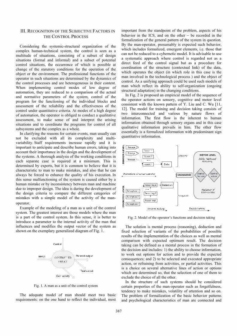
387

III. RECOGNITION OF THE SUBJECTIVE FACTORS IN

THE CONTROL PROCESS

Considering the systemic-structural organization of the complex human-technical system, the control is seen as a multitude of situations, consisting of a subset of design situations (formal and informal) and a subset of potential control situations, the occurrence of which is possible at change of the statutory conditions for the operation of the object or the environment. The professional functions of the operator in such situations are determined by the dynamics of the control processes and are heterogeneous in their content. When implementing control modes of low degree of automation, they are reduced to a comparison of the actual and normative parameters of the system, control of the program for the functioning of the individual blocks and assessment of the reliability and the effectiveness of the control under quantitative criteria. At modes of a high degree of automation, the operator is obliged to conduct a qualitative assessment, to make sense of and interpret the arising situations and to coordinate the programs for control of all subsystems and the complex as a whole.

In clarifying the reasons for certain events, man usually can not be excluded with all its complexity and multi-variability. Staff requirements increase rapidly and it is important to anticipate and describe human errors, taking into account their importance in the design and the development of the systems. A thorough analysis of the working conditions in each separate case is required at a minimum. This is determined by experts, but it is common to believe that it is characteristic to man to make mistakes, and also that he can always be forced to enhance the quality of his execution. In this sense malfunctioning of the system is caused either by a human mistake or by inconsistency between man and machine due to improper design. The idea is during the development of the design criteria to compare the different categories of mistakes with a simple model of the activity of the man-operator.

Example of the modeling of a man as a unit of the control system. The greatest interest are those models where the man is a part of the control system. In this sense, it is better to introduce a parameter to the internal activity of the man that influences and modifies the output vector of the system as shown on the exemplary generalized diagram of Fig. 1.

Fig. 1. A man as a unit of the control system

The adequate model of man should meet two basic requirements: on the one hand to reflect the individual, most

important from the standpoint of the problem, aspects of his behavior in the ICS, and on the other be recorded in the formalization of the general pattern of the system in question. By the man-operator, presumably is expected such behavior, which includes formalized, emergent elements, i.e. those that can not be reduced to a cybernetic model. It is advisable to use a systematic approach where control is regarded not as a direct feed of the control signal but as a procedure for coordination of the structure (contextual link) of the data, which operates the object (in which role in this case is the man involved in the technological process ) and the object of control. As a unifying approach could be used such models of man which reflect its ability to self-organization (ongoing structural adaptation) in the changing conditions.

In Fig. 2 is proposed an empirical model of the sequence of the operator actions on sensory, cognitive and motor level consistent with the known pattern of Y. Liu and C. Wu [11, 12]. The model for training and decision taking consists of two interconnected and various by nature flows of information. The first flow is the inherent to human information obtained through sensory organs and in this case qualitative information prevails in him. The other flow essentially is a formalized information with predominant sign quantitative information.

Fig. 2. Model of the operator’s functions and decision taking

The solution is mental process (reasoning), deduction and fixed selection of variants of the probabilities of possible results of the implementation of the choices as well as mental comparison with expected optimum result. The decision taking can be defined as a mental process in the formation of the decision and includes: 1) the ability to choose information, to work out options for action and to provide the expected consequences; and 2) to be selected and executed appropriate action, or refraining from activities, or partial activities. This is a choice on several alternative lines of action or options which are determined so, that the selection of one of them to exclude the choice of all the other.

In the structure of such systems should be considered certain properties of the man-operator such as forgetfulness, tendency to make mistakes, volatility of attention and so on. The problem of formalization of the basic behavior patterns and psychological characteristics of man are connected and

388

the attempts to create a mathematical models of his activities in the automation process. The peculiarities of perception and processing of the information by the man in the ICS impose a restriction on the possibility of using of stored data and in the specifying of the intelligence limits could be distinguished two levels of information processing - sensory channels and intellectual potential. On the first level, the transformation of the information is distributed among five sensor perceptions of man (visual, auditory, tactile, olfactory and taste) that have individual limits on the transmission of the information: the visual analyzer provides up to 90% of the total flow of information, but only about 10 % is allocated to the auditory and other sensory channels. On the second level, the intellect creates a model of the environment based on the received data. Because the brain and the nervous system of humans have limited resources, it determines the range of the solved problems. The main limitations of the brain are associated with the processing speed of the information and its final volume storage. Each event from the outside world is estimated by us (consciously or unconsciously) in accordance with our knowledge. The most important conditions that need to be taken into account in the implementation of the decision taken by the operator are: the existence of a deficit of information; shortage of time and lack of experience.

IV. CONCLUSION

From the said can be concluded that during the creation and the operation of complex systems, their effectiveness will be determined not only by the difficulties in the development of mathematical, software and technological support, but also by the complexity of the reporting of the interaction with the psychological, physiological and social phenomenon called "human factor".

• The identified in the article guidelines and models reporting the requirements to the operator allows to formalize the whole process of functioning of the complex human-technical systems;

• The inherent human mental and professional characteristics (emotions, temperament, sensory-motor, fast-acting, etc.) should necessarily be taken into account when defining the control in the information-control systems;

• The unsanctioned interference of the operator in the system and its mistakes and wrong actions in the control process can lead to serious and unforeseen consequences.

Considering the complexity and the multidisciplinary of the problem, realization of simulation experiments safe for humans and for the technical systems is appropriate. Especially important is the relationship and the complementarity of the various sciences such as engineering

and social psychology, physiology, cybernetics, organization and safety of labour, technical aesthetics, medicine, general systems theory, etc.

ACKNOWLEDGEMENTS

This paper is financed by Operaional Programme ”Development of competitiveness of Bulgarian economy” 2007-2013. Cofinaced by the European fund for Regional Developmen - Project BG161PO003–1.2.04–0053 “Inforrmation Complex for Aerospace Monitoring of Environment“.

REFERENCES

[1] A. Andonov, Z. Hubenova, "Modeling of the Human Operator in a Complex System Functioning Under Extreme Conditions", “V. Levski” National Military University, Proceedings 2006, Part II, p. 257-263.

[2] P. H. Lindsay, and D. A. Norman, Human Information Processing, Academic Press Inc.,U.S, 1992.

[3] T. B. Sheridan, and W. R. Ferrell, Men-Machine Systems: Information, Control and Decision Models of Human Performance, Hardcover, 2002.

[4] P. Getzov, Z. Hubenova, D. Yordanov, and W. Popov, "Modeling of the Human Operator in a Complex System Functioning Under Extreme Conditions", Journal Aerospace Research in Bulgaria, Bulgarian Academy of Sciences, vol. 25, рp. 206-227, Sofia, 2013.

[5] Handbook of Human Factors and Ergonomics, edited by G. Salvendy, Purdue University, 2006, Canada.

[6] Handbook of Human Factors and Ergonomics Methods, CRC Press, edited by Neville Stanton et al., 2015 www.cpe.ku.ac.th/~jan/ergonomics/HumanFactors.pdf

[7] A. Andonov, and Z. Hubenova, "Functional Stability of Information Control Complexes in Case of Their Critical Applications", Sofia, 2011.

[8] J. Rasmussen, Information Processing and Human-machine Interaction: An Approach to Cognitive Engineering, New York, Elsevier Science Ltd. 1986.

[9] E. D. Hutchison, Dimensions of Human Behavior: Person and Environment, SAGE Publication, London, 2003.

[10] Z. Hubenova, and K. Metodiev, "Training and Evaluation of UAV Operators by Means of C-Star Simulator", Twelfth Scientific Conference with International Participation, SPACE, ECOLOGY, SAFETY - SES 2016, Session 2 Aerospace Technologies and Biotechnologies, Sofia, 2016.

[11] C . W u , a n d Y . L i u , "Queuing Network Modeling of Transcription Typing", ACM Transactions on Computer Human Interaction, vol. 15, 2008, pp. 1-45.

[12] Y. H. J. Chang, and A. Mosleh, "Cognitive Modeling and Dynamic Probabilistic Simulation of Operating Crew Response to Complex System Accidents, Part 2: IDAC Performance Influencing Model", Reliability Engineering and System Safety, vol. 92, no. 8, pp. 1014-1040, 2007.

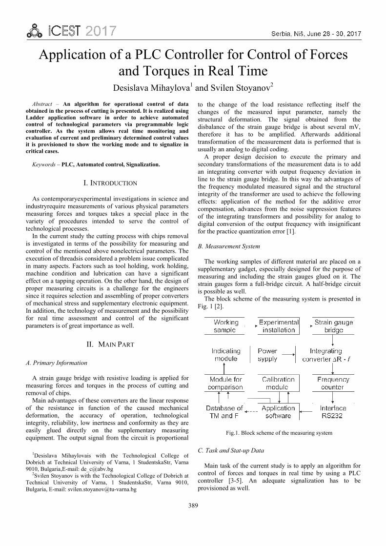
389

Application of a PLC Controller for Control of Forces and Torques in Real Time

Desislava Mihaylova1 and Svilen Stoyanov2

Abstract – An algorithm for operational control of data obtained in the process of cutting is presented. It is realized using Ladder application software in order to achieve automated control of technological parameters via programmable logic controller. As the system allows real time monitoring and evaluation of current and preliminary determined control values it is provisioned to show the working mode and to signalize in critical cases.

Keywords – PLC, Automated control, Signalization.

I. INTRODUCTION

As contemporaryexperimental investigations in science and industryrequire measurements of various physical parameters measuring forces and torques takes a special place in the variety of procedures intended to serve the control of technological processes.

In the current study the cutting process with chips removal is investigated in terms of the possibility for measuring and control of the mentioned above nonelectrical parameters. The execution of threadsis considered a problem issue complicated in many aspects. Factors such as tool holding, work holding, machine condition and lubrication can have a significant effect on a tapping operation. On the other hand, the design of proper measuring circuits is a challenge for the engineers since it requires selection and assembling of proper converters of mechanical stress and supplementary electronic equipment. In addition, the technology of measurement and the possibility for real time assessment and control of the significant parameters is of great importance as well.

II. MAIN PART

A. Primary Information

A strain gauge bridge with resistive loading is applied for measuring forces and torques in the process of cutting and removal of chips.

Main advantages of these converters are the linear response of the resistance in function of the caused mechanical deformation, the accuracy of operation, technological integrity, reliability, low inertness and conformity as they are easily glued directly on the supplementary measuring equipment. The output signal from the circuit is proportional

to the change of the load resistance reflecting itself the changes of the measured input parameter, namely the structural deformation. The signal obtained from the disbalance of the strain gauge bridge is about several mV, therefore it has to be amplified. Afterwards additional transformation of the measurement data is performed that is usually an analog to digital coding.

A proper design decision to execute the primary and secondary transformations of the measurement data is to add an integrating converter with output frequency deviation in line to the strain gauge bridge. In this way the advantages of the frequency modulated measured signal and the structural integrity of the transformer are used to achieve the following effects: application of the method for the additive error compensation, advances from the noise suppression features of the integrating transformers and possibility for analog to digital conversion of the output frequency with insignificant for the practice quantization error [1].

B. Measurement System

The working samples of different material are placed on a supplementary gadget, especially designed for the purpose of measuring and including the strain gauges glued on it. The strain gauges form a full-bridge circuit. A half-bridge circuit is possible as well.

The block scheme of the measuring system is presented in Fig. 1 [2].

Fig.1. Block scheme of the measuring system

C. Task and Stat-up Data

Main task of the current study is to apply an algorithm for control of forces and torques in real time by using a PLC controller [3-5]. An adequate signalization has to be provisioned as well.

1Desislava Mihaylovais with the Technological College ofDobrich at Technical University of Varna, 1 StudentskaStr, Varna9010, Bulgaria,E-mail: [email protected]

2Svilen Stoyanov is with the Technological College of Dobrich atTechnical University of Varna, 1 StudentskaStr, Varna 9010,Bulgaria, E-mail: [email protected]

390

Tapping parameters obtained in the process of cutting with chips removal are shown in Table 1. The relevant values have been determined in separate investigations [2] and it should be noted that only new thread tools have been used.

Attention should be paid on the output signal from the sensor, herein a strain gauge bridge full-circuit. This signal is analog and in terms of the frequency. To ensure the possibility for comparison of the registered signal from the sensor and the relevant tapping parameters in real time, the last need to be scaled and adjusted. In the current measurement a scaling factor of 30 is determined. Additionally, the value of 1490 Hz is added to each scaled parameter, since this is the initial signal obtained at no loading condition.

TABLE I TAPPING PARAMETERS

Type of the thread tool

Normal working mode

Maximal /Threshold working mode

Critical working mode

Mnom N Mmax M Mthr E Mc C

M4 1,4 1532 2,4 1562 2,2 1556 3,6 1598

M5 2,9 1577 5,8 1664 5,3 1649 8,7 1751

M6 4,1 1613 7,2 1706 6,4 1682 10,8 1814

M8 5,9 1667 10,3 1799 9,1 1763 15,5 1955

M10 8,4 1742 11,7 1841 10,2 1796 17,6 2018

M12 9,7 1781 14,6 1928 12,5 1865 21,9 2147 Note: N = Mnom*30 + 1490; M = Mmax*30 + 1490; E =Mthr*30 + 1490; C = Mc*30 + 1490.

As seen in Table 1 the signalization system will indicate via

LED lighting and a buzzer in the most critical case. The signalization circuits are displayed in Fig. 2.

Fig. 2. Signalization circuits

At normal working mode, respectively nominal values Mnom (N) of forces and torques (and below the threshold values Mthr (E)), the PLC is to display NORMAL working mode and green LED light is on. When the measured values increase and reach the maximal control parameters and above the yellow LED lights on. And the worst case, when the critical values of tapping parameters Mc (C) are reached thisis signalized with red LED and a sound effect.

D. Application Algorithm

At first, the PLC interface is programed and a database is created in terms of editable variables, whose values are saved as MI (memory integer /registers/) and appear at PLC power-up.

Some of the main variables used in the project are shown in Figs. 3 and 4.

Fig. 3. Main variables in HMI of the PLC – numeric value as MI

(editable) and a list variable for the working modes

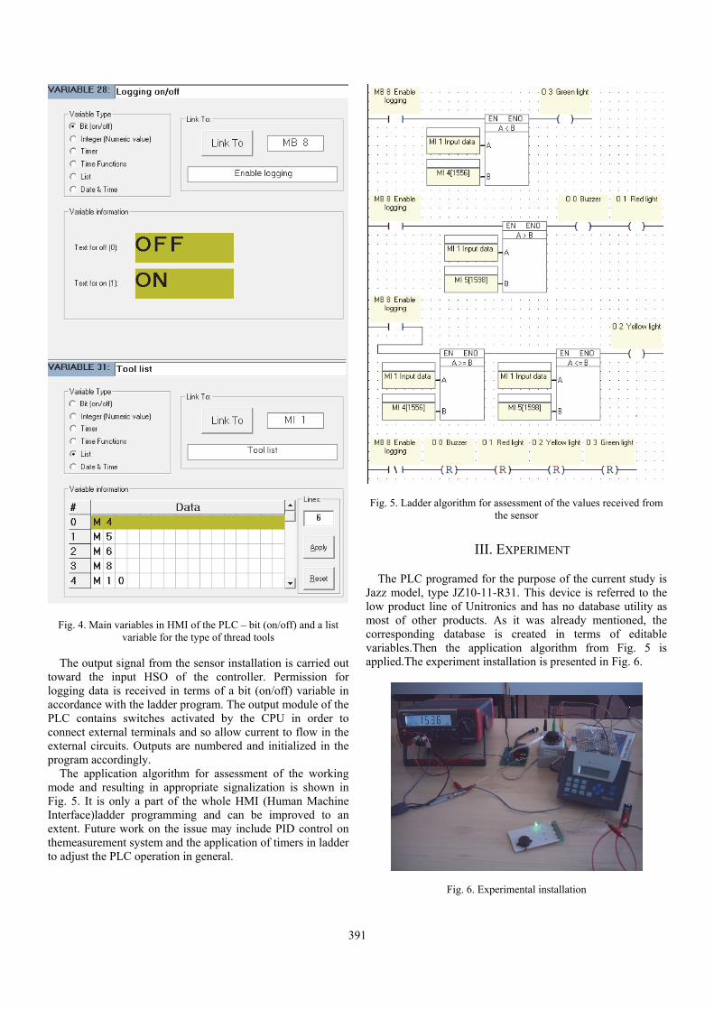
391

Fig. 4. Main variables in HMI of the PLC – bit (on/off) and a list variable for the type of thread tools

The output signal from the sensor installation is carried out

toward the input HSO of the controller. Permission for logging data is received in terms of a bit (on/off) variable in accordance with the ladder program. The output module of the PLC contains switches activated by the CPU in order to connect external terminals and so allow current to flow in the external circuits. Outputs are numbered and initialized in the program accordingly.

The application algorithm for assessment of the working mode and resulting in appropriate signalization is shown in Fig. 5. It is only a part of the whole HMI (Human Machine Interface)ladder programming and can be improved to an extent. Future work on the issue may include PID control on themeasurement system and the application of timers in ladder to adjust the PLC operation in general.

Fig. 5. Ladder algorithm for assessment of the values received from the sensor

III. EXPERIMENT

The PLC programed for the purpose of the current study is Jazz model, type JZ10-11-R31. This device is referred to the low product line of Unitronics and has no database utility as most of other products. As it was already mentioned, the corresponding database is created in terms of editable variables.Then the application algorithm from Fig. 5 is applied.The experiment installation is presented in Fig. 6.

Fig. 6. Experimental installation

392

IV. CONCLUSION

An intelligent system for registering and monitoring the technological parameters in the process of cutting internal threads is assembled. The control functions are executed via PLC controller, which has been programed according to the task requirements. The system allows comparative study of current parameters and their control values in real time, implying algorithms for assessment and processing. A signalizing circuit is provisioned.

ACKNOWLEDGEMENT

Authors wish to acknowledge the Bulgarian Ministry of Science and Education and Technical University of Varna for the financial support under the scientific project НП17/2017 of Technological College of Dobrich.

REFERENCES

[1] H. Gigov, Measuring Electronics, Technical University of Varna, Bulgaria, 2013.

[2] S. Stoyanov, "Study the Possibilities for Improvement the Quality of Technological Processes on the Basis of the Application of Integrating Measuring Converters (in Russian)", XII International Conference Proceedings, May 30 – June 2, 2016, Technical University of Varna, Bulgaria, vol. 1, pp. 282- 288, 2016.

[3] www.PAControl.com, Fundamentals of Control, 2006. [4] H. Jack, Automating Manufacturing Systems with PLCs,

Version 4.7, 2005 and Version 5, 2007. [5] A.J. Crispin, Programmable Logic Controllers and Their

Engineering Applications, 2nd Ed., The McGraw - Hill Companies, London, 1997.

393

System for Flight Control and Technical Condition of Unmanned Aeral System

Krume Andreev1, Ivo Dochev2 and Rumen Arnaudov3

Abstract – For unmanned aerial systems (UAS) to be successfully deployed and integrated into the national airspace, it is imperative that they possess the capability to effectively complete their missions without compromising the safety of other aircraft, as well as people and property on the ground. This necessity creates a natural requirement for UAS that can respond to uncertain environmental conditions and emergent failures in real-time, with robustness and resilience close enough to those of manned systems. This report introduce a system that meets this requirement with the design of a real-time on-board system for flight control and technical condition capability to continuously monitor sensors, software and hardware components. This system can detect and diagnose failures and violations of safety or performance rules during the flight of a UAS.

Keywords – UAS, Unmanned aerial systems, Technical condition, Multi-purpose development platform.

I. INTRODUCTION

In the last decade has seen a rapid development of unmanned aerial systems (UAS). Companies producing this type of aircraft equipment continuously strive to improve and develop new ones with improved functional parameters. UASs can be used only if they can effectively complete their mission and respond to the problems and uncertain environmental conditions. They should always keep safety in relation to other aircraft, to people and property on the ground.

Extremely important is the development and the need to develops systems and algorithms for flight control and technical condition of the UAS. It is important to provide a method for developing and implementing, a powerful system operating in real time on the board of a UASs, hardware combined with software systems and sensors for the management of the technical condition of unmanned aircraft [1].

This report shows the architecture of a system for flight control and technical condition of the UAS, built using a Multi-purpose development platform.

II. ARCHITECTURE OF A SYSTEM FOR THE

CONTROL OF FLIGHT AND TECHNICAL CONDITION

A. Multi-Purpose Development Platform for Collecting and Processing Data

Fig. 1 shows the architecture of Multi-purpose development platform. It is characterized by a high degree of integration. It is built based on a system on a chip (SoC), including in himself all the basic building blocks of modern computer systems - a central processing unit (CPU), memory (RAM), GSM module, telemetry, card reader (SD), universal serial interface (USB), digital inputs and outputs of a general purpose (I/O). Telemetry and GSM module enables the multi-purpose development platform to connect to the ground

1Krume Andreev Ph.D. student is with the Faculty ofTelecommunications at Technical University of Sofia, 8 Kl. OhridskiBlvd, Sofia 1000, Bulgaria, E-mail: [email protected]

2Ph.D. Ivo Dochev Assoc. Prof. is with the Faculty ofTelecommunications at Technical University of Sofia, 8 Kl. OhridskiBlvd, Sofia 1000, Bulgaria, E-mail: [email protected]

3Ph.D. Rumen Arnaudov Professor is with the Faculty ofTelecommunications at Technical University of Sofia, 8 Kl. OhridskiBlvd, Sofia 1000, Bulgaria, E-mail: [email protected]

Fig. 1. Architecture of a multi-purpose development platform

394

station and sending messages. The card reader is designed to carry the appropriate memory card, on which is installed on the operation system of the platform. USB ports may be used to connect different compatible devices for settings: a computer mouse, keyboard, power adapter, etc. Digital input-output ports general purpose can be used for receiving data from the sensors on board and subsequent processing, and to send data or making control signals to other devices, i.e. for interfacing between systems. B. System for Flight Control and Technical Condition of the UAS, Built Using a Multi-Purpose Development Platform

The system purposes are detecting malfunctions and violations of safety regulations or performance during the flight of UAS by solving logic problems [2].

The system must be able to perform the following tasks:

• Monitoring of a multiple sensory signals and software in dynamic mode;

• Based on them to make substantial conclusions for the prevention and diagnosis of defects;

• Does not interfere and influence in any way the flight software, on hardware, and not hinder to other computing devices on board.

The flight control and technical condition system must be

able to ensure the proper functioning of the aircraft and alarms at issue in the main control, has the ability to constantly monitor the sensors, software and hardware components for detection and diagnosis of malfunctions and disturbances of the safety rules or productivity during the flight of UAS. [3]

Fig. 2 shows the architecture of the system for flight control and technical condition, built using a multifunctional platform development. A system contains sensors, a multifunctional platform for a development, platform for the collection and processing of data, platform for interaction with other systems on board and link with ground stations.

Multi-purpose development platform has the task to manage as initialization of the sensors and the flow of information received from them. Through its programs provide development platform will check for the accuracy of the data, sorts the data received record them in a database, sends them to the user in appropriate type and interact through a common bus interface with other systems onboard of the UAS. In this way provides user access to chronologically recorded data and transmits data in real time with the relevant connection between them, e.g. the amendment of speed, altitude, direction, etc., for a certain period of time. By suitable graphic or web interface development platform provides real-time data on remote distance via GSM module and the telemetry. The main task of the GUI is to enable the user to review the data, preparation of reports, notice of problems on board, building a statistical graphs and tables with data recorded by the system [4].

The system has all the features of flight computer and control of sensor payloads. The individual components are connected by a common bus interface and work on C/C++ architecture that provides a component-based plug-and-play infrastructure. Typical sensors include a sensor for barometric pressure, airspeed indicator, GPS, and a laser altimeter to measure the height above the ground [5].

Fig. 2. Multi-purpose development platform

395

The requirements of the proposed safety system operation of UAS can be categorized into the following three points:

• Control of multiple values of various parameters;

• Relationships between different systems and flight parameters;

• Control of the flight rules.

Checks for various values of the data check if they are realistic. As an example in this category includes checks on the range - for example, the maximum safe level of climb or descent. For safe operation, values should always be within certain limits. Such checks can be combined with further conditions (e.g., during the flight phase or above a minimum level) or time range (for example, the maximum succumbing from the battery current does not exceed 50A for more than 60 seconds to avoid overheating of the battery) [5].

The relationships encode dependencies between the data from the sensors, which may originate from different subsystems. For example, the measured altitude obtained from a GPS-altitude measured from the sensor for barometric pressure must be strongly connected. For another example may be indicated when a UAS is in flight [6]. Then the measured airspeed must be greater than its rate of collapse, if not greater definitely a problem.

Finally, the flight rules. Unfortunately, in Bulgaria still no regulation of the flight rules for UASs. Flight rules are defined by national and international institutions. For example, in the US there are already regulated by strict rules (Federal Aviation Administration, 2013), part 91 of the Federal Aviation (FAR)) [7], or by limitations of the systems that manage flights. For example, a rule for the minimum flight height, which must reach the aircraft after take-off is that the UAS must climb or reach a height of 600 feet within five minutes after takeoff. Similarly, it can specify time-out procedure for landing UAS. For example, after receiving a command for landing, the set command must be fulfilled within three minutes.

C. Algorithm of the System for Flight Control and Technical Condition for Collecting and Processing Data from Sensors on Board

Fig. 3 shows the algorithm of the system for flight control and technical condition for collecting and processing data from sensors on board.

After starting the device а follows initialization [8]. Initialization is performed by the controller, i.e. self-initialization and initialization on all sensors on board that directly depend on the system for flight control and monitor the technical condition of the UAS. After initialization follows read of the input data and is expected acceptance of command. Commands are three, as follows, for start, stop and system setup. For a given command start the system begins to read the data sent by sensors on board of the UAS and began to perform the functions of the system (the system functions described above in the textpoint section B). After receiving the data from sensors follows the process on the received data and the system makes the right decision. [9] The steps are as

Fig. 3. Algorithm for operation of the system for flight control and technical condition for collecting and processing data from sensors

onboard the UAS

396

follows filtering of the sensors data for eliminate the noise, comparing the received sensor data with the input system data, processing the received data and decision-making.

In the case of need for an interaction of the system for flight control and technical condition of UAS with the other sub-system on the board of the UAS i.e., in this case, the system for flight control. In this case, the decision taken in the form of data is sent to the flight control system i.e. to the UAV’s autopilot [10].

III. CONCLUSION

This report proposed architecture and algorithm of the system for flight control and technical condition for collecting and processing data from sensors on board, built using multi-purpose development platform. They are the basis for the design and development of intelligent UAS and to develop a regulatory framework for standardization and rules for their flight. Such systems may find wide application in other areas, especially where the combined requirements for high operational reliability and service while making quick decisions. In cases of:

• Accidents and disasters, detection and monitoring of injured regions in distress;

• Agriculture for inspection of crops, search for lost animals, a wide view of the farm;

• Ecology for monitoring of flora and fauna, monitoring the condition of the areas affected by natural disasters;

• Security system to monitor large areas.

This report introduces a system that meets this requirement with the design of a real-time onboard system for flight control and technical condition capability to continuously monitor sensors and hardware components. This system can detect and diagnose failures and violations of safety or performance rules during the flight of a UAS.

ACKNOWLEDGEMENT

The proposed architecture and algorithm have been developed with the support of NIS at TU-Sofia, through participation in research projects to help graduate "System for flight control and technical condition of unmanned aerial systems" (session 2017) 172PD0005-07.

REFERENCES

[1] D. Musliner, J. Hendler, A.K. Agrawala, E. Durfee, J.K. Strosnider, and C.J. Paul, "The Challenges of Real-Time AI", IEEE Computer, pp. 58-66, 1995.

[2] J. Schumann, O.J. Mengshoel, and T. Mbaya, "Integrated Software and Sensor Health Management for Small Spacecraft", 2011 IEEE Fourth International Conference on Space Mission Challenges for Information Technology, pp. 77-84, 2011.

[3] S. Poll, A. Patterson-Hine, J. Camisa, D. Garcia, D.C. Hall, C. Lee, and X. Koutsoukos, "Advanced Diagnostics and Prognostics Testbed", 18th International Workshop on Principles of Diagnosis, DX-07, pp. 178-185, 2007.

[4] R.A. Di Lorenzo, and M.A. Bayer, "A Prognostics and Health Management System for an Unmanned Combat Aircraft System – A Defense Acquisition University Case Study", pp.1-12, 2009.

[5] J. Schumann, K.Y. Rozier, T. Reinbacher, O.J. Mengshoel, T. Mbaya, and C. Ippolito, "Towards Real-time, On-board, Hardware-supported Sensor and Software Health Management for Unmanned Aerial Systems", pp.1-27, 2014.

[6] J. Schumann, K.Y. Rozier, T. Reinbacher, O.J. Mengshoel, T. Mbaya, and C. Ippolito, "Towards Real-time, On-board, Hardware-supported Sensor and Software Health Management for Unmanned Aerial Systems", pp.1-21, 2013.

[7] Federal Aviation Administration, Federal Aviation, Regulation §91, 2013.

[8] Y. Zhao, and K.Y. Rozier, "Formal Specification and Verification of a Coordination Protocol for an Automated air Traffic Control System", pp. 65-123, 2012.

[9] Reg Austin, "Unmanned Aircraft Systems – UAVS Design, Development and Deployment", pp. 16-56, 2010.

[10] D. Basin, F. Klaedtke, and E. Zalinescu, "Algorithms for Monitoring Real-time Properties", pp. 260-275, 2011.

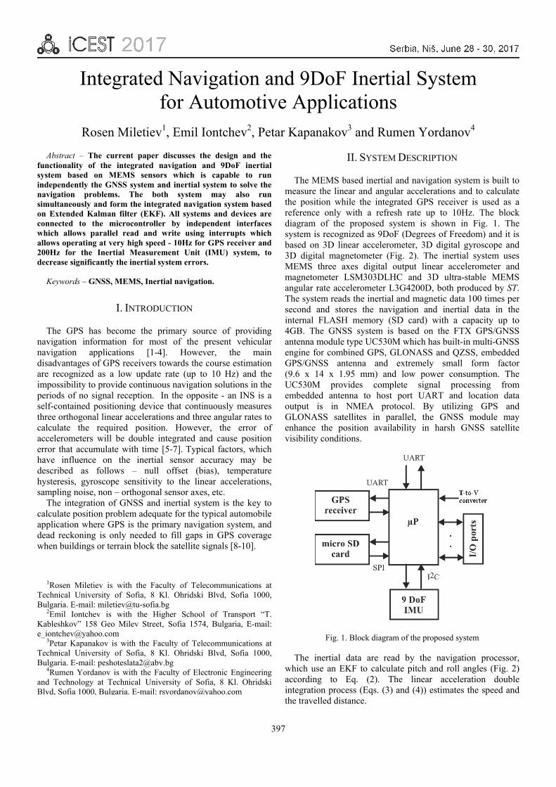
397

Integrated Navigation and 9DoF Inertial System for Automotive Applications

Rosen Miletiev1, Emil Iontchev2, Petar Kapanakov3 and Rumen Yordanov4

Abstract – The current paper discusses the design and the functionality of the integrated navigation and 9DoF inertial system based on MEMS sensors which is capable to run independently the GNSS system and inertial system to solve the navigation problems. The both system may also run simultaneously and form the integrated navigation system based on Extended Kalman filter (EKF). All systems and devices are connected to the microcontroller by independent interfaces which allows parallel read and write using interrupts which allows operating at very high speed - 10Hz for GPS receiver and 200Hz for the Inertial Measurement Unit (IMU) system, to decrease significantly the inertial system errors.

Keywords – GNSS, MEMS, Inertial navigation.

I. INTRODUCTION

The GPS has become the primary source of providing navigation information for most of the present vehicular navigation applications [1-4]. However, the main disadvantages of GPS receivers towards the course estimation are recognized as a low update rate (up to 10 Hz) and the impossibility to provide continuous navigation solutions in the periods of no signal reception. In the opposite - an INS is a self-contained positioning device that continuously measures three orthogonal linear accelerations and three angular rates to calculate the required position. However, the error of accelerometers will be double integrated and cause position error that accumulate with time [5-7]. Typical factors, which have influence on the inertial sensor accuracy may be described as follows – null offset (bias), temperature hysteresis, gyroscope sensitivity to the linear accelerations, sampling noise, non – orthogonal sensor axes, etc.

The integration of GNSS and inertial system is the key to calculate position problem adequate for the typical automobile application where GPS is the primary navigation system, and dead reckoning is only needed to fill gaps in GPS coverage when buildings or terrain block the satellite signals [8-10].

II. SYSTEM DESCRIPTION

The MEMS based inertial and navigation system is built to measure the linear and angular accelerations and to calculate the position while the integrated GPS receiver is used as a reference only with a refresh rate up to 10Hz. The block diagram of the proposed system is shown in Fig. 1. The system is recognized as 9DoF (Degrees of Freedom) and it is based on 3D linear accelerometer, 3D digital gyroscope and 3D digital magnetometer (Fig. 2). The inertial system uses MEMS three axes digital output linear accelerometer and magnetometer LSM303DLHC and 3D ultra-stable MEMS angular rate accelerometer L3G4200D, both produced by ST. The system reads the inertial and magnetic data 100 times per second and stores the navigation and inertial data in the internal FLASH memory (SD card) with a capacity up to 4GB. The GNSS system is based on the FTX GPS/GNSS antenna module type UC530M which has built-in multi-GNSS engine for combined GPS, GLONASS and QZSS, embedded GPS/GNSS antenna and extremely small form factor (9.6 x 14 x 1.95 mm) and low power consumption. The UC530M provides complete signal processing from embedded antenna to host port UART and location data output is in NMEA protocol. By utilizing GPS and GLONASS satellites in parallel, the GNSS module may enhance the position availability in harsh GNSS satellite visibility conditions.

Fig. 1. Block diagram of the proposed system

The inertial data are read by the navigation processor, which use an EKF to calculate pitch and roll angles (Fig. 2) according to Eq. (2). The linear acceleration double integration process (Eqs. (3) and (4)) estimates the speed and the travelled distance.

1Rosen Miletiev is with the Faculty of Telecommunications atTechnical University of Sofia, 8 Kl. Ohridski Blvd, Sofia 1000,Bulgaria. E-mail: [email protected]

2Emil Iontchev is with the Higher School of Transport “T.Kableshkov” 158 Geo Milev Street, Sofia 1574, Bulgaria, E-mail:[email protected]

3Petar Kapanakov is with the Faculty of Telecommunications atTechnical University of Sofia, 8 Kl. Ohridski Blvd, Sofia 1000,Bulgaria. E-mail: [email protected]

4Rumen Yordanov is with the Faculty of Electronic Engineeringand Technology at Technical University of Sofia, 8 Kl. OhridskiBlvd, Sofia 1000, Bulgaria. E-mail: [email protected]

398

3D Gyroscope

3D Accelerometer

3D Magnetometer

KalmanFilter

roll

pitch

yawCompass

distance

speedNavigationprocessor

9 DoFIMU system

Fig. 2. Proposed signal processing algorithm

The obtained results are used in the tilt-compensated compass to calculate the yaw angle. In the same time the gyroscope angular accelerations x, y, z are numerically integrated using trapezoidal rule to calculate the yaw angle (heading) of the moving object according to the equations [11]:

t

iiii

tii

ii

tii

ii

zzzz

yyyy

xxxx

2

11

2

11

2

11

(1)

The tilt-compensated compass calculated the heading angle

using magnetometer data Mx, My, Mz according to the equations [12]:

ndeclinatio

H

H

ZYH

ZYXH

M

Yarctg

MMY

MMMX

0

0

sincos

sincossinsincos

(2)

where rollpitch , angles.

The declination angle declination for Sofia (Bulgaria) is equal to +420 [13]. The 3D magnetometer is also preliminary calibrated towards soft-iron and iron-iron effects according to the algorithm described at [14].

In the same time the accelerometer data are numerically integrated using trapezoidal rule to calculate the speed v and travelled distance d of the moving object according to the equations [11]:

t

iaiaiviv cc

2

11 (3)

t

ivividid cc

cc

2

11 (4)


The proposed system is tested on the road and the data are recorded on MMC/SD card and processed by MATLAB routine later. The system is placed between the front seats near the vehicle mass center and the IMU axes are orientated towards the vehicle axes according to Fig. 3.

The sampling frequency of the inertial data is limited to 200Hz due to the limited time to send data to PC via RS232 interface. The test results are accomplished using lower sampling frequency which is equal to 20Hz. This sampling frequency is also chosen because the inertial blocks from 40 frames are stored in the single block of MMC/SD card and the sampling frequency have to be multiple to 40Hz. Meanwhile the update rate of the GPS data is equal to 1Hz but it may be increased up to 10Hz in such matter that the IMU update ratio towards the GPS update ratio remains equal to 20.

Fig. 3. System orientation

The system is tested to record the navigation and the

inertial data during some hours and the track is shown in Fig. 4. It is clearly visible that the track is continuous except of the marked region with the red color. This region is extracted from the whole track and is shown below. There are three place named A, B and C where the track is interrupted which corresponded to the three tunnels (see the right map) due to the GPS signal lost.

This interruption is also clearly visible on the speed and course over ground shown in Figs. 5 and 6 respectively.

Therefore the task of the inertial system is to restore the interrupted track and to ensure the course and the speed of the vehicle when the GPS signal is weak or lost. The restoration of the data is based on the calculation of the heading angle according to the signal processing algorithm (Fig. 2). The calculated pitch and roll angles from the Kalman filter are used for the yaw angle estimation (heading angle). Simultaneously the speed and the travelled distance are also estimated by the navigation processor using a numerical integration of the accelerations (according to Eq. (3)) and speed (Eq. (4)) respectively.

399

Fig. 4. Track representation

0 100 200 300 400 500 600 700 800

Time,s

40

50

60

70

80

90

100

110

120

130

Spe

ed,k

m/h

Fig. 5. Recorded speed over ground (SOG)

Cou

rse,

deg

Fig. 6. Recorder course over ground (COG)

400

The course is calculated in two ways and compared with the known COG data when GPS coverage is still active – the first value is obtained by the numerical integration of the angular rate gyroscope on the Z axis according to Eq. (1) and the second value is calculated by the e-compass according to Eq. (2). The results are shown in Fig. 7.

Fig. 7. Heading angle estimation

The results show that both systems (gyroscope and magnetometer) correctly calculate the heading angle before entering into the first tunnel (approximately 150s from the track beginning). As the GPS signal is lost the gyroscope and the magnetometer continuously estimate the car course and when the GPS signal is restored the calculated heading angle from both systems is equal to the course of ground value from GNSS. The same situation appears when the car entered in the second tunnel but the estimated heading angle from the magnetometer is distorted probably by the steel elements in the tunnel structure. In a short period of time after beginning (approximately 400s) the gyroscope heading value starts to decline from the real value due to the uncompensated gyroscope bias accumulation. Therefore the gyroscope offset has to be compensated after the GPS signal restoration.

IV. CONCLUSION

The proposed system is tested towards the course estimation from GNSS and IMU systems and analysis of the IMU accuracy and behavior during the dead reckoning situation. It is shown that IMU system may accurately calculate the heading angle in two ways – numerical integration of the Z gyroscope data and Kalman filter implementation for the magnetometer data for a limited period of time. In the same time the angle estimation may be distorted by the numerical integration errors for the gyroscope or soft-iron effects for the magnetometer.

The future work will investigate the system capabilities towards reduction of the numerical integration errors by increasing the sampling frequency of the IMU system up to 200Hz. It is known that this error depends from the third degree of the sampling intervals so this error may be reduced significantly.

The IMU system may be used for inertial navigation based on the EKF due to the high sampling frequency and small integration errors, gaming, motion control, gyro stabilized platforms, MVEDR (Motor Vehicle Event Data Recorder) systems or crash monitor for aircrafts, trains or cars.

REFERENCES

[1] B.W. Parkins, and J.J. Spilker, Eds., Global Positioning System: Theory and Applications, Washington, DC: Amer. Inst. Aeronautics Astronautics, 1996, vol. II.

[2] P. Misra, B.P. Burke, and M.M. Pratt, "GPS Performance in Navigation", Proceedings of the IEEE, vol. 87, no. 1, pp. 65-85, January 1999.

[3] G.W. Hein, From GPS and GLONASS via EGNOS to Galileo-positioning and Navigation in the Third Millennium, in GPS Solutions, vol. 3, no. 4, pp. 39-47, April 2000.

[4] J. Huang, and H-S. Tan, "A Low-order DGPS-based Vehicle Positioning System Under Urban Enviroment", IEEE/ASME Trans. Mechatronics, vol. 5, no. 1-2, pp. 567-575, October 2006.

[5] M.J. Caruso, Applications of Magnetic Sensors for Low Cost Compass Systems, PLANS, London 2000, p. 177.

[6] Electronic Tilt Compensation, Application Note AN-00MM-004, Memsic 2008.

[7] Talat Ozyagcilar - Implementing a Tilt-Compensated eCompass using Accelerometer and Magnetometer Sensors, Freescale Semiconductor, Document Number: AN4248, Rev.3, 01/2012.

[8] A.Kh. Mohammed, R.A. Mokhtar, and H. A.E. Eltahir, "Target Coordinates Calculation using GPS/inertial-aided Sensors", 2015 International Conference on Computing, Control, Networking, Electronics and Embedded Systems Engineering (ICCNEEE), 7-9 Sept. 2015.

[9] R.M. Rogers, Applied Mathematics in Integrated Navigation Systems, American Institute of Aeronautics and Astonautics, Inc, 2000.

[10] E.-H. Shin, Accuracy Improvement of Low Cost INS/GPS for Land Applications, MA thesis University of Calgary, Calgary, 2001.

[11] M. Arraigada, and M. Partl, "Calculation of Displacements of Measured Accelerations, Analysis of Two Accelerometers and Application in Road Engineering", 6th Swiss Transport Research Conference, Monte Verità/Ascona, March 15-17, 2006.

[12] C. Valenti, Microchip Technology Inc.AN996, Designing a Digital Compass Using the PIC18F2520 Microcontroller, 2005

[13] http://magnetic-declination.com/ [14] T. Stork, Philips Semiconductors, AN00022 - Electronic

Compass Design using KMZ51 and KMZ52, 2000.

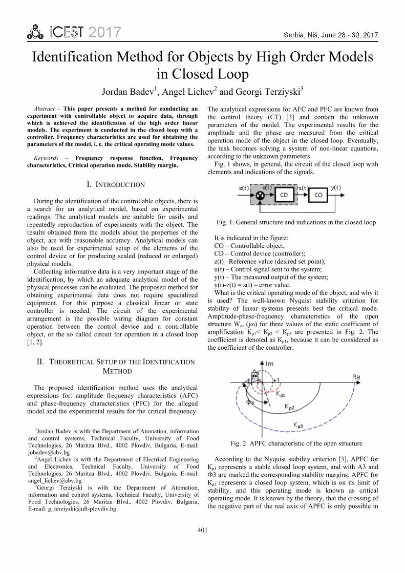
401

Identification Method for Objects by High Order Models in Closed Loop

Jordan Badev1, Angel Lichev2 and Georgi Terziyski3

Abstract – This paper presents a method for conducting an experiment with controllable object to acquire data, through which is achieved the identification of the high order linear models. The experiment is conducted in the closed loop with a controller. Frequency characteristics are used for obtaining the parameters of the model, i. e. the critical operating mode values.

Keywords – Frequency response function, Frequency characteristics, Critical operation mode, Stability margin.

I. INTRODUCTION

During the identification of the controllable objects, there is a search for an analytical model, based on experimental readings. The analytical models are suitable for easily and repeatedly reproduction of experiments with the object. The results obtained from the models about the properties of the object, are with reasonable accuracy. Analytical models can also be used for experimental setup of the elements of the control device or for producing scaled (reduced or enlarged) physical models.

Collecting informative data is a very important stage of the identification, by which an adequate analytical model of the physical processes can be evaluated. The proposed method for obtaining experimental data does not require specialized equipment. For this purpose a classical linear or state controller is needed. The circuit of the experimental arrangement is the possible wiring diagram for constant operation between the control device and a controllable object, or the so called circuit for operation in a closed loop [1, 2].

II. THEORETICAL SETUP OF THE IDENTIFICATION METHOD

The proposed identification method uses the analytical expressions for: amplitude frequency characteristics (AFC) and phase-frequency characteristics (PFC) for the alleged model and the experimental results for the critical frequency.

The analytical expressions for AFC and PFC are known from the control theory (CT) [3] and contain the unknown parameters of the model. The experimental results for the amplitude and the phase are measured from the critical operation mode of the object in the closed loop. Eventually, the task becomes solving a system of non-linear equations, according to the unknown parameters.

Fig. 1 shows, in general, the circuit of the closed loop with elements and indications of the signals.

Fig. 1. General structure and indications in the closed loop

It is indicated in the figure: CO – Controllable object; CD – Control device (controller); z(t) –Reference value (desired set point); u(t) – Control signal sent to the system; y(t) – The measured output of the system; y(t)-z(t) = ε(t) – error value. What is the critical operating mode of the object, and why it

is used? The well-known Nyquist stability criterion for stability of linear systems presents best the critical mode. Amplitude-phase-frequency characteristics of the open structure Woс (jω) for three values of the static coefficient of amplification Кр1< Кр2 < Кр3 are presented in Fig. 2. The coefficient is denoted as Кр1, because it can be considered as the coefficient of the controller.

Fig. 2. APFC characteristic of the open structure

According to the Nyquist stability criterion [3], APFC for

Кр1 represents a stable closed loop system, and with A3 and Ф3 are marked the corresponding stability margins. APFC for Кр2 represents a closed loop system, which is on its limit of stability, and this operating mode is known as critical operating mode. It is known by the theory, that the crossing of the negative part of the real axis of APFC is only possible in

1Jordan Badev is with the Department of Atomation, information and control systems, Technical Faculty, University of Food Technologies, 26 Maritza Blvd., 4002 Plovdiv, Bulgaria, E-mail: [email protected]

2Angel Lichev is with the Department of Electrical Engineering and Electronics, Technical Faculty, University of Food Technologies, 26 Maritza Blvd., 4002 Plovdiv, Bulgaria, E-mail: [email protected]

3Georgi Terziyski is with the Department of Atomation, information and control systems, Technical Faculty, University of Food Technologies, 26 Maritza Blvd., 4002 Plovdiv, Bulgaria, E-mail: [email protected]

402

case of third and higher order open loop system without transportation lag. The critical operating mode is possible only for first and second order systems.

The parameters of this mode are widely used: for setting the controllers in the loop; as asymptotic quality parameters, which keep performance unchanged; at the design stage and in particular to the identification of the systems. The critical operating mode is characterized by the following parameters:

Critical frequency – ωкр, this is the frequency at which: the module of the | Wос(j ωcr) | = A(ωкр) =1 and the phase

arg( Woс(j ωкр)) = Ф(ωкр) = -π. The last of this also implies that the process (for Кр2 and

ωкр) at the outcome y(t) will oscillate with constant amplitude, and will be in anti-phase with the input signal u(t). The last fact is used for simple experimental achieving of the critical operation mode, by soft settings variation of the controllers (linear and state).

III. A SETTING OF THE CLOSED LOOP FOR CRITICAL OPERATION MODE

The critical operating mode in the closed loop can be realized by proportional (linear) or two state (on/off) controller.

In case of operation with classical PID controller, the critical operating mode shall be set up as follows:

1. It is set for operation as P controller, and the integral and the derivative terms are excluded, by setting the appropriate values of the parameters for setting (Ти→∞, Тд→0).

2. An average value is set in the adjustment interval – the reference value

3. A small value is defined of the coefficient of proportionality Kп, for which the process of the output y(t) decreases.

4. The coefficient Kп is increased smoothly, and the process of the output y(t) is monitored. The process is supposed to change to a slower attenuation and to an increase of the oscillation. Kп continues to increase until fluctuations with constant amplitude Δykр and constant frequency ωкр are established. These are the parameters which are necessary for the further identification and they are as accurately as possible defined from the diagram of the established fluctuations.

In case of operation with classic two state controller, the critical operation mode is set as follows:

1. A two state controller is set without non unique function (hysteresis→0),

зср yy = (1)

2. A set point is set z(t) = constant, by absolute value in the middle of the adjustment interval, corresponding to a set point in relative units z% = 50%, where

%100%min)(max)(

min)(

∞∞

∞

−−

=yy

yyz ср (2)

The variables in the last formula are:

maxmax)( uKy об ∗=∞ (3)

– steady state value, which is achieved by maximum control effect in Fig.3

minmin)( uKy об ∗=∞ (4)

– steady state value, which is achieved by minimum control effect in Fig.3

yav – average value of the steady state oscillations – Fig. 3.

Fig. 3. Operation of a two state controller with a high order

object The completion of the critical process is easier with the two

state controller, because significant state interference by the operator is needed in the first case.

The following parameters are needed for the identification which is calculated with the experimental diagram of the critical process – Fig. 3:

- Critical frequency

кр

кр Tπω 2

= (5)

- Fluctuation range of the controllable (output) variable

minmax yyyкр −=∆ (6)

- Variation range of the control impact for: sinusoidal impact

minmax uuu −=∆ (7)

rectangular pulses

)(4minmax uuu −=∆

π (8)

- Average value of the controllable variable

2

minmax yyyср−

= (9)

- Average value of the control impact

2uuср

∆= (10)

403

IV. AN ALGORITHM FOR THE CALCULATION METHOD OF THE PARAMETERS OF MODELS

TF, AFC and PFC of the models, which are defined by the method are shown in Table 1.

The identification method can be depicted with the following algorithm:

1. Preparation and realization of the experiment and construction of the process in Fig. 3.

2. Calculation of the static coefficient of the object by the formula:

ср

сроб u

yK = (11)

3. Calculation of the critical frequency by the formula:

кр

кр Tπω 2

= (12)

4. Calculation of the critical module by the formula:

u

yA кр

кр ∆= (13)

5. For the models 1 and 2 in Table 1, it is easy T and τ to be defined – first T from AFC and after that τ from PFC

6. For the models 3, the system is nonlinear according to T and n. The second equation can be simplified, i. e.

n

обкр nKA

=

πcos (14)

– in this form, it is suitable for nomograms. Methods for solving non-linear equations systems are

known from theory. - It is cleared that the unknown n is number of first order

lags in the model and can accept equivalent and positive units only, which are greater than or equal to 3, i. e. (n ≥ 3)

- The unknown T is meant as a time constant and thus it can accept positive values only, i. e. T ≥ 0.

The system in the Table.1 (for the third kind of models) can be solved by building the graphics of the functions: n = f1(T), n = f2(T) and defining the coordinates of the intersection of the graphics. The co-ordinate on the axis (n) is approximated to the nearest equivalent and positive unit. It is accepted as an order of TF.

The right kind of the functions is:

)()( 1 Tf

Tarctgn

кр

==ωπ

(15)

)())(1lg(

)lg(

22Tf

T

АK

nкр

кр

об

=+

=ω

(16)

TABLE 1 MODELS OF APFC AND PFC [3]

TF of the model System of PFC and AFC

1. sоб eТsK τ−∗+1

)( Tarctg кркр ωτωπ +=

uy

TKA кр

кр

обcr ∆

∆=

+=

2)(1 ω

2. sоб e

ТsK τ−∗+ 2)1(

)(2 Tarctg кркр ωτωπ ∗+=

uy

TKA кр

кр

обcr ∆

∆=

+= 2)(1 ω

3. nоб

ТsK

)1( +

)( Tarctgn крωπ ∗=

uy

TKA cr

nкр

обcr ∆

∆=

+=

))(1( 2ω

V. VALIDATION OF THE METHOD, RESULTS AND CONCLUSIONS

The presented method is validated in the computing environment of MATLAB [1, 2]. Numbers of closed loops are simulated with the two kinds of controllers (S and two state). Each of the controllers control objects with different models, from the presented in Table 1. In all cases, satisfactory results are reached (considering carefully the graphics). There are no doubts that the method is correct.

For approbation of the method, an example of fourth order model is proposed with simulated data. The reader can verify the results, in order to convince himself in the merits of the method. The two variants for achieving a critical operating mode are shown – by the circuit in Fig. 1.

TF of the controllable object is:

4)( )110(50+

=s

W soy (17)

and the desired set point is:

)(125)( ttz ∗= (18)

404

Fig. 4. (a)

Fig. 4. (b)

Variant: (a) – a loop with linear P controller с Kp = 0,08 Variant: (b) – a loop with two state controller, without

hysteresis and umin = 0 and umax = 1 The following quantities are reported from the last graphics

of the Fig. 4a and 4b: Δyкр, Tкр, yav, Δu, uср It is calculated from the reported values in Table 2:

ωср = 2π/Tкр; Kоб = yср/uср; Aкр = Δyкр/Δu

TABLE 2 Ωкр Kоб Aкр

(a) 0.0967 40.8831 12.2807 (b) 0.0977 50.00 12.5984

The system of equations (1) and (2) is solved graphically by

the obtained values in Table 2. As a result, the graphics in Fig. 5 are obtained.

Fig. 5. (a)

Fig. 5. (b)

On the basis of the results which are obtained (the

coordinates of the intersections), the following conclusions can be drawn:

1. The case a) – the results for T and n are with unacceptable accuracy. That is seen in the graphic an can be calculated by the formula [4]:

1 1 1 25 50.08 50oc p oб

Z ZK K K

ε = = = =∗ ∗

(19)

If the value of Koб in the table is being corrected with this value, the system of equations (1) and (2) are going to be changed and the inaccuracy of the result is going to decrease.

2. The case b) – from the graphic b), the results are: T ≈ 10s and n ≈ 4, which is acceptable accuracy.

3. It appeared preferable to realize the experiment in loop with two state controller. This is due to the easier set-up of the critical operating mode, and the lack of the steady state error, by which the experimental results are corrected.

REFERENCES

[1] L. Ljung, System Identification, Prentice Hall, 1987. [2] L. Ljung, System Identification Toolbox – User’s Guide, The

Math Works, Inc., 2016. [3] F. Golnaraghi, and B. Kuo, Automatic Control Systems, John

Wiley & Sons, Inc., 2010. [4] I. Dragotinov, Technological Processes Automation, UFT,

2003.

405

A New Method for Parallel Operation Units by Synchronized Instrument Transformers

Associated with Switchboards Shaker J. Gatan

Abstract - A methodology plan for parallel power generation units are essential. Many industrial plants are suffering from a repeating of shut downs for intertie between a self-power as generators, and the national grid specifically with type of 6.6KV when connected with the national grid rating of 33KV/6.6KV because of anonhomogeneous of transformers CTs and VTs and a load shedding system.

Azzawayia Refining Company (ARC) have many experiences of black out because of the tie-connection unit with national grid and the existing oil circuit breakers 6.6KV ES-1 switch board connecting with 33KV/6.6KV national grid. Moreover the instrument protection system is not reliable fora full operating works.

This paper focuses on the understanding of switching surge phenomena relatively with circuit breakers, including the necessary of parallel operating methods and synchronizing both CTs & VTs for steady operation with stream power flows between tie systems for full operation loads.

Keywords - Arcingcurrents and chopping currents,

Synchronizing CTs &VTs.

I. INTRODUCTION

The Switch board power plants works for transferring a power to the facilities, but thoroughly the normal operation, some terms effective under operating such as ; firstly a switching surge phenomena ,this critical circuit conditions : such as arcing currents and chopping currents with generated high frequency over voltages and frequency of re-ignition . Secondly, the none homogenous of instrumentation and malfunctions also effect to critical case condition.

ARC has running a three steam turbines to generate 7200KVA each , including a gas turbine of 23MVA as the self-unit connects with national grid with two feeders of IF1 & IF2 of 63MVA, but from time to time have many shut downs have been abruptly.

I was made a deeply investigation analysis for this critical

conditions and studying precisely for make diagnoses about why do the repeated shut downshappened. This analysis of characteristics of power switch board basically on NEPLAN software as followings:

1. Circuit breaker conditions 2. Instrument transformers functions 3. Characteristics of protection Relays 4. Characteristics of Load shedding device

Fig. 1. Single line diagram of ES-1

II. ANALYSIS APPLICATION

Circuit breaker using different media for interrupter current

my exhibit different characteristics with respect to all of primary functional requirements of the breaker. Each type of circuit breaker has a unique set of characteristics which must be thoroughly understood before the breaker can be applied with safety and confidence.

The switching surge phenomena usually associated with both oil circuit breakers and vacuum interrupters. This includes current chopping, multiple re-ignitions, and prestrikes over voltages. Current chopping refers to the prospective over voltage events which can result with certain of inductive loads( Transformers & motors) due to the premature suppression of the power frequency current before normal current-zero inside electroplates of interrupters [1].

A. Chopping Currents Calculation

The process of current chopping is the premature suppression of 50 Hz or 60 Hz circuit current before normal current zero due to instability of the arcs in a vacuum interrupter [2]-[4]. Although the current in the vacuum interrupter can chop to zero almost instantaneously (fraction of microsecond) , the current in the load inductance cannot attain zero value instantaneously. Time is required for magnetic energy to be transferred from the inductance "Transform inductance loads", and for the magnetic field associated with stored energy to collapse . When current chop occurs, the energy stored in the effective load inductance is transferred to the available load-side capacitance to produce the so called chop overvoltage, given by Ic√(1-γ) Lb/Cs where CI called chopping current level and √ Lb/Cs

ionization of medium voltage impedance; γ represents circuit Shaker J. Gatan is with Riga Technical University, Azenesiela

12/1, Riga LV-1048, Latvia, E-mail: [email protected]

406

losses generate joule heating and lightning impulse, especially ions loss and very significant in limiting chop overvoltage [2]-[5]. For determine the actual value of first peak of chopping current

T C LOADV I Z= ⋅ (1)

TV – Voltage transient,

CI – Current chop, First peak value,

LOADZ – Load impedance, U – Operating voltage of inductance Load- KV Ur – Rated voltage –maximum RMS –KV U d – Insulation level - Rated power frequency RMS-KV Up – Rated lightning impulse withstand level –KV; 1.2/50us

withstand level of IEEE

Fig. 2. Chopping currents characteristics

Fig. 3.First peak value of transient over voltage According to the Eq. (1), I was made my calculation thoroughly both physically and software application for the cubicles no.7 & 8 in main switchboard of ES-1.

= 0.5A*3000Ω = 1500 volt VMax = VRMS+ Vt = 1.5+7.5= 9KV This is a first calculation which is acceptable value for the first peak value of transient over voltage N:B The specification of circuit breaker U= 6.6KV Ur=7.2KV –RMS-KV Ud= 20KV- Maximum withstand level of Insulation

TABLE I FIRST TABLE CALCULATION AT Z=3000Ω

Ic UMAX Ud Max Rated level

Notes

0.5A 9KV 20KV Acceptable IEC T 0.7A 9.3KV 20KV Acceptable IEC T

0.75A 9.45KV 20KV Acceptable IEC T 0.8A 9.6KV 20KV Acceptable IEC T 0.9A 9.9KV 20KV Acceptable IEC T 1A 10.2KV 20KV Acceptable IEC T 2A 13.2KV 20KV Acceptable IEC T 3A 16.2KV 20KV Acceptable IEC T 5A 22.2KV 20KV Acceptable IEC T 6A 25.2KV 20KV Not Acceptable S 10A 37.2KV 20KV Disruptive S 11A 40.2KV 20KV Disruptive S 12A 43.2KV 20KV Disruptive S

The above table explains the effective of transient over voltages due to increasing multi chopping current of the cubicles (C.Bs) because very fast transients caused the over voltage to be non-uniformly distributed in the transformer windings and circuit breaker together. The abruptly shut down was caused to stop parallel operation machines together and the all digital Relays were not involving about this critical condition . When the two feeders were connected together which tieswith ES-1 , the existing two oil circuit breaker were explosiondue tohigh chopping currents in both of C.Bs going to up to maximum of scale 12A.

III. CALBRATION AND SYNCHRONING

In order to ensure of a parallel operating power generators its necessary to make a new method of measurement of all CTs and VTs for the maintain correctly connection as following ;

1. Measurement of ohmsΩ reading for all instruments. 2. A new calibration for magnitude &rotating phasors. 3. An Integrated tests by using of A Relay SPAU-140C

(calibrating tests) [6]. Since the rated burden of a c.t .is referred to its rated current of each c.t.. One method is to calculate the rated burdens of each c.t. and all the equipment connected to it in ohms. The purpose of this experiment is to facilities for connection all current instrument for a parallel operating correctly. To maintain its accuracy, the maximum ohmic burdens c.t. is

But the burdens in ohms are different for each single of c.t. when connected with the each cubicle of ES-1. ALF needs to be recalculating to get a homogenous synchronous of parallel operation CTs mode.

407

TABLE II Feeder No.

C.T Ratio

Power VA

Type Theoretical Ω

Reading Ω

IF1 1600/5/5A 50VA 5p10 2 0.770Ω IF2 1600/5/5A 50VA 5p10 2 0.773Ω G1 600/5/5A 50VA 5p10 2 0.664Ω G2 600/5/5A 50VA 5p10 2 0.668Ω G3 600/5/5A 50VA 5p10 2 0.661Ω G901 2000/5/5A 50VA 5p10 2 0.882Ω

According to the actual elements of all c.ts and v.ts in the

site, there is a need for circuits which have balanced for each element has ability to detect any variation abruptly from one level of power flows to another when the input voltage of each c.t reach a selected value of each power generation changes, may be very slow or fast.We need a transducer which detects this rise or fall of values in large capacity. Such circuits are known for calibration is called a comparator circuit or trigger circuits [6]-[8].

A comparator circuit using an operational amplifier, in which Vr is a stable reference of negative polarity, is shown in Fig 4.

Fig. 4. Comparator circuit for alignment of c.ts The characteristic of the circuit is shown in Fig. 5.

Fig. 5. Out put of trigger circuit

And we see that when the input voltage V1 is greater than Vr theout put voltage is zero. When V1<Vr, the output voltage is = R1∙Vr/R2

𝑅𝑅1𝑅𝑅2

∙Vr………(3)

Fig. 6. Measurement set up of two c.ts

Fig. 7. Parallel operating tests for CTs synchronizing

408

Fig. 8. Synchronizing VTs by a new system

The basic idea is to drive a current through the primary

windings of the two CTs to be compared in series and to measure the two currents in the secondary windings of the CTs . If the current through the primary windings is equal, the ratio of the two secondary currents measured is equal to the ratios, one of which is the reference ratio and the other is the ration to be determined [9, 10].

2-1. Parallel operation mode for CTs The parallel operating modes shall be implemented by

choosing of c.ts of steam turbine G1 as a reference and making alignment to be all cts of G2, G3, G901 and two feeders of IF1 & IF2. That indicates on the actual site experiment Fig. 7 [10, 11].

2-2. Synchronizing operation mode for VTs It is very necessary for all voltage transformer instrument to

making synchronizing together by using a synchro scope device similar tocts that the scheme must prevent an incoming circuit being connected to the busbars if the wrong voltages are selected , it should be easy to operate with load shedding instrument [9-11].

IV. CONCLUSIONS

The main conclusions and recommendations are given below

1. Current Transformers Instrument Analysis of the flux and calibrating of each c.t is necessary

for balancing of burdens, basically withone of G1,G2, and G3 as a reference point and ensure that all other c.ts shall be not becoming saturation knee point in actual and practical conditions.

The protective Relays should have as small a burden as possible ,and should operate correctly when the current transformers under full opration faults before saturation current .

2. Voltage Transformers Instrument The main task of the duty of the 33KV transformer Vts that

shall be balanced with the measuring cubicle of 6.6KV of ES-1 .

ARC have many problems when tie-connection with national grid of IF1 or IF2 that after synchronizing IF1or IF2 that The load shedding device have some detection of frequency detects and making load shed abruptly.

REFERENCES [1] J.F. Perkins, "Evaluation of Switching Surge over Voltage

Power System", Westinghouse Electric Corporation, Switchgear Division, IEEE Trans.on Power Apparatus and Systems, vol. PAS-101, no. 6, June 1982.

[2] A.N. Greenwood, "The Effect of Current Chopping in Circuit Breaker on Networks and Transformers, part II", Trans. AIEEE, vol. 79, part III, pp. 545-555, 1960.

[3] E.J. Tuohy, and J. Panek, "Chopping of Transformer Magnetizing Currents: part I; Single Phase Transformers, paper no. F77 096-1, IEEE PES Winter Meeting, New York, Feb. 1977.

[4] S.E. Childs, and A.N. Greenwood, "Events Associated with Zero Current Passage During the Rapid Commutation of a Vacuum".

[5] S.E. Childs, and A.N. Greenwood, "A Model for DC Interruption in Diffuse Mode", IEEE Trans. Plasma Science,vol. ps-8, pp. 289-294, Dec. 1980.

[6] General Specification, Description of Operation and Installation of SPAU-140C, ABB Network Control & Protection.

[7] Z. Wu, K. Thoma, R. Sun, V.A. Centeno, and A.G Phadke, "Three-Phase Instrument Transformer Calibration with Synchronized Phasor Measurements", IEEE PES Innovative Smart Grid Technologies, 2012.

[8] N.M. Morris, Control Engineering, (Measuring Signal A/D circuit, Digital Techniques and Digital Computer Control), 1968.

[9] H.E. van der Brom, L.Jol, G. Rietveld, and E. So, "High-Current AC Transformer Calibration Using an Automated Sampling System", 2012 Conference on Precision Electromagnetic Measurements, Washington, US, 2012.

[10] L. Jol, and G. Rietveld, "Improved Sampling Wattmeter for low Frequencies (45Hz-55Hz)" , CPEM 2004 Conf. Digest, pp. 297-298, June 2004.

[11] W. Gary, and A. Wright, "Voltage Transformers and Current Transformers Associated with Switchgear", Measurements Section IEEE 621.314.22:621.316.3/.5, IEE - Part II: Power Engineering, vol. 100, no. 75, pp. 223-236, June 1953.

409

Artificial Neural Network for Identification of Multicomponent Mixtures of Tea

Mariyana Sestrimska1, Tanya Titova2 and Veselin Nachev3

Abstract – In the present paper two types of artificial neural networks adapted to recognize the multicomponent tea mixed with fruit ingredients are presented. The experimental study is based on VIS/NIR spectroscopy, measurement of color and pH. Principal components analysis (PCA) is use to reduced high dimensional feature space to three specific factors.

The results of neural networks: Backpropagation Artificial Neural Network (BP-ANN) and Kohonen's Self-organizing map (SOM) shows recognize the analyzed samples with an accuracy of 99.4% and 98%, respectively.

Keywords – VIS/NIR spectral analysis, principle component

analysis, artificial neural network, self-organizing maps, tea

I. INTRODUCTION

Tea is a beverage which is obtained by brewing of various herbs, dried flowers or fruits of various plants. It is among the most consumed beverage in the world.

The qualities of tea are determined by a large content of various organic compounds such as polyphenols, alkaloids, flavonoids, caffeine and others. The leaves of the tea plant contains many vitamins such as vitamin C, E, B1, B6, carotene, folic acid, and also the minerals - manganese, potassium, fluoride and etc. [1,2].

Traditionally, the quality characteristics of tea are determined by a combination of organoleptic analysis and conventional analytical instrumentation. These methods are costly in terms of the time and labor, and also inaccurate for a number of reasons.

The purpose of this paper is to synthesize and train artificial neural networks, in particular Backpropagation Artificial Neural Network (BP-ANN) and Kohonen's Self-organizing map (SOM), to identify the types of tea with different fruit ingredients.

II. MATERIALS AND METHODS

A. Preparation of the Samples

This study used 500 samples of six different types of tea multicomponent mixtures purchased from market. Samples

are pre-selected in six groups, each of which receives an identification code (label). The distribution of the tea samples in groups, and the label of each of the groups are presented in Table I.

TABLE I GROUPING OF TEA SAMPLES

Identification code (label)

Number of

samples Ingredients

Cluster 1 50

Chamomile, hibiscus, walnuts, almonds Dried fruits: papaya, passion fruit, melon, bigaradiya

Cluster 2 60 Ceylon mélange tea

Cluster 3 60 Green tea (Camellia sinensis), ginkgo biloba, lemon grass

Cluster 4 60 Ceylon tea, lemon

Cluster 5 120 Black tea, rose leaves (10%), rose flavoring (3%)

Cluster 6 150 Tea (Camellia sinensis), strawberries, raspberries, blackberries, blueberries

* Information on ingredients and origin of the tea samples is taken from the product label.

The tea packages (2-3g) was put (from 3 to 5 minutes) in the distilled water which is heated at 100°C previously.

So prepared samples were cooled to the room temperature 22-23°C, poured in 20 ml glass tubes closed and prepared for further processing.

All samples of tea are prepared and stored under identical conditions.

B. Measurement on Color and pH

To determine the pH of the samples tested tea used digital pH-meter PH-201, the measurement was performed at the room temperature.

Color characteristics of tea samples (L*, a*, b*, с*, h*) were measured by a spectrophotometer optic USB4000, equipped with a suitable sample holder and the necessary optics. In CIELAB color space, chromaticity coordinates of the samples are defined as follows: L* - illumination (relative brightness); 0 – to black color and 100 – to white; * - tone relation between the colors red (+ *) and green (− *); * - tone relation between the colors yellow (+ *) and blue (− *); * - color saturation; h* - color shade.

1Mariyana Sestrimska, Department Automation and ControlSystems University of Food Technologies, 26 Maritza Blvd,Plovdiv, 4002 Bulgaria, e-mail: [email protected]

2Tanya Titova, Department Automation and Control SystemsUniversity of Food Technologies, 26 Maritza Blvd, Plovdiv, 4002Bulgaria, e-mail: [email protected]

3Veselin Nachev, Department Automation and Control SystemsUniversity of Food Technologies, 26 Maritza Blvd, Plovdiv, 4002Bulgaria, e-mail: [email protected]

410

C. VIS/NIR Spectral Analysis

Spectral characteristics of diffuse reflection in VIS/NIR range of the electromagnetic spectrum of light from 460 to 975,43nm are collected for all types of tea. Each sample is placed in a glass Petri dish with a diameter 9 cm, height 1 cm, as the liquid fills 2/3 of the volume. The light source of the spectrophotometer (FO-THLS-3100) is positioned 15 cm from Petri dish, and fiber-optic probe is placed at an angle of 45° to a height of 10 cm [3]. For each sample are measured five spectral characteristics of reflection. They were averaged to obtain one pattern.

So acquired spectral characteristics are subject to preliminary processing where the curves are smoothed by the method of moving average defined with:

l

kkili R

lR

02/ 1

1, (1)

where: l is width of the line filter accepting odd values; iR

are values for spectral reflection (Reflection %) in the range 460÷975,43nm, for different wavelengths λ.

On the basis of performed measurements is obtained so-

called matrix of experiment 275500X , which contains data

about pH, color and spectral characteristics of diffuse reflection.

Experimental matrix is subject to PCA-analysis (Principal components analysis), in order to reduce the factor space and extracting the most valuable informative signs characterizing the samples.

D. Principal Components Analysis (PCA)

The method of principal components analysis is a mathematical procedure in which a plurality of output probability of correlated variables is transformed into a smaller number of uncorrelated variables called principal components. PCA mathematically is defined as an orthogonal linear transformation that converts the output factor space in a new coordinate system so that the greatest variation for each projection data contained in the first coordinate called the first principal component. The amount of information not described the first principal component contained in the second and so on.

The reduction of dimensionality (number of features) for the method of principal components analysis is a projection of the objects studied by multidimensional space of signs in k-dimensional space factor. This transformation is a convenient way for graphical representation and interpretation of multifactor dataset.

E. Kohonen’s Self-organizing Map

Self-organizing neural networks or called Kohonen networks (Self-organizing maps, SOM) are unsupervised learning system, which are able to present the multidimensional input space in 2-D space factor called self-organizing map (SOM). Kohonen networks having two-layer structure in which the first (input) layer contains as neurons, as are sign elements and the object and the output (second)

layer is connected to each neuron of the input layer. The number of neurons in the output layer is determined by the operator [4]. Fig. 1 present the basic structure of self-organizing neural network of Kohonen.

i m

1

2

m

j

1 2 3 … 1

1 11 12 13 … 1 1 1 2 21 22 23 … 2 1 2 3 31 32 33 … 3 1 3

…

…

…

…

… …

…

n 1 2 3 … 1

Input Layer

Sample units

1

2

m

j

1 2 3 … 1

1 11 12 13 … 1 1 1 2 21 22 23 … 2 1 2 3 31 32 33 … 3 1 3

…

…

…

…

… …

…

n 1 2 3 … 1

Output Layer

Weight vector

Input variables

1 2 … … … i m1

2

m

j

1 2 3 … 1

1 11 12 13 … 1 1 1 2 21 22 23 … 2 1 2 3 31 32 33 … 3 1 3

…

…

…

…

… …

…

n 1 2 3 … 1

Input Layer

Sample units

1

2

m

j

1 2 3 … 1

1 11 12 13 … 1 1 1 2 21 22 23 … 2 1 2 3 31 32 33 … 3 1 3

…

…

…

…

… …

…

n 1 2 3 … 1

Output Layer

Weight vector

Input variables

1 2 … … …

Fig. 1. Basic structure of the self-organizing map

(n –number of analyzed samples; r - Number of input variables - factors)

Each node j (element) of the output layer, is connected to

each element i of the input layer. The weight vector )(tW ,

consisting of weights )(tijW presents the relationship between

input and output layer and adaptive changes for each iteration

t of the learning process. In the initial stage of training )(tW is randomly and uniformly distributed in the architecture of the network. When the input of the network is submitted input vector data of each neuron of the output layer strive to achieve the greatest similarity with the elements of the input vector in the space of a predefined metric (Euclidean most often) [2]. The neurons of the output layer of the network, calculate the cumulative distance between its the weight coefficient of and the elements of the input vector, such as "winner" becomes this neuron whose weight vector represents the minimum distance to the corresponding input vector [5, 6].


Fig. 2 shows the average spectral characteristics of diffuse reflection for six types of tea. In addition to characteristics of reflectance of tea samples, characteristics of color (L*, a*, b*, с*, h*) and the pH were measured.

Fig. 3 is shown the location of tea samples in feature space generated by the first three principal components resulting from PCA - analysis are formed (with some overlap) six clusters corresponding to the six types of tea.

411

Fig. 2. Averaged spectral characteristics of six types of tea mixtures

Fig. 3. Score cluster plot with first three principal components

Fig. 4 is presented the relationship between the number of principal components and the value of the eigenvectors, and the informative value of the first three principal components. The first three eigenvectors reflects the aggregate 97.87% of the variance of the output experimental data. Precisely this is the reason why they were selected as the inputs of the artificial neural network.

Eigenvalues of covariance matrix

91,19%

5,06%1,62%

-50 0 50 100 150 200 250 300

Eigenvalue number

-50

0

50

100

150

200

250

300

Eig

enva

lue

91,19%

5,06%1,62%

Fig. 4. Relationship between the number of principal components and the value of the eigenvectors

A. Back Propagation Artificial Neural Network (BP-ANN)

The classification of tea samples done is this paper used one-way feed-forward artificial neural network trained with the backpropagation method, using the Matlab (version R2015a).

Backpropagation algorithm aims at minimizing the mean square error of the output of the network, which is carried out using a gradient procedure [4].

In this case, a multilayer perceptron is constructed with a three-layer structure consisting of an input, an hidden layer and an output layer, and is trained with backpropagation method. As activation functions in the hidden and output network layer are used respectively tangent-sigmoid function and Softmax function. The number of input neurons of the network is three corresponding to the first three most informative principal components obtained from PCA-analysis of the output test data. In the hidden layer of neuron network has three neurons, and in the output layer 6 neurons, corresponding to six different types of tea. To each of the six groups of tea corresponds one of 6 neurons in the output layer network whose elements can take binary value 0 and 1. The unit position shows the belonging of a particular element (sample) for the respective cluster group (Table II).

TABLE II ENCODING THE ELEMENTS IN THE OUTPUT LAYER OF THE ANN

Neurons from the output layer of the network

Binary mask

Neuron 1 1 0 0 0 0 0 Neuron 2 0 1 0 0 0 0 Neuron 3 0 0 1 0 0 0 Neuron 4 0 0 0 1 0 0 Neuron 5 0 0 0 0 1 0 Neuron 6 0 0 0 0 0 1

The percentage distribution of the experimental database is randomly as follows: 60% (325 samples) in training, 20% (100 samples) for validation, 20% (100 samples) for test. Fig. 5 illustrates the change of the mean square error training, test and validation of a neural network. Curves on validation and testing, has similar, decreasing trend. Indication of likely ineffective training would be the presence of a significant increase on test before the growth of validation curve.

Fig. 5. Amendment of the mean square error for the learning

process, test and validation of ANN

PC 1 91,19 %

PC 2 5,06 %

PC 3 1,62 %

Total: 97,87 %

412

Fig. 6 presents a summary table of the errors, which shows the diagnostic accuracy of neural classifier. The table of errors is seen that a sample of cluster 1 (with a volume 50 samples) is mistakenly identified as part of the cluster 5 and two samples of cluster 5 (with a volume 120 samples) were incorrectly classified in cluster 3. The total diagnostic accuracy of the network, expressed as a percentage is 99.4%, i.e BP-ANN committed an error within 0.6%.

Fig. 6. Confusion matrix

B. Kohonen’s Self-organizing Map (SOM)

High-dimensional experimental feature space (500×275) is adapted to the self-organizing artificial neural network of Kohonen, where 500 are the number of samples analyzed and 275 – experimentals quality features, as colour descriptors, pH and the reflection data for different wavelengths λ. SOM has 275 input neurons.

Fig. 7 presents output layer of self-organizing neural network of Kohonen. It is a two-dimensional hexagonal card with size 10×10. The number of neurons in the network layer is determined by the operator in the Matlab programming environment. In this case, it is chosen structure 10×10 neurons in which achieved the best classification accuracy and best visual interpretation of the result achieved.

Dark hexagons represent 'winners' neurons. Their size is proportional to the number of samples strongly associated with this element. Units with low density are considered border of clusters.

Fig. 7. Clustering through data learning by the self-organizing map

Fig. 7 shows that the network divides the tested samples of 6 cluster groups. There is overlap between the clusters 2 and 3. In this case, SOM mistakenly identified 10 tea samples. One sample is classified in cluster 3, instead of the cluster 6 and 9 samples were recognized as part of the cluster 2, instead of cluster 3. The total classification accuracy of artificial neural network is 98% (or error within 2%).

IV. CONCLUSION

This paper presents an approach for synthesis and training of neural classifiers for identifying different types of tea with fruit ingredients based on Backpropagation Artificial Neural Network and Kohonen's Self-organizing map. The experimental study includes collected spectral characteristics in the range 460÷975,43nm, measurement of color and pH of the tea samples. The resulting high rate of accuracy confirms the successful realization for classification task. The proposed methodology could be seen as an opportunity to identify the different types of tea with different ingredients, geographic origin and ratio of the components.

REFERENCES

[1] Y. He, X. Li, and X. Deng, "Discrimination of Varieties of Tea Using Near Infrared Spectroscopy by Principal Component Analysis and BP-model", Journal of Food Engineering, vol. 79, pp. 1238-1242, 2009.

[2] F. Liu, X. Ye, Y. He, and L. Wang, "Application of Visible/Near Infrared Spectroscopy and Chemometric Calibrations for Variety Discrimination of Instant Milk Teas", Journal of Food Engineering, vol. 93, pp. 127-133, 2009.

[3] L.Gang, and H. Yang, "Discrimination of Different Brands of Nescafé Coffee Using VIS-NIR Spectroscopy and Comparative Study", International Conference on Agricultural and Biosystems Engineering, 2011.

[4] Ch. Damyanov, Non-Destructive Quality Recognition in Automatic Food Sorting Systems, UFT Academic Publishing House, Plovdiv, 2006 (in Bulgarian).

[5] M. Bieroza, A. Baker, and J. Bridgeman, "Exploratory Analysis of Excitation-Emission Matrix Fluorescence Spectra with Self-Organizing Maps as a Basis for Determination of Organic Matter Removal Efficiency at Water Treatment Works", Journal of Geophysical Research, 2009.

[6] T. Marique, S. Pennincx, and A. Kharoubi, "Image Segmentation and Bruise Identification on Potatoes Using a Kohonen’s Self-Organizing Map", Journal of Food Science, 2005.

Cluster 1

Cluster 3Cluster 4

Cluster 2

Cluster 5Cluster 6Error

Cluster 1

Cluster 3Cluster 4

Cluster 2

Cluster 5Cluster 6Error

Session PO6:

3C - ELECTRONICS, MEASUREMENT

SCIENCE AND TECHNOLOGY

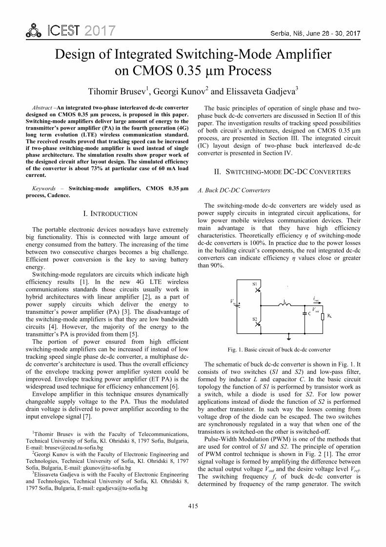
415

Design of Integrated Switching-Mode Amplifier on CMOS 0.35 µm Process

Tihomir Brusev1, Georgi Kunov2 and Elissaveta Gadjeva3

Abstract –An integrated two-phase interleaved dc-dc converter designed on CMOS 0.35 µm process, is proposed in this paper. Switching-mode amplifiers deliver large amount of energy to the transmitter’s power amplifier (PA) in the fourth generation (4G) long term evolution (LTE) wireless communication standard. The received results proved that tracking speed can be increased if two-phase switching-mode amplifier is used instead of single phase architecture. The simulation results show proper work of the designed circuit after layout design. The simulated efficiency of the converter is about 73% at particular case of 60 mA load current.

Keywords – Switching-mode amplifiers, CMOS 0.35 µm process, Cadence.

I. INTRODUCTION

The portable electronic devices nowadays have extremely big functionality. This is connected with large amount of energy consumed from the battery. The increasing of the time between two consecutive charges becomes a big challenge. Efficient power conversion is the key to saving battery energy.

Switching-mode regulators are circuits which indicate high efficiency results [1]. In the new 4G LTE wireless communications standards those circuits usually work in hybrid architectures with linear amplifier [2], as a part of power supply circuits which deliver the energy to transmitter’s power amplifier (PA) [3]. The disadvantage of the switching-mode amplifiers is that they are low bandwidth circuits [4]. However, the majority of the energy to the transmitter’s PA is provided from them [5].

The portion of power ensured from high efficient switching-mode amplifiers can be increased if instead of low tracking speed single phase dc-dc converter, a multiphase dc-dc converter’s architecture is used. Thus the overall efficiency of the envelope tracking power amplifier system could be improved. Envelope tracking power amplifier (ET PA) is the widespread used technique for efficiency enhancement [6].

Envelope amplifier in this technique ensures dynamically changeable supply voltage to the PA. Thus the modulated drain voltage is delivered to power amplifier according to the input envelope signal [7].

The basic principles of operation of single phase and two-phase buck dc-dc converters are discussed in Section II of this paper. The investigation results of tracking speed possibilities of both circuit’s architectures, designed on CMOS 0.35 µm process, are presented in Section III. The integrated circuit (IC) layout design of two-phase buck interleaved dc-dc converter is presented in Section IV.

II. SWITCHING-MODE DC-DC CONVERTERS

A. Buck DC-DC Converters

The switching-mode dc-dc converters are widely used as power supply circuits in integrated circuit applications, for low power mobile wireless communication devices. Their main advantage is that they have high efficiency characteristics. Theoretically efficiency η of switching-mode dc-dc converters is 100%. In practice due to the power losses in the building circuit’s components, the real integrated dc-dc converters can indicate efficiency η values close or greater than 90%.

Fig. 1. Basic circuit of buck dc-dc converter

The schematic of buck dc-dc converter is shown in Fig. 1. It

consists of two switches (S1 and S2) and low-pass filter, formed by inductor L and capacitor C. In the basic circuit topology the function of S1 is performed by transistor work as a switch, while a diode is used for S2. For low power applications instead of diode the function of S2 is performed by another transistor. In such way the losses coming from voltage drop of the diode can be escaped. The two switches are synchronously regulated in a way that when one of the transistors is switched-on the other is switched-off.

Pulse-Width Modulation (PWM) is one of the methods that are used for control of S1 and S2. The principle of operation of PWM control technique is shown in Fig. 2 [1]. The error signal voltage is formed by amplifying the difference between the actual output voltage Vout and the desire voltage level Vref. The switching frequency fs of buck dc-dc converter is determined by frequency of the ramp generator. The switch

1Tihomir Brusev is with the Faculty of Telecommunications, Technical University of Sofia, Kl. Ohridski 8, 1797 Sofia, Bulgaria, E-mail: [email protected]

2Georgi Kunov is with the Faculty of Electronic Engineering and Technologies, Technical University of Sofia, Kl. Ohridski 8, 1797 Sofia, Bulgaria, E-mail: [email protected]

3Elissaveta Gadjeva is with the Faculty of Electronic Engineering and Technologies, Technical University of Sofia, Kl. Ohridski 8, 1797 Sofia, Bulgaria, E-mail: [email protected]

http://www.tu-sofia.bg/eng_new/Fakulteti/faculties/fett/fett-menu.php



416

control signal is formed at the output of the comparator. This signal determines the states of the buck converter’s switches. The frequency fs is constant for PWM control technique. The PWM control technique is suitable for constant envelope signals, when stable dc output voltage of the converter is desired.

Fig. 2. Principle of operation of PWM control technique for buck

dc-dc converter In the 4G LTE standard, the envelope amplifiers, which

have to supply voltage to the PA, should have fast tracking speed because the envelope frequency is increased. The disadvantage of the PWM controlled switching converters is that they are low bandwidth circuits. The switching frequency fs of the dc-dc converter has to be about ten times higher than the bandwidth of the LTE signal [4].

B. Two-Phase Interleaved Buck DC-DC Converters

The two-phase interleaved dc-dc converter architecture is illustrated in Fig. 3.

Fig. 3. Two-phase interleaved buck dc-dc converter

This circuit’s architecture helps to reduction of the output

current ripple Δiout of the converter. This is possible because

the phase shifted inductor current ripples respectively of the first and second sub-converter stage ΔiL1 and ΔiL2 are summed at the output. The output current ripple Δiout of the two-phase interleaved buck converter with non-coupled inductors can be expressed in the form [8]:

( )1 2 ,outout s

Vi D T

L∆ = − (1)

where Ts is the switching period of converter, L is the value of filter inductors if L1=L2. If the duty cycle of the converter D is close to 0.5 then minimum values of the output current ripples Δiout could be obtained. The inductor current ripples of the single phase buck dc-dc converter and two-phase interleaved buck converter with non-coupled inductors have equal values ΔiL, and can be expressed in the form [8]:

( )1 .outL s

Vi D T

L∆ = − (2)

The architecture of two-phase interleaved dc-dc converters permits to be obtained equal output current ripples as those of single-phase dc-dc converters using smaller inductance values of output filter inductors. Therefore those circuits can be used for LTE applications, when envelope amplifier has to be fast in order to track high frequency envelope signal. For example two-phase interleaved dc-dc converter can be used instead of the single phase switching-mode regulator in hybrid envelope amplifier structure. This will result in higher part of energy distributed from high efficient switching-mode dc-dc converter, leading to efficiency increasing of envelope amplifier. The reason is that the portion of power distributed from low efficient linear amplifier to PA will be smaller, compared to the case when switching-mode amplifier is a single phase dc-dc converter.

III. INVESTIGATION OF PWM CONTROLLED TWO-PHASE SWITCHING-MODE AMPLIFIER

Two-phase interleaved buck dc-dc converter controlled with PWM technique is designed on CMOS 0.35 µm. The block circuit is presented in Fig. 4.

Fig. 4. PWM controlled two-phase switching-mode amplifier

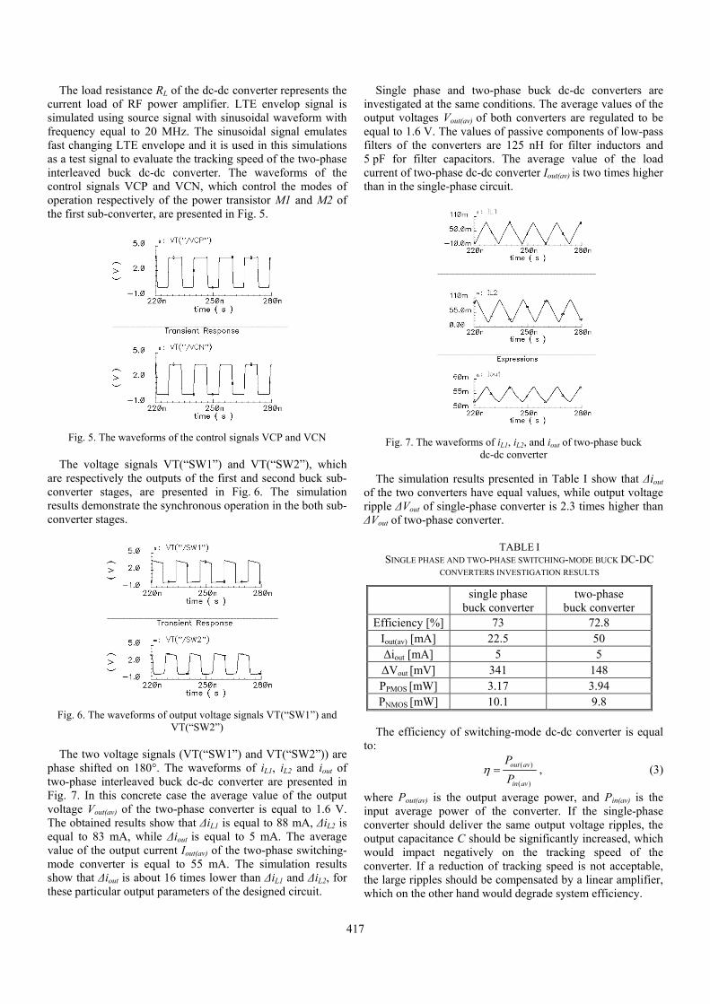
417

The load resistance RL of the dc-dc converter represents the current load of RF power amplifier. LTE envelop signal is simulated using source signal with sinusoidal waveform with frequency equal to 20 MHz. The sinusoidal signal emulates fast changing LTE envelope and it is used in this simulations as a test signal to evaluate the tracking speed of the two-phase interleaved buck dc-dc converter. The waveforms of the control signals VCP and VCN, which control the modes of operation respectively of the power transistor M1 and M2 of the first sub-converter, are presented in Fig. 5.

Fig. 5. The waveforms of the control signals VCP and VCN

The voltage signals VT(“SW1”) and VT(“SW2”), which

are respectively the outputs of the first and second buck sub-converter stages, are presented in Fig. 6. The simulation results demonstrate the synchronous operation in the both sub-converter stages.

Fig. 6. The waveforms of output voltage signals VT(“SW1”) and

VT(“SW2”) The two voltage signals (VT(“SW1”) and VT(“SW2”)) are

phase shifted on 180°. The waveforms of iL1, iL2 and iout of two-phase interleaved buck dc-dc converter are presented in Fig. 7. In this concrete case the average value of the output voltage Vout(av) of the two-phase converter is equal to 1.6 V. The obtained results show that ΔiL1 is equal to 88 mA, ΔiL2 is equal to 83 mA, while Δiout is equal to 5 mA. The average value of the output current Iout(av) of the two-phase switching-mode converter is equal to 55 mA. The simulation results show that Δiout is about 16 times lower than ΔiL1 and ΔiL2, for these particular output parameters of the designed circuit.

Single phase and two-phase buck dc-dc converters are investigated at the same conditions. The average values of the output voltages Vout(av) of both converters are regulated to be equal to 1.6 V. The values of passive components of low-pass filters of the converters are 125 nH for filter inductors and 5 pF for filter capacitors. The average value of the load current of two-phase dc-dc converter Iout(av) is two times higher than in the single-phase circuit.

Fig. 7. The waveforms of iL1, iL2, and iout of two-phase buck

dc-dc converter The simulation results presented in Table I show that Δiout

of the two converters have equal values, while output voltage ripple ΔVout of single-phase converter is 2.3 times higher than ΔVout of two-phase converter.

TABLE I SINGLE PHASE AND TWO-PHASE SWITCHING-MODE BUCK DC-DC

CONVERTERS INVESTIGATION RESULTS

single phase buck converter

two-phase buck converter

Efficiency [%] 73 72.8 Iout(av) [mA] 22.5 50 Δiout [mA] 5 5 ΔVout [mV] 341 148 PPMOS [mW] 3.17 3.94 PNMOS [mW] 10.1 9.8

The efficiency of switching-mode dc-dc converter is equal

to:

( )

( )

,out av

in av

PP

η = (3)

where Pout(av) is the output average power, and Pin(av) is the input average power of the converter. If the single-phase converter should deliver the same output voltage ripples, the output capacitance C should be significantly increased, which would impact negatively on the tracking speed of the converter. If a reduction of tracking speed is not acceptable, the large ripples should be compensated by a linear amplifier, which on the other hand would degrade system efficiency.

418

IV. LAYOUT DESIGN OF PWM CONTROLLED TWO-PHASE SWITCHING-MODE AMPLIFIER ON CMOS

0.35 µM PROCESS

The layout of PWM controlled two-phase switching-mode amplifier is designed on CMOS 0.35 µm process using Virtuoso layout tool of Cadence. The whole converter layout, including power stage and control feedback circuits, is shown in Fig. 8. The re-simulation of layout after the extraction of parasitic capacitance is made in order to verify the proper work of the system.

Fig. 8. Layout of PWM controlled two-phase switching-mode

amplifier The simulated waveforms of output current iout of the two-

phase buck dc-dc converter, respectively of schematic and layout with extracted parasitics, are presented in Fig. 9.

Fig. 9. The waveforms of output current iout of the two-phase buck

DC-DC converter The obtained results shown in Fig. 9 prove the proper work

of two-phase switching-mode amplifier after layout design. The slight difference between the two curves is due to the extracted parasitic capacitance. They are formed by overlapping layers of metal used for wiring. The total estimated parasitic capacitance after layout designed is equal to 1.9 pF. More than 90% of overall parasitic capacitance is contributed from power stage of the switching-mode amplifier. All four metal layers connected in parallel are used

in order to ensure the output current of the converter. If smaller number of metal layers is used in layout design, the parasitic capacitance could be decreased, but more silicon area will be occupied.

V. CONCLUSION

Two-phase switching-mode amplifier designed on CMOS 0.35 µm technology has been proposed in this paper. The investigations show that if two-phase switching-mode amplifier is used instead of single phase architecture, tracking speed can be increased. In this way the overall efficiency of envelope amplifier, which delivers the energy of transmitter’s PA for LTE applications, could be improved. The proper work of the circuit is proved by re-simulation of the whole system with extracted parasitic capacitance after the layout design.

ACKNOWLEDGEMENT

The research described in this paper was carried out within the framework of UNIK – dog. DUNK – 01/03 – 12.2009.

REFERENCES

[1] N. Mohan, T. Undeland, and W. Robbins, Power Electronics, JWES, NY, 2003.

[2] Y. Xiao, C. Yao, Y. Liu, Z. Li, and H. Zhang, "A Power Amplifier with Envelope Tracking Used for Cellular Front-end Module Based on 0.18µm SOI CMOS Process", 2015 IEEE International Symposium on Radio-Frequency Integration Technology (RFIT), pp. 160-162, Sendai, 2015.

[3] M. Hassan, L. Larson, V. Leung, and P. Asbeck, "A Combined Series-Parallel Hybrid Envelope Amplifier for Envelope Tracking Mobile Terminal RF Power Amplifier Applications", IEEE Journal of Solid-State Circuits, vol. 47, no. 5, pp.1185-1198, May 2012.

[4] J. Sankman, M. K. Song, and D. Ma, "A 40-MHz 85.8%-Peak-Efficiency Switching-Converter-Only Dual-Phase Envelope Modulator for 2-W 10-MHz LTE Power Amplifier", Symposium on VLSI Circuits Digest of Technical Papers, June 2014, Honolulu, pp. 1-2.

[5] F. Wang, D. Kimball, D. Lie, P. Asbeck and L. Larson, “A Monolithic High-Efficiency 2.4-GHz 20-dBm SiGe BiCMOS Envelope-Tracking OFDM Power Amplifier”, IEEE Journal of Solid-State Circuits, vol.42, no. 6, pp. 1271-1281, June 2007.

[6] D. Kim, D. Kang, J. Choi, J. Kim, Y. Cho and B. Kim, "Optimization for Envelope Shaped Operation of Envelope Tracking Power Amplifier", IEEE Transactions on Microwave Theory and Techniques, vol. 59, no. 7, pp. 1787-1795, July 2011.

[7] J. Bae, H. Kim, J. Ham, W. Lim, S. Cho and Y. Yang, "CMOS Dynamic Supply Switching Power Amplifier for LTE Applications", 2015 Asia-Pacific Microwave Conference (APMC), pp. 1-3, Nanjing, 2015.

[8] J. P. Lee, H. Cha, D. Shin, K. J. Lee, D. W. Yoo, and J. Y. Yoo. “Analysis and Design of Coupled Inductors for Two-Phase Interleaved DC-DC Converters”, Journal of Power Electronics, vol. 13, no. 3, May 2013, pp. 339-348.

419

Efficiency Investigation of BUCK DC-DC Converter with ZVS Using SPICE

Georgi Kunov1, Tihomir Brusev2 and Elissaveta Gadjeva3

Abstract – In this paper the efficiency of BUCK DC-DC converter with Zero Voltage Switching (ZVS) is an object of investigation. A simulation scheme of Gate Driver with Adaptive Dead Time (ADT) is proposed, which provides the independence of ZVS from the current value at which the transistors are switched. The influence on the switching losses of an externally connected drain-source capacitor is simulated using PSpice. Macros in the graphical analyzer Probe are proposed for calculating the average value of the currents, the losses in transistors and the efficiency. The simulation results are presented graphically as a function of the junction temperature.

Keywords – Power electronics, Switch mode power supply, Buck DC-DC converters, Zero Voltage Switching.

I. INTRODUCTION

The switched mode DC-DC converters are widely used to convert one level of electrical voltage into another level by switching action. These converters have received an increasing deal of interest in many areas, such as: cellular phones, tablets, laptops, radio-frequency power amplifiers, light emitting diode (LED) drivers, etc.

The most commonly used is the BUCK DC-DC converter with Pulse-Width Modulation. Recently, due to its better efficiency, the BUCK DC-DC converter with ZVS is approved. This type of control, with respect to their principle of operation, is similar to Hysteresis Current Mode Control (HCMC).

The BUCK DC-DC converter with HCMC and ZVS is characterized in that the lower hysteresis level has a minimum negative value and is a constant. The regulation of the output power is performed by changing the upper hysteresis level [1, 2]. The application of this control approach leads to optimal output-voltage transient response [3,4] in addition to improving the efficiency.

A subject of the present paper is the construction of a simulation model of BUCK DC-DC converter with HCMC and ZVS, which allows efficiency investigation.

An example study is performed using Infineon’s SPICE Model of the transistor BSC024NE2LS [5].

II. BUCK DC-DC CONVERTER WITH HCMC AND ZVS

A. Power Circuit and Control System

The power circuit of the BUCK DC-DC converter is shown in Fig. 1. The selected SPICE model for the transistors Qt (top) and Qb (bottom) allows the study to be performed depending on the crystal temperature of the transistors.

Vin

12Vdc

+-

H1 HGAIN = 1

0

Vgb

V

Vgt

Gdrv_Qb

In

D

G

S

Tj

QbBSC024NE2LS

0IL

PARAM ET ERS:ILm ax = 35V

0

Vout

1.5Vdc

Tj_b

25

I

A

In-Gdrv_t

C0b670pF

Tj

QtBSC024NE2LS

0

In-Gdrv_b

V

L 1.5uHGdrv_Qt

In

D

G

S

Cot670pF

Tj_t

25

Fig. 1. BUCK DC-DC Converter The control system of the DC-DC converter with HCMC

and ZVS is shown in Fig. 2. Using the comparators EL (low level) and EH (high level), pulses are generated, corresponding to the Low and High Level of the current IL through the inductor L.

The comparator is realized by the Analog-Behavioral Model (ABM) element of EFREQ type using the function: 5*(sgn(V(% IN+,% IN-))+1)/2. The comparator EL sets the R-S trigger (U1,U2) in state "1" and as a result the transistor Qt is turn-on and the transistor Qb is turn-off.

The comparator EH sets the R-S trigger in state "0", whereby the transistor Qt is turn-off and the transistor Qb is turn-on.

EL5*(sgn(V(%IN+, %IN-))+1)/2

OUT+OUT-

IN+IN-

U4

0SW1 TOPEN = 0.1us

0

0V

EH5*(sgn(V(%IN+, %IN-))+1)/2

OUT+OUT-

IN+IN-

VL-1Vdc

ILU1

U3

Reset

Vgt

0

0

Vgb

Set

VCC

U2

VHILm ax

Rsw 1k

V

Fig. 2. Hysteresis current mode control system

1Georgi Kunov is with the Faculty of Electronic Engineering andTechnologies, Technical University of Sofia, Kl. Ohridski 8 Blvd.,1797 Sofia, Bulgaria, E-mail: [email protected]

2Tihomir Brusev is with the Faculty of Telecommunications,Technical University of Sofia, Kl. Ohridski 8 Blvd., 1797 Sofia,Bulgaria, E-mail: [email protected]

3Elissaveta Gadjeva is with the Faculty of Electronic Engineeringand Technologies, Technical University of Sofia, Kl. Ohridski 8Blvd., 1797 Sofia, Bulgaria, E-mail: [email protected]

420

The principle of operating of the control system is illustrated by the waveforms shown in Fig. 3.

The value IL,LowLewel = 1A is selected for the low level of the current IL. The high level of the current IL is a simulation parameter and changes in the range from 2A to 35A.

Fig. 3. Waveforms illustrating the principle of operation of BUCK Converter with ZVS

In this case of HCMC, the switching frequency depends on

the hysteresis window ΔIL [6]:

1 out in out

SWL in

V V Vf

L I V

, (1)

where

, ,L L HighLevel L LowLevelI I I .

B. Gate Driver with Adaptive Dead Time

In order for ZVS to be possible, it is necessary the transistor turn-on pulse Vgs to be applied after the moment when the output capacitance of the MOSFET transistor is discharged by the current IL during the dead time (DT).

The duration of DT (tDT) is a function of the instantaneous value of the current IL,HighLevel. The Gate Driver scheme with adaptive dead time is shown in Fig. 4. In this case, the index "t" corresponds to the top Gate Driver (for the bottom Gate Driver the index "b" is used).

Ut3AND2

D

In

Ut1

50nsDELAY

G

Ut2AND2

+

-

+

-

S2t S

VON = 1.0VVOFF = 2.0V S

Ut4OR2

+

-

+

-

St1 S

VON = 5.0VVOFF = 0.5V

+

-

+

-

S1t S

VON = 2.0VVOFF = 1.0V

Ut5

10nsDELAY

VCC

Rgt2 0.5

Rt1 1k

0

Vdct10Vdc

0

Rgt1 2.7

Fig. 4. Gate Driver with Adaptive Dead Time

Using the voltage-controlled switch St1 and the delay element Ut5, a comparator model is realized (with propagation time 10ns).

When the voltage Vds is less than 0.5V, the logical element Ut2 allows the applied pulse at the input In to reach the transistor's gate. The delay element Ut1 and the logical element Ut3 form a maximum value of tDT-max. This value is needed by the starting the DC-DC converter, since then the current IL = 0. The switches S1t and S2t represent a classical driver of two transistors (n-p-n and p-n-p).

III. SIMULATION RESULTS

The BUCK DC-DC converter with HCMC and ZVS is investigated using the program Cadence PSpice [7]. The simulation is performed for the time interval from 0 to 250 μs.

The following macro-definitions in the graphical analyzer Probe are defined for the postprocessing of the simulation results:

- The values of the currents and voltages in top and bottom power MOSFET transistors: Id_b=I(Qb:DD) Id_t=I(Qt:DD) Vds_b=V(Qb:DD) Vds_t=V(Qt:DD)-V(Qt:S0)

- The values of dissipated power in top and bottom power MOSFET transistors: Pds_t=Vds_t*Id_t Pds_b=Vds_b*Id_b

- The average value of dissipated power: avg_Pds_b=max(S(M(Pds_b))/249us) avg_Pds_t=max(S(M(Pds_t))/249us)

- The average value of the output current and output power: Iout=YatX(AVG(I(L)),250u) Pout=1.5*Iout

- The efficiency: efficiency=Pout/(Pout+avg_Pds_t+avg_Pds_b)

The macros thus defined can be reused. The waveforms illustrating the ZVS transistor switching are

presented in Fig. 5 as follows: – Fig. 5a and Fig. 5c – Qb-off, Qt-on (IL= –1A); – Fig. 5b and Fig. 5d – Qt-off, Qb-on (IL=35A); – Fig. 5a and Fig. 5b – without additional capacitor drain-

source (only with parasitic capacitance Co=650pF of transistor BSC024NE2LS);

– Fig. 5c and Fig. 5d – with additional capacitors Cot=Cob=670pF.

The switching losses Pds-t and Pds-b are presented on the coordinate systems (1) and (2). It is seen that the main switching losses are in the transistor Qt, at the moment of its turn-off, when the current IL = 35A. The additional capacitor Cot leads to a two-fold reduction of the amplitude of Pds-t, but at the expense of longer duration.

The input pulses InGdrv_t and In-Gdrv_b of the Gate Driver are shown on the coordinate system (3), plot 1 and the gate pulses Vgs_t and Vgs_b – on plot 2.

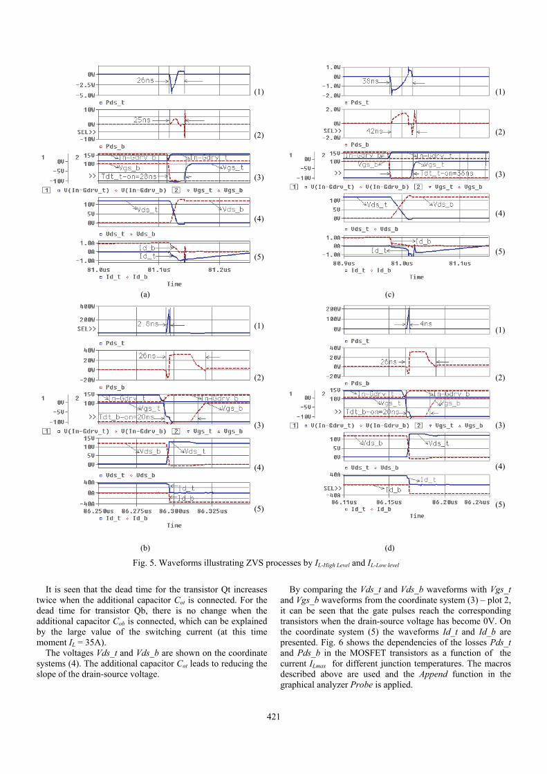
421

(1)

(2)

(3)

(4) (5)

(1)

(2)

(3) (4) (5)

(a) (c) (1)

(2) (3)

(4)

(5)

(1) (2) (3)

(4) (5)

(b) (d) Fig. 5. Waveforms illustrating ZVS processes by IL-High Level and IL-Low level

It is seen that the dead time for the transistor Qt increases

twice when the additional capacitor Cot is connected. For the dead time for transistor Qb, there is no change when the additional capacitor Cob is connected, which can be explained by the large value of the switching current (at this time moment IL = 35A).

The voltages Vds_t and Vds_b are shown on the coordinate systems (4). The additional capacitor Cot leads to reducing the slope of the drain-source voltage.

By comparing the Vds_t and Vds_b waveforms with Vgs_t and Vgs_b waveforms from the coordinate system (3) – plot 2, it can be seen that the gate pulses reach the corresponding transistors when the drain-source voltage has become 0V. On the coordinate system (5) the waveforms Id_t and Id_b are presented. Fig. 6 shows the dependencies of the losses Pds_t and Pds_b in the MOSFET transistors as a function of the current ILmax for different junction temperatures. The macros described above are used and the Append function in the graphical analyzer Probe is applied.

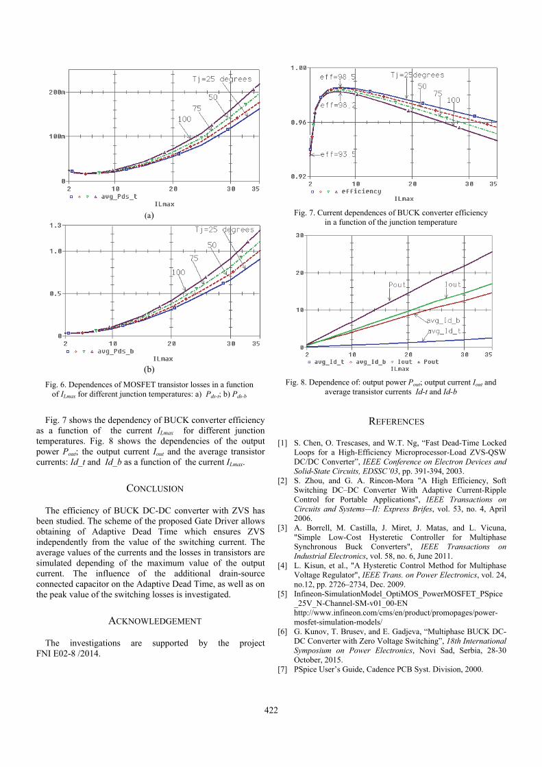
422

(a)

(b)

Fig. 6. Dependences of MOSFET transistor losses in a function of ILmax for different junction temperatures: a) Pds-t; b) Pds-b

Fig. 7 shows the dependency of BUCK converter efficiency

as a function of the current ILmax for different junction temperatures. Fig. 8 shows the dependencies of the output power Pout; the output current Iout and the average transistor currents: Id_t and Id_b as a function of the current ILmax.

CONCLUSION

The efficiency of BUCK DC-DC converter with ZVS has been studied. The scheme of the proposed Gate Driver allows obtaining of Adaptive Dead Time which ensures ZVS independently from the value of the switching current. The average values of the currents and the losses in transistors are simulated depending of the maximum value of the output current. The influence of the additional drain-source connected capacitor on the Adaptive Dead Time, as well as on the peak value of the switching losses is investigated.

ACKNOWLEDGEMENT

The investigations are supported by the project FNI E02-8 /2014.

Fig. 7. Current dependences of BUCK converter efficiency in a function of the junction temperature

Fig. 8. Dependence of: output power Pout; output current Iout and average transistor currents Id-t and Id-b

REFERENCES

[1] S. Chen, O. Trescases, and W.T. Ng, “Fast Dead-Time Locked Loops for a High-Efficiency Microprocessor-Load ZVS-QSW DC/DC Converter”, IEEE Conference on Electron Devices and Solid-State Circuits, EDSSC’03, pp. 391-394, 2003.

[2] S. Zhou, and G. A. Rincon-Mora "A High Efficiency, Soft Switching DC–DC Converter With Adaptive Current-Ripple Control for Portable Applications", IEEE Transactions on Circuits and Systems—II: Express Brifes, vol. 53, no. 4, April 2006.

[3] A. Borrell, M. Castilla, J. Miret, J. Matas, and L. Vicuna, "Simple Low-Cost Hysteretic Controller for Multiphase Synchronous Buck Converters", IEEE Transactions on Industrial Electronics, vol. 58, no. 6, June 2011.

[4] L. Kisun, et al., "A Hysteretic Control Method for Multiphase Voltage Regulator", IEEE Trans. on Power Electronics, vol. 24, no.12, pp. 2726–2734, Dec. 2009.

[5] Infineon-SimulationModel_OptiMOS_PowerMOSFET_PSpice _25V_N-Channel-SM-v01_00-EN http://www.infineon.com/cms/en/product/promopages/power-mosfet-simulation-models/

[6] G. Kunov, T. Brusev, and E. Gadjeva, “Multiphase BUCK DC-DC Converter with Zero Voltage Switching”, 18th International Symposium on Power Electronics, Novi Sad, Serbia, 28-30 October, 2015.

[7] PSpice User’s Guide, Cadence PCB Syst. Division, 2000.

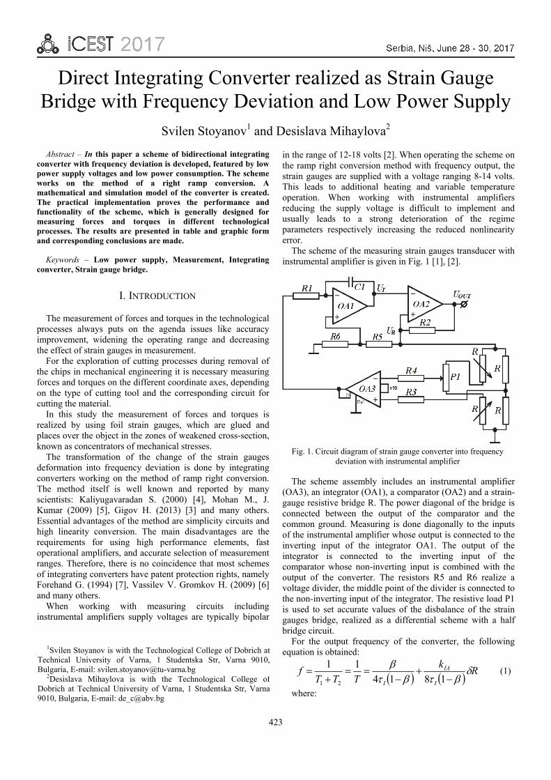
423

Direct Integrating Converter realized as Strain Gauge Bridge with Frequency Deviation and Low Power Supply

Svilen Stoyanov1 and Desislava Mihaylova2

Abstract – In this paper a scheme of bidirectional integrating converter with frequency deviation is developed, featured by low power supply voltages and low power consumption. The scheme works on the method of a right ramp conversion. A mathematical and simulation model of the converter is created. The practical implementation proves the performance and functionality of the scheme, which is generally designed for measuring forces and torques in different technological processes. The results are presented in table and graphic form and corresponding conclusions are made.

Keywords – Lоw power supply, Measurement, Integrating

converter, Strain gauge bridge.

I. INTRODUCTION

The measurement of forces and torques in the technological processes always puts on the agenda issues like accuracy improvement, widening the operating range and decreasing the effect of strain gauges in measurement.

For the exploration of cutting processes during removal of the chips in mechanical engineering it is necessary measuring forces and torques on the different coordinate axes, depending on the type of cutting tool and the corresponding circuit for cutting the material.

In this study the measurement of forces and torques is realized by using foil strain gauges, which are glued and places over the object in the zones of weakened cross-section, known as concentrators of mechanical stresses.

The transformation of the change of the strain gauges deformation into frequency deviation is done by integrating converters working on the method of ramp right conversion. The method itself is well known and reported by many scientists: Kaliyugavaradan S. (2000) [4], Mohan M., J. Kumar (2009) [5], Gigov H. (2013) [3] and many others. Essential advantages of the method are simplicity circuits and high linearity conversion. The main disadvantages are the requirements for using high performance elements, fast operational amplifiers, and accurate selection of measurement ranges. Therefore, there is no coincidence that most schemes of integrating converters have patent protection rights, namely Forehand G. (1994) [7], Vassilev V. Gromkov Н. (2009) [6] and many others.

When working with measuring circuits including instrumental amplifiers supply voltages are typically bipolar

in the range of 12-18 volts [2]. When operating the scheme on the ramp right conversion method with frequency output, the strain gauges are supplied with a voltage ranging 8-14 volts. This leads to additional heating and variable temperature operation. When working with instrumental amplifiers reducing the supply voltage is difficult to implement and usually leads to a strong deterioration of the regime parameters respectively increasing the reduced nonlinearity error.

The scheme of the measuring strain gauges transducer with instrumental amplifier is given in Fig. 1 [1], [2].

The scheme assembly includes an instrumental amplifier (OA3), an integrator (OA1), a comparator (OA2) and a strain-gauge resistive bridge R. The power diagonal of the bridge is connected between the output of the comparator and the common ground. Measuring is done diagonally to the inputs of the instrumental amplifier whose output is connected to the inverting input of the integrator OA1. The output of the integrator is connected to the inverting input of the comparator whose non-inverting input is combined with the output of the converter. The resistors R5 and R6 realize a voltage divider, the middle point of the divider is connected to the non-inverting input of the integrator. The resistive load P1 is used to set accurate values of the disbalance of the strain gauges bridge, realized as a differential scheme with a half bridge circuit.

For the output frequency of the converter, the following equation is obtained:

Rk

TTTf

I

IA

I

1814

11

21

(1)

where:

1Svilen Stoyanov is with the Technological College of Dobrich atTechnical University of Varna, 1 Studentska Str, Varna 9010, Bulgaria, E-mail: [email protected]

2Desislava Mihaylova is with the Technological College ofDobrich at Technical University of Varna, 1 Studentska Str, Varna9010, Bulgaria, E-mail: [email protected]

Fig. 1. Circuit diagram of strain gauge converter into frequency deviation with instrumental amplifier

424

-T – the output period of the converter; -T1 and T2 – half periods of the converter, and T1=T2

-21

2

RR

R

– coefficient of the voltage divider;

-kIA – the gain of the instrumental amplifier; - I – time constant of the integrator; -δR – relative change of the resistance of the strain gauges

load (deformation). The first part of the equation represents the base frequency,

and the second part is the change of the base frequency under bidirectional load. From Eq. (2), the output frequency needs to meet the following condition:

1418 II

IA Rk (2)

According to this condition, the converter is linear for both positive and negative change of δR

In operating mode it was found that bilateral converting deformation of strain gauges is possible only at the smallest gain of the instrumental amplifier k = 10 V/V. In the other ranges, a number of limitations exist in terms of the gain due to non-compliance with condition 2. The scheme with instrumental amplifier has stable performance only when bipolar voltages above 15 volts [2] are applied, which leads to localized heating of the strain gauges and certain change of temperature regimes of the test objects.

II. DEVELOPMENT OF BILATERAL INTEGRATING

CONVERTER WITH REDUCED SUPPLY VOLTAGES

The proposed scheme in Fig. 2 avoids most disadvantages. The scheme represents a linear integrating converter realized by strain gauge bridge with frequency deviation and reduced supply voltages.

The main difference in the scheme is the replacement of the instrument amplifier INA110 of a precise operational amplifier. The last is adjusted for leveling the values of the voltages at the two inputs at zero disbalans of the bridge by the potentiometer P2.

Fig. 2. The circuit diagram of the proposed direct integrating

converter with low power supply

III. METROLOGICAL ANALYSIS OF THE ERRORS OF

THE DIFFERENTIAL AMPLIFIER

A. Metrological Analysis of Errors due to the Tolerance of the Values of the Resistors

The amplification of small changes in input voltage at disbalans of the strain gauge bridge of the converter is realized using differential amplifier. The deviations of the values of resistors R5, R6, R7 and R8 of the differential amplifier from their nominal values cause multiplicative and additive error.

The output voltage of the differential amplifier can be determined by the following formula [3]:

25

71

5

7

6

86

8 11

1ininout V

R

RV

R

R

R

RR

RV

(3)

After conversion of formula 3 and applying the superposition principle for the input differential voltage VD of the strain gauge bridge and its input in-phase voltage VCM it is obtained:

aDDCMDout VKRRR

RRRRV

RRR

RRRRRRVV

865

6785

865

678587

2

2 (4)

From (3) it can be concluded that the inaccuracy of the coefficient KD leads to a multiplicative error, and the expression

6785 RRRRR , when unequal to 0, leads to

additive error а. Additive error is determined by the method of logarithmic differential. The absolute value of the additive error caused by errors of the resistors is obtained:

867586

8 RRRRRR

RVCMa

(5)

In case of differential amplifiers additive error is caused from the common mode rejection ratio Mc (СMRR) as well. The absolute value of this error relevant to the input V1 can be calculated by the following formula [3]:

86

81)(RR

R

M

VM

cca (6)

The scheme in Figure 3 requires the use of resistors with a tolerance of 0.1%. The inaccuracy of the coefficient KD is determined about 0.007 at normalized gain of value 30, which corresponds to 0.022932 %. The absolute value of the additive error as described in formula 5 is 0,0193548*VCM. The absolute value of additive error caused by the common mode rejection ratio using operational amplifier type OPA134PA [9] is 0,000332226*VCM and can be ignored.

B. Analysis of the Error of the Input Offset Voltage of the Differential Amplifier

The residual voltage has a great impact on the accuracy of measurement due to the low values of the voltages coming from the two diagonals of the strain gauge bridge. This tension cannot be compensated in any way. In the circuit of the converter it is necessary to use operational amplifiers with very low values of the input offset voltage. Further equalizing the voltages of the two inputs of the differential amplifier is reached by using trimmer potentiometer P2 and the split beam oscilloscope.

425

IV. MATHEMATICAL MODELLING THE EQUATION

OF CONVERSION

The equation of conversion (1) is modeled in the environment of MATLAB [1]. The values of the elements significant in the equation of conversion are: resistor of the integrator RI = 10kΩ, the capacitor of the integrator CI = 1,7nF, strain gauges with resistance R = 120Ω, and a coefficient of the voltage divider = 0,115. Default bilateral amendment resistance R of strain gauges from -0,5 Ω to + 0,5Ω with step 0,1Ω. The initial frequency of the converter at R = 0 is 1910,934 Hz, but its change is a linear function –Table I.

TABLE I RESULT FROM MODELING

R, T, ms f, Hz R, T, ms f, Hz

0.5 0.33904 2949.49 -0.1 0.58712 1703.22

0.4 0.36473 2741.78 -0.2 0.66867 1495.51

0.3 0.39462 2534.06 -0.3 0.77652 1287.8

0.2 0.42986 2326.35 -0.4 0.92585 1080.09

0.1 0.472 2118.64 -0.5 1.14629 872.383

0 0.5233 1910.93

V. SIMULATION MODELING OF THE CONVERTER

In Fig. 3 a simulation model of the converter is shown, developed in the MULTISIM interface.

Fig. 3. Simulation model of the converter The values of the components are the same as for

mathematical modeling. In line with the integrator and comparator a dual voltage feedback amplifiers AD8056 are used [8] with the following important parameters: 5V power supplies, 5mA typ/amplifier power supply current, 300 MHz −3 dB bandwidth, 1400 V/μs slew rate, 0,02° differential phase error, 0,01% differential gain error, temperature range of −40°C to +125°C. For the differential amplifier High Performance Operational Amplifiers OPA134РА are selected [9] with the following important parameters: supply range ±2,5 V to ±18V, slew rate 20 V/μs, bandwidth 8 MHz,

common-mode rejection 100dB, input offset voltage ±0,5V, temperature range of −40°C to +85°C.

The operation of the converter is examined at a voltage of 2.5 to 6 volts. Initially, the amplitudes of the two input signals of the differential amplifier are equalized via the potentiometer R14, and dual beam oscilloscope XSC2. Two strain gauges R5 and R11 are simulated, differentially connected with values variation ± 0,5 . This is performed by means of the potentiometer R4 step 0,1 . Additionally connected are a dual beam oscilloscope XSC1, frequency counter XFC1 and spectrum analyzer XSA1. The resulting output frequency is given in Table II.

TABLE II OUTPUT FREQUENCY OF THE CONVERTER

R [Ω]

fout, Hz при Ucc=, V

6 5 4 3 2.5 2

0.5 3046 3074 3121 3239 3407 4289

0.4 2834 2860 2904 3014 3169 3983

0.3 2622 2646 2687 2788 2932 3676

0.2 2410 2432 2470 2562 2694 3368

0.1 2198 2218 2252 2336 2456 3059

0 1985 2003 2034 2110 2217 2748

-0.1 1772 1788 1816 1883 1978 2434

-0.2 1560 1574 1598 1657 1739 2117

-0.3 1346 1359 1379 1429 1499 1796

-0.4 1133 1143 1161 1202 1258 1467

-0.5 919.8 927.9 941.7 974.1 1017 1127

The results obtained were processed and the corresponding

points of linearized frequency fout-lin were calculated (not shown herein) and the reduced error of non-linearity in % as per formula (7) [3] - Table III:

%100min_max_

_

outout

linoutout

ff

ff

TABLE III THE REDUCED ERROR OF NON-LINEARITY IN %

6 5 4 3 2.5 2

0.5 0 0 0 0 0 0

0.4 0.0292 0.0284 -0.1097 -0.4841 -0.9209 -4.2584

0.3 0.0292 0.0284 -0.1097 -0.5307 -0.8751 -4.305

0.2 0.0292 0.0284 -0.1097 -0.5307 -0.9209 -4.3516

0.1 0.0292 0.0284 -0.1556 -0.5307 -0.9209 -4.3982

0 -0.0179 -0.0182 -0.1556 -0.5307 -0.9668 -4.4914

‐0.1 -0.0179 -0.0182 -0.1556 -0.5773 -0.9668 -4.6312

-0.2 0.0292 0.0284 -0.1556 -0.5307 -0.9668 -4.771

‐0.3 -0.0649 -0.0182 -0.2014 -0.6239 -1.0127 -4.9574

-0.4 -0.0179 -0.0648 -0.1556 -0.5773 -1.0586 -5.3301

‐0.5 0 0 0 0 0 0

R [Ω]γ, % при Ucc=, V

(7)

426

The results obtained from the simulation are presented graphically in Figs. 4 and 5. The maximum reduced error at Ucc≤4V is 0,2014%, and in case of Ucc 2,5÷3V is about 1%.

Below 3V the circuit does not work stably. Fig. 4. Output frequency at different supply voltages

Fig. 5. The reduced error of non-linearity in %

VI. EXPERIMENTAL RESULT

Experiments were performed under the same conditions as in the simulation. Modification of the resistance with step of 0,1Ω is performed by means of an exemplary pair with accuracy 0.02%. The resistors R7, R8 R9 and R13 have tolerances ± 0,1% and TCS ± 100ppm, and the rest ones ± 1% and ± 100ppm TCS. The capacitor with value 1,7nF is pre-selected and tested (2 capacitors in the kit).

The obtained experimental results are given in Table IV. For the mentioned supply voltages the corresponding output frequency f are included as well as the calculated reduced error of non-linearity from formula 7 [3].

TABLE IV EXPERIMENTAL RESULT

f out , Hz γ, % f out , Hz γ, % f out , Hz γ, %

0,5 2701 0 2877 0 2879 0

0,4 2496 -0,005 2678 0,1044 2676 -0,05

0,3 2285 -0,298 2477 0,005 2475 0,0495

0,2 2079 -0,054 2276 0,005 2273 0

0,1 1868 -0,298 2077 0,1044 2075 0,198

0 1664 0,0439 1868 -0,393 1867 -0,297

‐0,1 1448 -0,542 1667 0,005 1662 -0,149

-0,2 1232 -0,542 1468 0,1044 1460 0

‐0,3 1013 -0,688 1267 0,005 1259 0,0495

-0,4 752 -2,738 1063 -0,144 1053 -0,198

‐0,5 652 0 866 0 859 0

R, ΩUcc=3V Ucc=4V Ucc=5V

The scheme shows a stable work at Ucc=3÷5V. The maximum reduced error at Ucc=4÷5V is 0,393%, and at Ucc=3V it is 2,738 %.

VII. CONCLUSION

An integrating strain gauge convertor is developed operating with low power voltages by using the ramp right conversion method.

The accomplished metrological analysis of the differential amplifier and the converter simulations prove the high metrological characteristics if correct selection of the electronic components is made.

Experimentally, the schematic shows a robust operation at 4-5V supply voltages with an error of less than 0.5%. For supply voltages ranging from 3-4V the error of non-linearity is increased to 2.8%, which must be taken into account when a battery or rechargeable power supply is utilized. In case of supply voltages below 3 V and above 5 V the device cannot operate appropriately.

The main application of the developed transducer is to study mechanical forces and torques of technological processes in real-time.

ACKNOWLEDGEMENT

The work has been performed under the contract number НП17/2017 with Technical University of Varna, Bulgaria.

REFERENCES

[1] S. Stoyanov, "“Modeling Integrating Strain Gauges Measuring Converter whit Instrumental Amplifier", МНК’16, Proceedings of TU Ruse, vol. 55, book 3.1, pp.14-18, Ruse, Bulgaria, 2016.

[2] S. Stoyanov, "Research Methods of Enhancing the Metrological Parameters and Characteristics of Bidirectional Frequency Strain Gauges Converter", EF 2015, Proceedings of TU Sofia, vol. 66, no. 1, pp. 305-314, Sofia, Bulgaria, 2016.

[3] H. Gigov, Measuring Electronics, Technical University Varna, Bulgaria, 2013.

[4] S. Kaliyugavaradan, "A Linear Resistance-To-Time Converter with High Resolution", IEEE Transaction on Instrumentation and Measurement, vol. 62, pp. 151-153, Madras, India, 2013.

[5] M.Mohan, and J.Kumar, "Direct Digital Converter for a Single Active Element Resistive Sensor", I2MTC 2009 Conference, pp. 828-831, Singapore, 2009.

[6] V. Vasilev, and N. Gromkov, "Frequency Converter of the Signal Strain Gauges Bridge Disbalance with a Reduced Temperature Error", patent RU 2395060/2009, Russian Federation.

[7] G.Forehand, "Temperature to Frequency Converter", United States Patent, 5277495, 11.01.1994.

[8] http://www.analog.com/data-sheets/AD8055_8056.pdf. [9] http://www.ti.com/lit/ds/symlink/opa134.pdf.

,

[%]

,

[%]

R [Ω]

R [Ω]

427

A Bidirectional Series Resonant DC-DC Converter with Improved Characteristics

Aleksandar Vuchev1 Nikolay Bankov2 and Angel Lichev3

Abstract – The following paper considers a bidirectional series resonant DC-DC converter operating above the resonant frequency. The disadvantages of the classical implementation are discussed. A control method for the converter is proposed providing control characteristics improvement and decrease of the losses of the circuit elements. On the base of existing theoretical analysis, optimized characteristics are obtained demonstrating the improvements of the proposed converter.

Keywords – Bidirectional Converter, Series Resonant DC-DC Converter, Control Characteristics, Efficiency.

I. INTRODUCTION

The bidirectional series resonant DC-DC converters are far well-known [1]. They hold a lot of advantages one of which are the low switching losses. During operation above the resonant frequency similarly to the other series resonant converters, their power switches are able to commutate at zero voltage (ZVS) [2].

Recently, the use of bidirectional converters have become more and more popular, for example, in the hybrid renewable source energy systems [3]. In such application, they allow optimization of the energy sources operation [4] and of the system as a whole.

In [5], an analytical modeling of the resonant tank processes of a bidirectional DC-DC converter operating above the resonant frequency is presented. As a result, load and control characteristics at phase-shift control are obtained in [6]. The investigation shows that the converter behaves as an ideal current source independently from the energy flow direction. Moreover, it is able to operate without violating the ZVS conditions in a wide range of control parameter variation. Two major drawbacks are also observed. Firstly, the control characteristics hold a considerable nonlinearity. Secondly, the losses in the converter elements are significant even in no-load mode.

In the following paperwork, a different control method is proposed for compensation of the bidirectional series resonant DC-DC converter disadvantages pointed out.

II. CONVERTER WITH A PHASE-SHIFT CONTROL

Fig. 1 presents the circuit of the examined converter. It consists of two identical full-bridge inverter stages, a resonant tank (L, С), a matching transformer Tr, capacitive input and output filters (Cd and C0). Fig. 1 also shows the snubber capacitors C1÷C8 via which ZVS is obtained.

A voltage Ud is applied to the DC terminals of the “input” inverter (transistors Q1÷Q4 with freewheeling diodes D1÷D4), and a voltage U0 is applied to those of the “output” one (transistors Q5÷Q8 with freewheeling diodes D5÷D8).

The converter operation is discussed in [5] where the possible operating modes are determined. The first of them is called DIRECT MODE. In this mode, it is assumed that the energy flows from the Ud to the U0 voltage source. During the second one – the REVERSE MODE, the energy flows backwards – from U0 to Ud.

Waveforms illustrating the converter operation in DIRECT MODE are presented in fig. 2.

The „input” inverter generates the uab voltage which has a rectangular shape and a magnitude of Ud. The „output” inverter generates the ucd voltage which also has a rectangular shape and a magnitude of U0. This voltage is phase-shifted from uab at an angle δ. At δ < π, DIRECT MODE is observed, and at δ > π – REVERSE MODE is observed. Thus, the output power control is achieved by variation of the phase shift δ.

1Aleksandar Vuchev is with the Department of ElectricalEngineering and Electronics, Technical Faculty, University of FoodTechnologies, 26 Maritza Blvd., 4002 Plovdiv, Bulgaria, E-mail: [email protected]

2Nikolay Bankov is with the Department of Electrical Engineeringand Electronics, Technical Faculty, University of FoodTechnologies, 26 Maritza Blvd., 4002 Plovdiv, Bulgaria, E-mail: [email protected]

3Angel Lichev is with the Department of Electrical Engineeringand Electronics, Technical Faculty, University of FoodTechnologies, 26 Maritza Blvd., 4002 Plovdiv, Bulgaria, E-mail: [email protected]

Fig. 1. Circuit of the bidirectional resonant DC/DC converter

428

Angle φ corresponds to the “input” stage reverse diodes interval of conduction, and angle α – to the “output stage” transistors interval of conduction. The converter operates at a constant frequency ωS higher than the resonant ω0. Angles φ, α and δ are measured with respect to the operating frequency ωS.

III. RESULTS OF THE THEORETICAL ANALYSIS

For the purposes of the analysis, the following assumptions are made: all the circuit elements are ideal, the transformer Tr has a ratio k, the commutations are instantaneous, and the ripples of the voltages Ud and U0 negligible.

The analysis in [5] shows that, independently from the converter operating mode, any half period can be divided into three intervals (Fig. 2). For each of these intervals, a constant equivalent voltage UEQ is applied to the resonant tank. Fig. 2 also presents the initial values (IL1÷IL3, UC1÷UC3) of the inductor L current iL and the capacitor C voltage uC for each of the intervals mentioned.

In accordance with the assumptions made, the resonant frequency, the characteristic impedance and the frequency detuning are as follows:

LC/10 ; ;/0 CL 0/ S (1)

In order to obtain generalized results, all magnitudes are normalized as follows: the voltages with respect to Ud, and the currents – with respect to Ud/ρ0. For each of the intervals mentioned, the normalized values of the inductor L current iL and the capacitor C voltage uC are defined as:

jEQEQjCjLjC

jEQjCjLjL

UUUIu

UUIi

j

cossin

sincos (2)

where j is the interval number; I'Lj and U'Cj are normalized values of the inductor current and the capacitor voltage at the interval beginning; θ = 0÷Θj; Θj – interval angle with respect

to the resonant ω0; U'EQj – normalized values of the voltage applied to the resonant tank during the interval.

Fig. 2 and Fig. 3 show that the value of i'L at the end of given interval appears to be the initial value for the following one. The same is for the voltage u'C. Therefore:

jEQjEQjCjjLjC

jjEQjCjjLjL

UUUIU

UUII

j

cossin

sincos

1

1 (3)

The interval at which I'L1 = 0 and U'C1 = – U'CМ is assumed to be first. Then, the initial current (I'L2 and I'L3) and voltage values (U'C2 and U'C3) for the second and the third interval are calculated on the base of equations (3). The necessary for this purpose parameters Θj and U'EQj for a half period are presented in Table I.

TABLE I

MODE Parameter Number of interval

1 2 3

DIRECT Θj

U'EQj 1+kU'0 1–kU'0 –1–kU'0

REVERCE Θj

U'EQj 1+kU'0 –1+kU'0 –1–kU'0

In [5], analytical expressions are obtained for determination of the voltages U'0 and U'CM normalized values which also depend on the control parameter δ and the angle φ:

sinsin

sinsin1

0 kU (4)

0

0

1sin

sinsin2 Uk

UU CM

(5)

In [6], expressions for determination of the normalized average values of the converter circuit currents are obtained. For example, for the DIRECT MODE, the output current can be determined as:

111110 cos1sin EQCL UUIk

I

3

2

cos1sinj

jjEQjCjjL UUIk (6)

By using expressions (3)÷(6), values for U'0 и I'0 can be calculated for a fixed value of the control δ and variation of the angle φ. On the base of these values, output and control characteristics of the converter can easily be built [6].

Fig. 2. Waveforms at DIRECT MODE

429

The theoretical analysis shows that the output voltage does not depend on the output current. Therefore, the converter behaves as an ideal current source. Moreover, the output voltage does not change its polarity and can significantly exceed the input voltage independently from the energy flow direction. However, at values of the control parameter in the range –π/2 ≤ δ ≤ +π/2, the converter ZVS operation area is very limited.

IV. IMPROVEMENT OF THE CHARACTERISTICS

Exemplary control characteristics of the converter are presented in fig.3. They are obtained for different values of the frequency detuning ν at U'0 = 1 and k = 1. The characteristics show that the converter has unlimited ZVS operation with variation of the control parameter in the range π/2 ≤ δ ≤ 3π/2, changing both the magnitude and the direction of the transferred energy. The nonlinearity of these characteristics can be pointed out as a disadvantage.

Applying a combined control, this drawback can be corrected. Fig. 4 presents a „conventional” control characteristic for the DIRECT MODE (with thick line). It is obtained at U'0 = 1, k = 1, ν = const = 1,15 and variation of the control angle in the range π/2 ≤ δ ≤ π. Additionally, a new desired linear characteristic is presented (with dotted line), defined by the two limit states – at maximum output current value (δ = π/2) and at idle mode (δ = π).

A point A1 of the first characteristic corresponds to a value of the angle δ = δA at which the output current value is I'01. A point A2 is obtained on the desired characteristic again for value of the angle δ = δA. Now the output current has a smaller value I'02 < I'01. It is known that when a series-resonant converter operates above the resonant frequency its output current value can be reduced via increase of the operating frequency ωS, in this case – the frequency detuning ν. Only at δ = π/2 the frequency is one and the same for both the old and the new characteristics.

For variation of the control angle in the range π/2 ≤ δ ≤ π, by the use of iteration procedure, the necessary variation of the detuning ν is determined. Fig. 5 presents several such dependences obtained from the „conventional” control characteristics at different values of the detuning ν. They are monotonously increasing and have small nonlinearity. It can

be observed that in order to obtain the desired linear control characteristic, the detuning has to be altered with the angle δ increase from a minimum νmin to a maximum value νmax. For example, νmax = 1,27178 is obtained for νmin = 1,15.

Because the control characteristic is symmetrically located in relation to δ = π, a similar solution is achieved for REVERSE MODE.

In order to realize the desired linear control characteristic of the converter, a normalized control variable σ is introduced with range from 0 to 1. By this variable two parameters will be altered together – the angle δ and the frequency detuning ν:

2/21 (7)

5,0,1

5,0,

minmaxmin

minmaxmin (8)

For DIRECT MODE σ≤0,5 and for REVERSE MODE σ>0,5.

Although the dependence of the frequency detuning ν on the control parameter σ is nonlinear, the linear approximation from (8) provides a very good result. This is demonstrated in Fig. 6 where a „conventional” control characteristic is compared to one obtained from expressions (4) ÷ (8).

The proposed control method provides another advantage – the losses in the converter circuit elements are decreased. For example the RMS value I'L_RMS of the inductor L current decreases. The normalized expression for this value is:

Fig. 3. The phase-shift control characteristics

Fig. 4. The control characteristic correction at DIRECT MODE

Fig. 5. The wanted variation of the frequency distraction

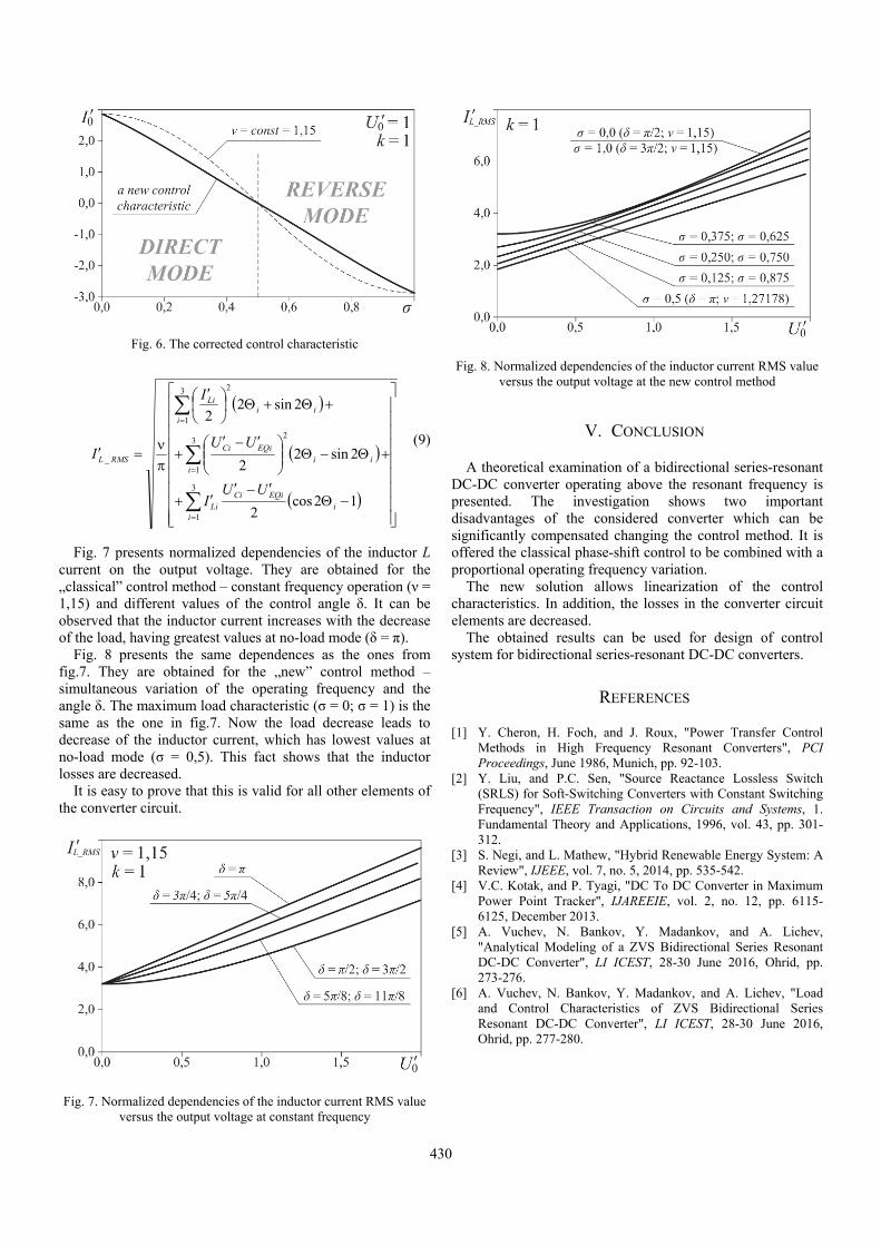
430

3

1

3

1

2

3

1

2

_

12cos2

2sin22

2sin22

ii

EQiCiLi

iii

EQiCi

iii

Li

RMSL

UUI

UU

I

I (9)

Fig. 7 presents normalized dependencies of the inductor L current on the output voltage. They are obtained for the „classical” control method – constant frequency operation (ν = 1,15) and different values of the control angle δ. It can be observed that the inductor current increases with the decrease of the load, having greatest values at no-load mode (δ = π).

Fig. 8 presents the same dependences as the ones from fig.7. They are obtained for the „new” control method – simultaneous variation of the operating frequency and the angle δ. The maximum load characteristic (σ = 0; σ = 1) is the same as the one in fig.7. Now the load decrease leads to decrease of the inductor current, which has lowest values at no-load mode (σ = 0,5). This fact shows that the inductor losses are decreased.

It is easy to prove that this is valid for all other elements of the converter circuit.

V. CONCLUSION

A theoretical examination of a bidirectional series-resonant DC-DC converter operating above the resonant frequency is presented. The investigation shows two important disadvantages of the considered converter which can be significantly compensated changing the control method. It is offered the classical phase-shift control to be combined with a proportional operating frequency variation.

The new solution allows linearization of the control characteristics. In addition, the losses in the converter circuit elements are decreased.

The obtained results can be used for design of control system for bidirectional series-resonant DC-DC converters.

REFERENCES

[1] Y. Cheron, H. Foch, and J. Roux, "Power Transfer Control Methods in High Frequency Resonant Converters", PCI Proceedings, June 1986, Munich, pp. 92-103.

[2] Y. Liu, and P.C. Sen, "Source Reactance Lossless Switch (SRLS) for Soft-Switching Converters with Constant Switching Frequency", IEEE Transaction on Circuits and Systems, 1. Fundamental Theory and Applications, 1996, vol. 43, pp. 301-312.

[3] S. Negi, and L. Mathew, "Hybrid Renewable Energy System: A Review", IJEEE, vol. 7, no. 5, 2014, pp. 535-542.

[4] V.C. Kotak, and P. Tyagi, "DC To DC Converter in Maximum Power Point Tracker", IJAREEIE, vol. 2, no. 12, pp. 6115- 6125, December 2013.

[5] A. Vuchev, N. Bankov, Y. Madankov, and A. Lichev, "Analytical Modeling of a ZVS Bidirectional Series Resonant DC-DC Converter", LI ICEST, 28-30 Junе 2016, Ohrid, pp. 273-276.

[6] A. Vuchev, N. Bankov, Y. Madankov, and A. Lichev, "Load and Control Characteristics of ZVS Bidirectional Series Resonant DC-DC Converter", LI ICEST, 28-30 Junе 2016, Ohrid, pp. 277-280.

Fig. 6. The corrected control characteristic

Fig. 7. Normalized dependencies of the inductor current RMS value versus the output voltage at constant frequency

Fig. 8. Normalized dependencies of the inductor current RMS value versus the output voltage at the new control method

431

Design and Realization of a HB LLC Resonant Converter with Synchronous Rectification Zoran B. Zivanovic1 and Vladimir J. Smiljakovic2

Abstract – In this paper the design of a half-bridge (HB) LLC resonant converter is presented. The operating principles are briefly explained, including the functional block diagram. The prototype has been built and experimental results are presented to support the theoretical analysis and to demonstrate the converter performance.

Keywords – HB, LLC, Resonant, Synchronous, ZVS.

I. INTRODUCTION

Growing demand for higher power density, higher efficiency and lower profile have resulted in increase of the frequency in switching power supplies. Operation at higher frequencies significantly reduces the size of magnetic components, such as transformers and chokes. On the other hand, switching losses are considerably higher at higher frequencies. To reduce the switching losses, resonant converters with zero voltage switching (ZVS) have been developed. ZVS means that voltage across the switch drops to zero before switch turns on. Focus was first on resonant square wave converters (phase shift full bridge) and recently on fully resonant converters with sinusoidal currents instead of trapezoidal currents. Fully resonant converters process power conversion with frequency modulation instead of pulse-width modulation.

II. LLC CONVERTER BASICS

Simplified schematic of a half-bridge LLC resonant converter is shown in Fig. 1. This is a type of series resonant converter that allows operation in a relatively wide input voltage range and output load range compared to other resonant topologies. The converter consists of four main sections: the square wave generator, the resonant circuit, the rectifier circuit and the feedback loop (not shown in Fig.1). The square wave generator generates square wave voltage by driving the power switches Q1 and Q2 with alternating 50% duty cycle for each switch. Of course, a small dead time is always introduced between successive transitions. For all normal load conditions, the power switches are in zero voltage switching condition. The resonant circuit consists of the resonant capacitor Cr, resonant inductor Lr and transformers magnetizing inductance Lm that acts as a shunt inductor.

Fig. 1. HB LLC converter

The magnetizing inductance Lm is three to eight times larger than the inductance of resonant inductor Lr. This is usually accomplished by introducing an air gap in the transformer. Operation frequency is near the resonant frequency determined by Lr and Cr. Because of that, the resonant circuit filters the higher harmonics of current produced by square wave voltage. Sinusoidal current lags the applied voltage which enables the ZVS condition for power switches. Sometimes it is practical to use the leakage inductance of the transformer as a resonant inductor, so that only one magnetic component is used. The resonant capacitor must be of high voltage type (over 600V). The rectifier circuit produces DC voltage by rectifying alternating current with diodes and capacitive output filter. Instead of diodes, for higher efficiency the synchronous rectifiers are used (power switches Q3 and Q4 as shown in Fig. 1). The rectifier circuit is usually used in center taped configuration with two windings (as shown in Fig. 1). For lower output currents the bridge configuration is used. In both cases, rectifier works in zero current switching condition. Feedback loop is similar to other topologies and the only difference is that it uses frequency variation to maintain the output regulation.

III. DESIGN AND ANALYSIS

The goal is to design a half-bridge LLC resonant converter using CoolMOS MOSFETS for the primary power switches and OptiMOS MOSFETs for synchronous rectification. Achieving the efficiency over 90% is the primary objective. We will choose the switching frequency to be around 100 kHz, which is a compromise between efficiency and size. Good choice for the transformer and the inductor core are PQ cores.

We will use a discrete solution for the resonant circuit because in that case we can use any Lr and Lm value. This complicates insulation between primary and secondary windings, but lowers radiated EMI emission. Besides that, drawback is assembling of two magnetic components instead of one.

Design input parameters are given in Table I.

1Zoran Zivanovic is with the IMTEL KOMUNIKACIJE AD,Bul. Mihajla Pupina 165b, 11070 Belgrade, Serbia, E-mail:[email protected].

2Vladimir Smiljakovic is with the IMTEL KOMUNIKACIJE AD,Bul. Mihajla Pupina 165b, 11070 Belgrade, Serbia, E-mail:[email protected].

432

TABLE I DESIGN INPUT PARAMETERS

Min Typ Max Input voltage VIN 320 360 400 V Output voltage VO 28 V Output power PO 500 W Full load efficiency η 92 % Resonant frequency fO 110 kHz

Starting from design input parameters we will now

calculate basic parameters of the resonant circuit (Table II) using Eqs. (1), (2) and (3).

2

IN

O

Vn

V (1)

_ min_ max

2( )

2O F

gIN

V Vm n

V

(2)

_ max_ min

2( )

2O F

gIN

V Vm n

V

(3)

TABLE II RESONANT CIRCUIT PARAMETERS

Min Typ Max Transformer turns ratio n 6.43 Min. voltage gain mg-min 0.92 Max. voltage gain mg-max 1.30 From peak gain curves given in Fig. 2, we will select the point with Mg=1.55, inductance ratio Ln=4 and quality factor Qe=0.4.

Fig. 2. Peak gain curves

Now we can calculate resonant circuit components using the Eqs. (4), (5), (6), (7) and (8). The results are given in Table III.

2

2

8 Oe

O

n VR

I (4)

1

2re o e

CQ f R

(5)

1

2eo e r

Qf R C

(6)

2

1

2r

o r

Lf C

(7)

m n rL L L (8)

TABLE III RESONANT CIRCUIT COMPONENTS

Typ Equivalent load resistance Re 56 Ω Resonant capacitor Cr 66 nF Quality factor Qe 0.383 Resonant inductor Lr 32 µH Magnetizing inductance Lm 128 µH

The suitable selection for the transformer is a core PQ35/35 material 3C96 and for inductor we will use core PQ26/25 material N97. Now it is time to calculate the basic parameters for the transformer (Table IV) and inductor (Table V).

TABLE IV TRANSFORMER BASIC PARAMETERS

Transformer Typ Primary inductance LP 128 µH Number of prim. turns NP 19 Number of sec. turns NS 3 Primary RMS current IPRMS 3.4 A Resonant RMS current Ir 4.4 A Secondary RMS current ISRMS 15.49 A Core gap s 0.55 mm

TABLE V INDUCTOR BASIC PARAMETERS

Resonant inductor Typ Inductance Lr 32 µH Number of turns N 11.5 RMS current IRMS 4.4 A Core gap s 0.65 mm

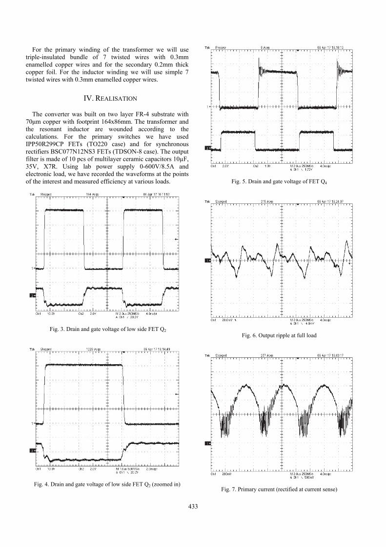
433

For the primary winding of the transformer we will use triple-insulated bundle of 7 twisted wires with 0.3mm enamelled copper wires and for the secondary 0.2mm thick copper foil. For the inductor winding we will use simple 7 twisted wires with 0.3mm enamelled copper wires.

IV. REALISATION

The converter was built on two layer FR-4 substrate with 70μm copper with footprint 164x86mm. The transformer and the resonant inductor are wounded according to the calculations. For the primary switches we have used IPP50R299CP FETs (TO220 case) and for synchronous rectifiers BSC077N12NS3 FETs (TDSON-8 case). The output filter is made of 10 pcs of multilayer ceramic capacitors 10µF, 35V, X7R. Using lab power supply 0-600V/8.5A and electronic load, we have recorded the waveforms at the points of the interest and measured efficiency at various loads.

Fig. 3. Drain and gate voltage of low side FET Q2

Fig. 4. Drain and gate voltage of low side FET Q2 (zoomed in)

Fig. 5. Drain and gate voltage of FET Q4

Fig. 6. Output ripple at full load

Fig. 7. Primary current (rectified at current sense)

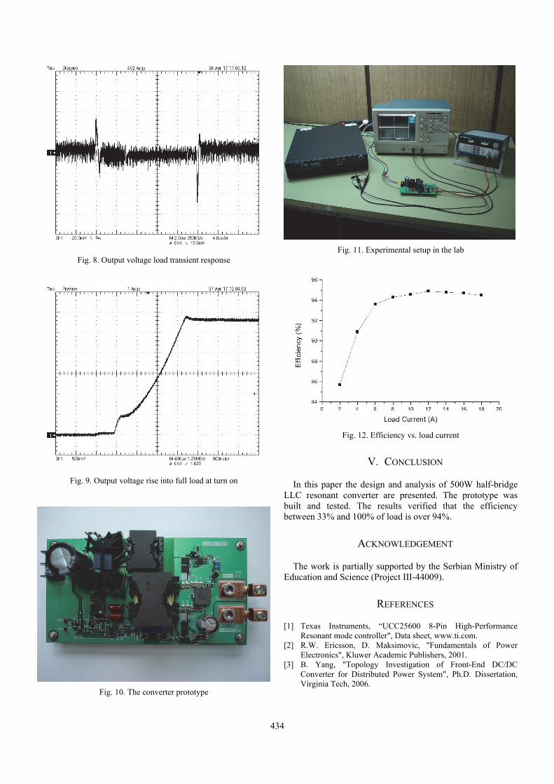
434

Fig. 8. Output voltage load transient response

Fig. 9. Output voltage rise into full load at turn on

Fig. 10. The converter prototype

Fig. 11. Experimental setup in the lab

Fig. 12. Efficiency vs. load current

V. CONCLUSION

In this paper the design and analysis of 500W half-bridge LLC resonant converter are presented. The prototype was built and tested. The results verified that the efficiency between 33% and 100% of load is over 94%.

ACKNOWLEDGEMENT

The work is partially supported by the Serbian Ministry of Education and Science (Project III-44009).

REFERENCES

[1] Texas Instruments, “UCC25600 8-Pin High-Performance Resonant mode controller", Data sheet, www.ti.com.

[2] R.W. Ericsson, D. Maksimovic, "Fundamentals of Power Electronics", Kluwer Academic Publishers, 2001.

[3] B. Yang, "Topology Investigation of Front-End DC/DC Converter for Distributed Power System", Ph.D. Dissertation, Virginia Tech, 2006.

435

Modeling of the Optimal Trajectory Control System of Constant Frequency Series Resonant Converter

Nikolay Bankov1 and Aleksandar Vuchev2

Abstract – An optimal trajectory control system (CS) of series resonant converter (SRC) operating at constant frequency (CF) above the resonant one is proposed. CS is designed on the base of state-plane analysis of SRC and is realized on the principle of the Analog Behavioral Modeling, set in the OrCAD PSpice simulator. The aim is to determine the time intervals in the commutation process when the oscillating circuit voltage and current alter according to an optimal trajectory. This approach gives the opportunity to obtain minimum response time at guaranteed stable converter operation.

Keywords – Resonant DC/DC converters, Control system,

Optimal trajectory control, Behavioural modelling.

I. INTRODUCTION

In the recent years, different methods for control of series resonant converters (SRC) operating above the resonant frequency have been widely discussed and compared [1, 2]. One of them is the method for optimal control of the desired converter operation trajectory. Advantages of the considered optimal control method compared to the other control methods are reduction of the reactive and switching circuit components voltage stresses, as well as, fast dynamic response in case of large variations in the operating conditions at guaranteed stable converter operation.

By the state-plane analysis, accurate description of the converter operation in static and dynamic mode is obtained [2]. On the base of this analysis, optimal trajectory control of SRC is presented for both variable [3] and constant frequency [4].

In [4], block-diagram of optimal trajectory control system (CS) of SRC operating at constant frequency above the resonant is presented.

Deeper investigations are presented in the following paperwork as a particular version of CS is proposed realized on the principle of Analog Behavioral Modeling by the means of the OrCAD PSpice simulator.

The obtained results are presented and analyzed evidencing proper converter operation accomplished by optimal trajectory control.

II. STATE-PLANE ANALYSIS OF CF-SRC

The circuit of the examined converter is presented in Fig. 1. For the analysis purposes, the following assumptions are made: the switches are ideal and have zero switching time; the resonant tank quality factor is infinitely large; the filter capacitor C0 has significant capacitance so that the output voltage remains constant within several commutation cycles. Switches Q1 and Q3 commutate at constant frequency (fS), receiving control signals with duty cycle of 50%. Switches Q2 and Q4 are switched on and off by signals with the same steady-state frequency as the one for Q1 and Q3 but phase shifted, so that Q2 (Q4) switch on before Q1 (Q3). The operating frequency is above the resonant one.

+

−

+

−

iL

Q1

L

D1

C

Ud

Q3 D3

Q2 D2

Q4 D4

D5

D7

uc

D6

D8

C0 RL U0

Fig. 1. CF-SRC Configuration

At deep variation of the load and the phase shift between the control pulses, two different operating modes of the converter can be observed. They are illustrated in Fig. 2 and Fig. 3 with the state trajectory in the state plane LC IyUx ; . For each conduction interval of the power

switches and the freewheeling diodes, ark from a circle is drawn with radius determined by the initial values of the capacitor voltage U'C0 and current I'L0 and center (U'0, 0), (1+U'0, 0), (1-U'0, 0) or the mirror images of these points with respect to the I'L axis. It should be emphasized that all the magnitudes in the phase plane are normalized – voltages with respect to the supply voltage Ud, currents with respect to the

current factor CLU d .

In Fig. 2, the transition from the conduction interval of Q1-D2 to the interval D2-D3 and from Q3-D4 to D1-D4 is realized by the switching of Q1 and Q3 with constant frequency. In Fig. 3, the transition from the interval Q4-D3 to Q1-Q4 and from Q2-D1 to Q3-Q2 is realized by switching of Q1 and Q3 with constant frequency. In both the two figures, the transition from Q1-Q4 to Q1-D2 and from Q2-Q3 to Q3-D4 is obtained by switching of Q2 and Q4.

After the switching of Q2 (Q4), the interval Q1-D2 (Q3-D4) begins, describing ark of a circle with radius R and centre (-U'0, 0) or (+U'0, 0).

1Nikolay Bankov is with the Department of Electrical Engineeringand Electronics, Technical Faculty, University of FoodTechnologies, 26 Maritza Blvd., 4002 Plovdiv, Bulgaria, E-mail:[email protected]

2Aleksandar Vuchev is with the Department of ElectricalEngineering and Electronics, Technical Faculty, University of FoodTechnologies, 26 Maritza Blvd., 4002 Plovdiv, Bulgaria, E-mail:[email protected]

436

-U'Cm

1

R

Q2-Q3

Q3-D4

D1-D4

1+U'0 1-U'0 -1-U'0 U'Cm -U'0

Q1-Q4

U'0

3

2

Q1-D2

D2-D3

I'L

U'C

D

Fig. 2. State-plane Trajectory-Mode1

R Q1-D2

Q2-Q3

D

1 D3-Q4

1-U'0 -U'0

Q1-Q4

3 2

I'L

U'C

Q3-D4

D1-Q2

Fig. 3. State-plane Trajectory-Mode2

The parameter R characterises the converter resonant tank “momentary” energy. Therefore, it can be used as a parameter for control of the energy transfer between the power supply, the oscillating circuit and the load in a way similar to the one used in [2]. Such direct control of the resonant tank energy leads to reduction of the transient processes time and fast settling of the inductor current and the switching capacitor voltage at optimal trajectory.

The aim of the optimal trajectory control is to determine the moments of switching of Q2 and Q4 which accelerate the settling of the capacitor voltage and the inductor current at optimal trajectory for the given operating mode. In this way, the duration of the transient processes is minimized and steady state is achieved for short period of time. For this purpose,

when the converter operates in the interval Q1-Q4 (Q2-Q3), the distance D measured from the center (-U'0, 0) or (+U'0, 0) to the trajectory is constantly observed, and when it equals the parameter R desired value, switches Q2(Q4) commutate.

Q3-D4

I'L

U'C

1+U'0

1-U'0

-1-U'0 -U'0

U'0 D2-D3

Q2-Q3

Q1-Q4

Q1-Q4

-1+U'0

Fig. 4. Transition from a small to a large value of the parameter R

I'L

U'C1+U'0

1-U'0 -1-U'0 -U'0

U'0

D2-D3

Q2-Q3

Q1-D2

-1+U'0

Q3-D4

Q3-D4

Fig. 5. Transition from a large to a small value of the parameter R

In the conduction interval of Q1-Q4, the distance D is determined by:

220 LC IUUD (1)

In the conduction interval of Q2-Q3, the expression for D is:

220 LC IUUD (2)

437

Fig. 6. Converter control system

In this way, the switching of Q2 and Q4 can be determined by:

220 LC IUUR (3)

The plus sign (+) corresponds to the first half period when I'L>0, and the minus sign (-) – to the second half period at I'L<0.

The transient processes at intermittent increase or decrease of the parameter R are shown in Fig. 4 and Fig. 5, respectively. The figures also present the power switches commutation sequence at optimal trajectory control. It can be observed that in both of the cases the transient processes duration is less than a period.

The commutation of the switches Q2 and Q4, as it has been described, happens at D=R. During the transition from a small to a large value of the parameter R, D<R. Then, Q2 and Q4 switch together with Q1 and Q3 ( 02 ) to D=R (Fig. 4). In

this way, the resonant circuit energy has the fastest increase. During the transition from a large to a small value of the

parameter R, D>R and Q2 and Q4 switch immediately. The interval Q1-Q4 (Q2-Q3) is shortened or completely disappears, and intervals Q1-D2 (Q3-D4) and D2-D3 (D1-D4) are extended to D=R (Fig. 5). Thus, the resonant circuit energy has the fastest decrease.

III. CONTROL SYSTEM

CS of the converter is realized on the principle of theAnalog Behavioral Modeling set in the PSPICE A/D simulator [5]. This approach allows versatile description of the electronic components on the base of transfer function or

tabular assignments. In other words, instead of real components for modelling of circuit parts, their mathematical description is applied. With this, a combination of significant calculation efficiency and adequate component modelling is achieved.

The converter circuit, as well as, its control system are presented in Fig.6. MOSFET transistors are used as switching elements.

The distance D from the point that characterizes the resonant circuit state to the commutation center in relative units has the following form:

220sgn LLC IUIUD (4)

The distance D is calculated by BLOCK1 as follows: the information for the resonant tank current is obtained via a current controlled subordinate voltage source Н1. The signals for the output voltage and the switching capacitor voltage are sent to voltage controlled subordinate voltage sources EVALUE (Е2 and Е3). The current sign (sgnI'L) is obtained via voltage controlled subordinate voltage sources EVALUE Е1 which realizes the following function:

SGN(V(%IN+, %IN-)) (5)

The obtained value for D (the BLOCK1 output) is sent to BLOCK2 for comparison with the reference Ur. The pulses formed by the comparator S1 and the logic element U1 are submitted to the latch U2. It forms two channels of pulses phase shifted at 180° for control of the switches Q2 and Q4.

The forced increase of the resonant circuit energy at 02

(Fig.4) is realized by BLOCK3 which contains the voltage controlled subordinate voltage sources EVALUE (Е4 and Е5),

438

monostable multivibrators 74121 (U6 and U7), as well as, logic elements U3, U4 and U5.

BLOCK4 contains pulse voltage sources V3 and V4 for constant frequency control of Q1 and Q3, as well as, controlled voltage sources Е6 and Е7 which provide the necessary power, magnitude and galvanic isolation of the control signals for Q2 and Q4.

The operation of the resonant converter CS is illustrated by the waveforms in Fig. 7.

Time

180us 185us 190us 195us 200us 205us 210us 215us 220usV(G4,S4) V(G1,S1)

0V

10V

SEL>>

V(3)0V

2.0V

4.0V

2

V(1) V(Ur)0V

2.0V

4.0VI(L)

-20A

0A

20A

Fig. 7. Control system main waveforms.

Figs. 8, 9 and 10 presents results from the computer

simulations with OrCAD PSpice, as the converter response is examined at significant variation of the control signal. Fig. 8 presents the converter start-up at R = 3.0, Fig. 9 and Fig. 10 illustrate the converter operation at intermittent alteration of the control system input signal - from R = 1.2 to R= 3.0 and respectively from R = 3.0 to R= 1.2.

V(Uc)

-800V -600V -400V -200V 0V 200V 400V 600V 800V-900VI(L)

-20A

0A

20A

Fig. 8. Converter start-up R = 3.0

V(Uc)

-800V -600V -400V -200V 0V 200V 400V 600V 800V-900VI(L)

-20A

0A

20A

Fig. 9. Response of optimal trajectory control for

Control increase R = 1.2 → R= 3.0

V(Uc)

-800V -600V -400V -200V 0V 200V 400V 600V 800VI(L)

-20A

0A

20A

Fig. 10. Response of optimal trajectory control for

Control decrease R = 3.0 → R= 1.2

At start-up (Fig. 8), the initially gained resonant circuit

energy is zero, and at R = 1.2 (Fig. 9) its value is very small. During the transition to R = 3.0, only the energy accumulation stage exists, whereat the two power switch commutate without phase shift between them.

In the other case (Fig. 10), beginning at the steady state at R = 3.0, the value of the accumulated resonant tank energy is too large. This forces one of the power switch couples to switch off, ceasing in this way the energy accumulation in the resonant circuit.

In all the three cases, the system reaches the steady trajectory for the minimum possible time, which is restricted only by the resonant converter features. From the figures, the stable converter operation with optimal trajectory control can be observed.

IV. CONCLUSION

A control method for series-resonant DC-DC converter operating at constant frequency above the resonant is considered. Computer models of the converter and the optimal trajectory control system realized in the environment of OrCAD PSpice are presented.

The simulation results show a very good dynamic response and steady converter operation.

The obtained results can be used for design and practical realization of resonant DC-DC converters using the considered optimal trajectory control.

REFERENCES

[1] Y. Cheron, H. Foch, and J. Roux, "Power Transfer Control Methods in High Frequency Resonant Converters", PCI Proceedings, June 1986, Munich, pp. 92-103.

[2] R. Oruganti, and F.C. Lee, "Resonant Power Processor: Part II - Methods of Control", Proc. IEEE-IAS’84 Ann. Meet., pp. 868-878, 1984.

[3] N. Bankov, Ts. Grigorova, "Load Characteristics and Control System Behavioral Modeling Under Optimal Trajectory Control of Series Resonant DC/DC Converters", Journal of Electrical Engineering, vol. 56, No. 9-10, 2005, 258-264.

[4] K. Natarajan, and S. Sivakumar, "Optimal Trajectory Control of Constant Frequency Series Resonant Converter", 24th Annual IEEE Power Electronics Specialists Conference PESC '93, pp. 215-221, June 1993.

[5] OrCAD PSpice A/D User’s Guide, OrCAD Inc., USA, 1999.

439

An Overview of Power Supplies with Constant Output Power and their Common Design Method

Nikolay Madzharov

Abstract – This paper gives an overview of high frequency power supply with constant output power, so called converters with energy dosing (CED). A characteristic feature of the CED is the fact that, by their operation principle, they provide energy dosing in the load.The output voltage obtained on that basis corresponds to the particular load parameters, the power always being equal to the specified value.Some converters are presented together with their modifications.The new advancements of CED and their design are also discussed in this paper.For most of the ideas, schemes, design and mathematical interpretation of electromagnetic processes there are author claims.

Keywords – Energy dosing, Converter, Harmonic analysis,

Load matching, Self-harmonization.

I. INTRODUCTION

Although modern power supply sources constitute a greatly electronized and highly intelligent system, they still contain complex controllable power elements, such as transformers, autotransformers, capacitor banks, chokes [1-6]. Along with their undoubted advantages, they have certain disadvantages relating to the methods, the hardware and the quality of their matching with the variable load. The same is true about the regulation and the assigning of a specific value for their output power.

CED are sources of a new type [7-9] and they successfully solve some of the problems in this area. What distinguishes them from the sources we have been familiar with so far is the fact that their output power is assigned in a definite way, and in the process of operation it does not depend on the load parameters, remaining equal to the assigned value.

Fig. 1 presents the schematic diagram of the CED. It is shown schematically that between the source of DC voltage (the rectifier) and the HF converter another block is connected - a doser. By means of this block the energy is transmitted to the load in definite portions (doses).

Fig. 1. The schematic diagram of CED

The doser consists of a reactive element, normally a capacitor (an inductor is also possible) and a diode connected in anti-parallel to it. The capacitor charged up to voltage +E of the supply source is either discharged completely or recharged up to voltage - E in the course of one half-period, its energy being transformed into the converter and transmitted to the load.

The dose of energy W and the power Pare equal, respectively

(1)

/ , (2)

where Cd is the capacitance of the dosing capacitor; f - converter switching frequency; k - a coefficient dependent on the circuit of the doser and the converter; UL - effective value of the output voltage, ZL - load resistance. According to (2) when the values of E, Cd and f do not vary, the power Phas a constant value independent of the load parameters and its changes. In practice, this means that the output voltage of the CED (voltage UL) changes in strict accordance with the concrete load parameters, i.e. self-harmonization with the specific load is performed, naturally, without the influence of the control system.

A large proportion of the ideas in this field have been thoroughly investigated both theoretically and experimentally, and are being used in real practice [10-12].The main purpose of the present paper is in this direction - overview of circuits of CED and the investigations performed on them and common method for their analysis and design.

II. AN OVERVIEW OF CONVERTERS

WITH ENERGY DOSING

A great number of circuits of CED are known [1-3], [8], [12]. Their distinctive feature is the presence of a dosing capacitor included in series in the load loop through the interval of energy consuming by the main. All of them provide dosing of the energy supplied to the load, reliable work of loads changing from idle running to short circuit and high commutation stability in the dynamic operating mode.

In Fig. 2 are shown the basic circuit and their time intervals, illustrating the principle of energy dosing.It can be seen that the dosing capacitor voltage is fixed always to the value of the supplying DC voltage. Consequently, at constant work frequency the power given in the load will always be one and the same. For the circuits with combined recharge of the dosing capacitor, in the expression for the power takes part the coefficient k which is less than 1 and depend on the load parameters.

Nikolay Madzharov is with the Faculty of EEE at Technical University of Gabrovo H. Dimitar str. 4, 5300 Gabrovo, Bulgaria, E-mail: [email protected]

440

(a) CED with capacitor recharging by load current -time intervals and power:0t1- VT1; t1t2- VT2t2 - VD1 ; P=E2Cdf.

(b) CED with combined recharge of the dosing capacitor - time intervals and power: 0t1-VT1, VT6; t1t2- VT1, VT4, VT6; t2t3 - VD1, VD2; t3t4- VT3, VT5; t4t5 - VT2, VT3, VT5; t5 - VD1, VD2; P=kE2Cdf

(c) CED combining energy converting and dosing - time intervals and power: 0t1- VT1, VT6, VD1; t1t2- VT1, VT3; t2t3 - VD1, VD2 ; t3t4 - VT4, VT5, VD2; t4t5 - VT2, VT4 ; t5 - VD1, VD2; P=kE2Cdf

(d) CED with capacitor recharging by equivalent load of current fed invertor - time intervals and power:0t1- VT1, VT3, VT5, VT7; t1-

VD1, VT1, VT3; P=4E2CDf

(e) half-bridge CED - time intervals and power: 0t1 - VT1; t1 - VT1, VD3; P=E2CKf

f) full-bridge CED - time intervals and power:0t1-VT1, VT3 , VD8; t1 - VT3, VD6; P=4E2CKf

Fig. 2. Typical schematics of CED

The comparative analysis of the presented circuits and results from the examinations in previous works [2-5], [11] gives the main feature of CED: at the lack of requirements to the load current pulsations

it is expedient to be used the circuit from Fig. 2a; at the necessity of supporting small output current

pulsations, at a wide regulation range are used the circuit from Fig. 2b. Theoretically, it do not have limits in the regulation characteristics;

for CED from Fig. 2b and Fig. 2c it is important to note that to keep the small output current pulsations at a range of regulation k >3 it is necessary to install inductance L with high value;

the output power of current fed inverter canbeadjusted very accurately within a wide range by CED working frequency - Fig. 2d;

by changing the working frequency of CED from Fig. 2e and Fig. 2f the output voltage can be supported constantly when the load value and/or the input voltage are changed.

III. STUDY METHOD A unified approach and methodology have been suggested

for the analysis and design of CED. The basis of the generalization suggested is the harmonic analysis, the general parameters of fluctuation circuits comprising resonant converter and as well as the information that is contained in the time-chart of their alternating current [2]. With minor modifications, the method is applicable to any CED circuits.

From a great variety of presented circuits and ways of operationa half-bridge CED (HBCED) with forced turn-off of the transistors before half-period has been chosen (Fig. 2e) for analysis. According to the power levels and the load additional serial and/or parallel capacitors can be included in the load circuit. Current and voltage waveforms are shown in Fig. 3. Because of earlier transistors turn-off before half-period end alternating current pulse “shrinking” is obtained. In moments π, 2π,…, nπ it is equal to zero and its fall sector with the biggest damping is cut. This pulse is closer to sinusoidal wave shape than with other resonant converters. Therefore HBCED research and design procedure based on the harmonic analysis are used and AC voltage being accepted to a clear sinusoid.

441

The transistor current pulse has natural frequencyn (see curve 1 on fig.3)

2 2 / (3)

where ωC is control frequency. Relation / is equal to

/ / 1(4)

Proceeding from the obligatory ratio in resonant converters [2], [4]

/ ; 1,2 1,5 / (5)

and assigning 0,5 0,8 . (6)

(to is input datum) angle δ can be determined. δ is the phase angle at the resonant converter AC circuit after the inductor Lk.

Fig. 3. Time-charts of HBCED – uCVT1-2 - control pulses;

iab- alternating current; iVT1, iVD2 - current through transistor VT1 and diode VD2; uC, uCK - voltage over capacitors C and CK

After that, the phase φ1 of the alternating current first

harmonic and the amplitude of the voltage across the load

circuit Ucm= Ugm are respectively calculate

tg 0,406tgδ– 0,165tg δ– 0,188 / (7)

π. E/ 2. cos δ– (8)

It is easy to determine all converter quantities and elements:

- staggering 1/ / of the load circuit

/ , ; (9)

- capacitor C value

1/ . . ; (10)

- active Re and reactive Xe equivalent resistances of the load circuit

1/ . . / 1 ; (11)

. ; (12)

- chokeLk using the frequency ωn

1/ / 4. / ; (13)

- the moments: d- at which the energy consumption from the power supply stops, m - at which the alternating current has maximum value:

/ / 2 / / / , (14)

2 / / / (15)

- dosing capacitor:

/ . (16)

The converter current equation is formed:

(17)

The average and maximum values of the currents across the transistors and the reverse diodes are equal to:

,

, ,

, ,

, ,

(18)

The approach suggested and the methodology for a unified analysis and design has been carried out for all CED and has been confirmed by computer and real experiments.

IV.COMPUTER AIDED AND EXPERIMENTAL STUDY

CED have been studied well both theoretically and in practice.In order to prove the properties and the characteristics of the presented circuits, experimental study has been carried outwith the following input data: P=5 kW; f=30 kHz; E=300 V. Table I presents the results of the investigations, with a change of the load parameters by 25% of the following circuits:

-CED from Fig. 2b - RL=0,15; Lk=1,06H; Cd=2F; -CED from Fig. 2c - RL=0,15; Lk=1,06H; Cd=0,5F.

442

TABLE I TEST RESULTS OF THE CED FORM Fig.2b AND Fig. 2c

Electrical parameters and elements values

CED type RLnom(-25%) RLnom. RLnom(+25%)

CED with combined

recharge of the dosing

capacitor

URL m = 80V

Iin= 10,4A

IVTm = 302A

IVT = 10,4A P = 5,2kW

URL m = 95V

Iin= 10A

IVTm = 242A

IVT = 10A P = 5kW

URL m = 84V

Iin= 10,6A

ImVT = 245,9A

IVT = 10,6A P = 5,3kW

CED combining

energy converting and

dosing

URL m = 239V

Iin= 10,7A

IVTm = 350A

IVT = 10,7A P = 5,35kW

URL m = 93,8V

Iin= 10,1A

IVTm = 290,2A

IVT = 10,1A P = 5 kW

URL m = 258,55V

Iin= 10,8A

Im VT= 255,3A

IVT = 10,8A P =5,4kW

The design of the half bridge CED converter (Fig. 2e) is

based on the expressions, obtained in paragraph III. The purpose is to be defined the values of all elements and phase correlations providing not only efficiency, but also guaranteeing the output parameters and characteristics. The obtained values of the elements and the quantities from the computer simulation calculations and from the practical experiment are presented in Fig. 4 and Table II. There is a good coincidence among the results on the three directions from the transformer examination.

200us 210us 220us 230us 240us 250us 260us 270us

-250V

550V

-170A

170A

0A

170A

I0=30A i0

iab

uò;Uòm=231V

uñê1

Fig. 4. Test results of half-bridge CED at P=5 kW and f=30 kHz – input current, AC current and load and dosing capacitor voltages

TABLE II

DESIGNING, COMPUTER EXPERIMENT AND PRACTICAL EXAMINATION RESULTS

P=5kW ; f=30kHz; E=300V; R=4,3 ; LK=15 H ; Cd =0,462F

quantity UOUT

V IIN A

IVT m A

IVT A

IVD

A POUT

kW

calculated 148 16,2 82,9 18,3 2,08 5,09 computer

experiment 151,5 16,2 81,1 18,2 2 5,33

practical experiment 152 17 86,2 19,2 2,3 5,37

From the information in Table II it can be drawn the conclusion that the output power is in correspondence with expression (2), i.e. there are dosing qualities. This is determined by the average value of the consumed current Iin

and by the voltage on the load Uout. Obtaining the given power can be proven with a third result, as well. The difference between the capacitor and the diode current is equal to the input current and energetically it satisfies the processes of energy consuming in the interval 0d and the short circuit of the alternating converter circuit of the interval d (see Fig. 3).

V. CONCLUSION

This paper described an overview, design and experimental studyofpower supplies with constant output power, so called CED. A 5 kW converter was designed and implemented to verify the validity of the developed common analysis.The basis of the generalization suggested is the harmonic analysis and the information that is contained in the time-chart of the alternating current. The obtained expressions giving the law for operating mode with a purpose to keep the output power constant when the load parameters are changed.It can be concluded that the developed CED may contribute to higher system efficiency and good matching characteristics.

RFERENCES

[1] O.G. Boulatov, and A.I. Tsarenko, Thyristor-Capacitor Converters, Energoizdat, 1982 (in Russian).

[2] T.S. Todorov, N.D. Madgarov, D.T. Alexiev, and P.T. Ivanov, Autonomous Inverters, Gabrovo, 1996.

[3] T.S. Todorov, and N.D. Madgarov, "Wide-Range Resonance Inverters with Energy Dosing with Zero Current of Switching Device", PCIM’97, Power Conversion, Nurnberg, Germany, pp. 385-392, 1997.

[4] G. Kraev, N. Hinov, D. Arnaudov, N. Ranguelov, and N. Gradinarov, "Multiphase DC-DC Converter with Improved Characteristics for Charging Supercapacitors and Capacitors with Large Capacitance", Annual Journal of Electronics, V6,B1,TU of Sofia, Faculty of EET, pp. 128-131, 2012.

[5] N. Bankov, Al. Vuchev, and G. Terziyski, "Operating Modes of a Series-Parallel Resonant DC/DC Converter", Annual Journal of Electronics, Sofia, 2009, vol. 3, no. 2, pp. 129-132.

[6] R. Erickson, and D. Maksimovic, Fundamentals of Power Electronics, Springer Science Business Media, LLC, Second Edition, 2001.

[7] N. Madzharov, and V. Petkov, "Analysis of Expedient Operating Modes of Industrial IPT Systems", Acta Technica, vol. 62, no. 1, 2017, pp. 93-106.

[8] N. Madzharov, "High-Frequency Power Source with Constant Output Power", Journal of Engineering Science and Technology Review, vol. 9, 2017, pp. 157-162.

[9] N.D. Madzharov, "A DC/DC Converter with Energy Dosing", Proceeding PCIM’04, Nurnberg, Germany, 2004.

[10] N.D. Madzharov, R.T. Ilarionov, and A.T. Tonchev, “System for Dynamic Inductive Power Transfer”, Indian Journal of Applied Research, vol. 4, no. 7, 2014.

[11] N.D. Madzharov, and A.T. Tonchev, “Inductive High Power Transfer Technologies for Electric Vehicles”, Journal of Electrical Engineering, vol. 65, no. 2, pp. 125-128, 2014.

[12] N.D. Madzharov, and R.T. Ilarionov, "Battery Charging Station for Electromobiles with Inverters with Energy Dosing", PCIM’11, Power Conversion, Nurnberg, Germany, 2011.

443

A Short Survey on Wireless Interfaces in Embedded Systems

Valentina Rankovska1 and Stanimir Rankovski 2

Abstract – A short survey on the main features and parameters of wireless interfaces is presented in the present paper in relation to their application in the modern embedded systems. They are more and more widely used to connect the increasing number of “intelligent”, programmable peripherals - sensors, actuators, etc., allowing not only reducing the number of the wires, but also distance monitoring and control of the object.

Keywords – Wireless Interfaces, Еmbedded Systems.

I. INTRODUCTION

The embedded microprocessor systems are widely spread long ago almost in all the areas of our life - industry, home, office, automobiles, public activities, etc. This leads to continuous and rapid improvement of their features, such as reliability, flexibility, security, adaptability, cost, dimensions, etc.

Along with the control devices - microcontrollers, having a wide variety of building blocks and improved features, the peripherals (sensors, actuators, etc.) quickly evolve too, becoming more "intelligent". This coupled with the fact that embedded systems are sometimes used in extreme ambient conditions - electromagnetic interference, temperature variations, humidity, dust, vibration, etc., leads to the need of improving the means of communication: between the man and the embedded system; between the components of the embedded system (Fig. 1); in a network of embedded systems. As an example we could take the development of user interface in embedded systems over the years - beginning with buttons, keyboard, seven-segment indication, LCD, to the possible and comfortable use of modern touchscreen devices, such as widely spread personal mobile devices - smartphones, tablets, etc.

The increasing number of programmable devices in embedded systems supposes rapid development of wireless interfaces in order to avoid cable connections. There is a large variety of them depending on the embedded systems application areas [1], [2]. Presently they are mostly used at smart home applications, access control, smart sensor networks, remote industrial monitoring and control, etc. in the Machine-to-Machine and Man-Machine interaction, and sensor connections.

The present paper examines some of the most common modern wireless interfaces in the areas of home automation and Internet-of-Things (IoT) in relation to study cases in Microprocessor Circuits and Embedded Systems for the Bachelor degree students in Electronics at the Technical University of Gabrovo.

Fig. 1. Hypothetic block diagram of an embedded system

II. A SHORT SURVEY ON WIRELESS INTERFACES

FOR EMBEDDED SYSTEMS APPLICATIONS

Infrared Data Association (IrDA) IrDA is an optical open channel interface, allowing peer-to-

peer communication in short distances. The baud rate is 2,4 kbps - 1 Gbps in 1 m distance according to several specifications defining six ranges with different data coding and application areas [3]. The light emitter and detector angles are respectively 15- 30 and up to 15. Therefore, the two communicating devices must be pointing at each other. The consumed power is very low.

This is a low cost technology, comparatively regulation free and there is no interference with the RF technologies. The optical channel is a drawback, as it needs the devices to be in a line of sight, but it is also an advantage as it provides a comparatively good data transfer safety.

IrDA evolves as a perspective optical wireless communication technology providing data rates 5 and 10 Gigabits per second, at 3 m distance and larger angles.

The IrDA interface is applicable in small autonomous embedded systems, mobile control devices (smartphones, tablets, etc.), medical and industrial equipment, etc. because of the short distance communication.

Many microcontrollers provide built-in IrDA standard support through their UART modules and an additional IR Encoder/Decoder and IR Transceiver - for instance some Microchip’s 16-bit and 32-bit microcontrollers [4].

1Valentina Rankovska is with the Faculty of ElectricalEngineering and Electronics at Technical University of Gabrovo, 4H. Dimitar str., Gabrovo 5300, Bulgaria, E-mail: [email protected].

2Stanimir Rankovski is with the Faculty of Electrical Engineeringand Electronics at Technical University of Gabrovo, 4 H. Dimitarstr., Gabrovo 5300, Bulgaria, E-mail: [email protected].

444

Bluetooth Bluetooth (IEEE Standard 802.15.1) is initially intended

especially to replace the wire cables in computer periphery but nowadays it is also one of the technologies used for wireless connectivity in embedded systems. It uses unlicensed industry, scientific, and medical (ISM) 2.4 GHz radio band [5].

Every Bluetooth has its own address with which the others could identify it. The devices make the connection automatically without any actions of the user.

All the devices in such a Bluetooth system form a so called piconet. A master device in a piconet communicates with not more than seven slave devices, and the slave can communicate with the others only through the master. A device could be a member of four piconets at the same time, but only one of them is master. The master acts as a bridge between the piconets. After initiating data transfer, the members of the piconet synchronize their frequencies in a way that they would be in a contact with each other.

The advantages of the Bluetooth technology are small equipment size, easy usage, data safety, good support and development of the standard. Some drawbacks are comparatively high power consumption and impossibility to arrange complex network configurations.

ZigBee ZigBee (IEEE Standard 802.15.4) is intended for shorter

distance range, lower cost, lower power consumption, lower data transfer rates, more compact, and simpler variant of wireless personal area networks (WPANs) in comparison to Bluetooth. It uses the same frequency range of 2,4 GHz [6].

ZigBee realizes various network topologies - star, tree and mesh.

The devices (nodes) in the ZigBee network can be: ZigBee Coordinator, (one in a piconet) which can

communicate with other networks and to save data about its own;

ZigBee Router, which can pass data on from other devices and serves as an intermediate router;

ZigBee End Device – the simplest kind of device, which can communicate only with the above two.

The minimal power consumption is a result of the fact that the slaves are in sleep mode most of the time. They activate for short time intervals only to confirm their presence in the network.

There are four main application areas for ZigBee technology: smart homes, connected lighting, utility industry, zigbee smart energy. The last one is a standard for interoperable products that monitor, control, inform, and automate the delivery and use of energy and water.

Radio-Frequency Identification (RFID) RFID uses electromagnetic fields to automatically identify

and track tags attached to objects. The typical components of a RFID system are a tag, a

reader and an antenna. Various types of tags and readers are used. They can work in several frequency ranges, providing data exchange in different distances: low frequencies (LF) - 125 kHz - 134 kHz, in a distance up to 10 cm; high frequencies (HF) - 13,56 MHz in a distance up to 30 cm;

ultra-high frequencies (UHF) 433 MHz and 856 MHz - 960 MHz in a distance up to 100 m; 2450-5800 MHz (microwave) - 1 - 2 m and 3.1–10 GHz ultra-wideband (UWB) - 200 m.

The various frequency ranges of RFID are specified in the ISO/IEC 18000 standard, except the last, which is not standardized. ISO/IEC 14443 and ISO/IEC 15693 define smart card and proximity card interfaces operating in the HF range [7].

The tags are three types: passive, semi-passive and active. Passive tags have no their own power supply. They are supplied by the electromagnetic energy received from the reader. That is why the distance allowed is shorter than at the the active - typically to 10 m. Active tags (with own power supply - battery) transmit signal to send information stored in the chip at distances up to 100 m. Typically, active tags are used to identify large objects, wagons, containers, etc., which should be monitored over long distances, electronic labels in warehousing, etc. [8].

Active tags themselves are of two types: transponders, which are awakened by the reader, switch on their power and response, and beacons, which periodically wake, switch on and transmit a signal to the reader.

The semi-passive tags use own power source only to switch on the tag. Unlike active transponders, they have a transmitter. They are used for larger distances and transmit in the frequency range of 850 to 950 MHz.

The common application of RFID technology in the field of embedded systems is in the first two frequency ranges - such as access control, pet identification, tracking of goods, etc. Various forms of tags exist: bracelets, badges, stickers, labels, chips, cards, pins tags for clothing, ampoules for pets chipping, etc.

Although RF technologies in their origin are not appropriate for Internet access, their further development makes it possible [9].

The technology is comparatively easy to implement using microcontrollers with RF transmitters, like Microchip’s PIC12/16.

Near Field Communication (NFC) NFC (ISO/IEC 14443 and ISO/IEC 18000-3) is a modern

variety of RFID in the 13,56 MHz frequency range, allowing very short distance communication – up to 10 cm [10]. It is applicable for assets identification, access control, contactless payment, etc.

There are three NFC communication modes: NFC peer-to-peer - for data exchange between two

paired mobile devices; NFC reader/writer - in which one of the devices is

active - it sends signals and receives the data sent form the passive device;

NFC card emulation - NFC-enabled devices like smartphones could be used as credit cards for contactless payment or ticketing.

Initially the technology is designed for access control (identification) and digital tickets in public transportation. Later it is introduced in payment cards (as integrated chips) and smartphones for contactless payment.

NFC is very suitable for configuring of embedded systems using the results of other applications available for smart

445

devices like graphics processing, complex calculations, GPS positioning, Internet communications. Similarly, NFC applies when the smart device wishes to obtain information from an embedded system.

Other useful applications of NFC include passive tags, embedded in advertisement posters and information boards, thereby sending useful information to the users, like scanning QR code.

Smartphones can operate as a reader and as a tag, which makes possible peer-to-peer communication. By holding the smartphone to the NFC-enabled device, the user is able to connect via Bluetooth much faster than pairing devices manually.

The main implementation problems are the proper infrastructure and the data safety.

Z-Wave Z-Wave is one of the newest wireless technologies in the

RF range. It operates in the sub-GHz band, thereby avoiding interference with other wireless technologies in the 2.4 GHz range (Bluetooth, ZigBee, etc.) [11], [12].

It is designed especially for home automation and Internet of Things. A Z-Wave hub (network controller) manages the communication. It allows a distance control via remote web access.

Up to 232 devices could be connected in a mesh network topology in a line of sight up to 100 m. Repeaters (hops) are used in case of obstacles - maximum four hops in a network, increasing the distance up to 200 m.

The devices are interoperable - all they apply ITU-T G.9959 global radio standard and they are compatible, regardless the manufacturer or brand.

Presently over 1700 interoperable Z-Wave products for various home automation applications are available: lighting, lock, various sensors, power management, irrigation, thermostats, etc. Over 70 million products are sold worldwide [12].

WiFi IEEE wireless network standard WLAN 802.11is initially

intended to connect wirelessly mobile devices in a local network, beginning later to be used for Internet connection [13].

While the above wireless standards can be used quite successfully to connect a microcontroller with a periphery for relatively short distances, the WiFi is used in two directions:

To connect the user with the system using the widely spread mobile devices - smartphones, tablets, laptops, in short distance.

The advantage is that a regular user without professional qualification could easily configure the connection with new devices, unlike ZigBee for instance.

To connect embedded systems and their blocks with World Wide Web [14];

It is a rapidly growing technology with a great potential. On one hand it gives an opportunity for flexible and rapid monitoring and control of wirelessly connected embedded client devices, so called “Internet of Things” (or “Wireless Connectivity of Things”), аnd on the other it could be applied successfully together with perspective cloud computing.

Another advantage of WiFi is the high data rate. An amendment to the IEEE 802.11-2007 wireless-networking standard specifies significant increased data rates - from 54 Mbit/s to 600 Mbit/s, using multiple antennas in order to improve network throughput.

It is the most expensive technology in comparison to the above mentioned, but is getting cheaper through the years. In addition, it is significantly cheaper than using a dedicated touch panel for an embedded system.

WiFi is a suitable way to configure and control remotely embedded systems from long distances around the world and from a variety of devices.

Table. 1 presents a short summary of the main features of

the above examined short range wireless technologies.

III. CONCLUSION

A short survey on the features, parameters and application areas of modern wireless technologies has been made in the present paper in relation to embedded systems and more exactly home automation and IoT.

WiFi and Bluetooth, initially designed for office and personal communication, are the most widely used wireless technologies nowadays. They are continually developing under IEEE802 subgroups of standards, effective and reliable, allowing the use of conventional personal digital devices. WiFi is the most expensive approach but the most flexible and extensible. Both technologies are perfect to implement universal man-machine interface.

The features and thus the application areas of the radio frequency range interfaces differ. LF devices do not need to communicate in a line of sight. They are intended for short distance, low data transfer communication. The connection is stable close to metal objects, water, etc. unlike HF, UHF and microwave. Their main application areas are objects tracking and positioning, access control, etc.

Modern rapidly developing areas such as building and industrial automation, IoT, sensor networks, imply further development of the wireless interfaces and the emergence of new ones, such as Z-Wave, Wireless Sensor and Actuator Network protocol DASH7, networking protocol for Internet of Things (IoT) Thread, EnOcean and Insteon technologies for home automation, etc.

ACKNOWLEDGEMENT

The present work is supported by the Science Research Fund at the Ministry of Education, Youth and Science under contract 1708Е/2017.

REFERENCES

[1] R. Johnson, and S. Cotton, „Electronic Sensors: Making the Connection“, The Technology Teacher, May/June 2008, pp. 5-9.

[2] A. Flammini, "Wired and Wireless Sensor Networks for Industrial Applications", Microelectronics Journal, vol. 40, no. 9, September 2009, pp. 1322-1336.

446

TABLE I MAIN FEATURES OF SHORT RANGE WIRELESS TECHNOLOGIES IN RELATION TO EMBEDDED SYSTEMS APPLICATIONS

Technology Network topology

Data transfer rate

Wavelength/ Frequency range

Distance, m Power

consumption Internet

connectivity Smart mobile devices access

peer-to-peer 2,4 kbps-1 Gbps 850–900 nm 0,1-1 low difficult not very suitable

peer-to-peer;star;

piconets with up to 7 nodes

1 - 3 Мbps ISM: 2,4 GHz 0,1 - 100 1 - 100 mW yes most suitable

peer-to-peer; star; mesh

250 kbps (20 kbps)

ISM: 2,4 GHz (868 MHz in

Europe) 10-100

1 - 100 mW; typically 1

mW yes not suitable

peer-to-peer

LF: 4-8 kbps; HF: 6.7 kbps to

848 kbps

LF: 125–134 kHz HF: 13.56MHz

LF: up to 10 cm

HF: up to 100 cm

very low difficult not suitable

peer-to-peer

106, 212 or 424 kbps

13.56MHz < 20 cm;

typical - 4 cm

Tag: none Reader: very

low; typically 1

mW

difficult most suitable

star

11 (b), 54 (g), 600 (n) Мbps, (ac) 1,3 Gbps; (ad) 7 Gbps

(n) ISM: 2,4 GHz и/или 5 GHz;

(ac) 5 GHz 30-100 highest excellent most suitable

peer-to-peer; mesh,

up to 232 nodes

40 - 100 kbps ISM: 868.42 MHz

(Europe)

up to100 m; up to 200 m with 4 hops;

typically up to 30m

very low; typically 1

mW

difficult most suitable

[3] http://www.irda.org/ [4] K. Otten, "IrDA Standard Stack for Microchip 16-bit and 32-bit

Microcontrollers", Microchip Technology Inc., 2010. [5] https://www.bluetooth.com/ [6] http://www.zigbee.org/ [7] K. Sattlegger, and U. Denk, "Navigating Your Way Through the

RFID Jungle", Texas Instruments White Paper, March 2014. [8] S. A. Weis, "RFID (Radio Frequency Identification): Principles

and Applications", MIT CSAIL, 2007.

[9] T. Kamigaki, "Object-Oriented RFID with IoT: A Design Concept of Information Systems in Manufacturing", Electronics, MDPI AG, Basel, Switzerland, 2017.

[10] http://nearfieldcommunication.org/ [11] http://www.z-wave.com/ [12] http://z-wavealliance.org/about_z-wave_technology/ [13] http://www.wi-fi.org/ [14] N. Venkatesh, "Designing Wi-Fi Connectivity into Your

Embedded "Internet Thing", Redpine Signals, July 11, 2011.

447

Wireless System for Battery Cell Voltage Monitoring Dimiter Badarov1, Georgy Mihov2 and Racho Ivanov3

Abstract – The subject of this article is the development and the testing of a wireless battery voltage monitoring system. A smart device using Wi-Fi interface is developed to measure the voltage and temperature of each cell of a battery. This device makes possible the construction of a smart battery monitoring system for control and optimization of the charge/discharge cycles of a battery.

Keywords – Battery monitoring, Smart sensor, Data acquisition, Wi-Fi interface, Internet of Things.

I. INTRODUCTION

Most of the batteries consist of a number of cells connected in series. Usually in the process of charge and discharge the voltage of the whole battery is monitored but not that of the individual cells. This principle relies on that all cells from the same battery are with identical parameters and are always in an equal state of charge. When the battery gets older, the cells change its parameters. The capacity of some cells drops more than others and the internal resistance of some cells is getting higher than others. These differences are leading to a non-equal state of charge of the different cells. The weaker cells go into a deep discharge and overcharge frequently. At the same time the stronger cells stay undercharged. This puts the cells into a non-optimal mode of operation and the asymmetries are getting worse with time and soon the battery reaches its end of life [1].

For the purpose of the battery monitoring a cheap device with small size and Wi-Fi interface is developed. The device is mounted on each individual cell of the battery and monitors the voltage and the temperature of the cell. The current through the battery is monitored also. All the data is sent through a Wi-Fi interface to a central station where the data from the whole battery is collected and processed. This gives information for actual parameters of each individual cell and can be used to optimize the mode of operation of the battery. With this methodology one can provide the required measures to counteract the cell degradation in the exact time and prolong the battery life.

II. STRUCTURE OF THE CELL VOLTAGE

MONITORING MODULE

The structural diagram of the cell voltage monitoring device is represented in Fig. 1.

Fig. 1. Structural diagram It consists of a power supply module, Wi-Fi interface

module, CPU module and some peripheral devices like Analog-to-Digital Converter (ADC), sensors etc. The microcontroller Cortex M0+ is a low power microcontroller which controls the whole measurement process and communication through the Wi-Fi interface. The used Wi-Fi interface module is based on ESP8266 device and has serial interface for data transfer and Printed Circuit Board (PCB) antenna [2]. The cell voltage monitoring module also incorporates Analog-to-Digital Converter, digital temperature sensor and current sensor.

The microcontroller program algorithm does the measurements, sends the data through the Wi-Fi, receives control packets of data from the central station and puts the microcontroller and all peripheral modules to low power mode, called ‘Sleep’. A wakeup timer is started and when it counts to zero the microcontroller wakes up and does the routine again. This is a key measure to reduce the power consumption of the module and the self-discharge of the cell.

III. POWER SUPPLY

The power supply module generates all of the supply voltages needed for the system from the voltage of the battery cell itself. The voltage of the cell varies in a wide range based on the type of the battery and the state of charge. The DC-DC converter uses TPS61200 device. Its input voltage interval is from 0.5 to 5.5V which covers almost every battery cell voltage and state of charge. The DC-DC converter features reduced idle power consumption and high efficiency by using synchronous rectifier. The specific application requires the

1Dimiter Badarov is with the Department of Electronics, Facultyof Electronic Engineering and Technologies, Technical University –Sofia, 8 Kliment Ohridski blvd., 1000 Sofia, Bulgaria, E-mail:[email protected]

2Georgy Mihov is with the Department of Electronics, Faculty ofElectronic Engineering and Technologies, Technical University –Sofia, 8 Kliment Ohridski blvd., 1000 Sofia, Bulgaria, E-mail:[email protected]

3Racho Ivanov is with the Department of Electronics, Faculty ofElectronic Engineering and Technologies, Technical University –Sofia, 8 Kliment Ohridski blvd., 1000 Sofia, Bulgaria, E-mail:[email protected]

448

power supply to withstand significantly higher voltage than the standard cell voltage in case of open circuit into the battery cell. In such scenario the whole battery voltage can appear over the cell terminals with the reverse polarity [3]. In such case the power supply should shut down safely. The power supply can shut down also in case of deep discharge of the battery cell. In these cases the central station loses connection to that cell which is interpreted as failure in the cell.

IV. COMMUNICATION PROTOCOL

The data transfer through the Wi-Fi is organized in 64 bit packets Fig. 2. Every packet starts with the 16 bit battery identification number followed by 4 bit cell number. The next information transmitted is the 12 bit temperature value followed by the two 16 bit values for the current and the voltage. As the current is equal for all cells in a battery only one module measures the current. This is either the module of the first or the last cell. The current value transmitted from all other cell modules is 0x0000.

Fig. 2. Structure of the data packet The power consumption of the module is proportional to

the frequency of the measurements, Fig. 3.

Fig. 3. Power-to-frequency relation A two-way communication protocol is developed for self-

discharge reduction. If the cell module cannot connect to the central station the turn on frequency is low - one turn on per minute. This reduces the power consumption and the self-discharge When the connection with the central station is established the station responds to the cell module with a data packet which contains the desired frequency of measurement in the form of a value for the sleep timer of the microcontroller. If needed a continuous mode of measurement can be activated.

The program algorithm of the cell module is represented on Fig 4:

Fig. 4. Cell module program algorithm After a restart the microcontroller performs initialization of

all peripheral modules. Then it measures the temperature, current and voltage and filters the data to eliminate the noise. After that it sends the processed data to the central station and receives the control data packet. From the packet it extracts the sleep timer value, loads the timer and puts the peripheral modules and the processor to sleep. When the sleep timer expires the processor wakes up and repeats the algorithm.

V. DATA FILTERING

In the process of battery usage electromagnetic interferences are generated either from different loads or from a charging station. This interference can affect the accuracy of the measurements and introduce significant error.

In the process of the DC voltage and the current measurement a simple averaging on n samples can be performed to eliminate the noise influence. In some cases when a lower data delay is required, more complex algorithms as moving average can be implemented.

The microcontroller in the module does the moving average on n samples before sending the results to the central station.

VI. CENTRAL STATION

The central station consists of a Wi-Fi server and a microprocessor system with a user interface. It performs all of the control and communication with the cell modules and collects the data. Based on the information for the cell voltages, currents and temperatures it can calculate the best mode of operation for the battery at the exact time and send it to the charge/discharge controller for correction.

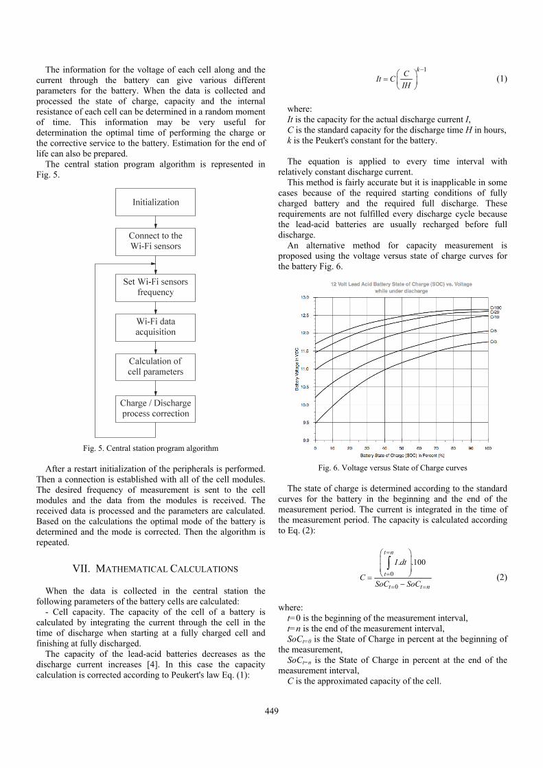
449

The information for the voltage of each cell along and the current through the battery can give various different parameters for the battery. When the data is collected and processed the state of charge, capacity and the internal resistance of each cell can be determined in a random moment of time. This information may be very useful for determination the optimal time of performing the charge or the corrective service to the battery. Estimation for the end of life can also be prepared.

The central station program algorithm is represented in Fig. 5.

Fig. 5. Central station program algorithm After a restart initialization of the peripherals is performed.

Then a connection is established with all of the cell modules. The desired frequency of measurement is sent to the cell modules and the data from the modules is received. The received data is processed and the parameters are calculated. Based on the calculations the optimal mode of the battery is determined and the mode is corrected. Then the algorithm is repeated.

VII. MATHEMATICAL CALCULATIONS

When the data is collected in the central station the following parameters of the battery cells are calculated:

- Cell capacity. The capacity of the cell of a battery is calculated by integrating the current through the cell in the time of discharge when starting at a fully charged cell and finishing at fully discharged.

The capacity of the lead-acid batteries decreases as the discharge current increases [4]. In this case the capacity calculation is corrected according to Peukert's law Eq. (1):

1kC

It CIH

(1)

where: It is the capacity for the actual discharge current I, C is the standard capacity for the discharge time H in hours, k is the Peukert's constant for the battery. The equation is applied to every time interval with

relatively constant discharge current. This method is fairly accurate but it is inapplicable in some

cases because of the required starting conditions of fully charged battery and the required full discharge. These requirements are not fulfilled every discharge cycle because the lead-acid batteries are usually recharged before full discharge.

An alternative method for capacity measurement is proposed using the voltage versus state of charge curves for the battery Fig. 6.

Fig. 6. Voltage versus State of Charge curves The state of charge is determined according to the standard

curves for the battery in the beginning and the end of the measurement period. The current is integrated in the time of the measurement period. The capacity is calculated according to Eq. (2):

0

0

. .100t n

t

t t n

I dt

CSoC SoC

(2)

where: t=0 is the beginning of the measurement interval, t=n is the end of the measurement interval, SoCt=0 is the State of Charge in percent at the beginning of

the measurement, SoCt=n is the State of Charge in percent at the end of the

measurement interval, C is the approximated capacity of the cell.

450

For lead-acid batteries the calculated value C is corrected using the Peukert's law to get the standard 20h discharge capacity.

These capacity measurement algorithms are not so accurate in comparison to the measurement using a constant discharge current. However, these algorithms give a rough idea for the capacity of each cell.

- Static internal resistance of the cell. The static internal resistance of a battery cell is important parameter. It is used for determining the state of charge, the aging of the cell and the optimal charge/discharge current. It is calculated from the variation of the cell voltage versus the variation of the current through the cell and is given by Eq.(3):

iU

RI

(3)

where: Ri is the internal resistance of the cell, ΔU is the variation of the cell voltage, ΔI is the variation of the current through the cell. The internal resistance is calculated every time when a load

current variation occurs. The natural wide interval of load current variations allows the building of a load curve for each cell of the battery and also a curve of the static internal resistance versus the load current.

- End of life prediction. Based on the above calculations the end of life of the battery can be predicted. A rapid increase of the internal resistance of one of the cells or rapid decrease of the capacity is sign for a problem with the cell. The cell can be serviced accordingly or a corrective charge can be applied. This way the life of the battery can be extended [5].

The method of equalizing charge can be applied if the state of charge of the different cells of a lead-acid battery differs too much. The equalizing charge is applied until the state of charge is equalized. The usage of the data from the cell modules can help determining the exact moment of application of equalizing charge as well as the application period. This extends the life of the battery [6].

VIII. CONCLUSION

The developed battery cell voltage monitoring device helps gaining much information about the battery in the field of application. This information can be useful as for better studying the processes in the battery, as for optimizing the battery usage to extend its life.

The calculations for the different battery parameters are done in the software of the central station and can be modified according to the type of the used batteries. A new parameters can be added any time based on the existent data from the battery modules. This makes the developed system very flexible.

Wi-Fi interface is chosen for communication between the modules and the central station despite its higher energy

consumption due to the lower cost of the commercial Wi-Fi modules and for the flexibility which gives the interface. For example when using Wi-Fi any standard laptop or tablet with appropriate software can be used for central station instead of a dedicated device. The usage of standard Wi-Fi interface also gives the opportunity to use already existent Wi-Fi networks to exchange the data with the central station. This is useful if the battery is mobile for example on a forklift or another electric vehicle which has a several hundreds of meters working field. An individual static IP address can be defined for every group of cell modules and the central station can recognize the group based on the IP address. This way it is possible to connect the cell modules to the central station through the internet using a mobile internet modem. This can extend the working range of the system even more. In all cases the monitored batteries should be pre-defined manually with their unique numbers in the central station in order to recognize them and to collect the data which they are sending.

The developed two-way communication protocol between the central station and the battery modules reduces the power consumption of the modules. The frequency of turning on and sending data over the Wi-Fi is changed dynamically on demand which reduces the consumption in the time the battery is not in use.

ACKNOWLEDGEMENT

This paper is a part of a project under contract 162ПД0027-03/2016, which is funded by the research program of the TU – Sofia, Bulgaria.

REFERENCES

[1] M. Abdul-Hak, N. Al-Holou "ITS based Predictive Intelligent Battery Management System for plug-in Hybrid and Electric vehicles", Vehicle Power and Propulsion Conference, 7-10 Sept., pp. 138-144, 2009.

[2] 802.11p-2010 - IEEE Standard for Local and Metropolitan Area Networks - Specific requirements Part 11: Wireless LAN Medium Access Control (MAC) and Physical Layer (PHY) Specifications Amendment 6: Wireless Access in Vehicular Environments.

[3] O. Jiang, "Low-Voltage, Reverse-Battery Protection Circuit Using the TPS61200 Boost Converter", Texas Instruments Application Report SLVA315, 2009.

[4] M. Cugnet, M. Dubarry, B. Liaw, "Peukert's Law of a Lead-Acid Battery Simulated by a Mathematical Model", ECS Trans., pp. 223-233, 2010.

[5] Y. Feng, Y. Han, F. Cao, Z. Shen, W. Chen, and J. Wu, "Intelligent Battery Management for Electric and Hybrid Electric Vehicles: A Survey", IEEE International Conference on Industrial Technology (ICIT 2016), United States, 14-17 March, pp. 1436-1441, 2016.

[6] P. Krein, and R. Balog, "Life Extension Through Charge Equalization of Lead-Acid Batteries", INTELEC, Paper 32.1, 2002.

451

Arduino-based Wireless Sensor Nodes Milen Todorov1, Boyanka Nikolova2, Georgi Nikolov3, Milena Terzieva4

Abstract – ZigBee is one of the main standards for low-data-rate, short-range communications used in wireless sensor networks. The main advantages of this standard are mesh networking, low-power, low-complexity, reliability and operation on unlicensed frequency band, available Worldwide. In this paper is presented an approach to develop low-cost sensor nodes using an open-source hardware and software platforms, such as Arduino.

Keywords – Arduino, IEEE 802.15.4, Wireless Sensor Networks, XBee, XCTU, ZigBee.

I. INTRODUCTION

While numerous sensors are connected directly, through the use of existing local area networks, with controllers and data processing stations, the numbers of sensors that send information wirelessly are increasing. This is important because many network applications require hundreds or thousands of sensor nodes, often located in remote and inaccessible areas. Therefore the sensor node, except the sensor element should have processing and data storage capabilities. Sensor networks are ideal for all forms of environmental monitoring. Due to the sensors’ small size, low energy requirements, and low-cost, implementers can install them at sites or at specific stations or machines for precise reporting. Sensors can be used to measure observations at key locations, the measured data is sent to a computer or even to a server in the cloud.

The microcontroller platform in this paper is Arduino. This is an open-source electronics platform based on hardware and software. The most significant advantages of Arduino over other systems are: Relatively inexpensive compared to other microcontroller

platforms; Cross-platform – the Arduino Software (IDE) runs on

different operating systems; Simple and clear programming environment; Open source and extensible software. The language can be

expanded through C++ libraries; Open source and extensible hardware – circuit designers can

make, extend and improve the module.

ZigBee is a standard that defines a set of communication protocols for low-data-rate short-range wireless networking. The standard is developed by the ZigBee Alliance, which has hundreds of member companies, from the semiconductor industry and software developers to original equipment manufacturers (OEMs) and installers. The ZigBee standard uses IEEE 802.15.4 as its Physical Layer (PHY) and Medium Access Control (MAC) protocols. IEEE 802.15.4 uses spreading methods to improve the receiver sensitivity level, increase the jamming resistance, and reduce the effect of multipath. The signal spreading by the transmitter and despreading by the receiver reduce the effect of the interferers [1-3].

II. SENSOR NODE CONFIGURATION

Arduino boards do not come with ZigBee connectivity. The proposed option in this paper is to use a shield. A shield is basically an extension board that can be placed on top of the Arduino board. Shields are used to extend the hardware features of the Arduino. Another option is to use an external component, mounted on a breakout board, which are connected to Arduino. The used digital relative humidity and temperature sensor RHT03 measures the concentration of water (moisture) in the air. Humidity sensors react to these phenomena and generate a voltage that the microcontroller of Arduino read and calculate a value on a scale. A basic, low-cost humidity sensor is the DHT-22. The DHT-22 is designed to measure temperature as well as humidity. It generates a digital signal on the output (data pin). It should be used to track data at a reasonably slow rate (no more frequently than about once every 3 or 4 seconds). When this sensor generates data, that data is transmitted as a series of high and low voltages that the microcontroller reads and use to form a value. In this case, the microcontroller reads a value 40 bits in length. The first two bytes are the value for humidity, the second two are for temperature, and the fifth byte is the checksum value to ensure an accurate read [4]. DHT-22 temperature and humidity sensor requires pull up resistor to pull up the data value to the voltage level to ensure a valid logic on the wire. The sensor is temperature compensated and calibrated in accurate calibration chamber and the calibration-coefficient is saved in type of programme in one-time programmable (OTP) EPROM. When the sensor is detecting, it will read this coefficient from memory [5]. The sensor uses its own protocol.

The XBee and XBee-PRO Radio Frequency modules meet IEEE 802.15.4 standards and support the needs of low-cost, low-power wireless sensor networks. The modules require minimal power and provide reliable delivery of data between devices. The modules operate within ISM 2.4 GHz frequency band and are pin-for-pin compatible with each other [6, 7]. The XBee/XBee-PRO modules interface to a host device

1Milen Todorov is with the Faculty of Telecommunications atTechnical University of Sofia, 8 Kl. Ohridski Blvd, Sofia 1000, Bulgaria

2Boyanka Nikolova is with the Faculty of Telecommunications atTechnical University of Sofia, 8 Kl. Ohridski Blvd, Sofia 1000, Bulgaria, E-mail: [email protected]

3Georgi Nikolov is with Faculty of Electronic Engineering andTechnologies at Technical University of Sofia, 8 Kl. Ohridski Blvd, Sofia 1000, Bulgaria

4Milena Terzieva is a PhD student from the Faculty of Telecommunications at Technical University of Sofia, Bulgaria

452

through a logic-level asynchronous serial port. Through its serial port, the module can communicate with any logic and voltage compatible UART or through a level translator to any serial device (e.g. RS-232, USB interface board). By default modules operate in Transparent Mode. In this mode, the modules act as a serial line replacement – all UART data received through the DI pin is queued up for RF transmission. When RF data is received, the data is sent out the DO pin. If the module can not immediately transmit, the serial data is stored in the DI Buffer. The data is packetized and sent at any RO timeout or when maximum packet size are received. If the DI buffer becomes full, hardware or software flow control must be implemented in order to prevent overflow – loss of data between the host and module. Application Programming Interface (API) Operation is an alternative to the default Transparent Operation. The frame-based API extends the level to which a host application can interact with the networking capabilities of the module. When in API mode, all data entering and leaving the module is contained in frames that define operations or events within the module. The API provides alternative means of configuring modules and routing data at the host application layer. A host application can send data frames to the module that contain address and payload information instead of using command mode to modify addresses [8]. By default XBee modules are configured to operate within a peer-to-peer network topology, i.e. modules are synchronized without use of master/server configurations. A peer-to-peer network can be established by configuring each module to operate as an End Device, disabling End Device Association in all modules and setting ID and CH parameters to be identical across the network.

III. NETWORK DEPLOYMENT

Fig. 1 shows the discovered radio module that is connected to the computer and remote radio modules in the same network as the local module.

Fig. 1. Detected local and remote modules

The detected network topology is shown of Fig. 2. The network perspective is only available in API operating mode of detecting module. Radio modules in AT (transparent) mode do not support the network discovery process. Each module is labelled with its role (C – coordinator, R – router).

Fig. 2. Network topology

As can be seen from the figure each node is connected to its

neighbours with solid lines (active connections) or dotted lines (undiscovered connections), with arrows indicating the direction of communication. The bidirectional quality and status of the connection between two nodes are displayed next to the line that connects them. The link quality is represented by Link Quality Indication (LQI) with number between 0 and 255 where 0 is the weakest and 255 is the strongest.

Fig. 3 shows table view of detected radio modules. The green background (first row) denotes the local radio module used for the detection. The blue background (second row) denotes the selected module. The table gives the role of each device, 64-bit address of the modules, network address (for ZigBee network) or node identifier (for networks working with other protocols), scan number when the devices were last discovered. Even when a radio module leaves the network, some devices continue to store information about their relationship. On Connection column can be seen the remote modules which are connected to the selected module. Also are displayed their: role in the network, 64-bit address, LQI and status.

Fig. 3. Table view of detected nodes The quality of the wireless signal can be affected by many

factors, most important of which are absorption, reflection of waves, line of sight issues, antenna style and location. Therefore was carried out a range test, which shows the radio frequency (RF) range and link quality between two selected

453

XBee modules. The LQI is an indication of the quality of the data packets received by the receiver and it is recorded for each received packet, indicating the signal energy or the signal-to-noise ratio. The LQI is only one of the decision factors in selecting a path to route a message. A method to calculate the link cost is to use a lookup table to map different levels of LQI directly to the link cost levels of 0 to 7. The table is created based on the average results of several experiments. Other factors such as routing energy efficiency considerations, can also influence the route selection [2]. Fig. 4 shows the results from the test. During the test the local module send data packets and waits for the echo from the remote module. The XCTU software tool counts the number of the packets sent and received and measures the signal strength of the both sides as a Received Signal Strength Indicator (RSSI) value. The performed test type is Cluster ID 0x12, which uses explicit addressing frames directed to the Cluster ID 0x12 on the data endpoint 0xE8, which returns the received data to the sender. As can be seen from the figure, during the test session were sent 100 packets with transmit interval of three seconds and response timeout before considering a packet to be lost also three seconds.

Fig. 4. Results from range test tool

Fig. 5 shows the results from Throughput tool of XCTU, which measures the transfer rate between two radio modules in the ZigBee sensor network. The throughput type was bidirectional – Cluster ID 0x12. It is important to note that not

all protocols and operation modes support Bidirectional – Cluster ID 0x12 Throughput type of test. The duration of the test was 300 s and were sent 1034 packets with 86856 bytes.

Fig. 5. Results from the throughput session

Fig. 6 shows the collected data from a single sensor node in

the ZigBee network.

Fig. 6. Measured relative humidity and temperature

IV. ACQUIRING DATA IN LABVIEW

ENVIRONMENT

The presented approach can be extended for use in graphical programming environments. Such environment is LabVIEW, that is a high level programming language, which inherits the internal structures of C language, but offers more simplicity and functionality about making signal processing

454

calculations and control techniques of instruments. The main advantage that LabVIEW offers is that it is a graphical language [9, 10]. The programs in this language have, from the user side, the same appearance as a front panel of an electronic device, with buttons, graphic screens, numerical indicators, etc.

LINX is a free software package installed in LabVIEW. This package makes easy to use graphical programming language for interacting with some embedded platforms such as Arduino, chipKIT and myRIO. With LINX installed in LabVIEW it is possible to easily access the device’s digital inputs and outputs, analog inputs and outputs, SPI, I2C, UART, PWM and more features. Inside LINX functions, there are several options for the user to choose. The Open and Close functions are used to start and end the communication with the Arduino microcontroller. In palette Peripherals the user finds different options for general digital and analog inputs or outputs. There are also different options for PWM, I2C, SPI and UART communication. The user can also find sensors functions that are already prepared to work with specific sensors. There are different types such as temperature sensors, light sensors, motion sensors, etc.

In the presented work as example for using Arduino as wireless sensor node in LabVIEW, PIR movement sensor HC-SR501with digital output is connected to Arduino. Movement detectors based on this PIR sensor could be used for automatically sensing light for a room, bathroom, basement, porch, warehouse, garage, etc. It can also be used to get ventilators to work. In safety applications, obviously it can work as an alarm to detect when a person is entering some place. Actually, the wireless network topology is the same as in Fig. 2. The difference is in the graphical way to send command and receive data from sensor nodes.

Fig. 7. LabVIEW block diagram for communication with Arduino and Xbee explorer

Graphical programing code with specific LINX functions is shown in Fig. 7. As can be seen in the figure only three functions are needed to receive data from wireless node: Open, Close and Read Digital.

The front panel of wireless communication with sensor is shown in Fig. 8. It is used to control only virtual serial port and number of digital pin connected to the motion detection sensor.

Fig. 8. Front panel of application for motion detection

V. CONCLUSION

In present project is suggested an approach for organizing wireless sensor network that use communication protocols according to the standard ZigBee. The proposed and implemented approach extends the performance of sensors, by using open source platform for development of low-cost wireless sensor nodes. In addition as alternative method for wireless communication between the sensor nodes, programing code in LabVIEW graphical programming environment is created.

ACKNOWLEDGEMENT

This research is supported by Project 171ПР0013-07.

REFERENCES

[1] L. Gavrilovska et al., Eds. Application and Multidisciplinary Aspects of Wireless Sensor Networks: Concepts, Integration, and Case Studies, Springer, 2011.

[2] S. Farahani, ZigBee Wireless Networks and Transceivers, Elsevier Ltd., 2008.

[3] ZigBee Specification, 053474r17, Jan. 2008. [4] C. Bell, Beginning Sensor Networks with Arduino and

Raspberry Pi, Apress, 2013. [5] MaxDetect Technology Co., Ltd., “Digital relative humidity &

temperature sensor RHT03” RHT03 datasheet. [6] Dargie, W., C. Poellabauer. Fundamentals of Wireless Sensor

Networks: Theory and Practice. John Wiley & Sons Ltd., 2010. [7] F. Eady, Hands-On ZigBee: Implementing 802.15.4 with

Microcontrollers, Elsevier Inc, 2007. [8] Digi International, XBee/XBee-PRO RF Modules 802.15.4

Product Manual, 2015. [9] M. Schwartz, and Ol. Manickum, Programming Arduino with

LabVIEW, Packt Publ., 2015. [10] R. W. Larsen, LabVIEW for Engineers, Prentice Hall Publ.,

2011.

455

A Cost-Effective Linearization System used for Resolution and Accuracy Increase of

an Angular Position Encoder Jelena Jovanović1 and Dragan Denić2

Abstract – This paper presents a cost-effective angular position encoder linearization system based on a PIC18F2550 microcontroller. The linearization system is developed and employed to increase the encoder resolution and accuracy. More specifically, the encoder resolution is increased by three bits, while the maximal absolute measurement error is reduced by ten times.

Keywords – Angular position determination, linearization, pseudo-linear signal, sine and cosine signal processing.

I. INTRODUCTION

The angular position encoders are widely used transducers in many systems that contain rotating parts [1]. However, the non-linearity of the encoder static transfer function results in low sensitivity, meaning that even significant change in the measured angle leads to insignificant output voltage variation [1, 2]. Sometimes these output voltage variations are so small that the noise present in the signal or signal distortion can mask them. If the variation of encoder output voltage is not detected, the measured angle change will not be detected as well, producing in this manner a significant measurement error. In order to avoid this kind of error, a linearization technique can be used [3-6].

To gain more accurate information about the absolute angular position, one can use the interpolation electronics for processing of encoder output sine and cosine signals [7]. However, the interpolation method is based on information about the relative difference between sine and cosine signal amplitudes and phases, so the deviation of these signals from the ideal signal waveforms can cause an error. Therefore, it is important to eliminate these deviations before the signals are brought to the inputs of the interpolation electronics.

The aforementioned problems can be avoided using the encoder linearization system presented in this paper. The developed linearization system is reliable and by its price cost-effective solution that enables the angular position measurement resolution increase by three bits. The system is consisted of a linearization circuit (a network of logic circuits, comparators, operational amplifiers and a multiplexer) and the PIC18F2550 microcontroller (MCU). Result of the application

of this system is lower absolute measurement error, while the shortcomings of complex and processor demanding digital linearization methods are avoided [8].

II. LINEARIZATION SYSTEM DESIGN, FUNCTIONING AND APPLICATION RESULTS

Angular position encoder generates highly nonlinear sine and cosine signals at its output as a response to an angular position change, [1]. By processing these signals with the proposed linearization circuit more linear resulting signal, so-called pseudo-linear signal, is obtained. Pseudo-linear signal is composed of the most linear parts of sine and cosine signal. In addition to the output pseudo-linear signal, the proposed linearization circuit generates three bits used for coding of an octant, π/4 [rad] wide, (within the range of 2π [rad]) to which the measured angle belongs. Further processing of the signal (for example A/D conversion using the A/D converter (ADC) built-in in the MCU) is carried out within one octant, so that the ADC input range is narrowed down.

The proposed linearization system is tested using a PC with the LabVIEW virtual instrument used to generate the encoder output signals that are brought to the respective inputs of the linearization circuit via PCI-6251/CB-68LP Academic Starter Kit (consisted of the PCI-6251 multi-function acquisition card and CB-68LP connecting block). In addition to the linearization circuit, the newly-designed printed circuit board contains the PIC18F2550 MCU whose built-in 10-bit ADC performs conversion of analog pseudo-linear signal of improved linearity into digital domain. The shape of the pseudo-linear signal (voltage), that is being further digitized, is the same as the shape of the sine function within the range from 0 to π/4 [rad]. The MCU forwards the 10-bit digitized voltage to the PC via built-in HID USB connection. Additional virtual instrument, installed on the PC, determines the value of the angular position using the first three bits and the output of the 10-bit ADC, and displays the result on the front panel. Testing scheme of the proposed linearization system is shown in Fig. 1.

Electrical scheme of the linearization circuit used for the pseudo-linear signal generation is shown in Fig. 2a. The sine and cosine signals are brought to the inputs of the comparators in order to be compared with the zero reference voltage, or in order to be mutually compared. By bringing digital signals A, B, C and D to the inputs of the logic circuits shown in Fig. 2a, special logical operations are performed, while the following bits are generated:

1Jelena Jovanović is with the University of Niš, Faculty ofElectronic Engineering, Aleksandra Medvedeva 14, 18000 Niš,Serbia, E-mail: [email protected].

2Dragan Denić is with the University of Niš, Faculty of ElectronicEngineering, Aleksandra Medvedeva 14, 18000 Niš, Serbia, E-mail:[email protected].

456

2 AD , (1)

1 A XOR BD , (2)

0 A XOR B XOR C XOR DD . (3)

LabVIEW VIfor sine and cosinesignal generation

PCI-6251/CB-68LPAcademic Starter

Kit

LINEARIZATIONCIRCUIT

PIC18F2550-I/SPLabVIEW VI for

measurement resultsdisplaying

cos(x)

sin(x) 3 bits

PCI

pseudo-linearsignal

USB

13 bits

Fig. 1. Testing scheme of the proposed linearization system

TABLE I SIGNALS AND BITS GENERATED IN THE PROPOSED LINEARIZATION CIRCUIT

Measured angle x [rad]

A: sin(x)>0

B: cos(x)>0

C: cos(x)>sin(x)

D: sin(x)+cos(x)>0

D2 D1 D0 Output signal

0-π/4 1 1 1 1 0 0 0 +sin(x) π/4-π/2 1 1 0 1 0 0 1 +cos(x) π/2-3π/4 1 0 0 1 0 1 0 -cos(x) 3π/4-π 1 0 0 0 0 1 1 +sin(x) π-5π/4 0 0 0 0 1 0 0 -sin(x) 5π/4-6π/4 0 0 1 0 1 0 1 -cos(x) 6π/4-7π/4 0 1 1 0 1 1 0 +cos(x) 7π/4-2π 0 1 1 1 1 1 1 -sin(x)

-sin(x)

+sin(x)AnalogMUX

(8 to 1)

cos(x) S/H

sin(x) S/HD1

D

cos(x)

-cos(x)

sin(x)

C

B

D0

A D2

A2 A1 A0X 0

X 1

X 2

X 3

X 4

X 5

X 6

X 7

Y 0

Pseudo-linearsignal

(a)

(b)

Fig. 2. (a) Electrical scheme of the linearization circuit used for pseudo-linear signal generation, (b) Output pseudo-linear signal

(bolded line)

The octant to wich the current value of the measured angle belongs is represented by the bits D2, D1 and D0. Also, these bits are intended for the control of the analog 8-to-1 multiplexer, as shown in Fig. 2a. The waveforms of sine, cosine and pseudo-linear signal are shown in Fig. 2b. In Table I are given logical values of A, B, C and D digital signals obtained at the comparators’ outputs, the bits D2, D1 and D0, and the waveforms of the output signal related to the current octant. It can be observed that in the measurement range of 2π [rad] the pseudo-linear signal represents a combination of the most linear parts of the following signals: sin(x), cos(x), -sin(x) and -cos(x). As shown in Fig. 2a, signals -sin(x) and -cos(x) are generated in the linearization circuit, and together with the input signals sin(x) and cos(x) are brought to the inputs of the analog 8-to-1 multiplexer. Which signal will be available at the output of the analog multiplexer depends on the corresponding octant of the current angle value x, i.e. it depends on the combination of bits D2, D1 and D0.

In order to obtain a monotonically rising static transfer function of the complete measurement system (including position encoder, linearization circuit and the 10-bit ADC of the MCU), it is necessary to perform the inversion of ADC output bits when the current angle value x belongs to even octants, because in these octants the slope of the pseudo-linear signal waveform is negative. Since D0 has a logical value of 1 in even octants, the most convenient manner to perform the aforementioned inversion is to bring the output bits of the ADCA/D converter together with D0 to the inputs of ten logical XOR circuits. In comparison to the bits D2, D1 and D0, the 10-bit ADC output bits are of less significance (weight).

For example, if the current value of the measured angle x belongs to the octant spanning from π to 5π/4 [rad], at the output of the multiplexer will be obtained the most linear part

457

of the signal -sin(x) (see the last column in the Table I and see the Fig. 2b, while the coding bits for this octant are 1 0 0. Since the signal -sin(x) has only positive values for this octant and has the same shape and slope as the signal sin(x) in the range from 0 to π/4 [rad], the inversion of ADC output bits is not necessary. In the following octant (from 5π/4 to 6π/4), the pseudo-linear signal is represented by signal -cos(x), which has the same shape, but the negative slope in comparison to the signal sin(x) in the range from 0 to π/4 [rad]. In this case, the inversion of ADC output bits needs to be performed.

(a)

(b)

Fig. 3. (a) Front panel of the VI used for sine and cosine signal simulation; (b) Front panel of the VI used for calculation and

displaying of angular position measurement results

In Fig. 3a, the front panel of the virtual instrument, designed to generate signals from the encoder output, is shown. This virtual instrument offers the possibility of adjusting the amplitude, phase and frequency of sine and cosine signal in accordance with the rotating speed of the observed object whose angular position is measured (it is assumed that the speed of rotation, in the observed time interval, is constant). The cosine signal is obtained by phase shifting of the sine signal (with the same amplitude and frequency) by π/2 [rad]. The generated signals are brought to the designated inputs of the proposed linearization system over the CB-68LP connecting block and the PCI-6251 multifunction acquisition card. Fig. 3b shows the front panel of the virtual instrument designed to calculate and display the angular position after the linearization is finished. The virtual instrument determines the angular position x [rad] based on the values of bits D2, D1 and D0 (which define the current octant number n), and on the basis of the voltage u [V] that is brought to the 10-bit ADC input. In precise, the following expressions are implemented in the virtual instrument: when the angle value x belongs to an odd octant:

rad 1 arcsin V4

x n u

, n=1,3,5,7, (4)

and when the angle value x belongs to an even octant:

rad arcsin V4

x n u

, n=2,4,6,8. (5)

The printed circuit board (PCB) of the proposed linearization system, consisted of the linearization circuit and the MCU, is shown in Fig. 4. The linearization circuit is realized using: two integrated circuits LM2903P, each of which has two comparators, integrated circuit CD4049UBE with six logical inverters, integrated circuit CD4030BE with four logical XOR circuits, integrated circuit LM224N with four operational amplifiers, DG408DJ multiplexer 8-to-1 and the PIC18F2550 MCU with the built-in multi-channel 10-bit ADC.

Fig. 4. PCB of the proposed linearization system

(a)

(b)

Fig. 5. (a) sin(x), cos(x) and pseudo-linear signal; (b) Bits D2, D1 and D0

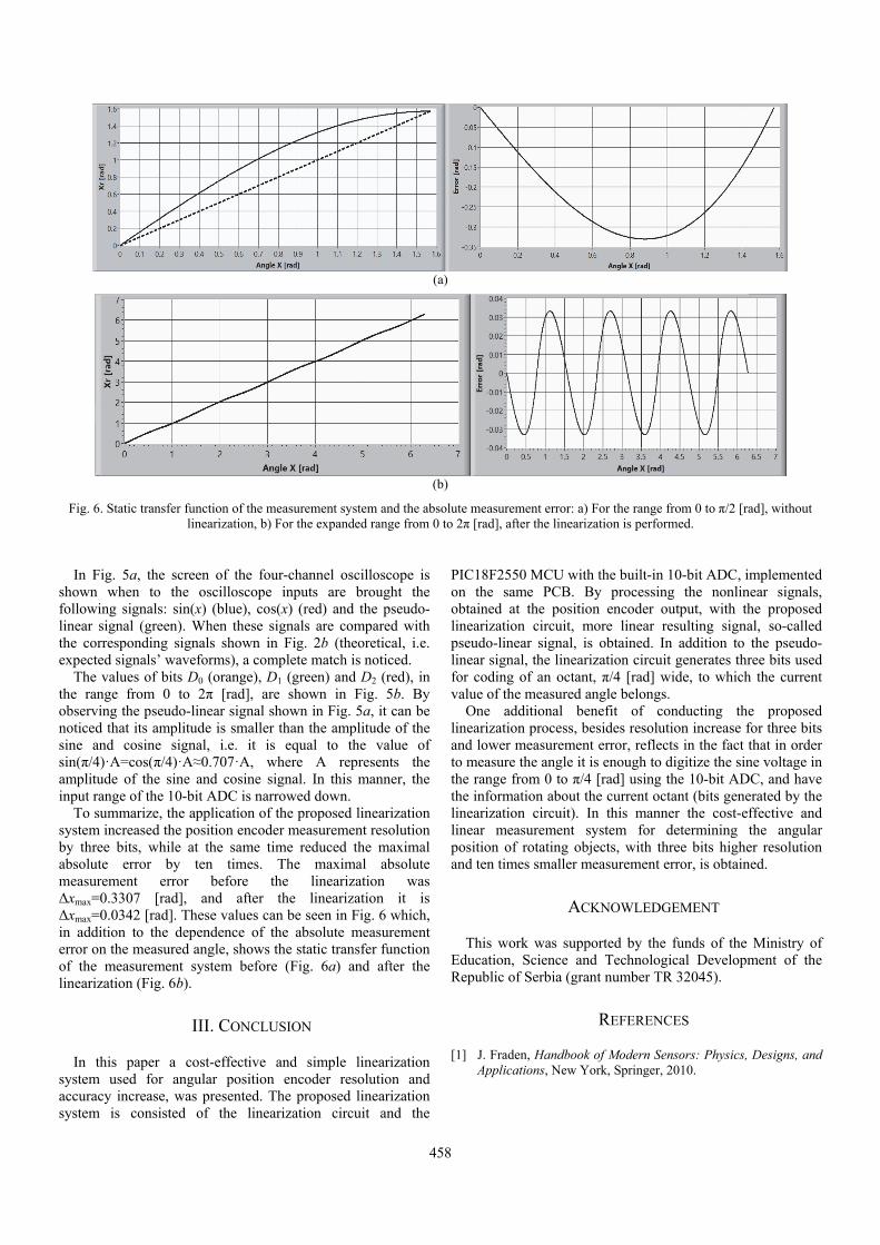
458

(a)

(b)

Fig. 6. Static transfer function of the measurement system and the absolute measurement error: a) For the range from 0 to π/2 [rad], without linearization, b) For the expanded range from 0 to 2π [rad], after the linearization is performed.

In Fig. 5a, the screen of the four-channel oscilloscope is

shown when to the oscilloscope inputs are brought the following signals: sin(x) (blue), cos(x) (red) and the pseudo-linear signal (green). When these signals are compared with the corresponding signals shown in Fig. 2b (theoretical, i.e. expected signals’ waveforms), a complete match is noticed.

The values of bits D0 (orange), D1 (green) and D2 (red), in the range from 0 to 2π [rad], are shown in Fig. 5b. By observing the pseudo-linear signal shown in Fig. 5a, it can be noticed that its amplitude is smaller than the amplitude of the sine and cosine signal, i.e. it is equal to the value of sin(π/4)·A=cos(π/4)·A≈0.707·A, where A represents the amplitude of the sine and cosine signal. In this manner, the input range of the 10-bit ADC is narrowed down.

To summarize, the application of the proposed linearization system increased the position encoder measurement resolution by three bits, while at the same time reduced the maximal absolute error by ten times. The maximal absolute measurement error before the linearization was Δxmax=0.3307 [rad], and after the linearization it is Δxmax=0.0342 [rad]. These values can be seen in Fig. 6 which, in addition to the dependence of the absolute measurement error on the measured angle, shows the static transfer function of the measurement system before (Fig. 6a) and after the linearization (Fig. 6b).

III. CONCLUSION

In this paper a cost-effective and simple linearization system used for angular position encoder resolution and accuracy increase, was presented. The proposed linearization system is consisted of the linearization circuit and the

PIC18F2550 MCU with the built-in 10-bit ADC, implemented on the same PCB. By processing the nonlinear signals, obtained at the position encoder output, with the proposed linearization circuit, more linear resulting signal, so-called pseudo-linear signal, is obtained. In addition to the pseudo-linear signal, the linearization circuit generates three bits used for coding of an octant, π/4 [rad] wide, to which the current value of the measured angle belongs.

One additional benefit of conducting the proposed linearization process, besides resolution increase for three bits and lower measurement error, reflects in the fact that in order to measure the angle it is enough to digitize the sine voltage in the range from 0 to π/4 [rad] using the 10-bit ADC, and have the information about the current octant (bits generated by the linearization circuit). In this manner the cost-effective and linear measurement system for determining the angular position of rotating objects, with three bits higher resolution and ten times smaller measurement error, is obtained.

ACKNOWLEDGEMENT

This work was supported by the funds of the Ministry of Education, Science and Technological Development of the Republic of Serbia (grant number TR 32045).

REFERENCES

[1] J. Fraden, Handbook of Modern Sensors: Physics, Designs, and Applications, New York, Sрringеr, 2010.

459

[2] J. J. Carr, Sensors and Circuits: Sensors, Transducers, and Supporting Circuits for Electronic Instrumentation Measurement and Control, New Jersey, Prentice Hall, 1993.

[3] G. Ye, H. Liu, S. Fan, et al., “Precise and Robust Position Estimation for Optical Incremental Encoders Using a Linearization Technique”, Sens. Actuators. A Phys., vol. 232, pp. 30-38, 2015.

[4] D. Živanović, J. Lukić, and D. Denić, “A Novel Linearization Method of sin/cos Sensor Signals Used for Angular Position Determination”, J. Electr. Eng. Technol., vol. 9, no. 4, pp. 1437-1445, 2014.

[5] J. Lukić, D. Živanović, and D. Denić, “Linearization Method for Angular Position Sensors”, SAUM 2014, Conference Proceedings, pp. 229-232, Niš, Serbia, 2014.

[6] J. Lukić, D. Živanović, and D. Denić, “A Compact and Cost-Effective Linearization Circuit Used for Angular Position Sensors”, FU Aut. Cont. Rob., vol. 14, no. 2, pp. 123-134, 2015.

[7] K.K. Tan, H.X. Zhou, and T.H. Lee, “New Interpolation Method for Quadrature Encoder Signals”, IEEE Trans. Instrum. Meas., vol. 51, no. 5, pp. 1073–1079, 2002.

[8] N. Hamdy, Applied Signal Processing: Concepts, Circuits, and Systems, Boca Raton, CRC Press, 2008.

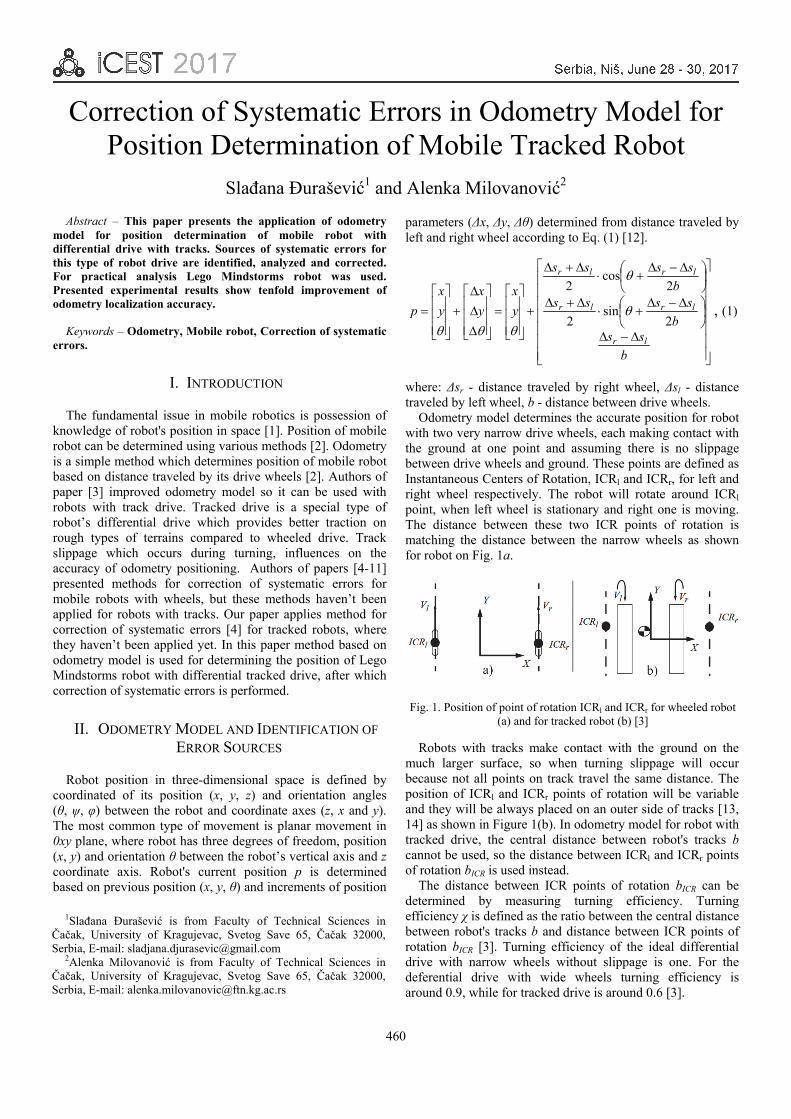
460

Correction of Systematic Errors in Odometry Model for Position Determination of Mobile Tracked Robot

Slađana Đurašević1 and Alenka Milovanović2

Abstract – This paper presents the application of odometry model for position determination of mobile robot with differential drive with tracks. Sources of systematic errors for this type of robot drive are identified, analyzed and corrected. For practical analysis Lego Mindstorms robot was used. Presented experimental results show tenfold improvement of odometry localization accuracy.

Keywords – Odometry, Mobile robot, Correction of systematic errors.

I. INTRODUCTION

The fundamental issue in mobile robotics is possession of knowledge of robot's position in space [1]. Position of mobile robot can be determined using various methods [2]. Odometry is a simple method which determines position of mobile robot based on distance traveled by its drive wheels [2]. Authors of paper [3] improved odometry model so it can be used with robots with track drive. Tracked drive is a special type of robot’s differential drive which provides better traction on rough types of terrains compared to wheeled drive. Track slippage which occurs during turning, influences on the accuracy of odometry positioning. Authors of papers [4-11] presented methods for correction of systematic errors for mobile robots with wheels, but these methods haven’t been applied for robots with tracks. Our paper applies method for correction of systematic errors [4] for tracked robots, where they haven’t been applied yet. In this paper method based on odometry model is used for determining the position of Lego Mindstorms robot with differential tracked drive, after which correction of systematic errors is performed.

II. ODOMETRY MODEL AND IDENTIFICATION OF

ERROR SOURCES

Robot position in three-dimensional space is defined by coordinated of its position (x, y, z) and orientation angles (θ, ψ, φ) between the robot and coordinate axes (z, x and y). The most common type of movement is planar movement in 0xy plane, where robot has three degrees of freedom, position (x, y) and orientation θ between the robot’s vertical axis and z coordinate axis. Robot's current position p is determined based on previous position (x, y, θ) and increments of position

parameters (Δx, Δy, Δθ) determined from distance traveled by left and right wheel according to Eq. (1) [12].

b

ssb

ssssb

ssss

y

x

y

x

y

x

p

lr

lrlr

lrlr

2sin

2

2cos

2

, (1)

where: Δsr - distance traveled by right wheel, Δsl - distance traveled by left wheel, b - distance between drive wheels.

Odometry model determines the accurate position for robot with two very narrow drive wheels, each making contact with the ground at one point and assuming there is no slippage between drive wheels and ground. These points are defined as Instantaneous Centers of Rotation, ICRl and ICRr, for left and right wheel respectively. The robot will rotate around ICRl point, when left wheel is stationary and right one is moving. The distance between these two ICR points of rotation is matching the distance between the narrow wheels as shown for robot on Fig. 1a.

Robots with tracks make contact with the ground on the much larger surface, so when turning slippage will occur because not all points on track travel the same distance. The position of ICRl and ICRr points of rotation will be variable and they will be always placed on an outer side of tracks [13, 14] as shown in Figure 1(b). In odometry model for robot with tracked drive, the central distance between robot's tracks b cannot be used, so the distance between ICRl and ICRr points of rotation bICR is used instead.

The distance between ICR points of rotation bICR can be determined by measuring turning efficiency. Turning efficiency χ is defined as the ratio between the central distance between robot's tracks b and distance between ICR points of rotation bICR [3]. Turning efficiency of the ideal differential drive with narrow wheels without slippage is one. For the deferential drive with wide wheels turning efficiency is around 0.9, while for tracked drive is around 0.6 [3].

1Slađana Đurašević is from Faculty of Technical Sciences inČačak, University of Kragujevac, Svetog Save 65, Čačak 32000, Serbia, E-mail: [email protected]

2Alenka Milovanović is from Faculty of Technical Sciences inČačak, University of Kragujevac, Svetog Save 65, Čačak 32000,Serbia, E-mail: [email protected]

Fig. 1. Position of point of rotation ICRl and ICRr for wheeled robot (a) and for tracked robot (b) [3]

461

10

ICRICRICR b

b

xx

b

lr

. (2)

Turning efficiency χ is calculated as ratio between measured turning angle θm and expected turning angle θ0, when robot is rotated around its vertical axis. Distance which tracks need to travel with same speed, but in the opposite directions in order to make expected turn angle θ0 is calculated based on the central distance between robot's tracks b. Due track slippage, measured turning angle θm will be smaller than expected turning angle θ0. When calculated turning efficiency is replaced it Eq. (2), the distance between ICR points of rotation of tracked drive is been calculated [3].

Due approximations in odometry model for determining robot's position and other influences such as: unequal circumference of drive tracks, uncertainty of effective distance between ICR points of rotation, directionless of tracks, finite encoder resolution and finite sampling time systematic errors can occur [15]. Systematic errors are the dominant type of errors on smooth surfaces and their influence is constant and accumulates over time and can be determined and corrected in odometry model. Influence due unequal circumference of drive tracks on odometry error is represented by Ed parameter:

l

rd O

OE , (3)

where: Or – circumference of right track, Ol – circumference of left track.

Uncertainty of effective distance between ICR points of rotation is caused due large track’s contact surface with ground and is represented by Eb ratio:

ICR

ICRb b

bE

*

, (4)

where: b*ICR – corrected distance between ICR points of

rotation of tracks, bICR – distance between ICR points of rotation of tracks before correction.

Nonsystematic errors are caused when the robot moves on the rough and uneven ground, where slippage or contact with other objects can occur. It is not possible to correct the influence of such errors since their occurrence is unpredictable and in that case, the robot will always reach difference final position for the repeated movement. Influence of nonsystematic errors on odometry model can be expressed statistically as the uncertainty of the determined position of the mobile robot.

Systematic odometry errors can be measured using bidirectional test [16] in which robot moves on the quadratic path with the length of segment of L. In one set of experiments, robot moves on the quadratic path in clockwise (CW) direction, and in other set in counterclockwise (CCW) direction (Fig. 2). Influence of Ed parameter is dominant in straight parts of the paths, while the influence of Eb parameter becomes dominant at path turns. Using bidirectional test, the influence of Ed and Eb parameters can be separated from each other, because when robot moves on path in one direction

influence of these parameters adds up, while for other direction their influence cancel each other. The robot starts movement in one direction from the Start point (x0, y0 and θ0). The robot is programmed to move on four line segments of length L, and at end of the each segment, the robot stops and turns for 90º. Such movement would in ideal case return robot in starting point Start, but due the influence of systematic and nonsystematic errors robot will finish its movement in some other point marked Stop with position (x1, y1 and θ1). Difference between start and final position represents odometry error as shown by Eq. (5):

.; 1010 yyyxxx (5)

Due influence of systematic errors, end points in which robots finishes its movements will be grouped into sets centered around points CW(xcg(cw), ycg(cw)) and CCW(xcg(ccw), ycg(ccw)). Coordinates of these center points will be used in order to correct the influence of systematic errors in odometry model. When turning, robot will make turning error for angle α, due uncertainty of effective distance between ICR points of rotation. When moving in the straight line robot will diverge in one direction for angle β, because of unequal circumference of drive tracks. The value of these two angles α and β is calculated using Eq. (6) and Eq. (7) [16]:

180

4)()(

L

xx ccwcgcwcg

, (6)

180

4)()(

L

xx ccwcgcwcg

. (7)

The ratio of the unequal circumference of drive tracks, represented by Ed parameter is acquired by Eq. (8):

2/sin

2/sin

ICR

ICR

L

Rd bL

bL

O

OE

. (8)

The uncertainty of effective distance between ICR points of rotation can be corrected using Eb ratio calculated by Eq. (9):

ICRICRICR

ICRb bb

b

bE

90

90

90

90 **

. (9)

Fig. 2. Robot movement in bidirectional test on quadratic path

462


Lego Mindstorms EV3 Home Edition [17] is set of components which are used for assembly of various types of mobile robots. EV3RSTORM is one of these robot models, which has differential track drive. The maximum speed of movement is around 300 mm/s with movement resolution of 0.3 mm per degree of rotation of drive motors. Track width is 20 mm while length of track in contact with the ground is 110 mm with the central distance between tracks of 128 mm.

In order to make full turn of 360° around its vertical axis, robot tracks need to travel 402 mm in opposite directions, based on distance between center of tracks (b=128 mm) Measurement results presented in Table I show that measured turning angle is much smaller than expected turning angle due track slippage with average value is 239.9º. Based on the measured angle of rotation we determined turning efficiency of χ = 0.667 which is further used to calculate the effective distance between ICR points of rotation of 192 mm later used in odometry model.

TABLE I

MEASURED TURNING ANGLES OF MOBILE ROBOT

No Meas. Measured turning angle θm [°] 1 240 2 238 3 247 4 239 5 235 6 241 7 237 8 243 9 240

10 239 Average 239.9

Robot is programmed to move on the quadratic path and ten bidirectional tests are conducted for both directions and results of odometry errors are presented in Table II and Fig. 3.

TABLE II

ODOMETRY ERRORS IN BIDIRECTIONAL TEST PRIOR CORRECTION

No. Meas.

CCW CW εxccw(mm) εyccw(mm) εxcw(mm) εycw(mm)

1 -148 41 -268 -274 2 -300 120 -266 -205 3 -300 134 -128 -84 4 -280 180 -268 -342 5 -249 108 -122 -58 6 -242 118 -115 -156 7 -105 55 -112 -96 8 -122 65 -218 -274 9 -108 26 -105 -109

10 -100 40 -234 -237 Average -195.4 88.7 -183.6 -183.5

Results of experiments carried both in CW and CCW directions represent odometry errors grouped around centers of gravity for each test direction. Absolute odometry error represents the furthest distance of center of gravity of CW or CCW cluster and is equal to 259.6 mm prior correction.

6.259),max( )()()max( cwcgcwcgsys rre mm. (10)

Based on coordinates for the centers of CW and CCW cluster, correction angles α and β are determined which are used to correct the influence of systematic errors in odometry model.

42.5180

4)()(

L

xx ccwcgcwcg , (11)

17.0180

4)()(

L

xx ccwcgcwcg . (12)

Based on determined values of α and β angles, values of correction parameters Ed and Eb are also determined:

9988.0

2/sin

2/sin

bL

bL

O

OE

L

Rd , (13)

3.20490

90064.1

90

90

bbE eb

mm. (14)

The value of Ed parameter is very close to one and influence could be ignored. Using Eb parameter effective distance between ICR points of rotation is corrected to 204.3 mm. Bidirectional test was repeated with corrected parameters and results are presented in Table III and Fig. 4.

Absolute odometry error after correction of 25.3 mm represents the substantial increase of odometry position accuracy, which justifies the usage of this method for systematic error correction in practice.

3.25),max( )()()max( cwcgcwcgsys rre mm. (15)

Fig. 3. Odometry errors in bidirectional test prior correction

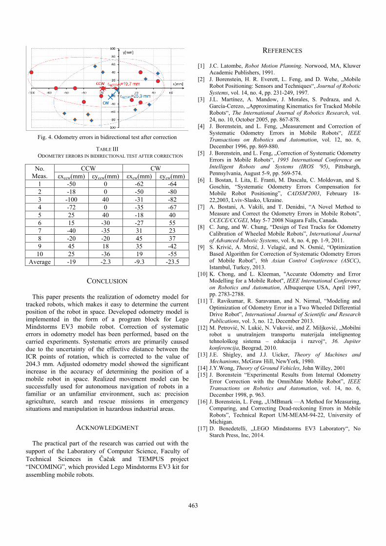
463

Fig. 4. Odometry errors in bidirectional test after correction

TABLE III ODOMETRY ERRORS IN BIDIRECTIONAL TEST AFTER CORRECTION

No. Meas.

CCW CW εxccw(mm) εyccw(mm) εxcw(mm) εycw(mm)

1 -50 0 -62 -64 2 -18 0 -50 -80 3 -100 40 -31 -82 4 -72 0 -35 -67 5 25 40 -18 40 6 15 -30 -27 55 7 -40 -35 31 23 8 -20 -20 45 37 9 45 18 35 -42

10 25 -36 19 -55 Average -19 -2.3 -9.3 -23.5

CONCLUSION

This paper presents the realization of odometry model for tracked robots, which makes it easy to determine the current position of the robot in space. Developed odometry model is implemented in the form of a program block for Lego Mindstorms EV3 mobile robot. Correction of systematic errors in odometry model has been performed, based on the carried experiments. Systematic errors are primarily caused due to the uncertainty of the effective distance between the ICR points of rotation, which is corrected to the value of 204.3 mm. Adjusted odometry model showed the significant increase in the accuracy of determining the position of a mobile robot in space. Realized movement model can be successfully used for autonomous navigation of robots in a familiar or an unfamiliar environment, such as: precision agriculture, search and rescue missions in emergency situations and manipulation in hazardous industrial areas.

ACKNOWLEDGMENT

The practical part of the research was carried out with the support of the Laboratory of Computer Science, Faculty of Technical Sciences in Čačak and TEMPUS project “INCOMING”, which provided Lego Mindstorms EV3 kit for assembling mobile robots.

REFERENCES

[1] J.C. Latombe, Robot Motion Planning. Norwood, MA, Kluwer Academic Publishers, 1991.

[2] J. Borenstein, H. R. Everett, L. Feng, and D. Wehe, „Mobile Robot Positioning: Sensors and Techniques“, Journal of Robotic Systems, vol. 14, no. 4, pp. 231-249, 1997.

[3] J.L. Martínez, A. Mandow, J. Morales, S. Pedraza, and A. García-Cerezo, „Approximating Kinematics for Tracked Mobile Robots“, The International Journal of Robotics Research, vol. 24, no. 10, October 2005, pp. 867-878.

[4] J. Borenstein, and L. Feng, „Measurement and Correction of Systematic Odometry Errors in Mobile Robots“, IEEE Transactions on Robotics and Automation, vol. 12, no. 6, December 1996, pp. 869-880.

[5] J. Borenstein, and L. Feng, „Correction of Systematic Odometry Errors in Mobile Robots“, 1995 International Conference on Intelligent Robots and Systems (IROS '95), Pittsburgh, Pennsylvania, August 5-9, pp. 569-574.

[6] I. Bostan, I. Lita, E. Franti, M. Dascalu, C. Moldovan, and S. Goschin, “Systematic Odometry Errors Compensation for Mobile Robot Positioning”, CADSM'2003, February 18-22,2003, Lviv-Slasko, Ukraine.

[7] A. Bostani, A. Vakili, and T. Denidni, “A Novel Method to Measure and Correct the Odometry Errors in Mobile Robots”, CCECE/CCGEI, May 5-7 2008 Niagara Falls, Canada.

[8] C. Jung, and W. Chung, “Design of Test Tracks for Odometry Calibration of Wheeled Mobile Robots”, International Journal of Advanced Robotic Systems, vol. 8, no. 4, pp. 1-9, 2011.

[9] S. Krivić, A. Mrzić, J. Velagić, and N. Osmić, “Optimization Based Algorithm for Correction of Systematic Odometry Errors of Mobile Robot”, 9th Asian Control Conference (ASCC), Istambul, Turkey, 2013.

[10] K. Chong, and L. Kleeman, "Accurate Odometry and Error Modelling for a Mobile Robot", IEEE International Conference on Robotics and Automation, Albuquerque USA, April 1997, pp. 2783-2788.

[11] T. Ravikumar, R. Saravanan, and N. Nirmal, “Modeling and Optimization of Odometry Error in a Two Wheeled Differential Drive Robot”, International Journal of Scientific and Research Publications, vol. 3, no. 12, December 2013.

[12] M. Petrović, N. Lukić, N. Vuković, and Z. Miljković, „Mobilni robot u unutrašnjem transportu materijala intelignentog tehnološkog sistema – edukacija i razvoj“, 36. Jupiter konferencija, Beograd, 2010.

[13] J.E. Shigley, and J.J. Uicker, Theory of Machines and Mechanisms, McGraw Hill, NewYork, 1980.

[14] J.Y.Wong, Theory of Ground Vehicles, John Willey, 2001 [15] J. Borenstein “Experimental Results from Internal Odometry

Error Correction with the OmniMate Mobile Robot”, IEEE Transactions on Robotics and Automation, vol. 14, no. 6, December 1998, p. 963.

[16] J. Borenstein, L. Feng, „UMBmark —A Method for Measuring, Comparing, and Correcting Dead-reckoning Errors in Mobile Robots”, Technical Report UM-MEAM-94-22, University of Michigan.

[17] D. Benedetelli, „LEGO Mindstorms EV3 Laboratory“, No Starch Press, Inc, 2014.

AUTHOR INDEX A Amelio, Alessia 139 Anastasijević, Ivan 321 Anastasov, Jelena 249 Andreev, Krume 393 Angelov, Kliment 113 Antonov, Svetlin 195, 309 Antoska-Knights, Vesna 79 Arnaudov, Rumen 67, 393 Atanasković, Aleksandar 216 Atanasov, Ivaylo 157, 161 Atanasovski, Metodija 48 B Babar, Sachin 165 Badarov, Dimiter 447 Badev, Jordan 401 Bakal, Kalpit 261 Bankov, Nikolay 427, 435 Bankovic, Bojan 350, 354 Blagojević, Vesna 228 Boumbarov, Ognian 40 Božinovski, Adrijan 123 Brodić, Darko 40,139, 301 Brusev, Tihomir 415, 419 C Chikov, Ognyan 277 Christoff, Nicole 44 Cvetković, Aleksandra 228, 245, 249 Cvetković, Nenad 337 Cvetković, Zlata 93 D Denić, Dragan 455 Deskovski, Stojce 79 Dimitrijević, Tijana 224 Dimitrov, Kalin 85, 358 Dimitrova, Petia 195 Dimov, Aleksandar 143 Dimova, Rozalina 157 Dinev, Pavel 40 Dinkić, Nikola 287 Djordjević, Goran Lj. 25, 182 Djordjević, Goran T. 241 Djorić, Aleksandra 216 Djošić, Sandra 25, 182 Djošić, Danijel 291 Djurašević, Sladjana 460 Djurić, Ivan 291

Dochev, Ivo 393 Dončov, Nebojša 97, 211, 224 Draganov, Ivo 40, 139 Drotár, István 101, 105 Džaković, Nikola 287 Džunić, Željko 333 E Eslami, Amir 17 F Filipović, Filip 350, 354 Frtunić Gligorijević, Milena 131 G Gacovski, Zoran 79 Gadjeva, Elissaveta 415, 419 Garabitov, Angel 9 Gatan, Shaker 341, 345, 405 Georgiev, Ginko 362, 366 Georgiev, Ivan 169 Georgieva, Veska 358, 370, 374 Gerov, Radmila 71 Getsov, Peter 385 Guliashki, Vassil 329 H Hachim, Fall 21 Hristov, Hristo 85 Hubenov, Pavel 63 Hubenova, Zoya 385 I Iliev, Georgi 165, 273 Iontchev, Emil 397 Ivanov, Racho 447 J Janevska, Gordana 48 Janjić, Aleksandar 325, 333 Janković, Dragan 135 Janković, Slađana 283 Joković, Jugoslav 224, 287 Jovanović, Goran 59 Jovanović, Milica 25, 182 Jovanović, Aleksandar 173 Jovanović, Aleksandra 305 Jovanović, Dejan 337 Jovanović, Ivan 305 Jovanović, Jelena 455

Jovanović, Zoran 71 K Kalinovska, Kalina 113 Kapanakov, Petar 397 Karabulut Kurt, Gunes 17 Khan, Rameez 75 Kireva-Mihova, Denitsa 381 Kolev, Alexander 89 Kolev, Pencho 161 Kolev, Stanyo 85, 358, 370, 374 Koleva, Alexandra 143 Korunovic, Lidija 321 Kostić, Dijana 301 Kostić, Vojkan 350 Kostov, Mitko 48 Kotevska, Elena 48 Kovachev, Yordan 203 Kunov, Georgi 415, 419 Kurkute, Swapnil 309 Kushlev, Stoyan 52 L Laskov, Lyubomir 358, 370, 374 Letskovska, Silvija 362, 366 Lichev, Angel 401, 427 Liszi, Máté 101, 105 M Madzharov, Nikolay 439 Maleš-Ilić, Nataša 216 Malik, Fahad Mumtaz 75 Mandrić-Radivojević, Vanja 97 Mančić, Žaklina 207 Marinković, Sladjana 235 Marinov, Tsvetan 273 Marinov, Zoran 191 Marinova, Galia 277, 329 Marjanović, Ivica 291 Markoski, Aleksandar 191 Mihaylov, Kaloyan 67 Mihaylov, Viktor 85 Mihaylova, Antoniya D. 314 Mihaylova, Desislava 389, 423 Mihov, Georgy 447 Milenković, Aleksandar 135 Milenković, Marijana 291 Miletiev, Rosen 397 Milić, Dejan 249, 291 Milijić, Marija 109 Milivojević, Zoran 265, 297, 301 Milosavljević, Aleksandar 173

Milovanovic, Alenka 460 Milovanović, Bratislav 97, 109, 211 Milovanović, Ivan 211, 253 Milović, Daniela 245, 249 Mirchev, Kalin 381 Mironov, Rumen 52 Mitkov, Dimitar 195 Mitrović, Nebojša 350, 354 Mitsev, Tsvetan 5, 203 Mladenović, Snežana 283 Mohamed,Yahyai 21 N Nachev, Ivaylo 221 Nachev, Veselin 409 Nagy, Szilvia 101, 105 Nedelchev, Marin 89 Nenova, Maria 273 Nešić, Aleksandar 109 Nešić, Nataša 97 Nikolić, Goran 59 Nikolić, Tatjana 59 Nikolić, Jelena 36 Nikolov, Anastas 157 Nikolov, Georgi 451 Nikolov, Neven 269 Nikolova, Boyanka 451 Nikolova, Kamelia 169 P Pacheco, Cláudia 257 Pacheco de Carvalho, José 257 Panagiev, Oleg 199 Panajotović, Aleksandra 245 Patil, Dipak 309 Pavlović, Vlastimir 31 Pencheva, Evelina 157, 161 Perić, Zoran 36 Petkov, Peter 221 Petković, Milica 241 Petronijević, Milutin 350, 354 Petrović, Branislav 59 Petrović, Vladimir 207 Popović, Nemanja 127 Prukner, Péter 101, 105 Puflović, Darko 131 R Radkov, Rosen 147 Radmanović, Miloš 119 Radojević, Vladimir 178 Rahnev, Pavlik 362, 366

Rajković, Predrag 235 Rankovska, Valentina 443 Rankovski, Stanimir 443 Raza, Abid 75 Reis, António 257 Rupčić, Slavko 97 S Sarevska, Maja 211 Seimenliyski, Kamen 362, 366 Sekulović, Nikola 245 Sestrimska, Mariyana 409 Shaikh, Javed 165 Slavov, Miroslav 161 Smiljaković, Vladimir 431 Sonar, Pallavi S. 309 Sotirov, Georgi 385 Spalević, Petar 253 Stajić, Zoran 325 Stanković, Miomir 235 Stanković, Radomir 119 Stanković, Vladimir 178 Stanković, Zoran 211 Stanojević, Milan 253 Stanojčić, Saša 253 Srefanović, Mihajlo 291 Stevanović, Nikola 325 Stoimenov, Leonid 131, 287 Stojanović, Igor 25, 182 Stojanović, Dragan 153 Stojanović, Miodrag 337 Stojanović, Violeta 297 Stojčev, Mile 59 Stojković, Suzana 127 Stojnev, Aleksandra 153 Stoyanov, Svilen 389, 423 Stoyanov, Viktor 13, 195 Stošić, Biljana 31, 93

T Tasić, Dragan 337 Terzieva, Milena 451 Terziyski, Georgi 401 Titova, Tanya 409 Todorov, Milen 451 Tomić, Stefan 36 Tsenov, Aleksandar 9 U Ugrenović, Slađana 305 Uzelac, Ana 283 V Vaidya, Pushkar 261 Valkov, Nikolay 195 Valkova-Jarvis, Zlatka 13 Veiga, Hugo 257 Velimirović, Jelena 333 Velimirović, Lazar 333 Veličković, Marko 265 Veličković, Zoran 265, 297 Veljanovski, Aleksandar 135, 178 Veljanovski, Marija 135 Vitanov, Rosen 221 Vuchev, Aleksandar 427, 435 Y Yordanov, Rumen 397 Z Zdravković, Stefan 283 Zlatev, Juli 67 Zytoune, Ouadoudi 21 Ž Živanović, Zoran 431

Proceedings of Papers - ICEST 2021 Conference

Documents

Transcript of Proceedings of Papers - ICEST 2021 Conference