
Proceedings of International Conference on Electrical ...
114
Interscience Research Network Interscience Research Network Interscience Research Network Interscience Research Network Conference Proceedings - Full Volumes IRNet Conference Proceedings 12-9-2012 Proceedings of International Conference on Electrical, Electronics Proceedings of International Conference on Electrical, Electronics & Computer Science & Computer Science Prof.Srikanta Patnaik Mentor IRNet India, [email protected] Follow this and additional works at: https://www.interscience.in/conf_proc_volumes Part of the Electrical and Electronics Commons, and the Systems and Communications Commons Recommended Citation Recommended Citation Patnaik, Prof.Srikanta Mentor, "Proceedings of International Conference on Electrical, Electronics & Computer Science" (2012). Conference Proceedings - Full Volumes. 61. https://www.interscience.in/conf_proc_volumes/61 This Book is brought to you for free and open access by the IRNet Conference Proceedings at Interscience Research Network. It has been accepted for inclusion in Conference Proceedings - Full Volumes by an authorized administrator of Interscience Research Network. For more information, please contact [email protected].
-
Upload
khangminh22 -
Category
Documents
-
view
2 -
download
0
Transcript of Proceedings of International Conference on Electrical ...

Interscience Research Network Interscience Research Network
Interscience Research Network Interscience Research Network
Conference Proceedings - Full Volumes IRNet Conference Proceedings
12-9-2012
Proceedings of International Conference on Electrical, Electronics Proceedings of International Conference on Electrical, Electronics
& Computer Science & Computer Science
Prof.Srikanta Patnaik Mentor IRNet India, [email protected]
Follow this and additional works at: https://www.interscience.in/conf_proc_volumes
Part of the Electrical and Electronics Commons, and the Systems and Communications Commons
Recommended Citation Recommended Citation Patnaik, Prof.Srikanta Mentor, "Proceedings of International Conference on Electrical, Electronics & Computer Science" (2012). Conference Proceedings - Full Volumes. 61. https://www.interscience.in/conf_proc_volumes/61
This Book is brought to you for free and open access by the IRNet Conference Proceedings at Interscience Research Network. It has been accepted for inclusion in Conference Proceedings - Full Volumes by an authorized administrator of Interscience Research Network. For more information, please contact [email protected].

Interscience Research Network (IRNet)
Bhubaneswar, India
Proceedings of International Conference on
Electrical, Electronics & Computer Science
(ICEECS-2012) 9th December, 2012
BHOPAL, India

Rate Compatible Punctured Turbo-Coded Hybrid Arq For Ofdm System
International Conference on Electrical, Electronics Engineering 9th December 2012, Bhopal, ISBN: 978-93-82208-47-1
1
RATE COMPATIBLE PUNCTURED TURBO-CODED HYBRID ARQ
FOR OFDM SYSTEM
DIPALI P. DHAMOLE1& ACHALA M. DESHMUKH2
1,2Department of Electronics and Telecommunications, Sinhgad College of Engineering, Pune 411041, Maharashtra
Abstract-Now a day’s orthogonal frequency division multiplexing (OFDM) is under intense research for broadband wireless
transmission because of its robustness against multipath fading. A major concern in data communication such as OFDM is to
control transmission errors caused by the channel noise so that error free data can be delivered to the user. Rate compatible
punctured turbo (RCPT) coded hybrid ARQ (RCPT HARQ) has been found to give improved throughput performance in a
OFDM system. However the extent to which the RCPT HARQ improves the throughput performance of the OFDM system
has not been fully understood. HARQ has been suggested as a means of providing high data rate and high throughput
communication in next generation systems through diversity combining transmit attempts at the receiver. The combination
of RCPT HARQ with OFDM provides significant bandwidth at close to capacity rates of channel. In this paper, we evaluate
by computer simulations the throughput performance of RCPT code HARQ for OFDM system as compared to that of
conventional OFDM.
Keywords: OFDM, hybrid ARQ, rate compatible punctured turbo codes, mobile communication, multipath fading
I. INTRODUCTION
Orthogonal frequency division multiplexing has been
considered as one of the strong standard candidates
for the next generation mobile radio communication
systems. Multiplexing a symbol data serial stream
into a large number of orthogonal sub channels makes
the OFDM [1] signals spectral bandwidth efficient.
Recently, high speed and high quality packet data
communication is gaining more importance. A major
concern in wireless data communication is to control
transmission errors caused by the channel noise so
that error free data can be delivered to the user. For
successful packet data communication, hybrid
automatic repeat request (HARQ) is the most reliable
error control technique for the OFDM systems as in
HARQ schemes, channel coding is used for the error
correction which is not applied in the Simple ARQ
schemes. In HARQ, the advantage of obtaining high
reliability in ARQ system is coupled with advantage
of forward error correction system to provide a good
throughput even in poor channel conditions. Turbo
codes, introduced in 1993 by Berrou et al., have been
intensively studied as the error correction code for
mobile radio communications. Rate compatible
punctured turbo (RCPT) coded HARQ (RCPT
HARQ) scheme was proposed in [2] and shown to
achieve enhanced throughput performance over an
additive white Gaussian noise (AWGN) channel. In
[3] it is shown that the throughput of the RCPT
hybrid ARQ scheme outperforms other ARQ schemes
over fading and shadowing channels.
In this paper, we evaluate the throughput performance
of RCPT coded HARQ for OFDM system over
additive white Gaussian noise channel. When the
number of allowable retransmissions is unlimited,
transmitting minimum amount of redundancy bits
with each transmission would result in the highest
throughput as unnecessary redundancy is avoided.
However in a practical system, [4] the number of
retransmissions allowed is limited to avoid
unacceptable time delay before the successful
transmission. When the number of retransmissions is
limited, the residual bit error is produced.
II. RCPT ENCODER/DECODER AND RCPT
HARQ
The RCPT encoder and decoder are included as a part
of the transmission system model shown in fig.1.
RCPT encoder consists of a turbo encoder, a puncture
and a buffer. Turbo encoder /decoder parameters are
shown in Table 1.
Table 1. Turbo encoder/ decoder parameters
Encoder
Rate 1/3
Component
encoder
RSC
Interleaver S-random
(S = K ½)
Decoder
Component
decoder
Log-MAP
Number of
iterations
8
Turbo encoder considered in this paper is a rate 1/3
encoder. Turbo encoded sequences are punctured by
the puncturer and the different sequences obtained are
stored in the transmission buffer for possible
retransmissions. With each retransmission request, a
new sequence (previously unsent sequence) is
transmitted. Turbo decoder consists of a depuncturer,
buffer and a turbo decoder. At the RCPT decoder, a
newly received punctured sequence is combined with

Rate Compatible Punctured Turbo-Coded Hybrid Arq For Ofdm System
International Conference on Electrical, Electronics Engineering 9th December 2012, Bhopal, ISBN: 978-93-82208-47-1
2
the previously received sequences stored in the
received buffer. The depuncturer inserts a channel
value of 0 for those bits that are not yet received and
3 sequences, each equal to the information sequence
length, are input to the turbo decoder where decoding
is performed as if all 3 sequences are received. In this
paper the type I HARQ is considered. For type I
HARQ, the two parity bit sequences are punctured
with P = 2 and the punctured bit sequence is
transmitted along with the systematic bit sequence. If
the receiver detects errors in the decoded sequence, a
retransmission of that packet is requested. The
retransmitted packet uses the same puncturing matrix
as the previous packet. Instead of discarding the
erroneous packet, it is stored and combined with the
retransmitted packet utilizing the packet combining or
time diversity (TD) combing effect.
III. TRANSMISSION SYSTEM MODEL
The OFDM system model with RCPT coded HARQ
is shown in Fig 1. At the transmitter a CRC coded
sequence of length K bits is input to the RCPT
encoder where it is coded, punctured and stored in the
buffer for possible retransmissions. The parity
sequences are punctured before transmission based on
adopted HARQ scheme. The punctured sequences are
of different length for different puncturing periods.
The sequence to be transmitted is block interleaved
by a channel interleaver and then transformed into
PSK symbol sequence. The Nc data modulated
symbols are mapped onto Nc orthogonal subcarriers
to obtain the OFDM signal waveform. This is done
by applying the inverse fast Fourier transform (IFFT).
After the insertion of a guard interval (GI), the
OFDM signal is transmitted over Additive white
Gaussion noise channel and received by multiple
antennas at the receiver. The OFDM signal received
on each antenna is decomposed into the Nc
orthogonal subcarrier components by applying the
fast Fourier transform (FFT) and each subcarrier
component coherently detected to be combined with
those from other antennas based on maximal ratio
combining. The MRC combined soft decision sample
[5] sequence is de-interleaved and input to the RCPT
decoder which consists of a de-puncturer, a buffer
and a turbo decoder. Error detection is performed by
the CRC decoder which generates the ACK/NAK
command and recovers the information in case of no
errors.
Fig. 1. OFDM with HARQ system model
IV. SIMULATION RESULTS
The turbo encoder/decoder parameters are as shown
in Table 1. The computer simulation conditions are
summarized in Table 2.
In this paper, the information sequence length K =
1024 bits is assumed. The turbo encoded sequence is
interleaved with a random interleaver. The data
modulation scheme considered is BPSK modulation
and the ideal channel estimation is assumed for data
demodulation at receiver. We assume OFDM using
N= 512 sub-channels, number of pilots P= N/8, total
number of data sub-channels S=N-P and guard
interval length GI=N/4. In our simulation, we assume
channel length L=16, pilot position interval 8 and the
number of iterations in each evaluation are 500. A
rate 1/3 turbo encoder is assumed and a log-map
decoding is carried out the receiver. The numbers of
frame errors to count as a stop criterion are limited to
15.

Rate Compatible Punctured Turbo-Coded Hybrid Arq For Ofdm System
International Conference on Electrical, Electronics Engineering 9th December 2012, Bhopal, ISBN: 978-93-82208-47-1
3
Table 2. Simulation Conditions
Information sequence length K = 210 214 bits
Channel interleaver Block interleaver
Modulation / demodulation BPSK
OFDM
No. Of subcarreiers Nc = 256
Subcarrier spacing 1/Ts
Guard interval Tg = 8/Ts
ARQ Type Type I
Max. No. Of tx. Ω
Propagation channel Forward Additive white gaussion noise
Reverse Ideal
The throughput in bps/Hz is defined as
.....(1)
Fig. 2 shows the bit error rate as a function of average
bit energy- to- additive white Gaussian noise
(AWGN) power spectrum density ratio. The
throughput in bps/Hz is defined as [6] the ratio of the
number of information bits over the total number of
transmitted bits, where the throughput loss due to GI
insertion is taken into consideration. In fig.2 the blue
line indicates the bit error rate of conventional OFDM
for a given range of signal-to noise ratio (SNR) while
the red line shows the bit error rate (BER) for turbo
coded type I HARQ for the same range of given
SNR. From graph (fig. 2) below it can be seen that
the bit error rate of turbo coded HARQ decreases
with the increase in SNR however the BER for the
conventional OFDM remains as it is for the entire
range of SNR, hence we can get improved throughput
for turbo coded HARQ as compared to that of
conventional OFDM. Fig. 3 shows the bit error rate
as a function of given range of signal to noise ratio.
Here the BER decrease is shown in between 0 to 1,
where the BER changes rapidly for the lower SNR
and we can get a very low BER even for higher SNR.
0 5 10 15 20 25 300
0.5
1
1.5
2
2.5
3
3.5
4
4.5
SNR
Bit E
rror Rate
Fig. 2. BER of conventional OFDM (+) and turbo coded HARQ (x)

Rate Compatible Punctured Turbo-Coded Hybrid Arq For Ofdm System
International Conference on Electrical, Electronics Engineering 9th December 2012, Bhopal, ISBN: 978-93-82208-47-1
4
0 5 10 15 20 25 300.38
0.4
0.42
0.44
0.46
0.48
0.5
0.52
0.54
0.56
0.58
SNR
Bit E
rror Rate
of Turb
o c
ode
Fig. 3. BER of turbo code
V. CONCLUSIONS
The throughput for the RCPT coded HARQ for an
OFDM system was evaluated. It is shown that the bit
error rate of turbo coded HARQ decreases with the
increase in signal to noise ratio, and hence we can get
a improved throughput for the OFDM with turbo
coded HARQ as compared to that of conventional
OFDM. It is shown that the throughput is almost
insensitive to the information sequence length.
REFERENCES
[1] R. Prasad, “OFDM for wireless communications systems.” Ist
ed, Artech House, Inc. Boston London, 2004.
[2] Berrou, C., “Near optimum error correcting coding and
decoding: turbo codes.” IEEE Transactions on
Communications vol. 44, No. 10, 1261-1271, 1996.
[3] Garg, D. Adachi, F. “Rate compatible punctured turbo-coded
hybrid ARQ for OFDM in a frequency selective fading
channel.” IEEE, 2725-2729, 2008.
[4] Lifeng, Y., Zhifang, L. “A hybrid automatic repeat request
(HARQ) with turbo codes in OFDM system.” IEEE.
[5] Gacanin, H., Adachi, F. “Throughput of Type II HARQ-
OFDM/TDM using MMSE-FDE in a multipath channel.”
Research Letters in Communications. 1-4, 2009.
[6] Bahri, M.W. Boujemaa, H., Siala, M. “Performance
comparison of Type I, II and III Hybrid ARQ schemes over
AWGN channels.” IEEE International Conference on
Industrial Technology, 1417-1421, 2004.
[7] Sklar, B., Ray, P.K. “Digital communications: Fundamentals
and applications”. (2nd Edition) Pearson Publications, New
Delhi, 2008.

Comparison Between Construction Methods of Unknown Input Reduced Order observer Using Projection Operator Approach And
Generalized Matrix Inverse
International Conference on Electrical, Electronics Engineering 9th December 2012, Bhopal, ISBN: 978-93-82208-47-1
5
COMPARISON BETWEEN CONSTRUCTION METHODS OF
UNKNOWN INPUT REDUCED ORDER OBSERVER USING
PROJECTION OPERATOR APPROACH AND GENERALIZED
MATRIX INVERSE
AVIJIT BANERJEE1 & GOURHARI DAS
2
1,2Dept. of Electrical Engineering, Jadavpur University(PG. Control System)Kolkata, India
Abstract—In this article a detailed comparison between two construction methods of unknown input reduced order observer
is presented. The methods are namely - projection operator approach and generalized matrix inverse. An experimental study
reveals that the order of the observer dynamics constructed using projection operator approach is dependent on the
dimension of unknown input vector. Similarities and dissimilarities between the above mentioned methods are illustrated
using an example and verified with experimental result.
Keywords-Reduced order observer, Unknown Input Observer (UIO), Generalized Matrix Inverse, Das &Ghosal
Observer(DGO), Projection Method Observer(PMO)
I. INTRODUCTION
Over the past three decades many researchers have
paid attention to the problem of estimating the state of
a dynamic system subjected to both known and
unknown inputs. They have developed the reduced
and full order unknown input observers by different
approaches[5-9]. In many application like fault
detection and isolation, cryptography, chaos
synchronization, unknown input observer[10-12] has
shown enormous importance and lots of work can be
found in the literature. StefenHui and Stanislaw H.Zak
[2, 3] developed full order and reduced order
unknown input observer (UIO) using projection
method (PMO) to state estimation. In [1] reduced
order Das and Ghosal observer (DGO) [4], which uses
generalized matrix inverse approach, is extended to
construct reduced order UIO. In contrast to the well
known and well established Luenberger observer
theory, these two proposed methods does not pre
assume the observer structure and it is not necessary
for the system output matrix to be in specific form as
[I : 0] and the corresponding co-ordinate
transformation is not required [13]. Both the
construction methods consider the system state to
decompose into known and unknown components.
PMO pre-assumes the unknown component as a skew
symmetric projection (not necessarily orthogonal) of
whole state along the subspace of available state
component.In contrast.DGO considers the unknown
component is an orthogonal projection of known
component
In this paper first both of the methods are
discussed briefly and then elaborated comparison is
done on the basis of observer structure and their
performances. Numerical examples and simulation
results are given for justifying the comparison.
II. LIST OF NOTATIONS AND SYMBOLS
All the symbols and notations used by two
observer construction methods have been listed in
table I TABLE I.
Serial
No
List of Notations and Symbols
Notations or
SymbolsPurpose
Dimensio
n
1. A System matrix
2. B Input matrix
3. C Output coupling matrix
4. E Unknown input coupling
Matrix
5. r Rank(C) Scalar
6. L Linearly independent
column of such that LLg=(I-CgC)
n n‐r
7. L Generalized Inverse of L
matrix n‐r n
8. C Generalized Inverse of C
matrix
9. M Real matrix, is designed
such that
(I-MC) Ed=0
10. H Arbitrary Design
parameter matrix[2] for
M
11. H Arbitrary Design
parameter matrix for K
[1]
n‐r p
12. p Projection matrix P=I-MC
13. Q Co-ordinate
transformation matrix
14. x State Vector 1
15. x Estimated State Vector 1
16. h Immeasurable State
Vector used in [1] 1
17. q Observer State [1] n‐r 1

Comparison Between Construction Methods of Unknown Input Reduced Order observer Using Projection Operator Approach And
Generalized Matrix Inverse
International Conference on Electrical, Electronics Engineering 9th December 2012, Bhopal, ISBN: 978-93-82208-47-1
6
Serial
No
List of Notations and Symbols
Notations or
Symbols Purpose
Dimensio
n
18. q Observer State [2] 119. I Identity matrix )
20. y Output Vector 1
21. u Control Input 1
22. K Observer Gain matrix
used in [1] n‐r p
23. L Observer Gain matrix
used in [2]
III. MATHEMATICAL PRELIMINARIES
For a system of equation Ax y … (1) where A is a
given (m×n) matrix, y is a given (m×1) vector, x is an
unknown (n×1) vector. Also an (n×m) matrix is
taken such that …(2) …(3)
AA A A ...(4) A AA A …(5)
are satisfied where superscript T indicates
transpose. The matrix is called the Moore-
PenroseGeneralized Matrix Inverse of A and is
unique for A. Now eqn. (1) is consistent if and only
if ...(6) and if eqn. (1) is consistent then its
general solution is given by
...(7)where I is the identity matrix of proper
dimension and is an arbitrary (n×1) vector (Graybill
1969, Grayville 1975).
Lemma1 used by DGO
For an (m×n) matrix C and an (n×k) matrix L, if
the linear space spanned by columns of L is equal to
the linear space spanned by the columns of (I CgC ,
then LLg is equal to . So by this Lemma, proposed by
Das and Ghosal, 1981: (I CgC = LLg... (8).
Lemma2 used by PMO
If P: be a projection and Rank (
, then there is an invertible matrix Q, having
columns same as eigenvector of such that 00 0 … (9) (Smith, 1984,
pp. 156-158 and pp. 194-195)
IV. BRIEF CONSTRUCTION METHODS
A. Design of Reduced Order Unknown Input Das &
Ghosal Observer(DGO)
If an LTI system subjected to unknown input is
described in state space form as x Ax Bu E w … (10) (eqn.12
of [1]).
The reduced order unknown input DGO is
governed by the following equations and conditions. L E L E CE CE 0 ... (11) (eqn. 21
of [1]; condition for existence of unknown input
DGO). In general unknown input DGO dynamics is
given by the equation: q L AL KCAL q L AL KCAL KL AC KCAC y L B KCB u … (12)
(eqn. 23 of [1])
The estimated states are given by, x Lq C LK y … (13) (eqn. 19
of [1])
To made the unknown input ineffective in observer
dynamics the observer gain K is designed by
following equation: K L E CE H ICE CE
… (14) (eqn. (22)
of[1])
such that, 0. …(15) (eqn.(20)
of[1])
B. Design of Reduced Order Unknown Input
Projection Method Observer (PMO)
The condition for existence of unknown input
PMO is given by the following equation.
Rank(C = Rank ( [pp. 432,434 of
[2])
The observer dynamics can be expressed as: 0 … (16)
where, ... (16.a)
... (16.b)
… (16.c) (eqn. (13) of [2])
and ...(16.d)
Whereas the observed state vector is represented as:
0 … (17)
The contribution of unknown input in observer
dynamics has been eliminated by proper design of M
such that, I MC E 0 … (18)
Eqn.(18) provides the solution of M as,
… (19)
(Pp.433 of [2])
Hence forth throughout the article DGO represents
unknown input reduced order Das and Ghosal
observer similarly PMO represents unknown input
reduced order projection method observer.
V. NUMERICAL EXAMPLES
To study the performance of the DGO and the
PMO, we will consider the numerical example of the
5th order lateral axis model of an L-1011 fixed-wing
aircraft [2,3] at curies flight conditions neglecting
actuator dynamics (example.2 [2]). The following
numerical values [2] for the system matrices have
been taken for the class of aircraft model.

Comparison Between Construction Methods of Unknown Input Reduced Order observer Using Projection Operator Approach And
Generalized Matrix Inverse
International Conference on Electrical, Electronics Engineering 9th December 2012, Bhopal, ISBN: 978-93-82208-47-1
7
The unknown input reduced order PMOfor the above
system has been realizedin [2] by following the
equations (16&17) as bellow:
A. Matlab Simulation Responses
Simulation has been carried out to analyze the
performance of the DGO and the PMO. Their
responses for the above numerical example are given
in figure (4.1-4.5).

Comparison Between Construction Methods of Unknown Input Reduced Order observer Using Projection Operator Approach And
Generalized Matrix Inverse
International Conference on Electrical, Electronics Engineering 9th December 2012, Bhopal, ISBN: 978-93-82208-47-1
8
VI. COMPARATIVE STUDY
A. Structure wise comparison
Se
ria
l
No
Unknown Input Reduced Order Das And Ghosal
Observer(DGO)
In unknown input DGO the system state variable has
been decomposed into known and unknown
components such that the unknown component is the
orthogonal projection of known component and
described as : x C y Lh ...(22)
Here the matrix L is orthogonal to the matrixC .
The observer state variable is represented asq where, q h Ky ... (24)
Or, q K I yh
The observer dynamic equation in presence of
unknown input for DGO is given by: q L AL KCAL q L AL KCAL KL AC KCAC y L B KCB uL E KCE w …(26 )
To eliminate the effect of unknown input from the
observer dynamics, for DGO the observer gain
parameter K has been designed such that,
LgEd-KCEd=0 and the solution for such K is given by
eqn. (14)
The condition for existence of the DGO is as follows:
1) LgEd-LgEd(CEd)g
CEd =0…(28 ) 2) The pair , has to be completely
observable.
Here the order of the observer is n r .
Order of DGO (n-r) ≤ Order of PMO (n-m2)
Special case:
When r=n the order of the DGO always reduces to
zero.
Here the observed state variable is given by, x Lq C LK y
Or, x L C LK qy
Here the observer error dynamics can be expressed
as: L AL KCAL … (30)
The error dynamics e(t) teds to zero if L ALKCAL is asymptotically stable.
The gain K consists of two components. The
arbitrariness of K depends on the arbitrary parameter
H. From the properties of generalized matrix inverse
we can infer that the observer poles cannot be placed
arbitrarily if the matrix CE is of full row rank.
L can be directly obtained from the independent
column of and no additional
transformation required.
TABLE II.
Serial
No
Unknown Input Reduced Order Projection
Method Observer (PMO)
1.
In unknown input PMO also the system state
variable has been partitioned into two
components where the unknown component is a
skew sympatric projection of the state and the
decomposition of state vector is given by
… (23)
Here the matrix (I-MC) is a projection which is
not necessarily orthogonal to M.
2.
The observer dynamic variable is considered as
. Where
… (25)
And
3.
The observer dynamic equation in presence of
unknown input for PMO can be written in the
form: 0 E ...
(27)
4.
In PMO the effect of unknown input has been
nullified from observer dynamics by proper
selection of M so that, 0 and the solution for such M is
given by eqn. (19)
5.
The existing condition for the PMO can be
stated as:
1) Rank (E Rank CE
m2≤r n-m2 ≥(n-r). …(29)
2) The pair , needs to be
completely observable.
6.Here the order of the observer is .
7.Here it can be infer that
Order of PMO (n-m2) ≥ Order of DGO (n-r)
8.
Special case:
When r=n the order of the PMO varies from
zero to n depending on the number of unknown
input
9.
Here the observed state variable is expressed
as, 0
Or, 0
10
Here the estimation error is given by … (31) (eqn. (20) of [2])
11Here The error dynamics e(t) teds to zero for
asymptotically stable
12
For the PMO it has been observed that for some
specific combination of C and E observer poles
may not be placed arbitrarily.
13Here the transformation Q
-1PQ=P=
In-m20
0 0
is necessary to construct the observer.

Comparison Between Construction Methods of Unknown Input Reduced Order observer Using Projection Operator Approach And
Generalized Matrix Inverse
International Conference on Electrical, Electronics Engineering 9th December 2012, Bhopal, ISBN: 978-93-82208-47-1
9
B. Coefficient-wise comparison based on observer
equations
Comparing the coefficients of observer dynamic
equations (eqns. (12) with eqn. (16)) and output
equations (eqn. (13) and eqn. (14)) we get the
following observations presented in table III TABLE III.
Coefficient-
wise
comparison
Comparative study
Unknown Input
Reduced Order DGO
Unknown Input Reduced
Order PMO
1.
LgAL Where,
LLg=(In-CgC)
A11 where
A=Q-1AQ=A11 A12
A21 A22
Q-1
PQ=P=In-m2
0
0 0
2.
CAL C1 where
C=CQ= C1 C2
3.
K=(LgEd)(CEd)g+
H(I- CEd CEd)g
L1where
4. LgAL-KCAL A11-L1C1
LgAL-KCAL K
+
LgACg-KCAC
g
In-m2
0m2 × Q AM +
In-m20m2 ×
L(Ip-CM)
5.
L B KCB
In-m2
0m2 × Q B
6.
L
QIn-m2
0m2×n-m2
7.
Cg+LK
M=(Ed(CEd)g
+H0(Ip- CEd CEd)g
It can be found from table III referring table I that,
the complexity of each term for DGO is relatively less
and involves less computation compare to the PMO.
C. Performance-wise comparison
From the numerical example of the 5th order
system [2] consisting offour independent outputs
given in section V, following observation have been
summarize in the table IV. TABLE IV.
Performanc
e-wise
comparison
Comparative study
Unknown Input
Reduced Order DGO
Unknown Input Reduced
Order PMO
1. 1st order observer 3rd order observer
2.
Single pole has to
placed and placed at
(-5.1439
3 poles have to place
and placed at -3,-4,-5
3.
States X1 and X4
are directly available
in the output. Hence
it matches with the
corresponding
observed state right
from the initial
condition. (figure 1
State X1 and X4 in this
case does not match that
with the observed ones
right from the beginning
(pp. 439 of [2])
Performanc
e-wise
comparison
Comparative study
Unknown Input
Reduced Order DGO
Unknown Input Reduced
Order PMO
and figure 4)
VII. CONCLUSION
In this paper a detailed and exhaustive
comparative study between the unknown input
reduced order DGO and the PMO based on their
structures, co-efficient of observer equations and
performances have been done. It has come out from
the study that the order of the DGO is always less or
at best equal to that of the PMO. The unknown input
reduced order PMO and the DGO be of same order
only when the number of unknown input to a system
exactly matches with the number of independent
output. The construction method of the DGO is
relatively simpler and involves less complex
computation than that for the PMO. Finally a
practical numerical example has been considered (L-
1011 lateral axis aircraft model) and both the
observers have been applied for the system to
understand their performances.
REFERENCES
[1] Avijit Banerjee, Parijat Bhowmick and Prof. Gourhari Das,
“Construction of unknown input reduced order observer
using generalized matrix inverse and Application to Missile
Autopilot”, International Journal of Engineering Research
and Development, Vol.4, issue.2, pp.15-18,2012
[2] Stefen Hui and Stanislaw H. Zak, “Observer design for
systems with unknown inputs”, Int. J. Appl. Math. Comput.
Sci., 2005, Vol. 15, No. 4, 431–446
[3] Hui S. and ˙Z ak S. H. “Low-orderunknown input observers”,
Proc. Amer. Contr. Conf., Portland, pp. 4192–4197.
[4] G. Das and T.K. Ghosal, “Reduced-order observer
construction by generalized matrix inverse”, International
Journal of Control, vol. 33, no. 2, pp. 371-378, 1981.
[5] Shao-Kung Chang, Wen-Tong Youand Pau-Lo Hsu,
“General-Structured unknown input observers”,Proceedings
of the American Control Conference, Baltimore, Maryland,
June 1994.
[6] Shao-Kung Chang, Wen-Tong Youand Pau-Lo Hsu, “Design
of general structured observers for linear systems with
unknown inputs”, J. Franklin Inst. Vol. 334B, No. 2, pp. 213
232, 1997.
[7] Yuping Guan and Mehrdad Saif, “A novel approach to the
design of unknown input observers”, IEEE Transactions on
Automatic Control, Vol. 36, No. 5, May 1991.
[8] P. Kudva, N. Viswanadharn, and A. Ramakrishna,
“Observers for linear systems with unknown inputs,’’ IEEE
Trans. Automat.Contr., vol. AC-25, pp. 113-115, 1980
[9] Huan-Chan Ting, Jeang-Lin Chang, Yon-Ping Chen,
“Unknown input observer design using descriptor system
approach”, SICE Annual conference, pp. 2207-2213, Taipei,
Taiwan, August 2010

Comparison Between Construction Methods of Unknown Input Reduced Order observer Using Projection Operator Approach And
Generalized Matrix Inverse
International Conference on Electrical, Electronics Engineering 9th December 2012, Bhopal, ISBN: 978-93-82208-47-1
10
[10] Jeang-Lin Chang, Tusi-Chou Wu, “Robust dissidence
attenuation with unknown input observer and sliding mode
controller” Electrical Engineering (Archiv Fur
Elektrotechnik) ,Vol.90, no 7, pp.493-502, 2008, doi:
10.1007/s00202-008-0099-1.
[11] Mou Chen, Changsheng Jiang, “Disturbance observer based
robust synchronization control of uncertain chaotic system,
Nonlinear Dynamics, Vol.70, no. 4, pp. 2421-2432, 2012.
[12] Maoyin Chen, Wang Min, “Unknown input observer based
chaotic secure communication”, Physics Letters A, 372 (2008)
1595-1600, October 2007.
[13] ParijatBhowmick and Dr.Gourhari Das, “A detail
Comparative study between Reduced Order Luenbergerand
Reduced Order Das &Ghoshal Observer and their
Application” Proceedings of the International Conference in
Computer, Electronics and Electronics Engineering, pp. 154 –
161, Mumbai, March 2012, doi:10.3850/978-981-07-1847-3
P0623.
[14] Victor Lovass-Nagy, Richard J. Miller and David L. Powers,
“An Introduction to the Application of the Simplest Matrix-
Generalized Inverse in System Science”, IEEE Transactions
on Circuits and Systems, Vol. CAS-25, no. 9, pp. 766-771,
Sep. 1978
[15] F.A. Graybill, “Introduction to Matrices with Applications in
Statistics”, Belmont, CA: Wadsworth, 1969.
[16] A. Ben-Israel and T.N.E. Greville, “Generalized Inverses,
Theory and Applications”, New York: Wiley, 1974
[17] J. O’Reilly, “Observers for Linear Systems”, London,
Academic Press, 1983.
[18] Elbert Hendrics, Ole Jannerup and Paul Hasse Sorensen,
“Linear Systems Control – Deterministic and stochastic
Methods”, 1st Edition, Berlin, Springer Publishers, 2008.

A Low Area High Speed Cluster Based 4x4 Multiplier
International Conference on Electrical, Electronics Engineering 9th December 2012, Bhopal, ISBN: 978-93-82208-47-1
11
A LOW AREA HIGH SPEED CLUSTER BASED 4X4 MULTIPLIER
GURWINDER SINGH CHEEMA1, JASPREET VIRDI
2 & GAUTAM CHOUHAN
3
1,2&3Dept. of Electronics and Communication, Lovely Professional University, Phagwara, India
Abstract- In this paper, a new architecture for low-power design of parallel multipliers is proposed. Reduction of power
consumption is achieved by circuit activity reduction at the architecture level of the smaller multipliers when cluster based
multiplication is performed. Reducing the number of gates required to perform the multiplication, the switching power is
reduced. Thus 4-bit multiplier is proposed which uses the improved low power architecture of two bit multiplier. Thus the
proposed architecture results in twenty-two percent dip in power delay product, when synthesized using Cadence
development tools.
Keywords:- Multipliers, cluster based, high speed, reduced area multiplier.
I. INTRODUCTION
Multiplication is an essential arithmetic operation
for common DSP (Digital Signal Processors)
applications. In recent years, three areas i.e. power,
speed and area are emphasized by the researchers.
Hence among the three fields one of the most
important areas to be concentrate is the power. To
achieve high execution speed, parallel array
multipliers are widely used. Due to high capacitive
load, these structures become the most energy-
consuming units in modern DSP circuits. These
multipliers tend to consume most of the power in
DSP computations, and thus power efficient
multipliers are very important for the design of low
power DSP systems. Also, need of more applications
on a single processor will increase the number of
transistors on a chip and cause increases to power
consumption. [1][5]Thus due to the emergence of
battery powered electronic products specially
portable systems, it is essential to come up with new
design techniques that results in less power
consumption so that the battery lifetime can be
increased.
The main idea of our approach is based on the
observation that most modern multipliers produce a
large number of signal transitions. In this paper, the
focus is to reduce the power at the architectural level.
At different design levels of hierarchy, with the
efficient technique whether algorithmic or
architectural or logic and circuit levels, the problem
of power can be tackled and reduced. Therefore the
system performance is much better if the reduction is
done at the higher level of hierarchy. With the
changes at the architectural level, this technique is
able to achieve reduction in power, due to use of less
number of gates, making design more efficient.
This paper is organized as follows. Introduction is
discussed in the section I. In the next section, basics
of the power consumption in the CMOS circuits and
some preliminary information about the basic design
of the multiplication circuits which obtain the result
by dividing into clusters of smaller multipliers are
discussed. The efficient design of the 4x4 multiplier
is discussed in the section III. Experimental results on
the performance of multipliers are discussed in
Section IV. Next, the work is concluded.
II. BACKGROUND
A. Component of Power Consumption
It is believed that CMOS circuits dissipate a very
little amount of power. Power dissipation in CMOS
circuits is caused by three sources: Switching power,
Short circuit power, Continuous power due to leakage
current. The first 2 components are referred to as
dynamic power while the third component is referred
to as the static power. Equation (1) below shows the
power consumption in CMOS circuits, which can be
divided into dynamic and static power consumption.
Ps=α fclk CL V DD2 +ISCVDD + Ileakage VDD (1)
Where α is the switching activity, fclk is the clock
frequency, CL is the output capacitance, VDD is the
supply voltage, ISC is the short circuit current, and
Ileakage is the leakage current. The leakage current
which is primarily determined by the fabrication
technology consists of reverse bias current in the
parasitic diodes formed between source and drain
diffusions and the bulk region in a MOS transistor as
well as the sub threshold current that arises from the
inversion charge that exists at the gate voltages below
the threshold voltage [3]. The short-circuit (rush-
through) current which is due to the DC path between
the supply rails during output transitions and the
charging and discharging of capacitive loads during
logic changes.
From the equation above it can be said that power
consumption can be reduced by decreasing the
number of switching activities. Many previous works
tried to reduce the switching activity of the array
multiplier.

A Low Area High Speed Cluster Based 4x4 Multiplier
International Conference on Electrical, Electronics Engineering 9th December 2012, Bhopal, ISBN: 978-93-82208-47-1
12
Figure 1: general example of 4x4 multiplication
B. Cluster based design
Consider the multiplication of two unsigned n-bit
numbers, the multiplicand A = an-1 an-2, . . . , a0 and
the multiplier B = bn-1 bn-2, . . . , b0. [2] Equation
(2) represents the product P = P2n-1P2n-2, . . . , P0.
P P0P1….P2n-1 = (aibj) 2 i+j
Generally, in the multiplication process, partial
products are generated. In the figure 1, each row
represents a partial product. These partial products
are generated using an array of AND gates and then
all of these partial products are added, using an array
of full adder cells, to obtain the overall product.
Therefore, this general multiplication can be shown
as in the figure 2.
Whereas in this multiplication process of the array
multipliers, arrays of full adder are added up for the
final product. The array multiplier processes bit by bit
addition of the partial products. And a lot of work is
done for maintain speed and reducing power
consumption of the array multiplier, which include
the row bypassing, column bypassing, 2-D bypassing,
row-column bypassing, etc[4].
Instead, another technique to improve the
performance can be adopted in which partial product
of group of bits can be taken and added. [7] The half
of total number of bits, N/2 bits of both operands are
used for taking the partial products. This helps in
taking the performance upwards. Such a design is
known as cluster based design, clusters of partial
products, and such design for the 4x4 multiplier is
shown in figure 2, where AL and BL are the least
significant N/2 nibbles and AH and BH are the most
significant N/2 nibbles of the operands A and B,
respectively. Equation (3) represents the overall
product calculated in mathematical form, as the
partial products are generated.
Figure 2: Cluster based design of 4x4 multiplier
The figure 2 presents the cluster based
architecture for the N bit operands. In this design,
each of the operand consists of two cluster of N/2 bit
corresponding to 4 multiplication clusters.
P = (aibj)2i+j + (aibj)2
i+j + (aibj)2i+j + (aibj) 2
i+j For large operand, the multiplication circuit
can be further divided into larger number smaller
multipliers. Operands A and B are divided into two
nibbles each, cross multiplied by each other, and
added for the final output.
III. PROPOSED APPROACH
Based on the cluster based designs, the 4x4
multiplier is implemented using the new efficient 2x2
multipliers. On the addition of the new efficient 2x2
multiplier to the cluster based design, the four bit
multiplier become more suitable for low power and
high speed applications. The proposed low power
high speed proposed designs are discussed below.
A. Proposed 2x2multiplier
In the proposed design, emphasis is given to
reduce the activity factor or the transitions required to
perform the multiplication. The architectural
modification of the design is then presented to
achieve the reduction in the switching activity. With
the proposed design we are able to reduce the
switching activity and enhance the speed due to the
usage of less number of gates; furthermore silicon
area requirement is also reduced. The design of the
2x2 multiplier is shown in the Figure 3.
Figure 3: Efficient 2x2 multiplier
While talking about the number of gates, in the
proposed design of the 2x2 multiplier, as seen in the
figure, only single exor & not gate & 6 ‘and’ gates
are used. On the contrary, in conventional 2x2
multiplier circuit, which uses one half adder preceded
by the full adder perform multiplication, uses 2 exor
gates, 6 and gates, except the same number of ‘and’
gates for generating partial products. Thus with the
proposed design we are actually able to decrease the
switching activity, worst path delay and even the
silicon area consumption and this improvement is

A Low Area High Speed Cluster Based 4x4 Multiplier
International Conference on Electrical, Electronics Engineering 9th December 2012, Bhopal, ISBN: 978-93-82208-47-1
13
only possible with the decrease in the requirement of
number of gates.
Figure 4: Cluster based architecture where efficient 2x2
multiplier is used.
On comparing our design with the conventional
two bit multiplier, it can be stated that instead of one
exor gate only one not gate is required, while
cancelling other gates requirement. Furthermore, each
of the output bit directly depends upon the input bits,
not like in conventional 2 bit multiplier where output
of the third and fourth bit depends upon the inputs
(most significant bits) as well as result of the least
significant bits, and thus the worst path delay is
reduced and helps in making design more fast and
efficient. The results of the proposed design are
discussed in the section IV.
B. Efficient 4x4 design
For enhancing the performance of the 4x4
multiplier, the fast-low power two bit multiplier is
used in the clustered based architecture of the 4x4
multiplier. [7]The architecture used for the
implementation is shown in the figure 4.
The usage of cluster based design makes it more
beneficial in improving the speed of the multiplier.
While comparing this design with array multiplier or
its bypassed designs, [4] it can be easily seen that the
switching power heads upward but the opposite dip
with more percentage can be seen in the design which
uses the efficient 2x2 multiplier in the cluster based
design. The results from the clusters are added with
each at the final stage, according to the architecture,
to achieve desired output. Due to its good
performance this design proves to be better
alternative than the cluster based design with
conventional two bit multiplier.
IV. RESULTS AND EVALUATION
Table I represents the post synthesis results of the
conventional and the proposed 2x2 multiplier and
Table II exhibits the post synthesis results of the
proposed structures and of the bypassing based array
multiplier in terms of delay and area and power for
the 4x4 multiplier. The circuit design in this paper has
been developed using Verilog-HDL and synthesized
in Cadence RTL compiler using 180nm generic
library.
The area indicates the total cell area of the design;
the total power is the sum of dynamic power, internal
power, net power and leakage power. The delay is the
critical path delay of the architecture.
Figure 5: Cell Area of proposed 2x2 multiplier
Figure 6: Power Consumption of proposed 2x2 multiplier
Figure 7: Cell Area for proposed 4x4 multiplier
As from the table I, the difference in the area
requirement, power consumption and the worst path
delay, can be calculated easily. The improvement
amounts to 27.2% for decrease in the power
consumption, 29.9% less silicon requirement, and
making design 40.4 % more faster. These
improvements are the result of the dip in the number
of gates, reducing switching activity.
Also, from the table II, the improvements can be
easily seen due to the effect of the proposed 2x2
multiplier design. While looking at the results, it
comes into picture that proposed four bit multiplier
design is a fast design with less area requirement than
that of the bypassing based array design. Although

A Low Area High Speed Cluster Based 4x4 Multiplier
International Conference on Electrical, Electronics Engineering 9th December 2012, Bhopal, ISBN: 978-93-82208-47-1
14
the switching power goes up, but the minimization of
logic helps in bringing good power-delay product.
Figure 8: Power Consumption of proposed 4x4 multiplier
Table I: Area overhead, delay and Power dissipation of 2x2
multiplier.
Multiplier Design Proposed 2x2
multiplier
Conventional
2x2
multiplier
Estimate Total
Power
dissipation(mW)
0.03915 0.05384
Area overhead 24.70 35.28
Delay (ps) 197.7 331.9
Table II: Area overhead, delay and Power dissipation in an 4x4
cluster based designs
Multiplier Design Using
proposed 2x2
multiplier
Bypassed
array
multiplier [4]
Estimate Total
Power
dissipation(mW)
0.60 0.48
Area overhead 249.08 329.52
Delay (ps) 1351.6 2195.3
“Fig 5, 6, 7, 8” shows the results of the proposed
two bit and four bit multiplier in context to cell area
and the total power consumption. Due to the
minimization of logic, the area overhead decreases by
24.4%. Although, this design consumes 25% more
power but on the other hand the proposed design
marks 38.4% decrease is achieved for the worst path
delay, when compared with bypassed array based
design. In addition to the realization of above results,
as discussed, results depicts that the proposed
architecture provides the dip of 22.7% in the Power
delay product (PDP), when compared. This shows
that the design identifies itself a better alternative for
use in low power and high speed arithmetic
architectures.
CONCLUSION
In this paper we have presented an efficient 2 bit
multiplier with less number of gates leading to
reduced switching activity, when the structure has
been synthesized with Cadence RTL compiler using
180nm technology. The proposed structure proves to
be an easier solution for improving the power
consumption of the 4x4 multiplier when this efficient
design is used. Thus the proposed design founds to
consume less power and less silicon area
consumption and providing high speed, thus proving
to be more efficient in terms of PDP, and more
suitable for the DSP applications.
ACKNOWLEDGMENT
The authors would like to thank the Department
of Electronics and Communication Engineering,
Lovely Professional University, Punjab, India for the
support rendered in carrying out this work.
REFERENCES
[1] B. Parhami, “Computer Arithmetic: Algorithms and
Hardware Designs”, Oxford University Press, 2000
[2] Jan M. Rabaey, Anantha Chandrakasan and Borivoje Nikolic,
“Digital Integrated Circuits- A design Perspective”, Second
edition, PHI-2004.
[3] Neil H.E.Weste, David Harris and Ayan Banerjee, “CMOS
VLSI Design-A Circuits and System Perspective”, Pearson
Education, Third edition, 2009.
[4] Jin-Tai Yan and Zhi-Wei Chen, “Low-Cost Low-Power
Bypassing-Based Multiplier”, IEEE International
Symposium, 2010
[5] V. H. Hamacher, Z. G. Vranesic and S. G. Zaky, “Computer
Organization”, McGraw-Hill, 1990.
[6] Puneet Gupta , Parag Kulkarni, “Trading accuracy for power
in a Multiplier Architecture”
[7] Ayman A. Fayed, Magdy A. Bayoumi, “A Novel
Architecture for Low-Power Design of Parallel Multipliers”,
IEEE International Symposium on Circuits and Systems,
2001

Fpga Implementation of Mpeg-4 AAC Audio Decoder
International Conference on Electrical, Electronics Engineering 9th December 2012, Bhopal, ISBN: 978-93-82208-47-1
15
FPGA IMPLEMENTATION OF MPEG-4 AAC AUDIO DECODER
SUYOG V PANDE1, M.A.GAIKWAD2 & D.R.DANDEKAR3
1,2&3Electronicsdept, BDCOE, Sewagram,India
Abstract: Now a day’s technology is growing in every aspect but the basic needs to save the memory and Power required is
still remains. Whenever we deal with any kind of data (audio, video, text) we are bound to compress the data to minimize the
space and it work on low power.
This paper presents an investigation & implementation of low complexity profile high quality MPEG4 AAC Audio Decoder
at a sampling_ frequency of 48khz on a Field programmable gate array. Being a popular codec low complexity profile AAC
must reach to these needs.
Keywords: complexity, memory, power, quality
I. INTRODUCTION
In recent contexts of multimedia and applications,
new demands for audio coding arise[4]. As the high
coding efficiency with Low power has become the
issue of most importance, a new MPEG standard,
called advanced audio coding (MPEG-2 AAC,
ISO/IEC 13818-7 [1]) has been standardized. This
new standard exhibits many advantages over other
MPEG audio standards. The MPEG-4 AAC standard
provides very high audio quality without
compatibility-based restrictions.
AAC is an advance of the successful MP3 format and
its superior performance arises from the efficient use
of existing coding tools and the introduction of new
coding tools [4]. On average, AAC‘s compression
rate is 30% higher than that of MP3 while providing
better sound quality[1][3].
The AAC standard itself is not secure, but —is only
being licensed in the context of secure distribution.
Encoders and players each have their own Digital
Rights Management mechanisms, and interoperability
between devices is not possible.“[1]
Advanced Audio Coding offers features like High
Quality Compression, Multichannel Support (1 to 48
audio channel), Low Computational Complexity,
Wide Application Range[11]
A) Profile & Profile Interoperability:
AAC system offers different tradeoffs between
quality and complexity depending on the application.
For this purpose three profiles have been defined:
main profile, low-complexity (LC) profile,
and sample rate scalable (SRS) profile [1].
Among these three profiles, the main profile provides
the highest quality but also demands the highest
complexity since it contains all the tools the
exception of the gain control tool [2].
The AAC decoding process makes use of a number of
required tools and a number of optional tools. Table 1
lists the tools and their status as required or optional.
Required tools are mandatory in any possible profile.
Optional tools may not be required in some
profiles[3].
Main: The Main profile is used when memory cost is not
significant, and when there is substantial processing
power available. With the exception of the gain
control tool, all parts of the tools may be used in
order to provide the best data compression
possible[2]
Low Complexity:
The Low Complexity profile is used when RAM
usage, processing power, and compression
requirements are all present. In the low complexity
profile, prediction, and gain control tool are not
permitted and TNS order is limited[3]
Scalable Sampling Rate
In the Scalable Sampling Rate profile, the gain-
control tool is required. Prediction and coupling
channels are not permitted, and TNS order and
bandwidth are limited[1][3]
Table 1: AAC Decoder profile-Tools[4]
Tool
Name
Required/
Optional
Mai
n
LC SSR
Bit-
stream
formatter
Required
Noiseless
decoding
Required
Inverse
quantizati
on
Required
Scale-
factors
Required
M/s Optional /
x
prediction Optional x x
Intensity/
Coupling
Optional /
x
x
TNS Optional
Filter-
bank
Required
Gain
control
Optional
x
x

Fpga Implementation of Mpeg-4 AAC Audio Decoder
International Conference on Electrical, Electronics Engineering 9th December 2012, Bhopal, ISBN: 978-93-82208-47-1
16
There are two major common sample rate bases
44.1 kHz and 48 kHz .As most studio equipment uses
recording and digital signal processing equipment
working at a sample rate based on (a multiple of)
48 kHz the final result has to be re-sampled to the
standard CD-format sample rate to be finally
transferred onto a CD for distribution[11].
In this paper, we propose & implement low
complexity profile high quality MPEG4 AAC Audio
Decoder at a sampling_ frequency of 48khz .
Block Diagram : The implementation contains the
minimum number of decoding tools but will
successfully decode the L1_fs bit-stream. Figure 3-2
shows the block diagram[1]
Fig 3-2: AAC Low complexity profile
This is the overall block for AAC Decoder. Here we
have separate module for [2]
1. Bit-stream.
2. Bit-stream demultiplex
3. Noiseless decoding.
4. Inverse quantizer.
5. Scale factor.
6. Filter bank.
The characteristic of the tools are summarized as
follows[4]
II. BIT-STREAM:
There are two basic formats for the bi t-stream & the
use of a particular format is determined by the
application[1][3]
1. Audio Data Interchange Format (ADIF)
ADIF format contain only one header at the start of
bit-stream which contains all decoding necessary
information followed by raw data.
ADIF is used when decoding only occurs from the
start of the bit-stream and never from within, such as
decoding from a disk file
2. Audio Data Transport Stream (ADTS ADTS file contains multiple ADTS Header, one
before each frame of raw data. ADTS is suited to
streaming applications
III. BIT-STREAM DEMULTIPLEXER:
The input to the bitstream demultiplexer tool is the
13818-7 AAC bit stream. The demultiplexer
separates the parts of the MPEG-AAC data stream
into the parts for each tool, and provides each of the
tools with the bitstream information related to that
tool[1] The outputs from the bitstream demultiplexer
tool are[3]:
The sectioning information for the noiselessly coded
spectra
The M/S decision information (optional)
The predictor state information (optional)
The intensity stereo control information and
coupling channel control information (both optional)
The temporal noise shaping (TNS) information
(optional)
The filter-bank control information
The gain control information (optional)
Both control and data information are sorted, and
information concerning the bit stream, such as profile
type, sampling frequency index, copyright ID is
obtained[3].
The bit streams are decoded using the shift register,
down counter and the header[5]. The serial in
parallel out shift register is used to shift the data
received from the 13818-7 coded audio stream. The
header is used to set the values for the counters and
manages the operation of the encoding process. The
down counter is used to down count the set value
from the header to generate the encoded result[1].
Three components to design Bit stream de-mux. They
are Bit Stream state machine. Bit stream counter ( 11
bits ). Shift register (SIPO) ( 32 bits )[1]

Fpga Implementation of Mpeg-4 AAC Audio Decoder
International Conference on Electrical, Electronics Engineering 9th December 2012, Bhopal, ISBN: 978-93-82208-47-1
17
Bit Demux internal structure
Declaration of Bit stream De multiplexer
IV. NOISELESS DECODING:
The noiseless decoding tool takes information from
the bit-stream de-multiplexer, parses that information,
decodes the Huffman coded data, and reconstructs the
quantized spectra and the Huffman and DPCM coded
scale-factors[1].
The inputs to the noiseless decoding tool are[3]:
The sectioning information for the noiselessly coded
spectra
The noiselessly coded spectra
The outputs of the Noiseless Decoding tool are[3]:
The decoded integer representation of the scale-
factors
The quantized values for the spectra
Declaration of Noiseless Decoding
V. INVERSE QUANTIZATION:
The inverse quantizer tool takes the quantized values
for the spectra, and converts the integer values to the
non-scaled, reconstructed spectra. This quantizer is a
non-uniform quantizer[3].
Declaration of Inverse quantization
The input to the Inverse Quantizer tool is[3]:
The quantized values for the spectra
The input range of quantization is [2]:
0 <= x_quant <= +32
IQ is to calculate for the 4/3-th power of a quantized
spectrum, which is given by[2]
X_invquant = sign ( x_quant ) * | x_quant |^4/3.
• Where, X_invquant is output of the given
quantization value &
• Sign(x_quant ) is a sign bit, it indicate
wheather the input is a +ve or –ve
• Fig a shows the structure of inverse
quantization[1]
• Fib b shows plotting of X_invquart verses
X_quant [1]
Fig a: internal structure of inverse quantization

Fpga Implementation of Mpeg-4 AAC Audio Decoder
International Conference on Electrical, Electronics Engineering 9th December 2012, Bhopal, ISBN: 978-93-82208-47-1
18
Fig b: plotting X_invquart verses X_quant
The output of the inverse quantizer tool is
The un-scaled, inversely quantized spectra
Steps to find inverse quantization. Substitute the x_quant value instead of the above
formula if x_quant = 9 & X_quant ^4/3 = 18.72 [1]
Multiply by 8 = 18.72 * 8. Result = 149.76.
Rounding the above result value. X_invquant = 150.
Likewise, Substitute the input value from 0 to 32[2].
VI. SCALE FACTOR:
The rescaling tool converts the integer representation
of the scale-factors to the actual values, and
multiplies the un-scaled inversely quantized spectra
by the relevant scale-factors[1].
The inputs to the rescaling tool are[3]:
The decoded integer representation of the scale-
factors
The un-scaled, inversely quantized spectra
The output from the scale-factors tool is[3]:
The scaled, inversely quantized spectra
Declaration of Scale Factor
For scale factor[1]
Overall block for scale factor[1]
A) SF LUT:-
We have 8bit input for SF LUT. From this msb 2bit is
used for selecting LONG_WINDOW, SHORT
WINDOW. Remaining six bit is an input for the
windows[1].
Fig b: approximation of gain functions
VII. FILTER BANK:
The filter bank / block switching tool applies the
inverse of the frequency mapping that was carried out
in the encoder. An inverse modified discrete cosine
transform (IMDCT) is used for the filter bank tool.
The IMDCT can be configured to support either one
set of 128 or 1024, or four sets of 32 or 256 spectral
coefficients[3][8].
The filter bank converts the frequency-domain signals
into time-domain signals. The encoder uses Modified
Discrete Cosine Transform (MDCT) to convert the
signals from time domain to the frequency domain
where it is then compressed and transmitted. At the
decoder the signals in frequency domain are
transformed into time-domain using IMDCT. This is
then followed by windowing and overlap addition of
the windowed coefficients[10].
Windows are sometimes used in the design of digital
filters, in particular to convert an "ideal" impulse
response of infinite duration, such as a sinc function,
to a finite impulse response (FIR) filter design. That
is called the window method[1][6].
There are two window method 1) Kaiser window 2)
sin window. Out of which The Kaiser window is
0.00
100.00
200.00
0 4 8 12 16 20 24 28 32
x_
invq
ua
nt
x_quant
Quantisation
-2.0E+11
0.0E+00
2.0E+11
4.0E+11
0 32 64 96 128160192224256
gain
sf
Scalefactors

Fpga Implementation of Mpeg-4 AAC Audio Decoder
International Conference on Electrical, Electronics Engineering 9th December 2012, Bhopal, ISBN: 978-93-82208-47-1
19
used in the Advanced Audio Coding digital audio
format[2].
Internal Structure of Filter Bank[2]:
The inputs to the filterbank tool are:
The inversely quantized spectra
The filterbank control information
The output(s) from the filterbank tool is (are):
The time domain reconstructed audio
signal(s).
Declaration of Filter Bank
Here, we have registers, multiplier and addition. The
output coming from scale factor is the input for filter
bank. The input read data is split into three terms and
want to give to D register. Combine these three
register output and give as one input for multiplier
and another input for multiplier is window
coefficient. And combine last two resister output
(x_value) and give as one input for addition block1
and take another input for addition block1 is zero.
And give x_value as a one input for addition block2
and another input for addition block2 is output of
addition block1. And combine the addition block2
output and multiplier output and store the value in
register. Finally, combine addition block2 output,
multiplier output and addition block1 output and store
the value in register (WREG) and take the final
output from WREG.
CONCLUSION:
The goal of the project was to investigate & implement
an architecture of MPEG-4 AAC audio decoder, which
can realize high quality sound for a portable music
player. The operation is carried out at a sampling
frequency of 48khz dissipating low-power.
REFERENCES:
[1]. ADVANCED AUDIO CODING ON AN FPGA By
Ryan Linneman
[2]. VLSI Implementation of Portable MPEG-4 Audio
Decoder ”by Shinya Hashimotot , Akimasa Niwat,
Hiroyuki Okuhatatt , Takao Onoyettf and Isao
Shirakawai
[3]. Information technology — Generic coding of moving
pictures and associated audio information —Part
7:Advanced Audio Coding (AAC)
[4]. Data Compression Scheme of Dynamic Huffman Code
for Different Languages by Shivani Pathak1, Shradha
Singh2, Smita Singh3,Mamta Jain4, Anand Sharma5
[5]. M. Bosi, K. Brandenburg, S. Quackenbush, L. Fielder,
K. Akagiri, H. Fuchs, M. Dietz, J. Herre, G. Davidson,
Y. Oikawa, “ISO/IEC MPEG-2 Advanced Audio
Coding”, Journal of the Audio Engineering Society,
Vol. 45, no. 10, pp. 789-814, October 1997.
[6]. ISO/IEC 13818-1, Information technology — Generic
coding of moving pictures and associated audio
information — Part 7: advance audio coding( AAC)
[7]. ARM MPEG-4 AAC LC decoder technical
specification, ARM, Jun. 2003. S. Steele, “Audio - the
audio power-play from arm,” Information Quarterly
Magazine.
[8]. “A Low- cost Multi-standard Audio Decoder
Architecture Design” By Tao Zhang, Fengping Yu,
Haojun Quan.
[9]. “A Hardware implementation of an MP3 Decoder” by
Irina Faltman, Marcus Hast, Andreas Lundgren,
[10]. “A Low Power MPEG 1/11 Layer 3 Audio Decoder” by
S.J. Nani, B.H. Kim, C.D. Inz, J.B. Kim, S.J. Lee, S.S.
Jeong, J.K. Kinz, and S.J. Park
[11]. “ MPEG-3 application” document .
[12]. “Impact of MPEG Standards on Multimedia Industry”
by LEONARDO CHIARIGLIONE

Steady State And Transient Response of HVDC Transmission System
International Conference on Electrical, Electronics Engineering 9th December 2012, Bhopal, ISBN: 978-93-82208-47-1
20
STEADY STATE AND TRANSIENT RESPONSE OF HVDC
TRANSMISSION SYSTEM
MS.SUJATA L.BANSOD1 & MANISHA D.KHARDENVIS
2
1(EPS)in Electrical Dept., at Government college of Engg., Amravati, India
2Electrical Engg Dept at Government college of Engg., Amravati, India
Abstract— This paper focuses on study of the modeling and simulation of the HVDC system using simulation tools
PSB/SIMULINK. The HVDC system. Steady-state and transient situations have been carried out. The HVDC system is
suitable for interconnecting two asynchronous power systems, as well as for undersea and underground electric transmission
systems. For bulk power transmission over long distances, HVDC systems are less expensive and suffer lower losses
compared to high voltage alternating current (HVAC) transmission systems.
By using simulation Comparison of steady-state and transient situations has been carried out, and a high degree of
agreement in most of the cases has been observed.
Keywords—HVDC Transmission, Modeling, Simulation, weak AC system
I. INTRODUCTION
Alternating current (AC) is the most convenient form
of electricity for industry/residential use and in
electric distribution systems. [2]Direct current (DC)
has some distinct advantages over AC for high power
long distance electric transmission systems,
underground and undersea electric transmission
systems, and for interconnecting two asynchronous
power systems. Flexible AC transmission system
.HVDC technology was first used for the undersea
cable interconnections to Gotland (1954) and Sardina
(1967), and for the long distance transmission to
Pacific Intertie (1970) and Nelson River (1973). By
2008, a total transmission capacity of 100,000 MW
HVDC has been installed in over 100 projects
worldwide, more than 25,000 MW HVDC is under
construction in 10 projects, and an additional 125,000
MW HVDC transmission capacity has been planned
in 50 projects. The main motivation for using the
HVDC System in this paper is that not only is it a
widely used test system but also it is complex
enough, with deliberate difficulties introduced for a
comprehensive
performance evaluation of the two simulation tools.
[2] MATLAB/SIMULINK is high-performance
multifunctional software that uses functions for
numerical computation, system simulation, and
application development. Power System Blockset
(PSB) is one of its design tools for modeling and
simulating electric power systems within the
SIMULINK environment [2], [11]. It contains a block
library with common components and devices found
in electrical power networks that are based on
electromagnetic and electromechanical equations.
PSB/SIMULINK can be used for modeling and
simulation of both power and control systems. PSB
solves the system equations through state-variable
analysis using either fixed or variable integration
time-step.
In this paper modeling and simulation of HVDC
Transmission systems has been carried out with
various AC/DC faults using PSB/SIMULINK.
II. HIGH VOLTAGE DIRECT CURRENT
TRANSMISSION
An HVDC transmission system consists of three
basic parts: 1) A rectifier station to convert AC to
DC, 2) A DC transmission line, and 3) An inverter
station to convert DC back to AC. Fig. 1 shows the
schematic diagram of a typical HVDC transmission
system.

Steady State And Transient Response of HVDC Transmission System
International Conference on Electrical, Electronics Engineering 9th December 2012, Bhopal, ISBN: 978-93-82208-47-1
21
Fig 2. Single line diagram of HVDC Transmission System
An HVDC transmission system can be configured in
many ways based on cost, flexibility, and/or
operational requirements.
The Single line diagram of HVDC system shown in
Fig. 2.The system is a mono-polar 500-kV,1000-MW
HVDC link with 12-pulse converters on both rectifier
and inverter sides, connected to weak ac systems
(short circuit ratio of 2.5 at a rated frequency of 50
Hz) that provide a considerable degree of difficulty
for dc controls. Damped filters and capacitive
reactive compensation are also provided on both
sides. The power circuit of the converter consists of
the following subcircuits.
A. AC Side
The ac sides of the HVDC system consist of supply
network, filters, and transformers on both sides of the
converter. The ac supply network is represented by a
Thévénin equivalent voltage source with an
equivalent source impedance. AC filters are added to
absorb the harmonics generated by the converter as
well as to supply reactive power to the converter.
B. DC Side
The dc side of the converter consists of smoothing
reactors for both rectifier and the inverter side. The dc
transmission line is represented by an equivalent T
network, which can be tuned to fundamental
frequency to provide a difficult resonant condition for
the modeled system.
C. Converter
The converter stations are represented by 12-pulse
configuration with two six-pulse valves in series. In
the actual converter, each valve is constructed with
many thyristors in series. Each valve has a limiting
inductor, and each thyristor has parallel RC snubbers.
III. POWER CIRCUIT MODELLING
1) Converter Model: The converters (rectifier and
inverter)
are modeled using six-pulse Graetz bridge block,
which includes an internal Phase Locked Oscillator
(PLO), firing and valve blocking controls, and firing
angle α /extinction angle γ measurements. It also
includes built-in RC snubber circuits for each
thyristor.
2) Converter Transformer Model: Two transformers
on the
rectifier side are modeled by three-phase two winding
transformer, one with grounded Wye–Wye
connection and the other with grounded Wye–Delta
connection. The model uses saturation characteristic
and taps setting arrangement. The inverter side
transformers use a similar model.
3) DC Line Model: The dc line is modeled using an
equivalent-T network with smoothing reactors
inserted on both sides.
4) Supply Voltage Source: The supply voltages on
both rectifier and inverter sides have been represented
through three phase ac voltage sources.
5) Filters and Reactive Support: Tuned filters and
reactive
support are provided at both the rectifier and the
inverter ac
side as shown in Fig 2.
IV. CONTROL SYSTEM
Following are the controllers used in the control
schemes:
Extinction Angle Controller;
dc Current Controller;
Voltage Dependent Current Limiter (VDCOL).
1) Rectifier Control: The rectifier control system uses
Constant Current Control (CCC) technique. The
reference for current limit is obtained from the
inverter side. This is done to ensure the protection of
the converter in situations when inverter side does not
have sufficient dc voltage support (due to a fault)or
does not have sufficient load requirement (load
rejection).The reference current used in rectifier
control depends on the dcvoltage available at the
inverter side. Dc current on the rectifier side is
measured using proper transducers and passed
through necessary filters before they are compared to
produce the error signal. The error signal is then
passed through a PI ontroller,which produces the
necessary firing angle order . The firing circuit

Steady State And Transient Response of HVDC Transmission System
International Conference on Electrical, Electronics Engineering 9th December 2012, Bhopal, ISBN: 978-93-82208-47-1
22
Fig 3. HVDC system control in Simulink a)Rectifier control b)Gamma controller c)Inverter Control
uses this information to generate the equidistant
pulses for the valves using the technique described
earlier.
2) Inverter Control: The Extinction Angle Control or
control and current control have been implemented
on the inverter side. The CCC with Voltage
Dependent Current Order Limiter (VDCOL) have
been used here through PI controllers. The reference
limit for the current control is obtained through a
comparison of the external reference (selected by the
operator or load requirement) and VDCOL output.
The measured current is then subtracted from the
reference limit to produce an error signal that is sent
to the PI controller to produce the required angle
order. The control uses another PI controller to
produce gamma angle order for the inverter. The two
angle orders are compared, and the minimum of the
two is used to calculate the firing instant. IV. SIMULATION
The HVDC system simulated in this study is modeled
based on the HVDC system. The normal operation of
the HVDC system is affected by faults on the DC
line, converters, or the AC system. The impact of a
fault is reflected through the action of converter
controls. In an AC system, relays and circuit breakers
are used to detect and remove faults.
HVDC System Responses without any Fault: To make
sure that the HVDC model is working, a simulation is
conducted without any fault as shown in Fig.4 DC
currents and AC voltages reach the steady state
within 300 ms after the initial transient. The initial
overshoots for Inverter side DC currents are 2.75 pu
for a very brief period of time. The initial overshoot
for inverter side AC voltage is 1.2 pu. Once the
system reaches the steady state, it stays in the steady
state as long as there is no further disturbance.
Single Line-to-Ground Fault on the AC Side of the
Inverter: An unsymmetrical single line-to ground
fault is applied at 1.0 sec Fig 5 shows Inverter side
AC voltage and DC current. The overshoot in the
inverter DC current is 1.4 pu and for the rectifier DC
current, 1.1 pu. The rectifier side AC voltage is not
affected by this fault.
DC Line Fault: A DC line fault is applied at the
midpoint of the DC line at 1.0 seconds. Fig 6 shows
Inverter side AC voltage and DC current. The
overshoot in the inverter DC voltage is 3.2pu and for
the rectifier side DC current,1.3 pu.
Three Phase to Ground Fault: Inverter side DC
current rise to 1.4 p.u Inverter side AC voltage is 1.2
p.u before the fault. Inverter side AC voltages (all
three phase)goes to zero during the fault. Both AC
voltage and DC current recovered after fault is
cleared.
Fig4.Inverter side AC voltage without any fault
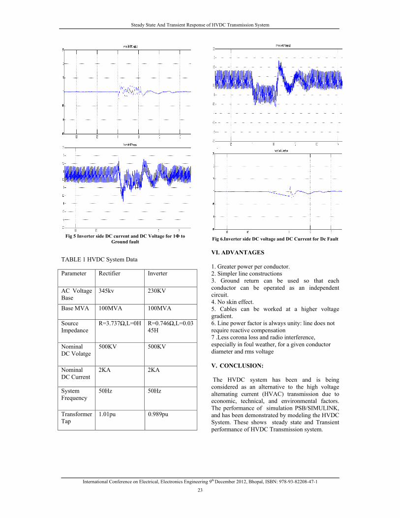
Steady State And Transient Response of HVDC Transmission System
International Conference on Electrical, Electronics Engineering 9th December 2012, Bhopal, ISBN: 978-93-82208-47-1
23
Fig 5 Inverter side DC current and DC Voltage for 1Φ to
Ground fault
TABLE 1 HVDC System Data
Fig 6.Inverter side DC voltage and DC Current for Dc Fault
VI. ADVANTAGES
1. Greater power per conductor.
2. Simpler line constructions
3. Ground return can be used so that each
conductor can be operated as an independent
circuit.
4. No skin effect.
5. Cables can be worked at a higher voltage
gradient.
6. Line power factor is always unity: line does not
require reactive compensation
7 .Less corona loss and radio interference,
especially in foul weather, for a given conductor
diameter and rms voltage
V. CONCLUSION:
The HVDC system has been and is being
considered as an alternative to the high voltage
alternating current (HVAC) transmission due to
economic, technical, and environmental factors.
The performance of simulation PSB/SIMULINK,
and has been demonstrated by modeling the HVDC
System. These shows steady state and Transient
performance of HVDC Transmission system.
Parameter Rectifier Inverter
AC Voltage
Base
345kv 230KV
Base MVA 100MVA 100MVA
Source
Impedance
R=3.737Ω,L=0H R=0.746Ω,L=0.03
45H
Nominal
DC Volatge
500KV 500KV
Nominal
DC Current
2KA 2KA
System
Frequency
50Hz 50Hz
Transformer
Tap
1.01pu 0.989pu

Steady State And Transient Response of HVDC Transmission System
International Conference on Electrical, Electronics Engineering 9th December 2012, Bhopal, ISBN: 978-93-82208-47-1
24
Fig. 7 hvdc system model in psb/simulink
REFERENCES
[1] Kala Meah,, and Wayne Blanding” Introducing High
Voltage Direct Current Transmission into an Undergraduate
Power Systems Course” American Society for Engineering
Education, 2009
[2]. M.O.Faruque,Yuyan Zhang and Venkata Dinavahi,
member,IEEE “ Detailed Modeling of CIGRE HVDC
Benchmark system’’. IEEE transaction on power
delivery,vol 21,Jan2006
[3]. A. Ekstrom and G. Liss, “A Refined HVDC Control
System,” IEEE Transactions on Power Apparatus and
Systems, Vol. PAS-89, No. 5, May/June 1970, pp.723-732.
[4]. M. Szechtman, T. Wess , and C. V. Thio, “First benchmark
model for HVDC control studies,” Electra, no. 135, pp. 54–
67, Apr. 1991
[5]. P. Kundur, Power System Stability and Control, Power
System Engineering Series, EPRI,1994, ISBN: 0-07-
035958-X
[6]. W.Brueur, D Povh,D Retzmann “Trends for Future HVDC
Application” Siemens Germany, Nov.2006.
Iris Recognition System Using Statistical Analysis, Gabor Filter And Morlet Wavelet
International Conference on Electrical, Electronics Engineering 9th December 2012, Bhopal, ISBN: 978-93-82208-47-1
25
IRIS RECOGNITION SYSTEM USING STATISTICAL ANALYSIS,
GABOR FILTER AND MORLET WAVELET
JAYSHREE M. CHAUDHARI1 & S. A .MORE
2
1,2Dept of Electronics and Telecommunication, R. C. Patel Institute of Technology, Shirpur, India
Abstract— Among all Biometrics Iris recognition is considered as one of most unique, reliable and accurate identification
system. Iris recognition system consist of preprocessing, segmentation, feature extraction and matching. In this paper we
have segmented iris using edge detection method and circular hough transform. Circular iris is converted into rectangular
image by using Daugman’s rubber sheet model. This paper mainly concentrated on the different feature extraction method
and their comparison. Features are extracted using statistical analysis, Morlet wavelet and Gabor filter. Image require are
obtain from CASIA database.(Institute of Automation, Chinese Academy of Sciences)
Keywords---feature vector; iris recognition; matching and segmentation.
I. INTRODUCTION
Biometric is science of recognition person base on its
physical and behavioral characteristics. e.g. palm
print, finger recognition, gait, face, signature, iris,
voice recognition. All biometric are different but
work in similar manner. They extract unique feature
from physical and behavioral characteristics and store
them in database as template. For comparison and
matching these templates are uses.
Because of many advantages such as stability,
uniqueness, does not require physical contact with
device iris recognition is most popular recognition
system among all biometric. Human eye consist of
sclera, pupil and iris. As shown in Fig.1 white part of
eye is called as sclera and small, dark ring of human
eye is called as pupil. Portion which is between sclera
and pupil is called as iris. Iris is unique for each
person. Even left and right eye of person has different
iris.
In 1936, a ophthalmologist Frank Bruch
proposed a concept of using iris patterns as a method
of recognizing an individual. In the year 1885, a
French ophthalmologist, Alphonse Bertillon first
proposed iris pattern as a basis for personal
identification. In1987, Flom and Safir obtained an
unimplemented concept of automated iris biometrics
system. A report was published by Johnston in 1992
without any experimental results. Dr.Flom
approached Dr.John Daugman to develop algorithm
for automated identification of human Iris. Daugman
use integrodifferential operator in order to detect
pupil and iris boundary.
Figure.1 Human eye
He used Dugmans rubber sheet model for
normalization. In 1994 Dr.Daugman awarded for
patent for his automated.
Wilds use canny edge detection and circular hough
transform for segmentation of iris, he proposed a
method of Gauss-Laplace filter for feature extraction.
Computation require for this method was huge[4].
Boles and Boashash proposed algorithm base on
zero crossing detection of wavelet transform but
recognition rate of this algorithm was low[5].
Yingi Du used standard procedure that is applied
canny edge detection method in order to get
edgemap. After segmentation he used daugman’s
rubber sheet model in order to convert circular
portion of iris into rectangular area. He prove that
eyelashes and eyelids affect recognition process so
partial portion of normalize iris that is right top side
can be use for recognition system.[6]
In this paper we are going to compare three
method of iris recognition. All these methods are
using common method for segmentation that is canny
edge detection to generate edgemap and circular
hough transform for segmentation of iris. For feature
extraction we are using three different methods. First
is statistical method, second is Gabor filter based
method, and third is Morlet Wavelet Method. Root
mean square method is use for feature matching.
Flow Chart for iris recognition system is as shown in
Fig 2.
II. IMPLIMENTATION
A. Image Acquisition
Image required for system are acquired from
CASIA database.(Institute of Automation, Chinese
Academy of Sciences) and UBIRIS.

Iris Recognition System Using Statistical Analysis, Gabor Filter And Morlet Wavelet
International Conference on Electrical, Electronics Engineering 9th December 2012, Bhopal, ISBN: 978-93-82208-47-1
26
Figure 2. Flow Chart for Iris recognition System
B. Preprocessing and segmentation
Preprocessing is require in order to remove noise
present in image. In this stage, RGB image is
converted in to gray scale image. Gaussian filter is
use to remove noise present in image.
After preprocessing segmentation is perform.
Segmentation is most critical step in iris recognition
system. Most of performance of system is depend on
good segmentation of iris image. Main objective of
iris recognition system is to separate out iris from eye
image. Separation is carried out on basis of
knowledge that iris is circular part present in eye
image. In order to separate out this circular portion
form eye image first it is converted into binary edge
map. Canny edge detection is use to convert to image
into binary edge map. Circular Hough Transform is
use to detect the iris circle in eye image. Circular
hough transform require large computation time. To
reduce its impact we limit its region to iris circle and
circular hough transform applied again to separate the
pupil circle form iris. We got the iris circle with
separated pupil from it. Fig 3 shows Output of
segmentation.
C. Normalization
In order to compare two iris image we have to
convert this circular iris image into fix dimension
image called as normalized image. For normalization
we are using Daugman’s rubber sheet model. In this
step, pupil separated circular iris, is converted into
rectangular image.
Unwrapping is start form right horizontal pupil
boundary. We are mapping using polar to rectangular
conversion to unwrap circular image to rectangular
image. It is impossible to get exact rectangular image
from circular iris image as inner circle has small
radius as compare to outer so bilinear interpolation of
gray value pixel is use to unwrap iris.
Figure. 3 Original eye Binary Egdemap
Segmented Iris
Iris and pupil center may or may not be concentric so
Remapping is used.The normalization of the iris
image I(x,y) from raw coordinates (x,y) to a doubly
dimensionless and non concentric coordinate system
(r, θ) can be represented as shown in (1) and (2) [2]:
Where (xp , yp ) is the set of papillary boundary
points and (xi, yi) the set of outer boundary points
determined by iris segmentation process. r belongs to
the interval [0,1] and θ is the variable angle belonging
to [0..2 π][2].
(1)
(2)
After normalization we got the image if size 48X512
size.
D. Feature Extraction
Once we get normalized image we can use it as
reference image and we can apply feature extraction
method on it. In this step, unique pattern of iris is
generated by applying suitable feature extraction
method. This unique pattern is called as iris code.
There are different methods for feature extraction.
Statistical analysis is one of the oldest methods
used in biometrics for feature extraction. It is one of
simplest method used for feature extraction. This
method require very few component to calculate and
take less time to generate feature vector, Normalized
iris image is divided into three rectangular images.
First ring consist of all rows which are between row
number first to row number sixteen. Second ring
consist of all rows between row seventeen to row
number thirty three. Third ring consist of all rows
which is between row number thirty four to row
number forty eight. For each rectangular image we
calculate the mean, mode, median, variance and
standard deviation. Feature vector consist of mean,
median, mode, variance and standard deviation of
three rings. Feature Vector for statistical analysis
obtain for iris image is shown in Fig 4.
Figure. 4 Feature vector obtain from statistical analysis
Gabor filter analysis, Gabor elementary functions
are Gaussian modulated by oriented complex
sinusoidal functions [2]. Right top corner of
normalized image of iris contain maximum feature.
For feature extraction using Gabor filter we consider
only image of size 240 X 40. This part is right top
portion of normalized image.
Gabor filter can be computed in the spatial domain by
using (3)[2]:
(3)

Iris Recognition System Using Statistical Analysis, Gabor Filter And Morlet Wavelet
International Conference on Electrical, Electronics Engineering 9th December 2012, Bhopal, ISBN: 978-93-82208-47-1
27
Where
and
Where:
f ( x, y) is the original image.
q( x, y) is the filtered image.
λ is wavelength of sinusoidal factor, θ is
orientation of Gabor filter, Ψ is phase offset, σ is
sigma, is spatial aspect ratio are important
parameter of Gabor filter. We divided image into 6
sub image of size 40Χ40 and applied bank of filter on
those images. We choose wavelength of 2, 4, 6 and 8
at angle of θ = 0, 45, 90 and 135. We have calculated
AAD that is “Average Absolute Deviation” for each
40Χ40 image so we have got total 16 feature value.
40X40 iris image with different filtered image is
shown in Fig.5.
(4)
Where N = no of significant pixels in image block, m
is mean, and f(x,y) value at point (x,y). We got 96
feature. These feature vector are shown in Fig 6.
Figure 5. Filtered images with different orientation and
wavelength
Figure 6. Feature vector obtain from Gabor analysis
Morlet Wavelet Analysis:
As right top corner of iris image contain maximum
feature we consider only first 31 row of and column
starting from 240 th column of normalized image of
iris for recognition. We have calculated morlet
wavelet coefficient for different scale m = 2,4,8,16
for each point f(x,y) on the image[3] using (5)
(5)
If morlet coefficient for the pixel f(x,y) is greater
than 0 or equal to zero then position code for that
pixel is scale “1” and marks that point as
characteristic point. If morlet coefficient for the pixel
f(x,y) is less than 0 then position code for that pixel
is scale “0” and marks that point as non-characteristic
point. Feature vector obtain from this analysis is too
large to display
E. Matching
Matching is important process used after extraction of
features. In matching process we measure the
distance between feature vectors of two iris. We used
RMS(root mean square) for comparison of two iris.
We calculate RMS value of difference in two iris
feature vector. Two vectors are said to be similar if
RMS value is less than predefine threshold value.
This threshold value we have calculated by
comparing different iris image of CASIA database.
We consider 400 images of CASIA database. It
contain left and right eye of 10 people. We compare
some similar iris and some nonsimilar iris. From
graph we got the value of threshold. Good threshold
value obtain from graph is between 28 and 40.
III. EXPERIMENTAL RESULTS
We calculated FAR “false acceptance rate” and
FRR “false rejection rate” of Three different method
at threshold value of 30 we got the result as shown in
table.
From experimental analysis we got 94% accuracy
for statistical analysis. For Gabor filter accuracy is
96% and for Morlet wavelet accuracy is 99%.
TABLE 1 EXPERIMENTAL RESULT OF DIFFERENT
METHOD
Method FAR FRR Mttch(ms)
Statistical 0.8% 2.65% 2.4
Gabor 0.32% 0.56% 4.1
Morlet 0.30% 0.411% 6.2

Iris Recognition System Using Statistical Analysis, Gabor Filter And Morlet Wavelet
International Conference on Electrical, Electronics Engineering 9th December 2012, Bhopal, ISBN: 978-93-82208-47-1
28
IV. CONCLUSION
In this paper we have compare three different
methods of feature extraction. We have use canny
edge detection method in order generate binary edge
map. For segmentation of iris we have used circular
hough transform which take lot of computation time
but accurate method for segmentation. Three different
methods used for extraction are statistical analysis,
Gabor filter based method and Morlet wavelet
analysis method. All three methods are tested on
CASIA and UBIRIS.Accuracy of statistical analysis
94%, Gabor filter is 96% , Morlet wavelet is 99%.
Statistical Analysis take less time for matching as it
has small feature vector to compare
REFERENCES
[1] Khin Sint Sint Kyaw, "Iris Recognition System using
statistical features for Biometric Identification," 2009
International Conference on Electronic Computer
Technology.
[2] Feddaoui nadia, hamrouni kamel “An efficient and reliable
algorithm for iris recognition based on Gabor Filters” 2009
6th international conference on signal, system and devices.
[3] Zhonghua Lin Bibo Lu “Iris Recognition Method Based on
the Imaginary coefficients of Morlet Wavelet Transform”
2010 International Conference on Intelligent computation and
technology And Automation
[4] R. P. Wildes, “ Automated iris recognition:An emerging
biometris technology,” Proceedings of IEEE 85 1348-
1363(1997)
[5] W. W. Boles, B. Boashash, “A human identification
technique usingc images of the iris and wavelet transform.
IEEE Transaction on Signal Processing”, 1998, 46(4): 1185–
1188.
[6] Yingi Du, “Analysis of Partial Iris recognition using a 1-D
Approach”, IEEE 2005.
[7] V. V. Satyanarayana Tallapragada and E.G.Rajan “Iris
Recognition Based on Combined Feature of GLCM and
Wavelet TransForm”, 2010 First International Conference on
Integrated Intelligent Computing.
[8] N. Popescu-Bodorin, Member, IEEE and V.E. Balas, “
Comparing Haar-Hilbert and Log-Gabor Based Iris Encoders
on Bath Iris Image Database”,2010 IEEE.

International Conference on Electrical, Electronics Engineering 9th December 2012, Bhopal, ISBN: 978-93-82208-47-1
29
IMPLEMENTATION AND COMPARISON OF 32 BIT FIBONACCI
LFSR PRODUCING 8-BIT RANDOM VALUES IN VHDL
ANKITA RASTOGI
ECE Deptt., Final year, Guru Gobind Singh Indraprastha University, Delhi, India
Abstract— Random numbers are useful for a variety of purposes such as generating data encryption keys, simulating and
modelling complex phenomena and for selecting random samples from larger data sets[1]. The linear feedback shift register
(LFSR) is one of the most useful techniques for generating psuedo-random numbers. The limitation with typical LFSR lies
in the fact that it only produces one new random bit each time on shift . This is applicable for white noise source but for
some applications, a random 8-bit value is needed. A 32-bit LFSR will produce a sequence of 4294967295 random bits . If
we output them as audio at 96KHz, the noise won't repeat for an hour and by then we’ll have forgotten what the beginning
sounded like. To overcome this problem, a method is proposed in this paper by implementing 32 bit LFSR in VHDL on 1
byte shift basis rather than single bit shift . A performance comparative study of 32 bit LFSR is also shown here to
understand the efficiency of this method over typical LFSR. This implementation is based on Fibonacci LFSR. Also XOR
operation is used for taping and four taps are used. For FPGA implementation , Xilinx ISE software is used to produce the
RTL schematic of the desired circuit.
Keywords-FIBONACCI LFSR, FPGA, VHDL.
1. INTRODUCTION
A random number generator requires a naturally
occurring source of randomness. A random number is
a number generated by a process, whose outcome is
unpredictable, and which cannot be subsequentially
reliably reproduced. Random numbers are used in
literature and music, and are of course ever popular
for games and gambling. When discussing single
numbers, a random number is one that is drawn from
a set of possible values, each of which is equally
probable, i.e. a uniform distribution. When discussing
a sequence of random numbers, each number drawn
must be statistically independent of the other.
Random number generator is a computational device
to generate a sequence of numbers or that lack any
pattern. Random number generators based on natural
sources of randomness are influenced by external
factors so it becomes essential that such devices be
tested periodically by using the statistical tests.
Random number generators are based on Hardware
and Software. Methods for generating random results
have existed since ancient times, including dice, coin
flipping, the shuffling of playing cards, the use of
yarrow stalks, and many other techniques. Most of
the methods to compute random numbers are based
on linear congruential equations and require a
number of time consuming arithmetic operations. In
contrast, the use of feedback shift registers permits
very fast generation of binary sequences. Shift
register sequences of maximum length (m-sequences)
are well suited to simulate truly random binary
sequences . However, they cannot be used in
applications which require a decimal random
sequence. The method used in this paper is for
creating noise generator. A Noise generator is a
circuit that produces electrical noise (i.e., a random
signal). Noise generators are also used for generating
random numbers.
2. FIBONACCI LFSR
A shift register is a circuit that shifts the elements of
a bit array by one position. A shift register has an
input (one bit) and an output (also one bit), and is
driven by a clock pulse. When the clock pulse
happens, the input bit is shifted to the position of the
least significant bit, the most significant bit is sent to
the register output, and all other bits are shifted by
one position to the direction of the array's most
significant bit (towards the output). A Linear
Feedback Shift Register (LFSR) is a shift register in
which the input bit is determined by the value of
the EXCLUSIVE-OR of some of the register bits
before the clock pulse. The bits that are used in the
register's feedback are called taps. The figure below
shows a LFSR with 8 bits and three taps (bits 0,3 and
5).
Figure -1-
3. FEEDBACK FUNCTION
In an LFSR, the bits contained in selected positions in
the shift register are combined in some sort of
function and the result is fed back into the register's
input bit. By definition, the selected bit values are
collected before the register is clocked and the result
of the feedback function is inserted into the shift

Implementation and Comparison of 32 Bit Fibonacci LFSR Producing 8-Bit Random Values in VHDL
International Conference on Electrical, Electronics Engineering 9th December 2012, Bhopal, ISBN: 978-93-82208-47-1
30
register during the shift, filling the position that is
emptied as a result of the shift.The feedback function
in an LFSR has several names: XOR, odd parity, sum
modulo 2. Steps are as follows[9]:
1) Add the selected bit values,
2) If the sum is odd, the output of the function is one;
otherwise the output is zero.
The bit positions selected for use in the feedback
function are called "taps". The list of the taps is
known as the "tap sequence". Conventionally, the
output bit of an LFSR that is n bits long is the nth bit;
the input bit of an LFSR is bit 1.
4. MAXIMAL LENGTH TAP SEQUENCES
LFSR's can have multiple maximal length tap
sequences. A maximal length tap sequence also
describes the exponents in what is known as a
primitive polynomial mod 2.
For example, a tap sequence of 4, 1 describes the
primitive polynomial
x^4 + x^1 + 1
Finding a primitive polynomial mod 2 of degree n
(the largest exponent in the polynomial) will yield a
maximal length tap sequence for an LFSR that is n
bits long.
There is no quick way to determine if a tap sequence
is maximal length. However, there are some ways to
tell if one is not maximal length:
1) Maximal length tap sequences always have an even
number taps.
2) The tap values in a maximal length tap sequence
are all relatively prime. A tap sequence like 12, 9, 6, 3
will not be maximal length because the tap values are
all divisible by 3.
Discovering one maximal length tap sequence leads
automatically to another. If a maximal length tap
sequence is described by [n, A, B, C], another
maximal length tap sequence will be described by [n,
n-C, n-B, n-A]. Thus, if [32, 3, 2, 1] is a maximal
length tap sequence, [32, 31, 30, 29] will also be a
maximal length tap sequence. An interesting behavior
of two such tap sequences is that the output bit
streams are mirror images in time.
5. VHDL
VHDL (VHSIC hardware description language) is
a hardware description language used in electronic
design automation to describe digital and mixed-
signal systems such as field-programmable gate
arrays and integrated circuits. VHDL is commonly
used to write text models that describe a logic circuit.
Such a model is processed by a synthesis program,
only if it is part of the logic design. A simulation
program is used to test the logic design using
simulation models to represent the logic circuits that
interface to the design. This collection of simulation
models is commonly called a testbench[4].
We can design hardware in a VHDL IDE (for FPGA
implementation such as Xilinx ISE, Altera Quartus,
Synopsys Synplify or Mentor Graphics HDL
Designer) to produce the RTL schematic of the
desired circuit. After that, the generated schematic
can be verified using simulation software which
shows the waveforms of inputs and outputs of the
circuit after generating the appropriate test bench. To
generate an appropriate test bench for a particular
circuit or VHDL code, the inputs have to be defined
correctly. For example, for clock input, a loop
process or an iterative statement is required.
6. LFSR
A. WORKING
We will consider a 32-bit LFSR with four taps at
positions 32, 30, 26, and 25. LFSR taps are
numbered starting on one, so we take one off the
tap position to get the bit that represents. So we
need bits 31, 29, 25, and 24 as described below:
Figure -2-[2]
A 32-bit LFSR takes a series of bits called taps i.e.
bits 31,29,25 and 24 from shift register, XORs
them together to come up with a resultant bit, shifts
the register along one bit, and then sticks the new
bit back into the beginning of the register.
B. LIMITATION WITH LFSR
The problem with the typical LFSR is that it only
produces one new random bit each time when we
shift it. This works fine for some things like white
noise source, but a random 8-bit value (or a
random 16-bit value) is required for some
applications. For this, we run the code 8 times,
which is ok but it is very inefficient method, and
number of instruction cycles will also increase.
C. MODIFICATION IN EXISTING LFSR
DESIGN
To overcome this problem in typical LFSR , we do
a modification by shifting a byte rather than shifting
a single bit at a time. To do this . for tap 32, when
the first time we run the code, we pull out bit 31.
The next time we run it, the register has shifted, so
we pull out what was bit 30. The time after that, we

Implementation and Comparison of 32 Bit Fibonacci LFSR Producing 8-Bit Random Values in VHDL
International Conference on Electrical, Electronics Engineering 9th December 2012, Bhopal, ISBN: 978-93-82208-47-1
31
get bit 29, etc. Over the eight runs, we get all of the
bits of the top byte of the register.
A similar thing happens with each of the other taps.
Tap 30 gives us a byte from bit 29 to bit 22, tap 26
a byte from bit 25 to bit 18, tap 25 from bit 24 to bit
17.
Figure -3-[2]
Now take these four bytes and XOR them together as
bytes than bit by bit. To perform this, I have to shift
the bytes in the register so that they all line up. We
can then XOR, and finish up with a result byte which
has all eight of the required bits for the front of the
register in it. The final step is to shift the register over
8 bits. Since this is a one byte shift, this is much
quicker method and number of instruction cycles will
also reduce.
7. IMPLEMENTATION AND SIMULATION
In this design, we describe the RTL-level of the
LFSR pseudo-random number generator for 32 bit
both for generating 1 bit and repeating the code 8
times & for generating one byte using VHDL
language, and use the Xilinx’s software.
Then we synthesize, place and route on the Xilinx
ISE platform. Finally we use ISE Simulator to do a
timing simulation . Refer figure 4 & figure 5 for
Simulation Result.
8. PERFORMANCE ANALYSIS
For the same initial input values in LFSR, the
performance analysis of both is made.It is observed
that for 32 bit LFSR 8 random bit generator, the
timing simulation takes 140ns to produce 8 random
bits whereas in case of 1 byte generator, only a single
clock period at 400ns is used to generate one byte of
pseudo random numbers which is much quicker and
efficient method to produce random bytes for noise
generation It is also observed that the vhdl code for
bit shift analysis uses 6 instruction cycle for 1 bit
generation and total of 6X8=48 instruction cycles for
8 random bits generation whereas 1 byte shift
analysis uses instruction cycles.
9. CONCLUSION
It is clearly found from the synthesis and simulation
result that 32 bit LFSR for generating random 8 bits
with 4 tappings at 31,29,25 and 24 that the
performance is better in 32 bit LFSR :1 byte shift as
compared to bit by bit shift. The only limitation
with this method is that you can't use taps that are
within the part that you replace in the final step.
That is why, the set of taps 32, 30, 26, 25 are
chosen because if we do so then when we run the
single-bit-shift version eight times - they get
modified by new bits going into the register.
Method proposed in this paper assumes this will not
occur, so it only works with sets of taps where this
assumption holds true.
REFERENCES
[1]. Pseudo-Random-Generator. Wikipedia website [Online]
Available:http://en.wikipedia.org/wiki/Pseudorandom_number
_generator
[2]. Linear Feedback Shift Register, Wikipedia website.
[Online].Available:http://en.wikipedia.org/wiki/Linear_feedba
ck_shift_register.
[3]. PIC Microcontroller, website [Online] Available:
http://www.electricdruid.net/index.php?page=techniques.practi
calLFSRs
[4]. Bhasker J, “A VHDL Primer”, P T R Prentice Hall
[5]. Xilinx, Inc. Xilinx Libraries Guide.
[6]. Katti, R.S. Srinivasan, S.K., “Efficient hardware
implementation of a new pseudo-random bit sequence
generator” IEEE International Symposium on Circuits and
Systems, 2009. ISCAS 2009.
[7]. C. Li and B. Sun, “Using linear congruential generators for
cryptographic purposes”, In Proceedings of the ISCA 20th
International Conference on Computers and Their
Applications, pp. 13-18, March 2005.
[8]. Ding Jun, Li Na, Guo Yixiong, “A high-performance pseudo-
random number generator based on FPGA” 2009 International
Conference on Wireless Networks and Information Systems.
[9]. Amit Kumar Panda, Praveena Rajput, Bhawna Shukla,
“DESIGN OF MULTI BIT LFSR PNRG AND
PERFORMANCE COMPARISON ON FPGA USING
VHDL” International Journal of Advances in Engineering &
Technology, March 2012, Vol. 3, Issue 1, pp. 566-571.
[10]. FPGA, Wikipedia website. [Online] Available:
http://en.wikipedia.org/wiki/Field_Programmable
_Gate_Array.

Implementation and Comparison of 32 Bit Fibonacci LFSR Producing 8-Bit Random Values in VHDL
International Conference on Electrical, Electronics Engineering 9th December 2012, Bhopal, ISBN: 978-93-82208-47-1
32
Simulation Result of 32-Bit LFSR for 8 random values : bit by bit shift
Fig 4. The timing simulation for 8 random values is shown from 1020 to 1160ns.
Simulation Result of 32-Bit LFSR for 8 random values : byte shift
Fig 5. The timing simulation for 1 byte at 400ns

International Conference on Electrical, Electronics Engineering 9th December 2012, Bhopal, ISBN: 978-93-82208-47-1
33
SIMULATION OF A THREE PHASE INDUCTION MOTOR
PALAK G. SHARMA
Student of Department of Electrical Engineering, Ramdeobaba Collage of Engineering and Management Nagpur
Abstract — This paper presents dynamic simulation of three phase induction machine based on mathematical modelling.
The theory of reference frame has been used to analyze the performance of three phase induction machine. In this paper
simulink implementation of induction machine using dq0 axis transformation is used.
I. INTRODUCTION
Three phase induction motor have well
known advantages of simple construction, reliability,
ruggedness, low maintenance and low cost which has
led to their wide use in industrial application. The
voltage and the torque equation which describes the
dynamic behaviour of induction motor are times
varying. A change of variables are used to reduce the
complexity caused by the time varying inductance in
the induction motor by eliminating the time varying
inductance. By this method a multi phase winding
can be reduced to a set of two phase winding with
their magnetic axes formed in quadrature. That is, the
stator and the rotor windings of an induction motor
are transferred to a reference frame. Such a reference
frame is known as arbitrary reference frame [1, 2].
The equivalent Circuit of induction machine in
arbitrary reference frame is shown in Fig.1.
Fig.1. Equivalent circuit model of an induction motor in
arbitrary reference frame.
The dynamic analysis of the symmetrical induction
machines in the arbitrary reference frame has been
intensively used as a standard simulation approach. In
this paper Simulink is used to simulate the dynamic
performance of an induction motor model whose
variables are referred to an arbitrary reference frame.
II. INDUCTION MOTOR MODEL
The Model equations can be generated from the
equivalent circuit of induction machine in arbitrary
reference frame Fig.1.
The three phase stator voltage equations of an
induction motor under balanced conditions are:-
The above three phase equations are transferred to
synchronously rotating frame in two phases, this can
be done by using Parks and Clarke Transformation in
equation (4, 5).

Simulation of A Three Phase Induction Motor
International Conference on Electrical, Electronics Engineering 9th December 2012, Bhopal, ISBN: 978-93-82208-47-1
34
III. MATLAB/SIMULINK IMPLEMENTATION
In this the three phase induction machine model is
implemented using the equation (1-18) stated in
section II. Complete simulation of three phase
induction machine model is shown in Fig.2.
Fig.2.The Three Phase Induction Machine
Matlab/Simulink Model.
In this model simulation stats with generation of
stator voltage from equation(1, 2, 3) and then
transforming these voltages to synchronously rotating
frame using the Park and Clarke Transformation as in
equations (4, 5).once Vq &Vd are obtained from
equation(4, 5) then the flux and current equations are
implemented, so as to calculate current iqs, ids, iqr, idr,
according to equation (13-16).
The internal structure of induction motor d-q
model is shown in Fig.3.
Fig.3. Internal structure of induction motord-q model
The matlab simulink model to find flux linkages as
stated by equation (6-12) is shown in Fig.4.
Fi
Fig.4(a).
Fig.4(b).

Simulation of A Three Phase Induction Motor
International Conference on Electrical, Electronics Engineering 9th December 2012, Bhopal, ISBN: 978-93-82208-47-1
35
Fig.4(c).
Fig.4(d).
Fig.4(e).
Fig.4.(f)
Fig.4. Internal structure of the block to calculate flux
linkages.
Fig.5.(a)
Fig.5.(b)
Fig.5.(c)
Fig.5.(d)
Fig.5. shows the simulink block to calculate current iqs, ids,
iqr, idr, according to equation (13-16).
Fig.6. Internal structure to calculate torque according to
equation(17).
Fig.7.Internal structure to calculate angular speed
according to equation (18).

Simulation of A Three Phase Induction Motor
International Conference on Electrical, Electronics Engineering 9th December 2012, Bhopal, ISBN: 978-93-82208-47-1
36
IV. SIMULATION RESULT
Induction motor shown in the model has been
tested for:-
Hp =3;
Pole =4;
VL =220V;
Frequency =60Hz;
Stator Resistance =0.435;
Rotor Resistance =0.816;
Stator Impedance =0.754;
Rotor Impedance =0.754;
Mutual Impedance =26.13;
Moment of Inertia =0.089;
The result obtained after simulation are shown
below:-
Fig.8. Machine Variables during free acceleration of a three
phase induction motor.
V. CONCLUSION
In this paper Implementation and Dynamic
simulation of a three phase induction motor using
Matlab is studied. The model was tested for 3hp
motor, 50Hz. The result obtain are satisfactory.
VI. REFERENCE
[1] B. Ozpineci, L. M. Tolbert, “Simulink implementation of
induction machine model- A Modular approach”,
IEEE,2003,pp 728-734.
[2] H. C. Stanley,” An Analysis of the Induction Motor”,
AIEE Transactions, vol.57 (supplement), 1938,pp.751-
755.
[3] Byoung-Kuk Lee ,Mehrdad Ehsani “A Simplified
Functional Simulation Model for Three-Phase Voltage-
Source Inverter Using Switching Function Concept”.
IEEE transactions on industrial
electronics,vol.48,no.2,april2001.
[4] P. C. Krause, O. Wasynczuk, S. D. Sudhoff “Analysis of
Electric Machinery and Drive Systems”, IEEE Press, A
John Wiley & Sons, Inc. Publication Second Edition,
2002.
[5] P.C. Krause and C. H. Thomas, “Simulation of
Symmetrical Induction Machinery”, IEEE Transaction
on Power Apparatus and Systems, Vol. 84, November
1965, pp. 1038-1053..

Design & Development of Mppt Based Converter for Efficient Solar Power Conversion
International Conference on Electrical, Electronics Engineering 9th December 2012, Bhopal, ISBN: 978-93-82208-47-1
37
DESIGN & DEVELOPMENT OF MPPT BASED CONVERTER FOR
EFFICIENT SOLAR POWER CONVERSION
PRASHANT MESHRAM1 & SABYASACHI BHATTACHARYA
2
1,2Department of Electrical engineering, Ramdeobaba College of Engineering & Management,
Nagpur, Maharashtra, India
Abstract— The design of a Maximum Power Tracking (MPPT) controller for a solar photovoltaic battery charging system
is proposed utilizing a buck-converter topology. Solar panel voltage and current are continuously monitored by a closed-loop
microcontroller based control system, and the duty cycle of the buck converter will be continuously adjusted to extract the
maximum power. MATLAB Simulation will be used for the initial validation of the proposed scheme and for the selection of
circuit parameters. Actual controller will be implemented using AVR series microcontroller
Keywords-Solar PV technology, MPPT, Efficiency of PV system.
I. INTRODUCTION
A Electrical Power is the basic need for economic
development of any country. Conventional sources of
energy like Coal, Natural Gas and Oil etc., contribute
about 92% of total power generation in world. These
source are limited & will be exhausted in near future,
also they produce greenhouse gases leading to global
warming and other environmental hazards. Non-
conventional energy sources such as Solar, Wind, Sea,
Geothermal, Biomass are eco-friendly. The solar PV
module converts solar energy directly into usable
electrical energy with no bi-products, which is not
possible with fossil fuels. As the demand of power is
increasing, new developments in the field of non-
conventional energy are also being presented. As Sun
is considered to be the only never ending source of
energy known to mankind, solar energy seems to be
the best solution for our future energy requirements.
Currently India is generating 2,06,456.04 MW of
electricity out of which only 12.10 % i.e.
24,998.46MW is contributed by renewable energy
sources. As India receives a large number of sunshine
hours over the year, there is great scope of solar
photovoltaic technology. The lower power conversion
efficiency of PV systems is the major problem
affecting the large scale implementation of solar PV
systems.
This Project work aims at the development of
Maximum Power point based Converter for Efficient
Solar Power Conversion. Maximum power point
tracking (MPPT) is used in photovoltaic (PV) systems
to maximize the photovoltaic array output power,
irrespective of the temperature and solar irradiation
conditions and of the load electrical characteristics. A
microcontroller based MPPT system has been
proposed, consisting of a Buck-type DC-DC
converter. Solar panel voltage and current are
continuously monitored by a closed-loop control
system, and the duty cycle of the buck converter will
be continuously adjusted to extract the maximum
power. A comparative study of various MPPT
algorithms will be done to understand the operation
and compare the performance.
.
II. LITERATURE REVIEW
A number of MPPT control algorithms namely
Perturb & Observe (P&O) ,Incremental conductance
(INC), Parasitic capacitance (PC),Constant voltage
(CV),Open circuit voltage (OCV) and Short circuit
current (SCC)have been proposed and discussed in
wide literature available[2,7].
One algorithm, the perturb-and-observe (P&O)
algorithm, is by far the most commonly used in
commercial MPPT[6]. However, there is as yet no
consensus on which algorithm is ‘best’, and many
authors have suggested that perhaps the P&O
algorithm is inferior to others. This lack of consensus
stems in part from the fact that the literature contains
no comparisons of absolute efficiencies of MPPT
algorithms, with all algorithms using optimized
parameters and operating on a standardized MPPT
hardware. Most of the reported comparisons are made
between an MPPT algorithm and a direct coupled
system or between an MPPT algorithm and a
converter designed for a fixed operating point.
Following table shows the Summary of previously
reported MPPT efficiencies for the four algorithms[5]
Sr.No MPPT Algorithm Reported
Efficiencies
1 Perturb-and-observe 85%
2 Incremental
conductance
88%
3 Constant voltage 73%
4 Parasitic
capacitance
99%

Int
III. SOLA
TOPO
A. Grid C
The gr
with the el
the utility
synchroniz
features a
islanding. G
size, but al
convert the
electricity,
wiring and
the first gr
hundred ki
centralized
voltage ele
large therm
Anothe
small hous
PV modu
connected
connected
the array d
loads, and
using micr
At night, t
grid. If the
more energ
Instead of
can genera
this electric
On man
with peak
regions pe
because ai
loads are m
and thus t
during a
generated
advantage
A grid-
cost adva
transmissio
distribution
systems ca
supply by r
conditionin
B. Off grid
The ter
a grid, mai
the main o
electricity
mini-grids
with elec
approach t
areas with
or distant p
Desi
ternational Confer
AR PHOTOVO
OLOGIES
Connected Syste
rid-connected
lectric utility gr
via the grid
zed with the g
are essential
Grid-connected
ll consist of so
e DC output o
and other c
d module moun
rid-connected
ilowatts of PV
d array, which
ectricity grid i
mal generator.
er form of gr
se hold applica
ule at their h
supply. For
rooftop PV sy
during the day
the excess ene
ro grid inverter
the local loads
e PV system is
gy into the grid
receiving a bi
ate revenue fro
city.
ny electricity n
solar power p
eak loads occ
ir conditioners
more expensiv
the electricity
peak load is
at times of low
of grid connec
-connected PV
antages when
on line, since
n losses and he
an also be use
reducing 'noise
ng on a transmi
d Photovoltaic
rm off-grid ref
inly used in ter
or local transm
off-grid can
typically to p
ctricity. Off-g
to access elect
little access to
population. It c
gn & Developmen
rence on Electrical
OLTAIC SYS
em electing a T
systems opera
rid and supply
. The inverter
rid and additio
in the invert
d PV systems
olar modules, i
of the solar mo
omponents su
nting structure
systems consis
V modules laid
fed power into
in much the s
rid connected
ation users, whi
house along w
these types o
ystem, the powe
y can be used t
ergy is fed into
rs for other cus
s are simply s
s large enough
d than is used
ll every month
om their utility
networks, peak
production. Exa
cur on summ
s are used ext
e to satisfy tha
generated by
of greater va
w demand. Th
ted PV system
system offers
placed at th
it reduces tra
elps stabilize li
ed to improve
e' or providing
ission line.
c system
fers to not bein
rms of not bein
mission grid in
be stand-alon
provide a smal
grid electrific
tricity used in
o electricity, d
can be any kin
nt of Mppt Based C
l, Electronics Engi
STEM
Template
ate in paralle
solar power to
r needs to be
onal protection
ter to preven
vary greatly in
inverters which
odules into AC
uch as MPPT
es etc. Most o
sted of severa
d out in a large
o the local high
same way as a
system is for
ich connect the
with the grid
of small grid-
er produced by
to supply loca
o the local grid
stomers to use
upplied by the
h, it can supply
by local loads
h, the customer
for generating
k loads coincide
ample in many
mer afternoons
tensively. Peak
an other loads
a PV system
alue than tha
his is an major
.
other potentia
he end of a
ansmission and
ine voltage. PV
the quality of
reactive power
ng connected to
ng connected to
n electricity. In
ne systems or
ler community
cation is an
n countries and
due to scattered
nd of electricity
Converter for Effic
ineering 9th Decem
l
o
e
n
nt
n
h
C
T,
f
al
e
h
a
r
e
d
-
y
al
d
e.
e
y
s.
r
g
e
y
s
k
s,
m
at
r
al
a
d
V
f
r
o
o
n
r
y
n
d
d
y
generatio
self-suffi
more pub
The sola
attractive
diesel ge
energy is
battery b
involved
MPPT ch
inverters,
Blo
Componen
• S
P
numb
comb
the v
conve
when
energ
turn,
varies
intens
T
constr
1. M
2. P
3. A
4.
The
materials
light sour
20% in c
film pho
amorphou
consist o
sheet of g
then used
good eff
crystallin
from a c
condition
silicon ar
however
connected
They wei
and are ab
cells attai
cient Solar Power
mber 2012, Bhopal,
on. The term o
cient manner
blic utilities.
ar off grid s
e economical
enerators. In O
s consumed u
banks for a lat
in off grid sy
harge controlle
, etc.
ck Diagram of O
nts of Off Grid
Solar Photovolt
Photovoltaic (P
ber of internal s
ined in series
oltage or curr
ert solar energ
the photovolt
y causing the c
produces an
s with the size o
sity.
The most co
ruction of these
Mono crystalli
Polycrystalline
Amorphous sil
Copperindium
ese PV cells con
are capable
rces and usual
ommercial use
otovoltaic tech
us silicon arr
of a layer of s
glass and a she
d to mark out in
ficiency on s
ne silicon based
onsiderable dr
ns. Mono-cry
rrays are const
are made up
d together to
igh less than th
bout half the s
in as high effic
Conversion
, ISBN: 978-93-82
ff grid can ref
without relia
system alread
alternatively
Off grid PV
upon generatio
er use. The m
ystems are sol
ers, Battery b
Off grid Photovolt
d Solar System
taic Array
V) array essen
silicon based p
and in paralle
rent requireme
gy into electric
taic cells are e
cells electrons t
electric curren
of individual c
ommon mater
e modules are
ine silicon
e silicon
licon
m selenide (CI
nsisting of suc
of generating
lly have effici
e.The most pop
hnologies are
rays. These th
silicon sandwi
eet of plastic. A
ndividual cells.
sunny days, b
d cells. Howev
rop in efficienc
ystalline and
tructed in much
p of individu
achieve the
he amorphous
ize. Although m
ciencies as the a
2208-47-1
fer to living in
ance on one
dy represent a
to convention
system, the P
on or stored
main componen
lar PV module
ank, DC to A
taic system
ntiallyconsist of
photovoltaic cel
el, depending o
ents. These cel
city. This occu
exposed to sol
to drift which,
nt. This curre
ells and the lig
rials used f
IS)
h semiconduct
electricity fro
encies of 6%
pular type of th
CIS arrays an
hin film pane
iched between
A laser scribe
. They have ve
better then th
er they do suff
cy under cloud
polycrystallin
h the same wa
ual 0.5 V cel
desired voltag
and CIS array
mono crystallin
amorphous cel
n a
or
an
nal
PV
in
nts
es,
AC
f a
lls
on
lls
urs
lar
in
ent
ght
for
tor
om
hin
nd
els
a
is
ery
he
fer
dy
ne
ay,
lls
ge.
ys,
ne
ls,

Design & Development of Mppt Based Converter for Efficient Solar Power Conversion
International Conference on Electrical, Electronics Engineering 9th December 2012, Bhopal, ISBN: 978-93-82208-47-1
39
they do perform better under cloudy conditions,
making them very suitable for year round use.
• Battery
Batteries are used to store the excess charge
developed during the day time electricity
generation which can be used later in the non-sun
shine hours. There are basically two types of
battery which are mainly used i) Lead Acid battery
and ii) Nickel Cadmium battery. The most
commonly used is lead acid battery whereas nickel
cadmium battery has many advantages such as
long life, high energy density, good performance
under low temperature etc. As the Ni-Cd batteries
are much expensive, these batteries are less
preferred. Avoid combining SI and CGS units,
such as current in
• Charge Controller
In PV systems charge controllers are designed for
monitoring & controlling various dc to dc
converters which are integrated in it. The charge
controller operates the converters for extracting
and managing generated power to achieve the
maximum efficiency. The main functions of a
charge controller in concern with battery are
protection from reverse current and battery
overcharge. Charge controllers are also designed
to prevent battery over discharge, protect from
electrical overload, and/or display battery status
and the flow of power.
• Solar Inverter
A solar inverter, or PV inverter, converts the
variable direct current (DC) output of a
photovoltaic (PV) solar panel into a alternating
current (AC) that can be fed into a commercial
electrical grid or used by a local, off-grid electrical
network. It is a critical component in a
photovoltaic system, allowing the use of ordinary
AC appliances. The solar inverters are basically
classified into three main categories
1. Stand-alone inverters
2. Grid-tie inverters
3. Battery backup inverters
IV. MAXIMUM POWER POINT TRACKING
Solar cells are characterized by i) maximum Open
Circuit Voltage (Voc) at zero output current and ii)
Short Circuit Current (Isc) at zero output voltage. The
solar power can be computed using equation:
P = I * V
A PV array under constant uniform irradiance has
a current–voltage (I–V) characteristic like that shown
in Figure1. There is a unique point on the curve,
called the maximum power point (MPP) at which the
array operates with maximum efficiency and
produces maximum output power. When a PV array
is directly connected to a load (a so-called ‘direct-
coupled’ system), the system’s operating point will be
at the intersection of the I–V curve of the PV array
and load line shown in Figure 1.In general, this
operating point is not at the PV array’s MPP, which
can be clearly seen in Figure 1. Thus, in a direct-
coupled system, the PV array must usually be
oversized to ensure that the load’s power
requirements can be supplied. This leads to an overly
expensive system.
Figure 1.
To overcome this problem, a switch-mode power
converter, called a maximum power point tracker
(MPPT),can be used to maintain the PV array’s
operating point at the MPP. The MPPT does this by
controlling the PV array’s voltage or current
independently of those of the load. If properly
controlled by an MPPT algorithm, the MPPT can
locate and track the MPP of the PV array. However,
the location of the MPP in the I–V plane is not known
a priori. It must be located, either through model
calculations or by a search algorithm. The situation is
further complicated by the fact that the MPP depends
in a nonlinear way on irradiance and temperature, as
illustrated in Figure 2. Figure 2(a) shows a family of
PV I–V curves under increasing irradiance, but at
constant temperature, and Figure 2(b) shows I–V
curves at the same irradiance values, but a higher
temperature. Note the change in the array voltage at
which the MPP occurs.
Figure 2(a) Figure2(b)
There are many different approaches to
maximizing the power from a PV system, these range
from using simple voltage relationships to more
complex multiple sample based analysis. Depending
on the end application and the dynamics of the
irradiance, the proper method is implemented. These
are called MPPT algorithms. There are various

Design & Development of Mppt Based Converter for Efficient Solar Power Conversion
International Conference on Electrical, Electronics Engineering 9th December 2012, Bhopal, ISBN: 978-93-82208-47-1
40
algorithms to track the maximum power point and
operate the PV module on that point to extract the
maximum power. Some of the algorithms are listed
below:
1. Perturb & Observe (P&O)
2. Incremental conductance (INC)
3. Parasitic capacitance (PC)
4. Constant voltage (CV)
5. Open circuit voltage (OCV)
6. Short circuit current (SCC)
V. DESIGN OF MPPT BASED SOLAR
CHARGE CONTROLLER
The MPPT algorithm embedded in charge
controller takes voltage and current feedback from
the panel and adjusts the control signals to operate the
panel at its peak power. In this project we are
implementing Perturb & Observe (P&O) algorithm to
obtain maximum power. The perturb and observe
(P&O) algorithm is the most commonly used in
practice because of its ease of implementation. Figure
3, shows a family of PV array power curves as a
function of voltage (P–V curves), at different
irradiance (G) levels, for uniform irradiance and
constant temperature. These curves have global
maxima at the MPP. Assume the PV array to be
operating at point A in Figure 5, which is far from the
Maximum Power Point. In the P&O algorithm, the
operating voltage of the PV array is perturbed by a
small increment, and the resulting change in power,
_P, is measured. If _P is positive, then the
perturbation of the operating voltage moved the PV
array’s operating point closer to the MPP. Thus,
further voltage perturbations in the same direction
(that is, with the same algebraic sign) should move
the operating point toward the MPP. If _P is negative,
the system operating point has moved away from the
MPP, and the algebraic sign of the perturbation
should be reversed to move back toward the MPP.
Figure 3
A. Specifications of PV System
The project work, the PV system will be designed
for maximum load of 100Watts with the system
operating voltage of 12 Volts DC with considering 5
hours of sunshine daily. Design is based on the thumb
rules normally used for solar PV systems.
Load = 100Watts
Duty Factor = 1
No of battery backup hours = 4hours
Total watt-hour = 100×4 = 400Whr
• For Battery sizeing:
Supply Whr = 400 Whr
Depth of discharge (DOD) = It’s a measurement of
how much battery is discharged in a cycle before it is
charged again. The optimum value generally
suggested for longer life of battery is 60%. Hence
Depth of discharge (DOD) = 0.6
Battery Efficiency factor (BEF) = 0.85 (for lead acid
batteries)
AC system efficiency factor (ACEF) = This
parameter is consider mainly for the losses occurring
in the dc to ac conversion i.e. inverter efficiency &
AC cable loss factor. For small system generally less
than 1KW the ACEF is taken as 0.9 whereas for large
systems it has to be calculated precisely.
Battery Whr= (Whr )/(DOD×BEF×ACEF)
= 400/(0.6×0.85×0.9) =872
Battery Voltage =12 volt
Battery Ampere Hour = 872/12 = 71 Ahr
Hence selecting one Battery of 12volt/120Ahr.
• Daily Energy Requirement:
As calculated above the power to be
supplied daily is 400 Whr, according to this load the
required watts of PV module and number of PV
modules as per availability is calibrated.
System Efficiency Factor (SYSEF) = The overall
efficiency of the complete system which includes PV
loss factors, DC and AC system losses along with
battery efficiency factor.
SYSEF = DCEF × BEF × ACEF = 0.79×0.85×0.9 =
0.6
Peak PV watts, Wp = Whr/(4×SYSEF)
= 400/(4×0.6) = 130 Wp
Hence we need to connect the solar
photovoltaic module which collectively will generate
130Wp. A wide range and rating of PV modules are
available in market; accordingly we can connect them
in series & parallel combinations to achieve the
desired output.
Each PV module available is of 40 Wp
The number of PV modules Required = 3
• Charge Controller Ratings:
For 12 volt system, Load current = 100/ 12 = 8.33
Amp (max).

Int
B. Design
• Fo
be
Inp
Output
Maxim
VI. HARDW
The pr
hardwar
The tota
as follow
Desi
ternational Confer
of Buck Conve
or buck conver
used. Design p
put DC voltage
voltage = 12 v
mum load curren
WARE IMPLE
roposed desig
re. Figure show
al hardware is d
ws:
gn & Developmen
rence on Electrical
erter
rter switching
parameters are
e = 17 volts (V1
volts (V0)
nt = 8.33 amp (
EMENTATIO
gn will be r
ws the hardwar
divided in three
nt of Mppt Based C
l, Electronics Engi
MOSFET wil
as follows
1)
(IL)
ON
realized using
re arrangement
e main sections
Converter for Effic
ineering 9th Decem
l
g
t.
s
1. Vo
2. Mic
3. DC
A
voltage at
current
measurem
voltage
implemen
Microcon
PWM si
converter
ensure th
point.
VII. C
The p
algorithm
literature,
count, go
charge co
algorithm
REFERE
[1].
A
[2]. A
H
M
C
I
A
[3]. R
H
T
O
J
[4]. E
o
P
T
V
[5]. A
H
M
C
I
A
[6]. W
I
T
E
[7]. D
M
T
V
cient Solar Power
mber 2012, Bhopal,
ltage and Curre
crocontroller S
C-DC converter
A simple resis
ttenuation and
sensor ACS-
ment of current
and current.
nted using
ntroller will b
ignals to driv
r. firmware wi
e operation of
CONCLUSION
project work aim
ms used in off
, as P&O al
ood reliability
ontroller will
m.
ENCES
Solar Photovoltai
Application by Ch
Azadeh Safari a
Hardware Implem
MPPT With Di
Converter”in,
INDUSTRIAL E
APRIL 2011
Roger Gules, Julia
Hey and Johninso
Tracking System
Stand-Alone Appl
ON INDUSTRIAL
JULY 2008
EftichiosKoutrouli
of a Microcontr
Power Point Tr
TRANSACTIONS
VOL. 16, NO. 1, J
Azadeh Safari a
Hardware Implem
MPPT With Di
Converter” in,
INDUSTRIAL E
APRIL 2011
Weidong Xiao,
Interface for Maxi
TRANSACTIONS
ELECTRONICS,
D. P. Hohm and
Maximum Power
TRANSACTIONS
VOL. 26, NO. 5, J
Conversion
, ISBN: 978-93-82
ent measureme
Section
r section
ster attenuator
measurement w
712-30T will
t. Based on me
P&O algo
g the
be programm
ve the MOSF
ill set the duty
solar panel at m
N
ms at the study
grid solar syst
gorithm has
and better eff
be developed
ic Fundamental,
hetan Singh Solank
and SaadMekhilef
mentation of Increm
irect Control M
IEEE TRAN
ELECTRONICS,
ano De Pellegrin P
onImhoff, “A Max
With Parallel C
lications” in, IEEE
L ELECTRONIC
is, Kostas Kalaitz
roller-Based Phot
racking Control
S ON POWER
JANUARY 2001
and SaadMekhilef
mentation of Increm
irect Control M
IEEE TRAN
ELECTRONICS,
“Topology Stud
imum Power Point
S ON
VOL.54, NO. 3, JU
M. E. Ropp, “Co
Point Tracking A
S ON POWER
JANUARY 2008.
2208-47-1
ent section
will be used f
while Hall effe
l be used f
easured values
rithm will b
microcontrolle
med to genera
FET of DC-D
y ratio so as
maximum pow
y of various MP
tems. As per th
low compone
fficiency, a sol
using the sam
, Technologies a
ki
f, “Simulation a
mental Conductan
Method Using C
SACTIONS O
VOL. 58, NO.
Pacheco, HélioLeã
ximum Power Po
Connection for P
E TRANSACTION
S, VOL. 55, NO.
zakis, “Developme
tovoltaic Maximu
System” in,IEE
R ELECTRONIC
f, “Simulation a
mental Conductan
Method Using C
NSACTIONS O
VOL. 58, NO.
dy of Photovolta
t Tracking” in , IEE
INDUSTRIA
UNE 2007
omparative Study
lgorithms” in ,,IEE
R ELECTRONIC
for
ect
for
of
be
er.
ate
DC
to
wer
PP
he
ent
lar
me
and
and
nce
Cuk
ON
4,
ães
oint
PV
NS
7,
ent
um
EE
CS,
and
nce
Cuk
ON
4,
aic
EE
AL
of
EE
CS,

Modeling & Simulation Of Passive Shunt Filter for Power Quality Improvement by TCR And TSC Combination Using Matlab/Simulink
International Conference on Electrical, Electronics Engineering 9th December 2012, Bhopal, ISBN: 978-93-82208-47-1
42
MODELING & SIMULATION OF PASSIVE SHUNT FILTER FOR
POWER QUALITY IMPROVEMENT BY TCR AND TSC
COMBINATION USING MATLAB/SIMULINK
KIRTI KUSHWAH1, HIMANSHU CHATURVEDI
2 & R.D. PATIDAR
3
EEE department, Mandsaur Institute of Technology, Mandsaur, M.P. India
Abstract- Power system harmonics are a menace to electric power system with disastrous consequences. The line current
harmonics cause increase in losses, instability, and also voltage distortion. This paper presents the combination of passive
shunt filters with Thyristors-Controlled Reactor (TCR) and Thyristor Switch Capacitor (TSC) using MATLAB /Simulink are
designed and analyzed to improve the power quality at AC mains. Both passive and active filters have been used near
harmonic producing loads or at the point of Common coupling to block current harmonics. Shunt filters still dominate the
harmonic compensation at medium/high voltage level, whereas active filters have been proclaimed for low/medium voltage
ratings. With diverse applications involving reactive power together with harmonic compensation, active filters are found
suitable. One of the way out to resolve the issue of reactive power would be using filters and TCR, TSC with combination in
the power system
Keywords – Passive filters, Harmonics, Synchronous Reference frame Controller, TCR, TSC
I. INTRODUCTION
Harmonics and reactive power regulation are
upcoming issues and increasingly being adopted in
distributed power system and industries. Vital use of
power electronic appliances has made power
management smart, flexible and efficient. But side by
side they are leading to power pollution due to
injection of current and voltage harmonics. Harmonic
pollution creates problems in the integrated power
systems. It is expected that the continuous efforts by
power electronics researchers and engineers will
make it possible to absorb the increased cost for
solving the harmonic pollution. The thyristor
controlled reactors (TCR) of various network
configurations are widely used in industries and
utility systems for harmonic mitigation and dynamic
power factor correction these thyristor controlled
reactor operates as a variable reactance in both the
inductive and capacitive domains.
The main emphasis of the investigation
has been on compactness of configurations,
simplicity in control, reduction in rating of
components, thus finally leading to saving in overall
cost. Based on these considerations, a wide range of
configurations of power quality mitigators are
developed for providing a detailed exposure to the
design engineer in selection of a particular
configuration for a specific application under the
given constraints of economy and the desired
performance. Fig (1) shows a classical shunt passive
filter is connected the power system through common
coupling point (PCC). Because of using non-linear
load, the load current is highly non-linear in nature.
The compensating current which is the output of the
shunt passive filter is injected in PCC, by this process
the harmonic cancellation take place and
current between the sources is sinusoidal in nature.
The passive filter is popular in cancellation of
harmonic voltage in power system.
Fig (1) -The Classical Shunt Passive Filter
An overwhelming breadth of the literature,
covering different techniques for power quality
improvement at ac mains of ac-dc converter is
available. The use of passive filters for three phase
supply systems, use of thyristor controlled reactor
(TCR) and thyristor switched capacitor (TSC) with
combination has been the significant developments.
Mitigation of power quality problems is synonymous
with reduction of harmonic currents or voltage
distortion at ac mains. These problems can also be
mitigated by improving the immunity of the
equipment using better quality material along with
proper protection arrangements but it may not result
in an effective and economical solution. The design
of the passive shunt filter is carried out as per the
reactive power requirements. This filter is designed to
compensate the requirements of reactive power of the
system. Therefore, this passive filter helps in

Modeling & Simulation Of Passive Shunt Filter for Power Quality Improvement by TCR And TSC Combination Using Matlab/Simulink
International Conference on Electrical, Electronics Engineering 9th December 2012, Bhopal, ISBN: 978-93-82208-47-1
43
maintaining the dc link voltage regulation within
limits along with the power factor improvement. It
also sinks the harmonic voltages of frequencies at
which the active filters have been tuned.
II. CONTROL TECHNIQUES APPLIED TO
PASSIVE SHUNT FILTER
a) SYNCHRONOUS REFERENCE FRAME
CONTRO- LLER
The synchronous reference frame theory or d-q
theory is based on time-domain reference signal
estimation techniques. It performs the operation in
steady-state or transient state as well as for generic
voltage and current waveforms. It allows controlling
the active power filters in real time system. Another
important characteristic of this theory is the
simplicity of the calculations, which involves only
algebraic calculation. The basic structure of SRF
controller consists of direct (d-q) and inverse (d-q)-1
park transformations as shown in fig.(2). These can
useful for the evaluation of a specific harmonic
component of the input signals.
Fig (2) - Synchronous d-q-0 reference frame based
compensation algorithm
The reference frame transformation is formulated
from a three-phase a-b-c stationary system to the
direct axis (d) and quadratic axis (q) rotating co-
ordinate system. In a-b-c, stationary axes are
separated from each other by 1200 as shown in fig.
(3). the instantaneous space vectors, Va and ia are set
on the a-axis, Vb and ib are on the b-axis, similarly
VC and iC are on the c-axis. The d-q transformation
output signals depend on the load current
(fundamental and harmonic components) and the
performance of the Phase Locked Loop (PLL). The
PLL circuit provides the rotation speed (rad/sec) of
the rotating reference frame, where ωt is set as
fundamental frequency component. The PLL circuit
provides the vectorized 50 Hz frequency and 30’
phase angle followed by sinθ and cosθ for
synchronization. The id-iq current are sent through
low pass filter (LPF) for filtering the harmonic
components of the load current, which allows only
the fundamental frequency components. The P-I
controller is used to eliminate the steady-state error of
the DC component of the d-axis reference signals.
Furthermore, it maintains the capacitor voltage nearly
constant. The DC side capacitor voltage of PWM-
voltage source inverter is sensed and compared
with desired reference voltage for calculating the
error voltage. This error voltage is passed through a
P-I controller whose propagation gain (KP) and
integral gain (KI) is 0.1 and 1 respectively.
Fig (3) - a-b-c to d-q-0 transformation
b) THYRISTOR-CONTROLLED REACTOR
(TCR) AND THYRISTOR SWITCH
CONTROL (TSC)
(i) TCR
A TCR is one of the most important building blocks
of thyristor-based SVCs.Although it can be used
alone; it is more often employed in conjuction with
fixed or thyristor-switched capacitors to provide
rapid, continuous control of reactive power over the
entire selected lagging-to-leading range.
(ii) TSC
It consists of capacitor in series with bidirectional
thyristor switch. It is supplied from a ac voltage
source. The analysis of the current transients after
closing the switch brings two cases:
1. The capacitor voltage is not equal to the supply
voltage when the thyristors are fired. Immediately
after closing the switch, a current of infinite
magnitude flows and charges the capacitor to the
supply voltage in an infinitely short time. The switch
realized by the thyristor cannot withstand this stress
and would fail.
2. The capacitor voltage is equal to the supply voltage
when the thyristors are fired. The current will jump
immediately to the value of the steady-state current.
Although the magnitude of the current does not
exceed the steady-state values, the thyristor have an
upper limit of di/dt that they can withstand during the
firing process. Here di/dt is infinite, and the thyristor
switch will again fail.
(ii) TCR-TSC COMBINATION
The TCR-TSC comprises usually n-series of TSC and
single TCR that are connected in parallel. The
capacitor can be switched in discrete steps, whereas
continuous control within the reactive power span of
each step is

Modeling & Simulation Of Passive Shunt Filter for Power Quality Improvement by TCR And TSC Combination Using Matlab/Simulink
International Conference on Electrical, Electronics Engineering 9th December 2012, Bhopal, ISBN: 978-93-82208-47-1
44
providedbyTCR
Fig (4) - Circuit diagram of TCR-TSC Combination
As the size of TCR is small the harmonic generation
is sub stantially reduced. The TSC branches are tuned
with series reactor to different dominant harmonic
frequencies.
The main motivations in developing TCR_TSC
were for enhancing the operational flexibility of the
compensator during large disturbances and for
reducing the steady-state losses. What particularly
aggravate the problem in which several voltage
swings are experienced and followed by the load
rejection. But TCR-TSC can quickly operate to
disconnect all the capacitor from the compensator,
producing resonant oscillations. The proposed
configuration for active shunt filter with TCR and
TSC is shown in fig. (5).
Fig (5) - Proposed Configuration for passive shunt filters with
TCR and TSC combination.
c) MODELING AND DESIGN OF PASSIVE
FILTER WITH TCR-TSC COMBINATION
Fig (6) - Circuit diagram of TCR-TSC Combination
Kirchhoff’s law equation in Stationary
reference frame
= + dt (1)
For k=1, 2, 3
Differentiating equation (1) once result in
(2)
d) MODELING AND DESIGN OF P-I
CONTROLLER
The usefulness of PI control lies in their general
applicability to most control systems. When the
mathematical model of the plant is not known and
therefore analytical design methods cannot be used;
PI controls prove to be most useful. The standard
approach to design is this: a mathematical model is
built making necessary assumptions about various
uncertain quantities on the dynamics of the system. If
the objectives well defined in precise mathematical
terms, then control strategies can be derived
mathematically.
The control law is applied to the dynamic model
equation-
(3)
(4)
For making system equation (3) & (4)
linear, we substitute the two input variables ud and uq
such
(5)
(6)
The input transformation given in the (5) & (6), the
coupled dynamics of the tracking problem have been
transformed into decoupled dynamics. Thus the
system equation (5) & (6) becomes linear ones.
The corresponding transfer functions are:
(7)
Fig (7) - Block diagram of the closed loop system.

Modeling & Simulation Of Passive Shunt Filter for Power Quality Improvement by TCR And TSC Combination Using Matlab/Simulink
International Conference on Electrical, Electronics Engineering 9th December 2012, Bhopal, ISBN: 978-93-82208-47-1
45
By using error signals = and =
then applying P-I compensation ud and uq are chosen
such that
dt
dt (8)
The transfer function of the P-I controllers is given as
G(s) = = (9)
And the closed-loop transfer function of the current
loop is
=
(10)
Fig (8) - Block diagram of the closed loop system in q-axis.
Fig (9) - Block diagram of the closed loop system in d-
axis.
Fig (10) - P-I Controller diagram
III. RESULTS
(a) SIMULATION RESULTS
The simulation results are obtained through Power
System toolboxes in SIMULINK by taking system
parameter as given below.
i. SYSTEM PARAMETERS
The system parameters considered for the study of
Passive shunt filter with TCR and TSC combination
is given below in Table (1) TABLE (1) . Specification for Test System
Components Specifications
AC Source Vs=415 v, freq-50Hz
Non linear load Three phase thyristor rectifier
Passive filter
LPF=16(mH), RPF=0.83(Ω) CPF=25(µF)
(b) MATLAB BASED MODELING OF PASSIVE
FILTER
To demonstrate the performance of these passive
filters feeding a three-phase converter with R-L load,
these passive filters are modeled in MATLAB
environment along with SIMULINK and power
system block set toolboxes. Different components of
these converters such as low pass filter with R-L load
are simulated in MATLAB/SIMULINK.
(c) MATLAB BASED MODELING OF PASSIVE
FILTER WITH TCR AND TSC
To demonstrate the performance of these passive
filters with TCR and TSC feeding a three-phase
converter with R-L load, these are modeled in
MATLAB environment along with SIMULINK and
power system block set toolboxes. Different
components of these converters such as low pass
filter with R-L load are simulated in
MATLAB/SIMULINK.
(i) Passive Shunt Filter Based Converter with R-L
Load
Fig.4 shows the MATLAB model of a passive series
filter based six pulse ac-dc converters with R-L load.
Depending on the harmonic spectrum of the supply
current, the passive filters designed are low pass filter
tuned for 5th order harmonic frequency. The
subsystem named shunt filter consists of 5th
harmonic frequency. Based on the design carried out
the filter component values are L=16mH, C=25μF,
R=0.83Ω.

Modeling & Simulation Of Passive Shunt Filter for Power Quality Improvement by TCR And TSC Combination Using Matlab/Simulink
International Conference on Electrical, Electronics Engineering 9th December 2012, Bhopal, ISBN: 978-93-82208-47-1
46
Fig (11) - MATLAB based model of a six pulse ac-dc converter
R-L load passive filter with TCR and TSC combination.
Fig (12) - Inductance and alpha response in star delta
connections
Fig (13) - Reactive Power and alpha response
Fig (14) - Susceptance and alpha response
Fig (15) - Voltage and current response of the ac-dc converter
with passive filter, TCR and TSC combination.
TABLE (2) Comparisons THD with Different Schemes
MATLAB
SIMULIK
MODEL
VOLTAE
THD%
CURRENT
THD%
Q
KVAR
WITHOUT
FILTER
29.83
7.49
5
WITH
FILTER
21.55
1.42
0
FILTER AND
TCR-TSC
7.19
0.7466
0
IV. CONCLUSION
• The effect of multiple harmonic sources can
be investigated by applying the
superposition principle.
• The SVC harmonic generation modeled by
positive-, negative-, and zero-sequence
harmonic sources.
• The system represented by linear models at
each harmonic frequency.
• The precise evaluation of harmonic
distortion must have accurate load modeling.
• Hence the TCR-TSC combination is better
in SVC.
REFERENCES
[1] Power Quality :R.C. Duggan, P.C. Sen.
[2] H. Akagi, “Performance and Modeling of a Shunt
Active Filter for Installation on Power Distribution
Systems,” IEEE PES, ICHQP-96, Las Vegas, USA,
October 1996, pp. 254-259.
[3] IEEE Std 519-1992, “IEEE recommended practice and
requirements for harmonic control in electrical power
systems,” IEEE, New York (U.S.A.),
[4] Power system harmonics :A.J. Arrillga
[5] 5. Power electronic converter harmonics: Derek A.
Paice
[6] [4] L. A. Moran, J. W. Dixon, J. R. Espinoza, and R. R.
Wallace, “Using active power filters to improve power
quality,” in 5th Brazilian Power Electronics Conference
COBEP99,1999.
[7] [12] H. Fujita, and H. Akagi, “A practical approach to
harmonics compensation in power systems series
connection of passive and active filters,” IEEE
Transactions on Industry Applications, vol. 27, no. 6,
pp. 1020-1025, Nov. 1991.
[8] [13] H. Fujita, and H. Akagi, “Design strategy for the
combined system of shunt passive and series active
filters,” in Industry Applications Society Annual
Meeting, 1991, pp. 898- 903

Simulation of 24 Pulse Ac To Dc Converter for UHVDC Application
International Conference on Electrical, Electronics Engineering 9th December 2012, Bhopal, ISBN: 978-93-82208-47-1
47
SIMULATION OF 24 PULSE AC TO DC CONVERTER FOR UHVDC
APPLICATION
PRASHANT MESHRAM1, PRAKASH YEMDE
2 & SABYASACHI BHATTACHARYA
3
1,2&3Department of Electrical engineering, Ramdeobaba College of Engineering & Management, Nagpur, Maharashtra, India
Abstract—A 24-pulse rectifier is designed for high voltage, low current applications. Four 3-phase rectifiers are connected
in cascaded format to obtain 24 pulse output dc. The connection are made from a single 3-phase source using three-phase
and single-phase transformers. Two 30º displaced 3-phase systems feeding two 6-pulse rectifiers that are connected in
series, a 12-pulse rectifier topology is obtained. Thus, from the four 3-phase systems that are displaced by 15º two 12-pulse
rectifiers are obtained that are cascaded to realize a 24-pulse rectifier. Phase shifts of 15º and 30º are made using phasor
addition of relevant line voltages with a combination of single-phase and three-phase transformers respectively. MATLAB
based Simulation is performed to obtain the rectified DC output.
Keywords— Rectifier, Transformers, Harmonics, UHVDC
I. INTRODUCTION
Conventional ac-dc converters are developed using
diodes and thyristor to provide controlled and
uncontrolled unidirectional and bidirectional
problems of poor power quality in terms of
injected current harmonics, resultant voltage
distortion and slowly varying rippled dc output at
load end, low efficiency, and large size of ac and dc
filters. To overcome these drawbacks and maintain
power quality standards multiple pulse rectifier are
introduced.
Multipulse rectifiers are unidirectional
multipulse converters that are used for high power
applications which involve high voltage and low
current. This paper is about the
design of a 24-pulse rectifier involving the
transformation of a single 3-phase system to four 3-
phase systems displaced by 15º. using novel
interconnection of conventional three-phase and
single phase transformers. A 12-pulse rectifier is
implemented by cascading two 6-pulse rectifiers fed
from two 3-phase systems displaced by 30º. The 24-
pulse rectifier topology is obtained by cascading two
12-pulse rectifier systems which equivalent to
cascading of four 6-pulse rectifiers fed from four 3-
phase systems.
A. Multipulse converters
A rectifier converts the sinusoidal ac input into dc
input. The no of switching devices connected in
the bridge defines the number of output pulses in
the dc output. The switching devices that can be
used are thyristor, Mosfet, etc. Thyristor are
mainly used due to their high power rating and
capacity to handle the high voltages.
Multipulse rectifier system is implemented in the
high voltage system only.
TABLE I
VARIATION OF HARMONICS AND RIPPLE WITH PULSE
NUMBERS.
B. System design
The implementation of the 24 pulse rectifier
system is done by deriving 4 ac systems from single
source of supply which are 15 degrees displaced
from each other. The following phasor diagram
shows the representation of 4 3-phase systems.
C. Simulink Model
For designing this model an 3-phase ac source with
50 Hz frequency is taken with natural grounded. Then
two transformers are connected ton star-star & star-
delta connection. Y-Y connection gives zero degree
of phase shift into the supply, this first supply is
given to the thyristor bridge. The supply is then
connected to the Y-D which gives 30° phase shift in
the supply feed to the thyristor bridge 2. Then by
using the two supply’s with 30° phase shift, six single
phase transformers are interconnected in such a way
that their output gives 15° phase shifted supply. Then
again by Y-D connection of three phase transformer
the supply is phase shifted by 30°. Thus the combined

Simulation of 24 Pulse Ac To Dc Converter for UHVDC Application
International Conference on Electrical, Electronics Engineering 9th December 2012, Bhopal, ISBN: 978-93-82208-47-1
48
resultant output of the supply system gives us the 3
phase supply with 15° phase shift from each other.
D. Firing & control circuit
The 4 thyristor bridges are fired by gate pules
generated by sensing the supply phase voltages
mainly Vab, Vbc, Vca. The supply is then compared
with rising & falling edge detector. By appropriate
delay and processing the six gate pulses are generated
which fire each thyristor bridge.
Figure:1 Matlab Simulink model
Figure2: gate firing and control subsytem
Fig 3: Three phase supply
Fig 4: six pule output of single thyristor bridge.

Simulation of 24 Pulse Ac To Dc Converter for UHVDC Application
International Conference on Electrical, Electronics Engineering 9th December 2012, Bhopal, ISBN: 978-93-82208-47-1
49
The above figure shows the output of the
single six pulse bridge. The time period is 0.02 sec
which is equivalent to frequency of 50 Hz.
Fig 5: Twelve pule output of two thyristor bridge
The 12 pulse are generated by cascading two
six pulse bridges output. As seen in fig 4 we had six
pulses in time period of 0.02 sec, here in this fis we
have 12 pulses in the same period. The 12 pulses
output contains lesser harmonics than the six pulse
output.
Fig 5: 24 pulse dc output of four thyristor bridges.
The figure shows the 24 pulse output of the complete
model where all the 4 bridges are connected together.
The fig also shows the sinosoidal ac waveform, in one
one complete cycle of 0.02 sec 24 pulses can be seen.
E. Harmonics
As we increase the number of pulses we get the
more pure dc output. At the same time the ac
harmonics content in the dc output is redused. The
harmonics are present in the order of
24n±1 . which mean the 23rd and 25th harmonics
will bw present predominantly. As its easier to remove
the higher order harmonics the can be eliminated
easily.
Another major concern is the ripples produced in
the supply due to the switching operation of the
switching devices. The supply current gets distorted
and ripples are found. Its an power quality issue which
is taken under consideration while designing.
II. CONCLUSIONS
The 24 pulse converter is simulated in Matlab. The
practical implementation of the 24 pulse converter
involve greater consideration of the supply side ripples
and the harmonics magnitude. For practical use in
HVDC systems the six pulse converters are used
worldwide.
ACKNOWLEDGMENT
The design of this model is progressed under the
guidance of Prof. M.M. Renge, Head Electrical
department at Ramdeobaba college of engineering &
management, Nagpur .A special thanks to Renge sir.
This project could not have been possible without
comments & suggestions of all my M.tech friends,
thanks to all.
,
REFERENCES
[1] HVDC by K R Padihar
[2] HVDC & FACTS controllers by S. Rao.

Specific Hidden web Crawling Based on Data Extraction Techniques
International Conference on Electrical, Electronics Engineering 9th December 2012, Bhopal, ISBN: 978-93-82208-47-1
50
SPECIFIC HIDDEN WEB CRAWLING BASED ON DATA
EXTRACTION TECHNIQUES
SAAKSHI A. SHANKARPURKAR
1 & AARTI S. HAJARI
2
1,2Department of Electronics & Communication, Engineering, Bhabha Engineering and Research Institute, Bhopal, INDIA
Abstract— The web crawler is run and monitored through a dynamic web-based user interface that interacts with the distributed crawler through messaging. The World Wide Web continues to grow at an exponential rate which makes exploiting all useful information a standing challenge. Search engines crawl and index a large amount of information, ignoring valuable data that represent 80% of the content on the Web, this portion of web called Hidden Web (HW), they are "Hidden" in databases behind search interfaces. In this paper, a framework of a HW crawler is proposed to crawl and extract hidden web pages. Compared to the standard web search engines, focused crawlers yield good recall as well as good precision by restricting themselves to a limited domain. In this paper we will introduce the technique of focused crawling of country based financial data. The effectiveness of proposed algorithms is evaluated through experiments using real web sites. The preliminary results are very promising. For instance, one of these algorithms proves to be accurate. Keywords- Image indexing, Web crawling, Focused Crawler; Information retrieval, Financial data.
I. INTRODUCTION
A Web partition in a fully distributed manner enhancing the system’s robustness and scalability. However, many essential questions for distributed Web crawling such as latency reduction, load balancing, distributed data storage and indexing etc. still need to be optimized. The scheduling problem can be described as follows: Given a set of peers (crawling nodes) and a set of resources (Web sites), we want to establish the peer-resource relationship in which a peer is responsible for a set of resources. At the same time one single resource is only owned by one single peer, ignoring the replications of crawling tasks. The peer-resource relationship is achieved so that the resources are uniformly distributed among peers; at the same time, the network distance between each peer and the resources that the peer holds (we call peer-resource distance) is short. The problem should be solved in a distributed manner since the sets of peers and resources are subject to constant change. In the Apoidea approach, the peers and resources are randomly mapped onto the DHT space, which introduces topological inconsistencies between the physical network and the logical overlay. As a result, although optimization is mentioned, the Apoidea system only establishes a peerresource relationship with uncontrolled peer-resource distances. Different from the Apoidea approach, we choose the NC-CAN[3] as the DWC system’s underlying DHT algorithm. In this system, the peers and the resources are mapped onto CAN’s coordinate space by the Network Coordinate System (NC)[4-6]. This idea transforms the task scheduling problem to the routing problem on the DHT overlay, and establishes the peer-resource relationship according to the actual network distance. In this paper, we propose a forwarding-based load balancing method for the NC-CAN-based system to solve the task
scheduling problem mentioned above. The method is designed to cope with the severe uneven distribution f nodes on the network latency space of the NC. In the method, the load balancing operation is only performed when each resource (as a resource) is inserted into the system avoiding migrations of crawling tasks. Meanwhile, the peer-resource distances are also well shortened by examining the regular patterns appeared on the forwarding paths. II. CRAWLING STRUCTURE
A. Basic Web Crawler Structure A crawler must have a good crawling strategy [3], but it also needs a highly optimized architecture. Our basic crawling steps are following: 1. Put all previous links in URL queue. 2. Start Crawling from top URL in URL queue or
from seed URL. 3. Check the content type to categorize the page
means doc, html, pdf etc. If valid page means HTML page then fetch module read the content of the page.
4. The url checker module that uses to check the url s alive or dead. That means check HTTP error, URL error etc. If valid then save the page in zip format.
5. The parsing module that extracts set of links from a fetched web page.
6. A duplicate elimination module that determines whether an extracted link is already in the URL frontier or has recently been fetched.
7. The duplicate elimination module that determines whether an extracted link is already in the URL queue or has recently been fetched.
8. If the link is new then DNS resolution module solve DNS problem and put the link in URL queue.
9. Then repeat step 2.

Specific Hidden web Crawling Based on Data Extraction Techniques
International Conference on Electrical, Electronics Engineering 9th December 2012, Bhopal, ISBN: 978-93-82208-47-1
51
10. End B. Pseudo Code for Basic Web Crawler
Here's a pseudo code summary of the algorithm for a simple web crawler: While not empty (the list of URLs to search) Take the first URL from the URLs queue If the URL protocol is not HTTP then break; go back to while If robots.txt file exist on site then If file includes “Disallow” statement then break; go back to while Fetch the URL If the opened URL is not HTML file then Break; Go back to while Save Page content in zip format Extract link from HTML file While not empty (all extract link) If the link in URLs queue break; go back to while else Push link in URLs queue The pseudo code mainly has two parts: • Specify the starting URL on web from
which the crawler should start crawling. • Add the URL to the empty list of URLs or
previous crawl URLs to search C. Difficulties and Challenges
It is fairly easy to build a slow crawler that downloads one or few pages per second for a short period of time, building a high-performance system that can download hundreds of millions of pages over several weeks presents a number of challenges in system design, I/O and network efficiency, and robustness and manageability. Hence here arise some difficulties to solve the following challenges: 1. URL already Seen 2. Re-crawling pages for updates (freshness) 3. Efficient URL caching for web crawling 4. Detecting near duplicates for web crawling 5. Crawling Dynamic Pages and hidden web 6. Bandwidth management and DNS resolution 7. Politeness, Robustness, and Distribution Policy D. Efficient URL caching for World Wide Web
crawling
If we represent web pages as nodes in a graph and hyperlinks as directed edges among these nodes, then crawling becomes a process known as graph traversal. Breadth-First is effective and efficient for crawler of broad search engine. However, crawling the web is not a trivial programming exercise but a serious algorithmic and system design challenge because of the following two reasons as described above: 1) The web is very large and the web has doubled every 9- 12 months.
2) Web pages are changing rapidly. If we define “change” as “any change”, then a statistics we found that, about 40% of all web pages change weekly. Even if we consider only pages that change by a third or more, about 7% of all web pages change weekly. Caching is the idea of storing frequently used items from a slower memory in a faster memory. In the web crawler, since the number of visited URLs becomes too large to store in main memory, we store the collection of visited URLs on disk, and cache a small portion in main memory. E. Detecting near duplicates for web crawling
The quality of a web crawler increases if it cans assess whether a newly crawled web page is a near-duplicate of a previously crawled web page or not. - Generic crawlers crawl documents and links belonging to a variety of topics. - Focused crawlers use some specialized knowledge to limit the crawl to pages pertaining to specific topics. Documents that are exact duplicates of each other (due to World Wide Web Multi-threaded Downloader Error Checking (e.g. HTTP error) mirroring and plagiarism) are easy to identify by standard check-summing techniques. A system for detection of near-duplicate pages faces a number of challenges: - First is the issue of scale: search engines index billions of web-pages; this amounts to a multi-terabyte database. - Second, the crawl engine should be able to crawl billions of web-pages per day. so the decision to mark a newly crawled page as a near-duplicate of an existing page should be made quickly. - Finally, the system should use as few machines as possible. F. Bandwidth Management
We managed the bandwidth by multithreaded system. We calculate every page download speed and total bandwidth. If the bandwidth is high then we increase the thread. By increasing and decreasing of thread we properly manage the full bandwidth. II. FOCUSED WEB CRAWLING
A. Focused Crawler
Babouk starts from a potentially small set of seed terms or URLs and tries to maximize the ratio of relevant documents over the total number of documents fetched (also called “Harvest rate” in the focused crawling literature). To achieve this goal, the crawler selects relevant documents and follows links that are most relevant to the user-defined domain. The categorization step is achieved using a weightedlexicon- based thematic filter to compute

Specific Hidden web Crawling Based on Data Extraction Techniques
International Conference on Electrical, Electronics Engineering 9th December 2012, Bhopal, ISBN: 978-93-82208-47-1
52
web pages relevance. This lexicon is automatically built at runtime, during the first iteration of the crawling process: user given input is expanded to a large lexicon using the BootCaT procedure. Then, the new lexicon is weighted automatically using a web-based measure called “Representativity”. Finally, a calibration phase, during which a categorization threshold is computed automatically, is applied. A comparative evaluation against machine learning based models is on-going. In order to guide the crawler to process the most relevant pages first (a process called “crawl frontier ordering” in the crawling literature), the crawler uses the thematic score of the pages to rank URLs in a way similar to the OPIC criterion. B. Crawl options
Crawling the web is a recursive process that will solely stop when no more relevant documents are found. While this strategy is theoretically founded, the crawl duration might still be very long. This is why several stopping criteria were added: users can specify a maximum amount of tokens or documents to retrieve, a maximum crawl depth or even an upper bound time limit. In order to get high quality webpages, users can also force pages size to be in a certain range (either as number of tokens or as HTML Kilobytes). Moreover, a live contentbased web-spam filtering is applied. Finally, users can limit the crawl to specific domains or file formats (such as Microsoft Office, Open Office, Adobe PDF, or HTML) and apply a blacklist of unwanted URLs/domains. C. Under the hood
From a technical point of view, Babouk is based on the latest version of Apache Nutch and is distributed across a cluster of computers (optionally in the cloud). The « scale out » approach ensures scalability in terms of computational resources required for many simultaneous large crawls. Crawl results and documents meta-information are stored in a distributed database. III. FOCUSED CRAWLER FOR FINANCIAL
DATA
Focused crawlers are programs designed to selectively retrieve web pages relevant to a specific domain for the use of domain-specific search engines and digital libraries, exploiting the graph structure of the web to move from page to page. Unlike the simple crawlers behind most general search engines which collect any reachable web pages in breadth-first order, focused crawlers try to “predict” whether or not a target URL is pointing to a relevant and high-quality web page before actually fetching the page. There has been much research on algorithms designed to determine the quality of web pages. Our
efficient focused crawler is made for collecting the financial data for a specific country. The Technique to get the financial data for a specific country: 1.We have to determine for which country we are
developing the system. Now in current world every country has a unique domain extension. For Bangladesh the domain name ends with ‘.bd’, and for Canada ‘.ca’ etc. From the domain name we can easily detect the country specific origin of the website.
2. Local web site may be ended up with ‘.com’, ‘.org’, ‘.net’ etc. But from the domain name we can easily find the IP address and it is then geo-mapped to find out the country name.
REFERENCES [1] http://en.wikipedia.org/wiki/Web_crawler
[2] Castillo, C. (2004). Effective Web Crawling. PhD thesis, University of Chile.
[3] Cho, J., Garcia-Molina, H., and Page, L. (1998). "Efficient crawlin through URL ordering".
[4] Vladislav Shkapenyuk and Torsten Suel Design and Implementation of a High-Performance Distributed Web Crawler.
[5] Brin, S. and Page, L. (1998). The anatomy of a large-scale hypertextual Web search engine. Computer Networks and ISDN Systems.
[6] Lawrence, S. and Giles, C. L. (2000). Accessibility of information on the web. Intelligence.
[7] Focused Web Crawling: A Generic Framework for Specifying the User Interest and for Adaptive Crawling Strategies Martin Ester, Matthias Groß, Hans-Peter Kriegel Institute for Computer Science, University of MunichOettingenstr. 67, D-80538 München, Germany.
[8] Exploiting Interclass Rules for Focused Crawling Ismail Sengör Altingövde and Özgür Ulusoy, Bilkent University.
[9] A SURVEY OF FOCUSED WEB CRAWLING ALGORITHMS Blaž Novak, Department of Knowledge Technologies Jozef Stefan Institute amova 39, 1000 Ljubljana, Slovenia
[10] S. Abiteboul, M. Preda, and G. Cobena, “Adaptive on-line page importance computation, ” Proceedings of the twelfth international conference on World Wide Web - WWW, New York, New York, USA: ACM Press, 2003, pp. 280-290.
[11] M. Baroni and S. Bernardini, “BootCaT: Bootstrapping Corpora and Terms from the Web,” Proceedings of the LREC 2004 conference, 2004, pp. 1313-1316.
[12] M. Baroni and M. Ueyama, “Building general- and special-purpose corpora by Web crawling,” NIJL International Symposium, Language Corpora, 2006, pp. 31-40.
[13] S. Chakrabarti, M.V. den Berg, and B. Dom, “Focused crawling: a new approach to topic-specific Web resource discovery,” Computer Networks, 1999, pp. 1623-1640.
[14] J. Cho, H. Garcia-Molina, and L. Page, “Efficient crawling through URL ordering,” Computer Networks and ISDN Systems, 1998, pp.

Hardware Implementation of Linear & Circular Convolution Targeting to Improve Performance In sdr's(SW Defined Radio)
International Conference on Electrical, Electronics Engineering 9th December 2012, Bhopal, ISBN: 978-93-82208-47-1
53
HARDWARE IMPLEMENTATION OF LINEAR & CIRCULAR
CONVOLUTION TARGETING TO IMPROVE PERFORMANCE IN
SDR'S(SW DEFINED RADIO)
V.VANI
Abstract-Software-defined radio can currently be used to implement simple radio modem technologies. In the long run,
software-defined radio is expected by its proponents to become the dominant technology in radio communications. In the
implementation of SDR, The major software hurdle that has been encountered is the inherent time delay that creeps in due to
the various Mathematical calculations that go into the real time analysis & modulation schemes that the radio uses, the most
frequently used operations being FFT, DFT, Linear & Circular Convolutions, If we reduce the time delay in implementing
the mathematical functions in a companion chip(FPGA in our case), traditionally sitting on the COM Port of the system, the
problem can be resolved.
Index Terms— Software Defined Radio,circular and linear convolution
I. INTRODUCTION
The term “Software Radio(SR)” refers to
reconfigurable or reprogrammable radios that can
show different functionality with the same hardware.
Because the functionality is defined in software, a
new technology can easily be implemented in a
software radio with a software upgrade. Physical
radios can function over different services providing
seamless operation. More efficient use of spectrum is
possible because same equipment is able to operate in
different standards.By using Verilog in this paper we
can implement the linear and circula convolution to
reduce the mathematical calculations i.e. time delay
and to increase the performance of the SR.
Before dealing with the software radio let us
look at how traditional radio works and the
drawbacks of it. The traditional radios are based on
hardware-oriented approach. The hardware-oriented
approach is the main cause of the high development
costs, long times, low flexibility.
The wireless industry has emerged as one of
the fastest growing industries in the world. So as the
industry is increasing rapidly there is a lot of
competition and hence there are a lot of improved
services. But all the equipment will not be able to
support the new technologies. It requires a hardware
upgrade and hence it is very costly. New wireless
systems take up large spectrum areas. Spectrum is a
scarce resource and therefore allocating spectrum to
new standards and systems would hinder the
development of future systems.
One of the main problems in the wireless systems is
the interoperability. To communicate between two
separate standards it is not possible with the
traditional radio.
To overcome all these problems the concept
of Software Radio has evolved. SR proposes the new
way of developing wireless systems. The traditional
radios are hardware based but SR is a
software-oriented application.
Let us consider a traditional cell phone with
dual channel mode (i.e. GSM/IS-95) and a software
radio with dual channel mode (i.e. GSM/IS-95). We
need to upgrade both the phones to a new standard
known as DCS. If we consider the traditional one the
phone consists of hardware for GSM and IS-95.So to
upgrade to DCS standard new hardware must be
installed on the phone. The software control also has
to be up graded. This up gradation is a very costly
process and also increases the size of the cell phone.
To upgrade a SR to a new standard we just
need to download the new software (DCS standard)
and the rest of the hardware need not be changed.
This up gradation is quite a cheap process and doesn’t
increase the size of the cell phone.
II.SOFTWARE DEFINED RADIO
Software-defined radio (SDR), sometimes
shortened to software radio (SR), refers to wireless
communication in which the transmitter modulation is
generated or defined by a computer, and the receiver uses a
computer to recover the signal intelligence. To select the
desired modulation type, the proper programs must be run
by microcomputers that control the transmitter and receiver.
A typical voice SDR transmitter, such as might
be used in mobile two-way radio or cellular telephone
communication, consists of the following stages. Items with
asterisks represent computer-controlled circuits whose
parameters are determined by the programming (software).
Microphone.
Audio amplifier. Analog-to-digital converter (ADC) that converts the voice
audio to ASCII data.
Modulator that impresses the ASCII intelligence onto a
radio-frequency (RF) carrier. Series of amplifiers that boosts the RF carrier to the power
level necessary for transmission.
Transmitting antenna.
A typical receiver designed to intercept the above-
described voice SDR signal would employ the following
stages, essentially reversing the transmitter's action. Again,

Hardware Implementation of Linear & Circular Convolution Targeting to Improve Performance In sdr's(SW Defined Radio)
International Conference on Electrical, Electronics Engineering 9th December 2012, Bhopal, ISBN: 978-93-82208-47-1
54
items followed by asterisks represent programmable
circuits.
Receiving antenna.
Super heterodyne system that boosts incoming RF signal
strength and converts it to a constant frequency.
Demodulator that separates the ASCII intelligence from
the RF carrier.
Digital-to-analog converter (DAC) that generates a voice
waveform from the ASCII data.
Audio amplifier
Speaker, earphone, or headset.
The most significant asset of SDR is versatility.
Wireless systems employprotocols that vary from one
service to another. Even in the same type of service,
forexample wireless fax, the protocol often differs from
country to country. A singleSDR set with an all-inclusive
software repertoire can be used in any mode, anywherein
the world. Changing the service type, the mode, and/or the
modulation protocolinvolves simply selecting and
launching the requisite computer program, and makingsure
the batteries are adequately charged if portable operation is
contemplated.
The ultimate goal of SDR engineers is to provide
a single radio transceiver capable of playing the roles of
cordless telephone, cell phone, wireless fax, wireless email
system, pager, wireless videoconferencing unit, wireless
Web browser, Global Positioning System (GPS) unit, and
other functions still in the realm of science fiction, operable
from any location on the surface of the earth, and perhaps
in space as well. In a software radio channel modulation
waveforms are defined in software. That is, waveforms are
generated as sampled digital signals, converted from digital
to analog via a wideband DAC and then possibly up-
converted from IF to RF. The receiver, similarly, employs a
wideband Analog to Digital Converter (ADC) that captures
all of the channels of the software radio node. The receiver
then extracts and down-converts and demodulates the
channel waveform using software on a general
purpose processor. This is in contrast to most radios in
which the processing is done with either analog circuitry or
analog circuitry combined with digital chips. POWER
SDR is a free software toolkit for building software
radios.
Software radio is a revolution in radio
design due to its ability to create radios that
change on the fly, creating new choices for users. At
the baseline, software radios can do pretty much
anything a traditional radio can do. The exciting part
is the flexibility that software provides you. Instead
of a bunch of fixed function gadgets, in the next few
years we'll see a move to universal communication
devices. The emergence of a promising, versatile
technology into the commercial world seems
to set the entire communication industry into pure
excitement. Not only has it definitely become a major focus
of attention, but it is also catalyzing enhancement of new
standards as the industry is taking its big steps towards the
age of 3G communication. Software defined radio (SDR) is
receiving enormous recognition as the next evolutionary
stage of wireless technology, getting support from
governmental agencies as well as civil and commercial
entities. The numerous benefits provided by SDR have
created widespread interest, and the triumphal procession of
software-based radio systems now only remains a question
of time.
Perhaps most exciting of all is the potential to
build decentralized communicationsystems. If you look at
today's systems, the vast majority is infrastructure-based.
Broadcast radio and TV provide a one-way channel, are
tightly regulated and the content is controlled by a handful
of organizations. Cell phones are a great convenience, but
the features your phone supports are determined by the
operator's interests, not yours.
A centralized system limits the rate of innovation.
Instead of cell phones being second-class citizens, usable
only if infrastructure is in place and limited to the
capabilities determined worthwhile by the operator, we
could build smarter devices. These user-owned devices
would generate the network. They'd create a mesh among
themselves, negotiate for backhaul and be free to evolve
new solutions, features and applications.
The SDR is a technology wherein software
modules running on a generic hardware platform consisting
of DSP’s are used to implement radio functions such as
generation of transmitted signal (modulation) at transmitter
and tuning/detection of received radio signal
(demodulation) at receiver. Here the SDR is PC based
hence the RF front end is used to down convert received RF
signal to IF signal which is processed in the PC. The
hardware that doubles up is SoftRock40 in our project.
Figure1.Functional Block Diagram of SDR
A: Software Radio: A Software Approach
The traditional radio follows a hardware-oriented
approach. Hence dedicated hardware is required for every
application. Contrary to the traditional approach, the SR
follows a software-based approach. It is Software that plays
the major role in extracting the information but not the
hardware. In SR receivers, analog-to-digital converters
(A/D) digitalize the analog RF signals.
Signal processing techniques extract the
information from the digitalized samples. As in traditional
radios, the information is presented with the aid of digital-
to-analog converters (D/A) in a suitable form like audio or
video to the final user. In software radios, general-purpose
processors that run special software, together with A/Ds
and D/As, replace the chain of hardware components of
traditional radios. SR software carries out not only usual
radio functions, but also advanced features like channel
selection and error correction.
The use of general-purpose processors and signal-
processing software increases theflexibility to adapt to new
services and standards. New software is installed and

Hardware Implementation of Linear & Circular Convolution Targeting to Improve Performance In sdr's(SW Defined Radio)
International Conference on Electrical, Electronics Engineering 9th December 2012, Bhopal, ISBN: 978-93-82208-47-1
55
hardware pieces do not need to be replaced. Software
development and production require lower times and costs
than the development of hardware modules. A/D converters
digitalize the user information and provide the software
running over general-purpose processors with the digital
samples. These samples are treated and D/A converters
generate the signal to be transmitted by the antenna.
III. MATHEMATICAL IMPLIMENTATION
CONVOLUTION
The convolution of ƒ and g is written ƒ g. It is defined as
the integral of the productof the two functions after one is
reversed and shifted. As such, it is a particular kind of
integral transform:
While the symbol t is used above, it need not represent the
time domain. But in that context, the convolution formula
can be described as a weighted average of the function ƒ(τ) at the moment t where the weighting is given by g(−τ) simply shifted by amount t. As t changes, the weighting
function emphasizes different parts of the input function.
More generally, if f and g are complex-
valued functions on Rd, then their convolution may
be defined as the integral
Circular Convolution
Example of Circular Convolution
Standard Convolution using Circular Convolution
Example of Circular Convolution

Hardware Implementation of Linear & Circular Convolution Targeting to Improve Performance In sdr's(SW Defined Radio)
International Conference on Electrical, Electronics Engineering 9th December 2012, Bhopal, ISBN: 978-93-82208-47-1
56
V. SIMULATION RESULT ANALYSIS
By using this approach we can reduse the
calculations as follows
REFFERENCES
[1]. J. H. Reed, "Software Radio Modern Approach to Radio
Engineering ", Prentice Hall, Upper Saddle River,NJ 13-
18, 2002.
[2]. H Lee and all, "Software Defined Radio - A High
Performance Embedded Challenge ", , Intl. Conference
on High Performance Embedded Architecture and
Compiler.2005.
[3]. F.~Jondral Software Defined Radio Enabling
Technologie (by Walter Tuttlebee), book, chapter
Parametrization - A technique for SDR Implementation.
Wiley, 2002..
[4]. J. Palicot, C.~Roland FFT: a basic Function for a
Reconfigurable Receiver, ICT'2003, Papeete, Tahiti,Feb.
2003..
[5]. Rodriguez, C. Moy, J. Palicot, Install or invoke?: The
optimal trade-off between performance and cost in the
design of multi-standard reconfigurable radios, Wiley
InterScience, Wireless Communications and Mobile
Computing Journal, to appear, 2007.
[6]. P. Elias Coding for Noisy Channels, IRE Conv. Rec.,
Part 4, pp. 37-47, 1955.
[7]. A. J. Viterbi Error bounds for convolutional codes and
an asymptotically optimum decoding algorithm, IEEE
Trans. Inf. Theory, vol. IT-13, pp. 260-269, Apr 1967.
[8]. Diana Gohringer, Jonathan Obie, André, L. S. Braga,
Michael Hubner, Carlos H. Llanos, and Jurgen Becker
“Exploration of the Power Performance
TradeoffthroughParameterization of FPGA-Based
Multiprocessor Systems”, International Journal of
Reconfigurable Computing Volume 2011.
[9]. P. Manet, and all An Evaluation of Dynamic Partial
Reconfiguration for Signal and Image Processing in
Professional Electronics Applications, EURASIP Journal
on Embedded Systems, 2008..
[10]. P. Lysaght, B. Blodget, J. Mason, B. Bridgford, and J.
Young Enhanced Architectures, Design Methodologies
and CAD Tools for dynamic reconfiguration of XILINX
FPGAs, in 16th Int. Conf. on Field Programmable Logic
and Applications (FPL2006), pp. 12-17, 2006..
[11]. Cindy Kao Benefits of Partial Reconfiguration Take
advantage of even more capabilities in your FPGA, Xcell
Journal Xilinx, vol. I, pp. 65-67, 2005..
[12]. V. Rodriguez, C. Moy, and J. Palicot An optimal
architecture for a multi-standard reconfigurable radio:
Cost-minimising common operators under latency
constraints, IST Mobile Summit'06, Mykonos : Greece,
2006..
[13]. J. Delorme, A. Nafkha, P. Leray, and C. Moy , New
OPBHWICAP interface for real-time partial
reconfiguration of FPGA, ReConFig'09, Cancun :
Mexico. 2009.
[14]. Y.Thonnart, E.Beigne, and P.Vivet, Design and
Implementation of a GALS Adapter for ANoC Based
Architectures, ASYNC'09, pp.13-22, 2009.
[15]. S. Liu, R. N Pittman, and A. Forin, Energy reduction
with run-time partial reconfiguration, in Proc. FPGA,
2010.
[16]. R.V. Kshirsagar and S. Sharma, difference based partial
reconfiguration, International Journal of Advances in
Engineering and Technology, Vol. 1,Issue 2,pp.194-197,
May 2011..
[17]. Two flows for Partial Reconfiguration: Module Based or
Difference based, xilinx Application Note XAPP290
(v2.0) December 3, 2007.
[18]. B. Krill, A. Ahmad, A. Amira, and H. Rabah, An
efficient FPGA-based dynamic partial reconfiguration
design flow and environment for image and signal
processing IP cores, Journal of Signal Proc.: Image
Comm., vol. 25(5), pp. 377-387, 2010.

Development of Laboratory Model of Transmission Line
International Conference on Electrical, Electronics Engineering 9th December 2012, Bhopal, ISBN: 978-93-82208-47-1
57
DEVELOPMENT OF LABORATORY MODEL OF TRANSMISSION
LINE
SAGAR V. CHAVAN1, NILESH J.KUMBHAR
2, P. M. JOSHI
3 & SACHIN S. PATIL
4
1,2,3&4Electrical Engg. Dept. Govt. College of Engg. karad,Maharashtra ,India, India
Abstract –Transmission lines happens to be one of the important subjects in Electrical Power System curriculum.
Unfortunately, the theoretical concepts learned in the class room can not be verified in a laboratory. The development of
laboratory model to perform experiments is very much essential. This paper discusses the steps involved in the design and
development of laboratory model of transmission line. Moreover, the MATLAB based simulation of the designed line is
also presented.
Keywords:Transmission line; laboratory model;fabricaton; & testing; MATLAB simulation ;experiments
I. INTRODUCTION
An electric power system consists of three
principle divisions: the generating station, the
transmission line and the distribution systems.
Transmissions lines are the connecting links between
the generating stations and the distribution systems
and lead to other power systems over
interconnections. Though, the transmission lines can
be used both for transmission of electrical energy at
power frequency and for sending communication
signals at high frequency, here a power transmission
line transferring electrical power from one end to
other is modeled. A transmission line is an
electrically conductive medium delivering electrical
energy among various circuits in an electric power
system. For the purpose of analysis, a transmission
line is said to have a sending end and a receiving end.
The power frequency transmission lines usually carry
higher voltages and currents at power frequency
(50Hz or 60Hz). This paper highlights design,
fabrication and testing of transmission line.
II. CHARACTERIZATION OF
TRANSMISSION LINE
The transmission line is generally characterized
by a few parameters like R (series resistance), L
(series inductance), C (shunt capacitance), G (shunt
conductance), measured per unit length and Z0
(characteristic or surge impedance) and γ (propagation constant). Conventionally, R, L, G and
C are bunched to be named as primary constants
while Z0 and γ are classified as secondary constants.
A transmission line may electrically be
represented as a circuit consisting of series resistance
R and series inductance L along with shunt
capacitance C and leakage conductance G. When the
circuit elements are assumed to be lumped with
impedance Z in series and admittance Y in shunt
having lumped single parameters like resistance,
inductance, capacitance etc., then this equivalent
representation is called lumped parameter
representation Though, the transmission line
parameters are distributed throughout the entire line,
the lumped parameter representation can be used to
get clearer understanding of the concepts involved.
Fig.1 shows a π section representation of
transmission line.
Fig.1: Circuit representation of a transmission line using π
section
In fig (1),
CjGY
LjRZ
ωω
+=+=
The relationships between the primary and secondary
constants of the transmission line are as follows;
))((
/
CjGLiRZY
kmCjG
LiR
Y
ZZo
ωωγ
ωω
++==
Ω++
==
In analysis, frequently lines are treated as lossless
(i.e. neglecting r = 0, g = 0), making
LCj
C
LZo
ωγ =
=
Here, Z0 is independent of line length. For
the lossless line, Z0 is a real quantity and is often
called natural impedance of the line. It is also called

Development of Laboratory Model of Transmission Line
International Conference on Electrical, Electronics Engineering 9th December 2012, Bhopal, ISBN: 978-93-82208-47-1
58
as a characteristic impedance or surge impedance of
the line. Power frequency transmission lines transmit
bulk electrical power with a balanced three phase
load. The analysis can conveniently be made on per
phase basis and the line on per phase basis can be
regarded as a two port network, wherein the sending
end voltage VS and current IS are related to the
receiving end voltage VR and current IR through
ABCD (transmission) parameters as:
⎥⎦
⎤⎢⎣
⎡⎥⎦
⎤⎢⎣
⎡=⎥
⎦
⎤⎢⎣
⎡
S
R
S
S
I
V
DC
BA
I
V
III. DESIGN OF TRANSMISSION LINE
MODEL:
This work includes developing a scaled down
laboratory model of transmission line. This
transmission line model is now put in practice to
perform different power system experiments.
To develop the laboratory scales down model of three
phase line from the actual transmission line of 400
Km, 173 MVA (SIL), and 289 kV is scaled down to
8.66 KVA and 400 Volts. For developing this model
the transmission line parameters such as series
resistance and inductance, shunt capacitance given in
per kilometer length are used. Then the Load bank
with RLC load is designed and fabricated.
It is decided to represent entire length of 400 Km
using eight π section consisting of resistance,
inductance and shunt capacitances. Thus, each π
section is representing 50 Km line. By using the
following data the various quantities related to
transmission line model and load bank are calculated.
A. Transmission line model ratings-:
The ratings of actual transmission line are as follows:
Surge impedance loading of the line: - 173MVA
Voltage rating of the line: 289KV
Resistance: 0.073Ω/Km
Inductive Reactance: 0.4794Ω/Km
Shunt Admittance: 3.36μmho/Km
Frequency: 50Hz
1) The current in the line is calculated as:
Current (I), V
PI
2=
Giving, I = 345.61Amp
2) Base Impedance (Z)-I
VZ =
Base impedance Z=836.20Ω
3) Series Inductance fLX L π2=
Giving:, L=1.525mH
Series Inductance L=1.525mH
4) Shunt Admittance CY ω=
Giving: Shunt Capacitance C=10.70×10⁻⁹F
5) Propagation Constant (γ) LC=γ
Giving: γ =4.03×10⁻⁶
B. Per unit values-:
Per unit values of Resistance
Per unit values of Reactance
C. Scaled down model for 8.66 KVA and 400
Volt
Current (I) =
I =12.5 Amp
Base impedance (Z) =
Z =32Ω
D. The actual values of Resistances &
Reactance’s in the scaled down model
(The subscript SD stands for scale down)
1)
2)
Fig. 2 Model transmission line

Development of Laboratory Model of Transmission Line
International Conference on Electrical, Electronics Engineering 9th December 2012, Bhopal, ISBN: 978-93-82208-47-1
59
3)
E. Line parameters for 50Km Line Mode
The line parameters for each π section are then
calculated as follows:
Resistance
50×= SDL RR
=0.24 Ω
Inductance
Capacitance
F Design of Load Bank
A three phase load bank as fabricated which can
supply a resistive inductive and capacitive current
of 7.5A(maximum) in step of 0.5A. Thus any
combination of phasor relation can be obtained
between receiving end voltage and current.
VI. PERFORMANCE TESTING
The performance of a transmission line model was
then tested and a laboratory manal is then prepared
for conduct of many following is the list of few
experiments: Voltage regulation on short, medium and
long transmission line
Voltage profile on transmission line
Ferranti effect
ABCD parameters of transmission line
Circle diagram
Reactive power exchange
Effect of line parameters on power flow
Additionally, a SIMULIK model of the
line was developed to supprort the
experimental results.
V. CONCLUSIONS
This paper explains development of
laboratory model of transmission line and also
steps involved in design, fabrication and testing of
transmission line. The reactive power exchange
cannot seen because of the limitations of the
metering facilities. However, the effect can be seen
by measuring the voltage at the receiving end. The
developed laboratory model of transmission line is
used for performing the experiments related to
transmission line for undergraduate and
postgraduate students. Further, the same model will
be used to develop the laboratory setup for
demonstration of different series and shunt FACTS
devices.
REFERENCES
[1] Narain.G.Hingorani, Laszio Gyugi, “Understanding
FACTS-Concepts and Technology of Flexible A
transmission system,” IEEE Press, 2001.
[2] R.Jayabharati, M .R Sindhu, N. Devarajan, T. N.
p.Nambiar, “Development of Laboratory model of
Hybrid Static Var compensator”
[3] N.G. Hingorani, “High power electronics and flexible AC
transmission system”, IEEE Power Engineering Review,
Vol.8, No.7, pp.3-4, July 1988.
[4] L. Gyugyi, "Dynamic compensation of ac transmission lines
by solid-state synchronous voltage sources," IEEE Trans.
Power Del., vol. 9, no. 2, pp. 904-911, Apr. 1994.
[5] Paserba, J.J.; “How FACTS controllers benefit AC
transmission systems”, Power Engineering Society General
Meeting, IEEE, Vol.2, June 2004, pp:1257 – 1262 ”
[6] Muhammad Ali Mazidi and Janice Gillispie Mazidi, “The
8051 Microcontroller and Embedded Systems, Pearson
Prentice Hall Publication” microcontroller and Embedded
system”

Health Assessment of Transformer Oil Using UV-Vis Spectral Response Based Fuzzy Logic
International Conference on Electrical, Electronics Engineering 9th December 2012, Bhopal, ISBN: 978-93-82208-47-1
60
HEALTH ASSESSMENT OF TRANSFORMER OIL USING UV-VIS
SPECTRAL RESPONSE BASED FUZZY LOGIC
NAVNEET THAKUR 1 & CHILAKA RANGA
2
1,2EEE Dept., MIT CEM, Bani (H.P.)-174304, India.
Abstract—UV-Spectrophotometer response is a nonintrusive test used to determine the transformer integrity. Information
about the health of the power transformer that can be use to plan cost, maintenance, relocation and operational criteria can
be accurately interpreted using UV-Spectrophotometer. As UV scan can only show the pictorial information of the age of
the oil hence it is not advantageous in all aspects. In the present paper a Fuzzy logic method to determine the health
assessment of the transformer oil introduced. The Fuzzy logic uses the UV/VIS spectroscopy absorbance values of the
transformer oil which are in service at several locations. The Fuzzy logic method is designed so that the results of
transformer oil can be examined quickly and automatically. The results obtained are interesting and accurate.
Index Terms—Aeging, fuzzy logic, transformer oil, Ultraviolet spectrophotometer.
I. INTRODUCTION
RANSFORMER is the key element in the
transmission and distribution system for
maintaining the power system reliability.
Transformers are used for varying the voltage and
current levels by maintaining same power transfer.
However, if a fault near a transformer affects the
transformer electrical circuit, bushing, core and
clamping structure, tap changers, cooling medium,
tank, transformer oil and many. Vice versa the faulty
behavior of these components affects the transformer
operation. Consequently, an occurrence of fault in the
transformer disturbs the power system operation
within a range leading to non-uniform power supply.
The fault occurrence cannot be avoided at all times
but complete monitoring of the transformer condition
is useful in taking precautions. The monitoring can be
done on any part of a transformer and oil which
forms coolant part of transformer behaves exactly
with the abnormal operation transformer. The aging
of the oil is also an important aspect which maintains
the steady operation of transformer. Various tests on
transformer oil can be done to ensure exact operation.
Nowadays new monitoring and diagnostic
technologies are introduced for the purpose of
condition assessment of transformers. The various
test which can be done on transformers oil are viz
Dissolved gas analysis(DGA), Sweep frequency
response analysis( SFRA), Tan Delta tests,
Breakdown voltage (BDV), Interfacial tension (IFT),
and Ultraviolet spectrophotometer (UV/VIS). The
DGA
test is done so that the level of the gases present in
the oil can be determined. It is a very efficient way in
monitoring the oil health and the process is a bit
lengthy. SFRA is an OFF line testing method and it
can be carried out for any voltage rating of Power
Transformer, Generator Transformer and Distribution
Transformer. The measurement of SFRA can be a
part of regular transformer maintenance. The SFR
Analyzer identifies the core movement, winding
deformation and displacement, faulty core ground,
partial winding collapse, hoop buckling, broken or
loosened clamping structures, shorted turns and open
winding abnormalities in the transformer before they
lead to failure. The Technique of SFRA is a major
advance in transformer condition monitoring
analysis. Break down voltage (BDV) method
measures the stability of the oil to with stand electric
stress. The measurement of break down voltage,
indicate the presence of the contaminants such as
water or conducting particles. Tan-Delta test Tan
Delta, also called Loss Angle or Dissipation Factor
testing, is a diagnostic method of dielectrics present
in a transformer to determine the quality of the
insulation. This is done to predict the remaining life
expectancy and in order to prioritize cable
replacement and/or injection. It is also useful for
determining what other tests may be worthwhile.
Interfacial Tension (IFT) between oil and water
provides a means of detecting soluble polar
contaminants and products of deterioration.
Besides these methods UV Spectrophotometry is a
method which provides a platform for visual
identification of the age of the oil. Though the
method is not supreme compared to the other
methods but it got some advantages in terms of
accuracy and visualization. UV/Vis
Spectrophotometer is a technique used for the ageing
analysis of the transformer oil with respect to the
contamination present in it. The oil gets contaminated
mainly due to ageing, acid, sludge, moisture and dust
particles due to which the oils chemical and physical
properties changes. The Ultraviolet
spectrophotometer is an OFF line test, this test
method characterize by spectrophotometer the
relative level of dissolve decay products in mineral
insulating oil of petroleum origin. Visual
identification will be efficient only if a person
T

Health Assessment of Transformer Oil Using UV-Vis Spectral Response Based Fuzzy Logic
International Conference on Electrical, Electronics Engineering 9th December 2012, Bhopal, ISBN: 978-93-82208-47-1
61
conversant with the technical aspects. Hence the
present paper concentrates on using expert system
based on UV/VI Spectrophotometer response for
determining the health assessment of the transformer
oil. As the test method is
applicable to compare the extent of dissolve decay
products for oil in service, seven samples of
transformer oil from different substations are
collected and analyzed using UV/VI
Spectrophotometer. These oil samples are scanned
using UV scan and the absorbance values obtained
are used to feed the decision tree for identification.
UV SPECTROPHOTOMETER
UV Spectrophotometer is an accurate method to
analyze the impurities and determining age based on
it. The ultraviolet spectroscopy refers to absorption
spectroscopy in ultraviolet visible spectral region.
This test is generally carried out on transformer oil by
using light absorbing properties of the sample. The
absorption in visible range directly affects the
perceived color of the chemical involved. This test
method is applicable to compare the extent of
dissolve decay products for oil in service. A
spectrophotometer measures the transmission,
absorption or reflection of the light spectrum for the
given wavelength.
The Beer’s law provides a linear relationship
between absorbance and concentration of an absorber
of electromagnetic radiation such as:
A = aλ× b × c (1)
where A is the measured absorbance, λ is a
wavelength dependent on absorption coefficient, b is
the path length, and c is the sample concentration,
also:
A = ελ ×b × c (2)
where is the wavelength dependent on the molar
absorption. The λ subscript is often dropped with the
understanding that a value for ε is for a specific
wavelength. If multiple species that absorb light at a
given wavelength are present in a sample, the total
absorbance at that wavelength is the sum due to all
substances:
A = (1×b ×c1) + (2×b ×c2) +…………… (3)
The subscripts 1,2 refer to the molar absorption
and concentration of different absorbing impurities
present in the sample. Experimental measurements
are made in terms of transmittance T which is defined
as:
T = P/ Po (4)
where P is the power of light after it passes through
the sample and Po is the initial power of the light. The
relation between A and T are defined as:
A=- log (T) =-log P/P₀ (5)
UV/VIS has been in general use for last 35 years
and over this period has become most important
analytic instrument. The UV spectrophotometer
provides reasonable information on the power
transformer to plan relocation and operational
criteria.
II. EXPERIMENTAL SETUP AND
PROCEDURE
An experiment is carried out to obtain the
absorbance values of various samples of transformer
oil. The experiment has been done according to
ASTM D-6802 [REF]. Initially the UV
Spectrophotometer is zeroed with spectral grade
heptane. During this process heptane is placed in
10mm path length glass cuvette, which is installed in
UV/VI spectrophotometer. The cuvette with Heptane
is then placed in the reference position in the
instrument. The second cuvette is filled with the
transformer mineral oil sample to be tested. The
cuvette holder and cuvette containing the Heptane
and transformer oil is pictorially represented in Fig 1.
Fig. 1 Cuvette holder and cuvette containing oil sample
The cuvette with oil is placed so that the
absorbance curve of the mineral oil can be
determined. The absorbance curve is obtain from the
instrument which scans in the range of 360-600nm.
The graph is obtained between wavelength versus
absorbance of the given oil samples. The relationship
exists between the absorbance curve and the total
amount of dissolve decay products in mineral
insulating oil. The absorbance curve to the shorter
wavelength indicates that the oil is new. The shift of
the absorbance curve to shorter wavelength after
reclaiming used or stored oil indicates the selective
removal of dissolved decay products whereas, the
shift under the longer wavelength indicates an
increases content of the dissolved decay products in
the oil. Thus it indicates the condition of transformer
oil. The complete setup of the procedure discussed
above is shown in Fig 2.

Health Assessment of Transformer Oil Using UV-Vis Spectral Response Based Fuzzy Logic
International Conference on Electrical, Electronics Engineering 9th December 2012, Bhopal, ISBN: 978-93-82208-47-1
62
Fig. 2 An assembly of uv/vis with oil samples and PC interface
The assembly shows the complete setup of UV
Spectrophotometer, the function of each equipment is
as explained above. The graphs obtained from the
UV Spectrophotometer for different oil sample are
shown from Figures 3 to 6.
Fig 3 shows the UV spectrophotometer plot
obtained from the Heptane sample which forms the
base line. This is done to fulfill the zero condition of
the instrument by adjusting it to read zero
absorbance. The value obtained is constant and is
equal to -0.082. The wavelength which the
instrument is scan is in range of 360-600nm.
Fig. 3 Show the base line (heptanes
Fig. 4 shows the UV Spectrophotometer plot
obtained for fresh oil sample. For obtaining this
graph the heptane-filled cuvette is moved to the
reference position as mentioned previously. Now the
second glass cuvette is filled with the transformer oil
sample and placed into sample holder. Then the UV
scan is started to obtain the plot. As it is seen from
Fig. 4 that there is a shift of the absorbance curve
obtained from UV scan. It is seen that absorbance
value decreases from wavelength 360-600nm. Such
behavior of the change in the shift of the absorbance
curve indicates that the oil is fresh and indicates that
there is a removal of dissolved decay products.
Fig. 4 Fresh transformer oil
Fig. 5 Medium age transformer oil
The UV Spectrophotometer plot obtained for
medium aged transformer oil is shown in Fig. 5. The
initial value of the absorbance has increased
compared to the value in Fig. 4. The behavior of the
absorbance versus wavelength is same but there is
deviation in the curve, which indicates the presence
of the dissolve decay products and impurities in the
oil which due to aging of the oil.The UV
Spectrophotometer plot obtained for highly aged
transformer oil is shown in fig. 6. Interestingly the
value of the absorbance has increased in this case too
as compared to Fig. 5. The absorbance curve
which is obtained from this graph after UV scan
indicates that there is increased content of dissolved
decay products in transformer oil. An overall
observation of all the plots obtained from the UV
spectrophotometer shows that the curve shifts from
the lower to higher side if there is a presence of
impurities in the sample oil. However, such
information will be helpful to the persons who are
well conversant with technical background.
The efficiency of the method will be high if it is
possible to automatically identify the age of the oil. It
will be more useful to the technicians if the
information about the age of the oil is identified
automatically. Hence, the decisive output regarding

Health Assessment of Transformer Oil Using UV-Vis Spectral Response Based Fuzzy Logic
International Conference on Electrical, Electronics Engineering 9th December 2012, Bhopal, ISBN: 978-93-82208-47-1
63
age of the oil in terms of characteristics like new oil,
medium aged oil and highly aged oil is more useful.
For designing an
a Fig. 6 Highly aged transformer oil
utomatic system the parameters obtained from the UV
Spectrophotometer scan can be used. A decision tree
is proposed in the paper. The age of the oil is
classified as new, medium and highly aged oil. If the
oil is not in commission or of 1 year age it
categorized as new oil. The oil is of medium age if
the oil is tested after 6 years. Finally, the oil sample
tested after 10 years is named as highly aged.
III. FUZZY LOGIC BASED DISSOLVED
DECAY PRODUCT ESTIMATION
The parameters used as input for the fuzzy logic
model of this research will be the UV-Vis spectral
response wavelength and its absorption. These two
parameters will be used in estimating the decay
product availability in the oil. Even though this
method by Fuzzy Logic approach is less precise than
ASTM D6802-02, their use is closer to human
intuition because it is built on rules from human
experiences and not based on formula. With a
sufficient amount of data, fuzzy logic can be
convenient way to map an input space to an output
space. Mapping input to output is the starting point of
all fuzzy logic modeling. The graphical presentation
of an input-output map for the model that present the
decay product based on UV-Vis spectral response
absorption and wavelength is shown in fig. 7 As
shown in Fig. inserting UV-Vis range absorption and
wavelength into the fuzzy logic model, the output
from the model is the decay product value.
Fig. 7 Input-Output map for decay product estimation
A. Fuzzy-Model
Fig. 8 shows the fuzzy model that is summarizing
the procedures for the software development of decay
content estimation based on Fuzzy Logic approach.
The model is built by using the graphical user
interface tools provided in MATLAB. This is the
design detail procedures of the “Black Box” in fig. 7.
Inputs variable for the model are the values of
absorption test wavelength and maximum absorption
collected from UV-Vis spectrometry test.
Fig. 8 Fuzzy Inference model for DDP measurement
B. Input-Output System Modeling in MATLAB
A Fuzzy Logic simulation model was developed
using MATLAB. The simulation model was able to
predict the decay product based on the input
parameters of UV-Vis spectral response wavelength
and absorption value. In reference to equation 1, the
corresponding curve for the input variable of
wavelength is depicted in fig. 9. The simulation
model was able to predict the decay products based
on the input parameters of UV-Vis spectral response
wavelength and absorption maximum peak value.
Fig. 9 Triangular combination membership function curves for
UV-Vis absorption bandwidth
Using the same equation, the curve for the input
variable of maximum absorption peak is depicted in
fig. 10.

Health Assessment of Transformer Oil Using UV-Vis Spectral Response Based Fuzzy Logic
International Conference on Electrical, Electronics Engineering 9th December 2012, Bhopal, ISBN: 978-93-82208-47-1
64
Fig. 10 Triangular membership functions for maximum
absorption peak
In reference to equation 2, the corresponding 13 sets
of fuzzified triangular shaped membership curves are
plotted in fig 11.
Fig. 11 Triangular membership functions for decay product
output
The Fuzzy Logic model is governed by IF-Then
rule. As there are 13 sets of membership function
available, a total of 13 set of rules were added into
the system to allow the system to aggregate across all
possible outcomes. The completed decay estimation
model is shown in fig. the model developed was able
to estimate the decay product with more than 96%
accuracy compare to spectrophotometer result.
Variable wavelength and absorption represent the
spectral response bandwidth and peak absorbance
respectively, as an input data to the fuzzy model and t
is the step time for the fuzzy model simulation.
Fig.12 illustrates the interface which shows the
estimated decay content level based on the input of
wavelength and absorption peak to the decay product
output is illustrated in a three-dimensional graph
shown in fig.13
Fig. 12 Decay concentration level estimation display based on
the wavelength and absorption peak inputs
Fig. 13 Three-dimensional mapping from wavelength and
absorption peak to decay Product concentration
IV. RESULTS AND DISCUSSION
The simulation model developed was able to
estimate decay content with more than 96% accuracy
compared to the measurement result from ASTM
D6802-02. The maximum range of the output
parameter is sufficient to indicate the deterioration of
solid insulation inside the transformer. As the decay
contents higher, the possibility of transformer failure
is very high. Summary of the percentage of error for
the simulation model compared to spectrophotometer
measurement result is shown in table 1.
Table 1 Comparison between simulation and field measurement
result
V. CONCLUSION
In this paper, fuzzy logic method based on UV
Spectrophotometer absorbance values is used for
automatic health assessment of the transformer oil.
Various samples of oil have been taken and the curve
is a plot through which the condition of oil is

Health Assessment of Transformer Oil Using UV-Vis Spectral Response Based Fuzzy Logic
International Conference on Electrical, Electronics Engineering 9th December 2012, Bhopal, ISBN: 978-93-82208-47-1
65
determined. The outputs obtained from the fuzzy
logic method are compared with the UV/VIS
response. It is found from comparison that all the
results obtained from fuzzy logic are same with
accuracy of 96% as obtained from the UV spectrum.
The results obtained are very efficient and fast. Such
information is highly needed for a person at the
monitoring point.
REFERENCES
[1] Hasmat Malik, R.K. Jarial, A.Zeem and A.K.Y, "Application
of Modern Technology for Fault Diagnosis in Power
Transformers Energy Management", IEEE International
Conference on Communication Systems and Network
Technologies, pp. 376- 381, June 2011.
[2] M. Arshad Syed M. Islam, “Power Transformer Condition
Assessment Using Oil UVUV-Spectrophotometry,” Annual
Report Conference on Electrical Insulation and Dielectric
Phenomena, 2007.
[3] Test method for the determination of the relative dissolve
decay products in mineral insulating oil by
spectrophotometry.
[4] A. Abu-Siada, Lai Sin Pin, and Syed Islam, “Remnant Life
Estimation of Power Transformer using Oil UV Vis Spectral
Response” Paper accepted for presentation at IEEE PSCE 09
that held in USA, March, 2009.
[5] Sin P. Lai1, A. Abu-Siada , Syed M. Islam and Gary Lenco,
“Correlation between UV-Vis Spectral Response and Furan
Measurement of Transformer Oil”, International Conference
on Condition Monitoring and Diagnosis, Beijing, China,
April 21-24, 2008.
[6] M. Arshad and S. Islam, “A Novel Fuzzy Logic Based Power
Transformer Condition Assessment Using Oil UV-
Spectrophotometry, “2004.
[7] “IEEE Guide for Acceptance and Maintenance of Insulating
Oil in Equipment, “IEEE Std C57.106-2006 (Revision of
IEEE standard C57.106-2002), pp.1-36, 2006.
[8] Reference Book: IEEMA Journal Volume XXVI No. 5
May 2006
[9] Alireza Setayeshmehr, Alireza Akbari, Hossien Bosri, Ernst
Gockenbach, “A Procedure for Diagnosis and Condition
based Maintenance for Power Transformer” IEEE
Symposium on Electrical Insulation, Indianapolis, IN USA,
19-22 September 2004.
[10] Muhammad Arshad and Syed M. Islam, “Power Transformer
Condition Monitoring and Assessment for Strategic Benefits”
Curtin University of Technology Department of Electrical &
Computer Engineering, Perth, WA 6845, AUSTRALIA.
[11] M. Arshad and S. Islam, “Power Transformer Condition
Monitoring and Assessment for Strategic Benefits”
Australian Universities Power Engineering Conference
(AUPEC’2003). Christchurch New Zealand.
[12] MATLAB 7.6
[13] Manual T90/T90+ “UV/VIS Spectrophotometer” [PG
Instrument] TIFAC-CORE “NIT-HAMIRPUR”.

Wavelet based condition monitoring of Induction motor
International Conference on Electrical, Electronics Engineering 9th December 2012, Bhopal, ISBN: 978-93-82208-47-1
66
WAVELET BASED CONDITION MONITORING OF
INDUCTION MOTOR
CHILAKA RANGA1 &NAVNEET THAKUR
2
1,2EEE Dept., MIT CEM,Bani (H.P.)-174304, India.
Abstract—Induction motors are used worldwide as the “workhorse” in industrial applications. Although, these
electromechanical devices are highly reliable, they are susceptible to many types of faults. Such fault can
became catastrophic and cause production shutdowns, personal injuries, and waste of raw material. However,
induction motor faults can be detected in an initial stage in order to prevent the complete failure of an induction
motor and unexpected production costs. To prevent the unexpected failure of large 3-phase induction motors it
is necessary to detect fault mechanisms at an early stage when the motor is still in service.
Index Terms—Sub synchronous cascade drive, digital signal processing, fast Fourier transform, wavelets.
I. INTRODUCTION
Inductionmotors are complex electro-mechanical
devices utilized in most industrial applications for the
conversion of power from electrical to mechanical
form. Induction motors are used worldwide as the
workhorse in industrial applications. Such motors are
robust machines used not only for general purposes,
but also in hazardous locations and severe
environments. General purpose applications of
induction motors include pumps, conveyors, machine
tools, centrifugal machines, presses, elevators, and
packaging equipment[1]. on the other hand,
applications in hazardous locations include
petrochemical and natural gas plants, while severe
environment applications for induction motors
include
grain elevators, shredders, and equipment for coal
plants. Additionally, induction motors are highly
reliable, require low maintenance, and have relatively
high efficiency. Moreover, the wide range of power
of induction motors, which is from
hundreds of watts to megawatts satisfies the
production needs of most industrial processes.
However, induction motors are susceptible
to many types of fault in industrial applications. A
motor failure that is not identified in an initial stage
may become catastrophic and the induction motor
may suffer severe damage. Thus, undetected motor
faults may cascade into motor failure, which in turn
may cause production shutdowns. Such shutdowns
are costly in terms of lost production time,
maintenance costs, and wasted raw materials[2]. The
motor faults are due to mechanical and electrical
stresses. Mechanical stresses are caused by overloads
and abrupt load changes, which can produce bearing
faults and rotor bar breakage. On the other hand,
electrical stresses are usually associated with the
power supply. Induction motors can be energized
from constant frequency sinusoidal power supplies or
from adjustable speed ac drives. However, induction
motors are more susceptible to fault when supplied by
ac drives. This is due to the extra voltage stress on the
stator windings, the high frequency stator current
components, and the induced bearing currents, caused
by ac drives[3]. In addition, motor over voltages can
occur because of the length of cable connections
between a motor and an ac drive. This last effect is
caused by reflected wave transient voltages [4]. Such
electrical stresses may produce stator winding short
circuits and result in a complete motor failure.
II. FAULTS IN INDUCTION MOTOR
Many critical industrial processes require reliability
and safety operation of electric motors. However,
unexpected machinery failures provide loss of
production, high emergency maintenance costs,
damages to other related machinery, and extended
process downtime[5]. Thus, very expensive
scheduled maintenance is performed in order to
detect machine Problems before they can result in
catastrophic failure. Therefore, there is a considerable
demand to reduce maintenance costs and prevent
unscheduled downtimes for electrical drive systems.
The major faults of electrical machines can broadly
be classified as the following[6]:
1) Stator faults resulting in the opening or shorting of
one or more of stator phase windings;
2) Abnormal connection of the stator windings;
3) Broken rotor bar or cracked rotor end-rings;
4) Static and/or dynamic air-gap irregularities;
5) Bent shaft which can result in a rub between the
rotor and stator, causing serious damage to stator
core and windings;
6) Shorted rotor field winding;
7) Bearing and gearbox failures.
Of the aforementioned types of faults,
bearing faults, stator faults, and broken bars are the
most prevalent, although almost 40%–50% of all
failures are bearing related. Bearing faults might

Wavelet based condition monitoring of Induction motor
International Conference on Electrical, Electronics Engineering 9th December 2012, Bhopal, ISBN: 978-93-82208-47-1
67
manifest themselves as rotor asymmetry faults which
are usually covered under the category of eccentricity
related faults. Stator faults are usually related to
insulation failure; they manifest themselves through
phase-to-ground connections or phase-to-phase faults.
Also, stator faults manifest themselves by abnormal
connection of the stator windings. Almost 30%–40%
of all reported induction motor failures fall in this
category. The rotor fault now accounts for around
5%–10% of the total induction rotor failures. The
principal reasons for rotor bar and ring breakage are
thermal stresses due to thermal overload and
unbalance.
Broken rotor bars: A broken bar can be partially or completely
cracked. Such bars may break because of
manufacturing defects, frequent starts at rated
voltage, thermal stresses, and/or mechanical stress
caused by bearing faults and metal fatigue. A broken
bar causes several effects in induction motors. A
well-know effect of a broken bar is the appearance of
the so-called sideband components[8]. These
sidebands are found in the power spectrum of the
stator current on the left and right sides of the
fundamental frequency component. The lower side
band component is caused by electrical and magnetic
asymmetries in the rotor cage of an induction motor,
while the right sideband component is due to
consequent speed ripples caused by the resulting
torque pulsations. The frequencies of these sideband
are given by: where s is the slip in per unit and f is the
fundamental frequency of the stator current (power
supply). The sideband components are extensively
used for induction motor fault classification purposes.
Other electric effects of broken bars are used for
motor fault classification purposes including speed
oscillations, torque ripples, instantaneous stator
power oscillations, and stator current envelopes. In
this thesis, the fault monitoring method is based on
torque ripples for broken bar detection, while the
fault diagnostic method is based on the three-phase
stator current envelope for classification of broken
rotor bars and inter-turn short circuits[9].
III. MOTOR CURRENT SIGNATURE
ANALYSIS
Induction motors are a critical component of many
industrial processes and are frequently integrated in
commercially available equipment and industrial
processes. Motor-driven equipment often provide
core capabilities essential to business success and to
safety of equipment and personnel. There are many
published techniques and many commercially
available
tools to monitor induction motors to insure a high
degree of reliability uptime. In spite of these tools,
many companies are still faced with unexpected
system failures and reduced motor lifetime. The
studies of induction motor behavior during abnormal
conditions and the possibility to diagnose these
conditions have been a challenging topic for many
electrical machine researchers[10]. The major faults
of electrical machines can broadly be classified as the
following:
Stator faults resulting in the opening or shorting of
one or more of a stator phase windings,
a. Abnormal connection of the stator windings,
b. Broken rotor bar or cracked rotor end rings.
c. Static and/or dynamic air-gap irregularities,
Bent shaft which can result in a rub between the rotor
and stator, causing serious damage to stator core and
windings. In recent years, intensive research effort
has been focused on the technique of monitoring and
diagnosis of electrical machines and can be
summarized as follows:
• Time and frequency domain analysis.
• Time domain analysis of the electromagnetic
torque and flux phasor.
• Temperature measurement, infrared
recognition, radio frequency (RF) emission
monitoring,
• Motor current signature analysis (MCSA)
• Detection by space vector angular
fluctuation (SVAF)
• Noise and vibration monitoring,
• Acoustic noise measurements,
• Harmonic analysis of motor torque and
speed,
• Model, artificial intelligence and neural
network based techniques. Of all the above
techniques, MCSA is the best possible
option: it is non-intrusive and uses the stator
winding as the search coil; It is not affected
by the type of load and other
asymmetries[11].
• Motor current signature analysis
Motor Current Signature Analysis (MCSA) is a
system used for analyzing or trending dynamic,
energized systems. Proper analysis of MCSA results
assists the technician in identifying:
1. Incoming winding health
2. Stator winding health
3. Rotor Health
4. Air gap static and dynamic eccentricity
5. Coupling health, including direct, belted and
geared systems
6. Load issues
7. System load and efficiency
8. Bearing health
Basic steps for analysis:
There are a number of simple steps that can be used
for analysis using MCSA. The steps are as follow:
1. Map out an overview of the system being analyzed.
2. Determine the complaints related to the system in
question. For instance, is there reason for analysis due
to improper operation of the equipment, etc. and is
there other data that can be used in an analysis.
3. Take data.
4. Review data and analyze:

Wavelet based condition monitoring of Induction motor
International Conference on Electrical, Electronics Engineering 9th December 2012, Bhopal, ISBN: 978-93-82208-47-1
68
IV. PRACTICAL SETUP
Fig.1
V. RESULTS
1) Signature of the Stator B-phase current at no-
load:
2) With a load of 1.8A:
3) With a load of 2.4A:
4) Signature of the Stator B-phase current at no-
load with stator R-phase open:
Signature of the rotor B-phase current:
At no-load:
At a load of 2.4 A:
1) With Rotor R-phase open:

Wavelet based condition monitoring of Induction motor
International Conference on Electrical, Electronics Engineering 9th December 2012, Bhopal, ISBN: 978-93-82208-47-1
69
b) Extended:
2) With Y-phase open:
Fig.2
Here we can easily observe that the change in the
signatures of the currents with or without faults. As
the load increases the speed is reducing
correspondingly. The rotor field voltage and the DC
link currents are almost constant. As the load
increases the magnitude of the current spectrum is
increasing. In order to get the further information of
the signal i.e. frequency response for analyzing
purpose, we have to transfer the signal into another
domain.
VI. DIGITAL SIGNAL PROCESSING TOOLS
Most signals are represented in the time domain.
More information about the time signals can be
obtained by applying signal analysis, i.e. the time
signals are transformed using an analysis function.
The Fourier transform is the most commonly known
method to analyze a time signal for its frequency
content. A relatively new analysis method is the
wavelet analysis. The wavelet analysis differs from
the Fourier analysis by using short wavelets instead
of long waves for the analysis function[12]. The
wavelet analysis has some major advantages over
Fourier transform which makes it an interesting
alternative for many applications. The use and fields
of application of wavelet analysis have grown rapidly
in the last years.
WAVELET ANALYSIS
The analysis of a non-stationary signal using the FT
or the STFT does not give satisfactory results. Better
results can be obtained using wavelet analysis. One
advantage of wavelet analysis is the ability to perform
local analysis. Wavelet analysis is able to reveal
signal aspects that other analysis techniques miss,
such as trends, breakdown points, discontinuities, etc.
In comparison to the STFT, wavelet analysis makes it
possible to perform a multiresolution analysis.
Multi resolution analysis:
The time-frequency resolution problem is caused by
the Heisenberg uncertainty principle and exists
regardless of the used analysis technique. For the
STFT, a fixed time-frequency resolution is used. By
using an approach called multiresolution analysis
(MRA) it is possible to analyze a signal at different
frequencies with different resolutions. The change in
resolution is schematically displayed in Fig.
Fig.3
For the resolution of Fig. 3 it is assumed that low
frequencies last for the entire duration of the signal,
whereas high frequencies appear from time to time as
short burst. This is often the case in practical
applications. The wavelet analysis calculates the
correlation between the signal under consideration
and a wavelet function f(t). The similarity between
the signal and the analyzing wavelet function is
computed separately for different time intervals,
resulting in a two dimensional representation. The
analyzing wavelet function f(t) is also referred to as
the mother wavelet.
Wavelets:
In comparison to the Fourier transform, the analyzing
function of the wavelet transform can be chosen with
more freedom, without the need of using sine-forms.
A wavelet function F (t) is a small wave, which must

Wavelet based condition monitoring of Induction motor
International Conference on Electrical, Electronics Engineering 9th December 2012, Bhopal, ISBN: 978-93-82208-47-1
70
be oscillatory in some way to discriminate between
different frequencies. The wavelet contains both the
analyzing shape and the window. Fig. 3 shows an
example of a possible wavelet, known as the Morlet
wavelet. For the CWT several kind of wavelet
functions are developed which all have specific
properties.
Fig.4
Continuous wavelet transforms:
The continuous wavelet transform is defined as
The transformed signal XWT (_, s) is a function of
the translation parameter and the scale parameter s.
The mother wavelet is denoted by, the indicates that
the complex conjugate is continuous wavelet
transform used in case of a complex wavelet. The
signal energy is normalized at every scale by dividing
the wavelet coefficients by 1/p |s| [1]. This ensures
that the wavelets have the same energy at every scale.
The mother wavelet is contracted and
dilated by changing the scale parameter s. The
variation in scale s changes not only the central
frequency fc of the wavelet, but also the window
length. Therefore the scale s is used instead of the
frequency for representing the results of the wavelet
analysis. The translation parameter specifies the
location of the wavelet in time, by changing the
wavelet can be shifted over the signal. For constant
scale s and varying translation the rows of the time-
scale plane are filled, varying the scale s and keeping
the translation constant fills the columns of the time-
scale plane. The elements in XWT (_, s) are called
wavelet coefficients; each wavelet coefficient is
associated to a scale (frequency) and a point in the
time domain. The WT also has an inverse
transformation, as was the case for the FT and the
STFT. The inverse continuous wavelet transformation
(ICWT) is defined.
One-Stage Filtering: Approximations and Details:
For many signals, the low-frequency content is the
most important part. It is what gives the signal its
identity. The high-frequency content, on the other
hand, imparts flavour or nuance. Consider the human
voice. If you remove the high-frequency components,
the voice sounds different, but you can still tell what's
being said. However, if you remove enough of the
low-frequency components, you hear gibberish. In
wavelet analysis, we often speak of approximations
and details. The approximations are the high-scale,
low-frequency components of the signal. The details
are the low-scale, high-frequency components. The
filtering process, at its most basic level, looks like
this.
Fig.5
The original signal, S, passes through two
complementary filters and emerges as two signals.
Unfortunately, if we actually perform this operation on a real digital signal, we wind up with twice as
much data as we started with. Suppose, for instance,
that the original signal S consists of 1000 samples of
data. Then the resulting signals will each have 1000
samples, for a total of 2000.These signals A and D
are interesting, but we get 2000 values instead of the
1000 we had. There exists a more subtle way to
perform the decomposition using wavelets. By
looking carefully at the computation, we may keep
only one point out of two in each of the two 2000-
length samples to get the complete information. This
is the notion of down sampling. We produce two
sequences called cA and cD.
Fig.6
The process on the right, which includes down
sampling, produces DWT coefficients. To gain a
better appreciation of this process, let's perform a
one-stage discrete wavelet transform of a signal. Our
signal will be a pure sinusoid with high-frequency
noise added to it. Here is our schematic diagram with
real signals inserted into it.

Wavelet based condition monitoring of Induction motor
International Conference on Electrical, Electronics Engineering 9th December 2012, Bhopal, ISBN: 978-93-82208-47-1
71
where db2 is the name of the wavelet we want to use
for the analysis. Notice that the detail coefficients cD
are small and consist mainly of a high-frequency
noise, while the approximation coefficients cA
contain much less noise than does the original signal.
You may observe that the actual lengths of the detail
and approximation coefficient vectors are slightly
more than half the length of the original signal[14].
This has to do with the filtering process, which is
implemented by convolving the signal with a filter.
The convolution "smears" the signal, introducing
several extra samples into the result.
Multiple-Level Decomposition:
The decomposition process can be iterated, with
successive approximations being decomposed in turn,
so that one signal is broken down into many lower
resolution components. This is called the wavelet
decomposition tree.
Wavelet results:

Wavelet based condition monitoring of Induction motor
International Conference on Electrical, Electronics Engineering 9th December 2012, Bhopal, ISBN: 978-93-82208-47-1
72
VII. CONCLUSION
An investigation of the rotor fault modes of the three
phase induction motor and the sub synchronous
cascade drive has been carried out. A novel approach
for fault detection has been investigated, based on the
stator current signature analysis.. In case of open
circuit faults the proposed approach can easily detect
and locate the fault with the help of digital signal
processing (DSP) tools like FFT, wavelets etc.
REFERENCES
[1] D. Leggate, J. Pankau, D. Schlegel, R. Kerkman, and G.
Skibinski, "Reflected waves and their associated current," in
Proceedings of the IEEE Industry Applications Conference.
Thirty-Third IAS Annual Meeting, vol. 1, pp. 789-798, 1998.
[2] I. C. Report, "Report of large motor reliability survey of
industrial and commercial installation, Part I and Part II,"
IEEE Transactions on Industry Applications, vol. 21, pp.
853-872, 1985.
[3] P. F. Albrecht, J. C. Appiarius, and D. K. Sharma,
"Assessment of the reliability of motors in utility
applications-Updated," IEEE Transactions on Energy
Conversion, vol. 1, pp. 39-46, 1986.
[4] S. Nandi, H. A. Toliyat, and X. Li, "Condition Monitoring
and Fault Diagnosis of Electrical Motors - A Review," IEEE
Transactions on Energy Conversion, vol. 20, pp. 719-729,
2005.
[5] J. Penman, H. G. Sedding, B. A. Lloyd, and W. T. Fink,
"Detection and location of interturn short circuits
in the stator windings of operating motors," IEEE
Transactions on Energy Conversion, vol. 9, pp. 652-658,
1994.
[6] C. J. Dister and R. Schiferl, "Using temperature, voltage,
and/or speed measurements to improve trending of induction
motor RMS currents in process control and diagnostics," in
Proceedings of the IEEE Industry Applications Conference.
Thirty-Third IAS Annual Meeting, vol. 1, pp. 312-318, 1998.
[7] B. Mirafzal and N. A. O. Demerdash, "Induction machine
broken-bar fault diagnosis using the rotor magnetic field
space-vector orientation," IEEE Transactions on Industry
Applications, vol. 40, pp. 534-542, 2004.
[8] M. E. H. Benbouzid, "Bibliography on induction motors
faults detection and diagnosis," IEEE Transactions on Energy
Conversion, vol. 14, pp. 1065-1074, 1999.
[9] A. Bellini, F. Filippetti, G. Franceschini, C. Tassoni, and
G. B. Kliman, "Quantitative evaluation of induction motor
broken bars by means of electrical signature analysis," IEEE
Transactions on Industry Applications, vol. 37, pp. 1248-
1255, 2001.
[10] M. E. H. Benbouzid, "A review of induction motors
signature analysis as a medium for faults detection," IEEE
Transactions on Industrial Electronics, vol. 47, pp. 984-993,
2000.
[11] M. E. H. Benbouzid and H. Nejjari, "A simple fuzzy logic
approach for induction motors stator condition
monitoring," in Proceedings of the IEEE International
Electric Machines and Drives Conference, pp. 634-639,
2001.
[12] M. Chow and S. O. Yee, "Methodology for on-line
incipient fault detection in single-phase squirrel-cage
induction motors using artificial neural networks," IEEE
Transactions on Energy Conversion, vol. 6, pp. 536-545,
1991.
[13] L. Cristaldi, M. Lazzaroni, A. Monti, F. Ponci, and F. E.
Zocchi, "A genetic algorithm for fault identification in
electrical drives: a comparison with neuro-fuzzy
computation," in Proceedings of the 21st IEEE
Instrumentation and Measurement Technology Conference
IMTC 04, vol. 2, pp. 1454-1459, 2004.
[14] S. M. A. Cruz and A. J. M. Cardoso, "Rotor cage fault
diagnosis in three-phase induction motors by the total
instantaneous power spectral analysis," in Proceedings of the
IEEE Industry Applications Conference. Thirty-Fourth IAS
Annual Meeting, vol. 3, pp. 1929-1934 vol.3, 1999.
[15] F. Filippetti, G. Franceschini, and C. Tassoni, "Neural
networks aided on-line diagnostics of induction motor rotor
faults," in Proceedings of the IEEE Industry Applications
Society Annual Meeting, pp. 316-323 vol.1, 1993.

Temperature Based condition Monitoring of Induction Motor
International Conference on Electrical, Electronics Engineering 9th December 2012, Bhopal, ISBN: 978-93-82208-47-1
73
TEMPERATURE BASEDCONDITION MONITORING OF
INDUCTION MOTOR
CHILAKA RANGA1, GOPAL SINGH NARYAL
2 & YASH PAL
3
1,2&3EEE Dept, MIT CEM, Bani (H.P.)-174304, India.
Abstract— Induction motors are used worldwide as the “workhorse” in industrial applications. Although, these
electromechanical devices are highly reliable, they are susceptible to many types of faults. Such fault can became
catastrophic and cause production shutdowns, personal injuries, and waste of raw material. However, induction motor faults
can be detected in an initial stage in order to prevent the complete failure of an induction motor and unexpected production
costs. To prevent the unexpected failure of large 3-phase induction motors it is necessary to detect fault mechanisms at an
early stage when the motor is still in service.
Index Terms—Hydrodynamic lubrication, fluid bearings, Origin Lab project files , journal bearing test rig.
I. NTRODUCTION
Fluid bearings are bearings which support the
bearing's loads solely on a thin layer of liquid or gas.
They can be broadly classified as fluid dynamic
bearings or hydrostatic bearings. Hydrostatic bearings
are externally pressurized fluid bearings, where the
fluid is usually oil, water or air, and the pressurization
is done by a pump. Hydrodynamic bearings rely on
the high speed of the journal self-pressurizing the
fluid in a wedge between the faces. Fluid bearings are
frequently used in high load, high speed or high
precision applications where
ordinary ball bearings have short life or high noise
and vibration. They are also used increasingly to
reduce cost. For example, hard disk drive motor fluid
bearings are both quieter and cheaper than the ball
bearings they replace.Fluid bearings use a thin layer
of liquid or gas fluid between the bearing faces,
typically sealed around or under the rotating shaft.
There are two principal ways of getting the fluid into
the bearing.
• In fluid static, hydrostatic and many gas or air
bearings, the fluid is pumped in through an orifice
or through a porous material.
• In fluid-dynamic bearings, the bearing rotation
sucks the fluid on to the inner surface of the
bearing, forming a lubricating wedge under or
around the shaft.
Hydrostatic bearings rely on an external pump [1].
The power required by that pump contributes to
system energy loss just as bearing friction otherwise
would. Better seals can reduce leak rates and
pumping power, but may increase friction.
Hydrodynamic bearings rely on bearing motion to
suck fluid into the bearing and may have high friction
and short life at speeds lower than design or during
starts and stops. An external pump or secondary
bearing may be used for startup and shutdown to
prevent damage to the hydrodynamic bearing. A
secondary bearing may have high friction and short
operating life, but good overall service life if bearing
starts and stops are infrequent.
Hydrodynamic lubrication:Hydrodynamic (HD)
lubrication, also known as fluid film lubrication has
essential elements:
1. A lubricant, which must be a viscous fluid.
2. Hydrodynamic flow behavior of fluid
between bearing and journal.
3. The surfaces between which the fluid films
move must be convergent.
Hydrodynamic (Full Film) Lubrication is obtained
when two mating surfaces are completely separated
by a cohesive film of lubricant. The thickness of the
film thus exceeds the combined roughness of the
surfaces [2]. The coefficient of friction is lower than
with boundary-layer lubrication. Hydrodynamic
lubrication prevents wear in moving parts, and metal
to metal contact is prevented. Hydrodynamic
lubrication requires thin, converging fluid films.
These fluids can be liquid or gas, so long as they
exhibit viscosity. In computer components, like a
hard disk, heads are supported by hydrodynamic
lubrication in which the fluid film is the atmosphere.
The scale of these films is on the order of
micrometers. Their convergence creates pressures
normal to the surfaces they contact, forcing them
apart.
Types of bearings include:
• Self-acting: Film exists due to relative
motion.
e.g. spiral groove bearings.
• Squeeze film: Film exists due to relative
normal motion.
• Externally pressurized: Film exists due to
external pressurization.
Conceptually the bearings can be thought of as two
major geometric classes: bearing-journal (Anti
Friction), and plane-slider (Friction). The Reynolds
equations can be used to derive the governing
principles for the fluids. Note that when gases are

Temperature Based condition Monitoring of Induction Motor
International Conference on Electrical, Electronics Engineering 9th December 2012, Bhopal, ISBN: 978-93-82208-47-1
74
used, their derivation is much more involved. The
thin films can be thought to have pressure and
viscous forces acting on them. Because there is a
difference in velocity there will be a difference in the
surface traction vectors. Because of mass
conservation we can also assume an increase in
pressure, making the body forces different.
Characteristics and principles of operation:
Fluid bearings can be relatively cheap compared to
other bearings with a similar load rating. The bearing
can be as simple as two smooth surfaces with seals to
keep in the working fluid. In contrast, a conventional
rolling-element bearing may require many high-
precision rollers with complicated shapes.
Hydrostatic and many gas bearings do have the
complication and expense of external pumps. Most
fluid bearings require little or no maintenance, and
have almost unlimited life [3]. Conventional rolling-
element bearings usually have shorter life and require
regular maintenance. Pumped hydrostatic and
aerostatic (gas) bearing designs retain low friction
down to zero speed and need not suffer start/stop
wear, provided the pump does not fail. Fluid bearings
generally have very low friction—far better than
mechanical bearings. One source of friction in a fluid
bearing is the viscosity of the fluid. Hydrostatic gas
bearings are among the lowest friction bearings.
However, lower fluid viscosity also typically means
fluid leaks faster from the bearing surfaces, thus
requiring increased power for pumps or seals.
When a roller or ball is heavily loaded, fluid
bearings have clearances that change less under load
(are "stiffer") than mechanical bearings. It might
seem that bearing stiffness, as with maximum design
load, would be a simple function of average fluid
pressure and the bearing surface area. In practice,
when bearing surfaces are pressed together, the fluid
outflow is constricted. This significantly increases the
pressure of the fluid between the bearing faces. As
fluid bearing faces can be comparatively larger than
rolling surfaces, even small fluid pressure differences
cause large restoring forces, maintaining the gap.
However, in lightly loaded bearings, such as disk
drives, the typical ball bearing stiffness’s are ~10^7
MN/m. Comparable fluid bearings have stiffness of
~10^6 MN/m.Because of this, some fluid bearings,
particularly hydrostatic bearings, are deliberately
designed to pre-load the bearing to increase the
stiffness.Fluid bearings often inherently add
significant damping. This helps attenuate resonances
at the gyroscopic frequencies of journal bearings
(sometimes called conical or rocking modes).It is
very difficult to make a mechanical bearing which is
atomically smooth and round; and mechanical
bearings deform in high-speed operation due to
centripetal force. In contrast, fluid bearings self-
correct for minor imperfections.Fluid bearings are
typically quieter and smoother (more consistent
friction) than rolling-element bearings [4]. For
example, hard disks manufactured with fluid bearings
have noise ratings for bearings/motors on the order of
20-24 dB, which is a little more than the background
noise of a quiet room. Drives based on rolling-
element bearings are typically at least 4 dB noisier.
Fluid bearings can be made with a lower NRRO (non
repeatable run out) than a ball or rolling element
bearing. This can be critical in modern hard disk
drive and ultra precision spindles. Tilting pad
bearings are used as radial bearings for supporting
and locating shafts in compressors.
Disadvantages:Overall power consumption is
typically higher compared to ball bearings. Power
consumption and stiffness or damping greatly varies
with temperature, which complicates the design and
operation of a fluid bearing in wide temperature range
situations. Fluid bearings can catastrophically seize
under shock situations. Ball bearings deteriorate more
gradually and provide acoustic symptoms. Like cage
frequency vibration in a ball bearing, the half
frequency whirl is a bearing instability that generates
eccentric precession which can lead to poor
performance and reduced life, fluid leakage, keeping
fluid in the bearing can be a challenge. Oil fluid
bearings are impractical in environments where oil
leakage can be destructive or where maintenance is
not economical. Fluid bearing "pads" often have to be
used in pairs or triples to avoid the bearing from
tilting and losing the fluid from one side.
Some fluid bearings:
1. Foil bearings:
Foil bearings are a type of fluid dynamic air bearing
that was introduced in high speed turbine applications
in the 1960s by Garrett Air search. They use a gas as
the working fluid, usually air and require no external
pressurization system.
.2. Journal bearings:
Pressure-oiled journal bearings appear to be plain
bearings but are arguably fluid bearings. For
example, journal bearings in gasoline (petrol) and
diesel engines pump oil at low pressure into a large-
gap area of the bearing [5]. As the bearing rotates, oil
is carried into the working part of the bearing, where
it is compressed, with oil viscosity preventing the
oil's escape. As a result, the bearing hydroplanes on a
layer of oil, rather than on metal-on-metal contact as
it may appear. This is an example of a fluid bearing
which does not use a secondary bearing for start/stop.
In this application, a large part of the bearing wear
occurs during start-up and shutdown, though in
engine use, substantial wear is also caused by hard
combustion contaminants that bridge the oil film.
3. Air bearings:
Unlike contact-roller bearings, an air bearing (or air
caster) utilizes a thin film of pressurized air to
provide an exceedingly low friction load-bearing
interface between surfaces. The two surfaces don't
touch. Being non-contact, air bearings avoid the
traditional bearing-related problems of friction, wear,
particulates, and lubricant handling, and offer distinct
advantages in precision positioning, such as lacking

Temperature Based condition Monitoring of Induction Motor
International Conference on Electrical, Electronics Engineering 9th December 2012, Bhopal, ISBN: 978-93-82208-47-1
75
backlash and striation, as well as in high-speed
applications. The fluid film of the bearing is air that
flows through the bearing itself to
the bearing surface. The design of the air bearing is
such that, although the air constantly escapes from
the bearing gap, the pressure between the faces of the
bearing is enough to support the working loads [6].
II. PRACTICAL SETUP
The stand PG II-1 L is one of the many test machines
which are installed in the researchlaboratory of the
faculty of mechanical engineering, machine
designand maintenance
department. It was built in 1970-ies and since then
has been modified many times. It is used for different
kinds of research both scientific and industrial.Test
rig PG II 1Ł is used for testing static characteristics of
journal sliding bearings. General view of the rig is
shown below. The stand is fully computer controlled
with internal feedback loop for input parameters
adjustment and has a computerized data acquisition
(high repeatability of test conditions and immunity to
interference). Radial force and rotational speed can be
changed according to a pre – programmed function.
Bearings can be tested both with oil, water
lubrication (important for ceramic and composite
bearings). The stand is equipped with an accurate
friction force sensor.
Fig.1
The stand consists of four main units:
• housing for tested bearings,
• driving unit,
• hydraulic units for generating radial force
and lubrication of support bearings,
• automatic control and data acquisition
computer system
• lubricating unit for tested bearings
Specifications:
• Radial load: up to 15 000 N
• Tilting torque: 5000 Nm
• Rotational speed: 0 – 4000 rpm
• Journal diameter of tested bearings: 30 - 100
mm
• Separated unit of lubrication of the tested
bearing (water, oil etc.)
Measured quantities:
• Friction force
• Radial force
• Temperature (of sliding elements, of inlet
lubrication)
• Rotational speed
• Tilting torque
Automatic control and data acquisition:
The stand is fully computer controlled with internal
feedback loop for input parameters adjustment and
has a computerized data acquisition. Radial force and
rotational speed can be changed according to a pre-
programmed function [7]. It guarantees the
repeatability of the tests. The each and every test
parameters (the function of load change and function
of rotational speed change) are saved as computer
file. A special computer program for automatic
control and data acquisition is used.
The computer system controls following parameters:
• radial load and the tilting torque of the tested
bearing,
• rotational speed of journal shaft,
• limit values of signals (for emergency stop).
• temperature of lubricating oil
III. SENSORS
Temperature sensors:
22 no of temperature sensors are inserted on bearing
circumference to measure journal temperature at 45
degrees apart on the bearing circumference at start,
middle and end positions. The ends of sensors are
terminated on metal box from there cables carries
signal to controller [8]. Another temperature sensor is
fixed before pressure gauges to measure inlet
temperature of oil. As journal temperature increases
under load when rotated, it is acquired and displayed
on PC.
Fig.2

Temperature Based condition Monitoring of Induction Motor
International Conference on Electrical, Electronics Engineering 9th December 2012, Bhopal, ISBN: 978-93-82208-47-1
76
IV. RESULTS
1. Temperature of the bearings at no-load condition:
2. Temperature of the bearings at load of 800 N
conditions:
3. Temperature of the bearings at load of 1000 N
condition:
4. Temperature of the bearings at load of 1500 N
condition:
5. Temperature of the bearings at a full load of 2000
N condition:
Fig.3
Origin software:
Origin is a proprietary computer program for
interactive scientific graphing and data analysis. It is
produced by Origin Lab Corporation, and runs on
Microsoft Windows [9]. It has inspired several
platform-independentopen-sourceclones like QtiPlot
or SciDAVis.. Graphing support in Origin includes
various 2D/3D plot types [11]. Data analyses in
Origin include statistics, signal processing, curve
fitting and peak analysis. Origin's curve fitting is
performed by the nonlinear least squares fitter which
is based on the Levenberg–Marquardt algorithm.
Origin imports data files in various formats such as
ASCII text, Excel, NI TDM, DIA Dem, Net CDF,
SPC, etc. It also exports the graph to various image
file formats such as JPEG, GIF, EPS, TIFF, etc.
There is also a built-in query tool for accessing
database data via ADO.
Features: Origin is primarily a GUI software with a
spreadsheet front end. Unlike popular spreadsheets
like Excel, Origin's worksheet is column oriented.
Each column has associated attributes like name,
units and other user definable labels. Instead of cell
formulae, Origin uses column formulae for
calculations. Origin also has a scripting language
(Lab Talk) for controlling the software, which can be
extended using a built-in C/C++-based compiled
language (Origin C).Origin can be also used as a
COM server for programs which may be written in
Visual Basic .NET, C#, Lab VIEW, etc. Origin Lab
project files (.OPJ) can be read by the open-source
library lib origin.
1. At a speed of 200 RPM:
2. At a speed of 3000 RPM:

Temperature Based condition Monitoring of Induction Motor
International Conference on Electrical, Electronics Engineering 9th December 2012, Bhopal, ISBN: 978-93-82208-47-1
77
3. At a speed of 4000 RPM:
4. At a speed of 500RPM:
Fig.4
From the above observation tables we
can observe that as the speed of the motor increases
then the temperature is also increasing which are
observed by the sensors. If we set a relay between the
motor and the circuit with desired limits, it will keep
the motor safe from the abnormal conditions.
V. CONCLUSION
An investigation of the rotor fault modes of the three
phase induction motor and the sub synchronous
cascade drive has been carried out by using
temperature analysis. A novel approach for fault
detection has been investigated based on journal
bearing test rig to find out the different rotor faults of
induction motor.
REFERENCES
[1] Y.-R. Kim, S.-K. Sul and M.-H. Park, "Speed sensor less
vector control of induction motor using extended Kalman
filter," IEEE Transactions on Industry Applications, vol. 30,
pp. 1225-1233, 1994.
[2] R. Blasco-Gimenez, G. M. Asher, M. Sumner, and K. J.
Bradley, "Performance of FFT-rotor slot harmonic speed
detector for sensor less induction motor drives," in
Proceedings of the IEEE Electric Power Applications, vol.
143, pp. 258-268, 1996.
[3] R. Blasco, M. Sumner, and G. M. Asher, "Speed measurement
of inverter fed induction motors using the FFT and the rotor
slot harmonics," in Proceedings of the Fifth International
Conference on Power Electronics and Variable-Speed
Drives, pp. 470-475, 1994.
[4] K. D. Hurst and T. G. Habetler, "Sensor less speed
measurement using current harmonic spectral estimation in
induction machine drives," IEEE Transactions on Power
Electronics, vol. 11, pp. 66-73, 1996.
[5] J. Holtz, "Sensorless position control of induction motors-an
emerging technology," IEEE Transactions on Industrial
Electronics, vol. 45, pp. 840-851, 1998.
[6] A. V. Oppenheim and R. W. Schafer, Discrete-Time Signal
Processing, 2nd ed. New Jersey: Prentice-Hall, 1999.
[7] M. Aiello, A. Cataliotti, and S. Nuccio, "An induction motor
speed measurement method based on current harmonic
analysis with the chirp-Z transform," IEEE Transactions on
Instrumentation and Measurement, vol. 54, pp. 1811-1819,
2005.
[8] A. Ferrah, K. J. Bradley, and G. M. Asher, "An FFT-based
novel approach to non-invasive speed measurement in
induction motor drives," IEEE Transactions on
Instrumentation and Measurement, vol. 41, pp. 797-802,
1992.
[9] A. Ferrah, K. J. Bradley, P. J. Hogben, M. S. Woolfson, and G.
M. Asher, "A transputer-based speed identifier for induction
motor drives using real-time adaptive filtering," in
Proceedings of the Thirty-First IAS Annual Meeting, vol. 1,
pp. 394-400, 1996.
[10] M. T. Johnson, R. J. Povinelli, A. C. Lindgren, J. Ye, X. Liu,
and K. M. Indrebo, "Time-domain isolated phoneme
classification using reconstructed phase spaces," IEEE
Transactions on Speech and Audio Processing, vol. 13, pp.
458-466, 2005.

Scheduling of Flexible Manufacturing System Using GA And PSO: Case Study
International Conference on Electrical, Electronics Engineering 9th December 2012, Bhopal, ISBN: 978-93-82208-47-1
78
SCHEDULING OF FLEXIBLE MANUFACTURING SYSTEM USING GA
AND PSO: CASE STUDY
S.V.KAMBLE1 & .K.S.KADAM2
1,2Textile& Engg.Institute, Ichalkaranji
Abstract:-This paper focus on the problem of simultaneous scheduling of machine and automated guided vehicle (AGV) in a
flexible manufacturing system (FMS) so as to minimize the makespan The FMS scheduling problem has been tackled by
various traditional optimization techniques. While these methods can give an optimal solution tosmall-scale problems, different
scheduling mechanisms are designed to generate optimum scheduling; these include non-traditional approaches such as genetic
algorithm (GA), memetic algorithm (MA) and particle swarm algorithm (PSA) by considering multiple
bjectives,i.e.,minimising the idle time of the machine andminimising the total penalty cost for not meeting the deadline
concurrently. Two optimization algorithms ( genetic algorithm and particle swarm algorithm) are compared and conclusions are
presented
Keywords Flexible manufacturing system · Genetic algorithm, Particleswarm algorithm · Scheduling · Simulated annealing
1. INTRODUCTION
A FMS is highly sophisticated manufacturing
system it meets customers requirement. FMS system
has been developed to combine job shop and
productive of flow line []. In these system consist of
three major parts, system including number of CNC
machine, automated material- handling system to
link with these machine and control system via
computer to controlling overall operation of FMS [ ].
In FMS scheduling not only includes sequencing of
jobs on machine but also required to transfer or
routing the jobs on the system. Not only machine or
job scheduling consideration takes place but also
material handling device AGV and AS/RS must be
considering during scheduling during scheduling of
FMS.
Scheduling of FMS is different than job- shop
scheduling because in FMS each operation of a job
may be performed by several machine. an AGV is a
material handling equipment that travels on a guided
path. The guided path is a segment on which the
vehicle is assumed to travel to constant speed.
The goal of schedule is to determine the routing for
jobs processing sequence of operation on machine
and the starting time for operation in order to balance
the work load between machines and maximize the
utilization level of machine as well as satisfy the
customers demand in time. The measure criterion is
minimizing the sum of makes span and average
tardiness of scheduling solution.
2. LITERATURE REVIEW
Oboth C, Batta R, Karwan (1999), presents a
heuristic method to solve routing and dispatching
problem but not simultaneously scheduling is
performed first and sequential path generation
heuristic is used to generate conflict free route.
Krishnamurthy et a(1993) they propose an
optimization approach. Their objective is to minimize
the makespan. They assume that the assignment of
tasks of AGV’S is given and they solve the routing
problem by column generation
Ayoub Insa Correa et al (2007) developed a
hybrid approach for scheduling and routing of
automated guided vehicles.
Giffler &Thomson(1960), developed
procedure to generate all active scheduling for the
general ‘n’ job ‘m’ machine problem.
Majid Aboutalebi (2011), distributed
flexible manufacturing system (DFMS) scheduling
using memtic algorithm, particle swarm optimization
& timed petri net.
Reddy and Rao (2006) addressed the
simultaneous scheduling problem as a multiobjective
problem in scheduling with conflicting objectives.
They solved the problem by using a non- dominating
sorting evolutionary algorithm.
Abdelmaguid et al(2004) presented a new
hybrid genetic algorithm for the simultaneous
scheduling problem for the makespan minimization
objectives. The hybrid GA is composed of GA and a
heuristic.
3. PROBLEM DESCRIPTION
1. Types and number of machine known.
2. Processing, set-up, loading,unloading time are
available.
3. Number of AGV identical and same speed.
4. Flow path layout is given travel time well known.
5. Load/Unload station servers a distribution center.
6. AGV’S carry a single unit load at time.
7. Assignment of operation to machine made machine
loading.
8. Ready times of all job are known.

Int
3.1 Assum
1. Sp
2. M
-Allocation
- Assignme
3. Distan
between lo
3.2 Object
To minimi
This study
where tot
parameters
Minimized
Oij = Tij + P
Where i= j
operation p
Job Compl
Makespan
3.3 Layou
ternational Confer
mption
peed AGV= 40
Machine loading
n of tools to ma
ent of operatio
nce between
oading/ unloadi
tive Function
ze the makespa
y is based on
tal operation
s that need to b
d. Total operati
Pij
job, j= operati
processing time
letion Time (C
=max (C1,C2,
ut of FMS
Fig (A) F
Scheduling of Fl
rence on Electrical
0 m/min
g
achine.
n to machine a
two machines
ing are known.
an operation
n single obje
completion
be
ion completion
(1)
ion, Tij= trave
e.
Ci)= (2)
,C3---------Cn)
FMS Structure
lexible Manufactur
l, Electronics Engi
are made.
s and distance
.
ective function
time is the
n time,
eling time, Pij=
)
ring System Using
ineering 9th Decem
e
n
e
=
4. GEN
A Geneti
search a
evolution
applying
solution
some fi
populatio
solutions
populatio
Fig
Step 1.Ge
size of th
the gener
Step 2. C
the initial
Step 3. C
member
fitness va
initial po
values of
Step 4. S
used for r
Step 5. A
mutation,
parents w
populatio
is equal t
otherwise
Step 6.
maximum
move to s
g GA And PSO: C
mber 2012, Bhopal,
NETIC ALGO
ic Algorithm i
algorithm that
n by taking a
genetic operat
in the populat
tness measur
on are used for
are generate
on are replaced
(B) Flow chart of
enerate the ini
he population
ration.
Calculate the fit
l population.
Calculate the
of the initial
alue of that
opulation to t
f the individual
elect a pair of
reproduction u
Apply the genet
, and inversio
with the new
on. Check the s
o the initial po
e go to step 4.
If the curren
m number of t
step 2.
ase Study
, ISBN: 978-93-82
ORITHM
is an `intellige
t simulates t
population o
tors in each rep
tion is evaluat
re. Fitter so
reproduction.
d and unfit s
d.
f Classical Geneti
itial population
and the maxim
tness value of
selection prob
population us
the summation
l solutions.
members (par
using selection
tic operators su
n to the paren
w o€ spring t
size of the new
opulation size, t
nt generation
the generation
2208-47-1
ent’ probabilist
the process
of solutions an
production. Eac
ted according
lutions in th
New `off sprin
solutions in th
ic Algorithm.
n. Determine th
mum number
each member
bability of eac
sing the ratio
n of the fitne
ents) that can b
probability.
uch as crossove
nts. Replace th
to form a ne
w population. If
then go to step
is equal to th
n then stop, el
tic
of
nd
ch
to
he
ng’
he
he
of
of
ch
of
ess
be
er,
he
ew
f it
p 6,
he
lse

Scheduling of Flexible Manufacturing System Using GA And PSO: Case Study
International Conference on Electrical, Electronics Engineering 9th December 2012, Bhopal, ISBN: 978-93-82208-47-1
80
4.1 Particle Swarm Optimization Algorithm
Particle swarm optimization (PSO) algorithm is an
evolutionary technique developed by Eberhart and
Kennedy (1995). Inspired by social behavior of bird
flocking or fish schooling and this also been used by
many researcher.PSO is similar to genetic algorithm
(GA) in that the system is initialized with a
population of random solution it is unlike a GA,
however, in that each potential solution is also
assigned a randomized velocity, and the potential
solution, called particle, are then “flown” through
the problem space. Each particle keep track of its
coordinates in the problem space which are
associated with the best solution (fitness ) it has
achieved so far. (the fitness value is also stored ) this
value is called pbest. Another “best” value that is
tracked by the global version of the particle swarm
optimizer is the overall best value, and its location,
obtained so far by any particle in the population this
location is called gbest.
After finding the two best values, the particle updates
its velocity and positions with Eqs. 1 and 2 below:
V[] =V[]+c1 *rand()*(pbest[]−present[])
+c2*rand()*(gbest[]−present[])---------------(1)
Present[] = present[]+V[], -------------------------(2)
Where
V[] is the particle velocity
present[] is the current particle (solution).
pbest[] and gbest[] are defined as stated before.
rand() is a random number between (0,1). c1, c2 are
learning factors. Usually c1 = c2 = 2.
4.1.1 Algorithm Steps in PSO
1. Initialize a population of n particle randomly.
2.Calculate fitness value for each particle. If the
fitness value is better than the best fitness value
(pbest) in history. Set current value as the new pbest
3. Choose particle with the best fitness value of all
the particle as the gbest.
4. For each particle, calculate particle velocity
according to the equation
V[]=c1*rand()*(pbest[]-
present[]+c2*rand( )*(gbest[ ]-present[ ])
Where present[ ]=present[ ]+v[ ]
V[ ] is the particle velocity,present [ ] is the current
particle (solution) , rand ( ) is a random function in
the range [ 0, 1].
C1,C2 are learning factor=0.5
5. Particle velocity on each dimension are clamped to
a maximum velocity Vmax. If the sum of acceleration
would cause the velocity on that dimension to exceed
max (specified by the user), the velocity on the
dimension is limited to Vmax.
6. Terminates if maximum number of iteration is
reached. Else, goto step 2.
CONCLUSION
The advantages of PSO are that PSO is easy to
implement and there are few parameters to adjust.
However, PSO does not have genetic operators like
crossover and mutation. Particles update themselves
with the internal velocity. the information sharing
mechanism in PSO is significantly different. In GAs,
chromosomes share information with each other. So
the whole population moves like a one group towards
an optimal area. In PSO, only gBest (or lBest) gives
out the information to others. It is a one -way
information sharing mechanism. The evolution only
looks for the best solution. Particle swarm algorithm
is found to be superior and gives the minimum
combined objective function.
PSO is suitable tool for this kind of scheduling
problems among the non traditional techniques. PSO
algorithm is very effective in generating optimal
solution for FMS
REFERENCE
[1]. GnanavelBabu.A,Jerald.J,Noorul Haq.A(2010)”particle
swarm optimization for scheduling of machine and
automated guided vehicle in flexible manufacturing
system”(IJMMO) jan-june 2010,pp-1-11
[2]. Ayoub Insa Correa,Andre Langevin,Louis-Martin
Rousseau(2007) “Scheduling and routing of automated
guided vehicles: A hybrid approch.” Computer and
operation Reserch,34(6):1688-1707
[3]. Eberhart R.C, Kennedy J(1995) A new optimizer using
particle swarm theory,Processdings of the Sixth
International Symposium on Micro Machine and Human
Science,Nagoya,japan,39-43.Piscataway,NJ:IEEE service
Center.
[4]. Abdelmaguid TF, Nassef AO,Kamaml BA,Hassan MF(2004)
“A hybrid GA/heuristic approach to the simultaneous
scheduling of machine and automated guided vehicle,Int J
Prod Res 42:267-281.
[5]. Giffeler.B,Thompson G.L (1960) “Algorithm for solving
Production-scheduling Problem” Operation Research,
8,No.4.,1960,487-503.
[6]. Jerald.J,Asokan.P(2005) “Scheduling Optimization of
flexible manufacturing system using particle swarm
optimization algorithm.int.J Adv Manuf Technology
25:964-971
[7]. Reddy B.S.P,C.S.P Rao(2006),”A hybrid multi objective
GA for simultaneous scheduling of machine and AGVs in
FMS.” Int J Adv Manuf.Tech.(2006)31:602-613
[8]. Flix T.S.Chan, S.H.Chung (2005) “Solving distributed FMS
scheduling problem subject to maintenance: Genetic
algorithm approach” Robotics and computer-integrated
manu. 22 (2006)493-504
[9]. Majid Aboutalebi,HosseinShirgahi (2011) “Distributed
flexible manufacturing system(FMS) scheduling using
Memetic algorithm, particle swarm optimization and timed
petri net” Int.J.Physical Science vol.6(14),pp,3557-
3563,2011
[10]. Liangwen Liu,Jianxiong Ye (2011) “An approach to
scheduling of Flexible Manufacturing System”
Int.Conference onElectronic & Mech. Engg. And Info.Tech.
2011
[11]. Li Nie,Yuewei Bai(2012) “ An agent- based Dynamic
Scheduling approach for flexible manufacturing system”
IEEE 16th International conference on Computer Supported
Cooperative Work in Design-2012.
[12]. Russell C.Eberhart,Yuhui Shi (2001),”PSO:
Development,Application and Resources” IEEE-2001

Study Of Different Computational Reduction Methods for Support Vectormachine
International Conference on Electrical, Electronics Engineering 9th December 2012, Bhopal, ISBN: 978-93-82208-47-1
81
STUDY OF DIFFERENT COMPUTATIONAL REDUCTION
METHODSFOR SUPPORT VECTORMACHINE
RITU R. AGRAWAL1, PURNIMA SINGH
2 & HETAL B. BHAVSAR
3
1,2Computer Engg. Department, Parul Inst. of Engg. and Technology, Limda, Gujarat, India.
3Information Technology Department, SVIT, Vasad, Gujarat, India.
Abstract—Support vector machines (SVMs) have been recognized as one of the most successful classification methods
for many applications. In order to classify the other samples of the data set, we adopt SVM as the classifier for its ability to
analyze the small sample sets. Even though the computational complexity of training in support vector machines may be
independent of the dimension of the feature space, reducing computational complexity is an essential issue to handle a
large number of terms in practical applications. Recently three kinds of reduction techniques which aimed at saving
training time and reduce the computational complexity for SVM problems with nonlinear kernels were discussed. Instead
of solving the standard SVM formulation, these methods explicitly alter the SVM formulation, and solutions for them are
used to classify data. In addition, we would like to see for large problems how they outperform SVM on training time.
Keywords— Support vector machines (SVM), Reduction Technique, Quadratic programming (QP), Sequential
minimization optimization (SMO), Reduced support vector machine (RSVM).
I. INTRODUCTION
The data classification is the main analyzing
method for the information extracting. A
classification task usually involves separating data
into training and testing sets. Each instance in the
training set contains one “target value” (i.e. the class
labels) and several “attributes” (i.e. the features or
observed variables). When we classify the high
dimensional data using supervised learning method,
the selection of the training data influence the
classification result [1]. How can we get the training
data from the data itself without other previous
knowledge? Various classification methods have
been studied in order to solve this problem. Because
the different objects result in the data’s different
assembling state in some different dimensions, [2]
given a method to get the objects’ information
through analyzing their relative dimensions blindly,
[3] designed a scheme for clustering points in a high
dimensional data sequence for the subsequent
indexing and similar search; a newneural networks
architecture and a resulting algorithm were proposed
in [4] to find the projected clusters for data sets in
high dimensional spaces.
The Support vector machine (SVM) is a
statistical classification method proposed by Vapnik
in 1998 [5]. SVM is a new popular supervised
classification algorithm, because of its ability to
“learn” classification rules from a set of
training data [6], and moreover it is fit for processing
the high dimensional data.
After the recent development, it has become an
important topic in machine learning and pattern
recognition.In the field of Machine Learning one
considers the important question of how to make
machines able to “learn”. SVM is a new type of
learning machine that keeps the training error fixed
(i.e., within given boundaries), and minimizes the
confidence interval, i.e., it matches the machine
capacity to data complexity. SVM that uses
quadratic programming (QP) in calculating support
vectors has very sound theoretical basis and it works
almost perfectly for not too large data sets. When the
number of data points is large (say more then 2000),
the QP problem becomes extremely difficult to solve
with standard methods and program solvers.
However, SVM runs the risk of learning the
training data too closely, resulting in SVM do not
perform well when presented with new, unknown
data. So, how to select the training data is an
important work during the application course of the
SVM, usually it mainly depends on user’s
experiences.
Some methods have been discussed to guarantee
the quality of the training data. [7] proposed an
efficient caching strategy to accelerate the
decomposition methods and the Platt’s Sequential
Minimization Optimization (SMO) algorithm was
improved by the caching strategy, which could
increase classification accuracy also.
Unfortunately, there are some difficulties when
one tries to scale up SVM to large data sets. First,
training time increases dramatically with the size of
the training data set; second, memory requirements
may increase quadratically with data; third,
prediction time is scaled up with the number of
support vectors. We concentrate on methods which
reduce the memory requirement by modifying the
SVM formulations.

Study Of Different Computational Reduction Methods for Support Vectormachine
International Conference on Electrical, Electronics Engineering 9th December 2012, Bhopal, ISBN: 978-93-82208-47-1
82
II. BACKGROUND
A. Support Vector Machine
Consider a typical classification problem. Some
input vectors (feature vectors) and some labels are
given. The objective of the classification problem is
to predict the labels of new input vectors so that the
error rate of the classification is minimal.
There are many algorithms to solve such kind of
problems. Some of them require that the input data is
linearly separable. But for many applications this
assumption is not appropriate. Even if the
assumption holds, most of the time there are many
possible solutions for the hyperplane. Fig. 1
illustrates this.
Figure 1: Positive samples (green boxes) and negative samples
(red circles). There are many possible solutions for the
hyperplane.
The original idea of SVM is to use a linear
separating hyperplane to separate training data in
two classes. SVM finds a linear hyper plan that
separates these two classes. The basis of this
approach is the projection of the low-dimensional
training data in a higher dimensional feature space,
because in this higher dimensional feature space it is
easier to separate the input data. Moreover through
this projection it is possible, that training data, which
couldn’t be separated linearly in the low-
dimensional feature space can be separated linearly
in the high-dimensional space. This projection is
achieved by using kernel functions.
The margin is the distance of the example to the
separation boundary and a large margin classifier
generates decision boundaries with large margins to
almost all training examples. SVMs are so called
maximum margin classifier. This means that the
resulting hyperplane maximizes the distance
between the ’nearest’ vectors of different classes
with the assumption that a large margin is better for
the generalization ability of the SVM. These
’nearest’ vectors are called support vectors (SV) and
SVMs consider only these vectors for the
classification task. All other vectors can be ignored.
Fig. 2 illustrates a maximum margin classifier and
the support vectors.
Figure 2: Maximum margins, the vectors on the dashed lines
are the support vectors.
B. Some Mathematical Background
To get a better understanding, how support
vector machines work; we have to consider some
mathematical background [6], [10].
First we have to define a hyperplane , 0(1)
Where w is a weight vector, x is an input vector
and b is the bias.
Let (X, d) be a compact metric space and Y =
1,-1. A binary classifier f: X → 1,-1 is a
function from X to Y which divides the input space
X into two classes. Given m labeled training
samples, , | , 1,1 , 1,2, … , ,
SVM is able to generate a separation hypersurface
that has maximum generalization ability. The
separating hyperplane is determined by minimizing
the structure risk instead of the empirical error.
Minimizing the structure risk is equivalent to
seeking the optimal margin between two classes.
This functional coincides with the functional for
finding the optimal hypersurface. The learning
machines that construct decision functions of the
type eq. (2) are called Support Vector Machines
(SVM).

Study Of Different Computational Reduction Methods for Support Vectormachine
International Conference on Electrical, Electronics Engineering 9th December 2012, Bhopal, ISBN: 978-93-82208-47-1
83
In order to boost the training and recognizing
efficiency, we take the following measures: The eq.
(2) shows that only the support vectors judge the
optimum hypersurface for classification and the
other non-support vectors has little action on the
classification. The representative sample sets are the
typical samples belong to each class and they do not
intercross, so, the marginal samples would near the
ones which would construct the support vectors of
the SVM.
C. The Kernel and Its Type
The projection of data points from a low-
dimensional feature space into a high-dimensional
feature space is achieved by so called kernels. To
understand why kernels work, we have to consider
that in the definition of the classifier and in the Dual
Problem of eq. (3), the training points xi are only
used in inner products. If we have a function Φ (also
called feature map) :
Which maps the input space into the high-
dimensional feature space, there can be a problem to
calculate the inner products (it is often not possible
actually), if this feature space is too large. So we
replace the inner products by a kernel function K,
which is in but is , ,
In the kernel function, we do not have to
explicitly know .A kernel function has some
special properties (theorem of mercer):
K (p,q) must be symmetric
K must be positive definite
There are also some reasons for using kernels in
SVM. They are as follows:
• The kernel function is important because it
creates the kernel matrix, which summarizes all
the data
• Many principles have been proposed (diffusion
kernel, Fisher kernel, string kernel, …)
• There is even research to estimate the kernel
matrix from available information
• Probably the trickiest part of using SVM.
We have seen how projection into a high-
dimensional feature space works. There are many
possible kernel functions but as in [11] stated these
kernel types are common: 1. , 2. : , ,0 3. : , exp , 0
4. Radial Basis Function (RBF): , tanh
As we can see, depending on the kernel type we
choose, the kernel parameters (γ, r, d) have to be set.
Which kernel type (and which parameters) performs
best, depends on the application and can be
determined by using cross-validation. As a rule of
thumb, if the number of features is large (as in the
field of text classification) the linear kernel is
sufficient. It is also worth to consider the bias-
variance analysis of the different kernel types
presented in [12]. If the used kernel is linear, then
the SVM is called linear SVM, otherwise, non-line
SVM.
III. COMPUTATIONAL REDUCTION
METHODS FOR SVM
The QP problem involves a kernel matrix, which
has a number of elements equal to the square of the
number of training samples. If there are more than
thousands of training samples, kernel matrix will not
be able to fit into a 128-Megabyte memory (assume
each element is 8-byte double). Thus, the QP
problem will become intractable via standard QP
techniques. There were a lot of efforts to meet this
challenge and finally the SMO gave a perfect
solution [14] in 1999.
SMO breaks the large QP problem into a series
of smallest possible QP problems. Solving those
small QP optimizations analytically only needs O(1)
memory. In this way, the scalability of SVM is
enhanced dramatically. Since the training problem
was cracked by SMO, the focus of efforts has been
transferred to the evaluation of SVM [8]: improve
accuracy and evaluation speed. Increasing accuracy
is quite challenging, while the evaluation speed has
much margin to work on. To enhance the SVM
evaluation speed, we should refer back to eq. (3),
from which we can imagine there are following
possible ways to achieve speedup:
1. Reduce the number of SVs directly. w is
described by a linear combination of SVs and to
obtain g(x), x needs to do inner product with all
SVs. Thus, reducing the total number of SVs
can directly reduce the computational time of
SVM in test phase. However, the method for
determining the reduced set is computationally
very expensive. Exploring in this direction
further, Downs et al. found a method to identify
and discard unnecessary SVs (those SVs who
linearly depend on other SVs) while leaving the
SVM decision unchanged [15]. A reduction in
SVs as high as 40.96% was reported there in.
2. Reduce the size of QP and thus reduce the
number of SVs indirectly. A method called
RSVM (Reduced Support Vector Machines) was
proposed by Lee et al. [9]. It preselects a subset
of training samples as SVs and solves a smaller
QP. The authors reported that RSVM needs
much less computational time and memory
usage than standard SVM. A comparative study
on RSVM and SVM by Lin et al.[16] show that
standard SVM possesses higher generalization
ability, while RSVM may be suitable in very

Study Of Different Computational Reduction Methods for Support Vectormachine
International Conference on Electrical, Electronics Engineering 9th December 2012, Bhopal, ISBN: 978-93-82208-47-1
84
large training problems or those that have a
large portion of training samples becoming SVs.
3. Reduce the number of vector components.
Suppose the length of vector is originally n, can
we reduce the length to p n by removing non
discriminative components or features? To the
best of our knowledge, there are very few
efforts, if any, have been done in this direction.
Since there are mature fruits in dimension
reduction and feature selection, we propose to
make use of successful techniques gained by the
applications of SVM in feature selection to
improve SVM, especially multiclass SVM.
IV. REDUCED SUPPORT VECTOR
MACHINE
This section discuss the scheme which is to be
applied for reduce the support vector in most of
applications. The Reduced support vector machine
(RSVM) [9], preselects a subset of data as support
vectors and solves a smaller optimization problem.
An algorithm of RSVM is generates a nonlinear
kernel-based separating surface that requires as little
as 1% of a large dataset for its explicit evaluation.
To generate this nonlinear surface, the entire dataset
is used as a constraint in an optimization problem
with very few variables corresponding to the 1% of
the data kept. The remainder of the data can be
thrown away after solving the optimization problem.
This is greatly reduces the size of the quadratic
program to be solved and simplifies the
characterization of the nonlinear separating surface.
Two major problems that confront large data
classification by a nonlinear kernel are:
1. The sheer size of the mathematical programming
problem (QP) that needs to be solved and the time it
takes to solve, even for moderately sized datasets.
2. The dependence of the nonlinear separating
surface on the entire dataset which creates unwieldy
storage problems that prevents the use of nonlinear
kernels for anything but a small dataset.
Computational results indicate that test set
correctness for the RSVM, with a nonlinear
separating surface that depends on a small randomly
selected portion of the dataset, is better than that of a
conventional SVM with a nonlinear surface that
explicitly depends on the entire dataset, and much
better than a conventional SVM using a small
random sample of the data. Computational times, as
well as memory usage, are much smaller for RSVM
than that of a conventional SVM using the entire
dataset.
V. SVM APPLICATIONS
After the previous theoretical discussion we
focus now on the applications of Support Vector
Machines. SVMs are one of the most promising
machine learning algorithms and there are many
examples, where SVMs are used successfully, e.g.
text classification, face recognition, OCR,
bioinformatics. On these data sets SVMs perform
very well and often outperform other traditional
techniques. Of course they are no magic bullet and
as in [12] exposed, there are still some open issues
like the incorporation of domain knowledge, a new
way of model selection or the interpretation of the
results produced by SVMs.
VI. CONCLUSION
This may be of particular interest in modern days
applications while processing a huge amount of data
(say several dozens of thousands) that cannot be
processed by the contemporary QP solvers. The
results presented here are inconclusive in the sense
that much more investigations and comparisons with
a QP based SVs selection on both real and ‘artificial’
data sets should be done. SVM is a useful alternative
to neural networks. Here we have seen that a
Reduced Support Vector Machine (RSVM) that uses
a randomly selected subset of the data that is
typically 10% or less of the original dataset to obtain
a nonlinear separating surface. This may be
attributable to a reduction in data over fitting. This is
very important for massive datasets such as those
used in fraud detection which number in the
millions. We may think that all the information in
the discarded data has fact test set correctness. In
contrast, a random choice for a data sub matrix for a
conventional SVM has standard deviation of test set
correctness which is more than ten times that of
RSVM. With all these properties, RSVM appears to
be a very promising method for handling large
classification problems using a nonlinear separating
surface.
REFERENCES
[1] Edoardo Pasolli, Farid Melgani, and Yakoub Bazi, Support
Vector Machine Active Learning Through Significance
Space Construction. IEEE GEOSCIENCE AND REMOTE
SENSING LETTERS, VOL. 8, NO. 3, MAY 2011.
[2] W. C. Zhao, G. R. Ji, C. Feng, R. Nian, Blindly Selecting
Method of Training Samples Based Hyper-spectral Image's
Intrinsic Character for Object Recognition. Proceedings of
2005 IEEE International Workshop on VLSI Design and
Video Technology. Suzhou, China, 2005, pp. 113-116.
[3] S. L. Lee, C. W. Chung, On the effective clustering of
multidimensional data sequences. Information Processing
Letters, vol. 80, 2001, pp. 87-95.
[4] Y. Q. Cao, J. H. Wu, Projective ART for clustering data sets in
high dimensional spaces. Neural Networks, vol. 15, 2002,
pp. 105-120.

Study Of Different Computational Reduction Methods for Support Vectormachine
International Conference on Electrical, Electronics Engineering 9th December 2012, Bhopal, ISBN: 978-93-82208-47-1
85
[5] V. Vapnik. Statistical Learning Theory. Wiley, New York,
1998.
[6] C. Nello, S. T. John, An Introduction to Support Vector
Machines and Other Kernel-based Learning Methods.
Cambridge University Press, Cambridge, England, 2000.
[7] J. Sun, N. N. Zheng, Z. H. Zhang, An Improved Sequential
Minimization Optimization Algorithm for Support Vector
Machine Training. Journal of Software, vol. 13, 2002, pp.
2007-2013.
[8] F. Markowetz. Klassifikation mit support vector
machines.http://lectures.molgen.mpg.de/statistik03/docs/
Kapitel 16.pdf, 2003.
[9] Y.-J. Lee and O. L. Mangasarian. RSVM: Reduced support
vector machines. In Proceedings of the First SIAM
International Conference on Data Mining, 2001.
[10] S. Fine and K. Scheinberg. Efficient svm training using low-
rank kernel representations. Journal of Machines Learning
Research, 2:243-264, 2001.
[11] C.-J. L. Chih-Wei Hsu, Chih-Chung Chang. A practical
guide to support vector classification.
citeseer.ist.psu.edu/689242.html.
[12] G. Valentini and T. G. Dietterich. Bias-variance analysis of
support vector machines for the development of svm-based
ensemble methods. J. Mach. Learn. Res., 5:725–775, 2004.
[13] J. Platt. Fast training of support vector machines using
sequential minimal optimization. In Advancesin Kernel
Methods - Support Vector Learning, pages 185;208,
Cambridge, MA, 1999. MIT Press.
[14] T. Downs, K. Gates, and A. Masters. Exact simplification of
support vector solutions. Journal of Machine Learning
Research, vol. 2:293;297, 2001.
[15] K.-M. Lin and C.-J. Lin. Lin a study on reduced support
vector machines. IEEE Transactions on NeuralNetworks,
vol. 14:1449;1559, 2003.

Detection Of Pima Indian Diabetes Using Principal Component Analysis and Multiplicative Neural Network
International Conference on Computer Science & Information Technology 9th December 2012, Bhopal, ISBN: 978-93-82208-47-1
86
DETECTION OF PIMA INDIAN DIABETES USING PRINCIPAL
COMPONENT ANALYSIS AND MULTIPLICATIVE NEURAL
NETWORK
RAJ ANAND1, VISHNU PRATAP SINGH KIRAR
2 & KAVITA BURSE
3
1Dept. of Computer Science, Oriental College of Technology, Bhopal, India
2Dept. of E&C, Truba Inst. of Engg & IT, Bhopal, India 3Oriental College of Technology, Bhopal, India
Abstract—Neural network techniques have been successfully used for detection of Pima Indian diabetes. The classification
accuracy of these methods can further be improved by pre processing techniques. We propose a multiplicative neural
network, for Type II diabetes diagnosis, trained by back propagation learning algorithm. The pre-processing techniques used
are normalization and Principal Component Analysis (PCA). PCA allows reducing dimensionality of measured data and
removing the unused part of information. The performance of pre-processing techniques are evaluated and compared.
Keywords-Pima Indian Diabetes, Multiplicative Neural Network, Normalisation, Principal Component Analysis(PCA).
I. INTRODUCTION
Diabetes can have long term complications of
health which include high risk of kidney failure,
nervous system damage, blindness and heart diseases.
Diagnosis of type II diabetes in early stages is very
challenging task due to complex inter dependence on
various factors. It requires the critical need to develop
medical diagnostic support systems which can be
helpful for the medical practitioners in the diagnostic
process. Recently, more then 70% people with
diabetes live in low and middle income countries.
India has world largest diabetes population, followed
by China with 43.2 million. The age of 40-59 years is
the largest group which may be affected from
diabetes, which is expected to move to 196 million
cases at the age of 60-79 years. The estimated global
expenditure on diabetes will be at least 428 billion
dollors in 2010 and 561 billion dollors in 2030 [1].
There has been a wide research in health care benefits
involving the applications of artificial neural
networks (ANN) to the clinical diagnosis, prognosis
and survival analysis in medical domain [2]-[3]. ANN
classification systems enable medical data analysis in
shorter time and remain unaffected by human errors
caused by inexperience or fatigue. M Islam et al have
proposed a back propagation chaotic learning
algorithm (BPCL) [4]. Standard BP trains NNs with a
constant value of learning rate. On the other hand,
biological systems such as human brain involve chaos
and the learning rate is modified using a chaotic time
series. It is shown that BPCL has good generalization
ability and also fast convergence rate than BP. Wyk
et al have proposed to replace the bounded activation
function in feed forward neural network by particle
swarm optimization (PSO) that uses adaptive sigmoid
activation function and the algorithm is tested on
diabetes diagnosis. PSO removes the need for scaling
the inputs as required by a bounded activation
function of fixed domain [5]. The fuzzy models
integrated with neural networks enhance the learning
capabilities of diabetes diagnosis system. Linear
discriminant analysis adaptive fuzzy inference system
(LDA-ANFIS) for diabetes diagnosis is proposed in
[6] The diagnosis is done in two phases: in the first
phase, LDA is used to separate features variables
between healthy and diabetes data. In the second
phase, the healthy and diabetes features obtained in
first phase are given to inputs of ANFIS classifier.
The LDA-ANFIS is a five layered structure with 7
inputs, 256 rules and 1 output. The input membership
functions are the type bell shaped. The sum squared
error obtained is 0.000001 in 1543 epochs. The
classification accuracy of this LDA-ANFIS
intelligent system was obtained about 84.61%.
Neural network training can be made more
efficient by performing certain pre-processing steps on
the network inputs and targets. If a training data set
contains irrelevant attributes, classification analysis
may produce less accurate results. There are many
techniques for data pre processing like k-nearest
neighbour (k-NN) method for missing diabetes
data, principle component analysis (PCA), LDA
and fuzzy neural network. The main shortcoming of
k-NN is the lack of any probabilistic semantics
which would allow posterior predictive
probabilities to be employed in for example,
assigning variable losses in a consistent manner. In
addition the selection of the value of k, the number
of nearest neighbours, is not straightforward
without resorting to cross-validation (CV) [7]. PCA
is a very popular pre-processing method. Principal
Component’s normalization is based on the premise
that the salient information in a given set of features
lies in those features that have the largest variance.

Detection Of Pima Indian Diabetes Using Principal Component Analysis and Multiplicative Neural Network
International Conference on Computer Science & Information Technology 9th December 2012, Bhopal, ISBN: 978-93-82208-47-1
87
This means that for a given set of data, the features
that exhibit the most variance are the most descriptive
for determining differences between sets of data. This
is accomplished by using eigenvector analysis on
either the covariance matrix or correlation matrix for a
set of data. Polat and Gunes have used neuro-fuzzy
interface system and PCA for diabetes diagnosis.
The proposed system has two stages. In the first
stage, dimension of diabetes disease dataset that has
8 features is reduced to 4 features using principal
component analysis. In the second stage, diagnosis
of diabetes disease is conducted via adaptive neuro-
fuzzy inference system classifier. The obtained
classification accuracy of the system is 89.47% [8].
Linear Discriminant Analysis (LDA) is a widely used
technique for pattern classification. It seeks the linear
projection of the data to a low dimensional subspace
where the data features can be modeled with maximal
discriminative power. The main computation involved
in LDA is the dot product between LDA base vector
and the data, which is costly element-wise floating
point multiplications [9].
This paper is organised as follows: Section 2
proposes the multiplicative neural network (MNN)
model with PCA data processing for detection of
diabetes on Pima Indian data set. Section 3 discusses
the simulation and results and section 4 concludes the
paper.
II. MNN MODEL WITH PCA DATA PRE-
PROCESSING
Data preprocessing is required to improve the
predictive accuracy. The problem of missing data
poses difficulty in the analysis and decision-making
processes and the missing data is replaced before
applying it to NN model. Without this pre-processing,
training the neural networks would have been very
slow. Preprocessing also scales the data in the same
range of values for each input feature in order to
minimize bias within the neural network for one
feature to another. The source of Pima Indian
diabetes data set is the UCI machine learning
repository [10]. The data source uses 768 samples
with two class problems to test whether the patient
would test positive or negative for diabetes. All the
patients in this database are Pima Indian women at
least 21 years old and living near Phoenix Arizona,
USA. This data set is most commonly used for
comparison of diabetes diagnosis algorithms [11].
The dataset consists of 9 attributes as shown in Table
1. [12]-[13].
Figure 1. Feed Forward NN model for Diabetes diagnosis
TABLE I. Atribute of Diabetes Data Set
No. Attribut
e
Description Missing
Value
1. Pregnant A record of the
number of times the
woman pregnant
110
2 Plasma
glucose
Plasma glucose
concentration
measured using two
hours oral glucose
tolerance test (mm
Hg)
5
3. Diastoli
c BP
Diastolic blood
pressure
35
4. Triceps
SFT
Triceps skin fold
thickness (mm)
227
5. Serum-
Insulin
Two hours serum
insulin (muU/ml).
374
6. BMI Body mass index
(weight Kg/height in
(mm) ²)
11
7. DPF Diabetes pedigree
function
0
8. Age Age of patient(year) 0
9. Class Diabetes on set
within five year
0
The class distribution is mentioned in Table 2.
TABLE II. CLASS DISTRIBUTION
Class Value Number of instances
0 500
1 268
An error back propagation (BP) based learning
using a norm-squared error function is described as
follows [14]. The aggregation function is considered
as a product of linear functions in different
dimensions of space. A bipolar sigmoidal activation
function is used at each node. This kind of neuron
itself looks complex in the first instance but when
used to solve a complicated problem needs less
number of parameters as compared to the existing

Detection Of Pima Indian Diabetes Using Principal Component Analysis and Multiplicative Neural Network
International Conference on Computer Science & Information Technology 9th December 2012, Bhopal, ISBN: 978-93-82208-47-1
88
conventional models. Figure 2 shows a feed forward
multiplicative neural network (MNN).
Figure 2. Node Structure of MNN
Figure 3. Multiplicative Neural Network
Here the operator P is a multiplicative operation
and the aggregation u before applying activation
function is given by:
)(1
bixiwi
n
iu +
=Π= (1)
The output at the node y is given by
ee
u
u
ufy −
−
+
−==
1
1)( (2)
The mean square error is given by
2
1
)(2
1yy
p
d
N
p
p
NE −= ∑
=
(3)
Where, p is the number of input patterns.
The weight update equation for the split complex
back propagation algorithm is given by
ww
i
i d
dEη−=Δ
xbxw
i
iii
uyydy
)()1)(1)((
2
1
+−+−−= η (4)
where, η is the learning rate and d is the desired
signal. The bias is updated as
bb
i
i d
dEη−=Δ
)()1)(1)((
2
1
bxw iii
uyydy
+−+−−= η (5)
www i
old
i
new
iΔ+= (6)
bbb i
old
i
new
iΔ+=
(7)
The weights are updated after the entire training
sequence has been presented to the network once. This
is called learning by epoch. The algorithm is extended
to train multi layer multiplicative feed forward neural
network.
III. SIMULATION AND RESULTS
The MNN architecture has 8 inputs nodes, 2 nodes
in the hidden layer 1, 2 nodes in the hidden layer 2
and 1 output node. The MSE performance for
normalized Pima Indian diabetes data and PCA is
compared in Table 3. We observed that MSE is
substantially reduced for PCA processed data even
when 100 patient data is used for training. The testing
error is compared in Table 4. TABLE III. TRAINING PERFORMANCE TABLE
Number of
Training
Patterns
MSE for
Normalization
MSE for
PCA
100 0.0050 7.1819e-05
200 0.0025 3.5704e-05
300 0.0017 2.4487e-05
400 0.0013 1.9728e-05
500 0.0010 1.5220e-05
TABLE IV. TESTING PERFORMANCE TABLE
Number of
Testing
Patterns
MSE for
Normalization
MSE for
PCA
100 0.0265 2.3077e-05
200 9.3254e-04 1.1403e-04
300 1.7186e-06 2.3049e-06
400 2.3494e-04 1.4718e-05
500 1.1176e-04 2.6855e-09

Detection Of Pima Indian Diabetes Using Principal Component Analysis and Multiplicative Neural Network
International Conference on Computer Science & Information Technology 9th December 2012, Bhopal, ISBN: 978-93-82208-47-1
89
Figure 4. Compares the Convergence performance for 50
iterations
Figure 5. Depicts the testing error for normalisation and PCA
data
IV. CONCLUSION
In this paper, we proposed a comparative study of
Pima Indian diabetes by using principal component
analysis and Normalization classification. The results
are comparing for various training and testing
patterns. The algorithm proves that diagnosis results
of diabetes by MNN using PCA give more accurate
results than Normalization.
REFERENCES
[1] http://www.worlddiabetesfoundation.org
[2] P.J.G. Lisboa, “A review of evidence of health benefit
from artificial neutral networks in medical intervention,
Neural Network,” pp. 11-39, 2002.
[3] M. Shanker, M.Y. Hu, and M.S. Hung, “Estimating
probabilities of diabetes mellitus using neural network”,
“SAR and QSAR in Environment Research,” vol. 2, pp.
133-147, 2000.
[4] M. Islam, Md. R. Rana, S. U. Ahmed, A. N. M. Enamul
Kabir, Md Shahjahan, “Training neural network with
chaotic learning rate,” proc. Of IEEE International
Conference on Emerging trend in Electrical and
Computer Technology (ICETECT 2011), pp. 781-785,
India (2011).
[5] A. B. Van Wyk, A. P. Engelbrecht, “Lambda-Gamma
learning with feed forward neural networks using
particle swarm optimization,” proc. IEEE symposium
on swarm intelligence, pp. 1-8, Paris, 2011.
[6] E. Dogantekin, A. Dogantekin, D. Avci, and L. L. Avci,
“An intelligent diagnosis system for diabetes on linear
discriminant analysis and adaptive network based fuzzy
inference system: LDA-ANFIS,” Digital Signal
Processing, vol. 20, pp. 1248-1255, 2010.
[7] S. Manocha and M. A. Girolami, “An empirical
analysis of the probabilistic K-nearest neighbour
classifier,” pattern recognition letters, vol. 28, pp. 1818-
1824, 2007.
[8] K. Polat and S. Güneş, “An expert system approach
based on principal component analysis and adaptive
neuro-fuzzy inference system to diagnosis of diabetes
disease,” Digital image processing, 17 vol. 4, pp.
702-710, 2007.
[9] F. Tang, and H.Tao, “Fast linear discriminant analysis
using binary bases,” Proc. of the 18th International
Conference on Pattern Recognition (ICPR’06), 2006.
[10] A. Frank and A. Asuncion, “UCI Machine Learning
Repository [http://archive.ics.uci.edu/ml]. Irvine, CA:
University of California, School of Information and
Computer Science,” 2010.
[11] M. Giardina, Y. Huo, F. Auaje, P. McCullagh, “A
missing data estimation analysis in type II diabetes
databases,” proc. of the 18th IEEE Symposium on
Computer-Based Medical Systems, pp. 347-352, 2005.
[12] H. Temurtas, N. Yumusak, and F. Temurtas, “A
comparative study on diabetes disease diagnosis using
neural network: Expert System with Applications,” vol.
36, pp. 8610-8615, 2009.
[13] A. J. Seibel, “Diabetes Guide WebMD,”
http://diabetese.webmd.com/guide/oral-glucose-
tolerance-test, 2007.
[14] Kavita Burse, R. N. Yadav, S. C. Srivastava, Vishnu
Pratap Singh Kirar, “A Compact Pi Network for
Reducing Bit Error Rate in Dispersive FIR Channel
Noise Model,” International Journal of Electrical and
Computer Engineering, vol. 4:11, pp. 697-700,2009.

Adaptive Mouse Replacement for Person with Disabilities using Human Computer Interface
International Conference on Computer Science & Information Technology 9th December 2012, Bhopal, ISBN: 978-93-82208-47-1
90
ADAPTIVE MOUSE REPLACEMENT FOR PERSON WITH
DISABILITIES USING HUMAN COMPUTER INTERFACE
PRIYANKA G. JAISWAL1, PRAGATI PATIL
2 & PARUL BHANAKAR.
3
1CSE (IIndYear), AGPCET, Nagpur, (India)
2,3AGPCET, Nagpur, (India)
Abstract-The intention of this paper is to provide an overview on the subject of Human-Computer Interaction. Due to recent
increase of computer power and decrease of camera cost, it has become very common to see a camera on top of a computer
monitor. The overview of HCI includes the audio and video based interaction between a computer and a human, which is
basically used for people with motor impairments. Here, we are Introducing Camera-based mouse-replacement system
which allows people with motor impairments to control the mouse pointer with head or nose movements if they are unable to
use their hands. The system tracks the computer user’s movements with a video camera and translates them into the
movements of the mouse pointer on the screen. This system can be most beneficial to those who retain the ability to control
their head movements, but do not have control of their extremities, for students and small children for playing games and
adults with degenerative condition.
Keywords: HCI (human Computer Interaction), Adaptive User Interfaces, Video-Based Interfaces, Camera Mouse.
Overview of HCI
Utilizing computers had always begged the
question of interfacing. The methods by which human
has been interacting with computers has travelled a
long way. The journey still continues and new
designs of technologies and systems appear more and
more every day and the research in this area has been
growing very fast in the last few decades.
The growth in Human-Computer Interaction
(HCI) field has not only been in quality of interaction,
it has also experienced different branching in its
history. Instead of designing regular interfaces, the
different research branches have had different focus
on the concepts of multimodality rather than
unimodality, intelligent adaptive interfaces rather
than command/action based ones, and finally active
rather than passive interfaces.[1]
I. INTRODUCTION
For user with motor impairments who
cannot use their hands to operate a computer mouse
but wish to operate a computer, For such people
Introducing adaptive mouse control functions for use
in video-based mouse replacement interface systems
by people with severe motion disabilities. My target
user population is generally non-verbal and has some
voluntary control of their head motion, but are unable
to use traditional interface devices such as mouse or
keyboard. We will track the user’s head or facial
feature positions to control mouse pointer movement
on the screen. Head or facial feature positions may be
detected by camera-based systems such as Camera
Mouse. Motion of the head or tracked feature in the
video frame is typically scaled by a constant factor
and transferred to control the mouse pointer. This
resulted in constricted motion of the mouse pointer
when mouse pointer control functions with constant
scale factors were used. With an adaptive function,
the user is able to move the mouse pointer to all
positions on the screen with head movements that are
most comfortable. This paper describes assistive
technology system and challenges faced by motor
impairments people can be addressed by adaptive
mouse control functions. Here scaling factor plays a
vital role which enables configurable faster or slower
mouse pointer motion. [2]
II. IMPORTANCE OF NOSE FOR FACE
TRACKING
Due to human physiology, our nose, as the
most protruding and also the furthest from the axes of
head rotation part of our face, has the largest degree
of motion freedom, as compared to other parts of the
face. As such, when in need to point at something
hands-free, we would probably use nose as a
replacement for a finger; eye pupils are less suitable
for the task, since, because of the large amount of
involuntary saccadic motion they exhibit they are
much more difficult to control. Let us show now that
nose is also a feature which is extremely useful for
vision-based face-tracking.[4]
III. PROPOSED SYSTEM ARCHITECTURE
The System which we want to implement
consisting of Web camera now a day’s which is
easily available with monitor and microphone, which
fully emulates the functionality normally associated
with a mouse device. This section is providing a short
overview of the image-processing algorithms and
speech-interaction technologies on which the system
is based. The system consists of two signal-
processing units and interpretation logic (As shown in
Figure 1). Image processing algorithms can be
applied to the video stream to detect the user’s face

Adaptive Mouse Replacement for Person with Disabilities using Human Computer Interface
International Conference on Computer Science & Information Technology 9th December 2012, Bhopal, ISBN: 978-93-82208-47-1
91
and follow tracking points to determine nose
movements. The audio stream is analyzed by the
speech recognition engine to determine relevant voice
commands. The interpretation logic in turn receives
relevant parameters from the signal-processing units
and translates these into on-screen actions by the
mouse pointer.
Figure 1. Flowchart of Interfacing of System
So, from the above figure Processing of system is
consisting of mainly two parts
1. Face detection
2. Tracking of Nose movements
A. Face Detection
The face-detection component is fundamental to the
functioning of our system for this we will use Haar-
Classifier cascade algorithm. This algorithm was
first introduced by Viola and Jones (Viola & Jones,
2001). It is appearance-based and uses a boosted
cascade of simple feature classifiers, providing a
robust framework for rapid visual detection of frontal
faces in grey scale images. The process of face
detection is complicated by a number of factors.
Variations in pose (frontal, non-frontal and tilt) result
in the partial or full occlusion of facial features.
Beards, moustaches and glasses also hide features.
The algorithm is based on AdaBoost classification,
where a classifier is constructed as a linear
combination of many simpler, easily constructible
weak classifiers. [5]
B.Tracking of Nose Movements
Our optical tracking component uses an
implementation of the Lucas-Kanade optical flow
algorithm (Lucas & Kanade, 1981), which first
identifies and then tracks features in an image. These
features are pixels whose spatial gradient matrices
have a large enough minimum eigen value. When
applied to image registration, the Lucas-Kanade
method is usually carried out in a coarse-to-fine
iterative manner, in such a way that the spatial
derivatives are first computed at the coarse scale in
the pyramid, one of the images is warped by the
computed deformation, and iterative updates are then
computed at successively finer scales.[6]
REFERENCES
[1] Fakhreddine Karray, Milad Alemzadeh, Jamil Abou Saleh and
Mo Nours Arab Pattern Analysis and Machine Intelligence
Lab., Department of Electrical and Computer Engineering
University of Waterloo, Waterloo, Canada “ Human-Computer
Interaction: Overview on State-of-the-art”
[2] John J. Magee, Samuel Epstein, Eric S. Missimer, Christopher
Kwan and Margrit BetkeComputer Science Department,
Boston University 111 Cummington St., Boston, MA 02215
USA“Adaptive mouse-replacement interface control functions
for users with disabilities”
[3] Dmitry O. Gorodnichy*, Gerhard Roth, Institute for
Information Technology, National Research Council of
Canada, M-50 Montreal Rd, Ottawa. Ont., Canada K1A 0R6
Received 31 July 2003; received in revised form 2 December
2003; accepted 22 March 2004 “Nouse ‘use your nose as a
mouse’ perceptual vision technology for hands-free games and
interfaces”
[4] Kesari Verma, Aniruddha S. Thoke, Pritam Singh,
International Journal of Computer and Information
Engineering 6 2012 “Neural Network Based Approach for
FaceDetection cum Face Recognition”
[5] Phillip Ian Wilson Texas A&M University – Corpus Christi
6300 Ocean Dr., Corpus Christi, TX 78412 361-877-9062,
“FACIAL FEATURE DETECTION USING HAAR
CLASSIFIERS*
[6] http://eprints.qut.edu.au
[7] http:// vision.opticalflow.com

Classification of Wisconsin Breast Cancer (Original) Database and Wisconsin Breast Cancer (Diagnostic) Database using Polynomial
Neural Network
International Conference on Computer Science & Information Technology 9th December 2012, Bhopal, ISBN: 978-93-82208-47-1
92
CLASSIFICATION OF WISCONSIN BREAST CANCER (ORIGINAL)
DATABASE AND WISCONSIN BREAST CANCER (DIAGNOSTIC)
DATABASE USING POLYNOMIAL NEURAL NETWORK
SHWETA SAXENA1 & KAVITA BURSE
2
1Dept. of Computer Science & Engineering, Oriental College of Technology, Bhopal, India
2Oriental College of Technology, Bhopal, India
Abstract— Breast cancer is the most common form of cancer in women. Diagnosis of breast cancer at very early stage is
recondite due to various factors, which are cryptically interconnected to each other. We are oblivious to many of them. Until
an effective preventive measure becomes widely available, early detection followed by effective treatment is the only
recourse for reducing breast cancer mortality. Several Artificial Neural Network (ANN) techniques have been intensively
applied to detection of breast cancer. In this research we applied two different data sets named Wisconsin Breast Cancer
(Original) dataset (WBCD) and Wisconsin Breast Cancer (Diagnostic) dataset (WDBCD) on Polynomial Neural Network
(PNN) model for diagnosis of breast cancer. Data pre-processing technique named Principal Component Analysis (PCA) is
also applied on WDBCD to deal with missing values and to improve the predictive accuracy of the neural network.
Keywords- breast cancer detection, multiplicative neural network, wisconsin breast cancer (original) dataset, wisconsin
breast cancer (Diagnostic) dataset, principal component analysis.
I. INTRODUCTION
Breast cancer is the major cause of death by cancer in
the female population [1]. Most breast cancer cases
occur in women aged 40 and above but certain
women with high-risk characteristics may develop
breast cancer at a younger age[2].Cancer is a disease
in which cells become abnormal and form more cells
in an uncontrolled way. With breast cancer, the
cancer begins in the tissues that make up the breasts.
The cancer cells may form a mass called a tumor.
They may also invade nearby tissue and spread to
lymph nodes and other parts of the body. The most
common types of breast cancer are- Ductal carcinoma
and Lobular carcinoma. Ductal carcinoma cancer
begins in the ducts and grows into surrounding
tissues. About 8 in 10 breast cancers are this type.
Lobular carcinoma cancer begins in lobules and
grows into surrounding tissues. About 1 in 10 breast
cancers are of this type[3]. There is much research on
medical diagnosis of breast cancer with WBC data in
neural network literature. In[4] The performance of
the statistical neural network structures, radial basis
network, general regression neural network (GRNN)
and probabilistic neural network are examined on the
WBC data. According to the results, GRNN gives the
best classification accuracy when the test set is
considered. In [5] it was found that the recent use of
the combination of Artificial Neural Networks in
most of the instances gives accurate results for the
diagnosis of breast cancer. In [8] a comparison
among the different classifiers decision tree (J48),
Multi-Layer Perception (MLP), Naive Bayes,
Sequential Minimal Optimization (SMO), and
Instance Based for K-Nearest neighbor (IBK) is
presented on three different databases WBCD,
WDBCD and Wisconsin Prognosis Breast Cancer
dataset (WPBCD) by using classification accuracy
and confusion matrix based on 10-fold cross
validation method. The experimental results show
that in the classification using fusion of MLP and J48
with Principal Component Analysis (PCA) is superior
to the other classifiers using WBCD and in WDBCD
the classification using SMO only or using fusion of
SMO and MLP or SMO and IBK is superior to the
other classifiers. In[6] a feed forward neural network
is constructed and the Back propagation algorithm is
used to train the network. The proposed algorithm is
tested on the WBCD. In this paper six training
algorithms are used, among these six methods,
Levenberg Marquardt method gave the good result of
99.28%. Preprocessing using min-max normalization
is used in this diagnosis. This paper is organized as
follows: Section 2 presents the details of WBCD and
WDBCD. Section 3 presents the PNN model used for
simulating the results along with PCA data pre-
processing Section 4 discusses the simulation and
results and section 5 concludes the paper.
II. DATASET DESCRIPTION
The Wisconsin Breast Cancer datasets from the UCI
Machine Learning Repository is used [10], to
distinguish malignant (cancerous) from benign (non-
cancerous) samples. The database is publicly
available in the Internet and provided by university of
Wisconsin hospital, Madison from Dr. William H.
Wolberg.
A. Wisconsin Breast Cancer Dataset (Original) [8]
:
This database has 699 instances and 10 attributes
including the class attribute. Attribute 1 through 9 are

Classification of Wisconsin Breast Cancer (Original) Database and Wisconsin Breast Cancer (Diagnostic) Database using Polynomial
Neural Network
International Conference on Computer Science & Information Technology 9th December 2012, Bhopal, ISBN: 978-93-82208-47-1
93
used to represent instances. Each instance has one of
two possible classes: benign or malignant. According
to the class distribution 458 or 65.5% instances are
Benign and 241 or 34.5% instances are Malignant.
Table 1 provides the attribute information.
Table 1:
In the Clump thickness benign cells tend to be
grouped in monolayer, while cancerous cells are often
grouped in multilayer. In the Uniformity of cell
size/shape the cancer cells tend to vary in size and
shape. In the case of Marginal adhesion the normal
cells tend to stick together, where cancer cells tend to
lose this ability. So loss of adhesion is a sign of
malignancy. In the Single epithelial cell size the size
is related to the uniformity mentioned above.
Epithelial cells that are significantly enlarged may be
a malignant cell. The Bare nuclei is a term used for
nuclei that is not surrounded by cytoplasm (the rest of
the cell). Those are typically seen in benign tumours.
The Bland Chromatin describes a uniform texture of
the nucleus seen in benign cells. In cancer cells the
chromatin tends to be coarser. The Normal nucleoli
are small structures seen in the nucleus. In normal
cells the nucleolus is usually very small if visible. In
cancer cells the nucleoli become more prominent, and
sometimes there are more of them. Finally, Mitoses is
nuclear division plus cytokines and produce two
identical daughter cells during prophase. It is the
process in which the cell divides and replicates.
Pathologists can determine the grade of cancer by
counting the number of mitoses.
B. Wisconsin Diagnosis Breast Cancer
Dataset(WDBCD) [8]
This database has 569 instances and 31 attributes
including the class attribute. Attribute 1 through 30
are used to represent instances. Each instance has one
of two possible classes: benign or malignant.
According to the class distribution 357 instances are
Benign and 212 instances are Malignant. The details
of the attributes found in WDBC dataset are:
Diagnosis (M = malignant, B = benign) and ten real-
valued features are computed for each cell nucleus:
Radius, Texture, Perimeter, Area, Smoothness,
Compactness, Concavity, Concave points, Symmetry
and Fractal dimension [11]. These features are
computed from a digitized image of a fine needle
aspirate (FNA) of a breast mass. They describe
characteristics of the cell nuclei present in the image
[12]. When the radius of an individual nucleus is
measured by averaging the length of the radial line
segments defined by the centroid of the snake and the
individual snake points. The total distance between
consecutive snake points constitutes the nuclear
perimeter. The total distance between consecutive
snake points constitutes the nuclear perimeter. The
area is measured by counting the number of pixels on
the interior of the snake and adding one-half of the
pixels on the perimeter. The perimeter and area are
combined to give a measure of the compactness of
the cell nuclei using the formula perimeter2/area.
Smoothness is quantified by measuring the difference
between the length of a radial line and the mean
length of the lines surrounding it. This is similar to
the curvature energy computation in the snakes.
Concavity captured by measuring the size of the
indentation (concavities) in the boundary of the cell
nucleus. Chords between non-adjacent snake points
are drawn and measure the extent to which the actual
boundary of the nucleus lies on the inside of each
chord. Concave Points: This feature is Similar to
concavity but counted only the number of boundary
point lying on the concave regions of the boundary.
In order to measure symmetry, the major axis, or
longest chord through the center, is found. Then the
length difference between lines perpendicular to the
major axis to the nuclear boundary in both directions
is measured. The fractal dimension of a nuclear
boundary is approximated using the coastline
approximation described by Mandelbrot. The
perimeter of the nucleus is measured using
increasingly larger rulers. As the ruler size increases,
decreasing the precision of the measurement, the
observed perimeter decreases. Plotting log of
observed perimeter against log of ruler size and
measuring the downward slope gives the negative of
an approximation to the fractal dimension. With all
the shape features, a higher value corresponds to a
less regular contour and thus to a higher probability
of malignancy. The texture of the cell nucleus is
measured by finding the variance of the gray scale
intensities in the component pixels.
III. MULTIPLICATIVE NEURAL NETWORK
MODEL WITH PCA DATA
PREPROCESSING
PCA data preprocessing is added with WBCD to deal
with missing values and to improve the predictive
accuracy, whereas WDBCD is directly provided to
PNN because it doesn’t have missing data. Pre-
processing is the process of transforming data into
simpler, more effective, and in accordance with user
needs. Preprocessing involves feature selection and
feature extraction. Feature selection is the process of
S.no Attribute Domain
1 Clump thickness 1-10
2 Uniformity of cell
size
1-10
3 Uniformity of cell
shape
1-10
4 Marginal adhesion 1-10
5 Single epithelial
cell size
1-10
6 Bare nuclei 1-10
7 Bland chromatin 1-10
8 Normal nucleoli 1-10
9 Mitosis 1-10
Class 2 for benign, 4 for
malignant

Classification of Wisconsin Breast Cancer (Original) Database and Wisconsin Breast Cancer (Diagnostic) Database using Polynomial
Neural Network
International Conference on Computer Science & Information Technology 9th December 2012, Bhopal, ISBN: 978-93-82208-47-1
94
finding a subset of the original variables, with the aim
to reduce and eliminate the noise dimension. Feature
extraction is a technique to transform high-
dimensional data into lower dimensions[7]. PCA is a
mathematical procedure that uses an orthogonal
transformation to convert a set of observations of
possibly correlated variables into a set of values of
linearly uncorrelated variables called principal
components. The number of principal components is
less than or equal to the number of original
variables[8].
Figure 1. Feed Forward NN model for Breast Cancer diagnosis
PCA finds linear transformations of data that retain
the maximal amount of variance[9] . An error back
propagation based learning using a norm-squared
error function is described as follows [13].The
aggregation function is considered as a product of
linear functions in different dimensions of space. A
bipolar sigmoidal activation function is used at each
node. This kind of neuron itself looks complex in the
first instance but when used to solve a complicated
problem needs less number of parameters as
compared to the existing conventional models. PNN
is a type of feed forward NN. Fig. 1[14] shows a feed
forward NN for breast cancer diagnosis. Fig. 2[14]
shows a schematic diagram of a generalized single
multiplicative or polynomial neuron. The operator
is a multiplicative operation as in (1) and (2) with
the weights wi and biases bi being the parameter θ of
the operator. Fig. 3 shows an architecture of PNN.
Figure 2. Node Structure of PNN
Figure 3. Polynomial Neural Network
Here the operator P is a multiplicative operation
and the aggregation u before applying activation
function is given by:
= X, θ) (1)
)(1
bixiwi
n
iu +
=Π= (2)
The output at the node y is given by
ee
u
u
ufy −
−
+
−==
1
1)( (3)
The mean square error is given by
2
1
)(2
1yy
p
d
N
p
p
NE −= ∑
= (4)
Where, p is the number of input patterns.
The weight update equation for the split complex
back propagation algorithm is given by
ww
i
i d
dEη−=Δ
xbxw
i
iii
uyydy
)()1)(1)((
2
1
+−+−−= η (4)
where, η is the learning rate and d is the desired
signal.
The bias is updated as-
bb
i
i d
dEη−=Δ
)()1)(1)((
2
1
bxw iii
uyydy
+−+−−= η (5)
www i
old
i
new
iΔ+= (6)
bbb i
old
i
new
iΔ+= (7)
The weights are updated after the entire training
sequence has been presented to the network once. This
is called learning by epoch. The algorithm is extended

Classification of Wisconsin Breast Cancer (Original) Database and Wisconsin Breast Cancer (Diagnostic) Database using Polynomial
Neural Network
International Conference on Computer Science & Information Technology 9th December 2012, Bhopal, ISBN: 978-93-82208-47-1
95
to train multi layer multiplicative feed forward neural
network.
IV. SIMULATION AND RESULTS
A. Wisconsin Breast Cancer Dataset (Original)
PCA data preprocessing is used in this dataset to deal
with missing data. PNN architecture has 10 input
nodes 2 nodes in the hidden layer 1, 2 nodes in the
hidden layer 2 and 1 output node. The MSE
performance for normalized WBC data and WBC
data after applying PCA is compared in Table 2. We
observed that MSE is substantially reduced for PCA
processed data even when 400 instances are used for
training. The testing error is compared in Table 3.
TABLE 2 TRAINING PERFORMANCE TABLE
Number of
Training
Patterns
MSE for
Normalization
MSE for PCA
100 0.0050 0.0011
200 0.0025 6.6408e-04
300 0.0017 4.1121e-04
400 0.0013 3.0468e-04
TABLE 3 TESTING PERFORMANCE TABLE
Number of
Testing
Patterns
MSE for
Normalization
MSE for PCA
100 0.0076 3.3319e-04
200 9.7617e-05 4.1995e-04
300 3.6278e-04 1.5611e-04
400 1.4996e-04 3.0486e-04
500 1.6873e-04 9.5419e-05
600 1.0297e-04 3.8735e-05
699 1.0078e-05 2.2117e-05
B. Wisconsin Diagnosis Breast Cancer Dataset
WDBC data do not have missing values so there is no
need to preprocess the data. The PNN architecture
has 31 inputs nodes, 2 nodes in the hidden layer 1, 2
nodes in the hidden layer 2 and 1 output node. The
MSE performance for normalized WDBC data is
given in Table 4. The testing error is compared in
Table 5.
TABLE 4 TRAINING PERFORMANCE TABLE
Number of Training
Patterns
MSE for Normalization
100 0.0050
200 0.0026
300 0.0017
400 0.0013
TABLE 5 TESTING PERFORMANCE TABLE
Number of Testing
Patterns
MSE for Normalization
100 0.0340
200 0.0016
300 7.6359e-04
400 5.7702e-04
500 1.9828e-04
569 8.8298e-05
V. CONCLUSION
In this paper, we applied WBC and WDBC data on
PNN. The results are compared for various training
and testing patterns. The algorithm proves that
diagnosis results of breast cancer by PNN using PCA
in WBC data give more accurate results than
Normalization, whereas WDBC data do not require
preprocessing.
REFERENCES
[1] Cancer Facts and Figures 2010[online]. Available:
http://www.cancer.org/Research/CancerFactsFigures/CancerF
actsFigures/ cancer-facts-and-figures-2010.
[2] Tawam's 2012 Breast Cancer Awareness Campaign[online].
Available:http://www.ameinfo.com/tawams-2012-breast-
cancer-awareness-campaign-312992.
[3] Breast Cancer [online]. Available:
http://www.womenshealth.gov/ breast-cancer/what-is-breast-
cancer.
[4] T. Kiyan and T Yildirim. “Breast cancer diagnosis using
statistical neural networks”, J. of Elect. & Electron. Eng., vol
.4-2, 2004, pp. 1149- 1153.
[5] M. M. Beg and M. Jain, “An Analysis Of The Methods
Employed For Breast Cancer Diagnosis”, Int. J. of Research
in Comput. Sci., vol. 2, no. 3, 2012, pp. 25-29.
[6] F. Paulin and A. Santhakumaran, “Classification of Breast
Cancer by comparing Back propagation training algorithms”,
Int. J. on Comput. Sci. and Eng., vol. 3, no. 1, Jan. 2011, pp.
327-332.
[7] R. W. Sembiring and J. M. Zain,“The Design of Pre-
Processing Multidimensional Data Based on Component
Analysis”, Comput. and Inform. Sci., vol. 4, no. 3, pp. 106-
115, May 2011.
[8] G. I. Salama, M. B. Abdelhalim, and M. A. Zeid, “Breast
Cancer Diagnosis on Three Different Datasets Using Multi-
Classifiers”, Int. J. of Comput. and Inform. Technology, vol.
1, no. 1, pp. 2277 – 0764 , Sept. 2012.
[9] A. Ilin and T. Raiko, “Practical Approaches to Principal
Component Analysis in the Presence of Missing Values”, J.
of Mach. Learning Research , vol. 11, pp. 1957-2000, 2010.
[10] A. Frank and A. Asuncion(2010). UCI Machine Learning
Repository[Online]. Available: http://archive.ics.uci.edu/ml.
Irvine, CA: University of California, School of Information
and Computer Science.
[11] W. N. Street, W. H. Wolberg, and O. L. Mangasarian,
“Nuclear feature extraction for breast tumor diagnosis”, Proc.
IS&T/ SPIE Int. Symp. on Electron. Imaging: Sci. and
Technology, 1993, vol. 1905, pp. 861–870.

Classification of Wisconsin Breast Cancer (Original) Database and Wisconsin Breast Cancer (Diagnostic) Database using Polynomial
Neural Network
International Conference on Computer Science & Information Technology 9th December 2012, Bhopal, ISBN: 978-93-82208-47-1
96
[12] W. H. Wolberg, W. Nick Street, Dennis M. Heisey and O. L.
Mangasarian, “Computerized breast cancer diagnosis and
prognosis from fine needle aspirates”, Archieves of Surgery ,
vol. 130, no. 5, May 1995, pp. 511-516, doi:
10.1001/archsurg.1995.014300500 6101 0.
[13] K. Burse, R. N. Yadav, S. C. Srivastava, V. P. S. Kirar, “A
Compact Pi Network for Reducing Bit Error Rate in
Dispersive FIR Channel Noise Model,” Int. J. of Elect. and
Comput. Eng., vol. 3, no. 3, 2009, psp. 150-153.
[14] R.N. Yadav, P.K. Kalra, and J. John, “Time series prediction
with single multiplicative neuron model”, Applied Soft
Computing, vol. 7, pp. 1157-1163, 2007.

Corpora for Natural Language Processing: A Survey
International Conference on Computer Science & Information Technology 9th December 2012, Bhopal, ISBN: 978-93-82208-47-1
97
CORPORA FOR NATURAL LANGUAGE PROCESSING: A SURVEY
S.SARALA1 & S.KAVITHA
2
1,2Department of Information Technology, Bharathiar University, Coimbatore-641 046, India.
Abstract—: Corpus is the base of Corpus Linguistics, which is widely used in the field of Natural Language Processing
(NLP). The base and grammatical structure of the language is known as corpora. Corpora are being created for various
languages. The Corpora helps the new language learners to learn the foreign language easily. The purpose of the research is
to have a survey on the Corpus linguistics.)
Keywords- Corpus creation, Corpora, Corpora for English language.
I. INTRODUCTION
Corpus or text corpus in the linguistics is
structured set of large amount of data i.e. words of a
language represented in electronical data. In order to
make the corpora more useful for doing linguistic
research process is known as annotation.
During 1960’s, Henry Kucera and W. Nelson
Francis introduced modern corpus linguistics by
Computational Analysis of Present-Day American
English. The work was based on the analysis of
Brown corpus.
Annotating a corpus is part-of-speech (POS)
tagging, where information about each word's part of
speech (verb, noun, adjective, etc.) are added to the
corpus in the form of tags, the lemma (base) of each
word. Some corpora have structured levels of
analysis. Small number of corpora can be
fully parsed. Those corpora are usually referred
as Treebanks or Parsed Corpora. The completely and
consistently annotated corpora are usually smaller
corpora, that contains 1 to 3 million words. Corpora
are the main knowledge base of corpus linguistics.
The analysis and processing of various types of
corpora are included in computational
linguistics, speech recognition and machine
translation, where the methods are often used to
create hidden Markov models for part of speech
tagging and other purposes. Corpora and frequency
lists that are derived are useful for language teaching.
Corpora can be considered as a type of foreign
language writing aid which as the contextualised
grammatical knowledge acquired by non-native
language researchers or users through exposure to
authentic texts in corpora. It allows learners to grasp
the manner of sentence formation in the target
language, which enables the effective writing.
Oxford English Corpus
A corpus is a collection of texts of written or
spoken language presented in electronic form. It
provides the evidence of how language is used in real
situations, from which lexicographers can write
accurate and meaningful dictionary entries.
Cambridge English Corpus
A corpus is a large collection of samples of a
language held on computer. The samples can
come from anywhere in speech and writing of the
language.
The corpora for English are available according
to the regional English. Such corpora are:
American English
Australian E nglish
British English
East African English
Indian English
New Zealand English
Philippine English
Singapore English
English as a Lingua Franca
II. LITERATURE REVIEW
The authors Sunita Arora et.al [1], have presented
an approach for automatic creation of Hindi-Punjabi
parallel corpus from comparable corpus. The
proposed system is an automatic alignment system,
which aligns Hindi-Punjabi text at sentence level
using two-pass approach. This approach uses various
alignment parameters simply from considering the
sentence length to linguistic parameters like syntactic
level similarity. Different modules like transliteration,
stemming and postposition identifiers are used in
linguistic similarity searching. The methodology is
tested on comparable corpus of approximately 35K
words of the mentioned languages, which has resulted
in 92% precision.
The authors Asif Iqbal Sarkar et.al [2],addresses
the issue of automatic Bangla corpus creation, which
will significantly help the processes of Lexicon
development, Morphological Analysis, Automatic
Parts of Speech Detection and Automatic grammar
Extraction and machine translation. The authors
collect all free Bangla documents on the World Wide
Web and offline documents available and extract all
the words to make a huge repository of text. This
body of text or corpus will be used for several

Corpora for Natural Language Processing: A Survey
International Conference on Computer Science & Information Technology 9th December 2012, Bhopal, ISBN: 978-93-82208-47-1
98
purposes of Bangla language processing after it is
converted to Unicode text. The conversion process is
also one of the associated and equally important
research and development issue. The authors focused
on a combination of font and language detection and
Unicode conversion of retrieved Bangla text as a
solution for automatic Bangla corpus creation and the
methodology has been described.
The authors James L. Carroll et.al [3], have
introduce a decision-theoretic model of the annotation
process suitable for ancient corpus annotation. It
clarifies these interactions and can guide the
development of a corpus creation project. The
purposes is to analyze the machine learning sequence
annotation problem from the perspective of Bayesian
utility and decision theory. Based on these
observations that can be used to improve accuracy
and decrease cost in the upcoming creation of an
annotated Syriac corpus. They have presented several
suggestions based upon the observations made above
concerning: how to deal with different parts of the
corpus having different requirements of quality;
building a user interface to minimize ;
performing a user study to assess/approximate ;
estimating the quality of an annotator; necessary
modifications and enhancements of the machine
learning algorithm itself; and selecting examples for
active learning.
The authors Paul Baker et.al [4], describe the
work carried out on the Enabling Minority Language
Engineering (EMILLE) Project undertaken by the
Universities of Lancaster and Sheffield. The primary
resource developed by the project is the EMILLE
Corpus, which consists of a series of monolingual
corpora for fourteen South Asian languages, totaling
more than 96 million words and a parallel corpus of
English and five of these languages. The EMILLE
Corpus also includes an annotated component,
namely part-of0speech tagged Urdu data together
with written Hindi corpus files annotated to show the
nature of a demonstrative use in Hindi.
The authors Ravi Teja Rachakonda et.al [5],
describe the Penn Discourse Treebank guidelines on a
Tamil corpus to create an annotated corpus of
discourse relations in Tamil. The developed Tamil
Discourse Relation Bank is a resource for further
research in Tamil discourse. The agglutinative nature
of the Tamil language required a deeper analysis to
look into suffixes that act as discourse connectives. It
occurs as unbounded lexical items. They also found
that were distinct from other observed approaches in
relatively less morphologically rich languages like
English.
The authors Benjamin K. Tsou et.al [6], have
discussed about the gigantic synchronous and
homothemetic corpus of Chinese LIVAC,
contribution to the monitoring of the linguistic
homogeneity and heterogeneity diachronically and
synchronically. They have examined the aspects of
the nature and extent of lexical and morphological
divergence and convergence in the Chinese language
of Hong Kong, Taipei and Beijing. The authors
discussed about the cover creation and relexification
of neologisms, categorical fluidity and the associate
challenges to terminology standardization like
renditions of non – Chinese personal names. They
have explored how the associated socio-cultural
developments can be fruitfully monitored by the
unique spatial – temporal corpus.
The authors Diego Molla and Maraia Elena
Santiago – Martinez [7], have developed a corpus for
the task of multi-document query-focused
summarisation. The corpus was build combining the
automated extraction of text, manual annotation and
crowd sourcing to find reference IDs. The Clinical
Inquiries section of the Journal of Family Practice
and the set of manual and automatic methods for the
extraction and annotation is the source of information
for this research.
The authors J. Porta et.al [8], have developed a
synchronic corpus in scientific Spanish named Iberia
for terminological studies. They have described the
infrastructure for the Iberia’s acquisition, processing,
and exploitation mark-up, linguistic annotation,
indexing, and the user interface. De-hypernation and
identification of other languages’ text fragments are
the tasks that affect a large number of words and
described. Iberia is an institutional corpus. Fast and
easy extension is possible due to the Iberia corpus’
design.
The authors Praveen Dakwale et,al [9], have
proposed a scheme for anaphora annotation in Hindi
Dependency Treebank. The goal is to identify and
handle the challenges that arise in the annotation of
reference relations in Hindi. Some of the anaphora
annotation issues specific to Hindi like distribution of
markable span, along with other problems like
sequential annotation, representation format, multiple
referents etc. are identified. The scheme had
incorporated some issue-specific characteristics to
resolve them, among which the key characteristic is
the head-modifier separation in referent selection.
The utilization of the modifier-modified dependency
relations inside a markable span provides for this
head-modifier distinction. A part of the Hindi
Dependency Treebank, of around 2500 sentences has
been annotated with anaphoric relations and an inter-
annotator study was carried out which shows a
significant agreement over selection of the head
referent. The current annotation is done for a limited
set of pronominal categories and in the future, we
intend to include other categories into the annotation
work, as well. .
III. METHODOLOGIES
The corpus is of two types, namely annotated
corpora and unannotated corpora. The annotated

Corpora for Natural Language Processing: A Survey
International Conference on Computer Science & Information Technology 9th December 2012, Bhopal, ISBN: 978-93-82208-47-1
99
corpora are part-of-speech tagged corpora. The
unannotated corpora are plain text stored. Usually
annotated corpora are used for experimentation. The
different types of corpora are namely: Specialized
corpora, general corpora, comparable corpora,
parallel corpora, leaner corpora, pedagogic corpora,
historical or diachronic corpora, annotated corpora,
and monitor corpora.
a. Specialized corpora is a corpus of texts of a
particular type, such as newspapers editorials,
geography textbooks, academic articles in a
particular subject, lectures, casual conversations,
essay written by students etc.
b. General corpora are a corpus of texts of many
types. A general corpus is usually larger than a
specialized corpus.
c. Comparable corpora include two or more corpora
in different languages or in different varieties of
a language. They are designed along with the
same lines.
d. Parallel corpora is designed as two or more
corpora in different languages, each one contains
texts that have been translated from one language
into the other or texts that have been produced
simultaneously in two or more languages.
e. Learner corpus is a collection of texts like essays
produced by learners of a language.
f. Pedagogic corpora is a corpus that consists of all
the language a learner has been exposed to. Corpus Linguistics has generated a number of
research methods, the first introduced methods are
called 3A perspectives.
Annotation consists of the application of a
scheme to texts like structural mark – up, part –
of – speech tagging, parsing, and numerous other
representations.
Abstraction consists of the translation
(mapping) of terms in the scheme to terms in a
theoretically motivated model or dataset.
Abstraction typically includes linguist-directed
search but may include e.g., rule-learning for
parsers.
Analysis consists of statistically probing,
manipulating and generalising from the dataset.
Analysis might include statistical evaluations,
optimisation of rule-bases or knowledge
discovery methods.
Corpus Linguistics collocation defines a sequence
of words or terms that co-occur more often than
would be expected by chance. There are six main
types of collocations: adjective+noun, noun+noun,
verb+noun, adverb+adjective, verbs+prepositional
phrase, and verb+adverb. Collocations are in effect
partly or fully fixed expressions that become
established through repeated context-dependent use.
Such terms as 'crystal clear', 'middle management',
'nuclear family', and 'cosmetic surgery' are examples
of collocated pairs of words. Collocations can be in
a syntactic relation, lexical relation, or they can be
in no linguistically defined relation. Knowledge of
collocations is vital for the competent use of a
language: a grammatically correct sentence will stand
out as awkward if collocational preferences are
violated. This makes collocation an interesting area
for language teaching.
Corpus Linguistics specify a Key Word in
Context (KWIC) and identify the words immediately
surrounding them which produces an idea of the way
the words are used.
The processing of collocations involves a
number of parameters, the most important of which is
the measure of association, which evaluates whether
the co-occurrence is purely by chance or
statistically significant. Due to the non-random nature
of language, most collocations are classified as
significant, and the association scores are simply used
to rank the results.
Oxford Corpora The Oxford English Corpus can be used in many
different ways to study the English language and the
cultures in which it is used. Because it is large, also it
is made up of text from many different subject areas
and types of text. It acts as a representative slice of
contemporary English from which all aspects of
written language can be studied.
The Oxford English Corpus is based mainly on
material collected from pages on the World Wide
Web. Some printed texts, such as academic journals,
have been used to supplement certain subject areas.
The corpus is divided into 20 major subject areas
such as blog, agriculture, arts business, computing
environment, fiction, games, humanities, law, leisure,
medicine, military, transport, sports, society,
science religion, news, paranormal and
unclassified. Each main subject area is divided
into a series of more specific categories. This
makes it possible to explore the language of a
particular subject area, or to compare two
subject areas, or to investigate how the
behaviour of a word changes in different
contexts.
Cambridge English Corpus
The Cambridge English Corpus (CEC) is a very
large collection of English texts, stored in a
computerised database, which can be searched to see
how English is used. It has been built up by
Cambridge University Press over the last ten years to
help in writing books for learners of English. The
English in the CEC comes from newspapers, best-
selling novels, non-fiction books on a wide range of
topics, websites, magazines, junk mail, TV and radio
programmes, recordings of people's everyday
conversations and many other sources.
The Cambridge English Corpus includes the
following corpora:
a. Cambridge and Nottingham Corpus of
Discourse in English (CANCODE), which

Corpora for Natural Language Processing: A Survey
International Conference on Computer Science & Information Technology 9th December 2012, Bhopal, ISBN: 978-93-82208-47-1
100
has recordings of spoken English across
the United Kingdom consisting 5 million
words. The examples of how English is
spoken today and to check facts about
what people really say when they talk to
each other.
b. Cambridge and Nottingham Spoken
Business English (CANBEC), has the
recordings of business language in
commercial companies with 1 million
words.
c. Cambridge Cornell Corpus of Spoken
North American English, has the
recordings of spoken English across North
America with half a million words.
d. Cambridge Corpus of Business English
consists of Business reports and
documents from the UK and US with 200
million words.
e. Cambridge Corpus of Legal English,
which consists of data from law related
books and articles from the UK and US
with 48 million words.
f. Cambridge Corpus of Financial English,
which consists of data from books and
articles related to Economics and Finance
from the UK and US with 83 million
words.
g. Cambridge Learner Corpus which consists
of exam scripts written by students taking
Cambridge ESOL exams, with 45 million
words.
h. Cambridge Corpus of Academic English
which has text from academic books and
journals from the UK and US with 320
million words.
Corpus analysis tools
There are number of corpus analysis tools.
Such tools are AntConc, ConcApp, Concordance,
KwicFinder, MonoConcPro, Simple Concordance
Program, TextSTAT, and Wordsmith Tools.
Simple Concordance Program
It is a free ware program for people who have to
create word lists and search natural language text files
for words, phrases, and patterns. SCP is a
concordance and word listing program that reads
texts written in many languages. There are built-in
alphabets for English, French, German, Polish,
Greek, Russian, and more. SCP contains an editor for
alphabet which is used to create alphabets for any
other language. It has features such as generating
concordances, words or phrases searching, saving
concordances, creating users own word lists and
sorting them in alphabetical order either in
descending or ascending, specifying words and
phrases using a prefix, a suffix, specific words, or
using a pattern, selecting a group of words to
produce concordances and word lists,
excluding words using a stoplist,
displaying statistics of letter and word-frequency
usage, etc.
Wordsmith Tools
This tool is an integrated suite of programs for
looking at the behaviour of the words in texts. In
WordList tool list of all the words or word-clusters in
a text, set out in alphabetical or frequency order can
be viewed by the user. The concordancer, Concord, is
a program used to check any word or phrase in
context. KeyWords is program which is used to find
the keywords in the text.
IV. CONCLUSION
The various Corpora that are used are mentioned
in the previous titles. Oxford and the Cambridge
Corpora are used worldwide by the dictionary users.
The corpora analysis tools are mentioned earlier. The
basics of corpus are discussed in the paper. The
Corpora developed for other fields than Natural
Language Processing has been discussed.
REFERENCES
[1] Sunita Arora, Rajni Tyagi, Somi Ram Singla, “Creation of
Parallel Corpus from Comparable Corpus”, Annual
Seminar of CDAC - Noida Technologies-ASCNT, 2010.
[2] Asif Iqbal Sarkar, Dewan Shahriar Hossain Pavel and
Mumit Khan, “Automatic Bangla Corpus Creation”,
Journal of Research Gate, 2007.
[3] James L. Carroll, Robbie Haertel, Peter McClanahan, Eric
Ringger, and Kevin Seppi, “Modeling the Annotation
Process for Ancient Corpus Creation”, Proceedings of the
International Conference of Electronic Corpora of Ancient
Languages (ECAL), 2007.
[4] Paul Baker, Andrew Hardie, Tony McEnery, Richard
Xiao, Kalina Bontcheva, Hamish Cunningham, Robert
Gaizauskas, Oana Hamza, Diana Maynard, Valetin Tablan,
Cristian Ursu, B. D. Jayaram, Mark Leisher, “Corpus
Linguistics and South Asian Languages: Corpus Creation
and Tool Develpment”, Literary and Linguistic
Computing, Vol. 19, No. 4, 2004.
[5] Ravi Teja Rachakonda, Dipti Misra Sharma, “Creating an
Annotated Tamil Corpus as a Discourse Resource”,
Proceedings of the Fifth Law Workshop , pages: 119–123,
2011.
[6] Benjamin K. Tsou, Andy C. Chin, Oi Yee Kwong, “From
Synchronous Corpus to Monitoring Corpus, LIVAC: The
Chinese Case”, The Third International Conference of
Advances in Databases, Knowledge of Data Applications,
2011.
[7] Diego Molla, Maria Elena Santiago and Martinez,
“Development of a corpus for Evidence Based Medicine
Summarisation”, Proceeding of Australasian Language
Techonoloy Association Workshop, pages: 86-94, 2011.
[8] Jordi Porta Zamorano, Emilio del Rosal Garcia, Ignacio
Ahumada Lara, “Design and Development of Iberia: a

Corpora for Natural Language Processing: A Survey
International Conference on Computer Science & Information Technology 9th December 2012, Bhopal, ISBN: 978-93-82208-47-1
101
corpus of Scientific Spanish”, Vol. No. 6(2), Edinburgh
University Press, Corpora 2011.
[9] Praveen Dakwale, Himanshu Sharma and Dipti Misra
Sharma, “Anaphora Annotation in Hindi Dependency
TreeBank”, Workshop on Indian Language and Data:
Resources and Evaluation, Eight International Conference
on Language Resources and Evaluation, 2012.

Design Of Broadband Microstrip Patch Antenna Using Three Dimensional Finite Difference Time Domain Method
International Conference on Computer Science & Information Technology 9th December 2012, Bhopal, ISBN: 978-93-82208-47-1
102
DESIGN OF BROADBAND MICROSTRIP PATCH ANTENNA
USING THREE DIMENSIONAL FINITE DIFFERENCE TIME
DOMAIN METHOD
NEHA TIWARI1, S.B BURJE
2 & A.G. KULKARNI
3
1RCET, Bhilai
2Dept of ET&T, RCET, Bhilai 3Dept of ET&T, REC, Raipur
Abstract: This work deals with design studies in the development for a lightweight, low volume, low profile planar
microstrip antenna in the application for a military band short range radio communication system (UHF), at a frequency
range of 200Mhz - 400Mhz. Currently, most military aviation platforms are equipped with UHF communication system for
their operational requirements. As most conventional communication antennas fitted onboard the aerial platforms are dipole-
type and these antennas are located on the external structure of the platforms, this protruding antenna configuration will
increase the aerial platform’s radar cross section (RCS) significantly as these antenna fins will act as a radar reflector.
Antenna size is dictated by its operating frequency and the lower the frequency, the larger the antenna. In addition, these
antennas will also affect the aerodynamics and handling of the aerial platforms. Altering the antenna size would be more
cost-effective than other measures to improve aerodynamics, which may inadvertently affect radar, visual or any other
signatures of the aircraft. As microstrip antennas have several advantages compared to conventional microwave antennas,
these can be used to replace the antenna currently onboard the platforms. The microstrip antenna can also be made low
profiled and conformal to fit on each individual platform, hence reducing or even eliminating antenna visual and radar
signatures and increasing platform survivability significantly. However, the main disadvantage of the microstrip antennas is
the narrow bandwidth.In this work, three dimensional finite difference time domain method is used to design the microstrip
patch antenna.
INTRODUCTION:
An antenna is a device designed to transmit or
receive electromagnetic waves. It is used in radio
equipment to convert radio waves into electrical
currents or electrical currents into radio waves. The
only difference between a transmitting antenna and a
receiving antenna is the direction the signal is
traveling. A microstrip antenna is used to transmit or
receive signals in the ultra-high frequency spectrum.
These are waves with frequencies between 300 MHz
and 3000 MHz (3GHz).
The most common type of microstrip antenna
is the microstrip patch antenna. It is made by etching
the antenna pattern into metal trace. This etching is
bonded to a layer of insulating material, such as
plastic, certain ceramics, glass, or certain types of
crystal, and then the insulating layer, known as the
dielectric substrate, is bonded to a layer of metal. It is
possible to create a microstrip antenna without a
dielectric substrate. The resulting antenna is not as
strong but gets better bandwidth, meaning it can
process more information at once.
A microstrip antenna can also be printed
directly onto a circuit board. Since the microstrip
antenna requires few materials, it is low cost, easy to
manufacture and light weight. These characteristics
make microstrip antennas ideal for use in cell phones
and other small electronic devices.
The size of the microstrip antenna is
inversely proportional to its frequency. That means
the larger the antenna, the lower the frequency it is
able to detect. For this reason, microstrip antennas are
generally used for ultra-high frequency signals. A
microstrip antenna capable of sensing frequencies
lower than microwave would be too large to use.
The microstrip concept was first proposed
by G.A. Deschamps in 1953. The concept did not
become practical to implement until the 1970s, when
soft substrate materials, such as plastics, became
readily available. At that time, the idea was further
developed by Robert E. Munson and John Q. Howell.
Research is still being done to improve microstrip
antennas. Scientists are especially looking for ways to
reduce the size of the microstrip antennas to allow for
their use in even smaller electronic devices.
A patch antenna is a narrowband, wide-
beam antenna fabricated by etching the antenna
element pattern in metal trace bonded to an insulating
dielectric substrate, such as a printed circuit board,
with a continuous metal layer bonded to the opposite
side of the substrate which forms a ground plane.
Common microstrip antenna shapes are square,
rectangular, circular and elliptical, but any continuous
shape is possible. Some patch antennas do not use a
dielectric substrate and instead made of a metal patch
mounted above a ground plane using dielectric
spacers; the resulting structure is less rugged but has
a wider bandwidth. Because such antennas have a
very low profile, are mechanically rugged and can be
shaped to conform to the curving skin of a vehicle,
they are often mounted on the exterior of aircraft and
spacecraft, or are incorporated into mobile
communications devices.
The most commonly employed microstrip
antenna is a rectangular patch. The rectangular patch

Design Of Broadband Microstrip Patch Antenna Using Three Dimensional Finite Difference Time Domain Method
International Conference on Computer Science & Information Technology 9th December 2012, Bhopal, ISBN: 978-93-82208-47-1
103
antenna is approximately a one-half wavelength long
section of rectangular microstrip transmission line.
When air is the antenna substrate, the length of the
rectangular microstrip antenna is approximately one-
half of a free-space wavelength. As the antenna is
loaded with a dielectric as its substrate, the length of
the antenna decreases as the relative dielectric
constant of the substrate increases. The resonant
length of the antenna is slightly shorter because of the
extended electric "fringing fields" which increase the
electrical length of the antenna slightly. An early
model of the microstrip antenna is a section of
microstrip transmission line with equivalent loads on
either end to represent the radiation loss.
Different Method To Design Microstrip
Antenna:
1) Finite Element Method
The finite element method (FEM) (its practical
application often known as finite element analysis
(FEA)) is a numerical technique for finding
approximate solutions to partial differential equations
(PDE) and their systems, as well as (less often)
integral equations. In simple terms, FEM is a method
for dividing up a very complicated problem into small
elements that can be solved in relation to each other.
FEM is a special case of the more general Galerkin
method with polynomial approximation functions.
The solution approach is based on eliminating
the spatial derivatives from the PDE. This
approximates the PDE with
• a system of algebraic equations for steady
state problems,
• a system of ordinary differential equations
for transient problems.
These equation systems are linear if the underlying
PDE is linear, and vice versa. Algebraic equation
systems are solved using numerical linear algebra
methods. Ordinary differential equations that arise in
transient problems are then numerically integrated
using standard techniques such as Euler's method or
the Runge-Kutta method.
In solving partial differential equations, the primary
challenge is to create an equation that approximates
the equation to be studied, but is numerically stable,
meaning that errors in the input and intermediate
calculations do not accumulate and cause the
resulting output to be meaningless. There are many
ways of doing this, all with advantages and
disadvantages. The finite element method is a good
choice for solving partial differential equations over
complicated domains (like cars and oil pipelines),
when the domain changes (as during a solid state
reaction with a moving boundary), when the desired
precision varies over the entire domain, or when the
solution lacks smoothness. For instance, in a frontal
crash simulation it is possible to increase prediction
accuracy in "important" areas like the front of the car
and reduce it in its rear (thus reducing cost of the
simulation). Another example would be in Numerical
weather prediction, where it is more important to
have accurate predictions over developing highly
nonlinear phenomena (such as tropical cyclones in
the atmosphere, or eddies in the ocean) rather than
relatively calm areas.
FEM analysis of problems involves the
following steps:
· defining the problem’s computational domain;
· choosing the shape of discrete elements;
· generation of mesh (preprocessing);
· applying wave equation on each element;
· for statics, applying Laplace’s/Poisson’s
equations on each element;
· applying boundary conditions;
· assembling element matrices to form overall
sparse matrix;
· solving matrix system;
· Post processing field data to extract parameters,
such as capacitance, impedance, radar cross
section and so on .
Method of Moments (MOM)
Consider the following inhomogeneous equation
L g
where L is an operator which can be differential or
integral; g is the known excitation or source function;
and is the response or unknown function to be
found. It is assumed that L and g are given and the
task is to determine .
The procedure of solving the above equation as
presented by Roger F. Harrington is called method of
moments. The procedure expands as a series of
functions
a n n
and multiples by a set of weighting functions wn
and finally solves for an
In other words, MOM reduces L g into matrix
equations by using a method known as the method of
weighted residuals.
MOM has been successfully used to model: · scattering by wires and rods;
· scattering by two-dimensional (2D) metallic
and dielectric cylinders;
· scattering by three-dimensional (3D)
metallic and electric objects of arbitrary
shapes; and
· many other scattering problems.
Disadvantages of MOM:
• MOM requires significant computer memories
• MOM is not suitable for analyzing the interior of
conductive enclosures .

Design Of Broadband Microstrip Patch Antenna Using Three Dimensional Finite Difference Time Domain Method
International Conference on Computer Science & Information Technology 9th December 2012, Bhopal, ISBN: 978-93-82208-47-1
104
3. Finite Difference Time Domain (FDTD) method
The Finite Difference Time Domain
(FDTD) method is an application of the finite
difference method, commonly used in solving
differential equations, to solve Maxwell’s equations.
In FDTD, space is divided into small portions called
cells. On the surfaces of each cell, there are assigned
points. Each point in the cell is required to satisfy
Maxwell’s equations. In this way, electromagnetic
waves are simulated to propagate in a numerical
space, almost as they do in real physical world.
FDTD is one of the commonly used methods to
analyse electromagnetic phenomena at radio and
microwave frequencies. Computer programs written
in MATLAB can display electromagnetic phenomena
in movies.
The basic algorithm of FDTD was first
proposed by K.S. Yee in 1966. In 1975, Allen
Taflove and M.E. Brodwin obtained the correct
criterion for numerical stability for Yee’s algorithm
and, firstly solved the sinusoidal steady-state
electromagnetic scattering problems, in two- and
three-dimensions. This solution becomes a classical
computer program example in many FDTD
textbooks. Many researchers follow; and among them
are G. Mur and J.P. Berenger. Mur published the first
numerically stable absorbing boundary condition
(ABC) in 1981.
Comparison between FDTD and FEM FDTD is good for Radio Frequency (RF)
and microwave applications. It is not too difficult to
write computer programs to implement FDTD and
there is no need to solve matrix equations. The final
results of FDTD computer programs are displayed in
movies and therefore easy to understand, and good
for physical insight. As a result, FDTD is suitable for
teaching purposes.
FEM is more suitable for low frequency of 50 Hz. It
uses fewer elements than FDTD. FEM needs more
Pre-processing and post processing.
Comparison between FDTD and MOM
FDTD permits the modeling of
electromagnetic wave interactions with a level of
detail as high as that of MOM. For FDTD, the overall
computer storage and running time requirements are
linearly proportional to N, the number of field
unknowns, but MOM requires more storage and
running time. MOM leads to systems of linear
equations having dense, full coefficient matrices,
which require computer storage proportional to N2, N
being the number of field unknowns. The computer
execution time to invert the MOM system matrix has
N2 to N3 dependence.
Although FDTD has computer running time
proportional to N, and MOM has computer execution
time of N2 to N3 dependence, FDTD has very large N,
and MOM can have quite small N.
Justification for the Use of FDTD:
In 1970s and 1980s, researchers realized the
limitations of frequency-domain techniques. This led
to an alternative approach: the FDTD.
The advantages of FDTD are as follows:
· Frequency-domain integral-equation and
finite-element methods can model 106
electromagnetic field unknowns. FDTD can
model 109 unknowns.
· In FDTD, specifying a new structure is only
a problem of mesh generation, which is much
easier than the complex reformulation of an
integral equation.
· The rapid development of computer visualization
capabilities is beneficial to FDTD. FDTD
generates time-marched arrays of fields and is
suitable to be displayed as movies.
FINITE DIFFERENCE TIME DOMAIN
METHOD:
·
The finite-difference time-domain (FDTD) algorithm
is an especially popular tool because it is simple,
robust, and easy to understand. Basically, the
algorithm works by taking the telegrapher's equations
and approximating all of the derivatives as finite-
differences. The system is then incremented by little
time steps, and the solution effectively \plays itself
out" in time. In fact, virtually any physical system
that is governed by a time-dependent partial
differential equation (PDE) can be readily simulated
through the use of FDTD. Engineers routinely test
their designs through FDTD simulations of the heat
equation, Maxwell's equations, and even the
Schrodinger equation.
FDTD FORMULATION: · The 3D source free ( J = 0) Maxwell’s
curl equations of inhomogeneous medium are:
F o r a ˆz -directed, ˆx-polarized TEM
wave(Hz=Ez= 0),incident upon a modeled
geometry with no variations in the ˆx and ˆy
direction, i.e. ∂/ ∂x=∂/ ∂y= 0; e q u a t i o n s ( 1 )
a n d ( 2 ) reduce down to the 1D case:

Design Of Broadband Microstrip Patch Antenna Using Three Dimensional Finite Difference Time Domain Method
International Conference on Computer Science & Information Technology 9th December 2012, Bhopal, ISBN: 978-93-82208-47-1
105
·
Combining the partial space derivatives of (3) with
the partial t i m e d e r i v a t i v e o f ( 4 ) o r v i c e
v e r s a p r o d u c e s t h e 1 D s c a l a r wave
equation:
·
Where ψ represents either Ex or Hy .In the case of
free-space where =0 and µ= µ0, equation (5)
takes on the familiar form:
·
Where c=1/√0µ0 is the speed of light in
vacuum.
PEC and PMC Boundary: Perfect electric
conductor (PEC) and perfect magnetic conductor
(PMC) boundaries are specified by simply
setting the boundary electric field node Ex = 0 or
the boundary magnetic field node Hy = 0,
respectively.
·
RESULTS AND CONCLUSION:
Figure 1 shows the simulated result of the
return loss of the proposed antenna. The two closely
excited
resonant frequencies at 1.93 GHz and at 2.18 GHz as
shown in the figure gives the measure of the
wideband characteristic of the patch antenna. The
simulated impedance bandwidth (VSWR≤2) of
21.79% from 1.84 GHz to 2.29 GHz is achieved at 2
dB return loss.
To implement an FDTD solution of
Maxwell's equations, a computational domain must
first be established. The computational domain is
simply the physical region over which the simulation
will be performed. The E and H fields are determined
at every point in space within that computational
domain. The material of each cell within the
computational domain must be specified. Typically,
the material is either free-space (air), metal, or
dielectric. Any material can be used as long as the
permeability, permittivity, and conductivity are
specified.
The permittivity of dispersive materials in
tabular form cannot be directly substituted into the
FDTD scheme. Instead, it can be approximated using
multiple Debye, Drude, Lorentz or critical point
terms. This approximation can be obtained using
open fitting programs and does not necessary have
physical meaning.
Once the computational domain and the grid
materials are established, a source is specified. The
source can be current on a wire, applied electric field
or impinging plane
Wave. In the last case FDTD can be used to simulate
light scattering from arbitrary shaped objects, planar
periodic structures at various incident angles, and
photonic band structure of infinite periodic structures.
Since the E and H fields are determined directly, the
output of the simulation is usually the E or H field at
a point or a series of points within the computational
domain. The simulation evolves the E and H fields
forward in time.
Processing may be done on the E and H fields
returned by the simulation. Data processing may also
occur while the simulation is ongoing.
While the FDTD technique computes electromagnetic
fields within a compact spatial region, scattered
and/or radiated far fields can be obtained via near-to-
far-field transformations.
In our project we have selected FINITE
DIFFERENCE TIME DOMAIN METHOD for
analysis of microstrip patch antenna. Our first part is
concluded by three dimensional analysis using FDTD
method. This analysis is done by converting
Maxwell’s equation into its partial differential form
by using central approximation method.
This work demonstrates a working 3D-FDTD code
that correctly implements PEC, PMC, Mur and SS/TF
boundaries. The code is applied to investigate pulse
reflections from dielectric slabs of various thickness;
it is found through simulation that λg/2 and λg/4 thick
dielectric slabs produce the minimum and maximum
reflection , respectively. Increasing the thickness of
the slabs drastically reduces the low- reflectivity
bandwidth. We have also shown that grid dispersion
occurs when one operates off the magic-time-step; it
delays the pulse phase and distorts the pulse shape.

Design Of Broadband Microstrip Patch Antenna Using Three Dimensional Finite Difference Time Domain Method
International Conference on Computer Science & Information Technology 9th December 2012, Bhopal, ISBN: 978-93-82208-47-1
106
Figure 1: Simulated return loss of the proposed patch antenna.
Figure 2: Distribution of field toward Ex
Figure 3: Distribution of field toward
Ey
Figure.4 Distribution of field toward Ex
REFERENCES:
[1] Weigand, S., G. H. Hu , K. H. Pan, and J. T. Bernard,
“Analysis and design of broadband single layer U-slot
microstrip patch antennas,” IEEE Transactions on
Antennas and Propagation Vol. 51, No. 3, 457–468,
March 2003.
[2]. Eldek, A. A., “Numerical analysis of a small ultra
wideband microstrip-fed tap monopole antenna,” Progress
In Electromagnetics Research, PIER 65, 59–69, 2006.
[3]. Eldek, A. A., A. Z. Elsherbeni, and C. E. Smith,
“Rectangular slot antenna with patch stub for ultra
wideband applications and phased array systems,”
Progress In Electromagnetics Research PIER 53, 227–
237, 2005.
[4]. Mehdipour, A., K. Mohammadpour-Aghdam, and R.
Faraji- Dana, “Complete dispersion analysis of vivaldi
antenna for ultra Progress In Electromagnetics Research,
PIER 77, 85–96, 2007.
[5]. Row, J. S. and S. H. Chen, “Wideband monopolar square
ring patch antenna,”IEEE Transactions on Antennas and
Propagation, Vol. 54, No. 4, 1335–1339, April 2006.
[6]. Joardar, S. and A. B. Bhattacharya, “Two new ultra
wideband dual polarized antenna-feeds using planar log
periodic antenna and innovative frequency independent re
ectors,” Journal of Electromagnetic Waves and
Applications, Vol. 20, No. 11, 1465–1479, 2006.
[7]. Chen, X. and K. Huang, “Wideband properties of fractal
bowtie dipoles,” Journal of Electromagnetic Waves and
Applications Vol. 20, No. 11, 1511–1518, 2006.
[8]. Chair, R., A. A. Kishk, K. F. Lee, C. E. Smith, and D.
Kajfez, “Microstrip line and CPW FED ultra wideband
slot antennas with U-shaped tuning stub and rector,”
Progress In Electromagnetics Research, PIER 56, 163–
182, 2006.
[9]. Sze, J.-Y. and K.-L. Wong, “Bandwidth enhancement of a
microstrip line fed printed wide-slot antenna,” IEEE
Transactions on Antennas and Propagation, Vol. 49,
1020–1024, July 2001.
[10]. S. G. Johnson, “Numerical methods for computing
Casimir interactions,” in Casimir Physics (D. Dalvit, P.
Milonni, D. Roberts, and F. da Rosa, eds.), vol. 834 of
Lecture Notes in Physics, ch. 6, pp. 175–218, Berlin:
Springer, June 2011.
[11]. I. Ahmed, E. K. Chua, E. P. Li and Z. Chen (2008).
"Development of the three-dimensional unconditionally
stable LOD-FDTD method". IEEE Transactions on
Antennas and Propagation 56 (11): 3596–3600. Bibcode
2008ITAP...56.3596A. voi:10.1109/TAP.2008.2005544.

International Conference on Electrical, Electronics Engineering 9th December 2012, Bhopal, ISBN: 978-93-82208-47-1
107
WEBAPPS SECURITY WITH RIPS
HUDA KHAN1 & DEVEN SHAH2
1,2Information Technology Department, Terna Engineering College, Mumbai, India
Abstract- WebApps securities best define in Open Web Application Security Project (OWASP).OWASP educate developer, how to write a code in such a way that hacker cannot able to hack web Applications. RIPS is the static source code tool that detects and help to correct top two security issues of OWASP that is cross site scripting and SQL injection.
Keywords- Web Application Security; Vulnerabilities; OWASP; RIPS Tool;
I. INTRODUCTION
Since last year there are fast flowing and turbulent stretch of websites has been observed. Now a days most of the websites using dynamic content in their websites which increases the interest of learning scripting languages like PHP, ASP, Java script etc. Today some common features of scripting environment used to deploy dynamic web application on web servers. No web browser is fully secure and research shows that vulnerabilities in web browsers are a target for hackers and criminals. Patching your browser will reduce the risk of a security breach. And there is good reason why. In 2011, as in 2010, web browsers had the higher number of security vulnerabilities reported compared to other applications. And these vulnerabilities can be used to target web servers, web applications and end-user machines, thus the considerable interest around them. There are number of well-known security vulnerabilities that exist in many web applications. Here are some examples: Malicious file execution, where a malicious user causes the server to execute malicious code.SQL injection, SQL commands affected on the database by providing formatted input. Cross site scripting (XSS), causes the hacker to execute a malicious script at a user’s browser these vulnerabilities are typically due to errors in user validated input or lack of user input validation. For testing web applications organization hired penetration tester for reviewing the code. Taster test large application line by line, it requires lot of time. Review of code must be incomplete in manual testing. Because these reason tools can help in penetration testing to mitigate costs and time .through the automation tool we can reviewing source code easily. In this paper TOP TWO open web application security project (OWASP) vulnerabilities are explained out of TOP TEN and also define how they
are used to analyzed static source code. Also new static source code analyzer tool RIPS is introduced, which identifies the PHP source code for potential security flaws. RIPS is open source tool available at http://www.sourceforge.net/projects/rips-scanner/. The result of RIPS easily reviewed by penetration tester without reviewing the whole source code. This paper describes how RIPS is only work with static source code for PHP. II. EASE OF USE
A. Application Security Risk
Attackers can use different paths that can be going through the application to do harm to your organization. Each paths represents a risk that may, or may not, is serious enough to get attention. Sometimes, paths are difficult to find and exploit and sometimes they are extremely trivial. Similarly, the harm that is caused may range from nothing, all the way through putting you out of business. B. Motivation
The scripting language PHP is the most popular scripting language on the World Wide Web today. It is very easy to learn and even a programmer with very limited programming skills can build complex web applications in short time. But very often security is only a minor matter or not implemented at all, putting the whole web server at risk. In the last year, 30% of all vulnerabilities found in computer software were PHP-related [1]. The wide distribution of PHP and the many PHP-related vulnerabilities occurring lead to a high interest of finding security vulnerabilities in PHP source code quickly. This interest is shared by source code reviewers with good and bad intents. Johannes Dahse personal intent was to find security vulnerabilities quickly during Capture the Flag (CTF) contests [5]. During a CTF contest each participating team sets up a web server with vulnerable web applications and connects to a virtual private network

WebApps Security with RIPS
International Conference on Electrical, Electronics Engineering 9th December 2012, Bhopal, ISBN: 978-93-82208-47-1
108
[5]. The source code is then analyzed by the teams and security vulnerabilities have to be found, patched and exploited [5]. By exploiting security vulnerabilities it is possible to capture flags from opposing team’s web servers that are awarded with points. The team with the most captured flags wins [5]. About 22% of all distributed web applications by CTF organizers have been written in PHP so far thus making PHP the most popular scripting language in CTFs as well[5]. Build in a tool that automates the process of finding security vulnerabilities can help to better secure your own source code, find potentially vulnerabilities in your own or open source PHP applications and to win CTF contests. In all cases it is helpful to find vulnerabilities accurately and in a short amount of time [2]. In this paper submission a RIPS tool is introduced that can reduce Penetration testing time This needed in automating the process of identifying potential security flaws in PHP source code by using static source code analysis. RIPS can detect two most important flaws, which are top two flaws define by OWASP that is cross site scripting and SQL injection. It takes an input source code of any websites written in PHP, and generates a report of the holes in the system. And also define the solution which may include in RIPS tool to improve its performance. III. WEBAPPS SECURITY AND
VULNERABILITIES
A web application is a computer application that is deployed on a web server and accessible through a web-based user interface by the client. The HTTP server (e.g. Apache or Microsoft IIS) accepts HTTP requests send by the client (normally by a web browser such as Mozilla Firefox or Microsoft Internet Explorer) and hands back a HTTP response with the result of the request [2].
Figure 1. Typical web server setup [3]
When a HTTP request is send by the client it is parsed by the HTTP server (step 1 in Figure 1). The HTTP server extracts the file name that is being requested and the parameters send (for example GET
or POST parameters)[3]. When it detects a request for a dynamic file (in example a PHP script) it fetches the source code from the file system (step 2 in Figure 1) and passes it along with the parameters to the scripting language interpreter (step 3 in Figures 1)[3]. The interpreter executes the source code and handles external resources like databases (step 4 and 5 in Figure 1) or files. It then creates the result (normally a HTML file) and sends it back to the client where the result is displayed in the web browser [2]. A. Cross-Site Scripting
Cross site scripting, known as XSS, XSS is TOP Two issue of OWASP. XSS attack happens whenever any application takes data that from a authenticated user and sends it to a web browser without validating. XSS allows hacker to send malicious script through the authenticated user’s browser on the behalf of authenticated user, over the user’s browser using scripting malware. The malicious script usually in JavaScript, but any scripting language supported by the victim’s browser is a potential target for this attack. Example 1: Unsanitized output of user input <? Php echo(‘<h1>Username: ’ . $_GET [‘name’] . ‘</h1>’); ?> Example 1 shows a typical XSS vulnerability. A user can specify a name by GET parameter and the name is embedded into the HTML result page. Instead of choosing an alphanumerical name he can also choose a name that consists of HTML/JavaScript code like, <? Php echo (‘<h1>Username: <scrip>window.location = ‘evil.com’</script></h1>’) ?> The code will be embedded into the output and send back to the client’s browser which will parse the HTML and execute the JavaScript code. An attacker can abuse this by sending this modified link with his payload in the GET parameter to a victim which will execute the JavaScript code unintentially. Example 2: Resulting HTML of application in example 1 with injected JavaScript <h1> Username: </ h1>< s c r i p t > evil.com< / s c r i p t > </ h1> To patch this vulnerability the output has to be validated. Characters like < and > as well as quotes can be replaced by their HTML entities. This way the characters will still be displayed by the browser but not rendered as HTML tags. In PHP the building function htmlentities () (htmlentities — convert all applicable characters to HTML entities) and htmlspecialchars() can be used for output validation[2]. Note: Entity names are case sensitive!

WebApps Security with RIPS
International Conference on Electrical, Electronics Engineering 9th December 2012, Bhopal, ISBN: 978-93-82208-47-1
109
TABLE I. HTML useful character entities
Example 3: Code using HTML entities <? Php echo(‘<h1>Username: ’ . htmlentities($_GET[‘name’]) . ‘</h1>’); ?> From the above code browser convert HTML tag into HTML entities. Advantage of using HTML entities is it’s preventing browser to run raw HTML code so that it cannot relocated to other side. B. SQL Injection
Injection occurs when user-supplied data is sent to an interpreter as part of a command or a particular query. Attackers trick the interpreter into executing unintended commands via supplying specially crafted data. Injection flaws allow attackers to create, read, update, or delete any arbitrary data available to the application. In the worst case scenario, these flaws allow an attacker to completely compromise the application and the underlying systems, even bypassing deeply nested firewalled environments. Example 4: SQL query build with unsanitized user input <?php $ i d = $_POST ['id' ] ; $que ry = "SELECT id,title,content FROM news WHERE id = $id" ; mysql_query ( $que ry ) ; ?> Example 4 shows SQL Injection vulnerability. A user can specify an id by POST parameter that is embedded unsanitized into a SQL query and send to the database. The database will respond with news article from the table news corresponding to the specified ID. An attacker can inject own SQL syntax to modify the result of the query and gain sensitive information: id =1+UNION+SELECT+1,username,password+FROM+users Example shows the SQL query that will be building at runtime when posting this id. The injected SQL syntax will read sensitive information from the table users. Example 5 :SQL query with injected SQL code
$que ry = "SELECT id,inhalt FROM news WHERE id = 1 UNION SELECT 1, username, password FROM users”; Depending on the database management system, configuration and privileges even attacks on the web server could follow by abusing SQL functionalities. To patch this vulnerability user input has to be sanitized before embedding it into the query. Expected integer values should be type casted to assure no SQL syntax can be embedded. Expected strings are normally embedded into quotes. Example 6: Sanitized string embedded in quotes <?php $name = my s q l _ r e a l _ e s c a p e _ s t r i n g ( $_POST ['name' ] ) ; $que ry = "SELECT id,message FROM users WHERE name = '$name' " ; mysql_query ( $que ry ) ; ?> In this case it is sufficient to avoid a break out of these quotes by escaping the quote character so that it is handled as regular character and not as SQL syntax. In PHP the buildin function mysql_real_escape_string() can be used for escaping strings before placing them into a MySQL query as shown in example [2]. C. Other vulnerabilities
There are many other taint-style vulnerabilities like File Disclosure and File Manipulation vulnerabilities that allow an attacker to read and write to arbitrary files[2]. File Inclusion vulnerabilities enables an attacker to include arbitrary PHP files and execute PHP code. Uncommon vulnerabilities like Remote Code Execution or Remote Command Execution vulnerabilities even allow an attacker to execute arbitrary system commands on the web server. However all taint-style vulnerabilities rely on the same principle as XSS and SQL Injection: a PVF is called with untrusted and unsanitized data allowing malicious users to change the behavior and actions of this PVF to their advantage. Depending on the vulnerability there may be PHP building functions that can prevent this type of vulnerability [2]. IV. RIPS IMPLEMENTATION
RIPS is a tool written in PHP to find vulnerabilities in PHP applications using static code analysis. The goal of RIPS is to build a new approach of this written in PHP itself using the build-in tokenize functions [4]. For RIPS first u has to setup your local web server settings in order to use it. Also, it can be controlled completely using a practical web interface that allows scanning files for vulnerabilities while customizing the verbosity level, the vulnerabilities to analyze, and

WebApps Security with RIPS
International Conference on Electrical, Electronics Engineering 9th December 2012, Bhopal, ISBN: 978-93-82208-47-1
110
even the code style in which results are presented. In addition to that, RIPS is open source available at http://rips-scanner.sourceforge.net It is introduced which automates the process of identifying potential security flaws in PHP source code. The result of the analysis can easily be reviewed by the penetration tester in its context without reviewing the whole source code again [2]. V. INSTALLATION
RIPS installation is really straightforward for both operating systems windows as well as Linux. For installation u need to download the packages from Source Forge and be sure to include Johannes’ RIPS paper (rips-paper.pdf) as it is essential reading as reference material. Unpack rips-0.53.zip latest version in /var/www, or whatever is the appropriate web root (for windows, Xampp \ hddoc \.) for your preferred system. Be sure to then unpack the optional rips-0.53-patch_SaveGraph.zip.Then open Mozilla Firefox browser and write localhost/rips-0.53/. VI. WEB INTERFACE
Johannes mentions in his paper, RIPS can be completely controlled by a web interface. To start a scan a user simply has to provide a file or directory name, choose the vulnerability type and click scan. RIPS will only scan files with file extensions that have been configured. Additionally a verbosity level can be chosen to improve the results:
• The default verbosity level 1 scans only for PVF calls which are tainted with user input without any detected securing actions in the trace [2].
• The second verbosity level also includes files and database content as potentially malicious user input. This level is important to find vulnerabilities with persistent payload storage but it might increase the false positive rate [2].
• The third verbosity level will also output secured PVF calls. This option is important to detect insufficient securing which can be hard to detect by static source code analysis [2].
• The fourth verbosity level also shows additional information RIPS collected during the scan. This includes found exits, notes about the success of analyzing included files and calls of functions that has been defined in the interesting functions array. On large PHP applications, this information gathering can lead to a very large and unclear scan result [2].
• The last verbosity level 5 shows all PVF calls and its traces no matter if tainted by user input
or not. This can be useful in scenarios where a list of static input to PVF calls is of interest. However, this verbosity level will lead to a lot of false positives [2].
Download the latest version of rips tool, unzip the setup file and place it into local host directory and run the tool from the browser. Following screen short shows RIPS TOOL GUI. Displays the selection criteria or type of scan selected by user.
Figure 2. RIPS UI
The RIPS UI is simple, but there are some nuances. The first is specific to verbosity levels. Experiment with this a bit; you’ll be most satisfied with results from verbosity levels 1 and 2. As the level increases though, so, too, do the false positives [6]. Also important in the RIPS UI is the vulnerability type. I almost always select All, but you can narrow the approach to server-side (SQLi, file inclusion, etc) or XSS. Note that you can also tweak code style rendering to your preference. I favor phps. VII. RESULTS
I am going to explore a PHP-based web application, which has cross site scripting and SQL injection security issues. RIPS scan all the pages of web application, generate the result and provide effected code and also provide help how to recover from it.
• First I write the URL of web application where it’s locally resided. Select the verbosity level, types of vulnerabilities then click on scan this will produce screen like below in Fig 3
• As per result I am trying to sort out the security issues, which are look like below in Fig 4.
• You’ll find four icons in the upper left-hand corner of each SQL and XSS finding in the RIPS UI. Clockwise, in order from the upper left, these buttons provide review code, minimize, exploit, and help. To check the vulnerable code open the code viewer window[4]which are look like below in Fig 5.
• After viewing in code viewer try to take help from RIPS tool for better result, help window look like below in Fig 6.

WebApps Security with RIPS
International Conference on Electrical, Electronics Engineering 9th December 2012, Bhopal, ISBN: 978-93-82208-47-1
111
Figure 3. RIPS results
Figure 4. RIPS results shows SQL injection Vulnerability
Figure 5. RIPS results shows Cross site scripting Vulnerability
Figure 6. RIPS results shows CodeViewer of SQL Injection
Vulnerability
• After viewing in code viewer try to take help from RIPS tool for better result, help window look like below,
Figure 7. RIPS helps for SQL injection Vulnerability
Figure 8. RIPS helps for Cross site sripting Vulnerability
• Analyzing whole scenario and helps I edit my vulnerable php code then again scan it and RIPS give me result like below,
Figure 9. RIPS results after editing php code
• I found its very user friendly; RIPS solve TOP TWO issues of OWASP very quickly.
VIII. CONCLUSION
RIPS is a new approach using the build in PHP tokenizer functions. It is specialized for fast source

WebApps Security with RIPS
International Conference on Electrical, Electronics Engineering 9th December 2012, Bhopal, ISBN: 978-93-82208-47-1
112
code audits and can save a lot of time. RIPS is capable of finding known and unknown security flaws in large PHP-based web applications within seconds. It is User friendly, by selecting verbosity levels and type of vulnerability developer easily come to know which function or parameter affected on script or database. RIPS solved very important issues like Cross site scripting and SQL injection that are define in OWASP. These are top two vulnerability of web Applications easily handled by RIPS. ACKNOWLEDGEMENT
— Johannes Dahse, RIPS developer and
project lead.
REFERENCES
[1] Fabien Coelho, PHP-related vulnerabilities on the National
Vulnerability Database http://www.coelho.net/php_cve.html
[2] Dahse, J. (2010, 08 23). Retrieved from http://websec.wordpress.com/2010/06/11/rips-a-static-source-code-analyser-for-vulnerabilities-in-php-scripts/
[3] Nico L. de Poel, Automated Security Review of PHP Web Applications with Static Code Analysis http://scripties.fwn.eldoc.ub.rug.nl/FILES/scripties/Informatica/Master/2010/Poel.N.L.de./INF-MA-2010-N.L._de_Poel.pdf.
[4] Dahse, J. (2011, 11 28). Retrieved 04 28, 2012, from http://rips scanner.sourceforge.net/#about
[5] Russ McRee–ISSA member, Puget Sound(Seattle),USA Chapter http://holisticinfosec.org/toolsmith/pdf/july2011.pdf
[6] Vieira, & Marques, F. J. (2011). Realistic Vulnerability Injections in PHP Web Applications.
[7] The PHP Group, Prede_ned Variables http://www.php.net/manual/en/reserved.variables.php
[8] The PHP Group, token get all - Split given source into PHP tokens http://www.php.net/token-get-all
[9] OWASP,OWASP SWAAT Project http://www.owasp.org/index.php/Category:OWASP_SWAAT_Project