Probabilistic Run-out Modeling of a Debris Flow in Barcelonnette, France
107
Probabilistic Run-out Modeling of a Debris Flow in Barcelonnette, France HAYDAR YOUSIF HUSSIN February, 2011 SUPERVISORS: Prof. Dr. V.G. Jetten Dr. C.J. van Westen
-
Upload
independent -
Category
Documents
-
view
4 -
download
0
Transcript of Probabilistic Run-out Modeling of a Debris Flow in Barcelonnette, France
Probabilistic Run-out
Modeling of a Debris Flow in
Barcelonnette, France
HAYDAR YOUSIF HUSSIN
February, 2011
SUPERVISORS:
Prof. Dr. V.G. Jetten
Dr. C.J. van Westen
Thesis submitted to the Faculty of Geo-Information Science and Earth
Observation of the University of Twente in partial fulfillment of the
requirements for the degree of Master of Science in Geo-information Science
and Earth Observation.
Specialization: Applied Earth Sciences
SUPERVISORS:
Prof. Dr. V.G. Jetten
Dr. C.J. Van Westen
THESIS ASSESSMENT BOARD:
Dr. D. Alkema (Chair)
Dr. L.P.H. van Beek (External Examiner, Utrecht University)
Prof. Dr. V.G. Jetten (1st Supervisor)
Dr. C.J. van Westen (2nd Supervisor)
Probabilistic Run-out
Modeling of a Debris Flow in
Barcelonnette, France
HAYDAR YOUSIF HUSSIN
Enschede, The Netherlands, February, 2011

DISCLAIMER
This document describes work undertaken as part of a programme of study at the Faculty of Geo-Information Science and
Earth Observation of the University of Twente. All views and opinions expressed therein remain the sole responsibility of the
author, and do not necessarily represent those of the Faculty.
i
ABSTRACT
The occurrence of debris flows have been recorded for more than a century in the European Alps
forming a risk to settlements and other human infrastructure that have led to death, building damage and
traffic disruptions. The aim of this study was to model the run-out of a channelized debris flow, in order
to characterize the sensitivity of the outputs to the model input parameters and to spatially evaluate the
possible ranges of the affected areas. A DEM was produced of the study area, which is located in the
Barcelonnette Basin in the Southern French Alps, where two major debris flows had occurred in 1996 and
2003. These events were used for calibration of a debris flow with the 2D dynamic RAMMS (Rapid Mass
Movements) modeling software applying the Voellmy rheology. A sensitivity analysis was carried out
based on the calibrated input parameters and the available literature, resulting in 53 modeled run-outs. The
resulting run-outs were applied to estimate the spatial frequency probability of the run-out distance onto
the debris fan and the probability of the maximum debris flow height. The run-out distance and debris
flow height was found to be most sensitive to the Voellmy turbulent coefficient , while the total deposit
volume was most sensitive to the RAMMS entrainment coefficient K. The estimated spatial probability of
the debris flow run-out reaching the village on the debris fan was 75%. This estimation was based on the
53 modeled run-outs with an initiation volume of 16,728.4 m³ and their corresponding input parameter
values. The probability of the maximum debris height reaching 4 m at the fan apex was estimated at 26%,
while a 4 m height at the village had a 2% probability. This research concluded that when an adequate
DEM is used for modeling, RAMMS is capable of predicting a 4.7 km channelized debris flow from the
initiation to the deposit zone. Furthermore, RAMMS can be a powerful modeling tool that can be used in
the spatial estimation of the run-out probability, which forms one of the components in the hazard and
risk assessment of debris flows.
ii
ACKNOWLEDGEMENTS
In the name of God, Most Gracious, Most Merciful. All praise to the Creator of this magnificent planet
we live on with its fascinating landscapes we study.
Before I start acknowledging everyone that has supported me during my research, I would like to
summarize my experience at the I.T.C. in one sentence:
“I have never experienced an educational program where I have been able absorb so much knowledge in
such a short period of time; it was truly a unique experience”.
I would like to start off by thanking my father and mother, Dr. Yousif Ali Hussin and Mrs. Shahzanan
Shaker for motivating me to complete my M.Sc. studies at the I.T.C. and their support throughout this
period.
I thank the course director of the Applied Earth Sciences department Drs. Tom Loran for smoothly
transitioning me into the M.Sc. program four months after it had started.
Thanks go to my supervisor Professor Victor Jetten for sharing his knowledge and comments on my
thesis and how to approach the objectives and the physical modeling within my research. I have been
acquainted with Professor Jetten since following his courses on land degradation at Utrecht University and
he is truly a man with a lot of experience and knowledge.
Since my first years of following the B.Sc. program at Utrecht University I have been fascinated by the
landslide phenomena. One morning in 2003 an expert in landslide hazard and risk assessment gave us a
guest lecture on landslides. Who knew that this guest lecturer, Dr. Cees van Westen would become 8 years
later my supervisor at the I.T.C. I would like to thank him for sharing his knowledge throughout the M.Sc.
course and for his guidance and constructive comments on my thesis work.
I am in great debt to Mr. Byron Quan Luna. He has not only been an advisor to me but also a mentor.
With his efforts I was introduced to the modeling software that made this thesis possible. His patience,
lengthy discussions and comments on my thesis have further increased my knowledge on landslide
mechanics and modeling. I wish him all the success in the completion of his Ph.D. at the I.T.C. and
beyond.
Special thanks go to Marc Christen, Christoph Graf and Yves Bühler at the WSL/SLF Swiss Federal
Institute for Snow Avalanche Research for giving me the chance to work with the powerful RAMMS
(Rapid Mass Movements) modeling software they developed. I also thank them for their help on optimally
using the software for my research.
I thank Dr. Jean-Philippe Malet, Prof. Theo van Asch and Dr. Santiago Beguería for sharing their
knowledge and data on the study area and for their constructive meetings and advice on my research.
Thanks also go to Dr. Alexandre Remaître, the Mountain Risks Project consortium and the French
Forestry Office (ONF) for sharing the essential data of the study area for my research.
Thanks go to Drs. Nanette Kingma for sharing her experience, guidance and knowledge throughout the
M.Sc. course and for all her help in the fieldwork in the French Alps. She seems to always care for her
students and is truly the “Mother” of the Applied Earth Sciences department at the I.T.C.

iii
I would like to thank Ir. Bart Krol, Dr. Dinand Alkema, Dr. Menno Straatsma and Mr. Wan Bakx for their
discussions and insight in modeling, their information on fieldwork methods and manipulation of Digital
Elevation Models. Thanks go to Dr. David Rossiter for opening my eyes to the fascinating world of
statistics and also for his discussions on my work.
Further thanks and appreciation go to Mr. Benno Masselink, Mr. Job Duim and all the other staff
members at the I.T.C. for the technical assistance and support.
Finally, I thank Darwin Edmund Riguer, Pooyan Rahimy, Syams Nashrrullah Suprijatna, Viet Tran, Rana
Wiratama, Adeyemi Ezekiel Adetoro and all the other M.Sc. students for the good times and laughs
throughout the M.Sc. program, in the fieldwork and in the final weeks of the thesis writing process in our
M.Sc. room on the 5th floor of the I.T.C. building.
iv
TABLE OF CONTENTS
1. Introduction ................................................................................................. 1
1.1. Background ................................................................................................................................. 1
1.2. Problem Statement .................................................................................................................... 2
1.3. Reasearch Objectives ................................................................................................................. 2
1.4. Research Hypotheses ................................................................................................................. 3
1.5. Thesis Structure .......................................................................................................................... 3
2. Literature Review ........................................................................................ 5
2.1. The Debris Flow Phenomenon ............................................................................................... 5
2.2. The Concept of Debris Flow Hazard and Risk ..................................................................... 7
2.3. Debris Flow Run-out Modeling ............................................................................................... 9
2.4. Parameter Uncertainty in Rheological models .................................................................... 11
3. Study Area .................................................................................................. 13
3.1. Overview .................................................................................................................................. 13
3.2. The 1996 and 2003 Debris Flow Events ............................................................................. 15
3.2.1. 1996 Debris Flow .............................................................................................................. 15
3.2.2. 2003 Debris Flow .............................................................................................................. 16
3.2.3. The 1996 and 2003 Debris Flow Variables and Intensity Parameters ....................... 19
3.3. Previous Debris Flow Modeling at the Faucon Catchment ............................................. 20
4. Methods and Materials .............................................................................. 23
4.1. Overview .................................................................................................................................. 23
4.2. Fieldwork ................................................................................................................................. 23
4.3. Determining the Initation Zone ........................................................................................... 25
4.4. Generating a DEM for Modeling ......................................................................................... 26
4.4.1. Available Elevation Data .................................................................................................. 26
4.4.2. Topographic Data Analysis .............................................................................................. 26
4.4.3. Creating the New DEM ................................................................................................... 27
4.5. The Dynamic RAMMS Modeling Software ........................................................................ 28
4.5.1. Description of the RAMMS Software ............................................................................ 28
4.5.2. Governing Equations ........................................................................................................ 29
4.5.3. RAMMS Model Inputs ..................................................................................................... 31
4.5.4. RAMMS Model Outputs .................................................................................................. 33
4.6. Model Calibration ................................................................................................................... 34
4.6.1. Calibration Inputs .............................................................................................................. 34
4.6.2. Initiation Zone ................................................................................................................... 34
4.6.3. Entrainment Zone ............................................................................................................. 35
4.6.4. Friction Parameters ........................................................................................................... 35
4.6.5. Entrainment Coefficient K .............................................................................................. 36
4.6.6. Earth Pressure Coefficient Lambda................................................................................ 37
4.6.7. Calibration Outputs........................................................................................................... 37
4.7. Sensitivity Analysis .................................................................................................................. 37
v
4.8. Probability Analysis ................................................................................................................. 38
5. Results ........................................................................................................ 41
5.1. Introduction ............................................................................................................................. 41
5.2. The Produced DEM ............................................................................................................... 41
5.3. Calibration Results .................................................................................................................. 42
5.3.1. Calibrated Inputs ................................................................................................................ 42
5.3.2. Calibrated Outputs ............................................................................................................ 43
5.4. Results of the Sensitivity Analysis ......................................................................................... 47
5.4.1. Sensitivity to the Friction Coefficient µ (Mu) ................................................................ 47
5.4.2. Sensitivity to the Turbulent Coefficient ξ (Xi)............................................................... 48
5.4.3. Sensitivity to the Entrainment Coefficient K ................................................................ 50
5.4.4. Sensitivity to the Earth Pressure Coefficient Lambda ................................................. 51
5.4.5. Sensitivity of the Deposit Volume to the Input Parameters ....................................... 52
5.4.6. Sensitivity of the Run-out Distance to the Input Parameters ..................................... 53
5.4.7. Sensitivity of the Debris Flow Height to the Input Parameters ................................. 54
5.4.8. Summary of the Sensitivity Analysis ............................................................................... 55
5.5. Results of the Probability Analysis ....................................................................................... 56
5.5.1. Run-out Probability ........................................................................................................... 56
5.5.2. Probability of the Maximum Debris Height .................................................................. 58
6. Discussion ................................................................................................. 59
6.1. DEM Accuracy ........................................................................................................................ 59
6.2. Initiation Zone ......................................................................................................................... 60
6.3. Entrainment Zone ................................................................................................................... 60
6.4. Model Calibration .................................................................................................................... 61
6.5. Sensitivity Analysis .................................................................................................................. 62
6.5.1. Deposit Volume ................................................................................................................. 62
6.5.2. Run-out Distance ............................................................................................................... 63
6.5.3. Maximum Debris Flow Height ........................................................................................ 63
6.6. Spatial Probability .................................................................................................................... 64
7. Conclusions and Recommendations ........................................................ 65
7.1. Conclusions .............................................................................................................................. 65
7.2. Recommendations ................................................................................................................... 66
List of References ........................................................................................... 69
Appendix I ...................................................................................................... 73
Appendix II ..................................................................................................... 77
Appendix III ................................................................................................... 79
Appendix IV .................................................................................................... 93
vi
LIST OF FIGURES
Figure 1 (a) Hillslope and (b) channelized debris flows (after: Nettleton et al. (2005)) ..................................... 6
Figure 2 Schematic of a debris flow path (after: DNV (2011)) ............................................................................. 7
Figure 3 Framework summarizing the steps in a landslide risk assessment (adapted from: Dai et al. (2002))
.......................................................................................................................................................................................... 7
Figure 4 Aspects of debris flow risk. (A) Processes determining debris flow hazards: (A1) Landslide
initiation, (A2) erosion, (A3) Shallow slides, (A4) natural dams, (A5) incision and bank erosion, (A6)
overflow onto the debris fan. (B) Impact of humans to debris flow hazards: (B1) deforestation, (B2)
urbanization, (B3) Drainage routing, (B4) land cultivation and degradation. (C) Mitigation: (C1) early
warning, (C2) check dams, (C3) storage basins, (C4) reforestation, (C5) clearing storage systems and
channels, (C6) deflection walls, (C7) land use planning (after: Remaître & Malet (2010)) ................................ 8
Figure 5 Summary of the run-out prediction approaches (adapted from: Chen & Lee (2004)) ..................... 10
Figure 6 Location of the Barcelonnette Basin and the Faucon catchment (traced) ......................................... 13
Figure 7 A sketch of the Barcelonnette basin and the Faucon catchment (red). The bottom right chart
indicates monthly number of debris flow occurrences (adapted from: Remaître et al. (2005b)) ................... 13
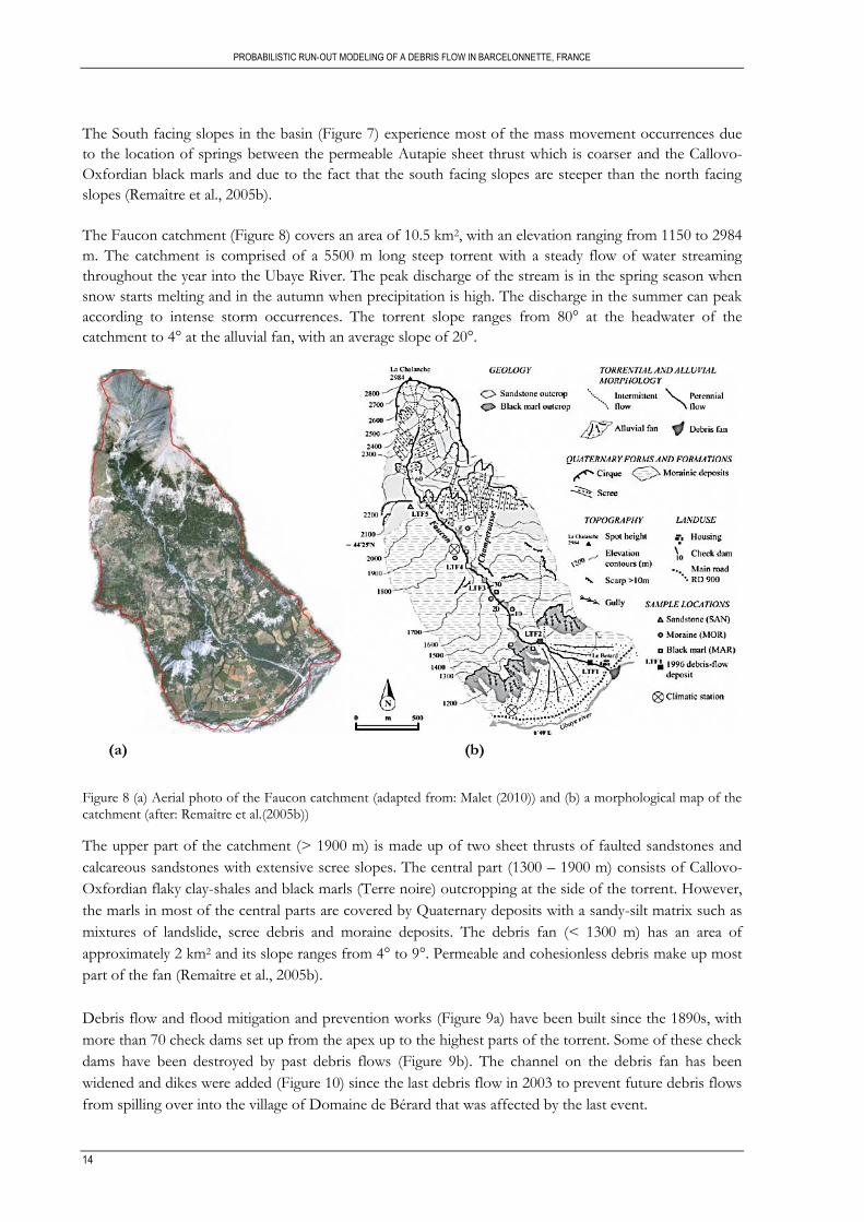
Figure 8 (a) Aerial photo of the Faucon catchment (adapted from: Malet (2010)) and (b) a morphological
map of the catchment (after: Remaître et al.(2005b)) ............................................................................................ 14
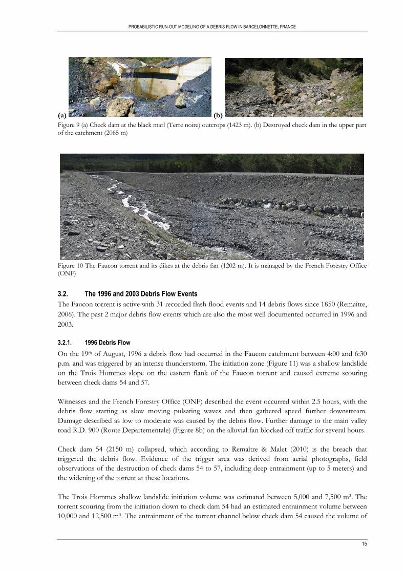
Figure 9 (a) Check dam at the black marl (Terre noire) outcrops (1423 m). (b) Destroyed check dam in the
upper part of the catchment (2065 m) ..................................................................................................................... 15
Figure 10 The Faucon torrent and its dikes at the debris fan (1202 m). It is managed by the French
Forestry Office (ONF) ............................................................................................................................................... 15
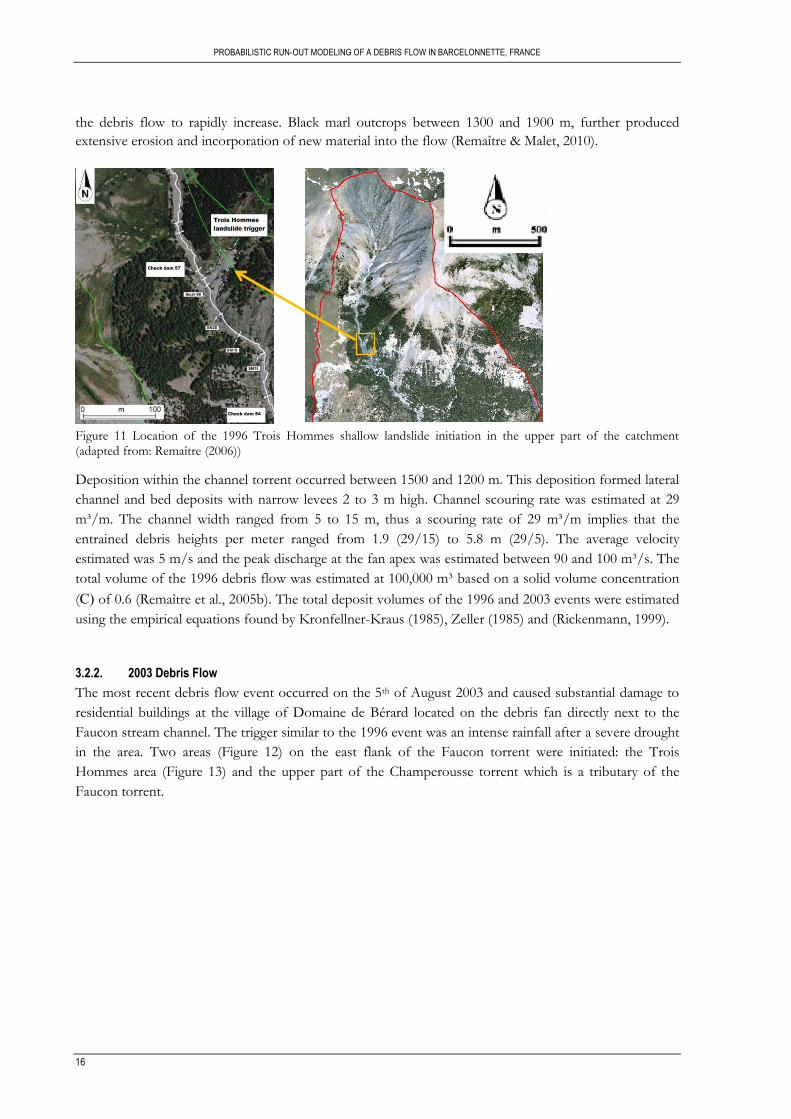
Figure 11 Location of the 1996 Trois Hommes shallow landslide initiation in the upper part of the
catchment (adapted from: Remaître (2006)) ........................................................................................................... 16
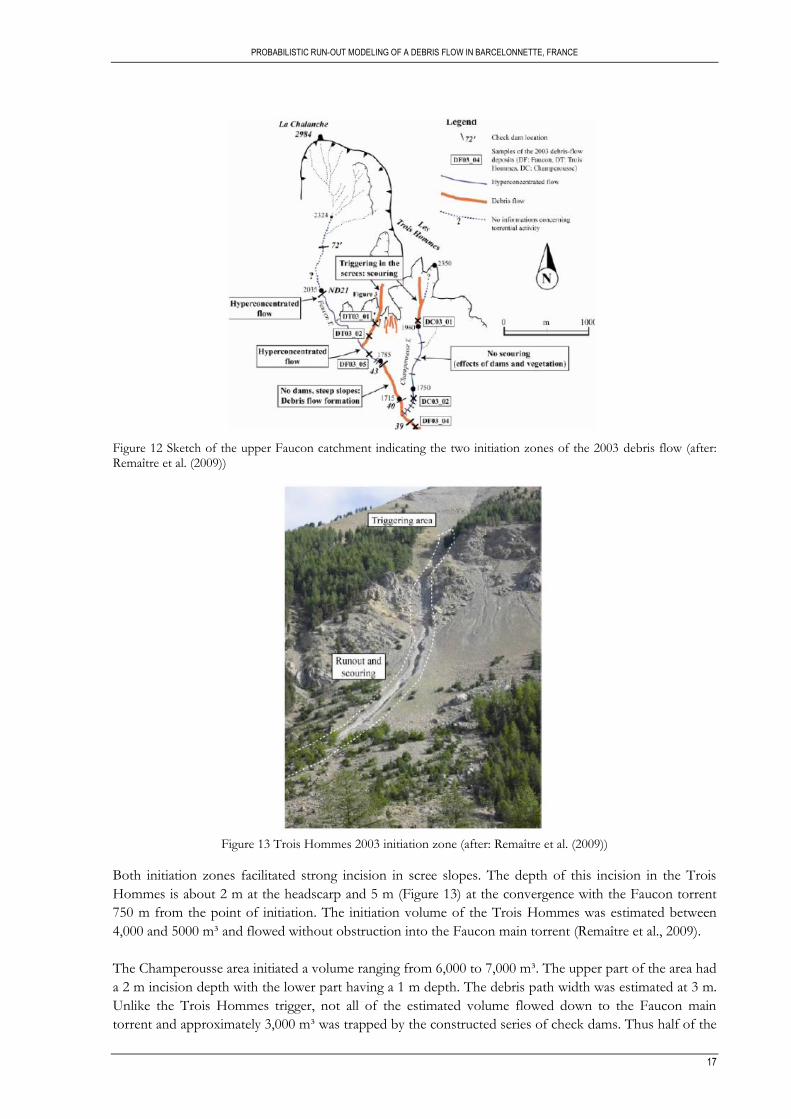
Figure 12 Sketch of the upper Faucon catchment indicating the two initiation zones of the 2003 debris
flow (after: Remaître et al. (2009)) ............................................................................................................................ 17
Figure 13 Trois Hommes 2003 initiation zone (after: Remaître et al. (2009)) ................................................... 17
Figure 14 Morphological sketch of the entrainment and deposition zones of the 2003 debris flow (after:
Remaître et al. (2009)) ................................................................................................................................................. 18
Figure 15 The 2003 debris flow run-out affecting Domaine de Bérard and blocking two main bridges
(adapted from: Remaître (2006)) ............................................................................................................................... 19
Figure 16 Modeled run-out distances with their estimated initiation volumes (after: Remaître et al.
(2005a)). ........................................................................................................................................................................ 20
Figure 17 (Left) the 2D run-out model of the 2003 event with the Coulomb-viscous rheology (after:
Beguería et al. (2009)) and (right) the location of the model on the debris fan. ............................................... 21
Figure 18 Flow chart of the methodology............................................................................................................... 23
Figure 19 Areas surveyed in the Fieldwork of September/October 2010 ......................................................... 24
Figure 20 (a) Point 37 surveyed at the debris fan torrent and a (b) photograph of fieldwork point 37 ....... 24
Figure 21 Part of the database on debris heights in the Faucon catchment ...................................................... 25
Figure 22 (a) The Trois Hommes area determined to be the most susceptible to future debris flow
initiation (adapted from: Remaître (2006)). (b) A 3D visual representation of the Trois Hommes slope
indicating the susceptible area (orange) and the initiation zone used in the modeling (purple) ..................... 25
Figure 23 3D visualization of the preliminary model run in RAMMS using the 5 m DEM interpolated
from the available 5 m contour lines ........................................................................................................................ 26
Figure 24 Shapefile of the channel geometry based on field observations ........................................................ 27
Figure 25 (a) 1 m contour lines derived from the 1 m DEM before channel removal and (b) the contour
lines after removing the channel ............................................................................................................................... 27
vii
Figure 26 Datasets interpolated to create the final DEM: (blue) 5 m contour lines, (red) corrected channel
geometry and (yellow) 1 m contour lines ................................................................................................................ 28
Figure 27 The Cartesian coordinate system in the RAMMS software, where Z is the topography and the
horizontal coordinates are X and Y (after: Christen, 2010b)............................................................................... 29
Figure 28 RAMMS inputs and the user interface .................................................................................................. 31
Figure 29 (a) Simulation parameters and (b) release information in RAMMS ................................................. 32
Figure 30 Assigning the friction parameters in RAMMS ..................................................................................... 32
Figure 31 User defined entrainment polygons in RAMMS ................................................................................. 33
Figure 32 The initiation zone .................................................................................................................................... 34
Figure 33 Entrainment zones in RAMMS. Red indicating 2.0 m entrainment height, and purple indicating
a height of 0.5m. ......................................................................................................................................................... 35
Figure 34 Frequency density histograms and curves of (a) the friction coefficient (Mu) and (b) the
turbulent coefficient (Xi) (after: Quan Luna et al. (2010)) ................................................................................ 36
Figure 35 (Top) Using distance intervals to obtain the frequency of the debris flow run-out. The
frequencies in this illustration are only an example and not the actual frequencies found in the research.
(Bottom) Example of the frequency distribution of the run-out distance according to the information on
the left image. .............................................................................................................................................................. 39
Figure 36 (Top) The number of debris flows reaching an interval height is counted and (bottom) the
frequency is plotted versus the debris flow height. This example uses 0.5 m intervals; however in this
research 10 cm intervals were used. ......................................................................................................................... 40
Figure 37 Resulting contour lines of the final interpolation at the transitional zone between the corrected
channel geometry and the 1m DEM ....................................................................................................................... 41
Figure 38 (a) Hillshade of the final 5 m DEM. (b) 3D visualization of the terrain after the DEM is
imported in RAMMS including the calculation domain....................................................................................... 41
Figure 39 (Left) Model run of the maximum debris heights with the old 5 m contour derived DEM and
(right) the result of modeling with the new created 5 m DEM........................................................................... 42
Figure 40 (Left) Maximum debris flow height of the calibrate model and (right) the deposit thickness at
the end of the flow. .................................................................................................................................................... 44
Figure 41 Deposit height of the calibrated debris flow at the debris fan. ......................................................... 45
Figure 42 (a) Run-out profile of the calibrated debris flow. (b) The cross section of the debris flow deposit
(blue) and the corresponding height (red) near the V.C. 3 Bridge location. ..................................................... 46
Figure 43 Maximum calibrated velocities at the debris fan ................................................................................. 46
Figure 44 Extent of the debris flow run-out for different friction coefficient (Mu) values ........................... 47
Figure 45 Longitudinal profile of the calibrated run-out versus run-outs calculated with higher friction
(Mu) coefficient values ............................................................................................................................................... 48
Figure 46 Extent of the debris flow run-out for different turbulent coefficient (Xi) values.......................... 49
Figure 47 Longitudinal profiles for different turbulent coefficient (Xi) values ................................................ 50
Figure 48 Extent of the debris flow run-out for different entrainment coefficient (K) values ..................... 50
Figure 49 Longitudinal profiles for different entrainment coefficient (K) values............................................ 51
Figure 50 Extent of the debris flow run-out for different earth pressure coefficients (Lambda) values ..... 51
Figure 51 Longitudinal profiles for different earth pressure coefficient (Lambda) values ............................. 52
Figure 52 (a) Sensitivity of the deposit volume to the friction coefficient Mu, (b) turbulent coefficient Xi,
(c) entrainment coefficient K and (d) the earth pressure coefficient Lambda. ................................................. 52
Figure 53 Sensitivity of the run-out distance to the four input parameters: friction coefficient (Mu),
turbulent coefficient (Xi), entrainment coefficient (K) and the earth pressure coefficient (Lambda) .......... 53
viii
Figure 54 Sensitivity of the debris flow height at the V.C. 3 Bridge to the four input parameters: friction
coefficient (Mu), turbulent coefficient (Xi), entrainment coefficient (K) and the earth pressure coefficient
(Lambda) ....................................................................................................................................................................... 54
Figure 55 (Top) Probability of the run-out between 3000 and 5000 m of the run-out path. (Bottom)
locations of the points of interest. ............................................................................................................................ 57
Figure 56 Probability of the maximum debris height at the fan apex................................................................. 58
Figure 57 Probability of the maximum debris height at the V.C. 3 Bridge ....................................................... 58
Figure 58 (Top) Smoothed channel geometry at the debris fan in the created DEM. (Bottom) The actual
trapezoidal shape of the channel as observed in the field. ................................................................................... 59
Figure 59 (Top) The 2003 debris flow run-out extent onto the debris fan (adapted from: Remaître (2006))
and (bottom) the calibrated model run-out. ........................................................................................................... 62
Figure 60. The 2003 event versus the modeled debris flow at Domaine de Bérard ........................................ 62
Figure 61 (Left) The effect of the entrainment coefficient on the entrainment rate and (right) on the flow
height (after: Christen et al. (2010c)) ........................................................................................................................ 63
ix
LIST OF TABLES
Table 1 The classification of flow type landslides (after: Jakob & Hungr (2005)) .............................................. 5
Table 2 Landslide rates of movement (after: WP/WLI (1995)) ............................................................................ 6
Table 3 Summary of the parameters of the 1996 and 2003 debris flows based on the literature.................. 19
Table 4 Field observations compared with the BING model parameters (after: Remaître et al. (2003)) .... 21
Table 5 2003 debris flow initiation versus the new initiation zone .................................................................... 34
Table 6 Summary of value ranges for the Voellmy rheology parameters based on a wide variety of studies
(adapted from: Sosio et al. (2008)) ........................................................................................................................... 36
Table 7 The ranges used in the sensitivity analysis................................................................................................ 38
Table 8 Summary of the Calibrated inputs ............................................................................................................. 42
Table 9 Past events versus calibrated intensity parameters .................................................................................. 43
Table 10 Sensitivity of the deposit volume, run-out and debris height to changes in the friction coefficient
Mu. The calibrated outputs are shaded in grey. ..................................................................................................... 47
Table 11 Sensitivity of the deposit volume, run-out distance and debris height to changes in the turbulent
coefficient Xi. The calibrated outputs are shaded in grey. ................................................................................... 49
Table 12 The 53 modeled run-out distances including the calibrated model run shaded in grey ................. 56
Table 13 Probability of run-out onto the locations of interest ........................................................................... 57

PROBABILISTIC RUN-OUT MODELING OF A DEBRIS FLOW IN BARCELONNETTE, FRANCE
1
1. INTRODUCTION
1.1. Background
The term “landslide” encompasses a whole variety of slope movements and is defined by Cruden &
Varnes (1996) as the “movement of a mass of rock, debris or earth down a slope” due to the slope failing
under the force of gravity. A recent accepted method classifies landslides by their type of movement (fall,
slide, flow) and material (rock, debris, earth) (Cruden & Varnes, 1996).
One of the most fascinating and destructive types of landslides are debris flows. A debris flow is exactly
what the name suggests: a type of slope failure whereby material made up of debris ranging from
unconsolidated soil particles to large boulders descends down a slope in a saturated flow like movement.
They can move as granular rocky flows, muddy cement like flows, or as gradual change to floods with
increasing water content such as hyper-concentrated flows (Jakob & Hungr, 2005). The debris flow
phenomenon is especially challenging for researchers not only due to the wide ranging types of debris
incorporated within the flow, but also due to the behavior of the debris flow run-out which can range
from flowing on an open slope to being confined to a completely channelized environment.
Channeled debris flows have been extensively studied in the European Alps. One of these locations,
where a large amount of data is available on past debris flow events, is the Barcelonnette basin in Southern
France (Beguería et al., 2009; Flageollet et al., 1999; Malet et al., 2005; Maquaire et al., 2003; Remaître,
2006; Remaître & Malet, 2010). The basin has experienced since the 17th century extensive clear cutting of
forests on slopes due to an increase in cultivation and tourism; this in turn has made the area more
susceptible to debris flow hazards. The occurrence of debris flows have been recorded over more than a
century in the Barcelonnette basin and form a risk to settlements and human infrastructure, leading to
death, building damage and traffic disruptions (Flageollet et al., 1999). The expansion of infrastructure for
tourism and winter recreational purposes has further increased the risk of people and property being
affected by the debris flows. However, in the past decades the French government through the RTM
(French Mountain Terrain Restoration Agency) and the ONF (French Forestry Office) have tried
rehabilitating the affected areas by means of reforestation and the building of mitigation works in the form
of check dams (Remaître & Malet, 2010).
The aim of this thesis is to model the run-out and debris flow height of a channeled debris flow in the
Faucon catchment located within the Barcelonnette basin, in order to characterize sensitivity of the
outputs to the model input parameters and to evaluate the possible ranges of the areas affected by the run-
out.
The RAMMS (Rapid Mass Movements) numerical dynamic model (Christen et al., 2010c) developed by
the Swiss Federal Institute for Snow Avalanche Research (WSL / SLF), which applies the Voellmy
rheology will be used to model the run-out of the debris flow. Numerous studies have applied frictional
and specifically the Voellmy rheology to model a wide range of mass movements like snow avalanches
(Christen et al., 2010a; Christen et al., 2010c), rock avalanches (Hungr & Evans, 1996; Pirulli et al., 2004)
and debris flows (Cesca & D‟Agostino, 2006; Kowalski, 2008). Furthermore, the Voellmy rheological
approach has found to be stable and robust when 2D modeling and back-analyzing channeled debris flows
in the European Alps (Ayotte & Hungr, 2000; Rickenmann et al., 2006).
PROBABILISTIC RUN-OUT MODELING OF A DEBRIS FLOW IN BARCELONNETTE, FRANCE
2
1.2. Problem Statement
Studies have been conducted in recent years on the Barcelonnette area to characterize past debris flow
events (Flageollet et al., 1999; Maquaire et al., 2003). The most recent and well documented debris flows in
the Faucon catchment took place in 1996 and 2003, causing significant damage to roads, bridges and
property. Remaître et al. (2003) and Remaître et al. (2005a) modeled and back-analyzed the Faucon 1996
debris flow using the Herschel-Bulkley rheology with the Bing model (Imran et al., 2001). The model
showed reasonably good results. However, this was a 1D model where entrainment was neglected and the
velocities of the flow were overestimated.
The 2003 event was modeled in 2D by both Remaître (2006) and Beguería et al. (2009) using the
Cemagref 2-D and MassMov2D models, respectively. The 2D advantage of these models was obvious,
showing how the debris flow overflowed its channel on the debris fan. However, both of these studies
only took the final 300 m of the debris flow run-out into consideration where the village of Domaine de
Bérard was affected by the debris flow overtopping its channel.
There are several factors that determine the „reach‟ of a debris flow and the associated hazard: the initial
mass, the friction components during the flow and the amount of material picked up during the flow
(scouring). The dynamic RAMMS model is based on the Voellmy-Salm model which assumes that the
total basal friction of the flow can be split into a velocity independent dry-Coulomb friction coefficient
and a velocity dependent turbulent coefficient (Christen et al., 2010c). These rheological parameters can
determine to a large part the run-out distance. Hence the so called Voellmy friction parameters are very
important in run-out modeling and the associated hazard. Furthermore the DEM determines where the
debris flow will occur, and in how far it will be confined to natural or artificial channels that occur in the
landscape. The DEM quality therefore is important in the debris flow behavior.
This study attempts for the first time to model a complete channelized debris flow event in the Faucon
catchment from the initiation zone till the run-out zone over a distance of 4.7 km in 2D with the
physically based dynamic model RAMMS (Christen et al., 2010c), incorporating the process of
entrainment and assessing the spatial probability of the modeled run-outs and debris flow heights.
RAMMS was originally developed for modeling snow avalanches, thus making its application to debris
flow modeling even more interesting. However, there have been studies that have applied RAMMS to
model debris flows in the past (Cesca & D‟Agostino, 2006; Kowalski, 2008).
1.3. Reasearch Objectives
The main objective of this research is to use a probabilistic method to assess the run-out and debris flow
heights of a debris flow located in the Barcelonnette Basin in the Southern French Alps. Model
parameterization and calibration is required to obtain run-outs and deposit heights based on real events
that have occurred in the catchment. The sensitivity of the model to the input parameters will be assessed
and finally the probability of the run-out and deposit heights are obtained using a simple probabilistic
method. The sub-objectives of this research are:
1. To assess the applicability of the Voellmy rheology applied by the RAMMS software, originally
designed for snow avalanches, to model debris flow run-outs in channelized environments
2. To calibrate the model input parameters in order to obtain debris flow run-outs and heights based
on the past events in the Faucon catchment
PROBABILISTIC RUN-OUT MODELING OF A DEBRIS FLOW IN BARCELONNETTE, FRANCE
3
3. To determine the sensitivity of the RAMMS dynamic model with respect to the various input
parameters
4. To study the effect of the DEM used as input in the run-out model
5. To obtain the spatial probability of the modeled debris flow run-out and deposit height
1.4. Research Hypotheses
The hypotheses are based on some of the research objectives and are stated as follows:
The Voellmy rheology should be capable of modeling debris flows in the given catchment. This
Hypothesis is based on the fact that the Voellmy rheology has been used to model debris flows in
other areas in recent studies (Cesca & D‟Agostino, 2006; Hungr & Evans, 1996; Kowalski, 2008).
The DEM accuracy can significantly influence the output of the run-out model.
The RAMMS dynamic model can be used to analyze the run-out probability in the given
catchment.
1.5. Thesis Structure
This thesis is structured as follows:
Chapter 1 introduces the thesis by explaining why the research should be carried out and stating the
objectives of this research.
Chapter 2 is a literature review describing the debris flow phenomena and gives insight on the aspect of
debris flow modeling.
Chapter 3 describes the Faucon catchment study area and summarizes the 1996 and 2003 debris flow
events.
Chapter 4 is dedicated to the methods and materials used in this research, from the fieldwork phase until
the final stages of modeling the debris flow. It includes the calibration and the sensitivity analysis of the
model parameters and the method used to obtain the probability of the run-out and debris heights.
Chapter 5 reveals the results of the DEM creation, physical modeling of the debris flow and the associated
sensitivity analysis and probability analysis.
Chapter 6 discusses each part of the results revealed in Chapter 5.
Chapter 7 finally concludes this research by stating which objectives have been met and giving
recommendations for future studies.

PROBABILISTIC RUN-OUT MODELING OF A DEBRIS FLOW IN BARCELONNETTE, FRANCE
5
2. LITERATURE REVIEW
2.1. The Debris Flow Phenomenon
The terminology of debris flows is wide ranging and has been updated over the years by researchers
studying the phenomena. Debris is defined as a mixture of unsorted material which can contain everything
from clays to cobbles, boulders and organic material. It is described has having a low plasticity and is
produced by mass wasting processes (Hungr et al., 2001). The definition of debris flows by Varnes (1978),
which is part of a landslide classification, is commonly used by researchers and states that “flows are rapid
movements of material as a viscous mass where inter-granular movements predominate over shear surface
movements. These can be debris flows, mudflows or rock avalanches, depending upon the nature of the
material involved in the movement”. Hungr et al. (2001) however proposed what they call “more precise
terms” for the classification of flow type landslides and defined a debris flow as “a very rapid to extremely
rapid flow of saturated non-plastic debris in a steep channel. Plasticity index is less than 5% in sand and
finer fractions”. Plasticity is the ability of a material to retain its shape attained by pressure deformation.
The classification further describes debris flows as being confined to well established channels where the
water content increases as the flow descends down its path (Table 1).
Whatever the definition used, it is obvious that debris flows have an interaction between fluid and solid
forces (Iverson, 1997) which discriminates them from other types of landslides. Furthermore, the type of
material, movement and velocity gives debris flows their distinct character.
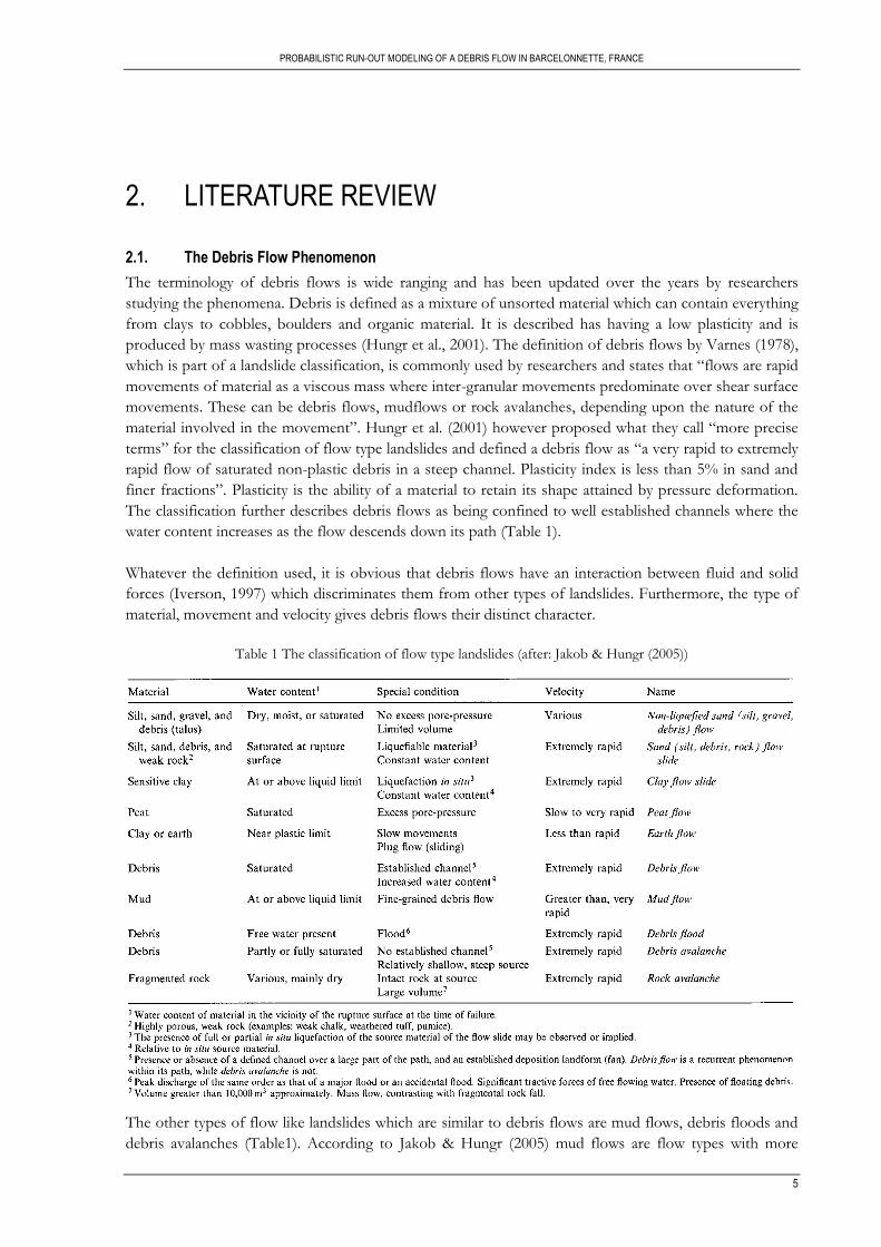
Table 1 The classification of flow type landslides (after: Jakob & Hungr (2005))
The other types of flow like landslides which are similar to debris flows are mud flows, debris floods and
debris avalanches (Table1). According to Jakob & Hungr (2005) mud flows are flow types with more
PROBABILISTIC RUN-OUT MODELING OF A DEBRIS FLOW IN BARCELONNETTE, FRANCE
6
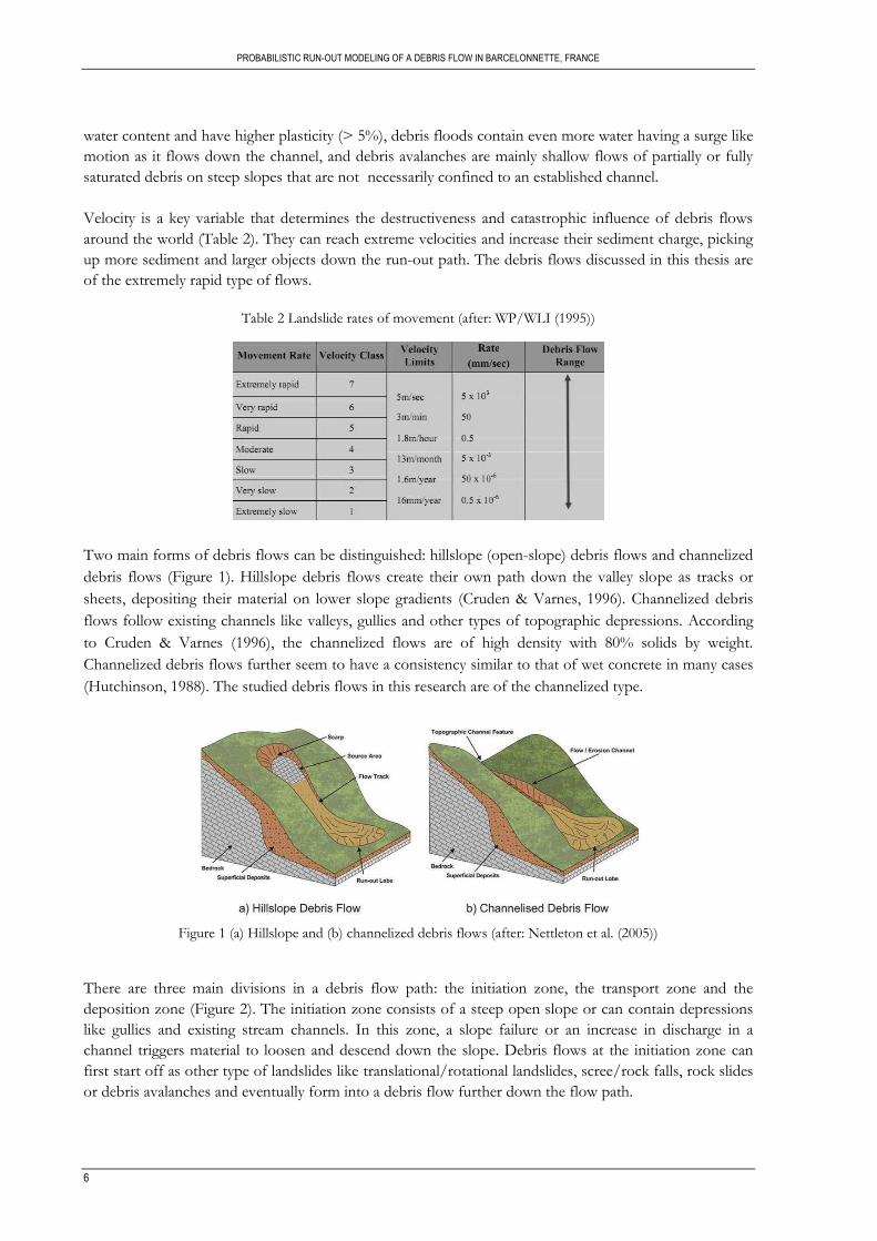
water content and have higher plasticity (> 5%), debris floods contain even more water having a surge like
motion as it flows down the channel, and debris avalanches are mainly shallow flows of partially or fully
saturated debris on steep slopes that are not necessarily confined to an established channel.
Velocity is a key variable that determines the destructiveness and catastrophic influence of debris flows
around the world (Table 2). They can reach extreme velocities and increase their sediment charge, picking
up more sediment and larger objects down the run-out path. The debris flows discussed in this thesis are
of the extremely rapid type of flows.
Table 2 Landslide rates of movement (after: WP/WLI (1995))
Two main forms of debris flows can be distinguished: hillslope (open-slope) debris flows and channelized
debris flows (Figure 1). Hillslope debris flows create their own path down the valley slope as tracks or
sheets, depositing their material on lower slope gradients (Cruden & Varnes, 1996). Channelized debris
flows follow existing channels like valleys, gullies and other types of topographic depressions. According
to Cruden & Varnes (1996), the channelized flows are of high density with 80% solids by weight.
Channelized debris flows further seem to have a consistency similar to that of wet concrete in many cases
(Hutchinson, 1988). The studied debris flows in this research are of the channelized type.
Figure 1 (a) Hillslope and (b) channelized debris flows (after: Nettleton et al. (2005))
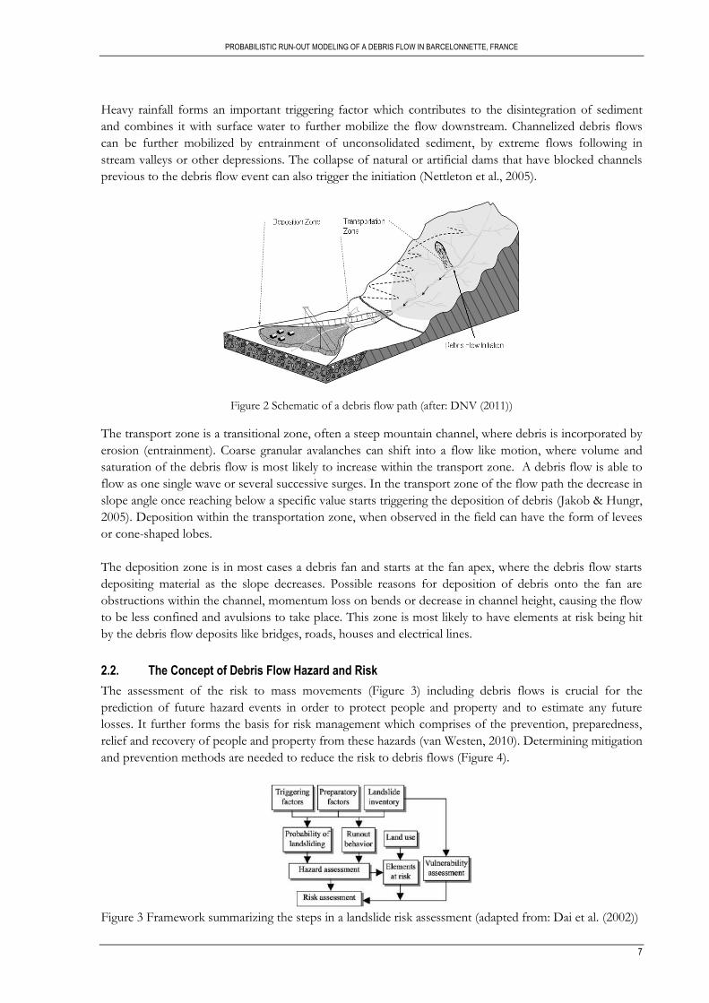
There are three main divisions in a debris flow path: the initiation zone, the transport zone and the
deposition zone (Figure 2). The initiation zone consists of a steep open slope or can contain depressions
like gullies and existing stream channels. In this zone, a slope failure or an increase in discharge in a
channel triggers material to loosen and descend down the slope. Debris flows at the initiation zone can
first start off as other type of landslides like translational/rotational landslides, scree/rock falls, rock slides
or debris avalanches and eventually form into a debris flow further down the flow path.
PROBABILISTIC RUN-OUT MODELING OF A DEBRIS FLOW IN BARCELONNETTE, FRANCE
7
Heavy rainfall forms an important triggering factor which contributes to the disintegration of sediment
and combines it with surface water to further mobilize the flow downstream. Channelized debris flows
can be further mobilized by entrainment of unconsolidated sediment, by extreme flows following in
stream valleys or other depressions. The collapse of natural or artificial dams that have blocked channels
previous to the debris flow event can also trigger the initiation (Nettleton et al., 2005).
Figure 2 Schematic of a debris flow path (after: DNV (2011))
The transport zone is a transitional zone, often a steep mountain channel, where debris is incorporated by
erosion (entrainment). Coarse granular avalanches can shift into a flow like motion, where volume and
saturation of the debris flow is most likely to increase within the transport zone. A debris flow is able to
flow as one single wave or several successive surges. In the transport zone of the flow path the decrease in
slope angle once reaching below a specific value starts triggering the deposition of debris (Jakob & Hungr,
2005). Deposition within the transportation zone, when observed in the field can have the form of levees
or cone-shaped lobes.
The deposition zone is in most cases a debris fan and starts at the fan apex, where the debris flow starts
depositing material as the slope decreases. Possible reasons for deposition of debris onto the fan are
obstructions within the channel, momentum loss on bends or decrease in channel height, causing the flow
to be less confined and avulsions to take place. This zone is most likely to have elements at risk being hit
by the debris flow deposits like bridges, roads, houses and electrical lines.
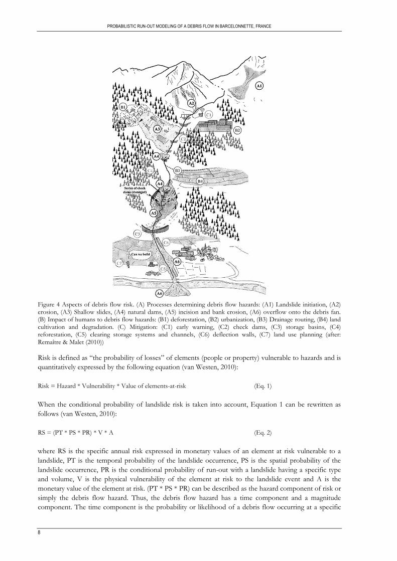
2.2. The Concept of Debris Flow Hazard and Risk
The assessment of the risk to mass movements (Figure 3) including debris flows is crucial for the
prediction of future hazard events in order to protect people and property and to estimate any future
losses. It further forms the basis for risk management which comprises of the prevention, preparedness,
relief and recovery of people and property from these hazards (van Westen, 2010). Determining mitigation
and prevention methods are needed to reduce the risk to debris flows (Figure 4).
Figure 3 Framework summarizing the steps in a landslide risk assessment (adapted from: Dai et al. (2002))
PROBABILISTIC RUN-OUT MODELING OF A DEBRIS FLOW IN BARCELONNETTE, FRANCE
8
Figure 4 Aspects of debris flow risk. (A) Processes determining debris flow hazards: (A1) Landslide initiation, (A2) erosion, (A3) Shallow slides, (A4) natural dams, (A5) incision and bank erosion, (A6) overflow onto the debris fan. (B) Impact of humans to debris flow hazards: (B1) deforestation, (B2) urbanization, (B3) Drainage routing, (B4) land cultivation and degradation. (C) Mitigation: (C1) early warning, (C2) check dams, (C3) storage basins, (C4) reforestation, (C5) clearing storage systems and channels, (C6) deflection walls, (C7) land use planning (after: Remaître & Malet (2010))
Risk is defined as “the probability of losses” of elements (people or property) vulnerable to hazards and is
quantitatively expressed by the following equation (van Westen, 2010):
Risk = Hazard * Vulnerability * Value of elements-at-risk (Eq. 1)
When the conditional probability of landslide risk is taken into account, Equation 1 can be rewritten as
follows (van Westen, 2010):
RS = (PT * PS * PR) * V * A (Eq. 2)
where RS is the specific annual risk expressed in monetary values of an element at risk vulnerable to a
landslide, PT is the temporal probability of the landslide occurrence, PS is the spatial probability of the
landslide occurrence, PR is the conditional probability of run-out with a landslide having a specific type
and volume, V is the physical vulnerability of the element at risk to the landslide event and A is the
monetary value of the element at risk. (PT * PS * PR) can be described as the hazard component of risk or
simply the debris flow hazard. Thus, the debris flow hazard has a time component and a magnitude
component. The time component is the probability or likelihood of a debris flow occurring at a specific
PROBABILISTIC RUN-OUT MODELING OF A DEBRIS FLOW IN BARCELONNETTE, FRANCE
9
time in the future and is expressed as an annual probability or the chance of an even occurring within a
specific return period like 5, 10 or 50 years.
The magnitude component of the debris flow can be expressed in run-out distance, peak discharge or
volume (Jakob, 2005). The run-out distance is the distance from the point of initiation until the point of
complete deposition and stoppage of the flow. The peak discharge is the maximum cross-sectional area
multiplied by the debris flow velocity at a specific time interval when the flow occurs at the maximum
cross-sectional area. The impact pressure is also considered a magnitude component if it is used in relating
it to the vulnerability of a house or other elements at risk to the actual force applied by the incoming
debris flow (van Westen, 2010).
Estimating debris flow volumes is crucial for mitigation works and structurally confining the flow,
whether it is building check dams or adjusting the channel at the debris fan. The total debris flow volume
(Vt) reaching the fan apex is calculated by the following equation (Jakob, 2005):
Vt = ∑ Vi + ∑ Ve - ∑ Vd (Eq. 3)
where ∑ Vi is the total initiation volume for all the initiation zones combined, ∑ Ve is the total entrained
volume and ∑ Vd is the total volume of deposition on the transport zone and deposition zone. Remote
sensing (photogrammetry) and field observations can be used to estimate the average depth of debris flow
scars, the initiation volumes and the deposited volumes. However, in most cases the exact information on
deposit volumes after the occurrence of the event, is not well known and must be estimated using
empirical relationships (Rickenmann, 1999). Estimating the entrainment volume is a more difficult task,
however the simplest method is to assume all available debris and stored material is entrained by the
debris flow in the transport zone. If the available debris is unknown prior to the event, than initiation
volume can be subtracting from the total deposited volume.
Debris flow hazard magnitudes can be further determined by the hazard intensity. Debris flow hazard
intensity parameters are: velocity, flow depth, maximum deposit thickness, impact force and the debris
flow run-up onto elements at risk (Jakob, 2005).
This thesis specifically looks at the spatial probability of the run-out distance and debris flow heights.
Debris volumes, velocities and deposit heights are further assessed in this research to calibrate with past
events as will be discussed in Chapter 4.
2.3. Debris Flow Run-out Modeling
Prediction of debris flow run-outs are important to assess areas that will be affected by the hazard, to
determine the debris flow intensity parameters and to produce hazard and risk maps (Rickenmann, 2005).
Researchers have developed a considerable number of methods over the past several decades to predict
the run-out of debris flows. Spatial modeling is a tool that has been used to replicate past debris flow
events in order to understand their behavior and to predict future events. Brunsden (1999) explains that
there is no single model that can perfectly replicate the complexity of landslides, however he mentions
“considerable progress has been made in isolating many of the variables involved” in the modeling of
landslides.
PROBABILISTIC RUN-OUT MODELING OF A DEBRIS FLOW IN BARCELONNETTE, FRANCE
10
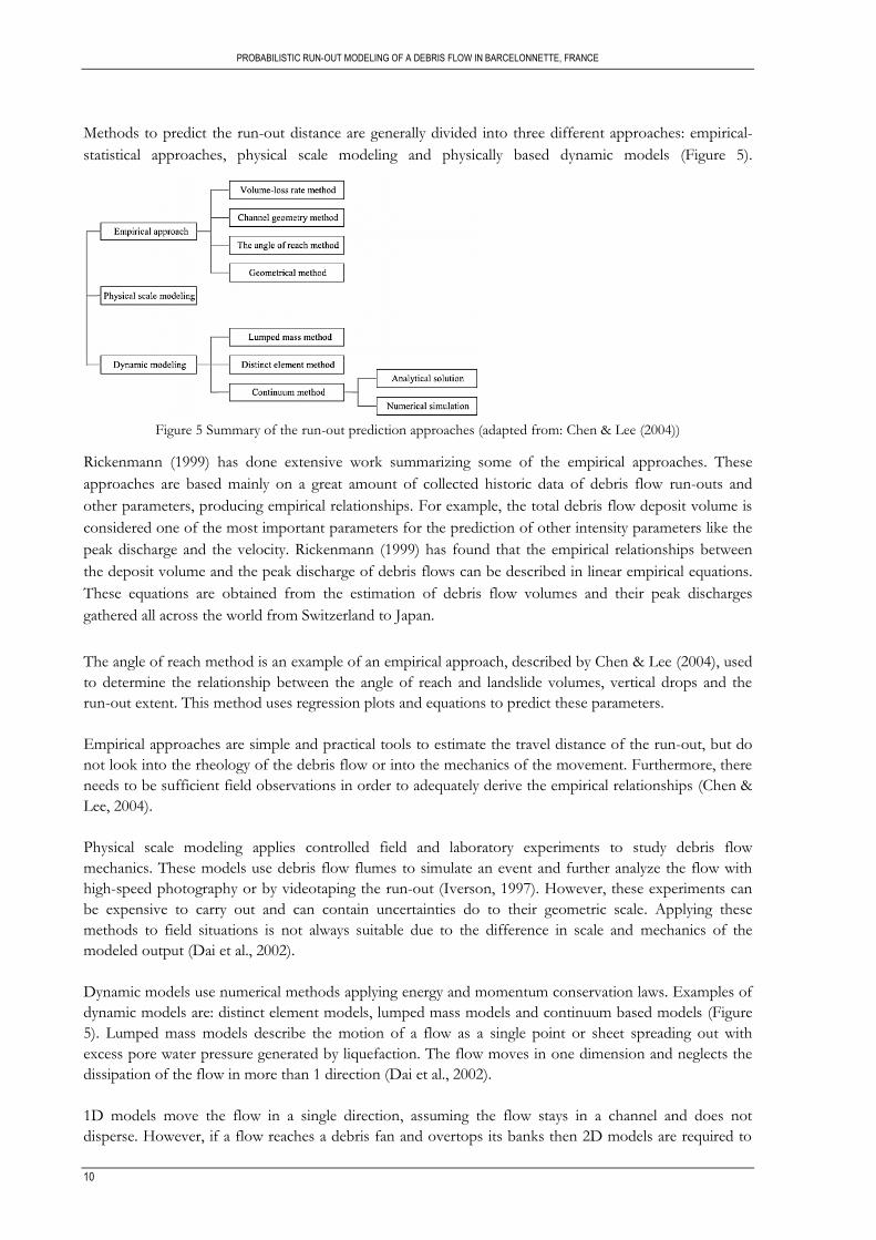
Methods to predict the run-out distance are generally divided into three different approaches: empirical-
statistical approaches, physical scale modeling and physically based dynamic models (Figure 5).
Figure 5 Summary of the run-out prediction approaches (adapted from: Chen & Lee (2004))
Rickenmann (1999) has done extensive work summarizing some of the empirical approaches. These
approaches are based mainly on a great amount of collected historic data of debris flow run-outs and
other parameters, producing empirical relationships. For example, the total debris flow deposit volume is
considered one of the most important parameters for the prediction of other intensity parameters like the
peak discharge and the velocity. Rickenmann (1999) has found that the empirical relationships between
the deposit volume and the peak discharge of debris flows can be described in linear empirical equations.
These equations are obtained from the estimation of debris flow volumes and their peak discharges
gathered all across the world from Switzerland to Japan.
The angle of reach method is an example of an empirical approach, described by Chen & Lee (2004), used
to determine the relationship between the angle of reach and landslide volumes, vertical drops and the
run-out extent. This method uses regression plots and equations to predict these parameters.
Empirical approaches are simple and practical tools to estimate the travel distance of the run-out, but do
not look into the rheology of the debris flow or into the mechanics of the movement. Furthermore, there
needs to be sufficient field observations in order to adequately derive the empirical relationships (Chen &
Lee, 2004).
Physical scale modeling applies controlled field and laboratory experiments to study debris flow
mechanics. These models use debris flow flumes to simulate an event and further analyze the flow with
high-speed photography or by videotaping the run-out (Iverson, 1997). However, these experiments can
be expensive to carry out and can contain uncertainties do to their geometric scale. Applying these
methods to field situations is not always suitable due to the difference in scale and mechanics of the
modeled output (Dai et al., 2002).
Dynamic models use numerical methods applying energy and momentum conservation laws. Examples of
dynamic models are: distinct element models, lumped mass models and continuum based models (Figure
5). Lumped mass models describe the motion of a flow as a single point or sheet spreading out with
excess pore water pressure generated by liquefaction. The flow moves in one dimension and neglects the
dissipation of the flow in more than 1 direction (Dai et al., 2002).
1D models move the flow in a single direction, assuming the flow stays in a channel and does not
disperse. However, if a flow reaches a debris fan and overtops its banks then 2D models are required to
PROBABILISTIC RUN-OUT MODELING OF A DEBRIS FLOW IN BARCELONNETTE, FRANCE
11
replicate the extent of the run-out onto the debris fan. Distinct element methods represent the flow as an
assemblage of blocks formed as connected fractures in the separate blocks. The motion of these blocks
are solved by equations of motion replicating the contact between the blocks (Hungr et al., 2005).
Continuum numerical models use fluid mechanics applying conservation equations of mass, momentum
and energy for describing the debris flow dynamic motion. These models use rheology to further describe
the behavior of the debris flow material (Brunsden, 1999). What is essential in dynamic continuum
modeling of debris flows is the choice of the right rheology and the associated friction parameters
(Rickenmann, 2005). Physically based continuum numerical models are able to determine the deposition
and flow parameters along the whole debris flow path. The continuum models applying the rheological
conservation laws of momentum and energy use friction parameters to explain the channel roughness and
turbulence within a debris flow (Rickenmann, 2005).
There are several rheological models that have been used to describe the motion of debris flows like the
Bingham fluid model, where the fluid acts as a rigid body at low shear stress and flows like a viscous fluid
at higher rates of shear stress, thus described as a visco-plastic fluid (Jakob & Hungr, 2005). The Herschel-
Bulkley fluid model is another non-Newtonian fluid, which gives a non-linear relationship between the
stress and strain. Both the Bingham and Herschel-Bulkley models were used by Remaître et al. (2003) to
model a past debris flow event in Barcelonnette, France, further discussed in Chapter 3. The Bingham
model was modified to incorporate the Coulomb friction leading to the Coulomb-Viscous model which
was also used to model a debris flow in the Barcelonnette area by Beguería et al. (2009).
The Voellmy rheology is another rheological model that has been extensively used to simulate debris flows
(Ayotte & Hungr, 2000; Hungr & Evans, 1996; Rickenmann et al., 2006) and applies the frictional-
turbulent resistance to model the resistance at the base of the flow. This research will approach the
modeling of the debris flow using the dynamic continuum numerical method, applying the Voellmy
rheology in the RAMMS dynamic modeling software (Christen et al., 2010c) and will be discussed in detail
in Chapter 4.
2.4. Parameter Uncertainty in Rheological models
Assessing the risk of mass movements requires estimating the probability of the hazard component. There
are numerous studies that have summarized the methods used to assess this probability (Dai et al., 2002;
Soeters & van Westen, 1996). Dynamic continuum models are one of the most sophisticated and widely
used methods applied to assess the hazard of mass movements. The rheological models used in dynamic
continuum approaches require the user to estimate the corresponding values for the rheological
parameters. There are three main approaches to estimate these parameters: they can be derived from
laboratory tests or empirical laws from samples gathered in the field after the occurrence of an event, they
can be obtained from back-calibrating a model to a past event, or can be derived from previous back-
calibrated events and values published in literature (Quan Luna et al., 2010). Obtaining rheological
parameters for calibrating a debris flow event is subjected to uncertainties due to the variation in the value
parameters.
Probability density functions (pdf) are used to describe the likelihood of a continuous random variable to
occur at a given point. They are produced by classing the frequency of the parameter value in intervals and
approximating the frequency with a curve. Quan Luna et al. (2010) produced pdfs for the frictional-
turbulent Voellmy parameters. These pdfs can be used in the future to assess the uncertainty of a
parameter in a stochastic approach by randomly generating the rheological parameter and using it as an
input into a continuum model.
PROBABILISTIC RUN-OUT MODELING OF A DEBRIS FLOW IN BARCELONNETTE, FRANCE
12
The Monte Carlo approach applies random sampling (stochastic approach) of input parameters to provide
estimates of their uncertainty. The approach is based on methods of random sampling of variables that
have significant uncertainties in inputs, using computational algorithms to output their results and are
often applied in risk assessment (Hubbard, 2007). Monte Carlo methods are capable of repeatedly
generating rheological parameter values randomly from existing probability density functions. The outputs
can then be used as inputs into the dynamic continuum models. Furthermore, the Monte Carlo approach
has been applied in other aspects of landslide hazard and risk assessment (Calvo & Savi, 2009; Gorsevski
et al., 2006; Liu, 2008).
When the probability density function is unknown or simply unavailable, other methods are needed to
approximate the uncertainty of the input parameter. The FOSM (first-order second-moment) approach is
used to estimate a pdf by using the first-order approximations of Taylor series expansions of the mean and
the variance (second-moment parameters) of parameter values, thus estimating their uncertainty (Uzielli et
al., 2006). The FOSM method has been applied for probabilistic slope stability analysis (Düzgün &
Özdemir, 2006; Griffiths et al., 2008) and landslide vulnerability estimations (Uzielli et al., 2006).
The range of the rheological input parameters for calibrating the model in this research were obtained
from a literature study. Based on the calibrated parameter values, a systematic sampling approach within
the given range was used for the sensitivity analysis as will be described in Chapter 4. Due to the lack of
time and material, the uncertainty of the parameter values could not be quantified as will be discussed in
Chapter 6.
PROBABILISTIC RUN-OUT MODELING OF A DEBRIS FLOW IN BARCELONNETTE, FRANCE
13
3. STUDY AREA
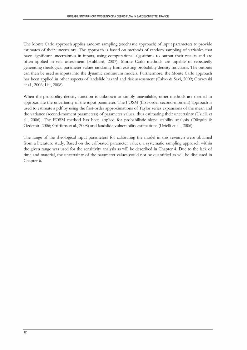
3.1. Overview
The study area is the Faucon catchment forming part of the Faucon commune and located in the
Barcelonnette basin (Figure 6 and 7), in the department of Alpes-de-Haute-Provence in the French Alps.
The basin is one of the sections of the Ubaye river valley, located in the Southern French Alps. The
French commune is the lowest level of administrative division within the French Republic and their
division in the Alps is based on natural boundaries or sub-catchments. The elevation in the basin ranges
from 1100 to 3000 m and slope gradients vary from 20° to 50°. The landuse is mainly forest (60%),
agricultural lands and bare lands with bad-lands and gullying. The basin experiences strong storm
intensities (over 50 mm/h) in the summer and around 130 days of freezing per year, having a dry and
mountainous Mediterranean climate.
Figure 6 Location of the Barcelonnette Basin and the Faucon catchment (traced)
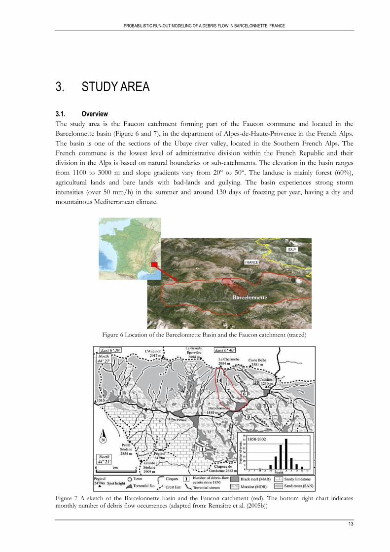
Figure 7 A sketch of the Barcelonnette basin and the Faucon catchment (red). The bottom right chart indicates monthly number of debris flow occurrences (adapted from: Remaître et al. (2005b))
Barcelonnette
PROBABILISTIC RUN-OUT MODELING OF A DEBRIS FLOW IN BARCELONNETTE, FRANCE
14
The South facing slopes in the basin (Figure 7) experience most of the mass movement occurrences due
to the location of springs between the permeable Autapie sheet thrust which is coarser and the Callovo-
Oxfordian black marls and due to the fact that the south facing slopes are steeper than the north facing
slopes (Remaître et al., 2005b).
The Faucon catchment (Figure 8) covers an area of 10.5 km2, with an elevation ranging from 1150 to 2984
m. The catchment is comprised of a 5500 m long steep torrent with a steady flow of water streaming
throughout the year into the Ubaye River. The peak discharge of the stream is in the spring season when
snow starts melting and in the autumn when precipitation is high. The discharge in the summer can peak
according to intense storm occurrences. The torrent slope ranges from 80° at the headwater of the
catchment to 4° at the alluvial fan, with an average slope of 20°.
(a) (b)
Figure 8 (a) Aerial photo of the Faucon catchment (adapted from: Malet (2010)) and (b) a morphological map of the catchment (after: Remaître et al.(2005b))
The upper part of the catchment (> 1900 m) is made up of two sheet thrusts of faulted sandstones and
calcareous sandstones with extensive scree slopes. The central part (1300 – 1900 m) consists of Callovo-
Oxfordian flaky clay-shales and black marls (Terre noire) outcropping at the side of the torrent. However,
the marls in most of the central parts are covered by Quaternary deposits with a sandy-silt matrix such as
mixtures of landslide, scree debris and moraine deposits. The debris fan (< 1300 m) has an area of
approximately 2 km2 and its slope ranges from 4° to 9°. Permeable and cohesionless debris make up most
part of the fan (Remaître et al., 2005b).
Debris flow and flood mitigation and prevention works (Figure 9a) have been built since the 1890s, with
more than 70 check dams set up from the apex up to the highest parts of the torrent. Some of these check
dams have been destroyed by past debris flows (Figure 9b). The channel on the debris fan has been
widened and dikes were added (Figure 10) since the last debris flow in 2003 to prevent future debris flows
from spilling over into the village of Domaine de Bérard that was affected by the last event.
PROBABILISTIC RUN-OUT MODELING OF A DEBRIS FLOW IN BARCELONNETTE, FRANCE
15
(a) (b)
Figure 9 (a) Check dam at the black marl (Terre noire) outcrops (1423 m). (b) Destroyed check dam in the upper part of the catchment (2065 m)
Figure 10 The Faucon torrent and its dikes at the debris fan (1202 m). It is managed by the French Forestry Office (ONF)
3.2. The 1996 and 2003 Debris Flow Events
The Faucon torrent is active with 31 recorded flash flood events and 14 debris flows since 1850 (Remaître,
2006). The past 2 major debris flow events which are also the most well documented occurred in 1996 and
2003.
3.2.1. 1996 Debris Flow
On the 19th of August, 1996 a debris flow had occurred in the Faucon catchment between 4:00 and 6:30
p.m. and was triggered by an intense thunderstorm. The initiation zone (Figure 11) was a shallow landslide
on the Trois Hommes slope on the eastern flank of the Faucon torrent and caused extreme scouring
between check dams 54 and 57.
Witnesses and the French Forestry Office (ONF) described the event occurred within 2.5 hours, with the
debris flow starting as slow moving pulsating waves and then gathered speed further downstream.
Damage described as low to moderate was caused by the debris flow. Further damage to the main valley
road R.D. 900 (Route Departementale) (Figure 8b) on the alluvial fan blocked off traffic for several hours.
Check dam 54 (2150 m) collapsed, which according to Remaître & Malet (2010) is the breach that
triggered the debris flow. Evidence of the trigger area was derived from aerial photographs, field
observations of the destruction of check dams 54 to 57, including deep entrainment (up to 5 meters) and
the widening of the torrent at these locations.
The Trois Hommes shallow landslide initiation volume was estimated between 5,000 and 7,500 m³. The
torrent scouring from the initiation down to check dam 54 had an estimated entrainment volume between
10,000 and 12,500 m³. The entrainment of the torrent channel below check dam 54 caused the volume of
PROBABILISTIC RUN-OUT MODELING OF A DEBRIS FLOW IN BARCELONNETTE, FRANCE
16
the debris flow to rapidly increase. Black marl outcrops between 1300 and 1900 m, further produced
extensive erosion and incorporation of new material into the flow (Remaître & Malet, 2010).
Figure 11 Location of the 1996 Trois Hommes shallow landslide initiation in the upper part of the catchment (adapted from: Remaître (2006))
Deposition within the channel torrent occurred between 1500 and 1200 m. This deposition formed lateral
channel and bed deposits with narrow levees 2 to 3 m high. Channel scouring rate was estimated at 29
m³/m. The channel width ranged from 5 to 15 m, thus a scouring rate of 29 m³/m implies that the
entrained debris heights per meter ranged from 1.9 (29/15) to 5.8 m (29/5). The average velocity
estimated was 5 m/s and the peak discharge at the fan apex was estimated between 90 and 100 m³/s. The
total volume of the 1996 debris flow was estimated at 100,000 m³ based on a solid volume concentration
(C) of 0.6 (Remaître et al., 2005b). The total deposit volumes of the 1996 and 2003 events were estimated
using the empirical equations found by Kronfellner-Kraus (1985), Zeller (1985) and (Rickenmann, 1999).
3.2.2. 2003 Debris Flow
The most recent debris flow event occurred on the 5th of August 2003 and caused substantial damage to
residential buildings at the village of Domaine de Bérard located on the debris fan directly next to the
Faucon stream channel. The trigger similar to the 1996 event was an intense rainfall after a severe drought
in the area. Two areas (Figure 12) on the east flank of the Faucon torrent were initiated: the Trois
Hommes area (Figure 13) and the upper part of the Champerousse torrent which is a tributary of the
Faucon torrent.
PROBABILISTIC RUN-OUT MODELING OF A DEBRIS FLOW IN BARCELONNETTE, FRANCE
17
Figure 12 Sketch of the upper Faucon catchment indicating the two initiation zones of the 2003 debris flow (after: Remaître et al. (2009))
Figure 13 Trois Hommes 2003 initiation zone (after: Remaître et al. (2009))
Both initiation zones facilitated strong incision in scree slopes. The depth of this incision in the Trois
Hommes is about 2 m at the headscarp and 5 m (Figure 13) at the convergence with the Faucon torrent
750 m from the point of initiation. The initiation volume of the Trois Hommes was estimated between
4,000 and 5000 m³ and flowed without obstruction into the Faucon main torrent (Remaître et al., 2009).
The Champerousse area initiated a volume ranging from 6,000 to 7,000 m³. The upper part of the area had
a 2 m incision depth with the lower part having a 1 m depth. The debris path width was estimated at 3 m.
Unlike the Trois Hommes trigger, not all of the estimated volume flowed down to the Faucon main
torrent and approximately 3,000 m³ was trapped by the constructed series of check dams. Thus half of the
PROBABILISTIC RUN-OUT MODELING OF A DEBRIS FLOW IN BARCELONNETTE, FRANCE
18
triggered volume of the Champerousse initiation ranging between 3,000 and 3,500 m³ continued to the
Faucon torrent‟s main track.
According to Remaître (2006) a value of 8,500 m³ was considered to be the best estimation of the total
solid volume of the two initiation zones. Previous studies indicate (Malet et al., 2005; Remaître et al.,
2005b) that the range of the solid concentration (C) ranges from 0.50 to 0.60 in debris flows occurring in
the Barcelonnette area. This implies that 8,500 m³ is the solid part of the debris flow and forms 50 to 60%
of the total volume of the flow, with the rest of the 40% to 50% forming the fluid part. Thus the total
volume of the initiation zone, with solids and fluids combined, ranges from 14,000 (C = 0.60) to 17,000
m³ (C = 0.50) (Remaître et al., 2009).
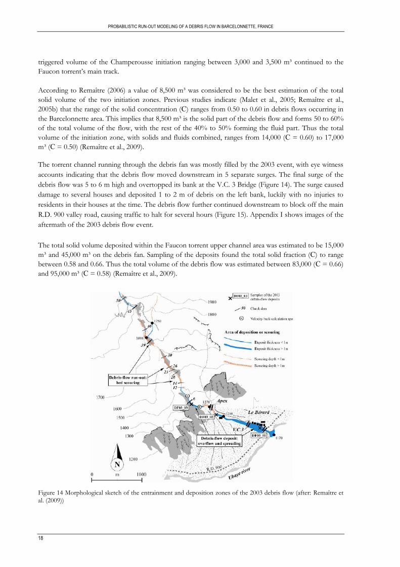
The torrent channel running through the debris fan was mostly filled by the 2003 event, with eye witness
accounts indicating that the debris flow moved downstream in 5 separate surges. The final surge of the
debris flow was 5 to 6 m high and overtopped its bank at the V.C. 3 Bridge (Figure 14). The surge caused
damage to several houses and deposited 1 to 2 m of debris on the left bank, luckily with no injuries to
residents in their houses at the time. The debris flow further continued downstream to block off the main
R.D. 900 valley road, causing traffic to halt for several hours (Figure 15). Appendix I shows images of the
aftermath of the 2003 debris flow event.
The total solid volume deposited within the Faucon torrent upper channel area was estimated to be 15,000
m³ and 45,000 m³ on the debris fan. Sampling of the deposits found the total solid fraction (C) to range
between 0.58 and 0.66. Thus the total volume of the debris flow was estimated between 83,000 (C = 0.66)
and 95,000 m³ (C = 0.58) (Remaître et al., 2009).
Figure 14 Morphological sketch of the entrainment and deposition zones of the 2003 debris flow (after: Remaître et al. (2009))
PROBABILISTIC RUN-OUT MODELING OF A DEBRIS FLOW IN BARCELONNETTE, FRANCE
19
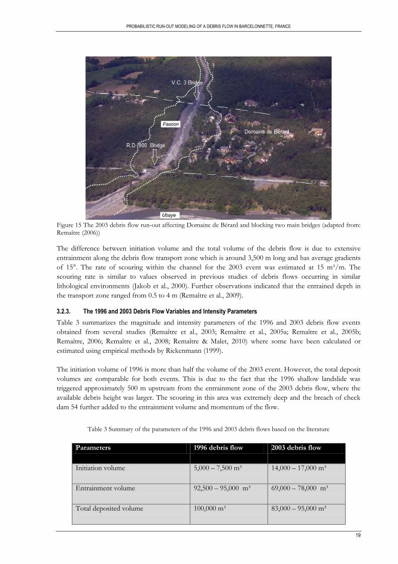
Figure 15 The 2003 debris flow run-out affecting Domaine de Bérard and blocking two main bridges (adapted from: Remaître (2006))
The difference between initiation volume and the total volume of the debris flow is due to extensive
entrainment along the debris flow transport zone which is around 3,500 m long and has average gradients
of 15°. The rate of scouring within the channel for the 2003 event was estimated at 15 m³/m. The
scouring rate is similar to values observed in previous studies of debris flows occurring in similar
lithological environments (Jakob et al., 2000). Further observations indicated that the entrained depth in
the transport zone ranged from 0.5 to 4 m (Remaître et al., 2009).
3.2.3. The 1996 and 2003 Debris Flow Variables and Intensity Parameters
Table 3 summarizes the magnitude and intensity parameters of the 1996 and 2003 debris flow events
obtained from several studies (Remaître et al., 2003; Remaître et al., 2005a; Remaître et al., 2005b;
Remaître, 2006; Remaître et al., 2008; Remaître & Malet, 2010) where some have been calculated or
estimated using empirical methods by Rickenmann (1999).
The initiation volume of 1996 is more than half the volume of the 2003 event. However, the total deposit
volumes are comparable for both events. This is due to the fact that the 1996 shallow landslide was
triggered approximately 500 m upstream from the entrainment zone of the 2003 debris flow, where the
available debris height was larger. The scouring in this area was extremely deep and the breach of check
dam 54 further added to the entrainment volume and momentum of the flow.
Table 3 Summary of the parameters of the 1996 and 2003 debris flows based on the literature
Parameters 1996 debris flow 2003 debris flow
Initiation volume 5,000 – 7,500 m³ 14,000 – 17,000 m³
Entrainment volume 92,500 – 95,000 m³ 69,000 – 78,000 m³
Total deposited volume
100,000 m³ 83,000 – 95,000 m³
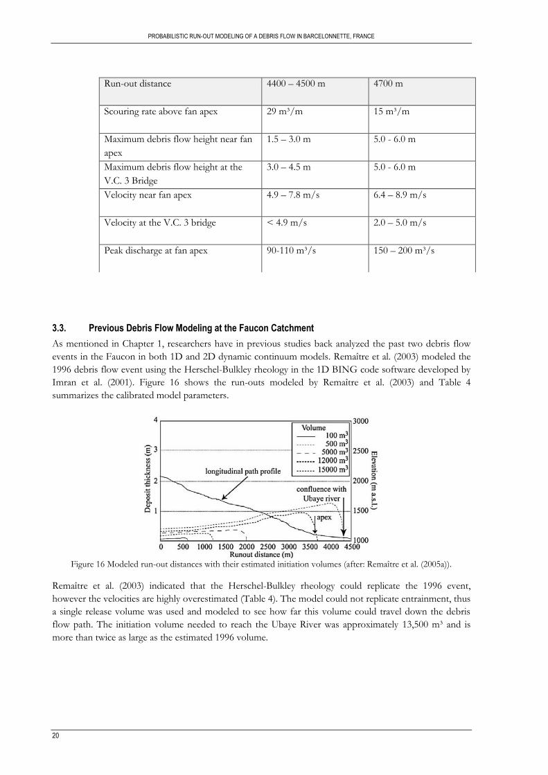
PROBABILISTIC RUN-OUT MODELING OF A DEBRIS FLOW IN BARCELONNETTE, FRANCE
20
3.3. Previous Debris Flow Modeling at the Faucon Catchment
As mentioned in Chapter 1, researchers have in previous studies back analyzed the past two debris flow
events in the Faucon in both 1D and 2D dynamic continuum models. Remaître et al. (2003) modeled the
1996 debris flow event using the Herschel-Bulkley rheology in the 1D BING code software developed by
Imran et al. (2001). Figure 16 shows the run-outs modeled by Remaître et al. (2003) and Table 4
summarizes the calibrated model parameters.
Figure 16 Modeled run-out distances with their estimated initiation volumes (after: Remaître et al. (2005a)).
Remaître et al. (2003) indicated that the Herschel-Bulkley rheology could replicate the 1996 event,
however the velocities are highly overestimated (Table 4). The model could not replicate entrainment, thus
a single release volume was used and modeled to see how far this volume could travel down the debris
flow path. The initiation volume needed to reach the Ubaye River was approximately 13,500 m³ and is
more than twice as large as the estimated 1996 volume.
Run-out distance 4400 – 4500 m 4700 m
Scouring rate above fan apex 29 m³/m 15 m³/m
Maximum debris flow height near fan
apex
1.5 – 3.0 m 5.0 - 6.0 m
Maximum debris flow height at the
V.C. 3 Bridge
3.0 – 4.5 m 5.0 - 6.0 m
Velocity near fan apex 4.9 – 7.8 m/s 6.4 – 8.9 m/s
Velocity at the V.C. 3 bridge < 4.9 m/s 2.0 – 5.0 m/s
Peak discharge at fan apex 90-110 m³/s 150 – 200 m³/s
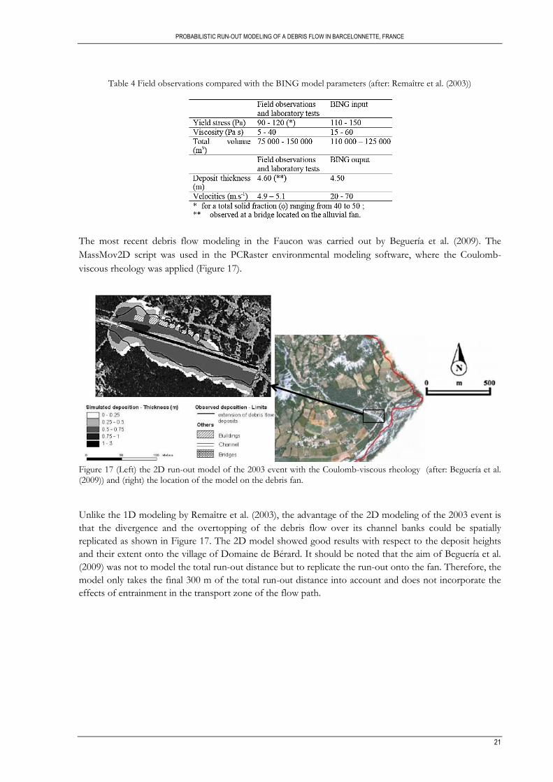
PROBABILISTIC RUN-OUT MODELING OF A DEBRIS FLOW IN BARCELONNETTE, FRANCE
21
Table 4 Field observations compared with the BING model parameters (after: Remaître et al. (2003))
The most recent debris flow modeling in the Faucon was carried out by Beguería et al. (2009). The
MassMov2D script was used in the PCRaster environmental modeling software, where the Coulomb-
viscous rheology was applied (Figure 17).
Figure 17 (Left) the 2D run-out model of the 2003 event with the Coulomb-viscous rheology (after: Beguería et al. (2009)) and (right) the location of the model on the debris fan.
Unlike the 1D modeling by Remaître et al. (2003), the advantage of the 2D modeling of the 2003 event is
that the divergence and the overtopping of the debris flow over its channel banks could be spatially
replicated as shown in Figure 17. The 2D model showed good results with respect to the deposit heights
and their extent onto the village of Domaine de Bérard. It should be noted that the aim of Beguería et al.
(2009) was not to model the total run-out distance but to replicate the run-out onto the fan. Therefore, the
model only takes the final 300 m of the total run-out distance into account and does not incorporate the
effects of entrainment in the transport zone of the flow path.

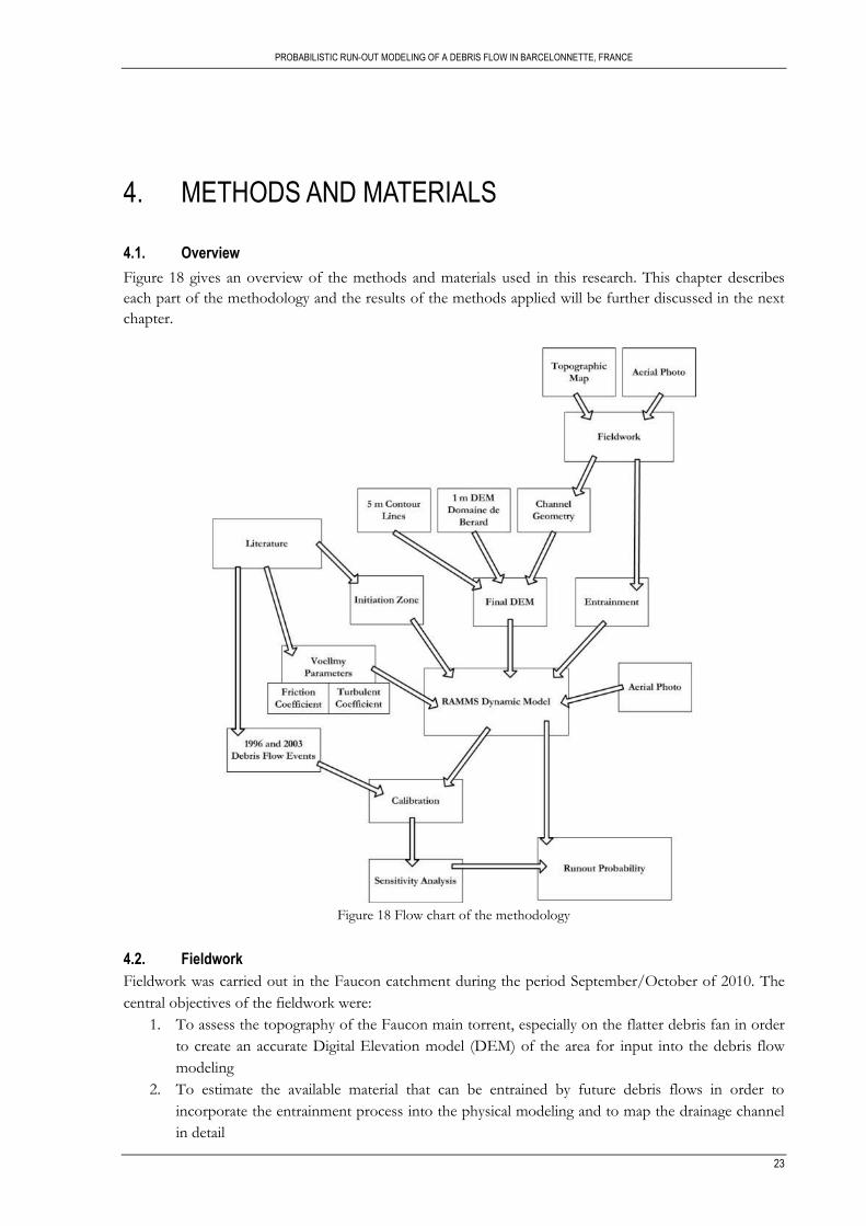
PROBABILISTIC RUN-OUT MODELING OF A DEBRIS FLOW IN BARCELONNETTE, FRANCE
23
4. METHODS AND MATERIALS
4.1. Overview
Figure 18 gives an overview of the methods and materials used in this research. This chapter describes
each part of the methodology and the results of the methods applied will be further discussed in the next
chapter.
Figure 18 Flow chart of the methodology
4.2. Fieldwork
Fieldwork was carried out in the Faucon catchment during the period September/October of 2010. The
central objectives of the fieldwork were:
1. To assess the topography of the Faucon main torrent, especially on the flatter debris fan in order
to create an accurate Digital Elevation model (DEM) of the area for input into the debris flow
modeling
2. To estimate the available material that can be entrained by future debris flows in order to
incorporate the entrainment process into the physical modeling and to map the drainage channel
in detail
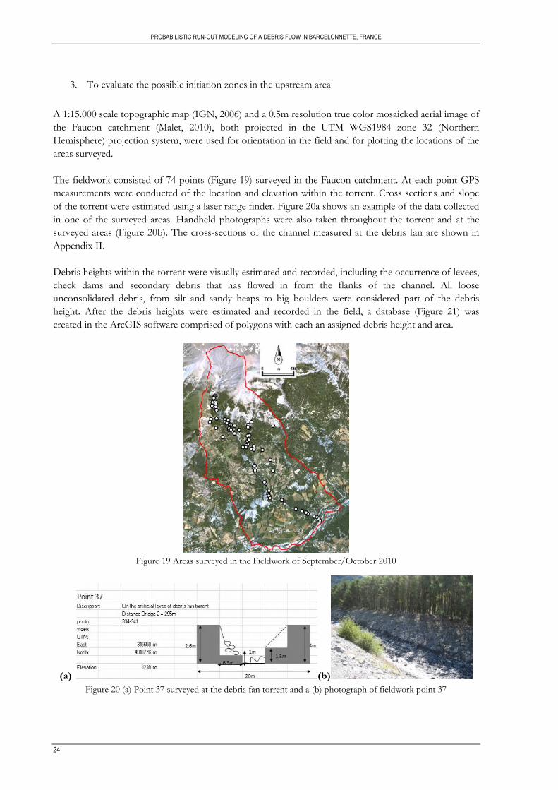
PROBABILISTIC RUN-OUT MODELING OF A DEBRIS FLOW IN BARCELONNETTE, FRANCE
24
3. To evaluate the possible initiation zones in the upstream area
A 1:15.000 scale topographic map (IGN, 2006) and a 0.5m resolution true color mosaicked aerial image of
the Faucon catchment (Malet, 2010), both projected in the UTM WGS1984 zone 32 (Northern
Hemisphere) projection system, were used for orientation in the field and for plotting the locations of the
areas surveyed.
The fieldwork consisted of 74 points (Figure 19) surveyed in the Faucon catchment. At each point GPS
measurements were conducted of the location and elevation within the torrent. Cross sections and slope
of the torrent were estimated using a laser range finder. Figure 20a shows an example of the data collected
in one of the surveyed areas. Handheld photographs were also taken throughout the torrent and at the
surveyed areas (Figure 20b). The cross-sections of the channel measured at the debris fan are shown in
Appendix II.
Debris heights within the torrent were visually estimated and recorded, including the occurrence of levees,
check dams and secondary debris that has flowed in from the flanks of the channel. All loose
unconsolidated debris, from silt and sandy heaps to big boulders were considered part of the debris
height. After the debris heights were estimated and recorded in the field, a database (Figure 21) was
created in the ArcGIS software comprised of polygons with each an assigned debris height and area.
Figure 19 Areas surveyed in the Fieldwork of September/October 2010
(a) (b)
Figure 20 (a) Point 37 surveyed at the debris fan torrent and a (b) photograph of fieldwork point 37
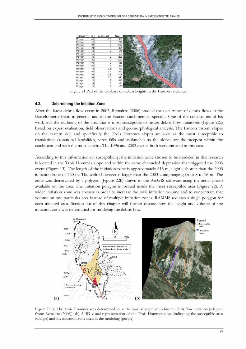
PROBABILISTIC RUN-OUT MODELING OF A DEBRIS FLOW IN BARCELONNETTE, FRANCE
25
Figure 21 Part of the database on debris heights in the Faucon catchment
4.3. Determining the Initation Zone
After the latest debris flow event in 2003, Remaître (2006) studied the occurrence of debris flows in the
Barcelonnette basin in general, and in the Faucon catchment in specific. One of the conclusions of his
work was the outlining of the area that is most susceptible to future debris flow initiations (Figure 22a)
based on expert evaluation, field observations and geomorphological analysis. The Faucon torrent slopes
on the eastern side and specifically the Trois Hommes slopes are seen as the most susceptible to
translational/rotational landslides, scree falls and avalanches as the slopes are the steepest within the
catchment and with the most activity. The 1996 and 2003 events both were initiated in this area.
According to this information on susceptibility, the initiation zone chosen to be modeled in this research
is located in the Trois Hommes slope and within the same channeled depression that triggered the 2003
event (Figure 13). The length of the initiation zone is approximately 615 m, slightly shorter than the 2003
initiation zone of 750 m. The width however is larger than the 2003 zone, ranging from 8 to 16 m. The
zone was demarcated by a polygon (Figure 22b) drawn in the ArcGIS software using the aerial photo
available on the area. The initiation polygon is located inside the most susceptible area (Figure 22). A
wider initiation zone was chosen in order to increase the total initiation volume and to concentrate that
volume on one particular area instead of multiple initiation zones. RAMMS requires a single polygon for
each initiated area. Section 4.6 of this chapter will further discuss how the height and volume of the
initiation zone was determined for modeling the debris flow.
(a) (b)
Figure 22 (a) The Trois Hommes area determined to be the most susceptible to future debris flow initiation (adapted from: Remaître (2006)). (b) A 3D visual representation of the Trois Hommes slope indicating the susceptible area (orange) and the initiation zone used in the modeling (purple)
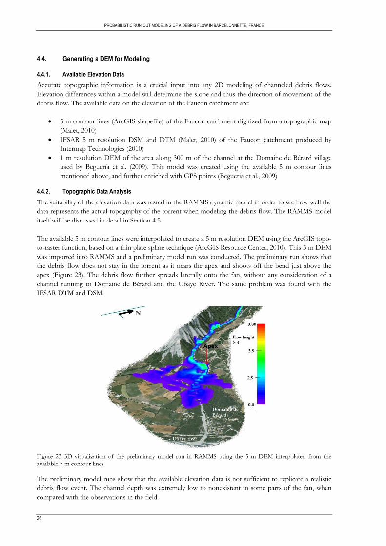
PROBABILISTIC RUN-OUT MODELING OF A DEBRIS FLOW IN BARCELONNETTE, FRANCE
26
4.4. Generating a DEM for Modeling
4.4.1. Available Elevation Data
Accurate topographic information is a crucial input into any 2D modeling of channeled debris flows.
Elevation differences within a model will determine the slope and thus the direction of movement of the
debris flow. The available data on the elevation of the Faucon catchment are:
5 m contour lines (ArcGIS shapefile) of the Faucon catchment digitized from a topographic map
(Malet, 2010)
IFSAR 5 m resolution DSM and DTM (Malet, 2010) of the Faucon catchment produced by
Intermap Technologies (2010)
1 m resolution DEM of the area along 300 m of the channel at the Domaine de Bérard village
used by Beguería et al. (2009). This model was created using the available 5 m contour lines
mentioned above, and further enriched with GPS points (Beguería et al., 2009)
4.4.2. Topographic Data Analysis
The suitability of the elevation data was tested in the RAMMS dynamic model in order to see how well the
data represents the actual topography of the torrent when modeling the debris flow. The RAMMS model
itself will be discussed in detail in Section 4.5.
The available 5 m contour lines were interpolated to create a 5 m resolution DEM using the ArcGIS topo-
to-raster function, based on a thin plate spline technique (ArcGIS Resource Center, 2010). This 5 m DEM
was imported into RAMMS and a preliminary model run was conducted. The preliminary run shows that
the debris flow does not stay in the torrent as it nears the apex and shoots off the bend just above the
apex (Figure 23). The debris flow further spreads laterally onto the fan, without any consideration of a
channel running to Domaine de Bérard and the Ubaye River. The same problem was found with the
IFSAR DTM and DSM.
Figure 23 3D visualization of the preliminary model run in RAMMS using the 5 m DEM interpolated from the available 5 m contour lines
The preliminary model runs show that the available elevation data is not sufficient to replicate a realistic
debris flow event. The channel depth was extremely low to nonexistent in some parts of the fan, when
compared with the observations in the field.
N
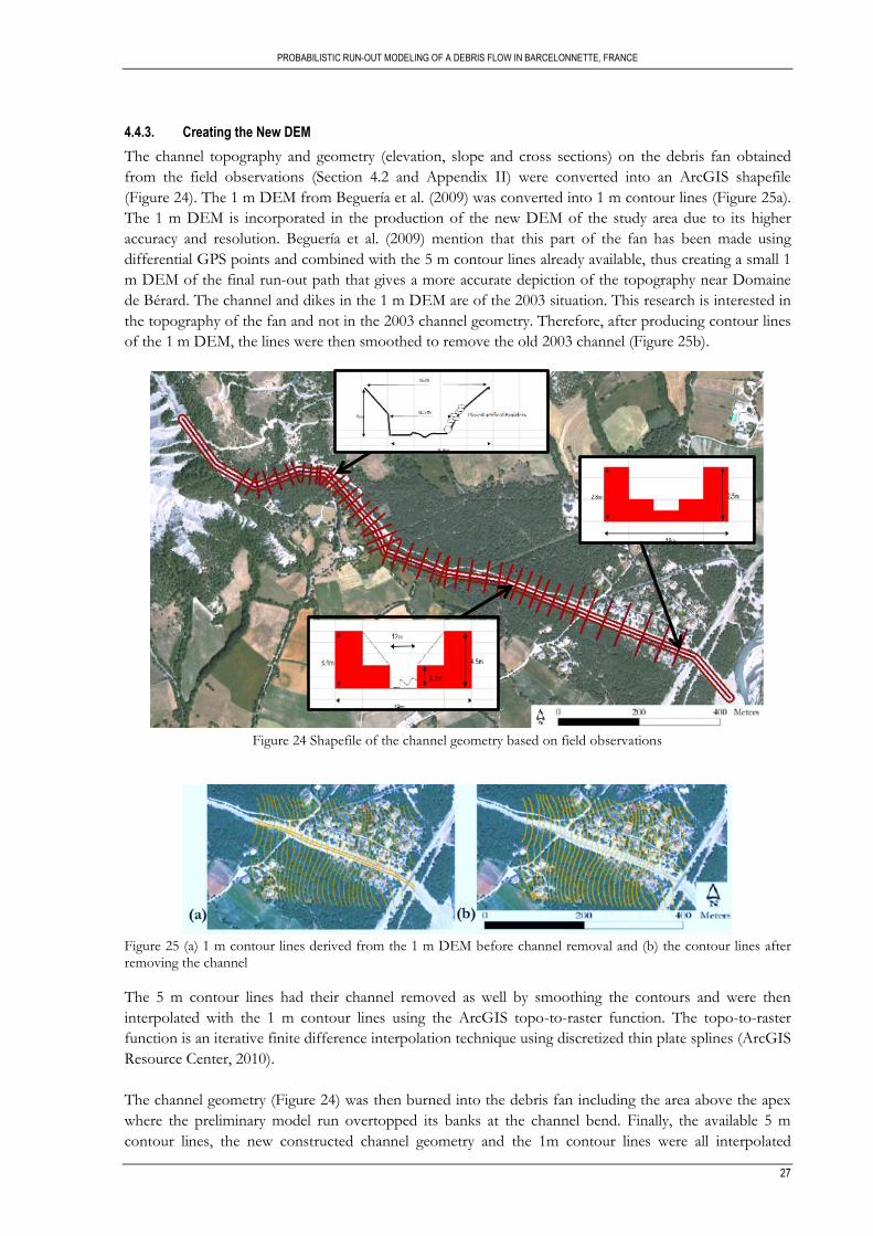
PROBABILISTIC RUN-OUT MODELING OF A DEBRIS FLOW IN BARCELONNETTE, FRANCE
27
4.4.3. Creating the New DEM
The channel topography and geometry (elevation, slope and cross sections) on the debris fan obtained
from the field observations (Section 4.2 and Appendix II) were converted into an ArcGIS shapefile
(Figure 24). The 1 m DEM from Beguería et al. (2009) was converted into 1 m contour lines (Figure 25a).
The 1 m DEM is incorporated in the production of the new DEM of the study area due to its higher
accuracy and resolution. Beguería et al. (2009) mention that this part of the fan has been made using
differential GPS points and combined with the 5 m contour lines already available, thus creating a small 1
m DEM of the final run-out path that gives a more accurate depiction of the topography near Domaine
de Bérard. The channel and dikes in the 1 m DEM are of the 2003 situation. This research is interested in
the topography of the fan and not in the 2003 channel geometry. Therefore, after producing contour lines
of the 1 m DEM, the lines were then smoothed to remove the old 2003 channel (Figure 25b).
Figure 24 Shapefile of the channel geometry based on field observations
Figure 25 (a) 1 m contour lines derived from the 1 m DEM before channel removal and (b) the contour lines after removing the channel
The 5 m contour lines had their channel removed as well by smoothing the contours and were then
interpolated with the 1 m contour lines using the ArcGIS topo-to-raster function. The topo-to-raster
function is an iterative finite difference interpolation technique using discretized thin plate splines (ArcGIS
Resource Center, 2010).
The channel geometry (Figure 24) was then burned into the debris fan including the area above the apex
where the preliminary model run overtopped its banks at the channel bend. Finally, the available 5 m
contour lines, the new constructed channel geometry and the 1m contour lines were all interpolated
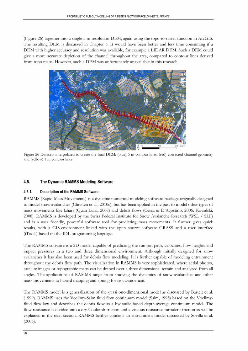
PROBABILISTIC RUN-OUT MODELING OF A DEBRIS FLOW IN BARCELONNETTE, FRANCE
28
(Figure 26) together into a single 5 m resolution DEM, again using the topo-to-raster function in ArcGIS.
The resulting DEM is discussed in Chapter 5. It would have been better and less time consuming if a
DEM with higher accuracy and resolution was available, for example a LIDAR DEM. Such a DEM could
give a more accurate depiction of the channel throughout the area, compared to contour lines derived
from topo maps. However, such a DEM was unfortunately unavailable in this research.
Figure 26 Datasets interpolated to create the final DEM: (blue) 5 m contour lines, (red) corrected channel geometry and (yellow) 1 m contour lines
4.5. The Dynamic RAMMS Modeling Software
4.5.1. Description of the RAMMS Software
RAMMS (Rapid Mass Movements) is a dynamic numerical modeling software package originally designed
to model snow avalanches (Christen et al., 2010c), but has been applied in the past to model other types of
mass movements like lahars (Quan Luna, 2007) and debris flows (Cesca & D‟Agostino, 2006; Kowalski,
2008). RAMMS is developed by the Swiss Federal Institute for Snow Avalanche Research (WSL / SLF)
and is a user friendly, powerful software tool for predicting mass movements. It further gives quick
results, with a GIS-environment linked with the open source software GRASS and a user interface
(iTools) based on the IDL programming language.
The RAMMS software is a 2D model capable of predicting the run-out path, velocities, flow heights and
impact pressures in a two and three dimensional environment. Although initially designed for snow
avalanches it has also been used for debris flow modeling. It is further capable of modeling entrainment
throughout the debris flow path. The visualization in RAMMS is very sophisticated, where aerial photos,
satellite images or topographic maps can be draped over a three dimensional terrain and analyzed from all
angles. The applications of RAMMS range from studying the dynamics of snow avalanches and other
mass movements to hazard mapping and zoning for risk assessment.
The RAMMS model is a generalization of the quasi one-dimensional model as discussed by Bartelt et al.
(1999). RAMMS uses the Voellmy-Salm fluid flow continuum model (Salm, 1993) based on the Voellmy-
fluid flow law and describes the debris flow as a hydraulic-based depth-average continuum model. The
flow resistance is divided into a dry-Coulomb friction and a viscous resistance turbulent friction as will be
explained in the next section. RAMMS further contains an entrainment model discussed by Sovilla et al.
(2006).
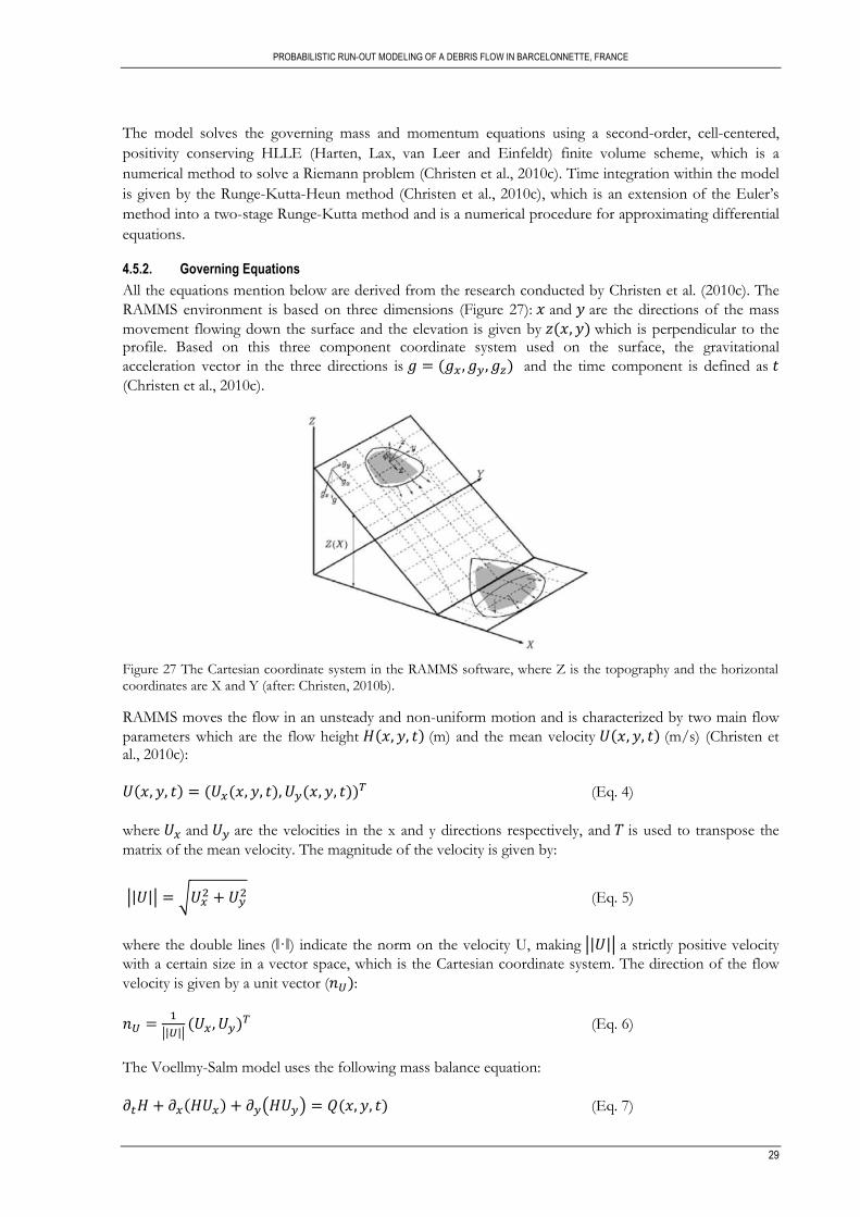
PROBABILISTIC RUN-OUT MODELING OF A DEBRIS FLOW IN BARCELONNETTE, FRANCE
29
The model solves the governing mass and momentum equations using a second-order, cell-centered,
positivity conserving HLLE (Harten, Lax, van Leer and Einfeldt) finite volume scheme, which is a
numerical method to solve a Riemann problem (Christen et al., 2010c). Time integration within the model
is given by the Runge-Kutta-Heun method (Christen et al., 2010c), which is an extension of the Euler‟s
method into a two-stage Runge-Kutta method and is a numerical procedure for approximating differential
equations.
4.5.2. Governing Equations
All the equations mention below are derived from the research conducted by Christen et al. (2010c). The
RAMMS environment is based on three dimensions (Figure 27): and are the directions of the mass
movement flowing down the surface and the elevation is given by which is perpendicular to the profile. Based on this three component coordinate system used on the surface, the gravitational
acceleration vector in the three directions is and the time component is defined as (Christen et al., 2010c).
Figure 27 The Cartesian coordinate system in the RAMMS software, where Z is the topography and the horizontal coordinates are X and Y (after: Christen, 2010b).
RAMMS moves the flow in an unsteady and non-uniform motion and is characterized by two main flow
parameters which are the flow height (m) and the mean velocity (m/s) (Christen et al., 2010c):
(Eq. 4)
where and are the velocities in the x and y directions respectively, and is used to transpose the
matrix of the mean velocity. The magnitude of the velocity is given by:
|| || √
(Eq. 5)
where the double lines (‖·‖) indicate the norm on the velocity U, making || || a strictly positive velocity
with a certain size in a vector space, which is the Cartesian coordinate system. The direction of the flow
velocity is given by a unit vector ( :
|| ||
(Eq. 6)
The Voellmy-Salm model uses the following mass balance equation:
( ) (Eq. 7)
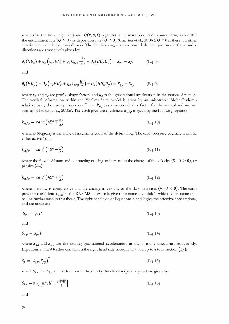
PROBABILISTIC RUN-OUT MODELING OF A DEBRIS FLOW IN BARCELONNETTE, FRANCE
30
where is the flow height (m) and (kg/m2s) is the mass production source term, also called
the entrainment rate or deposition rate (Christen et al., 2010c). = 0 if there is neither entrainment nor deposition of mass. The depth-averaged momentum balance equations in the x and y directions are respectively given by:
(
) ( ) (Eq. 8)
and
( ) (
) ( ) (Eq. 9)
where and are profile shape factors and is the gravitational acceleration in the vertical direction.
The vertical information within the Voellmy-Salm model is given by an anisotropic Mohr-Coulomb
relation, using the earth pressure coefficient as a proportionality factor for the vertical and normal
stresses (Christen et al., 2010c). The earth pressure coefficient is given by the following equation:
(
) (Eq. 10)
where (degrees) is the angle of internal friction of the debris flow. The earth pressure coefficient can be
either active :
(
) (Eq. 11)
where the flow is dilatant and contracting causing an increase in the change of the velocity , or
passive :
(
) (Eq. 12)
where the flow is compressive and the change in velocity of the flow decreases . The earth
pressure coefficient in the RAMMS software is given the name “Lambda”, which is the name that
will be further used in this thesis. The right hand side of Equations 8 and 9 give the effective accelerations, and are noted as:
(Eq. 13)
and
(Eq. 14)
where and are the driving gravitational accelerations in the x and y directions, respectively.
Equations 8 and 9 further contain on the right hand side frictions that add up to a total friction ( ):
( )
(Eq. 15)
where and are the frictions in the x and y directions respectively and are given by:
*
|| ||
+ (Eq. 16)
and
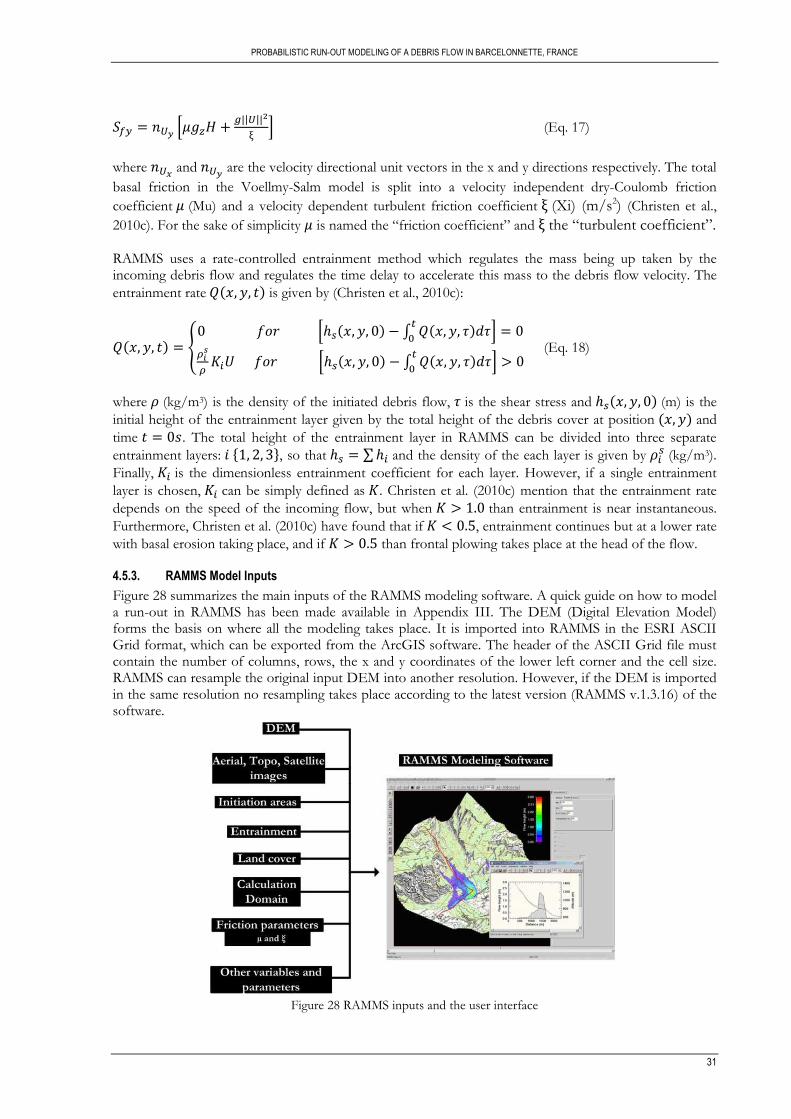
PROBABILISTIC RUN-OUT MODELING OF A DEBRIS FLOW IN BARCELONNETTE, FRANCE
31
*
|| ||
+ (Eq. 17)
where and
are the velocity directional unit vectors in the x and y directions respectively. The total
basal friction in the Voellmy-Salm model is split into a velocity independent dry-Coulomb friction
coefficient (Mu) and a velocity dependent turbulent friction coefficient (Xi) (m/s2) (Christen et al.,
2010c). For the sake of simplicity is named the “friction coefficient” and the “turbulent coefficient”. RAMMS uses a rate-controlled entrainment method which regulates the mass being up taken by the incoming debris flow and regulates the time delay to accelerate this mass to the debris flow velocity. The
entrainment rate is given by (Christen et al., 2010c):
{ * ∫
+
* ∫
+
(Eq. 18)
where (kg/m3) is the density of the initiated debris flow, is the shear stress and (m) is the
initial height of the entrainment layer given by the total height of the debris cover at position and
time . The total height of the entrainment layer in RAMMS can be divided into three separate
entrainment layers: { }, so that ∑ and the density of the each layer is given by (kg/m3).
Finally, is the dimensionless entrainment coefficient for each layer. However, if a single entrainment
layer is chosen, can be simply defined as . Christen et al. (2010c) mention that the entrainment rate
depends on the speed of the incoming flow, but when than entrainment is near instantaneous.
Furthermore, Christen et al. (2010c) have found that if , entrainment continues but at a lower rate
with basal erosion taking place, and if than frontal plowing takes place at the head of the flow.
4.5.3. RAMMS Model Inputs
Figure 28 summarizes the main inputs of the RAMMS modeling software. A quick guide on how to model a run-out in RAMMS has been made available in Appendix III. The DEM (Digital Elevation Model) forms the basis on where all the modeling takes place. It is imported into RAMMS in the ESRI ASCII Grid format, which can be exported from the ArcGIS software. The header of the ASCII Grid file must contain the number of columns, rows, the x and y coordinates of the lower left corner and the cell size. RAMMS can resample the original input DEM into another resolution. However, if the DEM is imported in the same resolution no resampling takes place according to the latest version (RAMMS v.1.3.16) of the software.
Figure 28 RAMMS inputs and the user interface
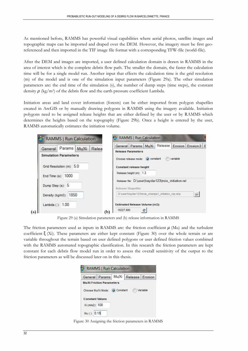
PROBABILISTIC RUN-OUT MODELING OF A DEBRIS FLOW IN BARCELONNETTE, FRANCE
32
As mentioned before, RAMMS has powerful visual capabilities where aerial photos, satellite images and
topographic maps can be imported and draped over the DEM. However, the imagery must be first geo-
referenced and then imported in the TIF image file format with a corresponding TFW-file (world-file).
After the DEM and images are imported, a user defined calculation domain is drawn in RAMMS in the
area of interest which is the complete debris flow path. The smaller the domain, the faster the calculation
time will be for a single model run. Another input that effects the calculation time is the grid resolution
(m) of the model and is one of the simulation input parameters (Figure 29a). The other simulation
parameters are: the end time of the simulation (s), the number of dump steps (time steps), the constant
density (kg/m3) of the debris flow and the earth pressure coefficient Lambda.
Initiation areas and land cover information (forests) can be either imported from polygon shapefiles
created in ArcGIS or by manually drawing polygons in RAMMS using the imagery available. Initiation
polygons need to be assigned release heights that are either defined by the user or by RAMMS which
determines the heights based on the topography (Figure 29b). Once a height is entered by the user,
RAMMS automatically estimates the initiation volume.
(a) (b)
Figure 29 (a) Simulation parameters and (b) release information in RAMMS
The friction parameters used as inputs in RAMMS are: the friction coefficient (Mu) and the turbulent
coefficient (Xi). These parameters are either kept constant (Figure 30) over the whole terrain or are
variable throughout the terrain based on user defined polygons or user defined friction values combined
with the RAMMS automated topographic classification. In this research the friction parameters are kept
constant for each debris flow model run in order to assess the overall sensitivity of the output to the
friction parameters as will be discussed later on in this thesis.
Figure 30 Assigning the friction parameters in RAMMS
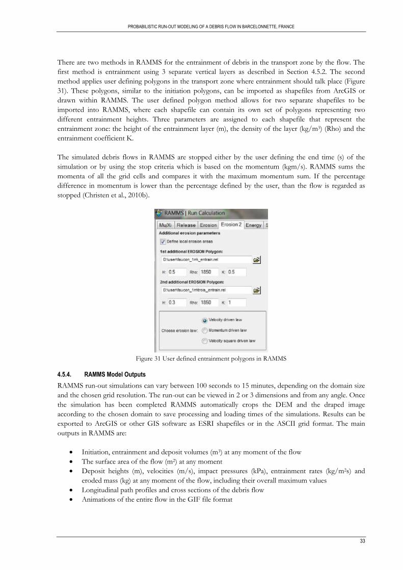
PROBABILISTIC RUN-OUT MODELING OF A DEBRIS FLOW IN BARCELONNETTE, FRANCE
33
There are two methods in RAMMS for the entrainment of debris in the transport zone by the flow. The
first method is entrainment using 3 separate vertical layers as described in Section 4.5.2. The second
method applies user defining polygons in the transport zone where entrainment should talk place (Figure
31). These polygons, similar to the initiation polygons, can be imported as shapefiles from ArcGIS or
drawn within RAMMS. The user defined polygon method allows for two separate shapefiles to be
imported into RAMMS, where each shapefile can contain its own set of polygons representing two
different entrainment heights. Three parameters are assigned to each shapefile that represent the
entrainment zone: the height of the entrainment layer (m), the density of the layer (kg/m3) (Rho) and the
entrainment coefficient K.
The simulated debris flows in RAMMS are stopped either by the user defining the end time (s) of the
simulation or by using the stop criteria which is based on the momentum (kgm/s). RAMMS sums the
momenta of all the grid cells and compares it with the maximum momentum sum. If the percentage
difference in momentum is lower than the percentage defined by the user, than the flow is regarded as
stopped (Christen et al., 2010b).
Figure 31 User defined entrainment polygons in RAMMS
4.5.4. RAMMS Model Outputs
RAMMS run-out simulations can vary between 100 seconds to 15 minutes, depending on the domain size
and the chosen grid resolution. The run-out can be viewed in 2 or 3 dimensions and from any angle. Once
the simulation has been completed RAMMS automatically crops the DEM and the draped image
according to the chosen domain to save processing and loading times of the simulations. Results can be
exported to ArcGIS or other GIS software as ESRI shapefiles or in the ASCII grid format. The main
outputs in RAMMS are:
Initiation, entrainment and deposit volumes (m3) at any moment of the flow
The surface area of the flow (m2) at any moment
Deposit heights (m), velocities (m/s), impact pressures (kPa), entrainment rates (kg/m2s) and
eroded mass (kg) at any moment of the flow, including their overall maximum values
Longitudinal path profiles and cross sections of the debris flow
Animations of the entire flow in the GIF file format
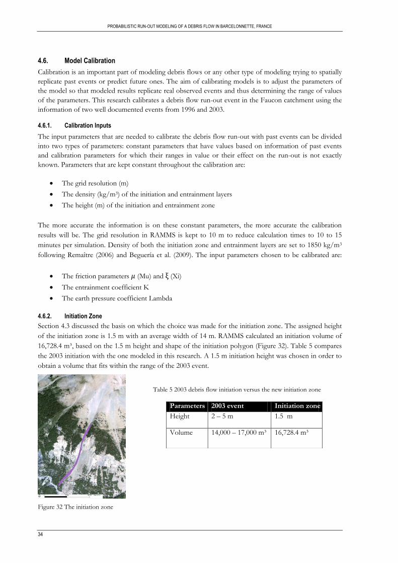
PROBABILISTIC RUN-OUT MODELING OF A DEBRIS FLOW IN BARCELONNETTE, FRANCE
34
4.6. Model Calibration
Calibration is an important part of modeling debris flows or any other type of modeling trying to spatially
replicate past events or predict future ones. The aim of calibrating models is to adjust the parameters of
the model so that modeled results replicate real observed events and thus determining the range of values
of the parameters. This research calibrates a debris flow run-out event in the Faucon catchment using the
information of two well documented events from 1996 and 2003.
4.6.1. Calibration Inputs
The input parameters that are needed to calibrate the debris flow run-out with past events can be divided
into two types of parameters: constant parameters that have values based on information of past events
and calibration parameters for which their ranges in value or their effect on the run-out is not exactly
known. Parameters that are kept constant throughout the calibration are:
The grid resolution (m)
The density (kg/m3) of the initiation and entrainment layers
The height (m) of the initiation and entrainment zone
The more accurate the information is on these constant parameters, the more accurate the calibration
results will be. The grid resolution in RAMMS is kept to 10 m to reduce calculation times to 10 to 15
minutes per simulation. Density of both the initiation zone and entrainment layers are set to 1850 kg/m3
following Remaître (2006) and Beguería et al. (2009). The input parameters chosen to be calibrated are:
The friction parameters (Mu) and (Xi)
The entrainment coefficient K
The earth pressure coefficient Lambda
4.6.2. Initiation Zone
Section 4.3 discussed the basis on which the choice was made for the initiation zone. The assigned height
of the initiation zone is 1.5 m with an average width of 14 m. RAMMS calculated an initiation volume of
16,728.4 m³, based on the 1.5 m height and shape of the initiation polygon (Figure 32). Table 5 compares
the 2003 initiation with the one modeled in this research. A 1.5 m initiation height was chosen in order to
obtain a volume that fits within the range of the 2003 event.
Table 5 2003 debris flow initiation versus the new initiation zone
Figure 32 The initiation zone
Parameters 2003 event Initiation zone
Height 2 – 5 m 1.5 m
Volume 14,000 – 17,000 m³ 16,728.4 m³
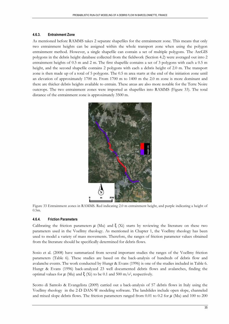
PROBABILISTIC RUN-OUT MODELING OF A DEBRIS FLOW IN BARCELONNETTE, FRANCE
35
4.6.3. Entrainment Zone
As mentioned before RAMMS takes 2 separate shapefiles for the entrainment zone. This means that only
two entrainment heights can be assigned within the whole transport zone when using the polygon
entrainment method. However, a single shapefile can contain a set of multiple polygons. The ArcGIS
polygons in the debris height database collected from the fieldwork (Section 4.2) were averaged out into 2
entrainment heights of 0.5 m and 2 m. The first shapefile contains a set of 3 polygons with each a 0.5 m
height, and the second shapefile contains 2 polygons with each a debris height of 2.0 m. The transport
zone is then made up of a total of 5 polygons. The 0.5 m area starts at the end of the initiation zone until
an elevation of approximately 1700 m. From 1700 m to 1400 m the 2.0 m zone is more dominant and
there are thicker debris heights available to entrain. These areas are also more notable for the Terre Noire
outcrops. The two entrainment zones were imported as shapefiles into RAMMS (Figure 33). The total
distance of the entrainment zone is approximately 3500 m.
Figure 33 Entrainment zones in RAMMS. Red indicating 2.0 m entrainment height, and purple indicating a height of 0.5m.
4.6.4. Friction Parameters
Calibrating the friction parameters (Mu) and (Xi) starts by reviewing the literature on these two
parameters used in the Voellmy rheology. As mentioned in Chapter 1, the Voellmy rheology has been
used to model a variety of mass movements. Therefore, the ranges of friction parameter values obtained
from the literature should be specifically determined for debris flows.
Sosio et al. (2008) have summarized from several important studies the ranges of the Voellmy friction
parameters (Table 6). These studies are based on the back-analysis of hundreds of debris flow and
avalanche events. The work conducted by Hungr & Evans (1996) is one of the studies included in Table 6.
Hungr & Evans (1996) back-analyzed 23 well documented debris flows and avalanches, finding the
optimal values for (Mu) and (Xi) to be 0.1 and 500 m/s2, respectively.
Scotto di Santolo & Evangelista (2009) carried out a back-analysis of 57 debris flows in Italy using the
Voellmy rheology in the 2-D DAN-W modeling software. The landslides include open slope, channeled
and mixed slope debris flows. The friction parameters ranged from 0.01 to 0.2 for (Mu) and 100 to 200
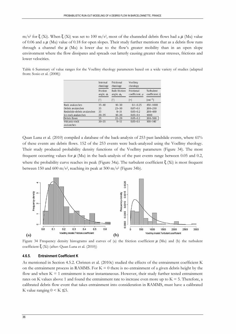
PROBABILISTIC RUN-OUT MODELING OF A DEBRIS FLOW IN BARCELONNETTE, FRANCE
36
m/s2 for (Xi). When (Xi) was set to 100 m/s2, most of the channeled debris flows had a (Mu) value
of 0.06 and a (Mu) value of 0.18 for open slopes. Their study further mentions that as a debris flow runs
through a channel the (Mu) is lower due to the flow‟s greater mobility than in an open slope
environment where the flow dissipates and spreads out latterly causing greater shear stresses, frictions and
lower velocities.
Table 6 Summary of value ranges for the Voellmy rheology parameters based on a wide variety of studies (adapted from: Sosio et al. (2008))
Quan Luna et al. (2010) compiled a database of the back-analysis of 253 past landslide events, where 61%
of these events are debris flows. 152 of the 253 events were back-analyzed using the Voellmy rheology.
Their study produced probability density functions of the Voellmy parameters (Figure 34). The most
frequent occurring values for (Mu) in the back-analysis of the past events range between 0.05 and 0.2,
where the probability curve reaches its peak (Figure 34a). The turbulent coefficient (Xi) is most frequent
between 150 and 600 m/s2, reaching its peak at 500 m/s2 (Figure 34b).
(a) (b)
Figure 34 Frequency density histograms and curves of (a) the friction coefficient (Mu) and (b) the turbulent
coefficient (Xi) (after: Quan Luna et al. (2010))
4.6.5. Entrainment Coefficient K
As mentioned in Section 4.5.2. Christen et al. (2010c) studied the effects of the entrainment coefficient K
on the entrainment process in RAMMS. For K = 0 there is no entrainment of a given debris height by the
flow and when K = 1 entrainment is near instantaneous. However, their study further tested entrainment
rates on K values above 1 and found the entrainment rate to increase even more up to K = 5. Therefore, a
calibrated debris flow event that takes entrainment into consideration in RAMMS, must have a calibrated
K value ranging 0 < K 5.
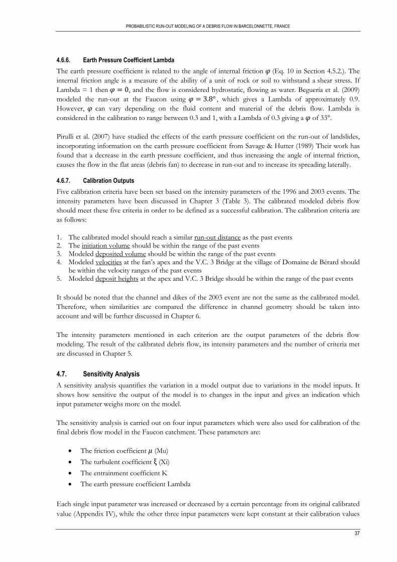
PROBABILISTIC RUN-OUT MODELING OF A DEBRIS FLOW IN BARCELONNETTE, FRANCE
37
4.6.6. Earth Pressure Coefficient Lambda
The earth pressure coefficient is related to the angle of internal friction (Eq. 10 in Section 4.5.2.). The
internal friction angle is a measure of the ability of a unit of rock or soil to withstand a shear stress. If
Lambda = 1 then , and the flow is considered hydrostatic, flowing as water. Beguería et al. (2009)
modeled the run-out at the Faucon using , which gives a Lambda of approximately 0.9.
However, can vary depending on the fluid content and material of the debris flow. Lambda is
considered in the calibration to range between 0.3 and 1, with a Lambda of 0.3 giving a of 33°.
Pirulli et al. (2007) have studied the effects of the earth pressure coefficient on the run-out of landslides,
incorporating information on the earth pressure coefficient from Savage & Hutter (1989) Their work has
found that a decrease in the earth pressure coefficient, and thus increasing the angle of internal friction,
causes the flow in the flat areas (debris fan) to decrease in run-out and to increase its spreading laterally.
4.6.7. Calibration Outputs
Five calibration criteria have been set based on the intensity parameters of the 1996 and 2003 events. The
intensity parameters have been discussed in Chapter 3 (Table 3). The calibrated modeled debris flow
should meet these five criteria in order to be defined as a successful calibration. The calibration criteria are
as follows:
1. The calibrated model should reach a similar run-out distance as the past events 2. The initiation volume should be within the range of the past events 3. Modeled deposited volume should be within the range of the past events 4. Modeled velocities at the fan‟s apex and the V.C. 3 Bridge at the village of Domaine de Bérard should
be within the velocity ranges of the past events 5. Modeled deposit heights at the apex and V.C. 3 Bridge should be within the range of the past events
It should be noted that the channel and dikes of the 2003 event are not the same as the calibrated model.
Therefore, when similarities are compared the difference in channel geometry should be taken into
account and will be further discussed in Chapter 6.
The intensity parameters mentioned in each criterion are the output parameters of the debris flow
modeling. The result of the calibrated debris flow, its intensity parameters and the number of criteria met
are discussed in Chapter 5.
4.7. Sensitivity Analysis
A sensitivity analysis quantifies the variation in a model output due to variations in the model inputs. It
shows how sensitive the output of the model is to changes in the input and gives an indication which
input parameter weighs more on the model.
The sensitivity analysis is carried out on four input parameters which were also used for calibration of the
final debris flow model in the Faucon catchment. These parameters are:
The friction coefficient (Mu)
The turbulent coefficient (Xi)
The entrainment coefficient K
The earth pressure coefficient Lambda
Each single input parameter was increased or decreased by a certain percentage from its original calibrated
value (Appendix IV), while the other three input parameters were kept constant at their calibration values
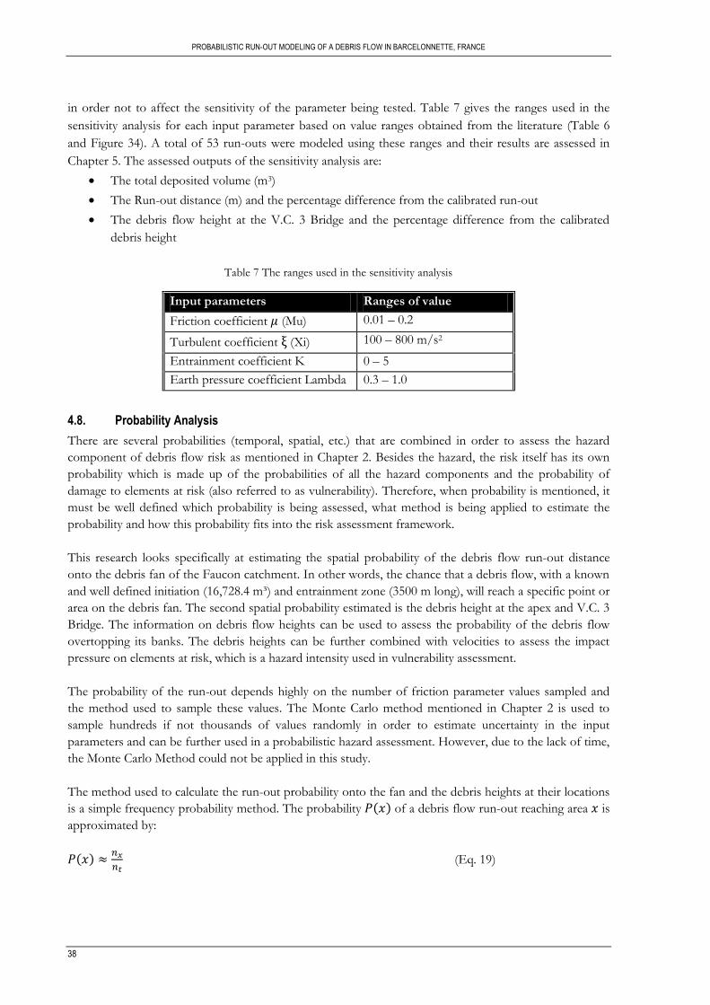
PROBABILISTIC RUN-OUT MODELING OF A DEBRIS FLOW IN BARCELONNETTE, FRANCE
38
in order not to affect the sensitivity of the parameter being tested. Table 7 gives the ranges used in the
sensitivity analysis for each input parameter based on value ranges obtained from the literature (Table 6
and Figure 34). A total of 53 run-outs were modeled using these ranges and their results are assessed in
Chapter 5. The assessed outputs of the sensitivity analysis are:
The total deposited volume (m3)
The Run-out distance (m) and the percentage difference from the calibrated run-out
The debris flow height at the V.C. 3 Bridge and the percentage difference from the calibrated
debris height
Table 7 The ranges used in the sensitivity analysis
Input parameters Ranges of value
Friction coefficient (Mu) 0.01 – 0.2
Turbulent coefficient (Xi) 100 – 800 m/s2
Entrainment coefficient K 0 – 5
Earth pressure coefficient Lambda 0.3 – 1.0
4.8. Probability Analysis
There are several probabilities (temporal, spatial, etc.) that are combined in order to assess the hazard
component of debris flow risk as mentioned in Chapter 2. Besides the hazard, the risk itself has its own
probability which is made up of the probabilities of all the hazard components and the probability of
damage to elements at risk (also referred to as vulnerability). Therefore, when probability is mentioned, it
must be well defined which probability is being assessed, what method is being applied to estimate the
probability and how this probability fits into the risk assessment framework.
This research looks specifically at estimating the spatial probability of the debris flow run-out distance
onto the debris fan of the Faucon catchment. In other words, the chance that a debris flow, with a known
and well defined initiation (16,728.4 m³) and entrainment zone (3500 m long), will reach a specific point or
area on the debris fan. The second spatial probability estimated is the debris height at the apex and V.C. 3
Bridge. The information on debris flow heights can be used to assess the probability of the debris flow
overtopping its banks. The debris heights can be further combined with velocities to assess the impact
pressure on elements at risk, which is a hazard intensity used in vulnerability assessment.
The probability of the run-out depends highly on the number of friction parameter values sampled and
the method used to sample these values. The Monte Carlo method mentioned in Chapter 2 is used to
sample hundreds if not thousands of values randomly in order to estimate uncertainty in the input
parameters and can be further used in a probabilistic hazard assessment. However, due to the lack of time,
the Monte Carlo Method could not be applied in this study.
The method used to calculate the run-out probability onto the fan and the debris heights at their locations
is a simple frequency probability method. The probability of a debris flow run-out reaching area is
approximated by:
(Eq. 19)
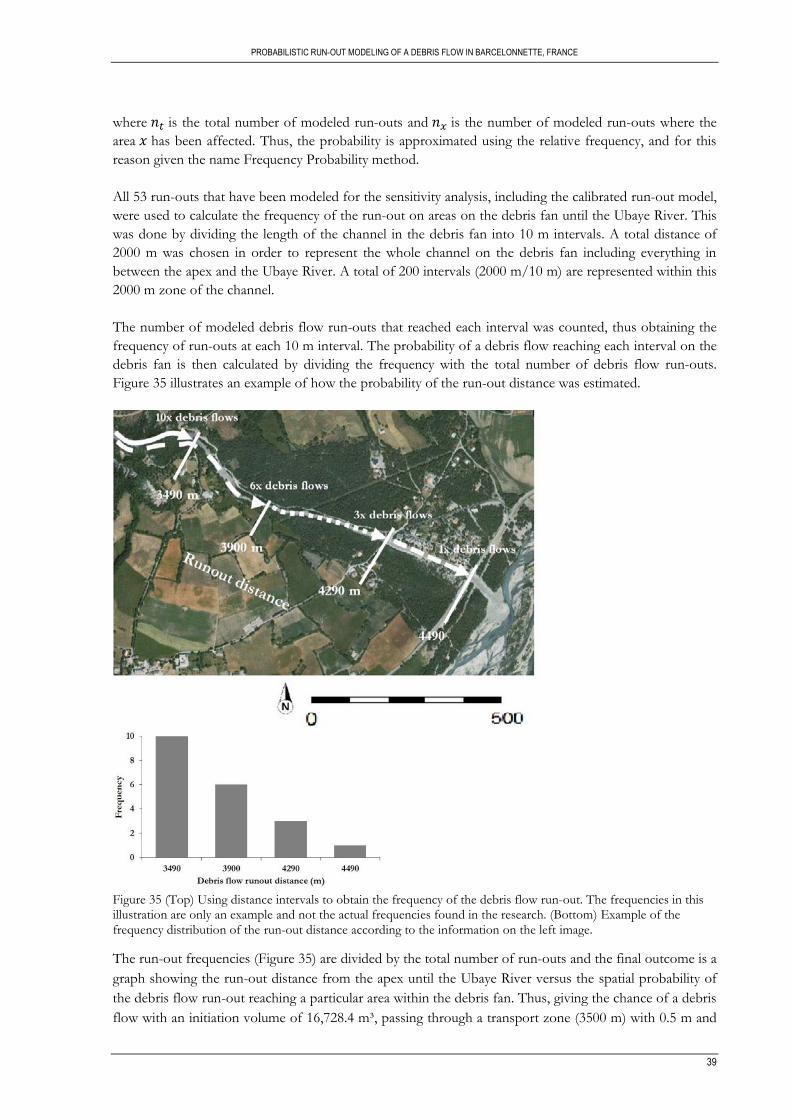
PROBABILISTIC RUN-OUT MODELING OF A DEBRIS FLOW IN BARCELONNETTE, FRANCE
39
where is the total number of modeled run-outs and is the number of modeled run-outs where the
area has been affected. Thus, the probability is approximated using the relative frequency, and for this
reason given the name Frequency Probability method.
All 53 run-outs that have been modeled for the sensitivity analysis, including the calibrated run-out model,
were used to calculate the frequency of the run-out on areas on the debris fan until the Ubaye River. This
was done by dividing the length of the channel in the debris fan into 10 m intervals. A total distance of
2000 m was chosen in order to represent the whole channel on the debris fan including everything in
between the apex and the Ubaye River. A total of 200 intervals (2000 m/10 m) are represented within this
2000 m zone of the channel.
The number of modeled debris flow run-outs that reached each interval was counted, thus obtaining the
frequency of run-outs at each 10 m interval. The probability of a debris flow reaching each interval on the
debris fan is then calculated by dividing the frequency with the total number of debris flow run-outs.
Figure 35 illustrates an example of how the probability of the run-out distance was estimated.
Figure 35 (Top) Using distance intervals to obtain the frequency of the debris flow run-out. The frequencies in this illustration are only an example and not the actual frequencies found in the research. (Bottom) Example of the frequency distribution of the run-out distance according to the information on the left image.
The run-out frequencies (Figure 35) are divided by the total number of run-outs and the final outcome is a
graph showing the run-out distance from the apex until the Ubaye River versus the spatial probability of
the debris flow run-out reaching a particular area within the debris fan. Thus, giving the chance of a debris
flow with an initiation volume of 16,728.4 m³, passing through a transport zone (3500 m) with 0.5 m and
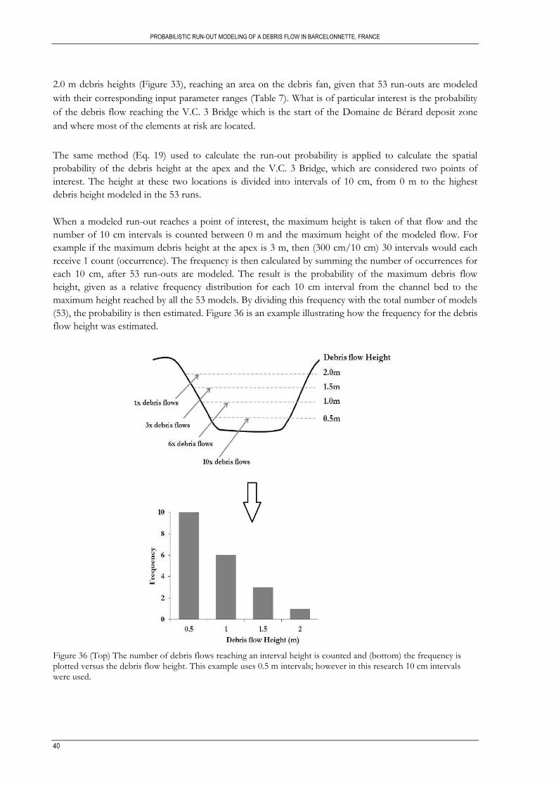
PROBABILISTIC RUN-OUT MODELING OF A DEBRIS FLOW IN BARCELONNETTE, FRANCE
40
2.0 m debris heights (Figure 33), reaching an area on the debris fan, given that 53 run-outs are modeled
with their corresponding input parameter ranges (Table 7). What is of particular interest is the probability
of the debris flow reaching the V.C. 3 Bridge which is the start of the Domaine de Bérard deposit zone
and where most of the elements at risk are located.
The same method (Eq. 19) used to calculate the run-out probability is applied to calculate the spatial
probability of the debris height at the apex and the V.C. 3 Bridge, which are considered two points of
interest. The height at these two locations is divided into intervals of 10 cm, from 0 m to the highest
debris height modeled in the 53 runs.
When a modeled run-out reaches a point of interest, the maximum height is taken of that flow and the
number of 10 cm intervals is counted between 0 m and the maximum height of the modeled flow. For
example if the maximum debris height at the apex is 3 m, then (300 cm/10 cm) 30 intervals would each
receive 1 count (occurrence). The frequency is then calculated by summing the number of occurrences for
each 10 cm, after 53 run-outs are modeled. The result is the probability of the maximum debris flow
height, given as a relative frequency distribution for each 10 cm interval from the channel bed to the
maximum height reached by all the 53 models. By dividing this frequency with the total number of models
(53), the probability is then estimated. Figure 36 is an example illustrating how the frequency for the debris
flow height was estimated.
Figure 36 (Top) The number of debris flows reaching an interval height is counted and (bottom) the frequency is plotted versus the debris flow height. This example uses 0.5 m intervals; however in this research 10 cm intervals were used.
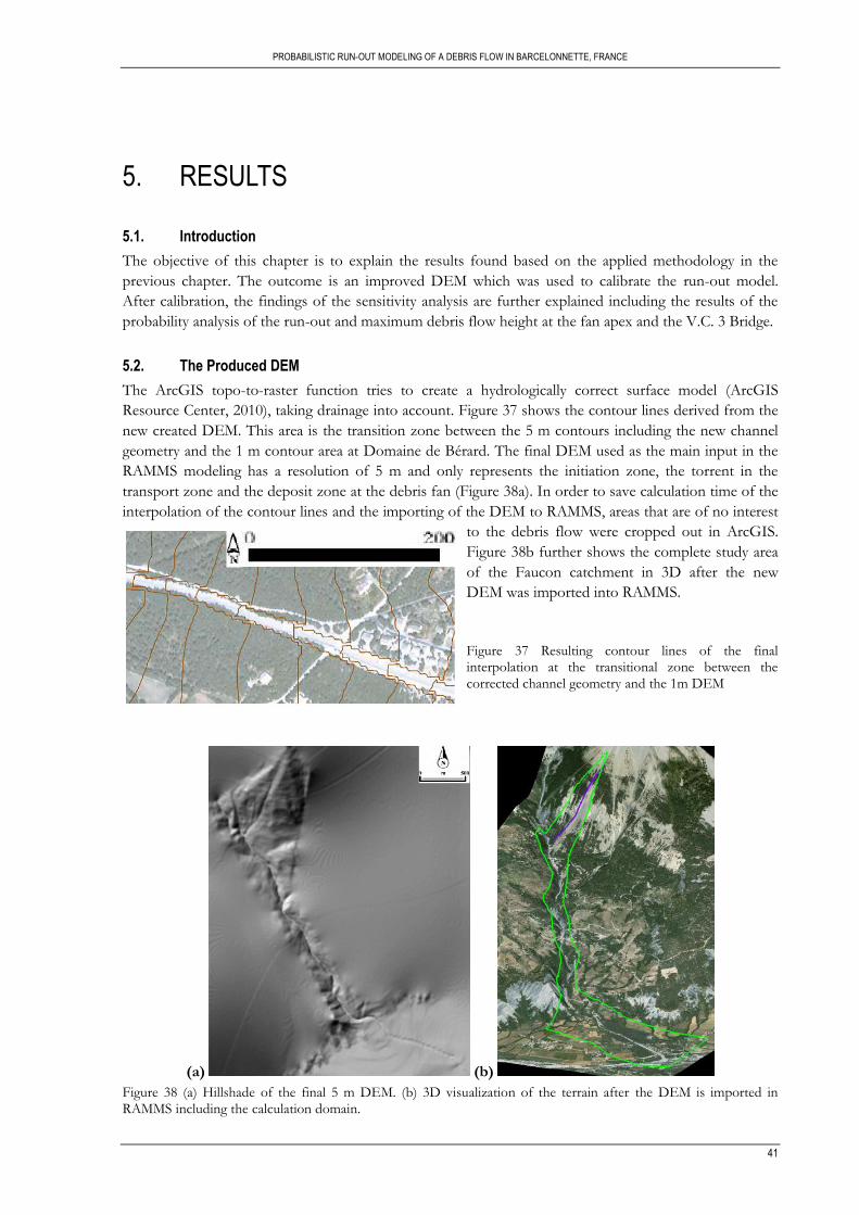
PROBABILISTIC RUN-OUT MODELING OF A DEBRIS FLOW IN BARCELONNETTE, FRANCE
41
5. RESULTS
5.1. Introduction
The objective of this chapter is to explain the results found based on the applied methodology in the
previous chapter. The outcome is an improved DEM which was used to calibrate the run-out model.
After calibration, the findings of the sensitivity analysis are further explained including the results of the
probability analysis of the run-out and maximum debris flow height at the fan apex and the V.C. 3 Bridge.
5.2. The Produced DEM
The ArcGIS topo-to-raster function tries to create a hydrologically correct surface model (ArcGIS
Resource Center, 2010), taking drainage into account. Figure 37 shows the contour lines derived from the
new created DEM. This area is the transition zone between the 5 m contours including the new channel
geometry and the 1 m contour area at Domaine de Bérard. The final DEM used as the main input in the
RAMMS modeling has a resolution of 5 m and only represents the initiation zone, the torrent in the
transport zone and the deposit zone at the debris fan (Figure 38a). In order to save calculation time of the
interpolation of the contour lines and the importing of the DEM to RAMMS, areas that are of no interest
to the debris flow were cropped out in ArcGIS.
Figure 38b further shows the complete study area
of the Faucon catchment in 3D after the new
DEM was imported into RAMMS.
Figure 37 Resulting contour lines of the final interpolation at the transitional zone between the corrected channel geometry and the 1m DEM
(a) (b)
Figure 38 (a) Hillshade of the final 5 m DEM. (b) 3D visualization of the terrain after the DEM is imported in RAMMS including the calculation domain.
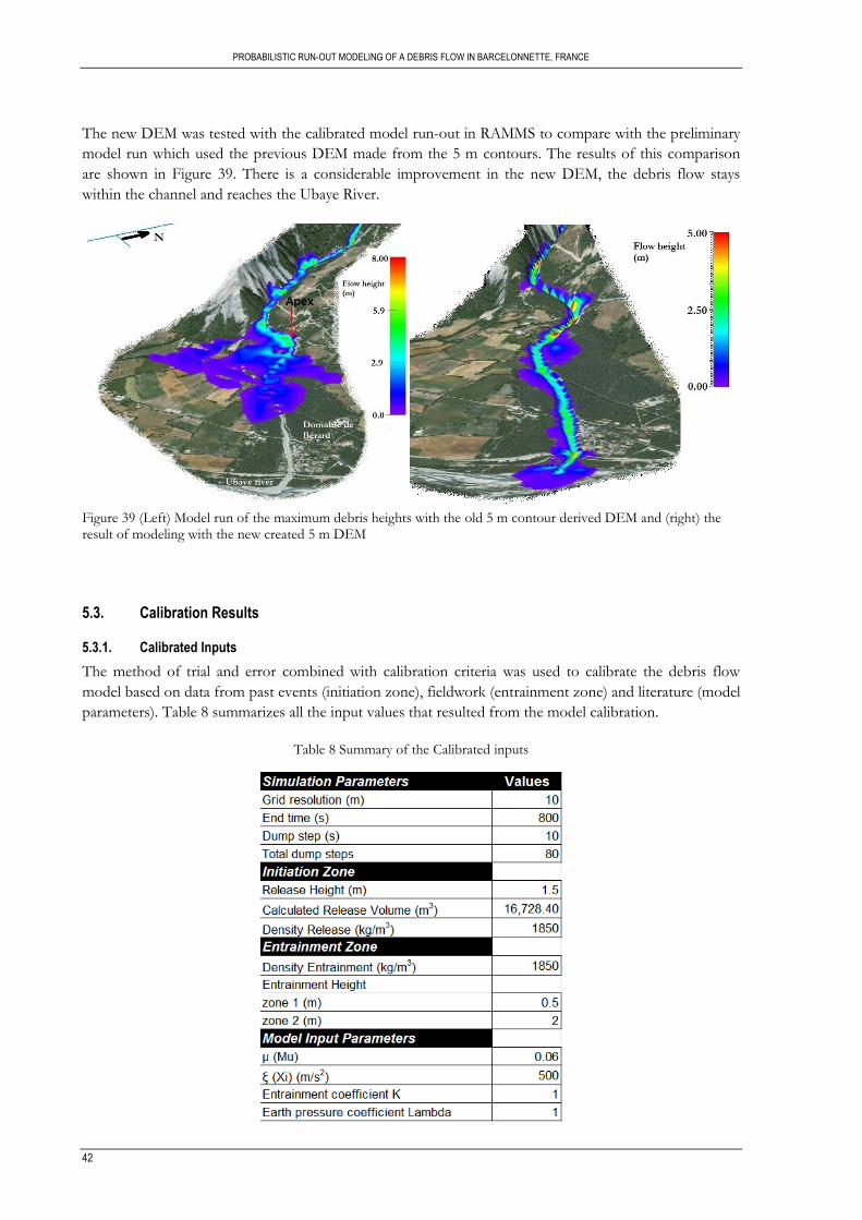
PROBABILISTIC RUN-OUT MODELING OF A DEBRIS FLOW IN BARCELONNETTE, FRANCE
42
The new DEM was tested with the calibrated model run-out in RAMMS to compare with the preliminary
model run which used the previous DEM made from the 5 m contours. The results of this comparison
are shown in Figure 39. There is a considerable improvement in the new DEM, the debris flow stays
within the channel and reaches the Ubaye River.
Figure 39 (Left) Model run of the maximum debris heights with the old 5 m contour derived DEM and (right) the result of modeling with the new created 5 m DEM
5.3. Calibration Results
5.3.1. Calibrated Inputs
The method of trial and error combined with calibration criteria was used to calibrate the debris flow
model based on data from past events (initiation zone), fieldwork (entrainment zone) and literature (model
parameters). Table 8 summarizes all the input values that resulted from the model calibration.
Table 8 Summary of the Calibrated inputs
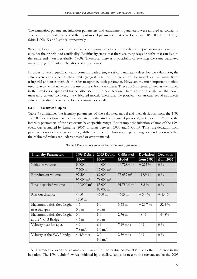
PROBABILISTIC RUN-OUT MODELING OF A DEBRIS FLOW IN BARCELONNETTE, FRANCE
43
The simulation parameters, initiation parameters and entrainment parameters were all used as constants.
The optimal calibrated values of the input model parameters that were found are 0.06, 500, 1 and 1 for
(Mu), (Xi), K and Lambda, respectively.
When calibrating a model that can have continuous variations in the values of input parameters, one must
consider the principle of equifinality. Equifinality states that there are many ways or paths that can lead to
the same end (von Bertalanffy, 1968). Therefore, there is a possibility of reaching the same calibrated
output using different combinations of input values.
In order to avoid equifinality and come up with a single set of parameter values for the calibration, the
values were constrained to their limits (ranges) based on the literature. The model was run many times
using trial and error methods in order to optimize each parameter. However, the most important method
used to avoid equifinality was the use of the calibration criteria. These are 5 different criteria as mentioned
in the previous chapter and further discussed in the next section. There was not a single run that could
meet all 5 criteria, including the calibrated model. Therefore, the possibility of another set of parameter
values replicating the same calibrated run-out is very slim.
5.3.2. Calibrated Outputs
Table 9 summarizes the intensity parameters of the calibrated model and their deviation from the 1996
and 2003 debris flow parameters estimated by the studies discussed previously in Chapter 3. Most of the
intensity parameters of the past events have specific ranges. For example the initiation volume of the 1996
event was estimated by Remaître (2006) to range between 5,000 and 7,500 m2. Thus, the deviation from
past events is calculated in percentage difference from the lowest or highest range depending on whether
the calibrated values are underestimated or overestimated.
Table 9 Past events versus calibrated intensity parameters
The difference between the volumes of 1996 and of the calibrated model is due to the difference in the
initiation. The 1996 debris flow was initiated by a shallow landslide next to the torrent, unlike the 2003
Intensity Parameters 1996 Debris
Flow
2003 Debris
Flow
Calibrated
Model
Deviation
from 1996
Deviation
from 2003
Initiation volume 5,000 –
7,500 m³
14,000 –
17,000 m³
16,728.4 m³ + 223 % 0 %
Entrainment volume 92,500 –
95,000 m³
69,000 –
78,000 m³
75,052 m³ - 18.9 % 0 %
Total deposited volume
100,000 m³ 83,000 –
95,000 m³
91,780.4 m³ - 8.2 % 0 %
Run-out distance 4400 –
4500 m
4700 m 4765 m
+ 5.9 % + 1.4 %
Maximum debris flow height
near fan apex
1.5 –
3.0 m
5.0 –
6.0 m
3.38 m + 26.7 % - 32.4 %
Maximum debris flow height
at the V.C. 3 Bridge
3.0 –
4.5 m
5.0 –
6.0 m
2.76 m - 8 % - 44.8%
Velocity near fan apex 4.9 –
7.8 m/s
6.4 –
8.9 m/s
7.19 m/s 0 %
0 %
Velocity at the V.C. 3 bridge < 4.9 m/s 2.0 –
5.0 m/s
2.59 m/s 0 % 0 %
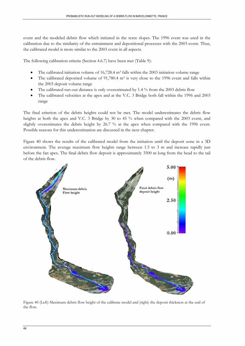
PROBABILISTIC RUN-OUT MODELING OF A DEBRIS FLOW IN BARCELONNETTE, FRANCE
44
event and the modeled debris flow which initiated in the scree slopes. The 1996 event was used in the
calibration due to the similarity of the entrainment and depositional processes with the 2003 event. Thus,
the calibrated model is more similar to the 2003 event in all aspects.
The following calibration criteria (Section 4.6.7) have been met (Table 9):
The calibrated initiation volume of 16,728.4 m³ falls within the 2003 initiation volume range
The calibrated deposited volume of 91,780.4 m³ is very close to the 1996 event and falls within
the 2003 deposit volume range
The calibrated run-out distance is only overestimated by 1.4 % from the 2003 debris flow
The calibrated velocities at the apex and at the V.C. 3 Bridge both fall within the 1996 and 2003
range
The final criterion of the debris heights could not be met. The model underestimates the debris flow
heights at both the apex and V.C. 3 Bridge by 30 to 45 % when compared with the 2003 event, and
slightly overestimates the debris height by 26.7 % at the apex when compared with the 1996 event.
Possible reasons for this underestimation are discussed in the next chapter.
Figure 40 shows the results of the calibrated model from the initiation until the deposit zone in a 3D
environment. The average maximum flow heights range between 1.5 to 3 m and increase rapidly just
before the fan apex. The final debris flow deposit is approximately 3500 m long from the head to the tail
of the debris flow.
Figure 40 (Left) Maximum debris flow height of the calibrate model and (right) the deposit thickness at the end of the flow.
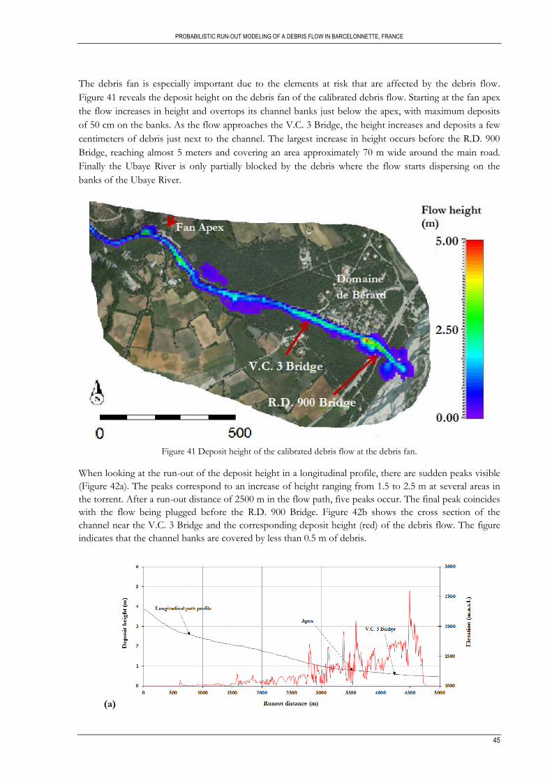
PROBABILISTIC RUN-OUT MODELING OF A DEBRIS FLOW IN BARCELONNETTE, FRANCE
45
The debris fan is especially important due to the elements at risk that are affected by the debris flow.
Figure 41 reveals the deposit height on the debris fan of the calibrated debris flow. Starting at the fan apex
the flow increases in height and overtops its channel banks just below the apex, with maximum deposits
of 50 cm on the banks. As the flow approaches the V.C. 3 Bridge, the height increases and deposits a few
centimeters of debris just next to the channel. The largest increase in height occurs before the R.D. 900
Bridge, reaching almost 5 meters and covering an area approximately 70 m wide around the main road.
Finally the Ubaye River is only partially blocked by the debris where the flow starts dispersing on the
banks of the Ubaye River.
Figure 41 Deposit height of the calibrated debris flow at the debris fan.
When looking at the run-out of the deposit height in a longitudinal profile, there are sudden peaks visible
(Figure 42a). The peaks correspond to an increase of height ranging from 1.5 to 2.5 m at several areas in
the torrent. After a run-out distance of 2500 m in the flow path, five peaks occur. The final peak coincides
with the flow being plugged before the R.D. 900 Bridge. Figure 42b shows the cross section of the
channel near the V.C. 3 Bridge and the corresponding deposit height (red) of the debris flow. The figure
indicates that the channel banks are covered by less than 0.5 m of debris.
(a)
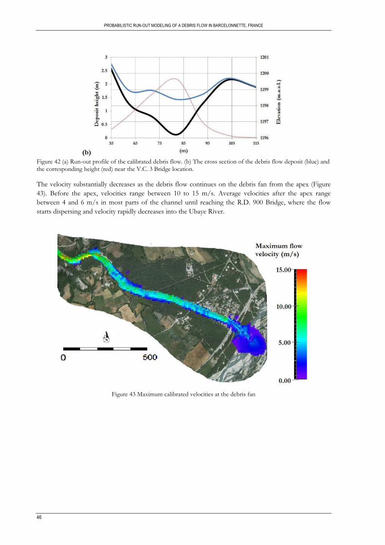
PROBABILISTIC RUN-OUT MODELING OF A DEBRIS FLOW IN BARCELONNETTE, FRANCE
46
(b)
Figure 42 (a) Run-out profile of the calibrated debris flow. (b) The cross section of the debris flow deposit (blue) and
the corresponding height (red) near the V.C. 3 Bridge location.
The velocity substantially decreases as the debris flow continues on the debris fan from the apex (Figure
43). Before the apex, velocities range between 10 to 15 m/s. Average velocities after the apex range
between 4 and 6 m/s in most parts of the channel until reaching the R.D. 900 Bridge, where the flow
starts dispersing and velocity rapidly decreases into the Ubaye River.
Figure 43 Maximum calibrated velocities at the debris fan
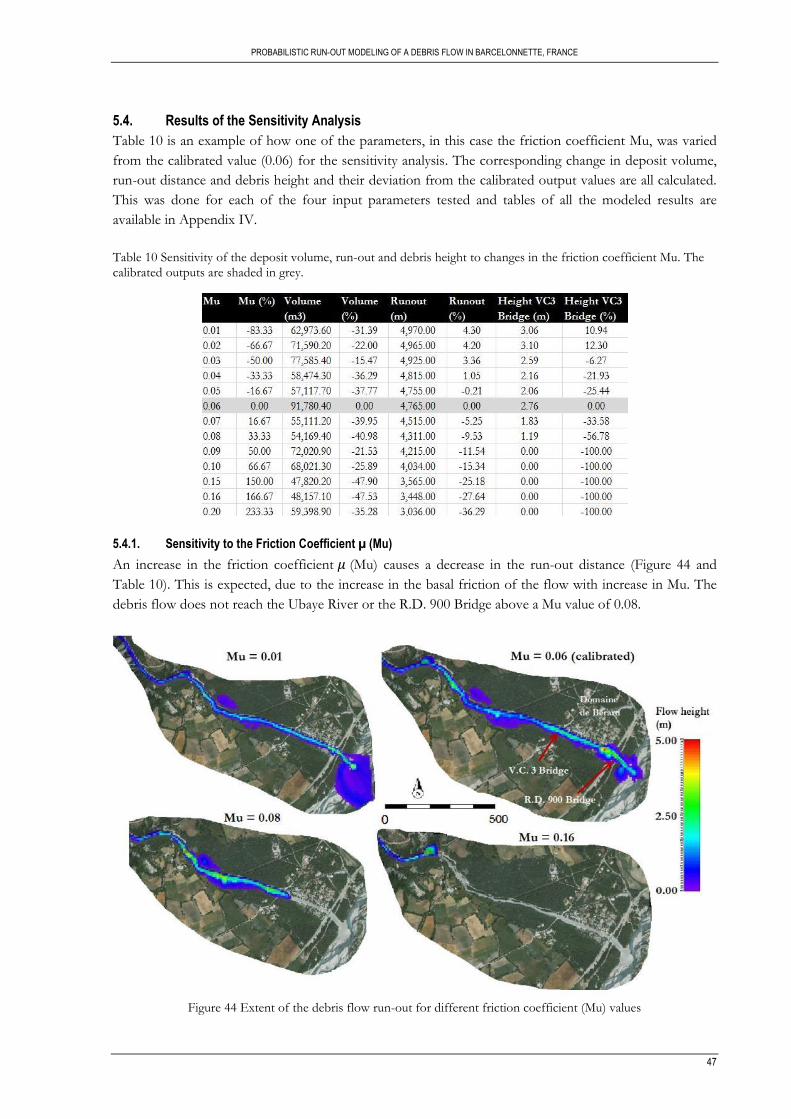
PROBABILISTIC RUN-OUT MODELING OF A DEBRIS FLOW IN BARCELONNETTE, FRANCE
47
5.4. Results of the Sensitivity Analysis
Table 10 is an example of how one of the parameters, in this case the friction coefficient Mu, was varied
from the calibrated value (0.06) for the sensitivity analysis. The corresponding change in deposit volume,
run-out distance and debris height and their deviation from the calibrated output values are all calculated.
This was done for each of the four input parameters tested and tables of all the modeled results are
available in Appendix IV.
Table 10 Sensitivity of the deposit volume, run-out and debris height to changes in the friction coefficient Mu. The calibrated outputs are shaded in grey.
5.4.1. Sensitivity to the Friction Coefficient µ (Mu)
An increase in the friction coefficient (Mu) causes a decrease in the run-out distance (Figure 44 and
Table 10). This is expected, due to the increase in the basal friction of the flow with increase in Mu. The
debris flow does not reach the Ubaye River or the R.D. 900 Bridge above a Mu value of 0.08.
Figure 44 Extent of the debris flow run-out for different friction coefficient (Mu) values
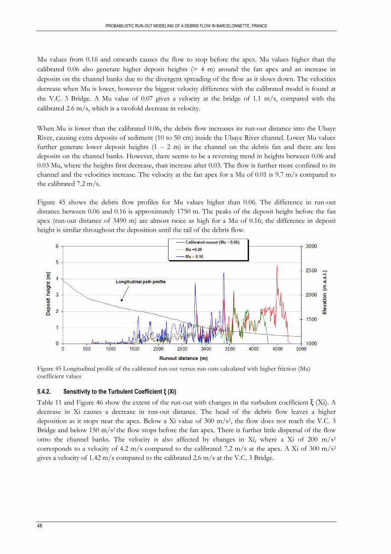
PROBABILISTIC RUN-OUT MODELING OF A DEBRIS FLOW IN BARCELONNETTE, FRANCE
48
Mu values from 0.16 and onwards causes the flow to stop before the apex. Mu values higher than the
calibrated 0.06 also generate higher deposit heights (> 4 m) around the fan apex and an increase in
deposits on the channel banks due to the divergent spreading of the flow as it slows down. The velocities
decrease when Mu is lower, however the biggest velocity difference with the calibrated model is found at
the V.C. 3 Bridge. A Mu value of 0.07 gives a velocity at the bridge of 1.1 m/s, compared with the
calibrated 2.6 m/s, which is a twofold decrease in velocity.
When Mu is lower than the calibrated 0.06, the debris flow increases its run-out distance into the Ubaye
River, causing extra deposits of sediment (10 to 50 cm) inside the Ubaye River channel. Lower Mu values
further generate lower deposit heights (1 – 2 m) in the channel on the debris fan and there are less
deposits on the channel banks. However, there seems to be a reversing trend in heights between 0.06 and
0.03 Mu, where the heights first decrease, than increase after 0.03. The flow is further more confined to its
channel and the velocities increase. The velocity at the fan apex for a Mu of 0.01 is 9.7 m/s compared to
the calibrated 7.2 m/s.
Figure 45 shows the debris flow profiles for Mu values higher than 0.06. The difference in run-out
distance between 0.06 and 0.16 is approximately 1750 m. The peaks of the deposit height before the fan
apex (run-out distance of 3490 m) are almost twice as high for a Mu of 0.16; the difference in deposit
height is similar throughout the deposition until the tail of the debris flow.
Figure 45 Longitudinal profile of the calibrated run-out versus run-outs calculated with higher friction (Mu) coefficient values
5.4.2. Sensitivity to the Turbulent Coefficient ξ (Xi)
Table 11 and Figure 46 show the extent of the run-out with changes in the turbulent coefficient (Xi). A
decrease in Xi causes a decrease in run-out distance. The head of the debris flow leaves a higher
deposition as it stops near the apex. Below a Xi value of 300 m/s2, the flow does not reach the V.C. 3
Bridge and below 150 m/s2 the flow stops before the fan apex. There is further little dispersal of the flow
onto the channel banks. The velocity is also affected by changes in Xi, where a Xi of 200 m/s2
corresponds to a velocity of 4.2 m/s compared to the calibrated 7.2 m/s at the apex. A Xi of 300 m/s2
gives a velocity of 1.42 m/s compared to the calibrated 2.6 m/s at the V.C. 3 Bridge.
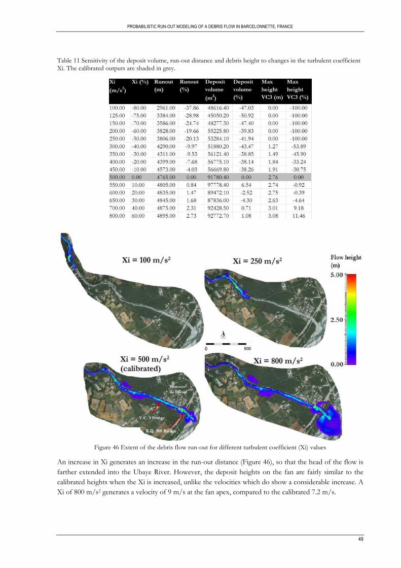
PROBABILISTIC RUN-OUT MODELING OF A DEBRIS FLOW IN BARCELONNETTE, FRANCE
49
Table 11 Sensitivity of the deposit volume, run-out distance and debris height to changes in the turbulent coefficient Xi. The calibrated outputs are shaded in grey.
Figure 46 Extent of the debris flow run-out for different turbulent coefficient (Xi) values
An increase in Xi generates an increase in the run-out distance (Figure 46), so that the head of the flow is
farther extended into the Ubaye River. However, the deposit heights on the fan are fairly similar to the
calibrated heights when the Xi is increased, unlike the velocities which do show a considerable increase. A
Xi of 800 m/s2 generates a velocity of 9 m/s at the fan apex, compared to the calibrated 7.2 m/s.
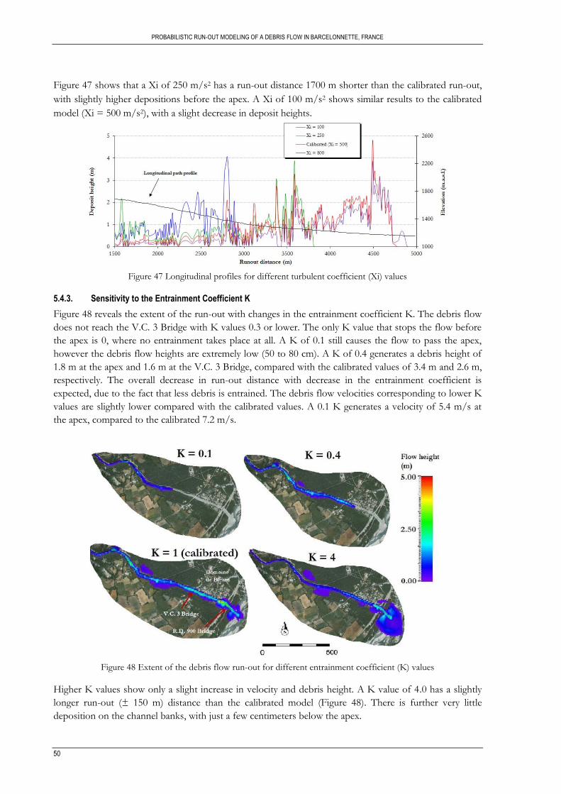
PROBABILISTIC RUN-OUT MODELING OF A DEBRIS FLOW IN BARCELONNETTE, FRANCE
50
Figure 47 shows that a Xi of 250 m/s2 has a run-out distance 1700 m shorter than the calibrated run-out,
with slightly higher depositions before the apex. A Xi of 100 m/s2 shows similar results to the calibrated
model (Xi = 500 m/s2), with a slight decrease in deposit heights.
Figure 47 Longitudinal profiles for different turbulent coefficient (Xi) values
5.4.3. Sensitivity to the Entrainment Coefficient K
Figure 48 reveals the extent of the run-out with changes in the entrainment coefficient K. The debris flow
does not reach the V.C. 3 Bridge with K values 0.3 or lower. The only K value that stops the flow before
the apex is 0, where no entrainment takes place at all. A K of 0.1 still causes the flow to pass the apex,
however the debris flow heights are extremely low (50 to 80 cm). A K of 0.4 generates a debris height of
1.8 m at the apex and 1.6 m at the V.C. 3 Bridge, compared with the calibrated values of 3.4 m and 2.6 m,
respectively. The overall decrease in run-out distance with decrease in the entrainment coefficient is
expected, due to the fact that less debris is entrained. The debris flow velocities corresponding to lower K
values are slightly lower compared with the calibrated values. A 0.1 K generates a velocity of 5.4 m/s at
the apex, compared to the calibrated 7.2 m/s.
Figure 48 Extent of the debris flow run-out for different entrainment coefficient (K) values
Higher K values show only a slight increase in velocity and debris height. A K value of 4.0 has a slightly
longer run-out (± 150 m) distance than the calibrated model (Figure 48). There is further very little
deposition on the channel banks, with just a few centimeters below the apex.
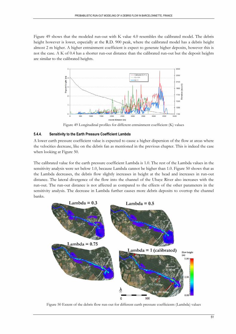
PROBABILISTIC RUN-OUT MODELING OF A DEBRIS FLOW IN BARCELONNETTE, FRANCE
51
Figure 49 shows that the modeled run-out with K value 4.0 resembles the calibrated model. The debris
height however is lower, especially at the R.D. 900 peak, where the calibrated model has a debris height
almost 2 m higher. A higher entrainment coefficient is expect to generate higher deposits, however this is
not the case. A K of 0.4 has a shorter run-out distance than the calibrated run-out but the deposit heights
are similar to the calibrated heights.
Figure 49 Longitudinal profiles for different entrainment coefficient (K) values
5.4.4. Sensitivity to the Earth Pressure Coefficient Lambda
A lower earth pressure coefficient value is expected to cause a higher dispersion of the flow at areas where
the velocities decrease, like on the debris fan as mentioned in the previous chapter. This is indeed the case
when looking at Figure 50.
The calibrated value for the earth pressure coefficient Lambda is 1.0. The rest of the Lambda values in the
sensitivity analysis were set below 1.0, because Lambda cannot be higher than 1.0. Figure 50 shows that as
the Lambda decreases, the debris flow slightly increases in height at the head and increases in run-out
distance. The lateral divergence of the flow into the channel of the Ubaye River also increases with the
run-out. The run-out distance is not affected as compared to the effects of the other parameters in the
sensitivity analysis. The decrease in Lambda further causes more debris deposits to overtop the channel
banks.
Figure 50 Extent of the debris flow run-out for different earth pressure coefficients (Lambda) values
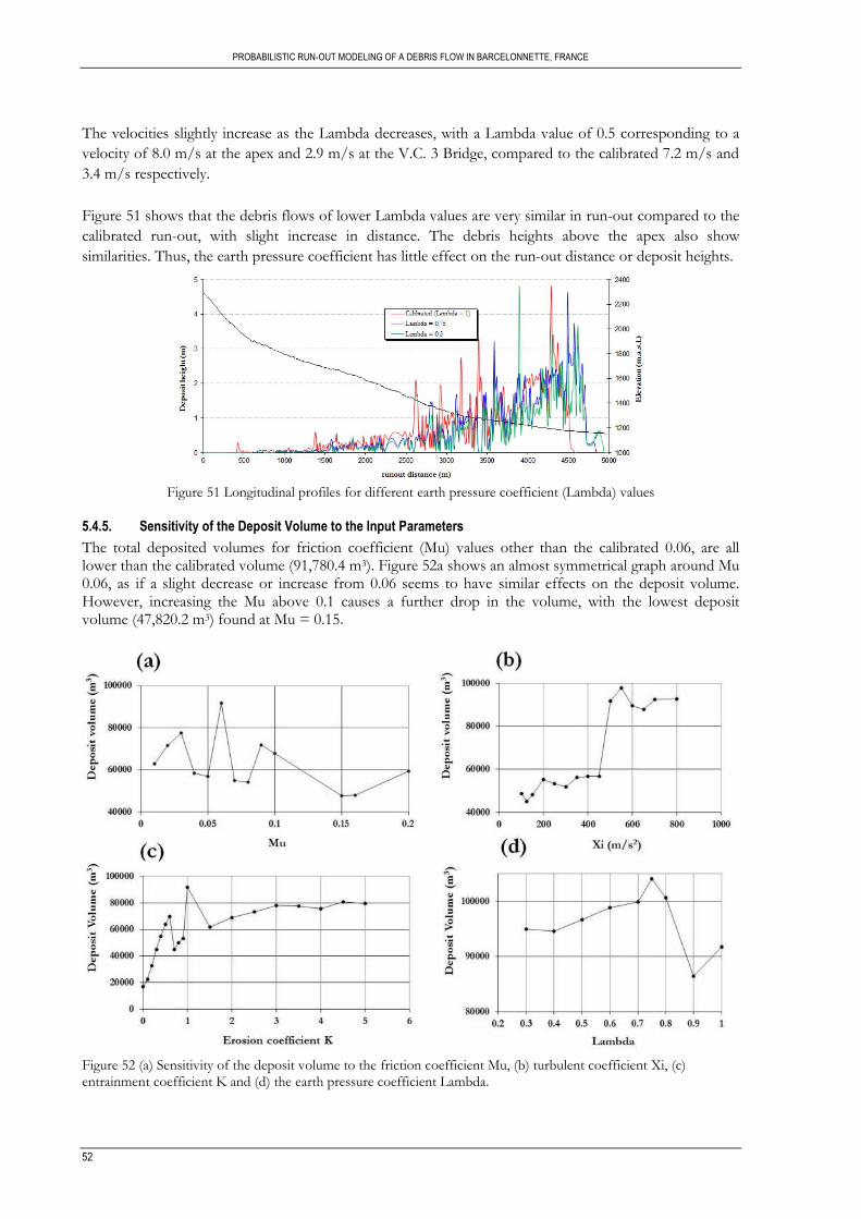
PROBABILISTIC RUN-OUT MODELING OF A DEBRIS FLOW IN BARCELONNETTE, FRANCE
52
The velocities slightly increase as the Lambda decreases, with a Lambda value of 0.5 corresponding to a
velocity of 8.0 m/s at the apex and 2.9 m/s at the V.C. 3 Bridge, compared to the calibrated 7.2 m/s and
3.4 m/s respectively.
Figure 51 shows that the debris flows of lower Lambda values are very similar in run-out compared to the
calibrated run-out, with slight increase in distance. The debris heights above the apex also show
similarities. Thus, the earth pressure coefficient has little effect on the run-out distance or deposit heights.
Figure 51 Longitudinal profiles for different earth pressure coefficient (Lambda) values
5.4.5. Sensitivity of the Deposit Volume to the Input Parameters
The total deposited volumes for friction coefficient (Mu) values other than the calibrated 0.06, are all lower than the calibrated volume (91,780.4 m3). Figure 52a shows an almost symmetrical graph around Mu 0.06, as if a slight decrease or increase from 0.06 seems to have similar effects on the deposit volume. However, increasing the Mu above 0.1 causes a further drop in the volume, with the lowest deposit volume (47,820.2 m3) found at Mu = 0.15.
Figure 52 (a) Sensitivity of the deposit volume to the friction coefficient Mu, (b) turbulent coefficient Xi, (c) entrainment coefficient K and (d) the earth pressure coefficient Lambda.
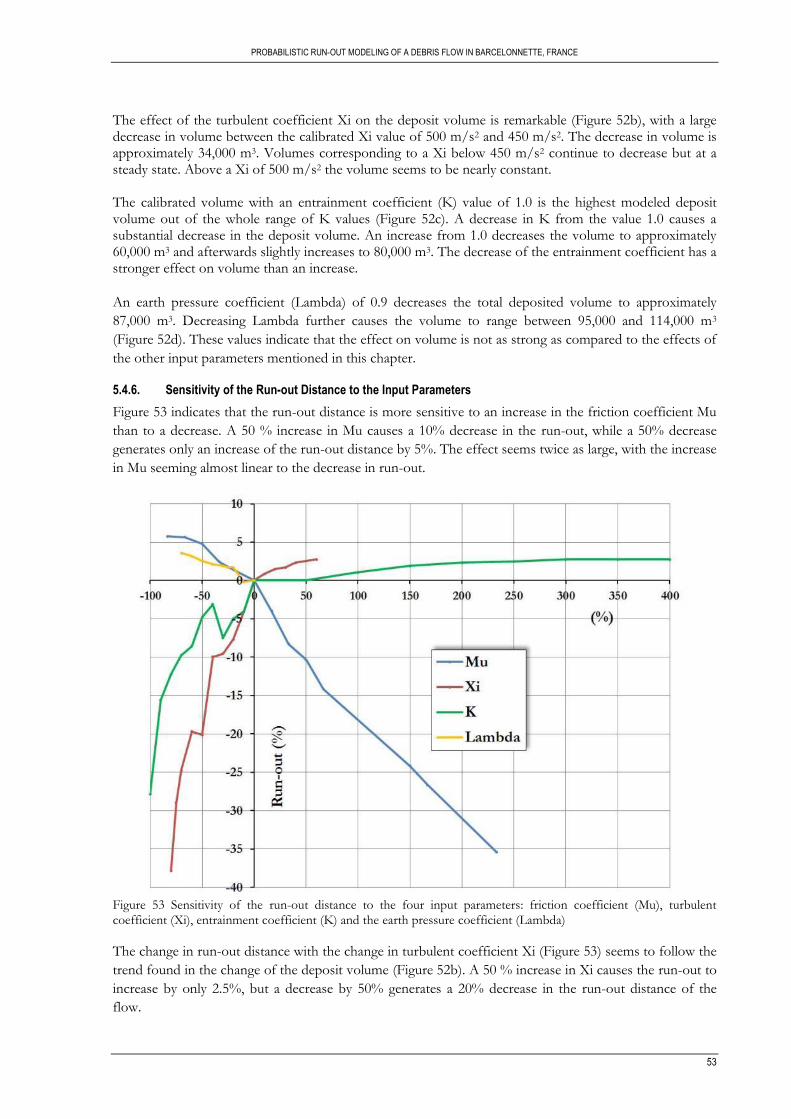
PROBABILISTIC RUN-OUT MODELING OF A DEBRIS FLOW IN BARCELONNETTE, FRANCE
53
The effect of the turbulent coefficient Xi on the deposit volume is remarkable (Figure 52b), with a large decrease in volume between the calibrated Xi value of 500 m/s2 and 450 m/s2. The decrease in volume is approximately 34,000 m3. Volumes corresponding to a Xi below 450 m/s2 continue to decrease but at a steady state. Above a Xi of 500 m/s2 the volume seems to be nearly constant. The calibrated volume with an entrainment coefficient (K) value of 1.0 is the highest modeled deposit volume out of the whole range of K values (Figure 52c). A decrease in K from the value 1.0 causes a substantial decrease in the deposit volume. An increase from 1.0 decreases the volume to approximately 60,000 m3 and afterwards slightly increases to 80,000 m3. The decrease of the entrainment coefficient has a stronger effect on volume than an increase.
An earth pressure coefficient (Lambda) of 0.9 decreases the total deposited volume to approximately
87,000 m3. Decreasing Lambda further causes the volume to range between 95,000 and 114,000 m3
(Figure 52d). These values indicate that the effect on volume is not as strong as compared to the effects of
the other input parameters mentioned in this chapter.
5.4.6. Sensitivity of the Run-out Distance to the Input Parameters
Figure 53 indicates that the run-out distance is more sensitive to an increase in the friction coefficient Mu
than to a decrease. A 50 % increase in Mu causes a 10% decrease in the run-out, while a 50% decrease
generates only an increase of the run-out distance by 5%. The effect seems twice as large, with the increase
in Mu seeming almost linear to the decrease in run-out.
Figure 53 Sensitivity of the run-out distance to the four input parameters: friction coefficient (Mu), turbulent coefficient (Xi), entrainment coefficient (K) and the earth pressure coefficient (Lambda)
The change in run-out distance with the change in turbulent coefficient Xi (Figure 53) seems to follow the
trend found in the change of the deposit volume (Figure 52b). A 50 % increase in Xi causes the run-out to
increase by only 2.5%, but a decrease by 50% generates a 20% decrease in the run-out distance of the
flow.
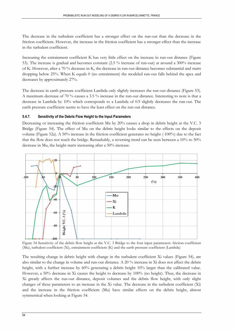
PROBABILISTIC RUN-OUT MODELING OF A DEBRIS FLOW IN BARCELONNETTE, FRANCE
54
The decrease in the turbulent coefficient has a stronger effect on the run-out than the decrease in the
friction coefficient. However, the increase in the friction coefficient has a stronger effect than the increase
in the turbulent coefficient.
Increasing the entrainment coefficient K has very little effect on the increase in run-out distance (Figure
53). The increase is gradual and becomes constant (2.5 % increase of run-out) at around a 300% increase
of K. However, after a 70 % decrease in K, the decrease in run-out distance becomes substantial and starts
dropping below 25%. When K equals 0 (no entrainment) the modeled run-out falls behind the apex and
decreases by approximately 27%.
The decrease in earth pressure coefficient Lambda only slightly increases the run-out distance (Figure 53).
A maximum decrease of 70 % causes a 3.5 % increase in the run-out distance. Interesting to note is that a
decrease in Lambda by 10% which corresponds to a Lambda of 0.9 slightly decreases the run-out. The
earth pressure coefficient seems to have the least effect on the run-out distance.
5.4.7. Sensitivity of the Debris Flow Height to the Input Parameters
Decreasing or increasing the friction coefficient Mu by 20% causes a drop in debris height at the V.C. 3
Bridge (Figure 54). The effect of Mu on the debris height looks similar to the effects on the deposit
volume (Figure 52a). A 50% increase in the friction coefficient generates no height (-100%) due to the fact
that the flow does not reach the bridge. Remarkably, a reversing trend can be seen between a 10% to 50%
decrease in Mu, the height starts increasing after a 50% increase.
Figure 54 Sensitivity of the debris flow height at the V.C. 3 Bridge to the four input parameters: friction coefficient (Mu), turbulent coefficient (Xi), entrainment coefficient (K) and the earth pressure coefficient (Lambda)
The resulting change in debris height with change in the turbulent coefficient Xi values (Figure 54), are
also similar to the change in volume and run-out distance. A 20 % increase in Xi does not affect the debris
height, with a further increase by 60% generating a debris height 10% larger than the calibrated value.
However, a 50% decrease in Xi causes the height to decrease by 100% (no height). Thus, the decrease in
Xi greatly affects the run-out distance, deposit volumes and the debris flow height, with only slight
changes of these parameters to an increase in the Xi value. The decrease in the turbulent coefficient (Xi)
and the increase in the friction coefficient (Mu) have similar effects on the debris height, almost
symmetrical when looking at Figure 54.
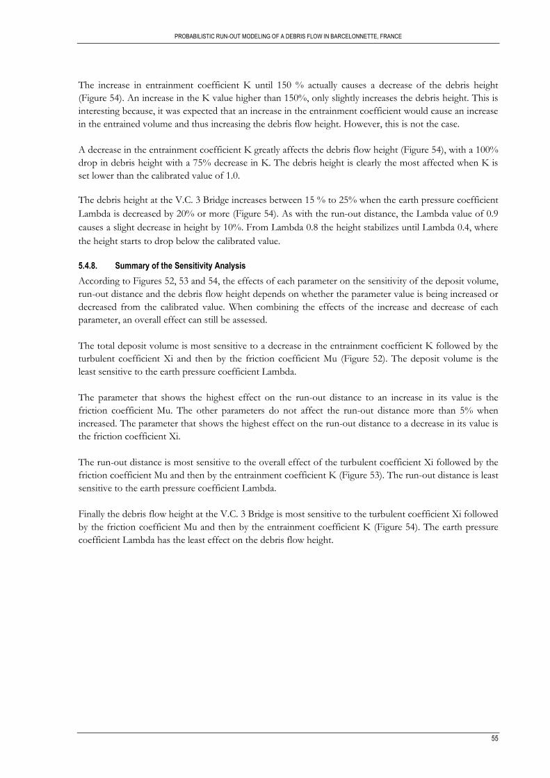
PROBABILISTIC RUN-OUT MODELING OF A DEBRIS FLOW IN BARCELONNETTE, FRANCE
55
The increase in entrainment coefficient K until 150 % actually causes a decrease of the debris height
(Figure 54). An increase in the K value higher than 150%, only slightly increases the debris height. This is
interesting because, it was expected that an increase in the entrainment coefficient would cause an increase
in the entrained volume and thus increasing the debris flow height. However, this is not the case.
A decrease in the entrainment coefficient K greatly affects the debris flow height (Figure 54), with a 100%
drop in debris height with a 75% decrease in K. The debris height is clearly the most affected when K is
set lower than the calibrated value of 1.0.
The debris height at the V.C. 3 Bridge increases between 15 % to 25% when the earth pressure coefficient
Lambda is decreased by 20% or more (Figure 54). As with the run-out distance, the Lambda value of 0.9
causes a slight decrease in height by 10%. From Lambda 0.8 the height stabilizes until Lambda 0.4, where
the height starts to drop below the calibrated value.
5.4.8. Summary of the Sensitivity Analysis
According to Figures 52, 53 and 54, the effects of each parameter on the sensitivity of the deposit volume,
run-out distance and the debris flow height depends on whether the parameter value is being increased or
decreased from the calibrated value. When combining the effects of the increase and decrease of each
parameter, an overall effect can still be assessed.
The total deposit volume is most sensitive to a decrease in the entrainment coefficient K followed by the
turbulent coefficient Xi and then by the friction coefficient Mu (Figure 52). The deposit volume is the
least sensitive to the earth pressure coefficient Lambda.
The parameter that shows the highest effect on the run-out distance to an increase in its value is the
friction coefficient Mu. The other parameters do not affect the run-out distance more than 5% when
increased. The parameter that shows the highest effect on the run-out distance to a decrease in its value is
the friction coefficient Xi.
The run-out distance is most sensitive to the overall effect of the turbulent coefficient Xi followed by the
friction coefficient Mu and then by the entrainment coefficient K (Figure 53). The run-out distance is least
sensitive to the earth pressure coefficient Lambda.
Finally the debris flow height at the V.C. 3 Bridge is most sensitive to the turbulent coefficient Xi followed
by the friction coefficient Mu and then by the entrainment coefficient K (Figure 54). The earth pressure
coefficient Lambda has the least effect on the debris flow height.
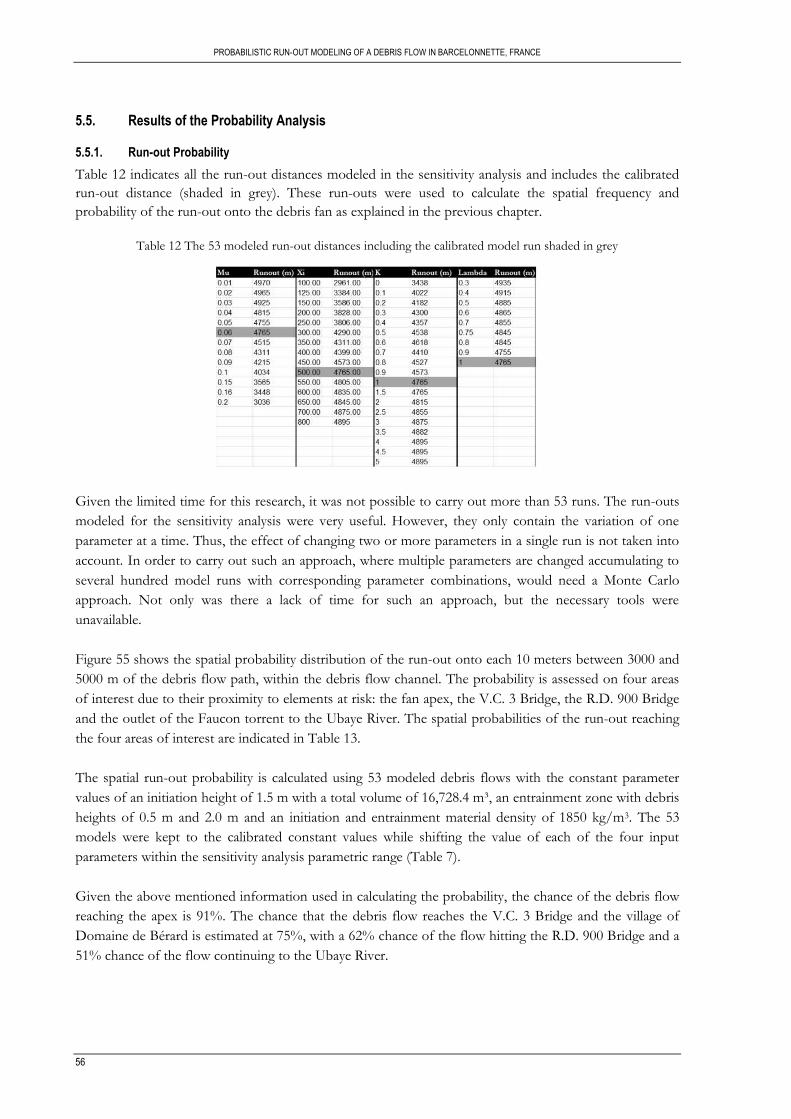
PROBABILISTIC RUN-OUT MODELING OF A DEBRIS FLOW IN BARCELONNETTE, FRANCE
56
5.5. Results of the Probability Analysis
5.5.1. Run-out Probability
Table 12 indicates all the run-out distances modeled in the sensitivity analysis and includes the calibrated
run-out distance (shaded in grey). These run-outs were used to calculate the spatial frequency and
probability of the run-out onto the debris fan as explained in the previous chapter.
Table 12 The 53 modeled run-out distances including the calibrated model run shaded in grey
Given the limited time for this research, it was not possible to carry out more than 53 runs. The run-outs
modeled for the sensitivity analysis were very useful. However, they only contain the variation of one
parameter at a time. Thus, the effect of changing two or more parameters in a single run is not taken into
account. In order to carry out such an approach, where multiple parameters are changed accumulating to
several hundred model runs with corresponding parameter combinations, would need a Monte Carlo
approach. Not only was there a lack of time for such an approach, but the necessary tools were
unavailable.
Figure 55 shows the spatial probability distribution of the run-out onto each 10 meters between 3000 and
5000 m of the debris flow path, within the debris flow channel. The probability is assessed on four areas
of interest due to their proximity to elements at risk: the fan apex, the V.C. 3 Bridge, the R.D. 900 Bridge
and the outlet of the Faucon torrent to the Ubaye River. The spatial probabilities of the run-out reaching
the four areas of interest are indicated in Table 13.
The spatial run-out probability is calculated using 53 modeled debris flows with the constant parameter
values of an initiation height of 1.5 m with a total volume of 16,728.4 m³, an entrainment zone with debris
heights of 0.5 m and 2.0 m and an initiation and entrainment material density of 1850 kg/m3. The 53
models were kept to the calibrated constant values while shifting the value of each of the four input
parameters within the sensitivity analysis parametric range (Table 7).
Given the above mentioned information used in calculating the probability, the chance of the debris flow
reaching the apex is 91%. The chance that the debris flow reaches the V.C. 3 Bridge and the village of
Domaine de Bérard is estimated at 75%, with a 62% chance of the flow hitting the R.D. 900 Bridge and a
51% chance of the flow continuing to the Ubaye River.
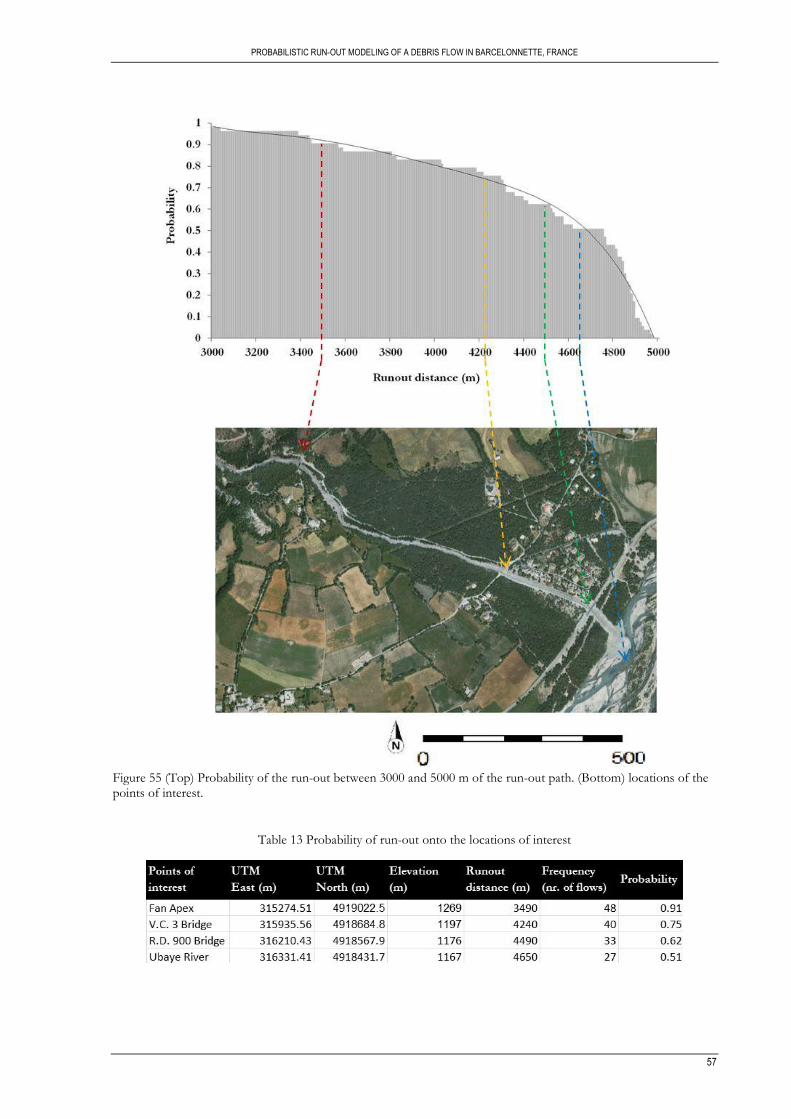
PROBABILISTIC RUN-OUT MODELING OF A DEBRIS FLOW IN BARCELONNETTE, FRANCE
57
Figure 55 (Top) Probability of the run-out between 3000 and 5000 m of the run-out path. (Bottom) locations of the points of interest.
Table 13 Probability of run-out onto the locations of interest
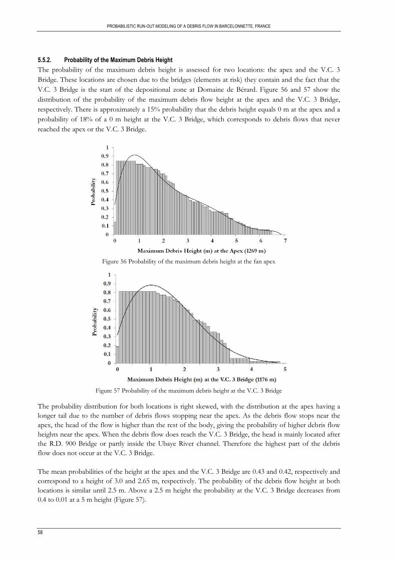
PROBABILISTIC RUN-OUT MODELING OF A DEBRIS FLOW IN BARCELONNETTE, FRANCE
58
5.5.2. Probability of the Maximum Debris Height
The probability of the maximum debris height is assessed for two locations: the apex and the V.C. 3
Bridge. These locations are chosen due to the bridges (elements at risk) they contain and the fact that the
V.C. 3 Bridge is the start of the depositional zone at Domaine de Bérard. Figure 56 and 57 show the
distribution of the probability of the maximum debris flow height at the apex and the V.C. 3 Bridge,
respectively. There is approximately a 15% probability that the debris height equals 0 m at the apex and a
probability of 18% of a 0 m height at the V.C. 3 Bridge, which corresponds to debris flows that never
reached the apex or the V.C. 3 Bridge.
Figure 56 Probability of the maximum debris height at the fan apex
Figure 57 Probability of the maximum debris height at the V.C. 3 Bridge
The probability distribution for both locations is right skewed, with the distribution at the apex having a
longer tail due to the number of debris flows stopping near the apex. As the debris flow stops near the
apex, the head of the flow is higher than the rest of the body, giving the probability of higher debris flow
heights near the apex. When the debris flow does reach the V.C. 3 Bridge, the head is mainly located after
the R.D. 900 Bridge or partly inside the Ubaye River channel. Therefore the highest part of the debris
flow does not occur at the V.C. 3 Bridge.
The mean probabilities of the height at the apex and the V.C. 3 Bridge are 0.43 and 0.42, respectively and
correspond to a height of 3.0 and 2.65 m, respectively. The probability of the debris flow height at both
locations is similar until 2.5 m. Above a 2.5 m height the probability at the V.C. 3 Bridge decreases from
0.4 to 0.01 at a 5 m height (Figure 57).
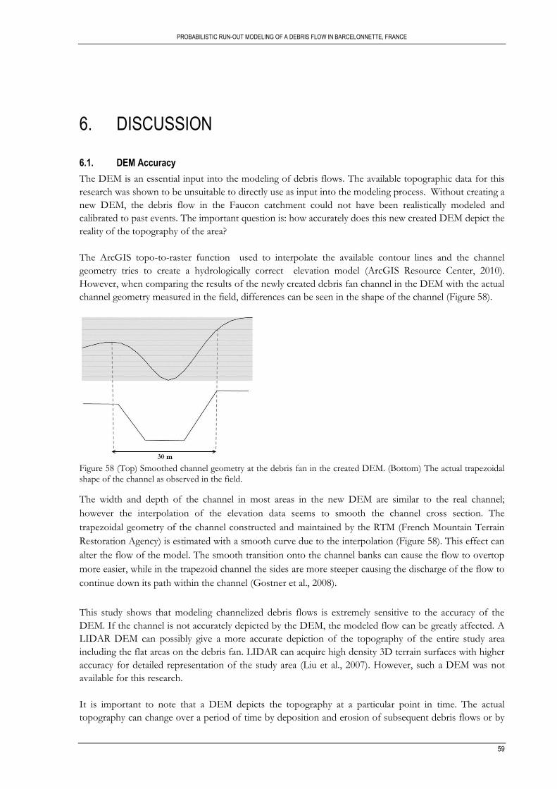
PROBABILISTIC RUN-OUT MODELING OF A DEBRIS FLOW IN BARCELONNETTE, FRANCE
59
6. DISCUSSION
6.1. DEM Accuracy
The DEM is an essential input into the modeling of debris flows. The available topographic data for this
research was shown to be unsuitable to directly use as input into the modeling process. Without creating a
new DEM, the debris flow in the Faucon catchment could not have been realistically modeled and
calibrated to past events. The important question is: how accurately does this new created DEM depict the
reality of the topography of the area?
The ArcGIS topo-to-raster function used to interpolate the available contour lines and the channel
geometry tries to create a hydrologically correct elevation model (ArcGIS Resource Center, 2010).
However, when comparing the results of the newly created debris fan channel in the DEM with the actual
channel geometry measured in the field, differences can be seen in the shape of the channel (Figure 58).
Figure 58 (Top) Smoothed channel geometry at the debris fan in the created DEM. (Bottom) The actual trapezoidal shape of the channel as observed in the field.
The width and depth of the channel in most areas in the new DEM are similar to the real channel;
however the interpolation of the elevation data seems to smooth the channel cross section. The
trapezoidal geometry of the channel constructed and maintained by the RTM (French Mountain Terrain
Restoration Agency) is estimated with a smooth curve due to the interpolation (Figure 58). This effect can
alter the flow of the model. The smooth transition onto the channel banks can cause the flow to overtop
more easier, while in the trapezoid channel the sides are more steeper causing the discharge of the flow to
continue down its path within the channel (Gostner et al., 2008).
This study shows that modeling channelized debris flows is extremely sensitive to the accuracy of the
DEM. If the channel is not accurately depicted by the DEM, the modeled flow can be greatly affected. A
LIDAR DEM can possibly give a more accurate depiction of the topography of the entire study area
including the flat areas on the debris fan. LIDAR can acquire high density 3D terrain surfaces with higher
accuracy for detailed representation of the study area (Liu et al., 2007). However, such a DEM was not
available for this research.
It is important to note that a DEM depicts the topography at a particular point in time. The actual
topography can change over a period of time by deposition and erosion of subsequent debris flows or by
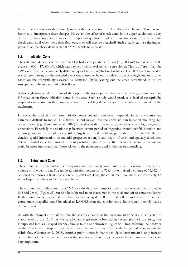
PROBABILISTIC RUN-OUT MODELING OF A DEBRIS FLOW IN BARCELONNETTE, FRANCE
60
human modifications to the channel, such as the construction of dikes along the channel. This research
has tried to incorporate these changes. However, the effect of check dams in the upper catchment is very
difficult to incorporate in the model. An important question to ask in future studies on the area: will the
check dams hold when the debris flow occurs or will they be breached? Such a study can use the impact
pressure on the check dams which RAMMS is able to calculate.
6.2. Initiation Zone
The calibrated debris flow that was modeled had a comparable initiation (16,728.4 m³) to that of the 2003
event (14,000 – 17,000 m³), which was a type of debris avalanche in scree slopes. This is different than the
1996 event that had a completely different type of initiation (shallow landslide). The 2003 event initiated in
two different areas, but the modeled event was chosen to be only modeled from one single initiation zone,
based on the susceptibility assessed by Remaître (2006), leaving out the areas determined to be less
susceptible to the initiation of debris flows.
A thorough susceptibility analysis of the slopes in the upper part of the catchment can give more accurate
information on future initiation zones in the area. Such a study would produce a detailed susceptibility
map that can be used in the future as a basis for modeling debris flows or other mass movements in the
catchment.
However, the prediction of future initiation zones, initiation modes and especially initiation volumes, are
extremely difficult to model. This thesis has not looked into the uncertainty in initiation modeling, but
other studies (e.g. Kuriakose et al., 2010) have shown that the initiation also has a very high degree of
uncertainty. Especially the relationship between return period of triggering events (rainfall duration and
intensity) and initiation volumes is still a largely unsolved problem, partly due to the unavailability of
detailed spatial information on material properties (strength and depth of soils) and spatially distributed
detailed rainfall data. In terms of run-out probability the effect of the uncertainty in initiation volume
could be more important than those related to the parameters used in the run-out modeling.
6.3. Entrainment Zone
The entrainment of material in the transport zone is extremely important to the production of the deposit
volume on the debris fan. The modeled initiation volume of 16,728.4 m³ entrained a volume of 75,052 m³
of debris to produce a final deposition of 91,780.4 m³. Thus, the entrainment volume is approximately 4.5
times larger than the actual initiation volume.
The entrainment method used in RAMMS of dividing the transport zone in two averaged debris heights
(0.5 and 2.0 m) (Figure 33) can also be subjected to an inaccuracy in the total amount of entrained debris.
If the entrainment height did not have to be averaged to 0.5 m and 2.0 m and if more than two
entrainment shapefiles could be added to RAMMS, than the entrainment volume would possibly have a
different value.
As with the channel at the debris fan, the steeper channel of the entrainment zone is also subjected to
inaccuracies in the DEM. A V-shaped channel geometry observed in several parts of the zone, was
interpolated into a U-shaped channel, similar to the one shown in Figure 58. Thus, affecting the behavior
of the flow in the transport zone. A narrower channel can increase the discharge and velocities of the
debris flow (Gostner et al., 2008). Another point to note is that the modeled entrainment is only focused
on the base of the channel and not on the side walls. Therefore, changes in the entrainment height are
very important.
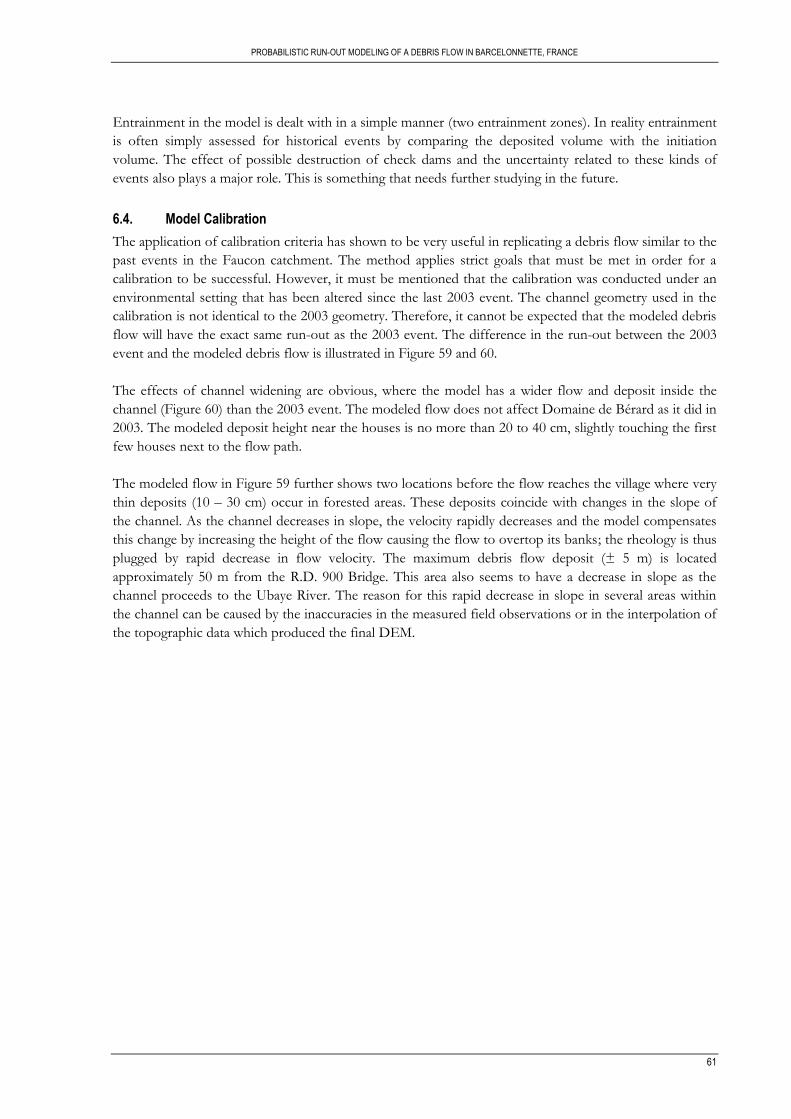
PROBABILISTIC RUN-OUT MODELING OF A DEBRIS FLOW IN BARCELONNETTE, FRANCE
61
Entrainment in the model is dealt with in a simple manner (two entrainment zones). In reality entrainment
is often simply assessed for historical events by comparing the deposited volume with the initiation
volume. The effect of possible destruction of check dams and the uncertainty related to these kinds of
events also plays a major role. This is something that needs further studying in the future.
6.4. Model Calibration
The application of calibration criteria has shown to be very useful in replicating a debris flow similar to the
past events in the Faucon catchment. The method applies strict goals that must be met in order for a
calibration to be successful. However, it must be mentioned that the calibration was conducted under an
environmental setting that has been altered since the last 2003 event. The channel geometry used in the
calibration is not identical to the 2003 geometry. Therefore, it cannot be expected that the modeled debris
flow will have the exact same run-out as the 2003 event. The difference in the run-out between the 2003
event and the modeled debris flow is illustrated in Figure 59 and 60.
The effects of channel widening are obvious, where the model has a wider flow and deposit inside the
channel (Figure 60) than the 2003 event. The modeled flow does not affect Domaine de Bérard as it did in
2003. The modeled deposit height near the houses is no more than 20 to 40 cm, slightly touching the first
few houses next to the flow path.
The modeled flow in Figure 59 further shows two locations before the flow reaches the village where very
thin deposits (10 – 30 cm) occur in forested areas. These deposits coincide with changes in the slope of
the channel. As the channel decreases in slope, the velocity rapidly decreases and the model compensates
this change by increasing the height of the flow causing the flow to overtop its banks; the rheology is thus
plugged by rapid decrease in flow velocity. The maximum debris flow deposit (± 5 m) is located
approximately 50 m from the R.D. 900 Bridge. This area also seems to have a decrease in slope as the
channel proceeds to the Ubaye River. The reason for this rapid decrease in slope in several areas within
the channel can be caused by the inaccuracies in the measured field observations or in the interpolation of
the topographic data which produced the final DEM.
PROBABILISTIC RUN-OUT MODELING OF A DEBRIS FLOW IN BARCELONNETTE, FRANCE
62
Figure 59 (Top) The 2003 debris flow run-out extent onto the debris fan (adapted from: Remaître (2006)) and (bottom) the calibrated model run-out.
Figure 60. The 2003 event versus the modeled debris flow at Domaine de Bérard
6.5. Sensitivity Analysis
6.5.1. Deposit Volume
The total deposit volume was found to be most sensitive to the entrainment coefficient K (Figure 52c).
The change in K values between 0 and 1 greatly influence the entrainment rate and thus the deposit
volume. Interesting to note is that the entrainment coefficient has little effect on the deposit volume
above a value of 1 (Figure 52c). According to Christen et al. (2010c), as the K value increases from 1 to 5,
the debris flow height and the entrainment rate increases (Figure 61). This research indeed shows that
higher entrainment coefficient values increase the debris flow height (Figure 54). However, K values
higher than 1 do not produce larger deposit volumes than the calibrated 91,780.4 m³. Even if the
calibrated entrainment volume of 75,052 m³ is assumed to be the maximum available entrainment volume,
why do entrainment coefficient values of 2 or 5 do not pick up this entire volume, like the K value of 1?
This question remains to be answered. Further studies are needed in the future to see how exactly the
entrainment coefficient used in RAMMS effects the total entrained and deposited volumes
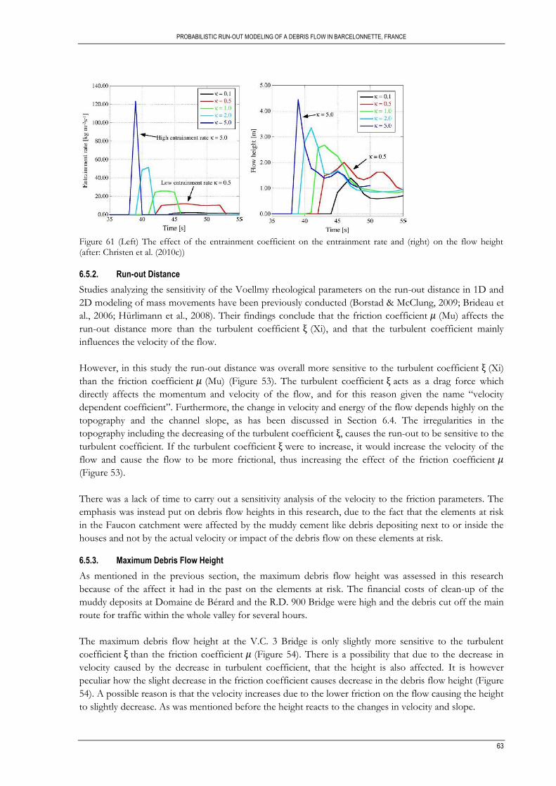
PROBABILISTIC RUN-OUT MODELING OF A DEBRIS FLOW IN BARCELONNETTE, FRANCE
63
Figure 61 (Left) The effect of the entrainment coefficient on the entrainment rate and (right) on the flow height (after: Christen et al. (2010c))
6.5.2. Run-out Distance
Studies analyzing the sensitivity of the Voellmy rheological parameters on the run-out distance in 1D and
2D modeling of mass movements have been previously conducted (Borstad & McClung, 2009; Brideau et
al., 2006; Hürlimann et al., 2008). Their findings conclude that the friction coefficient (Mu) affects the
run-out distance more than the turbulent coefficient (Xi), and that the turbulent coefficient mainly
influences the velocity of the flow.
However, in this study the run-out distance was overall more sensitive to the turbulent coefficient (Xi)
than the friction coefficient (Mu) (Figure 53). The turbulent coefficient acts as a drag force which
directly affects the momentum and velocity of the flow, and for this reason given the name “velocity
dependent coefficient”. Furthermore, the change in velocity and energy of the flow depends highly on the
topography and the channel slope, as has been discussed in Section 6.4. The irregularities in the
topography including the decreasing of the turbulent coefficient , causes the run-out to be sensitive to the
turbulent coefficient. If the turbulent coefficient were to increase, it would increase the velocity of the
flow and cause the flow to be more frictional, thus increasing the effect of the friction coefficient
(Figure 53).
There was a lack of time to carry out a sensitivity analysis of the velocity to the friction parameters. The
emphasis was instead put on debris flow heights in this research, due to the fact that the elements at risk
in the Faucon catchment were affected by the muddy cement like debris depositing next to or inside the
houses and not by the actual velocity or impact of the debris flow on these elements at risk.
6.5.3. Maximum Debris Flow Height
As mentioned in the previous section, the maximum debris flow height was assessed in this research
because of the affect it had in the past on the elements at risk. The financial costs of clean-up of the
muddy deposits at Domaine de Bérard and the R.D. 900 Bridge were high and the debris cut off the main
route for traffic within the whole valley for several hours.
The maximum debris flow height at the V.C. 3 Bridge is only slightly more sensitive to the turbulent
coefficient than the friction coefficient (Figure 54). There is a possibility that due to the decrease in
velocity caused by the decrease in turbulent coefficient, that the height is also affected. It is however
peculiar how the slight decrease in the friction coefficient causes decrease in the debris flow height (Figure
54). A possible reason is that the velocity increases due to the lower friction on the flow causing the height
to slightly decrease. As was mentioned before the height reacts to the changes in velocity and slope.
PROBABILISTIC RUN-OUT MODELING OF A DEBRIS FLOW IN BARCELONNETTE, FRANCE
64
Thus, the heights depend also on the topography. If there are sudden decreases in slope as mentioned
previously in this chapter, the velocity can drastically decrease while at the same time increasing the height.
This is possibly the cause of the irregularities found in the change of the debris height in the sensitivity
analysis (Figure 54).
6.6. Spatial Probability
The probability was calculated using the output of the sensitivity analysis, which are the 53 modeled run-
outs. The trend in the spatial run-out and debris height probability seems logic (Figure 55, 56 and 57). A
longer run-out distance or a higher debris flow height has a lower probability of occurrence than a shorter
run-out or a lower height. However the actual probabilities seem high, like a 91% chance of a debris flow
reaching the fan apex. The reason for these high probabilities is the number of debris flows modeled and
the parameter values chosen. Due to a lack of time more runs could not be carried out.
This study has first calibrated the model based on past events and on the basis of the calibrated input
parameters, a systematic sampling scheme starting at the calibrated value was applied. If sampling occurs
from a specific calibrated point, than it cannot be considered random. The uncertainty of the input
parameters is therefore determined by the calibrated parameters.
If the Voellmy parameter values would have been sampled randomly including the probability for a single
parameter value from a probability density function, instead of using a systematic sampling method (0.06,
0.08, 0.1…etc.) from the calibrated value, than a more accurate probability could have been found. Also
the number of modeled runs can be increased in future studies to get a better probability.
A Monte-Carlo method can be applied in the future to randomly sample the parameter values including
the uncertainty of the parameters and applying them to a numerical model. This would produce hundreds
or even thousands of run-outs for a whole range of parameters. The parameters would not have to be
kept constant in such a method due to the vast number of runs that can be conducted. Such a study could
also give indications of parameters having influence on other parameters and if there is any statistical
relationship between them. Due to the lack of time and material in this research, a random generation of
input parameters including the assessment of their uncertainty could not be conducted. Therefore, it is
highly advised to look at the uncertainties of the parameters when approaching debris flow modeling in a
stochastic manner.
65
7. CONCLUSIONS AND RECOMMENDATIONS
7.1. Conclusions
The main objective of this thesis was to model the run-out and debris height of a channeled debris flow
located within the Barcelonnette basin, in order to evaluate the possible ranges of the areas affected by the
run-out, to characterize the ranges of the input parameters in the modeling and to assess the probability of
the output. The sub-objectives and the conclusions drawn from them are stated as follows:
1. To assess the applicability of the Voellmy rheology applied by the RAMMS software, originally
designed for snow avalanches, to model debris flow run-outs in channelized environments.
This study has shown that the Voellmy rheology imbedded in the RAMMS dynamic modeling
software can be applied to model channelized debris flow run-outs successfully, assuming that the
user knows which input parameter values are needed and has gathered knowledge on the
environmental setting and the past debris flow events in the area.
2. To calibrate the model input parameters in order to obtain debris flow run-outs and heights based
on the past events in the Faucon catchment
The method of applying calibration criteria has shown to be a successful approach for obtaining
the calibrated input parameters, thus narrowing down the possibility of having more than one
combination of input parameters giving the same output. The resulting calibrated model has been
able to accurately reproduce the run-out distance within the ranges of the past events at the
catchment. The under prediction of the model to the debris heights is due to the change in
channel geometry since the last debris flow event. However, it can be concluded that the
construction carried out on the channel after 2003 are considered to be adequate for protecting
the village from debris flows with the same deposit volumes as those in 1996 and 2003.
3. To determine the sensitivity of the RAMMS dynamic model with respect to the various input
parameters
The total deposit volume of the debris flow modeled in RAMMS is most sensitive to the
entrainment coefficient K. The run-out distance and the maximum debris flow height of the
modeled debris flow is most sensitive to changes in the turbulent coefficient followed by the
friction coefficient . This is based on the irregularities found in the topography which have
influenced the velocity of the debris flow in its channel.
4. To study the effect of the DEM used as input in the run-out model
The study has found that the DEM accuracy greatly affects the topography of the area and the
geometry of the debris flow channel. This directly affects the behavior of the debris flow in terms
of velocity and debris flow height. A rapid decrease of the channel slope causes a decrease in
velocity and run-out distance leading to an increase in the deposit height at the head of deposited
debris flow. If the channel is simply not being depicted in the DEM, than the DEM must be
66
adjusted in order to recreate the actual topography, otherwise using the DEM would lead to
unrealistic results.
5. To obtain the spatial probability of the modeled debris flow run-out and deposit height
The spatial probability of a debris flow reaching the elements at risk at the village of Domaine de
Bérard is estimated at 75% and is based on an initiation volume of 16,728.4 m³ with 53 modeled
run-outs including their corresponding input parameter ranges. The probability of the debris flow
reaching a height of 4 m is 26% at the apex and only 2% at the village of Domaine de Bérard.
The RAMMS dynamic model with the embedded Voellmy rheology seems very useful to accurately model
debris flow run-outs. This powerful modeling tool, if incorporated into a full scale risk assessment can
possibly give very good results. The output of the probability of the initiation (temporal and spatial) can be
incorporated into modeling software like RAMMS to assess the spatial run-out probability. The output
intensity parameters associated with the run-out probability can then be used to assess the vulnerability of
the elements at risk on the debris fan. Thus, powerful modeling software like RAMMS which has shown
to be capable of modeling run-outs accurately can be used as a stepping stone between the probability of
initiation and the vulnerability assessment within the risk assessment framework.
7.2. Recommendations
A LIDAR DEM can be very useful as input into the RAMMS software in order to accurately
model the channelized debris flows at the Faucon catchment in the future. This does not only
apply to the Faucon area or the RAMMS software, but also to any 2D modeling software trying to
model channelized debris flows over long run-out distances.
It is advised to thoroughly analysis the change in slope of the debris flow channel in the DEM
and the effect of this slope on the changes in the velocities of the flow. This is important when
using RAMMS in specific or other 2D rheological continuum models in general.
When dealing with modeling of channelized debris flows and their extent onto debris fans or
other flat areas, high resolution imagery can be of great use to show where exactly the debris flow
strikes the elements at risk. The more accurate this data is, the better the hazard assessment will
be.
The grid resolution chosen for modeling these types of debris flows in RAMMS can be increased
to a 5 or even a 1 m grid cell resolution in order to generate more detail in the extent of the
deposits at the debris fan. However, the user must be aware of the increase in calculation times.
Future studies can use a Monte-Carlo approach to obtain the uncertainties of the rheological
input parameters used in 2D numerical continuum modeling. The parameter uncertainty can be
further applied in the hazard or risk assessment of landslides. However, one must find a practical
solution to automatically enter the high number of randomly generated parameter values into the
modeling process. RAMMS as it is would not be suitable for that, as it is currently not possible to
automate the input procedure for the parameters, using some sort of batch file approach. It can
be recommended to the model developers to make such an approach possible, and develop some
kind of Monte Carlo simulation interface for the model.
67
RAMMS is capable of producing other intensity parameters that have not been thoroughly
assessed in this research, like the velocity and impact pressure. Future studies using RAMMS can
test the sensitivity of these outputs to the rheological parameters.
The compiled data in this thesis can be used to find relationships between other types of outputs
like the total surface extent of the run-out, the vertical travel distance and the change in the
energy of the flow (momentum, kinetic energy) versus the input parameters or the initiation
volume.
Further study is needed on how the entrainment process in RAMMS exactly affects the
entrainment and deposit volume outputs. It may be possible to study entrainment and
depositional features in the transport zone (levees, scouring) after a debris flow has taken place, at
least to determine the areas of entrainment even if the volume is unknown.
The data acquired in this thesis can be used as the spatial component of a hazard assessment.
However, it is advised to increase the number of runs based on a stochastic method to optimize
the spatial probability and to find the uncertainties of the input parameters.

69
LIST OF REFERENCES
ArcGIS Resource Center. (2010). How Topo to Raster works. Retrieved December 1st, 2010, from
http://help.arcgis.com/en/arcgisdesktop/10.0/help/index.html#/How_Topo_to_Raster_works/009z0000007m000000/
Ayotte, D., & Hungr, O. (2000). Calibration of a runout prediction model for debris-flows and avalanches. In G. F. Wieczorek & N. D. Naeser (Eds.), Debris-Flow Hazards Mitigation: Mechanics, Prediction, and Assessment, Proc. 2nd International DFHM Conference (pp. 505-514). Taipei, Taiwan.
Bartelt, P., Salm, B., & Gruber, U. (1999). Calculating dense-snow avalanche runout using a Voellmy-fluid model with active/passive longitudinal straining. Journal of Glaciology, 45(150), 242-254.
Beguería, S., van Asch, T. W. J., Malet, J.-P., & Gröndahl, S. (2009). A GIS-based numerical model for simulating the kinematics of mud and debris flows over complex terrain. Natural Hazards and Earth System Science, 9(6), 1897-1909.
Borstad, C. P., & McClung, D. M. (2009). Sensitivity analyses in snow avalanche dynamics modeling and implications when modeling extreme events. Canadian Geotechnical Journal, 46(9).
Brideau, M. A., Stead, D., Millard, T., & Patton, G. (2006). Runout Characteristics of Open Slope Landslides in Harvested Terrain on Vancouver Island: Preliminary Results of an Integrated Field-Dynamic Modelling Based Study, Sea to Sky; Canadian Geotechnical Society Conference 2006 (pp. 342 - 350). Vancouver, BC.
Brunsden, D. (1999). Some geomorphological considerations for the future development of landslide models. Geomorphology, 30(1-2), 13-24.
Calvo, B., & Savi, F. (2009). A real-world application of Monte Carlo procedure for debris flow risk assessment. Computers & Geosciences, 35(5), 967-977.
Cesca, M., & D‟Agostino, V. (2006). Comparison between FLO-2D and RAMMS in debris-flow modelling: a case study in the Dolomites International Conference on Monitoring, simulation, prevention and remediation of Dense and Debris Flows II 60, 197-206.
Chen, H., & Lee, C. F. (2004). Geohazards of slope mass movement and its prevention in Hong Kong. Engineering Geology, 76(1-2), 3-25.
Christen, M., Bartelt, P., & Kowalski, J. (2010a). Back calculation of the In den Arelen avalanche with RAMMS: interpretation of model results. Annals of Glaciology, 51(54), 161-168.
Christen, M., Buehler, Y., Bartelt, P., & Schumacher, L. (2010b). RAMMS User Manual v1.01. Retrieved August 30th, 2010, from http://ramms.slf.ch/ramms/index.php?option=com_content&view=article&id=53&Itemid=70
Christen, M., Kowalski, J., & Bartelt, P. (2010c). RAMMS: Numerical simulation of dense snow avalanches in three-dimensional terrain. Cold Regions Science and Technology, 63(1-2), 1-14.
Cruden, D. M., & Varnes, D. J. (1996). Landslide types and process. In A. K. Turner & R. J. Schuster (Eds.), Landslides: Investigation and Mitigation, Special Report 247 (pp. 36–75).
Dai, F. C., Lee, C. F., & Ngai, Y. Y. (2002). Landslide risk assessment and management: an overview. Engineering Geology, 64(1), 65-87.
DNV. (2011). Understanding Debris Flows. Retrieved January 26th, 2011, from http://www.dnv.org/article.asp?c=1031
Düzgün, H., & Özdemir, A. (2006). Landslide risk assessment and management by decision analytical procedure for Dereköy, Konya, Turkey. Natural Hazards, 39(2), 245-263.
Flageollet, J.-C., Maquaire, O., Martin, B., & Weber, D. (1999). Landslides and climatic conditions in the Barcelonnette and Vars basins (Southern French Alps, France). Geomorphology, 30(1-2), 65-78.
Gorsevski, P. V., Gessler, P. E., Boll, J., Elliot, W. J., & Foltz, R. B. (2006). Spatially and temporally distributed modeling of landslide susceptibility. Geomorphology, 80(3-4), 178-198.
Gostner, W., Bezzola, G. R., Schatzmann, M., & Minor, H.-E. (2008). Water-Related Natural Disasters: Strategies to Deal With Debris Flows: The Case of Tschengls, Italy. In E. Wiegandt (Ed.), Mountains: Sources of Water, Sources of Knowledge (Vol. 31, pp. 221-241): Springer Netherlands.
Griffiths, D. V., Huang, J., & Fenton, G. A. (2008). Probabilistic Stability Analysis of Shallow Landslides using Random Fields. International Association for Computer Methods and Advances in Geomechanics (IACMAG), 3014-3020.
Hubbard, D. W. (2007). How to Measure Anything: Finding the Value of Intangibles in Business: John Wiley & Sons.
70
Hungr, O., & Evans, S. G. (1996). Rock avalanche runout prediction using a dynamic model. In K. Senneset (Ed.), Landslides, Proceedings of the 7th International Symposium on landslides, Trondheim, Norway (Vol. 1, pp. 233–238). Rotterdam: A.A. Balkema.
Hungr, O., Evans, S. G., Bovis, M. J., & Hutchinson, J. N. (2001). A review of the classification of landslides of the flow type. Environmental & Engineering Geoscience, 7(3), 221-238.
Hungr, O., Corominas, J., & Eberhardt, E. (2005). Estimating landslide motion mechanism, travel distance and velocity. In O. Hungr, R. Fell, R. Couture & E. Eberhardt (Eds.), Landslide Risk Management (pp. 99-128). London: Taylor and Francis.
Hürlimann, M., Rickenmann, D., Medina, V., & Bateman, A. (2008). Evaluation of approaches to calculate debris-flow parameters for hazard assessment. Engineering Geology, 102(3-4), 152-163.
Hutchinson, J. N. (1988). General Report: Morphological and geotechnical parameters of landslides in relation to geology and hydrogeology. In C. Bonnard (Ed.), Proceedings, Fifth International
Symposium on Landslides (Vol. 1, pp. 3-35): Rotterdam: Balkema. IGN. (2006). Carte de Randonee, Aiguille de Chambeyron, Cols de Larche et de Vars. Paris: Institut Geographique
National. Imran, J., Harff, P., & Parker, G. (2001). A numerical model of submarine debris flow with graphical user
interface. Computers & Geosciences, 27(6), 717-729. Intermap Technologies. (2010). Retrieved December 1st, 2010, from http://www.intermap.com/ Iverson, R. M. (1997). The physics of debris flows. Reviews of Geophysics, 35(3), 245-296. Jakob, M., Anderson, D., Fuller, T., Hungr, O., & Ayotte, D. (2000). An unusually large debris flow at
Hummingbird Creek, Mara Lake, British Columbia. Canadian Geotechnical Journal, 37, 1109-1125. Jakob, M. (2005). Debris-flow hazard analysis. In M. Jakob & O. Hungr (Eds.), Debris-flow Hazard and
Related Phenomena (pp. 411-443). Chichester: Springer-Praxis. Jakob, M., & Hungr, O. (2005). Debris-flow Hazards and Related Phenomena. Chichester: Springer-Praxis. Kowalski, J. (2008). Two-Phase Modeling of Debris Flows. PhD Thesis, Swiss Federal Institute of
Technology, Zurich. Kronfellner-Kraus, G. (1985). Quantitative estimation of torrent erosion. International Symposium on Erosion,
Debris Flow and Disaster Prevention (pp. 107-110). Tsukuba, Japan. Kuriakose, S. L., van Beek, L. P. H., & van Westen, C. J. (2010). Comparison of physically based models
for debris flow initiation – A case study in the Tikovil River basin of the Western Ghats of Kerala, India. Computers and Geosciences (Under review).
Liu X., Zhang, Z., Peterson, J., & Chandra, S. (2007). The effect of LIDAR dat density on DEM accuracy Proceedings of the International Congress on Modelling and Simulation 'MODSIM07', 10 -13 December (pp. 1363-1369). Christchurch, New Zealand.
Liu, C. N. (2008). Landslide Hazard Mapping Using Monte Carlo Simulation- a Case Study in Taiwan. In H. Liu, A. Deng & J. Chu (Eds.), Geotechnical Engineering for Disaster Mitigation and Rehabilitation (pp. 189-194): Springer Berlin Heidelberg.
Malet, J. P., Laigle, D., Remaître, A., & Maquaire, O. (2005). Triggering conditions and mobility of debris flows associated to complex earthflows. Geomorphology, 66(1-4), 215-235.
Malet, J. P. (2010). Data Access - Barcelonnette area. Retrieved October 1st, 2010, from http://eost.u-strasbg.fr/omiv/data_access_Barcelonnette.html
Maquaire, O., Malet, J. P., Remaître, A., Locat, J., Klotz, S., & Guillon, J. (2003). Instability conditions of marly hillslopes: towards landsliding or gullying? The case of the Barcelonnette Basin, South East France. Engineering Geology, 70(1-2), 109-130.
Nettleton, I. M., Martin, S., Hencher, S., & Moore, R. (2005). Debris flow types and mechanisms. In M. G. Winter, F. Macgregor & L. Shackman (Eds.), Scottish Road Network Landslides Study (pp. 45-67). Edinburgh: The Scottish Executive.
Pirulli, M., Scavia, C., & Hungr, O. (2004). Determination of rock avalanche run-out parameters through back analyses. In W. A. Lacerda, M. Ehrlich, S. A. B. Fontoura & A. S. F. Sayão (Eds.), Proceedings of the 9th International Symposium on Landslides, Rio de Janeiro (pp. 1361-1366). London: Balkema.
Pirulli, M., Bristeau, M., -O, Mangeney, A., & Scavia, C. (2007). The effect of the earth pressure coefficients on the runout of granular material. Environmental Modelling & Software, 22(10), 1437-1454.
Quan Luna, B. (2007). Assessment and modelling of two lahars caused by “Hurricane Stan” at Atitlan, Guatemala, October 2005. M.Sc. Thesis, University of Oslo, Oslo.
Quan Luna, B., van Westen, C. J., Jetten, V., Cepeda, J., Stumpf, A., Malet, J.-P., et al. (2010). A preliminary compilation of calibrated rheological parameters used in dynamic simulations of landslide run - out. In J.-P. Malet, T. Glade & N. Casagli (Eds.), Mountain risks : bringing science to
71
society : proceedings of the Mountain Risks International Conference, Firenze, Italy (pp. 255-260). Strasbourg: CERG.
Remaître, A., Malet, J.-P., Maquaire, O., Ancey, C., Laigle, D., & Locat, J. (2003). Torrential hazard assessment using a debris-flow runout model. The case of the Faucon stream. Fast Slope Movements-Prediction and Prevention for Risk Mitigation, 445–452.
Remaître, A., Malet, J.-P., Maquaire, O., Ancey, C., & Locat, J. (2005a). Flow behaviour and runout modelling of a complex debris flow in a clay-shale basin. Earth Surface Processes and Landforms, 30(4), 479-488.
Remaître, A., Malet, J.-P., & Maquaire, O. (2005b). Morphology and sedimentology of a complex debris flow in a clay-shale basin. Earth Surface Processes and Landforms, 30(3), 339-348.
Remaître, A. (2006). Morphologie et dynamique des laves torrentielles : application aux torrents des Terres Noires du bassin de Barcelonnette (Alpes du Sud). PhD Thesis, University of Caen Basse-Normandie, Caen, France.
Remaître, A., van Asch, T. W. J., Malet, J.-P., & Maquaire, O. (2008). Influence of check dams on debris-flow runout intensity. Natural Hazards and Earth System Sciences, 8, 1403-1416.
Remaître, A., Malet, J.-P., & Maquaire, O. (2009). Sediment budget and morphology of the 2003 Faucon debris flow (South French Alps): scouring and channel-shaping processes. In J.-P. Malet, A. Remaître & T. A. Boogard (Eds.), Proceedings of the International Conference 'Landslide Processes: from geomorpholgic mapping to dynamic modelling' (pp. 75-80). Strasbourg: CERG.
Remaître, A., & Malet, J.-P. (2010). The effectiveness of torrent check dams to control channel instability: example of debris-flow events in clay shales. In C. C. Garcia & M. A. Lenzi (Eds.), Check dams, morphological adjustements and erosion control in torrential streams (pp. 211-237). New York: Nova Science Publishers Inc.
Rickenmann, D. (1999). Empirical Relationships for Debris Flows. Natural Hazards, 19(1), 47-77. Rickenmann, D. (2005). Runout prediction methods. In M. Jakob & O. Hungr (Eds.), Debris-flow Hazard
and Related Phenomena (pp. 305-324). Chichester: Springer-Praxis. Rickenmann, D., Laigle, D., McArdell, B., & Hübl, J. (2006). Comparison of 2D debris-flow simulation
models with field events. Computational Geosciences, 10(2), 241-264. Salm, B. (1993). Flow, flow transition and runout distances of flowing avalanches. Annals of Glaciology, 18,
221-226. Savage, S. B., & Hutter, K. (1989). The motion of a finite mass of granular material down a rough incline.
Journal of Fluid Mechanics, 199(-1), 177-215. Scotto di Santolo, A., & Evangelista, A. (2009). Some observations on the prediction of the dynamic
parameters of debris flows in pyroclastic deposits in the Campania region of Italy. Natural Hazards, 50(3), 605-622.
Soeters, R., & van Westen, C. J. (1996). Slope instability recognition, analysis, and zonation. In: Landslides, investigation and mitigation / ed. by. A.K. Turner and R.L. Schuster. Washington, D.C. National Academy Press, ( Transportation Research Board, National Research Council, Special Report ; 247), pp. 129 - 177.
Sosio, R., Crosta, G. B., & Hungr, O. (2008). Complete dynamic modeling calibration for the Thurwieser rock avalanche (Italian Central Alps). Engineering Geology, 100(1-2), 11-26.
Sovilla, B., Burlando, P., & Bartelt, P. (2006). Field experiments and numerical modelling of mass entrainment in snow avalanches. Journal of Geophyscial research, 111, 16 p.
Uzielli, M., Duzgun, S., & Vangelsten, B. V. (2006). A first-order Second-moment framework for probabilistic estimation of vulnerability of landslides. Geohazards, 24, 2006, ECI Confrence on Geohazards, Lillehammer, Norway.
van Westen, C. J. (2010). Multi-Hazard risk assessment: RiskCity, distance education. Enschede, The Netherlands: ITC.
Varnes, D. J. (1978). Slope movement types and processes. In: Special Report 176: Landslides: Analysis and Control (Eds: Schuster, R. L. & Krizek, R. J.), Transportation and Road Research Board, National Academy of Science, Washington D. C., pp.11-33.
von Bertalanffy, L. (1968). General systems theory. New York: Braziller. WP/WLI. (1995). A suggested method for describing the rate of movement of a landslide. Bulletin of the
International Association of Engineering Geology, 52, 75-78. Zeller, J. (1985). Schutz vor Hochwassershäden und Rutshungen im Gebirge; ein Überlick. Schweizerische
Zeitschrifte für Forstwesen, 127, 129-137.

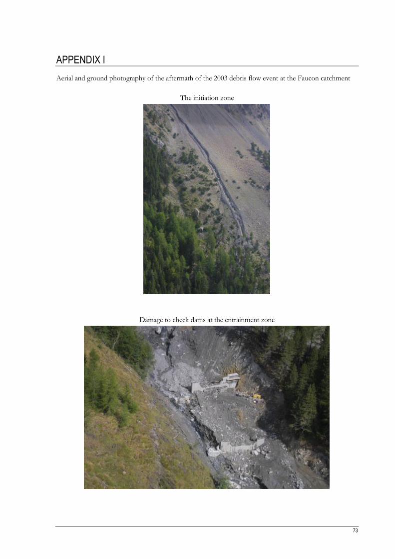
73
APPENDIX I
Aerial and ground photography of the aftermath of the 2003 debris flow event at the Faucon catchment
The initiation zone
Damage to check dams at the entrainment zone
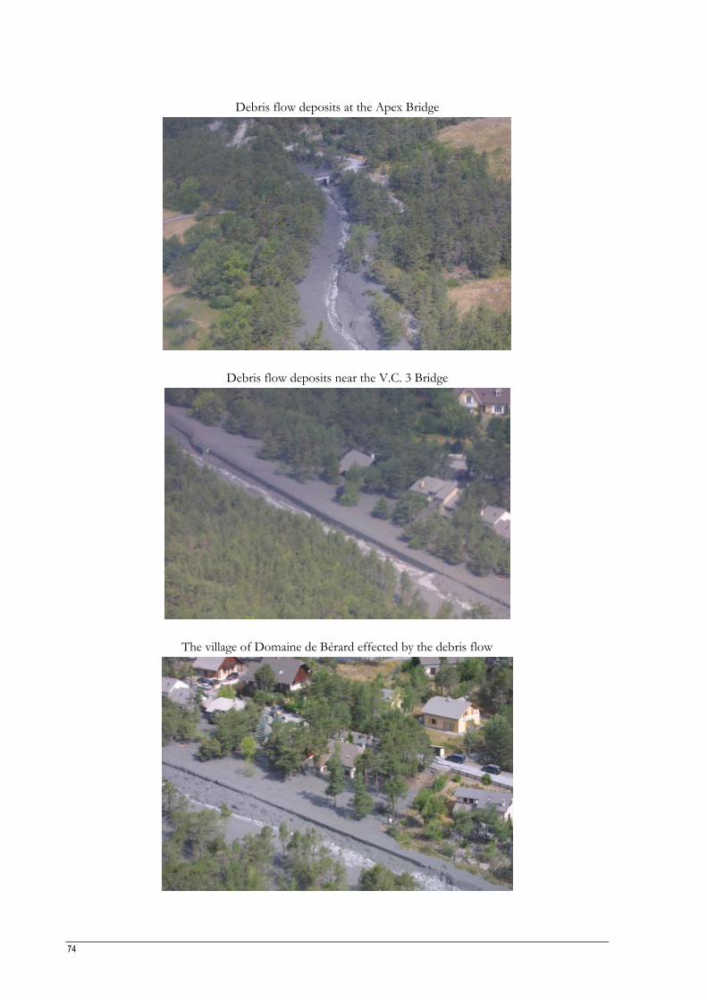
74
Debris flow deposits at the Apex Bridge
Debris flow deposits near the V.C. 3 Bridge
The village of Domaine de Bérard effected by the debris flow
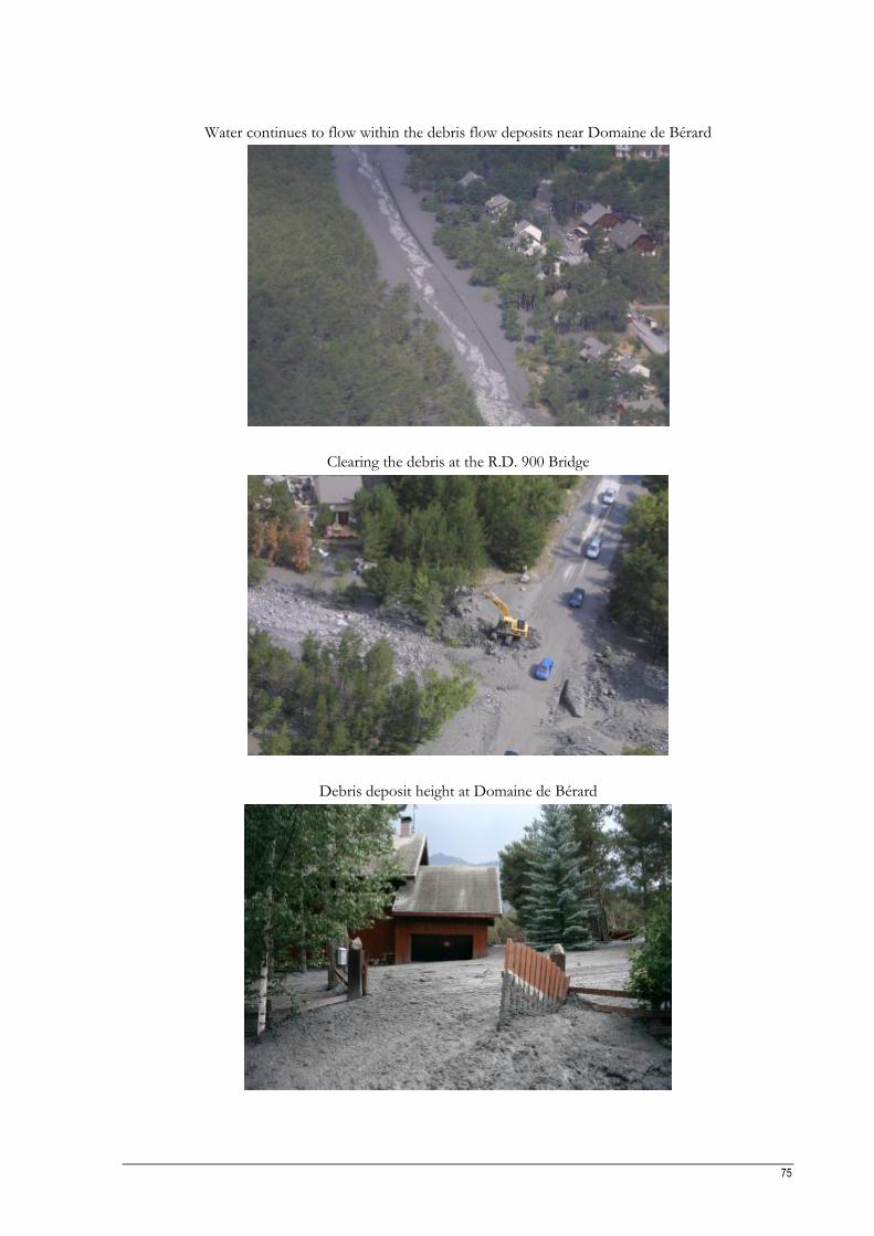
75
Water continues to flow within the debris flow deposits near Domaine de Bérard
Clearing the debris at the R.D. 900 Bridge
Debris deposit height at Domaine de Bérard

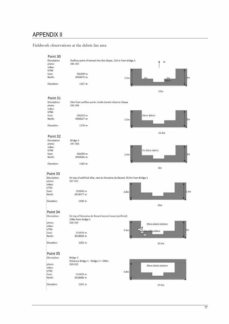
77
APPENDIX II
Fieldwork observations at the debris fan area
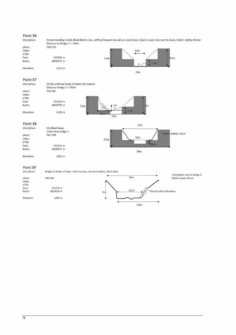
78
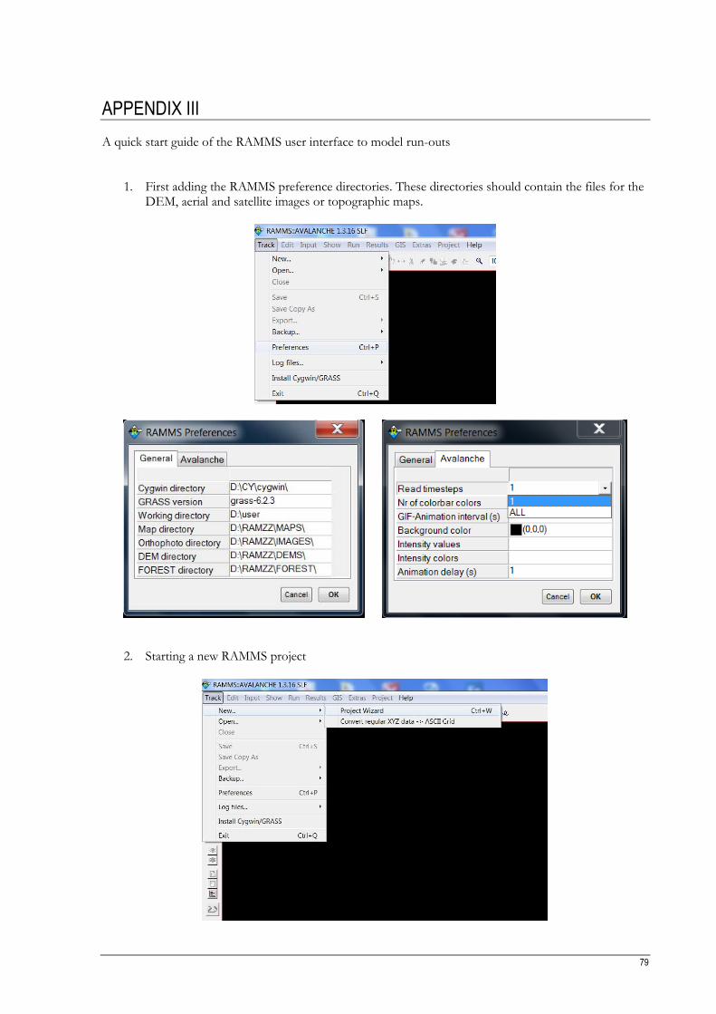
79
APPENDIX III
A quick start guide of the RAMMS user interface to model run-outs
1. First adding the RAMMS preference directories. These directories should contain the files for the DEM, aerial and satellite images or topographic maps.
2. Starting a new RAMMS project
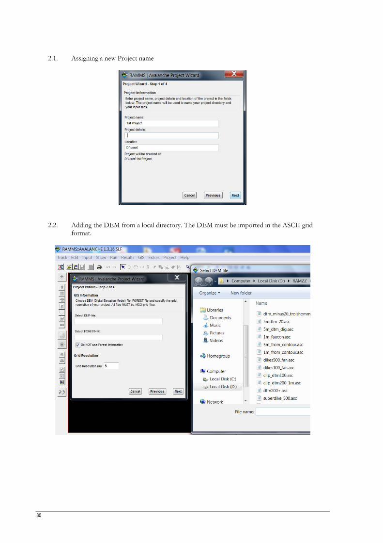
80
2.1. Assigning a new Project name
2.2. Adding the DEM from a local directory. The DEM must be imported in the ASCII grid format.
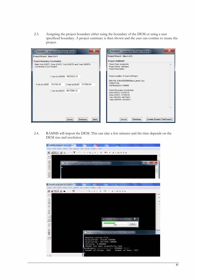
81
2.3. Assigning the project boundary either using the boundary of the DEM or using a user
specificed boundary. A project summary is then shown and the user can continu to create the project.
2.4. RAMMS will import the DEM. This can take a few minutes and the time depends on the DEM size and resolution
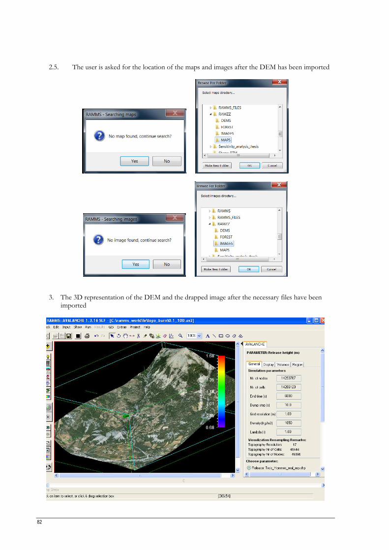
82
2.5. The user is asked for the location of the maps and images after the DEM has been imported
3. The 3D representation of the DEM and the drapped image after the necessary files have been imported
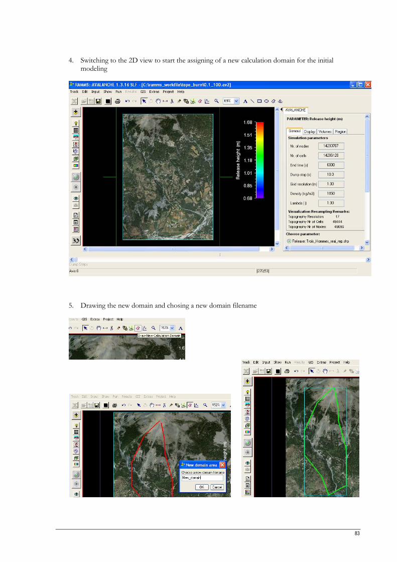
83
4. Switching to the 2D view to start the assigning of a new calculation domain for the initial modeling
5. Drawing the new domain and chosing a new domain filename
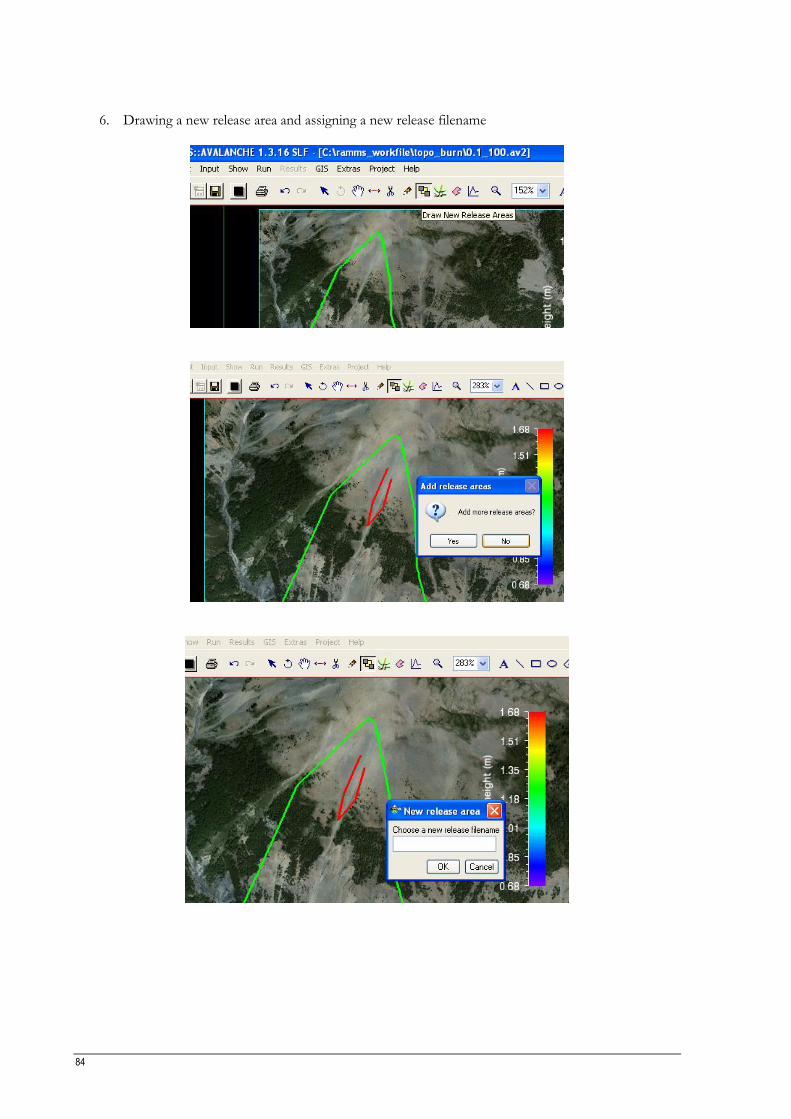
84
6. Drawing a new release area and assigning a new release filename
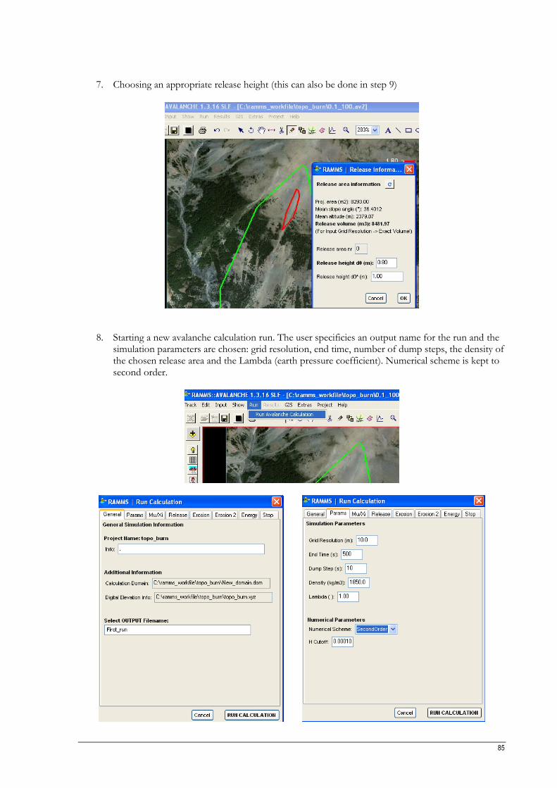
85
7. Choosing an appropriate release height (this can also be done in step 9)
8. Starting a new avalanche calculation run. The user specificies an output name for the run and the simulation parameters are chosen: grid resolution, end time, number of dump steps, the density of the chosen release area and the Lambda (earth pressure coefficient). Numerical scheme is kept to second order.
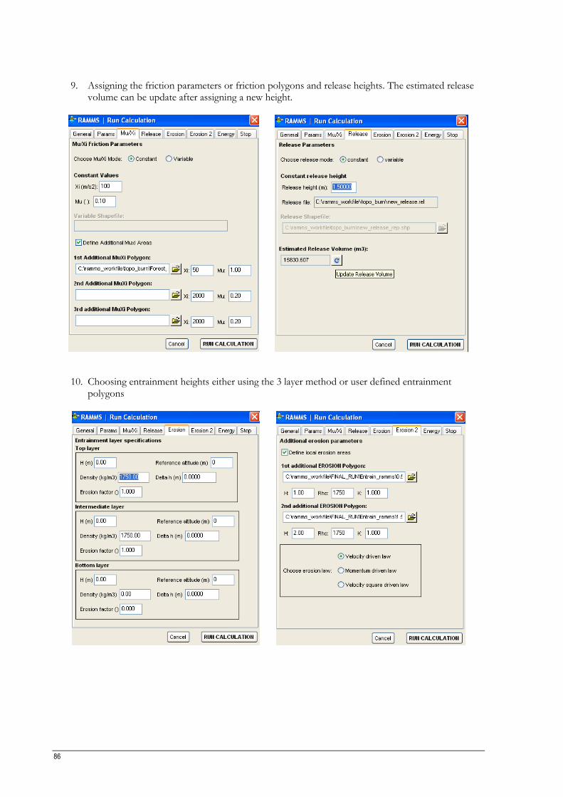
86
9. Assigning the friction parameters or friction polygons and release heights. The estimated release volume can be update after assigning a new height.
10. Choosing entrainment heights either using the 3 layer method or user defined entrainment polygons
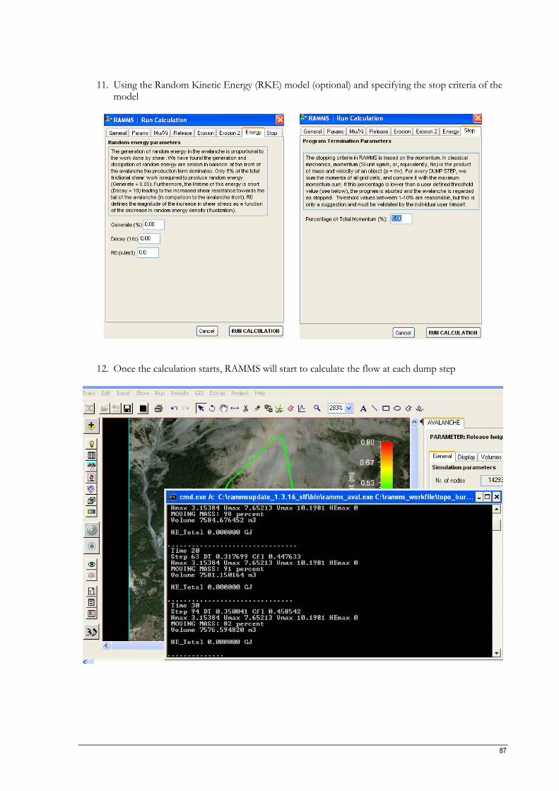
87
11. Using the Random Kinetic Energy (RKE) model (optional) and specifying the stop criteria of the model
12. Once the calculation starts, RAMMS will start to calculate the flow at each dump step
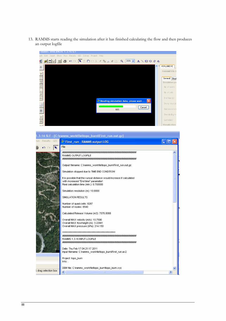
88
13. RAMMS starts reading the simulation after it has finished calculating the flow and then produces
an output logfile
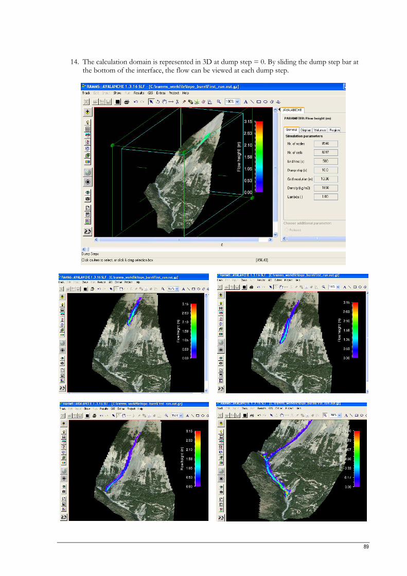
89
14. The calculation domain is represented in 3D at dump step = 0. By sliding the dump step bar at the bottom of the interface, the flow can be viewed at each dump step.
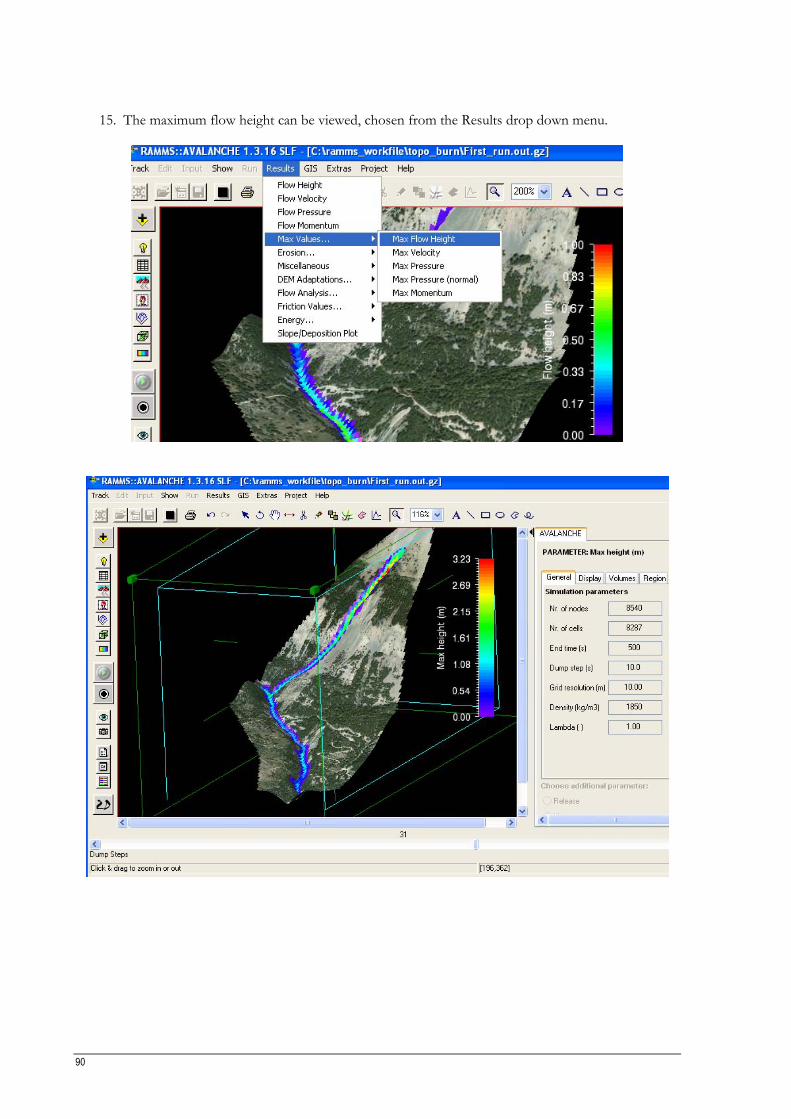
90
15. The maximum flow height can be viewed, chosen from the Results drop down menu.
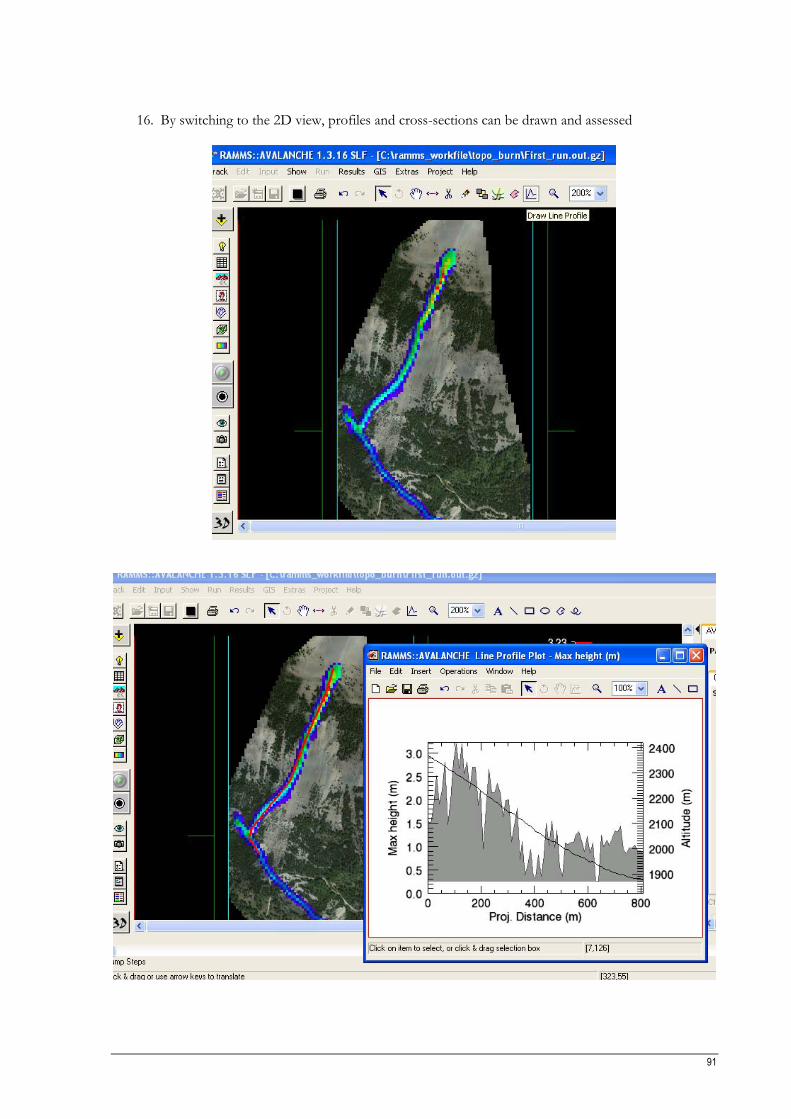
91
16. By switching to the 2D view, profiles and cross-sections can be drawn and assessed
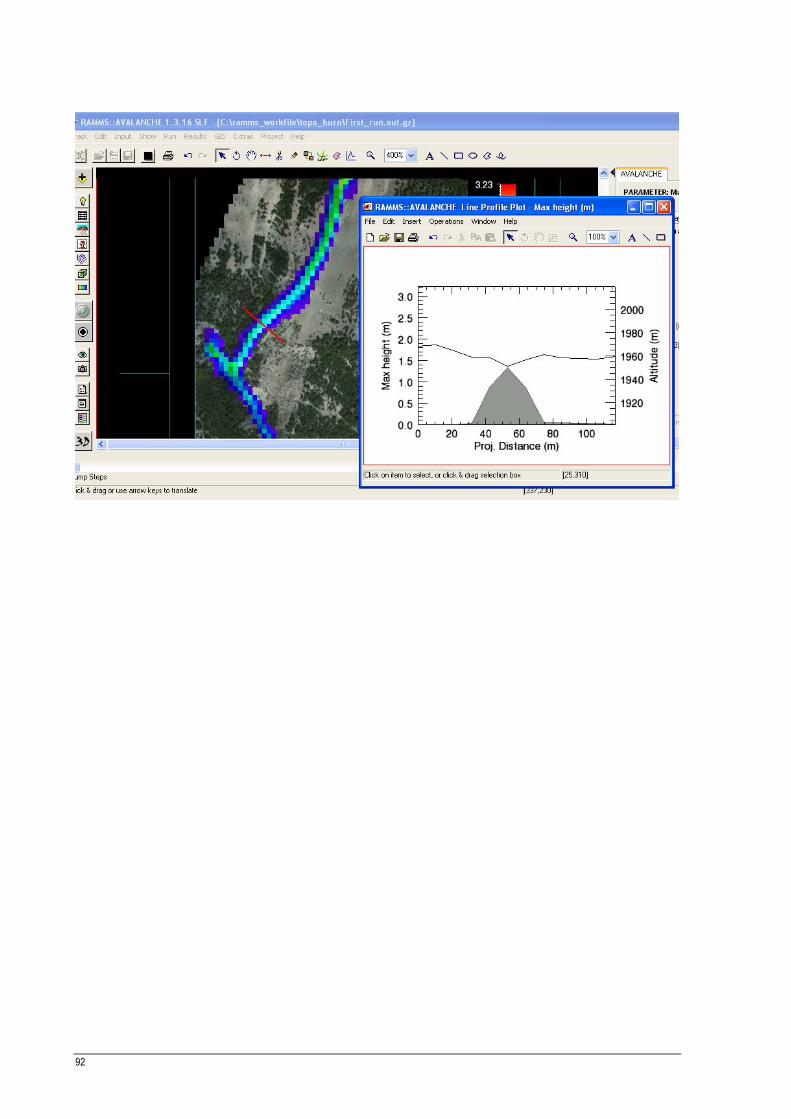
92
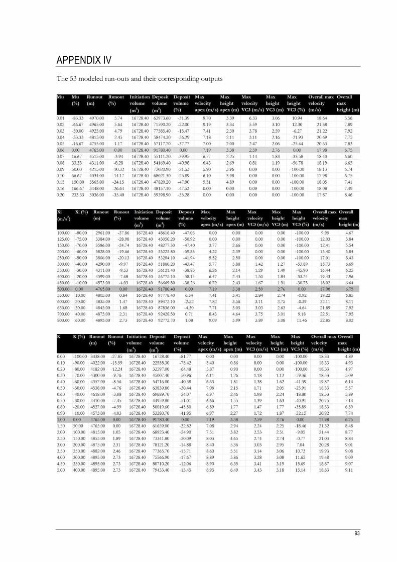
93
APPENDIX IV
The 53 modeled run-outs and their corresponding outputs
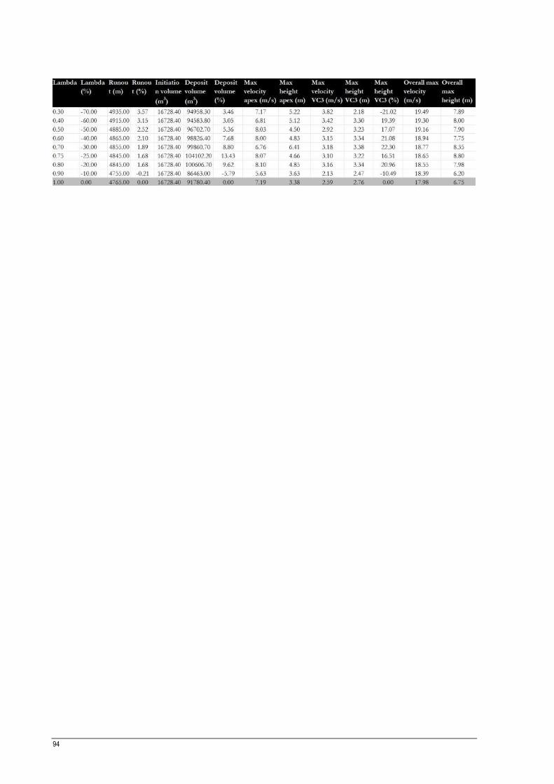
94