Probabilistic Gas Quantification with MOX Sensors in

Open Sampling Systems - A Gaussian Process Approach

Javier G. Monroy, Achim Lilienthal, Jose Luis Blanco, JavierGonzalez-Jimenez and Marco Trincavelli12

Abstract

Gas quantification based on the response of an array of metal oxide (MOX)

gas sensors in an open sampling system is a complex problem due to the

highly dynamic characteristic of turbulent airflow and the slow dynamics of

the MOX sensors. However, many gas related applications require to deter-

mine the gas concentration the sensors are being exposed to. Due to the

chaotic nature that dominates gas dispersal, in most cases it is desirable to

provide, together with an estimate of the mean concentration, an estimate

of the uncertainty of the prediction. This work presents a probabilistic ap-

proach for gas quantification with an array of MOX gas sensors based on

Gaussian Processes, estimating for every measurement of the sensors a pos-

terior distribution of the concentration, from which confidence intervals can

be obtained. The proposed approach has been tested with an experimental

setup where an array of MOX sensors and a Photo Ionization Detector (PID),

used to obtain ground truth concentration, are placed downwind with respect

to the gas source. Our approach has been implemented and compared with

standard gas quantification methods, demonstrating the advantages when

estimating gas concentrations.

Keywords: Gas Quantification, Open Sampling System, MOX sensors,

Preprint submitted to Sensors and Actuators B: Chemicals May 30, 2013

Gaussian Processes

1. Introduction

Gas sensing applications often require continuous and direct exposition

of gas sensors to the environment to be analyzed. Some examples are the

on-line monitoring of landfill sites and industrial processes [1], pollution mon-

itoring [2, 3], exploration of hazardous areas [4] or de-mining.

This configuration, to which we refer as Open Sampling System (OSS), is

the preferred solution when limitations in dimension, payload or energy con-

sumption do not allow the adoption of a sampling system where the sensors

are hosted in a chamber with controlled airflow, temperature and humidity.

In addition, the dynamic response of the sensor when directly exposed to the

environment contains useful information about the nature of a gas plume, in-

formation which may be inaccessible for sensors hosted inside a chamber and

affected by a controlled airflow. The information gained from the dynamic

response may be crucial for solving tasks like gas source localization [5, 6, 7]

or gas distribution mapping [8, 9].

The most common gas sensing technology for OSS applications is metal

oxide (MOX) gas sensors. MOX sensors are conductometric sensors, which

means that the conductance of the oxide changes when a gas interacts with

the sensing surface. The most prominent reasons for the popularity of MOX

sensors are their wide commercial availability, low price, and a higher sensi-

tivity to the compounds of interest in comparison to most other gas sensing

technologies. However, this technology presents among other drawbacks, an

important lack of selectivity, that it does not provide true concentration read-

2

ings, suffers from long and short term drift and is rather slow [10], especially

when recovering to the baseline [11] (i.e. the steady output value given by a

gas sensor when exposed to clean air).

The problem addressed in this paper is the estimation of gas concentration

from the readings of an array of MOX sensors deployed in an OSS. In other

words, the problem can be formalized as finding a function that maps the

readings of N gas sensors together with any other extra parameters (like

temperature and humidity) to a posterior distribution over concentrations.

Concentration estimation is a crucial step for realistic gas sensing appli-

cations since legal requirements and regulations are expressed in terms of

absolute gas concentration, toxicity levels, etc. For example, it would be of

little utility for many applications if we could detect a gas leak in an in-

dustrial scenario but we were unable to quantify the amount of leaked gas:

should an alarm be issued for workers to abandon the area, or is localization

of the source and subsequent notification to the maintenance unit enough to

handle the problem?

Gas quantification using an array of MOX sensors in an OSS is indeed an

important problem. Surprising, only few attempts to approach this problem

can be found in the literature. Most of the previous works dealing with

OSS do not estimate the concentration of the gas but work directly with the

sensor signal (conductance readings in case of MOX gas sensors). However, in

contrast to gas quantification with sensors within a sensing chamber (where

controlled conditions can be imposed), gas quantification with sensors in OSS

implies additional complications due to the many sources of uncertainty. The

most relevant source of uncertainty is the exposition of the sensors to the

3

turbulent airflow that brings the chemical compound in contact with the

sensors. As a consequence, given the slow dynamics of MOX gas sensors and

the rapid fluctuations in concentration due to turbulent airflow, the sensors

never reach a steady state but continuously fluctuate [12]. In other words, the

true concentration causes a range of different response levels due to the effects

introduced by the slow transient in the response and the quick fluctuations

due to turbulence. This range corresponds to a wide variance of the posterior

distribution over concentration.

In order to deal with the identified difficulties for MOX sensors in OSS,

in this paper we present an approach for concentration estimation that, in-

stead of trying to find a deterministic function for mapping directly the

sensors readings to concentration values, calculates instead a posterior distri-

bution over concentrations c at time t given the measurements of N sensors

rt = (r1(t), r2(t) . . . rN(t)) at times t = (t1, . . . , tk). That is, we search a

probability density function:

p (c(t)|rt1 , . . . , rtk) (1)

where k is the number of past sensor readings considered for the prediction.

A key advantage of having a full posterior distribution instead of a single

prediction value of the gas concentration is that probabilistic inference is pos-

sible, which uses the notion of uncertainty about the actual concentration.

Tasks like chemical detection, gas source localization, gas distribution map-

ping, and odour trail tracking are common tasks for working in OSS. For this

kind of systems it is acceptable to have only an approximate estimate of the

concentration if there is also an indication of the corresponding confidence.

4

This is exactly what the method proposed in this work provides.

In this paper we propose to estimate the posterior in Eq. (1) using a

Gaussian Process (GP) model [13]. Gaussian Processes provide principled

supervised machine learning methods which, given a set of samples (i.e. pairs

of sensor readings and their corresponding concentration), can estimate the

posterior joint probability of the process. The ground truth concentration

values are obtained using a Photo Ionization Detector (PID) placed in the

vicinity of the MOX sensor array. Unlike MOX gas sensors, if the chemical

compound is known, the PID provides true concentration measurements.

Moreover the response dynamics of a PID is much quicker compared to MOX

sensors, and, therefore the latter can follow the true concentration changes

more closely.

However, PIDs are of little help when the gas to quantify is unknown

since they provide a concentration value corresponding to the mixture of

all present gases with an ionization energy below what their ionization unit

delivers. Furthermore, they are also expensive, and it is therefore also of

economical interest to be able to estimate gas concentrations accurately with

inexpensive MOX sensors, considering in particular also applications in a

sensor network.

We analyze gas quantification using either a single sensor or the whole

sensor array, extending our previous work [14] where only a single sensor

was employed. In the latter context we additionally investigate how Au-

tomatic Relevance Determination (ARD) [15] [16] can be used to identify

which sensors in the array contribute most to the estimate of the concentra-

tion posterior distribution. Finally, we analyze to which extent considering

5

past sensor readings can improve the accuracy of probabilistic calibration.

The structure of this article is as follows. After a discussion of related

work in Section 2, we introduce in Section 3 the basics of Gaussian Process

regression for gas quantification, giving special attention to learning a GP

from the data. Then, Section 4 presents the experimental setup and finally,

comparative results under different configurations of the GP are presented

in Section 5, followed by conclusions and suggestions for future work in Sec-

tion 6.

2. Related Work

Estimation of gas concentration from raw readings of MOX-based gas

sensors has been a major research topic for many years. Research has been

traditionally focused on setups where such sensors are enclosed inside a cham-

ber, where environmental conditions, gas exposure times and concentrations

are known and controlled. This setup allows the measurement of steady state

values, which are used as input to a regressor. Under such controlled condi-

tions, the relation between sensor conductance (Ω−1) and gas concentration

(ppm) is usually modelled as an exponential [17]:

gi ≡1

ri= Ai · cαi (2)

where gi is the conductance of sensor i within the array (inverse of sensor

resistance ri), c is the gas concentration, and Ai and αi are the parameters

of the exponential model to be estimated during an initial training process.

For concentration estimation with an array of MOX sensors, multivariate

linear regression methods like Principal Component Regression (PCR) and

6

Partial Least Squares Regression (PLSR) have been proposed [18, 19, 20].

The main motivation behind the use of these two methods is the strong

correlation of the response of different MOX sensors. This allows both, PCR

and PLSR, to reduce the dimensionality of the input space before fitting a

regression function, thus reducing the possibility of curse of dimensionality

related issues. Alternatively, non-linear estimation methods like Artificial

Neural Networks (ANN) [21, 22] or kernel algorithms like Support Vector

Regression (SVR) [23, 24] have also been proposed.

It is worth noting that some authors consider the transient information

for MOX sensor calibration. In [25], a multi-exponential model is used to

describe the sensor dynamics and to predict the steady state value of the

sensors which is then mapped to a concentration based on the initial values

of the transient state.

These existing calibration approaches rely on steady state measurements

of the sensor. Thus, they are not immediately applicable to OSS because

steady state values are almost never reached [12], due to turbulent advection,

which dominates gas transport in the target environments.

The work in [26] addressed calibration of an e-nose for urban pollution

monitoring. Measurements collected over a long period of time are aver-

aged out and therefore the dynamic information in the sensor response is

discarded. The focus of our work is instead on applications where sensors

are deployed in a highly dynamic environment, where they are exposed to

intermittent patches of gas.

Most of the work in mobile robot olfaction avoids calibration issues and

use instead the conductance readings of the sensors as an approximate mea-

7

sure of the gas concentration. An exception is [27], where Ishida et al.

propose to use steady state calibration to obtain a rough approximation of

gas concentration with an OSS.

All the methods mentioned ignore the uncertainty in the calibration,

which is present in an OSS with MOX sensors due to the turbulence-dominated

gas transport mechanisms, the sensor dynamics and environmental factors

such as temperature or humidity (temperature and humidity are not ad-

dressed in this work, however). It is desirable to quantify the uncertainty

together with the concentration estimate. The GP-based method proposed

in this paper generates an estimate of the uncertainty (as a variance), which

can be used, for example, to calculate confidence intervals for the predictions.

3. The algorithm for estimation of gas concentration.

This section details our proposal for the concentration estimation in

MOX-OSS. Initially, two signal preprocessing methods and their influence

on the posterior distribution estimation are described. Next, Gaussian Pro-

cess regression for the particular case of gas quantification with an array of

sensors is summarized, and how Automatic Relevance Determination can be

used to select the model parameters. Finally, two different loss functions

are proposed for evaluating the results, allowing a comparison between the

various proposed configurations.

3.1. Signal Preprocessing

In the first step, the raw sensor resistance readings ri(t) are divided by the

baseline of the sensor at t = 0, that is, ri(0). This transformation in Eq. (3),

8

known as relative baseline manipulation [28],is applied for drift compensation

and dynamic range enhancement:

rt = [ri(t)]Ni=1 , ri(t) =

ri(t)

ri(0)(3)

Next, GP regression is used to predict the gas concentration c(t) from

the values rt. However, considering the commonly assumed exponential re-

lation between sensor resistance and the concentration, see Eq. (2), we will

also investigate applying a logarithmic transformation and perform regression

between log (rt) and log (c(t)).

In summary, we will compare two regression problems:

c(t) = f1 (rt) (4)

log c(t) = f2 (log rt) (5)

3.2. Gaussian Process Regression for Gas Concentration Estimation

In the general case, the process of inferring the relationship f : rt 7−→ c(t)

between the response of an array of sensors and the gas concentration using

a training dataset D = (rtj , c(tj)|j = 1, ..., n is a supervised machine learn-

ing problem. Among the numerous available options, GPs provide a powerful

non-parametric tool for Bayesian inference and learning [13]. GPs can be

seen as a generalization of the Gaussian probability distribution to distribu-

tions over functions. That is, they perform inference directly in the space of

functions, starting with a prior distribution over all possible functions and

subsequently learning the target function from data samples. Defining a prior

over functions corresponds to making assumptions about the characteristics

9

of the function f , as otherwise any function which is consistent with the

training data will be equally valid and therefore the learning problem would

be ill-defined.

A GP is completely specified by its mean and covariance functions, m(rt)

and k(rt, rt′) respectively:

m(rt) = E [f(rt)] , (6)

k(rt, rt′) = cov (f(rt), f(rt′)) (7)

= E [(f(rt)−m(rt))(f(rt′)−m(rt′))] . (8)

we denote the GP as:

f (rt) ∼ GP (m(rt), k(rt, rt′)) . (9)

To account for noise in the sensor it is assumed that the observed concen-

tration values c(t) are corrupted with an additive i.i.d. Gaussian noise with

zero mean and variance σ2n, that is:

c(t) = f(rt) + ε, (10)

ε ∼ N (0, σ2n).

It is important to notice that we did not assess experimentally whether the

noise is i.i.d. with Gaussian distribution. We rather make this assumption

to obtain a closed form solution, and validate the resulting predictions with

real sensor data.

10

In our case of study we consider GPs with zero mean and the commonly

used squared exponential (SE) covariance function, that is:

m(rt) = 0, (11)

k(rt, rt′) = σ2f exp

(−1

2

‖ rt − rt′ ‖2

`2

), (12)

where σ2f is the overall variance hyper-parameter and ` is the characteristic

length scale. It is common but not necessary to consider GPs with zero

mean. Note that the mean of the posterior process is not restricted to be

zero. The choice of the SE covariance function leads to GP predictions that

are smooth over the characteristic length scale. That is, if rt ≈ rt′ , then

k(rt, rt′) approaches its maximum and f(rt) is strongly correlated with f(rt′).

For large distances between rt and rt′ , k(rt, rt′) approaches 0. So, when

predicting the concentration value for new data points, distant observations

will have a negligible effect. The region of influence, depends on the scale

parameter `.

The regression model depends on the selection of the hyper-parameters,

which are summarized in a vector θ = (`2, σ2f , σ

2n). The optimal hyper-

parameters are found by maximizing the marginal likelihood function p (c|R,θ),

where c is a vector of training concentration values, R is the matrix contain-

ing the measurements of the sensor array, and θ are the hyper-parameters. As

it is common practice, we minimize the corresponding negative log-likelihood

to avoid numerical issues:

11

− log (p(c|R,θ)) =1

2c>K−1c +

1

2log |K|+ n

2log 2π (13)

where K = k(rt, rt′) + σ2nI

To find the minimum of Eq. (13) we use the scaled conjugate gradient

method, which requires the calculation of the partial derivatives of the log

marginal likelihood w.r.t. the hyper-parameters:

∂

∂θjlog (p(c|R,θ)) =

1

2tr

[(αα> −K−1

) ∂K

∂θj

](14)

whereα = K−1c

The complexity of this step is dominated by the matrix inversion K−1 in

Eq. (14), which has a complexity O(n3) with n being the number of training

points. This represents one of the principal inconveniences of GP.

Learning the calibration GP corresponds to the selection of the hyper-

parameters. The GP then allows to predict gas concentration values c∗ and

a corresponding variance for arbitrary sensor resistances r∗.

The posterior distribution over functions (our prediction) is also a Gaus-

sian, and it is given by:

c∗|R, c,R∗ ∼ N (c∗, cov(c∗)) ,where (15)

c∗ , E[c∗|R, c,R∗] = K(R∗,R)[K(R,R) + σ2nI]−1c

cov(c∗) = K(R∗,R∗)−K(R∗,R)[K(R,R) + σ2nI]−1K(R,R∗)

and where R = r1...rn is the n × N matrix of the n training samples of

dimensionality N , R∗ the matrix for the testing inputs, K(·, ·) refers to the

12

matrix with the entries given by the covariance function k(·, ·) and c the

vector of the observed concentrations ci.

Note that the predictive distribution is based on a mean value c∗ (our

best estimate for c∗), which is a linear combination of the observed values c,

and a variance value cov(c∗) which denotes the uncertainty in our estimation,

and does not depend on the observed targets but only on the inputs.

3.3. Automatic Relevance Determination

Automatic Relevance Determination (ARD) is a method based on Bayesian

interference for pruning large feature sets with the aim to obtain a sparse

explanatory subset. Making use of this powerful tool we can consider dif-

ferent configurations of the input space of higher dimensionality, and then

allow ARD to select the most relevant features, which avoids overfitting due

to high input dimensionality. In order to introduce ARD Eq. (12) can be

rewritten as:

k(rt, rt′) = σ2f exp

(−1

2(rt − rt′)

>M(rt − rt′)

), (16)

where M denotes the diagonal weight matrix M = `−2I.

We have seen how maximizing the log marginal likelihood can be used to

determine the value of the hyper-parameters. By incorporating a separate

hyper-parameter `i for each input variable [13], i.e. for each sensor in the

array, we modify M to be:

M = diag([`−2

1 , `−22 , . . . , `−2

n ])

(17)

where ` = [`1, `2, . . . , `n] is a vector of positive values, corresponding to the

13

length-scale of each input variable. This is in contrast to a global hyper-

parameter ` for all input variables.

Since the inverse of the length-scale determines how relevant an input is,

the extension (17) enables to identify the importance of each different input–

if the length-scale has a very large value, the covariance will become almost

independent of that input, effectively ignoring its values during the inference.

ARD is performed during the training phase of the GP, specifically dur-

ing the selection of the covariance function hyper-parameters. When the

inputs related to a sensor are discarded by ARD, the corresponding sensors

can be excluded from the array. In this work, ARD has been applied for

two different configurations of the input space: (i) when the whole sensor

array is considered at one instant of time in the inference process and (ii)

when additional features from previous time steps of the sensor response are

considered to account for the dynamics of the signal.

3.4. Evaluation of the Predictions

To compare different configurations of the GP based calibration proposed

in this paper, among themselves, and with other methods previously pro-

posed in the literature, two performance measures are proposed:

Root Mean Squared Error (RMSE): The RMSE is calculated as the

difference between the ground-truth concentration (obtained with the

readings from a PID sensor) and the expected value of the predictive

distribution obtained from Eq. (15).

RMSE =

√√√√ 1

n

n∑i=1

(ci − c∗i)2 (18)

14

Notice that the RMSE takes only into account the predictive mean,

while it ignores its uncertainty. However, this indicator allows to com-

pare the predictions of the proposed GP calibration approach with

other regression methods, like Partial Least Squares Regression (PLSR)

or Support Vector Regression (SVR), which do not provide any esti-

mation of the prediction uncertainty.

Negative Log Predictive Density (NLPD): The NLPD is a standard

criterion to evaluate probabilistic models (see Eq. (19)).

NLPD = − 1

n

n∑i=1

log(p(ci|ri)) (19)

It is worth noting that the NLPD considers the whole posterior dis-

tribution and not only its expected value. In general, more negative

NLPD values indicate better predictions with a small uncertainty.

Considering the two preprocessing methods proposed in Section 3.1,

two different NLPD formulas arise. In the first case (linear prepro-

cessing - Eq. (4)), the posterior distribution of the concentration is

a normal distribution, while in the second case, (logarithmic prepro-

cessing - Eq. (5)), the posterior distribution of the concentration is a

log-normal distribution. Therefore the NLPD is calculated for the two

cases respectively:

NLPDnormal =log(2π)

2+

1

2N

n∑i=1

[log(σ2(ci)) +

(ci − µ(ci))2

σ2(ci)

](20)

15

NLPDlog−normal =log(2π)

2+

1

2N

n∑i=1

[log(c2

iσ2(ci)) +

(log(ci)− µ(ci))2

σ2(ci)

]where ci is the ground truth gas concentration, σ(ci) is the predictive

standard deviation, and µ(ci) the predictive mean.

4. Experimental Setup

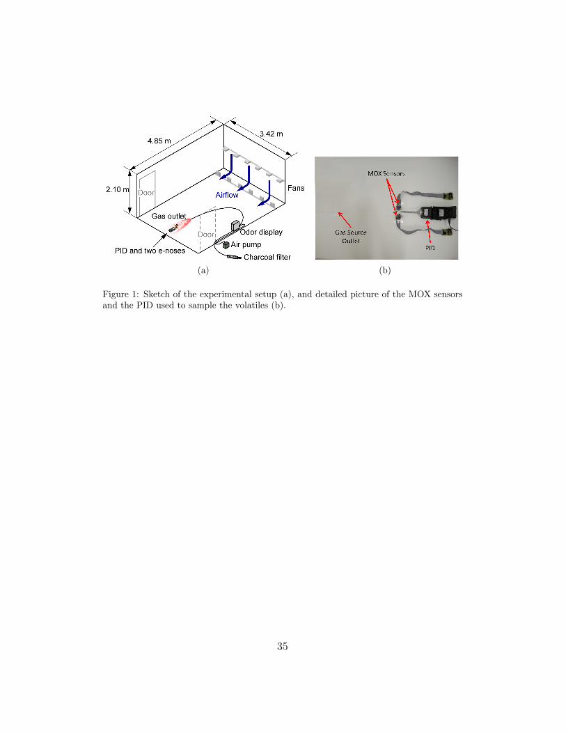
The experiments are carried out in a 4.85 m × 3.42 m × 2 m room

with an induced artificial airflow of approximately 0.1 m/s. The airflow is

created using two arrays of six standard microprocessor cooling fans. The

gas source is an odour blender (olfactory display), a device described in [29]

that can mix up to 13 gas components from arbitrary recipes using rapidly

switching solenoid valves. The odour blender samples from the headspace of

the compounds, which are kept in liquid phase. This odour blender enables

rapid switching of compound and concentration. The odour blender uses

headspace sampling and therefore does not intensify evaporation, contrary

to an odour bubbler [30]. The outlet of the olfactory blender is placed on

the floor, 0.5 m upwind with respect to an array of 11 MOX gas sensors

and a PID3. The airflow at the outlet of the odour blender is set to 1 l/min.

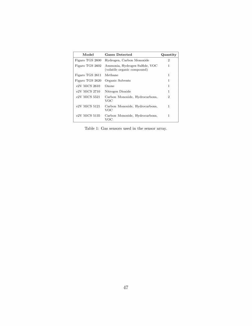
Figure 1 displays the configuration of the experiments. The sensors included

in the array are listed in Table 1. The sensors are sampled at 4 Hz. The

PID is placed next to the array of MOX sensors in order to obtain calibrated

measurements in the proximity of the active area of the MOX sensors. This

is important since, due to diffusion and advection, the estimation of the gas

3PID model ppbRAE2000 from RAESystem with a 10.6 eV UV lamp.

16

concentration at the sensors would be very complicated if only the intensity

of the gas source would be available. The position of the MOX sensors and

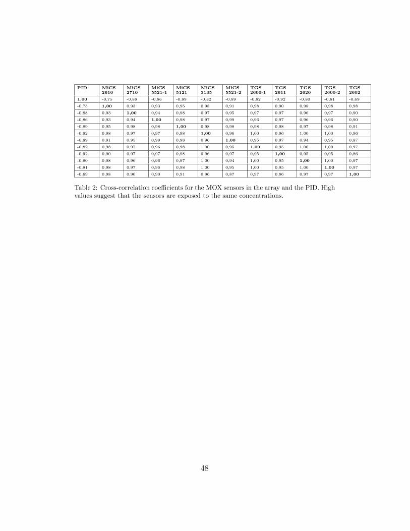
the PID has been carefully chosen in order to ensure that the sensors are ex-

posed to a very similar gas concentration. This can be verified calculating the

Pearson’s coefficient to estimate the linear correlation among the response of

the sensors. From the results reported in Table 2 it is clear that the response

of the MOX sensors and the PID are highly correlated and therefore it can be

inferred that the sensors are exposed to very similar concentration profiles.

Due to the faster sensor dynamics, the correlation of the PID response with

the response of the MOX sensors is in general slightly lower than the corre-

lation between the response of two MOX sensors. The compound selected

for these experiments is ethanol, which is heavier than air and, consequently,

forms plumes at ground level.

[Figure 1 about here.]

[Table 1 about here.]

[Table 2 about here.]

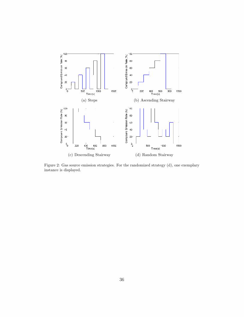
In order to create a dataset that represents a variety of scenarios, four

different odour emitting profiles have been used (see Figure 2). For all the

profiles the gas source emits clean air for two minutes (i.e. no gas is released)

and the signal of the sensors during this period is assumed as the baseline.

Also, at the end of all the experiments the source emits clean air for 2 minutes.

Overall, the dataset includes a total of 18 experiments, 3 for the deterministic

emission strategies and 9 for the randomized emission strategy.

[Figure 2 about here.]

17

5. Results

In this section we present and compare the gas sensor calibration results

obtained with the two preprocessing methods (linear & logarithmic).

We further compare three different sets of input variables. First, we

consider the sensors independently. Second, we compare to the case where

the whole array is considered as the input to the inference process. Third, we

discuss the effect of including the dynamics of MOX sensors by using delayed

sensor samples as part of the input space.

For the evaluation we used cross-validation, selecting the folds at the

experiment level and not at the sample level. This means that if samples

from an experiment have been used during the training procedure, no sample

from that experiment was used for calculating the performance measures.

In this way an optimistic bias in the results due to evaluation with samples

collected in the same trial, i.e. under exactly equal environmental conditions,

is avoided. All the experiments have been carried out in the time span of

one week and therefore effects due to long term drift are not considered in

this work. Furthermore, due to the computational complexity of the training

algorithm of the GP (which is dominated by the inversion of the kernel

matrix, to be performed at every step of the maximization of the marginal

likelihood) a subset of 1000 points from the experiments considered for the

training set, was randomly selected for training the GP.

We compare the proposed calibration method with Partial Least Squares

Regression (PLSR) and Support Vector Machine Regression (SVR) for all

input configurations. Since both methods only provide an estimate of the gas

concentration without information about its uncertainty, only the RMSE can

18

be used as a performance indicator for comparison. Please note that PLSR

and SVR have been widely used in classical sensor calibration in controlled

environments. Nevertheless, in this work we apply PLSR and SVR to data

obtained with an OSS in a very dynamic environment.

5.1. Gas Quantification Using a Single Sensor

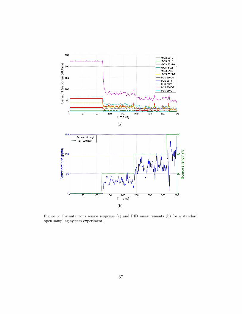
A typical sensor response in an OSS is depicted in Figure 3. The PID

measurements displayed in Figure 3(b) show the fast fluctuations around an

average value to which the MOX sensors are exposed when the output of the

gas source is steady. These fluctuations are caused by the turbulent airflow

and are the reason why the MOX gas sensors do not reach a steady state.

[Figure 3 about here.]

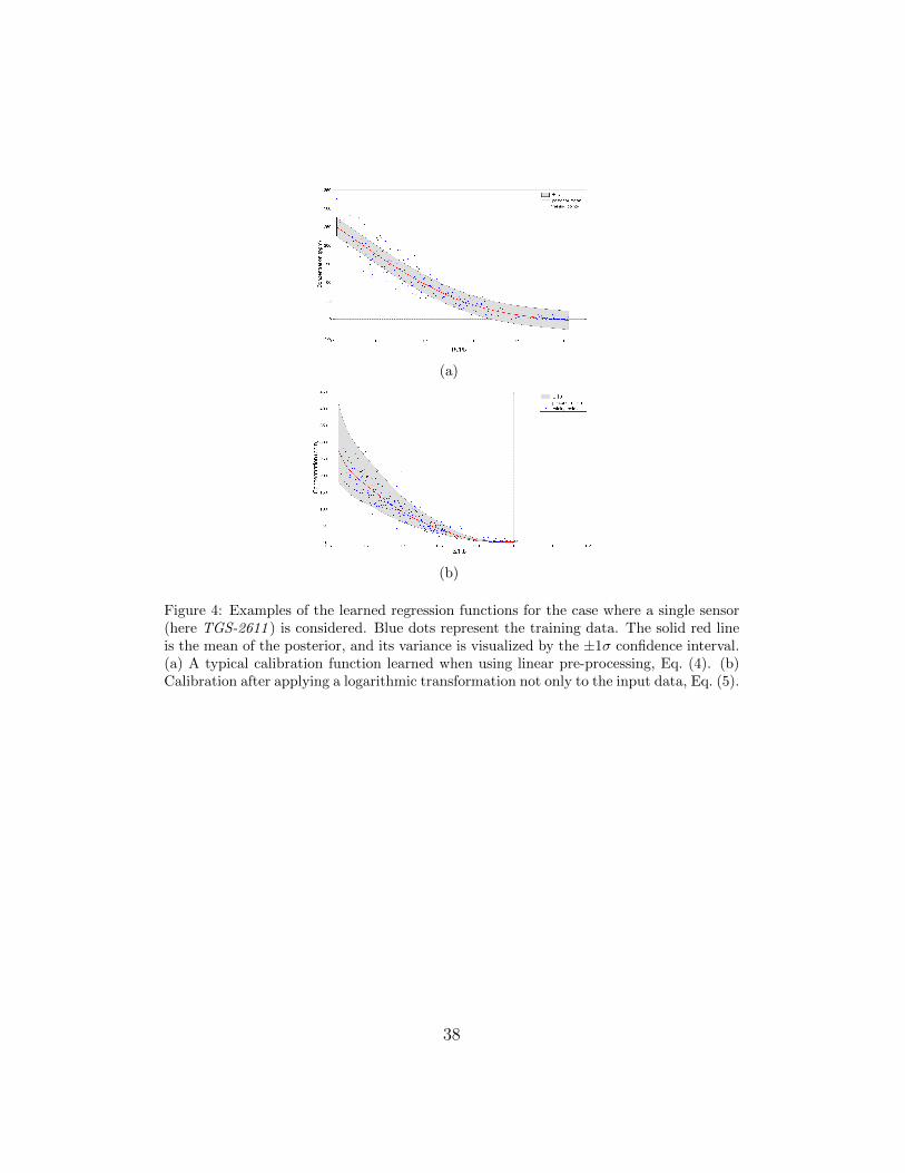
For the case of single gas sensor input, i.e. a univariate function f :

ri 7−→ c, it is possible to plot the relation between sensor resistance and

gas concentrations obtained in the experiments (see Figure 4). Notice how

the distribution of training points (represented by blue dots) corresponds to

uncertainty about the measured concentration.

[Figure 4 about here.]

The predictive variance is not necessarily constant across the whole input

space, but it depends on the density and dispersion of the training points.

If many training points are available in a certain region, then the predictive

variance goes down to the global estimate of the signal variance (given by

the hyper-parameter σf ). On the other hand, when few or no training points

19

are available in a region, the predictive variance in that region increases

indicating less reliable estimates.

In our case, since we used a uniform distribution to sample the input

space for selecting the training points, the posterior variance turns out to

be almost constant over the input space (see Figure 4(a)). It can be seen in

Figure 4 that a constant variance does not describe the true signal variance

adequately. When the inference is carried out after applying the logarithmic

transformation to the sensor resistance and gas concentration, however, the

predictive variance represents more accurately the variance in the training

points, see Figure 4(b). This shows that the process generating the data

is indeed not Gaussian and is therefore modelled better by a Log-Normal

(non-Gaussian) process. Nevertheless, we can efficiently obtain this non-

Gaussian Process by applying a non-linear transformation to the data and

then performing Gaussian Process regression.

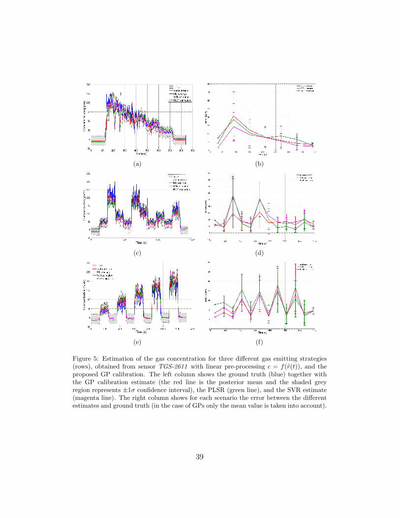
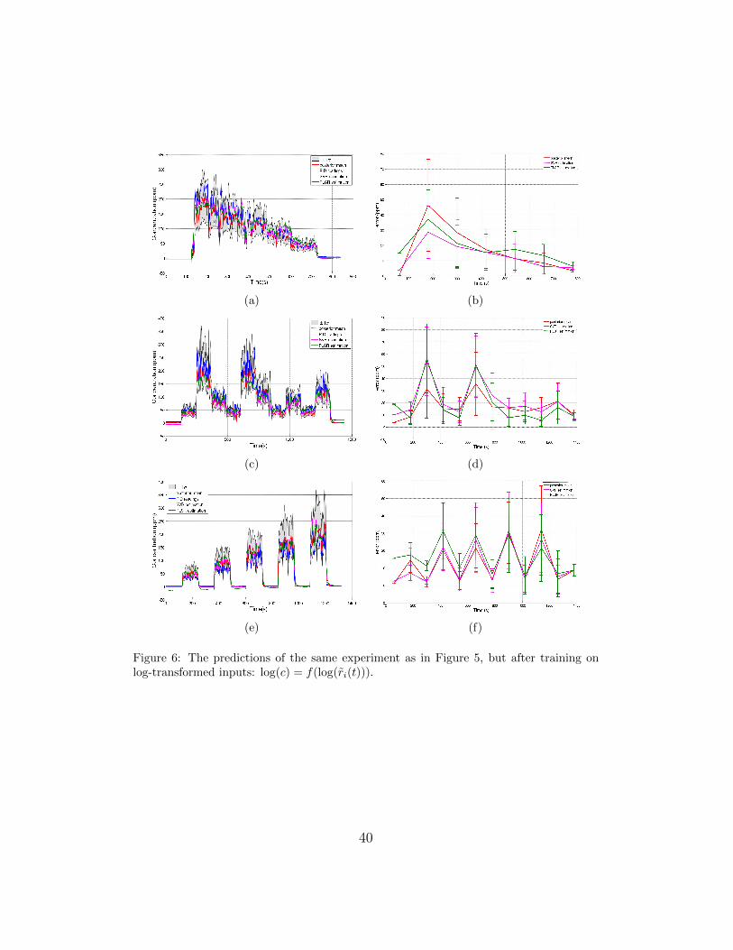
The estimated gas concentrations for three different gas emitting strate-

gies are displayed in Figure 5 and Figure 6 for the linear and logarithmic

preprocessing respectively. A notable difference exists between the predic-

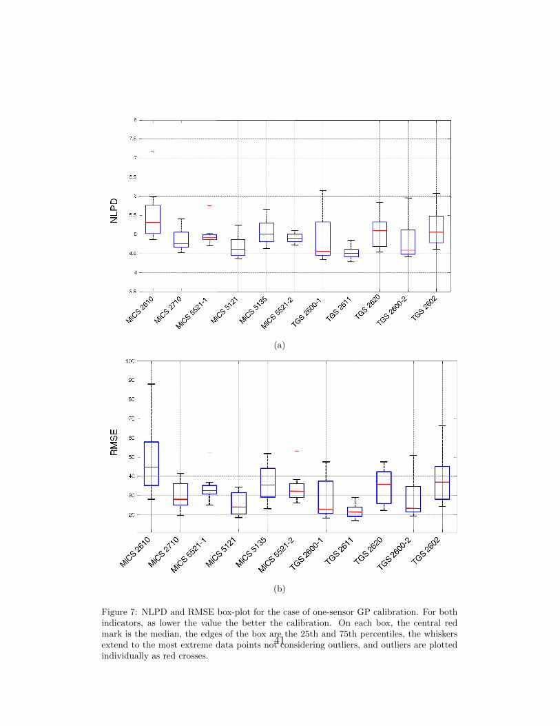
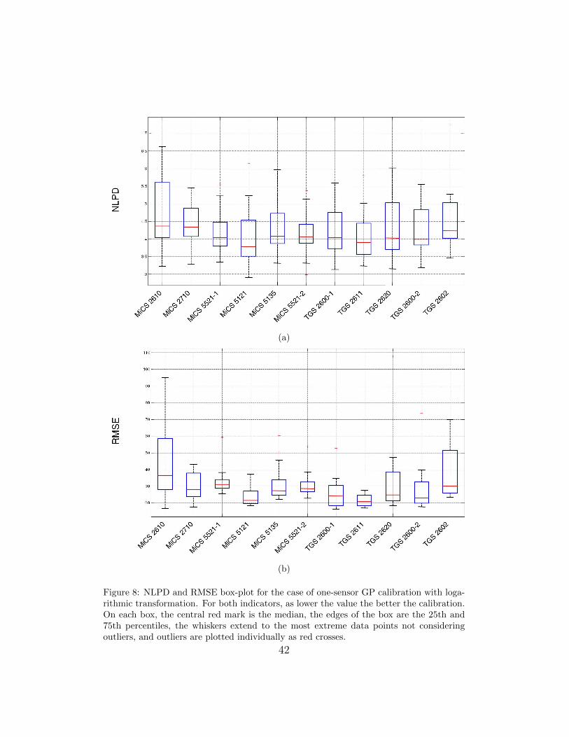
tive uncertainty in the two cases. In Figure 7 and Figure 8 the NLPD and

RMSE are plotted for each sensor in the array using a box-plot format. When

calibrating using the linear relation we obtain, in average over all the sensors,

a RMSE of 35.15± 10.32ppm, and a NLPD of 5.16± 0.71, while for logarith-

mic preprocessing the achieved average RMSE is 31.17 ± 6.27ppm and the

NLPD is 4.27 ± 0.18. The results after applying the log transformation in

Eq. (5) are better according to both performance measures.

[Figure 5 about here.]

20

[Figure 6 about here.]

[Figure 7 about here.]

[Figure 8 about here.]

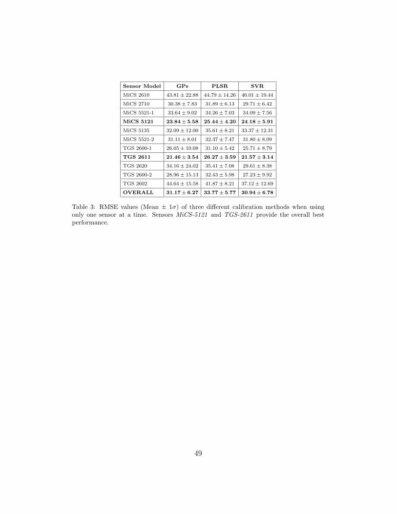
From the results in Figures 7 and 8 we can also see that the sensors TGS-

2611 and MiCS-5121 perform best for the specific target gas (ethanol).

Table 3 summarizes the comparison of the proposed GP calibration with

PLSR and SVR. For the same input, the RMSE, averaged over all sensors is

33.77 ± 5.77ppm for the PLSR approach and 30.94 ± 6.78ppm for the SVR

approach. The PLSR approach performs slightly worse than SVR, and SVR

is on par with the GP approach considering only the RMSE. A possible

explanation for this result is that PLSR is a linear method while both SVR

and GP are non-linear and use an SE (RBF) kernel.

[Table 3 about here.]

5.2. Gas Quantification Using a Sensor Array

In OSS applications where the goal is discriminating among several dif-

ferent odours [31], an array of MOX sensors is usually employed instead of a

single sensor. For this reason, we investigate whether also gas quantification

benefits from using the whole sensor array. In order to do this we apply the

GP calibration method with an input space of dimension d = 11, and apply

ARD (see Section 3.3) to automatically select the most relevant inputs, that

is, the most relevant gas sensors in the array.

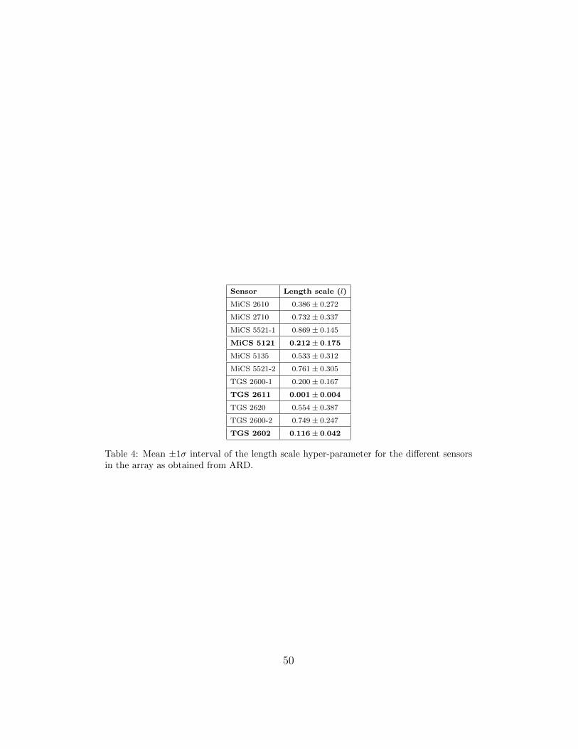
Table 4 summarizes the mean and the ± 1σ confidence interval of the nor-

malized length scale hyper-parameter (l) for the different sensors in the array,

21

after ARD has been computed for the 13 folds used in the cross-validation.

As explained in Section 3, large values of the length scale corresponds to less

relevant sources of information.

[Table 4 about here.]

Our results show that sensors which perform well in the case of single

sensor calibration are in most cases also relevant for array calibration. An

exception is the sensor TGS-2602, which did not perform well individually,

but was found to provide valuable information when considering the whole

array (TGS-2602 is the second most relevant sensor according to ARD but

was ranked last in its individual GP calibration performance, see Table 3).

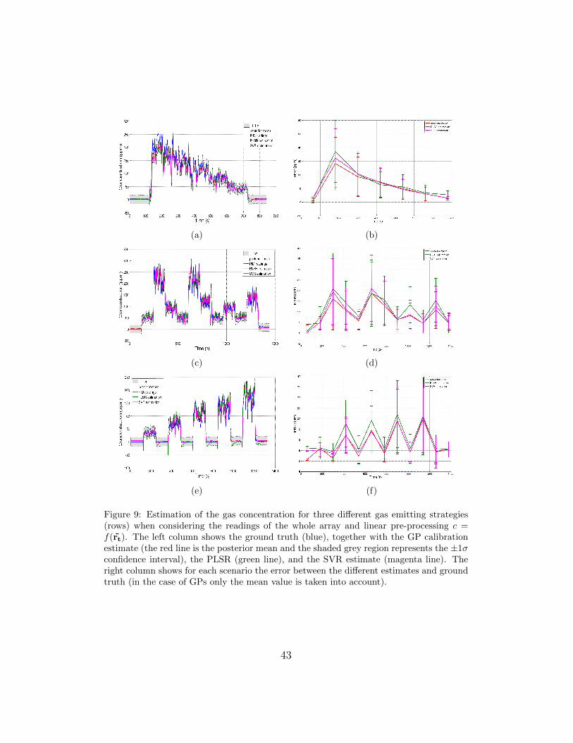
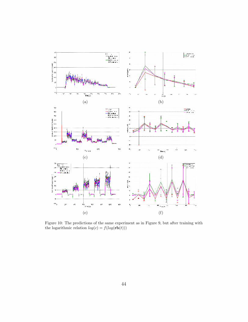
Figures 9 and 10 show gas concentration estimates for three different scenar-

ios when considering the readings of the eleven sensors at once.

[Figure 9 about here.]

[Figure 10 about here.]

In general, the gas concentration estimation obtained using the whole

array of sensors outperforms the estimation based on a single sensor. Linear

preprocessing provides an average RMSE of 16.44 ± 3.38ppm and a NLPD

of 4.22± 0.20, while for the logarithmic preprocessing the results are slightly

better: RMSE of 15.97± 2.77ppm, NLPD of 3.59± 0.76.

In comparison, PLSR applied to the same input achieves a RMSE of

17.55± 2.42ppm which, is slightly worse than the GPs calibration, as in the

single sensor case (Section 5.1). SVR achieves a RMSE of 16.20± 2.50ppm,

22

very similar to the results obtained with the GP approach but without pro-

viding the additional information about the uncertainty in the prediction.

The uncertainty estimate is particularly meaningful when the posterior

distribution is modelled as a Log-Normal distribution, rather than with a

Gaussian distribution. High uncertainty estimates (which can be identified

in the left column of Figure 10 and Figure 8 in the case of predictions per-

formed with a single sensor) correspond to an increased mean and variance

of the RMSE (observable in the right column of Figures 10 and 8). This

describes the observed fluctuations in the signal well and thus provides a

reliable confidence measure for concentration predictions.

Our results also lead to the conclusion that it is recommendable to start

using the whole sensor array and select the most relevant sensors with ARD.

This allows for better concentration estimate.

5.3. Taking into account the dynamics of MOX gas sensors

The signals from MOX gas sensors in an OSS are strongly influenced by

the sensor dynamics. The uncertainty about concentration estimates is due

to the chaotic nature of gas transport in combination with the sensor dynam-

ics, i.e. the non-negligible response and recovery times of the MOX sensors.

In this section we propose two different extensions so that the proposed GP

calibration can automatically account for the dynamics of MOX sensors.

Both methods augment the input signal: the first method (”Memory”) by

additionally considering delayed samples of every sensor in the input vari-

ables (in a so called tapped delay line). The second method (”Derivatives”)

accounts for the dynamics of each sensor by considering the derivatives of the

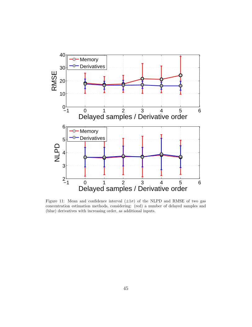
signal in addition to the signal itself. Figure 11 depicts the gas quantification

23

results when considering both alternatives. For the first case (”Memory”),

the x-axis k = 0 . . . 5 represents the number of additional delayed samples

for each training point, while in the second case it represents the maximum

order of derivatives taken into account as additional inputs to the inference

process.

[Figure 11 about here.]

The first conclusion from these results is that our GP calibration was not

able to infer the dynamics of MOX sensors from delayed samples of the sensor

signals, and thus, the calibration results do not improve when increasing k.

Furthermore, and possibly due to the increase in the input dimensionality,

the results tend to get worse for high values of k, probably due to curse of

dimensionality. On the other hand, the ”Derivatives” approach yields slightly

positive results. The improvement is mainly observable in the RMSE where

mean as well as the confidence intervals decrease when increasing k.

6. Conclusions and Future Work

In this paper we proposed a new approach for gas concentration estima-

tion using an array of MOX gas sensors in a Open Sampling System (OSS).

Despite its importance, this topic has been largely neglected. We addressed

the problem in a probabilistic manner and used Gaussian Processes to esti-

mate a posterior distribution over the gas concentration given the response

from an array of MOX sensors. This has the advantage of enabling not only

predictions of the expected gas concentration but also predictions of the un-

certainty of this estimate. This advantage is particularly relevant for OSS

applications where typically many sources of uncertainty exist.

24

In the first part of this work, we focussed on gas quantification using a

single MOX sensor, and then turned to gas quantification using a sensor array.

We found a clearly improved prediction quality with a sensor array compared

to using a single sensor. Given the high correlation among different MOX

sensors, we used ARD to exclude sensors that are not relevant for estimating

the posterior distribution. This proves useful in keeping the dimensionality

of the input space low.

We also analysed two data preprocessing strategies, one that performs

GP regression directly with the sensor response and ground truth gas con-

centrations, and a second one that performs GP regression on the logarithms

of sensor response and ground truth concentrations. Logarithmic prepro-

cessing has proven advantageous both for the estimation of the expected gas

concentration and for uncertainty prediction.

Finally, we studied approaches to mitigate the effect of the slow dynam-

ics of MOX sensors by taking into account past sensor readings in the GP

regression. Neither using additional inputs from previous time steps, nor

adding the signal derivatives, produced a significant improvement over the

concentration estimation algorithm that considers only the current sensors

readings.

Future works will include exploring sparse Gaussian Processes like the

Relevance Vector Machine (RVM) or Informative Vector Machine (IVM) to

improve over the currently random selection of training points, which is a

major bottleneck for GP regression. Another interesting aspect to study is

the generation of confidence intervals on the prediction and in particular how

the Bayesian approach we propose here compares with frequentist approaches

25

like Conformal Prediction (CP). Finally, another aspect to investigate is the

use of kernels for time series like the Autoregressive (AR) or Dynamic Time

Warping (DTW) kernel to study if they can efficiently model the dynamics of

MOX sensors, and therefore produce even more accurate gas concentration

estimates.

Acknowledgements

The authors would like to thank Hiroshi Ishida, Yuichiro Fukazawa and

Yuta Wada for the support in the data collection phase.

This work has been partly supported by the Regional Government of

Andalucıa and the European Union (FEDER) under research contract P08-

TEP-4016.

References

[1] V. Hernandez Bennetts, A. Lilienthal, M. Trincavelli, Creating true gas

concentration maps in presence of multiple heterogeneous gas sources,

2012, pp. 554–557.

[2] M. Trincavelli, M. Reggente, S. Coradeschi, H. Ishida, A. Loutfi, A. J.

Lilienthal, Towards environmental monitoring with mobile robots, in:

Proceedings of the IEEE/RSJ International Conference on Intelligent

Robots and Systems (IROS), 2008, pp. 2210 – 2215.

[3] M. Reggente, A. Mondini, G. Ferri, B. Mazzolai, A. Manzi, M. Gabel-

letti, P. Dario, A. J. Lilienthal, The dustbot system: Using mobile robots

26

to monitor pollution in pedestrian area, Chemical Engineering Transac-

tions 23 (2010) 273–278. doi:10.3303/CET1023046.

[4] P. P. Neumann, S. Asadi, A. J. Lilienthal, M. Bartholmai, J. H. Schiller,

Autonomous gas-sensitive microdrone: Wind vector estimation and gas

distribution mapping, Robotics Automation Magazine, IEEE 19 (1)

(2012) 50–61. doi:10.1109/MRA.2012.2184671.

[5] G. Kowadlo, R. A. Russell, Robot odor localization: A taxonomy and

survey, The International Journal of Robotics Research 27 (8) (2008)

869–894.

[6] A. J. Lilienthal, A. Loutfi, T. Duckett, Airborne chemical sensing with

mobile robots, Sensors 6 (2006) 1616–1678.

[7] H. Ishida, T. Nakamoto, T. Moriizumi, T. Kikas, J. Janata, Plume-

tracking robots: A new application of chemical sensors, The Biological

Bulletin 200 (2) (2001) 222–226.

[8] J.-L. Blanco, J. G. Monroy, J. Gonzalez-Jimenez, A. Lilienthal, A

kalman filter based approach to probabilistic gas distribution mapping,

in: 28th Symposium On Applied Computing (SAC), 2013.

[9] A. J. Lilienthal, M. Reggente, M. Trincavelli, J. L. Blanco, J. Gonzalez,

A statistical approach to gas distribution modelling with mobile robots

the kernel dm+v algorithm, in: Proceedings of the IEEE/RSJ Interna-

tional Conference on Intelligent Robots and Systems (IROS), 2009, pp.

570–576.

27

[10] A. J. Lilienthal, T. Duckett, A stereo electronic nose for a mobile in-

spection robot, in: Proceedings of the IEEE International Workshop on

Robotic Sensing (ROSE), Orebro, Sweden, 2003.

[11] J. Gonzalez-Jimenez, J. G. Monroy, J. L. Blanco, The multi-chamber

electronic nose - an improved olfaction sensor for mobile robotics, Sen-

sors 11 (6) (2011) 6145–6164. doi:10.3390/s110606145.

[12] M. Trincavelli, Gas discrimination for mobile robots, Kunstliche Intelli-

genz 25 (4) (2011) 351 – 354.

[13] C. Rasmussen, C. Williams, Gaussian processes for machine learning,

Adaptive computation and machine learning, MIT Press, 2006.

[14] J. Monroy, A. Lilienthal, J. Blanco, J. Gonzalez-Jimenez, M. Trin-

cavelli, Calibration of mox gas sensors in open sampling systems

based on gaussian processes, in: Sensors, 2012 IEEE, 2012, pp. 1–4.

doi:10.1109/ICSENS.2012.6411464.

[15] R. Neal, Bayesian learning for neural networks, Lecture notes in statis-

tics, Springer, 1996.

[16] D. J. C. MacKay, Bayesian methods for back-propagation networks,

Models of neural networks 3, Springer, 1994, pp. 211–254.

[17] K. Ihokura, J. Watson, The stannic oxide gas sensor: principles and

applications, CRC Press, 1994.

[18] P. J. Gemperline, J. R. Long, V. G. Gregoriou, Nonlinear multi-

variate calibration using principal components regression and artifi-

28

cial neural networks, Analytical Chemistry 63 (20) (1991) 2313–2323.

doi:10.1021/ac00020a022.

[19] H. Sundgren, F. Winquist, I. Lukkari, I. Lundstrom, Artificial neural

networks and gas sensor arrays: Quantification of individual components

in a gas mixture, Measurement Science and Technology 2 (5) (1991)

464–469.

[20] K. Domansk, D. L. Baldwin, J. W. Grate, T. B. Hall, J. Li, M. Josow-

icz, J. Janata, Development and calibration of field-effect transistor-

based sensor array for measurement of hydrogen and ammonia gas

mixtures in humid air, Analytical Chemistry 70 (3) (1998) 473–481.

doi:10.1021/ac970427x.

[21] L. Hadjiiski, P. Geladi, P. Hopke, A comparison of modeling nonlinear

systems with artificial neural networks and partial least squares, Chemo-

metrics and Intelligent Laboratory Systems 49 (1) (1999) 91–103.

[22] M. Blanco, J. Coello, H. Iturriaga, S. Maspoch, J. Pags, Calibration

in non-linear near infrared reflectance spectroscopy: A comparison of

several methods, Analytica Chimica Acta 384 (2) (1999) 207–214.

[23] A. Shmilovici, G. Bakir, S. Marco, A. Perera, Finding the best calibra-

tion points for a gas sensor array with support vector regression, in: In-

telligent Systems, 2004. Proceedings. 2004 2nd International IEEE Con-

ference, Vol. 1, 2004, pp. 174 – 177 Vol.1. doi:10.1109/IS.2004.1344660.

[24] R. P. Cogdill, P. Dardenne, Least-squares support vector machines for

29

chemometrics: An introduction and evaluation, Journal of Near Infrared

Spectroscopy 12 (2) (2004) 93–100.

[25] C. D. Natale, S. Marco, F. Davide, A. D’Amico, Sensor-array calibration

time reduction by dynamic modelling, Sensors and Actuators B: Chem-

ical 25 (1-3) (1995) 578 – 583, proceedings of the Fifth International

Meeting on Chemical Sensors. doi:10.1016/0925-4005(95)85126-7.

[26] S. D. Vito, E. Massera, M. Piga, L. Martinotto, G. D. Francia, On field

calibration of an electronic nose for benzene estimation in an urban pol-

lution monitoring scenario, Sensors and Actuators B: Chemical 129 (2)

(2008) 750 – 757. doi:10.1016/j.snb.2007.09.060.

[27] H. Ishida, T. Nakamoto, T. Moriizumi, Remote sensing of gas/odor

source location and concentration distribution using mobile sys-

tem, Sensors and Actuators B: Chemical 49 (1-2) (1998) 52 – 57.

doi:10.1016/S0925-4005(98)00036-7.

[28] T. Pearce, Handbook of machine olfaction: electronic nose technology,

Wiley-VCH, 2003.

[29] T. Nakamoto, K. Yoshikawa, Movie with scents generated by olfactory

display using solenoid valves, IEICE Trans. Fundam. Electron. Commun.

Comput. Sci. E89-A (11) (2006) 3327–3332. doi:10.1093/ietfec/e89-

a.11.3327.

[30] R. Russell, Odour Detection by Mobile Robots, World Scientific Pub-

lishing Co, London, UK, 1999.

30

[31] M. Trincavelli, S. Coradeschi, A. Loutfi, Online classification of gases

for environmental exploration, in: Proceedings of the IEEE/RSJ Inter-

national Conference on Intelligent Robots and Systems (IROS), 2009,

pp. 3311 – 3316.

Javier G.Monroy received his MSc degree (2007) in Electrical Engineering

from the University of Malaga, Spain. Currently, he is a graduate student

at the Dept. of System Engineering and Automation, University of Malaga.

During spring 2011 he visited the Center for Applied Autonomous Sensor

Systems, Orebro University, Sweden, as a guest researcher. His research

interests include autonomous mobile robots and artificial olfaction.

Achim Lilienthal is associate professor at AASS, Orebro University, Swe-

den, where he is leading the Mobile Robotics and Olfaction Lab. His main

research interests are mobile robot olfaction, rich 3D perception, robot vi-

sion, and safe navigation for autonomous transport robots. Achim Lilienthal

obtained his Ph.D. in computer science from Tubingen University, Germany

and his M.Sc. and B.Sc. in Physics from the University of Konstanz, Ger-

many. The Ph.D. thesis addresses gas distribution mapping and gas source

localisation with a mobile robot. The M.Sc. thesis is concerned with an

investigation of the structure of (C60)+n clusters using gas phase ion chro-

matography.

Jose Luis Blanco was born in Linares, Spain, in 1981. He received the

European PhD and the M.S. degree in Electrical Engineering from the Uni-

versity of Malaga, Malaga, Spain in 2009 and 2005, respectively. Currently,

he teaches as a Lecturer at the University of Almerıa, Spain. He is the

author or coauthor of about 20 journal and conference papers. His current

31

research interests include robot autonomous navigation, world modeling, and

computer vision.

Javier Gonzalez-Jimenez received the B.S. degree in Electrical Engineer-

ing from the University of Seville in 1987. He joined the Department of

”Ingeniera de Sistemas y Automatica” at the University of Malaga in 1988

and received the Ph.D. from this University in 1993. In 1990-1991 he was

at the Field Robotics Center, Robotics Institute, Carnegie Mellon University

(USA) working on mobile robots as part of his PhD. Since 1996 he has been

leading Spanish and European projects on mobile robotics and perception.

Currently, he is a professor at the University of Malaga and head of the

Machine Perception and Intelligent Robotics (MAPIR) group. His research

interest includes mobile robot navigation, olfactory robotics and computer

vision. In these fields he has published three books and more than 100 papers.

Marco Trincavelli received both his BSc degree (2003) and his MSc de-

gree (2006) in Computer Engineering from the Politecnico di Milano, Mi-

lan, Italy. He additionally received a MSc degree in Electrical Engineering

and Computer Science from the Lund Tekniska Hogskola, Lund, Sweden, in

2006. In 2007-2010 he has been a graduate student at the Center for Applied

Autonomous Sensor Systems, Orebro University, Orebro, Sweden. During

autumn 2009 he visited the Tokyo University of Agriculture and Technology

as a guest researcher. In autumn 2010 he spent another period as a guest

researcher at the BioCircuits Institute at the University of California, San

Diego. His research interests include machine learning and artificial olfaction

with particular focus on mobile robotics applications.

32

List of Figures

1 Sketch of the experimental setup (a), and detailed picture ofthe MOX sensors and the PID used to sample the volatiles (b). 35

2 Gas source emission strategies. For the randomized strategy(d), one exemplary instance is displayed. . . . . . . . . . . . . 36

3 Instantaneous sensor response (a) and PID measurements (b)for a standard open sampling system experiment. . . . . . . . 37

4 Examples of the learned regression functions for the case wherea single sensor (here TGS-2611 ) is considered. Blue dots rep-resent the training data. The solid red line is the mean of theposterior, and its variance is visualized by the ±1σ confidenceinterval. (a) A typical calibration function learned when usinglinear pre-processing, Eq. (4). (b) Calibration after applyinga logarithmic transformation not only to the input data, Eq. (5). 38

5 Estimation of the gas concentration for three different gasemitting strategies (rows), obtained from sensor TGS-2611with linear pre-processing c = f(r(t)), and the proposed GPcalibration. The left column shows the ground truth (blue)together with the GP calibration estimate (the red line is theposterior mean and the shaded grey region represents ±1σconfidence interval), the PLSR (green line), and the SVR esti-mate (magenta line). The right column shows for each scenariothe error between the different estimates and ground truth (inthe case of GPs only the mean value is taken into account). . . 39

6 The predictions of the same experiment as in Figure 5, butafter training on log-transformed inputs: log(c) = f(log(ri(t))). 40

7 NLPD and RMSE box-plot for the case of one-sensor GP cal-ibration. For both indicators, as lower the value the betterthe calibration. On each box, the central red mark is the me-dian, the edges of the box are the 25th and 75th percentiles,the whiskers extend to the most extreme data points not con-sidering outliers, and outliers are plotted individually as redcrosses. . . . . . . . . . . . . . . . . . . . . . . . . . . . . . . . 41

33

8 NLPD and RMSE box-plot for the case of one-sensor GP cali-bration with logarithmic transformation. For both indicators,as lower the value the better the calibration. On each box,the central red mark is the median, the edges of the box arethe 25th and 75th percentiles, the whiskers extend to the mostextreme data points not considering outliers, and outliers areplotted individually as red crosses. . . . . . . . . . . . . . . . 42

9 Estimation of the gas concentration for three different gasemitting strategies (rows) when considering the readings ofthe whole array and linear pre-processing c = f(rt). The leftcolumn shows the ground truth (blue), together with the GPcalibration estimate (the red line is the posterior mean andthe shaded grey region represents the ±1σ confidence inter-val), the PLSR (green line), and the SVR estimate (magentaline). The right column shows for each scenario the error be-tween the different estimates and ground truth (in the case ofGPs only the mean value is taken into account). . . . . . . . . 43

10 The predictions of the same experiment as in Figure 9, but af-ter training with the logarithmic relation log(c) = f(log(rb(t))) 44

11 Mean and confidence interval (±1σ) of the NLPD and RMSEof two gas concentration estimation methods, considering: (red)a number of delayed samples and (blue) derivatives with in-creasing order, as additional inputs. . . . . . . . . . . . . . . . 45

34

(a) (b)

Figure 1: Sketch of the experimental setup (a), and detailed picture of the MOX sensorsand the PID used to sample the volatiles (b).

35

(a) Steps (b) Ascending Stairway

(c) Descending Stairway (d) Random Stairway

Figure 2: Gas source emission strategies. For the randomized strategy (d), one exemplaryinstance is displayed.

36

(a)

(b)

Figure 3: Instantaneous sensor response (a) and PID measurements (b) for a standardopen sampling system experiment.

37

(a)

(b)

Figure 4: Examples of the learned regression functions for the case where a single sensor(here TGS-2611 ) is considered. Blue dots represent the training data. The solid red lineis the mean of the posterior, and its variance is visualized by the ±1σ confidence interval.(a) A typical calibration function learned when using linear pre-processing, Eq. (4). (b)Calibration after applying a logarithmic transformation not only to the input data, Eq. (5).

38

(a) (b)

(c) (d)

(e) (f)

Figure 5: Estimation of the gas concentration for three different gas emitting strategies(rows), obtained from sensor TGS-2611 with linear pre-processing c = f(r(t)), and theproposed GP calibration. The left column shows the ground truth (blue) together withthe GP calibration estimate (the red line is the posterior mean and the shaded greyregion represents ±1σ confidence interval), the PLSR (green line), and the SVR estimate(magenta line). The right column shows for each scenario the error between the differentestimates and ground truth (in the case of GPs only the mean value is taken into account).

39

(a) (b)

(c) (d)

(e) (f)

Figure 6: The predictions of the same experiment as in Figure 5, but after training onlog-transformed inputs: log(c) = f(log(ri(t))).

40

(a)

(b)

Figure 7: NLPD and RMSE box-plot for the case of one-sensor GP calibration. For bothindicators, as lower the value the better the calibration. On each box, the central redmark is the median, the edges of the box are the 25th and 75th percentiles, the whiskersextend to the most extreme data points not considering outliers, and outliers are plottedindividually as red crosses.

41

(a)

(b)

Figure 8: NLPD and RMSE box-plot for the case of one-sensor GP calibration with loga-rithmic transformation. For both indicators, as lower the value the better the calibration.On each box, the central red mark is the median, the edges of the box are the 25th and75th percentiles, the whiskers extend to the most extreme data points not consideringoutliers, and outliers are plotted individually as red crosses.

42

(a) (b)

(c) (d)

(e) (f)

Figure 9: Estimation of the gas concentration for three different gas emitting strategies(rows) when considering the readings of the whole array and linear pre-processing c =f(rt). The left column shows the ground truth (blue), together with the GP calibrationestimate (the red line is the posterior mean and the shaded grey region represents the ±1σconfidence interval), the PLSR (green line), and the SVR estimate (magenta line). Theright column shows for each scenario the error between the different estimates and groundtruth (in the case of GPs only the mean value is taken into account).

43

(a) (b)

(c) (d)

(e) (f)

Figure 10: The predictions of the same experiment as in Figure 9, but after training withthe logarithmic relation log(c) = f(log(rb(t)))

44

−1 0 1 2 3 4 5 62

3

4

5

6

NLP

D

Delayed samples / Derivative order

MemoryDerivatives

−1 0 1 2 3 4 5 60

10

20

30

40R

MS

E

Delayed samples / Derivative order

MemoryDerivatives

Figure 11: Mean and confidence interval (±1σ) of the NLPD and RMSE of two gasconcentration estimation methods, considering: (red) a number of delayed samples and(blue) derivatives with increasing order, as additional inputs.

45

List of Tables

1 Gas sensors used in the sensor array. . . . . . . . . . . . . . . 472 Cross-correlation coefficients for the MOX sensors in the array

and the PID. High values suggest that the sensors are exposedto the same concentrations. . . . . . . . . . . . . . . . . . . . 48

3 RMSE values (Mean ± 1σ) of three different calibration meth-ods when using only one sensor at a time. Sensors MiCS-5121and TGS-2611 provide the overall best performance. . . . . . 49

4 Mean ±1σ interval of the length scale hyper-parameter for thedifferent sensors in the array as obtained from ARD. . . . . . 50

46

Model Gases Detected Quantity

Figaro TGS 2600 Hydrogen, Carbon Monoxide 2

Figaro TGS 2602 Ammonia, Hydrogen Sulfide, VOC(volatile organic compound)

1

Figaro TGS 2611 Methane 1

Figaro TGS 2620 Organic Solvents 1

e2V MiCS 2610 Ozone 1

e2V MiCS 2710 Nitrogen Dioxide 1

e2V MiCS 5521 Carbon Monoxide, Hydrocarbons,VOC

2

e2V MiCS 5121 Carbon Monoxide, Hydrocarbons,VOC

1

e2V MiCS 5135 Carbon Monoxide, Hydrocarbons,VOC

1

Table 1: Gas sensors used in the sensor array.

47

PID MiCS2610

MiCS2710

MiCS5521-1

MiCS5121

MiCS3135

MiCS5521-2

TGS2600-1

TGS2611

TGS2620

TGS2600-2

TGS2602

1,00 -0,75 -0,88 -0,86 -0,89 -0,82 -0,89 -0,82 -0,92 -0,80 -0,81 -0,69

-0,75 1,00 0,93 0,93 0,95 0,98 0,91 0,98 0,90 0,98 0,98 0,98

-0,88 0,93 1,00 0,94 0,98 0,97 0,95 0,97 0,97 0,96 0,97 0,90

-0,86 0,93 0,94 1,00 0,98 0,97 0,99 0,96 0,97 0,96 0,96 0,90

-0,89 0,95 0,98 0,98 1,00 0,98 0,98 0,98 0,98 0,97 0,98 0,91

-0,82 0,98 0,97 0,97 0,98 1,00 0,96 1,00 0,96 1,00 1,00 0,96

-0,89 0,91 0,95 0,99 0,98 0,96 1,00 0,95 0,97 0,94 0,95 0,87

-0,82 0,98 0,97 0,96 0,98 1,00 0,95 1,00 0,95 1,00 1,00 0,97

-0,92 0,90 0,97 0,97 0,98 0,96 0,97 0,95 1,00 0,95 0,95 0,86

-0,80 0,98 0,96 0,96 0,97 1,00 0,94 1,00 0,95 1,00 1,00 0,97

-0,81 0,98 0,97 0,96 0,98 1,00 0,95 1,00 0,95 1,00 1,00 0,97

-0,69 0,98 0,90 0,90 0,91 0,96 0,87 0,97 0,86 0,97 0,97 1,00

Table 2: Cross-correlation coefficients for the MOX sensors in the array and the PID. Highvalues suggest that the sensors are exposed to the same concentrations.

48

Sensor Model GPs PLSR SVR

MiCS 2610 43.81± 22.88 44.79± 14.26 46.01± 19.44

MiCS 2710 30.38± 7.83 31.89± 6.13 29.71± 6.42

MiCS 5521-1 33.64± 9.02 34.26± 7.03 34.09± 7.56

MiCS 5121 23.84± 5.58 25.44± 4.20 24.18± 5.91

MiCS 5135 32.09± 12.00 35.61± 8.21 33.37± 12.31

MiCS 5521-2 31.11± 8.01 32.37± 7.47 31.80± 8.09

TGS 2600-1 26.05± 10.08 31.10± 5.42 25.71± 8.79

TGS 2611 21.46± 3.54 26.27± 3.59 21.57± 3.14

TGS 2620 34.16± 24.02 35.41± 7.08 29.61± 8.38

TGS 2600-2 28.96± 15.13 32.43± 5.98 27.23± 9.92

TGS 2602 44.64± 15.58 41.87± 8.21 37.12± 12.69

OVERALL 31.17± 6.27 33.77± 5.77 30.94± 6.78

Table 3: RMSE values (Mean ± 1σ) of three different calibration methods when usingonly one sensor at a time. Sensors MiCS-5121 and TGS-2611 provide the overall bestperformance.

49

Sensor Length scale (l)

MiCS 2610 0.386± 0.272

MiCS 2710 0.732± 0.337

MiCS 5521-1 0.869± 0.145

MiCS 5121 0.212± 0.175

MiCS 5135 0.533± 0.312

MiCS 5521-2 0.761± 0.305

TGS 2600-1 0.200± 0.167

TGS 2611 0.001± 0.004

TGS 2620 0.554± 0.387

TGS 2600-2 0.749± 0.247

TGS 2602 0.116± 0.042

Table 4: Mean ±1σ interval of the length scale hyper-parameter for the different sensorsin the array as obtained from ARD.

50