Probabilistic analyses of a strip footing on horizontally

stratified sandy deposit using advanced constitutive model

R. Suchomel and D. Masın1

Charles University in Prague

Faculty of Science

Albertov 6

12843 Prague 2, Czech Republic

E-mail: masin@natur.cuni.cz

Tel: +420-2-2195 1552, Fax: +420-2-2195 1556

January 6, 2011

Submitted to Computers and Geotechnics

1corresponding author

1 Abstract

An advanced hypoplastic constitutive model is used in probabilistic analyses of a typical geotech-

nical problem, strip footing. Spatial variability of soil parameters, rather than state variables, is

considered in the study. The model, including horizontal and vertical correlation lengths, was cali-

brated using a comprehensive set of experimental data on sand from horizontally stratified deposit.

Some parameters followed normal, whereas other followed lognormal distributions. Monte-Carlo

simulations revealed that the foundation displacementuy for a given load followed closely the log-

normal distribution, even though some model parameters were distributed normally. Correlation

length in the vertical directionθv was varied in the simulation. The case of infinite correlation

length was used for evaluation of different approximate probabilistic methods (first order second

moment method and several point estimate methods). In the random field Monte-Carlo analyses

with finite θv, the vertical correlation length was found to have minor effect on the mean value of

uy, but significant effect on its standard deviation. As expected, it decreased with decreasingθvdue to spatial averaging of soil properties.

Key Words: Probabilistic methods; constitutive models; random fields; foundation settlement

2 Introduction

Parameters of simple constitutive models, which are typically used in probabilistic analyses of

geotechnical problems, are dependent on the soil state. These models thus do not allow us to

distinguish whether the measured variability of soil properties is caused by the variability of soil

type or soil state. Contrary to this, advanced constitutivemodels adopt soil parameters that are

specific to the given soil granulometry and mineralogical composition of soil particles. State vari-

ables (such as void ratioe) then incorporate the state-dependency of the soil behaviour. In this

respect, the sources of the objective (aleatory [25]) uncertainty in soil mechanical behaviour can

be subdivided into two groups:

1. In some situations, soil mineralogy and granulometry maybe regarded as spatially invariable,

and the uncertainty in the mechanical properties of soil deposit come from variability in the

soil state. In this case, soilparametersof advanced models may be considered as constants,

and in the analyses it is sufficient to consider spatial variability of state variablesdescribing

the relative density of soil.

2. In other cases, soil properties are variable due to varying granulometry and mineralogy of soil

grains. Such a situation is for example typical for soil deposits of sedimentary basins, where

1

the granulometry varies due to the variable geological conditions during the deposition. In

such a case, it is necessary to consider spatially variable soil parametersin the simulations.

Application of advanced constitutive models within probabilistic numerical analyses still remains

relatively uncommon in the geotechnical scientific literature. Moreover, most of the applications

of probabilistic methods in combination with advanced soilconstitutive models consider the un-

certainty in the state variable only, while keeping constant values of the model parameters. As an

example, Hicks and Onisiphorou [27] studied stability of underwater sandfill berms. Their aim was

to study whether presence of ’pockets’ of liquifiable material may be enough to cause instability

in a predominantly dilative fill. They used a double-hardening constitutive model Monot [33] with

probabilistic distribution of the Been and Jefferies statevariableψ [3]. As the aim of the research

was to study whether pockets of loose material may cause failure of the berm, the approach cho-

sen (variation in the state variable only) is fully justifiable. In other applications, Tejchman [45]

studied the influence of the fluctuation of void ratio on formation of the shear zone in the biax-

ial specimen using the hypoplastic model by von Wolffersdorff [47]. Similar procedure and the

same constitutive model was used by other researchers in finite element simulations of different

geotechnical problems [34, 36]. Finally, Andrade et al. [1]considered random porosity fields in

combination with an advanced constitutive model and studied their influence on strength and shear

band formation in a biaxial specimen.

The goal of this paper is to present a complete evaluation of the influence of parameter variability

of an advanced constitutive model and its influence on predictions of a typical geotechnical prob-

lem. To utilise the advantage of the non-linear formulationof the constitutive model adopted, we

study settlement of a rigid strip foundation subjected to a given load. While most application of

probabilistic methods to the foundation problems focus on the evaluation of the bearing capacity

[17, 15, 7, 11, 28, 29, 21, 13], less attention is payed to the quantification of the uncertainty in

serviceability limit states. In the available studies, theauthors focus on different aspects of the

problem, such as foundation size and geometry [30], uncertainty in the foundation load [5], 3D

effects [19, 14], differential settlement issues between two footings [12, 14, 34], cross-correlation

between elastic parametersE andν [35], the effects of layers of different materials in the subsoil

[32], and comparison with simpler probabilistic methods (such as the first order second moment

method) [20]. In many publications, the authors address theinfluence of the correlation length

[35, 14, 19, 12]. In most of these works, however, the soil is modelled as a linear elastic material

(or elastic material with stress-dependent Young modulus [30]). An exception is the contribution

by Niemunis et al. [34], who used non-linear hypoplastic model with constant parameters and ran-

dom fields of void ratio in the cyclic analyses of two adjacentstrip footings. Most of the available

studies thus do not consider the non-linear soil behaviour,which is important for correct predictions

of foundation displacements. This issue is addressed in thepresent work.

2

3 Experimental program

The material for the investigation comes from the south partof upper Cretaceous Trebon basin in

south Bohemia (Czech Republic) from the sand pit Kolny [42]. The pit is located in the upper part

of the so-called Klikovske layers, youngest (senon) strata of the south Bohemian basins. These

fluvial layers are characterised by a rhythmical variation of gravely sands, sands and clayey sands.

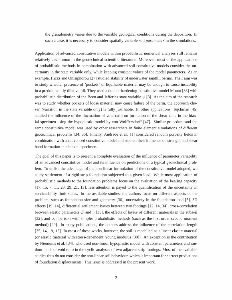
Altogether forty samples were obtained from a ten meters high pit wall in a regular rectangular

grid (Fig. 1). The laboratory program was designed to provide for each of the samples enough

Figure 1: The wall of the sand pit in south part of the Trebonbasin. Black dots represent positionsof specimens for the laboratory investigation.

information to calibrate the hypoplastic model for granular materials by von Wolffersdorff [47].

The following tests were performed on each of the 40 samples:

• Oedometric compression tests on initially very loose specimens with loading steps 100, 200,

400, 800, 1600, 3200 and 6400 kPa.

• Drained triaxial compression test on specimen dynamicallycompacted to void ratio corre-

sponding to the densein-situ conditions. One test per specimen at the cell pressure of 200

kPa.

• Measurement of the angle of repose.

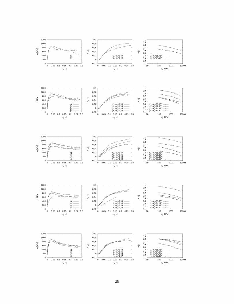
Results of all the laboratory experiments are presented in the Appendix. Location of the specimens,

labeled asa1 to j4, is indicated in Fig. 1. Note that 4 specimens (c1, e4, f1, f2) showed unusual

behaviour, and these specimens were not used in the evaluation.

3

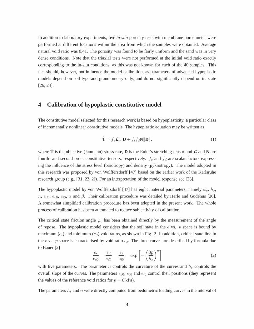
In addition to laboratory experiments, fivein-situ porosity tests with membrane porosimeter were

performed at different locations within the area from whichthe samples were obtained. Average

natural void ratio was 0.41. The porosity was found to be fairly uniform and the sand was in very

dense conditions. Note that the triaxial tests were not performed at the initial void ratio exactly

corresponding to the in-situ conditions, as this was not known for each of the 40 samples. This

fact should, however, not influence the model calibration, as parameters of advanced hypoplastic

models depend on soil type and granulometry only, and do not significantly depend on its state

[26, 24].

4 Calibration of hypoplastic constitutive model

The constitutive model selected for this research work is based on hypoplasticity, a particular class

of incrementally nonlinear constitutive models. The hypoplastic equation may be written as

T = fsL : D + fsfdN‖D‖. (1)

whereT is the objective (Jaumann) stress rate,D is the Euler’s stretching tensor andL andN are

fourth- and second order constitutive tensors, respectively. fs andfd are scalar factors express-

ing the influence of the stress level (barotropy) and density(pyknotropy). The model adopted in

this research was proposed by von Wolffersdorff [47] based on the earlier work of the Karlsruhe

research group (e.g., [31, 22, 2]). For an interpretation ofthe model response see [23].

The hypoplastic model by von Wolffersdorff [47] has eight material parameters, namelyϕc, hs,

n, ed0, ec0, ei0, α andβ. Their calibration procedure was detailed by Herle and Gudehus [26].

A somewhat simplified calibration procedure has been adopted in the present work. The whole

process of calibration has been automated to reduce subjectivity of calibration.

The critical state friction angleϕc has been obtained directly by the measurement of the angle

of repose. The hypoplastic model considers that the soil state in thee vs. p space is bound by

maximum (ei) and minimum (ed) void ratios, as shown in Fig. 2. In addition, critical stateline in

thee vs. p space is characterised by void ratioec. The three curves are described by formula due

to Bauer [2]ecec0

=eded0

=eiei0

= exp

[

−(

3p

hs

)n]

(2)

with five parameters. The parametern controls the curvature of the curves andhs controls the

overall slope of the curves. The parametersed0, ec0 andei0 control their positions (they represent

the values of the reference void ratios forp = 0 kPa).

The parametershs andn were directly computed from oedometric loading curves in the interval of

4

Figure 2: The dependency of the reference void ratiosed, ec andei on the mean stress (Herle andGudehus [26]).

Figure 3: Computed curves usinghs, n, ec0 parameters for one column of specimens.

σa ∈ 〈100, 1000〉 kPa using procedure detailed in [26]. Following Herle and Gudehus [26], initial

void ratioemax of a loose oedometric specimen was considered equal to the critical state void ratio

at zero pressureec0. Figure 3 shows comparison of compression curves calculated using formula

by Bauer (2) with compression curves obtained from the oedometric test (for illustration purposes

specimens from one column of the sampling grid only).

Void ratiosed0 andei0 were obtained from empirical relations. The physical meaning of ed0 is

the reference void ratio at maximum density, whereas void ratio ei0 represents the intercept of the

isotropic normal compression line withp = 0 axis. Void ratioei0 was obtained by multiplyingec0by a factor 1.2 [26]. The minimum void ratioed0 was also calculated fromec0. ec0 was multiplied

by a factor0.379. This ensured that the initial void ratio for triaxial specimens was always higher

thaned and the initial state was close to the state of maximum density. The state thus corresponded

5

to the densein-situ conditions.

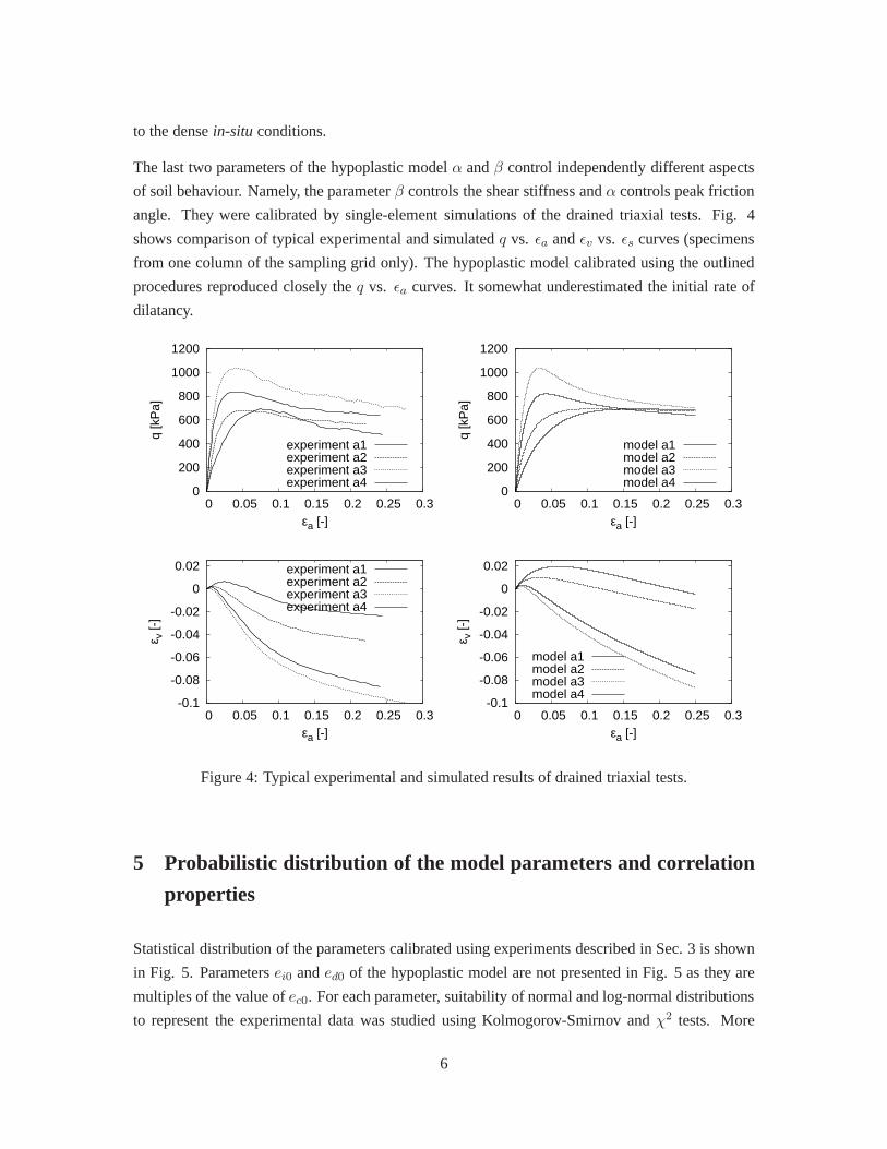
The last two parameters of the hypoplastic modelα andβ control independently different aspects

of soil behaviour. Namely, the parameterβ controls the shear stiffness andα controls peak friction

angle. They were calibrated by single-element simulationsof the drained triaxial tests. Fig. 4

shows comparison of typical experimental and simulatedq vs. ǫa andǫv vs. ǫs curves (specimens

from one column of the sampling grid only). The hypoplastic model calibrated using the outlined

procedures reproduced closely theq vs. ǫa curves. It somewhat underestimated the initial rate of

dilatancy.

0

200

400

600

800

1000

1200

0 0.05 0.1 0.15 0.2 0.25 0.3

q [k

Pa]

εa [-]

experiment a1experiment a2experiment a3experiment a4

0

200

400

600

800

1000

1200

0 0.05 0.1 0.15 0.2 0.25 0.3

q [k

Pa]

εa [-]

model a1model a2model a3model a4

-0.1

-0.08

-0.06

-0.04

-0.02

0

0.02

0 0.05 0.1 0.15 0.2 0.25 0.3

ε v [-

]

εa [-]

experiment a1experiment a2experiment a3experiment a4

-0.1

-0.08

-0.06

-0.04

-0.02

0

0.02

0 0.05 0.1 0.15 0.2 0.25 0.3

ε v [-

]

εa [-]

model a1model a2model a3model a4

Figure 4: Typical experimental and simulated results of drained triaxial tests.

5 Probabilistic distribution of the model parameters and correlation

properties

Statistical distribution of the parameters calibrated using experiments described in Sec. 3 is shown

in Fig. 5. Parametersei0 anded0 of the hypoplastic model are not presented in Fig. 5 as they are

multiples of the value ofec0. For each parameter, suitability of normal and log-normal distributions

to represent the experimental data was studied using Kolmogorov-Smirnov andχ2 tests. More

6

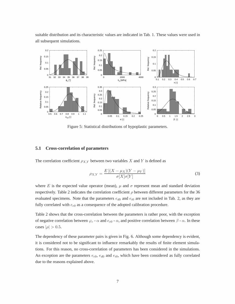
suitable distribution and its characteristic values are indicated in Tab. 1. These values were used in

all subsequent simulations.

0

0.05

0.1

0.15

0.2

31 32 33 34 35 36 37 38 39

Rel

. fre

quen

cy

ϕc [°]

0

0.05

0.1

0.15

0.2

0.25

0 2000 4000

Rel

. fre

quen

cy

hs [MPa] 0

0.05

0.1

0.15

0.2

0.1 0.2 0.3 0.4 0.5 0.6 0.7

Rel

. fre

quen

cy

n [-]

0

0.05

0.1

0.15

0.2

0.25

0.5 0.6 0.7 0.8 0.9 1 1.1

Rel

ativ

e fr

eque

ncy

ec0 [-] 0

0.05

0.1

0.15

0.2

0.25

0.3

0.35

0.05 0.1 0.15 0.2 0.25

Rel

. fre

quen

cy

α [-]

0

0.05

0.1

0.15

0.2

0.25

0.3

0 0.5 1 1.5 2 2.5 3

Rel

ativ

e fr

eque

ncy

β [-]

Figure 5: Statistical distributions of hypoplastic parameters.

5.1 Cross-correlation of parameters

The correlation coefficientρX,Y between two variablesX andY is defined as

ρX,Y =E [(X − µX)(Y − µY )]

σ[X]σ[Y ](3)

whereE is the expected value operator (mean),µ andσ represent mean and standard deviation

respectively. Table 2 indicates the correlation coefficient ρ between different parameters for the 36

evaluated specimens. Note that the parametersed0 andei0 are not included in Tab. 2, as they are

fully correlated withec0 as a consequence of the adopted calibration procedure.

Table 2 shows that the cross-correlation between the parameters is rather poor, with the exception

of negative correlation betweenϕc - α andec0 - α, and positive correlation betweenβ - α. In these

cases|ρ| > 0.5.

The dependency of these parameter pairs is given in Fig. 6. Although some dependency is evident,

it is considered not to be significant to influence remarkablythe results of finite element simula-

tions. For this reason, no cross-correlation of parametershas been considered in the simulations.

An exception are the parametersec0, ed0 andei0, which have been considered as fully correlated

due to the reasons explained above.

7

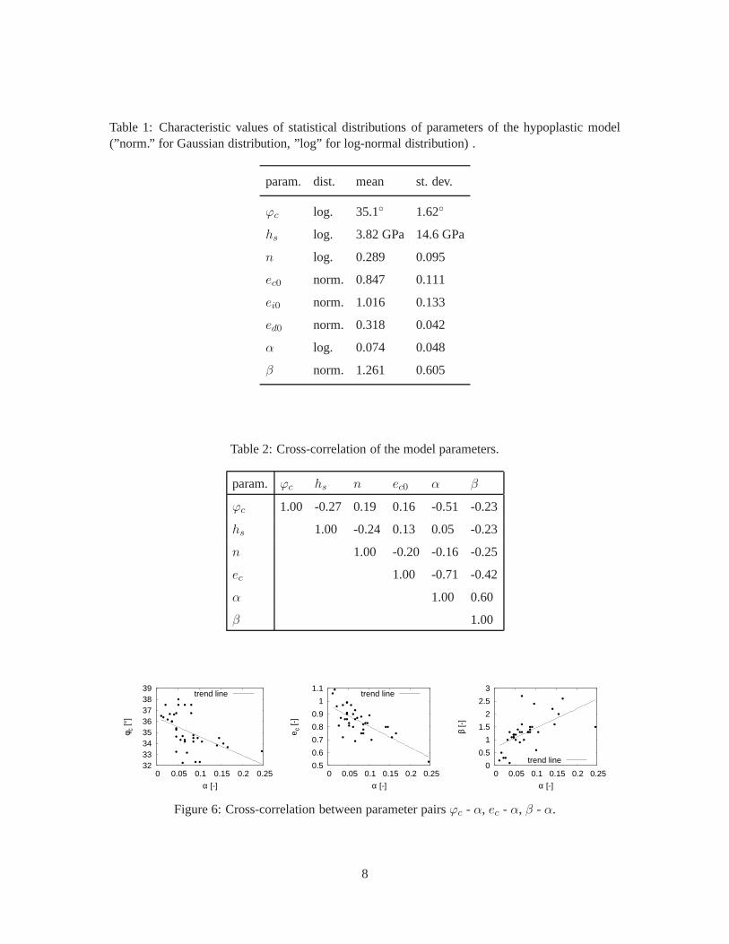
Table 1: Characteristic values of statistical distributions of parameters of the hypoplastic model(”norm.” for Gaussian distribution, ”log” for log-normal distribution) .

param. dist. mean st. dev.

ϕc log. 35.1◦ 1.62◦

hs log. 3.82 GPa 14.6 GPa

n log. 0.289 0.095

ec0 norm. 0.847 0.111

ei0 norm. 1.016 0.133

ed0 norm. 0.318 0.042

α log. 0.074 0.048

β norm. 1.261 0.605

Table 2: Cross-correlation of the model parameters.

param. ϕc hs n ec0 α β

ϕc 1.00 -0.27 0.19 0.16 -0.51 -0.23

hs 1.00 -0.24 0.13 0.05 -0.23

n 1.00 -0.20 -0.16 -0.25

ec 1.00 -0.71 -0.42

α 1.00 0.60

β 1.00

32 33 34 35 36 37 38 39

0 0.05 0.1 0.15 0.2 0.25

φ c [°

]

α [-]

trend line

0.5

0.6

0.7

0.8

0.9

1

1.1

0 0.05 0.1 0.15 0.2 0.25

e c [-

]

α [-]

trend line

0

0.5

1

1.5

2

2.5

3

0 0.05 0.1 0.15 0.2 0.25

β [-

]

α [-]

trend line

Figure 6: Cross-correlation between parameter pairsϕc - α, ec - α, β - α.

8

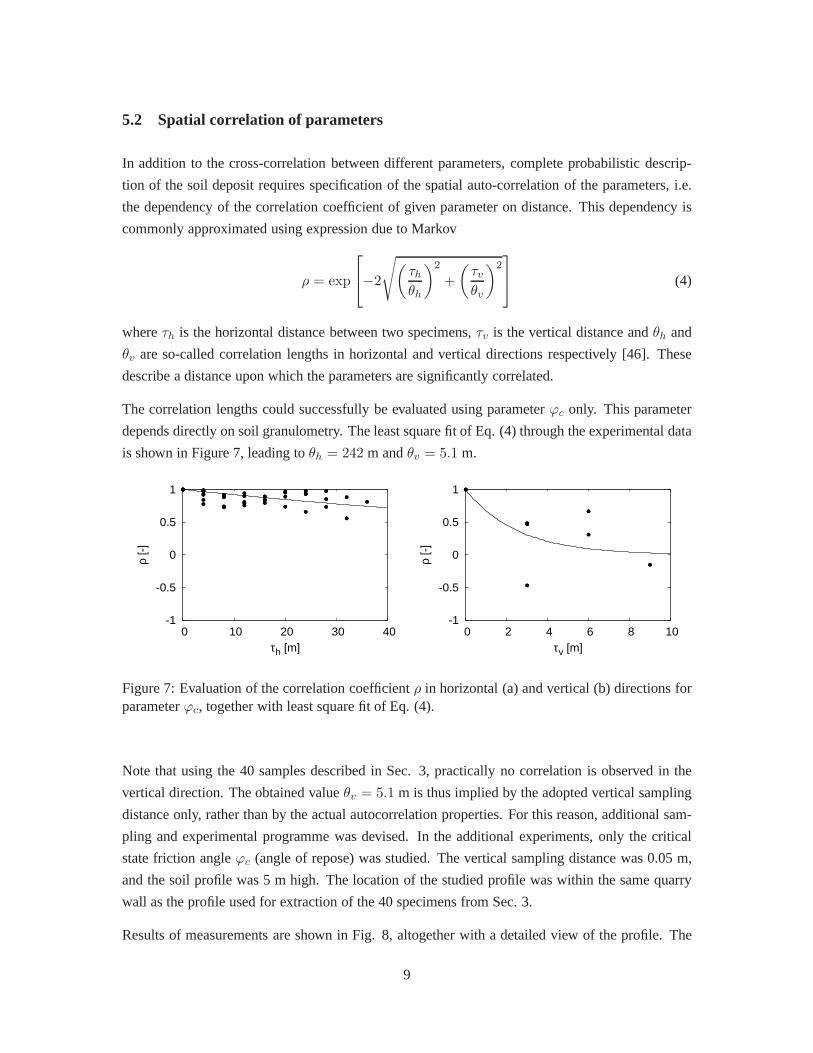
5.2 Spatial correlation of parameters

In addition to the cross-correlation between different parameters, complete probabilistic descrip-

tion of the soil deposit requires specification of the spatial auto-correlation of the parameters, i.e.

the dependency of the correlation coefficient of given parameter on distance. This dependency is

commonly approximated using expression due to Markov

ρ = exp

−2

√

(

τhθh

)2

+

(

τvθv

)2

(4)

whereτh is the horizontal distance between two specimens,τv is the vertical distance andθh and

θv are so-called correlation lengths in horizontal and vertical directions respectively [46]. These

describe a distance upon which the parameters are significantly correlated.

The correlation lengths could successfully be evaluated using parameterϕc only. This parameter

depends directly on soil granulometry. The least square fit of Eq. (4) through the experimental data

is shown in Figure 7, leading toθh = 242 m andθv = 5.1 m.

-1

-0.5

0

0.5

1

0 10 20 30 40

ρ [-

]

τh [m]

-1

-0.5

0

0.5

1

0 2 4 6 8 10

ρ [-

]

τv [m]

Figure 7: Evaluation of the correlation coefficientρ in horizontal (a) and vertical (b) directions forparameterϕc, together with least square fit of Eq. (4).

Note that using the 40 samples described in Sec. 3, practically no correlation is observed in the

vertical direction. The obtained valueθv = 5.1 m is thus implied by the adopted vertical sampling

distance only, rather than by the actual autocorrelation properties. For this reason, additional sam-

pling and experimental programme was devised. In the additional experiments, only the critical

state friction angleϕc (angle of repose) was studied. The vertical sampling distance was 0.05 m,

and the soil profile was 5 m high. The location of the studied profile was within the same quarry

wall as the profile used for extraction of the 40 specimens from Sec. 3.

Results of measurements are shown in Fig. 8, altogether witha detailed view of the profile. The

9

measurements are highly scattered. Nonetheless, an attempt has been made to distinguish zones of

different average friction angles (shown as bold lines in Fig. 7). Average length of these zones was

used as an approximation of the vertical correlation length, leading toθv = 0.31 m. Figure 8 also

shows random field (see Sec. 8.3) ofϕc, generated with parameters from Tab. 1 andθv = 0.31 m

andθh = 242 m. The generated profile approximates well the measured distribution ofϕc and the

observed layered structure of the soil deposit.

31 34 37

φc [∘]

0

0.2

0.4

0.6

0.8

1

1.2

1.4

1.6

1.8

2

2.2

2.4

2.6

2.8

3

3.2

3.4

3.6

3.8

4

4.2

4.4

4.6

4.8

5

h [

m]

φc [ ] φc random fieldin situ photo

Figure 8: Evaluation of the vertical correlation length using detailed measurements ofϕc. Randomfield for θv = 0.31 m.

10

6 Strip footing problem

The influence of spatial variation of parameters of the hypoplastic model was studied by simu-

lations of a typical geotechnical problem – settlement of a strip footing [44]. Simulations were

performed using a finite element packageTochnog Professional[38]. The individual simulations

were deterministic. Probabilistic aspects were introduced in Sec. 8 by variation of the input mate-

rial parameters and evaluation of the simulations outputs.

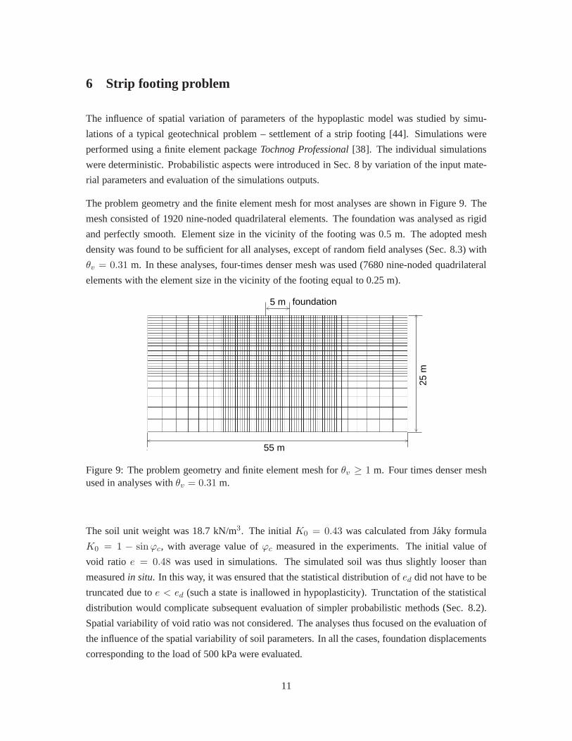
The problem geometry and the finite element mesh for most analyses are shown in Figure 9. The

mesh consisted of 1920 nine-noded quadrilateral elements.The foundation was analysed as rigid

and perfectly smooth. Element size in the vicinity of the footing was 0.5 m. The adopted mesh

density was found to be sufficient for all analyses, except ofrandom field analyses (Sec. 8.3) with

θv = 0.31 m. In these analyses, four-times denser mesh was used (7680 nine-noded quadrilateral

elements with the element size in the vicinity of the footingequal to 0.25 m).

55 m

25 m

5 m foundation

Figure 9: The problem geometry and finite element mesh forθv ≥ 1 m. Four times denser meshused in analyses withθv = 0.31 m.

The soil unit weight was 18.7 kN/m3. The initialK0 = 0.43 was calculated from Jaky formula

K0 = 1 − sinϕc, with average value ofϕc measured in the experiments. The initial value of

void ratio e = 0.48 was used in simulations. The simulated soil was thus slightly looser than

measuredin situ. In this way, it was ensured that the statistical distribution ofed did not have to be

truncated due toe < ed (such a state is inallowed in hypoplasticity). Trunctationof the statistical

distribution would complicate subsequent evaluation of simpler probabilistic methods (Sec. 8.2).

Spatial variability of void ratio was not considered. The analyses thus focused on the evaluation of

the influence of the spatial variability of soil parameters.In all the cases, foundation displacements

corresponding to the load of 500 kPa were evaluated.

11

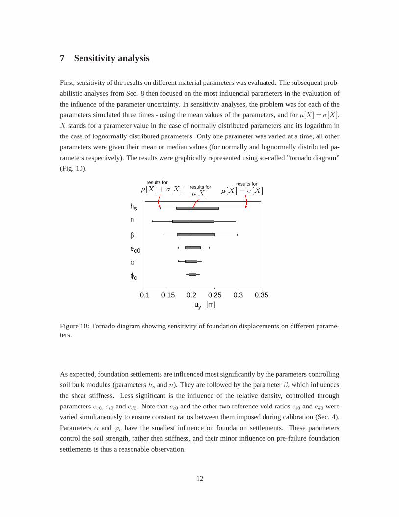
7 Sensitivity analysis

First, sensitivity of the results on different material parameters was evaluated. The subsequent prob-

abilistic analyses from Sec. 8 then focused on the most influencial parameters in the evaluation of

the influence of the parameter uncertainty. In sensitivity analyses, the problem was for each of the

parameters simulated three times - using the mean values of the parameters, and forµ[X]± σ[X].

X stands for a parameter value in the case of normally distributed parameters and its logarithm in

the case of lognormally distributed parameters. Only one parameter was varied at a time, all other

parameters were given their mean or median values (for normally and lognormally distributed pa-

rameters respectively). The results were graphically represented using so-called ”tornado diagram”

(Fig. 10).

β

α

h

c0

s

e

n

0.30.1 0.2 0.25 0.350.15

ϕc

[m]uy

results forresults for

results for

Figure 10: Tornado diagram showing sensitivity of foundation displacements on different parame-ters.

As expected, foundation settlements are influenced most significantly by the parameters controlling

soil bulk modulus (parametershs andn). They are followed by the parameterβ, which influences

the shear stiffness. Less significant is the influence of the relative density, controlled through

parametersec0, ei0 anded0. Note thatec0 and the other two reference void ratiosei0 anded0 were

varied simultaneously to ensure constant ratios between them imposed during calibration (Sec. 4).

Parametersα andϕc have the smallest influence on foundation settlements. These parameters

control the soil strength, rather then stiffness, and theirminor influence on pre-failure foundation

settlements is thus a reasonable observation.

12

8 Probabilistic analyses

In the analysis of uncertain systems, the uncertainty of theinput variables is propagated through

the system leading to the assesment of uncertainty of its response [41]. The strip footing problem

in scope of this study can be for thegiven parameter setconsidered as deterministic. Such a

problem can be solved using probabilistic numerical methods. The probabilistic characteristics

of the problem are studied by variation of the input parameters and evaluation of the simulation

output.

The following probabilistic methods have been evaluated inthe present work. First of all, the

strip footing problem has been simulated without considering spatial variability of the parameters

(i.e. with infinite correlation length) using a fully general Monte-Carlo method. These results

serve as a benchmark for the simulation using approximate probabilistic methods. Then, different

approximate analytical probabilistic methods for evaluation of the first two statistical moments

of the performance function have been evaluated. These methods are much less computationally

demanding, and they are thus more suitable for practical applications provided they give accurate

results. Finally, spatial variability of the parameters have been introduced through Monte-Carlo

simulations based on random field theory by Vanmarcke [46].

The geotechnical problem of the interest could be, apart from the above mentioned probabilis-

tic methods, solved using more general stochastic numerical analysis. Two main variants of the

stochastic finite element method (SFEM) are available in theliterature [41]: i) perturbation ap-

proach, which is based on a Taylor series expansion of the response vector and ii) the spectral

stochastic finite element method, where each response quantity is represented using a series of ran-

dom Hermite polynomials [16]. In the SFEM methods, the uncertainty is typically treated within

the finite element discretisation, and it is thus often not possible to apply the existing determin-

istic finite element tools without major modifications. Suchmethods are not readily available to

prectitioners as yet. They are thus outside the scope of the present work.

8.1 Monte-Carlo analyses with infinite correlation length

The probabilistic aspects of the problem analysed in this contribution are fairly complex. The con-

stitutive model and thus also the dependency ofuy on the parameter vectorX are non-linear. Some

of the model parameters follow Gaussian distributions, whereas other follow lognormal distribu-

tions. For this reason, to obtain reference values unbiasedby simplifications involved in approx-

imate solutions (Sec. 8.2), analyses with spatially invariable fields of input variables were first

performed using Monte-Carlo method. Another reason for running the Monte-Carlo analyses was

that the approximate methods do not provide any informationon the type of the statistical distribu-

13

tion of the output variable. They only approximate the first statistical moments (typically the first

two moments, i.e. mean and standard deviation). In Monte-Carlo analyses, uniformly distributed

random numbers were generated by an unbiased random number generator. Gaussian distributions

of the parameters were then obtained by the Box-Muller transformation method [4].

The Monte-Carlo method is fully general, but depending on the problem solved it may require

significantly large number of realisations and consequently a considerable computational effort.

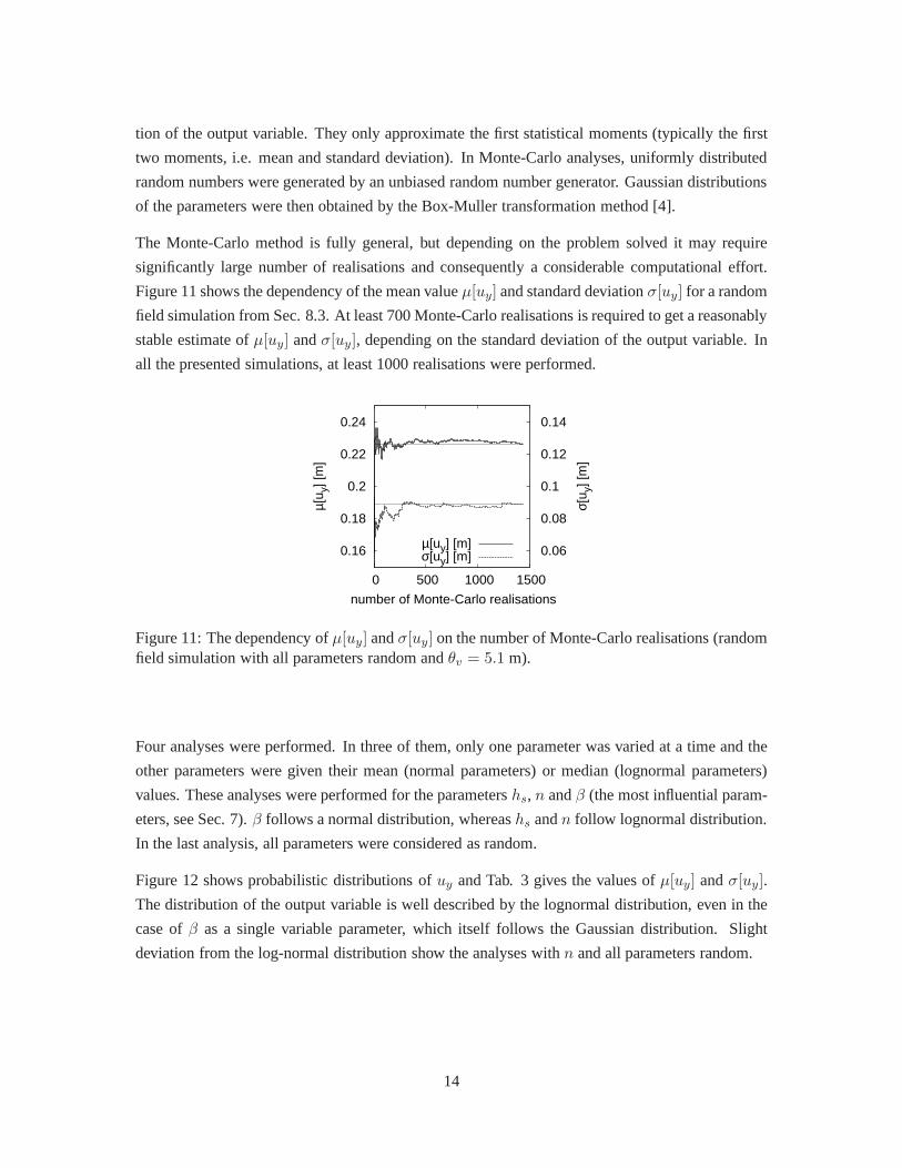
Figure 11 shows the dependency of the mean valueµ[uy] and standard deviationσ[uy] for a random

field simulation from Sec. 8.3. At least 700 Monte-Carlo realisations is required to get a reasonably

stable estimate ofµ[uy] andσ[uy], depending on the standard deviation of the output variable. In

all the presented simulations, at least 1000 realisations were performed.

0.16

0.18

0.2

0.22

0.24

0 500 1000 1500

0.06

0.08

0.1

0.12

0.14

µ[u y

] [m

]

σ[u y

] [m

] number of Monte-Carlo realisations

µ[uy] [m]σ[uy] [m]

Figure 11: The dependency ofµ[uy] andσ[uy] on the number of Monte-Carlo realisations (randomfield simulation with all parameters random andθv = 5.1 m).

Four analyses were performed. In three of them, only one parameter was varied at a time and the

other parameters were given their mean (normal parameters)or median (lognormal parameters)

values. These analyses were performed for the parametershs, n andβ (the most influential param-

eters, see Sec. 7).β follows a normal distribution, whereashs andn follow lognormal distribution.

In the last analysis, all parameters were considered as random.

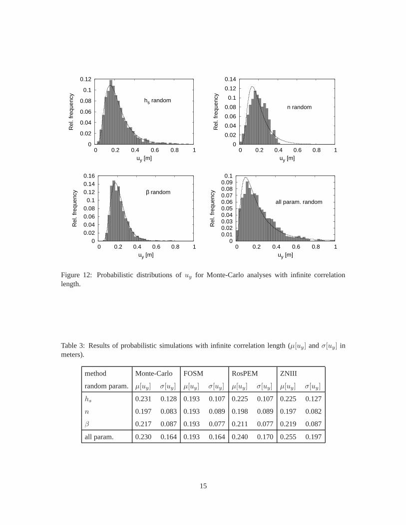
Figure 12 shows probabilistic distributions ofuy and Tab. 3 gives the values ofµ[uy] andσ[uy].

The distribution of the output variable is well described bythe lognormal distribution, even in the

case ofβ as a single variable parameter, which itself follows the Gaussian distribution. Slight

deviation from the log-normal distribution show the analyses withn and all parameters random.

14

0

0.02

0.04

0.06

0.08

0.1

0.12

0 0.2 0.4 0.6 0.8 1

Rel

. fre

quen

cy

uy [m]

hs random

0

0.02

0.04

0.06

0.08

0.1

0.12

0.14

0 0.2 0.4 0.6 0.8 1

Rel

. fre

quen

cy

uy [m]

n random

0 0.02 0.04 0.06 0.08 0.1

0.12 0.14 0.16

0 0.2 0.4 0.6 0.8 1

Rel

. fre

quen

cy

uy [m]

β random

0 0.01 0.02 0.03 0.04 0.05 0.06 0.07 0.08 0.09

0.1

0 0.2 0.4 0.6 0.8 1

Rel

. fre

quen

cy

uy [m]

all param. random

Figure 12: Probabilistic distributions ofuy for Monte-Carlo analyses with infinite correlationlength.

Table 3: Results of probabilistic simulations with infinitecorrelation length (µ[uy] andσ[uy] inmeters).

method Monte-Carlo FOSM RosPEM ZNIII

random param. µ[uy] σ[uy] µ[uy] σ[uy] µ[uy] σ[uy] µ[uy] σ[uy]

hs 0.231 0.128 0.193 0.107 0.225 0.107 0.225 0.127

n 0.197 0.083 0.193 0.089 0.198 0.089 0.197 0.082

β 0.217 0.087 0.193 0.077 0.211 0.077 0.219 0.087

all param. 0.230 0.164 0.193 0.164 0.240 0.170 0.255 0.197

15

8.2 Simulations with approximate analytical probabilistic methods

The Monte-Carlo method, used in the previous section, is fully general, but requires large number

of trials (approx. 1000 in the present case, Fig. 11). This limits its practical applicability. For this

reason, approximate approaches to evaluate statistical distribution of the performance function,

which require remarkably lower number of simulations, are popular in geotechnical engineering

applications. This section is devoted to evaluation of the applicability of several popular methods

to simulate the complex non-linear probabilistic problem studied in this paper.

The problem solved may be in general written asY = g(X1,X2, . . . ,Xn), whereY is the per-

formance function (in the present case,Y = uy), andX = Xi is the vector of random vari-

ables (in the present case,X is the vector of model parameters). Only independent (covariance

Cov[Xi,Xj ] = 0) normal random variablesXi are considered in this work. Log-normal distribu-

tions of several parameters were converted to normal distributions by considering their logarithms

in the computations. The parametersec0, ed0 andei0 were varied simulatenously so they were

treated as a single random parameter.

The first method studied, possibly the most popular in geotechnical engineering, is based on ap-

proximatingY by a Taylor series expanded about the expected values of input random variables

Xi. Neglecting the second- and higher order terms leads to the following expressions for the first

two statistical moments ofY (meanµ[Y ] and standard deviationσ[Y ]):

µ[Y ] = g(µ[X1], µ[X2], ...µ[Xn]) (5)

σ2[Y ] =

n∑

i=1

(

∂Y

∂Xi

σ[Xi]

)2

(6)

where the partial derivative derivatives∂Y /∂Xi are taken at theµ[Xi]. The most common ap-

proach uses finite differences for their approximations [9]. Although the derivative at the point is

most precisely evaluated using a very small increment ofXi, evaluating the derivative over a range

of ±σ[Xi] may according to some authors better capture some of the non-linear behaviour of the

function over a range of likely values [48]. Thus, we have

∂Y

∂Xi

=g (µ[Xi] + σ[Xi])− g (µ[Xi]− σ[Xi])

2σ[Xi](7)

Eqs. (5) - (7) describe the so-called first-order (only first-order terms of Taylor series expansion

are considered) second-moment (only the first two statistical moments ofY are calculated) method

(FOSM). The method requires2n + 1 simulations (n is a number of random variables) and it

is accurate for performance functions linear inXi. With increasing non-linearity ofY in Xi,

however, omission of the higher order terms of Taylor seriesexpansion and the finite-difference

16

approximation of∂Y /∂Xi leads to an accumulation of an error [6].

In the second class of methods (denoted as point estimate methods, PEM), probability distributions

for continuous random variablesXi are replaced by discrete distributions. Each component of

the discrete distribution (point estimate) is associated with the corresponding weight such that the

discrete distribution has the same first few moments as the continuous random variable. Transfor-

mationY = g(X) can be used to calculate the associated discrete distribution of the performance

functions, whose moments approximate the moments ofY in the continuous case [8]. This proce-

dure is equivalent to the calculation of the integral ofY using numerical quadrature [8, 49].

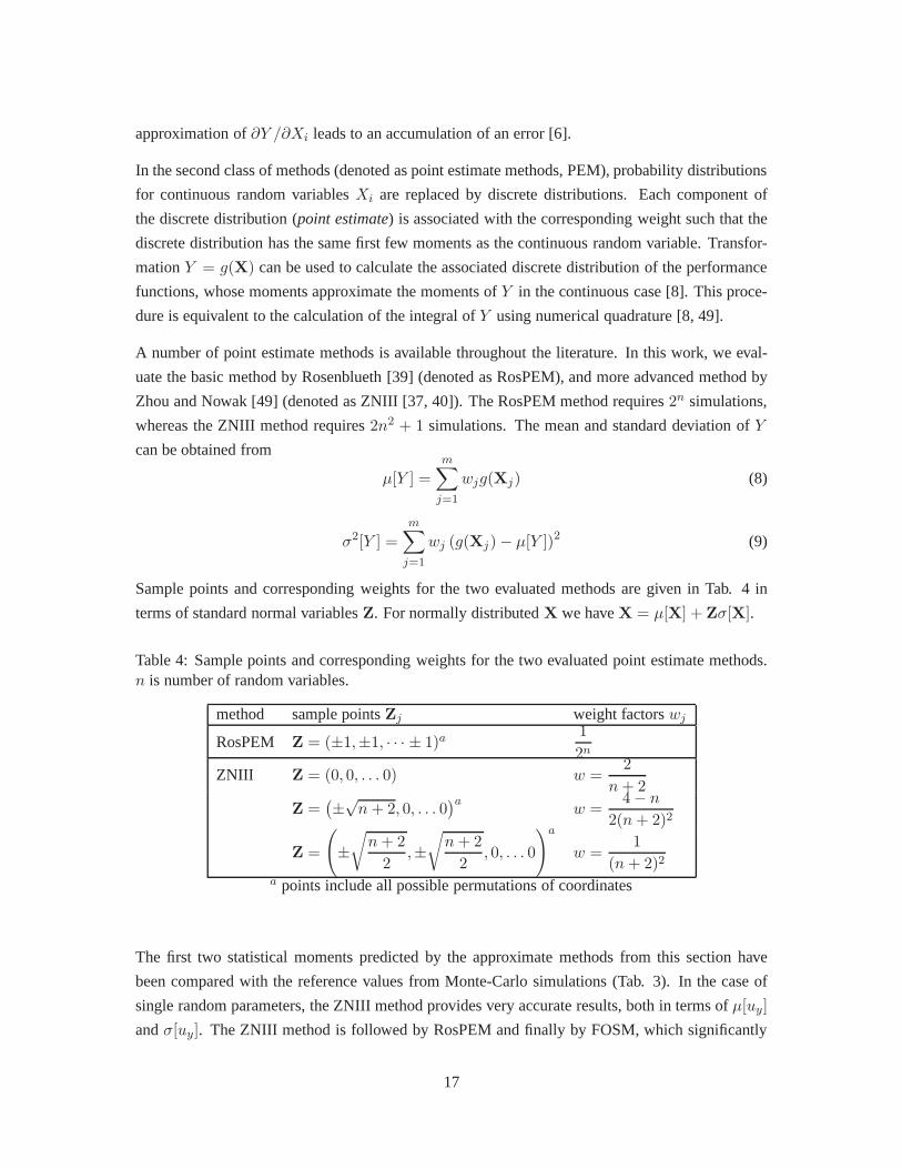
A number of point estimate methods is available throughout the literature. In this work, we eval-

uate the basic method by Rosenblueth [39] (denoted as RosPEM), and more advanced method by

Zhou and Nowak [49] (denoted as ZNIII [37, 40]). The RosPEM method requires2n simulations,

whereas the ZNIII method requires2n2 + 1 simulations. The mean and standard deviation ofY

can be obtained from

µ[Y ] =

m∑

j=1

wjg(Xj) (8)

σ2[Y ] =

m∑

j=1

wj (g(Xj)− µ[Y ])2 (9)

Sample points and corresponding weights for the two evaluated methods are given in Tab. 4 in

terms of standard normal variablesZ. For normally distributedX we haveX = µ[X] + Zσ[X].

Table 4: Sample points and corresponding weights for the twoevaluated point estimate methods.n is number of random variables.

method sample pointsZj weight factorswj

RosPEM Z = (±1,±1, · · · ± 1)a1

2n

ZNIII Z = (0, 0, . . . 0) w =2

n+ 2

Z =(

±√n+ 2, 0, . . . 0

)aw =

4− n

2(n+ 2)2

Z =

(

±√

n+ 2

2,±√

n+ 2

2, 0, . . . 0

)a

w =1

(n+ 2)2

a points include all possible permutations of coordinates

The first two statistical moments predicted by the approximate methods from this section have

been compared with the reference values from Monte-Carlo simulations (Tab. 3). In the case of

single random parameters, the ZNIII method provides very accurate results, both in terms ofµ[uy]

andσ[uy]. The ZNIII method is followed by RosPEM and finally by FOSM, which significantly

17

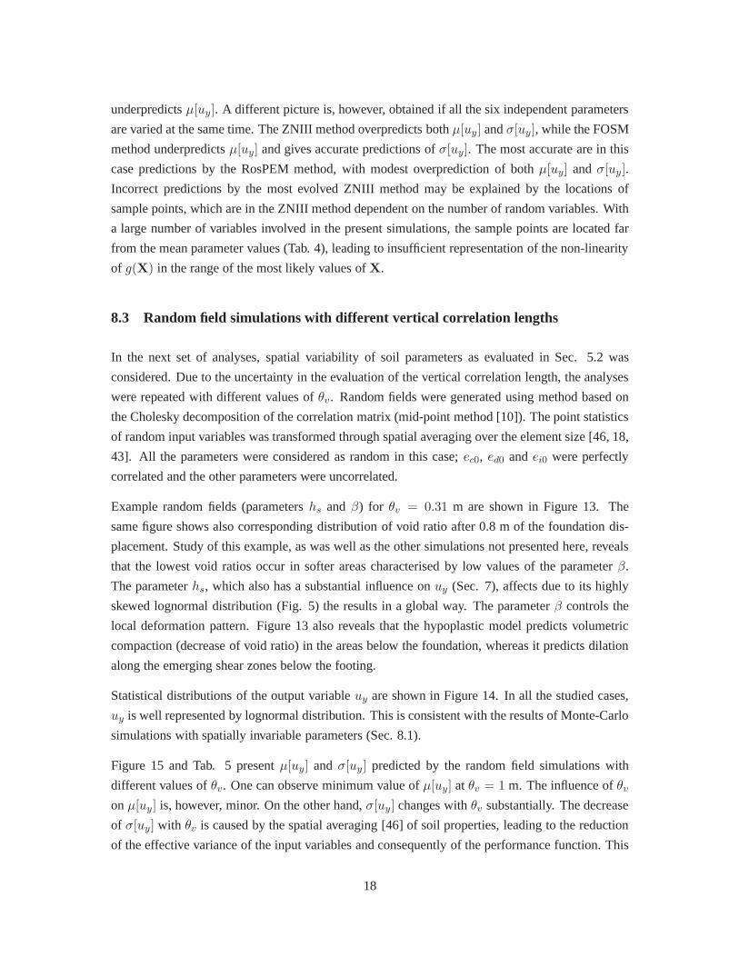
underpredictsµ[uy]. A different picture is, however, obtained if all the six independent parameters

are varied at the same time. The ZNIII method overpredicts both µ[uy] andσ[uy], while the FOSM

method underpredictsµ[uy] and gives accurate predictions ofσ[uy]. The most accurate are in this

case predictions by the RosPEM method, with modest overprediction of bothµ[uy] andσ[uy].

Incorrect predictions by the most evolved ZNIII method may be explained by the locations of

sample points, which are in the ZNIII method dependent on thenumber of random variables. With

a large number of variables involved in the present simulations, the sample points are located far

from the mean parameter values (Tab. 4), leading to insufficient representation of the non-linearity

of g(X) in the range of the most likely values ofX.

8.3 Random field simulations with different vertical correlation lengths

In the next set of analyses, spatial variability of soil parameters as evaluated in Sec. 5.2 was

considered. Due to the uncertainty in the evaluation of the vertical correlation length, the analyses

were repeated with different values ofθv. Random fields were generated using method based on

the Cholesky decomposition of the correlation matrix (mid-point method [10]). The point statistics

of random input variables was transformed through spatial averaging over the element size [46, 18,

43]. All the parameters were considered as random in this case; ec0, ed0 andei0 were perfectly

correlated and the other parameters were uncorrelated.

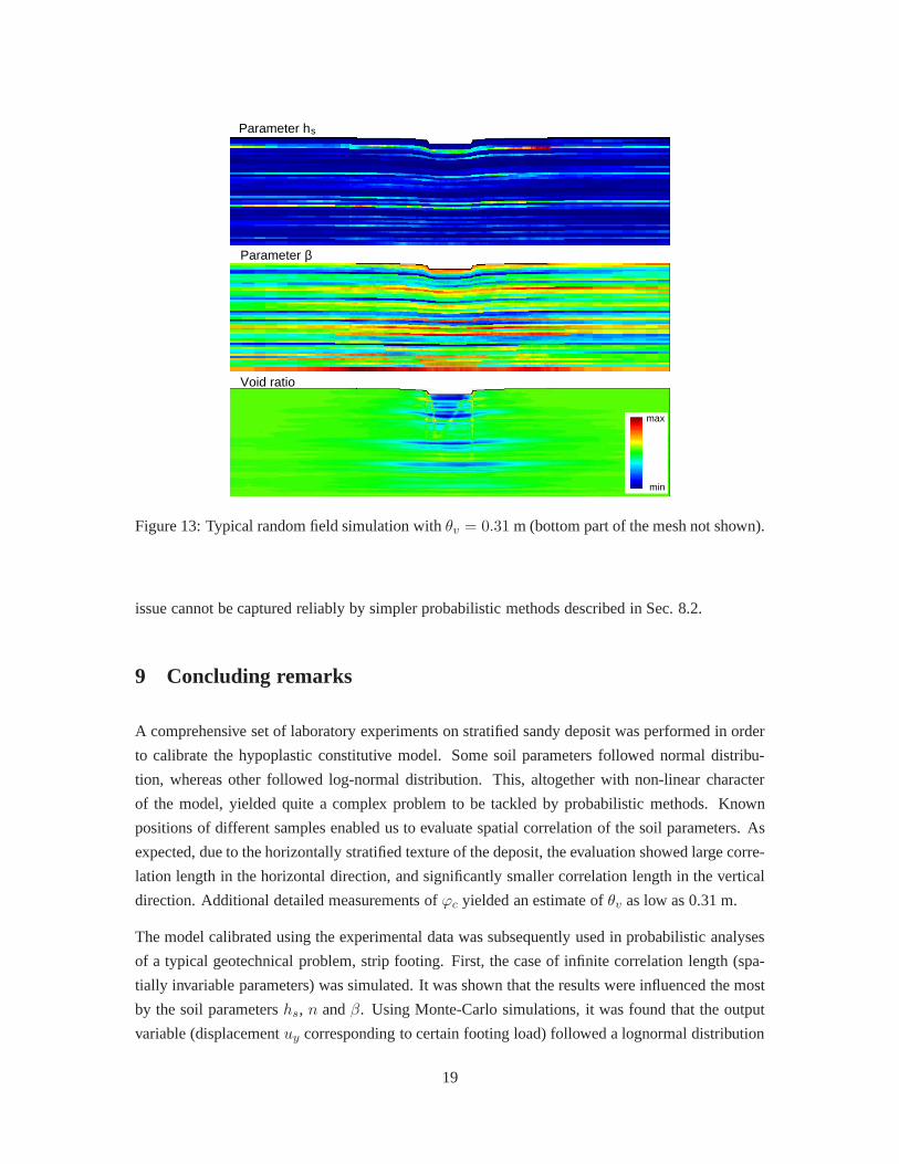
Example random fields (parametershs andβ) for θv = 0.31 m are shown in Figure 13. The

same figure shows also corresponding distribution of void ratio after 0.8 m of the foundation dis-

placement. Study of this example, as was well as the other simulations not presented here, reveals

that the lowest void ratios occur in softer areas characterised by low values of the parameterβ.

The parameterhs, which also has a substantial influence onuy (Sec. 7), affects due to its highly

skewed lognormal distribution (Fig. 5) the results in a global way. The parameterβ controls the

local deformation pattern. Figure 13 also reveals that the hypoplastic model predicts volumetric

compaction (decrease of void ratio) in the areas below the foundation, whereas it predicts dilation

along the emerging shear zones below the footing.

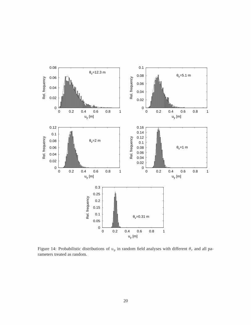
Statistical distributions of the output variableuy are shown in Figure 14. In all the studied cases,

uy is well represented by lognormal distribution. This is consistent with the results of Monte-Carlo

simulations with spatially invariable parameters (Sec. 8.1).

Figure 15 and Tab. 5 presentµ[uy] andσ[uy] predicted by the random field simulations with

different values ofθv. One can observe minimum value ofµ[uy] at θv = 1 m. The influence ofθvonµ[uy] is, however, minor. On the other hand,σ[uy] changes withθv substantially. The decrease

of σ[uy] with θv is caused by the spatial averaging [46] of soil properties, leading to the reduction

of the effective variance of the input variables and consequently of the performance function. This

18

sParameter h

Void ratio

Parameter β

max

min

Figure 13: Typical random field simulation withθv = 0.31 m (bottom part of the mesh not shown).

issue cannot be captured reliably by simpler probabilisticmethods described in Sec. 8.2.

9 Concluding remarks

A comprehensive set of laboratory experiments on stratifiedsandy deposit was performed in order

to calibrate the hypoplastic constitutive model. Some soilparameters followed normal distribu-

tion, whereas other followed log-normal distribution. This, altogether with non-linear character

of the model, yielded quite a complex problem to be tackled byprobabilistic methods. Known

positions of different samples enabled us to evaluate spatial correlation of the soil parameters. As

expected, due to the horizontally stratified texture of the deposit, the evaluation showed large corre-

lation length in the horizontal direction, and significantly smaller correlation length in the vertical

direction. Additional detailed measurements ofϕc yielded an estimate ofθv as low as 0.31 m.

The model calibrated using the experimental data was subsequently used in probabilistic analyses

of a typical geotechnical problem, strip footing. First, the case of infinite correlation length (spa-

tially invariable parameters) was simulated. It was shown that the results were influenced the most

by the soil parametershs, n andβ. Using Monte-Carlo simulations, it was found that the output

variable (displacementuy corresponding to certain footing load) followed a lognormal distribution

19

0

0.02

0.04

0.06

0.08

0 0.2 0.4 0.6 0.8 1

Rel

. fre

quen

cy

uy [m]

θv=12.3 m

0

0.02

0.04

0.06

0.08

0.1

0 0.2 0.4 0.6 0.8 1

Rel

. fre

quen

cy

uy [m]

θv=5.1 m

0

0.02

0.04

0.06

0.08

0.1

0.12

0 0.2 0.4 0.6 0.8 1

Rel

. fre

quen

cy

uy [m]

θv=2 m

0 0.02 0.04 0.06 0.08

0.1 0.12 0.14 0.16

0 0.2 0.4 0.6 0.8 1

Rel

. fre

quen

cy

uy [m]

θv=1 m

0

0.05

0.1

0.15

0.2

0.25

0.3

0 0.2 0.4 0.6 0.8 1

Rel

. fre

quen

cy

uy [m]

θv=0.31 m

Figure 14: Probabilistic distributions ofuy in random field analyses with differentθv and all pa-rameters treated as random.

20

Table 5: Results of Monte-Carlo random field simulations with variable vertical correlation length(µ[uy] andσ[uy] in meters).

θv µ[uy] σ[uy]

∞ 0.230 0.164

12.3 m 0.225 0.119

5.1 m 0.226 0.089

2 m 0.219 0.059

1 m 0.215 0.039

0.31 m 0.217 0.023

0

0.05

0.1

0.15

0.2

0.25

0 2 4 6 8 10 12 14 0

0.05

0.1

0.15

µ[u y

] [m

]

σ[u y

] [m

]

θ [m]

µ[uy] [m]σ[uy] [m]

Figure 15: The dependency ofµ[uy] andσ[uy] onθv predicted by the random field method.

21

closely, even in the case when normally distributed parameters (such asβ) were varied. The results

of Monte-Carlo analyses were then used for evaluation of different simpler probabilistic methods

(the first order second moment method and different point estimate methods). For the complex

problem of all parameters treated as random, neither the FOSM method, nor the advanced ZNIII

method yielded correct results, for different reasons discussed in the paper. The basic PEM method

by Rosenblueth [39] was found the most accurate, although itstill overpredicted the mean and

standard deviation ofuy. Finally, spatial correlation of the soil parameters was taken into account

in Mone-Carlo random field analyses. As expected, spatial averaging of parameters led to a reduc-

tion of variance ofuy. This was particularly significant forθv = 0.31 m evaluated using detailed

measurements ofϕc. The influence ofθv on the mean value ofuy was minor.

Acknowledgment

The authors wish to thank to Ms. M. Englmaierova and Mr. P. Zmek for performing parts of

the experimental programme during their MSc projects. Financial support by the research grants

GACR 205/08/0732, GAUK 31109 and MSM 0021620855 is greatly appreciated.

References

[1] J. E. Andrade, J. W. Baker, and K. C. Ellison. Random porosity fields and their influence on

the stability of granular media.International Journal for Numerical and Analytical Methods

in Geomechanics, 32:1147–1172, 2008.

[2] E. Bauer. Calibration of a comprehensive constitutive equation for granular materials.Soils

and Foundations, 36(1):13–26, 1996.

[3] K. Been and M. G. Jefferies. A state parameter for sands.Geotechnique, 35(2):99–112, 1985.

[4] G. E. P. Box and M. E. Muller. A note on the generation of random normal deviates.Ann.

Math. Stat., 29:610–611, 1958.

[5] W. Brzakała and W. Puła. A probabilistic analysis of foundation settlements.Computers and

Geotechnics, 18(4):291–309, 1996.

[6] C.-H. Chang, Y.-K. Tung, and Y. J.-C. Evaluation of probability point estimate methods.

Appl. Math. Modelling, 19:95–105, 1995.

22

[7] S. E. Cho and H. C. Park. Effect of spatial variability of cross-correlated soil properties on

bearing capacity of strip footing.International Journal for Numerical and Analytical Methods

in Geomechanics, 34:1–26, 2010.

[8] J. T. Christian and G. B. Baecher. Point-estimate methodas numerical quadrature.Journal of

Geotechnical and Geoenvironmental Engineering ASCE, 125(9):779–786, 1999.

[9] J. T. Christian, C. C. Ladd, and G. B. Baecher. Reliability applied to slope stability analysis.

Journal of Geotechnical Engineering ASCE, 120(12):2180–2207, 1994.

[10] A. Der Kiureghian and J.-B. Ke. The stochastic finite element method in structural reliability.

Prob Engng Mech, 3(2):83–91, 1988.

[11] M. D. Evans and D. V. Griffiths. 3D finite analysis of bearing capacity failure in clay. In

Proc. 16th Int. Conf. Soil Mechanics and Geotechnical Engineering, volume 2, pages 893–

896. Millpress Rotterdam Netherlands, 2006.

[12] G. A. Fenton and D. V. Griffiths. Probabilistic foundation settlement on a spatially random

soil. Journal of Geotechnical and Geoenvironmental EngineeringASCE, 128(5):381–390,

2002.

[13] G. A. Fenton and D. V. Griffiths. Bearing-capacity prediction of spatially randomc-φ soils.

Canadian Geotechnical Journal, 40:64–65, 2003.

[14] G. A. Fenton and D. V. Griffiths. Three-dimensional probabilistic foundation settlement.

Journal of Geotechnical and Geoenvironmental EngineeringASCE, 131(2):232–239, 2005.

[15] G. A. Fenton, D. V. Griffiths, and X. Zhang. Load and resistance factor design of shallow

foundations against bearing failure.Canadian Geotechnical Journal, 45:1556–1571, 2008.

[16] R. Ghanem and P. Spanos.Stochastic Finite Elements: A Spectral Approach. Springer-Verlag,

Berlin, 1991.

[17] D. V. Griffiths and G. A. Fenton. Bearing capacity of spatially random soil: the undrained

clay Prandtl problem revisited.Geotechnique, 51(4):351–359, 2001.

[18] D. V. Griffiths and G. A. Fenton. Probabilistic slope stability analysis by finite elements.

Journal of Geotechnical and Geoenvironmental EngineeringASCE, 130(5):507–518, 2004.

[19] D. V. Griffiths and G. A. Fenton. Probabilistic settlement analysis of rectangular footings. In

Proc.16th Int. Conf. Soil Mechanics and Geotechnical Engineering, volume 2, pages 1041–

1044. Millpress Rotterdam Netherlands, 2006.

23

[20] D. V. Griffiths and G. A. Fenton. Probabilistic settlement analysis by stochastic and random

finite element methods.Journal of Geotechnical and Geoenvironmental EngineeringASCE,

135(11):1629–1637, 2009.

[21] D. V. Griffiths, G. A. Fenton, and N. Manoharan. Bearing capacity of rough rigid strip foot-

ing on cohesive soil: probabilistic study.Journal of Geotechnical and Geoenvironmental

Engineering ASCE, 128(9):743–755, 2002.

[22] G. Gudehus. A comprehensive constitutive equation forgranular materials.Soils and Foun-

dations, 36(1):1–12, 1996.

[23] G. Gudehus and D. Masın. Graphical representation ofconstitutive equations.Geotechnique,

52(2):147–151, 2009.

[24] V. Hajek, D. Masın, and J. Bohac. Capability of constitutive models to simulate soils with

different OCR using a single set of parameters.Computers and Geotechnics, 36(4):655–664,

2009.

[25] J. C. Helton. Uncertainty and sensitivity analysis in the presence of stochastic and subjective

uncertainty.Journal of Statistical Computation and Simulation, 57:3–76, 1997.

[26] I. Herle and G. Gudehus. Determination of parameters ofa hypoplastic constitutive model

from properties of grain assemblies.Mechanics of Cohesive-Frictional Materials, 4:461–486,

1999.

[27] M. A. Hicks and C. Onisiphorou. Stochastic evaluation of static liquefaction in a predomi-

nantly dilative sand fill.Geotechnique, 55(2):123–133, 2005.

[28] M. Huber, P. A. Vermeer, and A. Bardossy. Evaluation ofsoil variability and its consequences.

In T. Benz and S. Nordal, editors,Proc. 7th European Conference on Numerical Methods in

Geomechanics (NUMGE), Trondheim, Norway, pages 363–368. Taylor & Francis Group,

London, 2010.

[29] K. Kasama, Z. K., and A. J. Whittle. Effects of spatial variability of cement-treated soil

on undrained bearing capacity. InProc. Int. Conference on Numerical Simulation of Con-

struction Processes in Geotechnical Engineering for UrbanEnvironment, pages 305–313.

Bochum, Germany, 2006.

[30] B. S. N. Kim. Probabilistic analysis of settlement for afloating foundation on soft clay.KSCE

Journal of Civil Engineering, 6(2):235–241, 2002.

[31] D. Kolymbas. Computer-aided design of constitutive laws. International Journal for Numer-

ical and Analytical Methods in Geomechanics, 15:593–604, 1991.

24

[32] Y. L. Kuo, M. B. Jaksa, W. S. Kaggwa, G. A. Fenton, D. V. Griffiths, and J. S. Goldsworthy.

Probabilistic analysis of multi-layered soil effects on shallow foundation settlement. In9th

Australia New Zealand Conference on Geomechanics, Auckland, New Zealand, volume 2,

pages 541–547, 2004.

[33] F. Molenkamp. Elasto-plastic double hardening model Monot. Technical report, LGM Report

CO-218595, Delft Geotechnics, 1981.

[34] A. Niemunis, T. Wichtmann, Y. Petryna, and T. Triantafyllidis. Stochastic modelling of set-

tlements due to cyclic loading for soil-structure interaction. In G. Augusti, G. Schueller, and

M. Ciampoli, editors,Proceedings of the 9th International Conference on Structural Safety

and Reliability, ICOSSAR’05, Rome, Italy. Millpress, Rotterdam, 2005.

[35] A. Nour, A. Slimani, and N. Laouami. Foundation settlement statistics via finite element

analysis.Computers and Geotechnics, 29:641–672, 2002.

[36] K. Nubel and C. Karcher. FE simulations of granular material with a given frequency distri-

bution of voids as initial condition.Granular Matter, 1:105–112, 1998.

[37] G. M. Peschl and H. F. Schweiger. Raliability analysis in geotechnics with finite elements -

Comparison of probabilistic, stochastic and fuzzy set methods. InProc.3rd.

[38] D. Rodemann.Tochnog Professional user’s manual. http://www.feat.nl, 2008.

[39] E. Rosenblueth. Two-point estimates in probabilities. Appl. Math. Modelling, 5(2):329–335,

1981.

[40] H. F. Schweiger and R. Thurner. Basic concepts and applications of point estimate methods

in geotechnical engineering. In D. V. Griffiths and G. A. Fenton, editors,Probabilistic Meth-

ods in Geotechnical Engineering, volume 491 ofCISM International Centre for Mechanical

Sciences, pages 97–112. Springer Vienna, 2007.

[41] G. Stefanou. The stochastic finite element method: Past, present and future.Comput. Methods

Appl. Mech. Engrg., 198:1031–1051, 2009.

[42] R. Suchomel and D. Masın. Calibration of an advanced soil constitutive model for use in

probabilistic numerical analysis. In P. et al., editor,Proc. Int. Symposium on Computational

Geomechanics (ComGeo I), Juan-les-Pins, France, pages 265–274, 2009.

[43] R. Suchomel and D. Masın. Comparison of different probabilistic methods for predicting

stability of a slope in spatially variable c-phi soil.Computers and Geotechnics, 37:132–140,

2010.

25

[44] R. Suchomel and D. Masın. Spatial variability of soilparameters in an analysis of a strip

footing using hypoplastic model. In T. Benz and S. Nordal, editors, Proc. 7th European

Conference on Numerical Methods in Geomechanics (NUMGE), Trondheim, Norway, pages

383–388. Taylor & Francis Group, London, 2010.

[45] J. Tejchman. Effect of fluctuation of current void ratioon the shear zone formation in granular

bodies within micro-polar hypoplasticity.Computers and Geotechnics, 33(1):29–46, 2006.

[46] E. H. Vanmarcke.Random fields: anaylisis and synthesis. M.I.T. press, Cambridge, Mass.,

1983.

[47] P. A. von Wolffersdorff. A hypoplastic relation for granular materials with a predefined limit

state surface.Mechanics of Cohesive-Frictional Materials, 1:251–271, 1996.

[48] T. F. Wolff. Evaluating the reliability of existing levees. Technical report, U.S. Army Engineer

Waterways Experiment Station, Geotechnical Laboratory, Vicksburg, MS, 1994.

[49] J. Zhou and A. S. Nowak. Integration formulas to evaluate functions of random variables.

Structural Safety, 5:267–284, 1988.

26

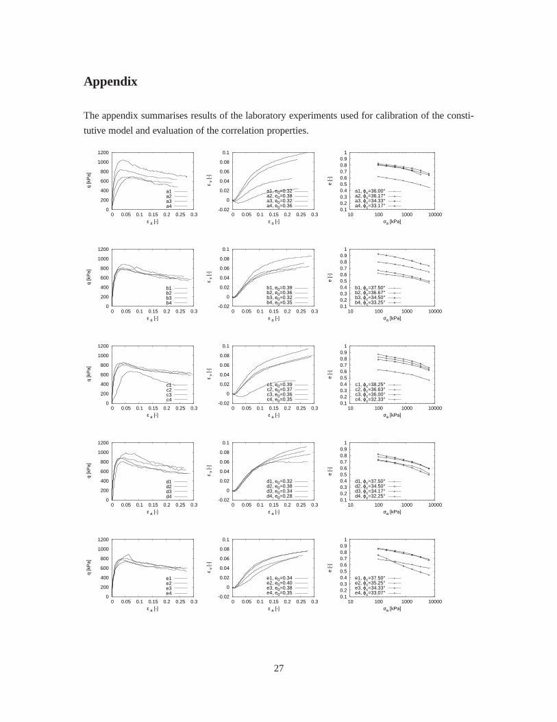
Appendix

The appendix summarises results of the laboratory experiments used for calibration of the consti-

tutive model and evaluation of the correlation properties.

0

200

400

600

800

1000

1200

0 0.05 0.1 0.15 0.2 0.25 0.3

q [k

Pa]

ε a [-]

a1a2a3a4

-0.02

0

0.02

0.04

0.06

0.08

0.1

0 0.05 0.1 0.15 0.2 0.25 0.3 ε

v [-

]

ε a [-]

a1, e0=0.32a2, e0=0.38a3, e0=0.32a4, e0=0.36

0.1 0.2 0.3 0.4 0.5 0.6 0.7 0.8 0.9

1

10 100 1000 10000

e [-

]

σa [kPa]

a1, ϕc=36.00°a2, ϕc=36.17°a3, ϕc=34.33°a4, ϕc=33.17°

0

200

400

600

800

1000

1200

0 0.05 0.1 0.15 0.2 0.25 0.3

q [k

Pa]

ε a [-]

b1b2b3b4

-0.02

0

0.02

0.04

0.06

0.08

0.1

0 0.05 0.1 0.15 0.2 0.25 0.3

ε v

[-]

ε a [-]

b1, e0=0.39b2, e0=0.36b3, e0=0.32b4, e0=0.35

0.1 0.2 0.3 0.4 0.5 0.6 0.7 0.8 0.9

1

10 100 1000 10000

e [-

]

σa [kPa]

b1, ϕc=37.50°b2, ϕc=36.67°b3, ϕc=34.50°b4, ϕc=33.25°

0

200

400

600

800

1000

1200

0 0.05 0.1 0.15 0.2 0.25 0.3

q [k

Pa]

ε a [-]

c1c2c3c4

-0.02

0

0.02

0.04

0.06

0.08

0.1

0 0.05 0.1 0.15 0.2 0.25 0.3

ε v

[-]

ε a [-]

c1, e0=0.39c2, e0=0.37c3, e0=0.36c4, e0=0.35

0.1 0.2 0.3 0.4 0.5 0.6 0.7 0.8 0.9

1

10 100 1000 10000

e [-

]

σa [kPa]

c1, ϕc=38.25°c2, ϕc=36.63°c3, ϕc=36.00°c4, ϕc=32.33°

0

200

400

600

800

1000

1200

0 0.05 0.1 0.15 0.2 0.25 0.3

q [k

Pa]

ε a [-]

d1d2d3d4

-0.02

0

0.02

0.04

0.06

0.08

0.1

0 0.05 0.1 0.15 0.2 0.25 0.3

ε v

[-]

ε a [-]

d1, e0=0.32d2, e0=0.38d3, e0=0.34d4, e0=0.28

0.1 0.2 0.3 0.4 0.5 0.6 0.7 0.8 0.9

1

10 100 1000 10000

e [-

]

σa [kPa]

d1, ϕc=37.50°d2, ϕc=34.50°d3, ϕc=34.17°d4, ϕc=32.25°

0

200

400

600

800

1000

1200

0 0.05 0.1 0.15 0.2 0.25 0.3

q [k

Pa]

ε a [-]

e1e2e3e4

-0.02

0

0.02

0.04

0.06

0.08

0.1

0 0.05 0.1 0.15 0.2 0.25 0.3

ε v

[-]

ε a [-]

e1, e0=0.34e2, e0=0.40e3, e0=0.38e4, e0=0.35

0.1 0.2 0.3 0.4 0.5 0.6 0.7 0.8 0.9

1

10 100 1000 10000

e [-

]

σa [kPa]

e1, ϕc=37.50°e2, ϕc=35.25°e3, ϕc=34.33°e4, ϕc=33.07°

27

0

200

400

600

800

1000

1200

0 0.05 0.1 0.15 0.2 0.25 0.3

q [k

Pa]

ε a [-]

f2f3

-0.02

0

0.02

0.04

0.06

0.08

0.1

0 0.05 0.1 0.15 0.2 0.25 0.3

ε v

[-]

ε a [-]

f2, e0=0.37f3, e0=0.40

0.1 0.2 0.3 0.4 0.5 0.6 0.7 0.8 0.9

1

10 100 1000 10000

e [-

]

σa [kPa]

f2, ϕc=36.75°f3, ϕc=34.17°

0

200

400

600

800

1000

1200

0 0.05 0.1 0.15 0.2 0.25 0.3

q [k

Pa]

ε a [-]

g1g2g3g4

-0.02

0

0.02

0.04

0.06

0.08

0.1

0 0.05 0.1 0.15 0.2 0.25 0.3

ε v

[-]

ε a [-]

g1, e0=0.38g2, e0=0.34g3, e0=0.35g4, e0=0.33

0.1 0.2 0.3 0.4 0.5 0.6 0.7 0.8 0.9

1

10 100 1000 10000

e [-

]

σa [kPa]

g1, ϕc=38.00°g2, ϕc=37.50°g3, ϕc=34.63°g4, ϕc=34.50°

0

200

400

600

800

1000

1200

0 0.05 0.1 0.15 0.2 0.25 0.3

q [k

Pa]

ε a [-]

h1h2h3h4

-0.02

0

0.02

0.04

0.06

0.08

0.1

0 0.05 0.1 0.15 0.2 0.25 0.3

ε v

[-]

ε a [-]

h1, e0=0.37h2, e0=0.36h3, e0=0.38h4, e0=0.34

0.1 0.2 0.3 0.4 0.5 0.6 0.7 0.8 0.9

1

10 100 1000 10000

e [-

]

σa [kPa]

h1, ϕc=36.38°h2, ϕc=35.38°h3, ϕc=33.30°h4, ϕc=33.67°

0

200

400

600

800

1000

1200

0 0.05 0.1 0.15 0.2 0.25 0.3

q [k

Pa]

ε a [-]

i1i2i3i4

-0.02

0

0.02

0.04

0.06

0.08

0.1

0 0.05 0.1 0.15 0.2 0.25 0.3

ε v

[-]

ε a [-]

i1, e0=0.38i2, e0=0.33i3, e0=0.34i4, e0=0.38

0.1 0.2 0.3 0.4 0.5 0.6 0.7 0.8 0.9

1

10 100 1000 10000

e [-

]

σa [kPa]

i1, ϕc=36.50°i2, ϕc=34.17°i3, ϕc=33.83°i4, ϕc=34.00°

0

200

400

600

800

1000

1200

0 0.05 0.1 0.15 0.2 0.25 0.3

q [k

Pa]

ε a [-]

j1j2j3j4

-0.02

0

0.02

0.04

0.06

0.08

0.1

0 0.05 0.1 0.15 0.2 0.25 0.3

ε v

[-]

ε a [-]

j1, e0=0.38j2, e0=0.35j3, e0=0.38j4, e0=0.37

0.1 0.2 0.3 0.4 0.5 0.6 0.7 0.8 0.9

1

10 100 1000 10000

e [-

]

σa [kPa]

j1, ϕc=36.75°j2, ϕc=34.67°j3, ϕc=34.75°j4, ϕc=32.33°

28