Resonant and Near-Resonant Internal Wave

Interactions

Yuri V. Lvov1, Kurt L. Polzin2 and Naoto Yokoyama3

1 Department of Mathematical Sciences, Rensselaer Polytechnic Institute, Troy NY 12180

2 Woods Hole Oceanographic Institution, MS#21, Woods Hole, MA 02543

3 Department of Aeronautics and Astronautics, Kyoto University, Kyoto, Kyoto 606-8501 JAPAN

Abstract

We report evaluations of a resonant kinetic equation that suggest the slow time

evolution of the Garrett and Munk spectrum isnot, in fact, slow. Instead nonlin-

ear transfers lead to evolution time scales that are smallerthan one wave period at

high vertical wavenumber. Such values of the transfer ratesare inconsistent with

conventional wisdom that regards the Garrett and Munk spectrum as an approxi-

mate stationary state and puts the self-consistency of a resonant kinetic equation at

a serious risk. We explore possible reasons for and resolutions of this paradox.

Inclusion of near-resonant interactions decreases the rate at which the spectrum

evolves. This leads to improved self-consistency of the kinetic equation.

1

1. Introduction

Wave-wave interactions in stratified oceanic flows have beena subject of intensive research

in the last four decades. Of particular importance is the existence of a “universal” internal-

wave spectrum, the Garrett and Munk spectrum. It is generally perceived that the existence

of a universal spectrum is, at least in part and perhaps even primarily, the result of nonlinear

interactions of waves with different wavenumbers. Due to the quadratic nonlinearity of the

underlying primitive equations and the fact that the linearinternal-wave dispersion relation can

satisfy a three-wave resonance condition, waves interact in triads. Therefore the question arises:

how strongly do waves within a given triad interact? What arethe oceanographic consequences

of this interaction?

Wave-wave interactions can be rigorously characterized byderiving a closed equation rep-

resenting the slow time evolution of the wavefield’s wave action spectrum. Such an equation is

called akinetic equation(?) and significant efforts in this regard are listed in Table 8.

A kinetic equation describes, under the assumption of weak nonlinearity, the resonant spec-

tral energy transfer on theresonant manifold. The resonant manifold is a set of wavevectorsp,

p1 andp2 that satisfy

p = p1 + p2, ωp = ωp1+ ωp2

, (1)

where the frequencyω is given by a linear dispersion relation relating wave frequencyω with

wavenumberp.

The reduction of all possible interactions between three wavevectors to a resonant mani-

fold is a significant simplification.Even furthersimplification can be achieved by taking into

account that, of all interactionson the resonant manifold, the most important are those which

2

involve extreme scale separations? between interaction wavevectors. It is shown in? that

Garrett and Munk spectrum of internal waves is stationary with respect to one class of such in-

teractions, called Induced Diffusion. Furthermore, a comprehensive inertial-range theory with

constant downscale transfer of energy was obtained by patching these mechanisms together in

a solution that closely mimics the empirical universal spectrum (GM)(?). It was therefore con-

cluded that that Garrett and Munk spectrum constitutes an approximate stationary state of the

kinetic equation.

In this paper we revisit the question of relation between Garrett and Munk spectrum and the

resonant kinetic equation. At the heart of this paper (Section a) are numerical evaluations of the

? internal wave kinetic equation demonstrating changes in spectral amplitude at a rate less than

an inverse wave period at high vertical wavenumber for the Garrett and Munk spectrum. This

rapid temporal evolution implies that the GM spectrum isnot a stationary state and is contrary

to the characterization of the GM spectrum as an inertial subrange. This result gave us cause to

review published work concerning wave-wave interactions and compare results. The product of

this work is presented in Sections 3&4. In particular, we concentrate on four different versions

of the internal wave kinetic equation:

• a noncanonical description using Lagrangian coordinates (???),

• a canonical Hamiltonian description in Eulerian coordinates (?),

• a dynamical derivation of a kinetic equation without use of Hamiltonian formalisms in

Eulerian coordinates (?),

• a canonical Hamiltonian description in isopycnal coordinates (??).

We show in Section 3 that, without background rotation, all the listed approaches areequivalent

3

on the resonant manifold. In Section 4 we demonstrate that the two versions of the kinetic

equation that consider non-zero rotation rates are againequivalenton the resonant manifold.

This presents us with our first paradox: if all these kinetic equations are the same on the resonant

manifold and exhibit a rapid temporal evolution, then why isGM considered to be a stationary

state? The resolution of this paradox, presented in Section7, is that: (i) numerical evaluations

of the? kinetic equation demonstrating the induced diffusion stationary states require damping

in order to balance the fast temporal evolution at high vertical wavenumber, and (ii) the high

wavenumber temporal evolution of the? kinetic equation is tentatively identified as being

associated with the elastic scattering mechanism rather than induced diffusion.

Having clarified this, we proceed to the following observation: Not only do our numeri-

cal evaluations imply that the GM spectrum isnot a stationary state, the rapid evolution rates

correspond to a strongly nonlinear system. Consequently the self-consistency of the kinetic

equation, which is built on an assumption of weak nonlinearity, is at risk. Moreover, reduc-

tion of all resonantwave-wave interactions exclusively to extreme scale separations is also not

self-consistent.

Yet, we are not willing to give up on the kinetic equation. Oursecond paradox is that, in a

companion paper (?) we show how a comprehensive theory built on a scale invariant resonant

kinetic equation helps to interpret theobserved variabilityof the background oceanic internal

wavefield. The observed variability, in turn, is largely consistent with the induced diffusion

mechanism being a stationary state!

Thus the resonant kinetic equation demonstrates promisingpredictive ability and it is there-

fore tempting to move towards a self-consistent internal wave turbulence theory. One possible

route towards such theory is to include to the kinetic equation near-resonant interactions, de-

4

fined as

p = p1 + p2, | ωp − ωp1− ωp2

|< Γ,

whereΓ is the resonance width. We show in Section b that such resonant broadening leads

to slower evolution rates, potentially leading to a more self consistent description of internal

waves.

We conclude and list open questions in Section 8. Our numerical scheme for evaluating near-

resonant interactions is discussed in Section 5. An appendix contains the interaction matrices

used in this study.

2. Background

A kinetic equation is a closed equation for the time evolution of the wave action spectrum

in a system of weakly interacting waves. It is usually derived as a central result of wave tur-

bulence theory. The concepts of wave turbulence theory provide a fairly general framework

for studying the statistical steady states in a large class of weakly interacting and weakly non-

linear many-body or many-wave systems. In its essence, classical wave turbulence theory (?)

is a perturbation expansion in the amplitude of the nonlinearity, yielding, at the leading order,

linear waves, with amplitudes slowly modulated at higher orders by resonant nonlinear interac-

tions. This modulation leads to a redistribution of the spectral energy density among space- and

time-scales.

While the route to deriving the spectral evolution equationfrom wave amplitude is fairly

standardized (Section b), there are substantive differences in obtaining expressions for the evo-

5

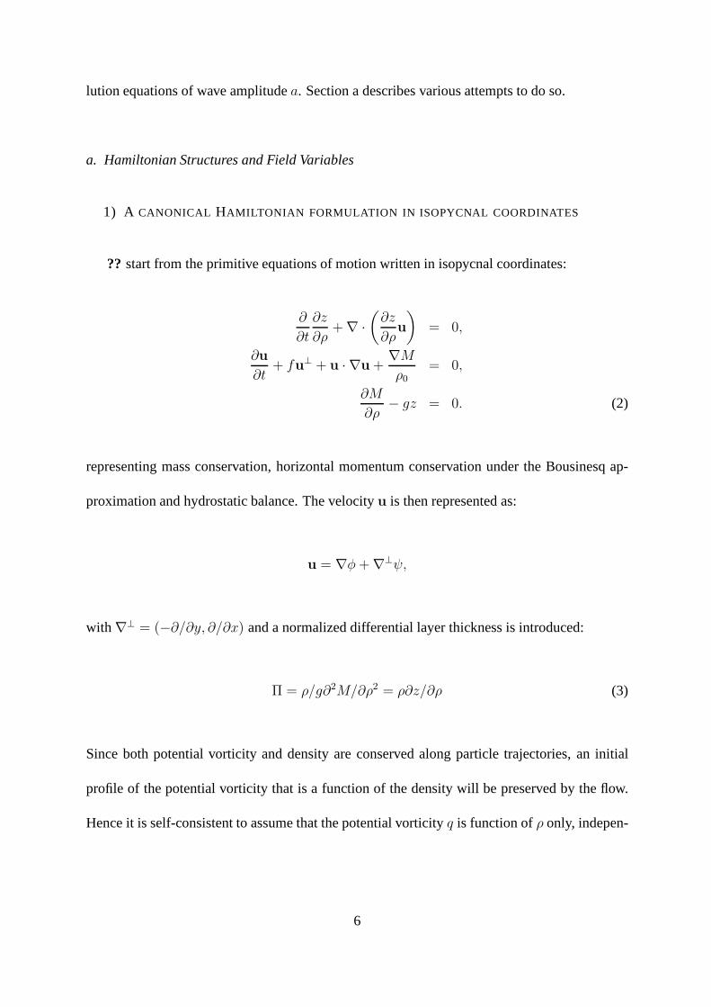
lution equations of wave amplitudea. Section a describes various attempts to do so.

a. Hamiltonian Structures and Field Variables

1) A CANONICAL HAMILTONIAN FORMULATION IN ISOPYCNAL COORDINATES

?? start from the primitive equations of motion written in isopycnal coordinates:

∂

∂t

∂z

∂ρ+∇ ·

(

∂z

∂ρu

)

= 0,

∂u

∂t+ fu⊥ + u · ∇u+

∇Mρ0

= 0,

∂M

∂ρ− gz = 0. (2)

representing mass conservation, horizontal momentum conservation under the Bousinesq ap-

proximation and hydrostatic balance. The velocityu is then represented as:

u = ∇φ+∇⊥ψ,

with ∇⊥ = (−∂/∂y, ∂/∂x) and a normalized differential layer thickness is introduced:

Π = ρ/g∂2M/∂ρ2 = ρ∂z/∂ρ (3)

Since both potential vorticity and density are conserved along particle trajectories, an initial

profile of the potential vorticity that is a function of the density will be preserved by the flow.

Hence it is self-consistent to assume that the potential vorticity q is function ofρ only, indepen-

6

dent ofx andy:

q(ρ) = q0(ρ) =f

Π0(ρ), (4)

whereΠ0(ρ) = −g/N(ρ)2 is a reference stratification profile with background buoyancy fre-

quency,N = (−g/(ρ∂z/∂ρ|bg))1/2, independent ofx andy. The variableψ can then be elim-

inated by assuming that potential vorticity is constant on an isopycnal so thatf + ∆ψ = q0Π

and one obtains two equations inΠ andφ:

Πt +∇ · (Π(∇φ+∇⊥∆−1(q0Π− 1))) = 0

φt +1

2| ∇φ+∇⊥∆−1(q0Π− 1) |2 +∆−1∇ · [q0Π(∇⊥φ−∇∆−1(q0Π− 1))]+

1

ρ

∫ ρ ∫ ρ′ Π− Π0

ρ1dρ1dρ

′ = 0(5)

Here∆−1 is the inverse Laplacian andρ′ represents a variable of integration rather than pertur-

bation. Serendipitously, the variableΠ is the canonical conjugate ofφ:

∂Π

∂t=δHδφ

,∂φ

∂t= −δH

δΠ, (6)

under a HamiltonianH:

H =

∫

dxdρ

(

−1

2(Π0 +Π(x, ρ))

∣

∣

∣

∣

∇φ(x, ρ) + f

Π0∇⊥∆−1Π(x, ρ)

∣

∣

∣

∣

2

+g

2

∣

∣

∣

∣

∫ ρ

dρ′Π(x, ρ′)

ρ′

∣

∣

∣

∣

2)

.

(7)

that is the sum of kinetic and potential energies.

Switching to Fourier space, and introducing a complex field variableap through the trans-

7

formation

φp =iN

√ωp√

2g|k|(

ap − a∗−p

)

,

Πp = Π0 −N Π0 |k|√

2 gωp

(

ap + a∗−p

)

, (8)

where the frequencyω satisfies the linear dispersion relation

ωp =

√

f 2 +g2

ρ20N2

|k|2m2

, (9)

the equations of motion (2) adopt the canonical form

i∂

∂tap =

δHδa∗p

, (10)

with the Hamiltonian

H =

∫

dpωp|ap|2

+

∫

dp012

(

δp+p1+p2(Up,p1,p2

a∗pa∗p1a∗p2

+ c.c.) + δ−p+p1+p2(V p

p1,p2a∗pap1

ap2+ c.c.) .

)

(11)

Eq. (10) is Hamilton’s equation and (11) is the standard formof the Hamiltonian of a system

dominated by three-wave interactions (?). Calculations of interaction coefficientsU andV are

tedious but straightforward task, completed in??.

We emphasize that (10) is, with simply a Fourier decomposition and assumption of uniform

potential vorticity on an isopycnal,precisely equivalentto the fully nonlinear equations of mo-

tion in isopycnal coordinates (2). All other formulations of an internal wave kinetic equation

8

depend upon a linearization prior to the derivation of the kinetic equation via an assumption of

weak nonlinearity.

The difficulty is that, in order to utilize Hamilton’s Equation (10), the Hamiltonian (7) must

first be constructed as a function of the generalized coordinatesand momenta (Π andφ here). It

is not always possible to do sodirectly, in which case one must set up the associated Lagrangian

(L below) and then calculate the generalized coordinates and momenta.

2) HAMILTONIAN FORMALISM IN CLEBSCH VARIABLES IN (?)

Voronovich starts from the non-rotating equations in Eulerian coordinates:

∂u

∂t+ u · ∇u =

−1

ρ∇p− gz

∇ · u = 0

∂ρ

∂t+ u · ∇ρ = 0 . (12)

The Hamiltonian of the system is

H =

∫(

(ρ0 + ρ)v2

2+ Π(ρo + ρ)− Π(ρo) + ρgz

)

dr, (13)

whereρ0(z) is the equilibrium density profile,ρ is the wave perturbation andΠ is a potential

energy density function:

Π(ρo + ρ)− Π(ρo) + ρgz = g

∫ η(ρo)

η(ρo+ρ)

[ρ0 + ρ− ρ0(ξ)]dξ (14)

with η(ξ) being the inverse ofρo(z). The intent is to useρ and Lagrange multiplierλ as the

9

canonically conjugated Hamiltonian pair:

λ =∂H∂ρ

= −(v∇)λ+ g(z − η(ρo + ρ)) (15)

ρ = −∂H∂λ

= −(v∇)(ρo + ρ)

(16)

with z − η(ρo + ρ) being the vertical displacement of a fluid parcel and the second equation

representing continuity. The issue is to express the velocity v as a function ofλ andρ, and to

this end one introduces yet another functionΦ with the harmonious feature

δHδΦ

= 0 (17)

and a constraint. That constraint is provided by:

∇ · v = −δHδΦ

= 0 (18)

? then identifies the functional relationship:

v =1

ρ0 + ρ(∇Φ+ λ∇(ρ0 + ρ)) ∼= 1

ρ(∇Φ + λ∇(ρ0 + ρ)) , (19)

with the right-hand-side representing the Boussinesq approximation. The only thing stopping

progress at this point is the explicit appearance ofξ in (14), and to eliminate this explicit de-

pendence a Taylor series in density perturbationρ relative toρ0 is used to express the potential

10

energy in terms ofρ andλ. The resulting HamiltonianH is

H =

∫

[v2

2+Π(ρo+ρ)−Π(ρo)+ρgz]dr ∼=

1

2

∫

[λ∇(ρo+ρ)(∇Φ+λ∇(ρo+ρ))−g

ρ′oρ2+

gρ′′oρ′3o

ρ3

3]dr

(20)

with primes indicating∂/∂z.

The only approximations that have been made to obtain (20) are the Bousinesq approxi-

mation in the nonrotating limit, the specification that the velocity be represented as (19) and a

Taylor series expansion. The Taylor series expansion is used to express the Hamiltonian in terms

of canonically conjugated variablesρ andλ. Truncation of this Taylor series is the essence of

the slowly varying (WKB) approximation that the vertical scale of the internal wave is smaller

than the vertical scale of the background stratification, which requires, for consistency sake, the

hydrostatic approximation.

The procedure of introducing additional functionals (Φ) and constraints (18) originates in

?. See? for an discussion of Clebsch variables and also Section 7.1 of the textbook?. Finally,

the evolution equation for wave amplitudeak is produced by expressing the cubic terms in the

Hamiltonian with solutions to the linear problem represented by the quadratic components of

the Hamiltonian. This is an explicit linearization of the problem prior to the formulation of the

kinetic equation.

11

3) OLBERS, MCCOMAS AND MEISS

Derivations presented in?, ?, and? are based upon the Lagrangian equations of motion:

x− f y =−1

ρpx

y + fx =−1

ρpy

z + g =−1

ρpz

∂(x1, x2, x3)/∂(r1, r2, r3) = 1 (21)

expressing momentum conservation and incompressibility.Herer is the initial position of a

fluid parcel atx: these are Lagrangian coordinates. In the context of Hamiltonian mechanics,

the associated Lagrangian density is:

L =1

2ρ (xixj + ǫjklfixkxl)− ρgδj3xj + P(J − 1)

wherexj = xj(r, t) is the instantaneous position of the parcel of fluid which wasinitially at

r, P(x) is a Lagrange multiplier corresponding to pressure, andJ = ∂x/∂r is the Jacobian,

which ensures the fluid is incompressible.

In terms of variables representing a departure from hydrostatic equilibrium:

ξj(r, t) = xj(r, t)− rj , π(r, t) = P (x, t)− Pk(r).

the Boussinesq Lagrangian densityL for slow variations in background densityρ is:

L =1

2[ξ2i + ǫjklfiξkξl −N2ξ23 + π(

∂ξi∂xi

+∆ii +∆)] (22)

12

with ∂ξi∂xi

+∆ii +∆ representing the continuity equation where∆ = det(∂ξi/∂xj).

This Lagrangian is then projected onto a single wave amplitude variablea using the linear

internal wave constancy relations1 based upon plane wave solutions [e.g.?, (2.26)] and a pertur-

bation expansion in wave amplitude is proposed. This process has two consequences: The use

of internal wave consistency relations places a condition of zero perturbation potential vorticity

upon the result, and the expansion places a small amplitude approximation upon the result with

ill defined domain of validity relative to the (later) assertion of weak interactions.

The evolution equation for wave amplitude is Lagrange’s equation:

d

dt

∂L∂a0

− ∂L∂a0

= 0 (23)

in whicha0 is the zeroth order wave amplitude. After a series of approximations, this equation

is cast into a field variable equation similar to (10). We emphasize that to get there small

displacement of parcel of fluid was used, together with the built in assumption of resonant

interactions between internal wave modes. The (??) approach is free from such limitations.

4) CAILLOL AND ZEITLIN

A non-Hamiltonian kinetic equation for internal waves was derived in?, their (61) directly

from the dynamical equations of motion, without the use of the Hamiltonian structure.? invoke

the Craya-Herring decomposition for non-rotating flows which enforces a condition of zero

perturbation vorticity on the result.

1Wave amplitudea is defined so thata∗a is proportional to wave energy.

13

5) KENYON AND HASSELMANN

The first kinetic equations for wave-wave interactions in a continuously stratified ocean

appear in?, ? and?. ? states (without detail) that? and? give numerically similar results.

We have found that? differs from the four approaches examined below on one of theresonant

manifolds, but have not pursued the question further. It is possible this difference results from

a typographical error in?. We have not rederived this non-Hamiltonian representation and thus

exclude it from this study.

6) PELINOVSKY AND RAEVSKY

An important paper on internal waves is?. Clebsch variables are used to obtain the interac-

tion matrix elements for both constant stratification rates, N = const., and arbitrary buoyancy

profiles,N = N(z), in a Lagrangian coordinate representation. Not much details are given,

but there are some similarities in appearance with the Eulerian coordinate representation of?.

The most significant result is the identification of a scale invariant (non-rotating, hydrostatic)

stationary state which we refer to as the Pelinovsky-Raevsky in the companion paper (?). It is

stated in? that their matrix elements are equivalent to those derived in their citation [11], which

is ?. Because? and? are in Russian and not generally available, we refrain from including

them in this comparison.

7) MILDER

An alternative Hamiltonian description was developed in?, in isopycnal coordinates without

assuming a hydrostatic balance. The resulting Hamiltonianis an iterative expansion in powers

14

of a small parameter, similar to the case of surface gravity waves. In principle, that approach

may also be used to calculate wave-wave interaction amplitudes. Since those calculations were

not done in?, we do not pursue the comparison further.

b. Weak Turbulence

Here we derive the kinetic equation following?. We introduce wave action as

np = 〈a∗pap〉, (24)

where〈. . . 〉 means the averaging over statistical ensemble of many realizations of the inter-

nal waves. To derive the time evolution ofnp we multiply the amplitude equation (10) with

Hamiltonian (11) bya∗p, multiply the amplitude evolution equation ofa∗p by a, subtract the two

equations and average〈. . . 〉 the result. We get

∂np

∂t= ℑ

∫

(

V pp1p2

Jpp1p2

δ(p− p1 − p2)

−V p2

pp1Jp2

pp1δ(p2 − p− p1)

)

dp1dp2

−V p1

pp2Jp1

pp2δ(p1 − p2 − p)

)

dp1dp2, (25)

where we introduced a triple correlation function

Jpp1p2

δ(p1 − p− p2) ≡ 〈a∗pap1ap2

〉. (26)

If we were to have non-interacting fields, i.e. fields withV pp1p2

being zero, this triple correlation

function would be zero. We then use perturbation expansion in smallness of interactions to

15

calculate the triple correlation at first order. The first order expression for∂np/∂t therefore

requires computing∂Jpp1p2

/∂t to first order. To do so we take definition (26) and use (10) with

Hamiltonian (11) and apply〈. . . 〉 averaging. We get

(

i∂

∂t+ (ωp1

− ωp2− ωp3

)

)

Jp1

p2p3

=

∫[

−1

2(V p1

p4p5)∗Jp4p5

p2p3δ(p1 − p4 − p5)

+(V p4

p2p5)∗Jp1p5

p3p4δ(p4 − p2 − p5)

+V p4

p3p5Jp1p5

p2p4δ(p4 − p3 − p5)

]

dp4dp5. (27)

Here we introduced the quadruple correlation function

Jp1p2

p3p4δ(p1 + p2 − p3 − p4) ≡ 〈a∗p1

a∗p2ap3

ap4〉. (28)

The next step is to assume Gaussian statistics, and to express Jp1p2

p3p4as a product of two two-

point correlators as

Jp1p2

p3p4= np1

np2

[

δ(p1 − p3)δ(p2 − p4) + δ(p1 − p4)δ(p2 − p3)]

.

Then

[

i∂

∂t+ (ωp1

− ωp2− ωp3

)

]

Jp1

p2p3= (V p1

p2p3)∗ (n1n3 + n1n2 − n2n3) . (29)

Time integration of the equation forJp1

p2p3will contain fast oscillations due to initial value of

Jp1

p2p3and slow evolution due to the nonlinear wave interactions. Contribution from first term

16

will rapidly decrease with time, so neglecting these terms we get

Jp1

p2p3=

(V p1

p2p3)∗ (n1n3 + n1n2 − n2n3)

ωp1− ωp2

− ωp3+ iΓp1p2p3

. (30)

Here we introduced the nonlinear damping of the wavesΓp1p2p3. We will elaborate onΓp1p2p3

in Section (a). We now substitute (30) into (25), assume for now that the damping of the wave

is small, and use

lim∆→0

ℑ[

1

∆ + iΓ

]

= −πδ(∆). (31)

We then obtain the three-wave kinetic equation (???):

dnp

dt= 4π

∫

|V pp1,p2

|2 fp12 δp−p1−p2δ(ωp − ωp1

− ωp2)dp12

−4π

∫

|V p1

p2,p|2 f12p δp1−p2−p δ(ωp1− ωp2

− ωp) dp12

−4π

∫

|V p2

p,p1|2 f2p1 δp2−p−p1

δ(ωp2− ωp − ωp1

) dp12 ,

with fp12 = np1np2

− np(np1+ np2

) . (32)

Herenp = n(p) is a three-dimensional wave action spectrum (spectral energy density di-

vided by frequency) and the interacting wavevectorsp, p1 andp2 are given by

p = (k, m),

i.e. k is the horizontal part ofp andm is its vertical component. We assume the wavevectors

are signed variables and wave frequenciesωp are restricted to be positive. The magnitude of

wave-wave interactionsV p2

p,p1is a matrix representation of the coupling between triad members.

It serves as a multiplier in the nonlinear convolution term in what is now commonly called the

17

Zakharov equation – equation in the Fourier space for the waves field variable. This is also an

expression that multiplies the cubic convolution term in the three-wave Hamiltonian.

We re-iterate that typical assumptions needed for the derivation of kinetic equations are:

• Weak nonlinearity,

• Gaussian statistics of the interacting wave field in wavenumber space and

• Resonant wave-wave interactions

We note that the derivation given here is schematic. A more systematic derivation can be ob-

tained using only an assumption of weak nonlinearity.

c. The Boltzmann Rate

The kinetic equation allows us to numerically estimate the life time of any given spectrum.

In particular, we can define a wavenumber dependent nonlinear time scale proportional to the

inverse Boltzmann rate:

τNLp =

np

np

. (33)

This time scale characterizes the net rate at which the spectrum changes and can be directly

calculated from the kinetic equation.

One can also define the characteristic linear time scale, equal to a wave period

τLp = 2π/ωp.

The non-dimensional ratio of these time scales can characterize the level of nonlinearity in the

18

nonlinear system:

ǫp =τLpτNLp

=2πnp

npωp

(34)

We refer to (34) as a normalized Boltzmann rate.

The normalized Boltzmann rate serves as a low order consistency check for the various

kinetic equation derivations. AnO(1) value of ǫp implies that the derivation of the kinetic

equation is internally inconsistent. The Boltzmann rate represents thenet rate of transfer for

wavenumberp. The individual rates of transfer into and out ofp (called Langevin rates) are

typically greater than the Boltzmann rate, (??). This is particularly true in the Induced Diffusion

regime (defined below in Section 3) in which the rates of transfer into and out ofp are one to

three orders of magnitude larger than their residual and theBoltzmann rates we calculate are

not appropriate for either spectral spike or potentially for smooth, homogeneous but anisotropic

spectra (?). Estimates of the individual rates of transfer into and outof p can be addressed

through Langevin methods (?). We focus here simply on the Boltzmann rate to demonstrate

inconsistencies with the assumption of a slow time evolution. Estimates of the Boltzmann rate

andǫp require integration of (32). In this manuscript such integration is performed numerically.

3. Resonant wave-wave interactions - nonrotational limit

How one can compare the function of two vectorsp1 andp2, and their sum or difference?

First one realizes that out of 6 components ofp1 andp2, only relative angles between wavevec-

tors enter into the equation for matrix elements. That is because the matrix elements depend on

the inner and outer products of wavevectors. The overall horizontal orientation of the wavevec-

tors does not matter: relative angles can be determined froma triangle inequality and the mag-

19

nitudes of the horizontal wavevectorsk, k1 andk2. Thus the only needed components are|k|,

|k1|, |k2|, m andm1 (m2 is computed fromm andm1). Further note that in thef = 0 and

hydrostatic limit, all matrix elements become scale invariant functions. It is therefore sufficient

to choose an arbitrary scalar value for|k|, andm, since only|k1|/|k|, |k2|/|k| andm1/m enter

the expressions for matrix elements. We make the particular(arbitrary) choice that|k| = m = 1

for the purpose of numerical evaluation, and thus the only independent variables to consider are

|k1|, |k2| andm1. Finally,m1 is determined from the resonance conditions, as explained in the

next subsection below. As a result, we are left with a matrix element as a function of only two

parameters,k1 andk2. This allows us to easily compare the values of matrix elements on the

resonant manifold by plotting the values as a function of thetwo parameters.

a. Reduction to the Resonant Manifold

When confined to the traditional form of the kinetic equation, wave-wave interactions are

constrained to the resonant manifolds defined by

a)

p = p1 + p2

ω = ω1 + ω2

b)

p1 = p2 + p

ω1 = ω2 + ω

c)

p2 = p+ p1

ω2 = ω + ω1

. (35)

To compare matrix elements on the resonant manifold we are going to use the above resonant

conditions and the internal-wave dispersion relation (51). To determine vertical components

m1 andm2 of the interacting wavevectors, one has to solve the resulting quadratic equations.

Without restricting generality we choosem > 0. There are two solutions form1 andm2 given

below for each of the three resonance types described above.

20

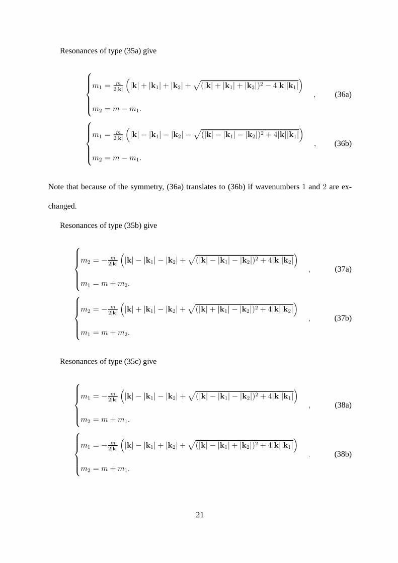
Resonances of type (35a) give

m1 =m2|k|

(

|k|+ |k1|+ |k2|+√

(|k|+ |k1|+ |k2|)2 − 4|k||k1|)

m2 = m−m1.

, (36a)

m1 =m2|k|

(

|k| − |k1| − |k2| −√

(|k| − |k1| − |k2|)2 + 4|k||k1|)

m2 = m−m1.

, (36b)

Note that because of the symmetry, (36a) translates to (36b)if wavenumbers1 and2 are ex-

changed.

Resonances of type (35b) give

m2 = − m2|k|

(

|k| − |k1| − |k2|+√

(|k| − |k1| − |k2|)2 + 4|k||k2|)

m1 = m+m2.

, (37a)

m2 = − m2|k|

(

|k|+ |k1| − |k2|+√

(|k|+ |k1| − |k2|)2 + 4|k||k2|)

m1 = m+m2.

, (37b)

Resonances of type (35c) give

m1 = − m2|k|

(

|k| − |k1| − |k2|+√

(|k| − |k1| − |k2|)2 + 4|k||k1|)

m2 = m+m1.

, (38a)

m1 = − m2|k|

(

|k| − |k1|+ |k2|+√

(|k| − |k1|+ |k2|)2 + 4|k||k1|)

m2 = m+m1.

. (38b)

21

Because of the symmetries of the problem, (37a) is equivalent to (38a), and (37b) is equivalent

to (38b) if wavenumbers1 and2 are exchanged.

b. Comparison of matrix elements

As explained above, we assumef = 0 and hydrostatic balance. Such a choice makes

the matrix elements to be scale-invariant functions that depend only upon|k1| and |k2|. As

a consequence of the triangle inequality we need to considermatrix elements only within a

“kinematic box” defined by

||k1| − |k2|| < |k| < |k1|+ |k2|.

The matrix elements will have different values depending onthe dimensions so that isopycnal

and Eulerian approaches will give different values (49)-(50). To address this issue in the sim-

plest possible way, we multiply each matrix element by a dimensional number chosen so that

all matrix elements are equivalent for some specific wavevector. In particular, we choose the

scaling constant so that|V (|k1| = 1, |k2| = 1)|2 = 1. This allows a transparent comparison

without worrying about dimensional differences between various formulations.

1) RESONANCES OF THE“ SUM” TYPE (35A)

Figure 1 presents the values of the matrix element|V pp1,p2 (36b)

|2 on the resonant sub-manifold

given explicitly by (36b). All approaches give equivalent results. This is confirmed by plotting

the relative ratio between these approaches, and it is givenby numerical noise (not shown). The

solution (36a) gives the same matrix elements but with|k1| and|k2| exchanged owing to their

22

symmetries.

2) RESONANCES OF THE“ DIFFERENCE” TYPE (35B) AND (35C)

We then turn our attention to resonances of “difference” type (35b) for which (35c) could be

obtained by symmetrical exchange of the indices. All the matrix elements|V p1

p2,p(37a)|2 on the

resonant sub-manifold (37a), are shown in Fig. 2. All the matrix elements are equivalent. The

relative differences between different approaches are given by numerical noise (not shown).

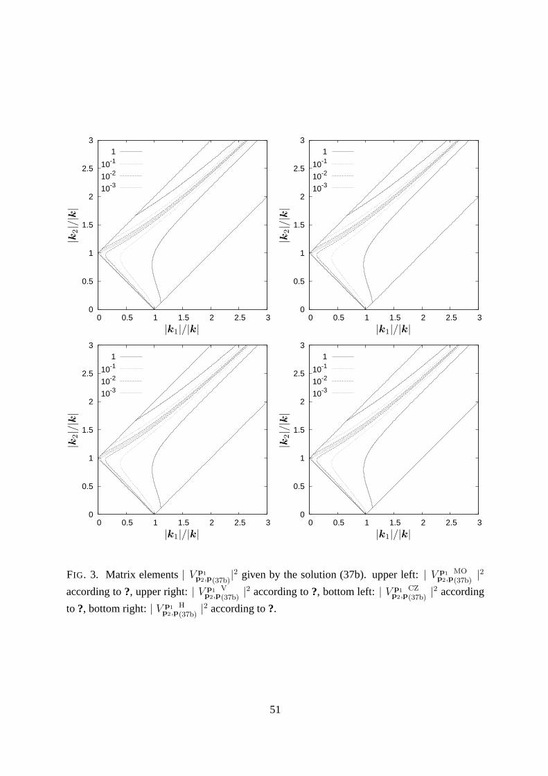
Finally, |V p1

p2,p(37b)|2 on the resonant sub-manifold (37b) are shown in Fig. 3. Again, all the

matrix elements are equivalent.

The solutions (38a) and (38b) give the same matrix elements but with |k1| and |k2| ex-

changed as the solutions (37a) and (37b) owing to their symmetries.

3) SPECIAL TRIADS

Three simple interaction mechanisms are identified by? in the limit of an extreme scale

separation. In this subsection we look in closer detail at these special limiting triads to confirm

that all matrix elements are indeed asymptotically consistent. The limiting cases are:

• the vertical backscattering of a high-frequency wave by a low frequency wave of twice

the vertical wavenumber into a second high-frequency wave of oppositely signed vertical

wavenumber and nearly the same wavenumber magnitude. This type of scattering is

called elastic scattering (ES). The solution (36a) in the limit |k1| → 0 corresponds to this

type of special triad.

• The scattering of a high-frequency wave by a low-frequency,small-wavenumber wave

23

into a second, nearly identical, high-frequency large-wavenumber wave. This type of

scattering is called induced diffusion (ID). The solution (36b) in the limit that|k1| → 0

corresponds to this type of special triad.

• The decay of a low wavenumber wave into two high vertical wavenumber waves of ap-

proximately one-half the frequency. This is called parametric subharmonic instability

(PSI). The solution (37a) in the limit that|k1| → 0 corresponds to this type of triad.

To study the detailed behavior of the matrix elements in the special triad cases, we choose

to present the matrix elements along a straight line defined by

(|k1|, |k2|) = (ǫ, ǫ/3 + 1)|k|.

This line is defined in such a way so that it originates from thecorner of the kinematic box in

Figs. 1–3 at(|k1|, |k2|) = (0, |k|) and has a slope of 1/3. The slope of this line is arbitrary. We

could have takenǫ/4 or ǫ/2. The matrix elements here are shown as functions ofǫ in Fig. 4.

We see that all four approaches are againequivalenton the resonant manifold for the case of

special triads.

In this section we demonstrated that all four approaches we considered produceequiva-

lent results on the resonant manifold in the absence of background rotation. This statement is

not trivial, given the different assumptions and coordinate systems that have been used for the

various kinetic equation derivations.

24

4. Resonant wave-wave interactions - in the presence of Back-

ground Rotations

In the presence of background rotation, the matrix elementsloose their scale invariance due

to the introduction of an additional time scale (1/f ) in the system. Consequently the comparison

of matrix elements is performed as a function of four independent parameters.

We perform this comparison in the frequency-vertical wavenumber domain. In particular,

for arbitraryω, ω1, m andm1, ω2 andm2 can be calculated by requiring that they satisfy

the resonant conditionsω = ω1 + ω2 andm = m1 + m2. We then can check whether the

corresponding horizontal wavenumber magnitudesk, given by

ki =miNρog

√

ω2i − f 2 (isopycnal coordinates) and

ki = mi

√

ω2i − f 2

N(Lagrangian coordinates) (39)

satisfy the triangle inequality. The matrix elements of theisopycnal and Lagrangian coordinate

representations are then calculated. We are performed thiscomparison for1012 points on the

resonant manifold. After being multiplied by an appropriate dimensional number to convert

between Eulerian and isopycnal coordinate systems, the twomatrix elements coincide up to

machine precision.

One might, with sufficient experience, regard this as an intuitive statement. It is, however,

far from trivial given the different assumptions and coordinate representations. In particular,

we note that derivations of the wave amplitude evolution equation in Lagrangian coordinates

(???) do not explicitly contain a potential vorticity conservation statement corresponding to

25

assumption (4) in the isopycnal coordinate (?) derivation. We have inferred that the Lagrangian

coordinate derivation conserves potential vorticity as that system is projected upon the linear

modes of the system having zero perturbation potential vorticity.

5. Resonance Broadening and Numerical Methods

a. Nonlinear frequency renormalization as a result of nonlinear wave-wave interactions

The resonant interaction approximation is a self-consistent mathematical simplification which

reduces the complexity of the problem for weakly nonlinear systems. As nonlinearity in-

creases, near-resonant interactions become more and more pronounced and need to be ad-

dressed. Moreover, near-resonant interactions play a major role in numerical simulations on

a discrete grids (?), for time evolution of discrete systems (?), in acoustic turbulence (?),

surface gravity waves (??), and internal waves (??).

To take into account the effects of near-resonant interactions self-consistently, we revisit

Section b. Now wedo not take the limitΓpp1p2→ 0. Then, instead of the kinetic equation

with the frequency conserving delta-function, we obtain thegeneralizedkinetic equation

dnp

dt= 4

∫

|V pp1,p2

|2 fp12 δp−p1−p2L(ωp − ωp1

− ωp2)dp12

−4

∫

|V p1

p2,p|2 f12p δp1−p2−p L(ωp1

− ωp2− ωp) dp12

−4

∫

|V p2

p,p1|2 f2p1 δp2−p−p1

L(ωp2− ωp − ωp1

) dp12 ,

with fp12 = np1np2

− np(np1+ np2

) ,

(40)

26

with L is defined as

L(∆ω) = Γk12

(∆ω)2 + Γ2k12

. (41)

Here, as in section (b)Γk12 is the total broadening of each particular resonance, and isgiven

below.

The difference between kinetic equation (32) and the generalized kinetic equation (40) is

that the energy conserving delta-functions in Eq. (32),δ(ωp − ωp1− ωp2

), was “broadened”.

The physical motivation for this broadening is the following: when the resonant kinetic equa-

tion is derived, it is assumed that the amplitude of each plane wave is constant in time, or, in

other words, that the lifetime of single plane wave is infinite. The resulting kinetic equation,

nevertheless, predicts that wave amplitude changes. Consequently the wave lifetime is finite.

For small level of nonlinearity this distinction is not significant, and resonant kinetic equation

constitutes a self-consistent description. For larger values of nonliterary this is no longer the

case, and the wave lifetime is finite and amplitude changes need to be taken into account. Con-

sequently interactions may not be strictly resonant. This statement also follows from the Fourier

uncertainty principle. Waves with varying amplitude can not be represented by a single Fourier

component. This effect is larger for larger normalized Boltzmann rates.

If the nonlinear frequency renormalization tends to zero, i.e. Γk12 → 0, L reduces to the

delta function (compare to (31):

limΓk12→0

L(∆ω) = πδ(∆ω).

Consequently, in the limit resonant interactions (i.e. no broadening) (40) reduces to (32) .

If, on the other hand, one does not take theΓpp1p2→ 0 limit, then one has to calculate

27

Γpp1p2self-consistently. To achieve this we realize that by deriving the generalized kinetic

equation (40) we allow changes in wave amplitude. The rate ofchange can be identified from

equation (40) in the following way. Let us go through (40) term by term, and identify all

term that multiply thenp on the right-hand-side. Those terms can be loosely interpreted as a

nonlinear wave damping acting on the given wavenumber:

γp = 4

∫

|V pp1,p2

|2 (np1+ np2

) δp−p1−p2L(ωp − ωp1

− ωp2)dp12

−4

∫

|V p1

p2,p|2 (np2− np1

) δp1−p2−pL(ωp1− ωp2

− ωp) dp12

−4

∫

|V p2

p,p1|2 (np1

− np2) δp2−p−p1

L(ωp2− ωp − ωp1

) dp12 .

(42)

The interpretation of this formula is the following: nonlinear wave-wave interactions lead to the

change of wave amplitude, which in turn makes the lifetime ofthe waves to be finite. This, in

turn, makes the interactions to be near-resonant.

The next question is how to relate the individual wave dampingγp with the overall broaden-

ing of the resonances of three interacting waves. As we have rigorously shown in (?) the errors

add up, so that

Γk12 = γp + γp1+ γp2

. (43)

It means that the total resonance broadening is the sum of individual frequency broadening, and

can be thus seen as the “triad interaction” frequency.

A rigorous derivation of the kinetic equation with a broadened delta function is given in

details for a general three-wave Hamiltonian system in (?). The derivation is based upon the

Wyld diagrammatic technique for non-equilibrium wave systems and utilizes the Dyson-Wyld

28

line resummation. This resummation permits an analytical resummation of the infinite series

of reducible diagrams for Greens functions and double correlators. Consequently, the resulting

kinetic equation is not limited to the Direct Interaction Approximation (DIA), but also includes

higher order effects coming from infinite diagrammatic series. We emphasize, however, that

the approachis perturbative in nature and there are neglected parts of the infinite diagrammatic

series. The reader is referred to? for details of that derivation. The resulting formulas are given

by (40)-(43).

A self-consistent estimate ofγp requires an iterative solution of (40) and (42) over the entire

field: the width of the resonance (42) depends on the lifetimeof an individual wave [from (40)],

which in turn depends on the width of the resonance (43). Thisnumerically intensive computa-

tion is beyond the scope of this manuscript. Instead, we makethe uncontrolled approximation

that:

γp = δωp. (44)

We note that this choice is made for illustration purposes only, we certainly do not claim

that it represents a self consistent choice. Below, we will takeδ to be10−3 and10−2 and10−1.

These values are rather small, therefore we remain in the closest proximity to the resonant

interactions. To show the effect of strong resonant manifold smearing we also investigate the

case withδ = 0.5.

We note in passing that the near-resonant interactions of the waves were also considered

in the (?). There, instead of ourL(x) function, given by (41), the corresponding function was

given bysin(πx)/x. We have shown in? that the resulting kinetic equation doesnot retain

positive definite values of wave action. To get around that difficulty, self-consistent formula for

broadening or rigorous diagrammatic resummation should beused.

29

b. Numerical Methods

Estimates of near-resonant transfers are obtained by assuming horizontal isotropy and inte-

grating (40) over horizontal azimuth:

∂np

∂t= 4π

∫

k1k2Sp12

|V pp1,p2

|2 fp12 δp−p1−p2L(ωp − ωp1

− ωp2)dk12dm1

−4π

∫

k1k2S12p

|V p1

p2,p|2 f12p δp1−p2−p L(ωp1− ωp2

− ωp) dk12dm1

−4π

∫

k1k2S2p1

|V p2

p,p1|2 f2p1 δp2−p−p1

L(ωp2− ωp − ωp1

) dk12dm1 , (45)

whereSp12 is the area of the trianglek = k1+k2. We numerically integrated (45) forp’s which

have frequencies fromf toN and vertical wavenumbers from2π/(2b) to 260π/(2b). The limits

of integration are restricted by horizontal wavenumbers from2π/105 to 2π/5 meters−1, vertical

wavenumbers from2π/(2b) to 2π/5 meters−1, and frequencies fromf toN . The integrals over

k1 andk2 are obtained in the kinematic box ink1 − k2 space. The grids in thek1 − k2 domain

have217 points that are distributed heavily around the corner of thekinematic box. The integral

overm1 is obtained with213 grid points, which are also distributed heavily for the small vertical

wavenumbers whose absolute values are less than5m, wherem is the vertical wavenumber.

To estimate the normalized Boltzmann rate we need to choose aform of spectral energy

density of internal waves. We utilize the Garrett and Munk spectrum as an agreed-upon repre-

sentation of the internal waves:

E(ω,m) =4f

π2m∗E0

1

1 + ( mm∗

)21

ω√

ω2 − f 2. (46)

30

Here the reference wavenumber is given by

m∗ = πj∗/b, (47)

in which the variablej represents the vertical mode number of an ocean with an exponential

buoyancy frequency profile having a scale height ofb.

We choose the following set of parameters:

• b = 1300 m in the GM model

• The total energy is set as:

E0 = 30× 10−4 m2 s−2.

• Inertial frequency is given byf = 10−4rad/s, and buoyancy frequency is given byN0 =

5× 10−3rad/s.

• The reference density is taken to beρ0 = 103kg/m3.

• A roll-off corresponding toj∗ = 3.

We then calculate the normalized Boltzmann rate (34) using four values ofδ in (44): δ =

10−3, δ = 10−2, δ = 10−1 andδ = 0.5.

6. Time Scales

a. Resonant Interactions

Here we present evaluations of the? kinetic equation. These estimates differ from evalua-

tions presented in???? in that the numerical algorithm includes a finite breadth to the resonance

31

surface whereas previous evaluations have beenexactlyresonant. Results discussed in this sec-

tion are as close to resonant as we can make (δ = 1× 10−3).

We see that for small vertical wavenumbers the normalized Boltzmann rate is of the order of

tenth of the wave period. This can be argued to be relatively within the domain of weak nonlin-

earity. However for increased wavenumbers the level of nonlinearity increases and reaches the

level of wave-period (red, or dark blue). There is also a white region indicating values smaller

than minus one.

We also define a “zero curve” - It is the locus of wavenumber-frequency where the normal-

ized Boltzmann rate and time-derivative of waveaction is exactly zero. The zero curve clearly

delineates a pattern of energy gain for frequenciesf < ω < 2f , energy loss for frequencies

2f < ω < 5f and energy gain for frequencies5f < ω < N . We interpret the relatively sharp

boundary between energy gain and energy loss acrossω = 2f as being related to the Parame-

teric Subharmonic Instability and the transition from energy loss to energy gain atω = 5f as

a transition from energy loss associated with the Parametric Subharmonic Instability to energy

gain associated with the Elastic Scattering mechanism. SeeSection 7 for further details about

this high frequency interpretation.

TheO(1) normalized Boltzmann rates at high vertical wavenumber aresurprising given the

substantial literature that regards the GM spectrum as a stationary state. We do not believe this

to be an artifact of the numerical scheme for the following reasons. First, numerical evalua-

tions of the integrand conserve energy to within numerical precision as the resonance surface is

approached, consistent with energy conservation propertyassociated with the frequency delta

function. Second, the time scales converge as the resonant width is reduced, as demonstrated

by the minimal difference in time scales usingδ = 1 × 10−3 and 1 × 10−2. Third, our results

32

are consistent with approximate analytic expressions (e.g. ?) for the Boltzmann rate. Finally,

in view of the differences in the representation of the wavefield, numerical codes and display

of results, we interpret our resonant (δ = 0.001) results as being consistent with numerical

evaluations of the resonant kinetic equations presented in????.

As a quantitative example, consider estimates of the time rate of change of low-mode energy

appearing in Table 1 of?, repeated as row 3 of our Table 82. We find agreement to better than a

factor of two. In order to explain the remaining differences, you have to examine the details:?

use a Coriolis frequency corresponding to30 latitude, neglect internal waves having horizontal

wavelengths greater than 100 km (same as here) and exclude frequenciesω > No/3, with

No = 3 cph. We include frequenciesf < ω < No with Coriolis frequency corresponding to45

latitude. Of possible significance is that? use a vertical mode decomposition with exponential

stratification with scale heightb = 1200 m (we useb = 1300 m). Table 8 presents estimates of

the energy transfer rate by taking the depth integrated transfer rates of?, assumingE ∝ N2 and

normalizing toN = 3 cph. While this accounts for the nominal buoyancy scaling of the energy

transport rate, it doesnot account for variations in the distribution ofE(m) associated with

variations inN viam∗ =NNoj∗/b in their model. Finally, their estimates ofE(m) are arrived at

by integrating only over regions of the spectral domain for which E(m,ω) is negative.

b. Near-Resonant Interactions

Substantial motivation for this work is the question of whether the GM76 spectrum repre-

sents a stationary state. We have seen that numerical evaluations of a resonant kinetic equation

returnO(1) normalized Boltzmann rates and hence we are lead to concludethat GM76 isnota

2A potential interpretation is that this net energy flow out ofthe non-equilibrium part of the spectrum representsthe energy requirements to maintain the spectrum.

33

stationary state with respect to resonant interactions. But the inclusion of near-resonant inter-

actions could alter this judgement.

Our investigation of this question is currently limited by the absence of an iterative solu-

tion to (40) and (42) and consequent choice to parameterize the resonance broadening in terms

of (44). However, as we go from nearly resonant evaluations (10−3 and10−2) to incorporat-

ing significant broadening (10−1 and 0.5), we find a significant decreases in the normalized

Boltzmann rate. The largest decreases are associated with an expanded region of energy loss

associated the Parametric Subharmonic Instability, in which minimum normalized Boltzmann

rates change from -3.38 to -0.45 at(ω,mb/2π) = (2.5f, 150). Large decreases here are not sur-

prising given the sharp boundary between regions of loss andgain in the resonant calculations.

Smaller changes are noted within the Induced Diffusion regime. Maximum normalized Boltz-

mann rates change from 2.6 to 1.5 at(ω,mb/2π) = (8f, 260). Broadening of the resonances to

exceed the boundaries of the spectral domain could be makinga contribution to such changes.

We regard our calculations here as a preliminary step to answering the question of whether

the GM76 spectrum represents a stationary state with respect to nonlinear interactions. Comple-

mentary studies could include comparison with analyses of numerical solutions of the equations

of motion.

7. Discussion

a. Resonant Interactions

Several loose ends need to be tied up regarding the assertionthat the GM76 spectrum does

not constitute a stationary state with respect to resonant interactions. The first is the interpre-

34

tation of ?’s inertial-range theory with constant downscale transferof energy. This constant

downscale transfer of energy was obtained by patching together the induced diffusion and para-

metric subharmonic instability mechanisms and is attendedby the following caveats: First, the

inertial subrange solution is found only after integratingover the frequency domain and numer-

ical evaluations of the kinetic equation demonstrate that the ”inertial subrange” solution also

requires dissipation to balance energy gain at high vertical wavenumber. It takes a good deal of

patience to wade through their figures to understand how figures in? plots relate to the initial

tendency estimates in Figure 5. Second,? argue that GM76 is an near-equilibrium state because

of a 1-3 order of magnitude cancellation between the Langevin rates in the induced diffusion

regime. But this is just theω2/f 2 difference between the fast and slow induced diffusion time

scales. It does NOT imply small values of the slow induced diffusion time scale, which are

equivalent to the normalized Boltzmann rates. Third, the large normalized Boltzmann rates

determined by our numerical procedure are associated with the elastic scattering mechanism

rather than induced diffusion. Normalized Boltzmann ratesfor the induced diffusion and elastic

scattering mechanisms are:

ǫid = π2

20mmc

m2

m2+m2∗

ω2

f2

ǫes = π2

20mmc

m2

m2+0.25m2∗

in whichm∗ represents the low wavenumber roll-off of the vertical wavenumber spectrum (ver-

tical mode-3 equivalent here),mc is the high wavenumber cutoff, nominally at 10 m wave-

lengths and the GM76 spectrum has been assumed. The normalized Boltzmann rates for ES and

ID are virtually identical at high wavenumber. They differ only in how their respective triads

connect to theω = f boundary. Induced diffusion connects along a curve whose resonance con-

35

dition is approximately that the high frequency group velocity match the near-inertial vertical

phase speed,ω/m = f/mni. Elastic scattering connects along a simplerm = 2mni. Evalua-

tions of the kinetic equation reveal nearly vertical contours throughout the vertical wavenumber

domain, consistent with ES, rather than sloped along contours of ω ∝ m emanating from

m = m∗ as expected with the ID mechanism.

The identification of the ES mechanism as being responsible for the large normalized Boltz-

mann rates at high vertical wavenumber requires further explanation. The role assigned to the

ES mechanism by? is the equilibration of a vertically anisotropic field. Thiscan be seen

by taking the near-inertial component of a triad to represent p1, assuming that the action den-

sity of the near-inertial field is much larger than the high frequency fields, and taking the limit

(k, l,m) = (k2, l2,−m2) ≡ p−. Thus:

fp12 = np1np2

− np(np1+ np2

) ∼= np1[np− − np]

and transfers proceed until the field is isotropic:np− = np . But this isnot the complete

story. A more precise characterization of the resonance surface takes into account the frequency

resonance requiringω − ω2 = ω1∼= f requiresO(ω/f) differences inm and−m2 if k = k2

andO(ω/f) differences ink andk2 if m = −m2. For an isotropic field:

fp12 = np1np2

− np(np1+ np2

) ∼= np1[np+δp − np] ∼= np1[δp · ∇np]

and due care needs to be taken thatp1 is on the resonance surface in the vicinity of the inertial

cusp.

36

b. Near-Resonant Interactions

The idea of trying to self consistently find the smearing of the delta-functions is not new.

For internal waves it appears in???.

? set up a general framework for a self consistent calculationsimilar in spirit to?, using

a path-integral formulation of the diagrammatic technique. The paper makes an uncontrolled

approximation that their nonlinear frequency renormalizationΣ(p, ω) is independent ofω, and

shows that this assumption is not self-consistent.? present a more sophisticated approach to a

self-consistent approximation to the operatorΣ(p, ω). In particular,? suggests

Σ(p, ω) = Σ(p, ωp),

while ? propose a more self-consistent

Σ(p, ω) = Σ[p, ωp + iℑΣ(p,Ωp)].

? evaluate the self-consistency of the resonant interactionapproximation and find that for

high-frequency-high-wavenumbers, the resonant interaction representation is not self-consistent.

A possible critique of these papers is that they use resonantmatrix elements given by? with

out appreciating that those elements can only be used strictly on the resonant manifold.

? present similar expressions for two-dimensional stratified internal waves. There the ki-

netic equation is (7.4) with the triple correlation time given byΘ (ourL) of their (8.7). The key

step is to find the level of smearing of the delta-function, denoted asµk in their (8.7) (ourγ).

This can be achieved by their (8.6), which is similar to our (42). The only difference is that (8.6)

hFas slightly different positions of the polesi(γp1+ γp2

), instead of oursi(γp1+ γp2

+ γp).

37

Carnavale points out that the Direct Interaction Approximation leads to his expression, not the

sum of all threeγ’s. We respectfully disagree. However, this is irrelevant for the purpose of this

paper, since we do not solve it self consistently anyway, butpropose an uncontrolled approxi-

mation (44). The main advantage of our approach over? is that we use systematic Hamiltonian

structures which are equivalent to the primitive equationsof motion, rather than a simplified

two-dimensional model.

8. Conclusion

Our fundamental result is that the GM spectrum isnotstationary with respect to the resonant

interaction approximation. This result is contrary to muchof the perceived wisdom and gave

us cause to review published results concerning resonant internal wave interactions. We then

included near-resonant interactions and found significantreductions in the temporal evolution

of the GM spectrum.

We compared the interaction matrices for three different Hamiltonian formulations and one

non-Hamiltonian formulation in the resonant limit. Two of the Hamiltonian formulations are

canonical and one (?) avoids a linearization of the Hamiltonian prior to assuming an expan-

sion in terms of weak nonlinearity. Formulations in Eulerian, isopycnal and Lagrangian co-

ordinate systems were considered. All four representations lead toequivalentresults on the

resonant manifold in the absence of background rotation. The two representations that include

background rotation, a canonical Hamiltonian formulationin isopycnal coordinates and a non-

canonical Hamiltonian formulation in Lagrangian coordinates, also lead toequivalentresults

on the resonant manifold. This statement is not trivial given the different assumptions and coor-

38

dinate systems that have been used for the derivation of the various kinetic equations. It points

to an internal consistency on the resonant manifold that we still do not completely understand

and appreciate.

We rationalize the consistent results as being associated with potential vorticity conserva-

tion. In the isopycnal coordinate canonical Hamilton formulation potential vorticity conser-

vation is explicit. In the Lagrangian coordinate non-canonical Hamiltonian, potential vorticity

conservation results from a projection onto the linear modes of the system. The two non-rotating

formulations prohibit relative vorticity variations by casting the velocity as a the gradient of a

scalar streamfunction.

We infer that the non-stationary results for the GM spectrumare related to a higher order

approximation of the elastic scattering mechanism than considered in? and?.

Our numerical results indicate evolution rates of a wave period at high vertical wavenumber,

signifying a system which is not weakly nonlinear. To understand whether such non-weak

conditions could give rise to competing effects that renderthe system stationary, we considered

resonance broadening. We used a kinetic equation with broadened frequency delta function

derived for a generalized three-wave Hamiltonian system in(?). The derivation is based upon

the Wyld diagrammatic technique for non-equilibrium wave systems and utilizes the Dyson-

Wyld line resummation. This broadened kinetic equation is perceived to be more sophisticated

than the two-dimensional direct interaction approximation representation pursued in? and the

self-consistent calculations of? which utilized the resonant interaction matrix of?. We find a

tendency of resonance broadening to lead to more stationaryconditions. However, our results

are limited by an uncontrolled approximation concerning the width of the resonance surface.

Reductions in the temporal evolution of the internal wave spectrum at high vertical wavenum-

39

ber were greatest for those frequencies associated with thePSI mechanism, i.e.f < ω < 5f .

Smaller reductions were noted at high frequencies.

A common theme in the development of a kinetic equation is a perturbation expansion

permitting the wave interactions and evolution of the spectrum on a slow time scale, e.g. Section

b. An assumption of Gaussian statistics at zeroth order permits a solution of the first order triple

correlations in terms of the zeroth order quadruple correlations. Assessing the adequacy of this

assumption for the zeroth order high frequency wavefield is achallenge for future efforts. Such

departures from Guassianity could have implications for the stationarity at high frequencies.

Nontrivial aspects of our work are that we utilize the canonical Hamiltonian representation

of ? which results in a kinetic equation without first linearizing to obtain interaction coefficients

defined only on the resonance surface and that the broadened closure scheme of? is more so-

phisticated than the Direct Interaction Approximation. Inclusion of interactions between inter-

nal waves and modes of motion associated with zero eigen frequency, i.e. the vortical motion

field, is a challenge for future efforts.

We found no coordinate dependent (i.e. Eulerian, isopycnalor Lagrangian) differences

between interaction matrices on the resonant surface. We regard it as intuitive that there will be

coordinate dependent differences off the resonant surface. It is a robust observational fact that

Eulerian frequency spectra at high vertical wavenumber arecontaminated by vertical Doppler

shifting: near-inertial frequency energy is Doppler shifted to higher frequency at approximately

the same vertical wavelength. Use of an isopycnal coordinate system considerably reduces

this artifact (?). Further differences are anticipated in a fully Lagrangian coordinate system

(?). Thus differences in the approaches may represent physical effects and what is a stationary

state in one coordinate system may not be a stationary state in another. Obtaining canonical

40

coordinates in an Eulerian coordinate system with rotationand in the Lagrangian coordinate

system are challenges for future efforts.

41

1) *

Acknowledgments.

We thank V. E. Zakharov for presenting us with a book (?) and for encouragement. We also

thank E. N. Pelinovsky for providing us with?. We greatfully acknowledge funding provided by

a Collaborations in Mathematical Geosciences (CMG) grant from the National Science Foun-

dation. YL is also supported by NSF DMS grant 0807871 and ONR Award N00014-09-1-0515.

We are grateful to YITP in Kyoto University for permitting use of their facility.

42

Matrix Elements

Our attention is restricted to the hydrostatic balance case, for which

| k |≪| m | . (48)

A minor detail is that the linear frequency has different algebraic representations in isopycnal

and Cartesian coordinates. The Cartesian vertical wavenumber,kz, and the density wavenum-

ber,m, are related asm = −g/(ρ0N2)kz whereg is gravity,ρ is density with reference value

ρ0, N is the buoyancy (Brunt–Vaisala) frequency andf is the Coriolis frequency. In isopycnal

coordinates the dispersion relation is given by,

ω(p) =

√

f 2 +g2

ρ20N2

| k |2m2

. (49)

In Cartesian coordinates,

ω(p) =

√

f 2 +N2| k |2k2z

. (50)

In the limit of f = 0 these dispersion relations assume the form

ωp ∝ | k || m | ∝

| k || kz |

(51)

43

Muller and Olbers

Matrix elements derived in? are given by| V pp1,p2

MO |2= T+/(4π) and | V p1

p2,pMO |2=

T−/(4π). We extractedT± from the Appendix of?. In our notation, in the hydrostatic balance

approximation, their matrix elements are given by

|V pp1,p2

MO|2 = (N20 − f 2)2

32ρ0ωω1ω2

∣

∣

∣

∣

|k||k1||k2|ωω1ω2|p||p1||p2|

−

(

−m1k1·k2−ifk2·k⊥

1/ω1

k21

+m2

)(

−m2k1·k2−ifk1·k⊥

2/ω2

k22

+m1

)

m

−

(

−m2k2·k+ifk2·k⊥/ω2

k22

+m)(

−mk2·k−ifk·k⊥

2/ω

k2+m2

)

m1

−

(

−mk·k1−ifk·k⊥

1/ω

k2+m1

)(

−m1k·k1+ifk1·k⊥/ω1

k21

+m)

m2

∣

∣

∣

∣

∣

∣

2

. (52)

Taking af = 0 limit reduces the problem to scale invariant problem. We getthe following

simplified expression:

|V pp1,p2

MO|2 ∝ |k||k1||k2||mm1m2|

(

− 1

m

(

−m2k1 · k2

|k2|2+m1

)(

−m1k2 · k1

|k1|2+m2

)

+1

m1

(

m2k · k2

|k2|2−m

)(

−mk2 · k|k|2 +m2

)

+1

m2

(

−mk1 · k|k|2 +m1

)(

m1k · k1

|k1|2−m

))2

(53)

This simplified expression is going to be used for comparisonof approaches in section (3).

44

Voronovich

We formulate the matrix elements for Voronovich’s Hamiltonian using his formula (A.1).

This formula is derived for general boundary conditions. Tocompare with other matrix ele-

ments of this paper, we assume a constant stratification profile and Fourier basis as the vertical

structure functionφ(z). That allows us to solve for the matrix elements defined via Eq. (11)

and above it in his paper. Then the convolutions of the basis functions give delta-functions in

vertical wavenumbers. Vornovich’s equation (A.1) transforms into:

|V pp1,p2

V|2 ∝ |k||k1||k2||mm1m2|

(

−m(

1

|k||m|

(

k · k1|m1||k1|

+k · k2|m2|

|k2|

)

+ω1 + ω2 − ω

ω

)

+m1

(

1

|k1||m1|

(

k · k1|m||k| +

k1 · k2|m2||k2|

)

− ω1 + ω2 − ω

ω1

)

+m2

(

1

|k2||m2|

(

k · k2|m||k| +

k2 · k1|m1||k1|

)

− ω1 + ω2 − ω

ω2

))2

.

(54)

Note that Eq. (54) shares structural similarities with the interaction matrix elements inisopy-

cnal coordinates, Eq. (57) below.

Caillol and Zeitlin

A non-Hamiltonian kinetic equation for internal waves was derived in?, Eq. (61) directly

from the dynamical equations of motion, without the use of the Hamiltonian structure.

To make it appear equivalent to more traditional form of kinetic equation, as in?, we make

a change of variablesl → −l in the second line, andk → −k in the third line of (61) of?.

If we further assume that all spectra are symmetric,n(−p) = n(p), then the kinetic equation

45

assumes traditional form, as in Eq. (32), see????.

The matrix elements according to? are shown asXk,l,p andY ±k,l,p in Eqs. (62) and (63),

where|V pp1,p2

CZ|2 = Xp1,p2,p and|V p1

p2,pCZ|2 = Y +

p1,−p2,p. In our notation it reads

|V pp1,p2

CZ|2 ∝ (|k|sgn(m) + |k1|sgn(m1) + |k2|sgn(m2))2 (m2 −m1m2)

2

|m||m1||m2||k||k1||k2|

×( |k|2 − |k1|sgn(m1)|k2|sgn(m2)

m2 −m1m2m− |k1|2

m1− |k2|2

m2

)2

. (55)

This expression is going to be used for comparison of approaches in section (3).

Isopycnal Hamiltonian

Finally, in ? the following wave-wave interaction matrix element was derived based on a

canonical Hamiltonian formulation in isopycnal coordinates:

|V 01,2

H|2 = N2

32g

((

kk1 · k2

k1k2

√

ω1ω2

ω+k1k2 · kk2k

√

ω2ω

ω1

+k2k · k1

kk1

√

ωω1

ω2

+f 2

√ωω1ω2

k21k2 · k− k22k · k1 − k2k1 · k2

kk1k2

)2

+

(

fk1 · k⊥

2

kk1k2

(√

ω

ω1ω2(k21 − k22)−

√

ω1

ω2ω(k22 − k2)−

√

ω2

ωω1(k2 − k21)

))2)

.

(56)

46

? is a rotationless limit of?. Taking thef → 0 limit, the ? reduces to?, and (56) reduces to

|V pp1,p2

H|2 ∝ 1

|k||k1||k2|

(

|k|k1 · k2

√

∣

∣

∣

∣

m

m1m2

∣

∣

∣

∣

+ |k1|k2 · k√

∣

∣

∣

∣

m1

m2m

∣

∣

∣

∣

+ |k2|k · k1

√

∣

∣

∣

∣

m2

mm1

∣

∣

∣

∣

)2

.

(57)

Observe that in this form, these equations share structuralsimilarities with Eq. (54).

47

List of Figures

1 Matrix elements| V pp1,p2(36b)

|2 given by the solution (36b). upper left:|

V pp1,p2

MO(36b)

|2 according to?, upper right: | V pp1,p2

V(36b)

|2 according to?, bot-

tom left: | V pp1,p2

CZ(36b)

|2 according to?, bottom right:| V pp1,p2

H(36b)

|2 according

to ?. . . . . . . . . . . . . . . . . . . . . . . . . . . . . . . . . . . . . . . . . 49

2 Matrix elements| V p1

p2,p(37a)|2 given by the solution (37a). upper left:| V p1

p2,pMO

(37a)|2

according to?, upper right:| V p1

p2,pV

(37a)|2 according to?, bottom left:| V p1

p2,pCZ

(37a)|2

according to?, bottom right:| V p1

p2,pH(37a)

|2 according to?. . . . . . . . . . . . 50

3 Matrix elements| V p1

p2,p(37b)|2 given by the solution (37b). upper left:| V p1

p2,pMO(37b)

|2

according to?, upper right:| V p1

p2,pV

(37b)|2 according to?, bottom left:| V p1

p2,pCZ

(37b)|2

according to?, bottom right:| V p1

p2,pH

(37b)|2 according to?. . . . . . . . . . . . 51

4 upper: Matrix elements| V pp1,p2ES

|2 given by the solution (36a). middle: Ma-

trix elements| V pp1,p2 ID

|2 given by the solution (36b). bottom: Matrix ele-

ments| V p1

p2,pPSI|2 given by the solution (37a), which gives PSI as| k1 |→ 0

(ǫ → 0). The matrix elements here are shown as functions ofǫ such that

(|k1|, |k2|) = (ǫ, ǫ/3 + 1)|k|. All four versions of the Matrix elements are

plotted here: the appearance of a single line in each figure panel testifies to the

similarity of the elements on the resonant manifold. . . . . . .. . . . . . . . 52

5 Normalized Boltzmann rates (34) for the Garrett and Munk spectrum (46) cal-

culated via (40). Figures represent normalized Boltzmann rate calculated using

?, equation (56) withδ = 10−3, (upper-left),δ = 10−2, (upper-right),δ = 10−1,

(lower-left),δ = 0.5, (lower-right). On these figures white region on the figure

corresponds to extremely fast time scales, faster then a linear time scale. . . . . 53

48

0

0.5

1

1.5

2

2.5

3

0 0.5 1 1.5 2 2.5 3

1

10-1

10-2

10-3

|k1|/|k|

|k2|/|k|

0

0.5

1

1.5

2

2.5

3

0 0.5 1 1.5 2 2.5 3

1

10-1

10-2

10-3

|k1|/|k|

|k2|/|k|

0

0.5

1

1.5

2

2.5

3

0 0.5 1 1.5 2 2.5 3

1

10-1

10-2

10-3

|k1|/|k|

|k2|/|k|

0

0.5

1

1.5

2

2.5

3

0 0.5 1 1.5 2 2.5 3

1

10-1

10-2

10-3

|k1|/|k|

|k2|/|k|

FIG. 1. Matrix elements| V pp1,p2 (36b)

|2 given by the solution (36b). upper left:| V pp1,p2

MO

(36b)|2

according to?, upper right:| V pp1,p2

V(36b)

|2 according to?, bottom left:| V pp1,p2

CZ(36b)

|2 according

to ?, bottom right:| V pp1,p2

H(36b)

|2 according to?.

49

0

0.5

1

1.5

2

2.5

3

0 0.5 1 1.5 2 2.5 3

1

10-1

10-2

10-3

|k1|/|k|

|k2|/|k|

0

0.5

1

1.5

2

2.5

3

0 0.5 1 1.5 2 2.5 3

1

10-1

10-2

10-3

|k1|/|k|

|k2|/|k|

0

0.5

1

1.5

2

2.5

3

0 0.5 1 1.5 2 2.5 3

1

10-1

10-2

10-3

|k1|/|k|

|k2|/|k|

0

0.5

1

1.5

2

2.5

3

0 0.5 1 1.5 2 2.5 3

1

10-1

10-2

10-3

|k1|/|k|

|k2|/|k|

FIG. 2. Matrix elements| V p1

p2,p(37a)|2 given by the solution (37a). upper left:| V p1

p2,pMO

(37a)|2

according to?, upper right:| V p1

p2,pV(37a)

|2 according to?, bottom left: | V p1

p2,pCZ(37a)

|2 according

to ?, bottom right:| V p1

p2,pH(37a)

|2 according to?.

50

0

0.5

1

1.5

2

2.5

3

0 0.5 1 1.5 2 2.5 3

1

10-1

10-2

10-3

|k1|/|k|

|k2|/|k|

0

0.5

1

1.5

2

2.5

3

0 0.5 1 1.5 2 2.5 3

1

10-1

10-2

10-3

|k1|/|k|

|k2|/|k|

0

0.5

1

1.5

2

2.5

3

0 0.5 1 1.5 2 2.5 3

1

10-1

10-2

10-3

|k1|/|k|

|k2|/|k|

0

0.5

1

1.5

2

2.5

3

0 0.5 1 1.5 2 2.5 3

1

10-1

10-2

10-3

|k1|/|k|

|k2|/|k|

FIG. 3. Matrix elements| V p1

p2,p(37b)|2 given by the solution (37b). upper left:| V p1

p2,pMO

(37b)|2

according to?, upper right:| V p1

p2,pV(37b)

|2 according to?, bottom left: | V p1

p2,pCZ(37b)

|2 according

to ?, bottom right:| V p1

p2,pH(37b)

|2 according to?.

51

10-6

10-5

10-4

10-3

10-2

10-1

100

10-6 10-5 10-4 10-3 10-2 10-1 100

ǫ

ǫ

|Vp p1,p

2E

S|2

10-6

10-5

10-4

10-3

10-2

10-1

100

10-6 10-5 10-4 10-3 10-2 10-1 100

ǫ

ǫ1/2

|Vp p1,p

2ID|2

10-12

10-10

10-8

10-6

10-4

10-2

100

10-6 10-5 10-4 10-3 10-2 10-1 100

ǫ

ǫ2

|Vp

1

p2,p

PSI|2

FIG. 4. upper: Matrix elements| V pp1,p2ES

|2 given by the solution (36a). middle: Matrixelements| V p

p1,p2 ID|2 given by the solution (36b). bottom: Matrix elements| V p1

p2,pPSI|2 given

by the solution (37a), which gives PSI as| k1 |→ 0 (ǫ → 0). The matrix elements here areshown as functions ofǫ such that(|k1|, |k2|) = (ǫ, ǫ/3 + 1)|k|. All four versions of the Matrixelements are plotted here: the appearance of a single line ineach figure panel testifies to thesimilarity of the elements on the resonant manifold.

52

0

0

0

0

0

00

0

log10(vertical wavenumber) (mode−equivalent)

log1

0(fr

eque

ncy)

(/f)

Time Scale in Wave Periods: n(p) ∝ α−4.0β0.00, δ=1.e−3

2f

5f

10f

j=3 30 1500 0.5 1 1.5 2

0.2

0.4

0.6

0.8

1

1.2

1.4

1.6

−1

−0.8

−0.6

−0.4

−0.2

0

0.2

0.4

0.6

0.8

1

0

00

0

00

0

log10(vertical wavenumber) (mode−equivalent)

log1

0(fr

eque

ncy)

(/f)

Time Scale in Wave Periods: n(p) ∝ α−4.0β0.00, δ=1.e−2

2f

5f

10f

j=3 30 1500 0.5 1 1.5 2

0.2

0.4

0.6

0.8

1

1.2

1.4

1.6

−1

−0.8

−0.6

−0.4

−0.2

0

0.2

0.4

0.6

0.8

1

0

0

0

0

0

0

0

log10(vertical wavenumber) (mode−equivalent)

log1

0(fr

eque

ncy)

(/f)

Time Scale in Wave Periods: n(p) ∝ α−4.0β0.00, δ=1.e−1

2f

5f

10f

j=3 30 1500 0.5 1 1.5 2

0.2

0.4

0.6

0.8

1

1.2

1.4

1.6

−1

−0.8

−0.6

−0.4

−0.2

0

0.2

0.4

0.6

0.8

1

0

0

0

0

0

0

log10(vertical wavenumber) (mode−equivalent)

log1

0(fr

eque

ncy)

(/f)

Time Scale in Wave Periods: n(p) ∝ α−4.0β0.00, δ=5.e−1

2f

5f

10f

j=3 30 1500 0.5 1 1.5 2

0.2

0.4

0.6

0.8

1

1.2

1.4

1.6

−1

−0.8

−0.6

−0.4

−0.2

0

0.2

0.4

0.6

0.8

1

FIG. 5. Normalized Boltzmann rates (34) for the Garrett and Munkspectrum (46) calculatedvia (40). Figures represent normalized Boltzmann rate calculated using?, equation (56) withδ = 10−3, (upper-left),δ = 10−2, (upper-right),δ = 10−1, (lower-left),δ = 0.5, (lower-right).On these figures white region on the figure corresponds to extremely fast time scales, faster thena linear time scale.

53

List of Tables

1 A list of various kinetic equations. Results from?, ? and? are reviewed in?,

who state that?, ? and an unspecified Eulerian representation are consistent on

the resonant manifold.? utilizes Langevin techniques to assess nonlinear trans-

ports.? characterizes those Langevin results as being mutually consistent with

the direct evaluations of kinetic equations presented in? and?. ? states (without

detail) that? and? give numerically similar results. A formulation in terms of

discrete modes will typically permit an arbitrary buoyancyprofile, but obtain-

ing results requires specification of the profile. Of the discrete formulations,?

use an exponential profile and the others assume a constant stratification rate.

The kinetic equations marked by† are investigated in Section 3, while kinetic

equations marked by‡ are investigated further in Section a. . . . . . . . . . . . 55

2 Numerical evaluations of∫ N

fE(m,ω)dω for vertical mode numbers 1-8. The

sum is given in the right-most column. . . . . . . . . . . . . . . . . . . .. . 56

54

TABLE 1. A list of various kinetic equations. Results from?, ? and ? are reviewed in?,who state that?, ? and an unspecified Eulerian representation are consistent on the resonantmanifold. ? utilizes Langevin techniques to assess nonlinear transports. ? characterizes thoseLangevin results as being mutually consistent with the direct evaluations of kinetic equationspresented in? and?. ? states (without detail) that? and? give numerically similar results.A formulation in terms of discrete modes will typically permit an arbitrary buoyancy profile,but obtaining results requires specification of the profile.Of the discrete formulations,? use anexponential profile and the others assume a constant stratification rate. The kinetic equationsmarked by† are investigated in Section 3, while kinetic equations marked by‡ are investigatedfurther in Section a.

source coordinate vertical rotation hydro- specialsystem structure static

? Lagrangian discrete no no?? Eulerian discrete no no non-Hamiltonian?†‡ Lagrangian cont. yes no?? Lagrangian cont. yes yes? Lagrangian cont. no no Clebsch?† Eulerian cont. no yes Clebsch? Lagrangian discrete yes no Langevin? Isopycnal n/a no no?† Eulerian cont. no no non-Hamiltonian?† Isopycnal cont. no yes canonical?‡ Isopycnal cont. yes yes canonical

55

TABLE 2. Numerical evaluations of∫ N

fE(m,ω)dω for vertical mode numbers 1-8. The sum is

given in the right-most column.

E × 10−10 W/kg mode-1 2 3 4 5 6 7 8 Σ

? GM76 -1.46 -1.72 -1.76 -1.69 -1.57 -1.40 -1.08 -0.81 -11.5

? GM76 -1.83 -2.17 -2.17 -1.83 -1.67 -1.00 -10.7

56