Simulation of phase transitions in fluids

P1: FLM/FLK/FKR P2: FHP/FLM/FGM QC: FHP/TKJ T1: FDX

August 11, 1999 11:26 Annual Reviews AR091-14

?Annu. Rev. Phys. Chem. 1999. 50:377–411

Copyright c© 1999 by Annual Reviews. All rights reserved

SIMULATION OF PHASE TRANSITIONS IN FLUIDS

Juan J. de Pablo,1 Qiliang Yan,1 and Fernando A. Escobedo21Department of Chemical Engineering, University of Wisconsin-Madison, Madison,Wisconsin 53706, and2Department of Chemical Engineering, Cornell University, Ithaca,New York 14853; e-mail: [email protected], [email protected], [email protected]

Key Words configurational bias, histogram reweighting, pseudo-ensembles,expanded ensembles, Gibbs ensemble

■ Abstract This review provides a discussion of recent techniques for simula-tion of phase equilibria of complex fluids. Monte Carlo methods are emphasized overmolecular dynamics methods. We describe recent developments, such as the use ofexpanded-ensemble, tempering, or histogram reweighting techniques. Our discussionof such developments is aimed at a general audience and is intended to provide anoverview of the main advantages and limitations of each particular technique. Refer-ences are provided to allow interested readers to identify and trace back most recentapplications of a particular simulation technique. We conclude with general guidelinesregarding selection of suitable simulation methods for particular problems and systemsof interest.

INTRODUCTION

Significant advances in methods for molecular simulation of complex fluids areoccurring at a breathtaking pace; even for researchers in this field, it is difficult tostay abreast of the latest developments. One of the challenges for users of thesemethods, whether novice or expert, is selection of an appropriate methodology forthe problem of interest. This review provides an overview of simulation methodsthat are useful for simulating the phase behavior of complex fluids. It also providessome general guidelines that will help users identify the best tools available fortheir particular interests.

The discussion is limited to the molecular simulation of phase behavior forcomplex fluids, including polymers. It emphasizes the use of Monte Carlo meth-ods, which have in general proven to be more useful for study of phase transitionsthan molecular dynamics. Note, however, that many of the analysis techniques dis-cussed here could also be applied to trajectories generated via molecular dynamics.We focus on this particular topic because phase transitions are ubiquitous in phys-ical chemistry, and their simulation provides important insights into the behaviorof complex fluids. Because of space limitation, this review is centered around fluid

0066-426X/99/1001-0377$08.00 377



?378 DE PABLO ■ YAN ■ ESCOBEDO

phase equilibria, as opposed to solid-fluid equilibria. Rather than provide an ex-haustive review of recent simulations of phase transitions, however, we have optedfor a limited description of a few specific examples that are particularly illustra-tive, and for a more extensive discussion of the limitations of well-establishedtechniques and the promises offered by newer, less-developed methodologies.

Several texts and monographs on the subject of simulation have appeared inthe past few years (1–11a). Readers seeking a more thorough discussion of themethodological aspects pertaining to a particular simulation technique are there-fore referred to such works. The field of complex-fluid simulation is evolving sofast, however, that recent extensions of older methods and several new techniqueswere not included in earlier reports; these techniques are discussed below.

We begin with a brief, general section describing some of the typical problemsencountered in a simulation and a few specific examples that illustrate them. Thenext section describes some of the methods that are used to move molecules aroundduring a simulation. This is followed by a discussion of the evaluation of free en-ergies or chemical potentials, which play a central role in the study of phase tran-sitions. We then proceed to describe several specific methods that have receivedconsiderable attention in recent years, along with their advantages and shortcom-ings. We conclude with thoughts on the challenges and needs for the years to come.

COMMON PROBLEMS ENCOUNTEREDIN MOLECULAR SIMULATIONS

The main ingredients of a molecular simulation are a molecular architecture, aforcefield describing interactions between atoms or molecules, a simulation ge-ometry (e.g. a cubic box surrounded by periodic boundaries), and a set of rules formoving particles around. The main objective is to generate a sequence of configu-rations (“snapshots” of the system), which are distributed according to a specifiedprobability distribution function. In the case of molecular dynamics, the latter rulesare the equations of motion for the particles (e.g. Hamilton’s equations). In the caseof Monte Carlo methods, these rules consist of trial “moves” of particles, whichare accepted or rejected according to appropriate importance sampling criteria.

Consider, for example, a simple oligomeric fluid at a high density (e.g. a longalkane). If particles are displaced according to Newton’s equations of motion, amolecular dynamics simulation is limited by the time step required to ensure anumerically stable algorithm for integration of such equations, which is typicallyon the order of 10−15 s. For a system comprising a few thousand atoms, it iscurrently possible to simulate trajectories of a few nanoseconds in a matter ofdays of computer time. For a simple alkane oligomer, this is barely sufficientto encompass a single characteristic time, the latter quantity being defined asthe ratio of the radius of gyration of the molecule divided by the center-of-massdiffusion coefficient. A molecular dynamics simulation is therefore able to providereliable information regarding properties, that depend on the fast-scale motion ofthe molecules, but it is insufficient to generate reliable information regarding the



?PHASE TRANSITIONS IN COMPLEX FLUIDS 379

long-time relaxation phenomena that occur, for example, in polymeric materials.If particles are instead moved by na¨ıve random displacements of individual atoms,as in a conventional Monte Carlo simulation, the configurations accessible to themolecules of a complex fluid cannot be adequately sampled during a simulation(at least not in a reasonable amount of time).

Efficient Monte Carlo simulations require that clever algorithms be developedto displace molecules in such a way as to overcome the configurational or dynamicbottlenecks that characterize a complex fluid system. In this review we describeseveral relatively recent simulation methods that have proven to be particularlyuseful in overcoming such bottlenecks.

SIMULATION OF FLUID-PHASE EQUILIBRIA

Several phases can coexist when the following equations are satisfied:

Tα = Tβ,

Pα = Pβ,

µαi = µβi i = 1, . . . ,m,

1.

whereT is the temperature,P is the pressure,µi is the chemical potential ofcomponenti, andm is the number of components, and where superscriptsα andβare used to denote two coexisting phases at equilibrium. In general, simulationsof phase behavior are conducted at a specified temperature. For homogeneous,bulk phases, the pressureP can be determined directly through the virial equation.Calculation of the chemical potential, however, is slightly more delicate and, forcomplex fluids, often requires sophisticated and elaborate simulation methods.

Simulating the phase behavior of a pure fluid corresponds to finding the twodensities of phasesα andβ for which Equations 1 are satisfied. For a multicom-ponent system, in addition to the density, the composition of each phase must alsobe determined. Clearly, a na¨ıve trial-and-error approach, in which these quanti-ties are simply guessed, would be too costly. An “efficient” Monte Carlo methodcould therefore be viewed as a robust numerical algorithm capable of generating asolution to Equations 1 with a modest computational effort. Most of the methodsdescribed in this review were designed with that end in mind.

DETAILED BALANCE AND BIASED SAMPLING

A useful concept for construction of well-defined acceptance/rejection rules isto enforce the condition of detailed balance, or microscopic reversibility (13).Consider a system in stateX, whereX serves to denote collectively the coordinatesof all atoms in the system. This condition states that the probability of finding thesystem in some stateX, times the probability of “moving” the system from such




stateX to some other stateY, should be equal to the probability of finding thesystem in stateY and then moving it fromY to X. This can be written as

K (X | Y) f (X) = K (Y | X) f (Y), 2.

where f (X) is the probability of being atX, andK (X | Y) denotes the probabilityof being atXand then moving toY. The latter function can be further separated intotwo probabilities, that of proposing a transition,T(X | Y), and that of acceptingthe transition,A(X | Y). With this division, Equation 2 can be rewritten as

A(X | Y)T(X | Y) f (X) = A(Y | X)T(Y | X) f (Y). 3.

The way in which “moves” are proposed is arbitrary; any functionT(X | Y) canbe used, provided it satisfies the normalization condition∫

T(X | Y) dY = 1. 4.

Detailed balance, however, imposes severe restrictions on the form that functionA(X | Y) can have. In the prescription of Metropolis et al (12), moves are acceptedwith probability

A(X | Y) = min

(1,

T(Y | X) f (Y)

T(X | Y) f (X)

), 5.

where min is a function that yields the smaller of its two arguments. It can beshown that, in the limit of a large number of trial moves, such acceptance criterialead to a sequence of configurations that follow probability distribution functionf.

The condition of detailed balance is unnecessarily strong; algorithms that sat-isfy a weaker balance condition can be constructed that also sample the desiredprobability distribution function (14). Most Monte Carlo algorithms for complexfluids, however, have been constructed in such a way as to obey detailed balance.Although this goal has not always been attained, it has been useful for developmentof novel simulation techniques.

Many algorithms and tricks have been proposed in various ensembles to gen-erate “trial” moves. It turns out, however, that with minor adjustments one cantranslate a specific algorithm for one type of ensemble into an algorithm for adifferent type of ensemble. In general, however, removing particles and insertingthem back into a system provides fairly efficient algorithms, because diffusionallimitations are eliminated altogether. We therefore limit most of our discussion toopen-ensemble (i.e. grand canonical) simulations, where the number of moleculesis allowed to fluctuate.

SIMULATION OF FREE ENERGIESAND CHEMICAL POTENTIALS

For a pure fluid, the free energy or the chemical potential of the system is the re-versible work required to insert an individual molecule into the fluid. This quantitycan be evaluated by a number of methods, which range from slowly “growing” a




particle in the system, to bringing two particles slowly together and determiningthe work required to do so. One of the most widely used techniques for calculationof chemical potentials, however, is based on the mean value theorem (15). In thatmethod, the residual chemical potential of the system is related to the averageenergy of interaction that a molecule would experience if it were introduced at arandom point in the actual fluid. This can be expressed as

βµr = −ln⟨exp(−βU (t)

)⟩, 6.

whereβ denotes the reciprocal of the product ofkB, Boltzmann’s constant, andT,the temperature. In Equation 6,U (t) is the interaction energy of a “test” particlewith the actual fluid; the brackets denote an average over many different realiza-tions of the system of interest. Superscriptr denotes a residual quantity, i.e. thedifference between the actual property of interest and that of an ideal gas at thesame temperature.

For systems at high densities, or for long, flexible molecules, the energy ofinteraction between a test particle and the host fluid is generally large (as a result ofoverlaps), with an occasional “lucky” insertion that gives rise to a low value ofU (t).The resulting average required for Equation 6, therefore, consists mostly of zerosand a few (if any) rare positive numbers. The statistical quality of such an averageis poor, and the resulting chemical potential is not reliable. As discussed below,these problems can be alleviated by resorting to biased-sampling techniques.

Alternatively, a free energy can be estimated by simple thermodynamic inte-gration, according to an equation of the form

βA = N∫ ρ

0Pd

(1

ρ

)const. T. 7.

In practice, however, use of Equation 7 requires multiple simulations at vari-ous densities to carry out the prescribed integration of pressure. More recently,histogram analysis techniques (discussed below) have provided a simple andpowerful tool for extracting free energies or chemical potentials from such simula-tions, thereby reducing the number of individual calculations required to estimateintegrals such as that in Equation 7.

MOVING MOLECULES AROUND

Although in this review we limit discussion to the techniques employed in practiceto simulate phase equilibria (i.e. the algorithms devised to find a solution toEquations 1), such techniques would be useless without a method capable ofsampling efficiently the configuration space of the system of interest. This section,therefore, is devoted to description of the methods that are used to displace or movecomplex molecules. These methods constitute the heart of a simulation algorithm,and without them, simulations of the phase behavior of complex fluids would notbe possible.




Static Methods: Pruned-Enriched Sampling

Most of the methods used in practice to simulate complex fluids are examplesof dynamic Monte Carlo algorithms, in which a new configuration is generatedby proposing a change to an already existing sample of the system. In contrast,in static Monte Carlo methods, every move is designed to generate a completelynew configuration of the system. Until recently, static methods had found limitedapplications in the study of complex fluids. Recently, however, a powerful staticmethod, the so-called pruned-enriched Rosenbluth method (PERM), was proposedby Grassberger (27) to simulate the structure and properties of complex molecules,including polymers and model proteins.

The algorithm is based on a chain growth process, and on ideas dating backto the early days of Monte Carlo simulations, namely the Rosenbluth-Rosenbluthmethod (R2) (16) and enrichment (17), both of which are modifications of simplesampling (SS) techniques (18). In simple sampling, a chain is built randomly ina segmental manner. In order to generate correct statistics, any attempt to place amonomer at an occupied site during the growth process must be penalized bydiscarding the entire chain. This leads to an exponential “attrition,” which makesthe method useless for long chains. In the enrichment method, the partial chaingenerated so far is replicatedm times everyb steps. For every replica, simplesampling is used to continue the growth process. By careful selection ofmandb,this exponential duplication cancels the attrition, thereby improving performance.In practice, however, the choice ofmandb is not easy; ill-chosenmandbcould leadto either exponential attrition or an explosion in population. And, more important,this method is not well-suited for many-chain systems.

In theR2 method, occupied neighbors are avoided without discarding the chain,but the bias introduced by the growth process is eliminated by weighting the result-ing chain according to its Rosenbluth factor. Below, we discuss configurationalbias and Rosenbluth weights in the context of continuum simulations. These ideas,however, are easier to visualize on a lattice. For concreteness, assume that therearemi unoccupied neighbors around the (i − 1)-th monomer. One out of thesemi

positions is chosen with probabilitypk(i ) = 1/mi . Note that in the SS method, aposition is chosen with probabilitypSS

k = 1/z, wherez is the coordination numberof the lattice. The relative weight of the configuration of the fullN-bond chaingrown according to anR2 method is therefore

WN =N∏

i=1

pSSk

pk(i )=

N∏i=1

mi

z. 8.

TheR2 method works for chain lengths of moderate length. For dilute chains neartheθ temperature, it can generate results for chains of up to about 1000 sites in asimple cubic lattice; for longer chains, the method leads to weighted samples withhighly uneven weights, i.e. rare configurations with largeWN tend to dominatestatistical averages.




One possible solution to the problem is to use more elaborate choices ofpk(i ) atevery step of the growth process. The ideal choice ofpk(i ) should be proportionalto the conditional partition sum of the chain when thekth position is selected.Unfortunately, this partition sum is unknown, unless one is able to scan all possibleconfigurations (which for long chains is practically impossible.) An alternative isto look ahead just a fewb steps at a time and estimate the conditional partitionsum by scanning all possible chain continuations over theseb steps. Such anapproach leads to the scanning method proposed by Meirovitch (19–21). Thescanning method has been applied to phase transitions of single lattice polymers(22, 23) and to concentrated polymer systems (24). It has also been used to simulatethe adsorption of polymer chains onto planar surfaces (25, 26). For practicalreasons, however, the number of steps that can be scanned is limited (b ≤ 6 forsimple cubic lattice), therefore the chain lengths amenable to simulation are stilllimited.

Instead of controlling the growth process by looking ahead, one can also controlit by feedback. This is the main idea behind PERM. In this method, the partialweightWn of the chain generated so far is monitored. If the weight exceeds someupper threshold valueW>

n , the configuration is duplicated and the weight of eachcopy is taken to be half of the original weight. If the weight goes below a lowerthresholdW<

n , the configuration is pruned by eliminating it with probability onehalf, and by doubling the weights of surviving configurations. In this manner,configurations with largeWn are visited more frequently, and configurations withlow weights are eliminated. The variance of observables (e.g. radius of gyration,configurational energy, etc) can be reduced dramatically through pruning andenriching processes.

Different choices of the thresholdW>n , W<

N , and the probabilitypk(i ) give someflexibility to PERM. Forθ polymers, a good choice of thresholdW>

n andW<n is

to let them be proportional to the estimated partition sumZn,

W>n = c>Zn, 9.

W<n = c<Zn, 10.

wherec> andc< are constants of order unity. With this choice, Grassberger (27)was able to simulateθ polymers of up to 1,000,000 sites in a simple cubic lattice.

One of the advantages of a static method over a dynamic one is that it isfree of slow-down effects at low temperatures. This makes PERM suitable forstudy of polymer adsorption. Grassberger & Hegger (28, 29) had used an earlierversion of PERM to study the adsorption of long homopolymer chains onto planarsurfaces. A more recent variation of PERM has been successfully used to studythe folding of model proteins, and although the algorithm is particularly usefulfor isolated molecule systems, its application is not restricted to such systems. Arecent extension of PERM has been proposed for study of the critical behavior oflong polymer solutions on a simple cubic lattice (31) and for study of long alkanesin a continuum (32).




Figure 1 Efficiency of the pruned-enriched Rosenbluth method (PERM). Statistical errorsin the chemical potential of chains of up to 2000 segments, in a simple cubic lattice polymersolution, as a function of chain length. Results are shown for both PERM and simpleconfigurational-bias methods. The polymer volume fraction of the solution isφ = 0.12and the temperature isT∗ = 3.607. For both methods, 5000 samples were generated. Thisfigure illustrates that, for the longest chain lengths considered here, the statistical error fromPERM is only one tenth of that from a simple configurational-bias method. This impliesthat PERM is nearly two orders of magnitude more efficient than configurational bias.

As an example of the efficiency of PERM, Figure 1 shows the statistical errorsassociated with simulations of the chemical potential of a chain of up to 2000segments in a cubic lattice, at a volume fraction ofφ = 0.12. Results are shownfor a simple configurational bias method, and for PERM. It can be seen that forthis particular application PERM is clearly superior to configurational bias.

Dynamic Monte Carlo Methods

One of the simplest and more generally applicable ways of displacing moleculesis to integrate Newton’s equations of motion (as in molecular dynamics). Fur-thermore, a molecular dynamics algorithm can be turned into a Monte Carlomethod by resorting to a hybrid Monte Carlo formalism (33). In general, however,




molecular dynamics techniques are unable to generate drastic configurationalchanges of complex molecules in reasonable amounts of computer time. For long,complex molecules, straightforward Monte Carlo algorithms such as simple sam-pling (18), kink-jump and crankshaft (34, 35), and reptation algorithms (36, 37) areoften also insufficient. A considerable improvement over such methods is providedby the pivot algorithm (38, 39), which starts from a given chain on a lattice or ina continuum, and generates new configurations by rotating one part of the chainaround a randomly selected bond. The pivot algorithm works well for isolated ordilute chains, but it becomes inefficient in dense or constrained systems wheremost of the global moves are forbidden. The methods described below have beendeveloped in an attempt to obviate such limitations.

Rosenbluth Sampling and Configurational Bias Configurational bias ideas(40–47) are best explained in the context of chain molecules, although they are byno means limited to such systems. For concreteness, we briefly consider a systemof fully flexible chain molecules consisting ofn tangent spheres connected by rigidbonds.

For simplicity, consider that a Monte Carlo move consists of taking a chainmolecule out of the system and reinserting it again in a different position. Alsoconsider that the first site of the “reinserted” molecule is placed at a random pointin the system. To avoid overlaps with existing molecules, consider the gradualcreation of a chain molecule on a segment-by-segment basis. Furthermore, ratherthan place segments at random positions in the system, it is possible to introduce abias that favors low-energy orientations, thereby increasing the likelihood that theregrowth process will lead to a configuration with a large Boltzmann weight. Moreprecisely, every time a new segmentk is appended to a growing chain, several trialorientations are evaluated and one of these is chosen with probability

p(k)i =exp(−βU (k)

i

)∑Nsampj=1 exp

(−βU (k)j

) , 11.

whereNsamp is the number of trial orientations, andU (k)j is the actual energy of

interaction of the relevant segment (k) with the host system in orientationj. Theproduct over all appended segments of the denominators of Equation 11, i.e.

Rw =N∏

k=2

( Nsamp∑j=1

exp(−βU (k)

j

))12.

is called the Rosenbluth weight of the regrown chain. In the language of Equa-tions 2 and 5, a chain regrown according to this procedure is generated with aprobability proportional to

T(X | Y) =N∏

k=2

p(k)i . 13.




To enforce detailed balance, trial moves should be accepted with a probability dic-tated by Equation 5. To complete a configurational bias move, it is therefore neces-sary to evaluate the probability of making the “reverse” move, i.e. the probabilityof generating a chain with the original configuration using the same algorithm.This can be done by placing the first site of the chain in its original position; thechain is then regrown segment by segment, and several orientations are consideredat every step of the process. This time, however, one of these orientations mustcorrespond to the original configuration of the molecule; furthermore, that partic-ular orientation must be selected, lest the molecule adopt a different conformation.Had the chain been grown with a configurational bias algorithm, the probabilityof choosing that orientation would have been

p(k)1 =exp(−βU (k)

1

)∑Nsampj=1 exp

(−βU (k)j

) , 14.

where subscript 1 is used to emphasize the fact that the original orientation of seg-mentk was selected. The probability of the reverse move is therefore proportionalto

T(Y | X) =N∏

k=2

p(k)1 . 15.

In a simple configurational bias algorithm in the canonical ensemble, acceptingtrial moves with probability

Pacc= min

(1,

Rneww

Roldw

)16.

satisfies detailed balance by construction and, therefore, leads to sampling of thedesired, canonical ensemble probability distribution function.

A useful byproduct of the calculations described above is the chemical potentialof the system; when a configurational bias algorithm is used to grow test particles,the residual chemical potential is given by

βµr = −ln

⟨Rw

N N−1

samp

exp(−βU (1)

)⟩, 17.

whereU (1) is the energy of interaction of the first site of the “trial” chain moleculewith the system.

Several subtleties arise when configurational bias techniques are applied tosimulate molecules with complicated, branched architectures. These have beendiscussed in the context of fully flexible polymer networks (48), and in the contextof chemically detailed models of branched and linear alkanes (49). Useful detailsfor efficient implementation of configurational bias methods have recently alsobeen discussed (50).

Configurational bias algorithms have been used extensively in the literature tosimulate complex molecules and to estimate their chemical potential. Applications




have ranged from study of phase equilibria for long alkanes (44, 51–54), to studiesof sorption of long alkanes in zeolites (49). However, their range of applicability islimited to molecules of moderate size: Not only does the acceptance rate for con-figurational bias moves decrease considerably as the size of a molecule increases,but significant finite-size effects render dangerous the use of such methods forlong molecules at liquid-like densities. Escobedo & de Pablo (48) showed that,for freely jointed hard-sphere chains at liquid-like densities, configurational-biasmethods (and Equation 17) become unreliable for chains of approximately 12 seg-ments; as discussed below, beyond that length it is necessary to resort to alternativetechniques to estimate a chemical potential or to perform a simulation.

A recent and interesting extension of configurational bias techniques proposesto grow “retractable fillers” from a growing chain in order to anticipate whethera particular path will lead to successful growth of the molecule. The details ofthe so-called recoil-growth method can be found in the original reference (55); itappears to provide significant advantages over the conventional configurational-bias prescription.

The configurational-bias sampling outlined in this section is not limited tolong, flexible molecules. In their work with water, for example, Cracknell et al(56) employed these ideas to calculate chemical potentials, and applications toalcohol and benzene have also been reported in the literature (57, 58).

Extended Configurational Bias Several recent developments have widened con-siderably the applications of configurational bias techniques for simulation of com-plex polymeric molecules. One such development is the extended configurationalbias technique, in which a middle section of a molecule is deleted and regrown;the difficulty of such a move resides in preserving the connectivity of the molecule(8, 59–62). In a sense, such a move consists of generating a pseudo-random walkbetween two fixed points, which are the segments to which the destroyed portionof the molecule was originally attached. The reconnection process between thesepoints is carried out in a segmental manner, and in the spirit of configurational biastechniques, every time a new segment is appended to the growing molecule, onecalculates not only the energy of that segment but also the feasibility of eventually“closing” the molecule (thereby satisfying the required connectivity constraints)at the end of the move.

Extended configurational bias methods can be implemented in a number of ways(8, 60–63). Although some of these might be slightly more efficient than others, thedifferences are not considerable and depend significantly on the particular natureof the system under study. These methods have permitted simulation of certainclasses of polymeric networks that could not be simulated by any other MonteCarlo technique (61, 64). In a different application, similar ideas have also beenused to locate and characterize transition paths in systems that exhibit a ruggedenergy landscape (65).

As originally implemented, however, extended configurational bias techniquesare limited to study of relatively flexible molecules. For atomistically detailed,




rigid-bond, and rigid-angle molecules, concerted-rotation or end-bridging movesare more appropriate.

Concerted Rotations and Bridging MovesConcerted-rotation moves and ex-tended configurational bias are similar in spirit, although their actual implemen-tation is sufficiently different to have them be classified in different categories.As its name suggests, a concerted-rotation move consists of rotating a “driver”angle around its main axis; to preserve connectivity, several subsequent segmentsalong the backbone must also rotate, lest the rigid-bond and rigid-angle con-straints that define the structure of the molecule be violated (66–68). Dependingon the particular geometry of the molecule, only a finite number of conforma-tions can be found that satisfy these constraints. In principle, all of these must befound in order to construct an algorithm that satisfies detailed balance. Part of thecomputational burden of this method therefore resides in solving (numerically)nonlinear equations with multiple solutions. This can be done fairly efficiently,and concerted-rotation moves have now been used successfully to study a numberof chemically detailed polymeric systems, ranging from polyethylene (67, 68) tocyclic polypeptides (69, 70).

Concerted rotations have now been taken a step further. Rather than a midportion of an individual chain being deleted and reconnected, two chains can bedissected simultaneously; in a rebridging move (71, 72), instead of reattaching eachmolecule onto its original self, the two molecules are now interconnected, therebychanging considerably the overall morphology of the system. Such an algorithmis not appropriate for simulation of dilute polymeric blends or for certain classesof branched or random copolymers. Furthermore, for the algorithm to be efficientone must be willing to simulate a slightly polydisperse material. When applicable,however, this method offers clear and considerable advantages over most otherMonte Carlo techniques for simulation of chemically detailed polymeric systems.

SIMULATIONS IN OPEN ENSEMBLES

Open ensembles are particularly suitable for simulations of phase equilibria. Theseensembles permit fluctuations in the number of particles between the various phasesthat constitute a system.

Grand Canonical Ensemble

In the grand canonical ensemble, the chemical potential, the volume, and thetemperature are all specified; the number of particles is allowed to fluctuate (1). Forsimple fluids, trial insertions or destructions of particles do not present a significantproblem (except at elevated densities or low temperatures). For complex fluids,however, it is necessary to resort to some of the configurational-bias ideas outlinedabove.




In the case of a simple fluid, a trial insertion into the fluid is accepted withprobability

Pacc= min

[1, exp

(−βδU + ln

zV

N + 1

)], 18.

wherez is the activity of the fluid [defined byz= exp(βµ)/33, with3 being thede Broglie thermal length],N is the instantaneous number of particles, andV isthe volume. The quantityδU corresponds to the change in energy induced by thecreation of a molecule, i.e. to the energy of interaction of the trial molecule withthe rest of the system.

For reasons discussed above, this simple prescription is not efficient for complexmolecules. It can, however, be modified by using configurational bias ideas tofacilitate insertions (or destructions) of particles. For insertion of a chain molecule,Equation 18 becomes

Pacc= min

[1,

RwN N−1

samp

exp

(−βU (1) + ln

zV

N + 1

)], 19.

where the similarity with Equation 17 is apparent. Just as for evaluation of thechemical potential, in practice a configurational-bias grand canonical simulationis limited to chains of approximately 12 segments (for a tangent-sphere chainmodel at liquid-like density); beyond that limit, the method is prone to significantfinite-size effects and should be used with caution.

Gibbs Ensemble

Over the past decade, the Gibbs ensemble method of Panagiotopoulos (73a) hasbecome widely used for simulation of fluid-phase equilibria. This turn of eventshas been partly due to the simplicity and relative robustness of the method. Severalreviews on this subject have appeared in the literature. Here we simply describe themain ingredients of the method, and we postpone discussion of recent extensionsto later sections.

Rather than a calculation being conducted in a single simulation box, it is donein two or more boxes at the same temperature. Each box represents the distinctphases that coexist at a phase transition (e.g. a vapor in equilibrium with a liquidat saturation.) There is not, however, a physical interface between these boxes; theother conditions for phase equilibrium, namely equality of pressure and chemicalpotential of each component, are satisfied by exchanges of volume and particlesbetween them.

This methodology avoids calculation of the chemical potential (its equality incoexisting phases is satisfied by construction), but molecules still must be removedfrom one phase and inserted in the coexisting phase. The method thus suffers fromthe same limitations as grand canonical simulations, i.e. its efficiency decreasesat elevated densities, as the strength of interactions increases, or as the complexityof a molecular structure increases. As before, these problems can be partially




alleviated by resorting to configurational bias ideas. This involves evaluation of aRosenbluth weight for the molecule to be transferred both before and after a trialmove. The details of the method can be found in the original publications (44, 45).In this method, the overall composition (or density, for a pure component) mustremain constant and must lie well within the coexistence region. This requires arough, preliminary idea of the position of phase boundaries relevant to a particularsimulation.

In recent years, applications of the Gibbs ensemble method and its configura-tional-bias extension have dealt with increasingly complex fluids (74). It has nowbeen used to study the phase behavior of model electrolyte systems, the phasebehavior of hydrogen-bonding fluids, and the phase behavior of alkanes of inter-mediate length (e.g. hexadecane) and their mixtures. Even when used in conjunc-tion with configurational bias ideas, however, it suffers from significant finite-sizeeffects; as mentioned earlier, these methods should be used with extreme cautionfor study of long molecules (e.g. tangent-sphere chains of more than a dozen sitesor linear alkanes of more than about 20 carbon atoms).

OTHER USEFUL ENSEMBLES FOR SIMULATIONOF PHASE EQUILIBRIA

Semigrand Ensemble

For mixtures, a useful variant of the conventional Gibbs ensemble technique isobtained by permitting transfer of only some of the components of the mixture,and by allowing for identity changes (interconversion of species) within each ofthe coexisting phases. This is particularly useful when some of the molecules haveparticularly complex structures or when they are just too large. In such cases, itbecomes easier to transfer only the simpler, smaller particles from one box to thenext, and to later try to interchange the identity of a small molecule with that of alarger molecule.

This technique has been called a semigrand-ensemble method (75) and hasbeen used for a number of important applications, including the study of partialmiscibility in polymer blends. Identity-interchange trial moves, however, are onlyefficient when the components under study are similar in both size and shape.When that is not the case, the usefulness of the semigrand ensemble is limited.

Phase coexistence can also be determined from a series of semigrand ensemblesimulations in a single box. For symmetric binary systems, a single simulation isrequired, as the chemical potential change associated with an identity-change moveis zero. This approach has been used by different authors to study binodal curvesfor symmetric blends of simple fluids and polymers (76–80); the critical point insuch systems can be extracted by combining histogram reweighting techniquesand finite-size scaling methods (76). Figure 2 shows simulated binodal curvesfor a symmetric blend of chain-like molecules whose (nonbonded) sites interact




Figure 2 Simulated (symbols) and theoretical (full lines) binodal curves for a symmetricblend of Lennard-Jones polymers. The pressure is held constant at a vanishing value. Thechemical mismatch between components amounts to∼0.35% (i.e. the difference between theLennard-Jones energy interaction parameter for like and unlike species). Theoretical curveswere calculated with Sanchez-Lacombe theory and parameters fitted to pure component data.(Adapted from Reference 80.)

through a modified Lennard-Jones potential energy function (80); the simulationswere conducted at a constant, vanishing value of pressure (relevant to atmosphericconditions). These calculations allowed us to characterize the corrections to scal-ing that arise in the critical unmixing temperature of polymer blends of finitemolecular weight.

Pseudo-Ensembles

As briefly alluded to above, inserting and removing particles circumvents the dy-namic or diffusional bottlenecks that plague complex fluids. It therefore providesa particularly effective way of sampling phase space for such systems. Most con-ventional ensembles can be turned into open ensembles (which permit fluctuations




of particles) or other types of ensembles by using a so-called pseudo-ensemble for-malism (81).

For concreteness, consider an isothermal-isobaric (NPT) ensemble. Simula-tions in such an ensemble are traditionally conducted by proposing trial volumefluctuations in the system; the number of particles remains constant. From ther-modynamics we have

d P = ρ dµ T = constant, 20.

whereP is the pressure andρ is the density. If the system is in some initial statedenoted by subscripto, and we seek to evaluate thermodynamic properties forsome equilibrium state denoted by subscripteq, we can write to first order (82)

βµeq= βµo + 1

2

(1

ρ+ 1

ρo

)(βPeq− βPo), 21.

wherePeq is the specified value of pressure at which a conventionalNPTsimulationwould otherwise be run. In a pseudo-NPTsimulation, the chemical potentialµo andthe pressurePo are evaluated for some initial densityρo. The chemical potential isthen updated intoµeq by means of Equation 21. A grand canonical simulation cannow be performed at that value of chemical potential; the resulting block averagedensity can be used to further updateρ andβµeq in Equation 21. After a fewiterations, the density converges to a stable valueρ1 corresponding toβµeq. Atthat pointρo is replaced byρ1, and the whole process is repeated until globalconvergence is attained.

The pseudo-NPT method outlined above is only advantageous if particle in-sertions and destructions can be performed efficiently. Otherwise, a conventionalNPTsimulation is superior for determining the sought-after equilibrium density ofa fluid. As illustrated below, when complemented with expanded-ensemble andconfigurational-bias ideas, a pseudo-NPT simulation can be significantly moreeffective than anNPTsimulation for polymeric molecules.

If, however, insertions are indeed more difficult than simple volume moves, apseudo-µV T algorithm can be constructed to replace a conventional, insertion-dependentµV T technique by a volume-fluctuating,NPT-type technique. In fact,the concept of pseudo-ensembles was first proposed and implemented to performprecisely these types of calculations (81, 83). In that event, Equation 20 is againemployed but this time it is integrated in the form

Peq = Po + 1

2(ρ + ρo)(µeq− µo), 22.

whereµeq is the specified chemical potential of the system, and where all otherquantities are evaluated in a manner analogous to that outlined for Equation 21.

As noted above, a simulation in the Gibbs ensemble requires that the overallcomposition (or density) of the system lie well within the boundaries of the co-existence region. In some cases, this requirement poses serious difficulties. Forlyotropic liquid crystalline materials, for example, the range of density whereisotropic and nematic phases coexist is particularly narrow; a Gibbs ensemble




simulation would require that a good guess of the answer be known prior to con-ducting an actual simulation. This difficulty can be circumvented by formulatinga pseudo-Gibbs method, in which two independent simulations corresponding toeach coexisting phase can be conducted simultaneously. The starting compositions(or densities) of these phases need not be within the phase boundaries; the methodis designed to approach coexistence through a series of concerted changes of theensemble parameters.

Equations 22 and 20 are essentially extrapolation formulae for a thermodynamicproperty based on a first-order, truncated Taylor series expansion. In principle,better estimates of such a property could be obtained by using higher-order Taylorseries truncations (which may include other independent variables such asT ),provided that accurate coefficients for the additional terms can be extracted from thesimulation. The main advantage of such a pseudo-ensemble variant would be thatfewer iterations could be required to achieve global convergence; the extrapolationswould become reliable over wider ranges of parameter space. Of particular interestis the infinite-order Taylor series expansion for a given thermodynamic property,because it is isomorphic to a histogram reweighting representation of that property(84). Such isomorphism is important because it provides a connection amongseveral seemingly different methods, some based on the histogram reweightingapproach and others on lower-order extrapolation schemes (83, 85, 86). Given thefreedom associated with the formulation of pseudo-ensembles, it can be arguedthat they provide a unifying methodological framework for techniques based onan underlying extrapolation strategy to locate coexistence conditions. Assigningsuch a unifying role to pseudo-ensembles (and not to other related methods) is, ofcourse, arbitrary; it can also be argued that it is the histogram reweighting techniquethat constitutes the grand scheme, because it encompasses the other methods assimple approximate variants.

High-order extrapolation schemes such as the histogram reweighting technique(see below) are ideal for studying phase equilibrium and critical properties be-cause they maximize the use of information collected throughout different simula-tions. Nonetheless, low-order extrapolation schemes can still be useful in situationswhere histogram reweighting becomes less efficient (e.g. far from critical points).A general and systematic formulation of low-order pseudo-ensembles for simula-tion of phase equilibria in multicomponent systems has been presented (84). Alsoimportant is that low-order pseudo-ensemble formulations can be readily reducedto prescriptions to perform Gibbs-Duhem integrations (84), a technique describedbelow.

GIBBS-DUHEM INTEGRATION

Simply stated, a Gibbs-Duhem integration is a thermodynamic integration along acoexistence line. The constraining equations that must be enforced to remain at co-existence are the Gibbs-Duhem equations; they essentially describe how variationsin thermodynamic properties from different phases are related. A comprehensive




review of this methodology was given by Kofke (87). In this section we outlinethe basic elements of the method and discuss several key applications.

The principle of operation of a Gibbs-Duhem integration can be best describedby analyzing the familiar Clapeyron equation for a single fluid,

d P

dβ= − hI − hII

β(v I − vII ), 23.

whereh andv denote the molar enthalpy and volume, respectively (superscriptsIandII identify the phase). Equation 23 results from combining the Gibbs-Duhemequation applied to each of two coexisting phases. Kofke (88) has shown thatthis first-order ordinary differential equation can be integrated numerically byemploying molecular simulation techniques. To initiate the integration, an initialcondition (a coexistence point) must be known; such a point can be generatedby some other means (e.g. by a Gibbs ensemble simulation). Implementing anumerical integration technique also requires a means for evaluating the derivatived P/dβ; this can be achieved by measuringh andv for each coexisting phase atany prescribedT andP (e.g. by performing isobaric-isothermal simulations). Theintegration process between two points (0 and 1) along the vapor-liquid coexistencecurve is sketched in Figure 3 for a trapezoid predictor-corrector algorithm. Anappealing feature of Kofke’s method is that, for pure systems, calculation of thechemical potential is not required, thereby avoiding the perils of particle insertiontechniques.

Gibbs-Duhem integration has been applied to investigate solid-fluid equilibriumfor simple fluids (89) and to study changes of coexistence conditions inducedby varying the strength of the intermolecular potential energy parameter and thepolydispersity of simple systems (90, 91). The method has also been applied tostudy isotropic-nematic phase transitions in model semiflexible rod-like polymers(93), elongated spherocylinders (92), ellipsoids (94), and chain-like mesogens(96).

Gibbs-Duhem integrations are not restricted to theNPTensemble; they can beconducted in semigrand ensembles (97), osmotic ensembles (84, 97), and grandcanonical ensembles (82, 84). In the latter case, and for a single-component sys-tem, Gibbs-Duhem equations must be solved for the chemical potential derivative(and not for the pressure derivative, as in Clapeyron’s equation); as a result, calcu-lation of the relevant properties of the coexisting phases (to perform the integra-tion) requires grand canonical simulations. Figure 3 illustrates the similarities anddifferences between this variant and the original prescription for Gibbs-Duhemintegration. This method can be useful for polymeric systems because particleinsertions are greatly facilitated by an expanded ensemble approach (see below).

Several other extensions of the basic Gibbs-Duhem integration methodologyhave been reported (87, 95). Such implementations bring thermodynamic integra-tion closer in spirit to a histogram reweighting approach (see below) and illustratethe deeper connection between different methods that are based on numericalextrapolation (84).




Figure 3 Two algorithms to conduct Gibbs-Duhem integrations to trace the vapor-liquid coexistence line in a simple fluid. The pressure route (upper left) correspondsto integration of Clapeyron’s equation and entails NPT ensemble simulations of bothphases (boxes) (88). The chemical potential route (upper right) entailsµV T sim-ulations (82). In both cases, a trapezoidal predictor-corrector integration scheme isillustrated for simplicity. The integration advances from point 0 to point 1.




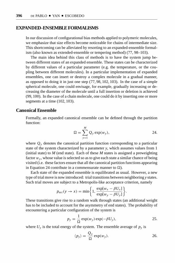
EXPANDED-ENSEMBLE FORMALISMS

In our discussion of configurational bias methods applied to polymeric molecules,we emphasize that size effects become noticeable for chains of intermediate size.This shortcoming can be alleviated by resorting to an expanded-ensemble formal-ism (also known as extended-ensemble or tempering method) (77, 98–103).

The main idea behind this class of methods is to have the system jump be-tween different states of an expanded ensemble. These states can be characterizedby different values of a particular parameter (e.g. the temperature, or the cou-pling between different molecules). In a particular implementation of expandedensembles, one can insert or destroy a complex molecule in a gradual manner,as opposed to doing it in just one step (77, 98, 102, 103). In the case of a simplespherical molecule, one could envisage, for example, gradually increasing or de-creasing the diameter of the molecule until a full insertion or deletion is achieved(99, 100). In the case of a chain molecule, one could do it by inserting one or moresegments at a time (102, 103).

Canonical Ensemble

Formally, an expanded canonical ensemble can be defined through the partitionfunction:

� =M∑

y=1

Qy exp(wy), 24.

whereQy denotes the canonical partition function corresponding to a particularstate of the system characterized by a parametery, which assumes values from 1(initial state) toM (end state). Each of theseM states is assigned a preweightingfactorwy, whose value is selected so as to give each state a similar chance of beingvisited (i.e. these factors ensure that all the canonical partition functions appearingin Equation 24 contribute in a commensurate manner to�).

Each state of the expanded ensemble is equilibrated as usual. However, a newtype of trial move is now introduced: trial transitions between neighboringystates.Such trial moves are subject to a Metropolis-like acceptance criterion, namely

pacc(y→ x) = min

{1,

exp[wx − βUx]

exp[wy − βUy]

}.

These transitions give rise to a random walk through states (an additional weighthas to be included to account for the asymmetry of end states). The probability ofencountering a particular configuration of the system is

py = 1

�exp(wy) exp(−βUy), 25.

whereUy is the total energy of the system. The ensemble average ofpy is

〈py〉 = Qy

�exp(wy). 26.




For any two statesy andx it follows that

Qy

Qx= 〈py〉〈px〉 exp(wx − wy). 27.

Once a histogram of visits to each state has been constructed, the ratio of proba-bilities appearing in Equation 27 can be calculated, thereby permitting evaluationof the ratio of the partition functions for any twox andy:

βAy − βAx = −log

[Qy

Qx

]= −log

[ 〈py〉〈px〉

]+ wy − wx. 28.

For the particular case ofx = 1 andy = M , Equation 28 gives the desired total freeenergy change. To ensure that end states are sampled regularly, all intermediatestates must be sampled with approximately the same frequency; in the case forwhich 〈px〉 = 〈py〉, it follows from Equation 28 thatβAy = wy (within anadditive constant). This suggests an iterative scheme to progressively refine initialestimates of the preweighting factors (77).

The parametery that defines the various states of an expanded ensemble shouldbe chosen so as to facilitate simulation of the relevant free-energy change. Forthe particular case of a chemical potential evaluation,y must gradually couple anddecouple a “tagged” molecule from the system. This coupling can be achievedisotropically, e.g. by varying the strength of the intermolecular potential energyparameters of all sites in the molecule simultaneously (77, 99, 100), or it can beimplemented anisotropically, i.e. by changing the number of sites,ny, of the taggedmolecule (e.g. the chain length, for the case of a linear molecule) (102). The prin-ciple of operation of this latter approach is illustrated in Figure 4. The advantage

Figure 4 Schematic illustration of the anisotropic implementation of the expanded-ensemble formalism for a linear chain molecule. Trial moves between neighboringystates are implemented by appending or removing a block of segments (four segmentsin the figure) to or from the end of the tagged chain. The tagged chain shown in thefigure has four differenty states(M = 4). In the first state(y = 1), the tagged chainhas zero length and is completely decoupled from the rest of the system. In the laststate(y = 4), the tagged chain has full length and is fully coupled to the rest of thesystem.




of an anisotropic coupling is that preweighting factors are related to segmentalchemical potentials, and therefore, for ann-mer homopolymer we could write

wy ≈ ny

n(βAM − βA1),

which reduces the preliminary work required to estimate preweighting factors tothat of obtaining an estimate of the desired free-energy change.

The efficiency of expanded-ensemble simulations can be further increased byimplementing a configurational bias scheme for the insertion and deletion pro-cesses associated with the segmental coupling-decoupling of the tagged chain(102).

Other Ensembles

The main advantage of the expanded ensemble approach is that it provides anatural framework for inserting and removing chain molecules from a system.By facilitating such insertion-deletion moves, chemical potential equilibration canbe effectively attained in grand canonical and Gibbs ensemble simulations (103).In a Gibbs-type of ensemble, a simultaneous gradual coupling-decoupling occursfor a tagged molecule, which is split into two sections, each residing in one ofthe two simulation boxes. For multicomponent systems, one split tagged chain isrequired for every species in the system. Note that the conventional Gibbs ensembleformulation can be recovered by specifying only two states of the tagged chain:the fully decoupled and the fully coupled states. For applications involving flexiblehomonuclear polymers, expanded-Gibbs ensemble simulations have the advantagethat the preweighting factors essentially cancel out from the acceptance criterion,and consequently, there is no need for preliminary simulations (103).

Applications of the expanded-ensemble approach have been reported for thepartitioning of polymers between a slit-pore and the bulk (64, 96, 103), and forfluid-fluid equilibria (51, 82, 96, 104–107). Figure 5 shows results for a chemicallydetailed model of a binary mixture of short and long alkanes (51). The agreementbetween simulation and experiment is satisfactory. More important, these resultsserve to illustrate the fact that it is now possible to simulate phase diagrams formixtures of engineering importance at a modest computational expense (51, 52).

The expanded-ensemble method has been shown to be capable of handlingmolecules withO(102) sites. The obvious disadvantages of the method are thatpreliminary, iterative simulations are sometimes needed and that, as the numberof sites per molecule increases, the number of intermediate states must increaseaccordingly.

PARALLEL TEMPERING

Over the past few years, the study of glassy systems by computer simulation hasled to development of a number of techniques designed to overcome the often highand unpredictable energy barriers that arise in the potential energy surface of such




Figure 5 Phase-equilibrium experimental data [diamonds(108)] and results of sim-ulations (squares) for the binary ethylene-tetracontane mixture atP = 96.5 bar. Thelines correspond to equation-of-state predictions (SAFT,dotted line; Peng-Robinson,solid line).

systems. One such technique that offers considerable promise for simulation ofcomplex fluids is parallel tempering (109–112).

In parallel tempering, a series of noninteracting replicas of a system are sim-ulated simultaneously. In the same spirit of expanded-ensemble methods, eachreplica of the system can be viewed as being in a different state, characterizedby some variable (e.g. temperature). The parallel feature of the method, however,introduces a fundamental difference between expanded-ensemble methods andparallel tempering. For concreteness, consider a canonical ensemble, and considereach replica of the system to be at a different temperature. The partition functionfor the overall system is now given by

Q =r∏i

Qi(N,V, Ti

), 29.




wherer denotes the number of replicas andTi is the temperature of replicai. Inaddition to conventional Monte Carlo moves for thermal equilibration within eachof the replicas, the identity of any two replicas is allowed to mutate; for replicasiandj, such a mutation is accepted with probability

Pacc= min[1, exp(1βi j1Ui j )

], 30.

where1Ui j is the difference in energy between replicasi andj, and where1βi j

is the difference between their inverse temperatures. Exciting new applications ofparallel tempering techniques have appeared recently (70, 109, 113).

As can be inferred from Equation 30, however, the acceptance rate for mutationmoves will be sufficiently high only when the energy distribution functions fordistinct states overlap significantly. Such distribution functions, however, becomeincreasingly narrow as the size of the simulated system increases. For a complexfluid requiring simulation of large systems (e.g. a block copolymer), efficientimplementation of the technique might demand the use of too many replicas. At thispoint it is difficult to predict how useful the method will be for such applications,but given the success experienced with expanded ensemble methods (which areexamples of nonparallel tempering), further research into the application of paralleltempering techniques to complex fluids is certainly warranted.

MULTICANONICAL METHODS

As discussed above, the bottlenecks encountered in simulations of complex fluidsare often associated with the occurrence of multiple energy minima separated byhigh-energy barriers. In many of the simulation strategies outlined above, algo-rithms are designed to jump over such barriers. Alternatively, think of an efficientMonte Carlo simulation scheme as an algorithm that essentially flattens out theenergy landscape of the original system. This view is particularly apparent inmulticanonical Monte Carlo methods (119, 120).

In a multicanonical ensemble, the probability distribution is defined by

Pmu(U ) ∝ �(U )w(U ), 31.

where� is the microcanonical partition function (the density of states). The pre-assigned weightw(U ) is chosen so that the probability distribution is relativelyflat over the range of energy of interest. In other words, one tries to achieve

Pmu(U ) = const. 32.

In this representation all energy levels are given equal weight, thereby eliminatingenergy barriers from the system. A standard Metropolis-style scheme can be usedto update configurations; trial moves are accepted with probability

Pacc= min

[1,w(Unew)

w(Uold)

]. 33.




During a simulation, a histogramH(U ) for the probability distribution is collected.The canonical distribution function of the system can be recovered from

P(U ) ∝ H(U )

w(U )exp(−U/kBT). 34.

All thermodynamic properties of interest can then be calculated by resorting to ahistogram reweighting technique.

From Equations 31 and 32, we have

w(U ) ∝ �−1(U ). 35.

The actual weightsw(U ), however, are not known a priori. To determine them,one must use an iterative procedure. As an example, one can start fromw(0)(U ) =exp(−U/kBT) (i.e. a conventional canonical ensemble) and can collect the his-togramH(U ) for the energy distribution. The next estimate ofw(U ) can be cal-culated from that histogram according to

w(n+1)(U ) = w(n)(U )/H(U ). 36.

The above process is repeated until the distributionH(U ) becomes reasonably flatin the energy range of interest.

At first glance, the fact that the multicanonical method samples the wholeenergy landscape uniformly might seem counterintuitive and contrary to the ideasof importance sampling. However, the power of the multicanonical method residesin its ability to overcome high-energy barriers. Furthermore, if one is interestedin simulating thermodynamic properties over a wide range of temperatures, thisuniform sampling technique permits their calculation from just one simulation.Not surprisingly, the multicanonical method has proven to be a useful tool forthe study of first-order phase transitions (120–122) and spin glasses (123–125). Ithas also been used to study the protein folding problem (126, 127). With fewexceptions (131, 132), however, applications to many-molecule complex fluidshave been scarce.

It is important to note that the multicanonical method belongs to a more generalclass of broad-energy ensemble methods. The umbrella sampling method of Torrie& Valleau (128) appears to be the first method of this kind. Yet another variantof this class of methods is provided, for example, by the 1/k sampling technique(129). The multicanonical method is closely related to the simulated temperingmethod, as discussed by Hansmann & Okamoto (130).

ANALYSIS OF RESULTS: Histogram Reweighting

In all of the methods discussed above, the main result of a phase-equilibrium simu-lation has been a coexistence point, e.g. the orthobaric densities and vapor pressureat a specified temperature (for a pure fluid), or the composition of two coexisting




phases (for a mixture). It is often of interest to estimate second-derivative quan-tities, such as heat capacities, at coexistence. Near first- or second-order phasetransitions, such quantities exhibit pronounced peaks and discontinuities, and theirdirect evaluation (via simple fluctuation expressions) is prone to large statisticalerrors. It is well known, however, that a simulation at a single state point canreveal much more useful information than a few thermodynamic-property values.Histogram reweighting techniques provide a simple and powerful means of ex-tracting as much information as possible from each individual simulation, therebyproviding an attractive framework in which to analyze the results of simulations.It is still necessary to have an efficient simulation algorithm capable of samplingconfiguration space efficiently (see below); histogram reweighting methods onlyprovide a technique to analyze the results of such an algorithm.

The main idea behind histogram reweighting is to use the knowledge of theequilibrium probability distribution at one state point to determine the probabilitydistribution at another state point. The idea of using histograms is not new: Itsapplication dates back to 1959 (114). However, earlier uses of histogram reweight-ing were limited to a single histogram, and the applicability of the method wastherefore limited. Ferrenberg & Swendsen (115–117) later proposed a simple andelegant idea to combine data from multiple histograms, which constitutes the basisfor many of the current applications of this technique.

Single-Histogram Method

The histogram reweighting analysis technique can be better understood by dis-cussing it in the context of a single histogram. Consider a grand canonical simula-tion of a fluid system. The relevant thermodynamic variables are the temperatureT and the chemical potentialµ. A simple grand canonical simulation can be con-ducted atT = T0 andµ = µ0, and a two-dimensional histogram of energy andnumber of molecules can be constructed. The entries to such a histogramH(N,U )are the number of times that the system is observed withN particles and potentialenergyU . If the total number of realizations of the system is denoted byK , theprobability P(N,U, T0, µ0) that the system hasN particles and energyU at T0

andµ0 is given by

P(N,U, T0, µ0) = H(N,U )/K . 37.

The probability distribution for a grand canonical ensemble is given by

P(N,U, T, µ) = �(N,V,U ) exp(−βU + Nβµ)

4(µ,V, T), 38.

where�(N,V,U ) is the microcanonical partition function (density of states atNandU ), and4 is the grand partition function, given by

4(µ,V, T) =∑

N

∑U

�(N,V,U ) exp(−βU + Nβµ). 39.




Combining Equations 37 and 38 provides a Monte Carlo estimate of�(N,V,U ), given by

�(N,V,U ) = wH(N,U ) exp(β0U − Nβ0µ0), 40.

wherew = 4(µ,V, T)/K is a proportionality constant; the exact value ofw is notimportant, as it cancels out in subsequent manipulations. Because�(N,V,U ) isindependent ofT andµ, the probability that the system hasN particles and energyU at T andµ is given by

P(N,U, T, µ) = H(N,U ) exp[−(β − β0)U + N(βµ− β0µ0)]∑N

∑U H(N,U ) exp[−(β − β0)U + N(βµ− β0µ0)]

. 41.

The average value of any function ofN andU can therefore be estimated accordingto

〈A〉 =∑

N

∑U

A(U )P(N,U, T, µ). 42.

For example, the average energyU at (T, µ) is given by

〈U (T, µ)〉 =∑

N

∑U U H(N,U ) exp[−(β − β0)U + N(βµ− β0µ0)]∑

N

∑U H(N,U ) exp[−(β − β0)U + N(βµ− β0µ0)]

43.

and the pressurep is given by

〈p〉 = kT

Vln∑

N

∑U

wH(N,U ) exp[−(β − β0)U + N(βµ− β0µ0)]. 44.

Determination of Phase Coexistence

We now turn our attention to the use of histograms for calculations of phasecoexistence. In the thermodynamic limit, the criteria for phase equilibrium aregiven by Equation 1. For a finite-size system, these criteria correspond to well-defined relationships for the probability distribution function of the system. If, forexample, simulations of a pure fluid are conducted in a grand canonical ensemble,the probability distribution function corresponding to finding aµ,V, T systemwith N particles, i.e.

P(N) =∑

U �(N,V,U ) exp(−βU + Nβµ)∑N

∑U �(N,V,U ) exp(−βU + Nβµ)

, 45.

has two peaks in the vicinity of a coexistence point (Figure 6). If the so-calledtwo-state approximation is adopted (118), the criteria dictated by Equation 1 are




Figure 6 Histograms of volume fraction for a bond-fluctuation lattice polymer so-lution. The polymer chain consists of 20 monomers. The corresponding temperatureand chemical potential isT∗ = 1.740, βµ = −15.103.

equivalent to requiring that the areas under the two peaks be equal. The determi-nation of the precise location of a coexistence point can therefore be achieved bysimply tuning the chemical potential at any given temperature, until the areas underthe two peaks become the same. The coexisting densities of the two coexistingphases correspond to the mean densities under these two peaks; the vapor pressurecan then be determined from Equation 44.

Multiple-Histogram Method

The multiple-histogram method combines data from multiple simulations to ob-tain information over a wide range of thermodynamic space, thereby expandingconsiderably the range of applicability of the method.

The bridge used in multiple-histogram methods to combine data from differentsimulation runs is the fact that the microcanonical partition function�(N,V,U ) isindependent of temperature and chemical potential. Estimates of�(N,V,U ) byEquation 40 from different simulations should agree (within the statistical uncer-tainty of the calculations). If histograms from different runs overlap sufficiently,it is possible to find a set of proportionality constants{w} so that this require-ment is fulfilled. An optimal estimate of�(N,V,U ) can then be determined asa weighted average of�’s extracted from different runs.

Ferrenberg & Swendsen (116, 117) devised a self-consistent method to deter-mine the sought-after proportionality constants and the weighting factors. The final




equations for the (unnormalized) probability distribution are

P(N,U ;µ, β) =∑R

n=1 Hn(N,U ) exp(−βU + Nβµ)∑Rm=1 Km exp(−βmU + Nβmµm − Cm)

, 46.

whereKm is the total number of realizations in runm, andR is the number ofdistinct simulation runs. The constantsCm must be determined self-consistentlyby the iterative relationship

exp(Cm) =∑

N

∑U

P(N,U ;µm, βm). 47.

Applications

By nature, histogram reweighting methods are highly appropriate for study ofphase transitions, particularly in the vicinity of the critical point. Not surprisingly,such methods are being used in an increasing number of applications in a widevariety of systems, ranging from simple Ising models to polymer solutions.

A particularly exciting application of reweighting techniques concerns the studyof critical behavior in polymer solutions and blends; after combining them with

Figure 7 Critical volume fraction as a function of chain length for polymer solutionson a lattice. (Diamonds) Bond fluctuation model; (squares) simple cubic lattice. Thesecorrespond to results of our own simulations, using an expanded grand canonicalmethod.+, Corresponds to results by Wilding (9) for the bond fluctuation model;×,corresponds to results by Panagiotopoulos et al (30) for a simple cubic lattice.




Figure 8 Upper critical solution temperature as a function of chain length for polymersolutions on a lattice. Symbols have the same meaning as in Figure 7.

mixed-field finite-size scaling techniques (9, 30, 31), it has been possible to deter-mine with high precision the values of critical exponents for polymeric systems.As an example, Figures 7 and 8 show some of our own results for the criticalvolume fraction and the critical temperature, respectively, for polymers on a cu-bic lattice as long as 4000 segments. They serve to illustrate how new simulationalgorithms and faster computers are rapidly changing the range and magnitude ofproblems amenable to molecular simulation.

As with parallel tempering techniques, a histogram reweighting method relieson the overlap of local histograms of the probability distribution. Far from the criti-cal point, or for large system sizes, the method becomes inefficient because in suchinstances the local probability distribution functions become sharp and narrow;many different simulation runs are then required to achieved the desired overlap ofdistinct histograms. In these cases, other interpolation or extrapolation methods,such as pseudo-ensembles or Gibbs-Duhem integrations, are more appropriate.

CONCLUSIONS

The main ingredients of a molecular simulation are an algorithm to generateconfigurations of the system of interest, and a statistical mechanical ensemble.An efficient algorithm can reduce dramatically the computational demands of a




simulation; selection of a suitable ensemble can simplify significantly a phase-equilibrium calculation.

The algorithms available to generate configurations (or trajectories) of a sys-tem range from conventional molecular dynamics methods to fairly involvedMonte Carlo techniques. For relatively small molecules (e.g. small carbohydrates,hydrocarbons of moderate size, etc), a combination of molecular dynamics andparallel tempering techniques provides a simple and powerful tool for samplingconfiguration space efficiently. Simulations in open ensembles, however, requirethat molecules be inserted or removed from the system; when molecules are nottoo large, methods based on configurational-bias ideas are effective.

For more complex, larger molecules and polymers, it is necessary to resort toMonte Carlo moves capable of generating more drastic configurational changes.Simple molecular dynamics or other local moves must be supplemented by re-bridging or expanded-ensemble moves. The latter can be used to insert relativelylong molecules into a dense system, thereby permitting simulations in open ensem-bles. The efficiency of algorithms based on rebridging and expanded-ensemble(in its growth-deletion modality) moves can be further increased by resorting toconfigurational-bias ideas. More recent methods, such as PERM and recoil-growthshow promise and should be further investigated in the context of more realistic,many-molecule complex fluids. Further combination of different methods is likelyto result in even more powerful simulation techniques.

The grand canonical ensemble and the Gibbs ensemble are particularly use-ful for simulations of phase equilibria. Care must be exercised near a criticalpoint; in such instances, finite-size scaling and field-mixing techniques coupledto a histogram-reweighting analysis of results provide a powerful framework forstudy of criticality. Both of these ensembles require insertion and destruction ofmolecules which, as mentioned above, can be facilitated by configurational-biasand expanded-ensemble techniques. In some situations, however, such moves aredifficult (e.g. at elevated densities and low temperatures) and one can resort toa semigrand methodology (for mixtures), a Gibbs-Duhem integration procedure,a suitable pseudo-ensemble variant, or thermodynamic integration. Data analysiscould be improved by histogram reweighting.

It has now become apparent that histogram-reweighting analysis of simula-tions provides a powerful tool for generating relatively complete thermodynamic-property information, including phase equilibria, from a limited number ofsimulation runs. The overhead associated with histogram reweighting is mini-mal, and this analysis technique should therefore be used whenever possible. Theaccuracy of results obtained by histogram reweighting relies on the degree ofoverlap between distinct histograms; in some situations (e.g. large systems) goodaccuracy would only be achievable for state points located near each other, therebyrequiring a large number of calculations to generate a phase diagram. For con-ditions remote from a critical point, Gibbs ensemble, Gibbs-Duhem integration,pseudo-ensemble, and multicanonical techniques provide a reliable and efficientmeans for locating phase transitions.




ACKNOWLEDGMENTS

We are grateful for the financial support of the National Science Foundation througha PECASE award to JJdP. JJdP is also grateful to the Dreyfus Foundation for aTeacher-Scholar Award. Part of this review was carried out while JJdP was avisiting professor at the Institut f¨ur Polymere, ETH, Z¨urich; JJdP is grateful toETH and, in particular, to Hans ChristianOttinger for his hospitality during thisvisit. The final sections of this work were completed at the Mexican PetroleumInstitute (IMP); JJdP is grateful to Gustavo Chapela for his hospitality during asabbatical stay at the IMP.

Visit the Annual Reviews home page at http://www.AnnualReviews.org

LITERATURE CITED

1. Allen MP, Tildesley DJ. 1987.Com-puter Simulation of Liquids. Oxford, UK:Clarendon

2. Binder K, ed. 1984.Applications ofthe Monte Carlo Method in StatisticalPhysics. New York: Springer

3. Binder K, Heermann DW. 1992.MonteCarlo Simulation in Statistical Physics.New York: Springer. 2nd ed.

4. Frenkel D. 1995. See Ref. 131, pp. 357–419

5. Baumgartner A. 1995. InThe MonteCarlo Method in Condensed MatterPhysics, ed. K Binder, pp. 285–316.Berlin: Springer-Verlag. 2nd ed.

6. Leontidis E, Forrest BM, Widman AH,Suter UW. 1995.J. Chem. Soc. FaradayTrans.91:2355–68

7. Kremer K. 1996. InMonte Carlo, Molec-ular Dynamics of Condensed Matter Sys-tems, Conf. Proc., ed. K Binder, G Cic-cotti, 49:600-50

8. Frenkel D, Smit B. 1996.UnderstandingMolecular Simulation. New York: Aca-demic

9. Wilding NB. 1997. J. Phys. Condens.Matter9:585–612

10. de Pablo JJ, Escobedo FA. 1999. See Ref.133, pp. 337–67

11. Deem MW. 1999.AIChE J.44:2569–9611a. Valleau JP. 1999. See Ref. 133, pp. 369–

404

12. Metropolis N, Rosenbluth AW, Rosen-bluth MN, Teller AH, Teller E. 1953.J.Chem. Phys.21:1087–92

13. Kalos MH, Whitlock PA. 1986.MonteCarlo Methods. New York: Wiley

14. Manousiouthakis VI, Deem MW. 1999.J.Chem. Phys.110:2753–56

15. Widom B. 1963.J. Chem. Phys.39:2808

16. Rosenbluth MN, Rosenbluth AW. 1955.J. Chem. Phys.23:356–59

17. Wall FT, Erpenbeck JJ. 1959.J. Chem.Phys.30:634–37

18. Kremer K, Binder K. 1988.Comput.Phys. Rep.7:259–310

19. Meirovitch H. 1983.J. Chem. Phys.79:502–8. Erratum. 1984.J. Chem. Phys.81:1053

20. Meirovitch H. 1985.Phys. Rev. A32:3699–708

21. Meirovitch H. 1985.Macromolecules18:563–69

22. Meirovitch H, Lim HA. 1989.Phys. Rev.A 39:4186–94

23. Meirovitch H, Lim HA. 1989.J. Chem.Phys.91:2544–54

24. Ottinger HC. 1985.Macromolecules18:93–98

25. Livne S, Meirovitch H. 1988.J. Chem.Phys.88:4498–506

26. Livne S, Meirovitch H. 1988.J. Chem.Phys.88:4507–15




27. Grassberger P. 1997.J. Chem. Phys.56:3682–93

28. Hegger R, Grassberger P. 1994.J. Phys. A27:4069–81

29. Grassberger P, Hegger R. 1995.Phys. Rev.E 51:2674–76

30. Panagiotopoulos AZ, Wong V, FlorianoMA. 1998.Macromolecules31:912–18

31. Frauenkron H, Grassberger P. 1997.J.Chem. Phys.107:9599–608

32. Sadanobu J, Goddard WA III. 1997.J.Chem. Phys.106:6722–29

33. Mehlig B, Heermann DW, Forrest BM.1992.Phys. Rev. B45:679–85

34. Verdier PH, Stockmayer WH. 1962.J.Chem. Phys.36:227–35

35. Lax M, Brender K. 1977.J. Chem. Phys.67:1785–87

36. Wall FT, Mandel F. 1975.J. Chem. Phys.63:4592–95

37. Mandel F. 1979.J. Chem. Phys.70:3984–88

38. Lal M. 1969.Mol. Phys.17:57–6439. Madras N, Sokal AD. 1988.J. Stat. Phys.

50:109–8640. Harris J, Rice SA. 1988.J. Chem. Phys.

88:1298–30641. de Pablo JJ, Laso M, Suter UW. 1992.J.

Chem. Phys.96:2395–40342. de Pablo JJ, Laso M, Suter UW. 1993.

Macromolecules26:6180–8343. de Pablo JJ, Laso M, Suter UW. 1992.J.

Chem. Phys.96:6157–6244. Laso M, de Pablo JJ, Suter UW. 1992.J.

Chem. Phys.97:2817–1945. Mooij GCAM, Frenkel D, Smit B.

1992.J. Phys. Condens. Matter4:L255–59

46. Frenkel D, Mooij GCAM, Smit B.1992. J. Phys. Condens. Matter4:3053–76

47. Siepmann JI, Frenkel D. 1992.Mol. Phys.75:59–70

48. Escobedo FA, de Pablo JJ. 1996.Mol. Phys.89:1733–55

49. Macedonia MD, Maginn EG. 1999.Mol.Phys.In press

50. Vlugt TJH, Martin MG, Smit B, SiepmannJI, Kirshna R. 1998.Mol. Phys.4:727–33

51. Nath SK, Escobedo FA, de Pablo JJ. 1998.J. Chem. Phys.108:9905–11

51a. Nath SK, Escobedo FA, de Pablo JJ, Patra-mai I. 1998.Ind. Eng. Chem. Res.37:3195–202

52. Martin MG, Siepmann JI. 1998.J. Phys.Chem.102:2569–77

53. Cui ST, Cummings PT, Cochran HD. 1997.Fluid Phase Equilib.141:45–61

54. Cui ST, Siepmann JI, Cochran HD, Cum-mings PT. 1998.Fluid Phase Equilib.146:51–61

55. Consta S, Wilding NB, Frenkel D, Alex-androwicz Z. 1999.J. Chem. Phys.110:3220–28

56. Cracknell RF, Nicholson D, Parsonage NG,Evans H. 1990.Mol. Phys.71:931–43

57. Iwai Y, Koga Y, Arai Y. 1996.Fluid PhaseEquilib. 116:267–74

58. Koga Y, Iwai Y, Yamamoto M, AraiY. 1997. Fluid Phase Equilib.131:83–96

59. Dijkstra M, Frenkel D, Hansen J-P. 1995.J. Chem. Phys.101:3179–89

60. Escobedo FA, de Pablo JJ. 1995.J. Chem.Phys.102:2636–52


62. Vendruscolo M. 1997.J. Chem. Phys.106:2970–76

63. Yong CW, Clarke JHR, Freire JJ, BishopM. 1996. J. Chem. Phys.105:9666–73


65. Dellago C, Bolhuis PG, Csajka FS, Chan-dler D. 1998.J. Chem. Phys.108:1964–77

66. Go N, Sheraga HA. 1970.Macromolecules3:178–87

67. Dodd LR, Boone TD, Theodorou DN.1993.Mol. Phys.78:961–96

68. Leontidis E, de Pablo JJ, Laso M, SuterUW. 1994.Adv. Polymer Sci.116:283–318




69. Deem MW, Bader JS. 1996.Mol. Phys.87:1245–60

70. Wu MG, Deem MW.Mol. Phys.In press71. Pant PVK, Theodorou DN. 1995.Macro-

molecules28:7224–3472. Mavrantzas VG, Boone TD, Zervopoulou

E, Theodorou DN. Submitted for publica-tion

73. Panagiotopoulos AZ. 1987.Mol. Phys.61:813–26

73a. Panagiotopoulos AZ, Quirke N, Staple-ton M, Tildesley DJ. 1988.Mol. Phys.63:527–45

74. Panagiotopoulos AZ. 1995. See Ref. 132,pp. 463–501

75. Kofke DA, Glandt ED. 1988.Mol. Phys.64:1105–31

76. Deutsch HP, Binder K. 1992.Macro-molecules25:6214–30

77. Wilding NB, Muller M. 1994.J. Chem.Phys.101:4324–30

78. Kumar SK, Weinhold JD. 1996.Phys.Rev. Lett.77:1512–15

79. Grest GS, Lacasse MD, Kremer K, GuptaAM. 1996.J. Chem. Phys.105:10583–94

80. Escobedo FA, de Pablo JJ. 1999.Macro-molecules32:900–10

81. Mehta M, Kofke DA. 1995.Mol. Phys.86:139–47


83. Camp PJ, Allen MP. 1996.Mol. Phys.88:1459–69

84. Escobedo FA. 1998.J. Chem. Phys.108:8761–72

85. Moller D, Fischer J. 1990.Mol. Phys.69:463–73

86. Spyriouni T, Economou IG, TheodorouDN. 1998.Phys. Rev. Lett.80:4466–69

87. Kofke DA. 1999.Adv. Chem. Phys.105:405–41

88. Kofke DA. 1993.J. Chem. Phys.98:4149–62

89. Agrawal R, Kofke DA. 1995.Mol. Phys.85:43–59

90. Agrawal R, Kofke DA. 1995.Mol. Phys.85:23–42

91. Bolhuis PG, Kofke DA. 1996.Phys. Rev.E 54:634–43

92. Bolhuis PG, Frenkel D. 1997.J. Chem.Phys.106:666–87

93. Dijkstra M, Frenkel D. 1995.Phys. Rev.E 51:5891–98

94. Camp P, Mason CP, Allen MP, Khare AA,Kofke DA. 1996. J. Chem. Phys.105:2837–49

95. Forsman J, Woodward CE. 1997.Mol.Phys.90:637–52


97. Mehta M, Kofke DA. 1994.Chem. Eng.Sci.49:2633–45

98. Lyubartsev AP, Martsinovski AA,Shevkunov SV, Vorontsov-VelyaminovPN. 1992.J. Chem. Phys.96:1776–83

99. Attard P. 1993.J. Chem. Phys.98:2225–31

100. Kaminsky RD. 1994.J. Chem. Phys.101:4986–94

101. Marinari E, Parisi G. 1992.Europhys.Lett.19:451–58



104. Luna-Barcenas G, Meredith C, SanchezIC, Johnston KP, Gromov DG, de PabloJJ. 1997.J. Chem. Phys.107:10782–92

105. Gromov DG, de Pablo JJ, Luna-BarcenasG, Sanchez IC, Johnston KP. 1998.J.Chem. Phys.108:4647–53

106. Gromov DG, de Pablo JJ. 1998.J. Chem.Phys.109:10042–52

107. Meredith C, Sanchez IC, Johnston KP, dePablo JJ. 1998.J. Chem. Phys.109:6424–34

108. Peters CJ, de Roo JL, LichtenthalerRN. 1987.Fluid Phase Equilib.34:287–308

109. Hansmann UHE. 1997.Chem. Phys. Lett.281:140–50

110. Marinari E, Parisi G, Ruiz-Lorenzo J.1998. InDirections in Condensed Matter




Physics, ed. AP Young, 12:59–98. Singa-pore: World Sci.

111. Geyer CJ, Thompson EA. 1995.J. Am.Stat. Assoc.90:909–20

112. Tesi MC, van Renseburg EJJ, OrlandiniE, Whittington SG. 1996.J. Stat. Phys.82:155–81

113. Iba Y, Chikenji G, Kikuchi M. 1998.J.Phys. Soc. Jpn.67:3327–30

114. Salsburg ZW, Jackson JD, Fickett W,Wood WW. 1959.J. Chem. Phys.30:65–72

115. Ferrenberg AM, Swendsen RH. 1988.Phys. Rev. Lett.23:2635–38

116. Ferrenberg AM, Swendsen RH. 1989.Phys. Rev. Lett.63:1195–98

117. Ferrenberg AM, Swendsen RH. 1989.Comput. Phys.Sept/Oct:101–4

118. Hill TL. 1964.Thermodynamics of SmallSystems. New York: Benjamin

119. Berg BA, Neuhaus T. 1991.Phys. Lett. B267:249–53

120. Berg BA, Neuhaus T. 1992.Phys. Rev.Lett.68:9–12

121. Berg BA, Hansmann U, Neuhaus T. 1993.Phys. Rev. B47:497–500

122. Berg BA, Hansmann U, Neuhaus T. 1993.Z. Phys. B90:229–39

123. Berg BA, Celik T. 1992.Phys. Rev. Lett.69:2292–95

124. Berg BA, Celik T, Hansmann U. 1993.Europhys. Lett.22:63–68

125. Celik T, Hansmann UHE, Katoot M.1993.J. Stat. Phys.73:775–88

126. Hansmann UHE, Okamoto Y. 1994.Phys-ica A212:415–37

127. Schofield J, Ratner M. 1998.J. Chem.Phys.109:9177–91

128. Torrie GM, Valleau JP. 1977.J. Comput.Phys.23:187–99

129. Hesselbo B, Stinchcombe RB. 1995.Phys. Rev. Lett.74:2151–55

130. Hansmann UHE, Okamoto Y. 1996.Phys.Rev. E54:5863–65

131. Wilding NB. 1995.Phys. Rev. E52:602–11

132. Baus M, Rull LR, Ryckaert JP, eds.1995. Observation, Prediction, Simula-tion of Phase Transitions in Complex Flu-ids. Dordrecht, The Netherlands: KluwerAcad.

133. Ferguson DF, Siepmann JI, Truhlar DG,eds. 1999.Advances in Chemical Physics,Vol. 150.Monte Carlo Methods in Chem-ical Physics, Ser. ed. I Prigogine, S Rice.New York: Wiley & Sons

Simulation of phase transitions in fluids

Documents

Transcript of Simulation of phase transitions in fluids