STRUCTURAL CONTROL AND HEALTH MONITORINGStruct. Control Health Monit. 2007; 14:357–383Published online 27 April 2006 in Wiley InterScience (www.interscience.wiley.com). DOI: 10.1002/stc.162

Prestressed active post-tensioned tendons control forbridges under moving loads

Khaldoon A. Bani-Hani1,*,y,z and Musa R. Alawneh2,}

1Jordan University of Science & Technology, Irbid, Jordan2E. Construct, FZ-LLC, Dubai, U.A.E.

SUMMARY

This paper proposes a new innovative mechanism for active bridge vibration control due to moving loadusing active prestressed post-tensioned tendons. King Abdullah’s Hospital Bridge at the Jordan Universityof Science and Technology is employed in this study. This bridge consists of eight spans each is 25mresulting in a total length of 200m. The bridge system is treated as an elastic continuum coupled with asingle degree of freedom moving oscillator representing the moving vehicle. A linear time-varying modelused to simulate the bridge–vehicle system. The dynamic behaviour of the prestressed concrete bridgestudied for the uncontrolled case, and the effect of the prestressing force on the response of bridge–oscillator system is illustrated. Two linear quadratic gaussian (LQG) controllers with time-varying gainsand constant gains designed to mitigate the bridge vibration due to the moving oscillator for differentvelocities. The control strategy regulates the post-tensioned tendons’ force so that the system vibrationdiminished. The results indicate that the proposed control mechanism is efficient for reducing the verticaldisplacements of both the oscillator and the bridge by up to 83% and the vertical accelerations by up to 83and 42%, respectively. Additionally, the robustness of the controllers are investigated and illustrated. Theresults show that the proposed mechanism is robust and stable. Copyright# 2006 John Wiley & Sons, Ltd.

KEY WORDS: vibration; bridge; active control; oscillator; prestressed; moving load

1. INTRODUCTION

Recent advancements in design technology and material quality in civil engineering applicationssupported the construction of lighter and more slender structures, which causes structures to bevulnerable to dynamic loads, particularly moving loads. Large deflections and vibrationsinduced by heavy and high-speed vehicles affect significantly the safety and serviceability ofbridges. Vibrations induced by moving loads may significantly increase the maximum internalstress of bridges and deteriorate serviceability. Therefore, vibration control using special controldevices is a very efficient solution to suppress the response of bridges and, thus, to enhance the

Received 27 July 2005Revised 20 October 2005

Accepted 31 October 2005Copyright # 2006 John Wiley & Sons, Ltd.

yE-mail: khaldoon@just.edu.jozAssistant Professor.

*Correspondence to: Khaldoon A. Bani-Hani, Jordan University of Science & Technology, Irbid, Jordan.

}Structural Engineer.

structural safety and serviceability of bridges. The dynamic response of the bridge–vehiclesystem depends on the dynamic properties of the traversing vehicles and bridge, vehicleoperating speeds, surface quality of the roadway among others.

Few researchers have studied active control of bridges under moving loads. Kwon et al. [1]analysed the behaviour of studied three span bridges under moving loads and controlled thebridges using a tuned mass damper (TMD). The TMD is considered as a passive-type controldevice. The maximum vertical displacement induced by a train is decreased by 21% and freevibration dies out quickly. Michalopoulos et al. [2] studied passive control of bridges based onprestressed tendon systems using two-level prestressing cable systems. Permanent (dead) loadswere relieved by the first-level prestressing cables while moving loads together with excessivedisplacements were supported by second-level prestressing system. Lin and Trethewey [3]analysed a beam subjected to moving loads using the finite element method, then controlled thebeam using a spring attached below the beam to serve as both a passive and active controldevice. By controlling the extension and contraction of the spring, the active moments could becreated at the left and right control arms locations to suppress the beam vibration. Stavroulakiset al. [4] proposed a new design concept for large bridges that is based on an integrated hangingcable and deck–structure system with unilaterally connected blocks which were stabilized byprestressed cables. Wang et al. [5] studied the applicability of passive TMD (PTMDs) tosuppress train-induced vibration on bridges. The results from simply supported bridges ofTaiwan High-Speed Railway (THSR) under German I.C.E., Japanese S.K.S. and FrenchT.G.V. trains showed that the proposed PTMD was a useful vibration control device inreducing bridge vertical displacements, absolute acceleration, end rotations and trainaccelerations during resonant speeds, as the train axle arrangement was regular. Gerco andSantini [6] studied the effect of using rotational viscous dampers on the dynamic response ofsimple beams subjected to moving loads. Dyke and Johnson [7] used an active controller toreduce the response of bridge under moving oscillator. The active control device was placed inparallel with a spring and dashpot elements that represent the suspension of the oscillator. Theresults indicated that this control system was effective in reducing the responses of both theoscillator and the continuum.

The problem of calculating the dynamic response of a distributed parameter system carryingone or more travelling subsystems is crucial in several engineering applications related tobridges, cable railways, etc. Over the years, several mathematical models have been used tosimulate the behaviour of the moving loads. In general, three types of models have beenconsidered in literature. The first had the vehicle modelled as a moving force producing adynamic response of the continuum but neglecting both the inertia of the vehicle and thedynamics of its suspension. The second modelled the vehicle as a moving mass taking intoaccount the inertia of the moving subsystem and assuming infinite stiffness of the couplingbetween the vehicle and the distributed system. The third model represented the vehicle as amoving oscillator model. Pesterev and Bergman [8, 9], Pesterev et al. [10], Pesterev and Bergman[11], and Pesterev et al. [12, 13] showed that the coupled model had definitely cope the dynamicresponse of the bridge–vehicle system and significantly larger than the static response alone.

In this study, a new inventive control mechanism based on the activation of the prestressedtendons in the prestressed reinforced concrete bridge is studied. The mechanism presents a newtechnique of exploiting the post-tensioned cables to suppress the bridge vibrations due to heavytrucks and moving loads. A side, the dynamic behaviour of the prestressed concrete bridgesunder moving loads is investigated. The active tendons are regulated using a linear quadratic

Copyright # 2006 John Wiley & Sons, Ltd. Struct. Control Health Monit. 2007; 14:357–383

K. A. BANI-HANI AND M. R. ALAWNEH358

Gaussian (LQG) regulator. To implement the active control method proposed in this paper,three feedback sensors were used and located on strategic spots in the bridge deck to measurethe acceleration of the bridge Furthermore, an actuator was placed on the live end of theprestressed tendons to generate the active prestressing force to produce the required controlforce.

2. METHODOLOGY

The bridge–vehicle system under study is considered as a single beam with a rigidity equivalentto that of the combined system of floor, stringers and main girders. Additionally, only thefundamental modes of vibration are considered while all higher modes are neglected. Finally,the vehicle is represented by a system with one degree of freedom only, e.g. a moving oscillatorwith constant speed. The weight of the vehicle is applied at the vehicle’s mass centre rather thanat the wheels’ point of contact with the bridge floor. Material properties are assumed elastic,isotropic and homogeneous. The deflection of the beam is considered to be a result of bendingmoment effects only, the inertial properties of the beam section in rotation and beamdeformation due to shear were ignored. Such a model is referred often to as the Euler–Bernoullibeam [14, 15].

The dynamic model of the bridge–vehicle system is developed as a vehicle traversing along thebridge with a constant speed, V. The bridge is modelled as a simply supported Euler-Bernoullibeam. The coupled mathematical model comprehends the dynamic behaviour of the Bernoulli-Euler beam taking into account the passive and active prestressed cables’ force exerted on thebridge.

2.1. Equations of motion

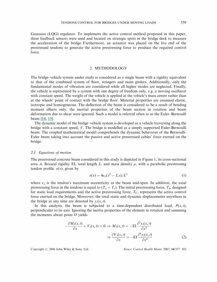
The prestressed concrete beam considered in this study is depicted in Figure 1, its cross-sectionalarea A, flexural rigidity EI, total length L, and mass density r, with a parabolic prestressingtendon profile, eðxÞ; given by

eðxÞ ¼ 4eoðx2 � LxÞ=L2 ð1Þ

where eo is the tendon’s maximum eccentricity at the beam mid-span. In addition, the axialprestressing force in the tendons is equal to ðTo þ TcÞ: The initial prestressing force, T0, designedfor static load requirements and the active prestressing force, TC; represents the active controlforce exerted on the bridge. Moreover, the total static and dynamic displacements anywhere inthe bridge at any time are denoted by ytðx; tÞ:

In this analysis, the beam is subjected to a time-dependent distributed load, Pðx; tÞ;perpendicular to its axis. Ignoring the inertia properties of the element in rotation and summingthe moments about point O yields

�@Mtðx; tÞ

@xþ Vtðx; tÞ ¼ 0 )Mtðx; tÞ ¼ �EI

@2ytðx; tÞ@x2

)@Vtðx; tÞ@x

¼ �EI@4ytðx; tÞ@x4

ð2Þ

Copyright # 2006 John Wiley & Sons, Ltd. Struct. Control Health Monit. 2007; 14:357–383

TENDONS CONTROL FOR BRIDGES UNDER MOVING LOADS 359

Next, taking force equilibrium in the y-direction yields

@Vtðx; tÞ@x

� ðTo þ TCÞ@yðx; tÞ@x

� rA@2ytðx; tÞ@t2

¼ �Pðx; tÞ þ ðTo þ TCÞdgðxÞdx� rAg ð3Þ

where y ¼ @ytðx; tÞ=@x; g ¼ deðxÞ=dx and g is the gravitational acceleration. Therefore, usingresults in Equations (1) and (2), Equation (3) may be written as

� EI@4ytðx; tÞ@x4

� ðTo þ TCÞ@2ytðx; tÞ@x2

� rA@2ytðx; tÞ@t2

¼ �Pðx; tÞ þ ðTo þ TCÞde2ðxÞdx2

� rAg ð4Þ

where ytðx; tÞ ¼ yoðxÞ þ yðx; tÞ and represents the summation of the static and dynamic verticaldisplacements. Therefore, the governing partial differential equation of motion is

EI@4yoðxÞ@x4

þ@4yðx; tÞ@x4

� �þ ðTo þ TCÞ

@2yoðxÞ@x2

þ@2yðx; tÞ@x2

� �

þ rA@2yðx; tÞ@t2

¼ rAgþ Pðx; tÞ � ðTo þ TCÞde2ðxÞdx2

� �ð5Þ

Figure 1. The internal equilibrium of the prestressed bridge.

Copyright # 2006 John Wiley & Sons, Ltd. Struct. Control Health Monit. 2007; 14:357–383

K. A. BANI-HANI AND M. R. ALAWNEH360

Additionally, the beam equation of equilibrium for static loadings alone is given by

EI@4yoðxÞ@x4

� �þ To

@2yoðxÞ@x2

� �¼ rAg� To

de2ðxÞdx2

� �ð6Þ

and the static displacement function considering the prestressing force effect is computed from

yoðxÞ ¼rAgL2 � 8Toeo

24 EI L2ðx4 � 2Lx3 þ L3xÞ ð7Þ

Assuming a uniformly distributed mass and an unvarying stiffness along the continuum andusing the results in Equations (1)–(7) the equation of motion can be rewritten as

EI@4yðx; tÞ@x4

þ ðTo þ TCÞ@2yðx; tÞ@x2

þ rA@2yðx; tÞ@t2

¼ Pðx; tÞ � TCrAgL2 � 8Toeo

2 EI L2ðx2 � LxÞ þ

8eo

L2

� �ð8Þ

The response of the bridge given by Equation (8) is approximated by a linear combination and aseries expansion of the eigenfunctions as follows:

yðx; tÞ ¼ UTðxÞqðtÞ ¼XNn¼1

fnðxÞqnðtÞ ð9Þ

where UTðxÞ ¼ ½f1 f2 ::: fn:::�; and fnðxÞ is the mode shape function of the nth mode of thesimply supported beam given by

fnðxÞ ¼

ffiffiffiffiffiffiffiffiffiffi2

rAL

sSin

npxL

� �such that

Z L

0

rA f2nðxÞ dx ¼ 1 ð10Þ

Also, qðtÞ ¼ ½q1 q2 ::: qn:::�T; and qnðtÞ is the nth modal amplitude and is defined as

.qnðtÞ þ o2nTqnðtÞ ¼

Z L

0

frðxÞPðx; tÞ dx� EnTC for n ¼ 1; 2; 3; . . . ;N ð11Þ

that is obtained by substituting Equation (9) into Equation (8), multiplying each term by frðxÞ;integrating with respect to x between 0 and L, and applying the orthogonal properties of themodes.

onT is the nth modal natural frequency of the simply supported beam considering the axialprestressing force and given by

o2nT ¼

EI

rAnpL

� �4�ðTo þ TCÞ

rAnpL

� �2ð12Þ

Copyright # 2006 John Wiley & Sons, Ltd. Struct. Control Health Monit. 2007; 14:357–383

TENDONS CONTROL FOR BRIDGES UNDER MOVING LOADS 361

and En is a constant results from the integration process and given as

En ¼

ffiffiffiffiffiffiffiffiffiffi2

rAL

s8eo

npL�

rAgL3 � 8LToeo

EI n3p3

� �ð1� cos npÞ ð13Þ

2.2. The moving vehicle dynamics

Figure 2 shows a moving oscillator traversing along a bridge at a constant velocity replacingthe distributed load, Pðx; tÞ: The oscillator, representing the vehicle, has a total mass mv; linearstiffness of its suspension kv ðnatural frequency¼ovÞ; suspension viscous damper coefficientcv ðdamping ratio¼ xvÞ; vehicle velocity v, and a vertical displacement from its equilibriumposition, zðtÞ; as shown in Figure 2. Subsequently the general form of moving oscillator may beexpressed as

Pðx; tÞ ¼ HðtÞ �H t�L

v

� �� �mvgþ f ðtÞð Þdðx� vtÞ ð14Þ

where Hð : Þ is the Heaviside function, dð Þ is the Dirac’s delta function and, f ðtÞ is the forceapplied to the sprung mass and beam and is expressed as

f ðtÞ ¼ kvðzðtÞ � yðx; tÞÞ þ cvð’zðtÞ � ’yðx; tÞÞ ð15Þ

The moving oscillator dynamics governed by equations of motion given as follows:

mv.zþ f ðtÞ ¼ 0 ) .z ¼ o2vðyðx; tÞ � zðtÞÞ þ 2xvovð’yðx; tÞ � ’zðtÞÞ ð16Þ

Substituting Equation (9) into Equation (15), the force expression is

f ðtÞ ¼ kv zðtÞ �UTðxÞqðtÞ�

þ cv ’zðtÞ �UTðxÞ’qðtÞ�

ð17Þ

2.3. Time-varying state-space

The derivations of the linear dynamic equation of equilibrium for the bridge–vehicle systempresented in the proceedings paragraphs are formulated in a state-space form. This isaccomplished by first limiting the time of attention when the vehicle is traversing the bridge (i.e.t 2 0;L=v �

), and next substituting Equation (14) into Equation (11) and integrating to get

.qnðtÞ þ o2nTqnðtÞ ¼ fnðvtÞðmvgþ f ðtÞÞ � EnTC for n ¼ 1; 2; 3; . . . ;N ð18Þ

Substituting Equations (9) and (17) into Equation (16) and Equation (17) into Equation(18), the coupled time-varying system is produced as below

.zðtÞ ¼ o2vU

TðvtÞqðtÞ � o2vzðtÞ þ 2xvovU

TðvtÞ’qðtÞ � 2xvov ’zðtÞ ð19Þ

Figure 2. The moving vehicle traversing on the prestressed bridge (bridge–vehicle model).

Copyright # 2006 John Wiley & Sons, Ltd. Struct. Control Health Monit. 2007; 14:357–383

K. A. BANI-HANI AND M. R. ALAWNEH362

.qnðtÞ ¼ � o2nTqnðtÞ þ fnðvtÞkvzðtÞ � fnðvtÞkvU

TðvtÞqðtÞ

þ fnðvtÞcv ’zðtÞ � fnðvtÞcvUTðvtÞ’qðtÞ þ fnðvtÞmvg� EnTC ð20Þ

Finally, defining a state vector xðtÞ ¼ z q ’z ’q½ �T; Equations (19) and (20) are written in atime-varying state-space as

’xðtÞ ¼ AðtÞxðtÞ þ BðtÞuðtÞ

yðtÞ ¼ CðtÞxðtÞ þDðtÞuðtÞþtðtÞ

yrðtÞ ¼ CrðtÞxðtÞ þDrðtÞuðtÞþtðtÞ

ð21Þ

where uðtÞ ¼½mvg TC� is a two-dimensional vector represents the external forces, tðtÞ is themeasurement noise vector, yðtÞ ¼ z q .z .q½ �T is a 2(N+1)-dimensional vector that representsthe observed response, yrðtÞ ¼ z q½ �T is an (N+1)-dimensional vector that represents theregulated states and AðtÞ; BðtÞ; CðtÞ; DðtÞ; CrðtÞ and DrðtÞ are time-varying state-spacecoefficient matrices given as

AðtÞ ¼0 I

A21ðtÞ A22ðtÞ

" #; BðtÞ ¼

0

B21ðtÞ

" #; CðtÞ ¼

I 0

A21ðtÞ A22ðtÞ

" #ð22Þ

DðtÞ ¼ B21ðtÞ½ �; CrðtÞ ¼ I 0 �

and DrðtÞ ¼ 0½ �

where

A21 ¼

�o2v o2

vf1ðvtÞ . . . o2vfNðvtÞ

kvf1ðvtÞ � o21T þ kvðf1ðvtÞÞ

2 �

�kvf1ðvtÞf2ðvtÞ �kvf1ðvtÞfNðvtÞ

. . . . . . . . . . . .

kvfNðvtÞ �kvfNðvtÞf1ðvtÞ . . . � o2NT þ kvðfNðvtÞÞ

2 �

2666664

3777775 ð23Þ

A22 ¼

�2xvov 2xvovf1ðvtÞ . . . 2xvovfNðvtÞ

cvf1ðvtÞ �cvðf1ðvtÞÞ2 �cvf1ðvtÞf2ðvtÞ �cvf1ðvtÞfNðvtÞ

. . . . . . . . . . . .

cvfNðvtÞ �cvfNðvtÞf1ðvtÞ . . . �cvðfNðvtÞÞ2

2666664

3777775 ð24Þ

B21 ¼

0 0

f1ðvtÞ �E1

. . . . . .

fNðvtÞ �EN

2666664

3777775 ð25Þ

Copyright # 2006 John Wiley & Sons, Ltd. Struct. Control Health Monit. 2007; 14:357–383

TENDONS CONTROL FOR BRIDGES UNDER MOVING LOADS 363

2.4. Verification model

To illustrate the effectiveness of the proposed control mechanism, King Abdullah HospitalBridge (Irbid, Jordan University of Science and Technology in Jordan) is used for verification.The bridge under study consists of eight spans each span is 25m long resulting in a total lengthof 200m. Each span is regarded as a simply supported beam with a cross-section as shown inFigure 3. The bridge has four lanes, each lane is 3.7m wide and the total width of the bridge is19m, supported on nine piers. The bridge is design as prestressed concrete BIV-48 box-girderun-bonded post-tensioned parabolic tendons. Two post-tensioned tendons sets utilized: passivetendons and active tendons. The bridge is modelled as a Bernoulli–Euler beam with equalstiffness regardless of its complex box-type cross-section.

The bridge mass density r ¼ 2840 kg/m3, concrete Young’s modulus Ec ¼ 25 907MPa; andconcrete compressive strength f 0c ¼ 30MPa: Additionally, the post-tensioned steel cables’modulus of elasticity Est ¼ 200 GPa: The total length between supports L ¼ 25 m; girder cross-sectional area AC ¼ 1:81 m2 and moment of inertia Ic ¼ 0:2311 m4: Three natural modes areconsidered in the eigenfunction’s expansion to express the response of the bridge in terms of itseigenmodes (Equation 9). The mass of the vehicle mv ¼ 30 tonnes and the vehicle’s springstiffness kv ¼ 6900 kN=m: The vehicle natural frequency, if considered as an independentsubsystem, ov ¼ 15:16 rad=s and the damping coefficient of the vehicle corresponds toa damping ratio xv ¼ 2% in the uncoupled system.

Figure 3. King Abdullah Hospital Bridge, Irbid, Jordan.

Copyright # 2006 John Wiley & Sons, Ltd. Struct. Control Health Monit. 2007; 14:357–383

K. A. BANI-HANI AND M. R. ALAWNEH364

2.5. Control force design limits

The total prestressing force in the bridge serves the purpose of controlling both cracking anddeflection, and permits the member to respond essentially as if it were un-cracked. When themember is subjected to the prestressing force ðTo þ TCÞ and the moving vehicle, the concretestress f1 at the top face of the member and f2 at the bottom face can be computed bysuperimposing axial and bending effects:

f1 ¼ �ðTo þ TCÞ

AC1�

eoC1

r2

� ��

Mt

S1ð26Þ

f2 ¼ �ðTo þ TCÞ

AC1þ

eoC2

r2

� �þ

Mt

S2ð27Þ

where AC is the area of the concrete cross-section, r2 is the radius of gyration(r2 ¼ IC=AC ¼ 0:1276 m2), C1 and C2 are the distance from the concrete cancroids to the topand bottom surfaces of the member, respectively, and S1 ¼ IC=C1 ¼ 0:4622 m3 and S2 ¼IC=C2 ¼ 0:4622 m3 are the section moduli with respect to the top and bottom surfaces of thebeam. In addition, eo is the tendon’s maximum eccentricity at beam mid-span and is equal to0.4m and Mt is being the total moment due to self-weight and moving load at mid-span given as

Mt ¼rAcgL

2

8þ

mvgL

4¼ 5778 kNm ð28Þ

The concrete stress should not exceed the tensile rupture stress or the allowable compressionstress in the concrete. Thus, to find the minimum and the maximum control force, f1 and f2 arecontrolled by Equation (29) [16].

fcs ¼ �0:45f0

c ¼ �13:5MPa and fts ¼ 0:5ffiffiffiffif 0c

p¼ 2:7386 MPa ð29Þ

Substituting these values in Equations (26) and (27), the maximum and minimum control forcescan be computed. Firstly, stresses at the bottom face of the beam at the mid-span should notexceed the tensile rupture stress or the allowable compression stress given in Equation (29).That is

�13:5MPa 4�ðTo þ TCÞ

1:811þð0:4Þð0:5Þ0:1276

� �þ

5778

0:46224 2:738MPa ð30Þ

Therefore, 18334 kN 5To þ TC5 6885 kN. Nevertheless, the top fibre stress should not exceedthe allowed compression stress for concrete or the rupture stress

2:738MPa 5�ðTo þ TCÞ

1:811�ð0:4Þð0:5Þ0:1276

� ��

5778

0:46225� 13:5MPa ð31Þ

Consequently, 48 654 kN 5To þ TC5 �3184 kN (Tension). The lower value indicates acompressive force on the tendons which is not obtainable; hence, the lower value is replaced byzero. Therefore, the above calculations generate the lower and upper bounds of the prestressingforce: 6885 kN 4To þ TC4 18 334 kN. Additionally, To is the required prestressing force tobalance the self-weight of the beam and calculated as follows

To ¼wselfweightL

2

8e0¼

rAgL2

8e0¼ 9848 kN ð32Þ

Copyright # 2006 John Wiley & Sons, Ltd. Struct. Control Health Monit. 2007; 14:357–383

TENDONS CONTROL FOR BRIDGES UNDER MOVING LOADS 365

Equation (32) is derived based on an equivalent upward load produced by a parabolic tendons(To) equivalent to downward load produced by bridge’s own weight, in which all transverseforces are cancelled [17]. For this unique balanced load condition, there are no bendingmoments applied to the beam, no flexural stresses exist, but only the axial stresses produced bythe longitudinal component of the prestressing forces (axial compression force).

Subsequently, the lower and upper bounds of the control force, TC were found to be

Zero 4 TC 4 8486 kN ð33Þ

This result was considered in developing the proposed LQG controllers.

2.6. Active control force losses due to friction

The active control force in post-tensioned members is generated using unbonded post-tensionedtendons. The tendons are anchored at one end and controlled with hydraulic actuator in theother end. As the steel tendon slides through the duct, friction is buildup and force at theanchored end is less than the hydraulic end. These losses are results of wobble friction, due tounintentional misalignment, and curvature friction. When a curved tendons is used to prestress abeam, the total tension loss in the unbonded pre-greased wire tendons due to friction (ACI Sec.18.6.2) [18] is computed by

TCðx; tÞ ¼ TCðL; tÞ=eKxþmaðxÞ ð34Þ

where TCðx; tÞ is the developed force at distance x from the active end, TCðL; tÞ is the issuedactive force at the active end, K is a wobble friction coefficient (m�1), m is friction coefficientbetween tendon and duct and a is the total angle change between active end and distance x fromit. Table R18.6.2 of ACI building code commentary, 318/318R-270 [18], suggests averagenumerical values for K ¼ 0:0037 m�1 and m ¼ 0:1: Considering these values and estimatingaðxÞ ¼ deðxÞ=dx using Equation (1), then the maximum loss at the anchored end (x ¼ L ¼ 25 m;a ¼ 0:064 rad) is estimated to be 9% of the active force. Therefore, the control force issued bythe actuator has to be increased by 9% to substitute for the losses induced by friction.Immediate losses due to anchorage slip and concrete elastic shortening, and time-dependentlosses due creep, shrinkage of concrete and steel relaxation can be developed, however, theselosses are either initially or with time lost while the major losses induced when the active tendonsare in operation are generated by the friction [17].

2.7. Response of the uncontrolled bridge

The resulting time-varying linear state-space model given in Equations (21) and (22) wasencoded in a SIMULINK [19] model using MATLAB [20] software. The mathematical modelserved to simulate the response of the prestressed bridge under the moving vehicle (oscillator).The uncontrolled response is referred to when TC is set to zero. This response is compared to thecontrolled response in order to examine the feasibility and effectiveness of the proposed controlmechanism (Figure 4).

The axial compression force exerted by the prestressing tendons reduces the natural frequencyof the prestressed beam as may be seen in Equation (12). However, the cost of natural frequencyreduction in dynamic vibration with prestressed tendons is much less than the cost of staticdeflection without the prestressing tendons. Figure 5 shows the variation of the firstfundamental natural frequency of the prestressed beam as the control force changes. It was

Copyright # 2006 John Wiley & Sons, Ltd. Struct. Control Health Monit. 2007; 14:357–383

K. A. BANI-HANI AND M. R. ALAWNEH366

Figure 4. Controller configuration for bridge–vehicle model.

Figure 5. Effect of axial compressive force on the bridge dynamic response.

Copyright # 2006 John Wiley & Sons, Ltd. Struct. Control Health Monit. 2007; 14:357–383

TENDONS CONTROL FOR BRIDGES UNDER MOVING LOADS 367

found that the natural frequency was reduced by approximately 2%. This result is reflected onthe response of the active prestressed bridge in the dynamic analysis as shown in Figure 5. Inshort, the effect of axial compression force was that of ‘stiffness degradation’, which decreasedthe natural frequencies of the beam. Consequently, the beam became more flexible, and thedeflection of the bridge increased. Additionally, it was noted that the vehicle speed affectedthe response of bridge–vehicle response significantly. For example, the vertical displacement ofthe vehicle and the bridge were increased by 40 and 17%, respectively, as the vehicle’s speedvaried from 10 to 35m/s. Also, the vertical acceleration of the vehicle and the bridge wereincreased by 83 and 73.5%, respectively.

3. CONTROL DESIGN

As stated earlier, the prestressed tendons exert variable forces as the vehicle transverses thebridge. To make optimal use of the tendons, the output force has to follow optimal path tominimize both vehicle vertical motion as well as the bridge vertical displacement. Two optimallinear quadratic regulators (LQR) were designed and constructed as a prelude to control thebridge–vehicle system. The first controller calculates the optimal control force TC at any timeusing time-varying gains based on a full state feedbacks that is, xðtÞ ¼ z q1 q2 q3 ’z ’q1 ’q2 ’q3½ �T:The controller path was determined using a performance index that weighted the regulatedoutput vector, yr(t), and given as:

#JðtÞ ¼ limt!1

1

tE

Z t

0

ðCrðtÞxr þDrðtÞTCÞTQ

�ðCrðtÞxr þDrðtÞTCÞ þ R½TC�2

dt

� �ð35Þ

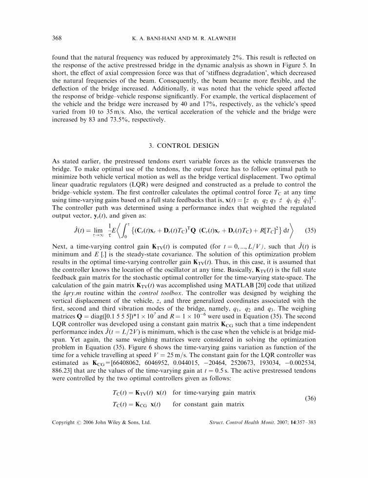
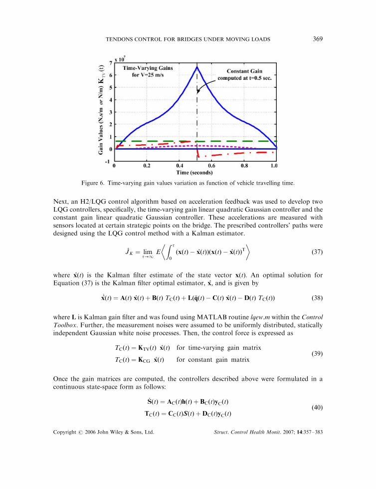
Next, a time-varying control gain KTVðtÞ is computed (for t ¼ 0; :::;L=V), such that #JðtÞ isminimum and E [.] is the steady-state covariance. The solution of this optimization problemresults in the optimal time-varying controller gain KTVðtÞ: Thus, in this case, it is assumed thatthe controller knows the location of the oscillator at any time. Basically, KTVðtÞ is the full statefeedback gain matrix for the stochastic optimal controller for the time-varying state-space. Thecalculation of the gain matrix KTVðtÞ was accomplished using MATLAB [20] code that utilizedthe lqry.m routine within the control toolbox. The controller was designed by weighing thevertical displacement of the vehicle, z, and three generalized coordinates associated with thefirst, second and third vibration modes of the bridge, namely, q1; q2 and q3: The weighingmatrices Q ¼ diag([0.1 5 5 5])*1� 107 and R¼ 1� 10�6 were used in Equation (35). The secondLQR controller was developed using a constant gain matrix KCG such that a time independentperformance index #Jðt ¼ L=2VÞ is minimum, which is the case when the vehicle is at bridge mid-span. Yet again, the same weighing matrices were considered in solving the optimizationproblem in Equation (35). Figure 6 shows the time-varying gains variation as function of thetime for a vehicle travelling at speed V ¼ 25 m=s: The constant gain for the LQR controller wasestimated as KCG=[66408062, 6046952, 0.044015, �20464, 2520673, 193034, �0.002534,886.23] that are the values of the time-varying gain at t ¼ 0:5 s: The active prestressed tendonswere controlled by the two optimal controllers given as follows:

TCðtÞ ¼ KTVðtÞ xðtÞ for time-varying gain matrix

TCðtÞ ¼ KCG xðtÞ for constant gain matrixð36Þ

Copyright # 2006 John Wiley & Sons, Ltd. Struct. Control Health Monit. 2007; 14:357–383

K. A. BANI-HANI AND M. R. ALAWNEH368

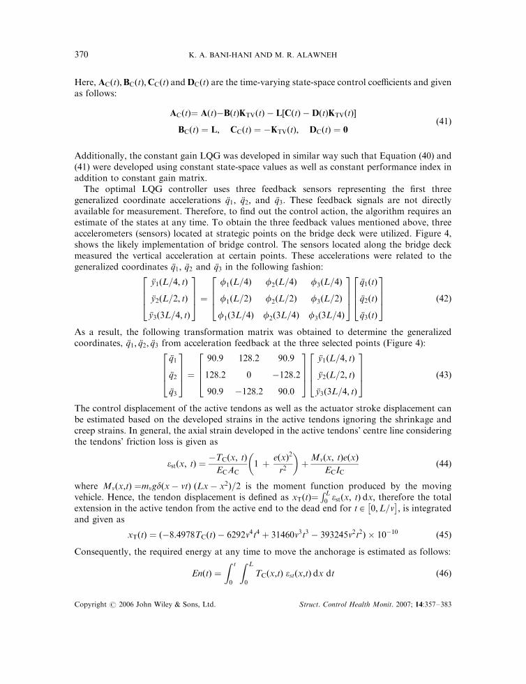
Next, an H2/LQG control algorithm based on acceleration feedback was used to develop twoLQG controllers, specifically, the time-varying gain linear quadratic Gaussian controller and theconstant gain linear quadratic Gaussian controller. These accelerations are measured withsensors located at certain strategic points on the bridge. The prescribed controllers’ paths weredesigned using the LQG control method with a Kalman estimator.

#JK ¼ limt!1

E

Z t

0

ðxðtÞ � #xðtÞÞðxðtÞ � #xðtÞÞT� �

ð37Þ

where #xðtÞ is the Kalman filter estimate of the state vector xðtÞ: An optimal solution forEquation (37) is the Kalman filter optimal estimator, #x; and is given by

’#xðtÞ ¼ AðtÞ #xðtÞ þ BðtÞ TCðtÞ þ Lð.qðtÞ � CðtÞ #xðtÞ �DðtÞ TCðtÞÞ ð38Þ

where L is Kalman gain filter and was found using MATLAB routine lqew.m within the ControlToolbox. Further, the measurement noises were assumed to be uniformly distributed, staticallyindependent Gaussian white noise processes. Then, the control force is expressed as

TCðtÞ ¼ KTVðtÞ #xðtÞ for time-varying gain matrix

TCðtÞ ¼ KCG #xðtÞ for constant gain matrixð39Þ

Once the gain matrices are computed, the controllers described above were formulated in acontinuous state-space form as follows:

’SðtÞ ¼ ACðtÞhðtÞ þ BCðtÞyCðtÞ

TCðtÞ ¼ CCðtÞSðtÞ þDCðtÞyCðtÞð40Þ

Figure 6. Time-varying gain values variation as function of vehicle travelling time.

Copyright # 2006 John Wiley & Sons, Ltd. Struct. Control Health Monit. 2007; 14:357–383

TENDONS CONTROL FOR BRIDGES UNDER MOVING LOADS 369

Here, ACðtÞ;BCðtÞ;CCðtÞ andDCðtÞ are the time-varying state-space control coefficients and givenas follows:

ACðtÞ¼ AðtÞ�BðtÞKTVðtÞ � L½CðtÞ �DðtÞKTVðtÞ�

BCðtÞ ¼ L; CCðtÞ ¼ �KTVðtÞ; DCðtÞ ¼ 0ð41Þ

Additionally, the constant gain LQG was developed in similar way such that Equation (40) and(41) were developed using constant state-space values as well as constant performance index inaddition to constant gain matrix.

The optimal LQG controller uses three feedback sensors representing the first threegeneralized coordinate accelerations .q1; .q2; and .q3: These feedback signals are not directlyavailable for measurement. Therefore, to find out the control action, the algorithm requires anestimate of the states at any time. To obtain the three feedback values mentioned above, threeaccelerometers (sensors) located at strategic points on the bridge deck were utilized. Figure 4,shows the likely implementation of bridge control. The sensors located along the bridge deckmeasured the vertical acceleration at certain points. These accelerations were related to thegeneralized coordinates .q1; .q2 and .q3 in the following fashion:

.y1ðL=4; tÞ

.y2ðL=2; tÞ

.y3ð3L=4; tÞ

2664

3775 ¼

f1ðL=4Þ f2ðL=4Þ f3ðL=4Þ

f1ðL=2Þ f2ðL=2Þ f3ðL=2Þ

f1ð3L=4Þ f2ð3L=4Þ f3ð3L=4Þ

2664

3775

.q1ðtÞ

.q2ðtÞ

.q3ðtÞ

2664

3775 ð42Þ

As a result, the following transformation matrix was obtained to determine the generalizedcoordinates, .q1; .q2; .q3 from acceleration feedback at the three selected points (Figure 4):

.q1

.q2

.q3

2664

3775 ¼

90:9 128:2 90:9

128:2 0 �128:2

90:9 �128:2 90:0

2664

3775

.y1ðL=4; tÞ

.y2ðL=2; tÞ

.y3ð3L=4; tÞ

2664

3775 ð43Þ

The control displacement of the active tendons as well as the actuator stroke displacement canbe estimated based on the developed strains in the active tendons ignoring the shrinkage andcreep strains. In general, the axial strain developed in the active tendons’ centre line consideringthe tendons’ friction loss is given as

estðx; tÞ ¼�TCðx; tÞECAC

1 þeðxÞ2

r2

� �þ

Mvðx; tÞeðxÞECIC

ð44Þ

where Mvðx;tÞ ¼mvgdðx� vtÞ ðLx� x2Þ=2 is the moment function produced by the movingvehicle. Hence, the tendon displacement is defined as xTðtÞ¼

R L0 estðx; tÞ dx; therefore the total

extension in the active tendon from the active end to the dead end for t 2 0;L=v �

; is integratedand given as

xTðtÞ ¼ ð�8:4978TCðtÞ � 6292v4t4 þ 31460v3t3 � 393245v2t2Þ � 10�10 ð45Þ

Consequently, the required energy at any time to move the anchorage is estimated as follows:

EnðtÞ ¼Z t

0

Z L

0

TCðx;tÞ estðx;tÞ dx dt ð46Þ

Copyright # 2006 John Wiley & Sons, Ltd. Struct. Control Health Monit. 2007; 14:357–383

K. A. BANI-HANI AND M. R. ALAWNEH370

Finally, Figure 7 illustrates a SIMULINK model for both the time-varying and constant gainsLQG controllers.

4. ANALYTICAL RESULTS

4.1. Performance assessment for the active prestressed tendons

The controllers designed in the previous section were intended to alleviate the vibration responseof both the vehicle and the bridge under study. To achieve this, new mechanism utilizing activeprestressed tendons was employed to mitigate both the bridge vibration response as well as thevehicle response. The effectiveness of the proposed mechanism was investigated using the linearquadratic regulators LQR; time-varying gain and constant gain controllers, which weredeveloped as a preface for two other acceleration feedback linear quadratic Gaussian LQGcontrollers. Results of LQR and LQG controllers, when the vehicle is traversing at a constantspeed of 25m/s, are presented in part as shown in Figures 8 and 9. Figure 8 presents acomparison of the controlled and uncontrolled response of the bridge. It is apparent fromFigure 8 that the vertical deflection of the bridge was reduced by about 89 and 88% for the time-varying LQR and the constant gain LQR, respectively. Similarly, the response was reduced byabout 87 and 85% for the time-varying LQG and the constant gain LQG, respectively. It is clearthat the performance differences in the LQR and LQG controllers were very small.Consequently, the LQG controllers are of the main focus in this study due to their practicalityand implementation simplicity. The results of the response of the controlled vehicle arepresented in Figure 9, which shows that the vertical response of the vehicle is compared to the

Figure 7. SIMULINK model for both time-varying LQG controller and constant gain LQG controller.

Copyright # 2006 John Wiley & Sons, Ltd. Struct. Control Health Monit. 2007; 14:357–383

TENDONS CONTROL FOR BRIDGES UNDER MOVING LOADS 371

uncontrolled and the controlled case for both the LQR and the LQG. Moreover, Figure 9reveals that the maximum control forces exerted by the active tendons, TCmax

; was 3686 kN, andcompares results for the different controllers mentioned above. The difference between thecontrol forces generated by LQR or LQG is small and in the range of 4%. It was also noted thatthe required control force is varying smoothly with almost constant acceleration. Additionally,the stroke displacements and the applied force of the active actuator are shown in Figure 9. Peakvalues of the stroke are about 4.41mm for constant gain LQG and about 4.55mm for time-varying LQG and maximum exerted energy is about 7.2 kNm.

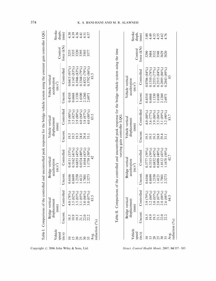
The effectiveness of the active prestressed tendons is illustrated numerically using time-varying and constant gain LQG controllers. The results are presented in Tables I and II. Table I

Figure 8. Comparisons of the vibration response of the uncontrolled and controlled bridge for a movingvehicle with speed of 25m/s, using time-varying and constant gains LQR and LQG controllers.

Copyright # 2006 John Wiley & Sons, Ltd. Struct. Control Health Monit. 2007; 14:357–383

K. A. BANI-HANI AND M. R. ALAWNEH372

compares the peak values of the vertical displacements and vertical accelerations in theuncontrolled and the controlled bridge–vehicle system and outline the corresponding peakvalues of the active tendon forces and the actuator stroke displacement for the moving vehicle atvarious speeds ranging from 10 to 35m/s. It is clear from Table I that the constant gain LQGcontroller was effective in peak response reduction. For example, the vertical displacements andaccelerations of the vehicle decreased by on average value of 83.5% and, on average, the bridgevertical displacement decreased by 83.5% and the vertical acceleration decreased by 42% for theselected speed range. Similarly, Table II presents the same comparative results for the controlledand uncontrolled peak values of the vertical response of the vehicle–bridge when traveling atvarious speeds of 10–35m/s for the time-varying LQG controller. Results demonstrate that the

Figure 9. Comparisons of the control forces and the energy and actuator stroke history for thedifferent controllers, in addition the vertical vibration response of the uncontrolled and controlled

moving vehicle with speed of 25m/s is compared.

Copyright # 2006 John Wiley & Sons, Ltd. Struct. Control Health Monit. 2007; 14:357–383

TENDONS CONTROL FOR BRIDGES UNDER MOVING LOADS 373

TableI.

Comparisonsofthecontrolled

anduncontrolled

peakresponse

forthebridge–vehicle

system

usingtheconstantgain

controller

LQG.

Vehicle

speed

Bridgevertical

displacement

(mm)

Bridgevertical

acceleration

(m/s2)

Vehicle

vertical

displacement

(mm)

Vehicle

vertical

acceleration

(m/s2)

Control

Stroke

displs.

(m/s)

Uncont.

Controlled

Uncont.

Controlled

Uncont.

Controlled

Uncont.

Controlled

force(kN)

(mm)

10

18.5

4.0

(78%

)0.6166

0.4111(33%

)19.5

3.9

(80%

)0.4510

0.0415(91%

)3253

4.30

15

19.9

3.5

(82%

)0.8699

0.5162(41%

)19.5

3.5

(82%

)0.6868

0.1143(83%

)3355

4.39

20

19.3

3.3

(83%

)1.2350

0.6855(45%

)19.3

3.9

(80%

)1.1330

0.1946(83%

)3320

4.36

25

21.1

3.1

(85%

)1.4121

0.8524(40%

)24.8

4.0

(84%

)1.6100

0.3344(79%

)3395

4.41

30

22.0

3.0

(86%

)1.7801

1.0164(43%

)29.4

3.8

(87%

)2.1260

0.4521(79%

)3503

4.51

35

22.2

3.0

(87%

)2.3273

1.1758(50%

)33.1

4.0

(88%

)2.6971

0.3792(86%

)3577

4.57

Avg.

reduction(%

)83.5

42

83.5

83.5

TableII.Comparisonsofthecontrolled

anduncontrolled

peakresponse

forthebridge–vehicle

system

usingthetime

varyinggain

controller

LQG.

Vehicle

speed

Bridgevertical

displacement

(mm)

Bridgevertical

acceleration

(m/s2)

Vehicle

vertical

displacement

(mm)

Vehicle

vertical

acceleration

(m/s2)

Control

Stroke

displs.

(m/s)

Uncont.

Controlled

Uncont.

Controlled

Uncont.

Controlled

Uncont.

Controlled

force(kN)

(mm)

10

18.5

3.9

(79%

)0.6166

0.3777(39%

)19.5

4.0

(80%

)0.4510

0.0706(84%

)3290

5.00

15

19.9

3.2

(84%

)0.8699

0.5315(39%

)19.5

3.6

(77%

)0.6868

0.1510(78%

)3484

4.49

20

19.3

3.0

(85%

)1.2350

0.6832(45%

)19.3

3.9

(80%

)1.1330

0.2553(77%

)3532

4.53

25

21.1

2.8

(87%

)1.4121

0.8490(40%

)24.8

3.5

(86%

)1.6100

0.2515(84%

)3548

4.55

30

22.0

2.8

(88%

)1.7801

1.0112(43%

)29.4

3.1

(89%

)2.1260

0.2895(86%

)3629

4.62

35

22.2

2.6

(88%

)2.3273

1.1678(50%

)33.1

3.2

(90%

)2.6971

0.2843(89%

)3820

4.76

Avg.

reduction(%

)84.5

42.7

83.7

83

Copyright # 2006 John Wiley & Sons, Ltd. Struct. Control Health Monit. 2007; 14:357–383

K. A. BANI-HANI AND M. R. ALAWNEH374

time-varying LQG controller reduced the vehicle vertical displacement by 83.7% and thevertical acceleration by 83% on the average for the selected speeds. Moreover, comparisonbetween the bridge peak values is illustrated for the time-varying LQG. In this case, the peakvalues were reduced by 84.5 and 42.7%, respectively. The maximum control force as well as theactuator stroke peaks for the LQG controllers are shown in Tables I and II and the maximumforce is within the limits discussed in Section 4.

In general, the results show that the constant gain LQG and the time-varying LQGcontrollers were successful in bridge–vehicle vibration mitigation as well. Again, it is clear thatthe constant gain controller performed as well as the time-varying controller with insignificantdifferences. Based on this observation it was decided to adopt the constant gain LQG as ageneral controller throughout this study.

Additional demonstration is presented in Figure 10 that displays the vertical acceleration ofthe uncontrolled and controlled bridge for a moving vehicle with a constant speed of 25m/s.Figure 10 shows that the constant gain LQG controller reduced the maximum verticalacceleration to 0.8524m/s2 at distance of 5.25m from the beam support when the vehicle is at2.25m from the support, compared to the maximum uncontrolled response of 1.4121m/s2 atdistance equal to 11.5m and traveling time equal to 0.27 s. On the other hand, the time-varyingLQG controller decreased the peak vertical acceleration to 0.849m/s2 at a distance of 5.25mwhen the vehicle is 2.25m away from the starting support.

Additional results are depicted in Figures 11–13 where the controlled responses of the movingvehicle and the bridge are outlined for two vehicle speeds, 15 and 35m/s as the constant gainLQG controller operates on the active prestressed tendons. Figure 11 shows that the peak valuesof the vehicle vertical displacement decreased by 82% for V ¼ 15 m=s and by 88% forV ¼ 35 m=s: Similarly, the peak values of the vehicle vertical acceleration were reduced by 83and 86% for V ¼ 15 and 35, respectively. Figure 12 shows that the bridge vertical response forV ¼ 15 m=s was reduced, by 82.4 and 40.7%, for the displacement and acceleration,respectively. Similar comparison is depicted in Figure 13 for V ¼ 35 m=s revealing peaksreductions by 86.5 and 49.5%. It is noteworthy that the constant gain LQG was developed for

Figure 10. Comparisons of the vertical acceleration of the uncontrolled and controlled bridge for a movingvehicle with speed of 25m/s, using time-varying and constant gains LQG controllers.

Copyright # 2006 John Wiley & Sons, Ltd. Struct. Control Health Monit. 2007; 14:357–383

TENDONS CONTROL FOR BRIDGES UNDER MOVING LOADS 375

the case of vehicle speed V ¼ 25 m=s: Numerical comparison is also presented in Tables I and IIas mentioned earlier.

4.2. Robustness of the active prestressed tendons

In order to explore the robustness of the active prestressed mechanism, a number of analyseswere performed and discussed. In the first place, the bridge–vehicle model uncertainty wasconsidered for two conditions: the flexural rigidity, EI, and the mass density, r, of the bridge by�20%: Those situations are obtained by multiplying the original values of the EI and r by 1.2or 0.8, and denoting the results by ‘D(EI, r) =�20%’. Additionally, uncertainty in thecontroller state-space coefficients (AC, BC, CC and DC) was considered by adjusting their valuesby�15% and referring to the results by ‘(AC, BC, CC, DC)=�15%’. Likewise, effects of time-delay as well as high-level measurement noises were examined. The time-delay considered was0.01 s and the measurement noises were modelled as Gaussian rectangular pulse processes. Thepulse width was 0.01 s and a two-sided spectral density of 0.1, 0.25 and 0.25m2Hz/s3 for thegeneralized coordinates .q1; .q2 and .q3 to give noise level up to �10; �15; �15 m=s2;respectively. The controllers were experimented when some feedback sensors failed to send thecorrect signal and transmitted measurement noise instead. Finally, the stability of the activetendons for friction loss over/under-estimation is evaluated.

Figure 11. Comparisons of the vertical response of the uncontrolled and controlled moving vehicle withspeeds of 15 and 35m/s, using constant gains LQG controllers computed for V ¼ 25 m=s.

Copyright # 2006 John Wiley & Sons, Ltd. Struct. Control Health Monit. 2007; 14:357–383

K. A. BANI-HANI AND M. R. ALAWNEH376

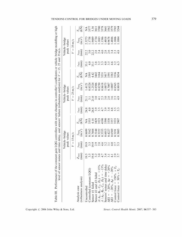
The uncertainty in flexural rigidity and the mass density for the two conditions ‘D(EI, r) =�20%’, were obtained and response analyses were carried out using the time-varyingSIMULINK model. The peak values response quantities for the above-mentioned robustnessanalyses were calculated for the constant gain LQG controller with three velocity cases representthe expected mean velocity, V ¼ 25 m=s; lower (trucks) velocity, 15m/s, and upper (fast car)velocity, 35m/s, and presented in Table III. Results in Table III reports the vertical responses ofthe vehicle-bridge system, zmax; ymaxðx; tÞ; .ymaxðx; tÞ and the control forces for the robustnessanalysis cases discussed above. As seen, the peak response quantities are susceptible to theflexural rigidity and mass density uncertainties whereas peak response values were slightlyaffected by controller uncertainty. Yet, in all cases, the controller was robust within the scope ofits design. Equally, the constant gain LQG controller is sensitive to the case of high sensorsnoise combined to a time-delay. In comparison to the response of the controlled system, thepeak values of the bridge–vehicle system for the D(AC, BC, CC, DC)=�15% cases, were slightlyaffected. Moreover, the peak values of the vehicle vertical displacement, zmax; bridge verticaldisplacement, ymaxðx; tÞ; and vertical acceleration, .ymaxðx; tÞ; for the D(EI, r) =�20%; increased,

Figure 12. Comparisons of the vertical response of the uncontrolled and controlled bridge for a movingvehicle with speeds of 15m/s, using constant gains LQG controllers computed for V ¼ 25m=s.

Copyright # 2006 John Wiley & Sons, Ltd. Struct. Control Health Monit. 2007; 14:357–383

TENDONS CONTROL FOR BRIDGES UNDER MOVING LOADS 377

respectively, by 17, 14 and 27%, and for the D(EI, r) =þ20%; decreased by �11.4%, �11.4%and �18.1% for V ¼ 15 m=s: Similar percentage can be computed using results in Table III forV ¼ 25 and 35m/s. Furthermore, the sensor noise combined to the time-delay has affected thepeak values by �3, �15 and +16%, for V ¼ 25 m=s; respectively, again results outline othervalues for V ¼ 15 and 35m/s. In general, it is advised not to overestimate the EI and r of thebridge when designing the controller. On the other hand, the peak values of the vehicle–bridgesystem: z; ymaxðx; tÞ and .ymaxðx; tÞ; were affected slightly to severely as some sensors have failedto operate as required. Results in Table III show that the peak response values are insensitive tothe failure of sensors 2 and 3. However, failure of sensor 1 had a catastrophic effect on thecontroller performance. As shown in Table III, the controller was paralysed and did notresponse as demanded but it issued about 0.1% of the active force power. These resultsestablished the significance of the mid-span sensor that requires extra emphasis on its robustnessand design. Therefore, it is recommended to install additional sensor in the mid-span in case offirst one failure, to ensure control system effectiveness. Additionally, Table III discloses thebridge–vehicle response when the control force was amplified and reduced by 50% for friction

Figure 13. Comparisons of the vertical response of the uncontrolled and controlled bridge for a movingvehicle with speeds of 35m/s, using constant gains LQG controllers computed for V ¼ 25 m=s:

Copyright # 2006 John Wiley & Sons, Ltd. Struct. Control Health Monit. 2007; 14:357–383

K. A. BANI-HANI AND M. R. ALAWNEH378

TableIII.

Perform

ance

oftheconstantgain

LQG

controllerswithseverechanges

incontroller’scoeffi

cientsorvehicle–bridgemodellingorhigh

level

ofsensornoises

andtimedelay,andsensors’failure

(robustnessanalysis)

forV¼

15;25and35m/s.

Vehicle–bridge

peakvalues

Vehicle–bridge

peakvalues

Vehicle–bridge

peakvalues

V¼

15m=s

V¼

25m=s

V¼

35m=s

Analysiscase

(robustnessanalysis)

Zmax

(mm)

ymax

(mm)

.ymax

(m/s2)

Tc m

ax

(kN)

z max

(mm)

ymax

(mm)

.ymax

(m/s2)

Tc m

ax

(kN)

z max

(mm)

ymax

(mm)

.ymax

(m/s2)

Tc m

ax

(kN)

Uncontrolled

19.5

19.9

0.8699

NA

24.8

21.1

1.4121

NA

33.1

22.2

2.3273

NA

Controlled

(constantLQG)

3.5

3.5

0.5162

3355

4.0

3.1

0.8524

3395

4.0

3.0

1.1758

3577

Sensor#1failed

19.4

19.9

0.7684

4.14

24.8

21.0

1.2524

4.42

33.1

22.2

1.9489

5.34

Sensor#2and#3failed

3.2

2.9

0.5144

3429

3.9

3.0

0.8506

3442

3.8

2.8

1.1734

3611

D(AC,BC,CC,D

C)=

+15%

3.0

2.8

0.5222

3523

3.5

4.1

0.8250

3184

3.2

2.4

1.1883

3700

D(AC,BC,CC,D

C)=�15%

4.7

4.6

0.5355

4190

4.7

2.5

0.8618

3531

5.3

4.0

1.1386

3378

Sensors’noises

andtimedelay

3.4

3.2

0.6013

3390

3.9

3.0

1.0075

3417

4.0

2.8

1.4018

3641

DEI=

+20%

,Dr=

+20%

3.1

3.1

0.4227

3338

3.4

2.8

0.7007

3391

3.5

2.6

0.9678

3562

DEI=�20%

,Dr=�20%

4.1

4.0

0.6569

3357

4.8

3.6

1.0807

3382

4.6

3.4

1.4886

3579

Controlforce=

150%�TC

2.9

2.7

0.5191

3535

3.5

2.5

0.8565

3536

3.2

2.3

1.1806

3705

Controlforce=

50%�TC

5.7

5.5

0.5805

2907

5.3

4.9

0.8018

3034

6.3

4.8

1.1084

3244

Copyright # 2006 John Wiley & Sons, Ltd. Struct. Control Health Monit. 2007; 14:357–383

TENDONS CONTROL FOR BRIDGES UNDER MOVING LOADS 379

loss. Results proved that the control force was stable and effective with friction lossmiscalculation or variation for any reason.

For more demonstrations of the system robustness, Figure 14 reveals the effects of �15%uncertainty on controller state-space coefficients (D(AC, BC, CC, DC)=�15%) for V ¼ 25 m/s.It may be readily seen that the performance of the LQG degraded for the bridge mid-spanvertical displacement but faintly affected the corresponding accelerations. Furthermore,Figure 14 presents selected comparisons of the responses for the bridge when the mid-spansensor failed and when sensors 2 and 3 failed. It is clear that the controller performancedeteriorated when the mid-span sensor stopped working but unaffected when sensors 2 and 3failed. However, the controller performance maintained its stability, and the worst that couldhappen was that the controller would stop working rather than excessively destructs the bridge.Finally, Figure 15 layouts a comparison between the LQG controller with uncertainty in EI andr by D(EI, r) ¼ �20% for the mean velocity, V ¼ 25 m=s: Figure 15 shows how the response ofthe vehicle–bridge system was affected while the vehicle was in motion.

Figure 14. Comparison between the bridge responses when the constant gain LQG controller has beenmodified by 15% of its computed values and when some sensors failed to report the correct feedbacks

for vehicle traversing at 25m/s (robustness analysis).

Copyright # 2006 John Wiley & Sons, Ltd. Struct. Control Health Monit. 2007; 14:357–383

K. A. BANI-HANI AND M. R. ALAWNEH380

The controller stability was ensured by controlling the closed-loop eigen values of the time-varying controller state-space given in Equations (40) and (41). This was achieved by ensuringthat the real parts of the eigenvalues of the time-varying matrix Ac(t) is always less than zero[21].

5. CONCLUSIONS

Actively controlled post-tensioned un-bonded prestressed tendons mechanism was proposed tomitigate the dynamic response of a prestressed concrete bridge under a moving oscillator

Figure 15. Comparison between the vehicle–bridge responses when the constant gain LQG controller iscontrolling a modified flexural rigidity as well as mass density by 20% of its computed values for

vehicle velocity equal to 25m/s (robustness analysis).

Copyright # 2006 John Wiley & Sons, Ltd. Struct. Control Health Monit. 2007; 14:357–383

TENDONS CONTROL FOR BRIDGES UNDER MOVING LOADS 381

(vehicle). Results have indeed shown that the axial compression force decreased the naturalfrequency of the system while the dynamic response slightly increased for both the bridge andvehicle, however, the pluses of prestressed tendons in static response reduction exceed theminuses of the slight increase in dynamic response. The performance of the controllers wereconsidered and outlined. The results indicated that this control system is equally effective forreducing the vibrations of both the vehicle and the bridge. Additionally, results revealed that thetime-varying gain LQG performed slightly better than the constant gain LQG. However, bothcontrollers were quite successful in reducing the bridge–vehicle vibration response, thus, theconstant gain controller was deemed more practical and simpler. High-level measurementsnoises, computation time-delay, model uncertainties, controller uncertainties and feedbacksensors’ failure, are all severe conditions considered in the robustness analysis for the LQGcontroller. Furthermore, the study indicated that the LQG controller is robust within thebounds of its scope but severely deteriorated for the mid-span sensor failure demonstrating theimportance of the mid-span sensor. Whatever the case may be, the controller force was observednot to violate the allowable stresses for the concrete bridge which is reflected on the controlforce limits.

Moreover, the results demonstrated the reliability and stability of the tendons in the sense ofthe optimal control design as well as the significant attractive feature of using accelerationfeedbacks, which constitutes a practical, reliable and efficient control methodology. Finally, theresults of this study illustrate the potential strength of the use of active prestressed tendons forvibration mitigation of prestressed reinforced concrete bridges under moving load.

REFERENCES

1. Kwon H-C, Kim M-C, Lee I-W. Vibration control of bridges under moving loads. Computers and Structures 1998;66(4):473–480.

2. Michalopoulos A, Stavroulakis GE, Zacharenakis EC, Panagiotopoulos PD. A prestressed tendon based passivecontrol system for bridges. Computer and Structures 1997; 63(6):1165–1175.

3. Lin Y-H, Trethewey MW. Active vibration suppression of beam structures subjected to moving loads: a feasibilitystudy using finite elements. Journal of Sound and Vibration 1993; 166(7):383–395.

4. Stavroulakis GE, Michalopoulos A, Panagiotopoulos PD, Zacharenakis EC. A multiblock unilateral concept forpassive Control of Prestressed Bridges. Structural Multidisciplinary Optimization 2000; 19(3):225–236.

5. Wang JF, Lin CC, Chen BL. Vibration suppression for high-speed railway bridges using tuned mass dampers.International Journal of Solid Structures 2003; 40(10):465–491.

6. Greco A, Santini A. Dynamic response of a flexural non-classically damped continuous beam under movingloadings. Computers and structures 2002; 80(3):1945–1953.

7. Dyke SJ, Johnson SM. Active control of a moving oscillator on an elastic continuum. Proceedings of the StructuralSafety and Reliability Conference, Newport Beach, CA, U.S.A., 17–22 June 2001.

8. Pesterev AV, Bergman LA. Response of elastic continuum carrying moving linear oscillator. Journal of EngineeringMechanics (ASCE) 1997; 123(8):878–884.

9. Pesterev AV, Bergman LA. Vibration of elastic continuum carrying acceleration oscillator. Journal of EngineeringMechanics (ASCE) 1997; 123(8):886–889.

10. Pesterev AV, Yang B, Bergman LA, Tan CA. Response and stress calculations of an elastic continuum carryingmultiple moving oscillators. Proceedings of the International Conference on Advances in Structural Dynamics, HongKong, December 2000, 13–15.

11. Pesterev AV, Bergman LA. An improved series expansion of the solution to the moving oscillator problem. Journalof Vibration and Acoustics (ASME) 2000; 122(1):54–61.

12. Pesterev AV, Yang B, Bergman LA, Tan CA. Response of elastic continuum carrying multiple moving oscillators.Journal of Engineering Mechanics (ASCE) 2001; 127(3):260–265.

13. Pesterev AV, Tan CA, Bergman LA. A new method for calculating bending moment and shear force in moving loadproblems. Journal of Applied Mechanics 2001; 68(3):252–259.

14. Clough RW, Penzien J. Dynamics of Structures. McGraw Hill: New York, 1993.

Copyright # 2006 John Wiley & Sons, Ltd. Struct. Control Health Monit. 2007; 14:357–383

K. A. BANI-HANI AND M. R. ALAWNEH382

15. Chopra AK. Dynamics of Structures: Theory and Applications to Earthquake Engineering. Prentice-Hall: New Jersey,2002.

16. AASHTO LRFD. Bridge Design Specifications: Si Units. American Association of State Highway, 2003.17. Nilson AH. Design of Prestressed Concrete. Wiley: New York, 1987.18. ACI Committee. ACI 318-270, Building Code Requirements for Reinforced Concrete. American Concrete Institute,

2002.19. The Math works Inc. SIMULINK, Natick, MA, 2001.20. The Math works Inc. MATLAB, Natick, MA, 2001.21. Vegate JV de. Feedback Control Systems (3rd edn). Prentice-Hall: Englewood Cliffs, NJ, 1994.

Copyright # 2006 John Wiley & Sons, Ltd. Struct. Control Health Monit. 2007; 14:357–383

TENDONS CONTROL FOR BRIDGES UNDER MOVING LOADS 383