Preliminary On Design Tests of the M12REST Scramjet in the T4 Shock Tunnel

On-Design Tests of the M12REST

Scramjet in the T4 Shock Tunnel

Dr. Milinda SURAWEERA

Mr Yann Moule

A/Prof. Michael SMART

SCHOOL OF MINING AND MECHANICAL ENGINEERING

THE UNIVERSITY OF QUEENSLAND

AUSTRALIA

Submitted

DECEMBER 2009

2

_________________________________________________________________________________________

EXECUTIVE SUMMARY

___________________________________________________________________________

A report of the M12REST scramjet ground test program at ‘on-design’ test

conditions, conducted from January 1st to June 24th, 2009 in the T4 Shock Tunnel

Facility at the Centre for Hypersonics, The University of Queensland, is presented.

The study was performed to investigate discrepancies between numerical and

experimental results of a previous 2007 test program involving the M12REST

scramjet engine. Off-design results of the engine in the 2007 study demonstrated

good agreement between numerical and experimental results (Suraweera and

Smart, 2009). However, on-design experimental results showed a large pressure

region on the forward section of the inlet that could not be replicated using a

computational fluid dynamics (CFD) code (White and Morrison, 1999). The present

study trialled combinations of ten distinct boundary layer trip configurations, in order

to investigate whether this large pressure region was the result of local flow

separation. A blunt 3 mm radius leading edge and a longer 500 mm forebody were

also separately tested. Three new ‘on-design’ flow conditions (four in total) were

also tested. Pressure and heat transfer measurements were taken along the engine

flowpath.

A description of the T4 Shock Tunnel and its operating characteristics has been

given. Drawings of the proposed test model and extraneous test articles have also

been provided. All 45 test runs executed during the experimental campaign have

been listed, along with the corresponding flow properties for four test conditions.

Mean pressure and Stanton number distributions for significant tunnel runs,

illustrating the effects of various boundary layer trip and engine fuelling

configurations, have been presented. The fuel used was gaseous hydrogen.

Supersonic and subsonic combustion was measured at a range of fuel equivalence

ratios for two of the test conditions (3 and 4). Inlet injection was found to produce

separated flow regions within the inlet, and hence the fuelling scheme was

discontinued. Step injection was tested successfully at a range of equivalence

3

ratios. In terms of combustion induced increases in pressure, higher levels were

seen when engine was run with the M11 enthalpy test condition 4. However, the

engine was able to operate in true scramjet mode with the inflow of the M12

enthalpy test condition 3. Furthermore, the engine was found to be more stable at

this condition as the combustion induced pressure rise was contained by the

isolator.

4

________________________________________________________________________________________

CONTENTS

___________________________________________________________________________

EXECUTIVE SUMMARY ..................................................... 2

LIST OF FIGURES............................................................... 7

LIST OF TABLES ............................................................... 10

NOMENCLATURE ............................................................. 11

TEST FACILITY AND INSTRUMENTATION ..................... 15

1.1 INTRODUCTION 15

1.2 T4 SHOCK TUNNEL 15

1.2.1 DESCRIPTION 15

1.2.2 PRINCIPLE OF OPERATION 16

1.2.3 NOZZLE 17

1.3 INSTRUMENTATION 18

1.4 MEASUREMENT UNCERTAINTY ANALYSIS 21

1.4.1 STATIC PRESSURE UNCERTAINTY 21

EXPERIMENTAL TESTING ............................................... 22

2.1 INTRODUCTION 22

2.2 TEST MODEL 22

2.2.1 GENERAL LAYOUT 22

2.2.1 INSTRUMENTATION AND DATA ACQUISITION 25

5

2.3 FUEL SYSTEM 26

2.3.1 FUEL INJECTION 26

2.3.2 FUEL VALVE CALIBRATION 27

2.4 TEST CONDITIONS 28

2.5 TEST TIME DETERMINATION 31

EXPERIMENTAL RESULTS .............................................. 33

3.1 INTRODUCTION 33

3.2 TEST SUMMARY 33

3.2.1 TEST SHOTS 33

3.2.2 RUN DESCRIPTIONS 35

3.3 ENGINE EXPERIMENTAL RESULTS 37

3.3.1 M12REST 2007 RESULTS AND CONCLUSIONS 38

3.3.2 INITIAL BOUNDARY LAYER TRIP RESULTS AND CONCLUSIONS 39

3.3.3 TEST CONDITION 3 RESULTS AND CONCLUSIONS 40

3.3.3 TEST CONDITION 4 RESULTS AND CONCLUSIONS 43

3.4 RECOMMENDATIONS 46

REFERENCES .................................................................. 47

4.1 REFERENCES 47

KULITE MOUNTING .......................................................... 51

A.1 KULITE MOUNTING ARRANGEMENT 52

DATA ACQUISITION ......................................................... 53

B.1 DATA ACQUISTION TRANSDUCER SETUP 54

UNCERTAINTY ANALYSIS ............................................... 56

6

C.1 UNCERTAINTY ANALYSIS THEORY 56

C.1.1 GENERAL 56

C.1.2 LINEAR REGRESSION 58

C.1.3 TEST CONDITION UNCERTAINTY ANALYSIS 59

FUEL CALIBRATION ......................................................... 62

D.1 FUEL CALIBRATION 62

EXPERIMENTAL RUN SUMMARY ................................... 63

E.1 EXPERIMENTAL RUN SUMMARY 64

INLET INJECTION RESULTS ........................................... 66

F.1 INLET INJECTION ANOMALIES 66

DRAWINGS ....................................................................... 68

G.1 MODEL PARTS AND BOUNDARY LAYER TRIPS 68

7

_________________________________________________________________________________________

LIST OF FIGURES

___________________________________________________________________________

Figure Title Page

Figure 1.1. Schematic of T4 Shock Tunnel (adapted from Kelly, 1992). ................ 16

Figure 1.2. Ideal x-t diagram of wave processes after diaphragm rupture for a

tailored operating condition (adapted from Odam, 2004). ................................. 17

Figure 1.3. PCBTM static pressure transducer mounting arrangement (from

Rowan, 2003)……………………………………………… .................................... 19

Figure 1.4. Pitot pressure transducer mounting arrangement (from Smith, 1999). . 19

Figure 1.5. Thin Film heat transfer gauge (from Hayne, 2003). .............................. 20

Figure 2.1. Main components of the initial Mach 12 REST scramjet with 150 mm

forebody in assembled test orientation. ............................................................. 23

Figure 2.2. Fueling stations of the Mach 12 REST scramjet. ................................... 24

Figure 2.3. Side view of the Mach 12 REST scramjet mounted in the T4 test

section………………………………………….. .................................................... 24

Figure 2.4. Front view of the Mach 12 REST scramjet mounted in the T4 test

section……………………………………………….. ............................................. 24

Figure 2.5. Schematic of fuel valve control system. ................................................ 27

Figure 2.6. Measured test time for 10% driver contamination without nozzle

starting losses (adapted from Skinner, 1994). ................................................... 32

Figure 3.1. Normalised pressure distributions; bodyside CFD and experimental

results, cond. 1, fuel-off, M12REST 2007 Study. ............................................... 38

Figure 3.2a. Typical bodyside pressure distributions; cond. 1 and 2, fuel-off. ........ 39

8

Figure 3.2a. Typical cowlside pressure distributions; cond. 1 and 2, fuel-off. ......... 40

Figure 3.3. Initial Stanton number results and predictions; cond. 1 and 2, fuel-

off………………………………………………. ..................................................... 40

Figure 3.4a. Bodyside pressure distributions; clean and BL trips, cond. 3, fuel-

off……………………………………………………….. .......................................... 41

Figure 3.4b. Cowlside pressure distributions; clean and BL trips, cond. 3, fuel-

off…………………………………………………………….. ................................... 41

Figure 3.5a. Bodyside pressure distributions; BL7/BL6/BL1 trips, cond. 3, step

fuel-on…………………………………………………………….. ............................ 42

Figure 3.5b. Cowlside pressure distributions; BL7/BL6/BL1 trips, cond. 3, step

fuel-on………………………………………………………… ................................. 42

Figure 3.6a. Bodyside pressure distributions; clean and BL trips, cond. 4, fuel-

off…………………………………………………………………….. ........................ 43

Figure 3.6b. Cowlside pressure distributions; clean and BL trips, cond. 4, fuel-

off………………………………………………………………… ............................. 44

Figure 3.7a. Bodyside pressure distributions; BL7/BL1 trips, cond. 4, step fuel-

on………………………………………………………………………….. ................. 45

Figure 3.7b. Cowlside pressure distributions; BL7/BL1 trips, cond. 4, step fuel-

on…………………………………………………………………… .......................... 45

Figure. A.1. Kulite Mounting Arrangement for M12REST Experimental Campaign . 52

Figure. D.1. Typical equivalence ratios vs plenum chamber pressure for step

injection, Condition 1 (35ms valve open time). .................................................. 62

Figure. D.2. Typical equivalence ratios vs plenum chamber pressure for step

injection, Condition 2 (35ms valve open time). .................................................. 62

Figure F.2. Thrust coefficient as a function of equivalence ratio for inlet injection

runs…………………………………………………………………………. ............... 67

9

Figure. G.1. M12REST LE Plate – Blunt 3 mm radius ............................................. 69

Figure. G.2. M12REST LE Extended Forebody ....................................................... 70

Figure. G.2a. M12REST LE Extended Plate BLTrip Blank ...................................... 71

Figure. G.2b. M12REST LE Extended Plate Ramp BL Trip..................................... 72

Figure. G.3. M12REST Inlet TFG Installation Modification ...................................... 73

Figure. G.4. BL1 Sawtooth Trip Configuration ......................................................... 74

Figure. G.5. BL3 Distributed Trip Configuration ....................................................... 74

Figure. G.6. BL6 Discrete Ramp Trip Configuration ................................................ 75

Figure. G.7. Pattern of BL10 Diamond Trip Configuration, Top View, (6 mm high) . 75

10

_________________________________________________________________________________________

LIST OF TABLES

___________________________________________________________________________

Table Title Page

Table 1.1. Nozzle dimensions used in the study ..................................................... 17

Table 2.1. Nominal T4 input conditions................................................................... 29

Table 2.2. Summary of nominal nozzle-supply conditions ...................................... 30

Table 2.3. Summary of nominal nozzle exit conditions ........................................... 30

Table 2.4. Summary of calculated nominal forebody conditions ............................. 31

Table 2.5. Summary of calculated nominal flight conditions ................................... 31

Table 3.1. Boundary Layer Trip Configurations ...................................................... 33

Table 3.2. M12REST Scramjet Shot Summary, 2009 ............................................ 34

Table 3.3. M12REST Scramjet Shot Summary Continued 1, 2009 ........................ 35

Table B.1. Data Acquisition Transducer w/o Long Forebody Setup ....................... 54

Table B.2. Data Acquisition Transducer Setup ....................................................... 55

Table E.1. M12REST Scramjet 2009 On-Design Experimental Run Summary ...... 64

Table E.2. M12REST Scramjet 2009 On-Design Experimental Run Summary

continued……………………………………………………………. ........................ 65

11

_________________________________________________________________________________________

NOMENCLATURE

___________________________________________________________________________

ENGLISH SYMBOLS

a speed of sound

App. appendix

Al aluminium

b pressure calibration gradient, wingspan

B bias error estimate at specific confidence interval

f fuel equivalence ratio

g acceleration due to gravity

h, H specific enthalpy

l characteristic length

m mass, metre

mm millimetres

m mass flow rate

M Mach number

ms millisecond

p, P pressure

R Universal gas constant: 8.3145 J/mol. K, correlation coefficient

r recovery factor, radius

r2 coefficient of determination

s second

S standard deviation of a sample

12

t time

T temperature

u, U velocity

V volume, volts

x downstream distance from leading edge

y cartesian coordinate, spanwise distance from centre-line

z cartesian coordinate, sensing element protrusion

GREEK SYMBOLS

fuel calibration constant,

systematic error size, shock angle

equivalence ratio

ratio of specific heats, v

p

c

c

estimate of total uncertainty at specific confidence interval

viscosity, micro

3.141593…

density

SUBSCRIPTS

1 forebody condition

avg average

aw adiabatic wall condition

c compressible condition

13

cap. capture

e nozzle exit flow condition

expt experimental

f final

H2 hydrogen

i injection condition, initial condition

max maximum

min minimum

nom nominal condition

r recovery

s stagnation condition, supply condition

ss shock speed

u unit length

∞ flight condition

ACRONYMS

AOA angle of attack

BL boundary layer

cb combustor bodyside

cc combustor cowlside

CFD computational fluid dynamics

CT compression tube

DAQ data acquisition

DC direct current

DVM digital voltage meter

14

ESTC Equilibrium Shock Tube Calculation

fp fuel pressure

FS full scale

ib inlet bodyside

LE leading edge

NENZF Non-equilibrium Nozzle Flow

nb nozzle bodyside

nc nozzle cowlside

PCB PCB Piezotronics Inc.

RMS root mean square

RSS root sum square

SLS selective laser sintering

SSM Sommer Short Method

spa stagnation probe A

spal stagnation probe A, long time base

spb stagnation probe B

spbl stagnation probe B, long time base

SS shock speed

ST shock tube

ABBREVIATIONS

App. Appendix

Est. establishment

Fig. figure

rec. recoil

15

_________________________________________________________________________________________

TEST FACILITY AND INSTRUMENTATION

___________________________________________________________________________

1.1 INTRODUCTION

The experiments for the present study were carried out in the T4 free piston

reflected shock tunnel located in the School of Mining and Mechanical Engineering,

at The University of Queensland. In this section the shock tunnel facility, and the

nozzle used in the experiments are detailed. In addition, the instrumentation and the

data acquisition system used for measurements in the test facility and on the model

test surface are outlined. An uncertainty analysis for the experimental pressure

measurements obtained in the study has not been included in this draft.

1.2 T4 SHOCK TUNNEL

1.2.1 Description

The T4 facility is a free piston driven, reflected shock tunnel. The shock tunnel

facility has a driver of 229 mm internal diameter that is 26 m in length, and a 75 mm

internal diameter shock tube that is 10 m in length. A layout of the shock tunnel is

presented in Fig. 1.1. It is capable of producing flows with nozzle-supply enthalpies

in excess of 20 MJ/kg (Mee, 2002). Typical operating conditions result in flows with

nozzle-supply enthalpies in the range of 3 MJ/kg to 12 MJ/kg, with test times of

approximately 3.0 ms to 0.5 ms. Stagnation pressures approaching 90 MPa can be

achieved. The shock tunnel facility consists of an annular reservoir, free piston,

compression (or driver) tube, shock tube, nozzle, test section, and dump tank. An

unscored brightform steel primary diaphragm of varying thickness separates the

driver gas in the compression tube from the test gas in the shock tube. A secondary

0.1 mm thick mylar diaphragm separates the shock tube section from the test

section. The contoured Mach 10 Nozzle was utilised for this test program.

16

Figure 1.1. Schematic of T4 Shock Tunnel (adapted from Kelly, 1992).

1.2.2 Principle of Operation

An x-t diagram of the wave processes after primary diaphragm rupture is given in

Fig. 1.2. Behind the primary shock wave is the interface (contact surface) between

the test gas and driver gas. In the preferred “tailored interface mode” (Wittliff et al.,

1959) the pressure ratio and the velocity change across the reflected shock on both

sides of the interface are the same. The reflected shock will then pass through the

interface without producing additional compression or expansion waves which are

reflected towards the nozzle. The test time is theoretically limited by the arrival of

expansion waves that attenuate the nozzle-supply pressure, however, in reality the

interface is not well defined and the driver gas does contaminate the test gas. The

driver gas contamination results in the termination of useful test flow while nozzle-

supply pressure is still constant (Skinner, 1994). In a free piston-driven shock

tunnel, the motion of the piston after the diaphragm rupture is tuned to try to

maintain a constant driver supply pressure as the driver gas expands into the shock

tube. This is referred to as “tuning” the condition. Tuned conditions are obtained by

varying the proportion of helium and argon in the compression tube and the shock

tube filling pressure.

17

Figure 1.2. Ideal x-t diagram of wave processes after diaphragm rupture for a tailored operating

condition (adapted from Odam, 2004).

1.2.3 Nozzle

An axi-symmetric contoured nozzle capable of producing flows of Mach 10 was used

in the present study. The main dimensions of the nozzle are presented in Table 1.1.

The nozzle consists of an initial conical section to produce an expanded uniform

source flow, and a contoured section to straighten the flow with the tunnel axis.

Table 1.1. Nozzle dimensions used in the study

Nozzle Throat Diameter Exit Diameter Length

(mm) (mm) (mm)

Mach 10 9.52 380 1670

A 2008 Pitot survey (Suraweera, 2008) of the Mach 10 Nozzle was conducted at a

nozzle-supply enthalpy and pressure of 7.68 MJ/kg and 81.4 MPa, respectively, at

downstream locations 275 mm, 350 mm, and 500 mm from the nozzle exit plane.

The Pitot survey indicated a maximum test core flow diameter of 300 mm at the

nozzle exit plane, and a consistent contracted core flow diameter of approximately

190 mm at a range of 275 mm to 500 mm from the nozzle exit plane. The measured

18

Pitot to nozzle-supply pressure ratio ranged from 0.0145 to 0.0155 across the core

flow diameters.

1.3 INSTRUMENTATION

A combination of KuliteTM and PCBTM piezoelectric pressure transducers were used

to measure pressure levels within the test model. Thin film gauges, manufactured at

The University of Queensland, were used to measure the instantaneous heat

transfer on the model. A National Instruments data acquisition system recorded and

stored the signal time histories of the model and tunnel transducers.

1.3.1 Model Pressure Measurements

Static pressure was measured on the test surface using KuliteTM XTEL-190M

piezoelectric pressure transducers. The pressure transducers had an excitation

voltage of 10 V and had pressure ranges of 0 –10 psi, 0 – 25 psi, and 0 – 100 psi.

The transducers’ sensing faces were thermally protected from the flow by 25m

cellophane discs which covered the sensing diaphragms. A layer of silicone grease

separated the cellophane discs from the sensing face. All pressure transducers

were recess mounted. The pressure tap holes in the test surface were at least 1.5

mm in depth and 2 mm in diameter. For a more comprehensive schematic of the

KuliteTM pressure transducer mounting arrangement refer to App. A.

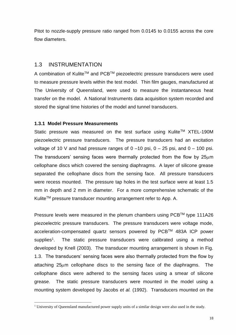
Pressure levels were measured in the plenum chambers using PCBTM type 111A26

piezoelectric pressure transducers. The pressure transducers were voltage mode,

acceleration-compensated quartz sensors powered by PCBTM 483A ICP power

supplies1. The static pressure transducers were calibrated using a method

developed by Knell (2003). The transducer mounting arrangement is shown in Fig.

1.3. The transducers’ sensing faces were also thermally protected from the flow by

attaching 25m cellophane discs to the sensing face of the diaphragms. The

cellophane discs were adhered to the sensing faces using a smear of silicone

grease. The static pressure transducers were mounted in the model using a

mounting system developed by Jacobs et al. (1992). Transducers mounted on the

1 University of Queensland manufactured power supply units of a similar design were also used in the study.

19

plenum chambers were isolated mechanically and electrically using a combination of

rubber o-rings, fibre washes, and brass sleeves (see Fig. 1.3).

Figure 1.3. PCBTM static pressure transducer mounting arrangement (from Rowan, 2003)

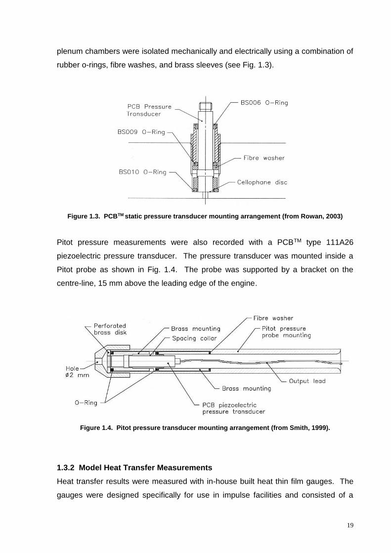
Pitot pressure measurements were also recorded with a PCBTM type 111A26

piezoelectric pressure transducer. The pressure transducer was mounted inside a

Pitot probe as shown in Fig. 1.4. The probe was supported by a bracket on the

centre-line, 15 mm above the leading edge of the engine.

Figure 1.4. Pitot pressure transducer mounting arrangement (from Smith, 1999).

1.3.2 Model Heat Transfer Measurements

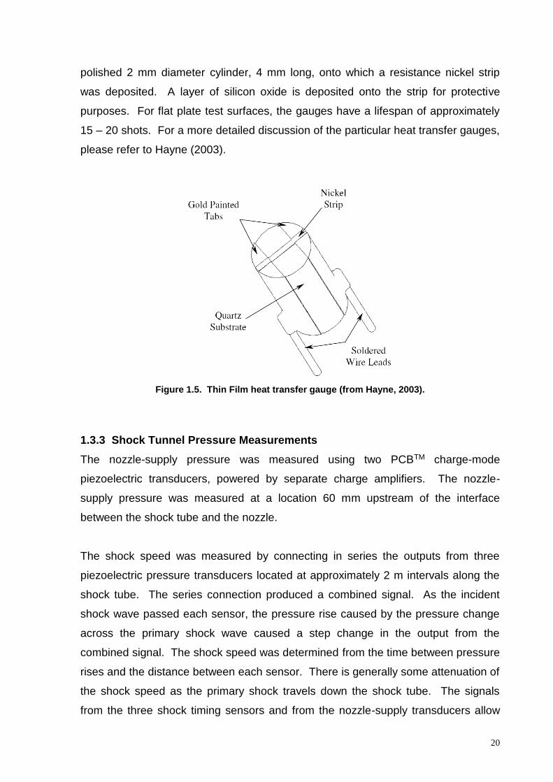
Heat transfer results were measured with in-house built heat thin film gauges. The

gauges were designed specifically for use in impulse facilities and consisted of a

20

polished 2 mm diameter cylinder, 4 mm long, onto which a resistance nickel strip

was deposited. A layer of silicon oxide is deposited onto the strip for protective

purposes. For flat plate test surfaces, the gauges have a lifespan of approximately

15 – 20 shots. For a more detailed discussion of the particular heat transfer gauges,

please refer to Hayne (2003).

Figure 1.5. Thin Film heat transfer gauge (from Hayne, 2003).

1.3.3 Shock Tunnel Pressure Measurements

The nozzle-supply pressure was measured using two PCBTM charge-mode

piezoelectric transducers, powered by separate charge amplifiers. The nozzle-

supply pressure was measured at a location 60 mm upstream of the interface

between the shock tube and the nozzle.

The shock speed was measured by connecting in series the outputs from three

piezoelectric pressure transducers located at approximately 2 m intervals along the

shock tube. The series connection produced a combined signal. As the incident

shock wave passed each sensor, the pressure rise caused by the pressure change

across the primary shock wave caused a step change in the output from the

combined signal. The shock speed was determined from the time between pressure

rises and the distance between each sensor. There is generally some attenuation of

the shock speed as the primary shock travels down the shock tube. The signals

from the three shock timing sensors and from the nozzle-supply transducers allow

21

the shock speed to be calculated after three successive 2 m internals. Stalker and

Morgan (1988) argue that the gas that has been processed last by the shock wave

enters the nozzle and test section first. Hence, the shock speed was determined

from the last two shock timing stations.

1.4 MEASUREMENT UNCERTAINTY ANALYSIS

This section presents the uncertainty analysis for the pressure measurements, and

the data acquisition system. In the analysis uncertainties were assumed to be

normally distributed and uncorrelated. A short review of the theory used in this

analysis is given in App. C.1.1.

1.4.1 Static Pressure Uncertainty

The systematic uncertainty in static pressure measurements, P, was determined

from previous studies by Daniel (1990), Goyne (1998), and Suraweera (2006B).

The contributing factors to pressure measurement uncertainty are listed for both

KuliteTM and PCBTM transducers below.

KuliteTM pressure transducer calibration, P 2%

Transducer mounting effects, P 1%

Measurement of voltage output in data recording, P 0.5%

The total systematic uncertainty in P measured by KuliteTM transducers, determined

from root-sum-square (RSS) of the contributing variables, is 2.3%.

PCBTM pressure transducer calibration, P 2%

Transducer mounting effects, P 3%

Measurement of voltage output in data recording, P 0.5%

The total systematic uncertainty in P measured by PCBTM transducers, determined

from root-sum-square (RSS) of the contributing variables, is 3.6%.

22

__________________________________________________________________________________

EXPERIMENTAL TESTING

_____________________________________________________________________

2.1 INTRODUCTION

This section gives a general description of the test model and fuel injection

system used for this experimental investigation in the T4 shock tunnel. In

addition, the input and derived T4 test conditions are summarised. The

determination of the test time is also outlined.

2.2 TEST MODEL

2.2.1 General Layout

The M12REST scramjet model used in the test program, shown in Fig. 2.1,

was 1980 mm long and had a maximum width of 180 mm. The test model

consisted of four components; a forebody plate, a REST inlet, an elliptical

combustor, and a generic elliptical nozzle. The forebody and inlet sections

were 150 mm and 1062 mm long, respectively, with 0.7 mm leading edge

radii. A 150 mm length forebody with a 3 mm leading edge radius was also

tested (see Fig. G.1, App. G). In addition, a longer 500 mm forebody section

with a 0.7 mm leading edge radius was tested for 8 shots during the

experimental campaign (see Fig. G.2, App. G,). The inlet had a total

geometric contraction ratio of 6.61, an internal contraction ratio of 2.26 and a

short isolator downstream of the throat. The 150 mm wide frontal capture

area of the inlet was 113 cm2 and all leading edges (including the forebody

plate) had radii of 0.7 mm. Inlet injection was through three 4 mm diameter

portholes angled at 45 to the local flow, at a downstream distance of 652 mm

from the leading edge of the model. The portholes were sized using

McClinton (1972) to enable the fuel jets to penetrate through the inlet

boundary layer to facilitate mixing in the mainstream flow of the engine. The

aspect ratio of the elliptical cross-section at the end of the inlet was 1.76. The

inlet section was terminated by a 2.5 mm rearward facing circumferential step

23

(area ratio = 1.245) where fuel could be injected through a set of 48

portholes, 1.5 mm in diameter, angled at 10° to the axis of the combustor.

The step height was sized to be smaller than the local boundary layer

thickness to promote combustion of fuel within the boundary layer. Sonic

injection was employed for both fuel stations and a fast response solenoid

valve was used to supply gaseous hydrogen fuel to either or both the fueling

stations.

A cross section of the test model along the symmetry plane is shown in Fig.

2.2 to illustrate both fueling stations in finer detail. The combustor entrance

height immediately downstream of the step was H = 40.3 mm, and was

angled at 6 to the inlet axis in order to re-align the local flow with the nominal

flight direction. The combustor consisted of a constant area section, 322 mm

in length (L/H = 8.0), and a diverging section, 242 mm in length (L/H = 6.0) to

an area ratio of 2.0 relative to the inlet throat. The angle of divergence was

kept constant around the circumference at approximately 1.6. The generic

thrust nozzle was an elliptical cone with a 201 mm length and an area ratio of

4.0. In Fig. 2.3 the scramjet engine is shown mounted in the shock tunnel

test section along with the Pitot probe used for the tests in Fig. 2.4.

Figure 2.1. Main components of the initial Mach 12 REST scramjet with 150 mm

forebody in assembled test orientation.

24

Figure 2.2. Fueling stations of the Mach 12 REST scramjet.

Figure 2.3. Side view of the Mach 12 REST scramjet mounted in the T4 test section.

Figure 2.4. Front view of the Mach 12 REST scramjet mounted in the T4 test section.

Pitot Probe

25

The inlet was machined using a three-axis mill from a plastic material called

NECURON® 6519 which has a density of 660 kg/m3 and a yield strength of 30

MPa. Due to the complexity of the geometry, the inlet was machined in two

halves, and bonded together with epoxy adhesive. Fibreglass layers were

applied to the external body of the inlet, aft of the leading edges, to provide

additional structural strength. The combustor section was made in a similar

manner to the inlet. The elliptical nozzle was manufactured with a glass filled

nylon material called CAPFormTM using a Selective Laser Sintering (SLS)

technique, and was then hand polished. The fuel reservoirs and injectors

were machined from aluminum and mild steel, respectively. The process of

machining enabled a high manufacturing tolerance of ±0.05 mm, while the

SLS technique produced an acceptable precision level of ±0.15 mm in the

nozzle. The model has survived 109 shots, over two separate test programs,

relatively intact. However, touch-up work using car body filler, particularly in

the inlet crotch area, was needed approximately every 2 - 5 shots.

2.2.1 Instrumentation and Data Acquisition

The test surfaces comprised the intake wall and both the upper (body-side)

and lower (cowl-side) sections of the combustor and nozzle. The centre-line

of each test surface was instrumented with KuliteTM, Series XTEL-190M

pressure transducers at intervals ranging from 25 mm to 100 mm in length.

As stated earlier, three pressure ranges were used in the test model: 0 - 68.8

kPa (0 - 10 psi), 0 - 172.3 kPa (0 - 25 psi), and 0 - 689.4 kPa (0 - 100 psi).

The error associated with the use of these pressure transducers was ±1.0%

of full scale. Both fuel plenum chambers were instrumented with two PCBTM,

Model 111A26 piezoelectric pressure transducers each. The error associated

with the use of these pressure transducers was ±2.0% of full scale. The

forebody inlet sections were also instrumented with a total of four in-house

(three sans long forebody) built heat thin film transfer gauges, located on the

centre-line. For all transducer types used, please refer to App. B, Table B.1

and Table B.2 for sensitivities and test model x-locations.

The data acquisition system for the T4 shock tunnel consists of a National

Instruments PXI data acquisition system, and a LabVIEWTM visual interface

program (Ridings and Turner, 2007). Sampling periods of 1s and 50s were

26

used to gather data for the short time base and long time base signals,

respectively. The data recorder captured data concurrently on 10 banks of up

to 12 channels. For typical T4 operation, the data acquisition triggered from

the pressure jump associated with the arrival of the primary shock wave at

one of the two nozzle-supply pressure transducer signals. Refer to Table B.1

and Table B.2, App. B.1 to see the transducer configuration for the data

acquisition system.

A LabVIEWTM visual interface program, specifically designed for this test

campaign, was used to configure and control the data recorder. The program

was also used for data transfer, and system troubleshooting. The Python

computer codes Condition, version 1.0 (Turner, 2008A), and PDC, version 2.0

(Turner, 2008B), were principally used to analyse the measurements

recorded during each experimental run.

2.3 FUEL SYSTEM

2.3.1 Fuel Injection

Hydrogen fuel was injected from a room temperature reservoir through a fast-

acting solenoid valve. The fuel reservoir consisted of a coiled (14.19 m)

Ludwieg tube which kept the temperature of the fuel approximately constant

at 300 K during injection. The injection flow was initiated at least 3 ms prior to

test flow arrival. A ½ inch Joucomatic Asco solenoid valve, type SC

B223A103, was used during the test program as it was suitable for operation

at reservoir pressures between 200 kPa and 2000 kPa. The fuel valve was

controlled by a controller board assembled in-house at The University of

Queensland. A schematic of the system controlling the fuel valve is shown in

Fig. 2.5. A signal from a linear voltage displacement transducer, LVDT, which

measures the recoil of the tunnel as the shot is fired, was used as a trigger for

the fuel valve. Depending on the specific test condition, two inputs of ‘recoil

threshold’ and ‘valve open time’ were entered by the experimenter into the

National Instruments LabVIEWTM program controlling the valve. Once the

specified recoil threshold was reached, two successive electrical pulses were

sent via a controller board and relay switch to open and close the solenoid

valve during the test time.

27

The pressure levels in both the inlet and step injection plenum chambers

were recorded by two PCBTM transducers. The inlet plenum chamber

pressure levels during the test time were constant to within 4%, while the

combustor plenum chamber pressure levels were constant to within 3%.

Figure 2.5. Schematic of fuel valve control system.

2.3.2 Fuel Valve Calibration

For each of the injection schemes (inlet and throat), the fuel system was

calibrated prior to testing to determine the mass flow rate of hydrogen as a

function of the reservoir and plenum pressures. Contributing factors to the

pressure measurement uncertainty are pressure transducer calibration,

transducer mounting effects, and measurement of data signal voltage output.

The calibration procedure for the shock tunnel fuel system is described by

Robinson et al. (2003). The instantaneous mass flow rate of the fuel is given

by

2γ

1γ

f

2γ

1γ

io,f PPα

1m

, (2.1)

where is the experimentally determined fuel calibration constant given by

f

i

t

t

2

1

fi,o

i,of,oo

i,ofPP

)PP(V

TR, (2.2)

T4 Tunnel

Test Section

Fuel Valve

LVDT

Controller Board

RelaySwitch

PC

28

And Po,i = initial pressure in the fuel reservoir,

Po,f = final pressure in the fuel reservoir,

Pf = measured pressure in the plenum chamber,

Vo = volume of fuel reservoir (1.66 10-3 m3)

To,i = initial temperature in fuel reservoir (300 K),

Rf = ideal gas constant of the fuel,

ti = initial time, and

tf = final time.

For inlet and step fuelled runs, the calibration constant was calculated for

each successive fuel-on shot during the experimental campaign in order to

determine the fuel equivalence ratio. The calibration constants were always

within 9% of the calibration mean values. The relationships between

hydrogen equivalence ratio and plenum chamber pressure for step injection

are shown in Appendix D.

2.4 TEST CONDITIONS

The engine was tested in a standard semi-freejet mode due to test facility

constraints. The facility nozzle simulated the flows over the forebody section

of the engine. The engine was assumed to be installed on a vehicle with a

forebody equivalent to a 6 degree wedge.

Conditions in the nozzle-supply region were calculated using the Equilibrium

Shock Tube Calculation (ESTC) numerical code developed by McIntosh

(1968). ESTC is a one-dimensional numerical code that has as inputs the

shock tube filling pressure and temperature, the measured speed of the

incident shock, and the nozzle-supply pressure during the test time. ESTC

calculations are based on an inviscid mixture of reacting gases in

thermodynamic equilibrium. The species considered for air test gas are e¯,

N2, O2, Ar, N, O, NO, and NO+. For nitrogen test gas, N2, and N are

considered.

29

Four distinct test conditions were employed in the present study. The details

of each are given below:

Test condition 1 was used to simulate a flight altitude of approximately

41.0 km, a flight Mach number of approximately 12.0, and an angle of

attack (AOA) of 0 degrees.

Test condition 2 was used to simulate a flight altitude of approximately

38.0 km, a flight Mach number of approximately 11.1, and an AOA of

-2 degrees (simulating pitch down). For this test condition, the AOA

was a virtual configuration rather than a physical one (another way to

look at it is to assume a semi-freejet condition where the forebody is at

4 degrees relative to the vehicle body axis).

Test condition 3 was similar to test condition 1, but with an AOA of +2

degrees.

Test condition 4 was similar to test condition 2, but with no AOA.

It should be noted that with the last two conditions, the model was physically

pitched up by 2 degrees. The T4 operational input conditions for each

nominal tunnel run in the present study are summarised in Table 2.1.

Table 2.1. Nominal T4 input conditions

Test

Condition

Diaphragm

Thickness

Reservoir

Pressure

Driver

Pressure

Driver Gas

Composition

Shock Tube

Pressure

(mm) (MPa) (kPa) (%Ar / %He) (kPa)

1 6 12.0 156 35 / 65 150

2 6 12.0 156 35 / 65 190

3 6 12.0 156 35 / 65 150

4 6 12.0 156 35 / 65 190

ESTC calculations were made for each distinct tunnel run and the properties

for each test condition are presented in Table 2.2.

30

Table 2.2. Summary of nominal nozzle-supply conditions

Test

Condition

Supply

Pressure

Primary Shock

Speed

Stagnation

Temperature

Stagnation

Enthalpy

(MPa) (m/s) (K) (MJ/kg)

1 80.6 2637 5097 7.47

2 81,8 2493 4680 6.58

3 80.6 2637 5097 7.47

4 81.8 2493 4680 6.58

The flow properties and the chemical composition at the nozzle exit were

determined using the one-dimensional Non-equilibrium Nozzle Flow (NENZF)

numerical code developed by Lordi et al. (1966). Inputs to the NENZF code

are the nozzle-supply temperature determined from the ESTC code, the

nozzle-supply pressure and the nozzle length required to match the measured

or expected Pitot to nozzle-supply pressure ratio. NENZF calculations were

made for each T4 run and nominal flow properties at the nozzle exit for each

test condition are presented in Table 2.3. For test conditions 1 and 2, the

nozzle exit flow properties are also the forebody flow properties. The nozzle

exit flow properties for each distinct tunnel run are presented in Table E.1 and

Table E.2, App. E.

Table 2.3. Summary of nominal nozzle exit conditions

Test Te Pe e Ue Me Reu 106

Condition (K) (kPa) (kg/m3) (m/s) (1/m)

1 396 1.116 0.0098 3670 9.21 1.58

2 331 1.053 0.0111 3454 9.48 1.93

3 396 1.116 0.0098 3670 9.21 1.58

4 331 1.053 0.0111 3454 9.48 1.93

The forebody conditions for the engine are presented in Table 2.4. The

forebody flow properties for test conditions 3 and 4 were determined by

processing the nozzle exit flow properties downstream of an oblique shock,

generated from essentially a planar 2 degree wedge as a result of pitching up

the engine.

31

Table 2.4. Summary of calculated nominal forebody conditions

Test T1 P1 1 U1 M1 Reu 106


1 396 1.116 0.0098 3670 9.21 1.58

2 331 1.053 0.0111 3454 9.48 1.93

3 449 1.728 0.0133 3652 8.61 1.96

4 337 1.650 0.0153 3434 8.84 2.39

The nominal flight conditions for the study are presented in Table 2.5. The

flight conditions were determined by processing the nozzle exit flow properties

upstream of an oblique shock generated from a planar 6 degree wedge.

Table 2.5. Summary of calculated nominal flight conditions

Test T∞ P∞ ∞ U∞ M∞ Reu 106


1 253 0.242 0.0033 3820 12.0 0.79

2 245 0.365 0.0052 3484 11.1 1.15

3 253 0.242 0.0033 3820 12.0 0.79

4 245 0.365 0.0052 3484 11.1 1.15

2.5 TEST TIME DETERMINATION

The beginning of the test time is dependent on the nozzle starting process

and the model flow establishment time. The nozzle starting process is

initiated by the rupture of the secondary diaphragm and is completed when

the unsteady expansion created in start-up is swept out of the nozzle, and the

boundary layers on the nozzle wall are fully established (Smith, 1966). For

the T4 shock tunnel, the onset of steady nozzle flow is taken to be the point in

time when the ratio of the Pitot pressure to nozzle-supply pressure has

reached a steady level. A transit time is included to allow for the flow to travel

from the location where the nozzle-supply pressure is measured, 60 mm

upstream of the end of the shock tube, and the location of Pitot pressure

measurement.

32

Once the nozzle start-up has been achieved (approximately 0.9 ms for the

M10 Nozzle), the test flow must have sufficient time to fully establish. The

establishment time is the time required for the flow to reach steady state after

flow onset. Past experimental and numerical studies for flat plates in shock

tunnel flows have correlated measurements for establishment time in terms of

the number of model flow lengths (Felderman, 1968; Davies and Bernstein,

1969; East et al., 1980). Attached laminar and turbulent boundary layers take

approximately 3.3 and 2.0 flow lengths, respectively, to reach steady state.

As the boundary layers on the test surface were expected to be both laminar

and turbulent for the present study, an arbitrary value of 3.0 flow lengths was

considered sufficient along the test surface for full flow establishment.

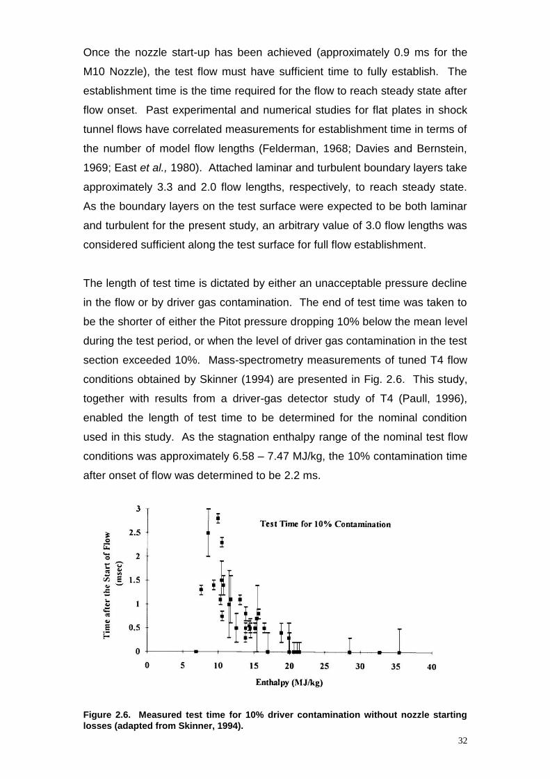
The length of test time is dictated by either an unacceptable pressure decline

in the flow or by driver gas contamination. The end of test time was taken to

be the shorter of either the Pitot pressure dropping 10% below the mean level

during the test period, or when the level of driver gas contamination in the test

section exceeded 10%. Mass-spectrometry measurements of tuned T4 flow

conditions obtained by Skinner (1994) are presented in Fig. 2.6. This study,

together with results from a driver-gas detector study of T4 (Paull, 1996),

enabled the length of test time to be determined for the nominal condition

used in this study. As the stagnation enthalpy range of the nominal test flow

conditions was approximately 6.58 – 7.47 MJ/kg, the 10% contamination time

after onset of flow was determined to be 2.2 ms.

Figure 2.6. Measured test time for 10% driver contamination without nozzle starting

losses (adapted from Skinner, 1994).

33

__________________________________________________________________________________

EXPERIMENTAL RESULTS

_____________________________________________________________________

3.1 INTRODUCTION

This section gives a general overview of the successful tunnel runs executed

in this experimental study.

3.2 TEST SUMMARY

3.2.1 Test Shots

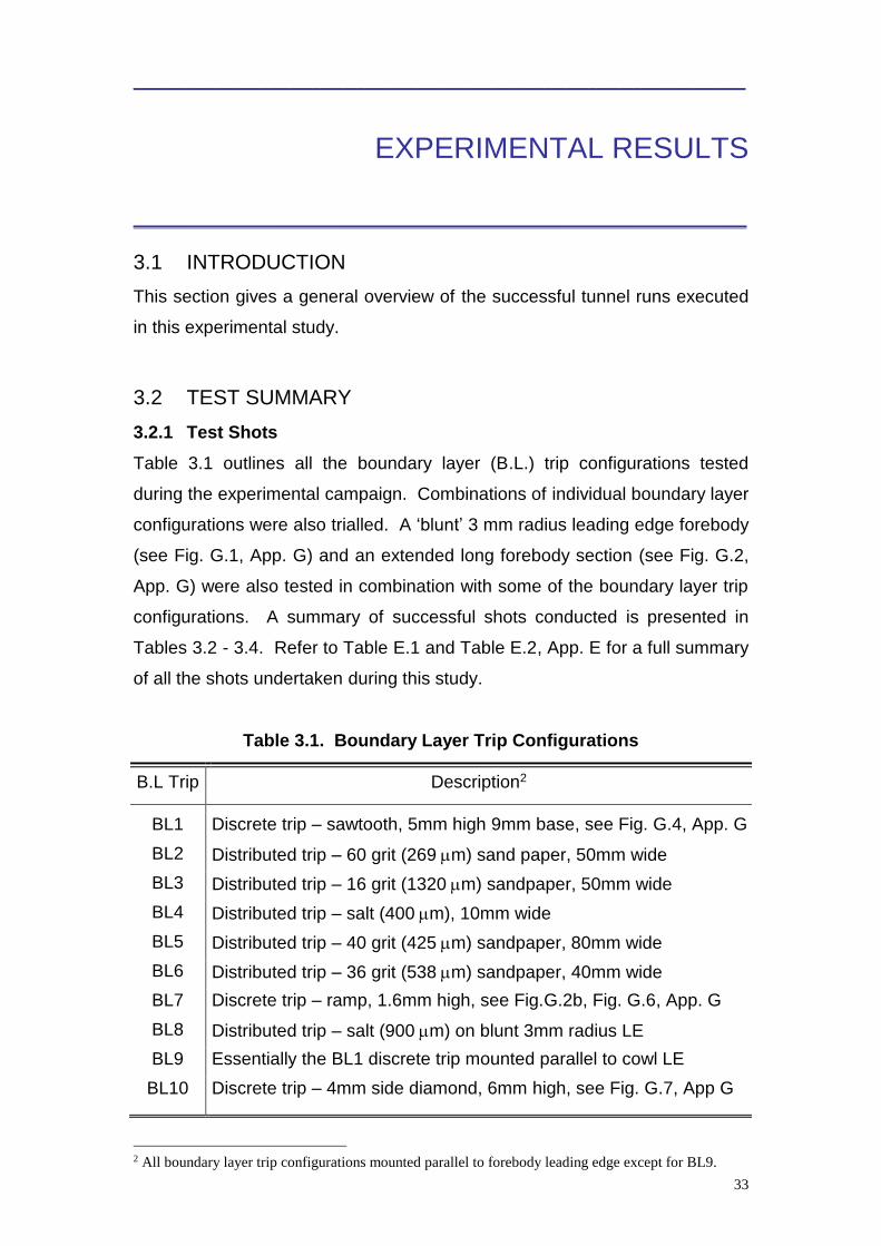
Table 3.1 outlines all the boundary layer (B.L.) trip configurations tested

during the experimental campaign. Combinations of individual boundary layer

configurations were also trialled. A ‘blunt’ 3 mm radius leading edge forebody

(see Fig. G.1, App. G) and an extended long forebody section (see Fig. G.2,

App. G) were also tested in combination with some of the boundary layer trip

configurations. A summary of successful shots conducted is presented in

Tables 3.2 - 3.4. Refer to Table E.1 and Table E.2, App. E for a full summary

of all the shots undertaken during this study.

Table 3.1. Boundary Layer Trip Configurations

B.L Trip Description2

BL1 Discrete trip – sawtooth, 5mm high 9mm base, see Fig. G.4, App. G

BL2 Distributed trip – 60 grit (269m) sand paper, 50mm wide

BL3 Distributed trip – 16 grit (1320m) sandpaper, 50mm wide

BL4 Distributed trip – salt (400m), 10mm wide



BL7 Discrete trip – ramp, 1.6mm high, see Fig.G.2b, Fig. G.6, App. G

BL8 Distributed trip – salt (900m) on blunt 3mm radius LE

BL9 Essentially the BL1 discrete trip mounted parallel to cowl LE

BL10 Discrete trip – 4mm side diamond, 6mm high, see Fig. G.7, App G

G?

2 All boundary layer trip configurations mounted parallel to forebody leading edge except for BL9.

34

Table 3.2. M12REST Scramjet Shot Summary, 2009

No. Shot No. Date Test gas Injector Total BL Trip Comments 1 10245 13/01/09 Air - 0.00 Clean Cond.1: shakedown

2 10246 13/01/09 Air - 0.00 BL1 @135mm Cond.1: No HT change



5

10250

27/01/09

Air

-

0.00

BL1 @320mm BL2 @90mm

Cond.1: No HT change

6

10251

25/02/09

Air

-

0.00

BL1 @ 10mm BL3 @100mm


7

10252

03/03/09

Air

-

0.00

BL4 @0mm BL5 @10mm BL6 @90mm




10

10260

24/05/09

Air

-

0.00

BL8 @0mm BL7 @20mm


11

10262

27/05/09

N2

Inlet

0.52

BL8 @0mm BL7 @20mm


12

10263

29/05/09

Air

-

0.00

Long Forebody BL7 @50mm

Cond.2: HT inconclusive

13

10264

29/05/09

Air

-

0.00


BL6 @100mm BL1 @360mm


14

10265

30/05/09

Air

-

0.00


BL6 @100mm BL1 @360mm BL9 @10mm


15

10266

01/06/09

Air

-

0.00


BL6 @100mm BL1 @360mm BL1 @895mm BL9 @10mm


16

10267

01/06/09

Air

-

0.00


BL6 @100mm BL1 @360mm

BL1 @1095mm


17

10268

03/06/09

Air

-

0.00


BL6 @100mm BL1 @360mm

Cond.4: HT N/A

18

10269

04/06/09

Air

-

0.00


BL6 @100mm BL1 @360mm

Cond.3: HT N/A

19

10270

04/06/09

N2

Inlet

0.54


BL6 @100mm BL1 @360mm

Cond.4: HT N/A Flow separation

20

10271

05/06/09

Air

Inlet

0.56


BL6 @100mm BL1 @360mm

Cond.4: HT N/A: Flow separation

21

10272

09/06/09

Air

Step

0.76


BL6 @100mm BL1 @360mm


35

Table 3.3. M12REST Scramjet Shot Summary Continued 1, 2009

No. Shot No. Date Test gas Injector Total BL Trip Comments

22

10274

12/06/09

Air

-

0.00


BL10 @520mm Cond.4: HT N/A

23

10275

12/06/09

Air

-

0.00



24

10276

16/06/09

Air

Step

0.48



25

10277

17/06/09

Air

-

0.00


BL1 @360mm

Cond.4 HT N/A Repeat of 10275

26

10278

17/06/09

Air

-

0.00


BL1 @360mm

Cond.4: HT N/A Repeat of 10277

27

10279

18/06/09

Air

Step

1.19


BL1 @360mm

Cond.4: HT N/A

28

10280

19/06/09

N2

Step

1.19



29

10281

19/06/09

Air

-

0.00


BL6 @100mm BL1 @360mm

Cond.3: HT N/A

30

10282

19/06/09

Air

Step

0.76


BL6 @100mm BL1 @360mm

Cond.3: HT N/A

31

10283

22/06/09

Air

Step

1.05


BL6 @100mm BL1 @360mm

Cond.3: HT N/A

32

10285

23/06/09

N2

Step

1.14


BL6 @100mm BL1 @360mm

Cond.3: HT N/A

33

10286

23/06/09

Air

Step

0.44


BL6 @100mm BL1 @360mm

Cond.3: HT N/A

34 10287 23/06/09 Air - 0.00 Clean Cond.3: HT N/A

35 10288 24/06/09 Air - 0.00 Clean Cond.4: HT N/A

3.2.2 Run Descriptions

The experimental campaign tested two different injection schemes: inlet and

step injection. For the nominal flow conditions three cases were tested. Test

runs were carried out with air as the test gas and no fuel injection (fuel-off),

with air as the test gas with hydrogen injection (fuel-on), and with nitrogen as

the test gas with hydrogen injection (suppressed combustion). The

differences between fuel-on and suppressed combustion were used to

determine the effects of combustion. A brief description and the rationale

behind each group of shot conditions and trip configurations are given below:

36

Shot 1 – 6: The model was initially tested at test condition 1 (M12

enthalpy), fuel-off, 0 degrees AOA, with trip configurations ranging

from a clean forebody, to sawtooth only trips (BL1) at various positions

along the bodyside surfaces on the forebody and inlet, to combinations

with distributed trips (BL2 and BL3). The 150 mm sharp leading edge

forebody was used for this series of tests. These combination trip

configurations (and all others in the study) were tested to promote

transition and deter re-laminarization of the local flow.

Shot 7: The flow and model conditions were kept the same as the

previous shots. Several distributed BL trips (BL4-6) were combined in

an effort to trip the flow with a gradually increasing rough surface (grain

size), beginning from the leading edge of the forebody.

Shot 8 – 11: The model was tested with the 3 mm radius ‘blunt’

leading edge forebody at test condition 2 (M11 enthalpy), fuel-off, 0

degrees AOA, with trip configurations ranging from a discrete ramp trip

(BL7), to combinations with a distributed trip (BL8). With shot 11, inlet

fuel injection into nitrogen test gas was used as a boundary layer trip in

combination with other trips (see shot 10).

Shot 12 – 16: The model was tested with the long forebody at test

condition 2, fuel-off, 0 degrees AOA, with trip configurations ranging

from a discrete ramp trip (BL7), to combinations with a discrete ramp

trip, two discrete sawtooths (BL1), and distributed trips (BL7 and BL9).

Shot 17: The model was tested with the long forebody at test condition

4 (M11 enthalpy), fuel-off, +2 degrees AOA, with a combination trip

configuration of two discrete trips (BL7 and BL1) and a distributed trip

(BL6). The model was pitched up to increase the local Reynolds

number, in order to support natural as well as assisted flow transition.

Shot 18: The model was tested with an identical model and trip

configuration to shot 17 at test condition 3 (M12 enthalpy). The model

was pitched up to increase the local Reynolds number, in order to

support natural as well as assisted flow transition.


condition 4, +2 degrees AOA, with a combination trip configuration of

two discrete trips (BL7 and BL1) and a distributed trip (BL6). Shot 19

37

was a suppressed combustion run (using inlet injection), shot 20 was a

corresponding inlet fuel-on run, and shot 21 was a step fuel-on run.


4, fuel-off, +2 degrees AOA, with a combination trip configuration of a

discrete trip (BL7) and a discrete diamond trip (BL10) further

downstream.



two discrete trips (BL7 and BL1). Shots 24 and 27 were step fuel-on

runs at mid and high equivalence ratios, respectively. Shot 28 was a

suppressed combustion run using step injection at a high equivalence

ratio.



two discrete trips (BL7 and BL1) and a distributed trip (BL6). Shot 29

was a fuel-off run. The remaining shots employed step injection at mid

and high fuel equivalence ratios. Shot 32 was a suppressed

combustion run at a high equivalence ratio.


3, fuel-off, +2 degrees AOA, with a clean configuration for baseline

results.


4, fuel-off, +2 degrees AOA, with a clean configuration for baseline

results.

3.3 ENGINE EXPERIMENTAL RESULTS

For the following pressure distributions in Fig. 3.1 to Fig. 3.7, each pressure

measurement represents a mean value of the pressure time history during the

test time. The static pressures measurements were normalised by the

measured nozzle supply pressure, Ps, for the test run (to account for shot-to-

shot variations), and then multiplied by the nominal condition pressure ratio,

Ps nom / P1 nom, so that measured values are relative to the nominal static

pressure entering the engine.

38

3.3.1 M12REST 2007 Results and Conclusions

Figure 3.1 shows a comparison of typical bodyside pressure

distributions of 2007 experimental and numerical results for a fuel-off

‘on-design’ test condition 1. Comparisons between 2007 experimental

and numerical results for an ‘off-design’ condition had shown good

agreement. However for this ‘on-design’ test case, experimental

results exhibited consistently larger pressure levels on the inlet from

x=700 mm to x=1050 mm. Downstream of this region, the shock

structure was not predicted well for either bodyside or cowlside test

surfaces. Several laminar and turbulent inflow conditions were run at

this condition, but no CFD results were able to closely match

experimental measurements.

It was postulated that the mismatch between experimental and

numerical results, for the ‘on-design’ case, was due to separation of

laminar flow on the forward bodyside section of the inlet, as a result of

geometry change and vortices. For test condition 1, an earlier

transition study suggested that flow over the majority of the inlet was

laminar (He and Morgan, 1994). The current 2009 study was

implemented with the aim of tripping the laminar flow in the hope that

turbulent flow would be less susceptible to local separations.

0

20

40

60

0.0 0.2 0.4 0.6 0.8 1.0 1.2 1.4 1.6 1.8 2.0

Distance from Forebody LE (m)

(P/P

s)

x (

Ps n

om

./P1

no

m.)

0.000

0.002

0.004

0.006

0.008

0.010

0.012

0.014

0.016

Are

a (

m2)

CFD: Bodyside

Fuel Off: Bodyside

Fuel Locations

Area

Figure 3.1. Normalised pressure distributions; bodyside CFD and experimental results,

cond. 1, fuel-off, M12REST 2007 Study.

39

3.3.2 Initial Boundary Layer Trip Results and Conclusions

For test condition 1, the multitude of combinations of discrete and

distributed boundary layer trips, together with the 150 mm sharp

leading edge forebody, did not garner any successful results. For test

condition 2, the use of the blunt leading edge forebody combined with

several boundary layer trip configurations, including inlet injection, also

failed to trip the flow over the inlet. For both test conditions, the high

pressure region in the forward section of the inlet remained and was in

some cases worse. Examples of this can be seen in pressure

measurements in Fig. 3.2a and Fig. 3.2b. As typified in Fig. 3.3, no

sustained tripping of flow over the bodyside surface of the inlet was

observed in heat transfer results. Figure 3.3 presents Stanton number

measurements of several tunnel runs. Predictions of Stanton number

for laminar and turbulent flow, using a reference temperature method

(Sommer and Short, 2002), are also plotted for test condition 1.

The use of the 500 mm long forebody combined with several boundary

layer trip configurations provided some signs of transition. However

among the operational thin film gauges, no definite turbulent heat

transfer results were measured. The experimental results for test

conditions 3 and 4 with the long forebody will be discussed in the next

two sections. For the two test conditions, BL7/BL6/BL1 and BL7/BL1

trip configurations (see Table 3.1 – 3.3) were used, respectively.

0

20

40

60

0.0 0.2 0.4 0.6 0.8 1.0 1.2 1.4 1.6 1.8 2.0


(P/P

s)

x (

Ps n

om

./P1

no

m.)

0.000

0.002

0.004

0.006

0.008

0.010

0.012

0.014

0.016

Are

a (

m2)

10260: Bodyside

10251: Bodyside

CFD: Bodyside

Fuel Locations

Area

Figure 3.2a. Typical bodyside pressure distributions; cond. 1 and 2, fuel-off.

40

0

20

40

60

0.0 0.2 0.4 0.6 0.8 1.0 1.2 1.4 1.6 1.8 2.0


(P/P

s)

x (

Ps n

om

./P1

no

m.)

0.000

0.002

0.004

0.006

0.008

0.010

0.012

0.014

0.016

Are

a (

m2)

10260: Cowlside

10251: Cowlside

CFD: Cowlside

Fuel Locations

Area

Figure 3.2a. Typical cowlside pressure distributions; cond. 1 and 2, fuel-off.

0.0000

0.0005

0.0010

0.0015

0.0020

150 200 250 300 350 400

Distance from LE (mm)

Sta

nto

n N

um

be

r

SSM Laminar

SSM Turbulent

no trip - 10245

BL trip - 10246

BL trip - 10247

BL trip - 10249

BL trip - 10250

BL trip - 10252

BL trip - 10260

Figure 3.3. Initial Stanton number results and predictions; cond. 1 and 2, fuel-off.

3.3.3 Test Condition 3 Results and Conclusions

At this point of the experimental campaign, the last three downstream

thin film gauges (x=0.445 m, x=0.612 m, x=0.695 m3) where transition

to turbulent flow was to be measured, were generally not operational.

This was due to several factors. These positions were the most

3 Long forebody length taken into account. However for all pressure plots, this has not been done.

41

exposed to the flow, as they were near or on geometry variations, and

hence the gauges were damaged quite easily. Replacement of gauges

was also difficult due to time constraints and the lack of work area

within the test section and model. It was therefore impossible to verify

if the inlet inflow was turbulent. However as seen in Fig. 3.4a and Fig.

3.4b, there was a significant difference in pressure results between

clean (no BL trips) and trip configurations. From 2007 CFD (these are

for cond. 1 though) and current experimental results, it can be inferred

that the flow separation is not as significant as in the 2007 study.

0

20

40

60

0.0 0.2 0.4 0.6 0.8 1.0 1.2 1.4 1.6 1.8 2.0


(P/P

s)

x (

Ps n

om

./P1

no

m.)

0.000

0.002

0.004

0.006

0.008

0.010

0.012

0.014

0.016

Are

a (

m2)

10287: Bodyside: Clean

10281: Bodyside: BL Trips

CFD: Bodyside

Fuel Locations

Area

Figure 3.4a. Bodyside pressure distributions; clean and BL trips, cond. 3, fuel-off.

0

20

40

60

0.0 0.2 0.4 0.6 0.8 1.0 1.2 1.4 1.6 1.8 2.0


(P/P

s)

x (

Ps n

om

./P1

no

m.)

0.000

0.002

0.004

0.006

0.008

0.010

0.012

0.014

0.016

Are

a (

m2)

10287: Cowlside: Clean

10281: Cowlside: BL Trips

CFD: Cowlside

Fuel Locations

Area

Figure 3.4b. Cowlside pressure distributions; clean and BL trips, cond. 3, fuel-off.

42

As seen in Fig. 3.5a, there appears to be an upstream influence in the

isolator due to fuel addition at the step for high equivalence ratios

(=1.14 and =1.05). This pressure rise is not seen for the low

equivalence ratio fuel-on run (=0.44).

Sustained combustion was initially measured at a fuelled run with a

=0.76. Ignition was first measured on the cowlside at x=1.306 m.

Some localised combustion was observed at a =0.44 in the mid

section of the combustor (see Fig. 3.5b).

0

20

40

60

0.0 0.2 0.4 0.6 0.8 1.0 1.2 1.4 1.6 1.8 2.0


(P/P

s)

x (

Ps n

om

./P1

no

m.)

0.000

0.002

0.004

0.006

0.008

0.010

0.012

0.014

0.016

Are

a (

m2)

10281: Bodyside: f=1.14

10286: Bodyside: f=0.44

10282: Bodyside: f=0.76

10283: Bodyside: f=1.05

Fuel Locations

Area

Figure 3.5a. Bodyside pressure distributions; BL7/BL6/BL1 trips, cond. 3, step fuel-on.

0

20

40

60

0.0 0.2 0.4 0.6 0.8 1.0 1.2 1.4 1.6 1.8 2.0


(P/P

s)

x (

Ps n

om

./P1

no

m.)

0.000

0.002

0.004

0.006

0.008

0.010

0.012

0.014

0.016

Are

a (

m2)

10281: Cowlside: f=1.14

10286: Cowlside: f=0.44

10282: Cowlside: f=0.76

10283: Cowlside: f=1.05

Fuel Locations

Area

Figure 3.5b. Cowlside pressure distributions; BL7/BL6/BL1 trips, cond. 3, step fuel-on.

43

For most equivalence ratios, supersonic burning was evident when

combustion occurred. However for the fuelled run at =1.05, local flow

within the constant area section of the combustor was inferred to be

separated (see Fig. 3.5a and Fig. 3.5b). No fuel-on conditions lead to

an unstart of the engine, as the combustion induced increase in

pressure levels was contained at the downstream end of the isolator.

A maximum pressure rise of p/p1~44, due to combustion, was

measured at =1.14 on the bodyside test surface at x=1.440 m (see

Fig. 3.5a).

3.3.3 Test Condition 4 Results and Conclusions

Due to non-operational heat transfer gauges at this point in the

experimental campaign, only pressure measurements could be used to

infer the effect of trip configurations. As seen in Fig. 3.6a and Fig.

3.6b, there was no significant difference in pressure results between

clean and trip configurations. If indeed the flow has naturally

transitioned, this result is not surprising as condition 4 has the highest

Reynolds number (2.39 106) of all conditions tested in this study.

0

20

40

60

0.0 0.2 0.4 0.6 0.8 1.0 1.2 1.4 1.6 1.8 2.0


(P/P

s)

x (

Ps n

om

./P1 n

om

.)

0.000

0.002

0.004

0.006

0.008

0.010

0.012

0.014

0.016A

rea (

m2)

10288: Bodyside: Clean

10277: Bodyside: BL Trips

CFD: Bodyside

Fuel Locations

Area

Figure 3.6a. Bodyside pressure distributions; clean and BL trips, cond. 4, fuel-off.

44

0

20

40

60

0.0 0.2 0.4 0.6 0.8 1.0 1.2 1.4 1.6 1.8 2.0


(P/P

s)

x (

Ps n

om

./P1

no

m.)

0.000

0.002

0.004

0.006

0.008

0.010

0.012

0.014

0.016

Are

a (

m2)

10288: Cowlside: Clean

10277: Cowlside: BL Trips

CFD: Cowlside

Fuel Locations

Area

Figure 3.6b. Cowlside pressure distributions; clean and BL trips, cond. 4, fuel-off.

At this condition, inlet injection together with the BL7/BL6/BL1

boundary layer trip configuration produced a large separated region in

the isolator. Testing of the inlet injection scheme was suspended as a

result (this also applied to test condition 3).

Sustained combustion was initially measured at a fuelled run with a

=0.76. Ignition was first measured at the entrance of the combustor

at x=1.231 m (see Fig. 3.7a).

Although regions of supersonic burning were evident, all fuel-on runs

exhibited signs of separated flow within the combustor (see Fig. 3.7a

and Fig. 3.7b). The fuelled run at =1.09 was on the verge of an

engine unstart. Transient pressure traces of the run suggest that the

combustion induced pressure rise was barely contained in the isolator.

Similar levels of combustion induced pressure rise in the fuel-on runs

of =0.48 and =0.76 point toward mixing limitations, as the fuel is

largely entrained within the boundary layer. However, this is not the

case for =1.09.

A maximum pressure rise of p/p1~52, due to combustion, was

measured for a =1.09 on the cowl-side test surface at x=1.520 m

(see Fig. 3.7b).

45

As shown in Fig 3.7a, increased pressure levels due to the influence of

fuel addition were measured further upstream in the isolator for all fuel

equivalence ratios.

0

20

40

60

80

0.0 0.2 0.4 0.6 0.8 1.0 1.2 1.4 1.6 1.8 2.0


(P/P

s)

x (

Ps n

om

./P1

no

m.)

0.000

0.002

0.004

0.006

0.008

0.010

0.012

0.014

0.016

Are

a (

m2)

10280: Bodyside: f=1.09

10276: Bodyside: f=0.48

10272: Bodyside: f=0.76

10279: Bodyside: f=1.09

Fuel Locations

Area

Figure 3.7a. Bodyside pressure distributions; BL7/BL1 trips, cond. 4, step fuel-on.

0

20

40

60

80

0.0 0.2 0.4 0.6 0.8 1.0 1.2 1.4 1.6 1.8 2.0


(P/P

s)

x (

Ps n

om

./P1

no

m.)

0.000

0.002

0.004

0.006

0.008

0.010

0.012

0.014

0.016

Are

a (

m2)

10281: Cowlside: f=1.09

10276: Cowlside: f=0.48

10272: Cowlside: f=0.76

10279: Cowlside: f=1.09

Fuel Locations

Area

Figure 3.7b. Cowlside pressure distributions; BL7/BL1 trips, cond. 4, step fuel-on.

46

3.4 RECOMMENDATIONS

CFD results of the new nominal test conditions 2, 3 and 4 should be

completed and compared with typical experimental results from the

present study. 2007 CFD results plotted in the Results section were

only shown for general interest.

Coefficient of thrust values need to be determined for test conditions 3

and 4.

A closer investigation of experimental heat transfer results for test

conditions 3 and 4 should be completed to see if there are any

indications of flow transition.

Further testing of the M12REST engine with condition 3 (and variations

of the condition) should be considered to expand this successful

segment of the test matrix.

Complete development of threaded mounts for thin film gauges for use

in future experimental programs. This would ease gauge replacement

problems experienced in the present study.

If the M12REST engine is again subjected to the inflow properties

produced by test condition 4, boundary layer trips are probably not

needed to aid in flow transition.

The use of more resilient materials, such as aluminium (6 or 7 series),

should be used in the manufacture of future combustor sections (such

as in the HIFiRE VII 2009 study) to reduce erosion effects, and hence

possible anomalies in experimental results.

A replaceable insert for the crotch should be implemented in future

M12REST inlets for shock tunnel testing (such as in the HIFiRE VII

2009 study). This would eradicate the need to constantly retouch the

area after shots.

Kulite pressure taps should be installed on the cowlside surface of the

inlet to elucidate the local flow field (such as in the HIFiRE VII 2009

study).

If these high pressure runs are to be attempted in the future, the M10

Nozzle insert insert and expanded section need a complete redesign,

in order to reduce the extreme thermal loads placed on the parts

during shots.

47

__________________________________________________________________________________

REFERENCES

_____________________________________________________________________

4.1 REFERENCES

Coleman, H.W. and Steele, W.G., Experimentation and Uncertainty Analysis

For Engineers, 2nd ed., John Wiley and Sons, U.S.A., 1995.

Daniel, B. C., “Transient Recorder Users Guide,” Unpublished Report,

Department of Mechanical Engineering, The University of Queensland,

Australia, 1990.

Davies, W. and Bernstein, L., “Heat transfer and transition to turbulence in the

shock-induced boundary layer on a semi-infinite flat plate,” Journal of Fluid

Mechanics, Vol. 3, No. 1, 1969, pp. 87 – 112.

Draper, N. and Smith, H., Applied Regression Analysis, 2nd ed., John Wiley

and Sons, New York, U.S.A., 1981.

East, R. A., Stalker, R. J., and Baird, J. P., “Measurements of heat transfer to

a flat plate in a dissociated high-enthalpy laminar air flow,” Journal of Fluid

Mechanics, Vol. 97, No. 4, 1980, pp. 673 – 699.

Felderman, E. J., “Heat transfer and shear stress in the shock-induced

unsteady boundary layer on a flat plate,” AIAA Journal, Vol. 6, No. 3, 1968,

pp. 408 – 412.

Goyne, C, P., “Skin Friction Measurements in High Enthalpy Flows at High

Mach Number”, Ph.D. thesis, Department of Mechanical Engineering, The

University of Queensland, Australia, 1998.

Hayne, M, “The Manufacture and Mounting of Thin Film Gauges for Heat

Transfer,” Division of Mechanical Engineering Report 2003/20, The University

of Queensland, Australia, 2003.

He, Y., and Morgan, R. G., “Transition of Compressible High Enthalpy

Boundary Layer Flow over a Flat Plate,” Aeronautical Journal, Vol. 98, No.

972, 1994, pp 25 – 34.

Jacobs, P. A. and Stalker, R. J., “Design of Axisymmetric Nozzles for

Reflected Shock Tunnels,” Department of Mechanical Engineering Report

1/89, The University of Queensland, Australia, 1989.

48

Jacobs, P. A., Rogers, R. C., Weidner, E. H., and Bittner, R. D., “Flow

Establishment in a Generic Scramjet Combustor,” Journal of Propulsion and

Power, Vol. 8, No. 4, 1992, pp. 890 – 899.

Kelly, G., “A Study of Reynolds Analogy in a Hypersonic Boundary Layer

Using a New Skin Friction Gauge”, Ph.D. thesis, Department of Mechanical

Engineering, The University of Queensland, Australia, 1992.

Knell, M., “Calibration of a Mach 7.6 Nozzle.” Department of Mechanical

Engineering Report, The University of Queensland, Australia, 2003.

Krek, R. M., and Jacobs, P. A., “STN: Shock tube and nozzle calculations for

equilibrium air,” Department of Mechanical Engineering Report 2, The

University of Queensland, Feb. 1993.

Lordi, J. A., Mates. R. E., and Moselle, J. R., “Computer program for the

numerical solution on nonequilibrium expansions of reacting gas mixtures,”

NASA CR-472, 1966.

McClinton, C. R., “The Effect of Injection Angle on the Interaction Between

Sonic Secondary Jets and a Supersonic Free Stream,” NASA TN D-6669,

Feb 1972.

McIntosh, M. K., “Computer program for numerical calculation of frozen and

equilibrium conditions in shock tunnels”, Tech. Rep., Department of Physics,

Australian National University, Australia, 1968.

Mee, D. J., “Uncertainty analysis of conditions in the test section of the T4

shock tunnel,” Research Report 4/93, Department of Mechanical Engineering,

The University of Queensland, Australia, 1993.

Mee, D. J., “Boundary Layer Transition Measurements in Hypervelocity Flows

in a Shock Tunnel,” AIAA Journal, Vol. 40, No. 8, Aug. 2002, pp. 1542 –

1548.

Odam, J., “Scramjet Experiments Using Radical Farming,” Ph.D. Thesis,


Australia, 2004.

Paull, A., “A simple shock tunnel driver gas detector,” Shock Waves, Vol. 6,

No. 5, 1996, pp. 309 – 312.

Ridings, A. and Turner, J. C., “LabVIEW generic program for T4 DAQ,”


Australia, 2007.

49

Robinson, M. J., Rowan, S. R., and Odam, J., “T4 Free Piston Shock Tunnel

Operator’s Manual,” Department of Mechanical Engineering Report, No.

2003-1, The University of Queensland, Australia, 2003.

Rowan, S. R., “Viscous Drag Reduction in a Scramjet Combustor”, Ph.D.

thesis, Department of Mechanical Engineering, The University of Queensland,

Australia, 2003.

Skinner, K. A., “Mass Spectrometry in Shock Tunnel Experiments of

Hypersonic Combustion,” Ph.D. Thesis, Department of Mechanical


Smith, C. E., “The Starting Process in a Hypersonic Nozzle,” Journal of Fluid

Mechanics, Vol. 24, No. 4, pp. 625 – 640, 1966.

Smith, A. L., “Multiple Component Force Measurement in Short Duration Test

Flows,” Ph.D. Thesis, Department of Mechanical Engineering, The University


Sommer, S. C., and Short, B. J., “Free-Flight Measurements of Turbulent-

Boundary-Layer Skin Friction in the Presence of Severe Aerodynamic Heating

at Mach Numbers From 2.8 to 7.0,” NACA TN 3391, U.S.A., 1955.

Stalker, R. J. and Morgan, R. G., “The University of Queensland free piston

shock tunnel T4 – initial operation and preliminary calibration,” Presented at

4th National Space Engineering Symposium, Adelaide, Australia June 12 –

14, 1988.

Suraweera, M. V., “Application of Mounting Configurations for Kulite Pressure

Transducers in T4 Shock Tunnel,” Department of Mechanical Engineering,

The University of Queensland, Australia, 2006.

Suraweera, M. V., “TZM M10 Nozzle Insert,” Internal Report, The University


Suraweera, M. V, and Smart, M. K, “Shock Tunnel Experiments with a Mach

12 REST Scramjet at Off-Design Conditions,” Journal of Propulsion and

Power, Vol. 25, No. 3, 2009, pp. 555 – 564.

Taylor, J. R., An Introduction to Error Analysis, University Science Books,

U.S.A., 1982.

Turner, J. C., “Condition ver. 1.0, tunnel analysis python code,” Department of

Mechanical Engineering, The University of Queensland, Australia, 2008.

Turner, J. C., “PDC ver. 2.0, results python code,” Department of Mechanical


50

White, J. A. and Morrison, J. H, “A Pseudo-Temporal Multi-Grid Relaxation

Scheme for Solving the Parabolized Navier-Stokes Equations,” AIAA Paper

99-3360, 14th AIAA Computational Fluid Dynamics Conference, Jun. 28 – Jul.

1, 1999.

Wittliff, C. E., Wilson, M. R., and Hertzberg, A., “The tailored-interface

hypersonic shock tunnel,” Journal of Aerospace Sciences, Vol. 26, No. 4,

1959, pp. 219 – 228.

51

APPENDIX A

__________________________________________________________________________________

KULITE MOUNTING

_____________________________________________________________________

52

A.1 KULITE MOUNTING ARRANGEMENT

N.B: For models manufactured out of NECURONTM, the BS009 o-ring was not included in the mounting arrangement.

Figure. A.1. Kulite Mounting Arrangement for M12REST Experimental Campaign

53

APPENDIX B

__________________________________________________________________________________

DATA ACQUISITION

_____________________________________________________________________

54

B.1 DATA ACQUISTION TRANSDUCER SETUP

Table B.1. Data Acquisition Transducer w/o Long Forebody Setup4

Transducer Channel ID Gain Sensitivity x Position Serial No. Description

(V/kPa) (mm)

Ib1 2 4 0 200 1.4649E-3 227.34 R65-96 Pressure

Ib2 2 5 0 200 1.4610E-3 297.34 R65-97 Pressure

Ib3 2 6 0 100 1.4553E-3 399.01 R65-98 Pressure

Ib5 2 7 0 100 1.4462E-3 599.00 R65-79 Pressure

Ib6 3 0 0 100 1.4383E-3 698.70 R65-80 Pressure

Ib7 3 1 0 100 1.4568E-3 798.60 R65-81 Pressure

Ib9 3 2 0 100 1.4592E-3 878.70 R65-83 Pressure

Ib11 3 3 0 100 1.4618E-3 958.80 R65-84 Pressure

Ib13 3 4 0 100 5.8001E-4 1039.20 D66-8 Pressure

Ib14 3 5 0 100 5.8059E-4 1090.00 D66-9 Pressure

Ib15 3 6 0 100 5.7986E-4 1140.20 D66-11 Pressure

cb1 3 7 0 50 5.8900E-04 1231.40 R65-36 Pressure

cb3 4 0 0 50 1.4500E-04 1370.70 L77-98 Pressure

cb4 4 1 0 50 1.4600E-04 1440.30 J79-26 Pressure

cb5 4 2 0 50 1.4600E-04 1485.00 J79-27 Pressure

cb6 4 3 0 50 1.4600E-04 1519.80 J79-28 Pressure

cb7 4 4 0 50 1.4600E-04 1549.00 J79-29 Pressure

cb9 4 5 0 50 1.4600E-04 1613.40 J79-30 Pressure

cb11 4 6 0 50 1.4600E-04 1747.20 J79-31 Pressure

cc2 4 7 0 50 5.8305E-04 1305.90 R65-42 Pressure

cc3 5 0 0 50 5.8436E-04 1375.50 V65-81 Pressure

cc4 5 1 0 50 1.4500E-04 1445.20 J79-32 Pressure

cc5 5 2 0 50 1.4600E-04 1489.90 J79-33 Pressure

cc6 5 3 0 50 1.4600E-04 1524.70 J79-34 Pressure

cc7 5 4 0 50 1.4600E-04 1553.90 L77-94 Pressure

cc9 5 5 0 50 1.4600E-04 1618.60 L77-95 Pressure

cc10 5 6 0 50 1.3700E-04 1683.40 L77-96 Pressure

cc11 5 7 0 50 1.4500E-04 1753.20 L77-97 Pressure

nb1 6 0 0 50 5.8146E-04 1791.00 R65-37 Pressure

nb2 6 1 0 50 5.8523E-04 1815.50 V65-85 Pressure

nb4 6 2 0 100 1.4550E-03 1864.30 R65-85 Pressure

nb5 6 3 0 100 1.4626E-03 1889.00 R65-86 Pressure

nb6 6 4 0 100 1.4660E-03 1913.40 R65-87 Pressure

nb7 6 5 0 100 1.4697E-03 1937.80 R65-90 Pressure

nb8 6 6 0 100 1.4523E-03 1962.20 R65-91 Pressure

nc1 6 7 0 50 5.8552E-04 1797.80 V65-82 Pressure

nc2 7 0 0 100 1.4588E-03 1823.10 R65-82 Pressure

nc4 7 1 0 100 1.4621E-03 1873.60 V65-55 Pressure

nc5 7 2 0 100 1.4137E-03 1898.90 V65-78 Pressure

nc6 7 3 0 100 1.4088E-03 1924.10 V65-79 Pressure

nc8 7 4 0 100 1.4494E-03 1974.50 R65-89 Pressure

tf0 8 3 0 10 1.0000E+00 320.00 ID-36 TFG

tf1 8 0 0 10 1.0000E+00 195.00 ID-111 TFG

tf2 8 1 0 10 1.0000E+00 262.16 ID-68 TFG

tf3 8 2 0 10 1.0000E+00 345.00 ID-53 TFG

4 Add 350mm to all pressure transducers, tf1, tf2, and tf3 x positions for long forebody configuration

55

Table B.2. Data Acquisition Transducer Setup

Transducer Channel ID Gain Sensitivity x Position Serial No. Description

(V/kPa) (mm)

spal 9 0 0 1 3.7390E-05 - 5563 Pressure

spbl 9 1 0 1 3.4860E-05 - 5564 Pressure

fia 9 2 0 1 1.4416E-03 - 12491 Pressure

fca 9 3 0 1 1.3550E-03 - 12495 Pressure

fcb 9 4 0 1 1.4140E-03 - 7448 Pressure

recoil 9 5 0 1 4.7450E-02 - none LVDT

TTL 9 6 0 1 1.0000E+00 - none Fuel Trig.

camTTL 7 7 0 1 1.0000E+00 - none Cam. Trig

resrec 9 7 0 1 1.0000E+00 - none LVDT

56

APPENDIX C

__________________________________________________________________________________

UNCERTAINTY ANALYSIS

_____________________________________________________________________

C.1 UNCERTAINTY ANALYSIS THEORY

C.1.1 General

Uncertainty analysis methodology reviews can be found in such publications

as Coleman and Steele (1995), and Taylor (1982). An error can be defined

as the difference between the experimentally determined result, and the truth

(Coleman and Steel, 1995). An estimate of the error, termed uncertainty, ,

is usually given at some confidence level. Expressed as a percentage, this

level gives the probability of the true result of the quantity lying within a

interval about the experimental value. Confidence levels are typically set at

95% or 99%.

The total estimate of error has two components. The first component, known

as random or precision error, , relates to the scatter of the data. The second

component is the systematic or bias error, , and is likely to be equally

positive or negative. The random and systematic components are assumed

to be normally distributed (Coleman and Steel, 1995).

A general representation of a data reduction equation is

)x,...x,x(rr j21 , (C.1)

where the experimental result, r, is ascertained from j measured variables xi.

An experimental value of a variable, x, is then given by

truexx . (C.2)

57

The total uncertainty, , in the quantity becomes

2j

1i

i

i

2j

1i

i

i

2

r

2

r

2

r Px

rB

x

rPB

, (C.3)

where Br is the bias limit, and Pr the precision. It is assumed that the

systematic and random uncertainties are all uncorrelated and normally

distributed. The derivatives can be ascertained exactly or by a finite

difference scheme.

In cases were the experiment is performed m times at the same test

condition, the mean of a sample of 1 to m results, rk, is the average result, r .

The random error that should be associated with a single result, rk, is shown

by

rr tSP , (C.4)

where t is the value for a two-tailed t distribution for a certain confidence level

and number of degrees of freedom, Sr is the standard deviation of the

sample. If m 10, using a 95% confidence interval t can be approximated to

2 (Coleman and Steel, 1995). For samples where m 10, t can be

determined from two-tailed distributions tables (e.g. White et al., 1977). If the

random error of each rk is equal, the random error associated with the

average result, r , becomes

m

tSP r

r . (C.5)

With the standard deviation of the mean accounted for, the total uncertainty,

r , associated with the mean r is

2

r2

r

2

rm

tSB

. (C.6)

58

C.1.2 Linear Regression

Linear regression analysis was performed on calibration results using the

method of least squares as illustrated in Taylor (1982). In general X is

defined as the predictor, and Y the response, and (xi, yi) are the observed

values of X and Y for i =1,2,…,m. The measurement errors are assumed to

be larger in Y than in X. The model therefore is

iii eBxAy m,...,1i (C.7)

where A, B, and ei are unknowns. A and B are correlated. ei is independently

and normally distributed with a zero mean, with estimates of A and B made

such that 2

ie is minimised. The least squares estimates of A and B given

by Taylor (1982) are

iiii

2

i yxxyxA (C.8)

and

iiii yxyxmB , (C.9)

where

2i

2

i xxm . (C.10)

The variance (square of standard deviation) in y is given by

m

1i

2

ii

2

y BxAy2m

1S (C.11)

and the variance in A and B by

2

i

2

y2

A

xSS (C.12)

and

2

y2

B

mSS . (C.13)

59

A confidence interval for the random uncertainty in y, A, and B can

determined from these variances and the following equation

tSP , (C.14)

where t is the value for a two-tailed t distribution for a certain confidence level

(typically 95% or 99%) and number of degrees of freedom, and standard

deviation S is Sy, SA, or SB, respectively.

A measure of the degree to which the data points support a linear relationship

is given by the correlation coefficient, R. The coefficient of determination, R2,

is given by the equation (Draper and Smith, 1981)

2

i

2

i2

yy

yBxAR , (C.15)

where y is mean of all yi. For a given correlation coefficient, Ro, 0m rrP

is the probability that for a given correlation coefficient, Ro, m measurements

of two uncorrelated variables would give a coefficient R as large as Ro. The

correlation is termed significant if 0m rrP is less than or equal to 5%.

The correlation is defined as highly significant if 0m rrP is less than or

equal to 1%. 0m rrP is ascertained from probability tables (Taylor,

1982).

C.1.3 Test Condition Uncertainty Analysis

The uncertainty analysis for the test conditions in T4 is based on a 95%

confidence interval. Thus a parameter whose nominal value is denoted by x

is said to have an uncertainty of x. There is a 95% probability that the true

value of the parameter lies within the interval x x. Correspondingly, if the

value of the derived parameter, y, is function of the parameter x, then the

uncertainty in y is given by

60

xx

yy

. (C.16)

When y is a function of multiple parameters, xi (i = 1,…,n), by considering the

uncertainties in y separately due to each parameter, (y)i, and provided the

parameters are independent and normally distributed, the uncertainty

components can be combined using

2n2

2

2

1 y...yyy . (C.17)

The individual uncertainties in y due each xi are given by

i

i

i xx

yy

. (C.18)

If the relative uncertainty is denoted by X, then y

y gives

2ny

2

2y

2

1yy X...XXX , (C.19)

where the relative uncertainties (Xy)i, are given by

ixiyiy XSX , (C.20)

where (Sy)i, is the sensitivity of y to changes in xi.

For the test conditions in T4 shock tunnel, the input parameters and the

subsequent derived parameters are presented in Table C.1. The sensitivities

of the derived parameters to the input parameters can be estimated

numerically for a specific test condition by a sequential perturbation process

(Figliola and Beasley, 1995). By perturbing each input parameter about its

nominal value and noting the change in each of the derived parameters, the

sensitivities are determined. A finite difference formula is then used to

estimate the partial derivatives. Hence, if

ix and

ix are the positive and

61

negative perturbations of the nominal ix value, and

iy and

iy are the

corresponding function values, then the finite difference estimate of the

sensitivity of y to xi is given by

i

ii

i

ii

iy

x

xx

y

yy

S

. (C.21)

TBD

62

APPENDIX D

__________________________________________________________________________________

FUEL CALIBRATION

_____________________________________________________________________

D.1 FUEL CALIBRATION

y = 1.8555E-13x2 + 7.4449E-07x

0.0

0.1

0.2

0.3

0.4

0.5

0.6

0.7

0.8

0.9

1.0

1.1

1.2

1.3

1.4

1.5

0.0E+00 2.0E+05 4.0E+05 6.0E+05 8.0E+05 1.0E+06 1.2E+06 1.4E+06 1.6E+06 1.8E+06 2.0E+06

Poi (pa)

Figure. D.1. Typical equivalence ratios vs plenum chamber pressure for step injection,

Condition 1 (35ms valve open time).

y = 1.1430E-13x2 + 7.8714E-07x

0.0

0.1

0.2

0.3

0.4

0.5

0.6

0.7

0.8

0.9

1.0

1.1

1.2

1.3

1.4

1.5

0.0E+00 2.0E+05 4.0E+05 6.0E+05 8.0E+05 1.0E+06 1.2E+06 1.4E+06 1.6E+06 1.8E+06 2.0E+06

Poi (pa)

Figure. D.2. Typical equivalence ratios vs plenum chamber pressure for step injection,

Condition 2 (35ms valve open time).

63

APPENDIX E

__________________________________________________________________________________

EXPERIMENTAL RUN SUMMARY

_____________________________________________________________________

64

E.1 EXPERIMENTAL RUN SUMMARY

Table E.1. M12REST Scramjet 2009 On-Design Experimental Run Summary

Shot No. PRes. PCT Ar / He PST Diaph. ss Recoil Ps (avg.) Ts Hs PPitot Pe Te e Ue Me

(MPa) (kPa) (% / %) (kPa) (mm) (m/s) (mm) (MPa) (K) (MJ/kg) (kPa) (kPa) (K) (kg/m3) (m/s)

10244 12.0 156 35 / 65 150 6 2714 150.1 83.62 - - - - - - - - -

10245 12.0 156 35 / 65 150 4 2703 150.4 80.12 5214 7.29 123.4 1.11 382 0.0100 3628 9.26 1.398

10246 12.0 156 35 / 65 150 6 2696 150.2 82.95 5231 7.75 114.7 1.03 405 0.0088 3739 9.27 1.397

10247 12.0 156 35 / 65 150 6 2671 152.3 78.27 5134 7.56 127.9 1.10 399 0.0095 3691 9.22 1.397

10248 12.0 156 35 / 65 150 6 2636 152.1 81.76 5107 7.48 145.5 1.43 425 0.0117 3666 8.88 1.395

10249 12.0 156 35 / 65 150 6 2721 152.5 82.85 5277 7.85 124.1 1.16 425 0.0094 3758 9.10 1.396

10250 12.0 156 35 / 65 150 6 2714 152.8 82.51 5260 7.81 131.9 1.26 432 0.0102 3747 9.00 1.395

10251 12.0 156 35 / 65 150 6 2629 152.8 82.32 5096 7.46 122.6 1.12 393 0.0099 3668 9.24 1.397

10252 12.0 156 35 / 65 150 6 2618 152.7 74.38 4993 7.27 112.1 1.00 379 0.0092 3621 9.28 1.398

10253 5.6 120 30 / 70 120 6 2664 137.8 44.91 4812 7.03 69.4 0.62 360 0.0059 3549 9.31 1.400

10254 5.6 120 30 / 70 110 6 2692 137.6 42.87 - - - - - - - - -

10255 12.0 156 35 / 65 150 6 2476 152.9 76.38 4757 6.76 115.4 1.00 343 0.0102 3498 9.43 1.400

10256 12.0 156 35 / 65 190 6 2470 150.2 82.06 4644 6.51 127.0 1.10 331 0.0115 3434 9.42 1.400

10257 12.0 156 35 / 65 190 6 2405 150.3 81.35 4520 6.26 121.9 1.02 306 0.0116 3369 9.60 1.401

10258 12.0 156 35 / 65 190 6 2133 150.7 76.55 3982 5.25 124.2 0.98 231 0.0148 3006 9.85 1.401

10259 12.0 156 35 / 65 190 6 2467 150.5 80.81 4627 6.48 122.1 1.03 320 0.0112 3427 9.55 1.400

10260 12.0 156 35 / 65 190 6 2519 150.2 83.57 4748 6.72 130.5 1.14 343 0.0116 3488 9.39 1.399

10261 12.0 156 35 / 65 190 6 2302 150.3 81.79 4336 5.90 119.945 0.97 277 0.0122 3267 9.79 1.401

10262 12.0 156 35 / 65 190 6 2542 150.2 81.09 4766 6.76 120.436 1.03 339 0.0105 3501 9.48 1.400

10263 12.0 156 35 / 65 190 6 2507 150.5 82.06 4710 6.64 126.33 1.11 339 0.0113 3468 9.39 1.400

10264 12.0 156 35 / 65 190 6 2507 150.2 82.45 4715 6.65 124.06 1.07 335 0.0111 3473 9.46 1.400

10265 12.0 156 35 / 65 190 6 2494 150.2 83.82 4705 6.63 127.55 1.10 336 0.0114 3466 9.44 1.400

10266 12.0 156 35 / 65 190 6 2482 150.2 82.02 4666 6.55 126.69 1.09 329 0.0115 3446 9.46 1.400

10267 12.0 156 35 / 65 190 6 2504 150.2 80.74 4693 6.61 129.74 1.08 334 0.0112 3461 9.44 1.400

10268 12.0 156 35 / 65 190 6 2501 150.1 81.95 4698 6.62 122.84 1.05 331 0.0110 3464 9.49 1.400

65

Table E.2. M12REST Scramjet 2009 On-Design Experimental Run Summary continued

Shot No. PRes. PCT Ar / He PST Diaph. ss Recoil Ps (avg.) Ts Hs PPitot Pe Te e Ue Me

(MPa) (kPa) (% / %) (kPa) (mm) (m/s) (mm) (MPa) (K) (MJ/kg) (kPa) (kPa) (K) (kg/m3) (m/s)

10269 12.0 156 35 / 65 150 6 2588 150.2 80.51 5005 7.27 121.35 1.09 381 0.0100 3623 9.26 1.398

10270 12.0 156 35 / 65 190 6 2479 150.4 81.01 4651 6.52 124.50 1.08 332 0.0113 3438 9.41 1.400

10271 12.0 156 35 / 65 190 6 2513 150.2 81.00 4712 6.65 115.23 1.00 331 0.0105 3473 9.52 1.400

10272 12.0 156 35 / 65 190 6 2501 150.3 82.38 4702 6.62 122.48 1.06 334 0.0111 3465 9.44 1.400

10273 12.0 156 35 / 65 190 6 2504 150.3 83.95 4724 6.67 120.11 1.04 333 0.0109 3478 9.52 1.400

10274 12.0 156 35 / 65 190 6 2464 150.4 80.26 4614 6.45 118.90 1.02 323 0.0110 3419 9.48 1.400

10275 12.0 156 35 / 65 190 6 2482 150.2 80.99 4656 6.53 116.82 0.99 322 0.0107 3443 9.57 1.400

10276 12.0 156 35 / 65 190 6 2510 150.4 81.07 4657 6.54 119.53 1.05 333 0.0110 3440 9.40 1.400

10277 12.0 156 35 / 65 190 6 2519 150.5 81.99 4733 6.69 121.81 1.05 336 0.0108 3483 9.48 1.400

10278 12.0 156 35 / 65 190 6 2494 150.5 80.47 4673 6.57 119.19 1.02 328 0.0108 3452 9.50 1.400

10279 12.0 156 35 / 65 190 6 2470 150.2 81.29 4637 6.50 120.81 1.04 326 0.0111 3432 9.48 1.400

10280 12.0 156 35 / 65 190 6 2449 150.9 79.33 4564 6.35 117.53 0.98 311 0.0110 3395 9.61 1.400

10281 12.0 156 35 / 65 150 6 2664 150.5 80.59 5144 7.57 117.77 1.06 396 0.0093 3696 9.27 1.397

10282 12.0 156 35 / 65 150 6 2639 150.3 80.45 5098 7.47 120.15 1.09 393 0.0097 3672 9.24 1.397

10283 12.0 156 35 / 65 150 6 2598 150.8 82.38 5043 7.34 121.34 1.13 389 0.0101 3641 9.21 1.398

10284 12.0 156 35 / 65 150 6 2622 150.3 78.34 5044 7.36 115.71 1.04 385 0.0094 3645 9.26 1.398

10285 12.0 156 35 / 65 150 6 2585 150.5 78.15 4972 7.21 114.06 1.01 371 0.0095 3610 9.35 1.399

10286 12.0 156 35 / 65 150 6 2653 150.3 81.21 5132 7.54 118.26 1.07 395 0.0094 3689 9.26 1.397

10287 12.0 156 35 / 65 150 6 2636 150.6 82.27 5112 7.49 122.01 1.11 395 0.0097 3677 9.23 1.397

10288 12.0 156 35 / 65 190 6 2488 151.2 82.70 4683 6.59 124.29 1.05 327 0.0112 3457 9.54 1.400

66

APPENDIX F

__________________________________________________________________________________

INLET INJECTION RESULTS

_____________________________________________________________________

F.1 INLET INJECTION ANOMALIES

During the experimental campaign, the engine was initially tested with inlet

injection. After a review of overall results towards the end of the test program,

inlet injection was judged to be the most promising of all the fuelling schemes

tested. It was decided that further shots with inlet injection were needed to

better characterise the engine’s operational envelope over a range of

equivalence ratios. From the onset of the second round of inlet injection runs,

measured results did not follow the earlier trend. For all the equivalence

ratios tested, no supersonic burning was measured with separated flow first

observed in the combustor at a =0.38. Figure F.1 shows a typical

comparison of first and second round inlet injection runs at 0.50. For the

second round inlet run (=0.48), the flow is separated within the combustor

with some upstream influence visible in the downstream end of the isolator.

Shots: 9775, 9745, 9742

0

20

40

60

80

100

0.0 0.2 0.4 0.6 0.8 1.0 1.2 1.4


P/P

e

0.000

0.002

0.004

0.006

0.008

0.010

0.012

0.014

Are

a (

m2)

Fuel: Bodyside f=0.48

Fuel: Cowlside f=0.48

Fuel: Bodyside f=0.51

Fuel: Cowlside f=0.51

Fuel Off: Bodyside

Fuel Off: Cowlside

Fuel Locations

Area

Hs = 3.08 MJ/kg

M1 = 6.44

U1 = 2345 m/s

P1 = 2.99 kPa

Figure F.1. Typical normalised pressure distributions; inlet injection, AOA=0°.

67

Estimates of thrust coefficient as a function of equivalence ratio for the first

and second round inlet fuel injection configuration are shown in Fig. F.2.

Measured thrust values were higher for the second round of runs as a result

of subsonic combustion. The engine also unstarted earlier at approximately

=0.658. No definitive cause for this deviation in trend was established. The

internal geometry of the combustor at the upstream end had changed slightly

as a result of combustion. The accumulated deterioration towards the end of

the experimental program, may have contributed to the anomalies in inlet

injection results.

0.0

0.1

0.2

0.3

0.4

0.5

0.6

0.7

0.8

0.9

1.0

0.0 0.2 0.4 0.6 0.8 1.0 1.2

CT

Air

N2

Inlet

Inlet New

Inlet-N2

Intake inj. unstartNew intake inj. unstart

Figure F.2. Thrust coefficient as a function of equivalence ratio for inlet injection runs

68

APPENDIX G

__________________________________________________________________________________

DRAWINGS

_____________________________________________________________________

G.1 MODEL PARTS AND BOUNDARY LAYER TRIPS

69

Figure. G.1. M12REST LE Plate – Blunt 3 mm radius

70

Figure. G.2. M12REST LE Extended Forebody

71

Figure. G.2a. M12REST LE Extended Plate BLTrip Blank

72

Figure. G.2b. M12REST LE Extended Plate Ramp BL Trip

73

Figure. G.3. M12REST Inlet TFG Installation Modification

74

Figure. G.4. BL1 Sawtooth Trip Configuration

Figure. G.5. BL3 Distributed Trip Configuration

75

Figure. G.6. BL6 Discrete Ramp Trip Configuration

Figure. G.7. Pattern of BL10 Diamond Trip Configuration, Top View, (6 mm high)

Preliminary On Design Tests of the M12REST Scramjet in the T4 Shock Tunnel

Documents

Transcript of Preliminary On Design Tests of the M12REST Scramjet in the T4 Shock Tunnel