Data Mining: T4 A
15
Data Mining: Assignment 4.1 Antonio Villacorta Benito [email protected] March 16, 2013 1 Introduction In this assignment, an exercise on classifier evaluation will be performed. 2 Experiment Description Taking the Weka file iris.arff as input, 10 partitions of 10 blocks each one will be created. Each partition will then be passed through a Bayes and a decision tree classifier using cross- validation. Performance differences will be presented in a list, following the average over sorted runs approach discussed in [2]. Finally, a Student’s t-test will be performed to check if the performance difference between both classifiers is statistically significant. A classifier is a function f that maps input feature vectors x ∈ X to output class labels y ∈{1, ..., C }, where X is the feature space. In general, it is assumed that the class labels are unordered (categorical) and mutually exclusive. The goal is to learn f from a labeled training set of N input-output pairs, (x n ,y n ),n =1: N . This is an example of supervised learning. 2.1 Bayes Classifier Let U = {x 1 , ..., x k },k ≥ 1 be a set of variables. A Bayesian network B over a set of variables U is a network structure B S , which is a directed acyclic graph over U and a set of probability tables B P = {p(u|pa(u))|u ∈ U } where pa(u) is the set of parents of u in B S . A Bayesian network represents a probability distributions P (U )= Q u∈U p(u|pa(u)) [1]. The classification task consist of classifying a variable y = x 0 called the class variable given a set of variables x = x 1 ...x k , called attribute variables. A classifier h : x → y is a function that maps an instance of x to a value of y. The classifier is learned from a dataset D consisting of samples over (x, y). The learning task consists of finding an appropriate Bayesian network given a data set D over U. 1
-
Upload
independent -
Category
Documents
-
view
1 -
download
0
Transcript of Data Mining: T4 A
Data Mining: Assignment 4.1
Antonio Villacorta [email protected]
March 16, 2013
1 Introduction
In this assignment, an exercise on classifier evaluation will be performed.
2 Experiment Description
Taking the Weka file iris.arff as input, 10 partitions of 10 blocks each one will be created.Each partition will then be passed through a Bayes and a decision tree classifier using cross-validation.
Performance differences will be presented in a list, following the average over sortedruns approach discussed in [2]. Finally, a Student’s t-test will be performed to check if theperformance difference between both classifiers is statistically significant.
A classifier is a function f that maps input feature vectors x ∈ X to output class labelsy ∈ {1, ..., C}, where X is the feature space. In general, it is assumed that the class labelsare unordered (categorical) and mutually exclusive. The goal is to learn f from a labeledtraining set of N input-output pairs, (xn, yn), n = 1 : N . This is an example of supervisedlearning.
2.1 Bayes Classifier
Let U = {x1, ..., xk}, k ≥ 1 be a set of variables. A Bayesian network B over a set ofvariables U is a network structure BS , which is a directed acyclic graph over U and a setof probability tables BP = {p(u|pa(u))|u ∈ U} where pa(u) is the set of parents of u in BS .A Bayesian network represents a probability distributions P (U) =
∏u∈U p(u|pa(u)) [1].
The classification task consist of classifying a variable y = x0 called the class variablegiven a set of variables x = x1...xk, called attribute variables. A classifier h : x → y is afunction that maps an instance of x to a value of y. The classifier is learned from a datasetD consisting of samples over (x, y). The learning task consists of finding an appropriateBayesian network given a data set D over U.
1
2.2 Decision Tree Classifier
The goal of a decision tree is to create a model that predicts the value of a target variablebased on several input variables. In the tree, each interior node corresponds to one of theinput variables; there are edges to children for each of the possible values of that inputvariable. Each leaf represents a value of the target variable given the values of the inputvariables represented by the path from the root to the leaf [4].
J48 is an open source Java implementation of the C4.5 algorithm in the Weka datamining tool. C4.5 builds decision trees from a set of training data using the concept ofinformation entropy. The training data is a set S = {s1, s2, ...} of already classified samples.Each sample si = {x1, x2, ...} is a vector where x1, x2, ... represent attributes or features ofthe sample. The training data is augmented with a vector C = {c1, c2, ...} where c1, c2, ...represent the class to which each sample belongs [4]. At each node of the tree, C4.5 choosesone attribute of the data that most effectively splits its set of samples into subsets enrichedin one class or the other. Its criterion is the normalized information gain (difference inentropy) that results from choosing an attribute for splitting the data. The attribute withthe highest normalized information gain is chosen to make the decision. The C4.5 algorithmthen recurses on the smaller sublists.
3 Cross Validation Classification Results
Classification results for each block for both classifiers are presented in Appendix A andAppendix B.
3.1 Average over sorted runs
The average over sorted runs is a sampling scheme for obtaining a sample x1, ..., xn [2].It combines results from different runs by first sorting the results for the individual k-foldcross validation experiments and then taking the average. This way, the estimate for theminimum value is calculated from the minimum values in all folds, the one but lowest fromthe one but lowest results in all folds, etc. Sorting the folds before averaging effectivelybreaks the dependence between the various cases.
Results are shown in table 1.
4 Median error and variance
In k-fold cross-validation, being k = 10 in our assignment, the initial data is randomlypartitioned into k mutually exclusive subsets or “folds,” D1, D2, ..., Dk, each of approximatelyequal size. Training and testing is performed k times. In iteration i, partition Di is reservedas the test set, and the remaining partitions are collectively used to train the model. That is,in the first iteration, subsetsD2, ..., Dk collectively serve as the training set in order to obtaina first model, which is tested on D1; the second iteration is trained on subsets D1, D3, ..., Dk
and tested on D2; and so on. Each sample is used the same number of times for training andonce for testing. For classification, the accuracy estimate is the overall number of correct
2
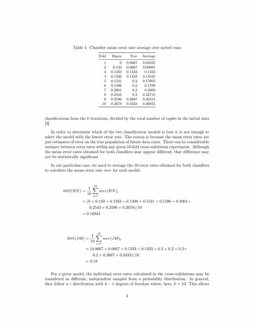
Table 1: Classifier mean error rate average over sorted runs
Fold Bayes Tree Average
1 0 0.0667 0.033352 0.133 0.0667 0.099853 0.1333 0.1333 0.13334 0.1336 0.1333 0.133455 0.1521 0.2 0.176056 0.1596 0.2 0.17987 0.2001 0.2 0.20008 0.2543 0.2 0.227159 0.2596 0.2667 0.26315
10 0.2678 0.3333 0.30055
classifications from the k iterations, divided by the total number of tuples in the initial data[3].
In order to determine which of the two classification models is best it is not enough toselect the model with the lowest error rate. The reason is because the mean error rates arejust estimates of error on the true population of future data cases. There can be considerablevariance between error rates within any given 10-fold cross-validation experiment. Althoughthe mean error rates obtained for both classifiers may appear different, that difference maynot be statistically significant.
In our particular case, we need to average the 10 error rates obtained for both classifiersto calculate the mean error rate mer for each model:
mer(BN) =1
10
10∑i=1
mer(BN)i
= (0 + 0.133 + 0.1333 + 0.1336 + 0.1521 + 0.1596 + 0.2001+
0.2543 + 0.2596 + 0.2678)/10
= 0.16934
mer(J48) =1
10
10∑i=1
mer(J48)i
= (0.0667 + 0.0667 + 0.1333 + 0.1333 + 0.2 + 0.2 + 0.2+
0.2 + 0.2667 + 0.3333)/10
= 0.18
For a given model, the individual error rates calculated in the cross-validations may beconsidered as different, independent samples from a probability distribution. In general,they follow a t distribution with k − 1 degrees of freedom where, here, k = 10. This allows
3

us to do hypothesis testing where the significance test used is the t-test, or Student’s t-test,discussed in the next section.
The variance is a numerical measure of how the data values are dispersed around themean. In particular, the sample variance is defined as:
σ2 =1
n− 1
n∑i=1
(xi − µ)2
Variances obtained for Bayes and Decision Tree classifier respectively are:
var(BN) = 0.0065
var(J48) = 0.0069
5 t-Student Test
5.1 Definition
The t-Student test is a parametric test applied to find out whether the difference in meansbetween the results of two classifiers applied to the same data set with matching random-izations and partitions is significant.
The t-statistic for pairwise comparison between two classifiers C1 and C2 is computedas follows:
t =mer(C1)−mer(C2)√
var(C1 − C2)/k
where
var(C1 − C2) =1
k − 1
k∑i=1
[mer(C1)i −mer(C2)i − (mer(C1)−mer(C2))]2
mer(C1)i and mer(C2)i are the error rates of model C1 and C2 respectively, on round i.The error rates for C1 are averaged to obtain a mean error rate for C1, denoted mer(C1).Similarly mer(C2) is obtained. The variance of the difference between the two models isdenoted var(C1 − C2).
5.2 Results
For our example, t calculation is below:
4
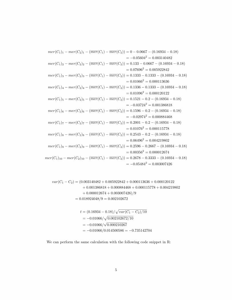
mer(C1)1 −mer(C2)1 − (mer(C1)−mer(C2)) = 0− 0.0667− (0.16934− 0.18)
= −0.056042 = 0.003140482
mer(C1)2 −mer(C2)2 − (mer(C1)−mer(C2)) = 0.133− 0.0667− (0.16934− 0.18)
= 0.076962 = 0.005922842
mer(C1)3 −mer(C2)3 − (mer(C1)−mer(C2)) = 0.1333− 0.1333− (0.16934− 0.18)
= 0.010662 = 0.000113636
mer(C1)4 −mer(C2)4 − (mer(C1)−mer(C2)) = 0.1336− 0.1333− (0.16934− 0.18)
= 0.010962 = 0.000120122
mer(C1)5 −mer(C2)5 − (mer(C1)−mer(C2)) = 0.1521− 0.2− (0.16934− 0.18)
= −0.037242 = 0.001386818
mer(C1)6 −mer(C2)6 − (mer(C1)−mer(C2)) = 0.1596− 0.2− (0.16934− 0.18)
= −0.029742 = 0.000884468
mer(C1)7 −mer(C2)7 − (mer(C1)−mer(C2)) = 0.2001− 0.2− (0.16934− 0.18)
= 0.010762 = 0.000115778
mer(C1)8 −mer(C2)8 − (mer(C1)−mer(C2)) = 0.2543− 0.2− (0.16934− 0.18)
= 0.064962 = 0.004219802
mer(C1)9 −mer(C2)9 − (mer(C1)−mer(C2)) = 0.2596− 0.2667− (0.16934− 0.18)
= 0.003562 = 0.000012674
mer(C1)10 −mer(C2)10 − (mer(C1)−mer(C2)) = 0.2678− 0.3333− (0.16934− 0.18)
= −0.054842 = 0.003007426
var(C1 − C2) = (0.003140482 + 0.005922842 + 0.000113636 + 0.000120122
+ 0.001386818 + 0.000884468 + 0.000115778 + 0.004219802
+ 0.000012674 + 0.003007426)/9
= 0.018924048/9 = 0.002102672
t = (0.16934− 0.18)/√var(C1 − C2)/10
= −0.01066/√
0.002102672/10
= −0.01066/√0.000210267
= −0.01066/0.014500586 = −0.735142704
We can perform the same calculation with the following code snippet in R:
5

> x <− c ( 0 , 0 . 1 330 , 0 . 1 333 , 0 . 1 336 , 0 . 1 521 , 0 . 1 596 , 0 . 2 001 , 0 . 2 543 , 0 . 2 596 , 0 . 2 678 )> y <− c ( 0 . 0 6 6 7 , 0 . 0 6 6 7 , 0 . 1 3 3 3 , 0 . 1 3 3 3 , 0 . 2 , 0 . 2 , 0 . 2 , 0 . 2 , 0 . 2 6 6 7 , 0 . 3 3 3 3 )> t . test (x , y , paired=T )
Paired t−test
data : x and yt = −0.7351 , df = 9 , p−value = 0.481alternative hypothesis : true difference in means i s not equal to 095 percent confidence interval :−0.04346262 0.02214262
sample estimates :mean of the differences
−0.01066
To determine whether C1 and C2 are significantly different, t is computed and a signif-icance level, sig, is selected. In practice, a significance level of 5% or 1% is typically used.For our test, we use 5%. This value is implying that the difference between C1 and C2 issignificantly different for 95% of the population.
The confidence limit z is defined as sig/2, which in this case is 0.025. If t > z or t < −z,then our value of t lies in the rejection region, within the tails of the distribution. Thismeans that we can reject the null hypothesis that the means of C1 and C2 are the same andconclude that there is a statistically significant difference between the two models. In ourtest, as –0.7351 < 0.025 we cannot reject the null hypothesis. We then conclude that anydifference between C1 and C2 can be attributed to chance.
Another way of doing the same validation considering the results obtained using R isto check the p-value returned. If the p-value is greater than 0.05, then we can acceptthe hypothesis of equality of the means. In conclusion, there are no statistical differencesbetween both classifiers.
6 Conclusion
A comparison between the Bayes and the J48 decision tree classifier performance over theiris.arff test data has been performed. In order to know if the performance differencebetween the two is statistically significant, a t-Student test has been applied over the dataresults collected from Weka. No statistical differences have been found between the two.Results have been presented and analyzed.
References
[1] R. Bouckaert. Bayesian network classifiers in Weka. Tech. rep. 14/2004. Departmentof Computer Science, Hamilton, New Zealand: The University of Waikato, 2004.
[2] Remco Bouckaert. “Estimating Replicability of Classifier Learning Experiments”. In:In Proceedings of ICML. 2004.
[3] Jiawei Han. Data Mining: Concepts and Techniques. San Francisco, CA, USA: MorganKaufmann Publishers Inc., 2005.
6

[4] Wikimedia Foundation Inc. Wikipedia. http://en.wikipedia.org/wiki/Decision_tree_learning. 2012.
7
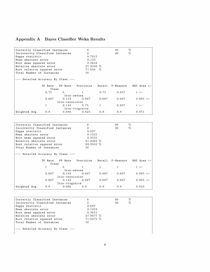
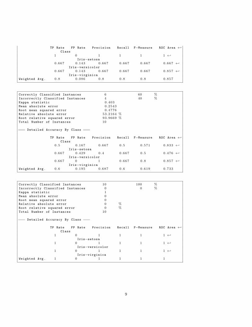
Appendix A Bayes Classifier Weka Results
Correctly Classified Instances 8 80 %Incorrectly Classified Instances 2 20 %Kappa statistic 0 .7015Mean absolute error 0 .133Root mean squared error 0 .3642Relative absolute error 27.8346 %Root relative squared error 71 .656 %Total Number of Instances 10
=== Detailed Accuracy By Class ===
TP Rate FP Rate Precision Recall F−Measure ROC Area ←↩Class
0 .75 0 1 0 .75 0 .857 1 ←↩Iris−setosa
0 .667 0 .143 0 .667 0 .667 0 .667 0 .905 ←↩Iris−versicolor
1 0 .143 0 .75 1 0 .857 1 ←↩Iris−virginica
Weighted Avg . 0 . 8 0 .086 0 .825 0 .8 0 .8 0 .971
Correctly Classified Instances 8 80 %Incorrectly Classified Instances 2 20 %Kappa statistic 0 .697Mean absolute error 0 .1521Root mean squared error 0 .3555Relative absolute error 31.8403 %Root relative squared error 69.9502 %Total Number of Instances 10
=== Detailed Accuracy By Class ===
TP Rate FP Rate Precision Recall F−Measure ROC Area ←↩Class
1 0 1 1 1 1 ←↩Iris−setosa
0 .667 0 .143 0 .667 0 .667 0 .667 0 .905 ←↩Iris−versicolor
0 .667 0 .143 0 .667 0 .667 0 .667 0 .905 ←↩Iris−virginica
Weighted Avg . 0 . 8 0 .086 0 .8 0 .8 0 .8 0 .943
Correctly Classified Instances 8 80 %Incorrectly Classified Instances 2 20 %Kappa statistic 0 .697Mean absolute error 0 .1333Root mean squared error 0 .3651Relative absolute error 27.9077 %Root relative squared error 71.8375 %Total Number of Instances 10
=== Detailed Accuracy By Class ===
8
TP Rate FP Rate Precision Recall F−Measure ROC Area ←↩Class
1 0 1 1 1 1 ←↩Iris−setosa
0 .667 0 .143 0 .667 0 .667 0 .667 0 .667 ←↩Iris−versicolor
0 .667 0 .143 0 .667 0 .667 0 .667 0 .857 ←↩Iris−virginica
Weighted Avg . 0 . 8 0 .086 0 .8 0 .8 0 .8 0 .857
Correctly Classified Instances 6 60 %Incorrectly Classified Instances 4 40 %Kappa statistic 0 .403Mean absolute error 0 .2543Root mean squared error 0 .4776Relative absolute error 53.2164 %Root relative squared error 93.9669 %Total Number of Instances 10
=== Detailed Accuracy By Class ===
TP Rate FP Rate Precision Recall F−Measure ROC Area ←↩Class
0 .5 0 .167 0 .667 0 .5 0 .571 0 .833 ←↩Iris−setosa
0 .667 0 .429 0 .4 0 .667 0 .5 0 .476 ←↩Iris−versicolor
0 .667 0 1 0 .667 0 .8 0 .857 ←↩Iris−virginica
Weighted Avg . 0 . 6 0 .195 0 .687 0 .6 0 .619 0 .733
Correctly Classified Instances 10 100 %Incorrectly Classified Instances 0 0 %Kappa statistic 1Mean absolute error 0Root mean squared error 0Relative absolute error 0 %Root relative squared error 0 %Total Number of Instances 10
=== Detailed Accuracy By Class ===
TP Rate FP Rate Precision Recall F−Measure ROC Area ←↩Class
1 0 1 1 1 1 ←↩Iris−setosa
1 0 1 1 1 1 ←↩Iris−versicolor
1 0 1 1 1 1 ←↩Iris−virginica
Weighted Avg . 1 0 1 1 1 1
9
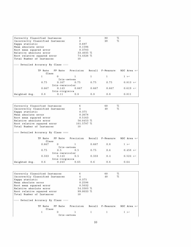
Correctly Classified Instances 8 80 %Incorrectly Classified Instances 2 20 %Kappa statistic 0 .697Mean absolute error 0 .1596Root mean squared error 0 .3783Relative absolute error 33.4035 %Root relative squared error 74.4326 %Total Number of Instances 10
=== Detailed Accuracy By Class ===
TP Rate FP Rate Precision Recall F−Measure ROC Area ←↩Class
1 0 1 1 1 1 ←↩Iris−setosa
0 .75 0 .167 0 .75 0 .75 0 .75 0 .813 ←↩Iris−versicolor
0 .667 0 .143 0 .667 0 .667 0 .667 0 .619 ←↩Iris−virginica
Weighted Avg . 0 . 8 0 .11 0 .8 0 .8 0 .8 0 .811
Correctly Classified Instances 6 60 %Incorrectly Classified Instances 4 40 %Kappa statistic 0 .375Mean absolute error 0 .2678Root mean squared error 0 .5163Relative absolute error 56.0453 %Root relative squared error 101.5787 %Total Number of Instances 10
=== Detailed Accuracy By Class ===
TP Rate FP Rate Precision Recall F−Measure ROC Area ←↩Class
0 .667 0 1 0 .667 0 .8 1 ←↩Iris−setosa
0 .75 0 .5 0 .5 0 .75 0 .6 0 .458 ←↩Iris−versicolor
0 .333 0 .143 0 .5 0 .333 0 .4 0 .524 ←↩Iris−virginica
Weighted Avg . 0 . 6 0 .243 0 .65 0 .6 0 .6 0 .64
Correctly Classified Instances 6 60 %Incorrectly Classified Instances 4 40 %Kappa statistic 0 .375Mean absolute error 0 .2596Root mean squared error 0 .5032Relative absolute error 54.3303 %Root relative squared error 99.0033 %Total Number of Instances 10
=== Detailed Accuracy By Class ===
TP Rate FP Rate Precision Recall F−Measure ROC Area ←↩Class
1 0 1 1 1 1 ←↩Iris−setosa
10

0 .75 0 .5 0 .5 0 .75 0 .6 0 .833 ←↩Iris−versicolor
0 0 .143 0 0 0 0 .81 ←↩Iris−virginica
Weighted Avg . 0 . 6 0 .243 0 .5 0 .6 0 .54 0 .876
Correctly Classified Instances 8 80 %Incorrectly Classified Instances 2 20 %Kappa statistic 0 .6875Mean absolute error 0 .1336Root mean squared error 0 .365Relative absolute error 27.9722 %Root relative squared error 71.8189 %Total Number of Instances 10
=== Detailed Accuracy By Class ===
TP Rate FP Rate Precision Recall F−Measure ROC Area ←↩Class
0 .667 0 1 0 .667 0 .8 0 .952 ←↩Iris−setosa
1 0 .333 0 .667 1 0 .8 0 .792 ←↩Iris−versicolor
0 .667 0 1 0 .667 0 .8 0 .952 ←↩Iris−virginica
Weighted Avg . 0 . 8 0 .133 0 .867 0 .8 0 .8 0 .888
Correctly Classified Instances 7 70 %Incorrectly Classified Instances 3 30 %Kappa statistic 0 .5385Mean absolute error 0 .2001Root mean squared error 0 .4459Relative absolute error 41.8745 %Root relative squared error 87.7265 %Total Number of Instances 10
=== Detailed Accuracy By Class ===
TP Rate FP Rate Precision Recall F−Measure ROC Area ←↩Class
1 0 1 1 1 1 ←↩Iris−setosa
0 .75 0 .333 0 .6 0 .75 0 .667 0 .792 ←↩Iris−versicolor
0 .333 0 .143 0 .5 0 .333 0 .4 0 .714 ←↩Iris−virginica
Weighted Avg . 0 . 7 0 .176 0 .69 0 .7 0 .687 0 .831
11

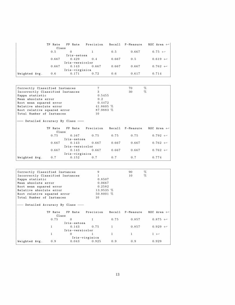
Appendix B J48 Decision Tree Classifier Weka Results
Correctly Classified Instances 8 80 %Incorrectly Classified Instances 2 20 %Kappa statistic 0 .7015Mean absolute error 0 .1333Root mean squared error 0 .3651Relative absolute error 27 .907 %Root relative squared error 71.8421 %Total Number of Instances 10
=== Detailed Accuracy By Class ===
TP Rate FP Rate Precision Recall F−Measure ROC Area ←↩Class
0 .75 0 1 0 .75 0 .857 0 .875 ←↩Iris−setosa
0 .667 0 .143 0 .667 0 .667 0 .667 0 .762 ←↩Iris−versicolor
1 0 .143 0 .75 1 0 .857 0 .929 ←↩Iris−virginica
Weighted Avg . 0 . 8 0 .086 0 .825 0 .8 0 .8 0 .857
Correctly Classified Instances 7 70 %Incorrectly Classified Instances 3 30 %Kappa statistic 0 .5455Mean absolute error 0 .2Root mean squared error 0 .4472Relative absolute error 41.8605 %Root relative squared error 87.9883 %Total Number of Instances 10
=== Detailed Accuracy By Class ===
TP Rate FP Rate Precision Recall F−Measure ROC Area ←↩Class
1 0 1 1 1 1 ←↩Iris−setosa
0 .667 0 .286 0 .5 0 .667 0 .571 0 .69 ←↩Iris−versicolor
0 .333 0 .143 0 .5 0 .333 0 .4 0 .595 ←↩Iris−virginica
Weighted Avg . 0 . 7 0 .129 0 .7 0 .7 0 .691 0 .786
Correctly Classified Instances 6 60 %Incorrectly Classified Instances 4 40 %Kappa statistic 0 .4118Mean absolute error 0 .2667Root mean squared error 0 .5164Relative absolute error 55 .814 %Root relative squared error 101.6001 %Total Number of Instances 10
=== Detailed Accuracy By Class ===
12
TP Rate FP Rate Precision Recall F−Measure ROC Area ←↩Class
0 .5 0 1 0 .5 0 .667 0 .75 ←↩Iris−setosa
0 .667 0 .429 0 .4 0 .667 0 .5 0 .619 ←↩Iris−versicolor
0 .667 0 .143 0 .667 0 .667 0 .667 0 .762 ←↩Iris−virginica
Weighted Avg . 0 . 6 0 .171 0 .72 0 .6 0 .617 0 .714
Correctly Classified Instances 7 70 %Incorrectly Classified Instances 3 30 %Kappa statistic 0 .5455Mean absolute error 0 .2Root mean squared error 0 .4472Relative absolute error 41.8605 %Root relative squared error 87.9883 %Total Number of Instances 10
=== Detailed Accuracy By Class ===
TP Rate FP Rate Precision Recall F−Measure ROC Area ←↩Class
0 .75 0 .167 0 .75 0 .75 0 .75 0 .792 ←↩Iris−setosa
0 .667 0 .143 0 .667 0 .667 0 .667 0 .762 ←↩Iris−versicolor
0 .667 0 .143 0 .667 0 .667 0 .667 0 .762 ←↩Iris−virginica
Weighted Avg . 0 . 7 0 .152 0 .7 0 .7 0 .7 0 .774
Correctly Classified Instances 9 90 %Incorrectly Classified Instances 1 10 %Kappa statistic 0 .8507Mean absolute error 0 .0667Root mean squared error 0 .2582Relative absolute error 13.9535 %Root relative squared error 50.8001 %Total Number of Instances 10
=== Detailed Accuracy By Class ===
TP Rate FP Rate Precision Recall F−Measure ROC Area ←↩Class
0 .75 0 1 0 .75 0 .857 0 .875 ←↩Iris−setosa
1 0 .143 0 .75 1 0 .857 0 .929 ←↩Iris−versicolor
1 0 1 1 1 1 ←↩Iris−virginica
Weighted Avg . 0 . 9 0 .043 0 .925 0 .9 0 .9 0 .929
13
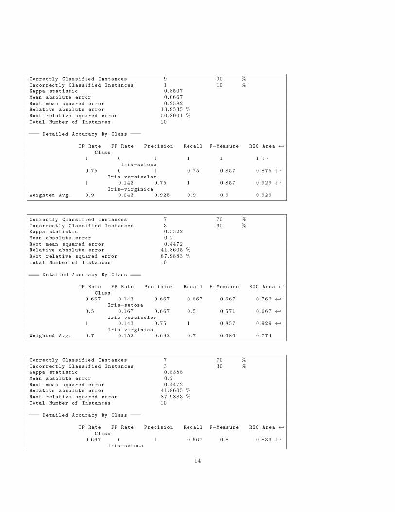
Correctly Classified Instances 9 90 %Incorrectly Classified Instances 1 10 %Kappa statistic 0 .8507Mean absolute error 0 .0667Root mean squared error 0 .2582Relative absolute error 13.9535 %Root relative squared error 50.8001 %Total Number of Instances 10
=== Detailed Accuracy By Class ===
TP Rate FP Rate Precision Recall F−Measure ROC Area ←↩Class
1 0 1 1 1 1 ←↩Iris−setosa
0 .75 0 1 0 .75 0 .857 0 .875 ←↩Iris−versicolor
1 0 .143 0 .75 1 0 .857 0 .929 ←↩Iris−virginica
Weighted Avg . 0 . 9 0 .043 0 .925 0 .9 0 .9 0 .929
Correctly Classified Instances 7 70 %Incorrectly Classified Instances 3 30 %Kappa statistic 0 .5522Mean absolute error 0 .2Root mean squared error 0 .4472Relative absolute error 41.8605 %Root relative squared error 87.9883 %Total Number of Instances 10
=== Detailed Accuracy By Class ===
TP Rate FP Rate Precision Recall F−Measure ROC Area ←↩Class
0 .667 0 .143 0 .667 0 .667 0 .667 0 .762 ←↩Iris−setosa
0 .5 0 .167 0 .667 0 .5 0 .571 0 .667 ←↩Iris−versicolor
1 0 .143 0 .75 1 0 .857 0 .929 ←↩Iris−virginica
Weighted Avg . 0 . 7 0 .152 0 .692 0 .7 0 .686 0 .774
Correctly Classified Instances 7 70 %Incorrectly Classified Instances 3 30 %Kappa statistic 0 .5385Mean absolute error 0 .2Root mean squared error 0 .4472Relative absolute error 41.8605 %Root relative squared error 87.9883 %Total Number of Instances 10
=== Detailed Accuracy By Class ===
TP Rate FP Rate Precision Recall F−Measure ROC Area ←↩Class
0 .667 0 1 0 .667 0 .8 0 .833 ←↩Iris−setosa
14
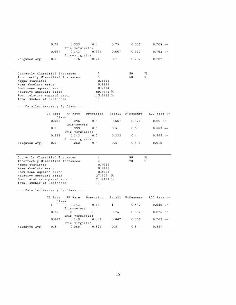
0 .75 0 .333 0 .6 0 .75 0 .667 0 .708 ←↩Iris−versicolor
0 .667 0 .143 0 .667 0 .667 0 .667 0 .762 ←↩Iris−virginica
Weighted Avg . 0 . 7 0 .176 0 .74 0 .7 0 .707 0 .762
Correctly Classified Instances 5 50 %Incorrectly Classified Instances 5 50 %Kappa statistic 0 .2424Mean absolute error 0 .3333Root mean squared error 0 .5774Relative absolute error 69.7674 %Root relative squared error 113.5924 %Total Number of Instances 10
=== Detailed Accuracy By Class ===
TP Rate FP Rate Precision Recall F−Measure ROC Area ←↩Class
0 .667 0 .286 0 .5 0 .667 0 .571 0 .69 ←↩Iris−setosa
0 .5 0 .333 0 .5 0 .5 0 .5 0 .583 ←↩Iris−versicolor
0 .333 0 .143 0 .5 0 .333 0 .4 0 .595 ←↩Iris−virginica
Weighted Avg . 0 . 5 0 .262 0 .5 0 .5 0 .491 0 .619
Correctly Classified Instances 8 80 %Incorrectly Classified Instances 2 20 %Kappa statistic 0 .7015Mean absolute error 0 .1333Root mean squared error 0 .3651Relative absolute error 27 .907 %Root relative squared error 71.8421 %Total Number of Instances 10
=== Detailed Accuracy By Class ===
TP Rate FP Rate Precision Recall F−Measure ROC Area ←↩Class
1 0 .143 0 .75 1 0 .857 0 .929 ←↩Iris−setosa
0 .75 0 1 0 .75 0 .857 0 .875 ←↩Iris−versicolor
0 .667 0 .143 0 .667 0 .667 0 .667 0 .762 ←↩Iris−virginica
Weighted Avg . 0 . 8 0 .086 0 .825 0 .8 0 .8 0 .857
15