Control-Relevant Modeling, Analysis, and Design for Scramjet-Powered Hypersonic Vehicles

Control-Relevant Modeling, Analysis, and Design for

Scramjet-Powered Hypersonic Vehicles

Armando A. Rodriguez ∗ Jeffrey J. Dickeson † Srikanth Sridharan ‡

Akshay Korad § Jaidev Khatri ¶

Dept. of Electrical Eng., Fulton School of Eng., Arizona State University, Tempe, AZ, 85287, U.S.A.

Jose Benavides ‖ Don Soloway ∗∗

Guidance, Navigation, and Control, NASA Ames Research Center, Moffett Field, CA, 94035, U.S.A.

Atul Kelkar †† Jerald M. Vogel ‡‡

Dept. of Aerospace Eng., College of Eng., Iowa State University, Ames, IA, 50011, U.S.A.

Within this paper, control-relevant vehicle design concepts are examined using a widelyused 3 DOF (plus flexibility) nonlinear model for the longitudinal dynamics of a genericcarrot-shaped scramjet powered hypersonic vehicle. Trade studies associated with vehi-cle/engine parameters are examined. The impact of parameters on control-relevant staticproperties (e.g. level-flight trimmable region, trim controls, AOA, thrust margin) and dy-namic properties (e.g. instability and right half plane zero associated with flight path an-gle) are examined. Specific parameters considered include: inlet height, diffuser area ratio,lower forebody compression ramp inclination angle, engine location, center of gravity, andmass. Vehicle optimizations is also examined. Both static and dynamic considerations areaddressed. The gap-metric optimized vehicle is obtained to illustrate how this control-centric concept can be used to “reduce” scheduling requirements for the final controlsystem. A classic inner-outer loop control architecture and methodology is used to shedlight on how specific vehicle/engine design parameter selections impact control system de-sign. In short, the work represents an important first step toward revealing fundamentaltradeoffs and systematically treating control-relevant vehicle design.

I. INTRODUCTION AND OVERVIEW

Motivation. With the historic 2004 scramjet-powered Mach 7 and 10 flights of the X-43A1–4 , hypersonicsresearch has seen a resurgence. This is attributable to the fact that air-breathing hypersonic propulsion isviewed as the next critical step toward achieving (1) reliable, affordable, routine access to space, as well as(2) global reach vehicles. Both of these objectives have commercial as well as military implications. Whilerocket-based (combined cycle) propulsion systems5 are needed to reach orbital speeds, they are much moreexpensive to operate because they must carry oxygen. This is particularly costly when traveling at loweraltitudes through the troposphere (i.e. below 36,152 ft). Current rocket-based systems also do not exhibitthe desired levels of reliability and flexibility (e.g. airplane like takeoff and landing options). For this reason,

∗Professor, Dept. of Electrical Engineering, Arizona State University, and AIAA Member. This research has been supported,in part, by NASA grant NNX07AC42A.

†NASA PhD Fellow, Dept. of Electrical Engineering, Arizona State University, and AIAA Student Member.‡MS Student, Dept. of Electrical Engineering, Arizona State University, and AIAA Student Member.§MS Student, Dept. of Electrical Engineering, Arizona State University, and AIAA Student Member.¶MS Student, Dept. of Electrical Engineering, Arizona State University, and AIAA Student Member.‖Hardware/Controls Engineer, Mission Critical Technologies, Inc. and AIAA Member.

∗∗Hypersonics Project Associate Principal Investigator, NASA Ames Research Center, and AIAA Member.††Professor, Dept. of Aerospace Engineering, Iowa State University, and AIAA Member.‡‡Emeritus Professor, Dept. of Aerospace Engineering, Iowa State University, and AIAA Member.This research has been

supported, in part, by NASA grant NNL08AA38C.

1 of 45

American Institute of Aeronautics and Astronautics

much emphasis has been placed on two-stage-to-orbit (TSTO) designs that involve a turbo-ram-scramjetcombined cycle first stage and a rocket-scramjet second stage. This paper focuses on control challengesassociated with scramjet-powered hypersonic vehicles. Such vehicles are characterized by significant aero-thermo-elastic-propulsion interactions and uncertainty1–18.

Controls-Relevant Hypersonic Vehicle Modeling. The following significant body of work (2005-2007)7–9, 19–28 examines aero-thermo-elastic-propulsion modeling and control issues using a first principlesnonlinear 3-DOF longitudinal dynamical model which exploits inviscid compressible oblique shock-expansiontheory to determine aerodynamic forces and moments, a 1D Rayleigh flow scramjet propulsion model witha variable geometry inlet, and an Euler-Bernoulli beam based flexible model. The vehicle is 100 ft long withweight (density) 6154 lb per foot of depth and has a bending mode at about 21 rad/sec. The controls include:elevator, stoichiometrically normalized fuel equivalency ratio (FER), diffuser area ratio (not considered inthis work), and a canard (not considered in this work). A more complete description of the vehicle modelcan be found in previous works7, 29.

More recent modeling efforts have focused on improved propulsion modeling30, 31 that captures precombus-tion shocks, dissociation, wall heat transfer, skin friction, fuel-air mixing submodel, and finite-rate chemistry.The computational time associated with the enhanced model is significant, thus making it cumbersome forcontrol-relevant analysis. The simple 1D Rayleigh flow engine model discussed within7, 19, 26, 29 will be usedin the current paper.

Hypersonic Vehicle Control Issues. Within this paper, we exploit the generic carrot-shaped vehicle3DOF (plus flexibility) model presented in7, 19, 26, 29. A myriad of issues exist that make control design forthis hypersonic vehicle a potentially challenging problem:

• Input/Output Coupling. For this system, velocity control is achieved via the FER input. Flight pathangle (FPA) control is achieved with the elevator32. However, there is significant coupling betweenFER and FPA.

• Unstable/Nonminimum Phase. Tail controlled vehicles are characterized by a non-minimum phase(right half plane, RHP) zero that is associated with the elevator to FPA map28. This RHP zero limitsthe achievable elevator-FPA bandidth (BW)33–35. In addition, the rearward situated scramjet and cg(center of gravity), implies an inherent pitch-up vehicle instability. This instability requires a minimumBW for stabilization29. To address these potentially conflicting specifications, one approach has beento exploit the addition of a canard19, 32, 36–38. It is understood, of course, that any canard approachwould face severe heating, structural, and reliability issues.

• Varying Dynamic Characteristics. Within29, it is shown that the nonlinear model changes significantlyas a function of the flight condition. Specifically, it is shown that the vehicle pitch-up instability andnon-minimum phase (NMP) zero vary significantly across the vehicle’s trimmable region. In addition,the mass of the vehicle can be varied during a simulation in order to represent fuel consumption.Several methods have been presented in the literature to deal with the nonlinear nature of the model.

Papers addressing modeling issues include: nonlinear modeling of longitudinal dynamics28, heatingeffects and flexible dynamics9, 24, 39, FPA dynamics36, unsteady and viscous effects8, 20, and high fidelityengine modeling30, 31, 40.

Papers addressing nonlinear control issues include: control via classic inner-outer loop architecture41,nonlinear robust/adaptive control32, robust linear output feedback38, control-oriented modeling19, lin-ear parameter-varying control of flexible dynamics42, saturation prevention22, 43, 44, and thermal chokingprevention29, 44.

• Uncertain Flexible Modes and Coupling to Propulsion. Flexible dynamics have been captured withinthe model by approximating a free-free Euler-Bernoulli beam using the assumed modes method24.Three flexible modes are used to approximate the structural dynamics. A damping factor of ζ = 0.02is assumed. The associated mode frequencies are ω1 = 21.02 rad/sec, ω2 = 50.87 rad/sec, ω3 = 101rad/sec. These modes must be adequately addressed within the control system design process. Whileperformance can be improved by increasing controller complexity (e.g. higher order notches)42, one

2 of 45


must be wary of, and careful in dealing with, modal/damping uncertainty issues. This is particularlyimportant because structural flexing impacts the bow shock. This, in turn impacts the scramjet’s inletproperties, thrust generated, aft body forces, the associated pitching moments, and hence the vehicle’sattitude. Given the tight altitude-Mach flight regime - within the air-breathing corridor5 - that suchvehicle must operate within, the concern is amplified. In short, one must be careful that the controlsystem BW and complexity are properly balanced so that these lightly damped flexible modes are notoverly excited.

• Control Saturation Constraints. Control saturation is of particular concern for unstable vehicles suchas the one under consideration. Two specific saturation nonlinearities are a concern for any controlsystem implementation.

– Maximum Elevator/Canard Deflection and Instability. FPA is controlled via the elevator/canardcombination36. Because these dynamics are inherently unstable, elevator saturation can resultin instability43. Classical anti-windup methods may be inadequate to address the associated is-sues - particularly when the vehicle is open loop unstable. The constraint enforcement methodwithin43, 45 and generalized predictive control46 have been used to address such issues.It should be noted that control surface/actuator rate limits must also be properly addressed bythe control system in order to avoid instability.

– Thermal Choking/Unity FER: State Dependent Constraint. As heat is added within the combus-tor, the supersonic air flow is slowed. If enough heat is added, the combustor exit Mach numberwill approach unity, and the flow is said to be thermally choked47. If additional heat is added,the upstream conditions can be altered. This can (in principle) lead to engine unstart5 - a highlyundesirable condition. The amount of FER that causes thermal choking at a particular flightcondition is referred to as the thermal choking FER, or FERTC . In general, FERTC dependsupon the free-stream Mach, free-stream temperature, pressure, and density (which depend on thealtitude), and the flow turn angle (vehicle geometry + AOA + elastic deflection)29, 46. In addition,since the model does not capture what happens when FER ≥ 128, it is natural to restrict FERbelow unity. Given the above, it follows that the minimum of these two constraints dictates theavailable FER at a given flight condition. The resulting state dependent FER constraint can becomputed (on-line) based on the flight condition, and must be accounted for by the control law.Here, uncertainty is of great concern because of the potential unstart issues - issues not capturedwithin the model. Engineers, of course, would try to “build-in protection” so that this is avoided.As such, engineers are forced to tradeoff operational envelop for enhance unstart protection.

Control-Relevant Vehicle Design Issues. Despite the successful integrated approach taken by the X-43A team, as well as other prior successful flight control efforts, far too often aerospace vehicle design has notsignificantly involved the discipline of controls until very late in the vehicle design process or even afterwards.Research programs over the past two decades have suggested that for the anticipated hypersonic vehicles, thetraditional “sequential” approach is not likely to work. This is attributable, in part, to complex uncertainnonlinear coupled unstable, non-minimum phase, flexible dynamics together with stringent flight corridorand variable constraints (e.g. specific impulse, fuel use, maximum dynamic pressure, engine temperaturesand pressures). For such vehicles, an integrated multidisciplinary “parallel” approach - involving multipledisciplines up front - is essential. This is particularly true when tight flight control specifications must besatisfied in the presence of significant uncertainty.

Goals and Contributions of Paper. This paper addresses a myriad of issues that are of concern to bothvehicle and control system designers. In short, this paper represents a step toward answering the followingcritical control-relevant vehicle design questions:

1. How do vehicle/engine design properties impact a vehicle’s static and dynamic properties?

2. How do these impact control system design?

3. How should a hypersonic vehicle be designed to permit/facilitate the development of an adequatelyrobust control system?

4. What fundamental tradeoffs exist between vehicle design objectives and vehicle control objectives?

3 of 45


More specifically, in this paper we consider how the following parameters impact the static and dynamicproperties of a vehicle:

• engine inlet height, diffuser area ratio, compression ramp inclination, engine location (distance behindvehicle nose), vehicle cg (center-of-gravity), and vehicle mass

Vehicle optimization is also considered. It is specifically shown that a gap-optimized vehicle can “reduce”control system scheduling requirements. A classic decentralized inner-outer loop control system architectureis used to illustrate how vehicle/engine parameter selection The gap metric represents a system-theoreticmeasure that quantifies the “distance” between two dynamical systems and whether or not a common con-troller can be deployed for the systems under consideration48, 49. Within this paper, the gap metric is used toobtain a “gap-optimized vehicle” which “reduces” how much the vehicle varies throughout the trimmable re-gion is obtained. A nonlinear pull-up maneuver is used to show that a “gap-optimized vehicle” can “reduce”control system scheduling requirements. Future work will examine the utility of pursuing gap-optimizedvehicles or optimizing vehicles subject to gap constraints.

In short, this paper illustrates fundamental tradeoffs that vehicle and control system designers should jointlyconsider during the early stages of vehicle conceptualization/design. The paper also sheds light on howspecific vehicle/engine parameter selections impact control system design - thus providing a contribution tocontrol-relevant vehicle design. While vehicle designers may want to use a higher fidelity model (e.g. Eulerbased CFD with boundary layer reconstruction or Navier-Stokes based CFD50) to conduct more accuratevehicle trade studies, this paper shows that a (first principles) 3DOF nonlinear engineering model - suchas that used in the paper - may be very useful during the early stages of vehicle conceptualization and design.

Organization of Paper. The remainder of the paper is organized as follows.

• Section II provides an overview of the dynamical model to be used in our studies.

• Section III presents engine parameter trade study results as well as a new set of nominal engineparameter values.

• Section IV presents vehicle parameter trade study results.

• Section V presents vehicle optimization results.

• Section VI discusses how control system design is impacted by vehicle/engine design parameter selec-tion.

• Section VII summarizes the paper and presents directions for future research.

II. DESCRIPTION OF NONLINEAR MODEL

In this paper, we consider a first principles nonlinear 3-DOF dynamical model for the longitudinal dy-namics of a generic scramjet-powered hypersonic vehicle7–9, 19–28. The vehicle is 100 ft long with weight(density) 6,154 lb per foot of depth and has a bending mode at about 22 rad/sec. The controls include:elevator, stoichiometrically normalized fuel equivalency ratio (FER), diffuser area ratio (not considered inour work), and a canard. The vehicle may be visualized as shown in Figure 18.

Modeling Approach. The following summarizes the modeling approach that has been used.

• Aerodynamics. Pressure distributions are computed using inviscid compressible oblique-shock andPrandtl-Meyer expansion theory10, 16, 28, 47. Air is assumed to be calorically perfect; i.e. constant specificheats and specific heat ratio γ

def= cp

cv= 1.410, 47. A standard atmosphere is used.

Viscous drag effects (i.e. an analytical skin friction model) are captured using Eckerts temperaturereference method8, 10. This relies on using the incompressible turbulent skin friction coefficient formulafor a flat plate at a reference temperature. Of central importance to this method is the so-called walltemperature used. The model assumes a nominal wall temperature of 2500◦R8. While our analysis hasshown that this assumption is reasonable for conducting preliminary trade studies, the wall temperature

4 of 45


−20 0 20 40 60 80 100

−10

−8

−6

−4

−2

0

2

4

6

8

Feet

Fee

tP

u, M

u, T

u

P1, M

1, T

1

Pb, M

b, T

b

Pe, M

e, T

e

CG

τu

τl

τ2

Oblique Shock

Fre

estr

eam

Expansion Fan

Shear Layer (Plume)

CombustorNozzle

Elevator

Diffuser

Inlet

Figure 1. Schematic of Hypersonic Scramjet Vehicle

used should (in general) depend upon the flight condition being examined. As such, modeling heattransfer to the vehicle via parabolic heat equation partial differential equations (pdes) as well asmodeling a suitable thermal protection system is essential for obtaining insight into wall temperatureselection9. This will be addressed more comprehensively in a subsequent publication.

Unsteady effects (e.g. due to rotation and flexing) are captured using linear piston theory8, 51. The ideahere is that flow velocities induce pressures just as the pressure exerted by a piston on a fluid inducesa velocity.

• Propulsion. A single (long) forebody compression ramp provides conditions to the rear-shifted scramjetinlet. The inlet is a variable geometry inlet (variable geometry is not exploited in our work).

The model assumes the presence of an (infinitely fast) cowl door which uses AOA to achieve shock-on-lip conditions (assuming no forebody flexing). Forebody flexing, however, results in air mass flowspillage28. At the design cruise condition, the bow shock impinges on the engine inlet (assuming noflexing). At speeds below the design-flight condition and/or larger flow turning angles, the cowl movesforward to capture the shock. At larger speeds and/or smaller flow turning angles, the bow shock isswallowed by the engine. In either case, there is a shock reflected from the cowl or within the inlet(i.e. we have a bow shock reflection). This reflected shock further slows down the flow and steers itinto the engine. It should be noted that shock-shock interactions are not modeled. For example, atlarger speeds and smaller flow turning angles there is a shock off of the inlet lip. This shock interactswith the bow shock. This interaction is not captured in the model.

The model uses liquid hydrogen (LH2) as the fuel. It is assumed that fuel mass flow is negligiblecompared to the air mass flow. The model also captures linear fuel depletion. Thrust is linearlyrelated to FER for all expected FER values. For large FER values, the thrust levels off. In practice,when FER > 1, the result is decreased thrust. This phenomena28 is not captured in the model. Assuch, control designs based on this nonlinear model (or derived linear models) should try to maintainFER below unity.

The model also captures thermal choking. In what follows, we show how to compute the FER requiredto induce thermal choking as well as the so-called thermal choking FER margin. The above will lead to auseful FER margin definition - one that is useful for the design of control systems for scramjet-poweredhypersonic vehicles.

Finally, it should be noted that the model offers the capability for addressing linear fuel depletion.This feature was exploited for the nonlinear simulation presented in this paper.

• Structural. A single free-free Euler-Bernoulli beam partial differential equation (infinite dimensionalpde) model is used to capture vehicle elasticity. As such, out-of-plane loading, torsion, and Timoshenko

5 of 45


effects are neglected. The assumed modes method (based on a global basis) is used to obtain naturalfrequencies, mode shapes, and finite-dimensional approximants. This results in a model whereby therigid body dynamics influence the flexible dynamics through generalized forces. This is in contrast tothe model described within [28] which uses fore and aft cantilever beams (clamped at the center ofgravity) and leads to the rigid body modes being inertially coupled to the flexible modes (i.e. rigidbody modes directly excite flexible modes). Within the current model, forebody deflections influencethe rigid body dynamics via the bow shock which influences engine inlet conditions, thrust, lift, drag,and moment24. Aftbody deflections influence the AOA seen by the elevator. As such, flexible modesinfluence the rigid body dynamics.

The nominal vehicle is 100 ft long. The associated beam model is assumed to be made of titanium.It is 100 ft long, 9.6 inches high, and 1 ft wide (deep). This results in the nominal modal frequenciesω1 = 21.02 rad/sec, ω2 = 50.87 rad/sec, ω3 = 101 rad/sec. When the height is reduced to 6 inches,then we obtain the following reduced modal frequencies: ω1 = 10.38 rad/sec, ω2 = 25.13 rad/sec,ω3 = 49.89 rad/sec. Future work will examine vehicle mass-flexibility-control trade studies19.

• Actuator Dynamics. Simple first order actuator models (contained within the original model) were usedin each of the control channels: elevator - 20

s+20 , FER - 10s+10 , canard - 20

s+20 (Note: canard not used in ourstudy). These dynamics did not prove to be critical in our study. An elevator saturation of ±30◦ wasused.22, 43 It should be noted, however, that these limits were never reached in our studies41. Withinthis paper, we consider a pull up maneuver that does not result in elevator saturation. Future workwill consider more aggressive pull up maneuvers where elevator position and rate saturation becomevery important given the vehicle’s (open loop) unstable dynamics. A (state dependent) saturationlevel - associated with FER (e.g. thermal choking and unity FER) - was also directly addressed41. This(velocity bandwidth limiting) nonlinearity is discussed below.

Generally speaking, the vehicle exhibits unstable non-minimum phase dynamics with nonlinear aero-elastic-propulsion coupling and critical (state dependent) FER constraints. The model contains 11 states: 5 rigidbody states (speed, pitch, pitch rate, AOA, altitude) and 6 flexible states.

Unmodeled Phenomena/Effects. All models possess fundamental limitations. Realizing model limita-tions is crucial in order to avoid model misuse. Given this, we now provide a (somewhat lengthy) list ofphenomena/effects that are not captured within the above nonlinear model. (For reference purposes, flowphysics effects and modeling requirements for the X-43A are summarized within [52].)

• Dynamics. The above model does not capture longitudinal-lateral coupling and dynamics53 and theassociated 6DOF effects.

• Aerodynamics. Aerodynamic phenomena/effects not captured in the model include the following:boundary layer growth, displacement thickness, viscous interaction, entropy and vorticity effects, lam-inar versus turbulent flow, flow separation, high temperature and real gas effects (e.g. caloric im-perfection, electronic excitation, thermal imperfection, chemical reactions such as 02 dissociation)10,non-standard atmosphere (e.g. troposphere, stratosphere), unsteady atmospheric effects6, 3D effects,aerodynamic load limits.

• Propulsion. Propulsion phenomena/effects not captured in the model include the following: cowldoor dynamics, multiple forebody compression ramps (e.g. three on X-43A54, 55), forebody boundarylayer transition and turbulent flow to inlet54, 55, diffuser losses, shock interactions, internal shock effects,diffuser-combustor interactions, fuel injection and mixing, flame holding, engine ignition via pyrophoricsilane3 (requires finite-rate chemistry; cannot be predicted via equilibrium methods56, finite-rate chem-istry and the associated thrust-AOA-Mach-FER sensitivity effects31, internal and external nozzle losses,thermal choking induced phenomena (2D and 3D) and unstart, exhaust plume characteristics, cowldoor dynamics, combined cycle issues5.

Within [31], a higher fidelity propulsion model is presented which addresses internal shock effects,diffuser-combustor interaction, finite-rate chemistry and the associated thrust-AOA-Mach-FER sensi-tivity effects. While the nominal Rayleigh-based model (considered here) exhibits increasing thrust-AOA sensitivity with increasing AOA, the more complex model in31 exhibits reduced thrust-AOAsensitivity with increasing AOA - a behavior attributed to finite-chemistry effects.

6 of 45


Future work will examine the impact of internal engine losses, high temperature gas effects, andnozzle/plume issues.

• Structures. Structural phenomena/effects not captured in the model include the following: out of planeand torsional effects, internal structural layout, unsteady thermo-elastic heating effects, aerodynamicheating due to shock impingement, distinct material properties,57 and aero-servo-elasticity58, 59.

– Heating-Flexibility Issues. Finally, it should be noted that Bolender and Doman have addressed avariety of effects in their publications. For example, within [9,24] the authors address the impactof heating on (longitudinal) structural mode frequencies and mode shapes.Within [9], the authors consider a sustained two hour straight and level cruise at Mach 8, 85 kft.It is assumed that no fuel is consumed (to focus on the impact of heat addition). The paperassumes the presence of a thermal protection system (TPS) consisting of a PM2000 honeycombouter skin followed by a layer of silicon dioxide (SiO2) insulation. The vehicle - modeled by atitanium beam - is assumed to be insulated from the cryogenic fuel. The heat rate is computed viaclassic heat transfer equations that depend on speed (Mach), altitude (density), and the thermalproperties of the TPS materials as well as air - convection and radiation at the air-PM2000 surface,conduction within the three TPS materials. The initial temperature of all three TPS materialswas set to 559.67◦R = 100◦F ). The maximum heat rate (achieved at the flight’s inception)was approximately 12 BTU

ft2sec (1 foot aft of the nose). By the end of the two hour level flight,the average temperature within the titanium increased by 125◦R and it was observed that thevehicle’s (longitudinal) structural frequencies did not change appreciably (< 2%) [9, page 18].When one assumes a constant 15 BTU

ft2sec heat rate at the air-PM2000 surface (same initial TPStemperature of 559.67◦R = 100◦F ), then after two hours of level flight the average temperaturewithin the titanium increased by 200◦R [9, page 19]. In such a case, it can be shown that thevehicle’s (longitudinal) structural frequencies do not change appreciably (< 3%). This high heatrate scenario gives one an idea by how much the flexible mode frequencies can change by. Suchinformation is critical in order to suitably adapt/schedule the flight control system.Comprehensive heating-mass-flexibility-control studies will be examined further in a subsequentpublication.

• Actuator Dynamics. Future work will examine the impact of actuators that are rate limited; e.g. ele-vator, fuel pump.

It should be emphasized that the above list is only a partial list. If one needs fidelity at high Mach numbers,then many other phenomena become important; e.g. O2 dissociation10.

Longitudinal Dynamics. The equations of motion for the 3DOF flexible vehicle are given as follows:

v =[T cosα − D

m

]− g sin γ (1)

α = −[L + T sinα

mv

]+ q +

[g

v− v

RE + h

]cos γ (2)

q =MIyy

(3)

h = v sinγ (4)θ = q (5)

ηi = −2ζωiηi − ω2i ηi + Ni i = 1, 2, 3 (6)

γdef= θ − α (7)

g = g0

[RE

RE + h

]2

(8)

where L denotes lift, T denotes engine thrust, D denotes drag, M is the pitching moment, Ni denotesgeneralized forces, ζ demotes flexible mode damping factor, ωi denotes flexible mode undamped natural

7 of 45


frequencies, m denotes the vehicle’s total mass, Iyy is the pitch axis moment of inertia, g0 is the accelerationdue to gravity at sea level, and RE is the radius of the Earth.

• States. Vehicle states include: velocity v, FPA γ, altitude h, pitch rate q, pitch angle θ, and the flexiblebody states η1, η1, η2, η2, η3, η3. These eleven (11) states are summarized in Table 1.

� Symbol Description Units1 v speed kft/sec2 γ flight path angle deg3 α angle-of-attack (AOA) deg4 q pitch rate deg/sec5 h altitude ft6 η1 1st flex mode -7 η1 1st flex mode rate -8 η2 2nd flex mode -9 η2 2nd flex mode rate -10 η3 3rd flex mode -11 η3 3rd flex mode rate -

Table 1. States for Hypersonic Vehicle Model

• Controls. The vehicle has three (3) control inputs: a rearward situated elevator δe, a forward situatedcanard δc

a, and stoichiometrically normalized fuel equivalence ratio (FER). These control inputs aresummarized in Table 2. In this paper, we will only consider elevator and FER; i.e. the canard has beenremoved.

� Symbol Description Units1 FER stoichiometrically normalized fuel equivalence ratio -2 δe elevator deflection deg3 δc canard deflection deg

Table 2. Controls for Hypersonic Vehicle Model

In the above model, we note that the rigid body motion impacts the flexible dynamics through the generalizedforces. As discussed earlier, the flexible dynamics impact the rigid body motion through thrust, lift, drag,and moment. Nominal model parameter values for the vehicle under consideration are given in Table 3.Additional details about the model may be found within the following references7–9, 19–28.

Scramjet Model. The scramjet engine model is that used in28, 60. It consists of an inlet, an isentropicdiffuser, a 1D Rayleigh flow combustor (frictionless duct with heat addition47), and an isentropic internalnozzle. A single (long) forebody compression ramp provides conditions to the rear-shifted scramjet inlet.Although the model supports a variable geometry inlet, we will not be exploiting variable geometry in thispaper; i.e. diffuser area ratio Ad

def= A2A1

will be fixed with Ad = 1, see Figure 2).

Bow Shock Conditions. A bow shock will occur provided that the flow deflection angle δs is positive; i.e.

δsdef= AOA + forebody flexing angle + τ1l > 0◦ (9)

where τ1l = 6.2◦ is the lower forebody wedge angle (see Figure 1). If δs < 0, a Prandtl-Meyer expansionwill occur. Given the above, a bow shock occurs when the following flow turning angle (FTA) condition issatisfied:

FTA def= AOA + forebody flexing angle > −6.2◦. (10)aIn this paper, we have removed the canard. Future work will examine the potential utility of a canard as well as its viability.

8 of 45


Parameter Nominal Value Parameter Nominal ValueTotal Length (L) 100 ft Lower forebody angle (τ1L) 6.2o

Forebody Length (L1) 47 ft Tail angle (τ2) 14.342o

Aftbody Length (L2) 33 ft Mass per unit width 191.3024 slugs/ftEngine Length 20 ft Weight per unit width 6,154.1 lbs/ft

Engine inlet height hi 3.25 ft Mean Elasticity Modulus 8.6482× 107 psiUpper forebody angle (τ1U ) 3o Moment of Inertia Iyy 86,723 slugs ft2/ft

Elevator position (-85,-3.5) ft Center of gravity (-55,0) ftDiffuser exit/inlet area ratio 1 Elevator Area 17 ft2

Titanium Thickness 9.6 in Nozzle exit/inlet area ratio 6.35First Flex. Mode (ωn1) 22.2 rad/s Second Flex. Mode (ωn2) 48.1 rad/sThird Flex. Mode (ωn3) 94.8 rad/s Flex. Mode Damping (ζ) 0.02

Table 3. Vehicle Nominal Parameter Values

Figure 2. Schematic of Scramjet Engine

Properties Across Bow Shock. Let (M∞, T∞, p∞) denote the free-stream Mach, temperature, andpressure. Let γ

def= cp

cv= 1.4 denote the specific heat ratio for air - assumed constant in the model; i.e. air is

calorically perfect.10 The shock wave angle θs = θs(M∞, δs, γ) can be found as the middle root (weak shocksolution) of the following shock angle polynomial28, 47:

sin6θs + bsin4θs + csin2θs + d = 0 (11)

where

b = −M2∞ + 2M2∞

− γsin2δs c =2M2∞ + 1

M4∞+

[(γ + 1)2

4+

γ − 1M2∞

]sin2δs d = −cos2δs

M4∞(12)

The above can be addressed by solving the associated cubic in sin2θs. A direct solution is possible ifEmanuel’s 2001 method is used [47, page 143].

After determining the shock wave angle θs, one can determine properties across the bow shock using classicrelations from compressible flow [47, page 135]; i.e. Ms, Ts, ps - functions of (M∞, δs, γ):

Ts

T∞=

(2γM2∞ sin2 θs + 1 − γ)((γ − 1)M2∞ sin2 θs + 2)(γ + 1)2M2∞ sin2 θs

(13)

ps

p∞= 1 +

2γ

γ + 1(M2

∞ sin2 θs − 1)

(14)

M2s sin2(θs − δs) =

M2∞ sin2 θs(γ − 1) + 2

2γM2∞ sin2 θs − (γ − 1)(15)

9 of 45


It should be noted that for large M∞, the computed temperature Ts across the shock will be larger than itshould be because our assumption that air is calorically perfect (i.e. constant specific heats) does not captureother forms of energy absorption; e.g. electronic excitation and chemical reactions10.

Properties Across Prandtl-Meyer Expansion. An expansion fan occurs when there is a flow over aconvex corner; i.e. flow turns away from itself. More specifically to the bow, if δs < 0 a Prandtl-Meyerexpansion will occur. To determine the properties across the expansion, let (M∞, T∞, p∞) denote thefree-stream (supersonic) Mach, temperature, and pressure, respectively. If we let δ = −δs > 0 denote theexpansion ramp angle (in radians), the properties across the expansion fan (Me, Te, pe) can be calculatedas follows28, 47:

ν1 =√

γ + 1γ − 1

tan−1

(√γ − 1γ + 1

(M2∞ − 1))− tan−1

(√M2∞ − 1

)(16)

ν2 = ν1 + δ (17)

f(Me) =√

γ + 1γ − 1

tan−1

(√γ − 1γ + 1

(M2e − 1)

)− tan−1

(√M2

e − 1)− ν2 = 0 (18)

Pe

P∞=

[1 + γ−1

2 M2∞1 + γ−1

2 M2e

] γγ−1

(19)

Te

T∞=

[1 + γ−1

2 M2∞

1 + γ−12 M2

e

](20)

ν1 is the angle for which a Mach 1 flow must be expanded to attain the free stream Mach.

Translating Cowl Door. The model assumes the presence of an (infinitely fast) translating cowl door whichuses AOA to achieve shock-on-lip conditions (assuming no forebody flexing). Forebody flexing, however,results in an oscillatory bow shock and air mass flow spillage28. A bow shock reflection (off of the cowl orinside the inlet) further slows down the flow and steers it into the engine. Shock-shock interactions are notmodeled.

• Impact of Having No Cowl Door. Associated with a translating cowl door are potentially verysevere heating issues. For our vehicle, the translating cowl door can extend a great deal. For example,at Mach 5.5, 70kft, the trim FTA is 1.8◦ and the cowl door extends 14.1 ft. Of particular concern, dueto practical cowl door heating/structural issues, is what happens when the cowl door is over extendedthrough the bow shock. This occurs, for example, when structural flexing results in a smaller FTA (andhence a smaller bow shock angle) than assumed by the rigid-body shock-on-lip cowl door extensioncalculation. This is certainly a major concern. It leads one to ask the question: What happens tothe vehicle properties if no cowl door is present? When the FTA is large or when the vehicle Mach islow, the shock angle increases and more air mass spillage would occur. Our analysis shows that theimpact of neglecting the cowl door on the vehicle’s static properties is significant while the impact onthe vehicle’s dynamic properties is negligible. This will receive further examination in a subsequentpublication.

Inlet Properties. The bow reflection turns the flow parallel into the scramjet engine28. The oblique shockrelations are implemented again, using Ms as the free-stream input, δ1 = τ1l as the flow deflection angleto obtain the shock angle θ1 = θ1(Ms, δ1, γ) and the inlet (or diffuser entrance) properties: M1, T1, p1 -functions of (Ms, θ1, γ).

Diffuser Exit-Combustor Entrance Properties. The diffuser is assumed to be isentropic. The combus-tor entrance properties are therefore found using the formulae in28, [47, pp. 103-104] - M2 = M2(M1, Ad, γ),

10 of 45


T2 = T2(M1, M2, γ), p2 = p2(M1, M2, γ):

[1 + γ−1

2 M22

] γ+1γ−1

M22

= A2d

[1 + γ−1

2 M21

] γ+1γ−1

M21

(21)

T2 = T1

[1 + 1

2 (γ − 1)M21

1 + 12 (γ − 1)M2

2

](22)

p2 = p1

[1 + 1

2 (γ − 1)M21

1 + 12 (γ − 1)M2

2

] γγ−1

(23)

where Addef= A2

A1is the diffuser area ratio. Also, one can determine the total temperature Tt2 = Tt2(T2, M2, γ)

at the combustor entrance can be found using [47, page 80]:

Tt2 =[1 +

γ − 12

M22

]T2. (24)

Since Ad = 1 in the model, it follows that M2 = M1, T2 = T1, p2 = p1, and Tt2 =[1 + γ−1

2 M21

]T1 = Tt1 .

FER. The model uses liquid hydrogen (LH2) as the fuel. If f denotes fuel-to-air ratio and fst denotesstoichiometric fuel-to-air ratio, then the stoichiometrically normalized fuel equivalency ratio is given byFER

def= ffst

,5.28 FER is the engine control. While FER is primarily associated with the vehicle velocity, itsimpact on FPA is significant (since engine is situated below vehicle cg). This coupling will receive furtherexamination in what follows.

Combustor Exit Properties. In this model, we have a constant area combustor where the combustionprocess is captured via heat addition. To determine the combustor exit properties, one first determines thechange in total temperature across the combustor28:

ΔTc = ΔTc(Tt2 , FER, Hf , ηc, cp, fst) =[

fstFER

1 + fstFER

] (Hfηc

cp− Tt2

)(25)

where Hf = 51, 500 BTU/lbm is the heat of reaction for liquid hydrogen (LH2), ηc = 0.9 is the combustionefficiency, cp = 0.24 BTU/lbm◦R is the specific heat of air at constant pressure, and fst = 0.0291 is thestoichiometric fuel-to-air ratio for LH25. Given the above, the Mach M3, temperature T3, and pressure p3 atthe combustor exit are determined by the following classic 1D Rayleigh flow relationships28, [47, pp. 103-104]:

M23

[1 + 1

2 (γ − 1)M23

](γM2

3 + 1)2=

M22

[1 + 1

2 (γ − 1)M22

](γM2

2 + 1)2+

[M2

2

(γM22 + 1)2

]ΔTc

T2(26)

T3 = T2

[1 + γM2

2

1 + γM23

]2 (M3

M2

)2

(27)

p3 = p2

[1 + γM2

2

1 + γM23

]. (28)

Given the above, one can then try to solve equation (26) for M3 = M3

(M2,

ΔTc

T2, , γ). This will have a

solution provided that M2 is not too small, ΔTc is not too large (i.e. FER is not too large or T2 is not toosmall. See discussion below.

Thermal Choking FER (M3 = 1). Once the change in total temperature ΔTc = ΔTc(Tt2 , FER, Hf , ηc, cp, fst)across the combustor has been computed, it can be substituted into equation (26) and one can “try” to solvefor M3. Since the left hand side of equation (26) lies between 0 (for M3 = 0) and 0.2083 (for M3 = 1), itfollows that if the right hand side of equation (26) is above 0.2083 then no solution for M3 exists. Sincethe first term on the right hand side of equation (26) also lies between 0 and 0.2083, it follows that thisoccurs when ΔTc is too large; i.e. too much heat is added into the combustor or too high an FER. In short,a solution M3 will exist provided that FER is not too large, T2 is not too small (i.e. altitude not too high),and the combustor entrance Mach M2 is not too small (i.e. FTA not too large). When M3 = 1, a conditionreferred to as thermal choking5, 47 is said to exist. The FER that produces this we call the thermal chokingFER - denoted FERTC . In general, FERTC will be a function of the following: M∞, T∞, and FTA.

11 of 45


Physically, the addition of heat to a supersonic flow causes it to slow down. If the thermal choking FER(FERTC) is applied, then we will have M3 = 1 (i.e. sonic combustor exit). When thermal choking occurs, itis not possible to increase the air mass flow through the engine. Propulsion engineers want to operate nearthermal choking for engine efficiency reasons5. However, if additional heat is added, the upstream conditionscan be altered and it is possible that this may lead to engine unstart. This is highly undesirable. For thisreason, operating near thermal choking has been described by some propulsion engineers as “operating nearthe edge of a cliff.” In general, thermal choking will occur if FER is too high, M∞ is too low, altitude is toohigh (T∞ too low), FTA is too high. See discussion below.

Internal Nozzle. The exit properties Me = Me(M3, An, γ), Te = Te(M3, Me, γ), pe = pe(M3, Me, γ) of thescramjet’s isentropic internal nozzle are founds as follows:

[1 + γ−1

2 M2e

] γ+1γ−1

M2e

= A2n

[1 + γ−1

2 M23

] γ+1γ−1

M23

(29)

Te = T3

[1 + 1

2 (γ − 1)M23

1 + 12 (γ − 1)M2

e

](30)

pe = p3

[1 + 1

2 (γ − 1)M23

1 + 12 (γ − 1)M2

e

] γγ−1

(31)

where Andef= Ae

A3is the internal nozzle area ratio (see Figure 2). An = 6.35 is used in the model.

Thrust due to Internal Nozzle. The purpose of the expanding internal nozzle is to recover most of thepotential energy associated with the compressed (high pressure) supersonic flow. The thrust produced bythe scramjet’s internal nozzle is given by47

Thrustinternal = ma(ve − v∞) + (pe − p∞)Ae (32)

where ma is the air mass flow through the engine, ve is the exit flow velocity, v∞ is the free-stream flowvelocity. pe is the pressure at the engine exit plane, A1 is the engine inlet area, Ae is the engine exit area,ve = Mesose, v∞ = M∞sos∞, sose =

√γRTe, sos∞ =

√γRT∞, and R is the gas constant for air. Because

we assume that the internal nozzle to be symmetric, this internal thrust is always directed along the vehicle’sbody axis. The mass air flow into the inlet is given as follows:

ma =

⎧⎪⎪⎪⎨⎪⎪⎪⎩

p∞M∞√

γRT∞

[L1

sin(τ1l−α)tan(τ1l)

+ hicos(α)]

Oblique bow shock (swallowed by engine)

p∞M∞√

γRT∞

hi

[sin(θs)cos(τ1l)sin(θs−α−τ1l)

]Oblique bow shock - shock on lip

p∞M∞√

γRT∞

hicos(τ1l) Lower forebody expansion fan

(33)

External Nozzle. The purpose of the expanding external nozzle is recover the rest of the potential energyassociated with the compressed supersonic flow. A nozzle that is too short would not be long enough torecover the stored potential energy. In such a case, the nozzle’s exit pressure would be larger than the freestream pressure and we say that it is under-expanded [47, Page-209]. The result is reduced thrust. A nozzlethat is too long would result in the nozzle’s exit pressure being smaller than the free stream pressure and wesay that it is over-expanded [47, Page-209]. The result, again, is reduced thrust. When the nozzle length is“properly selected,” the exit pressure is equal to the free stream pressure and maximum thrust is produced.Within [61, page 5],62 the authors say that the optimum nozzle length is about 7 throat heights. This includesthe internal as well as the external nozzle. For our vehicle, the internal nozzle has no assigned length. Thisbecomes an issue when internal losses are addressed. For the Bolender, et. al. model, the external nozzlelength is 10.15 throat heights (with throat height hi = 3.25 ft). For the new engine design presented lateron in this paper, the external nozzle length is 7.33 throat heights (with throat height hi = 4.5 ft). Theexternal nozzle contributes a force on the upper aft body. This force can be resolved into 2 components - thecomponent along the fuselage water line is said to contribute to the total thrust. This component is givenby the expression:

Thrustexternal = p∞La

(pe

p∞

) ⎡⎣ ln

(pe

p∞

)pe

p∞ − 1

⎤⎦ tan(τ2 + τ1U ). (34)

12 of 45


Plume Assumption. The engine’s exhaust is bounded above by the aft body/nozzle and below by theshear layer between the gas and the free stream atmosphere. The two boundaries define the shape of theexternal nozzle. Within [60, page 1315],7, a critical assumption is made regarding the shape of the externalnozzle-and-plume in order to facilitate (i.e. speed up) the calculation of the aft body pressure distribution. Inshort, the so-called “plume assumption” implies that the external nozzle-and-plume shape does not changewith respect to the vehicle’s body axes. This implies that the plume shape is independent of the flight con-dition. Our (limited) studies to date show that this assumption is suitable for preliminary trade studies buta higher fidelity aft body pressure distribution calculation is needed to understand how properties changeover the trimmable region. In short, our fairly limited studies suggest that the plume assumption impactsstatic properties significantly while dynamic properties are only mildly impacted. The impact of the plumeassumption will be examined further in a subsequent publication.

Total Thrust. The total thrust is obtained by adding the thrust due to the internal and external nozzles.

Trimmable Region and Vehicle Properties. Within this paper (and all our work to date), trim refersto a non-accelerating state; i.e. no translational or rotational acceleration. Moreover, all trim analysis hasfocused on level flight. Figure 3 shows the level-flight trimmable region for the nominal vehicle being con-sidered7, 19, 26, 29, 41 (using the original nominal engine parameters). We are interested in how the static anddynamic properties of the vehicle vary across this region. Static properties of interest include: trim controls(FER and elevator), internal engine variables (e.g. temperature and pressure), thrust, thrust margin, AOA,L/D. Dynamic properties of interest include: vehicle instability and RHP transmission zero associated withFPA. Understanding how these properties vary over the trimmable region is critical for designing a robustnonlinear (gain-schedulted/adaptive) control system that will enable flexible operation. For example, con-sider a TSTO flight. The mated vehicles might fly up along q = 2000 psf to a desired altitude, then conducta pull-up maneuver to reach a suitable staging altitude.

4 5 6 7 8 9 10 11 12 1370

75

80

85

90

95

100

105

110

115

120

Mach

Alti

tude

(kf

t)

500 psf

2000 psf

FER = 1

Thermal Choking

100 psf increments

Figure 3. Visualization of Trimmable Region: Level-Flight, Unsteady-Viscous Flow, Flexible Vehicle, 2 Controls

III. Engine Parameter Studies

This section examines the impact of varying the engine inlet height hi and the diffuser area ratio Ad. Threebasic engine designs were considered: (1) current (nominal, slow or small), (2) new (intermediate speed orsize), and (3) aggressive (fast or large). In what follows, he denotes the internal nozzle exit height and An

is the internal nozzle area ratio.

13 of 45


1. Current (Nominal, Slow or Small) Engine Design. The current (nominal, slow or small) enginedesign parameters are as follows7:

• hi = 3.25 he = 5 Ad = 1 An = 6.35.

These parameters are not geometrically compatible with the vehicle shown in Figures 1 and 2; i.e. itwould be impossible for the vehicle to have the pictorially implied flat base; i.e. internal nozzle exitheight he equal to inlet height hi.

Given the above, we set out to examine engines with he = hi. This implies that An = 1Ad

.

2. New (Intermediate Speed or Size) Engine Design. The new (intermediate speed or size) enginedesign parameters were selected as follows:

• he = hi = 4.5 Ad = 0.15 An = 1Ad

= 6.67.

It should be noted that the value Ad = 0.1 was used within30, 31. This new engine design will be usedlater in the paper for analysis and control system design purposes.

3. Aggressive (Fast or Large) Engine Design. An aggressive (fast or large) engine design was alsoconsidered:

• he = hi = 6 Ad = 0.125 An = 1Ad

= 8.

Constraints for Engine Parameter Trade Studies (Mach 8, 85 kft, Level Flight). The aboveengines were obtained by conducting parametric trade studies at Mach 8, 85 kft, level flight. The followingconstraints were assumed in our studies:

• Flat base (internal nozzle exhaust height he equal to inlet height hi); i.e. he = hi and An = A−1d ;

• Inlet height hi was varied between ±50% of nominal 3.25 ft;

• Engine mass mengine was varied between ±50% of nominal 10 klbs;

• Diffuser area ratio Ad was varied between 0.1 and 0.35.

III..1. Impact of Engine Parameters on Static Properties (Mach 8, 85 kft, Level Flight)

Figure 4 shows the impact of varying (hi, Ad) on FER, combustor temperature (assuming calorically perfectair), thrust, thrust margin at Mach 8, 85 kft, level flight.

Trim FER. From Figure 4 (upper left), one observes that the:

• trim FER decreases with decreasing Ad for a fixed hi;

• trim FER decreases with increasing hi when hi < 7.

These suggests choosing Ad small (i.e. significant diffuser compression) and hi large (i.e. large air mass flow)in order to achieve a small trim FER. The above, however, does not tell the full story since fuel consumption(trim fuel rate) - shown in Figure 4 (upper right) - increases with increasing hi, and the thrust margindecreases for Ad < 0.125.

Trim Combustor Temperature. From Figure 4 (lower left), one also observes that:

• Trim combustor temperature is a concave up function of (hi, Ad) - minimized at hi ≈ 5.5, Ad ≈ 0.125.

• Trim combustor temperature exhibits a steep gradient for Ad > 0.2

14 of 45


0.3

0.3

0.3

0.4

0.4

0.4

0.4

0.5

0.5

0.5

0.5

0.6

0.6

0.60.6

0.7

0.7

0.7

Engine Diffuser Area Ratio

Eng

ine

Inle

t Hei

ght (

ft)

FER at Mach 8, 85kft

0.1 0.15 0.2 0.25 0.3 0.352

3

4

5

6

7

8

0.1

0.2

0.3

0.4

0.5

0.6

0.7

0.05

0.05

0.1

0.1

0.1

0.1

0.15

0.15

0.15

0.15

0.2

0.2

0.2

0.25

0.250.3

Engine Inlet Height (ft)

Eng

ine

Diff

user

Are

a R

atio

Fuel consumption (slugs/s) at Mach 8, 85kft

0.1 0.15 0.2 0.25 0.3 0.352

3

4

5

6

7

8

0.05

0.1

0.15

0.2

0.25

0.3

4500

4500

4500

000 5000

5000

5000

5000

5000

55005500

5500

5500

5500

6000

6000

6000

6000

7000

7000

7000


Eng

ine

Inle

t Hei

ght (

ft)

Combustor Temperature (R) at Mach 8, 85kft

0.1 0.15 0.2 0.25 0.3 0.352

3

4

5

6

7

8

4000

4500

5000

5500

6000

6500

7000

20002000

2000

2000

2000

30003000

3000

3000

3000

0 40004000

4000

40000

50005000

5000

5000

5000

6000

6000

6000

6000

00

70007000


Eng

ine

Inle

t Hei

ght (

ft)

Thrust Margin at Mach 8, 85kft

0.1 0.15 0.2 0.25 0.3 0.352

3

4

5

6

7

8

1000

2000

3000

4000

5000

6000

7000

Figure 4. Trim FER, Combustor Temperature, Thrust, Thrust Margin: Dependence on hi, Ad (Mach 8, 85 kft)

Since air is assumed to be calorically perfect, it follows that high temperature effects63 are not capturedwithin the model. As such, the combustor temperatures in Figure 4 (lower left) may be excessively large.Future work will consider high temperature gas effects within the combustor. This is important becausematerial temperature limits within the combustor are stated as 4500◦R within64.

Trim Thrust Margin. From Figure 4 (lower right), we also observe that

• Trim thrust margin is a concave down function of (hi, Ad) - maximized at hi ≈ 6, Ad ≈ 0.125.

Trim Elevator and AOA. Figure 5 shows how trim elevator and AOA depend on (hi, Ad). From Figure 5,one observes that the:

5

5

5

5.5

5.5

5.5

6

6

6

6

6

6

6.5

6.5

6.5

6.5

6.57 7

7

77

7


Eng

ine

Inle

t Hei

ght (

ft)

Elevator Deflection (deg) at Mach 8, 85kft

0.05 0.1 0.15 0.2 0.25 0.3 0.352

3

4

5

6

7

8

5

5.5

6

6.5

7

1.5 1.5 1.5 1.5

22222

2.52.52.52.52.5

333333

3.53.53.53.53.5

4444444

4 4.54.54.54.55 5 5 55.5 5.5 5.5 5.5

6

6 6 6 6 66.5 6.5 6.5 6.57 7 7 7 77.5 7.5 7.5 7.5


Eng

ine

Inle

t Hei

ght (

ft)

Angle of Attack (deg) at Mach 8, 85kft

0.05 0.1 0.15 0.2 0.25 0.3 0.352

3

4

5

6

7

8

2

3

4

5

6

7

Figure 5. Trim Elevator Deflection and Trim AOA: Dependence on (hi, Ad) - Mach 8, 85 kft, Level Flight

• Trim elevator increases with increasing hi for a fixed Ad;

• Trim elevator increases with decreasing Ad for a fixed hi;

15 of 45


• Trim AOA increases with increasing hi for fixed Ad. Trim AOA decreases with increasing Ad for fixedhi. (For hi sufficiently large, trim AOA becomes nearly independent of Ad.)

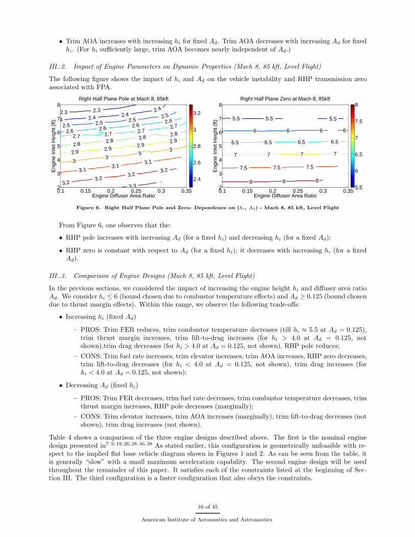
III..2. Impact of Engine Parameters on Dynamic Properties (Mach 8, 85 kft, Level Flight)

The following figure shows the impact of hi and Ad on the vehicle instability and RHP transmission zeroassociated with FPA.

2.3 2.3

2.4 2.4 2.42.4

2.5 2.5 2.52.5

2.6 2.6 2.62.6

2.72.7

2.72.7 2.82.8

2.82.8 2.9

2.92.9

2.9 33

33 3.1

3.13.1

3.23.2

3.23.2

3.3


Eng

ine

Inle

t Hei

ght (

ft)

Right Half Plane Pole at Mach 8, 85kft

0.1 0.15 0.2 0.25 0.3 0.352

3

4

5

6

7

8

2.4

2.6

2.8

3

3.25.5 5.5 5.5

6 6 6 6 6

6.56.56.56.5

7777

7.57.57.5

8 8 8


Eng

ine

Inle

t Hei

ght (

ft)

Right Half Plane Zero at Mach 8, 85kft

0.1 0.15 0.2 0.25 0.3 0.352

3

4

5

6

7

8

5.5

6

6.5

7

7.5

8

Figure 6. Right Half Plane Pole and Zero: Dependence on (hi, Ad) - Mach 8, 85 kft, Level Flight

From Figure 6, one observes that the:

• RHP pole increases with increasing Ad (for a fixed hi) and decreasing hi (for a fixed Ad);

• RHP zero is constant with respect to Ad (for a fixed hi); it decreases with increasing hi (for a fixedAd).

III..3. Comparison of Engine Designs (Mach 8, 85 kft, Level Flight)

In the previous sections, we considered the impact of increasing the engine height hi and diffuser area ratioAd. We consider hi ≤ 6 (bound chosen due to combustor temperature effects) and Ad ≥ 0.125 (bound chosendue to thrust margin effects). Within this range, we observe the following trade-offs:

• Increasing hi (fixed Ad)

– PROS: Trim FER reduces, trim combustor temperature decreases (till hi ≈ 5.5 at Ad = 0.125),trim thrust margin increases, trim lift-to-drag increases (for hi > 4.0 at Ad = 0.125, notshown),trim drag decreases (for hi > 4.0 at Ad = 0.125, not shown), RHP pole reduces;

– CONS: Trim fuel rate increases, trim elevator increases, trim AOA increases, RHP zero decreases,trim lift-to-drag decreases (for hi < 4.0 at Ad = 0.125, not shown), trim drag increases (forhi < 4.0 at Ad = 0.125, not shown);

• Decreasing Ad (fixed hi)

– PROS: Trim FER decreases, trim fuel rate decreases, trim combustor temperature decreases, trimthrust margin increases, RHP pole decreases (marginally);

– CONS: Trim elevator increases, trim AOA increases (marginally), trim lift-to-drag decreases (notshown), trim drag increases (not shown).

Table 4 shows a comparison of the three engine designs described above. The first is the nominal enginedesign presented in7–9, 19, 26, 28, 36, 38 As stated earlier, this configuration is geometrically unfeasible with re-spect to the implied flat base vehicle diagram shown in Figures 1 and 2. As can be seen from the table, itis generally “slow” with a small maximum acceleration capability. The second engine design will be usedthroughout the remainder of this paper. It satisfies each of the constraints listed at the beginning of Sec-tion III. The third configuration is a faster configuration that also obeys the constraints.

16 of 45


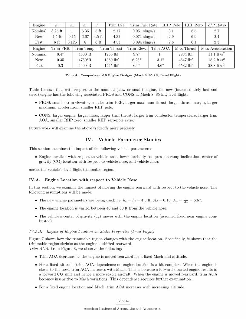
Engine hi Ad An he Trim L2D Trim Fuel Rate RHP Pole RHP Zero Z/P RatioNominal 3.25 ft 1 6.35 5 ft 2.17 0.051 slugs/s 3.1 8.5 2.7

New 4.5 ft 0.15 6.67 4.5 ft 4.32 0.071 slugs/s 2.9 6.9 2.4Fast 6 ft 0.125 8 6 ft 4.53 0.094 slugs/s 2.6 6.1 2.3

Engine Trim FER Trim Temp. Trim Thrust Trim Elev. Trim AOA Max Thrust Max AccelerationNominal 0.47 4500◦R 1250 lbf 9.7◦ 1◦ 2834 lbf 11.1 ft/s2

New 0.35 4750◦R 1380 lbf 6.25◦ 3.1◦ 4647 lbf 18.2 ft/s2

Fast 0.3 4400◦R 1445 lbf 6.9◦ 4.6◦ 6582 lbf 28.8 ft/s2

Table 4. Comparison of 3 Engine Designs (Mach 8, 85 kft, Level Flight)

Table 4 shows that with respect to the nominal (slow or small) engine, the new (intermediately fast andsized) engine has the following associated PROS and CONS at Mach 8, 85 kft, level flight:

• PROS: smaller trim elevator, smaller trim FER, larger maximum thrust, larger thrust margin, largermaximum acceleration, smaller RHP pole;

• CONS: larger engine, larger mass, larger trim thrust, larger trim combustor temperature, larger trimAOA, smaller RHP zero, smaller RHP zero-pole ratio.

Future work will examine the above tradeoffs more precisely.

IV. Vehicle Parameter Studies

This section examines the impact of the following vehicle parameters:

• Engine location with respect to vehicle nose, lower forebody compression ramp inclination, center ofgravity (CG) location with respect to vehicle nose, and vehicle mass

across the vehicle’s level-flight trimmable region.

IV.A. Engine Location with respect to Vehicle Nose

In this section, we examine the impact of moving the engine rearward with respect to the vehicle nose. Thefollowing assumptions will be made:

• The new engine parameters are being used; i.e. he = hi = 4.5 ft, Ad = 0.15, An = 1Ad

= 6.67.

• The engine location is varied between 40 and 60 ft from the vehicle nose.

• The vehicle’s center of gravity (cg) moves with the engine location (assumed fixed near engine com-bustor).

IV.A.1. Impact of Engine Location on Static Properties (Level Flight)

Figure 7 shows how the trimmable region changes with the engine location. Specifically, it shows that thetrimmable region shrinks as the engine is shifted rearward.Trim AOA. From Figure 8, we observe the following:

• Trim AOA decreases as the engine is moved rearward for a fixed Mach and altitude.

• For a fixed altitude, trim AOA dependence on engine location is a bit complex. When the engine iscloser to the nose, trim AOA increases with Mach. This is because a forward situated engine results ina forward CG shift and hence a more stable aircraft. When the engine is moved rearward, trim AOAbecomes insensitive to Mach variations. This dependence requires further examination.

• For a fixed engine location and Mach, trim AOA increases with increasing altitude.

17 of 45


4 6 8 10 12 14 1670

75

80

85

90

95

100

105

110

115

120

Mach

Alti

tude

(kf

t)

Envelope Variations with Engine Location

500

500

2100

2100

2100

50 ft55 ft60 ft

Figure 7. Impact of Engine Location on (Level Flight) Trimmable Region

40 45 50 55 600

2

4

6

8

Engine Position (ft)

AO

A (

deg)

AOA vs. Engine Position, h=100 kft

Mach 8Mach 9Mach 10Mach 11

40 45 50 55 601

2

3

4

5

6


AO

A (

deg)

AOA vs. Engine Position, M=8

85 kft 90 kft 95 kft100 kft

Figure 8. Impact of Engine Location on Trim AOA

A smaller AOA is typically desirable when a designer wishes to increase the vehicle’s stall margin. (Generallyspeaking, an AOA that is too large results in flow separation and loss of lift.)

40 45 50 55 600

5

10

15

20


Ele

vato

r de

flect

ion

(deg

)

Elevator vs. Engine Position, h=100 kft


40 45 50 55 600

5

10

15

20


Ele

vato

r de

flect

ion

(deg

)

Elevator vs. Engine Position, M=8


Figure 9. Impact of Engine Location on Trim Elevator

18 of 45


Trim Elevator. From Figure 9, we observe the following:

• The trim elevator deflection increases as the engine is moved rearward for a fixed Mach and altitude.

• For a fixed altitude, the dependence of trim elevator on engine location is nearly linear with the slopedecreasing with increasing Mach. When the engine is closer to the nose (more stable vehicle), trimelevator increases with increasing Mach. When the engine is closer to the rear (more unstable vehicle),trim elevator increases with decreasing Mach. From this, it follows that flight at a fixed altitude and alow (high) Mach requires less (more) elevator for a forward situated engine (more stable vehicle), andmore (less) elevator for a rearward situated engine (more unstable vehicle).

• For a fixed Mach, the dependence of trim elevator on engine location is almost linear with the slopeincreasing slightly with increasing altitude. When the engine location is also fixed, the trim elevatorincreases with increasing altitude.

• Trim elevator deflection increases with increasing altitude.

Trim FER. Figure 10 illustrates how trim FER depends on engine location. From the figure, the following

40 45 50 55 600.4

0.5

0.6

0.7

0.8

0.9


FE

R

FER vs. Engine Position, h=100 kft


40 45 50 55 60

0.35

0.4

0.45

0.5

0.55

0.6

0.65


FE

R

FER vs. Engine Position, M=8


Figure 10. Impact of Engine Location on Trim FER

is observed:

• Trim FER is a concave up function with respect to engine location for a fixed altitude and Mach - withtrim FER being minimized near 45 ft for most flight conditions.

• For a fixed engine location and altitude (or Mach), trim FER increases with increasing Mach (oraltitude).

IV.A.2. Impact of Engine Location on Dynamic Properties (Level Flight)

40 45 50 55 601

2

3

4

5


RH

P P

ole

RHP Pole vs. Engine Position, h=100 kft


40 45 50 55 601

2

3

4

5

6


RH

P P

ole

RHP Pole vs. Engine Position, M= 8


Figure 11. Impact of Engine Location on Right Half Plane Pole

RHP Pole. Figure 11 shows that the

19 of 45


• instability increases (roughly linearly) as the engine is moved rearward;

• instability increases with increasing Mach and decreasing altitude.

Moving the engine rearward, moves the center of gravity (cg) rearward with respect to the aerodynamiccenter (ac) - thus making the airplane more unstable.

Motivation for Increased Instability. From the above, a designer may wish to increase the vehicle insta-bility in order to make the vehicle more maneuverable in terms of following aggressive flight path angleor vertical acceleration commands. It may also be desirable in order to facilitate the attenuation of highfrequency wind disturbances. (The link between instability and maneuverability was understood by theWright Brothers early on in their work [65, page 39]. This could be important for a missile going after agiletargets. Such might be the case for military applications. In such a case, one should note that a largerinstability requires a larger minimum control system bandwidth for vehicle stabilization.41 This, however,may conflict with higher frequency non-minimum phase, structural, aero-elastic, and actuator dynamics. Inthe same spirit, a larger bandwidth at the elevator would typically require a faster control surface actuator.Such considerations must be rigorously addressed at some point in the design process - the sooner, the better.

40 45 50 55 604.5

5

5.5

6

6.5


RH

P Z

ero

RHP Zero vs. Engine Position, h=100 kft


40 45 50 55 604.5

5

5.5

6

6.5

7

7.5


RH

P Z

ero

RHP Zero vs. Engine Position, M= 8


Figure 12. Impact of Engine Location on Right Half Plane Zero

RHP Zero. From Figure 12, one observes that the:

• RHP zero varies little with engine position for a fixed altitude and Mach

• RHP zero increases with increasing Mach and decreasing altitude

Increasing RHP Zero: Moving Engine Rearward. From the above, it follows that one might move the enginerearward (making the vehicle more unstable) in order to maximize the right half plane zero. By so doing,a vehicle designer can (in principle) increase the maximum achievable flight path angle bandwidth.41 Onemust, of course, note that flexible modes, the associated uncertainty, and the control system simplicity canalso limit the achievable bandwidth. This will be the case when the flexible modes lie within a decade of theright half plane zero. Additional pros associated with moving the engine rearward include: less fuel usage- minimized near 55 ft (not shown). Associated cons include the following: trim L/D drops (monotonicallyfor 40 to 60 ft interval), trim FER increases (FER/thrust/acceleration margin decreases).

IV.B. Lower Forebody Inclination

In this section, we examine the impact of varying the lower forebody inclination angle. The following isassumed:

• New engine parameters; i.e. he = hi = 4.5 ft, Ad = 0.15, An = 1Ad

= 6.67.

• Lower forebody inclination varied from 4.2◦ to 8.2◦ (nominal value = 6.2◦)

• All lengths (forebody, aftbody, engine length), upper forebody angle kept constant

20 of 45


• Tail angle and total vehicle height change as a result

• CG assumed to be fixed

• Heating effects due to slender nose are not considered

IV.B.1. Impact of Lower Forebody Inclination on Static Properties (Level Flight)

Trimmable Region. Figure 13 shows how the trimmable region changes with lower forebody inclination angle.From Figure 13, one observe that the:

4 6 8 10 12 14 1670

75

80

85

90

95

100

105

110

115

120

Mach

Alti

tude

(kf

t)

Envelope Variations with Lower Forebody Inclination

500

500

2100

2100

2100

4.2 deg5.2 deg6.2 deg7.2 deg8.2 deg

Figure 13. Impact of Lower Forebody Inclination on (Level Flight) Trimmable Region

• Trimmable region shrinks with increasing lower forebody inclination

• Pinch point moves toward a higher Mach and lower altitude with increasing lower forebody inclination

Trim AOA. Figure 14 shows how AOA varies with lower forebody inclination angle. From Figure 14, oneobserves that the:

4 5 6 7 8 94

4.5

5

5.5

6

6.5

Lower forebody inclination (deg)

AO

A (

deg)

AOA vs. Lower forebody inclination, h=100 kft


4 5 6 7 8 92

3

4

5

6

7


AO

A (

deg)

AOA vs. Lower forebody inclination, M=8


Figure 14. Impact of Lower Forebody Inclination on Trim AOA

• Trim AOA decreases linearly with increasing lower forebody inclination for a fixed altitude

21 of 45


• Trim AOA decreases with Mach at lower Mach numbers for a fixed altitude;

• Trim AOA increases with increasing altitude for a fixed Mach

Trim Elevator. Figure 15 shows how elevator varies with lower forebody inclination angle. From Figure 15,one observes that the:

4 5 6 7 8 911

11.5

12

12.5

13

13.5

14


Ele

vato

r A

OA

(de

g)

Elevator AOA vs. Lower forebody inclination, h=100 kft


4 5 6 7 8 96

8

10

12

14


Ele

vato

r A

OA

(de

g)

Elevator AOA vs. Lower forebody inclination, M=8


Figure 15. Impact of Lower Forebody Inclination on Trim Elevator

• Trim elevator deflection increases linearly with increasing forebody inclination

• Trim elevator deflection increases with increasing Mach, increasing altitude

Trim FER. Figure 16 shows how FER varies with lower forebody inclination angle.

4 5 6 7 8 90.45

0.5

0.55

0.6

0.65

0.7

0.75


FE

R

FER vs. Lower forebody inclination, h=100 kft


4 5 6 7 8 9

0.35

0.4

0.45

0.5


FE

R

FER vs. Lower forebody inclination, M=8


Figure 16. Impact of Lower Forebody Inclination on Trim FER


• Trim FER increases almost linearly with increasing lower forebody inclination

IV.B.2. Impact of Lower Forebody Inclination on Dynamic Properties (Level Flight)

RHP Pole. Figure 17 shows how the RHP pole varies with lower forebody inclination. From Figure 17, oneobserves that the:

• RHP pole increasing with increasing lower forebody inclination

• RHP pole increases with Mach and decreasing altitude

RHP Zero. Figure 18 shows how the RHP pole varies with lower forebody inclination. From Figure 18, oneobserves that the:

• RHP zero increases with increasing lower forebody inclination

• RHP zero increases with increasing Mach and decreasing altitude

22 of 45


4 5 6 7 8 92

2.2

2.4

2.6

2.8


RH

P P

ole

RHP Pole vs. Lower forebody inclination, h=100 kft


4 5 6 7 8 92

2.5

3

3.5


RH

P P

ole

RHP Pole vs. Lower forebody inclination, M= 8


Figure 17. Impact of Lower Forebody Inclination on Right Half Plane Pole

4 5 6 7 8 94.5

5

5.5

6

6.5


RH

P Z

ero

RHP Zero vs. Lower forebody inclination, h=100 kft


4 5 6 7 8 94.5

5

5.5

6

6.5

7

7.5


RH

P Z

ero

RHP Zero vs. Lower forebody inclination, M= 8


Figure 18. Impact of Lower Forebody Inclination on Right Half Plane Zero

IV.C. Center of Gravity

This section examines the impact of varying the center of gravity (cg) location. The following assumptionsare made:


= 6.67.

• CG varied from 45ft to 65ft artificially (no internal changes are made to achieve this shift)

• For dynamic properties, we only consider CG locations for which vehicle is open loop unstable

IV.C.1. Impact of Center of Gravity on Static Properties (Level Flight)

Trimmable Region. Figure 19 shows how the trimmable region changes with a shifting vehicle CG. FromFigure 19, one observes that the

• trimmable region decreases slightly as the vehicle CG is moved rearward.

Trim AOA. Figure 20 shows how trim AOA depends on the vehicle’s CG location.Figure 20 shows that the

• Trim AOA decreases as the vehicle CG moves rearward.

Trim Elevator. Figure 21 shows how trim elevator depends on cg location.

• Trim elevator deflection increases as the vehicle CG moves rearward.

Trim FER. Figure 22 shows how trim FER depends on vehicle CG location. Figure 22 shows that the

• Trim FER increases as the vehicle CG moves rearward.

23 of 45


4 6 8 10 12 14 1670

80

90

100

110

120

Mach

Alti

tude

(kf

t)

Envelope Variations with CG Location

500

500

2100

2100

2100

−65 ft−62 ft−60 ft−58 ft−55 ft

Figure 19. Impact of Vehicle CG Location on (Level Flight) Trimmable Region

−65−60−55−50−453

4

5

6

7

CG Location (ft)

AO

A (

deg)

AOA vs. CG Location, h=100 kft


−65−60−55−50−452

3

4

5

6

7

CG Location (ft)

AO

A (

deg)

AOA vs. CG Location, M=8


Figure 20. Impact of Vehicle CG Location on Trim AOA

−65−60−55−50−450

5

10

15

CG Location (ft)

Ele

vato

r de

flect

ion

(deg

)

Elevator vs. CG Location, h=100 kft


−65−60−55−50−450

5

10

15

CG Location (ft)

Ele

vato

r de

flect

ion

(deg

)

Elevator vs. CG Location, M=8


Figure 21. Impact of Vehicle CG Location on Trim Elevator

IV.C.2. Impact of Center of Gravity on Dynamic Properties (Level Flight)

RHP Pole. Figure 23 shows how the vehicle instability depends on the CG location. Figure 23 shows thatthe vehicle

24 of 45


−65−60−55−50−450.45

0.5

0.55

0.6

0.65

0.7

0.75

CG Location (ft)

FE

R

FER vs. CG Location, h=100 kft


−65−60−55−50−45

0.35

0.4

0.45

0.5

0.55

CG Location (ft)

FE

R

FER vs. CG Location, M=8


Figure 22. Impact of Vehicle CG Location on Trim FER

−10−8−6−4−202

2.5

3

3.5

CG Location ft

RH

P P

ole

RHP Pole vs. CG Location, h=100 kft


−10−8−6−4−202

2.5

3

3.5

4

4.5

CG Location ft

RH

P P

ole

RHP Pole vs. CG Location, M= 8


Figure 23. Impact of Vehicle CG Location on Right Half Plane Pole

• RHP pole increases linearly as the vehicle CG moves rearward.

RHP Zero. Figure 24 shows how the RHP zero depends on the CG location. Figure 24 shows that thevehicle

−10−8−6−4−204.5

5

5.5

6

CG Location ft

RH

P Z

ero

RHP Zero vs. CG Location, h=100 kft


−10−8−6−4−204.5

5

5.5

6

6.5

7

CG Location ft

RH

P Z

ero

RHP Zero vs. CG Location, M= 8


Figure 24. Impact of Vehicle CG Location on Right Half Plane Zero

• RHP zero decreases linearly as the vehicle CG moves rearward.

IV.D. Vehicle Mass

This section examines the impact of varying the vehicle’s (total) mass. The following assumptions are made:


= 6.67.

25 of 45


• Mass of vehicle modified without changing any material or subsystem properties.

IV.D.1. Impact of Vehicle Mass on Static Properties

Trimmable Region. Figure 25 shows how the trimmable region depends on vehicle mass.

4 6 8 10 12 14 1670

80

90

100

110

120

130

140

Mach

Alti

tude

(kf

t)

Envelope Variations with Mass Ratio

500

500

2100

2100

2100

0.50.8 11.21.5

Figure 25. Impact of Vehicle Mass on (Level Flight) Trimmable Region


• Trimmable region shrinks as the vehicle mass is increased.

Trim AOA. Figure 26 shows how trim AOA depends on vehicle mass. The figure shows that the:

0.5 1 1.5 22

4

6

8

10

Mass Ratio

AO

A (

deg)

AOA vs. Mass Ratio, h=100 kft


0.5 1 1.5 21

2

3

4

5

6

7

Mass Ratio

AO

A (

deg)

AOA vs. Mass Ratio, M=8


Figure 26. Impact of Vehicle Mass on Trim AOA

• Trim AOA increases as the vehicle mass is increased.

Trim Elevator. Figure 27 shows how trim elevator depends on vehicle mass. The figure shows that the:

• Trim elevator deflection increases as the vehicle mass is increased.

Trim FER. Figure 28 shows how trim FER depends on vehicle mass. The figure shows that the:

• Trim FER increases as the vehicle mass is increased.

26 of 45


0.5 1 1.5 26

7

8

9

10

11

12

Mass Ratio

Ele

vato

r de

flect

ion

(deg

)

Elevator vs. Mass Ratio, h=100 kft


0.5 1 1.5 24

6

8

10

12

Mass Ratio

Ele

vato

r de

flect

ion

(deg

)

Elevator vs. Mass Ratio, M=8


Figure 27. Impact of Vehicle Mass on Trim Elevator

0.5 1 1.5 20.2

0.4

0.6

0.8

1

Mass Ratio

FE

R

FER vs. Mass Ratio, h=100 kft


0.5 1 1.5 2

0.35

0.4

0.45

0.5

Mass Ratio

FE

R

FER vs. Mass Ratio, M=8


Figure 28. Trim FER vs Vehicle Mass

IV.D.2. Impact of Vehicle Mass on Dynamic Properties (Level Flight)

RHP Pole. Figure 29 shows how the vehicle instability depends on vehicle mass. The figure shows that the:

0.5 1 1.5 21.5

2

2.5

3

3.5

4

Mass Ratio

RH

P P

ole

RHP Pole vs. Mass Ratio, h=100 kft


0.5 1 1.5 21.5

2

2.5

3

3.5

4

4.5

Mass Ratio

RH

P P

ole

RHP Pole vs. Mass Ratio, M= 8


Figure 29. Impact of Vehicle Mass on Right Half Plane Pole

• RHP pole decreases as the vehicle mass is increased.

RHP Zero. Figure 30 shows how the RHP zero depends on vehicle mass. The figure shows that the:

• RHP zero decreases as the vehicle mass is increased.

27 of 45


0.5 1 1.5 24

5

6

7

8

Mass Ratio

RH

P Z

ero

RHP Zero vs. Mass Ratio, h=100 kft


0.5 1 1.5 24

5

6

7

8

9

10

Mass Ratio

RH

P Z

ero

RHP Zero vs. Mass Ratio, M= 8


Figure 30. Impact of Vehicle Mass on Right Half Plane Zero

IV.E. Summary of Level Flight Trim Trade Studies

The following tables summarize each of the conducted level-flight trim trade studies.

Rearward Engine Shift. Table 5 summarizes trends for a rearward shifting engine. The engine is shiftedrearward (with the CG) with the vehicle height kept constant; i.e. the lower forebody inclination angle isdecreasing, thus making the vehicle sharper. As the engine is shifted rearward, we observe specific monotonictrends and tradeoffs that result in the following PROS and CONS:

• PROS: trim AOA decreases, trim lift remains nearly constant;

• CONS: trim elevator increases (CG rearward), trim drag increases, trim L/D decreases, RHP poleincreases.

We also observe the following more complex (non-monotonic) behavior:

• trim fuel rate decreases (min near 55 ft) and then increases;

• trim FER decreases (min near 45 ft - thrust/acceleration margin increases) and then increases (thrust/accelerationmargin decreases).

Property Pro Con

Trim Lift Almost Constant Almost ConstantTrim Drag Increases monotonicallyTrim L/D Decreases monotonicallyTrim AOA Decreases monotonicallyTrim Elevator Increases monotonicallyTrim FER Decreases till 45 ft Increases after 45 ftTrim Fuel Rate Decreases till 55 ft Increases after 55 ftRHP Pole Increases monotonicallyRHP Zero Increases after 45 ft Decreases till 45 ftRHP Z/P Ratio Decreases monotonically

Table 5. Trends for Rearward Engine Shift

Lower Forebody Angle Increase. Table 6 summarizes trends for an increasing lower forebody angle. Here,the horizontal engine location is fixed and the engine is moved downward - thus increasing the height of thevehicle. As the lower forebody angle is increased, we observe specific monotonic trends and tradeoffs thatresult in the following PROS and CONS:

28 of 45


• PROS: trim AOA decreases, RHP zero increases, RHP zero increases, RHP zero-pole ratio almostconstant;

• CONS: trim elevator increases, trim drag increases, trim L/D decreases, trim FER increases, trim fuelrate increases, RHP pole increases.

Non-monotonic patterns are not observed in this case.

Property Pro Con

Trim Lift Almost Constant Almost ConstantTrim DragTrim L/D Decreases monotonicallyTrim AOA Decreases monotonicallyTrim Elevator Increases monotonicallyTrim FER Increases monotonicallyTrim Fuel Rate Decreases monotonicallyRHP Pole Increases monotonicallyRHP Zero Increases monotonicallyRHP Z/P Ratio Almost constant Almost constant

Table 6. Trends for Increasing Lower Forebody Inclination

Rearward CG Shift. Table 7 summarizes trends for a rearward shifting CG. As the CG is shifted rearward,we observe specific monotonic trends and tradeoffs that result in the following PROS and CONS:

• PROS: trim AOA decreases, trim fuel rate almost constant;

• CONS: trim elevator increases, trim drag increases, trim L/D decreases, trim FER increases, RHP poleincreases, RHP zero decreases, RHP zero-pole ration decreases.

Non-monotonic patterns are not observed in this case.

Property Pro Con

Trim Lift Almost Constant Almost ConstantTrim Drag Increases monotonicallyTrim L/D Decreases monotonicallyTrim AOA Decreases monotonicallyTrim Elevator Increases monotonicallyTrim FER Increases monotonicallyTrim Fuel Rate Almost constantRHP Pole Increases monotonicallyRHP Zero Decreases monotonicallyRHP Z/P Ratio Decreases monotonically

Table 7. Trends for Rearward CG Shift

Vehicle Mass Increase. Table 8 summarizes trends for increasing mass. As the vehicle mass is increased, weobserve specific monotonic trends and tradeoffs that result in the following PROS and CONS:

• PROS: RHP pole decreases, RHP zero-pole ratio almost constant;

• CONS: trim elevator and trim AOA increase, trim FER and fuel rate increase, RHP zero decreases.

We also observe the following more complex (non-monotonic) behavior:

29 of 45


• trim L/D is a concave down function of mass for a fixed Mach and altitude; mass at which peak occursincreases with Mach (altitude fixed); decreases with altitude (Mach fixed).

Property Pro Con

Trim Lift Increases monotonicallyTrim Drag Increases monotonicallyTrim L/D (peak) Increases with Mach (altitude fixed) Decreases with altitude (Mach fixed)Trim AOA Increases monotonicallyTrim Elevator Increases monotonicallyTrim FER Increases monotonicallyTrim Fuel Rate Increases monotonicallyRHP Pole Decreases monotonicallyRHP Zero Decreases monotonicallyRHP Z/P Ratio Almost constant Almost constant

Table 8. Trends for Increasing Mass

V. Vehicle Optimization

Various schemes have been considered for the optimization of space vehicles. Within66, a conceptualdesign process - that takes factors like cost analysis into consideration - is described. The non-hierarchicalnature of the design process is illustrated and several optimization methods - parameter based, gradientbased, and stochastic methods - are examined. Within67, a probabilistic approach to vehicle design istaken in order to account for uncertainties. For air-breathing hypersonic aircraft, the coupling between theairframe and the engine introduces additional constraints into the design process. The importance of amultidisciplinary design optimization approach is illustrated within68. A collaborative approach69 for launchvehicle design is considered within70. The design is decomposed into several subsystem design problems.A system level optimizer coordinates the integration of subsystem designs while taking into account inter-subsystem coupling and constraints. Such a subsystem-based algorithm is well suited to exploit parallelcomputing architectures.

In this section, we address optimizing the generic carrot shaped hypersonic vehicle under consideration.The flat base assumption is made; i.e. he = hi, An = 1

Ad. The goal is twofold: (1) understand what config-

urations result when very simple optimizations are considered, (2) understand how the gap matric can beused to design a control-friendly vehicle.

Admissible Parameter Values. Optimizations are conducted over the following control surface and engineparameter values:

• Elevator area Selev : [8.5, 25.5] ft2 (nominal: 17 ft2)

• Horizontal elevator position xelev : [70, 90] ft from nose (nominal: 85 ft)

• Inlet height hi: [2.25, 6.75] ft (nominal: 4.5 ft)

• Lower forebody inclination τ1L: [4.2◦, 8.2◦] (nominal: 6.2◦)

Overview of Trim Optimization Algorithm. A nonlinear simplex optimization method was used. Noderivatives are calculated because trimming the vehicle results in each iteration being expensive.71, 72 Anoverview of the vehicle optimization algorithm is as follows:

1. Choose cost function (e.g. trim AOA, trim fuel, trim elevator, trim FER, trim L/D);

2. Select values for parameters being optimized over; e.g. Selev , xelev , hi, τ1L;

3. Trim the vehicle at selected flight condition; i.e. Mach 8, 85 kft, level flight;

30 of 45


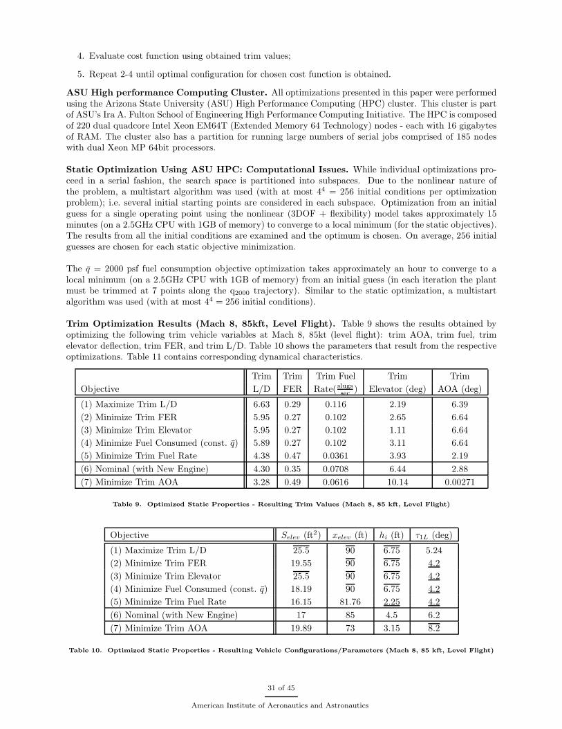
4. Evaluate cost function using obtained trim values;

5. Repeat 2-4 until optimal configuration for chosen cost function is obtained.

ASU High performance Computing Cluster. All optimizations presented in this paper were performedusing the Arizona State University (ASU) High Performance Computing (HPC) cluster. This cluster is partof ASU’s Ira A. Fulton School of Engineering High Performance Computing Initiative. The HPC is composedof 220 dual quadcore Intel Xeon EM64T (Extended Memory 64 Technology) nodes - each with 16 gigabytesof RAM. The cluster also has a partition for running large numbers of serial jobs comprised of 185 nodeswith dual Xeon MP 64bit processors.

Static Optimization Using ASU HPC: Computational Issues. While individual optimizations pro-ceed in a serial fashion, the search space is partitioned into subspaces. Due to the nonlinear nature ofthe problem, a multistart algorithm was used (with at most 44 = 256 initial conditions per optimizationproblem); i.e. several initial starting points are considered in each subspace. Optimization from an initialguess for a single operating point using the nonlinear (3DOF + flexibility) model takes approximately 15minutes (on a 2.5GHz CPU with 1GB of memory) to converge to a local minimum (for the static objectives).The results from all the initial conditions are examined and the optimum is chosen. On average, 256 initialguesses are chosen for each static objective minimization.

The q = 2000 psf fuel consumption objective optimization takes approximately an hour to converge to alocal minimum (on a 2.5GHz CPU with 1GB of memory) from an initial guess (in each iteration the plantmust be trimmed at 7 points along the q2000 trajectory). Similar to the static optimization, a multistartalgorithm was used (with at most 44 = 256 initial conditions).

Trim Optimization Results (Mach 8, 85kft, Level Flight). Table 9 shows the results obtained byoptimizing the following trim vehicle variables at Mach 8, 85kt (level flight): trim AOA, trim fuel, trimelevator deflection, trim FER, and trim L/D. Table 10 shows the parameters that result from the respectiveoptimizations. Table 11 contains corresponding dynamical characteristics.

Trim Trim Trim Fuel Trim TrimObjective L/D FER Rate( slugs

sec ) Elevator (deg) AOA (deg)

(1) Maximize Trim L/D 6.63 0.29 0.116 2.19 6.39(2) Minimize Trim FER 5.95 0.27 0.102 2.65 6.64(3) Minimize Trim Elevator 5.95 0.27 0.102 1.11 6.64(4) Minimize Fuel Consumed (const. q) 5.89 0.27 0.102 3.11 6.64(5) Minimize Trim Fuel Rate 4.38 0.47 0.0361 3.93 2.19(6) Nominal (with New Engine) 4.30 0.35 0.0708 6.44 2.88(7) Minimize Trim AOA 3.28 0.49 0.0616 10.14 0.00271

Table 9. Optimized Static Properties - Resulting Trim Values (Mach 8, 85 kft, Level Flight)

Objective Selev (ft2) xelev (ft) hi (ft) τ1L (deg)

(1) Maximize Trim L/D 25.5 90 6.75 5.24(2) Minimize Trim FER 19.55 90 6.75 4.2(3) Minimize Trim Elevator 25.5 90 6.75 4.2(4) Minimize Fuel Consumed (const. q) 18.19 90 6.75 4.2(5) Minimize Trim Fuel Rate 16.15 81.76 2.25 4.2(6) Nominal (with New Engine) 17 85 4.5 6.2(7) Minimize Trim AOA 19.89 73 3.15 8.2

Table 10. Optimized Static Properties - Resulting Vehicle Configurations/Parameters (Mach 8, 85 kft, Level Flight)

31 of 45


Objective RHP Pole RHP Zero RHP Zero-Pole ratio

(1) Maximize Trim L/D 1.60 (-45.18%) 5.83 (-16.02%) 3.6325 (+53.18%)(2) Minimize Trim FER 1.95 (-33.43%) 5.62 (-19.06%) 2.8833 (+21.59%)(3) Minimize Trim Elevator 1.48 (-49.56%) 5.80 (-16.46%) 3.928 (+65.64%)(4) Minimize Fuel Consumed (const. q) 2.05 (-30.07%) 5.61 (-19.15%) 2.7416 (15.61%)(5) Minimize Trim Fuel Rate 3.14 (+7.23%) 7.32 (+5.44%) 2.3319 (-1.66%)(6) Nominal (with New Engine) 2.93 (0.00%) 6.94 (0.00%) 2.37 (0.00%)(7) Minimize Trim AOA 3.55 (+21.23%) 6.34 (-8.59%) 1.788 (-24.60%)

Table 11. Optimized Static Properties - Resulting Dynamic Characteristics (Mach 8, 85 kft, Level Flight)

Within Table 10, over bars imply that the maximum admissible parameter was achieved; underlines implythat the minimum admissible parameter bound was achieved. From Tables 9-10, one observes the following:

1. Maximizing Trim L/D. Maximizing trim L/D results in a small FER - marginally above that obtainedwhen trim FER is directly minimized. As when trim FER is minimized, maximizing L/D also results ina large trim AOA. In short, maximizing trim L/D yields results comparable to minimizing trim FER.Maximizing trim L/D, however, results in a larger elevator surface area and lower forebody inclinationvis-a-vis when trim FER is minimized. For this case, Selev , xelev , and hi, were maximized to yield amaximally large elevator, a maximally effective elevator, a maximally large engine.

2. Minimizing Trim FER. Minimizing trim FER produces results that are comparable to those obtainedwhen L/D is maximized - with L/D reduced 10.3% from the maximum L/D, FER reduced by 12.1%,and AOA increased by only 3.9%. In contrast to maximizing L/D, minimizing FER results in a muchsmaller elevator surface area (23.3%) and lower forebody angle (19.9%). For this case, xelev , and hi

were maximized while τ1L was minimized to yield a maximally effective elevator, a maximally largeengine, and a very aerodynamic lower forebody.

3. Minimizing Trim Elevator. Minimizing trim elevator produces results (L/D, Fuel, FER, AOA) thatare comparable to minimizing trim FER with less than half the elevator. For this case, Selev , xelev , andhi were maximized while τ1L was minimized to yield a maximally large elevator and effective elevator,a maximally large engine, and a very aerodynamic lower forebody.

4. Minimizing Fuel Consumed (const. q). Minimizing the fuel consumed along a constant dynamicpressure trajectory produces results that are comparable to minimizing trim FER with xelev and hi

maximized and τ1L minimized to yield a maximally effective elevator, a maximally large engine, and avery aerodynamic lower forebody. This optimization is more involved than the others being considered.Hence some additional explanation is required.

The objective here is to minimize the total fuel consumed while flying along the q = 2000 psf altitude-Mach profile from Mach 5.52 at 70kft to Mach 11.08 at a 100kft. To do so, we approximate the totalfuel consumed. For simplicity, vehicle mass changes are ignored. The method used to approximate fuelconsumption is described below.

(a) Trim at Selected Points. Select points along the stated q = 2000 psf profile spaced 5 kft. Thisyields the

altitudes: [70, 75, 80, 85, 90, 95, 100] kft and the correspondingMachs: [5.52, 6.21, 6.98, 7.85, 8.81, 9.88, 11.08].

This divides the profile into 6 legs. Trim the vehicle at each point.

(b) Approximate Maximum Accelerations. Approximate the maximum horizontal acceleration possi-ble at the left end point of each leg. Do so using the FER margin at each left end point. The FERmargin is used to determine the maximum FER. This is used to compute the associated thrustTh(FERmax)i. The trim drag Di and trim AOA αi are then used to approximate the maximumacceleration at the left end point: ai ≈

[Th(FERmax)i cos αi−Di

m

]where m is the total mass of the

vehicle.

32 of 45


(c) Determine Average Accelerations for Each Leg. Assume that the average acceleration in leg iis the mean of the two end-point accelerations; i.e. ai = ai+ai+1

2 where ai is the approximatemaximum acceleration at the left end point of the ith leg and ai+1 is that at the right end point.

(d) Approximate Time to Fly Each Leg. Approximate the time to fly leg i as Ti ≈ vi+1−vi

ai.

(e) Approximate the average fuel rate for leg i (Fi) as the mean of the fuel rates at the end points(where we have maximum acceleration); i.e. Fi = Fi+ ˙Fi+1

2

(f) Approximate Fuel Consumed During Each Leg. Approximate the fuel consumed during leg i asFi ≈ Fi × Ti

(g) Approximate Total Fuel Consumed Over Flight Profile. Approximate the total fuel consumed(objective to be minimized) as

Total fuel consumed ≈6∑

i=1

Fi (35)

(h) Inadmissible Designs. We also want to maintain a reasonable FPA. The average FPA for the ith

leg is approximated as

γ ≈ hi+1 − hi

vi × Ti(36)

where (vi, hi) are the velocity and altitude at the left end point of the ith leg and hi+1 is thealtitude at the right end point. Designs for which the average FPA in any leg exceeded 3◦ weredeemed inadmissible and discarded.

5. Minimizing Trim Fuel Rate. Minimizing trim fuel rate produces results that lie between those obtainedwhen trim AOA is minimized and elevator is minimized (or trim FER is minimized or trim L/D ismaximized). Surprisingly, for this case both hi and τ1L are minimized to yield a maximally smallengine with a very aerodynamic lower forebody. This optimization results in low trim air mass flowto the engine (and low trim AOA) so that even with the resulting larger trim FER and increased trimthrust, the trim fuel rate is small.

6. Nominal Vehicle. Observe that the nominal values Selev = 17, hi = 4.5, τ1L = 6.2 are midpointswhile the nominal value xelev = 85 is near the right end point. Note that this case can be viewed asa tradeoff between minimizing trim fuel rate and trim AOA when looking at trim L/D and elevator,elevator area, and lower forebody angle. Otherwise, trim FER, fuel rate, AOA, elevator rearwarddistance, and engine inlet height are larger.

7. Minimizing Trim AOA. Minimizing trim AOA uses excessive trim elevator for lift. This results inexcessive drag and results in a small trim L/D. It also produces a large trim FER and small trim fuelrate. The resulting low trim fuel rate is due to the reduced trim air mass flow to the engine (due tothe smaller trim AOA). From a vehicle configuration perspective, this case results in the largest lowerforebody inclination (least aerodynamic shape) - achieving the maximum admissible value for τ1L.

Motivation for Gap Metric Based Optimization. The gap metric represents a system-theoretic measurethat quantifies the “distance” between two dynamical systems and whether or not a common controller canbe deployed for the systems under consideration48. Within49, the gap between two LTI dynamical systems(P1, P2) is defined as follows:

g(P1, P2)def= max{ inf

Q∈H∞‖ [

D1N1

] − [D2N2

]Q ‖∞, inf

Q∈H∞‖ [

D2N2

] − [D1N1

]Q ‖∞ } (37)

where P1 = N1D−11 , P2 = N2D

−12 , and (Ni, Di) denotes a normalized right coprime factorization for Pi

(i = 1, 2) in the sense of73. The gap metric (and the ν gap74) has often been considered from a robustnessperspective in the stabilization of feedback systems75. Within76, the authors relate the gap metric with tra-ditional stability margins. The gap metric has also been considered for the design of controllers for spacevehicles77, 78. Given the importance of this metric from a controller design perspective, it may be very useful

33 of 45


to consider the gap metric during the vehicle design phase. This motivates the vehicle optimization whichwe consider below.

Vehicle Optimization Using Gap Metric: Minimizing Plant Variability. We now consider vehicleoptimization using the gap metric. Details of the optimization are now given.

• The optimization is conducted with respect to the four parameters: Selev , xelev , hi, τ1L.

5 6 7 8 9 10 11 1270

80

90

100

110

120

Mach

Alti

tude

(kf

t)

Directed set − Gap Optimization

Figure 31. Directed Set of Level Flight Operating Points for Cumulative Gap Calculation

• Figure 31 shows the set of operating points used - a directed set - over which a cumulative gap isdefined. The figure shows 17 operating points. (The operating points were selected in a way so asto span the desired trimmable region. How to do this systematically will be pursued in future work.)Associated with these 17 points are 16 gaps: gapi = gap(Pi, Pi+1), i = 1, 2, . . . , 16. The cumulativegap associated with these 17 points (along the directed set) is defined as follows:

cumulative gap def=16∑

i=1

gapi (38)

A vehicle configuration is selected during optimization. The vehicle is trimmed at each point along thedirected set. The gap between each pair of neighbors (along the directed set) is calculated and addedto the running total for the vehicle configuration being considered.

• If a particular vehicle configuration is not able to trim at some point along the directed set, a penaltyis added to the cumulative gap in lieu of the gap between this frozen point and its neighbors (alongthe directed set).

Gap Optimization Using ASU HPC: Computational Issues. Obtaining a gap-optimized vehicle froman initial guess takes approximately 4 hours on an ASU HPC 2.5GHz CPU with 1GB of memory. (Duringeach iteration, the plant must be trimmed and linearized at each of the 17 selected operating points inaltitude-Mach space.) As for the static optimization, a multistart algorithm was used (with at most 34 = 81initial conditions).

Vehicle Optimization Results: Gap-Optimized Versus Nominal. The parameters for the nominalvehicle (with new engine design) are as follows:

• Nominal Vehicle Parameters (with New Engine)

Selev = 17ft2 xelev = 85ft hi = 4.5ft τ1L = 6.2◦

The cumulative gap for the nominal vehicle (with new engine design) is 4.4994 (mean gap = 0.28121).

The final parameters for the gap-optimized vehicle are as follows:

• Gap-Optimized Vehicle Parameters

Selev = 25.5ft2 xelev = 90ft hi = 6.12ft τ1L = 4.2◦

The cumulative gap for the optimized vehicle is 3.3989 (mean gap = 0.21243).

34 of 45


Note that with respect to the nominal vehicle, the gap-optimized vehicle has a

• larger elevator which is slightly shifted rearward (more effective elevator), larger engine inlet height(faster vehicle), smaller lower forebody inclination angle (more aerodynamic).

Modulo the simplicity of the nonlinear (3DOF + flexibility) model being used in this study and its associ-ated limitations, the results given below suggest that these trends may significantly simplify control systemdesign. More comprehensive studies are (of course) required in order to make definitive claims. Such a studycould, for example, involve the 6DOF models being developed within79.

RHP Pole Variation Over Level Flight Trimmable Region: Gap-Optimized Versus Nominal.Figure 32 (left) shows how the RHP pole varies across the trimmable region when the cumulative gap isminimized across the trimmable region (as discussed above). The variation for the nominal system (usingthe new engine design) is also given in Figure 32 (right).

6 8 10 1270

80

90

100

110

120

Mach

Alti

tude

(kf

t)

Gap Optimized Plant − RHP Pole

1

1.5

2

2.5

3

6 8 10 1270

80

90

100

110

120

Mach

Alti

tude

(kf

t)

Nominal Plant − RHP Pole

1

1.5

2

2.5

3

Figure 32. RHP Pole Over Trimmable Region - Nominal and Gap Optimized Vehicle

Figure 32 (left) shows that the

• RHP pole variation has decreased significantly when the vehicle is gap optimized; we will see that thisimplies that less adaptation (i.e. scheduling) will be required in the final control system design withrespect to that required for the system associated with Figure 32 (right);

• Trimmable region has been expanded at low Mach and altitudes

VI. Control System Design Studies

A classic decentralized inner-outer loop control system architecture was used to illustrate control designissues. Such an architecture was examined within [41]. It can be visualized as shown in Figure 33.

�r�−

e � Ko(s) �uPI� �u

� � �

di

up

��

ni

��

no

P (s)�

yp

xr

� y��

do

��uiKi(s)

�−

�

�

Figure 33. Inner Outer Loop Control System

35 of 45


Outputs: yp = [ v γ ]T Controls: u = [ FER δe ]T State Feedback: xr = [ θ θ ]T

Overview of Nominal Control System Architecture. Within Figure 33, we have an inner loop con-troller:

Ki(s) =

[0 0

−giziao

bo

[s2+b1s+bo

s2+a1s+ao

]−gi

ao

bo

[s2+b1s+bo

s2+a1s+ao

] ](39)

and an outer loop controller:

Ko(s) =

⎡⎢⎣ gb(s+zb)

s

[10

s+10

]3

0

0 gγ(s+zγ)s

[20

s+20

]3

⎤⎥⎦ (40)

The inner-outer loop structure is now described.

1. Velocity Control Via Single Loop PI. A PI controller (with roll off) is used to control velocity. Twoparameters are associated with velocity control: (gb, zb). A simple anti-windup method (not discussedin the paper) is used to address the state-dependent thermal choking nonlinearity discussed earlier.

2. FPA Control Via Inner-Outer Loop. A PD (proportional plus derivative with notch) inner-loop con-troller is used on pitch to stabilize the vehicle’s pitch dynamics and make the modified dynamics lookfriendly to the outer-loop FPA PI (proportional plus integral) controller. The inner loop’s notch pro-vides lead to assist with the first flexible mode’s complex zero-pole pair (near 21 rad/sec). As mightbe expected with this inner-outer loop structure, the inner loop is generally much faster than the outerloop. Its bandwidth must be large enough to stabilize the vehicle and follow outer-loop commands, butnot too high so that the flexible dynamics are overly excited. (It should be noted that any practical“real-world” implementation of the PD controller should include additional roll off in order to attenuatehigh frequency noise ni resulting from θ and theta measurements.)

A PI (proportional plus integral with roll off) outer-loop controller is used for FPA. The outer loop isgenerally much slower than the inner loop. The maximum achievable outer loop bandwidth is limitedby the vehicle’s flexible dynamics as well as the right half plane zero associated with the elevator-FPAmap.

Four parameters are associated with FPA control: (gi , zi) for the inner-loop PD controller, gγ , zγ) forthe outer-loop PI controller.

Command pre-filters are also included: Wb = zb

s+zbfor velocity reference commands, WFPA = zγ

s+zγfor FPA

reference commands. (These reference command pre-filters are not shown within Figure 33.)

Additional information about controller parameter selection can be found within41. Nominal controlsystem parameter values are given in Table 12.

gi zi gγ zγ gb zb a0 a1 b0 b1

1 4.5 21.23 0.404 2.2437 0.0278 30 900 15 250

Table 12. Control System Parameters for Nominal Hypersonic Vehicle (Mach 8, 85kft, Level Flight)

VI.A. Impact of Engine Location on Control System Design

This section shows how a nominal control system design is impacted by the selection of the engine locationwith respect to the nose.

Impact on Velocity Loop’s PI. As the engine is moved rearward (and the vehicle becomes more unstable),the (see Figure 34 - right)

• velocity loop’s PI controller gain increases (smaller slope than FPA PI gain)

36 of 45


40 45 50 550.6

0.7

0.8

0.9

1

1.1

1.2

1.3

Velocity PI

g/g

nom.

z/znom.

40 45 50 550.6

0.7

0.8

0.9

1

1.1

1.2

1.3

FPA Inner Loop PD

g/g

nom.

z/znom.

40 45 50 550.6

0.7

0.8

0.9

1

1.1

1.2

1.3

FPA Outer Loop PI

g/g

nom.

z/znom.

Figure 34. Control System Parameter Dependencies on Engine Location

• velocity loop’s PI controller zero remains constant

Impact on FPA Inner-Loop PD. As the engine is moved rearward (and the vehicle becomes moreunstable), the

• inner-loop PD gain remains constant

• inner-loop PD zero increases linearly - due to linearly increasing RHP Pole (see Figure 11)

Impact on FPA Outer-Loop PI. As the engine is moved rearward (and the vehicle becomes moreunstable), the

• outer-loop PI controller gain increases; as inner-loop becomes more aggressive (due to increasing PDzero), the outer-loop must compensate - hence similar slope on outer-loop gain

• outer-loop PI controller zero increases linearly (with a small slope)

FPA Command Time Responses - Impact on Engine Location. Figure 35 shows the response toa step FPA command (with and without a command pre-filter) for three FPA control system designs -each corresponding to a distinct engine location. The three designs were implemented to achieve a singletarget FPA time response; i.e. Figure 35 shows that a similar performance profile was achievable for thethree distinct engine locations. Figure 36 contains the corresponding elevator responses. The figure showsthat as the engine is moved rearward (and the vehicle becomes more unstable), more elevator is required.As the engine is moved rearward, so does the vehicle CG. This reduces the elevator’s moment arm and iteffectiveness - hence the need for more elevator as the engine is moved rearward.

0 2 4 6 8 10−0.5

0

0.5

1

1.5

Time (sec)

FPA response (w/pre−filter)

Eng Loc = 53 ftEng Loc = 47 ftEng Loc = 41 ft

0 2 4 6 8 10−0.5

0

0.5

1

1.5

FP

A (

deg)

Time (sec)

FPA response (w/o pre−filter)


Figure 35. FPA Response to Step FPA Reference Commands: Control Designs for Three Engine Locations

37 of 45


0 2 4 6 8 10−1

0

1

2

3

4

5

Time (sec)

δe response (w/pre−filter)


0 2 4 6 8 10−10

0

10

20

30

Time (sec)

δe response (w/o pre−filter)


Figure 36. Elevator Response to Step FPA Reference Commands: Control Designs for Three Engine Locations

From the unfiltered elevator response in Figure 36 (right), one observes that the as the vehicle becomesmore unstable the flexible mode effects become more pronounced; i.e. the control system cannot simulta-neously provide the larger bandwidth required to stabilize the more unstable vehicle while not exciting theflexible dynamics. The following rough rules of thumb are observed:

• Minimum BW @ Controls: 2 times unstable pole

• Maximum BW @ Controls: 1/2-2/3 the frequency of the first flexible mode (21 rad/s)

The results show that a vehicle with a RHP pole between 5.5-7.5 becomes difficult to control with the chosencontrol system architecture; i.e. a vehicle that is too unstable may require some combination of the following:

• a more complex control system architecture (e.g. additional notches, MIMO)

• sensors capable of feeding back flexible mode information

• a more rigid vehicle; i.e. larger flexible mode frequencies

VI.B. Nonlinear Simulations

Within this section, we consider a constant q = 2076 psf flight profile followed by a pull-up maneuver.The complete guidance and flight control systems may be visualized as shown below in Figure 37. To

track constant dynamic pressure commands, a PI feedback structure (with roll off) was used for guidance:

Kguidance(s) =[k(s + z)

s

] [zγ

s + zγ

](41)

where k = 1/7846, z = 15.7. zγ is determined from the outer-loop FPA controller - it is roughly selected tobe the FPA outer-loop’s PI controller’s zero or larger. The second term in brackets is the FPA commandpre-filter.

• Fuel depletion is modeled via linear decreasing mass from 6,154.1 lbs/ft to 3,049.0 lbs/ft

• A simple PI guidance system (which processes dynamic pressure error eq = q2076 psf − qactual) is usedto generates FPA guidance commands until Mach 8, 85 kft;

• A step velocity reference command is used to take the vehicle along q = 2076 psf from Mach 5.7 at 70kft to Mach 8 at 85 kft.

• Once Mach 8, 85 kft is reached, the pull-up maneuver is executed; To accomplish this, a FPA commandof 3.5◦ is held for 100 seconds.

Two vehicles are considered:

38 of 45


�r�−

e � Ko(s) �uPI� �u

� � �

di

up

��

ni

��

no

P (s)�

yp

xr

��

Kguidance(s) rq = 2076 psf

q

−eq

� y��

do

��uiKi(s)

�−

�

�

Figure 37. Inner-Outer Loop Architecture and Guidance System

1. One vehicle is the gap optimized vehicle (blue) - faster vehicle, larger engine, larger elevator, smallerlower forebody inclination (more aerodynamic);

2. The other vehicle is our nominal vehicle (with the new engine design) - slower vehicle, smaller engine,smaller elevator, larger lower forebody inclination (less aerodynamic);

Figure 38 contains relevant trajectory data. Figure 39 contains the corresponding Mach, FPA, AOA, andFER responses. Figure 40 contains the corresponding elevator responses as well as altitude-Mach profiles.

39 of 45


0 100 200 300 400 500 60070

80

90

100

110

120

130

140

Distance Traveled (miles)

Alti

tude

(kf

t)

Gap OptimizedNominal

0 50 100 150 200 250 300 350 400 45070

80

90

100

110

120

130

140

t (sec)

Alti

tude

(kf

t)


0 50 100 150 200 250 300 350 400 4500

100

200

300

400

500

t (sec)

Dis

tanc

e T

rave

led

(mile

s)


Figure 38. Nonlinear Time Responses for Vehicle Maneuver: Trajectory Data

40 of 45


0 50 100 150 200 250 300 350 400 4505.5

6

6.5

7

7.5

8

8.5

t (sec)

Mac

h


0 50 100 150 200 250 300 350 400 4500

1

2

3

4

t (sec)

FP

A (

deg)


0 50 100 150 200 250 300 350 400 4500

2

4

6

8

10

12

t (sec)

AO

A (

deg)


0 50 100 150 200 250 300 350 400 4500

0.2

0.4

0.6

0.8

1

t (sec)

FE

R

Gap OptimizedG.O. Thermal ChokingNominalNom. Thermal Choking

Figure 39. Nonlinear Time Responses for Vehicle Maneuver: Mach, FPA, AOA, FER

41 of 45


0 50 100 150 200 250 300 350 400 4505

10

15

20

t (sec)

Ele

vato

r (d

eg)


5 5.5 6 6.5 7 7.5 8 8.5 970

80

90

100

110

120

130

140

Mach No.

Alti

tude

(kf

t)

q200

q500

q1000

q1500q2000

Figure 40. Nonlinear Time Responses for Vehicle Maneuver: Elevator, Altitude-Mach Profile

In short, the figures show that

• AOA < 12◦ with the peak occurring at the beginning of the pull-up

• The vehicle’s climb to an altitude of ∼ 135 kft

• Dynamic pressure decreases to ∼ 200 psf

The benefits of the gap-optimized vehicle are as follows:

• The maneuver is completed ∼ 30% faster (due to increased thrust margin provided by the larger enginefor the gap-optimized vehicle)

• While the non gap-optimized vehicle control system is scheduled on dynamic pressure to accomplishthe pull-up maneuver, this is not required for the gap-optimized vehicle’s control system. The gap-optimized vehicle thus requires a less sophisticated (less adaptive) control system.

For a more detailed discussion on gain scheduling of the nominal design, see [41]. Within [80] the authoralso examines gain scheduling issues for the nominal vehicle model.

VII. Summary and Directions for Future Work

Summary. An engine redesign has been conducted based upon traditional as well as control-relevantmetrics. A complete parametric study involving inlet capture area, diffuser area ratio, internal nozzle ratio,and nozzle exit area is presented to justify the engine redesign. Care was been taken to ensure that theengine parameters are feasible with respect to the geometry of the vehicle.

Vehicle geometry studies were also conducted. These involved engine location and forebody compressionramp angle. Their impact on the vehicle’s trimmable envelope (region in altitude-Mach space), static (equi-librium) conditions at trim, and dynamic properties as they relate to control system design was addressed for

42 of 45


level flight. These vehicle geometry trade studies were then used to obtain optimized vehicle parameters forvarious performance metrics at a single flight condition (Mach 8, 85 kft): (1) maximizing lift-to-drag (L/D),(2) minimizing fuel consumption, FER, elevator, or AOA. The gap metric was also used to minimize dynamiccharacteristics across the flight envelope (trimmable region). This was done with the intention of simplifyingcontrol system design. Finally, a simple (classic inner-outer loop decentralized) control system architecturewas used to illustrate how vehicle parameter selection impacts control system design. Specifically, it wasshown how a gap-optimized vehicle can simplify control system parameter scheduling. In short, the paperoffers contributions to control-relevant vehicle design.

Conclusions. This paper has shown how a nonlinear (3DOF + flexibility) longitudinal model can be usedfor analysis, conducting vehicle trade studies, performing vehicle optimization, and control system design.It was shown that a gap-optimized vehicle can simplify the control system design/scheduling process.

Directions for Future Work. The work presented in this paper provides motivation for conductingcomprehensive trade studies using higher fidelity vehicle models; i.e. 6DOF + flexibility79. As such, thework motivates the development of general 6DOF tools that adequately address control-relevant modeling,analysis, and design issues for hypersonic vehicles during the early vehicle conceptualization/design phases.One specific concern will be to assess when conclusions obtained from a 3DOF model may be misleading.This work is currently being pursued by the team79.

References

1E. Baumann, C. Bahm, B. Strovers, R. Beck, and M. Richard, “The X-43A Six Degree of Freedom Monte Carlo Analysis,”in 46th AIAA Aerospace Sciences Meeting and Exhibit, Paper No. 2008-203, 2008.

2C. Peebles, Road to Mach 10: Lessons Learned from the X-43A Flight Research Program. AIAA, 2008.3C. R. McClinton, “X-43 Scramjet Power Breaks the Hypersonic Barrier Dryden Lectureship in Research for 2006,”

44thAIAA Aerospace Sciences Meeting and Exhibit, Paper No. 2006-1, 2007.4V. L. Rausch, C. R. McClinton, and J. L. Crawford, “Hyper-X Flight Validation of Hypersonic Airbreathing Technology,”

Technical Report, NASA Hyper-X Program Office, pp. 1 – 7, 1997.5W. H. Heiser, D. T. Pratt, D. Daley, and U. Mehta, Hypersonic Airbreathing Propulsion. AIAA, 1994.6M. Davis and J. White, “X-43A Flight-Test-Determined Aerodynamic Force and Moment Characteristics at Mach 7.0 ,”

J. of Spacecraft and Rockets, vol. 45, no. 3, pp. 472–484, 2008.7M. A. Bolender and D. B. Doman, “A Non-Linear Longitudinal Dynamical Model of an Air-Breathing Hypersonic

Vehicle,” J. Spacecraft and Rockets, vol. 44 no. 2, pp. 373 – 387, 2007.8M. Bolender, M. Oppenheimer, and D. Doman, “Effects of Unsteady and Viscous Aerodynamics on the Dynamics of a

Flexible Air-Breathing Hypersonic Vehicle,” in AIAA Atmospheric Flight Mechanics Conf, & Exhibit, Paper No. 2007-6397.9M. Bolender and D. Doman, “Modeling Unsteady Heating Effects on the Structural Dynamics of a Hypersonic Vehicle,”

in AIAA Atmospheric Flight Mechanics Conf. and Exhibit, Paper No. 2006-6646, 2006.10J. Anderson, Hypersonic and High-Temperature Gas Dynamics. Second Edition. AIAA, 2006.11E. A. Morelli, S. D. Derry, and M. S. Smith, “Aerodynamic Parameter Estimation for Flight 2 of the X-43A,” Joint

Army Navy NASA Air Force JANNAF Conf., 2005.12S. D. Holland, W. C. Woods, and W. C. Engelund, “Hyper-X Research Vehicle Experimental Aerodynamics Test Program

Overview,” J. Spacecraft and Rockets, vol. 38, no. 6, pp. 828–835, 2001.13Q. Wang and R. F. Stengel, “Robust Nonlinear Control of a Hypersonic Vehicle,” J. Guidance, Control, and Dynamics,

pp. 577 – 585, 2000.14B. Cobleigh, “Development of the X-33 Aerodynamic Uncertainty Model,” NASA/TP-1998-206544, April 1998.15H. Buschek and A. Calise, “Uncertainty Modeling and Fixed-Order Controller Design for a Hypersonic Vehicle Model,”

J. Guidance, Control and Dynamics, pp. 42 – 48, 1997.16J. J. Bertin, Hypersonic Aerothermodynamics. AIAA Education Series, 1994.17H. Buschek and A. J. Calise, “Robust Control of Hypersonic Vehicles Considering Propulsive and Aeroelastic Effects,”

Paper No. AIAA-1993-3762, pp. 1 – 11, 1993.18J. Young and J. Underwood, “Development of Aerodynamic Uncertainties for the Space Shuttle Orbiter ,” J. of Spacecraft

and Rockets, vol. 20, no. 6, pp. 513–517, 1983.19J. T. Parker, A. Serrani, S. Yurkovich, M. A. Bolender, and D. B. Doman, “Control-oriented modeling of an air-breathing

hypersonic vehicle,” AIAA J. Guidance, Control, and Dynamics, 2007.20M. Oppenheimer, D. Doman, M. Bolender, and T. Skujins, “A Flexible Hypersonic Vehicle Model Developed with Piston

Theory,” in AIAA Atmospheric Flight Mechanics Conference and Exhibit, Paper No. 2007-6396, 2007.21D. Doman, M. Oppenheimer, and M. Bolender, “Progress in Guidance and Control Research for Space Access and

Hypersonic Vehicles,” Air Force Research Laboratory (AFRL), Wright Patterson Air Force Base, pp. 1 – 18, Tech. Rep., 2006.22D. Sigthorsson, A. Serrani, S. Yurkovich, M. Bolender, and D. Doman, “Tracking Control for an Overactuated Hypersonic

Air-Breathing Vehicle with Steady State Constraints,” in AIAA Guidance, Navigation and Control Conf., Paper No. 2006-6558,2006.

43 of 45


https://www.researchgate.net/publication/234387793_Nonlinear_Longitudinal_Dynamical_Model_of_an_Air-Breathing_Hypersonic_Vehicle?el=1_x_8&enrichId=rgreq-89033b6ad2c393084d6def39dc058f14-XXX&enrichSource=Y292ZXJQYWdlOzI2NTgwMTA4MztBUzoyMTU5NzI1NDA2MjA4MDBAMTQyODUwMzI3NDEzOA==

https://www.researchgate.net/publication/234387793_Nonlinear_Longitudinal_Dynamical_Model_of_an_Air-Breathing_Hypersonic_Vehicle?el=1_x_8&enrichId=rgreq-89033b6ad2c393084d6def39dc058f14-XXX&enrichSource=Y292ZXJQYWdlOzI2NTgwMTA4MztBUzoyMTU5NzI1NDA2MjA4MDBAMTQyODUwMzI3NDEzOA==

23T. Adami, J. Zhu, M. Bolender, D. Doman, and M. Oppenheimer, “Flight Control of Hypersonic Scramjet Vehicles Usinga Differential Algebraic Approach,” in AIAA Guidance, Navigation and Control Conf., Paper No. 2006-6559, 2006.

24T. Williams, M. A. Bolender, D. Doman, and O. Mortaya, “An Aerothermal Flexible Mode Analysis of a HypersonicVehicle,” Airforce Research Laboratory (AFRL), Wright Patterson Air Force Base, pp. 1 – 25,, Tech. Rep., 2006.

25J. T. Parker, A. Serrani, S. Yurkovich, M. Bolender, and D. Doman, “Approximate feedback linearization of an air-breathing hypersonic vehicle,” Air Force Research Laboratory (AFRL), Wright Patterson Air Force Base, pp. 1 – 20, Tech.Rep., 2005.

26K. Groves, D. Sigthorsson, A. Serrani, S. Yurkovich, M. Bolender, and D. Doman, “Reference Command Tracking fora Linearized Model of an Air-Breathing Hypersonic Vehicle,” in AIAA Guidance, Navigation and Control Conf. and Exhibit,Paper No. 2005-6144, 2005.

27K. P. Groves, A. Serrani, S. Yurkovich, M. Bolender, and D. Doman, “Anti-windup control for an air-breathing hypersonicvehicle model,” Air Force Research Laboratory (AFRL), Wright Patterson Air Force Base, pp. 1 – 27, Tech. Rep., 2005.

28M. A. Bolender and D. B. Doman, “A Non-Linear Model for the Longitudinal Dynamics of a Hypersonic Air-BreathingVehicle,” in Proceedings of the 2005 Guidance, Navigation and Control Conf., Paper No. 2005-6255, 2005.

29A. Rodriguez, J. Dickeson, O. Cifdaloz, R. McCullen, J. Benavides, S. Sridharan, A. Kelkar, J. Vogel, and D. Soloway,“Modeling and Control of Scramjet-Powered Hypersonic Vehicles: Challenges, Trends, & Tradeoffs,” in AIAA Conf. on Guid-ance, Navigation and Control, AIAA-2008-6793, 2008.

30S. Torrez, J. Driscoll, M. Bolender, M. Oppenheimer, and D. Doman, “Effects of Improved Propulsion Modeling on theFlight Dynamic of Hypersonic Vehicles,” in AIAA Atmospheric Flight Mechanics Conf. and Exhibit, Paper No. 2008-6386,2008.

31S. Torrez, N. Scholten, J. Driscoll, M. Bolender, M. Oppenheimer, and D. D. Doman, “A Scramjet Engine ModelIncluding Effects of Precomubstions Shocks and Dissociation,” in 44th AIAA/ASME/SAE/ASEE Joint Propulsion Conferenceand Exhibit, Paper No. 2008-6386, 2008.

32L. Fiorentini, A. Serrani, M. Bolender, and D. Doman, “Nonlinear Robust/Adaptive Controller Design for an Air-breathing Hypersonic Vehicle Model,” in AIAA Guidnace Navigation and Control Conf. and Exhibit, Paper No. 2007-6329,2007.

33G. Stein, “Respect the Unstable,” IEEE Control Systems Magazine, August 2003, pp. 12 - 25.34M. W. Oppenheimer and D. B. Doman, “Control of Unstable, Nonminimum Phase Hypersonic Vehicle,” in IEEE

Aerospace Conf., pp. 5782 – 5787, 2006.35A. A. Rodriguez, Analysis and Design of Multivariable Feedback Control Systems. Control3D, LLC, 2004.36M. Bolender and D. Doman, “Flight Path Angle Dynamics of Air-Breathing Hypersonic Vehicles,” AIAA Guidance

Navigation and Control Conf and Exhibit, Paper No. 2006-6692, Tech. Rep., 2006.37P. Jankovsky, D. Sigthorsson, A. Serrani, S. Yurkovich, M. Bolender, and D. Doman, “Output Feedback Control and

Sensor Placement for a Hypersonic Vehicle Model,” in AIAA Guidance, Navigation and Control Conference and Exhibit, PaperNo. AIAA 2007-6327, 2007.

38D. Sigthorsson, P. Jankovsky, A. Serrani, S. Yurkovich, M. Bolender, and D. Doman, “Robust Linear Output FeedbackControl of an Airbreathign Hypersonic Vehicle,” J. of Guidnace, Control and Dynamics, vol. 31, pp. 1–15, 2008.

39A. Culler, T. Williams, and M. Bolender, “Aerothermal modeling and dynamic analysis of a hypersonic vehicle,” in AIAAAtmospheric Flight Mechanics Conference and Exhibit 2007 Paper. No. 2007-6395, 2007.

40S. Torrez, J. Driscoll, D. Dalle, M. Bolender, and D. Doman, “Hypersonic vehicle thrust sensitivity to angle of attackand mach number,” in AIAA Atmospheric Flight Mechanics Conference 2009, Paper No. 2009-6152, 2009.

41J. Dickeson, A. Rodriguez, S. Sridharan, J. Benavides, D. Soloway, A. Kelkar, and J. Vogel, “Decentralized control of anairbreathing scramjet-powered hypersonic vehicle,” in AIAA Conf. on Guidance, Navigation and Control, AIAA-2009-6281,2009.

42S. Bhat and R. Lind, “Control-oriented analysis of thermal gradients for a hypersonic vehicle,” in Proc. ACC ’09.American Control Conference, 10–12 June 2009, pp. 2513–2518.

43K. Groves, A. Serrani, S. Yurkovich, M. Bolender, and D. Doman, “Anti-Windup Control for an Air-Breathing HypersonicVehicle Model,” in AIAA Guidance, Navigation, and Control Conf. and Exhibit, Paper No. AIAA 2006-6557, 2006.

44A. Zinnecker, A. Serrani, M. Bolender, and D. Doman, “Combined reference governor and anti-windup design for con-strained hypersonic vehicles models,” in AIAA Guidance, Navigation, and Control Conference 2009, Paper No. 2009-6283,2009.

45A. Teel and N. Kapoor, “The L2 anti-windup problem: Its definition and solution.” in Proc. of the European ControlConf., 1997.

46D. Soloway, A. Rodriguez, J. Dickeson, O. Cifdaloz, J. Benavides, S. Sridharan, A. Kelkar, and J. Vogel, “Constraint En-forcement for Scramjet-Powered Hypersonic Vehicles with Significant Aero-Elastic-Propulsion Interactions,” in 2009 AmericanControl Conference, Accepted for Publication, 2009.

47J. D. Anderson, Modern Compressible Flow, 3rd Edition. McGraw-Hill, 2002.48K. Glover, G. Vinnicombe, and G. Papageorgiou, “Guaranteed multi-loop stability margins and the gap metric,” in

Proceedings of the 39th IEEE Conference on Decision and Control, 2000.49T. T. Georgiou, “On the computation of the gap metric,” in Proceedings of the 27th Conference on Decision and Control,

1988.50B. M. Meyer, “Tip to Tail Preflight Prediction,” in Joint Army Navy NASA Air Force (JANNAF) Conf., 2005.51M. W. Oppenheimer and D. B. Doman, “A Hypersonic Vehicle Model Developed with Piston Theory,” in AIAA 2006-

6637, 2006.52C. E. Cockrell, W. C. Englelund, R. D. Bittner, T. N. Jentink, A. D. Dilley, and A. Frendi, “Integrated Aeropropulsive

Computational Fluid Dynamics Methodology for the Hyper-X Flight Experiment,” J. of Spacecraft and Rockets, pp. 836 – 843,2001.

44 of 45


53C. Breitsamter, T. Cvrlje, B. Laschka, M. Heller, and G. Sachs, “Lateral–Directional Coupling and Unsteady AerodynamicEffects of Hypersonic Vehicles,” J. Spacecraft and Rockets, pp. 159 – 167, 2001.

54S. Berry, K. Daryabeigi, K. Wurster, and R. Bittner, “Boundary Layer Transition on X-43A ,” in 38th Fluid DynamicsConf. and Exhibit, Paper No. 2008-3736, 2008.

55S. A. Berry, A. H. Auslender, A. D. Diller, and J. F. Calleja, “Hypersonic Boundary-Layer Trip Development for Hyper-X,” J. Spacecraft and Rockets, pp. 853 – 864, 2001.

56R. Starkey, D. Liu, R. Chang, and P. Chem, “Rapid Conceptual Design and Analysis of a Hypersonic Air-BreathingMissile ,” in 15th AIAA International Space Planes and Hypersonic Systems and Technologies Conf., 2008-2590, 2008.

57D. Glass, “Ceramic Matrix Composite (CMC) Thermal Protection Systems (TPS) and Hot Structures for HypersonicVehicles ,” in 15th AIAA International Space Planes and Hypersonic Systems and Technologies Conf/, 2008.

58D. H. Baldelli, R. Lind, and M. Brenner, “Nonlinear Aeroelastic/Aeroservoelastic Modeling by Block-Oriented Identifi-cation,” J. Guidance, Control and Dynamics, pp. 1056 – 1064, 2005.

59R. Lind and M. Brenner, Robust Aeroservoelastic Stablity Analysis: Flight Test Applications. Springer, 1999.60F. R. Chavez and D. K. Schmidt, “Analytical Aeropropulsive/Aeroelastic Hypersonic-Vehicle Model with Dynamic Anal-

ysis,” J. Guidance, Control and Dynamics, pp. 1308 – 1319, 1994.61D. K. Schmidt, “Dynamics and Control of Hypersonic Vehicles- The integration Challenge for the 1990’s,” in rd Intl.

Aerospace Planes Conf., Paper No.1991-5057, 1991.62W. J. S. J. P. Weidner and J. A. Penland, “Scramjet Integration on Hypersonic Research Airplane Concepts,” J. Aircraft,

vol. 14, no. 5, pp. 460–466, May 1977.63J. c. T. S. Srinivasan and K. J. Weilmuenster, “Simplified Curve Fits for the Thermodynamic Properties of Equilibrium

Air, NASA Reference Publication 1181,” NASA, Tech. Rep., 1987.64R. Starkey and M. Lewis, “Critical design issues for airbreathing hypersonic waverider missles,” J. of Spacecraft and

Rockets, vol. 38, 2001.65R. Nelson, Flight Stability and Automatic Control. McGraw-Hill Science/Engineering/Math, 1997.66L. F. Rowell and R. D. Braun, “Multidisciplinary conceptual design optimization of space transportation systems,”

Journal of Aircraft, vol. Vol. 36, No. 1, pp. 218 – 226, 1999.67N. D. Mavris, O. Bandte, and D. A. DeLaurentis, “Robust design simulation: A probabilistic approach to multidisciplinary

design,” Journal of Aircraft, vol. Vol. 36, No. 1, pp. 298 – 307, 1999.68K. G. Bowcutt, “Multidisciplinary optimization of airbreathing hypersonic vehicles,” Journal of Propulsion and Power,

vol. Vol. 17, No. 6, pp. 1184 – 1190, 2001.69R. Braun, “Collaborative optimization: An architecture for large-scale distributed design,” Ph.D. dissertation, Stanford

University, 1996.70R. D. Braun, A. A. Moore, and I. M. Kroo, “Collaborative approach to launch vehicle design,” Journal of Spacecrafts

and Rockets, vol. Vol. 34, No. 4, pp. 478 – 486, 1997.71J. Nelder and R. Mean, “A Simplex Method for Funciton Minimization,” Computer J., vol. 5, pp. 308–313, 1965.72K. Bowcutt, “Hypersonic Aircraft Optimization Including Aerodynamic, Propulsion, and Trim Effects,” no. AIAA-1992-

5055, 1992.73M. Vidyasagar, “The graph metric for unstable plants and robustness estimates for feedback stability,” IEEE Transactions

On Automatic Control, vol. Vol. 29, pp. 403–418, 1984.74G. Vinnicombe, “Structured uncertainty and the graph topology,” in Proceedings of the 30th Conference on Decision

and Control, 1991.75K. E. Ahmed, “The gap metric: Robustness of stabilization of feedback systems,” IEEE Transactions On Automatic

Control, vol. Vol. 30, No. 3, pp. 240 – 247, 1985.76K. Glover, G. Vinnicombe, and G. Papageorgiou, “Guaranteed multi-loop stability margins and the gap metric,” in

Proceedings of the 39th IEEE Conference on Decision and Control, 2000.77A. Fujimori, F. Terui, and P. N. Nikiforuk, “Flight control designs using v-gap metric and local multi-objective gain-

scheduling,” in AIAA Guidance, Navigation, and Control Conference and Exhibit, AIAA 2003-5414, 2003.78——, “Flight control design of an unmanned space vehicle using gain scheduling,” Journal of Guidance, Control and

Dynamics, vol. Vol. 28, No. 1, pp. 96 – 105, 2005.79V. J. W. C. S. A. Kelkar, A. and A. Rodriguez, “Modeling and Analysis Framework for Early Stage Studies in Scramjet-

Powered Hypersonic Vehicles,” in 16th AIAA/DLR/DGLR International Space Planes and Hypersonic Systems and Technolo-gies Conf., Paper No. 2009-7325, 2009.

80D. Sigthorsson, A. Serrani, M. Bolender, and D. Doman, “Lpv control design for over-actuated hypersonic vehiclesmodels,” in AIAA Guidance, Navigation, and Control Conference 2009, Paper No. 2009-6280, 2009.

45 of 45


https://www.researchgate.net/publication/268483859_Rapid_Conceptual_Design_and_Analysis_of_a_Hypersonic_Air-Breathing_Missile?el=1_x_8&enrichId=rgreq-89033b6ad2c393084d6def39dc058f14-XXX&enrichSource=Y292ZXJQYWdlOzI2NTgwMTA4MztBUzoyMTU5NzI1NDA2MjA4MDBAMTQyODUwMzI3NDEzOA==

https://www.researchgate.net/publication/268483859_Rapid_Conceptual_Design_and_Analysis_of_a_Hypersonic_Air-Breathing_Missile?el=1_x_8&enrichId=rgreq-89033b6ad2c393084d6def39dc058f14-XXX&enrichSource=Y292ZXJQYWdlOzI2NTgwMTA4MztBUzoyMTU5NzI1NDA2MjA4MDBAMTQyODUwMzI3NDEzOA==

Control-Relevant Modeling, Analysis, and Design for Scramjet-Powered Hypersonic Vehicles

Documents

Transcript of Control-Relevant Modeling, Analysis, and Design for Scramjet-Powered Hypersonic Vehicles