Air Force Institute of Technology Air Force Institute of Technology

AFIT Scholar AFIT Scholar

Theses and Dissertations Student Graduate Works

3-14-2006

Assessing the Potential for Improved Scramjet Performance Assessing the Potential for Improved Scramjet Performance

through Application of Electromagnetic Flow Control through Application of Electromagnetic Flow Control

Martin F. Lindsey

Follow this and additional works at: https://scholar.afit.edu/etd

Part of the Electromagnetics and Photonics Commons, Fluid Dynamics Commons, and the Propulsion

and Power Commons

Recommended Citation Recommended Citation Lindsey, Martin F., "Assessing the Potential for Improved Scramjet Performance through Application of Electromagnetic Flow Control" (2006). Theses and Dissertations. 3345. https://scholar.afit.edu/etd/3345

This Dissertation is brought to you for free and open access by the Student Graduate Works at AFIT Scholar. It has been accepted for inclusion in Theses and Dissertations by an authorized administrator of AFIT Scholar. For more information, please contact richard.mansfield@afit.edu.

Assessing the Potential for Improved Scramjet Performance

Through Application of Electromagnetic Flow Control

DISSERTATION

Martin Forrester Lindsey, Major, USAF

AFIT/DS/ENY/06-05

DEPARTMENT OF THE AIR FORCE

AIR UNIVERSITY

AIR FORCE INSTITUTE OF TECHNOLOGY

Wright-Patterson Air Force Base, Ohio

APPROVED FOR PUBLIC RELEASE; DISTRIBUTION UNLIMITED.

The views expressed in this dissertation are those of the author and do not reflect theofficial policy or position of the United States Air Force, Department of Defense, orthe United States Government.

AFIT/DS/ENY/06-05

Assessing the Potential for Improved Scramjet

Performance Through Application of Electromagnetic

Flow Control

DISSERTATION

Presented to the Faculty

Department of Aeronautical and Astronautical Engineering

Graduate School of Engineering and Management

Air Force Institute of Technology

Air University

Air Education and Training Command

In Partial Fulfillment of the Requirements for the

Degree of Doctor of Philosophy

Martin Forrester Lindsey, B.S., M.A.E., M.S.

Major, USAF

March 2006

APPROVED FOR PUBLIC RELEASE; DISTRIBUTION UNLIMITED.

AFIT/DS/ENY/06-05

Abstract

Sustained hypersonic flight using scramjet propulsion is the key technology

bridging the gap between turbojets and the exoatmospheric environment where a

rocket is required. Recent efforts have focused on electromagnetic (EM) flow control

to mitigate the problems of high thermomechanical loads and low propulsion efficien-

cies associated with scramjet propulsion. This research effort is the first flight-scale,

three-dimensional computational analysis of a realistic scramjet to determine how EM

flow control can improve scramjet performance. Development of a quasi-one dimen-

sional design tool culminated in the first open source geometry of an entire scramjet

flowpath. This geometry was then tested extensively with the Air Force Research

Laboratory’s three-dimensional Navier-Stokes and EM coupled computational code.

As part of improving the model fidelity, a loosely coupled algorithm was developed

to incorporate thermochemistry. This resulted in the only open-source model of fuel

injection, mixing and combustion in a magnetogasdynamic (MGD) flow controlled

engine. In addition, a control volume analysis tool with an electron beam ionization

model was presented for the first time in the context of the established computational

method used. Local EM flow control within the internal inlet greatly affected drag

forces and wall heat transfer but was only marginally successful in raising the average

pressure entering the combustor. The use of an MGD accelerator to locally increase

flow momentum was an effective approach to improve flow into the scramjet’s isolator.

Combustor-based MGD generators proved superior to the inlet generator with respect

to power density and overall engine efficiency. MGD acceleration was shown to be

ineffective in improving overall performance, with all of the bypass engines having ap-

proximately 33% more drag than baseline and none of them achieving a self-powered

state.

iv

Acknowledgements

As in all things, I would like to begin by thanking God, the source of all blessings,

including this opportunity. I would like to express my never ending gratitude and

love for my wife for always taking care of the truly important things in life, so I could

pursue this study. I would like to thank my son who always motivates me to do my

best. Without even knowing it, he has always brought balance to my life, a constant

reminder that I should ‘maintain an even strain.’ I would also like to thank my

mother, father, and sister whose love and support throughout my life have sustained

and equipped me to reach this point. It is to all of them that I dedicate this work.

No student succeeds without the support and mentoring of his teacher, and in

this I am forever in the debt of my advisor Maj Jeff McMullan. Whenever my efforts

would diverge from the goal, he would refocus me, especially when the inevitable

setbacks would cause me to question my own motivation and ability. In this same

manner, I would like to thank the entire research committee. Their guidance ensured

the scope of this effort did not exceed my reach. While not an official member of my

committee, I owe a great debt of gratitude to Dr. Datta Gaitonde, Air Force Research

Laboratory, who not only provided the computational code which formed the basis

of this research but also served as an invaluable source of technical advice.

I received support from several other individuals whom I would like to recognize.

Lt Col Ray Maple taught me as much about CFD and the correct way to write code as

anyone. Dr Ralph Anthenien literally taught me everything I know about combustion

and was always ready to answer my questions. Dave Doak and Jason Speckman

provided top-notch computational support for my use of the Unix cluster. Likewise,

Dr Alan Minga of Cray, Inc., did the same regarding use of the Cray X1 at both the

ERDC and AHPCRC. Finally, I would like to thank ALL of my fellow PhD students

whose camaraderie and fellowship made this shared journey enjoyable.

Martin Forrester Lindsey

v

Table of ContentsPage

Abstract . . . . . . . . . . . . . . . . . . . . . . . . . . . . . . . . . . . . . iv

Acknowledgements . . . . . . . . . . . . . . . . . . . . . . . . . . . . . . . v

List of Figures . . . . . . . . . . . . . . . . . . . . . . . . . . . . . . . . . ix

List of Tables . . . . . . . . . . . . . . . . . . . . . . . . . . . . . . . . . . xiii

List of Symbols . . . . . . . . . . . . . . . . . . . . . . . . . . . . . . . . . xiv

List of Abbreviations . . . . . . . . . . . . . . . . . . . . . . . . . . . . . . xviii

I. Introduction . . . . . . . . . . . . . . . . . . . . . . . . . . . . . 1-11.1 Scramjet Operation, Design Challenges, and a Brief History 1-1

1.2 A Review of Flow Control Concepts with an Emphasis onMagnetogasdynamics . . . . . . . . . . . . . . . . . . . . 1-4

1.3 Thesis . . . . . . . . . . . . . . . . . . . . . . . . . . . . 1-91.4 Document Scope and Organization . . . . . . . . . . . . 1-10

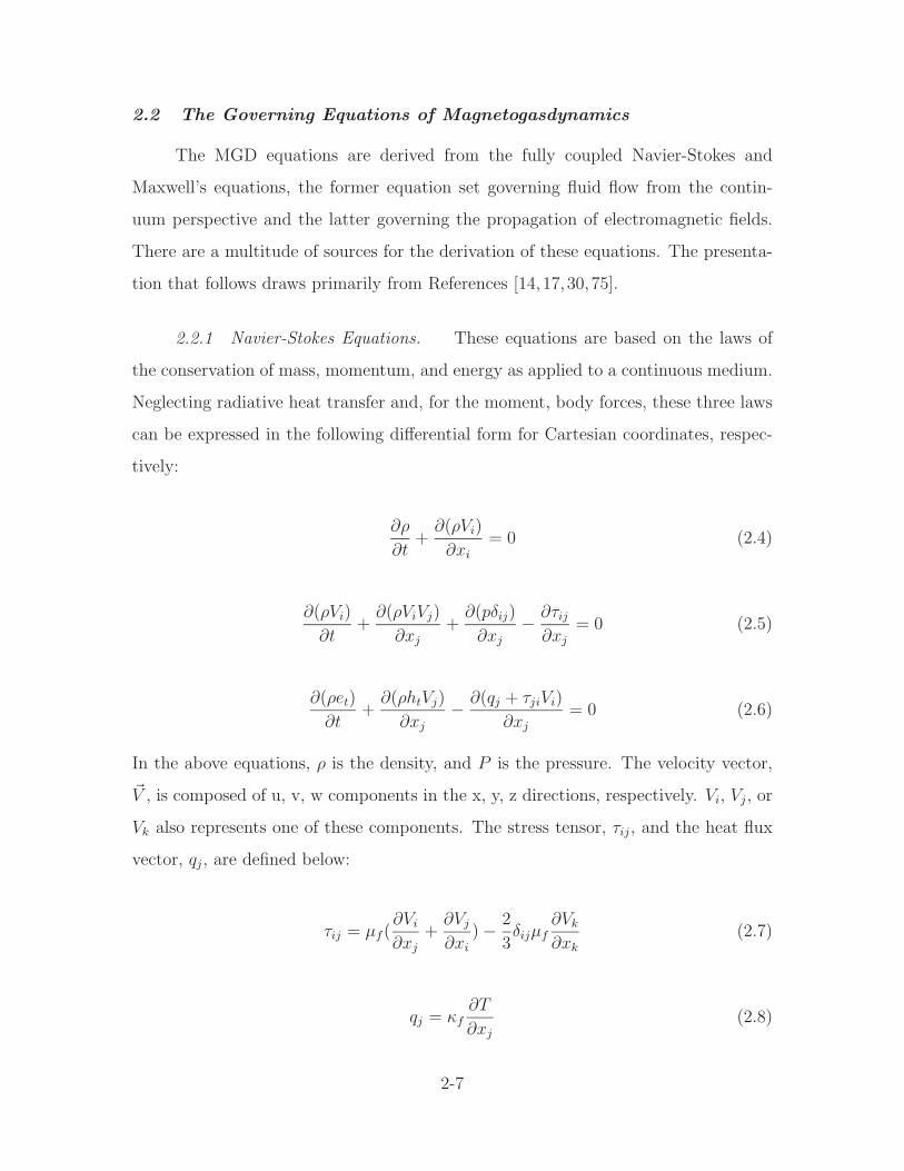
II. Research Foundations and Governing Equations . . . . . . . . . . 2-1

2.1 Description of the Computational Method . . . . . . . . 2-1

2.2 The Governing Equations of Magnetogasdynamics . . . . 2-7

2.2.1 Navier-Stokes Equations . . . . . . . . . . . . . 2-7

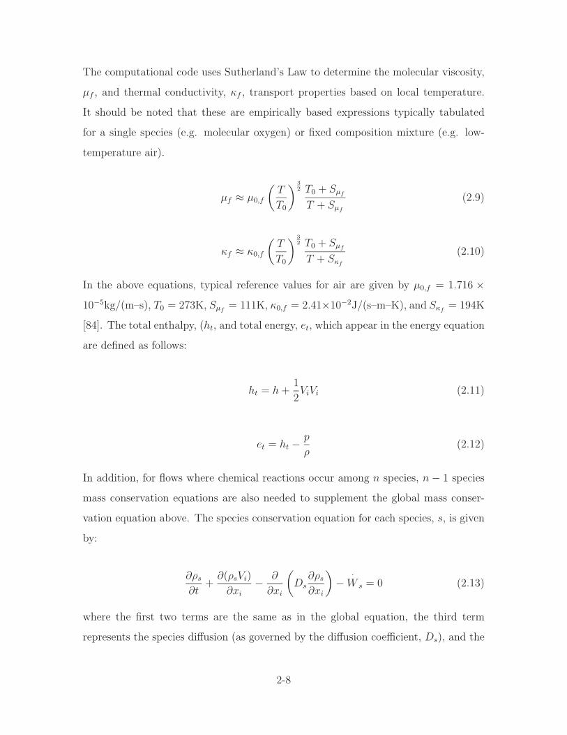
2.2.2 Ideal Gas Equation of State . . . . . . . . . . . 2-9

2.2.3 Vector Form of the Navier-Stokes Equations . . 2-9

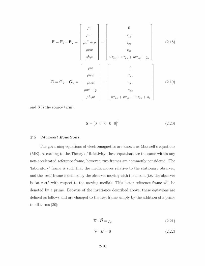
2.3 Maxwell Equations . . . . . . . . . . . . . . . . . . . . . 2-10

2.3.1 Ohm’s Law . . . . . . . . . . . . . . . . . . . . 2-112.3.2 Additional Constitutive Relations . . . . . . . . 2-112.3.3 Magnetogasdynamic Assumptions . . . . . . . . 2-12

2.3.4 Maxwell Equations for Magnetogasdynamic Flow 2-14

2.4 The Magnetogasdynamic Equations: Source Term Formu-lation . . . . . . . . . . . . . . . . . . . . . . . . . . . . 2-142.4.1 Non-dimensionalization of the Magnetogasdynamic

Equations . . . . . . . . . . . . . . . . . . . . . 2-15

2.4.2 Vector Form of the Magnetogasdynamic Equations 2-18

2.4.3 Curvilinear Transformation . . . . . . . . . . . 2-182.5 Summary of the Numerical Methods Used to Implement

the Computational Model . . . . . . . . . . . . . . . . . 2-21

2.6 The Control Volume Approach and Performance Analysis 2-22

2.7 Approximating the Non-Equilibrium Ionization with a Sim-plified Electron Beam Model . . . . . . . . . . . . . . . . 2-25

vi

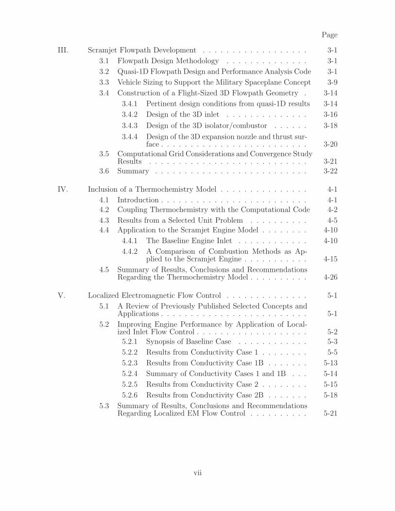
Page

III. Scramjet Flowpath Development . . . . . . . . . . . . . . . . . . 3-1

3.1 Flowpath Design Methodology . . . . . . . . . . . . . . 3-1

3.2 Quasi-1D Flowpath Design and Performance Analysis Code 3-1

3.3 Vehicle Sizing to Support the Military Spaceplane Concept 3-9

3.4 Construction of a Flight-Sized 3D Flowpath Geometry . 3-14

3.4.1 Pertinent design conditions from quasi-1D results 3-14

3.4.2 Design of the 3D inlet . . . . . . . . . . . . . . 3-16

3.4.3 Design of the 3D isolator/combustor . . . . . . 3-18

3.4.4 Design of the 3D expansion nozzle and thrust sur-face . . . . . . . . . . . . . . . . . . . . . . . . . 3-20

3.5 Computational Grid Considerations and Convergence StudyResults . . . . . . . . . . . . . . . . . . . . . . . . . . . 3-21

3.6 Summary . . . . . . . . . . . . . . . . . . . . . . . . . . 3-22

IV. Inclusion of a Thermochemistry Model . . . . . . . . . . . . . . . 4-1

4.1 Introduction . . . . . . . . . . . . . . . . . . . . . . . . . 4-14.2 Coupling Thermochemistry with the Computational Code 4-2

4.3 Results from a Selected Unit Problem . . . . . . . . . . 4-54.4 Application to the Scramjet Engine Model . . . . . . . . 4-10

4.4.1 The Baseline Engine Inlet . . . . . . . . . . . . 4-10

4.4.2 A Comparison of Combustion Methods as Ap-plied to the Scramjet Engine . . . . . . . . . . . 4-15

4.5 Summary of Results, Conclusions and RecommendationsRegarding the Thermochemistry Model . . . . . . . . . . 4-26

V. Localized Electromagnetic Flow Control . . . . . . . . . . . . . . 5-1

5.1 A Review of Previously Published Selected Concepts andApplications . . . . . . . . . . . . . . . . . . . . . . . . . 5-1

5.2 Improving Engine Performance by Application of Local-ized Inlet Flow Control . . . . . . . . . . . . . . . . . . . 5-25.2.1 Synopsis of Baseline Case . . . . . . . . . . . . 5-3

5.2.2 Results from Conductivity Case 1 . . . . . . . . 5-5

5.2.3 Results from Conductivity Case 1B . . . . . . . 5-13

5.2.4 Summary of Conductivity Cases 1 and 1B . . . 5-14

5.2.5 Results from Conductivity Case 2 . . . . . . . . 5-15

5.2.6 Results from Conductivity Case 2B . . . . . . . 5-18

5.3 Summary of Results, Conclusions and RecommendationsRegarding Localized EM Flow Control . . . . . . . . . . 5-21

vii

Page

VI. Application of MGD Energy Bypass to Flowpath . . . . . . . . . 6-1

6.1 Introduction . . . . . . . . . . . . . . . . . . . . . . . . . 6-16.2 MGD Power Generation . . . . . . . . . . . . . . . . . . 6-2

6.2.1 The Conventional Bypass Approach: MGD PowerGeneration Upstream of the Combustor . . . . . 6-2

6.2.2 Combustor-Based MGD Power Generation . . . 6-136.3 MGD Flow Acceleration and Energy Bypass . . . . . . . 6-19

6.4 Summary of Results, Conclusions and RecommendationsRegarding MGD Power Generation and Energy Bypass . 6-24

VII. Summary, Conclusions, and Recommendations . . . . . . . . . . . 7-1

7.1 Summary . . . . . . . . . . . . . . . . . . . . . . . . . . 7-1

7.2 Conclusions . . . . . . . . . . . . . . . . . . . . . . . . . 7-57.3 Recommendations for Future Research . . . . . . . . . . 7-7

Bibliography . . . . . . . . . . . . . . . . . . . . . . . . . . . . . . . . . . BIB-1

Vita . . . . . . . . . . . . . . . . . . . . . . . . . . . . . . . . . . . . . . . VITA-1

viii

List of FiguresFigure Page

1.1. Typical Scramjet Engine Schematic . . . . . . . . . . . . . . . 1-2

1.2. Airbreathing Engine Performance Regimes [11] . . . . . . . . . 1-4

1.3. Magneto-Plasma Chemical Engine (MPCE) Schematic . . . . . 1-9

2.1. AFRL/VA Scramjet Model [21] . . . . . . . . . . . . . . . . . . 2-5

2.2. Examples of 3D MGD-Flow Interaction in AFRL Scramjet Inlet

Model[21] . . . . . . . . . . . . . . . . . . . . . . . . . . . . . . 2-6

2.3. Magnetic Field Requirements for Varying Q,σ . . . . . . . . . . 2-26

3.1. Comparison with HAP Burner Models . . . . . . . . . . . . . . 3-3

3.2. Performance Envelope for AFRL Engine as given by Author in

AIAA 2003-0172. . . . . . . . . . . . . . . . . . . . . . . . . . . 3-7

3.3. Performance Envelope for Engine as given by Author in AIAA

2003-0172 except maximum heating applied in burner. . . . . . 3-7

3.4. Performance Envelope for Engine as given in AIAA 2003-0172

except maximum burner temperature capped at 2500K. . . . . 3-8

3.5. Performance Envelope for optimized geometry engine with max-

imum burner temperature capped at 2500K. . . . . . . . . . . . 3-9

3.6. Overall Efficiency Contours for 2-Parameter Study of Mach 10

Engine . . . . . . . . . . . . . . . . . . . . . . . . . . . . . . . 3-15

3.7. Combustor Exit Temperature Contours for 2-Parameter Study

of Mach 10 Engine . . . . . . . . . . . . . . . . . . . . . . . . . 3-15

3.8. Scramjet Inlet Grid Normalized by Freestream Capture Width 3-17

3.9. Scramjet Isolator-Combustor, Internal Nozzle Grid Normalized

by Inlet Width . . . . . . . . . . . . . . . . . . . . . . . . . . . 3-20

ix

Figure Page

3.10. Grid Convergence Comparison Using Internal Portion of Scram-

jet Inlet

(a) Difference in pressure normalized by the average of the two

values.

(b) Difference in Mach Number normalized by the freestream

value. . . . . . . . . . . . . . . . . . . . . . . . . . . . . . . . 3-23

4.1. Combustion Nozzle Species Distribution . . . . . . . . . . . . . 4-6

4.2. Combustion Nozzle . . . . . . . . . . . . . . . . . . . . . . . . 4-9

4.3. Mean Values of Static Pressure and Temperature within Baseline

Inlet . . . . . . . . . . . . . . . . . . . . . . . . . . . . . . . . 4-11

4.4. Mean Values of Mach Number and Normalized Axial Velocity

within Baseline Inlet . . . . . . . . . . . . . . . . . . . . . . . 4-12

4.5. Mass Spillage at Cowl Lip . . . . . . . . . . . . . . . . . . . . . 4-13

4.6. Baseline Inlet Results . . . . . . . . . . . . . . . . . . . . . . . 4-14

4.7. Temperature Contours in Baseline Inlet Normalized by T0 = 233K 4-15

4.8. Pressure Contours and Vortical Structures in Baseline Inlet . . 4-16

4.9. Flowfield Properties in Cold-Flow Combustor-Nozzle . . . . . . 4-18

4.10. Combustor Temperature Contours, Normalized by T0 = 233K,

Using Heating Rate Source Term . . . . . . . . . . . . . . . . . 4-19

4.11. Flowfield Properties in QC Combustor-Nozzle . . . . . . . . . . 4-20

4.12. Reactant Mass Fractions in Combustor-Nozzle with Chemistry 4-21

4.13. Product Mass Fractions in Combustor-Nozzle with Chemistry . 4-24

4.14. Thermodynamic Properties in Combustor-Nozzle with Chemistry 4-25

4.15. Quasi-1D Comparison of Combustor Properties . . . . . . . . . 4-27

x

Figure Page

5.1. Full Cross-section Non-Dimensional Conductivity (SIGMA) Pro-

files in Inlet

(a) Case 1: Conductive region is limited to upstream of separa-

tion region.

(b) Case 2: Conductive region extends from cowl lip to inlet

throat.

(c) Case 1B: Conductive region centered outside of boundary

layer. . . . . . . . . . . . . . . . . . . . . . . . . . . . . . . . . 5-4

5.2. Mean Inlet Pressure for Case 1 with Varying k and Q = 5 . . . 5-6

5.3. Inlet Efficiencies, Case 1 . . . . . . . . . . . . . . . . . . . . . . 5-7

5.4. Comparison of Net Inlet Drag for Conductivity Case 1 . . . . . 5-7

5.5. Mass Spillage at Cowl Lip . . . . . . . . . . . . . . . . . . . . . 5-8

5.6. Comparison of Normalized Heat Transfer for Conductivity Cases

1 and 1B . . . . . . . . . . . . . . . . . . . . . . . . . . . . . . 5-9

5.7. Separation Region Comparison . . . . . . . . . . . . . . . . . . 5-11

5.8. Comparison of Net Electric Power Generated/Required for Con-

ductivity Cases 1 and 1B as Defined by Pgen − Pion . . . . . . . 5-12

5.9. Comparison of Enthalpy Extraction/Addition for Conductivity

Cases 1 and 1B . . . . . . . . . . . . . . . . . . . . . . . . . . . 5-12

5.10. Mean Inlet Pressure for Case 2 with Varying k and Q = 5 . . . 5-15

5.11. Comparison of Net Inlet Drag for Conductivity Case 2 and 2B 5-16

5.12. Comparison of Wall Heat Transfer for Conductivity Cases 2 and

2B . . . . . . . . . . . . . . . . . . . . . . . . . . . . . . . . . . 5-17

5.13. Comparison of Net Electric Power Generated/Required for Con-

ductivity Cases 2 and 2B . . . . . . . . . . . . . . . . . . . . . 5-18

5.14. Inlet Efficiencies, Case 2 . . . . . . . . . . . . . . . . . . . . . . 5-19

6.1. Conductivity Profiles for Isolator-Based Generators with Speci-

fied Electric Field . . . . . . . . . . . . . . . . . . . . . . . . . 6-3

6.2. Electrode Configurations for Isolator-Based Generators with Spec-

ified Electric Potential . . . . . . . . . . . . . . . . . . . . . . 6-4

xi

Figure Page

6.3. Comparison of Electrical Power Generation/Consumption for Isolator-

Based MGD Generators . . . . . . . . . . . . . . . . . . . . . . 6-4

6.4. Profiles of Normalized Conduction Current and Net EM Energy

Interaction for the K-elec Configuration. (k = 0.6(nominal),

Q = 5) . . . . . . . . . . . . . . . . . . . . . . . . . . . . . . . 6-8

6.5. Comparison of Selected Cross-Sectional Averaged Flow Proper-

ties for Isolator-Based MGD Power Generation with Specified

Electrodes. (Q = 5) . . . . . . . . . . . . . . . . . . . . . . . . 6-10

6.6. Increase in Inlet Drag and Heat Transfer Relative to Baseline for

Isolator-Based MGD Power Generation . . . . . . . . . . . . . 6-11

6.7. Comparison of Inlet Efficiencies for Isolator-Based MGD Power

Generation . . . . . . . . . . . . . . . . . . . . . . . . . . . . . 6-12

6.8. Combustor-based MGD Electrode Placement Super-Imposed on

Results for Z-Midplane Pressure Contours Using Four Electrode

Case (Note: Negative Electrodes Not Shown for Clarity) . . . . 6-13

6.9. Comparison of Selected Cross-Sectional Averaged Flow Proper-

ties for Combustor-Based MGD Power Generation with Specified

Electrodes. (Q = 5) . . . . . . . . . . . . . . . . . . . . . . . . 6-15

6.10. Net Electrical Power Production (in MW) for Combustor-Based

MGD Generators . . . . . . . . . . . . . . . . . . . . . . . . . . 6-16

6.11. Comparison of Component and Total Axial Force, Control Vol-

ume Heat Transfer, and Total Pressure Ratio for Combustor-

Based MGD Power Generation Using Specified Electrodes. (Q =

5) . . . . . . . . . . . . . . . . . . . . . . . . . . . . . . . . . . 6-18

6.12. Comparison of Selected Cross-Sectional Averaged Flow Proper-

ties for k = 2.0 MGD Acceleration with Specified Electrodes. . 6-21

6.13. Comparison of Component and Total Axial Force and Net Elec-

tric Power Balance for MGD Energy Bypass Scramjets Using

Specified Electrodes. . . . . . . . . . . . . . . . . . . . . . . . 6-23

xii

List of TablesTable Page

3.1. Comparison of Quasi-1D and 3D Model Results at M0 = 8.0 . . 3-4

3.2. Quasi 1D Method Comparison of Baseline and Optimized Ge-

ometries . . . . . . . . . . . . . . . . . . . . . . . . . . . . . . . 3-8

3.3. Freestream Properties at Design Point . . . . . . . . . . . . . . 3-11

3.4. MSP Scramjet Threshold Performance Values . . . . . . . . . . 3-13

3.5. 3D Computational Mesh Sizes . . . . . . . . . . . . . . . . . . 3-22

4.1. Hydrogen-Air Ignition Times . . . . . . . . . . . . . . . . . . . 4-6

4.2. Comparison of Water Production . . . . . . . . . . . . . . . . . 4-7

4.3. Scramjet Combustor Performance Comparison without MGD . 4-28

5.1. Pertinent Baseline Scramjet Inlet Results . . . . . . . . . . . . 5-5

5.2. Selected Results for MGD Accelerators, k = 1.3, Q = 5 . . . . . 5-20

xiii

List of SymbolsSymbol Page

~B Magnetic flux Density (Tesla) . . . . . . . . . . . . . . . . 1-8

k Load factor . . . . . . . . . . . . . . . . . . . . . . . . . . 1-8

σ Electrical conductivity (scalar, mhos/meter) . . . . . . . . 1-8

ISP Specific impulse (sec) . . . . . . . . . . . . . . . . . . . . . 1-8

Rem Magnetic Reynold’s number . . . . . . . . . . . . . . . . . 2-1

V0 Reference speed (meters/second) . . . . . . . . . . . . . . 2-2

L0 Reference length (meters) . . . . . . . . . . . . . . . . . . 2-2

σ0 Reference conductivity (mhos/meter) . . . . . . . . . . . . 2-2

µe Magnetic permeability (kilogram-meter/(second-Ampere)2) 2-2

M Mach number . . . . . . . . . . . . . . . . . . . . . . . . . 2-2

~E Electric field (Volts/meter) . . . . . . . . . . . . . . . . . 2-3

φ Scalar electric potential (Volts) . . . . . . . . . . . . . . . 2-3

~j Conduction current (Amperes/meter2) . . . . . . . . . . . 2-3

~V Velocity (meters/second) . . . . . . . . . . . . . . . . . . . 2-3

Re Reynold’s number . . . . . . . . . . . . . . . . . . . . . . 2-4

T Temperature (Kelvin) . . . . . . . . . . . . . . . . . . . . 2-4

ρ Density (kilogram/meter3) . . . . . . . . . . . . . . . . . . 2-7

P Pressure (Pascals) . . . . . . . . . . . . . . . . . . . . . . 2-7

u, v, w Velocity components (meters/second) . . . . . . . . . . . . 2-7

x, y, z Cartesian coordinates (meters) . . . . . . . . . . . . . . . 2-7

τij Stress tensor (Newtons/meter2) . . . . . . . . . . . . . . . 2-7

qj Conductive heat flux vector (Watts/meter2) . . . . . . . . 2-7

µf Molecular viscosity (kilograms/(meter-second)) . . . . . . 2-8

κf Thermal conductivity (Watts/(meter-Kelvin)) . . . . . . . 2-8

ht Total enthalpy (Joules/kilogram) . . . . . . . . . . . . . . 2-8

xiv

Symbol Page

et Total energy (Joules/kilogram) . . . . . . . . . . . . . . . 2-8

Ds Species diffusion coefficient (meters2/second) . . . . . . . . 2-8

Ws Species production rate (kilograms/(meter3-second)) . . . 2-9

R Specific gas constant (Joules/(kilogram-Kelvin)) . . . . . . 2-9

U Conserved variables vector . . . . . . . . . . . . . . . . . . 2-9

E, F, G Flux Vectors . . . . . . . . . . . . . . . . . . . . . . . . . 2-9

S Source term vector . . . . . . . . . . . . . . . . . . . . . . 2-10

~D Electric flux density (Coulombs/meter) . . . . . . . . . . . 2-11

ρe Space charge density (Coulombs/meter2) . . . . . . . . . . 2-11

~H Magnetic Field (Amperes/meter) . . . . . . . . . . . . . . 2-11

c Speed of light (meters/second) . . . . . . . . . . . . . . . 2-11

ǫe Permittivity (Farads/meter) . . . . . . . . . . . . . . . . . 2-12

µe,0 Free-space value of permeability . . . . . . . . . . . . . . . 2-12

ǫe,0 Free-space value of permittivity . . . . . . . . . . . . . . . 2-12

~fL Lorentz electromagnetic body force density (Newtons/meter3) 2-15

WEM Electromagnetic energy interaction (Watts/meter3) . . . . 2-15

M0 Reference Mach number . . . . . . . . . . . . . . . . . . . 2-16

Pr Prandtl number . . . . . . . . . . . . . . . . . . . . . . . . 2-16

Q Interaction parameter . . . . . . . . . . . . . . . . . . . . 2-16

ξ,η,ζ Generalized coordinates . . . . . . . . . . . . . . . . . . . 2-18

J Jacobian of transformation (1/meters3) . . . . . . . . . . . 2-20

Fx, Fy, and FzForce components in control volume formulation (Newtons) 2-23

Qht Heat transfer rate in control volume formulation (Watts) . 2-23

πc Total pressure ratio . . . . . . . . . . . . . . . . . . . . . . 2-24

ηKE Kinetic energy efficiency . . . . . . . . . . . . . . . . . . . 2-24

∆s/Cp Dimensionless entropy increase . . . . . . . . . . . . . . . 2-24

ηc Adiabatic compression effciency . . . . . . . . . . . . . . . 2-24

ηg Enthalpy extraction ratio . . . . . . . . . . . . . . . . . . 2-24

xv

Symbol Page

Pion Required ionization power (Watts) . . . . . . . . . . . . . 2-25

Pgen Generated electrical power (Watts) . . . . . . . . . . . . . 2-25

τb Stagnation temperature ratio across quasi-1D combustor . 3-6

q0 Freestream dynamic pressure (Pascals) . . . . . . . . . . . 3-10

F Uninstalled thrust (Newtons) . . . . . . . . . . . . . . . . 3-10

m0 Freestream mass flow rate (kilograms/second) . . . . . . . 3-10

D Drag (Newtons) . . . . . . . . . . . . . . . . . . . . . . . . 3-11

T Installed engine thrust (Newtons) . . . . . . . . . . . . . . 3-11

De Engine installation drag (Newtons) . . . . . . . . . . . . . 3-11

η0 Engine overall efficiency . . . . . . . . . . . . . . . . . . . 3-11

hpr Fuel heating value (Joules/kilogram) . . . . . . . . . . . . 3-11

mf Fuel mass flow rate (kilograms/second) . . . . . . . . . . . 3-11

R Range (meters) . . . . . . . . . . . . . . . . . . . . . . . . 3-11

Πf Fuel mass fraction . . . . . . . . . . . . . . . . . . . . . . 3-12

Fmo

Uninstalled specific thrust (meters/second) . . . . . . . . . 3-12

f Fuel-to-air mass flow ratio . . . . . . . . . . . . . . . . . . 3-12

Πe Empty (structural) mass fraction . . . . . . . . . . . . . . 3-13

Πp Payload mass fraction . . . . . . . . . . . . . . . . . . . . 3-13

φe Installation drag penalty . . . . . . . . . . . . . . . . . . . 3-13

γb Combustor specific heat ratio . . . . . . . . . . . . . . . . 3-14

Rb Combustor specific gas constant (Joules/(kilogam-Kelvin)) 3-14

Tt Total (stagnation) temperature (Kelvin) . . . . . . . . . . 3-19

ω Expansion nozzle turning angle . . . . . . . . . . . . . . . 3-21

hfs Species heat of formation (Joules/kilogram) . . . . . . . . 4-2

∆h298Ks Species enthalpy wrt standard conditions (Joule/kilogram) 4-2

Ys Species mass fraction . . . . . . . . . . . . . . . . . . . . . 4-2

s Chemical species . . . . . . . . . . . . . . . . . . . . . . . 4-3

MWs Species molecular weight (gramm/mole) . . . . . . . . . . 4-3

xvi

Symbol Page

R Reactant . . . . . . . . . . . . . . . . . . . . . . . . . . . 4-3

P Product . . . . . . . . . . . . . . . . . . . . . . . . . . . . 4-3

Meff,m Third-body efficiency . . . . . . . . . . . . . . . . . . . . . 4-3

kfmForward reaction rate constant . . . . . . . . . . . . . . . 4-3

kbmBackward reaction rate constant . . . . . . . . . . . . . . 4-3

Xi Species mole fraction . . . . . . . . . . . . . . . . . . . . . 4-3

ρs Species density (kilograms/meter3) . . . . . . . . . . . . . 4-3

tref Convective time scale (seconds) . . . . . . . . . . . . . . . 4-5

QC Volumetric Heating Rate Source Term (Watts/meter3) . . 4-17

xvii

List of AbbreviationsAbbreviation Page

HRE Hypersonic Research Engine . . . . . . . . . . . . . . . . . 1-2

NASP National Aerospace Plane . . . . . . . . . . . . . . . . . . 1-3

MGD Magnetogasdynamics . . . . . . . . . . . . . . . . . . . . . 1-5

OSU The Ohio State University . . . . . . . . . . . . . . . . . . 1-6

RF Radio Frequency . . . . . . . . . . . . . . . . . . . . . . . 1-6

HSRI Hypersonic Systems Research Institute . . . . . . . . . . . 1-8

MPCE Magneto-Plasma Chemical Engine . . . . . . . . . . . . . 1-8

MHD Magnetohydrodynamics . . . . . . . . . . . . . . . . . . . 1-8

EM Electromagnetic . . . . . . . . . . . . . . . . . . . . . . . 1-10

AFRL Air Force Research Laboratory . . . . . . . . . . . . . . . 2-1

CFD Computational Fluid Dynamics . . . . . . . . . . . . . . . 2-1

RK4 4th order Runge-Kutta . . . . . . . . . . . . . . . . . . . . 2-3

ME Maxwell’s Equations . . . . . . . . . . . . . . . . . . . . . 2-10

MLT Maxwell-Lorentz Transformations . . . . . . . . . . . . . . 2-11

MGDE Magnetogasdynamic Equations . . . . . . . . . . . . . . . 2-14

CV Control Volume . . . . . . . . . . . . . . . . . . . . . . . . 2-22

H-P Heiser and Pratt text, Ref. 25 . . . . . . . . . . . . . . . . 3-1

MSP Military Space Plane . . . . . . . . . . . . . . . . . . . . . 3-9

AFRL/PR AFRL Propulsion Directorate . . . . . . . . . . . . . . . . 3-14

AFT Adiabatic Flame Temperature . . . . . . . . . . . . . . . . 4-19

xviii

Assessing the Potential for Improved Scramjet

Performance Through Application of Electromagnetic

Flow Control

I. Introduction

1.1 Scramjet Operation, Design Challenges, and a Brief History

Jet engines of all varieties depend on the compression of ambient air to provide the

oxidizer needed for combustion. This is in contrast to a rocket engine which must

carry its own oxidizer at a substantial vehicle performance penalty. Probably the most

widely known application of a jet engine is the turbojet which relies on a compressor

driven by a turbine in the engine exhaust flow to perform this function. This method

is particularly efficient for subsonic and low supersonic applications and as a concept

dates back to the work of Guillame in 1921 [25]. By contrast, a ramjet compresses

the ambient air entirely through deceleration of the freestream flow, typically by

one or more inlet shockwaves. Therefore, the ram compression process is one of

conversion of freestream kinetic energy to internal energy as manifested by increased

temperature, pressure, and density and lower relative Mach number. The ramjet

concept is actually seven years older than the turbojet, but because a ramjet does not

provide compression as efficiently at low speed flows, it wasn’t until 1928 that a patent

for a ramjet for supersonic flight was issued to Albert Fono of Hungary [25]. Ramjets

are most efficient when operated in a freestream regime of approximately Mach 3 -

6. At speeds approaching Mach 6, the aerodynamic losses (e.g. total pressure, drag),

heating, and increased structural requirements that accompany compression of the

flow to subsonic combustion speeds render the ordinary ramjet excessively inefficient.

Thus, to extend the airbreathing performance envelope to higher Mach numbers,

supersonic combustion has been pursued.

1-1

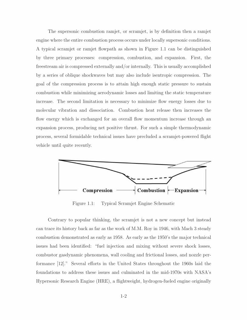
The supersonic combustion ramjet, or scramjet, is by definition then a ramjet

engine where the entire combustion process occurs under locally supersonic conditions.

A typical scramjet or ramjet flowpath as shown in Figure 1.1 can be distinguished

by three primary processes: compression, combustion, and expansion. First, the

freestream air is compressed externally and/or internally. This is usually accomplished

by a series of oblique shockwaves but may also include isentropic compression. The

goal of the compression process is to attain high enough static pressure to sustain

combustion while minimizing aerodynamic losses and limiting the static temperature

increase. The second limitation is necessary to minimize flow energy losses due to

molecular vibration and dissociation. Combustion heat release then increases the

flow energy which is exchanged for an overall flow momentum increase through an

expansion process, producing net positive thrust. For such a simple thermodynamic

process, several formidable technical issues have precluded a scramjet-powered flight

vehicle until quite recently.

Figure 1.1: Typical Scramjet Engine Schematic

Contrary to popular thinking, the scramjet is not a new concept but instead

can trace its history back as far as the work of M.M. Roy in 1946, with Mach 3 steady

combustion demonstrated as early as 1958. As early as the 1950’s the major technical

issues had been identified: “fuel injection and mixing without severe shock losses,

combustor gasdynamic phenomena, wall cooling and frictional losses, and nozzle per-

formance [12].” Several efforts in the United States throughout the 1960s laid the

foundations to address these issues and culminated in the mid-1970s with NASA’s

Hypersonic Research Engine (HRE), a flightweight, hydrogen-fueled engine originally

1-2

envisioned for the X-15 program. Upon the cancellation of the X-15 program, two

HRE prototypes were converted to ground test articles that throughout the 1970s

established a comprehensive database on inlet and combustor performance in the low

hypersonic range (Mach 5-7) [25]. Concurrent efforts by the U.S. Air Force and Navy

to develop scramjets for potential missile applications came together with the HRE.

Technology from the HRE evolved into the National Aerospace Plane (NASP) pro-

gram of the 1980s. NASP’s goal was to to develop the X-30 Single-Stage-To-Orbit

vehicle which would rely on a hydrogen-fueled scramjet for operation in the Mach 4-15

range [12]. Although the NASP program produced a wealth of designs and ground

test data, the X-30 was never built and by 1995 the program had been terminated

due to lack of funding.

An offshoot of the NASP, NASA’s X-43 program began in the late 1990s and,

with its successful flight test in March 2004, currently represents the state-of-the-art

in scramjet propulsion [11]. The X-43A uses a hydrogen-fueled scramjet engine which

is highly integrated with the airframe. This flight demonstration vehicle is released

from a B-52 and accelerated to flight test conditions by the first stage of a Pegasus

expendable launch vehicle. Upon reaching these conditions, the X-43 is released from

its booster and is then self-propelled by its scramjet engine. On 27 March 2004,

the vehicle became the first scramjet device to demonstrate net thrust [16] and set a

world speed record for airbreathing aircraft with its 11 second flight at Mach 6.83 and

100,000 feet [57]. By 16 November 2004, a second X-43A pushed the speed record

even further, achieving Mach 9.6 during a 10-second burn of its engine after being

“boosted to an altitude of 33,223 meters (109,000 feet) by a Pegasus rocket launched

from beneath a B52-B jet aircraft.” [58]

Although a great milestone has been reached with the X-43, all of the broad

technical challenges quoted above remain. Of these, the greatest issues continue to

be thermal control, maximizing component and system efficiencies and achieving ade-

quate fuel mixing and combustion within typical combustor residence times measured

in milliseconds. Various flow control mechanisms have been proposed, especially with

1-3

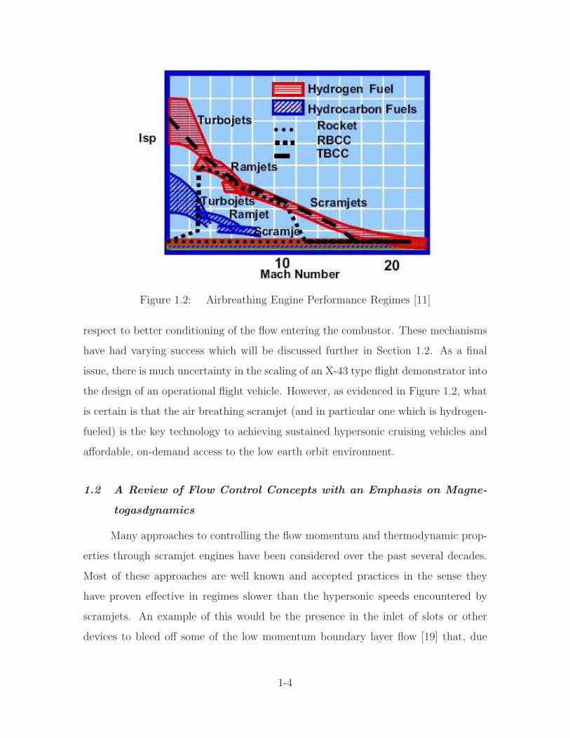
Figure 1.2: Airbreathing Engine Performance Regimes [11]

respect to better conditioning of the flow entering the combustor. These mechanisms

have had varying success which will be discussed further in Section 1.2. As a final

issue, there is much uncertainty in the scaling of an X-43 type flight demonstrator into

the design of an operational flight vehicle. However, as evidenced in Figure 1.2, what

is certain is that the air breathing scramjet (and in particular one which is hydrogen-

fueled) is the key technology to achieving sustained hypersonic cruising vehicles and

affordable, on-demand access to the low earth orbit environment.

1.2 A Review of Flow Control Concepts with an Emphasis on Magne-

togasdynamics

Many approaches to controlling the flow momentum and thermodynamic prop-

erties through scramjet engines have been considered over the past several decades.

Most of these approaches are well known and accepted practices in the sense they

have proven effective in regimes slower than the hypersonic speeds encountered by

scramjets. An example of this would be the presence in the inlet of slots or other

devices to bleed off some of the low momentum boundary layer flow [19] that, due

1-4

to the high area contraction ratios in scramjet inlets, tends to cause large regions of

flow separation and extreme wall heating in the inlet [65]. These same devices can

also be effective in lowering the overall mass flow rate into the engine to promote

engine starting. The downside of this approach is a structure and drag penalty due

to the bleed plenum as well as a loss of some of the freestream mass flow. In a differ-

ent approach to the same issue, some experiments, including the X-43A wind tunnel

models, have used boundary layer trip devices on the external compression surfaces

to induce a turbulent boundary layer [6] and likewise prevent flow separation. How-

ever, turbulent flow has more drag than laminar flow, which again decreases vehicle

performance. Although these examples have focused on conditioning the inlet flow,

just as much if not more effort, has focused on using various geometries to control fuel

mixing and combustion [4,5,15,24]. What is obvious is that all of these methods have

drawbacks and thus in the past several years researchers have begun to turn towards

more exotic flow control methods.

As far back as the 1960s, practical magnetogasdynamic (MGD) applications

were studied in earnest, not only for terrestrial electrical power generation [70] but

also for electrical propulsion and aerodynamic control [75]. Magnetogasdynamics (also

referred to as magnetohydrodynamics or magnetofluidmechanics by various authors)

is broadly defined by Hughes and Young in their seminal textbook as “the study of

the flow of electrically conducting fluids in the presence of a magnetic field under

certain special assumptions [30].” In short, the fluid flow is coupled to Maxwell’s

equations for electromagnetism through an electromagnetic body force known as the

Lorentz Force and its associated energy interaction. This coupling is defined in detail

in the equations presented in Chapter II. In the infancy of hypersonic flight, it was

recognized that the air within the hypersonic shock layer surrounding the vehicle could

become appreciably ionized. This fact “prompted research on methods of magnetically

interacting with the flow to produce various effects, including control of drag or angle

of attack, and boundary-layer control to increase the transition Reynolds number or to

reduce the hypersonic heat transfer” [75]. Recent experimental and numerical research

1-5

efforts have focused on internal MGD flow control and electrical power generation (i.e.

within scramjet engines) as well as the external aerodynamics, with key goals being

the mitigation of the high thermomechanical loads and low propulsion efficiencies

typical of the examples described in the previous paragraph.

These recent MGD flow control efforts have ranged from basic scientific explo-

ration of the concept to simple analytical and experimental applications. A good

example of the former is the MGD flow characterization conducted in the Mach 3

and Mach 4 plasma tunnels at The Ohio State University (OSU) [53, 55, 59]. These

experiments are investigating basic unit problems specifically relevant to MGD flow

control by exploring three-dimensional supersonic flow in a channel. Specific work

at this facility has sought to attain and characterize a sustainable, non-equilibrium

plasma. Various approaches using high intensity radio frequency (RF) discharges

have been taken to accomplish this ionization. Flowing nitrogen at Mach 3 through

a 3-cm wide test section, a sustained RF discharge at 1kW was capable of achieving

a conductivity of 0.24mho/m in the presence of a magnetic field of 1.5 Tesla (T).

From the standpoint of required ionization power, a more efficient approach demon-

strated a pulsed-RF signal with a 20ns duration and 40kHz repetition rate with a

peak power approaching 1MW. When combined with a sustaining direct current elec-

tric field, both air and nitrogen Mach 4 flows produced uniform, stable plasmas with

conductivities of 0.09mho/m and 0.18mho/m, respectively.

Complementing this basic scientific exploration, a significant amount of analyt-

ical work exists with respect to both creating/sustaining a non-equilibrium plasma as

well as putting this plasma to work through MGD interaction. However, it should be

immediately noted that in order to make most practical analytical problems tractable,

significant simplifying assumptions must be made. For example, the analytical work

described in the remainder of this section was either 1D or 2D and assumed inviscid

flow. Furthermore, except for some of the electron ionization models, chemical com-

position is assumed fixed, and typically the assumption of a calorically perfect gas

is made. With this in mind, a large body of work to this effect has been produced

1-6

by Macheret and associates at Princeton University. In 1997, they proposed using a

30keV electron beam to ionize a Mach 10.6 wind tunnel flow and then use the Lorentz

force to accelerate the flow to Mach 14.3 [44]. In 2001 and 2002, they put forward

several detailed papers focused on non-equilibrium ionization methods with applica-

tion toward supersonic MGD power generation. Two years prior to the OSU work

described above, they explored both electron beams and steady and pulsed electric

fields, concluding high energy electron beams (order of 10–1000s of eV) required 1-2

orders of magnitude lower input power than a comparable ionization produced by an

electric field [48]. Applying this conclusion to a simplified 2D analysis of a MGD-

controlled scramjet inlet, they predicted the ability to maintain the shock-on-cowl-lip

condition for Mach numbers of two greater than the geometrical design Mach num-

ber [47]. Although some of this effect was attributable to heating, the work done by

the Lorentz force was shown to be a significant contributor as well. This same work

also demonstrated more electrical power was generated by the MGD interaction than

was required to power the electron beam ionization source. Similar calculations for

a 3x0.25x0.25-meter inlet at flight Mach numbers of 4–10, subjected to a 7T mag-

netic field, generated several MW of excess power by converting approximately 1/3

of the flow enthalpy to electrical power [45, 46]. In the past two years, 1D and 2D

analytical work has predicted MW-class power generation using more moderate 1T

magnetic fields in potassium-seeded combustor flows; power that would then be made

available for applications such as the control of inlet shock location using virtual cowl

shapes created by MGD and/or plasma-controlled external combustion [50, 73, 74].

Finally, recent research has extended these concepts to wind tunnel models of simple

aerodynamic structures [7] providing evidence to support the basic science and an-

alytical work and reinforcing the need to continue exploration of flight vehicle-sized

applications such as the MGD-energy bypass discussed next.

The most ambitious overall MGD system application is without a doubt the

MGD-energy bypass method which has been examined in several contexts by multi-

ple researchers [10, 21, 43, 54, 60, 67]. However, the most frequently cited example of

1-7

the application of an MGD energy bypass method remains that originally espoused

by Russian researchers led by A.L. Kuranov at the Hypersonic Systems Research

Institute (HSRI) in St. Petersburg. HSRI researchers developed a conceptual hy-

personic aircraft, known as AJAX, which relied on their Magneto-Plasma Chemical

Engine (MPCE) for both power and propulsion [8, 9, 35]. The conceptual work on

the AJAX vehicle was among the first to show the potential for electromagnetic-fluid

interactions to improve the performance of scramjet engines. Specific to the AJAX ap-

proach was the use of a parameter-based quasi-1D analysis (as well 2D inlet-specific

numerical studies). This analysis utilized the inviscid subset of the Navier-Stokes

fluid flow equations (i.e. the Euler equations) coupled to a source term formulation

of Maxwell’s equations for electromagnetic fields [35]. The latter equations were cast

in terms of the applied magnetic flux density, ~B, the load factor, k, and a scalar

electrical conductivity, σ. In addition, the model assumed a calorically perfect gas

existed throughout the flow. A final, critical supposition was that the flow sustained

a level of ionization sufficient to ensure appreciable MGD interaction. Assuming all

of the enthalpy extracted from the flow was made available to the MGD accelerator,

the MPCE was shown in some cases to produce 5-10 percent higher specific impulse

(ISP ) than a conventional scramjet of the same geometry when approximately 10 per-

cent of the freestream enthalpy was extracted from the flow. Further studies defined

the self-powered MGD bypass system envelope for a Mach 6 engine in terms of the

magnetic field, ionization power and relative effectiveness of the electromagnetic in-

teraction [34]. In this model, self-powered operation was attained for magnetic fields

stronger than about 0.8T when the ionization power was on the order of 2W/cm3. As

pointed out by the authors’ conclusions though, the “extent of magnetohydrodynamic

(MHD) influence on scramjet performance essentially depends on the type of MHD

generator, inlet characteristics, load factors, Hall parameter, ionizer parameters, and

flow parameters [33].”

Regarding the components of a typical MGD bypass system, Figure 1.3 presents

a simplified schematic of the MPCE with its key features. One or more MGD gen-

1-8

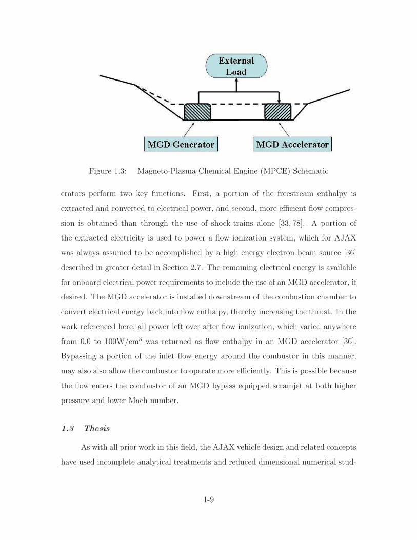
Figure 1.3: Magneto-Plasma Chemical Engine (MPCE) Schematic

erators perform two key functions. First, a portion of the freestream enthalpy is

extracted and converted to electrical power, and second, more efficient flow compres-

sion is obtained than through the use of shock-trains alone [33, 78]. A portion of

the extracted electricity is used to power a flow ionization system, which for AJAX

was always assumed to be accomplished by a high energy electron beam source [36]

described in greater detail in Section 2.7. The remaining electrical energy is available

for onboard electrical power requirements to include the use of an MGD accelerator, if

desired. The MGD accelerator is installed downstream of the combustion chamber to

convert electrical energy back into flow enthalpy, thereby increasing the thrust. In the

work referenced here, all power left over after flow ionization, which varied anywhere

from 0.0 to 100W/cm3 was returned as flow enthalpy in an MGD accelerator [36].

Bypassing a portion of the inlet flow energy around the combustor in this manner,

may also also allow the combustor to operate more efficiently. This is possible because

the flow enters the combustor of an MGD bypass equipped scramjet at both higher

pressure and lower Mach number.

1.3 Thesis

As with all prior work in this field, the AJAX vehicle design and related concepts

have used incomplete analytical treatments and reduced dimensional numerical stud-

1-9

ies. As a consequence, not all of the pertinent flow physics have been captured and

thus the conclusions previously reached are uncertain at best. The purpose of this

research, then, is to apply the first comprehensive three-dimensional computational

analysis to a flight-sized, Mach 10 cruise scramjet engine to determine if, and un-

der what circumstances, electromagnetic flow control can improve performance. Both

localized MGD flow control applications and the MGD energy bypass system are

explored. Comparisons are made to a baseline geometry without flow control. In

addition, numerous metrics exist for determining performance, and a portion of this

research explores which ones provide the most insight into the impacts of the flow

control applications. Unlike prior computational efforts in this field, this research

has removed many of the simplifying assumptions utilized in previous approaches

(e.g. unrealistic flowpath geometries, calorically perfect gases, and inviscid, 2D flow

solvers). In a significant new development, a finite rate chemistry model is applied

to this computational method for the first time, providing the only accurate model

of fuel injection, mixing and combustion in an MGD flow controlled engine. By do-

ing this and removing the other assumptions mentioned, these electromagnetic (EM)

flow control concepts are more fully examined and the viability of a flight-scale system

determined.

1.4 Document Scope and Organization

This document is organized into seven chapters, including this introduction.

The foundation of the research effort is provided in Chapter II, including a presenta-

tion of the governing equations used in the computational model. The other major

features of this chapter are the description of available efficiency metrics with their

advantages and disadvantages and the adoption of an existing ionization model to

the computational method. Chapter III provides a detailed description of the prelim-

inary research that resulted in defining the engine flowpath geometry based on the

requirements for an operationally sized Mach 10 cruise vehicle. The addition of finite

rate thermochemistry to the computational model, a key prerequisite underpinning

1-10

suitable model fidelity, is discussed in Chapter IV. Electromagnetic flow control is

addressed in two separate chapters. First, localized control is investigated in Chapter

V with respect to mitigating flow separation within the inlet. Then, the MGD energy

bypass method of improving engine efficiency and providing auxiliary electrical power

is explored in VI. Finally, Chapter VII summarizes the results of this research and

answers the fundamental question presented by the thesis: can electromagnetic flow

control improve the performance of a flight-representative scramjet engine?

1-11

II. Research Foundations and Governing Equations

2.1 Description of the Computational Method

Inspired in part by AJAX and related efforts, Air Force Research Laboratory

(AFRL) researchers extended the capability to analyze MGD flow control appli-

cations by developing a computational fluid dynamics (CFD) code to model the full,

three-dimensional set of coupled Navier-Stokes and Maxwell’s equations for a non-

ideal gas [20]. (As an aside, ‘non-ideal’ in this context refers to the non-uniform

conductivity found in the weakly ionized, less than perfectly conducting fluid typical

of the altitudes and low hypersonic Mach numbers encountered by scramjets.) How-

ever, the code did not address chemical kinetics but instead relied on a calorically

perfect gas model.

Initial work achieved success by using a compact spatial discretization based on

Pade type formulas and a traditional fourth order Runge-Kutta for temporal integra-

tion [20]. The compact differencing approach was chosen as it would work for nearly

all values of the magnetic Reynold’s number, Rem, which may be considered the ratio

of the induced magnetic field to the total magnetic field. Also, it would provide up

to sixth order accuracy, a necessity for discerning fine wave structures. However, two

drawbacks to this approach were the overall code complexity and the diffusiveness

of the central difference approach, especially when treating certain phenomena like

shock waves. This code was first verified against accepted analytical results for unit

problems such as simple Alfven wave propagation [20]. With the code verified, fur-

ther studies continued by examining external flows around hypersonic blunt bodies,

specifically an axisymmetric, spherical-nosed body with an imposed magnetic dipole

field [61]. Again, the numerical results compared well with the analytical solution.

First, it was shown for the levels of thermal ionization typical of reentry (∼100mho/m)

that magnetic flux densities greater than 1T could slow the flow in the shock layer,

increase drag, and increase the shock standoff distance. Then the same fields were

demonstrated to lower the wall heat flux in the stagnation point region, an effect

2-1

that increased with increasing magnetic field and decreased whenever the electrical

conductivity was non-ideal [62,63].

Having developed an approach to handle the full equation set, including the

generalized diffusivity terms, efforts commenced to increase the fidelity and efficiency

of the code [22], especially with respect to the flow regime dictated by the MGD ap-

proximations (which are presented in their entirety in Subsection 2.3.3). The MGD

approximations are ideally suited for the hypersonic flows of practical interest to

scramjet design. This is because they are certainly non-relativistic and occur at suf-

ficient dynamic pressure to maintain the gas as a dense, collision-dominated plasma.

The latter property ensures that although the plasma is conductive, the high fre-

quency of collisions promote both ionization and recombination, keeping both charge

separation and the conductivity relatively small (what is referred to commonly as

a weakly ionized plasma). Under these conditions, if the MGD interaction is to be

appreciable, the applied magnetic field has to be relatively large to make up for the

low conductivity. In fact, the applied magnetic field significantly influences the fluid

motion. However, the flow distorts the induced magnetic field which is assumed to be

relatively small compared to the externally applied field. This set of circumstances is

embodied in the low Rem condition which is expressed mathematically by Equation 2.1

where V0, L0, σ0, and µe are the reference values for velocity, length, conductivity, and

magnetic permeability, respectively. As an example, a one meter nose radius blunt

body, flying at 8 km/s at an altitude of 61 km would produce only σ = 300 mho/m in

the equilibrium flow downstream of the bow shock, resulting in Rem ∼ 3 [62]. This

example corresponds to a re-entry vehicle at a Mach number (M) greater than 20. At

the lower altitudes and Mach numbers envisioned for scramjets, Rem << 1 is a valid

assumption.

Rem = V0L0σ0µe (2.1)

The conclusion to be drawn from the combination of low σ and high ~B that de-

fines the low Rem regime is that electromagnetic effects may be added directly to the

2-2

Navier-Stokes equations as simple source terms. This approach proved conducive to

allowing traditional upwind spatial discretization schemes such as the Roe flux differ-

ence scheme that, while lower in order of spatial accuracy, were much less diffusive in

capturing flow discontinuities such as shocks. A Poisson solver was then incorporated

to provide the option of either calculating the electric field, ~E, or simply specifying

its vector components at every point [23]. When taking the former, higher fidelity,

approach, the scalar electric potential, φ, on the boundaries is specified and subse-

quently ~E = −∇φ is solved by enforcing current continuity as given by Equation 2.2

where the conduction current, ~j, is given by Ohm’s Law in the form of Equation 2.3.

(In Equation 2.3, ~V is the velocity and the other variables are as previously defined.)

As an aside, the generalized Ohm’s law, which is presented in Subsection 2.3.1, can be

applied to account for the Hall effect and ion-slip typically encountered in flows with

extremely high applied magnetic fields [22]. However, in this research, Hall Effect was

not factored into the results.

∇ ·~j = 0 (2.2)

~j = σ[

~E + ~V × ~B]

(2.3)

Finally, two more tools were added to the method, the first to improve stability

and the second to address turbulent flows. Regarding the former, an approximately-

factored Beam-Warming implicit method was developed to overcome the time-step

stability limitation of the previously used 4th order Runge-Kutta (RK4) scheme that

was encountered, especially when using highly stretched meshes [22]. The implicit

method, while limited to second-order accuracy, demonstrated several important ad-

vantages. These advantages were demonstrated on two sample problems of electro-

magnetic field diffusion and wave propagation which were also solved analytically and

with the explicit RK4 scheme. Both computational methods compared well with the

analytical solution, however the implicit method had a stable time step size three or-

ders of magnitude greater than the RK4 scheme, and each implicit time step required

2-3

only 5% more computational time than its explicit counterpart. As far as turbulent

flows were concerned, the magnetic field’s impact on turbulence presented a signifi-

cant challenge. This is due primarily to the anisotropy brought about the preferential

damping of turbulent fluctuations normal to the magnetic field [71]. Therefore, an

engineering-based approach using a two equation k − ǫ turbulence model based on

liquid metal flows was incorporated to “mimic some of the anticipated effects of the

magnetic field in a simple yet effective manner [22].” The k − ǫ equations are also

integrated implicitly in time but are loosely coupled to the flow equations. This loose

coupling considerably reduces the expense of computing the flux Jacobians. Several

calculations of turbulent flow over a flat plate were made to characterize the effect of

a transverse magnetic field on the flow. Among other things, decreases in the local

skin friction coefficient in the vicinity of the magnetic dipole were observed. In addi-

tion, it was “evident that in the context of the present model the dominant effect of

the magnetic field is on the interaction with the mean flow” [22] as demonstrated by

a thickening of the boundary layer and corresponding reduction in surface gradient.

Having all of these tools, the code was sufficiently developed to attempt modelling

problems of practical engineering interest.

With the code matured and verified, the first ever attempt was made to numeri-

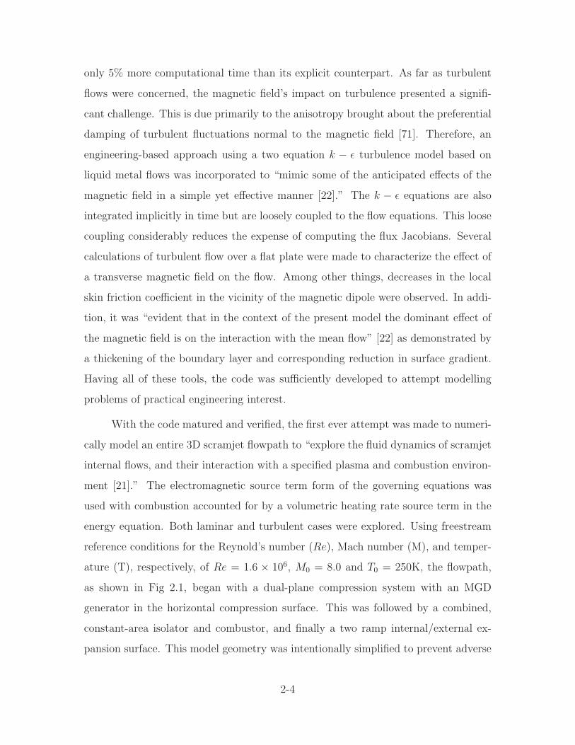
cally model an entire 3D scramjet flowpath to “explore the fluid dynamics of scramjet

internal flows, and their interaction with a specified plasma and combustion environ-

ment [21].” The electromagnetic source term form of the governing equations was

used with combustion accounted for by a volumetric heating rate source term in the

energy equation. Both laminar and turbulent cases were explored. Using freestream

reference conditions for the Reynold’s number (Re), Mach number (M), and temper-

ature (T), respectively, of Re = 1.6 × 106, M0 = 8.0 and T0 = 250K, the flowpath,

as shown in Fig 2.1, began with a dual-plane compression system with an MGD

generator in the horizontal compression surface. This was followed by a combined,

constant-area isolator and combustor, and finally a two ramp internal/external ex-

pansion surface. This model geometry was intentionally simplified to prevent adverse

2-4

effects like thermal choking, and no attempt at performance optimization was made.

Modelling simplifications were made to allow for the fact that detailed ionization

and thermochemistry models were not part of the code. In effect, flow conductivity

and combustion heat addition were modelled using Gaussian distributions that were

placed in the inlet/exit and combustor, respectively [21].

Figure 2.1: AFRL/VA Scramjet Model [21]

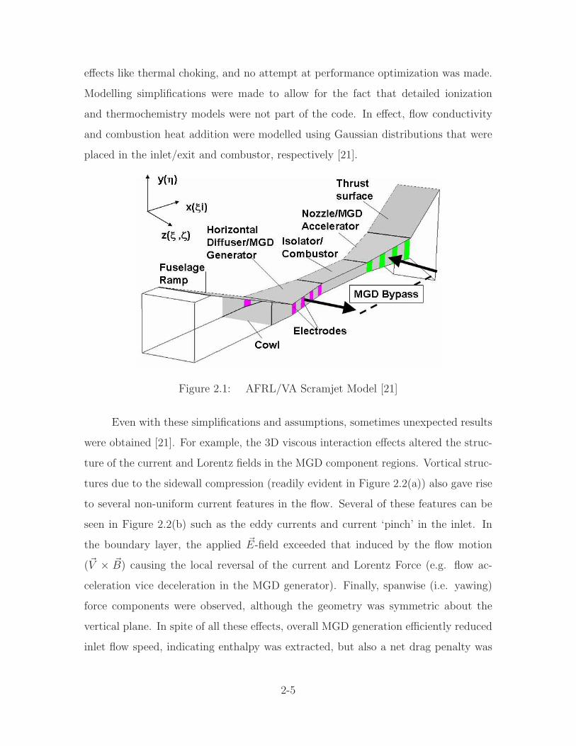
Even with these simplifications and assumptions, sometimes unexpected results

were obtained [21]. For example, the 3D viscous interaction effects altered the struc-

ture of the current and Lorentz fields in the MGD component regions. Vortical struc-

tures due to the sidewall compression (readily evident in Figure 2.2(a)) also gave rise

to several non-uniform current features in the flow. Several of these features can be

seen in Figure 2.2(b) such as the eddy currents and current ‘pinch’ in the inlet. In

the boundary layer, the applied ~E-field exceeded that induced by the flow motion

(~V × ~B) causing the local reversal of the current and Lorentz Force (e.g. flow ac-

celeration vice deceleration in the MGD generator). Finally, spanwise (i.e. yawing)

force components were observed, although the geometry was symmetric about the

vertical plane. In spite of all these effects, overall MGD generation efficiently reduced

inlet flow speed, indicating enthalpy was extracted, but also a net drag penalty was

2-5

(a) Streamtrace of Vortical Structures due toSidewall Interaction

(b) 3D-Flow Induced Effects on CurrentPath

Figure 2.2: Examples of 3D MGD-Flow Interaction in AFRL Scramjet InletModel[21]

accrued. Conversely, the MGD accelerator operation, as configured, experienced sig-

nificant heating in the boundary layer due to Joulean dissipation [21]. This loss, given

by∣

∣j∣

∣

2/σ, is an inevitable consequence of the plasma having a finite conductivity, and

can be a significant concern for the weakly ionized plasmas under consideration.

It was this preliminary investigation that revealed just how little was understood

about how this technology would apply to and impact an operational scramjet engine.

Therefore, the research documented herein was undertaken to expand upon the limited

knowledge of this subject. Before presenting this research, a few more items must be

presented. First, a brief presentation of the MGD equations and assumptions is made

along with how the computational code implements them. This is followed by the

control volume formulation of the equations as well as the electron beam ionization

model used. These two subjects are needed in order to determine the performance of

the flow control systems tested.

2-6

2.2 The Governing Equations of Magnetogasdynamics

The MGD equations are derived from the fully coupled Navier-Stokes and

Maxwell’s equations, the former equation set governing fluid flow from the contin-

uum perspective and the latter governing the propagation of electromagnetic fields.

There are a multitude of sources for the derivation of these equations. The presenta-

tion that follows draws primarily from References [14,17,30,75].

2.2.1 Navier-Stokes Equations. These equations are based on the laws of

the conservation of mass, momentum, and energy as applied to a continuous medium.

Neglecting radiative heat transfer and, for the moment, body forces, these three laws

can be expressed in the following differential form for Cartesian coordinates, respec-

tively:

∂ρ

∂t+

∂(ρVi)

∂xi

= 0 (2.4)

∂(ρVi)

∂t+

∂(ρViVj)

∂xj

+∂(pδij)

∂xj

− ∂τij

∂xj

= 0 (2.5)

∂(ρet)

∂t+

∂(ρhtVj)

∂xj

− ∂(qj + τjiVi)

∂xj

= 0 (2.6)

In the above equations, ρ is the density, and P is the pressure. The velocity vector,

~V , is composed of u, v, w components in the x, y, z directions, respectively. Vi, Vj, or

Vk also represents one of these components. The stress tensor, τij, and the heat flux

vector, qj, are defined below:

τij = µf (∂Vi

∂xj

+∂Vj

∂xi

) − 2

3δijµf

∂Vk

∂xk

(2.7)

qj = κf

∂T

∂xj

(2.8)

2-7

The computational code uses Sutherland’s Law to determine the molecular viscosity,

µf , and thermal conductivity, κf , transport properties based on local temperature.

It should be noted that these are empirically based expressions typically tabulated

for a single species (e.g. molecular oxygen) or fixed composition mixture (e.g. low-

temperature air).

µf ≈ µ0,f

(

T

T0

)3

2 T0 + Sµf

T + Sµf

(2.9)

κf ≈ κ0,f

(

T

T0

)3

2 T0 + Sµf

T + Sκf

(2.10)

In the above equations, typical reference values for air are given by µ0,f = 1.716 ×10−5kg/(m–s), T0 = 273K, Sµf

= 111K, κ0,f = 2.41×10−2J/(s–m–K), and Sκf= 194K

[84]. The total enthalpy, (ht, and total energy, et, which appear in the energy equation

are defined as follows:

ht = h +1

2ViVi (2.11)

et = ht −p

ρ(2.12)

In addition, for flows where chemical reactions occur among n species, n − 1 species

mass conservation equations are also needed to supplement the global mass conser-

vation equation above. The species conservation equation for each species, s, is given

by:

∂ρs

∂t+

∂(ρsVi)

∂xi

− ∂

∂xi

(

Ds

∂ρs

∂xi

)

−·

W s = 0 (2.13)

where the first two terms are the same as in the global equation, the third term

represents the species diffusion (as governed by the diffusion coefficient, Ds), and the

2-8

final term, Ws, represents the rate of species production or depletion due to chemical

reaction. As currently implemented, this code assumes the effect of species diffusion

may be neglected relative to the species convection and production terms.

2.2.2 Ideal Gas Equation of State. Excluding the species mass conservation

equations, the Navier-Stokes’ and associated equations presented above have six un-

knowns, (ρ, u, v, w, p, et). One additional independent equation is needed to close the

system. With the assumption that the medium behaves as an ideal gas, the ideal gas

equation of state is used, wherein R is the specific gas constant for the medium:

p = ρRT (2.14)

2.2.3 Vector Form of the Navier-Stokes Equations. To use the NSE given

above in a computational method, it is common to express them in the conservative

vector form as follows:

∂U

∂t+

∂E

∂x+

∂F

∂y+

∂G

∂z= S (2.15)

where U is the vector of conservative variables:

U = [ρ ρu ρv ρw ρet]T (2.16)

E, F, G are the total fluxes in the x, y, and z-directions, respectively, which decompose

into inviscid and viscous flux vectors:

E = Ei − Ev =

ρu

ρu2 + p

ρuv

ρuw

ρhtu

−

0

τxx

τxy

τxz

uτxx + vτxy + wτxz + qx

(2.17)

2-9

F = Fi − Fv =

ρv

ρuv

ρv2 + p

ρvw

ρhtv

−

0

τxy

τyy

τyz

uτxy + vτyy + wτyz + qy

(2.18)

G = Gi − Gv =

ρw

ρuw

ρvw

ρw2 + p

ρhtw

−

0

τxz

τyz

τzz

uτxz + vτyz + wτzz + qz

(2.19)

and S is the source term:

S = [0 0 0 0 0]T (2.20)

2.3 Maxwell Equations

The governing equations of electromagnetics are known as Maxwell’s equations

(ME). According to the Theory of Relativity, these equations are the same within any

non-accelerated reference frame, however, two frames are commonly considered. The

‘laboratory’ frame is such that the media moves relative to the stationary observer,

and the ‘rest’ frame is defined by the observer moving with the media (i.e. the observer

is “at rest” with respect to the moving media). This latter reference frame will be

denoted by a prime. Because of the invariance described above, these equations are

defined as follows and are changed to the rest frame simply by the addition of a prime

to all terms [30]:

∇ · ~D = ρe (2.21)

∇ · ~B = 0 (2.22)

2-10

∇× ~E = −∂ ~B

∂t(2.23)

∇× ~H = ~j +∂ ~D

∂t(2.24)

where ~D is the electric flux density, ρe is the space charge density, ~B is the magnetic

flux density, ~E is the electric field, ~H is the magnetic field, and ~j is the conduction

current.

2.3.1 Ohm’s Law. Just as the NSE require auxiliary relationships to close

the system, so do Maxwell’s Equations. The first of these is the constitutive relation

given by Ohm’s law which relates the conduction current to the electric field. It is

defined for linear isotropic media in the rest frame as follows:

j′i = σjiE′

j (2.25)

where σ is the conductivity.

The Maxwell-Lorentz transformations (MLT) are used to transform the Maxwell

equations from the rest frame to the laboratory frame, which is more commonly used

in MGD applications. When the media is nonuniform in all directions, i.e. anisotropic,

and V 2 << c2 (where c is the speed of light), Ohm’s law for a nonlinear media is as

follows [30]:

ji = σji[Ej + (~V × ~B)j] + ρeVi (2.26)

2.3.2 Additional Constitutive Relations. The constitutive relations are also

required to close the system. For linear, isotropic dielectrics and magnetic materials,

these relations are expressed in the rest frame as follows [30]:

~E ′ =~D′

ǫe

(2.27)

~B′ = µe~H ′ (2.28)

2-11

where µe is the permeability, and ǫe is the permittivity. The MLT are also used to

transform these constitutive relations to the laboratory frame. When |~V |2 << c2, and

the medium is isotropic, the constitutive relations are as follows [30]:

~D = ǫe[ ~E + (1 − 1ǫe

ǫe,0

µe

µe,0

)~V × ~B] (2.29)

~B = µe[ ~H − (1 − 1ǫe

ǫe,0

µe

µe,0

)~V × ~D] (2.30)

Note, that in media in which µe and ǫe both have their free space values, µe,0 and

ǫe,0, the constitutive relations also become frame invariant. Since this is nearly always

the case with the plasmas used in MGD applications, these relations can be used to

explicitly remove ~D and ~H from Maxwell’s equations to obtain:

∇ · ~E =ρe

ǫe,0

(2.31)

∇ · ~B = 0 (2.32)

∇× ~E = −∂ ~B

∂t(2.33)

∇× ~B = µe,0~j + µe,0ǫe,0

∂ ~E

∂t(2.34)

2.3.3 Magnetogasdynamic Assumptions. When an electrically conducting

fluid (or continuum gas) is moving in the presence of a magnetic field, the flow of the

fluid is influenced by the field and the field is influenced by the moving fluid. If certain

assumptions are made, these interactions can simplify the coupling of the Navier-

Stokes’ and Maxwell’s equations into a form referred to as the magnetogasdynamic

equations. These MGD assumptions are as follows [17,30]:

MGD Assumption 1: |~V |2 << c2, the magnitude of the velocities dealt with in

fluid dynamics are much less than the speed of light allowing the

√

1 − (|~V |/c)2

term to be set to unity.

2-12

MGD Assumption 2: ~E ≈ O(~V × ~B), the electric field is of the order of any

induced effects which implies that the applied magnetic field is much greater

than the induced magnetic field. Recall, this assumption defines the low Rem

regime and allows the electromagnetic body force and energy interaction to be

coupled to the NSE as source terms.

MGD Assumption 3: High frequency phenomena are not considered such that the

conduction current is dominant, i.e.∂ ~D∂t

≈ 0. ∂ ~E∂t

is also zero by the constitutive

relations. This assumption then implies that ∇ × ~B = µe,0~j. Finally, the

assumption implies the media is a conductor and not a dielectric. In an ionized

gas, this assumption holds up to microwave frequencies [30].

MGD Assumption 4: ǫe,0~E2 <<

~B2

µe,0, the electric energy is insignificant compared

to the magnetic energy. When combined with Assumption 3, this assumption

ensures the main interaction is between the magnetic field and the fluid.

MGD Assumption 5: The space charge may be neglected in Ohm’s Law, such that

in the laboratory frame it is given by ~j = σ( ~E + ~V × ~B). The conductivity is

also considered independent of magnetic field and constant with frequency. This

assumption implies that ~j′ = ~j.

MGD Assumption 6: The electromagnetic body force can be simplified to: ~fL =

ρe~E +~j × ~B. Furthermore, assuming the overall gas is electrically neutral (i.e.

a plasma), the space charge term may be neglected such that ~f = ~j × ~B

Although not an independent approximation, assumptions 1 and 3 may be combined

to get the current conservation equation ∇ ·~j + ∂ρe

∂t= 0. Assuming a dense, collision-

dominated plasma, or a conducting gas, the space charge derivative, ∂ρe

∂t, may again

be neglected and the current conservation equation in the form of Eqn 2.2 may be

used in place of Eqn 2.31.

2-13

2.3.4 Maxwell Equations for Magnetogasdynamic Flow. When the MGD

approximations above are applied to the ME, a new set of equations which govern

electromagnetic fields are formed. These equations in the laboratory frame are [30]:

∇× ~E = −∂ ~B

∂t(2.35)

∇× ~B = µe,0~j (2.36)

∇ ·~j = 0 (2.37)

∇ · ~B = 0 (2.38)

and Ohm’s law, as given by Assumption 5, becomes:

~j = σ( ~E + ~V × ~B) (2.39)

NOTE: All subsequent equations are written in the laboratory frame unless otherwise

noted.

2.4 The Magnetogasdynamic Equations: Source Term Formulation

The source term formulation of the Magnetogasdynamic Equations (MGDE)

result from the combination of the NSE and the ME subject to the MGD assumptions.

In other words, these equations describe the interaction between electromagnetic fields

and electrically conducting gases in a continuum governed by the MGD assumptions,

and in particular Assumption 2 regarding a low Rem. The MGDE are defined as

follows:

∂ρ

∂t+

∂(ρVi)

∂xi

= 0 (2.40)

∂(ρVi)

∂t+

∂(ρViVj)

∂xj

− ∂(pδij)

∂xj

− ∂τij

∂xj

= fiL (2.41)

2-14

∂(ρet)

∂t+

∂(ρhtVj)

∂xj

− ∂(qj + τjiVi)

∂xj

= WEM (2.42)

In Eqn 2.41, ~fL= (~j× ~B) is known as the Lorentz force and is the body force brought

about by the electromagnetic fields acting on the moving, charged particles (i.e. the

conduction current) in the plasma. This phenomena also gives rise to the electromag-

netic energy interaction given in Eqn 2.42 as WEM= ~E · ~j. This energy interaction

can be broken down into the sum of its two constituent parts by using the MLT for

the electric field and Ohm’s Law. When this is done, the first term is the Joulean

dissipation, given by∣

∣j∣

∣

2/σ, which is always energy put into the gas. The second

term is the rate at which ~fL does work on the fluid as given by ~V · (~j × ~B). Roughly

speaking, this term is positive when ~fL acts to accelerate the flow and negative when

it is decelerating the flow.

2.4.1 Non-dimensionalization of the Magnetogasdynamic Equations. By

non-dimensionalizing the equations, problems of different scale can be compared in-

dependent of the reference conditions. The dimensionless quantities used in the nor-

malization of the MGDE are as follows where an asterisk represents a dimensionless

quantity [30]:

L∗ =L

L0

ρ∗ =ρ

ρ0

~E∗ =~E

E0

~V ∗ =~V

V0

T ∗ =T

T0

~B∗ =~B

B0

(2.43)

These initial dimensional quantities of L0, V0, ρ0, T0, E0, and B0 are used

to non-dimensionalize the other variables, and all dimensionless variables are sub-

stituted into the MGDE. Several dimensionless parameters are formed during the

non-dimensionalization which help to characterize the MGD problem. The Reynolds

number, Re, is the ratio of inertial forces to viscous forces, defined as follows:

2-15

Re =ρ0V0L0

µ(2.44)

The magnetic Reynolds number, Rem, introduced in Section 2.1, is a measure of the

magnitude of the induced magnetic field compared to the total magnetic field. Recall,

it is given by Equation 2.1 as Rem = V0L0σ0µe.

The reference Mach number, M0, is the ratio of the reference flow speed to the speed

of sound and is therefore defined as follows:

M0 =V0

a0

(2.45)

The Prandtl number (Pr) is the ratio of kinematic viscosity to thermal diffusivity:

Pr =cP νfρ0

κf

(2.46)

The interaction parameter, Q, is used when the applied magnetic field is much larger

than the induced field, i.e. Rem << 1, and is defined as the ratio of the ponderomotive

force to the inertial force. In MGD applications it is typically O(1), and increasing

values typically correspond to increasing values of the applied magnetic field.

Q =σ0B

20L0

ρ0V0

(2.47)

The load factor, k, is defined by Equation 2.48 as the ratio of the applied electric

field to the field induced by the conducting fluid moving through the magnetic field.

An increase in k signifies a larger electric load placed on the system. The negative

sign in the following equation assumes that E0 is applied in a direction opposite to

V0B0, such that k is always positive. With this convention, when k < 1 the electrical

load is powered by the current generated by the conducting plasma moving through

the magnetic field, commonly referred to as MGD power generation. k > 1 means

the applied electric field produces a current that exceeds that induced by the plasma

2-16

motion and thus net electrical power is put back into the flow, a concept referred to as

MGD acceleration. Two special cases for k should also be kept in mind. k = 0 implies

that there is no electrical load, or in other words, there is a short-circuit condition.

When this occurs, the current generated by MGD interaction sets up entirely within

the flow and thus all the electrical energy generated must be dissipated within the

flow as heating. On the other hand, k = 1 conforms to the open-circuit case, where

the applied load exactly matches the current produced in the flow, and the overall

MGD interaction is minimized. Finally, it should be noted the definition of k given

here is based on the reference velocity and EM field values. However, in a real flow

field, the actual value of k is a typically a variable, as at the very least the velocity is

always changing.

k =−E0

B0V0

(2.48)

The non-dimensional MGDE are identical to their dimensional counterparts

except for the use of non-dimensional quantities and the differences in the stress

tensor, heat flux, and MGD source terms.

τ ∗

ij =µ∗

f

Re

[

(∂V ∗

i

∂x∗j

+∂V ∗

j

∂x∗i

) − 2

3δij

∂V ∗

k

∂x∗

k

]

(2.49)

q∗j =µ∗

f

(γ − 1)M20 RePr

∂T ∗

∂x∗j

(2.50)

The MGD source terms are now multiplied by the interaction parameter. The re-

sulting non-dimensional Lorentz force is Q(~j∗ × ~B∗), and the energy interaction is

Q( ~E∗ ·~j∗). The non-dimensional ideal gas law is defined by:

T ∗ =γM2

0 p∗

ρ∗(2.51)

with

2-17

p∗ = (γ − 1)ρ∗e∗ (2.52)

For the remainder of this document the * is dropped and all quantities are dimen-

sionless unless otherwise noted.

2.4.2 Vector Form of the Magnetogasdynamic Equations. The equations

resulting from the non-dimensionalization can then be written in a conservative vector

form with the electromagnetic effects in the source term as follows:

∂U

∂t+

∂E

∂x+

∂F

∂y+

∂G

∂z= S (2.53)

The only change from the non-dimensional conservative vector form of the NSE is in

the source term S, where:

S =

0

Q(jyBz − jzBy)

Q(jzBx − jxBz)

Q(jxBy − jyBx)

Q(Exjx + Eyjy + Ezjz)

(2.54)

2.4.3 Curvilinear Transformation. In order to accurately model most phys-

ical problems, the grid created for the physical domain has non-uniform spacing in at

least one direction. This mesh might also be body-fitted involving a non-orthogonal

coordinate system. To account for this, the vector form of the MGDE presented above

is transformed to a generalized coordinate system (ξ,η,ζ).

2-18

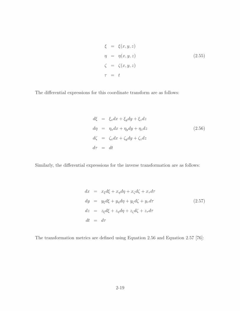
ξ = ξ(x, y, z)

η = η(x, y, z) (2.55)

ζ = ζ(x, y, z)

τ = t

The differential expressions for this coordinate transform are as follows:

dξ = ξxdx + ξydy + ξzdz

dη = ηxdx + ηydy + ηzdz (2.56)

dζ = ζxdx + ζydy + ζzdz

dτ = dt

Similarly, the differential expressions for the inverse transformation are as follows:

dx = xξdξ + xηdη + xζdζ + xτdτ

dy = yξdξ + yηdη + yζdζ + yτdτ (2.57)

dz = zξdξ + zηdη + zζdζ + zτdτ

dt = dτ

The transformation metrics are defined using Equation 2.56 and Equation 2.57 [76]:

2-19

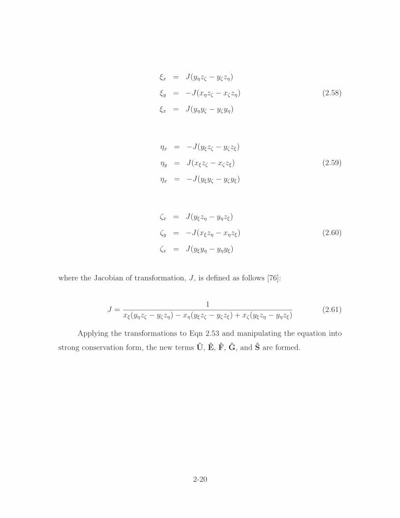
ξx = J(yηzζ − yζzη)

ξy = −J(xηzζ − xζzη) (2.58)

ξx = J(yηyζ − yζyη)

ηx = −J(yξzζ − yζzξ)

ηy = J(xξzζ − xζzξ) (2.59)

ηx = −J(yξyζ − yζyξ)

ζx = J(yξzη − yηzξ)

ζy = −J(xξzη − xηzξ) (2.60)

ζx = J(yξyη − yηyξ)

where the Jacobian of transformation, J , is defined as follows [76]:

J =1

xξ(yηzζ − yζzη) − xη(yξzζ − yζzξ) + xζ(yξzη − yηzξ)(2.61)

Applying the transformations to Eqn 2.53 and manipulating the equation into

strong conservation form, the new terms U, E, F, G, and S are formed.

2-20

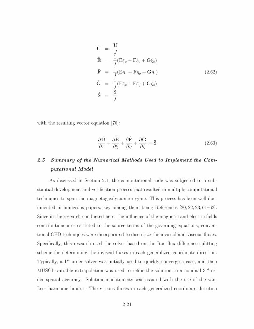
U =U

J

E =1

J(Eξx + Fξy + Gξz)

F =1

J(Eηx + Fηy + Gηz) (2.62)

G =1

J(Eζx + Fζy + Gζz)

S =S

J

with the resulting vector equation [76]:

∂U

∂τ+

∂E

∂ξ+

∂F

∂η+

∂G

∂ζ= S (2.63)

2.5 Summary of the Numerical Methods Used to Implement the Com-

putational Model

As discussed in Section 2.1, the computational code was subjected to a sub-

stantial development and verification process that resulted in multiple computational

techniques to span the magnetogasdynamic regime. This process has been well doc-

umented in numerous papers, key among them being References [20, 22, 23, 61–63].

Since in the research conducted here, the influence of the magnetic and electric fields

contributions are restricted to the source terms of the governing equations, conven-

tional CFD techniques were incorporated to discretize the inviscid and viscous fluxes.

Specifically, this research used the solver based on the Roe flux difference splitting

scheme for determining the inviscid fluxes in each generalized coordinate direction.

Typically, a 1st order solver was initially used to quickly converge a case, and then

MUSCL variable extrapolation was used to refine the solution to a nominal 3rd or-

der spatial accuracy. Solution monotonicity was assured with the use of the van-

Leer harmonic limiter. The viscous fluxes in each generalized coordinate direction

2-21

were discretized using central differences. The approximately factored implicit Beam-

Warming scheme was used for temporal integration. Finally, the predominance of

the work was accomplished using the k − ǫ turbulence model. All results should be

considered turbulent unless laminar flow is explicitly specified.

The MGDE resolve the flow within the domain, but boundary conditions must

be specified to define the flow conditions along the computational boundary. For

these simulations, the inflow boundary incorporated a supersonic inflow boundary

condition, in which all variables at inlet were set to a constant value. No-slip boundary

conditions were enforced along the tunnel walls, with the wall temperature limited

to a peak of 2000K. In addition, a zero normal pressure gradient was applied along

the wall. Likewise, for cases with thermochemistry, a zero normal gradient in species

mass fraction (i.e. non-catalytic wall) was enforced. Because the nominal flow was

supersonic everywhere except in the small, subsonic portion of the boundary layers,

the outflow boundary was set to supersonic extrapolation from the domain.

2.6 The Control Volume Approach and Performance Analysis

The control volume (CV) formulation of the governing equations of motion lends

itself to the determination of system-level interactions and overall performance. These

equations can be derived directly from the differential form of the equations by appli-

cation of Reynold’s transport theorem to a fixed control volume [83]. Furthermore,

if the flow properties can be assumed constant across the flow cross-section, then

the quasi-1D approach reduces the flow to dependence on a single spatial coordinate.

Even though the inlet flow considered here has a complex 3D character, by taking area

and volumetric averaging of the grid point flow properties, the quasi-1D approach can

provide reasonable, conservative results. Finally, two more assumptions are made to

obtain the equations that follow: (1) a single CV average value for the thermochemi-

cal properties can be taken (e.g. γ, CV , Cp, etc) and (2) the flow is steady in the sense

that the influence of any ∂/∂t terms is negligible with respect to the steady terms.

With this in mind, the CV equation for mass conservation is given by Equation 2.64.

2-22

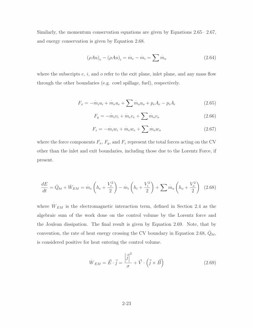
Similarly, the momentum conservation equations are given by Equations 2.65– 2.67,

and energy conservation is given by Equation 2.68.

(ρAu)e − (ρAu)i =·

me −·

mi =∑

·

mo (2.64)

where the subscripts e, i, and o refer to the exit plane, inlet plane, and any mass flow

through the other boundaries (e.g. cowl spillage, fuel), respectively.

Fx = − ·

miui +·

meue +∑

·

mouo + peAe − piAi (2.65)

Fy = − ·

mivi +·

meve +∑

·

movo (2.66)

Fz = − ·

miwi +·

mewe +∑

·

mowo (2.67)

where the force components Fx, Fy, and Fz represent the total forces acting on the CV

other than the inlet and exit boundaries, including those due to the Lorentz Force, if

present.

dE

dt= Qht + WEM =

·

me

(

he +V 2

e

2

)

− ·

mi

(

hi +V 2

i

2

)

+∑

·

mo

(

ho +V 2

o

2

)

(2.68)

where·

WEM is the electromagnetic interaction term, defined in Section 2.4 as the

algebraic sum of the work done on the control volume by the Lorentz force and

the Joulean dissipation. The final result is given by Equation 2.69. Note, that by

convention, the rate of heat energy crossing the CV boundary in Equation 2.68, Qht,

is considered positive for heat entering the control volume.

·

WEM = ~E ·~j =

∣

∣

∣

~j∣

∣

∣

2

σ+ ~V ·

(

~j × ~B)

(2.69)

2-23

Four measures are commonly used to describe performance: the total pres-

sure ratio, πc, the kinetic energy efficiency, ηKE, the dimensionless entropy increase,

∆s/Cp, and the adiabatic compression efficiency, ηc [25]. πc and ∆s/Cp both rely

on constant (or averaged) thermochemical properties to obtain analytical expressions

from the solution of Gibbs’ equation. Thus, while these measures by themselves will

lose some accuracy for the high stagnation enthalpy flows that characterize the scram-

jet flowpath, they remain useful in determining trends when varying flow parameters.

These two performance measures are given by Equations 2.70 and 2.71.

πc =pt,e

pt,i

=pe

pi

{

1 + γ−12

M2e

1 + γ−12

M2i

}γ

γ−1

(2.70)

∆s

Cp

= ln

(

Te

Ti

)

− γ − 1

γln

(

Pe

Pi

)

(2.71)

ηKE and ηc are both referenced to the freestream static conditions and thus are

generally preferred for this type of flow. ηKE (Equation 2.72) is defined as the ratio

of the square of the velocity the exit flow would achieve if isentropically expanded to

freestream conditions to the square of the freestream velocity. Similarly, ηc (Equa-

tion 2.73) is the ratio of the isentropic change in enthalpy to the actual change in

enthalpy, when both changes are referenced to the same change in static pressure.

ηKE =V 2

e

V 2i

+2CpTe

V 2i

[

1 −(

pi

pe

)γ−1

γ

]

(2.72)

ηc.=

he − hx

he − hi

(2.73)

where the subscript x denotes the conditions that would exist upon an isentropic

change in enthalpy across the actual static pressure change.

There is an additional performance measure commonly encountered when ex-

amining MGD flows. The enthalpy extraction/addition ratio or ηg is simply the ratio

of the change in stagnation enthalpy across the MGD region to the value at the be-

2-24

ginning of the MGD region [35, 42]. In order to obtain a simpler analytical model,

total enthalpy is often assumed conserved aside from the EM-interaction due to the

MGD device. However, as applied to this research, ηg includes not only the enthalpy

change due to this EM-interaction but also the change due to any other effects (e.g.

geometric compression, heat of combustion). Because of this it may be difficult or

impossible to separate out the EM contribution, especially when multiple factors are

acting synergistically. Therefore, ηg, is best viewed relative to similar flows as done,

for example, in the inlet comparisons of Chapter V.

2.7 Approximating the Non-Equilibrium Ionization with a Simplified

Electron Beam Model

Freestream flight conditions of ρ0 = 0.01022kg/m3, V0 = 3060m/s and the lead-

ing edge width reference length of 3.602m meant that σB2 ≈ 8.684Q or a maximum

of 43.4 for Q = 5. While large, these values are consistent with other proposed

values [21, 47]. Figure 2.3 presents the required magnetic field for a given value of

conductivity at the values of Q used. By way of comparison, the natural conductivity

of air at the freestream conditions was estimated to be approximately 0.03 mho/m,

implying that some form of non-equilibrium ionization is required to substantially

reduce the required magnetic field.

The computational code as currently implemented does not specify an ionization

method, but rather depends on the interaction parameter, Q, and the spatial distribu-

tion of the non-dimensionalized electro-magnetic field quantities to solve the coupled

equations. However, with this research, a first-order approximation of the average

magnitudes of σ0 and B0 is presented, as well as the required ionization power, Pion,

and generated electrical power, Pgen. To accomplish this, a model to approximate the

ionization was needed that could be adapted to the results generated by the existing

3D computational code. Based on the wealth of previous work done by many in the

field, it was decided the electron beam model provided a realistic approach to approx-

imating the non-equilibrium ionization that could be readily adapted to the existing

2-25

Figure 2.3: Magnetic Field Requirements for Varying Q,σ

computational method. Specifically, the model of Kuranov and Sheikin [34–36] was

used to determine the power spent on ionizing a unit volume of air, qi, as given by

Equation 2.74 where jb ≈ 1.0mA [45] is the electron beam current, e is the electron

charge, ρ is the flow density and Y (Eb) = 7.567MeV-cm2/gm is the electron stop-

ping power as a function of the electron energy. This last quantity was taken from

tabulated data for dry air with an electron energy of Eb = 30keV [1].

qi = (jb/e) ρY (Eb) (2.74)

The resulting conductivity is found from Equation 2.75 where me is the electron

mass, ke = 2 × 10−8cm3/s is the electron scattering constant [8], and ne/N is an

empirically-based expression for the ionization fraction as given by Equation 2.76 [36].

The number density, N , can be related to the density by N =(

RNA

Ru

)

ρ where R is the

specific gas constant, Ru is the universal gas constant, and NA is Avogadro’s number.

σ =e2

meke

(ne

N

)

(2.75)

2-26

ne

N= 1.17 × 10−5 ·

(

1034 qi

N2

)0.6

(2.76)

Having a value of qi and σ at each point, it is a simple matter to integrate over

the plasma volume defined by the modified Gaussian [21] to arrive at the total power

required for ionization, Pion, and an overall mean value for σ0. Then Equation 2.77

is used to obtain a corresponding value for the mean magnetic flux density where

the asterisked quantities are the non-dimensional values produced by the computa-

tional code. In a similar manner, the electrical power generated is simply found by

integrating Equation 2.78 over the plasma volume.

(σB2)0 =(

σ∗B∗2

)

(

ρV

L

)

0

Q (2.77)

Pgen =

∫ ∫ ∫

(

j · E)

d (V ol) (2.78)

2-27

III. Scramjet Flowpath Development

3.1 Flowpath Design Methodology

The effort to construct a realistic flowpath began with gaining a deep understand-

ing of the physical nature of scramjet flows. With regard to this goal, initial

work focused on an in-depth literature review. Specific references are annotated where

they were used, but there were also several sources of general information that proved

invaluable [12,13,25,27,51,64,77]. Following this review was the creation of a quasi-

1D computational scramjet analysis tool. This computational code was then applied

to meet the requirements of a proposed Air Force program for a hypersonic vehicle

with global reach. Various methods taken from the literature were then applied to

convert the quasi-1D engine design to a 3D geometry. Finally, computational runs of

the flowfield, to include a grid convergence study, were completed and an analysis of

this model was conducted to determine where improvements to the geometry could

be made subsequent to establishing the baseline performance model. This baseline

model would become the starting point for the ensuing EM flow control reseach.

3.2 Quasi-1D Flowpath Design and Performance Analysis Code

The preliminary effort in developing the 3D engine flowpath focused on creation

of a quasi-1D tip-to-tail scramjet engine analyzer that would both examine existing

geometries and create optimum geometries through rapid parametric study. The

quasi-1D approach allows one to take advantage of much simpler analytical techniques

while preserving the general nature of the scramjet flow physics. The approach used

here followed that taken by William Heiser and David Pratt (H-P) [25]. In summary,

for a given design point of free stream Mach number and dynamic pressure, the flow

path is divided into three subsystems or components: compression, combustion, and

expansion. The compression component is represented by a user-determined series of

oblique shock waves that are constrained by keeping the isolator inlet temperature

below a pre-determined maximum value. The combustion component is of the dual-

mode type, that is the ram-to-scramjet transition is attained by creating a thermally

3-1

choked flow or “throat” within the combustion chamber. This dual-mode design

consists of an isolator upstream of a fuel injection region, which is followed by a burner

that may be modelled with either constant area or with built-in adverse pressure

gradient relief. The expansion component is currently modelled by a simple adiabatic

expansion process where the user specifies either the area or pressure ratio with respect

to freestream. In addition to determining the detailed component thermodynamic

states and variations in cross-sectional area along the axial coordinate, the tip-to-tail

performance of the model is determined by performing a stream thrust analysis for

the uninstalled specific thrust. From this primary relationship, other relationships

provide various performance measures, including ISP and engine efficiency.

The approach described above was implemented as a Fortran 95 code which was

verified at the component level by comparing results with software available with the

H-P text [25]. Figures 3.1(a) and 3.1(b) demonstrate this verification for the most

complicated system, the dual-mode combustor. In these two figures, H-P’s results

from their HAP Burner design tool are depicted by the solid curves while the results

of this research code are shown by the discrete symbols. The reference conditions

for non-dimensionalization are taken at the isolator entrance (Station 2 in the figure

legends). The minor differences in the results are attributed to the fact that the

method of specifying the combustion heat addition was different than the method

used by the HAP Burner software.

Some of the capabilities implemented in this approach, not available in the

original HAP software, included:

1. combining the detailed component level and overall stream thrust analysis into

a single simulation,

2. adding a capability to analyze constant area burners in the context of the overall

flowpath analysis,

3. adding the ability to rapidly run parametric studies for any desired design vari-

able,

3-2

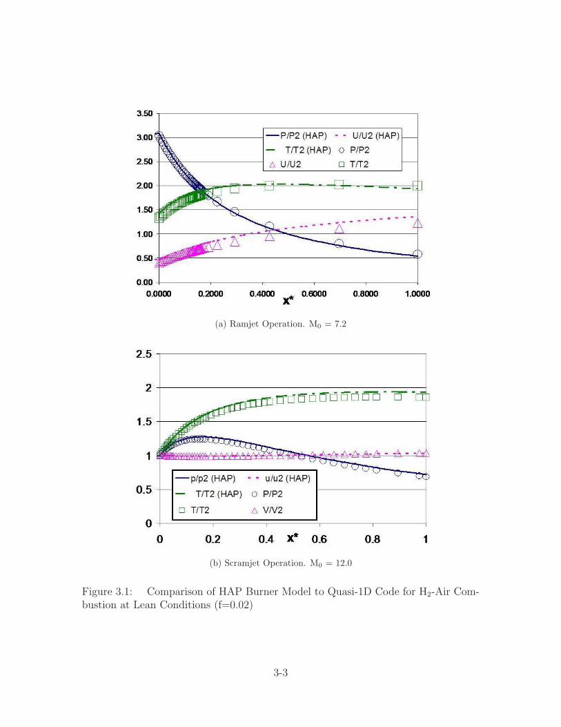
(a) Ramjet Operation. M0 = 7.2

(b) Scramjet Operation. M0 = 12.0

Figure 3.1: Comparison of HAP Burner Model to Quasi-1D Code for H2-Air Com-bustion at Lean Conditions (f=0.02)

3-3

Table 3.1: Comparison of Quasi-1D and 3D Model Results at M0 = 8.0

4. and creating an enhanced input-output interface that supported graphical post-

processing.

As an example of using these capabilities, the 3D model geometry previously published

by Gaitonde (see Section 2.1) was simplified to quasi-1D by taking representative

component cross-sectional areas along the axial coordinate. The quasi-1D code feature

allowing analysis of existing geometries was then used to compare results with those

obtained with the far more computationally expensive 3D CFD solver discussed in

Chapter II. Results were calculated using identical reference conditions of M0 = 8,

T0 = 250K, P0 = 1184Pa, and γ = 1.4. Table 3.1 presents comparison data between

these models with both centerline and off-centerline data collection taken from the 3D

CFD results as presented in Figures 13 and 14 of Ref [21]. The percent difference was

taken as the 3D value difference from the quasi-1D, divided by the quasi-1D value.

As can be seen in Table 3.1, the quasi-1D results agree very well in some places

and not well in others, but all differences are readily explainable. The centerline

results differ substantially at the isolator entrance; a discrepancy due largely to a

centerline vortical structure that develops in the horizontal diffuser/isolator sections

3-4

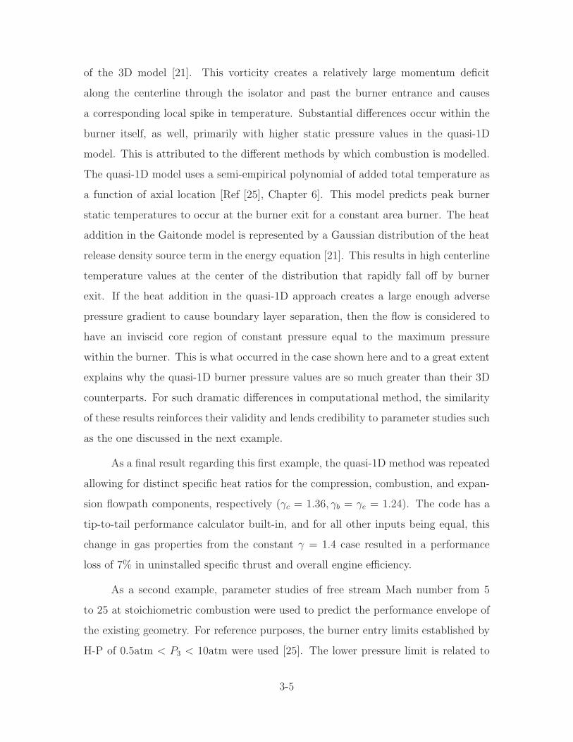
of the 3D model [21]. This vorticity creates a relatively large momentum deficit

along the centerline through the isolator and past the burner entrance and causes

a corresponding local spike in temperature. Substantial differences occur within the

burner itself, as well, primarily with higher static pressure values in the quasi-1D

model. This is attributed to the different methods by which combustion is modelled.

The quasi-1D model uses a semi-empirical polynomial of added total temperature as

a function of axial location [Ref [25], Chapter 6]. This model predicts peak burner

static temperatures to occur at the burner exit for a constant area burner. The heat

addition in the Gaitonde model is represented by a Gaussian distribution of the heat

release density source term in the energy equation [21]. This results in high centerline

temperature values at the center of the distribution that rapidly fall off by burner

exit. If the heat addition in the quasi-1D approach creates a large enough adverse

pressure gradient to cause boundary layer separation, then the flow is considered to

have an inviscid core region of constant pressure equal to the maximum pressure

within the burner. This is what occurred in the case shown here and to a great extent

explains why the quasi-1D burner pressure values are so much greater than their 3D

counterparts. For such dramatic differences in computational method, the similarity

of these results reinforces their validity and lends credibility to parameter studies such

as the one discussed in the next example.

As a final result regarding this first example, the quasi-1D method was repeated

allowing for distinct specific heat ratios for the compression, combustion, and expan-

sion flowpath components, respectively (γc = 1.36, γb = γe = 1.24). The code has a

tip-to-tail performance calculator built-in, and for all other inputs being equal, this

change in gas properties from the constant γ = 1.4 case resulted in a performance

loss of 7% in uninstalled specific thrust and overall engine efficiency.

As a second example, parameter studies of free stream Mach number from 5

to 25 at stoichiometric combustion were used to predict the performance envelope of

the existing geometry. For reference purposes, the burner entry limits established by

H-P of 0.5atm < P3 < 10atm were used [25]. The lower pressure limit is related to

3-5

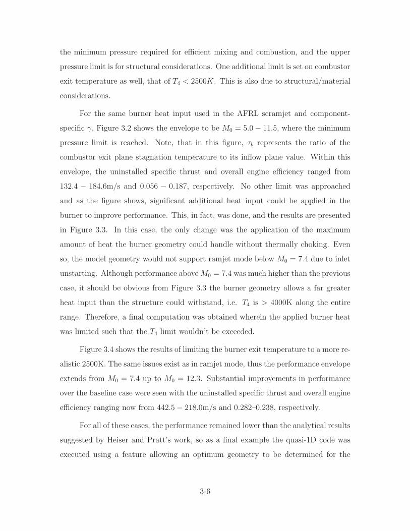
the minimum pressure required for efficient mixing and combustion, and the upper

pressure limit is for structural considerations. One additional limit is set on combustor

exit temperature as well, that of T4 < 2500K. This is also due to structural/material

considerations.

For the same burner heat input used in the AFRL scramjet and component-

specific γ, Figure 3.2 shows the envelope to be M0 = 5.0 − 11.5, where the minimum

pressure limit is reached. Note, that in this figure, τb represents the ratio of the

combustor exit plane stagnation temperature to its inflow plane value. Within this

envelope, the uninstalled specific thrust and overall engine efficiency ranged from

132.4 − 184.6m/s and 0.056 − 0.187, respectively. No other limit was approached

and as the figure shows, significant additional heat input could be applied in the

burner to improve performance. This, in fact, was done, and the results are presented

in Figure 3.3. In this case, the only change was the application of the maximum

amount of heat the burner geometry could handle without thermally choking. Even

so, the model geometry would not support ramjet mode below M0 = 7.4 due to inlet

unstarting. Although performance above M0 = 7.4 was much higher than the previous

case, it should be obvious from Figure 3.3 the burner geometry allows a far greater

heat input than the structure could withstand, i.e. T4 is > 4000K along the entire

range. Therefore, a final computation was obtained wherein the applied burner heat

was limited such that the T4 limit wouldn’t be exceeded.

Figure 3.4 shows the results of limiting the burner exit temperature to a more re-

alistic 2500K. The same issues exist as in ramjet mode, thus the performance envelope

extends from M0 = 7.4 up to M0 = 12.3. Substantial improvements in performance

over the baseline case were seen with the uninstalled specific thrust and overall engine

efficiency ranging now from 442.5 − 218.0m/s and 0.282–0.238, respectively.

For all of these cases, the performance remained lower than the analytical results

suggested by Heiser and Pratt’s work, so as a final example the quasi-1D code was

executed using a feature allowing an optimum geometry to be determined for the

3-6

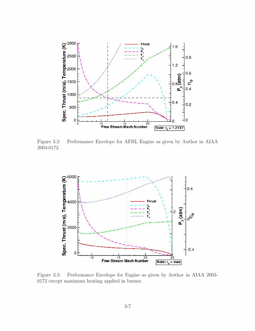
Figure 3.2: Performance Envelope for AFRL Engine as given by Author in AIAA2003-0172.

Figure 3.3: Performance Envelope for Engine as given by Author in AIAA 2003-0172 except maximum heating applied in burner.

3-7

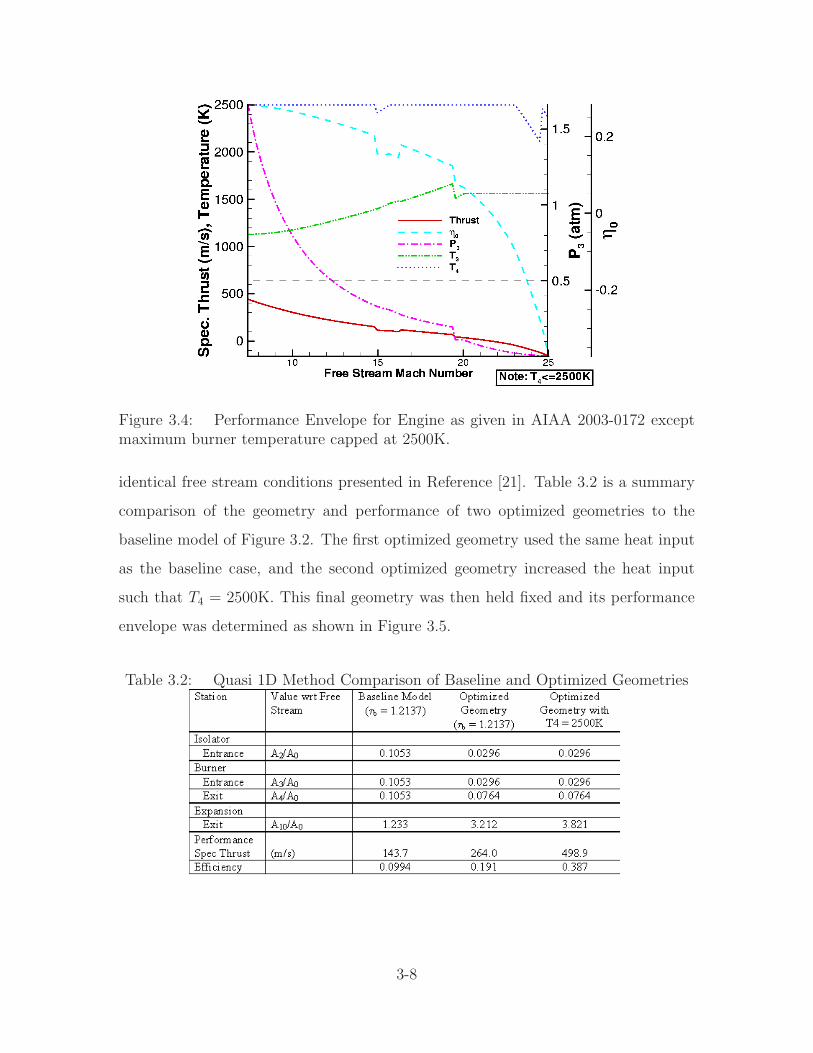
Figure 3.4: Performance Envelope for Engine as given in AIAA 2003-0172 exceptmaximum burner temperature capped at 2500K.

identical free stream conditions presented in Reference [21]. Table 3.2 is a summary

comparison of the geometry and performance of two optimized geometries to the

baseline model of Figure 3.2. The first optimized geometry used the same heat input

as the baseline case, and the second optimized geometry increased the heat input

such that T4 = 2500K. This final geometry was then held fixed and its performance

envelope was determined as shown in Figure 3.5.

Table 3.2: Quasi 1D Method Comparison of Baseline and Optimized Geometries

3-8

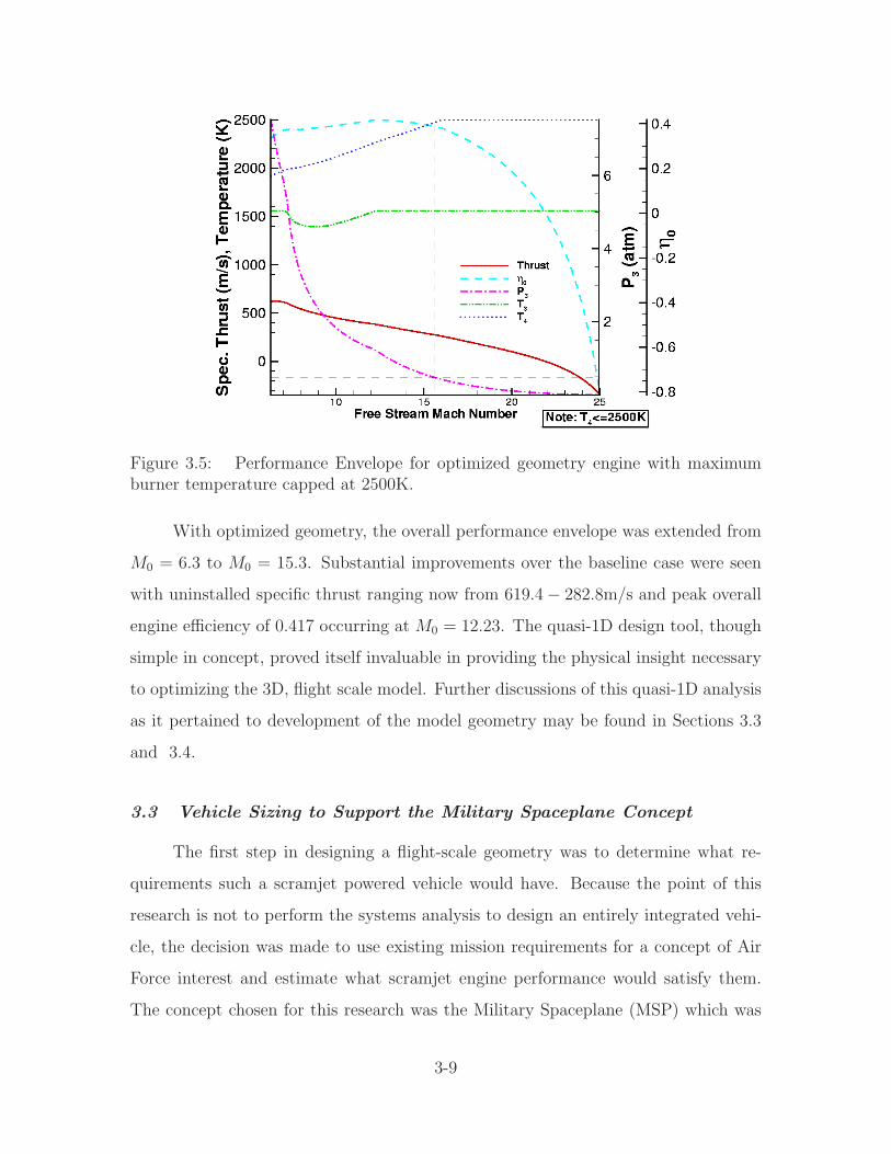
Figure 3.5: Performance Envelope for optimized geometry engine with maximumburner temperature capped at 2500K.

With optimized geometry, the overall performance envelope was extended from

M0 = 6.3 to M0 = 15.3. Substantial improvements over the baseline case were seen

with uninstalled specific thrust ranging now from 619.4 − 282.8m/s and peak overall

engine efficiency of 0.417 occurring at M0 = 12.23. The quasi-1D design tool, though

simple in concept, proved itself invaluable in providing the physical insight necessary

to optimizing the 3D, flight scale model. Further discussions of this quasi-1D analysis

as it pertained to development of the model geometry may be found in Sections 3.3

and 3.4.

3.3 Vehicle Sizing to Support the Military Spaceplane Concept

The first step in designing a flight-scale geometry was to determine what re-

quirements such a scramjet powered vehicle would have. Because the point of this

research is not to perform the systems analysis to design an entirely integrated vehi-

cle, the decision was made to use existing mission requirements for a concept of Air

Force interest and estimate what scramjet engine performance would satisfy them.

The concept chosen for this research was the Military Spaceplane (MSP) which was

3-9

established in the mid-1990s as an effort to have industry develop the technology

that was required for operationally responsive space access [82]. The program was to

have four demonstration phases that would continually improve on key performance

parameters such as payload delivered to orbit.

The pertinent requirements used for this research correspond to the MSP Mark

I, or non-orbital, demonstrator [82]. Specifically, these were to have a payload bay

of size 10’x5’x5’, with a weight capacity of 10,000 lbs (4540 kg), and the ability

to deliver at least 1-3klbs to any terrestrial location. In addition, the vehicle was

to have a sub-orbital “pop-up” capability of approximately Mach 16 at 300kft. To

meet these requirements, it was decided to size the engine for a hypersonic cruise

configuration at a design point of M0=10 and q0=1000lb/ft2(∼ 48kPa), where q0 is

the freestream dynamic pressure. Hypersonic vehicles tend to be optimized for a q0

in the range of 500–2000lb/ft2(20− 95kPa) [25]. Exceeding the high end of this range

would cause excessive vehicle drag and heating, and on the low end it would be very

difficult to generate enough lift with a reasonably-sized wing area. The freestream

Mach number was chosen on the bases that it would ensure scramjet operation vice

ramjet or dual-mode operation and that it would be operationally responsive. For

example, an unrefueled flight from New York to Melbourne, Australia (∼ 10, 000mi

or 16,700km) could be accomplished in approximately 1.5 hours. Because the cruise

speed chosen exceeds the typical maximum operating speed of a hydrocarbon-fueled

scramjet, hydrogen was chosen as the fuel. The remaining freestream conditions

corresponding to this design point were calculated by the quasi-1D code, using the

1976 Standard Atmosphere. These are presented in Table 3.3. Note, the stream

thrust definition used is the ratio of the uninstalled thrust, F , to the freestream air

mass flow rate into the engine, m0. These were the design point conditions which

served as the basis for the quasi-1D optimum engine sizing described in the following

paragraphs.

The essence of sizing the vehicle’s scramjet was determining the total thrust

needed to meet the performance specifications, in turn leading to the required mass

3-10

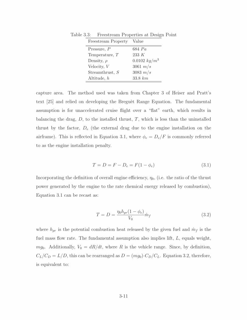
Table 3.3: Freestream Properties at Design Point

Freestream Property Value

Pressure, P 684 Pa

Temperature, T 233 K

Density, ρ 0.0102 kg/m3

Velocity, V 3061 m/s

Streamthrust, S 3083 m/s

Altitude, h 33.8 km

capture area. The method used was taken from Chapter 3 of Heiser and Pratt’s

text [25] and relied on developing the Breguet Range Equation. The fundamental

assumption is for unaccelerated cruise flight over a “flat” earth, which results in

balancing the drag, D, to the installed thrust, T , which is less than the uninstalled

thrust by the factor, De (the external drag due to the engine installation on the

airframe). This is reflected in Equation 3.1, where φe = De/F is commonly referred

to as the engine installation penalty.

T = D = F − De = F (1 − φe) (3.1)

Incorporating the definition of overall engine efficiency, η0, (i.e. the ratio of the thrust

power generated by the engine to the rate chemical energy released by combustion),

Equation 3.1 can be recast as:

T = D =η0hpr(1 − φe)

V0

mf (3.2)

where hpr is the potential combustion heat released by the given fuel and mf is the

fuel mass flow rate. The fundamental assumption also implies lift, L, equals weight,

mg0. Additionally, V0 = dR/dt, where R is the vehicle range. Since, by definition,

CL/CD = L/D, this can be rearranged as D = (mg0)·CD/CL. Equation 3.2, therefore,

is equivalent to:

3-11

mg0CD

CL

=η0hpr(1 − φe)

dR/dt

dmf

dt(3.3)

Finally, noting the fuel flow rate in the previous equation is the same as the rate at

which the vehicle mass is decreasing (i.e., dmf/dt = −dm/dt), Equation 3.3 can be

rearranged to provide the governing differential equation for thrust power versus drag:

dm

m= −

[

g0

η0hpr (1 − ϕe)CL

CD

]

dR = −C1dR (3.4)

If the term C1 is a constant, which is a good first order approximation for the funda-

mental assumption given, then the solution to 3.4 is the Breguet Range Equation:

mfinal

minitial

= e−C1R (3.5)

Introducing the concept of fuel mass fraction, Πf=mi−mf

mi, Equation 3.5 can be rear-

ranged one last time to get:

η0 =

g0R

hpr (1 − ϕe)CL

CDln

(

11−Πf

)

(3.6)

or in terms of the uninstalled specific thrust, Fmo

, and the fuel-to-air mass flow ratio,

f ,

F·

mo

=

fg0R

V0 (1 − ϕe)CL

CDln

(

11−Πf

)

(3.7)

To solve Equations 3.6 and 3.7 a few conditions beyond the design point needed to be

decided. First, the range was set at 10,000 miles to satisfy the MSP requirements [82].

For molecular hydrogen fuel, hpr = 1.2 × 108J/kg and f = 0.029 for stoichiometric

conditions. Finally, (1 − φe)CL

CD= 5 was assumed in accordance with Heiser and

Pratt [25]. With these factors in place, a short parameter study was undertaken to

discover the threshold performance values that would satisfy Equations 3.6 and 3.7

for a range of Πf . Based on this study, the results of which are reproduced in Ta-

3-12

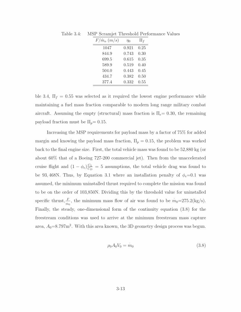
Table 3.4: MSP Scramjet Threshold Performance Values

F/mo (m/s) η0 Πf

1047 0.921 0.25

844.9 0.743 0.30

699.5 0.615 0.35

589.9 0.519 0.40

504.0 0.443 0.45

434.7 0.382 0.50

377.4 0.332 0.55

ble 3.4, Πf = 0.55 was selected as it required the lowest engine performance while

maintaining a fuel mass fraction comparable to modern long range military combat

aircraft. Assuming the empty (structural) mass fraction is Πe= 0.30, the remaining

payload fraction must be Πp= 0.15.

Increasing the MSP requirements for payload mass by a factor of 75% for added

margin and knowing the payload mass fraction, Πp = 0.15, the problem was worked

back to the final engine size. First, the total vehicle mass was found to be 52,880 kg (or

about 60% that of a Boeing 727-200 commercial jet). Then from the unaccelerated

cruise flight and (1 − φe)CL

CD= 5 assumptions, the total vehicle drag was found to

be 93, 468N. Thus, by Equation 3.1 where an installation penalty of φe=0.1 was

assumed, the minimum uninstalled thrust required to complete the mission was found

to be on the order of 103,850N. Dividing this by the threshold value for uninstalled

specific thrust, F·m0

, the minimum mass flow of air was found to be·

m0=275.2(kg/s).

Finally, the steady, one-dimensional form of the continuity equation (3.8) for the

freestream conditions was used to arrive at the minimum freestream mass capture

area, A0=8.797m2. With this area known, the 3D geometry design process was begun.

ρ0A0V0 =·

m0 (3.8)

3-13

3.4 Construction of a Flight-Sized 3D Flowpath Geometry

3.4.1 Pertinent design conditions from quasi-1D results. The construction

of the 3D geometry began with a parameter optimization study of quasi-1D configu-

rations for the design point discussed in Section 3.3. This was done in consultation

with scramjet experts in AFRL’s Propulsion Directorate (AFRL/PR) [41]. Results

from the quasi-1D code of this research were compared to an existing AFRL/PR

code which included a simple chemistry model for hydrogen combustion [41]. From

this collaboration several model parameters were established. First, it was decided

to limit the inlet and combustor static temperatures to 1700K and 3000K, respec-

tively, to prevent excessive molecular vibration and dissociation losses. Similarly for

the combustor, at temperatures greater than 3000K, most of the heat of combustion

is lost to these same molecular modes. When this occurs, the added heat energy

can not be effectively recovered during the mostly frozen expansion process. In ad-

dition, based on the combustor flow chemistry results of the AFRL/PR code, it was

decided to change the specific heat ratio and gas constant in the combustor of this re-

search code from γb= 1.238 to γb = 1.223 and Rb=287 Joule/(kg–Kelvin) to Rb=314.5

J/(kg–K). When these changes were inserted, the two independent codes produced

nearly identical results for the same design point. Finally, with the added confidence

in the quasi-1D results, a two-parameter variation study was performed wherein 100

cases were run for maximum allowed inlet and combustor temperatures in the range

of 1200-1700K and 2500-3000K, respectively. All cases were run for a constant pres-

sure combustor geometry, that is the combustor cross-sectional area expands in the

streamwise direction to balance the pressure rise due to total temperature increase

and prevent thermal choking. The results of this study can be seen in Figure 3.6 for

η0 and Figure 3.7 for the actual maximum burner temperature that occurred.

An analysis of these two figures quickly led to a conclusion of an optimum start-

ing point for designing the 3D geometry. From Figure 3.7, it was seen that on the

low end of peak inlet temperature, the flow was undercompressed and for a constant

pressure burner geometry it was not possible to approach peak allowable combustor

3-14

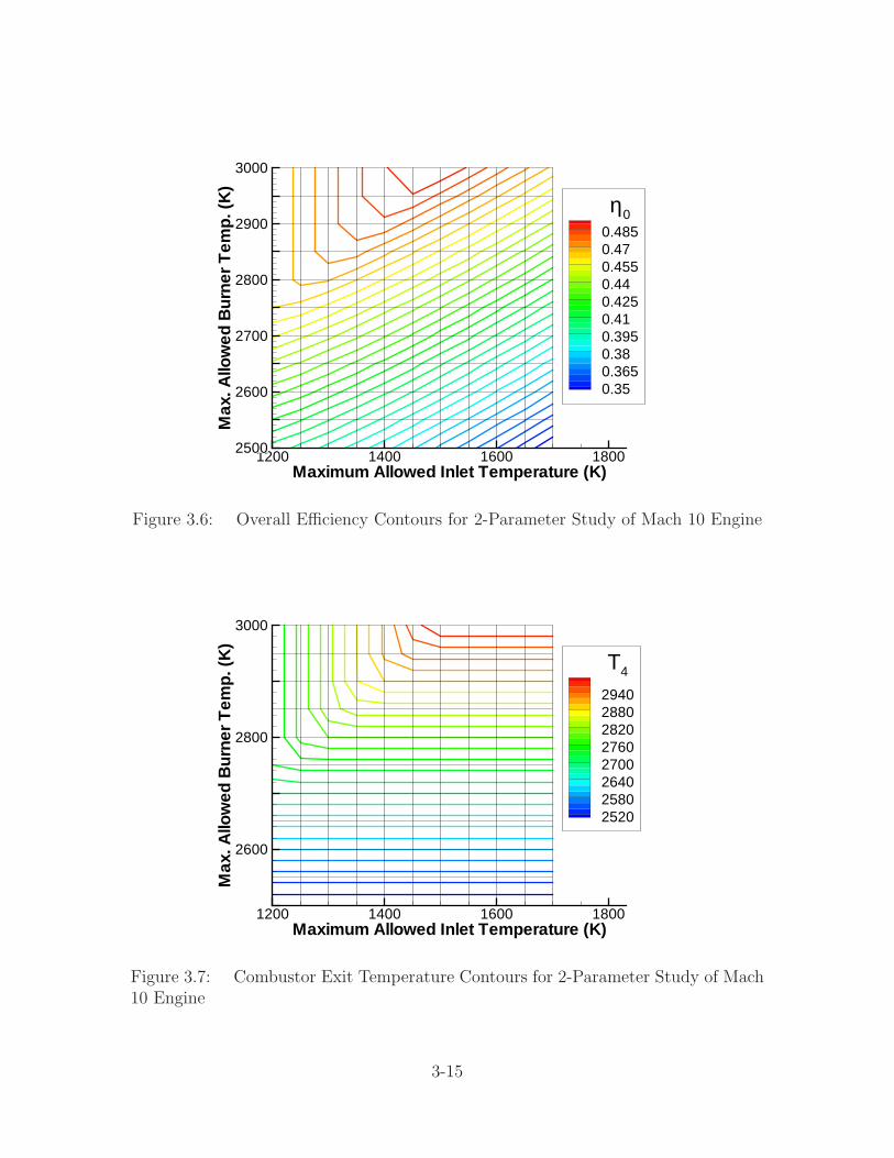
Maximum Allowed Inlet Temperature (K)

Max

.Allo

wed

Bur

nerT

emp.

(K)

1200 1400 1600 18002500

2600

2700

2800

2900

3000

η00.4850.470.4550.440.4250.410.3950.380.3650.35

Figure 3.6: Overall Efficiency Contours for 2-Parameter Study of Mach 10 Engine

Maximum Allowed Inlet Temperature (K)

Max

.Allo

wed

Bur

nerT

emp.

(K)

1200 1400 1600 1800

2600

2800

3000

T4

29402880282027602700264025802520

Figure 3.7: Combustor Exit Temperature Contours for 2-Parameter Study of Mach10 Engine

3-15

temperature. In fact, this condition held until inlet temperatures reached around

1450K. In addition, a review of Figure 3.6 revealed that peak engine efficiencies oc-

curred in the range of 1300−1550K for peak inlet temperatures. Therefore, assuming

there was still some level of uncertainty in the quasi-1D code and erring on the conser-

vative side, it was decided to take as the starting geometry that case which produced

a peak inlet temperature of 1300K and combustor temperature of 2850K.

3.4.2 Design of the 3D inlet.

“The goal in the design of any hypersonic inlet system is to define aminimum weight geometry that provides an efficient compression process,generates low drag, produces nearly uniform flow entering the combustor,and provides these characteristics over a wide range of flight and engineoperating conditions [13].”

With this in mind, several potential designs and their implications were considered in

the course of the literature review on this topic. As a small sampling of this review,

VanWie and Ault performed several experiments on a blunted 5◦ wedge followed by 5◦

of isentropic compression and a single cowl lip shock to realign the flow [3]. All com-

pression was performed in the pitch plane only. They showed that several factors in-

cluding Reynold’s number, leading edge bluntness, and wall cooling directly impacted

the boundary layer thickness, playing a vital role in determining the placement of the

cowl lip shock and the extent to which it was cancelled on the inlet expansion shoul-

der [3,80]. Holland devoted his dissertation to the experimental and numerical study

of sidewall compression inlets, demonstrating among other things the improvement

in startability attained by sweeping the sidewall leading edge [27, 28]. The results of

his research have seen practical application in the design of the X-43A [29]. Finally,

Mahoney’s text, Inlets for Supersonic Missiles, provided an excellent reference for

design methodology [51].

In the end, the design approach for the inlet followed that of Mahoney, using

a combination of results from the quasi-1D case previously selected and scaled sizing

of the published data for the X-43A [6] and its publicly released cousin, the Hyper-

3-16

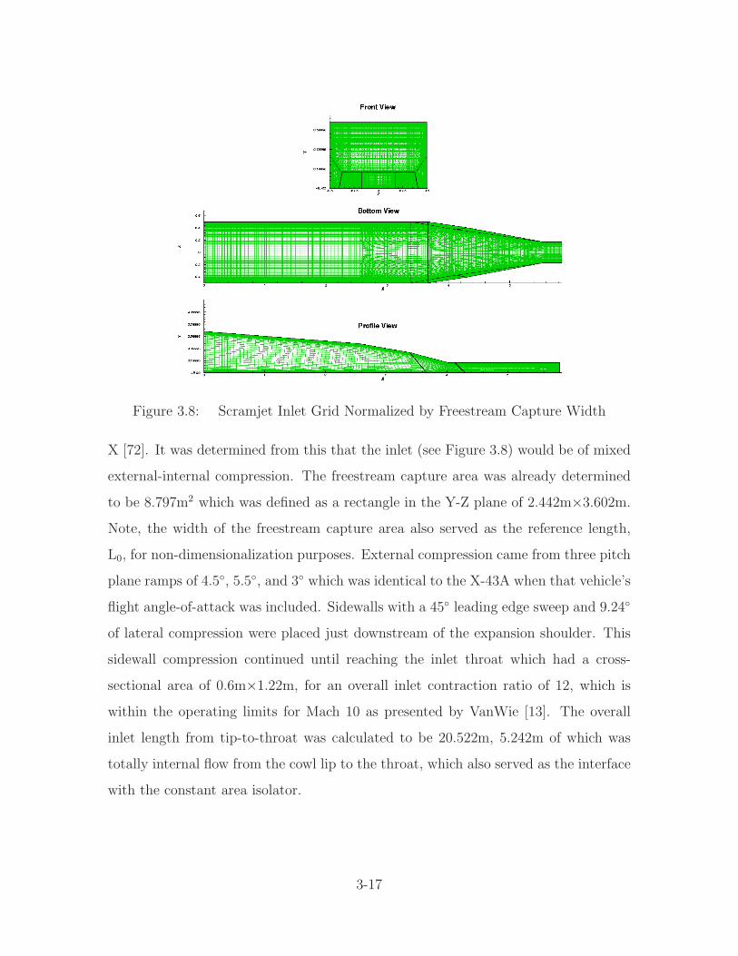
Figure 3.8: Scramjet Inlet Grid Normalized by Freestream Capture Width

X [72]. It was determined from this that the inlet (see Figure 3.8) would be of mixed

external-internal compression. The freestream capture area was already determined

to be 8.797m2 which was defined as a rectangle in the Y-Z plane of 2.442m×3.602m.

Note, the width of the freestream capture area also served as the reference length,

L0, for non-dimensionalization purposes. External compression came from three pitch

plane ramps of 4.5◦, 5.5◦, and 3◦ which was identical to the X-43A when that vehicle’s

flight angle-of-attack was included. Sidewalls with a 45◦ leading edge sweep and 9.24◦

of lateral compression were placed just downstream of the expansion shoulder. This

sidewall compression continued until reaching the inlet throat which had a cross-

sectional area of 0.6m×1.22m, for an overall inlet contraction ratio of 12, which is

within the operating limits for Mach 10 as presented by VanWie [13]. The overall

inlet length from tip-to-throat was calculated to be 20.522m, 5.242m of which was

totally internal flow from the cowl lip to the throat, which also served as the interface

with the constant area isolator.

3-17

3.4.3 Design of the 3D isolator/combustor. It became quickly apparent in

the literature review that the most widely studied and versatile scramjets had dual-

mode combustion elements. A dual-mode scramjet is one that can be made to operate

as either a ramjet or scramjet. This is made possible by two design concepts: the

thermal throat, which is only needed for ramjet flow, and the isolator. The thermal

throat works by varying the heat input into the aft end of the combustor (e.g. by

adding fuel injectors further downstream in the combustor), thus modulating the

local pressure and thereby constricting or relaxing the core burner flow as needed

to maintain subsonic flow in the combustor. Optimum design of a thermal throat

mechanism for a particular dual-mode scramjet application is beyond the scope of this

work and will not be discussed further. For both modes, however, the isolator plays

an important role, increasingly so for lower Mach numbers such as those typically

encountered in engine starting. Simply put, the first purpose of the isolator is to

prevent combustion-induced pressure instabilities from propagating upstream (in the

boundary layer for supersonic flow) into the inlet and causing inlet unstart. A second

role is to allow the flow to transition from the lower pressures of the inlet throat

to the higher pressures of the combustion chamber by passing through a series of

oblique shocks. As can be seen in Equation 3.9 [25], the isolator length-to-height ratio

increases inversely with inlet Mach number, Mi, and directly with the combustor-to-

inlet pressure ratio, pe/pi. The isolator length for this 3D geometry was determined

by applying Equation 3.9 to the inlet throat conditions that would exist at ramjet

speeds (∼ M0 = 6), and then rounding up to 2.80m to be conservative.

L

H=

√

θH

4√

Reθ

{

50(

pe

pi− 1

)

+ 170(

pe

pi− 1

)2}

(M2i − 1)

(3.9)

It was also readily obvious from the literature the constant-pressure combustor

offered greater performance than the constant-area design. By allowing the combus-

tor cross-sectional area to increase in the flow direction, the adverse effects of the

combustion-induced pressure rise could be somewhat mitigated. For a given heat ad-

3-18

dition profile and combustor inlet pressure (shown in the equation below in terms of

total temperature, Tt, and Mach number), the quasi-1D code integrated the gener-

alized differential equation given by Equation 3.10 [25] to obtain the axially varying

cross-sectional area profile. For the case under study, the resulting ratio of combustor

exit to inlet area was 2.1 and the corresponding pressure ratio was 1.03. To achieve

the desired area ratio, a rectangular cross-section was maintained and was increased

equally in the +Y and ±Z directions (see Figure 3.9). The −Y dimension wasn’t

changed to maintain a constant cowl contour. A 2◦ divergence angle was chosen for

the remaining sides as a balance between a reasonably short combustor length and

minimizing combustor flow divergence from the axial direction. Thus, the overall com-

bustor length, from the beginning of the divergence to the beginning of the internal

expansion nozzle was found to be 7.881m. The combustor exit plane cross-sectional

area was 0.871m×1.766m.

dM

dx= M

(

1 + γb+12

M2

1 − M2

)

{

−(

1

A

dA

dx

)

+1 + γbM

2

2

(

1

Tt

dTt

dx

)}

(3.10)

Between the isolator and the diverging section of the combustor, 10cm of con-

stant area duct was included for the fuel injectors. Numerous possible fuel injec-

tion and mixing designs have been proposed for scramjets. Some of these include,

strut-mounted, backward facing steps, ramp injectors, and channel or cavity flow

mixers [2, 4, 5, 15, 24, 32, 56]. Because the computational code required a stuctured-

grid, it was decided to use a simplified slot injector and forego the complexity of

a flameholding cavity or similar device. Sizing the fuel injectors began with deter-

mining the total fuel flow rate required by using the stoichiometric fuel-to-air ratio,

f = 0.029126, and the mass flow rate of air,·

ma, entering the combustor. The latter

amount was determined to be·

m0 minus any air spillage around the inlet cowl, which

during the inlet flow control analysis (see Chapter V) was found to be approximately

60kg/s. Thus, the required fuel mass flow rate was·

mf=6.3kg/s. From a thermody-

3-19

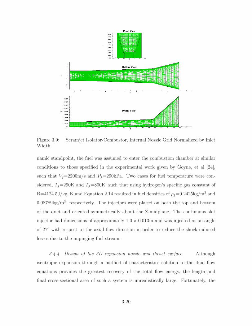
Figure 3.9: Scramjet Isolator-Combustor, Internal Nozzle Grid Normalized by InletWidth

namic standpoint, the fuel was assumed to enter the combustion chamber at similar

conditions to those specified in the experimental work given by Goyne, et al [24],

such that Vf=2200m/s and Pf=290kPa. Two cases for fuel temperature were con-

sidered, Tf=290K and Tf=800K, such that using hydrogen’s specific gas constant of

R=4124.5J/kg–K and Equation 2.14 resulted in fuel densities of ρf=0.2425kg/m3 and

0.08789kg/m3, respectively. The injectors were placed on both the top and bottom

of the duct and oriented symmetrically about the Z-midplane. The continuous slot

injector had dimensions of approximately 1.0 × 0.013m and was injected at an angle

of 27◦ with respect to the axial flow direction in order to reduce the shock-induced

losses due to the impinging fuel stream.

3.4.4 Design of the 3D expansion nozzle and thrust surface. Although

isentropic expansion through a method of characteristics solution to the fluid flow

equations provides the greatest recovery of the total flow energy, the length and

final cross-sectional area of such a system is unrealistically large. Fortunately, the

3-20

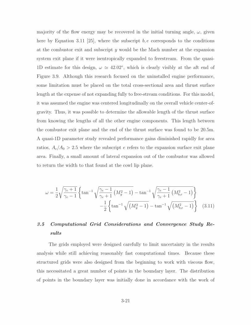
majority of the flow energy may be recovered in the initial turning angle, ω, given

here by Equation 3.11 [25], where the subscript b, e corresponds to the conditions

at the combustor exit and subscript y would be the Mach number at the expansion

system exit plane if it were isentropically expanded to freestream. From the quasi-

1D estimate for this design, ω ≃ 42.02◦, which is clearly visibly at the aft end of

Figure 3.9. Although this research focused on the uninstalled engine performance,

some limitation must be placed on the total cross-sectional area and thrust surface

length at the expense of not expanding fully to free-stream conditions. For this model,

it was assumed the engine was centered longitudinally on the overall vehicle center-of-

gravity. Thus, it was possible to determine the allowable length of the thrust surface

from knowing the lengths of all the other engine components. This length between

the combustor exit plane and the end of the thrust surface was found to be 20.5m.

A quasi-1D parameter study revealed performance gains diminished rapidly for area

ratios, Ae/A0 > 2.5 where the subscript e refers to the expansion surface exit plane

area. Finally, a small amount of lateral expansion out of the combustor was allowed

to return the width to that found at the cowl lip plane.

ω =1

2

√

γe + 1

γe − 1

{

tan−1

√

γe − 1

γe + 1

(

M2y − 1

)

− tan−1

√

γe − 1

γe + 1

(

M2b,e − 1

)

}

−1

2

{

tan−1√

(

M2y − 1

)

− tan−1√

(

M2b,e − 1

)

}

(3.11)

3.5 Computational Grid Considerations and Convergence Study Re-

sults

The grids employed were designed carefully to limit uncertainty in the results

analysis while still achieving reasonably fast computational times. Because these

structured grids were also designed from the beginning to work with viscous flow,

this necessitated a great number of points in the boundary layer. The distribution

of points in the boundary layer was initially done in accordance with the work of

3-21

Table 3.5: 3D Computational Mesh Sizes

Grid Dimensions (ξ × η × ζ) Total Points

Fine MeshInlet 178 × 112 × 143 2, 850, 848

Combustor/Nozzle 187 × 112 × 143 2, 994, 992

Coarse MeshInlet 178 × 57 × 71 720, 366

Combustor/Nozzle 187 × 57 × 71 756, 789

Vassberg, et al [81], utilizing a normalized value of ∆s = 5.0 × 10−6 off the wall.

The grids developed in this manner are referred to as the ‘fine mesh.’ Computational

runs of these fine meshes on a Cray X1E supercomputer still required three or more

weeks to converge a solution. The grids were coarsened to a point that cut the

computational time to less than half while preserving the flowfield solution. The

resulting grid dimensions and total size of each mesh are presented in Table 3.5.

Figure 3.10 demonstrates the coarse mesh spacing did indeed accurately capture

the fine mesh results. In the subfigures, selected flow properties as determined by the

cross-sectional area-weighted method of Section 2.6 are presented. As can be seen,

all differences between the two solutions are less than a few percent. Both solutions

were ran to the approximate steady state solution as determined by negligible changes

in the computed residual and the flow properties as typified by Figure 3.10. Minor

differences seen between the two grid sizes are attributed to both the presence of

sidewall vortices and other three-dimensional phenomena that prevent truly steady

flow from being obtained as well as the difference in grid spacing. In the end, it

was felt the significant improvement in computational speed was worth the slight

difference in results seen here.

3.6 Summary

At this point, the majority of the background review and research has been

presented. The key physical processes common to scramjet engines have been explored

and incorporated into the development of a first-of-its-kind open source scramjet

3-22

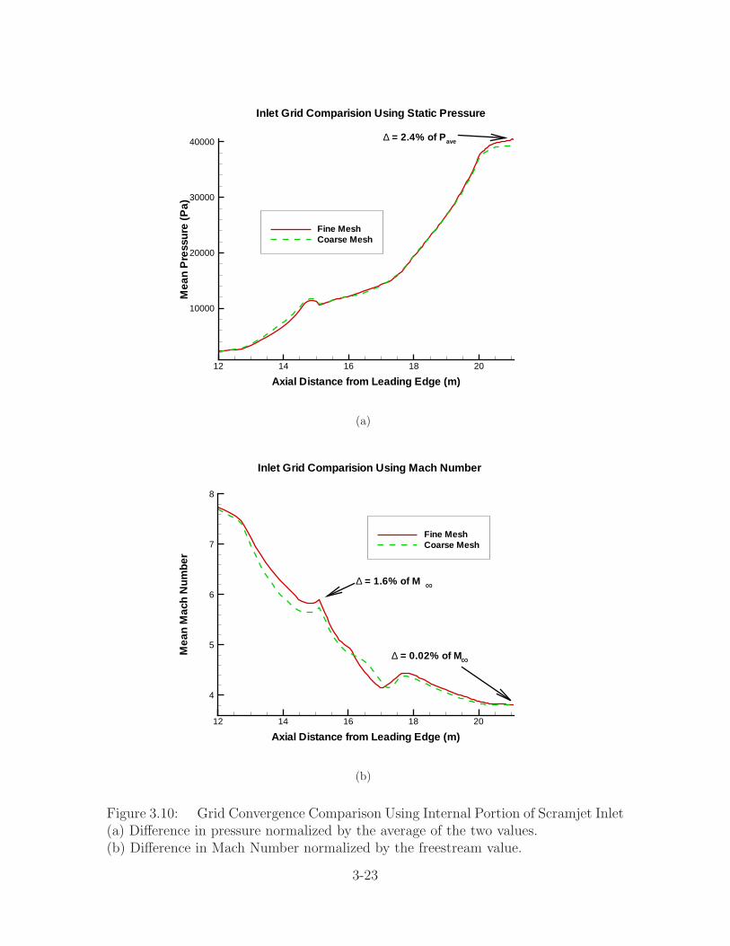
Axial Distance from Leading Edge (m)

Mea

nP

ress

ure

(Pa)

12 14 16 18 20

10000

20000

30000

40000

Fine MeshCoarse Mesh

Inlet Grid Comparision Using Static Pressure

∆ = 2.4% of P ave

(a)

Axial Distance from Leading Edge (m)

Mea

nM

ach

Num

ber

12 14 16 18 20

4

5

6

7

8

Fine MeshCoarse Mesh

Inlet Grid Comparision Using Mach Number

∆ = 1.6% of M ∞

∆ = 0.02% of M∞

(b)

Figure 3.10: Grid Convergence Comparison Using Internal Portion of Scramjet Inlet(a) Difference in pressure normalized by the average of the two values.(b) Difference in Mach Number normalized by the freestream value.

3-23

geometry. First, this was done through the development of the quasi-1D design tool

and then to a higher level of detail through the 3D baseline geometry design process.

Integral to this effort was sizing the engine to support the requirements of the Military

Spaceplane concept. Detailed computational analysis of this engine model will now

be presented in the context of the thermochemistry model developed in Chapter IV,

the localized flow control explored in Chapter V, and the MGD energy bypass concept

study of Chapter VI.

3-24

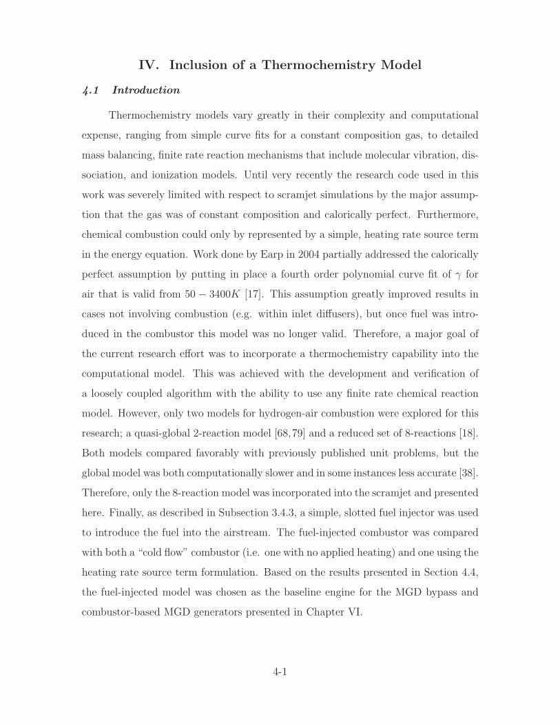
IV. Inclusion of a Thermochemistry Model

4.1 Introduction

Thermochemistry models vary greatly in their complexity and computational

expense, ranging from simple curve fits for a constant composition gas, to detailed

mass balancing, finite rate reaction mechanisms that include molecular vibration, dis-

sociation, and ionization models. Until very recently the research code used in this

work was severely limited with respect to scramjet simulations by the major assump-

tion that the gas was of constant composition and calorically perfect. Furthermore,

chemical combustion could only by represented by a simple, heating rate source term

in the energy equation. Work done by Earp in 2004 partially addressed the calorically

perfect assumption by putting in place a fourth order polynomial curve fit of γ for

air that is valid from 50 − 3400K [17]. This assumption greatly improved results in

cases not involving combustion (e.g. within inlet diffusers), but once fuel was intro-

duced in the combustor this model was no longer valid. Therefore, a major goal of

the current research effort was to incorporate a thermochemistry capability into the

computational model. This was achieved with the development and verification of

a loosely coupled algorithm with the ability to use any finite rate chemical reaction

model. However, only two models for hydrogen-air combustion were explored for this

research; a quasi-global 2-reaction model [68,79] and a reduced set of 8-reactions [18].

Both models compared favorably with previously published unit problems, but the

global model was both computationally slower and in some instances less accurate [38].

Therefore, only the 8-reaction model was incorporated into the scramjet and presented

here. Finally, as described in Subsection 3.4.3, a simple, slotted fuel injector was used

to introduce the fuel into the airstream. The fuel-injected combustor was compared

with both a “cold flow” combustor (i.e. one with no applied heating) and one using the

heating rate source term formulation. Based on the results presented in Section 4.4,

the fuel-injected model was chosen as the baseline engine for the MGD bypass and

combustor-based MGD generators presented in Chapter VI.

4-1

4.2 Coupling Thermochemistry with the Computational Code

While many current CFD codes address chemical kinetics in some way, until

now there have not been any coupled to an MGD solver and applied to a scramjet

flowpath. In addition, the kinetics models that are currently in use vary greatly in

their complexity and computational expense and are tailored to specific applications.

Therefore, a portion of the research was devoted to implement a thermochem-

istry model that addresses all the above issues. The overall goal was to accurately

and efficiently calculate the heat release and final composition of a mixture, but not

necessarily enforce time accuracy. Additionally, the chemistry model would be im-

plemented in such a way that the code could operate with or without its use, as

required. Because of this, a loosely coupled approach somewhat similar to that fol-

lowed by Hoffman and Chang [26] was taken, where across a given time step the

MGD flow equations (Eqns 2.40 - 2.42) were solved separately from the species con-

servation equation (Eqn 2.13). The subsequent change in chemical composition due

to the change in the flow state and chemical reaction was then used to update the

mass-averaged thermodynamic properties for the ensuing flow step. A general outline

of the algorithm is:

1. Initialize flow variables and chemical composition at each point.

2. At each time step, solve the flow equations, assuming a constant chemical com-

position. The resulting mixture pressure, p, as well as the mass fluxes, ρu, ρv

and ρw, will be considered invariant across the following chemistry step.

3. Calculate the mixture total enthalpy, ht, at each point. ht is likewise considered

constant across the chemistry step. The definition of the static enthalpy is

given in this context by Equation 4.1, which is the summation over all species

of the heat of formation, hfs , and the change in enthalpy relative to standard

conditions, ∆h298Ks , weighted by the corresponding species mass fraction, Ys.

Values of ∆h298Ks are determined using a temperature-based polynomial curve

fit of experimental data as shown in Equation 4.2 [40].

4-2

h =n

∑

s=1

(

hfs + ∆h298K

s

)

[Ys] (4.1)

∆h298Ks = AsT +

Bs

2T 2 +

Cs

3T 3 +

Ds

4T 4 − Es

T+ Fs − Hs (4.2)

4. Determine the change in species density due to reaction (i.e. the production

source term,·

W s) by solving the reaction rate equations as given by Equation 4.3.

Several terms in this equation require definition. First, the molecular weight of

species, s, is given by MWs. Next,(

υPs − υR

s

)

mis the change in stoichiometric

coefficient for s and reaction, m, as the reactants, R, are converted to products,

P . The third-body efficiency for each reaction, which is specific to the kinetics

model used, is given by Meff,m. The forward rate constants, kfm, and the

backward rate constants, kbm, are likewise dependent on the kinetics model and

for this research are defined by Equation 4.7 as discussed below. Finally, the

species mole fraction is given by Xi.

·

W s = MWs

#Rxn∑

m=1

(

υP

s − υR

s

)

mMeff,m

{

kfm

n∏

i=1

[Xi]υR

i − kbm

n∏

i=1

[Xi]υP

i

}

(4.3)

5. Solve the species continuity equation, Equation 2.13, for updated values of each

species density, ρs.

6. Use the updated values of ρs to get the new value for the mixture gas constant

and update the mixture’s heat of formation.

7. At this point, the change in temperature can be found from conservation of

total enthalpy across the chemistry step as reactants, R, are converted to prod-

ucts, P . Using the assumptions from Steps 2 and 3, this conservation equation

can be formulated as an implicit function of the temperature, T , as given by

Equation 4.4 and solved through the application of a Newton iteration.

4-3

hR

t − hP

t = 0 = hR

t −P

∑

s=1

(

hfs + ∆h298K

s

)

[Ys] −

∣

∣

∣

−→V P

∣

∣

∣

2

2(4.4)

where by Equation 4.5:

∣

∣

∣

−→V P

∣

∣

∣

2

=(ρu)2 + (ρv)2 + (ρw)2

ρ2=

[

( ρu)2 + ( ρv)2 + ( ρw)2](

RT

p

)2

(4.5)

8. Once the new value of T is known, a new value for mixture density, ρ is found

from the perfect gas equation of state. The mass fluxes are then divided by this

ρ to update the velocity components.

9. Finally, the solver returns to step 2 and repeats the algorithm until the solution

converges to steady state.

The chemistry model used for H2–air combustion was put forth by J.S. Evans

and C.J. Schexnayder, Jr. [18] and consisted of a finite rate mechanism of seven species

(six reacting species and inert N2) and eight reactions as given by Equation 4.6, where

the third body, M, varies as described in the reference.

H2 + M ←→ 2H + M

O2 + M ←→ 2O + M

H2O + M ←→ OH + H + M

OH + M ←→ O + H + M

H2O + O ←→ OH + OH

H2O + H ←→ OH + H2

O2 + H ←→ OH + O

H2 + O ←→ OH + H

(4.6)

4-4

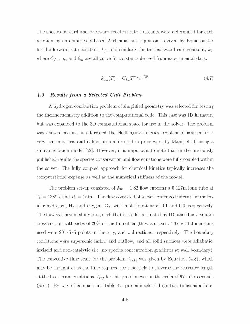
The species forward and backward reaction rate constants were determined for each

reaction by an empirically-based Arrhenius rate equation as given by Equation 4.7

for the forward rate constant, kf , and similarly for the backward rate constant, kb,

where Cfm, ηm and θm are all curve fit constants derived from experimental data.

kfm(T ) = Cfm

T ηme−θmT (4.7)

4.3 Results from a Selected Unit Problem

A hydrogen combustion problem of simplified geometry was selected for testing

the thermochemistry addition to the computational code. This case was 1D in nature

but was expanded to the 3D computational space for use in the solver. The problem

was chosen because it addressed the challenging kinetics problem of ignition in a

very lean mixture, and it had been addressed in prior work by Mani, et al, using a

similar reaction model [52]. However, it is important to note that in the previously

published results the species conservation and flow equations were fully coupled within

the solver. The fully coupled approach for chemical kinetics typically increases the

computational expense as well as the numerical stiffness of the model.

The problem set-up consisted of M0 = 1.82 flow entering a 0.127m long tube at

T0 = 1389K and P0 = 1atm. The flow consisted of a lean, premixed mixture of molec-

ular hydrogen, H2, and oxygen, O2, with mole fractions of 0.1 and 0.9, respectively.

The flow was assumed inviscid, such that it could be treated as 1D, and thus a square

cross-section with sides of 20% of the tunnel length was chosen. The grid dimensions

used were 201x5x5 points in the x, y, and z directions, respectively. The boundary

conditions were supersonic inflow and outflow, and all solid surfaces were adiabatic,

inviscid and non-catalytic (i.e. no species concentration gradients at wall boundary).

The convective time scale for the problem, tref , was given by Equation (4.8), which

may be thought of as the time required for a particle to traverse the reference length

at the freestream conditions. tref for this problem was on the order of 97-microseconds

(µsec). By way of comparison, Table 4.1 presents selected ignition times as a func-

4-5

X/L0

H2,

H2O O

2

OH

0 0.2 0.4 0.6 0.8 10

0.01

0.02

0.03

0.04

0.05

0.06

0.92

0.94

0.96

0.98

0

0.002

0.004

0.006

0.008

H2

O2

OHH2OH2O (Mani)

Figure 4.1: Combustion Nozzle Species Distribution

tion of static pressure and temperature for hydrogen-air combustion [69]. Based upon

these values, ignition was predicted to occur at approximately 12% of the domain

length for the given thermodynamic conditions.

tref =L0

U0

(4.8)

Table 4.1: Hydrogen-Air Ignition Times

T (K) p (atm) tign (10−6sec)

900 1.0 > 3E4

1250 1.0 18

1400 1.0 12

1100 2.0 25

As seen in Figure 4.1, the fuel-air mixture did indeed ignite at approximately

0.12L0 as evidenced by the extremely rapid rise in H2O coinciding with a similar

consumption of O2 and H2 and spike in the OH, or hydroxyl radical, production.

This agrees well with the kinetics model given by Equation 4.6 where it is seen that

4-6

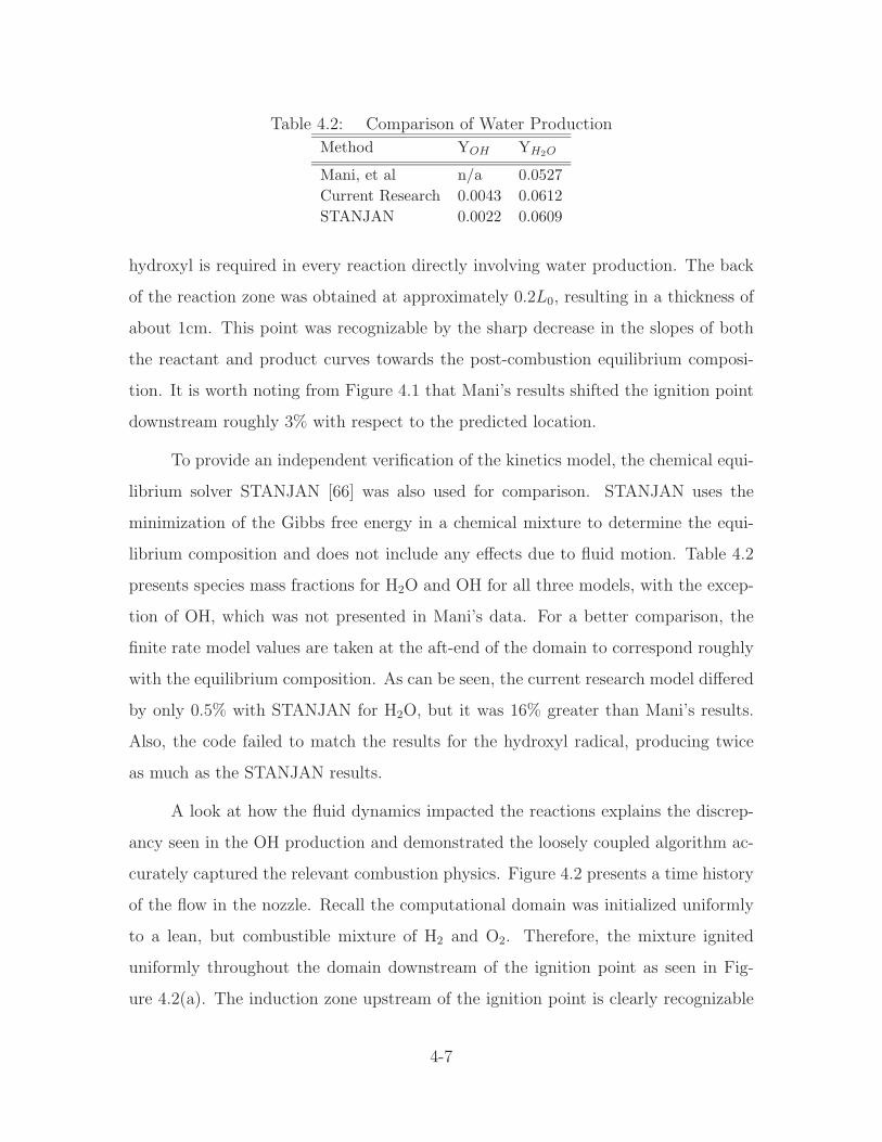
Table 4.2: Comparison of Water Production

Method YOH YH2O

Mani, et al n/a 0.0527

Current Research 0.0043 0.0612

STANJAN 0.0022 0.0609

hydroxyl is required in every reaction directly involving water production. The back

of the reaction zone was obtained at approximately 0.2L0, resulting in a thickness of

about 1cm. This point was recognizable by the sharp decrease in the slopes of both

the reactant and product curves towards the post-combustion equilibrium composi-

tion. It is worth noting from Figure 4.1 that Mani’s results shifted the ignition point

downstream roughly 3% with respect to the predicted location.

To provide an independent verification of the kinetics model, the chemical equi-

librium solver STANJAN [66] was also used for comparison. STANJAN uses the

minimization of the Gibbs free energy in a chemical mixture to determine the equi-

librium composition and does not include any effects due to fluid motion. Table 4.2

presents species mass fractions for H2O and OH for all three models, with the excep-

tion of OH, which was not presented in Mani’s data. For a better comparison, the

finite rate model values are taken at the aft-end of the domain to correspond roughly

with the equilibrium composition. As can be seen, the current research model differed

by only 0.5% with STANJAN for H2O, but it was 16% greater than Mani’s results.

Also, the code failed to match the results for the hydroxyl radical, producing twice

as much as the STANJAN results.

A look at how the fluid dynamics impacted the reactions explains the discrep-

ancy seen in the OH production and demonstrated the loosely coupled algorithm ac-

curately captured the relevant combustion physics. Figure 4.2 presents a time history

of the flow in the nozzle. Recall the computational domain was initialized uniformly

to a lean, but combustible mixture of H2 and O2. Therefore, the mixture ignited

uniformly throughout the domain downstream of the ignition point as seen in Fig-

ure 4.2(a). The induction zone upstream of the ignition point is clearly recognizable

4-7

as the region where the temperature remains nearly constant. The hydroxyl radical is

gradually increasing during this time, a fact not clearly visible in Figure 4.1 because

the relative mass fraction of OH is so low when compared to the reactants. Just prior

to the ignition, the temperature drops by a few degrees as the OH radicals spike. This

is to be expected as the production of OH is an endothermic reaction. The excess

OH is quickly consumed in the exothermic water-production reactions, resulting in a

temperature rise of 30K. Although not shown in these curves, the rapid rise in tem-

perature due to combustion occurs in conjunction with a decrease in mixture density.

By mass conservation, the flow has to accelerate due to the constant cross-sectional

area of the nozzle. This is indeed the case as seen in Figure 4.2(b), with the speed

increasing by 110m/s above free stream after 97µsec. Similarly, by momentum conser-

vation, the flow acceleration corresponds to a favorable pressure gradient, pushing the

flow along in the axial direction and resulting in a minimum exit pressure of 82kPa.

As the initial domain-wide deflagration concludes and is pushed out of the domain

by the convecting fluid, the ignition point remains stationary, as it must due to the

supersonic inflow.

At this point, the fluid dynamics begins to dominate the physics of the problem.

Because the mixture is so lean, barely within flammability limits, there is not much

continuous heat release available from combustion. Therefore, what little heat energy

that is released is quickly converted into kinetic form. By 194µsec, Figure 4.2(c), the

flow is approaching steady state. At this point, the flame location is still clearly rec-

ognizable as a slight rise in pressure and drop in speed within the reaction zone. The

heat release causes a nearly imperceptible increase in the temperature at the flame

front, which is quickly converted into a 12m/s speed increase over the domain and

a corresponding pressure decrease of 4kPa. By 310µsec, Figure 4.2(d), the flow has

reached a steady state condition. The lack of a significant temperature rise prevents

the combustion reaction from reaching completion. This results in excess hydroxyl

molecules departing the domain and explains why there is an abundance of OH rel-

ative to the STANJAN solution. All these results demonstrate the accuracy of the

4-8

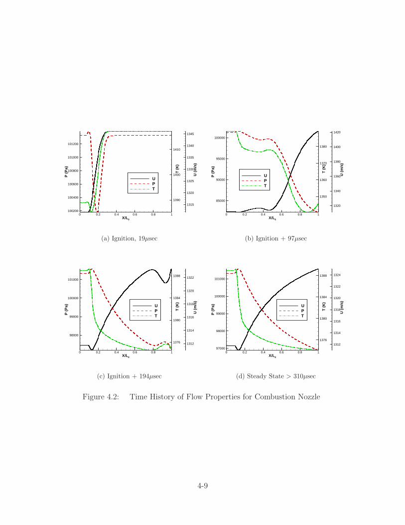
X/L0

P(P

a)

T(K

)

U(m

/s)

0 0.2 0.4 0.6 0.8 1100200

100400

100600

100800

101000

101200

1390

1400

1410

1315

1320

1325

1330

1335

1340

1345

UPT

(a) Ignition, 19µsec

X/L0

P(P

a)

T(K

)

U(m

/s)

0 0.2 0.4 0.6 0.8 1

85000

90000

95000

100000

1350

1360

1370

1380

1320

1340

1360

1380

1400

1420

UPT

(b) Ignition + 97µsec

X/L0

P(P

a)

T(K

)

U(m

/s)

0 0.2 0.4 0.6 0.8 1

98000

99000

100000

101000

1376

1380

1384

1388

1312

1314

1316

1318

1320

1322

UPT

(c) Ignition + 194µsec

X/L0

P(P

a)

T(K

)

U(m

/s)

0 0.2 0.4 0.6 0.8 197000

98000

99000

100000

101000

1376

1380

1384

1388

1312

1314

1316

1318

1320

1322

1324

UPT

(d) Steady State > 310µsec

Figure 4.2: Time History of Flow Properties for Combustion Nozzle

4-9

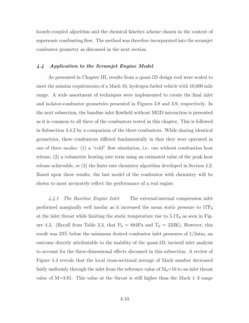
loosely-coupled algorithm and the chemical kinetics scheme chosen in the context of

supersonic combusting flow. The method was therefore incorporated into the scramjet

combustor geometry as discussed in the next section.

4.4 Application to the Scramjet Engine Model

As presented in Chapter III, results from a quasi-1D design tool were scaled to

meet the mission requirements of a Mach 10, hydrogen-fueled vehicle with 10,000 mile

range. A wide assortment of techniques were implemented to create the final inlet

and isolator-combustor geometries presented in Figures 3.8 and 3.9, respectively. In

the next subsection, the baseline inlet flowfield without MGD interaction is presented

as it is common to all three of the combustors tested in this chapter. This is followed

in Subsection 4.4.2 by a comparison of the three combustors. While sharing identical

geometries, these combustors differed fundamentally in that they were operated in

one of three modes: (1) a “cold” flow simulation, i.e. one without combustion heat

release, (2) a volumetric heating rate term using an estimated value of the peak heat

release achievable, or (3) the finite rate chemistry algorithm developed in Section 4.2.

Based upon these results, the last model of the combustor with chemistry will be

shown to most accurately reflect the performance of a real engine.

4.4.1 The Baseline Engine Inlet. The external-internal compression inlet

performed marginally well insofar as it increased the mean static pressure to 57P0

at the inlet throat while limiting the static temperature rise to 5.1T0 as seen in Fig-

ure 4.3. (Recall from Table 3.3, that P0 = 684Pa and T0 = 233K). However, this

result was 23% below the minimum desired combustor inlet pressures of 1/2atm, an

outcome directly attributable to the inability of the quasi-1D, inviscid inlet analysis

to account for the three-dimensional effects discussed in this subsection. A review of

Figure 4.4 reveals that the local cross-sectional average of Mach number decreased

fairly uniformly through the inlet from the reference value of M0=10 to an inlet throat

value of M=3.81. This value at the throat is still higher than the Mach 1–3 range

4-10

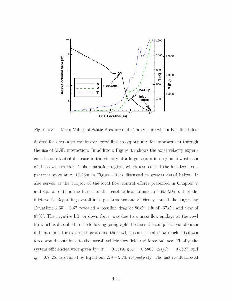
Axial Location (m)

Cro

ss-S

ectio

nalA

rea

(m2 )

T(K

)

P(P

a)

0 5 10 15 20

2

4

6

8

10

400

600

800

1000

1200

10000

20000

30000

APT

SidewallsCowl Lip

InletThroat

Figure 4.3: Mean Values of Static Pressure and Temperature within Baseline Inlet

desired for a scramjet combustor, providing an opportunity for improvement through

the use of MGD interaction. In addition, Figure 4.4 shows the axial velocity experi-

enced a substantial decrease in the vicinity of a large separation region downstream

of the cowl shoulder. This separation region, which also caused the localized tem-

perature spike at x=17.25m in Figure 4.3, is discussed in greater detail below. It

also served as the subject of the local flow control efforts presented in Chapter V

and was a contributing factor to the baseline heat transfer of 69.6MW out of the

inlet walls. Regarding overall inlet performance and efficiency, force balancing using

Equations 2.65 – 2.67 revealed a baseline drag of 86kN, lift of -67kN, and yaw of

870N. The negative lift, or down force, was due to a mass flow spillage at the cowl

lip which is described in the following paragraph. Because the computational domain

did not model the external flow around the cowl, it is not certain how much this down

force would contribute to the overall vehicle flow field and force balance. Finally, the

system efficiencies were given by: πc = 0.1519, ηKE = 0.8868, ∆s/Cp = 0.4827, and

ηc = 0.7525, as defined by Equations 2.70– 2.73, respectively. The last result showed

4-11

Axial Location (m)

Cro

ss-S

ectio

nalA

rea

(m2 )

Mac

hN

umbe

r

U(m

/s)

0 5 10 15 20

2

4

6

8

4

5

6

7

8

9

10

2400

2600

2800

3000

AUMach

SeparationRegion

Figure 4.4: Mean Values of Mach Number and Normalized Axial Velocity withinBaseline Inlet

the inlet performed somewhat less efficiently than the nominal value of ηc = 0.9 used

by Heiser and Pratt in their analysis [25]; a fact that was attributable to three key

inlet flow features.

First and foremost, 59 kg/s, or roughly 22%, of the freestream mass flow was

spilled at the bottom cowl lip, never making it into the internal compression portion

of the inlet. This spillage loss was a purely 3D effect attributable to the sidewall

interaction. The additional sidewall compression caused the flow to seek pressure

relief by turning downward, an effect previously documented by Holland [27,28]. This

effect was clearly visible in Figure 4.5(a) by the sharp decrease in mass flow rate at the

cowl lip and in Figure 4.5(b) by the increase in a negative v-velocity component near

the cowl. Normally, this spillage could be countered by moving the cowl lip forward,

however, the pressure relief is a desired effect for engine starting which would occur

at lower Mach numbers and higher pressures. Therefore, although it was not needed

for the cruise test conditions examined in this research, this geometric feature was

kept to improve the realism of the overall design.

4-12

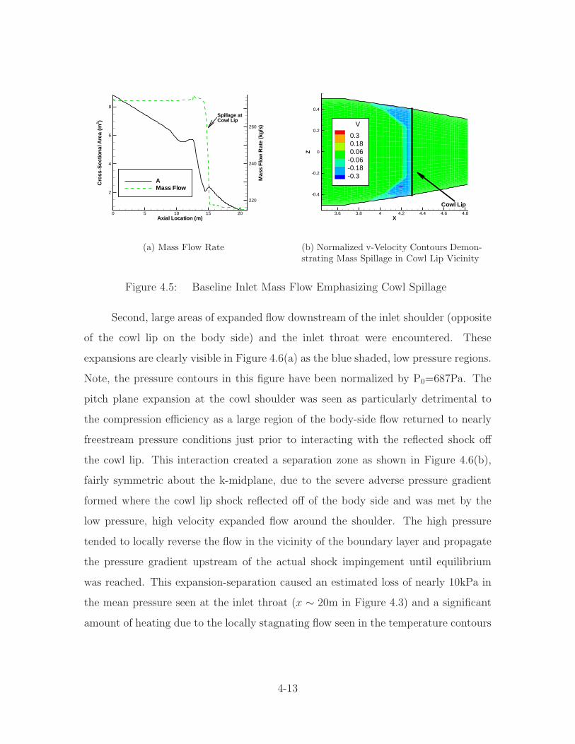
Axial Location (m)

Cro

ss-S

ectio

nalA

rea

(m2 )

Mas

sF

low

Rat

e(k

g/s)

0 5 10 15 20

2

4

6

8

220

240

260

AMass Flow

Spillage atCowl Lip

(a) Mass Flow Rate

X

Z

3.6 3.8 4 4.2 4.4 4.6 4.8

-0.4

-0.2

0

0.2

0.4

V

0.30.180.06

-0.06-0.18-0.3

Cowl Lip

(b) Normalized v-Velocity Contours Demon-strating Mass Spillage in Cowl Lip Vicinity

Figure 4.5: Baseline Inlet Mass Flow Emphasizing Cowl Spillage

Second, large areas of expanded flow downstream of the inlet shoulder (opposite

of the cowl lip on the body side) and the inlet throat were encountered. These

expansions are clearly visible in Figure 4.6(a) as the blue shaded, low pressure regions.

Note, the pressure contours in this figure have been normalized by P0=687Pa. The

pitch plane expansion at the cowl shoulder was seen as particularly detrimental to

the compression efficiency as a large region of the body-side flow returned to nearly

freestream pressure conditions just prior to interacting with the reflected shock off

the cowl lip. This interaction created a separation zone as shown in Figure 4.6(b),

fairly symmetric about the k-midplane, due to the severe adverse pressure gradient

formed where the cowl lip shock reflected off of the body side and was met by the

low pressure, high velocity expanded flow around the shoulder. The high pressure

tended to locally reverse the flow in the vicinity of the boundary layer and propagate

the pressure gradient upstream of the actual shock impingement until equilibrium

was reached. This expansion-separation caused an estimated loss of nearly 10kPa in

the mean pressure seen at the inlet throat (x ∼ 20m in Figure 4.3) and a significant

amount of heating due to the locally stagnating flow seen in the temperature contours

4-13

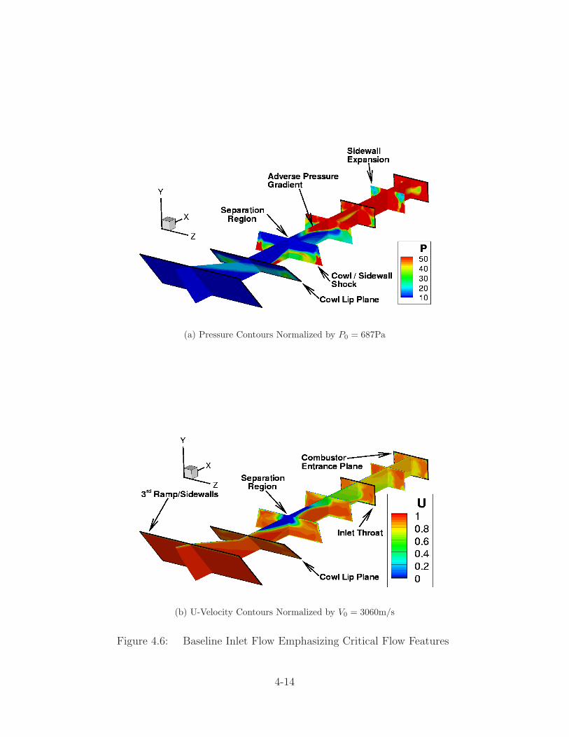
(a) Pressure Contours Normalized by P0 = 687Pa

(b) U-Velocity Contours Normalized by V0 = 3060m/s

Figure 4.6: Baseline Inlet Flow Emphasizing Critical Flow Features

4-14

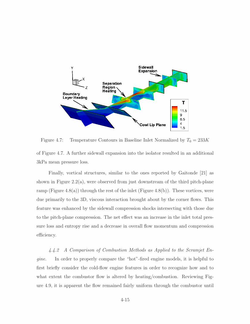
Figure 4.7: Temperature Contours in Baseline Inlet Normalized by T0 = 233K

of Figure 4.7. A further sidewall expansion into the isolator resulted in an additional

3kPa mean pressure loss.

Finally, vortical structures, similar to the ones reported by Gaitonde [21] as

shown in Figure 2.2(a), were observed from just downstream of the third pitch-plane

ramp (Figure 4.8(a)) through the rest of the inlet (Figure 4.8(b)). These vortices, were

due primarily to the 3D, viscous interaction brought about by the corner flows. This

feature was enhanced by the sidewall compression shocks intersecting with those due

to the pitch-plane compression. The net effect was an increase in the inlet total pres-

sure loss and entropy rise and a decrease in overall flow momentum and compression

efficiency.

4.4.2 A Comparison of Combustion Methods as Applied to the Scramjet En-

gine. In order to properly compare the “hot”-fired engine models, it is helpful to

first briefly consider the cold-flow engine features in order to recognize how and to

what extent the combustor flow is altered by heating/combustion. Reviewing Fig-

ure 4.9, it is apparent the flow remained fairly uniform through the combustor until

4-15

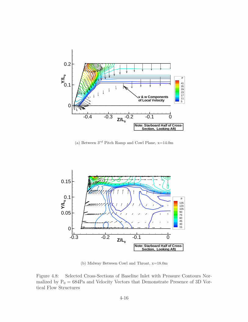
Z/L0

Y/L

0

-0.4 -0.3 -0.2 -0.1 0

0

0.1

0.2

P

4135292317115

Note: Starboard Half of Cross-Section, Looking Aft)

v & w Componentsof Local Velocity

(a) Between 3rd Pitch Ramp and Cowl Plane, x=14.0m

Z/L0

Y/L

0

-0.3 -0.2 -0.1 0

0

0.05

0.1

0.15

P

135120105907560453015

Note: Starboard Half of Cross-Section, Looking Aft)

(b) Midway Between Cowl and Throat, x=18.0m

Figure 4.8: Selected Cross-Sections of Baseline Inlet with Pressure Contours Nor-malized by P0 = 684Pa and Velocity Vectors that Demonstrate Presence of 3D Vor-tical Flow Structures

4-16

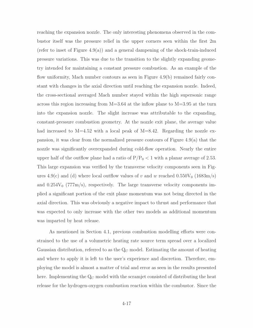
reaching the expansion nozzle. The only interesting phenomena observed in the com-

bustor itself was the pressure relief in the upper corners seen within the first 2m

(refer to inset of Figure 4.9(a)) and a general dampening of the shock-train-induced

pressure variations. This was due to the transition to the slightly expanding geome-

try intended for maintaining a constant pressure combustion. As an example of the

flow uniformity, Mach number contours as seen in Figure 4.9(b) remained fairly con-

stant with changes in the axial direction until reaching the expansion nozzle. Indeed,

the cross-sectional averaged Mach number stayed within the high supersonic range

across this region increasing from M=3.64 at the inflow plane to M=3.95 at the turn

into the expansion nozzle. The slight increase was attributable to the expanding,

constant-pressure combustion geometry. At the nozzle exit plane, the average value

had increased to M=4.52 with a local peak of M=8.42. Regarding the nozzle ex-

pansion, it was clear from the normalized pressure contours of Figure 4.9(a) that the

nozzle was significantly overexpanded during cold-flow operation. Nearly the entire

upper half of the outflow plane had a ratio of P/P0 < 1 with a planar average of 2.53.

This large expansion was verified by the transverse velocity components seen in Fig-

ures 4.9(c) and (d) where local outflow values of v and w reached 0.550V0 (1683m/s)

and 0.254V0 (777m/s), respectively. The large transverse velocity components im-

plied a significant portion of the exit plane momentum was not being directed in the

axial direction. This was obviously a negative impact to thrust and performance that

was expected to only increase with the other two models as additional momentum

was imparted by heat release.

As mentioned in Section 4.1, previous combustion modelling efforts were con-

strained to the use of a volumetric heating rate source term spread over a localized

Gaussian distribution, referred to as the QC model. Estimating the amount of heating

and where to apply it is left to the user’s experience and discretion. Therefore, em-

ploying the model is almost a matter of trial and error as seen in the results presented

here. Implementing the QC model with the scramjet consisted of distributing the heat

release for the hydrogen-oxygen combustion reaction within the combustor. Since the

4-17

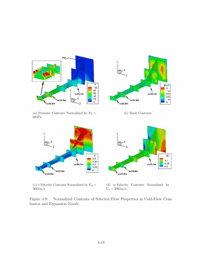
(a) Pressure Contours Normalized by P0 =684Pa

(b) Mach Contours

(c) v-Velocity Contours Normalized by V0 =3061m/s

(d) w-Velocity Contours Normalized byV0 = 3061m/s

Figure 4.9: Normalized Contours of Selected Flow Properties in Cold-Flow Com-bustor and Expansion Nozzle

4-18

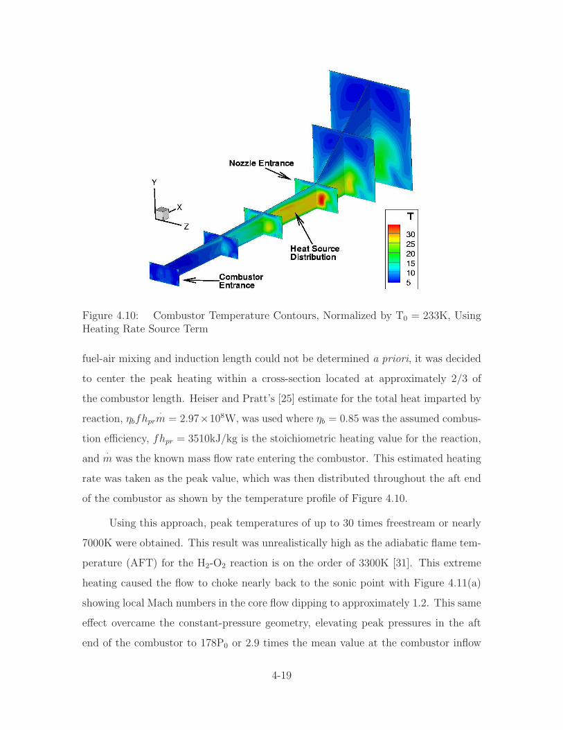
Figure 4.10: Combustor Temperature Contours, Normalized by T0 = 233K, UsingHeating Rate Source Term

fuel-air mixing and induction length could not be determined a priori, it was decided

to center the peak heating within a cross-section located at approximately 2/3 of

the combustor length. Heiser and Pratt’s [25] estimate for the total heat imparted by

reaction, ηbfhpr

·

m = 2.97×108W, was used where ηb = 0.85 was the assumed combus-

tion efficiency, fhpr = 3510kJ/kg is the stoichiometric heating value for the reaction,

and·

m was the known mass flow rate entering the combustor. This estimated heating

rate was taken as the peak value, which was then distributed throughout the aft end

of the combustor as shown by the temperature profile of Figure 4.10.

Using this approach, peak temperatures of up to 30 times freestream or nearly

7000K were obtained. This result was unrealistically high as the adiabatic flame tem-

perature (AFT) for the H2-O2 reaction is on the order of 3300K [31]. This extreme

heating caused the flow to choke nearly back to the sonic point with Figure 4.11(a)

showing local Mach numbers in the core flow dipping to approximately 1.2. This same

effect overcame the constant-pressure geometry, elevating peak pressures in the aft

end of the combustor to 178P0 or 2.9 times the mean value at the combustor inflow

4-19

(a) Mach Contours (b) Pressure Contours Normalized by P0 =684Pa

Figure 4.11: Normalized Contours of Selected Flow Properties in Combustor andExpansion Nozzle Using Distributed Heating Rate Source Term

plane. This outcome reinforced the difficulty of using this approach to achieving accu-

rate thermochemistry results for complex engineering problems such as the scramjet

engine. However, the QC results were still useful for comparison purposes as the they

represented the highest performance the combustor could achieve based solely on geo-

metrical considerations. Of course, the limitations embodied in the actual combustion

physics preclude this from occurring.

The finite rate chemistry model was expressly developed to overcome the limited

physical basis inherent in the volumetric heat source term, especially as applied to

geometries and scales of practical engineering interest. Therefore, it was expected to

produce the most realistic result for the scramjet tested, even if it did not produce

the best performance. However, the first question to answer was whether or not

combustion occurred, and if so, to what extent. Stable, efficient combustion has

traditionally been one of the greatest challenges to achieving scramjet propulsion. The

scramjet geometry used was predicted to have significant efficiency issues because the

structured grid required by the computational model would not easily facilitate the

inclusion of a detailed fuel injection and flameholding/mixing system. Recalling from

4-20

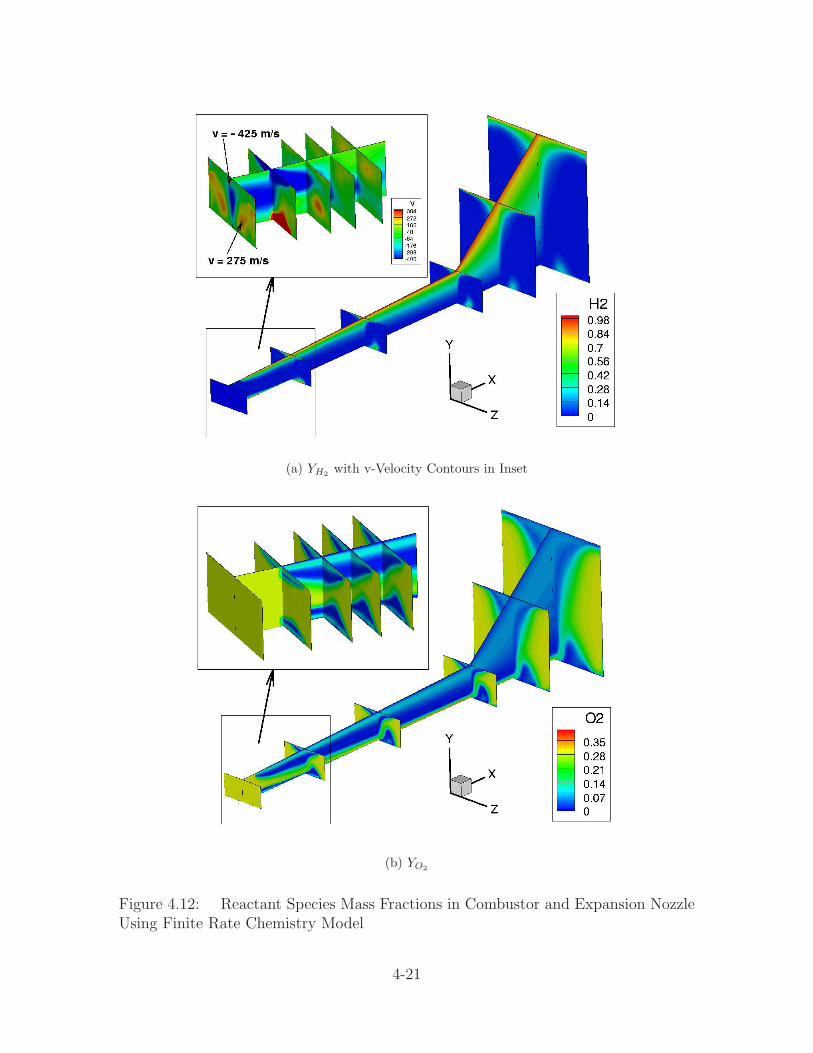
(a) YH2with v-Velocity Contours in Inset

(b) YO2

Figure 4.12: Reactant Species Mass Fractions in Combustor and Expansion NozzleUsing Finite Rate Chemistry Model

4-21

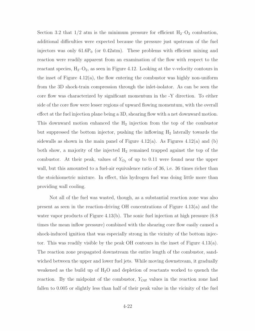
Section 3.2 that 1/2 atm is the minimum pressure for efficient H2–O2 combustion,

additional difficulties were expected because the pressure just upstream of the fuel

injectors was only 61.6P0 (or 0.42atm). These problems with efficient mixing and

reaction were readily apparent from an examination of the flow with respect to the

reactant species, H2–O2, as seen in Figure 4.12. Looking at the v-velocity contours in

the inset of Figure 4.12(a), the flow entering the combustor was highly non-uniform

from the 3D shock-train compression through the inlet-isolator. As can be seen the

core flow was characterized by significant momentum in the -Y direction. To either

side of the core flow were lesser regions of upward flowing momentum, with the overall

effect at the fuel injection plane being a 3D, shearing flow with a net downward motion.

This downward motion enhanced the H2 injection from the top of the combustor

but suppressed the bottom injector, pushing the inflowing H2 laterally towards the

sidewalls as shown in the main panel of Figure 4.12(a). As Figures 4.12(a) and (b)

both show, a majority of the injected H2 remained trapped against the top of the

combustor. At their peak, values of YO2of up to 0.11 were found near the upper

wall, but this amounted to a fuel-air equivalence ratio of 36, i.e. 36 times richer than

the stoichiometric mixture. In effect, this hydrogen fuel was doing little more than

providing wall cooling.

Not all of the fuel was wasted, though, as a substantial reaction zone was also

present as seen in the reaction-driving OH concentrations of Figure 4.13(a) and the

water vapor products of Figure 4.13(b). The sonic fuel injection at high pressure (6.8

times the mean inflow pressure) combined with the shearing core flow easily caused a

shock-induced ignition that was especially strong in the vicinity of the bottom injec-

tor. This was readily visible by the peak OH contours in the inset of Figure 4.13(a).

The reaction zone propagated downstream the entire length of the combustor, sand-

wiched between the upper and lower fuel jets. While moving downstream, it gradually

weakened as the build up of H2O and depletion of reactants worked to quench the

reaction. By the midpoint of the combustor, YOH values in the reaction zone had

fallen to 0.005 or slightly less than half of their peak value in the vicinity of the fuel

4-22

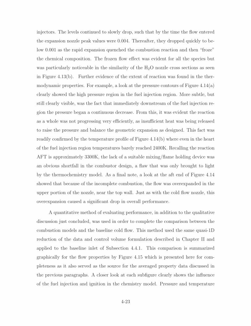
injectors. The levels continued to slowly drop, such that by the time the flow entered

the expansion nozzle peak values were 0.004. Thereafter, they dropped quickly to be-

low 0.001 as the rapid expansion quenched the combustion reaction and then “froze”

the chemical composition. The frozen flow effect was evident for all the species but

was particularly noticeable in the similarity of the H2O nozzle cross sections as seen

in Figure 4.13(b). Further evidence of the extent of reaction was found in the ther-

modynamic properties. For example, a look at the pressure contours of Figure 4.14(a)

clearly showed the high pressure region in the fuel injection region. More subtle, but

still clearly visible, was the fact that immediately downstream of the fuel injection re-

gion the pressure began a continuous decrease. From this, it was evident the reaction

as a whole was not progressing very efficiently, as insufficient heat was being released

to raise the pressure and balance the geometric expansion as designed. This fact was

readily confirmed by the temperature profile of Figure 4.14(b) where even in the heart

of the fuel injection region temperatures barely reached 2400K. Recalling the reaction

AFT is approximately 3300K, the lack of a suitable mixing/flame holding device was

an obvious shortfall in the combustor design, a flaw that was only brought to light

by the thermochemistry model. As a final note, a look at the aft end of Figure 4.14

showed that because of the incomplete combustion, the flow was overexpanded in the

upper portion of the nozzle, near the top wall. Just as with the cold flow nozzle, this

overexpansion caused a significant drop in overall performance.

A quantitative method of evaluating performance, in addition to the qualitative

discussion just concluded, was used in order to complete the comparison between the

combustion models and the baseline cold flow. This method used the same quasi-1D

reduction of the data and control volume formulation described in Chapter II and

applied to the baseline inlet of Subsection 4.4.1. This comparison is summarized

graphically for the flow properties by Figure 4.15 which is presented here for com-

pleteness as it also served as the source for the averaged property data discussed in

the previous paragraphs. A closer look at each subfigure clearly shows the influence

of the fuel injection and ignition in the chemistry model. Pressure and temperature

4-23

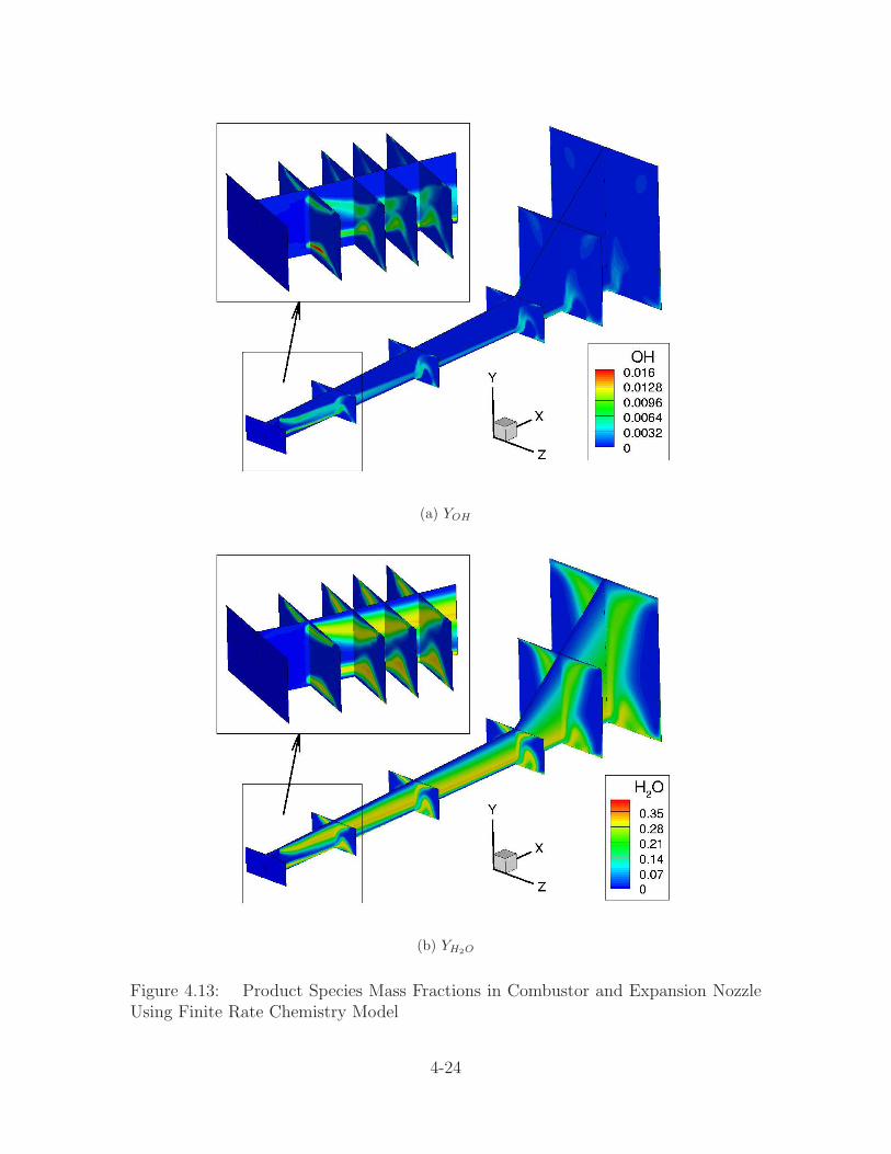
(a) YOH

(b) YH2O

Figure 4.13: Product Species Mass Fractions in Combustor and Expansion NozzleUsing Finite Rate Chemistry Model

4-24

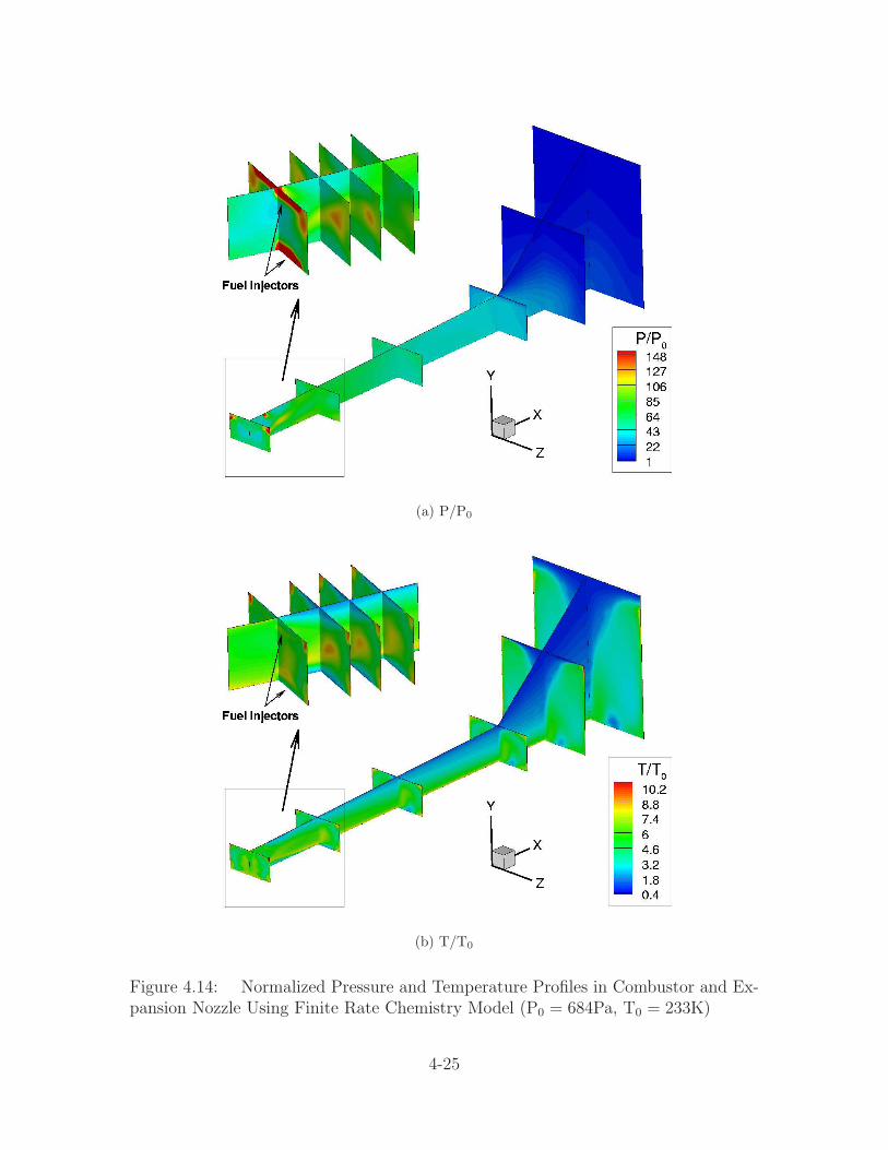
(a) P/P0

(b) T/T0

Figure 4.14: Normalized Pressure and Temperature Profiles in Combustor and Ex-pansion Nozzle Using Finite Rate Chemistry Model (P0 = 684Pa, T0 = 233K)

4-25

spike at 70% above their inflow values and then monotonically decrease until reaching

the expansion nozzle. As would be expected, the Mach number and velocity for all

the combustor models followed a trend as the inverse of the pressure and temperature.

The impact of the nozzle was likewise evident as pointed out in the figure. Other than

the fuel injection spike, what was most striking from these subfigures was just how

different the QC results were from both of the other models. It was clearly evident

that the QC method had released an unrealistic amount of heat into the combustor

with average temperatures and pressures reaching 4865K and 90.2kPa, respectively,

in the center of the heat release distribution.

Of course, with all of this energy imparted to the flow, the QC model far outper-

formed the chemistry model with respect to thrust and efficiency as demonstrated in

Table 4.3. (Note, the Baseline case in this table refers to the cold flow model and the

values include the contributions of the internal inlet and isolator.) Regarding forces,

the QC model imparted 4.6 times the axial force compared to the chemistry model

and 41% more vertical force. Yaw was relatively insignificant for all cases, being two

orders of magnitude lower for the heat release models and practically non-existent

for the baseline case. While 116.7MW of heat passed out through the walls of the

cold flow model due to frictional heating, a net of 112.0MW of heat was added by

the thermochemistry model, and an astounding 6 times that amount of combustion

heat was added by the QC distribution. Because the heat addition process typically

improves the total pressure ratio, it was not a surprise that this was the result here.

What was unexpected was by how much the QC model outperformed the other mod-

els. Due to the fact it added energy without any inherent losses, it had a πc of 2.7

times the chemistry model and nearly 11 times the cold flow model.

4.5 Summary of Results, Conclusions and Recommendations Regard-

ing the Thermochemistry Model

Stable, efficient combustion has traditionally been one of the greatest chal-

lenges for achieving scramjet propulsion. To address this challenge, a portion of this

4-26

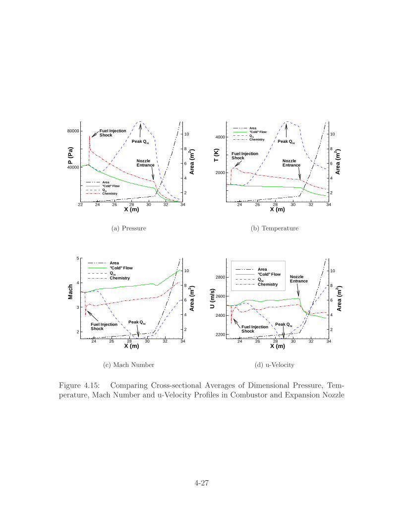
X (m)

P(P

a)

Are

a(m

2 )

22 24 26 28 30 32 34

40000

80000

2

4

6

8

10

Area"Cold" FlowQht

Chemistry

Fuel InjectionShock

NozzleEntrance

Peak Qht

(a) Pressure

X (m)T

(K)

Are

a(m

2 )

24 26 28 30 32 34

2000

4000

2

4

6

8

10

Area"Cold" FlowQht

Chemistry

Fuel InjectionShock

NozzleEntrance

Peak Qht

(b) Temperature

X (m)

Mac

h

Are

a(m

2 )

24 26 28 30 32 34

2

3

4

5

2

4

6

8

10

Area"Cold" FlowQht

Chemistry

Fuel InjectionShock

Peak Qht

(c) Mach Number

X (m)

U(m

/s)

Are

a(m

2 )24 26 28 30 32 34

2200

2400

2600

2800

2

4

6

8

10Area"Cold" FlowQht

Chemistry

Fuel InjectionShock

NozzleEntrance

Peak Qht

(d) u-Velocity

Figure 4.15: Comparing Cross-sectional Averages of Dimensional Pressure, Tem-perature, Mach Number and u-Velocity Profiles in Combustor and Expansion Nozzle

4-27

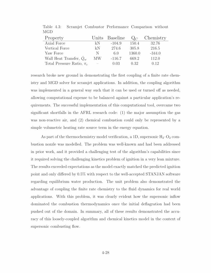
Table 4.3: Scramjet Combustor Performance Comparison withoutMGD

Property Units Baseline QC ChemistryAxial Force kN -104.9 150.4 32.76Vertical Force kN 274.6 305.8 216.5Yaw Force N 6.0 1360.0 -344.0

Wall Heat Transfer, Qw MW -116.7 669.2 112.0Total Pressure Ratio, πc – 0.03 0.32 0.12

research broke new ground in demonstrating the first coupling of a finite rate chem-

istry and MGD solver for scramjet applications. In addition, the coupling algorithm

was implemented in a general way such that it can be used or turned off as needed,

allowing computational expense to be balanced against a particular application’s re-

quirements. The successful implementation of this computational tool, overcame two

significant shortfalls in the AFRL research code: (1) the major assumption the gas

was non-reactive air, and (2) chemical combustion could only be represented by a

simple volumetric heating rate source term in the energy equation.

As part of the thermochemistry model verification, a 1D, supersonic H2–O2 com-

bustion nozzle was modelled. The problem was well-known and had been addressed

in prior work, and it provided a challenging test of the algorithm’s capabilities since

it required solving the challenging kinetics problem of ignition in a very lean mixture.

The results exceeded expectations as the model exactly matched the predicted ignition

point and only differed by 0.5% with respect to the well-accepted STANJAN software

regarding equilibrium water production. The unit problem also demonstrated the

advantage of coupling the finite rate chemistry to the fluid dynamics for real world

applications. With this problem, it was clearly evident how the supersonic inflow

dominated the combustion thermodynamics once the initial deflagration had been

pushed out of the domain. In summary, all of these results demonstrated the accu-

racy of this loosely-coupled algorithm and chemical kinetics model in the context of

supersonic combusting flow.

4-28

With the successful outcome of the unit problem, the method was incorporated

into the scramjet combustor geometry defined in Chapter III. The baseline inlet

flowfield without MGD interaction, common to all three of the combustors tested,

was characterized first. The inlet performed marginally well insofar as it increased the

mean static pressure to 57P0 at the inlet throat while limiting the static temperature

rise to 5.1T0, however, this pressure was still 23% below the minimum desired at the

combustor inlet. This shortfall was due to the quasi-1D inlet analysis that failed to

account for the adverse 3D effects that led to cowl spillage and regions of expansion

and separation. Solving these issues is the focus of Chapter V.

The inlet characterization was followed by a comparison of three combustors

models that shared identical geometries but differed fundamentally in that they op-

erated: (1) as a cold flow simulation, (2) with the pre-existing volumetric heat source

term, or (3) with the finite rate chemistry algorithm. While for the most part the cold-

flow simulation was unremarkable, it did provide the first indication the expansion

system had geometric design issues. From the normalized pressure contours of both

the cold-flow and chemistry models it was clear the expansion nozzle was significantly

overexpanded during these modes of operation with nearly the entire upper half of

the outflow plane having a ratio of P/P0 < 1. Additionally, the large transverse ve-

locity components implied a significant portion of the exit plane momentum was not

directed in the axial direction, causing a negative impact on thrust and performance.

Because engine-airframe integration was not part of this research, incorporating a

higher fidelity expansion system geometry was left as a suggestion for future research.

With respect to the two heat addition models tested, the QC model reached peak

temperatures of up to 30 times freestream (nearly 7000K), or twice the theoretical

limit. This resulted in the flow being choked nearly back to the sonic point with peak

pressures in the aft end of the combustor 2.9 times greater than the mean value at

the inflow plane. While this method did produce the most thrust for the geometry

used, the unrealistic outcome actually reinforced the difficulty of using this approach

4-29

to achieving accurate results for complex engineering problems such as the scramjet

engine.

Among other things, the thermochemistry model corroborated pre-existing con-

cerns that the geometry used would have significant efficiency issues due to the fact

the structured grid solver precluded the inclusion of a detailed fuel injection and

flameholding/mixing system. Throughout the combustor, much of the injected H2

remained trapped against the top wall, an effect only observable with the use of the

chemistry modelling tool. In effect, this hydrogen fuel was doing little more than

providing wall cooling. In spite of this, a substantial reaction zone was also present as

seen in the wide-ranging extent of the water vapor product of combustion. A shock-

induced ignition in the vicinity of the fuel injectors was especially strong near the

bottom injector. The reaction zone propagated downstream the entire length of the

combustor, sandwiched between the upper and lower fuel jets. The zone gradually

weakened as the build up of H2O and depletion of reactants worked to quench the

reaction. Immediately downstream of the fuel injection region the pressure began a

continuous decrease, additional evidence to support the conclusion the reaction as a

whole was not progressing very efficiently. This was attributed to insufficient heat

release (peak temperatures in the reaction zone were barely 2400K) to raise the pres-

sure and balance the geometric expansion as designed. Beyond any doubt, the lack

of a suitable mixing/flame holding device was an obvious shortfall in the combustor

design, again an issue only brought to light by the thermochemistry model.

The overall results can be summed up in a few conclusions and recommendations

for future research efforts. First, the loosely coupled approach to incorporate finite

rate chemistry was very successful with respect to modelling supersonic combustion

flow problems and is recommended over the code’s pre-existing approaches for these

problems. A recommendation for furthering the thermochemistry model would be

to add a species diffusion term, primarily to extend applicability to the subsonic

regime. In addition, higher fidelity models of viscosity and thermal conductivity exist

for multi-species flows that could be used in place of the single-equation Sutherland

4-30

model described in Chapter II. With regard to the actual scramjet design tested

here, the combustor with chemistry was conclusively shown to accurately reflect the

performance of a real engine. One caveat was that several problems with the geometry

were identified that could be traced back to the initial quasi-1D design iteration.

Because it was outside the scope and timeline of this research to undertake multiple

design iterations, it is recommended that future work use the current geometry as a

baseline upon which to make improvements. Finally, in a related specific conclusion,

under-compression and flow separation in the inlet was recognized as a good location

to test localized MGD flow control techniques.

4-31

V. Localized Electromagnetic Flow Control

5.1 A Review of Previously Published Selected Concepts and Applica-

tions

In recent years, numerous methods of using EM fields to locally improve scramjet

flow have been proposed. Additionally, a few more ambitious proposals have been

made to use these same concepts to both provide electrical energy to power the flow

ionizer and augment the vehicle’s thrust. Because scramjet vehicles are geometrically

optimized for a single design point, it is assumed a significant portion of their mission

will be spent operating at off design conditions. In addition, even while operating

at on-design conditions there will be regions of locally ill-conditioned flow due to

geometric or other constraints. Therefore, localized flow control aims to mitigate

these ill-conditioned regions or enhance favorable flow qualities. These flow control

techniques may be the deciding factor in success or failure for a particular engine

design.

Two localized approaches featured prominently in the literature: maintaining

the shock-on-cowl-lip condition and boundary layer transition and control. The former

of these is a design imperative as it is the most effective way of maintaining the proper

mass flow of air into the engine. Macheret and associates at Princeton University have

completed a great deal of analytical and some numerical work on this application. One

idea they have explored is to operate a near-surface MGD system just upstream of the

cowl that would use electron beams to ionize the flow [47]. The Lorentz force would

then be used to increase or decrease the flow momentum at the cowl to maintain the

shock-on-cowl-lip at off-design Mach numbers. Although their model was limited to

2D, inviscid flow, they were able to maintain the desired flowfield at Mach numbers of

2 less than the design point of 8. However, the penalty for using MGD was an increase

in total pressure loss which could be considered as a drag penalty. The investigation

of this drag penalty was left as future work. A second method Macheret, et al, have

investigated is to achieve the same effects by creating a virtual cowl of heated air in

front of the cowl lip [49, 50, 73]. Although the heating mechanism is unspecified, the

5-1

authors point out that it is possible that RF or microwave energy could be supplied to

an area pre-ionized by an electron beam or laser. If this is the case, then at best MGD

effects could prove both a satisfactory heating mechanism and a source of additional

electrical power. Even if the Joule heating from MGD interaction is not adequate for

this application, it could still serve as the electrical power supply for whatever heating

system is chosen.

Manipulating the boundary layer is another local flow control application that

preliminary studies have demonstrated may benefit from MGD application. This is

especially true with respect to controlling the transition from laminar to turbulent

flow as well as increasing the near wall flow momentum to prevent separation and

potential inlet unstart. The shock structure within 3D inlet flows is incredibly complex

as several researchers [21, 28, 37, 39] as well as this research have shown. Sidewall

interaction, low momentum vortical structures and large areas of flow separation are

common detrimental features. These structures are detrimental to the flow as they

increase total pressure losses, prevent a smooth flowfield at the combustor entrance,

and in the worst instances may cause inlet unstart. The next section identifies how the

application of MGD to a scramjet inlet can improve the inlet efficiency as measured by

the efficiency metrics discussed in Chapter II as well as increase the pressure entering

the combustor, a critical requirement for efficient combustor operation.

5.2 Improving Engine Performance by Application of Localized Inlet

Flow Control

Prior to this effort, only simulations without the application of EM fields had

been conducted on the flight-scale geometry. As illustrated in Subsection 4.4.1, side-

wall and corner flow-induced vortical structures throughout the internal diffuser were

observed. Large areas of expanded flow downstream of the inlet shoulder (opposite

of the cowl lip on the body side) led to a sizeable separation zone, and the expansion

fans at the inlet throat further decreased the average pressure entering the combus-

tor. The question then arose as to whether MGD could be applied in this situation

5-2

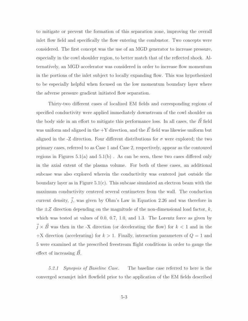
to mitigate or prevent the formation of this separation zone, improving the overall

inlet flow field and specifically the flow entering the combustor. Two concepts were

considered. The first concept was the use of an MGD generator to increase pressure,

especially in the cowl shoulder region, to better match that of the reflected shock. Al-

ternatively, an MGD accelerator was considered in order to increase flow momentum

in the portions of the inlet subject to locally expanding flow. This was hypothesized

to be especially helpful when focused on the low momentum boundary layer where

the adverse pressure gradient initiated flow separation.

Thirty-two different cases of localized EM fields and corresponding regions of

specified conductivity were applied immediately downstream of the cowl shoulder on

the body side in an effort to mitigate this performance loss. In all cases, the ~B field

was uniform and aligned in the +Y direction, and the ~E field was likewise uniform but

aligned in the -Z direction. Four different distributions for σ were explored; the two

primary cases, referred to as Case 1 and Case 2, respectively, appear as the contoured

regions in Figures 5.1(a) and 5.1(b) . As can be seen, these two cases differed only

in the axial extent of the plasma volume. For both of these cases, an additional

subcase was also explored wherein the conductivity was centered just outside the

boundary layer as in Figure 5.1(c). This subcase simulated an electron beam with the

maximum conductivity centered several centimeters from the wall. The conduction

current density, ~j, was given by Ohm’s Law in Equation 2.26 and was therefore in

the ±Z direction depending on the magnitude of the non-dimensional load factor, k,

which was tested at values of 0.0, 0.7, 1.0, and 1.3. The Lorentz force as given by

~j × ~B was then in the -X direction (or decelerating the flow) for k < 1 and in the

+X direction (accelerating) for k > 1. Finally, interaction parameters of Q = 1 and

5 were examined at the prescribed freestream flight conditions in order to gauge the

effect of increasing ~B.

5.2.1 Synopsis of Baseline Case. The baseline case referred to here is the

converged scramjet inlet flowfield prior to the application of the EM fields described

5-3

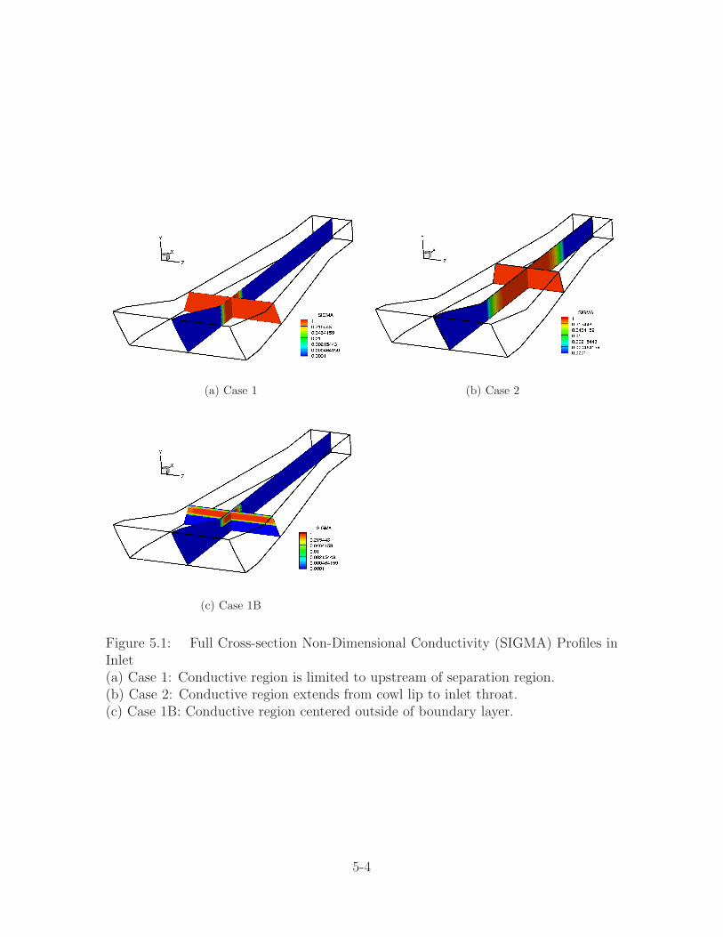
(a) Case 1 (b) Case 2

(c) Case 1B

Figure 5.1: Full Cross-section Non-Dimensional Conductivity (SIGMA) Profiles inInlet(a) Case 1: Conductive region is limited to upstream of separation region.(b) Case 2: Conductive region extends from cowl lip to inlet throat.(c) Case 1B: Conductive region centered outside of boundary layer.

5-4

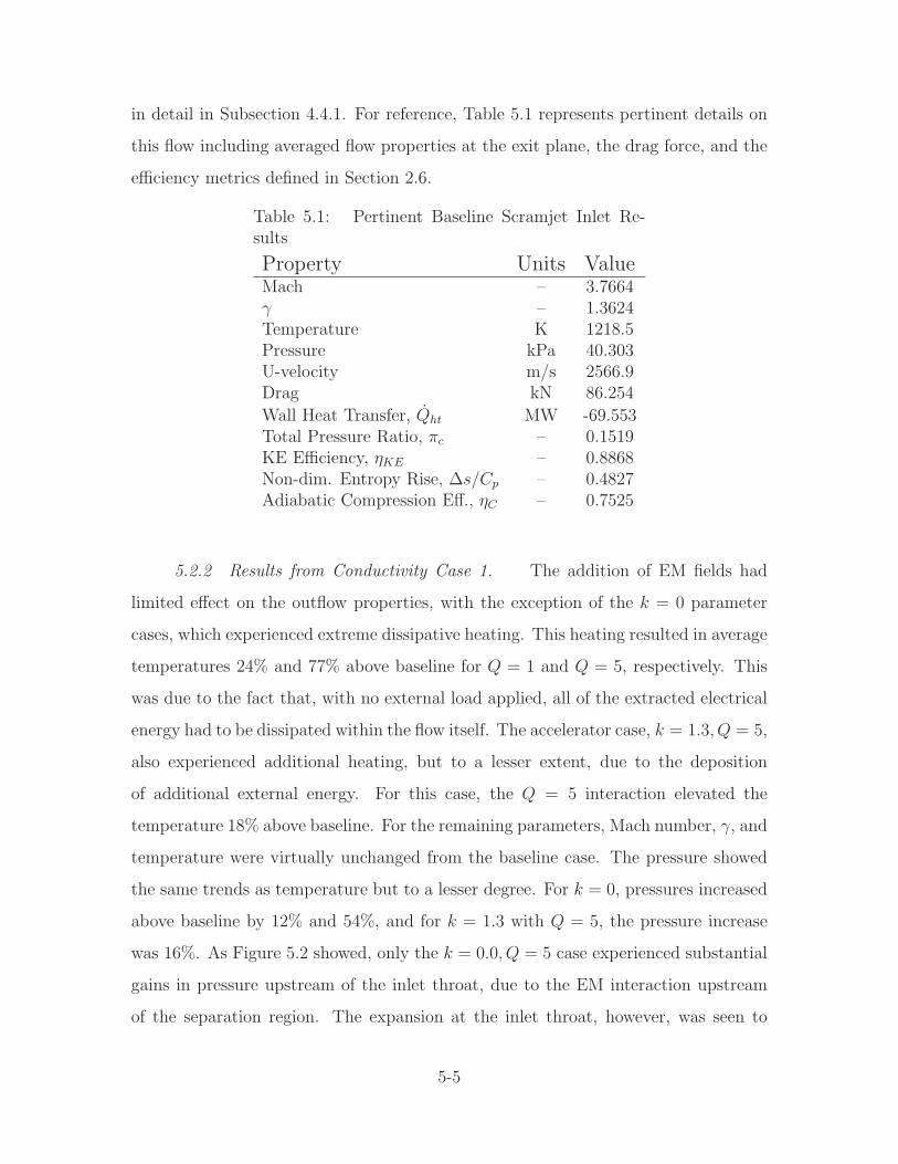
in detail in Subsection 4.4.1. For reference, Table 5.1 represents pertinent details on

this flow including averaged flow properties at the exit plane, the drag force, and the

efficiency metrics defined in Section 2.6.

Table 5.1: Pertinent Baseline Scramjet Inlet Re-sults

Property Units ValueMach – 3.7664γ – 1.3624Temperature K 1218.5Pressure kPa 40.303U-velocity m/s 2566.9Drag kN 86.254

Wall Heat Transfer, Qht MW -69.553Total Pressure Ratio, πc – 0.1519KE Efficiency, ηKE – 0.8868Non-dim. Entropy Rise, ∆s/Cp – 0.4827Adiabatic Compression Eff., ηC – 0.7525

5.2.2 Results from Conductivity Case 1. The addition of EM fields had

limited effect on the outflow properties, with the exception of the k = 0 parameter

cases, which experienced extreme dissipative heating. This heating resulted in average

temperatures 24% and 77% above baseline for Q = 1 and Q = 5, respectively. This

was due to the fact that, with no external load applied, all of the extracted electrical

energy had to be dissipated within the flow itself. The accelerator case, k = 1.3, Q = 5,

also experienced additional heating, but to a lesser extent, due to the deposition

of additional external energy. For this case, the Q = 5 interaction elevated the

temperature 18% above baseline. For the remaining parameters, Mach number, γ, and

temperature were virtually unchanged from the baseline case. The pressure showed

the same trends as temperature but to a lesser degree. For k = 0, pressures increased

above baseline by 12% and 54%, and for k = 1.3 with Q = 5, the pressure increase

was 16%. As Figure 5.2 showed, only the k = 0.0, Q = 5 case experienced substantial

gains in pressure upstream of the inlet throat, due to the EM interaction upstream

of the separation region. The expansion at the inlet throat, however, was seen to

5-5

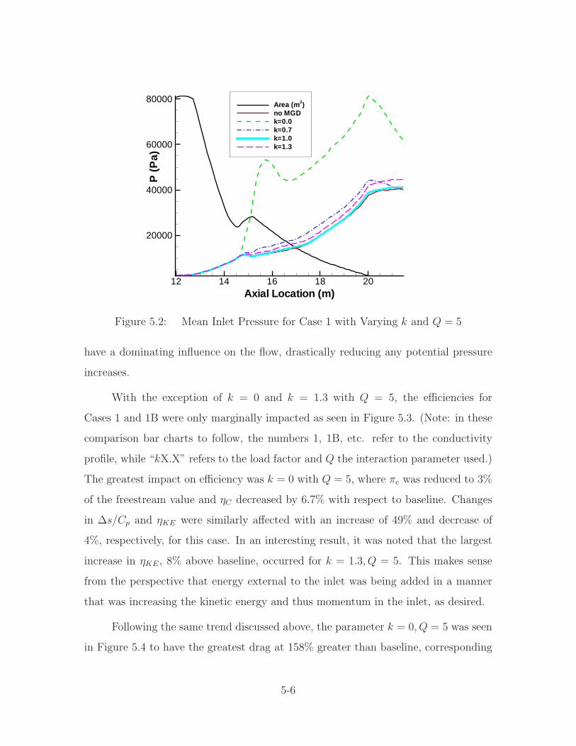
Axial Location (m)

P(P

a)

12 14 16 18 20

20000

40000

60000

80000Area (m 2)no MGDk=0.0k=0.7k=1.0k=1.3

Figure 5.2: Mean Inlet Pressure for Case 1 with Varying k and Q = 5

have a dominating influence on the flow, drastically reducing any potential pressure

increases.

With the exception of k = 0 and k = 1.3 with Q = 5, the efficiencies for

Cases 1 and 1B were only marginally impacted as seen in Figure 5.3. (Note: in these

comparison bar charts to follow, the numbers 1, 1B, etc. refer to the conductivity

profile, while “kX.X” refers to the load factor and Q the interaction parameter used.)

The greatest impact on efficiency was k = 0 with Q = 5, where πc was reduced to 3%

of the freestream value and ηC decreased by 6.7% with respect to baseline. Changes

in ∆s/Cp and ηKE were similarly affected with an increase of 49% and decrease of

4%, respectively, for this case. In an interesting result, it was noted that the largest

increase in ηKE, 8% above baseline, occurred for k = 1.3, Q = 5. This makes sense

from the perspective that energy external to the inlet was being added in a manner

that was increasing the kinetic energy and thus momentum in the inlet, as desired.

Following the same trend discussed above, the parameter k = 0, Q = 5 was seen

in Figure 5.4 to have the greatest drag at 158% greater than baseline, corresponding

5-6

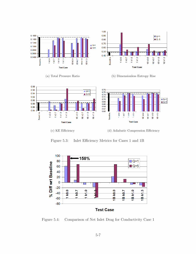
(a) Total Pressure Ratio (b) Dimensionless Entropy Rise

(c) KE Efficiency (d) Adiabatic Compression Efficiency

Figure 5.3: Inlet Efficiency Metrics for Cases 1 and 1B

Figure 5.4: Comparison of Net Inlet Drag for Conductivity Case 1

5-7

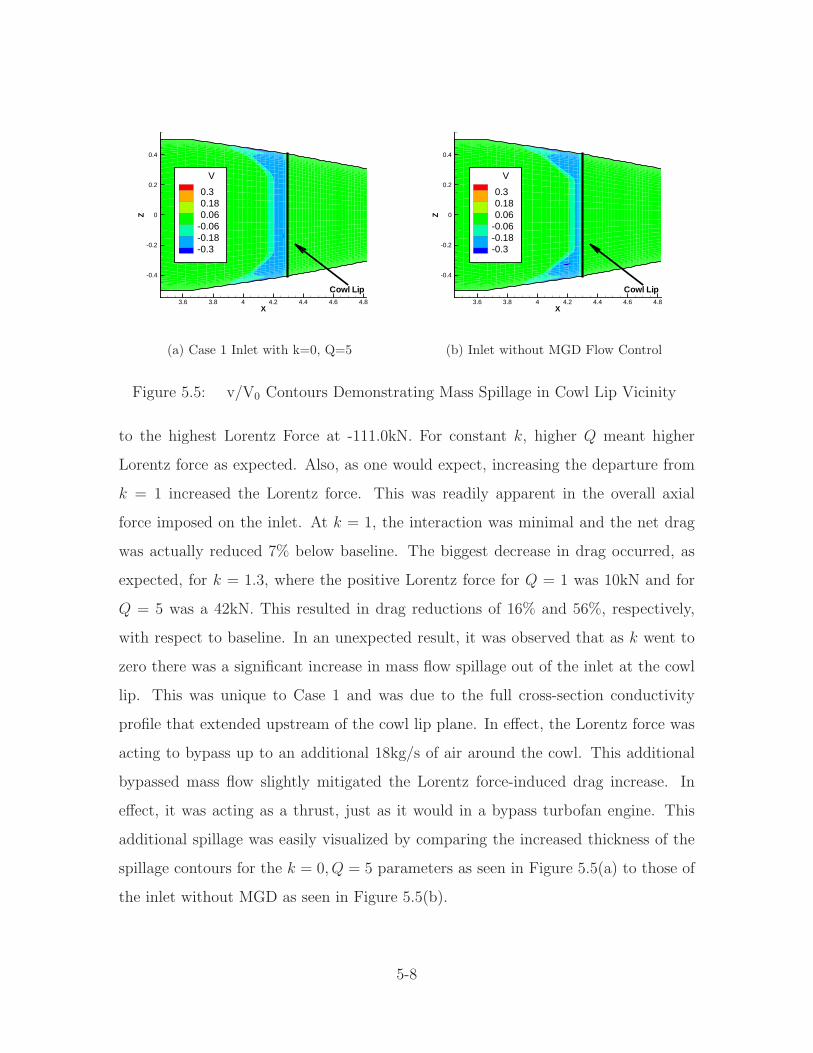
X

Z

3.6 3.8 4 4.2 4.4 4.6 4.8

-0.4

-0.2

0

0.2

0.4

V

0.30.180.06

-0.06-0.18-0.3

Cowl Lip

(a) Case 1 Inlet with k=0, Q=5

X

Z

3.6 3.8 4 4.2 4.4 4.6 4.8

-0.4

-0.2

0

0.2

0.4

V

0.30.180.06

-0.06-0.18-0.3

Cowl Lip

(b) Inlet without MGD Flow Control

Figure 5.5: v/V0 Contours Demonstrating Mass Spillage in Cowl Lip Vicinity

to the highest Lorentz Force at -111.0kN. For constant k, higher Q meant higher

Lorentz force as expected. Also, as one would expect, increasing the departure from

k = 1 increased the Lorentz force. This was readily apparent in the overall axial

force imposed on the inlet. At k = 1, the interaction was minimal and the net drag

was actually reduced 7% below baseline. The biggest decrease in drag occurred, as

expected, for k = 1.3, where the positive Lorentz force for Q = 1 was 10kN and for

Q = 5 was a 42kN. This resulted in drag reductions of 16% and 56%, respectively,

with respect to baseline. In an unexpected result, it was observed that as k went to

zero there was a significant increase in mass flow spillage out of the inlet at the cowl

lip. This was unique to Case 1 and was due to the full cross-section conductivity

profile that extended upstream of the cowl lip plane. In effect, the Lorentz force was

acting to bypass up to an additional 18kg/s of air around the cowl. This additional

bypassed mass flow slightly mitigated the Lorentz force-induced drag increase. In

effect, it was acting as a thrust, just as it would in a bypass turbofan engine. This

additional spillage was easily visualized by comparing the increased thickness of the

spillage contours for the k = 0, Q = 5 parameters as seen in Figure 5.5(a) to those of

the inlet without MGD as seen in Figure 5.5(b).

5-8

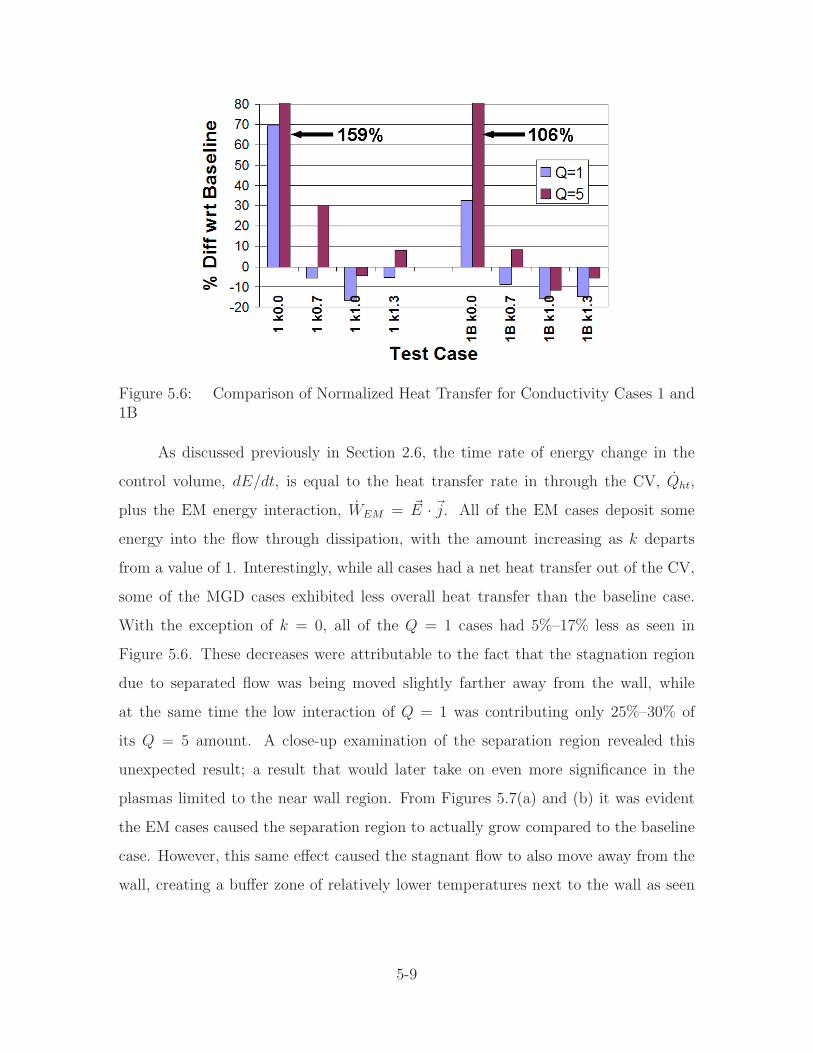
Figure 5.6: Comparison of Normalized Heat Transfer for Conductivity Cases 1 and1B

As discussed previously in Section 2.6, the time rate of energy change in the

control volume, dE/dt, is equal to the heat transfer rate in through the CV, Qht,

plus the EM energy interaction, WEM = ~E · ~j. All of the EM cases deposit some

energy into the flow through dissipation, with the amount increasing as k departs

from a value of 1. Interestingly, while all cases had a net heat transfer out of the CV,

some of the MGD cases exhibited less overall heat transfer than the baseline case.

With the exception of k = 0, all of the Q = 1 cases had 5%–17% less as seen in

Figure 5.6. These decreases were attributable to the fact that the stagnation region

due to separated flow was being moved slightly farther away from the wall, while

at the same time the low interaction of Q = 1 was contributing only 25%–30% of

its Q = 5 amount. A close-up examination of the separation region revealed this

unexpected result; a result that would later take on even more significance in the

plasmas limited to the near wall region. From Figures 5.7(a) and (b) it was evident

the EM cases caused the separation region to actually grow compared to the baseline

case. However, this same effect caused the stagnant flow to also move away from the

wall, creating a buffer zone of relatively lower temperatures next to the wall as seen

5-9

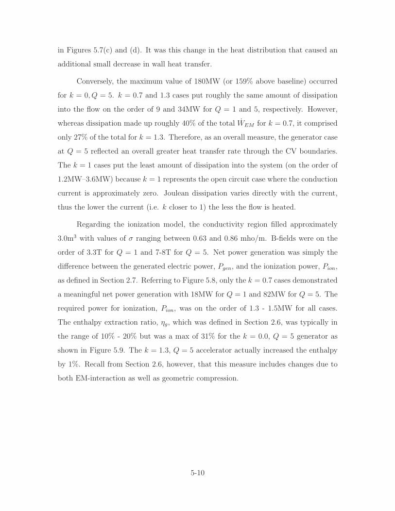
in Figures 5.7(c) and (d). It was this change in the heat distribution that caused an

additional small decrease in wall heat transfer.

Conversely, the maximum value of 180MW (or 159% above baseline) occurred

for k = 0, Q = 5. k = 0.7 and 1.3 cases put roughly the same amount of dissipation

into the flow on the order of 9 and 34MW for Q = 1 and 5, respectively. However,

whereas dissipation made up roughly 40% of the total WEM for k = 0.7, it comprised

only 27% of the total for k = 1.3. Therefore, as an overall measure, the generator case

at Q = 5 reflected an overall greater heat transfer rate through the CV boundaries.

The k = 1 cases put the least amount of dissipation into the system (on the order of

1.2MW–3.6MW) because k = 1 represents the open circuit case where the conduction

current is approximately zero. Joulean dissipation varies directly with the current,

thus the lower the current (i.e. k closer to 1) the less the flow is heated.

Regarding the ionization model, the conductivity region filled approximately

3.0m3 with values of σ ranging between 0.63 and 0.86 mho/m. B-fields were on the

order of 3.3T for Q = 1 and 7-8T for Q = 5. Net power generation was simply the

difference between the generated electric power, Pgen, and the ionization power, Pion,

as defined in Section 2.7. Referring to Figure 5.8, only the k = 0.7 cases demonstrated

a meaningful net power generation with 18MW for Q = 1 and 82MW for Q = 5. The

required power for ionization, Pion, was on the order of 1.3 - 1.5MW for all cases.

The enthalpy extraction ratio, ηg, which was defined in Section 2.6, was typically in

the range of 10% - 20% but was a max of 31% for the k = 0.0, Q = 5 generator as

shown in Figure 5.9. The k = 1.3, Q = 5 accelerator actually increased the enthalpy

by 1%. Recall from Section 2.6, however, that this measure includes changes due to

both EM-interaction as well as geometric compression.

5-10

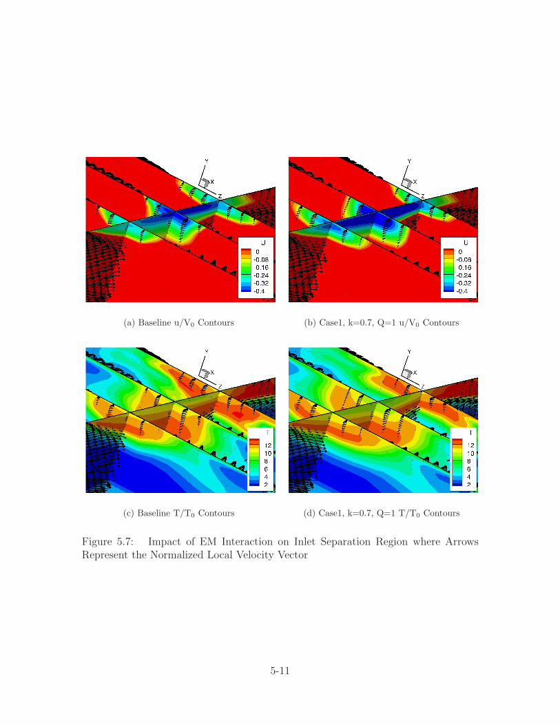
(a) Baseline u/V0 Contours (b) Case1, k=0.7, Q=1 u/V0 Contours

(c) Baseline T/T0 Contours (d) Case1, k=0.7, Q=1 T/T0 Contours

Figure 5.7: Impact of EM Interaction on Inlet Separation Region where ArrowsRepresent the Normalized Local Velocity Vector

5-11

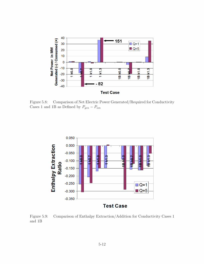
Figure 5.8: Comparison of Net Electric Power Generated/Required for ConductivityCases 1 and 1B as Defined by Pgen − Pion

Figure 5.9: Comparison of Enthalpy Extraction/Addition for Conductivity Cases 1and 1B

5-12

5.2.3 Results from Conductivity Case 1B. This case differed from Case 1

in that the conductivity was limited to the near-wall region of the cowl shoulder.

Case 1B, with a plasma volume of 1.44m3, more accurately simulated an electron

beam ionization source with the maximum conductivity centered several centimeters

from the wall and then falling off rapidly in the direction normal to the wall. As in

Case 1, the addition of EM fields had a small, but noticeable, effect on the outflow

properties, primarily with respect to temperature and pressure increases. However,

the magnitude of these changes was much less than for the same EM interaction

applied to Case 1. For example, the greatest change in exit pressure occurred for

k = 0.7, Q = 5 and amounted to a 6.7% increase above the baseline inlet. This was

to be expected in light of Case 1, as the interaction regions for 1B was only 48% of

Case1. However, forces, heat transfer and EM terms did vary for differing parameters

as applied to Case 1B, as discussed below.

Referring back to Figure 5.4, drag varied from 16% less than baseline for the

Q = 5 accelerator to 68% more than baseline for the k = 0.0, Q = 5 parameters.

Overall, these numbers reflected the same trends seen in Case 1 but typically at

magnitudes of 1/3 to 2/3 of their Case 1 counterparts. As with Case 1, for a given k,

there was an obvious change in drag for increased Q, due to the increasing Lorentz

force. The near-wall conductivity region (being limited to the opposite side of the

flow field away from the cowl lip) was unable to induce any additional mass spillage.

Therefore, there was no contribution to thrust due to bypassed air flow as seen in

Case 1. Regarding heating, all of the EM cases deposited energy into the flow through

dissipation, but typically in less amounts than for Case 1. This was reflected in the

heat transfer rates out of the control volume (Figure 5.6). For Case 1B, the minimum

and maximum Qw was 59MW and 143MW. The same trends as for Case 1 were seen

in that k = 0 by far produced the most Joulean dissipation, k = 1.3 and k = 0.7 were

comparable, and k = 1.0 produced the least amount. It was interesting to note that

at Q = 1 Cases 1 and 1B had very similar values of wall heating for corresponding

k values (with the exception of the k = 0 parameter). This fact demonstrated that

5-13

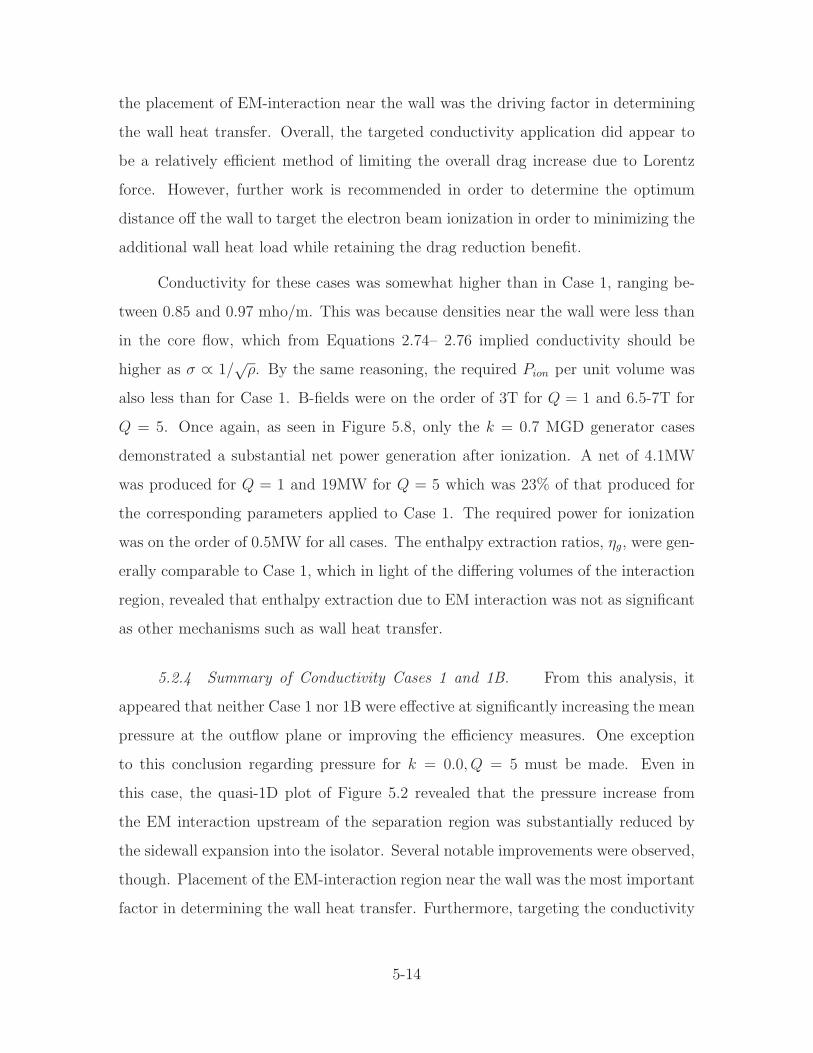
the placement of EM-interaction near the wall was the driving factor in determining

the wall heat transfer. Overall, the targeted conductivity application did appear to

be a relatively efficient method of limiting the overall drag increase due to Lorentz

force. However, further work is recommended in order to determine the optimum

distance off the wall to target the electron beam ionization in order to minimizing the

additional wall heat load while retaining the drag reduction benefit.

Conductivity for these cases was somewhat higher than in Case 1, ranging be-

tween 0.85 and 0.97 mho/m. This was because densities near the wall were less than

in the core flow, which from Equations 2.74– 2.76 implied conductivity should be

higher as σ ∝ 1/√

ρ. By the same reasoning, the required Pion per unit volume was

also less than for Case 1. B-fields were on the order of 3T for Q = 1 and 6.5-7T for

Q = 5. Once again, as seen in Figure 5.8, only the k = 0.7 MGD generator cases

demonstrated a substantial net power generation after ionization. A net of 4.1MW

was produced for Q = 1 and 19MW for Q = 5 which was 23% of that produced for

the corresponding parameters applied to Case 1. The required power for ionization

was on the order of 0.5MW for all cases. The enthalpy extraction ratios, ηg, were gen-

erally comparable to Case 1, which in light of the differing volumes of the interaction

region, revealed that enthalpy extraction due to EM interaction was not as significant

as other mechanisms such as wall heat transfer.

5.2.4 Summary of Conductivity Cases 1 and 1B. From this analysis, it

appeared that neither Case 1 nor 1B were effective at significantly increasing the mean

pressure at the outflow plane or improving the efficiency measures. One exception

to this conclusion regarding pressure for k = 0.0, Q = 5 must be made. Even in

this case, the quasi-1D plot of Figure 5.2 revealed that the pressure increase from

the EM interaction upstream of the separation region was substantially reduced by

the sidewall expansion into the isolator. Several notable improvements were observed,

though. Placement of the EM-interaction region near the wall was the most important

factor in determining the wall heat transfer. Furthermore, targeting the conductivity

5-14

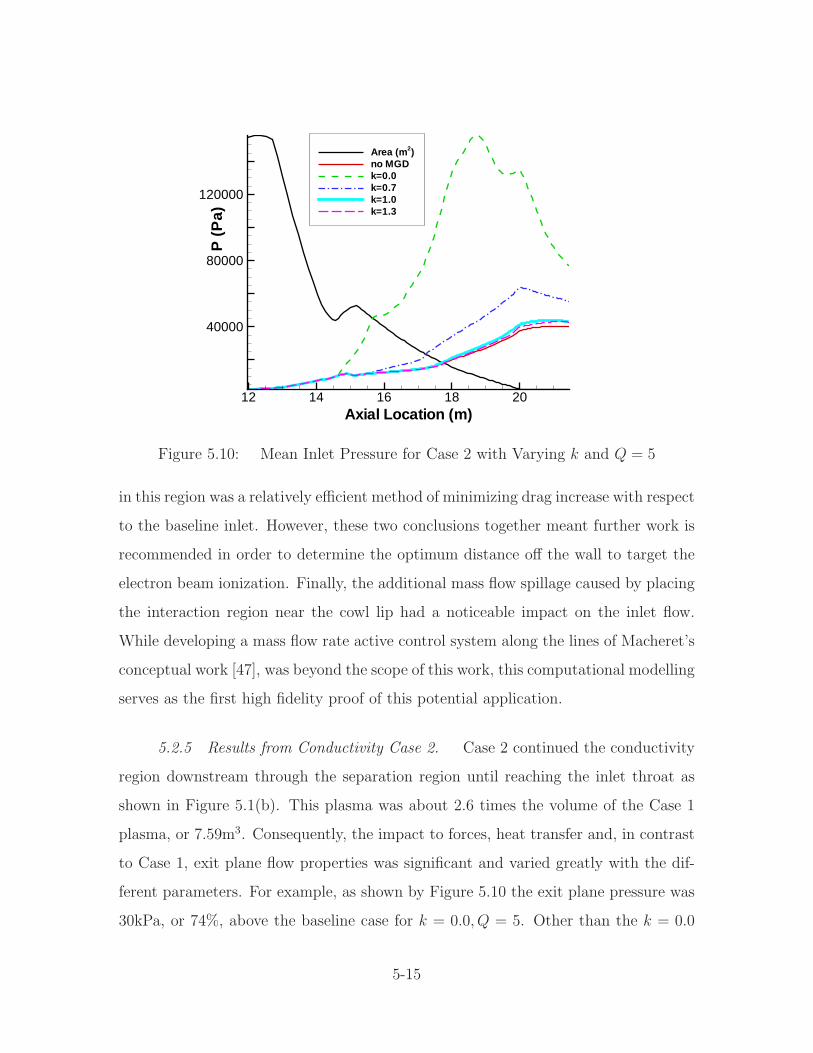
Axial Location (m)

P(P

a)

12 14 16 18 20

40000

80000

120000

Area (m 2)no MGDk=0.0k=0.7k=1.0k=1.3

Figure 5.10: Mean Inlet Pressure for Case 2 with Varying k and Q = 5

in this region was a relatively efficient method of minimizing drag increase with respect

to the baseline inlet. However, these two conclusions together meant further work is

recommended in order to determine the optimum distance off the wall to target the

electron beam ionization. Finally, the additional mass flow spillage caused by placing

the interaction region near the cowl lip had a noticeable impact on the inlet flow.

While developing a mass flow rate active control system along the lines of Macheret’s

conceptual work [47], was beyond the scope of this work, this computational modelling

serves as the first high fidelity proof of this potential application.

5.2.5 Results from Conductivity Case 2. Case 2 continued the conductivity

region downstream through the separation region until reaching the inlet throat as

shown in Figure 5.1(b). This plasma was about 2.6 times the volume of the Case 1

plasma, or 7.59m3. Consequently, the impact to forces, heat transfer and, in contrast

to Case 1, exit plane flow properties was significant and varied greatly with the dif-

ferent parameters. For example, as shown by Figure 5.10 the exit plane pressure was

30kPa, or 74%, above the baseline case for k = 0.0, Q = 5. Other than the k = 0.0

5-15

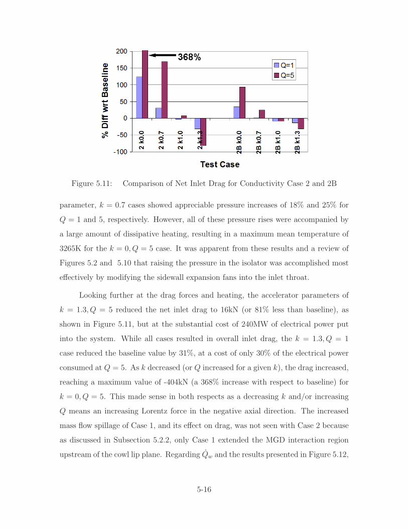
Figure 5.11: Comparison of Net Inlet Drag for Conductivity Case 2 and 2B

parameter, k = 0.7 cases showed appreciable pressure increases of 18% and 25% for

Q = 1 and 5, respectively. However, all of these pressure rises were accompanied by

a large amount of dissipative heating, resulting in a maximum mean temperature of

3265K for the k = 0, Q = 5 case. It was apparent from these results and a review of

Figures 5.2 and 5.10 that raising the pressure in the isolator was accomplished most

effectively by modifying the sidewall expansion fans into the inlet throat.

Looking further at the drag forces and heating, the accelerator parameters of

k = 1.3, Q = 5 reduced the net inlet drag to 16kN (or 81% less than baseline), as

shown in Figure 5.11, but at the substantial cost of 240MW of electrical power put

into the system. While all cases resulted in overall inlet drag, the k = 1.3, Q = 1

case reduced the baseline value by 31%, at a cost of only 30% of the electrical power

consumed at Q = 5. As k decreased (or Q increased for a given k), the drag increased,

reaching a maximum value of -404kN (a 368% increase with respect to baseline) for

k = 0, Q = 5. This made sense in both respects as a decreasing k and/or increasing

Q means an increasing Lorentz force in the negative axial direction. The increased

mass flow spillage of Case 1, and its effect on drag, was not seen with Case 2 because

as discussed in Subsection 5.2.2, only Case 1 extended the MGD interaction region

upstream of the cowl lip plane. Regarding Qw and the results presented in Figure 5.12,

5-16

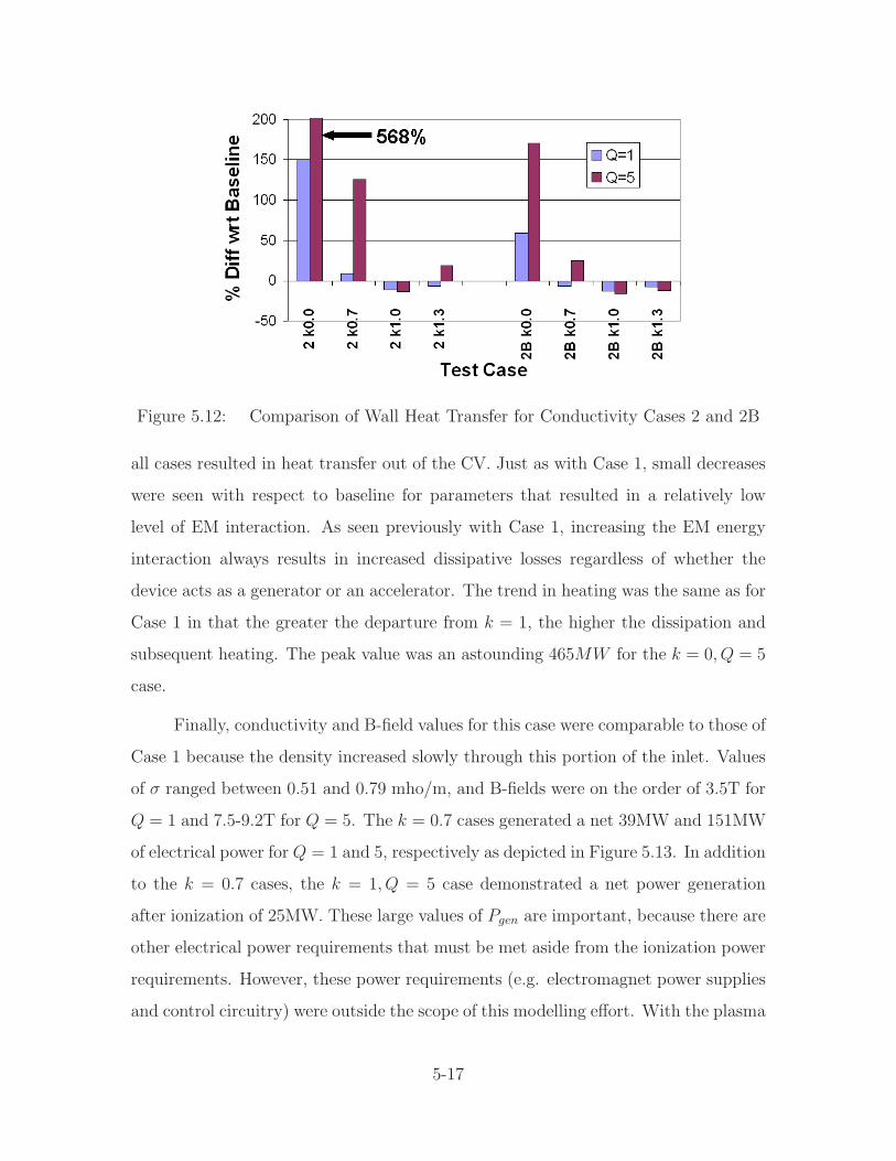
Figure 5.12: Comparison of Wall Heat Transfer for Conductivity Cases 2 and 2B

all cases resulted in heat transfer out of the CV. Just as with Case 1, small decreases

were seen with respect to baseline for parameters that resulted in a relatively low

level of EM interaction. As seen previously with Case 1, increasing the EM energy

interaction always results in increased dissipative losses regardless of whether the

device acts as a generator or an accelerator. The trend in heating was the same as for

Case 1 in that the greater the departure from k = 1, the higher the dissipation and

subsequent heating. The peak value was an astounding 465MW for the k = 0, Q = 5

case.

Finally, conductivity and B-field values for this case were comparable to those of

Case 1 because the density increased slowly through this portion of the inlet. Values

of σ ranged between 0.51 and 0.79 mho/m, and B-fields were on the order of 3.5T for

Q = 1 and 7.5-9.2T for Q = 5. The k = 0.7 cases generated a net 39MW and 151MW

of electrical power for Q = 1 and 5, respectively as depicted in Figure 5.13. In addition

to the k = 0.7 cases, the k = 1, Q = 5 case demonstrated a net power generation

after ionization of 25MW. These large values of Pgen are important, because there are

other electrical power requirements that must be met aside from the ionization power

requirements. However, these power requirements (e.g. electromagnet power supplies

and control circuitry) were outside the scope of this modelling effort. With the plasma

5-17

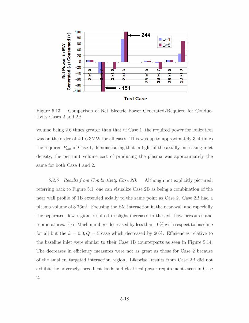
Figure 5.13: Comparison of Net Electric Power Generated/Required for Conduc-tivity Cases 2 and 2B

volume being 2.6 times greater than that of Case 1, the required power for ionization

was on the order of 4.1-6.3MW for all cases. This was up to approximately 3–4 times

the required Pion of Case 1, demonstrating that in light of the axially increasing inlet

density, the per unit volume cost of producing the plasma was approximately the

same for both Case 1 and 2.

5.2.6 Results from Conductivity Case 2B. Although not explicitly pictured,

referring back to Figure 5.1, one can visualize Case 2B as being a combination of the

near wall profile of 1B extended axially to the same point as Case 2. Case 2B had a

plasma volume of 3.76m3. Focusing the EM interaction in the near-wall and especially

the separated-flow region, resulted in slight increases in the exit flow pressures and

temperatures. Exit Mach numbers decreased by less than 10% with respect to baseline

for all but the k = 0.0, Q = 5 case which decreased by 20%. Efficiencies relative to

the baseline inlet were similar to their Case 1B counterparts as seen in Figure 5.14.

The decreases in efficiency measures were not as great as those for Case 2 because

of the smaller, targeted interaction region. Likewise, results from Case 2B did not

exhibit the adversely large heat loads and electrical power requirements seen in Case

2.

5-18

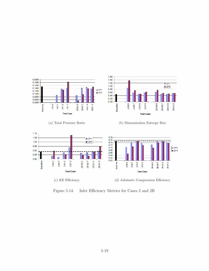
(a) Total Pressure Ratio (b) Dimensionless Entropy Rise

(c) KE Efficiency (d) Adiabatic Compression Efficiency

Figure 5.14: Inlet Efficiency Metrics for Cases 2 and 2B

5-19

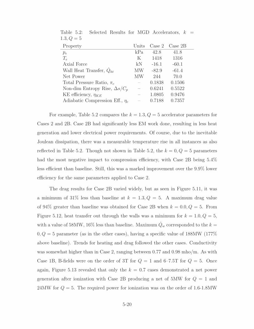
Table 5.2: Selected Results for MGD Accelerators, k =1.3, Q = 5

Property Units Case 2 Case 2Bpe kPa 42.8 41.8Te K 1418 1316Axial Force kN -16.1 -60.1

Wall Heat Transfer, Qht MW -82.9 -61.4Net Power MW 244 70.0Total Pressure Ratio, πc – 0.1838 0.1506Non-dim Entropy Rise, ∆s/Cp – 0.6241 0.5522KE efficiency, ηKE – 1.0805 0.9476Adiabatic Compression Eff., ηc – 0.7188 0.7357

For example, Table 5.2 compares the k = 1.3, Q = 5 accelerator parameters for

Cases 2 and 2B. Case 2B had significantly less EM work done, resulting in less heat

generation and lower electrical power requirements. Of course, due to the inevitable

Joulean dissipation, there was a measurable temperature rise in all instances as also

reflected in Table 5.2. Though not shown in Table 5.2, the k = 0, Q = 5 parameters

had the most negative impact to compression efficiency, with Case 2B being 5.4%

less efficient than baseline. Still, this was a marked improvement over the 9.9% lower

efficiency for the same parameters applied to Case 2.

The drag results for Case 2B varied widely, but as seen in Figure 5.11, it was

a minimum of 31% less than baseline at k = 1.3, Q = 5. A maximum drag value

of 94% greater than baseline was obtained for Case 2B when k = 0.0, Q = 5. From

Figure 5.12, heat transfer out through the walls was a minimum for k = 1.0, Q = 5,

with a value of 58MW, 16% less than baseline. Maximum Qw corresponded to the k =

0, Q = 5 parameter (as in the other cases), having a specific value of 188MW (177%

above baseline). Trends for heating and drag followed the other cases. Conductivity

was somewhat higher than in Case 2, ranging between 0.77 and 0.98 mho/m. As with

Case 1B, B-fields were on the order of 3T for Q = 1 and 6–7.5T for Q = 5. Once

again, Figure 5.13 revealed that only the k = 0.7 cases demonstrated a net power

generation after ionization with Case 2B producing a net of 5MW for Q = 1 and

24MW for Q = 5. The required power for ionization was on the order of 1.6-1.8MW

5-20

for all cases. Referring back to Figure 5.14, the MGD accelerators for Cases 2 and 2B

showed marginal improvement in flow properties as well as significant drag reduction

and increased ηKE. However, these cases also required a very large electrical power

input. This detrimental factor was reduced to a great extent by localizing the plasma

region to the near wall in Case 2B, resulting in an electrical power requirement of 27

and 70MW, for Q = 1 and Q = 5, respectively.

5.3 Summary of Results, Conclusions and Recommendations Regard-

ing Localized EM Flow Control

With respect to the specific application presented here, localized MGD flow

control was marginally successful in mitigating the pressure losses due to the expansion

around the cowl shoulder. The k = 0.0, Q = 5 parameter, in particular, was able to

significantly raise the average inlet pressure. Yet, the penalty in terms of drag and

heating excluded its consideration as a viable solution to the problem. All other

parameters for Cases 1 and 1B were not effective at significantly increasing the mean

pressure at the outflow plane or improving the inlet efficiency. Gains incurred by

these parameters from the EM interaction upstream of the separation region were all

but negated by the sidewall expansion into the isolator at the inlet throat.

Placement of the EM-interaction region near the wall was the most important

factor in determining the wall heat transfer, and targeting the conductivity to this

region did appear to be a relatively efficient method of limiting drag increases. How-

ever, further work is recommended in order to determine the optimum distance off the

wall to target the electron beam ionization. Finally, with respect to Case 1 only, the

additional mass flow spillage caused by placing the interaction region near the cowl

lip had a noticeable impact on the inlet flow. This computational model provided the

first high fidelity verification of the potential of using MGD to modulate the mass

flow rate into the engine.

For the MGD generator cases of k = 0.7, meaningful electrical power generation

was achieved. Although it only slightly increased the flow pressure going into the

5-21

isolator, MGD acceleration, particularly for Case 2B, was able to efficiently reduce

the net inlet drag. It did this while minimizing the increase in heat transfer and

decrease in overall efficiency measures. This was due primarily to increasing the

flow momentum as it passed through the sidewall expansion into the inlet throat.

Therefore, it was concluded the use of an MGD accelerator to locally increase flow

momentum was an effective approach to improve flow into the isolator of this scramjet

model. Further, if the Pion requirement is of prime consideration, limiting the ionized

flow to the near-wall region is an acceptable compromise.

5-22

VI. Application of MGD Energy Bypass to Flowpath

6.1 Introduction

A significant discussion in Chapters I and II, and in particular Section 1.2, ex-

plained the theory behind MGD power generation systems and the energy by-

pass concept. The reader is referred back to these parts of the document for details.

In summary, the MGD energy bypass method is a concept for both producing vehi-

cle electrical power and improving the scramjet’s performance. Theoretically, it does

this by efficiently removing a portion of the inlet’s high stagnation enthalpy, convert-

ing it to electrical power, and returning it directly to the expansion system. In this

way, the inlet compression is accomplished more efficiently than by the shock train

alone. Therefore, the combustor can impart more energy into the flow before running

into stagnation temperature limits. This application has been well documented in

References [10,21,34–36,43,54,60].

The research documented in this chapter tested this application to a level of

computational fidelity never before attempted. The next section documents the re-

sults for MGD power generation in this engine by first examining the traditional

configuration wherein the MGD generator is placed upstream of the combustor. In

addition, the concept of combustor-based MGD power generation was explored. This

concept, widely pursued in the 1960’s in the context of commercial electrical power

generation [70], has recently reappeared as a promising concept for scramjet engines

as proposed by Macheret, et al [50, 73, 74], among others. The isolator-based gener-

ator with the highest electrical power generation was selected for the MGD energy

bypass system and several different accelerators were analyzed as described in Sec-

tion 6.3. Finally, both of these sections are summarized and several conclusions and

recommendations specific to this chapter are presented.

6-1

6.2 MGD Power Generation

6.2.1 The Conventional Bypass Approach: MGD Power Generation Upstream

of the Combustor. Two approaches were taken to characterize the performance

of isolator-based MGD power generation in this engine. The first approach was a

parameter based study similar to that of Chapter V’s localized flow control. This

approach, which specified the electric field, was done in order to test a wide range of

conductivity profiles and load factors (k) at a single interaction parameter (Q = 1).

The second approach applied higher fidelity to select cases by specifying electrode

locations and their electric potential and solving for the resulting electric field and

conduction current as described in Section 2.1. In addition to Q = 1, the second

approach tested the higher magnetic field strengths associated with Q = 5. Among

other results, it will be shown that electrode placement was critical to successful power

generation, and that there was a large difference in performance depending on the

load factor, k, and interaction parameter, Q, used.

Numerous runs of the isolator-based MGD generator were performed. Most

of these runs specified the electric field. Runs were first delineated by how far the

conductivity region extended downstream from the inlet throat as a percentage of

the isolator length. Three lengths were tested, 20%, 60% and 100%, as shown in

Figures 6.1(a)–(c). As in Chapter V, both a full cross-section profile, referred to here

as Case 1E, and a near-wall profile, referred to as Case 2E (e.g. Figure 6.1(d)), were

compared. For each conductivity profile, load factors of 0.6, 0.7, and 0.8 were tested.

Additional runs were made where the electrode location and electric potential was

specified. Since the best results for the specified electric field runs occurred at full

isolator length, each electrode run evenly spaced four electrodes along this length as

seen in Figure 6.2. Half of the runs placed the electrodes on the +/- Z-faces (referred

to as ‘K-elec’ runs), while the remaining runs placed the electrodes on the +/- Y-faces

(‘J-elec’). As with the first approach, k = 0.6, 0.7, and 0.8 were examined, but this

time at both Q = 1 and 5. As a final note regarding the problem setup, the baseline

inlet without MGD characterized in Subsection 4.4.1 and used in Chapter V was again

6-2

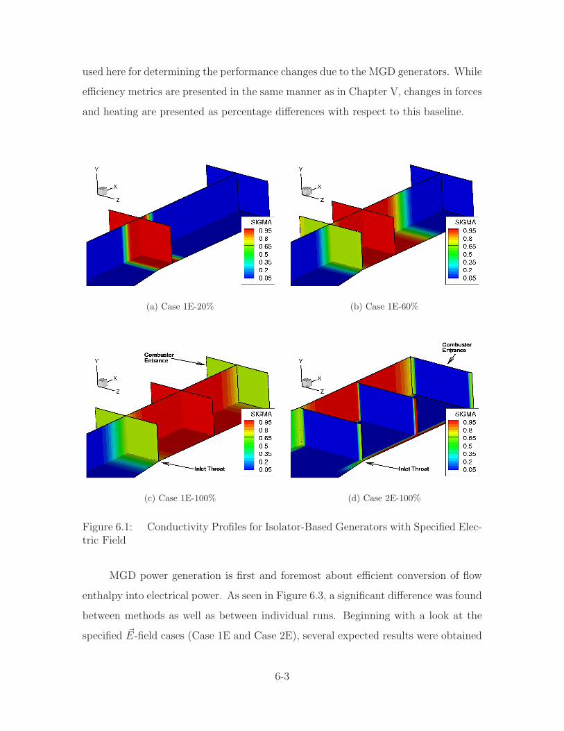
used here for determining the performance changes due to the MGD generators. While

efficiency metrics are presented in the same manner as in Chapter V, changes in forces

and heating are presented as percentage differences with respect to this baseline.

(a) Case 1E-20% (b) Case 1E-60%

(c) Case 1E-100% (d) Case 2E-100%

Figure 6.1: Conductivity Profiles for Isolator-Based Generators with Specified Elec-tric Field

MGD power generation is first and foremost about efficient conversion of flow

enthalpy into electrical power. As seen in Figure 6.3, a significant difference was found

between methods as well as between individual runs. Beginning with a look at the

specified ~E-field cases (Case 1E and Case 2E), several expected results were obtained

6-3

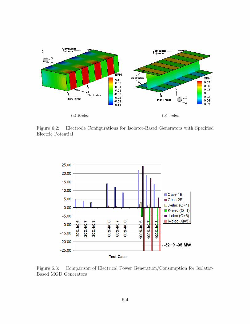
(a) K-elec (b) J-elec

Figure 6.2: Electrode Configurations for Isolator-Based Generators with SpecifiedElectric Potential

Figure 6.3: Comparison of Electrical Power Generation/Consumption for Isolator-Based MGD Generators

6-4

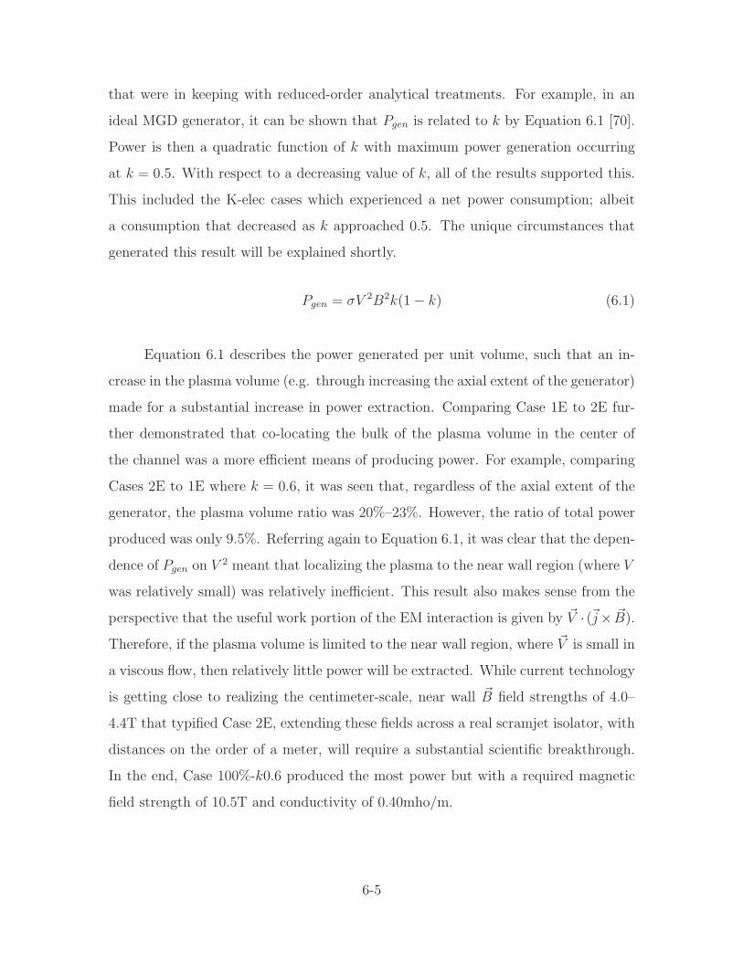
that were in keeping with reduced-order analytical treatments. For example, in an

ideal MGD generator, it can be shown that Pgen is related to k by Equation 6.1 [70].

Power is then a quadratic function of k with maximum power generation occurring

at k = 0.5. With respect to a decreasing value of k, all of the results supported this.

This included the K-elec cases which experienced a net power consumption; albeit

a consumption that decreased as k approached 0.5. The unique circumstances that

generated this result will be explained shortly.

Pgen = σV 2B2k(1 − k) (6.1)

Equation 6.1 describes the power generated per unit volume, such that an in-

crease in the plasma volume (e.g. through increasing the axial extent of the generator)

made for a substantial increase in power extraction. Comparing Case 1E to 2E fur-

ther demonstrated that co-locating the bulk of the plasma volume in the center of

the channel was a more efficient means of producing power. For example, comparing

Cases 2E to 1E where k = 0.6, it was seen that, regardless of the axial extent of the

generator, the plasma volume ratio was 20%–23%. However, the ratio of total power

produced was only 9.5%. Referring again to Equation 6.1, it was clear that the depen-

dence of Pgen on V 2 meant that localizing the plasma to the near wall region (where V

was relatively small) was relatively inefficient. This result also makes sense from the

perspective that the useful work portion of the EM interaction is given by ~V · (~j× ~B).

Therefore, if the plasma volume is limited to the near wall region, where ~V is small in

a viscous flow, then relatively little power will be extracted. While current technology

is getting close to realizing the centimeter-scale, near wall ~B field strengths of 4.0–

4.4T that typified Case 2E, extending these fields across a real scramjet isolator, with

distances on the order of a meter, will require a substantial scientific breakthrough.

In the end, Case 100%-k0.6 produced the most power but with a required magnetic

field strength of 10.5T and conductivity of 0.40mho/m.

6-5

In every respect, the specified ~E-field cases behaved as theory would suggest,

but at first glance the same could not be said in all regards for the electrode-based

cases. As the applied ~B-field grew (i.e. Q increasing), the EM-interaction increased

roughly as | ~B|2, which was expected. For the J-elec cases, increasing Q from 1 to 5

increased the total Pgen by factors from 3–4.5 as k decreased from 0.8 to 0.6. For the

K-elec cases, the net power consumption was increased by factors from 7–12 as the

nominal load factor decreased from 0.8 to 0.6. As was seen in Figure 6.3 and further

quantified here, the net EM-interaction was opposite between the J-elec case which

generated electricity and the K-elec case which required additional electricity from an

external source. This result was unexpected as only two changes were made between

the two configurations. First, the electrodes were placed on different walls and the

~B field was realigned accordingly (+By for K-elec and -Bz for J-elec, respectively).

Second, a higher electrode potential was used for the K-elec configuration to maintain

the same nominal k in spite of the greater distance between the cathode and anode

of each electrode pair.

Analysis uncovered the cause for the significantly different performance. For

every J-elec run, greater than 50% of the total EM-interaction took the form of work

done by Lorentz Forces on the fluid. The opposite was true for all of the K-elec runs,

where dissipation accounted for over half of the total interaction. In fact, for the

K-elec case of k = 0.8 and Q = 5, dissipation was 63% of the total interaction, or

1.8 times the corresponding J-elec case. Recall from Subsection 2.4, the EM energy

interaction, ~E ·~j, consists of the sum of the Joulean dissipation and the rate at which

the Lorentz Force does work on the gas as shown again here in Equation 6.2.

~E ·~j =∣

∣j∣

∣

2/σ + ~V · (~j × ~B) (6.2)

Furthermore, positive values of ~E ·~j, such as occurred with the K-elec configuration

mean the external circuit is supplying electricity to the gas, as occurs in an MGD

accelerator. However, in an accelerator, the ~V · (~j × ~B) work term would be positive

6-6

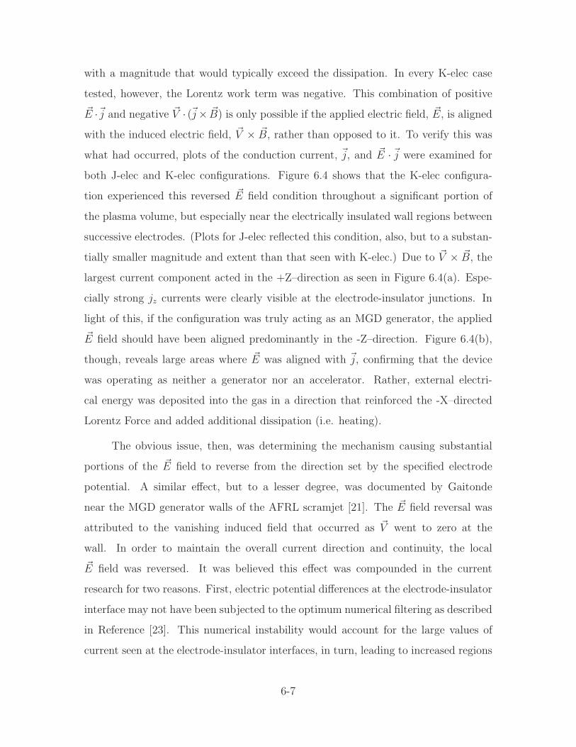
with a magnitude that would typically exceed the dissipation. In every K-elec case

tested, however, the Lorentz work term was negative. This combination of positive

~E ·~j and negative ~V · (~j× ~B) is only possible if the applied electric field, ~E, is aligned

with the induced electric field, ~V × ~B, rather than opposed to it. To verify this was

what had occurred, plots of the conduction current, ~j, and ~E · ~j were examined for

both J-elec and K-elec configurations. Figure 6.4 shows that the K-elec configura-

tion experienced this reversed ~E field condition throughout a significant portion of

the plasma volume, but especially near the electrically insulated wall regions between

successive electrodes. (Plots for J-elec reflected this condition, also, but to a substan-

tially smaller magnitude and extent than that seen with K-elec.) Due to ~V × ~B, the

largest current component acted in the +Z–direction as seen in Figure 6.4(a). Espe-

cially strong jz currents were clearly visible at the electrode-insulator junctions. In

light of this, if the configuration was truly acting as an MGD generator, the applied

~E field should have been aligned predominantly in the -Z–direction. Figure 6.4(b),

though, reveals large areas where ~E was aligned with ~j, confirming that the device

was operating as neither a generator nor an accelerator. Rather, external electri-

cal energy was deposited into the gas in a direction that reinforced the -X–directed

Lorentz Force and added additional dissipation (i.e. heating).

The obvious issue, then, was determining the mechanism causing substantial

portions of the ~E field to reverse from the direction set by the specified electrode

potential. A similar effect, but to a lesser degree, was documented by Gaitonde

near the MGD generator walls of the AFRL scramjet [21]. The ~E field reversal was

attributed to the vanishing induced field that occurred as ~V went to zero at the

wall. In order to maintain the overall current direction and continuity, the local

~E field was reversed. It was believed this effect was compounded in the current

research for two reasons. First, electric potential differences at the electrode-insulator

interface may not have been subjected to the optimum numerical filtering as described

in Reference [23]. This numerical instability would account for the large values of

current seen at the electrode-insulator interfaces, in turn, leading to increased regions

6-7

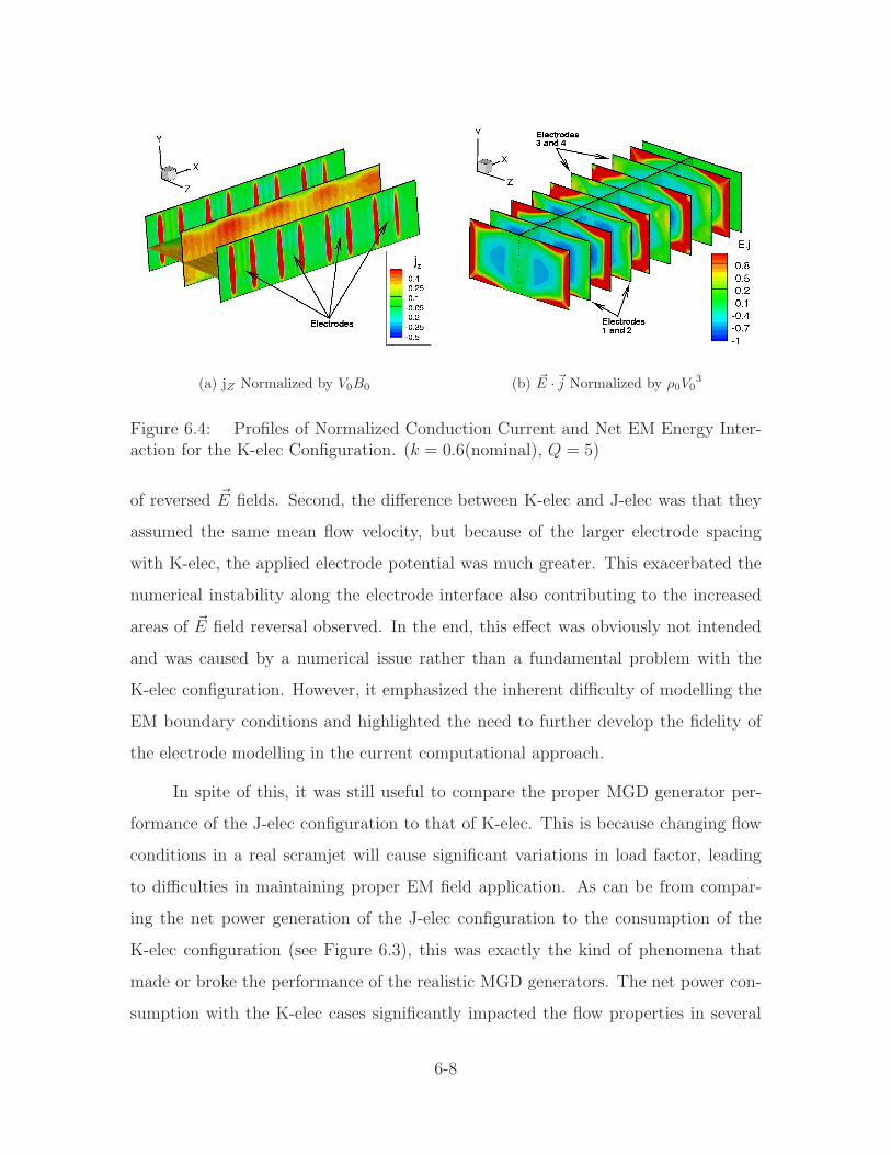
(a) jZ Normalized by V0B0 (b) ~E ·~j Normalized by ρ0V03

Figure 6.4: Profiles of Normalized Conduction Current and Net EM Energy Inter-action for the K-elec Configuration. (k = 0.6(nominal), Q = 5)

of reversed ~E fields. Second, the difference between K-elec and J-elec was that they

assumed the same mean flow velocity, but because of the larger electrode spacing

with K-elec, the applied electrode potential was much greater. This exacerbated the

numerical instability along the electrode interface also contributing to the increased

areas of ~E field reversal observed. In the end, this effect was obviously not intended

and was caused by a numerical issue rather than a fundamental problem with the

K-elec configuration. However, it emphasized the inherent difficulty of modelling the

EM boundary conditions and highlighted the need to further develop the fidelity of

the electrode modelling in the current computational approach.

In spite of this, it was still useful to compare the proper MGD generator per-

formance of the J-elec configuration to that of K-elec. This is because changing flow

conditions in a real scramjet will cause significant variations in load factor, leading

to difficulties in maintaining proper EM field application. As can be from compar-

ing the net power generation of the J-elec configuration to the consumption of the

K-elec configuration (see Figure 6.3), this was exactly the kind of phenomena that

made or broke the performance of the realistic MGD generators. The net power con-

sumption with the K-elec cases significantly impacted the flow properties in several

6-8

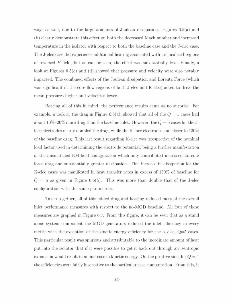
ways as well, due to the large amounts of Joulean dissipation. Figures 6.5(a) and

(b) clearly demonstrate this effect on both the decreased Mach number and increased

temperature in the isolator with respect to both the baseline case and the J-elec case.

The J-elec case did experience additional heating associated with its localized regions

of reversed ~E field, but as can be seen, the effect was substantially less. Finally, a

look at Figures 6.5(c) and (d) showed that pressure and velocity were also notably

impacted. The combined effects of the Joulean dissipation and Lorentz Force (which

was significant in the core flow regions of both J-elec and K-elec) acted to drive the

mean pressures higher and velocities lower.

Bearing all of this in mind, the performance results came as no surprise. For

example, a look at the drag in Figure 6.6(a), showed that all of the Q = 1 cases had

about 10%–20% more drag than the baseline inlet. However, the Q = 5 cases for the J-

face electrodes nearly doubled the drag, while the K-face electrodes had closer to 130%

of the baseline drag. This last result regarding K-elec was irrespective of the nominal

load factor used in determining the electrode potential; being a further manifestation

of the mismatched EM field configuration which only contributed increased Lorentz

force drag and substantially greater dissipation. This increase in dissipation for the

K-elec cases was manifested in heat transfer rates in excess of 130% of baseline for

Q = 5 as given in Figure 6.6(b). This was more than double that of the J-elec

configuration with the same parameters.

Taken together, all of this added drag and heating reduced most of the overall

inlet performance measures with respect to the no-MGD baseline. All four of these

measures are graphed in Figure 6.7. From this figure, it can be seen that as a stand

alone system component the MGD generators reduced the inlet efficiency in every

metric with the exception of the kinetic energy efficiency for the K-elec, Q=5 cases.

This particular result was spurious and attributable to the inordinate amount of heat

put into the isolator that if it were possible to get it back out through an isentropic

expansion would result in an increase in kinetic energy. On the positive side, for Q = 1

the efficiencies were fairly insensitive to the particular case configuration. From this, it

6-9

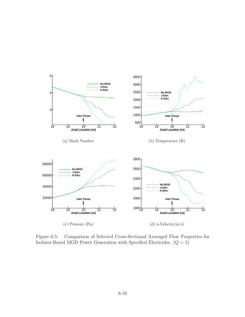
Axial Location (m)18 19 20 21 22

3

4

5

No MGDJ-ElecK-Elec

Inlet Throat

(a) Mach Number

Axial Location (m)18 19 20 21 22

500

1000

1500

2000

2500

3000

3500

No MGDJ-ElecK-Elec

Inlet Throat

(b) Temperature (K)

Axial Location (m)18 19 20 21 22

20000

40000

60000

80000

No MGDJ-ElecK-Elec

Inlet Throat

(c) Pressure (Pa)

Axial Location (m)18 19 20 21 221800

2000

2200

2400

2600

2800

No MGDJ-ElecK-Elec

Inlet Throat

(d) u-Velocity(m/s)

Figure 6.5: Comparison of Selected Cross-Sectional Averaged Flow Properties forIsolator-Based MGD Power Generation with Specified Electrodes. (Q = 5)

6-10

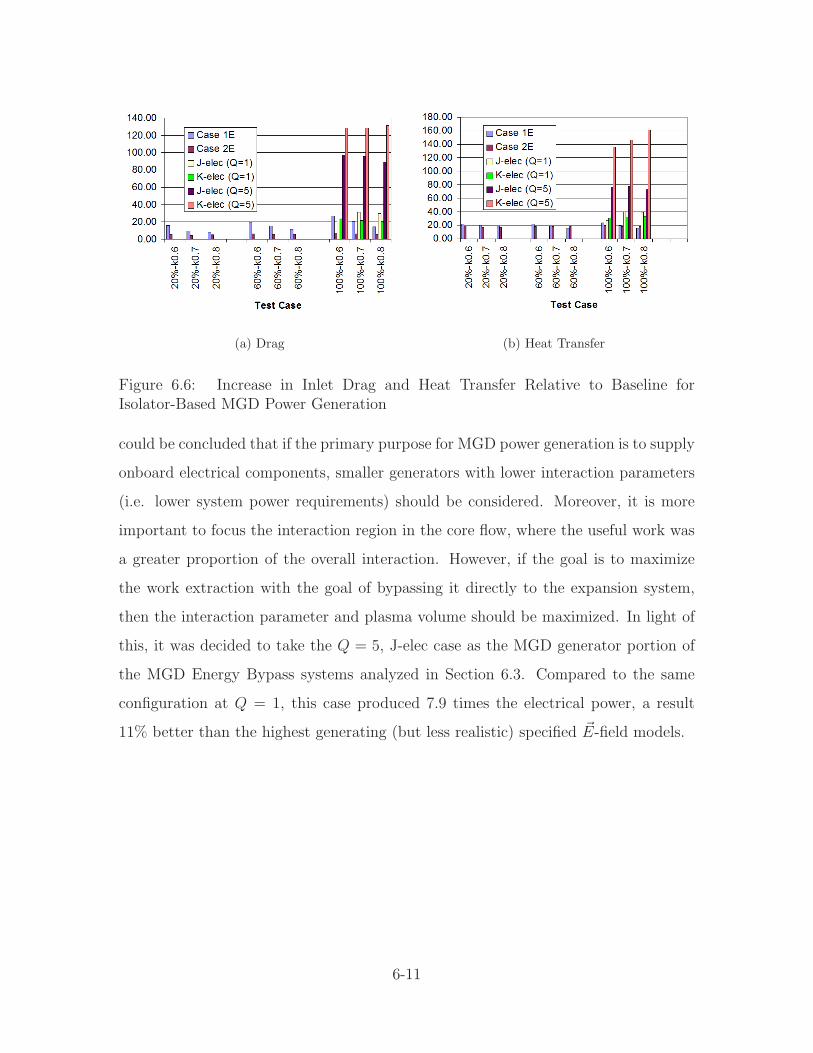
(a) Drag (b) Heat Transfer

Figure 6.6: Increase in Inlet Drag and Heat Transfer Relative to Baseline forIsolator-Based MGD Power Generation

could be concluded that if the primary purpose for MGD power generation is to supply

onboard electrical components, smaller generators with lower interaction parameters

(i.e. lower system power requirements) should be considered. Moreover, it is more

important to focus the interaction region in the core flow, where the useful work was

a greater proportion of the overall interaction. However, if the goal is to maximize

the work extraction with the goal of bypassing it directly to the expansion system,

then the interaction parameter and plasma volume should be maximized. In light of

this, it was decided to take the Q = 5, J-elec case as the MGD generator portion of

the MGD Energy Bypass systems analyzed in Section 6.3. Compared to the same

configuration at Q = 1, this case produced 7.9 times the electrical power, a result

11% better than the highest generating (but less realistic) specified ~E-field models.

6-11

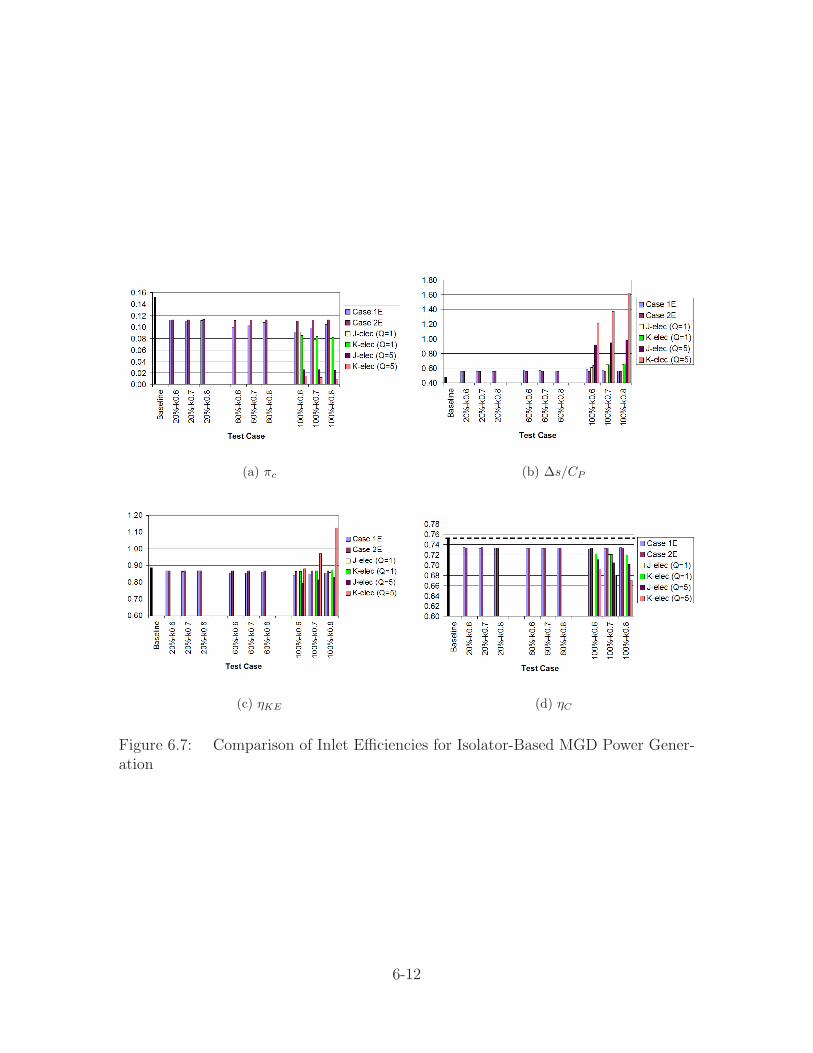
(a) πc (b) ∆s/CP

(c) ηKE (d) ηC

Figure 6.7: Comparison of Inlet Efficiencies for Isolator-Based MGD Power Gener-ation

6-12

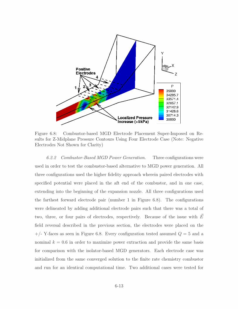
Figure 6.8: Combustor-based MGD Electrode Placement Super-Imposed on Re-sults for Z-Midplane Pressure Contours Using Four Electrode Case (Note: NegativeElectrodes Not Shown for Clarity)

6.2.2 Combustor-Based MGD Power Generation. Three configurations were

used in order to test the combustor-based alternative to MGD power generation. All

three configurations used the higher fidelity approach wherein paired electrodes with

specified potential were placed in the aft end of the combustor, and in one case,

extending into the beginning of the expansion nozzle. All three configurations used

the farthest forward electrode pair (number 1 in Figure 6.8). The configurations

were delineated by adding additional electrode pairs such that there was a total of

two, three, or four pairs of electrodes, respectively. Because of the issue with ~E

field reversal described in the previous section, the electrodes were placed on the

+/- Y-faces as seen in Figure 6.8. Every configuration tested assumed Q = 5 and a

nominal k = 0.6 in order to maximize power extraction and provide the same basis

for comparison with the isolator-based MGD generators. Each electrode case was

initialized from the same converged solution to the finite rate chemistry combustor

and run for an identical computational time. Two additional cases were tested for

6-13

comparison purposes. The baseline configuration provided the scramjet performance

without any MGD flow control, combining the baseline inlet with the finite rate

chemistry combustor. Finally, a case (referred to as Isogen) was run using the isolator-

based, J-Elec MGD Generator at k = 0.6 and Q = 5 and the finite rate chemistry

modelled combustor. Its purpose was to provide a basis for determining the relative

merit of the combustor-based MGD generators.

As expected, the addition of each electrode pair increasingly impacted the com-

bustor flow field properties as shown by Figures 6.9(a)–(d). Taken as a whole, the

figure shows that the localized effects caused by subsequent electrode pairs added

to the effects due to upstream electrodes creating a cumulative effect on flow prop-

erties. This cumulative effect was not simply additive, however. Without a doubt,

the single biggest effect was caused by the first electrode pair (EP1). For example,

EP1 decreased the average cross-sectional Mach number by 11% to 2.90, but going

from EP1 to EP4 only caused an additional 6.9% decline. This effect was visible in

the remaining line plots as well, and the cause was clearly evident in the centerline

pressure contours of Figure 6.8. In the forward portion of this figure, a decreasing

pressure gradient is seen at the trailing end of the combustion reaction zone. This

phenomena was discussed in detail in Section 4.4.2, and referring to the baseline case

in Figures 6.9(c), it was seen the pressure continued to decrease all the way through

the end of the domain. However, the addition of the MGD generator in this loca-

tion caused localized pressure increases in the vicinity of the electrodes, where the

conduction current, and therefore, the Lorentz Force was greatest. In fact, the pres-

sure increases coinciding with EP1 and EP2, began to take on the sharply defined

appearance of a small shock wave.

Regarding the performance of the combustor-based generators, electrical power

generation, axial force, heat transfer, and total pressure ratio were compared to each

other as well as the baseline and isolator-based generator cases. To begin, electrical

power generation was examined. It was apparent from the results presented in Fig-

ure 6.10 that the combustor-based generation was superior in this regard. Foremost,

6-14

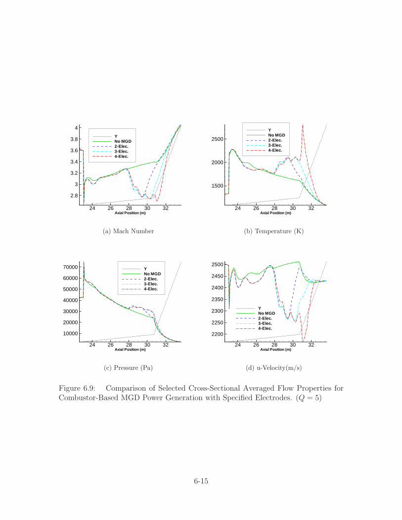
Axial Position (m)24 26 28 30 32

2.8

3

3.2

3.4

3.6

3.8

4

YNo MGD2-Elec.3-Elec.4-Elec.

(a) Mach Number

Axial Position (m)24 26 28 30 32

1500

2000

2500

YNo MGD2-Elec.3-Elec.4-Elec.

(b) Temperature (K)

Axial Position (m)24 26 28 30 32

10000

20000

30000

40000

50000

60000

70000 YNo MGD2-Elec.3-Elec.4-Elec.

(c) Pressure (Pa)

Axial Position (m)24 26 28 30 32

2200

2250

2300

2350

2400

2450

2500

YNo MGD2-Elec.3-Elec.4-Elec.

(d) u-Velocity(m/s)

Figure 6.9: Comparison of Selected Cross-Sectional Averaged Flow Properties forCombustor-Based MGD Power Generation with Specified Electrodes. (Q = 5)

6-15

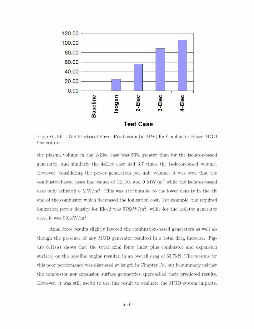
Figure 6.10: Net Electrical Power Production (in MW) for Combustor-Based MGDGenerators

the plasma volume in the 2-Elec case was 56% greater than for the isolator-based

generator, and similarly the 4-Elec case had 3.7 times the isolator-based volume.

However, considering the power generation per unit volume, it was seen that the

combustor-based cases had values of 12, 10, and 9 MW/m3 while the isolator-based

case only achieved 8 MW/m3. This was attributable to the lower density in the aft

end of the combustor which decreased the ionization cost. For example, the required

ionization power density for Elec2 was 578kW/m3, while for the isolator generator

case, it was 991kW/m3.

Axial force results slightly favored the combustion-based generators as well al-

though the presence of any MGD generator resulted in a total drag increase. Fig-

ure 6.11(a) shows that the total axial force (inlet plus combustor and expansion

surface) on the baseline engine resulted in an overall drag of 63.7kN. The reasons for

this poor performance was discussed at length in Chapter IV, but in summary neither

the combustor nor expansion surface geometries approached their predicted results.

However, it was still useful to use this result to evaluate the MGD system impacts.

6-16

In this regard, it was seen that the net effect of the isolator-based generator was

an overall drag increase of 33% to 84.6kN. The aft generators performed marginally

better in this regard with total drag ranging from 80.0kN – 80.8kN. Heat transfer,

however, favored the isolator-based generator, with the exception of the 2-Elec case.

As seen in Figure 6.11(b), the heat transfer for both of these cases was 44% above

the baseline combustor value. However, in the case of the isolator-based generator

this was an added heat load above that already incurred in the isolator. As expected,

the remaining combustor-based cases increased their heat transfer into the gas as the

number of elctrodes and the volume of the interaction region increased. Finally, a

look at total pressure ratio again favored the combustor-based generators. It should

be noted, that the ratio for the overall engine was taken as the product of the inlet

and combustor ratios. Figure 6.11(c) showed that the overall efficiency with respect to

this metric was low for all cases, with a value of 1.3% for the isolator-based generator

and 1.8% for both the baseline and combustor-based generator engines. In light of

this, the combustor-based generators were felt to be slightly more efficient.

6-17

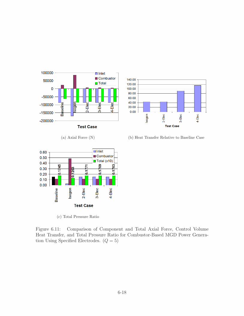
(a) Axial Force (N) (b) Heat Transfer Relative to Baseline Case

(c) Total Pressure Ratio

Figure 6.11: Comparison of Component and Total Axial Force, Control VolumeHeat Transfer, and Total Pressure Ratio for Combustor-Based MGD Power Genera-tion Using Specified Electrodes. (Q = 5)

6-18

6.3 MGD Flow Acceleration and Energy Bypass

Numerous cases were run with nominal load factors, k, greater than one in an

attempt to characterize the effectiveness of MGD acceleration in the aft end of the

combustor and obtain a self-powered MGD bypass system. In addition, for every

load factor tested interaction parameters, Q, of 1 and 5 were also tested to examine

the impact of increasing the ~B field. The specified electrode method was used for all

cases using the same configuration as the two and four electrode pair cases from the

combustor-based generation runs (refer to geometry in Figure 6.8).

Although all of the cases used a specified electrode potential based on k > 1

and a mean value of the local velocity, it was found that values of k = 1.1 and k = 1.3

actually acted in a generator fashion. Referring back to the discussion of Subsec-

tion 6.2.1, what happened in these cases was that the specified potential produced an

E-field that, in large areas of the interaction region, had a smaller magnitude than

~V × ~B. In other words, the Lorentz force was acting in the -X direction and net

work was being extracted from the flow, consistent with an MGD generator. Of all

the cases tested, only those with k = 2.0 established a strong enough electric field to

cause a net Lorentz force in the +X direction and deposit positive work into the flow.

Because of this, only these latter cases were subjected to the complete performance

analysis presented here.

Even more so than with the combustor-based MGD generators, it was helpful

to look at how the accelerators affected the flow properties. In fact, as seen in the

temperature profiles of Figure 6.12(a), the primary effect of all the MGD accelerators

was made clearly evident. In all instances, the accelerators increased the static tem-

perature in the interaction region as would be expected. Even at Q = 1, the effect

was significant with the peak temperature change relative to baseline being 120K and

250K for the 2-Elec and 4-Elec cases, respectively. However, at Q = 5 the heating

was extreme with peak differences of 800K and 1370K respectively. This last result

was 50% greater than the same effect produced by the upstream generator and 65%

6-19

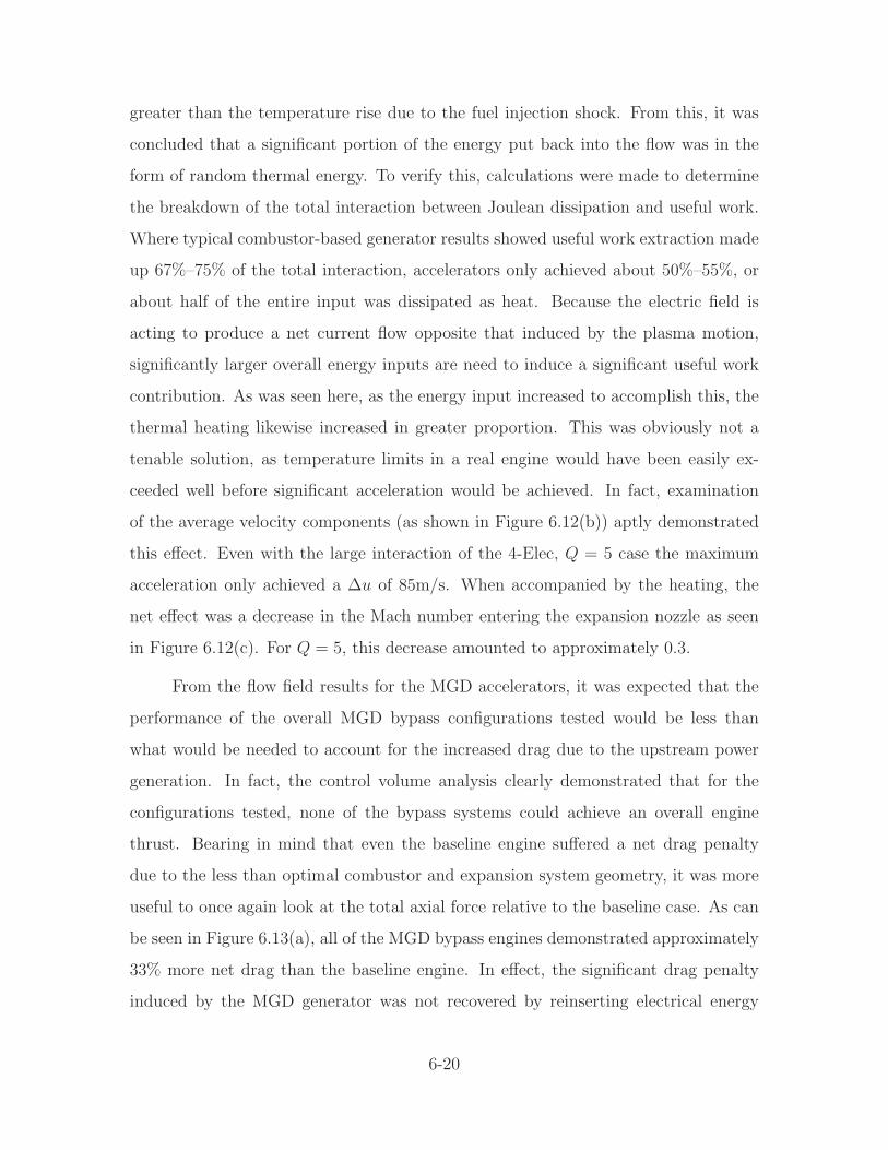
greater than the temperature rise due to the fuel injection shock. From this, it was

concluded that a significant portion of the energy put back into the flow was in the

form of random thermal energy. To verify this, calculations were made to determine

the breakdown of the total interaction between Joulean dissipation and useful work.

Where typical combustor-based generator results showed useful work extraction made

up 67%–75% of the total interaction, accelerators only achieved about 50%–55%, or

about half of the entire input was dissipated as heat. Because the electric field is

acting to produce a net current flow opposite that induced by the plasma motion,

significantly larger overall energy inputs are need to induce a significant useful work

contribution. As was seen here, as the energy input increased to accomplish this, the

thermal heating likewise increased in greater proportion. This was obviously not a

tenable solution, as temperature limits in a real engine would have been easily ex-

ceeded well before significant acceleration would be achieved. In fact, examination

of the average velocity components (as shown in Figure 6.12(b)) aptly demonstrated

this effect. Even with the large interaction of the 4-Elec, Q = 5 case the maximum

acceleration only achieved a ∆u of 85m/s. When accompanied by the heating, the

net effect was a decrease in the Mach number entering the expansion nozzle as seen

in Figure 6.12(c). For Q = 5, this decrease amounted to approximately 0.3.

From the flow field results for the MGD accelerators, it was expected that the

performance of the overall MGD bypass configurations tested would be less than

what would be needed to account for the increased drag due to the upstream power

generation. In fact, the control volume analysis clearly demonstrated that for the

configurations tested, none of the bypass systems could achieve an overall engine

thrust. Bearing in mind that even the baseline engine suffered a net drag penalty

due to the less than optimal combustor and expansion system geometry, it was more

useful to once again look at the total axial force relative to the baseline case. As can

be seen in Figure 6.13(a), all of the MGD bypass engines demonstrated approximately

33% more net drag than the baseline engine. In effect, the significant drag penalty

induced by the MGD generator was not recovered by reinserting electrical energy

6-20

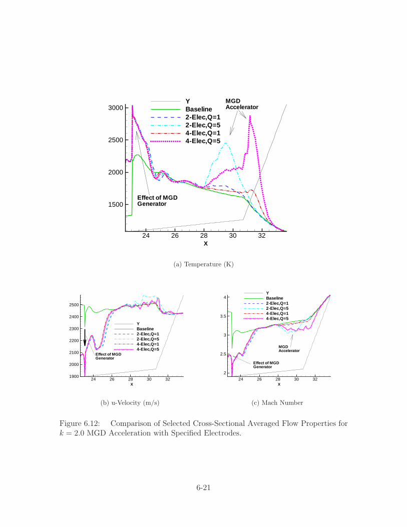
X24 26 28 30 32

1500

2000

2500

3000YBaseline2-Elec,Q=12-Elec,Q=54-Elec,Q=14-Elec,Q=5

MGDAccelerator

Effect of MGDGenerator

(a) Temperature (K)

X24 26 28 30 32

1900

2000

2100

2200

2300

2400

2500

YBaseline2-Elec,Q=12-Elec,Q=54-Elec,Q=14-Elec,Q=5

Effect of MGDGenerator

(b) u-Velocity (m/s)

X24 26 28 30 32

2

2.5

3

3.5

4YBaseline2-Elec,Q=12-Elec,Q=54-Elec,Q=14-Elec,Q=5

MGDAccelerator

Effect of MGDGenerator

(c) Mach Number

Figure 6.12: Comparison of Selected Cross-Sectional Averaged Flow Properties fork = 2.0 MGD Acceleration with Specified Electrodes.

6-21

into the flow. To make matters worse, because the MGD accelerators performed so

inefficiently with respect to producing useful work, substantially more energy had to

be put into the flow than had been taken out of the generator to produce the results

seen. From Figure 6.13(b), it was seen that none of the MGD bypass systems as a

whole had a net margin of positive electrical power production. Even the relatively

minor interactions from the Q = 1 accelerators produced system-level power deficits

of 8MW–10MW, which were insignificant compared to the 150MW-class deficits of

the Q = 5 systems.

In light of these results, it was easy to conclude that for the configurations tested,

MGD acceleration was ineffective for improving the performance of this scramjet.

Furthermore, when taken as an overall system, the energy bypass concept was unable

under any circumstance to be self-powered. While these conclusions must be kept in

the context of the segmented Faraday electrodes tested, it is felt that the physics of

MGD flow acceleration will in most configurations result in a disproportionate amount

of electrical energy being required to produce useful flow work and acceleration. In

addition, this work will always be accompanied by a significantly greater fraction of

the total energy input being dissipated as heat as compared to a similarly sized MGD

generator. However, it is recommended that any future work in the area of MGD

acceleration and energy bypass be directed towards the examination of alternative

electrode configurations (e.g. Hall current electrodes or diagonally offset Faraday

electrodes).

6-22

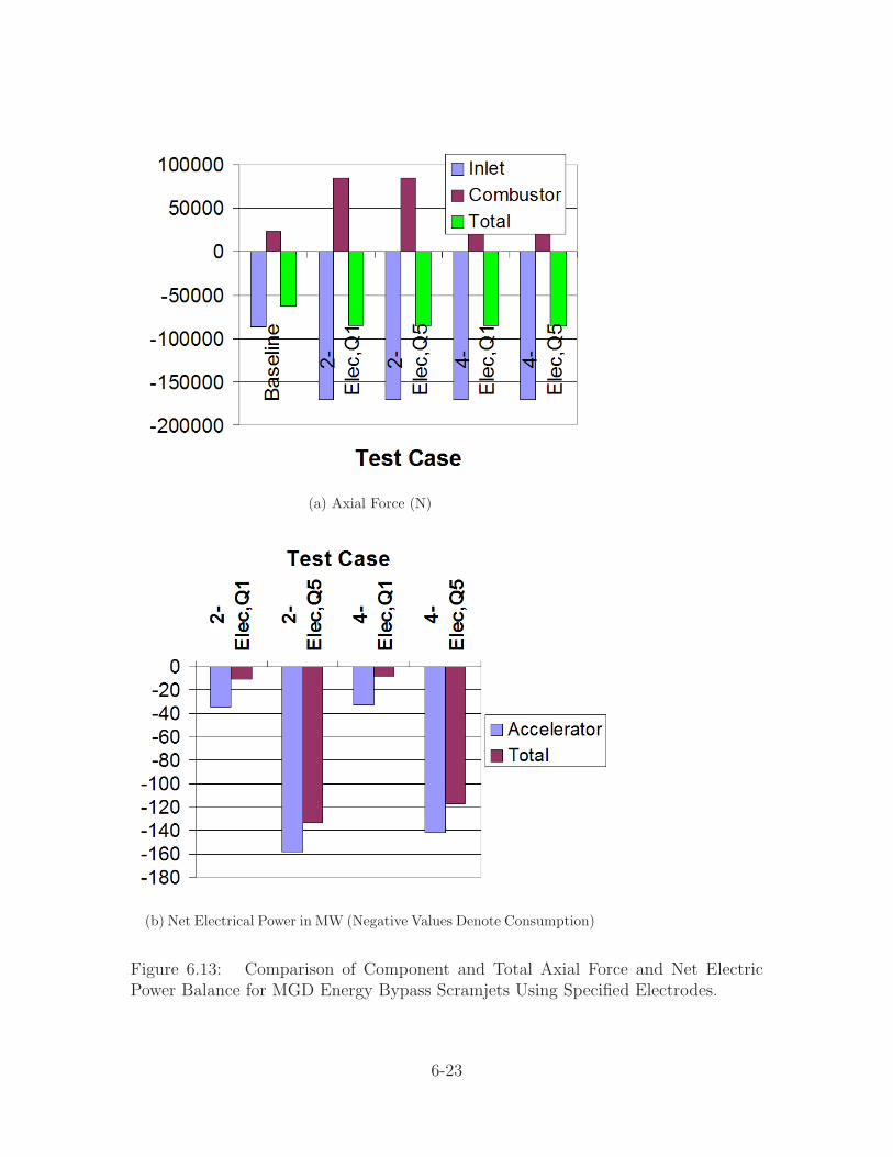
(a) Axial Force (N)

(b) Net Electrical Power in MW (Negative Values Denote Consumption)

Figure 6.13: Comparison of Component and Total Axial Force and Net ElectricPower Balance for MGD Energy Bypass Scramjets Using Specified Electrodes.

6-23

6.4 Summary of Results, Conclusions and Recommendations Regard-

ing MGD Power Generation and Energy Bypass

Regarding MGD power generation in general, and in particular, generation up-

stram of the combustor, MW-class electrical power generation was achieved, even for

the relatively small interaction parameter of Q = 1. However, this positive result

came with performance penalties in terms of a drag increase with respect to baseline

that varied anywhere from 10% to nearly double the baseline inlet value. This added

drag, as well as dissipation induced heating, reduced most of the overall inlet perfor-

mance measures with respect to the no-MGD baseline. From this, it was concluded

that if the primary purpose for MGD power generation is to supply onboard elec-

trical components, smaller generators with lower interaction parameters (i.e. lower

system power requirements) should be considered. Moreover, it is more important

to focus the interaction region in the core flow, where the useful work was a greater

proportion of the overall interaction. However, if the goal is to maximize the work

extraction with the goal of bypassing it directly to the expansion system, then the

interaction parameter and plasma volume should be maximized. Finally, comparing

combustor-based MGD power generation to its isolator-based counterpart revealed

that the combustor-based generators performed moderately better, in spite of local-

ized pressure increases in the vicinity of the electrodes which indicated the presence

of small shock waves.

During the course of examining the Faraday electrode configurations, it was

found that the research code’s method of specifying electric potential required mak-

ing some assumptions regarding the average local flow velocity. The difficulty with

this approach is that ~V is never constant and thus there existed electrode configu-

rations with substantial areas of reversed current flow. The net effect was in many

configurations MGD generators actually acted as accelerators and vice versa. In light

of this fact, it is recommended that future work focus on more accurate methods of

modelling the electrode potentials, including consideration of the modelling of the

external electric circuit in its entirety.

6-24

Finally, with respect to MGD acceleration and specifically the MGD energy

bypass concept, it was easy to conclude that for the configurations tested, MGD

acceleration was ineffective for improving the performance of this scramjet. Further-

more, when taken as an overall system, the energy bypass concept was unable under

any circumstance to be self-powered. Although this research focused on the seg-

mented Faraday electrode configuration, the physics of MGD flow acceleration will

in most configurations result in a disproportionate amount of electrical energy being

required to produce useful flow work and acceleration. In addition, this work will

always be accompanied by a significantly greater fraction of the total energy input

being dissipated as heat as compared to a similarly sized MGD generator. However,

it is recommended that any future work in the area of MGD acceleration and energy

bypass be directed towards the examination of alternative electrode configurations

(e.g. Hall current electrodes or diagonally offset Faraday electrodes).

6-25

VII. Summary, Conclusions, and Recommendations

7.1 Summary

Prior to this work, the analysis of electromagnetic (EM) flow control through

the application of magnetogasdynamics (MGD) relied upon simplified analytical treat-

ments and reduced dimensional numerical studies. These key limitations included un-

realistic flowpath geometries, calorically perfect gases, and inviscid, 2D flow solvers.

As a consequence, not all of the pertinent flow physics were included and thus the con-

clusions reached were limited in applicability. The effort concluded here contributes

directly to the advancement of this research field by removing these limitations, ap-

plying the first comprehensive three-dimensional analysis of EM flow control to a

flight-sized, scramjet engine.

The starting point for this research was a CFD code developed by the Air

Force Research Laboratory (AFRL) to model the full, three-dimensional set of cou-

pled Navier-Stokes and Maxwell’s equations [20]. Since the Mach 10 scramjet flow

under consideration can be considered a collision-dominated, weakly ionized plasma,

the typical MGD assumptions hold. The key assumption in this case was low elec-

trical conductivity and that the magnitude of the applied magnetic field was high.

This condition defines the low magnetic Reynold’s number regime, which allowed the

Lorentz Force and EM interaction to be coupled to the Navier-Stokes’ equations as

simple source terms. This coupling allows the use of conventional CFD techniques

could be employed. For this research, the Roe flux difference splitting scheme with the

vanLeer harmonic limiter and central differencing were used for spatial discretization,

while an implicit Beam-Warming method was used for temporal discretization. To

account for turbulent flow, the widely used k − ǫ model, modified for use with MGD,

was included.

Regarding the CFD modelling of the EM fields, all of the research conducted

specified the magnetic flux density, ~B, at all points and assumed it was invariant

in both time and space. The plasma conductivity, σ, was time invariant as well,

with a scalar value whose spatial growth and decay was held constant by a three-

7-1

dimensional Gaussian distribution. Two methods of calculating the electric field, ~E,

were employed. The first approach was the same as for ~B, wherein ~E was initialized

and then held invariant. This approach was simpler to implement and had a distinct

advantage in lower computational expense. However, the solutions obtained demon-

strated that it was likely to produce less realistic results. The second approach used a

higher fidelity approach, specifying the locations and electric potential for wall-based

electrodes. A Poisson solver was used with this approach to enforce current continu-

ity and obtain the ~E field. The advantage of this method was that it created an ~E

field that was coupled to the flow, such that as the EM interaction altered the flow,

the flow would simultaneously change the ~E field until reaching equilibrium. This

results in a more realistic capturing of the flow physics, but at a significant increase

in computational time. Where the first approach could converge the typical 750,000

point domain in less than a week using a Cray X1 supercomputer, it was common for

the latter approach to take 2 weeks to converge the same problem. More importantly,

accurately capturing the physics at electrode-insulator boundaries presented prob-

lems with some MGD device configurations, as did difficulties in applying optimized

numerical filtering.

As a final note, all of the electrode-based models tested used a segmented Fara-

day configuration where paired electrodes of opposite potential were placed on op-

posing wall boundaries. Because of this configuration, Hall current effects were not

included in this research.

Before EM flow control was considered, the key physical processes common to

scramjet engines were explored and incorporated into the development of a first-of-its-

kind open source scramjet geometry. First, this was done through the development of

a quasi-1D computational design tool. Verification of this tool was performed by com-

parison with similar computational models followed by application to the simplified

AFRL scramjet geometry given in Reference [21]. This computational code was then

applied to appropriately size the engine to support the requirements of the Military

Spaceplane concept [82], a proposed Air Force program for a hypersonic vehicle with

7-2

global reach. Once this was accomplished, various analytical methods and experi-

mental data were taken from literature and applied to convert the quasi-1D design

to a 3D geometry. Finally, an initial computational run of the engine was completed

and analyzed. Based on this analysis, which included a grid convergence study, im-

provements to the geometry were made in order to establish the baseline performance

model. This baseline model would be the starting point for the all of the remaining

research.

Two significant additions to the existing code were made to support the goals

of this research. The first was the creation of a post-CFD analysis tool that allowed

for a dimensional analysis of the EM impacts to the system and its performance. Key

to this addition was the inclusion of an electron beam model and routines to perform

cross-sectional and cell-based averages of flow and EM properties. These results were

then cast into a form suitable for taking a control volume approach that was used to

determine overall performance values, e.g. forces, heat transfer, and total pressure

ratios.

The second major addition was the development and verification of a finite

rate thermochemistry model. The primary purpose for undertaking this portion of

the research effort was because stable, efficient combustion has traditionally been

one of the greatest challenges to achieving scramjet propulsion. A portion of this

research broke new ground in demonstrating the first coupling of a finite rate chemistry

and MGD solver for scramjet applications. In addition, the coupling algorithm was

purposefully generalized such that it could be used or turned off as needed, allowing

computational expense to be balanced against a particular application’s requirements.

The successful implementation of this computational tool, overcame two significant

shortfalls in the AFRL research code: (1) the major assumption the gas was non-

reactive air, and (2) chemical combustion could only be represented by a simple

volumetric heating rate source term in the energy equation.

7-3

Culminating the research effort, a detailed computational analysis of this engine

in the context of both localized MGD flow control applications and the MGD energy

bypass system were explored. Regarding local EM flow control, this research explored

the possibility of mitigating a region of separated flow within the internal inlet and

increasing the average pressure entering the combustor. Two MGD concepts were

considered to address this issue: increasing pressure in the cowl shoulder region to

better match that of the reflected shock, or increasing flow momentum in the boundary

layer to overcome the adverse pressure gradient. A parametric study tested these

concepts by varying the spatial distribution of the plasma region, the load factor,

k, and the interaction parameter, Q. In summary, localized MGD flow control was

marginally successful in raising the average pressure entering the combustor, and even

more successful at reducing overall inlet drag.

The system-level MGD research was tested to a level of computational fidelity

never before attempted. Three distinct applications were investigated: (1) stand-

alone MGD power generation performed upstream of the combustor, (2) stand-alone

combustor-based MGD power generation, and (3) a full MGD energy bypass system.

Regarding MGD power generation in general, and in particular, generation upstram

of the combustor, MW-class electrical power generation was achieved, even for the

relatively small interaction parameter of Q = 1. However, this positive result came

with performance penalties in terms of a drag increase with respect to baseline that

varied anywhere from 10% to nearly double the baseline inlet value. This added drag,

as well as dissipation induced heating, reduced most of the overall inlet performance

measures with respect to the no-MGD baseline. Comparing combustor-based MGD

power generation to its isolator-based counterpart revealed that the combustor-based

generators performed moderately better, in spite of localized pressure increases in the

vicinity of the electrodes which indicated the presence of small shock waves.

With respect to MGD acceleration and specifically the MGD energy bypass

concept, none of the configurations tested improved the performance of this scramjet

with respect to net axial force. Rather, as compared to the baseline engine all of the

7-4

bypass engines experienced a net drag increase of approximately 33%. Furthermore,

none of the bypass engines could be considered self-powered. In every case, the power

produced by the most powerful generator tested was insufficient to both ionize the

flow and supply the power required by the MGD accelerators. While these conclusions

must be kept in the context of the segmented Faraday electrodes tested, it is felt

that the physics of MGD flow acceleration will in most configurations result in a

disproportionate amount of electrical energy being consumed to produce useful flow

work and acceleration. In addition, the flow work will always be accompanied by

a significantly greater fraction of the total energy input being dissipated as heat as

compared to a similarly sized MGD generator.

7.2 Conclusions

Based upon this research effort, the following conclusions were reached:

1. Coupling the thermochemistry with the fluid dynamics captured phenomena un-

seen by either model alone, improving the overall accuracy of the simulation.

Using this approach, results from the model problem exceeded expectations,

matching the predicted ignition point and differing by only 0.5% with respect

to the well-accepted STANJAN software.

2. The loosely coupled approach to incorporate finite rate chemistry was very suc-

cessful with respect to modelling supersonic combustion flow problems and is rec-

ommended over the existing polynomial gamma and heat source term approaches

for these problems. With regard to the actual scramjet modelling done, the in-

clusion of combustion chemistry resulted in the most accurate representation of

a real engine.

3. As a consequence, this successful addition to the AFRL computational electro-

magnetics code provides the only open-source model of fuel injection, mixing and

combustion for MGD flow control applications.

7-5

4. The placement of the EM interaction region, and in particular the electrodes,

is critical to successful exploitation of this technology. The extent of the flow-

EM interaction is only fully realized when the inherent complexity of the 3D,

viscous flow physics is taken into account. 1D or 2D, inviscid solutions by them-

selves are inadequate for accurately capturing the impacts to performance in the

scramjet engine. As an example, placement of the EM-interaction region near

the wall was the most important factor in determining the wall heat transfer,

and targeting the conductivity to this region was a relatively efficient method

of limiting drag increases.

5. MGD electrical power generation for the purpose of powering the vehicle’s on-

board electrical systems, to include the ionization source and any electromagnet

requirements, is certainly feasible with a flight-sized engine. This assumes of

course that the weight and complexity of the magnet and associated ionization

and control system does not prove prohibitive. For many of the MGD generator

cases, MW-class electrical power generation was achieved, verifying the results

of previous research. However, tying back to the previous conclusion, electrode

placement was critical to successful power generation and there was a large

difference in performance depending on the k and Q used.

6. The use of an MGD accelerator to locally increase flow momentum was an effec-

tive approach to improve flow into the isolator of this scramjet model. Although

it only slightly increased the flow pressure going into the isolator, MGD acceler-

ation, particularly for Case 2B, was able to efficiently reduce the net inlet drag.

It did this while minimizing the increase in heat transfer and decrease in overall

efficiency measures. This was due primarily to increasing the flow momentum

as it passed through the sidewall expansion into the inlet throat.

7. Combustor-based MGD power generation was superior to the inlet-based ap-

proach with respect to power density and overall engine efficiency. For elec-

trical power generation, then, an approach similar to that of ground-based,

combustion-fired MGD generators should be pursued.

7-6

8. For the electrode configurations tested, MGD acceleration was ineffective for

improving the performance of this scramjet. Furthermore, when taken as an

overall system, the energy bypass concept was unable under any circumstance

to be self-powered. MGD acceleration was shown to be ineffective in improving

overall performance, with all of the bypass engines having approximately 33%

more drag than baseline and none of them achieving a self-powered state. In

light of this, it is difficult to conceive of a viable MGD energy bypass system.

7.3 Recommendations for Future Research

1. It is recommended that this improved computational tool should be used to im-

prove upon the current geometry and establish an optimized baseline upon which

to further test flow control applications. Several problems with the geometry

were identified that could be traced back to the quasi-1D design iteration. The

deficiencies with the greatest performance impact were the lack of a combustor

flameholder and fuel-air mixing cavity as well as an oversimplified and over-

expanded expansion nozzle. The structured grid used by the computational

method precluded the addition of the complicated combustor geometry needed.

Finally, these combustion and expansion components are the most difficult parts

of the flow path to optimize and would require several more design iterations to

significantly improve.

2. Consideration should be given to adding species diffusion, thus extending appli-

cability to the subsonic regime. In addition, higher fidelity models of viscosity

and thermal conductivity could be incorporated.

3. Future work in the area of MGD acceleration and energy bypass should be

directed towards the examination of alternative electrode configurations (e.g.

Hall current electrodes or diagonally offset Faraday electrodes).

4. In this regard, a more detailed method of modelling the electrode potential should

be undertaken that better accounts for the electrode-insulator boundary condition.

7-7

This is necessary to eliminate detrimental effects such as near wall reversal of

the ~E field that was seen with some electrode configurations.

5. In conjunction with the two prior recommendations, the optimum distance off

the wall to target the electron beam ionization should be investigated further.

6. Finally, long term research in this area should include modelling of the external

electric circuit to understand the dynamic response of these flow control sys-

tems. This modelling should include, as a minimum, a detailed analysis of the

ionization and magnetic field generator power requirements as well as the load

presented by the vehicle’s overall electrical system.

7-8

Bibliography

1. Stopping Powers for Electrons and Positrons. Technical report, InternationalCommission on Radiation Units and Measurements, 1984.

2. Abdel-Salam, T.M. and R.A. Carson. “Three-Dimensional Numerical Study of aDual-Mode Scramjet Combustor”. 37th AIAA Thermophysics Conference, 1–10.AIAA, 2004.

3. Ault, D.A. and D.M. Van Wie. “Comparison of Experimental Results and Com-putational Analysis for the External Flowfield of a Scramjet Inlet at Mach 10 and14”. AIAA Fourth International Aerospace Planes Conference. AIAA, 1992.

4. Baurle, R.A. and D.R. Eklund. “Analysis of Dual-Mode Hydrocarbon ScramjetOperation at Mach 4 - 6.5”. Journal of Propulsion and Power, 18(5):990–1002,2002.

5. Ben-Yakar, A. and R.K. Hanson. “Cavity Flame-Holders for Ignition and FlameStabilization in Scramjets: An Overview”. Journal of Propulsion and Power,17(4):869–877, 2001.

6. Berry, S.A. and A.H. Auslender. “Hypersonic Boundary-Layer Trip Developmentfor Hyper-X”. Journal of Spacecraft and Rockets, 38(6):853–863, 2001.

7. Bityurin, V.A., A.N. Bocharov, and J.T. Lineberry. “Results of Experimentson MHD Hypersonic Flow Control”. 35th AIAA Plasmadynamics and LasersConference, 1–15. AIAA, 2004.

8. Brichkin, D.I., A.L. Kuranov, and E.G. Sheikin. “The Potentialities of MHDControl for Improving Scramjet Performance”. 1–11. AIAA 1999-4969.

9. Bruno, C. and P.A. Czysz. An Electro-Magneti-Chemical Hypersonic PropulsionSystem. Technical report, AIAA, 1998.

10. Burakhanov, B.M., A.P. Likhachev, S.A. Medin, V.A. Novikov, V.I. Okunev, V.Y.Rickman, and V.A. Zeigarnik. “Advancement of Scramjet MagnetohydrodynamicConcept”. Journal of Propulsion and Power, 17(6):1247–1252, 2001.

11. Cockrell, C.E.J., W.C. Engelund, R.D. Bittner, T.N. Jentink, A.D. Dilley, andA. Frendi. “Integrated Aeropropulsive Computational Fluid Dynamics Method-ology for the Hyper-X Flight Experiment”. Journal of Spacecraft and Rockets,38(6):836–843, 2001.

12. Curran, E.T. “Scramjet Engines: The First Forty Years”. Journal of Propulsionand Power, 17(6):1138–1148, 2001.

13. Curran, E.T. and S.N.B. Murthy. Scramjet Propulsion, volume 189 of Progressin Astronautics and Aeronautics. AIAA, 2000.

BIB-1

14. D’Ambrosio, D. and D. Giordano. “Electromagnetic Fluid Dynamics forAerospace Applications. Part I: Classification and Critical Review of PhysicalModels”. 35th AIAA Plasmadynamics and Lasers Conference, 1–14. AIAA, 2004.

15. Davis, D.L. “Numerical Analysis of Two and Three Dimensional Recessed Flame-holders for Scramjet Applications”, 1996.

16. Dornheim, M.A. “A Breath of Fast Air”. www.aviationnow.com, 2004.

17. Earp, B.E. Magnetogasdynamic Flow Control of a Mach Reflection. Master’sthesis, Air Force Institute of Technology, 2004.

18. Evans, J.S. and Jr. Schexnayder, C.J. “Influence of Chemical Kinetics andUnmixedness on Burning in Supersonic Hydrogen Flames”. AIAA Journal,18(2):188–193, 1980.

19. Fisher, S.A. “Three-Dimensional Flow Effects in a Two-Dimensional SupersonicAir Intake”. Journal of Propulsion and Power, 2(6):546–551, 1986.

20. Gaitonde, D.V. “Development of a Solver for 3-D Non-Ideal Magnetogasdynam-ics”. 30th AIAA Plasmadynamics and Lasers Conference, 1–15. AIAA, 1999.

21. Gaitonde, D.V. “Three-Dimensional Flow-Through Scramjet Simulation withMGD Energy Bypass”. 41st AIAA Aerospace Sciences Meeting and Exhibit, 1–19. AIAA, 2003.

22. Gaitonde, D.V. and J. Poggie. “An Implicit Technique for 3-D Turbulent MGDwith the Generalized Ohm’s Law”. 32nd AIAA Plasmadynamics and Lasers Con-ference, 1–17. AIAA, 2001.

23. Gaitonde, D.V. and J. Poggie. “Elements of a Numerical Procedure for 3-D MGDFlow Control Analysis”. 40th AIAA Aerospace Sciences Meeting and Exhibit, 1–17. AIAA, 2002.

24. Goyne, C.P., J.C. McDaniel, T.M. Quagliaroli, R.H. Krauss, and S.W. Day.“Dual-Mode Combustion of Hydrogen in a Mach 5, Continuous-Flow Facility”.Journal of Propulsion and Power, 17(6):1313–1318, 2001.

25. Heiser, W.H. and D.T. Pratt. Hypersonic Airbreathing Propulsion. AIAA Edu-cation Series. AIAA, 1994.

26. Hoffman, K.A. and S.T. Chiang. Computational Fluid Dynamics Volume II, 4thEdition, chapter 16. Engineering Education System, 2000.

27. Holland, S.D. “A Computational and Experimental Investigation of a Three-Dimensional Hypersonic Scramjet Inlet Flow Field”, 1991.

28. Holland, S.D. and J.N. Perkins. “Contraction Ratio Effects in a Generic Three-Dimensional Sidewall Compression Scramjet Inlet: A Computational and Ex-perimental Investigation”. AIAA 22nd Fluid Dynamics, Plasma Dynamics, andLasers Conference, 1–18. AIAA, 1991.

BIB-2

29. Holland, S.D., W.C. Woods, and W.C. Engelund. “Hyper-X Research VehicleExperimental Aerodynamics Test Program Overview”. Journal of Spacecraft andRockets, 38(6):828–835, 2001.

30. Hughes, W.F. and F.J. Young. The Electromagnetodynamics of Fluids.

31. Kanury, M. A. Introduction to Combustion Phenomena, 139. Gordon and BreachPublishers, 1995.

32. Kim, C.K., S.T. Yu, and Z.C. Zhang. “Cavity Flow in Scramjet Engine by Space-Time Conservation and Solution Element Method”. AIAA Journal, 42(5):912–919, 2004.

33. Kuranov, A.L., V.V. Kuchinsky, and E.G. Sheikin. “Scramjet with MHD Controlunder ”AJAX” Concept. Requirements for MHD Systems.” 32nd AIAA Plasma-dynamics and Lasers Conference, 1–11. AIAA, 2001.

34. Kuranov, A.L. and E.G. Sheikin. “MHD Control on Hypersonic Aircraft un-der ”AJAX” Concept. Possibilities of MHD Generator”. 40th AIAA AerospaceSciences Meeting and Exhibit, 1–11. AIAA 2002-0490.

35. Kuranov, A.L. and E.G. Sheikin. “The Potential of MHD Control for ImprovingScramjet Performance”. 30th AIAA Plasmadynamics and Lasers Conference, 1–9.AIAA 1999-3535.

36. Kuranov, A.L. and E.G. Sheikin. “Magnetohydrodynamic Control on Hyper-sonic Aircraft Under “Ajax” Concept”. AIAA Journal of Spacecraft and Rockets,40(2):174–182, 2003.

37. Lindsey, M.F. and R.J. McMullan. “Computational Study of MGD Flow Controlon a Flight-Scale Scramjet”. AIAA 2006-0371, 2006.

38. Lindsey, M.F., R.J. McMullan, and D.V. Gaitonde. “A Computational Ther-mochemistry Model for Scramjets with Electromagnetic Flow Control”. AIAA2005-3222, 2005.

39. Lindsey, M.F., R.J. McMullan, and D.V. Gaitonde. “Development of a Realistic3-D Scramjet Flowpath for MGD Energy Bypass”. AIAA 2005-1178, 2005.

40. Linstrom, P.J. and W.G. Mallard (editors). NIST Chemistry WebBook, NISTStandard Reference Database Number 69. National Institute of Standards andTechnology, Gaithersburg MD, 20899, 1995.

41. Liston, G. “Quasi-1D Scramjet Code Results Comparison and Discussion”, 2004.Personal correspondence with AFRL/PRA researchers.

42. Litchford, R.J., J.W. Cole, V.A. Bityurin, and J.T. Lineberry. Thermody-namic Cycle Analysis of Magnetohydrodynamic-Bypass Hypersonic AirbreathingEngines. Technical report, NASA TP-2000-210387, 2000.

BIB-3

43. Litchford, R.J., J.W. Cole, and J.T. Lineberry. “Thermodynamic Cycle Analysisof Magnetohydrodynamic-Bypass Hypersonic Airbreathing Engines”. Journal ofPropulsion and Power, 17(2):477–480, 2000.

44. Macheret, S.O., R.B. Miles, and G.L. Nelson. “Feasibility Study of a HybridMHD/Radiatively Driven Facility for Hypersonic Ground Testing”. AIAA 1997-2429, 1997.

45. Macheret, S.O., M.N. Shneider, and R.B. Miles. “Potential Performance of Su-personic MHD Power Generators”. 39th AIAA Aerospace Sciences Meeting andExhibit, 1–24. AIAA 2001-0795.

46. Macheret, S.O., M.N. Shneider, and R.B. Miles. “Energy-Efficient Generation ofNonequilibrium Plasmas and Their Applications to Hypersonic MHD Systems”.AIAA 2001-2880, 2001.

47. Macheret, S.O., M.N. Shneider, and R.B. Miles. “Magnetohydrodynamic Controlof Hypersonic Flows and Scramjet Inlets Using Electron Beam Ionization”. AIAAJournal, 40(1):74–81, 2002.

48. Macheret, S.O., M.N. Shneider, and R.B. Miles. “Modeling of Air Plasma Gen-eration by Repetitive High-Voltage Nanosecond Pulses”. IEEE Transactions ofPlasma Science, 30(3):1301–1314, 2002.

49. Macheret, S.O., M.N. Shneider, and R.B. Miles. Scramjet Inlet Control by Off-Body Energy Addition: A Virtual Cowl. 2002.

50. Macheret, S.O., M.N. Shneider, D.M. Van Wie, and R.B. Miles. “MHD PowerGeneration in Scramjet Engines in Conjunction with Inlet Control”. 42nd AIAAAerospace Sciences Meeting and Exhibit, 1–24. 2004.

51. Mahoney, J. Inlets for Supersonic Missiles. AIAA Education Series. AIAA, 1990.

52. Mani, M., R.H. Bush, and P. Vogel. “Implicit Equilibrium and Finite-Rate Chem-istry Models for High Speed Flow Applications”. AIAA 1991-3299, 1991.

53. McEldowney, B., R. Meyer, N. Chintala, and A.I. V. “Measurements of Elec-trical Parameters of a Supersonic Non-Equilibrium MGD Channel”. 34th AIAAPlasmadynamics and Lasers Conference, 1–14. AIAA, 2003.

54. Mehta, U.B., D.W. Bogdanoff, and C. Park. A Perspective on a CombinedMagneto-Hydrodynamic-Scramjet Engine. Technical report, NASA, 2001.

55. Meyer, R., B. McEldowney, N. Chintala, P. Palm, and I.V. Adamovich. “Experi-mental Studies of Plasma Assisted Ignition and MGD Supersonic Flow Control”.41st AIAA Aerospace Sciences Meeting and Exhibit. AIAA, 2003.

56. Mitani, T., N. Chinzei, and K. Takeshi. “Reaction and Mixing-Controlled Com-bustion in Scramjet Engines”. Journal of Propulsion and Power, 17(2):308–314,2001.

BIB-4

57. NASA. “Guinness World Records Recognizes NASA X-43A Speed Record”.NASA Dryden News Releases, 2004.

58. NASA. “Faster Than a Speeding Bullet: Guinness Recognizes NASA Scramjet”.NASA News Release: 05-156, 2005.

59. Nishihara, M., R. Meyer, M. Cundy, W.R. Lempert, and I.V. Adamovich. “De-velopment and Operation of a Supersonic Nonequilibrium MHD Channel”. 35thAIAA Plasmadynamics and Lasers Conference, 1–19. AIAA, 2004.

60. Park, C., D.W. Bogdanoff, and U.B. Mehta. “Theoretical Performance of Fric-tionless Magnetohydrodynamic-Bypass Scramjets”. Journal of Propulsion andPower, 17(3):591–598, 2001.

61. Poggie, J. and D.V. Gaitonde. “Magnetic Control of Hypersonic Blunt BodyFlow”. 38th AIAA Aerospace Sciences Meeting and Exhibit, 1–15. AIAA, 2000.

62. Poggie, J. and D.V. Gaitonde. “Computational Studies of Magnetic Control inHypersonic Flow”. 39th AIAA Aerospace Sciences Meeting and Exhibit, 1–12.AIAA, 2001.

63. Poggie, J. and D.V. Gaitonde. “Magnetic control of flow past a blunt body:Numerical validation and exploration”. Physics of Fluids, 14(5):1720–1731, 2002.

64. Powell, O.A., J.T. Edwards, R.B. Norris, and K.E. Numbers. “Development ofHydrocarbon-Fueled Scramjet Engines: The Hypersonic Technology (HyTech)Program”. Journal of Propulsion and Power, 17(6):1170–1176, 2001.

65. Reinartz, B.U., J. van Keuk, T. Coratekin, and J. Ballmann. “Computation ofWall Heat Fluxes in Hypersonic Inlet Flows”. 40th AIAA Aerospace SciencesMeeting and Exhibit, 1–10. 2002.

66. Reynolds, W.C. “STANJAN Chemical Equilibrium Solver, v3.91 IBM-PC”. Stan-ford University, 1987.

67. Riggins, D.W. “Analysis of the Magnetohydrodynamic Energy Bypass Engine forHigh-Speed Airbreathing Propulsion”. AIAA Journal of Propulsion and Power,20(5):779–792, 2004.

68. Rogers, R.C. and W. Chinitz. “On the Use of a Global Hydrogen-Air CombustionModel in the Calculation of Turbulent Reacting Flows”. AIAA 1982-0112, 1982.

69. Rogers, R.C. and Jr. Schexnayder, C.J. Chemical Kinetic Analysis of Hydrogen-Air Ignition and Reaction Times. Technical report, National Aeronautics andSpace Administration, 1981.

70. Rosa, R.J. Magnetohydrodynamic Energy Conversion. McGraw-Hill, 1968.

71. Sato, H. “The Hall Effect in the Viscous Flow of Ionized Gas between ParallelPlates under Transverse Magnetic Field”. J. Phys. Soc. of Japan, 16(7):1427–1433, July 1961.

BIB-5

72. Schneider, S.P. and C. Skoch. “Streamwise-Vortex Instability and Transition onthe Hyper-2000 Scramjet Forebody”. 22nd AIAA Ground Testing Conference,1–16. AIAA, 2003.

73. Shneider, M.N. and S.O. Macheret. “Modeling of Plasma Virtual Shape Controlof Ram/Scramjet Inlet and Isolator”. 35th AIAA Plasmadynamics and LasersConference, 1–19. AIAA 2004-2662, 2004.

74. Shneider, M.N. and S.O. Macheret. “Hypersonic Aerodynamic Control andThrust Vectoring by Nonequilibrium Cold-Air MHD Devices”. AIAA 2005-0979,2005.

75. Sutton, G.W. and A. Sherman. Engineering Magnetohydrodynamics. McGraw-Hill, 1965.

76. Tannehill, J.C., D.A. Anderson, and R.H. Pletcher. Computational Fluid Me-chanics and Heat Transfer. Taylor and Francis, 2 edition, 1997.

77. Townend, L.H. “Domain of the Scramjet”. Journal of Propulsion and Power,17(6):1205–1213, 1991.

78. Turchak, A., A. Kuranov, and A. Korabelnikov. “Hypersonic Technologies of the“AJAX” Concept”. AIAA 2002-5184, 2002.

79. Uenishi, K., R.C. Rogers, and G. Northam. “Three Dimensional Computationsof Transverse Hydrogen Jet Combustion in a Supersonic Airstream”. AIAA 1987-0089, 1987.

80. Van Wie, D.M. and D.A. Ault. “Internal Flowfield Characteristics of a ScramjetInlet at Mach 10”. Journal of Propulsion and Power, 12(1):158–164, 1996.

81. Vassberg, J.C., M.A. DeHaan, and A.J. Sclafani. “Grid Generation Requirementsfor Accurate Drag Predictions Based on OVERFLOW Calculations”. 16th AIAAComputational Fluid Dynamics Conference, 1–27. AIAA, 2003.

82. Vick, C.P., S.D. Berman, and C. Lindborg. Military Spaceplane, X-40 SpaceManeuver Vehicle, Integrated Tech Testbed. Federation of American Scientists,1999.

83. White, F.M. Fluid Mechanics, chapter 3. McGraw-Hill, 2 edition, 1986.

84. White, F.M. Viscous Fluid Flow, 29. McGraw-Hill, 2 edition, 1991.

BIB-6

Vita

Major Martin F. Lindsey graduated from Georgetown High School in George-

town, Texas, in 1989. He received his Bachelor of Science Degree in Aerospace Engi-

neering, specializing in astronautics, from the University of Texas at Austin in 1993.

Immediately thereafter, he reported to the United States Air Force Officer Training

School, Lackland Air Force Base, Texas, from which he graduated as a Distinguished

Military Graduate and was commissioned as a Second Lieutenant in September 1993.

Maj Lindsey served in several mission support and operational specialties while

simultaneously pursuing professional education. Beginning with a tour as a Min-

uteman III ICBM maintenance officer in Minot, North Dakota, he served in various

leadership positions including being the Maintenance Supervisor for the 742d Missile

Squadron and culminating in the Chief of the Maintenance Operations Center. In

this capacity, he was responsible for directing real-time maintenance scheduling, pri-

oritization and operations for 150 ICBMs and 15 launch control centers. During this

tour he began taking coursework towards his Masters of Aerospace Engineering from

Auburn University, Alabama. At the same time, he completed the Federal Aviation

Administration requirements to be granted Commercial, Instrument, and Certificated

Flight Instructor certificates.

In 1998, he was reassigned to Vandenberg AFB, California, for training as a

space and missile operator. Upon graduation as the Top Graduate and recipient of

the Air Education and Training Command Commander’s Trophy, he was assigned

to serve as a space launch operator at Cape Canaveral Air Force Station, Florida.

During four years at the Cape, Maj Lindsey served in several capacities for a variety

of organizations and launch platforms. As the Atlas Operations Flight Commander in

the 3rd Space Launch Squadron, he was responsible for all Air Force launch base op-

erations for the Atlas II/III launch system. Then, he was part of the initial Air Force

team to bring the Delta IV Evolved Expendable Launch Vehicle to operational capa-

bility with a successful first flight in November 2002. It was during this assignment,

VITA-1

that Maj Lindsey completed his Masters of Aerospace Engineering and then went on

to further earn a Masters of Science in Space Systems from the Florida Institute of

Technology.

At the end of 2002, he was assigned to the Air Force Institute of Technology at

Wright-Patterson AFB, Ohio, where he was enrolled as a student in the aeronautical

engineering doctoral program. Upon graduation he will be assigned to the Compu-

tational Aerodynamics Center at the Air Force Research Laboratories, Aeronautical

Vehicles Directorate, also at Wright-Patterson AFB.

Permanent address: 2950 Hobson WayAir Force Institute of TechnologyWright-Patterson AFB, OH 45433

VITA-2

REPORT DOCUMENTATION PAGE Form ApprovedOMB No. 0704–0188

The public reporting burden for this collection of information is estimated to average 1 hour per response, including the time for reviewing instructions, searching existing data sources, gathering andmaintaining the data needed, and completing and reviewing the collection of information. Send comments regarding this burden estimate or any other aspect of this collection of information, includingsuggestions for reducing this burden to Department of Defense, Washington Headquarters Services, Directorate for Information Operations and Reports (0704–0188), 1215 Jefferson Davis Highway,Suite 1204, Arlington, VA 22202–4302. Respondents should be aware that notwithstanding any other provision of law, no person shall be subject to any penalty for failing to comply with a collectionof information if it does not display a currently valid OMB control number. PLEASE DO NOT RETURN YOUR FORM TO THE ABOVE ADDRESS.

1. REPORT DATE (DD–MM–YYYY) 2. REPORT TYPE 3. DATES COVERED (From — To)

4. TITLE AND SUBTITLE 5a. CONTRACT NUMBER

5b. GRANT NUMBER

5c. PROGRAM ELEMENT NUMBER

5d. PROJECT NUMBER

5e. TASK NUMBER

5f. WORK UNIT NUMBER

6. AUTHOR(S)

7. PERFORMING ORGANIZATION NAME(S) AND ADDRESS(ES) 8. PERFORMING ORGANIZATION REPORTNUMBER

9. SPONSORING / MONITORING AGENCY NAME(S) AND ADDRESS(ES) 10. SPONSOR/MONITOR’S ACRONYM(S)

11. SPONSOR/MONITOR’S REPORTNUMBER(S)

12. DISTRIBUTION / AVAILABILITY STATEMENT

13. SUPPLEMENTARY NOTES

14. ABSTRACT

15. SUBJECT TERMS

16. SECURITY CLASSIFICATION OF:

a. REPORT b. ABSTRACT c. THIS PAGE

17. LIMITATION OFABSTRACT

18. NUMBEROFPAGES

19a. NAME OF RESPONSIBLE PERSON

19b. TELEPHONE NUMBER (include area code)

Standard Form 298 (Rev. 8–98)Prescribed by ANSI Std. Z39.18

23–03–2006 Doctoral Dissertation Jan 2003 — Mar 2006

Assessing the Potential for ImprovedScramjet Performance Through Application of

Electromagnetic Flow Control

2003-014

Lindsey Martin F., Maj, USAF

Air Force Institute of TechnologyGraduate School of Engineering and Management (AFIT/EN)2950 Hobson WayWPAFB OH 45433-7765

AFIT/DS/ENY/06-05

AFOSR/NADr. John Schmisseur801 N. Randolph Street, Rm 732Arlington, VA 22203-1977 (703) 696-6962

Approved for public release; distribution unlimited.

Hypersonic flight using scramjet propulsion bridges the gap between turbojets and rockets. Recent efforts focus on magnetogasdynamic(MGD) flow control to mitigate the problems of high thermomechanical loads and low efficiencies associated with scramjets. This research isthe first flight-scale, three-dimensional computational analysis of a realistic scramjet to assess how MGD flow control improves scramjetperformance. Developing a quasi-one dimensional design tool culminated in the first open source scramjet geometry. This geometry wastested with the Air Force Research Laboratory’s electromagnetic computational code. To increase fidelity, an algorithm was developed toincorporate thermochemistry, resulting in the only open-source model of combustion in an MGD controlled engine. A control volumeanalysis with electron beam ionization was presented for the first time with this approach. Local MGD control within the inlet affected dragand heat transfer and was marginally successful in raising combustor inflow pressure. MGD acceleration to increase flow momentum waseffective at improving flow into the scramjet’s isolator. Combustor-based MGD generators proved superior to inlet generators with respectto power density and engine efficiency. MGD acceleration was ineffective in improving performance with all the MGD engines havingapproximately 33% more drag than baseline and none of them achieving self-powered operation.

Supersonic Combustion Ramjet Engines, Magnetogasdynamics, Computational Fluid Dynamics, Hypersonic Vehicles

U U U UU 176

Richard J. McMullan (ENY)

(937) 255–3636, ext 4578