Survey of flight and numerical data of hypersonic rarefied ...

Survey of flight and numerical data of hypersonic rarefied flows

encountered in Earth orbit and atmospheric reentry

Marc Schoulera,∗, Ysolde Prevereauda, Luc Mieussensb

aONERA / DMPE, Universite de Toulouse, F-31055 Toulouse, FrancebBordeaux INP, Univ. Bordeaux, CNRS, IMB, UMR 5251, F-33400 Talence,France

Abstract

The control of the satellites end-of-life including deorbiting and atmospheric entry as well asthe investigation of orbital maneuvers for new space missions confer a growing importanceto the study of the hypersonic rarefied regime. While flight data are necessary for thevalidation of Direct Simulation Monte-Carlo numerical simulations, only a few studies anddata are available for this purpose. Therefore, this article aims at gathering ground wind-tunnel and flight data in rarefied regime as well as their numerical reconstruction from awide scope of space programs. A detailed analysis of these data will be presented. Aftera review of hypersonic low-density wind-tunnel experiments that are the main source ofnon-reacting hypersonic rarefied flow study cases, we address, with our own simulations,unexploited afterbody heating data from former space programs such as Mercury and Apollo.Numerically reconstructed flight data from OREX and the Space Shuttle are also considered.Finally, ionization and radiative environment are discussed through the data collected duringStardust, Fire II and RAM-C II Earth atmospheric entry.

Keywords: Direct Simulation Monte-Carlo, Rarefied hypersonic flow, Earth reentry,Experimental and flight data

Contents

1 Introduction 2

2 Low density wind tunnel experiments 32.1 Rarefied hypersonic flow over a flat plate . . . . . . . . . . . . . . . . . . . . 32.2 Rarefied hypersonic flow over a flat plate with a sharp leading edge . . . . . 42.3 Rarefied hypersonic flow over a 70◦ blunted cone . . . . . . . . . . . . . . . . 6

3 Aerothermodynamic flight data 103.1 The Mercury Project . . . . . . . . . . . . . . . . . . . . . . . . . . . . . . . 103.2 The Apollo Program . . . . . . . . . . . . . . . . . . . . . . . . . . . . . . . 14

3.2.1 Apollo 6: Aerodynamic coefficients simulation . . . . . . . . . . . . . 153.2.2 Apollo AS-202: Afterbody heat flux simulation . . . . . . . . . . . . 19

3.3 The Space Shuttle Orbiter . . . . . . . . . . . . . . . . . . . . . . . . . . . . 253.4 The Orbital Reentry Experiment - OREX . . . . . . . . . . . . . . . . . . . 283.5 MIRKA . . . . . . . . . . . . . . . . . . . . . . . . . . . . . . . . . . . . . . 30

∗Corresponding authorEmail address: [email protected] (Marc Schouler)

Preprint submitted to Progress in Aerospace Sciences August 6, 2020

4 Ionization and radiative flight data 314.1 Fire II . . . . . . . . . . . . . . . . . . . . . . . . . . . . . . . . . . . . . . . 324.2 RAM C-II . . . . . . . . . . . . . . . . . . . . . . . . . . . . . . . . . . . . . 354.3 The sample return capsule Stardust . . . . . . . . . . . . . . . . . . . . . . . 36

5 Conclusion 38

1. Introduction

A good knowledge of rarefied hypersonic flows is critical for the study of the feasibilityof satellite orbital transfer maneuvers from low to very low orbit, as well as for an accurateprediction of reentry trajectory of both space debris and spacecraft. Indeed, an accuratecomputation of the aerodynamic coefficients of a flying object in high atmosphere is crucialfor a precise prediction of its trajectory and its stability. In the same way, a precise estimationof the heat flux applied to satellites or spacecraft is required for a proper design of theirthermal protection system (TPS) and for the risk management of debris demise.

Usually the degree of rarefaction of a gas is quantified by the Knudsen number Kn = λ/Lwhere λ is the gas mean free path (m) and L is the characteristic length of the object in theflow (m). The rarefied regime can then be divided into three sub-regimes. When Kn > 10,the flow is free molecular which means that inter-molecular collisions can be neglected andthe gas only interacts with the object’s walls. The regime is said to be transitional for0.1 < Kn < 10. In this regime, inter-molecular collisions effects start to be significant butnot enough to reach a local equilibrium. When 0.001 < Kn < 0.1, the gas is in a slipflow regime and transitional non-equilibrium is important near surfaces only. Finally, theflow is considered to be in a continuum regime when Kn < 0.001. During the first phaseof atmospheric reentry, the object goes through all these regimes. Before the atmosphericlayers become dense enough for the flow to be in a continuum regime, a non negligibledeviation from the thermochemical equilibrium leads to the failure of the classical Navier-Stokes conservation equations and particle simulation methods must be used.

In this context, the Direct Simulation Monte-Carlo (DSMC) method introduced by Bird[1] has proven to be one of the most appropriate numerical approaches for the simulation ofrarefied flows (from near-continuum to free-molecular). This method consists of an algorithmthat solves the Boltzmann equation and which computes the outcome of particle collisionsthrough stochastic processes. Over the past decades, the method has continually increasedits capacities of simulating thermochemical non-equilibrium phenomena which are involvedin atmospheric reentry conditions [2]. The severe conditions found in such flows are hardlyreproducible in ground facilities, which is why flight data are particularly valuable for thevalidation of DSMC.

Several authors have addressed the issue of atmospheric entry and the gathering of flightdata but none of these were dedicated to the rarefied regime encountered during Earthatmospheric reentry. Wright et al. [3] investigated afterbody aeroheating flight data incontinuum regime and Reynier [4] gathered aerothermodynamics flight data in the frame ofMars exploration projects. Hollis and Borrelli [5] studied the aerothermodynamics of bluntbody entry vehicles. A specific part of this work discusses the rarefied regime for whichnumerical heat fluxes computed with DSMC and CFD are compared for a Mars ScienceLaboratory like vehicle between 85 and 95 km. Finally, Schwartzentruber and Boyd, intheir paper about progress of particle-based simulation of hypersonic flows [6], presenteddata from various experiments and flights. The double cones and cylinder-flares experimentsin the LENS facility (pressure and heat flux) as well as on-board measurements of the Bow-Shock Ultra-Violet-2 (ultra-violet emission) and the RAM-C II (electron number density)flights are discussed.

2

In this paper, the focus is given on experimental data obtained in ground facilitiesthat are commonly used for DSMC benchmark and validation purposes, on inferred dataand on flight data measured during Earth reentry. Some of these data have already beenused and published in a numerical validation context. Some data were processed and usedhere for the first time and some are given and analyzed but are yet to be fully exploited.

2. Low density wind tunnel experiments

Rarefied atmospheric reentry flows are characterized by low densities, hypersonic veloc-ities and high enthalpy. High-enthalpy shock facilities have been reviewed by Reynier [7] in2016. The only facilities able to reproduce reentry conditions are shock-tubes, shock-tunnels,expansion tubes and hot-shots. However, these facilities only work for short duration andtheir densities do not match those necessary to retrieve rarefied conditions. Hypersonic,high-enthalpy and low density flow synthesis is a technological challenge that is still underconsideration. Hence, the only low density wind tunnel results available are for non-reactiveflows.

2.1. Rarefied hypersonic flow over a flat plate

Hypersonic rarefied flows over flat plates have been largely studied both experimentallyand numerically. The simplicity of the geometry and the experimental results precisionmakes this case particularly useful for numerical validation. In this section, we focus on thestudy of the rarefied hypersonic flow over a flat plate with a truncated leading edge.

Initially, this experiment was conducted by Allegre et al. [8] in the SR3 wind tunnel ofCentre National de la Recherche Scientifique (CNRS) Meudon. A pure nitrogen (N2) flowwas injected with two freestream conditions: M∞ = 20.2, Re∞ = 2850 and Re∞ = 8380 at atemperature T∞ = 13.32 K. The density flowfields were monitored by electron beam surveysand the wall pressure and convective heat flux were measured through pressure orifices anda thin skin technique. The plate was 100 mm long (Lp), 100 mm wide, 5 mm thick and thewall temperature was maintained at 290 K. In this experiment, two angles of attack (0◦ and10◦) were investigated.

The results of this work were widely used afterwards for the benchmarking and thevalidation of DSMC codes implementation [9], [10], [11]. In this context, the purpose is tosimulate the hypersonic flow over the flat plate in the first freestream conditions and withoutincidence. We performed our own numerical simulations with the SPARTA DSMC code[12]. A total of around 4 million particles were simulated in a 2D domain [xmin;xmax] ×[ymin; ymax] = [−0.06; 0.12] × [−0.1025; 0.1025] with dimensions in m. A 360 × 410 gridwas used and Allegre’s first freestream conditions were applied. By using the variable hardsphere (VHS) collision model, the mean free path becomes:

λVHS∞ =

1√2π d2

ref n∞

(T∞Tref

)ω−1/2

. (1)

With a numerical density n∞ = 3.716× 1020 ·/m3, a molecular diameter dref = 4.17× 10−10

m and a viscosity index ω = 0.74 at reference temperature Tref = 273 K, this ultimatelyresults in a mean free path λ∞ = 1.6 mm and a Knudsen number Kn = 0.016. Thevelocity can be computed from the Mach number which gives U∞ = 1503 m/s. Similarlyto Padilla’s recommendations [9], energy exchange between the translational and rotationalmode was allowed and performed with the Larsen-Borgnakke model [13] with a constantrotational number Zrot = 5. The complementary numerical parameters (time step, samplingparameters, number of run, etc) were taken in accordance with those indicated in his paper.

3

Figures 1a and 1b show the evolution of the pressure and heat flux along the uppersurface of the plate. Similarly to what was suggested by Allegre, two simulations wererealized with different gas-surface interaction conditions. For the first simulation, diffusereflection is used with full thermal accommodation (w = 1) while the second simulation usesan accommodation coefficient w = 0.8. This value corresponds to literature prescriptionsfor a nitrogen flow over a steel plate at temperature Tw = 300 K [14], [15]. With w = 1and for both quantities, Padilla’s results [9] obtained with the DSMC codes DAC [16], andMONACO [17] show a very good agreement with our results obtained with SPARTA.However, Figure 1a displays significant differences between the experimental and numericalheat flux. The small change in the accommodation coefficients (w = 0.8) leads to a clearimprovement of both the pressure and the heat flux and an excellent agreement is reachedbetween SPARTA and the experimental results.

(a) Wall pressure distribution (b) Wall heat flux distribution

Figure 1: Comparison of the wall pressure and heat flux distributions over a flat plane obtained from DSMCsimulations and experimental tests at M∞ = 20.2, Kn = 0.016 and α = 0◦.

2.2. Rarefied hypersonic flow over a flat plate with a sharp leading edge

The investigation of the effect of sharp leading edge angles on pressure and heat fluxdistribution along the flat plate was conducted by Heffner et al. [18] and Lengrand et al.[19]. Bevel angles variation between 0 and 80◦ were tested by Heffner while Lengrand kept abevel angle of 20◦ but tested two angles of attack of respectively 0 and 10◦. In this section,the focus is given to Lengrand’s experiments conducted in the SR3 low density facility. Thelength of the flat illustrated in Figure 2 was Lp = 0.1 m and the tests were realized in similarconditions as those of the truncated flat plate presented in the previous section: U∞ = 1503m/s, n∞ = 3.716× 1020 ·/m3, T∞ = 13.32 K, Tw = 290 K and α = 0◦. The same quantitieswere monitored. Besides the experimental results, Lengrand also presented numerical resultsobtained with a CFD code using velocity slip and temperature jump boundary conditionsand results obtained with a DSMC code.

Many authors have simulated Lengrand’s experiment [11], [20], [21] with several DSMCcodes. They all obtained a good agreement with the experimental results but only Palharini’sresults obtained with the open source DSMC code dsmcFoam will be discussed in detailsherein. In the Benchmark of non-reacting gas flows using dsmcFoam, Palharin et al. [11]realized 3D simulations of the sharp plate experiment with a bevel angle of 20◦ and a 0◦

angle of attack. In the computations, 13 numerical particles per cell were modeled and a gridof 4.7 million cells was employed. The domain dimensions and all the numerical parametersare specified in the paper [11].

4

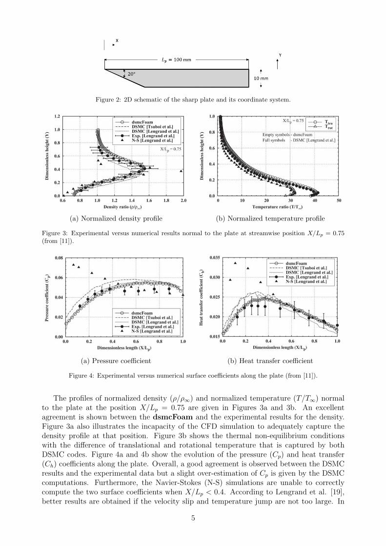
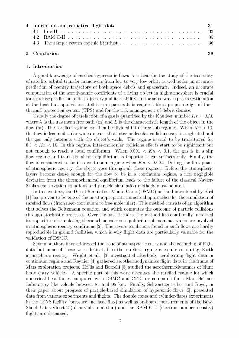
Figure 2: 2D schematic of the sharp plate and its coordinate system.

(a) Normalized density profile (b) Normalized temperature profile

Figure 3: Experimental versus numerical results normal to the plate at streamwise position X/Lp = 0.75(from [11]).

(a) Pressure coefficient (b) Heat transfer coefficient

Figure 4: Experimental versus numerical surface coefficients along the plate (from [11]).

The profiles of normalized density (ρ/ρ∞) and normalized temperature (T/T∞) normalto the plate at the position X/Lp = 0.75 are given in Figures 3a and 3b. An excellentagreement is shown between the dsmcFoam and the experimental results for the density.Figure 3a also illustrates the incapacity of the CFD simulation to adequately capture thedensity profile at that position. Figure 3b shows the thermal non-equilibrium conditionswith the difference of translational and rotational temperature that is captured by bothDSMC codes. Figure 4a and 4b show the evolution of the pressure (Cp) and heat transfer(Ch) coefficients along the plate. Overall, a good agreement is observed between the DSMCresults and the experimental data but a slight over-estimation of Cp is given by the DSMCcomputations. Furthermore, the Navier-Stokes (N-S) simulations are unable to correctlycompute the two surface coefficients when X/Lp < 0.4. According to Lengrand et al. [19],better results are obtained if the velocity slip and temperature jump are not too large. In

5

the conditions of study, this is not the case for the region X/Lp < 0.4. The nonequilibriumis too significant and cannot be properly modelled with such continuum approach.

Although this experiment is mostly used for validation purposes, such experiments havea larger scope of application. Gas-surface interaction models were assessed by Padilla [22],[23] with a similar flat plate experiment condutcted by Cecil and McDaniel [24]. In thiswork, the Boundary-layer profiles and surface-property distributions which were measuredby the experiment are compared with DSMC results obtained with Maxwell and Cercignani,Lampis and Lord (CLL) models. Results showed that both models lead to similar boundary-layer profiles and aerodynamic results for gas-surface accommodation between 50 and 100%.Moreover, a 90% gas-surface accommodation was found to produce the best agreement withthe velocity measurements but as stated by Padilla, additional study is required to assessthe models ability to retrieve heat transfer measurements.

2.3. Rarefied hypersonic flow over a 70◦ blunted cone

The AGARD working group and more specifically Moss and Lengrand [25] made a reviewof the experimental and numerical efforts carried out for the Mars Pathfinder which is a 70◦

blunted cone shaped probe. This report gathers data from experiments conducted in sixfacilities: the SR3 wind-tunnel in Meudon, the V2G-V3G-HEG of DLR-Gottingen and theLENS wind-tunnel at the University of Buffalo. Considering the experimental test conditionsof each facility, the focus is given to Allegre et al. experiments conducted in the SR3 wind-tunnel [26], [27], [28]. The experimental conditions are given in Table 1. Three freestreamconditions were generated in order to produce different levels of rarefaction and a probemodel presented in Figure 5 was used.

Case T0 (K) P0 (bar) M∞ Re∞/cm ρ∞ (kg/m3) U∞ (m/s) T∞ (K) λ∞ (mm) Gas1 1100 3.5 20.2 284 1.73× 10−5 1503 13.3 0.671 N2

2 1100 10 20 835 5.19× 10−5 1502 13.6 0.226 N2

3 1300 120 20.5 7235 46.62× 10−5 1634 15.3 0.027 N2

Table 1: Experimental test conditions of the SV3 wind-tunnel.

Similarly to what was done with the flat plate experiments, density measurements wereconducted with an electron beam and the wall temperature was kept around 290 K. For theaerodynamic forces measurements, an aluminum probe was used with a wall temperatureestimated around 350 K. Heat transfer measurements were made with a thin-wall techniqueon a steel probe whose wall temperature was kept at 300 K.

We performed several DSMC simulations with the DSMC code SPARTA for the freestreamconditions corresponding to the first case. The reference length (Lref) is equal to the cone ba-sis diameter which results in a Knudsen number Kn = 0.013. Once again, the flow is not en-ergetic enough to trigger the vibrational energy mode therefore, energy exchange between thetranslational and rotational mode only is activated and controlled by the Larsen-Borgnakkealgorithm [13]. The VHS collision model is used with a constant rotational number Zrot = 5.Two sets of simulations were completed with a varying angle of attack α ranging from 0to 30◦ and for each, the probe nose is placed at the origin of the simulation domain. Forthe first set, density contours and the heat transfer coefficient were computed with a walltemperature Tw = 290 K. For the case without incidence, an axi-symmetric simulation wasmade in a [xmin;xmax]× [ymin; ymax] = [−25; 125]× [0; 90] mm domain with a 750 by 450 meshand a time step ∆t = 1.3×10−7 s as prescribed by Klothakis and Nikolos [29]. For the caseswith incidence, a [xmin;xmax]× [ymin; ymax]× [zmin; zmax] = [−20; 80]× [−80; 80]× [0; 80] mmdomain was used with a symmetric boundary condition on the (x, y) plan. A uniform grid of250×250×100 cells was used and the adaptive mesh refinement algorithm of SPARTA was

6

Figure 5: Experimental probe instrumentation (Thermocouples) along the curvilinear abscissa S normalizedby the nose radius Rn (adapted from [27]). Dimensions in mm.

triggered in order to insure a cell size at least two times smaller than the local mean free pathin the simulation domain. For the second set of simulations, the aerodynamics forces werecomputed with a wall temperature of 350 K. The domain was kept the same for all angles ofattack. Thus, a [xmin;xmax]× [ymin; ymax]× [zmin; zmax] = [−20; 125]× [−80; 80]× [0; 80] mmdomain was used with a 360× 250× 100 initial grid and the same adaptive mesh refinementalgorithm. The aerodynamic forces were extracted from the nose up to 75 mm along thesting, according to the experimental conditions (Figure 5). For the axisymmetric simulation,the number of numerical particles was around 800 millions and for all the other simulations,this number was kept around one billion particles in order to ensure the presence of morethan 10 numerical particles per cell almost all over the domain.

Surface quantities were compared with Allegre’s experimental and Palharini’s numericaldata [11]. Figures 6a, 6b and 6c present respectively the aerodynamic coefficients of axial(CA) and normal (CN) forces as well as the pitching moment (Cm) coefficient whose momentreference point corresponds to the probe nose.

According to Allegre, the uncertainty on the measurement of the aerodynamic coefficientsis smaller than ±3%. An excellent agreement is visible between the DSMC and experimentalresults for the axial force coefficient (CA) with DSMC values in the interval of uncertainty.For the normal force coefficient (CN) the agreement is good overall but a non-negligibledeviation of 13% with SPARTA and a 8% with dsmcFoam is shown for α = 30◦. For bothcoefficients, the discrepancy increases with the angle of attack which inevitably impacts thepitching moment coefficient for which the numerical values deviation from the experimentalresults also increases with the angle of attack.

Figure 7 shows the heat transfer coefficient (Ch) for various angles of attack. The increasein α leads to the shifting of the stagnation point along the spherical part of the probe. Thus,on the lower surface, the stagnation point becomes closer to the attachment point of thesonic lines on the probe shoulder (Figure 8). Furthermore, the decrease of the boundarylayer thickness near the shoulder induces an increase of the heating peak in this region. Atthe conical trailing edge, the absence of sensor does not permit to experimentally retrieve theheat flux peak that is numerically predicted for the four angles of attack. Nonetheless, thediscrepancy between the DSMC and experimental results is significant for the closest sensor

7

(a) Axial force coefficient (b) Normal force coefficient

(c) Pitching moment coefficient

Figure 6: Comparison of the experimental and DSMC aerodynamic coefficients for various angles of attack.

to the trailing edge with differences from 6% to 24% according to the angle of attack. Thewall heat flux coefficient obtained by DSMC in the forebody region is in good accordance withthe experimental results for the 0 and 10 degrees angles of attack with mean discrepancieswithin ±10%, the range of estimated uncertainty [28]. However, the results in the forebodyregion show significant differences in the heat transfer coefficient of around 20 and 30%respectively for the 20 and 30 degree angles of attack. These differences can be due to thesimulation, the experiment or both. Moreover, because of the boundary layer separationnear the shoulder, the flow rapidly expands and the flow trapped under the shear layerforms a recirculation zone immediately behind the probe (Figure 8). In DSMC, ensuring asufficient number of numerical particles to reduce the statistical noise in such area requiresto simulate a great amount of particles which can be computationally expensive. Froman experimental perspective, the instrumentation is likely to reach its sensitivity limit insuch conditions. Consequently, the complexity of the flow in the wake region might notbe adequately captured numerically and experimentally [11]. The experimental uncertaintyis much higher in this region than in the front area of the probe. Finally, the differencesbetween the DSMC results come from the different mesh refinement and particle numbersthat were used. The SPARTA results show the capacity of DSMC to retrieve numericalmeasurements in the wake closure region if a sufficient number of numerical particles issimulated but significant discrepancies are still observed in the recirculation zone.

The double cones and cylinder flares [30], [31], [32] are two other common experimentsthat were mentioned in the introduction. The results are not discussed here because like forthe other experiments, the numerical and experimental values are in very good agreement in

8

(a) α = 0◦ (b) α = 10◦

(c) α = 20◦ (d) α = 30◦

Figure 7: Comparison of DSMC and experimental heat transfer coefficients (Ch) for different angles ofattack.

Figure 8: Illustration of the flow structure around the sphere-cone (adapted from [11]).

general and the flow is not energetic enough to trigger the vibrational mode nor any reactiveprocess.

To summarize the results of this part, many experiments were conducted in low-densityfacilities and were used for numerical comparison and validation. Experiments on flat plateshave been addressed as well as experiment on a 70◦ blunted cone. For the sharp leadingedge flat plate, significant differences between DSMC and CFD results have also been ob-served and showed the difficulty of CFD codes to retrieve experimental flowfield and surfacequantities even with slip and jump boundary conditions. The 70◦ blunted cone brings to

9

play complex mechanisms and the heat transfer coefficient in the front area of the cone hasproved to be hard to reproduce for angles of attack greater than 10◦. This indicates thateven in the absence of vibrational and reactive effects, the reproduction of surface quantitiescan be a challenging task and elementary DSMC models such as Gas-Surface interactionand translational-rotational energy exchange models call for improvements.

3. Aerothermodynamic flight data

The space race started with the cold war was a turning point for space exploration. Fromthe first human spaceflight program Mercury started in 1958 up to the successful landing ofthe first humans on the moon in 1969, a lot of effort were carried out for the prediction ofaerothermodynamic (ATD) coefficients. Although the most severe heat loads occur at lowaltitudes (between 40 and 60 km), depending on the entry velocity and the vehicle’s size,non negligible heat fluxes can be observed in the upper layers of the atmosphere. Since theentry point often coincides with an altitude close to 120 km, on-board measurement devicessometimes provide high altitude values that can be compared to DSMC simulations. Thefocus of this part is given to the study and exploitation of such ATD flight data.

On ground, afterbody aeroheating is particularly challenging to evaluate. Indeed, testfacilities usually use stings to maintain geometries position inside the wind-tunnel which canlead to interference effects. As a consequence, afterbody flight data are a very valuable sourceof validation data. So far, only a few afterbody aeroheating flight data are available andthe majority comes from 60s flights, like from the Mercury and Apollo programs. They canstill be used for validation purposes, especially since uncertainties in afterbody aeroheatingpredictions obtained with numerical tools stay quite large.

3.1. The Mercury Project

The Mercury project ran from 1958 up to 1963 and its objective was to send a man intoEarth orbit before returning him safely. The search for an appropriate design capable ofensuring the integrity of the structure and the survivability of the crew was a major prioritywhich led to several flight tests and experiments.

At the beginning of the program, a Mercury prototype capsule protected by a fiberglass-phenolic ablative heatshield was launched in 1959. For this flight which was nicknamed Big-Joe, the forebody and the afterbody were equipped with many sensors and thermocouples(TC). However, because of significant angle of attack oscillations, the data are not usablefor validation studies [3]. Following the first experiment, four Mercury-Atlas (MA) vehicles(Fig. 9) were launched in the entry conditions summarized in Table 2. In February 1961,the MA-2 made a reentry with an apogee of 185 km and a range of 1257 km. In November1961, the Ma-5 flight completed two orbits followed by the MA-7 manned 3 orbit missionlaunched in May 1962. Finally in October 1961, the MA-8 manned 6 orbit mission waslaunched with virtually identical altitude and velocity histories as those of MA-5 [33].

Flight Id. Entry date Afterbody TC number U∞ (km/s) α (deg.) γ (deg.)MA-2 21 Feb. 1961 17 5.5 12.5 -MA-5 29 Nov. 1961 9 7.4 0 -1MA-7 24 May 1962 12 7.4 0 -1MA-8 3 Oct. 1962 16 7.4 0 -1

Table 2: Entry flight conditions and instrumentation of the four Mercury-Atlas (MA) vehicles (adapted from[3], [33]).

10

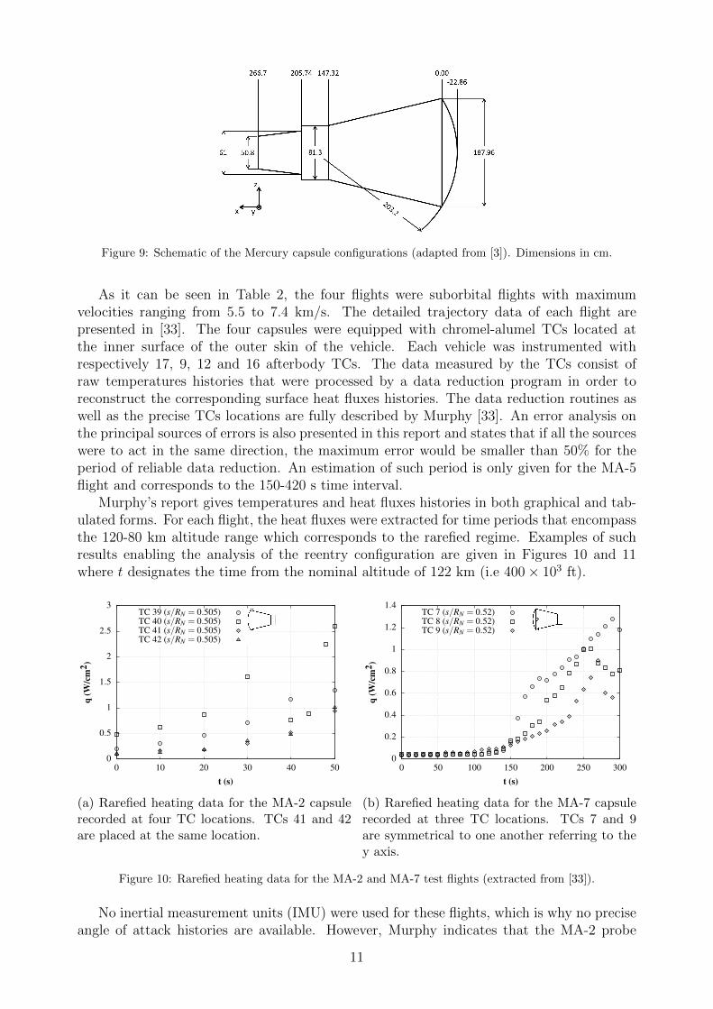
Figure 9: Schematic of the Mercury capsule configurations (adapted from [3]). Dimensions in cm.

As it can be seen in Table 2, the four flights were suborbital flights with maximumvelocities ranging from 5.5 to 7.4 km/s. The detailed trajectory data of each flight arepresented in [33]. The four capsules were equipped with chromel-alumel TCs located atthe inner surface of the outer skin of the vehicle. Each vehicle was instrumented withrespectively 17, 9, 12 and 16 afterbody TCs. The data measured by the TCs consist ofraw temperatures histories that were processed by a data reduction program in order toreconstruct the corresponding surface heat fluxes histories. The data reduction routines aswell as the precise TCs locations are fully described by Murphy [33]. An error analysis onthe principal sources of errors is also presented in this report and states that if all the sourceswere to act in the same direction, the maximum error would be smaller than 50% for theperiod of reliable data reduction. An estimation of such period is only given for the MA-5flight and corresponds to the 150-420 s time interval.

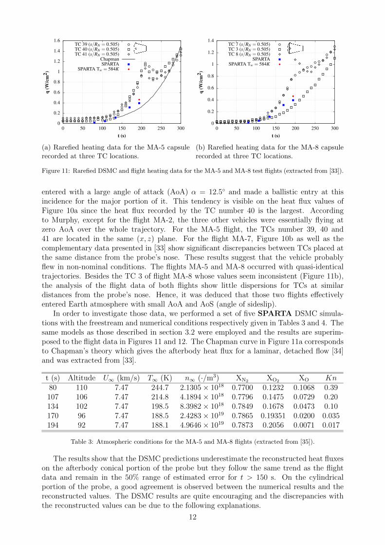
Murphy’s report gives temperatures and heat fluxes histories in both graphical and tab-ulated forms. For each flight, the heat fluxes were extracted for time periods that encompassthe 120-80 km altitude range which corresponds to the rarefied regime. Examples of suchresults enabling the analysis of the reentry configuration are given in Figures 10 and 11where t designates the time from the nominal altitude of 122 km (i.e 400× 103 ft).

0

0.5

1

1.5

2

2.5

3

0 10 20 30 40 50

q(W

/cm

2 )

t (s)

TC 39 (s/RN = 0.505)TC 40 (s/RN = 0.505)TC 41 (s/RN = 0.505)TC 42 (s/RN = 0.505)

(a) Rarefied heating data for the MA-2 capsulerecorded at four TC locations. TCs 41 and 42are placed at the same location.

0

0.2

0.4

0.6

0.8

1

1.2

1.4

0 50 100 150 200 250 300

q(W

/cm

2 )

t (s)

TC 7 (s/RN = 0.52)TC 8 (s/RN = 0.52)TC 9 (s/RN = 0.52)

(b) Rarefied heating data for the MA-7 capsulerecorded at three TC locations. TCs 7 and 9are symmetrical to one another referring to they axis.

Figure 10: Rarefied heating data for the MA-2 and MA-7 test flights (extracted from [33]).

No inertial measurement units (IMU) were used for these flights, which is why no preciseangle of attack histories are available. However, Murphy indicates that the MA-2 probe

11

0

0.2

0.4

0.6

0.8

1

1.2

1.4

1.6

0 50 100 150 200 250 300

q(W

/cm

2 )

t (s)


ChapmanSPARTA

SPARTA Tw = 584K

(a) Rarefied heating data for the MA-5 capsulerecorded at three TC locations.

0

0.2

0.4

0.6

0.8

1

1.2

1.4

0 50 100 150 200 250 300

q(W

/cm

2 )

t (s)


SPARTASPARTA Tw = 584K

(b) Rarefied heating data for the MA-8 capsulerecorded at three TC locations.

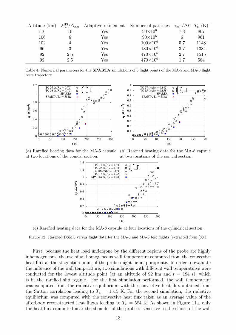
Figure 11: Rarefied DSMC and flight heating data for the MA-5 and MA-8 test flights (extracted from [33]).

entered with a large angle of attack (AoA) α = 12.5◦ and made a ballistic entry at thisincidence for the major portion of it. This tendency is visible on the heat flux values ofFigure 10a since the heat flux recorded by the TC number 40 is the largest. Accordingto Murphy, except for the flight MA-2, the three other vehicles were essentially flying atzero AoA over the whole trajectory. For the MA-5 flight, the TCs number 39, 40 and41 are located in the same (x, z) plane. For the flight MA-7, Figure 10b as well as thecomplementary data presented in [33] show significant discrepancies between TCs placed atthe same distance from the probe’s nose. These results suggest that the vehicle probablyflew in non-nominal conditions. The flights MA-5 and MA-8 occurred with quasi-identicaltrajectories. Besides the TC 3 of flight MA-8 whose values seem inconsistent (Figure 11b),the analysis of the flight data of both flights show little dispersions for TCs at similardistances from the probe’s nose. Hence, it was deduced that those two flights effectivelyentered Earth atmosphere with small AoA and AoS (angle of sideslip).

In order to investigate those data, we performed a set of five SPARTA DSMC simula-tions with the freestream and numerical conditions respectively given in Tables 3 and 4. Thesame models as those described in section 3.2 were employed and the results are superim-posed to the flight data in Figures 11 and 12. The Chapman curve in Figure 11a correspondsto Chapman’s theory which gives the afterbody heat flux for a laminar, detached flow [34]and was extracted from [33].

t (s) Altitude U∞ (km/s) T∞ (K) n∞ (·/m3) XN2 XO2 XO Kn80 110 7.47 244.7 2.1305× 1018 0.7700 0.1232 0.1068 0.39107 106 7.47 214.8 4.1894× 1018 0.7796 0.1475 0.0729 0.20134 102 7.47 198.5 8.3982× 1018 0.7849 0.1678 0.0473 0.10170 96 7.47 188.5 2.4283× 1019 0.7865 0.19351 0.0200 0.035194 92 7.47 188.1 4.9646× 1019 0.7873 0.2056 0.0071 0.017

Table 3: Atmospheric conditions for the MA-5 and MA-8 flights (extracted from [35]).

The results show that the DSMC predictions underestimate the reconstructed heat fluxeson the afterbody conical portion of the probe but they follow the same trend as the flightdata and remain in the 50% range of estimated error for t > 150 s. On the cylindricalportion of the probe, a good agreement is observed between the numerical results and thereconstructed values. The DSMC results are quite encouraging and the discrepancies withthe reconstructed values can be due to the following explanations.

12

Altitude (km) λHS∞ /∆x,y Adaptive refinement Number of particles τcoll/∆t Tw (K)

110 10 Yes 90×106 7.3 807106 6 Yes 90×106 6 961102 4 Yes 100×106 5.7 114896 3 Yes 180×106 3.7 138492 2.5 Yes 470×106 2.7 151592 2.5 Yes 470×106 1.7 584

Table 4: Numerical parameters for the SPARTA simulations of 5 flight points of the MA-5 and MA-8 flighttests trajectory.

0

0.2

0.4

0.6

0.8

1

1.2

0 50 100 150 200 250 300

q(W

/cm

2 )

t (s)

TC 35 (s/RN = 0.76)TC 38 (s/RN = 0.76)


(a) Rarefied heating data for the MA-5 capsuleat two locations of the conical section.

0

0.1

0.2

0.3

0.4

0.5

0.6

0.7

0.8

0.9

1

0 50 100 150 200 250 300

q(W

/cm

2 )

t (s)

TC 27 (s/RN = 0.842)TC 15 (s/RN = 0.858)


(b) Rarefied heating data for the MA-8 capsuleat two locations of the conical section.

0

0.2

0.4

0.6

0.8

1

1.2

1.4

0 50 100 150 200 250 300

q(W

/cm

2 )

t (s)

TC 12 (s/RN = 1.41)TC 26 (s/RN = 1.41)

TC 20 (s/RN = 1.471)TC 13 (s/RN = 1.35)

SPARTA (s/RN = 1.41)

(c) Rarefied heating data for the MA-8 capsule at four locations of the cylindrical section.

Figure 12: Rarefied DSMC versus flight data for the MA-5 and MA-8 test flights (extracted from [33]).

First, because the heat load undergone by the different regions of the probe are highlyinhomogeneous, the use of an homogeneous wall temperature computed from the convectiveheat flux at the stagnation point of the probe might be inappropriate. In order to evaluatethe influence of the wall temperature, two simulations with different wall temperatures wereconducted for the lowest altitude point (at an altitude of 92 km and t = 194 s), whichis in the rarefied slip regime. For the first simulation performed, the wall temperaturewas computed from the radiative equilibrium with the convective heat flux obtained fromthe Sutton correlation leading to Tw = 1515 K. For the second simulation, the radiativeequilibrium was computed with the convective heat flux taken as an average value of theafterbody reconstructed heat fluxes leading to Tw = 584 K. As shown in Figure 11a, onlythe heat flux computed near the shoulder of the probe is sensitive to the choice of the wall

13

temperature. The influence of the wall temperature seems to decrease when the distance withthe stagnation point increases, as illustrated by Figures 11a and 12a, at t = 194 s. Indeed,the relative discrepancy between the wall heat flux obtained with the two temperaturesis around 17% near the shoulder and 5% in the middle of the conical section. The idealboundary condition would be to use :

1. For the forebody : a wall temperature computed from a radiative equilibrium

2. For the afterbody : a temperature distribution interpolated from the temperaturemeasurements reported by Murphy

However, even if the use of a wall temperature distribution would locally give results closerto the experimental measurements, the results presented herein suggest that the differencebetween the DSMC and the experimental results at t = 194 s would remain significant andthat the effect of the wall temperature cannot be considered as the major source for thisdiscrepancy.

Another possible source of divergence comes from the fact that the two flights did notoccur on the same date. This indicates that atmospheric fluctuations may have significantlyinfluenced the TCs measurements and could explain the slight differences in amplitudebetween the two flight data. Since the simulations are based on the Jacchia model which isan averaged atmospheric model, such fluctuations cannot be captured by our computations.

In the same way, the fact that the vehicles were not carrying on board IMU impliesthat only the theoretical trajectory is known. This means that significant deviations fromthe nominal trajectory could have occurred without being noticed which also raises theuncertainty on the freestream conditions we used.

Finally, an additional limitation stems from the data reduction procedure which assumedthat the afterbody outer skin was thin enough to be neglected. This assumption enables tocompute the heat fluxes from the TCs temperature in a direct fashion whereas an inversemethod taking into account the TPS thickness would have been more precise. Contrary toMercury, the Apollo AS-202 module was carrying an IMU and was equipped with calorime-ters, the flight data are then free from such concerns.

3.2. The Apollo Program

Following President Kennedy’s speech expressing America’s objective of landing a manon the Moon before the end of the 60’s decade, two new space projects were launched. TheGemini and the Apollo programs started respectively in 1963 and 1961. The accumulatedtechniques and knowledge during the previous projects and the Flight Investigation of Re-Entry (FIRE) research program finally led to the Apollo Command Module (CM) illustratedin Figure 13.

In order to evaluate the module heat-shield, a series of test flights were conducted between1966 and 1968 (Table 5). One of these flights objectives was to evaluate the capacity ofanalytical models combining wind-tunnel experiments and theoretical models to predictthermal solicitations acting on the vehicle [36]. Another objective was to evaluate thethermal protection system (STS) performance [37]. The test flight trajectories are given in[36].

With the improvements of measurement techniques a large quantity of data were collectedduring these flights (pressure, convective and radiative heat fluxes . . .). Moreover, among thefour test flights, the AS-201 module was the only one which was not equipped with an IMU.However, Apollo flight data were only used and published for CFD-code validation purposes,50 years later, by Wright et al. [38] and Walpot et al. [39]. In DSMC, the simulation ofthe aerodynamic coefficients of the Apollo 6 command module was first completed by Moss[40], [41]. It then became a numerical validation case [42], [43], [44] but no aerodynamic

14

(a) AS-202 command module before flight. (b) Apollo 6 command module after flight (Fern-bank Science Center Atlanta).

Figure 13: Pictures of two Apollo test modules before and after atmospheric reentry (credits: NASA).

Flight Id. (date) Velocity (km/s) α (deg.) γ (deg.) Max. decel. (g) qthmax (W/m2)

AS-201 (02/26/1966) 7.67 20 -8.6 14.3 186AS-202 (08/25/1966) 8.29 18 -3.5 2.4 91

Apollo 4 (11/09/1967) 10.73 25 -5.9 4.6 237Apollo 6 (04/04/1968) 9.6 25 -6.9 7.3 488

α, γ and qthmax respectively denote the angle of attack, the flight path angle and the maximal theoretical heat flux.

Table 5: Reentry flight parameters of the Apollo flight tests (adapted from [38]).

flight data are available for this case of study which stays purely numerical. In fact, for mostof these flights, the lack of trajectory data, the sensors malfunction or the high velocitiesprevent the data exploitation for the rarefied portion of the reentry.

In the present paper, the decision was made to numerically compare SPARTA withother codes for the Apollo 6 test case. Then, the Apollo AS-202 flight experiment wassimulated and the results were compared with available flight data.

3.2.1. Apollo 6: Aerodynamic coefficients simulation

In 2005, NASA presented its new vision of habited space exploration vehicle based ona new generation of Crew Exploration Vehicle (CEV). Different versions were consideredin order to be usable for different tasks such as supplying the International Space Station(ISS) as well as being used for Moon and Mars exploration. The new generation of CEVis based on the Apollo design and efforts were directed towards the construction of ATDdatabase [40]. In this context, Moss worked on the simulation of aerodynamic coefficientsof the Apollo command module in the flight conditions of Apollo 6 [40], [41].

Our DSMC simulations were made with SPARTA in the same conditions as those de-scribed in Moss’ paper [40]. The objective is to simulate the reentry of the Apollo 6 commandmodule (Fig. 14a) between 200 and 65 km. In Moss’ work, the rarefied portion of the trajec-tory (between 200 and 85 km) was simulated with the DSMC code DS3V [45]. The DSMCparameters were taken as follows. Energy exchanges are permitted between the transla-tional mode and the rotational and vibrational modes according to the Larsen-Borgnakkemodel [13]. The rotational number was taken constant Zrot = 5 and the vibrational numberwas modeled with the Millikan-White model [46]. Non-catalytic walls were supposed with

15

constant temperature (Tw) computed by Moss [40]. Maxwell’s gas-surface interaction withcomplete thermal accommodation and a 5 species air model were used. Chemical reactionswere considered with the Total Collision Energy (TCE) model [1] and Park’s reaction ratecoefficients [47]. For the continuum portion of the trajectory, CFD simulations were madeby Moss with LAURA [48], [49].

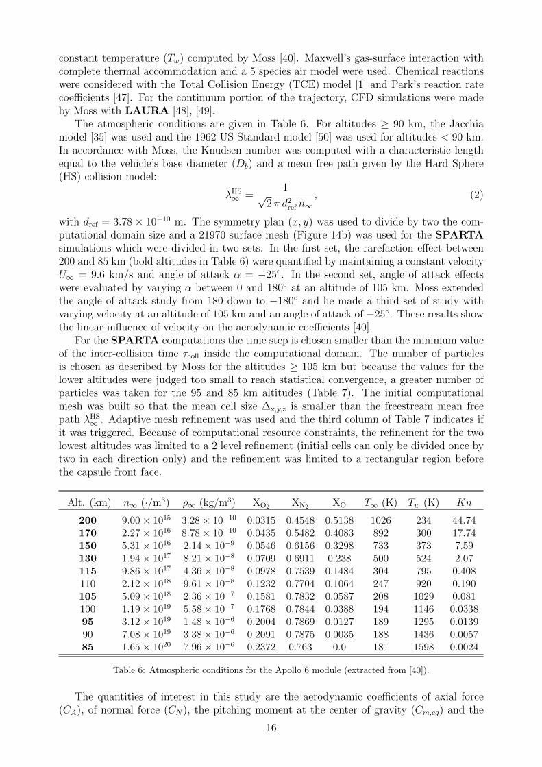
The atmospheric conditions are given in Table 6. For altitudes ≥ 90 km, the Jacchiamodel [35] was used and the 1962 US Standard model [50] was used for altitudes < 90 km.In accordance with Moss, the Knudsen number was computed with a characteristic lengthequal to the vehicle’s base diameter (Db) and a mean free path given by the Hard Sphere(HS) collision model:

λHS∞ =

1√2π d2

ref n∞, (2)

with dref = 3.78 × 10−10 m. The symmetry plan (x, y) was used to divide by two the com-putational domain size and a 21970 surface mesh (Figure 14b) was used for the SPARTAsimulations which were divided in two sets. In the first set, the rarefaction effect between200 and 85 km (bold altitudes in Table 6) were quantified by maintaining a constant velocityU∞ = 9.6 km/s and angle of attack α = −25◦. In the second set, angle of attack effectswere evaluated by varying α between 0 and 180◦ at an altitude of 105 km. Moss extendedthe angle of attack study from 180 down to −180◦ and he made a third set of study withvarying velocity at an altitude of 105 km and an angle of attack of −25◦. These results showthe linear influence of velocity on the aerodynamic coefficients [40].

For the SPARTA computations the time step is chosen smaller than the minimum valueof the inter-collision time τcoll inside the computational domain. The number of particlesis chosen as described by Moss for the altitudes ≥ 105 km but because the values for thelower altitudes were judged too small to reach statistical convergence, a greater number ofparticles was taken for the 95 and 85 km altitudes (Table 7). The initial computationalmesh was built so that the mean cell size ∆x,y,z is smaller than the freestream mean freepath λHS

∞ . Adaptive mesh refinement was used and the third column of Table 7 indicates ifit was triggered. Because of computational resource constraints, the refinement for the twolowest altitudes was limited to a 2 level refinement (initial cells can only be divided once bytwo in each direction only) and the refinement was limited to a rectangular region beforethe capsule front face.

Alt. (km) n∞ (·/m3) ρ∞ (kg/m3) XO2 XN2 XO T∞ (K) Tw (K) Kn

200 9.00× 1015 3.28× 10−10 0.0315 0.4548 0.5138 1026 234 44.74170 2.27× 1016 8.78× 10−10 0.0435 0.5482 0.4083 892 300 17.74150 5.31× 1016 2.14× 10−9 0.0546 0.6156 0.3298 733 373 7.59130 1.94× 1017 8.21× 10−8 0.0709 0.6911 0.238 500 524 2.07115 9.86× 1017 4.36× 10−8 0.0978 0.7539 0.1484 304 795 0.408110 2.12× 1018 9.61× 10−8 0.1232 0.7704 0.1064 247 920 0.190105 5.09× 1018 2.36× 10−7 0.1581 0.7832 0.0587 208 1029 0.081100 1.19× 1019 5.58× 10−7 0.1768 0.7844 0.0388 194 1146 0.033895 3.12× 1019 1.48× 10−6 0.2004 0.7869 0.0127 189 1295 0.013990 7.08× 1019 3.38× 10−6 0.2091 0.7875 0.0035 188 1436 0.005785 1.65× 1020 7.96× 10−6 0.2372 0.763 0.0 181 1598 0.0024

Table 6: Atmospheric conditions for the Apollo 6 module (extracted from [40]).

The quantities of interest in this study are the aerodynamic coefficients of axial force(CA), of normal force (CN), the pitching moment at the center of gravity (Cm,cg) and the

16

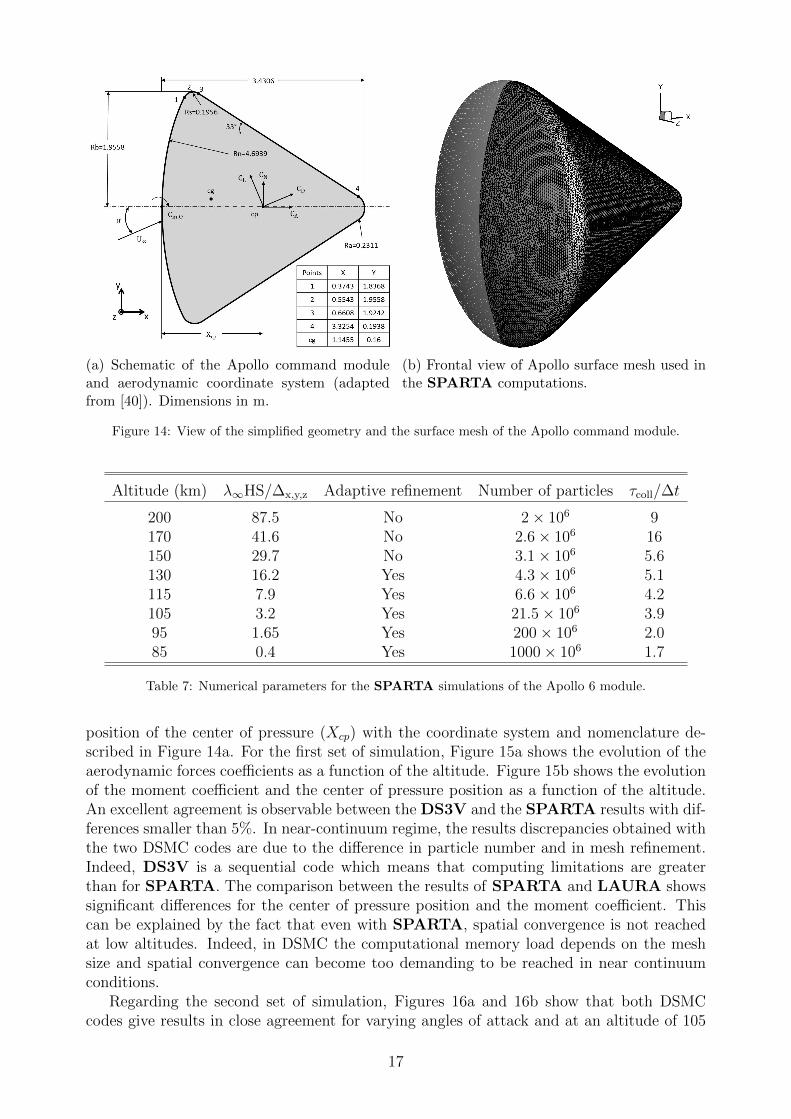
(a) Schematic of the Apollo command moduleand aerodynamic coordinate system (adaptedfrom [40]). Dimensions in m.

(b) Frontal view of Apollo surface mesh used inthe SPARTA computations.

Figure 14: View of the simplified geometry and the surface mesh of the Apollo command module.

Altitude (km) λ∞HS/∆x,y,z Adaptive refinement Number of particles τcoll/∆t

200 87.5 No 2× 106 9170 41.6 No 2.6× 106 16150 29.7 No 3.1× 106 5.6130 16.2 Yes 4.3× 106 5.1115 7.9 Yes 6.6× 106 4.2105 3.2 Yes 21.5× 106 3.995 1.65 Yes 200× 106 2.085 0.4 Yes 1000× 106 1.7

Table 7: Numerical parameters for the SPARTA simulations of the Apollo 6 module.

position of the center of pressure (Xcp) with the coordinate system and nomenclature de-scribed in Figure 14a. For the first set of simulation, Figure 15a shows the evolution of theaerodynamic forces coefficients as a function of the altitude. Figure 15b shows the evolutionof the moment coefficient and the center of pressure position as a function of the altitude.An excellent agreement is observable between the DS3V and the SPARTA results with dif-ferences smaller than 5%. In near-continuum regime, the results discrepancies obtained withthe two DSMC codes are due to the difference in particle number and in mesh refinement.Indeed, DS3V is a sequential code which means that computing limitations are greaterthan for SPARTA. The comparison between the results of SPARTA and LAURA showssignificant differences for the center of pressure position and the moment coefficient. Thiscan be explained by the fact that even with SPARTA, spatial convergence is not reachedat low altitudes. Indeed, in DSMC the computational memory load depends on the meshsize and spatial convergence can become too demanding to be reached in near continuumconditions.

Regarding the second set of simulation, Figures 16a and 16b show that both DSMCcodes give results in close agreement for varying angles of attack and at an altitude of 105

17

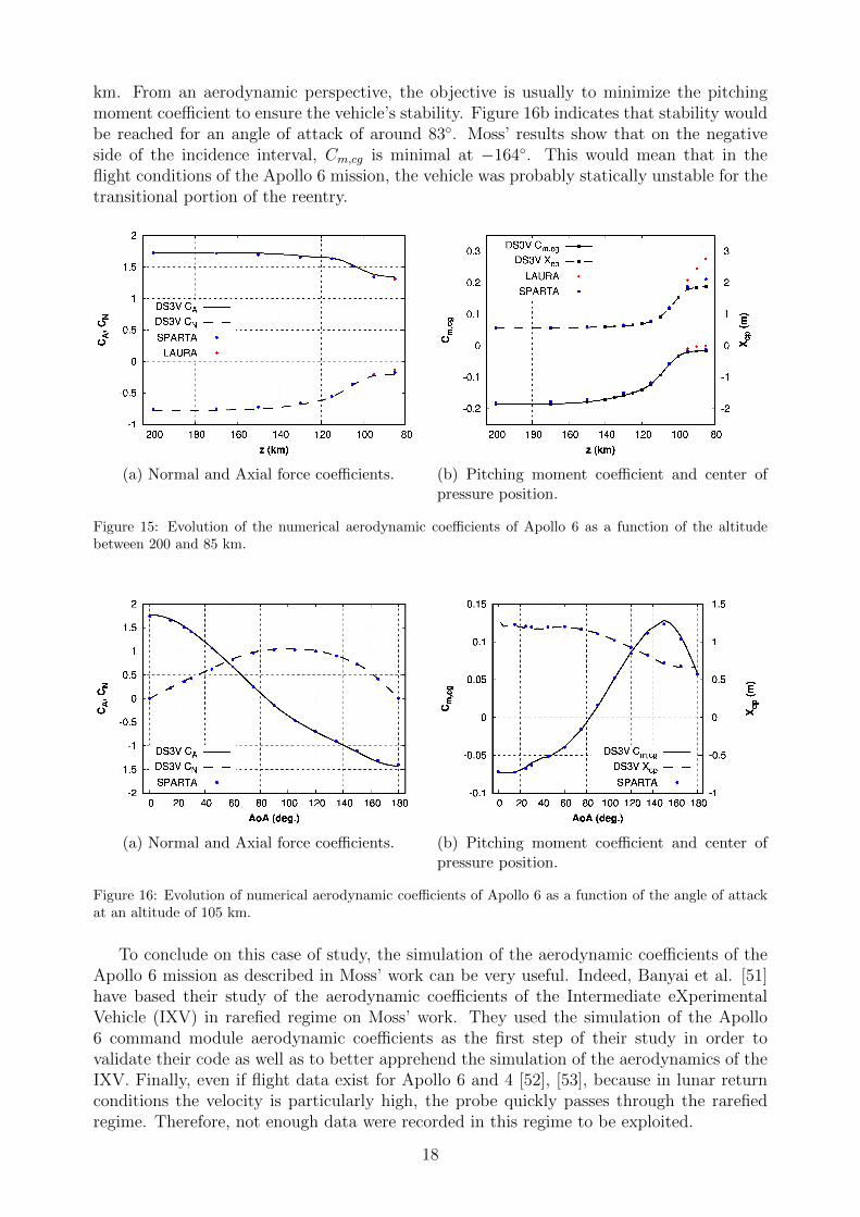
km. From an aerodynamic perspective, the objective is usually to minimize the pitchingmoment coefficient to ensure the vehicle’s stability. Figure 16b indicates that stability wouldbe reached for an angle of attack of around 83◦. Moss’ results show that on the negativeside of the incidence interval, Cm,cg is minimal at −164◦. This would mean that in theflight conditions of the Apollo 6 mission, the vehicle was probably statically unstable for thetransitional portion of the reentry.

(a) Normal and Axial force coefficients. (b) Pitching moment coefficient and center ofpressure position.

Figure 15: Evolution of the numerical aerodynamic coefficients of Apollo 6 as a function of the altitudebetween 200 and 85 km.

(a) Normal and Axial force coefficients. (b) Pitching moment coefficient and center ofpressure position.

Figure 16: Evolution of numerical aerodynamic coefficients of Apollo 6 as a function of the angle of attackat an altitude of 105 km.

To conclude on this case of study, the simulation of the aerodynamic coefficients of theApollo 6 mission as described in Moss’ work can be very useful. Indeed, Banyai et al. [51]have based their study of the aerodynamic coefficients of the Intermediate eXperimentalVehicle (IXV) in rarefied regime on Moss’ work. They used the simulation of the Apollo6 command module aerodynamic coefficients as the first step of their study in order tovalidate their code as well as to better apprehend the simulation of the aerodynamics of theIXV. Finally, even if flight data exist for Apollo 6 and 4 [52], [53], because in lunar returnconditions the velocity is particularly high, the probe quickly passes through the rarefiedregime. Therefore, not enough data were recorded in this regime to be exploited.

18

3.2.2. Apollo AS-202: Afterbody heat flux simulation

In this section, the focus is given to the flight Apollo AS-202 which is particularly inter-esting for several reasons. The AS-202 command module was the first Apollo test vehiclecarrying an IMU which means that precise trajectory data (angle of attack, sideslip angle,etc) are available. Moreover, because afterflight observations evidenced little charring dur-ing the AS-202 entry [38] and given the freestream conditions (velocity and density) of thetransitional portion, all ablative phenomena were assumed negligible in our analysis.

The AS-202 command module is represented in Figure 13a. It was made of a stain-less steel structure covered with Avcoat 5026/39G TPS, an ablator described in [3], [38].The module forebody was instrumented with 12 pressure transducers and 12 calorime-ters. Among the pressure transducers, 10 transducers provided usable data but none ofthe calorimeters. 24 pressure transducers and 23 calorimeters were placed on the afterbody.Only two pressure sensors recorded data just before the parachute opening. Unfortunately,all the pressure measurements correspond to the continuum regime only [54] and the forcemeasured during the low deceleration level phase which encompasses the rarefied portionhave uncertainties too high to be usable [55]. Among the afterbody calorimeters, 19 workedcorrectly (Figure 17). The precise positions of the calorimeters which take into account thethickness of the heatshield are given by Wright et al. [38] and were used in this study.

Figure 17: Calorimeters positions on the AS-202 afterbody. White symbols stand for non-working calorime-ters (adapted from [38]).

The calorimeters are Gardon gauges described in [56] and designed to measure heat fluxsmaller than 58 W/cm2. According to Wright et al., the gauges uncertainty is ±20% in theflight conditions considered. The NASA technical report does not give other uncertaintyestimation so the same assumption was made.

Hillje’s report [55] gives the history of the mission aerodynamic quantities which wasused to obtain the angle of attack α and the sideslip angle β. The references [38], [39] wereused to extract the velocity and altitude as a function of time. The flight data presented in[54] were extracted from Wright’s paper [38] and the study was limited to the time periodbetween the entry point and around t = 4500 s. Hence, a total of 6 flight points evenlyspaced by 5 km were simulated. The flight parameters are summarized in Table 8.

The values show that the angle of attack ranges from 19 to 25◦ and the sideslip angleoscillates between −1.5 and 3.5◦ with maximum values for 105 and 85 km. To take intoaccount the sideslip angle, no symmetry plane can be used which means that the compu-tational resources must be multiplied by a factor of two to keep the same precision as forthe Apollo 6 simulations. Moreover, for the 85 km altitude (Kn = 2.4× 10−3) which corre-

19

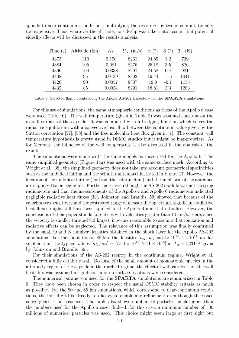
sponds to near-continuum conditions, multiplying the resources by two is computationallytoo expensive. Thus, whatever the altitude, no sideslip was taken into account but potentialsideslip effects will be discussed in the results analysis.

Time (s) Altitude (km) Kn U∞ (m/s) α (◦) β (◦) Tw (K)

4373 110 0.190 8261 24.85 1.2 7394384 105 0.081 8276 25.18 3.5 8264396 100 0.0338 8291 24.58 0.4 9214408 95 0.0139 8302 19.44 -1.5 10414420 90 0.0057 8307 19.9 -0.1 11554432 85 0.0024 8291 18.81 2.3 1283

Table 8: Selected flight points along the Apollo AS-202 trajectory for the SPARTA simulations.

For this set of simulations, the same atmospheric conditions as those of the Apollo 6 casewere used (Table 6). The wall temperature (given in Table 8) was assumed constant on theoverall surface of the capsule. It was computed with a bridging function which solves theradiative equilibrium with a convective heat flux between the continuum value given by theSutton correlation [57], [58] and the free molecular heat flux given in [1]. The constant walltemperature hypothesis is pretty usual in DSMC studies but it might be inappropriate. Asfor Mercury, the influence of the wall temperature is also discussed in the analysis of theresults.

The simulations were made with the same models as those used for the Apollo 6. Thesame simplified geometry (Figure 14a) was used with the same surface mesh. According toWright et al. [38], the simplified geometry does not take into account geometrical specificitiessuch as the umbilical fairing and the scimitar antennas illustrated in Figure 17. However, thelocation of the umbilical fairing (far from the calorimeters) and the small size of the antennasare supposed to be negligible. Furthermore, even though the AS-202 module was not carryingradiometers and that the measurements of the Apollo 4 and Apollo 6 radiometers indicatednegligible radiative heat fluxes [38], Johnston and Brandis [59] showed that because of thecalorimeters sensitivity and the restricted range of measurable spectrum, significant radiativeheat fluxes might still have been applied to the Apollo 4 and 6 afterbodies. However, theconclusions of their paper stands for entries with velocities greater than 10 km/s. Here, sincethe velocity is smaller (around 8.3 km/s), it seems reasonable to assume that ionization andradiative effects can be neglected. The relevance of this assumption was finally confirmedby the small O and N number densities obtained in the shock layer for the Apollo AS-202simulations. For the simulation at 85 km, the densities [nN , nO] = [2×1014, 1×1014] are farsmaller than the typical values [nN , nO] = [7.50 × 1015, 2.11 × 1015] at Ttr = 5231 K givenby Johnston and Brandis [59].

For their simulations of the AS-202 reentry in the continuum regime, Wright et al.considered a fully catalytic wall. Because of the small amount of monoatomic species in theafterbody region of the capsule in the rarefied regime, the effect of wall catalysis on the wallheat flux was assumed insignificant and no surface reactions were considered.

The numerical parameters used for the SPARTA simulations are summarized in Table9. They have been chosen in order to respect the usual DSMC stability criteria as muchas possible. For the 90 and 85 km simulations, which correspond to near-continuum condi-tions, the initial grid is already too heavy to enable any refinement even though the spaceconvergence is not reached. The table also shows numbers of particles much higher thanthe numbers used for the Apollo 6 case. Indeed, for this case, a minimum number of 500millions of numerical particles was used. This choice might seem large at first sight but

20

Altitude (km) λHS∞ /∆x,y,z Adaptive refinement Number of particles τcoll/∆t

110 3.7 Yes 500× 106 9.3105 3.2 Yes 500× 106 4.7100 2 Yes 500× 106 3.395 2 Yes 990× 106 2.290 1 No 1000× 106 2.485 0.6 No 1000× 106 1.5

Table 9: Numerical parameters for the SPARTA simulations of the flight points of the Apollo AS-202trajectory.

contrary to the Apollo 6 case, the objective of these simulations is to compute heat fluxeson the afterbody. Preliminary simulations have shown that the statistic sensitivity of theafterbody heat fluxes is radically more significant than the sensitivity of the aerodynamiccoefficients. Such numbers of particles minimize the statistical noise by ensuring a numberof particles per cell greater than 15 everywhere in the domain and even in the afterbodyarea.

The observation of the streamlines showed that the flow remains attached to the probedown to 95 km and detaches itself between 95 and 90 km. Examples of attached anddetached streamlines are illustrated in Figure 18. For the considered altitudes, the Reynoldsnumber of the lowest point is smaller than 3 × 104. As suggested by Wrigth et al. [38], noturbulent effects are expected for such values.

(a) Altitude of 100 km, M∞ = 29.7, Kn =0.0338 and Re = 1.3× 103.

(b) Altitude of 85 km, M∞ = 30.7, Kn = 0.0024and Re = 1.9× 104.

Figure 18: DSMC computed nondimensional temperature field and streamlines at 100 and 85 km duringthe reentry of the AS-202 module.

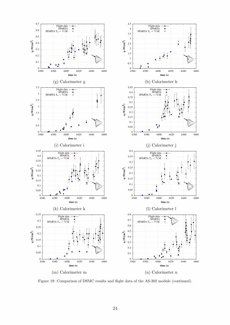
The heat fluxes are presented in Figure 19. These results show that for the calorimeterslocated on the windside, where the heat fluxes are the more severe, a good agreement isobserved. More generally, for 14 of the 19 calorimeters, the numerical results are in the±20% confidence interval. The five calorimeters which show the biggest differences arethe e, s, m, n and i calorimeters. The calorimeter e is particular in that it is located

21

at the top of the apex. This means that the discrepancies between the results could bedue to the geometrical differences between the actual geometry and the way the apex wassimplified. The calorimeter s is located on the leeward of the capsule and is symmetric tod located on the windward. However, both calorimeters recorded heat fluxes of the sameorder of magnitude. This observation also stands for the calorimeter n symmetric to f. Inthe same way, the heat flux measured by the calorimeter m is significantly greater thenneighboring calorimeters o and p but is surprisingly close to the heat flux measured by jlocated on the windward. However, due to important angles of attack (18.81 < α < 25.18)of the considered flight points, the temperature field and the flow topology around thecapsule are very different in the leeward and windward regions of the afterbody (Figure 18).Consequently, it is hard to understand why the heat fluxes recorded by some calorimetersare equivalent in the windward and leeward sides. Such anomalies could indicate that forthose calorimeters, the uncertainty of measurements is greater than the estimated 20% orthat they malfunctioned during the rarefied regime. For the calorimeter i, the numericalresults strongly underestimate the measurements.

This difference could be caused by the critical location of this calorimeter which standsat the shoulder of the module. Numerically, the heat flux is very sensitive to the surfaceelement where the heat flux is considered and can vary between 0.7 W/cm2 up to 1.3 W/cm2

for two adjacent surface elements. This puts into perspective the strong disagreement withthe measurements.

For most calorimeters, the computed value at the lowest altitude seems incorrect, with adrop more pronounced than expected. This tendency is likely due to the spatial convergencewhich is not reached for the reasons mentioned previously. In addition, for the 90 and 85km altitudes, the flow is detached and a recirculation zone appears behind the probe. Theseparated wake flow being likely unsteady, the reliability of the heat flux at these altitudescould be consolidated through the extension of the sampling procedure or by performingthe average of an ensemble of identical simulations. Given our computational resources,this altitude marks the limit of our DSMC capacities for the computation of the Apolloafterbody heat fluxes.

Since the differences are not specific to the 105 and 85 km altitudes, where the AoS ismaximal, but also observed for altitudes with very small AoS, it was concluded that thefailure to take into account the sideslip angle β has a small impact on the results.

As mentioned earlier, for the DSMC simulations, the wall temperature was assumedconstant and homogeneous on the vehicle surface. However, even in the rarefied regimethe wall temperature is inhomogeneous. As seen with the simulations of Mercury, the walltemperature can have a non negligible influence on the wall heat flux for points located nearthe shoulder region. At an altitude of 85 km (Kn = 2.4 × 10−3), the use of a modifiedSutton convective heat flux (with an enthalpy corrective factor) gives a wall temperatureTw = 713 K which is 44% smaller than the one used for the DSMC simulations. Thus, anew simulation was made with this temperature and heat fluxes variations were observed:from 2% for the sensors a, d, j and r up to 28% for the sensor e on the apex. Since smalldeviations of the order of 50 W/m2 can represent variations of 10% for some sensors, forcomplex 3D simulations, such change could be the result of statistical noise. Therefore,the relation between the calorimeter’s location and the sensitivity to the wall temperaturecan not be reaffirmed with those results. However, the discrepancies confirm that the walltemperature can have a non negligible impact on the computed afterbody heat fluxes andsimulations with a variable wall temperature might give more realistic results. In SPARTA,implementing such functionality requires to handle the synchronization of the changingtemperature across the processors which may share ownership of surface elements. This

22

has not been implemented in the 2019 version of SPARTA but is under consideration bySandia Laboratory and might be available in its upcoming versions.

0

0.1

0.2

0.3

0.4

0.5

0.6

0.7

0.8

0.9

4360 4380 4400 4420 4440 4460 4480

q(W

/cm

2 )

time (s)

Flight dataSPARTA

SPARTA Tw = 713K

(a) Calorimeter a

0

0.1

0.2

0.3

0.4

0.5

0.6

0.7

0.8

0.9

1

4360 4380 4400 4420 4440 4460

q(W

/cm

2 )

time (s)

Flight dataSPARTA

SPARTA Tw = 713K

(b) Calorimeter b

0

0.1

0.2

0.3

0.4

0.5

0.6

0.7

0.8

0.9

1

4360 4380 4400 4420 4440 4460

q(W

/cm

2 )

time (s)

Flight dataSPARTA

SPARTA Tw = 713K

(c) Calorimeter c

0

0.1

0.2

0.3

0.4

0.5

0.6

0.7

0.8

4340 4360 4380 4400 4420 4440 4460

q(W

/cm

2 )

time (s)

Flight dataSPARTA

SPARTA Tw = 713K

(d) Calorimeter d

0

0.1

0.2

0.3

0.4

0.5

0.6

0.7

0.8

4340 4360 4380 4400 4420 4440 4460

q(W

/cm

2 )

time (s)

Flight dataSPARTA

SPARTA Tw = 713K

(e) Calorimeter e

0

0.2

0.4

0.6

0.8

1

1.2

1.4

4360 4380 4400 4420 4440 4460

q(W

/cm

2 )

time (s)

Flight dataSPARTA

SPARTA Tw = 713K

(f) Calorimeter f

Figure 19: Comparison of DSMC and flight data of the AS-202 module.

23

0

0.1

0.2

0.3

0.4

0.5

0.6

0.7

4360 4380 4400 4420 4440 4460

q(W

/cm

2 )

time (s)

Flight dataSPARTA

SPARTA Tw = 713K

(g) Calorimeter g

0

0.5

1

1.5

2

2.5

3

3.5

4

4.5

4360 4380 4400 4420 4440 4460

q(W

/cm

2 )

time (s)

Flight dataSPARTA

SPARTA Tw = 713K

(h) Calorimeter h

0

0.5

1

1.5

2

2.5

3

3.5

4360 4380 4400 4420 4440 4460

q(W

/cm

2 )

time (s)

Flight dataSPARTA

SPARTA Tw = 713K

(i) Calorimeter i

0

0.05

0.1

0.15

0.2

0.25

0.3

0.35

0.4

0.45

4360 4380 4400 4420 4440 4460

q(W

/cm

2 )

time (s)

Flight dataSPARTA

SPARTA Tw = 713K

(j) Calorimeter j

0

0.05

0.1

0.15

0.2

0.25

0.3

0.35

0.4

0.45

4360 4380 4400 4420 4440 4460

q(W

/cm

2 )

time (s)

Flight dataSPARTA

SPARTA Tw = 713K

(k) Calorimeter k

0

0.05

0.1

0.15

0.2

0.25

0.3

0.35

0.4

4360 4380 4400 4420 4440 4460

q(W

/cm

2 )

time (s)

Flight dataSPARTA

SPARTA Tw = 713K

(l) Calorimeter l

0

0.05

0.1

0.15

0.2

0.25

0.3

0.35

4360 4380 4400 4420 4440 4460

q(W

/cm

2 )

time (s)

Flight dataSPARTA

SPARTA Tw = 713K

(m) Calorimeter m

0

0.1

0.2

0.3

0.4

0.5

0.6

0.7

0.8

4360 4380 4400 4420 4440 4460

q(W

/cm

2 )

time (s)

Flight dataSPARTA

SPARTA Tw = 713K

(n) Calorimeter n

Figure 19: Comparison of DSMC results and flight data of the AS-202 module (continued).

24

0

0.02

0.04

0.06

0.08

0.1

0.12

0.14

0.16

0.18

4360 4380 4400 4420 4440 4460

q(W

/cm

2 )

time (s)

Flight dataSPARTA

SPARTA Tw = 713K

(o) Calorimeter o

0

0.05

0.1

0.15

0.2

0.25

0.3

0.35

0.4

4360 4380 4400 4420 4440 4460

q(W

/cm

2 )

time (s)

Flight dataSPARTA

SPARTA Tw = 713K

(p) Calorimeter p

0

0.02

0.04

0.06

0.08

0.1

0.12

0.14

0.16

0.18

0.2

4360 4380 4400 4420 4440 4460

q(W

/cm

2 )

time (s)

Flight dataSPARTA

SPARTA Tw = 713K

(q) Calorimeter q

0

0.02

0.04

0.06

0.08

0.1

0.12

0.14

0.16

0.18

0.2

4360 4380 4400 4420 4440 4460

q(W

/cm

2 )

time (s)

Flight dataSPARTA

SPARTA Tw = 713K

(r) Calorimeter r

0

0.1

0.2

0.3

0.4

0.5

0.6

4360 4380 4400 4420 4440 4460

q(W

/cm

2 )

time (s)

Flight dataSPARTA

SPARTA Tw = 713K

(s) Calorimeter s

Figure 19: Comparison of DSMC results and flight data of the AS-202 module (end).

3.3. The Space Shuttle Orbiter

The Space Transportation System (STS) also known as the Space Shuttle was the firstpartially reusable spacecraft which flew from 1981 until 2011. The space shuttle fleet wascomposed of five shuttle systems: Columbia, Challenger, Discovery, Atlantis and Endeavour.With this fleet, a total of 135 missions were achieved for various tasks such as the ISSconstruction, the conduct of in orbit scientific experiments and the launch of satellites. TheShuttle was composed of the Orbiter itself, an external tank and solid rocket boosters (Figure20a) and was capable of transporting payload from and to Low Earth Orbit (LEO). Theshuttle was thus able to perform complex on-orbit operations such as rendezvous, dockingbefore de-orbiting and make precise landings [60] (Figure 20b).

The shuttle was envisaged as a vehicle that would behave like a spacecraft during the firstportion of entry and that would fly as an aircraft during the final phase of entry. Thus, theunique nature of this vehicle posed an unprecedented aerothermodynamic challenge. Indeed,the vehicle as envisioned was statically unstable for a period of its operation mode and the

25

(a) STS-1 launch on April 12, 1981(credits: NASA).

(b) Space Shuttle nominal mission phases (from [61]).

Figure 20: STS launch and operative phases.

accuracy required by manned flight implied the development of precise preflight aerodynamicpredictions [62]. The shuttle TPS design relied mostly on wind-tunnel test data which werethen evaluated with flight test data [63]. Finally, the TPS was made of reinforced carbon-carbon and reusable surface insulation which were chosen for high temperature and weightefficiency [64].

The shuttle orbiter’s entry presents complex phenomena involving nonequilibrium effectswith air dissociation and catalytic surface recombination. A lot of effort were carried outin order to accurately simulate such effects on the flowfield structure and on the surfaceheating [65]. In this respect, the shuttle’s flight data measured by the Development FlightInvestigation (DFI) were thoroughly investigated [66]. The DFI consisted in thermocoupleslocated within the TPS, at around 200 locations. These TCs measured temperature historiesthat were then used in an inverse 1D, transient heat-transfer analysis to determine convectiveheat fluxes on the surface [65]. The shuttle was also carrying an orthogonal triaxial set ofsensitive linear accelerometers used for the High Resolution Accelerometer Package (HiRAP)experiment. The objective of this experiment was to provide accurate measurements of low-level aerodynamic accelerations occurring in the rarefied flow regime along the shuttle’sprincipal axes [67], [68], [69].

The space shuttle is a very rich study case since both aerodynamic and heating rate flightdata are available. Since the shuttle’s geometry is much more complex than those mentionedin the present paper, getting access to a reliable design can be complicated. However, forNASA related work, several authors performed DSMC simulations of the shuttle orbiter’sentry for comparison purposes and DSMC was even used in support of the STS-107 accidentinvestigation [70].

Moss and Bird [71] investigated heat fluxes applied to the STS and only simulated thenose region of the shuttle between 92 and 150 km in the conditions given in Table 10.For the calculations, a hyperboloid of nose radius RN and body half angle θ was used asan equivalent axisymmetric body. As explained in Shinn’s paper [65], the concept of suchan equivalent axisymmetric body was introduced by Adams et al. [72] who obtained agood agreement between computed and experimental heat transfer data on the windward-ray of the shuttle at 30 degrees AoA. The same concept was further verified by Zoby [73]over a range of AoA varying from 25 to 45 degrees. The parameters θ and RN of thesimplified geometry used by Moss and Bird are given in [71]. According to their paper, the

26

Altitude (km) ρ∞ (kg/m3) U∞ (km/s) T∞ (K) XO2 XN2 XO Kn

92.35 2.184× 10−6 7.50 180 0.217 0.783 0 0.02899.49 5..906× 10−7 7.50 190 0.217 0.783 0 0.098104.93 2.457× 10−7 7.47 223 0.153 0.782 0.065 0.23109.75 1.146× 10−7 7.47 249 0.123 0.771 0.106 0.48

115 4.380× 10−8 7.50 304 0.098 0.754 0.148 1.22122.5 1.790× 10−8 7.50 401 0.080 0.723 0.197 2.91130 8.230× 10−9 7.50 500 0.071 0.691 0.238 6.20150 2.140× 10−9 7.50 733 0.055 0.615 0.330 22.7

Table 10: Freestream conditions for the STS flight simulations (adapted from [71]).

VHS model was used with the Larsen-Borgnakke phenomenological model [13] for energyexchanges between the translational and internal modes. For the simulation of chemicalreactions, Bird’s TCE model is employed with a 5-species air model and 34 reactions. TheDSMC results are compared with flight data and continuum predictions [74]. The sensitivityto the gas-surface interaction model (full thermal accommodation and 50% specular) as wellas surface catalysis are also investigated in [71] and discussed below.

The heat-transfer coefficient as a function of the Knudsen number is given in Figure21a. The results correspond to the position x/L = 0.025 where x is the distance fromthe nose to the orbiter and L = 32.9 m is the distance between the nose and the hingeline. With respect to the hyperboloid location x, this position corresponds to 0.2 m. Thecomparison between the DSMC results and the flight data show a good agreement at 92.35km. However, the differences between the results increase with altitude. Disparities are alsovisible in Figure 21b which compares flight data and DSMC simulations along the windwardcenterline in terms of the hyperboloid location x, at 110 km. Even if the gap between thenumerical results and the flight data decreases with x, it still remains significant. Possibleexplanations of such differences suggested by Moss and Bird are the mass addition to theflowfield due to outgassing phenomena that would reduce the heating and a non-full thermalaccommodation. Contrary to the former, the latter source of possible disagreement wasinvestigated and simulations with 50% specular reflections were made. These simulationsshowed a substantial change that reduces the differences but as stated by the authors, theagreement cannot be totally reached for realistic accommodation coefficients.

Bird [75] and Rault [76] performed DSMC computations of the STS with complex 3Dboundaries/grid generation described in each paper. In both works, the aerodynamic of theshuttle and the flow features are investigated from 170 to 120 km for Bird and from 170 to100 km for Rault. No explicit details are given concerning the DSMC models used by Birdbut as for Rault, the DSMC simulations are based on the F3-code and the DSMC modelsare discussed in details in [76].

The lift to drag ratio (L/D) computed by Bird between 170 and 120 km are comparedwith Blanchard’s HiRAP experiment in Figure 22. The figure shows that between 130 and150 km, the DSMC results follow the band’s trend. However, as explained by Bird, the valueat 120 km reaches the lower limit of the flight data band. This result is thought to be due tothe grid size which does not respect the DSMC accuracy requirements. Rault’s simulationsare more recent and the computations were pushed down to 100 km in the atmosphericconditions and with the grid discretization described in [76]. The results are given in Figure22 and a very good agreement is observed with the flight data for all simulated altitudes.Indeed, the figure shows that Rault managed to overcome Bird’s discretization limitation andobtained results in good agreement with the HiRAP experiment down to 100 km. Finally,

27

the differences between the wind tunnel and the flight data illustrated in Figure 22 showthat the wind tunnel experiments did not manage to exactly retrieve the rarefied conditionsencountered by the STS. This incapacity of perfect-gas wind tunnel tests to capture flightaerodynamics was established in the early 90s [77], [78].

(a) Heat transfer coefficient versus Knudsennumber at x/L = 0.025 (extracted from [71]).

(b) Heat transfer distribution along the wind-ward centerline at 109.75 km (extracted from[71]).

Figure 21: DSMC and Flight STS heating results.

Figure 22: Aerodynamic DSMC results [75], [76] versus experimental [79] and flight data [80].

The simulations presented in this section show how the evolution of computational re-sources enabled to perform more and more complex and accurate simulations. Since the lastresults, computational resources have kept growing and DSMC simulations of the completeShuttle geometry could now be performed below 100 km.

3.4. The Orbital Reentry Experiment - OREX

The Japanese Orbital Reentry Experiment (OREX) vehicle was launched the 4th ofFebruary 1994 with an H-II rocket, then executed a deorbit maneuver and performed aballistic flight during the reentry phase [81]. It was the first experiment of a three flightseries in preparation of Japan’s space program HOPE whose two objectives were to gatherflight data and test the TPS developed for HOPE [82]. The vehicle consisted of a 50◦

spherically blunted cone with a 1.35 m nose radius and a base diameter of 3.4 m (Figure23). Aerothermal data were collected between 120 and 40 km and the sensors locations onthe vehicle’s forebody are given in [82]. The vehicle’s TPS was mainly made of a carbon-carbon protective layer, an aluminum honeycomb shell and ceramic tiles [82].

28

Gupta, Moss and Price published their work on the OREX reentry in two papers. Thefirst paper [82] presents the results of a viscosity shock layer (VSL) analysis of the reentryflowfield around the forebody of the vehicle between 105 and 48.4 km. The results are com-pared with flight data; for high altitudes (superior to 80 km), the results are compared withDSMC results. These ones are the subject of the second paper [83]. Calculations between80 and 200 km are presented and compared with measured values such as axial acceleration,surface pressure and stagnation point heating. 2D/axisymmetric DSMC simulations wereperformed using the VHS collision model, a 5-species air model. The vibrational and rota-tional mode were activated and energy exchanges were performed with the Larsen-Borgnakkemodel [13]. Rotational and vibrational constant collision number were taken with values ofrespectively 5 and 50. For the calculations, the gas-surface interaction model was assumeddiffuse with full thermal accommodation and finite catalytic. For altitudes over 105 km, thewall temperature was assumed constant Tw = 331.8 K while for altitudes less than 105 km,Navier-Stokes solutions coupled with a material response code referenced in [83] were usedto obtain the surface temperature distributions. The atmospheric conditions and DSMCresults are tabulated in [83].

Figure 23: Schematic of OREX configuration (adapted from [83]). Dimensions in mm.

The stagnation-point heating results are given in Figures 24a and 24b. The heating ratesare inferred from the temperature measurements made on the back of the surface. For theheat transfer coefficient (Ch), the general trends of the DSMC calculations and inferred flightdata are consistent but differences up to 35% are observable at around 100 km. The authorsstate that the finite catalytic and non-catalytic boundary conditions give same results foraltitudes between 105 and 79.9 km which means that the wall catalycity is not responsiblefor the discrepancies. In order to investigate the disagreement for the three critical altitude(Table 11), we performed 3D simulations with SPARTA with the numerical parametersgiven in Table 12. The wall temperature was taken constant, the vibrational collision num-ber was calculated with the Millikan-White formula and two accommodation coefficients ofrespectively 1 and 0.8 were tested. The others parameters were taken accordingly to Moss’calculations. The results are given in Figure 24b. For the fully diffuse boundary condi-tion, similar DSMC results were obtained. With an accommodation coefficient w = 0.8,the difference with the flight data is reduced of approximately 10% for the 105 and 101 kmaltitudes. However, the change in the heat flux for the 96.8 km is too small to be noticed onthe Ch graph. It is then concluded that the accommodation coefficient, and thus gas-surfaceinteractions, play a significant role at some altitudes; here altitudes greater than 100 km.

During the vehicle’s reentry, two pressure measurements were made with systems de-scribed in [83]. For altitudes smaller than 95 km, the DSMC surface pressure agrees well

29

Alt. (km) U∞ (m/s) n∞ (·/m3) T∞ (K) Twa(K) Kn XO2 XN2 XO

105 7451 5.0515× 1018 211 331.8 0.0718 0.1528 0.7815 0.0657101.1 7454.6 1.0326× 1019 196.9 401.5 0.0346 0.1726 0.7839 0.043596.8 7456.3 1.9812× 1019 190.3 485.2 0.0179 0.1884 0.7863 0.0253

aStagnation temperatures from CFD calculations for altitudes of 105 and less.

Table 11: Freestream conditions for the OREX simulations (adapted from [83]).

Altitude (km) λ∞/∆x,y,z Adaptive refinement Number of particles τcoll/∆t

105 4.8 Yes 450× 106 3.6101.1 3.4 Yes 530× 106 396.8 3 Yes 590× 106 2.6

Table 12: Numerical parameters for the SPARTA simulations of the critical flight points of the OREXtrajectory.

(a) Heating rates (from [83]) (b) Heating rate coefficient

Figure 24: Comparison of the measured stagnation-point heating with DSMC results for OREX (from [83]).

with the measurements but the results diverge with increasing altitudes for altitudes greaterthan 95 km (Figure 25a). According to the results of Moss and Bird [84], this behavior isdue to the highly nonequilibrium state at the orifice inlet and along the tube connection tothe pressure transducer. Finally, the acceleration was computed from the drag coefficientfor an entry mass assumed constant at a value of 761 kg and a cross-sectional area of 9.0792m2. An excellent agreement is found with the flight data (Figure 25b).

In conclusion, the DSMC and flight data present a good correspondence overall whichis encouraging. Moreover, for most of the transitional flow regime, the heat transfer flightdata exhibit a behavior characteristic of a non-blowing surface (unlike the STS data) whichmakes these data unique. Moss et al. [83] concluded their paper expecting further heatingrate data however, to our knowledge, no complementary flight and computational results ofthe OREX vehicle in rarefied regime were published since then.

3.5. MIRKA

MIRKA is a 1 m diameter sphere shaped capsule launched in October 1997 by a RussianSOJUS rocket and FOTON capsule. It successfully reentered Earth’s atmosphere 14 dayslater along a ballistic trajectory. This German coordinated project had both aerothermody-namic measurement and heat-shield testing objectives. The heat-shield is made of a surfaceprotected ablator covered in a thin layer of C/SiC which preserves the spherical shape even

30

(a) Comparison of numerical and measured pres-sures on forebody cone (from [83]).

(b) Comparison of DSMC and flight acceleration(from [83]).

Figure 25: Comparison of the measured pressure and acceleration with DSMC results for OREX (from [83]).

as the ablator is melting. MIRKA was carrying three inboard experiments. The HEATINexperiment was designed for the measurement of temperatures inside the ablator. Back tem-peratures were measured with the PYREX experiment and the RAFLEX II was conceivedto measure pressure and heat flux at different positions (Figure 26) [85].

Figure 26: MIRKA geometry and RAFLEX instrumentation (adapted from [85]).

Several simulations were performed on this case [86], [87], [88] but none of them dealtwith the rarefied portion of the reentry. In this paragraph, the aim is to draw the attentionto Muller-Eigner et al. work [85] which presents and describes the RAFLEX aerother-modynamic data. In this reference, convective heat fluxes measured by the probes aregiven. Values of about 500 kW/m2 are found for altitudes around 80 km, corresponding toKn = 3.8×10−3. This leads to believe that significant heat fluxes are applied to the capsuleduring the rarefied portion of its reentry. The investigation of these results could then bea significant source of learnings. However, even if numerical trajectory reconstruction dataare available in [85], the capsule was not carrying onboard IMU. This means that no precisetrajectory data are available which might complicate the MIRKA reentry analysis [3].

4. Ionization and radiative flight data

High velocities of an order of magnitude of 10 km/s are characteristic of superorbitalreentry. In this context, the gas is partially ionized and the electronic mode gets excited. For

31

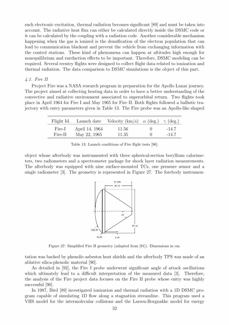
such electronic excitation, thermal radiation becomes significant [89] and must be taken intoaccount. The radiative heat flux can either be calculated directly inside the DSMC code orit can be calculated by the coupling with a radiation code. Another considerable mechanismhappening when the gas is ionized is the densification of the electron population that canlead to communication blackout and prevent the vehicle from exchanging information withthe control stations. These kind of phenomena can happen at altitudes high enough fornonequilibrium and rarefaction effects to be important. Therefore, DSMC modeling can berequired. Several reentry flights were designed to collect flight data related to ionization andthermal radiation. The data comparison to DSMC simulations is the object of this part.

4.1. Fire II

Project Fire was a NASA research program in preparation for the Apollo Lunar journey.The project aimed at collecting heating data in order to have a better understanding of theconvective and radiative environment associated to superorbital return. Two flights tookplace in April 1964 for Fire I and May 1965 for Fire II. Both flights followed a ballistic tra-jectory with entry parameters given in Table 13. The Fire probe was an Apollo-like shaped

Flight Id. Launch date Velocity (km/s) α (deg.) γ (deg.)

Fire-I April 14, 1964 11.56 0 -14.7Fire-II May 22, 1965 11.35 0 -14.7

Table 13: Launch conditions of Fire flight tests [90].

object whose afterbody was instrumented with three spherical-section beryllium calorime-ters, two radiometers and a spectrometer package for shock layer radiation measurements.The afterbody was equipped with nine surface-mounted TCs, one pressure sensor and asingle radiometer [3]. The geometry is represented in Figure 27. The forebody instrumen-

Figure 27: Simplified Fire II geometry (adapted from [91]). Dimensions in cm.

tation was backed by phenolic-asbestos heat shields and the afterbody TPS was made of anablative silica-phenolic material [90].

As detailed in [92], the Fire I probe underwent significant angle of attack oscillationswhich ultimately lead to a difficult interpretation of the measured data [3]. Therefore,the analysis of the Fire project data focuses on the Fire II probe whose entry was highlysuccessful [90].

In 1987, Bird [89] investigated ionization and thermal radiation with a 1D DSMC pro-gram capable of simulating 1D flow along a stagnation streamline. This program used aVHS model for the intermolecular collisions and the Larsen-Borgnakke model for energy

32

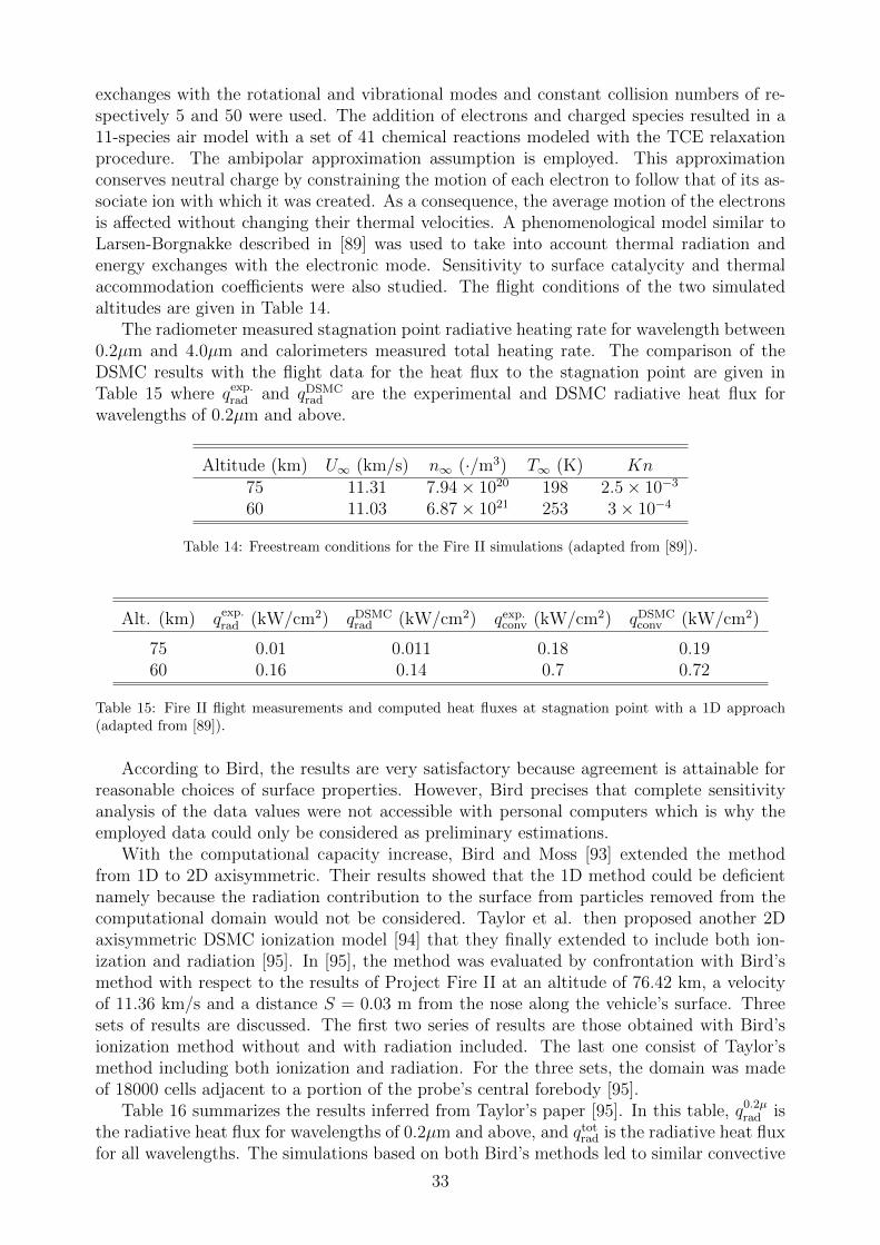
exchanges with the rotational and vibrational modes and constant collision numbers of re-spectively 5 and 50 were used. The addition of electrons and charged species resulted in a11-species air model with a set of 41 chemical reactions modeled with the TCE relaxationprocedure. The ambipolar approximation assumption is employed. This approximationconserves neutral charge by constraining the motion of each electron to follow that of its as-sociate ion with which it was created. As a consequence, the average motion of the electronsis affected without changing their thermal velocities. A phenomenological model similar toLarsen-Borgnakke described in [89] was used to take into account thermal radiation andenergy exchanges with the electronic mode. Sensitivity to surface catalycity and thermalaccommodation coefficients were also studied. The flight conditions of the two simulatedaltitudes are given in Table 14.

The radiometer measured stagnation point radiative heating rate for wavelength between0.2µm and 4.0µm and calorimeters measured total heating rate. The comparison of theDSMC results with the flight data for the heat flux to the stagnation point are given inTable 15 where qexp.

rad and qDSMCrad are the experimental and DSMC radiative heat flux for

wavelengths of 0.2µm and above.

Altitude (km) U∞ (km/s) n∞ (·/m3) T∞ (K) Kn75 11.31 7.94× 1020 198 2.5× 10−3

60 11.03 6.87× 1021 253 3× 10−4

Table 14: Freestream conditions for the Fire II simulations (adapted from [89]).

Alt. (km) qexp.rad (kW/cm2) qDSMC

rad (kW/cm2) qexp.conv (kW/cm2) qDSMC

conv (kW/cm2)

75 0.01 0.011 0.18 0.1960 0.16 0.14 0.7 0.72

Table 15: Fire II flight measurements and computed heat fluxes at stagnation point with a 1D approach(adapted from [89]).

According to Bird, the results are very satisfactory because agreement is attainable forreasonable choices of surface properties. However, Bird precises that complete sensitivityanalysis of the data values were not accessible with personal computers which is why theemployed data could only be considered as preliminary estimations.

With the computational capacity increase, Bird and Moss [93] extended the methodfrom 1D to 2D axisymmetric. Their results showed that the 1D method could be deficientnamely because the radiation contribution to the surface from particles removed from thecomputational domain would not be considered. Taylor et al. then proposed another 2Daxisymmetric DSMC ionization model [94] that they finally extended to include both ion-ization and radiation [95]. In [95], the method was evaluated by confrontation with Bird’smethod with respect to the results of Project Fire II at an altitude of 76.42 km, a velocityof 11.36 km/s and a distance S = 0.03 m from the nose along the vehicle’s surface. Threesets of results are discussed. The first two series of results are those obtained with Bird’sionization method without and with radiation included. The last one consist of Taylor’smethod including both ionization and radiation. For the three sets, the domain was madeof 18000 cells adjacent to a portion of the probe’s central forebody [95].

Table 16 summarizes the results inferred from Taylor’s paper [95]. In this table, q0.2µrad is

the radiative heat flux for wavelengths of 0.2µm and above, and qtotrad is the radiative heat flux

for all wavelengths. The simulations based on both Bird’s methods led to similar convective

33

heat flux. For the radiative heat flux, Taylor’s new electronic excitation procedure gives abetter value when only contributions from 0.2µm and above are considered but the methodgives similar radiative heat flux to Bird’s method when all wavelengths are considered.Hence, it is very important to be able to correctly model electronic relaxation for a goodprediction of radiation and wall heat flux. Moreover, the quality of the results could befortuitous and only the incorporation of an absorption model could confirm it.

Method q0.2µrad (W/cm2) qtot

rad (W/cm2) qconv (W/cm2)

Flight data 8.2 ±20% - 172 ±5%Bird without rad. - - 220

Bird with rad. 88 195 225Taylor 20 175 -

Table 16: Fire II flight measurements and computed heat fluxes at 0.03 m along the vehicle’s surface (adaptedfrom [95]).

More recently, Farbar and Boyd [96] presented axisymmetric DSMC simulations aboutthe Fire II with MONACO. Two points along the trajectory are considered: in the non-continuum region at 85 km and in near-continuum regime at 76 km. The ambipolar diffusionassumption was used and simulations with 5 and 11 species air were made. The workinvestigates the sensitivity to molecular interaction model for all the colliding pairs and thevibrational relaxation model for collisions of electrons and nitrogen molecules.

The measured total heat flux is compared to the values calculated by DSMC using the11-species chemistry. Simulations lead to a heat flux near the upper boarder of the ±5%uncertainty at an altitude of 85 km. At 76 km, the calculated heat flux including the radiativecomponent coincides with the lower boarder of the ±5% uncertainty. For both altitudes,the heat fluxes are compared to Taylor’s results [94], [95] and a much better agreement isreached for the new simulations.

Liechty [97] presented an updated version of NASA’s DSMC code DAC, capable ofsimulating charge-neutral ionized flows with electronic energy level transitions modeled withthe Quantum-Kinetic (Q-K) chemistry model [98] and which includes the electronic energymode. Comparisons were made between DAC, DS2V, the CFD code LAURA and theFire II flight test data point t = 1634 s which corresponds to an altitude of 76.42 km. In thisstudy, the radiative heat transfer were obtained by post-processing the flowfield solutionswith the non-equilibrium radiation code HARA described in [97] and [99]. All DSMCsimulations used the VHS collision model, an 11-species air with the TCE chemistry modeland a fully catalytic wall condition that converted atoms into their associate molecules andcharged species into their associate neutral species when they impact the surface. The walltemperature was taken constant at 615 K.

The results are summarized in Table 17 where DAC is the original version of NASA’sDSMC code, DAC-E is the updated version taking into account the electronic energy modeand the last column indicates the sum of the convective and fraction of radiative heating thatwould have been absorbed by the calorimeter on the vehicle. The results of convective heatflux show an improvement with respect to the flight data since the discrepancy decreasesfrom 35% (DAC) to 20% (DAC-E). The influence of DAC’s modifications are discussed indetails in [97]. The difference between the radiative heat flux calculated by DAC-E and theone measured during the flight is very important. One possible reason for such discrepancy isthe lack of radiation-flowfield coupling in Liechty’s simulations [97]. Indeed, Johnston [100]demonstrated that the radiation-flowfield coupling has almost no effect on the convectiveheat flux but can lead to a decrease of maximum 30% in the radiative heat flux. The way

34

the non-Boltzmann modeling of the atomic and molecular electronic states is consideredconstitutes another possible source of error. Recent improvements on that matter wereproposed by Panesi in [101].

Method qconv (W/cm2) qrad (W/cm2) qconv + k qrad (W/cm2)

LAURA 217 25 235DS2V 220 - -DAC 220 - -

DAC-E 195 52 232Flight data 162 18 175

The calorimeter absorbed fraction of radiative heating k = 0.72

Table 17: Fire II flight measurements and computed heat fluxes at 0.1 m from the symmetry axis (adaptedfrom [97]).

Fire II probably constitutes the most investigated case of study that deals with ionizedflows and thermal radiation. The results presented in this section have shown that a properreconstruction of the heating data is still a challenging task.

4.2. RAM C-II

The Radio Attenuation Measurement (RAM) experiments comprised several flight exper-iments at medium velocity designed to measure plasma parameters around a 9◦ hemisphere-cone with a nose radius RN = 0.1524 m and a total length of 1.3 m. The two first flightsRAM C-I and RAM C-II launched respectively in October 1967 and August 1968 are pre-sented in [102]. The first flight was conceived to evaluate the effect of water injection asplasma alleviation technique and the second flight discussed hereafter aimed at measuringthe electron density time and altitude histories between 90 and 60 km at different locationsalong the vehicle. For this purpose, the vehicle was instrumented with microwave reflectome-ters and electrostatic probes (Figure 28). The TPS was made of a non-ablative berylliumnose cap and a teflon afterbody in order to prevent additional ionization due to surface tooccur [103].

Figure 28: RAM C-II geometry and instrumentation (from [102]).

Although the onset of the communication blackout coincides with altitudes where bothsurface pressure and heat transfer are in agreement with the values computed from con-tinuum theory, the outer portion of the flowfield is not adequately predicted by continuumtheory and nonequilibrium chemical reactions occur. Therefore, non-continuum calculationsare required [103]. Because of the mass of electrons which is five order of magnitudes lowerthan neutral species, the simulation of electrons with DSMC poses three main problems[104]. The first concern is related to the electrons velocity of diffusion which is taken care

35

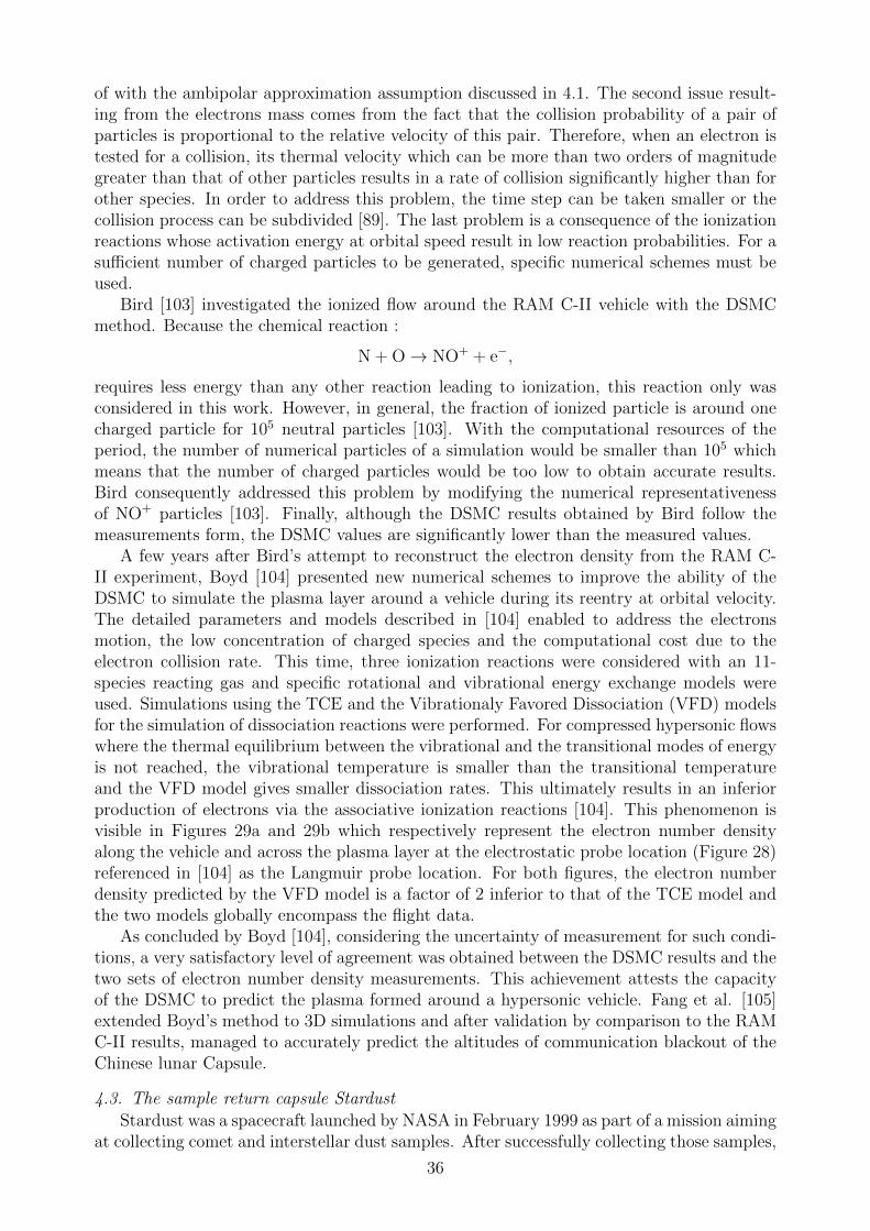
of with the ambipolar approximation assumption discussed in 4.1. The second issue result-ing from the electrons mass comes from the fact that the collision probability of a pair ofparticles is proportional to the relative velocity of this pair. Therefore, when an electron istested for a collision, its thermal velocity which can be more than two orders of magnitudegreater than that of other particles results in a rate of collision significantly higher than forother species. In order to address this problem, the time step can be taken smaller or thecollision process can be subdivided [89]. The last problem is a consequence of the ionizationreactions whose activation energy at orbital speed result in low reaction probabilities. For asufficient number of charged particles to be generated, specific numerical schemes must beused.

Bird [103] investigated the ionized flow around the RAM C-II vehicle with the DSMCmethod. Because the chemical reaction :

N + O→ NO+ + e−,

requires less energy than any other reaction leading to ionization, this reaction only wasconsidered in this work. However, in general, the fraction of ionized particle is around onecharged particle for 105 neutral particles [103]. With the computational resources of theperiod, the number of numerical particles of a simulation would be smaller than 105 whichmeans that the number of charged particles would be too low to obtain accurate results.Bird consequently addressed this problem by modifying the numerical representativenessof NO+ particles [103]. Finally, although the DSMC results obtained by Bird follow themeasurements form, the DSMC values are significantly lower than the measured values.

A few years after Bird’s attempt to reconstruct the electron density from the RAM C-II experiment, Boyd [104] presented new numerical schemes to improve the ability of theDSMC to simulate the plasma layer around a vehicle during its reentry at orbital velocity.The detailed parameters and models described in [104] enabled to address the electronsmotion, the low concentration of charged species and the computational cost due to theelectron collision rate. This time, three ionization reactions were considered with an 11-species reacting gas and specific rotational and vibrational energy exchange models wereused. Simulations using the TCE and the Vibrationaly Favored Dissociation (VFD) modelsfor the simulation of dissociation reactions were performed. For compressed hypersonic flowswhere the thermal equilibrium between the vibrational and the transitional modes of energyis not reached, the vibrational temperature is smaller than the transitional temperatureand the VFD model gives smaller dissociation rates. This ultimately results in an inferiorproduction of electrons via the associative ionization reactions [104]. This phenomenon isvisible in Figures 29a and 29b which respectively represent the electron number densityalong the vehicle and across the plasma layer at the electrostatic probe location (Figure 28)referenced in [104] as the Langmuir probe location. For both figures, the electron numberdensity predicted by the VFD model is a factor of 2 inferior to that of the TCE model andthe two models globally encompass the flight data.

As concluded by Boyd [104], considering the uncertainty of measurement for such condi-tions, a very satisfactory level of agreement was obtained between the DSMC results and thetwo sets of electron number density measurements. This achievement attests the capacityof the DSMC to predict the plasma formed around a hypersonic vehicle. Fang et al. [105]extended Boyd’s method to 3D simulations and after validation by comparison to the RAMC-II results, managed to accurately predict the altitudes of communication blackout of theChinese lunar Capsule.

4.3. The sample return capsule Stardust

Stardust was a spacecraft launched by NASA in February 1999 as part of a mission aimingat collecting comet and interstellar dust samples. After successfully collecting those samples,

36

(a) Maximum electron number density along thevehicle.

(b) Electron number density at the Langmuirprobe location.

Figure 29: Comparison of the measured electron number density with DSMC results at an altitude of 81km during the RAM-C II Earth entry (extracted from [104]).

they were taken down to Earth with the Sample Return Capsule (SRC) in January 2006.The SRC capsule represented in Figure 30 was protected with a 60◦ sphere-cone heat-shield,a truncated conical back-shell and entered Earth’s atmosphere at a 12.8 km/s velocity [106].The TPS consisted of a Phenolic-Impregnated Carbon Ablator (PICA) developed by NASAand the SRC was not instrumentated which means that no time-resolved measurements areavailable. Instead, an auxiliary mission to observe the entry from an airborne platformwas conducted [107]. This mission acquired imaging and spectroscopic data for a period

Figure 30: Stardust Sample Return Capsule after landing (credits: NASA).

of 60 s roughly centered around the peak of heating pulse. Eight instruments were usedwith different spectral and temporal resolutions for measuring the radiative signals from theshock layer surrounding the capsule [106].

Several numerical simulations were realized in the frame of the SRC’s reentry. DSMC,CFD and analytical models were used to study the aerodynamics of the capsule [108], [109].DSMC simulations were performed for the investigation of electronic excitation and radiationof the SRC flow at 68.9 km [110]. The aerodynamic heating reduction through the ablationprocess of the SRC’s TPS was studied with the DSMC code SMILE at altitudes of 68.9 and81 km [111]. Spectroscopic observations were studied by Jenniskens [112] by means of slitlessminiature echelle spectrograph onboard NASA’s airborne laboratory. Band emissions of airplasma from the shock layer, atomic and molecular band emissions from the heat-shield andatomic line emissions from the paint on top of the PICA material were captured. Flowfieldsobtained with the CFD code DPLR were processed with the spectral line-by-line radiationcode NEQAIR and compared against the airborne’s laboratory data [106].

37

Boyd et al. [113] investigated the SRC’s flowfield at 81 and 71 km. The freestreamconditions are given in Table 18. In this study, both CFD and DSMC methods were employedto model the flow of the probe’s forebody in near-continuum regime. For both methods an11-species air was used with 19 reactions. The 2D axisymmetric DSMC simulations assumedthe surface as fully diffuse at wall temperature indicated in Table 18 and fully catalytic to ionsand atoms. No ablation process was considered and chemical reactions were simulated withthe TCE and VFD models. Complementary details are available in [113]. In a companionpaper [114], Boyd et al. used the flowfield results to perform a radiation analysis with thenonequilibrium radiation code NEQAIR.

Alt. (km) T∞ (K) n∞ (·/m3) U∞ (km/s) XO2 XN2 Kn Tw (K)

81 217.6 2.643× 1020 12.385 23.67 76.23 0.005 200071 221.6 1.156× 1021 12.063 23.67 76.23 0.001 2700

Table 18: Freestream temperature, number density, velocity, number concentration and Knudsen numberas well as wall temperature (adapted from [114]).

In this work [114], both air species and metal species emissions of flux densities (W/m2/nm)were studied and compared with Jenniskens’ data [112]. At 81 km, the DSMC flowfield simu-lations gave good agreement with the measured spectra of emissions. Analysis of N+

2 systemalso led to a good level of agreement between the observation data and the DSMC predic-tions. However, at 71 km, the DSMC results tended to underpredict the emission spectra.This discrepancy was interpreted as the result of surface blowing phenomena which shouldbe taken into account. Hence, complementary DSMC simulations including fluxes of metal(particles/m2/s) blowing from the surface at 81 km were performed. The metal blowingfluxes were adjusted to fit at best the measured line intensities. Then, those blowing fluxesinferred from simulations were compared with the magnitude of the impurity of the materialwhich indicated that some emissions of flux density were due to the white paint and someto the TPS ablation. The mass fractions for blowing from the surface obtained at 81 kmwere then used for new simulations at 71 km and qualitative agreement was obtained withthe measured spectra.

Despite the absence of onboard instrumentation, spectroscopic observations enabled thecollection of a great amount of radiative signals. State of the art DSMC simulations wereperformed and inferred line-of sight radiation gave encouraging results compared to measureddata for two near-continuum altitudes. Obvious discrepancies are still noticeable whichindicates that complementary efforts need to be carried out in the context of ionization andradiation modeling.

Mankodi et al. [115] recently investigated the SRC reentry. In their work, the flow fieldaround the capsule and its surface properties were modeled with DSMC simulations usingtwo different chemical models. The first model is the classic TCE model while the secondis an ab initio model based on reactive cross sections calculated with a Quasi ClassicalTrajectory (QCT) method. Simulations at altitudes of 68, 80 and 100 km were carried out.Although the results show that the ab initio model predicts higher heat fluxes than the TCEmodel, the results were not compared to flight data.

5. Conclusion

In this survey, experimental, flight and numerical data were presented in the context ofhypersonic rarefied flows commonly encountered in the first phase of atmospheric reentry.These results have shown both some capacities and limitations of the DSMC method tosimulate rarefied flows that are generally out of the scope of classical CFD methods.

38

A large amount of low density experiments were conducted in low density facilities whichconstitute a solid comparison basis for the validation of DSMC and particle simulation meth-ods. However, the difficulty to retrieve high enthalpy conditions characteristic of atmosphericreentry restricts their use to the study of non-reactive flows. In these conditions, DSMChas proven to be capable of accurately predicting such flows over simple geometries likeflat planes with truncated or sharp leading edge. However, the 70◦ sphere-cone geometryrevealed that for high angles of attack, significant discrepancies were observable betweenDSMC results and measurements. The non-reactive aspect of the flows produced in low-density facilities indicates that improvements are attainable in elementary DSMC modelssuch as translational-rotational energy exchanges and gas-surface interaction models.

Even though the measurement of ATD data in the rarefied portion of the reentry is notthe primary objective of flight experiments, high altitude values measured during such flightsare sometimes available. Thus, heating rate of Mercury and Apollo AS-202 flight experimentswere extracted and compared to DSMC simulations. Another source of unexploited forebodyheat flux data inferred from the MIRKA reentry have been addressed. DSMC simulationswere performed and compared to aerothermodynamic flight data of other vehicles such asOREX and the Space Shuttle. Given the limited amount of flight data and the uncertaintyof the freestram conditions, the numerical results have shown a satisfactory agreement withthe measured aerodynamic data. However, the same conclusion cannot be drawn for theaerothermodynamic DSMC results which leave room for significant improvement.

Moreover, the SPARTA simulations showed that a better understanding of the gas-surface interaction could lead to better predictions through the role of the accommodationcoefficients and the use of a non-uniform wall temperature. These simulations also illustratedthe limitations of DSMC in nearcontinuum conditions.

Ionization, thermal radiation and electronic excitation usually happen at low altitudesor at superorbital velocities. However, analysis of various flight experiments involving suchphenomena have shown that even at near-continuum altitudes, strong non-equilibrium effectscan require the use of particle simulation methods. The last part of this work showed howthe various updates of the DSMC method enabled the simulation of complex ionized flowsfor altitudes lower than 80 km.

Concerning the evolution of the DSMC method, Gimelshein and Wysong outlined in [116]the fact that as for now, the oldest model of chemical reaction is still often the best option.The same paper indicates that only three major improvements from the initial version ofthe method gave the DMSC its current attractivity. This suggests that most of the oldcomputations presented herein still holds as seen with OREX. Furthermore, current effortsin the context of DSMC improvement are made in several directions. For example, state-to-state energy exchange procedures and chemistry models based on quantum considerationare under development [6] and recent work showed the capacity of such models to handlecomplex reactive air flows in place of the usual phenomenological models.

Finally, the lack of well-defined flight and ground-test measurements exploitable in therarefied regime does not permit to demonstrate the accuracy of DSMC for reliable simula-tions of reentry flows. The carrying of experiments in rarefied and hypersonic conditions areessential for the acquisition of complementary aerodynamic and aerothermodynamic dataas well as for the improvement of DSMC models. For that purpose, several requirementsmust be met:

• Using an advanced instrumentation made of sensors suited for such conditions

• Performing a thorough pre and post-experiment analysis of the object’s wall in orderto identify and quantify any catalytic, ablative and accomodation phenomenon

• Having access to a precise geometry of the tested object

39

• Knowing precisely the freestream test conditions in order to alleviate the major sourcesof uncertainty

To this day, dealing with all those criteria can be challenging but the design of specific flightmissions such as orbit transfers instead of classic reentries would be an ideal way of collectingsuch data while avoiding continuum conditions.

Acknowledgment

This work was supported by the ONERA and DGA (Direction Generale de l’Armement),the French Ministry of Armed Forces, through the co-funding of the PhD of M. Schouler.This work was also granted access to the HPC resources of CALMIP under the allocation2020 - Project 20018. ONERA HPC resources have also been used.

References

[1] G. A. Bird, Molecular gas dynamics and the direct simulation of gas flows, Clarendon Press, 1994.[2] I. D. Boyd, T. E. Schwartzentruber, Nonequilibrium gas dynamics and molecular simulation, Cam-

bridge University Press, Cambridge, 2017. doi:10.1017/9781139683494.[3] M. J. Wright, F. S. Milos, P. Tran, Afterbody aeroheating flight data for planetary probe thermal pro-

tection system design, Journal of Spacecraft and Rockets 43 (5) (2006) 929–943. doi:10.2514/1.17703.[4] P. Reynier, Survey of aerodynamics and aerothermodynamics efforts carried out in the

frame of Mars exploration projects, Progress in Aerospace Sciences 70 (2014) 1–27.doi:10.1016/j.paerosci.2014.03.004.

[5] B. R. Hollis, S. Borrelli, Aerothermodynamics of blunt body entry vehicles, Progress in AerospaceSciences 48-49 (2012) 42–56. doi:10.1016/j.paerosci.2011.09.005.

[6] T. E. Schwartzentruber, I. D. Boyd, Progress and future prospects for particle-based simulation ofhypersonic flow, Progress in Aerospace Sciences 72 (2015) 66–79. doi:10.1016/j.paerosci.2014.09.003.

[7] P. Reynier, Survey of high-enthalpy shock facilities in the perspective of radiation and chemical kineticsinvestigations, Progress in Aerospace Sciences 85 (2016) 1–32. doi:10.1016/j.paerosci.2016.04.002.

[8] J. Allegre, M. Raffin, A. Chpoun, L. Gottesdienert, Rarefied Hypersonic Flow over a Flat Plate withTruncated Leading Edge, American Institute of Aeronautics and Astronautics, Washington DC, 1994.doi:10.2514/5.9781600866326.0285.0295.

[9] J. F. Padilla, Comparison of DAC and MONACO DSMC Codes With Flat Plate Simulation, Tech.Rep. August, NASA (2010).

[10] C. White, M. K. Borg, T. J. Scanlon, S. M. Longshaw, B. John, D. R. Emerson, J. M. Reese,dsmcFoam+: An OpenFOAM based direct simulation Monte Carlo solver, Computer Physics Com-munications 224 (2018) 22–43. doi:10.1016/j.cpc.2017.09.030.

[11] R. C. Palharini, C. White, T. J. Scanlon, R. E. Brown, M. K. Borg, J. M. Reese, Benchmark numericalsimulations of rarefied non-reacting gas flows using an open-source DSMC code, Computers and Fluids120 (2015) 140–157. doi:10.1016/j.compfluid.2015.07.021.

[12] S. J. Plimpton, S. G. Moore, A. Borner, A. K. Stagg, T. P. Koehler, J. R. Torczynski, M. A. Gallis,Direct simulation Monte Carlo on petaflop supercomputers and beyond, Physics of Fluids 31 (8) (2019)1–18. doi:10.1063/1.5108534.

[13] C. Borgnakke, P. S. Larsen, Statistical collision model for Monte Carlo simulation of polyatomic gasmixture, Journal of Computational Physics 18 (4) (1975) 405–420. doi:10.1016/0021-9991(75)90094-7.

[14] D. J. Rader, J. N. Castaneda, J. R. Torczynski, T. W. Grasser, W. M. Trott, Measurements of thermalaccommodation coefficients., Tech. rep. (2005). doi:10.2172/876357.

[15] W. M. Trott, J. N. Castaeda, J. R. Torczynski, M. A. Gallis, D. J. Rader, An experimental assembly forprecise measurement of thermal accommodation coefficients, Review of Scientific Instruments 82 (3)(2011) 1–12. doi:10.1063/1.3571269.

[16] G. J. LeBeau, F. E. Lumpkin, Application highlights of the DSMC analysis code (DAC) software forsimulating rarefied flows, Computer Methods in Applied Mechanics and Engineering 191 (6-7) (2001)595–609. doi:10.1016/S0045-7825(01)00304-8.

[17] S. Dietrich, I. D. Boyd, Scalar and parallel optimized implementation of the direct simulation MonteCarlo method, Journal of Computational Physics 126 (2) (1996) 328–342. doi:10.1006/jcph.1996.0141.

[18] K. S. Heffner, L. Gottesdiener, A. Chpoun, J. C. Lengrand, Leading edge effect on rarefied hypersonicflow over a flat plate, in: AIAA 22nd Fluid Dynamics, Plasma Dynamics and Lasers Conference, 1991,1991. doi:10.2514/6.1991-1749.

40

[19] J.-C. Lengrand, A. Chpoun, Rarefied Hypersonic Flow over a Sharp Flat Plate: Numerical and Ex-perimental Results, no. November 2015, 1994. doi:10.2514/5.9781600866326.0276.0284.

[20] J. M. Burt, E. Josyula, I. D. Boyd, Novel Cartesian implementation of the direct simula-tion Monte Carlo method, Journal of Thermophysics and Heat Transfer 26 (2) (2012) 258–270.doi:10.2514/1.T3733.

[21] H. Yamaguchi, N. Tsuboi, Y. Matsumoto, 3D DSMC Simulation of rarefied hypersonic flow over asharp flat plate, in: AIP Conference Proceedings, Vol. 585, 2001, pp. 764–771. doi:10.1063/1.1407636.

[22] J. F. Padilla, I. D. Boyd, Assessment of gas-surface interaction models in DSMC analysis of rarefiedhypersonic flow, in: Collection of Technical Papers - 39th AIAA Thermophysics Conference, Vol. 1,2007, pp. 1–15. doi:10.2514/6.2007-3891.

[23] J. F. Padilla, I. D. Boyd, Assessment of Gas-surface interaction models for computation of rarefied hy-personic flow, Journal of Thermophysics and Heat Transfer 23 (1) (2009) 96–105. doi:10.2514/1.36375.

[24] E. Cecil, J. McDaniel, Planar Velocity and Temperature Measurements in Rarefied Hypersonic FlowUsing Iodine LIF, in: 38th AIAA Thermophysics Conference, American Institute of Aeronautics andAstronautics, Reston, Virigina, 2005. doi:10.2514/6.2005-4695.

[25] J. N. Moss, J.-C. Lengrand, Hypersonic Experimental and Computational Capability, Improvementand Validation, in: AGARD-AR-319 Vol. II, 1998, Ch. Rarefied F.

[26] J. Allegre, D. Bisch, J.-C. Lengrand, Experimental Rarefied Density Flowfields at Hypersonic Condi-tions over 70 Degree Blunted Cone, Journal of Spacecraft and Rockets 34 (6) (1997) 714–718.

[27] J. Allegre, D. Bisch, J.-C. Lengrand, Experimental Rarefied Heat Transfer at Hypersonic Conditionsover 70 Degree Blunted Cone, Journal of Spacecraft and Rockets 34 (6) (1997) 724–728.

[28] J. Allegre, D. Bisch, J.-C. Lengrand, Experimental Rarefied Aerodynamic Forces at Hypersonic Con-ditions over 70 Degree Blunted Cone, Journal of Spacecraft and Rockets 34 (6) (1997) 719–723.

[29] A. Klothakis, I. K. Nikolos, Modeling of Rarefied Hypersonic Flows Using the Massively Parallel DsmcKernel ” Sparta ”, in: 8th International Congress on Computational Mechanics, Vol. 12, 2015.

[30] J. N. Moss, T. Pot, B. Chanetz, M. Lefebvre, DSMC Simulation of Shock / Shock Interactions :Emphasis on Type IV Interactions, Tech. rep. (1998).

[31] J. N. Moss, About Simulations Sharp Double of Shock Cones Interactions, Tech. Rep. August, NASA(2000).

[32] J. N. Moss, G. A. Bird, G. N. Markelov, DSMC simulations of hypersonic flows and comparison withexperiments, in: AIP Conference Proceedings, Vol. 762, 2005, pp. 547–552. doi:10.1063/1.1941593.

[33] J. Murphy, Flight Test Aerodynamic Heating Data for the Afterbody of the Project Mercury SpacecraftWith Comparisons To Available Prediction Methods, Tech. rep., NASA (1967).

[34] D. R. Chapman, An Analysis of Base Pressure at Supersonic Velocities and Comparison with Exper-iment, Tech. rep., NASA (1951). doi:19930090963.

[35] L. Jacchia, Thermospheric Temperature, Density, and Composition: New Models, Tech. rep., NASA(1977).

[36] D. B. Lee, W. D. Goodrich, Apollo Experience Report - Aerothermodynamics Evaluation, Tech. rep.,NASA (1972).

[37] J. E. Pavlosky, L. G. St Leger, Apollo experience report: Thermal protection subsystem, Tech. Rep.January 1974, NASA (1974).

[38] M. J. Wright, D. K. Prabhu, E. R. Martinez, Analysis of apollo command module afterbody heatingpart I: AS-202, Journal of Thermophysics and Heat Transfer 20 (1) (2006) 16–30. doi:10.2514/1.15873.

[39] L. M. Walpot, M. J. Wright, P. Noeding, F. Schrijer, Base flow investigation of the Apollo AS-202 Com-mand Module, Progress in Aerospace Sciences 48-49 (2012) 57–74. doi:10.1016/j.paerosci.2011.06.006.

[40] J. N. Moss, C. E. Glass, F. A. Greene, DSMC simulations of apollo capsule aerodynamics for hyper-sonic rarefied conditions, in: 9th AIAA/ASME Joint Thermophysics and Heat Transfer ConferenceProceedings, Vol. 3, 2006, pp. 1733–1750. doi:10.2514/6.2006-3577.

[41] J. N. Moss, C. Glass, F. Greene, Blunt body aerodynamics for hypersonic low density flows, in: 25thInternational Symposium on Rarefied Gas Dynamics, 2006, pp. 1–6.

[42] K. C. Tseng, J. S. Wu, I. D. Boyd, Simulations of Re-entry vehicles by using DSMC withchemical-reaction module, in: A Collection of Technical Papers - 14th AIAA/AHI InternationalSpace Planes and Hypersonic Systems and Technologies Conference, Vol. 3, 2006, pp. 1789–1801.doi:10.2514/6.2006-8084.

[43] M.-C. Lo, C.-C. Su, J.-S. Wu, K.-C. Tseng, Modelling Rarefied Hypersonic Reactive Flows Using theDirect Simulation Monte Carlo Method, Communications in Computational Physics 18 (4) (2015)1095–1121. doi:10.4208/cicp.080115.010515s.

[44] J. F. Padilla, I. D. Boyd, Assessment of rarefied hypersonic aerodynamics modeling and windtunneldata, in: Collection of Technical Papers - 9th AIAA/ASME Joint Thermophysics and Heat TransferConference Proceedings, Vol. 2, 2006, pp. 1247–1262. doi:10.2514/6.2006-3390.

41

[45] G. A. Bird, The DS2V/3V program suite for DSMC calculations, in: AIP Conference Proceedings,Vol. 762, 2005, pp. 541–546. doi:10.1063/1.1941592.

[46] R. C. Millikan, D. R. White, Systematics of vibrational relaxation, The Journal of Chemical Physics39 (12) (1963) 3209–3213. doi:10.1063/1.1734182.

[47] C. Park, Review of chemical-kinetic problems of future NASA missions. I - Earth entries, Journal ofThermophysics and Heat Transfer 7 (3) (1993) 9–23. doi:10.2514/3.496.

[48] P. A. Gnoffo, R. N. Gupta, J. L. Shinn, Conservation equations and physical models for hypersonicair flows in thermal and chemical nonequilibrium, Tech. Rep. 2867, NASA (1989).

[49] P. A. Gnoffo, An upwind-biased, point-implicit relaxation algorithm for viscous, compressible perfect-gas flows., Tech. rep., NASA (1990).

[50] Anon, U. S. Standard Atmosphere, 1962, Tech. rep., NASA (1962).[51] T. Banyai, E. Torres, A. V. Kashkovsky, P. V. Vashchenkov, M. S. Ivanov, P. Rambaud, Direct Monte

Carlo Simulations of the Intermediate Experimental Vehicle at Early Stages of Reentry, in: Proc. of7th European Symposium on Aerothermodynamics, Brugge, 2011.

[52] D. B. Lee, W. D. Goodrich, The Aerothermodynamic Environment of the Apollo Command ModuleDuring Superorbital Entry, Tech. rep., NASA (1972).

[53] E. R. Hillje, Entry Aerodynamics at Lunar Return Conditions Obtained from the Flight of Apollo 4,Tech. rep., NASA (1969).

[54] D. B. Lee, J. J. Bertin, Heat-Transfer Rate and Pressure Measurements Obtained During ApolloOrbital Entries, Tech. rep., NASA (1970).

[55] E. R. Hillje, Entry Flight Aerodynamics from Apollo Mission AS-202, Tech. rep., NASA (1967).[56] R. Gardon, A Transducer for the Measurement of Heat-Flow Rate, Journal of Heat Transfer (1960)

396–398.[57] K. Sutton, A. J. Graves, A general stagnation-point convective-heating equation for arbitrary gas

mixtures, Tech. Rep. November 1971, NASA (1971).[58] K. Sutton, Air Radiation Revisited, in: AIAA 19th Thermophysics Conference, Snowmass, 1984.[59] C. O. Johnston, A. M. Brandis, Features of afterbody radiative heating for earth entry, Journal of

Spacecraft and Rockets 52 (1) (2015) 105–119. doi:10.2514/1.A33084.[60] D. Zimpfer, P. Hattis, J. Ruppert, D. Gavert, Space shuttle GN and C development history and

evolution, in: AIAA SPACE Conference and Exposition 2011, no. April, 2011. doi:10.2514/6.2011-7244.

[61] A. M. Whitnah, E. R. Hillje, Space Shuttle Wind Tunnel Testing Program Summary, Tech. rep.,NASA (1984). doi:10.2514/6.1982-562.

[62] J. C. Young, J. M. Underwood, E. R. Hillje, A. M. Whitnah, P. O. Romere, J. D. Gamble, B. B.Roberts, G. M. Ware, W. I. Scallion, B. Spencer, J. P. Arrington, D. C. Olsen, Aerodynamic Challengesof the Design and Development of the Space Shuttle Orbiter, in: NASA Conference Publication, no.pt 1, 1985, pp. 209–263.

[63] J. W. Haney, Orbiter Entry Heating Lessons Learned from Development Flight Test Program, in:NASA Conference Publication, no. pt 2, 1983, pp. 719–751.

[64] D. M. Curry, Space Shuttle Orbiter Thermal Protection System Design and Flight Experience, Tech.rep., NASA (1993).

[65] J. L. Shinn, J. N. Moss, A. Simmonds, Viscous-Shock-Layer Heating Analysis for the Shuttle Wind-ward Plane with Surface Finite Catalytic Recombination Rates, in: 3rd Joint Thermophysics, Fluids,Plasma and Heat Transfer Conference, 1982.

[66] D. A. Throckmorton, Shuttle entry aerothermodynamic flight research: The orbiter experiments(OEX) program, in: AIAA 17th Aerospace Ground Testing Conference, Vol. 30, 1992, pp. 449–465.doi:10.2514/6.1992-3987.

[67] R. C. Blanchard, G. M. Buckt, Determination of rarefied-flow aerodynamics of the shuttle orbiterfrom flight measurements on STS-6 and STS-7, in: AlAA 23rd Aerospace Sciences Meeting, 1985,1985. doi:10.2514/6.1985-347.

[68] R. C. Blanchard, J. F. Rutherford, Shuttle orbiter high resolution accelerometer package ex-periment: Preliminary flight results, Journal of Spacecraft and Rockets 22 (4) (1985) 474–480.doi:10.2514/3.25775.

[69] R. C. Blanchard, G. M. Buck, Rarefied-flow aerodynamics and thermosphere structure from shuttleflight measurements, Journal of Spacecraft and Rockets 23 (1) (1986) 18–24. doi:10.2514/3.25078.

[70] M. A. Gallis, K. A. Boyles, G. J. Lebeau, DSMC simulations in support of the STS-107 accidentinvestigation, in: AIP Conference Proceedings, Vol. 762, 2005, pp. 1211–1216. doi:10.1063/1.1941698.

[71] J. N. Moss, G. A. Bird, Direct Simulation of Transitional Flow for Hypersonic Reentry Conditions,in: AIAA, 1988, pp. 830–843. doi:10.2514/2.6909.

[72] J. C. Adams, W. R. Martindale, A. W. Mayne, M. E. O., Real gas scale effects on hypersonic laminar

42

boundary-layer parameters including effects of entropy-layer swallowing, in: AIAA 9th Fluid andPlasma Dynamics Conference, 1976, pp. 1–12. doi:https://doi.org/10.2514/6.1981-1042.

[73] E. V. Zoby, Approximate Heating Analysis for the Windward Symmetry Plane of Shuttle-Like BodiesAt Large Angle of Attack., Progress in Astronautics and Aeronautics 82 (1982) 229–247.

[74] J. L. Shinn, A. L. Simmonds, Comparison of Viscous-Shock-Layer Heating Analysis With ShuttleFlight Data in Slip Flow Regime, in: AIAA, 1984, pp. 1–9. doi:10.2514/5.9781600865718.0491.0510.

[75] G. A. Bird, Application of the Direct Simulation Monte Carlo Method to the Full Shuttle Geometry,in: AIAA/ASME 5th Joint Thermophysics and Heat Transfer Conference, 1990.

[76] D. RAULT, Aerodynamics of Shuttle Orbiter at high altitudes, Journal of Spacecraft and Rockets31 (6) (1994) 944–952. doi:10.2514/6.1993-2815.

[77] C. Park, S. Yoon, Calculation of real-gas effects on blunt-body trim angles, AIAA Journal 30 (4)(1992) 999–1007. doi:10.2514/3.11020.

[78] K. W. Iliff, M. F. Shafer, Space shuttle hypersonic aerodynamic and aerothermodynamic flight researchand the comparison to ground test results, Tech. rep. (1993).

[79] Unknown, Aerodynamic Design Data Book - Vol. I: Orbiter Vehicle, JSC-19654, 1978.[80] R. C. Blanchard, Rarefield Flow Lift-to-Drag Measurements of the Shuttle Orbiter, in: Congress of

the International Council of the Aeronautical Sciences, Vol. 2, 1986, pp. 1421–1430.[81] S. Matsumoto, Y. Kondoh, S. Nagai, R. Tagai, T. Imada, E. Nakano, Aerodynamic oscillation and

attitude control analysis for reentry capsule using OREX flight data and wind tunnel data, in: AIAAGuidance, Navigation, and Control Conference, no. January, 2016, pp. 1–11. doi:10.2514/6.2016-1131.

[82] R. N. Gupta, J. N. Moss, J. M. Price, Assessment of Thermochemical Nonequilibrium and Slip Effectsfor Orbital Reentry Expriment (OREX), in: 31st AIAA Thermophysics Conference, New Orleans,1996.

[83] J. N. Moss, R. N. Gupta, J. M. Price, DSMC Simulations of OREX Entry Conditions, Tech. rep.,NASA (1996).

[84] J. N. Moss, G. A. Bird, Monte carlo simulations in support of the shuttle upper atmosphericmass spectrometer experiment, Journal of Thermophysics and Heat Transfer 2 (2) (1988) 138–144.doi:10.2514/3.77.

[85] R. Muller-Eigner, G. Koppenwallner, B. Fritsche, Pressure and Heat Flux Measurement with RAFLEXII During MIRKA Re-entry, in: Third European Symposium on Aerothermodynamics for SpaceVehicles, Noordwijk, 1998.

[86] G. Herdrich, M. Fertig, D. Petkow, A. Steinbeck, Modeling approaches for gas-surface interactions, in:48th AIAA Aerospace Sciences Meeting Including the New Horizons Forum and Aerospace Exposition,2010. doi:10.2514/6.2010-1467.

[87] J. Pallegoix, J. Collinet, Atmospheric Re entry Demonstrator : Post Flight Analysis, Flight Rebuildingwith CFD Control., in: 2nd International Symposium Atmospheric Reentry Vehicles and Systems, no.March, Arcachon, 2001.

[88] M. Fertig, H.-H. Fruhauf, Detailed Computation of the Aerothermodynamic Loads of the Mirka Cap-sule, in: Aerothermodynamics for space vehicles, Proceedings of the 3rd European Symposium onAerothermodynamics for space vehicles held at ESTEC, Noordwijk, The Netherlands, 24-26 Novem-ber 1998, 1999, pp. 703–710.

[89] G. A. Bird, Nonequilibrium radiation during re-entry at 10 km/s, in: AIAA 22nd ThermophysicsConference, Honolulu, 1987. doi:10.2514/6.1987-1543.

[90] M. Wright, J. Brown, K. Sinha, G. Candler, Validation of Afterbody Aeroheating Predictions forPlanetary Probes: Status and Future Work, in: 2nd International Planetary Probe Workshop, no. 1,2005, pp. 275–286.

[91] M. Wright, M. Loomis, P. Papadopoulos, Aerothermal analysis of the project fire II afterbody flow,Journal of Thermophysics and Heat Transfer 17 (2) (2003) 240–249. doi:10.2514/2.6757.

[92] G. E. Woodbury, Angle-of-Attack analysis for Project Fire 1 Payload Reentry Flight, Tech. Rep. April,NASA (1966).

[93] J. N. Moss, G. A. Bird, V. Dogra, Nonequilibrium thermal radiation for an aeroassist flight experimentvehicle, in: 26th Aerospace Sciences Meeting, 1988. doi:10.2514/6.1988-81.

[94] J. C. Taylor, A. B. Carlson, H. A. Hassan, Monte Carlo Simulation of Reentry Flows With Ionization,in: 30th Aerospace and Sciences Meeting and Exhibit, 1992.

[95] J. C. Taylor, A. B. Carlson, H. A. Hassan, Monte Carlo simulation of radiating reentry flows, in:AIAA 28th Thermophysics Conference, Vol. 8, 1993, pp. 478–485. doi:10.2514/6.1993-2809.

[96] E. D. Farbar, I. D. Boyd, Simulation of FIRE II reentry flow using the direct simulation Monte Carlomethod, in: 40th AIAA Thermophysics Conference, 2008. doi:10.2514/6.2008-4103.

[97] D. S. Liechty, C. O. Johnston, M. J. Lewis, Comparison of DSMC and CFD solutions of fire II includingradiative heating, in: 42nd AIAA Thermophysics Conference, 2011, pp. 1–14. doi:10.2514/6.2011-3494.

43

[98] D. S. Liechty, M. J. Lewis, Extension of a kinetic-theory approach for computing chemical-reactionrates to reactions with charged particles, in: AIP Conference Proceedings, Vol. 1333, 2011, pp. 1239–1244. doi:10.1063/1.3562813.

[99] C. O. Johnston, B. R. Hollis, K. Sutton, Non-boltzmann modeling for air shock-layer radiation atlunar-return conditions, Journal of Spacecraft and Rockets 45 (5) (2008) 879–890. doi:10.2514/1.33006.

[100] C. O. Johnston, B. R. Hollis, K. Sutton, Nonequilibrium stagnation-line radiative heating for Fire II,Journal of Spacecraft and Rockets 45 (6) (2008) 1185–1195. doi:10.2514/1.33008.

[101] M. Panesi, T. Magin, A. Bourdon, A. Bultel, O. Chazot, Fire II flight experiment analysis by meansof a collisional-radiative model, Journal of Thermophysics and Heat Transfer 23 (2) (2009) 236–248.doi:10.2514/1.39034.

[102] W. L. J. Jones, A. E. Cross, Electrostatic-Probe Measurments of Plasma Parameters for ReentryFlight Experiments at 25000 Feet Per Second, Tech. rep., NASA (1972).

[103] G. A. Bird, Computation of electron density in high altitude re-entry flows, in: AIAA 20th FluidDynamics, Plasma Dynamics and Lasers Conference, 1989. doi:10.2514/6.1989-1882.

[104] I. D. Boyd, Modeling of associative ionization reactions in hypersonic rarefied flows, Physics of Fluids19 (9). doi:10.1063/1.2771662.

[105] M. Fang, Z. Li, Z. Li, C. Li, DSMC Approach for Rarefied Air Ionization during SpacecraftReentry 1 Introduction, Communications in Computational Physics 23 (4) (2018) 1167–1190.doi:10.4208/cicp.OA-2016-0186.

[106] Y. Liu, D. Prabhu, K. A. Trumble, D. Saunders, P. Jenniskens, Radiation modeling for the reentryof the stardust sample return capsule, Journal of Spacecraft and Rockets 47 (5) (2010) 741–752.doi:10.2514/1.37813.

[107] D. A. Kontinos, M. Stackpoole, Post-flight analysis of the stardust sample return capsule Earth Entry,in: 46th AIAA Aerospace Sciences Meeting and Exhibit, no. January, 2008. doi:10.2514/6.2008-1201.

[108] R. A. Micheltree, R. G. Wilmoth, F. M. Cheatwood, G. J. Brauckmann, F. A. Green, Aerodynamicsof Stardust Sample Return Capsule, AIAA, 1997.

[109] R. G. Wilmoth, R. A. Mitcheltree, J. N. Moss, Low-density aerodynamics of the Stardust samplereturn capsule, Journal of Spacecraft and Rockets 36 (3) (1999) 436–441. doi:10.2514/2.3464.

[110] T. Ozawa, Z. Li, I. Sohn, D. A. Levin, M. F. Modest, Modeling of electronic excitation and radiationfor hypersonic reentry flows in DSMC, in: 48th AIAA Aerospace Sciences Meeting Including the NewHorizons Forum and Aerospace Exposition, no. January, 2010, pp. 4–7. doi:10.2514/6.2010-987.

[111] J. Zhong, T. Ozawa, D. A. Levin, Modeling of stardust reentry ablation flows in the near-continuumflight regime, AIAA Journal 46 (10) (2008) 2568–2581. doi:10.2514/1.36196.

[112] P. Jenniskens, Observations of the stardust sample return capsule entry with a slitless echelle spec-trograph, Journal of Spacecraft and Rockets 47 (5) (2010) 718–735. doi:10.2514/1.37518.

[113] I. D. Boyd, K. A. Trumble, M. J. Wright, Modeling of stardust entry at high altitude, part 1: Flowfieldanalysis, Journal of Spacecraft and Rockets 47 (5) (2010) 708–717. doi:10.2514/1.37360.

[114] I. D. Boyd, P. M. Jenniskens, Modeling of stardust entry at high altitude, part 2: Radiation analysis,Journal of Spacecraft and Rockets 47 (6) (2010) 901–909. doi:10.2514/1.37357.

[115] T. K. Mankodi, U. V. Bhandarkar, B. P. Puranik, Hypersonic flow over Stardust Re-entry Capsuleusing ab-initio based chemical reaction model, Acta Astronautica 162 (January) (2019) 243–255.doi:10.1016/j.actaastro.2019.06.021.

[116] S. F. Gimelshein, I. J. Wysong, Bird’s total collision energy model: 4 decades and going strong,Physics of Fluids 31 (7) (2019) 1–16. doi:10.1063/1.5097706.

44

Survey of flight and numerical data of hypersonic rarefied ...

Documents

Transcript of Survey of flight and numerical data of hypersonic rarefied ...