Brigham Young University Brigham Young University

BYU ScholarsArchive BYU ScholarsArchive

Books

2018-12

Flight Vehicle Design Flight Vehicle Design

Andrew Ning Brigham Young University, aning@byu.edu

Follow this and additional works at: https://scholarsarchive.byu.edu/books

Part of the Aerospace Engineering Commons

Recommended Citation Recommended Citation Ning, Andrew, "Flight Vehicle Design" (2018). Books. 26. https://scholarsarchive.byu.edu/books/26

This Book is brought to you for free and open access by BYU ScholarsArchive. It has been accepted for inclusion in Books by an authorized administrator of BYU ScholarsArchive. For more information, please contact scholarsarchive@byu.edu, ellen_amatangelo@byu.edu.

Flight Vehicle Design

Andrew NingBrigham Young University

Figure: NASA, public domain

Copyright© 2018 Andrew Ning. All rights reserved.

ColophonThis document was typeset with LATEX.

PublicationFirst published electronically Dec 2018.

VersionLast compiled: December 19, 2019

Contents

Nomenclature 8

1 Atmosphere 161.1 Layers . . . . . . . . . . . . . . . . . . . . . . . . . . . . . . . . 161.2 Altitude . . . . . . . . . . . . . . . . . . . . . . . . . . . . . . 181.3 Hydrostatic Equation and Geopotential Altitude . . . . . . . 201.4 International Standard Atmosphere . . . . . . . . . . . . . . 221.5 Curve Fit to Standard Atmosphere . . . . . . . . . . . . . . . 251.6 Other Atmospheric Models . . . . . . . . . . . . . . . . . . . 25

2 Fundamentals 272.1 Airfoil Geometry . . . . . . . . . . . . . . . . . . . . . . . . . 272.2 Wing Geometry . . . . . . . . . . . . . . . . . . . . . . . . . . 292.3 Aerodynamic Forces and Moments . . . . . . . . . . . . . . . 312.4 Nondimensional Parameters . . . . . . . . . . . . . . . . . . . 332.5 Pressure Distributions . . . . . . . . . . . . . . . . . . . . . . 352.6 Lift Curves and Drag Polars . . . . . . . . . . . . . . . . . . . 40

3 Drag 443.1 Breakdown . . . . . . . . . . . . . . . . . . . . . . . . . . . . . 443.2 Parasitic Drag . . . . . . . . . . . . . . . . . . . . . . . . . . . 45

3.2.1 Skin Friction Drag . . . . . . . . . . . . . . . . . . . . 453.2.2 Pressure Drag . . . . . . . . . . . . . . . . . . . . . . . 49

3

Contents A. Ning

3.2.3 Putting it Together . . . . . . . . . . . . . . . . . . . . 513.2.4 Strip Theory . . . . . . . . . . . . . . . . . . . . . . . . 53

3.3 Induced Drag . . . . . . . . . . . . . . . . . . . . . . . . . . . 543.4 Tradeoffs in Parasitic and Induced Drag . . . . . . . . . . . . 623.5 Compressibility Drag . . . . . . . . . . . . . . . . . . . . . . . 62

3.5.1 Transonic Wave Drag . . . . . . . . . . . . . . . . . . . 653.5.2 Supersonic Wave Drag . . . . . . . . . . . . . . . . . . 693.5.3 High Mach or Blunt Bodies . . . . . . . . . . . . . . . 72

4 Wing Design 744.1 Fundamental Parameters . . . . . . . . . . . . . . . . . . . . . 744.2 Lift Distributions and Lift Coefficient Distributions . . . . . 774.3 Finite Wing Lift Curve Slopes . . . . . . . . . . . . . . . . . . 81

5 Stability 845.1 Definitions and Fundamentals . . . . . . . . . . . . . . . . . . 845.2 Longitudinal Static Stability . . . . . . . . . . . . . . . . . . . 905.3 Lateral Static Stability . . . . . . . . . . . . . . . . . . . . . . . 965.4 Coordinated Turns and Adverse Yaw . . . . . . . . . . . . . . 995.5 Tail Types and Statistical Tail Sizing . . . . . . . . . . . . . . . 1005.6 Dynamic Stability . . . . . . . . . . . . . . . . . . . . . . . . . 102

6 Propulsion 1086.1 DC Electric Motor . . . . . . . . . . . . . . . . . . . . . . . . . 1086.2 Propellers . . . . . . . . . . . . . . . . . . . . . . . . . . . . . 1106.3 Motor-Prop Matching . . . . . . . . . . . . . . . . . . . . . . . 1136.4 Gas Turbine Engines . . . . . . . . . . . . . . . . . . . . . . . 1176.5 Propulsion System Placement . . . . . . . . . . . . . . . . . . 123

7 Performance 1267.1 Range . . . . . . . . . . . . . . . . . . . . . . . . . . . . . . . . 126

7.1.1 Jet Powered . . . . . . . . . . . . . . . . . . . . . . . . 1277.1.2 Electric Powered . . . . . . . . . . . . . . . . . . . . . 130

7.2 Endurance . . . . . . . . . . . . . . . . . . . . . . . . . . . . . 1327.3 Optimal Lift Coefficients . . . . . . . . . . . . . . . . . . . . . 1327.4 Rate of Climb . . . . . . . . . . . . . . . . . . . . . . . . . . . 1377.5 Glide Ratio . . . . . . . . . . . . . . . . . . . . . . . . . . . . . 1397.6 Turning Radius . . . . . . . . . . . . . . . . . . . . . . . . . . 1407.7 High Lift Devices . . . . . . . . . . . . . . . . . . . . . . . . . 141

4

Contents A. Ning

7.8 Takeoff . . . . . . . . . . . . . . . . . . . . . . . . . . . . . . . 1447.9 Landing . . . . . . . . . . . . . . . . . . . . . . . . . . . . . . 149

8 Structures 1528.1 Typical Structural Elements . . . . . . . . . . . . . . . . . . . 1528.2 Wind Bending . . . . . . . . . . . . . . . . . . . . . . . . . . . 1548.3 Flight Envelope Preliminaries . . . . . . . . . . . . . . . . . . 1608.4 Speed-Altitude Flight Envelope . . . . . . . . . . . . . . . . . 1638.5 V-n Diagrams . . . . . . . . . . . . . . . . . . . . . . . . . . . 164

9 Rocket Fundamentals 1699.1 Types . . . . . . . . . . . . . . . . . . . . . . . . . . . . . . . . 1699.2 Thrust and Efficiency (Specific Impulse) . . . . . . . . . . . . 1739.3 Tsiolkovsky Rocket Equation . . . . . . . . . . . . . . . . . . 1759.4 Staging . . . . . . . . . . . . . . . . . . . . . . . . . . . . . . . 1789.5 Stability . . . . . . . . . . . . . . . . . . . . . . . . . . . . . . . 180

10 Rocket Propulsion 18210.1 Thermodynamics Review . . . . . . . . . . . . . . . . . . . . 182

10.1.1 Properties and Equations of State . . . . . . . . . . . . 18210.1.2 Laws of Thermodynamics . . . . . . . . . . . . . . . . 18410.1.3 Specific Heats . . . . . . . . . . . . . . . . . . . . . . . 18510.1.4 Isentropic Relationships . . . . . . . . . . . . . . . . . 187

10.2 Compressible Flow Primer . . . . . . . . . . . . . . . . . . . . 18810.2.1 Energy Equation . . . . . . . . . . . . . . . . . . . . . 18910.2.2 Area Velocity Relationship . . . . . . . . . . . . . . . 189

10.3 Nozzle Sizing . . . . . . . . . . . . . . . . . . . . . . . . . . . 19410.3.1 Exit Velocity . . . . . . . . . . . . . . . . . . . . . . . . 19410.3.2 Throat Size . . . . . . . . . . . . . . . . . . . . . . . . 19510.3.3 Combustion Chamber Sizing . . . . . . . . . . . . . . 19510.3.4 Exit Area Sizing . . . . . . . . . . . . . . . . . . . . . . 196

10.4 Lengths . . . . . . . . . . . . . . . . . . . . . . . . . . . . . . . 198

11 Orbital Mechanics 20311.1 Gravity . . . . . . . . . . . . . . . . . . . . . . . . . . . . . . . 20311.2 Orbits . . . . . . . . . . . . . . . . . . . . . . . . . . . . . . . . 20811.3 Hohmann Transfer . . . . . . . . . . . . . . . . . . . . . . . . 214

5

Contents A. Ning

A Supplementary Material 216A.1 Skin Friction Coefficient for a Flat Plate with Transition . . . 216A.2 Supersonic Wave Drag Equations . . . . . . . . . . . . . . . . 220A.3 Rocket Altitude . . . . . . . . . . . . . . . . . . . . . . . . . . 224A.4 Rocket Nozzle Performance . . . . . . . . . . . . . . . . . . . 225

A.4.1 Exit Velocity . . . . . . . . . . . . . . . . . . . . . . . . 227A.4.2 Throat Size . . . . . . . . . . . . . . . . . . . . . . . . 228A.4.3 Combustion Chamber Sizing . . . . . . . . . . . . . . 228A.4.4 Exit Area Sizing . . . . . . . . . . . . . . . . . . . . . . 229

6

Preface

Aircraft design is a multidisciplinary topic with many applications andcan’t possibly be fully covered in one text. Aircraft configurations arechanging rapidly, particularly with recent advances in electric powersystems and automated controls. Thus, this text primarily focuses onfundamental physics, as opposed to handbook or statistical methods. Thelast three chapters provide an introduction to rocket design.A few sections are more advanced, or involve lengthier derivations, andthese are put in the end in an Appendix. These chapters are not necessaryto understand the main text, but are provided as a reference for theinterested reader. Words in italics denote important terminology.

7

Nomenclature

Aircraft Nomenclature()∞ freestream

()r root

()t tip

()ac aerodynamic center

()c g center of gravity

()re f reference quantity

()sl sea level

α angle of attack

α0 zero lift angle of attack

β sideslip angle

Ûm mass flow rate

η efficiency

η spanwise lift centroid location

8

Contents A. Ning

Γ circulation

γ flight path angle

Λ sweep

λ taper ratio

µ dynamic viscosity

µ rolling coefficient of friction

Ω rotation rate (rad/s)

Φ bank angle

φ dihedral

ρ density

σ stress

τ shear stress

θ twist

A axial force

a speed of sound

AR aspect ratio

b span

c chord

CD drag coefficient

cd 2D drag coefficient

CD c compressibility drag coefficient

CD i induced drag coefficient

CD p parasitic drag coefficient

C f skin friction coefficient

9

Contents A. Ning

CL lift coefficient

cl 2D lift coefficient

CLmax maximum lift coefficient

cl max 2D maximum lift coefficient

Cm pitching moment coefficient

cm 2D pitching moment coefficient

CP power coefficient

Cp pressure coefficient

CQ torque coefficient

CT thrust coefficient

CY side force coefficient

cmac mean aerodynamic chord

Cn yawing moment coefficient

Croll rolling moment coefficient

D drag

D propeller diameter

D′ drag per unit span

Dc compressibility drag

Di induced drag

Dp parasitic drag

e Oswald efficiency factor

eb battery specific energy

einv inviscid span efficiency

EAS equivalent air speed

10

Contents A. Ning

f r fineness ratio

g acceleration of gravity

h altitude

h f fuel enthalpy

i current

J advance ratio

k form factor

Kv motor velocity constant

L lift

L′ lift per unit span

M Mach number

M pitching moment

M′ pitching moment per unit span

Mb bending moment

mb battery mass

m f fuel mass

Mbr root bending moment

Mcc crest critical Mach number

Mdd drag divergence Mach number

mTO total takeoff mass

N normal force

n load factor

n rotation rate (rev/s)

P power

11

Contents A. Ning

p roll rate

p pressure

Q torque

q pitch rate

R range

r yaw rate

R/C rate of climb

Rt turning radius

Re Reynolds number

S wing area

Sexp exposed area

Sgross gross area

Sre f reference area

Swet wetted area

s f c specific fuel consumption

T thrust

t thickness

T temperature

t/c thickness-to-chord ratio

TAS true air speed

V velocity

v voltage

VC design cruise speed

VD design dive speed

12

Contents A. Ning

Vs stall speed

W weight

w downwash

Y side force

Rocket Nomenclature()∞ freestream

()b burnout

()c after combustion

()e earth

()e exit

()t throat

()sl sea level

Ûm f propellant mass flow rate

ε nozzle expansion ratio

γ ratio of specific heats

µ GM, gravitational constant

ρ density

θ flight angle

θ0 orbit phase shift

A area

a semimajor axis of ellipse

C effective exit velocity

Cp specific heat at constant pressure

13

Contents A. Ning

Cv specific heat at constant volume

D drag

e orbit eccentricity

e specific internal energy

G universal gravitation constant

g acceleration of gravity

h altitude

h angular momentum per unit mass

h specific enthalpy

hT total enthalpy

Isp specific impulse

L∗ characteristic mixing length

M Mach number

m mass

mp propellant mass

ms structural mass

Mw molecular weight

mpa yload payload mass

MR mass ratio (initial/final)

p pressure

q heat added

r radius

Re radius of the earth

Ru universal gas constant

14

Contents A. Ning

s specific entropy

T kinetic energy

T temperature

T thrust

tb burn time

U potential energy

v specific volume

Ve exit velocity

15

CHAPTER1

Atmosphere

Aircraft, rockets, and spacecraft operate in or pass through the earth’satmosphere. Thus, we need to understand how atmospheric propertiesvary, at least with altitude. Primarily we are interested in pressure,density, and temperature, as well as what is meant by altitude. For thelower portion of the atmosphere, where aircraft operate, we will examine a“standard atmosphere” that is widely used as a first model. We will alsomention, though not discuss, a couple more detailed models for other usecases.

1.1 Layers

The earth’s atmosphere is not really composed of layers, but it isconvenient to characterize it that way. Figure 1.1 provides an overview ofthe lower layers of the atmosphere and a typical temperature profile.The troposphere extends from the surface of the earth to about 10–12 kmin altitude (varies with weather). About 80% of the mass of theatmosphere is contained in this layer and almost all of the water vapor. Itis the layer where almost all weather occurs.The next layer is the stratosphere, which extends roughly to 50 km. Mostof the ozone in the atmosphere exists in this layer. In this layertemperature actually increases with altitude because the ozone absorbs

16

Chapter 1. Atmosphere A. Ning

Figure 1.1: Depiction of layers in our atmosphere, and a typical temperatureprofile. Figure from Randy Russell, UCAR, public domain.

ultraviolet (UV) radiation from the sun (though it is still very cold!). Thistemperature inversion makes this layer very stable and thus there is littleturbulence, clouds, or other weather effects. Most commercial aircraft flynear the border between the troposphere and the stratosphere. A typicallycruising altitude for a commercial transport is somewhere between 10–13km (approximately 33,000-42,000 ft).Temperatures decrease again in the mesosphere, which extends to about85 km. This is the coldest part of our atmosphere. There is not muchactivity by aircraft or rockets in this area, other than sounding rockets (arocket designed to take measurements for research purposes).The thermosphere again experiences a rise in temperature. In fact thetemperature can be as high as 2000 C! Why then would you still feelfreezing cold? Recall that temperature is a measure of the average kineticenergy of the air molecules. But heat transfer depends also on the numberof particles. In this layer the air is so thin, or in other words the moleculesare spaced so far apart, that even though individual molecules have highenergy there are so few that very little heat is transferred. The height ofthis layer varies considerably with solar energy and can range from 500 to1,000 km in altitude. Some satellites exist in this layer.The exosphere is the last layer and varying definitions have it extending to

17

Chapter 1. Atmosphere A. Ning

somewhere between 10,000 km to 190,000 km (halfway to the moon). Theair is so thin here that molecular collisions are rare. Most satellites operatein this layer.

1.2 Altitude

We have used the word altitude several times already, but there areactually multiple definitions of altitude that we need to be aware of. Thefirst two are straightforward while the next two will need furtherexplanation.

• Geometric Altitude: the geometric height from sea level.

• Absolute Altitude: the geometric height from the center of the earth.

• Pressure Altitude: corresponding altitude in the standard atmospherethat has the same pressure as the current pressure.

• Geopotential Altitude: an equivalent altitude assuming constantacceleration of gravity.

A device that measures altitude is called an altimeter. One way to measureheight above ground is to use a radar altimeter. These are common inaircraft. They bounce radio waves off the ground and measure the returntime in order to calculate height above ground level (AGL). Note that thisis not the same as geometric altitude as the ground generally is not at sealevel.The most widely used type of altimeter is a pressure altimeter, also knownas a barometric altimeter. Pressure altimeters are used in aircraft, and theyare included in many smart phones and fitness tracking devices. Apressure altimeter takes a local reading of the pressure, then calculates thealtitude based on the pressure (we will see how this works shortly). Thiscalculation requires a model of the atmosphere, as it is not directlymeasuring height. Estimating altitude using pressure and an atmosphericmodel is what is meant by pressure altitude as it is not necessarily a truealtitude.Because of the reliance on pressure, this approach is subject to inaccuraciesdue to changes in air pressure that have nothing to do with altitudechange. For highly accurate altitude measurements, periodic calibration isnecessary. An aircraft must recalibrate before takeoff and make

18

Chapter 1. Atmosphere A. Ning

adjustments in flight based on measurements reported by air trafficcontrol. For casual-use with personal devices, calibration is usually lessnecessary as time scales are smaller and often only relative changes areneeded. More sophisticated altimeters blend pressure readings with othersensors (e.g., accelerometer, GPS) to provide a more accurate altitudeestimate.Another way to measure altitude is by using the Global PositioningSystem (GPS). Four or more satellite readings are necessary to provide analtitude estimate, though generally more satellites than four are availableoverhead at a given time. Figure 1.2 shows 9 visible satellites for aparticular location at a particular point in time (see here for an animatedversion). The GPS device’s position is triangulated based on the knownpositions of the satellites and the passage time for the radio waves (like aradar altimeter). The computed altitude is referenced relative to sea level,and is thus a geometric altitude. GPS-derived altitude estimates are subjectto inaccuracies caused by things like signal blockage and reflections (e.g.,buildings, trees) and interaction with particles in the ionosphere1 thatdelay the radio signals. GPS altitude measurements are less accurate thantheir horizontal measurements (with a rule of thumb of 3X difference inaccuracy). Typically, a GPS altitude measurement is accurate to withinabout 10–20 meters (35–70 ft), if the signal is good.

Figure 1.2: Visualization of GPS satellite locations around the earth for agiven instant in time. Wikimedia Commons, El pak, public domain.

1part of the atmosphere that is ionized by solar radiation and can include parts of themesosphere, thermosphere, and exosphere

19

Chapter 1. Atmosphere A. Ning

1.3 Hydrostatic Equation and Geopotential Altitude

You probably already know that as you go up in altitude the air pressureand density generally decrease, but we need to be able to quantify thisrelationship. We can relate pressure changes with altitude using ahydrostatic balance (hydrostatic means a fluid at rest). Consider anarbitrary cubic control volume (Fig. 1.3) and let’s assume the atmosphereis at static equilibrium. Gravity exerts a force downward from the center ofthe control volume with a magnitude of: ρdV g where dV is the volume ofthe control volume. There are also pressure forces on the top and bottom.The pressures can’t be identical, otherwise the total vertical force(including gravity) would not sum to zero. Because this is aninfinitesimally small control volume, the pressure on top differs by someinfinitesimal amount p + dp. Thus the force balance in the verticaldirection is:

pdA − (p + dp)dA − ρgdV 0 (1.1)We can simplify this, and use the fact that dV dAdh:

pdA − (p + dp)dA − ρgdV 0−dpdA − ρgdV 0−dp − ρgdh 0

dp −ρgdh

(1.2)

Figure 1.3: An arbitrary control volume in the atmosphere with pressureand gravitational forces.

This is called the hydrostatic equation, which we can integrate to findpressure as a function of altitude. One complication in the integration is

20

Chapter 1. Atmosphere A. Ning

that g actually varies with altitude. However, it is conventional to use aconstant value of g in the integration, specifically the acceleration ofgravity at sea-level gsl . In making this choice, h no longer corresponds tothe geometric altitude, but rather is a fictitious altitude called thegeopotential altitude. In other words:

gdh gsl dhGP (1.3)

where the subscript GP corresponds to the geopotential altitude, and dhwithout a subscript is the geometric altitude. We can use Newton’suniversal law of gravitation to relate the acceleration between sea-leveland some other altitude:2

g gsl

(R

R + h

)2

(1.4)

where R is the mean radius of the earth (mean sea-level), and h is thegeometric altitude from sea level corresponding to the location where wecompute g. If we substitute this relationship into the differential equationabove we have a relationship between geometric and geopotentialaltitudes:

dhGP

(R

R + h

)2

dh (1.5)

This equation can be integrated (skipping those steps) yielding:

hGP Rh

R + h(1.6)

or inverted:h

RhGP

R − hGP(1.7)

Thus, we can easily convert between geometric and geopotential altitudes.However, most of the time the distinction between geometric andgeopotential altitude is not particularly relevant. Only at altitudes largerthan 65 km do the two altitudes differ by more than 1%.

2This is still just an approximation because it assumes that the earth is a perfect sphereand that its mass distribution is radially symmetric.

21

Chapter 1. Atmosphere A. Ning

1.4 International Standard Atmosphere

Generally pressure and density both decrease with altitude, but, as notedin the description of the atmosphere layers, the temperature profile ismore complex. We need to quantify this relationship so we can estimatethermodynamic properties as a function of altitude. A common way this isdone is by using the international standard atmosphere. The internationalstandard atmosphere is an idealized, steady-state model. It does notrepresent actual atmospheric conditions, which of course vary bothspatially and temporally across the earth. Instead, it is a empirical modelmeant to represent typical conditions.The core of the standard atmosphere is the definition for the temperaturedistribution with altitude. The temperature profile is tabulated inTable 1.1, which contains some defined altitudes, and the temperaturegradient (also known as the lapse rate) between these altitudes. Forexample, from −0.61 km to 11 km the temperature decreases with altitudeat a rate of −6.5 K/km. From 11 km to 20 km the temperature is constant(isothermal), and so on. Note that the table uses geopotential altitude, notgeometric altitude, but as discussed that’s generally not an importantdistinction for most of the range of this table.The temperature profile is depicted pictorially in Fig. 1.4. For reference,the figure contains an aircraft around the altitude band where commercialaircraft fly, and a rocket near the Karman line or the “edge of space”.There is no precise transition from earth’s atmosphere to outer space; theKarman line is a convention defined as 100 km altitude.To compute temperature as a function of altitude, we still need a startingpoint, or reference point. The reference conditions are defined at sea level,and are tabulated in Table 1.2.

Table 1.2: Sea-level reference conditions.

Tsl temperature 288.15 Kpsl pressure 1.01325 × 105 Pagsl acceleration of gravity 9.80665 m/s2

With a reference temperature, and the defined temperature gradients, wecan estimate temperature at any altitude within the defined range.Pressure and density require additional relationships. We already deriveda hydrostatic balance that relates pressure and density as a function of

22

Chapter 1. Atmosphere A. Ning

Table 1.1: Defined temperaturegradients (lapse rates) in the stan-dard atmosphere.

Geopotential Temperaturealtitude (km) gradient (K/km)

-0.61 -6.511 020 +132 +2.847 051 -2.871 -2.0

84.852Figure 1.4: Graphical depiction ofthe temperature profile for the stan-dard atmosphere.

altitude Eq. (1.2). We can then relate pressure, density, and temperaturethrough the ideal gas law:

p ρRT (1.8)

where R is the specific gas constant for air, and as defined in the standardatmosphere is 287.053 J/(kg-K).There are two types of regions in the standard atmosphere: constanttemperature gradients (isothermal), and linear temperature gradients. Forboth cases, we can derive analytic expressions for these thermodynamicquantities. In the following derivations we will use the acceleration ofgravity at sea level, and thus all altitudes are geopotential altitude.However, we will drop the GP subscript for convenience.Let’s start with an isothermal layer. Using the hydrostatic equation, butreplacing density with pressure and temperature using the ideal gas law:

dp −p

RTgsl dh (1.9)

Separating terms to prepare for integration:

dpp

−gsl

RTdh (1.10)

Because this is an isothermal region, everything in the right-hand

23

Chapter 1. Atmosphere A. Ning

integrand is constant. Integrating between two points yields:

ln(

p2

p1

) −

gsl

RT(h2 − h1) (1.11)

orp2 p1 exp

(−

gsl(h2 − h1)RT

)(1.12)

For a linear temperature gradient we can express the temperaturedistribution as:

T2 T1 + s(h2 − h1) (1.13)

where s is the lapse rate. In differential form: dT sdh. We start with thesame differential expression from before:

dpp

−gsl

RTdh (1.14)

This time temperature is not constant so the integral is not asstraightforward. While we could express T as a function of altitude andintegrate with respect to altitude, it will be easier to integrate with respectto temperature. We make the substitution dh dT/s:

dpp

−gsl

sRTdT (1.15)

Pulling out the constants for integration∫ p2

p1

dpp

−gsl

sR

∫ T2

T1

dTT

(1.16)

After integrating, using the rules of logarithms, and simplifying we have:

p2 p1

(T2T1

) −gslsR

(1.17)

Thus, with a starting point for pressure, and a known temperaturedistribution we can now compute the pressure as a function of altitude.From pressure and temperature, we can compute density from the idealgas law:

ρ p

RT(1.18)

24

Chapter 1. Atmosphere A. Ning

Viscosity and the speed of sound are both functions of temperature. Theabsolute (dynamic) viscosity can be estimated using Sutherland’s Law:

µ βT3/2

T + S(1.19)

where β 1.458 × 10−6 k gsmK1/2 and S 110.4 K. The speed of sound (a) is

given by the following expression for an ideal gas:

a √γRT (1.20)

where γ is the ratio of specific heats, which is γ 1.4 for air.Online calculators can be handy for looking up atmospheric propertiesand/or comparing your results. Further details on this model can befound in a NASA report.

1.5 Curve Fit to Standard Atmosphere

The piecewise nature of the standard atmosphere can be a bit cumbersometo work with.3 Drela devised a curve fit that requires only one equation fortemperature and one for pressure [1]. The fit is only applicable foraltitudes below 47 km, but that spans the range of interest for mostaerodynamic aerospace applications. The equations are:4

T(h) Tsl − 71.5 + 2 ln[1 + exp(35.75 − 3.25h) + exp(−3 + 0.0003h3)

](1.21)

p(h) psl exp(−0.118h − 0.0015h2

1 − 0.018h + 0.0011h2

)(1.22)

where h must be in km and T in K. Figure 1.5 compares these fits againstthe standard atmosphere.

1.6 Other Atmospheric Models

Many other atmospheric models exist, and the appropriate one dependson the type of data and level of precision required. We will not provide a

3Also, it is not ideal for use in gradient-based optimization because it is not continuouslydifferentiable.

4The temperature equation is slightlymodified fromDrela’s to explicitly include sea leveltemperature.

25

Bibliography A. Ning

0 20000 40000 60000 80000 100000P (Pa)

0

10

20

30

40

50

60

70

80

90al

t (km

)

(a) pressure

180 200 220 240 260 280 300T (K)

0

10

20

30

40

50

60

70

80

90

alt (

km)

(b) temperature

Figure 1.5: Comparison between standard atmosphere (red dashed line)and the curve fit (blue solid line).

comprehensive list, but merely mention two examples. The NRLMSISE-00is a model of the upper atmosphere (up to 1000 km). It is an empiricalmodel and is particularly useful for higher altitudes (mesosphere andthermosphere). This atmospheric model can be used for things likeestimating drag on satellites, which would be far too inaccurate using thestandard atmospheric model.Cameron Beccario developed a nice visualization based on data frommultiple sources. Looking at just temperature, for example, it is clear thatthe assumption that temperature only varies with altitude is a crude one.Latitude, longitude, and time may be critical inputs depending on theaccuracy required for the application.

Bibliography

[1] Drela, M., Flight Vehicle Aerodynamics, MIT Press, Feb 2014.

26

CHAPTER2

Fundamentals

This chapter discusses a range of topics that are foundational in our studyof flight vehicle design. These topics include: nomenclature for airfoilsand wings, common nondimensional parameters, and lift curves and dragpolars.

2.1 Airfoil Geometry

A starting point for creating a lifting surface (e.g., a wing), is to define theairfoils that it is composed of. An airfoil is a 2D cross-section of a liftingsurface (Fig. 2.1). Airfoils use streamlined shapes to produce lift with lowdrag.Figure 2.2 highlights some of the main nomenclature associated with anairfoil. The leading edge of an airfoil is the forward most point, whereas thetrailing edge is the aft most point. The chord line is a straight line connectingthe leading and trailing edge. Its length is called its chord length or justchord.The shape of the airfoil between the leading and trailing edge is dividedinto upper and lower surfaces. For some applications, like a propeller, theconcept of upper and lower is less natural (because upper is notnecessarily up) and so the two sides are called the suction and pressure siderespectively.

27

Chapter 2. Fundamentals A. Ning

Figure 2.1: An airfoil is a 2D cross-section of a wing or other lifting surface.The streamlined shape is designed to produce lift efficiently with low drag.

The curve that is exactly halfway between the upper and lower surface iscalled the camber line. The local camber is the distance between the chordline, and the camber line. The maximum camber is simply referred to asthe airfoil’s camber. The local thickness is the distance between the upperand lower surface. The maximum thickness is simply referred to as theairfoil’s thickness. An important parameter for an airfoil is itsthickness-to-chord ratio, written as t/c. A typical t/c for aircraft airfoils(sometimes referred to as thickness) is between 8-14%.

Figure 2.2: Some nomenclature for an airfoil.

The shape of an airfoil can be described in many ways. One well-knowndesignation is the NACA 4-series. A NACA 4-series airfoil is defined by aset of equations, one for thickness and one for camber, that areparameterized by four digits. To describe what these parameters are wewill use the NACA 2412 as an example (see Fig. 2.3). The first digit definesthe maximum camber as a percentage of the chord (2% chord in thisexample). The second digit defines the location of the maximum camberin tenths of chord (0.4 chord in this example). The last two digits definethe thickness of the airfoil in percent chord (t/c 0.12 in this example). A

28

Chapter 2. Fundamentals A. Ning

NACA 00XX (where XX means any number), is a symmetric section. Inother words, there is no camber so the airfoil is symmetric. Symmetricsections are commonly used in tails and winglets.

Figure 2.3: An illustration of the key dimensions for a NACA 2412 airfoilwith unit chord.

While the NACA 4-series are well known, and are still sometimes used insimpler geometries like tails, they are rather limited and thus not generallyuseful for design. Several more general parameterization methods exist,like B-splines, but we will not elaborate on these methods.Airfoils for supersonic sections, like a low-sweep wing of a supersonicaircraft or fins on a rocket, will have a sharp rather than a blunt leadingedge (Fig. 2.4). This is because shock waves become the dominant source ofdrag and a sharp leading edge decreases the strength of the shock waves.

Figure 2.4: Two examples of airfoils used for locally supersonic flow.

2.2 Wing Geometry

Figure 2.5 highlights some of the main nomenclature associated with awing. The wingspan or just span (b) is the distance from tip-to-tip,projected on the plane of the wing. Wing area is generally denoted with anS and different types of wing areas are used depending on the application.In general, the chord distribution can vary continuously along the wing,but for a simple linearly tapered wing it can be parameterized in terms ofthe root chord (cr) and tip chord (ct). Similarly, the twist distribution canvary continuously, but for a linearly twisted wing is parameterized by the

29

Chapter 2. Fundamentals A. Ning

root twist (θr) and tip twist (θt). The dihedral angle (φ) is a rotation anglefrom horizontal. It can also be a distribution, rather than a constant value.Sweep is usually measured from the quarter-chord (a line/curveconnecting 1/4 the distance along the chord), but is sometimes measuredfrom the leading edge instead. Sweep need not be constant, but can varycontinuously along the span.

Figure 2.5: Some nomenclature for a wing or other lifting surface.

For a simple wing we define the taper ratio, which is the ratio of the tipchord to the root chord:

λ ct

cr(2.1)

Another fundamental parameter is aspect ratio, which applies to anywing, and is defined as:

AR b2

S(2.2)

Figure 2.6 shows wings with a high and low taper ratio and a high and lowaspect ratio.Often, we need a representative chord length for a wing. This is neededfor things like Reynolds number calculations and for normalizingmoments (both of these will be reviewed momentarily). A simple option isthe mean geometric chord:

c Sb

(2.3)

30

Chapter 2. Fundamentals A. Ning

Figure 2.6: Examples of a low and high taper ratio and a low and highaspect ratio.

However, this is not often used in practice. A better representative lengthis the mean aerodynamic chord. The mean aerodynamic chord is achord-weighted average chord:

cmac 2S

∫ b/2

0c2dy (2.4)

The mean aerodynamic chord is particularly important for stabilityanalysis. For a linearly tapered wing the mean aerodynamic chord is:

cmac 23

(cr + ct −

cr ct

cr + ct

)(2.5)

2.3 Aerodynamic Forces and Moments

A body in a fluid, is subject to both pressure and shear forces1 as seen inFig. 2.7. The differences in pressure drag and shear drag will haveimportant design implications, as we will see later. For now the importantpoint is that all aerodynamic forces come from pressure or shear. Fromstatics you should recall that we can reduce any distributed load into anequivalent representation with point loads/moments. In this case, theresult of the pressure and shear loads can be equivalently described bytwo forces and one moment as shown in Fig. 2.8 (for a 2D airfoil, in generalthere is three forces and three moments).The location where the forces/moments are specified could be any pointon the body, but typically it is defined at the quarter-chord. Thequarter-chord is the point on the chord line that is 1/4 of the chord lengthfrom the leading edge. The reason why the quarter-chord is typically used

1To be accurate, pressure and shear are not actually forces, but rather are tractions. Theirapplication over some area results in a force.

31

Chapter 2. Fundamentals A. Ning

Figure 2.7: Pressure and shear are the two types of forces for a body im-mersed in a fluid.

is that the quarter-chord is the theoretical location for a thin airfoil’saerodynamic center. We will define the aerodynamic center in the chapteron stability (Chapter 5). For now just think of it as the most convenientpoint to resolve aerodynamic forces/moments at. The aerodynamic centerfor a wing approximately occurs at the quarter chord point of thespanwise location on the wing where the local chord is equal to the meanaerodynamic chord. Hence, the significance of the mean aerodynamicchord.

Figure 2.8: The pressures and shear over any body can be resulted into anequivalent set of forces and moments, two forces and one moment in 2D,and three forces and three moments in 3D.

The moment for an airfoil is called the pitching moment. Two differentaxes are typically used in defining the forces as shown in Fig. 2.9. The firstis the body-axes, which are aligned with the airfoil. In this coordinatesystem to the two forces are called the normal force (N) and the axial force(A). For aerodynamicist, a more frequently used coordinate system is thewind-axes, which are aligned with the freestream direction, which isopposite the direction of flight. In this coordinate system the forces arecalled lift and drag. Drag is always defined parallel to the freestreamdirection, and lift is always defined perpendicular to the freestream

32

Chapter 2. Fundamentals A. Ning

direction. The angle between the freestream and the chord line is calledthe angle of attack (α). In practice, it is usually the aircraft that is rotatedrelative to a horizontal flight direction as shown in the insert.Mathematically it is equivalent to draw the chord line as horizontal, withthe freestream rotated as shown in the main part of the figure. The latter ismerely a convenience.

Figure 2.9: Definitions for normal and axial force in the body coordinatesystem, or lift and drag in the wind coordinate system. Angle of attack isthe angle between the freesteam direction and the chord line.

2.4 Nondimensional Parameters

In fluid dynamics you were exposed to the power of nondimensionalnumbers, and these are used heavily in aerodynamics. Before discussingfurther, let’s review a few nondimensional numbers from fluid mechanics.The Reynolds number:

Re ρVcµ

(2.6)

where ρ and µ are the fluid’s density and dynamic viscosity respectively,V is the freestream (or local) speed, and c is some relevant length scaleused in normalization, which for an airfoil would be the chord length andfor a wing would be the mean aerodynamic chord. The Reynolds numberis a ratio of inertial to viscous forces. For a commercial transport, theReynolds number is typically in the millions or tens of millions. In otherwords, outside of the boundary layer, the air speed is so high that inertialforces are much, much more important than viscous forces. For a smallUAV, the Reynolds number might be of order 10,000.

33

Chapter 2. Fundamentals A. Ning

TheMach number:M

Va

(2.7)

is a ratio between the freestream (or local) speed and the speed of sound.In other words, a Mach number of one means that the vehicle is moving atthe speed of sound. Mach numbers less than 1 are called subsonic, at 1 iscalled sonic, and above 1 is called supersonic. Mach numbers larger thanabout 5 are called hypersonic, although the number 5 is somewhat arbitraryas there is no fundamental change in flow physics right at that point likethere is at the sonic point. A flow field with Mach numbers less than about0.3 is essentially incompressible, and thus the Mach number is not arelevant parameter for that flow. There are other parameters you wereexposed to like the Froude number (ratio of inertial to gravitational forces),but, excepting lighter-than-air vehicle, the buoyancy force of the air isnegligible. For aerodynamics generally Reynolds number and Machnumber are the most important.The power of nomdimensionalization is that it can express a complicatedrelationship succinctly and universally, and it is the basis for all windtunnel testing. For example, the drag of a given airfoil is a function ofmany things, the angle of attack, air density, viscosity, speed of sound,freestream speed, its size, etc.:

D f (α, ρ, µ,V∞ , a , c) (2.8)

However, we can express the same relationship in terms of anon-dimensional drag coefficient as:

CD f (α, Re ,M) (2.9)

The power of this form is that the drag coefficient doesn’t depend ondensity directly (for example), but rather on Reynolds number. Thus, if wecreate the same Re and M with a scaled geometry, we can determine thedrag coefficient that would be experienced on the full airplane. Similarly,for a given shape, we can tabulate or calculate lift and drag coefficients as afunction of α, Re and if high speeds are important M and re-use them forvarious applications.Because an airfoil is 2D, the lift/drag is actually lift/drag per unit span,which we will represent as L′ and D′. We will also frequently use thedynamic pressure, which is defined as:

q∞ 12ρ∞V2

∞ (2.10)

34

Chapter 2. Fundamentals A. Ning

The lift/drag/moment coefficients are defined as follows:

cl L′

q∞c(2.11)

cd D′

q∞c(2.12)

cm M′

q∞c2 (2.13)

where c is the chord. Note that lower case letters are used to denote 2D(airfoil) coefficients.A three-dimensional body, like a wing, is defined similarly but with anextra length dimension in the denominator:

CL L

q∞Sre f(2.14)

CD D

q∞Sre f(2.15)

Cm M

q∞Sre f c(2.16)

Note the capital letters are used for denoting 3D coefficients. The type ofreference area Sre f used must be specified when providing coefficients.For a wing it is typically the planform area, whereas for a fuselage thecross-sectional area is typical. For a full aircraft the trapezoidal reference areais typically used (Fig. 2.10). This area is a trapezoid that matches the mainportion of the wing and extends all the way to the centerline. Its not theexact same shape as the wing, but is easier to use. Any area can be used aslong as it is consistent and is defined, it merely provides the length scalesused in the normalization.One last important nondimensional parameter is the pressure coefficient:

Cp p − p∞

q∞(2.17)

We will make use of this parameter in the next section.

2.5 Pressure Distributions

In fluid dynamics you likely studied flow around a cylinder. Figure 2.11ashows streamlines, and the pressure distribution around a cylinder,

35

Chapter 2. Fundamentals A. Ning

Figure 2.10: Half of the trapezoidal reference area shown overlaid on theaircraft. Attribution: Airplane Drawing Top View, CC BY-NC 4.0

assuming inviscid flow. The dark blue indicates high pressure, whilewhite indicates low pressure.We can visualize the pressure distribution around the cylinder in a 2D plotas shown in Fig. 2.11b. The angle θ starts at 0 at the leading edge of thecylinder and wraps around to the back (in either direction as the flow assymmetric). The pressure coefficient starts at 1 at the leading edge (whichindicates a stagnation point in incompressible flow, see Eq. (2.17)), andreaches a low of −3 and the top/bottom of the cylinder.Recall that this is an idealized, inviscid case and does not represent flowaround a real cylinder. One way to think about this is to use an analogy ofa ball rolling down a hill. It starts out at the top with no kinetic energy, allthe potential energy is converted to kinetic energy at the bottom, and ifthere is no friction it will return to the exact same height. The pressuredistribution follows the same kind of pattern. However, a real flow isviscous, and like the analogy with the ball, energy is lost and so it cannotreturn to the initial energy state.As the flow traverses the front part of the cylinder it is moving from highpressure to low pressure, this is called a favorable pressure gradient(“downhill” in our analogy). Conversely, as it moves from the top of thecylinder to the back it is moving from low pressure to high pressure,which is called an adverse pressure gradient (“uphill” in our analogy). Withthe presence of friction the flow cannot stay attached to the body all theway through the adverse pressure gradient. The flow will separate fromthe body creating a wake as depicted in Fig. 2.12. The corresponding

36

Chapter 2. Fundamentals A. Ning

(a) Streamlines and pressure contours forinvisicd flow around a cylinder. Imagefrom Thierry Dugnolle, Wikimedia, publicdomain.

(b) Pressure distribution around thecylinder starting from θ 0 correspondingto the leading edge and traversing to theback. The pressure coefficient starts at 1 atthe stagnation points, drops to -3 at thetop/bottom of the cylinder, and recoversback to 1 and the back end.

Figure 2.11: Pressure distribution around a cylinder

pressure distribution is shown in Fig. 2.13a. Note that the pressuredistribution does not recover to the same height. Now the pressuredistribution is no longer symmetric front to back (higher pressure infront), hence there is now a net drag force.

Figure 2.12: A real, viscous, fluid cannot navigate the adverse pressuregradientwithout separating and creating awake. Image fromNASA, publicdomain.

By convention we usually plot the negative of the pressure distribution onthe y-axis, for reasons we will see shortly. For the cylinder this is shown inFig. 2.13b. All the information is the same, but the rolling ball analogy isless natural.Now, let’s look at an airfoil. For an airfoil the pressure distribution and

37

Chapter 2. Fundamentals A. Ning

(a) The adverse gradient is too strong tonavigate without separating causing thereal pressure distribution to deviatefrom the idealized inviscid case.

(b) Same figure but with −Cp plotted onthe y-axis.

Figure 2.13: Pressure distribution for a viscous cylinder (solid) versus in-viscid (dashed). The parameter θ is the position on the cylinder, varyingfrom θ 0 at the leading edge and traversing to the trailing edge.

streamlines are visualized in Fig. 2.14a, and the pressure coefficient alongthe surface of the airfoil is plotted in Fig. 2.14b (as generated by XFOIL).Unlike, the cylinder, the airfoil is not symmetric and so we see a pressuredistribution for the upper and lower surfaces. Note that the negative of thepressure coefficient is plotted on the y-axis. We can now see the reason forthis choice. The upper part of the curve (negative pressures) correspondsto the upper surface of the airfoil, and the lower part of the curve (positivepressures) corresponds to the lower surface of the airfoil.The steepness of the adverse gradient is not as severe as the cylinder, andthus the flow can remain attached up to the trailing edge (likely there is asmall amount of separation right at the trailing edge). This greatly reducesthe pressure drag and is the reason the airfoil has the streamlined shape asopposed to the blunt shape of the cylinder. Notice that the pressurecoefficient on the aft end of the airfoil recovers to a much higher value thandoes the cylinder (though it is not a perfect recovery and there is stillpressure drag).The pressure coefficient plot can tell us a lot about the performance of theairfoil. For example, we can show that the lift coefficient of the airfoil is

38

Chapter 2. Fundamentals A. Ning

(a) Streamlines and pressurecontours around an airfoil forinviscid potential flow. Imagefrom Thierry Dugnolle,Wikimedia, public domain.

(b) Pressure distribution around airfoil as generatedby XFOIL.

Figure 2.14: Pressure around an airfoil.

directly related to the area between the two curves2:

cl ≈∫ 1

0

(Cp l − Cp u

)d( x

c

)(2.18)

where Cp l and Cp u are the pressure coefficient on the lower and uppersurface respective, and x/c is the normalized axial position along theairfoil from 0 to 1.As mentioned, the steepness of the adverse pressure gradient is a criticalfactor in keeping the flow attached and thus reducing drag. Much of theairfoil shaping is done to provide as much lift as possible while maintainattached flow to keep drag down. Note that these are competing priorities.As lift is increased (area between the curves) there will generally be asteeper adverse pressure gradient eventually leading to stall (discussedmore in the next section).Figure 2.15 shows the pressure distribution for an airfoil flying at higherspeeds. In this case, the airfoil is flying at subsonic speeds, but acceleration

2Actually, this formula gives the normal force rather than lift since we’d need the angle ofattack for the latter, and it ignores the contribution of shear stress. But in most applicationsthe normal force and lift force differ only slightly and the contribution of shear stress to liftis negligible.

39

Chapter 2. Fundamentals A. Ning

over the airfoil causes the local Mach number to become supersonic overportions of the airfoil. In this figure the critical pressure coefficient (Cp

critical) separates subsonic from supersonic flow. After the flow becomessupersonic a shock wave causes an abrupt increase in pressure during therecovery. A strong shock causes a lot of drag, and so airfoil shaping in thisflow regime must take care to reduce shock wave strength whilemaintaining lift.

Figure 2.15: Pressure coefficient for an airfoil flying at subsonic speeds,but with local supersonic flow from acceleration over the airfoil. Figure byphilip poppe, Wikipedia, public domain.

2.6 Lift Curves and Drag Polars

As discussed previously, the force/moment coefficients for a given airfoilare a function of the angle of attack, Reynolds number, and Mach number.For many applications we might only operate within a narrow range of Reand M where performance does not vary significant with theseparameters. In these cases the lift, drag, and moment coefficients areeffectively only a function of angle of attack. Or, variation with one or bothof Re and M may be important but it can still be helpful to visualize theseas separate curves (e.g., a separate plot for a set of discrete Re).The variation of lift coefficient with angle of attack is called the lift curveand an example is shown in Fig. 2.16. This example is for an airfoil (2D). Ifthe lift curve was for a full wing or full airplane then the y-axis wouldshow CL. Lift varies linearly with angle of attack until approaching stall.Stall occurs because the angle of attack becomes too large, the flow

40

Chapter 2. Fundamentals A. Ning

separates from the airfoil and causes a significant increase in drag and adecrease in lift.

Figure 2.16: A notional lift curve slope highlighting the zero-lift angle ofattack, lift curve slope, and maximum lift coefficient before stall.

The maximum lift coefficient that is achievable before stall is denoted ascl max or CLmax in 3D. The slope of the linear portion of the lift curve iscalled the lift curve slope. It is usually denoted with a m or an a. Thin airfoiltheory shows that the lift curve slope of a thin 2D airfoil is theoretically 2π.Real airfoils have a slope near this, but are slightly lower because ofviscous effects.A symmetric airfoil would have zero lift at an angle of attack of zero.Adding positive camber causes the zero-lift angle of attack (α0) to becomenegative. That means that at zero angle of attack, a cambered airfoilproduces lift. For a 2D airfoil, the lift coefficient prior to stall can becomputed as:

cl m(α − α0) (2.19)

where m is the lift curve slope shown in Fig. 2.16.If we add back in variation in Reynolds number the lift curve slope isgenerally negligibly affected. The main impact of Reynolds number is onstall (cl max), which is a viscous phenomenon. Mach number does notusually have a significant impact on lift, unless the change in Machnumber is large.The variation in drag coefficient with angle of attack (or lift coefficient) iscalled the drag polar. Figure 2.17 shows a notional drag polar, though moretypically it is plotted as a function of lift coefficient rather than angle ofattack. Again, for a full aircraft drag polar it would be plotted as CD as a

41

Chapter 2. Fundamentals A. Ning

function of CL. Reynolds number is often important for drag polars (aswould be expected since Reynolds number accounts for changes inviscosity). In this case a series of drag polars are shown at differentReynolds numbers. If the Mach number is less than 0.3 then there isgenerally no impact on drag, but for Mach numbers larger than 0.5 theimpact of Mach number is significant.

Figure 2.17: A notional drag polar. Plotted here versus angle of attack, butversus lift coefficient is more conventional.

Figure 2.18 shows the lift curve, drag polar, and moment curve for aNACA 2412 airfoil. Past stall the drag results are not reliable hence thevery steep slope on the drag polar. Prior to stall, moment coefficient alsohas (theoretically) linear behavior and in practice is usually close to linear.By plotting the drag polar as shown in the figure (cl on y-axis, cd onx-axis), we can determine the maximum lift to drag ratio graphically. Thelift to drag ratio L/D is an important measure of aerodynamic efficiency. Ifwe take a straight line from the origin and tilt it until it just touches thedrag polar, then the slope of that line is the max L/D, and thecorresponding lift coefficient (and angle of attack) is the operatingcondition that maximizes L/D.

42

Chapter 2. Fundamentals A. Ning

Figure 2.18: Lift curve, moment curve, and drag polar for a NACA 2412airfoil at a Reynolds number of 1 million and a Mach number of 0. Figureis generated by XFOIL.

43

CHAPTER3

Drag

The energy required by an aircraft is primarily used to overcome drag.Thus, drag estimation is a critical component of aircraft performance. Thischapter provides an overview of some simplified methods to estimatedrag. The interested reader is encouraged to study aerodynamics to learnmore about the physics behind these methods and to be exposed to moreaccurate means to estimate drag.

3.1 Breakdown

Drag is a vector (i.e., a magnitude and a direction). As discussed inChapter 2, drag is defined as the aerodynamic force in the direction of thefreestream. Thus, the essence of drag estimation is determining itsmagnitude.To make the process approachable, drag is usually decomposed intodifferent components, a process called drag breakdown. There are manyways this can be done, the essential requirements are that all importantsources of drag are accounted for, and that no source is double counted. Inthis text we will breakdown drag into three main sources:

1. Parasitic drag. Two types of stresses act on any body in a fluid:normal stresses (pressure) and shear stresses. Their contributions to

44

Chapter 3. Drag A. Ning

drag are known as pressure drag and skin friction drag, and theirsum is called parasitic drag, zero-lift drag, or sometimes just viscousdrag. For many aircraft, skin friction drag is the largest component ofdrag.

2. Induced drag. Lift cannot be created without expending energy. Theassociated additional drag caused by lift is called induced drag,vortex drag, or lift-dependent drag.

3. Compressibility drag. At high speeds shock waves are formed, andenergy is carried away by these shock waves. This type of drag iscalled compressibility drag or wave drag. For Mach numbers lessthan 0.3 compressibility drag is generally negligible. However, forcommercial aircraft, which typically fly around Mach 0.75–0.9, or jetswhich can fly well above the speed of sound, this is an important ifnot dominant source of drag.

We will use the subscripts p for parasitic, i for induced, and c forcompressibility. The total drag is the sum of these components.

D Dp + Di + Dc (3.1)

3.2 Parasitic Drag

Parasitic drag is a combination of skin friction and pressure drag. Each ofthese will be discussed separately, then combined into a total parasiticdrag estimate.

3.2.1 Skin Friction Drag

Skin friction drag is the drag caused by viscous shear stresses acting over abody. In this section we will provide an overview of the physicalmechanism and a means to estimate skin friction drag for a flat surface.From an introductory course in fluid mechanics or aerodynamics you mayrecall the concept of a boundary layer. For high Reynolds number flow,typical of most aircraft, the flow is essentially inviscid everywhere, exceptnear the body. This region near the body where viscous effects areimportant is called the boundary layer.At the body the flow must satisfy the no-slip condition. The no-slipcondition states that the relative fluid velocity at the surface of a solid

45

Chapter 3. Drag A. Ning

object must be zero. Physically, this condition arises from molecular levelmixing. In reality the fluid is not a continuum but rather a large collectionof molecules. Molecules exchange energy, and thus speed with nearbymolecules. Far away from the body the average speed of the moleculesmust be the freestream speed. But at the surface the average speed must bezero because the molecules are exchanging energy with the solid surfacethat is not moving (in the frame of reference of the solid object). Thus, aboundary layer forms to transition between the solid surface and theexternal velocity.Figure 3.1 shows a diagram of typical boundary layer behavior over anairfoil. The boundary layer starts from a stagnation point, and at first theboundary layer is laminar. Lamina means layer, and a laminar flow movesin “layers”. What this really means it that mixing only occurs at amolecular level, and so the fluid behaves almost like layers of flow withdifferent speeds. In contrast, turbulent flow is characterized by chaoticmixing across many scales.At some point the laminar boundary layer becomes unstable andtransitions to turbulent flow. Many things can cause these instabilities tooccur sooner including increasing surface roughness, increasing Reynoldsnumber, adverse pressure gradients, and surface heating. For the highReynolds numbers of aircraft, laminar flow can typically only be sustainedfor about 10–20% chord, except for favorable conditions with speciallyshaped designs.The boundary layer will generally not be able to stay attached to the bodyin an adverse pressure gradient and will separate, leaving a wake behind.Ideally, this wake is as small as possible as will be discussed in connectionwith pressure drag.

stagnation point

laminarturbulenttransition

separation

wakevelocity deficit

Figure 3.1: Depiction of a boundary layer in a high Reynolds number flow.Skin friction drag is caused by the interaction between the fluid and thebody and pressure drag is caused by the momentum deficit in the wake.

Figure 3.2 compares a laminar and turbulent boundary layer. Some

46

Chapter 3. Drag A. Ning

important observations include: 1) the turbulent boundary layer is fullercloser to the wall (i.e., has higher speeds closer to the wall), and 2) theturbulent boundary layer is larger (i.e., it returns to freestream speedfarther away from the wall).The first observation means that a turbulent boundary layer has a higherwall shear stress, and thus skin friction drag. We can see this by recallingthe definition of shear stress at the wall:

τw µdudy

y0

(3.2)

The turbulent boundary layer has a larger velocity gradient at the wall,thus higher shear stress.Higher speeds near the wall isn’t necessarily all bad. While it does lead tohigher skin friction drag, the increased momentum is able with withstandan adverse pressure gradient for longer, and thus delay separation anddecrease the wake size. For a blunt body, pressure drag is usuallydominant and so a turbulent boundary layer will often produce less totaldrag. This is why, at least in part, a golf ball has dimples. The dimpledshape forces turbulence allowing the ball to fly further when hit. For astreamlined shape, like an airfoil, skin friction drag is usually the biggercontributor and so sustaining a substantial section of laminar flow isdesirable. However, too much is not good either. A fully laminar section isprone to separation and premature stall.The skin friction drag, per unit length, is the integral of the shear stressacross the surface:

D′ ∫ L

0τw dx (3.3)

This drag is normalized, in the same manner as the drag coefficient, andfor this special case it is given the name skin friction coefficient:

C f D′

q∞L

1q∞

∫ 1

0τw d

( xL

)(3.4)

For a laminar boundary layer the skin friction coefficient on a flat platewith no pressure gradient can be solved analytically (known as the Blasiussolution, and something you would study in a more advanced fluids class):

C f 1.328√

Re(laminar) (3.5)

47

Chapter 3. Drag A. Ning

Figure 3.2: A comparison between laminar and turbulent boundary layerprofiles. The edge velocity Ue is the velocity outside of the boundary layer,and xt is the distance from the leading edge until transition.

For a turbulent boundary layer no analytic solution is possible. Variousempirical fits exist, below is one of the simpler versions in wide use [1]:

C f 0.074Re0.2 (turbulent) (3.6)

Note that in both of these formulas the Reynolds number is based on thetotal length of the boundary layer.For high speeds, a Mach number correction is needed. At high speeds theskin friction coefficient decreases (though not the skin friction dragbecause the dynamic pressure increases). The skin friction coefficientrelative to the above incompressible formulas is given by [2]:

C f

C f inc

(1 + 0.144M2)−0.65 (3.7)

This relationship is plotted in Fig. 3.3.An airfoil is not a flat plate, but we can reasonably use the same approachusing the length of the airfoil surface. An airfoil is generally not fullylaminar or fully turbulent although we sometimes approximate it the wayfor conceptual design. A more accurate approach to computing the skinfriction coefficient on an airfoil with both laminar and turbulent flow isdiscussed in Section A.1. The user must keep in mind that the aboveformulas are based on a smooth flat plate. Surface roughness can addconsiderable drag and so additional markup factors are necessary toaccount for roughness.

48

Chapter 3. Drag A. Ning

Figure 3.3: Reduction in skin friction coefficient at high Mach numbers.

3.2.2 Pressure Drag

Ideally an aircraft flies through though initially undisturbed air, and afterit passes, the air is again at rest. Thus, no net energy was transferred to theair. Unfortunately, perfect efficiency is not possible, and a wake will be leftbehind. Figure 3.1 depicts this velocity deficit, which means that there is apressure imbalance and thus a resultant drag.A streamlined shape will generally have much less drag than a bluntshape. For example, both the airfoil and the cylinder shown in Fig. 3.4have approximately the same drag for Reynolds numbers of low-speedaircraft [3]. This surprising result is why many early biplanes had suchpoor performance. The wire bracing, although seemingly small, created alarge amount of drag. This is also why performance cyclists go to greatlengths to use streamlined spokes, helmets, frames, etc.

Figure 3.4: The larger airfoil and the small cylinder have approximately thesame drag.

In general, predicting pressure drag is complex and requires solving the

49

Chapter 3. Drag A. Ning

flow field around an object. For our purposes we will use a simplifiedsemi-empirical model for lifting surfaces (e.g., wings, tails) and bodies ofrevolution (e.g., fuselages, pods, nose cones). A flat plate, at zero lift, hasno pressure drag. Adding thickness to an object will create pressure drag,and in this simple method we will multiply the skin friction coefficient bya form factor that accounts for the increase in drag due to thickness.For a lifting surface many semi-empirical methods exist for the form factor(k) [4]. In this text we use Shevell’s formula [5]:

k 1 + Ztc+ 100

( tc

)4(3.8)

where

Z (2 −M2

∞) cosΛ√1 −M2

∞ cos2Λ(3.9)

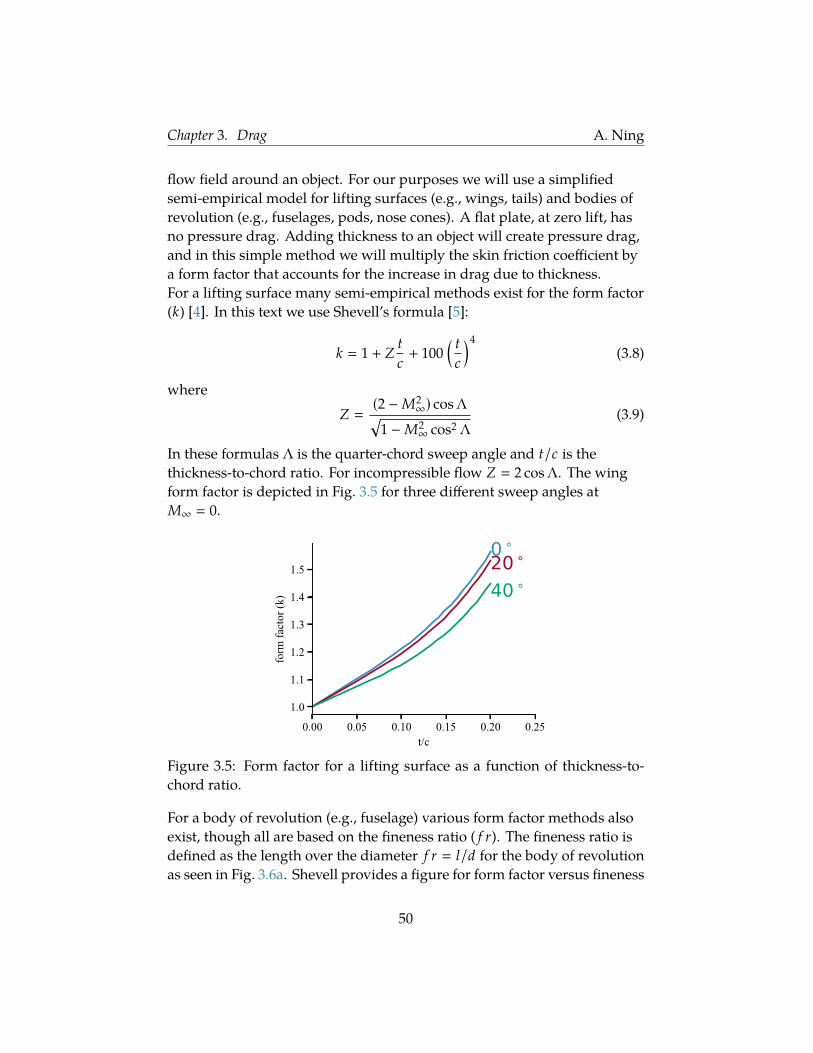
In these formulas Λ is the quarter-chord sweep angle and t/c is thethickness-to-chord ratio. For incompressible flow Z 2 cosΛ. The wingform factor is depicted in Fig. 3.5 for three different sweep angles atM∞ 0.

Figure 3.5: Form factor for a lifting surface as a function of thickness-to-chord ratio.

For a body of revolution (e.g., fuselage) various form factor methods alsoexist, though all are based on the fineness ratio ( f r). The fineness ratio isdefined as the length over the diameter f r l/d for the body of revolutionas seen in Fig. 3.6a. Shevell provides a figure for form factor versus fineness

50

Chapter 3. Drag A. Ning

ratio, but not an explicit formula [5]. A naive fit to the data would lead toform factors less than 1 for large fineness ratios, which is not physicallyconsistent. For this text we have developed the following expression usinga simple quadratic fit, but with the constraint that it bottoms out at 1.

k

1.675 − 0.09 f r + 0.003 f r2 5 < f r < 151 f r ≥ 15

(3.10)

This form factor is seen in Fig. 3.6b. Note that this method is not valid forfineness ratios smaller than 5. This formula can also be used fornon-circular cross sections. In that case one defines an effective diameterbased on the maximum cross sectional area (Smax) of the body ofrevolution:

de f f

√4Smax

π(3.11)

(a) Definition of length andmax diameter used indefining fineness ratio.

(b) Form factor as a function of fineness ratio.

Figure 3.6: A body of revolution.

3.2.3 Putting it Together

We can now put the skin friction and pressure drag together to formparasitic drag. The total parasitic drag is:

Dp kC f q∞Swet (3.12)

51

Chapter 3. Drag A. Ning

The first factor accounts for the pressure drag, the second for the skinfriction drag, and the last two are from the normalization of the skinfriction coefficient. The wetted area Swet is depicted in Fig. 3.7. Theparasitic drag acts only on the portions of the body that are exposed to thefluid. It is called a wetted area because it is the part of the vehicle thatwould be wet if dipped in a fluid.

Figure 3.7: Wetted area is the area of that component that would get wet ifdipped in a fluid. In this picture a portion of the wing carries through thefuselage (i.e., it is inside the fuselage and wouldn’t “get wet”.)

We can estimate wetted area for a lifting surface as:

Swet ≈ 2(1 + 0.2 t

c

)Sexposed (3.13)

The factor of 2 accounts for both sides of the exposed planform area(Sexposed), and the inclusion of the thickness to chord ratio (t/c) is toapproximate the additional area from curvature.For a cylindrical section of a fuselage the area is simply

Swet πdl (3.14)

For a rounded cylinder, like a nose cone, we can approximate the wettedarea as:

Swet 0.75πdl (3.15)

The last step is to normalize the drag to form a parasitic drag coefficient.Using the standard definition of the drag coefficient:

CD D

q∞Sre f(3.16)

where Sre f is some reference area for the aircraft that in general is differentfrom the wetted area of the particular component. We need to normalize

52

Chapter 3. Drag A. Ning

by the same area for all components so that drag coefficients can be addedtogether. The parasitic drag coefficient is then:

CD p kC fSwet

Sre f(3.17)

Additional sources of parasitic drag need to be added to this initialestimate. First, the method discussed estimates the parasitic drag of eachcomponent in isolation, but when assembled in an aircraft additionalinterference drag is created. It is possible that the interference could bebeneficial, but it is almost always detrimental with a typical increase indrag of 3–8% [2]. Second, we have assumed ideal lifting surfaces andaxisymmetric sections, but real aircraft require vary protuberances andhinges that create additional drag. For a jet transports these protuberancesadd about 2–5% additional drag, whereas a propeller-driven aircraft mayhave 5–10% additional drag [2]. A small RC aircraft is likely to have at leasta 10% drag markup from protuberances and could have much more if notcarefully designed. Other sources of additional parasitic drag includenacelle base drag, fuselage upsweep drag, control surface gap drag, etc.

3.2.4 Strip Theory

The proceeding method is easy to use, and appropriate in the early stagesof design, but it is oversimplified for many configurations and does notaddress some fundamental considerations like how drag changes withangle of attack. An alternative approach to computing parasitic drag thatis a bit more involved, but is generally more accurate, is strip theory. Inthis approach we subdivide the wing into a bunch of 2D strips, or in otherwords into airfoils (Fig. 3.8). Using 2D theory we compute the dragproduced by each airfoil, and then we integrate across the wing to get thetotal drag.For each section we find the angle of attack based on the local freestreamand twist, and simply use the drag polar for that airfoil to compute thedrag coefficient of that section:

cd f (α, Re ,M) (3.18)

The drag polar could come from any valid source including simulation,wind tunnel data, or flight testing. Obviously the better the source themore accurate the drag prediction.

53

Chapter 3. Drag A. Ning

Figure 3.8: Strip theory breaks thewingup into strips (i.e., airfoils), depictedin blue.

One wrinkle, is that the angle of attack we need to use is what is called theeffective angle of attack. This is the geometric angle of attack (what wenormally think of as angle of attack) minus the induced angle of attack(which will be defined in the next section):

αe f f αg − αi (3.19)

Computing the induced angle of attack generally requires a numericalsolution rather than a closed-form solution.Once we have the drag coefficient for each strip, we can get the total dragcoefficient through an integral (or summation):

CD p 1

Sre f

∫cd c (3.20)

where the above version of the formula assumes that the dynamicpressure is constant along the wing.This type of approach is used in XFLR5. Its main limitation is that itignores the three-dimensional nature of the flow across the wing,including crossflow, but for many applications that is reasonable, and theflat-plate based method we introduced shares the same limitation.

3.3 Induced Drag

Induced drag is the additional drag necessary to generate lift. There aremany ways to describe the physical mechanism. Perhaps one of the morefundamental is to consider Newton’s third law. If lift is generated, thatmeans that the surrounding air is generating a force on the vehicle to push

54

Chapter 3. Drag A. Ning

it upward. By Newton’s third law, the vehicle must be creating an equal anopposite force pushing the air downward.Indeed the air is pushed downward, but it does not continue downwardindefinitely. Instead, because the way vorticity is distributed along thewing (discussed in an aerodynamics course) the air circles around asshown in Fig. 3.9a. Generally, this circulation of air forms twocounter-rotating spiral vortices. One of these vortices is visualized from anaircraft flying through colored smoke in Fig. 3.9b

$OUG-C,EAN\7INGTIP$EVICES7HAT4HEY$OAND(OW4HEY$O)T

constitutes the vortex sheet that ends up streaming back from the wing trailing edge. The vortex sheet is a necessary part of the flowfield because the conservation laws of fluid mechanics dictate that the wing cannot produce the general flow pattern of Figure 3.1 without also producing the jump in spanwise velocity. On an intuitive level, the spanwise-‐velocity jump can be understood as being a result of the tendency of air to flow away from the high pressure under the wing toward the low pressure above the wing. The wing itself presents an obstacle to this motion and deflects it in the spanwise direction.

The development of the vortex sheet after it leaves the trailing edge is illustrated in Figure 3.2. Within the first couple of wingspans downstream, the sheet generally rolls up toward its outer edges to form two distinct vortex cores. (This is the general pattern for a wing in the "clean" condition, flaps-‐up. The flaps-‐down pattern is more complicated, with cores forming behind flap edges as well behind the wingtips.) Although the vortex cores are distinct, they are not as concentrated as they are sometimes portrayed, since a considerable amount of air that was initially non-‐vortical is entrained between the “coils” of the sheet during rollup.

In Figure 3.2 the vortex sheet is illustrated as having essentially zero thickness, and the idealized theories model it that way mathematically. In the real world the vortex sheet is a physical shear layer of finite thickness that has its origin in the turbulent boundary layers on the upper and lower surfaces of the wing and, like the boundary layers, it is filled with small-‐scale turbulent motions.

The vortex cores are often referred to as "wingtip vortices,” though this is a bit of a misnomer. While it is true that the cores line up fairly closely behind the wingtips, the term “wingtip vortices” implies that the wingtips are the sole sources of the vortices. Actually, as we saw in Figure 3.2, the vorticity that feeds into the cores generally comes from the entire span of the trailing edge, not just from the wingtips.

-C,EAN?FIG?

Figure 3.1. Velocities in a crossflow plane behind a lifting wing

Figure 3.2. The vortex wake behind a lifting wing

(a) Visualization of airflow in plane of thewing.

(b) Picture of aircraft flying throughcolored smoke to visualize the wakevortex. Picture from NASA, publicdomain.

Figure 3.9: Visualization of wake vortex.

If we look at a line between the two vortices the velocity distribution lookslike that shown in Fig. 3.10a. There is downward moving air between thetwo vortices, and upward moving air to the sides. As the vortices trailbehind the aircraft in a wake it forms a horseshoe pattern like that shownin Fig. 3.10b. This velocity distribution (partially) explains why manymigratory birds fly in a V shape (Fig. 3.11). If another bird flies behind andto the side of another bird then it can fly in a region of rising air and thusthe energy it is required to expend is reduced. By flying in this manner thebirds can increase their range (distance they can fly).Many misconceptions about induced drag exist. A common explanationfor the tip vortices is that there is high pressure below the wing and lowpressure above the wing and so the flow leaks around the edge (Fig. 3.12).This is true, and helps explain why the vortices circle around, but it is

55

Chapter 3. Drag A. Ning

(a) Induced velocity from the vortex pair.Downwash between the vortices andupwash outboard of the vortices.

(b) The vortices trail behind in a wakecausing downwash behind the wing andupwash to the sides.

Figure 3.10: Visualization of the downwash/upwash from the trailing vor-tices behind an aircraft.

Figure 3.11: Migratory birds in a V formation. Picture from Hamid Haji-husseini, CC BY 3.0.

56

Chapter 3. Drag A. Ning

incomplete. This perspective makes the process seem like a tip effect, andhas lead to the idea that the aerodynamic purpose of a winglet is tosuppress this tip vortex. This is misleading. By this logic a box wing(Fig. 3.13) should have no induced drag, as it has no tip. Lift is morefundamental than just a tip effect, and as pointed out by Newton’s thirdlaw, to create lift there must be energy left behind in the air. Certainly,vorticity is highest at the tip (and thus the center of vorticity is near there),but the formation of the vortices and the production of induced drag isaffected by the entire lifting surface and not just the tip. Winglets modifythe lift distribution in such a way that it acts like a span extension. We willsee shortly that increasing span decreases induced drag.

Figure 3.12: A simplified view of induced drag. The air leaks around thewing tip from the high pressure to low pressure side to form the vortex.

Figure 3.13: Box or annual wing. Image from Steelpillow, Wikimedia, CCBY-SA 3.0.

Another way to look at induced drag is to use the Kutta-Joukowskitheorem. This theorem says that the inviscid force per unit lengthgenerating by a lifting body is given by:

F′ ρ ®V × ®Γ (3.21)

where Γ is the circulation. Circulation is defined as a line integral of thevelocity around a closed contour:

Γ

∮®V · d®l (3.22)

57

Chapter 3. Drag A. Ning

For the airfoil in Fig. 3.14, if it is generating lift, its circulation will be intothe page as shown. Any closed contour, of any shape, taken around theairfoil will give the same value for the circulation. This is an admittedlyterse definition of circulation, but the important point for our purposes isthat the generated force is given by the cross product defined in theKutta-Joukowski theorem, also shown in that same figure.

Figure 3.14: Circulation is found by integrating around any closed contouraround the lifting body. Lift is given by the cross product of the freestreamvelocity and the circulation.

As discussed, when a wing generates lift it forces air downward. Thisdownward moving air is called downwash (w) and is shown in Fig. 3.15.The effective incoming velocity is no longer V∞ but rather Vr . Again,applying the Kutta-Joukowski theorem we see that the force vector hastilted backwards creating a component of the force in the lift direction anda component in the drag direction (lift and drag are defined relative toV∞). This component of drag is the induced drag.The formula for the induced drag, and induced drag coefficient is given by:

Di L2

q∞πb2einv(3.23)

CD i C2

L

πAReinv(3.24)

where AR b2/Sre f is the aspect ratio, and einv is the inviscid spanefficiency that will be discussed in more detail shortly. Notice the strongdependence on lift, and on span. As expected as we increase lift, theinduced drag increases. Increasing span allows for a decrease in induced

58

Chapter 3. Drag A. Ning

Figure 3.15: Induced drag from the viewpoint of the Kutta-Joukowski The-orem. The presence of downwash (w) tilts the incoming velocity vector andthus the resulting force. The component in the direction of the freestreamis induced drag.

drag. This is why high-efficiency aircraft, or birds, have long wing spansalthough with the tradeoff of generally slower speeds.It is important to note that this formula gives the inviscid induced drag. Allthe behavior we have discussed so far does not depend on the presence ofviscosity. The inviscid span efficiency einv hides some complicated flowphysics behind a single number. Effectively, it is a measure of how closethe lift distribution is to the one that produces minimum induced drag.For a planar wing, which means a wing whose planform is contained inone geometric plane (e.g., no winglets), the lift distribution for a fixed spanplanar wing with minimum induced drag is an elliptic shape as seen in Fig. 3.16.

Figure 3.16: An elliptic distribution of lift.

Most aircraft do not have an exact elliptic lift distribution, but will often befairly close. An elliptic distribution produces an inviscid span efficiency of1.0 and a typical value for a wing is 0.98. The presence of the fuselagetends to decrease the lift produced at the center as shown in Fig. 3.17. Fora wing/fuselage combination the inviscid span efficiency can be estimatedas:

einv 0.98

[1 − 2

(d f

b

)2]

(3.25)

59

Chapter 3. Drag A. Ning

where d f is the diameter of the fuselage, and b the wingspan (asimplification of the formula in [6]).

Figure 3.17: The presence of the fuselage causes a loss in lift productionnear the centerline.

The presence of lift also tends to increase the viscous component of drag.While this could potentially be book-kept with parasitic drag, we willinclude it with induced drag. Empirical data suggests that viscousinduced drag also increases proportionally with the square of the lift. Wecan estimate the viscous induced drag coefficient as:

CD i ,v KCD pC2L (3.26)

Note that quadratic dependence on lift. We also assume that it isproportional to the parasitic drag. The remaining factor, K, is an empiricalconstant determined to be approximately K 0.38 [5]. We can combinethe inviscid and viscous components as follows:

CD i C2

L

πAReinv+ KCD pC2

L

CD i C2

L

πAR

(1

einv+ KCD pπAR

) (3.27)

We would like to return our equation to a simple form like before, so wedefine everything in parenthesis as 1/e where e is a new term called theOswald efficiency factor. Now the induced drag coefficient is given by:

CD i C2

L

πARe(3.28)

wheree

11

einv+ KCD pπAR

(3.29)

60

Chapter 3. Drag A. Ning

Notice that our total induced drag coefficient equation looks the same asthe inviscid induced drag coefficient (Eq. (3.24)), except we have replacedeinv with e. Whereas a typical value for the inviscid span efficiency (einv) isclose to 1, a typical value for the Oswald efficiency factor (e) is between0.7–0.9. The induced drag in Eq. (3.23) transforms similarly with ereplacing einv .The previous section mentioned the induced angle of attack, which wewill touch on briefly. The presence of downwash changes the direction ofthe incoming velocity as explained earlier and shown in Fig. 3.15. Theinduced angle of attack is the angle created between the freestream andthe new relative velocity as shown in Fig. 3.18.

αi tan−1(−wV∞

)(3.30)

On the right side of the figure we see that the induced angle of attackreduces the angle of attack experienced by the airfoil:

αe f f αg − αi (3.31)

where αg is the geometric angle of attack. Thus, the presence ofdownwash decreases the angle of attack experienced by each section.

Figure 3.18: The induced angle of attack reduces the effective angle of attackof the section. Angle of attack of airfoil exaggerated for clarity of display.

For an elliptic lift distribution, the downwash is constant along the wingand the induced angle of attack is given (with a small angleapproximation) by:

αi CL

πAR(3.32)

In general, the downwash, and thus the induced angle of attack, variesalong the wing and must be determined through a numerical solutionsuch as lifting line theory or a vortex lattice method discussed in anaerodynamics course.

61

Chapter 3. Drag A. Ning

3.4 Tradeoffs in Parasitic and Induced Drag

For low Mach number (i.e., no compressibility drag) the total dragcoefficient or total drag of an aircraft is given by:

CD CD p +C2

L

πARe(3.33)

orD CD p q∞Sre f +

L2

q∞πb2e(3.34)

At low speeds the drag is dominated by induced drag (see q∞ indenominator), where as high speeds the drag is dominated by parasiticdrag (see q∞ next to CD p). The parasitic, induced, and total drag as afunction of speed, for an example aircraft, is shown in Fig. 3.19. The pointat which they cross, is the speed for minimum total drag, or in other wordsthe speed that maximizes the lift-to-drag ratio.

flight speed

drag

inducedparasitic

total

Figure 3.19: Tradeoff in parasitic and induced drag versus flight speed.

3.5 Compressibility Drag

Before discussing methods to estimate compressibility drag we need tounderstand the physical mechanism, and so we begin with sound waves.Disturbances in a fluid are communicated via soundwaves—infinitesimally weak pressure waves that travel at the speed of

62

Chapter 3. Drag A. Ning

sound. A familiar example is a river flowing around a rock. The water“senses” the presence of the rock and starts diverting its path before itreaches the rock. The mechanism that allows the water to sense the rock issound waves, or pressure waves, transmitted through the water. Theincreased pressure starts to divert the water well before it reaches the rock.Let’s reduce our rock to a point and rather than have the fluid movearound the rock, let’s have the point move through the fluid. Figure 3.20shows four scenarios with the point moving to the right. In the firstscenario the point is not moving. Pressure waves travel in all directions atequal speed (the speed of sound). In the second scenario the point ismoving to the right at subsonic speeds. The pressure waves in thedirection of travel bunch up, and the separation between the pressurewaves behind the point elongates. In the third scenario the point ismoving at the speed of sound. The pressure waves coalesce at the front asthey are all moving at exactly the same speed as the point. In the lastscenario the rock is moving faster than the speed of sound. In one instantof time the point sends off a pressure wave, but in the next instant of timethe rock has traveled past that sound wave. The envelope of pressurewaves forms a cone, known as a Mach cone. See this webpage for ananimated version of this concept.

Figure 3.20: Sound waves emanating from a point moving to the right forfour different Mach numbers.

Now let’s revisit our rock in the river example, but with an airplane and asmall region of air. The following is only an analogy as fluid propertiesvary throughout the flow, but illustrates the general principle. If theairplane is flying subsonically the air will “sense” that the airplane iscoming because of the pressure waves that emanate ahead of the aircraft.It will start moving ahead of time to flow around the airplane, like theriver around the rock.

63

Chapter 3. Drag A. Ning

Now let’s assume the airplane is flying supersonically. An air particle thatis in front of the airplane won’t know the airplane is approaching until it’salready there. It can’t know because the airplane is flying faster than thepressure waves. This is a problem because the air needs to move aroundthe aircraft, but won’t be able to until it’s too late. Nature’s solution is ashock wave.A shock wave is a narrow region that causes an instantaneous change inflow conditions.1 In an instant the pressure, density, and temperature allincrease, the Mach number decreases, and the flow direction changes (ifthe flow is perpendicular to the shockwave then the flow direction doesnot change).In the prior example the point was infinitely small and so it created aninfinitely weak disturbance. The resulting wave front is called aMach wave.For a finite disturbance the coalescence of sound waves creates a shockwave, or for an aircraft multiple shock waves (see Fig. 3.21).

Figure 3.21: Shock waves around an aircraft in a wind tunnel visualizedusing Schlieren photography. The Schlieren method takes advantage of thebending of light through density changes, and a shockwave produces a nearinstantaneous change in density. Image from NASA, public domain.

A course in compressible flow will discuss shockwave theory in more

1It’s not actually instantaneous. The shock wave is like a boundary layer—a very thinregion dominated by viscous effects. It’s so thin that to the external flow it is effectivelyinstantaneous. Note that even though shock waves have a viscous structure, they will stillbe correctly predicted in an inviscid solution.

64

Chapter 3. Drag A. Ning

detail. For aircraft design our main interest in shock waves is that theycarry energy away and thus increase our drag. The stronger the shockwave the more the drag increases. Shock strength increases with bluntershapes and with increasing Mach number.The following subsections discuss methods to estimate wave drag fortransonic speeds and supersonic speeds separately. Recall thatcompressibility drag is often referred to as wave drag.

3.5.1 Transonic Wave Drag

Transonic mean Mach numbers close to 1. Usually transonic refers only tosubsonic speeds, but sometimes transonic is used to mean both subsonicand supersonic speeds. In our case we mean the former, with a typicalrange of Mach 0.7–1.Even though the freestream speed is subsonic, as air is accelerated aroundthe aircraft regions of supersonic flow can occur. Figure 3.22 illustratesflow around an airfoil at three different Mach numbers. The first airfoilillustrates what is called the critical Mach number, or the Mach numberwhere the maximum velocity on the aircraft is sonic. This flight speed isthe point just before supersonic flow will appear. In aircraft design weusually care more about the crest critical Mach number (Mcc). This is theMach number where the crest (top) of the wing first becomes sonic.After passing the critical Mach number regions of supersonic flow exist onthe airfoil, highlighted in dark blue in the figure. As the freestream Machnumber increases the shock strength increases leading to highercompressibility drag. Viscous pressure drag may also increase. This isbecause speed drops significantly across the shock wave, thus making theboundary layer more likely to separate.The formation of shock waves leads to a precipitous increase in drag asMach 1 is approached. The rise is so sharp that it is often referred to as a“sound barrier” (Fig. 3.23). Not a barrier in a sense of impenetrability, buta barrier in the sense that a tremendous amount of energy is required topass through. The Concorde, for example, had to use afterburners to passthrough the sound barrier. Note that drag drops after Mach 1, though itdoes start increasing again (not shown on the plot).One of the major keys to unlocking efficient transonic flight was thediscovery by Adolf Busemann, and later independently by R. T. Jones, thata swept-back wing decreased transonic wave drag. In fact, this discovery is

65

Chapter 3. Drag A. Ning

Figure 3.22: Visualization of regions of supersonic flow over an airfoiltraveling at transonic speeds. Image from FAA, Airplane FlyingHandbook,public domain.

Figure 3.23: Notional plot of the steep compressible drag rise, or “soundbar-rier” prior to Mach 1. The crest critical Mach number and drag divergenceMach number are also shown.

66

Chapter 3. Drag A. Ning

considered one of the most important discoveries in aerodynamic history.2The concept can be motivated through a simple thought experiment.Imagine an infinite wing of constant cross-section in an inviscid flow. Ifthe wing started moving sideways at constant speed, and the flow wereinviscid, nothing would change. In a coordinate system moving at thewing speed, only the normal component of the inflow would exist. Inother words, the normal and tangential components of velocity areindependent. By adding a tangential component we have exactly recreateda swept wing flying obliquely (Fig. 3.24).

Figure 3.24: An unswept wing, on the left side, with normal (Mn) andtangential (Mt) components of Mach number, is exactly the same as a sweptwing flying obliquely as shown on the right side.

In other words, as only the normal component of velocity matters for thestraight wing, so too it is only the normal component of velocity thatmatters for the swept wing (Fig. 3.25). The implication of this idea is thatsweeping the wing allows the airfoils to see a reduced effective Machnumber. For example, if the flight Mach number was 0.8, and the sweepwas 30 degrees, then the airfoils (normal to the sweep) could be designedto operate as if the incoming flow was M 0.8 cos 30 0.69. That is alarge reduction and is what has enabled transport aircraft to fly at muchhigher speeds. This concept is called simple sweep theory as it is asimplification of the real flow because it assumes two-dimensional flowbehavior (that’s what an finite wing implies), that all sections are identical,and assumes inviscid flow (viscosity can be important for the crossflowboundary layer development). Despite the simplifying assumptions, inmost cases it approximates the real flow behavior quite well.A forward swept wing produces the same transonic drag reductionbenefits. However, forward sweep is aeroelastically unstable. For a

2https://www.nasa.gov/langley/hall-of-honor/robert-t-jones

67

Chapter 3. Drag A. Ning

Figure 3.25: For a swept wing only the normal component of the velocitymatters according to simple sweep theory.

forward swept wing an increase in lift at the tips typically causes them totwist up, which further increases lift creating a positive feedback loopleading to divergence. For a backward swept wing increased lift at the tipdecreases the twist, leading to decreased lift and thus a stableconfiguration. This instability is one of the main reasons why forwardsweep is much less common.For transonic speeds we generally want to fly as fast as possible withoutincurring a significant drag rise penalty. In other words, most transportaircraft fly at the point just as the curve in Fig. 3.23 starts to turn upward.This Mach number is called the drag divergence Mach number (Mdd) and islabeled in that figure. The drag divergence Mach number can be estimatedusing a modification of the Korn equation with simple sweep theory [7]:

Mdd 0.95

cosΛ− t/c

cos2Λ− CL

10 cos3Λ(3.35)

Notice that sweep plays a major factor, as expected, as does thickness andlift.The compressibility drag coefficient can then be estimated using thefollowing empirical relationship [8]:

CD c

0 for M∞ < Mcc

20(M∞ −Mcc)4 for Mcc < M∞ < 1(3.36)

Note the rapid rise in drag (quartic) with Mach numbers past Mcc . ForMach numbers less than Mcc there are no shock waves and thus no wavedrag.To complete the set of equations we need a way to relate Mdd (when dragstarts to rise rapidly) to Mcc (when there is no compressibility drag).Various definitions for the drag divergence Mach number exist. In the

68

Chapter 3. Drag A. Ning

following we use the definition that drag divergence occurs once the slopeof the drag curve equals 0.1:

dCD

dM 0.1 (3.37)

If we take the derivative of Eq. (3.36) and use the above definition of Mdd

we find the following relationship:

Mcc Mdd − 0.11 (3.38)

3.5.2 Supersonic Wave Drag

For supersonic flight the presence of shock waves is unavoidable. Tominimize drag, we generally want to have oblique shocks and this requiresa sharp leading edge and slender shapes as depicted in Fig. 3.26 or as seenin a concept supersonic aircraft (Fig. 3.27).

Figure 3.26: Depiction of an oblique shock around a sharp-nosed airfoil.

Figure 3.27: Supersonic transport concept showing sharp leading edges andslender shapes. Image from NASA, Boeing concept supersonic transport,Icon-II, public domain.

69

Chapter 3. Drag A. Ning

The minimum wave drag for a wing can be broken up into two parts: onedue to volume and one due to lift. The derivation assumes that the liftdistribution is elliptic in both directions. In other words, this is theminimum drag and so for a given design the drag could be much higher.The formulas are derived by R. T. Jones [9], and are manipulated inSection A.2 to a form consistent with our usage. The results are shownbelow.The wave drag of a wing due to volume is given by:

CD c ,v 4Sr

( tc

)2 (β2 + 2r2)(β2 + r2)1.5 (3.39)

whereβ

√M2 − 1, (3.40)

r πl2

4Sg(3.41)

and Sr Sg/Sre f is the ratio of the gross area to the reference area us ed inthe drag normalization. The wave drag of a wing due to lift is given by:

CD c ,l C2

Lr4Sr

√

1 +

(βSr

r

)2

− 1

Sre f

Sg(3.42)

The wave drag of a fuselage due to volume is given by:

CD c ,v π3

4d2

(l/d)2Sre f(3.43)

where l and d are the length and maximum diameter of the fuselagerespectively.In general, we can show that the volume dependent wave drag atsupersonic speeds is proportional to volume squared over length to thefourth power:

Dw ∝volume2

l4 (3.44)

In other words, for low drag, a supersonic transport should be long andhave as little volume as possible. The elongation effect is reflected in manydesigns, and is seen in the concept plane shown earlier (Fig. 3.27).

70

Chapter 3. Drag A. Ning

However, having low volume alone is not sufficient for low drag. The waythat volume is distributed also matters. R. T. Whitcomb made theimportant discovery that reducing the volume of the fuselage near thewing led to a large reduction in drag [10]. This “coke-bottle” shape is seenin many supersonic aircraft such as the redesigned version of the DeltaDart (Fig. 3.28).

Figure 3.28: NASA QF-106 Delta Dart, NASA, public domain.

This idea became known as the area rule and enabled new high speeds foraircraft. A more detailed look at the theory shows that the secondderivative of the area distribution appears in the drag calculation. Thismeans that the area distribution should change smoothly—sharp changesproduces high second derivatives in area and thus high drag. Bydecreasing the fuselage area, just as the wing area is increasing, asmoother cross-sectional area distribution can be maintained.The area rule is more complex than described. The distribution ofcross-sectional areas perpendicular to the body (Fig. 3.29) only applies atMach 1. In general, the cross-sectional areas are taken at the angle of theMach wave and are thus speed dependent. Because the aircraft willgenerally be flown through many speeds, this means that the areadistribution needs to be optimized for multiple conditions. Additionally,

71

Bibliography A. Ning

Figure 3.29: Cross sectional areas, as used in the area rule. Image by PetrDlouhý, Wikimedia Commons, public domain.

cuts need to be taken for geometric planes spanning all 360 degreesaround the aircraft.

3.5.3 High Mach or Blunt Bodies

As the Mach number is increased, or if the geometry is blunt rather thansharp, a detached bow shock will form (Fig. 3.30). A bow shock producesmuch higher drag than the oblique shocks discussed in the previoussection. For aircraft this is generally undesirable, but for a reentry vehiclehigh drag is desirable. The high drag slows the vehicle down, and reducesthe heat transfer to the vehicle. The temperature increase behind a bowshock is larger than that of an oblique shock, but because the shockdetaches, the separation distance more than makes up for the increasedtemperature leading to overall lower heating.

Bibliography

[1] Schlichting, H. and Gersten, K., Boundary-Layer Theory, SpringerScience & Business Media, May 2003.

[2] Raymer, D. P., Aircraft Design: A Conceptual Approach, AmericanInstitute of Aeronautics and Astronautics, 2012.

72

Bibliography A. Ning

Figure 3.30: Detached bow shock in front of a blunt reentry body. Image byNASA, public domain.

[3] Talay, T. A., “Introduction to the Aerodynamics of Flight,” NASASP-367, National Aeronautics and Space Administration, Washington,D.C., 1975.

[4] Takahashi, T. J., German, B. J., Shajanian, A., Daskilewicz, M. J., andDonovan, S., “Form Factor and Critical Mach Number Estimation forFinite Wings,” Journal of Aircraft, Vol. 49, No. 1, jan 2012, pp. 173–182.

[5] Shevell, R. S., Fundamentals of Flight, Pearson College Division, 1989.

[6] Kroo, I., Aircraft Design: Synthesis and Analysis, Stanford University,2006.

[7] Malone, B. and Mason, W. H., “Multidisciplinary optimization inaircraft design using analytic technology models,” Journal of Aircraft,Vol. 32, No. 2, mar 1995, pp. 431–438.

[8] Hilton, W. F., High-speed Aerodynamics, 1951.

[9] Jones, R. T.,Wing Theory, Princeton University Press, Jul 2014.

[10] Whitcomb, R. T., “A Study of the Zero-Lift Drag-Rise Characteristicsof Wing-Body Combinations Near the Speed of Sound,”NACA-TR-1273, National Advisory Committee for Aeronautics, Jan1956.

73

CHAPTER4

Wing Design

Wing design is at the heart of aircraft design. The wing (or sometimeswings) provides almost all of the lift of the aircraft, and its dimensionssignificantly affect the speed and performance of the aircraft.Appropriately designing the wing is critical.

4.1 Fundamental Parameters

One of the primary design parameters for a wing is its span. Its definitionis usually straightforward (Fig. 4.1). Span refers to the projected span asshown in the figure. In other words, a vertical winglet does not increasespan. Despite its apparent simplicity there are cases where the definitionof span is ambiguous. Many modern aircraft have highly flexible wingsand so the span will change depending on the flight conditions and/orfuel loading. In this case we would also need to specify the loadingcondition, for example span under a 1-g load (i.e., when lift equals weight).Often the most fundamental tradeoff in selecting span is balancing dragand weight (aerodynamics and structures). An increase in span decreasesinduced drag as 1/b2 as we saw in Chapter 3. Conversely, an increase inspan increases bending stresses and thus structural weight. For some cases(e.g., a flying wing) bending stress is not the dominant structuralconstraint, but other structural constraints like flutter similarly require

74

Chapter 4. Wing Design A. Ning

Figure 4.1: Depiction of wing span. The bottom shows a back view of thewing to demonstrate that span refers to the projected span, or the spanprojected onto a horizontal plane.

significant weight increases with increasing span.If the wing area is fixed then increasing span decreases the internalvolume (e.g., fuel/battery capacity). It also decreases the Reynoldsnumbers across the wing, which generally leads to increased parasitic dragand higher stall speeds because of reduced maximum lift coefficients.If the wing is swept back then increasing span moves the aerodynamiccenter back, which may or may not be desirable. This will have a strongeffect on stability as we will see in a later chapter.Wing area is another fundamental parameter. Many definitions are used(e.g., wetted area, reference area, projected area) depending on thecontext. One of the most common reasons to increase wing area is todecrease stall speed. The stall speed for level flight is given by:

Vs

√2W

CLmaxρSre f(4.1)

However, increasing wing area leads to increased parasitic drag and wingweight. Wing area also affects the optimal cruise lift coefficient, which mayor may not be desirable.Sweep is often defined relative to the quarter chord line (Fig. 4.2), but issometimes defined relative to the leading edge instead. The primaryreason to use sweep is to decrease transonic wave drag as discussed inSection 3.5.1. The other reason to use sweep is as a means to achievelongitudinal stability for a flying wing as will be discussed in Section 5.2.Beyond those two use cases, there is rarely good reason to use sweep asthere are many detrimental effects including an increase in structural spanwith a corresponding increase in weight, an increase in tip loads with a

75

Chapter 4. Wing Design A. Ning

corresponding increase in weight and a reduced margin for tip stall, and areduction in CLmax .

Figure 4.2: Sweep is generallymeasured about the quarter chord (but some-times about the leading edge). Itmaybe adistribution rather than a constantvalue.

Airfoil thickness is also primarily an aerodynamic/structural tradeoff.Thicker airfoils reduce wing weight if your wing is bending constrained(discussed in Section 8.2), usually increase CLmax (up to a point), and allowfor more internal volume. Conversely, thicker airfoils increase parasiticdrag and compressibility drag. Thus, aerodynamic considerations usuallyfavor thinner airfoils, while structural considerations usually favor thickerairfoils.

Figure 4.3: Section thickness.

Chord and twist (Fig. 4.4) are strongly coupled with the lift and liftcoefficient distributions as will be discussed in the next section. One of themain tradeoffs with chord is that more taper decreases wing weight, butcan lead to tip stall. Although we often use taper ratio, modern wingsincreasingly use composites and have more complex shapes than lineartaper.

Figure 4.4: Chord and twist.

76

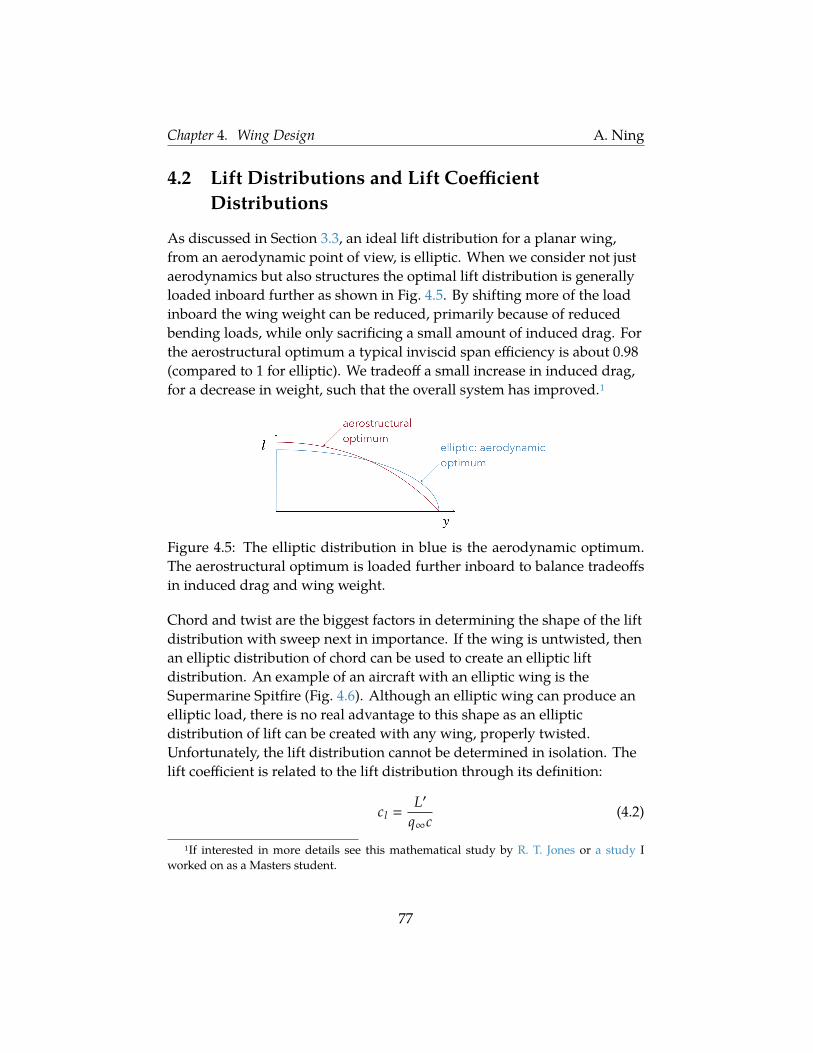
Chapter 4. Wing Design A. Ning

4.2 Lift Distributions and Lift CoefficientDistributions

As discussed in Section 3.3, an ideal lift distribution for a planar wing,from an aerodynamic point of view, is elliptic. When we consider not justaerodynamics but also structures the optimal lift distribution is generallyloaded inboard further as shown in Fig. 4.5. By shifting more of the loadinboard the wing weight can be reduced, primarily because of reducedbending loads, while only sacrificing a small amount of induced drag. Forthe aerostructural optimum a typical inviscid span efficiency is about 0.98(compared to 1 for elliptic). We tradeoff a small increase in induced drag,for a decrease in weight, such that the overall system has improved.1

Figure 4.5: The elliptic distribution in blue is the aerodynamic optimum.The aerostructural optimum is loaded further inboard to balance tradeoffsin induced drag and wing weight.

Chord and twist are the biggest factors in determining the shape of the liftdistribution with sweep next in importance. If the wing is untwisted, thenan elliptic distribution of chord can be used to create an elliptic liftdistribution. An example of an aircraft with an elliptic wing is theSupermarine Spitfire (Fig. 4.6). Although an elliptic wing can produce anelliptic load, there is no real advantage to this shape as an ellipticdistribution of lift can be created with any wing, properly twisted.Unfortunately, the lift distribution cannot be determined in isolation. Thelift coefficient is related to the lift distribution through its definition:

cl L′

q∞c(4.2)

1If interested in more details see this mathematical study by R. T. Jones or a study Iworked on as a Masters student.

77

Chapter 4. Wing Design A. Ning

Figure 4.6: The Supermarine Spitfire is a well-known example of an aircraftwith an elliptic wing. Image from Adrian Pingstone, Wikimedia, publicdomain.

Note that the lift coefficient distribution is a function of the lift distributionand the chord distribution.Before discussing an ideal lift coefficient distribution we first need todiscuss critical section theory. Critical section theory is a simplifiedapproach to predicting when a wing/aircraft will stall. We already knowthat an airfoil will stall at angles of attack past cl max , but how does thatapply to a wing where angle of attack, cl , and cl max can vary along thewing? The basic idea of critical section theory, is that the wing is predictedto stall when any one section would stall using 2D theory. Furthermore,the section that first stalls is predicted to be the location on the wing wherestall initiates.For example, from the lift distribution and Eq. (4.2) we can compute the liftcoefficient distribution. From airfoil data we can extract a distribution forcl max along the span. Now we increase the angle of attack until the cl

curve just touches the cl max curve as shown in Fig. 4.7. The figure alsopoints out the spanwise position where we expect stall to occur (at about30% of the span). Critical section theory is a simplification of how stalldevelops. It works well if there is negligible crossflow across the wing, inother words if the flow is basically two-dimensional at each section.At first glance it would seem that an ideal lift coefficient distribution

78

Chapter 4. Wing Design A. Ning

Figure 4.7: An illustration of critical section theory. Stall is predicted tooccur at the angle of attack at which these two curves meet, and at thespanwise location where they meet.

would be constant across the span. That would mean that every sectionwas equally contributing, and thus no section would stall prematurely.The problem with this distribution is that it doesn’t prevent tip stall, whichoccurs when stall initiates near the wing tips. Tip stall is problematic fortwo reasons: 1) a loss of lift far from the centerline of the wing creates alarge rolling moment that could be dangerous or at least degrade ridequality, and 2) ailerons (the control surfaces that affects roll) are generallylocated outboard to have maximum effect and if the ailerons stall then rollcontrol is lost. For these reason a good design must ensure that stall occursinboard first. Thus, an ideal cl distribution is roughly constant inboard,then drops off towards the tip so that stall occurs inboard first.Because both the lift and lift coefficient distribution are affected by chordand twist (at least indirectly), and the wing bending stress depends on thelift and chord distribution, creating an ideal balance can be challenging.Chord is perhaps the most impactful parameter. As discussed, by usingtwist we can create an elliptic lift distribution for any planform shape.However, that planform shape then dictates what the lift coefficientdistribution looks like. For example, Fig. 4.8 shows the impact of threedifferent planform shapes on the lift coefficient distribution, assuming anelliptically loaded lift distribution.Let’s examine each of these parameters in isolation. The top portion ofFig. 4.9 shows the impact of changing chord on the lift and lift coefficientdistributions. A high taper ratio means that the root and tip chord arerelatively close in size. That means that if there is no twist, the liftdistribution is relatively uniform. In contrast, a small taper ratio (with no

79

Chapter 4. Wing Design A. Ning

Figure 4.8: The lift coefficient distribution for three different planformshapes given an elliptic lift distribution.

twist) would produce higher lift at the root and lower lift at the tip.Because chord is also coupled with the lift coefficient, some potentiallyundesirable behavior is observed. For high taper ratio the chord isrelatively uniform and so the lift coefficient distribution looks fairly similarto the lift. The low taper ratio on the other hand has small tip chords, andso according to Eq. (4.2) the cl at the tip will be high. For structuralloading a smaller taper ratio is desirable, but we see that it increases thelikelihood of tip stall.The second row of Fig. 4.9 shows the impact of changing twist on anelliptically loaded wing for fixed lift. Increased twist at the tip is calledwash-in and decreased twist (i.e., increased negative twist) at the tip iscalled wash-out. Many wings have some wash-out in order to produce amore structurally efficient lift distribution. By reducing the twist at the tipthe lift at the tip is correspondingly reduced. Note that the effect of twist isthe same on lift and lift coefficient.The last row of Fig. 4.9 shows the impact of changing sweep relative to anelliptically loaded wing. Like twist, sweep affects both distributions in thesame way. Backward sweep increases the lift and the tip, whereas forwardsweep decreases it.One of the primary challenges of wing design is to create achord/twist/sweep combination with a desirable lift distribution thatbalances induced drag and structural considerations, and a lift coefficientdistribution that balances efficiency with preventing tip-stall. This is notalways easy and like most engineering decisions requires making some

80

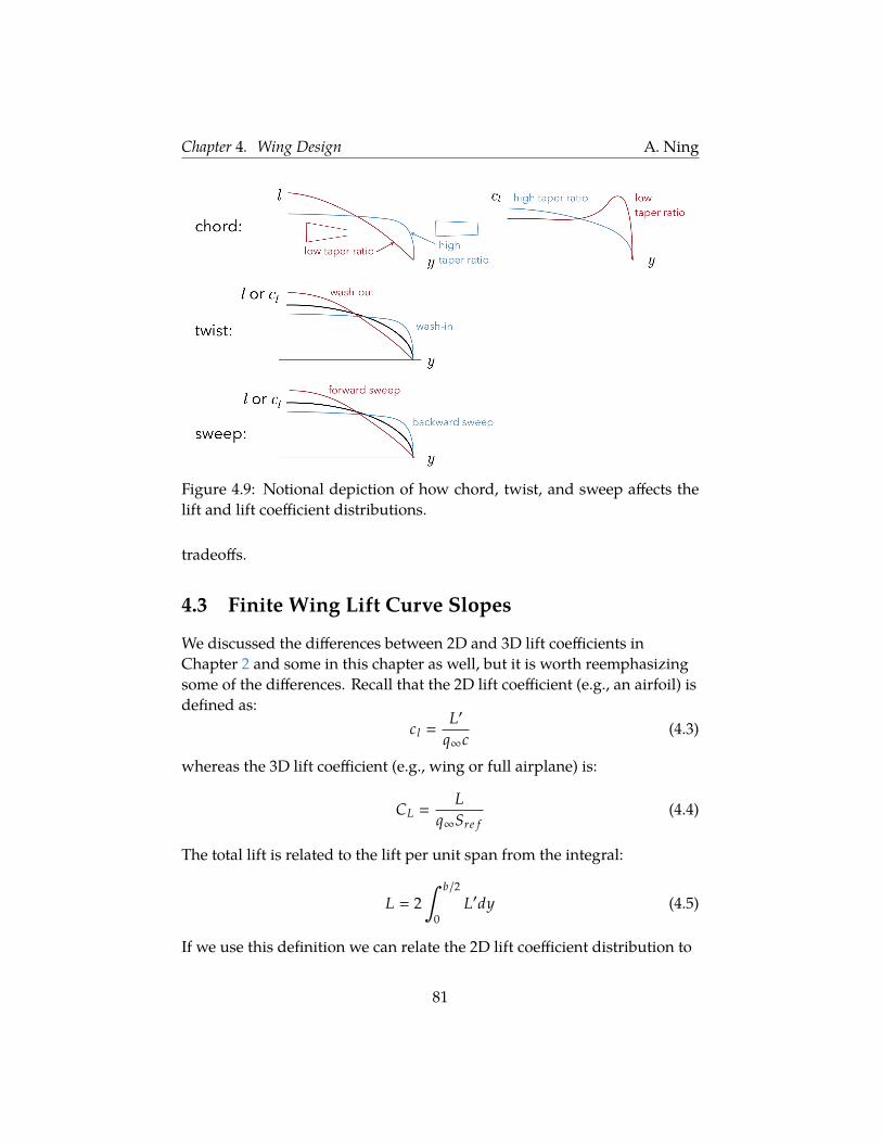
Chapter 4. Wing Design A. Ning

Figure 4.9: Notional depiction of how chord, twist, and sweep affects thelift and lift coefficient distributions.

tradeoffs.

4.3 Finite Wing Lift Curve Slopes

We discussed the differences between 2D and 3D lift coefficients inChapter 2 and some in this chapter as well, but it is worth reemphasizingsome of the differences. Recall that the 2D lift coefficient (e.g., an airfoil) isdefined as:

cl L′

q∞c(4.3)

whereas the 3D lift coefficient (e.g., wing or full airplane) is:

CL L

q∞Sre f(4.4)

The total lift is related to the lift per unit span from the integral:

L 2∫ b/2

0L′dy (4.5)

If we use this definition we can relate the 2D lift coefficient distribution to

81

Chapter 4. Wing Design A. Ning

the overall wing lift coefficient:

CL L

q∞Sre f(4.6)

2∫ b/2

0 L′dy

q∞Sre f(4.7)

2∫ b/2

0 cl q∞cdy

q∞Sre f(4.8)

2∫ b/2

0 cl cdy

Sre f(4.9)

(4.10)

If we divide the reference area by the span to define the mean geometricchord c then:

CL 2∫ b/2

0 cl cdy

bc(4.11)

CL

∫ 1

0

cl cc

dy∗ (4.12)

(4.13)

where y∗ yb/2 . What this equation shows is that for the case where the

chord is constant (c c) then the wing lift coefficient is the average of theairfoil lift coefficient distribution. For cases where the chord is notconstant, it is a chord weighted average.In Chapter 2 we learned that the theoretical lift curve slope of an airfoilwas 2π. The same is not true for a finite wing because of downwash. Let’sdenote the 2D lift curve slope as m. If we had an infinite wing, with aconstant airfoil then the wing lift coefficient would be:

CL m(α − α0) (4.14)

and the lift curve slope would be unchanged.However, for a finite wing there is downwash and so we need to includethe induced angle of attack:

CL m(α − α0 − αi) (4.15)

82

Chapter 4. Wing Design A. Ning

From finite wing theory, we can show that the induced angle of attack foran elliptic lift distribution is given by:

αi tan−1(

CL

πAR

)(4.16)

For small angles we can approximate this as:

αi ≈CL

πAR(4.17)

Substituting this in Eq. (4.15) gives:

CL ≈ m(α − α0 −CL

πAR) (4.18)

If we solve this for CL and take the derivative with respect to angle ofattack in order to get the wing lift curve slope we find:

dCL

dα

m1 +

mπAR

(4.19)

where m is the 2D lift curve slope, typically a value close to 2π. Notice thatas the aspect ratio goes to infinity we recover the 2D slope as expected.However, for finite wings the lift curve slope is reduced compared to thatof its airfoils (Fig. 4.10). For example, an aspect ratio 8 wing would have apredicted lift curve slope of 0.8(2π) or 80% of the 2D value. Keep in mindthat this is a simplified formula assuming constant airfoils, anapproximately elliptic load, and low Mach number.

Figure 4.10: Lift curve slope for airfoil and wing.

83

CHAPTER5

Stability

The best performing aircraft won’t be of much use if it is too unstable to fly.This chapter provides an introduction to static and dynamic stability offlight vehicles. For many aircraft the longitudinal and lateral dynamics areeffectively decoupled, and will be presented separately in this chapter.

5.1 Definitions and Fundamentals

We begin with a look at the forces and moments for a three-dimensionalaircraft. In Chapter 2 we discussed the difference between wind and bodyaxes for an airfoil. In three dimensions, we need one extra angle to definethe rotation between wind and body axes (sideslip angle). Recall that liftand drag are defined in the wind axes, and that the wind axes are alignedwith the freestream direction as shown in Fig. 5.1. The angle of attackdefines one of the rotation angles between the body axes and wind axes.As we move to 3D, we need two additional parameters: the sideslip angleβ and the side force Y.In two-dimensions the only moment was the pitching moment. Inthree-dimensions we have three moments as shown in Fig. 5.2: roll (l),pitch (m), and yaw (n). We define these moments about the wind axes.Conventionally, the letter l is used for roll even though this can easily beconfused with lift. In this text we will spell out roll in the coefficient.

84

Chapter 5. Stability A. Ning

Figure 5.1: Wind axes. Lift and drag are defined relative to these axes.Definitions for positive angle of attack and sideslip also shown.

Figure 5.2: The three moments for a flight vehicle have specific names: roll,pitch, and yaw.

85

Chapter 5. Stability A. Ning

The forces and moment coefficients are defined as follows:

CD D

q∞Sre f(5.1)

CY Y

q∞Sre f(5.2)

CL L

q∞Sre f(5.3)

Croll roll

q∞Sre f bre f(5.4)

Cm m

q∞Sre f cre f(5.5)

Cn n

q∞Sre f bre f(5.6)

(5.7)

Notice that roll and yaw use span as the second reference dimension,whereas pitch uses chord. This is because the dynamics of roll and yaware primarily effected by the change in inertia from span, whereas pitch isprimary affected by changes in chord.The rotation rates (e.g., rad/s) about the three axes are: roll rate (p), pitchrate (q), and yaw rate (r). These rotation rates are normalized as follows:

p pbre f

2V∞(5.8)

q qbre f

2V∞(5.9)

r rbre f

2V∞(5.10)

(5.11)

A wide variety of control surfaces exist, but the most common are:ailerons to control roll, elevators to control pitch, and rudder to controlyaw (see Fig. 5.3). An aircraft is said to be trimmed if the sum of its forcesand moments are zero. In other words it is in static equilibrium. Thecontrol surfaces must have adequate response to trim the aircraftthroughout its flight profile.Figure 5.4 overviews the different types of stability. The x-axis in eachfigure is time, and the y-axis is some response (e.g., deflection). The upper

86

Chapter 5. Stability A. Ning

Figure 5.3: Typical control surfaces and the moments they control.

left corner represents a statically unstable system, also known asdivergence. A disturbance from equilibrium causes the system to divergefurther and further from its equilibrium point. The bottom left cornerrepresents a statically stable system, also known as subsidence. Adisturbance is damped out and the response converges to a steady statecondition.

Figure 5.4: Four cases demonstrating static and dynamic stabil-ity/instability.

The upper right figure is statically stable, but dynamically unstable. This isalso known as a divergence oscillation. The static stability causes thesystem to return towards equilibrium, but it overshoots each time leadingto a dynamic instability. The bottom right figure is statically anddynamically stable, also known as a damped oscillation. One importanttakeaway from these figures is that it is possible to be statically stable andstill dynamically unstable. Thus, if stability is desired, it is important tolook at both the static and dynamic case.Most aircraft are designed to be both statically and dynamically stable.However, too much stability is generally undesirable as it makes it difficultto maneuver. In fact, for some applications a small amount of instability is

87

Chapter 5. Stability A. Ning

desirable. For example, many fighter aircraft are designed to be unstable.This instability allows the fighters to be highly maneuverable, but it alsorequires fly-by-wire stabilization otherwise the pilot workload would beunmanageable (kind of like balancing a broomstick upside down). Thetradeoff is perhaps more familiar by comparing a bicycle and a car. Abicycle is laterally unstable, whereas a car is laterally stable. The instabilityof a bicycle allows it to quickly maneuver side to side (conversely, itwouldn’t be so great if your car was at risk of tipping on to its sidewhenever it stopped). For a transport aircraft, strong stability and slowmovements are desirable, whereas for a fighter some instability with quickmovements are needed.Before proceeding there are two more concepts we need to understand.The first is the center of pressure. From statics you learned that thedistributed loads acting on a body can always be resolved in an equivalentset of point forces and moments, at any location. The center of pressure isthe location where the resultant moment is zero. Sometimes it is thoughtof as the point through which the resultant pressure field acts. Forexample, Fig. 5.5 shows a pressure distribution acting along an airfoil (justthe upper surface distribution is shown for simplicity), and three differentlocations where we have resolved the distributed load into an equivalentset of forces and moments. Note that in the middle figure the chosenlocation has zero moment. This location is the center of pressure.

Figure 5.5: The distributed loads can be converted to a set of pointforces/moments at any location, though the moment will differ dependingon the chosen location. Figure by Joaquim Martins, used by permission.

While the center of pressure seems like a reasonable place to resolve thedistributed load, it turns out to not be that useful for aircraft analysis. Theproblem with the center of pressure is that it moves around as the airplane

88

Chapter 5. Stability A. Ning

changes angle of attack. For example, Fig. 5.6 shows the airfoil at threedifferent angles of attack, and thus with three different load distributions.The resulting center of pressure for each case is at three different locations(note that for the last case the center of pressure is not even on the airfoil).Because an airplane must fly through a range of angles of attack,particularly in a dynamics analysis, the center of pressure concept iscumbersome. A more useful point is the aerodynamic center. Theaerodynamic center is the location on the vehicle where the moment doesnot change with angle of attack. In other words, it is the point where:

dCm

dα 0 (5.12)

Unlike the center of pressure, the aerodynamic center is independent ofangle of attack (by definition). For most airfoils, its aerodynamic center isat or near the quarter chord (c/4). For a wing, its aerodynamic center isnear the quarter-chord of the spanwise location where the chord equals themean aerodynamic chord. The aerodynamic center, as defined, generallydoesn’t exist past stall where the lift and moment behavior is nonlinear.Aerodynamic Center

13

lp −pu

xcp xcp xcp

c/4 c/4 c/4

α = 5 α = 0

α = −5

L’

(M’=0)

L’

M’

1.

2.

NondimensionalCoefficients

Theforcesandmomentdependonalargenumberofgeometricandflowparameters. Itisoftenadvantageoustoworkwithnondimensionalizedforcesandmoment,forwhichmostoftheseparameterdependenciesarescaledout. Forthispurposewedefinethefollowingreferenceparameters:

Referencearea: SReferencelength: ℓDynamicpressure: q∞ = 1

2ρV2∞

ThechoicesforSandℓarearbitrary,anddepend onthetypeofbodyinvolved.Foraircraft,traditionalchoicesarethewingareaforS,andthewingchordorwingspanforℓ. Thenondimensionalforceandmomentcoefficientsarethendefinedasfollows:

LLiftcoefficient: CL ≡

q∞S

DDragcoefficient: CD ≡

q∞S

MMomentcoefficient: CM ≡

q∞Sℓ

For2-Dbodiessuch asairfoils,theappropriatereferencearea/spanissimply thechordc,andthereferencelengthisthechordaswell.Thelocalcoefficientsarethendefinedasfollows.

L′LocalLiftcoefficient: cℓ ≡

D

q∞ c′

LocalDragcoefficient: cd ≡

M

q∞ c′

LocalMomentcoefficient: cm ≡q∞ c2

Theselocal coefficientsaredefinedforeach spanwiselocationonawing,and may vary acrossthespan. Incontrast,theCL,CD,CM aresinglenumberswhichapplytothewholewing.

5

Figure 5.6: As the angle of attack changes the location of the center pressurealso changes. The location for the aerodynamic center, however, staysconstant. Figure by Joaquim Martins, used by permission.

89

Chapter 5. Stability A. Ning

5.2 Longitudinal Static Stability

The aircraft shown in Fig. 5.7 is flying at static equilibrium. If the aircraftencounters a disturbance that increases its angle of attack, α, then for it tobe statically stable it requires a negative pitching moment, Cm , about theaircraft’s center of gravity. Conversely, if the angle of attack was decreased,then a positive pitching moment would return it to its starting point.

Figure 5.7: An aircraft in static equilibrium, used to illustrate longitudinalstatic stability.

Mathematically this condition can be expressed as:

∂Cm c g

∂α< 0 (5.13)

Indeed, this is the definition of longitudinal static stability. This partialderivative is called a stability derivative. There are many of them: all ofthe forces/moments with respect to various flight conditions includingα, β, p , q , r and sometimes M (Mach number) and Ûα (rate of change ofangle of attack). There are also control derivatives, which are the sameexcept the derivative is with respect to control inputs like δa (ailerondeflection), δe (elevator deflection), and δr (rudder deflection). Becausethere are many stability/control derivatives, a shorthand is often used.The above condition is written equivalently as:

Cm ,α < 0 (5.14)

Vocally, this notation is read as: Cm α is less than zero. The fact that themoment is about the center of gravity is implied.Consider the longitudinal forces and moments acting on an aircraftexpressed generically in Fig. 5.8. We have not yet made any assumptionson the signs for any quantity in the figure (other than weight). A dragforce also exists, but its effect on aircraft dynamics is generally negligible.

90

Chapter 5. Stability A. Ning

Figure 5.8: Longitudinal forces and moments acting on a generic aircraft.

The circle symbol with four quadrants is the symbol for the center ofgravity (cg).A force balance in the vertical direction shows that lift must be positive.Now let us sum moments about the cg.

Mc g Mac − xL (5.15)

We now divide everything by q∞, S, and c in order to normalize.

Cm c g Cm ac −xc

CL (5.16)

Longitudinal static stability requires that dCm c g/dα < 0. If we take thederivative of the previous equation to apply the stability criteria, and usethe definition of the aerodynamic center we have:

dCm c g

dα −x

cdCL

dα< 0 (5.17)

For an aircraft dCL/dα > 0 (lift increases with angle of attack), and so forstability we require x > 0. In other words, we require the center of gravityto be in front of the aerodynamic center. This is a general conclusion andso bears repeating: for longitudinal static stability the aircraft’s center of gravitymust be forward of the aircraft’s aerodynamic center.This quantity x/c is important enough that it has its own name: staticmargin (note that c is generally the mean aerodynamic chord, unless adifferent value of c was used in normalized the pitching momentcoefficient). The static margin is a measure of the stability of the aircraft.Using the above expression we can also express the static margin as:

static margin xc −

dCm c g/dαdCL/dα

−(

dCm

dCL

)c g

(5.18)

91

Chapter 5. Stability A. Ning

The neutral point is the cg location on the aircraft where the static margin iszero. In other words, this is the limit to the farthest aft position you canplace the cg and still have stability. The neutral point is the same thing asthe aerodynamic center for the full aircraft. The term aerodynamic centercan be used for components (e.g., the aerodynamic center of the tail, or theaerodynamic center of the wing), whereas the neutral point always refersto the full aircraft.A typical static margin is 10–15% for general aviation, 5–10% forcommercial/military transports, and < 0 for modern fighters. Sufficientstability is important, but more stability is not always better as it decreasesresponsiveness and because it incurs greater trim drag. Trim drag is theextra drag required to trim the aircraft. In other words, the deflection ofcontrol surfaces to zero out forces/moments causes extra parasitic andlift-dependent drag, which are bookkept as trim drag. Too much staticstability can also sometimes lead to a dynamic instability (see upper rightfigure of Fig. 5.4).Unfortunately, static stability is not enough. We also need the aircraft to betrimmed (in this case Cm c g 0). Otherwise, the aircraft is not inequilibrium. If we apply the trim condition then we have:

Cm c g Cm ac −xc

CL 0 (5.19)

or:Cm ac

xc

CL (5.20)

We already know that CL must be positive, and for stability we justdetermined that x must be positive. That means that we require Cm ac to bepositive. Unfortunately, Cm ac is negative for most any airfoil, and byextension most any wing. How then we do we trim the aircraft?For a flying wing (tailless aircraft) there are three options. The first is touse a reflexed airfoil. A reflexed airfoil has its aft end curved upward. Thisshape is very inefficient and sacrifices quite a bit of lift (the aft end actuallylifts downward), and it usually has a poor maximum lift coefficient. But itdoes allow for a positive Cm ac , which is what was needed to trim. Thesecond, and most common option, is to sweep the wing and use washout(twist tips down). At zero lift, the tips will actually lift down (the tipswon’t, or shouldn’t, lift down at the cruise angle of attack). It can be a bittricky to design well, but with an appropriate combination of sweep, twist,taper, and aspect ratio, one can relatively efficiently achieve stability and

92

Chapter 5. Stability A. Ning

trim. The third option is to use conventional airfoil/wing design, but justlet the airplane be unstable (x/c < 0) and instead rely on active controls tofly the airplane.Instead of using a flying wing, the more common solution is to add a tail.We analyze this scenario using the forces and moments shown in Fig. 5.9.Again, we neglect the minor impact of drag, and assume the offset of thetail relative to the wing is small. Usually, tails use symmetric airfoilsections so Mt 0 and is thus not shown. The fuselage, nacelles, and othercomponents of the aircraft do usually contribute a non-negligible moment,but don’t change the basic conclusions for this analysis so they areomitted. Generally, the lift from these other components is negligible.

Figure 5.9: Primary longitudinal forces and moments acting on a wing/tailcombination. The w subscripts correspond to the wing, and the t subscriptscorrespond to the tail.

The stability condition is unchanged (center of gravity must be forward ofaerodynamic center), but we now need to assess trim. Computingmoments about the center of gravity gives:

Mc g Mw − xwLw − xt Lt (5.21)

The normalizing parameters used for the wing lift coefficient, are differentfrom those used in the tail lift coefficient so we expand each term:

Cm c g q∞Sw cw Cm w q∞Sw cw − xwCLw q∞Sw − xt CLt qtSt (5.22)

Notice also that the dynamic pressure experienced by the tail is not q∞ asthe tail is generally in the wake of the wing. We now divide through byq∞Sw cw :

Cm c g Cm w −xw

cwCLw − CLtη

(St xt

Sw cw

)(5.23)

where η qt/q∞, the ratio of dynamic pressures, is called the tailefficiency. Typically it is about 0.85–0.9 [1]. The tail experiences a lower

93

Chapter 5. Stability A. Ning

dynamic pressure because it is the wake of the wing and/or the boundarylayer of the fuselage. For a T-tail, the tail is moved up high out of the wakeand so η 1. The quantity in parenthesis (St xt)/(Sw cw) is known as thetail volume coefficient and is often used for preliminary sizing of the tail(as we will see in Section 5.5).Recall that we need the pitching moment about the cg to be zero to trim:

Cm w −xw

cwCLw − CLtη

(St xt

Sw cw

) 0 (5.24)

The pitching moment on a typical wing Cm w is negative as discussed, andxw is positive for static stability (the wing provides most of the lift so theaerodynamic center will be near here) and so the second term is negativeas well. Thus, for trim we require the last term to be positive. This is mosteasily accomplished by making CLt negative. Indeed this is how aconventional configuration operates. The purpose of the horizontal tail isto lift downward and balance the moment generating by the wing,allowing for the aircraft to be trimmed. The downside is that the tail islifting down, and so there is increased drag both from the tail, but alsofrom the extra incremental lift you need to carry in the wing. Thislift-dependent drag can be reduced by moving the tail further aft, so as tomake the moment arm larger, and thus reducing the amount of downwardlift the tail must create. The tradeoff is the increase weight and drag of thestructure that allows the tail to move aft.The other alternative is to allow xt to be negative, or in other words to putthe “tail” in front of the wing. This type of configuration is called a canard(see for example Fig. 5.10). The advantage of this configuration is that thecanard can generate positive lift, allowing for a smaller main wing.However, the wake from the canard significantly affects the wing and sothe interference drag is larger. Additionally, to make the aircraft stable thecanard must stall before the main wing, which means that the main wingmust be larger than it would be otherwise—counteracting the main benefitof the configuration. In short, there is not an obvious aerodynamic netbenefit, but it can be more efficient in some cases. The design is morecomplex as the aerodynamic interference and cg sensitivity is usuallygreater. However, one nice operational benefit is that a canardconfiguration can be designed to be virtually stall proof. This isaccomplished by making the canard stall before the main wing. When thecanard stalls the lift drops forward of the cg and so the airplane returns

94

Chapter 5. Stability A. Ning

back to a stable configuration (conversely if the airplane were designed sothat the main wing stalled first, then the aircraft would pitch up furtherdeepening the stall, which could be catastrophic). This safety feature is anappealing benefit for home-built aircraft like the Long-EZ in Fig. 5.10.

Figure 5.10: The Rutan Long-EZ, a canard configuration designed to bestall-proof. Photo by Adrian Pingstone, public domain.

Flying wings, conventional tail, and canards are not the only configurationoptions to address longitudinal stability. Various configuration existincluding: a tandem wing, three surfaces, joined wing, box wing, twinfuselage with dual tails, etc.For longitudinal static stability we have learned that placing the center ofgravity ahead of the aerodynamic center is critical. Finding the center ofgravity is fairly straightforward, but how do we find the aerodynamiccenter? To figure this out, we will use Fig. 5.11. On the right is theaerodynamic center. We don’t know where it is located it, but we know itexists (as long as we are not stalled). On the left is some arbitrary pointthat we are going to take moments about. We want to solve for x whichwill tell us exactly where the aerodynamic center is relative to point we aretaking moments about.First, we take moments about the arbitrary point p:

Mp Mac − xL (5.25)

Now we take the derivative of the above equation with respect to angle ofattack

dMp

dα

dMac

dα− x

dLdα

(5.26)

95

Chapter 5. Stability A. Ning

By definition, the derivative of Mac with respect to α is 0. We can nowsolve for x:

x −dMp/dαdL/dα (5.27)

or normalizing:x

cre f −

dCm p/dαdCL/dα

(5.28)

where cre f is the chord used in normalizing the pitching momentcoefficient, normally the mean aerodynamic chord.

Figure 5.11: Diagram used in determining location of aerodynamic center.

Thus, we just need our full aircraft lift curve slope and the moment slopeabout any arbitrary point (although this equation could be a little moregeneral by adding drag and vertical offsets). Notice, that if I happened toalready be at the aerodynamic center then dMp/dα is 0 as so x is 0 asexpected.If you also want to find the value of Mac an easy way to do so is to refer toEq. (5.25) and note that if the lift is zero, then the corresponding moment isthe moment at the aerodynamic center. In other words, the zero-liftpitching moment (Cm0) is the pitching moment at the aerodynamic center.

5.3 Lateral Static Stability

Let’s now determine the criteria for yaw stability, also known asdirectional stability, by examining Fig. 5.12. Based on the sign conventionsshow in the figure we see that if a disturbance increases the sideslip angleβ, then we need a positive yawing moment to suppress the disturbance. Inother words:

dCn

dβ> 0 (5.29)

or in the simplified notation:Cn ,β > 0 (5.30)

96

Chapter 5. Stability A. Ning

Figure 5.12: Illustration of criteria for yaw (directional) stability through adisturbance in β.

Be careful with the sign conventions. Recall that a positive α is in thedirection of a positive pitching moment, but a positive β is in the directionof a negative yawing moment. A typical desired value for Cn ,β is around0.06–0.15 (with β in radians) [2, 3]. This is one stability derivative wherebigger is usually better. This is not to suggest that a bigger tail is alwaysdesirable, but unlike many of the other stability characteristics, if youcould get more directional stability for free then you would want it as itimproves handling.The vertical tail provides most of the directional stability, although thevertical tail is usually sized by control requirements rather than staticstability. Figure 5.12 also shows a vertical tail and its resultant lift force. Ifthe vertical tail is behind the cg then this lift provides a restoring momentto reduce sideslip.Roll stability is a little trickier to visualize. Figure 5.13 shows the forcesacting on an aircraft with a disturbance in the bank angle. The trickyaspect is that bank angle (like pitch and yaw angles) does not cause achange in aerodynamic forces directly. Aerodynamic forces only dependon the relative wind, and bank angle is independent of wind. Weight alsodoes not cause a change in moments as it always acts through the cg. Thereason a bank angle disturbance causes a potential instability is that thebank angle tilts the lift vector away from vertical and so a sidewayscomponent of force exists (to the right in the figure). That sideways force

97

Chapter 5. Stability A. Ning

causes the aircraft to move to the right, and so it begins to sideslip. Basedon the sign convention, this is a positive sideslip angle (if the aircraft ismoving from left to right, then the relative wind is from right to left). Toreduce the sideslip we need a negative rolling moment. Thus, the criteriafor roll stability is:

dCroll

dβ< 0 (5.31)

orCroll ,β < 0 (5.32)

Figure 5.13: Illustration of criteria for roll stability through a disturbance inroll angle. The aircraft is flying into the page.

Too much roll stability is undesirable as the aircraft becomes overlysensitive when turning. An ideal range for this stability derivative is muchmore variable, but as a rough reference point, a typical value for Croll ,β isbetween -0.1–0 [2].This stability derivative is also known as “effective dihedral”. That isbecause dihedral increases roll stability. To see this, consider the scenarioshown in Fig. 5.14. The scenario is identical to that shown in the previousfigure, namely a disturbance has created a positive bank angle. However,this time the wings have some dihedral. Like before, the relative windfrom sideslip comes from right to left shown in black (shown below theairplane so that the arrow directions are easier to see). We can break upeach black velocity vector into its components, the red vectors, parallel andperpendicular to the wing dihedral. The right wing experiences a upwardvelocity, whereas the left wing experiences a downward velocity. The neteffect is a restoring rolling moment to reduce the bank angle. Thus, addingdihedral increases roll stability. Winglets also help to increase roll stability.Negative dihedral, called anhedral, has the opposite effect and will reduceroll stability.

98

Chapter 5. Stability A. Ning

Figure 5.14: Positive dihedral increases roll stability.

5.4 Coordinated Turns and Adverse Yaw

As noted in Fig. 5.3 turning primarily occurs with ailerons, or in otherwords through a rolling moment. The turn is initiated throughantisymmetric aileron deflection. A right turn, for example, has the leftaileron deflect down and the right aileron deflect up. The aileron on theleft wing increases the local camber and thus lift, wheres the aileron on theright wing has the opposite effect and decreases lift. The increase in liftand the left, and decrease in lift on the right, causes a rolling moment(Fig. 5.15) and thus a component of lift to the right that allows for a rightturn.One of the challenges with this maneuver is that because the lift on the leftside increases, the induced drag on the left side also increases. Conversely,the induced drag on the right side decreases. The net effect is a yawingmoment opposite the turn direction that creates sideslip (see right side ofFig. 5.15). This phenomenon is called adverse yaw.

Figure 5.15: An illustration of adverse yaw.

99

Chapter 5. Stability A. Ning

Typically, the way this problem is addressed is to deflect the rudder at thesame time in order to eliminate the yawing moment (generally theelevators would be deflected as well because tilting the lift vector duringthe roll causes some loss in lift). Such a maneuver is called a coordinatedturn. Stated another way, a coordinated turn is a turn that occurs withoutany sideslip. Later, in the performance chapter, we will assume that turnsare coordinated.Rudder is not used to turn aircraft. Generally its only purpose is toeliminate yawing moments. Turning with rudder will induce a rollingmoment and the amplitude of that rolling moment is difficult to controlwith rudder. Furthermore, it will create a sideslip. Generally, this is aninefficient and (if carrying passengers) uncomfortable approach toturning. Small RC airplanes have low moments of inertia, and so withsufficient roll stability, sometimes just rudder is used for turning. Thebenefit is simplicity in controls for a beginning RC pilot.

5.5 Tail Types and Statistical Tail Sizing

The combination of horizontal and vertical tails is referred to as theempennage. There are many types of empennages, some of which areshown here.A T-tail is used to move the horizontal tail out of the engine exhaust andfuselage boundary layer. The effectiveness of its vertical tail is increasedbecause it is end-plated, similar to a winglet. However, a T-tail issusceptible to flutter problems (think of a weight at the end of a beam),and deep stall problems (where the aircraft is at a high angle of attack, andthe elevators on the horizontal tail becomes waked making it difficult orimpossible to escape the stall).A cruciform tail is a compromise between the conventional tail and theT-tail. The structural issues are mostly avoided, but you don’t get theend-plating benefit. A dual tail, also known as an H-tail when the verticaltails extend below, increases the effectiveness of the horizontal tail throughend-plating. Having two vertical tails allows for greater yawing momentsand can prevent issues with the rudder lining up with the propulsionsystem wake and becoming ineffective. The downside of the dual tail isthat the control linkage is more complex, and, in the case of a true H-tail,ground clearance is reduced.

100

Chapter 5. Stability A. Ning

A V-tail can increase ground clearance, but increases control complexity asthe rudder and elevator must be mixed. A Y-tail (not shown in that link)uses downward surfaces to protect a pusher propeller from ground strikeTail sizing is complex, and includes more factors than just stability, such ascontrol, drag, and weight. However, as a starting point, statistical methodscan be used to provide rough estimates for proper tail sizing. This type ofapproach assumes that you are designing a conventional aircraft, or moreprecisely one that is like the past aircraft that the fits are based on. Becausetails add both weight and wetted area, the designer will generally preferthe smallest tail possible that provides the necessary level of stability andcontrol.Some guidelines as an initial starting point are provided below, primarilybased on commercial transports and general aviation aircraft [4, 3]:

• A typical aspect ratio is 3–5 for a horizontal tail, and 1.3–2 for avertical tail.

• A typical taper ratio for a tail is 0.4–0.6.

• T-tails tends to have a higher aspect ratios (5–5.5) for the horizontaltail to avoid wake effects, and lower aspect ratios for the vertical tailalong with a higher taper ratio (0.85–1).

• A horizontal tail area is typically 20-25% of the wing area.

• The downward lift produced by the horizontal tail may be as high as5% of the aircraft weight.

• In the longitudinal stability analysis we saw a grouping ofcoefficients we referred to as the tail volume coefficient. There isactually a coefficient for both the horizontal and vertical tail:

Vh Sh lh

Sw cw, Vv

Sv lv

Sw bw(5.33)

where the w subscript corresponds to the wing, h to the horizontaltail, and v to the vertical tail. Note the use of span, rather than chord,in the normalization of the vertical tail coefficient. A typicallyhorizontal tail coefficient is 0.5–0.7 and a typical vertical tailcoefficient is 0.02–0.04.

• The tail arm is typically 45–65% of the fuselage length.

101

Chapter 5. Stability A. Ning

• Most tails use symmetric airfoil sections.

It should be emphasized again that these are only statistical correlationsand may or may not apply to an individual aircraft. These types of fitsshould only be used as starting points and are not a replacement forimportant sizing constraints like: stability, nose-wheel rotation, controlauthority, etc.

5.6 Dynamic Stability

As discussed in the first part of this chapter, static stability is important butnot enough. We must also examine dynamic stability. From a dynamicscourse you might recall that the stability of a dynamic system can beassessed from its eigenvalues. In general, these eigenvalues are complex,meaning that they have a real and an imaginary part. The real part of theeigenvalues tells us whether the response will decay or amplify. If the realpart (σ) is negative, then that particular mode is dynamically stable. Thecomplex part is the damped natural frequency. The larger the value, thehigher the frequency of oscillation in the dynamic response. Referringback to Fig. 5.4 we can associate eigenvalues with each case. The upper leftis real and positive, the lower left is real and negative, the upper right iscomplex with the real part positive, the lower right is complex with thereal part negative.Typically, these eigenvalues are plotted in the complex plane, like thatshown in Fig. 5.16. All eigenvalues on the left-half plane are dynamicallystable. The further to the left they are, the faster they decay. The plot alsohelps us visualize other parameters like the undamped natural frequency(ωn) or the damping ratio (ζ), both of which are shown in Fig. 5.16. Theseparameters can tell us about things like settling time, overshoot, etc.However, for this discussion our primary interest is in dynamic stability,which is indicated by the real part of the eigenvalue (σ).For an aircraft, the primary modes have names associated with them.Figure 5.17 shows the eigenvalues associated with the longitudinaldynamics. There are two modes: the short period and the phugoid.The short period and phugoid modes are visualized in Fig. 5.18a andFig. 5.18b respectively. The short period mode is generally highly damped,and thus not objectionable. Most pilots don’t even feel it. It results inoscillations caused by changes in angle of attack and altitude, but occurs

102

Chapter 5. Stability A. Ning

Figure 5.16: A pair of eigenvalues for a particular mode plotted in thecomplex plane.

Figure 5.17: Longitudinal dynamic modes for an aircraft.

103

Chapter 5. Stability A. Ning

mostly at constant airspeed. The frequency of the short period mode isstrongly related to the aircraft’s static margin.In contrast, the phugoid mode is lightly damped and has a low frequency(or long period—in fact sometimes it is referred to as the long periodmode). It is associated with gradual changes in altitude and airspeed,roughly at constant angle of attack. This mode is generally only verylightly damped, or sometimes it is somewhat unstable. If piloting undervisual flight rules (VFR, which means that visibility is good and the pilotcan fly just with external cues) then some phugoid instability is generallynot a problem. This is because the pilot response time is much faster thatthe instability period so it can be easily corrected, often without evennoticing. However, if piloting under instrument flight rules (IFR, whichmeans that visibility is poor and the pilot must rely on instrumentation),then low phugoid damping can be problematic.

(a) Short period mode (size greatlyexaggerated).

(b) Phugoid mode.

Figure 5.18: Visualization of longitudinal dynamic modes.

For lateral dynamics there are three modes: roll subsidence, spiral mode,and dutch roll (Fig. 5.19). The roll subsidence mode (Fig. 5.20a) is usuallyuninteresting. Typically it is highly damped with no oscillatorycomponent. The spiral mode (Fig. 5.20b) is slow and lightly damped.Because it is slow it can be corrected easily when detected, but if notcorrected the spiral continues to tighten with decreases in altitude, andeventually enters a high-speed dive.The dutch roll mode is a coupling between yawing and rolling. It can bequite noticeable in a flight and generally leads to passenger discomfort.Thus, for ride quality, higher damping is desirable even though it is often achallenging mode to dampen sufficiently.

104

Chapter 5. Stability A. Ning

Figure 5.19: Lateral dynamic modes for an aircraft.

105

Chapter 5. Stability A. Ning

(a) Roll subsidence mode.

(b) Spiral mode.

(c) Dutch roll mode.

Figure 5.20: Visualization of lateral dynamic modes.

106

Bibliography A. Ning

Bibliography

[1] Shevell, R. S., Fundamentals of Flight, Pearson College Division, 1989.

[2] Phillips, W. F.,Mechanics of Flight, John Wiley & Sons, Jan 2004.

[3] Raymer, D. P., Aircraft Design: A Conceptual Approach, AmericanInstitute of Aeronautics and Astronautics, 2012.

[4] Kroo, I., Aircraft Design: Synthesis and Analysis, Stanford University,2006.

107

CHAPTER6

Propulsion

Without a propulsion system an aircraft is just a glider. Historically,improvements in propulsion systems have contributed about half of thefuel-burn reductions for aviation. We start with electric motors andpropellers, which are used for small UAVs and are enabling emergingapplications like vertical takeoff and landing “air taxis”. Next, we discusssome of the basics of gas turbine engines. Finally, we end with a briefdiscussion on placement of the propulsion system.

6.1 DC Electric Motor

Figure 6.1 shows a diagram of a DC motor. A battery supplies a voltage(vb) across a motor with some resistance (R). The back emf (vm) is theelectromotive force caused by the spinning shaft. The end product of themotor is a torque (Q) at some rotation speed (Ω).The rotation speed is proportional to the back emf, for a constant magneticfield:

Ω Kv vm (6.1)

The motor velocity constant Kv is typically given in RPM/Volts. The torqueis generated by the magnetic field and so is proportional to current. To bemore accurate, there is a no-load current (i0) required just to overcome

108

Chapter 6. Propulsion A. Ning

Figure 6.1: Diagram of a DC motor.

friction before a positive torque is generated:

Q Kt(i − i0) (6.2)

From an energy balance we can show that the torque constant, Kt , must beequal to 1/Kv 1. Thus:

Q 1

Kv(i − i0) (6.3)

The battery must supply enough voltage to overcome the back emf and theresistance:

vb vm + iR (6.4)

If we solve this expression for vm , substitute vm into Eq. (6.1), andrearrange the expression in terms of current we have:

i (vb −

Ω

Kv

)1R

(6.5)

With the current known, we can now solve for the torque using Eq. (6.3).The power delivered to the shaft is then:

Psha f t QΩ (6.6)

The motor efficiency is the power out (shaft power) divided by power in(batter power):

ηm QΩivb

(6.7)

Thus, given the three motor constants: Kv , R, i0, and the battery voltage,we can solve for the motor current, torque, power, and efficiency as a

1See derivation and a more sophisticated model that includes heat transfer from MarkDrela

109

Chapter 6. Propulsion A. Ning

function of Ω. Motor constants can be found online for most electricmotors, but it can be worthwhile to measure these values for yourself.For example, consider a motor with the constants Kv 3, 691 RPM/V,i0 0.28 amps, R 1.04 Ohms, and a battery voltage of 6V. The resultingmotor torque, power, and efficiency as a function of rotation speed isshown in Fig. 6.2.

6.2 Propellers

A detailed look at propeller aerodynamics is beyond the scope of this text.For the purposes of design we just need a functional relationship betweeninputs like the operating condition and outputs like thrust and torque.In general, we could write the thrust as a function of many parameters likethe airspeed, rotation rate, propeller diameter, air density, air viscosity,speed of sound, blade shape, and pitch:

T f (V,Ω,D , ρ, µ, a , c , θ, θp) (6.8)

As discussed in Chapter 2, nondimensional analysis is fundamental tomany aerodynamic analyses, and we apply the same principles here.There are many ways the relevant parameters could be normalized, in thefollowing we use standard normalization for propellers. The thrustcoefficient is defined as:

CT T

ρn2D4 (6.9)

where n is the propeller rotation rate in revolutions per second, and D isthe propeller diameter. In other words if Ω is in radians per second then:

n Ω

2π(6.10)

and is given in revolutions per second. The torque coefficient is defined as:

CQ Q

ρn2D5 (6.11)

and the power coefficient is defined as:

CP P

ρn3D5 (6.12)

110

Chapter 6. Propulsion A. Ning

(a) Motor torque.

(b) Motor power.

(c) Motor efficiency.

Figure 6.2: Electric motor performance for an example configuration as afunction of RPM.

111

Chapter 6. Propulsion A. Ning

Based on these definitions you can show that these last two coefficients aredirectly related by:

CQ CP

2π(6.13)

Propeller efficiency is already nondimensional, and is a ratio of the usefulpower out from thrust, divided by the power in from the shaft (which isthe power out from the motor, assuming no additional losses):

η Pout

Pin

TVQΩ

(6.14)

For the inputs, most of the normalizations will already be familiar andinclude the Reynolds number, and the Mach number. One newnormalization is that of the rotation speed. The advance ratio is defined as aratio of forward speed to rotation speed (times a constant factor):

J V

nD(6.15)

Using these nondimensionalizations we can express thrust (or any of theother outputs) in a functional form with fewer inputs:

CT f (J, Re ,M, geometr y∗) (6.16)

where geometr y∗ means a normalized geometric description of the blade.For some applications the Reynolds number doesn’t change appreciablyacross the flight envelope, or the variation in performance with Reynoldsnumber is less significant. For smaller UAVs, the Mach number isinsignificant. In these cases, for a given propeller, we can determine thrust,torque, power, and efficiency as just a function of advance ratio:

CT f (J) (6.17)

Figure 6.3 shows the thrust coefficient, power coefficient, and efficiency ofan example propeller as a function of advance ratio.From experimental data, or an aerodynamics simulation, this type of datacan be tabulated for a given propeller. The UIUC Propeller Data Site, forexample, contains this kind of data for a large number of propellers usedfor small UAVs.Given the data for a propeller(s), and a known operating condition(freestream speed, and propeller rotation speed), the thrust coefficient,

112

Chapter 6. Propulsion A. Ning

(a) Thrust coefficient and power coefficient. (b) Efficiency.

Figure 6.3: Example propeller data as a function of advance ratio.

power coefficient or efficiency can be found as a function of advance ratiousing interpolation. Then the coefficients can be unnormalized to getthrust and torque for that operating condition. The difficulty is knowingwhat rotation speed the propeller will operate at, and this is the subject ofthe next section.

6.3 Motor-Prop Matching

The difficulty in choosing the right motor-propeller combination (actuallythe right motor-propeller-battery combination) is that their performance iscoupled. The rotation speed, for example is not an independent parameter.The motor shaft rotates the propeller so they must both have the samerotation speed, and the same torque.For example, Fig. 6.4 shows the torque of a motor using the methodsoutlined in Section 6.1 as a function of the rotation speed and the batteryvoltage. It also shows the torque of the propeller using the methodsoutlined in Section 6.2 as a function of rotation speed and freestreamvelocity. The operating torque and rotation speed, will be where these twocurves intersect. Thus the rotation speed is an implicit function of thefreestream speed and the voltage across the battery.Furthermore, that rotation speed then determines the motor efficiency,propeller efficiency, and propeller thrust. This is illustrated in Fig. 6.5. Thedashed line shows the rotation speed at which the two torque curves cross,and thus the operating rotation speed. The efficiency of the motor and the

113

Chapter 6. Propulsion A. Ning

Figure 6.4: The rotation rate and torque of the motor/prop combination isdetermined by the intersection of the motor and propeller torque curves. Inother words, the rotation rate and torque are implicit functions of velocityand voltage.

propeller are then determined from this speed. Note that the resultantefficiency for both the motor and propeller is poor compared to their peakefficiencies. We would call this system poorly matched. Finally, the thrust ofthe propeller is determined from this rotation speed, which may or maynot be sufficient for the aircraft.Let’s discuss the matching problem in more detail. Figure 6.6 shows twomotor/prop combinations. The one on the left is poorly-matched. Nomatter what speed we operate at, the efficiency will be relatively lowbecause the peaks for the two curves occur at very different locations. Incontrast, a well-matchedmotor/prop system is one where their peakefficiencies line up closely. The right hand graph in that figure is a muchbetter match as the peak efficiencies more closely line up.The currently outlined approach gives the outputs (thrust, torque, andefficiency) as a function of freestream velocity and battery voltage. For thepurposes of design we may want to look at the limiting case where we areusing full throttle (i.e., the full voltage of the battery). This means that thebattery sizing is also coupled in to this problem (both in terms of maxvoltage, but also in terms of weight). Note that if you wish to explore casesfor partial throttle, for conceptual design we will assume that theelectronic speed control scales throttle linearly with voltage. However, notall speed controllers have a linear scaling. In any case, using a knownbattery voltage reduces to computation of thrust, torque, and efficiency to

114

Chapter 6. Propulsion A. Ning

Figure 6.5: The rotation speed from the intersecting torque curves in turndetermines the efficiency of both the motor and the propeller, as well as thethrust of the propeller.

Figure 6.6: An example of a poorlymatched, and better (if notwell)matchedmotor-prop system.

115

Chapter 6. Propulsion A. Ning

just a function of flight speed.

T,Q , η f (V) (6.18)

To make sure the design is adequate we need to compare thrust across theflight speed range, with drag across the flight speed range. As discussedin Chapter 3 we can compute the drag as a function or airspeed:

D(V) CD p qSre f +L2

qπb2e(6.19)

Clearly, we need T > D across the speeds we want to fly at. Equality issufficient to maintain level flight, but in general we need excess thrust sothat we can climb (and to provide some margin for uncertainties in theseestimates).Choosing the right motor/prop/battery combination might seemdaunting, and indeed will require some iteration, but can be made easierby thinking about the most important parameters. For example, mostfixed-pitch small UAV propellers have a peak efficiency at around thesame advance ratio, generally between 0.4–0.7. If you know your designflight speed, and approximate propeller size, then you can compute thecorresponding rotation speed. For a small UAV you will likely use a 2- or3-cell LiPo battery, which has a voltage of 7.4 or 11.1 V respectively. With aknown battery you can compute the Kv value that will give you awell-matched RPM at say 70% max voltage. This thought process ignoresmany coupling effects, but is a starting point for further iteration. On ourwebsite2 there is a script to help you analyze how well yourmotor/prop/battery system is matched, and to plot thrust and drag acrossa range of speeds.One way to help size the motor is to look at the power-to-weight ratio. InChapter 7 we will learn more about why this is an important parameter forelectric-powered aircraft. For small UAVs a reasonable target is 150 W/kg,or for an aerobatic UAV perhaps as much as 300W/kg. Modern RC aircraftalmost always use brushless motors. The electronic speed controller (ESC)is sized by making sure it is rated for the maximum current of the motorand the maximum voltage of the battery (with some margin).

2http://flow.byu.edu/me415/

116

Chapter 6. Propulsion A. Ning

6.4 Gas Turbine Engines

A propulsion system, from a propeller to a rocket, can be representedgenerically as shown in Fig. 6.7. Air may enter the system at a mass flowrate of Ûm at the freestream speed of the vehicle, and leave at some exitvelocity Ve . In between, fuel may be injected at a mass flow rate of Ûm f . Thethrust generated by this system is given by a momentum balance(derivation omitted):

T Ûm(Ve − V∞) + Ûm f Ve + (pe − p∞)Ae (6.20)

where p is pressure, and Ae is the exit area. For a rocket engine Ûm 0 asthere is no air entering. For an electric motor there is no combustion soÛm f 0. For a jet engine, all of these terms are important. For subsonicapplications, or a fully expanded rocket nozzle (which is the idealcondition), pe p∞. Also for a jet engine the mass fuel rate is generallymuch lower than the mass flow rate of the air. Thus, for an electric motorand (approximately) for a jet engine at subsonic conditions the thrustequation reduces to:

T Ûm(Ve − V∞) (6.21)

We now have the intuitive result, that to generate thrust, an air-breathingpropulsion system must accelerate the incoming air.

Figure 6.7: A generic representation of a propulsion system with incomingair flow rate Ûm, fuel mass flow rate Ûm f , and exit velocity Ve .

The propulsion system must not only generate sufficient thrust, but shoulddo so efficiently. To analyze efficiency, we will look at the propulsionsystem in the ground frame of reference Fig. 6.8. The propulsion system,depicted as the blue box, travels at some speed V∞. Because we are in theground frame of reference, there is still (not-moving) air ahead of it, and inits wake the relative velocity is Ve − V∞. This energy in the wakerepresents wasted energy. Like the discussion with drag, if possible, we

117

Chapter 6. Propulsion A. Ning

would like the propulsion system to pass through and leave no wastedenergy in the wake. Unfortunately, this is not compatible with creatingthrust as seen in our thrust equation (Eq. (6.21)).

Figure 6.8: A propulsion system flying by in the perspective of the groundframe of reference.

The overall efficiency of a propulsion system is given by the product of thepropulsive efficiency and the thermal efficiency, and is the ratio of power inthe fuel (enthalpy times mass flow rate) to useful work out to the vehicle:

η ηtηp TV∞Ûm f h f

(6.22)

where h f is the enthalpy of the fuel. The thermal efficiency is the efficiencyof converting the power in the fuel to mechanical power in the workingfluid (power to vehicle plus power lost in wake):

ηt TV∞ +

12 ( Ûm + Ûm f )(Ve − V∞)2

Ûm f h f(6.23)

For our purposes, we are more interested in the propulsive efficiency.Propulsive efficiency is given by a ratio of the useful power out (thrust timesforward speed) to all the mechanical power produced (useful power outplus the power wasted in the wake):

ηp TV∞

TV∞ +12 ( Ûm + Ûm f )(Ve − V∞)2

(6.24)

If we use the simplified form of thrust (Eq. (6.21)) then the propulsiveefficiency reduces to:

ηp 2

1 +VeV∞

(6.25)

We can now see that there is a fundamental tradeoff between high thrustand high efficiency. To produce lots of thrust we want a large exit velocity(Ve) relative to V∞ (Eq. (6.21)). Unfortunately, the larger the exit velocitythe worse the efficiency (Eq. (6.25)). For ideal efficiency a propulsion

118

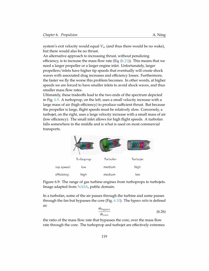
Chapter 6. Propulsion A. Ning

system’s exit velocity would equal V∞ (and thus there would be no wake),but there would also be no thrust.An alternative approach to increasing thrust, without penalizingefficiency, is to increase the mass flow rate (Eq. (6.21)). This means that weneed a larger propeller or a larger engine inlet. Unfortunately, largerpropellers/inlets have higher tip speeds that eventually will create shockwaves with associated drag increases and efficiency losses. Furthermore,the faster we fly the worse this problem becomes. In other words, at higherspeeds we are forced to have smaller inlets to avoid shock waves, and thussmaller mass flow rates.Ultimately, these tradeoffs lead to the two ends of the spectrum depictedin Fig. 6.9. A turboprop, on the left, uses a small velocity increase with alarge mass of air (high efficiency) to produce sufficient thrust. But becausethe propeller is large, flight speeds must be relatively slow. Conversely, aturbojet, on the right, uses a large velocity increase with a small mass of air(low efficiency). The small inlet allows for high flight speeds. A turbofanfalls somewhere in the middle and is what is used on most commercialtransports.

Figure 6.9: The range of gas turbine engines from turboprops to turbojets.Image adapted from NASA, public domain.

In a turbofan, some of the air passes through the turbine and some passesthrough the fan but bypasses the core (Fig. 6.10). The bypass ratio is definedas:

Ûmb ypass

Ûmcore(6.26)

the ratio of the mass flow rate that bypasses the core, over the mass flowrate through the core. The turboprop and turbojet are effectively extremes

119

Chapter 6. Propulsion A. Ning

of a turbofan where the turboprop has a very large bypass ratio and theturbojet has a bypass ratio of zero. Commercial transports continue topush the turbofan bypass ratio higher to increase efficiency whilemaintaining effectively the same incoming Mach number.

Figure 6.10: In a turbofan some of the air passes through the fan and intothe core, and some passes through the fan but bypasses the core. Image byK. Aainsqatsi, Wikimedia, CC BY-SA 3.0.

A gas turbine engine contains a compressor and a turbine and their bladesare shaped very differently as depicted in Fig. 6.11. Furthermore, there aremany stages in the compressor and only a few stages in the turbine as seenin Figs. 6.9 and 6.10. The reason for this is that air passing through thecompressor is moving from a low pressure region to a high pressureregion, or in other words through a strongly adverse pressure gradient.The airfoils can’t carry much lift without separating, hence the lightlycambered airfoils and the need for many stages, each stage creating a smallincrease in pressure. Conversely, air passing through the turbine ismoving from high to low pressure with a very favorable pressure gradient.The airfoils can be very aggressive with camber and thickness in order togenerate high lift and extract maximum power from the airflow.The compressor performs work on the air and turns the shaft, whereas theturbine extracts work from the fluid. Net work is achieved because thework extracted at the turbine is at a much higher temperature (see theBrayton cycle).We mentioned a turbojet as the extreme end of a turbofan, but there areactually more extreme options. As the Mach number gets past about Mach3 a turbojet is no longer a useful option. A ramjet (Fig. 6.12) gets rid of the

120

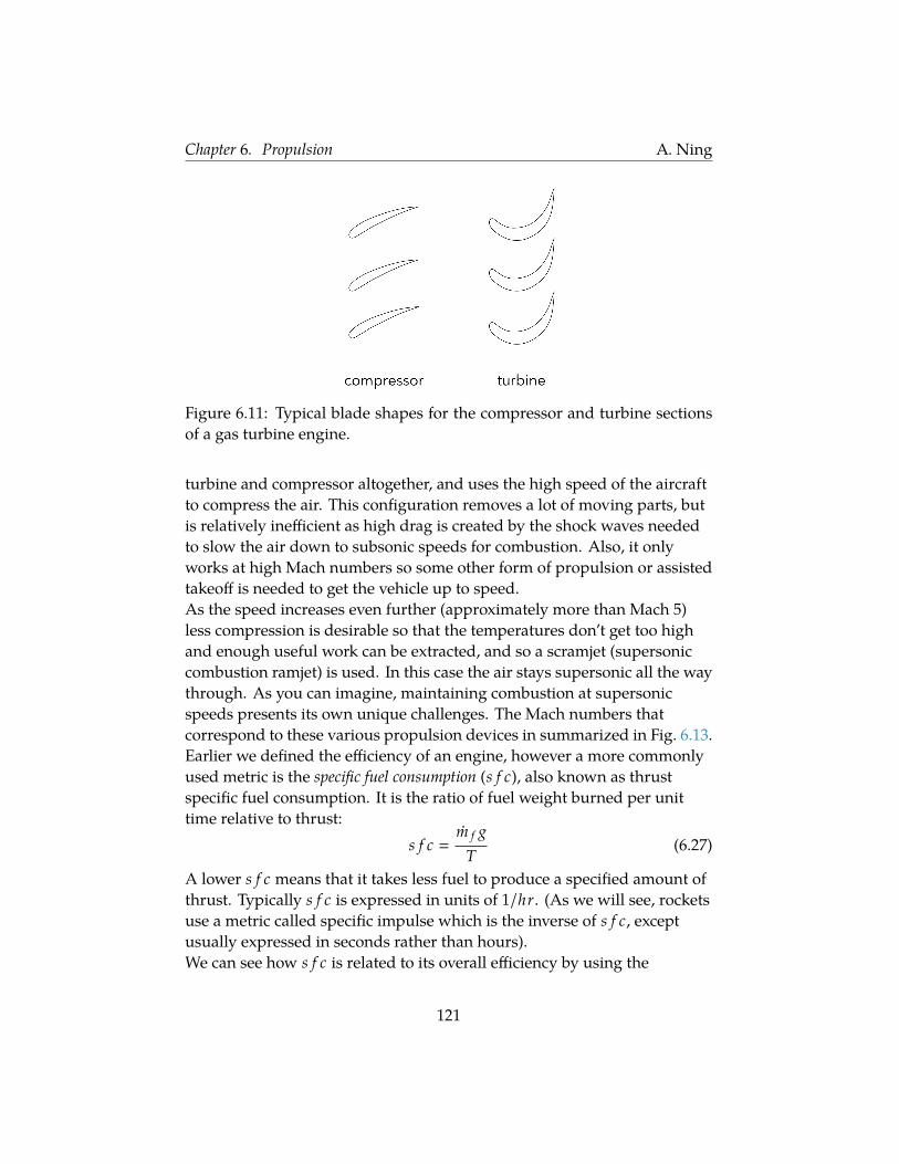
Chapter 6. Propulsion A. Ning

Figure 6.11: Typical blade shapes for the compressor and turbine sectionsof a gas turbine engine.

turbine and compressor altogether, and uses the high speed of the aircraftto compress the air. This configuration removes a lot of moving parts, butis relatively inefficient as high drag is created by the shock waves neededto slow the air down to subsonic speeds for combustion. Also, it onlyworks at high Mach numbers so some other form of propulsion or assistedtakeoff is needed to get the vehicle up to speed.As the speed increases even further (approximately more than Mach 5)less compression is desirable so that the temperatures don’t get too highand enough useful work can be extracted, and so a scramjet (supersoniccombustion ramjet) is used. In this case the air stays supersonic all the waythrough. As you can imagine, maintaining combustion at supersonicspeeds presents its own unique challenges. The Mach numbers thatcorrespond to these various propulsion devices in summarized in Fig. 6.13.Earlier we defined the efficiency of an engine, however a more commonlyused metric is the specific fuel consumption (s f c), also known as thrustspecific fuel consumption. It is the ratio of fuel weight burned per unittime relative to thrust:

s f c Ûm f gT

(6.27)

A lower s f c means that it takes less fuel to produce a specified amount ofthrust. Typically s f c is expressed in units of 1/hr. (As we will see, rocketsuse a metric called specific impulse which is the inverse of s f c, exceptusually expressed in seconds rather than hours).We can see how s f c is related to its overall efficiency by using the

121

Chapter 6. Propulsion A. Ning

Figure 6.12: Depiction of a ramjet. Image by Cryonic07, Wikimedia Com-mons, CC BY-SA 3.0.

Figure 6.13: Mach number range for different propulsion devices. Modifiedfrom a figure by Kashkhan, Wikimedia Commons, CC BY-SA 3.0

122

Chapter 6. Propulsion A. Ning

definition of overall efficiency (Eq. (6.22)) and replacing the thrust withthat of the Eq. (6.27):

η V∞g

s f c h f(6.28)

Thus, s f c and η are inversely related as we would expect.Jet engines have enabled the wonders of modern air transport in partbecause jet fuel (and petroleum-based fuels in general) is so energy dense.A typical energy density is approximately 42 MJ/kg, That means just 1 kgof jet fuel contains approximately the amount of energy needed to send 1kg of mass into orbit.

6.5 Propulsion System Placement

Beyond selecting a suitable motor/propeller combination, or a suitable gasturbine engine, one needs to determine how many propulsors to use andwhere the place them. Figure 6.14 shows two configurations, the one onthe left is called a single and the one on the right a twin. The primarybenefit of a single is simplicity. The main benefit of a twin is someredundancy allowing for the possibility of a recovery from an enginefailure. You can also use counter-rotating props, which provide somebenefit in terms of lateral trim drag. For small UAVs a twin is usually morecrash resistant and for hand launches can allow you to be out of the bladepath (especially for a pusher, discussed next). For piloted aircraft, a twinmoves the propulsion systems out of the primary field of view.

Figure 6.14: A single versus a twin propulsion system configuration.

While the historical trend has been to move from a large number ofengines to a small number (generally 1–2), recent advances in batterytechnology, motor power density, IMU capabilities, and autonomouscontrol are reversing that trend for electric-powered aircraft applications.Whereas jet engines are more efficient with fewer large systems, electric

123

Chapter 6. Propulsion A. Ning

motors can be (approximately) just as efficient with a large number ofsmall motors. Having a large number of small motors can allow for greaterredundancy, control, and effective mechanical actuation for applicationslike vertical takeoff. This type of system is called distributed propulsion(Fig. 6.15), and is an active area of research.

Figure 6.15: NASA X-57 Maxwell concept aircraft with 14 electric motors.Image from NASA, public domain.

Another major design decision, for a propeller-driven aircraft, is whetherto use a pusher or tractor configuration. Figure 6.16 shows these twoconfigurations with a pusher on the left and a tractor on the right. Apusher allows for improved visibility and directional stability (thepropulsion system acts kind of like a vertical tail). Some primarydisadvantages of a pusher are that it moves the center of gravity farther aftand is usually noisier because the prop ingests the wing wake. Efficiencytradeoffs are less clear. The wings on a pusher will be more efficientbecause they are not in the prop wash, but the propellers will be lessefficient because they are in the wing wake (and vice-versa for a tractor).

Figure 6.16: A pusher versus a tractor configuration.

Finally, placement of the propulsion system can be on the fuselage, on the

124

Chapter 6. Propulsion A. Ning

wing, in a pod, in the tail, etc. Determining proper placement requires anintegrated look at aerodynamic performance, structures, stability, andother system-level considerations.

125

CHAPTER7

Performance

Performance is an integration of the various subsystems into high-levelmetrics that describe how well the aircraft performs. Various metrics areimportant to the aircraft designer depending on the mission and flightenvelope of the vehicle. This chapter discusses some of the more commonperformance metrics.

7.1 Range

Range is the maximum distance that an aircraft can fly. We will developtwo expressions to estimate range: one for propulsion systems at constantthrust and one for systems at constant power. Recall from Chapter 6 thatthere are basically two extremes for propulsion systems: imparting a largevelocity change to a small mass of air, or imparting a small velocity changeto a large mass of air. The former corresponds to jet engines. Because theexit velocity is so large, the thrust is relatively insensitive to the freestreamspeed (Eq. (6.21)). In other words, the thrust is relatively constant withairspeed. The latter option corresponds to propeller systems. The thrust ofpropeller-driven systems varies significantly (generally decreasing withairspeed), but its power is relatively constant with changes in airspeed.While there are gas-powered piston engines with propellers, most modernuses of propellers are with electric power. Thus, we will only analyze

126

Chapter 7. Performance A. Ning

electric propeller-driven aircraft. In the following sections we will refer tojet powered and electric powered for convenience, but really mean constantthrust with fuel burn and constant power with no fuel burn respectively.

7.1.1 Jet Powered

We begin with estimating range for a jet-powered aircraft. Because theamount of fuel in the aircraft changes during the flight we need to startwith the specific range. The specific range is the distance flown per unitweight of fuel burned. We can express the specific range as follows:

specific range distance flownfuel burned

distance flown / timefuel burned / time

(7.1)

The numerator is the flight speed, and the denominator is the weight flowrate (mass flow rate times acceleration of gravity).

specific range V∞Ûm f g

(7.2)

In Chapter 6 we saw the following definition for the specific fuelconsumption (Eq. (6.27)):

s f c Ûm f gT

(7.3)

Thus, we can express the fuel burned per unit time ( Ûm f g) as s f c T. So, thespecific range is given by:

specific range V∞

s f c T(7.4)

If we assume steady, level flight then thrust equals the drag. Next, wemultiply the equation by lift over weight, which should be equal forsteady, level flight.

specific range V∞

s f c DLW

(7.5)

The range is the integration of specific range (distance/weight change)over the total change in weight across the flight. For a jet-powered aircraftthe weight of the aircraft decreases through the flight, so the range is givenby integrating the above expression from the initial weight (Wi) to the finalweight (W f ) :

R

∫ W f

Wi

V∞s f c

LD

1W(−dW) (7.6)

127

Chapter 7. Performance A. Ning

where a minus sign is used because the weight decreases from initial tofinal.In the following derivation we will make the simplifying assumption thatthe specific fuel consumption, lift-to-drag ratio, and velocity are constantduring the flight. The latter is equivalent to constant Mach number in theisothermal portion of the atmosphere. Making these assumptions allowsus to pull those constants out of the integral.

R V∞s f c

LD

∫ Wi

W f

dWW

(7.7)

After performing the integral we have an expression that allows us toestimate range:

R V∞s f c

LD

ln(

Wi

W f

)(jet powered) (7.8)

This is the well-known Breguet range equationFor comparing with electric vehicle later, it will be easier to specify theweights as a fuel fraction (weight of fuel relative to max total takeoffweight) and to use masses rather than weights. The initial mass is the totaltakeoff aircraft mass including fuel (mTO), whereas the final mass is thatminus the fuel mass mTO −m f . So the jet engine range estimates looks like:

R V∞s f c

LD

ln(

11 − m f /mTO

)(jet powered) (7.9)

As an aside, there are different range equations depending on whatyou choose to hold constant. In this case we have held velocity andCL constant (so that L/D is constant). That means that the densityis not constant (CL W/( 12ρV2Sre f )) and would need to decreasethrough the flight as the weight decreases. In other words, the air-craft would need to increase in altitude while flying (a cruise-climb).This is usually a preferably way to fly as it is closer to constant Machnumber, which is why we have used this form of the equation. Com-mercial transports can’t perform a continuous cruise-climb because ofair traffic control requirements, but for long flights do approximate itby shifting to higher altitude levels as the flight progresses. An alter-native approach is to hold CL and density (altitude) constant, leading

128

Chapter 7. Performance A. Ning

to a different estimate for range:

R 2 V∞s f c

√L

D

(√Wi −

√W f

)(7.10)

The Breguet range equation is simple to use and demonstrates that needfor balance between aerodynamic efficiency (L/D), propulsive efficiency(s f c), and structural efficiency (m f /mTO). The first two sub-metrics wehave seen already, but the “structural efficiency” is new. The most idealstructure would be one that is 100% fuel (i.e., no structure) and at the endof flight your airplane would weigh nothing. That would make Wi/W f

infinite, which means that your range was infinite in the sense that if yourairplane needed no structure, just fuel, you could add an infinite amountof fuel to fly forever. Of course, that is not possible, some finite amount ofstructure is always needed, and an all-fuel aircraft would be uselessbecause it couldn’t carry any payload. For a given amount of fuel, thelighter the structure is, then the better the structural efficiency is.Another way to express this range equation is in terms of the overallefficiency of the propulsion system. Recall from Chapter 6 that the overalefficiency was related to s f c by (Eq. (6.28)):

η V∞g

s f c h f(7.11)

where h f is the enthalpy of the fuel. We now solve this for V∞/s f c andsubstitute that into the Breguet range equation:

R h f

gη

LD

ln(

11 − m f /mTO

)(7.12)

This form of the equation is arguably more useful as the enthalpy and maxefficiency of jet engines are more universal than V∞ or even s f c.These equations are very useful for preliminary design, but recall thatmultiple assumptions were made. In detailed design we could relax theassumptions on steady-level flight and on constant properties. Instead, wewould perform a numerical integration through the flight trajectory toestimate range.

129

Chapter 7. Performance A. Ning

7.1.2 Electric Powered

Estimating the range of an electric powered vehicle is a little morestraightforward because the mass of the vehicle doesn’t change throughthe flight. Batteries are often characterized by their specific energy, whichis their energy per unit mass (eb). The total energy available from thebattery then is the specific energy, times its mass, times its thermalefficiency (as there are some losses).

Eavailable eb mbηb (7.13)

Note that eb should be an effective specific energy for the battery thataccounts for losses from temperature, depth of discharge, cycle life, etc.The energy expended from the propulsion system1

Eexpended TRηpηm

(7.14)

where R is the range, T is the average thrust across the flight, ηp is thepropeller efficiency, and ηm is the motor efficiency. For steady-level flightthe thrust equals the drag so

Eexpended DRηpηm

(7.15)

We can now equate the energy available to the energy expended and solvefor range:

R eb mbη

D(7.16)

where η ηbηmηp is the total efficiency of the propulsion system (battery,motor, propeller, etc.). To put this in a similar form to that of a jet enginewe will do the same thing we did in the previous section: multiply by liftover weight assuming steady, level flight:

R eb mbη

DLW

eb mbη

DLW

(7.17)

where W is the total mass of the aircraft including battery. Rearranging wehave:

R eb

gη

LD

mb

mTO(7.18)

1Actually, this is the minimum expended energy as there are various subsystems likelights, instrumentation, etc. that are also powered by the battery.

130

Chapter 7. Performance A. Ning

There are a lot of similarities between this equation and that of ajet-powered aircraft (Eq. (7.12)). Both have an efficiency term, lift-to-dragratio, and a structural efficiency. The structural efficiency followsessentially the same role here: an ideal structure would be all battery(excluding some mass for payload). However, the jet engine has someadvantage here as burning fuel during the flight decreases the aircraftweight. Figure 7.1 compares the two “efficiencies” (note this isn’t really anefficiency). A typical fuel fraction is around 40% or less so this generallyisn’t a major difference.

0.0 0.2 0.4 0.6 0.8fuel/battery fraction

0.0

0.5

1.0

1.5

"stru

ctur

al e

fficie

ncy"

jetelectric

Figure 7.1: Comparison of mb/mTO for a battery versus ln(1/(1 −m f uel/mTO)) for various mass fractions of battery/fuel.

Peak efficiencies for the two systems also differ. An efficient jet engine hasaround a 40% total efficiency, where as an electric system can beapproximately twice as efficient.However, both of these differences are relatively small compared to the lastdifference: the enthalpy of jet fuel compared to battery specific energy.The enthalpy of jet fuel is about 42.8 MJ/kg. Today’s best batteries (atscale) have a specific energy of approximately 300 Wh/kg or 1.08 MJ/kg.In other words, jet fuel is amazingly energy dense, about 40 times that of abattery! This factor explains the major difference in range capabilitiesbetween the two types of propulsion.Electric propulsion can’t compete on range, but it does have itsadvantages: no emissions, less noise, cheaper, fewer moving parts, higherefficiency, efficient at small sizes to allow for distributed propulsion, etc.

131

Chapter 7. Performance A. Ning

Thus, the current interest for short range applications, especially withvertical takeoff and landing (VTOL).

7.2 Endurance

Endurance is similar to range, but rather than a measure of flight distance,endurancemeasures flight time. For applications like search and rescue,time in the air is more important than distance flown.Specific endurance is time flown per unit weight of fuel burned:

specific endurance time

fuel burned

1

fuel burned / time

1Ûm f g

1

s f c T

(7.19)

Note that this is the same as specific range divided by V∞. Following thesame procedure as the previous section yields:

t 1

s f cLD

ln(

11 − m f /mTO

)

h f

gη

V∞LD

ln(

11 − m f /mTO

)(jet power)

(7.20)

t eb

gη

V∞LD

mb

mTO(electric) (7.21)

where t is the endurance.

7.3 Optimal Lift Coefficients

In this section we will explore the approximate optimal lift coefficient tofly at for different metrics. For a given altitude, this corresponds to anoptimal speed. This is easy to see using the definition of the lift coefficient

132

Chapter 7. Performance A. Ning

and rearranging:

CL L

12ρV2Sre f

(7.22)

V

√2L

ρSre f CL(7.23)

Lift coefficient is a more fundamental parameter, because it isnondimensional, so all derivations are in terms of lift coefficient eventhough we often speak in terms of speed. All the estimates in this sectionare simplified to allow for analytic formulas. This type of approach ishelpful to build intuition and to understand what parameters matter most,but as the aircraft design progresses a numerical computation of optimallift coefficients should be used rather than these analytic formulas.

Lift to Drag Ratio. The minimum drag speed of an aircraft is of coursezero. More interesting is the minimum drag speed for a fixed lift, which isequivalent to maximizing the lift-to-drag ratio. If the compressibility dragis negligible then the drag coefficient can be expressed as:

CD CD p +C2

L

πARe(7.24)

and the lift to drag ratio is then:

LD

CL

CD

CL

CD p +C2

LπARe

(7.25)

To find the lift coefficient that maximizes this expression we need to takethe derivative of this equation, with respect to CL, and set the result equalto zero (note that it’s a little simpler to instead minimize D/L rather thanmaximize L/D).

d(L/D)dCL

CD p +

C2L

πARe − CL2CLπARe(

CD p +C2

LπARe

)2 0 (7.26)

133

Chapter 7. Performance A. Ning

Thus,

CD p +C2

L

πARe− 2

C2L

πARe 0 (7.27)

CD p C2

L

πARe(7.28)

(7.29)

Or in other words, the lift coefficient that maximizes L/D occurs when theparasitic drag and induced drag are equal. Solving for the lift coefficientyields:

CLmax L/D

√CD pπARe (7.30)

The above derivation assumed that both e and CD p are independent of CL,though neither is strictly true. The inviscid span efficiency changes withlift coefficient, but usually not by much for modest changes in liftcoefficient. The parasitic drag coefficient isn’t a function of CL per se.However, both depend on Reynolds number and so because lift is fixedthey are implicitly related:

dCD p

dCL∂CD p/∂Re

∂CL/∂Re(7.31)

Both depend on Mach number as well, but we assume that is negligibleconsistent with our assumption that compressibility drag is negligible. Anumerical simulation, evaluating drag at each Reynolds number and Machnumber will yield a more accurate estimate, but the above formula isuseful for conceptual design purposes.

Range Jet Power. Recall that the specific range for a jet aircraft is:

V∞LD

1s f c W

(7.32)

Both weight and s f c are independent of the lift coefficient (if at constantaltitude—s f c changes some with density), and so to maximize range weneed to maximize

V∞LD

V∞CL

CD(7.33)

134

Chapter 7. Performance A. Ning

We can infer already that the speed for maximum range will be faster thanthe speed for minimum drag. That is because the presence of the V∞ termmeans that increasing speed has a linear effect whereas the decrease inL/D for increasing speed beyond the max L/D speed will initially be small.Using Eq. (7.23) and assuming steady level flight (L W) the metric weneed to maximize becomes: √

W12ρSre f CL

CL

CD(7.34)

For a given altitude, removing terms that are independent of CL reducesthe above expression to: √

CL

CD(7.35)

Thus, to maximize range we need to maximize the above expression, orminimize its inverse, with respect to CL. We will do the latter:

d CD√CL

dCL

ddCL

(CD p

C1/2L

+C3/2

L

πARe

)(7.36)

−12

CD p

C3/2L

+32

C1/2L

πARe 0 (7.37)

CD p 3C2

L

πARe(7.38)

In other words, for maximum range the parasitic drag is three times theinduced drag.

CLmax range, jet

√CD pπARe

3

1√3

CLmax L/D (7.39)

We see that indeed the optimal lift coefficient is lower than of max L/D, orreferring to Eq. (7.23), the maximum range speed is 31/4 times themaximum L/D speed. In other words, the maximum range speed is about32% faster.Again, keep in mind, that some simplifying assumptions were made likeassuming constant s f c, and so a numerical solution is preferable whenpossible. Still these analytic solutions are useful in lending insight intowhat parameters matter most and in determining approximate optimalconditions.

135

Chapter 7. Performance A. Ning

Range Electric Power. For an electric powered vehicle all the terms in therange equation (Eq. (7.18)) are constant with lift coefficient except ηL/D.Unfortunately, the efficiency term is not easily amenable to an analyticexpression. Generally it varies weakly with flight speed, as compared toL/D, and so for the purpose of this analysis we assume constant efficiency.If efficiency is constant with CL, then CL for maximum range under electricpower is the same as the CL for maximum L/D.

CLmax range, elec ≈ CLmax L/D (7.40)

Again, remember that this expression is only true if propeller efficiency isconstant. In practice, the maximum range speed is usually somewhatfaster than the maximum L/D speed. If the propulsion system has beenidentified then a numerical solutions should be sought.

Endurance Jet Power. For a jet, the only terms in the endurance equation(Eq. (7.20)) that vary with CL are L/D (again ignoring small variations insfc). That means that speed for max endurance is the same as the speed formax L/D.

CLmax endurance, jet CLmax L/D (7.41)

Endurance Electric Power. For an electric powered aircraft to maximizeendurance we must maximize the quantity

η

VLD

(7.42)

Again, we make the same approximation that η is constant. In that case, tomaximize endurance we need to maximize the quantity:

1V

LD

(7.43)

Using a similar procedure to that of maximizing range of a jet-poweredaircraft, we find that for optimizing endurance we need to minimize thequantity:

CD

C3/2L

(7.44)

136

Chapter 7. Performance A. Ning

Taking the derivative with respect to CL gives:

d CD

C3/2L

dCL

ddCL

(CD p

C3/2L

+C1/2

L

πARe

)(7.45)

−32

CD p

C5/2L

+12

C−1/2L

πARe 0 (7.46)

CD p 13

C2L

πARe(7.47)

In other words, for maximum endurance the parasitic drag is one third ofthe induced drag.

CLmax endurance, elec ≈√

3CD pπARe √

3CLmax L/D (7.48)

We see that indeed the optimal lift coefficient is higher than of max L/D,or referring to Eq. (7.23), the maximum endurance speed is 3−1/4 times themaximum L/D speed. In other words, the maximum endurance speed isabout 24% slower. As noted previously, a numerical solution is preferablyif the various in efficiency is known, though in general the max endurancespeed will be slower than the max L/D speed.

7.4 Rate of Climb

When climbing, the lift, drag, and thrust vectors tilt as shown in Fig. 7.2,whereas weight remains pointed downward. A force balance along thedirection of flight yields:

T D + W sin γ (7.49)

where γ is the climb angle. Rearranging the expression gives:

sin γ T − D

W(7.50)

The rate of climb is the speed we climb vertically. This is given by thecomponent of our flight speed in the vertical direction:

V∞ sin γ (7.51)

137

Chapter 7. Performance A. Ning

Using the previous equation gives the rate of climb:

R/C V∞(T − D)

W(7.52)

Figure 7.2: Depiction of forces on aircraft during a steady climb..

As discussed in the beginning of this chapter, for a jet-powered aircraftthrust is mostly independent of speed, so a good metric of climbperformance is the thrust-to-weight ratio: T/W . For electric-poweredaircraft power is mostly independent of speed, so a good metric of climbperformance is the power-to-weight ratio: P/W or TV/W . For jet power,the speed that maximizes the rate of climb is faster than the speed for maxL/D. For an electric powered aircraft, since power is constant, the speedthat maximizes rate of climb is the minimum power speed (which is thesame as the speed for maximum endurance). As long as the flight pathangle, γ, is not large, in conceptual design we usually assume that theaircraft drag is unchanged from its level flight value.Maximizing rate of climb means minimizing the time it takes to reach acertain altitude. However, various other climb metrics are sometimes usedincluding maximizing the gradient of climb (a slower speed) orminimizing the fuel/energy used to climb (a faster speed with a lower rateof climb).Another related metric is the ceiling. The absolute ceiling is the highestaltitude the aircraft can fly at, and is the altitude at which the rate of climbequals zero. As the altitude increases, density decreases, and the speed tomaintain level flight increases. This increase in speed requires morepower. Additionally, for jet engines the maximum power available tends todecrease with altitude, and propeller performance is affected by density aswell. In either case, there is some altitude at which there will be no excesspower and the aircraft will no longer be able to climb. A related, and

138

Chapter 7. Performance A. Ning

perhaps more useful metric is the service ceiling. This is the highest altitudeat which a given rate of climb can be sustained. The target climb rate isoften around 30 meters/minute for larger aircraft.

7.5 Glide Ratio

Gliding flight if when a heavier-than-air aircraft flies without any thrust.The glide ratio refers to the ratio of forward distance traveled relative tovertical distance descended. A high glide ratio is desirable because thatmeans for a given starting altitude, the aircraft can glide further. We candetermine the glide ratio starting from the same equation used previouslyin climbing (Eq. (7.50)). The only difference is that this time there is nothrust:

sin γ −DW

(7.53)

The negative sign denotes that the flight angle is decreasing rather thanincreasing as in the climb case. We will drop the negative sign goingforward, with the understanding that the angle is now positive down.Referring to Fig. 7.2 again, a force balance perpendicular to the flightdirection yields:

L W cos γ (7.54)

Solving for weight and substituting into the previous equation gives:

sin γ D

L cos γ(7.55)

After rearranging we have:

tan γ DL

(7.56)

The glide ratio as stated earlier is the ratio of forward distance relative tovertical distance. From Fig. 7.3 we can see that this is precisely 1/tan γ:

glide ratio 1

tan γ

LD

(7.57)

In other words the glide ratio is the same as the lift-to-drag ratio.

139

Chapter 7. Performance A. Ning

Figure 7.3: Depiction of a gliding aircraft showing that the glide ratio(forward distance / vertical distance) is exactly the lift to drag ratio.

7.6 Turning Radius

As discussed in Section 5.4, turning generally occurs by banking theaircraft in a coordinated turn. Figure 7.4 depicts how tilting at a bankangle (Φ) allows a component of the lift to turn the aircraft through acentripetal acceleration. A force balance in the vertical direction gives:

L cosΦ m g (7.58)

Applying Newton’s second law in the horizontal direction, using the formfor centripetal acceleration, gives:

L sinΦ mV2

Rt(7.59)

where Rt is the turning radius. If we combine these two equations we cansolve for the turning radius:

Rt V2

g tanΦ(7.60)

Figure 7.4: Depiction of an aircraft turning to allow determination of theturning radius.

140

Chapter 7. Performance A. Ning

We can’t do much about the acceleration of gravity so if we want to able tomake tighter turns we need to either fly slower (decrease stall speed) orincrease our bank angle. For small UAVs a fairly extreme bank angle isacceptable, but would be much more limited in passenger carrying aircraft.

7.7 High Lift Devices

Takeoff and landing performance are primarily functions of stall speed.Using Eq. (7.23) we see that the stall speed occurs once CL reaches itshighest value: CLmax .

Vstall

√2W

ρSre f CLmax(7.61)

This equation tells us what we can do if we want a slower stall speed andthus a shorter runway for takeoff/landing. We can’t control air density,but this equation does explain why we need a longer runway at airports athigh altitudes. Decreasing stall speed is a common reason for increasingwing area, but that choices comes with other design compromises. Clearly,increasing CLmax has a major effect on decreasing stall speed.Unfortunately, designing for high lift means that drag will be high too.What we really want is variable geometry: a high-lift configuration fortakeoff/landing, and a streamlined configuration for cruise. This is exactlyhow transport aircraft operate.There are two primary mechanisms for changing the geometry of a wingto increase its maximum lift coefficient: flaps and slats. Both are used incombination on transport aircraft. A variety of flaps are depicted inFig. 7.5a, with a picture of one in Fig. 7.5b.Flaps increase the effective camber of the airfoil, and thus the zero liftangle of attack (Fig. 7.6). Notice that for a given angle of attack the lift isincreased, and that the angle of attack for maximum lift is reduced. Noticealso that using flaps has almost no effect on cl max . The primary benefit offlaps is that maximum lift occurs at a lower angle of attack, which helpswith pilot visibility and decreases the amount of necessary fuselageupsweep (the aft end of the fuselage curves up to increase groundclearance during takeoff rotation).A slotted flap enables higher lift through two mechanisms. First, itreenergizes the boundary layer allowing for attached flow along the flap at

141

Chapter 7. Performance A. Ning

(a) A variety of flap options. Figure byNiD.29, Wikimedia Commons, CCBY-SA 3.0.

(b) A flap system on a transport aircraft.Picture by David Monniaux, WikimediaCommons, CC BY-SA 3.0.

Figure 7.5: Trailing edge flaps.

Figure 7.6: Flaps change the effective camber, and thus the zero lift angle ofattack. They have almost no effect on cl max however.

142

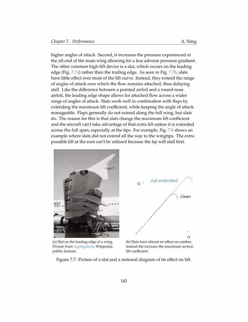
Chapter 7. Performance A. Ning

higher angles of attack. Second, it increases the pressure experienced atthe aft end of the main wing allowing for a less adverse pressure gradient.The other common high-lift device is a slat, which occurs on the leadingedge (Fig. 7.7a) rather than the trailing edge. As seen in Fig. 7.7b, slatshave little effect over most of the lift curve. Instead, they extend the rangeof angles of attack over which the flow remains attached, thus delayingstall. Like the difference between a pointed airfoil and a round-noseairfoil, the leading edge shape allows for attached flow across a widerrange of angles of attack. Slats work well in combination with flaps byextending the maximum lift coefficient, while keeping the angle of attackmanageable. Flaps generally do not extend along the full wing, but slatsdo. The reason for this is that slats change the maximum lift coefficientand the aircraft can’t take advantage of that extra lift unless it is extendedacross the full span, especially at the tips. For example, Fig. 7.8 shows anexample where slats did not extend all the way to the wingtips. The extrapossible lift at the root can’t be utilized because the tip will stall first.

(a) Slat on the leading edge of a wing.Picture from Arpingstone, Wikipedia,public domain.

(b) Slats have almost no effect on camber,instead the increase the maximum sectionlift coefficient.

Figure 7.7: Picture of a slat and a notional diagram of its effect on lift.

143

Chapter 7. Performance A. Ning

Figure 7.8: An example where slats extended only over a portion of thewing. In that case the extra increase in cl max is unusable.

7.8 Takeoff

We will discuss only the main principles involved in determining takeofffield length. For further details you are referred to the Federal AviationRegulations (FARs) See for example, Part 25 for transport aircraft.One critical speed during takeoff is called the decision speed and is denotedas V1. If you have an engine failure or other critical failure before thedecision speed then you abort the takeoff and put on full brakes. This iscalled the accelerate-stop distance. If you have a failure after the decisionspeed you must takeoff (there won’t be enough runway to brake), circlearound and land or divert to an alternate airport. This is called theaccelerate-climb distance. Takeoff field length considers not just therunway, but includes the total distance until the airplane is some heightabove the ground (Fig. 7.9), which is 35 feet for transport categoryairplanes and 50 feet for general aviation.

Figure 7.9: A critical factor in takeoff field length is the decision speedbetween braking and climbing. Takeoff distance is defined as not just theground roll portion, but also the distance required to clear an obstacle ofheight h.

The takeoff distance is determined from the balanced field length. Thebalanced field length is the point at which the accelerate-stop distance andaccelerate-climb distance are equal. This is the shortest possible field

144

Chapter 7. Performance A. Ning

length for safe takeoff of that aircraft.Figure 7.10 illustrates this concept. The gray line shows how much runwayyou would need to accelerate to the candidate value of V1. The verticaldistance from the gray to the blue curve corresponds to the extra distancerequired to stop assuming you decided to stop at the decision speed.Intuitively it makes sense that if we decide to stop at a later (higher) speed,then we will need more distance to come to a stop. hence the blue linemoves further and further away from the gray.The vertical distance from the gray to the red curve corresponds to thedistance required to clear the required obstacle height assuming youdecided to takeoff. This line drops down because the decision pointcorresponds to an engine failure event. If we fly further with two engines,it’ll take less runway to reach takeoff speeds with our remaining engines.Conversely, if we have a failure very early, and decide we’re still going totakeoff anyway, it’ll take more distance to get up to speed on our oneengine. Hence the red line is further away at low speeds.Clearly, it is not ideal to decide to takeoff if an engine failed early while stilltraveling slowly. Conversely, it is not ideal to decide to brake if we aremoving quickly. The minimum distance that balances these considerationsis the crossover point of the two curves and is called the balanced fieldlength. At that point the distance to stop and the distance to takeoff areidentical. This point defines the actual value of V1. If we are below thisspeed then its requires less distance to stop, and if we are above this speedthen it takes less distance to continue the takeoff.2There are too many uncertainties to predict takeoff field length accuratelyfrom an equation, but we can work out what parameters matter andprovide an expression that is useful in making relative comparisons intakeoff field length. Recall that we assume that jet powered aircraftoperated at constant thrust, whereas electric propeller-driven aircraftoperate at constant power.

2This article provides a good overview of these concepts if you’d like a little more detailwithout going all the way to the FARs.

145

Chapter 7. Performance A. Ning

Figure 7.10: An illustration of the balanced field length where the distanceto stop and the distance to climb are equal.

Takeoff Jet Power. We start by rearranging Newton’s second law andsetting up an integral from the start of the ground run to some time t:

F mdVdt

(7.62)

dt mF

dV (7.63)∫ t

0dt

∫ V

0

mF

dV (7.64)

We make the assumption that the net force is independent of speed, whichis reasonable if thrust is much larger than drag (drag itself is a strongfunction of speed). Then the integral simplifies to:

t mF

V (7.65)

We now perform a second integral to get distance (d) traveled andintegrate from the start of the ground run until lift off (LO). We also makeuse of Eq. (7.65) in order to express velocity as a function of time:

dLO

∫ tLO

0Vdt (7.66)

dLO

∫ tLO

0

Ftm

dt (7.67)

Again, we make the same assumption of constant force (net thrust) whenperforming the integral:

dLO Fm

t2LO

2(7.68)

146

Chapter 7. Performance A. Ning

Or, using Eq. (7.65) the distance to liftoff is:

dLO mV2

LO

2F(7.69)

We can reexpress this equation in terms of variables more usable to theaircraft designer by noting that m W/g, the force is the net thrust(F T − D), and the minimum lift-off speed is 20% greater than Vstall :

VLO 1.2

√2W

ρSre f CLmax(7.70)

Plugging these alternate parameters into our ground roll expression gives:

dLO 1.44 W2

gρSre f CLmax(T − D) (7.71)

Drag in this case is particularly difficult to predict. It’s not the same asdrag during level flight, but needs to include ground effect and rollingfriction including some alleviation in the normal force from lift:

D µ(W − L) + Daero (7.72)

Instead, we will assume that thrust is much bigger than drag (which isusually true and which we have already implicitly assumed by using aconstant force in the integrals), then takeoff distance should beproportional to the remaining parameters (removing constants):

dLO ∝W2

ρSre f CLmaxT(7.73)

Again, this procedure does not give us a accurate predictive function perse, but it does, for example, tell us that an aircraft that is twice as heavywill approximately require four times the takeoff length. Note that thisdiscussion has only focused on the ground roll distance (omitting theclimb over obstacle portion). For a transport aircraft the ground roll ismost of the total length (about 80%) so often it is the ground roll that isfocused on during conceptual design.

147

Chapter 7. Performance A. Ning

Electric Powered Takeoff. We follow the same procedure as before, butnow assume constant power rather than constant thrust. In the firstintegral: ∫ t

0dt

∫ V

0

mF

dV (7.74)

the force is not constant, but if we multiply top and bottom by velocity wewill have power: ∫ t

0dt

∫ V

0

mVP

dV (7.75)

Assuming power is constant during takeoff:

t mP

V2

2(7.76)

The second integral for distance, replacing V with the above expressiongives:

dLO

∫ tLO

0Vdt (7.77)

∫ tLO

0

√2Ptm

dt (7.78)

√2Pm

23

t3/2LO (7.79)

Using Eq. (7.76) to replace time in the above expression gives:

dLO mV3

LO

3P(7.80)

We make the same substitutions as before for stall speed giving:

dLO 1.629 W5/2

g(ρSre f CLmax)3/2Pnet(7.81)

where P is the net power including drag, though again we will usuallyassume the power from thrust is much larger.

dLO ∝W5/2

(ρSre f CLmax)3/2P(7.82)

Unlike transport aircraft, for electric powered aircraft the climbing phasemay be longer than the ground roll phase and thus would be important toinclude even in conceptual design. However, the details of transitioningfrom ground roll to climb are outside our scope.

148

Chapter 7. Performance A. Ning

7.9 Landing

Landing field length is perhaps even more difficult to predict because ofthe large number of uncertainties, but as we will see it is primarily afunction of stall speed. Landing consists of three phases: glide,deceleration, and ground roll (Fig. 7.11).

Figure 7.11: Notional depictionof landingwith aglidingphase, decelerationphase, and a ground roll phase.

During the gliding phase, we can use the glide ratio we derived earlier:

dglide h(

LD

)e f f

(7.83)

where h is the obstacle height (50 feet for transport aircraft under Part 25),and (L/D)e f f is an effective lift-to-drag ratio including ground effect.The deceleration phase is where the aircraft is just above the ground, butnot yet touching the ground. Deceleration occurs from aerodynamic drag.If we assume constant deceleration:

ddecel V2

g − V2L

2a(7.84)

V2

g − V2L

2 De f f

W/g

(7.85)

(LD

)e f f

12g(V2

g − V2L ) (7.86)

(7.87)

where Vg is the speed at the end of the glide phase, and VL is the landingspeed before touchdown.The ground phase is where the wheels are on the ground and the brakes

149

Chapter 7. Performance A. Ning

are applied. Assuming constant deceleration from friction:

ddecel V2

L

2a(7.88)

V2

L

2(µ(W − L) + D)/m (7.89)

V2

L W2g(µ(W − L) + D) (7.90)

(7.91)

where the drag is now higher with spoilers deployed.Spoilers are a critical component of a landing system (Fig. 7.12). Theyincrease aerodynamic drag, but more importantly they drasticallydecrease lift allowing for a bigger normal force and thus higher rollingresistance from the brakes. The total drag is a combination of rolling dragand aerodynamic drag. The rolling drag has the potential to be muchbigger so it is important to decrease lift quickly to allow the brakes to slowthe aircraft down.

Figure 7.12: Spoilers on an aircraft. Picture from Richardgm, WikimediaCommons, public domain.

Adding all the terms we see that landing distance is of the form (where Aand B are some constant independent of speed):

d A + BV2L (7.92)

150

Chapter 7. Performance A. Ning

and because the landing speed is proportional to the stall speed (where Cis a different constant):

d A + CV2s (7.93)

In the end, landing distance is primarily a function of stall speed. Inpractice, pilot skill in touching down quickly so that spoilers and brakescan be deployed, perhaps makes the biggest difference.

151

CHAPTER8

Structures

The aircraft structure must be designed to safely carry all loadsexperienced during flight. At the same time the structure should be assmall and light as possible so as to not increase the required lift or wettedarea. Aerodynamics and structures are often at odds and so careful designis necessary to achieve an optimal balance.

8.1 Typical Structural Elements

Most aircraft components are built using a semi-monocoque structure. Amonocoque structure is one in which loads are carried through an externalskin (e.g., an egg shell). A semi-monocoque structure uses a shell structurebut with reinforced frames. This type of design can be seen in the fuselageshown in Fig. 8.1.Figure 8.2 highlights some of the major structural components of thefuselage. The frames provide the shape and also increase bucklingstrength. The long skinny members between frames carry longitudinalloads and are called stringers or longerons. Often the terms are usedinterchangeably, but do have a small difference in meaning.1 The skin(besides providing a covering), primarily carries torsion and shear loads.

1This Wikipedia article discusses the difference.

152

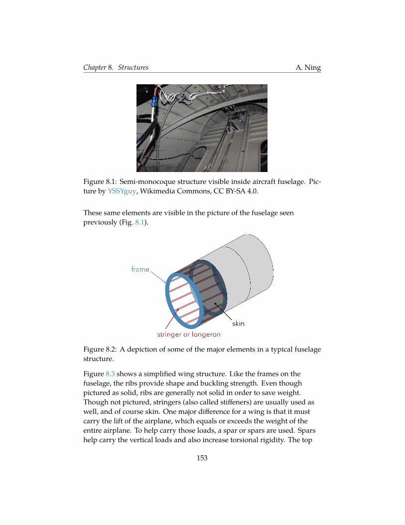
Chapter 8. Structures A. Ning

Figure 8.1: Semi-monocoque structure visible inside aircraft fuselage. Pic-ture by YSSYguy, Wikimedia Commons, CC BY-SA 4.0.

These same elements are visible in the picture of the fuselage seenpreviously (Fig. 8.1).

Figure 8.2: A depiction of some of the major elements in a typical fuselagestructure.

Figure 8.3 shows a simplified wing structure. Like the frames on thefuselage, the ribs provide shape and buckling strength. Even thoughpictured as solid, ribs are generally not solid in order to save weight.Though not pictured, stringers (also called stiffeners) are usually used aswell, and of course skin. One major difference for a wing is that it mustcarry the lift of the airplane, which equals or exceeds the weight of theentire airplane. To help carry those loads, a spar or spars are used. Sparshelp carry the vertical loads and also increase torsional rigidity. The top

153

Chapter 8. Structures A. Ning

and bottom of the spars, called the spar caps, carry bending loads.

ribs

spar

Figure 8.3: Some elements in a simple wing structure. Figure adapted fromthis figure and this figure, both by MLWatts, Wikimedia Commons, publicdomain.

Large transports typically use a box beam structure with a front spar andrear spar (depicted as 1 and 2 in Fig. 8.4). The region between these sparsforms a box beam structure. A cross-sectional view can be seen in Figure 5of this webpage.

8.2 Wind Bending

For many aircraft the critical loads in the wing come from bending.Figure 8.5 shows a typical load distribution across a conventional aircraft.Most of the weight (inertial load) is concentrated near the centerline,whereas the lift is distributed across the wing. Furthermore, the weight isdistributed throughout the entire aircraft whereas the lift in concentratedprimarily in the wing. In other words, the inertial loads from the wing arerelatively small compared to the lift in the wing. The wing, mounted to thefuselage, acts like a cantilevered beam, and the distributed aerodynamicloads create large bending moments in the wing. Flying wings are anexception where bending may not be a critical case. For a flying wing theaerodynamic and inertial loads are all contained in the wing so they tendto cancel out to a much greater degree.In the previous section, we discussed how transport wings typically use a

154

Chapter 8. Structures A. Ning

Figure 8.4: A more complex wing structure has a front and rear spar, ribs,and stringers, in a box beam construction. Figure from Tosaka, WikimediaCommons, CC BY 3.0.

Figure 8.5: Typical aerodynamic and inertial loaddistribution for a transportaircraft.

155

Chapter 8. Structures A. Ning

box beam structure. A simplified representation of one is depicted inFig. 8.6. The dashed portions of the wing contain just a thin skin, that iseffectively non-structural, with the primary purpose of creating theaerodynamic shape. A cross-section of the wing, with positive loading,experiences a bending moment like that shown in the figure. The uppersurface is in compression, while the lower surface is in tension.

Figure 8.6: A notional depiction of a box beam often used in large aircraftwing structures. It consists of a forward and rear spar, and spar caps on topand bottom.

In the following, we derive a simplified estimation of the mass of materialrequired to resist bending. This is not meant to be a highly accuratemethodology, but rather a simple analytic expression that can give insightinto what parameters most affect the structural weight of the wing.The wing can be approximated as a beam, and the bending stress can thenbe estimated from the beam bending equation (assuming uni-axialbending):

σ Mb c

I(8.1)

where Mb is the bending moment, c is the distance from the neutral axis,and I is the moment of inertia about the neutral axis. In this case, thedistance from the neutral axis to the upper (or lower) surface where thestress is highest is approximately t/2 where t is the airfoil thickness. Wecan approximate the moment of inertia as two rectangles each with areaA/2 as seen in Fig. 8.7. The sides of the box beam would contribute someto the moment of inertia, but the biggest contribution comes from the sparcaps (similar approximation often used in I-beams). Furthermore, weassume that the spar cap is thin relative to the airfoil thickness, which isusually a good approximation, so that the moment of inertia about its owncenter line is negligible. Using the parallel axis theorem, and multiplyingby two to account for both upper and lower surfaces, we estimate the boxbeam moment of inertia as: I 2(A/2)(t/2)2. Putting these terms togethergives:

σ 2Mb

At(8.2)

156

Chapter 8. Structures A. Ning

Figure 8.7: Simplified representation of the box beam for the purposes ofestimating its moment of inertia about the neutral axis.

The mass of bending structural material in the wing is given by integratingthe area A of material across the span:

mbendin g

∫ρAdy (8.3)

where ρ is the density of the structural material. If we solve the stressequation for A and plug it into this expression we find that the mass ofbending structural material can be estimated by the following expression:

mbendin g

∫ 2ρMb

σtdy (8.4)

If we further assume that the structure is as efficient as possible, and thusevery section is near its maximum stress (a constant), then the structuralbending weight of the wing is proportional to the local bending momentover the local airfoil thickness.

mbendin g ∝∫

Mb

tdy (8.5)

This expression explains why a thicker airfoil generally results in a lighterwing (if bending constrained). A thicker airfoil increases the moment ofinertia of the section, like separating the two ends of an I-beam, reducesstress, and thus reduces the amount of material needed in the wing toresist bending.In conceptual design it can be useful to constrain

∫Mb/t as a surrogate for

structural wing weight. The bending moment varies throughout the wing,but the maximum is generally the root bending moment, which is thebending moment at the root of the wing. Sometimes root bending momentis used as a simpler surrogate for structural wing weight.

157

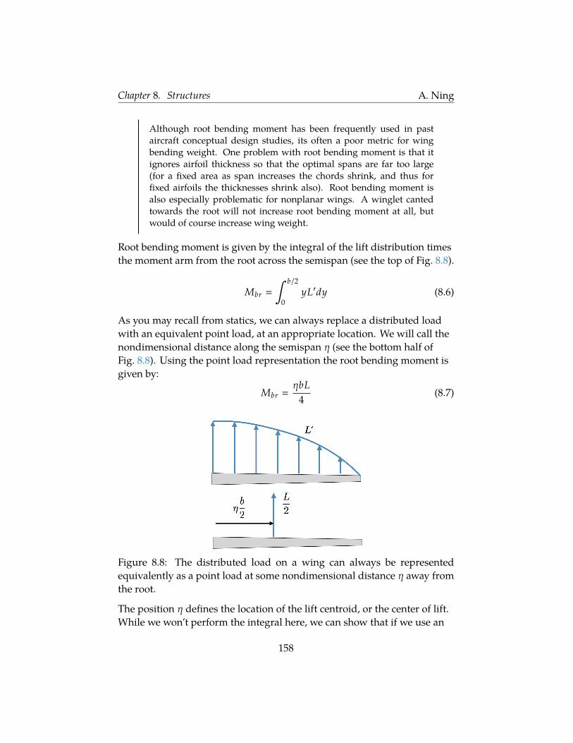
Chapter 8. Structures A. Ning

Although root bending moment has been frequently used in pastaircraft conceptual design studies, its often a poor metric for wingbending weight. One problem with root bending moment is that itignores airfoil thickness so that the optimal spans are far too large(for a fixed area as span increases the chords shrink, and thus forfixed airfoils the thicknesses shrink also). Root bending moment isalso especially problematic for nonplanar wings. A winglet cantedtowards the root will not increase root bending moment at all, butwould of course increase wing weight.

Root bending moment is given by the integral of the lift distribution timesthe moment arm from the root across the semispan (see the top of Fig. 8.8).

Mbr

∫ b/2

0yL′dy (8.6)

As you may recall from statics, we can always replace a distributed loadwith an equivalent point load, at an appropriate location. We will call thenondimensional distance along the semispan η (see the bottom half ofFig. 8.8). Using the point load representation the root bending moment isgiven by:

Mbr ηbL

4(8.7)

Figure 8.8: The distributed load on a wing can always be representedequivalently as a point load at some nondimensional distance η away fromthe root.

The position η defines the location of the lift centroid, or the center of lift.While we won’t perform the integral here, we can show that if we use an

158

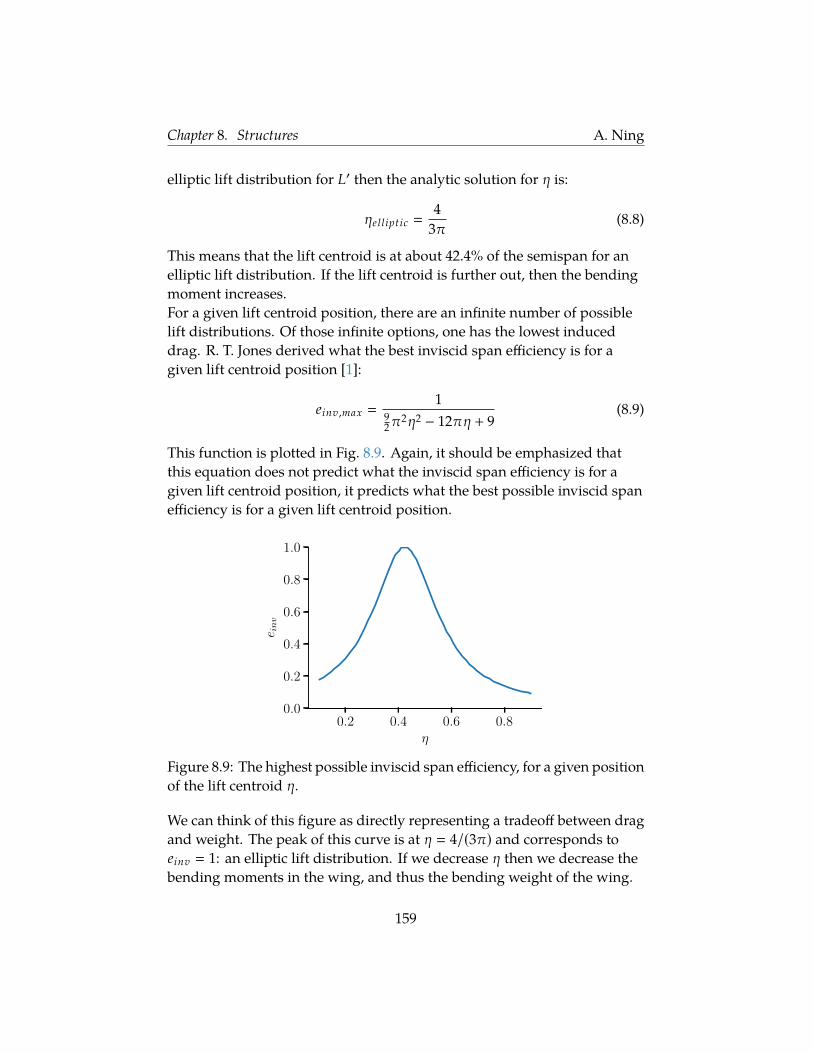
Chapter 8. Structures A. Ning

elliptic lift distribution for L′ then the analytic solution for η is:

ηelliptic 4

3π(8.8)

This means that the lift centroid is at about 42.4% of the semispan for anelliptic lift distribution. If the lift centroid is further out, then the bendingmoment increases.For a given lift centroid position, there are an infinite number of possiblelift distributions. Of those infinite options, one has the lowest induceddrag. R. T. Jones derived what the best inviscid span efficiency is for agiven lift centroid position [1]:

einv ,max 1

92π

2η2 − 12πη + 9(8.9)

This function is plotted in Fig. 8.9. Again, it should be emphasized thatthis equation does not predict what the inviscid span efficiency is for agiven lift centroid position, it predicts what the best possible inviscid spanefficiency is for a given lift centroid position.

0.2 0.4 0.6 0.8

0.0

0.2

0.4

0.6

0.8

1.0

e inv

Figure 8.9: The highest possible inviscid span efficiency, for a given positionof the lift centroid η.

We can think of this figure as directly representing a tradeoff between dragand weight. The peak of this curve is at η 4/(3π) and corresponds toeinv 1: an elliptic lift distribution. If we decrease η then we decrease thebending moments in the wing, and thus the bending weight of the wing.

159

Chapter 8. Structures A. Ning

However, we can see that we have to sacrifice some inviscid span efficiencyto make this happen, or in other words the induced drag will increase.For a given wing weight, with fixed area (so that parasitic drag is roughlyconstant), the optimal aerostructural lift distribution differs from theaerodynamic optimum as seen in Fig. 8.10. As we learned in the Chapter 3the minimum induced drag solution for a fixed span planar wing is anelliptic wing. However, if we consider structures we can maintain thesame wing weight but lower drag by shifting the load distribution inboardwhile simultaneously increasing the span. The resulting drop in inviscidspan efficiency is more than made up by the increase in span. The detailson what the optimal span increase and lift distribution is varyconsiderably depending on the wing taper, critical structural altitude, stallbehavior, etc [2]. However, the general principle is that the aircraftperformance is usually improved by shifting the load inboard slightly toallow for a higher span (or a lighter wing for a fixed span).

Figure 8.10: Comparison between aerodynamically optimum lift distribu-tion and aerostructural optimum.

8.3 Flight Envelope Preliminaries

There are various ways to look at an aircraft’s flight envelope. We will lookat two. The first is referred to by various names including a placard speeddiagram, a doghouse plot, or just a flight envelope. Sometimes thesenames refer to other types of diagrams. The plot we are interested in ismax/min true airspeed as a function of altitude. The second type of plot iscalled a V-n diagram. This plot shows the max/min load factors as a

160

Chapter 8. Structures A. Ning

function of speed. Specifically we will look at the maneuvering envelope.Before diving into the details we need to learn more about load factors andairspeeds. The n in V-n is called the load factor. It is a ratio of the lift to theweight of the aircraft:

n LW

(8.10)

In steady level flight, the aircraft flies with lift equal to weight, or a loadfactor of one (n 1). Typically, load factors are expressed in “g’s”. Forexample, n 1 is a load factor of 1g, whereas n 2 is a load factor of 2 g’s.This phrasing is used because at n 2, in the frame of the aircraft, objectswould appear to fall with an acceleration twice that of gravitationalacceleration (g). The same definition is used in turning flight (Section 7.6),e.g., a 3g turn.2The V in V-n refers to air speed. There are actually several different airspeeds that are used in connection with aircraft.

• True airspeed (TAS): the speed of the aircraft relative to the air. This iswhat we usually think of as V∞.

• Ground speed: the speed of the aircraft relative to the ground. If thereis no wind then ground speed is equal to true airspeed.

• Equivalent airspeed (EAS): an equivalent airspeed at sea level that hasthe same dynamic pressure the aircraft is currently flying at. We canrelate TAS and EAS with the following expression:

12ρ(TAS)2

12ρsl(EAS)2 (8.11)

where ρsl is the air density at sea level. Solving for EAS gives:

EAS TAS√

ρ

ρsl(8.12)

The benefit of EAS is that for structural loading, we don’t care aboutspeed per se, but rather about the dynamic pressure. If the flighthandbook specified limits in terms of true airspeed then it wouldneed different speed limits for every altitude (or really for everydensity). Alternatively, if we use equivalent airspeed to specify thelimits than those speeds apply no matter what altitude we fly at.

2From Eq. (7.58) we can see that in turning flight n 1/cosφ.

161

Chapter 8. Structures A. Ning

In an aircraft, airspeed is generally not measured directly anyway.Instead dynamic pressure is measured using a pitot tube. From adynamic pressure (q) measurement one can compute the equivalentairspeed:

EAS

√2qρsl

(8.13)

• Indicated airspeed: This speed (and the next one) are less importantfor our discussion, but are mentioned here to be complete. A pitottube measures static pressure and total pressure and from thosemeasurements one can compute dynamic pressure. In anintroductory fluids class you learned that dynamic pressure issimply the difference between those two pressures:

q pT − p (8.14)

However, that is not true at high speeds where compressibility isimportant. For compressible flow the dynamic pressure can becomputed from those two pressure measurements, but the formulais more complex:

q γ

γ − 1p

[(pT

p

) (γ−1)/γ− 1

](8.15)

An airspeed indicator reports the speed as estimated using thedifference in total and static pressure (and thus ignorescompressibility). The reason for this is that a pressure difference canbe measured with a purely mechanical device. The resulting speedfrom an airspeed indicator, is called the indicated airspeed. Withmodern air data computers, an airspeed indicator is less relevant,though may be used as a backup system.

• Calibrated airspeed. Also less relevant to our discussion, but this isindicated airspeed with instrumentation and position correctionsapplied. For example, at higher angles of attack the pitot tube is notin ideal alignment and will have additional error.

To summarize the different flight speeds: indicated airspeed uses a simpledifference in total pressure and static pressure. Indicated airspeed

162

Chapter 8. Structures A. Ning

becomes calibrated airspeed when corrections to instrumentation andposition errors are applied. Calibrated airspeed becomes equivalentairspeed, when compressibility is accounted for. Equivalent airspeedbecomes true airspeed when the local air density is used. True airspeedbecomes ground speed when the local wind is included.

8.4 Speed-Altitude Flight Envelope

In this section and the next we will use the equations and limits set fortransport category aircraft FAR Part 25.333, though the general principlesare applicable to other categories. We will only highlight the primaryconsiderations, the FARs provide many more requirements and detailsneeded for certification.One speed that is defined in the FARs is VC or MC, the design cruisingspeed or Mach number. It is intended to be the maximum cruising speed,and is typically about 6% higher than a normal cruise speed because theaircraft doesn’t usually cruise at max continuous power [3]. Note thatthere are other requirements in the FARs related to adequate separationfrom gust speeds.Another specified speed in the FARs is VD or MD , the design dive speed orMach number. If no other information is supplied it must be 1.25 times VC.However, the FARs allow for demonstration of a lower dive speed byflying at 7.5 below the nominal flight path for 20 seconds then pulling upat 1.5g. The speed increase from this type of maneuver is usually lowerthan the maximum required, as is typically close to 1.15 times VC [3].The flight envelope diagram shows true air speed on the x-axis andaltitude on the y axis (Fig. 8.11). The maximum speed is limited by VD orMD and structural limitations. For commercial transports, typically adesign dive Mach number is specified because of compressibility draglimitations. In the isothermal portion of the atmosphere that translates toconstant true air speed. However, at lower altitudes the temperatureincreases towards the ground. Thus, the speed of sound increases, and fora given Mach number, the true airspeed increases (blue curve in Fig. 8.11).As the altitude decreases, this true airspeed would continue to increase,and thus the dynamic pressure and resulting structural loads. However,there is no need to fly as fast at such low altitudes, and so the maximumdynamic pressure is constrained. This point is called the “knee” of the

163

Chapter 8. Structures A. Ning

curve.

75 100 125 150 175 200 225 250TAS (m/s)

0

2

4

6

8

10

12

14

16

altit

ude

(km

)constantMach

constant EAS

stall

ceiling

Figure 8.11: Anexampleflight envelope showing the rangeof true air speedsallowed as a function of altitude.

From this point downward the speed is constrained at constant dynamicpressure, or in other words constant equivalent airspeed. We can useEq. (8.11) to convert from EAS to TAS. As the density increases towards theground the resulting TAS decreases so as to maintain constant dynamicpressure (red curve in Fig. 8.11).The lower limit on speed is set by stall, and this we can compute simplyfrom its definition (Eq. (7.61)). As altitude is increased the densitydecreases and so the stall speed increases. This is shown in the greencurve. Generally some stall margin is added in, and the curve is adjustedat lower altitudes for flaps/slats. Finally the operational ceiling(Section 7.4) sets a limit on the maximum altitude that can be flown (theblack curve). For aircraft that would fly at higher altitudes, like supersonictransports, sometimes additional “knees” are added to the curveotherwise the allowable speeds at sea level would be excessive.

8.5 V-n Diagrams

A notional V-n diagram is shown in Fig. 8.12. We will break down howeach part is created, but for now we start with an overview. On the x-axisis the flight speed in equivalent airspeed. Recall, that EAS is more usefulthan true airspeed for this type of diagram because it is a measure of

164

Chapter 8. Structures A. Ning

dynamic pressure independent of altitude (always based on sea leveldensity). On the y-axis is the load factor. The region between the bluecurves defines our flight envelope. We can safely maneuver at anyspeed/load factor within that region. The flight envelope is limited bystall, maneuver limits, and gust limits.

Figure 8.12: A notional V-n diagram.

Let’s begin with stall. We are familiar with stall from previous chapters.However, the type of stall we computed before is called the 1g stall (levelflight), whereas now we compute stall for various load factors. Recall thatthe load factor is L/W . The maximum load factor that can be achievedbefore stall is given by:

nmax Lmax

W

CLmax12ρsl(EAS)2Sre f

W(8.16)

Clearly, we cannot fly at a load factor higher than stall will allow (for agiven speed), even if structural damage was not an issue. The equationabove defines a quadratic curve as a function of EAS, and is plotted inFig. 8.13 for both positive and negative angles of attack. The relationship isactually more complex as CLmax is a function of Mach number andReynolds number, but for this discussion we will treat it as a constant withflight speed. The other important point to remember is that CLmax is notthe same for positive and negative angles of attack, hence the curves arenot symmetric about the x-axis.The next limiting factor is maneuvers. As we saw in Fig. 7.4, maneuverslike turning are going to increase our load factor. The FARs limit themaximum allowable maneuver load factor:

nm ,max 2.1 +24, 000

W + 10, 000(8.17)

165

Chapter 8. Structures A. Ning

Figure 8.13: Stall limitations prevent higher load factors at low speeds.

where W is the maximum weight of the aircraft in lbs. The additionalinstruction in the FAR is: “except that n may not be less than 2.5 and neednot be greater than 3.8”. Most commercial aircraft are large enough suchthat their maximum maneuver limit load is 2.5. This limit load defines anupper limit that intersects with the stall curve (Fig. 8.14). A factor of safetyof 1.5 is also applied in testing for ultimate loading, though not shown onthe diagram.

Figure 8.14: The regulations specify a maximum maneuver limit load.

Next, we cannot exceed the dive speed discussed in the previous section,for the given altitude. Because we are plotting this in EAS, this limitapplies for the entire red part of the curve shown in Fig. 8.11, which is themost critical. The blue part the curve in Fig. 8.11, would have a lower EAS.We can see that VD limits the diagram on the right side as shown inFig. 8.12.Finally, for negative maneuver limit loads the FARs state that the lowerlimit may not be less than −1 at speeds up to VC and that it must varylinearly with speed from the value at VC to zero at VD (Fig. 8.15).The other structural consideration is gusts. A vertical gust can cause asignificant change in angle of attack and subsequently on load factors.

166

Chapter 8. Structures A. Ning

Figure 8.15: The negative maneuver limit load is capped at −1, and has alinear ramp from VC to VD .

However, the determining of critical gust loads is more complex as itrequires dynamic analysis and will not be covered here. More details arein the FARs and in corresponding advisory circulars.Once the complete V-n diagram is completed, we can identify the criticalpoints as shown in Fig. 8.16. The aircraft design must be shown to be safeat these critical points (including the 1.5 factor of safety). The four cornerstend to stress all parts of the spar cap in tension and compression (indifferent amounts) as shown in Fig. 8.17.

Figure 8.16: For structural testing/simulation we need to verify safety atthe extreme points (including safety factors).

167

Bibliography A. Ning

Figure 8.17: The extreme points of the V-n diagram stress different parts ofthe spar cap in tension and compression.

Bibliography

[1] Jones, R. T., “The Spanwise Distribution of Lift for Minimum InducedDrag of Wings Having A Given Lift and A Given Bending Moment,”Technical note 2249, National Advisory Committee For Aeronautics,Dec 1950.

[2] Ning, A. and Kroo, I., “Multidisciplinary Considerations in the Designof Wings and Wing Tip Devices,” Journal of Aircraft, Vol. 47, No. 2, Mar2010, pp. 534–543.

[3] Kroo, I., Aircraft Design: Synthesis and Analysis, Stanford University,2006.

168

CHAPTER9

Rocket Fundamentals

We now turn our attention to rockets. Rockets are certainly different fromaircraft, but we will find that many of the principles we have learned willtransfer over with minor adaptations. In this chapter we discuss somehigh-level principles and definitions related to rocket performance.

9.1 Types

Various types of rockets exist including chemical, nuclear, solar, electric,etc. Chemical rockets are the most common and are the only ones we willdiscuss in this book. The three primary types of chemical rockets include:solid propellant, liquid propellant, and hybrid propellant. The propellant of arocket consists of fuel and an oxidizer.A solid propellant rocket (Fig. 9.1), also called a solid rocket motor, uses asolid mixture of fuel and oxidizer called the grain. The main advantages ofa solid propellant rocket are no moving parts enabling a simpler design,the use of propellants that are usually stable enabling ease of storage andhandling, a compact design, and generally reduced costs. Their primarydisadvantage is that the burning rate must be determined beforehandthrough its design (discussed below), and so it cannot be throttled. It alsocan’t be shut off once ignited. Solid rockets also tend to have a lowerspecific impulse (a measure of efficiency discussed later).

169

Chapter 9. Rocket Fundamentals A. Ning

Figure 9.1: Depiction of a solid rocket. Figure by Pbroks13, WikimediaCommons, CC BY-SA 3.0.

The grain can have a variety of shapes in order to create the desired thrustprofile. A few simple shapes are shown in Fig. 9.2. The mass flow rate, andthus the thrust, is proportional to the burning surface area. So, forexample, the tube shape at the top of the figure increases in surface area asit is burned making the thrust increase with time. This is called aprogressive burn. The star shape maintains a relatively constant surfacearea, and thus constant thrust, in what is called a neutral burn. The lastexample has a double anchor shape with decreasing surface area, and thusdecreasing thrust, in what is called a regressive burn.These examples are simplistic—large solid rockets utilize much morecomplicated shapes. For example, the space shuttle solid rocket boostersused a combination of an 11-point star shape in the forward end anddouble truncated cone shapes in the aft end. The thrust profile for theseboosters is more complex and is depicted in Fig. 9.3.The highest stresses on the rocket occur when the dynamic pressure ishighest, a point referred to as max-q. As the rocket increases in altitude thespeed increases, but the density decreases creating a dynamic pressurecurve that starts out low at the ground, peaks, then decreases again at highaltitudes. For the space shuttle max-q occurs at about 10 km altitude.Besides structural limitations, the drag is also highest at max-q and so it ismore efficient to wait to increase thrust until after this point has past. Wecan now understand the reasoning behind the thrust profile in Fig. 9.3. Itis desirable to have high thrust at ignition, a reduction in thrust during thehigh dynamic pressures, then an increase in thrust after max-q.

170

Chapter 9. Rocket Fundamentals A. Ning

Figure 9.2: A few simple shapes for solid rocket grain cores and notionaldepictions of their corresponding thrust profiles over time.

Figure 9.3: Thrust profile for the space shuttle solid rocket boosters. Figurefrom NASA, Wikimedia Commons, public domain.

171

Chapter 9. Rocket Fundamentals A. Ning

A liquid propellant rocket (Fig. 9.4), also called a liquid rocket engine, usespressurized liquid propellants. The advantages/disadvantages of a liquidpropellant rocket are basically just the opposites of a solid rocket. A liquidrocket can be throttled as the flow rates of the fuel and oxidizer can beadjusted or even stopped completely. However, the complexity (andassociated cost) is much higher as they often require a turbopump, highpressures, and sometimes must be able to store cryogenic propellant.Liquid propellants tend to be more difficult to handle and store as theymay be extremely toxic, highly reactive, and/or require cryogenic storage.Liquids are also subject to cavitation and pogo, which is an unstablefeedback loop between thrust and flow rates.

Figure 9.4: Depiction of a liquid rocket. Figure by Nwbeeson, WikimediaCommons, CC BY-SA 3.0.

Hybrid rockets (Fig. 9.5) use a solid fuel with a liquid oxidizer (reversehybrids are also possible, which are a liquid fuel with a solid oxidizer).The goal is to try to get the advantages of both solid rockets and liquidrockets. A hybrid can be throttled and shut down, and is somewhatsimpler than a liquid rocket as less piping and values are required. Themain disadvantage is the mixing of a solid and liquid at burn time is lessreliable and is thus generally less efficient. Perhaps the best knownexample of a hybrid rocket is that used on SpaceShipOne.

Figure 9.5: Depiction of the hybrid rocket motor used on SpaceShipOne.Figure by Jack, Wikimedia Commons, public domain.

172

Chapter 9. Rocket Fundamentals A. Ning

9.2 Thrust and Efficiency (Specific Impulse)

Most rockets produce thrust in essentially the same manner: a pressurizedfuel/oxidizer mixture is combusted, and then thermodynamicallyexpanded through a nozzle to produce high exit velocities (Fig. 9.6).

Figure 9.6: A notional depiction of a chemical rocket. Figure from Duk,Wikimedia Commons, CC BY-SA 3.0

Previously, we introduced the thrust equation (Eq. (6.20)), which isrepeated here:

T ((((((Ûm(Ve − V∞) + Ûm f Ve + (pe − p∞)Ae (9.1)

Most rockets are not designed for air to pass through as a working fluid sothe first term is zero. For simplicity the last two terms are often combinedleading to the definition of an effective exit velocity C.

T Ûm f C (9.2)

whereC Ve +

(pe − p∞)Ae

Ûm f(9.3)

Typically, the Ûm f Ve term in the thrust equation is much larger than thepressure term so that the effective exit velocity is not far off from the actualexit velocity.

173

Chapter 9. Rocket Fundamentals A. Ning

Notice that because the first term is the thrust equation is zero, that thethrust of a rocket is independent of flight speed. It is not, however,independent of altitude. As we saw in Chapter 1, as altitude is increasedthe atmospheric pressure decreases. This means that thrust increases withaltitude, with a typical increase of about 10–30% [1].Recall also the definition of specific fuel consumption:

s f c Ûm f gT

(9.4)

Rockets instead use the inverse of this expression and call it the specificimpulse (actually this is simplified assuming constant thrust and constantmass flow rate as we will see shortly):

Isp TÛm f gsl

(9.5)

We can derive this by recalling the definition of an impulse (using thrustas the force below):

I ∫

Tdt (9.6)

The specific impulse then is impulse per unit weight of propellant.

Isp

∫Tdt

gsl∫Ûm f dt

(9.7)

We can see that for constant thrust and constant mass flow rate, the aboveexpression reduces to Eq. (9.8). We will use the simplified expression inthis book.Although the acceleration of gravity varies, the definition of Isp uses aconstant reference value for g, the value at sea level, so that the specificimpulse can be specified independent of altitude. The units of specificimpulse are typically given in seconds, although it is not a measure of time(it is thrust per weight flow rate). A higher value of Isp is better. If we usethe definition for thrust above (Eq. (9.2)) then we can relate specificimpulse and effective exhaust velocity:

Isp Cgsl

(9.8)

Thus, we can see that either Isp or C can be used as a measure of therocket’s propulsive efficiency.

174

Chapter 9. Rocket Fundamentals A. Ning

Usually specific impulse and thrust are inversely correlated for similarreasons to the efficiency/thrust tradeoffs we studied in Chapter 6. Alaunch vehicle with a chemical engine can produce a few million Newtonsof thrust and will have a specific impulse of a few hundred seconds.Whereas a deep space probe with an ion thruster will produce only a tenthof a Newton of thrust, but with a specific impulse in the thousands ofseconds.

9.3 Tsiolkovsky Rocket Equation

Consider the representation of a rocket shown in Fig. 9.7. Fuel is expelledout the back of the rocket in order the accelerate the rocket. We can derivean equation for the rocket acceleration using Newton’s second law:

F dpdt

(9.9)

We will examine the change in momentum of the system, as well as theexternal forces.

Figure 9.7: Depiction of a rocket where fuel is expelled to accelerate therocket.

The initial momentum of the system is:

pi (m + dm)V (9.10)

175

Chapter 9. Rocket Fundamentals A. Ning

The final momentum of the system is:

p f m(V + dV) − dm(C − V) (9.11)

Thus, the change in momentum per change in time is:

dpdt

p f − pi

dt m

dVdt− C

dmdt

(9.12)

The external forces acting on the rocket are primarily gravity andaerodynamic drag. Putting these together using Newton’s law gives:

mdVdt− C

dmdt

−m g − D (9.13)

For simplicity, in the following derivation we will neglect drag. Dragvaries through the rocket flight and so its impact would generally need tobe included numerically. This is usually a smaller term, so for thisfirst-order analysis we will neglect it:

mdVdt− C

dmdt

−m g (9.14)

dV − Cdmm

−gdt (9.15)∫dV −

∫C

dmm

−∫

gdt (9.16)

We now integrate during the the burn time of the rocket, approximating Cand g as constant during the time interval (neither is really constant sousing an average value would be more appropriate):

∆V C ln(

minitial

m f inal

)− gtb (9.17)

where tb is the burn time. We can also express this equation in terms of afuel fraction to more closely parallel how we expressed structuralefficiency of an aircraft:

∆V C ln(

11 − mp/minitial

)− gtb (9.18)

where mp is the propellant mass. In rockets a common nomenclature is touse the mass ratio (MR), which is defined as the initial mass divided by the

176

Chapter 9. Rocket Fundamentals A. Ning

final mass1. Using the mass ratio, the rocket equation becomes:

∆V C ln (MR) − gtb (9.19)

If the rocket is flying at an angle θ with respect to vertical, then only acomponent of gravity acts to slow down the rocket, and so the equation ismodified as:

∆V C ln (MR) − gtb cos θ (9.20)

These are all various forms of what is known as Tsiolkovsky’s rocketequation.This equation is kind of like the Breguet range equation for aircraftperformance as it combines various subsystem metrics into a high levelmetric. The change in velocity ∆V is an important parameter for rocketsand is a function of propulsive efficiency (C), structural efficiency(mp/minitial) and aerodynamic efficiency (drag is important but weneglected it in this simplified formula because it requires knowing howdrag changes in time).This equation gives insight into the magnitude of the challenge ofdesigning a rocket that can escape earth’s gravity. In order to get into lowearth orbit, accounting for gravity and drag, a ∆V of about 9 km/s isrequired. Some of the most energetic rocket propellants have an effectiveexhaust velocity (C) of 3–4 km/s. Using the rocket equation and solvingfor mp/minitial reveals that in order to get into the low earth orbit therocket needs to be about 90% propellant! Orbital launch systems aretypically closer to 85% propellant as they make use of staging (discussedin this next section), though this is still an amazingly high number.Compare that to a commercial aircraft that has approximately a 45% fuelfraction, or a car that has a fuel fraction of a few percent. This means thestructure of the rocket must be extremely efficient, and after the propellantand structure there isn’t much room left for payload. Indeed, the payloadfraction (mass of payload / initial mass) of the Saturn V was only 4% andthat of the space shuttle was about 1.5%.In Section A.3 this equation is integrated once more to estimate the changein altitude:

∆h

[V0 + C

(1 − ln(MR)

MR − 1

)− 1

2gtb cos θ

]tb cos θ (9.21)

1In some texts, the mass ratio is defined as the inverse of this definition, so be careful!

177

Chapter 9. Rocket Fundamentals A. Ning

9.4 Staging

The purpose of most rockets is to deliver a payload. However, to get thatpayload to its destination a lot of propellant and structure is required. Theprimary mass components of a rocket are the structural mass (ms),propellant mass (mp), and the payload mass (mpa yload).As propellent is burned some of the structure is no longer necessary and itis desirable to shed this structure to lighten the rocket. This isaccomplished with staging. A multi-stage rocket is depicted in Fig. 9.8.Staging increases the altitudes that can be reached, in fact a single stagerocket cannot reach orbit with current technology. Each stage might usedifferent types of motors optimized for the conditions it will be used in.The downside of staging is added complexity, and some inefficienciesassociated with lifting extra motor weight for stages that will be used later.

Figure 9.8: Depiction of a two stage rocket broken down into propellantmass (mp), structural mass (ms), and payload mass (mpa yload)

Using the example two-stage rocket in Fig. 9.8, the initial mass is given by:

minitial mp1 + ms1 + mp2 + ms2 + mpa yload (9.22)

The mass ratio for stage one (initial over final mass) is:

MR1 minitial

minitial − mp1(9.23)

Thus, the velocity change from stage one (ignoring losses from gravity for

178

Chapter 9. Rocket Fundamentals A. Ning

this example) is found by using Tsiolkovsky rocket equation:

∆V1 gsl Isp ln(MR1) (9.24)

For the second stage the mass ratio is (recalling the the structure fromstage one will be discarded):

MR2 minitial − mp1 − ms1

minitial − mp1 − ms1 − mp2(9.25)

The corresponding velocity change from stage two is:

∆V2 gsl Isp ln(MR2) (9.26)

The total increase in velocity across both stages is simply their sum:

∆V ∆V1 + ∆V2 (9.27)

We can perform a similar analysis to that just described, but repeated for arange of stages. It turns out that the optimal scenario for a staged rocket, isto design it so that each stage produces the same change in velocity (i.e.,∆V1 ∆V2 . . .). If we assume optimal staging, and that each stage hasthe same propellant fraction, we can compute an analytic expression forthe payload fraction that can be delivered [2].

payload fraction

[1 − 1

ζ+

1ζ

exp−∆V

nIsp gsl

]n

(9.28)

where n is the number of stages, and ζ is the propellant fraction per stage(identical for all stages).As an example, let’s consider a rocket where each stage is 90% propellant(optimistic), that the specific impulse of each stage is 350 seconds (towardsthe high end for a chemical rocket), and that the required ∆V is 9 km/s(low earth orbit). The results are shown in Fig. 9.9. Notice that one stagecannot get to orbit, that the additional benefit decreases rapidly with eachadditional stage, and that even in the best scenario no more than about 5%of the rocket can be payload. The small additional benefits relative to theincreased complexity of adding stages, explains why the use of more thanthree stages in a rocket is rare.

179

Chapter 9. Rocket Fundamentals A. Ning

1 2 3 4 5 6number of stages

0.00

0.01

0.02

0.03

0.04

0.05

0.06

payl

oad

mas

s fra

ctio

n

Figure 9.9: Maximum payload that can be carried to orbit as a function ofthe number of stages assuming optimal staging, 90% propellant per stage,and an Isp of 350 seconds.

9.5 Stability

Roll, pitch, and yaw are defined the same as for an aircraft. In fact, notmuch new needs to be said about rocket stability as the principle is thesame as for an aircraft. Namely that the center of gravity must be forwardof the aerodynamic center (and for a rocket, forward means above).However, for a rocket the angle of attack is essentially always zero.Because the angle of attack doesn’t really change, there is no real need todistinguish between the aerodynamic center and the center of pressurelike there is for an airplane. Thus, when discussing rockets the stabilitycriteria is typically expressed as requiring the center of gravity to be abovethe center of pressure (Fig. 9.10).

180

Bibliography A. Ning

Figure 9.10: A statically stable rocket has its center of gravity above thecenter of pressure.

Bibliography

[1] Sutton, G. P. and Biblarz, O., Rocket Propulsion Elements, John Wiley &Sons, Nov 2016.

[2] Cantwell, B. J., “AA 283: Aircraft and Rocket Propulusion,” CourseReader, Stanford University, Jan 2007.

181

CHAPTER10

Rocket Propulsion

It is rocket science! Rocket science isn’t a separate field per se, but isprimarily a combination of thermodynamics, compressible flow, andchemistry. We will start with a review of some thermodynamic principles.A comprehensive discussion of compressible flow is beyond our scope, butwe will learn some key principles and use some of the results. For thoseinterested, and that have a background in compressible flow, derivationsof the key equations are provided in appendices. Chemistry is beyond ourscope, and fortunately is not necessary for initial performance analysis.

10.1 Thermodynamics Review

We begin by reviewing some terms and concepts from thermodynamics.These include equations of state, the first and second laws ofthermodynamics, specific heats, and isentropic relations.

10.1.1 Properties and Equations of State

We need to add a few additional fluid properties to those we have alreadybeen using (p: pressure, ρ: density, T: temperature).

v: is the specific volume (volume per unit mass). It is not a newquantity, just an alternative to density: v 1/ρ.

182

Chapter 10. Rocket Propulsion A. Ning

e: is the specific internal energy (internal energy per unit mass)

h: is specific enthalpy (enthalpy per unit mass) and is given by:

h e + pv (10.1)

s: is specific entropy (entropy per unit mass)

The above quantities (including pressure, density, and temperature) are afunction of state. This means that these properties are related and if anytwo of them are specified, all the others can be determined. For example:

e f (p , T) (10.2)

orh f (e , v) (10.3)

and so on. These relationships are called equations of state.

I suspect this is part of the reason why compressible flow (rocketscience) is perceived as highly complicated. A given formula canbe expressed in a large variety of ways depending on the needs ofthe current analysis. There are publications dedicated to tabulatingsome of these variations (for example, this NASA publication). Don’tbe scared off by the apparent complexity. There is no need to learnall the variations, rather if one understands the core relationships,the important equations can be derived and rearranged to the formneeded.

The most well-known equation of state is the ideal gas law, which assumesthat intermolecular forces are negligible:

p ρRT (10.4)

where R is the specific gas constant. The specific gas constant is related tothe universal gas constant Ru by:

R Ru

Mw(10.5)

where Mw is the molecular weight of the particular gas (or gas mixture).For aircraft we were only concerned with air so we just used the specificgas constant, but for rockets the molecular weight will vary with the

183

Chapter 10. Rocket Propulsion A. Ning

propellants so we need to start from the universal gas constant. The valuefor the universal gas constant is:

Ru 8.314 JK mol

(10.6)

Its value was empirically determined, but it can also be derived fromstatistical mechanics.

10.1.2 Laws of Thermodynamics

The first law of thermodynamics is:

de δq + δw (10.7)

In words it says that for a closed system the change in internal energy isequal to the sum of the heat added (δq) and the work done on the system(δw). Heat and work use a inexact differential (δ rather than d) becausethey depend on the path and not just the state. For a fluid, the work doneon a control volume is from pressure:

δw −pdv (10.8)

Substituting into the first law gives:

de δq − pdv (10.9)

The second law of thermodynamics states that for a closed system theentropy does not decrease in time:

ds ≥δqT

(10.10)

where the equality holds only for an ideal reversible process. If wesubstitute this expression into the first law of thermodynamics (Eq. (10.9))we have Gibbs equation:

de + pdv − Tds ≤ 0 (10.11)

184

Chapter 10. Rocket Propulsion A. Ning

10.1.3 Specific Heats

Specific heat is the amount of heat needed to raise the temperature of aunit mass of a fluid by a unit degree:

C δqdT

(10.12)

There are two specific heats. The specific heat at constant volume is

Cv

(δq∂T

)v

(10.13)

and the specific heat at constant pressure is:

Cp

(δq∂T

)p

(10.14)

We can simplify these into more useful expressions using state variables.Recall the first law of thermodynamics, using the expression for work on afluid:

de δq − pdv (10.15)

At a constant volume we can see that the last term vanishes and thus:(δq∂T

)v

(∂e∂T

)v

(10.16)

Substituting this into the definition for Cv gives:

Cv

(∂e∂T

)v

(10.17)

Similarly, we can use the definition of enthalpy:

h e + pv (10.18)

differentiate:dh de + pdv + vdp (10.19)

then substitute into the first law of thermodynamics (Eq. (10.9)):

dh − vdp δq (10.20)

185

Chapter 10. Rocket Propulsion A. Ning

When we take partial derivatives at constant pressure the second termvanishes so: (

δq∂T

)p

(∂h∂T

)p

(10.21)

Thus, the specific heat at constant pressure is given by:

Cp

(∂h∂T

)p

(10.22)

The ratio of specific heats is:

γ Cp

Cv(10.23)

We’ve already been using this quantity though its value is no longer 1.4 formost propellants.Further simplification can be made for thermally perfect gases. A thermallyperfect gas has specific heats that are functions of temperature only. Oneexample of a thermally perfect gas is an ideal gas. It can be shown that foran ideal gas, the internal energy is a function of temperature only.1

e e(T) (10.24)

By extension, the enthalpy is only a function of temperature:

h e + pv (10.25) e + RT (10.26) e(T) + RT (10.27)

⇒h h(T) (10.28)

If the internal energy and enthalpy are only functions of temperature thenthe partial derivatives in the specific heat formulas become ordinaryderivatives.

Cv(T) dedT

(10.29)

Cp(T) dhdT

(10.30)

1This is also true for a mixture of ideal gases, as long as they are not chemically reacting.Actually it is true for any equation of the state of the form v f (p/T), with an ideal gasbeing the important practical case.

186

Chapter 10. Rocket Propulsion A. Ning

One further level of simplification is a calorically perfect gas. A caloricallyperfect gas has specific heats that are constant (i.e., independent oftemperature). In that case, the above expression can easiy be integratedyielding:

e CvT (10.31)

h CpT (10.32)

For reference, air behaves like a calorically perfect gas until about 1000 K,and after about 2500 K it no longer behaves like a thermally perfect gas andstarts to chemically react. For detailed rocket design a chemically reactingflow model should be used, but for conceptual design we can developreasonable initial models using calorically perfect gas assumptions.From the definition of enthalpy, the ideal gas law, and the definition of γ,we can show that for a calorically perfect gas:

h e + pv (10.33)CpT CvT + RT (10.34)

Cp − Cv R (10.35)

1 − 1γ

RCp

(10.36)

Cp γRγ − 1

(10.37)

Cv R

γ − 1(10.38)

10.1.4 Isentropic Relationships

An isentropic flow is one that is both adiabatic and reversible. Adiabaticmeans there is no heat or mass transfer (so only work can change theinternal energy). Isentropic means constant entropy. It is an idealizedstate, though often a good approximation for the flow in a rocket nozzleafter combustion.We start with Gibbs equation (Eq. (10.11)) and assume isentropic flow(ds 0). Note also that the equality holds because isentropic flow isreversible:

deT

+Pdv

T 0 (10.39)

187

Chapter 10. Rocket Propulsion A. Ning

Using the definition of Cv for a calorically perfect gas (Eq. (10.31)) and theideal gas law:

CvdTT

+ Rdvv

0 (10.40)

Integrating both sides from state 1 to state 2 gives:

Cv ln T2T1

+ R ln v2v1

0 (10.41)

If we express Cv in terms of R (Eq. (10.38)) we have:

1γ − 1

ln T2T1

+ ln v2v1

0 (10.42)

ln(

T2T1

)1/(γ−1)+ ln v2

v1 0 (10.43)

ln(

T2T1

)1/(γ−1) − ln v2

v1(10.44)

ln(

T2T1

)1/(γ−1) ln

ρ1

ρ1(10.45)(

T2T1

)1/(γ−1)ρ1

ρ1(10.46)

(10.47)

We can derive a similar expression for pressure if we replace the internalenergy with enthalpy in Gibbs equation. The end result is the isentropicrelationships:

p2

p1

(ρ2

ρ1

)γ

(T2T1

)γ/(γ−1)(10.48)

10.2 Compressible Flow Primer

Compressible flow is a deep subject spanning a course or two of its own.While we can’t hope to cover much, we will introduce some fundamentalprinciples required to understand rocket behavior.

188

Chapter 10. Rocket Propulsion A. Ning

10.2.1 Energy Equation

The energy equation for a fluid flow in differential form is given by:

ρ∂hT

∂t+ ρ ®V · ∇hT

∂p∂t

+ ρ Ûq (10.49)

where hT is called the total enthalpy (kind of like total pressure):

hT h +V2

2(10.50)

If the flow is steady then the time derivative terms are zero, and ifadiabatic then Ûq 0. This leaves:

®V · ∇hT 0 (10.51)

which means that the total enthalpy is constant along streamlines. For arocket the flow through the nozzle all comes from one reservoir so all thestreamlines have the same total enthalpy, and thus total enthalpy isconstant everywhere in the flow:

h1 +V2

12

h2 +V2

22

(10.52)

If heat is added between point 1 and 2 the equation can be modified as:

h1 +V2

12

+ q h2 +V2

22

(10.53)

10.2.2 Area Velocity Relationship

In all of our nozzle analyses we will make use of the quasi-1D assumptionillustrated in Fig. 10.1. The x direction follows the centerline of the nozzle.Each cross section is circular, and, in general, fluid properties (such asdensity) vary throughout the cross section as a function of y and z.However, if we use area-averaged properties:

ρ(x) 1A(x)

∫ρ(x , y , z)dydz (10.54)

then we can treat the flow as one dimensional (only varying in the xdirection). We will drop the overbars for convenience with theunderstanding that all fluid properties are area averaged.

189

Chapter 10. Rocket Propulsion A. Ning

x

(x, y, z)

(x)

Figure 10.1: Fluid properties vary across each cross section, but if we usearea averaged properties we can treat the flow as one-dimensional. This iscalled a quasi-1D assumption.

For a 1-dimensional flow, in additional to an energy balance that wasdiscussed in the previous section, we must also apply a mass andmomentum balance. A mass balance yields:

ρVA const (10.55)

or equivalentlyd(ρVA)

dx 0 (10.56)

An inviscid momentum balance yields (inviscid is a good approximationoutside of a very thin boundary layer, which could be thought of as aslight reduction in the outer wall dimensions):

ρVdVdx

+dpdx

0 (10.57)

Combining the mass and momentum balance, and using the definition forthe speed of sound give the following equation:

(M2 − 1) 1V

dVdx

1A

dAdx

(10.58)

This is an illuminating equation that will give us some insight into thebehavior of compressible flows. As an example, let’s consider a divergingnozzle (Fig. 10.2). For a diverging nozzle dA/dx is positive, and A isalways positive, so the entire right hand side of the equation is positive.The velocity V is also positive. There are three possibilities for the Machnumber:

190

Chapter 10. Rocket Propulsion A. Ning

Figure 10.2: A diverging nozzle

• Subsonic (M < 1): In this case the term in parenthesis is negative andso dV/dx must also be negative. This is the behavior that is familiarfrom an introductory fluids class: as the nozzle diverges the fluidmust slow down.

• Supersonic (M > 1): Now the term in parenthesis is positive and sodV/dx must also be positive. This gives the perhaps surprising resultthat a supersonic flow must accelerate through a diverging nozzle.

• Sonic (M 1): Now the term in parenthesis is zero. This means thatdA/dx 0, which implies that the area is a maximum or a minimumin the nozzle. While either is possible mathematically, physicallyonly the minimum area solution is possible. The implications of thiswill be discussed in more detail shortly.

The opposite behavior occurs for a converging nozzle (dA/dx < 0). Forsubsonic flow the behavior is the familiar one: acceleration in a convergingnozzle, and deceleration in a diverging nozzle. However, for supersonicflow the behavior is opposite: deceleration in a converging nozzle, andacceleration in a diverging nozzle. While that may seem strange, it is just aconsequence of a mass and momentum balance. It is fortunate as thisbehavior is what makes a nozzle work for propulsion.Consider the converging-diverging nozzle shown in Fig. 10.3. An initiallysubsonic flow will accelerate through the converging portion. If the speedis high enough then the flow will become sonic at the throat and in thediverging portion the flow will be supersonic and thus will continue toaccelerate through the diverging portion. Thus, the fluid can becontinuously accelerated through the nozzle and this is why rocketnozzles are shaped the way they are.Recall that we found that M 1 can only occur at dA/dx 0, or in otherwords where the area is a minimum. Such a point is called the throat of anozzle. It is important to note that the presence of a throat does not meanthe flow is necessarily sonic. It means that if there is a sonic point, it must

191

Chapter 10. Rocket Propulsion A. Ning

occur at the throat. A throat with a Mach number of 1 is said to be choked.The reason is that, as discussed in Section 3.5, information in a supersonicflow cannot travel upstream. So regardless of how the pressure decreasesdownstream, the flow upstream of the throat cannot change and is said tobe frozen. The mass flow rate through the nozzle cannot increase anyfurther.

Figure 10.3: A converging-diverging nozzle with sufficient pressure ratio toachieve supersonic flow.

Finally, we need to discuss the exit conditions of a nozzle. For subsonicflow the exit pressure must equal the ambient pressure. For supersonicflow this is no longer true. Again, in a supersonic flow information cannottravel upstream, so the flow inside a nozzle with supersonic exit speedscannot know about the ambient pressure. In other words the exit pressureis determined by the nozzle conditions and not the exterior atmosphere.For a supersonic nozzle (i.e., most rockets) there are three exit possibilities(Fig. 10.4). The exit pressure can be less than, equal to, or greater than theatmospheric pressure. If the exit pressure is greater than atmospheric thenthe nozzle is said to be underexpanded. The plume will expand quicklyonce it exits the nozzle. Once in space, or high altitudes, where theatmospheric pressure is essentially zero, the rocket will always beunderexpanded. This behavior can be seen in the exhaust plume of theSaturn V rocket shown in Fig. 10.5.If the exit pressure is equal to atmospheric pressure, then the rocket isideally expanded. This is the most efficient mode of operation for the rocket.As this condition will generally only occur for one altitude, the rocket isusually designed so that this occurs just after max-q where high thrust canbe used most efficiently. The last case occurs when the exit pressure is lessthan atmospheric, and is said to be overexpanded. In this case the plumewill contract to compress the gas. This is typical behavior at low altitudeswhere the atmospheric pressure is high (see here for example).

192

Chapter 10. Rocket Propulsion A. Ning

Figure 10.4: Three types of exit conditions for a nozzle with supersonicMach numbers at the exit. Figuremodified fromone byHohum,WikimediaCommons, public domain.

Figure 10.5: Exhaust plume of SaturnV rocket in flight. Picture fromNASA,Wikimedia Commons, public domain.

193

Chapter 10. Rocket Propulsion A. Ning

10.3 Nozzle Sizing

In the following discussion we will use the nozzle shown in Fig. 10.6. Thesubscript c refers to after combustion, t to the throat, and e to the exit.

Figure 10.6: A notional nozzle depicted station 1 upstream of combustion,station c after combustion, station t at the throat, and station e at the exit.

The analyses of this chapter use what is called an ideal rocket. Some of theassumptions of an ideal rocket include: adiabatic outside of thecombustion chamber, isentropic outside of the combustion chamber,calorically perfect ideal gases, chemical equilibrium, and no shock waves.These assumptions are more reasonable than they may seem at first, areaccepted practice for initial design, and predict actual measuredperformance within about 1–6% [1]. For detailed design, correction factorsor thermochemical analyses are used.The analyses of this section require a background in compressible flow. Asthat background is not expected at this stage, all of the derivations areplaced in Section A.4 and only the results are discussed in this chapter. Inthe following equations we will also make the assumption that the Machnumber in the combustion chamber is negligibly small so that totalquantities are equal to static quantities. This error is small (quantified inthe appendix), and is a typical assumption for initial rocket design. Theassumption is not necessary if the concept of total pressure and totaltemperature for a compressible flow is understood, but the level of errordoesn’t justify further diversion.

10.3.1 Exit Velocity

As derived in Section A.4.1, the exit velocity of a rocket can be estimated as:

Ve

√√√2γγ − 1

Ru

MwTc

[1 −

(pe

pc

) (γ−1)/γ](10.59)

194

Chapter 10. Rocket Propulsion A. Ning

where Tc is the temperature in the combustion chamber and pe/pc is thepressure ratio from combustion to exit. We see that for high exit velocity itis desirable to have a high combustion temperature and a low molecularweight for the propellants. The pressure ratio and the ratio of specificheats (γ) play a less significant role. Solid rockets have a lower exitvelocity as they have both a relatively high molecular weight and a lowercombustion temperature. They partially make up for that deficiency witha higher mass flow rate (recall that thrust is the product of mass flow rateand effective exit velocity). However, overall solid rockets tend to be lessefficient.

10.3.2 Throat Size

The throat must be large enough for the required mass flow rate. Asderived in Section A.4.2 the smallest throat area to sustain a givenpropellant mass flow rate ( Ûm f ) is given by:

At Ûm f

pc

√√RuTc

Mwγ

(γ + 1

2

) γ+1γ−1

(10.60)

where pc , Tc is the pressure and temperature in the combustion chamber.

10.3.3 Combustion Chamber Sizing

Next, we need to determine how large the combustion chamber should berelative to the throat (Fig. 10.7). In Section A.4.3 we derive the totalpressure loss that occurs in the combustion chamber as a function of thearea ratio between the combustion chamber and the throat. This functionis plotted in Fig. 10.8.

Figure 10.7: Depiction of crossx-sectional area of combustion chamber (Ac)and cross-sectional area of throat (At).

195

Chapter 10. Rocket Propulsion A. Ning

Ideally the total pressure ratio is one, which means there is no totalpressure loss. A smaller total pressure ratio means there is more entropy,decreased efficiency, and less thrust. We can see that as the combustionarea (relative to the throat area) becomes larger that the total pressure ratioapproaches one. As that area ratio becomes larger then the flow canaccelerate to Mach one at the throat from a slower initial Mach number inthe combustion chamber. A lower Mach number in the combustionchamber will experience less total pressure losses. However, the tradeoff isthat making the combustion chamber larger adds more weight and drag.From the figure we can see that there are diminishing returns, and that theresults are relatively insensitive to the propellant (γ of 1.1 and 1.6 covers areasonable range of propellants). Based on these tradeoffs, most rocketssettle on an area ratio of about three (Ac/At 3).

Figure 10.8: Total pressure ratio across combustion chamber for differentpropellantmixtures as a function of the combustion chamber cross-sectionalarea relative to the throat area.

10.3.4 Exit Area Sizing

The remaining cross-sectional area to determine is the exit area.Determining the ratio of the exit area relative to the throat area is one ofthe most critical parameters for rocket nozzle design. It is called the nozzleexpansion ratio and is important enough that it has its own symbol:

ε Ae

At(10.61)

196

Chapter 10. Rocket Propulsion A. Ning

In Section A.4.4 we derive how the thrust coefficient of the rocket varies asa function of nozzle expansion ratio. This relationship is plotted inFig. 10.9, where the thrust is normalized by total pressure in thecombustion chamber and the area of the throat. The figure shows that apropellant mixture with low γ is desirable, and that large expansion ratiosare necessary for high thrust. As a reference, the space shuttle mainengines have a large expansion ratio of 77 (Fig. 10.10).

Figure 10.9: Thrust coefficient of a rocket as a function of the nozzle expan-sion ratio for two different propellants.

As discussed in the last section, ideal performance occurs when the exitpressure equals the atmospheric pressure pe p∞. If we determine thedesign altitude where we want to optimize performance (generally justafter max-q) then we can determine the pressure ratio pc/pe requiredassuming ideal expansion at our design altitude (pe p∞). Then, asderived in Section A.4.4 the Mach number at the exit can be determinedfrom this pressure ratio by:

Me

√√√√√(

pc

pe

) γ−1γ

− 1 2γ − 1

(10.62)

The requisite expansion ratio to achieve that exit Mach number is thengiven by:

ε Ae

At

1Me

[2

γ + 1

(1 +

γ − 12

M2e

)] (γ+1)2(γ−1)

(10.63)

197

Chapter 10. Rocket Propulsion A. Ning

Figure 10.10: Space shuttle main engine. Picture from NASA, WikimediaCommons, public domain.

We have now determined all the requisite cross-sectional areas of thenozzle, and now need to determine the lengths/shapes of the nozzle.

10.4 Lengths

A notional nozzle with typical convergence and divergence angles isshown in Fig. 10.11. The acceleration of the subsonic flow through theconverging section is relatively insensitive to the length or nozzle shape.Thus, these parameters are less important for initial design, and a typicalangle of 60 will be assumed.The performance of the nozzle is much more sensitive to the shape of thediverging section. Ideally, the exit angle (15 in Fig. 10.11) should be smallso that streamlines are relatively straight and flow separation does notoccur. However, the smaller the exit angle then the longer the nozzle hasto be to reach the desired exit area and the more weight that is added.The divergence of the nozzle also causes a loss in the exit velocity and thusin the thrust. For a conical nozzle, if the streamlines were to remainstraight then the exit area would be the red projected area shown in

198

Chapter 10. Rocket Propulsion A. Ning

Figure 10.11: Typical equivalent angles for the converging and divergingportions of a rocket nozzle. Figure adapted fromHorsePunchKid, Wikime-dia Commons, CC BY-SA 3.0.

Figure 10.12: Depiction of the increase in area normal to the streamlinescaused by flow divergence.

199

Chapter 10. Rocket Propulsion A. Ning

Fig. 10.12, which is:Astrai ght πr2 (10.64)

However, because the streamlines must diverge to follow the conic shape,the actual exit area is the spherical shape shown in blue. Its area can befound from integrating in spherical coordinates as:

Aspherical 2πR2(1 − cos θ) (10.65)

Because this area is larger, for a given mass flow rate, the exit velocity isless than the ideal case and thus the thrust is reduced. We can calculateexactly how much the thrust is reduced by computing the area ratiobetween these two scenarios.

λ Astrai ght

Aspherical

πr2

2πR2(1 − cos θ) (10.66)

From the figure we see that sin θ r/R. Thus:

λ sin2 θ

2(1 − cos θ) (10.67)

If we use the trig identity sin2θ + cos2 θ 1 and simplify we have thedivergence loss factor:

λ 1 + cos θ

2(10.68)

where θ is the exit angle. This factor is plotted in Fig. 10.13. We see that anexit angle of 15 corresponds to about a 2% loss in thrust.2 However, this isnot the primary limiting factor. After 20 flow separation becomesincreasingly likely. Typical, nozzles have exit angles betweenapproximately 12–18 [1].For a conical nozzle, if we know the angles shown in Fig. 10.11 and theareas of the ends, then from geometry we can compute the requisitelengths. The length of the converging section is:

Lcon rc − rt

tan θcon(10.69)

and the length of the diverging section is:

Ldiv re − rt

tan θdiv(10.70)

200

Chapter 10. Rocket Propulsion A. Ning

Figure 10.13: Plot of the reduction in the exit velocity as a function of thespreading angle in the diverging section of a nozzle.

Conical nozzles are simple, but they are not the most efficient. The mostcommonly used shape for rocket nozzles, is the bell (or Rao) nozzle. Thisshape is optimized to minimize total pressure losses and direct the flow sothat streamlines are nearly parallel at the exit. The length of a bell nozzle istypical defined relative to a conical nozzle with a 15 exit angle. Forexample, an 80% bell nozzle means that it has 80% of the length of a 15conical nozzle with the same area ratios (Fig. 10.14). Length in this caserefers to the distance from the throat to the exit.

Figure 10.14: The length of a bell nozzle is referenced to a 15 conical nozzle,with the same area ratios.

2Actually this term should only be multiplied against the actual exit velocity (first termin Eq. (9.1)), rather than the total thrust, but this is a small difference.

201

Bibliography A. Ning

The length of the combustion chamber is more variable and is generallybased on past designs. However, as a estimate one can use thecharacteristic mixing length defined as:

L∗ Vc

At(10.71)

which is the ratio of the volume of the combustion chamber to the area ofthe throat. A typical value for L∗ is 0.8–3.0 m [1]. However, this providesonly a rough guideline to sizing as proper combustion chamber sizingdepends on the pressure, propellant, etc.

Bibliography

[1] Sutton, G. P. and Biblarz, O., Rocket Propulsion Elements, John Wiley &Sons, Nov 2016.

202

CHAPTER11

Orbital Mechanics

Orbital mechanics is the study of the motion of spacecraft or rockets inspace. Aerodynamics has little to no role here—gravity is the main force atwork. The study of orbital mechanics usually encompasses a full semester.In this chapter we will only hit a few highlights to give a flavor of the topic.

11.1 Gravity

Newton’s equation for the gravitational force between two objects is givenby:

F GMm

r2 (11.1)

where r is the distance between the objects, M and m are the masses of thetwo objects, and

G 6.674 × 10−11 Nm2

kg2 (11.2)

is the universal gravitation constant. We use the notation of capital M andlowercase m, because for our application one mass is usually large (e.g.,earth, or another celestial body), and the other mass is comparatively small(e.g., a spacecraft).

203

Chapter 11. Orbital Mechanics A. Ning

In vector form the equation is expressed as:

®F −GMmr2 r (11.3)

which shows that the gravitational force acts along the line joining thecenter of gravity of the two objects (r). The negative sign is necessarybecause the force is attractive (opposite the direction of r). Newtoniangravitation, and other aspects of classical physics, have been supplantedby Einstein’s general theory of relativity, however the extra accuracy ofgeneral relativity is negligible for our applications and so we will stickwith the classical theory of gravity.Gravity is a conservative force, or in other words it is path independent.This means that only the relative positions between two objects matter. Incontrast, friction is path dependent and so is a nonconservative force. Fora conservative force we can define an associated potential function and apotential energy. Potential functions are useful because they reduce athree-dimensional vector function (e.g., force of gravity) into aone-dimensional scalar function (e.g., gravitational potential energy). Thepotential energy that a body of mass m experiences in a gravitational fieldcreated by M is:

U −GMmr

(11.4)

Notice that the potential energy is negative and approaches zero as youmove infinitely far away from the object (r →∞). The form of potentialenergy gives rise to the concept of gravity wells. As r becomes small thepotential energy becomes highly negative like falling into a well (until youreach the surface of the object). A gravity well is depicted in Fig. 11.1. Thisconcept can help us understand why it takes a lot of energy to leave theearth and reach to the moon, but not nearly as much energy on the returntrip. For example, Fig. 11.2 shows the potential energy of a 1,000 kgspacecraft as it approaches the earth and the moon. Because the earth isover 80 times more massive than the moon it has a much deeper gravitywell.For our applications usually one of the bodies is earth and so it is oftenconvenient to combine G and M into one number where Me is the mass ofthe earth:

µe GMe 3.986 × 1014m3

s2 (11.5)

204

Chapter 11. Orbital Mechanics A. Ning

Figure 11.1: Gravitational potentialwell around auniformlydense sphericalbody. Figure from AllenMcC, Wikimedia Commons, CC BY-SA 3.0.

Figure 11.2: Potential energy of a 1,000 kg spacecraft as it approaches earthand the moon. The energy is truncated once the radius of the body isreached.

205

Chapter 11. Orbital Mechanics A. Ning

This parameter is called the geocentric gravitational constant. The effectivemean radius of the earth is

Re 6, 371 km (11.6)

Thus, an object on the surface of the earth experiences a force:

F GMe m

R2e

(11.7)

For applications near the surface of the earth we typically lump all of theconstant values into the acceleration of gravity g:

F m g (11.8)

wheregsl

GMe

R2e

(11.9)

Note, that using the values specified above will give a value that is close tobut not exactly the same as the standard gravity value: g 9.80665 m/s2.There are various factors that cause the discrepancy, but one is that theearth is not perfectly spherical and so the “radius” of the earth is notexactly well defined.Often we need the acceleration of gravity at other locations besides at sealevel. We can always go back to Newton’s law of gravity to compute theacceleration, but it is often convenient to perform the computation relativeto the acceleration of gravity at sea level. Using the same form as Eq. (11.9)we can compute g for any altitude:

g GMe

(Re + h)2 (11.10)

where for convenience we have defined the radius of interest relative to theradius of the earth. If we combine this equation with Eq. (11.9) we have:

g gslR2

e

(Re + h)2 gsl1

(1 + h/Re)2(11.11)

where the altitude h is zero starting from the radius of the earth. Note thateven at low earth orbit (about 2,042 km above the surface of the earth) theacceleration of gravity is still significant (about 57% of the acceleration ofgravity at sea level).

206

Chapter 11. Orbital Mechanics A. Ning

The concept of potential energy is convenient in answering many basicorbital mechanics questions. For example, what is the escape velocity fromthe surface of the earth? The escape velocity is the minimum speed neededfor a projectile object (no additional thrust after launch) to completelyescape from the gravitational influence of some body. From conservationof energy we can equate an initial state where both potential and kineticenergy exists, to a final state infinitely far away. If infinitely far away thepotential energy is zero, and if we are after the minimum speed to getthere then the final kinetic energy is zero:

12

mV2escape −

GMe mRe

0 (11.12)

We can now solve for the escape velocity (using values for the earth):

Vescape

√2GMe

Re 11, 186 m/s or 25,020 mph! (11.13)

Actually, the rotation of the earth (465 m/s at the equator) can reduce therequired speed a little if the launch is to the east in the direction of earth’srotation. This is why most rocket launch facilities are located close to theequator where the surface rotation speed is largest, and in a location whereocean is to the east. Escape velocity really corresponds to a projectile (thespeed required to launch an unpowered object into space), and so doesn’texactly represent the speed a rocket must obtain at launch. However, thesame energy balance can be used to estimate the ∆V required to obtain adesired orbit, like the 9 km/s to low earth orbit that we used in Chapter 9.Using the force of gravity we can answer the question: what velocity isnecessary to maintain a circular orbit? When in a circular orbit the force ofgravity is a centripetal force:

GMmr2

mV2orbit

r(11.14)

Solving for the velocity required to maintain a circular orbit:

Vorbit

√GM

r(11.15)

Notice that the orbit velocity is exactly a factor of 1/√

2 less than (or about71% of) the escape velocity for a given radius.

207

Chapter 11. Orbital Mechanics A. Ning

11.2 Orbits

We are primarily interested in the motion of one object around another(e.g., a spacecraft around the earth). If the only force acting on theseobjects is gravity, then the scenario is called the two body problem. Fortwo-body problems we can derive the orbit equation that describes allpossible trajectories.The orbit equation can be derived from Newton’s laws of motion but thevector math is fairly complex and it is easier (mathematically) to derivefrom an energy perspective using Lagrange’s equation. Lagrange’sequation may be unfamiliar to you, but it is commonly used in analyzingcomplex dynamic systems. Lagrange’s equation defines the Lagrangianfunction L as:

L T −U (11.16)

where T is the kinetic energy and U is the potential energy. Lagrange’sequation is:

ddt

(∂L∂ Ûxi

)− ∂L∂xi

0 for i 1, . . . n (11.17)

where xi are generalized coordinate directions.In the following we will take the perspective of finding the motion of massm relative to mass M (which is usually what we want when M is large).We already know that the potential energy of mass m is:

U −GMmr

(11.18)

we now just need its kinetic energy. In cartesian coordinates the kineticenergy of mass m is (assuming motion in a plane, which is the case for thetwo-body problem):

T 12

m( Ûx2+ Ûy2) (11.19)

Because we have used r in the previous equation it will be convenient todefine the kinetic energy in polar coordinates instead:

T 12

m( Ûr2+ (r Ûθ)2) (11.20)

Now we can form the Lagrangian:

L 12

m( Ûr2+ (r Ûθ)2) + GMm

r(11.21)

208

Chapter 11. Orbital Mechanics A. Ning

We have two coordinates: r and θ so we need to apply Lagrange’sequation twice. First, we take derivatives with respect to θ:

ddt

(∂L∂ Ûθ

)− ∂L∂θ

0 (11.22)

ddt

(mr2 Ûθ

) 0 (11.23)

This equation simply says that the angular momentum of the object(mr2 Ûθ) is constant, which we already know to be true as there is noexternal torque applied to the system.The second equation uses Lagrange’s equation with our other coordinate r:

ddt

(∂L∂ Ûr

)− ∂L∂r

0 (11.24)

ddt(m Ûr) − mr Ûθ2

+GMm

r2 0 (11.25)

m Ür − mr Ûθ2+

GMmr2 0 (11.26)

Ür − r Ûθ2+

GMr2 0 (11.27)

(11.28)

Notice that the mass of the spacecraft (m) cancelled out. This is adifferential equation, with derivatives of both r and θ, that can be used todescribe the motion of the spacecraft. However, we can simply thisexpression further by recalling from Eq. (11.23) that the angularmomentum is constant. As is convention, we define the the angularmomentum per unit mass:

h r2 Ûθ (11.29)

The differential equation then simplifies to one only in terms of r:

Ür − h2

r3 +µ

r2 0 (11.30)

where h, and µ GM and both constants.This differential equation has an analytic solution:

r h2/µ

1 + e cos(θ − θ0)(11.31)

209

Chapter 11. Orbital Mechanics A. Ning

where θ0 is a phase angle, and e is the eccentricity which can be exprsesedas [1]:

e

√1 + 2

(hµ

)2 (T −U)m

(11.32)

It turns out the orbit equation r(θ) is exactly of the same form as a conicsection in polar coordinates. What this means is that there are only a fewdifferent possible trajectories for the spacecraft:

• If T < U the orbit shape is an ellipse

• If T U the orbit shape is an parabola

• If T > U the orbit shape is an hyperbola

These three scenarios are visualized in Fig. 11.3. The parabola is just aboundary case separating bounded orbits (ellipse) from unbounded orbits(hyperbola). A circular orbit is the limiting case of an ellipse where theeccentricity (e) is zero. Note that eccentricities cannot be negative.

Figure 11.3: The possible orbits for a two body problem.

The unknown constants h and e and θ0 can be determined from theburnout conditions of the spacecraft. After burnout, the spacecraft isunpowered and follows the path described by the orbit equation, at leastuntil there is another powered trajectory adjustment. Consider thescenario depicted in Fig. 11.4. At burnout we need to know the radius

210

Chapter 11. Orbital Mechanics A. Ning

Figure 11.4: Variables used to determine trajectory based on conditions atburnout (end of powered phase).

from the center of the earth (or whatever object we are orbiting), thelatitude (θb), the speed (Vb), and any angle offset from the local horizon(βb). From these parameters we can then compute the angular momentum(which depends only on the perpendicular component of velocity becauseit is a cross product):

h r2 Ûθ rVθ rbVb cos(βb) (11.33)

the eccentricity (using Eq. (11.32)), and the phase angle by solving theorbit equation for θ0:

θ0 θb − cos−1[(

h2

µrb− 1

)1e

](11.34)

Figure 11.5 shows an example elliptical orbit around the earth, with theparameters used defined in the caption.Elliptical orbits (with circular as a special case) are the most common sowe will dive into elliptical orbits a bit deeper. The point of closestapproach during the orbit is called the periapsis (or perigee if the body beingorbited is earth), and the point on the orbit furthest away from M is calledthe apoapsis (or apogee if orbiting earth). We have already showed that theangular momentum is constant so that the quantity rVθ is constantthroughout the orbit. This means that the orbiting object is travelingfastest at periapsis, and slowest at apoapsis.More generally, we can compute the velocity at any point in the orbitthough it takes a bit more work to derive. We know that the total energy ofthe orbit is conserved (written per unit mass below, since mass is constant):

V2

2−µ

r ε (11.35)

211

Chapter 11. Orbital Mechanics A. Ning

20 15 10 5 0 5 10distance from center of earth (Mm)

10

5

0

5

10

dist

ance

from

cen

ter o

f ear

th (M

m)

Figure 11.5: An example orbit around the earth (in black) for an object witha burnout speed of 9 km/s, and an altitude of 800 km above the earth, alatitude of 30 and an inclination angle (β) of 5.

where ε is some unknown constant. In order to find a value for ε we justneed to evaluate the energy at some location where the energy state isknown. To do this, we will first evaluate the orbit equation at periapsis (rp)and apoapsis (ra), where we will choose the phase angle to be zero (it canbe chosen arbitrarily) with periapsis at 0 and apoapsis at 180. The resultis:

rp h2/µ1 + e

(11.36)

ra h2/µ1 − e

(11.37)

Evaluating the energy equation at rp gives (after simplification):

ε −µ2

2h2 (1 − e2) (11.38)

This expression applies to any orbit (not just elliptic) because we evaluatedat periapsis and all of the orbits have a point of closest approach.In the case of the ellipse we can simplify this using the geometry of anellipse. If we call the semimajor axis a then by definition:

2a rp + ra (11.39)

212

Chapter 11. Orbital Mechanics A. Ning

and using the definitions in Eqs. (11.36) and (11.37) and simplifying gives:

a h2

µ(1 − e2) (11.40)

Next, we substitute this value into the total energy (Eq. (11.38)) to give:

ε −µ

2a(11.41)

which shows that the total energy of an ellipse is always negative asexpected. Plugging this into Eq. (11.35) gives:

V2

2−µ

r −

µ

2a(11.42)

Finally, we can solve this for V to compute the speed at any point in theelliptical orbit as a function of r:

V

õ

(2r− 1

a

)(11.43)

Figure 11.6 illustrates the parameters that appear in this equation.

Figure 11.6: Depiction of the semimajor axis and velocity along the robit asa function of radius.

For the case of a circle a r and the expression simplifies to V õ/r,

which we found already in Eq. (11.15). As an aside: for a parabolic orbit weknow that the kinetic energy equals the potential energy so we can solvefor the velocity in a parabolic orbit as a function of r giving V

√2µ/r.

This is the escape velocity (Eq. (11.13)). Thus, another interpretation of theescape velocity is the speed needed to reach a parabolic trajectory.

213

Chapter 11. Orbital Mechanics A. Ning

11.3 Hohmann Transfer

We often would like to move the spacecraft from one orbit to another. Forexample, Fig. 11.7 depicts the starting orbit of a spacecraft, called theparking orbit, and a desired final orbit called the target orbit.

Figure 11.7: Depiction of the Hohmann transfer from a circular parkingorbit to a circular target orbit via an elliptical transfer orbit.

There are various types of orbit transfers, but the simplest is the Hohmanntransfer. The Hohmann transfer is the minimum energy transfer betweentwo coplanar circular orbits with a common center point (it can begeneralized to coplanar elliptical orbits). The transfer occurs along anelliptical orbit as depicted in the figure. An impulsive increase in speedtransfers into the elliptical transfer orbit, and a second impulsive increasein speed transfers into the target orbit. It may seem counterintuitive thatthe spacecraft must speed up twice, because we know that the speedrequired to maintain the larger circular orbit is less than that needed tomaintain the smaller circular orbit. The reason you need to speed up onboth transfers is that the spacecraft velocity decreases as it moves fromperiapsis to apoapsis on the far side of the transfer ellipse.We can compute the velocity required to maintain the circular parkingorbit from Eq. (11.15). We also can compute the velocity needed to enterthe elliptical transfer orbit at periapsis from Eq. (11.43). The difference invelocities gives the required ∆V and from the rocket equation discussed inChapter 9 we can then find the necessary amount of propellant to

214

Bibliography A. Ning

complete the transfer. Similar calculations are then repeated for movinginto the target orbit. If performing the opposite maneuver, the ∆V wouldbe the same in both cases, except that the rockets would be fired oppositeto the direction of motion to slow the spacecraft down.Hohmann transfers can also be used for interplanetary trajectories wherethe sun, rather than the earth, is the central point of the orbit. In our solarsystem the orbital planes of all planets are not exactly coplanar, but theyare fairly close. Another added difficulty of an interplanetary transfer isthat it is not enough just to get to the target orbit, we need to arrive at theright moment so we can rendezvous with the planet along that orbit.Thus, we have to wait for the right window of time to launch thespacecraft. For example, a Hohmann transfer from earth to Mars is onlypossible every 2.13 years [2]. Once the spacecraft reached Mars (in 258.8days), it would have to wait at least 453.8 days to start the return journeyleading to a total minimum mission time of 2.66 years. Each returnwindow that was missed would add another 2.13 years to the mission [2].

Bibliography

[1] Anderson, J. D., Introduction to Flight, McGraw-Hill Professional, 2005.

[2] Curtis, H. D., Orbital Mechanics: For Engineering Students, Elsevier, Jul2015.

215

APPENDIXA

Supplementary Material

A.1 Skin Friction Coefficient for a Flat Plate withTransition

In Chapter 3 we discussed how to estimate the skin friction coefficient forboth a laminar and turbulent flat plate boundary layer. However, most ofthe time an airfoil is not fully laminar or fully turbulent but rathertransitions somewhere along the airfoil. Accounting for this in a rationalway is the subject of this section.In the following derivation we will utilize the figure below. We start with alaminar region that extends up to the transition location xt . The turbulentboundary layer begins from there and continues to L. The turbulentboundary layer begins with some thickness, but we can imagine tracing itback to figure out where the turbulent boundary layer would have neededto start in order to develop the same thickness at xt . We will call this theeffective distance xe , and it is defined as a distance upstream of thetransition location. The three regions that we will perform separatecalculations on are labeled as 1, 2, and 3.Region 1 is the easiest. We simply use the laminar skin friction coefficientacting over a distance xt .

C f 1 1.328√

Rext(A.1)

216

Appendix A. Supplementary Material A. Ning

12

3

L

Figure A.1:

Region 3 is not as straightforward as we can’t just start the turbulentcalculation from the transition location. Our formulas are based onstarting from the beginning of the boundary layer. Thus, we first need tocalculate the effective distance xe .The size of the boundary layer can be measured by its momentumthickness θ (you will learn more about this if in an aerodynamics course).The Blasius solution provides a formula for this thickness, which we willevaluate over a distance xt

θl 0.664xt√

Rext(A.2)

This is the thickness of the boundary layer at the transition location. Towork backwards in the turbulent boundary layer we use a similar formula,but instead use one for a turbulent boundary layer. The Schlichtingempirical formula for momentum thickness of a turbulent boundary layerevaluate at a distance xe is [1]:

θt 0.036xe

Re0.2xe

(A.3)

These two momentum thicknesses must be equal. Since we can already

217

Appendix A. Supplementary Material A. Ning

compute θl we can now solve for xe :

θt 0.036xe

Re0.2xe

(A.4)

θl 0.036xe

Re0.2xe

(A.5)

θl 0.036xe(ρVxeµ

)0.2 (A.6)

x0.8e

θl

(ρVµ

)0.2

0.036(A.7)

x0.8e

θl

(ρVLµ

)0.2

0.036c0.2 (A.8)

(xe/c)0.8 (θl/c)Re0.2

L

0.036(A.9)

xe

c

((θl/c)Re0.2

L

0.036

)1.25

(A.10)

Now that we know the effective distance we can compute the skin frictioncoefficient for Region 3 using the Schlichting formula. The distance thatthis acts over is L − xt + xe . We will call this x f (for fictitious since itincludes the dashed fictitious portion that is not actually turbulent).

C f 3 0.074Re0.2

x f

(A.11)

We now need to deal with the overlapping Region 2, which we havedouble counted. We just calculated the skin friction coefficient for all ofRegion 3 but we need to subtract off Region 2. This is easy enough as it isjust a turbulent boundary layer acting over a distance xe .

C f 2 0.074Re0.2

xe(A.12)

We are now ready to put everything together. However, skin frictioncoefficients can’t just be added as they are normalized over different areas.It is the forces that we can add. Recall that

c f τ

q∞(A.13)

218

Appendix A. Supplementary Material A. Ning

Thus the drag force acting over region j is

D j C f j q∞x j(1) (A.14)

where x j is the distance that the skin friction acts over (with unit widthinto the page). Once we add all the drag forces we would like to normalizeby the length L so that we have one final skin friction coefficient.

C f τ

q∞(A.15)

Σ jD j/A

q∞(A.16)

Σ jD j

cq∞(A.17)

Σ jC f j q∞x j

cq∞(A.18)

Σ jC f j

x j

c(A.19)

(A.20)

Thus, rather than sum the skin friction coefficients we need to sum theskin friction coefficients times the area that act over. This is exactly thesame situation when adding drag coefficients that use different areas fornormalization.The total skin friction coefficient is then

C f C f 1

( xt

c

)+ C f 3

( x f

c

)− C f 2

( xe

c

)(A.21)

The last thing to note is that if we are given the Reynolds number for onelength scale

Rec ρVcµ

(A.22)

we can easily calculate it at another length scale as follows:

Rext ρVxt

µ Rec

xt

c(A.23)

219

Appendix A. Supplementary Material A. Ning

Summary:

The final algorithm is as follows (which we do nondimensionally):Given input:

xt

cand Rec (A.24)

Reynolds number and skin friction coefficient over Region 1:

Rext Recxt

c(A.25)

C f 1 1.328√

Rext(A.26)

Effective distance:θc

0.664(xt/c)√Rext

(A.27)

xe/c

((θ/c)Re0.2

c

0.036

)1.25

(A.28)

Reynolds number and skin friction coefficient over Region 2:

Rexe Rec(xe/c) (A.29)

C f 2 0.074Re0.2

xe(A.30)

Reynolds number and skin friction coefficient over Region 3:x f

c 1 − xt

c+

xe

c(A.31)

Rex f Recx f

c(A.32)

C f 3 0.074Re0.2

x f

(A.33)

Total skin friction coefficient

C f C f 1

( xt

c

)+ C f 3

( x f

c

)− C f 2

( xe

c

)(A.34)

A.2 Supersonic Wave Drag Equations

There is a lift-dependent and a volume-dependent component of wavedrag.

220

Appendix A. Supplementary Material A. Ning

Lift-dependent R.T. Jones derived the following expression forcombined vortex and wave drag due to lift of a minimum-drag ellipse witha given aspect ratio [? ].

CD C2

L

πAR

√1 + (M2 − 1)

(πAR

4

)2

(A.35)

We want just the wave drag so we will subtract off the vortex dragC2

L/(πAR) (we assume einv 1 because that is consistent with the aboveminimum-drag expression, which has an elliptic distribution of lift in alldirections).

CD c ,l C2

L

πAR

√

1 + (M2 − 1)(πAR

4

)2

− 1 (A.36)

Supersonic wings are generally longer than they are wide. A better fit toexperimental data is observed if we use an equivalent ellipse based onlength and area rather than span and area (aspect ratio). The area of anellipse of length l and width b is

Sellipse πbl

4(A.37)

We equate the gross area of the wing Sg with that of an equivalent ellipseand then solve for the span in terms of gross wing area and length:

b 4Sg

πl(A.38)

Thus, we can express aspect ratio in terms of length and area, recallingthat aspect ratio is defined using the reference area:

AR b2

Sre f(A.39)

b2Sg

Sre f Sg(A.40)

16S2

g

π2l2Sg

Sg

Sre f(A.41)

16Sg

π2l2

Sg

Sre f(A.42)

(A.43)

221

Appendix A. Supplementary Material A. Ning

Substituting into the the wave drag expression

CD c ,l C2

Lπl2Sre f

16S2g

√√√

1 + (M2 − 1)(

4S2g

πl2Sre f

)2

− 1

(A.44)

For convenience let’s define the following terms:

β

√M2 − 1 (A.45)

(the only reason why we use a sqrt is because this is a common term usedin supersonic aerodynamic analysis and this is how it is defined).

r πl2

4Sg(A.46)

Sr Sg

Sre f(A.47)

then the expression becomes

CD c ,l C2L

r4Sr

√

1 +

(βSr

r

)2

− 1 (A.48)

Volume Dependent For an elliptic wing with biconvex airfoil sectionsR.T. Jones derived the following expression for supersonicvolume-dependent wave drag [9]:

CD c ,v t2

a2(β2 + 2(a/e)2)(β2 + (a/e)2)1.5 (A.49)

where a is the ellipse semiaxis in the flight direction, e is the orthogonalsemiaxis, and t is the maximum thickness in the center of the wing.In terms of our typically used wing quantities a c/2 and e b/2 (wherec is the maximum chord at the center of the wing). Making thesubstitutions yields:

CD c ,v 4( t

c

)2 (β2 + 2(c/b)2)(β2 + (c/b)2)1.5 (A.50)

222

Appendix A. Supplementary Material A. Ning

however we again would like to eliminate span from the expression infavor of the length parameter (c in this case).We use the previous expression relating span to gross area and length (c),but interchange with the variable l we used previously

CD c ,v 4( t

c

)2 (β2 + 2(l2π/4Sg)2)(β2 + (l2π/4Sg)2)1.5

(A.51)

Using the new variable definitions simplifies the expression.

CD c ,v 4( t

c

)2 (β2 + 2r2)(β2 + r2)1.5 (A.52)

Finally, in order to add this drag to the other we need to use the samereference area. This volume-dependent drag is defined relative to thegross area. Thus, we must multiply by Sg/Sre f so that it is normalizedrelative to the same reference area.

CD c ,v 4( t

c

)2Sr(β2 + 2r2)(β2 + r2)1.5 (A.53)

Fuselage Volume Wave Drag The Sears-Haack minimum drag solutionfor a body of revolution with fixed length and diameter is

CD c ,v 4π2( r

l

)2(A.54)

We make the substitution r d/2 and because this drag is based on frontalarea, we need to multiply by the frontal area and divide by Sre f so that allof our drag coefficients use the same reference area:

CD c ,v 4π2 d2

4l2πd2

4Sre f(A.55)

or after simplifying:

CD c ,v π3

4d2

(l/d)2Sre f(A.56)

223

Appendix A. Supplementary Material A. Ning

A.3 Rocket Altitude

We start with Tsiolkovsky’s rocket equation:

∆V C ln (MR) − gtb cos θ (A.57)

which gives the change in velocity over some time period. We would liketo integrate this equation once more to find a final altitude.The final altitude will give given by:

h

∫ tb

0V cos θdt (A.58)

∫ tb

0(V0 + ∆V) cos θdt (A.59)

∫ tb

0(V0 + C ln (MR) − gt cos θ) cos θdt (A.60)

(A.61)

A numerical integration would be best, but for the purposes of creating asimple closed-form expression we will assume that C, g, and θ areconstant during the integration interval. The mass ratio is never constantso we must express in in terms of time t

MR m0

m0 − Ûmt(A.62)

and we will assume that Ûm is constant. The integral then becomes:

h

∫ tb

0(V0 + C ln

(m0

m0 − Ûmt

)− gt cos θ) cos θdt (A.63)

∫ tb

0V0 + C ln m0 − C ln(m0 − Ûmt) − gt cos θ) cos θdt (A.64)

V0 cos θtb + C ln m0 cos θtb − gt2

b

2cos2 θ (A.65)

− C cos θ[(

t − m0Ûm

)ln(m0 − Ûmt) − t

] tb

0(A.66)

After a bunch of algebraic manipulations the expression simplifies to:

h

[V0 + C

(1 − ln MR

MR − 1

)− 1

2gtb cos θ

]tb cos θ (A.67)

224

Appendix A. Supplementary Material A. Ning

A.4 Rocket Nozzle Performance

Figure A.2: A notional nozzle depicted station 1 upstream of combustion,station c after combustion, station t at the throat, and station e at the exit.

We use the same nozzle nomenclature depicted previously, but shownagain in Fig. A.2. The derivations in this section assume familiarity withcompressible flow. The only equation that may not be immediatelyrecognizable is the way the mass balance is defined. The equation for massflow rate is unambiguous, but when applied in a mass balance there arevarious ways it can be expressed. As a mass balance is perhaps the mostimportant equation for nozzle analysis this will be derived first.The mass flow rate is:

Ûm ρVA (A.68)

However, for a compressible flow Mach numbers are more fundamentalthan velocity. If we use the ideal gas law (p ρRT), express velocity interms of the Mach number and the speed of sound we have:

Ûm p

RTM

√γRTA (A.69)

pMA

√γ

RT(A.70)

(A.71)

Additionally, total pressures and temperatures are much more usefulquantities in a nozzle than static pressures and temperatures. The reasonis that for an adiabatic flow total temperature is constant, and for anisentropic flow total pressure is constant (whereas temperature andpressure are not constant). Using the definitions for total pressure andtotal temperature gives:

Ûm ptA√

Tt

√γ

RM

(1 +

γ − 12

M2)− (γ+1)

2(γ−1)(A.72)

225

Appendix A. Supplementary Material A. Ning

This expression is becoming complex, but we will make it easier to useshortly. First, we define a new function that depends only on the Machnumber for a given fluid:

f (M) M[

2γ + 1

(1 +

γ − 12

M2)] −(γ+1)

2(γ−1)(A.73)

This expression is actually the ratio of the cross-sectional area of a(potentially fictitious) location in the nozzle where the flow is sonic,relative to the local cross-sectional area (A∗/A in compressible flownomenclature). This is really beside the point, we could make up anyfunction we wanted, but this ends up being a convenient choice. If wesubstitute this choice for f (M) into the mass flow rate equation we canexpress it as:

Ûm pTA√

TT

√γ

R

(2

γ + 1

) γ+12(γ−1)

f (M) (A.74)

Usually we don’t care about the mass flow rate per se (although we willuse it once below). More generally, because the mass flow rate is constantthrough the nozzle, we wish to equate the mass flow rate at two points inthe nozzle. Because the fluid doesn’t change, γ and R are constant and sothe mass balance simplifies to the following important equation:

pT1A1 f (M1)√TT1

pT2A2 f (M2)√

TT2(A.75)

This equation is rather simple to remember, though most of the complexityis hidden in the function f (M). This function is defined above Eq. (A.73)and is plotted in Fig. A.3. There is no need to memorize the function, butthe key points to remember are that f (1) 1 (which ends up beingconvenient as we often use the throat as one of our evaluation points), andthat the value of the function is always between 0 and 1. This equation willeither be used to compute f (M) for a given Mach number, or to solve forthe Mach number that corresponds to a given value of f (M). The lattercan be solved with a root-finding method or interpolating with a table.

226

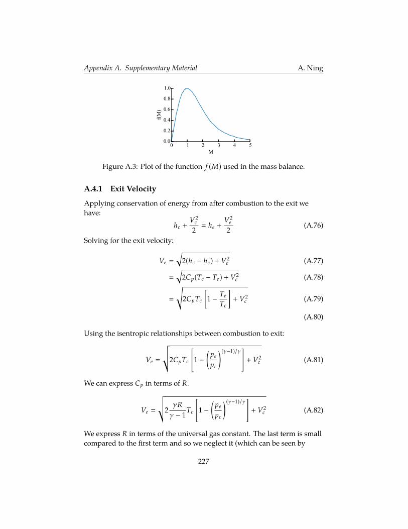
Appendix A. Supplementary Material A. Ning

0 1 2 3 4 5M

0.0

0.2

0.4

0.6

0.8

1.0

f(M

)Figure A.3: Plot of the function f (M) used in the mass balance.

A.4.1 Exit Velocity

Applying conservation of energy from after combustion to the exit wehave:

hc +V2

c

2 he +

V2e

2(A.76)

Solving for the exit velocity:

Ve

√2(hc − he) + V2

c (A.77)

√2Cp(Tc − Te) + V2

c (A.78)

√2CpTc

[1 − Te

Tc

]+ V2

c (A.79)

(A.80)

Using the isentropic relationships between combustion to exit:

Ve

√√√2CpTc

[1 −

(pe

pc

) (γ−1)/γ]+ V2

c (A.81)

We can express Cp in terms of R.

Ve

√√√2γRγ − 1

Tc

[1 −

(pe

pc

) (γ−1)/γ]+ V2

c (A.82)

We express R in terms of the universal gas constant. The last term is smallcompared to the first term and so we neglect it (which can be seen by

227

Appendix A. Supplementary Material A. Ning

expanding the term in terms of the Mach number). Physically, this meansthat the velocity in the combustion chamber is relatively small.

Ve

√√√2γγ − 1

Ru

MwTc

[1 −

(pe

pc

) (γ−1)/γ](A.83)

A.4.2 Throat Size

The nozzle throat must be large enough for the requisite mass flow rate.The general formula for the mass flow rate for a compressible flow wasgiven previously in Eq. (A.72). If we apply this equation at the throat,assuming that it is choked we have:

Ûm pTtAt√

Tt

√γ

R

(1 +

γ − 12

)− (γ+1)2(γ−1)

(A.84)

We can now solve for the required throat area given the mass flow rate:

At Ûm

pTt

√RTTt

γ

(γ + 1

2

) γ+12(γ−1)

(A.85)

The flow is isentropic from after combustion to the throat so TTt TTc andpTt pTc . Furthermore, like before, we assume that the velocity right aftercombustion is negligibly small so that TTc Tc and pTc pc . Makingthese substitutions and simplifying yields:

At Ûm

pc

√√RuTc

Mwγ

(γ + 1

2

) γ+1γ−1

(A.86)

This is the smallest throat area that can sustain a given mass flow rate.

A.4.3 Combustion Chamber Sizing

We now determine an appropriate size for the combustion chamber arearelative to the throat area. Using a mass balance from c to t the flow isisentropic and adiabatic so the mass balance simplified to:

Ac f (Mc) At f (Mt) (A.87)

228

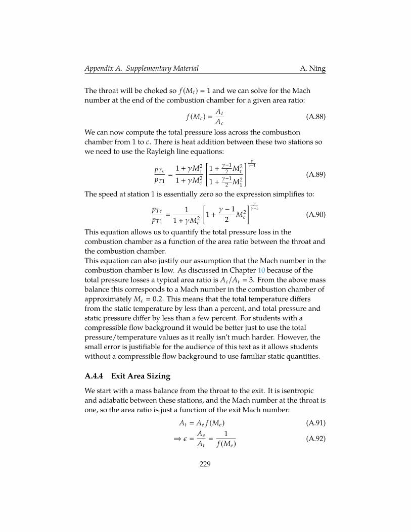
Appendix A. Supplementary Material A. Ning

The throat will be choked so f (Mt) 1 and we can solve for the Machnumber at the end of the combustion chamber for a given area ratio:

f (Mc) At

Ac(A.88)

We can now compute the total pressure loss across the combustionchamber from 1 to c. There is heat addition between these two stations sowe need to use the Rayleigh line equations:

pTc

pT1

1 + γM21

1 + γM2c

[1 +

γ−12 M2

c

1 +γ−1

2 M21

] γγ−1

(A.89)

The speed at station 1 is essentially zero so the expression simplifies to:

pTc

pT1

11 + γM2

c

[1 +

γ − 12

M2c

] γγ−1

(A.90)

This equation allows us to quantify the total pressure loss in thecombustion chamber as a function of the area ratio between the throat andthe combustion chamber.This equation can also justify our assumption that the Mach number in thecombustion chamber is low. As discussed in Chapter 10 because of thetotal pressure losses a typical area ratio is Ac/At 3. From the above massbalance this corresponds to a Mach number in the combustion chamber ofapproximately Mc 0.2. This means that the total temperature differsfrom the static temperature by less than a percent, and total pressure andstatic pressure differ by less than a few percent. For students with acompressible flow background it would be better just to use the totalpressure/temperature values as it really isn’t much harder. However, thesmall error is justifiable for the audience of this text as it allows studentswithout a compressible flow background to use familiar static quantities.

A.4.4 Exit Area Sizing

We start with a mass balance from the throat to the exit. It is isentropicand adiabatic between these stations, and the Mach number at the throat isone, so the area ratio is just a function of the exit Mach number:

At Ae f (Me) (A.91)

⇒ ε Ae

At

1f (Me)

(A.92)

229

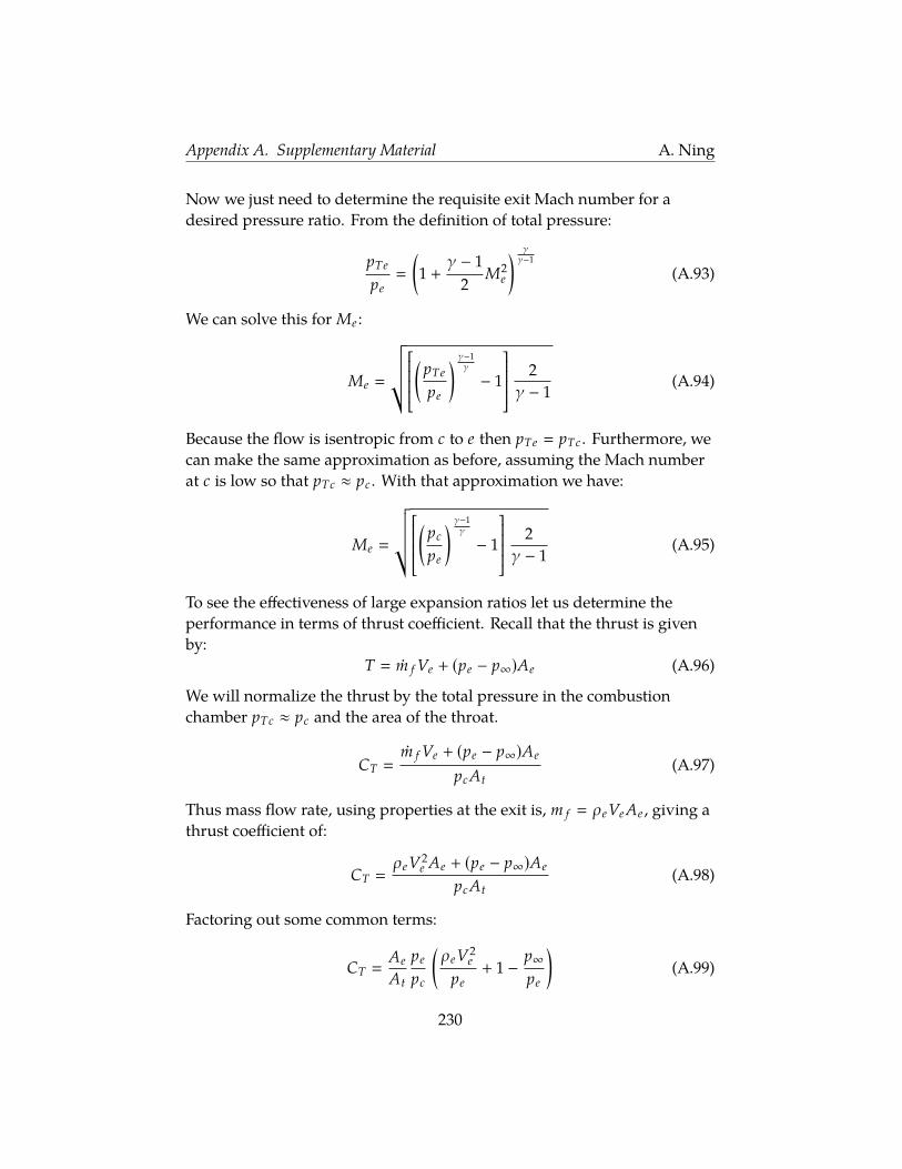
Appendix A. Supplementary Material A. Ning

Now we just need to determine the requisite exit Mach number for adesired pressure ratio. From the definition of total pressure:

pTe

pe

(1 +

γ − 12

M2e

) γγ−1

(A.93)

We can solve this for Me :

Me

√√√√√(

pTe

pe

) γ−1γ

− 1 2γ − 1

(A.94)

Because the flow is isentropic from c to e then pTe pTc . Furthermore, wecan make the same approximation as before, assuming the Mach numberat c is low so that pTc ≈ pc . With that approximation we have:

Me

√√√√√(

pc

pe

) γ−1γ

− 1 2γ − 1

(A.95)

To see the effectiveness of large expansion ratios let us determine theperformance in terms of thrust coefficient. Recall that the thrust is givenby:

T Ûm f Ve + (pe − p∞)Ae (A.96)

We will normalize the thrust by the total pressure in the combustionchamber pTc ≈ pc and the area of the throat.

CT Ûm f Ve + (pe − p∞)Ae

pcAt(A.97)

Thus mass flow rate, using properties at the exit is, m f ρeVeAe , giving athrust coefficient of:

CT ρeV2

e Ae + (pe − p∞)Ae

pcAt(A.98)

Factoring out some common terms:

CT Ae

At

pe

pc

(ρeV2

e

pe+ 1 −

p∞pe

)(A.99)

230

Appendix A. Supplementary Material A. Ning

The speed of sound is:

a

√γpρ

(A.100)

Making the substitution for pe/ρe gives:

CT Ae

At

pe

pc

(γV2

e

a2e

+ 1 −p∞pe

)(A.101)

If we assume ideal expansion then p∞ pe and the equation simplifies to:

CT Ae

At

pe

pcγM2

e (ideal expansion) (A.102)

231