Fundamentals of hypersonic flight - Properties of high ...

Fundamentals of hypersonic flight - Properties of hightemperature gases

P.F. Barbante ∗

Politecnico di Milano, ItalyT.E. Magin †

von Karman Institute for Fluid Dynamics, Belgium

Contents

1 Introduction 3

2 Governing Equations 72.1 Continuity equation . . . . . . . . . . . . . . . . . . . . . . . . . . . . . . . 72.2 Species continuity equation . . . . . . . . . . . . . . . . . . . . . . . . . . . 82.3 Momentum equation . . . . . . . . . . . . . . . . . . . . . . . . . . . . . . 82.4 Energy equation . . . . . . . . . . . . . . . . . . . . . . . . . . . . . . . . . 92.5 Mixture parameters and perfect gas law . . . . . . . . . . . . . . . . . . . . 9

3 Thermodynamic properties 113.1 Energy, enthalpy, specific heat . . . . . . . . . . . . . . . . . . . . . . . . . 113.2 Speed of sound . . . . . . . . . . . . . . . . . . . . . . . . . . . . . . . . . 16

4 Chemistry 194.1 Equilibrium chemistry . . . . . . . . . . . . . . . . . . . . . . . . . . . . . 194.2 Nonequilibrium chemistry . . . . . . . . . . . . . . . . . . . . . . . . . . . 204.3 Air nonequilibrium chemistry model . . . . . . . . . . . . . . . . . . . . . . 224.4 Catalycity . . . . . . . . . . . . . . . . . . . . . . . . . . . . . . . . . . . . 25

5 Transport properties 295.1 Boltzmann equation . . . . . . . . . . . . . . . . . . . . . . . . . . . . . . 305.2 Chapman-Enskog method . . . . . . . . . . . . . . . . . . . . . . . . . . . 335.3 Diffusion flux . . . . . . . . . . . . . . . . . . . . . . . . . . . . . . . . . . 355.4 Heat flux . . . . . . . . . . . . . . . . . . . . . . . . . . . . . . . . . . . . . 37

5.4.1 Heavy particle heat flux . . . . . . . . . . . . . . . . . . . . . . . . 375.4.2 Electron heat flux . . . . . . . . . . . . . . . . . . . . . . . . . . . . 385.4.3 Eucken correction . . . . . . . . . . . . . . . . . . . . . . . . . . . . 38

∗[email protected]†[email protected]

RTO-EN-AVT-116 5 - 1

Paper presented at the RTO AVT Lecture Series on “Critical Technologies for Hypersonic Vehicle Development”, held at the von Kármán Institute, Rhode-St-Genèse, Belgium, 10-14 May, 2004, and published in RTO-EN-AVT-116.

5.4.4 LTE heat flux . . . . . . . . . . . . . . . . . . . . . . . . . . . . . . 395.5 Stress tensor . . . . . . . . . . . . . . . . . . . . . . . . . . . . . . . . . . . 40

6 CFD example: OREX case 43

A Transport systems 49

Fundamentals of Hypersonic Flight – Properties of High Temperature Gases

5 - 2 RTO-EN-AVT-116

1 Introduction

It is well known that a fluid, in the most general case, is made of a mixture of atomsand molecules. Air at ambient temperature, for example, is a mixture made of molecularnitrogen, molecular oxygen, plus a small percentage of argon, carbon dioxide, neon, andsome other minor components. At moderate temperatures the gas behaves, with goodapproximation, as a calorically perfect gas. Gas pressure (p), density (ρ) and temperature(T ) are linked by the well known and simple state law: p = ρRT (where R is the so calledperfect gas specific constant). The gas specific heat are constant and internal energyand enthalpy are linear functions of the gas temperature. Also viscosity and thermalconductivity can be assumed to be constant, as a first approximation, or a simple powerlaw dependence on temperature can be assumed.

When Mach number rises and temperature too, this simple picture no longer exists:new phenomena (so called high temperature effects) appear and the gas nature is drasti-cally changed. We may grossly summarize such effects as follows:

- As temperature rises, the internal energy modes of the gas atoms and molecules,that at room temperature are dormant, are excited. Specific heats, internal energyand enthalpy are now nonlinear functions of the temperature. The specific heatsratio, also called γ, is no longer a constant. For air, excitation of the internal energymodes (vibrational) becomes important above temperatures of 500-800 K.

- As temperature further rises, chemical reactions can occur. Molecules dissociateinto atoms, new molecules are eventually formed, atoms and molecules can ion-ize. Mixture thermodynamic and transport properties become functions not only oftemperature but also of the chemical composition.

- Thermal nonequilibrium can also occur: internal energy modes are out of equilib-rium with respect to the translational one; we can say that they do not “share” thesame temperature. For example, when a fluid element crosses a shock wave, thetranslational energy of the fluid particles is suddenly increased; but a high numberof collisions is needed to equilibrate the internal energy modes with the transla-tional one (Park, 1990). Therefore, behind the shock, there will be a relaxationregion where the internal energy modes will try to “catch up” the translational one.Another example is when the fluid experiences a strong expansion. In this case thetranslational energy will rapidly decrease because of the expansion, but the internalone will remain higher.

- Ionization can occur and the gas becomes a partially ionized plasma, with a finiteelectrical conductivity. Therefore electromagnetic fields and associated forces, eitherself-induced or applied from an external source (Peterkin and Turchi, 2000; Suttonand Sherman, 1965), can act on the fluid, appreciably changing its behaviour withrespect to a neutral one. To make things more complex, an additional source of ther-mal nonequilibrium appears because energy exchange between mixture componentsand free electrons is highly inefficient due to the large mass disparity: in this casethe translational temperature of electrons can be different from the one of heavyparticles (Park, 1990).



- At high temperature (above 10000-11000 K for air) radiation emitted and absorbedby the gas can become important (Park, 1990) and eventually modify the energydistribution in the flowfield. Radiation modeling is a formidable task (Park, 1990;Sarma, 2000; Vincenti and Kruger, 1965), both numerically (a fluid element, a priori,is influenced by and influences all the others) and physically (an adequate spectraldata base is required).

- Chemical reactions can take place not only in the bulk of the gas but also at thesurface of the vehicle, due to catalytic effects of the wall material upon surfacechemistry. Usually such reactions have the negative property of increasing the heatflux experienced by the vehicle (Nasuti et al., 1996; Sarma, 2000).

We present now in a very qualitative manner two practical cases where high temper-ature gases showing some, if not all, of the previously described effects are encountered.

High speed vehicles

It is well known that, when an aerospace vehicle travels at high speed through the at-mosphere, a strong shock is formed in front of it. A major part of the kinetic energy ofthe free stream flow is converted into thermal energy across the shock and therefore hightemperature is reached in the flow region between the shock and the body (the shocklayer). The intense friction happening in the boundary layer increases too the tempera-ture triggering further chemical reactions. The high temperature effects can have a strongimpact on boundary layer stability and transition to turbulence. When the shock layertemperature is high enough the gas can ionize: the free electrons absorb radio waves andcause communication blackout to and from the vehicle. This is a serious problem andan accurate prediction of the electron number density in the shock layer is important.Emission and absorption of radiation can occur and, besides affecting the state of the gassurrounding the vehicle, can raise the heat flux experienced by the vehicle itself. Radia-tion from the hot vehicle wall to the ambient atmosphere can have a significant coolingeffect and must be taken into account in the thermal boundary condition (Sarma, 2000).

Ramjet and Scramjet engines

A Ramjet engine is essentially a duct where supersonic air is slowed down to subsonic speedat the entrance of the combustor. Fuel is injected in the combustor, the mixture burns andexpands through the nozzle. Ramjets have advantages over conventional turbine enginesin the Mach number regime from 2 to 5. However, some design concepts of hypersonicairbreathing transport vehicles assume a flight Mach number well in excess of 10 (anexample being the NASA X-43A). Under such conditions, if the incoming air is deceleratedto subsonic speed, it attains a temperature that is above the adiabatic flame temperatureof the fuel-air mixture burning in the combustor and therefore no combustion can takeplace. A possible solution is to keep the incoming air stream at supersonic speed in thecombustor: in this way air temperature is kept below the flame adiabatic temperature andcombustion can take place. The major drawback is that the combustion has to take placein a supersonic stream, leading to tremendous practical problems (flame stabilization,efficient mixing and burning) that are still not solved nowadays.



Lecture layout

In Sec. 2 we will recall the governing equations for a mixture of gases under conditions ofchemical nonequilibrium but thermal equilibrium. In Sec. 3 the thermodynamic propertiesof each mixture component will be given. In Sec. 4 a short discussion of chemistryand wall catalycity phenomena will be provided. Finally in Sec. 5 transport fluxes andrelated transport coefficients will be discussed. Some examples of computations of hightemperature reacting flows will be provided in Sec. 6.



2 Governing Equations

The governing equations are the mathematical expression of the physical principles ofconservation of mass, momentum and energy. They can be derived, for example, withthe control volume method, which is very general, not linked with a specific physico-chemical model and therefore does not give the expression of all the terms in the governingequations. The missing terms are provided by statistical mechanics and kinetic theory.Statistical mechanics provides the thermodynamic properties (internal energy, specificheat) and kinetic theory provides the transport properties (viscosity, thermal conductivity,diffusion).

High temperature fluids are in general made of different chemical species; in the rangeof pressure and temperature of interest here, each one behaves with good approximation asa perfect gas. We make the key assumption that the gas can be described as a continuum,i.e. there are always a sufficient number of molecules within the smallest significant volumeof the fluid and the macroscopic properties are given by average values of the appropriatemolecular quantities. We also assume that the gradients of the macroscopic variables (e.g.density, speed, temperature) have a characteristic length L that is much bigger than themean free path λ. Defining the Knudsen number as: Kn = λ/L, the previous assumptioncorresponds to: Kn � 1. The governing equations of such flows are the Navier-Stokesones and the transport terms (shear stresses, heat flux, diffusion fluxes) can be expressedas functions of macroscopic quantities (e.g. density, velocity, temperature, pressure). It isthe failure to meet this condition which imposes a limit in the continuum equations. TheNavier-Stokes equations tend to become inapplicable for Kn > 0.03, and even when theyare approximately applicable, the usual no-slip boundary conditions are not any morevalid. More specifically, the relative flow velocity at a surface, which is usually assumedto be zero, takes a finite value: this is called the slip velocity condition. In a similarfashion, the temperature, which is usually taken equal to the surface temperature, nowbecomes different: it is the temperature slip condition. A way to fix such a behaviour isto use slip boundary conditions with the Navier-Stokes equations, an approach that hasbeen proven to be quite effective (Gupta, 1996a,b) and gives good results up to Kn = 0.1.The error in the Navier-Stokes results is significant in regions of the flow where Kn > 0.1and the continuum model has to be replaced by the molecular model for Kn > 0.2. Asalready stated, the discussion presented in this lecture is valid in the continuous regimeand the slip effects are negligible.

2.1 Continuity equation

This equation simply expresses the conservation of global mass in the system. In Euleriandifferential form is written as:

∂ρ

∂t+∇ · (ρ~v) = 0 (1)

where ρ is the mixture density and ~v is the mixture average velocity. If ρi is the partialdensity of each mixture component, we have: ρ =

∑NS

i=1 ρi, where NS is the number ofmixture chemical species. If ~vi is the average velocity of each mixture component, then ~v



is defined as:

~v =

∑NS

i=1 ρi~vi

ρ(2)

2.2 Species continuity equation

The appropriate equations for each of the components must be established to computethe mixture chemical composition. Partial densities are a natural choice and the speciescontinuity equations are then:

∂ρi

∂t+∇ · (ρi~vi) = wi (3)

where wi is the chemical production term, i.e. the term that accounts for the rate ofproduction or depletion of species i due to chemical reactions. The average velocity forspecies i, ~vi, can be written as:

~vi = ~v + ~Vi (4)

where ~Vi is the diffusion velocity for species i. A related term is:

~Ji = ρi~Vi (5)

which is the diffusion flux and it plays a very important role in the framework of reactingflows. Naturally, summing up all the species continuity equations, we have to recover theglobal continuity equation. Indeed we have:

∑NS

i=1 ρi = ρ; and the chemical production

terms satisfy the property∑NS

i=1 wi = 0. From Eq. (2) and (4) we can deduce an importantproperty of diffusion fluxes:

NS∑i=1

~Ji =

NS∑i=1

ρi~Vi = 0 (6)

This taken into account we rewrite Eq. (3) under the form:

∂ρi

∂t+∇ ·

(ρi~v + ~Ji

)= wi (7)

2.3 Momentum equation

The momentum conservation equation can be written:

∂ρ~v

∂t+∇ · (ρ~v ⊗ ~v) +∇p = ∇ · ¯τ +

NS∑i=1

ρi

(~Fgi + ~Fei

)(8)

where p is the mixture pressure, ¯τ is the viscous stress tensor, ~Fgi is a nonelectromagnetic

body force and ~Fei is the electromagnetic force, both acting on the species i. If the speciesi is neutral the electromagnetic force is zero. ~Fgi reduces in the applications presentedhere to gravity and is always neglected; this is justified because in our applications thebuoyancy effects are negligible. ~Fei arises because of the presence of electromagnetic fieldsand has the form:

~Fei =qi

mi

(~E + ~Vi × ~B

)(9)



where mi is the mass of particle i and qi its charge. In the above equation, ~E is theelectric field and ~B the induced magnetic field. Usually Maxwell equations are needed tocompute the electric field and the induced magnetic field (Sutton and Sherman, 1965).In the presence of a ionized mixture, when no external fields are applied one can supposethat the magnetic field is negligible and the electric field is computed from the ambipolarconstraint, i.e. the diffusion current is zero in the flow:

NS∑i=1

qixi~Vi = 0 (10)

where xi is the molar fraction.

2.4 Energy equation

In compressible flows it is important to take into account both internal and kinetic energyin the energy equation, because there is a strong coupling between the two, throughconversion of one energy type into the other (as, for example, across a shock, wherekinetic energy is converted into thermal energy).

The total energy conservation equation for the mixture is:

∂ρE

∂t+∇ · [(ρE + p)~v]−∇ · (¯τ · ~v) +∇ · ~q =

NS∑i=1

(ρi~v + ρi

~Vi

)·(

~Fgi + ~Fei

)(11)

where E is the total energy (per unit mass) i.e. the sum of the mixture internal and kineticenergy: E = e + v2/2. The third term in the left hand side is the work of the viscousstresses, the fourth the heat flux, the term on the right hand side is the work of the bodyforces.

2.5 Mixture parameters and perfect gas law

The thermodynamic state of a mixture of perfect gases is uniquely defined once thetemperature T , the pressure or the density and the chemical composition are specified.For most problems in aerodynamics it is indeed reasonable to assume that each speciesis a perfect gas. Conditions that violates this assumptions are very high pressure (p >1000 bar) or low temperature (T < 30 K), both of which are far from the typical conditionsmet in aerospace applications. For each mixture component the equation of state linkingtemperature T and partial density ρi and pressure p is:

pi = ρiRiT (12)

Ri is the specific gas constant that may also be expressed as:

Ri =RMi

(13)

R is the universal gas constant, which is the same for all species (at least if they behaveas a perfect gas), Mi is the species molar mass, i.e. the mass of a mole of the species.



Dalton’s law for perfect gases states that the mixture pressure p is equal to the sumof the species partial pressures pi:

p =

NS∑i=1

pi (14)

The same law is valid for the partial densities ρi:

ρ =

NS∑i=1

ρi (15)

where ρ is, by definition, the mixture density. From Dalton’s law (Eq. 14) we infer thatonce the temperature and the partial pressures pi of each component are known, themixture is completely specified.

Other quantities are suited to describe the mixture chemical composition:

- The mass fractions yi = ρi

ρ(mass of species i per unit mass of mixture).

- The mole fractions xi (number of moles of species i per mole of mixture);

Both quantities satisfy the condition:

NS∑i=1

yi =

NS∑i=1

xi = 1

Mole and mass fractions can be used to compute mixture molar mass (M) and specificgas constant (R) respectively:

NS∑i=1

yiRi = R (16)

NS∑i=1

xiMi = M (17)

The formula to convert mole fractions into mass fractions (and vice versa) is:

yi =Mi

Mxi (18)

When using mole fractions one has to remember that the total number of moles in the sys-tem does change due to chemical reactions; the total mass, however, remains unchanged.


5 - 10 RTO-EN-AVT-116

3 Thermodynamic properties

3.1 Energy, enthalpy, specific heat

Atoms and molecules have different modes to store energy and each mode is quantized,i.e. it can only take discrete values (Anderson, 1989; Mayer and Mayer, 1946). In an atomthere are two energy modes:

- Translational energy mode: associated with the motion of centre of mass;

- Electronic energy mode: associated with the electrons orbiting around the nucleus.

For a molecule there are additional energy modes:

- Rotational energy mode: associated with the rotation of the molecule around or-thogonal axes in space;

- Vibrational energy mode: associated with the vibration of the atoms of the moleculewith respect to equilibrium positions within the molecule.

Every energy mode can assume an ensemble of, in theory infinite, different discrete values,or levels. Each level, in its turn, may manifest itself in a number of different ways(degeneracy, gk

i , of the levels).For a system of Ni particles of species i, distributed among an ensemble of k energy

levels, each of them with a different energy content, εki , the total energy Ei is:

Ei =∞∑

k=0

εki N

ki (19)

(with the constraint∑∞

k=0 Nki = Ni). Every distinguishable arrangement of the Ni parti-

cles among the levels is a macrostate. A way of computing the possible macrostates is toset up a differential equation for each level, an exceedingly complex task. To avoid such atask one can look for the existence of a macrostate that is much more likely to occur thanany other. Indeed such a state does exists, it is called the most probable macrostate (orthe most probable distribution), its probability is overwhelmingly higher than the one ofother possible macrostates (Vincenti and Kruger, 1965) and it occurs when the system isin thermodynamic equilibrium. The latter is a very important point because it restrictsthe use of the most probable macrostate to conditions of thermodynamic equilibrium orof slight nonequilibrium. The distribution of the particles over the different levels for themost probable macrostate is given by:

Nki = Ni

gki exp

(− εk

i

kBT

)Qi

(20)

(kB being the Boltzmann constant). The quantity Qi is the system partition function andis given by:

Qi =∞∑

k=0

gki exp

(− εk

i

kBT

)(21)


RTO-EN-AVT-116 5 - 11

The power of the partition function lies in the fact that the thermodynamic properties ofthe system can be determined from the partition function itself (Anderson, 1989; Clarkeand McChesney, 1964; Vincenti and Kruger, 1965). For example, the internal energy perunit mass of species i is given by:

ei = RiT2∂ ln Qi

∂T(22)

Once the expression for the energy content εki of the different quantum states is known,

the partition function can be computed by means of Eq. 21 and the internal energy isfinally evaluated from Eq. 22. It is customary to express the level energies, εk

i , relativeto the value they assume at absolute zero (also called the zero-point energy or groundstate), so that the computed energy is not the absolute energy but instead the sensibleone. The total energy is thus obtained by addition of the zero point energy e0,i.

For perfect gases the translational and the internal modes are independent of eachother and the partition function can be factored into two separate contributions: Q =QT Qint (where Qint belongs to the internal modes). In a real molecule the internal energymodes are not truly independent of each other: the energy content of an internal modeis affected by the state of the other internal modes (Mayer and Mayer, 1946). Therefore,when computing Qint, the contribution of a single mode cannot be factored separatelyfrom the others. However, for the simplest molecule model, which is the rigid rotator-harmonic oscillator, the rotational, vibrational and electronic energy modes are consideredto be independent each other and the molecular partition function can be factored as: Q =QT QRQV QE. (Subscript T refers to translation mode, R to rotational, V to vibrationaland E to electronic).

In agreement with the factorization property of the partition function, the internalenergy for an atom can be written as:

ei = eT,i + eE,i + e0,i

For a molecule the internal energy is:

ei = eT,i + eint,i + e0,i

Or, if all the internal modes are independent:

eint,i = eR,i + eV,i + eE,i

The translational energy is the same for both atoms and molecules and its value per unitmass is:

eT,i =3

2RiT (23)

The electronic energy for atoms (and also for molecules when it can be factored) has nosimple expression and reads (per unit mass):

eE,i = Ri

∑∞k=0 gk

EiθkE,i exp

(−θk

E,i

T

)∑∞

k=0 gkEi exp

(−θk

E,i

T

) (24)


5 - 12 RTO-EN-AVT-116

gkEi is the degeneracy for level k, θk

E,i is the characteristic electronic temperature for level k.The series in Eq. 24 diverges and has to be truncated. An empirical but effective criteriais to take into account the strictly necessary minimum number of electronic levels thatproduce a non-negligible change of energy in the temperature range of interest (Bottinet al., 1999).

For a linear molecule behaving as a rigid rotator-harmonic oscillator, the rotationalenergy per unit mass can be written as:

eR,i = RiT

(1− θR,i

θR,i + 3T

)(25)

θR,i is the rotational characteristic temperature and is usually equal to a few Kelvin, sothat the rotational mode is fully excited at temperatures considered here. The vibrationalenergy per unit mass is, in its turn:

eV,i = Ri

∑m

θmV,i

exp(

θmV,i

T

)− 1

(26)

θmV,i is the vibrational characteristic temperature associated with the vibrational mode

m. The vibrational energy contribution is less than RiT and approaches this value whenT � θm

V,i.The zero-point energy generally cannot be computed or measured; nevertheless it is

an important quantity. In a reacting mixture it is necessary to establish a common levelfrom which all the species energies are measured. In addition the zero-point energy islinked with the energy associated with chemical bonds. Consider for example a certainamount of nitrogen atoms; it is experimentally observed that, when they recombine toform molecular nitrogen, some energy is released. If the recombination happens at theabsolute zero, the energy released in the chemical reaction (∆h0

F ) is equal to the differencebetween the zero-point energy of the atomic nitrogen mixture e0,N and of the molecularnitrogen mixture e0,N2 . If the reaction proceeds in the opposite direction, exactly thesame amount of energy is absorbed by the system: it is the heat of formation of atomicnitrogen at absolute zero. From the point of view of the energy balance it is equivalent toassume e0,N 6= 0, e0,N2 6= 0 and ∆h0

F = e0,N−e0,N2 or e0,N = ∆h0F , e0,N2 = 0 and obviously

∆h0F = e0,N − e0,N2 . Therefore it follows that the zero-point energy e0,i of species i can be

replaced by the heat of formation ∆h0F,i of species i at the same temperature. The heat

of formation of the different species is available in literature (Chase et al., 1985).The enthalpy is simply computed from the energy by addition of the extra term: RiT .As previously mentioned, the rigid rotator-harmonic oscillator model for the molecules

does not truly represent the reality and so-called anharmonicity corrections can be used (Bot-tin et al., 1999): they take into account the fact that the energy modes are coupledtogether. Anharmonicity corrections often change appreciably the molecules internal en-ergy. It should be noticed, however, that this effect is more pronounced above 6000 K,a temperature at which, usually, molecules are highly dissociated. The correction has asmall effect on the mixture properties and can often be neglected.

The mixture energy and enthalpy per unit mass are obtained by means of the formulae:

e =

NS∑i=1

yiei h =

NS∑i=1

yihi (27)


RTO-EN-AVT-116 5 - 13

Enthalpy of Local Thermodynamic Equilibrium (LTE) air is shown in Fig. 1.

0 2500 5000 7500 10000 12500 15000T [K]

0

25

50

75

100

h [M

J.kg

-1]

Figure 1: Enthalpy of air at 1 atm.

Enthalpy of LTE carbon dioxide is given in Fig. 2. The negative value of enthalpyat low temperature results of the exothermic formation of the CO2 molecule at 0 K (theenthalpy of formation of carbon graphite and molecular oxygen gas is zero).

0 2500 5000 7500 10000 12500 15000T [K]

-25

0

25

50

75

100

125

h [M

J.kg

-1]

0 2500 5000 7500-0.5

0

0.5

1

1.5

2

Figure 2: Enthalpy of carbon dioxide at 1 atm.


5 - 14 RTO-EN-AVT-116

The single species specific heats are, by definition:

cv,i =

(∂ei

∂T

)v

cp,i =

(∂hi

∂T

)p

(28)

Both are functions of temperature only, as it is the case for the internal energy and theenthalpy.

The specific heat for a mixture requires a little bit more care. Let’s concentrate onthe constant pressure specific heat cp, the same being valid for cv. From Eq. 27 and 28we have:

cp =

(∂h

∂T

)p

=

NS∑i=1

[(∂yi

∂T

)p

hi + yi

(∂hi

∂T

)p

](29)

If no chemical reactions are taking place in the flow (the mixture is frozen) the firstderivative is identically zero and we have the frozen specific heat:

cp,fr =

NS∑i=1

yi

(∂hi

∂T

)p

=

NS∑i=1

yicp,i (30)

In case of a frozen mixture, chemical composition does not change (yi is constant) and cp,fr

is function only of temperature: a frozen mixture is therefore a thermally perfect gas. If,on the opposite, chemical equilibrium is established, the chemical composition is functiononly of two thermodynamic variables, e.g. pressure and temperature or, yi = yi(p, T ) andEq. 28 becomes:

cp,eq =

NS∑i=1

[(∂yi

∂T

)p

hi + yicp,i

](31)

In the intermediate case of a finite rate chemically reacting mixture, the chemical compo-sition is function not only of two thermodynamic variables, but also of the position andof the previous flow history. It follows that the derivative

(∂yi

∂T

)p

is not uniquely defined

and the only kind of specific heat that makes sense is the frozen specific heat cp,fr givenby Eq. 30.

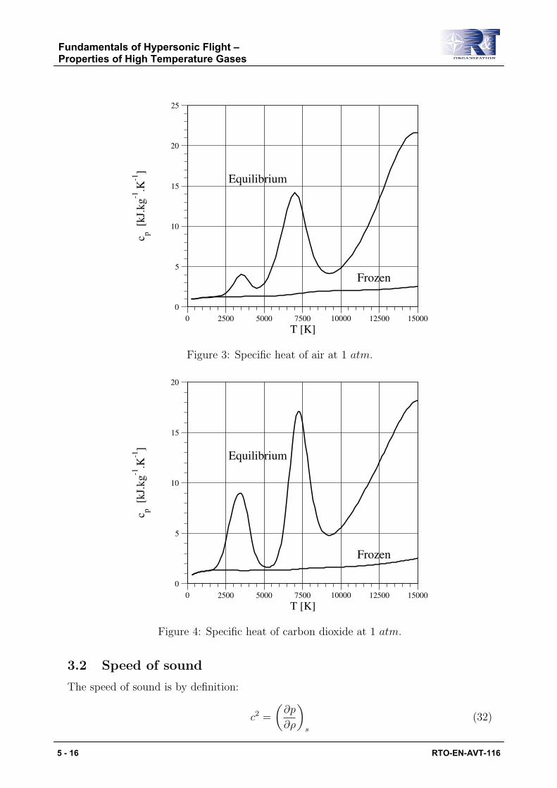
Frozen and equilibrium specific heat of LTE air are shown in Fig. 3. Frozen andequilibrium specific heat of LTE carbon dioxide are shown in Fig. 4.


RTO-EN-AVT-116 5 - 15

0 2500 5000 7500 10000 12500 15000T [K]

0

5

10

15

20

25

c p [kJ

.kg-1

.K-1

]

Frozen

Equilibrium

Figure 3: Specific heat of air at 1 atm.

0 2500 5000 7500 10000 12500 15000T [K]

0

5

10

15

20

c p [kJ

.kg-1

.K-1

]

Frozen

Equilibrium

Figure 4: Specific heat of carbon dioxide at 1 atm.

3.2 Speed of sound

The speed of sound is by definition:

c2 =

(∂p

∂ρ

)s

(32)


5 - 16 RTO-EN-AVT-116

i.e. the derivative of pressure with respect to density at constant entropy. As for thespecific heats we can define two different speeds of sound (Anderson, 1989; Clarke andMcChesney, 1964): a frozen speed of sound cfr and an equilibrium speed of sound ceq.The frozen sound speed is:

c2fr =

cp,fr

cv,fr

p

ρ= γfr

p

ρ= γfrRT (33)

The equilibrium speed of sound is:

c2eq =

cp,eq

cv,eq

p

ρ

1− ρ2

p

(∂e∂ρ

)T

1− ρ(

∂h∂p

)T

=cp,eq

cv,eq

1(∂ρ∂p

)T

(34)

When the flow is either frozen or in chemical equilibrium, there is no ambiguity on whichsound speed has to be used. In case of chemical nonequilibrium, disturbances with a period(the inverse of the frequency) much longer than the characteristic time of the chemistrypropagate with the equilibrium sound speed, disturbances with a period much smallerthan the chemistry time with the frozen sound speed and disturbances with a period ofthe same order as the chemistry time propagate with an intermediate speed (Clarke andMcChesney, 1964). This creates problems for the choice of the speed to use in a chemicallyreacting flow computation.

The frozen and equilibrium sound speed are given in Fig. 5 for LTE air.

0 2500 5000 7500 10000 12500 15000T [K]

0

1000

2000

3000

4000

5000

c [m

.s-1

]

Figure 5: Sound speed of air at 1 atm: −− frozen and equilibrium.

The equilibrium speed of sound is compared in Fig. 6 to the frozen speed of sound forLTE carbon dioxide.


RTO-EN-AVT-116 5 - 17

0 2500 5000 7500 10000 12500 15000T [K]

0

1000

2000

3000

4000

5000

c [m

.s-1

]

Figure 6: Sound speed of carbon dioxide at 1 atm: −− frozen and equilibrium.


5 - 18 RTO-EN-AVT-116

4 Chemistry

4.1 Equilibrium chemistry

Let’s now recall the species i continuity equation (Eq. 3) and let’s put aside, for themoment, the convective and diffusive terms. The equation reduces to the ordinary dif-ferential equation (ODE) ∂ρi

∂t= wi. Adding all the species we have a system of ODE’s

governing the evolution of the NS species. The system is, in general, nonlinear because ofthe structure of the production term (Eq. 38). In a first approximation we can linearizethe system around a known state ρ0

i .

∂ρi

∂t= w0

i +

NS∑j=1

∂wi

∂ρj

(ρj − ρ0j) = w

0

i +

NS∑j=1

∂wi

∂ρj

ρj i = 1, . . . , NS

or, in compact form:∂

∂t{ρi} =

{w

0

i

}+ [A] {ρi}

wi has dimensions kg/(m3s) and thus each element of the Jacobian [A] has dimensions1/s and is an index of the characteristic time of chemical reactions. The element ∂wi/∂ρj

may also be seen as the sensitivity, due to chemical reactions, of species i with respectto a variation of species j. For practical purposes, we can think of having only a globalvalue for the characteristic time of chemical reactions, instead of the NS by NS given bythe Jacobian. The norm of [A] (||[A]||) is taken as the desired value.

The next step is to compare a characteristic flow time (e.g. the time that the flow needsto cross the region of interest) with the chemistry time. In order to do this the speciescontinuity equation (Eq. 3) is conveniently non-dimensionalised. We define a referencelength Lref , a reference speed vref , a reference density ρref and a reference chemistry time1/τc = ||[A]||ref , the flow reference time being defined as τf = Lref/vref . The speciesequation in nondimensional form reads:

∂ρi

∂t+ ∇ ·

(ρi~vi

)= ˜wi||[A]||ref

Lref

vref

= Da1˜wi (35)

(where the ˜ superscript indicates a nondimensional quantity). The quantity Da1 = τf/τc

is the first Damkohler number and it is a parameter of fundamental importance in thestudy of similitude in reacting flows. By analyzing the previous equation we can definethe two following limiting cases:

• If τf � τc or Da1 → 0, the chemical reactions are negligible, the flow is called frozenflow and the species continuity equations reduce to:

∂ρi

∂t+∇ · (ρi~vi) = 0

• If τf � τc or Da1 →∞, the flow tends towards a state of local chemical equilibriumand the species continuity equations tend to the limit

wi = 0


RTO-EN-AVT-116 5 - 19

In this case the chemical composition is uniquely determined by the local values ofp and T or ρ and T . The species continuity equations may be eliminated from thesystem of governing equations and the chemical composition computed with an adhoc algorithm (Bottin et al., 1999; Anderson, 1989).

The computed equilibrium composition of air for Earth reentries and carbon dioxidefor Mars entries is shown in Figs. 7 and 8. The mixtures are defined as follows:

- An 11-species air mixture composed of N2, NO, O2, N, O, N+2 , NO+, N+, O+

2 , O+,and e−, with 79 % of nitrogen and 21 % of oxygen elements.

- An 8-species carbon dioxide mixture composed of CO, CO2, O2, C, O, C+, O+ ande−, with 1/3 of carbon and 2/3 of oxygen elements.

The net charge is zero.

0 2500 5000 7500 10000 12500 15000T [K]

0

0.2

0.4

0.6

0.8

x i

O

NO

N2

O2

N

e-

O+

N+

Figure 7: Major components of air at 1 atm.

4.2 Nonequilibrium chemistry

We begin by considering an elementary reaction (identified with index r), i.e. a reactionaccomplished in one step only, which can be formally written as:

NS∑i=1

ν ′irXi �NS∑i=1

ν ′′irXi (36)


5 - 20 RTO-EN-AVT-116

0 2500 5000 7500 10000 12500 15000T [K]

0

0.2

0.4

0.6

0.8

1.0x i

O

O

CO

CO

CO2

O2

Ce-

O+

C+

Figure 8: Components of carbon dioxide at 1 atm.

The species appearing on the left hand side are the reactants and the one appearingon the right hand side the products; Xi is a dummy symbol for the species i, ν ′ir isthe stoichiometric coefficient of reactant i and ν ′′ir is the stoichiometric coefficient forthe product i. An elementary reaction r can proceed in both directions and is alwaysreversible; when there is perfect balance between dissociation and recombination thereaction is in chemical equilibrium.

A typical example is the dissociation recombination of oxygen, which is an importantreaction for high temperature air chemistry:

O2 + X � O + O + X (37)

Molecular oxygen O2 collides with a third body X and dissociates in two oxygen atomsO if the collision energy is enough to activate the reaction. In the reverse reaction twooxygen atoms collide with the third body and recombine into one oxygen molecule if thethird body can carry out the energy released in the recombination. It should be noticedthat the third body does not change its chemical nature in the reaction.

In accordance with the Law of Mass Action and experimental evidence (Vincenti andKruger, 1965), the net rate of production of species i by the elementary reaction r justintroduced (Eq. 36) is:

wir = Mi

(ν ′′ir − ν ′ir)kfr

NS∏j=1

(ρj

Mj

)ν′jr

︸︷︷︸production (forward) rate

− (ν ′′ir − ν ′ir)kbr

NS∏j=1

(ρj

Mj

)ν′′jr

︸︷︷︸destruction (backward) rate

(38)


RTO-EN-AVT-116 5 - 21

Here we have divided the expression for wir into a production term that goes from leftto right (in the reaction 37, for example, this corresponds to the creation of O from O2)and a destruction term that goes from right to left (in the same reaction this correspondsto the disappearance of O into O2). The rate of production (or destruction) of a sub-stance is proportional to the product of the concentrations of the reactants raised to thestoichiometric coefficient power, the proportionality constant being the reaction rate.

The number of elementary reactions is arbitrary and, if we have Nr of them involvingthe species i, the production term for this species is obtained by summing over Eq. 38:

wi = Mi

Nr∑r=1

(ν ′′ir − ν ′ir)

{kfr

NS∏j=1

(ρj

Mj

)ν′jr

− kbr

NS∏j=1

(ρj

Mj

)ν′′jr

}(39)

kfr is the forward reaction rate for the reaction r and kbr the backward reaction ratealways for the reaction r. This equation should be valid also at equilibrium and the tworeaction rates are linked by: kbr =

kfr

Kcr, where Kcr is the equilibrium constant for the rth

reaction. This choice ensures that, if the flow approaches locally the chemical equilibrium,the chemical composition is correctly computed. Kcr is linked with the Gibbs free energyand for a perfect gas it is a function only of temperature. Referring to the elementaryreaction r (Eq. 36) Kcr reads (Anderson, 1989):

log Kcr(T ) = −NS∑i=1

(ν ′′ir − ν ′ir)gi(T )

RT− log (RT )

NS∑i=1

(ν ′′ir − ν ′ir) (40)

gi is the Gibbs free energy per unit mole of species i and is equal to hi−T si, where hi and si

are respectively the enthalpy and entropy of species i per unit mole. The same statisticalmechanics methods of section 3.1 are used to compute the Gibbs free energy. Two thingsshould be noticed: the first one is that there are as many equilibrium constants Kcr aselementary reactions, the second one is that, since Kcr is a function of the thermodynamicproperties, its effective value is affected by the models used for the computation of theseproperties. For example we can expect an effect of anharmonicity corrections.

It is possible to derive the forward reaction coefficient from kinetic theory, assuminga known form for the interaction potential, the elementary dissociation-recombinationprobabilities and the exact distribution functions. In practice this approach is not possiblebecause too much information is missing and a semiempirical formulation, the so calledArrhenius formulation, is used to compute the forward reaction rate:

kfr = ArTηre

−Ed,rkT (41)

Ar > 0 is a constant factor, ηr a positive or negative exponent and Ed,r is the so-calledactivation energy for the rth reaction. It has to be noticed that such an expression is rigor-ously valid only for thermal equilibrium. kfr is usually computed by fitting experimentaldata. Large differences exist among various authors, with coefficients often differing byone or more orders of magnitude.

4.3 Air nonequilibrium chemistry model

Air at ambient temperature is a mixture of molecular nitrogen (N2), molecular oxygen(O2), argon (Ar), carbon dioxide (CO2) and neon (Ne) (plus some other minor compo-


5 - 22 RTO-EN-AVT-116

nents). The first two species are the dominant ones and, for all the applications of interesthere, air can be assumed to be made, in volume, of 79% N2 and 21% O2. As temperatureincreases chemical reactions take place and the initial composition is profoundly changed.At a pressure of 1 atmosphere oxygen begins to dissociate in a temperature range be-tween 2000 K and 4000 K. The lower the pressure, the lower the temperature at whichthe dissociation starts and ends. At 100 Pa oxygen is fully dissociated at 3000 K andat 100000 Pa at 5000 K. Molecular nitrogen begins to dissociate by reaction with oxy-gen atoms to produce nitric oxide NO (this happens above 2000 K) and then the mainphase of dissociation takes place between 3500 K and 8000 K. Nitric oxide ion NO+

starts to appear around 4000 K; O+ and N+ above 6000 K. Therefore, depending on thetemperature and pressure range, we can distinguish among three main mixtures models:

• When the degree of ionization is negligible; air is well represented by a five speciesmixture (air-5): O2, N2, NO, O, N .

• When the degree of ionization is not any more negligible, but temperature is suffi-ciently low; air is well represented by a seven species mixture (air-7): O2, N2, NO,O, N , NO+, e−.

• When the temperature is higher than in the previous case; air is represented by aneleven species mixture (air-11): O2, N2, NO, O, N , O+

2 , N+2 , NO+, O+, N+, e−.

A suitable set of chemical reactions is needed to take into account all these phenomena.In air we can have seven main groups of reaction (Park, 1990, 1993; Gupta et al., 1990)that are detailed in Table 1.

• Thermal dissociation of O2, N2 and NO molecules by collisions with heavy particles(i.e. all the species except the free electrons); a priori anyone of the heavy particlespecies is involved (Park, 1993), but in some reaction models (Gupta et al., 1990)only some of them are taken into account. Park (Park, 1990, 1993) considers forthe dissociation of N2 also the electrons as possible third body.

• Bimolecular exchange reactions involving NO: O2 + N � NO + O and N2 + O �NO + N . They are the most important reactions for NO production and the latterremoves N2 from the system even more efficiently than the dissociation reaction.

• Associative ionization and its reverse dissociative neutralization. The first reactionof this group in Table 1 is almost immediately triggered by the presence of N andO atoms.

• Charge exchange reactions. NO+, N+2 , O+

2 are created by associative ionization andare converted into other ions. It is interesting to notice that, if the last group ofreactions (impact ionization) is negligible, atomic ion species cannot be generateddirectly but only through charge exchange reactions.

• Heavy particle impact ionization. These reactions are present only in some reactionschemes (Gupta et al., 1990) and they have very little effect, their activation energybeing very high.


RTO-EN-AVT-116 5 - 23

Thermal dissociation

O2 + X � O + O + XN2 + X � N + N + XNO + X � N + O + X

Bimolecular exchange

O2 + N � NO + ON2 + O � NO + N

Associative ionization-dissociative recombination

N + O � NO+ + e−

N + N � N+2 + e−

O + O � O+2 + e−

Charge exchange

NO+ + O � N+ + O2

O+2 + N � N+ + O2

O+ + NO � N+ + O2

N+ + N2 � N+2 + N

O+2 + N2 � N+

2 + O2

O+ + N2 � N+2 + O

NO+ + N � N+2 + O

O+2 + O � O+ + O2

NO+ + N � O+ + N2

NO+ + O2 � O+2 + NO

NO+ + O � O+2 + N

Heavy particle impact ionization

O2 + N2 � NO + NO+ + e−

NO + X � NO+ + e− + X

Electron impact ionization

O + e− � O+ + e− + e−

N + e− � N+ + e− + e−

Table 1: Chemical reactions scheme for 11 species air (from Ref. (Gupta et al., 1990;Park, 1993))


5 - 24 RTO-EN-AVT-116

• Electron impact ionization of N and O species. They have a very high activationenergy, but once they are triggered, they lead to an exponential increase of the freeelectrons number density.

4.4 Catalycity

In a typical very high speed flight, the gas surrounding an aerospace vehicle is dissociated.In such circumstances, atomic species can recombine not only in the boundary layer, butalso at the vehicle surface, thus releasing the reaction energy and increasing the thermalload; therefore his effect should be taken into account when computing the heat fluxexperienced by a flying vehicle.

A material can have different behaviours with respect to the recombination of atomsimpinging its surface. When the material surface is completely inert with respect to atomicrecombination we say that it is a noncatalytic wall, when, on the opposite, it promotes therecombination of all the impinging atoms we say that is a fully catalytic wall. The latterdefinition needs some more observations. We recall that a catalyzer promotes a chemicalreaction, but it does not alter its final state. In particular, a catalyzed reaction cannotgo beyond the local equilibrium conditions for the reaction itself. The definition of fullycatalytic wall as a wall that promotes the recombination of all the atoms impinging thewall itself is, therefore, not correct and it would be better to define as fully catalytic walla material that, in the limit, allows a local gas composition equal to the equilibrium one.In literature such a wall is often known as local equilibrium wall. When the material isneither noncatalytic nor fully catalytic it is called a partially catalytic wall.

Many different types of elementary reactions are possible on a surface; a generic set,valid on different kinds of materials, is as follows:

1. Atoms in the gas-phase can be adsorbed by a free active surface site or they canleave the surface by thermal desorption. The adsorbed atoms are called adatoms.The adsorption-desorption reaction is written symbolically as:

X + (S) � (X − S )

(S) is a free active surface site.

2. Atoms in the gas-phase can recombine with adatoms to form a molecule that leavesthe surface. This mechanism is known as Eley-Rideal (E-R) recombination.

Y + (X − S ) → XY + (S)

3. Adatoms migrate on the surface and recombine together in a molecule that leaves thesurface. This mechanism is known as Langmuir-Hilsenwood (L-H) recombination.

(Y − S ) + (X − S ) → XY + 2(S)

4. Molecules in the gas-phase can be adsorbed by a free site and released by thermaldesorption. This process usually does not contribute to the heat release, unless theadsorbed molecule is highly excited and releases the excess of energy to the surface,but it can modify the number of free sites and, therefore, the efficiency of E-R andL-H reactions.


RTO-EN-AVT-116 5 - 25

5. Molecules are adsorbed on the surface and dissociated (dissociative adsorption): itis in practice the reverse of the E-R and L-H reactions. This reaction can happenfor O2 molecule on metallic surfaces (Reggiani et al., 1996).

The final goal is to determine the rate of production or destruction of each speciesdue to the surface reactions by summing up over all the elementary steps: this gives theheterogeneous wall reaction rate wi,cat (mass of species i produced or destroyed per unitarea and per unit time).

Next to the surface, the mechanism that feeds the i species from the bulk of the gasto the surface itself is diffusion. Therefore, at steady state, the net amount of species iproduced or destroyed by catalytic reactions has to be balanced by the diffusion flux ofspecies i itself.

~Ji,w · ~nw = wi,cat (42)

(where ~nw is the normal to the wall, oriented from the gas towards the wall). Thisexpression is also the boundary condition for the species continuity equations (Eq. 3).

For practical applications the wall production rate wi,cat is often expressed in a sim-plified form. The simplest one is to assume that a first order reaction is happening at thewall. In this case, assuming that species i is recombining at the wall, the heterogeneouswall reaction rate reads:

wi,cat = Ki,wρwyi,w (43)

Ki,w is the catalytic speed for species i (it has dimensions m/s). It is a global index thathides completely every detail of the reactions taking place at the wall.

A more sophisticated approach is to define a suitable recombination probability. LetM↓

i be the number flux of species i impinging the surface and Mi,rec the number flux ofi species recombining at the surface. The recombination probability γi is defined as:

γi =Mi,rec

M↓i

(44)

The flux impinging the surface isM↓i and the flux leaving the surface isM↓

i −Mi,rec = (1− γi)M↓i .

The net flux ~Ji,w ·~nw is equal to the difference of the two multiplied by the i species mass

and therefore to γimiM↓i . From the last statement we deduce:

wi,cat = γimiM↓i (45)

Kinetic theory provides an expression for the impinging flux M↓i . Two different results

are possible, depending on the expression used for the particles distribution function atthe wall. If the Maxwell distribution is used the impinging flux M↓

i reads:

M↓i = ni

√kTw

2πmi

(46)

If the Chapman-Enskog perturbation term φi (see Sec. 5.2) is added it reads instead:

M↓i = ni

√kTw

2πmi

+1

2mi

~Ji · ~nw (47)


5 - 26 RTO-EN-AVT-116

In the first case the wall reaction rate reads (we have used Eq. 42):

wi,cat = γimini

√kTw

2πmi

(48)

In the second one:

wi,cat =2γi

2− γi

mini

√kTw

2πmi

(49)

The last two results are practically identical for γi � 1, but when γi → 1 the differenceis appreciable. In effect the right expression is the latter, because the wall reactionsperturb the distribution function making it non-Maxwellian and it is the expression thathas preferably to be used.

The expressions given in Eqs. 43, 48 and 49 show some inconsistencies. The first isin the link between Ki,w and γi, that changes depending if we choose Eqs. 43 and 48

or Eqs. 43 and 49. In one case the relation is Ki,w = γi

√kTw

2πmi(known also as Hertz-

Knudsen relation) and in the other Ki,w = 2γi

2−γi

√kTw

2πmi. The other inconsistency is that

none of the above formulations gives a wall chemical composition that tends correctlyto the local equilibrium composition limit for a fully catalytic wall, i.e. Ki,w → ∞ andγi = 1 respectively. The former condition implies yi,w = 0 and the latter yi,w equal toa small, but finite, value that is, in general, different from the local equilibrium one.This inconsistency, however, can be tolerated in our applications because the practicallysustainable wall temperatures allow only a negligible equilibrium atomic concentrations.


RTO-EN-AVT-116 5 - 27


5 - 28 RTO-EN-AVT-116

5 Transport properties

Transport fluxes, i.e. diffusion flux appearing in the species continuity equations (Eq. 7),stress tensor appearing in the momentum equation (Eq. 8) and heat flux appearing inthe energy equation (Eq. 11) are computed by the kinetic theory of gases (Chapman andCowling, 1970; Ferziger and Kaper, 1972; Giovangigli, 1999; Hirschfelder et al., 1964).

The kinetic theory approach we will present in the next sections is rigorously validunder the following assumptions:

Kn � 1. As already mentioned in Sec. 2, the Knudsen number Kn being small, thegas mixture is collision-dominated and the Navier-Stokes equations are the rightgoverning equations.

No chemical reactions. Ern and Giovangigli (Giovangigli, 1999) have shown that chem-ical reactions do not influence the transport properties if the characteristic time forchemistry is larger than that for collisions implied in transport phenomena. There-fore, for the sake of transport property computation we assume the gas mixture tobe frozen.

No internal energy. The internal energy is not taken into account when deriving trans-port coefficients. The influence of the internal degrees of freedom on transport prop-erties is addressed in various specialized publications cited in general Refs. (Ferzigerand Kaper, 1972; Giovangigli, 1999). Indeed, a rigorous treatment including theinternal energy leads to transport collision integrals difficult to estimate with accu-racy in high-temperature applications. As a matter of fact, the influence of internaldegrees of freedom on properties such as viscosity can be neglected. It is retained in-stead for diffusion and thermal conductivity by means of a simple correction due toEucken (Chapman and Cowling, 1970; Hirschfelder et al., 1964; Ferziger and Kaper,1972).

When the gas mixture under study is ionized we make the additional assumptions:

λD � L. The Debye length λD being smaller than a reference length L in the flow,quasi-neutrality of the plasma is prescribed.

Λ � 1. The plasma parameter Λ is proportional to the number of electrons in a sphereof radius equal to the Debye length. If the plasma parameter is sufficiently large,charged particle interactions can be treated as binary collisions with Debye-Huckelscreening of the Coulomb potential using the usual collision operator of Boltzmannequation (Delcroix and Bers, 1994).

ε =√

me/mh � 1. Our gas mixture is composed of NS species. The electron massreads me. A characteristic mass for heavy particles is given by mh. This hypothesisallows to simplify transport fluxes and transport coefficients evaluations.

|Te − Th| � Te ∼ Th. Due to the small electron heavy-particle mass-ratio, electrontemperature Te can differ from heavy particle temperature Th. The case of weakthermal nonequilibrium is studied here. Thermal equilibrium formulation can berecovered by setting: Th = Te = T .


RTO-EN-AVT-116 5 - 29

βe � Kn. The Hall parameter of electrons βe is assumed to be smaller than the Knudsennumber. Thus, the magnetic field influence on transport properties remains negligi-ble, the plasma is unmagnetized (Magin and Degrez, 2004b). The approach followedhere can be generalized to derive transport properties sensitive to a magnetic field.

Finally, to simplify the notation we will indicate with S the set of all mixture com-ponents, including free electrons and with H the set of heavy particles, i.e. the mixturecomponents minus the free electrons.

5.1 Boltzmann equation

The exact representation of the mixture state is not only impossible because it requiresthe knowledge of velocity, position and internal state of every particle in the mixture,but is also redundant for our continuum description. It seems therefore more practicaland convenient to use a statistical approach that, by its own nature, gives the “global”behaviour of the system under investigation.

Consider a particle belonging to species i (for simplicity we assume it has no internaldegrees of freedom): its state is completely characterized by its position ~r and its velocity~ci. The six-dimensional space having as components the three components of ~r andthe three components of ~ci is called the phase space. In the spirit of the continuumdescription, it would be enough to have a function fi(~r,~ci, t) that gives the expectedamount of i species particles in an elementary volume d~rd~ci of the phase space. In otherwords, Ni = fi(~r,~ci, t)d~rd~ci is the expected number of i species particles in the volumeelement d~r located at ~r, whose velocities lies in the interval d~ci about velocity ~ci at timet. Integration with respect to ~r and ~ci gives the total number of i species particles in thesystem. Integration with respect to ~ci gives the the total number of i species particles inthe volume d~r and the number density ni of i species is this number divided by d~r:

ni(~r, t) =

∫fi(~r,~ci, t)d~ci (50)

(the integration extends over the full velocity range). The partial density reads ρi = mini

where mi is the mass of the single species particle i.If ϕi(~r,~ci, t) is a generic property for species i, function of the particle velocity, its

average value is:

ϕi(~r, t) =1

ni(~r, t)

∫ϕi(~r,~ci, t)fi(~r,~ci, t)d~ci (51)

For example average velocity of species i (the same as the one defined in section 2.1)is:

~vi(~r, t) =1

ni(~r, t)

∫~cifi(~r,~ci, t)d~ci (52)

The mixture mass average velocity is identical to the one defined by Eq. 2. The differencebetween the species velocity of particle i and the mixture average velocity is the peculiarvelocity of species i:

~Ci = ~ci − ~v

The peculiar velocity is linked with the thermal motion of the molecules: in a mixtureat rest, without macroscopic gradients, particles are still subject to Brownian motion


5 - 30 RTO-EN-AVT-116

and this motion is nothing else than the peculiar velocity. The average kinetic energyassociated with the peculiar velocity may be identified as the translational component ofthe internal energy of each mixture component:

Ti(~r, t) =1

32kni

∫1

2miC

2i fi(~r,~ci, t)d~ci (53)

In our case Ti = Te for free electrons and Ti = Th for all the remaining mixture compo-nents.

In a gas under nonequilibrium conditions, gradients exist in one or more of the macro-scopic physical properties of the system: composition, velocity, temperature. The gradi-ents of these properties result in the molecular transport of mass, momentum and energythrough the mixture. The flux vector associated with the transport of the generic propertyϕi is:

~Φi(~r, t) =

∫ϕi(~r,~ci, t)~Cifi(~r,~ci, t)d~ci (54)

We point out that the velocity with which ϕi is transported is the peculiar velocity ~Ci ofi species particle and not the total velocity ~ci = ~Ci + ~v. In effect we are considering thetransport of ϕi through the mixture and the mixture average velocity ~v is responsible forthe transport of ϕi with respect to a fixed reference, but not through the mixture, thatis the task of the peculiar velocity.

We notice that, once the distribution function is known, we can completely determinethe hydrodynamic state of the mixture, i.e. density velocity, energy and their respectivefluxes.

Therefore it is time to introduce Boltzmann equation which governs the i speciesdistribution function evolution:

∂fi

∂t+ ~ci · ∇~rfi +

~Fi

mi

· ∇~cifi =

∑j∈S

Jij(fi, fj) (55)

Or, in compact notation:

Di(fi) = Ji (56)

The left hand side is the streaming operator and gives the change of the distributionfunction due to convection and the effect of the body forces ~Fi on the particles; the righthand side is the collision operator and gives the change in the distribution function due tothe collisional processes happening into the flow (Chapman and Cowling, 1970; Ferzigerand Kaper, 1972; Hirschfelder et al., 1964).

The total rate of change of the generic ϕi(~r,~ci, t) property for species i is obtainedmultiplying the Boltzmann equation (Eq. 55) by ϕi itself and integrating over ~ci: theequation thus obtained is called the equation of change of the property ϕi (Chapman andCowling, 1970; Ferziger and Kaper, 1972; Hirschfelder et al., 1964). Using the compactform of the Boltzmann equation it writes as:∫

ϕiDi(fi)d~ci =

∫ϕiJid~ci = ni

(∂ϕi

∂t

)coll

(57)


RTO-EN-AVT-116 5 - 31

The term (∂ϕi

∂t

)coll

=1

ni

∑j∈S

∫ϕi(~r,~ci, t)Jij(fi, fj)d~ci

is the rate of change of property ϕi due to particle collisions. The equation of change forthe mixture property ϕ = 1

n

∑i∈S niϕi is obtained by summing up over all the species the

equation of change.The mixture governing equations that have been presented in Sec. 2 can be obtained

from the equation of change (Mitchner and Kruger, 1973; Chapman and Cowling, 1970).

Species continuity. Identifying ϕi with the mass mi of species i, Eq. 57 gives the speciescontinuity equation (i.e. Eq. 7 of Sec. 2.2. We notice that in Eq. 7 the chemicalproduction term is included too).

Mixture momentum. Identifying now ϕi with the species momentum mi~ci and sum-ming over all the species, the mixture momentum equation is recovered (i.e. Eq. 8 ofSec 2.3). The change in momentum due to the collisional operator is zero becauseof the principle of conservation of momentum during collisions.

Mixture energy. Finally identifying ϕi with the species total energy 12mic

2i and sum-

ming over the species the mixture energy equation is recovered (i.e. Eq. 11 of Sec. 2.4,where also the contribution of species internal energy is taken into account). Thechange in energy due to the collisional operator is zero too, because of the principleof conservation of energy during collisions.

A comparison among the mixture equations obtained from the equations of changeand the ones presented in Sec. 2, allows one to do the following identifications:

Diffusion flux. The diffusion flux (Eq. 5) defined for the species continuity equation(Eq. 7) is given by:

ρi~Vi =

∫mi

~Cifi(~r,~ci, t)d~ci (58)

Stress tensor. The pressure viscous tensor −p ¯I+¯τ in the momentum (Eq. 8) and energy(Eq. 11) equations is given by the sum of the species momentum fluxes ¯Pi:

−p ¯I + ¯τ =∑i∈S

¯Pi =∑i∈S

∫mi

~Ci ⊗ ~Cifi(~r,~ci, t)d~ci (59)

Where ¯I is the unit tensor.

Heat flux. The heat flux vector ~q in the energy equation (Eq. 11) is given by the sumof the species heat fluxes ~qi:

~q =∑i∈S

~qi =∑i∈S

∫1

2miC

2i~Cifi(~r,~ci, t)d~ci (60)

As one can remark, the transport fluxes are function, among other things, of the distribu-tion function fi. If the distribution function, in its turn, has a one to one correspondencewith the macroscopic variables characterizing the mixture, the governing equations be-come self-contained, because transport fluxes can be expressed as suitable functions ofmacroscopic variables.


5 - 32 RTO-EN-AVT-116

5.2 Chapman-Enskog method

The Chapman-Enskog method gives the transport fluxes (Eq. 58, 59, 60) as linear func-tions of the macroscopic variable gradients through proportionality scalar quantities, thetransport coefficients. It is important to point out that the method is rigorously validfor small Knudsen number and weak deviation from thermal equilibrium. We distinguishbetween heavy particles, index h, and free electrons, index e. We allow heavy particlestemperature Th and electrons temperature Te to differ. The case of equal temperatures issimply recovered by taking: Th = Te = T .

The distribution function is developed in a series expansion with respect to a smallperturbation parameter ε proportional to the Knudsen number (Chapman and Cowling,1970; Ferziger and Kaper, 1972; Hirschfelder et al., 1964). Stopping the expansion to thefirst two terms of the series one has for species i:

fCEi = f

(0)i + εf

(1)i = f

(0)i (1 + εφi) (61)

The approximate solution of the Boltzmann equation is obtained by inserting the seriesexpansion into Eq. 55 and equating the coefficients of equal powers of ε [for more detailssee (Chapman and Cowling, 1970; Ferziger and Kaper, 1972; Hirschfelder et al., 1964)].The expression for the zero order approximation f 0

i is:

f(0)i = ni

(mi

2πkTi

) 32

e−miC2

i2kTi (62)

(We recall that in our case Ti = Te for free electrons and Ti = Th for all the remainingmixture components). This expression is the Maxwell distribution function and is assumedby the gas particles in case of thermal equilibrium. The equations we obtain sticking theMaxwell distribution into the equation of change Eq. 57 are the Euler equations. They arecharacterized by the absence of dissipation and therefore of transport fluxes, i.e. diffusionflux and heat flux are identically zero and the stress tensor reduces to the thermodynamicpressure p.

The perturbation term φi is solution of the following linear integral equation:

n2Ii (φ) = −f 0i

[n

ni

Θi~Ci · ~di +

(C 2

i − 5

2

)~Ci · ∇ log Ti

+2 (1− δie)

(~Ci ⊗ ~Ci −

C 2i

3¯I

): ∇~v

] (63)

The term Ii(φ) is a linearized collisional operator defined in (Magin and Degrez, 2004b).

The thermal nonequilibrium parameter Θ is defined as: Θi = Th/Ti. ~Ci is a non-dimensional velocity that writes:

~Ci =

(mi

2kTi

) 12

~Ci

The most general form of the unknown function φi is:

φi = − 1

n

[~Ah

i · ∇ log(Th) + ~Aei · ∇ log(Te) + ¯Bi : ∇~v +

∑j∈S

~Dji · ~dj

](64)


RTO-EN-AVT-116 5 - 33

~di is a vector of driving forces that reads:

~di =∇pi

nkTh

− yip∇ log p

nkTh

+ (yiq − xiqi)~E

kTh

(65)

where ~E is the electric field acting on charged particles. The driving forces are not linearlyindependent: ∑

i∈S

~di = 0 (66)

If the approximate solution fCEi = f 0

i (1 + εφi) is inserted into the equation of changeEq. 57, the Navier-Stokes equations are obtained. The diffusion flux, the pressure viscoustensor and the heat flux are obtained by computing the transport fluxes (Eqs. 58, 59, 60)with the approximate value of the distribution function.

The unknown coefficients ~Ahi , ~Ae

i ,¯Bi and ~Dj

i entering the expression 64 for φi arefunctions only of the peculiar velocities of mixture components and must take the form:

~Ahi = Ah

i (Ci) ~Ci (67a)

~Aei = Ae

i (Ci) ~Ci (67b)

¯Bi = Bi (Ci)

(~Ci ⊗ ~Ci −

C2i

3¯I

)(67c)

~Dji = Dj

i (Ci) ~Ci (67d)

They are solution of the integral equations:

Ii

(~D j)

=1

ni

f 0i (δij − yi) Θi

~Ci (68a)

Ii

(~A h)

=1

nf 0

i (1− δie)

(C 2

i − 5

2

)~Ci (68b)

Ii

(~A e)

=1

nf 0

i δie

(C 2

i − 5

2

)~Ci (68c)

Ii

(¯B)

=2

nf 0

i (1− δie)

(~Ci ⊗ ~Ci −

C 2i

3¯I

)(68d)

The vectors ~Dj are not linearly independent and the constraint∑

j yj~Dj = 0 is imposed

in order to derive for diffusion fluxes symmetric expressions in agreement with Onsager’sreciprocity relations (Ferziger and Kaper, 1972).

A closed form expression for Dji , Ah

i , Aei and Bi, solution of the respective integral equa-

tions, does not exist: an approximate solution is sought in the form of a finite polynomialexpansion. The Sonine polynomials, which have some useful orthogonality properties, are


5 - 34 RTO-EN-AVT-116

used (Chapman and Cowling, 1970; Ferziger and Kaper, 1972).

~Ahi = −

√mi

2kBTi

∑p∈P

ahi,p (ξ) S

(p)32

(C 2

i

)~Ci (69a)

~Aei = −

√mi

2kBTi

∑p∈P

aei,p (ξ) S

(p)32

(C 2

i

)~Ci (69b)

¯Bi =∑p∈P

bi,p (ξ) S(p)52

(C 2

i

)(~Ci ⊗ ~Ci −

C 2i

3¯I

)(69c)

~Dji =

√mi

2kBTi

∑p∈P

dji,p (ξ) S

(p)32

(C 2

i

)~Ci (69d)

where P = {0, . . . , ξ − 1}. The accuracy ξ of the approximation depends on how manyterms are kept in the polynomial expansion. The sequence is monotonically increasing andconverges to the exact solution of the integro-differential equation and so the transportproperties computed with the Sonine expansion tend asymptotically to the propertiescomputed with the exact Chapman-Enskog procedure (Ferziger and Kaper, 1972). Inthe remaining, when talking about the order of approximation in transport propertiesevaluation, we will mean how many terms are retained in the Sonine polynomial expan-sion. Substituting Eq. 69d into the integral equation (68a), Eq. 69a into the integralequation (68b), and Eq. 69b into the integral equation (68c), multiplying by the vec-

tor S(p)3/2 (C 2

i ) ~Ci, and integrating over ~ci, the transport systems for diffusion and heattransfer coefficients are obtained. Similarly, substituting Eq. 69c into the integral equa-

tion 68d, multiplying by the tensor S(p)5/2 (C 2

i )(

~Ci ⊗ ~Ci − C 2i

¯I/3)

and integrating over

~ci, the transport system for stress tensor coefficients is obtained.Here we will not go into the details of such a process; we refer to Refs. (Hirschfelder

et al., 1964; Chapman and Cowling, 1970; Ferziger and Kaper, 1972; Magin and Degrez,2004b). In the next sections instead we will give the final expressions for diffusion flux,stress tensor and heat flux along with the linear systems one need to solve in order tocompute the associated transport coefficients.

5.3 Diffusion flux

The diffusion flux is obtained by sticking fi = fCEi into Eq. 58; the contribution of the

Maxwellian part of the distribution function, f 0i , is zero and also the contribution of the

coefficient ¯Bi of φi. The final expression is:

ρi~Vi = −ρi

(∑j∈S

Dij~dj + Dh

T i∇ log Th + DeT i∇ log Te

)(70)

Dij are the multicomponent diffusion coefficients, they are symmetric, Dij = Dji andDii > 0 and the matrix formed by the coefficients is singular. Dh

T i and DeT i are the thermal

diffusion coefficients. We point out that Dij, DhT i and De

T i are not linearly independent:∑i∈S

yiDij = 0,∑i∈S

yiDhT i = 0,

∑i∈S

yiDeT i = 0


RTO-EN-AVT-116 5 - 35

Instead of the thermal diffusion coefficients we can use the thermal diffusion ratios:∑j∈S

DijkhTj = Dh

T i (71a)∑j∈S

DijkeTj = De

T i (71b)

∑j∈H

khTj +

Te

Th

khTe = 0 (71c)

∑j∈H

keTj +

Te

Th

keTe = 0 (71d)

Constraints 71c and 71d are introduced because the matrix of multicomponent diffusioncoefficients is singular. The diffusion flux now reads:

ρi~Vi = −ρi

∑j∈S

(Dij

~dj + khTj∇ log Th + ke

Tj∇ log Te

)(72)

The multicomponent diffusion coefficients Dij are computed by means of the solution ofsuitable linear systems. If the Sonine expansion is of order ξ one needs to solve NS systemseach one of dimensions ξNS by ξNS. The effective number of operations can be reducedby taking into account the symmetry property of the Dij’s, but it is still a considerablecomputational load. The thermal diffusion coefficients are computed from the solution ofa linear system of dimensions (ξ + 1)NS by (ξ + 1)NS.

Due to the high computational cost associated with the evaluation of the multicom-ponent and thermal diffusion coefficients, it is customary in literature to resort to somekind of Fick’s law approximation. The diffusion flux is replaced by an expression of thekind:

ρi~Vi = −ρDm

i ∇xi

where Dmi is a suitable multicomponent binary diffusion coefficient. This approximation

does not satisfy the constraint of mass conservation, i.e. Eq. 6, unless all the Dmi coeffi-

cients are equal, and can give very false values for heat flux (Sutton and Gnoffo, 1998).They were probably justified in the early days when computational power was very weak,but not nowadays and they have to be discarded. A more sophisticated approach is dueto Ramshaw (Ramshaw, 1990) and is equivalent to the Fick’s law plus a correction termto satisfy the mass conservation property. This approach is quite accurate for heat fluxdetermination, but still not satisfactory from the point of view of a strict adherence tokinetic theory.

Stefan-Maxwell equations

In this lecture we propose to use the exact kinetic theory approach to compute the diffusionfluxes, but instead of using Eq. 72 we reverse it; i.e. we express the diffusion driving forcesin function of the diffusion velocities. The new equations we obtain are the Stefan-Maxwellequations and they read: ∑

j∈H

G~Vij

~Vj = −~d′i +κi

κe

~d′e, i ∈ H (73)


5 - 36 RTO-EN-AVT-116

The Stefan-Maxwell equations keep the same structure independently of the Sonine ap-proximation order. The expression for the coefficients G

~Vij is given in Appendix A. The

modified driving forces and the electric field coefficients are:

~d′i =∇pi

nkTh

− yip

nkBTh

∇ log p + khT i (ξ)∇ log Th + ke

T i (ξ)Ti

Te

∇ log Te (74a)

κi =1

kBTh

(xiqi − yiq) (74b)

The modified driving forces and electric field coefficients are not linearly independent:∑j∈S

~d′j = 0,∑

j∈S κj = 0. It is important to point out that the Stefan-Maxwell equationsare not linearly independent and have to be supplied with the mass conservation constraint(see Eq. 6):

∑i∈H yi

~Vi = 0. The electron diffusion velocity is deduced from the ambipolar

constraint: ~Ve = −∑

j∈H xjqj~Vj/(xeqe). The ambipolar electric field is given by ~E =

~d′e/κe.

5.4 Heat flux

Due to the small electron heavy particles mass-ratio, the contributions of heavy particlesand free electrons to the heat flux vector can be split in two separate parts. This is a fortu-nate circumstance because in order to compute accurate heat flux values a higher numberof terms in the Sonine expansion should be taken for electron contribution compared toheavy particle one (Devoto, 1966, 1967).

5.4.1 Heavy particle heat flux

The heavy particles heat flux reads:

~qh = −λh∇Th +∑i∈H

hiρi~Vi + nkTh

∑i∈H

khT i

~Vi (75)

The translational heavy particles thermal conductivity is given, in the second Sonineapproximation denoted by λ(2), by the solution of the system:∑

j∈H

Gλhij αλh

j = xi, i ∈ H (76a)

λh(2) =∑j∈H

αλhj xj (76b)

Heavy particle thermal diffusion ratios are then obtained as follows:

khT i (2) =

5

2

∑j∈H

Λ01ij αλh

j , i ∈ H (77)

where∑

j∈H khTj = 0 and kh

Te = 0. It is important to notice that the translational thermalconductivity and thermal diffusion ratios of heavy particles do not depend on electrons.The expressions of the coefficients Gλh

ij and Λ01ij are given in the Appendix A. The term∑

i∈H hiρi~Vi accounts for the heat flux due to the transfer of particles enthalpy, hi, by

means of diffusion.


RTO-EN-AVT-116 5 - 37

5.4.2 Electron heat flux

The electrons heat flux reads:

~qe = −λe∇Te + heρe~Ve + nkTh

∑i∈H

keT i

~Vi (78)

The electron thermal conductivity reads in the second and third Sonine approximations:

λe(2) =x2

e

Λ11ee

(79a)

λe(3) =x2

eΛ22ee

Λ11eeΛ

22ee − (Λ12

ee)2 (79b)

Electron thermal diffusion ratios keT i are obtained from:

keT i (2) =

5

2

Te

Th

xeΛ01

ie

Λ11ee

(80a)

keT i (3) =

5

2

Te

Th

xeΛ01

ie Λ22ee − Λ02

ie Λ12ee

Λ11eeΛ

22ee − (Λ12

ee)2 (80b)

where∑

j∈H keTj + ke

TeTe/Th = 0. Expressions for the various coefficients are given inAppendix A.

5.4.3 Eucken correction

As already mentioned in Sec. 5, the particles internal energy has not been taken into ac-count in the derivation of the different transport fluxes. Nevertheless it is an experimentalevidence that internal energy (Ferziger and Kaper, 1972) affects the heat flux.

The first obvious effect is that internal energy has to be included in the transfer ofparticles enthalpy by means of diffusion; the second is that internal energy modes changethe value of thermal conductivity (Hirschfelder et al., 1964; Ferziger and Kaper, 1972).In the heavy particles heat flux (Eq. 75) one needs to add to the translational thermalconductivity λh the “internal” thermal conductivity that can be split into contributionsdue to rotational (λR), vibrational (λV ) and electronic (λE) internal energy modes. It isclear that rotational and vibrational contributions have to be taken into account only formolecules (symbol Hp being the molecules set). Using the Eucken correction these newcontributions read:

λR =∑i∈Hp

ρicR,i∑j∈H xj/Dij

(81a)

λV =∑i∈Hp

ρicV,i∑j∈H xj/Dij

(81b)

λE =∑i∈H

ρicE,i∑j∈H xj/Dij

(81c)

where cR,i, cV,i, and cE,i are the rotational, vibrational, and electronic species specificheats per unit mass. The coefficients Dij are the so called binary diffusion coefficientswhose expression is given in Appendix A.


5 - 38 RTO-EN-AVT-116

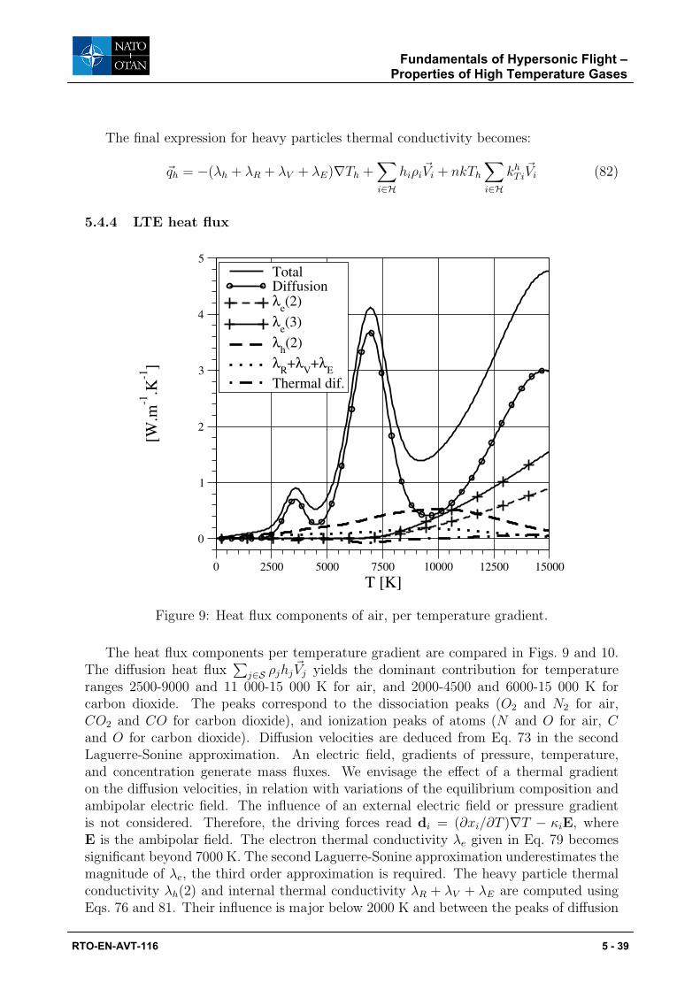
The final expression for heavy particles thermal conductivity becomes:

~qh = −(λh + λR + λV + λE)∇Th +∑i∈H

hiρi~Vi + nkTh

∑i∈H

khT i

~Vi (82)

5.4.4 LTE heat flux

0 2500 5000 7500 10000 12500 15000T [K]

0

1

2

3

4

5

[W.m

-1.K

-1]

TotalDiffusionλe(2)λe(3)λh(2)λR+λV+λEThermal dif.

Figure 9: Heat flux components of air, per temperature gradient.

The heat flux components per temperature gradient are compared in Figs. 9 and 10.The diffusion heat flux

∑j∈S ρjhj

~Vj yields the dominant contribution for temperatureranges 2500-9000 and 11 000-15 000 K for air, and 2000-4500 and 6000-15 000 K forcarbon dioxide. The peaks correspond to the dissociation peaks (O2 and N2 for air,CO2 and CO for carbon dioxide), and ionization peaks of atoms (N and O for air, Cand O for carbon dioxide). Diffusion velocities are deduced from Eq. 73 in the secondLaguerre-Sonine approximation. An electric field, gradients of pressure, temperature,and concentration generate mass fluxes. We envisage the effect of a thermal gradienton the diffusion velocities, in relation with variations of the equilibrium composition andambipolar electric field. The influence of an external electric field or pressure gradientis not considered. Therefore, the driving forces read di = (∂xi/∂T )∇T − κiE, whereE is the ambipolar field. The electron thermal conductivity λe given in Eq. 79 becomessignificant beyond 7000 K. The second Laguerre-Sonine approximation underestimates themagnitude of λe, the third order approximation is required. The heavy particle thermalconductivity λh(2) and internal thermal conductivity λR + λV + λE are computed usingEqs. 76 and 81. Their influence is major below 2000 K and between the peaks of diffusion


RTO-EN-AVT-116 5 - 39

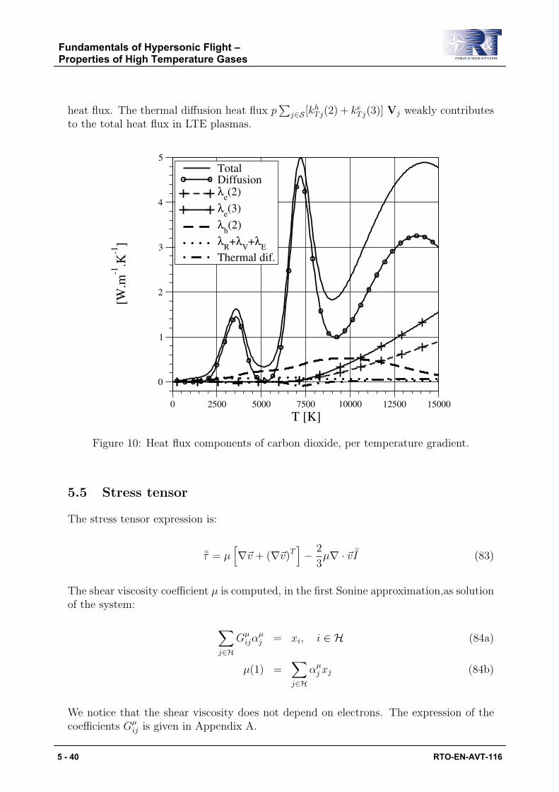
heat flux. The thermal diffusion heat flux p∑

j∈S [khTj(2) + ke

Tj(3)] Vj weakly contributesto the total heat flux in LTE plasmas.

0 2500 5000 7500 10000 12500 15000T [K]

0

1

2

3

4

5

[W.m

-1.K

-1]

TotalDiffusionλe(2)λe(3)λh(2)λR+λV+λEThermal dif.

Figure 10: Heat flux components of carbon dioxide, per temperature gradient.

5.5 Stress tensor

The stress tensor expression is:

¯τ = µ[∇~v + (∇~v)T

]− 2

3µ∇ · ~v ¯I (83)

The shear viscosity coefficient µ is computed, in the first Sonine approximation,as solutionof the system:

∑j∈H

Gµijα

µj = xi, i ∈ H (84a)

µ(1) =∑j∈H

αµj xj (84b)

We notice that the shear viscosity does not depend on electrons. The expression of thecoefficients Gµ

ij is given in Appendix A.


5 - 40 RTO-EN-AVT-116

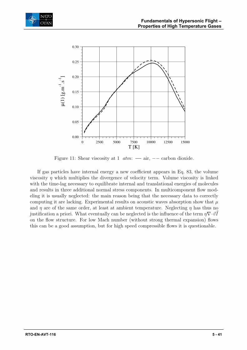
0 2500 5000 7500 10000 12500 15000T [K]

0.00

0.05

0.10

0.15

0.20

0.25

0.30

µ(1

) [g.

m-1

.s-1

]

Figure 11: Shear viscosity at 1 atm: air, −− carbon dioxide.

If gas particles have internal energy a new coefficient appears in Eq. 83, the volumeviscosity η which multiplies the divergence of velocity term. Volume viscosity is linkedwith the time-lag necessary to equilibrate internal and translational energies of moleculesand results in three additional normal stress components. In multicomponent flow mod-eling it is usually neglected: the main reason being that the necessary data to correctlycomputing it are lacking. Experimental results on acoustic waves absorption show that µand η are of the same order, at least at ambient temperature. Neglecting η has thus nojustification a priori. What eventually can be neglected is the influence of the term η∇·~v ¯Ion the flow structure. For low Mach number (without strong thermal expansion) flowsthis can be a good assumption, but for high speed compressible flows it is questionable.


RTO-EN-AVT-116 5 - 41


5 - 42 RTO-EN-AVT-116

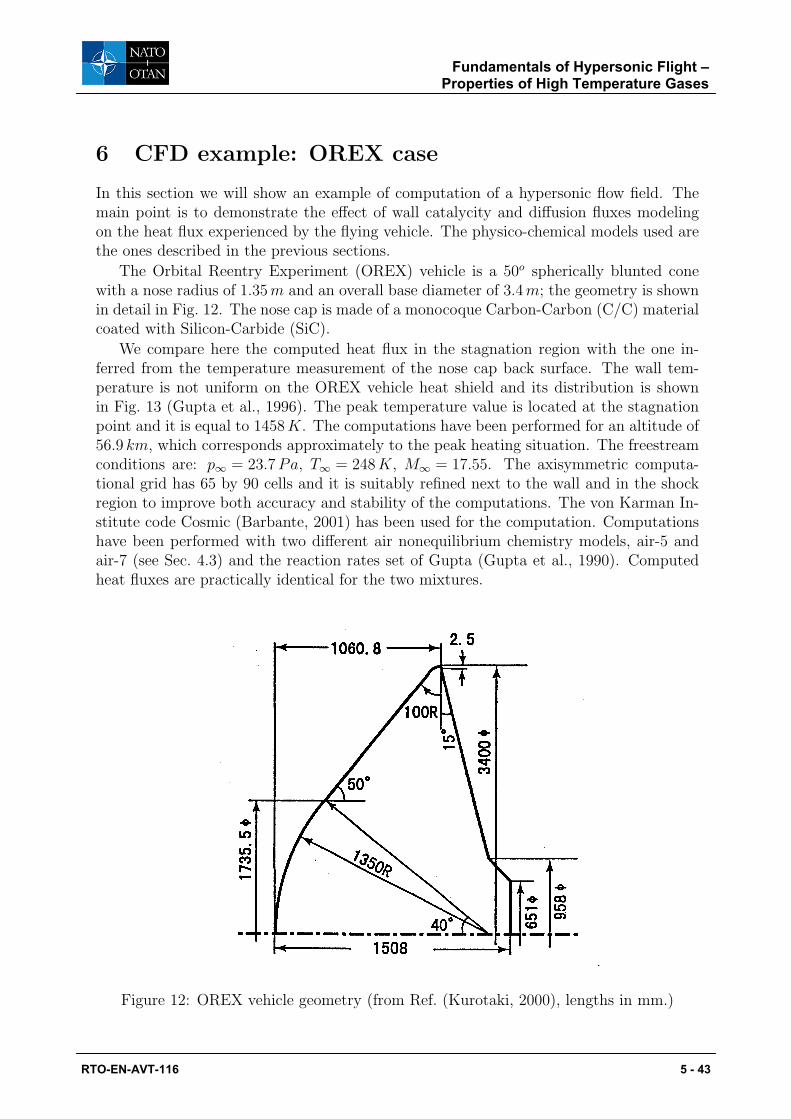
6 CFD example: OREX case

In this section we will show an example of computation of a hypersonic flow field. Themain point is to demonstrate the effect of wall catalycity and diffusion fluxes modelingon the heat flux experienced by the flying vehicle. The physico-chemical models used arethe ones described in the previous sections.

The Orbital Reentry Experiment (OREX) vehicle is a 50o spherically blunted conewith a nose radius of 1.35 m and an overall base diameter of 3.4 m; the geometry is shownin detail in Fig. 12. The nose cap is made of a monocoque Carbon-Carbon (C/C) materialcoated with Silicon-Carbide (SiC).

We compare here the computed heat flux in the stagnation region with the one in-ferred from the temperature measurement of the nose cap back surface. The wall tem-perature is not uniform on the OREX vehicle heat shield and its distribution is shownin Fig. 13 (Gupta et al., 1996). The peak temperature value is located at the stagnationpoint and it is equal to 1458 K. The computations have been performed for an altitude of56.9 km, which corresponds approximately to the peak heating situation. The freestreamconditions are: p∞ = 23.7 Pa, T∞ = 248 K, M∞ = 17.55. The axisymmetric computa-tional grid has 65 by 90 cells and it is suitably refined next to the wall and in the shockregion to improve both accuracy and stability of the computations. The von Karman In-stitute code Cosmic (Barbante, 2001) has been used for the computation. Computationshave been performed with two different air nonequilibrium chemistry models, air-5 andair-7 (see Sec. 4.3) and the reaction rates set of Gupta (Gupta et al., 1990). Computedheat fluxes are practically identical for the two mixtures.

Figure 12: OREX vehicle geometry (from Ref. (Kurotaki, 2000), lengths in mm.)


RTO-EN-AVT-116 5 - 43

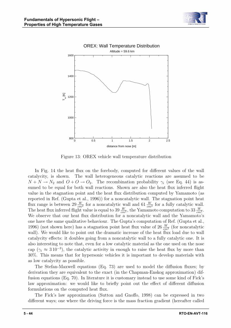
0 0.5 1 1.5 2 2.5

distance from nose [m]

800

1000

1200

1400

1600

Tw [K

]

OREX: Wall Temperature DistributionAltitude = 59.6 km

Figure 13: OREX vehicle wall temperature distribution

In Fig. 14 the heat flux on the forebody, computed for different values of the wallcatalycity, is shown. The wall heterogeneous catalytic reactions are assumed to beN + N → N2 and O + O → O2. The recombination probability γi (see Eq. 44) is as-sumed to be equal for both wall reactions. Shown are also the heat flux inferred flightvalue in the stagnation point and the heat flux distribution computed by Yamamoto (asreported in Ref. (Gupta et al., 1996)) for a noncatalytic wall. The stagnation point heatflux range is between 29 W

cm2 for a noncatalytic wall and 61 Wcm2 for a fully catalytic wall.

The heat flux inferred flight value is equal to 39 Wcm2 , the Yamamoto computation to 33 W

cm2 .We observe that our heat flux distribution for a noncatalytic wall and the Yamamoto’sone have the same qualitative behaviour. The Gupta’s computation of Ref. (Gupta et al.,1996) (not shown here) has a stagnation point heat flux value of 26 W

cm2 (for noncatalyticwall). We would like to point out the dramatic increase of the heat flux load due to wallcatalycity effects: it doubles going from a noncatalytic wall to a fully catalytic one. It isalso interesting to note that, even for a low catalytic material as the one used on the nosecap (γi ≈ 3 10−3), the catalytic activity in enough to raise the heat flux by more than30%. This means that for hypersonic vehicles it is important to develop materials withas low catalycity as possible.

The Stefan-Maxwell equations (Eq. 73) are used to model the diffusion fluxes; byderivation they are equivalent to the exact (in the Chapman-Enskog approximation) dif-fusion equations (Eq. 70). In literature it is customary instead to use some kind of Fick’slaw approximation: we would like to briefly point out the effect of different diffusionformulations on the computed heat flux.

The Fick’s law approximation (Sutton and Gnoffo, 1998) can be expressed in twodifferent ways; one where the driving force is the mass fraction gradient (hereafter called


5 - 44 RTO-EN-AVT-116

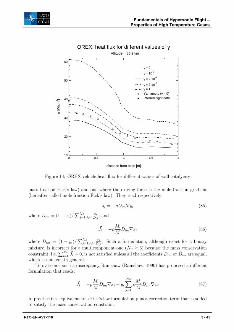
0 0.5 1 1.5 2

distance from nose [m]

10

20

30

40

50

60q

[W/c

m2 ]

γ = 0

γ = 10-3

γ = 2 10-3

γ = 3 10-3

γ = 1Yamamoto (γ = 0)Inferred flight data

OREX: heat flux for different values of γAltitude = 56.9 km

Figure 14: OREX vehicle heat flux for different values of wall catalycity

mass fraction Fick’s law) and one where the driving force is the mole fraction gradient(hereafter called mole fraction Fick’s law). They read respectively:

~Ji = −ρDim∇yi (85)

where Dim = (1− xi)/∑Ns

j=1,j 6=ixj

Dij; and

~Ji = −ρMi

MDim∇xi (86)

where Dim = (1 − yi)/∑Ns

j=1,j 6=ixj

Dij. Such a formulation, although exact for a binary

mixture, is incorrect for a multicomponent one (NS ≥ 3) because the mass conservation

constraint, i.e.∑NS

i=1~Ji = 0, is not satisfied unless all the coefficients Dim or Dim are equal,

which is not true in general.To overcome such a discrepancy Ramshaw (Ramshaw, 1990) has proposed a different

formulation that reads:

~Ji = −ρMi

MDim∇xi + yi

Ns∑j=1

ρMj

MDjm∇xj (87)

In practice it is equivalent to a Fick’s law formulation plus a correction term that is addedto satisfy the mass conservation constraint.


RTO-EN-AVT-116 5 - 45

In order to assess the effect of diffusion modeling on the computed solution, we cal-culate the OREX case with a recombination probability γi equal to 10−3 using the twoFick’s law formulations and the Ramshaw one in addition to the Stefan-Maxwell.

In Fig. 15 the computed heat flux is shown for the OREX case. The lowest heat fluxvalue is given by mole fraction Fick’s law (Eq. 86), the highest by mass fraction Fick’s law(Eq. 85). The difference with respect to the Stefan-Maxwell value is (in the stagnationpoint) of 5.8 % for the former and of 2 % for the latter. The Ramshaw formulation predictsa stagnation point heat flux that is 3.4 % lower than the Stefan-Maxwell one.

The trends predicted here agree with the ones of Ref. (Sutton and Gnoffo, 1998),where it is shown that, for higher freestream Mach number or for higher catalytic activitymaterials, the difference in computed heat flux can grow up to 40− 50 %.

0 0.5 1 1.5 2

x [m]

1e+05

2e+05

3e+05

4e+05

q w [W

/m2 ]

Stefan-MaxwellMole fraction gradientMass fractionRamshaw

OREX: Heat flux for different diffusion modelsPartially catalytic wall (γ = 3 10

-3)

Figure 15: Heat flux for different diffusion models on OREX vehicle

Concerning the computational cost we found out that Fick’s law approximation is25 % faster than Stefan-Maxwell and Ramshaw 14 % faster. From the previous discussionis clear that Fick’s law approximation has to be discarded for diffusion modeling, leavingRamshaw and Stefan-Maxwell as the only acceptable choices. Our suggestion is as follows:Ramshaw formulation is used in the transient phase of the computation to take advantageof the lower cost, Stefan-Maxwell formulation is switched on in the last phase of thecomputation to converge to the final solution.


5 - 46 RTO-EN-AVT-116

References

Anderson, J. D. (1989). Hypersonic and High Temperature Gas Dynamics. McGraw-Hill.

Barbante, P. F. (2001). Accurate and Efficient Modelling of High Temperature Nonequi-librium Air Flows. PhD thesis, ULB-VKI, Bruxelles, Belgium.

Bottin, B., Vanden Abeele, D., Carbonaro, M., Degrez, G., and Sarma, G. S. R. (1999).Thermodynamic and Transport Properties for Inductive Plasma Modeling. J. of Ther-mophysics and Heat Transfer, 13(3):343–350.

Capitelli, M., Gorse, C., Longo, S., and Giordano, D. (2002). Collision Integrals of High-temperature Air Species. J. of Thermophysics and Heat Transfer, 14(2):259–268.

Chapman, S. and Cowling, T. G. (1970). The Mathematical Theory of Non-UniformGases. Cambridge University Press.

Chase, M. W., Davies, C. A., Downey, J. R., Frurip, D. J., McDonald, R. A., and Syverud,A. (1985). JANAF Thermochemical Tables, Third Ed. Part II, Cr-Zr. J. of Phys. andChem., 14(suppl. 1).

Clarke, J. F. and McChesney, M. (1964). The Dynamics of Real Gases. Butterworths.

Delcroix, J.-L. and Bers, A. (1994). Physique des plasmas. Inter Editions, CNRS Editions.

Devoto, R. S. (1966). Transport Properties of Ionized Monoatomic Gases. The Physicsof Fluids, 9(6):1230–1240.

Devoto, R. S. (1967). Simplified Expressions for the Transport Properties of IonizedMonoatomic Gases. The Physics of Fluids, 10(10):2105–2112.

Ferziger, J. H. and Kaper, H. G. (1972). Mathematical Theory of Transport Processes inGases. North Holland.

Giovangigli, V. (1999). Multicomponent Flow Modeling. Birkhauser.

Gupta, R. N. (1996a). Two and Three-Dimensional Analysis of Hypersonic Nonequilib-rium Low-Density Flows. J. of Thermophysics and Heat Transfer, 10(2):267–276.

Gupta, R. N. (1996b). Viscous Shock-Layer Study of Thermochemical Nonequilibrium.J. of Thermophysics and Heat Transfer, 10(2):257–266.

Gupta, R. N., Moss, J. N., and Price, J. M. (1996). Assessment of ThermochemicalNonequilibrium and Slip Effects for Orbital Reentry Experiment OREX. AIAA Paper96-1859.

Gupta, R. N., Yos, J. M., Thompson, R. A., and Lee, K. P. (1990). A Review of ReactionRates and Thermodynamic and Transport Properties for an 11-Species Air Model forChemical and Thermal Nonequilibrium Calculations to 30000 K. RP 1232, NASA.

Hirschfelder, J. O., Curtiss, C. F., and Bird, R. B. (1954,1964). Molecular Theory ofGases and Liquids. John Wiley & Sons. Second printing, corrected, with notes.


RTO-EN-AVT-116 5 - 47

Kurotaki, T. (2000). Construction of Catalytic Model on SiO2 Based Surface and Ap-plication to Real Trajectory. In AIAA 34th Thermophysics Conference, AIAA Paper2000-2366.

Magin, T. and Degrez, G. (2004a). Transport Algorithms for Partially Ionized and Un-magnetized Plasmas. Journal of Computational Physics. To appear.

Magin, T. and Degrez, G. (2004b). Transport Properties of Partially Ionized and Unmag-netized Plasmas. Physical Review E. To appear.

Magin, T., Degrez, G., and Sokolova, I. (2002). Thermodynamics and transport propertiesof Martian atmosphere for space entry application. In 33rd Plasmadynamics and LasersConference, AIAA Paper 2002-2226.

Mayer, J. E. and Mayer, M. G. (1946). Statistical Mechanics. John Wiley & Sons.

Mitchner, M. and Kruger, C. H. (1973). Partially Ionized Gases. John Wiley & Sons.

Nasuti, F., Barbato, M., and Bruno, C. (1996). Material-Dependent Catalytic Recombina-tion Modeling for Hypersonic Flows. J. of Thermophysics and Heat Transfer, 10(1):131–136.

Park, C. (1990). Nonequilibrium Hypersonic Aerothermodynamics. John Wiley & Sons.

Park, C. (1993). Review of Chemical-Kinetics Problems of Future NASA Missions, I:Earth Entries. J. of Thermophysics and Heat Transfer, 7(3):385–398.

Peterkin, R. E. and Turchi, P. J. (2000). Magnetohydrodynamics Theory for HypersonicPlasma Flow: What’s Important and What’s Not. AIAA Paper 2000-2257.

Ramshaw, J. D. (1990). Self-Consistent Effective Binary Diffusion in MulticomponentGas Mixtures. J. of Non-Equilib. Thermodyn., 15:295–300.

Reggiani, S., Barbato, M., Bruno, C., and Muylaert, J. (1996). Model for HeterogeneousCatalysis on Metal Surfaces with Applications to Hypersonic Flows. In AIAA 31st

Thermophysics Conference, AIAA Paper 96-1902.

Sarma, G. S. R. (2000). Physico-Chemical Modelling in Hypersonic Flow Simulation.Progress in Aerospace Sciences, 36(3-4):281–349.

Sutton, G. W. and Sherman, A. (1965). Engineering Magnetohydrodynamics. McGraw-Hill.

Sutton, K. and Gnoffo, P. (1998). Multi-component Diffusion with Application to Com-putational Aerothermodynamics. In 7th AIAA/ASME Joint Thermophysics and HeatTransfer Conference, AIAA Paper 98-2575.

Vincenti, W. G. and Kruger, C. H. (1965). Introduction to Physical Gas Dynamics. JohnWiley & Sons.


5 - 48 RTO-EN-AVT-116

A Transport systems

The transport systems are expressed in terms of binary diffusion coefficients Dij, collision

integral ratios A?ij, B?

ij, C?ij, i, j ∈ H, and reduced collision integrals Q

(1,s)ie (s = 1, . . . , 5),

Q(2,2)ee , Q

(2,3)ee , Q

(2,4)ee defined by Magin and Degrez (2004a). The kinetic data used to

compute the transport coefficients are given by Capitelli et al. (2002) for air and Maginet al. (2002) for carbon dioxide.• Heavy-particle subsystem, i, j ∈ H

Gµij = Gµ

ji =1

Th

H00ij =

xixj

nDij

1

(mi + mj)

(6

5A?

ij − 2

), i 6= j, (88a)

Gµii =

1

Th

H00ii =

∑j∈Hj 6=i

xixj

nDij

1

(mi + mj)

(6

5

mj

mi

A?ij + 2

)+

x2i

ηi

, (88b)

Gλhij = Gλh

ji = Λ11ij =

1

25kB

xixj

nDij

mimj

(mi + mj)2

(16A?

ij + 12B?ij − 55

), i 6= j, (88c)

Gλhii = Λ11

ii =1

25kB

∑j∈Hj 6=i

xixj

nDij

1

(mi + mj)2

(30m2

i + 25m2j − 12m2

jB?ij + 16mimjA

?ij

)+

4

15kB

x2i mi

ηi

, (88d)

Λ01ij = Λ10

ji =1

25kB

xixj

nDij

mi

(mi + mj)

(12C?

ij − 10), i 6= j, (88e)

Λ01ii = Λ10

ii = − 1

25kB

∑j∈Hj 6=i

xixj

nDij

mj

(mi + mj)

(12C?

ij − 10), (88f)

G~Vij = G

~Vji = −xixj

Dij

(1 + ϕij) , i 6= j, (88g)

G~Vii =

∑j∈Hj 6=i

xixj

Dij

(1 + ϕij) . (88h)

Correction functions of the Stefan-Maxwell equation are obtained in various Laguerre-Sonine approximations: ∑

k∈H

Gλhik βkj,1 (2) = −2Λ01

ji , i, j ∈ H, (89a)

ϕij(1) = 0, (89b)

ϕij(2) = −25

8nkB

Dij

xixj

∑k∈H

Λ01ik βkj,1 (2) . (89c)

• Heavy-particle electron subsystem, i ∈ H

Λ01ie = Λ10

ei = −64xexi

75kB

Te

Th

√me

2πkBTe

(5

2Q

(1,1)ie − 3Q

(1,2)ie

), (90a)

Λ02ie = Λ20

ei = −64xexi

75kB

Te

Th

√me

2πkBTe

(35

8Q

(1,1)ie − 21

2Q

(1,2)ie + 6Q

(1,3)ie

). (90b)


RTO-EN-AVT-116 5 - 49

• Electron subsystem

Λ01ee = Λ10

ee =64xe

75kB

√me

2πkBTe

∑j∈H

xj

(5

2Q

(1,1)ej − 3Q

(1,2)ej

), (91a)

Λ11ee =

64xe

75kB

√me

2πkBTe

[∑j∈H

xj

(25

4Q

(1,1)ej − 15Q

(1,2)ej + 12Q

(1,3)ej

)+xe

√2Q(2,2)

ee

], (91b)

Λ02ee = Λ20

ee =64xe

75kB

√me

2πkBTe

∑j∈H

xj

(35

8Q

(1,1)ej − 21

2Q

(1,2)ej + 6Q

(1,3)ej

), (91c)

Λ12ee = Λ21

ee =64xe

75kB

√me

2πkBTe

[∑j∈H

xj

(175

16Q

(1,1)ej − 315

8Q

(1,2)ej + 57Q

(1,3)ej

−30Q(1,4)ej

)+ xe

√2

(7

4Q(2,2)

ee − 2Q(2,3)ee

)], (91d)

Λ22ee =

64xe

75kB

√me

2πkBTe

[∑j∈H

xj

(1225

64Q

(1,1)ej − 735

8Q

(1,2)ej +

399

2Q

(1,3)ej − 210Q

(1,4)ej

+90Q(1,5)ej

)+ xe

√2

(77

16Q(2,2)

ee − 7Q(2,3)ee + 5Q(2,4)

ee

)]. (91e)


5 - 50 RTO-EN-AVT-116

Fundamentals of hypersonic flight - Properties of high ...

Documents

Transcript of Fundamentals of hypersonic flight - Properties of high ...