Preictal state identification by synchronization changes in long-term

intracranial EEG recordings

Michel Le Van Quyena,*, Jason Sossb, Vincent Navarroa,c, Richard Robertsond,Mario Chaveza, Michel Baulacc, Jacques Martineriea

aLaboratoire de Neurosciences Cognitives et Imagerie Cerebrale, LENA,CNRS UPR 640, Hopital de la Pitie-Salpetriere, 75651 Paris, FrancebDepartment of Neurology, David Geffen School of Medicine, University of California at Los Angeles, Los Angeles, CA, USA

cEpileptology Unit, Hopital de la Pitie-Salpetriere, Paris, FrancedMathematics Department, California State Polytechnic University, Pomona, CA, USA

Accepted 7 October 2004

Available online 25 December 2004

Abstract

Objective: There is accumulated evidence that mesial temporal lobe seizures are preceded by a preictal transition that evolves over

minutes to hours. In the present study, we investigated these possible preictal changes in long-term intracranial recordings of five patients by

a measure of phase synchronization. In order to clearly distinguish preictal changes from all the other interictal states, we developed an

automatic extraction of representative patterns of interictal synchronization activity. This reference library was used to classify the

successive synchronization patterns of long-term recordings into groups of similar patterns. Altered states of brain synchronization were

identified as deviating from patterns in the reference library and were evaluated relative to the times of seizure onset in terms of sensitivity

and specificity.

Methods: A phase-locking measure was estimated using a sliding window analysis on 15 frequency bands (2 Hz steps between 0 and

30 Hz), for all pairs of EEG channels in the epileptogenic temporal lobe (14–20 channels), over the entire data sets (total analyzed duration

305 h). The preictal identification encompasses three basic stages: (1) a preprocessing stage involving the determination of a reference library

of characteristic interictal synchronization patterns using a K-means algorithm, and the identification of discriminant variables differentiating

interictal from preictal states, (2) a classification stage of the synchronization pattern via a minimum Mahalanobis distance to the reference

patterns, as well as detection of outliers, (3) an evaluation stage of the sensitivity and specificity of the detection by receiver-operating

characteristic curves.

Results: In most of the cases (36 of 52 seizures, i.e. 70%), a specific state of brain synchronization can be observed several hours before the

actual seizure. The changes involved both increases and decreases of the synchronization levels, occurring mostly within the 4–15 Hz

frequency band, and were often localized near the primary epileptogenic zone.

Conclusions: The analysis of phase synchronization offers a way to distinguish between a preictal state and normal interictal activity.

These findings suggest that brain synchronizations are preictally altered in the epileptogenic temporal lobe, inducing a pathological state of

higher susceptibility for seizure activity.

Significance: Phase synchronization is capable of extracting information from the EEG that allow the definition of a preictal state.

Although the proposed analysis does not constitute genuine seizure anticipation, these changes in neuronal synchronization may provide

helpful information for prospective seizure warning.

q 2004 International Federation of Clinical Neurophysiology. Published by Elsevier Ireland Ltd. All rights reserved.

Keywords: Seizure anticipation; Intracranial EEG; Synchronization; Temporal lobe epilepsy

1388-2457/$30.00 q 2004 International Federation of Clinical Neurophysiology.

doi:10.1016/j.clinph.2004.10.014

* Corresponding author. Tel.: C33 142161171; fax: C33 145862537.

E-mail address: lenalm@ext.jussieu.fr (M. Le Van Quyen).

1. Introduction

A fundamental issue in epilepsy research is the

identification of patho-physiological changes predictive

Clinical Neurophysiology 116 (2005) 559–568

www.elsevier.com/locate/clinph

Published by Elsevier Ireland Ltd. All rights reserved.

M. Le Van Quyen et al. / Clinical Neurophysiology 116 (2005) 559–568560

of an impending seizure. In recent years, new techniques for

seizure anticipation prior to visually detectable intracranial

electrical changes have been intensively investigated using

nonlinear analysis of EEG signals (Iasemedis et al., 1990;

Lehnertz and Elger, 1998; Le Van Quyen et al., 2001a,b;

Martinerie et al., 1998). These studies have shown that

information extracted from the EEG may allow the

definition of a preictal state and its distinction from the

interictal state. More recently, applications of a phase

synchronization measure have been shown to be useful in

gathering spatio-temporal information about the epilepto-

genic process (Le Van Quyen et al., 2001c; Mormann et al.,

2000). The method is based on direct estimation of the

instantaneous phase of the signal and, hence, is ideal for

analyzing nonstationary EEG recordings whose synchroni-

zation properties evolve over time (Lachaux et al., 1999).

Since transient phase-locking between different cortical

areas is ubiquitous during normal physiological conditions

such as sensory-motor processing or sleep (Varela et al.,

2001), assessment of phase synchronization in epilepsy is

also important to obtain a better insight into possible

intermittent dysfunction (Tass et al., 1998).

In this study, we examined the degree of phase

synchronization in long-term intracranial EEG recordings

of five patients suffering from mesial temporal lobe epilepsy

(see summary paper of the Bonn 2002 Workshop for patient

information and data descriptions). We have focused on

looking for quantifiable spatial or temporal shifts in preictal

synchronization far in advance of seizure onset detectable

on the EEG. Because normal EEG is enormously varied,

manifesting qualitative changes depending on behavioral

state, it is important to clearly distinguish preictal changes

from all the other interictal states. Therefore, its final

assessment should be carried out by a statistical approach

involving continuous recordings over long periods of time,

including, in particular, a systematic study of false positives.

In this paper, we propose a general patient-specific approach

for this purpose which involves three stages: (1) an initial

preprocessing stage to select a library of synchronization

patterns representing the normal interictal periods and to

improve the ability to distinguish between interictal and

preictal states, (2) a classification stage where shifts in

synchronization are detected, and (3) an assessment stage

evaluating the sensitivity and specificity of this approach for

preictal identification.

2. Methods

2.1. Synchronization analysis

The analysis of phase synchronization between neuronal

signals was introduced by Lachaux et al. (1999) and Tass

et al. (1998) to overcome some limitations of conventional

methods which not disentangle amplitudes and phases

(Bullock et al., 1995). The term ‘synchronization’ is used in

its strict sense, as a statistical measure of the degree to

which two signals are phase-locked during a short time

period. Recent studies have demonstrated the ability of this

measure to discriminate transient synchronization in

intracranial EEG data (Fell et al., 2001; Mormann et al.,

2000). Our analysis followed several steps: first, signals

from non-overlapping, consecutive 5 s periods were filtered

with a bandpass corresponding to a particular frequency

component. Second, the instantaneous phase of each filtered

window was extracted by means of the Hilbert transform.

Third, the degree of phase-locking between a pair of EEG

channels was quantified by the trial-average of the phase

differences on the unit circle in the complex plane

PLV Z k1

n

Xn

1

ei½f1ðtÞKf2ðtÞ�k

where n is the number of data points in each time window.

This phase-locking value (PLV) varies between 0 (inde-

pendent signals) and 1 (constant phase-lag between the two

signals). The PLVs were computed over consecutive signal

segments for P possible pairs of EEG channels in the

epileptogenic temporal lobe (from 14 to 20 channels, using

both medial and subdural temporal electrodes) and NZ15

frequency bands (2 Hz steps between 0 and 30 Hz). This

computation allows the characterization of the multi-

frequency synchronization patterns of each time window

t as a vector S(t) in a P!N dimensional space. For 20

channels, the dimension of this space is (20!19)/2!15Z2850. The phase-locking values were investigated over the

entire data sets (total analyzed duration 305 h, covering 52

seizures).

2.2. Detecting preictal changes: a general description

of the algorithm

Once the synchronization values are calculated, our

preictal state identification is based on a patient-specific

pattern recognition approach involving three stages:

Stage 1. A preprocessing stage is required in order to

reduce the number of variables used and to enhance the

ability to distinguish between interictal and preictal

features. This first implies extracting and selecting relevant

and appropriate features of the interictal state. For this

purpose, we chose long baseline controls (duration ranging

from 5 to 24 h), separated from any seizure by a few hours.

Because many seizures in the data sets were often close

together (less than 3 h apart), the baselines were typically

taken at the beginning of each data set. In theory, the values

of synchronization indices are dependent on the frequency

band, the channel pair and the time (Fig. 1A), which implies

a high degree of heterogeneity. Nevertheless, while the

number of possible synchronization patterns can be large,

we found that most of the interictal recordings can be

reasonably fit into 5–10 clusters. This indicates strong

recurrences in the pattern dynamics and may be related to

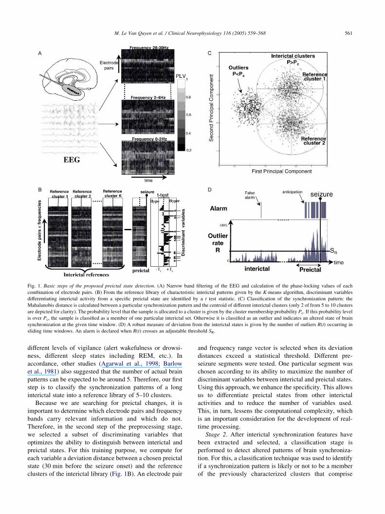
Fig. 1. Basic steps of the proposed preictal state detection. (A) Narrow band filtering of the EEG and calculation of the phase-locking values of each

combination of electrode pairs. (B) From the reference library of characteristic interictal patterns given by the K-means algorithm, discriminant variables

differentiating interictal activity from a specific preictal state are identified by a t test statistic. (C) Classification of the synchronization pattern: the

Mahalanobis distance is calculated between a particular synchronization pattern and the centroid of different interictal clusters (only 2 of from 5 to 10 clusters

are depicted for clarity). The probability level that the sample is allocated to a cluster is given by the cluster membership probability Pc. If this probability level

is over Pc, the sample is classified as a member of one particular interictal set. Otherwise it is classified as an outlier and indicates an altered state of brain

synchronization at the given time window. (D) A robust measure of deviation from the interictal states is given by the number of outliers R(t) occurring in

sliding time windows. An alarm is declared when R(t) crosses an adjustable threshold SR.

M. Le Van Quyen et al. / Clinical Neurophysiology 116 (2005) 559–568 561

different levels of vigilance (alert wakefulness or drowsi-

ness, different sleep states including REM, etc.). In

accordance, other studies (Agarwal et al., 1998; Barlow

et al., 1981) also suggested that the number of actual brain

patterns can be expected to be around 5. Therefore, our first

step is to classify the synchronization patterns of a long

interictal state into a reference library of 5–10 clusters.

Because we are searching for preictal changes, it is

important to determine which electrode pairs and frequency

bands carry relevant information and which do not.

Therefore, in the second step of the preprocessing stage,

we selected a subset of discriminating variables that

optimizes the ability to distinguish between interictal and

preictal states. For this training purpose, we compute for

each variable a deviation distance between a chosen preictal

state (30 min before the seizure onset) and the reference

clusters of the interictal library (Fig. 1B). An electrode pair

and frequency range vector is selected when its deviation

distances exceed a statistical threshold. Different pre-

seizure segments were tested. One particular segment was

chosen according to its ability to maximize the number of

discriminant variables between interictal and preictal states.

Using this approach, we enhance the specificity. This allows

us to differentiate preictal states from other interictal

activities and to reduce the number of variables used.

This, in turn, lessens the computational complexity, which

is an important consideration for the development of real-

time processing.

Stage 2. After interictal synchronization features have

been extracted and selected, a classification stage is

performed to detect altered patterns of brain synchroniza-

tion. For this, a classification technique was used to identify

if a synchronization pattern is likely or not to be a member

of the previously characterized clusters that comprise

M. Le Van Quyen et al. / Clinical Neurophysiology 116 (2005) 559–568562

the interictal library. For each sample, the probability level

of cluster membership Pc is calculated by the distance of the

corresponding synchronization pattern to all the interictal

reference clusters. If this probability level is over Pc, the

sample is classified as a member of one interictal reference

set. Otherwise it is classified as an outlier, indicating an

altered state of brain synchronization, deviating from all

interictal reference patterns. As an example, Fig. 1C

illustrates, in the space of the first two principal com-

ponents, cases where samples lie on the fringes of the

clusters or outside the Pc confidence intervals. In order to

obtain a robust measure of deviation from the interictal

states, we computed the number of outliers R(t) occurring in

sliding windows of 5 min duration, as a function of time t.

For detection purposes, an alarm was declared when R(t)

crossed an adjustable threshold SR (Fig. 1D).

Stage 3. Finally, we evaluated the threshold parameters

and the performance of the corresponding alarm sequences

relative to the times of seizure onset in terms of sensitivity

and specificity. For this validation, the accuracy of the

parameters was assessed by generating an ROC curve (Litt

et al., 2001), and plotting sensitivity versus specificity for a

range of adjustable parameters, here the probability levels

for cluster membership Pc and threshold values SR. On the

basis of the ROC curve, we carried out an in-sample

optimization of these two parameters, maximizing both

sensitivity and specificity for each patient.

2.3. Preprocessing stage

2.3.1. Selection of a library of interictal synchronization

patterns

To identify different synchronization patterns in the

interictal state, a K-means cluster analysis (Anderberg,

1973) was applied to the multi-frequency vectors S(t) of an

interictal state (duration ranging from 5 to 24 h), far

removed from any seizures (separated from them by

3–10 h, depending on the data set). The K-means algorithm

requires the fixing of the number K of clusters that are

expected in the data. Our own experimental evidence

suggests that most of the interictal recordings can be

reasonably fit into 5–10 clusters. After initialization of the

number of clusters, the K-means algorithm assigns each

vector to one of the K clusters, such that the within-cluster

sum of distances between member points and the centroid is

minimized (see mathematical Appendix A.1).

2.3.2. Identification of discriminant variables best

differentiating interictal from preictal periods

A deviation distance was computed to identify the

variables most capable of distinguishing one chosen preictal

state (30 min before the seizure onset) and the K reference

clusters of the interictal library. For this purpose, we

considered the t index between the PLVs of each electrode

pair and each frequency range

T Z ðmp KmiÞ=

ffiffiffiffiffiffiffiffiffiffiffiffiffiffiffiffiffiffiffiffiffiffiffiffiffiffis2

p=np Cs2i =ni

q

where mp and mi are the respective means of the preictal and

the interictal PLVs, with corresponding standard deviations

sp and si and sample sizes np and ni. A synchrony change is

considered to be statistically significant at the PZ0.01 level

(via the Student’s t test) when the absolute deviation

distance jTj is above the critical value jTcjZ2.5. An

electrode pair and frequency range is selected when its

deviation distances from the K reference clusters satisfy

either criterion: min(T1,.,TK)OTc (hyper-synchronization)

or max(T1,.,TK)!KTc (hypo-synchronization). Chosen in

this way, the selected electrode pairs and frequency ranges

define a set of discriminant vectors U(t) of S(t).

2.4. Classification of synchronization patterns and detection

of outliers

The goal of this step is to classify each discriminant

vector U(t) as a member of one of the previously

characterized interictal clusters or as ‘outlier’ when it

deviates from all these reference patterns, indicating an

altered state of brain synchronization. The synchronization

vectors U(t), containing m discriminant frequency and

electrode pair combinations, are classified by using a

minimum Mahalanobis distance criterion (Mahalanobis,

1936, see mathematical Appendix A.2). Let mi be the

multidimensional vector containing the average values of

the discriminating variables of cluster i; then the squared

Mahalanobis distance D2 between a vector U(t) and mi is

defined as

D2 Z ðUðtÞKmiÞT CK1

i ðUðtÞKmiÞ

where Ci is the covariance matrix of cluster i. The

distance of a sample from each of the synchronization

clusters can be calculated in this way. The sample is

allocated to the closest cluster of the interictal library or,

otherwise, is defined to be an ‘outlier’ when it lies outside

of all the interictal clusters (Chernoff, 1970). Visual

inspection of feature histograms indicated that the features

used here were approximately Gaussian in distribution. In

this case, probability levels for cluster membership are

determined from the Chi-square distribution, calculated

from the incomplete gamma function with m degrees of

freedom (Johnson and Wichern, 1988). This probability

level Pc can be used to classify samples based on the

simple rule: samples having a probability level over Pc are

classified as members of the training set, whereas samples

having a probability level under Pc are classified as

outliers.

2.5. Evaluation of the sensitivity and specificity

Deviations from baseline controls are coarsely estimated

by the outliers’ rate R(t), representing the number of outliers

M. Le Van Quyen et al. / Clinical Neurophysiology 116 (2005) 559–568 563

within a short time window [tKs,t]. We chose sZ5 min in

this study. Note that the value of each function is attributed

to the end of the window, so we do not depend on

information from the future. The emergence of an abnormal

synchronization pattern is recognized by the condition:

RðtÞRSR

We consider this condition as an ‘alarm’. The evaluation

of the anticipation performance makes sense only if the

success and error scores are insensitive to the variation of

adjustable parameters, here Pc and SR. The receiver-

operating characteristic (ROC) curve shows the relative

scores of successes and errors for different choices of

adjustable parameters (Litt et al., 2001). The vertical axis

of this graph represents the sensitivity of anticipation,

defined as the rate of confirmed anticipation on all the pre-

seizure recordings (duration 30 min). This is plotted

against the specificity of the anticipation, defined as the

rate of false alarm over 50 segments (duration 30 min) of

randomly selected interictal data. Different points corre-

spond to different probability levels Pc used to detect

outliers, with Pc varying from 10K1 at the highest point to

10K7 at the lowest point.

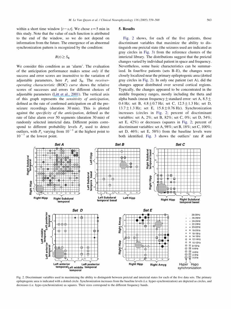
Fig. 2. Discriminant variables used in maximizing the ability to distinguish betw

epileptogenic area is indicated with a dotted circle. Synchronization increases from

decreases (i.e. hypo-synchronization) as squares. Their sizes correspond to the di

5. Results

Fig. 2 shows, for each of the five patients, those

discriminant variables that maximize the ability to dis-

tinguish one preictal state (the seizures used are indicated as

gray circles in Fig. 3) from the reference clusters of the

interictal library. The distributions suggest that the preictal

changes varied by individual patient in space and frequency.

Nevertheless, some basic characteristics can be summar-

ized. In four/five patients (sets B–E), the changes were

closely localized near the primary epileptogenic area (dotted

gray circles in Fig. 2). In only one patient (set A), did the

changes appear distributed over several cortical regions.

Typically, the changes appeared to be concentrated in the

middle frequency ranges, mostly including the theta and

alpha bands (mean frequencyGstandard error: set A, 8.5G0.4 Hz; set B, 4.8G0.7 Hz; set C, 12.5G1.3 Hz; set D,

13.7G1.3 Hz; set E, 15.8G0.76 Hz). Synchronization

increases (circles in Fig. 2; percent of discriminant

variables: set A, 2%; set B, 82%; set C, 0%; set D, 54%;

set E, 42%) or decreases (squares in Fig. 2; percent of

discriminant variables: set A, 98%; set B, 18%; set C, 100%;

set D, 46%; set E, 58%) from the baseline levels were

both identified. Fig. 3 shows the outliers’ rate R and

een preictal and interictal states for each of the five data sets. The primary

the baseline levels (i.e. hyper-synchronization) are depicted as circles, and

fferent frequency bands.

Fig. 3. Outliers’ rate for each data set and the corresponding alarm sequences for each of the five data sets. The seizures used in the determination of the

discriminant variables (see Fig. 2) are indicated as gray circles. The threshold value used, SR, is indicated as a doted line. Note that the R curve crossed the alarm

threshold several hours before the actual seizures and that, during the reference interictal state, there were only a few spurious detections.

M. Le Van Quyen et al. / Clinical Neurophysiology 116 (2005) 559–568564

the corresponding alarm sequences for each patient. In the

majority of the analyzed seizures, distinct differences

between interictal and preictal states were revealed (36/52

of all seizures, i.e. 70%). For example, in data set B, where

the longest interictal state was chosen for clustering

purposes (24 h), we see that R crossed the alarm threshold

several hours before the actual seizures and stayed at high

levels until the seizure onset. After the seizure, R often

dropped to low levels and increased again later. Note that,

during the reference interictal state, there were only a few

spurious detections, suggesting that the qualitative changes

in brain dynamics (like the wakefulness-sleep transitions)

did not induce false alarms. To better demonstrate this,

Fig. 4A shows the ROC curve for data set B, plotting

sensitivity versus specificity for different probability levels

Pc and threshold values SR. Choosing the parameters at the

‘corner’ of the ROC curve (PcZ2!10K3, SRZ10%

defining the parameters in Fig. 3), data epochs were

correctly classified as either preictal or interictal with a

sensitivity of 84% and specificity of 95%. It can be seen that

the performance is relatively insensitive to the variation of

adjustable parameters. For the other patients, using the

optimal parameters to obtain near 100% specificity, the

sensitivity of the analysis is: set A, 67%; set C, 66%; set D,

67%; set E, 86%. In order to estimate the time duration of

the preictal trends, we defined the preictal duration as the

first time at which the R curve crossed the SR level before a

particular seizure and after the preceding one. In this

estimation, we excluded the 10 min of post-ictal activity

from the preceding seizure. Mean time from declaration of

impending seizure to seizure EEG onset was 187G56 min

(set A, 23G12 min; set B, 274G66 min; set C, 117G45 min; set D, 253G148 min; set E, 164G46 min; Fig. 4B).

It is important to stress that these times are strongly

dependent on the criteria we used and should be regarded

as a weak estimate that allows both intra- and inter-

comparisons. Further improvements have to involve a

constraint on the length of time that R must remain at or

above the threshold (Le Van Quyen et al., 2001). The effects

of these stronger criteria on sensitivity and specificity for

Fig. 4. (A) Receiver-operating characteristic (ROC) curve for data set B, plotting sensitivity versus specificity for different probability levels Pc and threshold

values SR. The specificity of the anticipation is defined as the mean rate of (false) alarms occurring during randomly selected interictal segments. Choosing the

parameters PcZ2!10K3, SRZ10% at the ‘corner’ of the ROC curves, data epochs were classified as either preictal or interictal with a sensitivity of 84% and

specificity of 95%. (B) Preictal duration in hours, defined as the first time at which the R curve crossed the SR level before a particular seizure, excluding 10 min

of post-ictal activity from the preceding seizure. The black (resp. gray) bars indicate the preictal duration determined using no a priori (resp. some a priori)

knowledge of future behavior.

M. Le Van Quyen et al. / Clinical Neurophysiology 116 (2005) 559–568 565

individual or group optimization of the algorithm are

currently being investigated, but are beyond the scope of

this paper. Furthermore, for a rigorous definition of seizure

anticipation, the system’s output at time t must be solely a

function of the information available to that system at or

before time t (i.e. no use of future information from any time

later than t is allowed). In order to assess the anticipation

performance of our analysis, Fig. 4B shows using black bars

the preictal duration determined with no a priori knowledge

of future behavior. These results suggest that our approach

can be used for warning purposes.

Finally, we evaluated possible correlations between

changes in synchronization and visual inspection of EEG

recordings. First, visual inspection of the EEG recordings

sometimes showed the presence of undetected sub-clinical

electrographic seizures. For the data set D, in addition to the

six seizures with both EEG and clinical manifestations, we

observed 12 electrographic seizures between the first and

the last electro-clinical seizures. This can be related to the

fact that R crossed the alarm threshold in a sustained way

after the third electro-clinical seizure (Fig. 3). Second,

changes of the interictal epileptic activities were also

observed. For the data sets B and D, the seizures were

systematically preceded by changes of the spiking

discharges in the epileptogenic focus, consisting of spikes

and waves of long duration and high amplitude, becoming

rhythmic around 0.5–1.0 Hz (Fig. 5E). These changes

occurred 10–15 s before the seizures, but were also

observed temporally far from the seizures. For the data set

B, this activity did not show any clear correlation with the

time course of R (Fig. 5B). The mesial temporal focus also

presented another pattern of spiking discharges, more

frequent and more irregular, consisting of spikes, poly-

spikes, or spikes and waves (Fig. 5D). For the data set B, we

observed that this latter activity neither preceded the seizure

occurrence, nor was correlated with the time course of R

(Fig. 5B). Finally, we observed a third pattern of spiking

discharges (Fig. 5F) that consisted of spikes diffusing

locally (to the whole hippocampus) and regionally (to the

adjacent temporal neocortex). This activity did not precede

the seizure occurrence, but seemed to occur during periods

where R was below the alarm threshold (Fig. 5B).

6. Discussion

This study of five MTLE patients demonstrates that the

analysis of phase synchronization might offer a way to

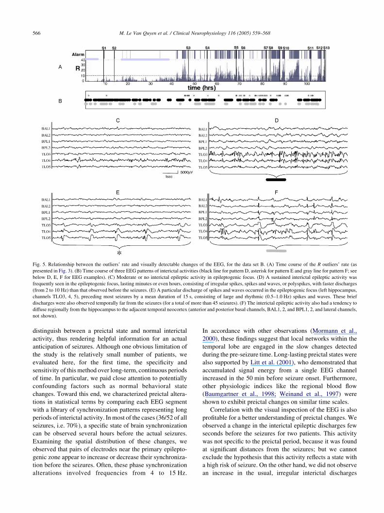
Fig. 5. Relationship between the outliers’ rate and visually detectable changes of the EEG, for the data set B. (A) Time course of the R outliers’ rate (as

presented in Fig. 3). (B) Time course of three EEG patterns of interictal activities (black line for pattern D, asterisk for pattern E and gray line for pattern F; see

below D, E, F for EEG examples). (C) Moderate or no interictal epileptic activity in epileptogenic focus. (D) A sustained interictal epileptic activity was

frequently seen in the epileptogenic focus, lasting minutes or even hours, consisting of irregular spikes, spikes and waves, or polyspikes, with faster discharges

(from 2 to 10 Hz) than that observed before the seizures. (E) A particular discharge of spikes and waves occurred in the epileptogenic focus (left hippocampus,

channels TLO3, 4, 5), preceding most seizures by a mean duration of 15 s, consisting of large and rhythmic (0.5–1.0 Hz) spikes and waves. These brief

discharges were also observed temporally far from the seizures (for a total of more than 45 seizures). (F) The interictal epileptic activity also had a tendency to

diffuse regionally from the hippocampus to the adjacent temporal neocortex (anterior and posterior basal channels, BAL1, 2, and BPL1, 2, and lateral channels,

not shown).

M. Le Van Quyen et al. / Clinical Neurophysiology 116 (2005) 559–568566

distinguish between a preictal state and normal interictal

activity, thus rendering helpful information for an actual

anticipation of seizures. Although one obvious limitation of

the study is the relatively small number of patients, we

evaluated here, for the first time, the specificity and

sensitivity of this method over long-term, continuous periods

of time. In particular, we paid close attention to potentially

confounding factors such as normal behavioral state

changes. Toward this end, we characterized preictal altera-

tions in statistical terms by comparing each EEG segment

with a library of synchronization patterns representing long

periods of interictal activity. In most of the cases (36/52 of all

seizures, i.e. 70%), a specific state of brain synchronization

can be observed several hours before the actual seizures.

Examining the spatial distribution of these changes, we

observed that pairs of electrodes near the primary epilepto-

genic zone appear to increase or decrease their synchroniza-

tion before the seizures. Often, these phase synchronization

alterations involved frequencies from 4 to 15 Hz.

In accordance with other observations (Mormann et al.,

2000), these findings suggest that local networks within the

temporal lobe are engaged in the slow changes detected

during the pre-seizure time. Long-lasting preictal states were

also supported by Litt et al. (2001), who demonstrated that

accumulated signal energy from a single EEG channel

increased in the 50 min before seizure onset. Furthermore,

other physiologic indices like the regional blood flow

(Baumgartner et al., 1998; Weinand et al., 1997) were

shown to exhibit preictal changes on similar time scales.

Correlation with the visual inspection of the EEG is also

profitable for a better understanding of preictal changes. We

observed a change in the interictal epileptic discharges few

seconds before the seizures for two patients. This activity

was not specific to the preictal period, because it was found

at significant distances from the seizures; but we cannot

exclude the hypothesis that this activity reflects a state with

a high risk of seizure. On the other hand, we did not observe

an increase in the usual, irregular interictal discharges

M. Le Van Quyen et al. / Clinical Neurophysiology 116 (2005) 559–568 567

before seizures. Such changes have been previously

reported (Litt et al., 2001), but also excluded by others

(Gotman and Marciani, 1985). Finally, we observed another

pattern of diffusing spikes that preferentially appeared when

the R index was low, suggesting that this activity may use a

network of synchronies that is not favorable to seizure

emergence.

It is important to point out that our proposed synchro-

nization analysis does not constitute genuine seizure

anticipation, because this would require a prospective

analysis of data when time to seizure is unknown. Never-

theless, in the present state, our analysis could, after more

extensive validation, be used for warning purposes. In

particular, the architecture of our algorithm is such that it

may be readily adapted to further improve its performance

in real-time conditions. Further improvements can be

obtained by selecting (on- or offline) multiple pre-seizure

segments for training purposes or by adding continuously

new synchronization clusters in the interictal library. For

example, if the method produces undesired detections of a

certain type of activity, a representative sample of this

activity can be included in the interictal library to prevent

similar undesired detections in the future. Furthermore, the

interictal library can be adapted to the changing clinical

status of the patient by including changes in medication or

post-ictal abnormalities. Also, expert-selected signal infor-

mation can also be included, depending on the type of signal

characteristics or changes the physician/user wants to detect

(or not detect).

There are numerous indications that the spatial and

temporal structures of synchronization patterns are dis-

tributed in space and transient in time (Bullock et al., 1995;

Fell et al., 2001). It was hypothesized that this transient

phase-locking between different parts of the brain could be a

basic mechanism for the functional large-scale integration

observed during cognition (Varela et al., 2001). Thus, given

this central role of synchrony in normal states, our results

suggest that the participation of particular networks in

normal physiological synchronizations appears to be

preictally altered, inducing a state of higher susceptibility

for seizure activity. This is also in accordance with

experimental models of epilepsy showing that specific

networks around the epileptic focus seem to be of crucial

importance in determining whether or not a seizure is likely

to occur and spread (Wyler et al., 1973). Our present

observations suggest that two related processes seem to be

involved here: (1) A state of increased synchronization. This

state may reflect recruitment phenomena within the primary

epileptogenic area and its surroundings regions. (2) A state

of decreased synchronization. This state may isolate

pathologically discharging neuronal populations of the

epileptic focus from the influence of activity in wider

brain areas, thus facilitating the development of local

pathological recruitments. On the other hand, a loss of

synchrony might also provide an ‘idle’ population of

neurons which may be more easily recruited into the

epileptic process (Mormann et al., 2000). Finally, the

preictal loss of synchrony could reflect a depression of

synaptic inhibition in areas surrounding the epileptogenic

focus, as in certain experimental models of epilepsy

(Matsumo and Ajmone Marsan, 1964).

Further investigations of the spatial characteristics of

phase synchronization or studies at a cellular level (Staba

et al., 2002) are necessary to validate these hypotheses.

Whatever the pathophysiologic basis of preictal changes,

the observed duration is sufficient to offer new possibilities

for therapeutic intervention. Such measures might include

preventive strategies to modify the synchronization around

the critical regions by direct electrical stimulation of brain

structures (Fanselow et al., 2000) or by cognitive therapies

(Birbaumer et al., 1990).

Appendix A. Mathematical appendix

A.1. K-means clustering

1.0 The goal of clustering is to reduce the amount of data

by categorizing or grouping similar data items together

Partitional clustering attempts to directly decompose the set

of objects, perhaps p-dimensional ‘feature’ vectors, into a

set of disjoint subsets called ‘clusters’. A commonly used

partitional clustering method is called K-means clustering,

which produces K different clusters that are intended to be

as distinct as possible (Anderberg, 1973).

1.1 A computer program for automating the K-means

algorithm starts with K random clusters and then moves

objects between those clusters with the dual goals of:

(1) minimizing variability within clusters, and (2)

maximizing variability between clusters. Each point

from the feature space is added to the closest cluster.

The ‘closeness’ to the cluster is determined by calculating

the distance between a point and the centroid of that

cluster. Then each point is visited again to recalculate the

distance to the updated cluster. If the closest cluster is not

the one to which it currently belongs, the point will

switch to the new cluster. When switching occurs,

centroids of both modified clusters have to be recalcu-

lated. This procedure is repeated until no more switching

takes place.

1.2 The measure of this variability within and between

clusters is based on a metric or distance function in the space

of p-dimensional feature vectors. One common choice for

such a distance function is the so-called Mahalanobis

metric.

A.2. The Mahalanobis distance

2.0 The Mahalanobis distance D is based on the notion of

‘standardized distance’ d. Let x(i) be the value of feature i of

vector x, with m(i,j) the mean of feature i for cluster j, and

s(i,j) the corresponding standard deviation.

M. Le Van Quyen et al. / Clinical Neurophysiology 116 (2005) 559–568568

Then

d2ðx;mjÞ Zxð1ÞKmð1; jÞ

sð1; jÞ

� �2

Cxð2ÞKmð2; jÞ

sð2; jÞ

� �2

C/

CxðpÞKmðp; jÞ

sðp; jÞ

� �2

;

where mj is the vector of feature means for cluster j (or, its

‘centroid’).

2.1 This metric has the important property that it is ‘scale

invariant’: if distances are measured in this way, the units

used for various features have no effect on the resulting

distances, and thus no effect on the final classification. The

Mahalanobis distance is a generalization of this standar-

dized distance.

2.2 The covariance of two features measures their

tendency to vary together, defined to be the average of the

products of the deviations of the feature values from their

means. More precisely, if {x(1,r),x(2,r),.,x(n,r)} and

{x(1,s),x(2,s),., x(n,s)} are the sets of features r and s for

the n points in a cluster, respectively (i.e. x(j,r) and x(j,s) are

the corresponding features of the jth point), then cðr; sÞZð1=nK1Þ

PnjZ1 ½xðj; rÞKmðrÞ�½xðj; sÞKmðsÞ�f g, with m(r) the

cluster mean of feature r and m(s) the mean of feature s.

2.3 The matrix of all these covariances CZ(c(r,s)), the

covariance matrix, provides a way to measure distance that

is invariant under linear transformations of the space of

feature vectors.

2.4 The matrix generalization of the scalar expression for

squared standardized distance, d2, from feature vector x to

cluster j’s mean vector (or centroid), mj, turns out to be just

D2ðx;mjÞZ ðxKmjÞtrCK1

j ðxKmjÞ, where Cj is the cluster’s

covariance matrix; D is called the Mahalanobis distance.

2.5 Let m1,m2,.,mK be the mean vectors for the K

clusters, with C1,C2,.,CK the corresponding covariance

matrices. A feature vector x is classified by calculating the

Mahalanobis distance D from x to each of the mj, and then

assigning x to the class for which D(x,mj) is a minimum.

2.6 The use of the Mahalanobis distance removes several

of the limitations of the standard Euclidean metric, such as:

(1) it automatically accounts for the scaling of the

coordinate axes, and (2) it corrects for correlations between

different features.

References

Agarwal R, Gotman J, Flanagan D, Rosenblatt B. Automatic EEG analysis

during long-term monitoring in the ICU. Electroencephalogr Clin

Neurophysiol 1998;107:44–58.

Anderberg MR. Cluster analysis for applications. New York: Academic

Press; 1973.

Barlow JS, Creutzfeldt OD, Michael D, Houchin J, Epelbaum H. Automatic

adaptive segmentation of EEGs. Electroencephalpogr Clin Neurophy-

siol 1981;51:512–25.

Baumgartner C, Serles W, Leutmezer F, Pataraia E, Aull S, Czech T,

Pietrzyk U, Relic A, Podreka I. Pre-ictal SPECT in temporal lobe

epilepsy: regional cerebral blood flow is increased prior to electro-

encephalography-seizure onset. J Nucl Med 1998;39:978–82.

Birbaumer N, Elbert T, Canavan A, Rockstroh B. Slow potentials of the

cerebral cortex and behavior. Physiol Rev 1990;70:1–41.

Bullock TH, McClune MC, Achimowicz JZ, Iragui-Madoz VJ, Duckrow RB,

Spencer SS. EEG coherence has structure in the millimeter domain:

subdural and hippocampal recordings from epileptic patients. Electro-

encephalogr Clin Neurophysiol 1995;95:161–77.

Chernoff H. Metric considerations in cluster analysis. Technical report 67.

Society of Statistics, Standford University; 1970.

Fanselow E, Reid A, Nicolelis M. Reduction of pentylenetrazole-induced

seizure activity in awake rats by seizure-trigeminal nerve stimulation.

J Neurosci 2000;20:8160–8.

Fell J, Klaver P, Lehnertz K, Grunwald T, Schaller C, Elger CE,

Fernandez G. Human memory formation is accompanied by rhinal–

hippocampal coupling and decoupling. Nat Neurosci 2001;4:1259–64.

Gotman J, Marciani MG. Electroencephalographic spiking activity, drug

levels, and seizure occurrence in epileptic patients. Ann Neurol 1985;

17:597–603.

Iasemedis LD, Sackellares JC, Zaveri HP, Williams WJ. Phase space

topography and the Lyapunov exponent of electrocorticograms in

partial seizures. Brain Topogr 1990;2:187–201.

Johnson RA, Wichern DW. Applied multivariate statistical analysis.

Englewood Cliffs, NJ: Prentice Hall; 1988. p. 134–5.

Lachaux JP, Rodriguez E, Martinerie J, Varela FJ. Measuring phase-

synchrony in brain signal. Hum Brain Mapp 1999;8:194–208.

Lehnertz K, Elger CE. Can epileptic seizures be predicted? Evidence from

nonlinear time series analysis of brain electrical activity Phys Rev Lett

1998;80:5019–22.

Le Van Quyen M, Martinerie J, Navarro V, Boon P, D’Have M, Adam C,

Renault B, Varela FJ, Baulac M. Anticipation of epileptic seizures from

standard EEG recordings. Lancet 2001a;357:183–8.

Le Van Quyen M, Martinerie J, Navarro V, Baulac M, Varela FJ.

Characterizing neurodynamic changes before seizures. J Clin Neuro-

physiol 2001b;18:191–208.

Le Van Quyen M, Fouchez J, Lachaux JP, Rodriguez E, Lutz A,

Martinerie J, Varela F. Comparison of Hilbert transform and wavelet

methods for the analysis of neuronal synchrony. J Neurosci Methods

2001c;111:83–98.

Litt B, Esteller R, Echauz J, D’Alessandro M, Shor R, Henry T, Pennel P,

Epstein C, Bakay R, Dichter M, Vachtsevanos G. Epileptic seizures

may begin hours in advance of clinical onset: a report of five patients.

Neuron 2001;30:51–64.

Mahalanobis PC. Proc Natl Inst Sci India 1936;2:49.

Martinerie J, Adam C, Le Van Quyen M, Baulac M, Clemenceau S,

Renault B, Varela FJ. Epileptic seizures can be anticipated by non-

linear analysis. Nat Med 1998;4:1173–6.

Matsumo H, Ajmone Marsan C. Cortical cellular phenomena in experimental

epilepsy: ictal manifestations. Exp Neurol 1964;9:305–26.

Mormann F, Lehnertz K, David P, Elger CE. Mean phase coherence as a

measure for phase synchronization and its application to the EEG of

epilepsy patients. Physica D 2000;144:358–69.

Staba RJ, Wilson Cl, Bragin A, Fried I, Engel J. Sleep states differentiate

single neuron activity recorded from human epileptic hippocampus,

entorhinal cortec and subiculum. J Neurosci 2002;22:5694–704.

Tass P, Rosenblum MG, Weule J, Kurths J, Pikovsky A, Volkmann J,

Schnitzler A, Freund HJ. Detection of n:m phase locking from noisy data:

application to magnetoencephalography. Phys Rev Lett 1998;81:3291–4.

Varela FJ, Lachaux JP, Rodriguez E, Martinerie J. The brainweb: phase

synchronization and large-scale integration. Nat Rev Neurosci 2001;2:

229–39.

Weinand ME, Carter LP, El-Saadany WF, Sioutos PJ, Labiner DM,

Oommen KJ. Cerebral blood flow and temporal lobe epileptogenicity.

J Neurosurg 1997;86:226–32.

Wyler AR, Fetz EE, Ward AA. Spontaneous firing patterns of epileptic

neurons in the monkey motor cortex. Exp Neurol 1973;40:567–85.