
Wall motion estimation in intracranial aneurysms
20
Wall motion estimation in intracranial aneurysms E. Oubel 1 , J. R. Cebral 2 , M. De Craene 1 , R. Blanc 3 , J. Blasco 4 , J. Macho 4 , C. M. Putman 5 and A. F. Frangi 1 1 Center for Computational Imaging & Simulation Technologies in Biomedicine (CISTIB), Information and Communication Technologies Department, Universitat Pompeu Fabra and with the Networking Center on Biomedical Research - CIBER-BBN 2 Center for Computational Fluid Dynamics, Dept. of Computational and Data Sciences, George Mason University, USA 3 Department of Interventional Neuroradiology, Rothschild Foundation, Paris, France 4 Department of Vascular Radiology, Hospital Clinic i Provincial de Barcelona, Barcelona, Spain 5 Department of Interventional Neuroradiology, Inova Fairfax Hospital, Falls Church (VA), USA E-mail: [email protected] Abstract. The quantification of wall motion in cerebral aneurysms is becoming 1 important owing to its potential connection to rupture, and as a way to incorporate 2 the effects of vascular compliance in computational fluid dynamics (CFD) simulations. 3 Most of papers report values obtained with experimental phantoms, simulated images, 4 or animal models, but the information for real patients is limited. In this paper, 5 we have combined non-rigid registration (IR) with signal processing techniques to 6 measure pulsation in real patients from high frame rate digital subtraction angiography 7 (DSA). We have obtained physiological meaningful waveforms with amplitudes in the 8 range 0mm-0.3mm for a population of 18 patients including ruptured and unruptured 9 aneurysms. Statistically significant differences in pulsation were found according to 10 the rupture status, in agreement with differences in biomechanical properties reported 11 in the literature. 12
-
Upload
independent -
Category
Documents
-
view
1 -
download
0
Transcript of Wall motion estimation in intracranial aneurysms
Wall motion estimation in intracranial aneurysms
E. Oubel1, J. R. Cebral2, M. De Craene1, R. Blanc3, J. Blasco4,
J. Macho4, C. M. Putman5 and A. F. Frangi1
1 Center for Computational Imaging & Simulation Technologies in Biomedicine
(CISTIB), Information and Communication Technologies Department, Universitat
Pompeu Fabra and with the Networking Center on Biomedical Research -
CIBER-BBN2 Center for Computational Fluid Dynamics, Dept. of Computational and Data
Sciences, George Mason University, USA3 Department of Interventional Neuroradiology, Rothschild Foundation, Paris, France4 Department of Vascular Radiology, Hospital Clinic i Provincial de Barcelona,
Barcelona, Spain5 Department of Interventional Neuroradiology, Inova Fairfax Hospital, Falls Church
(VA), USA
E-mail: [email protected]
Abstract. The quantification of wall motion in cerebral aneurysms is becoming1
important owing to its potential connection to rupture, and as a way to incorporate2
the effects of vascular compliance in computational fluid dynamics (CFD) simulations.3
Most of papers report values obtained with experimental phantoms, simulated images,4
or animal models, but the information for real patients is limited. In this paper,5
we have combined non-rigid registration (IR) with signal processing techniques to6
measure pulsation in real patients from high frame rate digital subtraction angiography7
(DSA). We have obtained physiological meaningful waveforms with amplitudes in the8
range 0mm-0.3mm for a population of 18 patients including ruptured and unruptured9
aneurysms. Statistically significant differences in pulsation were found according to10
the rupture status, in agreement with differences in biomechanical properties reported11
in the literature.12
WM estimation in aneurysms 2
1. Introduction13
Intracranial aneurysms are pathological dilations of cerebral arteries, which tend to14
occur at or near arterial bifurcations, mostly in the Circle of Willis (CoW). The15
optimal management of unruptured aneurysms is controversial and current decision-16
making is mainly based on considering their size and location, as derived from the17
International Study of Unruptured Intracranial Aneurysms (ISUIA) [1]. It is thought18
that the interaction between haemodynamics and wall mechanics plays a critical role19
in the formation, growth and rupture of aneurysms. The quantification of wall motion20
in aneurysms is becoming important since its likely connection with rupture [2, 3, 4]21
and its importance for incorporating patient-specific boundary conditions in CFD22
simulations [5].23
Many of the quantitative results of pulsation measurements reported in the24
literature correspond to experiments with phantoms, simulated images, or experimental25
models [6, 7, 3, 8]. Only a few attempts of in-vivo quantification have been reported.26
Wardlaw et al. [9] have measured pulsation in vivo by using Power Doppler Ultrasound27
(PD-US), and validated their method using phantoms [10]. However, many conclusions28
of the study with phantoms are valid for the large changes in size considered (42%29
of the cross section), but not necessary extendable for the small changes occurring in30
intracranial aneurysms. Meyer et al. [2] have measured aneurysmal volume changes31
by using Phase-Contrast Magnetic Resonance Angiography (PC-MRA). For ruptured32
aneurysms they obtained values of 51% ± 10%, which are quite large in comparison to33
the visual changes observed in our clinical experience. With the advent of ECG-gated34
4D Computed Tomography Angiography (4D-CTA), the visualization of aneurysmal35
pulsation seems to have become feasible [4, 11, 12]. However, this technique presents36
helical motion artifacts resulting from the lack of cone beam correction during image37
reconstruction [13], which are visualized as a wavelike motion and produce the apparent38
movement of bony structures [11]. This observation and other inconsistencies about39
the presence of bleb pulsation have been pointed out by Matsumoto et al. [14]. These40
problems seem to be corrected with 64-slice CT scanners, but so far only studies of41
feasibility have been carried out with phantoms [6]. Recently, Zhang et al. [8] have42
presented a method to recover pulsation by deforming the 3D Rotational Angiography43
(3D-RA) rendered volume to match its projections to the 2D acquisitions used for the44
volumetric reconstruction. However, this technique has been tested only with phantom45
data and its application in human beings must still be proven. Table 1 summarizes the46
previous work in this area.47
Recently, we have presented preliminary results of the application of non rigid48
registration techniques to recover in vivo wall motion from Digital Subtraction49
Angiography (DSA) sequences [15]. In this paper, we present an improved version50
of the method that solves some drawbacks of the initial approach. We have applied51
the technique to quantify wall motion in 15 patients and found a correlation between52
rupture and regional differences in pulsation.53

WM estimation in aneurysms 3
Table 1. Previous work on wall motion quantification in cerebral aneurysms.
R=Ruptured, U=Unruptured; WMO = Wall motion occurrence; WMQ = Wall motion
quantification.
Authors Modality Data Status WMOa WMQ
Hayakawa et al. [12] 4D-CTA in vivo All R 4/23 no
Kato et al. [4] 4D-CTA in vivo All U 2/15 no
Yaghmai et al. [6] 4D-CTA phantom - - yes
Boecher-S. et al.b [7] - animal model - 5/8 yes
Wardlaw et al. [9] PD-US in vivo All R 15/16 yes
Ueno et al. [3] PD-US phantom - - yes
Meyer et al. [2] PC-MRI in vivo 6 R / 10 U 15/16 yes
Zhang et al. [8] 3D-RA phantom - - yes
a Wall motion occurrence is the ratio between the number of cases that present
pulsation and the total number of cases.b The modality is not specified since the authors used an experimental system in
which the aneurysmal pulsation is measured by a laser displacement sensor.
2. Method54
2.1. Dataset55
Figure 1 shows the DSA sequences used in this paper. These sequences were acquired56
in three clinical centers: 1) Department of Interventional Neuroradiology, Inova57
Fairfax Hospital, 2) Department of Vascular Radiology, Hospital Clinic i Provincial de58
Barcelona, and 3) Department of Interventional Neuroradiology, Rothschild Foundation.59
At each center, an expert clinician measured neck, depth, and width of the aneurysms60
in the first frame using standard measuring tools of angiography scanners. To know61
the image resolution, the same magnitudes were measured in the 3D-RA image to avoid62
errors due to geometric magnification. Table 2 provides detailed information about each63
sequence.64

WM estimation in aneurysms 4
#1 #2 #3
#4 #5 #6
#7 #8 #9
#10 #11 #12
#13 #14 #15
#16 #17 #18
Figure 1. First frames of the DSA sequences used in this paper. The 3D-RA
reconstruction is shown at right when available.
WM
estimatio
nin
aneu
rysm
s5
Table 2. Table summarizing relevant information about the sequences used in this paper. M=Male, F=Female; FPS=Frames Per
Second; ICA=Internal Carotid Artery, ACA=Anterior Cerebral Artery, BA=Basilar Artery, PCom=Posterior Communicating Artery,
ACom=Anterior Communicating Artery, MCA=Middle Cerebral Artery; AR=Aspect Ratio; R=Ruptured, U=Unruptured; LAT=Lateral,
TER=Terminal; Y=Yes, N=No, n/a = not available
Patient Gender Age Location Size Resolution AR Status Type Injection FR Pulsation
# M/F years D × W× N (mm) µ/pxl R / U cc @ cc/s FPS Y / N
1 F 60 ICA 8.5 × 6.6 × 5.0 95 1.7 U LAT 9 cc @ 3 cc/s 30 Y
2 M 50 ACA 7.2 × 7.8 × 7.8 95 0.9 U LAT 9 cc @ 3 cc/s 30 Y
3 F 47 BA 11.3 × 9.7 × 3.8 93 3.0 R TER 9 cc @ 3 cc/s 30 Y
4 F 78 ACM 10.0 × 7.7 × 5.2 71 1.9 U TER 9 cc @ 3 cc/s 10 N
5 F 56 ICA 4.0 × 4.0 × 2.0 80 2.0 R LAT 9 cc @ 3 cc/s 30 N
6 F 47 BA 13.0 × 8.3 × 5.4 86 2.4 R TER 24 cc @ 4 cc/s 7.5 N
7 F 46 ICA 19.8 × 18.9 × 3.5 88 5.7 R LAT 24 cc @ 4 cc/s 3 Y
8 M 28 ICA 9.0 × 8.8 × n/a 74 n/a U TER 24 cc @ 4 cc/s 2 Y
9 F 71 ICA 12.2 × 9.2 × 2.9 97 4.2 R TER 24 cc @ 4 cc/s 7.5 Y
10 F 41 ICA 17.1 × 19.8 × 9.9 208 1.7 U LAT 15 cc @ 4 cc/s 30 Y
11 F 51 ICA 4.2 × 3.5 × 3.0 117 1.4 U LAT 15 cc @ 4 cc/s 30 N
12 F 37 PCom 7.2 × 6.2 × 2.4 135 3.0 R TER 15 cc @ 4 cc/s 60 Y
13 F 37 MCA 2.0 × 2.9 × 2.8 115 0.7 U TER 15 cc @ 4 cc/s 60 N
14 M 54 ACom 7.1 × × 3.3 210 2.2 R LAT 15 cc @ 4 cc/s 30 Y
15 M 21 PCom 5.2 × 5.0 × 1.9 148 2.7 U LAT 15 cc @ 4 cc/s 60 N
16 F 75 ICA 27.6 × 30.0 × 10.6 195 2.6 U LAT 15 cc @ 4 cc/s 30 Y
17 F 44 ICA 8.2 × 10.2 × 6.6 252 1.2 U LAT 15 cc @ 4 cc/s 30 N
18 M 46 ICA 4.2 × 4.0 × 2.5 283 1.7 U TER 15 cc @ 4 cc/s 60 N

WM estimation in aneurysms 6
2.2. Wall motion estimation65
The method applied for quantifying pulsation consists of three main steps described66
next (Figure 2).67
2.2.1. Image registration. A DSA study consists of an image sequence I(x, t) =68
I0(x) · · · In−1(x) of n phases that provides the voxel intensity at spatial position x and69
time t. To quantify temporal changes in the magnitude of interest, it is necessary70
to establish a dense point correspondence between images. This was performed by71
registering each frame It(x) to the first one I0(x), yielding a set of transformations72
T = {Ti(x)}i=1:n that provide such correspondence. In a previous paper [15], we applied73
an Optical Flow (OF) method [16] for IR since this type of methods are preferred for74
recovering small magnitude changes [17]. However, OF methods are quite sensitive to75
variations in intensity due to quantum noise [18] and inhomogeneities in the contrast76
distribution, and non-smooth deformation fields are obtained. To obtain a smoother77
deformation field, in this paper we have used Free-Form Deformations with B-Spline78
interpolation functions, and Mutual Information (MI) as metric.79
Mutual information (MI) is a concept from information theory and expresses the80
amount of information that one image A contains about a second image B. This81
similarity measure was independently introduced into medical image registration by82
Collignon [19] and Viola [20] and is defined as83
MI(A, B) = H(A) + H(B) − H(A, B) (1)84
where H(A) and H(B) are the marginal entropies of A and B, and H(A, B) their joint85
entropy. MI is an information-theoretic similarity measure particularly suited in cases86
where the intensity relationship of the images is unknown, which is exactly the case of87
DSA sequences.88
B-Spline-based Free-Form Deformations (FFD) is a type of transformation used89
initially in computer graphics for deforming objects [21, 22] and introduced later on in90
medical imaging by Rueckert et al [23]. The basic idea of this type of transformation91
is to deform an image by manipulating an underlying mesh of control points, whose92
displacements are propagated to the image by using B-Spline functions. The resulting93
displacement field is smooth (C2-continuous), which is a desired property when modeling94
biological deformations. The main advantage of B-Splines with respect to thin-plate95
splines [24] and elastic-body splines [25], is their compact support that allows to96
constrain spatially the deformation.97
2.2.2. Point propagation and feature quantification. We have analyzed temporal98
changes in aneurysm depth (d(t)), aneurysm width (w(t)), and artery diameter (a(t)).99
These variables were measured by taking the euclidean distance between pair of points100
placed in the first frame, and propagated over time with the set of transformations101
T . The points used to calculate the artery diameter were placed far away from the102
aneurysm to have a different condition of the vessel wall at the measurement point, and103

WM estimation in aneurysms 7
Figure 2. Wall motion estimation method.(1) image registration, (2) point
propagation and feature quantification, and 3) post-processing. Crosses (×), circles
(◦), and squares (�), show the points used to measure changes in the artery (a(t)),
depth (d(t)), and width (w(t)) of the aneurysm. IR = image registration; SP = signal
processing.
to avoid the influence of aneurysmal deformations. This is important for quantification104
of the differential pulsation between the aneurysm and the artery, as explained later.105
For the spacing between control points employed in this paper, the spatial support of106
each B-Spline was in the order of the aneurysm size, and landmarks placed close to the107
aneurysm could be modified even in the absence of artery deformation. The points used108
to define the depth and with of the aneurysm were placed as shown in Figure 2.109
2.2.3. Post-processing analysis. If changes in image intensity during the contrast filling110
were modeled linearly as It(x) = αI0(x) + c, with α and c constant values, the use of111
MI-based IR would account for these changes in intensity. This is because MI-based IR112
is robust to changes in intensity scale‡ as shown in Figure 3. However, intensity changes113
that occur during the contrast injection cannot be described accurately by this model,114
probably because of complex blood filling patterns. We have not found in the literature115
models of intensity changes due to contrast agent distribution to assess their influence on116
the IR, but a visual inspection of intensity profiles over time reveals that an exponential117
dependency of time is a reasonable approximation. Figure 4 shows that, even when118
the size of the aneurysm does not change, the optimizer will try to match the intensity119
‡ Note that this does not mean invariance of MI, in fact MI(A, αA) = H(A) + log‖α‖ [26]

WM estimation in aneurysms 8
0.8 0.9 1 1.1 1.20
0.2
0.4
0.6
0.8
MI
scale
(1.000,0.580)
(a) (b) (c)
Figure 3. Robustness of MI to intensity scaling. In this example, the pixel intensity
of the fixed image If (x) (a) is half the intensity of moving image Im(x) (b) (Im(x)
= 0.5*If(x)). (c) MI(If , Tis(Im)) as a function of the scaling factor for an isotropic
scaling transformation Tis. MI has a maximum at 1.
0.8 0.9 1 1.1 1.20.6
0.61
0.62
0.63
0.64
MI
scale
(1.01,0.631)
(a) (b) (c)
Figure 4. Overestimation of dilation when considering a non-linear relationship
of intensities. In this example, the fixed image If (x) (a) presents a quadratic
intensity profile, whereas the moving Image Im(x) (b) presents a quartic profile.
(c) MI(If , Tis(Im)) as a function of the scaling factor for an isotropic scaling
transformation Tis. MI has a maximum at a value higher than 1.
profiles by scaling the moving image. This overestimation of the aneurysmal size results120
in an increase in the mean value of the dilation curves over time. Fortunately, this121
change has low frequency with respect to pulsation, and can be removed by applying122
high-pass filters (Figure 5).123
2.3. Differential pulsation index124
As mentioned in the introduction, measuring pulsation is important to investigate the125
potential connection between regional differences in pulsation and rupture status. This is126
supported by the apparent concensus in the literature about a weakness of the vessel wall127
induced by a deficit in collagen and elastine [27, 28, 29, 30], components of the arterial128
wall playing an important role in its biomechanical properties [31]. What is more,129
collagenase and elastase activities seem to be increased in ruptured cerebral aneurysms130

WM estimation in aneurysms 9
0.5 1 1.5 20
0.02
0.04
0.06
0.08
0.1
time (s)
∆ d
(mm
)
0.5 1 1.5 2−0.02
0
0.02
0.04
0.06
0.08
time (s)
∆ d
(mm
)
(a) (b)
Figure 5. Distension waveform before (a) and after (b) filtering.
versus unruptured aneurysms [27]. Assuming that this deficit is higher in the aneurysm131
than in the parent artery, a difference in pulsation should be observed. To quantify this132
differential pulsation, we have defined the following index:133
µ =|max
{
D, W}
− A|
δart
(2)134
where D, W , A represent the peak-to-peak amplitude of d(t), w(t), a(t) respectively, and135
δart is the artery diameter. According to the definition, the index µ measures the136
difference in pulsation between aneurysm and artery, and expresses it as a fraction of137
the artery diameter. This normalization was added to compare aneurysms at different138
locations, since the same absolute difference in pulsation do not have the same meaning139
for arteries of different size. For example, a difference of 0.1mm in pulsation is more140
important at the level of the ACA with respect to the ICA for purposes of correlation141
with rupture.142
3. Results143
144
3.1. Accuracy145
To establish whether the detected motion could be discriminated from the intra-observer146
variability in delineating contours, a manual segmentation was performed by an expert147
observer in the first frame of patient #7 by selecting closely located points on the148
boundary of the aneurysm and subsequently fitting a spline to the series of points.149
By considering also the independently selected landmarks for this same frame, the150
distributions of distances derived from: a) original landmarks to the spline, and b)151
propagated landmarks and original landmarks, were compared. To this end, Student152

WM estimation in aneurysms 10
Figure 6. Illustration of the propagation of the landmarks between different frames.
[left] patient #7-frame #1, [middle] zoom corresponding to region containing the
lobule, [right] patient #7-frame #2.
paired t-test and ranked sum Wilcoxon tests were performed. As established before, the153
landmarks were tracked in the complete series in order to quantify the wall motion.154
The sequence #7 for presents features that make it suitable for this analysis like155
high signal-to-noise ratio, clear definition of borders, and visual pulsation. Figure 3.1156
illustrates the landmarks propagation from which wall deformation estimates follow.157
Statistically significant differences were found between the two distributions for 8/11158
frames (pTTEST < 0.04, pWIL < 0.02). In all of these cases, the average distance159
between propagated landmarks and original landmarks was larger than that due to160
intra-observer variability. Thus, although small deformation fields are obtained for all161
the images within the temporal series (see Figure 3.1), these differ in a statistically162
meaningful way from the error made in the manual delineation of the contours.163
164
3.2. Distension curves165
Figure 7 shows d(t), w(t), and a(t) for sequences exhibiting wall motion. To166
distinguish curves carrying information about wall motion from those containing just167
measurement noise, we have compared them to the model in Figure 10, and the168
presence/absence of wall motion was assessed based on the similarity. Since contrast169
injection times depend on the specific protocols of each clinical center, we show170
deformations for a single cardiac cycle for normalization purposes. As a consequence of171
the image acquisition issues mentioned Section 4, curves present distortions in some172
time intervals. This occurs in particular at the beginning and at the end of the173
contrast injection, where the largest changes in the image take place. Therefore, when174
information was available for several cardiac cycles, we selected the central part of the175
acquisition window to minimize distortions. Table 3 presents parameters extracted from176
d(t), w(t), and a(t) for all sequences in Figure 7.177
178

WM estimation in aneurysms 11
0 25 50 75 100−0.05
0
0.05
0.1
0.15
time (%)
∆ d
(mm
)
a(t)d(t)w(t)
0 25 50 75 100−0.02
0
0.02
0.04
0.06
time (%)
∆ d
(mm
)
a(t)d(t)w(t)
0 25 50 75 100−0.1
0
0.1
0.2
0.3
time (%)
∆ d
(mm
)
a(t)d(t)w(t)
#1 #2 #3
0 25 50 75 100−0.05
0
0.05
0.1
0.15
time (%)
∆ d
(mm
)
a(t)d(t)w(t)
0 25 50 75 100−0.1
0
0.1
0.2
0.3
time (%)
∆ d
(mm
)
a(t)d(t)w(t)
0 25 50 75 1000
0.005
0.01
0.015
time (%)
∆ d
(mm
)
a(t)d(t)w(t)
#6 #7 #8
0 25 50 75 100−0.05
0
0.05
0.1
0.15
time (%)
∆ d
(mm
)
a(t)d(t)w(t)
0 25 50 75 100−0.1
0
0.1
0.2
0.3
time (%)
∆ d
(mm
)
a(t)d(t)w(t)
0 25 50 75 100−0.05
0
0.05
0.1
0.15
time (%)
∆ d
(mm
)
a(t)d(t)w(t)
#9 #10 #12
0 25 50 75 100−0.4
−0.2
0
0.2
0.4
time (%)
∆ d
(mm
)
a(t)d(t)w(t)
0 25 50 75 100−0.2
0
0.2
0.4
0.6
time (%)
∆ d
(mm
)
a(t)d(t)
0 25 50 75 100−0.2
−0.1
0
0.1
0.2
0.3
time (%)
∆ d
(mm
)
a(t)d(t)w(t)
#15 #16 #18
Figure 7. Distention curves a(t), d(t), and w(t) over the cardiac cycle for sequences
showing wall motion. Time is expressed as percent of the cardiac cycle. w(t) is omitted
for sequence #16, since it could not be estimated because of defects in contrast filling.
WM estimation in aneurysms 12
Table 3. Parameters extracted from curves a(t), d(t), and w(t) for sequences showing
wall motion. R=Ruptured, U=Unruptured; µ = differential pulsation; D, W , A =
peak-to-peak amplitude of d(t), w(t), a(t) respectively; φda, φdw, φwa = phase difference
d(t)-a(t), d(t)-w(t), and w(t)-a(t), expressed as percent of the cardiac cycle.
Patient Status µ D W A φda φwa φdw
# R/U % mm mm mm % % %
1 U 2.26 0.15 0.14 0.074 0 -16 20
2 U 2.40 0.07 0.06 0.023 7 13 -7
3 R 15.97 0.29 0.04 0.042 -25 6 -34
6 R 5.16 0.08 0.03 0.005 33 0 33
7 R 8.02 0.26 0.07 0.018 31 31 0
8 U 0.17 0.01 0.01 0.005 0 0 0
9 R 3.53 0.14 0.11 0.013 -16 -16 0
10 U 2.34 0.12 0.07 0.017 -47 13 28
12 R 3.71 0.09 0.02 0.017 46 46 0
15 U 2.84 0.16 0.06 0.262 40 9 31
16a U 8.25 0.45 - 0.077 39 - -
18 U 0.52 0.19 0.17 0.204 38 38 0
a It was not possible to estimate w(t) for patient #16 because of defects in the
contrast filling. Therefore, measurements involving this curve are omitted in this
table.
3.3. Differential pulsation and rupture status179
Figure 8 (a) shows the distribution of the differential pulsation µ defined in180
Section 2.3 with respect to the rupture status. As shown in the Figure, the distribution181
of µ for ruptured aneurysms presents a higher mean value than the distribution for182
unruptured aneurysms (µR = 6.1% vs. µU = 1.3%). As the standard deviations are not183
small, a two-tailed unpaired t-test was performed to assess the statistical significance184
of these differences. The result of such test showed that the null hypothesis of equal185
means is rejected for p = 0.05, i.e. the differences are significant at a level of 5 %.186
187
3.4. Variations according to type188
We have also investigated variations in the pulsation magnitude according to type189
and size. Figure 8 (b) shows that terminal aneurysms present a higher pulsation190
amplitude than lateral aneurysms, but this difference is not significant according to191
a t-test. Figure 3.5 shows a linear correlation between µ, ∆dmax, and the logarithm of192
the aneurysm volume log(vol.). Table 4 summarizes the correlation values between the193
magnitudes. These results are in agreement with the difference in mean volume between194
ruptured (vR = 0.91cm3) and unruptured (vU = 0.58cm3) aneurysms.195
3.5. Measured vs. observed pulsation196
To study the consistency between measured and observed pulsation, the presence of197
visual pulsation was assessed by two observers in two sessions separated by one week.198
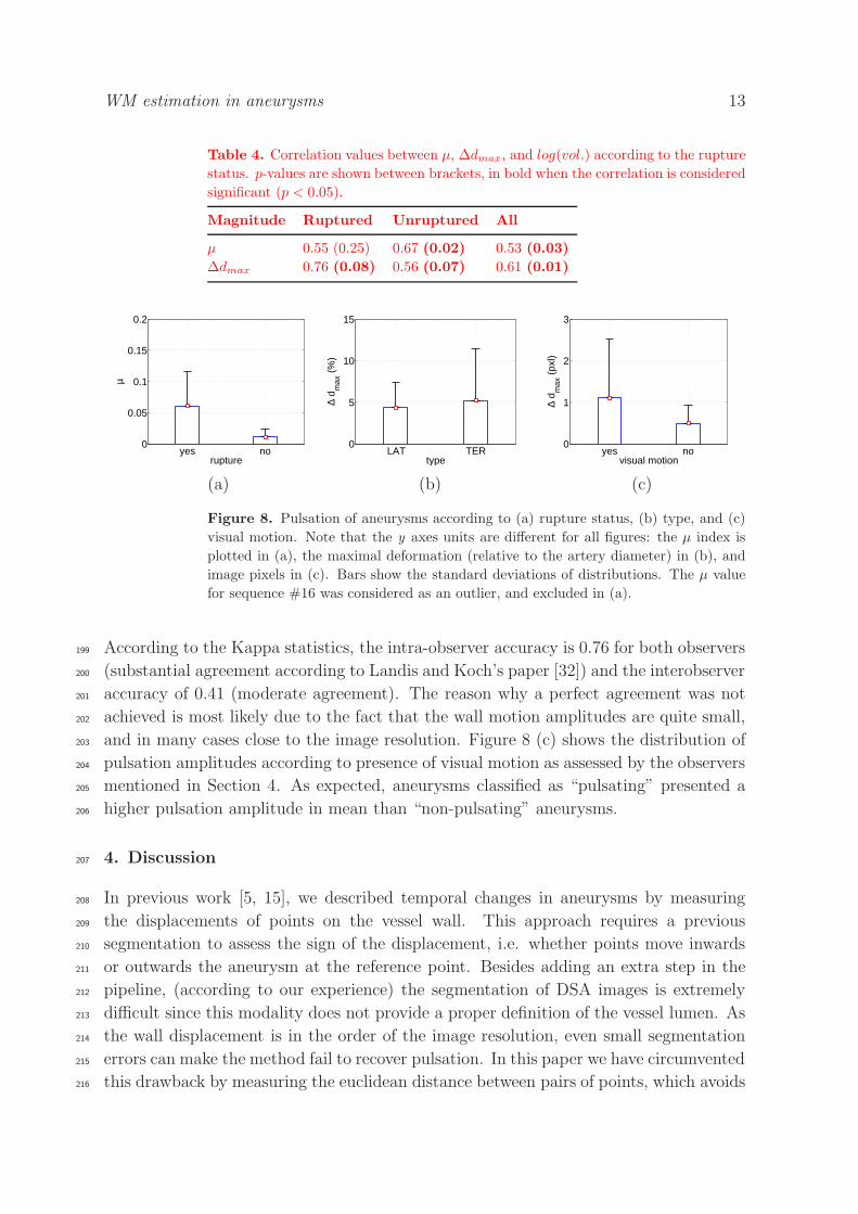
WM estimation in aneurysms 13
Table 4. Correlation values between µ, ∆dmax, and log(vol.) according to the rupture
status. p-values are shown between brackets, in bold when the correlation is considered
significant (p < 0.05).
Magnitude Ruptured Unruptured All
µ 0.55 (0.25) 0.67 (0.02) 0.53 (0.03)
∆dmax 0.76 (0.08) 0.56 (0.07) 0.61 (0.01)
yes no0
0.05
0.1
0.15
0.2
µ
ruptureLAT TER
0
5
10
15∆
d max
(%
)
typeyes no
0
1
2
3
∆ d m
ax (
pxl)
visual motion
(a) (b) (c)
Figure 8. Pulsation of aneurysms according to (a) rupture status, (b) type, and (c)
visual motion. Note that the y axes units are different for all figures: the µ index is
plotted in (a), the maximal deformation (relative to the artery diameter) in (b), and
image pixels in (c). Bars show the standard deviations of distributions. The µ value
for sequence #16 was considered as an outlier, and excluded in (a).
According to the Kappa statistics, the intra-observer accuracy is 0.76 for both observers199
(substantial agreement according to Landis and Koch’s paper [32]) and the interobserver200
accuracy of 0.41 (moderate agreement). The reason why a perfect agreement was not201
achieved is most likely due to the fact that the wall motion amplitudes are quite small,202
and in many cases close to the image resolution. Figure 8 (c) shows the distribution of203
pulsation amplitudes according to presence of visual motion as assessed by the observers204
mentioned in Section 4. As expected, aneurysms classified as “pulsating” presented a205
higher pulsation amplitude in mean than “non-pulsating” aneurysms.206
4. Discussion207
In previous work [5, 15], we described temporal changes in aneurysms by measuring208
the displacements of points on the vessel wall. This approach requires a previous209
segmentation to assess the sign of the displacement, i.e. whether points move inwards210
or outwards the aneurysm at the reference point. Besides adding an extra step in the211
pipeline, (according to our experience) the segmentation of DSA images is extremely212
difficult since this modality does not provide a proper definition of the vessel lumen. As213
the wall displacement is in the order of the image resolution, even small segmentation214
errors can make the method fail to recover pulsation. In this paper we have circumvented215
this drawback by measuring the euclidean distance between pairs of points, which avoids216

WM estimation in aneurysms 14
10−3
10−2
10−1
100
1010
0.1
0.2
vol. (cm3)
µ
rupturedunruptured
10−3
10−2
10−1
100
1010
0.1
0.2
0.3
0.4
0.5
vol. (cm3)
∆ d m
ax
rupturedunruptured
(a) (b)
Figure 9. Variations in the magnitude of pulsation with the size of the aneurysm. (a)
µ vs volume, (b) Maximum displacement vs. volume. The size of the aneurysms was
measured as the volume of the prolate ellipsoid with minor radii a = b = with and
major radius c = depth. The volume is represented by using a logarithmic scale, since
this is more appropriate for the distribution of volumes in our database.
the need for a previous image segmentation.217
In some cases, we found a rigid motion associated to the global pulsation of the218
intracranial vasculature that should be corrected before estimating the deformation.219
Fortunately, this motion was very small § and was captured by the non-rigid220
transformation. Therefore, the rigid motion was corrected automatically without adding221
an extra step.222
It is important to make some remarks with respect to image acquisition. The223
Nyquist theorem establishes that the minimum sampling frequency fmins that allows224
recovering the aneurysmal pulsation is twice the signal bandwidth (BW) [33]. To our225
knowledge, there are no measurements of temporal changes of intracranial aneurysms226
in the literature to estimate BW, and we have used simulated pressure data [34] for the227
Common Carotid Artery (CCA) (Figure 10) to estimate it. Two important assumptions228
are made here. 1) The wall displacement and pressure waveforms are the same (except229
for a scale factor): this is true if linear elasticity of the vessel wall is assumed, but230
both waveforms could differ slightly if a viscoelastic model and large mass-effects are231
considered. 2) The pressure waveform does not change from the CCA to the location232
of the aneurysm. Figure 10 shows that the most important frequency components233
are comprised in the range 0-4 Hz, and therefore we can establish a fmin
s=8 Hz as234
the minimum fs to recover aneurysmal pulsation. Even when this estimation is based235
on simulated data, it allowed obtaining curves resembling the typical arterial pressure236
waveform [35] (see for example sequences #1, #2, #9, #10, #12, #15 in Figure 7 ). This237
§ Note that the aneurysmal pulsation is also very small, and therefore any rigid motion must be
completely compensated to have an accurate estimation

WM estimation in aneurysms 15
0 0.2 0.4 0.6 0.8 10.5
0.6
0.7
0.8
0.9
1
1.1
time(s)
p(t)
0 2 4 6 8 100
2
4
6
8
10
freq. (Hz)
|DF
T|
(a) (b)
Figure 10. (a) Simulated pressure at the Common Carotid Artery (CCA) [34] (b)
Magnitude of its DFT (spacing of samples in the Fourier domain 1/T = 1, where T is
the period of the signal). The continuous component (f = 0) was removed from the
DFT for better visualization of high frequency components. Frequencies higher than
20 Hz were also omitted because of their small amplitude.
similarity supports the assumption that the recovered deformations effectively quantify238
the wall displacements of the vessel, and do not come from sources of variations like239
image noise, intensity changes, or movement artifacts.240
As shown in Table 2, some sequences were acquired at lower sampling frequency241
than this inferior limit. Sometimes, low fs values are preferred to obtain a higher image242
quality, and values as low as 2Hz can be found. Figure 7 shows the result when fs does243
not meet the requirements imposed by the Nyquist’s theorem (sequences #7 and #8).244
As the sampling frequency for these sequences (fs = 3Hz and fs = 2Hz, respectively),245
distension waveforms cannot be completely recovered. This has an influence on the246
correlation with rupture, since three of these sequences belong to the group of ruptured247
aneurysms. However, the fact of missing a peak has as a consequence a reduction in the248
differences between ruptured and unruptured aneurysms (already found significant). If249
the peak were not missed the differences between groups would be even larger.250
The dependency of the method on the contrast injection parameters (e.g. injection251
rate, total volume) is critical, since they must ensure a complete and homogeneous252
filling of the aneurysm for at least one cardiac cycle. It is very difficult to select a253
fixed set of parameters to satisfy these requirements in all aneurysms, since the filling254
depends strongly on factors like size, shape, and type of the aneurysm. The influence of255
type is well illustrated by terminal aneurysms of the basilar artery (Figure 1, patients256
#3 and #6). In these cases, the aneurysm receives the blood jet directly from the257
parent artery which produces a strong washout of contrast medium. A large size may258
be also problematic, since the filling is slower and sometimes the injected contrast is259
not sufficient to fill the aneurysm (Figure 1, patients #7 and #10). These problems260
are related to the upper limits imposed by the cellular effects of contrast media [36],261

WM estimation in aneurysms 16
(a) (b) (c) (d)
Figure 11. Relationship between blood flow and wall motion for a basilar aneurysm.
Figures (a)-(d) show the deformation of the aneurysm for four temporal points of the
cardiac cycle (shown as an empty circle at bottom left of each figure). Empty arrows
in the parent artery represent the blood blow (their length is proportional to the flow
magnitude). The small black arrows represent the wall displacement with respect to
the previous time instant.
and their connection to nephropathies [37]. If there were no such limits, the amount of262
contrast could be made big enough to compensate the effects of size and type. Figure263
7 shows that in some cases the recovered curves are out-of-phase. This cannot be264
attributed to the filters used for postprocessing, since the phase difference persists when265
filters are not applied (see patient # 6 for example). A possible explanation to this266
phenomenon is the asymmetric deformation of the aneurysm owing to specific blood267
flow patterns and asymmetric weakness of the arterial wall. Consider for example the268
same patient (# 6). As can be seen from Figure 1 this is a basilar aneurysm that receives269
a direct impingement of the blood flow coming from the basilar artery, which produces a270
differential pressure between the impingement region and the rest of the aneurysm. On271
the other hand, Meng et al. [38] have performed studies showing localized aneurysmal-272
type remodeling in regions of accelerating flow (in our case the region of impingement),273
which could create asymmetric weakness of the arterial wall. The combined effect of274
differential pressure and asymmetric weakness could explain the increase in depth at275
the expense of a decrease in width as shown in Figure 11. This explanation predicts a276
phase difference of 180 degrees, which in fact was the difference of phase found in the277
example. A similar analysis of other aneurysmal configurations should be performed to278
understand the regional differences in pulsation, and a CFD analysis could be useful for279
understanding the connection with the haemodynamics. Another explanation for these280
phase differences is the pulsation of extravascular structures (like the brain), which could281
pulsate synchronously with the artery and modify influence the expected deformation282
pattern of the aneurysm.283
Lateral and terminal aneurysms showed slight non significant differences in wall284
motion. However, terminal aneurysms receive a direct impact of the blood jet coming285
from the parent artery which should produce a larger deformations. A possible286
explanation are the differences in location of the considered aneurysms, which should be287
normalized to ensure similar haemodynamic conditions. Larger aneurysms exhibited a288
higher differential pulsation index, and wall motion amplitude. However, other papers289

WM estimation in aneurysms 17
(a) (b)
Figure 12. Influence of neighboring vessels: at the beginning of the contrast filling
the boundary of the aneurysm is free (a). As the contrast injection progresses, distal
vessels start appearing in the image causing local misregistration occurs due to lack of
point correspondence.
have reported no relationship between aneurysm size and volume increases [2].290
The method presented in this paper allows obtaining deformations in the image291
plane. This information could be complemented by a second acquisition in an orthogonal292
projection. However, according to our experience, the neighboring vessels make293
extremely difficult to obtain two orthogonal views showing the aneurysm without an294
overlapping with other vessels. The presence of neighboring vessels can also perturb295
the recovered displacement fields: at the beginning of the contrast filling, the aneurysm296
appears isolated from the rest of the vasculature and its boundary is well defined. As297
the contrast injection progresses, distal vessels start appearing in the image (Figure 12)298
and a local misregistration occurs due to the lack of correspondence [39].299
In this paper we have found statistically significant differences in the index µ300
according to the rupture status. However, even when there are some follow-up studies301
of unruptured aneurysms [40], the criterion adopted by the clinical centers involved in302
our study is to treat the aneurysm (coiling or stenting) immediately after identification303
by angiography to avoid the risk of hemorrhage. Therefore, the available sequences do304
not allow studying differences in pulsation before and after rupture [2, 41]. This is a305
limitation of most of works on rupture found in the literature. Therefore the underlying306
hypothesis of the experiments presented in this paper is that the pulsation properties of307
the aneurysm immediately before rupture are similar to those of ruptured aneurysms.308

WM estimation in aneurysms 18
5. Conclusions309
In this paper we have combined non-rigid registration methods with signal processing310
techniques to quantify wall motion of intracranial aneurysms from dynamic DSA311
sequences. We applied the presented methodology to a series of intracranial aneurysms312
and found a higher index of differential pulsation for ruptured aneurysms. These313
measurements and observations may help us better stratify aneurysm rupture risk and314
understand the wall motion effects on aneurysm haemodynamics and their evolution.315
References316
[1] D. O. Wiebers, J. P. Whisnant, J. Huston III, I. Meissner, R. D. Brown Jr., D. G. Piepgras,317
G. S. Forbes, K. Thielen, D. Nichols, W. M. O’Fallon, J. Peacock, L. Jaeger, N. F. Kassell,318
G. L. Kongable-Beckman, and J. C. Torner. International study of unruptured intracranial319
aneurysms investigators. unruptured intracranial aneurysms: Natural history, clinical outcome,320
and risks of surgical and endovascular treatment. Lancet, 362(9378):103–10, July 2003.321
[2] F. B. Meyer, J. Huston III, and S. S. Riederer. Pulsatile increases in aneurysm size determined322
by cine phase-contrast MR angiography. Journal of Neurosurgery, 78(6):879–83, June 1993.323
[3] J. Ueno, T. Matsuo, K. Sugiyama, and R. Okeda. Mechanism underlying the prevention of324
aneurismal rupture by coil embolization. Journal of Medical and Dental Sciences, 49(4):135–41,325
December 2002.326
[4] Y. Kato, M. Hayakawa, H. Sano, M. V. Sunil, S. Imizu, M. Yoneda, S. Watanabe, M. Abe, and327
T. Kanno. Prediction of impending rupture in aneurysms using 4D-CTA: histopathological328
verification of a real-time minimally invasive tool in unruptured aneurysms. Minimally Invasive329
Neurosurgery, 47(3):131–5, June 2004.330
[5] L. Dempere, E. Oubel, M. A. Castro, C. M. Putman, A. F. Frangi, and J. R. Cebral. CFD analysis331
incorporating the influence of wall motion: Application to intracranial aneurysms. In R. Larsen,332
M. Nielsen, and J. Sporring, editors, 8th International Conference on Medical Image Computing333
and Computer-Assisted Intervention, MICCAI 2006, volume 4190 of Lecture Notes in Computer334
Science, pages 438–45, Copenhagen, Denmark, October 2006. Springer.335
[6] V. Yaghmai, M. Rohany, A. Shaibani, M. Huber, H. Soud, E. J. Russell, and M. T. Walker.336
Pulsatility imaging of saccular aneurysm model by 64-slice CT with dynamic multiscan337
technique. Journal of Vascular and Interventional Radiology, 18(6):785–8, June 2007.338
[7] H. G. Boecher-Schwarz, K. Ringel, L. Kopacz, A. Heimann, and O. Kempski. Ex vivo study of339
the physical effect of coils on pressure and flow dynamics in experimental aneurysms. American340
Journal of Neuroradiology, 21(8):1532–6, September 2000.341
[8] C. Zhang, M. C. Villa-Uriol, M. De Craene, J. M. Pozo, and A. F. Frangi. Time-resolved 3D342
rotational angiography reconstruction: towards cerebral aneurysm pulsatile analysis. In H. U.343
Lemke, K. Inamura, K. Doi, M. W. Vannier, and A. G. Farman, editors, International Journal344
of Computer Assisted Radiology and Surgery, volume 3, pages S44–S46, Barcelona, Spain, June345
2008. Springer.346
[9] J. M. Wardlaw, J. Cannon, P. F. Statham, and R. Price. Does the size of intracranial aneurysms347
change with intracranial pressure? Observations based on color power transcranial Doppler348
ultrasound. Journal of Neurosurgery, 88(5):846–50, May 1998.349
[10] P. R. Hoskins, J. Prattis, and J. Wardlaw. A flow model of cerebral aneurysms for use with power350
Doppler studies. British Journal of Radiology, 71(841):76–80, January 1998.351
[11] F. Ishida, H. Ogawa, T. Simizu, T. Kojima, and W. Taki. Visualizing the dynamics of cerebral352
aneurysms with four-dimensional computed tomographic angiography. Neurosurgery, 57(3):460–353
71, 2005.354

WM estimation in aneurysms 19
[12] M. Hayakawa, K. Katada, H. Anno, S. Imizu, J. Hayashi, K. Irie, M. Negoro, Y. Kato, T. Kanno,355
and H. Sano. CT angiography with electrocardiographically gated reconstruction for visualizing356
pulsation of intracranial aneurysms: Identification of aneurysmal protuberance presumably357
associated with wall thinning. American Journal of Neuroradiology, 26(6):1366–9, 2005.358
[13] R. Manzke, M. Grass, T. Nielsen, G. Shechter, and D. Hawkes. Adaptive temporal resolution359
optimization in helical cardiac cone beam CT reconstruction. Medical Physics, 30(12):3072–80,360
December 2003.361
[14] M. Matsumoto, T. Sasaki, K. Suzuki, J. Sakuma, Y. Endo, and K. Kodama. Visualizing the362
dynamics of cerebral aneurysms with four-dimensional computed tomographic angiography.363
Neurosurgery, 58(5):E1003, May 2006.364
[15] E. Oubel, M. De Craene, C. M. Putman, J. R. Cebral, and A. F. Frangi. Analysis of intracranial365
aneurysm wall motion and its effects on hemodynamic patterns. In A. Manduca and X.P. Hu,366
editors, SPIE Medical Imaging 2007: Physiology, Function, and Structure from Medical Images,367
volume 6511, pages 10–11, San Diego, CA, USA, February 2007. SPIE press.368
[16] J. P. Thirion. Image matching as a diffusion process: an analogy with Maxwell’s demons. Medical369
Image Analysis, 2(3):243–60, September 1998.370
[17] J. Weickert, A. Bruhn, T. Brox, and N. Papenberg. Mathematical Models for Registration and371
Applications to Medical Imaging, volume 10 of Mathematics in Industry, chapter A Survey on372
Variational Optic Flow Methods for Small Displacements, pages 103–36. Springer, 2006.373
[18] S. Balter, D. Ergun, E. Tscholl, F. Buchmann, and L. Verhoeven. Digital substraction angiography:374
Fundamental characteristics. Radiology, 152(1):195–8, July 1984.375
[19] A. Collignon, F. Maes, D. Delaere, D. Vandermeulen, P. Suetens, and G. Marchal. Automated376
multi-modality image registration based on information theory. Lecture Notes in Computer377
Science, pages 263–74, Ile de Berder, France, June 1995. Kluwer Academic.378
[20] P. Viola and W. M. Wells. Alignment by maximization of mutual information. In E. Grimson,379
S. Shafer, A. Blake, and K. Sugihara, editors, Fifth International Conference on Computer380
Vision, pages 16–23, Los Alamitos, CA, USA, June 1995.381
[21] S. Lee, G. Wolberg, K-W. Chwa, and S. Y. Shin. Image metamorphosis with scattered382
feature constraints. IEEE Transactions on Visualization and Computer Graphics, 2(4):337–383
54, December 1996.384
[22] S. Lee, G. Wolberg, and S. Y. Shin. Scattered data interpolation with multilevel B-splines. IEEE385
Transactions on Visualization and Computer Graphics, 3(3):228–44, July-September 1997.386
[23] D. Rueckert, L. I. Sonoda, C. Hayes, D. L. G. Hill, M. O. Leach, and D. J. Hawkes. Nonrigid387
registration using free-form deformations: Application to breast MR images. IEEE Transactions388
on Medical Imaging, 18(8):712–21, August 1999.389
[24] F. L. Bookstein. Principal warps: Thin-plate splines and the decomposition of deformations.390
IEEE Transactions on Pattern Analysis and Machine Intelligence, 11(6):567–585, June 1989.391
[25] M. H. Davis, A. Khotanzad, D. P. Flamig, and S. E. Harms. A physics-based coordinate392
transformation for 3-D image matching. 16(3):317–328, 1997.393
[26] T. M. Cover and J. A. Thomas. Elements of information theory. Wiley-Interscience, 1991.394
[27] P. Gaetani, F. Tartara, V. Grazioli, F. Tancioni, L. Infuso, and R. Rodriguez y Baena. Collagen395
cross-linkage, elastolytic and collagenolytic activities in cerebral aneurysms: a preliminary396
investigation. Life Sciences, 63(4):285–92, June 1998.397
[28] B. J. Rajesh, S. Sandhyamani, and R. N. Bhattacharya. Clinico-pathological study of cerebral398
aneurysms. Neurology India, 52(1):82–6, March 2004.399
[29] A. I. Holodny, M. Deck, and C. K. Petito. Induction and subsequent rupture of aneurysms of400
the circle of willis after radiation therapy in Ehlers-Danlos syndrome: a plausible hypothesis.401
American Journal of Neuroradiology, 17(2):226–32, February 1996.402
[30] T. Mizutani and H. Kojima. Clinicopathological features of non-atherosclerotic cerebral arterial403
trunk aneurysms. Neuropathology, 20(1):91–7, March 2000.404
[31] E. Fonck, G. Prod’hom, S. Roy, L. Augsburger, D. A. Rufenacht, and N. Stergiopulos. Effect of405

WM estimation in aneurysms 20
elastin degradation on carotid wall mechanics as assessed by a constituent-based biomechanical406
model. American journal of physiology. Heart and circulatory physiology, 292(6):H2754–63,407
January 2007.408
[32] J. R. Landis and G. G. Koch. The measurement of observer agreement for cathegorical data.409
Biometrics, 33(1):159–74, March 1977.410
[33] A. V. Oppenheim and R. W Schafer. Digital Signal Processing. Prentice Hall, 1999.411
[34] J. Alastruey, K. Parker, J. Peiro, S. Byrd, and S. Sherwin. Modelling the circle of Willis to assess412
the effects of anatomical variations and occlusions on cerebral flows. Journal of Biomechanics,413
40(8):1794–805, October 2007.414
[35] A. C. Guyton and J. E. Hall. Textbook of Medical Physiology. Elsevier, 2006.415
[36] R. P. Franke, R. Fuhrmann, B. Hiebl, and F. Jung. Influence of various radiographic contrast416
media on the buckling of endothelial cells. Microvascular research, 76(2):110–3, August 2008.417
[37] S. K. Sharma. Iodinated contrast media and contrast-induced nephropathy: Is there a preferred418
cost-effective agent? The journal of invasive cardiology, 20(5):245–8, May 2008.419
[38] H. Meng, Z. Wang, Y. Hoi, L. Gao, E. Metaxa, D. D. Swartz, and J. Kolega. Complex420
hemodynamics at the apex of an arterial bifurcation induces vascular remodeling resembling421
cerebral aneurysm initiation. Stroke, 38(6):1924–31, June 2007.422
[39] S. Periaswamy and H. Faridb. Medical image registration with partial data. Medical Image423
Analysis, 10(3):452–64, June 2006.424
[40] S. Juvela, M. Porras, and K. Poussa. Natural history of unruptured intracranial aneurysms:425
probability of and risk factors for aneurysm rupture. Journal of Neurosurgery, 108(5):1052–60,426
May 2008.427
[41] S. Dhar, M. Tremmel, J. Mocco, M. Kim, J. Yamamoto, A. H. Siddiqui, L. N. Hopkins,428
and H. Meng. Morphology parameters for intracranial aneurysm rupture risk assessment.429
Neurosurgery, 63(2):185–96, August 2008.430