Journal of

Marine Science and Engineering

Article

Prediction of Shoreline Evolution. Reliability of aGeneral Model for the Mixed Beach Case

Giuseppe R. Tomasicchio 1,* , Antonio Francone 1, David J. Simmonds 2 ,Felice D’Alessandro 3 and Ferdinando Frega 4

1 Engineering Department, University of Salento, 73100 Lecce, Italy; antonio.francone@unisalento.it2 Faculty of Science and Engineering, University of Plymouth, Plymouth PL48AA, UK;

d.simmonds@plymouth.ac.uk3 Department of Environmental Science and Policy, University of Milan, 20122 Milan, Italy;

felice.dalessandro@unimi.it4 Department of Civil Engineering University of Calabria, 87100 Cosenza, Italy; ferdinando.frega@unical.it* Correspondence: roberto.tomasicchio@unisalento.it; Tel.: +39-0832-297715

Received: 30 April 2020; Accepted: 19 May 2020; Published: 21 May 2020�����������������

Abstract: In the present paper, after a sensitivity analysis, the calibration and verification of a novelmorphodynamic model have been conducted based on a high-quality field experiment data base.The morphodynamic model includes a general formula to predict longshore transport and associatedcoastal morphology over short- and long-term time scales. With respect to the majority of the existingone-line models, which address sandy coastline evolution, the proposed General Shoreline beachmodel (GSb) is suitable for estimation of shoreline change at a coastal mound made of non-cohesivesediment grains/units as sand, gravel, cobbles, shingle and rock. In order to verify the reliabilityof the GSb model, a comparison between observed and calculated shorelines in the presence of atemporary groyne deployed at a mixed beach has been performed. The results show that GSb gives agood agreement between observations and predictions, well reproducing the coastal evolution.

Keywords: longshore transport; morphodynamic model; field experiment; mixed beaches

1. Introduction

During the last decades, researchers and engineers inspired by coastal sediment phenomenahave conducted field and laboratory experiments to learn more about coastal processes and sedimentdynamics. Their efforts have resulted in a wealth of papers and documents published in books, journals,conference and symposium proceedings over the last 50 years [1].

One-line models have shown practical capability in predicting shoreline change, in assisting inthe selection of the most appropriate protection design, in the planning of projects located in thenearshore zone [2] and in assessing the longevity of beach nourishing projects. Among the others,the most popular models for shoreline change are Generalized Shoreline Change Numerical Model(GENESIS) [3], ONELINE [4], UNIform BEach Sediment Transport (UNIBEST) [5], LITtoral ProcessesAnd Coastline Kinetics (LITPACK) [6], BEACHPLAN [7], Sistema de Modelado Costero (SMC) [8],GENesis and CAscaDE (GENCADE) [9]. Each of the aforementioned models is suitable for one type ofbeach sediments composition solely (e.g., sandy beach or gravel beach) and is subjected to differentlimitations regarding its use (Table 1). The majority of existing large-scale coastline models addresssandy coastline evolution [10]. To date, no general one-line model valid for estimation of shorelinechange at a coastal mound made of non-cohesive sediment grains/units as sand, gravel, cobbles, shingleand rock has been proposed.

J. Mar. Sci. Eng. 2020, 8, 361; doi:10.3390/jmse8050361 www.mdpi.com/journal/jmse

J. Mar. Sci. Eng. 2020, 8, 361 2 of 17

Table 1. Main features of the existing one-line models.

ModelVariabilityof SeabedProprieties

DiffractionAround theStructures

LongshoreCurrent

LongshoreSedimentTransport

Groynes DetachedBreakwaters

GENESIS No Yes No CERC [11] Yes Yes

ONELINE No Yes No Kamphuis [12] Yes Yes

UNIBEST No No Yes

Bijker [13]Van Rijn [14]Bailard [15]CERC [11]

Yes No

LITPACK Yes Yes Yes STPQ3D [16] Yes Yes

BEACHPLAN Yes Yes Yes CERC [11] Yes Yes

SMC No Yes No CERC [11] No No

GENCADE No Yes No CERC [11] Yes Yes

Presently, there is a growing interest in properly defining the morphological processes of gravel,cobbles or shingle/mixed beaches due to an increasing interest for using of coarse sediments in theartificial nourishing of eroded beaches, as they provide a longer longevity of the nourishing interventionunder the forcing processes during storm events [17–19]. In this context, one has to consider that the useof models in practical design situations could also be linked to economic and financial considerationswhen a cost–benefit approach is part of the design; conversely, models can help in examining theeconomic implications of a design [20]. Moreover, when designing a coastal protection intervention,modern Coastal Engineering extensive use of numerical models to predict impact of the designedintervention before it is implemented.

Within this path, the focus of the present paper is to propose a novel model, named the GeneralShoreline beach model (GSb), for predicting shoreline change for beaches made of non-cohesivesediment grains/units and to show the results of a sensitivity analysis conducted to evaluate howmodel output changes with changes in input variables [21,22]; the sensitivity analysis allows to assessthe effects and sources of uncertainties oriented to the target to build a robust model for shorelineevolution. The calibration and verification of the GSb model for predicting shoreline change at a mixedbeach are performed based on a high-quality field experiment data base [23–25].

2. Materials and Methods

2.1. The General Longshore Transport Model (GLT)

Longshore transport due to oblique waves acting on beaches made of non-cohesive sedimentgrains/units as sand, gravel, cobbles, shingle and rock is determined by means of the General LongshoreTransport (GLT) model [26–28]. The GLT model belongs to the typology based on an energy fluxapproach combined with an empirical relationship between the wave induced forcing and the numberof moving sediment grains/units. Specifically, the GLT model considers an appropriate mobility indexand assumes that the units move during up- and down-rush with the same obliquity of breaking andreflected waves at the breaker depth [26]. A sediment grain/unit passes through a certain control sectionif and only if it is removed from an updrift area of extension equal to the longitudinal component ofthe displacement length, ld sinθd, where ld is the displacement length and θd is its obliquity (Figure 1).

J. Mar. Sci. Eng. 2020, 8, 361 3 of 17J. Mar. Sci. Eng. 2020, 8, x FOR PEER REVIEW 3 of 18

Figure 1. Definition sketch for the General Longshore Transport (GLT) model.

This process description is particularly true when considering the wave obliquity, the up-rush and related longshore transport at the swash zone. By assuming that the displacement obliquity is equal to the characteristic wave obliquity at breaking (θd = θk,b), and that a number Nod of particles removed from a nominal diameter, Dn50, wide strip moves under the action of 1000 waves, then the number of units passing a given control section in one wave is: = ∙ 1000 , = ( ∗∗), (1)

where: ∗∗ = ∆ ,,/ ( ) / . (2)∗∗ is the modified stability number [26] with: Hk = characteristic wave height; Ck = Hk/Hs,o, where Hs,o

= significant offshore wave height; θ0 = offshore wave obliquity; sm,0 = mean wave steepness at offshore conditions and sm,k = characteristic mean wave steepness (assumed equal to 0.03). Ns** resembles the traditional stability number, Ns [29,30], taking into account the effects of a non-Rayleighian wave height distribution at shallow water [31], wave steepness, wave obliquity and the nominal diameter of the sediment grains/units. The authors in [26,32] reported that Hk is to be considered equal to H1/50, but H2% can also be adopted. In the first case Ck = 1.55, in the second case Ck = 1.40. The second factor in Equation (2) is such that Ns** ≅ Ns for θ0 = 0 if sm,0 = sm,k.

In the case of a head-on wave attack, under the assumption that, offshore the breaking point, the wave energy dissipation is negligible and that waves break as shallow water waves, the following relation holds: = 1 8⁄ , = 1 8⁄ , , (3)

In Equation (3), F = wave energy flux, ρ = water density, g = gravity acceleration, H0 = offshore wave height, , = offshore wave group celerity, Hb = wave height at breaking and , = is the wave group celerity at breaking.

Equation (3), related to the breaker index γb = Hb/hb, with hb = breaking depth, implies: = / = / , (4)

The authors in [33] found the best agreement with field and laboratory data assuming γb = 1.42 or the proportionality constant q = 0.56. It follows that, considering the characteristic wave height at breaking, Hk,b, and sm,0 = sm,k = 0.03, Ns** can be also written as: ∗∗ ≅ 0.89 ,∆ , (5)

where ∆ = relative mass density of the sediment grain/unit = (ρs – ρ)/ρ and ρs = sediment grain/unit density.

According to the refraction theory for plane and monotonically decreasing profiles, Hk,b and sinθk,b, are evaluated as in the following [26,34]: , = / / , (6)

Figure 1. Definition sketch for the General Longshore Transport (GLT) model.

This process description is particularly true when considering the wave obliquity, the up-rushand related longshore transport at the swash zone. By assuming that the displacement obliquity isequal to the characteristic wave obliquity at breaking (θd = θk,b), and that a number Nod of particlesremoved from a nominal diameter, Dn50, wide strip moves under the action of 1000 waves, then thenumber of units passing a given control section in one wave is:

SN =ld

Dn50·

Nod1000

sinθk,b = f (N∗∗s ), (1)

where:

N∗∗s =Hk

CkDn50

(sm,0

sm,k

)−1/5

(cosθ0)2/5. (2)

N∗∗s is the modified stability number [26] with: Hk = characteristic wave height; Ck = Hk/Hs,o, where Hs,o

= significant offshore wave height; θ0 = offshore wave obliquity; sm,0 = mean wave steepness at offshoreconditions and sm,k = characteristic mean wave steepness (assumed equal to 0.03). Ns

** resemblesthe traditional stability number, Ns [29,30], taking into account the effects of a non-Rayleighian waveheight distribution at shallow water [31], wave steepness, wave obliquity and the nominal diameter ofthe sediment grains/units. The authors in [26,32] reported that Hk is to be considered equal to H1/50,but H2% can also be adopted. In the first case Ck = 1.55, in the second case Ck = 1.40. The second factorin Equation (2) is such that Ns

** � Ns for θ0 = 0 if sm,0 = sm,k.In the case of a head-on wave attack, under the assumption that, offshore the breaking point, the

wave energy dissipation is negligible and that waves break as shallow water waves, the followingrelation holds:

F = 1/8ρgH20c2

g,0 = 1/8ρgH2bc2

g,b, (3)

In Equation (3), F = wave energy flux, ρ = water density, g = gravity acceleration, H0 = offshorewave height, cg,0 = offshore wave group celerity, Hb = wave height at breaking and cg,b = is the wavegroup celerity at breaking.

Equation (3), related to the breaker index γb = Hb/hb, with hb = breaking depth, implies:

Hb = H0

(γb

4k0H0

)1/5

= qH0s−1/50 , (4)

The authors in [33] found the best agreement with field and laboratory data assuming γb = 1.42or the proportionality constant q = 0.56. It follows that, considering the characteristic wave height atbreaking, Hk,b, and sm,0 = sm,k = 0.03, Ns

** can be also written as:

N∗∗s �0.89Hk,b

CkDn50, (5)

where ∆ = relative mass density of the sediment grain/unit = (ρs − ρ)/ρ and ρs = sedimentgrain/unit density.

According to the refraction theory for plane and monotonically decreasing profiles, Hk,b andsinθk,b, are evaluated as in the following [26,34]:

J. Mar. Sci. Eng. 2020, 8, 361 4 of 17

Hk,b =(H2

k cgcosθo√γb/g

)2/5, (6)

sinθk,b =ck,b

csinθo, (7)

ck,b =√

gHk,b/γb, (8)

where cg = group celerity and ck,b is the characteristic wave celerity at breaking depth.The displacement length is calculated as [26]:

ld =(1.4N∗∗s − 1.3)

tanh2(kh)Dn50, (9)

where k = wave number and h = water depth.Nod has been determined following a calibration procedure based on the least-squares method,

taking into account nine high quality data sets of longshore transport from field and laboratoryexperiments for a wide mobility range of sediment grains/units: from stones to sand. In total, the ninedata sets consist of 245 cases [28]. In particular, Nod values are partitioned in two intervals: the firstinterval refers to Ns

**≤ 23, from reshaping type berm breakwaters [35] to gravel beaches; the second

one relates to Ns** > 23, for sandy beaches. For Ns

**≤ 23, a third order polynomial approximating

function provides a satisfactory agreement as shown by [28]. For Ns** > 23 a good agreement is

obtained by a linear regression in log–log plane. Nod is given as:

Nod =

{20N∗∗s (N∗∗s − 2)2 N∗∗s ≤ 23exp[2.72ln(N∗∗s ) + 1.12] N∗∗s > 23

, (10)

The estimated correlation coefficient is equal to 0.89 for Ns**≤ 23 and 0.92 for Ns

** > 23.The longshore transport rate, QLT, can be also expressed in terms of [m3/s] as in the following:

QLT =SND3

n50

(1− n)Tm, (11)

where Tm = mean wave period, and n = porosity factor.Figure 2 shows the flowchart summarizing the use of the GLT.

J. Mar. Sci. Eng. 2020, 8, x FOR PEER REVIEW 4 of 18

, = , , (7)

, = , ⁄ , (8)

where cg = group celerity and ck,b is the characteristic wave celerity at breaking depth. The displacement length is calculated as [26]: = (1.4 ∗∗ − 1.3)ℎ ( ℎ) , (9)

where k = wave number and h = water depth. Nod has been determined following a calibration procedure based on the least-squares method,

taking into account nine high quality data sets of longshore transport from field and laboratory experiments for a wide mobility range of sediment grains/units: from stones to sand. In total, the nine data sets consist of 245 cases [28]. In particular, Nod values are partitioned in two intervals: the first interval refers to Ns** ≤ 23, from reshaping type berm breakwaters [35] to gravel beaches; the second one relates to Ns** > 23, for sandy beaches. For Ns** ≤ 23, a third order polynomial approximating function provides a satisfactory agreement as shown by [28]. For Ns** > 23 a good agreement is obtained by a linear regression in log–log plane. Nod is given as: = 20 ∗∗( ∗∗ − 2) ∗∗ ≤ 232.72 ( ∗∗) + 1.12 ∗∗ > 23 , (10)

The estimated correlation coefficient is equal to 0.89 for Ns** ≤ 23 and 0.92 for Ns** > 23. The longshore transport rate, , can be also expressed in terms of [m3/s] as in the following: = (1 − ) , (11)

where Tm = mean wave period, and n = porosity factor. Figure 2 shows the flowchart summarizing the use of the GLT.

Figure 2. User flowchart.

Figure 2. User flowchart.

J. Mar. Sci. Eng. 2020, 8, 361 5 of 17

2.2. The General Shoreline Beach Model (GSb)

2.2.1. Theoretical Background

The GSb model belongs to the one-line model typology [36] and assumes that the beach cross-shoreprofile remains unchanged [37,38], thereby allowing beach change to be described uniquely in terms ofthe shoreline position.

The equilibrium cross-shore profile is calculated as proposed by [37,38] and is used to determinethe average nearshore bottom slope adopted in longshore transport equation. The average cross-shoreprofile is described by [37]:

h(y) = Ay2/3, (12)

where h is expressed in (m), A = scale parameter (m1/3) and y = offshore distance from the initialshoreline (m). The scale parameter A can be calculated as in the following [39]:

A = 0.41(Dn50)0.94, Dn50 < 0.4 mm, (13)

A = 0.23(Dn50)0.32, 0.4 mm ≤ Dn50 < 10.0 mm, (14)

A = 0.23(Dn50)0.28, 10.0 mm ≤ Dn50 < 40.0 mm, (15)

A = 0.46(Dn50)0.11, Dn50 ≥ 40 mm, (16)

The main peculiarity of the GSb model is the use of the GLT model, allowing to have an explicitdependence of shoreline evolution on Dn50 [28,40]. This finding is due to the fact that GSb uses the GLTmodel. Differently from GENESIS and similar models [7,8,41], which take into account two calibrationcoefficients, K1 and K2, the GSb presents one calibration coefficient, KGSb, which does not solely dependon the grain size diameter and depends on the longshore gradient in breaking wave height [42].

As in the case of most numerical models (e.g., GENCADE [9]), GSb is able to deal with thepresence of soft and hard coastal structures. Soft protection consists of nourishing an eroded beach.A hard intervention consists in deployment of one or more coastal structures (e.g., groynes, detachedbreakwaters and seawalls), composed by natural rock or artificial concrete units.

The model allows to determine short-term (daily base) or long-term (yearly base) shorelinechange [43,44] for arbitrary combinations and configurations of hard structures and beach fills that canbe represented on a modelled reach of coast.

GSb considers the sediment grain/unit passing around or through a coastal structure. Two typesof sediment movement around or through the structures can be simulated: bypass, when the sedimentpasses around the seaward end of the groynes, and transmission, where the sediment passes throughthe structures. Specifically, bypass occurs when the water depth at the tip of the structure, DG, is lessthan the depth of active longshore transport, DLT, calculated with [45]. To represent sediment bypass,a bypassing factor, BF, is defined as:

BF = 1−DGDLT

DG ≤ DLT, (17)

Transmission occurs due to permeability of the material, p, composing the coastal structure.With p = 0, the structure is completely transparent. On the contrary, for p = 1, the structure is fullyimpermeable. With the values of BF and p, GSb calculates the total fraction TF of sediment passingaround or through a structure as defined by [41]:

TF = p (1− BF) + BF, (18)

The TF value is calculated at every time step for each structure present in the model domain.GSb takes into account the wave transformation phenomena as shoaling, refraction and diffraction.

Shoaling and refraction are treated according to an internal wave model proposed by [39]. GSb uses

J. Mar. Sci. Eng. 2020, 8, 361 6 of 17

the simplified diffraction calculation procedure from waves with directional spread presented by [46]to represent diffraction at structures such as detached breakwaters and groynes.

The model requires predictive expressions for the longshore sediment transport rate.

2.2.2. Longshore Sediment Transport Rate

The GSb model uses the following equation for the longshore transport rate Ql:

Ql =SND3

n50

(1− n)Tm−

KGSb

8(ρsρ − 1

)(1− n) tan β 1.4167/2

H2s,bcg,b cos(θbs)

∂Hs,b

∂x, (19)

where tan β = average bottom slope from the shoreline to the closure depth, dc; Hs,b = significant waveheight at breaking; θbs = angle of breaking waves to the local shoreline; x = longshore distance.

The first term in Equation (19) accounts for longshore transport as from the “GLT formula” [26,27].The second term in Equation (19), similar to GENESIS [39], ONELINE [4], BEACHPLAN [7], SMC [8]and GENCADE [9], accounts for the longshore sediment transport induced by the longshore gradientin significant wave height at breaking [42], where Hs,b is calculated taking into account the wavepropagation shoaling, refraction and diffraction phenomena [39]. The original formulation of thesecond term in Equation (19) considers the root-mean-square (rms) wave height [42]. The factor 1.416is used to convert from significant wave height to root-mean-square (rms) wave height [39].

2.2.3. Sediment Continuity Equation

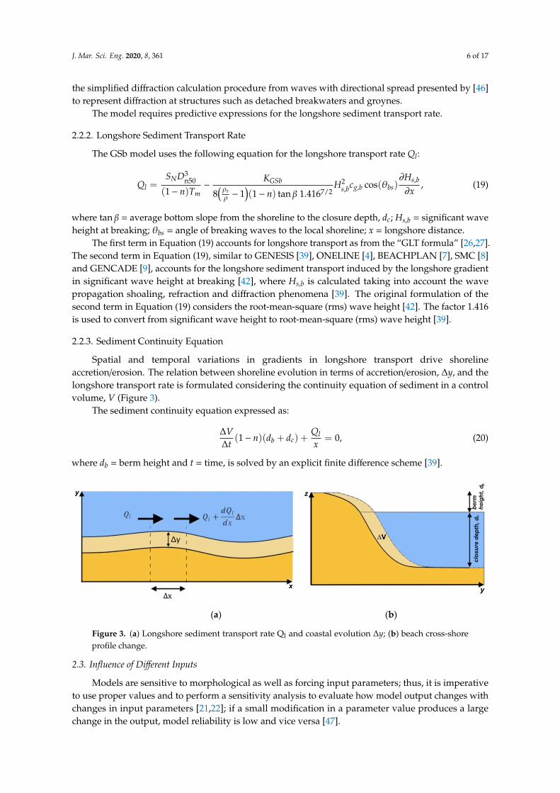
Spatial and temporal variations in gradients in longshore transport drive shorelineaccretion/erosion. The relation between shoreline evolution in terms of accretion/erosion, ∆y, and thelongshore transport rate is formulated considering the continuity equation of sediment in a controlvolume, V (Figure 3).

The sediment continuity equation expressed as:

∆V∆t

(1− n)(db + dc) +Qlx

= 0, (20)

where db = berm height and t = time, is solved by an explicit finite difference scheme [39].

J. Mar. Sci. Eng. 2020, 8, x FOR PEER REVIEW 6 of 18

GSb uses the simplified diffraction calculation procedure from waves with directional spread presented by [46] to represent diffraction at structures such as detached breakwaters and groynes.

The model requires predictive expressions for the longshore sediment transport rate.

2.2.2. Longshore Sediment Transport Rate

The GSb model uses the following equation for the longshore transport rate : = ( ) − ( ) . ⁄ , , cos( ) , , (19)

where tan = average bottom slope from the shoreline to the closure depth, ; , = significant wave height at breaking; = angle of breaking waves to the local shoreline; x = longshore distance.

The first term in Equation (19) accounts for longshore transport as from the “GLT formula” [26,27]. The second term in Equation (19), similar to GENESIS [39], ONELINE [4], BEACHPLAN [7], SMC [8] and GENCADE [9], accounts for the longshore sediment transport induced by the longshore gradient in significant wave height at breaking [42], where Hs,b is calculated taking into account the wave propagation shoaling, refraction and diffraction phenomena [39]. The original formulation of the second term in Equation (19) considers the root-mean-square (rms) wave height [42]. The factor 1.416 is used to convert from significant wave height to root-mean-square (rms) wave height [39].

2.2.3. Sediment Continuity Equation

Spatial and temporal variations in gradients in longshore transport drive shoreline accretion/erosion. The relation between shoreline evolution in terms of accretion/erosion, ∆y, and the longshore transport rate is formulated considering the continuity equation of sediment in a control volume, ∆ (Figure 3).

The sediment continuity equation expressed as: (1 − )( + ) + ∆∆ = 0, (20)

where = berm heightand = time, is solved by an explicit finite difference scheme [39].

(a) (b)

Figure 3. (a) Longshore sediment transport rate Ql and coastal evolution ∆y; (b) beach cross-shore profile change.

2.3. Influence of Different Inputs

Models are sensitive to morphological as well as forcing input parameters; thus, it is imperative to use proper values and to perform a sensitivity analysis to evaluate how model output changes with changes in input parameters [21,22]; if a small modification in a parameter value produces a large change in the output, model reliability is low and vice versa [47].

In the present paper, in order to evaluate the reliability of the GSb model, a sensitivity analysis for a range of selected input parameters has been conducted based on the simulation of the

Figure 3. (a) Longshore sediment transport rate Ql and coastal evolution ∆y; (b) beach cross-shoreprofile change.

2.3. Influence of Different Inputs

Models are sensitive to morphological as well as forcing input parameters; thus, it is imperativeto use proper values and to perform a sensitivity analysis to evaluate how model output changes withchanges in input parameters [21,22]; if a small modification in a parameter value produces a largechange in the output, model reliability is low and vice versa [47].

J. Mar. Sci. Eng. 2020, 8, 361 7 of 17

In the present paper, in order to evaluate the reliability of the GSb model, a sensitivity analysis fora range of selected input parameters has been conducted based on the simulation of the advance/retreatof an initial straight shoreline in presence of a single groyne. Specifically, three input parameters havebeen selected as representative of (i) wave characteristics (i.e., ϑo), (ii) sediment properties (i.e., Dn50)and (iii) short/long term predictions (i.e., duration of simulation, t).

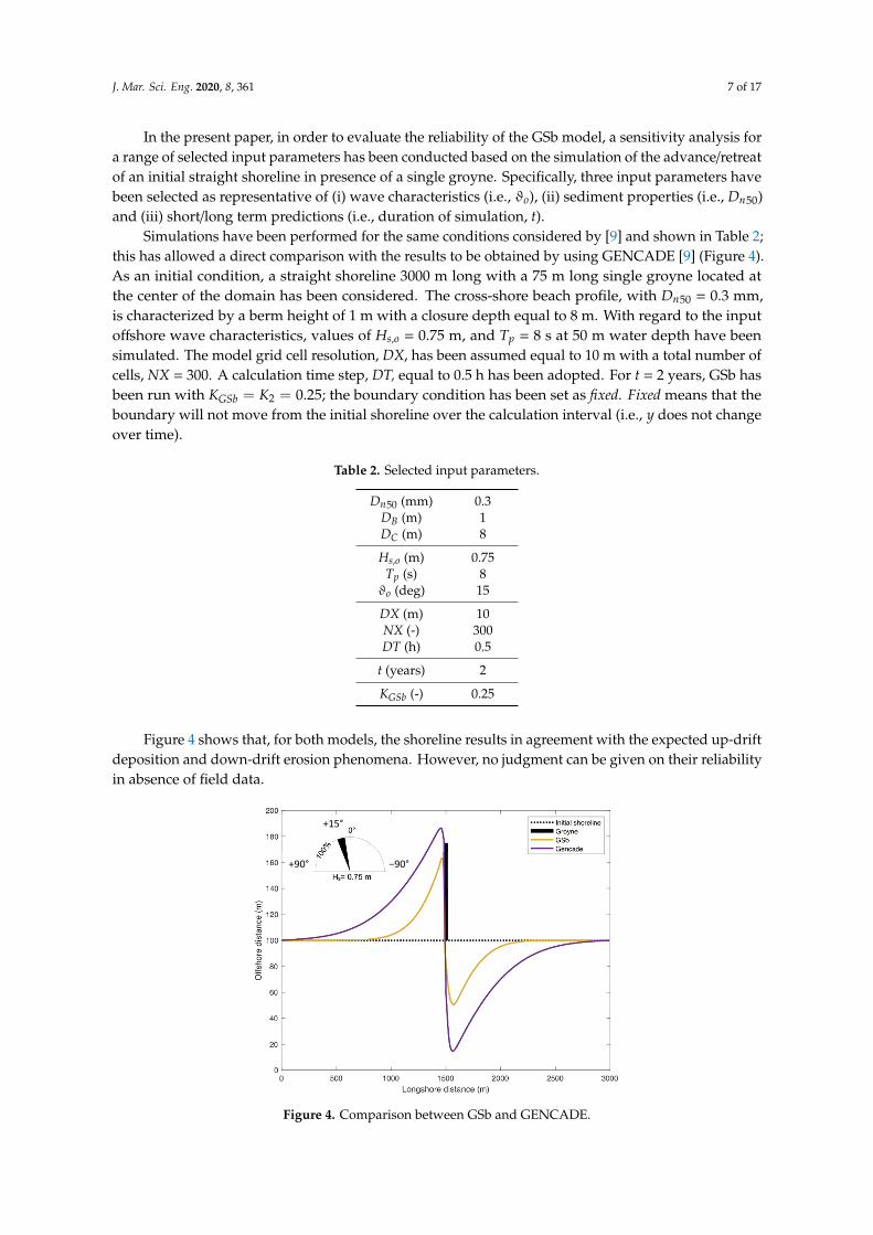
Simulations have been performed for the same conditions considered by [9] and shown in Table 2;this has allowed a direct comparison with the results to be obtained by using GENCADE [9] (Figure 4).As an initial condition, a straight shoreline 3000 m long with a 75 m long single groyne located atthe center of the domain has been considered. The cross-shore beach profile, with Dn50 = 0.3 mm,is characterized by a berm height of 1 m with a closure depth equal to 8 m. With regard to the inputoffshore wave characteristics, values of Hs,o = 0.75 m, and Tp = 8 s at 50 m water depth have beensimulated. The model grid cell resolution, DX, has been assumed equal to 10 m with a total number ofcells, NX = 300. A calculation time step, DT, equal to 0.5 h has been adopted. For t = 2 years, GSb hasbeen run with KGSb = K2 = 0.25; the boundary condition has been set as fixed. Fixed means that theboundary will not move from the initial shoreline over the calculation interval (i.e., y does not changeover time).

Table 2. Selected input parameters.

Dn50 (mm) 0.3DB (m) 1DC (m) 8

Hs,o (m) 0.75Tp (s) 8ϑo (deg) 15

DX (m) 10NX (-) 300DT (h) 0.5

t (years) 2

KGSb (-) 0.25

Figure 4 shows that, for both models, the shoreline results in agreement with the expected up-driftdeposition and down-drift erosion phenomena. However, no judgment can be given on their reliabilityin absence of field data.

J. Mar. Sci. Eng. 2020, 8, x FOR PEER REVIEW 7 of 18

advance/retreat of an initial straight shoreline in presence of a single groyne. Specifically, three input parameters have been selected as representative of (i) wave characteristics (i.e., ϑο), (ii) sediment properties (i.e., Dn50) and (iii) short/long term predictions (i.e., duration of simulation, t).

Simulations have been performed for the same conditions considered by [9] and shown in Table 2; this has allowed a direct comparison with the results to be obtained by using GENCADE [9] (Figure 4). As an initial condition, a straight shoreline 3000 m long with a 75 m long single groyne located at the center of the domain has been considered. The cross-shore beach profile, with Dn50 = 0.3 mm, is characterized by a berm height of 1 m with a closure depth equal to 8 m. With regard to the input offshore wave characteristics, values of Hs,o = 0.75 m, and Tp = 8 s at 50 m water depth have been simulated. The model grid cell resolution, DX, has been assumed equal to 10 m with a total number of cells, NX = 300. A calculation time step, DT, equal to 0.5 h has been adopted. For t = 2 years, GSb has been run with = = 0.25; the boundary condition has been set as fixed. Fixed means that the boundary will not move from the initial shoreline over the calculation interval (i.e., does not change over time).

Table 2. Selected input parameters.

Dn50 (mm) 0.3 DB (m) 1 DC (m) 8 Hs,o (m) 0.75 Tp (s) 8 (deg) 15

DX (m) 10 NX (-) 300 DT (h) 0.5

t (years) 2 KGSb (-) 0.25

Figure 4 shows that, for both models, the shoreline results in agreement with the expected up-drift deposition and down-drift erosion phenomena. However, no judgment can be given on their reliability in absence of field data.

Figure 4. Comparison between GSb and GENCADE.

2.3.1. Influence of Offshore Wave Angle

−90° +90°

+15°

Figure 4. Comparison between GSb and GENCADE.

J. Mar. Sci. Eng. 2020, 8, 361 8 of 17

2.3.1. Influence of Offshore Wave Angle

In order to evaluate the influence of the offshore wave angle on the shoreline evolution, differentvalues of ϑo in the interval from −45 to +45 deg have been considered. The adopted input parametersare given in Table 2, with ϑo = −45, −35, −15, −5, +5, +15, +25, +35, +45 deg.

Figure 5 shows the calculated shoreline evolution induced by longshore transport acting from (a)right to left for ϑo = −45, −35, −25, −15, −5 deg, and (b) from left to right for ϑo = +5, +15, +25, +35,+45 deg, respectively.

Maximum and minimum advance/retreat rates have been obtained for ϑo = ±35 andϑo = ±5, respectively.

J. Mar. Sci. Eng. 2020, 8, x FOR PEER REVIEW 8 of 18

In order to evaluate the influence of the offshore wave angle on the shoreline evolution, different values of in the interval from −45 to +45 deg have been considered. The adopted input parameters are given in Table 2, with = −45, −35, −15, −5, +5, +15, +25, +35, +45 deg.

Figure 5 shows the calculated shoreline evolution induced by longshore transport acting from (a) right to left for = −45, −35, −25, −15, −5 deg, and (b) from left to right for = + 5, +15, +25, +35, +45 deg, respectively.

(a) (b)

Figure 5. Calculated shoreline evolution for (a) = −45, −35, −15, −5 and (b) = +5, +15, +25, +35, +45.

Maximum and minimum advance/retreat rates have been obtained for = ±35 and = ±5, respectively.

2.3.2. Influence of Nominal Diameter

In order to evaluate the influence of the nominal diameter on the shoreline evolution, different values of Dn50 have been considered. The adopted input parameters are given in Table 2, with Dn50 = 0.3, 30 and 100 mm corresponding to sand, pebbles and cobbles, respectively.

Figure 6 shows the calculated shoreline evolution induced by longshore transport.

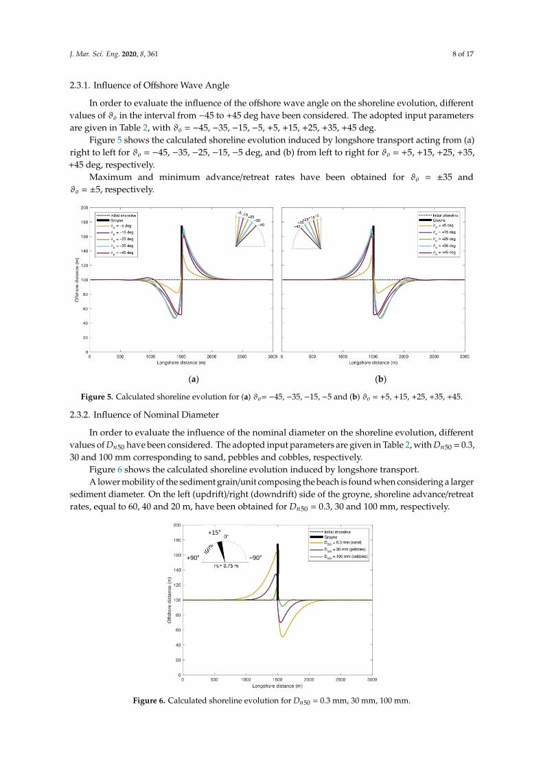
Figure 6. Calculated shoreline evolution for Dn50 = 0.3 mm, 30 mm, 100 mm.

A lower mobility of the sediment grain/unit composing the beach is found when considering a larger sediment diameter. On the left (updrift)/right (downdrift) side of the groyne, shoreline advance/retreat rates, equal to 60, 40 and 20 m, have been obtained for Dn50 = 0.3, 30 and 100 mm, respectively.

−90° +90°

+15°

Figure 5. Calculated shoreline evolution for (a) ϑo= −45, −35, −15, −5 and (b) ϑo = +5, +15, +25, +35, +45.

2.3.2. Influence of Nominal Diameter

In order to evaluate the influence of the nominal diameter on the shoreline evolution, differentvalues of Dn50 have been considered. The adopted input parameters are given in Table 2, with Dn50 = 0.3,30 and 100 mm corresponding to sand, pebbles and cobbles, respectively.

Figure 6 shows the calculated shoreline evolution induced by longshore transport.A lower mobility of the sediment grain/unit composing the beach is found when considering a larger

sediment diameter. On the left (updrift)/right (downdrift) side of the groyne, shoreline advance/retreatrates, equal to 60, 40 and 20 m, have been obtained for Dn50 = 0.3, 30 and 100 mm, respectively.

J. Mar. Sci. Eng. 2020, 8, x FOR PEER REVIEW 8 of 18

In order to evaluate the influence of the offshore wave angle on the shoreline evolution, different values of in the interval from −45 to +45 deg have been considered. The adopted input parameters are given in Table 2, with = −45, −35, −15, −5, +5, +15, +25, +35, +45 deg.

Figure 5 shows the calculated shoreline evolution induced by longshore transport acting from (a) right to left for = −45, −35, −25, −15, −5 deg, and (b) from left to right for = + 5, +15, +25, +35, +45 deg, respectively.

(a) (b)

Figure 5. Calculated shoreline evolution for (a) = −45, −35, −15, −5 and (b) = +5, +15, +25, +35, +45.

Maximum and minimum advance/retreat rates have been obtained for = ±35 and = ±5, respectively.

2.3.2. Influence of Nominal Diameter

In order to evaluate the influence of the nominal diameter on the shoreline evolution, different values of Dn50 have been considered. The adopted input parameters are given in Table 2, with Dn50 = 0.3, 30 and 100 mm corresponding to sand, pebbles and cobbles, respectively.

Figure 6 shows the calculated shoreline evolution induced by longshore transport.

Figure 6. Calculated shoreline evolution for Dn50 = 0.3 mm, 30 mm, 100 mm.

A lower mobility of the sediment grain/unit composing the beach is found when considering a larger sediment diameter. On the left (updrift)/right (downdrift) side of the groyne, shoreline advance/retreat rates, equal to 60, 40 and 20 m, have been obtained for Dn50 = 0.3, 30 and 100 mm, respectively.

−90° +90°

+15°

Figure 6. Calculated shoreline evolution for Dn50 = 0.3 mm, 30 mm, 100 mm.

J. Mar. Sci. Eng. 2020, 8, 361 9 of 17

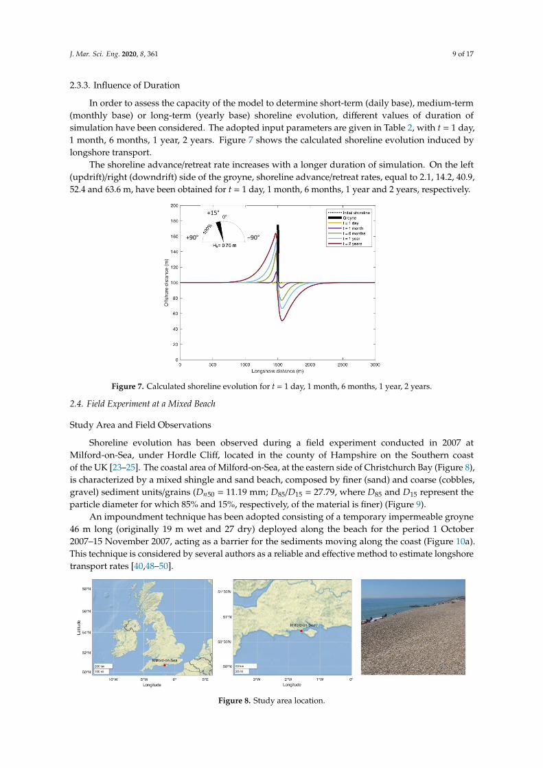
2.3.3. Influence of Duration

In order to assess the capacity of the model to determine short-term (daily base), medium-term(monthly base) or long-term (yearly base) shoreline evolution, different values of duration ofsimulation have been considered. The adopted input parameters are given in Table 2, with t = 1 day,1 month, 6 months, 1 year, 2 years. Figure 7 shows the calculated shoreline evolution induced bylongshore transport.

The shoreline advance/retreat rate increases with a longer duration of simulation. On the left(updrift)/right (downdrift) side of the groyne, shoreline advance/retreat rates, equal to 2.1, 14.2, 40.9,52.4 and 63.6 m, have been obtained for t = 1 day, 1 month, 6 months, 1 year and 2 years, respectively.

J. Mar. Sci. Eng. 2020, 8, x FOR PEER REVIEW 10 of 18

2.3.3. Influence of Duration

In order to assess the capacity of the model to determine short-term (daily base), medium-term (monthly base) or long-term (yearly base) shoreline evolution, different values of duration of simulation have been considered. The adopted input parameters are given in Table 2, with t = 1 day, 1 month, 6 months, 1 year, 2 years. Figure 7 shows the calculated shoreline evolution induced by longshore transport.

Figure 7. Calculated shoreline evolution for t = 1 day, 1 month, 6 months, 1 year, 2 years.

The shoreline advance/retreat rate increases with a longer duration of simulation. On the left (updrift)/right (downdrift) side of the groyne, shoreline advance/retreat rates, equal to 2.1, 14.2, 40.9, 52.4 and 63.6 m, have been obtained for t = 1 day, 1 month, 6 months, 1 year and 2 years, respectively.

2.4. Field Experiment at a Mixed Beach

Study Area and Field Observations

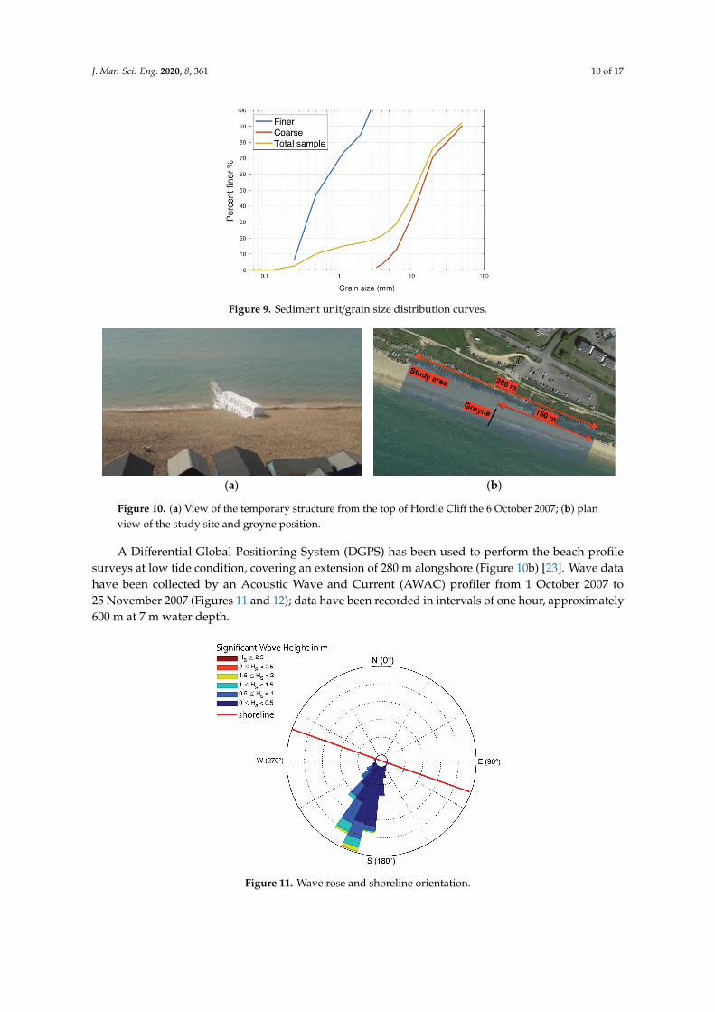
Shoreline evolution has been observed during a field experiment conducted in 2007 at Milford-on-Sea, under Hordle Cliff, located in the county of Hampshire on the Southern coast of the UK [23–25]. The coastal area of Milford-on-Sea, at the eastern side of Christchurch Bay (Figure 8), is characterized by a mixed shingle and sand beach, composed by finer (sand) and coarse (cobbles, gravel) sediment units/grains (Dn50 = 11.19 mm; D85/D15 = 27.79, where D85 and D15 represent the particle diameter for which 85% and 15%, respectively, of the material is finer) (Figure 9).

Figure 8. Study area location.

−90° +90°

+15°

Figure 7. Calculated shoreline evolution for t = 1 day, 1 month, 6 months, 1 year, 2 years.

2.4. Field Experiment at a Mixed Beach

Study Area and Field Observations

Shoreline evolution has been observed during a field experiment conducted in 2007 atMilford-on-Sea, under Hordle Cliff, located in the county of Hampshire on the Southern coastof the UK [23–25]. The coastal area of Milford-on-Sea, at the eastern side of Christchurch Bay (Figure 8),is characterized by a mixed shingle and sand beach, composed by finer (sand) and coarse (cobbles,gravel) sediment units/grains (Dn50 = 11.19 mm; D85/D15 = 27.79, where D85 and D15 represent theparticle diameter for which 85% and 15%, respectively, of the material is finer) (Figure 9).

An impoundment technique has been adopted consisting of a temporary impermeable groyne46 m long (originally 19 m wet and 27 dry) deployed along the beach for the period 1 October2007–15 November 2007, acting as a barrier for the sediments moving along the coast (Figure 10a).This technique is considered by several authors as a reliable and effective method to estimate longshoretransport rates [40,48–50].

J. Mar. Sci. Eng. 2020, 8, x FOR PEER REVIEW 10 of 18

2.3.3. Influence of Duration

In order to assess the capacity of the model to determine short-term (daily base), medium-term (monthly base) or long-term (yearly base) shoreline evolution, different values of duration of simulation have been considered. The adopted input parameters are given in Table 2, with t = 1 day, 1 month, 6 months, 1 year, 2 years. Figure 7 shows the calculated shoreline evolution induced by longshore transport.

Figure 7. Calculated shoreline evolution for t = 1 day, 1 month, 6 months, 1 year, 2 years.

The shoreline advance/retreat rate increases with a longer duration of simulation. On the left (updrift)/right (downdrift) side of the groyne, shoreline advance/retreat rates, equal to 2.1, 14.2, 40.9, 52.4 and 63.6 m, have been obtained for t = 1 day, 1 month, 6 months, 1 year and 2 years, respectively.

2.4. Field Experiment at a Mixed Beach

Study Area and Field Observations

Shoreline evolution has been observed during a field experiment conducted in 2007 at Milford-on-Sea, under Hordle Cliff, located in the county of Hampshire on the Southern coast of the UK [23–25]. The coastal area of Milford-on-Sea, at the eastern side of Christchurch Bay (Figure 8), is characterized by a mixed shingle and sand beach, composed by finer (sand) and coarse (cobbles, gravel) sediment units/grains (Dn50 = 11.19 mm; D85/D15 = 27.79, where D85 and D15 represent the particle diameter for which 85% and 15%, respectively, of the material is finer) (Figure 9).

Figure 8. Study area location.

−90° +90°

+15°

Figure 8. Study area location.

J. Mar. Sci. Eng. 2020, 8, 361 10 of 17J. Mar. Sci. Eng. 2020, 8, x FOR PEER REVIEW 11 of 18

Figure 9. Sediment unit/grain size distribution curves.

An impoundment technique has been adopted consisting of a temporary impermeable groyne 46 m long (originally 19 m wet and 27 dry) deployed along the beach for the period 1 October 2007–15 November 2007, acting as a barrier for the sediments moving along the coast (Figure 10a). This technique is considered by several authors as a reliable and effective method to estimate longshore transport rates [40,48–50].

A Differential Global Positioning System (DGPS) has been used to perform the beach profile surveys at low tide condition, covering an extension of 280 m alongshore (Figure 10b) [23]. Wave data have been collected by an Acoustic Wave and Current (AWAC) profiler from 1 October 2007 to 25 November 2007 (Figures 11 and 12); data have been recorded in intervals of one hour, approximately 600 m at 7 m water depth.

(a)

(b)

Figure 10. (a) View of the temporary structure from the top of Hordle Cliff the 6 October 2007; (b) plan view of the study site and groyne position.

Figure 9. Sediment unit/grain size distribution curves.

J. Mar. Sci. Eng. 2020, 8, x FOR PEER REVIEW 11 of 18

Figure 9. Sediment unit/grain size distribution curves.

An impoundment technique has been adopted consisting of a temporary impermeable groyne 46 m long (originally 19 m wet and 27 dry) deployed along the beach for the period 1 October 2007–15 November 2007, acting as a barrier for the sediments moving along the coast (Figure 10a). This technique is considered by several authors as a reliable and effective method to estimate longshore transport rates [40,48–50].

A Differential Global Positioning System (DGPS) has been used to perform the beach profile surveys at low tide condition, covering an extension of 280 m alongshore (Figure 10b) [23]. Wave data have been collected by an Acoustic Wave and Current (AWAC) profiler from 1 October 2007 to 25 November 2007 (Figures 11 and 12); data have been recorded in intervals of one hour, approximately 600 m at 7 m water depth.

(a)

(b)

Figure 10. (a) View of the temporary structure from the top of Hordle Cliff the 6 October 2007; (b) plan view of the study site and groyne position. Figure 10. (a) View of the temporary structure from the top of Hordle Cliff the 6 October 2007; (b) planview of the study site and groyne position.

A Differential Global Positioning System (DGPS) has been used to perform the beach profilesurveys at low tide condition, covering an extension of 280 m alongshore (Figure 10b) [23]. Wave datahave been collected by an Acoustic Wave and Current (AWAC) profiler from 1 October 2007 to25 November 2007 (Figures 11 and 12); data have been recorded in intervals of one hour, approximately600 m at 7 m water depth.J. Mar. Sci. Eng. 2020, 8, x FOR PEER REVIEW 12 of 18

Figure 11. Wave rose and shoreline orientation.

Figure 12. Time history of significant wave height, peak period and wave angle.

3. GSb Calibration and Verification for a Mixed Beach

3.1. Calibration

The calibration of the GSb model has been conducted based on the comparison between the observed and calculated shoreline evolution. Values of KGSb = 0.005, 0.01, 0.05, 0.1, 0.2 have been adopted. The first beach survey collected in presence of the groyne (1 October 2007) has been assumed as the initial shoreline. Based on an accurate evaluation of the cross-shore beach profile evolution over time, DC and DB have been selected equal to 1 m and 3 m, respectively (Figure 13) [23]. A value of Dn50 = 11.19 mm has been adopted. The considered groyne has been positioned at the 31st cell of the domain, corresponding to x = 150/155 m. Hourly wave conditions (Hs, Tp, Dir) have been considered in the simulations (Figures 11 and 12). The computational domain has been assumed 280 m long; DX has been set equal to 5 m with NX = 57. The calculation time step has been set to 0.05 h (180 s), for a total duration of simulation equal to 45 days from the groyne deployment (t = 0). In accordance with [11] the boundary conditions have been set as fixed, since they are located far away from the groyne (i.e., the length of the entire calculation domain is in the order of two or three groyne

Figure 11. Wave rose and shoreline orientation.

J. Mar. Sci. Eng. 2020, 8, 361 11 of 17

J. Mar. Sci. Eng. 2020, 8, x FOR PEER REVIEW 12 of 18

Figure 11. Wave rose and shoreline orientation.

Figure 12. Time history of significant wave height, peak period and wave angle.

3. GSb Calibration and Verification for a Mixed Beach

3.1. Calibration

The calibration of the GSb model has been conducted based on the comparison between the observed and calculated shoreline evolution. Values of KGSb = 0.005, 0.01, 0.05, 0.1, 0.2 have been adopted. The first beach survey collected in presence of the groyne (1 October 2007) has been assumed as the initial shoreline. Based on an accurate evaluation of the cross-shore beach profile evolution over time, DC and DB have been selected equal to 1 m and 3 m, respectively (Figure 13) [23]. A value of Dn50 = 11.19 mm has been adopted. The considered groyne has been positioned at the 31st cell of the domain, corresponding to x = 150/155 m. Hourly wave conditions (Hs, Tp, Dir) have been considered in the simulations (Figures 11 and 12). The computational domain has been assumed 280 m long; DX has been set equal to 5 m with NX = 57. The calculation time step has been set to 0.05 h (180 s), for a total duration of simulation equal to 45 days from the groyne deployment (t = 0). In accordance with [11] the boundary conditions have been set as fixed, since they are located far away from the groyne (i.e., the length of the entire calculation domain is in the order of two or three groyne

Figure 12. Time history of significant wave height, peak period and wave angle.

3. GSb Calibration and Verification for a Mixed Beach

3.1. Calibration

The calibration of the GSb model has been conducted based on the comparison between theobserved and calculated shoreline evolution. Values of KGSb = 0.005, 0.01, 0.05, 0.1, 0.2 have beenadopted. The first beach survey collected in presence of the groyne (1 October 2007) has been assumedas the initial shoreline. Based on an accurate evaluation of the cross-shore beach profile evolution overtime, DC and DB have been selected equal to 1 m and 3 m, respectively (Figure 13) [23]. A value ofDn50 = 11.19 mm has been adopted. The considered groyne has been positioned at the 31st cell of thedomain, corresponding to x = 150/155 m. Hourly wave conditions (Hs, Tp, Dir) have been consideredin the simulations (Figures 11 and 12). The computational domain has been assumed 280 m long;DX has been set equal to 5 m with NX = 57. The calculation time step has been set to 0.05 h (180 s),for a total duration of simulation equal to 45 days from the groyne deployment (t = 0). In accordancewith [11] the boundary conditions have been set as fixed, since they are located far away from the groyne(i.e., the length of the entire calculation domain is in the order of two or three groyne length). It assuresthat the boundary conditions are unaffected by changes that take place in the vicinity of the groyne.

J. Mar. Sci. Eng. 2020, 8, x FOR PEER REVIEW 13 of 18

length). It assures that the boundary conditions are unaffected by changes that take place in the vicinity of the groyne.

Figure 13. Surveyed cross-shore beach profile at Milford-on-Sea.

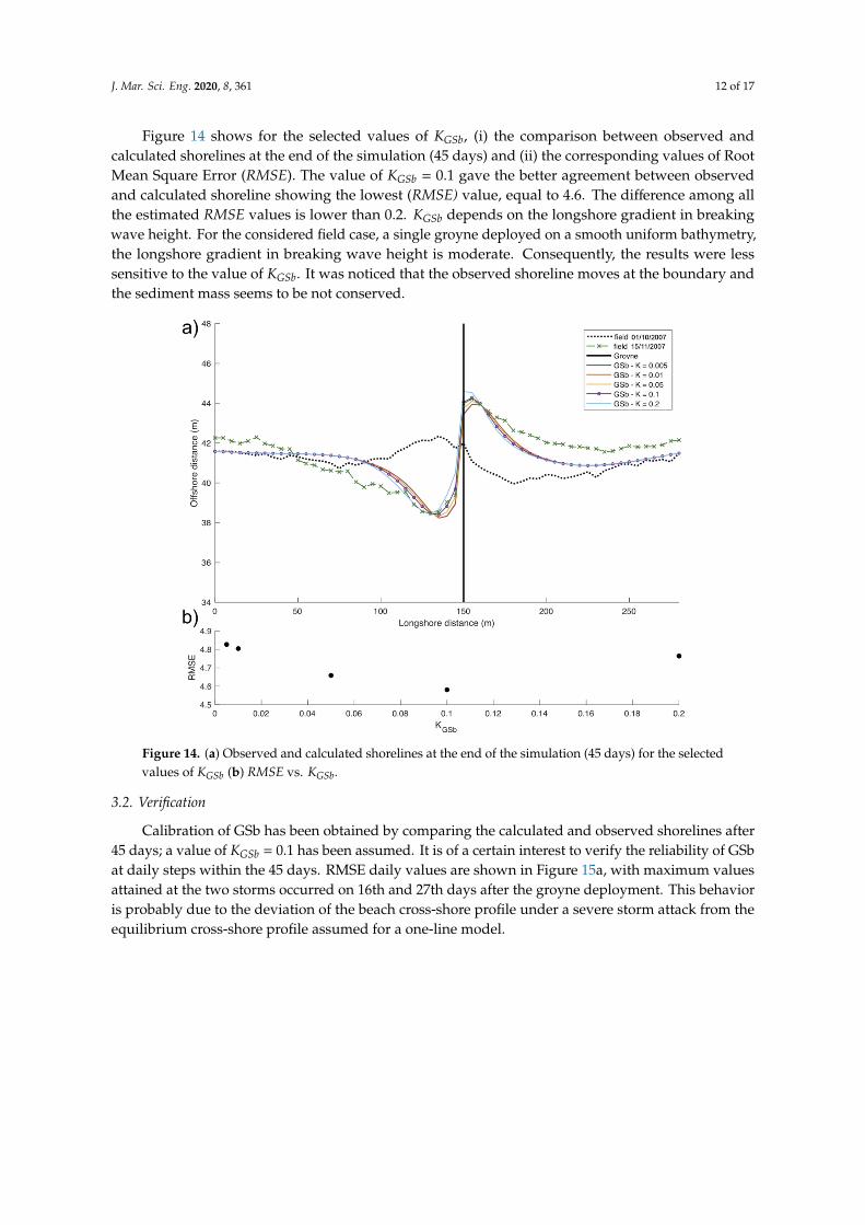
Figure 14 shows for the selected values of KGSb, (i) the comparison between observed and calculated shorelines at the end of the simulation (45 days) and (ii) the corresponding values of Root Mean Square Error (RMSE). The value of KGSb = 0.1 gave the better agreement between observed and calculated shoreline showing the lowest (RMSE) value, equal to 4.6. The difference among all the estimated RMSE values is lower than 0.2. KGSb depends on the longshore gradient in breaking wave height. For the considered field case, a single groyne deployed on a smooth uniform bathymetry, the longshore gradient in breaking wave height is moderate. Consequently, the results were less sensitive to the value of KGSb. It was noticed that the observed shoreline moves at the boundary and the sediment mass seems to be not conserved.

Figure 14. (a) Observed and calculated shorelines at the end of the simulation (45 days) for the selected values of KGSb (b) RMSE vs. KGSb.

Figure 13. Surveyed cross-shore beach profile at Milford-on-Sea.

J. Mar. Sci. Eng. 2020, 8, 361 12 of 17

Figure 14 shows for the selected values of KGSb, (i) the comparison between observed andcalculated shorelines at the end of the simulation (45 days) and (ii) the corresponding values of RootMean Square Error (RMSE). The value of KGSb = 0.1 gave the better agreement between observedand calculated shoreline showing the lowest (RMSE) value, equal to 4.6. The difference among allthe estimated RMSE values is lower than 0.2. KGSb depends on the longshore gradient in breakingwave height. For the considered field case, a single groyne deployed on a smooth uniform bathymetry,the longshore gradient in breaking wave height is moderate. Consequently, the results were lesssensitive to the value of KGSb. It was noticed that the observed shoreline moves at the boundary andthe sediment mass seems to be not conserved.

J. Mar. Sci. Eng. 2020, 8, x FOR PEER REVIEW 13 of 18

length). It assures that the boundary conditions are unaffected by changes that take place in the vicinity of the groyne.

Figure 13. Surveyed cross-shore beach profile at Milford-on-Sea.

Figure 14 shows for the selected values of KGSb, (i) the comparison between observed and calculated shorelines at the end of the simulation (45 days) and (ii) the corresponding values of Root Mean Square Error (RMSE). The value of KGSb = 0.1 gave the better agreement between observed and calculated shoreline showing the lowest (RMSE) value, equal to 4.6. The difference among all the estimated RMSE values is lower than 0.2. KGSb depends on the longshore gradient in breaking wave height. For the considered field case, a single groyne deployed on a smooth uniform bathymetry, the longshore gradient in breaking wave height is moderate. Consequently, the results were less sensitive to the value of KGSb. It was noticed that the observed shoreline moves at the boundary and the sediment mass seems to be not conserved.

Figure 14. (a) Observed and calculated shorelines at the end of the simulation (45 days) for the selected values of KGSb (b) RMSE vs. KGSb.

Figure 14. (a) Observed and calculated shorelines at the end of the simulation (45 days) for the selectedvalues of KGSb (b) RMSE vs. KGSb.

3.2. Verification

Calibration of GSb has been obtained by comparing the calculated and observed shorelines after45 days; a value of KGSb = 0.1 has been assumed. It is of a certain interest to verify the reliability of GSbat daily steps within the 45 days. RMSE daily values are shown in Figure 15a, with maximum valuesattained at the two storms occurred on 16th and 27th days after the groyne deployment. This behavioris probably due to the deviation of the beach cross-shore profile under a severe storm attack from theequilibrium cross-shore profile assumed for a one-line model.

J. Mar. Sci. Eng. 2020, 8, 361 13 of 17

J. Mar. Sci. Eng. 2020, 8, x FOR PEER REVIEW 14 of 18

3.2. Verification

Calibration of GSb has been obtained by comparing the calculated and observed shorelines after 45 days; a value of KGSb = 0.1 has been assumed. It is of a certain interest to verify the reliability of GSb at daily steps within the 45 days. RMSE daily values are shown in Figure 15a, with maximum values attained at the two storms occurred on 16th and 27th days after the groyne deployment. This behavior is probably due to the deviation of the beach cross-shore profile under a severe storm attack from the equilibrium cross-shore profile assumed for a one-line model.

Figure 15. (a) Estimated RMSE daily values. (b) Time history of significant wave height and wave angle.

Figures 16–18 show, as representative cases, the comparison between observed and calculated shorelines, and the difference, Yobs–YGSb, after 24 days (25 October 2007), 39 days (09 November 2007) and 45 days (15 November 2007) from the groyne deployment. Yobs and YGSb are the distances from the x-axis to the observed and calculated shorelines, respectively.

Figure 16. (a) Observed and calculated shorelines after 24 days from the groyne deployment. (b) Difference Yobs–YGSb.

Figure 15. (a) Estimated RMSE daily values. (b) Time history of significant wave height and wave angle.

Figures 16–18 show, as representative cases, the comparison between observed and calculatedshorelines, and the difference, Yobs–YGSb, after 24 days (25 October 2007), 39 days (09 November 2007)and 45 days (15 November 2007) from the groyne deployment. Yobs and YGSb are the distances fromthe x-axis to the observed and calculated shorelines, respectively.

The comparisons show a good agreement between observed and calculated shorelines at bothgroyne sides. In particular, after 24 days (Figure 16) from the groyne deployment, a shoreline advanceon the left side of the groyne has been observed; after 39 days (Figure 17) and 45 days (Figure 18)from the groyne deployment, a shoreline advance on the right side of the groyne has been observed.GSb calculated the up-drift side changes occurred during the entire period of the simulation.

J. Mar. Sci. Eng. 2020, 8, x FOR PEER REVIEW 14 of 18

3.2. Verification

Calibration of GSb has been obtained by comparing the calculated and observed shorelines after 45 days; a value of KGSb = 0.1 has been assumed. It is of a certain interest to verify the reliability of GSb at daily steps within the 45 days. RMSE daily values are shown in Figure 15a, with maximum values attained at the two storms occurred on 16th and 27th days after the groyne deployment. This behavior is probably due to the deviation of the beach cross-shore profile under a severe storm attack from the equilibrium cross-shore profile assumed for a one-line model.

Figure 15. (a) Estimated RMSE daily values. (b) Time history of significant wave height and wave angle.

Figures 16–18 show, as representative cases, the comparison between observed and calculated shorelines, and the difference, Yobs–YGSb, after 24 days (25 October 2007), 39 days (09 November 2007) and 45 days (15 November 2007) from the groyne deployment. Yobs and YGSb are the distances from the x-axis to the observed and calculated shorelines, respectively.

Figure 16. (a) Observed and calculated shorelines after 24 days from the groyne deployment. (b) Difference Yobs–YGSb.

Figure 16. (a) Observed and calculated shorelines after 24 days from the groyne deployment.(b) Difference Yobs–YGSb.

J. Mar. Sci. Eng. 2020, 8, 361 14 of 17J. Mar. Sci. Eng. 2020, 8, x FOR PEER REVIEW 15 of 18

Figure 17. (a) Observed and calculated shorelines after 39 days from the groyne deployment. (b) Difference Yobs–YGSb.

Figure 18. (a) Observed and calculated shorelines after 45 days from the groyne deployment. (b) Difference Yobs–YGSb.

The comparisons show a good agreement between observed and calculated shorelines at both groyne sides. In particular, after 24 days (Figure 16) from the groyne deployment, a shoreline advance on the left side of the groyne has been observed; after 39 days (Figure 17) and 45 days (Figure 18) from the groyne deployment, a shoreline advance on the right side of the groyne has been observed. GSb calculated the up-drift side changes occurred during the entire period of the simulation.

Figure 17. (a) Observed and calculated shorelines after 39 days from the groyne deployment.(b) Difference Yobs–YGSb.

J. Mar. Sci. Eng. 2020, 8, x FOR PEER REVIEW 15 of 18

Figure 17. (a) Observed and calculated shorelines after 39 days from the groyne deployment. (b) Difference Yobs–YGSb.

Figure 18. (a) Observed and calculated shorelines after 45 days from the groyne deployment. (b) Difference Yobs–YGSb.

The comparisons show a good agreement between observed and calculated shorelines at both groyne sides. In particular, after 24 days (Figure 16) from the groyne deployment, a shoreline advance on the left side of the groyne has been observed; after 39 days (Figure 17) and 45 days (Figure 18) from the groyne deployment, a shoreline advance on the right side of the groyne has been observed. GSb calculated the up-drift side changes occurred during the entire period of the simulation.

Figure 18. (a) Observed and calculated shorelines after 45 days from the groyne deployment.(b) Difference Yobs–YGSb.

4. Conclusions

To date, the development and use of morphodynamic models focusing on sandy beaches havereceived the bulk of the attention. Belonging to the one-line model typology, the GSb model is proposedincluding a general formula suitable for estimation of longshore transport at coastal mound made ofnon-cohesive sediment grains/units as sand, gravel, cobbles, shingle and rock.

As its main peculiarity, GSb allows to have an explicit dependence of shoreline evolution on Dn50.This finding is due to the fact that GSb uses the GLT model. Differently from GENESIS and similarmodels, which take into account two calibration coefficient, K1 and K2, the GSb model presents onecalibration coefficient, KGSb, which does not depend on the grain size diameter and depends on thelongshore gradient in breaking wave height, solely.

J. Mar. Sci. Eng. 2020, 8, 361 15 of 17

The reliability of the GSb model to predict coastal morphology over short- and medium-termtime scales has been verified based on a high-quality field experiment data base from a specific fieldcase at a mixed beach. Such a source of data is rarely available; indeed, most published sources ofshingle/mixed beach data failed on the lack of concurrent wave measurements and transport rates.As a result, the comparison between observed and calculated shorelines in the presence of a temporarygroyne shows the premonitory signs that the GSb model can represent a reliable engineering toolsuitable for predicting coastal evolution at a mixed beach.

A demo version of the numerical model can be downloaded by following the instructions in thesupplementary material section.

Supplementary Materials: A demo version of the GSb numerical model, for Mac and Windows systems, has beenmade available for the scientific community and can be downloaded at: www.scacr.eu, www.eumer.eu.

Author Contributions: Conceptualization, G.R.T., F.F. and A.F.; methodology, G.R.T., D.J.S., F.D. and A.F.; software,A.F., G.R.T. and F.F.; validation, G.R.T., F.F. and A.F.; formal analysis, G.R.T., F.D. and A.F.; investigation, G.R.T.,D.J.S., F.D., F.F. and A.F.; data curation, D.J.S.; supervision, G.R.T.; funding, G.R.T. and D.J.S. All authors have readand agreed to the published version of the manuscript.

Funding: The present work has been supported by the Regione Puglia through the grant to the budget of the projecttitled “Sperimentazione di tecnologie innovative per il consolidamento di dune costiere (INNO-DUNECOST),”POR Puglia FESR FSE 2014–2020-Sub-Azione 1.4.B, Contract n. RM5UKM3. The field experiment of the presentresearch was funded by the Faculty of Technology of Plymouth University and the EPSRC (Engineering andPhysical Sciences Research Council) under the Grant EP/C005392/1 “A Risk-based Framework for PredictingLong-term Beach Evolution”. The work has been also supported by Regione Calabria, through the PhD grant forinternational exchange.

Acknowledgments: We gratefully acknowledge the University of Salento, Department of Engineering,the University of Calabria, Department of Civil Engineering, and University of Plymouth, COAST EngineeringResearch Group, which permitted the international exchange making possible this research. We thank MarkDavidson of CPRG at Plymouth University for his contribution relating to field data. We gratefully acknowledgethe comments of the three anonymous reviewers who helped to substantially improve the original version ofthis manuscript.

Conflicts of Interest: The authors declare no conflict of interest.

References

1. Van Rijn, L.C.; Ribberink, J.S.; Werf, J.V.D.; Walstra, D.J. Coastal sediment dynamics: Recent advances andfuture research needs. J. Hydraul. Res. 2013, 51, 475–493. [CrossRef]

2. Güner, H.A.A.; Yüksel, Y.; Çevik, E.Ö. Determination of Longshore Sediment Transport and Modelling ofShoreline Change. Sediment Transp. 2011, 117. [CrossRef]

3. Hanson, H. GENESIS: A generalized shoreline change numerical model. J. Coast. Res. 1989, 5, 1–27.4. Dabees, M.; Kamphuis, J.W. ONELINE, a numerical model for shoreline change. In Proceedings of the 26th

Int. Conf. On Coastal Engineering, ASCE, Copenhagen, Denmark, 22–26 June 1998; pp. 2668–2681.5. Deltares. UNIBEST-CL+ Manual: Manual for Version 7.1 of the Shoreline Model UNIBEST-CL.; Deltares: Delft,

The Netherlands, 2011.6. DHI. Litpack: Noncohesive Sediment Transport in Currents and Waves. User Guide; Danish Hydraulic Institute:

Hørsholm, Denmark, 2005.7. Blanco, B. Beachplan (Version 04.01) Model. Description; HR Wallingford Report; Springer Nature:

Berlin/Heidelberg, Germany, 2003.8. González, M.; Medina, R.; González-Ondina, J.; Osorio, A.; Méndez, F.; García, E. An integrated coastal

modeling system for analyzing beach processes and beach restoration projects, SMC. Comput. Geosci. 2007,33, 916–931. [CrossRef]

9. Frey, A.E.; Connell, K.J.; Hanson, H.; Larson, M.; Thomas, R.C.; Munger, S.; Zundel, A. GenCade Version 1Model. Theory and User’s Guide; Engineer Research And Development Center, Vicksburg Ms Coastal InletsResearch Program: Vicksburg, MS, USA, 2012.

10. Vionnet, C.; García, M.H.; Latrubesse, E.; Perillo, G. River, Coastal and Estuarine Morphodynamics; RCEM 2009,Two Volume Set; CRC Press: Boca Raton, FL, USA, 2018.

J. Mar. Sci. Eng. 2020, 8, 361 16 of 17

11. USACE. Shore Protection Manual; Dept. of the Army, Waterways Experiment Station, Corps of Engineers;Coastal Engineering Research Center: Vicksburg, MS, USA, 1984.

12. Kamphuis, J.W. Alongshore sediment transport rate. J. Waterw. Port Coast. Ocean Eng. 1991, 117, 624–640.[CrossRef]

13. Bijker, E.W. Longshore transport computations. J. Waterw. Harb. Coast. Eng. Div. 1971, 97, 687–701.14. Van Rijn, L.C. Principles of Sediment Transport In Rivers, Estuaries And Coastal Seas; Aqua Publications:

Amsterdam, The Netherlands, 1993; Volume 1006.15. Bailard, J.A. An energetics total load sediment transport model for a plane sloping beach. J. Geophys.

Res. Ocean 1981, 86, 10938–10954. [CrossRef]16. DHI. Littoral Processes FM, User Guide; Danish Hydraulic Institute: Hørsholm, Denmark, 2017.17. Tomasicchio, G.R.; D‘Alessandro, F.; Musci, F. A multi-layer capping of a coastal area contaminated with

materials dangerous to health. Chem. Ecol. 2010, 26, 155–168. [CrossRef]18. Bramato, S.; Ortega-Sánchez, M.; Mans, C.; Losada, M.A. Natural Recovery of a Mixed Sand and Gravel

Beach after a Sequence of a Short Duration Storm and Moderate Sea States. J. Coast. Res. 2012, 28, 89–101.[CrossRef]

19. Van Rijn, L.C. A simple general expression for longshore transport of sand, gravel and shingle. Coast. Eng.2014, 90, 23–39. [CrossRef]

20. Hanson, H.; Kraus, N.C. Optimization of beach fill transitions. In Proceedings of the Coastal Zone, ASCE,New York, NY, USA, 19–23 July 1993; pp. 103–117.

21. Van Alphen, J.S.; Hallie, F.P.; Ribberink, J.S.; Roelvink, J.; Louisse, C.J. Offshore sand extraction and nearshoreprofile nourishment. In Proceedings of the 22nd Coastal Engineering Conference, Delft, The Netherlands,2–6 July 1991; pp. 1998–2009.

22. Hamm, L.; Capobianco, M.; Dette, H.; Lechuga, A.; Spanhoff, R.; Stive, M. A summary of European experiencewith shore nourishment. Coast. Eng. 2002, 47, 237–264. [CrossRef]

23. Martín-Grandes, I.; Hughes, J.; Simmonds, D.J.; Chadwick, A.J.; Reeve, D.E. Novel methodology for oneline model calibration using impoundment on mixed beach. In Proceedings of the Coastal Dynamics2009: Impacts of Human Activities on Dynamic Coastal Processes, Tokyo, Japan, 7–11 September 2009;World Scientific: Singapore, 2009; pp. 1–10.

24. Martin-Grandes, I.; Simmonds, D.J.; Karunarathna, H.; Horrillo-Caraballo, J.M.; Reeve, D.E. Assessingthe Variability of Longshore Transport Rate Coefficient on a Mixed Beach. In Proceedings of the CoastalDynamics, Helsingør, Denmark, 12–16 June 2017; pp. 642–653.

25. Martin-Grandes, I. Understanding Longshore Sediment Transport on a Mixed Beach. Ph.D. Thesis, PlymouthUniversity, Plymouth, UK, 2014.

26. Lamberti, A.; Tomasicchio, G.R. Stone mobility and longshore transport at reshaping breakwaters. Coast. Eng.1997, 29, 263–289. [CrossRef]

27. Tomasicchio, G.R.; D’Alessandro, F.; Frega, F.; Francone, A.; Ligorio, F. Recent improvements for estimationof longshore transport. Ital. J. Eng. Geol. Environ. 2018, 1, 179–187.

28. Tomasicchio, G.R.; D‘Alessandro, F.; Barbaro, G.; Malara, G. General longshore transport model. Coast. Eng.2013, 71, 28–36. [CrossRef]

29. Ahrens, J.P. Characteristics of Reef Breakwaters, (No. CERC-TR-87–17); Coastal Engineering Research Center:Vicksburg, MS, USA, 1987.

30. Van der Meer, J.W. Rock Slopes and Gravel Beaches under Wave Attack. Ph.D. Thesis, Delft HydraulicsLaboratory, Delft, The Netherlands, 1988.

31. Klopman, G.; Stive, M. Extreme waves and wave loading in shallow water. In Proceedings of the Wave andCurrent Kinematics and Loading: E&P Forum Workshop, Paris, France, 25–26 October 1989.

32. Battjes, J.A.; Groenendijk, H.W. Wave height distributions on shallow foreshores. Coast. Eng. 2000, 40,161–182. [CrossRef]

33. Komar, P.D.; Gaughan, M.K. Airy wave theory and breaker height prediction. In Proceedings of the 13thConf. on Coastal Engineering, Vancouver, Canada, 29 January 1972; pp. 405–418.

34. Tomasicchio, G.; Lamberti, A.; Guiducci, F. Stone movement on a reshaped profile. In Proceedings of the24th International Conf. on Coastal Engineering, ASCE, Kobe, Japan, 23–28 October 1994; pp. 1625–1640.

J. Mar. Sci. Eng. 2020, 8, 361 17 of 17

35. Tørum, A.; Sigurdarson, S. PIANC Working Group No. 40: Guidelines for the Design and Constructionof Berm Breakwaters. In Proceedings of the Breakwaters, Coastal Structures and Coastlines, London, UK,26–28 September 2001; pp. 373–384.

36. Pelnard-Considere, R. Essai de theorie de l’evolution des formes de rivage en plages de sable et de galets.In Proceedings of the Les Energies de la Mer: Compte Rendu Des. Quatriemes Journees de L’hydraulique,Paris, France, 13–15 June 1956. rapport 1, 74-1-10.

37. Bruun, P. Coast. Erosion and the Development of Beach Profiles; US Beach Erosion Board: Washington, DC, USA,1954; Volume 44.

38. Dean, R.G. Equilibrium Beach Profiles: US Atlantic and Gulf Coasts; Department of Civil Engineering andCollege of Marine Studies, Newark, University of Delaware: Newark, DE, USA, 1977.

39. Hanson, H.; Kraus, N.C. GENESIS: Generalized Model. for Simulating Shoreline Change. Report 1. TechnicalReference; Coastal Engineering Research Center: Vicksburg, MS, USA, 1989.

40. Tomasicchio, G.R.; D’Alessandro, F.; Barbaro, G.; Musci, E.; De Giosa, T.M. Longshore transport at shinglebeaches: An independent verification of the general model. Coast. Eng. 2015, 104, 69–75. [CrossRef]

41. Hanson, H. GENESIS: A Generalized Shoreline Change Numerical Model for Engineering Use; Department ofWater Resources Engineering, Lund University: Lund, Sweden, 1987.

42. Ozasa, H.; Brampton, A. Mathematical modelling of beaches backed by seawalls. Coast. Eng. 1980, 4, 47–63.[CrossRef]

43. Medellín, G.; Torres-Freyermuth, A.; Tomasicchio, G.R.; Francone, A.; Tereszkiewicz, P.A.; Lusito, L.;Palemón-Arcos, L.; López, J. Field and numerical study of resistance and resilience on a sea breeze dominatedbeach in Yucatan (Mexico). Water 2018, 10, 1806. [CrossRef]

44. Hamza, W.; Tomasicchio, G.R.; Ligorio, F.; Lusito, L.; Francone, A. A Nourishment Performance Index forBeach Erosion/Accretion at Saadiyat Island in Abu Dhabi. J. Mar. Sci. Eng. 2019, 7, 173. [CrossRef]

45. Hallermeier, R.J. Sand transport limits in coastal structure designs. In Proceedings of the Coastal Structures’83, Washington, DC, USA, 9–11 March 1983; pp. 703–716.

46. Goda, Y.; Takayama, T.; Suzuki, Y. Diffraction Diagrams for Directional Random Waves. In Proceedings ofthe 16th International Conference on Coastal Engineering, Hamburg, Germany, 27 August–3 September1978; Volume 1.

47. Larson, M. Numerical modeling. In Encyclopedia of Coastal Science; Schwartz, M., Ed.; Springer: Dordrecht,The Netherlands, 2005; pp. 730–733.

48. Bodge, K.R.; Dean, R.G. Short-term impoundment of longshore transport. In Proceedings of the CoastalSediments, New Orleans, Louisiana, 12–14 May 1987; pp. 468–483.

49. Wang, P.; Kraus, N.C. Longshore sediment transport rate measured by short-term impoundment. J. Waterw.Port Coast. Ocean Eng. 1999, 125, 118–126. [CrossRef]

50. Van Wellen, E.; Chadwick, A.; Mason, T. A review and assessment of longshore sediment transport equationsfor coarse-grained beaches. Coast. Eng. 2000, 40, 243–275. [CrossRef]

© 2020 by the authors. Licensee MDPI, Basel, Switzerland. This article is an open accessarticle distributed under the terms and conditions of the Creative Commons Attribution(CC BY) license (http://creativecommons.org/licenses/by/4.0/).