Predicting spatial and temporal patterns of soil temperature based on topography, surface cover and...

Predicting spatial and temporal patterns of soil temperaturebased on topography, surface cover and air temperature

S. Kang, S. Kim, S. Oh, D. Lee*

Department of Environmental Planning, Graduate School of Environmental Studies,

Seoul National University, Seoul 151-742, South Korea

Received 7 May 1999; accepted 26 September 1999

Abstract

Soil temperature is a variable that links surface structure to soil processes and yet its spatial prediction across landscapes

with variable surface structure is poorly understood. In this study, a hybrid soil temperature model was developed to predict

daily spatial patterns of soil temperature in a forested landscape by incorporating the effects of topography, canopy and ground

litter. The model is based on both heat transfer physics and empirical relationship between air and soil temperature, and uses

input variables that are extracted from a digital elevation model (DEM), satellite imagery, and standard weather records.

Model-predicted soil temperatures ®tted well with data measured at 10 cm soil depth at three sites: two hardwood forests and a

bare soil area. A sensitivity analysis showed that the model was highly sensitive to leaf area index (LAI) and air temperature.

When the spatial pattern of soil temperature in a forested watershed was simulated by the model, different responses of bare

and canopy-closed ground to air temperature were identi®ed. Spatial distribution of daily air temperature was geostatistically

interpolated from the data of weather stations adjacent to the simulated area. Spatial distribution of LAI was obtained from

Landsat Thematic Mapper images. The hybrid model describes spatial variability of soil temperature across landscapes and

different sensitivity to rising air temperature depending on site-speci®c surface structures, such as LAI and ground litter stores.

In addition, the model may be bene®cially incorporated into other ecosystem models requiring soil temperature as one of the

input variables. # 2000 Elsevier Science B.V. All rights reserved.

Keywords: Daily soil temperature; Hybrid model; LAI; Spatial mapping

1. Introduction

During the past decades, spatial data of meteoro-

logical and soil-physical conditions across landscapes

have received much attention. Many studies on spatial

patterns of air temperature (Hudson and Wackernagel,

1994; Goward et al., 1994; Willmott and Robeson,

1995; Thornton et al., 1997), precipitation (Daly et al.,

1994), humidity (Kimball et al., 1997), available soil

water capacity (Zheng et al., 1996), and soil water

content (Saha, 1995) have been carried out. Spatial

prediction of soil temperature, however, is still a

dif®cult task in spite of its importance in many

ecological processes. This is mainly because soil

temperature, if measured at all, has rarely been ana-

lyzed in relation to structural features although those

are necessarily linked to measured data for spatial

extrapolation across landscapes. It was reported that

root growth and physiological activity of plants, and

biological soil activity are largely in¯uenced by soil

Forest Ecology and Management 136 (2000) 173±184

* Corresponding author. Tel.: �82-2-880-5650;

fax: �82-2-873-5109.

E-mail address: [email protected] (D. Lee)

0378-1127/00/$ ± see front matter # 2000 Elsevier Science B.V. All rights reserved.

PII: S 0 3 7 8 - 1 1 2 7 ( 9 9 ) 0 0 2 9 0 - X

temperature (Kozlowski and Pallardy, 1997). Soil

temperature also in¯uences seasonal variation of

CO2 ef¯ux from forest soils (Raich and Schlesinger,

1992; Trumbore et al., 1996; Rochette and Gregorich,

1998; Russell and Voroney, 1998; Striegl and Wick-

land, 1998). The evidence indicates that the prediction

on spatial and temporal patterns of soil temperature

will enhance our understanding on the dynamics of

vegetation and soil organic matter across landscapes.

In soil heat physics, soil temperature is known as a

variable dependent on a number of other variables or

parameters, including meteorological conditions such

as surface global radiation and air temperature, soil

physical parameters such as albedo of surface, water

content and texture, topographical variables such as

elevation, slope and aspect, and other surface char-

acteristics such as leaf area index (LAI, projected leaf

area per unit of ground area) and ground litter stores.

Hence, spatial and temporal variation of those vari-

ables may be directly linked to soil temperature and

thus spatial heterogeneity of biogeochemistry in

forested landscape.

Soil temperature might be estimated by two differ-

ent approaches based upon: (1) soil heat ¯ow and

energy balance (Rosenberg et al., 1983; Thunholm,

1990; Marshall et al., 1996), and (2) empirical corre-

lations with easily acquired variables (Zheng et al.,

1993). Although the former approach can give accu-

rate predictions for an well-evaluated site, it is dif®cult

to apply across landscapes because of insuf®cient

database for calculating heat transfer equations.

Furthermore, temporal patterns of surface global

radiation across landscapes necessary for calculating

key boundary conditions is dif®cult to predict in

terrain area (Hungerford et al., 1989; Dozier and Frew,

1990; Dubayah, 1992, 1994; Dubayah and Loechel,

1997; Thornton et al., 1997; Antonic, 1998).

On the other hand, empirical regional regression

models, such as the one developed by Zheng et al.

(1993), require only a few variables such as air

temperature and LAI, but depend on good estimates

of some key regression coef®cients speci®c to each

region. In spite of the limitation, such a site-speci®c

empirical model can be improved when the structure

and parameterization process of model are modi®ed in

terms of heat transfer physics. Spatial and temporal

patterns of key input variables such as air temperature

and LAI can be incorporated into a model using

geostatistics (Hudson and Wackernagel, 1994; Will-

mott and Robeson, 1995; Thornton et al., 1997) and

remote sensing (Pierce and Running, 1988; Spanner

et al., 1990; Gower and Norman, 1991; Goward et al.,

1994; Fassnacht et al., 1997). If spatial information on

daily topographic global radiation is not available, this

approach may be a promising alternative for predict-

ing spatial and temporal patterns of soil temperature in

terrain regions.

The major objective of this study was to develop a

robust and easily parameterized model for estimating

spatial soil temperature in heterogeneous terrain. The

major task was to combine principles of heat transfer

physics with an empirical model proposed by Zheng

et al. (1993), using spatial data of air temperature and

LAI which were generated with geostatistical inter-

polation and remote sensing, respectively. In the

model, elevation is considered as a major topographic

variable. LAI and ground litter present important

surface characteristics. The model was validated with

data collected from three ®eld sites. It is shown that the

model can be applied to describe spatial heterogeneity

of soil temperature in a forested watershed with

heterogeneous topography and vegetation.

2. Development of a hybrid model

2.1. Derivation of damping ratio

Equations that formulate the conduction of heat

through a body can be derived from the Fourier

equation. The heat transfer equation for a soil matrix

is as follows:

@T

@t� l

rc

@2T

@z2(1)

where T is soil temperature (K), l the thermal con-

ductivity (Wmÿ1 Kÿ1), r the soil bulk density (gmÿ3),

c the specific heat capacity of soil (Jgÿ1 Kÿ1), z the

soil depth (m), and t the time. The value of rc indicates

volumetric heat capacity (JKÿ1). Eq. (1) can be solved

numerically (Becker et al., 1981). Initial and boundary

conditions, temperature, and heat flux at soil surface at

a given time can be calculated from incident short-

wave and longwave thermal radiation (Thunholm,

1990).

174 S. Kang et al. / Forest Ecology and Management 136 (2000) 173±184

Assuming that diurnal and annual temperature varia-

tions at soil surface follow a sinusoidal curve, we may

employ a known formula of wave function (Eq. (2)).

T � Tavg � A0 sinot (2)

where Tavg is the mean soil temperature, and A0 the

amplitude of temperature wave at soil surface (z � 0).

When T approaches Tavg with soil depth z, and the

thermal diffusivity ks � l/(rc) (m2 sÿ1) is constant

over time, the solution for Eq. (1) is given as follows

(Rosenberg et al., 1983).

T�z; t� � Ta � A0exp ÿzo

2ks

� �1=2" #

� sin ot ÿ zo

2ks

� �1=2 !

(3)

Now, a damping ratio of temperature range at a given

soil depth can be defined from Eq. (3) by

DRz � Az

A0

� exp ÿzpksp

� �1=2" #

(4)

where DRz is the damping ratio at soil depth of z (cm),

ks the thermal diffusivity (cm2 sÿ1), and p the period

of either diurnal or annual temperature variation (sec-

onds). Az and A0 represent the amplitude of tempera-

ture wave at soil depth z and 0, respectively. Eq. (4)

implies that in the northern hemisphere soil tempera-

ture decreases with increasing soil depth in summer

and vice versa in winter. When we use ks � 0.004

cm2 sÿ1, p � 86 400 s (1 year), and z � 10 cm, for

example, the damping ratio of temperature (A/A0)

is �0.95, and the soil temperature range at 10 cm

depth is �5% lower than that at soil surface (z � 0).

2.2. Description of the empirical model

Zheng et al. (1993) introduced two empirical equa-

tions to estimate daily soil temperature at 10 cm soil

depth under vegetation cover using a constant scaling

factor, M and the Beer±Lambert law. When Aj > Tjÿ1

and when Aj � Tjÿ1, respectively, mean soil tempe-

rature at 10 cm soil depth was estimated by Eqs. (5)

and (6):

Tj � Tjÿ1 � �Aj ÿ Tjÿ1�M exp�ÿk LAIj� (5)

Tj � Tjÿ1 � �Aj ÿ Tjÿ1�M (6)

where Tj and Tjÿ1 are the mean soil temperature under

vegetation on the current day and previous day,

respectively. Aj represents 11-day mean daily air

temperature. An averaging period of 11 days was

chosen empirically to reduce the effect of extremes

in air temperature. LAIj represents leaf area index on

the jth Julian day, k a extinction coefficient used in the

Beer±Lambert Law describing solar radiation inter-

ception through the canopy, and M a scaling factor

derived from regional regression equations using mea-

sured air temperature and soil temperature at 10 cm

soil depth. Note that soil temperature on the first

simulation day was determined from another regres-

sion equation on bare soil (Zheng et al., 1993).

2.3. Hybrid model

We modi®ed the model developed by Zheng et al.

(1993) to make it more general. Air temperature and

LAI were kept as input variables but we substituted

daily air temperatures for 11-day averages. In addi-

tion, we replaced the scaling factor, M with a damping

ratio (DRz) to better account for changes in tempera-

ture with soil depth. Our model is `hybrid' in the sense

that it incorporates equations describing vertical heat

exchange and uses empirical relations between soil

and air temperature. During the daytime, net radiative

heat transfer occurs downward, while at night, or on

cloudy days, the net exchange might be upward

through the emission of long-wave thermal radiation.

Heat radiation is partly absorbed by ground litter. Our

model captures these restrictions on heat exchange by

using both LAI and ground litter in the Beer±Lambert

Law. Ground litter is given as an equivalent LAI unit

and seasonally changes as leaves are shed in the

autumn and then decay during the year.

We assumed that soil temperature would not fall

below freezing, regardless of the snow depth. This

assumption is acceptable in most parts of Korea where

snow covers the forest ¯oor during winter. Daily mean

soil temperature can be estimated at any depth (z)

using the following equations:

When Aj > Tjÿ1,

Tj�z� � Tjÿ1�z� � �Aj ÿ Tjÿ1�z��

� exp ÿzpksp

� �1=2" #

exp �ÿk�LAIj � Litterj�� (7)

S. Kang et al. / Forest Ecology and Management 136 (2000) 173±184 175

and when Aj � Tjÿ1,

Tj�z� � Tjÿ1�z� � �Aj ÿ Tjÿ1�z��

� exp ÿzpksp

� �1=2" #

exp�ÿk� Litterj� (8)

where Aj is mean daily air temperature and Litterj is

LAI equivalent of ground litter. The other variables are

the same as above. Note that the initial value of soil

temperature is calculated by multiplying DRz by air

temperature of the first Julian day and LAI equivalent

of above-ground litter is assumed as a half of the

maximum LAI.

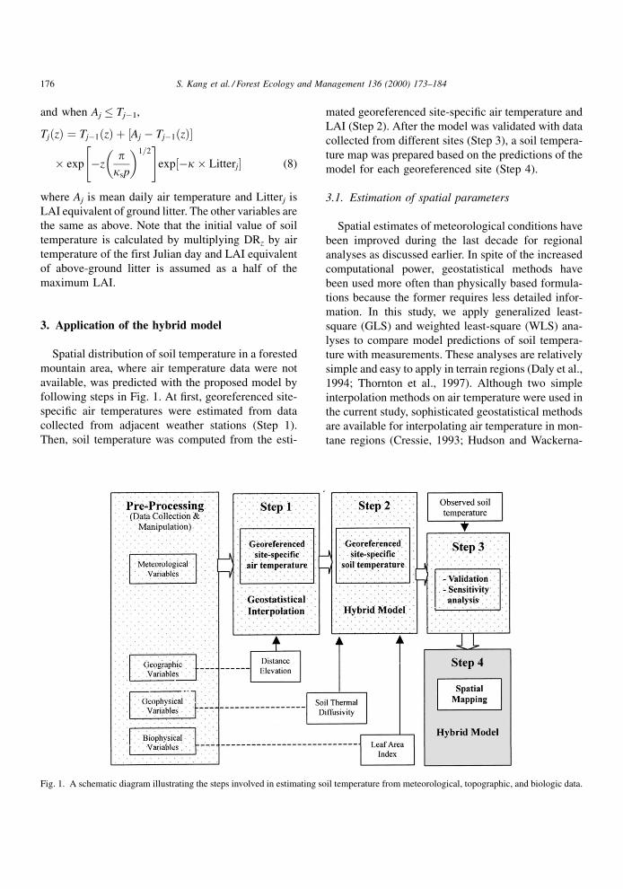
3. Application of the hybrid model

Spatial distribution of soil temperature in a forested

mountain area, where air temperature data were not

available, was predicted with the proposed model by

following steps in Fig. 1. At ®rst, georeferenced site-

speci®c air temperatures were estimated from data

collected from adjacent weather stations (Step 1).

Then, soil temperature was computed from the esti-

mated georeferenced site-speci®c air temperature and

LAI (Step 2). After the model was validated with data

collected from different sites (Step 3), a soil tempera-

ture map was prepared based on the predictions of the

model for each georeferenced site (Step 4).

3.1. Estimation of spatial parameters

Spatial estimates of meteorological conditions have

been improved during the last decade for regional

analyses as discussed earlier. In spite of the increased

computational power, geostatistical methods have

been used more often than physically based formula-

tions because the former requires less detailed infor-

mation. In this study, we apply generalized least-

square (GLS) and weighted least-square (WLS) ana-

lyses to compare model predictions of soil tempera-

ture with measurements. These analyses are relatively

simple and easy to apply in terrain regions (Daly et al.,

1994; Thornton et al., 1997). Although two simple

interpolation methods on air temperature were used in

the current study, sophisticated geostatistical methods

are available for interpolating air temperature in mon-

tane regions (Cressie, 1993; Hudson and Wackerna-

Fig. 1. A schematic diagram illustrating the steps involved in estimating soil temperature from meteorological, topographic, and biologic data.


gel, 1994; Wackernagel, 1995; Kitanidis, 1997; Bel-

lehumeur and Legendre, 1998; Goovaerts, 1998).

Among those, kriging with an external drift is one

of the prospective examples using digital elevation

model (DEM) (Hudson and Wackernagel, 1994).

Likewise, spatial variation in LAI can be determined

with satellite imagery (Pierce and Running, 1988;

Spanner et al., 1990; Gower and Norman, 1991;

Deblonde et al., 1994; Goward et al., 1994; Nemani

and Running, 1996; Fassnacht et al., 1997). One

simple method is to use empirical relationship

between vegetation index from satellite image and

georeferenced ground-measured LAI.

In the current study, georeferenced analyses were

carried out to demonstrate how soil temperature was

determined based on the information of topography

and vegetation cover across two sub-basins of Mt.

Jumbong area using the hybrid model. Based on DEM

of 30 m � 30 m resolution, an air temperature map

was prepared using GLS method. Spatial distribution

of LAI was derived from empirical algorithm between

NDVI and LAI. The algorithm was developed by

comparing NDVI from TM image on 12 August

1991 and LAI determined with LI-COR 2000 in late

August 1998 (Kim et al., unpublished paper).

A sensitivity analysis was employed to determine

main in¯uential parameters in model predictability. At

last, an example was illustrated to show how soil

temperature predictions are distributed across land-

scapes in relation to topography and vegetation.

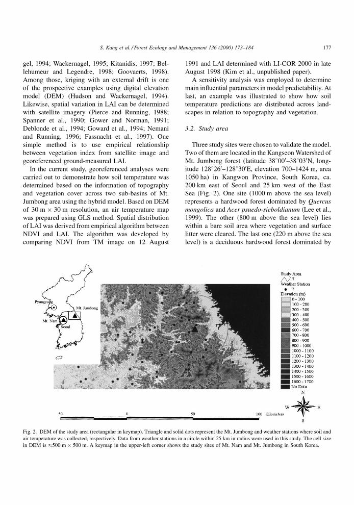
3.2. Study area

Three study sites were chosen to validate the model.

Two of them are located in the Kangseon Watershed of

Mt. Jumbong forest (latitude 388000±388030N, long-

itude 1288260±1288300E, elevation 700±1424 m, area

1050 ha) in Kangwon Province, South Korea, ca.

200 km east of Seoul and 25 km west of the East

Sea (Fig. 2). One site (1000 m above the sea level)

represents a hardwood forest dominated by Quercus

mongolica and Acer psuedo-sieboldianum (Lee et al.,

1999). The other (800 m above the sea level) lies

within a bare soil area where vegetation and surface

litter were cleared. The last one (220 m above the sea

level) is a deciduous hardwood forest dominated by

Fig. 2. DEM of the study area (rectangular in keymap). Triangle and solid dots represent the Mt. Jumbong and weather stations where soil and

air temperature was collected, respectively. Data from weather stations in a circle within 25 km in radius were used in this study. The cell size

in DEM is �500 m � 500 m. A keymap in the upper-left corner shows the study sites of Mt. Nam and Mt. Jumbong in South Korea.


Q. mongolica, located in the Mt. Nam forest within the

Seoul metropolitan area (Fig. 2).

4. Data collection

Soil temperature has been measured at 10 cm depth

using automatic data loggers (Hobo, Onset Computer

Corporation) at the hardwood forest site and bare-soil

site of Mt. Jumbong since 1996 and 1998, respectively,

and at the hardwood forest site of Mt. Nam since 1998.

Data were logged hourly from April to December and

every 2 h during winter due to inaccessibility under

thick snowpack and limited storage capacity of the

data logger. Logged data were downloaded every two

months (every four months in winter) using Log-

book1 Software (Onset Computer Corporation) and

used for calculation of daily averages of soil tempera-

ture (Table 1).

To estimate georeferenced air temperature for Mt.

Jumbong forest site where soil temperature was mon-

itored, we used air temperature data from all the

weather stations of Korean Meteorological Adminis-

tration within 25 km in radius (solid dots in Fig. 2). We

excluded the data from the stations whose data were

missing for more than 18 days (�5% of a year). As a

result, data of six meteorological stations, which are

situated from 110 to 771 m above the sea level, were

chosen. Short-term missing data were replaced by

interpolating with a moving average method. Since

April 1998, air temperature data collected hourly were

available at the bare-soil site of Mt. Jumbong, using a

weather monitoring system (Weatherlink II, Davis

Instruments). For the hardwood forest site of Mt.

Nam, we used air temperature data collected from a

weather station of Seoul (80 m above the sea level),

2.6 km away from the site. In this case, the elevation

effect was considered with an assumed temperature

lapse rate of ÿ88C kmÿ1.

Values of LAI were determined at the Mt. Jumbong

sites with a LI-COR 2000 Plant Canopy Analyzer

from May to August 1998. The combined values of

overstory and understory vegetation averaged

5.5 m2 mÿ2 in late August. A maximum LAI of

5.0 m2 mÿ2 was assumed for the Mt. Nam forest

since a clear-cut area for referencing to open-sky

irradiation was not available near the site. It was

also assumed that LAI varied sinusoidially during

the growing season, reaching the maximum plateau

in July.

4.1. Input parameters of the model

The extinction coef®cient for the Beer±Lambert law

was set at 0.45. Thickness of litter layer was assumed

to decrease at a rate of 0.01 per day in unit of LAI

equivalent, only when air temperature was above 08C.

The value was �10-times higher than the decomposi-

tion constant of leaf litter observed in the ®eld by a

litterbag method in 1996 (Yoo et al., 1999). For the

sake of simplicity, the exponential function of litter

decomposition at a constant rate was used in this study,

but a more reliable model of litter decomposition can

be incorporated to enhance predictability in the future.

The value of p was given 365 � 24 � 60 � 60 s to

represent annual variation. Soil thermal diffusivity

(ks) was set at 0.005 cm2 sÿ1. For a range of soil

texture, the value of ks varies from 0.001 to

0.01 cm2 sÿ1 (Rosenberg et al., 1983; Marshall

et al., 1996). This variation is associated not only

with soil texture but also with organic matter and

moisture content. Within the given range of ks, the

calculated damping ratio at 10 cm soil depth ranged

from 0.93 to 0.97. If soil texture is unknown, a value

between 0.93 and 0.97 can be given to estimate

seasonal variation of soil temperature. Alternatively,

predictions may be improved by considering multiple

soil layers with different values of thermal diffusivity

(ks). The latter approach should be considered if

ground is covered with a thick layer of litter or snow

(Thunholm, 1990).

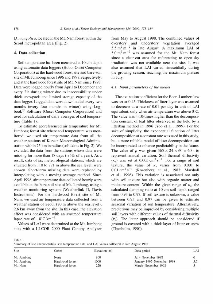
Table 1

Summary of site characteristics, soil temperature data, and LAI values collected in late August 1998

Site Cover Elevation (m) Data period LAI

Mt. Jumbong None 800 July±November 1998 0

Mt. Jumbong Hardwood forest 1000 January 1997±November 1998 5.5

Mt. Nam Hardwood forest 220 March±November 1998 5


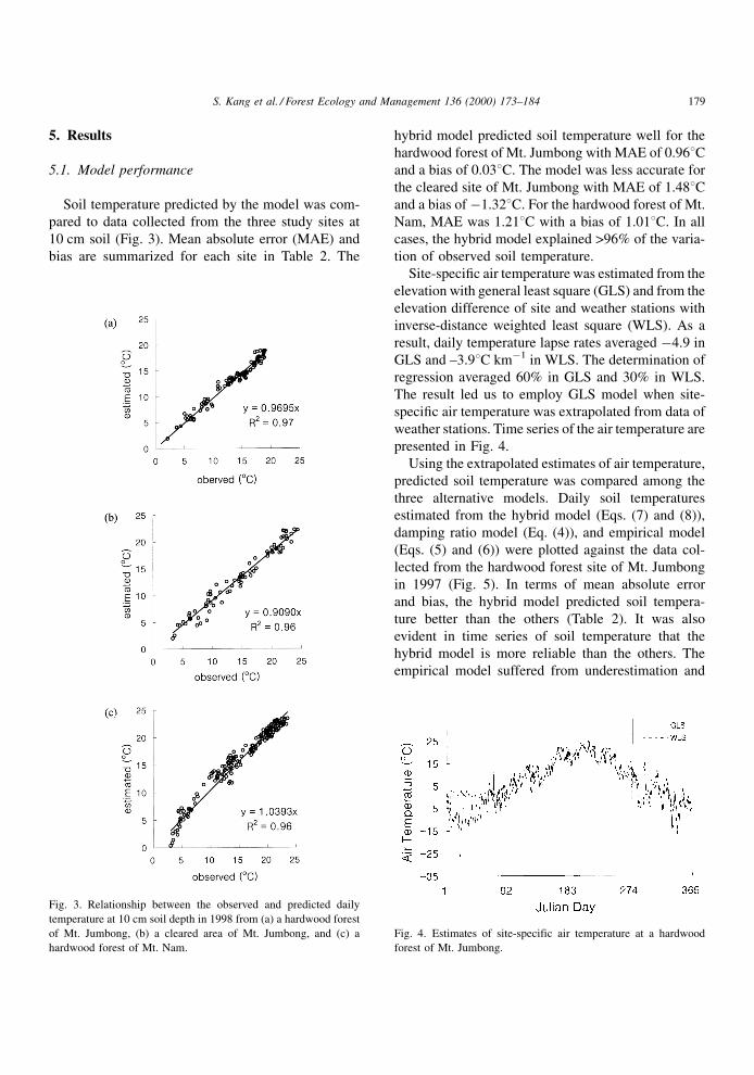
5. Results

5.1. Model performance

Soil temperature predicted by the model was com-

pared to data collected from the three study sites at

10 cm soil (Fig. 3). Mean absolute error (MAE) and

bias are summarized for each site in Table 2. The

hybrid model predicted soil temperature well for the

hardwood forest of Mt. Jumbong with MAE of 0.968Cand a bias of 0.038C. The model was less accurate for

the cleared site of Mt. Jumbong with MAE of 1.488Cand a bias ofÿ1.328C. For the hardwood forest of Mt.

Nam, MAE was 1.218C with a bias of 1.018C. In all

cases, the hybrid model explained >96% of the varia-

tion of observed soil temperature.

Site-speci®c air temperature was estimated from the

elevation with general least square (GLS) and from the

elevation difference of site and weather stations with

inverse-distance weighted least square (WLS). As a

result, daily temperature lapse rates averaged ÿ4.9 in

GLS and ±3.98C kmÿ1 in WLS. The determination of

regression averaged 60% in GLS and 30% in WLS.

The result led us to employ GLS model when site-

speci®c air temperature was extrapolated from data of

weather stations. Time series of the air temperature are

presented in Fig. 4.

Using the extrapolated estimates of air temperature,

predicted soil temperature was compared among the

three alternative models. Daily soil temperatures

estimated from the hybrid model (Eqs. (7) and (8)),

damping ratio model (Eq. (4)), and empirical model

(Eqs. (5) and (6)) were plotted against the data col-

lected from the hardwood forest site of Mt. Jumbong

in 1997 (Fig. 5). In terms of mean absolute error

and bias, the hybrid model predicted soil tempera-

ture better than the others (Table 2). It was also

evident in time series of soil temperature that the

hybrid model is more reliable than the others. The

empirical model suffered from underestimation and

Fig. 3. Relationship between the observed and predicted daily

temperature at 10 cm soil depth in 1998 from (a) a hardwood forest

of Mt. Jumbong, (b) a cleared area of Mt. Jumbong, and (c) a

hardwood forest of Mt. Nam.

Fig. 4. Estimates of site-specific air temperature at a hardwood

forest of Mt. Jumbong.


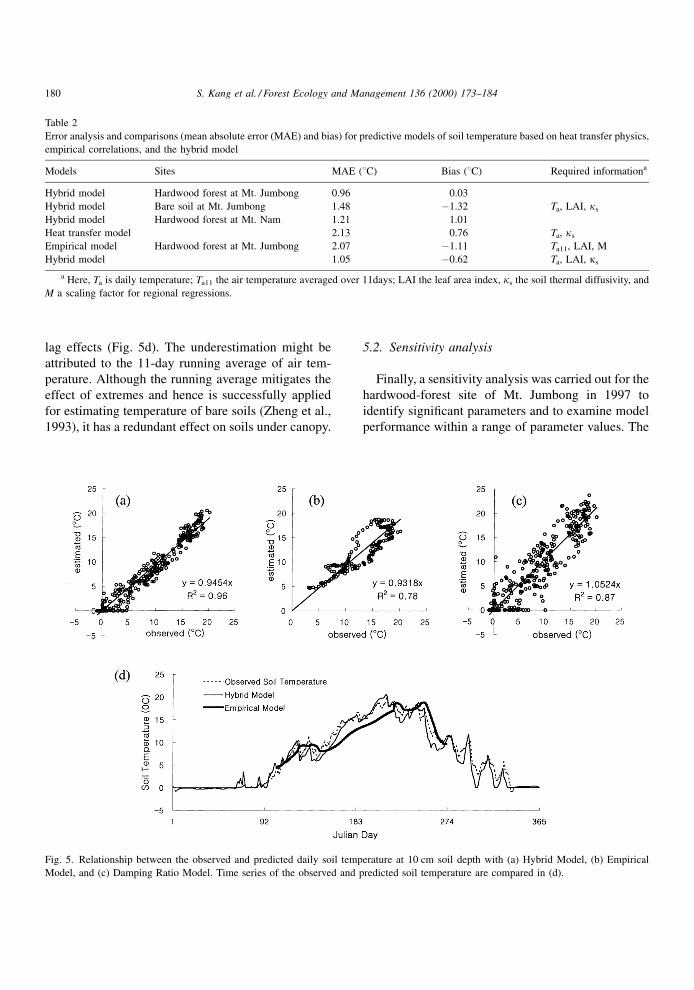
lag effects (Fig. 5d). The underestimation might be

attributed to the 11-day running average of air tem-

perature. Although the running average mitigates the

effect of extremes and hence is successfully applied

for estimating temperature of bare soils (Zheng et al.,

1993), it has a redundant effect on soils under canopy.

5.2. Sensitivity analysis

Finally, a sensitivity analysis was carried out for the

hardwood-forest site of Mt. Jumbong in 1997 to

identify signi®cant parameters and to examine model

performance within a range of parameter values. The

Table 2

Error analysis and comparisons (mean absolute error (MAE) and bias) for predictive models of soil temperature based on heat transfer physics,

empirical correlations, and the hybrid model

Models Sites MAE (8C) Bias (8C) Required informationa

Hybrid model Hardwood forest at Mt. Jumbong 0.96 0.03

Hybrid model Bare soil at Mt. Jumbong 1.48 ÿ1.32 Ta, LAI, ks

Hybrid model Hardwood forest at Mt. Nam 1.21 1.01

Heat transfer model 2.13 0.76 Ta, ks

Empirical model Hardwood forest at Mt. Jumbong 2.07 ÿ1.11 Ta11, LAI, M

Hybrid model 1.05 ÿ0.62 Ta, LAI, ks

a Here, Ta is daily temperature; Ta11 the air temperature averaged over 11days; LAI the leaf area index, ks the soil thermal diffusivity, and

M a scaling factor for regional regressions.

Fig. 5. Relationship between the observed and predicted daily soil temperature at 10 cm soil depth with (a) Hybrid Model, (b) Empirical

Model, and (c) Damping Ratio Model. Time series of the observed and predicted soil temperature are compared in (d).


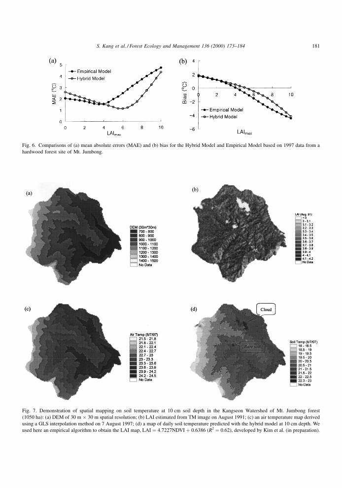
Fig. 6. Comparisons of (a) mean absolute errors (MAE) and (b) bias for the Hybrid Model and Empirical Model based on 1997 data from a

hardwood forest site of Mt. Jumbong.

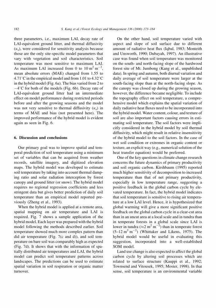
Fig. 7. Demonstration of spatial mapping on soil temperature at 10 cm soil depth in the Kangseon Watershed of Mt. Jumbong forest

(1050 ha): (a) DEM of 30 m � 30 m spatial resolution; (b) LAI estimated from TM image on August 1991; (c) an air temperature map derived

using a GLS interpolation method on 7 August 1997; (d) a map of daily soil temperature predicted with the hybrid model at 10 cm depth. We

used here an empirical algorithm to obtain the LAI map, LAI � 4.7227NDVI � 0.6386 (R2 � 0.62), developed by Kim et al. (in preparation).


three parameters, i.e., maximum LAI, decay rate of

LAI-equivalent ground litter, and thermal diffusivity

(ks), were considered for sensitivity analysis because

those are the only site-speci®c model parameters that

vary with vegetation and soil characteristics. Soil

temperature was most sensitive to maximum LAI.

As maximum LAI increased from 0 to 10 m2 mÿ2,

mean absolute errors (MAE) changed from 1.55 to

4.718C in the empirical model and from 1.01 to 4.328Cin the hybrid model (Fig. 6a). The bias varied from 2 to

ÿ48C for both of the models (Fig. 6b). Decay rate of

LAI-equivalent ground litter had an intermediate

effect on model performance during restricted periods

before and after the growing seasons and the model

was not very sensitive to thermal diffusivity (ks) in

terms of MAE and bias (not presented here). The

improved performance of the hybrid model is evident

again as seen in Fig. 6.

6. Discussion and conclusions

Our primary goal was to improve spatial and tem-

poral prediction of soil temperature using a minimum

set of variables that can be acquired from weather

records, satellite imagery, and digitized elevation

maps. The hybrid model was developed to estimate

soil temperature by taking into account thermal damp-

ing ratio and solar radiation interception by forest

canopy and ground litter (or snow). The hybrid model

requires no regional regression coef®cients and less

stringent data but gives better prediction of daily soil

temperature than an empirical model reported pre-

viously (Zheng et al., 1993).

When the hybrid model is applied at a remote area,

spatial mapping on air temperature and LAI is

required. Fig. 7 shows a sample application of the

hybrid model. Each layer was prepared with the hybrid

model following the methods described earlier. Soil

temperature showed much more complex pattern than

did air temperature (Fig. 7(c and d)), and soil tem-

perature on bare soil was comparably high as expected

(Fig. 7d). It shows that with the information of spa-

tially distributed air temperatures and LAI, the hybrid

model can predict soil temperature patterns across

landscapes. The predictions can be used to estimate

spatial variation in soil respiration or organic matter

turnover.

On the other hand, soil temperature varied with

aspect and slope of soil surface due to different

amount of radiative heat ¯ux (Iqbal, 1983; Monteith

and Unsworth, 1990; Dubayah, 1997). An illustrative

case was found when soil temperature was monitored

on the south- and north-facing slope of the hardwood

forest site of Mt. Jumbong (Kang et al., unpublished

data). In spring and autumn, both diurnal variation and

daily average of soil temperature were larger at the

south-facing slope than at the north-facing slope. As

the canopy was closed up during the growing season,

however, the difference became negligible. To include

the topography effect on soil temperature, a compre-

hensive model which explains the spatial variation of

daily radiative heat ¯uxes need to be incorporated into

the hybrid model. Water content, colour, and texture of

soil are also important factors causing errors in esti-

mating soil temperature. The soil factors were impli-

citly considered in the hybrid model by soil thermal

diffusivity, which might result in relative insensitivity

of the hybrid model to the soil factors. In the case of

wet soil condition or extremes in organic content or

texture, an explicit way (e.g., numerical solution of the

heat transfer equation) would be preferred.

One of the key questions in climate change research

concerns the future dynamics of primary productivity

and soil organic carbon. Kirshbaum (1995) reported

much higher sensitivity of decomposition to increased

temperature than that of net primary productivity,

especially in low temperature range, suggesting a

positive feedback in the global carbon cycle by ele-

vated temperature. In fact, the hybrid model indicates

that soil temperature is sensitive to rising air tempera-

ture at a low LAI level. Hence, it is hypothesized that

global warming will give a more signi®cant positive

feedback on the global carbon cycle in a clear-cut area

than in an uncut area at a local scale and in tundra than

in temperate forests in a global scale since LAI is

lower in tundra (�2 m2 mÿ2) than in temperate forest

(5±12 m2 mÿ2) (Whittaker and Likens, 1975). The

hybrid model would be useful in evaluating this

suggestion, incorporated into a well-established

SOM model.

Land use change is also expected to affect the global

carbon cycle by altering soil processes which are

related to surface structure (Kauppi et al., 1992;

Townsend and Vitousek, 1995; Mosier, 1998). In that

sense, soil temperature is an environmental variable


that links surface structure to soil processes directly.

This feature allows the hybrid model to be incorpo-

rated into other established models of soil organic

matter and vegetation to predict spatially variable

carbon cycle and its responses to land use change

such as deforestation or reforestation.

Acknowledgements

We are indebted to Mr. Chandra Park for helping us

collect ®eld data, and Drs. Hojeong Kang and Jae C.

Choe for giving constructive comments on an earlier

draft. Special thanks should go to Drs. Richard H.

Waring and Josef Eitzinger for their invaluable time

and suggestions in terms on both the scienti®c and

editing aspects of this paper. This research was sup-

ported by the Korean Science and Engineering Foun-

dation grant KOSEF 94-0401-01-01-03. We also

appreciate some helpful comments by the reviewers.

References

Antonic, O., 1998. Modelling daily topographic solar radiation

without site-specific hourly radiation data. Ecological Model-

ling 113, 31±40.

Becker, E.B., Carey, G.F., Oden, T., 1981. Finite elements: an

introduction. Prentice-Hall, New Jersey.

Bellehumeur, C., Legendre, P., 1998. Multiscale sources of

variation in ecological variables: modeling spatial dispersion,

elaborating sampling designs. Landscape Ecology 13, 15±25.

Cressie, N.A.C., 1993. Statistics for Spatial Data. Wiley, New York,

NY.

Daly, C., Neilson, R.P., Phillips, D.L., 1994. A statistical-

topographic model for mapping climatological precipitation

over mountainous terrain. J. Appl. Meteorol. 33, 140±158.

Deblonde, G., Penner, M., Royer, A., 1994. Measuring leaf index

with the LI-COR LAI-2000 in pine stands. Ecology 75, 1507±

1511.

Dozier, J., Frew, J., 1990. Rapid calculation of terrain parameters

for radiation modeling from digital elevation data. IEEE Trans.

Geosci. Remote Sens. 28, 963±969.

Dubayah, R., 1992. Estimating net solar radiation using Landsat

Thematic mapper and Digital Elevation Data. Water Resources

Research 28, 2469±2484.

Dubayah, R., 1994. Modeling a solar radiation topoclimatology for

the Rio Grande River Basin. J. Veg. Sci. 5, 627±640.

Dubayah, R., Loechel, S., 1997. Modeling topographic solar

radiation using GOES data. J. Appl. Meteorol. 36, 141±154.

Fassnacht, K.S., Gower, S.T., MacKenzie, M.D., Nordleim, E.V.,

Lillesand, T.M., 1997. Estimating the leaf area index of North

Central Wisconsin Forests using the Landsat Thematic Mapper.

Remote Sens. Environ. 61, 229±245.

Goovaerts, P., 1998. Geostatistical tools for characterizing the

spatial variability of microbiological and physico-chemical soil

properties. Biol. Fertil. Soils 27, 315±334.

Gower, S.T., Norman, J.M., 1991. Rapid estimation of leaf area

index in conifer and broad-leaf plantations. Ecology 72, 1896±

1900.

Goward, S.N., Waring, R.H., Dye, D.G., Yang, J., 1994. Ecological

remote sensing at OTTER: satellite macroscale observations.

Ecological Applications 4, 322±343.

Hudson, G., Wackernagel, H., 1994. Mapping temperature using

kriging with external drift: theory and an example from

Scotland. Int. J. Climatology 14, 77±91.

Hungerford, R.D., Nemani, R.R., Running, S.W., Coughlan, J.C.,

1989. MTCLIM: a mountain microclimate simulation model.

USDA Intermountain Research Station, Research Paper INT-

414.

Iqbal, M., 1983. An introduction to solar radiation. Academic

Press, NY.

Kauppi, P.E., Mielikainen, K., Kuusela, K., 1992. Biomass and

carbon budget of European forests, 1971±1990. Science 256,

70±74.

Kimball, J.S., Running, S.W., Nemani, R., 1997. An improved

method for estimating surface humidity from daily minimum

temperature. Agric. and Forest Meteorol. 85, 87±98.

Kirshbaum, M.U.F., 1995. The temperature dependence of soil

organic matter decomposition, and the effect of global warming

on soil organic C storage. Soil Biol. Biochem. 27, 753±760.

Kitanidis, P.K., 1997. Introduction to Geostatistics. Cambridge

University Press, New York, NY.

Kozlowski, T.T., Pallardy, S.G., 1997. Physiology of Woody Plants.

Academic Press, San Diego.

Lee, D., Yoo, G., Oh, S., Shim, J.H., Kang, S., 1999. Significance

of aspect and understory to leaf litter redistribution in a

temperate hardwood forest. Korean J. Biol. Sci. 3, 143±147.

Marshall, T.J., Holmes, J.W., Rose, C.W., 1996. Soil physics, 3rd

ed., Cambridge University Press, New York, NY.

Mosier, A.R., 1998. Soil processes and global change. Bio. Fertil.

Soils 27, 221±229.

Monteith, J.L., Unsworth, M.H., 1990. Principles of environmental

physics. Edward Arnold, A Division of Hodder and Stoughton,

London.

Nemani, R., Running, S.W., 1996. Implementation of a hierarchical

global vegetation classification in ecosystem function models.

J. Vegetation Sci. 7, 337±346.

Pierce, L., Running, S.W., 1988. Rapid estimation of coniferous

forest leaf area index using a portable integrating radiometer.

Ecology 69, 1762±1767.

Raich, J.W., Schlesinger, W.H., 1992. The global carbon dioxide

flux in soil respiration and its relationship to vegetation and

climate, Tellus 44B, 81±99.

Rochette, P., Gregorich, E.G., 1998. Dynamics of soil microbial

biomass C, Soluble organic C and CO2 evolution after three

years of manure application. Can. J. Soil Sci. 78, 283±290.

Rosenberg, N.J., Blad, B.L., Verma, S.B., 1983. Microclimate: The

Biological Environment, 2nd ed., Wiley, New York, NY.


Russell, C.A., Voroney, R.P., 1998. Carbon dioxide efflux from the

floor of a boreal aspen forest. I. Relationship to environmental

variables and estimates of C respired. Can. J. Soil Sci. 78, 301±

310.

Saha, S.K., 1995. Assessment of regional soil moisture conditions

by coupling satellite sensor data with a soil±plant system

heat and moisture balance model. Int. J. Remote Sens. 16, 973±

980.

Spanner, M.A., Pierce, L.L., Peterson, D.L., Running, S.W., 1990.

Remote sensing of temperate coniferous forest leaf area index:

the influence of canopy closure, understory vegetation and

background reflectance. Int. J. Remote Sens. 11, 95±111.

Striegl, R.G., Wickland, K.P., 1998. Effects of a clear-cut harvest

on soil respiration in a jack pine-lichen woodland. Can. J. For.

Res. 28, 534±539.

Thornton, P.E., Running, S.W., White, M.A., 1997. Generating

surfaces of daily meteorological variables over large regions of

complex terrain. J. Hydrology 190, 214±251.

Thunholm, B., 1990. A comparison of measured and simulated soil

temperature using air temperature and soil surface energy

balance as boundary condition. Agric. and Forest Meteorol. 53,

59±72.

Townsend, A.R., Vitousek, P.M., 1995. Soil organic matter

dynamics along gradients in temperature and land use on the

island of Hawaii. Ecology 76, 721±733.

Trumbore, S.E., Chadwick, O.A., Amundson, R., 1996. Rapid

exchange between soil carbon and atmospheric carbon dioxide

driven by temperature change. Science 272, 393±395.

Wackernagel, H., 1995. Multivariate Geostatistics. Springer, New

York, NY.

Whittaker, R.H., Likens, G.E., 1975. The biosphere and man. In:

Lieth, H., Whittaker, R.H. (Eds.), Primary Productivity of the

Biosphere. Springer, Berlin, 306 pp.

Willmott, C.J., Robeson, S.M., 1995. Climatologically aided

interpolation (CAI) of terrestrial air temperature. Int. J.

Climatology 15, 214±229.

Yoo, G., Park, E., Kim, S., Lee, H., Kang, S., Lee, D., 1999.

Transport and decomposition of leaf litter as affected by aspect

and understory in a temperate hardwood forest, submitted to

Forest Ecology and Management.

Zheng, D., Hunt Jr., E.R., Running, S.W., 1993. A daily soil

temperature model based on air temperature and precipitation

for continental applications. Climate Research 2, 183±191.

Zheng, D., Hunt Jr., E.R., Running, S.W., 1996. Comparison of

available soil water capacity estimated from topography and

soil series information. Landscape Ecology 11, 3±14.


Predicting spatial and temporal patterns of soil temperature based on topography, surface cover and...

Documents

Transcript of Predicting spatial and temporal patterns of soil temperature based on topography, surface cover and...