Pole force and inertial measurements to analyse cross-country ...

Pole force and inertial

measurements to analyse

cross-country skiing

performance in field

conditions

Journal Title

XX(X):2–26

c©The Author(s) 0000

Reprints and permission:

sagepub.co.uk/journalsPermissions.nav

DOI: 10.1177/ToBeAssigned

www.sagepub.com/

Antti Nikkola 1, Olli S arkk a1, Saku Suuriniemi 1, and Lauri Kettunen 2

Abstract

This study investigates the fusion of pole force measurement, inertial speed measurement, and video

analysis to determine cross-country skiing performance in field conditions. As a proof of concept, a

preliminary study was performed with different grip designs and double poling technique. The test

showed that with exploiting inertial measurements, the average speed could be determined for any

number of full cycles or separately for each cycle, which may be difficult with other methods in field

conditions. The exploited measurements were appropriate for determining the key characteristics

of the double poling cycle, which along with the estimated speed data, can be used for comparing

skiing economy, determining maximum performance, and finding differences in ski equipment.

Keywords

Double poling, inertial measurements, cycle frequency, pole angle, biomechanics, cross-country

skiing

Prepared usingsagej.cls [Version: 2015/06/09 v1.01]

2 Journal Title XX(X)

Introduction

Many studies in cross-country skiing aim to gain a better understanding of the factors affecting

performance. Equipment manufacturers, coaches, and the athletes themselves seek for approaches that

make it possible to compare different equipment and skiing techniques. Preferably, such measurements

are easy to obtain in field conditions.

In general, two important factors determine skiing performance: economy and maximum performance.

In long distance races, the most important aspect is the economy of motion. Economy corresponds to the

amount of work done per unit distance. Economy can be estimated, for example, by measuring oxygen

consumption.1 Maximum performance is related to the portion of maximum mechanical power that can

be exploited to forward motion. Maximum performance can be measured as the maximum achievable

speed, which is especially important during sprints and thefinish of mass start events.

Several methods have been proposed to study skiing performance, both in laboratory and field

conditions. Skiing studies often include measured force and various physiological characteristics, such

as muscle activation, oxygen consumption, heart rate and blood lactate concentration.2–6 A popular

method7–11 of studying skiing performance has entailed laboratory measurements on a treadmill using

roller skis.

In this paper, the main interest was double poling (DP) performance, which can be measured with an

upper-body ergometer12;13. Heil et al.12 employed a specialized testing ergometer to compare different

grip designs in laboratory conditions. The ergometer was used to measure the maximum DP upper

body power production. The method described in the study gives direct information about the power

1Department of Electrical Engineering, Tampere University of Technology, P.O. Box 692, FI-33101 Tampere, Finland 2Facultyof Information Technology, University of Jyvaskyla, P.O. Box 35, FI-40014 Jyvaskyla, Finland

Corresponding author:Antti Nikkola, Department of Electrical Engineering, Tampere University of Technology, Tampere, Finland.Email: [email protected]

Prepared usingsagej.cls

Nikkola, Sarkka, Suuriniemi, Kettunen 3

output, which is a good indicator of performance. However, tests with an ergometer require specialised

equipment that are not feasible in field conditions.

In this study, the authors focused on measuring the DP technique and instantaneous speed of the

skier in the field conditions by simultaneously exploiting inertial measurements (accelerometers and

gyroscopes) and pole force measurements. The accelerometers and gyroscopes were attached to a rigid

roller ski, and employed inertial measurements for a different purpose and with a different approach than

in previous studies. Fasel et al.14exploited inertial measurements to estimate the instantaneous speed

of the ski and cycle characteristics of diagonal stride in classical cross-country skiing on a treadmill.

Breitschadel et al.15 studied ski glide tests exploiting inertial measurements,and Myklebust, Losnegard,

et. al.16–19 analysed cross-country skiing kinematics and techniques.Physiological characteristics can

also be measured in field conditions as shown by Mahood et al.20, but these types of measurements were

not considered in this study.

Speed measurement are crucial in field tests, since, for example, the comparison of impulses or forces

is futile without information about the speed that is associated with the effort. The main advantage of

inertial speed measurement over light gates or video analysis is the instantaneous speed obtained with

a high sampling frequency. Skiing is a cyclic motion and the skier’s velocity varies substantially during

one poling cycle. Thus, in order to gain representative estimates of the average speed, the speed should be

calculated over several full cycles. Using light gates or video analysis is difficult because the distance over

which the speed is calculated has to be selected in advance. With inertial measurements, the measurement

range can be selected afterward from the gathered speed data, thus allowing additional flexibility in

determining the speed measurement. Average speed can, for example, be calculated separately for each

cycle.

The aim of this study was to demonstrate that inertial measurements, combined with force

measurements, are a feasible approach in estimating speed and comparing maximum performance in

cross-country skiing in field conditions. Another goal was to develop simple field testing methods

for coaches and equipment manufacturers. Special areas of interest included the skiing speed, pole



angle to estimate the horizontal pole force during the poling phase, and differences in ski equipment.

For a demonstration, a field test with two different handgripdesigns was conducted. In addition,

the concept to compare glide properties of the skis in DP was introduced in this study. To the best

knowledge of the authors, a method capable of cycle-by-cycle speed measurement, combined with the

pole force measurements, has not been previously studied inskiing. This is a topical issue, as all modern

smartphones include inertial sensors and the technology needed for the measurements, data processing,

and computations presented in this study.

Methods

Measurements

In this section, pole force measurements, inertial measurements, and video recordings are discussed in

detail.

Pole force measurements A uniaxial load cell was used to measure pole forces. The principle is well

described by Bortolan et al.21 A small button load cell manufactured by Strain MeasurementDevices22

weighing 13 g was installed in an aluminium case weighing 48 g. The load cell used four strain gauges in

full bridge configuration. This device was mounted on carbonracing poles directly below the grip. The

grip was attached to the top of the aluminium case with a screwin the side of the grip and could be easily

changed. Values were recorded with a portable data logger with 1 kHz per channel. The measurement

device is presented in Fig. 1a.

A specific calibration stand (Fig. 1c) was used to calibrate the load cells before each measurement. The

pole was placed vertically into the stand under an aluminiumplatform and different standard weights were

placed on the platform. Calibration measurements were madewithout any weight and with the weight of

the platform (2.236 kg) and with three standard weights (5, 10, 15 kg) in addition to the weight of the

platform.



(a) A separate load cell can be seen below the poles. Thedata logger is above right. Above left is the standard grip andbelow left is the hinged grip. Both were used in the field tests.

(b) The roller ski with the IMU in front of the binding.

(c) The calibration stand (on theleft) and the cube (on the right)were exploited to calibrate the loadcells and inertial sensors,respectively.

Figure 1. The force measurement device (a), IMU (b), and calibration equipment (c).

In calibration of the load cells, the scale factorc and biasb were estimated from the sensor error model

y = cx+ b, wherey is the measured force andx is the force due to the standard weight. The calibration

measurements were exploited to form an overdetermined system of linear equations and the bias and

scale factor were estimated by means of linear least squares. The standard deviations of the residual

describes how well the sensor error model fits to the calibration measurements. For the load cell in the

right and left pole, the standard deviation of the residualswere 1.15 N and 0.24 N, respectively.

Inertial measurements A custom made inertial measurement unit (IMU) was used to collect inertial

data needed to compute the skier’s instantaneous speed. TheIMU unit weighed 225 g with the battery



and the aluminium cover. A similar IMU was also exploited to analyse javelin throwing mechanics.23 In

general, inertial navigation exploits acceleration and angular velocity measurements to find the position,

velocity, attitude, and angular velocity of an object.24 The IMU contained an accelerometer25 and an

angular velocity sensor26 triad, measuring acceleration and angular velocity at 1 kHzsampling rate. The

measurement data was stored to the IMU’s memory.

The IMU was attached to the right roller ski also shown in Fig.1b. It would have been impossible to

attach the IMU to the centre of mass because the skier changeshis position considerably while skiing,

and thus, the position of his centre of mass also changes and can be outside the skier’s body.

Since the test was made on a horizontal plane along a straightline and the attitude of the ski did not

change significantly on DP, in this case the velocity of the ski was computed from the acceleration data

in the direction of motion (parallel to the longitudinal axis of the ski).

In order to improve the measurement accuracy, the sensors were calibrated before each measurement.

The technical details of the exploited calibration method are presented by Sarkka et al.27 and are

summarized below.

The purpose of calibration was to find as many deterministic sensor errors as possible. For

accelerometers, the sensor error model included the biases, scale factors, misalignments, and cross-

coupling errors. Stochastic errors were assumed to be normally distributed with zero expectation. The

variance of the noise of the accelerometers was in the order of 10−4 (m/s2)2.

The accelerometer triad was calibrated based on multi-position calibration, where sensors were kept in

a number of different positions with respect to a reference signal.24;28 The calibration device (a cube) is

presented in Fig. 1c. In this case, the reference signal was the local gravity. The IMU was installed inside

the cube, which was rotated in 24 different positions. In each position, the local gravity was measured for

approximately 5 seconds (5000 samples per sensor at 1 kHz). The averages of the measurements at each

position constituted the calibration measurements.

The exploited sensor error model, together with the gathered calibration measurements and reference

signals, constitute an overdetermined non-linear equation, which was solved with the method of least



squares in the order of a few seconds. The deterministic sensor errors were estimated and further used to

adjust the raw acceleration measurements.

The position and speed were estimated from the adjusted acceleration measurements and additional

position observations. The technical details can be found in the study by Nieminen29 and are summarized

below.

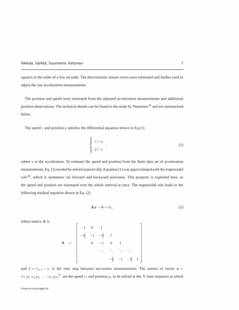
The speedv and positionp satisfies the differential equation shown in Eq.(1)

v = a

p = v, (1)

wherea is the acceleration. To estimate the speed and position fromthe finite data set of acceleration

measurements, Eq. (1) needed be solved numerically. Equation (1) was approximated with thetrapezoidal

rule30, which is symmetric for forward and backward processes. This property is exploited here, as

the speed and position are estimated over the whole intervalat once. The trapezoidal rule leads to the

following residual equation shown in Eq. (2)

Ax− b = r1, (2)

where matrixA is

A =

−1 0 1

−h

2−1 −

h

21

0 −1 0 1

. . .. . .

. . .. . .

−h

2−1 −

h

21

and h = ti+1 − ti is the time step between successive measurements. The entries of vectorx =

[v1 p1 v2 p2 . . . vN pN ]T are the speedvi and positionpi to be solved at theN time instances at which



acceleration was measured. The entries ofb =[

1

2(a1 + a2) 0

1

2(a2 + a3) 0 . . .

1

2(aN−1 + aN ) 0

]Tare

the measured accelerationsai, i = 1, . . . , N , andr1 is the residual.

The residual Eq. (2) is underdetermined withN measurements andN − 2 equations. For this reason,

additional speedv⋆ and positionp⋆ observations such as the initial position, zero initial speed and end

position were exploited to come up with supplementary residual equations as shown in Eq. (3)

B

C

x−

v⋆

p⋆

= r2 , (3)

where binary matricesB andC associate the velocities and positions inx, with v⋆ andp⋆, respectively.

Compiling the residual Eqs. (2) and (3) together results in Eq. (4)

Dx− c = r , (4)

whereD =[

ATB

TC

T]T

, c =[

bT v⋆T p⋆T]T

andr =[

rT1 rT

2

]T.

To estimatex, a linear least squares problem as shown in Eq. (5)

x = argminx

{

rTr}

, (5)

is solved31 yielding Eq. (6)

x =(

DTD)−1

DT c. (6)

The linear least squares method assumes the measurement errors are uncorrelated and homoscedastic

with the same variance.

In the test examples, the initial position was set to zero andadditional time stampings for position

observations at 40 m, 60 m, and 80 m from the starting point were employed. These were obtained from

video recordings. The additional position time stampings,together with the zero initial speed, make it



possible to solvex from a boundary value problem. In the test cases,x was solved in the domain from 0

to 80 m with the zero initial speed and the additional position time stamps given as additional constraints

for the solution. In principle, the approach makes it possible to exploit any speed, at any instance of time,

but in this case only the initial speed was available in the domain from 0 to 80 m.

Positions and speeds (i.e.,x) were solved as a post processing task after all the data was gathered. The

solution takes a few seconds of CPU time from most computers.

The position observations with time stamps guarantee the average speed over the whole region between

the boundary conditions is correct up to the measurement accuracy. The proposed approach is about

solving the moments, which are time stamps of when the measurement unit was at each point within the

region and what was the momentary speed at that moment. This is an optimal approach in the sense that

while the average speed is correct, the momentary speeds become specified by minimizing the error in

kinetic energy. In other words, the cumulative error in kinetic energy over the whole domain becomes

minimized.

In case of the test run results, the initial speed and the average speeds between 0-40 m, 40-60 m,

and 60-80 m were correct up to the measurement error. The momentary speeds in the subdomains 0-40

m, 40-60 m, and 60-80 m were solved from the accelerations, such that the error in kinetic energy was

minimized in each subdomain.

As in all position and velocity measurements, the absolute error is difficult to estimate. The absolute

error depends on the accuracy of the time stamped positions,sensor properties, and calibration. Improving

any of these factors will also decrease the absolute error. Accordingly, the approach yields an optimal

result within the unavoidable tolerances. Assumption of maximum error in acceleration measurements

would lead to pessimistic error bounds and conflict with the stochastic error model, where individual

large errors are improbable, but possible.

A more useful approach to error analysis is to estimate the standard deviations for the speed and

position. The measurement and observation errors (δc) in measured data (c) cause an error (δx) to the

estimated speed and position solved from the least squares problem. The error in measurement data and



the estimated speed and position are related by Eq. (7)

δx =(

DTD)−1

DT δc. (7)

The covariances of linear combinations condition fulfill Eq. (8)32;33

V (δx) =(

DTD)−1

DTV (δc)DT

(

DTD)−1

(8)

The covariance matrixV (δc) = δcI, whereδc is the variance andI is identity matrix. Thus, Eq. (8)

reduces to Eq. (9)

V (δx) = δc(

DTD)−1

(9)

The diagonal elements ofV (δx) are the variances of the error in estimated speed and position. In general,

the square root of the variance is the standard deviation. Inthe test cases,δc was set to10−4. The

standard deviations provide one with an estimate of the solution accuracy with respect to the measurement

accuracy.

Video recordings All DP skiing tests were video recorded with two cameras (200and 50 frames per

second) placed on the side of the track. The cameras were synchronized and the skier’s position was

obtained in 200 frames per second accuracy with linear interpolation. The recording was used to calculate

time intervals between designated marks on the track. The time stamps were determined manually from

the video after the test, but technically, it would not be difficult to automate this (for example with open

source imaging software libraries such as OpenCV34, which runs also on mobile phones). For each run,

the manual process took approximately 5-10 minutes, whereas an automated process (tested afterward in

Adobe After Effects software) took only seconds to run.

Pole angle during poling phase (PP) was also determined fromthe video recordings. The horizontal

component of the force is responsible for sustaining and accelerating forward motion, and ultimately



determining skiing speed. The vertical component of the pole force lifts the skier upward and has no

direct effect on forward motion. The angles of both poles with respect to the vertical were determined in

seven points during the push. Average evolution of pole angle was calculated separately for both grips as

shown in Fig. 2. A fourth degree polynomial was fitted to the data (best fit in a least-square sense). As

previously noted, this process can be automated with Adobe After Effects or OpenCV. An alternative to

image processing is to embed angular velocity sensors to thegrip to specify the pole angles.

The azimuthal angle of the camera induces parallax error to the pole angle. The magnitude of this

error changes with respect to the skier’s position during the push. Parallax error was compensated for

with the information about camera position (distance from the track and height), azimuthal camera angle,

elevation angle, and the skier’s position in the video frame. Each pole was assumed to travel in a plane.

Correction was made individually for each calculated pole angle. The greatest correction was 7.6 degrees.

The angleα between the pole and the vertical was used to divide the pole forceF into verticalFv and

horizontalFh components by using formulasFh = F sin(α) andFv = F cos(α).

Field testing

In order to determine whether the presented system can be used to measure differences in skiing speed

and DP skiing characteristics caused by differences in equipment, the system was tested with two slightly

different grip designs. The purpose was to demonstrate the measurement method and because only one

participant was included in the study, a statistical comparison could not be done between the two grips.

In addition, no claims about the superiority between the grips were made. A standard grip was tested

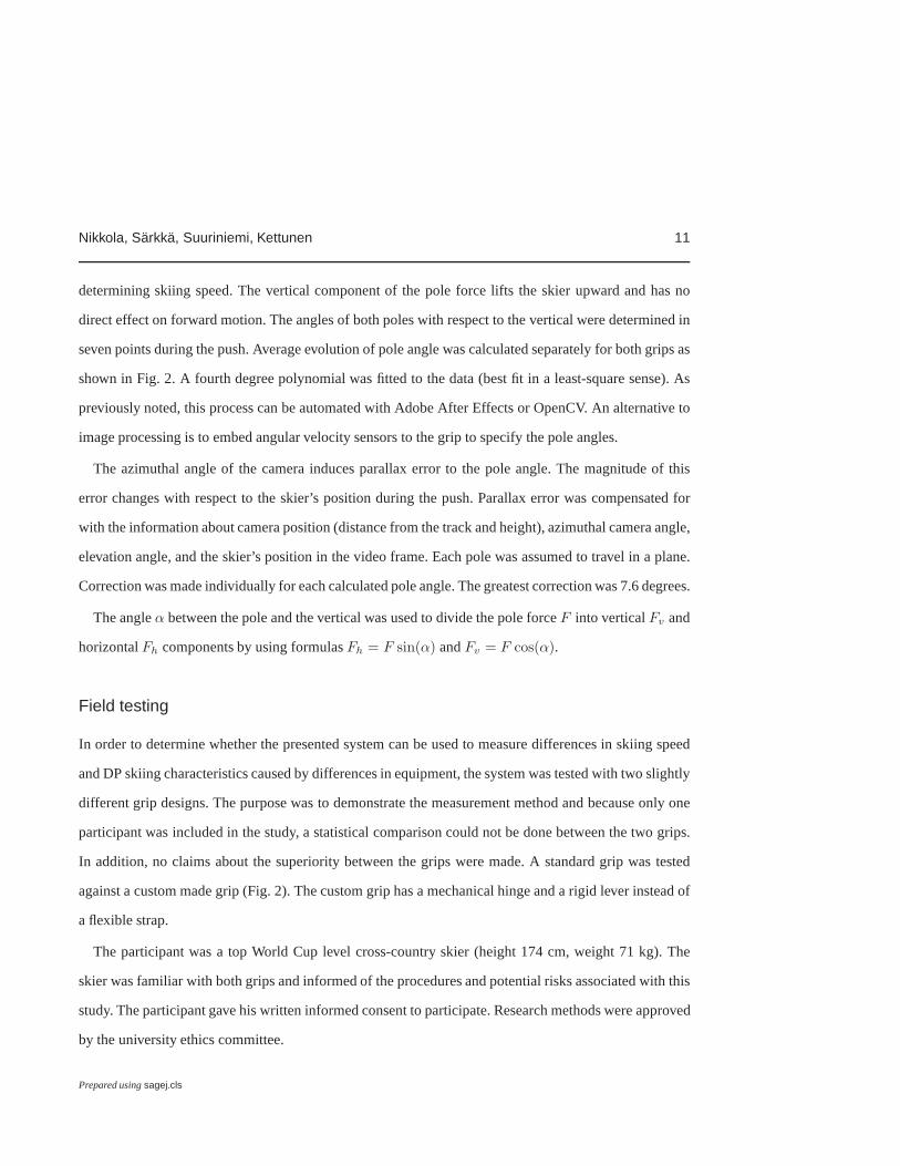
against a custom made grip (Fig. 2). The custom grip has a mechanical hinge and a rigid lever instead of

a flexible strap.

The participant was a top World Cup level cross-country skier (height 174 cm, weight 71 kg). The

skier was familiar with both grips and informed of the procedures and potential risks associated with this

study. The participant gave his written informed consent toparticipate. Research methods were approved

by the university ethics committee.



Effective increase

in pole length

New hinged grip design Standard grip

Rigid lever

Flexible strap

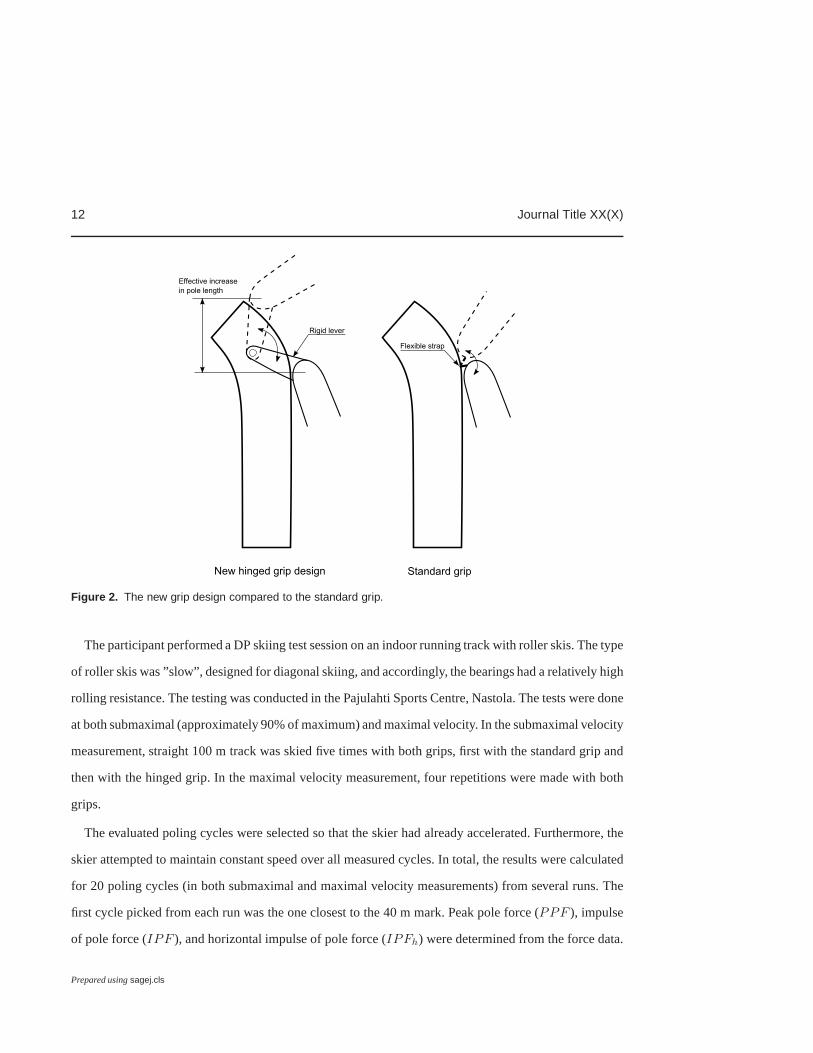
Figure 2. The new grip design compared to the standard grip.

The participant performed a DP skiing test session on an indoor running track with roller skis. The type

of roller skis was ”slow”, designed for diagonal skiing, andaccordingly, the bearings had a relatively high

rolling resistance. The testing was conducted in the Pajulahti Sports Centre, Nastola. The tests were done

at both submaximal (approximately 90% of maximum) and maximal velocity. In the submaximal velocity

measurement, straight 100 m track was skied five times with both grips, first with the standard grip and

then with the hinged grip. In the maximal velocity measurement, four repetitions were made with both

grips.

The evaluated poling cycles were selected so that the skier had already accelerated. Furthermore, the

skier attempted to maintain constant speed over all measured cycles. In total, the results were calculated

for 20 poling cycles (in both submaximal and maximal velocity measurements) from several runs. The

first cycle picked from each run was the one closest to the 40 m mark. Peak pole force (PPF ), impulse

of pole force (IPF ), and horizontal impulse of pole force (IPFh) were determined from the force data.



PPF is the maximum value of the force during the push, excluding the initial force peak caused by the

pole-ground impact.IPF andIPFh were calculated as an integral of the pole force and horizontal pole

force (the angle between the pole and vertical was determined from video recordings) over PP duration,

respectively. Values were calculated separately for both poles. The time characteristics measured for the

poling cycle in this study were time of the poling cycle (CT ), poling phase (PT ), recovery phase (RT )

and time to peak pole force (TPPF ). Poling frequency (Pf ) is the reciprocal ofCT (i.e.,Pf = 1/CT ).

A mean force curve of one push was determined for both grips.

The video cameras were positioned 50 m from the start point and at the 80 m mark. The camera at

50 m was panned during the runs, and the optical axes of the camera at the 80 m mark was aligned with

the mark on the track. Distances 40 m and 60 m were marked to thetrack in the same manner, and the

time stamps at these marks were obtained from the SMPTE35 timecode of the video images. The average

speed of the cycles was estimated from the inertial measurement data between starts of cycles for the

same stretch as the force data (from approximately 40 m to 60 m). The only speed observation employed

was the trivial zero initial speed, and hence, no additionalspeed observations took place.

The IMU and force sensors were synchronized before the test.The data logger of force sensors

contained an accelerometer triad, which was synchronic with the force sensors. The data logger was

placed on the top of the IMU and a knock was induced to the data logger. The knock creates a

recognizable signal in the accelerometer data. The pole-ground impact was exploited to synchronize

the force sensors and the two video recordings.

The load cell in the right pole broke during the maximum velocity measurement. The load cell in

the left pole did not work properly with the standard grip andgave substantially lower values than the

actual forces. Thus, the force measured for the left hand with standard grip and the right hand in maximal

velocity measurement, were excluded. However, the cycle parameters and speeds could be calculated for

all measurements.

All data is presented as means and standard deviations. All calculations and statistical analysis were

made with MATLAB R2013a (MathWorks) and Excel 2010 (Microsoft).



Results

Average pole force curves for one PP (Fig. 3), force and cyclecharacteristics and skiing speed (Table 1)

were determined. One poling cycle is divided into PP and recovery phase (RP). From the force point of

view, PP starts with a significant force peak which is caused by the pole-ground contact. After the initial

peak, force increases until reaching the maximum value (PPF ). After that, the force decreases gradually

until reaching zero at the end of PP. During RP, the skier lifts his centre of mass and prepares for the next

PP.

Measurements showed difference in the shape of the force curves and in the measured force and cycle

characteristics with the two grips. The results are presented in Table 1. The most significant differences

were detected inPPF ,Pf andRT . Force characteristics could not be compared in the maximalvelocity

measurement due to malfunctions in the measurement system.

No difference between grips was detected in the average speed (from approximately 40 m to 60 m)

in either test. In the submaximal velocity test, average speeds were23.0± 0.02 km/h and23.0± 0.03

km/h and in the maximal velocity test, average speeds were24.9± 0.03 km/h and24.9± 0.02 km/h

with standard and hinged grips, respectively.

The pole angle during one push in submaximal speed measurement is presented in Fig. 4(a). At the

start of the push, the pole is in nearly a vertical position and the pole angle increases nearly linearly

during the push. At the very end of the push, the angle stops increasing, or even slightly decreases, before

the end of the ground contact.

The horizontal pole force in submaximal speed measurement is presented in Fig. 4(b). PP starts with

the poles in nearly a vertical position, which greatly limits the horizontal force component in the early

stages of the push. Horizontal force curves, as shown in Fig.4(b), are different with different grips,

although the difference was smaller than in the total force curves.

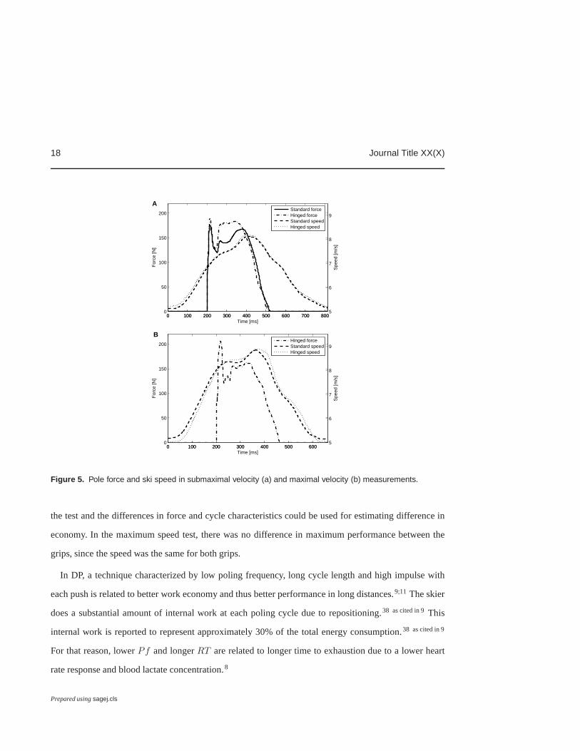
Instantaneous speed of the ski and the pole force for the submaximal and maximal velocity

measurements are presented in Fig. 5(a, b). The maximum standard deviation in the instantaneous speed

and position was±0.003 m/s and±0.022 m, respectively. There was considerable change in ski speed



0 50 100 150 200 250 300 3500

50

100

150

200

250

Time [m⋅s]

For

ce [N

]

AStandardHinged

0 50 100 150 200 250 300 3500

50

100

150

200

250

300

350

Time [m⋅s]

For

ce [N

]

BStandard

0 50 100 150 200 250 300 3500

50

100

150

200

250

300

350

Time [m⋅s]

For

ce [N

]

CHinged

Figure 3. Average pole force curves for both grips in the submaximal velocity measurement (a) and individualforce curves for both grips (b, c).

during the poling cycle. Average change in speed was 49.2% and 57.0% compared to the average speed

in submaximal and maximal velocity tests, respectively. Itshould be noted that the speed of the ski

differs considerably from the speed of the skier’s centre ofmass because the skier changes his position

considerably during the PP.



Table 1. Pole force and cycle parameters for all measurements.

Measurement Variables Mean ± SDStandard grip Hinged grip

Submaximal velocity Speed [km/h] 23.0±0.02 23.0±0.03CT [s] 0.93±0.03 0.94±0.03PT [s] 0.31±0.01 0.31±0.01RT [s] 0.61±0.03 0.63±0.02TPPF [s] 0.19±0.01 0.15±0.01Pf [Hz] 1.08±0.04 1.06±0.03PPF [N] 168.9±12.6 187.6±9.2IPF [Ns] 39.0±3.5 41.8±2.6PPFh [N] 158.3±10.4 163.9±6.2IPFh [Ns] 30.0±2.4 30.2±1.8

Maximal velocity Speed [km/h] 24.9±0.03 24.9±0.02CT [s] 0.68±0.03 0.67±0.03PT [s] 0.27±0.01 0.27±0.01RT [s] 0.41±0.03 0.40±0.02TPPF [s] 0.17±0.01 0.13±0.01Pf [Hz] 1.47±0.07 1.49±0.04PPF [N] – 165.1±11.4IPF [Ns] – 32.2±2.6PPFh [N] – 137.0±7.6IPFh [Ns] – 21.6±1.8

CT [s], cycle timePT [s], poling timeRT [s], recovery timeTPPF [s], time to peak pole forcePf [Hz], poling frequencyPPF [N], peak pole forceIPF [N s], impulse of pole forcePPFh [N], horizontal pole forceIPFh [Ns], horizontal impulse of pole force

PT RT

CT

Discussion

The objective of the present study was to demonstrate the combination of simple field measurements

to characterise skiing performance. The key quantities measured in this study werePf , RT , impulsesPrepared usingsagej.cls


0 50 100 150 200 250 300 3500

10

20

30

40

50

60

70

80

Time [ms]

Pol

e an

gle

[deg

rees

]

A

StandardHinged

0 50 100 150 200 250 300 3500

20

40

60

80

100

120

140

160

180

200

Time [ms]

Hor

izon

tal f

orce

[N]

BStandardHinged

Figure 4. Average pole angle (a) and horizontal pole force (b) for both grips in the submaximal speed test.

(IPF andIPFh) and skiing speed. These are subsequently used to estimate skiing economy, maximum

performance, and differences in ski equipment. As a method,pole force measurements and augmented

inertial speed measurements recordings appeared to be appropriate for determining these characteristics

in field conditions with DP technique. Both pole force and inertial measurement systems are portable

and can easily be used in any location. In this case, video recordings were used to augment the inertial

measurement, but also other methods, such as global navigation satellite system (GNSS)36;37 or light

gates, could be used.

In the field test, no difference in the average speed was detected between the grips in either test. In

the case of the submaximal speed test, this means that the athlete could maintain constant effort during



0 100 200 300 400 500 600 700 8000

50

100

150

200

Time [ms]

For

ce [N

]

A

0 100 200 300 400 500 600 700 8005

6

7

8

9

Spe

ed [m

/s]

Standard forceHinged forceStandard speedHinged speed

0 100 200 300 400 500 6000

50

100

150

200

Time [ms]

For

ce [N

]

B

0 100 200 300 400 500 6005

6

7

8

9

Spe

ed [m

/s]

Hinged forceStandard speedHinged speed

Figure 5. Pole force and ski speed in submaximal velocity (a) and maximal velocity (b) measurements.

the test and the differences in force and cycle characteristics could be used for estimating difference in

economy. In the maximum speed test, there was no difference in maximum performance between the

grips, since the speed was the same for both grips.

In DP, a technique characterized by low poling frequency, long cycle length and high impulse with

each push is related to better work economy and thus better performance in long distances.9;11 The skier

does a substantial amount of internal work at each poling cycle due to repositioning.38 as cited in 9This

internal work is reported to represent approximately 30% ofthe total energy consumption.38 as cited in 9

For that reason, lowerPf and longerRT are related to longer time to exhaustion due to a lower heart

rate response and blood lactate concentration.8



In the example case, there seemed to be noticeable difference in the temporal forces during the polling

cycle. LowerPf and longerRT were detected with the hinged grip in constant speed tests. Higher

impulse was also detected, which is in line with the observedcycle characteristics. No speed difference

was detected between the grips. Thus, the method seems suitable for detecting differences between

different ski equipment, suggesting there are differencesbetween the two grips. However, further research

with more participants and in different conditions is needed to validate these results.

A slight difference was also detected in the shape of the instantaneous speed curves. This difference in

ski speed implies a difference in the push with different grips. However, the instantaneous speed of the

centre of the mass cannot be directly obtained with this method, as it is impossible to attach the IMU to

the centre of mass of the skier, because its position changesconstantly. For this reason, the translational

power for the centre of the mass of the skier could not be estimated, which is unfortunate, since it would

give information about the performance of the skier in field conditions.

Although the inertial system enables more precise speed measurements, it adds an extra layer on

the measurement procedure. Measurements have to be augmented with additional observations about

the skier’s position and/or velocity along the track. Thus,some supporting measurements are needed.

With additional observations, speed can be solved as a boundary value problem. Solving the speed as an

initial value problem would give poor results, since the errors in measured acceleration accumulate to the

position and speed estimates with time.39 Analysing the data and calculating results also requires more

work than would be required with a light gate system.

In this study, the inertial measurement was used for measuring skiing speed in order to estimate

performance and difference between two different grip designs, but it also has other potential uses in

cross-country skiing studies. Information about the ski speed could be used, for instance, to compare the

glide properties of different skis in DP. If a skier has the same horizontal (impulse of) pole force with

different skis, but the skiing speed is greater with a given pair of skis, then this pair has better glide

properties in DP. If the same skiing speed is achieved with a smaller horizontal force with a given pair



of skis, then this pair can be considered better. This cannotbe demonstrated in this study, since the same

roller skis were used in the tests.

Conclusion

In this study, fusion of pole force measurements, inertial measurements, and video recordings were

exploited to compare cross-country skiing performance andfind differences in ski equipment in field

conditions. Special interest was focused on the use of inertial measurements with additional position

observations to estimate instantaneous and average speed in cyclic motions of DP. As a result, this study

demonstrated that the presented system can be used to find differences in speed and cycle parameters

of DP skiing characteristics, as well as two different grip designs, which were exploited in the tests.

In addition, the cycle parameters and speed were further exploited to determine whether there were

differences in the maximum performance. Also, the concept to compare glide properties of the skis in DP

was introduced. After this initial proof of concept, further development should focus on using alternative

methods (i.e., GNSS) for inertial measurement augmentation. Exclusion of the video camera would make

the system simpler and feasible to use on longer distances along an arbitrary track. These initial tests

lay the foundation for future development of light and portable performance measurement systems for

coaches and equipment manufacturers.

Acknowledgements

The authors thank the athlete for his participation, enthusiasm and cooperation and the Pajulahti Sports Center for

providing facilities for indoors testing.

Declaration of conflicting interests

The authors declare that there is no conflict of interests.



Funding

Our institution got monetary support for this submitted work from the Finnish national technology agency TEKES,

which is a governmental organization. For the tests, we received material support, including poles and roller skis,

from One Way Sport Oy, Finland.

References

1. Minetti AE. Passive tools for enhancing muscle-driven motion and locomotion.J Exp Biol2004; 207: 1265–

1272.

2. Vahasoyrinki P, Komi PV, Seppala S, et al. Effect of skiing speed on ski and pole forces in cross-country skiing.

Med Sci Sports Exerc2008; 40: 1111–1116

3. Nilsson J, Jakobsen V, Tveit P, et al. Pole length and ground reaction forces during maximal double poling in

skiing.Sport Biomech2003; 2: 227–236.

4. Stoggl T, Holmberg H–C. Force interaction and 3D pole movement in double poling.Scand J Med Sci Sport

2011; 21: 393–404.

5. Nilsson J, Tinmark F, Halvorsen K, et al. Kinematic, kinetic and electromyographic adaptation to speed and

resistance in double poling cross country skiing.Eur J Appl Physiol2013; 113: 1385–1394.

6. Gopfert C, Pohjola M, Linnamo V, et al. Forward acceleration of the centre of mass during ski skating calculated

from force and motion capture data.Sports Eng2017; 20: 141–153.

7. Holmberg H–C, Lindinger S, Stoggl T, et al. Biomechanical analysis of double poling in elite cross-country

skiers.Med Sci Sport Exerc2005; 37: 807–818.

8. Holmberg H-C, Lindinger S, Stoggl T, et al. Contributionof the legs to double-poling performance in elite

cross-country skiers.Med Sci Sport Exerc2006; 38: 1853–1860.

9. Lindinger S, Stoggl T, Muller E, et al. Control of speed during the double poling technique performed by elite

cross-country skiers.Med Sci Sport Exerc2009; 41: 210–220.

10. Lindinger S, Holmberg H–C, Muller E, et al. Changes in upper body muscle activity with increasing double

poling velocities in elite cross-country skiing.Eur J Appl Physiol2009; 106: 353–363.



11. Stoggl T, Lindinger S, Muller E. Analysis of a simulated sprint competition in classical cross country skiing.

Scand J Med Sci Sport2007; 17: 362–372.

12. Heil DP, Engen J, Higginson BK. Influence of ski pole grip on peak upper body power output in cross-country

skiers.Eur J Appl Physiol2004; 91: 481–7.

13. Bojsen-Møller J, Losnegard T, Kemppainen J, et al. Muscle use during double poling evaluated by positron

emission tomography.J Appl Physiol2010; 109: 1895–1903.

14. Fasel B, Favre J, Chardonnens J, et al. An inertial sensor-based system for spatio-temporal analysis in classic

cross-country skiing diagonal technique.J Biomech2015; 48: 3199–3205.

15. Breitschadel F, Berre V, Andersen R, et al. A comparisonbetween timed and IMU captured Nordic ski glide

tests. In:9th Conference of the International Sports Engineering Association (ISEA)2012; 34: 397–402.

16. Myklebust H, Losnegard T, Hallen J. Differences in V1 and V2 ski skating techniques described by

accelerometers.Scand J Med Sci Sport2014; 24: 882–893.

17. Losnegard T, Myklebust H, Skattebo Ø, et al. The Influenceof Pole Length on Performance, O2-Cost and

Kinematics in Double Poling.Int J Sports Physiol Perform2017; 12: 211-217

18. Myklebust H, Øyvind G, Jostein H. Validity of ski skatingcenter-of-mass displacement measured by a single

inertial measurement unit.J Appl Biomech2015; 31: 492–498.

19. Losnegard T, Myklebust H, Ehrhardt A, et al. Kinematicalanalysis of the V2 ski skating technique: A

longitudinal study.J Sports Sci2017; 35: 1219–1227

20. Mahood N V., Kenefick RW, Kertzer R, et al. Physiological determinants of cross-country skiing performance.

Med Sci Sport Exerc2001; 33: 1379–1384.

21. Bortolan L, Pellegrini B, Frederico S. Development and validation of a system for poling force measurement

in cross-country skiing and nordic walking. In:ISBS-Conference Proceedings Archive 2009(eds Harrison AJ,

Anderson R, Kenny I), Limerick, Ireland, 2009.

22. Strain measurement devices. S400-button load cell. Online Referencing,

http://www.smdsensors.com/Products/S400-Button-Load-Cell/ (2017, accessed 19 Jan 2017).



23. Sarkka O, Nieminen T, Suuriniemi S, et al. Augmented inertial measurements for analysis of javelin throwing

mechanics.Sports Eng2016; 19: 219–227.

24. Titterton D, Weston JL.Strapdown inertial navigation technology.American Institute of Aeronautics and

Astronautics, 2004, pp. 17–57.

25. Analog Devices. ADXL326 Accelerometer. Online Referencing, http://www.analog.com/static/

imported-files/data_sheets/ADXL326.pdf (2017, accessed 19 Jan 2017)

26. STMicroelectronics. LPY4150AL MEMS motion sensor. Online Referencing,https://media.digikey.

com/pdf/Data Sheets/ST Microelectronics PDFS/LPY4150AL.pdf (2017, accessed 19 Jan

2017).

27. Sarkka O, Nieminen T, Suuriniemi S, et al. A multi-position calibration method for consumer-grade

accelerometers, gyroscopes, and magnetometers to field conditions.IEEE S Journal2017; 17: 3470–3481

28. Chatfield AB.Fundamentals of high accuracy inertial navigation.American Institute of Aeronautics and

Astronautics, 1997.

29. Nieminen T.A non recursive solution method for fixed interval smoothingproblem applied to short-term inertial

navigation.PhD Thesis, Tampere University of Technology, Tampere, 2013. pp. 1–68.

30. Iserles A.A first course in the numerical analysis of differential equations.Cambridge University Press, 1996.

31. Hayashi F.Econometrics.Princeton University Press, 2000.

32. Lindgren BW.Statistical Theory, 3rd ed. New York: MacMillan, 1976.

33. Aster RC, Borchers B, Thurber CH.Parameter estimation and inverse problems, 2nd ed. Academic Press, 2013.

34. http://opencv.org

35. https://en.wikipedia.org/wiki/SMPTEtimecode

36. Farrell JA, Barth M.The global positioning system & inertial navigation.McGraw-Hill, 1999.

37. Grewal MS, Weill LR, Andrews AP.Global positioning system, inertial navigation, and integration. John Wiley

& Sons, 2001.

38. Holmberg H–C.The physiology of cross-country skiing: With special emphasis on the role of the upper body.

PhD Thesis, Karolinska Institutet, Stockholm, 2005.



39. Nieminen T, Kangas J, Suuriniemi S, et al. Accuracy improvement by boundary conditions for inertial

navigation,Int J Nav Obs2010.



A list of figure captions

Figure 1. The force measurement device (a), the IMU (b), and the calibration equipments (c).

Figure 1 (a). A separate load cell can been seen below the poles. The data logger is above right.

Above left is the standard grip and below left is the hinged grip, which both were used in the field tests.

Figure 1 (b). The roller ski with the IMU in front of the binding.

Figure 1 (c). The calibration stand (on the left) and the cube(on the right) were exploited to

calibrate the load cells and inertial sensors, respectively.

Figure 2. The new grip design compared to the standard grip.

Figure 3. Average pole force curves for both grips in the submaximal velocity measurement (a)

and individual force curves for both grips (b, c).

Figure 4. Average pole angle (a) and horizontal pole force (b) for both grips in the submaximal speed test.

Figure 5. Pole force and ski speed in submaximal velocity (a)and maximal velocity (b) measurements.



A list of notation

a Acceleration

b Bias

b Vector, which entries are acceleration measurements

c Scale factor

c Vector, which is compilation ofb, v⋆, andp⋆

h Time step between successive measurements

p Position

p⋆, v⋆ Vectors, which entries are additional position and speed observation

r, r1, r2 Residual vectors

v Speed

x Pole force due to standard weight

x Vector, which entries are position and speed

y Measured pole force

α Angle between pole and the vertical

δc Variance of the measurement errors

δc Vector, which entries are measurement and observation errors

δx Vector, which entries are errors in estimated speed and position

A Matrix, which depends onh

B, C Binary matrixes

D Matrix, which is compilation ofA, B, andC

F Pole force (calibrated)

Fh Horizontal pole force

Fv Vertical pole force

I Identity matrix

N Number of time instances


Pole force and inertial measurements to analyse cross-country ...

Documents

Transcript of Pole force and inertial measurements to analyse cross-country ...