PMT Test Results

PMT Test Results Gary Smith

[email protected]

Watchman Collaboration Meeting PMT Working Group

10th January 2019 08:00 HST (18:00 GMT)

OPERATIONSTimeline Test Rig Procedure

RESULTSGain Calibration Liz Kneale Gain Consistency Leon PickardPeak To Valley Matt NeedhamDark Rate Steve Quillin and Tom ShawAfterpulsing Anthony Ezeribe

CONCLUSIONSNext StageSummary

CONTENTS

2

OPERATIONS

Timeline

4

July – Aug Set up test stand in Edinburgh and Sheffield Aug - Sept Installation and commissioning at Boulby Sept – Oct Initial testing and refinement of procedure

Oct 12th First official tests begin – run one

Nov 15th Both tents operational – eight PMTs per day max. Nov 22nd Thanksgiving - all 101 PMTs tested at least once

Nov – Dec Underground testing of eight PMT sample

Tested PMTs Google Sheets

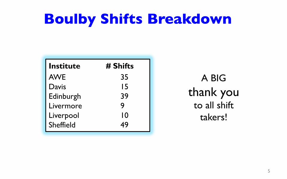
Boulby Shifts Breakdown

5

Institute # Shifts AWE 35 Davis 15 Edinburgh 39 Livermore 9 Liverpool 10 Sheffield 49

A BIG thank you to all shift

takers!

6

Phillips PM 5786B Pulse Generator

~10 kHz

Edinburgh LED driver

Boulby Test RigPS 776 10 x Amp.

CAEN V1730B 2 ns sampling (0.5 GHz) Up to 20 us readout

R7081 10 inch

PMT

Ortec 416 A Gate generator

Boulby Test Rig

7

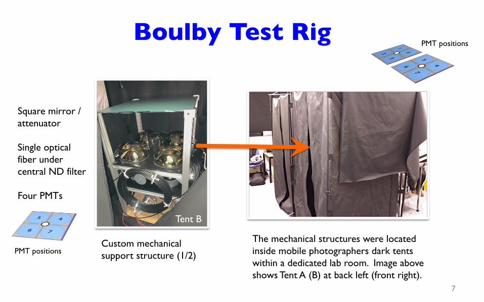
Square mirror /attenuator Single optical fiber under central ND filter Four PMTs

The mechanical structures were located inside mobile photographers dark tents within a dedicated lab room. Image above shows Tent A (B) at back left (front right).

Custom mechanical support structure (1/2)

Tent B

PMT positions

PMT positions

Data Taking ProcedureAfternoon Load next set of PMTs and ramp to nominal HV

Other tasks: PMT cable crimping, software development,…

Next morning Testing begins - follow operating instructions guide Main data taking steps shown in table below

•  Periodic checks (data volume, charge spectra) and e-log entries •  Meta-data recorded in Tested PMTs Google sheets:

o  PMT serial numbers, HV current, ambient temp, … •  Operations meeting conference call held daily

Test Events (M) Time (min) Gate (ns) Volume (G)

1 Nominal HV 3.0 5 220 0.7

2 Gain – 5 HV steps 3.0 x 5 25 220 3.5

3 Operating HV 3.0 5 220 0.7

4 Afterpulsing 0.5 15 10200

3.0

5 Dark Rate 9.0 15 220 2.1

Common Software Tools

9

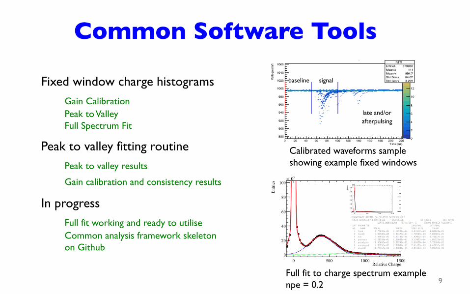
Fixed window charge histograms Gain Calibration Peak to Valley Full Spectrum Fit

Peak to valley fitting routine Peak to valley results

Gain calibration and consistency results

In progress Full fit working and ready to utilise Common analysis framework skeleton on Github

baseline signal

late and/or afterpulsing

Full fit to charge spectrum example npe = 0.2

Calibrated waveforms sample showing example fixed windows

RESULTS

Liz Kneale

PMT gain analysis

Gain Calibration

Gain Calibration

12

Procedure Record SPE spectrum at 5 HV settings

100 V intervals around operating voltage

Find SPE peak - three methods studied 1.  Maxima in fixed ranges above pedestal 2.  TSpectrum – use second peak 3.  TSpectrum then Gaussian from peak to valley fit

Determine HV for107 Gain

Fit TGraph with power law

Gain calculated relative to the charge of the electron R = 50 Ohms, electronics gain = 10 / 2 = 5 Gain = 107 for Q = 400 mV ns (or 8 pC)

Power law fit example

Gain Calibration

13

Results Good agreement with Hamamatsu shipping data Some workarounds required to include all data due to •  spectra with more than two peaks •  TSpectrum finding fake peaks •  No clear peak for some low HV steps

Areas which can developed further are understood

Gain Consistency Leon Pickard UC Davis

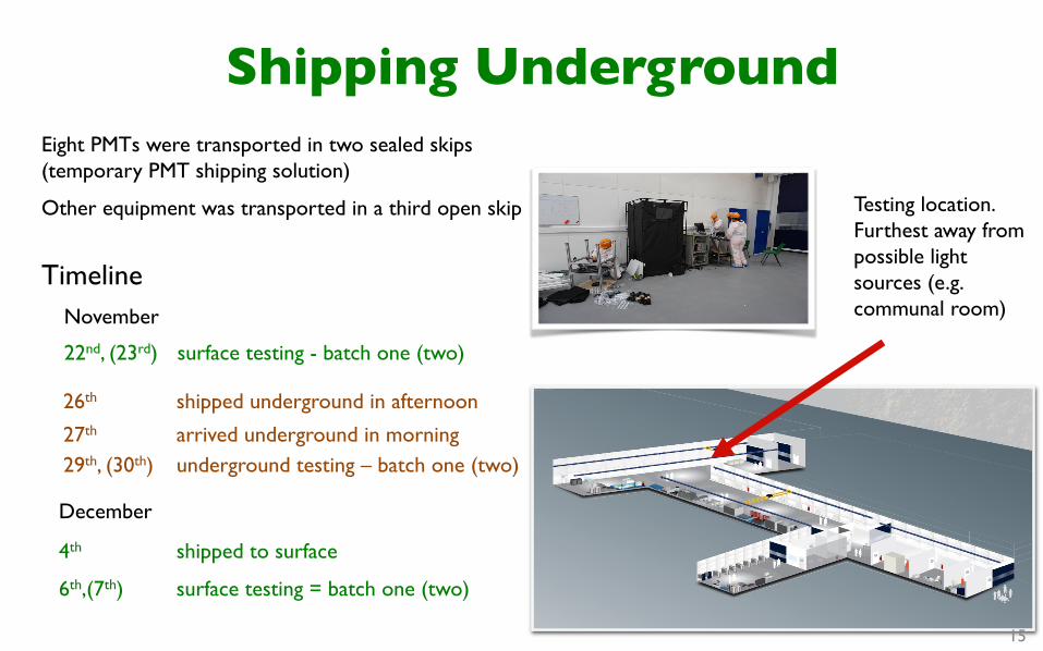
Shipping UndergroundEight PMTs were transported in two sealed skips (temporary PMT shipping solution)

Other equipment was transported in a third open skip

TimelineNovember

22nd, (23rd) surface testing - batch one (two)

26th shipped underground in afternoon

27th arrived underground in morning29th, (30th) underground testing – batch one (two)

December

4th shipped to surface

6th,(7th) surface testing = batch one (two)

Testing location. Furthest away from possible light sources (e.g. communal room)

15

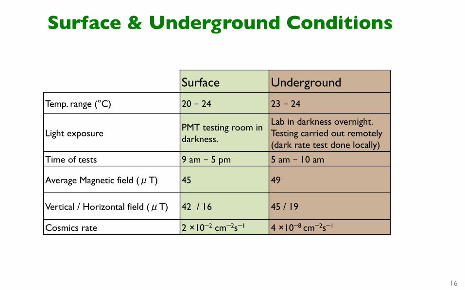
Surface & Underground Conditions

Surface Underground

Temp. range (°C) 20 – 24 23 – 24

Light exposure PMT testing room in darkness.

Lab in darkness overnight. Testing carried out remotely (dark rate test done locally)

Time of tests 9 am – 5 pm 5 am – 10 am

Average Magnetic field (μT) 45 49

Vertical / Horizontal field (μT) 42 / 16 45 / 19

Cosmics rate 2 ×10−2 cm−2s−1 4 ×10−8 cm−2s−1

16

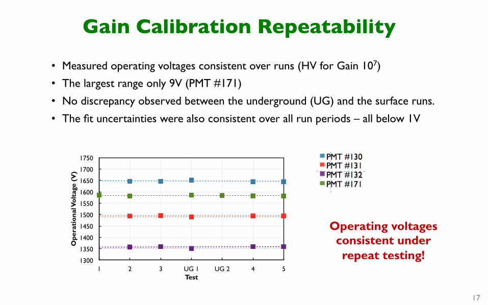
Gain Calibration Repeatability

•  Measured operating voltages consistent over runs (HV for Gain 107)

•  The largest range only 9V (PMT #171)

•  No discrepancy observed between the underground (UG) and the surface runs.

•  The fit uncertainties were also consistent over all run periods – all below 1V

1300

1350

1400

1450

1500

1550

1600

1650

1700

1750

1 2 3 UG 1 UG 2 4 5

Ope

rati

onal

Vol

tage

(V

)

Test

Operating voltages consistent under repeat testing!

17

Peak to Valley

Matthew Needham

18

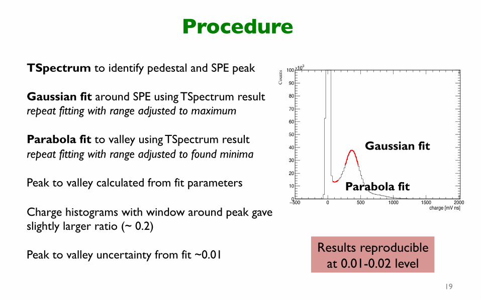
Procedure

19

TSpectrum to identify pedestal and SPE peak Gaussian fit around SPE using TSpectrum result repeat fitting with range adjusted to maximum Parabola fit to valley using TSpectrum result repeat fitting with range adjusted to found minima Peak to valley calculated from fit parameters Charge histograms with window around peak gave slightly larger ratio (~ 0.2) Peak to valley uncertainty from fit ~0.01 Results reproducible

at 0.01-0.02 level

Gaussian fit

Parabola fit

Results

Our results are clearly correlated with those from Hamamatsu J Most tubes measuring slightly smaller peak-to-valley L Peak-to-valley mostly above 2 though Double Chooz report higher ratios when using u-metal shield [ C. Bauer et al. 2011]

Results

21

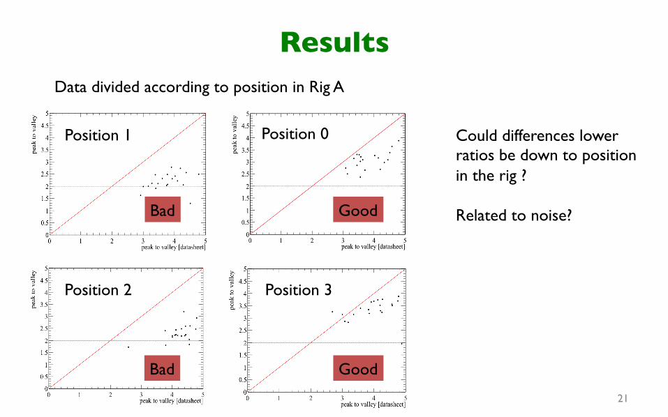
Data divided according to position in Rig A

Position 0 Could differences lower ratios be down to position in the rig ? Related to noise?

Good

Position 1

Bad

Position 3 Position 2

Good Bad

Results

22

Twenty PMTs were tested in the second rig (tent B) during run one 80 were tested in rig A

Good Bad

Good Bad

Data divided according to position in Rig B



Visible differences

23

PMT 42 in location 3 PMT 32 in location 6

Do results hint at noise or illumination playing a role ?

Surface and Underground

24

PMT ID Surface test 1 Underground Surface test 2

130 3.9 4.4 3.8

131 2.5 3.2 2.4

132 2.2 3.1 2.3

133 3.3 3.0 3.3

90 2.9 3.6 2.8

159 2.4 3.2 2.3

166 2.5 3.4 2.5

171 3.5 3.5 3.6

PMTs appear to perform better underground Could this be due to a less noisy environment?

Peak To Valley�Summary

•  Fits were successful for all PMT data

•  Surface results are similar before and after transit

•  Higher ratios for underground results not prescribed to underground specific conditions

•  Good comparison to Hamamatsu shipping data found for certain rig positions

•  Further investigations into consistency of grounding, illumination and background noise required

25

Dark Rate

26

Steve Quillin Tom Shaw

Dark Rate

27

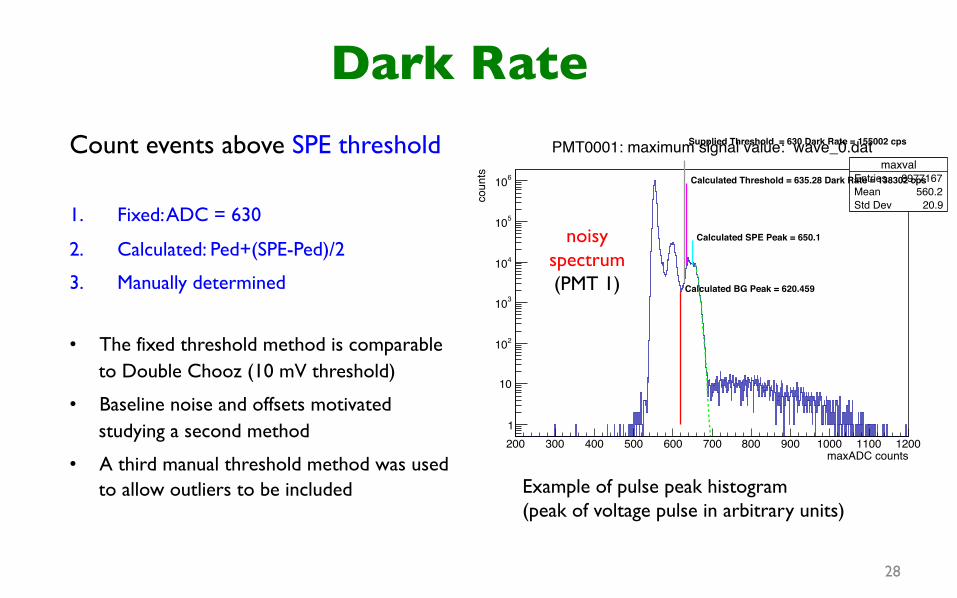
Count events above SPE threshold 1.  Fixed: ADC = 630

2.  Calculated: Ped+(SPE-Ped)/2

3.  Manually determined

•  The fixed threshold method is comparable to Double Chooz (10 mV threshold)

•  Baseline noise and offsets motivated studying a second method

maxvalEntries 9301868Mean 535Std Dev 9.064

200 300 400 500 600 700 800 900 1000 1100 1200 maxADC counts

1

10

210

310

410

510

610

coun

ts

maxvalEntries 9301868Mean 535Std Dev 9.064

Calculated Threshold = 645.14 Dark Rate = 3716.75 cps

Calculated BG Peak = 535.22

Calculated SPE Peak = 755.06

Supplied Threshold = 630 Dark Rate = 3887.29 cps

PMT0084: maximum signal value: wave_2.dat

Example of pulse peak histogram (peak of voltage pulse in arbitrary units)

clean spectrum (PMT 84)

maxvalEntries 8977167Mean 560.2Std Dev 20.9

200 300 400 500 600 700 800 900 1000 1100 1200 maxADC counts

1

10

210

310

410

510

610

coun

ts

maxvalEntries 8977167Mean 560.2Std Dev 20.9

Calculated Threshold = 635.28 Dark Rate = 138302 cps

Calculated BG Peak = 620.459

Calculated SPE Peak = 650.1

Supplied Threshold = 630 Dark Rate = 155002 cpsPMT0001: maximum signal value: wave_0.dat

28

Example of pulse peak histogram (peak of voltage pulse in arbitrary units)

noisy spectrum (PMT 1)

Count events above SPE threshold 1.  Fixed: ADC = 630

2.  Calculated: Ped+(SPE-Ped)/2

3.  Manually determined

•  The fixed threshold method is comparable to Double Chooz (10 mV threshold)

•  Baseline noise and offsets motivated studying a second method

•  A third manual threshold method was used to allow outliers to be included

Dark Rate

Dark Rate

29

0 1000 2000 3000 4000 5000 6000 7000 8000 9000 Hamamatsu Dark Rate

1000

2000

3000

4000

5000

6000

7000

8000

Mea

sure

d D

ark

Rat

e

1

36 79

10

12

14

26

272829

30

31

32

33

34

37

39

42

43

47

4849

50

51

53

54

55

56

57

59 61

63

65

6667

73

74

75

76

78

81

82

83

84

8788

90

92

94

969798

99

102

103

104

105

106

107

108

111

112

130

131

132

133

134135

136

138

139

140

141

142

143

145146

147

148149

150

152

153

154

155

157158159

160

161

162163

164

165 166167 169

170 171

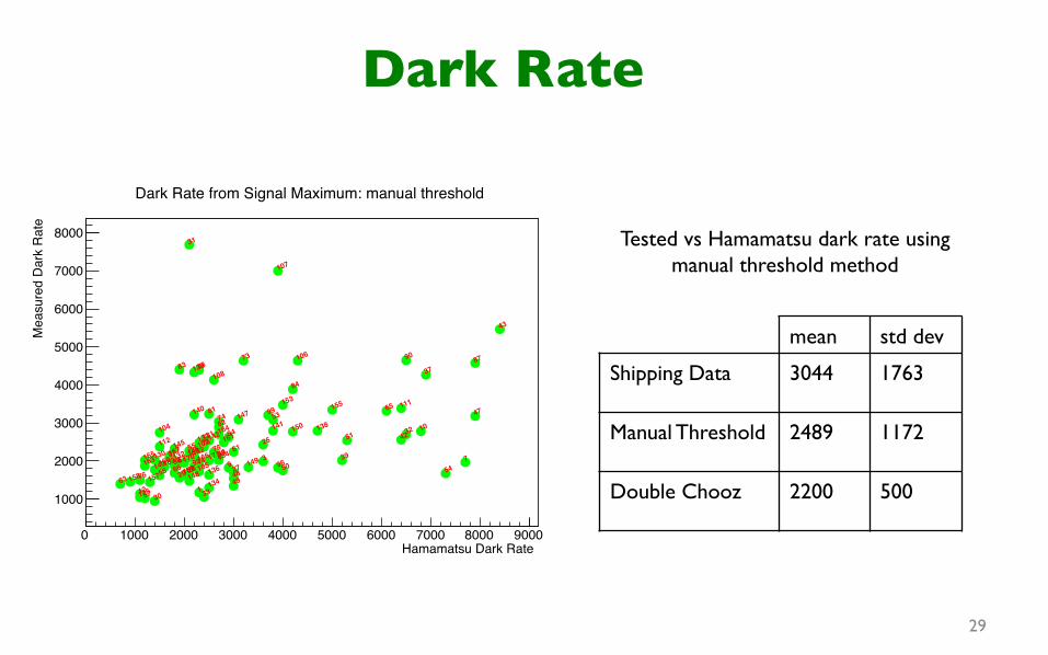
Dark Rate from Signal Maximum: manual threshold

Tested vs Hamamatsu dark rate using manual threshold method

mean std dev

Shipping Data 3044 1763

Manual Threshold 2489 1172

Double Chooz 2200 500

Dark Rate

30

1 2 3 4 5 6 7 Run Number

0

2000

4000

6000

8000

10000

12000

Mea

sure

d D

ark

Rat

e

90

130

131

132

133

159

90

96

9798

99

130

131

132

133

159166

90

159

166171

90

130

131

132

133

159

166171

98

130131

132

133

141

160

50

53

90

98

130131

132

133

141

155159

160

162163

166171

50

53

90

98130131

132

133141155

159160162

163166171

Fixed Threshold (630) Dark Rate from Signal Maximum

Comparison of dark rates for surface and underground testing The fixed threshold method used for these results Need to investigate noise and baseline

underground Run ID

Afterpulsing

31

Anthony C. Ezeribe

Types of Afterpulsing

32

Two categories of Afterpulsing1.  photoelectron in-elastically scatters off PMT dynode

- afterpulse arrives up to 80 ns after signal pulse2.  positive ion is created in PMT residual gas

- afterpulse arrives between 100 ns and 10.2 us after signal (delay can also be larger)

Late pulsing is caused by elastic scattering of electron off first dynode: not preceded by a initial pulse.

Aim to measure rates and multiplicities

Afterpulsing Examples

33

3.1 us

9.0 us

PMT: 131

Main Signal

CONCLUSIONS

35

Next Stages

•  The first pass analysis was carried out over the Christmas period •  More time is required to digest and refine the results •  Some areas clearly need attention

o  detailed understanding of noise o  relationship between figures of merit and light levels o  contribution of fields to noise and performance

•  After-pulsing analysis is underway •  Further data analysis and testing is necessary •  Documentation of analysis and results to come

36

Summary

ü  PMT testing was a real success

ü  Data was acquired for101 PMTs by thanksgiving

ü  A sample of 8 PMTs underwent testing underground

ü  Comparisons to Hamamatsu shipping data look good

ü  There are clear pathways forward to improve methods and automation towards large scale testing

ü  Great collaboration to work in!

Thanks! Gary Smith

[email protected]

PMT Test Results

Documents

Transcript of PMT Test Results