
LingTester Test Results – Passive (off-line) mode (vers b)
60
FRAILSAFE – H2020-PHC–690140 D4.13 Project Title: Sensing and predictive treatment of frailty and associated co-morbidities using advanced personalized models and advanced interventions Contract No: 690140 Instrument: Collaborative Project Call identifier: H2020-PHC-2014-2015 Topic: PHC-21-2015: Advancing active and healthy ageing with ICT: Early risk detection and intervention Start of project: 1 January 2016 Duration: 36 months Deliverable No: D4.13 LingTester Test Results – Passive (off-line) mode (vers b) Due date of deliverable: M24 (31 st December 2017) Actual submission date: 31 th December 2017 Version: 1.4 Date: 31 th December, 2017 Lead Author(s): C. Tsimpouris, N. Fazakis, K. Sgarbas (UoP) Lead partners: UoP - 1 - Ref. Ares(2017)6389645 - 31/12/2017
-
Upload
khangminh22 -
Category
Documents
-
view
1 -
download
0
Transcript of LingTester Test Results – Passive (off-line) mode (vers b)

FRAILSAFE – H2020-PHC–690140 D4.13
Project Title: Sensing and predictive treatment of frailty and associated co-morbidities using advanced personalized models and advanced interventions
Contract No: 690140 Instrument: Collaborative Project Call identifier: H2020-PHC-2014-2015 Topic: PHC-21-2015: Advancing active and healthy ageing with ICT:
Early risk detection and intervention Start of project: 1 January 2016 Duration: 36 months
Deliverable No: D4.13 LingTester Test Results – Passive
(off-line) mode (vers b)
Due date of deliverable: M24 (31st December 2017) Actual submission date: 31th December 2017 Version: 1.4 Date: 31th December, 2017 Lead Author(s): C. Tsimpouris, N. Fazakis, K. Sgarbas (UoP) Lead partners: UoP
- 1 -
Ref. Ares(2017)6389645 - 31/12/2017

FRAILSAFE – H2020-PHC–690140 D4.13
CHANGE HISTORY Ver
. Date Status Author (Beneficiary) Description
0.1 01/05/2017 draft
C. Tsimpouris (UoP),
N. Fazakis (UoP),
K. Sgarbas (UoP)
Initial draft (vers a)
0.2 07/06/2017 draft
C. Tsimpouris (UoP),
N. Fazakis (UoP),
K. Sgarbas (UoP)
First draft deliverable report, sent for internal review (vers a)
0.3 22/06/2017 draft
C. Tsimpouris (UoP),
N. Fazakis (UoP),
K. Sgarbas (UoP)
Second draft deliverable report, Text updates on introduction & chapters 2,4,5,6 (vers a)
0.4 23/06/2017 draft
L. Bianconi (SIGLA),
M. Toma (SIGLA)
K. Petridis (HYPERTECH)
Revision of the document (vers a)
1.0 29/06/2017 final
C. Tsimpouris (UoP),
N. Fazakis (UoP),
K. Sgarbas (UoP)
Final version circulated to partners (vers a)
1.1 30/06/2017 final
C. Tsimpouris (UoP),
N. Fazakis (UoP),
K. Sgarbas (UoP)
Minor corrections, accompanying files included (vers a)
1.2 20/10/2017 draft C. Tsimpouris (UoP) Image updates (vers b)
1.3 15/11/2017 draft N. Fazakis (UoP) Chapter 4, 5 updates (vers b)
1.4 22/12/2017 final
C. Tsimpouris (UoP),
N. Fazakis (UoP),
K. Sgarbas (UoP)
Final version (vers b)
- 2 -

FRAILSAFE – H2020-PHC–690140 D4.13
EXECUTIVE SUMMARY The LingTester Test Results (passive - offline mode) deliverable is the second deliverable of the Task 4.5 Processing social media which is part of the Work Package 4. In this deliverable the focus shifts from technical aspects of the LingTester tool, which prototype was presented in D4.11, to a more scientific approach regarding the test evaluation and results of the tool. This is achieved by concentrating on the essential tasks of the classification process. All the involving tasks, even if some of them seem to be trivial, in reality are equally important. The tasks are related to methodologies of collected data analysis, feature selection, classification and evaluation. In a more general view, LingTester is the FrailSafe language analysis tool that aims to process the user’s typed text and detect abnormal behaviour. At this point, the deliverable is able to perform classification according to levels of frailty. The main objective of this Work Package is to handle the collection, management and analysis of frailty older people data streamed through their social, behavioural and cognitive activities. Both offline and online methods have been developed. Moreover, the above methods have been applied in order to manage and analyze new data and also generate the FrailSafe patient models. Reader is strongly advised to read deliverables 4.11 and 4.12 in order to fully understand this report, as it is a follow up on how the prediction model has been updated.
- 3 -
FRAILSAFE – H2020-PHC–690140 D4.13
DOCUMENT INFORMATION Contract Number: H2020-PHC–690140 Acronym: FRAILSAFE
Full title Sensing and predictive treatment of frailty and associated co-morbidities using advanced personalized models and advanced interventions
Project URL http://frailsafe-project.eu/ EU Project officer Mr. Jan Komarek
Deliverable number: 4.13 Title: LingTester Test Results – Passive (off-line) mode (vers b)
Work package number: 4 Title: Data Management and Analytics
Date of delivery Contractual 31/12/2017 (M24) Actual 31/12/2017
Status Draft □ Final ⌧
Nature Report □ Demonstrator ⌧ Other □
Dissemination Level
Public ⌧ Consortium □
Abstract (for dissemination)
This deliverable reports on the choices made in the design of the prediction model of the LingTester tool and its regarding Test results. The main topics discussed are feature extraction/selection techniques, classification methods and Evaluation metrics. Firstly is given an overall introduction to the classification concepts and features selected; secondly a detailed test & evaluation of the results. Also, suicidal model tendency is discussed and analysed.
Keywords frailty, frailty classification, natural language processing, suicidal tendency
Contributing authors
(beneficiaries)
Tsimpouris Charalampos(UoP) Fazakis Nikos (UoP) Sgarbas Kyriakos (UoP) Megalooikonomou Vasileios (UoP)
Responsible author(s)
Sgarbas Kyriakos Email [email protected]
Beneficiary UoP Phone +30 2610 996470
- 4 -

FRAILSAFE – H2020-PHC–690140 D4.13
TABLE OF CONTENTS
CHANGE HISTORY 2 EXECUTIVE SUMMARY 3 DOCUMENT INFORMATION 3 TABLE OF CONTENTS 5 LIST OF FIGURES 7 LIST OF TABLES 7 LIST OF ANNEXES 7
1. Introduction 8
2. Frailty 8 2.1 General frailty description 8 2.2 Collected data 8 2.3 VPM Update 11
3. Feature Extraction 11 3.1 Primitive features 12 3.2 Derived Features 12
3.2.1 Misspellings 12 3.2.2 Term Frequencies 13 3.2.3 Sentiment analysis 14 3.2.3 Readability score 14
4. Prediction Model 17 4.1 Introduction 17 4.2 Machine Learning 18
4.2.1 History 18 4.2.2 The process 18
4.3 WEKA Software Package 19 4.2.2 Description & features 19 4.2.2 The Explorer package 19
4.4 Feature extraction 20 4.5 Feature selection 22 4.6 Classification 29 4.7 Semi-supervised learning 30
4.7.1 Introduction 30 4.7.2 Experiments 31 4.7.3 Conclusion 33
5. Frailty Model & Test Results 33 5.1 Introduction 33 5.2 Frailty model construction and evaluation 34 5.4 Final model parameters 39
- 5 -

FRAILSAFE – H2020-PHC–690140 D4.13
5.5 Final model results 40 5.5.1 Three class classification results 40 5.5.2 A simplification: Binary classification approach 42
5.6 Frailty Transition 43 5.7 Discussion of the results 45 5.8 Package Future 45
6. Suicidal Tendencies Detection 46 6.1 Introduction 46 6.2 State of the art 46 6.3 Database construction 46 6.4 Feature extraction 47 6.5 Information gain and Feature selection 48 6.6 Suicide tendency prediction 48
7. Ethics and Safety 50
8. References 52
9. File structure 54
10. Annexes 55 10.1 Goodreads crawler 55 10.2 FrailSafe demo video 60
- 6 -

FRAILSAFE – H2020-PHC–690140 D4.13
LIST OF FIGURES Figure 1. Submissions per language 9 Figure 2. Participants per frailty status 10 Figure 3. Distribution of patients per sex 11 Figure 4: Distribution of information gain per available token 14 Figure 5: Process for the construction of a prediction model 18 Figure 6: WEKA explorer package 20 Figure 7: Selected attributes 28 Figure 8: Example process of top-down induction of decision trees 30 Figure 9: Brief categorization of the SSC algorithms 32 Figure 10: Accuracy distribution 36 Figure 11: Frailty prediction results per prediction model 37 Figure 13: Old Decision tree visualization 41 Figure 14: Decision tree model results 42 Figure 15: Results of the final prediction model 43 Figure 16: Results of the final prediction model without the prefrail class 43 Figure 17: Distribution of information gain per available feature for the suicidal prediction model, based on Goodreads manually saved quotes.
48
Figure 18: Suicide tendency prediction accuracy per classifier 49 Figure 19: detailed statistical measures of Rotation Forest performing model 50 LIST OF TABLES
Table 1: List of features 22 Table 2: Subset accuracy scores of feature selection 26 Table 3: Instances that have a frailty class in conjunction to the unlabeled instances
31
Table 4: Accuracy of the Semi-supervised approach 33 Table 5: Frailty prediction results per prediction model 34 Table 6: Performance of the best 5 ensembles in Frailty prediction 38 Table 7: Explanation of parameters used 40 Table 8: Possible transition values 44 Table 9: List of features for suicidal tendency prediction 47 Table 10: Suicide tendency prediction accuracy per classifier 49 LIST OF ANNEXES
10.1 Goodreads crawler 55 10.2 FrailSafe demo video 60
- 7 -
FRAILSAFE – H2020-PHC–690140 D4.13
1. INTRODUCTION The main focus of this deliverable is to finalize a well performing predictive model taking in account the new populated participants data. The evaluation of the model is also an important aspect of the report, for this reason a satisfactory number of algorithms has been tested and compared. The evaluation of the test results is also presented and discussed on this text. The report is organized in six main chapters (excluding the auxiliary sections). The first main chapters attempts to briefly describe frailty and the collected project data related to the task. The next chapter studies the feature extraction techniques and methodologies used on LingTester tool. Following feature extraction, the next chapter focuses on the predictive model creation process. On chapter five, an introduction is given for the subject of suicidal tendencies detection and the methodologies followed to build the relevant model. Test and evaluation results are the subject of the next chapter which is numbered as section six. Finally, a discussion on the ethics and safety, related to the task, is made.
2. FRAILTY
2.1 General frailty description Frailty is a common clinical syndrome in older adults that carries an increased risk for poor health outcomes including falls, incident disability, hospitalization, and mortality [7, 8]. Frailty is theoretically defined as a clinically recognizable state of increased vulnerability resulting from aging-associated decline in reserve and function across multiple physiologic systems such that the ability to cope with everyday or acute stressors is comprised. In the absence of a gold standard, frailty has been operationally defined by Fried et al. as meeting three out of five phenotypic criteria indicating compromised energetics: low grip strength, low energy, slowed walking speed, low physical activity, and/or unintentional weight loss [9]. A pre-frail stage, in which one or two criteria are present, identifies a subset at high risk of progressing to frailty. Various adaptations of Fried’s clinical phenotype have emerged in the literature, which were often motivated by available measures in specific studies rather than meaningful conceptual differences.
2.2 Collected data Utilising eCRF API, we were able to retrieve all available raw data, stored by each medical team, containing detailed answers to the questionnaire, along with uploaded files of present and past text. For the purposes of our research, we retrieved only submissions with at least one file uploaded, and proceed to verify the uploaded content. Results were the following:
● Greece (UoP): 128 participants ○ 86 participants from the Start group
- 8 -

FRAILSAFE – H2020-PHC–690140 D4.13
○ 42 participants from the Main group ● Cyprus (Materia): 89 participants
○ 46 participants from the Start group ○ 43 participants from the Main group
● France (INSERM): 122 participants ○ 80 participants from the Start group ○ 42 participants from the Main group
For the aforementioned submissions, however, and after manual validation, we imported to our internal database only the non-empty ones that text was digitally available, ignoring during this phase all images or PDF files containing scanned images. As a result, submissions imported for the next phase were the following:
● Greece (UoP): 123 participants, 33 of which provided data from second visit ● Cyprus (Materia): 86 participants, 19 of which provided data from second visit ● France (INSERM): 95 participants, 24 of which provided data from second visit
An initial statistical analysis based on the current set of patient data returned the following results per classified feature:
Figure 1. Submissions per language
● Per language: ○ Data from 128 patients were provided in Greek, but 5 of them refused or were
unable to provide any written text, neither for the description of the image, nor for the personal event. Also, 33 of them provided extra data from second visit. Also, input from 3 participants were written in Greek polytonic. While it was not
- 9 -
FRAILSAFE – H2020-PHC–690140 D4.13
in our initial scope to differentiate this information, it was recorded in the offline database for future study
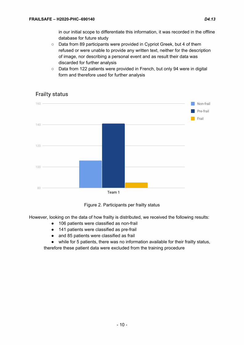
○ Data from 89 participants were provided in Cypriot Greek, but 4 of them refused or were unable to provide any written text, neither for the description of image, nor describing a personal event and as result their data was discarded for further analysis
○ Data from 122 patients were provided in French, but only 94 were in digital form and therefore used for further analysis
Figure 2. Participants per frailty status
However, looking on the data of how frailty is distributed, we received the following results:
● 106 patients were classified as non-frail ● 141 patients were classified as pre-frail ● and 85 patients were classified as frail ● while for 5 patients, there was no information available for their frailty status,
therefore these patient data were excluded from the training procedure
- 10 -
FRAILSAFE – H2020-PHC–690140 D4.13
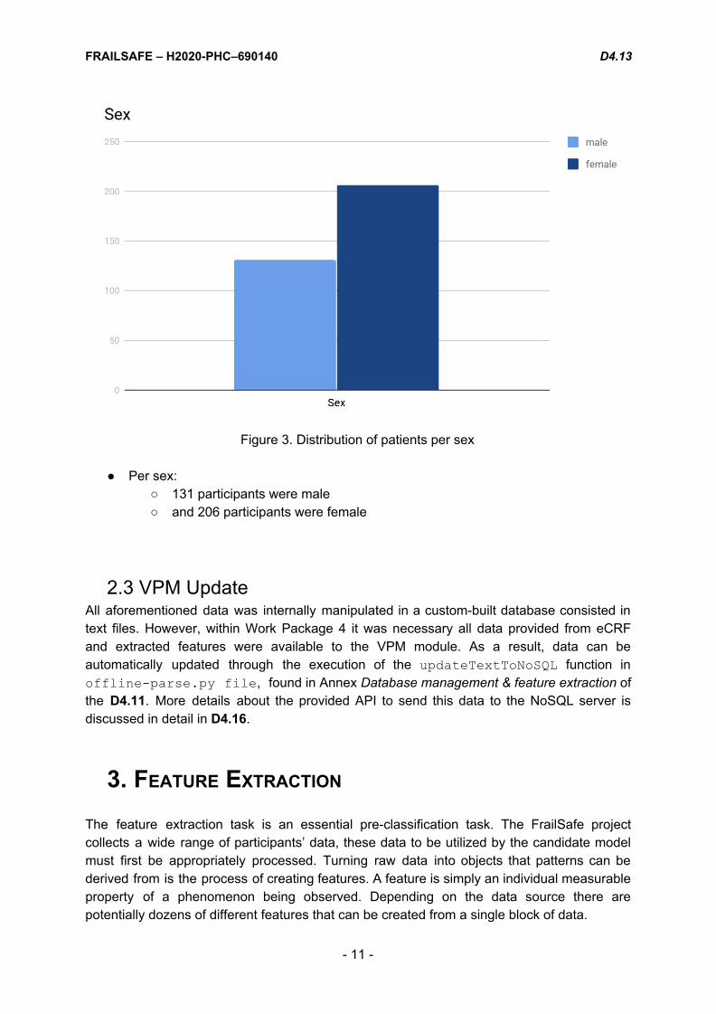
Figure 3. Distribution of patients per sex
● Per sex: ○ 131 participants were male ○ and 206 participants were female
2.3 VPM Update All aforementioned data was internally manipulated in a custom-built database consisted in text files. However, within Work Package 4 it was necessary all data provided from eCRF and extracted features were available to the VPM module. As a result, data can be automatically updated through the execution of the updateTextToNoSQL function in offline-parse.py file , found in Annex Database management & feature extraction of the D4.11. More details about the provided API to send this data to the NoSQL server is discussed in detail in D4.16.
3. FEATURE EXTRACTION The feature extraction task is an essential pre-classification task. The FrailSafe project collects a wide range of participants’ data, these data to be utilized by the candidate model must first be appropriately processed. Turning raw data into objects that patterns can be derived from is the process of creating features. A feature is simply an individual measurable property of a phenomenon being observed. Depending on the data source there are potentially dozens of different features that can be created from a single block of data.
- 11 -

FRAILSAFE – H2020-PHC–690140 D4.13
The feature extraction task starts from an initial set of measured data and builds derived values (features) intended to be informative and nonredundant, facilitating the subsequent learning and generalization steps, and in some cases leading to better human interpretations. Feature extraction involves reducing the amount of resources required to describe a large set of data. When performing analysis of complex data one of the major problems stems from the number of variables involved. Analysis with a large number of variables generally requires a large amount of memory and computation power, also it may cause a classification algorithm to overfit to training samples and generalize poorly to new samples. Feature extraction is a general term for methods of constructing combinations of the variables to get around these problems while still describing the data with sufficient accuracy.
3.1 Primitive features
Apart from existing features as stated in D4.11 chapter 5.1, extra ones were extracted programmatically for all patients with digital text from eCRF:
1. Year of birth 2. Profession 3. Residence zone 4. How many people do you follow on Twitter? 5. How many followers you have on twitter? 6. Family status 7. How many friends do you have on Facebook? 8. Do you consider yourself a familiar user of social media? 9. Do you use Facebook? 10. How often do you connect to the internet per week? 11. Have you changed your security settings in social media in order to protect your
personal data? We decided to retrieve only patient attributes that could be available directly or indirectly in the future through social media networks or other means to identify users’ electronic footprint.
3.2 Derived Features
3.2.1 Misspellings This feature is derived based on the percentage of misspellings found within a text (divided by all the words in the text). In order to achieve high accuracy, a known dictionary is used per language. The same dictionary is used by thousands of people that utilise LibreOffice , an 1
open office suite of applications. LibreOffice is community-driven and developed software, and is a project of the not-for-profit organization, The Document Foundation. LibreOffice is
1 https://www.libreoffice.org/
- 12 -

FRAILSAFE – H2020-PHC–690140 D4.13
free and open source software, originally based on OpenOffice.org (commonly known as OpenOffice), and is the most actively developed OpenOffice.org successor project.
3.2.2 Term Frequencies Proceeding to more NLP specific techniques the term frequency–inverse document frequency (tf-idf) is used. Tf-idf is a numerical statistic that is intended to reflect how important a word is to a document in a corpus. It is used as a weighting factor in text mining. The tf-idf value increases proportionally to the number of times a word appears in the document, but is offset by the frequency of the word in the corpus, which helps to adjust for the fact that some words appear more frequently in general (Salton et al, 1983). However, it became apparent that the use of the full list of the tf-idf features, which has decreased due to the stemming process, produces substantial error to the prediction model, and thus was removed. In order to overcome this issue, information gain (IG), also known as Mutual Information, has been used to extract only the terms (or small phrases) that indeed can help the prediction model improve in the overall accuracy. In general terms, the expected information gain is the change in information entropy H from a prior state to a state that takes some information as given:
Information gain for classification is a measure of how common a feature is in a particular class compared to how common it is in all other classes. A word that occurs primarily in non-frail patients and rarely in frail ones is high information. That makes sense because the point is to use only the most informative features and ignore the rest. One of the best metrics for information gain is chi square [1, 3]. The NLTK package, already used for other preprocessing tasks in more than one work packages, includes this in the BigramAssocMeasures class in the metrics package. To use it, first we need to calculate a few frequencies for each word: its overall frequency and its frequency within each class. This is done with a FreqDist class for overall frequency of words, and a ConditionalFreqDist class where the conditions are the class labels. Once we have those numbers, we can score words with the BigramAssocMeasures.chi_sq function, then sort the words by score and take the top X . We then put these words into a set, and use a set membership test in our feature selection function to select only those words that appear in the set. Now each text from a patient is classified based on the presence of these high information words. This process, has been constructed within the compute_ig python function, available also for other tasks. An example, of this task is shown below. It can be seen, that information gain is different per feature (word n our case), and thus is more than apparent that taking a small specific percent of this feature set, minimises the noise included by the rest of the words.
- 13 -

FRAILSAFE – H2020-PHC–690140 D4.13
Figure 4: Distribution of information gain per available token
3.2.3 Sentiment analysis Sentiment analysis is based on a overall rating sentiment of the patient’s text, trying to detect the polarity of the text. This feature is extracted using a dictionary and a basic algorithm which calculates the polarity of the text based on the sum of all polarities of words within the same text. The dictionary used can be found within the pattern python module and is available for the English language. Due to missing sentiment vocabulary for other languages, text is automatically translated in English for this step.
3.2.3 Readability score We decided that readability score may improve our prediction model, and we proceed to implement a series of various models that calculate readability, and see which one makes the difference. All methods measure textual difficulty, which indicates how easy a text is to read. The following readability scores have been implemented. Flesch Reading Ease The Flesch Reading Ease Scale measures readability as follows:
● 100: Very easy to read. Average sentence length is 12 words or fewer. No words of more than two syllables.
● 65: Plain English. Average sentence is 15 to 20 words long. Average word has two syllables.
● 30: A little hard to read. Sentences will have mostly 25 words. Two syllables usually. ● 0: Very hard to read. Average sentence is 37 words long. Average word has more
than two syllables.
- 14 -

FRAILSAFE – H2020-PHC–690140 D4.13
The higher the rating, the easier the text is to understand. By the very nature of technical subject matter, the Flesch score is usually relatively low for technical documentation. If the Flesch test is used regularly, one may develop a sense of what a reasonable score is for the type of documentation one is working on and aim to align with this score. The approach to calculating the Flesch score is as follows:
1. Calculate the average sentence length, L. 2. Calculate the average number of syllables per word, N. 3. Calculate score (between 0-100%).
SMOG Index The SMOG grade (Simple Measure of Gobbledygook) is a measure of readability that estimates the years of education needed to understand a piece of writing. The formula for calculating the SMOG grade was developed by G. Harry McLaughlin as a more accurate and more easily calculated substitute for the Gunning fog index and published in 1969. To make calculating a text's readability as simple as possible an approximate formula was also given — count the words of three or more syllables in three 10-sentence samples, estimate the count's square root (from the nearest perfect square), and add 3. To calculate SMOG:
1. Count a number of sentences (at least 30) 2. In those sentences, count the polysyllables (words of 3 or more syllables). 3. Calculate using
After numerous tests, this feature seem not affect the prediction model, as it was made apparent that Greek language is not fully supported by the underlying NLTK functions. Flesch–Kincaid Grade Level Although this method uses the same core measures (word length and sentence length) like the Flesch Reading Ease, they have different weighting factors. The results of the two tests correlate approximately inversely: a text with a comparatively high score on the Reading Ease test should have a lower score on the Grade-Level test. These readability tests are used extensively in the field of education. The "Flesch–Kincaid Grade Level Formula" instead presents a score as a U.S. grade level, making it easier for teachers, parents, librarians, and others to judge the readability level of various books and texts. It can also mean the number of years of education generally required to understand this text, relevant when the formula results in a number greater than 10. The grade level is calculated with the following formula:
- 15 -

FRAILSAFE – H2020-PHC–690140 D4.13
Coleman–Liau index The Coleman–Liau index is a readability test designed by Meri Coleman and T. L. Liau to gauge the understandability of a text. Like the Flesch–Kincaid Grade Level, Gunning fog index, SMOG index, and Automated Readability Index, its output approximates the U.S. grade level thought necessary to comprehend the text. The Coleman–Liau index was designed to be easily calculated mechanically from samples of hard-copy text. Unlike syllable-based readability indices, it does not require that the character content of words be analyzed, only their length in characters. Therefore, it could be used in conjunction with theoretically simple mechanical scanners that would only need to recognize character, word, and sentence boundaries, removing the need for full optical character recognition or manual keypunching. The Coleman–Liau index is calculated with the following formula:
L is the average number of letters per 100 words and S is the average number of sentences per 100 words. Automated readability index The formula for calculating the automated readability index is given below:
where characters is the number of letters and numbers, words is the number of spaces, and sentences is the number of sentences, which were counted manually by the typist when the above formula was developed. Non-integer scores are always rounded up to the nearest whole number, so a score of 10.1 or 10.6 would be converted to 11. Dale–Chall readability formula The Dale–Chall readability formula is a readability test that provides a numeric gauge of the comprehension difficulty that readers come upon when reading a text. It uses a list of 3000 words that groups of fourth-grade American students could reliably understand, considering any word not on that list to be difficult. The formula for calculating the raw score of the Dale–Chall readability score is given below:
Linsear Write Linsear Write is a readability metric for English text, purportedly developed for the United States Air Force to help them calculate the readability of their technical manuals.It was
- 16 -

FRAILSAFE – H2020-PHC–690140 D4.13
specifically designed to calculate the United States grade level of a text sample based on sentence length and the number of words used that have three or more syllables. The algorithm to calculate Linsear Write score includes various steps of preprocessing and statistical analysis of the text. Gunning fog index The Gunning fog index is calculated with the following algorithm:
1. Determine the average sentence length. (Divide the number of words by the number of sentences.)
2. Count the "complex" words: those with three or more syllables. Do not include proper nouns, familiar jargon, or compound words. Do not include common suffixes (such as -es, -ed, or -ing) as a syllable
3. Add the average sentence length and the percentage of complex words; and 4. Multiply the result by 0.4.
The complete formula is:
Discussion about readability scores All aforementioned scores are heavily used in English by teachers, writers and technicians to identify the difficulty of a text, manual and try to simplify it. Within the current work package, however, we tried to use them towards a different direction and identify how frailty is connected to the readability of the expressed text, provided by a patient. This is a hypothesis that hasn’t been discarded yet and needs to be thoroughly tested the following months, after improving the aforementioned readability scores to support better the Greek language.
4. PREDICTION MODEL
4.1 Introduction In this section of the report, will be presented a brief introduction of the major artificial intelligence techniques and methodologies that are used to produce predictive models. These methodologies can be found in the literature grouped under the term machine learning [10].
- 17 -

FRAILSAFE – H2020-PHC–690140 D4.13
4.2 Machine Learning
4.2.1 History The field inherits its methodologies from mathematics and statistics. The first real form of machine learning is discovered around 1950s with the very well known “Turing Test” [11], some of the most basic algorithms like “Nearest neighbours”, “Back propagation” and “Support vector machines” are getting discovered from 1970s through 1990s. Near this time the machine learning approach shifts from knowledge-driven to a more data-driven approach. After 2000s, technological advancements in computer chips give the ability to machine learning algorithms to utilize parallel processing and big data. Neural networks can now be run in a big number of cpu cores and this new methodology advances to become the “Deep learning” [12] approach. In the following years machine learning models are widely adopted in software programs, giving great solutions to problems in almost any real world sector.
4.2.2 The process The construction of a prediction model involves a number of tasks, basically the figure below summarizes the whole process.
Figure 5: Process for the construction of a prediction model
The first phase to the construction of a model is the raw data collection. FrailSafe project involves several number of teams under the umbrellas of different work packages in order to collect and parse all the related project data including clinical trials, hardware sensors data and higher level (analyzed) data. All the collected is potential input to the LingTester predictive model thus it has to be analyzed by the tasks of Feature extraction and Feature Selection which will be presented separately in the following sections. The next step of the process is the classification task, in this task a big number of available classification algorithms is applied and tested in order to finalize the candidate model giving the best
- 18 -

FRAILSAFE – H2020-PHC–690140 D4.13
predictive abilities. The finalized model is afterwards ready to be applied on real world instances.
4.3 WEKA Software Package
4.2.2 Description & features WEKA [13] Software is one of the most known packages used researchers and developers, it provides implementations of learning algorithms that you be easily applied to any dataset. It also includes a variety of tools for transforming datasets, such as the algorithms for discretization and sampling. A standard use casio scenario includes the preprocess of a dataset, the feed into a learning scheme, and the analysis of the resulting classifier and its performance. It was worth noting that every use flow the user wants to implement can be achieved by simply utilizing the GUI tools that accompany weka or in more complex scenarios, the user can access or alter directly the implemented source code through its own applications. Summarizing the most important features of the software:
● It is Freely available under the GNU General Public License. ● It is Portable, since it is fully implemented in the Java programming language and
thus runs on almost any modern computing platform. ● It includes a comprehensive collection of data preprocessing and modeling
techniques. ● It is Easy to use or alter due to its graphical user interfaces and extensible libraries.
4.2.2 The Explorer package The explorer package is WEKA’s main graphical user interface, it gives access to all its facilities using menu selection and form filling. It is illustrated in figure 6. To begin, there are six different panels, selected by the tabs at the top, corresponding to the various data mining tasks that weka supports. Further panels can become available by installing appropriate packages.
- 19 -

FRAILSAFE – H2020-PHC–690140 D4.13
Figure 6: WEKA explorer package All the classification task analysis done in this and the related reports was conducted using mainly using the explorer package. The tab Preprocess was used to alter accordingly the training dataset. For the evaluation of the available attributes the selection tab was used. The learner algorithms that were tested, were found on the Classify tab where the evaluation results are also found.
4.4 Feature extraction For the essential task of feature extraction, a python algorithm was developed. This script is highly complex and employs all the techniques that have already been discussed in deliverable D4.11. For better understanding and presentation, available features can be categorized by the extraction method that was used for their creation. The table below attempts to summarize this information.
Feature Names Type - Extraction Method
● transcript ○ yes ○ no
● language
Primitive Rules & filters on eCRF API data
- 20 -

FRAILSAFE – H2020-PHC–690140 D4.13
○ greek ○ greek-cypriot ○ french
● class ○ nonfrail ○ prefrail ○ frail
● data ○ Date of the submission for the
transition study ● sex
○ male ○ female
● do_you_consider_yourself_a_familiar
_user_of_social_media ○ beginner ○ less-familiar ○ very-familiar
● family_status ○ married-or-in-a-relationship ○ single ○ divorced, ○ widow
● habitation_zone ○ urban ○ semi-urban ○ rural
● have_you_changed_your_security_settings_in_social_media_in_order_to_protect_your_personal_data
○ yes ○ no
● year_of_birth ● con_per_week connections per week ● twitter_follows number if people user is
following on Twitter ● twitter_followers number of followers on
Twitter ● fb_friends number of friends on FB
● text_length ● number_of_sentences ● number_of_words ● number_of_words_per_sentence ● text_entropy
Derived Statistical Measures
● desc_image_ENG_sentiment ● desc_event_ENG_sentiment ● prev_text_ENG_sentiment
Derived Sentiment Analysis
● desc_image_misspelled Derived
- 21 -

FRAILSAFE – H2020-PHC–690140 D4.13
● desc_event_misspelled ● prev_text_misspelled
Percent of misspelled words based on known vocabulary
● tf-0 ● tf-1 ● ...
Derived Term frequency – Inverse document frequency, after feature selection based on information gain
● flesch_reading_ease ● smog_index ● flesch_kincaid_grade ● coleman_liau_index ● automated_readability_index ● dale_chall_readability_score ● difficult_words ● linsear_write_formula ● gunning_fog
Derived Readability score
Table 1: List of features
4.5 Feature selection Feature selection along with feature extraction are, as stated today in the majority of literature, the most essential tasks for creating a well performing predictive model. The prediction accuracy of a trained learner is directly depended on how much informative the selected model features are. The feature selection process, also known as variable selection, attribute selection or variable subset selection, is the process of selecting a subset of relevant features (variables, predictors) for use in model construction. The central premise when using a feature selection technique is that the data contains many features that are either redundant or irrelevant, and can thus be removed without incurring much loss of information [14]. Redundant or irrelevant features are two distinct notions, since one relevant feature may be redundant in the presence of another relevant feature with which it is strongly correlated. A number of techniques have been proposed in the literature using algorithms and even classifiers for automating the process of feature selection. The most common algorithms are the exhaustive, best first [15], simulated annealing [16] and the genetic algorithm [17]. In practice, the task of feature selection is a highly empirical process where algorithms and human intelligence are combined in order to find the optimal subset of features, thus constructing the final feature set that will be used in the classification task. As a first phase of the feature selection process we attempt to `Rank’ the available extracted features. The preliminary version of this document used the algorithm known as `OneR Attribute Evaluator’ that utilized the `One R’ [18] machine learning classifier and produced decent results. The classifier’s algorithm is presented in the following table. One R Classifier
- 22 -

FRAILSAFE – H2020-PHC–690140 D4.13
Input: Load the complete set of features (C) Count the number of all features (N) Loop for N
For each feature-class pair (P), For each value of that P, make a rule: Count how often each value of target (class) appears Find the most frequent class Make the rule assign that class to this value of the P Calculate the total error of the rules of each P
Output: Choose the P with the smallest total error.
Another approach was used in the final version of the document producing even better results. The worth of each feature was measured using Pearson’s correlation between it and the class. Pearson correlation coefficient (PCC), also referred to as Pearson's r , is a measure of the linear correlation between two variables X and Y . It has a value between +1 and −1 , where 1 is total positive linear correlation, 0 is no linear correlation, and −1 is total negative linear correlation.
where:
● n is the sample size ● xi ,yi are the single samples indexed with i
● , are the sample means The algorithm called `CorrelationAttributeEval’ (included in the WEKA package) was used to perform the attributes ranking using PCC. Nominal attributes are considered on a value by value basis by treating each value as an indicator. An overall correlation for a nominal attribute is arrived at via a weighted average. The Evaluator algorithm uses a small variation of PCC taking in account other evaluation metrics, like ReliefF, GainRatio, Entropy e.t.c., though the use of a Ranker package. The Attribute Evaluator algorithm was run and the full table of results are summarized in the next table. Attribute selection output:
=== Attribute Selection on all input data ===
Search Method:
- 23 -
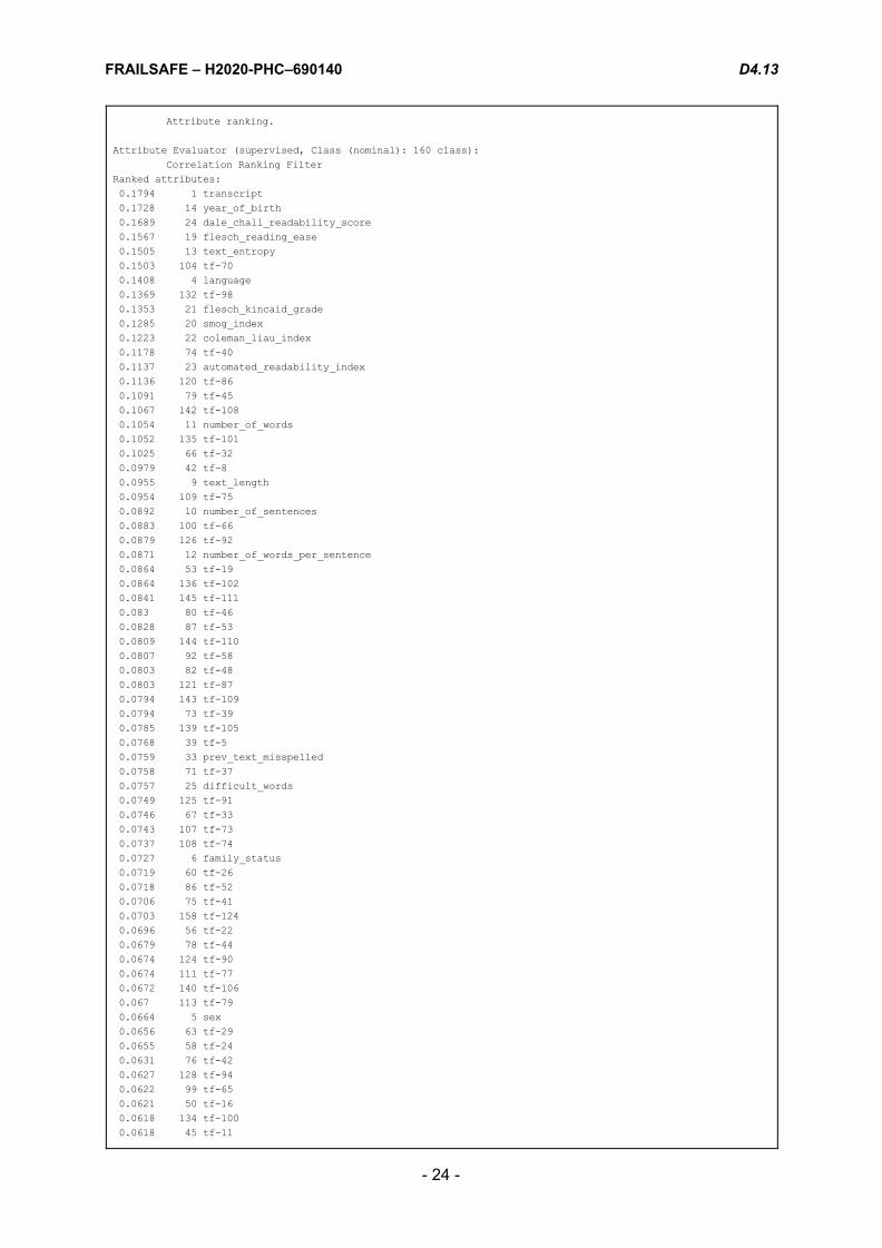
FRAILSAFE – H2020-PHC–690140 D4.13
Attribute ranking.
Attribute Evaluator (supervised, Class (nominal): 160 class):
Correlation Ranking Filter
Ranked attributes:
0.1794 1 transcript
0.1728 14 year_of_birth
0.1689 24 dale_chall_readability_score
0.1567 19 flesch_reading_ease
0.1505 13 text_entropy
0.1503 104 tf-70
0.1408 4 language
0.1369 132 tf-98
0.1353 21 flesch_kincaid_grade
0.1285 20 smog_index
0.1223 22 coleman_liau_index
0.1178 74 tf-40
0.1137 23 automated_readability_index
0.1136 120 tf-86
0.1091 79 tf-45
0.1067 142 tf-108
0.1054 11 number_of_words
0.1052 135 tf-101
0.1025 66 tf-32
0.0979 42 tf-8
0.0955 9 text_length
0.0954 109 tf-75
0.0892 10 number_of_sentences
0.0883 100 tf-66
0.0879 126 tf-92
0.0871 12 number_of_words_per_sentence
0.0864 53 tf-19
0.0864 136 tf-102
0.0841 145 tf-111
0.083 80 tf-46
0.0828 87 tf-53
0.0809 144 tf-110
0.0807 92 tf-58
0.0803 82 tf-48
0.0803 121 tf-87
0.0794 143 tf-109
0.0794 73 tf-39
0.0785 139 tf-105
0.0768 39 tf-5
0.0759 33 prev_text_misspelled
0.0758 71 tf-37
0.0757 25 difficult_words
0.0749 125 tf-91
0.0746 67 tf-33
0.0743 107 tf-73
0.0737 108 tf-74
0.0727 6 family_status
0.0719 60 tf-26
0.0718 86 tf-52
0.0706 75 tf-41
0.0703 158 tf-124
0.0696 56 tf-22
0.0679 78 tf-44
0.0674 124 tf-90
0.0674 111 tf-77
0.0672 140 tf-106
0.067 113 tf-79
0.0664 5 sex
0.0656 63 tf-29
0.0655 58 tf-24
0.0631 76 tf-42
0.0627 128 tf-94
0.0622 99 tf-65
0.0621 50 tf-16
0.0618 134 tf-100
0.0618 45 tf-11
- 24 -

FRAILSAFE – H2020-PHC–690140 D4.13
0.0618 119 tf-85
0.0618 117 tf-83
0.0618 153 tf-119
0.0618 98 tf-64
0.0617 91 tf-57
0.0617 57 tf-23
0.0611 106 tf-72
0.0605 115 tf-81
0.0599 141 tf-107
0.0591 8 have_you_changed_your_security_settings_in_social_media_in_order_to_protect_your_personal
0.0578 83 tf-49
0.054 51 tf-17
0.0537 59 tf-25
0.0536 72 tf-38
0.0527 110 tf-76
0.0518 131 tf-97
0.0508 147 tf-113
0.0508 40 tf-6
0.0508 64 tf-30
0.0508 77 tf-43
0.0508 81 tf-47
0.0508 55 tf-21
0.0508 41 tf-7
0.0508 150 tf-116
0.0508 101 tf-67
0.0508 146 tf-112
0.0508 84 tf-50
0.0508 97 tf-63
0.0508 157 tf-123
0.0508 116 tf-82
0.0508 85 tf-51
0.0505 96 tf-62
0.0503 31 desc_image_misspelled
0.0502 130 tf-96
0.0476 93 tf-59
0.0476 133 tf-99
0.0476 36 tf-2
0.0476 37 tf-3
0.0476 38 tf-4
0.0476 123 tf-89
0.0476 122 tf-88
0.0476 148 tf-114
0.0476 35 tf-1
0.0476 102 tf-68
0.0476 61 tf-27
0.0476 34 tf-0
0.0471 18 fb_friends
0.0464 151 tf-117
0.0462 159 tf-125
0.0461 27 gunning_fog
0.0451 156 tf-122
0.0444 129 tf-95
0.0436 68 tf-34
0.0436 46 tf-12
0.0436 118 tf-84
0.0436 47 tf-13
0.0436 137 tf-103
0.0436 70 tf-36
0.0436 69 tf-35
0.0436 89 tf-55
0.0436 88 tf-54
0.0436 90 tf-56
0.0436 43 tf-9
0.0433 62 tf-28
0.0428 103 tf-69
0.0427 152 tf-118
0.0422 29 desc_event_ENG_sentiment
0.0421 95 tf-61
0.0405 3 do_you_consider_yourself_a_familiar_user_of_social_media
0.0403 127 tf-93
0.0402 52 tf-18
- 25 -

FRAILSAFE – H2020-PHC–690140 D4.13
0.0398 155 tf-121
0.0391 105 tf-71
0.0371 154 tf-120
0.0365 48 tf-14
0.0365 94 tf-60
0.0358 32 desc_event_misspelled
0.0341 44 tf-10
0.0333 138 tf-104
0.0322 26 linsear_write_formula
0.0308 65 tf-31
0.0291 149 tf-115
0.0272 112 tf-78
0.0256 49 tf-15
0.0251 114 tf-80
0.0243 7 habitation_zone
0.0222 28 desc_image_ENG_sentiment
0.0184 54 tf-20
0.0161 30 prev_text_ENG_sentiment
0.0108 15 con_per_week
0 17 twitter_followers
0 16 twitter_follows
0 2 source
Selected attributes:
1,14,24,19,13,104,4,132,21,20,22,74,23,120,79,142,11,135,66,42,9,109,10,100,126,12,53,136,145,80,87,144,92,82
,121,143,73,139,39,33,71,25,125,67,107,108,6,60,86,75,158,56,78,124,111,140,113,5,63,58,76,128,99,50,134,45,1
19,117,153,98,91,57,106,115,141,8,83,51,59,72,110,131,147,40,64,77,81,55,41,150,101,146,84,97,157,116,85,96,3
1,130,93,133,36,37,38,123,122,148,35,102,61,34,18,151,159,27,156,129,68,46,118,47,137,70,69,89,88,90,43,62,10
3,152,29,95,3,127,52,155,105,154,48,94,32,44,138,26,65,149,112,49,114,7,28,54,30,15,17,16,2 : 159
As the size of the ranked feature space (RFS) is 160 (attributes), the examination of a few different subsets of the full (ranked)feature space, depending on their size, was considered as a first good approach to evaluate the need to use the full feature space in the final frailty model. Often in machine learning, it is highly possible for a subset of the feature space to have a relatively good information value almost as good as the full feature space or even better than it. Thus, giving the possibility of feature space reduction which is very good as this reduces also the model complexity and increases its performance without sacrificing the accuracy of the model. In the following table, different subsets of the ranked feature space where selected (always selected by rank order) and where classified using the Logistic Model Trees classifier. The classifier used, as explained in section 6, is a strong classifier and is part of the final ensemble classifier. The subset accuracy scores were as follows.
Size Full RFS(160)
Big RFS(100)
Medium RFS(60)
Medium RFS(52)
Small RFS(27)
Accuracy 57.73% 58.72% 60.19% 60.18% 55.03%
Table 2: Subset accuracy scores of feature selection It is clear that, a Medium sized RFS of 52 attributes performs relatively good to its size while it reduces the complexity of the model. It is also obvious by the table, that a very big feature space does always guarantee better overall performance. To further enhance the feature selection task, a simple yet effective process has been followed. The first steps of the process involve an iteration of classifications, using a Decision Tree model, where each individual feature was examined for its contribution to the accuracy
- 26 -

FRAILSAFE – H2020-PHC–690140 D4.13
of the temporary model, using the cross validation method [19]. After a sufficient number of iterations, the resulting decision tree was visualized and examined by hand in order to further optimize the resulting model. Final Feature Selection Algorithm
Input: Load the complete set of features (C) Count the number of all features (N) Classify with C and store the accuracy (A) Initialize pointer as zero (P) Loop for N
Remove C[P] Classify with C (Ac) If Ac < A
Restore C[P]
Validate features by tree visualization Output: Subset of features (S)
After the successful execution of all the above steps & procedures we combined the strongest results and we ended up with the following selected attributes to use for the final classification task.
- 27 -

FRAILSAFE – H2020-PHC–690140 D4.13
Figure 7: Selected attributes
- 28 -

FRAILSAFE – H2020-PHC–690140 D4.13
4.6 Classification This section is an attempt to describe briefly the classifier models that will be used to obtain the test results in chapter 6. It will also help to understand why a classifier is better suitable than another classifier for the given problem of frailty classification. The first big category of classifiers worth mentioning is the probabilistic or bayes classifiers. The classifiers aparting this category are based on the application of Bayes’ theorem with strong (naive) independence assumptions between the features. Naive Bayes [20], the most known classifier belonging in this category, has been studied extensively since the 1950s. It was introduced under a different name into the text retrieval community in the early 1960s and remains a popular method for text categorization, the problem of judging documents as belonging to one category or the other (such as spam or legitimate, sports or politics, etc.) with word frequencies as the features. With appropriate pre-processing, it is competitive in this domain with more advanced methods including support vector machines. It also finds application in automatic medical diagnosis. Abstractly, naive Bayes is a conditional probability model: given a problem instance to be classified, represented by a vector x representing some n features (independent variables), it assigns to this instance probabilities calculated by the formula:
for each of k possible outcomes or classes Ck. A second big category of classifiers is based on functions. The classifier family that is worth mentioning in this category, as it suits the problem, is Support Vector Machines [21]. SVMs are supervised learning models with associated learning algorithms that analyze data used for classification and regression analysis. Given a set of training examples, each marked as belonging to one or the other of two categories, an SVM training algorithm builds a model that assigns new examples to one category or the other, making it a non-probabilistic binary linear classifier. An SVM model is a representation of the examples as points in space, mapped so that the examples of the separate categories are divided by a clear gap that is as wide as possible. New examples are then mapped into that same space and predicted to belong to a category based on on which side of the gap they fall. In addition to performing linear classification, SVMs can efficiently perform a non-linear classification using what is called the kernel trick, implicitly mapping their inputs into high-dimensional feature spaces. In this category of classifiers the Multilayer perceptron is also considered a strong model. MLP is a feedforward artificial neural network model that maps sets of input data onto a set of appropriate outputs. An MLP consists of multiple layers of nodes in a directed graph, with each layer fully connected to the next one. Except for the input nodes, each node is a neuron (a processing element) with a nonlinear activation function. MLP utilizes a learning technique called backpropagation for training the network. The third category that will be mentioned is based on tree structures. Better known as Decision Trees [22], this set of classifiers mainly utilize a decision tree as a predictive model to go from observations about an item, represented in the nodes, to conclusions about the item's target value represented in the leaves. A tree can be trained by splitting the source set
- 29 -
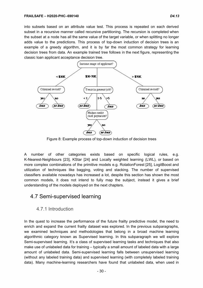
FRAILSAFE – H2020-PHC–690140 D4.13
into subsets based on an attribute value test. This process is repeated on each derived subset in a recursive manner called recursive partitioning. The recursion is completed when the subset at a node has all the same value of the target variable, or when splitting no longer adds value to the predictions. This process of top-down induction of decision trees is an example of a greedy algorithm, and it is by far the most common strategy for learning decision trees from data. An example trained tree follows in the next figure, representing the classic loan applicant acceptance decision tree.
Figure 8: Example process of top-down induction of decision trees
A number of other categories exists based on specific logical rules, e.g. K-Nearest-Neighbours [23], KStar [24] and Locally weighted learning (LWL), or based on more complex combinations of the primitive models e.g. RotationForest [25], LogitBoost and utilization of techniques like bagging, voting and stacking. The number of supervised classifiers available nowadays has increased a lot, despite this section has shown the most common models, it does not intend to fully map the subject, instead it gives a brief understanding of the models deployed on the next chapters.
4.7 Semi-supervised learning
4.7.1 Introduction In the quest to increase the performance of the future frailty predictive model, the need to enrich and expand the current frailty dataset was explored. In the previous subparagraphs, we examined techniques and methodologies that belong in a broad machine learning algorithmic category known as Supervised learning. In this subparagraph we will explore Semi-supervised learning. It’s a class of supervised learning tasks and techniques that also make use of unlabeled data for training – typically a small amount of labeled data with a large amount of unlabeled data. Semi-supervised learning falls between unsupervised learning (without any labeled training data) and supervised learning (with completely labeled training data). Many machine-learning researchers have found that unlabeled data, when used in
- 30 -
FRAILSAFE – H2020-PHC–690140 D4.13
conjunction with a small amount of labeled data, can produce considerable improvement in learning accuracy. The acquisition of labeled data for a learning problem often requires a skilled human agent (e.g. a doctor) or a physical experiment (e.g. clinical examination). The cost associated with the labeling process thus may render a fully labeled training set infeasible, whereas acquisition of unlabeled data is relatively inexpensive. In such situations, semi-supervised learning can be of great practical value. Semi-supervised learning is also of theoretical interest in machine learning and as a model for human learning.
4.7.2 Experiments The main idea here is to enrich the original frailty dataset with a bigger set of unlabeled instances (meaning the frailty class is not available) gathered from twitter public user quotes. The exact procedure of data gathering and pre-processing was a subject of D4.7 while the technical details of the construction of the enriched frailty dataset are presented in D4.11. In this report we will focus on the actual use and testing of the augmented semi-supervised frailty dataset. In the series of tests that were performed using semi-supervised learning algorithms, 4 datasets where constructed using different labeled ratios. With the term labeled ratio, we refer to the percentage of labeled instances (instances that have a frailty class) in conjunction to the unlabeled instances. The table below summarizes the datasets outlook.
Dataset name Labeled ratio Labeled instances
Unlabeled instances
semi-frailty-10 10% 178 1600
semi-frailty-20 20% 178 712
semi-frailty-30 30% 178 415
semi-frailty-40 40% 178 267
Table 3: Instances that have a frailty class in conjunction to the unlabeled instances The Semi-supervised Classification (SSC) problem can be defined as follows: Let x
pbe an
example where x p= (x
p1, x
p2 , ..., x pD , ω) , with x
pbelonging to a class ω and a
D-dimensional space in which x pi
is the value of the ith feature of the pth sample. Then, let us assume that there is a labeled set L which consists of n instances x
pwith ω known.
Furthermore, there is an unlabeled set U which consists of m instances x q
with ω unknown, let m > n . The L + U sets form the training set (denoted as TR ). The purpose of SSC is to obtain a robust learned hypothesis using TR instead of L alone. SSC Taxonomy
- 31 -

FRAILSAFE – H2020-PHC–690140 D4.13
SSC methods search iteratively for one or several enlarged labeled set(s) (EL) of prototypes to efficiently represent the TR. The Self-labeling taxonomy is oriented to categorize the algorithms regarding their main aspects related to their operation. The next figure (figure 9) gives a brief categorization of the SSC algorithms.
Figure 9: Brief categorization of the SSC algorithms
In order to apply the Semi-supervised approach in the frailty prediction problem, five of the most used used algorithms were selected:
● SelfTraining: An iterative method to label the unlabeled data and use them afterwards.
● CoForest: A semi-supervised algorithm, which exploits the power of ensemble learning and large amount of unlabeled data available to produce hypothesis with better performance.
● CoTraining: Two different views of the data are used to build a pair of models/classifiers.
● TriTraining: It generates three classifiers from the original labeled examples and then is refined using unlabeled examples in the tri-training process.
● RASCO: A random subspace method for co-training. The experiments gave the following in terms of accuracy %:
- 32 -

FRAILSAFE – H2020-PHC–690140 D4.13
Dataset name SelfTraining (C4.5)
CoForest CoTraining (NN,C4.5,NN)
TriTraining (NN,NN,NN)
RASCO (C4.5)
semi-frailty-10 46.0 50.1 48.1 46.4 47.9
semi-frailty-20 48.0 47.8 48.2 46.8 42.3
semi-frailty-30 47.9 51.5 48.1 46.6 46.6
semi-frailty-40 46.6 48 48.1 46.8 40.1
Table 4: Accuracy of the Semi-supervised approach
4.7.3 Conclusion In the previous paragraphs, a few of the most known Semi-supervised methods were applied to frailty classification problem. The reason behind the experimentation with this category of algorithms was to augment the frailty dataset in hopte to increase the final models performance. Judging the results of the Table 4 in contrary with the supervised approach accuracies presented in chapter 5, the semi-supervised techniques’ performance were not unrelated to those of supervised base classifiers but still they failed to significantly increase the overall accuracy. This outcome was not obvious from the beginning, as SSC in general scores good results on other areas of application. One should not underestimate that, frailty dataset is a very niche one and can not strongly correlate to data gathered from other sources, although they were collected with that in mind as described in D4.7.
5. FRAILTY MODEL & TEST RESULTS
5.1 Introduction The major subject of this report is the test results of the predictive model. In reality, everything done in the task is heavily tied with the performance increasement of the final model. As has been emphasized in chapter 4, the performance of a model is equally influenced by all the previous tasks of the classification process. The parts of feature extraction and feature selection are considered as highly important factors of the final predictive accuracy and require fairly more expensive resources like human expertise. As the above factors are not a hundred percent controlled by this task, a very strong and extensive testing process has to be done in order to select the final classification model and ensure the best possible prediction accuracy.
- 33 -

FRAILSAFE – H2020-PHC–690140 D4.13
This chapter presents the evaluation process followed to obtain the test results, the comparison of the various models, the parameters of the selected model and the statistics of the final model. Finally, this chapter ends with a brief discussion of the test results, as this is a preliminary report and the model is expected to change, and also a few words about the future steps of development.
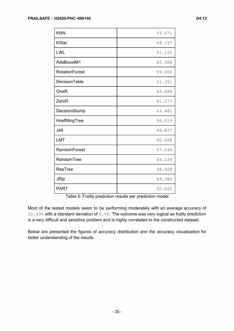
5.2 Frailty model construction and evaluation Machine learning offers a wide range of algorithms that can fit the data and build a predictive model. In order to test the possible model performances and select the most suitable for the case, an extensive experiment was organized. Totally, seventeen of the most widely used classifiers were selected from six different algorithm families. The measured metric was that of classification accuracy. The evaluation method that was used is the classic method of Cross Validation[26]. In general, cross validation is a model validation technique for assessing how the results of a statistical analysis will generalize to an independent data set. One round of cross-validation involves partitioning a sample of data into complementary subsets, performing the analysis on one subset (called the training set), and validating the analysis on the other subset (called the validation set or testing set). To reduce variability, multiple rounds of cross-validation are performed using different partitions, and the validation results are averaged over the rounds. One of the main reasons for using cross-validation instead of using the conventional validation (e.g. partitioning the data set into two sets of 70% for training and 30% for test) is that there is not enough data available to partition it into separate training and test sets without losing significant modelling or testing capability. In summary, cross-validation combines (averages) measures of fit (prediction error) to derive a more accurate estimate of model prediction performance. The table that follows presents the test results, measured in accuracy percent, for the extensive tested scenario, using the 10 fold cross validation method.
Classifier Accuracy %
NaiveBayes 47.665
Bayesian Network 41.227
Support Vector Machine 40.049
Logistic 56.756
Neural Network 56.265
Simple Logistic 61.179
SMO 56.756
- 34 -
FRAILSAFE – H2020-PHC–690140 D4.13
KNN 53.071
KStar 48.157
LWL 51.105
AdaBoostM1 43.488
RotationForest 59.950
DecisionTable 51.351
OneR 43.488
ZeroR 41.277
DecisionStump 43.481
HoeffdingTree 56.019
J48 49.877
LMT 60.688
RandomForest 57.248
RandomTree 44.226
RepTree 46.928
JRip 49.385
PART 50.800
Table 5: Frailty prediction results per prediction model Most of the tested models seem to be performing moderately with an average accuracy of 50.43% with a standard deviation of 6.58 . The outcome was very logical as frailty prediction is a very difficult and sensitive problem and is highly correlated to the constructed dataset. Below are presented the figures of accuracy distribution and the accuracy visualization for better understanding of the results.
- 35 -

FRAILSAFE – H2020-PHC–690140 D4.13
Figure 10: Accuracy distribution
- 36 -

FRAILSAFE – H2020-PHC–690140 D4.13
Figure 11: Frailty prediction results per prediction model As has been shown, the performance of the elemental classifier models seems to be moderate. In order to enhance the performance of the frailty model, a collection of performance boost techniques known as META classifiers was studied. The technique is also known as Ensemble learning. Ensemble methods use multiple learning algorithms to obtain better predictive performance than could be obtained from any of the constituent learning algorithms alone. Supervised learning algorithms are most commonly described as performing the task of searching through a hypothesis space to find a suitable hypothesis that will make good predictions with a particular problem. Even if the hypothesis space contains hypotheses that are very well-suited for a particular problem, it may be very difficult to find a good one. Ensembles combine multiple hypotheses to form a (hopefully) better hypothesis. An ensemble is itself a supervised learning algorithm, because it can be trained and then used to make predictions. The trained ensemble, therefore, represents a single hypothesis. This hypothesis, however, is not necessarily contained within the hypothesis space of the models from which it is built. Thus, ensembles can be shown to have more flexibility in the functions they can represent. The common ensemble methods include techniques like Bagging, Boosting, Stacking, Voting e.t.c. In our case, the most suitable technique was the Voting algorithm, as we already had identified a number of strong basic classifiers from the evaluation process of the elemental classifiers and we intent to combine their predictions in order to decrease the number of incorrectly classified instances. The Voting meta algorithm gives a number of ways to combine the different classifiers’ predictions, the most common are:
- 37 -
FRAILSAFE – H2020-PHC–690140 D4.13
● Average of classifiers’ prediction probabilities ● Product of classifiers’ prediction probabilities ● Majority voting of classifiers’ predictions ● Median of classifiers’ predictions ● Minimum/Maximum of classifiers’ prediction probabilities
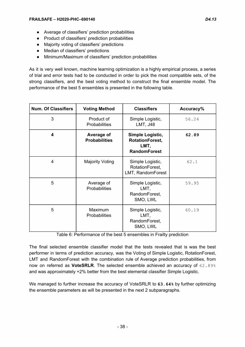
As it is very well known, machine learning optimization is a highly empirical process, a series of trial and error tests had to be conducted in order to pick the most compatible sets, of the strong classifiers, and the best voting method to construct the final ensemble model. The performance of the best 5 ensembles is presented in the following table.
Num. Of Classifiers Voting Method Classifiers Accuracy%
3 Product of Probabilities
Simple Logistic, LMT, J48
56.24
4 Average of Probabilities
Simple Logistic, RotationForest,
LMT, RandomForest
62.89
4 Majority Voting Simple Logistic, RotationForest,
LMT, RandomForest
62.1
5 Average of Probabilities
Simple Logistic, LMT,
RandomForest, SMO, LWL
59.95
5 Maximum Probabilities
Simple Logistic, LMT,
RandomForest, SMO, LWL
60.19
Table 6: Performance of the best 5 ensembles in Frailty prediction The final selected ensemble classifier model that the tests revealed that is was the best performer in terms of prediction accuracy, was the Voting of Simple Logistic, RotationForest, LMT and RandomForest with the combination rule of Average prediction probabilities, from now on referred as VoteSRLR. The selected ensemble achieved an accuracy of 62.89% and was approximately +2% better from the best elemental classifier Simple Logistic. We managed to further increase the accuracy of VoteSRLR to 63.64% by further optimizing the ensemble parameters as will be presented in the next 2 subparagraphs.
- 38 -

FRAILSAFE – H2020-PHC–690140 D4.13
5.4 Final model parameters The final ensemble classifier that was selected to be used in the LingTester tool is VoteSRLR. In the tool, an open source java version of this algorithm has been used. This version is capable of being tuned by a series of input parameters, mainly giving control of the final structure of the base learners. The available parameters have been gathered along with their description in the next table. The exact values that were used to produce the LingTester tool predictor are also presented on the table below. The process of model parameter optimization is a highly empirical process, although there have been some efforts in the field, for example Auto-Weka, but still no general method exists.
Parameter Name Description Optimum Value
Voting Algorithm
Combination Rule The combination to rule used. Average of Probabilities
Simple Logistic
Error On Probabilities
Use error on the probabilities as error measure when determining the best number of LogitBoost iterations.
False
Weight Trim Beta Set the beta value used for weight trimming in LogitBoost.
0.1
Use AIC The AIC is used to determine when to stop LogitBoost iterations
False
Max Boosting Iterations
Sets the maximum number of iterations for LogitBoost.
500
Heuristic Stop LogitBoost is stopped if no new error minimum has been reached in the last Heuristic Stop iterations.
50
RotationForest
Removed Percentage
The percentage of instances to be removed. 50
Max Group Maximum size of a group. 3
Min Group Minimum size of a group. 3
Projection Filter The filter used to project the data. Principal Components
- 39 -

FRAILSAFE – H2020-PHC–690140 D4.13
Classifier The base classifier to be used J48
LMT
Do Not Make Split Point Actual Value
If true, the split point is not relocated to an actual data value.
False
Weight Trim Beta Set the beta value used for weight trimming in LogitBoost.
0.0
Fast Regression Use heuristic that avoids cross-validating the number of Logit-Boost iterations at every node.
True
Min Num Instances Set the minimum number of instances at which a node is considered for splitting.
15
Split On Residuals Set splitting criterion based on the residuals of LogitBoost.
True
Convert Nominal Convert all nominal attributes to binary ones before building the tree.
False
RandomForest
Calc Out Of Bag Whether the out-of-bag error is calculated. False
Max Depth The maximum depth of the tree, 0 for unlimited. 0
Store Out Of Bag Predictions
Whether to store the out-of-bag predictions. Flase
Break Ties Randomly
Break ties randomly when several attributes look equally good.
True
Num Features Sets the number of randomly chosen attributes. 0
Compute Attribute Importance
Compute attribute importance via mean impurity decrease.
False
Table 7: Explanation of parameters used
5.5 Final model results
5.5.1 Three class classification results In the preliminary version of this report a much smaller frailty dataset was available at the time, thus a simple J48 model was able to achieve a 64% accuracy. The old tree model had the following simple decision structure.
- 40 -

FRAILSAFE – H2020-PHC–690140 D4.13
Figure 13: Old Decision tree visualization As this is the final version of the document, the FrailSafe dataset is already bigger than double and the old Decision Tree model as tested in section 6.3 could only score an accuracy of 49.87% . The complexity of the dataset has increased with the introduction of new instances and more information(french speaking participants were also added). For this reason a there was an argent need to construct a new learning model with higher information capacity that could also be re-trained and used with the future FrailSafe datasets. This led to the development of VoteSRLR which is already able to achieve almost the same accuracy of the old model with more complex datasets. As frailty prediction is a very hard problem bound to the participants profile, further prediction accuracy increments could lie on the enrichment of dataset. The final ensemble model that is embedded to the LingTester tool is capable of predicting the three possible frailty conditions (nonfrail, prefrail, frail) by an average prediction accuracy of 63.64% for out of sample instances. A statistical analysis of the model has been conducted and the most important metrics are presented below.
=== Stratified cross-validation ===
=== Summary ===
Correctly Classified Instances 259 63.64 %
Incorrectly Classified Instances 148 36.36 %
Kappa statistic 0.4331
Mean absolute error 0.3453
Root mean squared error 0.4116
Relative absolute error 79.4175 %
Root relative squared error 88.2764 %
Total Number of Instances 407
=== Detailed Accuracy By Class ===
TP Rate FP Rate Precision Recall F-Measure MCC ROC Area PRC Area Class
0.729 0.202 0.654 0.729 0.689 0.514 0.830 0.684 nonfrail
- 41 -
FRAILSAFE – H2020-PHC–690140 D4.13
0.649 0.314 0.592 0.649 0.619 0.331 0.713 0.604 prefrail
0.485 0.062 0.716 0.485 0.578 0.490 0.796 0.643 frail
Weighted Avg. 0.636 0.214 0.644 0.636 0.633 0.433 0.773 0.641
=== Confusion Matrix ===
a b c <-- classified as
102 34 4 | a = nonfrail
44 109 15 | b = prefrail
10 41 48 | c = frail
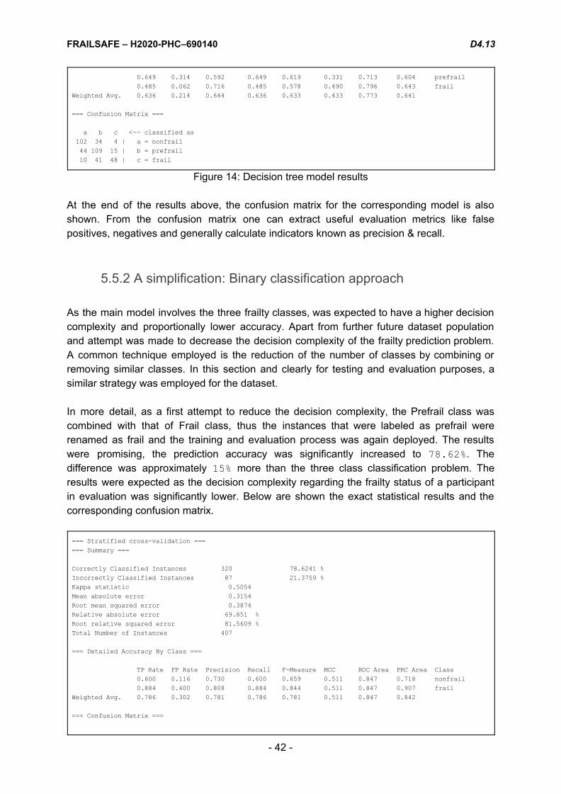
Figure 14: Decision tree model results At the end of the results above, the confusion matrix for the corresponding model is also shown. From the confusion matrix one can extract useful evaluation metrics like false positives, negatives and generally calculate indicators known as precision & recall.
5.5.2 A simplification: Binary classification approach As the main model involves the three frailty classes, was expected to have a higher decision complexity and proportionally lower accuracy. Apart from further future dataset population and attempt was made to decrease the decision complexity of the frailty prediction problem. A common technique employed is the reduction of the number of classes by combining or removing similar classes. In this section and clearly for testing and evaluation purposes, a similar strategy was employed for the dataset. In more detail, as a first attempt to reduce the decision complexity, the Prefrail class was combined with that of Frail class, thus the instances that were labeled as prefrail were renamed as frail and the training and evaluation process was again deployed. The results were promising, the prediction accuracy was significantly increased to 78.62% . The difference was approximately 15% more than the three class classification problem. The results were expected as the decision complexity regarding the frailty status of a participant in evaluation was significantly lower. Below are shown the exact statistical results and the corresponding confusion matrix.
=== Stratified cross-validation ===
=== Summary ===
Correctly Classified Instances 320 78.6241 %
Incorrectly Classified Instances 87 21.3759 %
Kappa statistic 0.5054
Mean absolute error 0.3154
Root mean squared error 0.3874
Relative absolute error 69.851 %
Root relative squared error 81.5609 %
Total Number of Instances 407
=== Detailed Accuracy By Class ===
TP Rate FP Rate Precision Recall F-Measure MCC ROC Area PRC Area Class
0.600 0.116 0.730 0.600 0.659 0.511 0.847 0.718 nonfrail
0.884 0.400 0.808 0.884 0.844 0.511 0.847 0.907 frail
Weighted Avg. 0.786 0.302 0.781 0.786 0.781 0.511 0.847 0.842
=== Confusion Matrix ===
- 42 -
FRAILSAFE – H2020-PHC–690140 D4.13
a b <-- classified as
84 56 | a = nonfrail
31 236 | b = frail
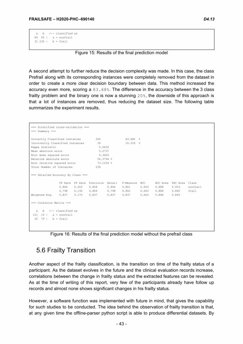
Figure 15: Results of the final prediction model A second attempt to further reduce the decision complexity was made. In this case, the class Prefrail along with its corresponding instances were completely removed from the dataset in order to create a more clear decision boundary between data. This method increased the accuracy even more, scoring a 83.68% . The difference in the accuracy between the 3 class frailty problem and the binary one is now a stunning 20% , the downside of this approach is that a lot of instances are removed, thus reducing the dataset size. The following table summarizes the experiment results.
=== Stratified cross-validation ===
=== Summary ===
Correctly Classified Instances 200 83.682 %
Incorrectly Classified Instances 39 16.318 %
Kappa statistic 0.6632
Mean absolute error 0.2737
Root mean squared error 0.3602
Relative absolute error 56.3794 %
Root relative squared error 73.1229 %
Total Number of Instances 239
=== Detailed Accuracy By Class ===
TP Rate FP Rate Precision Recall F-Measure MCC ROC Area PRC Area Class
0.864 0.202 0.858 0.864 0.861 0.663 0.888 0.916 nonfrail
0.798 0.136 0.806 0.798 0.802 0.663 0.888 0.860 frail
Weighted Avg. 0.837 0.175 0.837 0.837 0.837 0.663 0.888 0.893
=== Confusion Matrix ===
a b <-- classified as
121 19 | a = nonfrail
20 79 | b = frail
Figure 16: Results of the final prediction model without the prefrail class
5.6 Frailty Transition
Another aspect of the frailty classification, is the transition on time of the frailty status of a participant. As the dataset evolves in the future and the clinical evaluation records increase, correlations between the change in frailty status and the extracted features can be revealed. As at the time of writing of this report, very few of the participants already have follow up records and almost none shows significant changes in his frailty status. However, a software function was implemented with future in mind, that gives the capability for such studies to be conducted. The idea behind the observation of frailty transition is that, at any given time the offline-parser python script is able to produce differential datasets. By
- 43 -

FRAILSAFE – H2020-PHC–690140 D4.13
differential we mean, an algorithm that computes the scores of specific quantitative features between the clinical evaluations and creates derivative features that they decipit the score difference (transition) for each of them corresponding to a frailty transition status. The possible frailty transition statuses are:
Transition value
nonfrail_to_prefrail
prefrail_to_nonfrail
prefrail_to_frail
frail_to_prefrail
nonfrail_to_frail
frail_to_nonfrail
Table 8: Possible transition values An example dataset has been produced taking in account the participant records as appeared in eCRF up to M22.
Figure 17: Example dataset for transision strudy
As the transition dataset at this time does not have rich information value, no analysis can be conducted. In the near future, the FrailSafe project as planned, possibly will have enough collected data to be used as an input for the transition dataset creator. At that time, machine learning & statistical analysis approaches can be applied with the same tools that were
- 44 -
FRAILSAFE – H2020-PHC–690140 D4.13
presented in this document and possibly correlate the transitional data to frailty status changes.
5.7 Discussion of the results This chapter was devoted to the evaluation process and the extraction of the according evaluation metrics. A large experiment was organized and the twenty five of the most known models were trained and evaluated. The final model that was selected to be embedded to the LingTester tool, was a complex Meta classifier that bases its predictions on the average probabilities extracted by the base classifier Simple Logistic, RotationForest, LMT, RandomForest. It was selected due to its accuracy superiority, in comparison with the other evaluated algorithms, and also due to its learning capacity. The accuracy for the selected classifier was achieved after the parameter optimization process and was around 63.64% for three class classification problem. Further increase of the prediction performance could possibly lie on the qualitative and quantitative increase of future population of participants data or by further optimizing the model parameters. Binary classification is also an approach that was evaluated and seems tο perform relatively good mainly to the reduction of decision complexity. The achieved accuracy of this technique was at the levels of 83.68% . Further exploration of the approach may reveal useful relations between the dataset features and parameters.
5.8 Package Future
Although this is a final report, the FrailSafe project will still continue to gather data from partners and for a long time. We think this was a good first approach to the frailty prediction task in proportion to the data and operating structures we had available for use. All the tools and algorithms developed and presented in this report can be reapplied in the future of FrailSafe project, as they were designed with user friendliness and simplicity in mind. It is almost certain that as the data collection from the participants continues prediction models can further learn and increase their performance and accuracy. It seems promising to, on the one hand to evaluate the models in real case scenarios during the FrailSafe project and on the other hand to feedforward the system with this experience. Another important aspect of the package is its ability to log almost every possible derived information so other packages can retract it from the central FrailSafe database and built upon on LingTester’s output.
- 45 -

FRAILSAFE – H2020-PHC–690140 D4.13
6. SUICIDAL TENDENCIES DETECTION
6.1 Introduction The study of suicide risk is complex. Suicide is a medical disaster, but occurs at a relatively low frequency. The extensive body of suicide and self harm risk research has identified many risk factors, among them: diagnosed mental disorders, substance abuse, and a history of prior suicide attempts. However, much of this research has been based on retrospective study of suicide attempters and completers. The rarity of suicidal behavior limits the specificity of predicting future suicidal behavior based on relatively common risk factors. A recent survey of literature on screening tools to predict suicide attempts and death by suicide concluded that current evidence is insufficient to support reliance on screening tools based on presence or absence of risk factors in clinical practice [2], and so, the current standard of care for the at-risk patient remains in the domain of a skilled clinical assessment.
6.2 State of the art Fine-grained automatic emotion detection can benefit from from classifier optimization and a combined lexico-semantic feature representation can achieve scores up to 68.86% F-score [4]. Corpus for model construction and prediction has been a note corpus of positive only data, annotated with fine-grained emotions, released in the framework of the 2011 i2b2 NLP Challenge on emotion classification in suicide notes [5], allowing research on which emotions might be indicative of suicidal behavior, and how they can be found automatically. However, this dataset is no longer available. Also, vocabulary based methodology, manually annotated on Twitter posts and then classification using various classifier could not produce more than 64% accuracy [6].
6.3 Database construction According to the predefined work packages, no information could be available to identify suicidal patients, so a different approach was selected to create our dataset. We identified the Goodreads web page as a potential source for our scope. Among other things, this web 2
page provides famous quotes from known books, which have been manually saved by the Goodreads community. This manual process also forces each user to tag the quote with at least one keyword, and therefore various categories have appeared. A crawler for this purpose was constructed to identify and download all quotes set by the researchers, split in two main groups:
● suicide: quotes identified by the following keywords ○ suicide, ○ suicide-note,
2 https://www.goodreads.com/
- 46 -

FRAILSAFE – H2020-PHC–690140 D4.13
○ suicide-attempt and ○ suicidal-thoughts
● non-suicide: quotes identified by the following keywords ○ humor and ○ happy
To avoid an unbalanced dataset, the second category was filled randomly till we had the same amount of quotes in both categories. After the data collection, each group has 3184 instances.
6.4 Feature extraction Feature extraction was based on the same methodology as stated before, for the frailty prediction model. The derived feature space used for suicidal tendencies detection was intentionally kept familiar with the frailty feature space for consistency reasons. In contrast with the frailty detection process, the current task lacks the eCRF API data. Below, follows a brief description of the feature space in table 9.
Feature Names Feature Description
● class ○ suicide ○ non-suicide
goodreads crawler labels (see Annex 1 for details)
● text_length ● number_of_sentences ● number_of_words ● number_of_words_per_sentence ● text_entropy
Statistical Measures
● sentiment Sentiment Analysis of text data
● misspelled Percent of misspelled words based on known vocabulary
● tf-0 ● tf-1 ● ...
Term frequency – Inverse document frequency, after feature selection based on information gain
● flesch_reading_ease ● smog_index ● flesch_kincaid_grade ● coleman_liau_index ● automated_readability_index ● dale_chall_readability_score ● difficult_words ● linsear_write_formula ● gunning_fog
Readability score
- 47 -

FRAILSAFE – H2020-PHC–690140 D4.13
Table 9: List of features for suicidal tendency prediction
6.5 Information gain and Feature selection Also, feature selection and information gain was implemented to lower the dimensionality of features, while also removing excessive noise from the Tf-IDF feature extraction.
Figure 17: Distribution of information gain per available feature for the suicidal prediction model, based on Goodreads manually saved quotes.
6.6 Suicide tendency prediction In order to detect suicidal signs in written text, a series of tests on classification models had to be run. A case-study video has been created and displayed among partners, from which screenshots can be found in Annex 10.2 of current report. The classifiers deployed where the very common in text classification `Naive Bayes’, the classic `Decision Trees’ implementation (J48) and the more complex trees model known as `Rotation Forest’. The tests ran on the extracted feature space mentioned in section 5.4 using 10 - cross validation on the training dataset constructed as explained in the previous sections. The results of the experiment are presented in detail below. The following table summarizes the accuracies of the models along with the figure, giving a better visual comparison. Next, the detailed statistical measures of best performing model are shown.
- 48 -

FRAILSAFE – H2020-PHC–690140 D4.13
Classifier Accuracy %
NaiveBayes 68.35
J48 69.26
RotationForest 71.04
RandomTree 62.03
DecisionStump 55.76
SMO 71.15
KNN 65.07
OneR 52.03
JRip 64.02
Vote (RotationForest,SMO) 71.15
Table 10: Suicide tendency prediction accuracy per classifier
Figure 18: Suicide tendency prediction accuracy per classifier
=== Stratified cross-validation ===
=== Summary ===
Correctly Classified Instances 4533 71.1505 %
Incorrectly Classified Instances 1838 28.8495 %
Kappa statistic 0.423
Mean absolute error 0.2885
- 49 -
FRAILSAFE – H2020-PHC–690140 D4.13
Root mean squared error 0.5371
Relative absolute error 57.6989 %
Root relative squared error 107.4234 %
Total Number of Instances 6371
=== Detailed Accuracy By Class ===
TP Rate FP Rate Precision Recall F-Measure ROC Area Class
0.538 0.115 0.824 0.538 0.651 0.711 suicide
0.885 0.462 0.657 0.885 0.754 0.711 non-suicide
Weighted Avg. 0.712 0.289 0.74 0.712 0.703 0.711
=== Confusion Matrix ===
a b <-- classified as
1714 1471 | a = suicide
367 2819 | b = non-suicide
Figure 19: detailed statistical measures of Rotation Forest performing model The SMO model seems to be superior according to the accuracy comparison of the models. Thus, the relating subject is very sensitive and important, decision to alert the involved people can not be made only by judging the accuracy metric.
7. ETHICS AND SAFETY
Throughout the construction of the offline Lingtester tool, legal issues were kept in mind so as to protect sensitive information. First of all, as described before data anonymization is used, which confirms that the participants of the clinical trials can not be linked to their own data. The database where the collected data is stored, is always kept of offline, this fact ensures the impossibility of unauthorised access of the data. Furthermore, the LingTester tool in order to make its predictions uses an exported and pre-computed (at training phase) model thus securing the independence of participants’ training data and the tool which can be deployed on less secure environments. Moreover, the data persistence and analysis will comply with the data protection guidelines reported in deliverable "D9.9: Ethics, Safety and Health Barriers" (Section 6) with the aim of, at same time, keeping the maximum level of security and privacy of the data and allowing the successful performance of the other tasks of the project. Moreover, data will be obtained in accordance to the local ethics requirements. Any information regarding the participants will be treated as sensitive personal data (as defined in deliverable D9.9) and kept strictly private. Future provided data will be thoroughly checked by semi-automatic algorithms in order to anonymize any personal identifiers like full names, dates, emails, communication cellphone or landline numbers – hence falling outside the scope of legislation concerning personal data.
- 50 -

FRAILSAFE – H2020-PHC–690140 D4.13
Finally, the participants are already, fully informed and agree to share their clinical data with the FrailSafe program. In any time during the program they retain the right to quit the data collection process according to their will.
- 51 -
FRAILSAFE – H2020-PHC–690140 D4.13
8. REFERENCES [1] M. Pacharne and V. Nayak. "Feature Selection Using Various Hybrid Algorithms for Speech Recognition," in Computational Intelligence and Information Technology, 1st ed., V. Das and N. Thankachan, Ed. Berlin: Springer Berlin Heidelberg, 2011, pp. 652-656. [2] Haney EM, Carson S, Low A, et al.: Suicide Risk Factors and Risk Assessment Tools: A Systematic Review. U.S. Department of Veterans Affairs, Washington, D.C., 2012 [3] C. Jin, T. Ma and R. Hou, Chi-square statistics feature selection based on term frequency and distribution for text categorization, IETE J. Res. 61 (4) (2015) 351–362. [4] B. Desmet, V. Hoste, Emotion detection in suicide notes, Expert Systems with Applications 40 (2013) 6351–6358 [5] Pestian J, Nasrallah H, Matykiewicz P, Bennett A, Leenaars A. Suicide Note Classification Using Natural Language Processing: A Content Analysis. Biomedical Informatics Insights. 2010: 19-28. PMID 21643548 [6] A. Abboute, Y. Boudjeriou, G. Entringer, J. Azé, S. Bringay, P. Poncelet Mining twitter for suicide prevention Proceedings of the Natural Language Processing and Information Systems, Springer (2014), pp. 250–253 [7] Bandeen-Roche K, Xue QL, Ferrucci L, et al. Phenotype of frailty: Characterization in the women’s health and aging studies. Journals of Gerontology Series A-Biological Sciences and Medical Sciences. 2006;61(3):262–266. [8] Ensrud KE, Ewing SK, Cawthon PM, et al. A comparison of frailty indexes for the prediction of falls, disability, fractures, and mortality in older men. Journal of the American Geriatrics Society. 2009 Mar;57(3):492–498. [9] Fried LP, Tangen CM, Walston J, et al. Frailty in older adults: evidence for a phenotype. JGerontolA BiolSciMedSci. 2001;56(3):M146–M156. [10] Michalski, Ryszard S., Jaime G. Carbonell, and Tom M. Mitchell, eds. Machine learning: An artificial intelligence approach. Springer Science & Business Media, 2013. [11] "The Turing Test, 1950". turing.org.uk. The Alan Turing Internet Scrapbook. [12] N., Aizenberg, Naum; Joos., Vandewalle, (2000). Multi-Valued and Universal Binary Neurons : Theory, Learning and Applications. Springer US. ISBN 9781475731156. OCLC 851783812 [13] Hall, Mark, et al. "The WEKA data mining software: an update." ACM SIGKDD explorations newsletter 11.1 (2009): 10-18.
- 52 -

FRAILSAFE – H2020-PHC–690140 D4.13
[14] Bermingham, Mairead L.; Pong-Wong, Ricardo; Spiliopoulou, Athina; Hayward, Caroline; [15] Pearl, J. Heuristics: Intelligent Search Strategies for Computer Problem Solving. Addison-Wesley, 1984. [16] Khachaturyan, A.; Semenovskaya, S.; Vainshtein, B. (1979). "Statistical-Thermodynamic Approach to Determination of Structure Amplitude Phases". Sov.Phys. Crystallography. [17] Mitchell, Melanie (1996). An Introduction to Genetic Algorithms. Cambridge, MA: MIT Press. [18] R.C. Holte (1993). Very simple classification rules perform well on most commonly used datasets. Machine Learning, Vol. 11, pp. 63-91. [19] Geisser, Seymour (1993). Predictive Inference. New York, NY: Chapman and Hall. [20] Russell, Stuart; Norvig, Peter (2003) [1995]. Artificial Intelligence: A Modern Approach (2nd ed.). Prentice Hall. ISBN 978-0137903955. [21] Cortes, C.; Vapnik, V. (1995). "Support-vector networks". Machine Learning. 20 (3): 273–297. doi:10.1007/BF00994018. [22] Ross Quinlan (1993). C4.5: Programs for Machine Learning. Morgan Kaufmann Publishers, San Mateo, CA. [23] Sutton, Oliver. "Introduction to k nearest neighbour classification and condensed nearest neighbour data reduction." University lectures, University of Leicester (2012). [24] John G. Cleary, Leonard E. Trigg: K*: An Instance-based Learner Using an Entropic Distance Measure. In: 12th International Conference on Machine Learning, 108-114, 1995. [25] Juan J. Rodriguez, Ludmila I. Kuncheva, Carlos J. Alonso (2006). Rotation Forest: A new classifier ensemble method. IEEE Transactions on Pattern Analysis and Machine Intelligence. 28(10):1619-1630. [26] Kohavi, Ron. "A study of cross-validation and bootstrap for accuracy estimation and model selection." Ijcai. Vol. 14. No. 2. 1995.
- 53 -
FRAILSAFE – H2020-PHC–690140 D4.13
9. FILE STRUCTURE
● Folder: Deliverable
○ File: fraildata_v11a_tfidf_ngram1_1.arff ■ Extracted dataset
○ File: fraildata_feature_selected.arff ■ Feature selected dataset
○ File: fraildata_feature_selected_binary.arff ■ Binary feature selected dataset
○ File: fraildata_feature_selected_binary_removed_instances.arff ■ Binary via instance removement feature selected dataset
○ File: suicide_v1c_withtfidf_30_ngram1.arff ■ Suicide constructed dataset
○ File: final_model.model ■ Built frailty predictive model
○ File: suicide_model.model ■ Built suicide predictive model
○ File: offline-parser.py ■ Python script for feature extraction - creation & dataset creation
○ File: goodreads-downloader.py ■ Python crawler script for the suicidal dataset
- 54 -
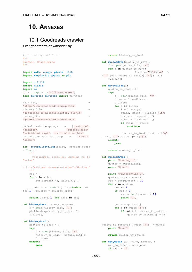
FRAILSAFE – H2020-PHC–690140 D4.13
10. ANNEXES
10.1 Goodreads crawler File: goodreads-downloader.py # -*- coding: utf-8 -*-
"""
@author: Charalampos
"""
import math, numpy, pickle, nltk import matplotlib.pyplot as plt
import urllib2 import pickle import re op = __import__ ( "offline-parser" ) from textstat.textstat import textstat
main_page =
'http://www.goodreads.com/quotes'
history_file =
'goodreads-downloader.history.pickle'
quotes_file =
'goodreads-downloader.quotes.csv'
default_suicide_groups = [ 'suicide' ,
'sadness' , 'suicide-note' ,
'suicide-attempt' , 'suicidal-thoughts' ] default_non_suicide_groups = [ 'humor' ,
'happy' ]
def sortedDictValues(adict, reverse_order
= True ): """
Taksinomisi leksikou, simfwna me to
"value"
http://wiki.python.org/moin/HowTo/Sorting/
"""
ret = []
for k in adict: ret.append( (k, adict[k]) )
ret = sorted (ret, key= lambda tdf:
tdf[ 1], reverse = reverse_order)
return [page[ 0] for page in ret]
def historySave(history_to_save): f = open (history_file, 'w' ) pickle.dump(history_to_save, f)
f.close()
def historyLoad(): history_to_load = {}
try: f = open (history_file, 'r' ) history_to_load = pickle.load(f)
f.close()
except: pass
return history_to_load
def quotesSave(quotes_to_save): f = open (quotes_file, 'w' ) for k in quotes_to_save:
f.write( " %s \t%s \n" %
( '|' .join(quotes_to_save[k][ 't' ]), k)) f.close()
def quotesLoad(): quotes_to_load = {}
try: f = open (quotes_file, 'r' ) lines = f.readlines()
f.close()
for k in lines: k = k.strip()
qtags, qtext = k.split( " \t" ) qtags = qtags.strip()
qtext = qtext.strip()
if qtags == qtext: continue
quotes_to_load[qtext] = { 'q' :
qtext, 't' : qtags.split( '|' )} except: pass
return quotes_to_load
def quotesByTag(): print 'Loading..' , quotes = quotesLoad()
print 'Done!'
print 'Transforming..' , quotes_to_return = {}
res = len (quotes) / 10 for q in quotes: res -= 1 if res < 0: res = len (quotes) / 10 print '.' ,
quote = quotes[q]
for t in quote[ 't' ]: if not t in quotes_to_return: quotes_to_return[t] = {}
quotes_to_return[t][quote[ 'q' ]] = quote print 'Done!'
return quotes_to_return
def getQuotes(tag, page, history): url_to_fetch = main_page
if tag != '' :
- 55 -

FRAILSAFE – H2020-PHC–690140 D4.13
url_to_fetch += '/tag/' + tag
if page > 1: url_to_fetch += '?page=' +
str (page)
if tag == '' : print "Fetching all quotes, page
%d " % page, else:
print "Fetching quotes for %s ,
page %d " % (tag, page),
try: request =
urllib2.Request(url_to_fetch)
contents =
urllib2.urlopen(request).read()
except: print '..Error!' return None
contents = contents.replace( '“' ,
'' ) contents = contents.replace( '”' ,
'' ) contents = contents.replace( '―' ,
'' ) contents = contents.replace( " \n" , '' )
new_tags = 0 for m in
re.finditer( '\/quotes\/tag\/([a-z\-]+)' , contents):
tag = m.group( 1) if not tag in history: history[tag] = 0 new_tags += 1
if new_tags > 0: print '.. %d new tags' % new_tags, historySave(history)
contents = contents.replace( '<div
class="quote mediumText ">' , "<div
class='quote'>" ) # contents =
contents.replace('quoteText">',
"quoteText'>")
text_quotes = contents.split( "<div
class='quote'>" ) # Useless del text_quotes[ 0]
quotes_to_return = {}
for q in text_quotes: m = re.search( 'quoteText">(.*?)<' ,
q)
qtext =
m.group( 1).strip().replace( " \t" , '' ) if qtext == '' : continue
ctags = []
for m in
re.finditer( '\/quotes\/tag\/([a-z\-]+)' ,
q):
if m.group( 1).strip() == '' or
m.group( 1).strip() == qtext: continue
ctags.append(m.group( 1))
if len (ctags) <= 0: continue
quotes_to_return[qtext] = { 'q' :
qtext, 't' : ctags}
print ' %d quotes' %
len (quotes_to_return), print '..Done!'
return quotes_to_return # print quotes_to_return # print contents
def getTagsByGroup(includeGroups,
excludeGroups = [], quotes_by_tag = None ,
no_more_than = 0): if quotes_by_tag is None : quotes_by_tag = quotesByTag()
excluded = {}
for g in excludeGroups: for q in quotes_by_tag[g]: quote = quotes_by_tag[g][q]
excluded[ quote[ 'q' ] ] = True
selected = {}
for g in includeGroups: for q in quotes_by_tag[g]: quote = quotes_by_tag[g][q]
if quote[ 'q' ] in excluded: continue
selected[ quote[ 'q' ] ] = quote if no_more_than > 0 and
len (selected) >= no_more_than: break
return selected
def getSeperateGroups(suicideGroups,
nonSuicideGroups, quotes_by_tag = None ): if quotes_by_tag is None : quotes_by_tag = quotesByTag()
group1 = getTagsByGroup(suicideGroups,
nonSuicideGroups, quotes_by_tag)
group2 =
getTagsByGroup(nonSuicideGroups,
suicideGroups, quotes_by_tag, len (group1))
print "suicide group: %d " %
len (group1) print "NON suicide group: %d " %
len (group2) return group1, group2
def startWorking(): quotes = quotesLoad()
history = historyLoad()
- 56 -

FRAILSAFE – H2020-PHC–690140 D4.13
if not '' in history: history[ '' ] = 0 historySave(history)
# for tag in ['suicide', 'sadness',
'suffering', 'suicide-note',
'failed-attempt', 'suicide-attempt',
'suicidal-thoughts']:
# if not tag in history: # history[tag] = 0
print " %d tags in my history" %
len (history) print " %d quotes already" %
len (quotes)
added = True while added: added = False for tag in history.keys(): if history[tag] >= 100: continue
print 'Tag " %s ", page %d ' %
(tag, history[tag])
lenbefore = len (quotes) while history[tag] < 100: history[tag] += 1
new_quotes =
getQuotes(tag, history[tag], history)
if len (new_quotes) <= 0: history[tag] = 100
quotes.update(new_quotes)
lenafter = len (quotes)
if lenafter > lenbefore: added = True
print 'Saving %d new
quotes' % (lenafter - lenbefore), quotesSave(quotes)
print '..Done' historySave(history)
print "Update ended"
def create_arff(relation = 'suicide' ,
includeTFIDF = True , group_suicide = None ,
group_non_suicide = None , TFIDF_thres =
20): """Create arff for WEKA with all
features availiable
"""
out = []
out.append( '@RELATION %s ' % relation) out.append( '' )
other_attributes = []
other_attributes.append( 'get_feature_length' )
other_attributes.append( 'get_feature_number_of_sentences' )
other_attributes.append( 'get_feature_word_
count' )
other_attributes.append( 'get_feature_words_per_sentence' )
other_attributes.append( 'get_feature_text_shannon_entropy' )
for attr in other_attributes: call = getattr (op, attr)
out.append( '@ATTRIBUTE %s %s ' %
(call( '' , 'title' ), call( '' , 'type' )))
read_scores = []
read_scores.append( 'flesch_reading_ease' ) read_scores.append( 'smog_index' )
read_scores.append( 'flesch_kincaid_grade' )
read_scores.append( 'coleman_liau_index' )
read_scores.append( 'automated_readability_index' )
read_scores.append( 'dale_chall_readability_score' ) read_scores.append( 'difficult_words' )
read_scores.append( 'linsear_write_formula')
read_scores.append( 'gunning_fog' ) for attr in read_scores:
out.append( '@ATTRIBUTE %s %s ' %
(attr, 'real' ))
out.append( '@ATTRIBUTE %s %s ' %
( 'sentiment' , 'real' )) out.append( '@ATTRIBUTE %s %s ' %
( 'misspelled' , 'real' ))
if group_suicide is None : group_suicide =
default_suicide_groups
if group_non_suicide is None : group_non_suicide =
default_non_suicide_groups
results =
getSeperateGroups(group_suicide,
group_non_suicide)
group_suicide_quotes = results[ 0] group_non_suicide_quotes = results[ 1]
filename = 'ARFFS/ %s .arff' % relation
texts = []
if includeTFIDF: s, score_words =
compute_ig({ 'suicide' : group_suicide_quotes, 'non-suicide' :
group_non_suicide_quotes})
mywords = s[:TFIDF_thres]
for q in group_suicide_quotes: temptext =
- 57 -
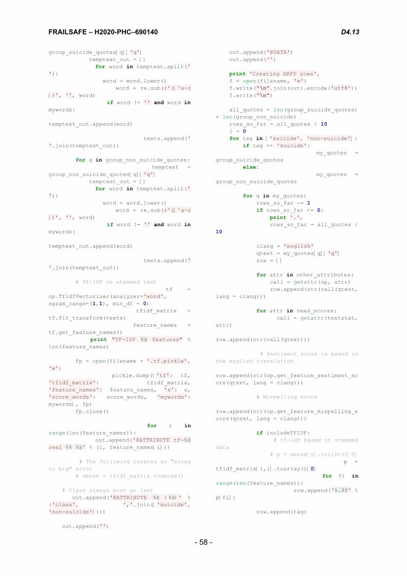
FRAILSAFE – H2020-PHC–690140 D4.13
group_suicide_quotes[q][ 'q' ] temptext_out = []
for word in temptext.split( '
' ): word = word.lower()
word = re.sub( r'([^a-z
])' , '' , word) if word != '' and word in
mywords:
temptext_out.append(word)
texts.append( '
' .join(temptext_out))
for q in group_non_suicide_quotes: temptext =
group_non_suicide_quotes[q][ 'q' ] temptext_out = []
for word in temptext.split( '
' ): word = word.lower()
word = re.sub( r'([^a-z
])' , '' , word) if word != '' and word in
mywords:
temptext_out.append(word)
texts.append( '
' .join(temptext_out))
# TF-IDF on stemmed text tf =
op.TfidfVectorizer(analyzer= 'word' , ngram_range=( 1, 1), min_df = 0)
tfidf_matrix =
tf.fit_transform(texts)
feature_names =
tf.get_feature_names()
print "TF-IDF %d features" %
len (feature_names)
fp = open (filename + '.tf.pickle' ,
'w' ) pickle.dump({ 'tf' : tf,
'tfidf_matrix' : tfidf_matrix,
'feature_names' : feature_names, 's' : s,
'score_words' : score_words, 'mywords' :
mywords}, fp)
fp.close()
for i in
range ( len (feature_names)): out.append( '@ATTRIBUTE tf- %d
real %% %s ' % (i, feature_names[i]))
# The following creates an "array
to big" error
# dense = tfidf_matrix.todense()
# Class always must go last out.append( '@ATTRIBUTE %s { %s }' %
( 'class' , ',' .join([ 'suicide' ,
'non-suicide' ])))
out.append( '' )
out.append( '@DATA' ) out.append( '' )
print 'Creating ARFF rows' , f = open (filename, 'w' ) f.write( " \n" .join(out).encode( 'utf8' ))
f.write( " \n" )
all_quotes = len (group_suicide_quotes)
+ len (group_non_suicide) rows_so_far = all_quotes / 10 i = 0 for tag in [ 'suicide' , 'non-suicide' ]: if tag == 'suicide' :
my_quotes =
group_suicide_quotes
else: my_quotes =
group_non_suicide_quotes
for q in my_quotes: rows_so_far -= 1 if rows_so_far <= 0: print '.' ,
rows_so_far = all_quotes /
10
clang = 'english' qtext = my_quotes[q][ 'q' ] row = []
for attr in other_attributes: call = getattr (op, attr)
row.append( str (call(qtext,
lang = clang)))
for attr in read_scores: call = getattr (textstat,
attr)
row.append( str (call(qtext)))
# Sentiment score is based in
the english translation
row.append( str (op.get_feature_sentiment_score(qtext, lang = clang)))
# Mispelling score
row.append( str (op.get_feature_mispelling_score(qtext, lang = clang)))
if includeTFIDF: # tf-idf based on stemmed
data
# p = dense[i].tolist()[0] p =
tfidf_matrix[i,:].toarray()[ 0] for fi in
range ( len (feature_names)): row.append( ' %.3f ' %
p[fi])
row.append(tag)
- 58 -

FRAILSAFE – H2020-PHC–690140 D4.13
f.write( ',' .join(row).encode( 'utf8' )) f.write( " \n" )
i += 1
f.close()
print '..Done'
def compute_ig(quotes_per_tag): """ compute_ig():
Compute information gain for each
word
"""
# With a little bit of help #
http://streamhacker.com/tag/information-ga
in/
from nltk.metrics import
BigramAssocMeasures
word_count_per_class = {}
all_word_count_per_class = {}
word_count_per_word = {}
all_words = 0
print "Loading files for ig.." , for tclass in quotes_per_tag: word_count_per_class[tclass] = {}
all_word_count_per_class[tclass] =
0
i = len (quotes_per_tag[tclass]) /
10
for quote in
quotes_per_tag[tclass]:
i -= 1 if i <= 0: print '.' ,
i =
len (quotes_per_tag[tclass]) / 10
data =
quotes_per_tag[tclass][quote][ 'q' ].split( ' ' )
for w in data: w = w.lower()
w = re.sub( r'([^a-z])' ,
'' , w)
if w == '' : continue
word_count_per_class[tclass][w] =
word_count_per_class[tclass].get(w, 0) + 1
all_word_count_per_class[tclass] += 1 word_count_per_word[w] =
word_count_per_word.get(w, 0) + 1 all_words += 1
del data
print "Evaluating.." , i = int ( len (word_count_per_word) / 10)
score_per_word = {}
for w in word_count_per_word: i -= 1 if i <= 0: print ',' ,
i =
int ( len (word_count_per_word) / 10)
freq = word_count_per_word[w]
score_per_word[w] = 0
for c in word_count_per_class: score_per_word[w] +=
BigramAssocMeasures.chi_sq(word_count_per_
class[c].get(w, 0), (freq,
all_word_count_per_class[c]), all_words)
del word_count_per_class,
all_word_count_per_class,
word_count_per_word
print "Sorting.." , s = sortedDictValues(score_per_word)
print "..Done" # del score_per_word
print "..Done"
nums = []
for w in s: nums.append(score_per_word[w])
print "Creating ig histogram" , plt.figure(figsize = ( 24, int ( 24.0 *
9.0 / 16.0)),) #
plt.hist(numpy.asarray(score_per_word.valu
es()), 5000, facecolor = 'g')
plt.plot(nums)
plt.xlabel( 'Lexicon values' ) plt.ylabel( 'IG Score' )
plt.title( 'IG Score per lexicon
lemma' ) plt.grid( True ) plt.show()
print "..Done" # del s
return s, score_per_word
- 59 -

FRAILSAFE – H2020-PHC–690140 D4.13
10.2 FrailSafe demo video This image is also in Annex 9.5 of D4.9 as both reports are responsible for this demo. File: frailsafe-showcase.wmv (frailsafe-showcase.jpeg)
- 60 -


![Passive design[1]](https://static.fdokumen.com/doc/165x107/63215c9580403fa2920cb59b/passive-design1.jpg)