Direct Passive Navigation

MASSACHUSETTS INSTITUTE O F TECHNOLOGY ARTIFICIAL INTELLIGEXCE LABORATORY

A.I. Memo No. 821 February, 1985

Direct Passive n'avigation

Shahriar Negahdaripour Berthold K.P. Horn

Abstract: In this paper, we show how to recover the motion of an observer relative to a planar surface directly from image brightness derivatives. We do not con~pute the optical flow as an intermediate step. We derive a set of nine non-linear equations using a least-squares formulation. A simple iterative scheme allows us to find either of two possible solutions of these equations. An initial pass over the relevmt image region is used to accumulate a number of moments of the image brightness derivatives. All of the quantities used in the iteration can be efficiently computed from these totals, without the need to refer back to the image. A new, compact notation allows us to show easily that there are a t most two planar solutions.

Key Words: Passive Navigation, Optical Flow, Structure and Motion, Least Squares, Planar Surface, Non-Linear Equations, Dual Solution, Planar Motion Field Equations.

Q Massachusetts Institute of Technology, 1985

n This report describes research done at the Artificial Intelligence Laboratory of the Mas- sachusetts Institute of Technology. Support for the laboratory's artificial intelligence research is provided in part by the System Development Foundation.

Introduction

1. Introduction

The problem of determining rigid body motion and surface structure from inlage data has been the topic of many recent research papers in the area of machine vision. Two types of approaches, discrete and continuous, have been pursued. In the discrete approach, information about a finite number of points is used to reconstruct the motion [4,5,9,10,13- 161. To do this, one has to identify and match feature points in a sequence of images. The minimum number of points required depends on the number of images. In the continuous approach, the optical flow that is the apparent velocity of brightness patterns is used a t every image point [I-3,12,17]. In general, the computation of the local flow field involves not only a least-squares for~nulation that uses a constraint equation between the optical flow and the image brightness derivatives a t every image point, but also an additional constraint, such as the smoothness of the flow field [7,8]. The additional constraint is required because information is 1o.t when the 3-D world is projected onto a 2-D image. Locally, the brightness variations in time-varying images only provide one constraint on the components of the optical flow. While the continuous approach requires more con~putation, it is robust with respect to errors in the optical flow data.

of the research work in recovering surface structure and motion has been re- stricted to using the optical flow information in the image. In this paper, we determine the motion of an observer relative to a planar surface directly from the image brightness derivatives: without having to compute the optical flow as an intermediate step. We restrict surselvc; to planar surfaces since only three parameters are needed to specify the surface structure. We will be considering less restricting constraints on the surface structure in a later paper.

2. Preliminaries

We first recall some details about perspective projection, the motion field, the brightness change constraint equation, rigid body motion and planar surfaces. This we do using vector notation in order to keep the resulting equations as compact as possible.

2.1. Perspective Projection

Let the center of projection be at the origin of a Cartesian coordinate system. Without loss of generality we assume that the effective focal length is unity. The image is formed on the plane z = 1, parallel to the xy-plane, that is, the optical axis lies along the z-axis. Let R be a point in the scene. Its projection in the inlage is r, where

The z-component of r is clearly equal to one, that is r 2 = 1.

.P. 2.2. Motion Field

The motion field is the vector field induced in the image plane by the relative motion of the observer with respect to the environment. The optical flow is the apparent motion of

2 Motion of Planar Objects

P. brightness patterns. Under favourable circumstances the optical flow is identical to the motion field. The velocity of the image r of a point R is given by

For convenience, we introduce the notation rt and Rt for the time derivatives of r and R, respectively. We then have

which can also be written in the compact form

since a x (b x c) = (c . a)b - (a. b)c. The vector rt lies in the image plane, and so (rt i) = 0. Further, rt = 0, if Rt 1 1 R, as expected.

Finally, noting tha t R = (R . &)r, we get

1 rt = - (BX (Rt x r ) ) .

R - &

2.3. R ig id B o d y M o t i o n

In the case of the observer moving relative to a rigid environment with translational velocity t and rotational velocity w , we find that the motion of a point in the environment relative to the observer is given by

Since R = (R &)r, we can write this as

Substituting for Rt in the forinula derived above for rt, we obtain

I t is important to remember tha t there is an inherent ambiguity here, since the same motion field results when distance and the translational velocity are multiplied by an arbitrary constant. This can be seen easily from the above equation since the same image plane velocity is obtained if one multiplies both R and t by sonle constant.

2.4. Br igh tnes s Change E q u a t i o n

The brightness of the image of a particular patch of a surface depends on many factors. I t may for example vary with the orientation of the patch. In 111any cases, however, it

Preliminaries 3

remains at least approximately constant as the surface moves in the environment. If we assume that the image brightness of a patch remains constant, we have

where aE,/ar = ( a E / a z , L ~ E / ~ ~ , O ) * is the image brightness gradient. It is convenient to use the notation E, for this quantity and Et for the time derivative of the brightness. Then we can write the brightness change equation in the simple form

Substituting for rt we get

Now Ere (2 x ( r x t)) = (E , x i) - (r x t) = ( (E , x 2) x r ) s t ,

and by similar reasoning

E,. (2 r (r x (r x w ) ) ) = ( ( ( E , x 2) x r ) x r ) . w ,

so we have

To make this constraint equation more compact, let us define c = Et, s = (Er x &) x r , and v = -s x r ; then, finally,

This is the brightness change equation in the case of rigid body motion.

2.5. Planar Surface

A particularly impoverished scene is one consisting of a single planar surface. The equation for such a surface is

R . n = 1,

where n/ In] is a unit normal to the plane, and 1/ /nj is the perpendicular distance of the plane from the origin. Since R = (R - &)r , we can write this as

so the constraint equation beconies

Motion of Planar Objects

This is the brightness change equation for a planar surface.

Note again the inherent ambiguity in the constraint equation. It is satisfied equally well by two planes with the same orientation but a t different distances provided that the translational velocities are in the same proportions.

3.. Recover ing M o t i o n a n d S t r u c t u r e

Given image brightness E ( x , y, t ) , and its spatial and time derivatives, E, and Et, over some region I in the image plane, we are to recover the translational and rotational motions, t and w , as well as the plane n . Using the constraint equation developed above, we could do this using image information a t just a small number of points. At each point we get one constraint and we have nine unknowns to recover-or rather, eight, since we can recover the distance of the plane and the translational velocity only up to a scale factor.

3.1. Least S q u a r e s Approach

Image brightness values are distorted with sensor noise and quantization error. These inaccuracies are further accentuated by methods used for estimating the brightness gra-

,m dient. Thus it is not advisable to base a method on measurements a t just a few points. Instead we propose to n~inilnize the error in the brightness constraint equation over the whole region I in the image plane. So we wish to minimize

by suitable choice of the translational and rotational motion vectors t and w , as well as the normal to the plane, n. We are particularly interested in the question of uniqueness of the solution and in computational efficiency.

For an extremum of J we must have

a J - a J = 0 , -

a J = 0, and - = 0. aw at dn

That is,

These equations comprise nine non-linear (scalar) algebraic equation in terms of the observer motion, t and w , and the surface norlnal n .

Iterative Solution Methods

4. Iterative Solution Methods

To recover the nlotion vectors t and w, and the surface nornlal n, we have to solve a set of non-linear equations, which we will call the planar motion field equations. Some observations about these equations are in order: The first equation is linear in w , t , and n. The second equation is linear in w and t , but quadratic in n. Finally, the last equation is linear in w and n, but quadratic in t . We will exploit the linearity of these equations to formulate two iterative schemes.

4.1. First Scheme

We can rearrange the motion and surface recovery equations to get

2 T [//l(s t ) (rr ) dx dy n = - [c + (v . w)](s t ) r dx dy, I iil The first pair can be grouped in the form -

where

Ml = dx dy,- M2 = / / l(r . n) (vsT) dx dy, MI = / l ( r . n)2(ssT) dx dy, I

dl = /l cv dz dy, and d2 = c ( ~ . n)s dz dy.

This can be solved for t and w, given the surface normal n. The last equation is

where

and can be solved for the surface nornlal n, given the pair of vectors t and w . The nlotion vectors are given by


where (-T) denotes the inverse of the transpose of a matrix. This can also be written in the form

Ma - M;M;'M~)-' (M;M;'dl - d2) ,

w = -M;' (d l + M2t).

or,

( - 1

w = MI - M~M;'M?) ( ~ 2 ~ i l d 2 - dl) ,

The surface normal is simply given by

All arrays are either 3 x 3 matrices or vectors of length 3, and therefore, the solutions for w , t , and n can be computed easily. Actually, most of the indicated matrix inversions do not have to be carried out explicitly, since it is computationally cheaper to solve these linear matrix equations by elimination.

So in summary: We start with an initial guess for n . Using above equations, we solve for t and w in terms of the current value of n , and then for n in terms of the current values of t and w . After this, we evaluate the improvement in the solution to either go to next iteration or stop if the solution has not improved.

4.2. Second Scheme

The first pair of the motion and surface recovery equations depend linearly on t and w. As before,

which can be solved for t and w in terms of n. Furthermore, the first and last equations depend linearly on n and w:

[/L(VVT) dx dy] w + [ ( t ) (v rT) dx dy ] n = - / 1 c v d z d y ,

Given t , these may be solvcd for n and w , For simplicity, let MI, Mz, M4, N4, dl, and d2 be as defined earlier, and let:

Iterative Solution Methods

Then

and

The solution of the above equations is given by

and

These may be rewritten in either of two asymmetrical forms as shown above. Again, most of the indicated matrix inversions do not have to be carried out explicitly,

since we can solve the equations by elimination. F-? In this scheme: We start with an initial guess for n. We solve for t and w in terms

of the current value of n , and update t , then solve for n and w in terms of the current value of t , and update n , and, finally, evaluate the improvement in the solution to either continue with the next iteration or stop if the solution has not improved.

4.3. Division of Labour

These methods would not be very at tractive, if we had to perform integrations over the whole image region I during each iteration, in order to collect the matrices and vectors appearing in the equations. Fortunately, this is not ncccessary. Oue can see this by writing the equations for the components of the matrices and vectors using the summation convention of tensor calculus (that is, there is an implicit summation over any index which appears twice in an expression):


and

M1 = N1 and dl = el do not depend on w , t , or n, and so need only be computed once. Also, (cv,), (vivj), (cs;rj), (rkv,s3)) and (rkrlsis3) depend only on r, E,, and q, and so can be integrated over the image once. This appears to be a set of 3 + 9 + 9 + 2 7 + 8 1 = 129 numbers, but, because of symmetry in (v,v,), and ( r k ~ l s , ~ 3 ) , only 81 numbers have to be stored. These accumulated totals represent all the image information needed to solve the motion recovery problem.

In the first scheme, we only perform 279 multiplications per iteration; The updating of the coefficients of the planar motion field equations involves 27 + 9 + 42 + 42 + 42 = 162

P"* multiplications to compute M2, d2, Mi, N 4 , and g (note that M4 and N 4 are symmetric). The updating of w , t , and n , in comparison, requires 117 multiplications.

In the second scheme, 696 multiplications are carried out a t each iteration; We compute the matrices M2, M4 and the vector d2, required for the first half of the iteration, in 27 + 42 + 9 = 78 multiplications. The same number of multiplications is needed to compute the matrices N2, N 4 and the vector e2 required in the second half. Further, solving for w and t takes about 270 multiplications, as does solving for w and n in the second half of each iterative step.

Through a selected example, we will show that the second scheme has a much better convergence rate at the expense of more computation per iteration.

5. Uniqueness

I t is important to establish whether more than one solution is possible. In general, this is clearly so, since an image of uniform brightness could correspond to an arbitrary, uniform surface moving in an arbitrary way. So the brightness gradients, or lack of brightness gradients, call conspire to make the problem highly anibiguous. What we are interested in here is whether two different planar surfaces can give rise to the same motion field given two different translational and rotational motions of the imaging system.

In our ternls then, the question beconles: given that the brightness change equ a t ' lon is satisfied for the motion t and w the planar surface n , is thcre <another motion t' and w' and another planar surface n' that satisfies the same equation at all points in the region I and for all possibly ways of marking the surface? Note that we have to consider a whole image region, since the problem is underconstrained if we only have

Uniqueness 9

F"", information along a line or a t a point in the image. We also have to include the condition that the constraint should be satisfied for all possible surface markings t o avoid the kind of ambiguity discussed above, where brightness gradients fortuitously line u p with the motion field to create ambiguity.

5.1. Dual S o l u t i o n

Suppose that two motions and two planar surfaces satisfy the brightness change equation. Then, we have

c + v . w + ( r . n ) ( s . t ) = 0 ,

c + v .wr + ( r . n t ) ( s t ') = 0.

Subtracting these equations, we get

Now v = -s x r , so

-(s x r ) . (W - w r ) + ( r . n ) ( s . t ) - ( r . n r ) ( s - t ') = 0,

or -r . ( ( w - w') x s ) + ( r e n ) ( s - t ) - ( r . n t ) ( s . t ') = 0.

f=- If we let w = (wi, wz, w3)T, then we can write

-w3 +w2 w x s = R s , where R =

is a suitable (3 x 3 ) skew-symmetric matrix. The (i, j)th element of R equals wkcijk, where q j k , is the permutation symbol. (It equals $1 when the ordered set i , j , k is obtained by an even permutation of the set 1, 2, and 3, it equals -1 when the ordered set is obtained by an odd permutation, and it is zero if two or more of the indices are equal.)

Using this notation we can now write

or just

This is to be true for all points r in the image region I and all possible brightness gradients. So

1 IT- - ( R - ~ ' ) + n t ~ - n t - 0 ,

where the zero on the right hand side here represents a 3 x 3 matrix of zeros. Now RT = -n, since R is skew-symmetric, so taking the transpose of the equation we get


Adding the two equations allows us to eliminate ($I - W), and we end up with

The trace (sum of the diagonal elements) of n t T is just (n . t) , so we see immediately tha t ( n . t) = (n' * tlT). But the above matrix equation involving the dyadic products of n and t as well as of n' and ti is much more constraining.

Consider the following three possibilities:

(1) If In'l = 0 or Itti = 0, then their dyadic product is a 3 x 3 matrix of zeros. In this case the above equation is satisfied if and only if In/ = 0 or /tl = 0.

(2) If n ' I / n , t' I / t and In'i It'[ = in ' iti, then the two sums of dyadic products are equal and the above equation is satisfied.

(3) If n ' / I t , t' I / n and jn'l lt'j = /n j It/, then the two sums of dyadic products are also equal and the above equation is satisfied,

I t turns out that there are no other ways to satisfy the equation. This can be shown using elementary properties of dyadic products (see Appendix) or by inspection of the six components of the above equation (because of symmetry there are only six independent components).

The first case above corresponds to purely rotational motion, because either the translational motion is zero, or the planar surface is infinitely far away, and the translation does not generzte a perceptible component of the motion field. The solution is unique in this case, because we find (l? - 0') = 0 , when we substitute back into the matrix equation. (This is nothing new, since it has been known for some time tha t the solution is unique in the case of purely rotational and purely translational motion 131.)

In the second case we find that n t T = n'tiT, since the vectors are parallel and the product of their size is constrained by the condition n . t = n' . t', derived earlier. Thus once again (0 - l?') = 0. Kothing new is obtained here, since we already know that we can change the lengths of the vectors n and t as long as the product of their lengths remains constant.

The third case is the most interesting. Here we have t n T = n'ttT so that

and thus -(n - nt)x + ( n t T - t n T ) x = 0,

for an arbitrary vector x. That is,

x x (w - w') + x x ( n x t) = 0,

for an arbitrary vector x, so tha t

B"a or w' = w + n x t. To sulnmarize then, if we ignore scaling of the normal and the translational velocity, we obtain a dual solution, given by

I n = t , t ' = n and w l = w + n x t .

A Selected Example 11

Hay was the first to show the existence of the dual solution [GI, although the result has apparently been independently rediscovered several times since then [11,13,15]. (The most recent of these papers [ll], came to our attention only after completion of our version of the proof.)

This dual solution is not different from the original one in the special case that the motion is perpendicular to the planar surface, that is, n I / t . In this case the solution is unique. Further, if t . & = 0, then n' . 2 = 0. This corresponds to a planar surface parallel to the observer's line of sight, and may be considered to be a degenerate case.

6. A Selected Example

We now present the results of a simulation. I t is noteworthy to mention that in all sinlulations performed, our algorithms have converged to a solution. However, the number of iterations for convergence to a solution depends on the initial condition (as is the case with all iterative schemes developed for solving nonlinear equations). In this example, we will demonstrate the sensitivity of both schemes to the initial condition. The image brightness function was generated using a multiplicative sinusoidal pattern (one that varies sinusoidally in both x and y directions), a 45" field of view was assumed, and the image brightness gradients were computed analytically to avoid errors due to image brightness quantization and finite difference approximations of the brightness gradient. In practice, the brightness a t inmge points in- two frames would be discretized first, and the gradient computed using finite difference methods,

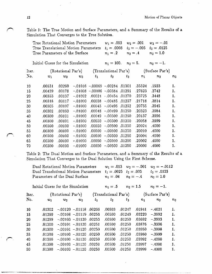
Table 1 shows the true motion and surface paranleters, and the results of a simulation that converged to the true solution using the first scheme described earlier. In Table 2, the dual solution for the true motion and surface parameters, and the results of a simulation that converged to the dual solution are tabulated, In both cases, the solutions after various number of iterations are given. The results show that in the first case, the error in each parameter after less than 30 iterations is within 10% of the exact value. In the second case, this accuracy is achieved in less than 20 iterations. Similar results are presented in tables 3 and 4 for the second scheme. Here, very good accuracy is achieved in less that 10 iterations for the true solution and about 5 iterations for the dual solution.

In similar tests, with various motion and surface parameters, accurate results have been obtained in less than 40 iterations using the first scheme and a variety of initial conditions. The same accuracy for the second scheme required less than 15 iterations. More importantly, both schemes eventually converged to one of the two possible solutions. However, the results for the particular case where the translational motion vector is (almost) parallel t o the surface normal have not been as satisfactory. In these cases, several hundred iterations were required to achieve reasonable accuracy, even with the second scheme. Although the nature of this behavior has not been investigated in detail, it appears to resemble that observed when the Newton-Raphson method is applied to a problem where two roots are very close to one another.


Table 1 : The True Motion and Surface Parameters, and a Summary of the Results of a Simulation That Converges to the True Solution.

True Rotational Motion Parameters w1 = .003 w2 = ,001 w3 = -.01 True Translational Motion Parameters t l = .0005 t2 = -.005 ts = .0125 True Parameters of the Surface n1 = .2 n2 = .4 n3 = 1.0

Initial Guess for the Simulation n l = 1 0 0 . n 2 = 5 . n3 = -1.

Iter. (Rotational Par's) (Translational Par's) (Surface Par's) No. w1 w2 w3 t 1 t 2 t 3 n1 722 n3

Table 2: The Dual Motion and Surface Parameters, and a Summary of the Results of a Simulation That Converges to the Dual Solution Using the First Scheme.

Dual Rotational Motion Parameters w l = ,013 w2 = -.001 w3 = -.0112 Dual Translational Motion Parameters t l = .0025 t 2 = .005 ts = .0125 Parameters of the Dual Surface nl = .04 n2 = -.4 n3 = 1.0

Initial Guess for the Simulation nl = .5 n2 = 1.5 n3 = -1.

Iter. (Rotational Par's) (Translational Par's) (Surface Par's) No. w1 w2 w3 t 1 t2 t 3 nl n2 n3

A Selected Example 13

Table 3: The True Motion and Surface Parameters, and a Summary of the Results of a Simulation That Converges to the True Solution Using the Second Scheme.

True Rotational Motion Parameters wl = .003 w2 = .001 w3 = -.01 True Translational Motion Parameters t l = .0005 t 2 = -.005 t3 = .0125 True Parameters of the Surface n1 = .2 n2 = .4 n3 = 1.0

Initial Guess for the Simulation n l = 1 0 0 . n 2 = 5 . n3 = -1.

Iter. (Rotational Par's) (Translational Par's) (Surface Par's) No. W 1 w2 w3 t 1 t 2 t3 n1 n2 n3

Table 4: The Dual Motion and Surface Parameters, and a Summary of the Results of a Simulation That Converges to the Dual Solution Using the Second Scheme.

Dual Rotational Motion Parameters w1 = .013 w2 = --.001 w3 = -.0112 Dual Translational Motion Parameters t l = .0025 t2 = .005 t3 = ,0125 Parameters of the Dual Surface n l = . 0 4 n2=-.4 n3=1.0

Initial Guess for the Simulation n l = . 5 n2=1.5 n3 = -1.

Iter. (Rotational Par's) (Translational Par's) (Surface Par's) No. w1 w2 w3 t 1 t 2 t3 nl n2 n3


7. Summary

The problem of recovering the motion of an observer relative to a planar surface directly from the changing inlages (direct passive navigation) was investigated, and formulated as one of unconstrained optimization. Using conditions for optimality, it was reduced to solving a set of nine sltnultaneous non-linear equations, which we termed the planar motion field equations. Two iterative schemes for solving these equations were presented.

. I t was shown that all information in the image concerning motion recovery can be cap- tured by the moments of the image brightness derivatives which constitute the coefficients of the motion and surface recovery equations. These moments are computed during an initial pass over the relevant image regions so that there is no need to refer to the image after every iteration. This reduces the computation to storing 81 moments and perform- ing less than 300 n~ultiplications per iteration in the first scheme and approximately 700 multiplications in the second scheme.

We also gave a con~pact proof that the problem can have a t most two planar solutions. Through a selected example with synthetic data, it was shown that both schemes may converge to either of the two solutions, depending on the initial condition. In practice, once a solution is obtained, the other can be computed using the equations given for the dual solution.

In the tests carried out, both algorithms have converged to a possible solution, and accurate solutions have been obtained in less than 40 iterations using the first scheme,

P"". and in less than 15 iterations in the second one, mentioned earlier, the results have not been as satisfactory when the translational motion component is perpendicular to the planar surface. These cases required several hundred iterations of either scheme for accurate solutions.

Even though both schemes require approximately the same number of computations for convergence to a solution (second scheme converges faster but requires more computation a t each iteration, as discussed earlier), the second one seems more appropriate for parallel implementation.

8. Acknowledgments

We would like to thank Alen Yuille, Mike Brady, Tomaso Poggio and Shinlon Ullman for helpful comments and pointers to obscure references.

Acknowledgments

Appendix

Lemma 1: (abT - baT)c = c x (a x b).

Proof: (abT - baT)c = a(a . b) - b(a . c) = c x (a x b). a Lemma 2: If abT = cdT , then either

(1) la1 = 0 or /b / = 0, and, /c/ = 0 or /dl = 0, or

(2) a 1 1 c and b / I d.

Proof: cT(abT)d = cT(cdT)d, or (c .a ) (b .d) = (c.c)(d.d). Now if / a = 0 or /bl = 0, 2 2 then ic/ jdj = 0, which implies that either /cj = 0 or Id; = 0. Conversely, if Icl = 0 or

Id/ = 0, then la1 = 0 or /bl = 0. For the rest of the proof we assume tha t la], Ib], Icl, and Id/ are non-zero. Now

(abT)b = (cdT)b so that a(b . b) = c(d - b). It follows that a 1 1 c. Similarly, aT(abT) = aT(cdT) so that (a . a)bT = (a c)dT. Therefore, b 1 d.

Lemma 3: If M and N are (3 x 3) skew-symmetric matrices and M~ = N2, then M = f N .

Proof: The result is immediate if M and N are zero. So from now on we assume that they are non-zero. If M2 = N2, then M 2 x = N ~ X for all vectors x. Using the isomorphism between (3 x 3) skew-symmetrical matrices and vectors we have

m x (m x x ) = n x (n x x),

where the vectors m and n correspond to the matrices M and N respectively. So

If this is to be true for all vectors x , we must have, [mmT - (m .m)l] = p n T - (n .n)I]. Taking the trace of both sides we get m . m = n n. Consequently, mm = nnT. Using Lemma 2, we see that m / / n. Taken together with /m/ = /nj this means that m = f n a n d s o M = f N .

Lemma 4: If abT + baT = cdT + dcT , then either

(1) la/ = 0 or Ib/ = 0, and, Icl = 0 or /dl = 0, or

(2) a 1 1 c and b I j d , or

(3) a 1 1 d and b 11 c.

Proof: We first show that either abT = cdT or abT = dcT, The proof then follows using lelnma 2. We also nced to show that a . b = c . d. This follows from the fact that ~ r a c e ( a b ~ ) = a . b and T'race(cdT) = c . d. Now (abT + = (cdT + d ~ ~ ) ~ , or

(a b)abT + ( b . b)aaT + (a - a)bbT + ( a . b)baT

= (c d)cdT + (d d)ccT + (c c)ddT + (c . d)dcT.


Further, since a . b = c . d, we have (a . b)(abT + baT) = (c - d)(cdT + dcT). Subtracting twice this amount from the previous equality we get

-(a b)abT + (b b)aaT + ( a . a)bbT - ( a . b)baT

which reduces to (abT - baT)2 = (cdT - d ~ ~ ) ~ . Using the result of lemma 3 now, we get (abT - baT) = i ( cdT - dcT). Adding abT + baT = cdT + dcT to this equality we find tha t either 2abT = 2cdT , or 2abT = 2dcT. The conclusion follows using Lemma 2. 1

Acknowledgments 17

References

[I] Adiv, G., "Determining 3-D Motion and Structure from Optical Flow Generated by Several Moving Objects," COIKS T R 84-07, Computer and Information Science, Uni- versity of Massachusett,~, Amherst, MA, April 1984.

[2] Ballard, D.H., Kimball, O.A., "Rigid Body Motion from Depth and Optical Flow," T R 70, Computer Science Department, University of Rochester, Rochester, NY, 1981.

[3] Bruss, A.R., Horn, B .K.P., "Passive Navigation," Computer Vision, Graphics, and Image Processing, Vol. 21, pp. 3-20, 1983.

141 Fang, J.Q., Huang, T.S., "Solving Three-Dimensional Small-Rotation Motion Equa- tions: Uniqueness, Algorithms, and Numerical Results," Computer Vision, Graphics, and Image Processing, Vol. 26, pp. 183-206, 1984.

[5] Fang, J.Q., Huang, T.S., LLSome Experiments on Estimating the 3-D Motion Param- eters of a Rigid Body from Two Consecutive Image Frames," IEEE Transactions on Pattern Analysis and Machine Intelligence, Vol. PAMI-6, No. 5, pp. 545-554, Septem- ber 1984.

[GI Hay, C.J., "Optical Motion and Space Perception, an Extension of Gibson's Analysis," Psychological Review, Vol. 73, pp. 550-565, 1966.

[7] Hildreth, E.C., The Measurement of Visual Motion, MIT Press, 1983.

[8] Horn, B.K.P., Schunck, B.G., "Determining Optical Flow," Artificial Intelligence, Vol. 17, pp. 185-203, 1981.

[9] Longuet-Higgins, K C . , "A Conlputer Algorithm for Reconstructing a Scene from Two Projections," Nature, Vol. 293, pg. 131-133, 1981.

[lo] Longuet-Higgins, H.C., Prazdny, K., '(The Interpretation of a Moving Retinal Image , Proceedings of the Royal Society of London, Series B 208, pp. 385-397, 1980.

[ll] Maybank, S.J., "The Angular Velocity Associated with the Optical Flow Field Due to a Single Moving Rigid Plane," Proceedings of the Sizth European Conference on Artificial Intelligence, pp. 641-644, September 1984.

[12] Sugihara, K., Sugie, N., "Recovery of Rigid Structure from Orthographically Pro- jected Optical Flow," T R 8304, Department of Information Science, Nagoya Univer- sity, Nagoya, Japan, October 1983.

[13] Tsai, R.Y., Huang, T.S., Zhu, W.L., "Three-Dimensional Motion Parameters of a Rigid Planar Patch, 11: Singular Value Decomposition," IEEE Ib.ansactions on Acous- tics, Speech, and Signal Processing, Vol. ASSP-30, No. 4, August 1982.

[14] Tsai, R.Y., Huang, T.S., "Uniqueness and Estimation of Three-Dimensional Motion Parameters of Rigid Objects with Curved Surfaces," IEEE Transactions on Pattern Analysis and Machine Intelligence, Vol. PAhlI-6, No. 1, January 1984.

[15] Waxman, A.M., Ullman, S., "Surface Structure and 3-D Motion from Image Flow: A Kinematic Analysis," CAR-TR-24, Computer Vision Laboratory, Center for Automa- tion Research, University of Maryland, College Park, MD, October 1983.


[16] Waxman, A.M., Wohn, K., "Contour Evolution, Neighborhood Deformation and Global Image Flow: Planar Surfaces in Motion," CAR-TR-58, Computer Vision Lab- oratory, Center for Automation Research, University of Maryland, College Park, MD, April 1984.

[17] Wohn, K., Davis, L.S., Thrift, P., "Motion Estimation Based on Multiple Local Con- straints and Nonlinear Smoothing," Pattern Recognition, Vol. 16, No. 6, pp. 563-570, 1983. .

Direct Passive Navigation

Documents

Transcript of Direct Passive Navigation