PhD Thesis Thomas Fetzer - OPUS - Universität Stuttgart
185
Heft 259 Thomas Fetzer Coupled Free and Porous-Medium Flow Processes Affected by Turbulence and Roughness – Models, Concepts and Analysis
-
Upload
khangminh22 -
Category
Documents
-
view
0 -
download
0
Transcript of PhD Thesis Thomas Fetzer - OPUS - Universität Stuttgart

Heft 259 Thomas Fetzer
Coupled Free and Porous-Medium Flow
Processes Affected by Turbulence and
Roughness
– Models, Concepts and Analysis

Coupled Free and Porous-Medium Flow Processes
Affected by Turbulence and Roughness
–
Models, Concepts and Analysis
von der Fakultät Bau- und Umweltingenieurwissenschaften der
Universität Stuttgart zur Erlangung der Würde eines
Doktor-Ingenieurs (Dr.-Ing.) genehmigte Abhandlung
vorgelegt von
Thomas Fetzer
aus Tübingen, Deutschland
Institut für Wasser- und Umweltsystemmodellierung der Universität Stuttgart
2018
Hauptberichter: Prof. Dr.-Ing. Rainer Helmig
Mitberichter: Prof. Dr. Patrick Jenny
Prof. Kathleen M. Smits, PhD
Prof. Dr. Jan Vanderborght
Tag der mündlichen Prüfung: 20. Februar 2018


Heft 259 Coupled Free and Porous-Medium Flow Processes Affected by Turbulence and Roughness – Models, Concepts and Analysis
von Dr.-Ing. Thomas Fetzer
Eigenverlag des Instituts für Wasser- und Umweltsystemmodellierung der Universität Stuttgart

D93 Coupled Free and Porous-Medium Flow Processes Affected by
Turbulence and Roughness – Models, Concepts and Analysis
Bibliografische Information der Deutschen Nationalbibliothek
Die Deutsche Nationalbibliothek verzeichnet diese Publikation in der Deutschen
Nationalbibliografie; detaillierte bibliografische Daten sind im Internet über
http://www.d-nb.de abrufbar
Fetzer, Thomas: Coupled Free and Porous-Medium Flow Processes Affected by Turbulence and
Roughness – Models, Concepts and Analysis, Universität Stuttgart. - Stuttgart: Institut für Wasser- und Umweltsystemmodellierung, 2018
(Mitteilungen Institut für Wasser- und Umweltsystemmodellierung, Universität
Stuttgart: H. 259) Zugl.: Stuttgart, Univ., Diss., 2018 ISBN 978-3-942036-63-4 NE: Institut für Wasser- und Umweltsystemmodellierung <Stuttgart>: Mitteilungen
Gegen Vervielfältigung und Übersetzung bestehen keine Einwände, es wird lediglich um Quellenangabe gebeten. Herausgegeben 2018 vom Eigenverlag des Instituts für Wasser- und Umweltsystem-modellierung
Druck: DCC Kästl e.K., Ostfildern
Danksagung
Ich mochte hier all denen danken, die mich auf dem Weg zur Fertigstellung dieser Arbeit
unterstutzt haben. Zuerst danke ich meiner wunderbaren Frau Anja fur ihr geduldiges
Zuhoren und ihre Motivation. Auch meinen Eltern und Schwiegereltern danke ich fur ihre
Unterstutzung, insbesondere der liebevollen Betreuung unserer Tochter Magdalena in meiner
intensiven Schreibphase.
Rainer Helmig hat mich mit seinem ansteckenden, endlosen Enthusiasmus und Optimismus
immer wieder aufs Neue motiviert. Seine fachliche Kompetenz zusammen mit seiner men-
schlichen, zugewandten Art die Arbeitsgruppe zu fuhren, haben mich gepragt und beein-
druckt. Daruber hinaus danke ich ihm fur unterhaltsame S-Bahn Fahrten und den ein oder
anderen Tratsch am Marktstand. Thanks to Kate Smits, Jan Vanderborght and Patrick Jenny
for writing the reports, the inspiring discussions and their willingness to share knowledge and
experimental data. I want to thank Kate Smits, Tissa Illangasekare and Andrew Trautz for
hosting me in Golden and the great time I have had there.
Maria Costa, Stefanie Siegert, Prudence Lawday, Michelle Hartnick und David Werner danke
ich fur ihre Hilfe bei burokratischen Hurden und Computerproblemen. Den Mitentwicklern
von DuMux, unter der Regie von Bernd Flemisch, danke ich fur die produktive Zusammenar-
beit. Fur die großartige, entspannte Arbeitsatmosphare am LH2 bedanke ich mich bei allen
meinen Kollegen. Mit ihnen konnte ich jederzeit alle fachlichen Fragen diskutieren und bei
ihnen wertvolle Tipps einholen. In diesem Sinne danke ich besonders meinen Zimmerkollegen
Johannes Hommel, Christoph Gruninger, Dennis Glaser, Martin Beck und Martin Schneider.
Christoph Gruninger bin ich dankbar, dass er als Mitentwickler der Kopplung und bei gemein-
samen Joggingrunden ein treuer Wegbegleiter war. Durch ihn wurden meine Fahigkeiten der
Softwareentwicklung immens bereichert. Nathanael und Benedikt danke ich fur die vielen
Gesprache und Ablenkung vom Promotionsalltag bei den gemeinsamen Essenspausen.
Der DFG danke ich fur die finanzielle Unterstutzung verschiedener Projekte von denen ich
profitieren durfte: das Graduiertenkolleg NUPUS (IRTG 1398), die internationale Forscher-
gruppe MUSIS (FOR 1083) und das Einzelprojekt SAtIn.


Contents
List of Figures III
List of Tables V
Nomenclature VII
Abstract XIII
Zusammenfassung XVII
1 Introduction 1
1.1 Research Goal and Hypotheses . . . . . . . . . . . . . . . . . . . . . . . . . 3
1.2 Related Studies . . . . . . . . . . . . . . . . . . . . . . . . . . . . . . . . . . 5
1.3 Structure of the Thesis . . . . . . . . . . . . . . . . . . . . . . . . . . . . . . 9
2 Fundamentals 11
2.1 Basic Definitions . . . . . . . . . . . . . . . . . . . . . . . . . . . . . . . . . 11
2.2 Equilibrium Processes and Assumptions . . . . . . . . . . . . . . . . . . . . 15
2.3 Material Properties . . . . . . . . . . . . . . . . . . . . . . . . . . . . . . . . 20
2.4 Fluid Flow . . . . . . . . . . . . . . . . . . . . . . . . . . . . . . . . . . . . 21
2.5 Porous Medium . . . . . . . . . . . . . . . . . . . . . . . . . . . . . . . . . . 25
2.6 Interface . . . . . . . . . . . . . . . . . . . . . . . . . . . . . . . . . . . . . . 30
3 Physical and Mathematical Model 35
3.1 Free Flow . . . . . . . . . . . . . . . . . . . . . . . . . . . . . . . . . . . . . 35
3.2 Porous Medium . . . . . . . . . . . . . . . . . . . . . . . . . . . . . . . . . . 49
3.3 Interface . . . . . . . . . . . . . . . . . . . . . . . . . . . . . . . . . . . . . . 51
4 Numerical Model 59
4.1 Discretization in Space . . . . . . . . . . . . . . . . . . . . . . . . . . . . . . 59
4.2 Discretization in Time . . . . . . . . . . . . . . . . . . . . . . . . . . . . . . 65
4.3 Implementation . . . . . . . . . . . . . . . . . . . . . . . . . . . . . . . . . . 65
I
5 Results and Discussion 71
5.1 Validation of the Free-Flow Code . . . . . . . . . . . . . . . . . . . . . . . . 71
5.2 Analysis of the Model Concepts . . . . . . . . . . . . . . . . . . . . . . . . . 72
5.3 Comparison with Experiments . . . . . . . . . . . . . . . . . . . . . . . . . 83
5.4 Investigation of Roughness . . . . . . . . . . . . . . . . . . . . . . . . . . . . 97
6 Summary 109
6.1 Conclusions . . . . . . . . . . . . . . . . . . . . . . . . . . . . . . . . . . . . 110
6.2 Outlook . . . . . . . . . . . . . . . . . . . . . . . . . . . . . . . . . . . . . . 111
A Soil Properties 113
B Code Validation 117
B.1 Analytical . . . . . . . . . . . . . . . . . . . . . . . . . . . . . . . . . . . . . 117
B.2 Numerical . . . . . . . . . . . . . . . . . . . . . . . . . . . . . . . . . . . . . 120
B.3 Physical . . . . . . . . . . . . . . . . . . . . . . . . . . . . . . . . . . . . . . 121
C Software and Hardware 123
Bibliography 125
II

List of Figures
1.1 Relevant processes, properties, and challenges for coupled porous-medium free-
flow problems . . . . . . . . . . . . . . . . . . . . . . . . . . . . . . . . . . . 3
2.1 Spatial and temporal averaging methods . . . . . . . . . . . . . . . . . . . . 12
2.2 Schematic sketch of Henry’s and Raoult’s law . . . . . . . . . . . . . . . . . 17
2.3 Wet-bulb temperatures . . . . . . . . . . . . . . . . . . . . . . . . . . . . . . 19
2.4 Density and dynamic viscosity of the gas and the liquid phase . . . . . . . . 22
2.5 Boundary layer evolution along a flat plate . . . . . . . . . . . . . . . . . . 24
2.6 Law of the wall . . . . . . . . . . . . . . . . . . . . . . . . . . . . . . . . . . 26
2.7 Capillary pressure–saturation relationships and Kelvin equation . . . . . . . 28
2.8 Relative permeability–saturation relationships . . . . . . . . . . . . . . . . . 29
2.9 Effective diffusivity reduction and effective thermal conductivity in a porous
medium . . . . . . . . . . . . . . . . . . . . . . . . . . . . . . . . . . . . . . 30
2.10 Schematic sketch of turbulent flow over rough surfaces . . . . . . . . . . . . 32
2.11 Schematic sketch of the evaporation rate evolution . . . . . . . . . . . . . . 33
3.1 Hierarchy of turbulence models . . . . . . . . . . . . . . . . . . . . . . . . . 38
3.2 Mixing-length concept . . . . . . . . . . . . . . . . . . . . . . . . . . . . . . 39
3.3 Comparison of two-layer and wall-function approaches . . . . . . . . . . . . 41
3.4 Boundary layer models for flux approximation . . . . . . . . . . . . . . . . . 47
3.5 Friction coefficients . . . . . . . . . . . . . . . . . . . . . . . . . . . . . . . . 58
3.6 Boundary layer thicknesses . . . . . . . . . . . . . . . . . . . . . . . . . . . 58
4.1 Spatial discretization methods . . . . . . . . . . . . . . . . . . . . . . . . . . 60
4.2 Location of primary variables at the coupling interface . . . . . . . . . . . . 62
4.3 Software structure for coupling DuMux and Dune-PDELab . . . . . . . . . 66
4.4 Pseudo code for the treatment of wall-related properties . . . . . . . . . . . 68
4.5 Flow chart implementation of switching positions and wall-function regions 69
5.1 Simulation setup for the parallel flow case . . . . . . . . . . . . . . . . . . . 74
5.2 Convergence of steady-state evaporation rates for the parallel flow case . . . 74
III

5.3 Simulation setup for the normal flow case . . . . . . . . . . . . . . . . . . . 75
5.4 Velocity profiles for the normal flow case . . . . . . . . . . . . . . . . . . . . 76
5.5 Evaporation rates for different model simplifications . . . . . . . . . . . . . 78
5.6 Evaporation rates for different turbulence models . . . . . . . . . . . . . . . 78
5.7 Convergence of steady-state evaporation rates for different turbulence models 80
5.8 Effect of turbulent Schmidt and turbulent Prandtl numbers . . . . . . . . . 81
5.9 Effect of the Beavers-Joseph coefficient . . . . . . . . . . . . . . . . . . . . . 82
5.10 Comparison of simulation results to experiments by Mosthaf et al. [2014] . . 86
5.11 Comparison of simulation results to experiments by Davarzani et al. [2014] 88
5.12 Comparison of simulation results to experiments by Belleghem et al. [2014] 90
5.13 Comparison of simulation results to experiments by Lu et al. [2005] . . . . . 91
5.14 Comparison of simulation results to experiments by Trautz [2015] . . . . . . 92
5.15 Simulation setup for the experiments by Haghighi and Or [2015] . . . . . . 93
5.16 Comparison of surface temperatures to experiments by Haghighi and Or [2015] 95
5.17 Simulation setup for the heterogeneity roughness case . . . . . . . . . . . . 98
5.18 Evaporation rates from a homogeneous soil and a soil with a heterogeneity . 100
5.19 Effect of the sand-grain roughness on the evaporation rate . . . . . . . . . . 102
5.20 Simulation setup for analyzing the influence of porous obstacles . . . . . . . 103
5.21 Evaporation rates for different obstacle heights and lengths . . . . . . . . . 104
5.22 Evaporation rates and cumulative mass losses for different obstacle shapes . 105
5.23 Velocity and temperature evolutions for different obstacle shapes . . . . . . 107
A.1 Hydraulic properties of the used soils . . . . . . . . . . . . . . . . . . . . . . 114
B.1 Relative l2-error convergence for the validation test by Donea and Huerta [2003] 117
B.2 Relative l2-error convergence for the validation test by Kovasznay [1947] . . 118
B.3 Relative l2-error convergence for the k-ε validation test . . . . . . . . . . . . 119
B.4 Relative l2-error convergence for the k-ω validation test . . . . . . . . . . . 119
B.5 Velocity profiles for the lid-driven cavity test case by Ghia et al. [1982] . . . 120
B.6 Contour surfaces for the mixinglayer test case, after Mohammadi and Piron-
neau [1994] . . . . . . . . . . . . . . . . . . . . . . . . . . . . . . . . . . . . 121
B.7 Velocity profiles for the pipe flow test case by Laufer [1954] . . . . . . . . . 122
IV

List of Tables
1.1 Applications and publications for coupled porous-medium free-flow problems 2
2.1 Used material laws for the components and the phases . . . . . . . . . . . . 20
2.2 Boundary layer regions and defining properties . . . . . . . . . . . . . . . . 25
5.1 Definition of boundary condition types for coupled problems . . . . . . . . . 72
5.2 Overview on performed free-flow validation cases . . . . . . . . . . . . . . . 72
5.3 Definition of the model names and available discretization methods . . . . . 73
5.4 Initial and boundary conditions for the parallel flow case . . . . . . . . . . . 74
5.5 Initial and boundary conditions for the normal flow case . . . . . . . . . . . 75
5.6 Relative l2-errors for the normal flow case . . . . . . . . . . . . . . . . . . . 76
5.7 Simulation run times and properties for different model concepts . . . . . . 79
5.8 Overview on the specifications of the experiment setups . . . . . . . . . . . 85
5.9 Comparison of evaporation rates to experiments by Haghighi and Or [2015] 94
5.10 Qualitative summary of a comparison study to various laboratory experiments 96
5.11 Initial and boundary conditions for the heterogeneity roughness case . . . . 98
5.12 Comparison of fully-coupled and one-dimensional evaporation rates . . . . . 101
A.1 Summary of the soil properties . . . . . . . . . . . . . . . . . . . . . . . . . 115
B.1 Relative l2-error norms for the validation test by Donea and Huerta [2003] . 117
B.2 Relative l2-error norms for the validation test by Kovasznay [1947] . . . . . 118
B.3 Relative l2-error norms for the k-ε validation test . . . . . . . . . . . . . . . 119
B.4 Relative l2-error norms for the k-ω validation test . . . . . . . . . . . . . . . 119
C.1 List of used DuMux and Dune modules . . . . . . . . . . . . . . . . . . . . 124
C.2 List of used programs and libraries . . . . . . . . . . . . . . . . . . . . . . . 124
V

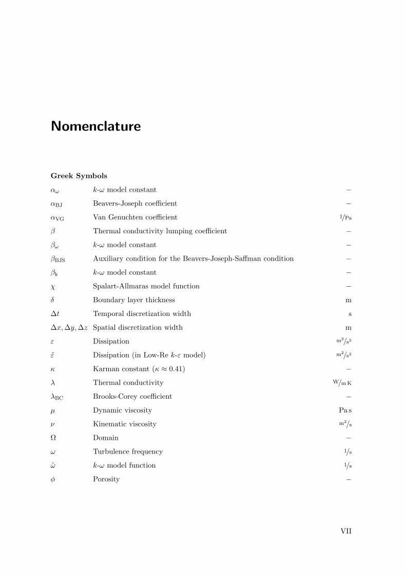
Nomenclature
Greek Symbols
αω k-ω model constant −
αBJ Beavers-Joseph coefficient −
αVG Van Genuchten coefficient 1/Pa
β Thermal conductivity lumping coefficient −
βω k-ω model constant −
βBJS Auxiliary condition for the Beavers-Joseph-Saffman condition −
βk k-ω model constant −
χ Spalart-Allmaras model function −
δ Boundary layer thickness m
∆t Temporal discretization width s
∆x,∆y,∆z Spatial discretization width m
ε Dissipation m2/s3
ε Dissipation (in Low-Re k-ε model) m2/s3
κ Karman constant (κ ≈ 0.41) −
λ Thermal conductivity W/m K
λBC Brooks-Corey coefficient −
µ Dynamic viscosity Pa s
ν Kinematic viscosity m2/s
Ω Domain −
ω Turbulence frequency 1/s
ω k-ω model function 1/s
φ Porosity −
VII
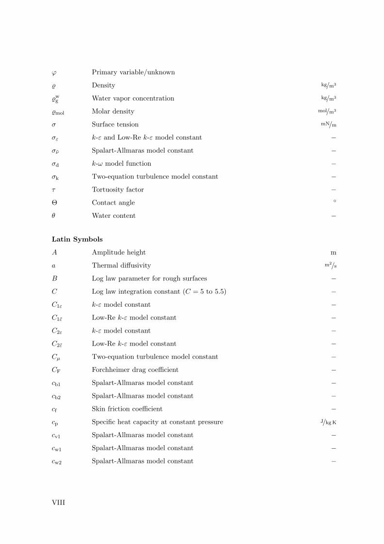
ϕ Primary variable/unknown
% Density kg/m3
%wg Water vapor concentration kg/m3
%mol Molar density mol/m3
σ Surface tension mN/m
σε k-ε and Low-Re k-ε model constant −
σν Spalart-Allmaras model constant −
σd k-ω model function −
σk Two-equation turbulence model constant −
τ Tortuosity factor −
Θ Contact angle
θ Water content −
Latin Symbols
A Amplitude height m
a Thermal diffusivity m2/s
B Log law parameter for rough surfaces −
C Log law integration constant (C = 5 to 5.5) −
C1ε k-ε model constant −
C1ε Low-Re k-ε model constant −
C2ε k-ε model constant −
C2ε Low-Re k-ε model constant −
Cµ Two-equation turbulence model constant −
CF Forchheimer drag coefficient −
cb1 Spalart-Allmaras model constant −
cb2 Spalart-Allmaras model constant −
cf Skin friction coefficient −
cp Specific heat capacity at constant pressure J/kg K
cv1 Spalart-Allmaras model constant −
cw1 Spalart-Allmaras model constant −
cw2 Spalart-Allmaras model constant −
VIII

cw3 Spalart-Allmaras model constant −
D Diffusion coefficient m2/s
Dε Low-Re k-ε damping function m2/s3
Ddisp Dispersion coefficient m2/s
d Diameter m
d50 Median sand grain diameter m
dhy Hydraulic diameter m
E Log law integration constant (E = 9.793) −
Ek Low-Re k-ε damping function m2/s4
e Evaporation rate mm/d
F Baldwin-Lomax model function m/s
Fkleb Baldwin-Lomax model function −
Fwake Baldwin-Lomax model function m2/s
f Darcy friction factor −
f1 Low-Re k-ε model constant −
f2 Low-Re k-ε model constant −
fµ Low-Re k-ε damping function −
fv1 Spalart-Allmaras model function −
fv2 Spalart-Allmaras model function −
fw Spalart-Allmaras model function −
g Grid grading factor −
gw Spalart-Allmaras model function −
H Henry coefficient Pa
h Specific enthalpy J/kg
I Turbulence intensity −
J Leverett J-function −
K Intrinsic permeability m2
k Turbulent kinetic energy m2/s2
kJ Johansen coefficient −
kr Relative permeability −
ks Sand grain roughness m
IX
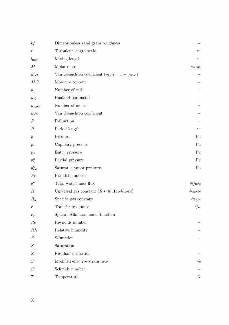
k+s Dimensionless sand grain roughness −
` Turbulent length scale m
lmix Mixing length m
M Molar mass kg/mol
mVG Van Genuchten coefficient (mVG = 1− 1/nVG) −
MC Moisture content −
n Number of cells −
nH Haaland parameter −
nmole Number of moles −
nVG Van Genuchten coefficient −
P P-function −
P Period length m
p Pressure Pa
pc Capillary pressure Pa
pd Entry pressure Pa
pκg Partial pressure Pa
pκsat Saturated vapor pressure Pa
Pr Prandtl number −
qw Total water mass flux kg/m2s
R Universal gas constant (R ≈ 8.3146 J/mol K) J/mol K
Rα Specific gas constant J/kg K
r Transfer resistance s/m
rw Spalart-Allmaras model function −
Re Reynolds number −
RH Relative humidity −
S S-function −
S Saturation −
Sr Residual saturation −
S Modified effective strain rate 1/s
Sc Schmidt number −
T Temperature K
X

t Time s
u Specific internal energy J/kg
u+ Dimensionless velocity −
uτ Wall friction velocity m/s
V Volume m3
X Mass fraction −
x Mole fraction −
y Wall distance m
y+ Dimensionless wall distance −
y+threshold Threshold for using the law of the wall −
Vectors
ω Vorticity 1/s
f Conductive energy flux J/m2s
g Gravitational acceleration: g = (0, . . . ,−9.81 m/s2)ᵀ m/s2
jmass Diffusive mass flux kg/m2s
jmol Diffusive molar flux mol/m2s
n Normal vector −
t Tangential vector −
v Velocity: v = (vx, vy, . . . )ᵀ m/s
x Space coordinates: x = (x, y, . . . )ᵀ m
Tensors
Ω Rotation rate 1/s
τ Shear stress kg/s2m
I Identity matrix −
S Strain rate 1/s
Subscripts
α Phase index: gas (g), liquid (l), or solid (s)
char Characteristic
XI
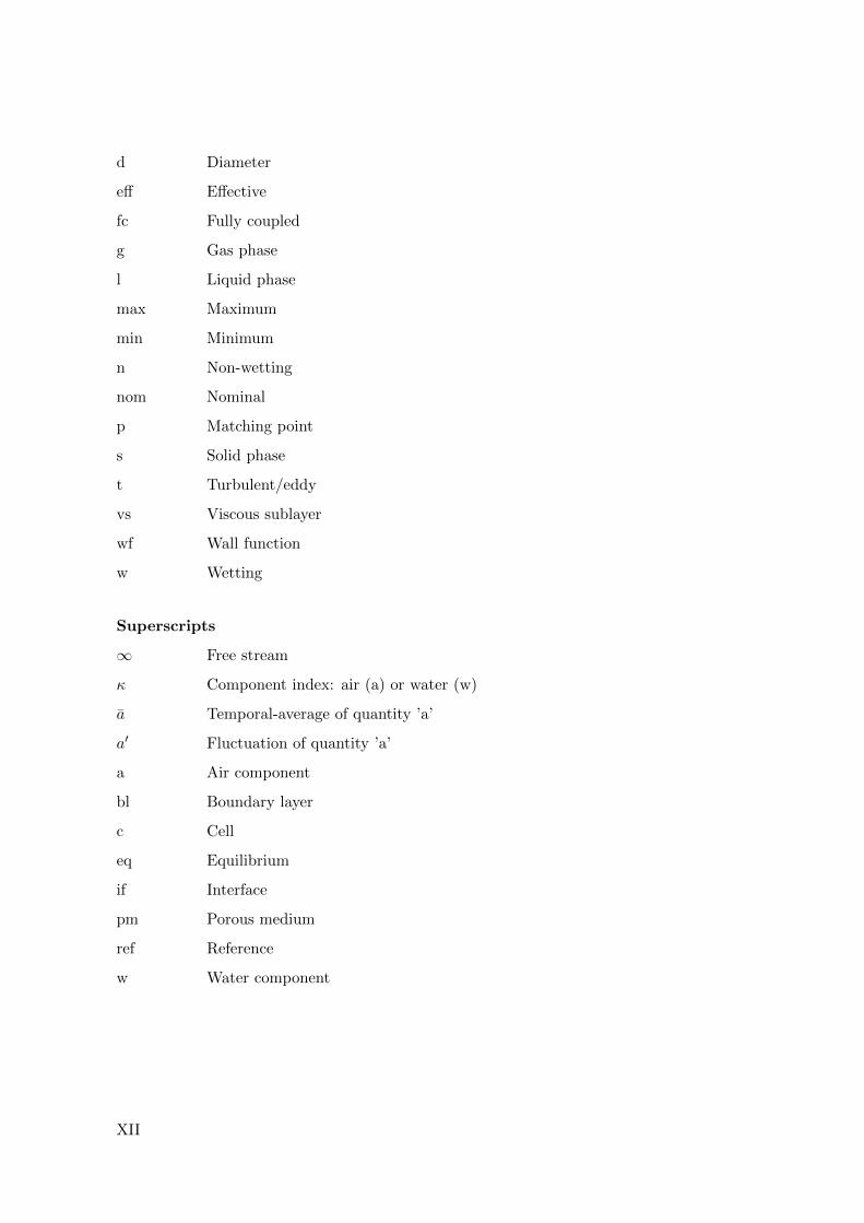
d Diameter
eff Effective
fc Fully coupled
g Gas phase
l Liquid phase
max Maximum
min Minimum
n Non-wetting
nom Nominal
p Matching point
s Solid phase
t Turbulent/eddy
vs Viscous sublayer
wf Wall function
w Wetting
Superscripts
∞ Free stream
κ Component index: air (a) or water (w)
a Temporal-average of quantity ’a’
a′ Fluctuation of quantity ’a’
a Air component
bl Boundary layer
c Cell
eq Equilibrium
if Interface
pm Porous medium
ref Reference
w Water component
XII
Abstract
Understanding the coupled exchange processes between a free flow and flow through a porous
medium is important for a wide spectrum of applications in many fields of research. Possible
applications arise from environmental science, medical science, aerospace engineering, civil
engineering, process engineering, energy supply, safety issues, and technical design problems.
A common feature in all these applications is the interface between the free-flow and the
porous-medium flow domain. In the vicinity of this interface, processes in both domains
control the coupled exchange fluxes. Therefore, modeling the interface region is a key challenge
and requires the consideration of various processes on different scales with varying physical
complexity, and thus the application of adequate modeling strategies.
First, understanding the relevant processes and the key properties in the free flow (e.g. tur-
bulence, boundary layer formation), in the porous medium (e.g. capillary flow, thermal
conduction), and at their common interface (e.g. roughness) is important for the analysis of
resulting coupled exchange fluxes. Second, bridging scales by properly accounting for effects
occurring on smaller spatial and temporal scales is important for an efficient simulation and
accurate results. Third, for the numerical modeling, numerical stable and mass conservative
schemes are required. In addition, inside the two domains the relevant scales and processes
are different and a sufficiently high resolution in interface-normal direction is required for a
good approximation of the exchange fluxes. Fourth, comparing numerical simulations with
laboratory experiments is difficult due the coupled interplay of mass, momentum, and energy
transport composed of advective and diffusive transport mechanisms which occur in a small
area around the interface.
The focus of this thesis is on improving the model concept for multi-phase porous-medium
flow coupled to a turbulent free flow, both including multi-component and energy transport.
It is aimed to develop an REV-scale two-domain concept which can handle two models in
two separated subdomains and to couple them via appropriate coupling conditions at a sharp
interface. One goal is to perform this coupling without introducing additional degrees of
freedom on the interface. An existing porous-medium model, using the equations by Darcy
or Forchheimer and discretized with the cell-centered finite volume method, is coupled to
a (Reynolds-Averaged) Navier-Stokes model discretized with a marker-and-cell scheme (also
known as staggered grid), cf. Gruninger et al. [2017]. In this framework, eddy-viscosity
based turbulence models of different complexity are presented and implemented. In addition,
simplifications of the coupling conditions are introduced and discussed. The implementation
is performed using the software modules DuMux and Dune. A fully implicit Euler method
is used and the resulting monolithic matrix is solved with a Newton method and the help of
a direct linear solver.
Numerical results for the analysis of different model concepts, parameters, and setups are
presented. In a first step, the developed model concepts and coupling methods are compared
to a previous work which uses the box method for spatial discretization, cf. Mosthaf [2014].
The results for both discretization methods are in a good agreement. The investigated tur-
bulence models produce differences in stage-I evaporation rates of about ±12% compared
to their mean rate. Under specific conditions, simplifications of the free-flow model concept
can speed-up the simulations by preserving the quality of the results. The analyses of the
turbulent Schmidt number, the turbulent Prandtl number, and the Beavers-Joseph coefficient
show an influence of up to +10% on stage-I evaporation rates when each value is varied from
unity to other physical meaningful values.
In a second study, the model results are compared to different evaporation experiments from
the literature and show a good qualitative and quantitative agreement. Most difficulties are
observed in reproducing the temperature evolution over time, or the transition from stage-I
to stage-II evaporation. The results show that the model predictions are sensitive to the
boundary conditions, the considered model dimension, and the porous-medium properties.
Finally, the effect of three different kinds of roughness is analyzed: heterogeneities, rough-
ness resulting from the sand-grains and from porous obstacles. The roughness of the porous
medium has a strong influence on the entire evaporation process and may add additional
stages to the typical evaporation stages known from flat and homogeneous media.
Based on the previous analyses and with respect to the research hypotheses, the following
conclusions are drawn:
Discretizations and Interface Model Concepts The discretization around the interface is
important. If degrees of freedom are located on the interface, grid-independent stage-I evap-
oration rates can be shown for a minimum discretization of ∆y+ < 5 at the interface. For
mainly interface-parallel flow, the proposed coupling methods without additional degrees of
freedom on the interface converge against the same results but with a stronger restriction:
∆y+ < 1. For flow normal toward a porous medium with multiple mobile phases, all methods
produce different results, because of the different ways to account for the phases’ resistance
to flow.
Turbulence Models and Simplifications Compared to the fully-coupled model concept, all
presented simplifications are shown to speed-up the simulation. Simplifying the free flow
XIV
is possible, e.g. by setting one-dimensional models as boundary conditions for the porous
medium or by calculating mass and energy transport on a given flow field without feedback
on the momentum transport. Wall functions for the k-ε model are especially helpful for larger
setups. Further, the choice of the turbulence model affects the predicted stage-I evaporation
rates.
Processes and Properties in Vicinity of the Interface The influence of the turbulent Prandtl
number and the turbulent Schmidt number on the stage-I evaporation rate is in a similar range
as the effect of the different turbulence models. The effect of the Beavers-Joseph coefficient
is minor. The comparison of simulation results with data from various experiments and the
case of a sharp heterogeneity without conductive energy transfer indicate the importance of
the energy transport inside the porous medium, but also across the porous-medium free-flow
interface or the insulation of the porous medium. A model which includes the sand-grain
roughness of an impermeable surface, is tested for its usage in the application of evaporation
through a permeable interface. Its influence on the stage-I evaporation rate only depends
on the dimensionless sand-grain roughness length k+s . Finally, different porous obstacles are
analyzed. Any change to the flat surface increases the stage-I evaporation rate, but also
leads to a shorter duration of stage-I. The area which is available for free-flow porous-medium
exchange inside one cavity between two porous obstacles has a distinct influence on the stage-
II evaporation rate.
XV

Zusammenfassung
Fur ein breites Spektrum an Anwendungen aus vielen Forschungsgebieten ist es wichtig, die
gekoppelten Austauschprozesse zwischen einer freien Stromung und einer Stromung durch ein
poroses Medium zu verstehen. Mogliche Anwendungen finden sich in Umweltwissenschaften,
Medizin, Luft- und Raumfahrttechnik, Bauingenieurwesen, Verfahrenstechnik, Energieversor-
gung, Sicherheitsaspekten oder Fragen des technischen Designs wieder. Eine Gemeinsamkeit
all dieser Anwendungen ist die Schnittstelle des Gebiets der freien Stromung mit dem Ge-
biet der porosen Stromung (von hier an Interface). In unmittelbarer Nahe dieses Interfa-
ces kontrollieren Prozesse in beiden Gebieten die gekoppelten Austauschflusse; deshalb ist
die Modellierung der Interface-Region eine der Hauptherausforderungen und erfordert die
Berucksichtigung von unterschiedlichen Prozessen auf unterschiedlichen Skalen und mit un-
terschiedlicher physikalischer Komplexitat und damit auch die Anwendung von passenden
Modellierungsstrategien.
Zuerst gilt es, die relevanten Prozesse und Eigenschaften in der freien Stromung (z. B. Tur-
bulenz, Grenzschichtentwicklung), im porosen Medium (z. B. kapillarer Fluss, thermische
Leitfahigkeit) und an dem gemeinsamen Interface (z. B. Rauigkeit) zu verstehen, um die
resultierenden Austauschflusse zu analysieren. Zweitens ist es wichtig, die unterschiedlichen
Skalen zu uberbrucken um genaue Ergebnisse zu erzielen und die Simulationen effizient durch-
zufuhren. Hierfur mussen Effekte auf kleineren ortlichen und zeitlichen Skalen entsprechend
integriert werden. Drittens sind fur das numerische Modellieren numerisch stabile und masse-
nerhaltende Methoden erforderlich. Daruber hinaus sind die relevanten Skalen und Prozesse
in den beiden Gebieten unterschiedlich und eine entsprechend hohe Auflosung der Richtung
normal zum Interface ist notwendig, um eine gute Annaherung der Austauschflusse sicherzu-
stellen. Zuletzt bleibt die Schwierigkeit, numerische Simulationen mit Laborexperimenten zu
vergleichen, da das gekoppelte Zusammenspiel von Masse-, Impuls-, und Energie-Transport,
bestehend aus advektiven und diffusiven Transportmechanismen, in einem sehr kleinen Be-
reich um das Interface stattfindet.
Das Hauptaugenmerk dieser Arbeit liegt auf der Verbesserung des Modellkonzeptes fur ei-
ne porose Mehrphasenstromung, die an eine turbulente freie Stromung gekoppelt ist; beide
Stromungen berucksichtigen den Transport mehrerer Komponenten und der Energie. Ein
REV-skaliger Zwei-Gebiets-Ansatz, der zwei Modelle in zwei getrennten Teilgebieten beruck-
sichtigen kann, wird angestrebt. Diese beiden Teilgebiete sollen uber entsprechende Bedin-
gungen an einem gemeinsamen, scharfen Interface gekoppelt werden. Ein Ziel ist es, diese

Kopplung umzusetzen ohne zusatzliche Freiheitsgrade auf dem Interface einzufuhren. Ein be-
stehendes Modell des porosen Mediums, basierend auf der Darcy oder der Forchheimer Glei-
chung und mit der zell-zentrierten Finiten-Volumen-Methode diskretisiert, wird mit einem
(Reynolds-gemittelten) Navier-Stokes Modell, diskretisiert mit der Marker-and-Cell-Methode
(auch bekannt als verschobenes Gitter), gekoppelt, siehe Gruninger et al. [2017]. In die-
sem Rahmen werden unterschiedlich komplexe Wirbelviskositat-Turbulenzmodelle vorgestellt
und implementiert. Daruber hinaus werden Vereinfachungen der Kopplungsbedingungen ein-
gefuhrt und diskutiert. Die Implementierung findet in den Software-Modulen DuMux und
Dune statt. Es wird die voll-implizite Euler-Methode benutzt und die resultierende, mono-
lithische Matrix wird mit der Newton-Methode und mit Hilfe eines direkten linearen Losers
gelost.
Mit den Ergebnissen numerischer Simulationen werden verschiedene Modellkonzepte, Para-
meter und Aufbauten untersucht. Im ersten Schritt werden die entwickelten Modellkonzepte
und Kopplungsmethoden mit einer vorherigen Arbeit verglichen, die die box-Methode fur
die ortliche Diskretisierung benutzt, siehe Mosthaf [2014]. Die Ergebnisse beider Diskretisie-
rungsmethoden sind in guter Ubereinstimmung. Die Verdunstungsraten der implementierten
Turbulenzmodelle weichen im ersten Abschnitt um bis zu±12% von deren Mittel ab. Unter be-
stimmten Voraussetzungen konnen, bei gleichbleibender Qualitat der Ergebnisse, vereinfachte
Modellkonzepte fur die freie Stromung die Simulationen beschleunigen. In einer Parameter-
studie wird der Einfluss der turbulenten Schmidt-Zahl, der turbulenten Prandtl-Zahl und des
Beavers-Joseph Koeffizienten analysiert. Eine Variation dieser Parameter von eins auf andere
physikalisch sinnvolle Werte ergibt eine Veranderung von bis zu +10% auf die Verdunstungs-
raten im ersten Abschnitt.
In einer zweiten Studie werden die Modellergebnisse mit verschiedenen Verdunstungsexpe-
rimenten aus der Literatur verglichen und zeigen eine gute qualitative und quantitative
Ubereinstimmung. Die großten Schwierigkeiten werden bei dem Abbilden der zeitlichen Tem-
peraturverlaufe und dem Ubergang zwischen dem ersten und dem zweiten Verdunstungsab-
schnitt beobachtet. Die Ergebnisse zeigen, dass die Modellvorhersagen sehr sensitiv bezuglich
der Randbedingungen, der berucksichtigten Modelldimensionen und der Eigenschaften des
porosen Mediums sind.
Zum Abschluss wird der Effekt von drei unterschiedlichen Arten von Rauheit analysiert: He-
terogenitaten, Sandkornrauheit und porose Hindernisse. Die Rauheit eines porosen Mediums
hat einen starken Einfluss auf das gesamte Verdunstungsverhalten und kann den typischen
Verdunstungsabschnitten, die von flachen und homogenen Medien bekannt sind, zusatzliche
Abschnitte hinzufugen.
Basierend auf diesen Analysen und in Bezug auf die Forschungshypothesen, werden folgende
Schlussfolgerungen gezogen:
XVIII
Diskretisierungen und Modellkonzepte des Interfaces Die Diskretisierung am Interface
zwischen dem porosem Medium und der freien Stromung ist wichtig. Falls Freiheitsgrade auf
dem Interface vorhanden sind, kann gezeigt werden, dass die Verdunstungsraten im ersten Ab-
schnitt fur eine minimale Diskretisierungsweite von ∆y+ < 5 gitterunabhangig werden. Die
Kopplungsmethoden ohne zusatzliche Freiheitsgrade am Interface konvergieren gegen die glei-
chen Ergebnisse, fur den Fall einer interface-parallelen Stromung, erfordern aber mit ∆y+ < 1
großere Einschrankungen. Fur eine Stromung die normal zum Interface stattfindet und die
mehrere mobile Phasen umfasst zeigen alle Methoden unterschiedliche Ergebnisse, da sie in
unterschiedlicher Weise den Fließwiderstand der Phasen berucksichtigen.
Turbulenzmodelle und Vereinfachungen Im Vergleich zum voll-gekoppelten Modellkonzept
konnen fur alle vorgestellten Vereinfachungen kurzere Simulationszeiten gezeigt werden. Eine
Vereinfachung der freien Stromung ist moglich, indem eindimensionale Modelle als Randbedin-
gungen fur das porose Medium gesetzt werden oder indem der Massen- und Energietransport
auf einem vorgegeben Stromungsfeld, ohne Ruckkopplung auf den Impulstransport, gerech-
net wird. Eine Vereinfachung des k-ε Modells mit Wandfunktionen ist besonders fur großere
Szenarien hilfreich. Daruber hinaus beeinflusst das gewahlte Turbulenzmodell die Verduns-
tungsraten im ersten Abschnitt.
Prozesse und Eigenschaften der interface-nahen Region Der Einfluss der turbulenten
Prandtl-Zahl und der turbulenten Schmidt-Zahl auf die Verdunstungsraten im ersten Ab-
schnitt ist vergleichbar mit dem der unterschiedlichen Turbulenzmodelle. Der Einfluss des
Beavers-Joseph Koeffizienten ist geringer. Der Vergleich von Simulationsergebnissen mit ver-
schiedenen Experimenten, aber auch Ergebnisse fur den Fall eines porosen Mediums mit
einer scharfen Heterogenitat, die keinen konduktiven Energietransfer zulasst, lassen auf die
Wichtigkeit des Energietransportes schließen. Dies umschließt den Energietransport inner-
halb des porosen Mediums, uber das Interface mit der freien Stromung und die Isolation
des porosen Mediums. Die Anwendbarkeit eines Modells, das die Sandkornrauheit auf ei-
ner undurchlassigen Oberflache beschreibt, wird bezuglich des Massentransports uber ein
durchlassiges Interface getestet. Der Einfluss auf die Verdunstungsraten des ersten Abschnitts
beruht allein auf der dimensionslosen Sandkornrauheitslange k+s . Zum Abschluss werden die
Auswirkungen von porosen Hindernissen analysiert. Jegliche Anderung an der flachen Ober-
flache erhoht die Verdunstungsraten im ersten Abschnitt, fuhrt aber auch zu einer kurzeren
Dauer des ersten Abschnitts. Die Flache des Interfaces, das fur den Austausch zwischen der
freien und der porosen Stromung zwischen zwei porosen Hindernissen zur Verfugung steht,
hat einen ausgepragten Einfluss auf die Verdunstungsraten im zweiten Abschnitt.
XIX

1 Introduction
Understanding the coupled exchange processes between a free flow and flow through a porous
medium is important for a wide spectrum of applications in many fields of research. Possi-
ble applications arise from environmental science [Das et al., 2002, Sophocleous, 2002, Ren
and Packman, 2005, Furman, 2008, Davarzani et al., 2014, Mosthaf et al., 2014, Jambhekar
et al., 2016, Broecker et al., 2018], medical science [Discacciati and Quarteroni, 2009, Baber
et al., 2016], aerospace engineering [Dahmen et al., 2014, Chen et al., 2016], civil engineer-
ing [Buccolieri et al., 2009, Defraeye, 2011, Defraeye et al., 2012b, Belleghem et al., 2014],
process engineering [Nassehi, 1998, Verboven et al., 2006, Targui and Kahalerras, 2008], en-
ergy supply [Salinger et al., 1994, Gurau et al., 2008, Baber et al., 2016, Suga, 2016], safety
issues [Das et al., 2001, Oldenburg and Unger, 2004, Smits et al., 2013, Masson et al., 2016],
or technical and design problems [Iliev and Laptev, 2004, Cimolin and Discacciati, 2013].
Modeling these applications requires the consideration of various processes on different scales
with varying physical complexity, and thus the application of adequate modeling strategies.
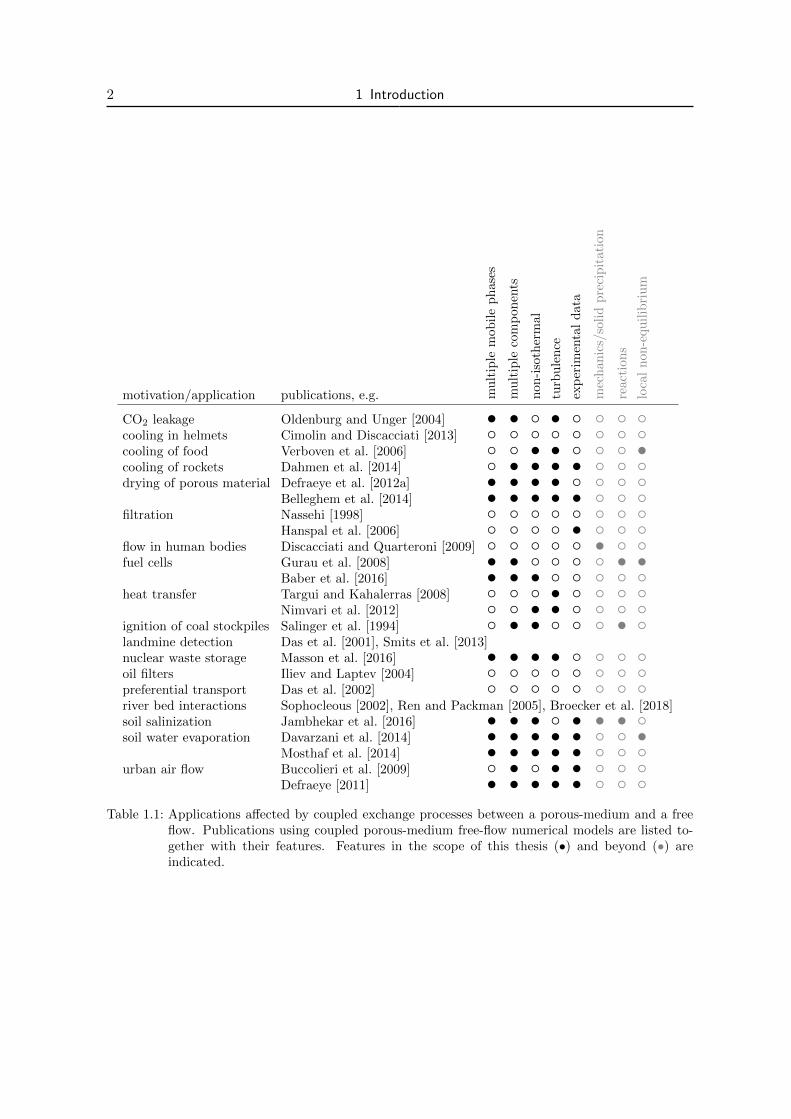
Tab. 1.1 gives an application-oriented overview on studies modeling coupled porous-medium
free-flow problems and the complexity of the models used therein. A common feature in all
these applications is the interface between the free-flow and the porous-medium flow domain.
In the vicinity of this interface, processes in both domains control the coupled interactions
and exchange processes. Therefore, modeling the interface region is a key challenge and it is
demanding for various reasons.
First, understanding the relevant processes and the key properties in the free flow (e.g. turbu-
lence, boundary layer formation, buoyancy, radiation), in the porous medium (e.g. capillary
flow, preferential transport, thermal conduction, turbulent pumping, vaporization/condensa-
tion), and at their common interface (e.g. roughness, slip condition) is important for the
interpretation and the analysis of resulting coupled exchange fluxes, see Fig. 1.1.
Second, bridging scales by properly accounting for effects occurring on smaller scales, a so-
called upscaling, is important for an efficient simulation and accurate results. This upscaling
has to be performed for both domains and the interface. For example, upscaling is neces-
sary for simulating larger-scale hazards such as the evaporation-driven soil salinization for
2 1 Introduction
motivation/application publications, e.g. mu
ltip
lem
obil
ep
hase
s
mu
ltip
leco
mp
on
ents
non
-iso
ther
mal
turb
ule
nce
exp
erim
enta
ld
ata
mec
han
ics/
soli
dp
reci
pit
ati
on
react
ion
s
loca
ln
on
-equ
ilib
riu
m
CO2 leakage Oldenburg and Unger [2004] • • • cooling in helmets Cimolin and Discacciati [2013] cooling of food Verboven et al. [2006] • • •cooling of rockets Dahmen et al. [2014] • • • • drying of porous material Defraeye et al. [2012a] • • • •
Belleghem et al. [2014] • • • • • filtration Nassehi [1998]
Hanspal et al. [2006] • flow in human bodies Discacciati and Quarteroni [2009] • fuel cells Gurau et al. [2008] • • • •
Baber et al. [2016] • • • heat transfer Targui and Kahalerras [2008] •
Nimvari et al. [2012] • • ignition of coal stockpiles Salinger et al. [1994] • • • landmine detection Das et al. [2001], Smits et al. [2013]nuclear waste storage Masson et al. [2016] • • • • oil filters Iliev and Laptev [2004] preferential transport Das et al. [2002] river bed interactions Sophocleous [2002], Ren and Packman [2005], Broecker et al. [2018]soil salinization Jambhekar et al. [2016] • • • • • • soil water evaporation Davarzani et al. [2014] • • • • • •
Mosthaf et al. [2014] • • • • • urban air flow Buccolieri et al. [2009] • • •
Defraeye [2011] • • • • • Table 1.1: Applications affected by coupled exchange processes between a porous-medium and a free
flow. Publications using coupled porous-medium free-flow numerical models are listed to-gether with their features. Features in the scope of this thesis (•) and beyond (•) areindicated.
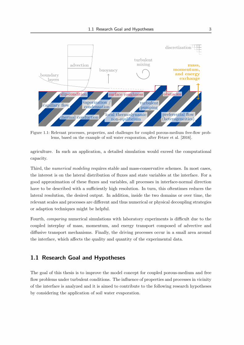
1.1 Research Goal and Hypotheses 3
advection
boundarylayers
turbulentmixing
buoyancy
discretization
slip-condition surface roughness obstacles
capillary flow
thermal conduction
vaporization /condensation
local thermodynamicnon-equlibrium
turbulentpumping
preferential flow(heterogeneities)
mass,momentum,and energy
exchange
Figure 1.1: Relevant processes, properties, and challenges for coupled porous-medium free-flow prob-lems, based on the example of soil water evaporation, after Fetzer et al. [2016].
agriculture. In such an application, a detailed simulation would exceed the computational
capacity.
Third, the numerical modeling requires stable and mass-conservative schemes. In most cases,
the interest is on the lateral distribution of fluxes and state variables at the interface. For a
good approximation of these fluxes and variables, all processes in interface-normal direction
have to be described with a sufficiently high resolution. In turn, this oftentimes reduces the
lateral resolution, the desired output. In addition, inside the two domains or over time, the
relevant scales and processes are different and thus numerical or physical decoupling strategies
or adaption techniques might be helpful.
Fourth, comparing numerical simulations with laboratory experiments is difficult due to the
coupled interplay of mass, momentum, and energy transport composed of advective and
diffusive transport mechanisms. Finally, the driving processes occur in a small area around
the interface, which affects the quality and quantity of the experimental data.
1.1 Research Goal and Hypotheses
The goal of this thesis is to improve the model concept for coupled porous-medium and free
flow problems under turbulent conditions. The influence of properties and processes in vicinity
of the interface is analyzed and it is aimed to contribute to the following research hypotheses
by considering the application of soil water evaporation.
4 1 Introduction
Hypothesis 1: For modeling coupled porous-medium free flow problems, the discretiza-
tion and conceptualization of the interface are important. Mosthaf et al. [2014] show
that a model concept for coupling free flow and porous-medium flow using the collocated box
method [cf. Mosthaf et al., 2011, Baber et al., 2012] can successfully be applied to simulate
evaporation fluxes from a porous medium into a mainly parallel free flow.
Nevertheless, some disadvantages and advantages are associated with this concept. First,
Baber [2014] shows that this method leads to stable pressure oscillations which may influence
the local exchange behavior between the two domains. Therefore, it may not be suited for
modeling mainly interface-normal flow. In this case, the pressure at the interface is necessary
to induce the flow through the porous medium and thus pressure fluctuations would lead to
unphysical lateral fluxes inside the porous medium. Hanspal et al. [2006] also mention the
importance of the near-interface discretization for the free flow field. Second, the box dis-
cretization scheme reveals difficulties to handle interface-corner points, which are necessary
for modeling non-planar surfaces. A major advantage of the box method is that a good ap-
proximation of the gradients at the interface, by using information from one subdomain only,
is possible. All relevant properties are available at the porous-medium free-flow interface from
each side. For cell-centered methods, which are used in this thesis, this is not straightforward,
cf. Gruninger [2017].
Hypothesis 2: It is possible to include the effects of turbulence while reducing the over-
all model complexity. Solving coupled flow and transport processes using one coefficient
matrix (monolithic scheme) while including information from the next time level (implicit)
is computationally expensive. Numerical techniques, as spatial and temporal decoupling are
available and show to reduce the computational cost, e.g. Rybak et al. [2015], Discacciati
et al. [2016], Masson et al. [2016]. However, it is also possible to reduce the complexity of the
physical model, if some limitations are respected. Compared to the full complex model, the
computational and qualitative performance as well as the limitations of models with reduced
complexity are explored.
Based on hypothesis 1, the developed full complex model is replaced by simpler approxima-
tions of the exchange fluxes: (i) neglecting lateral transport inside the free flow, so that only
the one-dimensional interface-normal fluxes have to be described, (ii) neglecting feedbacks of
the transported quantities on the momentum transport, and (iii) including wall functions to
approximate the exchange fluxes on a coarse mesh.
Hypothesis 3: The properties and processes in the vicinity of the porous-medium free-flow
interface strongly affect the resulting exchange fluxes. A common feature of flow along a
boundary with different properties than the main flow are the strong gradients which prevail
1.2 Related Studies 5
in the resulting boundary layers. Driven by these strong gradients, the diffusive processes
through the boundary layers have a substantial impact on the resulting evaporation fluxes,
see Haghighi et al. [2013], Mosthaf et al. [2014]. The relevance of boundary layers for flow
and transport phenomena is well known and described in various textbooks, e.g. Schlichting
and Gersten [2006], Bird et al. [2007]. The properties of and at the interface will alter the
boundary layers and thus the resulting exchange fluxes.
First, the surface of the porous medium may not always be perfectly smooth, roughness can
occur on different scales and will have an impact on the model results. Therefore, this study
aims at extending the concepts for flat and smooth surfaces and include roughness concepts
and highlight the influence of different aspects of roughness: (i) roughness resulting from the
sand grains themselves and (ii) roughness as discrete, porous objects. Second, heterogeneities
in porous-medium properties will affect the local fluxes across the interface and induce lat-
eral fluxes inside the porous medium. This is especially relevant if these heterogeneities are
located at the porous-medium surface. Third, at the porous-medium surface, the coupling of
tangential momentum [Beavers and Joseph, 1967] or the concept of a slip-velocity condition
[Saffman, 1971] involves a new parameter for which few experimental data is available. It will
be discussed, whether these aspects influence flow and transport under turbulent free flow
conditions.
1.2 Related Studies
For the numerical modeling of such coupled applications, two main approaches are found in
literature, the so-called one-domain and two-domain approaches.
In one-domain approaches, one set of equations is used in the entire problem area. With a
detailed knowledge of the (porous) structure, of the boundary conditions, and high spatial
and temporal resolutions, a direct numerical simulation (DNS) is possible. DNS studies are
performed for turbulent, single-phase flow above a well-defined pore geometry [e.g. Hahn
et al., 2002, Breugem and Boersma, 2005, Kuwata and Suga, 2016], but also above real
porous media [e.g. Krafczyk et al., 2015, Fattahi et al., 2016]. A DNS is computationally very
expensive, especially when non-isothermal, multi-phase, and multi-component flow processes
are included. The one-domain method by Brinkman [1949] uses one set of averaged equations
in which the features of both subdomains are integrated. By changing the parameters via
a specified region, a gradual transition from one subdomain to the other is achieved. This
is usually done for coupling laminar free flow with creeping flow in the porous medium.
The author is not aware of Brinkman-like approaches for multi-phase flow and turbulent
conditions.
In two-domain approaches, two different sets of equations are used in the two subdomains and
6 1 Introduction
connected by appropriate conditions on an interface with no thickness. This interface can be
modeled as a sharp simple interface [e.g. Mosthaf et al., 2011] or a sharp complex interface,
which allows to store mass at the interface, e.g. to account for drop formation [Baber et al.,
2016]. Discacciati et al. [2014] propose a decomposition approach using interface conditions
at the edges of an overlap region. Le Bars and Worster [2006] extend the influence of the
free-flow region, via a viscous transition zone, into the porous-medium domain. The two-
domain approaches offer the opportunity for adapting the model complexity to the needs of
each subdomain. The free flow and the porous-medium flow are usually modeled by upscaled
models. This study uses an upscaled two-domain approach based on Mosthaf et al. [2014]
and Gruninger [2017]. Therefore, the following literature study highlights different aspects of
such models and underlines their differences with respect to the free flow, the porous-medium
flow, their common interface, and numerical techniques. Finally, the attention is drawn to
the application of (soil water) evaporation.
Free Flow The effect of turbulence is usually captured by time-averaged turbulence models,
based on the Reynolds-averaged Navier-Stokes equations (RANS). These turbulence models
are classified by the number of partial differential equations for the transport of turbulent
properties. Available are relatively simple algebraic or zero-equation models [e.g. Baldwin
and Lomax, 1978, Cebeci and Smith, 1974], intermediate one-equation models [e.g. Spalart
and Allmaras, 1992], and more complex and more general two-equation models [cf. Patel
et al., 1985, Bardina et al., 1997]. To avoid the necessity for simulating the entire free flow,
boundary layer models can be used to mimic the exchange through a diffusion-dominated
boundary layer. The effect of roughness, as roughness elements on an impermeable surface,
on the free-flow processes is intensively discussed in fluid dynamics textbooks as Schlichting
and Gersten [2006]. Studies on roughness of permeable surfaces are discussed in the next
paragraphs.
Mosthaf et al. [2014] compare boundary layer approaches and zero-equation models to sim-
ulate soil water evaporation. Kuznetsov and Becker [2004] use a zero-equation model with
extensions for surface roughness as proposed in Cebeci [1978] to analyze heat transfer mech-
anisms. The more complex two-equation turbulence models, like the k-ε, Low-Re k-ε, or k-ω
turbulence models, are applied for a dimensionless analysis on heat transfer [Nimvari et al.,
2012, Jamarani et al., 2017], heat transfer over rough surfaces [Kuznetsov, 2004], drying prob-
lems [Defraeye et al., 2010, Belleghem et al., 2014], cooling applications [Dahmen et al., 2014],
or problems including turbulence inside the porous medium [Pedras and de Lemos, 2001, de
Lemos, 2009]. For the k-ε model, wall functions are required for a correct modeling of the
low-Reynolds flow near the wall. Even for smooth surfaces, these wall functions are found
to increase the transfer coefficients and thus the exchange fluxes by up to 50% compared to
1.2 Related Studies 7
other methods [Defraeye, 2011]. Wall-function models which includes a parametrization of
roughness are also available, e.g. Blocken et al. [2007]. Flow over discrete porous/non-porous
obstacles is a key topic in building physics [e.g. Lien et al., 2004, Buccolieri et al., 2009,
Defraeye et al., 2010], but also in limnology [e.g. Broecker et al., 2018], combustion processes
[e.g. Suga et al., 2013, Suga, 2016], or heat exchangers [e.g. Targui and Kahalerras, 2008,
Nimvari et al., 2012, Jamarani et al., 2017]. Haghighi and Or [2015] perform experiments to
analyze how arrangements of bluff non-evaporating obstacles affect the evaporation rate and
surface temperature distribution. Sugita and Kishii [2002] conduct experiments with different
distributions of evaporating obstacles and analyze the influence of different spacing by simple
roughness parametrizations.
Porous Medium The porous medium is normally described with one of the following up-
scaled/averaged models: the multi-phase Darcy law [e.g. Mosthaf et al., 2011, Baber et al.,
2012, Mosthaf et al., 2014], liquid-phase flow via Richards equation [e.g. Defraeye, 2011], or
the Forchheimer extension including inertia effects [e.g. Dahmen et al., 2014]. Nevertheless,
two-domain approaches with a pore representation of the porous medium are also available.
Beyhaghi et al. [2016] present a method for an isothermal coupling of turbulent free flow to
flow and transport in a pore-network model.
Characteristics of coupled exchange fluxes depend on the processes and properties inside the
porous medium. The influence of properties of homogeneous porous media on the evaporation
behavior is analyzed via numerical [e.g. Mosthaf et al., 2014] and experimental studies [e.g.
Shokri and Or, 2011]. Heterogeneities alter the evaporation behavior. Horizontal layers with
a coarse structure, so-called mulches, reduce the evaporation by restricting the flow of liquid
water [Modaihsh et al., 1985, Diaz et al., 2005, Shokri et al., 2010]. Iliev and Laptev [2004]
include anisotropic porous media which promote flow in certain directions. Porous-medium
models are oftentimes built on the assumption that locally all processes are in an equilibrium
state (local thermodynamic equilibrium). However, the multi-phase effects of evaporation,
the small time scale for phase transition, and the associated heat transfer, may indicate that
the underlying assumptions for local thermodynamic equilibrium are not always valid. The
effects of non-equilibrium models are analyzed for pure porous-medium systems [Smits et al.,
2011, Trautz et al., 2015] or including a pseudo free flow, which is a region with a large
porosity and permeability [Nuske et al., 2014].
Coupling and Interface Modeling The importance of the porous-medium free-flow inter-
face is known in soil science. For agricultural purposes, tillage is used to modify the interface
or surface behavior and thus the evaporation fluxes: Capillary pathways are destroyed, soil
portions with different hydraulic properties and water contents are brought to the surface
8 1 Introduction
[Unger and Cassel, 1991], or the increased roughness of the soil surface may influence the net
radiation [Potter et al., 1987]. The effect of vegetation is not considered here, even though it
plays a huge role in real applications [Shukla and Mintz, 1982].
Only few studies are performed regarding the influence of rough and permeable surfaces, espe-
cially in conjunction with flow and transport in the porous medium. Krafczyk et al. [2015] and
Kuwata and Suga [2016] use DNS to simulate single-phase flow above a porous bed. Pokrajac
and Manes [2009] and Manes et al. [2011] show that the effect of roughness of an impermeable
and of a permeable surface is different. At the porous-medium free-flow interface, non-zero
tangential velocities may occur as proposed and discussed in Beavers and Joseph [1967],
Saffman [1971], Sahraoui and Kaviany [1992], Auriault [2010]. According to references given
in Nield [2009], the resulting coefficient depends on the flow direction, Reynolds number, the
extend of the free flow domain, and the structure of the porous-medium surface. However, it
does neither explicitly include these parameters nor the effects of turbulence, roughness, or
the presence of multiple phases. Apart from Beavers et al. [1974], few experimental work is
performed on determining this coefficient. The sensitivity of evaporation rates to a slip con-
dition at the interface is analyzed for low velocities [Baber et al., 2012, Davarzani et al., 2014]
but not for higher velocities (turbulent conditions). A review on the interface as a hydrody-
namic boundary condition for the porous medium can be found in Nield and Bejan [2017,
Ch. 1.6] and is intensively discussed in Shavit [2009]. The interface is not only interesting
regarding its hydrodynamic properties, but also for mass and energy transport mechanisms.
The distribution of evaporating pores at the interface yields compensation mechanisms which
allow the porous medium to maintain a high evaporation rate, although its surface is only
partially wetted, see Suzuki and Maeda [1968], Schlunder [1988], Haghighi and Or [2015].
Numerical Modeling Techniques A large variety is found when looking at the discretization
schemes for two-domain approaches. Finite volume methods using collocated grids [Mosthaf
et al., 2011, Baber et al., 2012], pure staggered-grid schemes [Iliev and Laptev, 2004], combined
staggered and collocated approaches [Rybak et al., 2015, Masson et al., 2016, Gruninger,
2017], or in combination with finite element methods [Defraeye, 2011, Dahmen et al., 2014]
are applied. In addition, spatial [Dahmen et al., 2014, Discacciati et al., 2016, Masson et al.,
2016] or temporal decoupling [Rybak et al., 2015] of the two subdomains helps to improve
the model performance. A fully implicit monolithic scheme is also used by e.g. Mosthaf
et al. [2011], whereas the majority of the other publications applies an explicit scheme. The
uniqueness of this work is, that it combines a fully implicit monolithic scheme on an oscillation-
free spatial discretization to simulate turbulent free flow coupled to multi-phase flow inside
the porous medium.

1.3 Structure of the Thesis 9
(Soil Water) Evaporation This thesis focuses on the coupled modeling of soil water evap-
oration. In this field of research, detailed numerical studies are performed for laminar flow
and turbulent flow using simple turbulence models [Mosthaf et al., 2014], laminar flow us-
ing dispersion coefficients and local thermodynamic non-equilibrium [Davarzani et al., 2014],
and laminar flow including salinization [Jambhekar et al., 2016]. More work is performed on
analyzing the influence of evaporation on the soil processes and improving the boundary con-
ditions for the soil water modeling [Schneider-Zapp et al., 2010, Smits et al., 2012, Haghighi
et al., 2013, Tang and Riley, 2013].
Also, many experiments are performed to analyze soil water evaporation. Some of these ex-
periments are conducted without a forced free flow to analyze pore-scale effects [Laurindo
and Prat, 1998, Belhamri and Fohr, 1996, Assouline et al., 2010, Shahraeeni and Or, 2010,
Haghighi et al., 2013] or to analyze processes on the averaged scale [e.g. Schneider-Zapp et al.,
2010, Zhang et al., 2015].
Other studies include an atmospheric free flow in a wind tunnel. Shahraeeni et al. [2012] an-
alyze the effect of discrete pores on the evaporation process. Yamanaka et al. [1997] vary the
atmospheric boundary conditions and demonstrate the significance of the depth of the evap-
orating surface. Sugita and Kishii [2002] put their focus on different obstacle arrangements.
Experiments with focus on bound water are performed by Lu et al. [2005]. The influence of
evaporation from different porous roofing materials on the roof temperature is investigated by
Wanphen and Nagano [2009]. Combining experimental and numerical studies to analyze free
and porous-medium flow properties is done in Davarzani et al. [2014], Mosthaf et al. [2014].
In Trautz et al. [2015] different numerical models which account for non-equilibrium processes
are compared. Trautz [2015] presents various soil water evaporation experiments on different
scales and compares them with modeling results from porous-medium and coupled models.
Evaporation chambers are examined in Song et al. [2014] or in Aluwihare and Watanabe
[2003] under outdoor conditions.
Since a long period, evaporation experiments are carried out in the field. Penman [1948]
suggests theoretical estimates for the evaporation rate and compares them with different data
sets form all over the world. A review of near-surface wind speeds by McVicar et al. [2012]
implies the importance of atmospheric conditions on evaporation. Collecting and interpreting
evaporation data sets is still, with improving measurement techniques, an issue in soil science
[Vanderborght et al., 2010].
1.3 Structure of the Thesis
This chapter outlines the main motivation and goals of this thesis. Further, it contains a
literature review on publications related to this work. Chapter two introduces the relevant
10 1 Introduction
physical definitions and concepts. In the third chapter, the physical models and mathemat-
ical equations are explained. The fourth chapter illustrates the numerical models and their
implementations. Chapter five presents numerical results for various applications and setups.
Finally, chapter six summarizes the thesis and gives an outlook beyond the scope of this
work.
2 Fundamentals
This chapter provides the necessary basic definitions and conceptual background for the fur-
ther understanding of this work. In section 2.1, the fundamental terms are defined and
explained. Section 2.2 includes information about modeling equilibrium-based processes. Af-
terward, in section 2.3, the attention is drawn to material properties. Then, the defining
processes and properties of fluid flow (section 2.4), of porous media (section 2.5), and of the
interface (section 2.6) are highlighted.
2.1 Basic Definitions
In this section, some basic definitions are given.
2.1.1 Scales
Coupled processes between a free flow and flow in a porous medium occur on different spatial
and temporal scales with varying importance, which will be defined here.
Spatial Scales On the molecular scale, the interest is on the interactions between individual
molecules of one or more substances, e.g. attraction, collision, and polarity. If many molecules
are considered, average quantities can be constructed, e.g. pressure, density, and viscosity.
On this continuum scale, these quantities are continuous in space. This work is based on
continuum-scale considerations.
On the pore scale, all information about pore sizes and shapes, the distribution of pores,
and the connectivity between pores is available. For experimental and numerical works with
real porous media it is challenging to collect this information. Non-destructive measurement
technologies like x-ray or neutron tomography are needed to gain insight into the states and
processes while running the experiments [Wildenschild and Sheppard, 2013]. Resolving all ge-
ometrical details for simulations results in many unknowns and high computational demands
[Blunt et al., 2013]. To enable the simulation of more complex problems or larger domains,

12 2 Fundamentals
pore scale REV scale field scale
homogeneous
heterogeneous
space
characteristic quantitye.g. porosity φ
DNS scale RANS scale
steady state
accelerated
time
mean velocity vx
Figure 2.1: Averaging of quantities for the spatial scale in a porous medium (left, after Bear [1988]and Mosthaf [2014]), and the temporal scale in a turbulent free flow (right).
as for the transition from molecular to continuum scale, an averaging is neceassary. Here,
it is averaged over several pore volumes with the goal to obtain a representative elementary
volume (REV). Consequently, this is called the REV scale. On this scale, the information
about the pores is converted to volume-averaged quantities, as the porosity or the permeabil-
ity. An REV is achieved, if these characteristic quantities do not change, when changing the
size of the averaging volume, see Fig. 2.1 (left). Consequently, the lower and upper limits
of the REV size cannot be defined arbitrarily, but are limited by strong variations in the
beginning and the risk of averaging over heterogeneous parts of the porous medium [Bear,
1988]. The REV scale typically covers a range of centimeters to meters. For larger domains,
ranging from meters to kilometers, REV-scale models are still valid, however, the respective
volumes become larger and therefore this is often referred as field scale. Modeling on the field
scale is predominantly motivated by large-scale applications, like groundwater flow, oil or gas
production, geothermal power plants, CO2 storage, or soil remediation. The additional loss
of information caused by large REVs is traded for an efficient and practical model.
Temporal Scales On the one hand, the temporal scale is important for the porous medium to
ensure local thermodynamic equilibrium. The assumption of local thermodynamic equilibrium
typically does not hold if the temporal scale is too small for the relevant processes to reach
an equilibrium state. Reasons might be slow heat and mass transfer between the different
phases under the presence of high fluid velocities as it occurs in soil remediation [Ahrenholz
et al., 2011, Armstrong et al., 1994] or in the presence of a heat source. Smits et al. [2011]
show that non-equilibrium models can help to improve predictions for soil water evaporation.
However, non-equilibrium models are not the focus of this thesis.
On the other hand, the temporal scale is important for simulating turbulent flow. Then,

2.1 Basic Definitions 13
the detailed flow structure, influenced by so-called turbulent eddies, has to be resolved by
the spatial and temporal discretization. For such direct numerical simulation (DNS) the
Kolmogorov length and time scales give an approximation for the discretization requirements.
These turbulent scales depend on the viscosity of the fluid and the dissipation of the flow, e.g.
Kolmogorov [1941, 1991], Pope [2006], Schlichting and Gersten [2006]. In a turbulent flow,
larger eddies decay to smaller eddies until they finally dissipate into heat. The smallest eddies
which can exist are limited by the viscosity of the fluid. Because of the high computational
cost for simulating turbulence (all eddies have to be resolved by the spatial and temporal
discretization), turbulence is oftentimes not simulated but modeled (the effect of eddies on
the flow field is parametrized). Therefore, the velocity and other relevant quantities are time-
averaged. Small-scale velocity fluctuations, which cause viscous-like effects, can be upscaled
using turbulence models of different complexity, e.g. Wilcox [2006]. To achieve appropriate
results, the averaging period has to be much larger than the time scales of the relevant
turbulent fluctuations, see Fig. 2.1 (right). White [2011] suggests an averaging period ∆t ≈ 5 s
for gas and water.
2.1.2 Phases, Components, and their Interactions
This section defines terms which are relevant for multi-phase, multi-component systems.
Phases In general, a phase (α) is composed of one or more substances. The substances in one
phase have the same physical state: solid, liquid, supercritical, or gaseous. On the continuum
scale, the phase state is defined by its thermodynamic state, this means by pressure and
temperature. In multi-phase systems, the different phases are separated by a sharp interface
and a discontinuity of fluid properties. Theoretically, several liquid and solid phases can
coexist, but only one gas phase is possible. For the application of soil water evaporation two
fluid phases are considered: the liquid water phase (subscript l) and the gaseous air phase
(subscript g). The solid phase (subscript s) is rigid and immobile.
Components Each phase consists of at least one component (κ). The same component
may exist in different phases and may change between these phases by different processes
like vaporization, condensation, dissolution, or degassing. In this work, two components are
considered: water/water vapor (superscript w) and air (superscript a). In reality, air has a
variable composition of different substances (e.g. nitrogen, oxygen, etc.), here air is treated
as one pseudo-component and its properties do not depend on composition.
14 2 Fundamentals
Mole and Mass Fractions Different expressions can be used to define the composition of a
phase. The mole fraction of a component in a phase (xκα) is defined as the ratio of the number
of moles (nmole):
xκα :=nκmole,α
nmole,α=
nκmole,α∑i∈a,w n
imole,α
. (2.1)
Similar, the mass fraction of a component in a phase (Xκα) is defined as the ratio of masses.
The mole fractions can be converted in mass fraction by using the molar mass (M):
Xκα :=
xκαMκ
Mα=
xκαMκ∑
i∈a,w xiαM
i. (2.2)
From the definition of the mole and mass fractions follows that in a phase the sum of mole
or mass fractions equals one: ∑κ∈a,w
xκα =∑
κ∈a,w
Xκα = 1 . (2.3)
2.1.3 Interfaces
In the context of evaporation, different interfaces occur on different scales. Moeckel [1975]
defines an interface as: “... a singular surface at which three-dimensional thermodynamic
fields possess discontinuities.”. On the pore scale, fluid-solid interfaces can be found between
the soil grains and the adjacent gas or liquid phase and induce shear stresses. Fluid-fluid
interfaces separate mobile phases such as liquid and gas, and allow the transport of mass and
energy between these phases, e.g. by means of vaporization. Fluid-fluid-solid interfaces are
responsible for capillary forces that affect the phase distributions within the pores. All effects
of these pore-scale interfaces have to be integrated/upscaled in REV-scale models, as their
information is lost by the averaging process.
On the REV scale, material interfaces are present between different soil types or at het-
erogeneities. Also, the transition from the porous medium to the free flow domain is often
approximated by a sharp porous-medium free-flow interface. On the pore scale these are no
interfaces but continuous transitions. If the term interface is used in this work without further
specification, then it refers to the porous-medium free-flow interface.
2.1.4 Dimensionless Numbers
Dimensionless numbers can be helpful to analyze flow regimes with different fluids, flow
properties, or geometrical features. The dimensionless numbers are used to draw qualitative

2.2 Equilibrium Processes and Assumptions 15
conclusions about important processes, dominating forces, or relevant scales.
Reynolds Number The Reynolds number (Re) relates inertia and viscous forces and gives
information about the flow regime and the turbulence of a flow:
Re :=inertia force
viscous force=vchar xchar
ν. (2.4)
A characteristic velocity (vchar) and a characteristic length scale (xchar), together with the
kinematic fluid viscosity (ν), can be used to define different types of Reynolds numbers. The
characteristic velocity usually is the mean or maximum velocity. For pipe flows, the diameter
is oftentimes taken to identify the expected flow regime, whereas using a run length helps to
approximate boundary layer thicknesses or to estimate the flow regime for flow along a flat
plate.
Schmidt Number The Schmidt number (Sc) relates viscous and diffusive forces, which are
represented by the diffusion coefficient (D):
Sc :=viscous force
diffusive force=
ν
D. (2.5)
Prandtl Number The Prandtl number (Pr) relates viscous and conductive forces:
Pr :=viscous force
conductive force=ν
a=ν % cp
λ, (2.6)
in which a is the thermal diffusivity, % the density, cp the specific heat capacity, and λ the
thermal conductivity of the fluid.
2.2 Equilibrium Processes and Assumptions
This work is based on the assumption that all thermodynamic properties are locally in equi-
librium and thus the processes are in an equilibrium state. This means that kinetic phases
change is not be considered.

16 2 Fundamentals
2.2.1 Local Thermodynamic Equilibrium
The local thermodynamic equilibrium can be split in three parts, cf. Helmig [1997]. Mechan-
ical equilibrium is fulfilled if all forces acting on a certain body cancel out. This means that
all phase pressures are in equilibrium. In a porous medium pressure jumps can still occur,
but originate from capillary forces, see section 2.5.2. Chemical equilibrium is satisfied, if all
components have the same chemical potential. Finally, thermal equilibrium assumes that in
one REV all phases have the same temperature. Favorable conditions for the local thermody-
namic equilibrium are: low flow velocities, small storage capacities, and small source terms,
e.g. Nuske et al. [2014]. More information on local thermodynamic non-equilibrium processes
can be found, e.g. in Nuske et al. [2014], Trautz et al. [2015], Nield and Bejan [2017].
2.2.2 Ideal Gas Law
The equation of state for a hypothetical, ideal gas is called ideal gas law:
%g =pgMg
RT=
pg
RgT. (2.7)
The universal gas constant (R ≈ 8.3146 J/mol K) or the specific gas constant (Rg := R/Mg) are
used together with the pressure (p) and the temperature (T ).
2.2.3 Phase Change and Phase Composition
In this section, the basic laws for determining the composition of a phase are explained.
Dalton’s Law Under the assumption that the ideal gas law can not only be used to describe
pure substances but also mixtures, Dalton’s law states that the sum of all partial pressures
(pκg) equals the total gas-phase pressure:
pg =∑κ
pκg . (2.8)
The partial pressure is the hypothetical pressure of a component if it would occupy the entire
volume. For ideal gases, the partial pressure can be calculated with the help of its mole
fraction:
pκg = pgxκg . (2.9)
2.2 Equilibrium Processes and Assumptions 17
pκ g
[Pa]
0 xκl [−] 1
pκsat
Hen
ry, e
q.2.
10
(for
solu
tes) Raoult,
eq. 2.11
(for solven
t)
real behavior
Figure 2.2: Schematic sketch of Henry’s and Raoult’s law for calculating the partial pressure of acomponent above a liquid phase, after Class [2001] and Fetzer [2012]. The black line showsthe real behavior in contrast to Henry’s and Raoult’s law.
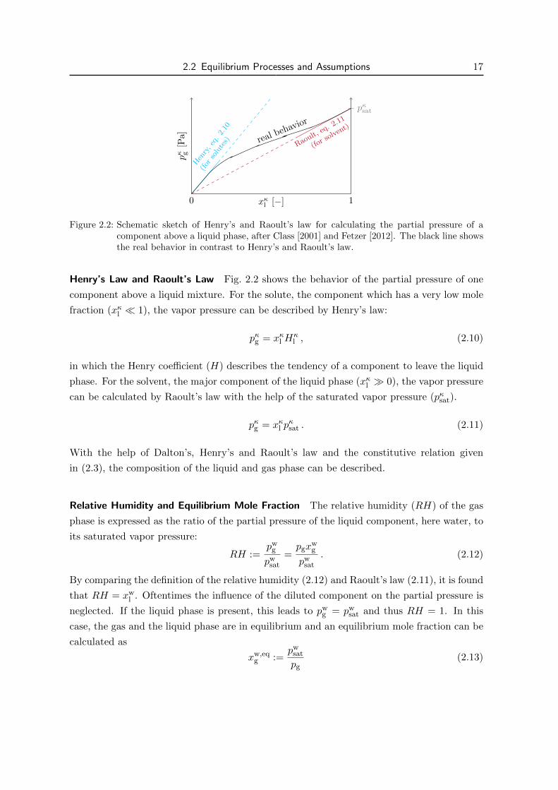
Henry’s Law and Raoult’s Law Fig. 2.2 shows the behavior of the partial pressure of one
component above a liquid mixture. For the solute, the component which has a very low mole
fraction (xκl 1), the vapor pressure can be described by Henry’s law:
pκg = xκl Hκl , (2.10)
in which the Henry coefficient (H) describes the tendency of a component to leave the liquid
phase. For the solvent, the major component of the liquid phase (xκl 0), the vapor pressure
can be calculated by Raoult’s law with the help of the saturated vapor pressure (pκsat).
pκg = xκl pκsat . (2.11)
With the help of Dalton’s, Henry’s and Raoult’s law and the constitutive relation given
in (2.3), the composition of the liquid and gas phase can be described.
Relative Humidity and Equilibrium Mole Fraction The relative humidity (RH) of the gas
phase is expressed as the ratio of the partial pressure of the liquid component, here water, to
its saturated vapor pressure:
RH :=pw
g
pwsat
=pgx
wg
pwsat
. (2.12)
By comparing the definition of the relative humidity (2.12) and Raoult’s law (2.11), it is found
that RH = xwl . Oftentimes the influence of the diluted component on the partial pressure is
neglected. If the liquid phase is present, this leads to pwg = pw
sat and thus RH = 1. In this
case, the gas and the liquid phase are in equilibrium and an equilibrium mole fraction can be
calculated as
xw,eqg :=
pwsat
pg(2.13)

18 2 Fundamentals
2.2.4 Diffusion and Dispersion
The diffusive molar flux (jmol) in a phase is modeled by Fick’s first law [Fick, 1855] using the
molar density (%mol):
j κmol,α = −Dκα%mol,α∇xκα . (2.14)
Fick’s first law is a good approximation for a binary system (a phase consisting of two com-
ponents), with a very diluted solute component which diffusion coefficient does not depend
on composition. If a phase is a binary system, the mole fraction gradients are related by:
∇xsoluteα = −∇xsolvent
α . Further, the net diffusive molar flux in one phase is zero:∑κ
j κmol,α = 0 , (2.15)
and thus the diffusion coefficients in one phase have to be identical. Normally they are
identical to the one of the solute component: Dα = Dsoluteα . The molar fluxes can be converted
to diffusive mass fluxes (j ) by the molar mass of each component:
j κmass,α = j κmol,αMκ = −Dκ
α%mol,αMκ∇xκα . (2.16)
For systems with more than two components or larger mole fractions of the solute component,
diffusion becomes more complex. Then, the interactions between the different solutes have
to be considered and the diffusion coefficients may depend on the composition of the phase.
These effects can be modeled using the Maxwell-Stefan equation for multi-component diffu-
sion. However, this work assumes binary, Fickian diffusion and for a more detailed discussion
of the Maxwell-Stefan equation, it is referred to Bird et al. [2007].
Another diffusion-like phenomenon is dispersion. Dispersion originates from the underlying
velocity field. Reasons leading to dispersion are tortuous pathways and velocity distributions
in a porous medium or velocity fluctuations in a turbulent free flow. Bear [1988] combines
diffusion and dispersion (Ddisp) to an effective or hydrodynamic dispersion (Deff):
Dκeff = Dκ
α +Ddisp . (2.17)
This hydrodynamic dispersion results in a spreading of a transported component “beyond the
region it is expected to occupy according to the average flow alone” [Bear, 1988].

2.2 Equilibrium Processes and Assumptions 19
275
280
285
290
295
300
305
310
0 0.2 0.4 0.6 0.8 1
wet
-bu
lbte
mp
eratu
re[K
]
RH [−]
278K
283K288K293K298K303K308K313K318K
323K
Figure 2.3: Wet-bulb temperatures for different temperature (gray lines) and humidity conditions(x-axis) of the ambient air. Data is obtained from a script provided by the TU Munchen1.However, it can also be extracted manually from a Mollier diagram or a psychrometricchart, as presented in Grassmann and Widmer [1974].
2.2.5 Thermal Conduction
Fourier’s law of heat conduction describes the conductive energy flux (f ) which is driven by
a temperature gradient together with the thermal conductivity:
f = −λ∇T . (2.18)
This law does not include the portion of energy transported with advective or diffusive mass
fluxes. In the above-mentioned form, it only applies for isotropic media: this is the case for
fluids, but solids may have preferred directions, see Bird et al. [2007] for a list of references.
2.2.6 Wet Bulb Temperature
The minimum temperature which can be reached by water evaporation only is called wet-bulb
temperature. The wet-bulb temperature at the evaporating surface depends on the energy
supply, and thus the temperature of the ambient air and its water vapor content. During
the evaporation process, the temperature at the evaporating surface will decrease and finally
form an equilibrium between energy supplied by the ambient air and energy extracted by the
vaporization process. Resulting wet-bulb temperatures are shown in Fig. 2.3.
1https://web.archive.org/web/20141019115010/http://www.td.mw.tum.de:80/tum-td/de/studium/
lehre/thermo_2/kgtsite/TD_KGT.htm, accessed on December 28, 2017 (in German).
20 2 Fundamentals
properties components phases references
density %a(p, T ) ideal gas law (2.7)%w(p, T ) [IAPWS, 2007]
%g =∑
κ %κxκg
%l(%w, xκg ,M
κ) [Class et al., 2002]
dynamic µa(p, T ) [Lemmon and Jacobsen, 2004]viscosity µw(p, T ) [IAPWS, 2008]
µg(µκ, xκg) [Poling et al., 2001]
µl = µw
diffusion Dwg (p, T ) [Vargaftik, 1975, Walker et al., 1981]
coefficient Dal (T ) [Ferrell and Himmelblau, 1967]
Henry Hal (T ) [Finsterle, 1993]
coefficient
saturated pwsat(T ) [IAPWS, 2007]
vap. pressure
specific cap(T ) [Kays et al., 2009]
heat capacity cwp (p, T ) [IAPWS, 2007]
cp,g(cκp, xκg)
cp,l = cwp
specific ha(T ) [Kays et al., 2009]enthalpy hw(p, T ) [IAPWS, 2007]
hg(hκ, Xκg ) [Class, 2001]
hl = hw
thermal λa = const.conductivity λw(p, T ) [IAPWS, 2011]
λg = λa
λl = λw
Table 2.1: Used material laws for the components and the phases.
2.3 Material Properties
This section describes basic features of the gas and the liquid phase. Tab. 2.1 shows the main
material laws for the components and the phases and their references. Further details on the
applied material laws can be found in the documentation and the inside-code comments of
DuMux 2.12 [Fetzer et al., 2017a].
Air Component and Gas Phase As already mentioned, the gas phase mainly consists of
the pseudo component air. Although the composition of air is variable in reality, a constant

2.4 Fluid Flow 21
composition is assumed: 78 Vol.% nitrogen, 22 Vol.% oxygen. The influence of other gases,
e.g. argon, carbon dioxide, is neglected. The properties of the gas phase depend on pres-
sure, temperature, and mole fractions of air and water vapor, see Fig. 2.4 (left figures) and
Tab. 2.1. During the evaporation process, the gas phase cools down and gets more humid at
the same time. Fig. 2.4 shows that for room conditions (T = 273±10 K), the influence of the
temperature on the gas-phase density is stronger than the influence of the composition. This
leads to higher densities for the gas above the evaporating surface and thus a more stable
layering.
Water Component and Liquid Phase The properties of water are essential for the liquid
phase. In contrast to the gas phase, in which substantial amounts of water vapor can occur,
air hardly dissolves into liquid water. Thus, many features of the liquid phase are mainly
influenced by the property of water, see Tab. 2.1. One unique feature of water is that its
highest density occurs at 4 C, which can be seen in Fig. 2.4. In contrast to the gases, the
dynamic viscosity of liquids decreases with increasing temperature.
2.4 Fluid Flow
When talking about fluid flow, the Reynolds number is an important quantity. Based on
the Reynolds number, different flow regimes can be classified. The Reynolds-number-based
classification is a good rule of thumb, however other factors as roughness, geometry, and fluc-
tuations in inflow conditions affect the real behavior, cf. White [2011]. This section is used to
present the different flow regimes and their special features. Another important phenomenon
presented in this section is the development of boundary layers. Further information about
fluid flow and involved processes can be found in: Pope [2006], Schlichting and Gersten [2006],
Wilcox [2006], White [2011].
2.4.1 Creeping Flow
In the absence of inertia forces compared to viscous forces (Re ≤ 1), the flow is called
creeping. Creeping flow is a basic assumption for many porous-medium models as well as for
the (unsteady) Stokes equation.
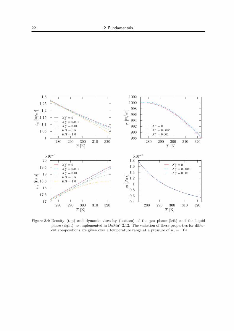
22 2 Fundamentals
1
1.05
1.1
1.15
1.2
1.25
1.3
280 290 300 310 320
%g
[kg /
m3]
T [K]
Xwg = 0
Xwg = 0.001
Xwg = 0.01
RH = 0.5
RH = 1.0
988
990
992
994
996
998
1000
1002
280 290 300 310 320
%l
[kg /
m3]
T [K]
Xal = 0
Xal = 0.0005
Xal = 0.001
17
17.5
18
18.5
19
19.5
20
280 290 300 310 320
x10−6
µg
[Pa
s]
T [K]
Xwg = 0
Xwg = 0.001
Xwg = 0.01
RH = 0.5
RH = 1.0
0.4
0.6
0.8
1
1.2
1.4
1.6
1.8
280 290 300 310 320
x10−3
µl
[Pa
s]
T [K]
Xal = 0
Xal = 0.0005
Xal = 0.001
Figure 2.4: Density (top) and dynamic viscosity (bottom) of the gas phase (left) and the liquidphase (right), as implemented in DuMux 2.12. The variation of these properties for differ-ent compositions are given over a temperature range at a pressure of pα = 1 Pa.
2.4 Fluid Flow 23
2.4.2 Laminar Flow
Laminar flow can be regarded as a system of well-ordered layers with little interaction. It is
characterized by a high momentum diffusion (viscous forces), but a low momentum advection
(inertia forces), however the inertia forces cannot be neglected.
2.4.3 Laminar-Turbulent Transition
Until now, the transition from laminar to turbulent flow is not fully understood and depends
on different processes and properties. This transition does not occur suddenly, but turbulence
starts with little disturbances and local turbulence, which gradually become larger. With
increasing Reynolds number, the non-linear nature of the inertia forces become more and
more important, and the viscous forces are not strong enough to overcome this effect. For
flow along a flat plate, Schlichting and Gersten [2006] and Pope [2006] propose a length-based
Reynolds number of Rex = 5e5 ∼ 1e6 for the transition from laminar to turbulent conditions.
For flow in a pipe, the diameter-based Reynolds number Red = 2300 can be considered as a
critical value above which the flow is turbulent [Pope, 2006].
2.4.4 Turbulent Flow
Turbulent flow is always irregular and chaotic, forming three-dimensional eddies which can
stretch and shrink. Therefore, turbulence is always a three-dimensional phenomenon. These
eddies are spreading over a wide-ranging length scale: The largest eddies reach sizes in the
order of magnitude of the domain size, the smallest eddies are determined by viscosity and
measure even less than millimeters. Kinetic energy is transferred from larger eddies to smaller
eddies and ultimately, by a process called dissipation, transformed into heat, see Kolmogorov
[1941, 1991]. With respect to component transport, the most prominent difference to laminar
flow is the enhanced mixing of the transported substances, see Schlichting and Gersten [2006,
Fig. 1.6]. More information about turbulent flow can be found in textbooks such as Oertel
[2011], Pope [2006], White [2011], Wilcox [2006].
2.4.5 Boundary Layers
When a fluid flows along a boundary with different properties, boundary layers will evolve.
The evolving boundary layers for mass, momentum, and energy can have different shapes
and properties. The most prominent example is a fluid flowing along a solid wall at which a
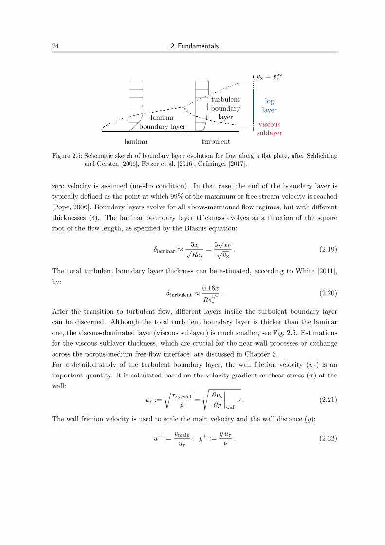
24 2 Fundamentals
laminar turbulent
laminarboundary layer
turbulentboundary
layerviscoussublayer
loglayer
vx = v∞x
Figure 2.5: Schematic sketch of boundary layer evolution for flow along a flat plate, after Schlichtingand Gersten [2006], Fetzer et al. [2016], Gruninger [2017].
zero velocity is assumed (no-slip condition). In that case, the end of the boundary layer is
typically defined as the point at which 99% of the maximum or free stream velocity is reached
[Pope, 2006]. Boundary layers evolve for all above-mentioned flow regimes, but with different
thicknesses (δ). The laminar boundary layer thickness evolves as a function of the square
root of the flow length, as specified by the Blasius equation:
δlaminar ≈5x√Rex
=5√xν√vx
. (2.19)
The total turbulent boundary layer thickness can be estimated, according to White [2011],
by:
δturbulent ≈0.16x
Re1/7x
. (2.20)
After the transition to turbulent flow, different layers inside the turbulent boundary layer
can be discerned. Although the total turbulent boundary layer is thicker than the laminar
one, the viscous-dominated layer (viscous sublayer) is much smaller, see Fig. 2.5. Estimations
for the viscous sublayer thickness, which are crucial for the near-wall processes or exchange
across the porous-medium free-flow interface, are discussed in Chapter 3.
For a detailed study of the turbulent boundary layer, the wall friction velocity (uτ ) is an
important quantity. It is calculated based on the velocity gradient or shear stress (τ ) at the
wall:
uτ :=
√τxy,wall
%=
√∣∣∣∣∂vx
∂y
∣∣∣∣wall
ν . (2.21)
The wall friction velocity is used to scale the main velocity and the wall distance (y):
u+ :=vmain
uτ, y+ :=
y uτν
. (2.22)
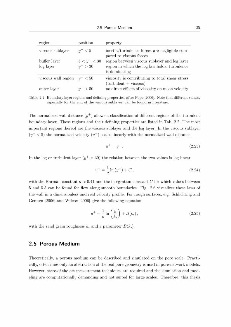
2.5 Porous Medium 25
region position property
viscous sublayer y+ < 5 inertia/turbulence forces are negligible com-pared to viscous forces
buffer layer 5 < y+ < 30 region between viscous sublayer and log layerlog layer y+ > 30 region in which the log law holds, turbulence
is dominating
viscous wall region y+ < 50 viscosity is contributing to total shear stress(turbulent + viscous)
outer layer y+ > 50 no direct effects of viscosity on mean velocity
Table 2.2: Boundary layer regions and defining properties, after Pope [2006]. Note that different values,especially for the end of the viscous sublayer, can be found in literature.
The normalized wall distance (y+) allows a classification of different regions of the turbulent
boundary layer. These regions and their defining properties are listed in Tab. 2.2. The most
important regions thereof are the viscous sublayer and the log layer. In the viscous sublayer
(y+ < 5) the normalized velocity (u+) scales linearly with the normalized wall distance:
u+ = y+ . (2.23)
In the log or turbulent layer (y+ > 30) the relation between the two values is log linear:
u+ =1
κln(y+)
+ C , (2.24)
with the Karman constant κ ≈ 0.41 and the integration constant C for which values between
5 and 5.5 can be found for flow along smooth boundaries. Fig. 2.6 visualizes these laws of
the wall in a dimensionless and real velocity profile. For rough surfaces, e.g. Schlichting and
Gersten [2006] and Wilcox [2006] give the following equation:
u+ =1
κln
(y
ks
)+B(ks) , (2.25)
with the sand grain roughness ks and a parameter B(ks).
2.5 Porous Medium
Theoretically, a porous medium can be described and simulated on the pore scale. Practi-
cally, oftentimes only an abstraction of the real pore geometry is used in pore-network models.
However, state-of the art measurement techniques are required and the simulation and mod-
eling are computationally demanding and not suited for large scales. Therefore, this thesis
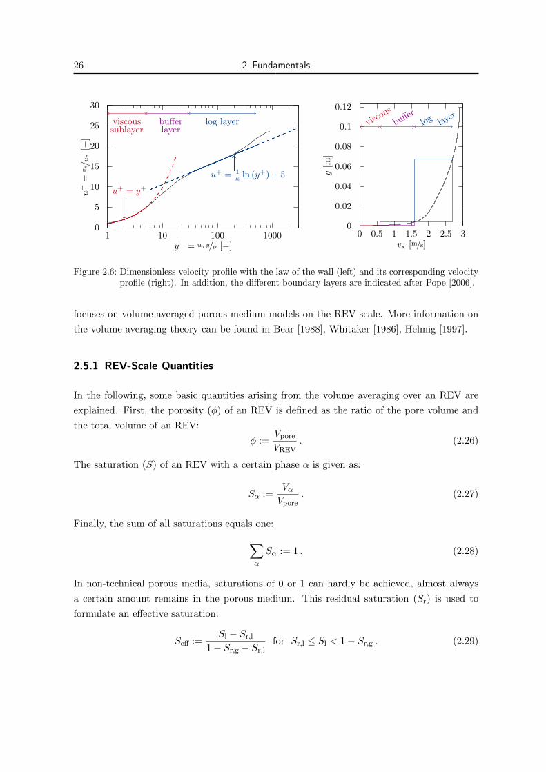
26 2 Fundamentals
0
5
10
15
20
25
30
1 10 100 1000
viscoussublayer
u+ = y+
bufferlayer
log layer
u+ = 1κ ln (y+) + 5
u+
=vx/u
τ[−
]
y+ = uτy/ν [−]
0
0.02
0.04
0.06
0.08
0.1
0.12
0 0.5 1 1.5 2 2.5 3
viscous
bufferlog lay
er
y[m
]
vx [m/s]
Figure 2.6: Dimensionless velocity profile with the law of the wall (left) and its corresponding velocityprofile (right). In addition, the different boundary layers are indicated after Pope [2006].
focuses on volume-averaged porous-medium models on the REV scale. More information on
the volume-averaging theory can be found in Bear [1988], Whitaker [1986], Helmig [1997].
2.5.1 REV-Scale Quantities
In the following, some basic quantities arising from the volume averaging over an REV are
explained. First, the porosity (φ) of an REV is defined as the ratio of the pore volume and
the total volume of an REV:
φ :=Vpore
VREV. (2.26)
The saturation (S) of an REV with a certain phase α is given as:
Sα :=VαVpore
. (2.27)
Finally, the sum of all saturations equals one:∑α
Sα := 1 . (2.28)
In non-technical porous media, saturations of 0 or 1 can hardly be achieved, almost always
a certain amount remains in the porous medium. This residual saturation (Sr) is used to
formulate an effective saturation:
Seff :=Sl − Sr,l
1− Sr,g − Sr,lfor Sr,l ≤ Sl < 1− Sr,g . (2.29)
2.5 Porous Medium 27
In soil science and hydrology, the water content (θ) is oftentimes used to describe the ratio
of liquid water to the total REV volume:
θ =Vl
VREV= φSl . (2.30)
2.5.2 Multi-Phase Effects
In contrast to single-phase free flow, the presence of multiple mobile phases and the influence of
the solid matrix ask for additional concepts. These effects strongly depend on the preference of
the fluids to cover or wet a certain solid material. Therefore, indices for the wetting phase (w)
and the non-wetting phase (n) are used. In hydrophilic porous media, as considered in this
thesis, liquid water is the wetting phase and gas is the non-wetting phase.
Capillary Pressure A prominent example is that the wetting phase rises in a capillary tube.
The capillary pressure (pc) is defined as the pressure difference between the two phases:
pc := pn − pw (2.31)
On the pore scale, the capillary pressure is described by the Young-Laplace equation, cf. Bear
[1988]. On the REV scale, many empirical or semi-empirical relationships for upscaling
capillary-driven effects can be found. The most prominent capillary pressure–saturation re-
lationships are those proposed by Brooks and Corey [1964]:
pc = pdS−1/λBCeff , (2.32)
or by van Genuchten [1980]:
pc =1
αVG
(S
−1/mVGeff − 1
)1/nVG. (2.33)
Both relationships, which mimic the primary drainage process, are visualized in Fig. 2.7. Even
if not considered in this thesis, it shall be mentioned that under the influence of reversing
flow directions, like switching from evaporation to condensation or precipitation, the capillary
pressure–saturation relationship is not unique and hysteresis effects occur, cf. Bear [1988],
Helmig [1997], Roth [2012]. The coefficients of the van Genuchten model are related by:
mVG = 1− 1/nVG.
If a residual water saturation exists, as shown in Fig. 2.7, the soil is not able to dry out. Once
the saturation approaches the residual threshold, the capillary forces become infinitely strong
and water would be supplied from any other soil portions or the capillary forces will hinder
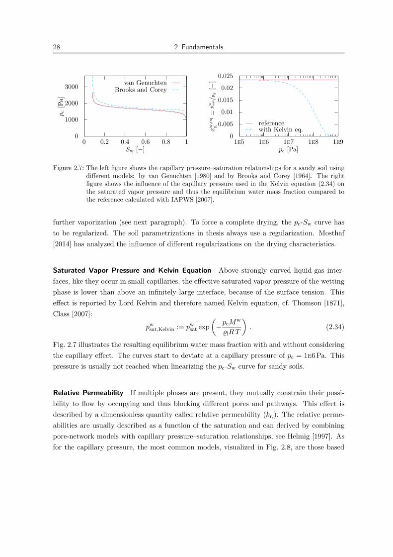
28 2 Fundamentals
0
1000
2000
3000
0 0.2 0.4 0.6 0.8 1
pc
[Pa]
Sw [−]
van GenuchtenBrooks and Corey
0
0.005
0.01
0.015
0.02
0.025
1e5 1e6 1e7 1e8 1e9
xw
,eq
g=pw sat /pg
[−]
pc [Pa]
referencewith Kelvin eq.
Figure 2.7: The left figure shows the capillary pressure–saturation relationships for a sandy soil usingdifferent models: by van Genuchten [1980] and by Brooks and Corey [1964]. The rightfigure shows the influence of the capillary pressure used in the Kelvin equation (2.34) onthe saturated vapor pressure and thus the equilibrium water mass fraction compared tothe reference calculated with IAPWS [2007].
further vaporization (see next paragraph). To force a complete drying, the pc-Sw curve has
to be regularized. The soil parametrizations in thesis always use a regularization. Mosthaf
[2014] has analyzed the influence of different regularizations on the drying characteristics.
Saturated Vapor Pressure and Kelvin Equation Above strongly curved liquid-gas inter-
faces, like they occur in small capillaries, the effective saturated vapor pressure of the wetting
phase is lower than above an infinitely large interface, because of the surface tension. This
effect is reported by Lord Kelvin and therefore named Kelvin equation, cf. Thomson [1871],
Class [2007]:
pwsat,Kelvin := pw
sat exp
(−pcM
w
%lRT
). (2.34)
Fig. 2.7 illustrates the resulting equilibrium water mass fraction with and without considering
the capillary effect. The curves start to deviate at a capillary pressure of pc = 1e6 Pa. This
pressure is usually not reached when linearizing the pc-Sw curve for sandy soils.
Relative Permeability If multiple phases are present, they mutually constrain their possi-
bility to flow by occupying and thus blocking different pores and pathways. This effect is
described by a dimensionless quantity called relative permeability (kr,). The relative perme-
abilities are usually described as a function of the saturation and can derived by combining
pore-network models with capillary pressure–saturation relationships, see Helmig [1997]. As
for the capillary pressure, the most common models, visualized in Fig. 2.8, are those based

2.5 Porous Medium 29
0
0.2
0.4
0.6
0.8
1
0 0.2 0.4 0.6 0.8 1
kr,
w[−
]
Sw [−]
van GenuchtenBrooks and Corey
0
0.2
0.4
0.6
0.8
1
0 0.2 0.4 0.6 0.8 1
kr,
n[−
]
Sw [−]
van GenuchtenBrooks and Corey
Figure 2.8: Relative permeability–saturation relationships, for the same sandy soil as in Fig. 2.7, usingmodels by van Genuchten [1980] and by Brooks and Corey [1964]. The figures show thewetting phase (left) and the non-wetting phase (right).
on Brooks and Corey [1964]:
kr,w = S2+λBCλBC
eff , (2.35)
kr,n = (1− Seff)2
(1− S
2+λBCλBC
eff
), (2.36)
or on van Genuchten [1980]:
kr,w =√Seff
(1−
(1− S
1mVGeff
)mVG)2
, (2.37)
kr,n = (1− Seff)13
(1− S
1mVGeff
)2mVG
. (2.38)
Diffusion and Tortuosity Diffusion in the porous medium is slower than in a free-flow region
due to tortuous pathways. This effect can be included by accounting for a tortuosity factor (τ),
see Millington [1959]. According to Helmig [1997], the effective porous-medium diffusion
coefficient (Dpm) and the molecular diffusion coefficient (D) can be related by:
Dpmα = DατφSα , (2.39)
with the following tortuosity factor
τα = φ1/3S
7/3α . (2.40)
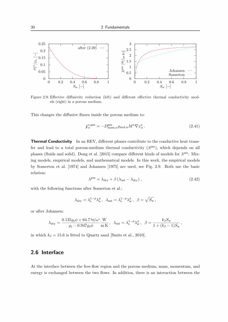
30 2 Fundamentals
0
0.05
0.1
0.15
0.2
0.25
0 0.2 0.4 0.6 0.8 1
Dpm
n/D
n[−
]
Sw [−]
after (2.39)
0
0.5
1
1.5
2
2.5
3
0 0.2 0.4 0.6 0.8 1
λpm
[W/(
mK
)]
Sw [−]
JohansenSomerton
Figure 2.9: Effective diffusivity reduction (left) and different effective thermal conductivity mod-els (right) in a porous medium.
This changes the diffusive fluxes inside the porous medium to:
j κ,pmα = −Dpm
mass,α%mol,αMκ∇xκα . (2.41)
Thermal Conductivity In an REV, different phases contribute to the conductive heat trans-
fer and lead to a total porous-medium thermal conductivity (λpm), which depends on all
phases (fluids and solid). Dong et al. [2015] compare different kinds of models for λpm: Mix-
ing models, empirical models, and mathematical models. In this work, the empirical models
by Somerton et al. [1974] and Johansen [1975] are used, see Fig. 2.9. Both use the basic
relation:
λpm = λdry + β (λsat − λdry) , (2.42)
with the following functions after Somerton et al.:
λdry = λ1−φs λφn , λsat = λ1−φ
s λφw , β =√Sw ,
or after Johansen:
λdry =0.135%sφ+ 64.7 kg/m3
%s − 0.947%sφ
W
m K, λsat = λ1−φ
s λφw , β =kJSw
1 + (kJ − 1)Sw,
in which kJ = 15.6 is fitted to Quartz sand [Smits et al., 2010].
2.6 Interface
At the interface between the free-flow region and the porous medium, mass, momentum, and
energy is exchanged between the two flows. In addition, there is an interaction between the
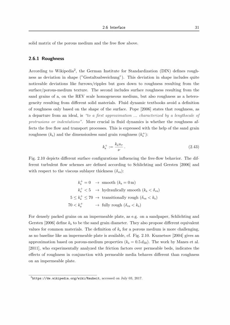
2.6 Interface 31
solid matrix of the porous medium and the free flow above.
2.6.1 Roughness
According to Wikipedia2, the German Institute for Standardization (DIN) defines rough-
ness as deviation in shape (”Gestaltsabweichung”). This deviation in shape includes quite
noticeable deviations like furrows/ripples but goes down to roughness resulting from the
surface/porous-medium texture. The second includes surface roughness resulting from the
sand grains of a, on the REV scale homogeneous medium, but also roughness as a hetero-
geneity resulting from different solid materials. Fluid dynamic textbooks avoid a definition
of roughness only based on the shape of the surface. Pope [2006] states that roughness, as
a departure from an ideal, is “to a first approximation ... characterized by a lengthscale of
protrusions or indentations”. More crucial in fluid dynamics is whether the roughness af-
fects the free flow and transport processes. This is expressed with the help of the sand grain
roughness (ks) and the dimensionless sand grain roughness (k+s ):
k+s :=
ksuτν
. (2.43)
Fig. 2.10 depicts different surface configurations influencing the free-flow behavior. The dif-
ferent turbulent flow schemes are defined according to Schlichting and Gersten [2006] and
with respect to the viscous sublayer thickness (δvs):
k+s = 0 → smooth (ks = 0 m)
k+s < 5 → hydraulically smooth (ks < δvs)
5 ≤ k+s ≤ 70 → transitionally rough (δvs < ks)
70 < k+s → fully rough (δvs < ks)
For densely packed grains on an impermeable plate, as e.g. on a sandpaper, Schlichting and
Gersten [2006] define ks to be the sand grain diameter. They also propose different equivalent
values for common materials. The definition of ks for a porous medium is more challenging,
as no baseline like an impermeable plate is available, cf. Fig. 2.10. Kuznetsov [2004] gives an
approximation based on porous-medium properties (ks = 0.5 d50). The work by Manes et al.
[2011], who experimentally analyzed the friction factors over permeable beds, indicates the
effects of roughness in conjunction with permeable media behaves different than roughness
on an impermeable plate.
2https://de.wikipedia.org/wiki/Rauheit, accessed on July 03, 2017.
32 2 Fundamentals
k+s = 0
smoothimpermeable
δvs
k+s < 5
hydraulically smoothimpermeable
δvs
ks
5 < k+s
(transitionally) roughimpermeable
δvs ks
5 < k+s
(transitionally) roughpermeable
δvsks
Figure 2.10: Schematic sketch of turbulent flow over rough surfaces.
2.6.2 Evaporation
A lot of work on analyzing coupled porous-medium free-flow exchange processes is performed
in the field of water evaporation from bare soil surfaces, e.g. van Brakel [1980], Brutsaert
[1982], Or et al. [2013]. During the evaporation process mainly two different stages are
discerned, depending on the source they are called stage-I/stage-II [e.g. Lehmann et al.,
2008], or constant-rate period (CRP)/falling-rate period (FRP) [e.g. Yiotis et al., 2007].
The stage-I period is characterized by higher and relatively constant evaporation rates, see
Fig. 2.11. In this thesis, the evaporation rate (e) is defined as the total water mass flux
across the porous-medium free-flow interface. This flux qw in kg/m2 s contains all advective
and diffusive water (vapor) fluxes in the liquid and in the gas phase:
e :=qw
%w· 1000 mm/m · 86400 s/d ≈ qw · 86400 s/d (2.44)
In stage-I, liquid water is present at the interface and thus the evaporation rate is constrained
by the atmospheric demand (vapor/partial-pressure gradient). As reported in Shahraeeni
et al. [2012], Or et al. [2013], the stage-I evaporation rate is not necessarily constant. In the
presence of very thin boundary layers, the evaporation rate can already drop during stage-I.
Another reason for a falling rate is that the system is far from its equilibrium state, e.g. due to
strong evaporative fluxes and the combined cooling effect [Lu et al., 2005, Mosthaf et al., 2014].
During the drying process, a pattern of wet pores evolves at the interface. Shahraeeni et al.
[2012] and Or et al. [2013] show that this is an efficient but limited compensation mechanism:
The evaporation rate per pore increases as a result of switching from one-dimensional to three-
dimensional diffusion. Mosthaf et al. [2014] and Fetzer et al. [2017c] show that REV-scale
simulations, without concepts accounting for pore-scale compensation effect as proposed by
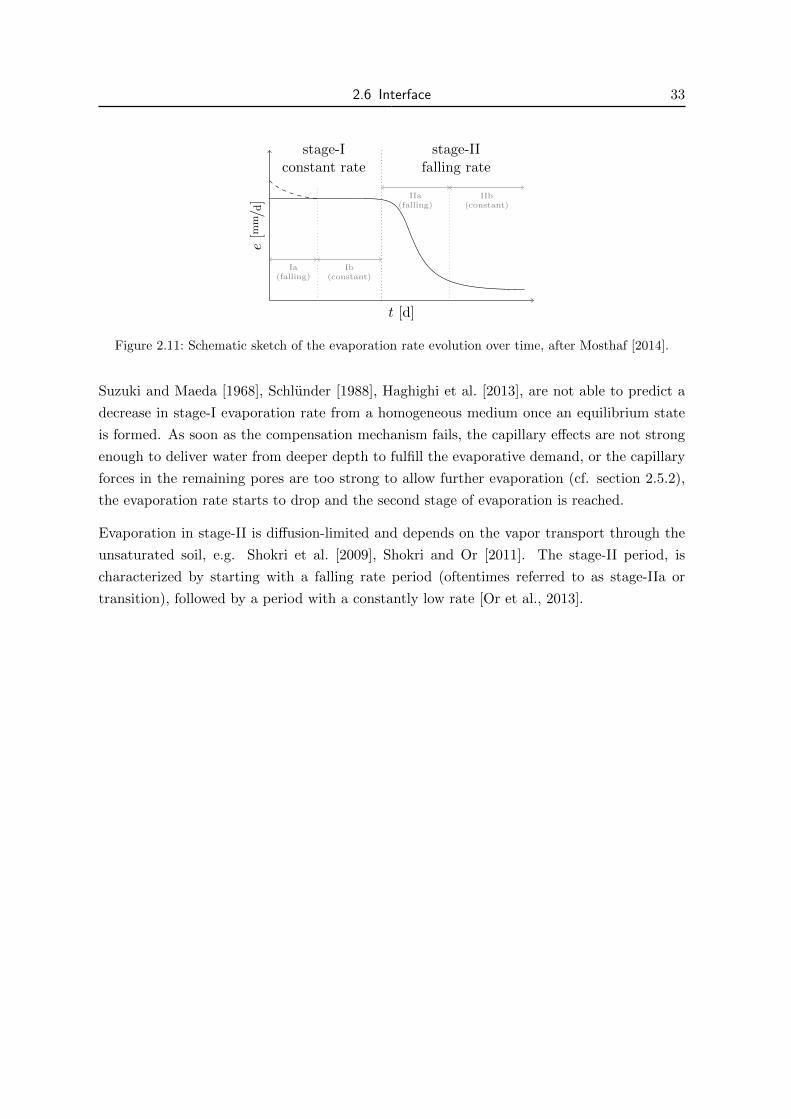
2.6 Interface 33
t [d]
e[m
m/d
]
stage-Iconstant rate
stage-IIfalling rate
Ia(falling)
Ib(constant)
IIa(falling)
IIb(constant)
Figure 2.11: Schematic sketch of the evaporation rate evolution over time, after Mosthaf [2014].
Suzuki and Maeda [1968], Schlunder [1988], Haghighi et al. [2013], are not able to predict a
decrease in stage-I evaporation rate from a homogeneous medium once an equilibrium state
is formed. As soon as the compensation mechanism fails, the capillary effects are not strong
enough to deliver water from deeper depth to fulfill the evaporative demand, or the capillary
forces in the remaining pores are too strong to allow further evaporation (cf. section 2.5.2),
the evaporation rate starts to drop and the second stage of evaporation is reached.
Evaporation in stage-II is diffusion-limited and depends on the vapor transport through the
unsaturated soil, e.g. Shokri et al. [2009], Shokri and Or [2011]. The stage-II period, is
characterized by starting with a falling rate period (oftentimes referred to as stage-IIa or
transition), followed by a period with a constantly low rate [Or et al., 2013].

3 Physical and Mathematical Model
In this chapter, the continuum-scale models are presented. First, the models for the two
subdomains, the free flow (section 3.1) and the porous medium (section 3.2) are explained,
then the coupling conditions are introduced (section 3.3).
3.1 Free Flow
The free flow is modeled with the Navier-Stokes equations. Further, the following assumptions
are made: (i) single-phase gas flow, composed of two components: water vapor (w) and
air (a), (ii) Newtonian fluid without dilation, and (iii) equilibrium processes, especially Fickian
diffusion.
3.1.1 Mass and Momentum Balance
The total mass balance is given by:
∂%g
∂t+∇ · (%gvg) +
∑κ
∇ · j κ,ffmass,eff = 0 . (3.1)
The total mass balance includes effective diffusive-dispersive fluxes (j κ,ffmass,eff), which will be
discussed in section 3.1.3. As shown in section 2.2.4, the mass-based diffusive-dispersive fluxes
for both components are not equal and have to be considered in the total mass balance. For
modeling momentum transport in the free flow region, the Navier-Stokes equations are used:
∂ (%gvg)
∂t+∇ ·
(%gvgv
ᵀg
)−∇ · τ g +∇ · (pgI)− %gg = 0 . (3.2)
The shear stress tensor is defined as:
τg := 2%gνgS = %gνg
(∇vg +∇vᵀ
g
), (3.3)
36 3 Physical and Mathematical Model
with the strain rate tensor S = 12 (∇vg +∇vᵀ
g) . In addition, the identity matrix (I) and
the gravitational acceleration g = (0, . . . ,−9.81 m/s2)ᵀ are needed. For laminar flow, the
Navier-Stokes equations can be solved quite easily (compared to the computational effort
for turbulent flow conditions). Then, as discussed in section 2.4, viscous/diffusive forces are
stronger than inertia/convective forces. The effect of turbulence, when the inertia forces are
dominating, is discussed in the next section. For creeping flow (Re < 1) and the absence of
gravitational forces, the Navier-Stokes equations simplify to the transient Stokes equations:
∂ (%gvg)
∂t−∇ · τ g +∇ · (pgI) = 0 . (3.4)
3.1.2 Turbulence Modeling
Two main approaches for simulating turbulent flow can be discerned. If specific requirements
are fulfilled, a direct numerical simulation (DNS) of the turbulent flow is possible. Otherwise,
the effects of the turbulent flow have to be modeled.
3.1.2.1 From DNS to RANS3
For the direct simulation of turbulent free flow, even the smallest eddies have to be resolved
correctly, otherwise physically unrealistic results are obtained. Therefore, the smallest eddies
have to be estimated. Referring to the Kolmogorov energy cascade [Kolmogorov, 1941],
energy is transferred from larger to smaller eddies and finally dissipates into heat. The
kinematic viscosity is a crucial quantity and determines the Kolmogorov micro scale, the
smallest possible eddy size. Eddies are always three-dimensional, so a microscale of 20µm
and thus an equidistant discretization with 10µm would result in 1 · 1012 cells for simulating
a cube of 0.1 m length. This results in a high computational demand, especially if non-linear
material laws or the influence of component and energy transport are considered. Examples
for direct numerical simulations of coupled porous-medium free-flow processes can be found
e.g. in Krafczyk et al. [2015] or Fattahi et al. [2016].
Large eddy simulations (LES) include first simplifications of the turbulent flow processes.
LES methods assume that the small-scale eddies are universal. As a consequence, the effect
of small-scale eddies is modeled with simpler turbulence models, whereas the larger eddies are
still simulated. More information about LES models can be found e.g. in Rodi et al. [2013].
3This section is based on T. Fetzer: Numerical analysis of the influence of turbulence on exchange processesbetween porous-medium and free flow, Master’s Thesis, Universitat Stuttgart, 2012.
3.1 Free Flow 37
The next level of model abstraction includes the loss of information about the detailed, instan-
taneous flow structure. The Reynolds decomposition assumes that any transported quantity
(e.g. the instantaneous velocity vx), is composed of a mean value (e.g. vx) and the fluctuations
around this mean value (e.g. v′x):
vx = vx + v′x . (3.5)
The mean values are a result of an averaging in time, in space, or over ensembles. Here, the
time-averaging method is considered, cf. Fig. 2.1. In a second step, the Reynolds averaging,
all decomposed quantities are inserted in the governing balance equations. Then, all balance
equations are time-averaged. For more information on the Reynolds averaging it is referred
to standard fluid mechanics textbooks as Pope [2006], Wilcox [2006], White [2011], or Oertel
[2012]. When the Reynolds averaging is applied on the Navier-Stokes equations (3.2), the
Reynolds-averaged Navier-Stokes equations (RANS) are obtained under the assumptions of
(i) steady state turbulence, meaning the mean value is in a steady state and (ii) negligible
influence of pressure fluctuations:
∂ (%gvg)
∂t+∇ ·
(%gvgv
ᵀg
)+∇ ·
(%gv ′gv
′gᵀ)−∇ · τ g +∇ · (pgI)− %gg = 0 . (3.6)
The overbar indicates that a quantity or expression is time-averaged. The mass balance
remains unchanged, the instantaneous values are only replaced by the mean values.
The Reynolds averaging yields a new expression: %gv ′gv′gᵀ. Even though this term results
from the advection term, it leads to viscous or diffusive effects. It is called Reynolds stress
tensor (τ t), which is a symmetric tensor with 3 × 3 entries. This leads to a closure prob-
lem, because no further relations to describe these additional Reynolds stresses (or turbulent
stresses) are provided. Models which find expressions for all six entries of this symmetric
tensor are called Reynolds stress models (RSM). Under specific simplifications, namely those
published by Boussinesq [1877], that turbulent stresses act in analogy to viscous stresses, the
number of unknowns is reduced. The Reynolds stresses are then modeled by an additional
viscosity, called eddy viscosity (νt), plus the contribution of the turbulent kinetic energy (k):
%gv ′gv′gᵀ = −τ t = −%gνt
(∇vg +∇vᵀ
g
)+
2
3%gkI . (3.7)
The name eddy accounts for the fact, that the eddy viscosity is a flow property and fully
depends on the turbulent flow field and not on the fluid. The turbulent kinetic energy is
defined via the turbulent velocity fluctuations, k := 1/2
(v′g,x
2 + v′g,y2 + v′g,z
2)
. Therefore, it
has to be included in (3.7) to match its definition for incompressible flow. Later, turbulence
models are presented which do not model the turbulent kinetic energy and thus do not include
the last term in (3.7). For simplicity, the contributions of the fluid shear stresses and the

38 3 Physical and Mathematical Model
DNS
LES
Boundary-Layere.g. Blasius, ...
RANS
RSM
Eddy-Viscosity Models
Zero-Equatione.g. Prandtl, ...
One-Equatione.g. Spalart, ...
Two-Equatione.g. k-ε, ...
Figure 3.1: Hierarchy of turbulence models, after Fetzer [2012] and Trautz [2015]. The models high-lighted in blue are used in this work.
turbulent/Reynolds stresses are combined to an effective stress term (τ eff):
τ eff = τ g + τ t = %gνg
(∇vg +∇vᵀ
g
)+ %gνt
(∇vg +∇vᵀ
g
)− 2
3%gkI . (3.8)
The turbulent flow field is strongly affected by the presence of solid walls. In this case, the
turbulence is wall-bounded, the fluid velocity decreases towards the wall and viscous effects
become more dominant. Also the porous-medium free-flow interface functions as such a wall
for the turbulent free flow. Therefore, it is crucial to correctly account for these walls and
to predict their influence on the turbulent flow field, which in turn influences the exchange
processes across the interface.
Various parametrizations of different complexity are available for calculating the eddy vis-
cosity, see Fig. 3.1. The eddy-viscosity models are characterized by the number of partial
differential equations (PDE) which have to be solved for the turbulent flow properties. Pope
[2006] writes that the two-equation turbulence models are complete in a sense that both, the
turbulent length and time scale are modeled and not predefined. These two scales can be
derived based on the turbulent kinetic energy (k) together with the dissipation (ε) or the tur-
bulence frequency (ω). These three turbulent quantities are linked by the following relation:
ε = ωk . (3.9)
The one-equation models use one PDE for one turbulent quantity together with a turbulent
length scale, here the mixing length (lmix), which depends on geometrical information, namely
the wall distance. Spalart [2015] explains that also one-equation models are complete in a
sense that the turbulent quantity contains a turbulent length and time scale. The zero-
equation models are the simplest eddy-viscosity models and do not include an additional
PDE. The eddy viscosity is calculated based on geometrical features, the mixing length, and
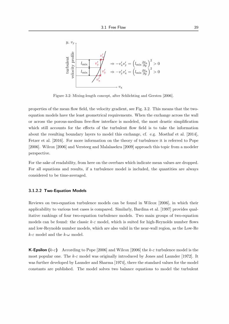
3.1 Free Flow 39
turb
ule
nt
velo
city
pro
file
y, vy
vx
v′x
v′y
v′x
v′y
lmix
lmix ⇒ −v′xv′y =(lmix
∂vx∂y
)2> 0
⇒ −v′yv′x =(lmix
∂vx∂y
)2> 0
Figure 3.2: Mixing-length concept, after Schlichting and Gersten [2006].
properties of the mean flow field, the velocity gradient, see Fig. 3.2. This means that the two-
equation models have the least geometrical requirements. When the exchange across the wall
or across the porous-medium free-flow interface is modeled, the most drastic simplification
which still accounts for the effects of the turbulent flow field is to take the information
about the resulting boundary layers to model this exchange, cf. e.g. Mosthaf et al. [2014],
Fetzer et al. [2016]. For more information on the theory of turbulence it is referred to Pope
[2006]. Wilcox [2006] and Versteeg and Malalasekra [2009] approach this topic from a modeler
perspective.
For the sake of readability, from here on the overbars which indicate mean values are dropped.
For all equations and results, if a turbulence model is included, the quantities are always
considered to be time-averaged.
3.1.2.2 Two-Equation Models
Reviews on two-equation turbulence models can be found in Wilcox [2006], in which their
applicability to various test cases is compared. Similarly, Bardina et al. [1997] provides qual-
itative rankings of four two-equation turbulence models. Two main groups of two-equation
models can be found: the classic k-ε model, which is suited for high-Reynolds number flows
and low-Reynolds number models, which are also valid in the near-wall region, as the Low-Re
k-ε model and the k-ω model.
K-Epsilon (k-ε) According to Pope [2006] and Wilcox [2006] the k-ε turbulence model is the
most popular one. The k-ε model was originally introduced by Jones and Launder [1972]. It
was further developed by Launder and Sharma [1974], there the standard values for the model
constants are published. The model solves two balance equations to model the turbulent

40 3 Physical and Mathematical Model
kinetic energy and the dissipation which are combined to calculate the eddy viscosity:
νt = Cµk2
ε. (3.10)
As explained in section 3.1.2, the turbulent kinetic energy is defined via the velocity fluc-
tuations. Unfortunately, these fluctuations are unknown in RANS models. Therefore, the
turbulent kinetic energy is modeled by the following balance equation:
∂ (k)
∂t+∇ · (vgk)−∇ ·
((νg +
νt
σk
)∇k)− 2νtS · S + ε = 0 . (3.11)
The tensor scalar product of the strain rate tensor is: S · S =∑
i
∑j SijSij . In addition, a
balance equation for the dissipation is needed. The dissipation can be seen as an energy-flow
rate in the energy cascade [Pope, 2006, Wilcox, 2006]:
∂ (ε)
∂t+∇ · (vgε)−∇ ·
((νg +
νt
σε
)∇ε)− C1ε
ε
k2νtS · S + C2ε
ε2
k= 0 . (3.12)
According to Pope, the model equation for the dissipation is “best viewed as being entirely
empirical” and not based on the exact equation which may also be derived.
The constants for both equations are, according to Launder and Sharma [1974]:
σk = 1.00 , σε = 1.30 , C1ε = 1.44 , C2ε = 1.92 , Cµ = 0.09 .
If the k-ε model is considered to be a purely high-Reynolds turbulence model, it holds that
νt νg. Nevertheless, formulations including the kinematic fluid viscosity νg can be found
in Wilcox [2006] and OpenFOAM, whereas it is neglected in Versteeg and Malalasekra [2009]
and Pope [2006]. The k-ε model is, in the presented form, not suited for flow with strong
viscous effects as they occur near walls. Possible remedies are explained in the subsequent
paragraphs.
Wall Functions: Wall functions use the law of the wall and its solution for the logarithmic
layer (2.24) and are, according to Pope [2006], originally proposed by Launder and Spalding
[1972]. Wall functions are generally useful, if the geometries are simple and the law of the wall
is valid. This might not be the case, e.g. for surface mass injection as reported by Andersen
et al. [1972] or [Wilcox, 2006, Fig. 4.27]. The wall-function method has constantly been
developed over the past years: e.g. Craft et al. [2002] adopted the wall-function treatment for
better predictions or Blocken et al. [2007] analyzed the influence of wall functions including
sand-grain roughness parametrizations for atmospheric boundary layer flow over buildings.
Based on the analytical law-of-the-wall solution, the wall shear stress and the wall friction
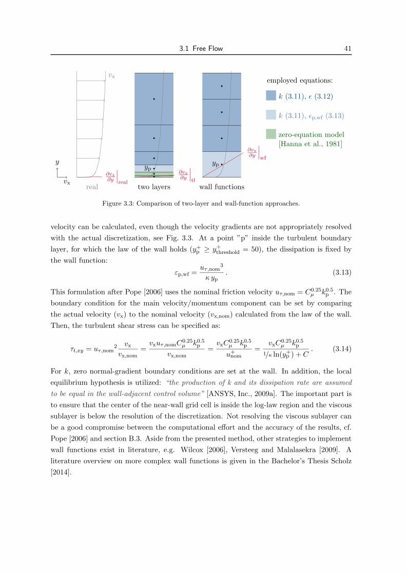
3.1 Free Flow 41
vx
y
vx
∂vx∂y
∣∣∣real
real
yp
two layers
∂vx∂y
∣∣∣tl
yp
wall functions
∂vx∂y
∣∣∣wf
employed equations:
k (3.11), ε (3.12)
k (3.11), εp,wf (3.13)
zero-equation model[Hanna et al., 1981]
Figure 3.3: Comparison of two-layer and wall-function approaches.
velocity can be calculated, even though the velocity gradients are not appropriately resolved
with the actual discretization, see Fig. 3.3. At a point ”p” inside the turbulent boundary
layer, for which the law of the wall holds (y+p ≥ y+
threshold = 50), the dissipation is fixed by
the wall function:
εp,wf =uτ ,nom
3
κ yp. (3.13)
This formulation after Pope [2006] uses the nominal friction velocity uτ,nom = C0.25µ k0.5
p . The
boundary condition for the main velocity/momentum component can be set by comparing
the actual velocity (vx) to the nominal velocity (vx,nom) calculated from the law of the wall.
Then, the turbulent shear stress can be specified as:
τt,xy = uτ ,nom2 vx
vx,nom=vxuτ ,nomC
0.25µ k0.5
p
vx,nom=vxC
0.25µ k0.5
p
u+nom
=vxC
0.25µ k0.5
p
1/κ ln(y+p ) + C
. (3.14)
For k, zero normal-gradient boundary conditions are set at the wall. In addition, the local
equilibrium hypothesis is utilized: “the production of k and its dissipation rate are assumed
to be equal in the wall-adjacent control volume” [ANSYS, Inc., 2009a]. The important part is
to ensure that the center of the near-wall grid cell is inside the log-law region and the viscous
sublayer is below the resolution of the discretization. Not resolving the viscous sublayer can
be a good compromise between the computational effort and the accuracy of the results, cf.
Pope [2006] and section B.3. Aside from the presented method, other strategies to implement
wall functions exist in literature, e.g. Wilcox [2006], Versteeg and Malalasekra [2009]. A
literature overview on more complex wall functions is given in the Bachelor’s Thesis Scholz
[2014].

42 3 Physical and Mathematical Model
Two Layers: If the viscous sublayer is resolved, the wall friction velocity can be approxi-
mated by the velocity gradient at the wall (Fig. 3.3). However, the k-ε equations can only be
used in the turbulent, high-Reynolds region of the flow and not throughout the entire simula-
tion domain. The lower bound is still indicated by the above-mentioned criterion (y+threshold).
In the region near the wall, which does not fulfill this criterion and where the flow is af-
fected by viscous forces, a zero-equation turbulence model is used to calculate νt. Again, the
dissipation value in the first cell which fulfills the y+-criterion is fixed by:
εp,wf =uτ
3
κ yp,
and k gets a zero-gradient boundary condition toward the near-wall region. The momentum
balance equation receives a classical no-slip condition at the wall. Approaches with a less
strict criterion are proposed by Menter [1994] who use more advanced blending functions to
continuously go from the k-ε model to a one or two-equation turbulence model near the wall.
Others: The k-ε models of the renormalization group (RNG) are deduced by a more strict
derivation out of the Navier-Stokes equations, e.g. Yakhot and Orszag [1986]. Durbin [1991]
discusses a near-wall closure without introducing damping functions as they are used e.g. for
the low-Re k-ε model which is discussed in the next section.
Low-Re K-Epsilon (low-Re k-ε) The low-Re k-ε models add extra terms or modify the
coefficients of the high-Re k-ε model to account for the near-wall behavior. A good overview
and comparison of these models is given by Patel et al. [1985]. They conclude that the model
by Chien [1982], which is presented here, performs considerably better than others. The
turbulent kinetic energy balance is identical with the one from the k-ε model (3.11), but the
dissipation includes a damping function (Dε):
ε = ε+Dε , (3.15)
and thus the equation for k can be written as:
∂ (k)
∂t+∇ · (vgk)−∇ ·
((νg +
νt
σk
)∇k)− 2νtS · S + ε+Dε = 0 . (3.16)
The dissipation balance is changed by introducing additional functions (Ek, f1, and f2) to
account for a damping towards the wall:
∂ (ε)
∂t+∇ · (vgε)−∇ ·
((νg +
νt
σε
)∇ε)− C1εf1
ε
k2νtS · S + C2εf2
ε2
k− Ek = 0 . (3.17)

3.1 Free Flow 43
Also, the kinematic eddy viscosity νt is dampened by fµ:
νt = Cµfµk2
ε. (3.18)
The auxiliary and damping functions are defined as:
Dε = 2νgk/y2 , Ek = −2νgε
y2exp
(−0.5y+
),
f1 = 1 , f2 = 1− 0.22 exp
(−(
Ret
6
)2), fµ = 1− exp
(−0.0115y+
), Ret =
k2
νε.
Finally, the model is closed with the following constants:
σk = 1.00 , σε = 1.30 , C1ε = 1.35 , C2ε = 1.80 , Cµ = 0.09 .
K-Omega (k-ω)4 The k-ω models are another group of models which allows for using the
same equations in the turbulent flow and near the walls. In these models, the transport of
turbulent kinetic energy is considered together with the turbulence frequency. As reported by
Pope [2006] and Wilcox [2006], the earliest versions of k-ω turbulence models were proposed
by Kolmogorov [1942] and Saffman [1970]. Later, David C. Wilcox and co-authors were the
main driving forces for the k-ω models, but also other popular contributions to k-ω models
are made, e.g. by Menter [1994]. In this thesis, the version published in Wilcox [2008] is
presented. The turbulent kinetic energy balance equation is given by:
∂ (k)
∂t+∇ · (vgk)−∇ ·
((νg + σk
k
ω
)∇k)− 2νtS · S + βkkω = 0 . (3.19)
The balance equation for the turbulence frequency is:
∂ (ω)
∂t+∇ · (vgω)−∇ ·
((νg + σω
k
ω
)∇ω)−αω
ω
k2νtS ·S + βωω
2− σd
ω∇k · ∇ω = 0 . (3.20)
The eddy viscosity is then calculated by:
νt =k
ω. (3.21)
4The k-ω model used in this work builds upon an implementation performed in a supervised Master’s Thesis,E. Coltman: Numerical investigation of turbulent flow around obstacles and evaporating porous media,Master’s Thesis, Universitat Stuttgart, 2017.

44 3 Physical and Mathematical Model
According to the model presented in Wilcox [2008], the following closure constants and rela-
tions are used:
αω = 0.52 , σk = 0.6 , σω = 0.5 , βk = 0.09 , βω = 0.0708 ,
ω = max
ω, 0.875
√2S · Sβk
, σd =
0 , if ∇k · ∇ω ≤ 0
0.125 , if ∇k · ∇ω > 0.
The boundary conditions for k and ω are presented in Wilcox [1988]. The condition for k is
set as a Dirichlet condition at the wall, whereas the condition for ω would lead to an infinite
value and thus ωp is set in the first cell away from the wall (p):
kwall = 0 , ωp =6νg
βωyp.
3.1.2.3 One-Equation Models
In this work, the model published by Spalart and Allmaras [1992] is used. However, after
further developments, a newer version can be found in Allmaras et al. [2012], but also earlier
versions of one-equation models are available, e.g. Baldwin and Barth [1990]. This one-
equation model transports the quantity ν, just called working variable [Allmaras et al., 2012].
This working variable already has the units of the eddy viscosity and can be converted via a
model function (fv1):
νt = νfv1 .
Wilcox [2006] and Versteeg and Malalasekra [2009] propose that the correction terms which
account for the transition or trip, might be dropped from the original equations, such that
the balance equation simplifies to:
∂ν
∂t+∇ · (νv)− cb1Sν −
1
σν∇ · ([ν + ν]∇ν)− cb2
σν|∇ν|2 + cw1fw
ν2
y2= 0 . (3.22)
This balance equation is linked to the flow geometry by the distance to the closest wall (y).
Further, the model uses the following functions and expressions:
χ =ν
ν, fv1 =
χ3
χ3 + c3v1
, fv2 = 1− χ
1 + fv1χ,
fw = gw
(1 + c6
w3
g6w + c6
w3
) 16
, gw = rw + cw2(r6w − rw) , rw = min
[ν
Sκ2y2, 10
].
3.1 Free Flow 45
Here, a modified mean effective strain rate (S) based on the mean rotation rate tensor (Ω) is
used:
S =√
2Ω ·Ω +ν
κ2y2fv2 , Ω =
1
2
(∇vg −∇vᵀ
g
).
Finally, the model is closed with the following constants:
σν = 2/3 , cb1 = 0.1355 , cb2 = 0.622 ,
cv1 = 7.1 , cw1 =cb1
κ2+
1 + cb2
σν, cw2 = 0.3 , cw3 = 2 .
3.1.2.4 Zero-Equation Models5
The zero-equation turbulence models (also named algebraic turbulence models) are the first
generation of turbulence models. Two different groups are presented in the following: mixing-
length models with one algebraic equation for the entire domain and two-layer approaches
with a switching mechanism.
Mixing-Length Models The first mixing-length model was proposed by L. Prandtl at the
begin of the 20th century. In analogy to the kinetic gas theory, it assumes a proportionality
of the main flow velocity gradient and the eddy viscosity (see also Fig. 3.2):
νt = l2mix
∣∣∣∣∂vx
∂y
∣∣∣∣ , (3.23)
which is the mixing length lmix = κy. Here, y is equivalent to the wall-normal distance and
vx denotes the main velocity component. This model was improved by van Driest [1956], who
changed the mixing length such that the eddy viscosity is dampened near the wall:
lmix = κy[1− exp
(−y+/26
)]. (3.24)
This model was again improved by Hanna et al. [1981], they corrected the asymptotic behavior
of the Reynolds shear stress:
lmix = κy1− exp (−y+/26)√1− exp(−0.26y+)
. (3.25)
5Parts of the zero-equation models and their implementations are revised versions of T. Fetzer: Numericalanalysis of the influence of turbulence on exchange processes between porous-medium and free flow, Master’sThesis, Universitat Stuttgart, 2012 and a supervised Master’s Thesis, P. Samantray: Implementation ofadvanced algebraic turbulence models on a staggered grid, Master’s Thesis, Universitat Stuttgart, 2014.

46 3 Physical and Mathematical Model
Two-Layer Models Baldwin and Lomax [1978] presented a model in which the eddy viscosity
depends on two equations which are valid in different areas of the flow:
νt =
νinner = l2mix |ω| y < ycross
νouter = 0.02688FwakeFkleb y ≥ ycross
. (3.26)
The switching point ycross is defined as the smallest value of y at which µinner = µouter. For
the inner region, Van Driest’s expression of the mixing length is used (3.24). Instead of the
velocity gradient, the magnitude of the vorticity (|ω|) is applied:
|ω| =
√(∂vx
∂y− ∂vy
∂x
)2
+
(∂vy
∂z− ∂vz
∂y
)2
+
(∂vz
∂x− ∂vx
∂z
)2
. (3.27)
However, in the case of a parallel flow field, all mean gradients despite ∂vx/∂y are negligible.
For the calculation of the eddy viscosity in the outer region, the following additional functions
are necessary:
Fwake = min
yFmaxFmax
0.25yFmax(∆U)2
Fmax
(3.28)
F = y |ω|[1− exp
(−y+/26
)](3.29)
Fmax = max F (3.30)
yFmax = y(Fmax) (3.31)
∆v =√v2
x,max + v2y,max + v2
z,max −√v2
x,min + v2y,min + v2
z,min (3.32)
Fkleb =
[1 + 5.5
(0.3y
yFmax
)6]−1
. (3.33)
A similar zero-equation turbulence model with a two-layer approach is proposed by Cebeci and
Smith [1974]. Because of their similarity, the Cebeci and Smith model is not further evaluated
in this work. Mavriplis [1990] showed how these two-layer models can be implemented for
non-flat geometries on unstructured grids.
3.1.2.5 Boundary Layer Models
The last approach is based on the boundary layer theory which is intensively discussed in
Schlichting and Gersten [2006]. In analogy to the viscous region in the law of the wall, in
which the velocity gradient and thus the viscous shear are relatively constant, it is assumed
that the same holds for the component and energy transport. The flow field is assumed to
be composed of a laminar, diffusion-dominated and a turbulent, fully-mixed sublayer, see
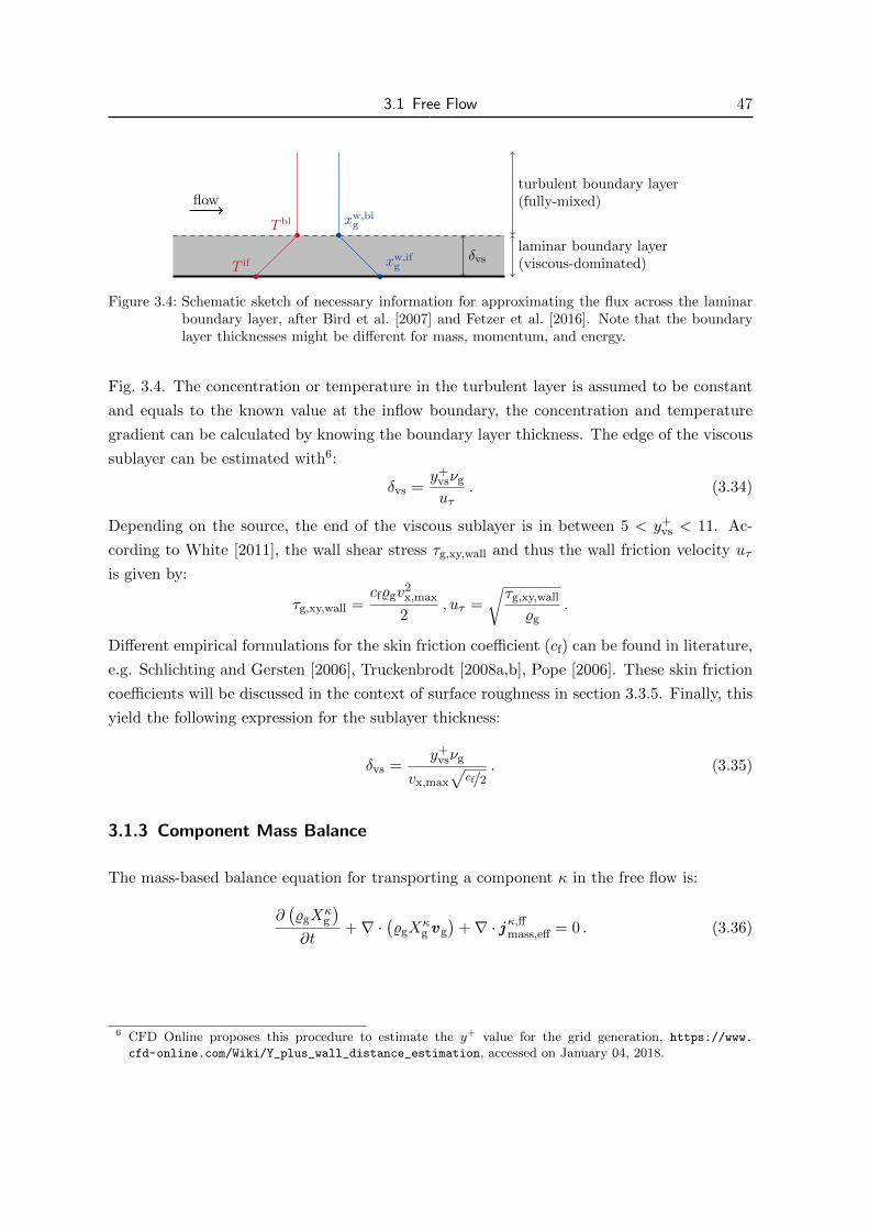
3.1 Free Flow 47
flow
T if
T bl
xw,ifg
xw,blg
δvslaminar boundary layer(viscous-dominated)
turbulent boundary layer(fully-mixed)
Figure 3.4: Schematic sketch of necessary information for approximating the flux across the laminarboundary layer, after Bird et al. [2007] and Fetzer et al. [2016]. Note that the boundarylayer thicknesses might be different for mass, momentum, and energy.
Fig. 3.4. The concentration or temperature in the turbulent layer is assumed to be constant
and equals to the known value at the inflow boundary, the concentration and temperature
gradient can be calculated by knowing the boundary layer thickness. The edge of the viscous
sublayer can be estimated with6:
δvs =y+
vsνg
uτ. (3.34)
Depending on the source, the end of the viscous sublayer is in between 5 < y+vs < 11. Ac-
cording to White [2011], the wall shear stress τg,xy,wall and thus the wall friction velocity uτ
is given by:
τg,xy,wall =cf%gv
2x,max
2, uτ =
√τg,xy,wall
%g.
Different empirical formulations for the skin friction coefficient (cf) can be found in literature,
e.g. Schlichting and Gersten [2006], Truckenbrodt [2008a,b], Pope [2006]. These skin friction
coefficients will be discussed in the context of surface roughness in section 3.3.5. Finally, this
yield the following expression for the sublayer thickness:
δvs =y+
vsνg
vx,max
√cf/2
. (3.35)
3.1.3 Component Mass Balance
The mass-based balance equation for transporting a component κ in the free flow is:
∂(%gX
κg
)∂t
+∇ ·(%gX
κg vg
)+∇ · j κ,ff
mass,eff = 0 . (3.36)
6 CFD Online proposes this procedure to estimate the y+ value for the grid generation, https://www.
cfd-online.com/Wiki/Y_plus_wall_distance_estimation, accessed on January 04, 2018.
48 3 Physical and Mathematical Model
For simplicity, the effective diffusive-dispersive flux (j κ,ffmass,eff) is used. This flux combines the
molecular transport by diffusion and the dispersive transport by turbulent fluctuations:
j κ,ffmass,eff = j κ,ff
mass,g + j κ,ffmass,t = −Dκ
g%mol,gMκ∇xκg −Dt%mol,gM
κ∇xκg . (3.37)
Note that the only difference between laminar and turbulent flow with respect to component
transport is that there are no turbulent dispersive fluxes, hence j κ,ffmass,t = 0. For turbulent
flow, the eddy viscosity can be converted to the eddy diffusivity (Dt) by the turbulent Schmidt
number, Sct = νt/Dt. Even though a value of 0.7 is a common choice for Sct, Flesch et al.
[2002] and Tominaga and Stathopoulos [2007] report a wide range of values. Tominaga and
Stathopoulos [2007] analyze the turbulent Schmidt numbers for urban flow, resulting in val-
ues between 0.2 and 1.3 which are discussed with respect to their influence. Flesch et al.
[2002] conclude that a value of 0.6 is appropriate for tracer plumes above a bare ground, by
evaluating their experiments.
An option to reduce the model complexity is to assume composition independent fluid prop-
erties. This allows for decoupling flow and transport equation as e.g. used in Masson et al.
[2016]. In this work, a model that does not consider a feedback from the component mass
transport to the momentum transport is called transport model.
3.1.4 Energy Balance
The energy transport in the free flow is modeled with the following balance equation:
∂ (%gug)
∂t+∇ · (%ghgvg) +
∑κ∈w,a
∇ ·(hκgj
κ,ffmass,eff
)−∇ · (λeff∇T ) = 0 . (3.38)
In which the specific internal energy (ug) is included in the storage term, and a transport
of enthalpy by the diffusive-dispersive fluxes: hκgjκ,ffmass,eff. In addition to the conductive flux
inside the fluid, a turbulent conductive flux is considered. Both are lumped in an effective
flux:
f eff = λeff∇T = λg∇T + λt∇T . (3.39)
The relation between the eddy viscosity and the eddy thermal conductivity (λt) is expressed
by the turbulent Prandtl number: Pr t = νt%αcp,α/λt. Wilcox [2006] proposes Pr t ≈ 0.9 for
boundary layers. According to Bird et al. [2007] and references therein values of 0.7 to 0.9 for
gas flow in conduits and 0.85 for circular tubes are proposed. However, Cebeci [1973] reports
a value of 1.22 for air at high Reynolds numbers.
3.2 Porous Medium 49
3.2 Porous Medium
The fundamental upscaled models for flow in porous media are well-established and were
proposed between the mid of the 19th century to the beginning of the 20th century. All models
presented here are based on the assumptions of (i) gas and liquid as mobile phases, (ii) a rigid
and isotropic porous medium, (iii) Fickian diffusion without dispersion, (iv) unique capillary
pressure–saturation relationship (no hysteresis), and (v) local thermodynamic equilibrium.
Further details on porous-medium models can be found in textbooks as Bear [1988], Helmig
[1997].
3.2.1 Mass and Momentum Balance
For balancing mass inside the porous medium, the porosity and the saturation have to be
considered for the storage term:
∑α∈l,g
φ∂ (%αSα)
∂t+∇ · (%αvα) +
∑κ∈w,a
∇ · j κ,pmmass,α
= 0 . (3.40)
In contrast to the free flow, where the Navier-Stokes equations are used for balancing mo-
mentum, different upscaled models are available for flow in a porous medium.
3.2.1.1 Darcy Law
The maybe most important experiments concerning flow in porous media, were performed by
Henry Darcy in 1856. He applied a gradient in fluid pressure and measured the flow through
soil samples. Finally, he found a proportionality factor between the pressure difference and
the velocity, which is called Darcy law:
vα = −kr,αK
µα(∇pα − %αg) . (3.41)
This equation is valid for creeping flow with Repore < 1. It considers an intrinsic permeabil-
ity K which is only a property of the porous medium. In general, the intrinsic permeability is
a tensor, but can be simplified as a scalar for isotropic porous media. For single-phase flow,
the relative permeability kr,α equals one. The parametrization of kr,α for multi-phase flow is
explained in section 2.5.2.
50 3 Physical and Mathematical Model
3.2.1.2 Richards Equation
Richards [1931] proposes a simplification of the Darcy law for flow in the unsaturated zone.
Assuming that the gas phase is more mobile than the liquid phase (µg µl), differences in gas-
phase pressure equilibrate immediately and no pressure gradient evolves. Thus, the gas-phase
pressure equals the pressure in the atmosphere and the liquid-phase pressure corresponds to
the capillary pressure. Based on this assumption, neither gas-phase flow nor transport therein
is considered in the model. It is obvious that this poses problems e.g. when diffusive transport
of water vapor in absence of liquid water is important, see Szymkiewicz [2013]. Vanderborght
et al. [2017] and references therein discuss remedies for this problem. One option is to model
an increased mobility of liquid water for low water saturations.
3.2.1.3 Dupuit-Forchheimer Equation
The above-mentioned laws are only valid for creeping flow (Repore < 1). If inertia effects
cannot be entirely neglected, based on findings by Dupuit in 1863 and Forchheimer in 1901,
the so-called Dupuit-Forchheimer equation can be used for single-phase flow, cf. Nield and
Bejan [2017]:
(∇pα − %αg) = −µαK
vα −%αCF√K|vα| vα . (3.42)
The last term in this equation represents the additional inertia forces, for which Nield and
Bejan [2017] and references therein propose a constant Forchheimer coefficient CF = 0.55.
However, there is no common sense how to transfer this single-phase equation to multi-phase
conditions: e.g. Wu [2002], Skjetne and Auriault [1999], and Nuske [2014] propose different
equations. In this thesis, the approach from Nuske [2014] is used, in which the relative
permeabilities are included:
(∇pα − %αg) = − µαkr,αK
vα −%αCF√Kkr,α
|vα| vα . (3.43)
3.2.2 Component Mass Balance
The mass-based balance equation for transporting a component κ in the porous medium is:
∑α∈l,g
(φ∂ (%αSαX
κα)
∂t+∇ · (%αXκ
αvα) +∇ · j κ,pmmass,α
)= 0 . (3.44)
If the equations for all components are summed-up, the total mass-balance (3.40) is gained.
3.3 Interface 51
3.2.3 Energy Balance
With the assumption of local thermodynamic equilibrium, the temperature in one REV is
the same for all phases and thus only one energy balance is required:
∑α∈l,g
(φ∂ (%αSαuα)
∂t+∇ · (%αhαvα)
)+ (1− φ) %scs
∂T
∂t−∇ · (λpm∇T ) = 0 . (3.45)
Properties of the solid matrix material are indicated by the subscript (s). It is assumed
that the imposed empirical model for the effective thermal conductivity (λpm) includes the
conductive energy fluxes as well as the energy fluxes transported by diffusive-dispersive mass
fluxes, see e.g. Roth [2012], Lu et al. [2011] for a detailed discussion of this topic.
3.3 Interface
This section presents the conditions for coupling mass, momentum, and energy transport
across a porous-medium free-flow interface. In addition to the coupling conditions for each
balance equation, possible simplifications are presented which can be included in the coupling
or can be applied as dynamic boundary conditions when simulating only one subdomain. In
the second part, it is shown how a rough interface can be considered in the model.
The interface coupling conditions are based on the assumptions of local thermodynamic equi-
librium and the continuity of fluxes. This is a common approach in literature, see e.g. Moeckel
[1975], Layton et al. [2002], Mosthaf et al. [2011]. The coupling conditions for a non-isothermal
multi-phase multi-component system, are based on the work presented in Mosthaf et al. [2011]
and Fetzer et al. [2016]. Vanderborght et al. [2017] describes different modeling techniques
for coupled or uncoupled porous-medium and free flow simulations.
The conditions are classified by the involved balance equations. Mosthaf et al. comprise the
conditions for the momentum and the total mass balances as mechanical equilibrium, the
conditions for the component mass balances as chemical equilibrium, and the conditions for
the energy balances as thermal equilibrium. The coupling conditions presented here differ
from previous versions [Mosthaf et al., 2011, Fetzer et al., 2016] by the diffusive-dispersive
fluxes which are considered in the mass-based total mass balance. In addition, it differs from
Mosthaf et al. [2011] by the ability of the diffusive-dispersive fluxes inside the free flow to
transport enthalpy.
In the following, the normal vector (n) is pointing outside of the respective subdomain and
thus nff = −npm.
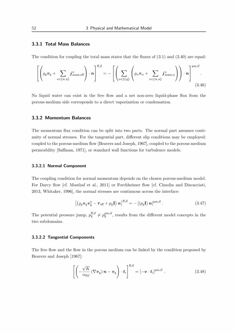
52 3 Physical and Mathematical Model
3.3.1 Total Mass Balances
The condition for coupling the total mass states that the fluxes of (3.1) and (3.40) are equal:%gvg +∑
κ∈w,a
j κmass,eff
· nff,if
= −
∑α∈l,g
%αvα +∑
κ∈w,a
j κmass,α
· npm,if
.
(3.46)
No liquid water can exist in the free flow and a net non-zero liquid-phase flux from the
porous-medium side corresponds to a direct vaporization or condensation.
3.3.2 Momentum Balances
The momentum flux condition can be split into two parts. The normal part assumes conti-
nuity of normal stresses. For the tangential part, different slip conditions may be employed:
coupled to the porous-medium flow [Beavers and Joseph, 1967], coupled to the porous-medium
permeability [Saffman, 1971], or standard wall functions for turbulence models.
3.3.2.1 Normal Component
The coupling condition for normal momentum depends on the chosen porous-medium model.
For Darcy flow [cf. Mosthaf et al., 2011] or Forchheimer flow [cf. Cimolin and Discacciati,
2013, Whitaker, 1996], the normal stresses are continuous across the interface:
[(%gvgv
ᵀg − τ eff + pgI
)n]ff,if
= − [(pgI)n ]pm,if . (3.47)
The potential pressure jump, pff,ifg 6= ppm,if
g , results from the different model concepts in the
two subdomains.
3.3.2.2 Tangential Components
The free flow and the flow in the porous medium can be linked by the condition proposed by
Beavers and Joseph [1967]:[(−√K
αBJ(∇vg)n − vg
)· t i
]ff,if
= [−v · t i]pm,if . (3.48)

3.3 Interface 53
This condition was originally derived for laminar single-phase flow, but work by Hahn et al.
[2002] indicates that it also works for turbulent flow.
Saffman Simplification This work uses the simplification proposed by Saffman. It assumes
that the tangential flow in the porous medium is negligible for the exchange of momentum, be-
cause: [v · t i]pm,if ≈ 0. Therefore, the condition can be used as a free-flow boundary condition
only, as it does not depend on porous-medium processes:[(−√K
αBJ(∇vg)n − vg
)· t i
]ff,if
= 0 . (3.49)
If this condition is extended such that multi-phase flow effects are included, the resulting
slip-velocity of the free gas flow is decreased, see Fritsch [2014].
Wall Functions As discussed earlier, wall functions for the k-ε model are necessary, if the
discretization is coarse and the near-wall region is not resolved appropriately. In this case, the
simplification of no-slip conditions, [vg · t i]ff,if = 0, is made and the standard wall functions
for the k-ε model are used, see (3.14).
3.3.3 Component Mass Balances
For a component κ, chemical equilibrium in terms of continuity of mass fractions is applied:
[Xκ
g
]ff,if=[Xκ
g
]pm,if. (3.50)
Mosthaf et al. [2011] write that, in general, it should be asked for continuity in chemical
potential. But, due to the unavoidable pressure jump, this would also result in jumps in mass
or mole fractions. The continuity of the respective component fluxes is given by:
[(%gX
κg vg + j κmass,eff
)· n]ff,if
= −
∑α∈l,g
(%αX
καvα + j κmass,α
)· n
pm,if
. (3.51)
Resistance Term Models The total mass flux over the interface can be simplified by using
one-dimensional transfer resistance models. This can be done via forward estimations or
backward fitting, cf. Vanderborght et al. [2017], Fetzer et al. [2017c] and reference therein.
Resistance term models can be used to downscale findings of a full complex to a less complex
model (one-dimensional or porous medium only). If the total water mass flux or evaporation

54 3 Physical and Mathematical Model
rate is known, the mass transfer resistance (rmass) can be fitted by evaluating the mole fraction
at the interface and at a reference height:
[(%gX
κg vg + j κmass,eff
)· n]ff,if
= − 1
rmass%mol,gM
κ(xκ,if
g − xκ,refg
). (3.52)
Boundary Layer Models Under the assumption that (i) diffusion through the viscous sub-
layer is the limiting factor for mass transfer and (ii) boundary layers form and the flow is
fully mixed outside the viscous sublayer, the diffusive fluxes in eq. (3.51) can be replaced by:
[j κmass,eff · n
]ff,if= −Dκ
g%mol,gMκx
κ,ifg − xκ,bl
g
δvs. (3.53)
The mole fraction gradient is build with a prescribed value at the edge of the boundary layer,
the implicitly calculated value at the interface, and a boundary layer thickness (see Fig. 3.4).
Wall Functions For two-equation turbulence models, the already mentioned wall functions
can be used to approximate the fluxes at the interface. According to the ANSYS Fluent
Theory’s guide [ANSYS, Inc., 2009a] and in analogy to the momentum wall function (3.14),
the wall function for a component κ can be formulated as:
[j κmass,eff · n
]ff,if= −
(xκ,if
g − xκg,p
)%mol,gM
κC0.25µ k0.5
p
Sct
(1/κ ln(y+
p E) + S) . (3.54)
This wall function uses the law of the wall, thus point ”p” has to be located in the turbulent log
law region (y+p ' 30). The log-law constant is E = 9.793 and equals the integration constant
C ≈ 5.5 ≈ 1/κ ln(E). The S-function is identical to the P-function used in the temperature
wall function (3.60), with the difference, that instead of Prandtl numbers Schmidt numbers
are used. For typical Schmidt numbers, e.g. Sct = 0.7 and Scg = 0.63, this results in a value
of S = −0.897.
Mass Transfer Models Until here, the diffusive fluxes across the interface are independent
of the saturation. Mosthaf et al. [2014] present different model concepts which include the
saturation at the interface or near-interface cell and analyze how these models affect the
evaporation rate.
3.3 Interface 55
3.3.4 Energy Balances
Finally, the coupling conditions are completed by ensuring continuity of temperature:
[T ]ff,if = [T ]pm,if , (3.55)
and energy fluxes:%ghgvg +∑
κ∈w,a
hκgjκmass,eff − λeff∇T
· nff,if
= −
∑α∈l,g
%αhαvα − λ∇T
· npm,if
.
(3.56)
Resistance Term Models If the total energy flux is known, the energy transfer resistance
(renergy) for a one-dimensional resistance term model can be fitted by evaluating the temper-
ature at the interface and at a reference height:%ghgvg +∑
κ∈w,a
hκgjκmass,eff − λeff∇T
· nff,if
= − 1
renergyλg
(T if − T ref
). (3.57)
Boundary Layer Models In similarity to the component boundary layer model it is assumed
that (i) conduction through the viscous sublayer is the limiting factor for energy transfer and
(ii) boundary layers form and the flow is fully mixed outside the viscous sublayer. Hence, in
addition to the diffusive fluxes, the conductive fluxes in eq. (3.56) can be replaced by:
[(λeff∇T ) · n ]ff,if = −λgT if − T bl
δvs. (3.58)
This formulation requires a fully-mixed temperature at the boundary layer edge, the interface
temperature, and a boundary layer thickness as model input (see Fig. 3.4).
Wall Functions More literature is available for temperature wall functions than for compo-
nent wall functions. Equivalent descriptions of such wall functions are found in Versteeg and
Malalasekra [2009], ANSYS, Inc. [2009a], and Defraeye et al. [2010], Defraeye [2011]:
[(λeff∇T ) · n ]ff,if = −(T if − Tp
)%cpC
0.25µ k0.5
p
Pr t
(1/κ ln(y+
p E) + P) . (3.59)

56 3 Physical and Mathematical Model
Again, the wall function should only be applied for y+p being inside the turbulent region,
however some authors apply it just outside the viscous sublayer y+p ' 11. According to Malin
[1987] different P-functions exist in literature to represent the resistance of heat transfer
(or mass transfer if Schmidt numbers are used) through the viscous sublayer. Here, the
P-function after Jayatilleke is used (see Malin [1987], Versteeg and Malalasekra [2009] and
reference therein):
P = 9.24
[(Prg
Pr t
)3/4
− 1
][1 + 0.28 exp (−0.007Prg/Prt)] , (3.60)
which results in P = −0.6711 for typical Prandtl numbers, e.g. Pr t = 0.8 and Prg = 0.74.
3.3.5 Roughness7
Sand-grain roughness may affect the boundary layer development and thus the diffusion-
dominated transport near the interface. When rough surfaces are considered, at least two dif-
ferent cases have to be considered: hydraulically smooth and rough surfaces, cf. section 2.6.1.
This section presents two concepts how the sand-grain roughness of the porous medium can
be included in coupled models. Both concepts are originally derived for roughness elements on
an impermeable plate and for both concepts the determination of a characteristic sand-grain
roughness length ks is critical.
3.3.5.1 Eddy-Viscosity Models
The first sand-grain roughness parametrization builds upon the eddy-viscosity concept. Ce-
beci [1978] writes that the wall distance and thus the eddy viscosity can be modified with the
sand-grain roughness parametrization as published by Rotta [1962]:
ywall = y + yrough , (3.61)
yrough = 0.9ν
uτ
[√k+
s − k+s exp
(−k+
s /6)]. (3.62)
The application range of this concept is limited to transitionally and fully rough surfaces, the
lower limit corresponds to hydrodynamically smooth surfaces:
4.535 < k+s =
uτks
ν< 2000 . (3.63)
7This section is based on T. Fetzer, K. M. Smits, and R. Helmig: Effect of Turbulence and Roughness onCoupled Porous-Medium/Free-Flow Exchange Processes, Transport in Porous Media, 114(2):395–424, 2016.doi: 10.1007/s11242-016-0654-6; but also provides some additional information to this publication.
3.3 Interface 57
This concept is also used by Kuznetsov and Becker [2004] to analyze how energy transfer is
altered due to the sand-grain roughness parameter.
3.3.5.2 Boundary Layer Models
As already discussed in section 3.1.2.5, the friction coefficient can be used to recalculate
the boundary layer thickness. The problem is that above fully rough surfaces, the viscous
boundary layer does not exist or is already fully merged inside the porous medium (δvs < ks).
Thus, no boundary condition via boundary layer models can be defined. For hydraulically
smooth surfaces, Truckenbrodt [2008b] proposes the following equation:
cf,hydr. smooth = 0.523
[ln
(0.06
v∞x x
ν
)]−2
. (3.64)
In the case of hydraulically smooth surfaces, the viscous boundary layer is larger than the
roughness elements (δvs > ks) and thus cf is unaffected by ks. In addition, Truckenbrodt
[2008b] presents a formula for fully rough surfaces:
cf,rough = [1.89− 1.62 log (ks/x)]−2.5 . (3.65)
This model can only be used under the assumption that (i) equation (3.65) is also valid in
the transition region even though a small bump occurs, see Fig. 3.5, (ii) a viscous sublayer
still exists in the transition region. With the help of Fig. 3.5, the smooth and rough model
can be combined via cf = max (cf,rough, cf,hydr. smooth).
The second approach uses the Darcy friction factor (f). Colebrook and White [Colebrook,
1939] developed an empirical formulation for flow in pipes or ducts which is converted to an
explicit formulation by Haaland [1983]:
cf =f
4=
1
4
(−1.8
nHlog
[(ks
3.75 dhy
)1.11nH
+
(6.9
Red
)nH])−2
, (3.66)
Haaland suggests nH = 3 to obtain a more abrupt transition between the limiting regimes
of smooth and fully rough cases. This formulation is valid for fully developed flow, thus the
boundary layer thickness does not depend on the run-length, see Fig. 3.6. Again, δvs > ks
has to be ensured.
In addition to all these limitations, the cf–expressions are empirical and alternative formu-
lations exist which lead to different results and finally the resulting boundary layer strongly
depends on the chosen y+ value, see (3.35).

58 3 Physical and Mathematical Model
1
10
1e5 1e6 1e7 1e8 1e9
x10−3
1e−3
1e−4
1e−5
hydraulicallysmooth
fully rough
transition
c f[−
]
Rex [−]
Figure 3.5: Friction coefficients for differentReynolds numbers, after Trucken-brodt [2008b]. The red line is validfor hydraulically smooth regimes(3.64), the solid blue lines are validfor fully rough surfaces (3.65),the magenta lines are valid in thetransition region.
0
0.5
1
1.5
2
2.5
3
0 1 2 3 4 5
ks = 0.4 mm
ks = 0.8 mm
ks = 1.2 mm
δ vs
[mm
]
x [m]
Figure 3.6: Boundary layer thicknesses accord-ing to friction coefficient models forvx,g = 1 m/s and y+ = 10. The graylines indicate the roughness heightsfor the respective line type. The redlines follow (3.66), the blue lines usethe maximum of (3.64) and (3.65).

4 Numerical Model
First, this chapter illustrates two different spatial discretization schemes together with their
numerical coupling concepts. Then, the discretization in time is explained, different aspects
regarding the implementation are looked at, and the used software is presented.
4.1 Discretization in Space
Two spatial discretization methods for coupled porous-medium free-flow problems are used
in this thesis. The first uses a vertex-centered finite-volume method (box) in both domains.
The second employs a cell-centered finite-volume method (CCFV) in the porous medium and
a staggered-grid or marker-and-cell finite-volume method (MAC) in the free flow. Fig. 4.1
visualizes the location of the primary variables (also called unknowns or degrees of freedom)
for both discretization types. The porous-medium velocities are secondary variables because
they are calculated with the Darcy or Forchheimer law (cf. section 3.2.1). For both methods
and both domains, an upwinding scheme is used for the advective terms and an averaging for
the diffusive and conductive terms.
4.1.1 Box–Box Coupling
For this coupling method, the box discretization method is used in both domains. First, a
finite-element mesh is constructed for the entire domain. Then all barycenters of neighboring
finite elements are connected via the midpoints of the faces between them. These faces form
different finite-volume boxes. At the porous-medium free-flow interface the boxes are cut in
two halves, each of them belonging to one subdomain, see Fig. 4.1.
4.1.1.1 Free-Flow and Porous-Medium Domains
For a detailed information about the used box method it is referred to Masson et al. [1994] and
Mosthaf et al. [2014] for the free flow and to Huber and Helmig [2000] for the porous medium.
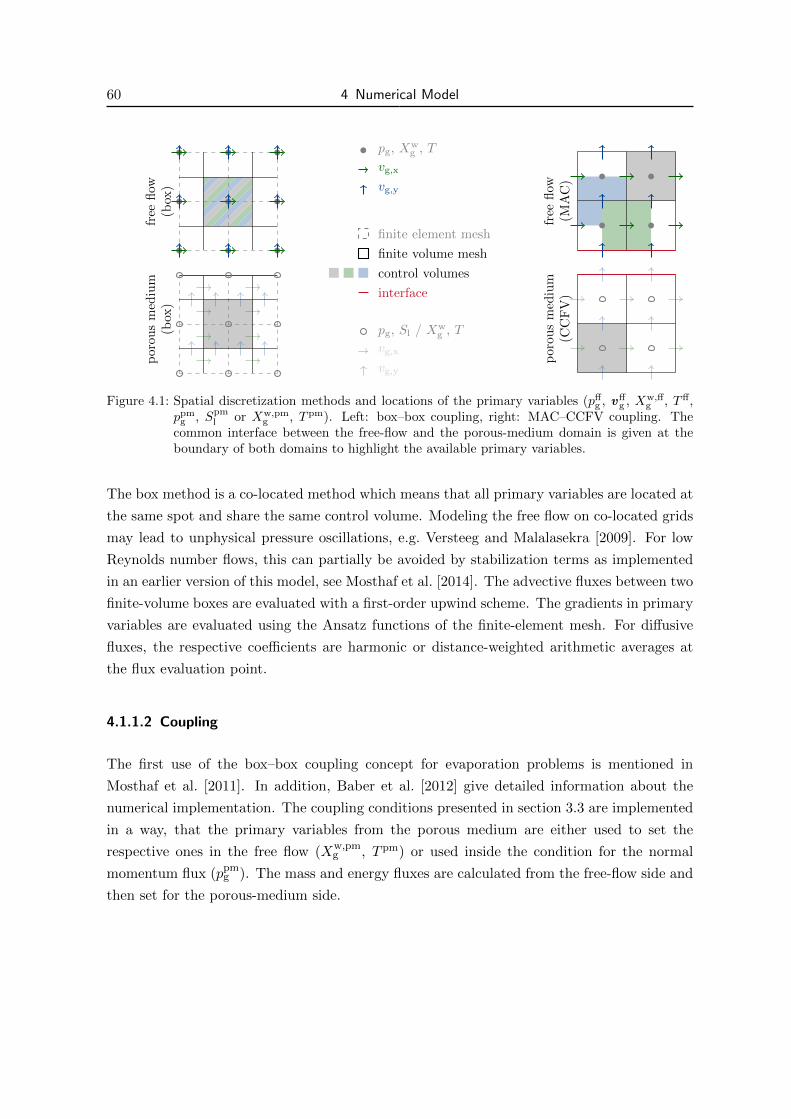
60 4 Numerical Model
free
flow
(box
)p
oro
us
med
ium
(box
)
pg, Xwg , T
vg,x
vg,y
finite element mesh
finite volume mesh
control volumes
interface
pg, Sl / Xwg , T
vg,x
vg,y
free
flow
(MA
C)
poro
us
med
ium
(CC
FV
)
Figure 4.1: Spatial discretization methods and locations of the primary variables (pffg , vff
g , Xw,ffg , Tff,
ppmg , Spm
l or Xw,pmg , T pm). Left: box–box coupling, right: MAC–CCFV coupling. The
common interface between the free-flow and the porous-medium domain is given at theboundary of both domains to highlight the available primary variables.
The box method is a co-located method which means that all primary variables are located at
the same spot and share the same control volume. Modeling the free flow on co-located grids
may lead to unphysical pressure oscillations, e.g. Versteeg and Malalasekra [2009]. For low
Reynolds number flows, this can partially be avoided by stabilization terms as implemented
in an earlier version of this model, see Mosthaf et al. [2014]. The advective fluxes between two
finite-volume boxes are evaluated with a first-order upwind scheme. The gradients in primary
variables are evaluated using the Ansatz functions of the finite-element mesh. For diffusive
fluxes, the respective coefficients are harmonic or distance-weighted arithmetic averages at
the flux evaluation point.
4.1.1.2 Coupling
The first use of the box–box coupling concept for evaporation problems is mentioned in
Mosthaf et al. [2011]. In addition, Baber et al. [2012] give detailed information about the
numerical implementation. The coupling conditions presented in section 3.3 are implemented
in a way, that the primary variables from the porous medium are either used to set the
respective ones in the free flow (Xw,pmg , T pm) or used inside the condition for the normal
momentum flux (ppmg ). The mass and energy fluxes are calculated from the free-flow side and
then set for the porous-medium side.
4.1 Discretization in Space 61
4.1.2 MAC–CCFV Coupling
In contrast to the box–box coupling, this coupling uses two different discretization schemes
with different locations of the primary variables.
4.1.2.1 Free-Flow and Porous-Medium Domains
To avoid the above-mentioned pressure oscillations, the free-flow equations are discretized
using the marker-and-cell scheme, cf. Harlow and Welch [1965] and Versteeg and Malalasekra
[2009]. The scalar primary variables (pffg , Xw,ff
g , T ff) are located at the center of each finite-
volume cell. The velocity components (vffg,i) and their control volumes are shifted to the faces,
see Fig. 4.1. For a more detailed description of the free-flow discretization it is referred to
Gruninger et al. [2017]. All porous-medium primary variables are located at the cell center.
The fluxes are calculated with a two-point flux approximation using a first-order upwind
scheme for advective fluxes and harmonic or distance-weighted arithmetic coefficients for
diffusive fluxes. The most important point to mention is that the normal velocity is the only
primary variable located on the porous-medium free-flow interface.
4.1.2.2 Coupling8
Despite the normal velocity component, none of the primary variables is located at the inter-
face (cf. Fig. 4.2). Therefore, the implementation of the coupling conditions is not straightfor-
ward. First, for the momentum coupling conditions, the interface gas-phase pressures (pff,ifg ,
ppm,ifg ) and the tangential velocities (vff,if
g,ti:= vff,if
g · t i) are missing. Second, for component
and energy transport, the gradients in mole fractions and temperature cannot be formulated
based one subdomain alone, but range over both domains. Third, continuity of mole fractions
and temperature has to be imposed implicitly.
In the following, first the momentum coupling conditions are examined. Afterward, the dif-
ferent coupling methods (CM) proposed and compared in Fetzer et al. [2017b] are presented.
It is started with CM4, the method closest to the continuous coupling conditions presented
in section 3.3. Then, from CM3 to CM1, more and more assumptions are made to simplify
the discretized coupling conditions.
8This section bases on T. Fetzer, C. Gruninger, B. Flemisch, and R. Helmig: On the Conditions for CouplingFree Flow and Porous-Medium Flow in a Finite Volume Framework, Finite Volumes for Complex Applica-tions VIII, Hyperbolic, Elliptic and Parabolic Problems (FVCA 8, Lille, France, June 2017):347–356, 2017.doi: 10.1007/978-3-319-57394-6_37.
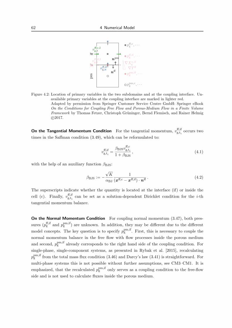
62 4 Numerical Model
ff
pff,cg , · · ·
vff,c,Ig,t
vff,ifg,n
nff
pm
ppm,cg , · · ·
npm
if
vff,if,Ig,t
pff,ifg , · · ·
ppm,ifg , · · ·
∇Xκ,ifg
∇T if
Figure 4.2: Location of primary variables in the two subdomains and at the coupling interface. Un-available primary variables at the coupling interface are marked in lighter red.Adapted by permission from Springer Customer Service Centre GmbH: Springer eBookOn the Conditions for Coupling Free Flow and Porous-Medium Flow in a Finite VolumeFramework by Thomas Fetzer, Christoph Gruninger, Bernd Flemisch, and Rainer Helmig©2017.
On the Tangential Momentum Condition For the tangential momentum, vff,ifg,ti
occurs two
times in the Saffman condition (3.49), which can be reformulated to:
vff,ifg,ti
=βBJSv
ff,cg,ti
1 + βBJS, (4.1)
with the help of an auxiliary function βBJS:
βBJS := −√K
αBJ
1
(xff,c − xff,if) · nff. (4.2)
The superscripts indicate whether the quantity is located at the interface (if) or inside the
cell (c). Finally, vff,ifg,ti
can be set as a solution-dependent Dirichlet condition for the i-th
tangential momentum balance.
On the Normal Momentum Condition For coupling normal momentum (3.47), both pres-
sures (pff,ifg and ppm,if
g ) are unknown. In addition, they may be different due to the different
model concepts. The key question is to specify ppm,ifg . First, this is necessary to couple the
normal momentum balance in the free flow with flow processes inside the porous medium
and second, ppm,ifg already corresponds to the right hand side of the coupling condition. For
single-phase, single-component systems, as presented in Rybak et al. [2015], recalculating
ppm,ifg from the total mass flux condition (3.46) and Darcy’s law (3.41) is straightforward. For
multi-phase systems this is not possible without further assumptions, see CM3–CM1. It is
emphasized, that the recalculated ppm,ifg only serves as a coupling condition to the free-flow
side and is not used to calculate fluxes inside the porous medium.
4.1 Discretization in Space 63
Coupling via an Interface Solver (CM4) The idea of this method is to make as few assump-
tions concerning interface conditions as possible. For each calculation of the fluxes across the
interface, a local system of equations which involves equations (3.46), (3.51), and (3.56) is
solved. The continuity of mole/mass fractions (3.50) and temperature (3.55) are integrated
into this system of equations and thus the additional local primary variables are: ppm,ifg , Sif
l
or Xκ,ifg , and T if. Now, the diffusive fluxes can be formulated for each subdomain separately.
After convergence, the continuity of fluxes is guaranteed and ppm,ifg is used to specify the
normal momentum condition.
The advantages of this method, compared to the following ones, are: (i) it is more accurate
as the gradients at the interface are better resolved and (ii) it can consider co-current flow of
the liquid phase and the gas phase for estimating the normal momentum flux and thus the
interface gas pressure.
However, it also bears some disadvantages. First, the switch from a two-phase system to a
one-phase system poses numerical problems: if Sifl drops below Sr,l, the liquid wetting phase
becomes immobile and as no storage term is included, the solution does not longer depend on
the local primary variable Sifl . To avoid this, a gradual switch to CM3 is implemented around
Sr,l. When the one-phase system is reached in a cell (Scl = 0), then, the local system of
equations is solved with Xκ,ifg as the primary variable. Second, a slope-limiter for the solution
of the local primary variable may has to be applied. This is necessary at the beginning of
a simulation, when the processes and state variables inside the porous medium and the free
flow are far from their equilibrium state. Third, it might be computationally more demanding
than the other methods.
Gas Momentum Coupling (CM3) This and all following methods avoid the additional, local
system of equations. They assume that the gradients of mole/mass fractions and temperature
can be built across the interface:
∇Xκ,ifg =
Xκ,ff,cg −Xκ,pm,c
g
xff,c − xpm,c, ∇T if =
T ff,c − T pm,c
xff,c − xpm,c.
The respective fluxes are then specified by the free-flow side. This assumption already involves
the continuity of mole fractions and temperature. Still, the gas-phase pressure at the interface
has to be recalculated using (3.41) and (3.46). It is assumed that the diffusive-dispersive
fluxes do not have a considerable effect on the resulting pressure at the interface and thus the
coupling condition can be simplified to:
[%gv
ifg · n
]ff=
[ ∑α∈l,g
%αkr,αK
%ανα
(pifα − pc
α
(x if − x c) · n− %αg · n
)]pm
. (4.3)

64 4 Numerical Model
The main assumption of this approach, in comparison to CM2, is: vpm,ifg vpm,if
l . In other
words, the contribution of the liquid-phase flow on the resulting gas-phase pressure at the
interface is negligible. This means that all liquid-phase terms in (4.3) are dropped and the
gas-phase pressure at the interface becomes:
ppm,ifg =
[%gv
ifg · n
]ff+[kr,gKνg
%gg · n]pm
kr,gKνg
(xpm,if − xpm,c
)· npm + ppm
g . (4.4)
In contrast to CM2, (i) a fully liquid-saturated system acts as an impermeable barrier to the
free gas-phase flow, (ii) no additional assumptions about the liquid state are required and
(iii) the lowest gas-flow resistance (kr,g/νg)−1 and thus the highest gas velocities are found for
Sl < Sr,l.
Total Momentum Coupling (CM2) As for CM3, the gas-phase pressure at the interface is
recalculated using (4.3). In (4.3), the liquid-phase pressure at the interface ppm,ifl is not known,
because it depends on the unknown liquid-phase saturation Spm,ifl . In this method, the main
assumption is that there is no difference in liquid-phase saturation between the cell and the
interface: Spm,ifl = Spm,c
l . This simplification results in the same pressure difference for both
phases and thus the same gradients contributing to the liquid-phase and the gas-phase flux.
With this simplification, the interface gas-phase pressure can be expressed as:
ppm,ifg =
[%gv
ifg · n
]ff+[∑
α∈l,gkr,αKνα
%αg · n]pm
∑α∈l,g
kr,αKνα
(xpm,if − xpm,c
)· npm + ppm,c
g . (4.5)
However, this method predicts the highest gas velocities, for the lowest gas-flow resistance(∑α∈l,g kr,α/να
)−1, which is found for a liquid-filled system (Sl > 1− Sr,g).
Simple Momentum Coupling (CM1) This method assumes no gas-phase pressure gradient:
ppm,ifg = ppm,c
g . Once the discretization is fine enough, this should be a good approximation of
the gas-phase pressure at the interface. For coarse grids or high fluxes, the pressure and thus
the flow resistance at the interface is over- or underestimated (depending on the direction of
the flow). The reason for this behavior is the neglected feedback between the mass flux across
and the resulting pressure at the interface. The absence of this feedback leads to difficulties
in predicting flow at corner cells of the porous medium. In this case, the influx over one face
can leave via the other face without affecting the pressure in the porous medium cell and thus
the momentum exchange to the free flow.
4.2 Discretization in Time 65
4.2 Discretization in Time
For the time discretization a fully implicit Euler method is used. In this work, a monolithic
matrix containing both subdomains and the coupling conditions is linearized and solved by
the Newton method in each time step. The time step size is variable and depends on the
convergence of the Newton method in the previous time step. Each Newton step is solved
with the help of a direct solver, see Appendix C. Gruninger [2017] investigates the use of
iterative solvers.
4.3 Implementation
This section presents the software concepts and modules in which the turbulent free flow and
the coupling conditions are implemented. Afterward, some aspects regarding the implemen-
tation of the turbulence models are mentioned.
4.3.1 Software
The model is implemented in the framework of the open-source simulator DuMux (DUNE for
Multi -phase, -physics, -component, -scale Flow in Porous Media), see Flemisch et al. [2011].
DuMux bases on the core modules of Dune (Distributed and Unified Numerics Environment),
see Bastian et al. [2008b,a] and Blatt et al. [2016]. Dune provides grid management tools,
local functions, and different solvers or backends. Further, this thesis requires the modules
Dune-PDELab and Dune-MultiDomain [Muthing, 2015].
DuMux already provides the box method (free flow and porous-medium flow), the CCFV
discretization (porous-medium flow), and the box–box coupling framework basing on Dune-
PDELab and Dune-MultiDomain. In the scope of this thesis, the MAC scheme was im-
plemented in Dune-PDELab, mainly because it supports mixed degree-of-freedom handling
for element and intersection centers. The coupling conditions are implemented within the
framework of Dune-MultiDomain. All code is open-source and online-available9, all details
about the used software versions are listed in Appendix C.
9T. Fetzer: dumux-Fetzer2018a (PhD thesis), https://git.iws.uni-stuttgart.de/dumux-pub/
Fetzer2018a, accessed on March 5, 2018.

66 4 Numerical Model
DuMux & PDELab driver(*.cc, *problem.hh, problem.hh, multidomainnewtonmethod.hh)
spatial multi-domain operator(problem.hh)
local operatorcoupling
(couplingoperator.hh)
local operatorfree flow
(base*staggeredgrid.hh)
PDELab wrapper(multidomainlocaloperator.hh)
local operatorporous-medium flow
(from DuMux)
transient multi-domain operator(problem.hh)
transient local operatorfree flow
(base*transientstaggeredgrid.hh)
transient local operatorzero operator
(multidomainlocaloperator.hh)
DuMux PDELab MultiDomain
Figure 4.3: Software structure for coupling DuMux, Dune-PDELab, and Dune-MultiDomain for cou-pled free-flow and porous-medium flow simulations.Adapted from Gruninger et al. [2017], changes: colors and legend position, Creative Com-mons license: https://creativecommons.org/licenses/by/4.0.
4.3.2 Software Coupling10
Dune-MultiDomainGrid and Dune-MultiDomain [Muthing, 2015] extend Dune-PDELab for
multi-physics and multi-domain simulations. Dune-MultiDomainGrid can subdivide a given
grid and handle the subdomains like grids of their own. Additionally, it offers an iterator
over the coupling interfaces. Dune-MultiDomain uses this structure and applies so-called
local operators to each subdomain and the coupling interface. The free-flow subdomain
local operator is the MAC scheme implemented in Dune-PDELab. The porous-medium
subdomain local operator is the DuMux-based CCFV code. As DuMux local operators are
incompatible to Dune-PDELab and MultiDomain, a wrapper to tunnel the residual and
Jacobian computation to Dune-PDELab has to be provided, see Fig. 4.3.
The DuMux porous-medium model has an internal state that stores the variable switch (if
10This section is based on C. Gruninger, T. Fetzer, B. Flemisch, and R. Helmig: Coupling DuMuX andDUNE-PDELab to investigate evaporation at the interface between Darcy and Navier-Stokes flow, StuttgartResearch Centre for Simulation Technology (SRC SimTech), Preprint Series (2017):1, 2017. doi: 10.18419/opus-9360.

4.3 Implementation 67
one phase vanished and consequently a different primary variable must be used). To update
its internal state and to check for variable switches, the DuMux model gets a copy of the
solution vector after every Newton step. A variable switch alters the associated value in the
solution vector, see Class et al. [2002], and as a consequence, the solution vector has to be
copied back. The solution vector cannot be reused by passing a reference, because the degree
of freedom ordering differs: DuMux has one solution vector entry for every element, and the
entry is a vector of all element unknowns. In contrast, Dune-PDELab uses a flat vector and
calculates the according indices. Additionally, the solution vector created by DuMux is too
large, as it is not aware of the subdomains and it considers all elements. In a pre-simulation
grid iteration, all elements in the porous-medium subdomain are collected in a vector and
used for indirect accesses to the DuMux solution vector. The function to copy the degrees of
freedom is part of the problem and is passed as a lambda function to the Newton method.
4.3.3 Turbulence Modeling and Wall Handling
This thesis focuses on the effects of wall-bounded turbulence. All turbulence models presented
in Chapter 3 depend to some degree on properties at the wall or the wall distance. Some
models, as the two-layer models, also require the determination of switching positions. First,
the algorithm for determining the wall sections and wall-related quantities is explained. Then
the different methods for zero-equation and two-equation two-layer models are compared.
Wall Variables The pseudo C++-code in Fig. 4.4 visualizes how to identify, for each element
inside the free flow domain, a wall intersection, its respective wall element, and the wall
distance. These relations are determined once at the beginning of the simulation. During the
simulation this relation is necessary, e.g. to calculate y+ or to identify switching positions.
The algorithm allows wall distances with the shortest absolute distance to the wall, regardless
of the grid orientation (predefinedWallAxis = −1) or the shortest distance along a specified
coordinate axis (predefinedWallAxis ≥ 0). This method is inspired by Mavriplis [1990], who
propose a kind of wall section strategy for the Baldwin-Lomax model on unstructured grids.
Switching Positions The flow-chart in Fig. 4.5 compares how the switching positions or
wall-function regions are determined. For the Baldwin-Lomax model this is necessary to
properly calculate the eddy viscosity based on the values for the inner and the outer region.
For the k-ε model this is necessary to identify: (i) at which boundaries and cells the wall
function have to be used or (ii) in which cells a zero-equation model should be used instead
of the k and ε equations. It is possible to update the switching positions after each Newton
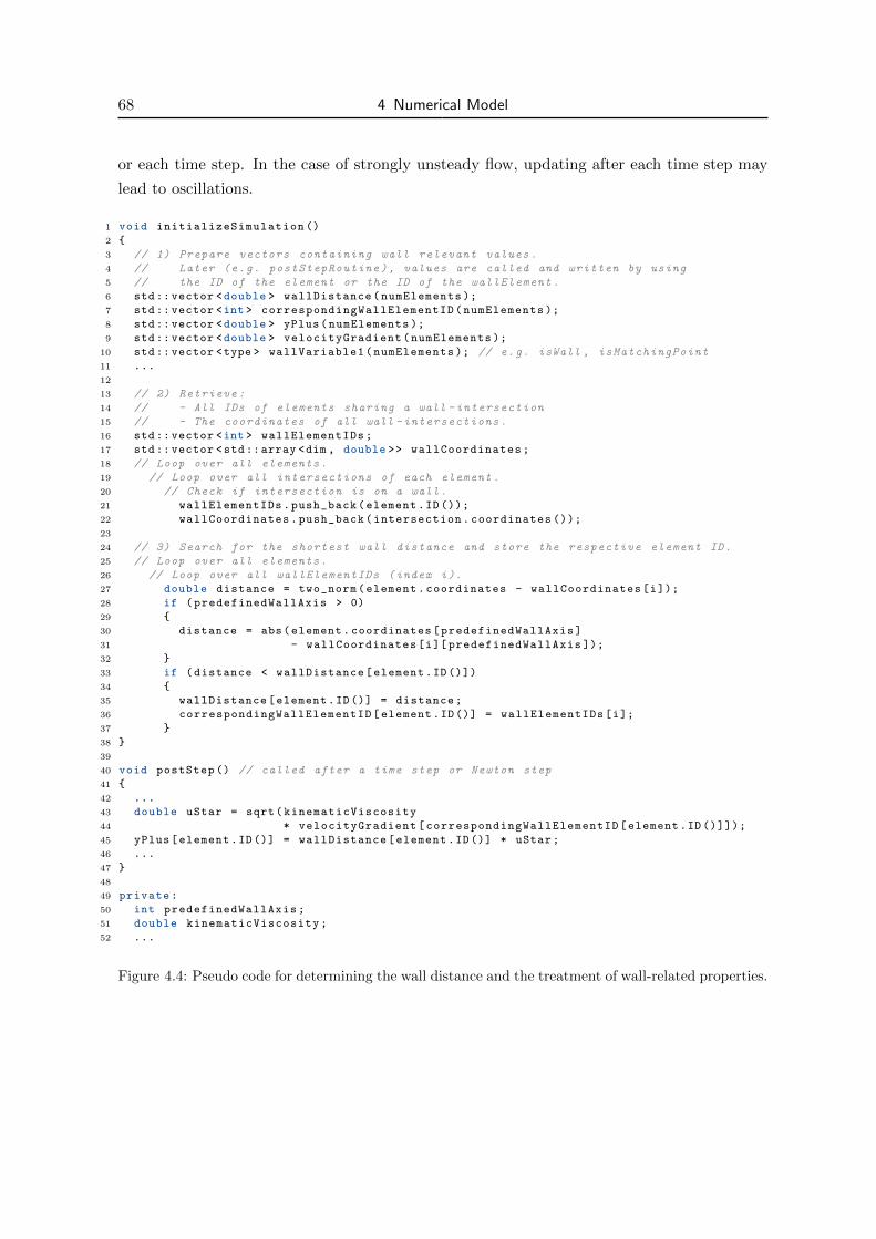
68 4 Numerical Model
or each time step. In the case of strongly unsteady flow, updating after each time step may
lead to oscillations.
1 void initializeSimulation ()
2
3 // 1) Prepare vectors containing wall relevant values.
4 // Later (e.g. postStepRoutine ), values are called and written by using
5 // the ID of the element or the ID of the wallElement .
6 std::vector <double > wallDistance(numElements );
7 std::vector <int > correspondingWallElementID(numElements );
8 std::vector <double > yPlus(numElements );
9 std::vector <double > velocityGradient(numElements );
10 std::vector <type > wallVariable1(numElements ); // e.g. isWall , isMatchingPoint
11 ...
12
13 // 2) Retrieve:
14 // - All IDs of elements sharing a wall - intersection
15 // - The coordinates of all wall - intersections .
16 std::vector <int > wallElementIDs;
17 std::vector <std::array <dim , double >> wallCoordinates;
18 // Loop over all elements.
19 // Loop over all intersections of each element.
20 // Check if intersection is on a wall.
21 wallElementIDs.push_back(element.ID());
22 wallCoordinates.push_back(intersection.coordinates ());
23
24 // 3) Search for the shortest wall distance and store the respective element ID.
25 // Loop over all elements.
26 // Loop over all wallElementIDs (index i).
27 double distance = two_norm(element.coordinates - wallCoordinates[i]);
28 if (predefinedWallAxis > 0)
29
30 distance = abs(element.coordinates[predefinedWallAxis]
31 - wallCoordinates[i][ predefinedWallAxis ]);
32
33 if (distance < wallDistance[element.ID()])
34
35 wallDistance[element.ID()] = distance;
36 correspondingWallElementID[element.ID()] = wallElementIDs[i];
37
38
39
40 void postStep () // called after a time step or Newton step
41
42 ...
43 double uStar = sqrt(kinematicViscosity
44 * velocityGradient[correspondingWallElementID[element.ID ()]]);
45 yPlus[element.ID()] = wallDistance[element.ID()] * uStar;
46 ...
47
48
49 private:
50 int predefinedWallAxis;
51 double kinematicViscosity;
52 ...
Figure 4.4: Pseudo code for determining the wall distance and the treatment of wall-related properties.

4.3 Implementation 69
Zero-equation models(e.g. Baldwin-Lomax)
Two-equation models(e.g. k-ε)
post step routine starts
for all wall sections:update basic quantities,
e.g. y+, u+, umax
reset switching positions
update tempo-rary quantities
determineswitching positions
update quantities
for all wall sections:ycross = max
for all elements:calculate νinner, νouter
for all wall sections:determine ycross
for all elements:
νt =
νinner, if y ≤ ycross
νouter, if y > ycross
for all elements:reset wall-function
quantities/properties
for all elements:pass current solution tothe wall-function routine
for all elements:use wall function if,y+ ≤ y+
threshold
for all elements:if y+ ≤ y+
threshold: use zero-eq. model, do not use k, ε
Figure 4.5: Flow chart implementation of switching positions and wall-function regions.

5 Results and Discussion
In this chapter, different simulation results are presented and discussed. It is started with
proving the implemented free-flow model concept in section 5.1. Afterward, the attention
is drawn to coupled porous-medium free-flow problems. First, different discretization tech-
niques, model concepts, model simplifications, and model parameters are investigated in sec-
tion 5.2. Then, section 5.3 compares simulation results with results from laboratory experi-
ments. Finally, section 5.4 analyzes the influence of roughness, resulting from heterogeneities,
the sand grains, or porous obstacles.
The definition of boundary conditions for such coupled problem setups is quite complex. For
improving the readability of the setup sketches, Tab. 5.1 contains predefined sets of boundary
conditions. The inflow boundary conditions for the turbulence models are always calculated
by a procedure proposed in ANSYS, Inc. [2009b] or Versteeg and Malalasekra [2009]:
νin =
√3
2vxI ` , kin =
3
2(vxI)2 , εin = C3/4
µ
k3/2in
`, ω =
k1/2in
C1/4µ `
.
The turbulence intensity (I) and the turbulent length scale (`) can be estimated by:
I =
√2/3k
vmean≈ 0.16Re−0.125
dhy, ` = 0.07dhy .
5.1 Validation of the Free-Flow Code
In this first study, all free-flow turbulence models which are implemented in the scope of
this thesis are tested for their proper functionality, see App. B. The respective models are
successfully validated with different testing methods: analytical, numerical, and physical (see
Tab. 5.2). The selection of respective testing methods is done according to common practice
and to available literature data.

72 5 Results and Discussion
domain type default exception
free flow inflow Dirichlet total mass balance is outflowoutflow zero-gradient p is Dirichletsymmetry zero-gradient vn = 0wall no-flow v = 0, ν = 0
k-ε (wall functions): see p. 40ffLow-Re k-ε: k = 0, ε = 0k-ω: see p. 43ff
interface coupling see p. 51ff ν, k, ε, and ω same as free-flow wall
porous medium symmetry no-flow -wall no-flow -const. T wall no-flow T is Dirichletinsulated wall no-flow energy is solution-dependent Neumann
Table 5.1: Definition of boundary condition types for coupled problems. For any primary variable ϕ,Dirichlet means the value on the boundary is fixed, solution-dependent Neumann meansthe boundary flux depends on the current solution, the cell properties, and the fixed valueon the boundary, zero-gradient means ∂ϕ/∂xn = 0, and no-flow means qϕadv + qϕdiff = 0.
analytical numerical physical(section B.1) (section B.2) (section B.3)
box Navier-Stokes X
zero-equation models X
MA
C
Navier-Stokes X Xzero-equation models Xone-equation models Xtwo-equation models X X X
Table 5.2: Overview on successfully performed validation cases for the implemented free-flow models.
5.2 Analysis of the Model Concepts
In this section, different model concepts, model simplifications, and discretization methods
are compared with the help of simple test cases. Tab. 5.3 provides a short overview on the
available model concepts. These concepts are then analyzed with respect to their effect on
the exchange fluxes, grid convergence, and computational costs.
5.2.1 Coupling Model Concepts
The differences between a box–box coupling and the different methods for the CCFV–MAC
coupling are highlighted with the help of two different setups. The first features a predomi-
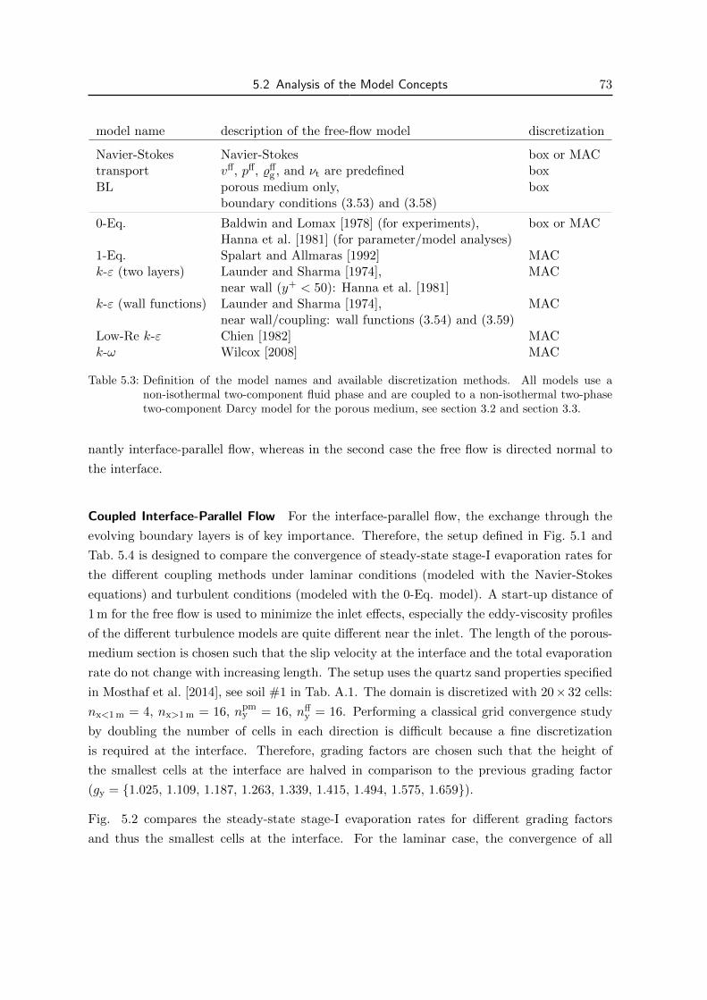
5.2 Analysis of the Model Concepts 73
model name description of the free-flow model discretization
Navier-Stokes Navier-Stokes box or MACtransport vff, pff, %ff
g , and νt are predefined box
BL porous medium only, boxboundary conditions (3.53) and (3.58)
0-Eq. Baldwin and Lomax [1978] (for experiments), box or MACHanna et al. [1981] (for parameter/model analyses)
1-Eq. Spalart and Allmaras [1992] MACk-ε (two layers) Launder and Sharma [1974], MAC
near wall (y+ < 50): Hanna et al. [1981]k-ε (wall functions) Launder and Sharma [1974], MAC
near wall/coupling: wall functions (3.54) and (3.59)Low-Re k-ε Chien [1982] MACk-ω Wilcox [2008] MAC
Table 5.3: Definition of the model names and available discretization methods. All models use anon-isothermal two-component fluid phase and are coupled to a non-isothermal two-phasetwo-component Darcy model for the porous medium, see section 3.2 and section 3.3.
nantly interface-parallel flow, whereas in the second case the free flow is directed normal to
the interface.
Coupled Interface-Parallel Flow For the interface-parallel flow, the exchange through the
evolving boundary layers is of key importance. Therefore, the setup defined in Fig. 5.1 and
Tab. 5.4 is designed to compare the convergence of steady-state stage-I evaporation rates for
the different coupling methods under laminar conditions (modeled with the Navier-Stokes
equations) and turbulent conditions (modeled with the 0-Eq. model). A start-up distance of
1 m for the free flow is used to minimize the inlet effects, especially the eddy-viscosity profiles
of the different turbulence models are quite different near the inlet. The length of the porous-
medium section is chosen such that the slip velocity at the interface and the total evaporation
rate do not change with increasing length. The setup uses the quartz sand properties specified
in Mosthaf et al. [2014], see soil #1 in Tab. A.1. The domain is discretized with 20× 32 cells:
nx<1 m = 4, nx>1 m = 16, npmy = 16, nff
y = 16. Performing a classical grid convergence study
by doubling the number of cells in each direction is difficult because a fine discretization
is required at the interface. Therefore, grading factors are chosen such that the height of
the smallest cells at the interface are halved in comparison to the previous grading factor
(gy = 1.025, 1.109, 1.187, 1.263, 1.339, 1.415, 1.494, 1.575, 1.659).
Fig. 5.2 compares the steady-state stage-I evaporation rates for different grading factors
and thus the smallest cells at the interface. For the laminar case, the convergence of all
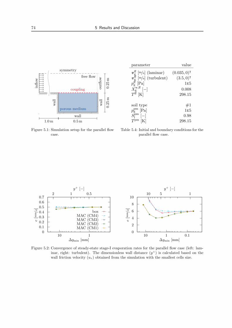
74 5 Results and Discussion
free flow
porous medium
1.0 m 0.5 m
0.25
m0.
25m
wall
wall
wal
lou
tflow
symmetry
infl
ow
coupling
Figure 5.1: Simulation setup for the parallel flowcase.
parameter value
vffg [m/s] (laminar) (0.035, 0)ᵀ
vffg [m/s] (turbulent) (3.5, 0)ᵀ
pffg [Pa] 1e5
Xw,ffg [−] 0.008
T ff [K] 298.15
soil type #1ppm
g [Pa] 1e5Spm
l [−] 0.98T pm [K] 298.15
Table 5.4: Initial and boundary conditions for theparallel flow case.
0
0.1
0.2
0.3
0.4
0.5
0.6
0.7
110
0.512
e[m
m/d
]
∆ymin [mm]
y+ [−]
boxMAC (CM4)MAC (CM3)MAC (CM2)MAC (CM1)
0
2
4
6
8
10
0.1110
5 110
e[m
m/d
]
∆ymin [mm]
y+ [−]
Figure 5.2: Convergence of steady-state stage-I evaporation rates for the parallel flow case (left: lam-inar, right: turbulent). The dimensionless wall distance (y+) is calculated based on thewall friction velocity (uτ ) obtained from the simulation with the smallest cells size.

5.2 Analysis of the Model Concepts 75
1.0 m
2.0
m
0.2 m 0.8 m
0.4
m1.2
m0.4
m
outflow
wall
sym
met
ry
inflow
cou
pli
ng
free flow
porousmedium
A B C
Figure 5.3: Simulation setup for the normal flowcase, after Fetzer et al. [2017b].
parameter value
vffg,x [m/s] 0
vffg,y [m/s] −0.016x2
pffg [Pa] 1e5
Xw,ffg [−] 0.0005
T ff [K] 303.15
soil type #2ppm
g [Pa] 1e5Spm
l [−] 0.85T pm [K] 293.15
Table 5.5: Initial and boundary conditions for thenormal flow case, after Fetzer et al.[2017b].
methods is comparable. The box method performs a little better, which is attributed to
the fact that for a coarser discretization the additional degree of freedom at the interface
is more important. When turbulence is considered, it is seen that the box method and
the coupling using CM4 have a better grid convergence behavior (for this interface-focused
grid refinement). This indicates the importance of an appropriate modeling of the interface
processes. For a sufficiently fine discretization, the results for all methods are comparable.
This discretization depends more on the dimensionless wall distance y+ than on the absolute
distance. For approximating the evaporation rates, a good modeling of the processes in the
viscous sublayer with at least one cell inside the viscous sublayer (y+ < 5) seems to be
inevitable. The simpler coupling methods CM1–CM3, require the smallest cells to be located
inside y+ ≈ 1 for both cases, laminar and turbulent.
Coupled Interface-Normal Flow11 The setup depicted in Fig. 5.3 and Tab. 5.5 is designed to
magnify the difference between CM1–CM3 as their main difference is in the normal momentum
exchange. For this test case, a standard grid refinement procedure is used. Staring with a
grid using 5 × 5 cells, in each refinement step (RS) the number of cells in each direction is
doubled. This test case is only performed for the Navier-Stokes model (Remax,d = 1000).
11The results presented here are an update of those published in: T. Fetzer, C. Gruninger, B. Flemisch,and R. Helmig: On the Conditions for Coupling Free Flow and Porous-Medium Flow in a Finite VolumeFramework, Finite Volumes for Complex Applications VIII, Hyperbolic, Elliptic and Parabolic Problems(FVCA 8, Lille, France, June 2017):347–356, 2017. doi: 10.1007/978-3-319-57394-6_37.
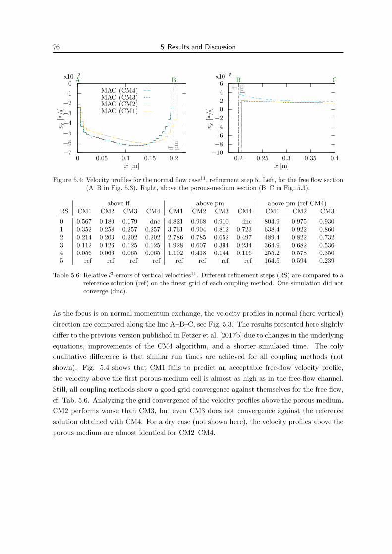
76 5 Results and Discussion
−7
−6
−5
−4
−3
−2
−1
0
0 0.05 0.1 0.15 0.2
ff pm
x10−2
A B
v y[m/s
]
x [m]
MAC (CM4)MAC (CM3)MAC (CM2)MAC (CM1)
−10
−8
−6
−4
−2
0
2
4
6
0.2 0.25 0.3 0.35 0.4
ffp
m
x10−5
B C
v y[m/s
]
x [m]
Figure 5.4: Velocity profiles for the normal flow case11, refinement step 5. Left, for the free flow section(A–B in Fig. 5.3). Right, above the porous-medium section (B–C in Fig. 5.3).
above ff above pm above pm (ref CM4)RS CM1 CM2 CM3 CM4 CM1 CM2 CM3 CM4 CM1 CM2 CM3
0 0.567 0.180 0.179 dnc 4.821 0.968 0.910 dnc 804.9 0.975 0.9301 0.352 0.258 0.257 0.257 3.761 0.904 0.812 0.723 638.4 0.922 0.8602 0.214 0.203 0.202 0.202 2.786 0.785 0.652 0.497 489.4 0.822 0.7323 0.112 0.126 0.125 0.125 1.928 0.607 0.394 0.234 364.9 0.682 0.5364 0.056 0.066 0.065 0.065 1.102 0.418 0.144 0.116 255.2 0.578 0.3505 ref ref ref ref ref ref ref ref 164.5 0.594 0.239
Table 5.6: Relative l2-errors of vertical velocities11. Different refinement steps (RS) are compared to areference solution (ref) on the finest grid of each coupling method. One simulation did notconverge (dnc).
As the focus is on normal momentum exchange, the velocity profiles in normal (here vertical)
direction are compared along the line A–B–C, see Fig. 5.3. The results presented here slightly
differ to the previous version published in Fetzer et al. [2017b] due to changes in the underlying
equations, improvements of the CM4 algorithm, and a shorter simulated time. The only
qualitative difference is that similar run times are achieved for all coupling methods (not
shown). Fig. 5.4 shows that CM1 fails to predict an acceptable free-flow velocity profile,
the velocity above the first porous-medium cell is almost as high as in the free-flow channel.
Still, all coupling methods show a good grid convergence against themselves for the free flow,
cf. Tab. 5.6. Analyzing the grid convergence of the velocity profiles above the porous medium,
CM2 performs worse than CM3, but even CM3 does not convergence against the reference
solution obtained with CM4. For a dry case (not shown here), the velocity profiles above the
porous medium are almost identical for CM2–CM4.

5.2 Analysis of the Model Concepts 77
5.2.2 Free-Flow Model Concepts
Two different types of model concepts are analyzed for turbulent conditions with the help of
the parallel-flow setup described in section 5.2.1. First, different simplifications of the coupled
porous-medium and free-flow model with respect to the representation of the turbulent free
flow are compared. Then, the impact of turbulence models of different complexity on the
evaporation rate is investigated. If not stated otherwise, the MAC implementation with CM4
is used from hereon.
Model Simplifications Simplifications of the porous-medium model are not subject of this
study and are more thoroughly discussed in Vanderborght et al. [2017] and Fetzer et al.
[2017c]. Here, the focus is on the effect of different simplifications of the turbulent free-flow
model on the resulting evaporation rate.
The transport model uses a pre-simulation step for calculating the flow field and the turbulent
quantities. This pre-simulation step may account for complex geometries and their feedback
on the flow field. Afterward, in the coupled simulation, no momentum balances are solved
and the transport of water mass and energy is calculated with the help of the given flow field.
The k-ε (wall functions) model only works for a flat interface and a coarse interface-normal dis-
cretization, when the cell center of the interface-adjacent free-flow cell is inside the turbulent
region. To keep the interface-normal/vertical grading consistent with the other simulations,
the number of cells in the free-flow region is reduced to 5 cells in vertical direction, resulting
in a minimum cell height of ∆y ≈ 10 mm.
The boundary layer models (BL) avoid a detailed modeling of the free-flow processes by using
the boundary layer information to specify one-dimensional boundary conditions for mass and
energy at the top of the porous-medium domain.
The evaporation process for the different simplifications is quite similar, but the predicted
stage-I evaporation rates differ, see Fig. 5.5 (left). For this plot, the BL models use y+ = 15 to
estimate the boundary layer thickness. This value is fitted to this specific setup with a porous-
medium section with a length of 0.5 m. A value of y+ = 30, which corresponds to the beginning
of the log law region (cf. Tab. 2.2), would lead to similar results as by the k-ε (wall functions)
model. The quality of the k-ε (wall functions) model depends on the length of the porous-
medium section. The advantage of the 0-Eq., the k-ε (wall functions), and the transport
model is their ability to predict lateral variation in free-flow conditions. This becomes visible
when the length of the porous-medium section is increased from 0.5 m to 128 m, see Fig. 5.5
(right). The BL models predict almost no variation in evaporation rate and are especially not
able to predict the decrease in rate for long porous-medium sections (' 100 m). Then, the
free flow approaches a relative humidity of 100% and no more evaporation can take place.

78 5 Results and Discussion
0
2
4
6
8
10
0 2 4 6 8 10 12 14
e[m
m/d
]
t [d]
0-Eq.k-ε (wall functions)
transportBL 2-DBL 1-D
0
2
4
6
8
10
1 10 100
e[m
m/d
]
length of porous-medium section [m]
0-Eq.k-ε (wall functions)
transportBL 2-D (y+ = 30)BL 1-D (y+ = 30)
Figure 5.5: Temporal evolution of the evaporation rate for different model simplifications (left). Effectof the length of the porous-medium section on the steady-state stage-I evaporation ratefor different model simplifications (right). Note that in the right plot a different y+-valueis used for the BL models.
0
2
4
6
8
10
0 2 4 6 8 10 12 14
e[m
m/d
]
t [d]
0-Eq.1-Eq.
k-ε (two layers)Low-Re k-ε
k-ωaverage
0
2
4
6
8
10
1 10 100
e[m
m/d
]
length of porous-medium section [m]
0-Eq.1-Eq.
k-ε (wall functions)k-ε (two layers)
Low-Re k-εk-ω
Figure 5.6: Temporal evolution of the evaporation rate for different turbulence models (left). Effect ofthe length of the porous-medium section on the steady-state stage-I evaporation rate fordifferent turbulence models (right).
Nevertheless, the BL models are attractive as they provide a considerable speed-up, see
Tab. 5.7. Their simulation times are less than 3% of the 0-Eq. model. Also, the trans-
port model shows a speed-up, even though it is not yet optimized (an explicit time dis-
cretization scheme and less solution-dependent fluid properties could be used). For the
k-ε (wall functions) model, half of the speed-up is caused by differences in the implemen-
tation of the box and the MAC scheme, the other half originates from less cells inside the
free-flow region.
Turbulence Models Fig. 5.6 (left) indicates a qualitatively similar behavior for the different
turbulence models, but differences in predicted stage-I evaporation rates (±12% compared to
their average rate). The key factor for this behavior is the usage of different damping functions
for the eddy viscosity which is important for a correct prediction of its value in the near-wall
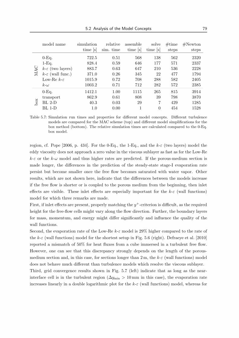
5.2 Analysis of the Model Concepts 79
model name simulation relative assemble solve #time #Newtontime [s] sim. time time [s] time [s] steps steps
MA
C
0-Eq. 722.5 0.51 568 138 562 23201-Eq. 828.4 0.59 646 177 571 2337k-ε (two layers) 883.7 0.63 647 210 536 2228k-ε (wall func.) 371.0 0.26 345 22 477 1794Low-Re k-ε 1015.9 0.72 708 288 582 2405k-ω 1003.2 0.71 712 282 572 2385
box
0-Eq. 1412.1 1.00 1115 265 815 3914transport 862.9 0.61 808 39 798 3870BL 2-D 40.3 0.03 29 7 429 1285BL 1-D 1.0 0.00 1 0 454 1528
Table 5.7: Simulation run times and properties for different model concepts. Different turbulencemodels are compared for the MAC scheme (top) and different model simplifications for thebox method (bottom). The relative simulation times are calculated compared to the 0-Eq.box model.
region, cf. Pope [2006, p. 434]. For the 0-Eq., the 1-Eq., and the k-ε (two layers) model the
eddy viscosity does not approach a zero value in the viscous sublayer as fast as for the Low-Re
k-ε or the k-ω model and thus higher rates are predicted. If the porous-medium section is
made longer, the differences in the prediction of the steady-state stage-I evaporation rate
persist but become smaller once the free flow becomes saturated with water vapor. Other
results, which are not shown here, indicate that the differences between the models increase
if the free flow is shorter or is coupled to the porous medium from the beginning, then inlet
effects are visible. These inlet effects are especially important for the k-ε (wall functions)
model for which three remarks are made.
First, if inlet effects are present, properly matching the y+-criterion is difficult, as the required
height for the free-flow cells might vary along the flow direction. Further, the boundary layers
for mass, momentum, and energy might differ significantly and influence the quality of the
wall functions.
Second, the evaporation rate of the Low-Re k-ε model is 29% higher compared to the rate of
the k-ε (wall functions) model for the shortest setup in Fig. 5.6 (right). Defraeye et al. [2010]
reported a mismatch of 50% for heat fluxes from a cube immersed in a turbulent free flow.
However, one can see that this discrepancy strongly depends on the length of the porous-
medium section and, in this case, for sections longer than 2 m, the k-ε (wall functions) model
does not behave much different than turbulence models which resolve the viscous sublayer.
Third, grid convergence results shown in Fig. 5.7 (left) indicate that as long as the near-
interface cell is in the turbulent region (∆ymin > 10 mm in this case), the evaporation rate
increases linearly in a double logarithmic plot for the k-ε (wall functions) model, whereas for
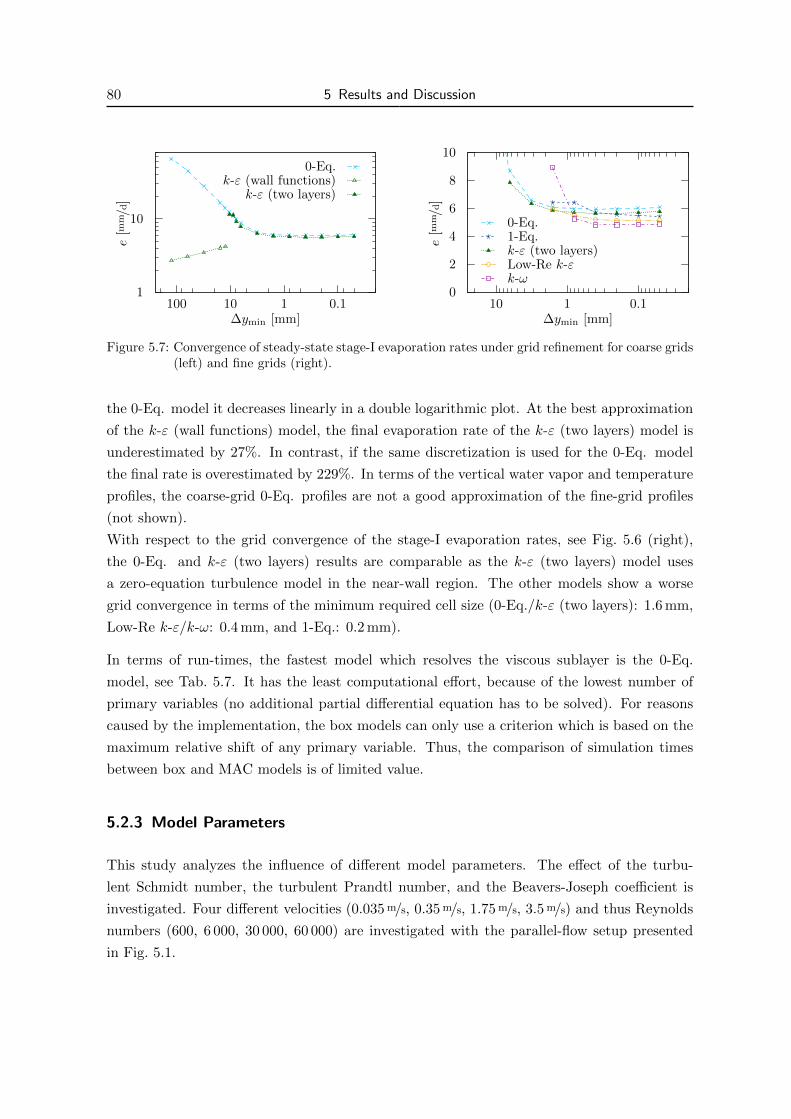
80 5 Results and Discussion
1
10
0.1110100
e[m
m/d
]
∆ymin [mm]
0-Eq.k-ε (wall functions)
k-ε (two layers)
0
2
4
6
8
10
0.1110
e[m
m/d
]
∆ymin [mm]
0-Eq.1-Eq.k-ε (two layers)Low-Re k-εk-ω
Figure 5.7: Convergence of steady-state stage-I evaporation rates under grid refinement for coarse grids(left) and fine grids (right).
the 0-Eq. model it decreases linearly in a double logarithmic plot. At the best approximation
of the k-ε (wall functions) model, the final evaporation rate of the k-ε (two layers) model is
underestimated by 27%. In contrast, if the same discretization is used for the 0-Eq. model
the final rate is overestimated by 229%. In terms of the vertical water vapor and temperature
profiles, the coarse-grid 0-Eq. profiles are not a good approximation of the fine-grid profiles
(not shown).
With respect to the grid convergence of the stage-I evaporation rates, see Fig. 5.6 (right),
the 0-Eq. and k-ε (two layers) results are comparable as the k-ε (two layers) model uses
a zero-equation turbulence model in the near-wall region. The other models show a worse
grid convergence in terms of the minimum required cell size (0-Eq./k-ε (two layers): 1.6 mm,
Low-Re k-ε/k-ω: 0.4 mm, and 1-Eq.: 0.2 mm).
In terms of run-times, the fastest model which resolves the viscous sublayer is the 0-Eq.
model, see Tab. 5.7. It has the least computational effort, because of the lowest number of
primary variables (no additional partial differential equation has to be solved). For reasons
caused by the implementation, the box models can only use a criterion which is based on the
maximum relative shift of any primary variable. Thus, the comparison of simulation times
between box and MAC models is of limited value.
5.2.3 Model Parameters
This study analyzes the influence of different model parameters. The effect of the turbu-
lent Schmidt number, the turbulent Prandtl number, and the Beavers-Joseph coefficient is
investigated. Four different velocities (0.035 m/s, 0.35 m/s, 1.75 m/s, 3.5 m/s) and thus Reynolds
numbers (600, 6 000, 30 000, 60 000) are investigated with the parallel-flow setup presented
in Fig. 5.1.
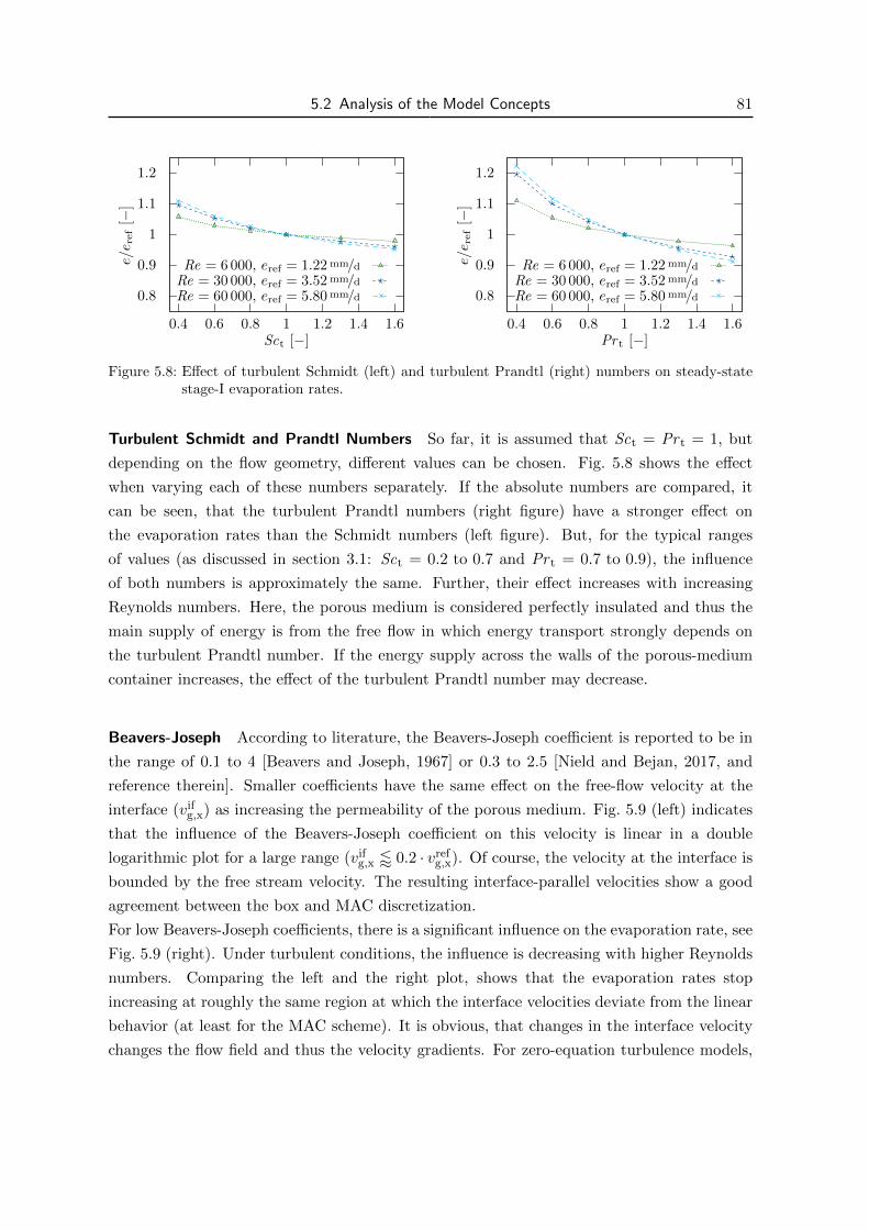
5.2 Analysis of the Model Concepts 81
0.8
0.9
1
1.1
1.2
0.4 0.6 0.8 1 1.2 1.4 1.6
e/e r
ef
[−]
Sct [−]
Re = 6 000, eref = 1.22 mm/dRe = 30 000, eref = 3.52 mm/dRe = 60 000, eref = 5.80 mm/d 0.8
0.9
1
1.1
1.2
0.4 0.6 0.8 1 1.2 1.4 1.6
e/e r
ef
[−]
Pr t [−]
Re = 6 000, eref = 1.22 mm/dRe = 30 000, eref = 3.52 mm/dRe = 60 000, eref = 5.80 mm/d
Figure 5.8: Effect of turbulent Schmidt (left) and turbulent Prandtl (right) numbers on steady-statestage-I evaporation rates.
Turbulent Schmidt and Prandtl Numbers So far, it is assumed that Sct = Pr t = 1, but
depending on the flow geometry, different values can be chosen. Fig. 5.8 shows the effect
when varying each of these numbers separately. If the absolute numbers are compared, it
can be seen, that the turbulent Prandtl numbers (right figure) have a stronger effect on
the evaporation rates than the Schmidt numbers (left figure). But, for the typical ranges
of values (as discussed in section 3.1: Sct = 0.2 to 0.7 and Pr t = 0.7 to 0.9), the influence
of both numbers is approximately the same. Further, their effect increases with increasing
Reynolds numbers. Here, the porous medium is considered perfectly insulated and thus the
main supply of energy is from the free flow in which energy transport strongly depends on
the turbulent Prandtl number. If the energy supply across the walls of the porous-medium
container increases, the effect of the turbulent Prandtl number may decrease.
Beavers-Joseph According to literature, the Beavers-Joseph coefficient is reported to be in
the range of 0.1 to 4 [Beavers and Joseph, 1967] or 0.3 to 2.5 [Nield and Bejan, 2017, and
reference therein]. Smaller coefficients have the same effect on the free-flow velocity at the
interface (vifg,x) as increasing the permeability of the porous medium. Fig. 5.9 (left) indicates
that the influence of the Beavers-Joseph coefficient on this velocity is linear in a double
logarithmic plot for a large range (vifg,x / 0.2 · vref
g,x). Of course, the velocity at the interface is
bounded by the free stream velocity. The resulting interface-parallel velocities show a good
agreement between the box and MAC discretization.
For low Beavers-Joseph coefficients, there is a significant influence on the evaporation rate, see
Fig. 5.9 (right). Under turbulent conditions, the influence is decreasing with higher Reynolds
numbers. Comparing the left and the right plot, shows that the evaporation rates stop
increasing at roughly the same region at which the interface velocities deviate from the linear
behavior (at least for the MAC scheme). It is obvious, that changes in the interface velocity
changes the flow field and thus the velocity gradients. For zero-equation turbulence models,
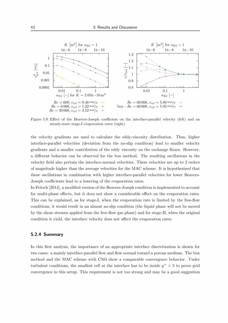
82 5 Results and Discussion
0.0001
0.001
0.01
0.1
1
0.01 0.1 1
1e−101e−81e−6
vif g,x
[m/s
]
αBJ [−] for K = 2.65e−10 m2
K[m2]
for αBJ = 1
0.8
0.9
1
1.1
1.2
1.3
0.01 0.1 1
1e−101e−81e−6
e/e r
ef
[−]
αBJ [−]
K[m2]
for αBJ = 1
Re = 600, eref = 0.46 mm/dRe = 6 000, eref = 1.22 mm/d
Re = 30 000, eref = 3.52 mm/d
Re = 60 000, eref = 5.80 mm/dbox - Re = 60 000, eref = 5.95 mm/d
Figure 5.9: Effect of the Beavers-Joseph coefficient on the interface-parallel velocity (left) and onsteady-state stage-I evaporation rates (right).
the velocity gradients are used to calculate the eddy-viscosity distribution. Thus, higher
interface-parallel velocities (deviation from the no-slip condition) lead to smaller velocity
gradients and a smaller contribution of the eddy viscosity on the exchange fluxes. However,
a different behavior can be observed for the box method. The resulting oscillations in the
velocity field also pertain the interface-normal velocities. These velocities are up to 2 orders
of magnitude higher than the average velocities for the MAC scheme. It is hypothesized that
these oscillations in combination with higher interface-parallel velocities for lower Beavers-
Joseph coefficients lead to a lowering of the evaporation rates.
In Fritsch [2014], a modified version of the Beavers-Joseph condition is implemented to account
for multi-phase effects, but it does not show a considerable effect on the evaporation rates.
This can be explained, as for stage-I, when the evaporation rate is limited by the free-flow
conditions, it would result in an almost no-slip condition (the liquid phase will not be moved
by the shear stresses applied from the free-flow gas phase) and for stage-II, when the original
condition is yield, the interface velocity does not affect the evaporation rates.
5.2.4 Summary
In this first analysis, the importance of an appropriate interface discretization is shown for
two cases: a mainly interface-parallel flow and flow normal toward a porous medium. The box
method and the MAC scheme with CM4 show a comparable convergence behavior. Under
turbulent conditions, the smallest cell at the interface has to be inside y+ < 5 to prove grid
convergence in this setup. This requirement is not too strong and may be a good suggestion
5.3 Comparison with Experiments 83
for other cases. Wilcox [2006, Ch.7.6] writes that “it is imperative to require” y+ < 1 for
turbulence models which integrate through the viscous sublayer; this is only not the case for
the k-ε (wall functions) and the BL models. The coupling methods CM1–CM3 can be applied
for fine discretizations (y+ < 1) and lead to the same results, if no relevant interface-normal
flow is present.
The stage-I evaporation rates of the investigated turbulence models differ by about ±12%
with respect to their mean rate. They also differ in their grid convergence of steady-state
stage-I evaporation rates and their simulation times. Simplifying the free-flow model is possi-
ble under certain conditions, e.g. the BL models provide a good and fast first approximation
for simple geometries, but involve fitting parameters with a strong influence. The k-ε (wall
functions) model also features some speed-up but the accuracy of the stage-I evaporation rate
depends on the optimization of the grid and the length of the porous-medium section. The
transport model, in which the flow field is solved in a pre-simulation step, shows the best
results for a simplified model and it might also be used for more complex geometries.
The parameter study reveals similar effects when varying the turbulent Schmidt and Prandtl
numbers. If they are changed from 1 to a lower, more geometry-specific value, the evapora-
tion rate increases. For a large range of Beavers-Joseph coefficients (especially all values in a
physically meaningful range) there is a log-log-linear relation between the Beavers-Joseph co-
efficient and the interface-parallel velocity. The relative increase in the evaporation rate is the
largest for low Reynolds numbers in a turbulent regime and low Beavers-Joseph coefficients.
However, very low Beavers-Joseph coefficients decrease the evaporation rate again. Different
behaviors are observed for the box and the MAC discretization. The box method shows a de-
crease in evaporation rate for lower coefficients, whereas the MAC scheme shows an increase.
It has to be said, that the box method reveals large oscillations in both, the interface-normal
and the interface-parallel velocity components, which have a strong influence on the resulting
exchange fluxes.
5.3 Comparison with Experiments
In this section, modeling results are compared and analyzed with the help of laboratory exper-
iments. Although enough experiments, which couple porous-medium and free-flow processes,
exist in literature, only a small number is suited for the validation of the presented numerical
model concept. The main reasons are: (i) the soil sample evaporates into a laminar free
flow or the open lab atmosphere [e.g. Lehmann et al., 2008, Shokri et al., 2010, Smits et al.,
2012, Zhang et al., 2015], (ii) the free flow is too complex [e.g. Belhamri and Fohr [1996] in-
clude laminar to turbulent transitions or Song et al. [2014] include inlet/jet effects], (iii) lack
of available geometrical information, input parameters, or measured data [e.g. Sugita and
84 5 Results and Discussion
Kishii, 2002], or (iv) radiation, precipitation, or other processes inside the porous medium
are involved [e.g. Yamanaka et al., 1997, Fujimaki et al., 2006, Wanphen and Nagano, 2009,
Jambhekar et al., 2015].
For stage-I evaporation, the free-flow conditions and especially the energy supply are crucial.
Therefore, the analysis focuses on matching evaporation rates and temperature evolutions.
Plotting the evaporation rates highlights differences during stage-I, when high evaporation
rates prevail. If one aims at comparing integral values or stage-II behavior, cumulative mass
loss plots are helpful. Fetzer et al. [2016] and Gruninger [2017] indicate that the problem
setup, e.g. the thermal boundary conditions and the considered geometry or dimensionality,
has a strong effect on the resulting transfer fluxes For this reason, the dimension at which
the problem is considered (2-D vs. 3-D) and the thermal boundary conditions: (i) a perfectly
insulated porous medium (perfectly insulated walls), (ii) a solution dependent energy transfer
across the porous-medium walls (insulated walls), and (iii) constant temperatures at the
porous-medium walls (const. T walls) are analyzed. Of course, the porous-medium properties
also contribute to the characteristics of the evaporation process. This is comprehensively
analyzed in Mosthaf et al. [2014].
In general, the basic experimental setups are comparatively similar. For all experiments, the
simulation setup is a variation of the parallel-flow setup in Fig. 5.1. Tab. 5.8 lists the different
setups with their geometrical information, porous-medium properties, boundary conditions,
and initial conditions. In all cases, it is most difficult to specify the position at which the
free-flow conditions are measured (start-up length) and the vertical profiles of velocity, rel-
ative humidity, and temperature. Therefore, spatially constant values are set at the inflow
boundary and the start-up length is specified according to estimations based on the respec-
tive publication. First, the model is compared to the experiments by Mosthaf et al. [2014] to
analyze how the changes in the underlying numerical model affect the simulation results. If
not stated otherwise, all simulations for this section are run with the Baldwin-Lomax 0-Eq.
model using the MAC discretization with CM4 and Sct = Pr t = 1.
5.3.1 Mosthaf et al. [2014]
Mosthaf et al. [2014] perform evaporation experiments in which water evaporates from an
insulated, rectangular, sand-filled Plexiglas box into a free air flow through a circular pipe. A
Styrofoam insulation is applied around this box to minimize the heat loss. The soil sample is
located on a balance which is used to determine the mass loss and thus the evaporation rate.
Thermocouples inside the sand box and the windtunnel are used to monitor the temperature
evolution over the experiment height and the run time.
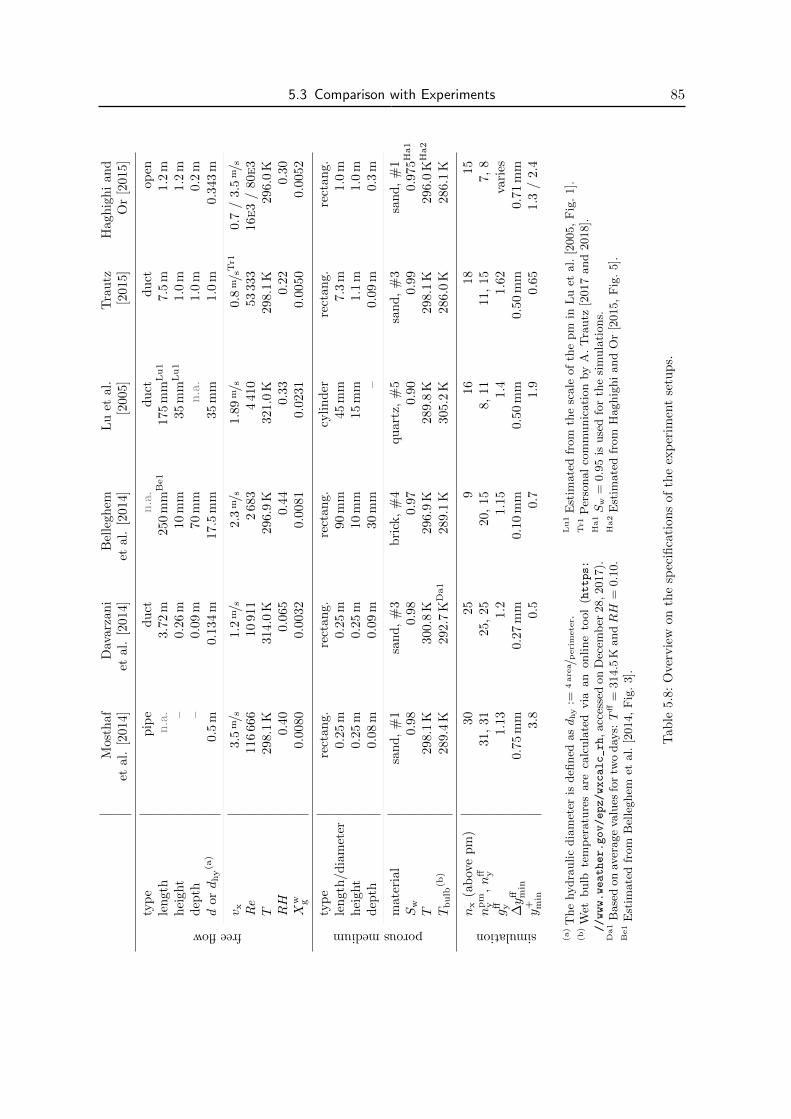
5.3 Comparison with Experiments 85M
osth
afD
avarz
an
iB
elle
gh
emL
uet
al.
Tra
utz
Hagh
igh
ian
det
al.
[201
4]et
al.
[2014]
etal.
[2014]
[2005]
[2015]
Or
[2015]
freeflow
typ
ep
ipe
du
ctn.a
.d
uct
du
ctop
enle
ngt
hn
.a.
3.7
2m
250
mm
Be1
175
mm
Lu1
7.5
m1.2
mh
eigh
t–
0.2
6m
10
mm
35
mm
Lu1
1.0
m1.2
md
epth
–0.0
9m
70
mm
n.a
.1.
0m
0.2
m
dord
hy
(a)
0.5
m0.1
34
m17.
5m
m35
mm
1.0
m0.3
43
m
v x3.
5m/s
1.2
m/s
2.3
m/s
1.89
m/s
0.8
m/s
Tr1
0.7
/3.
5m/s
Re
116
666
10
911
2683
4410
53
333
16e
3/
80e
3T
298.1
K314.
0K
296.
9K
321.
0K
298.
1K
296.
0K
RH
0.4
00.0
65
0.4
40.3
30.2
20.3
0X
w g0.
0080
0.0
032
0.0
081
0.0
231
0.0
050
0.0
052
porousmedium
typ
ere
ctan
g.re
ctan
g.
rect
an
g.
cyli
nd
erre
ctan
g.
rect
an
g.
len
gth
/dia
met
er0.
25m
0.2
5m
90
mm
45
mm
7.3
m1.0
mh
eigh
t0.
25m
0.2
5m
10
mm
15
mm
1.1
m1.0
md
epth
0.08
m0.0
9m
30
mm
–0.
09
m0.3
m
mat
eria
lsa
nd
,#
1sa
nd,
#3
bri
ck,
#4
qu
art
z,#
5sa
nd
,#
3sa
nd
,#
1S
w0.9
80.9
80.9
70.9
00.9
90.9
75
Ha1
T29
8.1
K300.
8K
296.
9K
289.
8K
298.
1K
296.0
KH
a2
Tbulb
(b)
289.4
K292.7
KD
a1
289.1
K305.
2K
286.
0K
286.
1K
simulation
nx
(ab
ove
pm
)30
25
916
18
15
npm
y,n
ff y31
,31
25,
25
20,
15
8,
11
11,
15
7,
8g
ff y1.
131.2
1.1
51.4
1.6
2va
ries
∆y
ff min
0.7
5m
m0.
27
mm
0.10
mm
0.50
mm
0.50
mm
0.71
mm
y+ m
in3.
80.5
0.7
1.9
0.6
51.3
/2.4
(a)
The
hydra
ulic
dia
met
eris
defi
ned
asd
hy
:=4
are
a /p
eri
mete
r.(b
)W
etbulb
tem
per
atu
res
are
calc
ula
ted
via
an
online
tool
(https:
//www.weather.gov/epz/wxcalc_rh,acc
esse
don
Dec
emb
er28,2017).
Da1
Base
don
aver
age
valu
esfo
rtw
oday
s:T
ff=
314.5
KandRH
=0.1
0.
Be1
Est
imate
dfr
om
Bel
leghem
etal.
[2014,
Fig
.3].
Lu1
Est
imate
dfr
om
the
scale
of
the
pm
inL
uet
al.
[2005,
Fig
.1].
Tr1
Per
sonal
com
munic
ati
on
by
A.
Tra
utz
[2017
and
2018].
Ha1S
w=
0.9
5is
use
dfo
rth
esi
mula
tions.
Ha2
Est
imate
dfr
om
Haghig
hi
and
Or
[2015,
Fig
.5].
Tab
le5.
8:O
ver
vie
won
the
spec
ifica
tion
sof
the
exp
erim
ent
setu
ps.
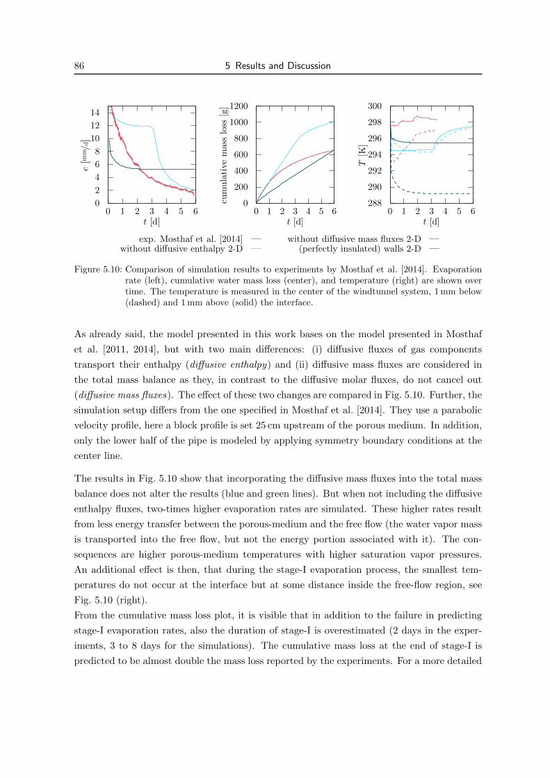
86 5 Results and Discussion
0
2
4
6
8
10
12
14
0 1 2 3 4 5 6
e[m
m/d
]
t [d]
0
200
400
600
800
1000
1200
0 1 2 3 4 5 6cu
mu
lati
vem
ass
loss
[g]
t [d]
288
290
292
294
296
298
300
0 1 2 3 4 5 6
T[K
]
t [d]
exp. Mosthaf et al. [2014]without diffusive enthalpy 2-D
without diffusive mass fluxes 2-D(perfectly insulated) walls 2-D
Figure 5.10: Comparison of simulation results to experiments by Mosthaf et al. [2014]. Evaporationrate (left), cumulative water mass loss (center), and temperature (right) are shown overtime. The temperature is measured in the center of the windtunnel system, 1 mm below(dashed) and 1 mm above (solid) the interface.
As already said, the model presented in this work bases on the model presented in Mosthaf
et al. [2011, 2014], but with two main differences: (i) diffusive fluxes of gas components
transport their enthalpy (diffusive enthalpy) and (ii) diffusive mass fluxes are considered in
the total mass balance as they, in contrast to the diffusive molar fluxes, do not cancel out
(diffusive mass fluxes). The effect of these two changes are compared in Fig. 5.10. Further, the
simulation setup differs from the one specified in Mosthaf et al. [2014]. They use a parabolic
velocity profile, here a block profile is set 25 cm upstream of the porous medium. In addition,
only the lower half of the pipe is modeled by applying symmetry boundary conditions at the
center line.
The results in Fig. 5.10 show that incorporating the diffusive mass fluxes into the total mass
balance does not alter the results (blue and green lines). But when not including the diffusive
enthalpy fluxes, two-times higher evaporation rates are simulated. These higher rates result
from less energy transfer between the porous-medium and the free flow (the water vapor mass
is transported into the free flow, but not the energy portion associated with it). The con-
sequences are higher porous-medium temperatures with higher saturation vapor pressures.
An additional effect is then, that during the stage-I evaporation process, the smallest tem-
peratures do not occur at the interface but at some distance inside the free-flow region, see
Fig. 5.10 (right).
From the cumulative mass loss plot, it is visible that in addition to the failure in predicting
stage-I evaporation rates, also the duration of stage-I is overestimated (2 days in the exper-
iments, 3 to 8 days for the simulations). The cumulative mass loss at the end of stage-I is
predicted to be almost double the mass loss reported by the experiments. For a more detailed
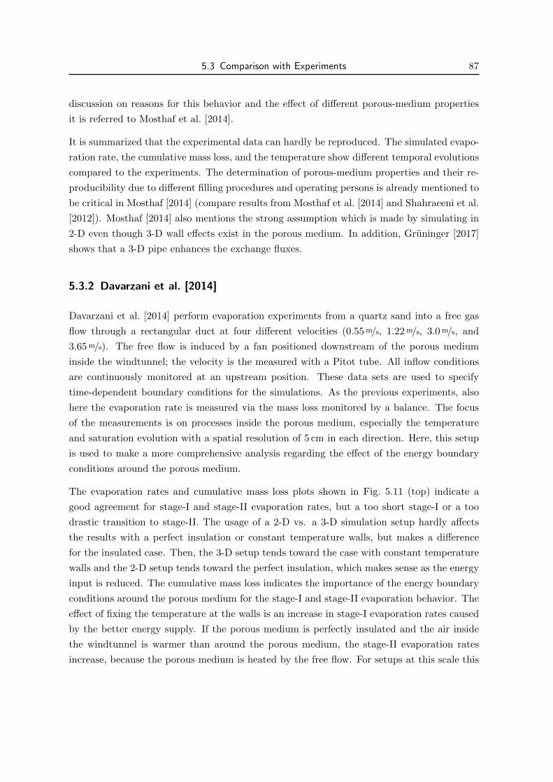
5.3 Comparison with Experiments 87
discussion on reasons for this behavior and the effect of different porous-medium properties
it is referred to Mosthaf et al. [2014].
It is summarized that the experimental data can hardly be reproduced. The simulated evapo-
ration rate, the cumulative mass loss, and the temperature show different temporal evolutions
compared to the experiments. The determination of porous-medium properties and their re-
producibility due to different filling procedures and operating persons is already mentioned to
be critical in Mosthaf [2014] (compare results from Mosthaf et al. [2014] and Shahraeeni et al.
[2012]). Mosthaf [2014] also mentions the strong assumption which is made by simulating in
2-D even though 3-D wall effects exist in the porous medium. In addition, Gruninger [2017]
shows that a 3-D pipe enhances the exchange fluxes.
5.3.2 Davarzani et al. [2014]
Davarzani et al. [2014] perform evaporation experiments from a quartz sand into a free gas
flow through a rectangular duct at four different velocities (0.55 m/s, 1.22 m/s, 3.0 m/s, and
3.65 m/s). The free flow is induced by a fan positioned downstream of the porous medium
inside the windtunnel; the velocity is the measured with a Pitot tube. All inflow conditions
are continuously monitored at an upstream position. These data sets are used to specify
time-dependent boundary conditions for the simulations. As the previous experiments, also
here the evaporation rate is measured via the mass loss monitored by a balance. The focus
of the measurements is on processes inside the porous medium, especially the temperature
and saturation evolution with a spatial resolution of 5 cm in each direction. Here, this setup
is used to make a more comprehensive analysis regarding the effect of the energy boundary
conditions around the porous medium.
The evaporation rates and cumulative mass loss plots shown in Fig. 5.11 (top) indicate a
good agreement for stage-I and stage-II evaporation rates, but a too short stage-I or a too
drastic transition to stage-II. The usage of a 2-D vs. a 3-D simulation setup hardly affects
the results with a perfect insulation or constant temperature walls, but makes a difference
for the insulated case. Then, the 3-D setup tends toward the case with constant temperature
walls and the 2-D setup tends toward the perfect insulation, which makes sense as the energy
input is reduced. The cumulative mass loss indicates the importance of the energy boundary
conditions around the porous medium for the stage-I and stage-II evaporation behavior. The
effect of fixing the temperature at the walls is an increase in stage-I evaporation rates caused
by the better energy supply. If the porous medium is perfectly insulated and the air inside
the windtunnel is warmer than around the porous medium, the stage-II evaporation rates
increase, because the porous medium is heated by the free flow. For setups at this scale this
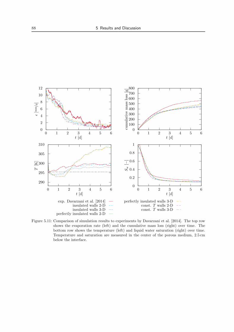
88 5 Results and Discussion
0
2
4
6
8
10
12
0 1 2 3 4 5 6
e[m
m/d
]
t [d]
0
100
200
300
400
500
600
700
800
0 1 2 3 4 5 6
cum
ula
tive
mass
loss
[g]
t [d]
290
295
300
305
310
0 1 2 3 4 5 6
T[K
]
t [d]
0
0.2
0.4
0.6
0.8
1
0 1 2 3 4 5 6
Sw
[−]
t [d]
exp. Davarzani et al. [2014]insulated walls 2-Dinsulated walls 3-D
perfectly insulated walls 2-D
perfectly insulated walls 3-Dconst. T walls 2-Dconst. T walls 3-D
Figure 5.11: Comparison of simulation results to experiments by Davarzani et al. [2014]. The top rowshows the evaporation rate (left) and the cumulative mass loss (right) over time. Thebottom row shows the temperature (left) and liquid water saturation (right) over time.Temperature and saturation are measured in the center of the porous medium, 2.5 cmbelow the interface.

5.3 Comparison with Experiments 89
means, that a substantial amount of energy is supplied or extracted through the walls of the
(insulated) porous-medium box.
The temporal temperature evolution in the center of the porous medium 2.5 cm below the
interface shows that both extreme scenarios cannot predict the correct behavior, see Fig. 5.11
(bottom left). The case which includes an insulation, qualitatively reflects the fluctuations
seen in the experiments and approaches the final stage-II temperature. The data sets from
temperature and saturation sensors only show a little variation inside one row and therefore
only one data set is compared with the simulations. For the sensor in the middle of the first
row of sensors, there is a good qualitative agreement between the measured and the simulated
saturation evolution Fig. 5.11 (bottom right). The match between data from experiments and
simulations is worse for the other sensors in vertical directions.
Possible error sources are the definition of free-flow boundary conditions, especially those for
the velocity. In comparison to the previous experiments, no flow straighteners are used and
the wind is induced by a downstream-located fan. However, for the simulations a block-shaped
velocity profile entering the upstream part of the windtunnel is assumed. The influence of
the position at which a block profile is assumed is analyzed in Fetzer et al. [2016]. Further, a
strong modeling assumption is that the temperature of the air flow is already constant over
position at the inflow boundary and therefore no heater section is modeled.
5.3.3 Belleghem et al. [2014]
The experiment by Belleghem et al. [2014] is conducted to improve the understanding of
moisture-transport related damages in building envelopes. A unique feature of this experi-
ment, compared to the other experiments investigated here, is that it uses brick instead of
sand as a porous medium. The rectangular brick sample is embedded in a Plexiglas and ex-
truded polystyrene foam (XPS) insulation and exposed to flow through a wider, rectangular
windtunnel. The water mass loss is tracked via a balance and different thermocouples are
installed to measure the temperature evolution over time in vertical direction.
The results visualized in Fig. 5.12 show an excellent agreement in terms of the cumulative
mass loss. The development of the evaporation rate, stage-I to stage-II transition, and the
total water mass loss are predicted quite accurately. The temperature data indicates the
importance of the energy supplied through the side walls of the brick insulation, which can
only be modeled in 3-D. However, due to the low Reynolds number (Re ≈ 2683), even the
maximum values of the eddy viscosity are still in the same magnitude as the fluid viscosity.
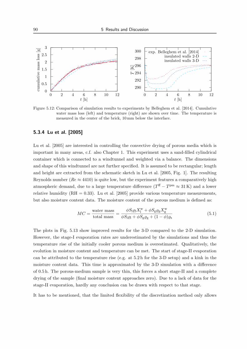
90 5 Results and Discussion
0
0.5
1
1.5
2
2.5
3
0 2 4 6 8 10 12
cum
ula
tive
mas
slo
ss[g
]
t [h]
290
292
294
296
298
300
0 2 4 6 8 10 12
T[K
]
t [h]
exp. Belleghem et al. [2014]insulated walls 2-Dinsulated walls 3-D
Figure 5.12: Comparison of simulation results to experiments by Belleghem et al. [2014]. Cumulativewater mass loss (left) and temperature (right) are shown over time. The temperature ismeasured in the center of the brick, 10 mm below the interface.
5.3.4 Lu et al. [2005]
Lu et al. [2005] are interested in controlling the convective drying of porous media which is
important in many areas, c.f. also Chapter 1. This experiment uses a sand-filled cylindrical
container which is connected to a windtunnel and weighted via a balance. The dimensions
and shape of this windtunnel are not further specified. It is assumed to be rectangular; length
and height are extracted from the schematic sketch in Lu et al. [2005, Fig. 1]. The resulting
Reynolds number (Re ≈ 4410) is quite low, but the experiment features a comparatively high
atmospheric demand, due to a large temperature difference (T ff − T pm ≈ 31 K) and a lower
relative humidity (RH = 0.33). Lu et al. [2005] provide various temperature measurements,
but also moisture content data. The moisture content of the porous medium is defined as:
MC =water mass
total mass=
φSl%lXwl + φSg%gX
wg
φSl%l + φSg%g + (1− φ)%s(5.1)
The plots in Fig. 5.13 show improved results for the 3-D compared to the 2-D simulation.
However, the stage-I evaporation rates are underestimated by the simulations and thus the
temperature rise of the initially cooler porous medium is overestimated. Qualitatively, the
evolution in moisture content and temperature can be met. The start of stage-II evaporation
can be attributed to the temperature rise (e.g. at 5.2 h for the 3-D setup) and a kink in the
moisture content data. This time is approximated by the 3-D simulation with a difference
of 0.5 h. The porous-medium sample is very thin, this forces a short stage-II and a complete
drying of the sample (final moisture content approaches zero). Due to a lack of data for the
stage-II evaporation, hardly any conclusion can be drawn with respect to that stage.
It has to be mentioned, that the limited flexibility of the discretization method only allows

5.3 Comparison with Experiments 91
0
0.05
0.1
0.15
0.2
0.25
0 2 4 6 8 10 12
MC
[−]
t [h]
exp. Lu et al. [2005]insulated walls 2-Dinsulated walls 3-D
300
305
310
315
320
0 2 4 6 8 10 12
T[K
]
t [h]
Figure 5.13: Comparison of simulation results to experiments by Lu et al. [2005]. Moisture con-tent (left) and temperature (right) evolution are shown over time. The temperatureis measured 8 mm below the interface, due to missing information, it is assumed that themeasurements takes place along the center line of the cylinder.
a coarse approximation of the cylindrical sand box with rectangular cells. An insulation
is indicated in the experiment setup [Lu et al., 2005, Fig. 1], but without any additional
information. Thus, these properties are estimated from the figure scale and Plexiglas walls
are assumed. Further, the size of the windtunnel is undefined and thus it is chosen such that
the length and depth of the domain only have a small influence.
5.3.5 Trautz [2015]
This experiment is run with the largest soil-atmosphere windtunnel equipment of this com-
parison study. The width of the porous-medium container is in similar size as the previous
experiments, but it is longer and especially of smaller width than the windtunnel. This data
set provides 3× 3 measurements of porous-medium temperatures and water saturations with
high temporal resolutions. In addition, the surface conditions are measured at three locations.
Trautz [2015] uses the same sand as Davarzani et al. [2014], but due to different packing and
compaction mechanisms, the resulting properties are different. For simplicity, the properties
specified in Davarzani et al. [2014] are used (soil #3).
Fig. 5.14 (left) shows two evaporation rates, which are obtained by two different means.
Trautz [2015] uses data from infrared radiometers and a surface energy balance based on the
publication by Shahraeeni and Or [2010]. Then, the evaporation rates at three different loca-
tions at the soil surface are calculated, see Trautz [2015, Fig. 7.6]. The author of this thesis
has extracted these evaporation rates from the mentioned figure and has calculated, via a
length-based average, the total evaporation rate for the entire porous medium (red line). The
second procedure uses the saturation data provided in Trautz [2015, Fig. 7.4] to recalculate
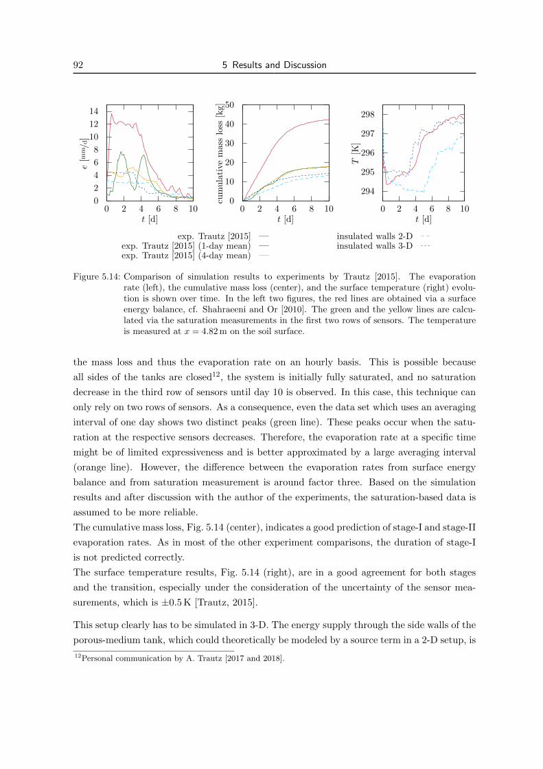
92 5 Results and Discussion
0
2
4
6
8
10
12
14
0 2 4 6 8 10
e[m
m/d
]
t [d]
0
10
20
30
40
50
0 2 4 6 8 10cu
mu
lati
vem
ass
loss
[kg]
t [d]
294
295
296
297
298
0 2 4 6 8 10
T[K
]
t [d]
exp. Trautz [2015]exp. Trautz [2015] (1-day mean)exp. Trautz [2015] (4-day mean)
insulated walls 2-Dinsulated walls 3-D
Figure 5.14: Comparison of simulation results to experiments by Trautz [2015]. The evaporationrate (left), the cumulative mass loss (center), and the surface temperature (right) evolu-tion is shown over time. In the left two figures, the red lines are obtained via a surfaceenergy balance, cf. Shahraeeni and Or [2010]. The green and the yellow lines are calcu-lated via the saturation measurements in the first two rows of sensors. The temperatureis measured at x = 4.82 m on the soil surface.
the mass loss and thus the evaporation rate on an hourly basis. This is possible because
all sides of the tanks are closed12, the system is initially fully saturated, and no saturation
decrease in the third row of sensors until day 10 is observed. In this case, this technique can
only rely on two rows of sensors. As a consequence, even the data set which uses an averaging
interval of one day shows two distinct peaks (green line). These peaks occur when the satu-
ration at the respective sensors decreases. Therefore, the evaporation rate at a specific time
might be of limited expressiveness and is better approximated by a large averaging interval
(orange line). However, the difference between the evaporation rates from surface energy
balance and from saturation measurement is around factor three. Based on the simulation
results and after discussion with the author of the experiments, the saturation-based data is
assumed to be more reliable.
The cumulative mass loss, Fig. 5.14 (center), indicates a good prediction of stage-I and stage-II
evaporation rates. As in most of the other experiment comparisons, the duration of stage-I
is not predicted correctly.
The surface temperature results, Fig. 5.14 (right), are in a good agreement for both stages
and the transition, especially under the consideration of the uncertainty of the sensor mea-
surements, which is ±0.5 K [Trautz, 2015].
This setup clearly has to be simulated in 3-D. The energy supply through the side walls of the
porous-medium tank, which could theoretically be modeled by a source term in a 2-D setup, is
12Personal communication by A. Trautz [2017 and 2018].
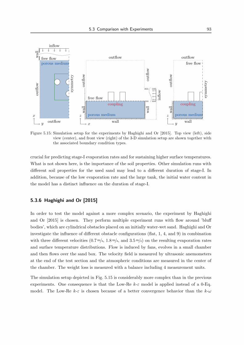
5.3 Comparison with Experiments 93
y
x
free flowporous medium
wall
outfl
ow
outflow
sym
met
ry
inflow
x
z porous medium
free flow
wall
wall
wall
infl
ow
outfl
ow
outflow
ou
tflow
coupling
y
z porous medium
free flow
wall
wall
outfl
ow
outflow
sym
met
ry
coupling
Figure 5.15: Simulation setup for the experiments by Haghighi and Or [2015]. Top view (left), sideview (center), and front view (right) of the 3-D simulation setup are shown together withthe associated boundary condition types.
crucial for predicting stage-I evaporation rates and for sustaining higher surface temperatures.
What is not shown here, is the importance of the soil properties. Other simulation runs with
different soil properties for the used sand may lead to a different duration of stage-I. In
addition, because of the low evaporation rate and the large tank, the initial water content in
the model has a distinct influence on the duration of stage-I.
5.3.6 Haghighi and Or [2015]
In order to test the model against a more complex scenario, the experiment by Haghighi
and Or [2015] is chosen. They perform multiple experiment runs with flow around ’bluff
bodies’, which are cylindrical obstacles placed on an initially water-wet sand. Haghighi and Or
investigate the influence of different obstacle configurations (flat, 1, 4, and 9) in combination
with three different velocities (0.7 m/s, 1.8 m/s, and 3.5 m/s) on the resulting evaporation rates
and surface temperature distributions. Flow is induced by fans, evolves in a small chamber
and then flows over the sand box. The velocity field is measured by ultrasonic anemometers
at the end of the test section and the atmospheric conditions are measured in the center of
the chamber. The weight loss is measured with a balance including 4 measurement units.
The simulation setup depicted in Fig. 5.15 is considerably more complex than in the previous
experiments. One consequence is that the Low-Re k-ε model is applied instead of a 0-Eq.
model. The Low-Re k-ε is chosen because of a better convergence behavior than the k-ω

94 5 Results and Discussion
vg,x [m/s] emean [kg/h]
flat 1 obstacle 4 obstacles
exp. 0.7 0.12 (0.05) 0.13 (0.05) 0.18 (0.08)sim. 0.7 0.11 0.11 0.12
exp. 3.5 0.25 (0.10) 0.33 (0.08) 0.60 (0.13)sim. 3.5 0.22 0.25 0.28
Table 5.9: Comparison of evaporation rates to experiments by Haghighi and Or [2015]. Values inparenthesis indicate the standard deviation of 4-5 runs for each configuration.
model. Due to limited computational power and available memory, the setup includes a
symmetry boundary along the center line of the experiments and the number of grid cells is
rather small. The area of each cylinder is resolved by 6 × 6 cells and a large grading factor
(gz = 3.5) is applied in vertical direction. With the aim to compare the different obstacle
setups without changing the spatial grid, the resolution is limited by the case including the
most obstacles (here 4) and results in a grid which reveals areas with an unnecessary high
number of cells for the cases with less obstacle.
Tab. 5.9 compares the mean evaporation rate over the entire duration of the experiment. The
evaporation rates for the flat surface are in good agreement with the experiment results. For
the low velocity case, the simulation results are always within the measurement uncertainty.
For the high velocity case, they are just inside this range for 1 obstacle, but for 4 obstacles the
evaporation rate is strongly underestimated. For both velocities, the increase in evaporation
rate associated with the increase in obstacles is underestimated.
The surface temperatures of experiments and simulations are compared for two selected con-
figurations in Fig. 5.16. Already for 1 obstacle and a low velocity, grid artifacts are visible,
e.g. rectangular temperature patterns around the obstacle. Qualitatively, the simulation can
prescribe the cooler and warmer areas upstream of the obstacle and the region of obstacle
influence. Downstream, more deficiencies are visible, the area directly behind the obstacle,
the shape of the cooling plume, and the outer areas. The temperature difference between the
simulations and the experiments is about ±1.0 K for lower velocities and less obstacles. For a
higher velocity and in combination with more obstacles, the temperature difference between
simulations and experiments increases to roughly ±1.5 K.
The major part of these discrepancies can be attributed to the free-flow side. First, the
numerical method (implicit and first-order upwind) may not be the most appropriate for
modeling flow around such obstacles. Second, the discretization is too coarse to resolve the
shape of the cylinders and the processes around them. Third, better free-flow models would
lead to a better description of the turbulent flow field, e.g. more turbulence resulting from the

5.3 Comparison with Experiments 95
simulations experiments[Haghighi and Or, 2015]
1 obstaclevg,x = 0.7 m/s
4 obstaclesvg,x = 3.5 m/s
Figure 5.16: Comparison of surface temperatures to experiments by Haghighi and Or [2015]. Surfacetemperature are extracted at the end of the simulation, the time at which the surfacetemperatures are measured in the experiments was not given. Note: (i) the figures do notuse the same temperature ranges, (ii) the figures extracted from Haghighi and Or [2015]show a mismatch in x-y-ratio.Results of the experiments are reprinted from Interactions of bluff-body obstacles withturbulent airflows affecting evaporative fluxes from porous surfaces, 530, Erfan Haghighiand Dani Or, Journal of Hydrology, 14, ©2015, with permission from Elsevier.
cylinder surface and thus enhanced turbulent exchange with higher evaporation rates. One
first step to circumvent this problem would be a transport model. Then, the turbulent free
flow has to be solved once via a two-equation turbulence model or more advanced turbulence
models from external software can be used. In addition, a higher spatial resolution can be
achieved.
The conversion from an experiment to a simulation setup bears some uncertainties. From
images in Haghighi and Or [2015], it seems as there is a small step from the chamber onto
the soil surface and also the soil surface is disturbed around the cylinders. In addition, the
velocity is measured at the end of the domain but set as inflow condition inside the chamber.
The porous medium is simplified by not integrating the water inflow from the bottom of
the domain and applying perfect insulation around the sand box. In reality there might be
an imperfect insulation and also the sand is connected to a Mariotte bottle to maintain a
constant water level, which leads to an inflow of water and its associated energy. However,
even if no water is supplied, the surface will not dry-out completely, the observed saturation
decrease is ∆Sl = 0.4. Finally, the boundary conditions in the free flow are quite undefined
and the effect of the assumed outflow conditions has to be analyzed.

96 5 Results and Discussion
tolerance Mos
thaf
etal
.[2
014
]
Dav
arza
ni
etal.
[2014
]
Bel
legh
emet
al.
[201
4]
Lu
etal.
[200
5]
Tra
utz
[201
5]
Hagh
igh
ian
dO
r[2
015
]
stag
e-I duration of stage-I 10% ↑ ↓ X X ↓ n.a.
e 10% ↓ X X ↓ X (X)T pm 1 K ↓ ↓ X ↑ X (X)T pm compared to Tbulb 0.2 K X X n.r. n.r. n.r. n.r.
stag
e-II cumulative mass loss 10% ↑ ↓ X X ↓ n.a.
e visual X X X n.a. X n.a.T pm 1 K ↓ X X X X n.a.
Table 5.10: Qualitative summary of a comparison study to various laboratory experiments. If available,the ’insulated walls 3-D’ simulation results are taken. The ’perfectly insulated walls’ casesare taken for the wet-bulb temperature comparison. It is indicated, whether experimentaldata is not available (n.a.) or simulation sets are not run (n.r.), e.g. perfect insulation forwet-bulb comparison. Values in parentheses are based on the outcome of the majority ofthe investigated setups.
5.3.7 Summary
In this section, six different laboratory experiments are used to compare and analyze simu-
lation results. The importance of changes in the model concepts, boundary conditions, and
dimensionality is highlighted. The results are qualitatively summarized in Tab. 5.10 with re-
spect to stage-I/stage-II transition, evaporation rates, and temperatures. For all setups with
a perfect insulation, the difference between simulated and expected wet-bulb temperatures is
below 0.2 K or 0.1%. In general, the evaporation rates and the temperatures in stage-II are
in good agreement. The cumulative mass loss is not predicted correctly, mainly because of
problems in predicting the stage-I to stage-II transition. The stage-I evaporation rates are
in a good agreement for most of the investigated setups. However, the temporal evolution of
the evaporation rates and the temporal and spatial temperature evolution can be improved.
The quality of simulated stage-I temperatures strongly depends on the available information
about the energy supply through the walls of the porous-medium container.
Three main error sources are detected from the simulation side: (i) the (free-flow) discretiza-
tion, (ii) the porous-medium properties, and (iii) the boundary conditions for the simulation
or in other words the transfer from laboratory to numerical experiments. The deficiencies

5.4 Investigation of Roughness 97
in the numerical (free-flow) concept are obvious in the last example, in which the free-flow
field is not resolved accurately enough, but also for the experiments with a cylindrical pipe or
cylindrical porous-medium container, the results can be improved with a better discretization.
Analyzing the effect of the Reynolds number on the simulation results would be interesting.
Here, the experiment with the lowest Reynolds number shows the best match. However, in
that study, many other conditions are also changed (e.g. brick instead of sand), so the influ-
ence of the Reynolds number on the quality of the simulation results is not clear. A correct
description of the free flow is strongly connected to the definition of boundary conditions. For
all experiments, block-shaped inflow conditions are assumed and often this inflow location is
guessed. In addition, important information about the free flow, the porous-medium, or the
room conditions are missing, e.g. Lu et al. [2005] keep the information about the windtunnel
quite short. A correct system setup and boundary conditions are not only a problem for the
free flow, but also for the porous medium. This comparison study includes examples in which
the results are clearly improved by using 3-D instead of 2-D simulations. The 2-D simulation
results could be improved by including a source term which accounts for the energy supply
through the walls, e.g. for the experiments by Belleghem et al. [2014] the main difference
between 2-D and 3-D is in the temperature evolution. As already discussed in Mosthaf et al.
[2014], the porous-medium properties have a distinct influence on the shape of the evapora-
tion rate and mismatches in the duration of stage-I might be attributed to them. For sand,
the filling and compaction procedures result in different porous-medium properties or local
heterogeneities for even the same material. These local heterogeneities influence the processes
at various interfaces, e.g. between the porous medium and the free flow, but also near the
walls of the porous medium, cf. Haghighi et al. [2013], Mosthaf [2014].
Despite all those error sources, only one publication provides error estimations based on
multiple runs for the same experiment setup [Haghighi and Or, 2015].
5.4 Investigation of Roughness
The last part highlights the effect of the roughness of porous media. This includes cases with
sharp heterogeneities, sand-grain roughnesses, and porous obstacles.

98 5 Results and Discussion
free flow
porous medium
0.1 m 0.2 m 0.1 m
0.05
m0.
45m
ou
tflow
symmetry
wall wall
infl
ow
coupling
Figure 5.17: Simulation setup for the heterogene-ity roughness case, after Fetzer et al.[2017c].
parameter value
vffg [m/s] (1.0, 0)ᵀ
pffg [Pa] 1e5
Xw,ffg [−] 0.0055
T ff [K] 293
soil type #6 and #7ppm
g [Pa] 1e5Spm
l [−] 0.97T pm [K] 293
Table 5.11: Initial and boundary conditions forthe heterogeneity roughness case, af-ter Fetzer et al. [2017c].
5.4.1 Heterogeneity Roughness13
To investigate the effect of soil types (e.g. silt and sandy loam) and its orientation on evapo-
ration, simulations are run in which two soil blocks are placed adjacent to each other as seen
in Fig. 5.17.
Impact of Heterogeneities in the Porous Medium Fig. 5.18 (left) shows the evaporation
rates from homogeneous and heterogeneous test cases. For the homogeneous silt case, a
steady state evaporation rate is obtained during the first day that remains constant until
day 3.5 when the evaporation rate decreases. Feedbacks between free and porous-medium
flow result in higher humidities as the air flows along the test section, the evaporation rate
from the downstream half of the test section is smaller than from the upstream half. The
evaporation rate from the upstream part decreases a little earlier than the downstream part,
which leads to a short peak in evaporation from the downstream part. Since the initial water
distribution is uniform in the simulation domain, this illustrates that lateral water flow in the
porous medium compensated for the higher evaporation losses in the upstream part. Lateral
variations in air humidity and temperature in the free flow, which lead to lateral variations
in evaporation rate, also induce lateral liquid flow in the porous medium.
In the heterogeneous test cases, the initial evaporation rates are only depending on their posi-
tion (atmospheric conditions) and not on the soil type (porous-medium properties). However,
the sandy loam section’s evaporation rate starts to decrease earlier than evaporation from the
13This section is, in a longer version, already published in: T. Fetzer, J. Vanderborght, K. Mosthaf, K. M.Smits, and R. Helmig: Heat and water transport in soils and across the soil-atmosphere interface: 2.Numerical analysis, Water Resources Research, 53(2):1080–1100, 2017. doi: 10.1002/2016WR019983. Thejournal publication presents quantitatively different results which are caused by the usage of a differentturbulence model and a bug in the calculation of the thermal conductivity in DuMux 2.9.
5.4 Investigation of Roughness 99
finer silty part, related to the differences in soil hydraulic properties. This falling rate period
correlates to the soil entering into stage II evaporation. The decrease in evaporation from the
sandy loam is accompanied by an increase in evaporation from the silt part. The silt material
functions as a wick that drained water from the adjacent sandy loam resulting in a longer sus-
tained high evaporation from the silt material than in the homogeneous silty test case. This
behavior is also demonstrated in lab experiments Lehmann and Or [2009]. The second smaller
decrease in evaporation rate from the sandy loam around day 4.5 (green, dotted) occurs when
the liquid water flow to the evaporation front in the sandy loam soil driven by gradients in
capillary forces is reduced by the limited water supply due to the no-flow bottom boundary
condition of the box. With a deeper porous-medium box, the decrease would be continuous.
Also, the second drop in evaporation rate from the sandy loam surface corresponds with a
further increase in evaporation rate from the silt surface, despite the drying of the silt surface.
After the second increase of evaporation from the silt, also the silt starts drying out. This
shows that for a heterogeneous surface, the evaporation rate may locally increase and become
even larger than from a homogeneous surface. The relative increase in evaporation from the
silt part is larger when it is located downstream of the sandy loam part. In this case, the
temperature and humidity of the air that flows over the silt part, respectively, increase and
decrease when the evaporation from the upstream part decreases.
When the finer silt part is upstream of the sandy loam, the evaporation rate from the silt also
increases when evaporation from the sandy loam part decreases. This indicates that, in this
case, lateral mixing in the air increased temperature and reduced humidity in the upstream
direction above the silt part. Another potential reason is the lateral heat flux in the porous
medium, which increases the temperature at the surface of the silt soil when evaporation from
the sandy loam part changed.
Impact of Lateral Gradients in the Free Flow To evaluate the influence of changes in lateral
gradients in the free flow above a drying heterogeneous porous medium on the evaporation,
the one-dimensional aerodynamic resistances rmass are derived in a first step:
qw1-D = %mol,gM
wxw,ifg − xw,ref
g
rmass=%w,if
g − %w,refg
rmass. (5.2)
These resistances are subsequently used to calculate the evaporation rates from the hetero-
geneous porous medium when evaporation of one of the parts ceased (after day 3.5) and
compared to those of the fully-coupled 0-Eq. model (fc):
qwfc = −
[(%gX
wg vg + jw
mass,eff
)· n]ff,if
. (5.3)
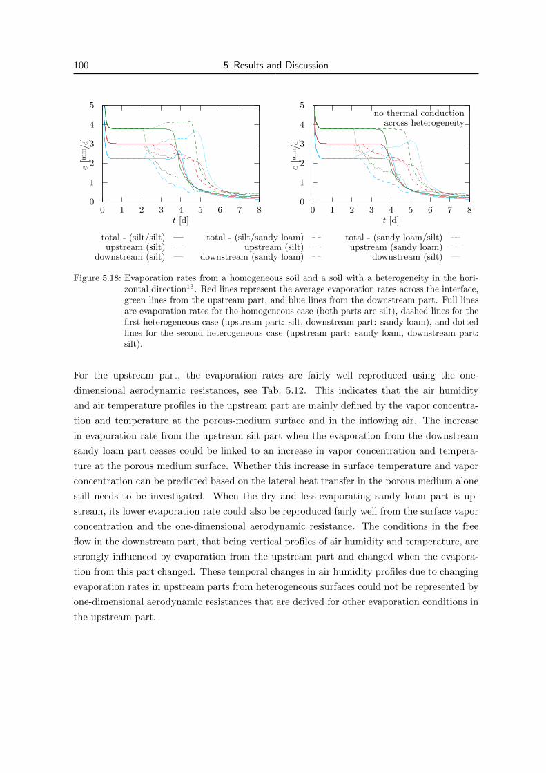
100 5 Results and Discussion
0
1
2
3
4
5
0 1 2 3 4 5 6 7 8
e[m
m/d
]
t [d]
0
1
2
3
4
5
0 1 2 3 4 5 6 7 8
no thermal conductionacross heterogeneity
e[m
m/d
]
t [d]
total - (silt/silt)upstream (silt)
downstream (silt)
total - (silt/sandy loam)upstream (silt)
downstream (sandy loam)
total - (sandy loam/silt)upstream (sandy loam)
downstream (silt)
Figure 5.18: Evaporation rates from a homogeneous soil and a soil with a heterogeneity in the hori-zontal direction13. Red lines represent the average evaporation rates across the interface,green lines from the upstream part, and blue lines from the downstream part. Full linesare evaporation rates for the homogeneous case (both parts are silt), dashed lines for thefirst heterogeneous case (upstream part: silt, downstream part: sandy loam), and dottedlines for the second heterogeneous case (upstream part: sandy loam, downstream part:silt).
For the upstream part, the evaporation rates are fairly well reproduced using the one-
dimensional aerodynamic resistances, see Tab. 5.12. This indicates that the air humidity
and air temperature profiles in the upstream part are mainly defined by the vapor concentra-
tion and temperature at the porous-medium surface and in the inflowing air. The increase
in evaporation rate from the upstream silt part when the evaporation from the downstream
sandy loam part ceases could be linked to an increase in vapor concentration and tempera-
ture at the porous medium surface. Whether this increase in surface temperature and vapor
concentration can be predicted based on the lateral heat transfer in the porous medium alone
still needs to be investigated. When the dry and less-evaporating sandy loam part is up-
stream, its lower evaporation rate could also be reproduced fairly well from the surface vapor
concentration and the one-dimensional aerodynamic resistance. The conditions in the free
flow in the downstream part, that being vertical profiles of air humidity and temperature, are
strongly influenced by evaporation from the upstream part and changed when the evapora-
tion from this part changed. These temporal changes in air humidity profiles due to changing
evaporation rates in upstream parts from heterogeneous surfaces could not be represented by
one-dimensional aerodynamic resistances that are derived for other evaporation conditions in
the upstream part.
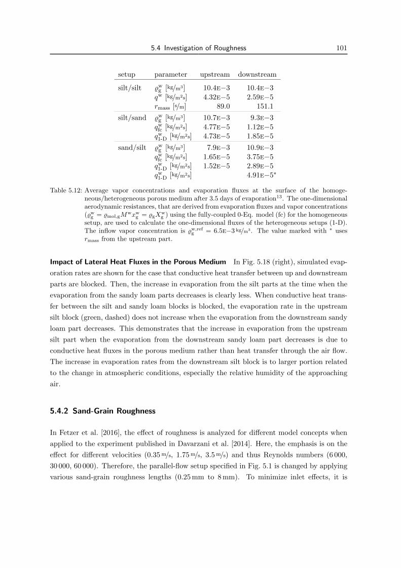
5.4 Investigation of Roughness 101
setup parameter upstream downstream
silt/silt %wg [kg/m3] 10.4e−3 10.4e−3
qw [kg/m2s] 4.32e−5 2.59e−5rmass [s/m] 89.0 151.1
silt/sand %wg [kg/m3] 10.7e−3 9.3e−3
qwfc [kg/m2s] 4.77e−5 1.12e−5qw
1-D [kg/m2s] 4.73e−5 1.85e−5
sand/silt %wg [kg/m3] 7.9e−3 10.9e−3
qwfc [kg/m2s] 1.65e−5 3.75e−5qw
1-D [kg/m2s] 1.52e−5 2.89e−5qw
1-D [kg/m2s] 4.91e−5∗
Table 5.12: Average vapor concentrations and evaporation fluxes at the surface of the homoge-neous/heterogeneous porous medium after 3.5 days of evaporation13. The one-dimensionalaerodynamic resistances, that are derived from evaporation fluxes and vapor concentrations(%w
g = %mol,gMwxw
g = %gXwg ) using the fully-coupled 0-Eq. model (fc) for the homogeneous
setup, are used to calculate the one-dimensional fluxes of the heterogeneous setups (1-D).The inflow vapor concentration is %w,ref
g = 6.5e−3 kg/m3. The value marked with ∗ usesrmass from the upstream part.
Impact of Lateral Heat Fluxes in the Porous Medium In Fig. 5.18 (right), simulated evap-
oration rates are shown for the case that conductive heat transfer between up and downstream
parts are blocked. Then, the increase in evaporation from the silt parts at the time when the
evaporation from the sandy loam parts decreases is clearly less. When conductive heat trans-
fer between the silt and sandy loam blocks is blocked, the evaporation rate in the upstream
silt block (green, dashed) does not increase when the evaporation from the downstream sandy
loam part decreases. This demonstrates that the increase in evaporation from the upstream
silt part when the evaporation from the downstream sandy loam part decreases is due to
conductive heat fluxes in the porous medium rather than heat transfer through the air flow.
The increase in evaporation rates from the downstream silt block is to larger portion related
to the change in atmospheric conditions, especially the relative humidity of the approaching
air.
5.4.2 Sand-Grain Roughness
In Fetzer et al. [2016], the effect of roughness is analyzed for different model concepts when
applied to the experiment published in Davarzani et al. [2014]. Here, the emphasis is on the
effect for different velocities (0.35 m/s, 1.75 m/s, 3.5 m/s) and thus Reynolds numbers (6 000,
30 000, 60 000). Therefore, the parallel-flow setup specified in Fig. 5.1 is changed by applying
various sand-grain roughness lengths (0.25 mm to 8 mm). To minimize inlet effects, it is
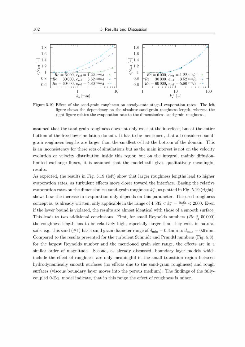
102 5 Results and Discussion
0.6
0.8
1
1.2
1.4
1.6
1.8
1 10
e/e r
ef
[−]
ks [mm]
Re = 6 000, eref = 1.22 mm/dRe = 30 000, eref = 3.52 mm/dRe = 60 000, eref = 5.80 mm/d 0.6
0.8
1
1.2
1.4
1.6
1.8
1 10 100
e/e r
ef
[−]
k+s [−]
Re = 6 000, eref = 1.22 mm/dRe = 30 000, eref = 3.52 mm/dRe = 60 000, eref = 5.80 mm/d
Figure 5.19: Effect of the sand-grain roughness on steady-state stage-I evaporation rates. The leftfigure shows the dependency on the absolute sand-grain roughness length, whereas theright figure relates the evaporation rate to the dimensionless sand-grain roughness.
assumed that the sand-grain roughness does not only exist at the interface, but at the entire
bottom of the free-flow simulation domain. It has to be mentioned, that all considered sand-
grain roughness lengths are larger than the smallest cell at the bottom of the domain. This
is an inconsistency for these sets of simulations but as the main interest is not on the velocity
evolution or velocity distribution inside this region but on the integral, mainly diffusion-
limited exchange fluxes, it is assumed that the model still gives qualitatively meaningful
results.
As expected, the results in Fig. 5.19 (left) show that larger roughness lengths lead to higher
evaporation rates, as turbulent effects move closer toward the interface. Basing the relative
evaporation rates on the dimensionless sand-grain roughness k+s , as plotted in Fig. 5.19 (right),
shows how the increase in evaporation only depends on this parameter. The used roughness
concept is, as already written, only applicable in the range of 4.535 < k+s = uτks
ν < 2000. Even
if the lower bound is violated, the results are almost identical with those of a smooth surface.
This leads to two additional conclusions. First, for small Reynolds numbers (Re / 50 000)
the roughness length has to be relatively high, especially larger than they exist in natural
soils, e.g. this sand (#1) has a sand grain diameter range of dmin = 0.3 mm to dmax = 0.9 mm.
Compared to the results presented for the turbulent Schmidt and Prandtl numbers (Fig. 5.8),
for the largest Reynolds number and the mentioned grain size range, the effects are in a
similar order of magnitude. Second, as already discussed, boundary layer models which
include the effect of roughness are only meaningful in the small transition region between
hydrodynamically smooth surfaces (no effects due to the sand-grain roughness) and rough
surfaces (viscous boundary layer moves into the porous medium). The findings of the fully-
coupled 0-Eq. model indicate, that in this range the effect of roughness is minor.
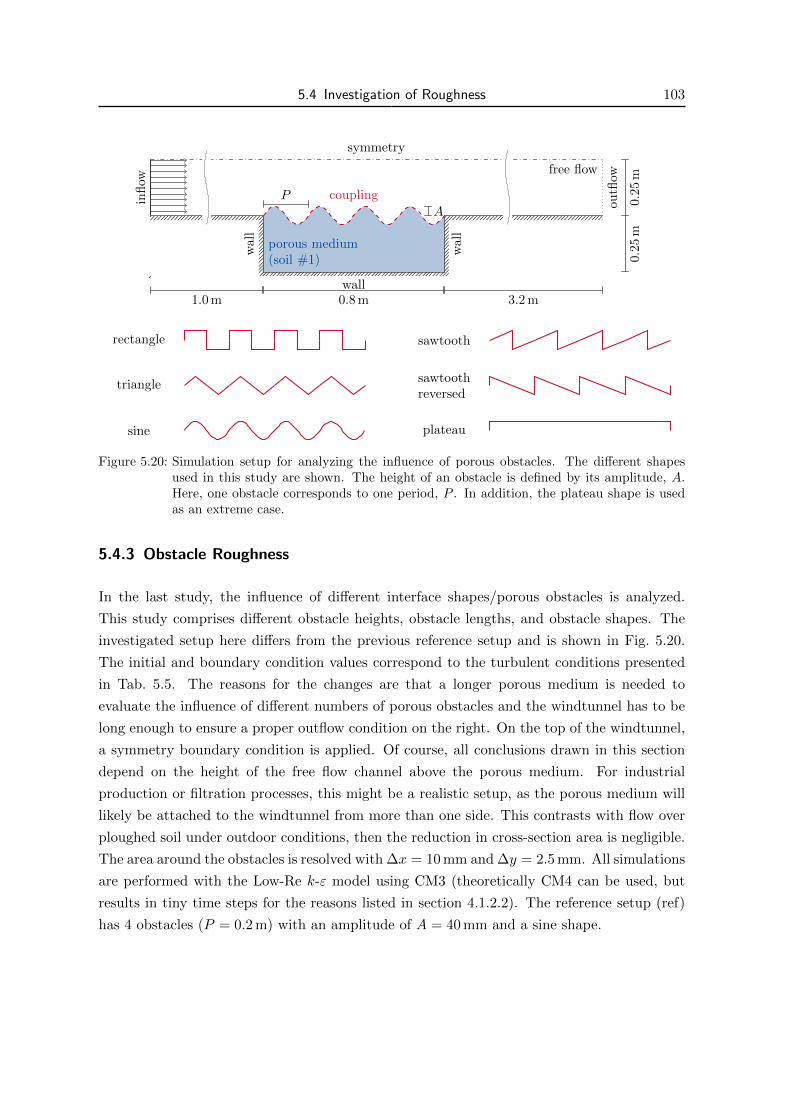
5.4 Investigation of Roughness 103
free flow
porous medium(soil #1)
1.0 m 0.8 m 3.2 m
0.25
m0.
25
m
wall
wall
wal
l
ou
tflow
symmetryin
flow
coupling
AP
rectangle
triangle
sine
sawtooth
sawtoothreversed
plateau
Figure 5.20: Simulation setup for analyzing the influence of porous obstacles. The different shapesused in this study are shown. The height of an obstacle is defined by its amplitude, A.Here, one obstacle corresponds to one period, P . In addition, the plateau shape is usedas an extreme case.
5.4.3 Obstacle Roughness
In the last study, the influence of different interface shapes/porous obstacles is analyzed.
This study comprises different obstacle heights, obstacle lengths, and obstacle shapes. The
investigated setup here differs from the previous reference setup and is shown in Fig. 5.20.
The initial and boundary condition values correspond to the turbulent conditions presented
in Tab. 5.5. The reasons for the changes are that a longer porous medium is needed to
evaluate the influence of different numbers of porous obstacles and the windtunnel has to be
long enough to ensure a proper outflow condition on the right. On the top of the windtunnel,
a symmetry boundary condition is applied. Of course, all conclusions drawn in this section
depend on the height of the free flow channel above the porous medium. For industrial
production or filtration processes, this might be a realistic setup, as the porous medium will
likely be attached to the windtunnel from more than one side. This contrasts with flow over
ploughed soil under outdoor conditions, then the reduction in cross-section area is negligible.
The area around the obstacles is resolved with ∆x = 10 mm and ∆y = 2.5 mm. All simulations
are performed with the Low-Re k-ε model using CM3 (theoretically CM4 can be used, but
results in tiny time steps for the reasons listed in section 4.1.2.2). The reference setup (ref)
has 4 obstacles (P = 0.2 m) with an amplitude of A = 40 mm and a sine shape.
104 5 Results and Discussion
0
2
4
6
8
10
12
0 2 4 6 8 10 12 14
e[m
m/d
]
t [d]
flat2.5 mm5.0 mm
10.0 mm20.0 mm
(ref) 40.0 mm
0
2
4
6
8
10
12
0 2 4 6 8 10 12 14
e[m
m/d
]
t [d]
flatvalley 1.6
hill 1.60.80.4
(ref) 0.2
Figure 5.21: Evaporation rates for different obstacle heights (left) and lengths (right).
Fig. 5.21 (left) shows that already small perturbations of the flat surface lead to higher stage-I
evaporation rates. The increase in steady-state stage-I evaporation rates is less than compared
to the increase caused by a sand grain-roughness model (the relative increases are e.g. for
A = ks = 2.5 mm: 1.2 vs. 1.4, and for A = ks = 10 mm: 1.3 vs. 1.9 (extrapolated)). If
the obstacle height increases, at least three different effects can be reported. First, for higher
obstacles, the deflection of the flow at the first obstacle is stronger and the flow requires a
longer distance to reattach to the top-level of the obstacles. Here, the symmetry boundary
condition has a considerable effect, as the flow is forced through a smaller channel which
increases the mean velocity therein (the cross-section compared to the flat surface is reduced
from 99% for 2.5 mm to 84% for 40 mm). Second, higher obstacles reduce the availability of
water at the top level. The capillary forces are too weak to overcome gravity and pull water
from the bottom of the porous-medium box, cf. Lehmann et al. [2008]. And third, also the
area of the cavities in between two hills increases and the vortices inside change their behavior.
These three effects may lead to the following observations. The stage-I evaporation rate does
not monotonously increase with height, but reach a maximum for obstacles of 20 mm height
in this setup. In contrast to the rate, the duration of stage-I does monotonously decrease
with height. Analyzing the cumulative mass loss (not shown here) indicates that for higher
obstacles, less water did evaporate when the transition to stage-II is reached. The transition
to stage-II is smoother for higher obstacles. An interesting observation is that the stage-II
evaporation rate is noticeably higher for the highest obstacles.
In Fig. 5.21 (right) the influence of different obstacle periods is shown. The period also
influences the number of obstacles and care must be taken, whether the observed effects are
caused by changing the period and thus the shape of the obstacles or the number of obstacles.
As for the obstacle height, the minimum stage-I evaporation rate is predicted for the flat
surface. Even the valley part of half an obstacle shows an increased rate. Driving forces for
this behavior are (i) a significant downward and upward flow, (ii) a higher porous-medium
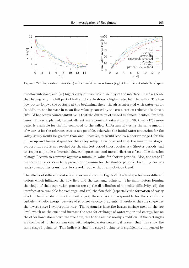
5.4 Investigation of Roughness 105
0
2
4
6
8
10
12
0 2 4 6 8 10 12 14
e[m
m/d
]
t [d]
0
10
20
30
40
50
0 2 4 6 8 10 12 14
cum
ula
tive
mass
loss
[kg]
t [d]
flattriangle
sawtoothsawtooth reversed
rectangle(ref) sine
plateau, Sw = 0.84
Figure 5.22: Evaporation rates (left) and cumulative mass losses (right) for different obstacle shapes.
free-flow interface, and (iii) higher eddy diffusivities in vicinity of the interface. It makes sense
that having only the hill part of half an obstacle shows a higher rate than the valley. The free
flow better follows the obstacle at the beginning, there, the air is saturated with water vapor.
In addition, the increase in mean flow velocity caused by the cross-section reduction is almost
30%. What seems counter-intuitive is that the duration of stage-I is almost identical for both
cases. This is explained, by initially setting a constant saturation of 0.98, thus ∼17% more
water is available for the hill compared to the valley. Unfortunately using the same amount
of water as for the reference case is not possible, otherwise the initial water saturation for the
valley setup would be greater than one. However, it would lead to a shorter stage-I for the
hill setup and longer stage-I for the valley setup. It is observed that the maximum stage-I
evaporation rate is not reached for the shortest period (most obstacles). Shorter periods lead
to steeper slopes, less favorable flow configurations, and more deflection effects. The duration
of stage-I seems to converge against a minimum value for shorter periods. Also, the stage-II
evaporation rates seem to approach a maximum for the shorter periods. Including cavities
leads to smoother transitions to stage-II, but without any obvious trend.
The effects of different obstacle shapes are shown in Fig. 5.22. Each shape features different
factors which influence the flow field and the exchange behavior. The main factors forming
the shape of the evaporation process are (i) the distribution of the eddy diffusivity, (ii) the
interface area available for exchange, and (iii) the flow field (especially the formation of cavity
flow). The sine shape has the least edges, these edges are responsible for the creation of
turbulent kinetic energy, because of stronger velocity gradients. Therefore, the sine shape has
the lowest stage-I evaporation rate. The rectangles have the largest surface area on the top
level, which on the one hand increase the area for exchange of water vapor and energy, but on
the other hand slows down the free flow, due to the almost no-slip condition. If the rectangles
are compared to the plateau case with adapted water content, it is seen that they show the
same stage-I behavior. This indicates that the stage-I behavior is significantly influenced by
106 5 Results and Discussion
the properties of the first obstacle. The triangle and the sawtooth show a more favorable flow
configuration, still featuring the sharp edges. Compared to the triangle, the slope of the first
sawtooth obstacle is half of the triangle one and the distance to the top is doubled, which can
explain the higher evaporation rates. The flow fields depicted in Fig. 5.23 show that for the
reversed sawtooth setup the flow deflection by the first obstacle directly feeds into the second
one which may explain the highest evaporation rates.
When looking at the cumulative mass loss in Fig. 5.22 (right), it can be seen, that one effect
of increased top-level area is that the stage-II begins for a smaller water mass loss (especially
visible for the rectangle and the plateau). If one is interested in a fast drying of the material,
the flat surface performs worst in the beginning, due to the low stage-I evaporation rate,
but it improves as time proceeds in stage-I. In stage-II, the importance of cavity flow for the
exchange behavior and the evaporation process can be seen when comparing the rectangle
and the plateau evaporation rates, then the rectangles show higher evaporation rate. From
Fig. 5.23 it can be seen that for stage-II (14 days), the rectangle setup has the largest interface
area in combination with available liquid water. This explains the high stage-II rates, as the
diffusive transport in the porous medium is slower than the advective-diffusive transport
inside the cavities.
Including the Forchheimer extension does not alter the results and therefore is not shown here.
At the first rectangle, the average velocity normal to the interface is vg,n = 0.0034 m/s. The
difference between Darcy and Forchheimer results is less than 0.1%. Even for a conservative
estimation of the pore diameter (dpore = 10 mm), the resulting Reynolds number is in the
validity range for the Darcy law (Repore = 0.22 < 1).
This study shows that the shape of the surface has a significant effect on all stages of the
evaporation process. Compared to the flat surface, all tested configurations show a higher
stage-I evaporation rate, but also a shorter stage-I. The stage-I evaporation rate is strongly
affected by inlet effects and the properties of the first obstacles. The main factor for an
increased stage-II evaporation rate is the enhanced transport inside the cavities.
However, this study uses a quite coarse discretization and the obstacle shapes could be better
resolved, which may lead to different results. With respect to the simulation of the free flow
field, the same suggestions as for simulating the experiment by Haghighi and Or [2015] can
be made.
5.4.4 Summary
This section analyzes the effect of three different kinds of roughness on the evaporation be-
havior. Heterogeneities in porous-medium properties lead to a heterogeneous distribution of
fluxes. These fluxes lead to compensation mechanisms, e.g. lateral exchange of mass and
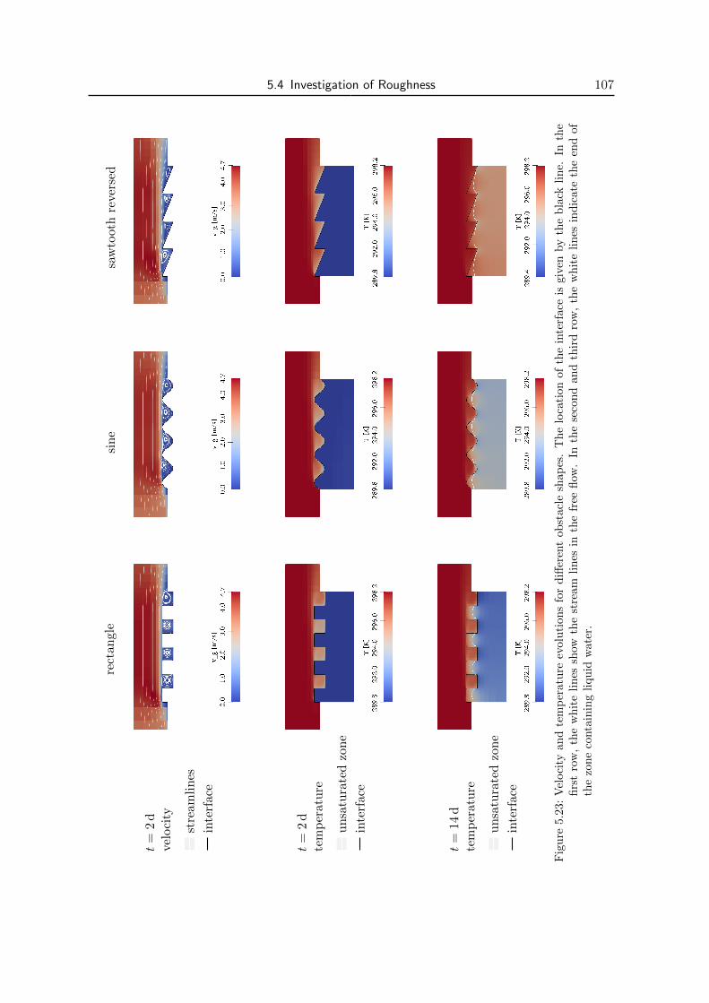
5.4 Investigation of Roughness 107
rect
angle
sin
esa
wto
oth
rever
sed
t=
2d
velo
city
stre
amli
nes
inte
rface
t=
2d
tem
per
atu
re
un
satu
rate
dzo
ne
inte
rface
t=
14
dte
mp
eratu
re
un
satu
rate
dzo
ne
inte
rface
Fig
ure
5.23
:V
eloci
tyan
dte
mp
erat
ure
evol
uti
ons
for
diff
eren
tob
stacl
esh
ap
es.
Th
elo
cati
on
of
the
inte
rface
isgiv
enby
the
bla
ckli
ne.
Inth
efi
rst
row
,th
ew
hit
eli
nes
show
the
stre
am
lines
inth
efr
eefl
ow.
Inth
ese
con
dan
dth
ird
row
,th
ew
hit
eli
nes
ind
icate
the
end
of
the
zon
eco
nta
inin
gli
qu
idw
ater
.
108 5 Results and Discussion
energy inside the soil. Because of these processes, a high evaporation rate can be maintained
and the stage-I to stage-II transition is altered in comparison to the transition behavior for
homogeneous media.
Including a sand-grain roughness concept from classical fluid dynamics leads to higher stage-I
evaporation rates. The increase in stage-I evaporation rates fully depends on the dimen-
sionless parameter k+s . However, due to the required fine discretization at the interface, the
sand-grain roughness height is of the same magnitude as the smallest grid cells. In addition,
there is no unique definition of the sand-grain roughness for a fully permeable medium and
this concept does not account for the effect of flow normal at and tangential to a porous
interface.
If the shape of the porous-medium surface is changed by porous obstacles of different heights,
lengths, or shapes the stage-I evaporation rate is increased. For a certain water content, the
duration of stage-I is affected by the height of the obstacles which limits the capillary trans-
port of liquid water to the surface. Compared to the flat surface, the stage-II evaporation rate
is enhanced by a more efficient transport inside the valleys/cavities in between obstacles. For
a small number of objects, as used here, the flow deflection around the first obstacle influences
the results.
6 Summary
The focus of this thesis is on improving the model concept for multi-phase porous-medium
flow coupled to a turbulent free flow, both including multi-component and energy transport.
As outlined in the introduction, such coupled interactions are relevant for different kinds of
applications from a variety of different research fields.
It is aimed to develop an REV-scale two-domain concept which can handle two models in
two separated subdomains and to couple them via appropriate coupling conditions at a sharp
interface. One goal is to perform this coupling without introducing additional degrees of
freedom on the interface. An existing porous-medium model, using the equations by Darcy
or Forchheimer and discretized with the cell-centered finite volume method, is coupled to
a (Reynolds-Averaged) Navier-Stokes model discretized with a marker-and-cell scheme (also
known as staggered grid), cf. Gruninger et al. [2017]. In this framework, eddy-viscosity
based turbulence models of different complexity are presented and implemented. In addition,
simplifications of the coupling conditions are introduced and discussed. The implementation
is performed using the software modules DuMux and Dune. A fully implicit Euler method
is used and the resulting monolithic matrix is solved with a Newton method and the help of
a direct linear solver.
In the previous chapter, several concepts, parameters, and setups are investigated. In a first
step, the developed model concepts and coupling methods are compared to a previous work
which uses the box method for spatial discretization, cf. Mosthaf [2014]. The results for
both discretization methods are in a good agreement. In contrast, the presented coupling
methods for the new discretization concept reveal differences. The investigated turbulence
models produce differences in stage-I evaporation rates of ±12% compared to their mean rate.
Simplifications of the free-flow model concept can speed-up the simulations and still, under
specific conditions, preserve the quality of the results. Afterward, analyses of the turbulent
Schmidt number, the turbulent Prandtl number, and the Beavers-Joseph coefficient show an
influence of up to +10% on stage-I evaporation rates when each value is varied from unity to
other physical meaningful values.
In a second study, the model results are compared to different evaporation experiments from
the literature and show a good qualitative and quantitative agreement. Most difficulties are

110 6 Summary
observed in reproducing the temperature evolution over time, or the transition from stage-I
to stage-II. The results show that the model predictions are sensitive to the boundary condi-
tions, the considered model dimension, and the porous-medium properties (see also Mosthaf
[2014]). Further, they reveal the deficiencies of the used implementation, which are the in-
flexible axis-parallel grid without local refinements and the memory-intense solving of the
monolithic matrix.
Finally, the effects of three different kinds of roughness are analyzed: heterogeneities, rough-
ness resulting from the sand-grains and from porous obstacles. The roughness of the porous
medium has a strong influence on the entire evaporation process and may add additional
stages to the typical evaporation stages known from flat and homogeneous media.
6.1 Conclusions
Based on the previous analyses and with respect to the research hypotheses, the following
conclusions are drawn.
Discretizations and Interface Model Concepts The discretization around the interface is
important; grid convergence of stage-I evaporation rates can only be shown for near-interface
cells with a height of ∆y+ < 5 (if a local system of equations is solved, CM4). The proposed
coupling methods which avoid additional degrees of freedom on the interface (CM1 to CM3)
converge against the same results for mainly interface-parallel flow, but require a finer dis-
cretization ∆y+ < 1. For flow normal toward a porous medium with multiple mobile phases,
all methods produce different results, because of the different ways to account for the phases’
resistance to flow. For one-phase porous-medium systems, CM2 to CM4 are identical with
respect to their normal-momentum coupling conditions.
Turbulence Models and Simplifications The presented fully-coupled model concept is quite
complex and in some cases simplifications are desirable. All presented simplifications are
shown to speed-up the simulation. One-dimensional boundary layer models can be used as
boundary conditions for the porous medium. These models give a good first estimation but are
limited to specific cases, e.g. flat, homogeneous porous media. Another option is to simulate
the transport of water vapor and energy on a given flow field (neglecting the feedback on the
momentum transport), this should also work for more complicated setups. Wall functions for
the k-ε model are especially helpful for larger setups. Further, the choice of the turbulence
model affects the predicted stage-I evaporation rates.

6.2 Outlook 111
Processes and Properties in Vicinity of the Interface The influence of the turbulent Prandtl
number and the turbulent Schmidt number on the stage-I evaporation rate is in a similar range
as the effect of the different turbulence models. Adapting these dimensionless numbers to the
geometry of a specific problem may improve the quality of the model prediction. Compared
to the influence of those two numbers, the effect of the Beavers-Joseph coefficient is minor.
The comparison of simulation results with data from various experiments and the case of a
sharp heterogeneity without conductive energy transfer indicate the importance of the energy
transport inside the porous medium, but also across the porous-medium free-flow interface
or the insulation of the porous-medium. A model which includes the sand-grain roughness
of an impermeable surface, is tested for its usage in the application of evaporation through a
permeable interface. It can be seen that the dimensionless sand-grain roughness length k+s is a
better indicator for the influence on the stage-I evaporation rate than the absolute roughness
length ks. Nevertheless, if an influence is present, the roughness length is already above the
minimum required discretization length. Finally, different porous obstacles are analyzed. Any
change to the flat surface increases the stage-I evaporation rate, but also leads to a shorter
duration of stage-I. The area which is available for free-flow porous-medium exchange inside
one cavity between two porous obstacles has a distinct influence on the stage-II evaporation
rate.
6.2 Outlook
This thesis considers some of the points which are mentioned in the outlook of Mosthaf [2014]
or Gruninger [2017], but also shows perspectives for further research.
Numerical Model Concept Many improvements are possible with respect to the numerical
model concept. First, the discretization of the free flow is not able to adequately resolve
geometric features and areas with highly dynamic processes. Consequences are an unnecessary
fine grid in unimportant areas and a large matrix. Adapting the grid to relevant areas, either
at the beginning or during the simulation, would help to reduce the computational costs and
improve the model predictions. In addition to that, Mortar concepts could be used to allow
for different discretizations in both domains at the interface. A third improvement would be
achieved by solving the matrix with an iterative solver, such that a parallelization of the code
is possible, cf. Gruninger [2017]. Fourth, the eddy-viscosity turbulence models (like k-ε or
k-ω) are a popular choice for turbulence models but could be improved by using Reynolds
stress models or large eddy simulations.
112 6 Summary
Simplifications This work proposes some possible simplifications, but the reported speed-up
can be increased by simplifying the material laws or their computations, by simplifying flow
and transport inside the porous medium [Vanderborght et al., 2017, Defraeye et al., 2010],
by decoupling the interactions in time [Rybak et al., 2015], in space [Masson et al., 2016],
or between the different transport processes (e.g. tracer components). In addition to the
previous points, neglecting the influence of mass and energy transport on the momentum
transport would allow to use free-flow fields from external software as OpenFOAM.
Experiments and Comparison Study Even though a lot of experiments are available in lit-
erature, many of them lack a precise description of the investigated setup or error estimations
based on multiple runs. A comparison with such experiments is inevitable to prove or further
develop a model concept. An alternative is to compare simulations based on averaged models
(RANS/REV) to simulations which resolve all details (DNS), but this is not yet possible for
non-isothermal, multi-phase, multi-component flow and transport. Comparing model results
for flow through and over porous obstacles with experiments would be interesting, cf. Suga
et al. [2013], Yang et al. [2018].
Relevant Processes Especially under outdoor conditions, turbulent pressure fluctuations
will affect the porous-medium flow and enhance the component transport (known as turbulent
pumping), e.g. Maier et al. [2012], Rutten [2015]. These pressure fluctuations are below the
time-scale of the turbulence models used here. Therefore, either more detailed turbulence
models have to be used or this effect has to be upscaled to RANS and REV models.
Applications with fast advection and high mass or energy transfer rates, as evaporation from
porous media, eventually violate the assumptions of local thermodynamic equilibrium. Some
studies are already performed, e.g. Nuske et al. [2014] and Trautz et al. [2015], but the effect
of the turbulent free flow is not yet sufficiently analyzed.
The importance of processes at the interface is highlighted in this thesis. Many other interface-
related processes exist, e.g. the wet-pore patterns influence the stage-I to stage-II transition
[Haghighi et al., 2013, Mosthaf et al., 2014], the formation of drops in a fuel cell [Baber et al.,
2016], or turbulent pumping. Replacing the sharp interface by lower-scale model concepts,
as pore-network models [cf. Beyhaghi et al., 2016], might be helpful to analyze the effect of
these processes.
From the perspective of an environmental engineer and with respect to outdoor conditions,
including plants [Heck, 2016, Koch et al., 2018], salt transport [Jambhekar et al., 2015],
radiation [Mosthaf, 2014], diurnal cycles (in wind speed, temperature, relative humidity), or
precipitation is interesting.
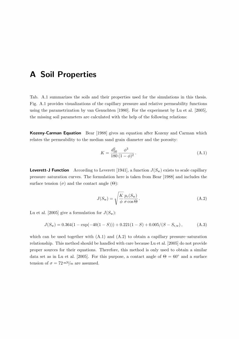
A Soil Properties
Tab. A.1 summarizes the soils and their properties used for the simulations in this thesis.
Fig. A.1 provides visualizations of the capillary pressure and relative permeability functions
using the parametrization by van Genuchten [1980]. For the experiment by Lu et al. [2005],
the missing soil parameters are calculated with the help of the following relations:
Kozeny-Carman Equation Bear [1988] gives an equation after Kozeny and Carman which
relates the permeability to the median sand grain diameter and the porosity:
K =d2
50
180
φ3
(1− φ)2. (A.1)
Leverett-J Function According to Leverett [1941], a function J(Sw) exists to scale capillary
pressure–saturation curves. The formulation here is taken from Bear [1988] and includes the
surface tension (σ) and the contact angle (Θ):
J(Sw) =
√K
φ
pc(Sw)
σ cos Θ. (A.2)
Lu et al. [2005] give a formulation for J(Sw):
J(Sw) = 0.364(1− exp(−40(1− S))) + 0.221(1− S) + 0.005/(S − Sr,w) , (A.3)
which can be used together with (A.1) and (A.2) to obtain a capillary pressure–saturation
relationship. This method should be handled with care because Lu et al. [2005] do not provide
proper sources for their equations. Therefore, this method is only used to obtain a similar
data set as in Lu et al. [2005]. For this purpose, a contact angle of Θ = 60 and a surface
tension of σ = 72 mN/m are assumed.
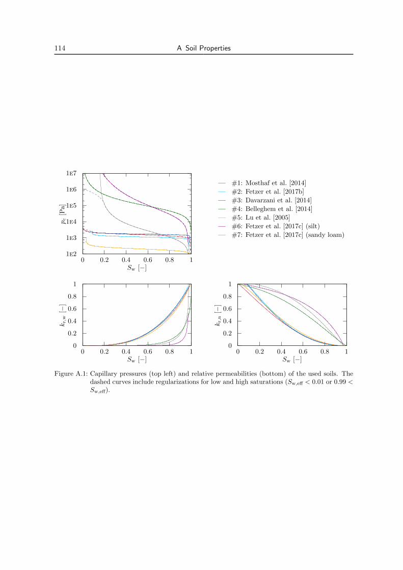
114 A Soil Properties
1e2
1e3
1e4
1e5
1e6
1e7
0 0.2 0.4 0.6 0.8 1
pc
[Pa]
Sw [−]
#1: Mosthaf et al. [2014]
#2: Fetzer et al. [2017b]
#3: Davarzani et al. [2014]
#4: Belleghem et al. [2014]
#5: Lu et al. [2005]
#6: Fetzer et al. [2017c] (silt)
#7: Fetzer et al. [2017c] (sandy loam)
0
0.2
0.4
0.6
0.8
1
0 0.2 0.4 0.6 0.8 1
kr,
w[−
]
Sw [−]
0
0.2
0.4
0.6
0.8
1
0 0.2 0.4 0.6 0.8 1
kr,
n[−
]
Sw [−]
Figure A.1: Capillary pressures (top left) and relative permeabilities (bottom) of the used soils. Thedashed curves include regularizations for low and high saturations (Sw,eff < 0.01 or 0.99 <Sw,eff).
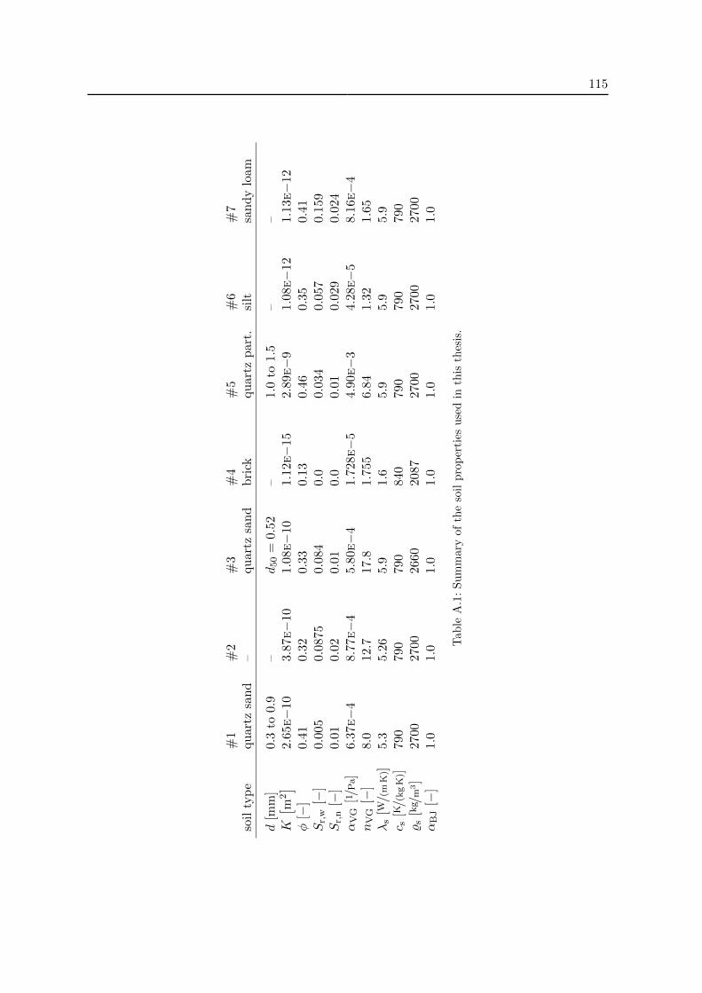
115
#1
#2
#3
#4
#5
#6
#7
soil
typ
equ
art
zsa
nd
–qu
artz
san
db
rick
qu
artz
par
t.si
ltsa
nd
ylo
am
d[m
m]
0.3
to0.
9–
d50
=0.
52–
1.0
to1.
5–
–K[ m
2]
2.6
5e−
10
3.8
7e−
10
1.0
8e−
101.1
2e−
152.8
9e−
91.0
8e−
12
1.1
3e−
12
φ[−
]0.
410.
320.
330.
130.
460.
35
0.41
Sr,
w[−
]0.0
050.
087
50.
084
0.0
0.03
40.
057
0.15
9S
r,n
[−]
0.01
0.02
0.01
0.0
0.01
0.029
0.024
αV
G[1/P
a]
6.3
7e−
48.7
7e−
45.8
0e−
41.7
28e−
54.9
0e−
34.2
8e−
58.1
6e−
4n
VG
[−]
8.0
12.7
17.8
1.75
56.
841.
321.
65λ
s[W/(
mK
)]5.3
5.26
5.9
1.6
5.9
5.9
5.9
c s[K/(
kg
K)]
790
790
790
840
790
790
790
%s
[kg /
m3]
2700
2700
2660
2087
2700
2700
270
0α
BJ
[−]
1.0
1.0
1.0
1.0
1.0
1.0
1.0
Tab
leA
.1:
Su
mm
ary
of
the
soil
pro
per
ties
use
din
this
thes
is.


B Code Validation
The purpose of this chapter is to summarize and present the performed validation tests. The
validation is performed to check the main functionality of the DuMux MAC-discretization
code written for this thesis, if not said otherwise, the results use this discretization method.
B.1 Analytical
Analytical tests are performed for the Stokes, Navier-Stokes, the k-ε, and the k-ω model.
B.1.1 Stokes [Donea and Huerta, 2003]
In this test case, known source terms for the mass and momentum balance trigger the desired
analytical solution of the stationary Stokes equation, cf. Donea and Huerta [2003, p. 306].
The equations are solved on a square domain Ω = [0, 1 m] × [0, 1 m] with constant values
of ν = 1 m2/s and % = 1 kg/m3 and Dirichlet boundary conditions everywhere. The resulting
l2-error norms are shown in Tab. B.1 and visualized in Fig. B.1.
0.001
0.01
0.1
1
0 1 2 3 4 5 6
l2-e
rror
refinement (ref.)
pv
Figure B.1: Relative l2-error convergence forpressure (p) and velocity (v) forthe test case by Donea and Huerta[2003].
ref. cells l2(p) l2(v)
0 42 2.24e-1 6.35e-11 82 1.13e-1 2.86e-12 162 5.69e-2 1.37e-13 322 2.85e-2 6.77e-24 642 1.42e-2 3.37e-25 1282 7.13e-3 1.68e-26 2562 3.56e-3 8.43e-3
Table B.1: Relative l2-error norms for pres-sure (p) and velocity (v) for the testcase by Donea and Huerta [2003].
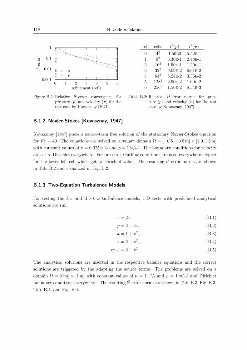
118 B Code Validation
0.001
0.01
0.1
1
0 1 2 3 4 5 6
l2-e
rror
refinement (ref.)
pv
Figure B.2: Relative l2-error convergence forpressure (p) and velocity (v) for thetest case by Kovasznay [1947].
ref. cells l2(p) l2(v)
0 42 1.50e0 5.52e-11 82 3.30e-1 2.48e-12 162 1.50e-1 1.29e-13 322 9.09e-2 6.61e-24 642 5.24e-2 3.36e-25 1282 2.90e-2 1.69e-26 2562 1.56e-2 8.54e-3
Table B.2: Relative l2-error norms for pres-sure (p) and velocity (v) for the testcase by Kovasznay [1947].
B.1.2 Navier-Stokes [Kovasznay, 1947]
Kovasznay [1947] poses a source-term free solution of the stationary Navier-Stokes equation
for Re = 40. The equations are solved on a square domain Ω = [−0.5,−0.5 m] × [1.0, 1.5 m]
with constant values of ν = 0.025 m2/s and % = 1 kg/m3. The boundary conditions for velocity
are set to Dirichlet everywhere. For pressure, Outflow conditions are used everywhere, expect
for the lower left cell which gets a Dirichlet value. The resulting l2-error norms are shown
in Tab. B.2 and visualized in Fig. B.2.
B.1.3 Two-Equation Turbulence Models
For testing the k-ε and the k-ω turbulence models, 1-D tests with predefined analytical
solutions are run:
v = 2x , (B.1)
p = 2− 2x , (B.2)
k = 1 + x2 , (B.3)
ε = 2− x2 , (B.4)
or ω = 2− x2 . (B.5)
The analytical solutions are inserted in the respective balance equations and the correct
solutions are triggered by the adapting the source terms. The problems are solved on a
domain Ω = [0 m] × [1 m] with constant values of ν = 1 m2/s and % = 1 kg/m3 and Dirichlet
boundary conditions everywhere. The resulting l2-error norms are shown in Tab. B.3, Fig. B.3,
Tab. B.4, and Fig. B.4.
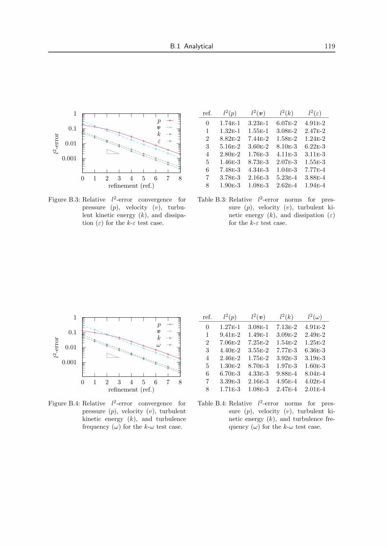
B.1 Analytical 119
0.001
0.01
0.1
1
0 1 2 3 4 5 6 7 8
l2-e
rror
refinement (ref.)
pvkε
Figure B.3: Relative l2-error convergence forpressure (p), velocity (v), turbu-lent kinetic energy (k), and dissipa-tion (ε) for the k-ε test case.
ref. l2(p) l2(v) l2(k) l2(ε)
0 1.74e-1 3.23e-1 6.07e-2 4.91e-21 1.32e-1 1.55e-1 3.08e-2 2.47e-22 8.82e-2 7.44e-2 1.58e-2 1.24e-23 5.16e-2 3.60e-2 8.10e-3 6.22e-34 2.80e-2 1.76e-3 4.11e-3 3.11e-35 1.46e-3 8.73e-3 2.07e-3 1.55e-36 7.48e-3 4.34e-3 1.04e-3 7.77e-47 3.78e-3 2.16e-3 5.23e-4 3.88e-48 1.90e-3 1.08e-3 2.62e-4 1.94e-4
Table B.3: Relative l2-error norms for pres-sure (p), velocity (v), turbulent ki-netic energy (k), and dissipation (ε)for the k-ε test case.
0.001
0.01
0.1
1
0 1 2 3 4 5 6 7 8
l2-e
rror
refinement (ref.)
pvkω
Figure B.4: Relative l2-error convergence forpressure (p), velocity (v), turbulentkinetic energy (k), and turbulencefrequency (ω) for the k-ω test case.
ref. l2(p) l2(v) l2(k) l2(ω)
0 1.27e-1 3.08e-1 7.13e-2 4.91e-21 9.41e-2 1.49e-1 3.09e-2 2.49e-22 7.06e-2 7.25e-2 1.54e-2 1.25e-23 4.40e-2 3.55e-2 7.77e-3 6.36e-34 2.46e-2 1.75e-2 3.92e-3 3.19e-35 1.30e-2 8.70e-3 1.97e-3 1.60e-36 6.70e-3 4.33e-3 9.88e-4 8.04e-47 3.39e-3 2.16e-3 4.95e-4 4.02e-48 1.71e-3 1.08e-3 2.47e-4 2.01e-4
Table B.4: Relative l2-error norms for pres-sure (p), velocity (v), turbulent ki-netic energy (k), and turbulence fre-quency (ω) for the k-ω test case.
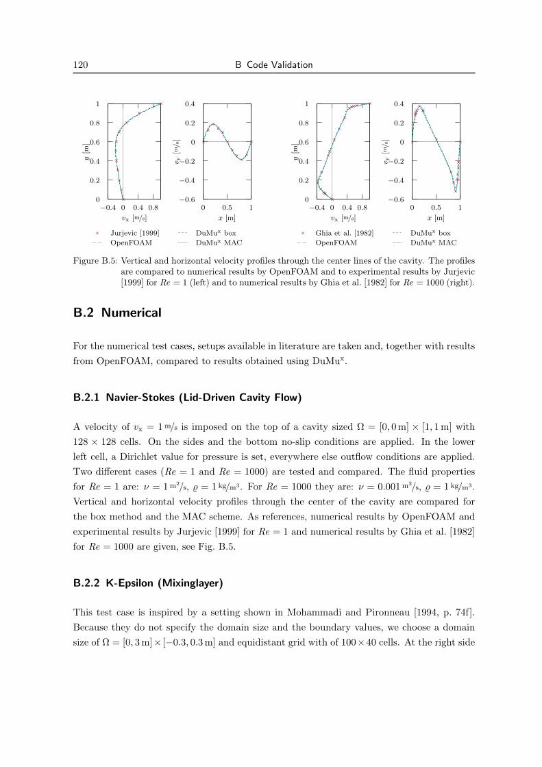
120 B Code Validation
0
0.2
0.4
0.6
0.8
1
−0.4 0 0.4 0.8
y[m
]
vx [m/s]
Jurjevic [1999]
OpenFOAM
DuMux box
DuMux MAC
−0.6
−0.4
−0.2
0
0.2
0.4
0 0.5 1
vy
[m/s
]
x [m]
0
0.2
0.4
0.6
0.8
1
−0.4 0 0.4 0.8
y[m
]
vx [m/s]
Ghia et al. [1982]
OpenFOAM
DuMux box
DuMux MAC
−0.6
−0.4
−0.2
0
0.2
0.4
0 0.5 1
vy
[m/s
]
x [m]
Figure B.5: Vertical and horizontal velocity profiles through the center lines of the cavity. The profilesare compared to numerical results by OpenFOAM and to experimental results by Jurjevic[1999] for Re = 1 (left) and to numerical results by Ghia et al. [1982] for Re = 1000 (right).
B.2 Numerical
For the numerical test cases, setups available in literature are taken and, together with results
from OpenFOAM, compared to results obtained using DuMux.
B.2.1 Navier-Stokes (Lid-Driven Cavity Flow)
A velocity of vx = 1 m/s is imposed on the top of a cavity sized Ω = [0, 0 m] × [1, 1 m] with
128 × 128 cells. On the sides and the bottom no-slip conditions are applied. In the lower
left cell, a Dirichlet value for pressure is set, everywhere else outflow conditions are applied.
Two different cases (Re = 1 and Re = 1000) are tested and compared. The fluid properties
for Re = 1 are: ν = 1 m2/s, % = 1 kg/m3. For Re = 1000 they are: ν = 0.001 m2/s, % = 1 kg/m3.
Vertical and horizontal velocity profiles through the center of the cavity are compared for
the box method and the MAC scheme. As references, numerical results by OpenFOAM and
experimental results by Jurjevic [1999] for Re = 1 and numerical results by Ghia et al. [1982]
for Re = 1000 are given, see Fig. B.5.
B.2.2 K-Epsilon (Mixinglayer)
This test case is inspired by a setting shown in Mohammadi and Pironneau [1994, p. 74f].
Because they do not specify the domain size and the boundary values, we choose a domain
size of Ω = [0, 3 m]× [−0.3, 0.3 m] and equidistant grid with of 100×40 cells. At the right side

B.3 Physical 121
v
k
ε
νt
DuMux MAC OpenFOAM
Figure B.6: Contour surfaces for the mixinglayer test case, after Mohammadi and Pironneau [1994].Results are shown for the DuMux MAC scheme and OpenFOAM.
outflow for v , k, and ε and Dirichlet for p are applied and the other way around for all other
boundaries. The constants as specified in 3.1.2.2 are used, the initial and boundary values
are:
v =
(2, 0 m/s)ᵀ, if y < 0
(1, 0 m/s)ᵀ, else, (B.6)
p = 1e5 Pa , (B.7)
k = 0.001 m2/s2 , (B.8)
ε = 0.001 m2/s3 . (B.9)
The fluid properties are constant with: ν = 0.00706 m2/s and % = 1.19 kg/m3. Fig. B.6 shows
contour surfaces for v , k, ε, and νt.
B.3 Physical (Pipe Flow, Laufer [1954])
Laufer [1954] performs a laboratory experiment in which air flows through a pipe at Re =
50 000. This experiment is simulated using a 2-D setup with a domain Ω = [0, 0 m] ×[10, 0.2469 m]. On the top and on the bottom no-slip conditions, and if necessary wall func-
tions, are applied. On the left, Dirichlet conditions with a constant velocity of v = (2.5, 0 m/s)ᵀ
is given, whereas the boundary conditions on the right are outflow. The problem is discretized
using 25 × 50 cells with a grading of 1.2 in vertical direction from each wall to the center.
For testing the wall functions of the k-ε model, an equal-spaced discretization with 20 cells in
vertical direction is used. Fig. B.7 shows the resulting velocity profiles for different turbulence
models.
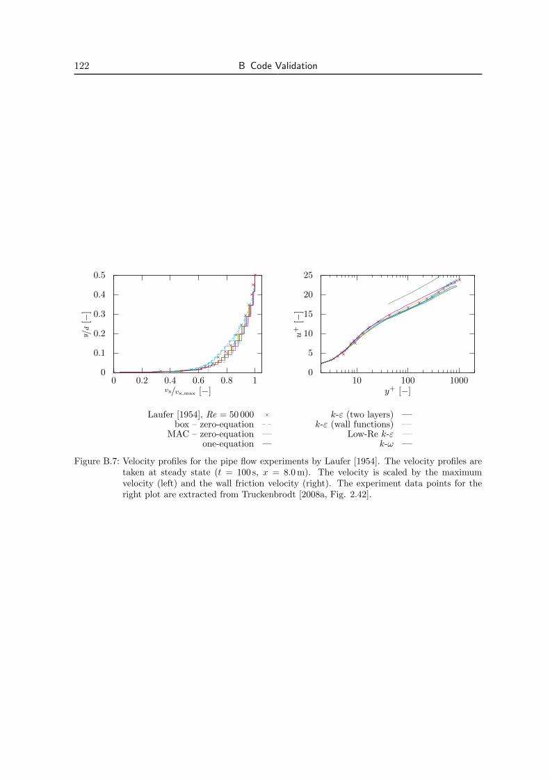
122 B Code Validation
0
0.1
0.2
0.3
0.4
0.5
0 0.2 0.4 0.6 0.8 1
y /d
[−]
vx/vx,max [−]
0
5
10
15
20
25
10 100 1000
u+
[−]
y+ [−]
Laufer [1954], Re = 50 000box – zero-equation
MAC – zero-equationone-equation
k-ε (two layers)k-ε (wall functions)
Low-Re k-εk-ω
Figure B.7: Velocity profiles for the pipe flow experiments by Laufer [1954]. The velocity profiles aretaken at steady state (t = 100 s, x = 8.0 m). The velocity is scaled by the maximumvelocity (left) and the wall friction velocity (right). The experiment data points for theright plot are extracted from Truckenbrodt [2008a, Fig. 2.42].

C Software and Hardware
The simulation results presented in this thesis are achieved using the open-source numerical
toolboxes DuMux and Dune. Tab. C.1 lists all required modules and Tab. C.2 provides a list
with other pre-compiled programs or library necessary for running the simulations. For unix
systems, a script which installs all necessary modules can be found at https://git.iws.
uni-stuttgart.de/dumux-pub/Fetzer2018a/raw/master/installFetzer2018a.sh 14.
The main module of this thesis (dumux-Fetzer2018a) has the following structure. First,
the release version of dumux has to be adapted with the patches provided in patches. The
appl/multidomain folder contains the problem specific source code for the presented results in
Ch. 5, whereas appl/staggeredgrid contains all basic MAC models. bin/jobfiles contains
script files to re-run all used simulations and scripts for all post-processing in bin/scripts.
In dumux, the basic transport model and input/output helper files are located. The plot
of material laws and fluid properties are performed by executables built from the material
folder. For re-simulating the OpenFOAM results, the files in openfoam can be used. The
data sets of which all plots and pictures in Ch. 5 are made of can be found in results. Note
that these data sets can be automatically reproduced by running the scripts from the bin
folder. Finally, test contains setups which ensure the basic functionality of the code. Some
of these setups are presented in Ch. B.
All simulation for which the simulation times and properties are given, are run on a Linux
computer using openSUSE 13.2 (Linux 3.16.7-35-default, kde 4.14.9), with four CPU cores
(Intel® Core™ i5-5300U @ 2.3GHz) and RAM of ≈11.85GB.
14Script was accessed on June 19, 2018
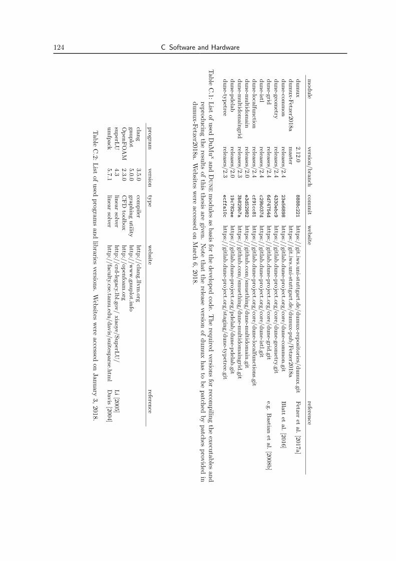
124 C Software and Hardware
module
versio
n/bra
nch
com
mit
web
sitereferen
ce
dum
ux
2.1
2.0
8888c221
http
s://git.iw
s.uni-stu
ttgart.d
e/dum
ux-rep
osito
ries/dum
ux.g
itF
etzeret
al.
[2017a]
dum
ux-F
etzer2018a
master
http
s://git.iw
s.uni-stu
ttgart.d
e/dum
ux-p
ub/F
etzer2018a
dune-co
mm
on
releases/
2.4
23e56898
http
s://gitla
b.d
une-p
roject.o
rg/co
re/dune-co
mm
on.g
itB
latt
etal.
[2016]
dune-g
eom
etryrelea
ses/2.4
4330ebc9
http
s://gitla
b.d
une-p
roject.o
rg/co
re/dune-g
eom
etry.git
dune-g
ridrelea
ses/2.4
6d74754d
http
s://gitla
b.d
une-p
roject.o
rg/co
re/dune-g
rid.g
ite.g
.B
astia
net
al.
[2008b]
dune-istl
releases/
2.4
c29b037d
http
s://gitla
b.d
une-p
roject.o
rg/co
re/dune-istl.g
itdune-lo
calfu
nctio
nrelea
ses/2.4
cf91cc81
http
s://gitla
b.d
une-p
roject.o
rg/co
re/dune-lo
calfu
nctio
ns.g
itdune-m
ultid
om
ain
releases/
2.0
e3d52982
http
s://gith
ub.co
m/sm
ueth
ing/dune-m
ultid
om
ain
.git
dune-m
ultid
om
ain
grid
releases/
2.3
3b829b7a
http
s://gith
ub.co
m/sm
ueth
ing/dune-m
ultid
om
ain
grid
.git
dune-p
dela
brelea
ses/2.0
19c782ee
http
s://gitla
b.d
une-p
roject.o
rg/p
dela
b/dune-p
dela
b.g
itdune-ty
petree
releases/
2.3
ecffa10c
http
s://gitla
b.d
une-p
roject.o
rg/sta
gin
g/dune-ty
petree.g
it
Tab
leC
.1:
List
ofu
sedD
uM
ux
andDune
mod
ules
as
basis
for
the
develo
ped
cod
e.T
he
requ
iredversion
sfor
recomp
iling
the
execu
tables
and
repro
du
cing
the
results
of
this
thesis
are
given
.N
ote
that
the
release
version
of
du
mu
xh
asto
be
patch
edby
patch
esp
rovid
edin
du
mu
x-F
etzer2018a.
Web
sitesw
ereaccessed
on
March
6,
2018.
pro
gra
mversio
nty
pe
web
sitereferen
ce
clang
3.5
.0co
mpiler
http
://cla
ng.llv
m.o
rggnuplo
t5.0
.0gra
phin
gutility
http
://w
ww
.gnuplo
t.info
Op
enF
OA
M2.3
.0C
FD
toolb
oxhttp
://op
enfo
am
.org
sup
erLU
4.3
linea
rso
lver
http
://crd
-legacy.lb
l.gov
/xia
oye/
Sup
erLU
/L
i[2
005]
um
fpack
5.7
.1lin
ear
solv
erhttp
://fa
culty.cse.ta
mu.ed
u/dav
is/su
itesparse.h
tml
Dav
is[2
004]
Tab
leC
.2:L
istof
used
prog
ram
san
dlib
raries
version
s.W
ebsites
were
accessed
onJan
uary
3,2018.
Bibliography
B. Ahrenholz, J. Niessner, R. Helmig, and M. Krafczyk. Pore-scale determination of param-
eters for macroscale modeling of evaporation processes in porous media. Water Resources
Research, 47(7):W07543, 2011. doi: 10.1029/2010WR009519.
S. R. Allmaras, F. T. Johnson, and P. R. Spalart. Modifications and Clarifications for the
Implementation of the Spalart-Allmaras Turbulence Model. In Seventh International Con-
ference on Computational Fluid Dynamics (ICCFD7), 2012.
S. Aluwihare and K. Watanabe. Measurement of Evaporation on Bare Soil and Estimat-
ing Surface Resistance. Journal of Environmental Engineering, 129(12):1157–1168, 2003.
doi: 10.1061/(ASCE)0733-9372(2003)129:12(1157).
P. S. Andersen, W. M. Kays, and R. J. Moffat. The Turbulent Boundary Layer on a Porous
Plate: An Experimental Study of the Fluid Mechanics for Adverse Free-Stream Pressure
Gradients. Report HMT-15, Department of Mechanical Engineering, Stanford University,
1972.
ANSYS, Inc. ANSYS FLUENT 12.0 - Theory Guide, 2009a.
ANSYS, Inc. ANSYS FLUENT 12.0 - User’s Guide, 2009b.
J. E. Armstrong, E. O. Frind, and R. D. McClellan. Nonequilibrium mass transfer between
the vapor, aqueous, and solid phases in unsaturated soils during vapor extraction. Water
Resources Research, 30(2):355–368, 1994. doi: 10.1029/93WR02481.
S. Assouline, K. Narkis, and D. Or. Evaporation from partially covered water surfaces. Water
Resources Research, 46(10):W10539, 2010. doi: 10.1029/2010WR009121.
J.-L. Auriault. About the Beavers and Joseph Boundary Condition. Transport in Porous
Media, 83(2):257–266, 2010. doi: 10.1007/s11242-009-9435-9.
K. Baber. Coupling free flow and flow in porous media in biological and technical applications:
From a simple to a complex interface description. PhD thesis, University of Stuttgart, 2014.
doi: 10.18419/opus-594.

126 Bibliography
K. Baber, K. Mosthaf, B. Flemisch, R. Helmig, S. Muthing, and B. Wohlmuth. Nu-
merical scheme for coupling two-phase compositional porous-media flow and one-phase
compositional free flow. IMA Journal of Applied Mathematics, 77(6):887–909, 2012.
doi: 10.1093/imamat/hxs048.
K. Baber, B. Flemisch, and R. Helmig. Modeling drop dynamics at the interface between
free and porous-medium flow using the mortar method. International Journal of Heat and
Mass Transfer, 99:660–671, 2016. doi: 10.1016/j.ijheatmasstransfer.2016.04.014.
B. S. Baldwin and T. J. Barth. A one-equation turbulence transport model for high Reynolds
number wall-bounded flows. NASA Technical Memorandum 102847, NASA, 1990.
B. S. Baldwin and H. Lomax. Thin Layer Approximation and Algebraic Model for Seperated
Turbulent Flows. ACM Trans Math Software, 78–257:1–9, 1978. doi: 10.2514/6.1978-257.
J. Bardina, P. Huang, T. Coakley, J. Bardina, P. Huang, and T. Coakley. Turbulence mod-
eling validation. In 28th Fluid Dynamics Conference, Fluid Dynamics and Co-located
Conferences. American Institute of Aeronautics and Astronautics, 1997. doi: 10.2514/
6.1997-2121.
P. Bastian, M. Blatt, A. Dedner, C. Engwer, R. Klofkorn, R. Kornhuber, M. Ohlberger, and
O. Sander. A Generic Grid Interface for Parallel and Adaptive Scientific Computing. Part
II: Implementation and Tests in DUNE. Computing, 82(2–3):121–138, 2008a. doi: 10.
1007/s00607-008-0004-9.
P. Bastian, M. Blatt, A. Dedner, C. Engwer, R. Klofkorn, M. Ohlberger, and O. Sander. A
Generic Grid Interface for Parallel and Adaptive Scientific Computing. Part I: Abstract
Framework. Computing, 82(2–3):103–119, 2008b. doi: 10.1007/s00607-008-0003-x.
J. Bear. Dynamics of fluids in porous media. Dover Publ., New York, 1988. ISBN 0-486-
65675-6.
G. S. Beavers and D. D. Joseph. Boundary conditions at a naturally permeable wall. Journal
of Fluid Mechanics, 30(1):197–207, 1967. doi: 10.1017/S0022112067001375.
G. S. Beavers, E. M. Sparrow, and B. A. Masha. Boundary Condition at a Porous Surface
Which Bounds a Fluid Flow. AIChE Journal, 20(3):596–597, 1974. doi: 10.1002/aic.
690200323.
A. Belhamri and J.-P. Fohr. Heat and mass transfer along a wetted porous plate in an air
stream. AIChE Journal, 42(7):1833–1843, 1996. doi: 10.1002/aic.690420705.
Bibliography 127
M. V. Belleghem, M. Steeman, H. Janssen, A. Janssens, and M. D. Paepe. Validation of a
coupled heat, vapour and liquid moisture transport model for porous materials implemented
in CFD. Building and Environment, 81:340–353, 2014. doi: 10.1016/j.buildenv.2014.
06.024.
S. Beyhaghi, Z. Xu, and K. M. Pillai. Achieving the Inside–Outside Coupling During Network
Simulation of Isothermal Drying of a Porous Medium in a Turbulent Flow. Transport in
Porous Media, 114(3):823–842, 2016. doi: 10.1007/s11242-016-0746-3.
R. B. Bird, W. E. Stewart, and E. N. Lightfoot. Transport Phenomena. Wiley, New York, 2
edition, 2007. ISBN 978-0-470-11539-8.
M. Blatt, A. Burchardt, A. Dedner, C. Engwer, J. Fahlke, B. Flemisch, C. Gersbacher,
C. Graser, F. Gruber, C. Gruninger, D. Kempf, R. Klofkorn, T. Malkmus, S. Muthing,
M. Nolte, M. Piatkowski, and O. Sander. The Distributed and Unified Numerics Environ-
ment, Version 2.4. Archive of Numerical Software, 4(100):13–29, 2016. doi: 10.11588/ans.
2016.100.26526.
B. Blocken, T. Stathopoulos, and J. Carmeliet. CFD simulation of the atmospheric boundary
layer: wall function problems. Atmospheric Environment, 41(2):238–252, 2007. doi: 10.
1016/j.atmosenv.2006.08.019.
M. J. Blunt, B. Bijeljic, H. Dong, O. Gharbi, S. Iglauer, P. Mostaghimi, A. Paluszny, and
C. Pentland. Pore-scale imaging and modelling. Advances in Water Resources, 51:197–216,
2013. doi: 10.1016/j.advwatres.2012.03.003.
J. V. Boussinesq. Essai sur la theorie des eaux courantes. Memoires Acad. des Sciences, 23
(1):1–680, 1877.
W. P. Breugem and B. J. Boersma. Direct numerical simulations of turbulent flow over a
permeable wall using a direct and a continuum approach. Physics of Fluids, 17(2):025103,
2005. doi: 10.1063/1.1835771.
H. C. Brinkman. A calculation of the viscous force exerted by a flowing fluid on a dense swarm
of particles. Applied Scientific Research, 1(1):27–34, 1949. doi: 10.1007/BF02120313.
T. Broecker, W. Elsesser, K. Teuber, I. Ozgen, G. Nutzmann, and R. Hinkelmann. High-
resolution simulation of free-surface flow and tracer retention over streambeds with ripples.
Limnologica, 68:46–58, 2018. doi: 10.1016/j.limno.2017.06.005.
R. H. Brooks and A. T. Corey. Hydraulic Properties of Porous Media. Technical report,
Colorado State University, Fort Collins, Colorado, 1964.

128 Bibliography
W. Brutsaert. Evaporation into the Atmosphere: Theory, History, and Applications, volume 1.
D. Reidel Publishing Company, Dordrecht, 1982. ISBN 90-277-1247-6. doi: 10.1007/
978-94-017-1497-6.
R. Buccolieri, C. Gromke, S. D. Sabatino, and B. Ruck. Aerodynamic effects of trees on
pollutant concentration in street canyons. Science of The Total Environment, 407(19):
5247–5256, 2009. doi: 10.1016/j.scitotenv.2009.06.016.
T. Cebeci. A Model for Eddy Conductivity and Turbulent Prandtl Number. Journal of Heat
Transfer, 95(2):227–234, 1973. doi: 10.1115/1.3450031.
T. Cebeci. Calculation of Incompressible Rough-Wall Boundary Layer Flows. AIAA Journal,
16(7):730–735, 1978. doi: 10.2514/3.7571.
T. Cebeci and A. M. O. Smith. Analysis of turbulent boundary layers. Academic Press, New
York, 1974. ISBN 0-12-164650-5.
CFD Online. www.cfd-online.com, 2017.
L. Chen, S. Wang, G. Li, C.-H. Lin, and T. Zhang. CFD modeling of moisture accumulation
in the insulation layers of an aircraft. Applied Thermal Engineering, 102:1141–1156, 2016.
doi: 10.1016/j.applthermaleng.2016.04.048.
K.-Y. Chien. Predictions of Channel and Boundary-Layer Flows with a Low-Reynolds-
Number Turbulence Model. AIAA Journal, 20(1):33–38, 1982. doi: 10.2514/3.51043.
F. Cimolin and M. Discacciati. Navier-Stokes/Forchheimer models for filtration through
porous media. Applied Numerical Mathematics, 72:205–224, 2013. doi: 10.1016/j.apnum.
2013.07.001.
H. Class. Theorie und numerische Modellierung nichtisothermer Mehrphasenprozesse in
NAPL-kontaminierten porosen Medien. PhD thesis, Technische Universitat Braunschweig,
2001. doi: 10.18419/opus-223.
H. Class. Models for non-isothermal compositional gas-liquid flow and transport in porous
media. Habilitation, University of Stuttgart, 2007. doi: 10.18419/opus-299.
H. Class, R. Helmig, and P. Bastian. Numerical simulation of non-isothermal multiphase
multicomponent processes in porous media.: 1. An efficient solution technique. Advances
in Water Resources, 25(5):533–550, 2002. doi: 10.1016/S0309-1708(02)00014-3.
C. F. Colebrook. Turbulent flow in pipes, with particular reference to the transition region
between smooth and rough pipe laws. Journal of the Institution of Civil Engineers, 11(4):
133–156, 1939. doi: 10.1680/ijoti.1939.13150.
Bibliography 129
T. J. Craft, A. V. Gerasimov, H. Iacovides, and B. E. Launder. Progress in the generalization
of wall-function treatments. International Journal of Heat and Fluid Flow, 23(2):148–160,
2002. doi: 10.1016/S0142-727X(01)00143-6.
W. Dahmen, T. Gotzen, S. Muller, and M. Rom. Numerical simulation of transpiration
cooling through porous material. International Journal for Numerical Methods in Fluids,
76(6):331–365, 2014. doi: 10.1002/fld.3935.
B. Das, J. Hendrickx, and B. Borchers. Modeling transient water distributions
around landmines in bare soils. Soil Science, 166(3):163–173, 2001. doi: 10.1097/
00010694-200103000-00002.
D. B. Das, V. Nassehi, and R. J. Wakeman. A finite volume model for the hydrodynamics of
combined free and porous flow in sub-surface regions. Advances in Environmental Research,
7(1):35–58, 2002. doi: 10.1016/S1093-0191(01)00108-3.
H. Davarzani, K. M. Smits, R. M. Tolene, and T. Illangasekare. Study of the effect of wind
speed on evaporation from soil through integrated modeling of the atmospheric boundary
layer and shallow subsurface. Water Resources Research, 50(1):1–20, 2014. doi: 10.1002/
2013WR013952.
T. A. Davis. Algorithm 832: UMFPACK V4.3—an Unsymmetric-pattern Multifrontal
Method. ACM Transactions on Mathematical Software, 30(2):196–199, 2004. doi: 10.
1145/992200.992206.
M. J. S. de Lemos. Turbulent Flow Around Fluid–Porous Interfaces Computed with a
Diffusion-Jump Model for k and ε Transport Equations. Transport in Porous Media, 78
(3):331–346, 2009. doi: 10.1007/s11242-009-9379-0.
T. Defraeye. Convective heat and mass transfer at exterior building surfaces. PhD thesis,
Katholieke Universiteit Leuven, 2011.
T. Defraeye, B. Blocken, and J. Carmeliet. CFD analysis of convective heat transfer at the
surfaces of a cube immersed in a turbulent boundary layer. International Journal of Heat
and Mass Transfer, 53(1–3):297–308, 2010. doi: 10.1016/j.ijheatmasstransfer.2009.
09.029.
T. Defraeye, B. Blocken, and J. Carmeliet. Analysis of convective heat and mass transfer
coefficients for convective drying of a porous flat plate by conjugate modelling. Inter-
national Journal of Heat and Mass Transfer, 55(1–3):112–124, 2012a. doi: 10.1016/j.
ijheatmasstransfer.2011.08.047.
130 Bibliography
T. Defraeye, B. Blocken, D. Derome, B. Nicolai, and J. Carmeliet. Convective heat and mass
transfer modelling at air–porous material interfaces: Overview of existing methods and
relevance. Chemical Engineering Science, 74:49–58, 2012b. doi: 10.1016/j.ces.2012.02.
032.
F. Diaz, C. C. Jimenez, and M. Tejedor. Influence of the thickness and grain size of tephra
mulch on soil water evaporation. Agricultural Water Management, 74(1):47–55, 2005.
doi: 10.1016/j.agwat.2004.10.011.
M. Discacciati and A. Quarteroni. Navier-Stokes/Darcy Coupling: Modeling, Analysis, and
Numerical Approximation. Revista Matematica Complutense, 22(2):315–426, 2009. doi: 10.
5209/rev_REMA.2009.v22.n2.16263.
M. Discacciati, P. Gervasio, and A. Quarteroni. Interface control domain decomposition
methods for heterogeneous problems. International Journal for Numerical Methods in
Fluids, 76(8):471–496, 2014. doi: 10.1002/fld.3942.
M. Discacciati, P. Gervasio, A. Giacomini, and A. Quarteroni. The Interface Control Domain
Decomposition Method for Stokes–Darcy Coupling. SIAM Journal on Numerical Analysis,
54(2):1039–1068, 2016. doi: 10.1137/15M101854X.
J. Donea and A. Huerta. Finite Element Methods for Flow Problems, volume 1. Wiley, 2003.
ISBN 978-0-470-01382-3. doi: 10.1002/0470013826.ch6.
Y. Dong, J. S. McCartney, and N. Lu. Critical Review of Thermal Conductivity Models for
Unsaturated Soils. Geotechnical and Geological Engineering, 33(2):207–221, 2015. doi: 10.
1007/s10706-015-9843-2.
P. A. Durbin. Near-wall turbulence closure modeling without “damping functions”. Theoret-
ical and Computational Fluid Dynamics, 3(1):1–13, 1991. doi: 10.1007/BF00271513.
E. Fattahi, C. Waluga, B. Wohlmuth, U. Rude, M. Manhart, and R. Helmig. Lattice Boltz-
mann methods in porous media simulations: From laminar to turbulent flow. Computers
& Fluids, 140:247– 259, 2016. doi: 10.1016/j.compfluid.2016.10.007.
R. T. Ferrell and D. M. Himmelblau. Diffusion coefficients of nitrogen and oxygen in water.
Journal of Chemical & Engineering Data, 12(1):111–115, 1967. doi: 10.1021/je60032a036.
T. Fetzer. Numerical analysis of the influence of turbulence on exchange processes between
porous-medium and free flow. Diploma thesis, University of Stuttgart, 2012.
T. Fetzer, K. M. Smits, and R. Helmig. Effect of Turbulence and Roughness on Coupled
Porous-Medium/Free-Flow Exchange Processes. Transport in Porous Media, 114(2):395–
424, 2016. doi: 10.1007/s11242-016-0654-6.

Bibliography 131
T. Fetzer, B. Becker, B. Flemisch, D. Glaser, K. Heck, T. Koch, M. Schneider, S. Scholz, and
K. Weishaupt. DuMuX 2.12.0, 2017a.
T. Fetzer, C. Gruninger, B. Flemisch, and R. Helmig. On the Conditions for Coupling Free
Flow and Porous-Medium Flow in a Finite Volume Framework, pages 347–356. Finite
Volumes for Complex Applications VIII - Hyperbolic, Elliptic and Parabolic Problems:
FVCA 8, Lille, France, June 2017. Springer International Publishing, Cham, 2017b. ISBN
978-3-319-57394-6. doi: 10.1007/978-3-319-57394-6_37.
T. Fetzer, J. Vanderborght, K. Mosthaf, K. M. Smits, and R. Helmig. Heat and water
transport in soils and across the soil-atmosphere interface: 2. Numerical analysis. Water
Resources Research, 53(2):1080–1100, 2017c. doi: 10.1002/2016WR019983.
A. Fick. Ueber Diffusion. Annalen der Physik, 170(1):59–86, 1855. doi: 10.1002/andp.
18551700105.
S. Finsterle. Inverse Modellierung zur Bestimmung hydrogeologischer Parameter eines
Zweiphasensystems. VAW Mitteilungen 121, ETH Zurich, 1993.
B. Flemisch, M. Darcis, K. Erbertseder, B. Faigle, A. Lauser, K. Mosthaf, S. Muthing,
P. Nuske, A. Tatomir, M. Wolff, and R. Helmig. DuMuX: DUNE for Multi-Phase, Com-
ponent, Scale, Physics, ... Flow and Transport in Porous Media. Advances in Water
Resources, 34(9):1102–1112, 2011. doi: 10.1016/j.advwatres.2011.03.007.
T. K. Flesch, J. H. Prueger, and J. L. Hatfield. Turbulent Schmidt number from a tracer
experiment. Agricultural and Forest Meteorology, 111(4):299–307, 2002. doi: 10.1016/
S0168-1923(02)00025-4.
M. Fritsch. Analysis of Processes and Properties at a Porous-Medium Free-Flow Interface
with the Application of Evaporation. Masther’s thesis, University of Stuttgart, 2014. Su-
pervisors: R. Helmig and T. Fetzer.
H. Fujimaki, T. Shimano, M. Inoue, and K. Nakane. Effect of a Salt Crust on Evaporation from
a Bare Saline Soil. Vadose Zone Journal, 5(4):1246–1256, 2006. doi: 10.2136/vzj2005.
0144.
A. Furman. Modeling Coupled Surface–Subsurface Flow Processes: A Review. Vadose Zone
Journal, 7(2):741–756, 2008. doi: 10.2136/vzj2007.0065.
U. Ghia, K. N. Ghia, and C. T. Shin. High-Re solutions for incompressible flow using the
Navier-Stokes equations and a multigrid method. Journal of Computational Physics, 48
(3):387–411, 1982. doi: 10.1016/0021-9991(82)90058-4.
132 Bibliography
P. Grassmann and F. Widmer. Einfuhrung in die thermische Verfahrenstechnik. de Gruyter,
Berlin, 2 edition, 1974. ISBN 3-11-004214-2.
C. Gruninger. Numerical Coupling of Navier-Stokes and Darcy Flow for Soil-Water Evapo-
ration. PhD thesis, University of Stuttgart, 2017.
C. Gruninger, T. Fetzer, B. Flemisch, and R. Helmig. Coupling DuMuX and DUNE-PDELab
to investigate evaporation at the interface between Darcy and Navier-Stokes flow. Preprint
Series 2017 – 1, Stuttgart Research Centre for Simulation Technology (SRC SimTech),
University of Stuttgart, 2017. doi: 10.18419/opus-9360.
V. Gurau, T. A. Zawodzinski, Jr., and J. A. Mann, Jr. Two-Phase Transport in PEM Fuel
Cell Cathodes. Journal of Fuel Cell Science and Technology, 5(2):021009–021009–12, 2008.
doi: 10.1115/1.2821597.
S. E. Haaland. Simple and Explicit Formulas for the Friction Factor in Turbulent Pipe Flow.
Journal of Fluids Engineering, 105(1):89–90, 1983. doi: 10.1115/1.3240948.
E. Haghighi and D. Or. Interactions of bluff-body obstacles with turbulent airflows affecting
evaporative fluxes from porous surfaces. Journal of Hydrology, 530:103–116, 2015. doi: 10.
1016/j.jhydrol.2015.09.048.
E. Haghighi, E. Shahraeeni, P. Lehmann, and D. Or. Evaporation rates across a convective air
boundary layer are dominated by diffusion. Water Resources Research, 49(3):1602–1610,
2013. doi: 10.1002/wrcr.20166.
S. Hahn, J. Je, and H. Choi. Direct numerical simulation of turbulent channel flow
with permeable walls. Journal of Fluid Mechanics, 450:259–285, 2002. doi: 10.1017/
S0022112001006437.
O. T. Hanna, O. C. Sandell, and P. R. Mazet. Heat and Mass Transfer in Turbulent Flow
Under Conditions of Drag Reduction. AIChE Journal, 27(4):693–697, 1981. doi: 10.1002/
aic.690270424.
N. S. Hanspal, A. N. Waghode, V. Nassehi, and R. J. Wakeman. Numerical Analysis of
Coupled Stokes/Darcy Flows in Iindustrial Filtrations. Transport in Porous Media, 64(1):
73–101, 2006. doi: 10.1007/s11242-005-1457-3.
F. H. Harlow and J. E. Welch. Numerical Calculation of Time-Dependent Viscous In-
compressible Flow of Fluid with Free Surface. Physics of Fluids, 8(12):2182–2189, 1965.
doi: 10.1063/1.1761178.

Bibliography 133
K. Heck. Numerical and experimental investigation of soil-root interactions. Masther’s thesis,
University of Stuttgart, 2016. Supervisors: R. Helmig, B. Flemisch, N. Schroder, T. Fetzer,
and A. Trautz.
R. Helmig. Multiphase Flow and Transport Processes in the Subsurface: A Contribution to
the Modeling of Hydrosystems. Springer, Berlin, 1997. ISBN 978-3-540-62703-6.
R. Huber and R. Helmig. Node-centered finite volume discretizations for the numerical simu-
lation of multiphase flow in heterogeneous porous media. Computers & Geosciences, 4(2):
141–164, 2000. doi: 10.1023/A:1011559916309.
IAPWS. Revised Release on the IAPWS Industrial Formulation 1997 for the Thermodynamic
Properties of Water and Steam. Technical Report IAPWS R7-97(2012), The International
Association for the Properties of Water and Steam, Lucerne, Switzerland, 2007.
IAPWS. Release on the IAPWS Formulation 2008 for the Viscosity of Ordinary Water Sub-
stance. Technical Report IAPWS R12-08, The International Association for the Properties
of Water and Steam, Berlin, Germany, 2008.
IAPWS. Release on the IAPWS Formulation 2011 for the Thermal Conductivity of Ordinary
Water Substance. Technical Report IAPWS R15-11, The International Association for the
Properties of Water and Steam, Plzen, Czech Republic, 2011.
O. Iliev and V. Laptev. On numerical simulation of flow through oil filters. Computing and
Visualization in Science, 6(2):139–146, 2004. doi: 10.1007/s00791-003-0118-8.
A. Jamarani, M. Maerefat, N. F. Jouybari, and M. E. Nimvari. Thermal Performance Eval-
uation of a Double-Tube Heat Exchanger Partially Filled with Porous Media Under Tur-
bulent Flow Regime. Transport in Porous Media, 120(3):449–471, 2017. doi: 10.1007/
s11242-017-0933-x.
V. A. Jambhekar, R. Helmig, N. Schroder, and N. Shokri. Free-Flow–Porous-Media Coupling
for Evaporation-Driven Transport and Precipitation of Salt in Soil. Transport in Porous
Media, 110(2):251–280, 2015. doi: 10.1007/s11242-015-0516-7.
V. A. Jambhekar, E. Mejri, N. Schroder, R. Helmig, and N. Shokri. Kinetic Approach
to Model Reactive Transport and Mixed Salt Precipitation in a Coupled Free-Flow–
Porous-Media System. Transport in Porous Media, 114(2):341–369, 2016. doi: 10.1007/
s11242-016-0665-3.
O. Johansen. Thermal conductivity of soils. PhD Thesis, (CRREL draft transl. 637, 1977),
Norwegian University of Science and Technology, Trondheim, Norway, 1975.
134 Bibliography
W. P. Jones and B. E. Launder. The prediction of laminarization with a two-equation model
of turbulence. International Journal of Heat and Mass Transfer, 15(2):301–314, 1972.
doi: 10.1016/0017-9310(72)90076-2.
R. Jurjevic. Modelling of two-dimensional laminar flow using finite element method. Interna-
tional Journal for Numerical Methods in Fluids, 31(3):601–626, 1999. doi: 10.1002/(SICI)
1097-0363(19991015)31:3<601::AID-FLD892>3.0.CO;2-Z.
W. M. Kays, M. E. Crawford, and B. Weigand. Convective heat and mass transfer. McGraw-
Hill Higher Education, 4 edition, 2009. ISBN 9780071238298.
T. Koch, K. Heck, N. Schroder, B. Flemisch, and R. Helmig. A new model concept for
plant-scale soil-root interaction including soil evaporation, growth and transport processes.
Vadose Zone Journal, accepted, 2018.
A. N. Kolmogorov. The local structure of turbulence in incompressible viscous fluid for very
large Reynolds numbers [in Russian]. Doklady Akademii Nauk SSSR, 30(4):301–305, 1941.
A. N. Kolmogorov. Equations of turbulent motion in an icompressible Fluid [in Russian].
Izvestia Academii Nauk USSR: Physics, 6(1–2):56–58, 1942.
A. N. Kolmogorov. The Local Structure of Turbulence in Incompressible Viscous Fluid for
Very Large Reynolds Numbers. Proceedings: Mathematical and Physical Sciences, 434
(1890):9–13, 1991.
L. I. G. Kovasznay. Laminar flow behind a two-dimensional grid. Mathematical Proceedings of
the Cambridge Philosophical Society, 44(1):58–62, 1947. doi: 10.1017/S0305004100023999.
M. Krafczyk, K. Kucher, Y. Wang, and M. Geier. DNS/LES Studies of Turbulent Flows
Based on the Cumulant Lattice Boltzmann Approach. In W. E. Nagel, D. H. Kroner, and
M. M. Resch, editors, High Performance Computing in Science and Engineering ’14, pages
519–531. Springer International Publishing, 2015. ISBN 978-3-319-10809-4. doi: 10.1007/
978-3-319-10810-0_34.
Y. Kuwata and K. Suga. Lattice Boltzmann direct numerical simulation of interface tur-
bulence over porous and rough walls. International Journal of Heat and Fluid Flow, 61:
145–157, 2016. doi: 10.1016/j.ijheatfluidflow.2016.03.006.
A. V. Kuznetsov. Numerical modeling of turbulent flow in a composite porous/fluid duct
utilizing a two-layer k–ε model to account for interface roughness. International Journal of
Thermal Sciences, 43(11):1047–1056, 2004. doi: 10.1016/j.ijthermalsci.2004.02.011.
Bibliography 135
A. V. Kuznetsov and S. M. Becker. Effect of the interface roughness on turbulent convective
heat transfer in a composite porous/fluid duct. International Communications in Heat and
Mass Transfer, 31(1):11–20, 2004. doi: 10.1016/S0735-1933(03)00197-0.
J. Laufer. The structure of turbulence in fully developed pipe flow. NACA Report, 1174:
417–434, 1954.
B. E. Launder and B. I. Sharma. Application of the energy-dissipation model of turbulence
to the calculation of flow near a spinning disc. Letters in Heat and Mass Transfer, 1(2):
131–137, 1974. doi: 10.1016/0094-4548(74)90150-7.
B. E. Launder and D. B. Spalding. Mathematical Models of Turbulence. Acadademic Press,
London, 1972.
J. B. Laurindo and M. Prat. Numerical and experimental network study of evaporation in
capillary porous media. Drying rates. Chemical Engineering Science, 53(12):2257–2269,
1998. doi: 10.1016/S0009-2509(97)00348-5.
W. J. Layton, F. Schieweck, and I. Yotov. Coupling fluid flow with porous media flow. SIAM
Journal on Numerical Analysis, 40(6):2195–2218, 2002. doi: 10.1137/S0036142901392766.
M. Le Bars and M. G. Worster. Interfacial conditions between a pure fluid and a porous
medium: implications for binary alloy solidification. Journal of Fluid Mechanics, 550:
149–173, 2006. doi: 10.1017/S0022112005007998.
P. Lehmann and D. Or. Evaporation and capillary coupling across vertical textural contrasts
in porous media. Physical Review E, 80(4):046318, 2009. doi: 10.1103/PhysRevE.80.
046318.
P. Lehmann, S. Assouline, and D. Or. Characteristic lengths affecting evaporative drying of
porous media. Physical Review E, 77(5):056309, 2008. doi: 10.1103/PhysRevE.77.056309.
E. W. Lemmon and R. T. Jacobsen. Viscosity and Thermal Conductivity Equations for
Nitrogen, Oxygen, Argon, and Air. International Journal of Thermophysics, 25(1):21–69,
2004. doi: 10.1023/B:IJOT.0000022327.04529.f3.
M. C. Leverett. Capillary Behavior in Porous Solids. Transactions of the AIME, 1(5), 1941.
doi: 10.2118/941152-G.
X. S. Li. An Overview of SuperLU: Algorithms, Implementation, and User Interface. ACM
Transactions on Mathematical Software, 31(3):302–325, 2005. doi: 10.1145/1089014.
1089017.

136 Bibliography
F. S. Lien, E. Yee, and Y. Cheng. Simulation of mean flow and turbulence over a 2D building
array using high-resolution CFD and a distributed drag force approach. Journal of Wind
Engineering and Industrial Aerodynamics, 92(2):117–158, 2004. doi: 10.1016/j.jweia.
2003.10.005.
S. Lu, T. Ren, Z. Yu, and R. Horton. A method to estimate the water vapour enhancement
factor in soil. European Journal of Soil Science, 62(4):98–504, 2011. doi: 10.1111/j.
1365-2389.2011.01359.x.
T. Lu, P. Jiang, and S. Shen. Numerical and experimental investigation of convective drying
in unsaturated porous media with bound water. Heat and Mass Transfer, 41(12):1103–1111,
2005. doi: 10.1007/s00231-005-0634-9.
M. Maier, H. Schack-Kirchner, M. Aubinet, S. Goffin, B. Longdoz, and F. Parent. Turbulence
Effect on Gas Transport in Three Contrasting Forest Soils. Soil Science Society of America
Journal, 76(5):1518–1528, 2012. doi: 10.2136/sssaj2011.0376.
M. R. Malin. On the calculation of heat transfer rates in fully turbulent wall flows. Applied
Mathematical Modelling, 11(4):281–284, 1987. doi: 10.1016/0307-904X(87)90143-0.
C. Manes, D. Pokrajac, V. I. Nikora, L. Ridolfi, and D. Poggi. Turbulent friction in flows
over permeable walls. Geophysical Research Letters, 38(3):L03402, 2011. doi: 10.1029/
2010GL045695.
C. Masson, H. J. Saabas, and B. R. Baliga. Co-located equal-order control-volume finite
element method for two-dimensional axisymmetric incompressible fluid flow. International
Journal for Numerical Methods in Fluids, 18(1):1–26, 1994. doi: 10.1002/fld.1650180102.
R. Masson, L. Trenty, and Y. Zhang. Coupling compositional liquid gas Darcy and free gas
flows at porous and free-flow domains interface. Journal of Computational Physics, 321:
708–728, 2016. doi: 10.1016/j.jcp.2016.06.003.
D. J. Mavriplis. Algebraic Turbulence Modeling for Unstructered and Adaptive Meshes.
AIAA Journal, 29(12):2086–2093, 1990. doi: 10.2514/3.10845.
T. R. McVicar, M. L. Roderick, R. J. Donohue, L. T. Li, T. G. V. Niel, A. Thomas, J. Grieser,
D. Jhajharia, Y. Himri, N. M. Mahowald, A. V. Mescherskaya, A. C. Kruger, S. Rehman,
and Y. Dinpashoh. Global review and synthesis of trends in observed terrestrial near-surface
wind speeds: Implications for evaporation. Journal of Hydrology, 416–417:182–205, 2012.
doi: 10.1016/j.jhydrol.2011.10.024.
F. R. Menter. Two-Equation Eddy-Viscosity Turbulence Models for Engineering Applications.
AIAA Journal, 32(8):1598–1605, 1994. doi: 10.2514/3.12149.
Bibliography 137
R. J. Millington. Gas diffusion in porous media. Science, 130(3367):100–102, 1959. doi: 10.
1126/science.130.3367.100-a.
A. S. Modaihsh, R. Horton, and D. Kirkham. Soil-water evaporation suppression by sand
mulches. Soil Science, 139(4):357–361, 1985. doi: 10.1097/00010694-198504000-00010.
G. P. Moeckel. Thermodynamics of an interface. Archive for Rational Mechanics and Analysis,
57(3):255–280, 1975. doi: 10.1007/BF00280158.
B. Mohammadi and O. Pironneau. Analysis of the K-Epsilon turbulence model. Wiley, Chich-
ester, 1994. ISBN 0-471-94460-2.
K. Mosthaf. Modeling and Analysis of Coupled Porous-Medium and Free Flow with Appli-
cation to Evaporation Processes. PhD thesis, Universitat Stuttgart, 2014. doi: 10.18419/
opus-519.
K. Mosthaf, K. Baber, B. Flemisch, R. Helmig, A. Leijnse, I. Rybak, and B. Wohlmuth. A cou-
pling concept for two-phase compositional porous-medium and single-phase compositional
free flow. Water Resources Research, 47(10):W10522, 2011. doi: 10.1029/2011WR010685.
K. Mosthaf, R. Helmig, and D. Or. Modeling and analysis of evaporation processes from
porous media on the REV scale. Water Resources Research, 50(2):1059–1079, 2014. doi: 10.
1002/2013WR014442.
S. Muthing. A Flexible Framework for Multi Physics and Multi Domain PDE Simulations.
PhD thesis, Universitat Stuttgart, 2015. doi: 10.18419/opus-3620.
V. Nassehi. Modelling of combined Navier–Stokes and Darcy flows in crossflow mem-
brane filtration. Chemical Engineering Science, 53(6):1253–1265, 1998. doi: 10.1016/
S0009-2509(97)00443-0.
D. A. Nield. The Beavers-Joseph boundary condition and related matters: A histori-
cal and critical note. Transport in Porous Media, 78(3):537–540, 2009. doi: 10.1007/
s11242-009-9344-y.
D. A. Nield and A. Bejan. Convection in Porous Media. Springer International Publishing,
5 edition, 2017. ISBN 978-3-319-49562-0. doi: 10.1007/978-3-319-49562-0.
M. E. Nimvari, M. Maerefat, and M. K. El-Hossaini. Numerical simulation of turbulent flow
and heat transfer in a channel partially filled with a porous media. International Journal
of Thermal Sciences, 60:131–141, 2012. doi: 10.1016/j.ijthermalsci.2012.05.016.
P. Nuske. Beyond local equilibrium: relaxing local equilibrium assumptions in multiphase flow
in porous media. PhD thesis, University of Stuttgart, 2014. doi: 10.18419/opus-597.

138 Bibliography
P. Nuske, V. Joekar-Niasar, and R. Helmig. Non-equilibrium in multiphase multicomponent
flow in porous media: An evaporation example. International Journal of Heat and Mass
Transfer, 74:128–142, 2014. doi: 10.1016/j.ijheatmasstransfer.2014.03.011.
H. Oertel. Stromungsmechanik. Vieweg+Teubner, Wiesbaden, 6 edition, 2011. ISBN 978-3-
8348-8110-6. doi: 10.1007/978-3-8348-8110-6.
H. Oertel. Prandtl - Fuhrer durch die Stromungslehre: Grundlagen und Phanomene.
Springer Vieweg, Wiesbaden, 13 edition, 2012. ISBN 978-3-8348-2315.1. doi: 10.1007/
978-3-8348-2315-1.
C. Oldenburg and A. Unger. Coupled vadose zone and atmospheric surface-layer transport
of CO2 from geologic carbon sequestration sites. Vadose Zone Journal, 3(3):848–857, 2004.
doi: 10.2136/vzj2004.0848.
D. Or, P. Lehmann, E. Shahraeeni, and N. Shokri. Advances in Soil Evaporation Physics –
A Review. Vadose Zone Journal, 12(4), 2013. doi: 10.2136/vzj2012.0163.
V. C. Patel, W. Rodi, and G. Scheuerer. Turbulence models for near-wall and low Reynolds
number flows - A review. AIAA Journal, 23(9):1308–1319, 1985. doi: 10.2514/3.9086.
M. H. J. Pedras and M. J. S. de Lemos. Macroscopic turbulence modeling for incompressible
flow through undeformable porous media. International Journal of Heat and Mass Transfer,
44(6):1081–1093, 2001. doi: 10.1016/S0017-9310(00)00202-7.
H. L. Penman. Natural Evaporation from Open Water, Bare Soil and Grass. Proceedings
of the Royal Society of London A: Mathematical, Physical and Engineering Sciences, 193
(1032):120–145, 1948. doi: 10.1098/rspa.1948.0037.
D. Pokrajac and C. Manes. Velocity Measurements of a Free-Surface Turbulent Flow Pene-
trating a Porous Medium Composed of Uniform-Size Spheres. Transport in Porous Media,
78(3):367–383, 2009. doi: 10.1007/s11242-009-9339-8.
B. E. Poling, J. M. Prausnitz, and J. P. O’Connell. The properties of gases and liquids,
volume 5. McGraw-Hill, New York, 2001. ISBN 0070116822. doi: 10.1036/0070116822.
S. B. Pope. Turbulent flows. Cambridge University Press, Cambridge, 4 edition, 2006. ISBN
978-0-521-59125-6.
K. N. Potter, R. Horton, and R. M. Cruse. Soil Surface Roughness Effects on Radiation
Reflectance and Soil Heat Flux. Soil Science Society of America Journal, 51(4):855–860,
1987. doi: 10.2136/sssaj1987.03615995005100040003x.
Bibliography 139
J. Ren and A. I. Packman. Coupled Stream–Subsurface Exchange of Colloidal Hematite
and Dissolved Zinc, Copper, and Phosphate. Environmental Science & Technology, 39(17):
6387–6394, 2005. doi: 10.1021/es050168q.
L. A. Richards. Capillary conduction of liquids through porous mediums. Journal of Applied
Physics, 1(5):318–333, 1931. doi: 10.1063/1.1745010.
W. Rodi, G. Constantinescu, and T. Stoesser. Large-Eddy Simulation in Hydraulics. IAHR
Monographs. CRC Press, 2013. ISBN 978-1-138-00024-7.
K. Roth. Soil Physics. Lecture Notes Autumn 2012. Heidelberg University, Institute of
Environmental Physics, 2012.
J. C. Rotta. Turbulent Boundary Layers in Incompressible Flow. Progress in Aerospace
Science, 2(1):1–219, 1962. doi: 10.1016/0376-0421(62)90014-3.
M. Rutten. Moisture in the topsoil: From large-scale observations to small-
scale process understanding. PhD thesis, TU Delft, 2015. doi: 10.4233/uuid:
89e13a16-b456-4692-92f0-7a40ada82451.
I. Rybak, J. Magiera, R. Helmig, and C. Rohde. Multirate time integration for coupled
saturated/unsaturated porous medium and free flow systems. Computers & Geosciences,
19(2):299–309, 2015. doi: 10.1007/s10596-015-9469-8.
P. G. Saffman. A model for inhomogeneous turbulent flow. Proceedings of the Royal Society
of London A: Mathematical, Physical and Engineering Sciences, 317(1530):417–433, 1970.
doi: 10.1098/rspa.1970.0125.
P. G. Saffman. On the boundary condition at the surface of a porous medium. Studies in
Applied Mathematics, 50(2):93–101, 1971. doi: 10.1002/sapm197150293.
M. Sahraoui and M. Kaviany. Slip and no-slip velocity boundary conditions at interface of
porous, plain media. International Journal of Heat and Mass Transfer, 35(4):927–943,
1992. doi: 10.1016/0017-9310(92)90258-T.
A. G. Salinger, R. Aris, and J. J. Derby. Finite element formulations for large-scale, coupled
flows in adjacent porous and open fluid domains. International Journal for Numerical
Methods in Fluids, 18(12):1185–1209, 1994. doi: 10.1002/fld.1650181205.
H. Schlichting and K. Gersten. Grenzschicht-Theorie. Springer, Berlin Heidelberg, 10 edition,
2006. ISBN 978-3-540-23004-5. doi: 10.1007/3-540-32985-4.

140 Bibliography
E.-U. Schlunder. Uber den Mechanismus des ersten Trocknungsabschnittes und seine mogliche
Bedeutung fur diffusionskontrollierte katalytische Gasphasen-Reaktionen. Chemie Inge-
nieur Technik, 60(2):117–120, 1988. doi: 10.1002/cite.330600209.
K. Schneider-Zapp, O. Ippisch, and K. Roth. Numerical study of the evaporation process and
parameter estimation analysis of an evaporation experiment. Hydrology and Earth System
Sciences, 14(5):765–781, 2010. doi: 10.5194/hess-14-765-2010.
S. Scholz. Study on porous-medium wall functions for k-ε and k-ω turbulence models. Bach-
elor’s thesis, University of Stuttgart, 2014. Supervisors: R. Helmig and T. Fetzer.
E. Shahraeeni and D. Or. Thermo-evaporative fluxes from heterogeneous porous surfaces
resolved by infrared thermography. Water Resources Research, 46(9):W09511, 2010.
doi: 10.1029/2009WR008455.
E. Shahraeeni, P. Lehmann, and D. Or. Coupling of evaporative fluxes from drying porous
surfaces with air boundary layer: Characteristics of evaporation from discrete pores. Water
Resources Research, 48(9):W09525, 2012. doi: 10.1029/2012WR011857.
U. Shavit. Special Issue on ”Transport Phenomena at the Interface Between Fluid and
Porous Domains”. Transport in Porous Media, 78(3):327–330, 2009. doi: 10.1007/
s11242-009-9414-1.
N. Shokri and D. Or. What determines drying rates at the onset of diffusion controlled
stage-2 evaporation from porous media? Water Resources Research, 47(9):W09513, 2011.
doi: 10.1029/2010WR010284.
N. Shokri, P. Lehmann, and D. Or. Critical evaluation of enhancement factors for vapor
transport through unsaturated porous media. Water Resources Research, 45(10):W10433,
2009. doi: 10.1029/2009WR007769.
N. Shokri, P. Lehmann, and D. Or. Evaporation from layered porous media. Journal of
Geophysical Research: Solid Earth, 115(B6):B06204, 2010. doi: 10.1029/2009JB006743.
J. Shukla and Y. Mintz. Influence of land–surface evapotranspiration on the earth’s climate.
Science, 215(4539):1498–1501, 1982. doi: 10.1126/science.215.4539.1498.
E. Skjetne and J.-L. Auriault. High-Velocity Laminar and Turbulent Flow in Porous Media.
Transport in Porous Media, 36(2):131–147, 1999. doi: 10.1023/A:1006582211517.
K. M. Smits, T. Sakaki, A. Limsuwat, and T. H. Illangasekare. Thermal Conductivity of
Sands under Varying Moisture and Porosity in Drainage–Wetting Cycles. Vadose Zone
Journal, 9(1):172–180, 2010. doi: 10.2136/vzj2009.0095.
Bibliography 141
K. M. Smits, A. Cihan, T. Sakaki, and T. H. Illangasekare. Evaporation from soils un-
der thermal boundary conditions: Experimental and modeling investigation to compare
equilibrium- and nonequilibrium-based approaches. Water Resources Research, 47(5):
W05540, 2011. doi: 10.1029/2010WR009533.
K. M. Smits, V. V. Ngo, A. Cihan, T. Sakaki, and T. H. Illangasekare. An evaluation of models
of bare soil evaporation formulated with different land surface boundary conditions and as-
sumptions. Water Resources Research, 48(12):W12526, 2012. doi: 10.1029/2012WR012113.
K. M. Smits, A. Cihan, T. Sakaki, S. E. Howington, J. F. Peters, and T. H. Illangasekare. Soil
Moisture and Thermal Behavior in the Vicinity of Buried Objects Affecting Remote Sensing
Detection: Experimental and Modeling Investigation. IEEE Transactions on Geoscience
and Remote Sensing, 51(5):2675–2688, 2013. doi: 10.1109/TGRS.2012.2214485.
W. H. Somerton, J. A. Keese, and S. L. Chu. Thermal behavior of unconsolidated oil sands.
Society of Petroleum Engineers Journal, 14(5):513–521, 1974. doi: 10.2118/4506-PA.
W.-K. Song, Y.-J. Cui, A. M. Tang, W.-Q. Ding, and T. D. Tran. Experimental study on water
evaporation from sand using environmental chamber. Canadian Geotechnical Journal, 51
(2):115–128, 2014. doi: 10.1139/cgj-2013-0155.
M. Sophocleous. Interactions between groundwater and surface water: the state of the science.
Hydrogeology Journal, 10(1):52–67, 2002. doi: 10.1007/s10040-001-0170-8.
P. R. Spalart. Philosophies and fallacies in turbulence modeling. Progress in Aerospace
Sciences, 74:1–15, 2015. doi: 10.1016/j.paerosci.2014.12.004.
P. R. Spalart and S. R. Allmaras. A one-equation turbulence model for aerodynamic flows. In
Aerospace Sciences Meetings, pages –. American Institute of Aeronautics and Astronautics,
1992. doi: 10.2514/6.1992-439.
K. Suga. Understanding and Modelling Turbulence Over and Inside Porous Media. Flow,
Turbulence and Combustion, 96(3):717–756, 2016. doi: 10.1007/s10494-015-9673-6.
K. Suga, S. Tominaga, M. Mori, and M. Kaneda. Turbulence Characteristics in Flows Over
Solid and Porous Square Ribs Mounted on Porous Walls. Flow, Turbulence and Combustion,
91(1):19–40, 2013. doi: 10.1007/s10494-013-9452-1.
F. Sugita and T. Kishii. Effect of roughness distribution on evaporation processes over non-
homogeneous sand surfaces: a wind tunnel investigation. Hydrological Processes, 16(11):
2141–2153, 2002. doi: 10.1002/hyp.1147.
142 Bibliography
S. Suzuki and S. Maeda. On the mechanism of drying of granular bed. Journal of Chemical
Engineering of Japan, 1(1):26–31, 1968. doi: 10.1252/jcej.1.26.
A. Szymkiewicz. Mathematical Models of Flow in Porous Media, pages 9–47. Springer
Berlin Heidelberg, Berlin, Heidelberg, 2013. ISBN 978-3-642-23559-7. doi: 10.1007/
978-3-642-23559-7_2.
J. Y. Tang and W. J. Riley. A new top boundary condition for modeling surface dif-
fusive exchange of a generic volatile tracer: theoretical analysis and application to soil
evaporation. Hydrology and Earth System Sciences, 17(2):873–893, 2013. doi: 10.5194/
hess-17-873-2013.
N. Targui and H. Kahalerras. Analysis of fluid flow and heat transfer in a double pipe heat
exchanger with porous structures. Energy Conversion and Management, 49(11):3217–3229,
2008. doi: 10.1016/j.enconman.2008.02.010.
S. W. Thomson. LX. On the equilibrium of vapour at a curved surface of liquid. Philosophical
Magazine, 42(282):448–452, 1871. doi: 10.1080/14786447108640606.
Y. Tominaga and T. Stathopoulos. Turbulent Schmidt numbers for CFD analysis with various
types of flowfield. Atmospheric Environment, 41(37):8091–8099, 2007. doi: 10.1016/j.
atmosenv.2007.06.054.
A. C. Trautz. Heat and Mass Transfer in Porous Media under the Influence of Near-Surface
Boundary Layer Atmospheric Flow. PhD thesis, Colorado School of Mines, 2015.
A. C. Trautz, K. M. Smits, and A. Cihan. Continuum-scale investigation of evaporation
from bare soil under different boundary and initial conditions: An evaluation of nonequi-
librium phase change. Water Resources Research, 51(9):7630–7648, 2015. doi: 10.1002/
2014WR016504.
E. Truckenbrodt. Grundlagen und elementare Stromungsvorgange dichtebestandiger Fluide.
In Fluidmechanik, Klassiker der Technik, pages XXVII, 364. Springer, Berlin Heidelberg, 4
edition, 2008a. ISBN 978-3-540-79017-4. doi: 10.1007/978-3-540-79018-1.
E. Truckenbrodt. Elementare Stromungsvorgange dichteveranderlicher Fluide. In Fluid-
mechanik, Klassiker der Technik, pages XVII, 414. Springer, Berlin Heidelberg, 4 edition,
2008b. ISBN 978-3-540-79023-5. doi: 10.1007/978-3-540-79024-2_1.
P. W. Unger and D. K. Cassel. Tillage implement disturbance effects on soil properties
related to soil and water conservation: a literature review. Soil and Tillage Research, 19
(4):363–382, 1991. doi: 10.1016/0167-1987(91)90113-C.
Bibliography 143
J. van Brakel. Advances in Drying, volume 1, chapter Mass transfer in convective drying,
pages 217–267. Hemisphere, 1980. ISBN 0-89116-185-6.
E. R. van Driest. On Turbulent Flow Near a Wall. AIAA Journal, 23(11):1007–1011, 1956.
doi: 10.2514/8.3713.
M. T. van Genuchten. A Closed-form Equation for Predicting the Hydraulic Conductivity of
Unsaturated Soils. Soil Science Society of America Journal, 44(5):892–898, 1980. doi: 10.
2136/sssaj1980.03615995004400050002x.
J. Vanderborght, A. Graf, C. Steenpass, B. Scharnagl, N. Prolingheuer, M. Herbst, H.-J. H.
Franssen, and H. Vereecken. Within-Field Variability of Bare Soil Evaporation Derived
from Eddy Covariance Measurements Special Section: Patterns. Vadose Zone Journal, 9
(4):943–954, 2010. doi: 10.2136/vzj2009.0159.
J. Vanderborght, T. Fetzer, K. Mosthaf, K. M. Smits, and R. Helmig. Heat and water
transport in soils and across the soil-atmosphere interface: 1. Theory and different model
concepts. Water Resources Research, 53(2):1057–1079, 2017. doi: 10.1002/2016WR019982.
N. B. Vargaftik. Tables on the thermophysical properties of liquids and gases. Advances
in Thermal Engineering. Hemisphere Publishing Corporation, 2 edition, 1975. ISBN
9780470903100.
P. Verboven, D. Flick, B. M. Nicolaı, and G. Alvarez. Modelling transport phenomena in
refrigerated food bulks, packages and stacks: basics and advances. International Journal
of Refrigeration, 29(6):985–997, 2006. doi: 10.1016/j.ijrefrig.2005.12.010.
H. Versteeg and W. Malalasekra. An Introduction to Computational Fluid Dynamics. Pearson
Education, Harlow, 2 edition, 2009. ISBN 978-0-13-127498-3.
W. R. Walker, J. D. Sabey, and D. R. Hampton. Studies of heat transfer and water migration
in soils. Final report. Technical Report DOE/CS/30139-T1, Colorado State University,
Fort Collins (USA), 1981.
S. Wanphen and K. Nagano. Experimental study of the performance of porous materials
to moderate the roof surface temperature by its evaporative cooling effect. Building and
Environment, 44(2):338–351, 2009. doi: 10.1016/j.buildenv.2008.03.012.
S. Whitaker. Flow in porous media I: A theoretical derivation of Darcy’s law. Transport in
Porous Media, 1(1):3–25, 1986. doi: 10.1007/BF01036523.
S. Whitaker. The Forchheimer equation: A theoretical development. Transport in Porous
Media, 25(1):27–61, 1996. doi: 10.1007/BF00141261.

144 Bibliography
F. M. White. Fluid mechanics. McGraw-Hill, New York, 7 edition, 2011. ISBN 978-0-07-
131121-2.
Wikipedia. Wikipedia: The Free Encyclopedia, www.en.wikipedia.org, 2017.
D. C. Wilcox. Reassessment of the Scale-Determining Equation for Advanced Turbulence
Models. AIAA Journal, 26(11):1299–1310, 1988. doi: 10.2514/3.10041.
D. C. Wilcox. Turbulence Modeling for CFD. DCW Industries, La Canada, California, 3
edition, 2006. ISBN 978-1-928729-08-2.
D. C. Wilcox. Formulation of the k-ω Turbulence Model Revisited. AIAA Journal, 46(11):
2823–2838, 2008. doi: 10.2514/1.36541.
D. Wildenschild and A. P. Sheppard. X-ray imaging and analysis techniques for quantifying
pore-scale structure and processes in subsurface porous medium system. Advances in Water
Resources, 51:217–246, 2013. doi: 10.1016/j.advwatres.2012.07.018.
Y.-S. Wu. Numerical Simulation of Single-Phase and Multiphase Non-Darcy Flow in Porous
and Fractured Reservoirs. Transport in Porous Media, 49(2):209–240, 2002. doi: 10.1023/
A:1016018020180.
V. Yakhot and S. A. Orszag. Renormalization group analysis of turbulence. I. Basic theory.
Journal of Scientific Computing, 1(1):3–51, 1986. doi: 10.1007/BF01061452.
T. Yamanaka, A. Takeda, and F. Sugita. A modified surface-resistance approach for represent-
ing bare-soil evaporation: Wind tunnel experiments under various atmospheric conditions.
Water Resources Research, 33(9):2117–2128, 1997. doi: 10.1029/97WR01639.
G. Yang, B. Weigand, A. Terzis, K. Weishaupt, and R. Helmig. Numerical Simulation of
Turbulent Flow and Heat Transfer in a Three-Dimensional Channel Coupled with Flow
Through Porous Structures. Transport in Porous Media, 122(1):145–167, 2018. doi: 10.
1007/s11242-017-0995-9.
A. G. Yiotis, I. N. Tsimpanogiannis, A. K. Stubos, and Y. C. Yortsos. Coupling between
external and internal mass transfer during drying of a porous medium. Water Resources
Research, 43(W06403):1–12, 2007. doi: 10.1029/2006WR005558.
C. Zhang, L. Li, and D. Lockington. A physically based surface resistance model for evapo-
ration from bare soils. Water Resources Research, 51(2):1084–1111, 2015. doi: 10.1002/
2014WR015490.
Institut für Wasser- und Umweltsystemmodellierung Universität Stuttgart Pfaffenwaldring 61 70569 Stuttgart (Vaihingen) Telefon (0711) 685 - 64717/64749/64752/64679 Telefax (0711) 685 - 67020 o. 64746 o. 64681 E-Mail: [email protected] http://www.iws.uni-stuttgart.de
Direktoren Prof. Dr. rer. nat. Dr.-Ing. András Bárdossy Prof. Dr.-Ing. Rainer Helmig Prof. Dr.-Ing. Silke Wieprecht Prof. Dr.-Ing. Wolfgang Nowak Vorstand (Stand 1.3.2017) Prof. Dr. rer. nat. Dr.-Ing. A. Bárdossy Prof. Dr.-Ing. R. Helmig Prof. Dr.-Ing. S. Wieprecht Prof. Dr. J.A. Sander Huisman Jürgen Braun, PhD apl. Prof. Dr.-Ing. H. Class Dr.-Ing. H.-P. Koschitzky Dr.-Ing. M. Noack Prof. Dr.-Ing. W. Nowak Dr. rer. nat. J. Seidel Dr.-Ing. K. Terheiden Dr.-Ing. habil. Sergey Oladyshkin Emeriti Prof. Dr.-Ing. habil. Dr.-Ing. E.h. Jürgen Giesecke Prof. Dr.h.c. Dr.-Ing. E.h. Helmut Kobus, PhD
Lehrstuhl für Wasserbau und Wassermengenwirtschaft Leiter: Prof. Dr.-Ing. Silke Wieprecht Stellv.: Dr.-Ing. Kristina Terheiden Versuchsanstalt für Wasserbau Leiter: Dr.-Ing. Markus Noack Lehrstuhl für Hydromechanik und Hydrosystemmodellierung Leiter: Prof. Dr.-Ing. Rainer Helmig Stellv.: apl. Prof. Dr.-Ing. Holger Class Lehrstuhl für Hydrologie und Geohydrologie Leiter: Prof. Dr. rer. nat. Dr.-Ing. András Bárdossy Stellv.: Dr. rer. nat. Jochen Seidel Hydrogeophysik der Vadosen Zone (mit Forschungszentrum Jülich) Leiter: Prof. Dr. J.A. Sander Huisman Lehrstuhl für Stochastische Simulation und Sicherheitsforschung für Hydrosysteme Leiter: Prof. Dr.-Ing. Wolfgang Nowak Stellv.: Dr.-Ing. habil. Sergey Oladyshkin VEGAS, Versuchseinrichtung zur Grundwasser- und Altlastensanierung Leitung: Jürgen Braun, PhD, AD Dr.-Ing. Hans-Peter Koschitzky, AD
Verzeichnis der Mitteilungshefte
1 Röhnisch, Arthur: Die Bemühungen um eine Wasserbauliche Versuchsanstalt an der Technischen Hochschule Stuttgart, und Fattah Abouleid, Abdel: Beitrag zur Berechnung einer in lockeren Sand gerammten, zwei-fach verankerten Spundwand, 1963
2 Marotz, Günter: Beitrag zur Frage der Standfestigkeit von dichten Asphaltbelägen im Großwasserbau, 1964
3 Gurr, Siegfried: Beitrag zur Berechnung zusammengesetzter ebener Flächentrag-werke unter besonderer Berücksichtigung ebener Stauwände, mit Hilfe von Rand-wert- und Lastwertmatrizen, 1965
4 Plica, Peter: Ein Beitrag zur Anwendung von Schalenkonstruktionen im Stahlwasserbau, und Petrikat, Kurt: Möglichkeiten und Grenzen des wasserbaulichen Versuchswesens, 1966

2 Institut für Wasser- und Umweltsystemmodellierung * Universität Stuttgart * IWS
5 Plate, Erich: Beitrag zur Bestimmung der Windgeschwindigkeitsverteilung in der durch eine Wand gestörten bodennahen Luftschicht, und Röhnisch, Arthur; Marotz, Günter: Neue Baustoffe und Bauausführungen für den Schutz der Böschungen und der Sohle von Kanälen, Flüssen und Häfen; Gestehungskosten und jeweilige Vorteile, sowie Unny, T.E.: Schwingungsuntersuchungen am Kegelstrahlschieber, 1967
6 Seiler, Erich: Die Ermittlung des Anlagenwertes der bundeseigenen Binnenschiffahrts-straßen und Talsperren und des Anteils der Binnenschiffahrt an diesem Wert, 1967
7 Sonderheft anläßlich des 65. Geburtstages von Prof. Arthur Röhnisch mit Beiträgen von Benk, Dieter; Breitling, J.; Gurr, Siegfried; Haberhauer, Robert; Honekamp, Hermann; Kuz, Klaus Dieter; Marotz, Günter; Mayer-Vorfelder, Hans-Jörg; Miller, Rudolf; Plate, Erich J.; Radomski, Helge; Schwarz, Helmut; Vollmer, Ernst; Wildenhahn, Eberhard; 1967
8 Jumikis, Alfred: Beitrag zur experimentellen Untersuchung des Wassernachschubs in ei-nem gefrierenden Boden und die Beurteilung der Ergebnisse, 1968
9 Marotz, Günter: Technische Grundlagen einer Wasserspeicherung im natürlichen Unter-grund, 1968
10 Radomski, Helge: Untersuchungen über den Einfluß der Querschnittsform wellenförmiger Spundwände auf die statischen und rammtechnischen Eigenschaften, 1968
11 Schwarz, Helmut: Die Grenztragfähigkeit des Baugrundes bei Einwirkung vertikal gezoge-ner Ankerplatten als zweidimensionales Bruchproblem, 1969
12 Erbel, Klaus: Ein Beitrag zur Untersuchung der Metamorphose von Mittelgebirgsschnee-decken unter besonderer Berücksichtigung eines Verfahrens zur Bestimmung der thermi-schen Schneequalität, 1969
13 Westhaus, Karl-Heinz: Der Strukturwandel in der Binnenschiffahrt und sein Einfluß auf den Ausbau der Binnenschiffskanäle, 1969
14 Mayer-Vorfelder, Hans-Jörg: Ein Beitrag zur Berechnung des Erdwiderstandes unter An-satz der logarithmischen Spirale als Gleitflächenfunktion, 1970
15 Schulz, Manfred: Berechnung des räumlichen Erddruckes auf die Wandung kreiszylin-drischer Körper, 1970
16 Mobasseri, Manoutschehr: Die Rippenstützmauer. Konstruktion und Grenzen ihrer Stand-sicherheit, 1970
17 Benk, Dieter: Ein Beitrag zum Betrieb und zur Bemessung von Hochwasserrückhaltebe-cken, 1970
18 Gàl, Attila: Bestimmung der mitschwingenden Wassermasse bei überströmten Fisch-bauchklappen mit kreiszylindrischem Staublech, 1971, vergriffen
19 Kuz, Klaus Dieter: Ein Beitrag zur Frage des Einsetzens von Kavitationserscheinungen in einer Düsenströmung bei Berücksichtigung der im Wasser gelösten Gase, 1971, vergriffen
20 Schaak, Hartmut: Verteilleitungen von Wasserkraftanlagen, 1971
21 Sonderheft zur Eröffnung der neuen Versuchsanstalt des Instituts für Wasserbau der Uni-versität Stuttgart mit Beiträgen von Brombach, Hansjörg; Dirksen, Wolfram; Gàl, Attila; Gerlach, Reinhard; Giesecke, Jürgen; Holthoff, Franz-Josef; Kuz, Klaus Dieter; Marotz, Günter; Minor, Hans-Erwin; Petrikat, Kurt; Röhnisch, Arthur; Rueff, Helge; Schwarz, Hel-mut; Vollmer, Ernst; Wildenhahn, Eberhard; 1972
22 Wang, Chung-su: Ein Beitrag zur Berechnung der Schwingungen an Kegelstrahlschiebern, 1972
23 Mayer-Vorfelder, Hans-Jörg: Erdwiderstandsbeiwerte nach dem Ohde-Variationsverfahren, 1972
24 Minor, Hans-Erwin: Beitrag zur Bestimmung der Schwingungsanfachungsfunktionen über-strömter Stauklappen, 1972, vergriffen
25 Brombach, Hansjörg: Untersuchung strömungsmechanischer Elemente (Fluidik) und die Möglichkeit der Anwendung von Wirbelkammerelementen im Wasserbau, 1972, vergriffen
26 Wildenhahn, Eberhard: Beitrag zur Berechnung von Horizontalfilterbrunnen, 1972

Verzeichnis der Mitteilungshefte 3
27 Steinlein, Helmut: Die Eliminierung der Schwebstoffe aus Flußwasser zum Zweck der un-terirdischen Wasserspeicherung, gezeigt am Beispiel der Iller, 1972
28 Holthoff, Franz Josef: Die Überwindung großer Hubhöhen in der Binnenschiffahrt durch Schwimmerhebewerke, 1973
29 Röder, Karl: Einwirkungen aus Baugrundbewegungen auf trog- und kastenförmige Kon-struktionen des Wasser- und Tunnelbaues, 1973
30 Kretschmer, Heinz: Die Bemessung von Bogenstaumauern in Abhängigkeit von der Tal-form, 1973
31 Honekamp, Hermann: Beitrag zur Berechnung der Montage von Unterwasserpipelines, 1973
32 Giesecke, Jürgen: Die Wirbelkammertriode als neuartiges Steuerorgan im Wasserbau, und Brombach, Hansjörg: Entwicklung, Bauformen, Wirkungsweise und Steuereigenschaf-ten von Wirbelkammerverstärkern, 1974
33 Rueff, Helge: Untersuchung der schwingungserregenden Kräfte an zwei hintereinander angeordneten Tiefschützen unter besonderer Berücksichtigung von Kavitation, 1974
34 Röhnisch, Arthur: Einpreßversuche mit Zementmörtel für Spannbeton - Vergleich der Er-gebnisse von Modellversuchen mit Ausführungen in Hüllwellrohren, 1975
35 Sonderheft anläßlich des 65. Geburtstages von Prof. Dr.-Ing. Kurt Petrikat mit Beiträgen von: Brombach, Hansjörg; Erbel, Klaus; Flinspach, Dieter; Fischer jr., Richard; Gàl, Attila; Gerlach, Reinhard; Giesecke, Jürgen; Haberhauer, Robert; Hafner Edzard; Hausenblas, Bernhard; Horlacher, Hans-Burkhard; Hutarew, Andreas; Knoll, Manfred; Krummet, Ralph; Marotz, Günter; Merkle, Theodor; Miller, Christoph; Minor, Hans-Erwin; Neumayer, Hans; Rao, Syamala; Rath, Paul; Rueff, Helge; Ruppert, Jürgen; Schwarz, Wolfgang; Topal-Gökceli, Mehmet; Vollmer, Ernst; Wang, Chung-su; Weber, Hans-Georg; 1975
36 Berger, Jochum: Beitrag zur Berechnung des Spannungszustandes in rotationssym-metrisch belasteten Kugelschalen veränderlicher Wandstärke unter Gas- und Flüs-sigkeitsdruck durch Integration schwach singulärer Differentialgleichungen, 1975
37 Dirksen, Wolfram: Berechnung instationärer Abflußvorgänge in gestauten Gerinnen mittels Differenzenverfahren und die Anwendung auf Hochwasserrückhaltebecken, 1976
38 Horlacher, Hans-Burkhard: Berechnung instationärer Temperatur- und Wärmespannungs-felder in langen mehrschichtigen Hohlzylindern, 1976
39 Hafner, Edzard: Untersuchung der hydrodynamischen Kräfte auf Baukörper im Tief-wasserbereich des Meeres, 1977, ISBN 3-921694-39-6
40 Ruppert, Jürgen: Über den Axialwirbelkammerverstärker für den Einsatz im Wasserbau, 1977, ISBN 3-921694-40-X
41 Hutarew, Andreas: Beitrag zur Beeinflußbarkeit des Sauerstoffgehalts in Fließgewässern an Abstürzen und Wehren, 1977, ISBN 3-921694-41-8, vergriffen
42 Miller, Christoph: Ein Beitrag zur Bestimmung der schwingungserregenden Kräfte an unter-strömten Wehren, 1977, ISBN 3-921694-42-6
43 Schwarz, Wolfgang: Druckstoßberechnung unter Berücksichtigung der Radial- und Längs-verschiebungen der Rohrwandung, 1978, ISBN 3-921694-43-4
44 Kinzelbach, Wolfgang: Numerische Untersuchungen über den optimalen Einsatz variabler Kühlsysteme einer Kraftwerkskette am Beispiel Oberrhein, 1978, ISBN 3-921694-44-2
45 Barczewski, Baldur: Neue Meßmethoden für Wasser-Luftgemische und deren Anwendung auf zweiphasige Auftriebsstrahlen, 1979, ISBN 3-921694-45-0
46 Neumayer, Hans: Untersuchung der Strömungsvorgänge in radialen Wirbelkammerver-stärkern, 1979, ISBN 3-921694-46-9
47 Elalfy, Youssef-Elhassan: Untersuchung der Strömungsvorgänge in Wirbelkammerdioden und -drosseln, 1979, ISBN 3-921694-47-7
48 Brombach, Hansjörg: Automatisierung der Bewirtschaftung von Wasserspeichern, 1981, ISBN 3-921694-48-5
49 Geldner, Peter: Deterministische und stochastische Methoden zur Bestimmung der Selbst-dichtung von Gewässern, 1981, ISBN 3-921694-49-3, vergriffen
4 Institut für Wasser- und Umweltsystemmodellierung * Universität Stuttgart * IWS
50 Mehlhorn, Hans: Temperaturveränderungen im Grundwasser durch Brauchwasserein-leitungen, 1982, ISBN 3-921694-50-7, vergriffen
51 Hafner, Edzard: Rohrleitungen und Behälter im Meer, 1983, ISBN 3-921694-51-5
52 Rinnert, Bernd: Hydrodynamische Dispersion in porösen Medien: Einfluß von Dichteun-terschieden auf die Vertikalvermischung in horizontaler Strömung, 1983, ISBN 3-921694-52-3, vergriffen
53 Lindner, Wulf: Steuerung von Grundwasserentnahmen unter Einhaltung ökologischer Kri-terien, 1983, ISBN 3-921694-53-1, vergriffen
54 Herr, Michael; Herzer, Jörg; Kinzelbach, Wolfgang; Kobus, Helmut; Rinnert, Bernd: Metho-den zur rechnerischen Erfassung und hydraulischen Sanierung von Grundwasser-kontaminationen, 1983, ISBN 3-921694-54-X
55 Schmitt, Paul: Wege zur Automatisierung der Niederschlagsermittlung, 1984, ISBN 3-921694-55-8, vergriffen
56 Müller, Peter: Transport und selektive Sedimentation von Schwebstoffen bei gestautem Abfluß, 1985, ISBN 3-921694-56-6
57 El-Qawasmeh, Fuad: Möglichkeiten und Grenzen der Tropfbewässerung unter besonderer Berücksichtigung der Verstopfungsanfälligkeit der Tropfelemente, 1985, ISBN 3-921694-57-4, vergriffen
58 Kirchenbaur, Klaus: Mikroprozessorgesteuerte Erfassung instationärer Druckfelder am Beispiel seegangsbelasteter Baukörper, 1985, ISBN 3-921694-58-2
59 Kobus, Helmut (Hrsg.): Modellierung des großräumigen Wärme- und Schadstofftransports im Grundwasser, Tätigkeitsbericht 1984/85 (DFG-Forschergruppe an den Universitäten Hohenheim, Karlsruhe und Stuttgart), 1985, ISBN 3-921694-59-0, vergriffen
60 Spitz, Karlheinz: Dispersion in porösen Medien: Einfluß von Inhomogenitäten und Dichte-unterschieden, 1985, ISBN 3-921694-60-4, vergriffen
61 Kobus, Helmut: An Introduction to Air-Water Flows in Hydraulics, 1985, ISBN 3-921694-61-2
62 Kaleris, Vassilios: Erfassung des Austausches von Oberflächen- und Grundwasser in hori-zontalebenen Grundwassermodellen, 1986, ISBN 3-921694-62-0
63 Herr, Michael: Grundlagen der hydraulischen Sanierung verunreinigter Porengrundwasser-leiter, 1987, ISBN 3-921694-63-9
64 Marx, Walter: Berechnung von Temperatur und Spannung in Massenbeton infolge Hydra-tation, 1987, ISBN 3-921694-64-7
65 Koschitzky, Hans-Peter: Dimensionierungskonzept für Sohlbelüfter in Schußrinnen zur Vermeidung von Kavitationsschäden, 1987, ISBN 3-921694-65-5
66 Kobus, Helmut (Hrsg.): Modellierung des großräumigen Wärme- und Schadstofftransports im Grundwasser, Tätigkeitsbericht 1986/87 (DFG-Forschergruppe an den Universitäten Hohenheim, Karlsruhe und Stuttgart) 1987, ISBN 3-921694-66-3
67 Söll, Thomas: Berechnungsverfahren zur Abschätzung anthropogener Temperaturanoma-lien im Grundwasser, 1988, ISBN 3-921694-67-1
68 Dittrich, Andreas; Westrich, Bernd: Bodenseeufererosion, Bestandsaufnahme und Bewer-tung, 1988, ISBN 3-921694-68-X, vergriffen
69 Huwe, Bernd; van der Ploeg, Rienk R.: Modelle zur Simulation des Stickstoffhaushaltes von Standorten mit unterschiedlicher landwirtschaftlicher Nutzung, 1988, ISBN 3-921694-69-8, vergriffen
70 Stephan, Karl: Integration elliptischer Funktionen, 1988, ISBN 3-921694-70-1
71 Kobus, Helmut; Zilliox, Lothaire (Hrsg.): Nitratbelastung des Grundwassers, Auswirkungen der Landwirtschaft auf die Grundwasser- und Rohwasserbeschaffenheit und Maßnahmen zum Schutz des Grundwassers. Vorträge des deutsch-französischen Kolloquiums am 6. Oktober 1988, Universitäten Stuttgart und Louis Pasteur Strasbourg (Vorträge in deutsch oder französisch, Kurzfassungen zweisprachig), 1988, ISBN 3-921694-71-X
Verzeichnis der Mitteilungshefte 5
72 Soyeaux, Renald: Unterströmung von Stauanlagen auf klüftigem Untergrund unter Berück-sichtigung laminarer und turbulenter Fließzustände,1991, ISBN 3-921694-72-8
73 Kohane, Roberto: Berechnungsmethoden für Hochwasserabfluß in Fließgewässern mit übeströmten Vorländern, 1991, ISBN 3-921694-73-6
74 Hassinger, Reinhard: Beitrag zur Hydraulik und Bemessung von Blocksteinrampen in fle-xibler Bauweise, 1991, ISBN 3-921694-74-4, vergriffen
75 Schäfer, Gerhard: Einfluß von Schichtenstrukturen und lokalen Einlagerungen auf die Längsdispersion in Porengrundwasserleitern, 1991, ISBN 3-921694-75-2
76 Giesecke, Jürgen: Vorträge, Wasserwirtschaft in stark besiedelten Regionen; Umweltfor-schung mit Schwerpunkt Wasserwirtschaft, 1991, ISBN 3-921694-76-0
77 Huwe, Bernd: Deterministische und stochastische Ansätze zur Modellierung des Stick-stoffhaushalts landwirtschaftlich genutzter Flächen auf unterschiedlichem Skalenniveau, 1992, ISBN 3-921694-77-9, vergriffen
78 Rommel, Michael: Verwendung von Kluftdaten zur realitätsnahen Generierung von Kluft-netzen mit anschließender laminar-turbulenter Strömungsberechnung, 1993, ISBN 3-92 1694-78-7
79 Marschall, Paul: Die Ermittlung lokaler Stofffrachten im Grundwasser mit Hilfe von Einbohr-loch-Meßverfahren, 1993, ISBN 3-921694-79-5, vergriffen
80 Ptak, Thomas: Stofftransport in heterogenen Porenaquiferen: Felduntersuchungen und stochastische Modellierung, 1993, ISBN 3-921694-80-9, vergriffen
81 Haakh, Frieder: Transientes Strömungsverhalten in Wirbelkammern, 1993, ISBN 3-921694-81-7
82 Kobus, Helmut; Cirpka, Olaf; Barczewski, Baldur; Koschitzky, Hans-Peter: Versuchsein-richtung zur Grundwasser und Altlastensanierung VEGAS, Konzeption und Programm-rahmen, 1993, ISBN 3-921694-82-5
83 Zang, Weidong: Optimaler Echtzeit-Betrieb eines Speichers mit aktueller Abflußregenerie-rung, 1994, ISBN 3-921694-83-3, vergriffen
84 Franke, Hans-Jörg: Stochastische Modellierung eines flächenhaften Stoffeintrages und Transports in Grundwasser am Beispiel der Pflanzenschutzmittelproblematik, 1995, ISBN 3-921694-84-1
85 Lang, Ulrich: Simulation regionaler Strömungs- und Transportvorgänge in Karstaquiferen mit Hilfe des Doppelkontinuum-Ansatzes: Methodenentwicklung und Parameteridenti-fikation, 1995, ISBN 3-921694-85-X, vergriffen
86 Helmig, Rainer: Einführung in die Numerischen Methoden der Hydromechanik, 1996, ISBN 3-921694-86-8, vergriffen
87 Cirpka, Olaf: CONTRACT: A Numerical Tool for Contaminant Transport and Chemical Transformations - Theory and Program Documentation -, 1996, ISBN 3-921694-87-6
88 Haberlandt, Uwe: Stochastische Synthese und Regionalisierung des Niederschlages für Schmutzfrachtberechnungen, 1996, ISBN 3-921694-88-4
89 Croisé, Jean: Extraktion von flüchtigen Chemikalien aus natürlichen Lockergesteinen mit-tels erzwungener Luftströmung, 1996, ISBN 3-921694-89-2, vergriffen
90 Jorde, Klaus: Ökologisch begründete, dynamische Mindestwasserregelungen bei Auslei-tungskraftwerken, 1997, ISBN 3-921694-90-6, vergriffen
91 Helmig, Rainer: Gekoppelte Strömungs- und Transportprozesse im Untergrund - Ein Bei-trag zur Hydrosystemmodellierung-, 1998, ISBN 3-921694-91-4, vergriffen
92 Emmert, Martin: Numerische Modellierung nichtisothermer Gas-Wasser Systeme in porö-sen Medien, 1997, ISBN 3-921694-92-2
93 Kern, Ulrich: Transport von Schweb- und Schadstoffen in staugeregelten Fließgewässern am Beispiel des Neckars, 1997, ISBN 3-921694-93-0, vergriffen
94 Förster, Georg: Druckstoßdämpfung durch große Luftblasen in Hochpunkten von Rohrlei-tungen 1997, ISBN 3-921694-94-9
6 Institut für Wasser- und Umweltsystemmodellierung * Universität Stuttgart * IWS
95 Cirpka, Olaf: Numerische Methoden zur Simulation des reaktiven Mehrkomponenten-transports im Grundwasser, 1997, ISBN 3-921694-95-7, vergriffen
96 Färber, Arne: Wärmetransport in der ungesättigten Bodenzone: Entwicklung einer thermi-schen In-situ-Sanierungstechnologie, 1997, ISBN 3-921694-96-5
97 Betz, Christoph: Wasserdampfdestillation von Schadstoffen im porösen Medium: Entwick-lung einer thermischen In-situ-Sanierungstechnologie, 1998, SBN 3-921694-97-3
98 Xu, Yichun: Numerical Modeling of Suspended Sediment Transport in Rivers, 1998, ISBN 3-921694-98-1, vergriffen
99 Wüst, Wolfgang: Geochemische Untersuchungen zur Sanierung CKW-kontaminierter Aquifere mit Fe(0)-Reaktionswänden, 2000, ISBN 3-933761-02-2
100 Sheta, Hussam: Simulation von Mehrphasenvorgängen in porösen Medien unter Einbezie-hung von Hysterese-Effekten, 2000, ISBN 3-933761-03-4
101 Ayros, Edwin: Regionalisierung extremer Abflüsse auf der Grundlage statistischer Verfah-ren, 2000, ISBN 3-933761-04-2, vergriffen
102 Huber, Ralf: Compositional Multiphase Flow and Transport in Heterogeneous Porous Me-dia, 2000, ISBN 3-933761-05-0
103 Braun, Christopherus: Ein Upscaling-Verfahren für Mehrphasenströmungen in porösen Medien, 2000, ISBN 3-933761-06-9
104 Hofmann, Bernd: Entwicklung eines rechnergestützten Managementsystems zur Beur-teilung von Grundwasserschadensfällen, 2000, ISBN 3-933761-07-7
105 Class, Holger: Theorie und numerische Modellierung nichtisothermer Mehrphasen-prozesse in NAPL-kontaminierten porösen Medien, 2001, ISBN 3-933761-08-5
106 Schmidt, Reinhard: Wasserdampf- und Heißluftinjektion zur thermischen Sanierung kon-taminierter Standorte, 2001, ISBN 3-933761-09-3
107 Josef, Reinhold:, Schadstoffextraktion mit hydraulischen Sanierungsverfahren unter An-wendung von grenzflächenaktiven Stoffen, 2001, ISBN 3-933761-10-7
108 Schneider, Matthias: Habitat- und Abflussmodellierung für Fließgewässer mit unscharfen Berechnungsansätzen, 2001, ISBN 3-933761-11-5
109 Rathgeb, Andreas: Hydrodynamische Bemessungsgrundlagen für Lockerdeckwerke an überströmbaren Erddämmen, 2001, ISBN 3-933761-12-3
110 Lang, Stefan: Parallele numerische Simulation instätionärer Probleme mit adaptiven Me-thoden auf unstrukturierten Gittern, 2001, ISBN 3-933761-13-1
111 Appt, Jochen; Stumpp Simone: Die Bodensee-Messkampagne 2001, IWS/CWR Lake Constance Measurement Program 2001, 2002, ISBN 3-933761-14-X
112 Heimerl, Stephan: Systematische Beurteilung von Wasserkraftprojekten, 2002, ISBN 3-933761-15-8, vergriffen
113 Iqbal, Amin: On the Management and Salinity Control of Drip Irrigation, 2002, ISBN 3-933761-16-6
114 Silberhorn-Hemminger, Annette: Modellierung von Kluftaquifersystemen: Geostatistische Analyse und deterministisch-stochastische Kluftgenerierung, 2002, ISBN 3-933761-17-4
115 Winkler, Angela: Prozesse des Wärme- und Stofftransports bei der In-situ-Sanierung mit festen Wärmequellen, 2003, ISBN 3-933761-18-2
116 Marx, Walter: Wasserkraft, Bewässerung, Umwelt - Planungs- und Bewertungsschwer-punkte der Wasserbewirtschaftung, 2003, ISBN 3-933761-19-0
117 Hinkelmann, Reinhard: Efficient Numerical Methods and Information-Processing Tech-niques in Environment Water, 2003, ISBN 3-933761-20-4
118 Samaniego-Eguiguren, Luis Eduardo: Hydrological Consequences of Land Use / Land Cover and Climatic Changes in Mesoscale Catchments, 2003, ISBN 3-933761-21-2
119 Neunhäuserer, Lina: Diskretisierungsansätze zur Modellierung von Strömungs- und Trans-portprozessen in geklüftet-porösen Medien, 2003, ISBN 3-933761-22-0
120 Paul, Maren: Simulation of Two-Phase Flow in Heterogeneous Poros Media with Adaptive Methods, 2003, ISBN 3-933761-23-9
Verzeichnis der Mitteilungshefte 7
121 Ehret, Uwe: Rainfall and Flood Nowcasting in Small Catchments using Weather Radar, 2003, ISBN 3-933761-24-7
122 Haag, Ingo: Der Sauerstoffhaushalt staugeregelter Flüsse am Beispiel des Neckars - Ana-lysen, Experimente, Simulationen -, 2003, ISBN 3-933761-25-5
123 Appt, Jochen: Analysis of Basin-Scale Internal Waves in Upper Lake Constance, 2003, ISBN 3-933761-26-3
124 Hrsg.: Schrenk, Volker; Batereau, Katrin; Barczewski, Baldur; Weber, Karolin und Ko-schitzky, Hans-Peter: Symposium Ressource Fläche und VEGAS - Statuskolloquium 2003, 30. September und 1. Oktober 2003, 2003, ISBN 3-933761-27-1
125 Omar Khalil Ouda: Optimisation of Agricultural Water Use: A Decision Support System for the Gaza Strip, 2003, ISBN 3-933761-28-0
126 Batereau, Katrin: Sensorbasierte Bodenluftmessung zur Vor-Ort-Erkundung von Scha-densherden im Untergrund, 2004, ISBN 3-933761-29-8
127 Witt, Oliver: Erosionsstabilität von Gewässersedimenten mit Auswirkung auf den Stofftransport bei Hochwasser am Beispiel ausgewählter Stauhaltungen des Oberrheins, 2004, ISBN 3-933761-30-1
128 Jakobs, Hartmut: Simulation nicht-isothermer Gas-Wasser-Prozesse in komplexen Kluft-Matrix-Systemen, 2004, ISBN 3-933761-31-X
129 Li, Chen-Chien: Deterministisch-stochastisches Berechnungskonzept zur Beurteilung der Auswirkungen erosiver Hochwasserereignisse in Flussstauhaltungen, 2004, ISBN 3-933761-32-8
130 Reichenberger, Volker; Helmig, Rainer; Jakobs, Hartmut; Bastian, Peter; Niessner, Jen-nifer: Complex Gas-Water Processes in Discrete Fracture-Matrix Systems: Up-scaling, Mass-Conservative Discretization and Efficient Multilevel Solution, 2004, ISBN 3-933761-33-6
131 Hrsg.: Barczewski, Baldur; Koschitzky, Hans-Peter; Weber, Karolin; Wege, Ralf: VEGAS - Statuskolloquium 2004, Tagungsband zur Veranstaltung am 05. Oktober 2004 an der Uni-versität Stuttgart, Campus Stuttgart-Vaihingen, 2004, ISBN 3-933761-34-4
132 Asie, Kemal Jabir: Finite Volume Models for Multiphase Multicomponent Flow through Po-rous Media. 2005, ISBN 3-933761-35-2
133 Jacoub, George: Development of a 2-D Numerical Module for Particulate Contaminant Transport in Flood Retention Reservoirs and Impounded Rivers, 2004, ISBN 3-933761-36-0
134 Nowak, Wolfgang: Geostatistical Methods for the Identification of Flow and Transport Pa-rameters in the Subsurface, 2005, ISBN 3-933761-37-9
135 Süß, Mia: Analysis of the influence of structures and boundaries on flow and transport pro-cesses in fractured porous media, 2005, ISBN 3-933761-38-7
136 Jose, Surabhin Chackiath: Experimental Investigations on Longitudinal Dispersive Mixing in Heterogeneous Aquifers, 2005, ISBN: 3-933761-39-5
137 Filiz, Fulya: Linking Large-Scale Meteorological Conditions to Floods in Mesoscale Catch-ments, 2005, ISBN 3-933761-40-9
138 Qin, Minghao: Wirklichkeitsnahe und recheneffiziente Ermittlung von Temperatur und Spannungen bei großen RCC-Staumauern, 2005, ISBN 3-933761-41-7
139 Kobayashi, Kenichiro: Optimization Methods for Multiphase Systems in the Subsurface - Application to Methane Migration in Coal Mining Areas, 2005, ISBN 3-933761-42-5
140 Rahman, Md. Arifur: Experimental Investigations on Transverse Dispersive Mixing in Het-erogeneous Porous Media, 2005, ISBN 3-933761-43-3
141 Schrenk, Volker: Ökobilanzen zur Bewertung von Altlastensanierungsmaßnahmen, 2005, ISBN 3-933761-44-1
142 Hundecha, Hirpa Yeshewatesfa: Regionalization of Parameters of a Conceptual Rainfall-Runoff Model, 2005, ISBN: 3-933761-45-X
143 Wege, Ralf: Untersuchungs- und Überwachungsmethoden für die Beurteilung natürlicher Selbstreinigungsprozesse im Grundwasser, 2005, ISBN 3-933761-46-8
8 Institut für Wasser- und Umweltsystemmodellierung * Universität Stuttgart * IWS
144 Breiting, Thomas: Techniken und Methoden der Hydroinformatik - Modellierung von kom-plexen Hydrosystemen im Untergrund, 2006, ISBN 3-933761-47-6
145 Hrsg.: Braun, Jürgen; Koschitzky, Hans-Peter; Müller, Martin: Ressource Untergrund: 10 Jahre VEGAS: Forschung und Technologieentwicklung zum Schutz von Grundwasser und Boden, Tagungsband zur Veranstaltung am 28. und 29. September 2005 an der Universi-tät Stuttgart, Campus Stuttgart-Vaihingen, 2005, ISBN 3-933761-48-4
146 Rojanschi, Vlad: Abflusskonzentration in mesoskaligen Einzugsgebieten unter Berücksich-tigung des Sickerraumes, 2006, ISBN 3-933761-49-2
147 Winkler, Nina Simone: Optimierung der Steuerung von Hochwasserrückhaltebecken-systemen, 2006, ISBN 3-933761-50-6
148 Wolf, Jens: Räumlich differenzierte Modellierung der Grundwasserströmung alluvialer Aquifere für mesoskalige Einzugsgebiete, 2006, ISBN: 3-933761-51-4
149 Kohler, Beate: Externe Effekte der Laufwasserkraftnutzung, 2006, ISBN 3-933761-52-2
150 Hrsg.: Braun, Jürgen; Koschitzky, Hans-Peter; Stuhrmann, Matthias: VEGAS-Statuskol-loquium 2006, Tagungsband zur Veranstaltung am 28. September 2006 an der Universität Stuttgart, Campus Stuttgart-Vaihingen, 2006, ISBN 3-933761-53-0
151 Niessner, Jennifer: Multi-Scale Modeling of Multi-Phase - Multi-Component Processes in Heterogeneous Porous Media, 2006, ISBN 3-933761-54-9
152 Fischer, Markus: Beanspruchung eingeerdeter Rohrleitungen infolge Austrocknung bindi-ger Böden, 2006, ISBN 3-933761-55-7
153 Schneck, Alexander: Optimierung der Grundwasserbewirtschaftung unter Berücksichti-gung der Belange der Wasserversorgung, der Landwirtschaft und des Naturschutzes, 2006, ISBN 3-933761-56-5
154 Das, Tapash: The Impact of Spatial Variability of Precipitation on the Predictive Uncertainty of Hydrological Models, 2006, ISBN 3-33761-57-3
155 Bielinski, Andreas: Numerical Simulation of CO2 sequestration in geological formations, 2007, ISBN 3-933761-58-1
156 Mödinger, Jens: Entwicklung eines Bewertungs- und Entscheidungsunterstützungs-systems für eine nachhaltige regionale Grundwasserbewirtschaftung, 2006, ISBN 3-933761-60-3
157 Manthey, Sabine: Two-phase flow processes with dynamic effects in porous media - parameter estimation and simulation, 2007, ISBN 3-933761-61-1
158 Pozos Estrada, Oscar: Investigation on the Effects of Entrained Air in Pipelines, 2007, ISBN 3-933761-62-X
159 Ochs, Steffen Oliver: Steam injection into saturated porous media – process analysis in-cluding experimental and numerical investigations, 2007, ISBN 3-933761-63-8
160 Marx, Andreas: Einsatz gekoppelter Modelle und Wetterradar zur Abschätzung von Nie-derschlagsintensitäten und zur Abflussvorhersage, 2007, ISBN 3-933761-64-6
161 Hartmann, Gabriele Maria: Investigation of Evapotranspiration Concepts in Hydrological Modelling for Climate Change Impact Assessment, 2007, ISBN 3-933761-65-4
162 Kebede Gurmessa, Tesfaye: Numerical Investigation on Flow and Transport Characteris-tics to Improve Long-Term Simulation of Reservoir Sedimentation, 2007, ISBN 3-933761-66-2
163 Trifković, Aleksandar: Multi-objective and Risk-based Modelling Methodology for Planning, Design and Operation of Water Supply Systems, 2007, ISBN 3-933761-67-0
164 Götzinger, Jens: Distributed Conceptual Hydrological Modelling - Simulation of Climate, Land Use Change Impact and Uncertainty Analysis, 2007, ISBN 3-933761-68-9
165 Hrsg.: Braun, Jürgen; Koschitzky, Hans-Peter; Stuhrmann, Matthias: VEGAS – Kolloquium 2007, Tagungsband zur Veranstaltung am 26. September 2007 an der Universität Stutt-gart, Campus Stuttgart-Vaihingen, 2007, ISBN 3-933761-69-7
166 Freeman, Beau: Modernization Criteria Assessment for Water Resources Planning; Kla-math Irrigation Project, U.S., 2008, ISBN 3-933761-70-0

Verzeichnis der Mitteilungshefte 9
167 Dreher, Thomas: Selektive Sedimentation von Feinstschwebstoffen in Wechselwirkung mit wandnahen turbulenten Strömungsbedingungen, 2008, ISBN 3-933761-71-9
168 Yang, Wei: Discrete-Continuous Downscaling Model for Generating Daily Precipitation Time Series, 2008, ISBN 3-933761-72-7
169 Kopecki, Ianina: Calculational Approach to FST-Hemispheres for Multiparametrical Ben-thos Habitat Modelling, 2008, ISBN 3-933761-73-5
170 Brommundt, Jürgen: Stochastische Generierung räumlich zusammenhängender Nieder-schlagszeitreihen, 2008, ISBN 3-933761-74-3
171 Papafotiou, Alexandros: Numerical Investigations of the Role of Hysteresis in Heterogene-ous Two-Phase Flow Systems, 2008, ISBN 3-933761-75-1
172 He, Yi: Application of a Non-Parametric Classification Scheme to Catchment Hydrology, 2008, ISBN 978-3-933761-76-7
173 Wagner, Sven: Water Balance in a Poorly Gauged Basin in West Africa Using Atmospher-ic Modelling and Remote Sensing Information, 2008, ISBN 978-3-933761-77-4
174 Hrsg.: Braun, Jürgen; Koschitzky, Hans-Peter; Stuhrmann, Matthias; Schrenk, Volker: VEGAS-Kolloquium 2008 Ressource Fläche III, Tagungsband zur Veranstaltung am 01. Oktober 2008 an der Universität Stuttgart, Campus Stuttgart-Vaihingen, 2008, ISBN 978-3-933761-78-1
175 Patil, Sachin: Regionalization of an Event Based Nash Cascade Model for Flood Predic-tions in Ungauged Basins, 2008, ISBN 978-3-933761-79-8
176 Assteerawatt, Anongnart: Flow and Transport Modelling of Fractured Aquifers based on a Geostatistical Approach, 2008, ISBN 978-3-933761-80-4
177 Karnahl, Joachim Alexander: 2D numerische Modellierung von multifraktionalem Schweb-stoff- und Schadstofftransport in Flüssen, 2008, ISBN 978-3-933761-81-1
178 Hiester, Uwe: Technologieentwicklung zur In-situ-Sanierung der ungesättigten Bodenzone mit festen Wärmequellen, 2009, ISBN 978-3-933761-82-8
179 Laux, Patrick: Statistical Modeling of Precipitation for Agricultural Planning in the Volta Ba-sin of West Africa, 2009, ISBN 978-3-933761-83-5
180 Ehsan, Saqib: Evaluation of Life Safety Risks Related to Severe Flooding, 2009, ISBN 978-3-933761-84-2
181 Prohaska, Sandra: Development and Application of a 1D Multi-Strip Fine Sediment Transport Model for Regulated Rivers, 2009, ISBN 978-3-933761-85-9
182 Kopp, Andreas: Evaluation of CO2 Injection Processes in Geological Formations for Site Screening, 2009, ISBN 978-3-933761-86-6
183 Ebigbo, Anozie: Modelling of biofilm growth and its influence on CO2 and water (two-phase) flow in porous media, 2009, ISBN 978-3-933761-87-3
184 Freiboth, Sandra: A phenomenological model for the numerical simulation of multiphase multicomponent processes considering structural alterations of porous media, 2009, ISBN 978-3-933761-88-0
185 Zöllner, Frank: Implementierung und Anwendung netzfreier Methoden im Konstruktiven Wasserbau und in der Hydromechanik, 2009, ISBN 978-3-933761-89-7
186 Vasin, Milos: Influence of the soil structure and property contrast on flow and transport in the unsaturated zone, 2010, ISBN 978-3-933761-90-3
187 Li, Jing: Application of Copulas as a New Geostatistical Tool, 2010, ISBN 978-3-933761-91-0
188 AghaKouchak, Amir: Simulation of Remotely Sensed Rainfall Fields Using Copulas, 2010, ISBN 978-3-933761-92-7
189 Thapa, Pawan Kumar: Physically-based spatially distributed rainfall runoff modelling for soil erosion estimation, 2010, ISBN 978-3-933761-93-4
190 Wurms, Sven: Numerische Modellierung der Sedimentationsprozesse in Retentionsanla-gen zur Steuerung von Stoffströmen bei extremen Hochwasserabflussereignissen, 2011, ISBN 978-3-933761-94-1

10 Institut für Wasser- und Umweltsystemmodellierung * Universität Stuttgart * IWS
191 Merkel, Uwe: Unsicherheitsanalyse hydraulischer Einwirkungen auf Hochwasserschutz-deiche und Steigerung der Leistungsfähigkeit durch adaptive Strömungsmodellierung, 2011, ISBN 978-3-933761-95-8
192 Fritz, Jochen: A Decoupled Model for Compositional Non-Isothermal Multiphase Flow in Porous Media and Multiphysics Approaches for Two-Phase Flow, 2010, ISBN 978-3-933761-96-5
193 Weber, Karolin (Hrsg.): 12. Treffen junger WissenschaftlerInnen an Wasserbauinstituten, 2010, ISBN 978-3-933761-97-2
194 Bliefernicht, Jan-Geert: Probability Forecasts of Daily Areal Precipitation for Small River Basins, 2011, ISBN 978-3-933761-98-9
195 Hrsg.: Koschitzky, Hans-Peter; Braun, Jürgen: VEGAS-Kolloquium 2010 In-situ-Sanierung - Stand und Entwicklung Nano und ISCO -, Tagungsband zur Veranstaltung am 07. Okto-ber 2010 an der Universität Stuttgart, Campus Stuttgart-Vaihingen, 2010, ISBN 978-3-933761-99-6
196 Gafurov, Abror: Water Balance Modeling Using Remote Sensing Information - Focus on Central Asia, 2010, ISBN 978-3-942036-00-9
197 Mackenberg, Sylvia: Die Quellstärke in der Sickerwasserprognose: Möglichkeiten und Grenzen von Labor- und Freilanduntersuchungen, 2010, ISBN 978-3-942036-01-6
198 Singh, Shailesh Kumar: Robust Parameter Estimation in Gauged and Ungauged Basins, 2010, ISBN 978-3-942036-02-3
199 Doğan, Mehmet Onur: Coupling of porous media flow with pipe flow, 2011, ISBN 978-3-942036-03-0
200 Liu, Min: Study of Topographic Effects on Hydrological Patterns and the Implication on Hydrological Modeling and Data Interpolation, 2011, ISBN 978-3-942036-04-7
201 Geleta, Habtamu Itefa: Watershed Sediment Yield Modeling for Data Scarce Areas, 2011, ISBN 978-3-942036-05-4
202 Franke, Jörg: Einfluss der Überwachung auf die Versagenswahrscheinlichkeit von Staustu-fen, 2011, ISBN 978-3-942036-06-1
203 Bakimchandra, Oinam: Integrated Fuzzy-GIS approach for assessing regional soil erosion risks, 2011, ISBN 978-3-942036-07-8
204 Alam, Muhammad Mahboob: Statistical Downscaling of Extremes of Precipitation in Mesoscale Catchments from Different RCMs and Their Effects on Local Hydrology, 2011, ISBN 978-3-942036-08-5
205 Hrsg.: Koschitzky, Hans-Peter; Braun, Jürgen: VEGAS-Kolloquium 2011 Flache Geother-mie - Perspektiven und Risiken, Tagungsband zur Veranstaltung am 06. Oktober 2011 an der Universität Stuttgart, Campus Stuttgart-Vaihingen, 2011, ISBN 978-3-933761-09-2
206 Haslauer, Claus: Analysis of Real-World Spatial Dependence of Subsurface Hydraulic Properties Using Copulas with a Focus on Solute Transport Behaviour, 2011, ISBN 978-3-942036-10-8
207 Dung, Nguyen Viet: Multi-objective automatic calibration of hydrodynamic models – development of the concept and an application in the Mekong Delta, 2011, ISBN 978-3-942036-11-5
208 Hung, Nguyen Nghia: Sediment dynamics in the floodplain of the Mekong Delta, Vietnam, 2011, ISBN 978-3-942036-12-2
209 Kuhlmann, Anna: Influence of soil structure and root water uptake on flow in the unsaturat-ed zone, 2012, ISBN 978-3-942036-13-9
210 Tuhtan, Jeffrey Andrew: Including the Second Law Inequality in Aquatic Ecodynamics: A Modeling Approach for Alpine Rivers Impacted by Hydropeaking, 2012, ISBN 978-3-942036-14-6
211 Tolossa, Habtamu: Sediment Transport Computation Using a Data-Driven Adaptive Neuro-Fuzzy Modelling Approach, 2012, ISBN 978-3-942036-15-3
Verzeichnis der Mitteilungshefte 11
212 Tatomir, Alexandru-Bodgan: From Discrete to Continuum Concepts of Flow in Fractured Porous Media, 2012, ISBN 978-3-942036-16-0
213 Erbertseder, Karin: A Multi-Scale Model for Describing Cancer-Therapeutic Transport in the Human Lung, 2012, ISBN 978-3-942036-17-7
214 Noack, Markus: Modelling Approach for Interstitial Sediment Dynamics and Reproduction of Gravel Spawning Fish, 2012, ISBN 978-3-942036-18-4
215 De Boer, Cjestmir Volkert: Transport of Nano Sized Zero Valent Iron Colloids during Injec-tion into the Subsurface, 2012, ISBN 978-3-942036-19-1
216 Pfaff, Thomas: Processing and Analysis of Weather Radar Data for Use in Hydrology, 2013, ISBN 978-3-942036-20-7
217 Lebrenz, Hans-Henning: Addressing the Input Uncertainty for Hydrological Modeling by a New Geostatistical Method, 2013, ISBN 978-3-942036-21-4
218 Darcis, Melanie Yvonne: Coupling Models of Different Complexity for the Simulation of CO2 Storage in Deep Saline Aquifers, 2013, ISBN 978-3-942036-22-1
219 Beck, Ferdinand: Generation of Spatially Correlated Synthetic Rainfall Time Series in High Temporal Resolution - A Data Driven Approach, 2013, ISBN 978-3-942036-23-8
220 Guthke, Philipp: Non-multi-Gaussian spatial structures: Process-driven natural genesis, manifestation, modeling approaches, and influences on dependent processes, 2013, ISBN 978-3-942036-24-5
221 Walter, Lena: Uncertainty studies and risk assessment for CO2 storage in geological for-mations, 2013, ISBN 978-3-942036-25-2
222 Wolff, Markus: Multi-scale modeling of two-phase flow in porous media including capillary pressure effects, 2013, ISBN 978-3-942036-26-9
223 Mosthaf, Klaus Roland: Modeling and analysis of coupled porous-medium and free flow with application to evaporation processes, 2014, ISBN 978-3-942036-27-6
224 Leube, Philipp Christoph: Methods for Physically-Based Model Reduction in Time: Analy-sis, Comparison of Methods and Application, 2013, ISBN 978-3-942036-28-3
225 Rodríguez Fernández, Jhan Ignacio: High Order Interactions among environmental varia-bles: Diagnostics and initial steps towards modeling, 2013, ISBN 978-3-942036-29-0
226 Eder, Maria Magdalena: Climate Sensitivity of a Large Lake, 2013, ISBN 978-3-942036-30-6
227 Greiner, Philipp: Alkoholinjektion zur In-situ-Sanierung von CKW Schadensherden in Grundwasserleitern: Charakterisierung der relevanten Prozesse auf unterschiedlichen Skalen, 2014, ISBN 978-3-942036-31-3
228 Lauser, Andreas: Theory and Numerical Applications of Compositional Multi-Phase Flow in Porous Media, 2014, ISBN 978-3-942036-32-0
229 Enzenhöfer, Rainer: Risk Quantification and Management in Water Production and Supply Systems, 2014, ISBN 978-3-942036-33-7
230 Faigle, Benjamin: Adaptive modelling of compositional multi-phase flow with capillary pres-sure, 2014, ISBN 978-3-942036-34-4
231 Oladyshkin, Sergey: Efficient modeling of environmental systems in the face of complexity and uncertainty, 2014, ISBN 978-3-942036-35-1
232 Sugimoto, Takayuki: Copula based Stochastic Analysis of Discharge Time Series, 2014, ISBN 978-3-942036-36-8
233 Koch, Jonas: Simulation, Identification and Characterization of Contaminant Source Archi-tectures in the Subsurface, 2014, ISBN 978-3-942036-37-5
234 Zhang, Jin: Investigations on Urban River Regulation and Ecological Rehabilitation Measures, Case of Shenzhen in China, 2014, ISBN 978-3-942036-38-2
235 Siebel, Rüdiger: Experimentelle Untersuchungen zur hydrodynamischen Belastung und Standsicherheit von Deckwerken an überströmbaren Erddämmen, 2014, ISBN 978-3-942036-39-9
12 Institut für Wasser- und Umweltsystemmodellierung * Universität Stuttgart * IWS
236 Baber, Katherina: Coupling free flow and flow in porous media in biological and technical applications: From a simple to a complex interface description, 2014, ISBN 978-3-942036-40-5
237 Nuske, Klaus Philipp: Beyond Local Equilibrium — Relaxing local equilibrium assumptions in multiphase flow in porous media, 2014, ISBN 978-3-942036-41-2
238 Geiges, Andreas: Efficient concepts for optimal experimental design in nonlinear environ-mental systems, 2014, ISBN 978-3-942036-42-9
239 Schwenck, Nicolas: An XFEM-Based Model for Fluid Flow in Fractured Porous Media, 2014, ISBN 978-3-942036-43-6
240 Chamorro Chávez, Alejandro: Stochastic and hydrological modelling for climate change prediction in the Lima region, Peru, 2015, ISBN 978-3-942036-44-3
241 Yulizar: Investigation of Changes in Hydro-Meteorological Time Series Using a Depth-Based Approach, 2015, ISBN 978-3-942036-45-0
242 Kretschmer, Nicole: Impacts of the existing water allocation scheme on the Limarí water-shed – Chile, an integrative approach, 2015, ISBN 978-3-942036-46-7
243 Kramer, Matthias: Luftbedarf von Freistrahlturbinen im Gegendruckbetrieb, 2015, ISBN 978-3-942036-47-4
244 Hommel, Johannes: Modeling biogeochemical and mass transport processes in the sub-surface: Investigation of microbially induced calcite precipitation, 2016, ISBN 978-3-942036-48-1
245 Germer, Kai: Wasserinfiltration in die ungesättigte Zone eines makroporösen Hanges und deren Einfluss auf die Hangstabilität, 2016, ISBN 978-3-942036-49-8
246 Hörning, Sebastian: Process-oriented modeling of spatial random fields using copulas, 2016, ISBN 978-3-942036-50-4
247 Jambhekar, Vishal: Numerical modeling and analysis of evaporative salinization in a cou-pled free-flow porous-media system, 2016, ISBN 978-3-942036-51-1
248 Huang, Yingchun: Study on the spatial and temporal transferability of conceptual hydrolog-ical models, 2016, ISBN 978-3-942036-52-8
249 Kleinknecht, Simon Matthias: Migration and retention of a heavy NAPL vapor and remedia-tion of the unsaturated zone, 2016, ISBN 978-3-942036-53-5
250 Kwakye, Stephen Oppong: Study on the effects of climate change on the hydrology of the West African sub-region, 2016, ISBN 978-3-942036-54-2
251 Kissinger, Alexander: Basin-Scale Site Screening and Investigation of Possible Impacts of CO2 Storage on Subsurface Hydrosystems, 2016, ISBN 978-3-942036-55-9
252 Müller, Thomas: Generation of a Realistic Temporal Structure of Synthetic Precipitation Time Series for Sewer Applications, 2017, ISBN 978-3-942036-56-6
253 Grüninger, Christoph: Numerical Coupling of Navier-Stokes and Darcy Flow for Soil-Water Evaporation, 2017, ISBN 978-3-942036-57-3
254 Suroso: Asymmetric Dependence Based Spatial Copula Models: Empirical Investigations and Consequences on Precipitation Fields, 2017, ISBN 978-3-942036-58-0
255 Müller, Thomas; Mosthaf, Tobias; Gunzenhauser, Sarah; Seidel, Jochen; Bárdossy, András: Grundlagenbericht Niederschlags-Simulator (NiedSim3), 2017, ISBN 978-3-942036-59-7
256 Mosthaf, Tobias: New Concepts for Regionalizing Temporal Distributions of Precipitation and for its Application in Spatial Rainfall Simulation, 2017, ISBN 978-3-942036-60-3
257 Fenrich, Eva Katrin: Entwicklung eines ökologisch-ökonomischen Vernetzungsmodells für Wasserkraftanlagen und Mehrzweckspeicher, 2018, ISBN 978-3-942036-61-0
258 Schmidt, Holger: Microbial stabilization of lotic fine sediments, 2018, ISBN 978-3-942036-62-7

Verzeichnis der Mitteilungshefte 13
259 Fetzer, Thomas: Coupled Free and Porous-Medium Flow Processes Affected by Turbu-lence and Roughness – Models, Concepts and Analysis, 2018, ISBN 978-3-942036-63-4
Die Mitteilungshefte ab der Nr. 134 (Jg. 2005) stehen als pdf-Datei über die Homepage des Insti-tuts: www.iws.uni-stuttgart.de zur Verfügung.