ALAM_SOWKAT_MSC_2021.pdf - OPUS
105
COMPUTER PROGRAM COMPLEXITY AND ITS CORRELATION WITH PROGRAM FEATURES AND SOCIOLINGUISTICS SOWKAT ALAM Bachelor of Science in Computer Science and Engineering, American International University-Bangladesh (AIUB), 2017 A thesis submitted in partial fulfilment of the requirements for the degree of MASTER OF SCIENCE in COMPUTER SCIENCE Department of Mathematics and Computer Science University of Lethbridge LETHBRIDGE, ALBERTA, CANADA © SOWKAT ALAM, 2021
-
Upload
khangminh22 -
Category
Documents
-
view
2 -
download
0
Transcript of ALAM_SOWKAT_MSC_2021.pdf - OPUS

COMPUTER PROGRAM COMPLEXITY AND ITS CORRELATION WITHPROGRAM FEATURES AND SOCIOLINGUISTICS
SOWKAT ALAMBachelor of Science in Computer Science and Engineering, American International
University-Bangladesh (AIUB), 2017
A thesis submittedin partial fulfilment of the requirements for the degree of
MASTER OF SCIENCE
in
COMPUTER SCIENCE
Department of Mathematics and Computer ScienceUniversity of Lethbridge
LETHBRIDGE, ALBERTA, CANADA
© SOWKAT ALAM, 2021

COMPUTER PROGRAM COMPLEXITY AND ITS CORRELATION WITHPROGRAM FEATURES AND SOCIOLINGUISTICS
SOWKAT ALAM
Date of Defence: December 09, 2020
Dr. J. Rice Professor Ph.D.Thesis Supervisor
Dr. N. Ng Professor Ph.D.Thesis Examination CommitteeMember
Dr. H. Cheng Associate Professor Ph.D.Thesis Examination CommitteeMember
Dr. J Anvik Associate Professor Ph.D.Chair, Thesis Examination Com-mittee

Dedication
I dedicate my thesis to the almighty for His blessings and my parents.
iii

Abstract
Machine learning techniques have been widely used to understand the use of various so-
ciolinguistic characteristics. These techniques can also be applied to analyze artificial lan-
guages. This research focuses on the influence of socio-characteristics, especially region
and gender, on an artificial language (programming language). Software complexity fea-
tures, 103 programming features, and their correlations (using pearson correlation) are also
explored in this work. Machine learning and statistical techniques are used to determine
whether any dissimilarities or similarities exist in the use of C++ programming language.
We show that machine learning models can predict the region of programmers with 78.36%
accuracy and the gender of programmers with 62.63% accuracy. We hypothesize that fea-
ture frequency difference may be a reason for lower accuracy in the gender-based program
classification. We also demonstrate that some features such as for-loops and if-else condi-
tions are closely correlated to the complexity of a computer program.
iv

Acknowledgments
At first, I would like to express my sincere gratitude to my supervisor, Dr. Jacqueline E.
Rice, for her continuous support and encouragement and giving me a wonderful opportunity
to study at this reputed university. She has been like a mother figure and guardian angel to
me for the last two years. I would not be able to come this far without her invaluable advice
and great supervision. I thank you, Dr. Rice, from the bottom core of my heart.
I am grateful to my my M.Sc. supervisory committee members, Dr. Howard Cheng and
Dr. Nathan Ng for their guidance and valuable suggestions throughout my research.
I would like to thank the School of Graduate Studies (SGS) of the University of Leth-
bridge for their financial support.
Finally, I must mention my late father, without whom I would not have become who I
am today. Thank you, Dad, for everything you have done for me. I would also like to thank
my mother and younger sister for encouraging and supporting me throughout my Master’s
Program.
v
Contents
Contents vi
List of Tables viii
List of Figures ix
1 Introduction 11.1 Contributions . . . . . . . . . . . . . . . . . . . . . . . . . . . . . . . . . 21.2 Organization of Thesis . . . . . . . . . . . . . . . . . . . . . . . . . . . . 3
2 Background and Related Work 42.1 Machine Learning . . . . . . . . . . . . . . . . . . . . . . . . . . . . . . . 42.2 Weka . . . . . . . . . . . . . . . . . . . . . . . . . . . . . . . . . . . . . 5
2.2.1 Supervised Learning . . . . . . . . . . . . . . . . . . . . . . . . . 62.2.2 Classification Algorithms . . . . . . . . . . . . . . . . . . . . . . 62.2.3 Attribute Selection . . . . . . . . . . . . . . . . . . . . . . . . . . 11
2.3 Data . . . . . . . . . . . . . . . . . . . . . . . . . . . . . . . . . . . . . . 132.3.1 Data Selection . . . . . . . . . . . . . . . . . . . . . . . . . . . . 132.3.2 Processing Data . . . . . . . . . . . . . . . . . . . . . . . . . . . . 142.3.3 Transforming Data . . . . . . . . . . . . . . . . . . . . . . . . . . 14
2.4 Model Evaluation Technique . . . . . . . . . . . . . . . . . . . . . . . . . 152.4.1 Evaluation Metrics . . . . . . . . . . . . . . . . . . . . . . . . . . 15
2.5 Related Work . . . . . . . . . . . . . . . . . . . . . . . . . . . . . . . . . 19
3 Methodology and Experiments 223.1 Dataset Creation . . . . . . . . . . . . . . . . . . . . . . . . . . . . . . . . 243.2 Data transformation . . . . . . . . . . . . . . . . . . . . . . . . . . . . . . 283.3 Feature Selection . . . . . . . . . . . . . . . . . . . . . . . . . . . . . . . 293.4 Experiments . . . . . . . . . . . . . . . . . . . . . . . . . . . . . . . . . . 34
3.4.1 Experiment 1 . . . . . . . . . . . . . . . . . . . . . . . . . . . . . 353.4.2 Experiment 1 Results . . . . . . . . . . . . . . . . . . . . . . . . . 363.4.3 Experiment 2 . . . . . . . . . . . . . . . . . . . . . . . . . . . . . 373.4.4 Experiment 2 Results . . . . . . . . . . . . . . . . . . . . . . . . . 383.4.5 Experiment 3 . . . . . . . . . . . . . . . . . . . . . . . . . . . . . 393.4.6 Experiment 3 Results . . . . . . . . . . . . . . . . . . . . . . . . . 403.4.7 Experiment 4 . . . . . . . . . . . . . . . . . . . . . . . . . . . . . 413.4.8 Experiment 4 Results . . . . . . . . . . . . . . . . . . . . . . . . . 42
3.5 Threats to Validity . . . . . . . . . . . . . . . . . . . . . . . . . . . . . . . 44
vi

CONTENTS
4 Discussion 464.1 Comparison of Models . . . . . . . . . . . . . . . . . . . . . . . . . . . . 464.2 Comparison with Previous Work . . . . . . . . . . . . . . . . . . . . . . . 474.3 Analysis of Features . . . . . . . . . . . . . . . . . . . . . . . . . . . . . 49
4.3.1 Frequency of Occurrence . . . . . . . . . . . . . . . . . . . . . . . 494.3.2 Frequency of Occurrence (region) . . . . . . . . . . . . . . . . . . 504.3.3 Frequency of Occurrence (gender) . . . . . . . . . . . . . . . . . . 54
4.4 Relationship between Programming Features and Complexity Features (re-gion) . . . . . . . . . . . . . . . . . . . . . . . . . . . . . . . . . . . . . . 58
4.5 Relationship between Programming Features and Complexity Features (gen-der) . . . . . . . . . . . . . . . . . . . . . . . . . . . . . . . . . . . . . . 64
5 Conclusion 685.1 Future Research Directions . . . . . . . . . . . . . . . . . . . . . . . . . . 72
Bibliography 73
A Detail of Features 76
B Frequency of Occurrence of Features 83
vii

List of Tables
2.1 Sample data for the Decision Table example. . . . . . . . . . . . . . . . . . 8
3.1 List of programming features. . . . . . . . . . . . . . . . . . . . . . . . . 303.2 Experiment 1 results. . . . . . . . . . . . . . . . . . . . . . . . . . . . . . 363.3 Most relevant features as identified by CFS Subset Evaluator (Experiment 2). 373.4 Experiment 2 (reduced features) results. . . . . . . . . . . . . . . . . . . . 393.5 Experiment 3 results. . . . . . . . . . . . . . . . . . . . . . . . . . . . . . 413.6 Most relevant features as identified by CFS Subset Evaluator (Experiment 4). 433.7 Experiment 4 (reduced features) results. . . . . . . . . . . . . . . . . . . . 44
4.1 Accuracy of five machine learning models. . . . . . . . . . . . . . . . . . . 474.2 Accuracy of machine learning models (gender based classification). . . . . 484.3 Accuracy of machine learning models (region based classification). . . . . . 494.4 Selected average frequency values for the region-based dataset. . . . . . . . 524.5 Selected average frequency values for the gender-based dataset. . . . . . . 554.6 List of top 5 programming features (Type: Control Flow) correlated with
the complexity, difficulty, effort, and expected bugs (region based dataset). . 614.7 List of top 5 programming features (Type: Keyword) correlated with the
complexity, difficulty, effort, and expected bugs (region based dataset). . . . 624.8 List of top 10 programming features (Type: Operator) correlated with the
complexity, difficulty, effort, and expected bugs (region based dataset). . . . 634.9 List of top 5 programming features (Type: Control Flow) correlated with
the complexity, difficulty, effort, and expected bugs (gender based dataset). 654.10 List of top 5 programming features (Type: Keyword) correlated with the
complexity, difficulty, effort, and expected bugs (gender based dataset). . . 664.11 List of top 10 programming features (Type: Operator) correlated with the
complexity, difficulty, effort, and expected bugs (gender based dataset). . . 67
A.1 C++ Operators and their meanings. . . . . . . . . . . . . . . . . . . . . . . 76A.2 C++ Keywords and their meanings. . . . . . . . . . . . . . . . . . . . . . 79
B.1 List of the average frequency of all features used (region based dataset). . . 83B.2 List of the average frequency of all features used (gender based dataset). . . 90
viii

List of Figures
2.1 Sample ARFF file. . . . . . . . . . . . . . . . . . . . . . . . . . . . . . . 52.2 Example of a meta classifier. . . . . . . . . . . . . . . . . . . . . . . . . . 72.3 Example of a tree classifier. . . . . . . . . . . . . . . . . . . . . . . . . . . 92.4 Example confusion matrix showing a machine learning classification result. 16
3.1 Steps in the experimental process. . . . . . . . . . . . . . . . . . . . . . . 233.2 Data collection process. . . . . . . . . . . . . . . . . . . . . . . . . . . . . 253.3 Columns for GitHub data collection. . . . . . . . . . . . . . . . . . . . . . 273.4 Total programs collected from the South Asian region. . . . . . . . . . . . 283.5 Total programs collected from the North American region. . . . . . . . . . 283.6 Types of features used in this work. . . . . . . . . . . . . . . . . . . . . . 303.7 Sample program (if-else block). . . . . . . . . . . . . . . . . . . . . . . . 313.8 Flow graph of the sample program given in Figure 3.7. . . . . . . . . . . . 323.9 Sample C++ program. . . . . . . . . . . . . . . . . . . . . . . . . . . . . . 33
5.1 Comparison between feature frequency differences in gender and regionaldatasets. . . . . . . . . . . . . . . . . . . . . . . . . . . . . . . . . . . . . 70
ix

Chapter 1
Introduction
Language is a means of communication that we use to share our ideas and thoughts. Lan-
guage can be categorized into two broad categories (natural and artificial). People use
natural language, whereas artificial language refers to the language of machines. The usage
of natural language among humans depends on various socio-characteristics, such as social
status, economic status, age, gender, and region [1]. As an example of this, one group of
researchers found that male authors favored religious terminology rooted within the church,
whereas women authors favored secular language to discuss spirituality [2]. Similarly, the
usage of artificial language may also depend on an individual’s sociolinguistic characteris-
tics.
A programming language is a set of words and rules that are used to create instructions for
a machine to carry out particular tasks. Although there are many rules to follow when writ-
ing a computer program, programmers can write the program in slightly different ways, still
following these rules. Here, writing the program in slightly different ways means solving
the same problem but using one’s own style or approach. We hypothesize that programmers
often prioritize certain types of iteration (for loop, while loop, do-while loop) and selection
(if-else, switch) statements over other types. For example, some programmers may prefer
to use for loops rather than while loops. Similarly, programmers may use if-else selection
statements more often than switch selection statements, or vice versa. As well, there are al-
ternative ways of writing comparison and increment-decrement statements. Thus, it is very
likely that programmers may write the same functionality differently. Since programmers
1

1.1. CONTRIBUTIONS
can be from different ethnicities, ages, and genders, we may find that a certain group of
programmers writes programs with similar characteristics.
In this work, we explore computer program complexity features and 103 programming fea-
tures. A distinctive characteristic of something, in this case a program, can be termed a
feature. By computer program features, we mean different program characteristics such as
keywords, operators, program complexity, and the length of the program. We try to un-
derstand how programming features and complexity features are used within a particular
group (male/female or South Asian/North American) of programmers. We then explore
the relationship between programming features and complexity features. Lastly, we try to
determine whether machine learning models can classify computer programs. If they can,
will it be possible to identify male/female written programs or the programs of a particular
region using machine learning models? What accuracy is it possible to achieve? We then
select the most effective features and perform computer program classification again. Here
we will try to determine whether the performance of machine learning models changes
depending on the features.
1.1 Contributions
In this thesis the complexity features, programming features, and classification of com-
puter programs were studied. This study offers the following contributions:
• We explored computer program complexity and examined its correlation with 103
programming features.
• We showed which features may be more likely to produce bugs in computer programs
and which alternative features may reduce these expected bugs.
• The features most effective in classifying computer programs by the programmer’s
region and gender were identified in this work.
• Some features that make computer programs easier to understand and write were also
2

1.2. ORGANIZATION OF THESIS
identified. These features may help with teaching and writing computer programs,
especially for those learning programming for the first time.
• This programming and complexity feature analysis may help to identify portions of
a program that need improvement.
• This work may help project managers monitor and improve program readability and
complexity.
• By identifying complex code, our work may help software engineers write more read-
able programs.
• This work may have the potential to improve programming learning practices at a
personal and professional level.
• We showed that machine learning classifiers can categorize computer programs based
on a specific class. A region-based dataset and a gender-based dataset were used in
our work. We found that the performance of the machine learning classifiers was
much higher on region-based data than on gender-based data. This suggests that
gender-based data may have more variation than region-based data, which may in
term explain the reduced performance of the machine learning classifiers.
1.2 Organization of Thesis
This thesis consists of the following chapters: Chapter 2 provides the background and
related work necessary for understanding this thesis. Chapter 3 describes the implementa-
tion details and experiments of our research work. Chapter 4 provides analysis on features
that were used in this work. Finally, Chapter 5 describes the conclusion and possible future
directions of this work.
3

Chapter 2
Background and Related Work
2.1 Machine Learning
Machine learning is a subset of artificial intelligence developed from two different
fields: computational learning theory and pattern recognition. In 1959, Samuel stated that
“Machine learning is the field of study that gives computers the ability to learn without
being explicitly programmed” [3]. In 1997, Mitchell described this process: “A computer
program is said to learn from experience E with respect to some task T and some perfor-
mance measure P, if its performance on T, as measured by P, improves with experience
E” [4]. In other words, a computer program can learn from experience if its performance in
completing a task increases through some experiences.
Machine learning plays an important role in the investigation of many types of data,
including video/image [5] and text classification [6, 7]. Machine learning can give insights
about large volumes of data and difficult problems. There are many types of machine
learning techniques [3]. Based on whether these techniques require supervision or not,
machine learning techniques can be classified into two main types: supervised learning
algorithms and unsupervised learning algorithms. In this work, only supervised learning
algorithms are used.
4

2.2. WEKA
2.2 Weka
WEKA (Waikato Environment for Knowledge Analysis) is an open-source software
system developed to apply machine learning techniques in various real-world problems [8].
WEKA was used in our work because it supports various machine learning activities, in-
cluding data processing, data selection, data filtering, and machine learning model building.
WEKA also supports classification, clustering, association rules mining, and attribute selec-
tion [9]. WEKA requires the attribute relation file format (ARFF) to perform experiments.
The ARFF file represents a matrix with rows and columns, whereas columns represent at-
tributes/features and rows represent instances [10]. An ARFF file consists of three tags:
@relation, @attribute, and @data. The first tag provides information about the relation that
is in @relation <relation-name> format. The second tag refers to the attribute and can be
represented as @attribute <attribute-name> <data-type> format. The data is separated
by commas after the @data tag. A sample ARFF file is given in Figure 2.1. “@relation
sociolinguistics” represents the relation, “@attribute char numeric” represents an attribute,
and “0.0028, 0.0027, 0.0026, 0.0025, female” represents an instance of the sample ARFF
file.
Figure 2.1: Sample ARFF file.
In our work, WEKA was mainly used for classification and attribute selection purposes.
5

2.2. WEKA
A brief description of the attribute selection and classification algorithms is given in the
following subsections.
2.2.1 Supervised Learning
In supervised learning, the training data provided to the system contains the desired
results. Supervised learning models are constructed based on known data [2]. Data may be
identified with its desired class label. For example, if based on the season and the amount
of wind, the system is asked whether it will rain or not on a specific day, the known answer
should be provided while training the system. Learning from the data already known, the
system may be able to predict whether there will be rain on a given day.
The prediction labels can be either categorical values or numerical values. Based on the
prediction labels, supervised learning techniques can be divided into supervised classifica-
tion techniques and supervised regression techniques. If the prediction labels are numerical
values, the supervised technique is known as a supervised regression technique, whereas
categorical values are used in supervised classification techniques. Classification is a com-
mon supervised learning task. A typical example of classification is identifying “good and
“bad” email, also known as ham/spam filtering. Another typical example of a supervised
classification problem is predicting the weather of a given day based on temperature, wind
condition, and humidity. In both examples, the task of a supervised classification model
is to output a category. Regression is another common supervised learning task for deter-
mining the numerical value of a product, for example, the price of a house or the price of
an air ticket. This thesis uses only supervised classification. A brief description of several
supervised classification techniques is given in Section 2.2.2.
2.2.2 Classification Algorithms
WEKA offers various types of classifiers. Algorithms that implement classification are
known as classifiers. Meta, rule, tree, function, and Bayesian classifiers were used in our
work. These are described briefly in the following subsections.
6

2.2. WEKA
Meta Classifiers
Meta classifiers use other classification algorithms to improve their performance [11]. In
Figure 2.2, assume a meta classifier uses four classification algorithms (c1, c2, c3, c4) to
make a prediction. For a given input, the meta classifier should predict class true or false.
The meta classifier will use all four classification algorithms to make the prediction. The
example in Figure 2.2 assumes true, true, false, and true are the predicted classes from the
four classification algorithms. The meta classifier will perform majority voting and select
true as the predicted class. WEKA offers several meta classifiers. The bagging classifier
was used in our work to build one of the classification models. Bagging classifier samples
the training data and creates x classifications models. Usually, the value of x is increased
until the model’s performance stabilizes. The bagging classifier uses the predictions from
each of those classifications models to develop a final prediction [11].
Figure 2.2: Example of a meta classifier.
Rule Based Classifiers
Different rules-based classifiers use different methods to generate rules. For example,
ZeroR uses average values (numeric) or the majority class (nominal) from the test data to
classify new data [11] while Decision Table uses a set of if-then rules [12]. WEKA offers
several rule-based classifiers. In our work, the Decision Table classifier was used to build
one of the classification models. A sample dataset is given in Table 2.1. In this example a
7

2.2. WEKA
football player decides to play or not play based on the weather outlook and wind condition.
Table 2.1: Sample data for the Decision Table example.
Outlook Windy Class
sunny true play
overcast true play
rain true don’t play
sunny false play
overcast false don’t play
rain false don’t play
If a Decision Table classifier is trained using the dataset given in Table 2.1, the classifier
will create a set of if-then rules as follows:
if(outlook = overcast and windy = true) then class = play
if(outlook = overcast and windy = false) then class = don’t play
if(outlook = sunny) then class = play
if(outlook = rain) then class = don’t play
For a new instance, the Decision Table model will classify the new instance using the
rules created from the training data. For example, if a new instance (outlook = overcast,
windy = false) is given to the model, the Decision Table model will match the rule in the
set of if-then rules to classify it as don’t play. If new values or combinations of new values
are given, the decision table will select a default class (play or don’t play) [13].
8

2.2. WEKA
Tree Classifiers
All classifiers in the tree classifier category are based on tree-like structures. Trees are
constructed based on the feature and feature values. A node represents the test on a feature,
branches represent the outcome of a test, and leaf nodes denote class labels [11]. WEKA
offers several tree classifiers. The Random Forest classifier was used in our work to build
one of the classification models. Multiple decision trees are created and used together
to build the Random Forest classifier [11]. Each decision tree predicts a class and the
most predicted class becomes the prediction of the Random Forest classifier. In Figure
2.2, assume a Random Forest classifier uses three decision trees (Tree-1, Tree-2, Tree-3)
to make a prediction. For a given input, each decision tree predicts either class m or class
n. Finally, the most predicted class (class m) becomes the prediction of the Random Forest
classifier.
Figure 2.3: Example of a tree classifier.
Bayesian Classifiers
Bayesian classifiers are based on Bayes theorem [9], and Bayesian classifiers build the
model by identifying the relationships between features [14]. Bayesian classifiers construct
a probabilistic model of the features and use the model to classify new data [14]. Based
on the prior knowledge of an event, Bayes Network calculates the probability of that event
[11]. WEKA offers several Bayesian classifiers. The Bayes Net classifier was used in
our work to build one of the classification models. According to the Bayes theorem, the
9

2.2. WEKA
conditional probability of an event occurs (a) given that another event (b) occurs is p(a|b) =
(p(b|a) p(a)) / p(b), where p(b|a) refers to the probability of an event occurs (b) given that
another event (a) occurs and p(a) and p(b) are the probability of events a and b. Based on
the Bayes theorem, for each feature condition the probability is calculated and the feature
condition with the highest probability is selected for the classification [11]. For example,
two events “test result” and “cancer” can be represented as a simple Bayesian network.
The goal is to determine the probability of a person having cancer when the test result is
positive. According to the Bayes theorem, it can be written : P(cancer|positive result) =P(positive result|cancer)∗P(cancer)
P(positive result)
Let us assume:
• 1% of people have cancer. Therefore, the probability of having cancer is P(cancer) =
.01,
• the probability of not having cancer is P(not cancer) = .99,
• if someone does have cancer, the probability of the test result being positive is
P(positive result|cancer) = 0.9,
• if someone does have cancer, the probability of the test result being negative is
P(negative result|cancer) = 0.1,
• if someone does not have cancer, the probability of the test result being positive is
P(positive result|not cancer) = 0.1, and
• if someone does not have cancer, the probability of the test result being negative is
P(negative result|not cancer) = 0.9.
The probability of a person having cancer when the test result is positive is
P(cancer|positiveresult) = P(positive result|cancer)∗P(cancer)P(positive result) = (.90)∗(.01)
(.01)(.90)+(.99)(.10) = .083= 8.3%.
If someone receives a positive test result, there is an 8.3% chance of actually having cancer.
Therefore, there is always hope.
10

2.2. WEKA
Function Based Classifiers Function based classifiers use mathematical equations to pre-
dict the class [11]. These classifiers create a relationship between the dependent variable
and the independent variable [8]. For example, Logistic Regression takes input values (a)
and returns the output as f(a) (either 1 or 0) [8]. According to [8] [3], the probability of
logistic regression is calculated using Equation 2.1:
P =1
1+ e−w0+−w1a1(2.1)
• where w0 and w1 are constants which gives the best fit line for the test data [8], and
• f(a) is 1 when p >= 0.5, and f(a) is 0 if p < 0.5.
For multiple features, the probability of logistic regression is calculated using Equation
2.2
P =1
1+ e−(w0+w1a1+w2a2+....+wnan)(2.2)
• where w0, w1, w2, and wn are constants which gives the best fit line for the test data,
and
• a1, a2, and an are the feature values for an individual example.
Let us assume that a model has to predict whether a person is male or female based
on their height. Given w0 is -80, w1 is 0.5, and using Equation 2.1, the probability of
male given height (145cm): P(male|height = 145cm) = 11+e80+−0.5∗145 = 0.00055277863.
Therefore, there is near zero chance that the person is a male.
2.2.3 Attribute Selection
A dataset consists of many features. Some of them are useful for machine learning
classification, while some are not. To improve the performance of machine learning mod-
els, irrelevant features should be removed and a dataset should be created using only the
11

2.3. DATA
relevant features [15]. Removing irrelevant features and creating a dataset using only the
relevant features is called attribute selection. WEKA supports various types of attribute
selection mechanisms. An attribute selection mechanism consists of two steps: attribute
evaluator selection and search method selection [16]. An attribute evaluator takes a subset
of features and returns a numerical value that guides the search method, whereas a search
method traverses the search space to select a good subset of features [16].
Correlation-based Feature Selection (CFS) Subset Evaluator and Greedy Stepwise search
method were used in our work. CFS Subset Evaluator uses the Greedy Stepwise search
method to select a subset of features that work well together (a subset of features highly cor-
related with the class but have low intercorrelation) [16]. Greedy Stepwise search method
traverses from the full attribute set to an empty attribute set (or vice versa) [16].
If there are three features (a,b,c), there can be a total of 23 feature subsets:
{},
{a}, {b}, {c}
{a,b}, {a,c}, {b,c}
{a,b,c}
Searching through all the subsets can be time-consuming. Therefore, the Greedy Step-
wise search method starts from either an empty or full set and stops traversing if the addi-
tion/deletion of a feature to a subset decreases the predictive ability [17]. For example, if the
addition of a feature b to the subset a reduces the predictive ability, the search method will
not process subset a,b and its subsequent feature subsets [17]. As a whole, the CFS Subset
Evaluator takes each attribute’s predictive ability, searches through the feature subsets us-
ing the Greedy Stepwise search method, and selects a subset of attributes whose combined
predictive ability is higher than any other subset.
12

2.3. DATA
2.3 Data
Data for machine learning can come from multiple sources and forms: for instance,
streams of binary data transmitted from satellites, information recorded automatically by
equipment such as fault logging devices, business information in SQL or other standard
database formats, or computer files created by human operators [16]. Data is the core of
every machine learning system or algorithm. The machine learning algorithm identifies
patterns or creates models based on the data it is provided. In machine learning, there is a
universe of objects that are of interest [18]. The universe of objects can be anything; for
instance, Wikipedia articles, images of faces, or computer programs in GitHub. There is
a requirement to process large amounts of data in machine learning. Usually, the machine
learning system is given a subset of data, also known as training data. The system extracts
information and patterns from the training data and performs classification on the test data.
2.3.1 Data Selection
Deciding the right data to use is the first step to solve any machine learning problem.
The dataset is selected largely depending on the problem being addressed. Different tech-
niques require different data types. Just as text or speech documents are needed to analyze
natural languages, computer programs are also required for the analysis of programming
languages. Open source computer programs were used for our research work. In this work,
one of our goals was to analyze the programming language. Two of the main parts of
our work were region-based computer program analysis and gender-based computer pro-
gram analysis. To perform region-based computer program analysis, we needed to collect
data from multiple regions. Programmers from all over the world upload their projects in
open source platforms such as GitHub. Therefore, we collected our data from GitHub. As
we wanted to analyze C++programs based on region and gender, C++ programs, authors’
gender, and the authors’ region were also collected. To perform feature analysis, we then
needed to count features from the computer programs. All the programs were collected in
13

2.3. DATA
a text format, which helped us to perform feature analysis easily.
2.3.2 Processing Data
Sometimes it may not be possible to work with raw data. Data that is not processed
for use is called raw data and is collected directly from the source. Raw data can be noisy
and incomplete as it can contain redundant and ambiguous information. Therefore, the data
might need to be processed before applying machine learning approaches. For example,
C++ program files were collected from GitHub as raw data in our work. WEKA requires
ARFF data format to perform machine learning experiments; therefore, part of our work
included modifying the data format.
If there is any incomplete data, cleaning may be required. Removing incomplete data
and ambiguous information is known as data cleaning. For example, the programmers’
gender is required to perform gender-based program analysis. However, it is not possible to
determine the gender from some programmers’ names, so we had to clean or remove those
programmers’ data from our dataset. In addition, program files in our dataset had introduc-
tory comments that had to be removed. Selecting a subset of data from the entire dataset is
known as sampling. Sampling is required when there is more data than required for analy-
sis. For example, computer programs from GitHub were collected in our work. However,
there were fewer female written programs than male written programs. Therefore, we had
to sample and balance our data by taking the same number of programs from both male and
female written programs.
2.3.3 Transforming Data
Data transformation means transforming or consolidating data so that the resulting min-
ing process may be more efficient and the patterns found may be easier to understand [16].
Data transformation should be performed according to the requirement of the learning al-
gorithm. A good example of data transformation is the Term Frequency-Inverse Docu-
ment Frequency (TF-IDF) technique which is used to create the numerical representation
14
2.4. MODEL EVALUATION TECHNIQUE
of textual documents [19, 20]. [19] performed text categorization by transforming textual
documents into a numerical representation using the TF-IDF approach. [20] examined the
relevance of words to text documents by transforming text documents into a numerical rep-
resentation using the TF-IDF approach. In this thesis TF-IDF was implemented to convert
computer programs into their numerical representation to apply supervised learning tech-
niques.
2.4 Model Evaluation Technique
Machine learning models must be evaluated to determine which are most effective at
the classification task. The different machine learning algorithms available in WEKA may
perform differently based on the provided data. In this work, a technique using separate
test and training sets was used to evaluate machine learning models. In the separate test and
training sets evaluation technique, the total dataset is divided into two subsets: a test set and
a training set [18]. Machine learning models are trained using the training set, and then the
models are evaluated using the test set. In the WEKA toolset, this technique is referred to
as the percentage-split technique.
2.4.1 Evaluation Metrics
The performance or quality of machine learning models is determined using various
evaluation metrics such as precision, recall, f-measure, and accuracy [16]. These evaluation
metrics are determined from a confusion matrix. The confusion matrix is a nxn (n = distinct
number of classes) matrix based on the FN (false negative), FP (false positive), TN (true
negative), and TP (true positive) results from a machine learning experiment [18]. P refers
to the positive class, and N refers to the negative class.
• False negative (FN) is the number of positive class instances that are classified as
negative class instances,
15

2.4. MODEL EVALUATION TECHNIQUE
• false positive (FP) is the number of negative class instances that are classified as
positive class instances,
• true negative (TN) is the number of negative class instances that are classified as
negative class instances,
• true positive (TP) is the number of positive class instances that are classified as posi-
tive class instances,
• P is the number of positive class instances, and
• N is the number of negative class instances.
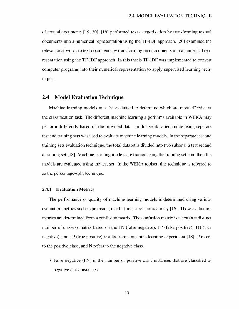
An example confusion matrix is given in Figure 2.4. North American programs refer
to NA, and South Asian programs refer to SA. Therefore TP, FP, TN, FN, P, and N can be
written as TSA, FSA, TNA, FNA, SA, and NA. The value of TSA, FSA, TNA, FNA, SA,
and NA are as follows:
Figure 2.4: Example confusion matrix showing a machine learning classification result.
• TSA (true South Asian programs): The model correctly classified 1574 computer
programs as South Asian programs.
• FSA (false South Asian programs): The model incorrectly classified 351 computer
programs as South Asian programs.
• TNA (true North American programs): The model correctly classified 1804 computer
programs as North American programs.
16

2.4. MODEL EVALUATION TECHNIQUE
• FNA (false North American programs): The model incorrectly classified 582 com-
puter programs as North American programs.
• SA (total South Asian programs): The model classified a total of 2156 South Asian
programs.
• NA (total North American programs): The model classified a total of 2155 North
American programs.
Using the value of TSA, FSA, TNA, FNA, SA, and NA, different evaluation metrics
can be calculated as follows:
• Accuracy: Accuracy is the ratio of the accurately labeled programs to the total pro-
grams. It can be calculated using the formula given in Equation 2.3.
Accuracy =T SA+T NA
SA+NA(2.3)
In this example, accuracy =T SA+T NA
SA+NA=
1574+18042156+2155
= .78358 = 78.358%
Therefore, the model is able to classify 78.358 out of 100 computer programs accu-
rately.
• Precision: Precision is the ratio of the correctly predicted South Asian programs
(TSA) to the total predicted South Asian programs (TSA+FSA). It can be calculated
using the formula given in Equation 2.4.
Precision =T SA
T SA+FSA(2.4)
In this example, precision =T SA
T SA+FSA=
15741574+351
= .81766 = 81.766%
Therefore, when the model classified a South Asian program, it is correct 81.766%
of the time.
17

2.4. MODEL EVALUATION TECHNIQUE
• Recall: Recall is the ratio of the correctly predicted South Asian programs (TSA)
to the total actual South Asian programs (TSA+FNA). It can be calculated using the
formula given in Equation 2.5.
Recall =T SA
T SA+FNA(2.5)
In this example, recall =T SA
T SA+FNA=
15741574+582
= .73006 = 73.006%
Therefore, the model is able to classify 73.006 out of 100 South Asian programs
accurately.
• F-measure: F-measure is the weighted average of recall and precision. It can be
calculated using the formula given in Equation 2.6.
F−measure =2∗Recall ∗Precision
Recall +Precision=
2∗T SA2∗T SA+FSA+FNA
(2.6)
In this example, f-measure =2∗1574
2∗1574+351+582= .77138 = 77.138%
Therefore, the weighted average of recall and precision is 77.138%, which is referred
to as the f-measure.
18

2.5. RELATED WORK
2.5 Related Work
Sociolinguistics is an area of study which investigates the relationships between lan-
guage and society with the goal being a better understanding of the structure of language
and how social factors can be better perceived through the study of language [21]. The use
of natural language among humans depends on factors such as social status, economic sta-
tus, gender, age, and region [1, 22]. These factors may affect the users of the programming
language or artificial language. For example, programmers in a particular region may learn
programming in a certain way that may affect their program writing style.
Many researchers have investigated the sociolinguistic factors of written documents in
different natural languages [23, 24]. [23] examined gender differences in English literature.
The authors explored differences in female and male writing in a subset of the British
National Corpus containing a total of 604 documents. The documents were of different
genres, such as fiction, nonfiction, and world affairs. A set of over 1000 features was
used. Features included function words, parts of speech, and commonly ordered triples of
parts of speech. An exponentiated gradient algorithm was used to select features that were
important to categorize a document. Significant differences in the use of noun modifiers and
pronouns were found in their work. Syntactic and lexical differences based on the authors’
gender were also found. In addition, [23] found that males use comparatively more noun
(car, country, app) specifiers, whereas females use more pronoun (their, her, myself, she,
you, I) specifiers.
[25, 9] focused on determining the impact of sociolinguistic characteristics of the author
on computer programs. Their goal was to determine whether computer programs could be
classified according to an author’s gender and in [9], also by an author’s region. Students
assignments were used as datasets. [25] used a set of 50 features to classify 100 C++ pro-
grams, whereas [9] used a set of 16 features to classify 160 computer programs. Supervised
learning techniques were used to categorize the computer programs. Both of the authors
examined features using various attribute selection algorithms. In addition, [25, 9] showed
19

2.5. RELATED WORK
the relationship between features.
[25] used 50 features in their work. Computer programs were first transformed into a
numerical representation using the Term Frequency-Inverse Document Frequency (TF-IDF)
technique [25]. Machine learning models such as Nearest Neighbor (K*), Naive Bayes
(NB), Decision Tree (J48), and Support Vector Machines (SVM) were used to classify
programs according to the author’s gender. A total of five experiments were performed and
showed that machine learning models were able to classify computer programs by gender
of the author. In addition, correlations among all the features were also shown in their
work. The mean frequencies of symbols and words such as /, ==, >=, and bool were found
to be higher in male-written programs, whereas the mean frequencies of +, double, char
were higher in female written programs. Features such as / and + had a stronger positive
relationship in male written programs than in female written programs [25].
[9] used a set of 16 features to transform computer programs into a numerical represen-
tation using the TF-IDF technique. In addition, computer program classification according
to the author’s gender and region, as well as feature analysis were performed in their work.
The numbers of source code lines and the percentages of mixed lines were found to be
higher in male-written programs, whereas the percentage of comment lines, the percentage
of blank lines, and the number of blank lines were higher in female-written programs. The
mixed lines include both comments and code lines. A visual analysis of Canadian written
and Bangladeshi written programs was also performed in their work. The number of total
functions, number of total commentary words, mixed line percentage, number of mixed
lines, comment line percentage, and number of comment lines were found to be higher in
Canadian written programs, whereas the average number of function lines was higher in
Bangladeshi written programs [9].
[26] explored code readability and software quality in their work. A software read-
ability model based on features that can be automatically extracted from the program was
described in their work. C++ features such as keywords, arithmetic operators, identifiers
20

2.5. RELATED WORK
were extracted in their work. 2.2 million lines of open source code from various released
projects were used to determine the relationships between their readability features and
software quality. Readability features were found to be strongly correlated with three soft-
ware quality measures: software defect log messages, automated defect reports, and code
change. Although a strong correlation was found between them, [26] did not mention
whether the correlation was positive or negative.
In [26] a total of 300 programming features were extracted by analyzing 226 stud-
ies published from 2010 to 2015. The authors identified software failures, code quality,
and code complexity were to be the most studied topics in the programming feature re-
search. The authors also identified four programming paradigms of features research such
as procedural programming, feature-oriented programming, aspect-oriented programming,
and object-oriented programming (OOP). Out of 300 programming features, OOP, McCabe
Cyclomatic complexity, and lines of code (loc) were found to be the most studied features.
OOP includes features such as coupling between objects, depth of inheritance, number of
children, and number of methods. Chidamber and Kemerer are pioneers in OOP feature
research, and described features such as inheritance, coupling, and cohesion. Overall, [27]
introduced us to various types of features, especially complexity features.
The authors described two types of complexity features: McCabe Cyclomatic complex-
ity and Halstead complexity. The Halstead complexity feature consists of several metrics
such as difficulty, effort, and expected bugs of a program. Both McCabe Cyclomatic com-
plexity and Halstead complexity features are widely known and commonly used in areas
such as complex networks, code smell detection, and software bug prediction [27].
Argamon [23, 25, 9] introduced us to sociolinguistics and its impact on programming.
[27] introduced us to various types of features and their usage. Finally, [26] gave us the
idea to explore programming features and complexity features and motivated us the most
to determine any correlation between those features.
21

Chapter 3
Methodology and Experiments
In this work computer programs were represented as vectors of the features in numeric
form, and machine learning models were applied to identify patterns and similarities from
those vectors. The machine learning models learned from the training data and made pre-
dictions based on the testing data. Figure 3.1 illustrates our experimental process.
The first step of our work was to create the dataset. We collected open-source programs
from GitHub along with information on the programs’ authors such as name, gender, and
region. Since our goal was to perform region-based and gender-based analysis, we cre-
ated two balanced subsets by taking the same number of programs from both male/female
programs and South Asian/North American programs. A python script was written to se-
lect two random samples from all male/female programs and South Asian/North American
programs. The python script used a sample function that returned a random sample of pro-
grams from all the programs. Because both subsets were created by randomly selecting
program files, there is a possibility of overlapping subsets. However, as the experiments
and the feature analysis tasks are independent for each subset, the result of experiments and
feature analyses will be separate.
A total of 103 programming features were selected to transform the dataset into the
TF-IDF format. After transforming the datasets into the TF-IDF format, we imported them
into the WEKA software. WEKA supports various types of machine learning classifiers
that were used to classify computer programs.
WEKA’s randomized filter was used to shuffle the order of the instance in the datasets.
22

3. METHODOLOGY AND EXPERIMENTS
Data randomization is important to increase diversity and reduce the chance of having a
biased dataset. Datasets were split into the test set and the training set using the percentage
split method in WEKA. After training and testing, we analyzed precision, recall, f-measure,
accuracy, and the confusion matrix for each experiment to determine which machine learn-
ing models maybe effective in computer program classification. An overview of our process
is shown in Figure 3.1. The following sections provide details on each stage of the process.
Figure 3.1: Steps in the experimental process.
23

3.1. DATASET CREATION
3.1 Dataset Creation
In this section we describe our dataset creation process. The dataset was mainly col-
lected with the help of Steven Deutekom, one of the undergraduate research assistants of
the University of Lethbridge. Open source programs were collected from GitHub along
with information on the programs’ authors such as name, gender, and region. With over
10 million Git repositories, GitHub has become the largest code host in the world [28] and
uses the Git version control system to support software development.
GitHub offers two types of visibility for hosted software projects: private and public.
GitHub does not share private projects whereas public projects can be seen and forked.
If a software developer creates a new project by copying another project and performs
some modifications, the newly created project is called a forked project. To collect data
from GitHub, the GHTorrent project was used which offers offline GitHub data through the
REST API [29]. The GHTorrent project is updated every few months.
GHTorrent offers GitHub data in two different formats: MySQL database and Mon-
goDB database. However, these databases are very large in size. Without proper hardware
and infrastructure, it is difficult and time-consuming to query large databases. Google Big-
Query solves the query problem by running “super-fast, SQL-like queries against append-
only tables, using the processing power of Google’s infrastructure” [30]. Therefore, Google
BigQuery was used to collect GitHub’s project information from the GHTorrent database.
By project information, we refer to the name of the project, the information of the program-
mer who created the project, and the information of the files in the project.
Although GHTorrent provides a great deal of information about the GitHub users, it
does not give any information about project author’s gender and full name. Therefore,
the GitHub API was used to collect the author’s full name and the Genderize.io API was
used to determine the gender based on the author’s first name. An API is software through
which a request goes to a server, which then returns data according to that request. The
Genderize.io API uses a dataset of 216286 unique names from 79 different countries and
24

3.1. DATASET CREATION
returns the gender of the name along with a probability [31]. The probability refers to how
likely a name is to be a male name or a female name [32].
GHTorrent does not contain any program files. It only contains file information such as
file id and file name. Thus, it was necessary to collect all the program files from GitHub. For
each project collected from the GHTorrent database, the entire repository was downloaded
locally. A repository or project may contain one or several files. Only files with correct
C++ extensions were collected so that unnecessary files (e.g., image and music files) would
not be added. In addition, only programs with between 10 and 1000 numbers of lines were
collected as a valid program to avoid collecting library files. Finally, programs along with
project information and author information were added into a local database. The overall
data collection process is given in Figure 3.2.
Figure 3.2: Data collection process.
• The first step was to load the GHTorrent project into the Google BigQuery web-
site (https://bigquery.cloud.google.com/dataset/ghtorrent-bq:ght) to extract computer
program files.
• As we did not require all of the GHTorrent database provided information, SQL
queries were executed to select only the information needed for this work. Figure
3.3 lists the fields that were extracted from the GHTorrent database.
25
3.1. DATASET CREATION
• The results of the SQL queries were then downloaded in JSON format.
• JSON files were read using a Python script. For each JSON item, an attempt was
made to get the programmer’s gender and full name. The full name was collected
using the GitHub API and the gender was collected using the Genderize.io API.
• If both full name and gender were found and the project contains only one contributor,
three of this information was added to the item. Otherwise, the process continues with
the next JSON item.
• The entire project repository was cloned locally. Cloning a project locally means
downloading the project from GitHub to a local computer.
• A project may contain one or several files. The entire project was searched to find all
the files that were contributed by the project owner.
• Each file was validated to see whether proper file extension could be found and the
line number was in the range of 10 to 1000. For example, a project may contain
not only program files but also image files, audio files, video files, and library files.
Therefore, file extensions were checked and only files with .cc and .cpp extensions
were collected. It is less likely that a single author writes more than 1000 lines in a
program file. Normally, library program files contain more than 1000 lines of code.
Therefore, files with between 10 and 100 line numbers were collected.
• Finally, programs along with author and project information were added into a local
database and the process was repeated for each JSON file item.
Two subsets of data were created from the collected dataset. For the gender-based
subset, only programs with authors that had a gender probability of more than 0.7 were
collected to make sure that male-written programs are written by male and female-written
programs are written by female programmers. Using this approach resulted in more male-
written programs than female-written programs. Thus a total of 6,017 female-written pro-
26

3.2. DATA TRANSFORMATION
Figure 3.3: Columns for GitHub data collection.
grams and another 6,017 male-written programs were randomly selected to create a bal-
anced subset. In total, the gender-based dataset included 12,034 computer programs.
The second subset consisted of programs written by North American and South Asian
programmers. Since there are a limited number of countries in North America and South
Asia, these two regions were selected. If we used Asia, Europe, or other regions with
many countries, a regional-based analysis task would have been more difficult. Figures 3.4
and 3.5 show the distribution of programs collected from all the South Asian and North
American countries. Countries with fewer than 100 programs were not included in the
region-based subset. Of these programs, a total of 6340 programs from the North American
region and another 6340 programs from the South Asian region were randomly selected in
order to balance the subset.
27

3.2. DATA TRANSFORMATION
4Afghanistan919Bangladesh
0Bhutan7149India
0Maldives27Nepal110Pakistan87Sri Lanka
0 7150
Figure 3.4: Total programs collected from the South Asian region.
33173United States538Mexico
5209Canada
0 1000 2000 3000
Figure 3.5: Total programs collected from the North American region.
3.2 Data transformation
Machine learning models require a vector of numeric values as input and give nominal
values as output. For each program file, the features were counted using a python script.
The feature count was then used to transform the dataset into the term frequency-inverse
document frequency (TF-IDF) format. TF-IDF is a way to tell how important a term/
feature is to a document. The term frequency (t f ) refers us how many times a term/feature
is used in a program [33]. The inverse document frequency (id f ) tells us how important a
term/feature is in all the programs. The term frequency is calculated using Equation 3.1:
t f (term, d) =tdnd
(3.1)
• where td is the count of the terms in the document (d), and
• nd is the number of terms in the document (d).
For example, if the frequency of the feature/term “switch” is 2 in a program (d) and the
28

3.3. FEATURE SELECTION
total number of term/feature in that program (d) is 200, the term frequency of “switch” in
that program (d) is t f (“switch”,d) = 0.01.
Document frequency (d f ) counts the occurrences of a term in the total number of doc-
uments (N). Since the inverse document frequency (id f ) tells us how important a term/fea-
ture is in all the programs, a larger id f value means the term is more important to all the
programs than other terms with less id f value. The inverse document frequency (id f ) is
calculated using Equation 3.2:
id f (term) = logN
d f (term)(3.2)
For example, if the total number of documents is 10 and the occurrences of the term
“switch” in the total number of documents is 5, the inverse document frequency (id f ) of
term “switch” is calculated as:
id f (“switch”) = log105
= 0.301.
The term frequency-inverse document frequency (TF-IDF) can be calculated by multi-
plying t f by id f , so t f id f (term,d) = t f (term,d)∗ id f (term).
After counting all the features, the two subsets were transformed into term frequency-
inverse document frequency format using a python script. We then used the TF-IDF data in
WEKA to train and evaluate machine learning models.
3.3 Feature Selection
We used three sets of features in our work: the McCabe Cyclomatic complexity feature,
Halstead complexity features, and 103 programming features. [26] examined code read-
ability and used a list of readability features to determine features related to software com-
plexity. A software readability model was presented in their work. The readability model
is based on features that can be extracted from a computer program. C++ keywords, arith-
29

3.3. FEATURE SELECTION
metic operators, and identifiers were used as features in their software readability model.
Since one of our goals was to understand the relationship between program complexity and
programming features, we decided to use similar features in our work. A chart of all of the
types of features used in this work is given in Figure 3.6. The programming features are
listed in Table 3.1 and their meanings are given in Tables A.1 and A.2.
Figure 3.6: Types of features used in this work.
Table 3.1: List of programming features.
30

3.3. FEATURE SELECTION
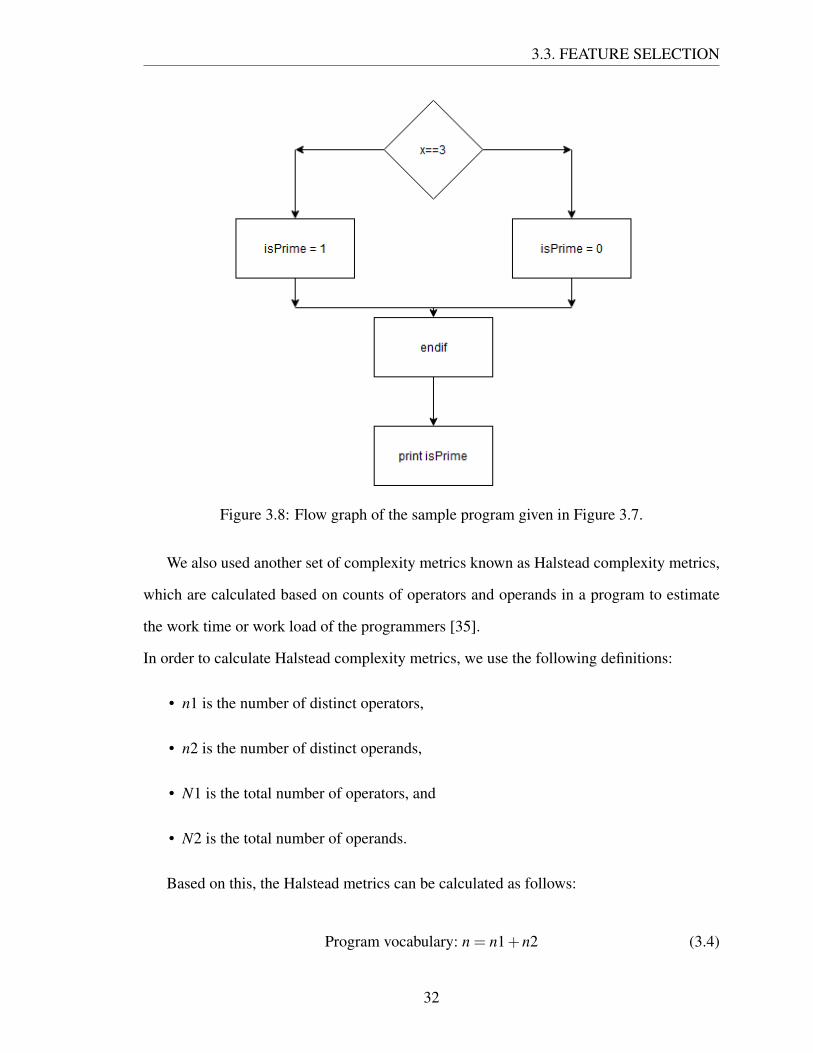
The McCabe cyclomatic complexity is a software metric that indicates the complexity
of a program. It can be computed by counting the conditional and iterative statements in
the program [34]. A sample program and its corresponding graph are given in Figures 3.7
and 3.8. The McCabe cyclomatic complexity is calculated using Equation 3.3:
McCabe cyclomatic complexity: m = e−n+2p (3.3)
• where n is the number of vertices,
• e is the number of edges, and
• p is the number of vertices which have exit points.
The flow graph in Figure 3.8 shows that the sample program has 5 vertices, 5 edges,
and 1 exit point, so the McCabe cyclomatic complexity is 5 - 5 + 2 = 2.
Figure 3.7: Sample program (if-else block).
31
3.3. FEATURE SELECTION
Figure 3.8: Flow graph of the sample program given in Figure 3.7.
We also used another set of complexity metrics known as Halstead complexity metrics,
which are calculated based on counts of operators and operands in a program to estimate
the work time or work load of the programmers [35].
In order to calculate Halstead complexity metrics, we use the following definitions:
• n1 is the number of distinct operators,
• n2 is the number of distinct operands,
• N1 is the total number of operators, and
• N2 is the total number of operands.
Based on this, the Halstead metrics can be calculated as follows:
Program vocabulary: n = n1+n2 (3.4)
32

3.3. FEATURE SELECTION
Program length: N = N1+N2 (3.5)
Difficulty: D =n12∗ N2
n2(3.6)
Volume: V = N ∗ log2 n (3.7)
Effort: E = D∗V (3.8)
Expected bugs: B =V
3000(3.9)
Figure 3.9: Sample C++ program.
In Figure 3.9, we have 8 distinct operators, 5 distinct operands, 11 total operators, and
6 total operands. Now, using the above information, we can write:
• Number of distinct operators: n1 = 8(i f , (, ), , , =, ==, else),
• Number of distinct operands: n2 = 5(x, 7, isPrime, 1, 0),
• Total number of operators: N1 = 11,
• Total number of operands: N2 = 6,
• Program vocabulary: n = n1+n2 = 13,
• Program length: N = N1+N2 = 17,
• Difficulty : D = n12 ∗
N2n2 = 4.8,
• Volume: V = N ∗ log2 n = 62.90747521,
33

3.4. EXPERIMENTS
• Effort: E = D∗V = 301.955881, and
• Expected bugs B = V3000 = .209691584.
A total of four experiments are described in Section 3.4. In experiments 1 and 3, a total
of 103 features were used, whereas CFS Subset Evaluator from WEKA was used to reduce
the features set in experiments 2 and 4. CFS Subset Evaluator returned two lists of the most
important features, one for each subset. All the features were removed from the two subsets
except for the features found from the CFS Subset Evaluator. Therefore, the only difference
between experiments 1, 2, 3, and 4 was the use of feature sets.
We examined the connection of programming features to the Halstead complexity met-
rics. As both Halstead complexity metrics and programming features use the same underly-
ing characteristics, we believe there are some relationships between the Halstead complex-
ity metrics and programming features. The relationships between the Halstead complexity
metrics and programming features are discussed in the Sections 4.4 and 4.5.
3.4 Experiments
In this section we describe four experiments. Two datasets containing region-based
program data and gender-based program data were transformed into the term frequency-
inverse document frequency (TF-IDF) format. These two datasets were then imported into
WEKA to perform machine learning experiments. WEKA was also used to shuffle and
split the datasets. WEKA’s randomized filter was used to shuffle the order of the instance
in the datasets and the percentage split (66% training data and 34% testing data) method
was used to split the datasets into a training set and a test set. At first, different training
and testing ratios with little change were used to determine if machine learning models’
performance changes. However, the performance did not change that much (around 1%
to 2%). Therefore, a fixed ratio (66% training data and 34% testing data) was used in this
work. WEKA also offers various types of machine learning models and so WEKA was used
34

3.4. EXPERIMENTS
to train all the machine learning models using the training set and evaluate those models
using the test set. WEKA required less than one second to train and evaluate each machine
learning model. WEKA also returns the value of precision, recall, f-measure, accuracy, and
confusion matrix after each experiment. These measures were then used to determine which
machine learning models are more or less effective in classification. Each experiment used
five machine learning algorithms to develop models to classify computer programs based
on either gender or region of the program’s author. The five algorithms are listed below.
• Bagging classifier was used from the meta type classifiers.
• Decision Table classifier was used from the rule based classifiers.
• Random Forest classifier was used from the tree classifiers.
• Logistic Regression classifier was used from the function based classifiers.
• Bayes Net classifier was used from the Bayesian classifiers.
Experiments 1 and 2 utilized the gender-based data, while experiments 3 and 4 attempted
to classify computer programs based on the program authors’ region. All 103 programming
features were used in the 1st and 3rd experiments. The top features were then selected using
the CFS Subset Evaluator, and these features were used in the 2nd and 4th experiments.
3.4.1 Experiment 1
The region-based dataset was used in experiment 1. This dataset consists of 12680 com-
puter programs, with 6340 programs from the North American region and the remaining
6340 from the South Asian region. A total of 103 programming features were selected to
transform the dataset into TF-IDF (term frequency-inverse document frequency) format.
The programs were then classified using the five machine learning models. The percentage
split (66% training data and 34% testing data) technique was used to evaluate the machine
learning models.
35

3.4. EXPERIMENTS
3.4.2 Experiment 1 Results
Table 3.2 shows the results of experiment 1. The Random Forest classifier gave a bet-
ter result (accuracy=78.36%) than the other four classifiers. The Random Forest classifier
was able to correctly classify most of the North American programs (correctly classified
= (1804/2155)*100 = 83.7%). The Random Forest classifier was able to correctly classify
more North American programs than any other classifier. The Random Forest classifier
accurately classified more South Asian programs than any other classifier (correctly clas-
sified=(1574/2156)*100=73%). Bagging was the second most accurate classifier with an
accuracy of 75.48%. Overall, all classifiers were able to correctly classify more North
American programs than South Asian programs.
Table 3.2: Experiment 1 results.
36

3.4. EXPERIMENTS
Table 3.3: Most relevant features as identified by CFS Subset Evaluator (Experiment 2).
Order of relevance Feature1 while2 goto3 auto4 const5 int6 long7 typedef8 namespace9 friend10 this11 throw12 true13 try14 using15 <
16 +17 ++18 –19 <=20 %21 bitwise NOT22 >>
23 .24 [
3.4.3 Experiment 2
In experiment 2, the CFS Subset Evaluator was used to determine which attributes are
more highly relevant for predictions. The evaluator returned the 24 most important at-
tributes. A list is given in Table 3.3. These 24 attributes were then used to transform the
region-based dataset into the TF-IDF format. The percentage split (66% training data and
34% testing data) technique was used to evaluate five machine learning models. The results
of experiment 2 are given in Section 3.4.4.
37

3.4. EXPERIMENTS
3.4.4 Experiment 2 Results
The results of experiment 2 are shown in Table 3.4. The accuracy of most of the machine
learning classifiers decreased slightly in experiment 2 as compared to experiment 1. The
reduced accuracy of the machine learning classifiers might be a outcome of the removal of
79 attributes from the dataset. The accuracy of Random forest and Bagging classifiers de-
clined the most at around 3% and 2%, respectively. Of the five classifiers, only the accuracy
of Bayes Net increased slightly in experiment 2 (about 0.30%). Although removing irrele-
vant features changed all machine learning models’ accuracy, changes in accuracy were so
little that might be called insignificant. Since any machine learning model’s performance
will change slightly each time it is trained, we performed experiment 1 and experiment 2
multiple times. We found almost the same results in all cases. Overall, it can be seen that
removing irrelevant features changed accuracy only slightly.
38
3.4. EXPERIMENTS
Table 3.4: Experiment 2 (reduced features) results.
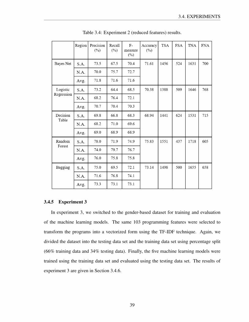
3.4.5 Experiment 3
In experiment 3, we switched to the gender-based dataset for training and evaluation
of the machine learning models. The same 103 programming features were selected to
transform the programs into a vectorized form using the TF-IDF technique. Again, we
divided the dataset into the testing data set and the training data set using percentage split
(66% training data and 34% testing data). Finally, the five machine learning models were
trained using the training data set and evaluated using the testing data set. The results of
experiment 3 are given in Section 3.4.6.
39

3.4. EXPERIMENTS
3.4.6 Experiment 3 Results
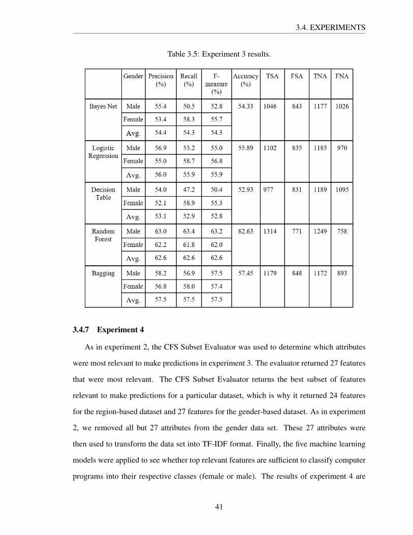
The results of experiment 3 are given in Table 3.5. We see that Random Forest has
surpassed all other learning models in terms of accuracy, precision, f-measure, and recall.
Random Forest achieved a 62.63% accuracy, while the other models’ accuracy was around
52% to 57%. If we look at the confusion metrics, we see that the Decision Table was able to
correctly classify less than 50% male computer programs. For this model, there were 2,082
actual male written computer programs, of which the model was able to correctly classify
only 977. In other words, the model was only able to correctly classify 48% male writ-
ten computer programs. On the other hand, Random Forest was able to correctly identify
62% of both male and female programs. Comparing experiments 1 and 2 with experiment
3 shows that the performance of machine learning models was higher in the region-based
dataset than in the gender-based dataset. One reason may be that the gender-based data has
more variation than region-based data. Since the gender-based dataset contains computer
programs from different parts of the world, the use of program features may also vary in
those programs. Therefore the gender-based dataset may more varied types of computer
programs, and this may be responsible for the low performance in this experiment. Com-
paring experiment 1 results with experiment 3 results shows that the accuracy of all machine
learning models declined around 16% to 18% in experiment 3 as compared to experiment
1.
40
3.4. EXPERIMENTS
Table 3.5: Experiment 3 results.
3.4.7 Experiment 4
As in experiment 2, the CFS Subset Evaluator was used to determine which attributes
were most relevant to make predictions in experiment 3. The evaluator returned 27 features
that were most relevant. The CFS Subset Evaluator returns the best subset of features
relevant to make predictions for a particular dataset, which is why it returned 24 features
for the region-based dataset and 27 features for the gender-based dataset. As in experiment
2, we removed all but 27 attributes from the gender data set. These 27 attributes were
then used to transform the data set into TF-IDF format. Finally, the five machine learning
models were applied to see whether top relevant features are sufficient to classify computer
programs into their respective classes (female or male). The results of experiment 4 are
41

3.4. EXPERIMENTS
given in Section 3.4.8.
3.4.8 Experiment 4 Results
The results of experiment 4 are given in Table 3.7. Again, most of the machine learn-
ing classifiers’ accuracy slightly decreased in experiment 4 as compared to experiment 3.
The accuracy of the Random forest classifier declined the most among all the classifiers at
around 3%. As in experiment 2, only the accuracy of Bayes Net increased slightly in exper-
iment 4 (about 1%). Overall, it can be seen that the machine learning models can classify
gender-based data with 52% to 60% accuracy. One way to improve the accuracy of machine
learning models might be reducing the variation in the gender-based dataset. Age-based or
region-based new subsets could be created from gender-based data to improve the accuracy
of machine learning models and this could be incorporated in future work.
42

3.4. EXPERIMENTS
Table 3.6: Most relevant features as identified by CFS Subset Evaluator (Experiment 4).
Order of relevance Feature1 while2 auto3 const4 extern5 int6 long7 register8 static9 typedef
10 void11 namespace12 static cast13 this14 public15 ==16 +17 ++18 &19 *20 ->21 <=22 /*23 (24 ,25 <<
26 .27 [
43

3.5. THREATS TO VALIDITY
Table 3.7: Experiment 4 (reduced features) results.
3.5 Threats to Validity
There are a few factors that may offer potential threats to the validity of our work.
• Programmers often include frameworks or libraries in their projects. It is difficult
to distinguish between authors’ written programs and library programs. One way to
differentiate between them may be to check the length of the programs. Since library
programs are very lengthy, only programs with length in the range 10 to 1000 lines
were added.
• Sometimes GitHub users use a different name from their actual name. This may give
incorrect gender information.
44

3.5. THREATS TO VALIDITY
• Determining the gender of Asian programmers’ names is especially difficult because
Genderize.io contains few names from Asian cultures, and some names seem to be
androgynous [36]. Therefore, Genderize.io appears to be less effective for Asian
names. In addition, programmer region information in GitHub may not always be
correct. Sometimes people can create fake GitHub account, or some may select a
predefined region while creating their accounts. Therefore, region and gender infor-
mation may not be a hundred percent correct.
• Only the C++ programming language was used in this work. Using other program-
ming languages could lead to different results.
• One of our understanding was that the gender-based dataset contains different types
of programs. Therefore the use of program features may also vary in those programs.
Since there is no way to determine program types from GitHub, we could not justify
our understanding.
• Although we performed region-based and gender-based computer program classifi-
cation and feature analysis, we did not consider the experience level or the age of the
programmers. Programs written by programmers with one year of experience will
likely not be the same as those written by programmers with ten years of experience.
It is expected that there will be differences in feature usage. Thus, if we could create
region-based and gender-based datasets with equally experienced programmers, our
findings might be different.
45

Chapter 4
Discussion
In this chapter, we discuss feature frequencies, compare machine learning models, and pro-
vide correlations between the 103 programming features and the complexity features. We
compare the five machine learning models that were used in our four experiments. We
provide a summary of which models performed better and possible reasons for the better
performance. An analysis of the features’ frequency is provided in Section 4.3. We tried to
determine whether a feature is more or less likely to be used in the programs from a par-
ticular region or written by people of a particular gender. Finally, the correlations between
programming features, McCabe complexity feature, and Halstead complexity features are
discussed in Sections 4.4 and 4.5.
4.1 Comparison of Models
A comparison of the five machine learning models is given in this section. The accuracy
of the five models in all four experiments is given in Table 4.1. The gender-based dataset
was used in experiments 3 and 4, whereas experiments 1 and 2 attempted to categorize
computer programs based on the program author’s gender. A total of 103 features were used
in experiments 1 and 3, while top features were selected using the CFS Subset Evaluator
and used in experiments 2 and 4.
In all four experiments, the Random Forest model and the Bagging model performed
better than the other machine learning models. In almost all the experiments, the Bagging
and Random Forest models’ accuracy was 8% to 10% higher than other machine learning
46

4.2. COMPARISON WITH PREVIOUS WORK
models. The higher accuracy could be because both Random Forest and Bagging mod-
els use multiple machine learning algorithms to make a prediction, as described in Sec-
tion 2.2.2. The Bagging model uses multiple machine learning models for the prediction
whereas the Random Forest model uses multiple decision trees to predict a class. Both of
them select the class most often predicted. In Sections 2.2.2, it can be seen that a single
algorithm was used by the Bayes Net, Decision Table, and Logistic Regression models. De-
cision Table creates a tree, Logistic Regression creates a mathematical equation, and Bayes
Net creates a probabilistic model to make their prediction. As Bagging and Random Forest
models use multiple machine learning algorithms to make predictions, their performance
was likely to be better than the other simpler machine learning models.
Table 4.1: Accuracy of five machine learning models.
Experiment 1 Experiment 2 Experiment 3 Experiment 4
Bayes Net 71.28% 71.61% 54.33% 55.25%
Logistic Regression 71.67% 70.38% 55.89% 55.11%
Decision Table 68.94% 68.94% 52.93% 52.96%
Random Forest 78.36% 75.83% 62.63% 59.60%
Bagging 75.48% 73.14% 57.45% 56.84%
4.2 Comparison with Previous Work
Two studies were performed previously in the area of sociolinguistics and computer
program classification. Naz [25] tried to classify computer programs according to the pro-
grammers’ gender. Naz used 100 student assignments as the dataset and 50 features as the
feature set. Naz used Naive Bayes and J48 machine learning classifiers in the experiment.
On the other hand, Rafee [9] tried to classify computer programs according to the program-
47

4.2. COMPARISON WITH PREVIOUS WORK
mers’ gender and region. Rafee used 160 student assignments as the dataset and 16 features
as the feature set. Rafee used Bayes Net and Random Forest classifiers in the experiment.
Both Naz and Rafee used WEKA to train and evaluate machine learning classifiers. Naive
Bayes and Bayes Net are Bayesian classifiers, whereas J48 and Random Forest are Tree
classifiers. In this work, a Bayesian classifier (Bayes Net) and a tree classifier (Random
Forest) were used in the experiment. In this section, the comparison between this work
results and the results of two previous works are described.
The comparison of gender-based classification is given in Table 4.2 whereas the com-
parison of region-based classification is shown in Table 4.3. Comparing all the experiments
results shows that the Tree classifier performed better than the Bayesian classifier in almost
all the experiments. In our gender-based classification, the Random Forest classifier was
able to classify 62.63% of programs correctly. Naz’s Tree classifier also achieved similar
accuracy (accuracy = 63%). Rafee’s Tree (Random Forest) classifier performed better than
all other classifiers. The classifier was able to classify 80.6% of programs accurately. In
the region-based classification, both of our classifiers performed better. In our experiment,
the Bayesian classifier (Bayes Net) correctly classified 71.28% of programs, whereas the
Tree classifier (Random Forest) was able to achieve 78.36% accuracy. On the other hand,
Rafee’s Tree (Random Forest) classifier correctly classified 89.4% of programs.
Table 4.2: Accuracy of machine learning models (gender based classification).
Naz’s Result Rafee’s Result Our Result
Bayesian classifier 66% 70% 54.33%
Tree classifier 63% 80.6% 62.63%
48

4.3. ANALYSIS OF FEATURES
Table 4.3: Accuracy of machine learning models (region based classification).
Rafee’s Result Our Result
Bayesian classifier 85% 71.28%
Tree classifier 89.4% 78.36%
Finally, it is worth noting that open-source C++ programs from GitHub were used in
our work, whereas both Naz and Rafee used students’ assignments. There is the possi-
bility that those assignments’ programs were written in a specific coding style, whereas
open-source programs are likely to have more variations in coding style. In addition, a total
of 103 programming features were used in our experiment, whereas Naz and Rafee used
50 features and 16 features, respectively. Although our machine learning models did not
perform particularly well on classifying program authors as male or female, subsequent fre-
quency analysis identified differences in the use of programming features. We also discuss
later that since open-source programs may contain data from all over the world or different
styles of programs, this may be one reason that the performance of our machine learning
models decreased.
4.3 Analysis of Features
4.3.1 Frequency of Occurrence
In [23] and [25], the authors computed the frequency of features to identify any gender-
based differences in how those features were used by the authors. [23] counted the feature
frequencies per 1,000 tokens whereas [25] took the mean of frequency count per 100 tokens.
[23] found that the frequencies of pronouns such as she, I, her, and you were higher in
female-written documents, whereas the frequencies of determiners such as that, the, a, and
these were higher in male-written documents. [25] showed that the mean frequency of
features /, ==, >=, and bool were higher in male-written programs, whereas the mean
49

4.3. ANALYSIS OF FEATURES
frequency of features +, double and char were higher in female-written programs.
To build on [23] and [25] we offer a similar analysis. We first counted how many times
each feature appears in each program. After that, we were interested in the mean of each
feature frequency count. The mean of a feature will give us an idea of the usage of that
feature in programs of a specific region or gender. After calculating the mean frequency
of the features, we tried to understand whether these features are more or less likely to be
used in the programs from a particular region or written by people of a particular gender.
We discuss the feature frequency in more detail in the following two sections.
4.3.2 Frequency of Occurrence (region)
In this work we used a total of 12680 computer programs. 6340 programs were taken
from the North American region and the remaining 6340 from the South Asian region. In
Table B.1 (in Appendix B), we see that the average length (Loc: Line of Code) of North
American programs is 44.75 percent larger than that of the South Asian programs. LOC is a
computer program metric that is measured by counting the total number of lines in the text
of a program’s code. We also can see that although the programs of South Asia are shorter in
length, the average frequency of some programming features is higher than in the programs
of North America. Table B.1 (in Appendix B) lists the average deviation of each feature.
Since the North American programs and the South Asian programs have different average
lengths, average deviation of a feature was calculated by dividing the average count of that
feature with the average line of code (LOC) value. In addition, since features’ frequency
differences will be analyzed based on the average deviation of features, the length of the
programs should not be an issue in the frequency analysis task. In Table B.1, it can be seen
that the average line of code (LOC) of the South Asian programs is 106.480126, whereas
the North American programs average line of code is 154.131388. The average counts
of the feature int in the South Asian and North American programs are 14.758517 and
15.797634, respectively. So the average deviation of the feature int in the regional-based
50

4.3. ANALYSIS OF FEATURES
dataset would be (15.797634/154.131388) - (14.758517/106.480126) = -0.036109. So, the
average frequency of the feature int in each line of South Asian programs is 3.61% higher
than in each line of North American programs. The positive deviation of a feature means
that the frequency of that feature is higher in the North American programs than in the
South Asian programs. The negative deviation of a feature means that the frequency of that
feature is higher in the South Asian programs than in the North American programs.
Table B.1 also compares the average features’ frequency. To compare the average fre-
quency of a feature, the average count of that feature was divided by the average line of
code (LOC). From Table B.1, it can be seen that the average frequency of the feature int
in each line of code in the South Asian and North American programs are (14.758517 /
106.480126) = 0.1386034893 and (15.797634 / 154.131388) = 0.1024945938, respectively.
Therefore, the average frequency of the feature int in each line of South Asian programs is
(0.1386034893 / 0.1024945938) = 1.352300 times higher than in each line of North Amer-
ican programs. The positive comparison value of a feature means that the frequency of that
feature is higher in the North American programs than in the South Asian programs. The
negative comparison value of a feature means that the frequency of that feature is higher in
the South Asian programs than in the North American programs.
A total of 103 features were used in this work. It is not possible to discuss all of
them. Therefore some particular features from Table B.1 (in Appendix B) are discussed in
this section. Those features are listed in Table 4.4. Since increment-decrement operators,
arithmetic operators, comparison operators, logical operators, and control flow keywords
are used to take decision based on specific conditions, perform logical and mathematical
calculations, they are discussed in Sections 4.3.2 and 4.3.3. In addition, we also discuss
the use of fundamental data types and boolean values as they are the primary pieces of
information that a person needs to know. Without knowing them, it’s impossible to write a
C++ program.
In Table B.1, since the average deviations and comparison value of some features (int,
51

4.3. ANALYSIS OF FEATURES
+, −, ++, >, <, >=, <=, %, ||, !, &&, for, while, goto) are negative, this indicates
that their usage in the South Asian programs is slightly higher than in the North American
programs. There could be several reasons for the higher usage of these features. For exam-
ple, the South Asian programmers may write some different types of programs than North
American programmers, or the ways the South Asian programmers learn programming may
be different from the North American programmers. Since the use of increment-decrement
operators, comparison operators, and control flow features are higher in South Asian pro-
grams, there is a possibility that their use increases the complexity and difficulty of the
South Asian programs. On the other hand, North American programmers use more funda-
mental data types (char, double, bool, and float), operators (/, ∗,−−, ==, !=), control flow
keywords (switch, case, break, continue, if), Boolean values (true and false), and exception
handling operators (try and catch) than South Asian programmers.
Table 4.4: Selected average frequency values for the region-based dataset.
Features North America South Asia Difference Comparison
case 1.739748 0.845268 0.003349 1.421901
switch 0.326341 0.159306 0.000621 1.415197
break 1.617666 0.836278 0.002642 1.336336
continue 0.242429 0.142429 0.000235 1.175882
if 11.638013 7.077287 0.009041 1.136029
false 1.423975 0.574763 0.003841 1.711556
double 1.821451 0.933754 0.003048 1.347605
bool 1.342902 0.626341 0.002830 1.481191
52

4.3. ANALYSIS OF FEATURES
true 1.374921 0.649211 0.002823 1.463084
char 2.472082 1.598580 0.001026 1.068331
float 1.417666 0.920820 0.000550 1.063596
/ 5.693375 3.619716 0.002944 1.086608
* 33.272713 19.616877 0.031642 1.171752
−− 16.423186 5.125079 0.058421 2.213779
== 7.656940 4.186435 0.010361 1.263538
!= 1.836751 1.215773 0.000499 1.043699
else 2.596845 2.004416 -0.001976 -1.117286
for 5.596530 4.326341 -0.004320 -1.118985
goto 0.118770 0.124763 -0.000401 -1.520553
while 0.938959 1.137224 -0.004588 -1.753161
% 2.122713 2.052524 -0.005504 -1.399650
- 7.081861 5.699211 -0.007577 -1.164903
+ 5.127445 4.656151 -0.010461 -1.314464
++ 4.063565 4.111514 -0.012249 -1.464593
> 7.089748 6.786120 -0.017733 -1.385521
< 9.393533 9.236120 -0.025795 -1.423256
>= 0.551577 0.509621 -0.001207 -1.337407
53

4.3. ANALYSIS OF FEATURES
<= 0.550946 0.826498 -0.004187 -2.171477
|| 0.862618 0.552366 0.000409 1.078870
! 1.889117 1.817981 -0.004817 -1.393006
&& 1.336435 1.189590 -0.002501 -1.288463
int 15.797634 14.758517 -0.036109 -1.352300
difficulty 54.734456 51.162911 -0.125377 -1.353060
MVG 16.772871 12.444953 -0.008054 -1.074010
4.3.3 Frequency of Occurrence (gender)
Of the total 12034 computer programs, 6017 programs were written by male authors and
6017 programs were written by female authors. Table B.2 (in Appendix B) lists the average
deviation of each feature. The positive deviation of a feature means that the frequency of
that feature is higher in the male-written programs than in the female-written programs.
The negative deviation of a feature means that the frequency of that feature is higher in
the female-written programs than in the male-written programs. Table B.2 also compares
the average feature frequency. The positive comparison value of a feature means that the
frequency of that feature is higher in the male-written programs than in the female-written
programs. The negative comparison value of a feature means that the frequency of that
feature is higher in the female-written programs than in the male-written programs.
Although a total of 103 features were used in this work, only increment-decrement
operators, arithmetic operators, comparison operators, logical operators, and control flow
keywords are discussed in this section. The reason for using these features is described in
Section 4.3.2. These features are listed in Table 4.5.
54

4.3. ANALYSIS OF FEATURES
Table 4.5 shows that the difficulty of the female programmers programs is slightly
higher than the male programmers programs. Since a program’s difficulty is measured
based on operators, and female programmers use more arithmetic operators (/, ∗, and +),
fundamental data types (int, char, double, and float), comparison operators (! =, >, <,
>=, and <= ), logical operator (&& and ||) and iteration operators (for and while) (see
Table 4.5), the difficulty of their programs is slightly higher than the male programmers’
programs. By contrast, male programmers use more control flow keywords (switch, case,
break, if, and goto) and Boolean values (true and false) than female programmers. In ad-
dition, since the average deviations and comparison value of exception handling operators
(try and catch) are positive, this indicates that male programmers tend to use more exception
handling functionality than female programmers.
Table 4.5: Selected average frequency values for the gender-based dataset.
gender male female difference comparison
case 1.437760 1.159880 0.001452 1.165447
switch 0.296493 0.241150 0.000285 1.155970
break 1.250956 1.125976 0.000380 1.044557
if 10.382749 9.086588 0.005108 1.074313
false 1.300150 1.151903 0.000533 1.061199
−− 13.731926 9.860562 0.023074 1.309330
bool 1.207579 1.113346 0.000167 1.019776
true 1.252950 1.058169 0.000907 1.113264
== 7.965930 6.355493 0.008579 1.178437
55

4.3. ANALYSIS OF FEATURES
goto 0.065980 0.043377 0.000141 1.430119
% 2.066811 1.824996 0.000894 1.064776
- 6.514875 5.986040 0.001053 1.023259
! 1.767991 1.580522 0.000618 1.051717
catch 0.096061 0.086256 0.000031 1.047073
try 0.571880 0.534153 0.000027 1.006604
double 1.785940 1.743394 -0.000486 -1.038268
char 2.348845 2.272727 -0.000487 -1.029138
float 1.259099 1.236995 -0.000402 -1.044934
/ 4.830647 5.798737 -0.009509 -1.276759
* 26.986040 33.460861 -0.061190 -1.318799
!= 1.563902 1.548945 -0.000594 -1.053434
else 2.287519 2.225860 -0.000568 -1.034937
for 4.733588 4.780622 -0.002497 -1.074174
while 0.868041 0.980057 -0.001240 -1.200858
+ 4.595313 4.764168 -0.003356 -1.102688
++ 3.434934 3.882001 -0.004936 -1.202037
> 6.914575 6.722287 -0.001673 -1.034028
< 9.037394 9.270068 -0.005849 -1.090989
56

4.3. ANALYSIS OF FEATURES
>= 0.514376 0.501246 -0.000133 -1.036456
<= 0.518697 0.612764 -0.000946 -1.256493
|| 0.692870 0.690710 -0.000297 -1.060290
&& 1.317434 1.251122 -0.000094 -1.010070
int 14.109024 14.879009 -0.012208 -1.121651
difficulty 52.322587 52.904981 -0.028076 -1.075445
continue 0.183314 0.198438 -0.000197 -1.151357
57

4.4. RELATIONSHIP BETWEEN PROGRAMMING FEATURES AND COMPLEXITYFEATURES (REGION)
4.4 Relationship between Programming Features and Complexity Fea-
tures (region)
In this section, the correlations between the 103 programming features, the McCabe
complexity metric (MVG), and the Halstead complexity metrics are discussed. The first
step was to determine the frequency of the features of all the programs. A python script was
written that takes a program as input and calculates each feature’s frequency. The second
step was to calculate the Halstead complexity metrics and McCabe Cyclomatic complexity
value of a program. The Halstead complexity metrics were calculated based on the counts
of operators and operands of a program. All the 103 programming features were used as op-
erators. On the other hand, a metrics tool, LocMetrics, was used to measure the Cyclomatic
complexity value of a program. Since Cyclomatic complexity is calculated by counting
the conditional and iterative statements of a program [34], the usage of some keywords (if,
else, switch, for, and while), and conditional ternary operator (?) may have a greater effect
on the complexity value. Finally, another python script was written to compute the correla-
tions between programming features, the Cyclomatic complexity metric, and the Halstead
complexity metrics.
The correlation was computed using Pearson’s correlation coefficient [11]. Pearson’s
correlation coefficient calculates how strongly two features or variables are connected with
each other and ranges from +1 to -1. A correlation value of 0 between two features indi-
cates that there is no relationship between them. A positive correlation value indicates that
as the value of one feature increases, so does the value of other feature. A negative corre-
lation value indicates that as the value of one feature increases, the value of other feature
decreases.
Tables 4.6 to 4.8 provide correlation data for three types of programming features.
From control flow features (see Table 4.6), selection operators (if and else) and iteration
operators (for and while) are strongly connected to the complexity, difficulty, effort, and
expected bugs of programs in both regions. Since all the selection operators and iteration
58

4.4. RELATIONSHIP BETWEEN PROGRAMMING FEATURES AND COMPLEXITYFEATURES (REGION)
operators are used to calculate the Cyclomatic complexity and the Halstead complexity,
their correlations may be stronger. One important piece of information we get from the
correlation is that for-loops have a greater effect on the complexity, difficulty, effort, and
expected bugs of a program than while-loops. One reason may be that the use of for-loops
is much higher than the use of while-loops in the region-based dataset.
This can be seen clearly from the average frequencies (see Table 4.4). The average
frequency of for-loops is more than three times higher than the average frequency of while-
loops. Therefore, the higher usage of for-loops may be a reason for the higher correlation
value. Another reason could be programmers normally use more keywords to implement
for-loops than while-loops. For example, programmers tend to declare and use local vari-
ables in every for-loop scope, whereas global variables or variables which are not limited to
the while-loops scope are used to implement while-loops. Our understanding is that since
more declaration or use of variables increases the complexity of a program, for-loops seem
to have higher correlation values than while-loops.
In Table 4.7, only the top 5 highly correlated keywords are listed. It can be seen that
Boolean values (true and false), function-return operators, and fundamental data types (int
and bool) are strongly correlated with the complexity, difficulty, effort, and expected bugs
than other programming features in both regions. Boolean values are used in mathemat-
ical expressions and programming conditions. The return keyword is used to control the
function return mechanism and terminate function execution. Both Boolean values and the
return keyword are likely to increase the Cyclomatic complexity more as they are used to
control or create program execution paths. In contrast, since the Halstead complexity is cal-
culated by counting the keywords, fundamental data types probably increase the Halstead
complexity. If we look in Table 4.7, we can justify our understanding. It can be seen that the
correlation values of Boolean values and the return keyword are higher for the Cyclomatic
complexity than for the Halstead complexity, whereas the correlation value of keyword (int)
is higher for the Halstead complexity than for the Cyclomatic complexity.
59

4.4. RELATIONSHIP BETWEEN PROGRAMMING FEATURES AND COMPLEXITYFEATURES (REGION)
Table 4.8 shows the correlation data of operator type features. Three features such as {,
(, and = are strongly associated with complexity, difficulty, effort, and expected bugs in both
regions. ) and }were not considered as features in this work. Since round and curly brackets
are always used together, the correlation of ( and { with the McCabe complexity and the
Halstead complexity should reflect the correlation of ) and } with the complexity metrics.
From Section 3.3, it can be seen that the McCabe cyclomatic complexity is determined
from the program by counting the conditional and iterative statements. In contrast, the
Halstead complexity metrics are calculated based on counts of operators and operands in
a program. (, =, and { may be the most used operators in a C++ program, which may be
why the correlation may be stronger with the Halstead complexity. However, to construct
conditional statements (if and else), iterative statements (for, while, and do-while), (, =, and
{ are needed. So, the correlation with the McCabe cyclomatic complexity could be more
substantial for this reason.
60

4.4. RELATIONSHIP BETWEEN PROGRAMMING FEATURES AND COMPLEXITYFEATURES (REGION)
Table 4.6: List of top 5 programming features (Type: Control Flow) correlated with thecomplexity, difficulty, effort, and expected bugs (region based dataset).
Features Corr-MVG Corr-Difficulty Corr-Effort Expected Bugs
N.A. S.A. N.A. S.A. N.A. S.A. N.A. S.A.
if 0.826061 0.853381 0.660064 0.688582 0.644988 0.717431 0.853381 0.779438
for 0.599727 0.70159 0.590386 0.640191 0.601629 0.678347 0.70159 0.735354
else 0.627211 0.639838 0.524861 0.538692 0.461758 0.537306 0.639838 0.553427
while 0.508014 0.433157 0.433476 0.435501 0.364374 0.295461 0.433157 0.324978
break 0.468032 0.416503 0.279956 0.289698 0.246711 0.257302 0.416503 0.314592
61

4.4. RELATIONSHIP BETWEEN PROGRAMMING FEATURES AND COMPLEXITYFEATURES (REGION)
Table 4.7: List of top 5 programming features (Type: Keyword) correlated with the com-plexity, difficulty, effort, and expected bugs (region based dataset).
Features Corr-MVG Corr-Difficulty Corr-Effort Expected Bugs
N.A. S.A. N.A. S.A. N.A. S.A. N.A. S.A.
return 0.732984 0.699077 0.512226 0.498561 0.416941 0.423385 0.699077 0.49805
int 0.599727 0.665603 0.614284 0.6518 0.575756 0.639057 0.665603 0.713249
true 0.560532 0.437309 0.380816 0.364367 0.334621 0.375525 0.437309 0.40532
false 0.528282 0.429703 0.326049 0.346103 0.259737 0.336693 0.253255 0.372204
bool 0.515951 0.487518 0.392684 0.408478 0.303358 0.315336 0.487518 0.365677
62

4.4. RELATIONSHIP BETWEEN PROGRAMMING FEATURES AND COMPLEXITYFEATURES (REGION)
Table 4.8: List of top 10 programming features (Type: Operator) correlated with the com-plexity, difficulty, effort, and expected bugs (region based dataset).
Features Corr-MVG Corr-Difficulty Corr-Effort Expected Bugs
N.A. S.A. N.A. S.A. N.A. S.A. N.A. S.A.
{ 0.827603 0.872833 0.732415 0.784903 0.64842 0.755858 0.872833 0.828944
( 0.749934 0.747197 0.765171 0.73059 0.754311 0.802068 0.747197 0.904406
= 0.730064 0.794745 0.765875 0.785845 0.727371 0.829346 0.794745 0.858133
!= 0.603159 0.603306 0.507423 0.530562 0.425862 0.437704 0.603306 0.462448
&& 0.539182 0.503173 0.482111 0.459431 0.423801 0.475318 0.503173 0.452703
& 0.491751 0.424097 0.477101 0.418026 0.393091 0.483102 0.331933 0.558185
< 0.465437 0.566129 0.547104 0.587359 0.480157 0.597492 0.566129 0.596961
[ 0.460916 0.529496 0.552039 0.628005 0.553716 0.652752 0.529496 0.551414
- 0.420523 0.427984 0.459867 0.538778 0.464771 0.591186 0.405049 0.612280
>= 0.433936 0.446485 0.381131 0.366865 0.330993 0.352079 0.244810 0.354131
63
4.5. RELATIONSHIP BETWEEN PROGRAMMING FEATURES AND COMPLEXITYFEATURES (GENDER)
4.5 Relationship between Programming Features and Complexity Fea-
tures (gender)
In this section, the correlations among the 103 programming features, the McCabe com-
plexity metrics (MVG), and the Halstead complexity metrics are discussed. The Halstead
complexity metrics, the Cyclomatic complexity metric, and the correlations were calculated
using the method described in Section 4.4.
Tables 4.9 to 4.11 provide correlation data for three types of programming features.
From all the control flow features (see Table 4.9), the iteration operators (for and while) and
the selection operators (if and else) were strongly connected to the complexity, difficulty,
effort, and expected bugs of the programs. The same type of correlation was found in the
South Asian and North American programs as well. Here, for-loops also appear to have a
more significant effect on the complexity, difficulty, effort, and expected bugs of a program
than while-loops. In Table 4.5, it can be seen that the average frequency of for-loops is
more than four times higher than the average frequency of while-loops. Therefore, we
hypothesize that the higher usage of for-loop may be a reason for the higher correlation
value.
Out of 51 keywords, the top 5 keywords are listed in Table 4.10. By looking at the
correlation between the programming features (Type: Keyword) and the Cyclomatic com-
plexity and the Halstead metrics, it can be seen that fundamental data types (int and bool),
true, false, and function-return operators are strongly correlated with the complexity, dif-
ficulty, effort, and expected bugs than other programming features in both regions. Our
understanding is that since the fundamental data types are some of the most used keywords
in programs, these keywords are highly correlated with complexity than the other types of
keywords. On the other hand, Cyclomatic complexity is based on conditional statements.
Therefore, the Cyclomatic complexity of a program increases if the number of conditional
statements increases. Since Boolean values (true and false) are highly used in conditional
statements, they are also strongly correlated with the Cyclomatic complexity. In Table 4.10,
64

4.5. RELATIONSHIP BETWEEN PROGRAMMING FEATURES AND COMPLEXITYFEATURES (GENDER)
it can be seen that both Boolean (true and false) keywords’ correlation values are higher
with the Cyclomatic complexity than with the difficulty, effort, and expected bugs of a
program.
Table 4.11 shows the correlation data of operator type features. Three features such
as {, (, and = are strongly associated with complexity, difficulty, effort, and expected bugs
in both regions. The same three features were found to be strongly correlated with the
complexity in the region dataset as well. Therefore, the reason also could be the same. Since
Halstead complexity metrics are calculated based on counts of operators and operands in
a program and operators such as (, =, and { are some of the most used operators in a C++
program, which may be why the correlation may be stronger with the Halstead complexity.
Table 4.9: List of top 5 programming features (Type: Control Flow) correlated with thecomplexity, difficulty, effort, and expected bugs (gender based dataset).
Features Corr-MVG Corr-Difficulty Corr-Effort Expected Bugs
M F M F M F M F
if 0.827829 0.80507 0.630326 0.55446 0.632127 0.137192 0.80507 0.586889
for 0.607048 0.560593 0.567504 0.544222 0.567192 0.179577 0.560593 0.647172
else 0.603629 0.613961 0.488304 0.444405 0.463596 0.10035 0.613961 0.424223
break 0.490175 0.455766 0.320864 0.238629 0.312091 0.047219 0.455766 0.228462
while 0.487311 0.475132 0.425664 0.350213 0.337632 0.063801 0.475132 0.27802
65

4.5. RELATIONSHIP BETWEEN PROGRAMMING FEATURES AND COMPLEXITYFEATURES (GENDER)
Table 4.10: List of top 5 programming features (Type: Keyword) correlated with the com-plexity, difficulty, effort, and expected bugs (gender based dataset).
Features Corr-MVG Corr-Difficulty Corr-Effort Expected Bugs
M F M F M F M F
return 0.72278 0.75851 0.499921 0.495434 0.403828 0.099277 0.75851 0.374325
int 0.61539 0.580547 0.607819 0.564918 0.554707 0.146775 0.580547 0.558738
bool 0.536519 0.465603 0.405339 0.364009 0.323805 0.075057 0.465603 0.3189
false 0.495356 0.498857 0.376765 0.325201 0.320805 0.068957 0.498857 0.328998
true 0.455188 0.461288 0.330625 0.312386 0.281354 0.069546 0.371831 0.330530
66

4.5. RELATIONSHIP BETWEEN PROGRAMMING FEATURES AND COMPLEXITYFEATURES (GENDER)
Table 4.11: List of top 10 programming features (Type: Operator) correlated with the com-plexity, difficulty, effort, and expected bugs (gender based dataset).
Features Corr-MVG Corr-Difficulty Corr-Effort Expected Bugs
M F M F M F M F
{ 0.756108 0.805584 0.678357 0.697477 0.617441 0.228527 0.805584 0.705082
= 0.754728 0.704499 0.736812 0.664846 0.737431 0.182145 0.704499 0.696679
( 0.692031 0.731827 0.675768 0.660658 0.695603 0.1868 0.731827 0.745063
!= 0.618002 0.603739 0.475558 0.446522 0.408474 0.107157 0.603739 0.380252
++ 0.606217 0.564037 0.577188 0.519781 0.506134 0.145679 0.564037 0.514379
! 0.549109 0.466319 0.377375 0.320586 0.336797 0.075773 0.456242 0.356284
&& 0.52595 0.570535 0.44873 0.46076 0.391328 0.113068 0.570535 0.386531
. 0.492511 0.485082 0.56916 0.498274 0.621522 0.141522 0.485082 0.597269
|| 0.472578 0.48465 0.356146 0.346931 0.312361 0.102874 0.48465 0.313586
& 0.469704 0.529074 0.490674 0.482895 0.416663 0.112408 0.529074 0.422345
67

Chapter 5
Conclusion
In this work, one of our main goals was to explore complexity and programming features.
In addition, we tried to determine the correlation between 103 programming features and
complexity features. We also wanted to see how effective these features were in classifying
computer programs. Overall, we found that it is possible to classify computer programs
using 103 programming features, but not all features were equally effective. We showed
that the accuracy of using 103 features and 24 most effective features was almost the same in
the region-based classification. In the gender-based classification, we reduced 103 features
to 27 most effective features, and found almost the same accuracy. From the feature analysis
and machine learning experiments, some interesting observations were made:
• All four experiments demonstrate that the performance of machine learning models
was much higher on region-based data than on gender-based data. The higher per-
formance suggests that gender-based data has more variation than region-based data.
The gender-based dataset contains programs from all parts of the world, and the pro-
gramming learning style of programmers in each area may not be the same, so the
higher variation may be found in the gender-based dataset. Therefore, features usage
may also vary in those programs. Since the gender-based dataset may contain com-
puter programs from all over the world, the performance of machine learning models
also decreased.
• For both datasets, it was found that Random Forest and Bagging models performed
better than other machine learning models. It could be because both Random Forest
68

5. CONCLUSION
and Bagging models use multiple machine learning algorithms’ prediction results. In
Section 2.2.2, it can be seen that Bagging uses multiple machine learning algorithms
for the predictions, and the most frequently predicted class becomes the Bagging
prediction. In Section 2.2.2, it is evident that Random Forest uses multiple decision
trees to predict a class and again selects the most frequently predicted class as its pre-
diction. Therefore, both Random Forest and Bagging models use multiple machine
learning algorithms to make predictions and select the class most often predicted.
Conversely, Decision Table, Logistic Regression, and Bayes Net (see Sections 2.2.2,
2.2.2, 2.2.2) use a single algorithm for the prediction. Decision Table creates a tree
to make its prediction, Logistic Regression creates a mathematical equation to make
its prediction, and Bayes Net creates a probabilistic model to make its prediction.
Since Random Forest and Bagging models use multiple machine learning algorithms
to make predictions, their performance was likely to be better than the other simpler
machine learning models.
• The performances of the machine learning models in region-based experiments (Ex-
periments 1 and 2) and gender-based experiments (Experiments 3 and 4) were almost
identical. The features sets were reduced and only the most important features were
used in Experiments 2 and 4. Although the reduced sets of features were used, the
change in the performance of the machine learning models was insignificant. This
demonstrates that it is possible to achieve almost the same performance by removing
irrelevant features in computer program classification.
• Regional and gendered differences in the frequency of features were found in the fea-
tures analysis section of our work. Although differences in the frequency of features
were found, machine learning models did not perform well in the computer program
classification, particularly for the gender-based program classification. Further analy-
sis may show a relationship between frequency differences and classification results.
In the case of the region-based and gender-based classifications, two most impor-
69

5. CONCLUSION
tant features sets were found using the CFS Subset Evaluator. These features were
most likely to be responsible for the results of the classifications. Figure 5.1 shows
some top features and the frequency differences in the two datasets. There were 15
Figure 5.1: Comparison between feature frequency differences in gender and regionaldatasets.
common features in the two top features sets. In the regional dataset, 14 out of 15
feature differences were higher. The small frequency difference of a feature in the
gender dataset means that the use of that feature was almost the same in both male
and female written programs, which might be a reason for the lower classification
results. The higher frequency difference of a feature in the regional dataset means
the use of that feature was either higher in South Asian programs or North American
programs. The larger differences might also be a reason for the comparatively good
classification results.
• South Asian programmers were found to use more increment-decrement operators,
comparison operators, and control flow features than North American programmers.
70

5. CONCLUSION
South Asian programmers’ programs also appear to be more complex and difficult
than those of the North American programs. We might conclude that using more
increment-decrement operators, comparison operators, and control flow features may
increase the program complexity and difficulty of programs.
71

5.1. FUTURE RESEARCH DIRECTIONS
5.1 Future Research Directions
Some of the potential future research directions of this work are given below:
• Only C ++ programs were used in this work. We would like to add some other popular
programming languages in future work.
• Only complexity features and 103 programming features were explored in this work.
We would like to explore some other features, such as object-oriented features and
aspect-oriented features in the future. It would be interesting to see the effectiveness
of object-oriented features and aspect-oriented features in the classification of com-
puter programs. In addition, we also would like to see if those two types of features
have any effect on computer program complexity.
• Our future plans also include feature analysis and program classification based on the
experience level and age of the programmers.
• In region-based dataset, most of the samples were from either India or USA. It would
be interesting to see if our experiment result changes for these two countries.
• We discussed that since the gender-based dataset may contain computer programs
from all over the world, the performance of machine learning models also decreased.
We would like to test our hypothesis by taking a single country from the gender-based
dataset.
• In text-mining and natural language processing tasks, one way to extract features is
to use n-grams. Features can be extracted by selecting sequence of tokens in this
method. In the future, it would be interesting to see how features from this method
perform in computer program classifications.
• Several features that appear to increase the complexity, difficulty, and expected bugs
of computer programs were found in this work. It would be very interesting to see
how we can reduce the program’s complexity by choosing alternative features.
72

Bibliography
[1] William Labov. The linguistic variable as a structural unit. 1966.
[2] Shlomo Argamon, Jean-Baptiste Goulain, Russell Horton, and Mark Olsen. Vive ladifference! text mining gender difference in french literature. Digital HumanitiesQuarterly, 3(2), 2009.
[3] Aurelien Geron. Hands-on machine learning with Scikit-Learn and TensorFlow: con-cepts, tools, and techniques to build intelligent systems. O’Reilly Media, Inc., 2017.
[4] T Mitchell. Machine learning’. mcgraw-hill, new york, 1997.
[5] Nick Littlestone. Learning quickly when irrelevant attributes abound: A new linear-threshold algorithm. Machine learning, 2(4):285–318, 1988.
[6] Nicu Sebe, Michael S Lew, Yafei Sun, Ira Cohen, Theo Gevers, and Thomas S Huang.Authentic facial expression analysis. Image and Vision Computing, 25(12):1856–1863, 2007.
[7] Thorsten Joachims. Text categorization with support vector machines: Learning withmany relevant features. In European conference on machine learning, pages 137–142.Springer, 1998.
[8] Geoffrey Holmes, Andrew Donkin, and Ian H Witten. Weka: A machine learningworkbench. In Proceedings of ANZIIS’94-Australian New Zealnd Intelligent Infor-mation Systems Conference, pages 357–361. IEEE, 1994.
[9] Md Mahmudul Hasan Rafee. Computer program categorization with machine learn-ing. Master’s thesis, Lethbridge, Alta.: University of Lethbridge, Department ofMathematics and Computer Science, 2017.
[10] Tom White. Hadoop: The definitive guide. ” O’Reilly Media, Inc.”, 2012.
[11] Jiawei Han, Jian Pei, and Micheline Kamber. Data mining: concepts and techniques.Elsevier, 2011.
[12] Sushilkumar Rameshpant Kalmegh. Comparative analysis of the weka classifiers rulesconjunctive rule & decision table on indian news dataset by using different test mode.International Journal of Engineering Science Invention (IJESI), 7(2Ver III):2319–6734, 2018.
73

BIBLIOGRAPHY
[13] Hongjun Lu and Hongyan Liu. Decision tables: Scalable classification exploringrdbms capabilities. In Proceedings of the 26th International Conference on Very LargeData Bases, VLDB’00, page 373, 2000.
[14] Ranjit Panigrahi and Samarjeet Borah. Classification and analysis of facebook met-rics dataset using supervised classifiers. Social Network Analytics: ComputationalResearch Methods and Techniques, page 1, 2018.
[15] Pedro Domingos. A few useful things to know about machine learning. Communica-tions of the ACM, 55(10):78–87, 2012.
[16] Jiawei Han, Micheline Kamber, and Jian Pei. Data mining concepts and techniquesthird edition. Waltham: Elsevier, 2012.
[17] Mark Andrew Hall. Correlation-based feature selection for machine learning. 1999.
[18] Max Bramer. Principles of data mining, volume 180. Springer, 2007.
[19] Bruno Trstenjak, Sasa Mikac, and Dzenana Donko. Knn with tf-idf based frameworkfor text categorization. Procedia Engineering, 69:1356–1364, 2014.
[20] Juan Ramos et al. Using tf-idf to determine word relevance in document queries. InProceedings of the first instructional conference on machine learning, volume 242,pages 133–142. New Jersey, USA, 2003.
[21] Ronald Wardhaugh. An introduction to sociolinguistics, volume 28. John Wiley &Sons, 2011.
[22] Maged Shalaby, Tarek Mehrez, Amr El Mougy, Khalid Abdulnasser, and Aysha Al-Safty. Automatic algorithm recognition of source-code using machine learning. In2017 16th IEEE International Conference on Machine Learning and Applications(ICMLA), pages 170–177. IEEE, 2017.
[23] Shlomo Argamon, Moshe Koppel, Jonathan Fine, and Anat Rachel Shimoni. Gender,genre, and writing style in formal written texts. Text-The Hague Then AmsterdamThen Berlin-, 23(3):321–346, 2003.
[24] Steven Burrows and Seyed MM Tahaghoghi. Source code authorship attribution usingn-grams. In Proceedings of the Twelfth Australasian Document Computing Sympo-sium, Melbourne, Australia, RMIT University, pages 32–39, 2007.
[25] Fariha Naz. Do sociolinguistic variations exist in programming? Master’s thesis,Lethbridge, Alta.: University of Lethbridge, Dept. of Mathematics and Computer Sci-ence, 2015.
[26] Raymond PL Buse and Westley R Weimer. Learning a metric for code readability.IEEE Transactions on Software Engineering, 36(4):546–558, 2009.
74

BIBLIOGRAPHY
[27] Alberto S Nunez-Varela, Hector G Perez-Gonzalez, Francisco E Martınez-Perez, andCarlos Soubervielle-Montalvo. Source code metrics: A systematic mapping study.Journal of Systems and Software, 128:164–197, 2017.
[28] Georgios Gousios, Bogdan Vasilescu, Alexander Serebrenik, and Andy Zaidman.Lean ghtorrent: Github data on demand. In Proceedings of the 11th working con-ference on mining software repositories, pages 384–387. ACM, 2014.
[29] Georgios Gousios and Diomidis Spinellis. Mining software engineering data fromgithub. In 2017 IEEE/ACM 39th International Conference on Software EngineeringCompanion (ICSE-C), pages 501–502. IEEE, 2017.
[30] Sergio Fernandes and Jorge Bernardino. What is bigquery? In Proceedings of the19th International Database Engineering & Applications Symposium, pages 202–203.ACM, 2015.
[31] Tamara Pico, Paul Bierman, K Doyle, and S Richardson. First authorship gender gapin the geosciences. Earth and Space Science, 7(8):e2020EA001203, 2020.
[32] Kamil Wais. Gender prediction methods based on first names with genderizer. The RJournal, 8(1):17–37, 2016.
[33] Hans Christian, Mikhael Pramodana Agus, and Derwin Suhartono. Single documentautomatic text summarization using term frequency-inverse document frequency (tf-idf). ComTech: Computer, Mathematics and Engineering Applications, 7(4):285–294,2016.
[34] DI De Silva, N Kodagoda, and H Perera. Applicability of three complexity metrics.In International Conference on Advances in ICT for Emerging Regions (ICTer2012),pages 82–88. IEEE, 2012.
[35] Tu Honglei, Sun Wei, and Zhang Yanan. The research on software metrics andsoftware complexity metrics. In 2009 International Forum on Computer Science-Technology and Applications, volume 1, pages 131–136. IEEE, 2009.
[36] Charles W Fox, C Sean Burns, Anna D Muncy, and Jennifer A Meyer. Gender dif-ferences in patterns of authorship do not affect peer review outcomes at an ecologyjournal. Functional Ecology, 30(1):126–139, 2016.
75

Appendix A
Detail of Features
The names of all the programming features with their meanings are given in Figures A.1and A.2. The meanings were taken from the following resources:
• Operators Detail
– http://www.cplusplus.com/doc/tutorial/operators/
– https://en.cppreference.com/w/cpp/language/operator_assignment
– https://en.wikibooks.org/wiki/C%2B%2B_Programming/Code/Style_Conventions/Comments
– https://en.cppreference.com/w/cpp/language/operators
• Keywords Detail
– https://doc.bccnsoft.com/docs/cppreference_en/keywords/index.html
Table A.1: C++ Operators and their meanings.
Description Keywords
Modulo %
Division /
Multiplication *
Subtraction -
Addition +
76

A. DETAIL OF FEATURES
Increment ++
Decrement −−
Less than or equal to <=
Greater than >
Greater than or equal to >=
Less than <
Not equal to !=
Equal to ==
Comma ,
Member access (member of object) .
Member access (member of pointer) ->
Shift bits right >>
Shift bits left <<
Unary complement (bit inversion) ˜
Bitwise exclusive OR ˆ
Bitwise inclusive OR |
Bitwise AND &
Assignment =
77

A. DETAIL OF FEATURES
Single-line comments //
Multi-line comments /*
Multi-line comments //*
Array subscript [
Explicit type casting (parentheses) (
Curly brackets {
Boolean operation NOT !
Boolean logical operation AND &&
Boolean logical operation OR ||
Conditional ternary ?
Addition assignment +=
Subtraction assignment -=
Multiplication assignment *=
Division assignment /=
Modulo assignment %=
Bitwise right shift assignment >>=
Bitwise left shift assignment <<=
Bitwise AND assignment &=
78
A. DETAIL OF FEATURES
Bitwise XOR assignment ˆ=
Bitwise OR assignment |=
Table A.2: C++ Keywords and their meanings.
Description Keywords
Break out of a loop break
Jump to a different part of the program goto
Bypass iterations of a loop continue
Alternate case for an if statement else
Looping construct while
A block of code in a switch statement case
Execute code based off of different possible values for a variable switch
Looping construct for
Execute code based off of the result of a test if
Declare a wide-character variable wchar t
Create a function that can be overridden by a derived class virtual
Import complete or partial namespaces into the current scope using
Declare a class or undefined type typename
79

A. DETAIL OF FEATURES
Describes an object typeid
Execute code that can throw an exception try
The boolean value of true true
Declare protected members of a class protected
Override a const variable mutable
Make memory available delete
Throws an exception throw
Declare public members of a class public
Optimize calls to short functions inline
Cast from const variables const cast
A pointer to the current object this
Declare private members of a class private
Grant non-member function access to private data friend
Declare a class class
Create generic functions template
Create overloaded operator functions operator
The boolean value of false false
Handles exceptions from throw catch
80
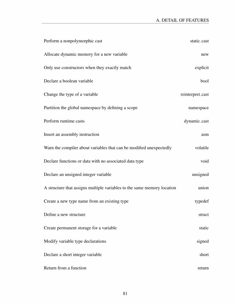
A. DETAIL OF FEATURES
Perform a nonpolymorphic cast static cast
Allocate dynamic memory for a new variable new
Only use constructors when they exactly match explicit
Declare a boolean variable bool
Change the type of a variable reinterpret cast
Partition the global namespace by defining a scope namespace
Perform runtime casts dynamic cast
Insert an assembly instruction asm
Warn the compiler about variables that can be modified unexpectedly volatile
Declare functions or data with no associated data type void
Declare an unsigned integer variable unsigned
A structure that assigns multiple variables to the same memory location union
Create a new type name from an existing type typedef
Define a new structure struct
Create permanent storage for a variable static
Modify variable type declarations signed
Declare a short integer variable short
Return from a function return
81
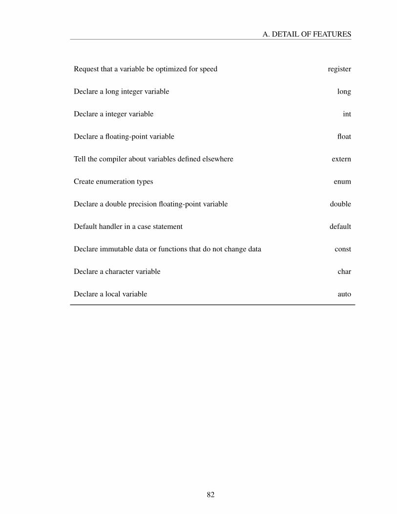
A. DETAIL OF FEATURES
Request that a variable be optimized for speed register
Declare a long integer variable long
Declare a integer variable int
Declare a floating-point variable float
Tell the compiler about variables defined elsewhere extern
Create enumeration types enum
Declare a double precision floating-point variable double
Default handler in a case statement default
Declare immutable data or functions that do not change data const
Declare a character variable char
Declare a local variable auto
82

Appendix B
Frequency of occurrence of features
Table B.1: List of the average frequency of all features used (region based dataset).
Features North America South Asia Difference Comparison
effort 778314.251108 446596.360192 855.504690 1.203974
timeRequired 43239.680617 24810.908900 47.528038 1.203974
programLength 915.756782 592.684385 0.375253 1.067417
−− 16.423186 5.125079 0.058421 2.213779
, 48.341325 27.589432 0.054533 1.210468
. 35.604890 18.989590 0.052664 1.295303
* 33.272713 19.616877 0.031642 1.171752
( 72.118612 46.877129 0.027660 1.062830
// 17.148107 9.484700 0.022182 1.249022
-> 10.958833 6.249369 0.012410 1.211450
const 3.663249 1.412618 0.010501 1.791510
83

B. FREQUENCY OF OCCURRENCE OF FEATURES
== 7.656940 4.186435 0.010361 1.263538
if 11.638013 7.077287 0.009041 1.136029
& 5.104890 2.611514 0.008595 1.350428
˜ 1.223344 0.191325 0.006140 4.417274
this 2.181703 0.940536 0.005322 1.602499
false 1.423975 0.574763 0.003841 1.711556
case 1.739748 0.845268 0.003349 1.421901
unsigned 1.078233 0.402524 0.003215 1.850539
/* 1.847003 0.947003 0.003090 1.347391
double 1.821451 0.933754 0.003048 1.347605
/ 5.693375 3.619716 0.002944 1.086608
bool 1.342902 0.626341 0.002830 1.481191
true 1.374921 0.649211 0.002823 1.463084
try 0.711356 0.197319 0.002762 2.490552
break 1.617666 0.836278 0.002642 1.336336
new 2.185804 1.280757 0.002153 1.179022
numberDeliveredBugs 2.390292 1.449402 0.001896 1.139304
auto 0.468297 0.129022 0.001827 2.507466
84

B. FREQUENCY OF OCCURRENCE OF FEATURES
static 0.533596 0.176656 0.001803 2.086708
void 3.681546 2.373028 0.001600 1.071778
return 5.790852 3.833912 0.001565 1.043465
? 0.690379 0.310883 0.001560 1.534151
throw 0.315931 0.075079 0.001345 2.907041
ˆ 0.332808 0.088801 0.001325 2.589127
| 0.830915 0.440694 0.001252 1.302558
default 0.367035 0.124132 0.001216 2.042684
char 2.472082 1.598580 0.001026 1.068331
delete 0.578864 0.293218 0.001002 1.363840
static cast 0.197634 0.054416 0.000771 2.509068
switch 0.326341 0.159306 0.000621 1.415197
float 1.417666 0.920820 0.000550 1.063596
catch 0.103312 0.017666 0.000504 4.040080
!= 1.836751 1.215773 0.000499 1.043699
reinterpret cast 0.094164 0.014669 0.000473 4.434676
|| 0.862618 0.552366 0.000409 1.078870
ˆ= 0.085331 0.016877 0.000395 3.492923
85

B. FREQUENCY OF OCCURRENCE OF FEATURES
enum 0.088328 0.025237 0.000336 2.417899
+= 1.164353 0.773186 0.000293 1.040347
register 0.168139 0.085174 0.000291 1.363763
&= 0.072871 0.024132 0.000246 2.086118
operator 0.303628 0.183754 0.000244 1.141517
continue 0.242429 0.142429 0.000235 1.175882
virtual 0.081861 0.032965 0.000222 1.715542
|= 0.116719 0.059779 0.000196 1.348871
signed 0.047950 0.017192 0.000150 1.926813
-= 0.210883 0.131073 0.000137 1.111491
volatile 0.024290 0.003628 0.000124 4.625277
short 0.143849 0.087066 0.000116 1.141394
asm 0.025552 0.008044 0.000090 2.194473
const cast 0.019558 0.005836 0.000072 2.315190
extern 0.083754 0.051577 0.000059 1.121830
mutable 0.010410 0.003312 0.000036 2.171390
explicit 0.013565 0.005678 0.000035 1.650448
typeid 0.004259 0.001262 0.000016 2.331448
86

B. FREQUENCY OF OCCURRENCE OF FEATURES
wchar t 0.022871 0.015615 0.000002 1.011860
LOC 154.131388 106.480126 0.000000 1.000000
typename 0.113407 0.078707 -0.000003 -1.004607
template 0.213565 0.148738 -0.000011 -1.008125
protected 0.010568 0.008991 -0.000016 -1.231509
dynamic cast 0.018612 0.016404 -0.000033 -1.275790
*= 0.118454 0.086120 -0.000040 -1.052390
//* 0.080915 0.061987 -0.000057 -1.108904
union 0.020189 0.020820 -0.000065 -1.492755
%= 0.006940 0.011987 -0.000068 -2.500193
<<= 0.020505 0.021451 -0.000068 -1.514294
private 0.090852 0.073975 -0.000105 -1.178618
>>= 0.018454 0.025710 -0.000122 -2.016667
friend 0.021767 0.030284 -0.000143 -2.013897
inline 0.095899 0.108202 -0.000394 -1.633216
goto 0.118770 0.124763 -0.000401 -1.520553
struct 0.838644 0.627760 -0.000454 -1.083524
/= 0.126656 0.140536 -0.000498 -1.606144
87

B. FREQUENCY OF OCCURRENCE OF FEATURES
public 0.200631 0.222397 -0.000787 -1.604551
class 0.475710 0.424448 -0.000900 -1.291531
{ 19.316719 13.459148 -0.001074 -1.008572
>= 0.551577 0.509621 -0.001207 -1.337407
else 2.596845 2.004416 -0.001976 -1.117286
typedef 0.102524 0.299842 -0.002151 -4.233401
&& 1.336435 1.189590 -0.002501 -1.288463
using 0.665615 0.833912 -0.003513 -1.813509
namespace 0.573975 0.780757 -0.003608 -1.968999
<= 0.550946 0.826498 -0.004187 -2.171477
for 5.596530 4.326341 -0.004320 -1.118985
while 0.938959 1.137224 -0.004588 -1.753161
! 1.889117 1.817981 -0.004817 -1.393006
% 2.122713 2.052524 -0.005504 -1.399650
long 0.705363 1.167508 -0.006388 -2.395906
>> 0.795426 1.303312 -0.007079 -2.371762
- 7.081861 5.699211 -0.007577 -1.164903
MVG 16.772871 12.444953 -0.008054 -1.074010
88

B. FREQUENCY OF OCCURRENCE OF FEATURES
+ 5.127445 4.656151 -0.010461 -1.314464
++ 4.063565 4.111514 -0.012249 -1.464593
<< 11.025079 8.971767 -0.012727 -1.177928
> 7.089748 6.786120 -0.017733 -1.385521
= 25.148423 19.399842 -0.019030 -1.116632
< 9.393533 9.236120 -0.025795 -1.423256
int 15.797634 14.758517 -0.036109 -1.352300
[ 14.428391 14.995899 -0.047222 -1.504448
difficulty 54.734456 51.162911 -0.125377 -1.353060
89

B. FREQUENCY OF OCCURRENCE OF FEATURES
Table B.2: List of the average frequency of all features used (gender based dataset).
gender male female difference comparison
−− 13.731926 9.860562 0.023074 1.309330
( 68.006482 62.597972 0.010149 1.021432
== 7.965930 6.355493 0.008579 1.178437
& 4.807213 3.761675 0.005735 1.201521
if 10.382749 9.086588 0.005108 1.074313
void 3.507728 2.850424 0.003386 1.157006
const 3.426957 2.874855 0.002626 1.120758
case 1.437760 1.159880 0.001452 1.165447
auto 0.603789 0.388898 0.001352 1.459717
this 2.085258 1.801396 0.001204 1.088353
unsigned 0.954296 0.751537 0.001102 1.193856
static 0.505900 0.336048 0.001056 1.415411
- 6.514875 5.986040 0.001053 1.023259
long 0.662623 0.485458 0.001040 1.283318
// 14.859232 13.841449 0.000977 1.009332
true 1.252950 1.058169 0.000907 1.113264
90

B. FREQUENCY OF OCCURRENCE OF FEATURES
% 2.066811 1.824996 0.000894 1.064776
/* 1.487286 1.307961 0.000684 1.069102
throw 0.271232 0.170683 0.000638 1.494067
! 1.767991 1.580522 0.000618 1.051717
template 0.270899 0.178660 0.000575 1.425605
false 1.300150 1.151903 0.000533 1.061199
+= 0.943493 0.819345 0.000512 1.082658
register 0.157886 0.080937 0.000511 1.834070
default 0.344025 0.257271 0.000501 1.257241
| 0.599801 0.504404 0.000450 1.118016
return 5.433771 5.053016 0.000422 1.011044
break 1.250956 1.125976 0.000380 1.044557
MVG 15.394050 14.426791 0.000353 1.003234
switch 0.296493 0.241150 0.000285 1.155970
typedef 0.152568 0.107030 0.000275 1.340223
|= 0.119827 0.078444 0.000259 1.436198
class 0.515706 0.451886 0.000249 1.072982
/= 0.167193 0.124979 0.000244 1.257767
91

B. FREQUENCY OF OCCURRENCE OF FEATURES
enum 0.095230 0.058002 0.000239 1.543654
static cast 0.171680 0.133788 0.000209 1.206485
virtual 0.075453 0.046867 0.000182 1.513661
bool 1.207579 1.113346 0.000167 1.019776
extern 0.081270 0.055177 0.000161 1.384814
&= 0.052019 0.028586 0.000154 1.710913
goto 0.065980 0.043377 0.000141 1.430119
typename 0.139937 0.116005 0.000118 1.134162
reinterpret cast 0.069304 0.050524 0.000111 1.289674
friend 0.027090 0.013129 0.000093 1.939977
const cast 0.019777 0.006648 0.000090 2.796976
public 0.204088 0.180322 0.000087 1.064114
volatile 0.020941 0.009141 0.000080 2.153887
asm 0.028918 0.016952 0.000077 1.603861
-= 0.176832 0.158385 0.000060 1.049702
? 0.569553 0.528004 0.000057 1.014183
signed 0.051022 0.041050 0.000052 1.168594
private 0.081436 0.069802 0.000051 1.096902
92

B. FREQUENCY OF OCCURRENCE OF FEATURES
<<= 0.019113 0.011966 0.000045 1.501755
wchar t 0.018946 0.012631 0.000039 1.410260
short 0.144923 0.131295 0.000038 1.037787
catch 0.096061 0.086256 0.000031 1.047073
try 0.571880 0.534153 0.000027 1.006604
explicit 0.010470 0.006482 0.000025 1.518647
protected 0.013462 0.009473 0.000024 1.336107
typeid 0.008808 0.005817 0.000019 1.423631
dynamic cast 0.027921 0.024597 0.000013 1.067255
>>= 0.017783 0.015290 0.000011 1.093495
LOC 140.597308 132.189297 0.000000 1.000000
union 0.011468 0.011468 -0.000005 -1.063606
ˆ= 0.020276 0.019943 -0.000007 -1.046138
%= 0.007479 0.011135 -0.000031 -1.583534
mutable 0.007977 0.016952 -0.000072 -2.260279
inline 0.088084 0.092903 -0.000076 -1.121795
&& 1.317434 1.251122 -0.000094 -1.010070
>= 0.514376 0.501246 -0.000133 -1.036456
93

B. FREQUENCY OF OCCURRENCE OF FEATURES
*= 0.094565 0.108526 -0.000148 -1.220630
continue 0.183314 0.198438 -0.000197 -1.151357
//* 0.048363 0.072461 -0.000204 -1.593572
namespace 0.570218 0.566063 -0.000227 -1.055856
˜ 0.368955 0.378095 -0.000236 -1.089954
struct 0.680406 0.678744 -0.000295 -1.061008
|| 0.692870 0.690710 -0.000297 -1.060290
Expected Bugs 2.055864 1.980541 -0.000360 -1.024637
float 1.259099 1.236995 -0.000402 -1.044934
using 0.606282 0.628719 -0.000444 -1.102967
double 1.785940 1.743394 -0.000486 -1.038268
char 2.348845 2.272727 -0.000487 -1.029138
else 2.287519 2.225860 -0.000568 -1.034937
!= 1.563902 1.548945 -0.000594 -1.053434
ˆ 0.198604 0.267243 -0.000609 -1.431196
delete 0.495596 0.553266 -0.000660 -1.187372
operator 0.291341 0.380256 -0.000804 -1.388210
<= 0.518697 0.612764 -0.000946 -1.256493
94

B. FREQUENCY OF OCCURRENCE OF FEATURES
>> 0.728270 0.837959 -0.001159 -1.223802
while 0.868041 0.980057 -0.001240 -1.200858
> 6.914575 6.722287 -0.001673 -1.034028
{ 17.816354 17.015124 -0.001999 -1.015774
for 4.733588 4.780622 -0.002497 -1.074174
new 1.902775 2.197441 -0.003090 -1.228317
+ 4.595313 4.764168 -0.003356 -1.102688
++ 3.434934 3.882001 -0.004936 -1.202037
-> 10.232009 10.326409 -0.005343 -1.073419
< 9.037394 9.270068 -0.005849 -1.090989
= 23.239488 22.661958 -0.006145 -1.037174
/ 4.830647 5.798737 -0.009509 -1.276759
. 29.114010 28.812697 -0.010892 -1.052598
int 14.109024 14.879009 -0.012208 -1.121651
<< 8.944823 10.078777 -0.012625 -1.198441
[ 12.854246 15.290344 -0.024244 -1.265177
difficulty 52.322587 52.904981 -0.028076 -1.075445
, 40.341699 42.988865 -0.038276 -1.133398
95

B. FREQUENCY OF OCCURRENCE OF FEATURES
* 26.986040 33.460861 -0.061190 -1.318799
timeRequired 36225.642496 41319.617340 -54.923838 -1.213168
effort 652061.564934 743753.112126 -988.629079 -1.213168
96