A system for crack pattern detection, characterization and diagnosis in concrete structures by means of image processing and machine learning techniques

Doctoral Thesis by:

Luis Alberto Sánchez Calderón

Supervisor:

Prof. Jesus Miguel Bairán García

Barcelona, October 2017

Universitat Politècnica de Catalunya, Barcelona Tech

Departament d´Enginyeria de la Construcció

PHD

DIS

SER

TATI

ON

Departament d’Enginyeria de la Construcció

Doctoral Thesis

A system for crack pattern detection, characterization and diagnosis in concrete

structures by means of image processing and machine learning techniques

Presented by

Luis Alberto Sánchez Calderón Civil Engineer, Escuela Superior Politécnica del Litoral (ESPOL) (Ecuador)

M.Sc. Structural Eng., Escuela Técnica Superior de Ingenieros de Caminos, Canales y Puertos de Barcelona (Spain)

for the degree of Doctor by the Universitat Politècnica de Catalunya, BarcelonaTech

Supervised by: Prof. Jesus M. Bairán García

This PhD thesis was financed by the SENECYCT ( Secretaria de Educación Superior, Ciencia, Tecnología e Innovación), an institution part of the government of Ecuador; by the projects BIA2012-36848 "Performance-Based Design of Partially Prestressed Concrete Structures" ,

BIA2015-64672-C4-1-R "Assessment of the shear and punching strength of concrete structures using mechanical models to extend their service life" from the Spanish Ministry of Economics and Competitiveness and "European Regional Development Fund (ERFD)" from the European

Union.

i

Acknowledgements

First, I have to thank especially my supervisor Jesus as he is the mind behind the initial idea for this work, he pointed me in the right direction every time and he has been supportive in every step of this research work. The road behind an investigation is not always clear, and in that sense Jesus’ experience, expertise and great will has been key to take this investigation in a good direction. I have to thank also Antoni Mari that as my other supervisor head of the department has always been supportive with the work done. My department colleagues Eva, Noemi, Ulric, Ana and Montse have always been charming and congenial with me making me feel included and making it feel as a family department.

I have to include the emotional support from my parents Giselda and Luis whose love and concern in my thesis were always appreciated; this work is also yours and I am glad I have this chance to mention you. Te amo mami y te amo papi. My partner Lucile’s affection, interest and company were crucial for this thesis and she has played her role in the closing of this work, reminding me that research can go on forever but researchers do not. Je t’aime ma petite puce adorée. My cousin Aida’s permanent support during my first year in Barcelona by hosting me and making her apartment a new home and a piece of Ecuador will never be forgotten. I can only describe my aunt Enmita as my third mom, her presence and advice permanent reminder of my heritage; the moments spent at her home were always enjoyable for the family atmosphere set with my cousin Omar and uncle Tanveer. Of course, I must mention my aunt’s exceptional culinary skills that made me feel closer to my country even when far. No debo olvidar a mi ñaño chiquito Bilito que sé que está muy orgulloso y a pesar de estar lejos no perdemos el cariño.

Tengo que incluir también agradecimientos a mi abuelita Norma que me hace unas sopitas “bien buenas”, a mis tías maternas Denis, Rosita, Nitza, a mi prima Paolita, que desde Guayaquil están pendientes de mis estudios y me envían su cariño siempre. A mis tías paternas de Babahoyo Toya, Piedad, Julia. Hago especial mención para mis abuelos Gonzalo y Aida a cuyo cariño nunca le encontré límites y sé que están pendientes de mi desde el cielo; los sigo extrañando y espero vivir a su altura. Debo mencionar por último también a un gran amigo y colega que se nos adelantó a conocer al creador; Héctor, que de haber estado aún con nosotros hubiera seguido un camino similar al mío, pero pisando mucho más fuerte de seguro.

ii

Summary

A system that attempts to find cracks in a RGB picture of a concrete beam, measure the cracks angles and widths; and classify crack patterns in 3 pathologies has been designed and implemented in the MATLAB programming language. The system is divided in three parts: Crack Detection, Crack Clustering and Crack Pattern Classification.

The Crack Detection algorithm attempts to detect pixels depicting cracks in a region of interest (ROI) and measure the crack angles and widths. The input ROI is segmented several times: First with an artificial Neural Network (NN) that classifies image patches in “Crack” or “Not Crack”, then with the Canny Edge detector and finally with the local Mean and Standard deviation of the intensities. Then all neighborhoods in the mask are passed through special modified line kernels called “orientation kernels” designed to detect cracks and measure their angles; in order to obtain the width measurement, a line of pixels perpendicular to the crack is extracted and with an approximation of the intensity gradient of that line the width is measured. This algorithm outputs a mask the same size as the input picture with the measured angles and widths.

The Crack Clustering algorithm groups up all the crack image patches recognized from the Crack Detection to approximate clusters that match the quantity of cracks in the image. To achieve this a special distance metric has been designed to group up aligned crack image patches; then with an algorithm based on the connectivity among the crack patches the clusters are obtained.

The Crack Pattern Classification takes the mask outputs from the Crack Detection step as input for a Neural Network (NN) designed to classify crack patterns in concrete beams in 3 classes: Flexion, Shear and Corrosion-Bond cracks. The width and angles masks are first transformed into a Feature matrix to reduce the degrees of freedom of the input for the NN. To achieve a desirable classification in cases when more than 1 pathology is present, every angle and width mask is separated in as many Features matrices as clusters found with the Clustering algorithm; then separately classified with the NN designed.

Several photos depicting concrete surfaces are presented as examples to check the accuracy of the width and angle measurements from the Crack Detection step. Other photos showing concrete beams with crack patterns are used to check the classification prowess of the Crack Pattern Classification step.

The most important conclusion of this work is the transference of empirical knowledge from rehabilitation of structures to a machine learning model in order to diagnose the damage on an element. This opens possibilities for new lines of research to make a larger system with wider utilities, more pathologies and elements to classify.

iii

Resumen

Se ha diseñado un sistema que a partir de una foto a color de una superficie de hormigón realiza las siguientes tareas: Detectar fisuras, medir su ángulo y ancho, clasificar los patrones de fisuración asociados a tres patologías del hormigón; el cual ha sido implementado en el lenguaje de programación MATLAB. El sistema se divide en tres partes: Detección y medición de fisuras; algoritmo de análisis de grupos de fisuras y clasificación de patrones de fisuración.

El algoritmo de detección de fisuras detecta los pixeles en donde hay fisuras dentro de una región de interés y mide el ancho y ángulos de dichas fisuras. La región de interés es segmentada varias veces: Primero con una red neuronal artificial que clasifica teselas de la imagen en dos categorías “Fisura” y “No fisura”; después se hace otra segmentación con un filtro Canny de detección de bordes y finalmente se segmenta con la media y desviaciones intensidades en teselas de la imagen. Entonces todas las localidades de la máscara de imagen obtenida con las segmentaciones anteriores se las pasa por varios filtros de detección de líneas diseñados para detectar y medir las fisuras. Este algoritmo resulta en dos máscaras de imagen con los anchos y ángulos de todas las fisuras encontradas en la región de interés.

El algoritmo de análisis de grupos de teselas reconocidas como fisuras se hace para intentar reconocer y contar cuantas fisuras aparecen en la región de interés. Para lograr esto se diseñó una función de distancia para que teselas de fisura alineadas se junten; después con un algoritmo basado en la conectividad entre estas teselas o vectores fisura se obtienen los grupos de fisura.

La clasificación de patrones de fisuración toma las máscaras de imagen del paso de detección de fisuras y lo toma como dato de entrada para una red neuronal diseñada para clasificar patrones de fisuración en tres categorías seleccionadas: Flexión, Cortante y Corrosión-Adherencia. Las máscaras de imagen de ancho y ángulo se transforman en una matriz de características para reducir los grados de libertad del problema, estandarizar un tamaño para la entrada al modelo de red neuronal. Para lograr clasificaciones correctas cuando más de 1 patología está presente en las vigas, cada máscara de imagen de ángulos y anchos de fisura se divide en cuantos cuantos grupos de teselas de fisuras haya en la imagen, y para cada uno se obtienen una matriz de características. Entonces se clasifican separadamente dichas matrices con la red neuronal artificial diseñada.

Varias fotos con superficies de hormigón se presentan como ejemplos para evaluar la precisión de las mediciones de ancho y ángulo del paso de detección de fisuras. Otras fotos mostrando patrones de fisuración en vigas de hormigón se muestran para revisar las capacidades de diagnóstico del paso de clasificación de patrones de fisuración.

La conclusión más importante de este trabajo es la transferencia del conocimiento empírico de la rehabilitación de estructuras hacia un modelo de inteligencia artificial para diagnosticar el daño en un elemento de la estructura. Esto abre un campo grande de líneas de investigación hacia el diseño e implementación de sistemas automatizados con más utilidades, más patologías y elementos para clasificar.

iv

Contents Acknowlegments…………………………………………………………………………………………………………………….. i

Summary…………………………………………………………………………………………………………………………………. ii

Resumen………………………………………………………………………………………………………………………………….iii

List of Symbols………………………………………………………………………………………………………………………. vii

List of Figures…………………………………………………………………………………………………………………………. x

List of Tables…………………………………..………………………..………………………..…………………………………..xv

1. Introduction .......................................................................................................................... 1

1.1. Research relevance ....................................................................................................... 1

1.2. Motivation ..................................................................................................................... 1

1.3. Scope and objectives ..................................................................................................... 2

1.3.1. General objective .................................................................................................. 2

1.3.2. Specific objectives ................................................................................................. 2

1.4. Methodology ................................................................................................................. 2

1.5. Outline of the Thesis ..................................................................................................... 3

2. State of the Art ...................................................................................................................... 5

2.1. Photogrammetry ........................................................................................................... 6

2.1.1. Definition ............................................................................................................... 6

2.1.2. Types of Photogrammetry..................................................................................... 6

2.1.3. Applications of close-range Photogrammetry ...................................................... 6

2.1.4. Applications in Civil Engineering ........................................................................... 7

2.1.5. Mathematical Foundations ................................................................................... 8

2.1.6. Thin Lenses ............................................................................................................ 9

2.1.7. Interior Orientation ............................................................................................. 10

2.1.8. External Orientation ............................................................................................ 15

2.2. Digital Image Processing ............................................................................................. 18

2.2.1. Spatial Filtering .................................................................................................... 18

2.2.2. Feature detection ................................................................................................ 20

2.3. Machine Learning ........................................................................................................ 24

2.3.1. Supervised Learning ............................................................................................ 25

2.3.2. Unsupervised Learning ........................................................................................ 33

2.4. Diagnosis of Structures................................................................................................ 37

2.4.1. General Problem ................................................................................................. 37

v

2.4.2. Causes of structural pathologies ......................................................................... 37

2.4.3. Symptoms in Buildings ........................................................................................ 38

2.4.4. Pathologies in concrete beams ........................................................................... 39

3. Crack Detection and Measurement .................................................................................... 49

3.1. Hypothesis ................................................................................................................... 50

3.2. Crack detection with a Neural Network ...................................................................... 50

3.2.1. Training Examples ............................................................................................... 50

3.2.2. Engineered Features ........................................................................................... 52

3.2.3. Hidden Layer Size ................................................................................................ 53

3.2.4. Learning Curves ................................................................................................... 55

3.2.5. Regularization ...................................................................................................... 55

3.2.6. Misclassification Error ......................................................................................... 56

3.2.7. Example ............................................................................................................... 58

3.3. Crack Measurement with Digital Image processing .................................................... 60

3.3.1. Algorithm ............................................................................................................. 60

3.4. Resume on Crack Detection Step ................................................................................ 67

4. Cracked Patch Clustering ..................................................................................................... 69

4.1. Problem statement ..................................................................................................... 70

4.2. Distance Metric ........................................................................................................... 70

4.3. Linkage Criteria ............................................................................................................ 72

4.4. Algorithm ..................................................................................................................... 73

4.4.1. Clustering with distance metric and patch size threshold .................................. 73

4.4.2. Cluster Filtering with endpoint distance and direction ....................................... 76

5. Crack Pattern Classification with Machine Learning ........................................................... 81

5.1. Problem statement ..................................................................................................... 82

5.2. Training Examples for Machine Learning Model......................................................... 82

5.2.1. Base Images Set ................................................................................................... 82

5.2.2. Transformation of Base images into Standardized images ................................. 84

5.2.3. Standardized Images to Training Image .............................................................. 85

5.2.4. Assumptions ........................................................................................................ 85

5.2.5. Expanding the number of Training Images ......................................................... 85

5.2.6. Transformation of Training Images into Feature Vectors ................................... 86

5.3. Model Selection .......................................................................................................... 88

5.3.1. Number of training examples .............................................................................. 88

5.3.2. Number of Hidden Units ..................................................................................... 89

5.3.3. Regularization Term ............................................................................................ 90

vi

5.3.4. Misclassification Error ......................................................................................... 90

5.3.5. Classification of real examples ............................................................................ 91

6. Case Studies ........................................................................................................................ 95

6.1. Shear-Flexure loading of partially prestressed beam ................................................. 95

6.2. Flexure loading of partially prestressed beam .......................................................... 100

6.3. FRC concrete beam loaded in shear .......................................................................... 105

6.4. Plastic hinge in fixed support of partially prestressed beam .................................... 109

6.5. Shear loading in FRC beam without transversal reinforcement ............................... 113

6.6. Local flange crack in I-shaped beam ......................................................................... 116

6.7. Remarks and commentaries...................................................................................... 119

7. Conclusions ....................................................................................................................... 121

7.1. Global conclusion ...................................................................................................... 121

7.2. Specific conclusions and problems found ................................................................. 121

7.3. Recommendations for future works ......................................................................... 122

References ................................................................................................................................. 125

Annex I ....................................................................................................................................... 131

Cracked Concrete Surfaces.................................................................................................... 131

Labeled Image Patches .......................................................................................................... 138

Training Set Examples ....................................................................................................... 138

Cross-Validation Set Examples .......................................................................................... 143

Test Set Predictions ........................................................................................................... 143

Annex II ...................................................................................................................................... 145

Base Images ........................................................................................................................... 145

Standardized Image Example ................................................................................................ 154

Training Image ....................................................................................................................... 155

vii

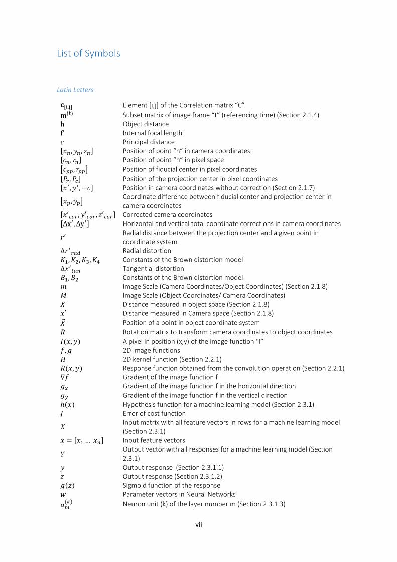
List of Symbols

Latin Letters

𝐜𝐜[𝐢𝐢,𝐣𝐣] Element [i,j] of the Correlation matrix “C” m(t) Subset matrix of image frame “t” (referencing time) (Section 2.1.4) h Object distance f′ Internal focal length 𝑐𝑐 Principal distance [𝑥𝑥𝑛𝑛,𝑦𝑦𝑛𝑛, 𝑧𝑧𝑛𝑛] Position of point “n” in camera coordinates [𝑐𝑐𝑛𝑛, 𝑟𝑟𝑛𝑛] Position of point “n” in pixel space �𝑐𝑐𝑝𝑝𝑝𝑝, 𝑟𝑟𝑝𝑝𝑝𝑝� Position of fiducial center in pixel coordinates [𝑃𝑃𝑟𝑟,𝑃𝑃𝑐𝑐] Position of the projection center in pixel coordinates [𝑥𝑥′,𝑦𝑦′,−𝑐𝑐] Position in camera coordinates without correction (Section 2.1.7)

�𝑥𝑥𝑝𝑝,𝑦𝑦𝑝𝑝� Coordinate difference between fiducial center and projection center in camera coordinates

[𝑥𝑥′𝑐𝑐𝑐𝑐𝑟𝑟,𝑦𝑦′𝑐𝑐𝑐𝑐𝑟𝑟, 𝑧𝑧′𝑐𝑐𝑐𝑐𝑟𝑟] Corrected camera coordinates [∆x′,∆y′] Horizontal and vertical total coordinate corrections in camera coordinates

𝑟𝑟′ Radial distance between the projection center and a given point in coordinate system

∆𝑟𝑟′𝑟𝑟𝑟𝑟𝑟𝑟 Radial distortion 𝐾𝐾1,𝐾𝐾2,𝐾𝐾3,𝐾𝐾4 Constants of the Brown distortion model ∆𝑥𝑥′𝑡𝑡𝑟𝑟𝑛𝑛 Tangential distortion 𝐵𝐵1,𝐵𝐵2 Constants of the Brown distortion model 𝑚𝑚 Image Scale (Camera Coordinates/Object Coordinates) (Section 2.1.8) 𝑀𝑀 Image Scale (Object Coordinates/ Camera Coordinates) 𝑋𝑋 Distance measured in object space (Section 2.1.8) 𝑥𝑥′ Distance measured in Camera space (Section 2.1.8) �⃗�𝑋 Position of a point in object coordinate system 𝑅𝑅 Rotation matrix to transform camera coordinates to object coordinates 𝐼𝐼(𝑥𝑥,𝑦𝑦) A pixel in position (x,y) of the image function “I” 𝑓𝑓,𝑔𝑔 2D Image functions 𝐻𝐻 2D kernel function (Section 2.2.1) 𝑅𝑅(𝑥𝑥,𝑦𝑦) Response function obtained from the convolution operation (Section 2.2.1) ∇𝑓𝑓 Gradient of the image function f 𝑔𝑔𝑥𝑥 Gradient of the image function f in the horizontal direction 𝑔𝑔𝑦𝑦 Gradient of the image function f in the vertical direction ℎ(𝑥𝑥) Hypothesis function for a machine learning model (Section 2.3.1) 𝐽𝐽 Error of cost function

𝑋𝑋 Input matrix with all feature vectors in rows for a machine learning model (Section 2.3.1)

𝑥𝑥 = [𝑥𝑥1 … 𝑥𝑥𝑛𝑛] Input feature vectors

𝑌𝑌 Output vector with all responses for a machine learning model (Section 2.3.1)

𝑦𝑦 Output response (Section 2.3.1.1) 𝑧𝑧 Output response (Section 2.3.1.2) 𝑔𝑔(𝑧𝑧) Sigmoid function of the response 𝑤𝑤 Parameter vectors in Neural Networks 𝑎𝑎𝑚𝑚

(𝑘𝑘) Neuron unit (k) of the layer number m (Section 2.3.1.3)

viii

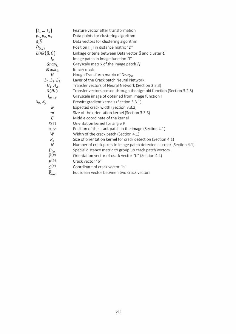
[𝑡𝑡1 … 𝑡𝑡𝑘𝑘] Feature vector after transformation 𝑝𝑝1,𝑝𝑝2,𝑝𝑝3 Data points for clustering algorithm �⃗�𝑎,𝑏𝑏�⃗ Data vectors for clustering algorithm 𝐷𝐷(𝑖𝑖,𝑗𝑗) Position [i,j] in distance matrix “D” 𝐿𝐿𝐿𝐿𝐿𝐿𝐿𝐿��⃗�𝑎, �̂�𝐶� Linkage criteria between Data vector �⃗�𝑎 and cluster 𝑪𝑪�

𝐼𝐼𝑘𝑘 Image patch in image function “I” 𝐺𝐺𝑟𝑟𝑎𝑎𝑦𝑦𝑘𝑘 Grayscale matrix of the image patch 𝐼𝐼𝑘𝑘 𝑀𝑀𝑎𝑎𝑀𝑀𝐿𝐿𝑘𝑘 Binary mask 𝐻𝐻 Hough Transform matrix of 𝐺𝐺𝑟𝑟𝑎𝑎𝑦𝑦𝑘𝑘

𝐿𝐿0,𝐿𝐿1,𝐿𝐿2 Layer of the Crack patch Neural Network 𝐻𝐻1,𝐻𝐻2 Transfer vectors of Neural Network (Section 3.2.3) 𝑆𝑆(𝐻𝐻1) Transfer vectors passed through the sigmoid function (Section 3.2.3) 𝐼𝐼𝑔𝑔𝑟𝑟𝑟𝑟𝑦𝑦 Grayscale image of obtained from image function I

𝑆𝑆𝑥𝑥, 𝑆𝑆𝑦𝑦 Prewitt gradient kernels (Section 3.3.1) 𝑤𝑤 Expected crack width (Section 3.3.3) 𝑚𝑚 Size of the orientation kernel (Section 3.3.3) 𝐶𝐶 Middle coordinate of the kernel

𝐾𝐾(𝜃𝜃) Orientation kernel for angle 𝜃𝜃 𝑥𝑥,𝑦𝑦 Position of the crack patch in the image (Section 4.1) 𝑊𝑊 Width of the crack patch (Section 4.1) 𝐾𝐾𝑆𝑆 Size of orientation kernel for crack detection (Section 4.1) 𝑁𝑁 Number of crack pixels in image patch detected as crack (Section 4.1) 𝐷𝐷𝑙𝑙𝑙𝑙𝑐𝑐 Special distance metric to group up crack patch vectors 𝑉𝑉�⃗ (𝑏𝑏) Orientation vector of crack vector “b” (Section 4.4) 𝑃𝑃(𝑏𝑏) Crack vector “b” 𝐶𝐶(𝑏𝑏) Coordinate of crack vector “b” 𝑉𝑉�⃗𝑒𝑒𝑒𝑒𝑐𝑐 Euclidean vector between two crack vectors

ix

Greek Letters

𝜑𝜑 Rotation angle between the X axis in the object coordinate system and the x’ axis in the camera coordinate system

𝜀𝜀 Rotation angle between the Y axis in the object coordinate system and the y’ axis in the camera coordinate system

𝜔𝜔 Rotation angle between the Z axis in the object coordinate system and the z’ axis in the camera coordinate system

𝜌𝜌 Radial length in polar coordinates 𝜃𝜃 Angle of the radius length (Section 2.2.2) 𝜃𝜃 = [Ө0 Ө0 … Ө𝑛𝑛] Parameter vector of the hypothesis function ℎ(𝑥𝑥) (Section 2.3.1) 𝜆𝜆 Regularization term factor 𝜕𝜕𝐽𝐽𝜕𝜕𝜃𝜃

Partial derivative of the cost function

𝛼𝛼 Learning rate of the iterative process to minimize the cost function J 𝜇𝜇𝑘𝑘 Mean of pixel intensities in image patch 𝐼𝐼𝑘𝑘 𝜎𝜎𝑘𝑘 Standard deviation of pixel intensities in image patch 𝐼𝐼𝑘𝑘 𝜃𝜃 Angle of the crack patch (Section 3.3.3) (Section 4.1)

x

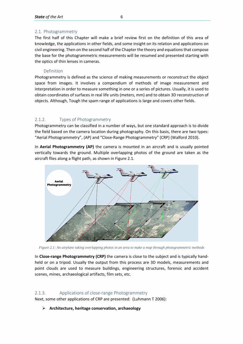
List of Figures

Figure 2.1: An airplane taking overlapping photos in an area to make a map through photogrammetric methods ........................................................................................................... 6 Figure 2.2: Detected displacement of subset m from time t to time t+1 (Blaber J 2015) ............ 8 Figure 2.3 : Ray tracing of the light going from an object in the real world through the camera lenses and into the camera sensor. ............................................................................................ 10 Figure 2.4: Pixels coordinates of a digital image and its fiducial center (FC) .............................. 11 Figure 2.5: Projection of the camera coordinate system with its origin on the projection center ..................................................................................................................................................... 11 Figure 2.6: Relations between the Camera Coordinate system and the pixel coordinate system ..................................................................................................................................................... 12 Figure 2.7: Perspective view to feature the projection relations between the camera coordinate system and pixel coordinate system ........................................................................ 13 Figure 2.8: Deformation of coordinates caused by barrel and pincushion type of distortion (Luhmann T 2006) ....................................................................................................................... 14 Figure 2.9: Visual representation of the misalignment between the camera sensor and the lenses causing tangential distortion (Mathworks, Camera Calibration 2016) ............................ 15 Figure 2.10 :Relation between object distance, principal distance and the camera and real coordinates (Luhmann T 2006) ................................................................................................... 16 Figure 2.11: Projection relations between the camera coordinate system and the object coordinate system ....................................................................................................................... 17 Figure 2.12: Example of the resulting matrix between a convolution operation done between an input matrix and a Sobel kernel (Sobel 1968) ........................................................................ 19 Figure 2.13: Computation of element R(1,1) of the output matrix ............................................ 20 Figure 2.14: A photo passed through the Canny edge detector ................................................. 22 Figure 2.15: Defining a line in the 2D plane with 𝜌𝜌 and 𝜃𝜃 as parameters .................................. 23 Figure 2.16: Graphic attempting to explain the difference between the usage of a too small or too large learning rate ................................................................................................................. 27 Figure 2.17: Sigmoid function in a domain subset of [-10,10] .................................................... 28 Figure 2.18: The generation of an output “y” in a simple neuron with 4 inputs ........................ 30 Figure 2.19: Architecture of a neural network with 1 hidden unit ............................................. 31 Figure 2.20: Architecture of a part of a neural network featuring the computation of the element 𝑎𝑎𝑚𝑚(𝐿𝐿 + 1)from elements on layer k ............................................................................ 32 Figure 2.21: Four different ways of forming clusters from a dataset (Tan, Steinback y Kumar 2006) ........................................................................................................................................... 34 Figure 2.22:The dendrogram and clusters for example points p1 to p4 (Tan, Steinback y Kumar 2006) ........................................................................................................................................... 35 Figure 2.23: Typical moment-curvature relation for a reinforced concrete section (Kwak Hyo 2002) ........................................................................................................................................... 40 Figure 2.24: Flexion cracks that curve a little as they progress through the section of a short beam............................................................................................................................................ 40 Figure 2.25: Flexion cracks in a simply supported concrete beam with a large span (Vidal 2007) ..................................................................................................................................................... 40 Figure 2.26: Flexion and shear crack patterns in double fixed beams (ce-ref.com s.f.) ............. 41 Figure 2.27 Strut and ties model for a concrete beam (Schlaich y Shafer, Toward a consistent design of Structural Concrete 1987) ........................................................................................... 41

xi

Figure 2.28: Shear cracks in concrete beams in a building (GHARPEDIA.COM 2016) ................ 42 Figure 2.29: Shear cracks in the web of a prestressed concrete beam (Celada 2018) ............... 42 Figure 2.30: Concrete beam with the bottom longitudinal reinforcement affected by corrosion (Muñoz 1994) .............................................................................................................................. 44 Figure 2.31: Corrosion induced cracking in a beam (Du, Chan y Clark 2013) ............................. 44 Figure 2.32: Local bond stress-slip law (Task Group 2000) ......................................................... 45 Figure 2.33: Different viewpoint of the splitting cracks caused by the compression on the struts around reinforced bars (Task Group 2000) ................................................................................. 46 Figure 2.34: Modes of bond failure: (a) pull-out failure, (b) splitting-induced pull out accompanied by crushing and shearing-off in the concrete below the ribs and (c) splitting accompanied by slip on the rib faces (Task Group 2000) ........................................................... 46 Figure 2.35:Hairlike splitting cracks along the bottom face of a beam-test specimen (Plizzari y Franchi 1996) ............................................................................................................................... 47 Figure 2.36: Crack pattern in a concreted partially prestressed beam presenting flexion, shear and bond cracks. (Duarte 2019) .................................................................................................. 47 Figure 3.1: GUI panel used to classify an image patch as “Crack” or “Not Crack” to generate examples ..................................................................................................................................... 51 Figure 3.2:Image patches labeled as “Crack” from the training set ........................................... 51 Figure 3.3 Image patches labeled as “Not Crack” in the training set .......................................... 52 Figure 3.4: Curve to determine ideal hidden layer size for the Neural Network for the Crack detection step ............................................................................................................................. 54 Figure 3.5: Architecture of the Neural Network for the Crack detection step ........................... 54 Figure 3.6:Learning curve for the Neural Network for the Crack detection step ....................... 55 Figure 3.7: Curve Error vs λ regularization term ......................................................................... 56 Figure 3.8: Image patches from Test predicted as “Not Cracks” ................................................ 57 Figure 3.9:Image patches from Test set predicted as “Crack” .................................................... 57 Figure 3.10: Picture of a prestressed concrete beam during testing .......................................... 58 Figure 3.11: Region of interest picked by user from picture in Figure 3-10 ............................... 59 Figure 3.12: Mask obtained by the NN segmentation of the picture in Figure 3-10 .................. 59 Figure 3.13:Function to generate the orientation kernel ........................................................... 61 Figure 3.14: Orientation kernel for 60 degrees and a size of 25x25 pixels, viewpoint 1 ............ 62 Figure 3.15: Orientation kernel for 60 degrees and a size of 25x25 pixels, viewpoint 2 ............ 63 Figure 3.16: Neighborhood from an input picture and the same neighborhood segmented with the mean detection thresholding .................................................................................................. 63 Figure 3.17: Response of the neighborhood shown in Figure 3-16 to the orientation kernels of size m=15 ..................................................................................................................................... 64 Figure 3.18: Theoretical color intensities in a line of pixels perpendicular to the crack width Where: BC is the color intensity of the background (concrete); CC is the color intensity of crack; C is the center of the line of pixels; w is the width of the crack ................................................. 65 Figure 3.19: Color intensities in a line of pixels perpendicular to the crack width. Where: BC is the color intensity of the background (concrete); CC is the color intensity of crack .................. 66 Figure 3.20: Gradient of the color intensities in a line of pixels perpendicular to the crack; Where: C is the center of the line of pixels; w is the width of the crack .................................... 66 Figure 3.21: Graphical resume of the transformations and processes ....................................... 68 Figure 4.1: The projection and distances between data points 𝑃𝑃(𝑎𝑎) and 𝑃𝑃(𝑏𝑏)when the Euclidean vector 𝑉𝑉𝑉𝑉𝑉𝑉𝑐𝑐 is almost perpendicular to both crack direction vectors 𝑉𝑉(𝑎𝑎)and 𝑉𝑉(𝑏𝑏) ..................................................................................................................................................... 71

xii

Figure 4.2: The projection and distances between data points 𝑃𝑃(𝑎𝑎) and 𝑃𝑃(𝑏𝑏)when the Euclidean vector 𝑉𝑉𝑉𝑉𝑉𝑉𝑐𝑐 is almost collinear to both crack direction vectors 𝑉𝑉(𝑎𝑎)and 𝑉𝑉(𝑏𝑏)....... 72 Figure 4.3: Minimum distance “d” between a cluster “A” and a cluster “B” .............................. 73 Figure 4.4: Flowchart for making up the crack clusters .............................................................. 74 Figure 4.5: Artificial cracks and symbols drawn in AutoCAD to use as input for the Crack detection algorithm ..................................................................................................................... 75 Figure 4.6: Mask with the widths of the cracks after passing the image in Figure 4-5 through the Crack Detection algorithm .................................................................................................... 75 Figure 4.7: Mask with the angles of the cracks after passing the image in Figure 4-5 through the Crack Detection algorithm .......................................................................................................... 76 Figure 4.8: Clusters found in the Mask presented in Figure 4-6 and Figure 4-7 ......................... 76 Figure 4.9: Concrete beam being tested in laboratory presenting a shear crack pattern in its web (Celada 2018)....................................................................................................................... 77 Figure 4.10: Angle Mask obtained from passing the image in Figure 4-9 through the crack detection described in chapter 3 ................................................................................................ 77 Figure 4.11: Result of the first step of the clustering algorithm explained in subsection 4.4.1 applied to the mask showed in Figure 4-10 ................................................................................ 78 Figure 4.12: Flowchart with the steps for the cluster filtering ................................................... 79 Figure 4.13: Clusters after merging all clusters whose endpoint crack points are close and have similar direction angles ............................................................................................................... 79 Figure 4.14: Final clusters after removing those whose length is smaller than 30 mm ............. 80 Figure 5.1: Flowchart with the inputs, model and outputs to solve the classification problem of assigning a crack pattern to a given pathology. .......................................................................... 82 Figure 5.2: Crack pattern from a test beam failing in (Cladera 2003) ........................................ 83 Figure 5.3: Photo from a test beam failing by shear (Walraven 1980) ....................................... 83 Figure 5.4: Photo of a beam in a building with shear cracks along all its web (Muñoz 1994) .... 83 Figure 5.5: Shear Crack pattern from testing on beams with corroded shear reinforcement (Takahashi 2013) ......................................................................................................................... 83 Figure 5.6: Typical crack pattern generated by flexion and shear (Broto Xavier 2006) .............. 84 Figure 5.7: A drawn crack pattern from a test in a concrete beam (Bairán, Mari y Cladera 2017) ..................................................................................................................................................... 84 Figure 5.8: Transformation of an example of a beam cracked by shear and flexion into a standardized image ..................................................................................................................... 84 Figure 5.9: Transformation of an example of a beam cracked by corrosion into a standardized image ........................................................................................................................................... 85 Figure 5.10: Separating a standardized image example in exclusive examples (Flexion and Shear) .......................................................................................................................................... 85 Figure 5.11: Transformation from the mask crack output with the angles and width into a feature matrix ............................................................................................................................. 86 Figure 5.12: Mapping of the crack pixels in the ROI inside the Angle Mask into the Feature Matrix .......................................................................................................................................... 87 Figure 5.13: Mapping of the Angle mask into the depth of the Feature matrix, the depth represents the angle interval where ........................................................................................... 87 Figure 5.14: Transformation from the feature matrix into a feature vector .............................. 88 Figure 5.15: Error in Training and Test Sets vs Number of Training Examples ........................... 89 Figure 5.16: Error in Training and Test set vs Number of Hidden Units in the NN ..................... 90 Figure 5.17 Test and Training Error vs the regularization parameter λ ...................................... 90 Figure 5.18: Crack clusters obtained from the width and angle masks ...................................... 91

xiii

Figure 5.19 Segmenting the width and angle masks based on individual crack clusters, 4 of the clusters 30 found are presented in the right side of the figure. ................................................. 92 Figure 5.20: Generating a Feature matrix from each angle and width mask segmented by their individual clusters........................................................................................................................ 93 Figure 5.21: Classification of each Feature matrix that belongs to each cluster crack with the NN designed ................................................................................................................................ 93 Figure 5.22: Final cluster classification for an example .............................................................. 94 Figure 6.1: Concrete beam I-181” loaded with 635 kN .............................................................. 95 Figure 6.2: Elevation viewpoint with the dimensions of beam I-181 ......................................... 96 Figure 6.3: Cross-Section of beam “I-181” in the ROI focused ................................................... 96 Figure 6.5: Region of interest (ROI) selected from the image presented in Figure 6-1 .............. 96 Figure 6.6: Segmentation by means of a NN of the ROI in Figure 6-3 ........................................ 97 Figure 6.7: Part of the Angle Mask obtained from the crack detection algorithm ..................... 97 Figure 6.8: Part of the Width Mask obtained from the crack detection algorithm .................... 98 Figure 6.9: First part of the clustering algorithm applied on the width and angle masks from Figure 6-5 and Figure 6-6. ........................................................................................................... 98 Figure 6.10: Second part of the clustering algorithm applied on the masks from Figure 6-5 and Figure 6-6. ................................................................................................................................... 99 Figure 6.11: Final classification mask of the example ................................................................. 99 Figure 6.12: Dimensions of the test beam “Biga 2” .................................................................. 100 Figure 6.13: Cross-section of test beam “Biga 2” ...................................................................... 100 Figure 6.14: Concrete beam “Biga 2” loaded with 486 kN ....................................................... 101 Figure 6.15: Region of interest chosen from the picture presented in Figure 6-12 ................. 101 Figure 6.16: Segmentation with a NN of the ROI presented in Figure 6-13 ............................. 102 Figure 6.17: Angle mask obtained from the crack detection algorithm ................................... 102 Figure 6.18: Width mask obtained from the crack detection algorithm .................................. 103 Figure 6.19: Clusters obtained with the first part of the clustering algorithm applied on the Width and Angle masks in Figure 6-15 and Figure 6-16 ........................................................... 103 Figure 6.20: Clusters obtained with the second part of the clustering algorithm applied on the Width and Angle masks in Figure 6-15 and Figure 6-16 ........................................................... 104 Figure 6.21: Final classification mask of the example ............................................................... 104 Figure 6.22: Beam geometry and reinforcement (Tetta, Koutas y Bournas 2015) ................... 105 Figure 6.23: Cracked fiber reinforced beam (Tetta, Koutas y Bournas 2015) ........................... 105 Figure 6.24: ROI selected from the picture presented in Figure 6-21 ...................................... 106 Figure 6.25: Segmentation with a NN of the ROI presented in Figure 6-22 ............................. 106 Figure 6.26: The Angle mask obtained for the ROI presented in Figure 6-22 ........................... 107 Figure 6.27: The Width mask obtained for the ROI presented in Figure 6-22 .......................... 107 Figure 6.28: The crack clusters obtained with the clustering algorithm from the width and angle masks presented in Figure 6-24 and Figure 6-25 ...................................................................... 108 Figure 6.29: Final Classification of the Crack pattern ................................................................ 108 Figure 6.30: Concrete beam “Biga 3” loaded with 570 kN........................................................ 109 Figure 6.31: Elevation viewpoint of test beam “Biga 3” ........................................................... 109 Figure 6.32: Cross-section of “Biga 3” with its transversal and longitudinal reinforcement .... 110 Figure 6.33: Region of interest (ROI) selected from the image presented in Figure 6-28 ........ 110 Figure 6.34: Mean detection segmentation of the ROI presented in Figure 6-31 .................... 110 Figure 6.35: Angle mask of the photo presented in Figure 6-28 .............................................. 111 Figure 6.36: Width mask of the photo presented in Figure 6-28 .............................................. 111

xiv

Figure 6.37: Clusters obtained from the angle and width masks presented in Figure 6-33 and Figure 6-34 ................................................................................................................................ 112 Figure 6.38: The final classification of the crack pattern in the photo in Figure 6-28 .............. 112 Figure 6.39: Photo of fiber reinforced concrete beam without transversal reinforcement after essay .......................................................................................................................................... 113 Figure 6.40: Mean segmentation mask obtained from the input picture presented in Figure 6-37 ........................................................................................................................................... 113 Figure 6.41: Angle mask obtained from the mean segmentation presented in Figure 6-38 .... 114 Figure 6.42: Width mask obtained from the mean segmentation presented in Figure 6-38 ... 114 Figure 6.43: Clustered crack patches obtained from the masks presented in Figure 6-39 and Figure 6-40 ................................................................................................................................ 115 Figure 6.44: Final classification of the crack pattern ................................................................ 115 Figure 6.45: Crack pattern on flange of concrete beam, the crack widths have been measured ................................................................................................................................................... 116 Figure 6.46: Elevation viewpoint of test beam “I181” .............................................................. 116 Figure 6.47: Mean detection segmentation from applied on the photo presented in Figure 6-43 ................................................................................................................................................... 117 Figure 6.48: Angle mask generated from the photograph presented in Figure 6-43 ............... 117 Figure 6.49: Width mask generated from the photograph presented in Figure 6-43 .............. 118 Figure 7.1: A general Flowchart with the steps in a complete diagnosis of concrete structures ................................................................................................................................................... 123

xv

List of Tables Table 2-1: The most common different dissimilarity or distance metric between data ............ 35 Table 2-2: Most used linkage criteria for hierarchical clustering algorithms.............................. 36 Table 2-3:An example with 8 data points, and each data points with 4 dimensions ................. 36 Table 2-4: The cosine distances matrix between the data points presented in Error! Not a valid bookmark self-reference. ............................................................................................................ 36 Table 3-1: Four outputs from the Neural Network for crack detection being classified with a Threshold of 0.5 .......................................................................................................................... 56 Table 3-2:Confusion matrix of the result of the NN in the Cross-Validation Set ........................ 58 Table 3-3: Confusion matrix of the results of the NN in the Test Set ......................................... 58 Table 5-1: Comparison of the performance of different machine learning models for the crack pattern classification problem .................................................................................................... 88 Table 5-2: Confusion Matrix with the percentages of true positives, false-positives and false negatives for the predictions of the NN model in the Test set. .................................................. 91 Table 6-1: Comparison of crack widths obtained with a measuring magnifier and ................. 118

Introduction 1

1. Introduction

1.1. Research relevance Cracking of concrete elements is something expected in service conditions of reinforced (RC) and partially prestressed concrete (PPC) structures. However, it should be controlled with adequate design, in order to assure durability and serviceability. This is done to ensure the durability of the concrete structures, as wider cracks make concrete elements vulnerable to chemical attacks such as carbonation, chlorides, sulphates and alkali-silica reaction. Being able to measure with precision the width of the fissures may help improve existing models (Bazant 1979) (Ho y R 1987) to predict the advance of these attacks in existing structures as almost all of them include the crack width in the calculations.

On the other hand, existence of particular crack patterns characteristics may inadequate performance or even that a structure may be prone to failure. Many resisting models, such as the aggregate interlock (Taylor 1970) (Walraven 1980) (Zararis 1997), relate to crack width and orientation and may use them explicitly in their formulations.

Moreover, rehabilitation of structures has been a problem even before the appearance of civil engineering as a standalone field. Rehabilitation starts with the inspection, diagnosing and identification of the damage caused pathology affecting the concrete structures as most authors on works on classic rehabilitation and diagnosing have stated ((AENOR) 2009) (Elizalde Javier 1980) (Muñoz 1994) (Woodson 2009). Multiple research works have been done on rehabilitation of concrete structures featuring uses of new materials (Mikulica, Laba y Hela 2017) (Saadatmanesh 1997), improvement of known techniques (Chau-Khun, y otros 2017), new techniques (Ihekwaba, Hope y Hansson 1996). But there is certainly a lack of studies on the topic of the visual diagnosing techniques on existing structures given that this task has always been very dependent on the experience and empirical criteria rather than in mathematical models. Very recently some works on the tasks of crack detection and measurement with image processing and machine learning have made their way in the field (Gopalakrishnan y Khaitan 2017) (Davoudi, Miller y Kutz 2017) (Pauley, Peel y S. 2017) (Kim, y otros 2017) and it is the start of a new wave towards the widespread usage of these techniques.

1.2. Motivation Early identification of undesirable crack patterns is usually considered as an indicator of malfunctioning or the existence of pathological behavior. Identifying these patterns and analysis is essential in diagnosis and inspection. Systematic inspection of large infrastructures networks can be costly, especially in regions that are of difficult access. Moreover, recognition of patterns and their analysis requires expertise, especially experience. Therefore, automatization of this

Introduction 2

process is relevant for cost reduction of maintenance, systematization and inspection of zones that are difficult to reach for man visual inspection. Therefore, an automatic identification and measurement system would be useful to combine with mechanical resisting models and identify need for repair a retrofit.

1.3. Scope and objectives

1.3.1. General objective

The general objective of this thesis is to develop a system that measures and detects cracks’ widths, lengths and able to identify the pathology that caused the given cracks. All this based on a digital color picture of a concrete surface or element.

1.3.2. Specific objectives

The general objective can be divided and expanded with the following arguments:

• Identify and characterize cracking patterns in reinforced concrete elements from the pictures taken in bare concrete surface with a digital camera using digital image processing techniques.

• Measure the direction and width of all the cracks detected in a concrete surface. • Develop a method to quantity the cracks in a picture and determine their separation and

direction. • Develop a method to diagnose a crack pattern on a concrete structure only from the picture

of this element using Machine Learning models.

1.4. Methodology

This Thesis uses different techniques to perform the tasks proposed in the objectives: Segmentation of the crack pixels, measuring of width and angle of cracks, Machine learning for classification and clustering of crack image patches.

The Machine Learning models for classification are validated by dividing the total training examples in Training, Cross-Validation and Test sets; training the model with the Training set and checking its performance in the unseen Cross-Validation and Tests sets.

The measurements of the crack widths and angles are validated with pictures focusing on single cracks whose widths has been measured manually with a measuring magnifier.

The results from the Segmentation of the crack pixels are evaluated subjectively by visual inspection as there is not a generally accepted way to measure in a quantitative way the performance of a segmentation algorithm.

The results from the crack clustering algorithm will be evaluated by visual inspection as they are linked to the segmentation results.

Introduction 3

1.5. Outline of the Thesis

This document has been divided in 7 chapters and 2 annexes being the current introduction the first of them in which the objectives, the relevance of the work and motivations are presented.

In the second chapter is the description of the State of the Art, where the most important concepts, equations, criteria and methods from the different areas of knowledge involved in this document are reviewed. These range from the bases of Photogrammetry, Digital Image Processing, Diagnosis of pathologies in Concrete Structures and Machine learning. Within these sub-sections the scope are the visual diagnosing techniques for cracks, the spatial filtering, image segmentation techniques, Neural Networks (NN).

The third chapter presents the method developed to detect and measure cracks in images from concrete surfaces using Neural Networks, segmentation and spatial filtering. This method is implemented in a script from the computer program MATLAB to present its outputs. This chapter is divided in two parts: the first being a description and evaluation of the NN designed to obtain image patches which may contain cracks in the given Region of Interest (ROI). The second part of the chapter presents a proposed algorithm to detect pixels which belong to a crack and to measure the orientation and width of these cracks by means of image segmentation, spatial filtering and other digital image processing techniques.

Chapter 4 deals with a clustering a method that takes the output from the process described in chapter 3 and attempts to use a new clustering technique to group up the pixels that are labeled as cracks in clusters. This clustering method is also used to decrease the amount of false positives detection from the output of chapter 3.

In Chapter 5, the filtered output from the method described in Chapter 3 is taken as starting point to train a classifier of crack patterns for concrete beams. This classifier is used to recognize crack patterns separated with the clustering technique presented in Chapter 4 and separate cracks from different pathologies.

In Chapter 6 presents a set of case studies that allows demonstrating the capabilities of the system developed as well as validation set. Here, the methods described in chapter 3 to 5 are used on 6 images of concrete beams with cracks in their surfaces in order to show the potential and limitations of the methods proposed.

Finally, in Chapter 7 the conclusions of this work are presented together with a discussion of the potential of the methods designed and future lines of work. Recommendation for further research are also given, highlighting the possible improvements of presented methods and spark interest towards Machine Learning and Digital Image Processing for improving models, experimental techniques and methods in Civil Engineering.

Annexes A and B include the databases of the images used to train the Neural Network in chapter 3 and the Neural Network to classify crack patterns in chapter 5.

Introduction 4

State of the Art 5

2. State of the Art

In the following chapter, a review of the most relevant techniques of digital image analysis, Photogrammetry is presented in the context of the different application sectors in which they have been implemented. Further, the basis of machine learning is also discussed. Different applications of machine learning exist nowadays in different engineering sectors. These are analyzed with emphasis on applications to computer vision and diagnosis through images. Finally, process of inspection and assessment of a concrete structures is discussed, highlighting the phase of visual inspection and expert opinion analysis, including the previous research works carried out. The requirements of a machine learning system to this task are identified and discussed.

State of the Art 6

2.1. Photogrammetry The first half of this Chapter will make a brief review first on the definition of this area of knowledge, the applications in other fields, and some insight on its relation and applications on civil engineering. Then on the second half of the Chapter the theory and equations that compose the base for the photogrammetric measurements will be resumed and presented starting with the optics of thin lenses in cameras.

Definition Photogrammetry is defined as the science of making measurements or reconstruct the object space from images. It involves a compendium of methods of image measurement and interpretation in order to measure something in one or a series of pictures. Usually, it is used to obtain coordinates of surfaces in real life units (meters, mm) and to obtain 3D reconstruction of objects. Although, Tough the spam range of applications is large and covers other fields.

2.1.2. Types of Photogrammetry Photogrammetry can be classified in a number of ways, but one standard approach is to divide the field based on the camera location during photography. On this basis, there are two types: “Aerial Photogrammetry”, (AP) and “Close-Range Photogrammetry” (CRP) (Walford 2010).

In Aerial Photogrammetry (AP) the camera is mounted in an aircraft and is usually pointed vertically towards the ground. Multiple overlapping photos of the ground are taken as the aircraft flies along a flight path, as shown in Figure 2.1.

Figure 2.1: An airplane taking overlapping photos in an area to make a map through photogrammetric methods

In Close-range Photogrammetry (CRP) the camera is close to the subject and is typically hand-held or on a tripod. Usually the output from this process are 3D models, measurements and point clouds are used to measure buildings, engineering structures, forensic and accident scenes, mines, archaeological artifacts, film sets, etc.

2.1.3. Applications of close-range Photogrammetry Next, some other applications of CRP are presented: (Luhmann T 2006):

Architecture, heritage conservation, archaeology

State of the Art 7

Engineering Medicine and physiology Forensic, including police work Automotive, machine and shipbuilding industries Aerospace industry

2.1.4. Applications in Civil Engineering

Topography The most widespread usage of Photogrammetry in Civil Engineering is its use in Topography, their relation goes way back to the invention of photography, as the first uses of Photogrammetry were as a tool to make-up maps, by Laussadat in 1849 (Polidori 2014), and that continues nowadays. Both fields (Topography and Photogrammetry) share the same concepts of perspective and projective geometry; and those methods are used for determining the positions of real life points.

Aerial Photogrammetry (AP) branched out from the relation Topography-Photogrammetry a while ago when the former developed its own devices (theodolites, total stations) specialized in achieving its main objective (measuring exact position of featured points in terrain in means of latitude, longitude and altitude or other local coordinate systems). Some books on aerial photogrammetry trace back to the beginning of the 20th century (Lüscher 1920) (Lassalle 1941) and the bases are still the same until the appearance of digital cameras that modified some processes to obtain the interior orientation (Luhmann T 2006) (Schenk 1999).

Generally speaking, AP is used to create topographical maps. Topographical maps are created so that both small and large geographical areas can be analyzed. In many cases, topographical maps are used in conjunction with geographic information systems (Sanders s.f.). Some other Topography-like applications works are on monitoring deformation in structures (Maas y Hampel 2006) (Albert, y otros 2002).

Digital Image Correlation Commonly known in its short version as DIC, Digital Image Correlation is a sub-field of Photogrammetry that concerns all optical methods and formulation to obtain displacement and strain fields in 2D or 3D of objects depicted by a digital image within a region of interest (ROI) (Phillip 2012).

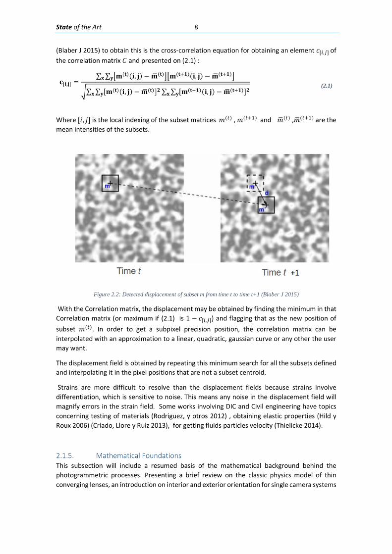
DIC uses image processing techniques in an attempt to solve this problem. The idea is to somehow obtain a one-to-one correspondence between object points in the reference (initial undeformed picture) and current (subsequent deformed pictures) configurations. DIC does this by taking small subsections of the reference image, called subsets, and determining their respective locations in the current configuration (block matching) (Blaber J 2015).

Algorithm Basis There are several formulations for the task of matching a subset in an image taken in a time “𝑡𝑡” and in the next image on time “𝑡𝑡 + 1” and with this computing the displacement of that subset.

The computation of the displacements starts by obtaining the correlation matrix 𝐶𝐶 between two subsets 𝑚𝑚(𝑡𝑡) and 𝑚𝑚(𝑡𝑡+1) that are part of images 𝐼𝐼(𝑡𝑡) and 𝐼𝐼(𝑡𝑡+1) , one of the several expressions

State of the Art 8

(Blaber J 2015) to obtain this is the cross-correlation equation for obtaining an element 𝑐𝑐[𝑖𝑖,𝑗𝑗] of the correlation matrix 𝐶𝐶 and presented on (2.1) :

Where [𝐿𝐿, 𝑗𝑗] is the local indexing of the subset matrices 𝑚𝑚(𝑡𝑡) , 𝑚𝑚(𝑡𝑡+1) and 𝑚𝑚� (𝑡𝑡) ,𝑚𝑚� (𝑡𝑡+1) are the mean intensities of the subsets.

Figure 2.2: Detected displacement of subset m from time t to time t+1 (Blaber J 2015)

With the Correlation matrix, the displacement may be obtained by finding the minimum in that Correlation matrix (or maximum if (2.1) is 1 − 𝑐𝑐[𝑖𝑖,𝑗𝑗]) and flagging that as the new position of subset 𝑚𝑚(𝑡𝑡). In order to get a subpixel precision position, the correlation matrix can be interpolated with an approximation to a linear, quadratic, gaussian curve or any other the user may want.

The displacement field is obtained by repeating this minimum search for all the subsets defined and interpolating it in the pixel positions that are not a subset centroid.

Strains are more difficult to resolve than the displacement fields because strains involve differentiation, which is sensitive to noise. This means any noise in the displacement field will magnify errors in the strain field. Some works involving DIC and Civil engineering have topics concerning testing of materials (Rodriguez, y otros 2012) , obtaining elastic properties (Hild y Roux 2006) (Criado, Llore y Ruiz 2013), for getting fluids particles velocity (Thielicke 2014).

2.1.5. Mathematical Foundations This subsection will include a resumed basis of the mathematical background behind the photogrammetric processes. Presenting a brief review on the classic physics model of thin converging lenses, an introduction on interior and exterior orientation for single camera systems

𝐜𝐜[𝐢𝐢,𝐣𝐣] =∑ ∑ �𝐦𝐦(𝐭𝐭)(𝐢𝐢, 𝐣𝐣) −𝐦𝐦� (𝐭𝐭)��𝐦𝐦(𝐭𝐭+𝟏𝟏)(𝐢𝐢, 𝐣𝐣) −𝐦𝐦� (𝐭𝐭+𝟏𝟏)�𝐲𝐲𝐱𝐱

�∑ ∑ [𝐦𝐦(𝐭𝐭)(𝐢𝐢, 𝐣𝐣) −𝐦𝐦� (𝐭𝐭)]𝟐𝟐 ∑ ∑ [𝐦𝐦(𝐭𝐭+𝟏𝟏)(𝐢𝐢, 𝐣𝐣) −𝐦𝐦� (𝐭𝐭+𝟏𝟏)]𝟐𝟐𝐲𝐲𝐱𝐱𝐲𝐲𝐱𝐱

(2.1)

State of the Art 9

including the most common optical errors (Radial Distortion and Tangential Distortion) in CRP processes.

2.1.6. Thin Lenses A lens with a thickness (distance along the optical axis between the two surfaces of the lens) that is negligible compared to the radius of curvature of its surface is known as a thin lens.

The thin lens approximation ignores optical effects due to the thickness of lenses and simplifies ray tracing calculations. It is often combined with the paraxial approximation in techniques such as ray transfer matrix analysis. Light rays follow simple rules when passing through a thin lens, this set of assumptions is known as the paraxial ray approximation (Hecht 2002):

• Any ray that enters parallel to the axis on one side of the lens proceeds towards the focal point F on the other side.

• Any ray that arrives at the lens after passing through the focal point on the front side, comes out parallel to the axis on the other side.

• Any ray that passes through the center of the lens will not change its direction.

By tracing these rays, the relationship between the object distance ℎ and the image distance 𝑐𝑐′ is described by Eq. (2.2).

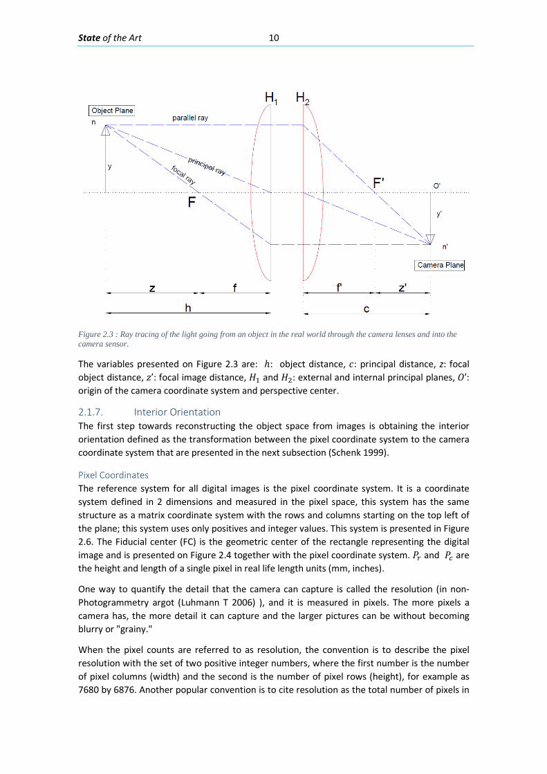
Thin lenses are one of the main components in a digital camera, as they determine how the image will be formed inside a camera. The trajectory of light rays from an object in space through thin converging lenses towards the camera sensor based on the paraxial approximation is illustrated in Figure 2.3. It is assumed that the camera uses some type of digital sensor and is not a film based camera (Luhmann T 2006).

1ℎ

+1𝑓𝑓′

=1𝑐𝑐

(2.2)

State of the Art 10

Figure 2.3 : Ray tracing of the light going from an object in the real world through the camera lenses and into the camera sensor.

The variables presented on Figure 2.3 are: ℎ: object distance, 𝑐𝑐: principal distance, z: focal object distance, 𝑧𝑧’: focal image distance, 𝐻𝐻1 and 𝐻𝐻2: external and internal principal planes, 𝑂𝑂’: origin of the camera coordinate system and perspective center.

2.1.7. Interior Orientation The first step towards reconstructing the object space from images is obtaining the interior orientation defined as the transformation between the pixel coordinate system to the camera coordinate system that are presented in the next subsection (Schenk 1999).

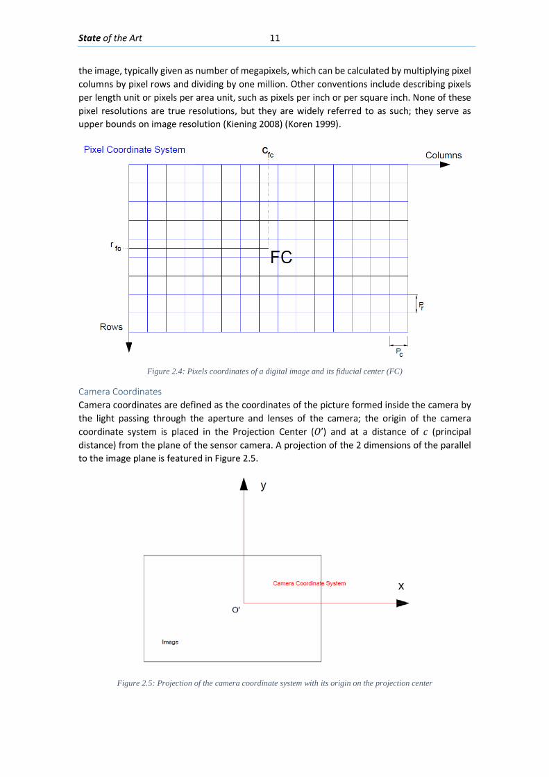
Pixel Coordinates The reference system for all digital images is the pixel coordinate system. It is a coordinate system defined in 2 dimensions and measured in the pixel space, this system has the same structure as a matrix coordinate system with the rows and columns starting on the top left of the plane; this system uses only positives and integer values. This system is presented in Figure 2.6. The Fiducial center (FC) is the geometric center of the rectangle representing the digital image and is presented on Figure 2.4 together with the pixel coordinate system. 𝑃𝑃𝑟𝑟 and 𝑃𝑃𝑐𝑐 are the height and length of a single pixel in real life length units (mm, inches).

One way to quantify the detail that the camera can capture is called the resolution (in non-Photogrammetry argot (Luhmann T 2006) ), and it is measured in pixels. The more pixels a camera has, the more detail it can capture and the larger pictures can be without becoming blurry or "grainy."

When the pixel counts are referred to as resolution, the convention is to describe the pixel resolution with the set of two positive integer numbers, where the first number is the number of pixel columns (width) and the second is the number of pixel rows (height), for example as 7680 by 6876. Another popular convention is to cite resolution as the total number of pixels in

State of the Art 11

the image, typically given as number of megapixels, which can be calculated by multiplying pixel columns by pixel rows and dividing by one million. Other conventions include describing pixels per length unit or pixels per area unit, such as pixels per inch or per square inch. None of these pixel resolutions are true resolutions, but they are widely referred to as such; they serve as upper bounds on image resolution (Kiening 2008) (Koren 1999).

Figure 2.4: Pixels coordinates of a digital image and its fiducial center (FC)

Camera Coordinates Camera coordinates are defined as the coordinates of the picture formed inside the camera by the light passing through the aperture and lenses of the camera; the origin of the camera coordinate system is placed in the Projection Center (𝑂𝑂’) and at a distance of 𝑐𝑐 (principal distance) from the plane of the sensor camera. A projection of the 2 dimensions of the parallel to the image plane is featured in Figure 2.5.

Figure 2.5: Projection of the camera coordinate system with its origin on the projection center

State of the Art 12

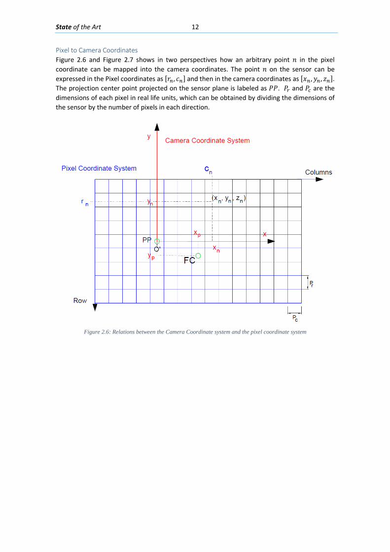
Pixel to Camera Coordinates Figure 2.6 and Figure 2.7 shows in two perspectives how an arbitrary point 𝐿𝐿 in the pixel coordinate can be mapped into the camera coordinates. The point 𝐿𝐿 on the sensor can be expressed in the Pixel coordinates as [𝑟𝑟𝑛𝑛, 𝑐𝑐𝑛𝑛] and then in the camera coordinates as [𝑥𝑥𝑛𝑛,𝑦𝑦𝑛𝑛, 𝑧𝑧𝑛𝑛]. The projection center point projected on the sensor plane is labeled as 𝑃𝑃𝑃𝑃. 𝑃𝑃𝑟𝑟 and 𝑃𝑃𝑐𝑐 are the dimensions of each pixel in real life units, which can be obtained by dividing the dimensions of the sensor by the number of pixels in each direction.

Figure 2.6: Relations between the Camera Coordinate system and the pixel coordinate system

State of the Art 13

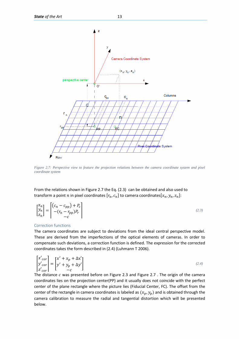
Figure 2.7: Perspective view to feature the projection relations between the camera coordinate system and pixel coordinate system

From the relations shown in Figure 2.7 the Eq. (2.3) can be obtained and also used to transform a point 𝐿𝐿 in pixel coordinates [𝑟𝑟𝑛𝑛, 𝑐𝑐𝑛𝑛] to camera coordinates[𝑥𝑥𝑛𝑛,𝑦𝑦𝑛𝑛, 𝑧𝑧𝑛𝑛]:

�𝑥𝑥𝑛𝑛𝑦𝑦𝑛𝑛𝑧𝑧𝑛𝑛� = �

�𝑐𝑐𝑛𝑛 − 𝑐𝑐𝑝𝑝𝑝𝑝� + 𝑃𝑃𝑐𝑐−(𝑟𝑟𝑛𝑛 − 𝑟𝑟𝑝𝑝𝑝𝑝)𝑃𝑃𝑟𝑟

−𝑐𝑐� (2.3)

Correction functions The camera coordinates are subject to deviations from the ideal central perspective model. These are derived from the imperfections of the optical elements of cameras. In order to compensate such deviations, a correction function is defined. The expression for the corrected coordinates takes the form described in (2.4) (Luhmann T 2006).

�𝑥𝑥′𝑐𝑐𝑐𝑐𝑟𝑟𝑦𝑦′𝑐𝑐𝑐𝑐𝑟𝑟𝑧𝑧′𝑐𝑐𝑐𝑐𝑟𝑟

� = �𝑥𝑥′ + 𝑥𝑥𝑝𝑝 + ∆x′𝑦𝑦′ + 𝑦𝑦𝑝𝑝 + ∆𝑦𝑦′

−𝑐𝑐� (2.4)

The distance 𝑐𝑐 was presented before on Figure 2.3 and Figure 2.7 . The origin of the camera coordinates lies on the projection center(PP) and it usually does not coincide with the perfect center of the plane rectangle where the picture lies (Fiducial Center, FC). The offset from the center of the rectangle in camera coordinates is labeled as (𝑥𝑥𝑝𝑝,𝑦𝑦𝑝𝑝) and is obtained through the camera calibration to measure the radial and tangential distortion which will be presented below.

State of the Art 14

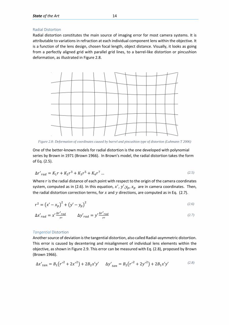
Radial Distortion Radial distortion constitutes the main source of imaging error for most camera systems. It is attributable to variations in refraction at each individual component lens within the objective. It is a function of the lens design, chosen focal length, object distance. Visually, it looks as going from a perfectly aligned grid with parallel grid lines, to a barrel-like distortion or pincushion deformation, as illustrated in Figure 2.8.

Figure 2.8: Deformation of coordinates caused by barrel and pincushion type of distortion (Luhmann T 2006)

One of the better-known models for radial distortion is the one developed with polynomial series by Brown in 1971 (Brown 1966). In Brown’s model, the radial distortion takes the form of Eq. (2.5).

∆𝑟𝑟′𝑟𝑟𝑟𝑟𝑟𝑟 = 𝐾𝐾1𝑟𝑟 + 𝐾𝐾2𝑟𝑟3 + 𝐾𝐾3𝑟𝑟5 + 𝐾𝐾4𝑟𝑟7 … (2.5)

Where 𝑟𝑟 is the radial distance of each point with respect to the origin of the camera coordinates system, computed as in (2.6). In this equation, 𝑥𝑥′, 𝑦𝑦′,𝑦𝑦𝑝𝑝, 𝑥𝑥𝑝𝑝 are in camera coordinates. Then, the radial distortion correction terms, for 𝑥𝑥 and 𝑦𝑦 directions, are computed as in Eq. (2.7).

𝑟𝑟2 = �𝑥𝑥′ − 𝑥𝑥𝑝𝑝�2 + �𝑦𝑦′ − 𝑦𝑦𝑝𝑝�

2 (2.6)

∆𝑥𝑥′𝑟𝑟𝑟𝑟𝑟𝑟 = 𝑥𝑥′ ∆𝑟𝑟′𝑟𝑟𝑟𝑟𝑟𝑟𝑟𝑟′

∆𝑦𝑦′𝑟𝑟𝑟𝑟𝑟𝑟 = 𝑦𝑦′ ∆𝑟𝑟′𝑟𝑟𝑟𝑟𝑟𝑟𝑟𝑟′

(2.7)

Tangential Distortion Another source of deviation is the tangential distortion, also called Radial-asymmetric distortion. This error is caused by decentering and misalignment of individual lens elements within the objective, as shown in Figure 2.9. This error can be measured with Eq. (2.8), proposed by Brown (Brown 1966).

∆𝑥𝑥′𝑡𝑡𝑟𝑟𝑛𝑛 = 𝐵𝐵1�𝑟𝑟′2 + 2𝑥𝑥′2�+ 2𝐵𝐵2𝑥𝑥′𝑦𝑦′ ∆𝑦𝑦′𝑡𝑡𝑟𝑟𝑛𝑛 = 𝐵𝐵2�𝑟𝑟′

2 + 2𝑦𝑦′2� + 2𝐵𝐵1𝑥𝑥′𝑦𝑦′ (2.8)

State of the Art 15

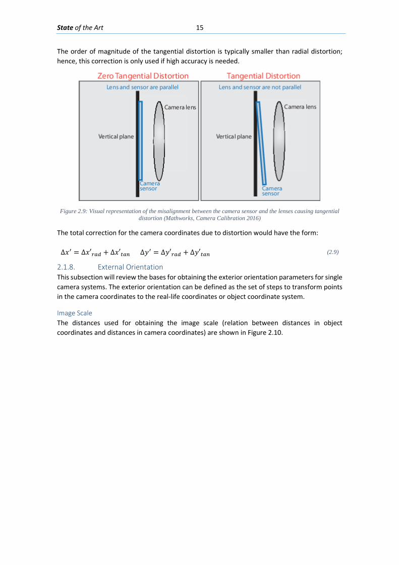
The order of magnitude of the tangential distortion is typically smaller than radial distortion; hence, this correction is only used if high accuracy is needed.

Figure 2.9: Visual representation of the misalignment between the camera sensor and the lenses causing tangential

distortion (Mathworks, Camera Calibration 2016)

The total correction for the camera coordinates due to distortion would have the form:

∆𝑥𝑥′ = ∆𝑥𝑥′𝑟𝑟𝑟𝑟𝑟𝑟 + ∆𝑥𝑥′𝑡𝑡𝑟𝑟𝑛𝑛 ∆𝑦𝑦′ = ∆𝑦𝑦′𝑟𝑟𝑟𝑟𝑟𝑟 + ∆𝑦𝑦′𝑡𝑡𝑟𝑟𝑛𝑛 (2.9)

2.1.8. External Orientation This subsection will review the bases for obtaining the exterior orientation parameters for single camera systems. The exterior orientation can be defined as the set of steps to transform points in the camera coordinates to the real-life coordinates or object coordinate system.

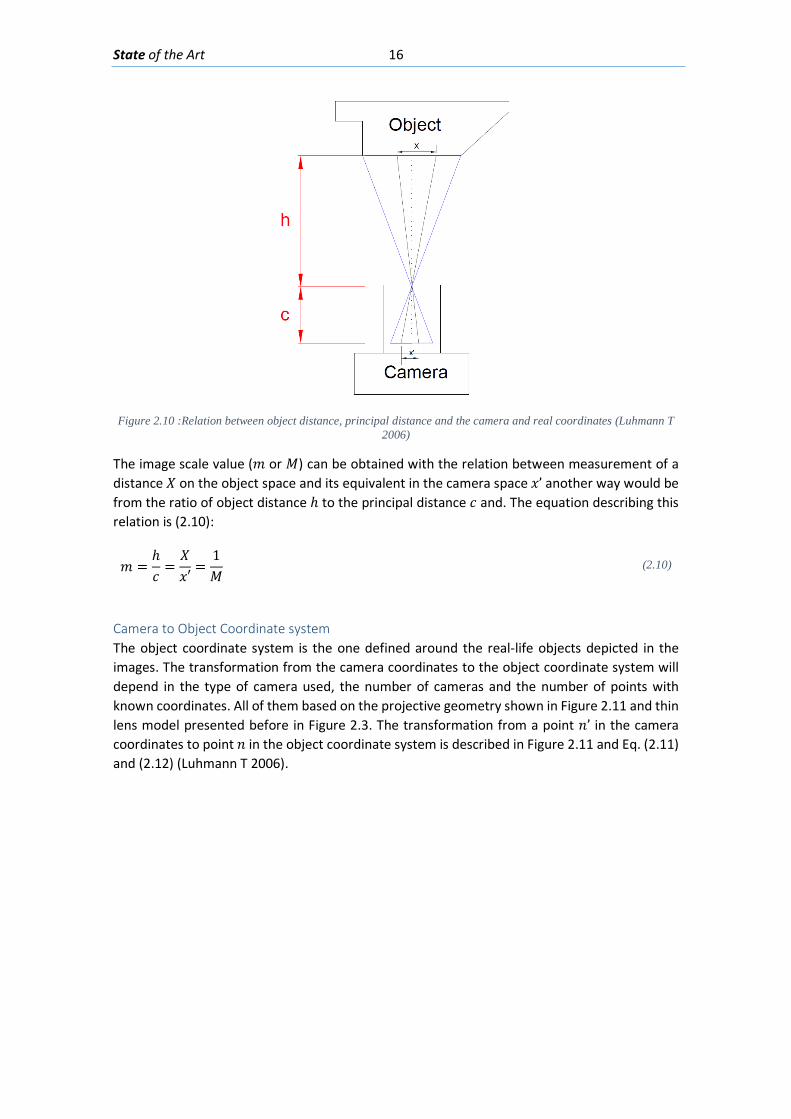
Image Scale The distances used for obtaining the image scale (relation between distances in object coordinates and distances in camera coordinates) are shown in Figure 2.10.

State of the Art 16

Figure 2.10 :Relation between object distance, principal distance and the camera and real coordinates (Luhmann T

2006)

The image scale value (𝑚𝑚 or 𝑀𝑀) can be obtained with the relation between measurement of a distance 𝑋𝑋 on the object space and its equivalent in the camera space 𝑥𝑥’ another way would be from the ratio of object distance ℎ to the principal distance 𝑐𝑐 and. The equation describing this relation is (2.10):

𝑚𝑚 =ℎ𝑐𝑐

=𝑋𝑋𝑥𝑥′

=1𝑀𝑀

(2.10)

Camera to Object Coordinate system The object coordinate system is the one defined around the real-life objects depicted in the images. The transformation from the camera coordinates to the object coordinate system will depend in the type of camera used, the number of cameras and the number of points with known coordinates. All of them based on the projective geometry shown in Figure 2.11 and thin lens model presented before in Figure 2.3. The transformation from a point 𝐿𝐿’ in the camera coordinates to point 𝐿𝐿 in the object coordinate system is described in Figure 2.11 and Eq. (2.11) and (2.12) (Luhmann T 2006).

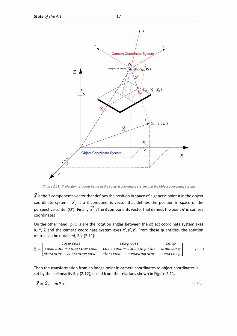
State of the Art 17

Figure 2.11: Projection relations between the camera coordinate system and the object coordinate system

�⃗�𝑋 is the 3 components vector that defines the position in space of a generic point 𝐿𝐿 in the object coordinate system. �⃗�𝑋0 is a 3 components vector that defines the position in space of the

perspective center (O’). Finally, 𝑥𝑥′���⃗ is the 3 components vector that defines the point 𝐿𝐿’ in camera coordinates

On the other hand, 𝜑𝜑,𝜔𝜔, 𝜀𝜀 are the rotation angles between the object coordinate system axes X, Y, Z and the camera coordinate system axes 𝑥𝑥’,𝑦𝑦’, 𝑧𝑧’. From these quantities, the rotation matrix can be obtained, Eq. (2.11):

𝑅𝑅 = �𝑐𝑐𝑐𝑐𝑀𝑀𝜑𝜑 𝑐𝑐𝑐𝑐𝑀𝑀𝜀𝜀 𝑐𝑐𝑐𝑐𝑀𝑀𝜑𝜑 𝑐𝑐𝑐𝑐𝑀𝑀𝜀𝜀 𝑀𝑀𝑉𝑉𝐿𝐿𝜑𝜑

𝑐𝑐𝑐𝑐𝑀𝑀𝜔𝜔 𝑀𝑀𝐿𝐿𝐿𝐿𝜀𝜀 + 𝑀𝑀𝐿𝐿𝐿𝐿𝜔𝜔 𝑀𝑀𝐿𝐿𝐿𝐿𝜑𝜑 𝑐𝑐𝑐𝑐𝑀𝑀𝜀𝜀 𝑐𝑐𝑐𝑐𝑀𝑀𝜔𝜔 𝑐𝑐𝑐𝑐𝑀𝑀𝜀𝜀 − 𝑀𝑀𝐿𝐿𝐿𝐿𝜔𝜔 𝑀𝑀𝐿𝐿𝐿𝐿𝜑𝜑 𝑀𝑀𝐿𝐿𝐿𝐿𝜀𝜀 𝑀𝑀𝐿𝐿𝐿𝐿𝜔𝜔 𝑐𝑐𝑐𝑐𝑀𝑀𝜑𝜑𝑀𝑀𝐿𝐿𝐿𝐿𝜔𝜔 𝑀𝑀𝐿𝐿𝐿𝐿𝜀𝜀 − 𝑐𝑐𝑐𝑐𝑀𝑀𝜔𝜔 𝑀𝑀𝐿𝐿𝐿𝐿𝜑𝜑 𝑐𝑐𝑐𝑐𝑀𝑀𝜀𝜀 𝑀𝑀𝐿𝐿𝐿𝐿𝜔𝜔 𝑐𝑐𝑐𝑐𝑀𝑀𝜀𝜀 + 𝑐𝑐𝑐𝑐𝑀𝑀𝜔𝜔𝑀𝑀𝐿𝐿𝐿𝐿𝜑𝜑 𝑀𝑀𝐿𝐿𝐿𝐿𝜀𝜀 𝑐𝑐𝑐𝑐𝑀𝑀𝜔𝜔 𝑐𝑐𝑐𝑐𝑀𝑀𝜑𝜑

� (2.11)

Then the transformation from an image point in camera coordinates to object coordinates is set by the collinearity Eq. (2.12), based from the relations shown in Figure 2.11.

�⃗�𝑋 = �⃗�𝑋0 +𝑚𝑚𝑅𝑅 𝑥𝑥′����⃗ (2.12)

State of the Art 18

2.2. Digital Image Processing Image processing and Photogrammetry has been increasingly used the last decades as the applications spread to all science. Researchers and engineers realize these techniques enable measurements and detection with low cost and with little or no affectation to the system performance.

A digital image may be defined as a two-dimensional function, 𝐼𝐼(𝑥𝑥,𝑦𝑦), where x and y are spatial coordinates, and the amplitude of 𝐼𝐼 at any pair of coordinates (𝑥𝑥,𝑦𝑦) is called the intensity or gray level of the image at that point. When 𝑥𝑥, 𝑦𝑦 and the amplitude of 𝐼𝐼 are all finite, discrete quantities, the image can be called a digital image. The field of digital image processing refers to managing information in digital images by means of a digital computer.

There are no clear boundaries in the continuum from image processing at one end to the field of computer vision at the other. However, attempts of categorizing the processes can be done as follows:

Low-level imaging processes These processes involve primitive operation such as: Intensity Transformations, Spatial Filtering, Frequency Domain Filtering, Logarithmic and Contrast-Stretching Transformations; Histogram transformations.

Mid-level processes These processes involve tasks such as: segmentation (partitioning an image into regions or objects), Edge detection, Corner detection, Image Sharpening, Hough Transform, Morphological operations,

High-level processes High-level processes involve “making sense” of an ensemble of recognized objects, as in image analysis, and at the far end of the continuum, performing the cognitive functions normally associated with human vision such as: neural networks for object recognition, convolutional neural networks, pattern matching, etc. (Gonzalez, Woods y Eddins 2010).

In the following subsections, a brief review will be made on the topics within digital image processing that are used with this work.

2.2.1. Spatial Filtering Spatial filtering or neighborhood processing is an image operation where each pixel value 𝑓𝑓(𝑥𝑥,𝑦𝑦) is changed by a function of the intensities of pixels in a neighborhood around pixel (𝑥𝑥,𝑦𝑦). It consists of mainly 4 steps (Gonzalez, Woods y Eddins 2010):

• Selecting a center point (𝑥𝑥,𝑦𝑦) in the image • Performing a number operation that involves only the pixels in a predefined

neighborhood about (𝑥𝑥,𝑦𝑦). • Letting the result of that operation be the response of the process at that point, it may

replace previous point or fabricate a new matrix with only the response values • Repeating the process for all the pixels in the image.

If the operations performed on the pixels of the neighborhoods are linear, the operation is called linear spatial filtering; otherwise, the filtering is referred as non-linear.

Most of the operations performed in spatial filtering fall in the category of linear spatial filtering. Most linear operation usually used imply the multiplication of each element in the neighborhood

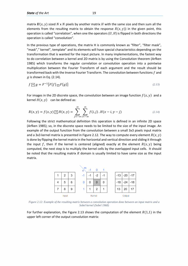
State of the Art 19

matrix 𝑼𝑼(𝑥𝑥, 𝑦𝑦) sized 𝑁𝑁 x 𝑁𝑁 pixels by another matrix 𝐻𝐻 with the same size and then sum all the elements from the resulting matrix to obtain the response 𝑅𝑅(𝑥𝑥,𝑦𝑦)) in the given point, this operation is called “correlation”, when one the operators (𝑈𝑈,𝐻𝐻) is flipped in both directions the operation is called “convolution”.

In the previous type of operations, the matrix H is commonly known as “filter”, “filter mask”, “mask”,” kernel”, template” and its elements will have special characteristics depending on the transformation that is wanted for the input picture. In many implementations, the fastest way to do correlation between a kernel and 2D matrix is by using the Convolution theorem (Arfken 1985) which transforms the regular correlation or convolution operation into a pointwise multiplication between the Fourier Transform of each argument and the result should be transformed back with the Inverse Fourier Transform. The convolution between functions 𝑓𝑓 and 𝑔𝑔 is shown in Eq. (2.14).

𝑓𝑓 ∗ 𝑔𝑔 = 𝐹𝐹−1�𝐹𝐹{𝑓𝑓} . 𝐹𝐹{𝑔𝑔}� (2.13)

For images in the 2D discrete space, the convolution between an image function 𝑓𝑓(𝑥𝑥,𝑦𝑦) and a kernel 𝐻𝐻(𝑥𝑥,𝑦𝑦) can be defined as:

𝑅𝑅(𝑥𝑥,𝑦𝑦) = 𝑓𝑓(𝑥𝑥,𝑦𝑦) ∗ 𝐻𝐻(𝑥𝑥,𝑦𝑦) = � � 𝑓𝑓(𝐿𝐿, 𝑗𝑗) .𝐻𝐻(𝑥𝑥 − 𝐿𝐿,𝑦𝑦 − 𝑗𝑗)∞

𝑖𝑖=−∞

∞

𝑗𝑗=−∞

(2.14)

Following the strict mathematical definition this operation is defined in an infinite 2D space (Arfken 1985); so, in the discrete space needs to be limited to the size of the input image. An example of the output function from the convolution between a small 3x3 pixels input matrix and a 3x3 kernel matrix is presented in Figure 2.12. The way to compute every element 𝑅𝑅(𝑥𝑥,𝑦𝑦) is done by flipping the kernel matrix in the horizontal and vertical direction and sliding it through the input 𝑓𝑓, then if the kernel is centered (aligned) exactly at the element 𝑅𝑅(𝑥𝑥,𝑦𝑦) being computed, the next step is to multiply the kernel cells by the overlapped input cells. It should be noted that the resulting matrix 𝑅𝑅 domain is usually limited to have same size as the input matrix.

Figure 2.12: Example of the resulting matrix between a convolution operation done between an input matrix and a

Sobel kernel (Sobel 1968)

For further explanation, the Figure 2.13 shows the computation of the element 𝑅𝑅(1,1) in the upper left corner of the output convolution matrix:

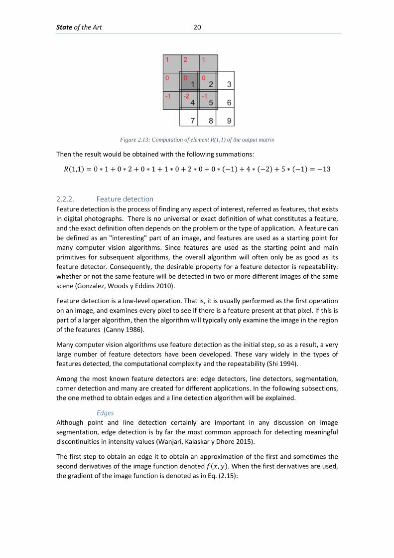
State of the Art 20

Figure 2.13: Computation of element R(1,1) of the output matrix

Then the result would be obtained with the following summations:

𝑅𝑅(1,1) = 0 ∗ 1 + 0 ∗ 2 + 0 ∗ 1 + 1 ∗ 0 + 2 ∗ 0 + 0 ∗ (−1) + 4 ∗ (−2) + 5 ∗ (−1) = −13

2.2.2. Feature detection Feature detection is the process of finding any aspect of interest, referred as features, that exists in digital photographs. There is no universal or exact definition of what constitutes a feature, and the exact definition often depends on the problem or the type of application. A feature can be defined as an "interesting" part of an image, and features are used as a starting point for many computer vision algorithms. Since features are used as the starting point and main primitives for subsequent algorithms, the overall algorithm will often only be as good as its feature detector. Consequently, the desirable property for a feature detector is repeatability: whether or not the same feature will be detected in two or more different images of the same scene (Gonzalez, Woods y Eddins 2010).

Feature detection is a low-level operation. That is, it is usually performed as the first operation on an image, and examines every pixel to see if there is a feature present at that pixel. If this is part of a larger algorithm, then the algorithm will typically only examine the image in the region of the features (Canny 1986).

Many computer vision algorithms use feature detection as the initial step, so as a result, a very large number of feature detectors have been developed. These vary widely in the types of features detected, the computational complexity and the repeatability (Shi 1994).

Among the most known feature detectors are: edge detectors, line detectors, segmentation, corner detection and many are created for different applications. In the following subsections, the one method to obtain edges and a line detection algorithm will be explained.

Edges Although point and line detection certainly are important in any discussion on image segmentation, edge detection is by far the most common approach for detecting meaningful discontinuities in intensity values (Wanjari, Kalaskar y Dhore 2015).

The first step to obtain an edge it to obtain an approximation of the first and sometimes the second derivatives of the image function denoted 𝑓𝑓(𝑥𝑥,𝑦𝑦). When the first derivatives are used, the gradient of the image function is denoted as in Eq. (2.15):

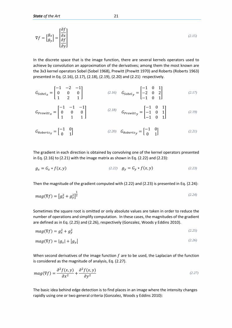
State of the Art 21

∇𝑓𝑓 = �𝑔𝑔𝑥𝑥𝑔𝑔𝑦𝑦� =

⎣⎢⎢⎡𝜕𝜕𝑓𝑓𝜕𝜕𝑥𝑥𝜕𝜕𝑓𝑓𝜕𝜕𝑦𝑦⎦⎥⎥⎤ (2.15)

In the discrete space that is the image function, there are several kernels operators used to achieve by convolution an approximation of the derivatives; among them the most known are the 3x3 kernel operators Sobel (Sobel 1968), Prewitt (Prewitt 1970) and Roberts (Roberts 1963) presented in Eq. (2.16), (2.17), (2.18), (2.19), (2.20) and (2.21) respectively.

𝐺𝐺𝑆𝑆𝑐𝑐𝑏𝑏𝑒𝑒𝑙𝑙𝑥𝑥 = �−1 −2 −10 0 01 2 1

� (2.16) 𝐺𝐺𝑆𝑆𝑐𝑐𝑏𝑏𝑒𝑒𝑙𝑙𝑦𝑦 = �−1 0 1−2 0 2−1 0 1

� (2.17)

𝐺𝐺𝑃𝑃𝑟𝑟𝑒𝑒𝑃𝑃𝑖𝑖𝑡𝑡𝑡𝑡𝑥𝑥 = �−1 −1 −10 0 01 1 1

� (2.18) 𝐺𝐺𝑃𝑃𝑟𝑟𝑒𝑒𝑃𝑃𝑖𝑖𝑡𝑡𝑡𝑡𝑦𝑦 = �

−1 0 1−1 0 1−1 0 1

� (2.19)

𝐺𝐺𝑅𝑅𝑐𝑐𝑏𝑏𝑒𝑒𝑟𝑟𝑡𝑡𝑙𝑙𝑥𝑥 = �−1 00 1�

(2.20) 𝐺𝐺𝑅𝑅𝑐𝑐𝑏𝑏𝑒𝑒𝑟𝑟𝑡𝑡𝑙𝑙𝑦𝑦 = �−1 00 1�

(2.21)

The gradient in each direction is obtained by convolving one of the kernel operators presented in Eq. (2.16) to (2.21) with the image matrix as shown in Eq. (2.22) and (2.23):

𝑔𝑔𝑥𝑥 = 𝐺𝐺𝑥𝑥 ∗ 𝑓𝑓(𝑥𝑥,𝑦𝑦) (2.22) 𝑔𝑔𝑦𝑦 = 𝐺𝐺𝑦𝑦 ∗ 𝑓𝑓(𝑥𝑥,𝑦𝑦) (2.23)

Then the magnitude of the gradient computed with (2.22) and (2.23) is presented in Eq. (2.24):

𝑚𝑚𝑎𝑎𝑔𝑔(∇𝑓𝑓) = �𝑔𝑔𝑥𝑥2 + 𝑔𝑔𝑦𝑦2�12 (2.24)

Sometimes the square root is omitted or only absolute values are taken in order to reduce the number of operations and simplify computation. In these cases, the magnitudes of the gradient are defined as in Eq. (2.25) and (2.26), respectively (Gonzalez, Woods y Eddins 2010).

𝑚𝑚𝑎𝑎𝑔𝑔(∇𝑓𝑓) = 𝑔𝑔𝑥𝑥2 + 𝑔𝑔𝑦𝑦2 (2.25)

𝑚𝑚𝑎𝑎𝑔𝑔(∇𝑓𝑓) = |𝑔𝑔𝑥𝑥| + �𝑔𝑔𝑦𝑦� (2.26)

When second derivatives of the image function 𝑓𝑓 are to be used, the Laplacian of the function is considered as the magnitude of analysis, Eq. (2.27).

𝑚𝑚𝑎𝑎𝑔𝑔(∇𝑓𝑓) =𝜕𝜕2𝑓𝑓(𝑥𝑥,𝑦𝑦)𝜕𝜕𝑥𝑥2

+𝜕𝜕2𝑓𝑓(𝑥𝑥,𝑦𝑦)𝜕𝜕𝑦𝑦2

(2.27)

The basic idea behind edge detection is to find places in an image where the intensity changes rapidly using one or two general criteria (Gonzalez, Woods y Eddins 2010):

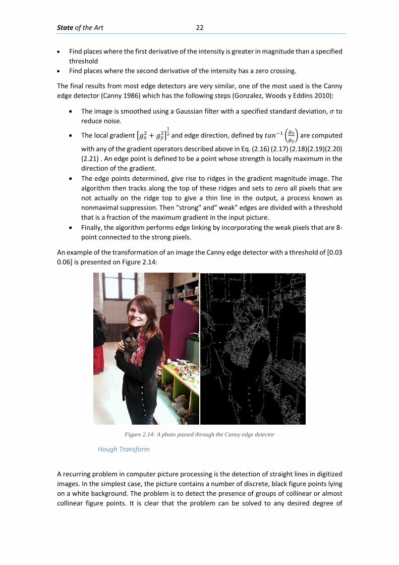
State of the Art 22

• Find places where the first derivative of the intensity is greater in magnitude than a specified threshold

• Find places where the second derivative of the intensity has a zero crossing.

The final results from most edge detectors are very similar, one of the most used is the Canny edge detector (Canny 1986) which has the following steps (Gonzalez, Woods y Eddins 2010):

• The image is smoothed using a Gaussian filter with a specified standard deviation, 𝜎𝜎 to reduce noise.

• The local gradient �𝑔𝑔𝑥𝑥2 + 𝑔𝑔𝑦𝑦2�12 and edge direction, defined by 𝑡𝑡𝑎𝑎𝐿𝐿−1 �𝑔𝑔𝑥𝑥

𝑔𝑔𝑦𝑦� are computed

with any of the gradient operators described above in Eq. (2.16) (2.17) (2.18)(2.19)(2.20) (2.21) . An edge point is defined to be a point whose strength is locally maximum in the direction of the gradient.

• The edge points determined, give rise to ridges in the gradient magnitude image. The algorithm then tracks along the top of these ridges and sets to zero all pixels that are not actually on the ridge top to give a thin line in the output, a process known as nonmaximal suppression. Then “strong” and” weak” edges are divided with a threshold that is a fraction of the maximum gradient in the input picture.

• Finally, the algorithm performs edge linking by incorporating the weak pixels that are 8-point connected to the strong pixels.

An example of the transformation of an image the Canny edge detector with a threshold of [0.03 0.06] is presented on Figure 2.14:

Figure 2.14: A photo passed through the Canny edge detector

Hough Transform

A recurring problem in computer picture processing is the detection of straight lines in digitized images. In the simplest case, the picture contains a number of discrete, black figure points lying on a white background. The problem is to detect the presence of groups of collinear or almost collinear figure points. It is clear that the problem can be solved to any desired degree of

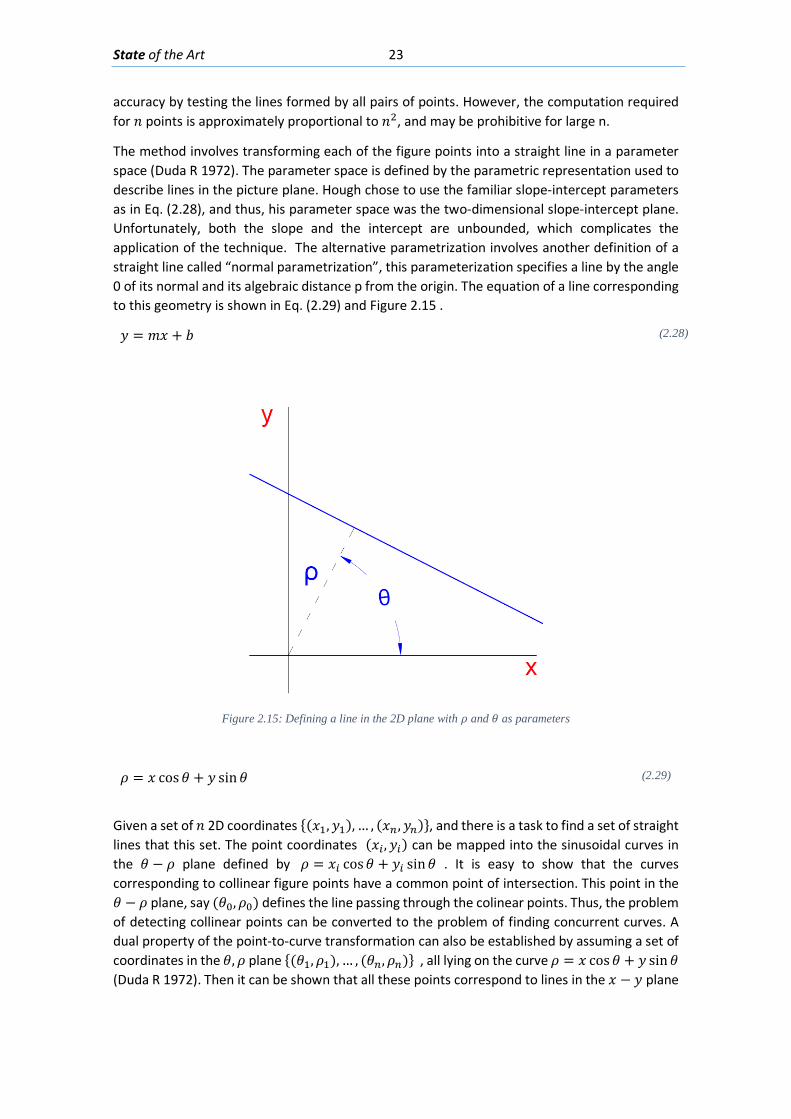
State of the Art 23

accuracy by testing the lines formed by all pairs of points. However, the computation required for 𝐿𝐿 points is approximately proportional to 𝐿𝐿2, and may be prohibitive for large n.

The method involves transforming each of the figure points into a straight line in a parameter space (Duda R 1972). The parameter space is defined by the parametric representation used to describe lines in the picture plane. Hough chose to use the familiar slope-intercept parameters as in Eq. (2.28), and thus, his parameter space was the two-dimensional slope-intercept plane. Unfortunately, both the slope and the intercept are unbounded, which complicates the application of the technique. The alternative parametrization involves another definition of a straight line called “normal parametrization”, this parameterization specifies a line by the angle 0 of its normal and its algebraic distance p from the origin. The equation of a line corresponding to this geometry is shown in Eq. (2.29) and Figure 2.15 .

𝑦𝑦 = 𝑚𝑚𝑥𝑥 + 𝑏𝑏 (2.28)

Figure 2.15: Defining a line in the 2D plane with 𝜌𝜌 and 𝜃𝜃 as parameters

𝜌𝜌 = 𝑥𝑥 cos𝜃𝜃 + 𝑦𝑦 sin𝜃𝜃 (2.29)

Given a set of 𝐿𝐿 2D coordinates {(𝑥𝑥1,𝑦𝑦1), … , (𝑥𝑥𝑛𝑛,𝑦𝑦𝑛𝑛)}, and there is a task to find a set of straight lines that this set. The point coordinates (𝑥𝑥𝑖𝑖,𝑦𝑦𝑖𝑖) can be mapped into the sinusoidal curves in the 𝜃𝜃 − 𝜌𝜌 plane defined by 𝜌𝜌 = 𝑥𝑥𝑖𝑖 cos𝜃𝜃 + 𝑦𝑦𝑖𝑖 sin𝜃𝜃 . It is easy to show that the curves corresponding to collinear figure points have a common point of intersection. This point in the 𝜃𝜃 − 𝜌𝜌 plane, say (𝜃𝜃0,𝜌𝜌0) defines the line passing through the colinear points. Thus, the problem of detecting collinear points can be converted to the problem of finding concurrent curves. A dual property of the point-to-curve transformation can also be established by assuming a set of coordinates in the 𝜃𝜃,𝜌𝜌 plane {(𝜃𝜃1,𝜌𝜌1), … , (𝜃𝜃𝑛𝑛,𝜌𝜌𝑛𝑛)} , all lying on the curve 𝜌𝜌 = 𝑥𝑥 cos𝜃𝜃 + 𝑦𝑦 sin𝜃𝜃 (Duda R 1972). Then it can be shown that all these points correspond to lines in the 𝑥𝑥 − 𝑦𝑦 plane

State of the Art 24

passing through the point (𝑥𝑥0,𝑦𝑦0). The most interesting properties of the point-to-curve transformation can be summarized as follows:

• A point in the picture plane corresponds to a sinusoidal curve in the parameter plane. Property

• A point in the parameter plane corresponds to a straight line in the picture plane. • Points lying on the same straight line in the picture plane correspond to curves through a

common point in the parameter plane. • Points lying on the same curve in the parameter plane correspond to lines through the same

point in the picture plane (Duda R 1972).

2.3. Machine Learning Since the invention of digital computers people have been trying to answer the question of whether a computer can ‘learn’, and before talking about theorems and algorithms it should be define d what ‘learning’ means for a machine.

Tom Mitchell (Mitchell 1997) provides a more explicit definition for Machine Learning: "A computer program is said to learn from experience E with respect to some class of tasks T and performance measure P, if its performance at tasks in T, as measured by P, improves with experience E."

Machine learning can also be defined as a subfield of computer science and artificial intelligence and also as a method of teaching computer programs to make and improve predictions or behaviors based on some data. In the context of this research, for the problem of learning to diagnosis damage, data can be considered as the crack pattern observed and identified through computer vision.

Machine learning can be divided in two great categories: Supervised and unsupervised learning. This field has had such a widespread in the last 10 years that its successful applications span through many tasks and fields. And there are many other applications that most users are unaware that are made using machine learning, some of these applications are listed below:

• Computer vision including object recognition, face recognition ( Facebook adding a tagging seed on all faces in a picture (Taigman 2014), Face Swap” type apps)

• Medical diagnosis • Natural language processing (WhatsApp predictive text) • Online advertising, real-time ads on web pages and mobile devices (Russell y Christothoulou

2010))) • Recommender systems (Google (News), Netflix (movies), Amazon (products) (Smith y Linden

2017), Facebook (ads and webpages), YouTube (recommended videos) (Davison, Liebald y Liu 2010))

• Search engines (Google (Brin y Page 1998), Yahoo, Bing) • Adaptive websites (Changing featured products, news based on last activities • Spam filtering (on any email service (Androutsopoulos 2000))

State of the Art 25

2.3.1. Supervised Learning Supervised Learning englobes all methods that have the task of inferring a function from labeled training data. The training data consist of a set of training examples. In supervised learning, each example is a pair consisting of an input object (typically a vector) and a desired output value. A supervised learning algorithm analyzes the training data and infers a function or model, which can be used for mapping new examples. One way to determine if the model is acceptable is to check if it correctly determines the class labels for unseen instances or training examples. This requires the learning algorithm to generalize from the training data to unseen situations in a "reasonable" way. (Ng, Machine Learning: Supervised Learning 2016).

Supervised learning problems are categorized into "regression" and "classification" problems. In a regression problem, the objective is to predict results within a continuous output, meaning that the objective is to map the input variables to some continuous function. In a classification problem, the prediction is a discrete output or to classify them into categories.

Some examples of both Regression and Classification tasks and problems:

2.3.1.1. Regression • Given the dimensions, compression, tensile strength of concrete, amount of steel

reinforcement, boundary conditions of a given beam; predict the maximum load it can bear.

• Given a set of atmospheric magnitudes measured in a given day predict the mm of rain for the next day. (an example would be 𝑥𝑥𝑛𝑛 =[ 𝑡𝑡𝑉𝑉𝑚𝑚𝑝𝑝𝑉𝑉𝑟𝑟𝑎𝑎𝑡𝑡𝑉𝑉𝑟𝑟𝑉𝑉,𝑎𝑎𝐿𝐿𝑟𝑟𝑉𝑉 𝑝𝑝𝑟𝑟𝑉𝑉𝑀𝑀𝑀𝑀𝑉𝑉𝑟𝑟𝑉𝑉,𝑤𝑤𝐿𝐿𝐿𝐿𝑤𝑤 𝑀𝑀𝑝𝑝𝑉𝑉𝑉𝑉𝑤𝑤,𝑚𝑚𝑐𝑐𝐿𝐿𝑡𝑡ℎ] )

• Given the grades a student has had in the current semester previous evaluations, predict the grade of the final evaluation.

2.3.1.2. Classification • Given an audio recording, recognize the words spoken in it • Given a picture or part of it, recognize if there is a face or not in that picture. • Given an email, decide whether it is spam or not

As a general trend researchers and engineers have realized that supervised learning has a greater potential to solve problems in the Classification category. Supervised learning can offer a solution for problems that do not have a clear or widely accepted idea of the type of mathematical model explaining the phenomena. The proposed problems presented in the paragraph above under the title “Classification” serve as excellent examples for this argument.

2.3.1.3. Mathematical Models Given a set of m training examples of the form {(𝑥𝑥1,𝑦𝑦1) , … , (𝑥𝑥𝑚𝑚,𝑦𝑦𝑚𝑚)} such that 𝑥𝑥𝑖𝑖 is the feature vector of the i-th example 𝑌𝑌 is the label or results vector (label or class for classification or real numbers for regression), a learning algorithm seeks a hypothesis function ℎ mapped as ℎ ∶ 𝑋𝑋 →𝑌𝑌, where X is the input space and 𝑌𝑌 is the output space.

Also, a cost or error function J, defined as ∶ 𝑋𝑋 × 𝑌𝑌 → ℝ ; this function sums up the error or difference between the hypothesis vector ℎ(𝑥𝑥) and the result vector 𝑦𝑦. The objective of the learning task is to minimize this cost function 𝐽𝐽 (so that it becomes zero) so that the in the ideal case the hypothesis ℎ is equal to 𝑦𝑦 for all the “m” examples.

State of the Art 26

There are some cost functions that can be used to measure the error; one frequently used is the mean squared error (MSE) shown in Eq. (2.30):

𝐽𝐽 = ��ℎ�𝑥𝑥𝑖𝑖� − 𝑦𝑦𝑖𝑖�2

𝑚𝑚

𝑚𝑚

𝑖𝑖=1

(2.30)

The learning from the program comes from the minimization of the cost function. Which can be done in several ways in response to the algorithm used.

Some models frequently used are:

- Linear Regression (Regression)

- Logistic Regression (Classification, Regression)

- Neural Networks (Classification, Regression)

- Support Vector Machine (Regression)

- Perceptron (Classification, Regression)

- Decision Trees (Regression)

- Naives-Bayes (Regression)

From all these models presented above, only the Linear Regression, Logistic Regression and Neural Networks will be explained in the following subsections as they used for the present work.

Linear Regression The linear regression has a hypothesis function or model function presented in (2.31):

ℎ(𝑥𝑥𝑖𝑖) = Ө𝑇𝑇 ∙ 𝑥𝑥𝑖𝑖 = [Ө0 Ө0 … Ө𝑛𝑛] ∙

⎣⎢⎢⎡𝑥𝑥0𝑥𝑥1..𝑥𝑥𝑛𝑛⎦⎥⎥⎤

(2.31)

Where 𝐿𝐿 is the dimension of the feature vector 𝑥𝑥. Both the 𝑦𝑦 response vector and hypothesis vector ℎ is made up of real numbers, Ө is the parameter vector that is what the “learning” procedure will attempt to modify. The value of 𝑥𝑥0 in the example vector is always 1, and its commonly known as the bias. Then the regularized cost function based on the least squares error has the form described in (2.32), where 𝜆𝜆 is the factor of the regularization term used to control the overfitting of the model.

𝐽𝐽 =1

2𝑚𝑚���ℎ�𝑥𝑥𝑖𝑖� − 𝑦𝑦𝑖𝑖�2 + �𝜆𝜆Ө𝑖𝑖2𝑛𝑛

𝑖𝑖=1

𝑚𝑚

𝑖𝑖=1

�

(2.32)

Then the derivative of the cost function with respect to the parameter vector Ө can be obtained deriving expression in Eq. (2.33).

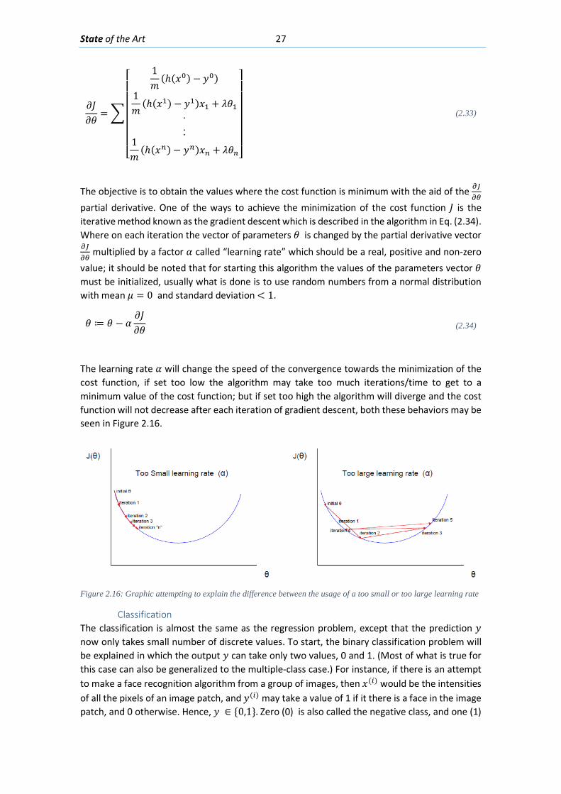
State of the Art 27

𝜕𝜕𝐽𝐽𝜕𝜕𝜃𝜃

= �

⎣⎢⎢⎢⎢⎢⎢⎡

1𝑚𝑚

(ℎ(𝑥𝑥0) − 𝑦𝑦0)

1𝑚𝑚

(ℎ(𝑥𝑥1) − 𝑦𝑦1)𝑥𝑥1 + 𝜆𝜆𝜃𝜃1...

1𝑚𝑚

(ℎ(𝑥𝑥𝑛𝑛)− 𝑦𝑦𝑛𝑛)𝑥𝑥𝑛𝑛 + 𝜆𝜆𝜃𝜃𝑛𝑛⎦⎥⎥⎥⎥⎥⎥⎤

(2.33)

The objective is to obtain the values where the cost function is minimum with the aid of the 𝜕𝜕𝜕𝜕𝜕𝜕𝜕𝜕

partial derivative. One of the ways to achieve the minimization of the cost function 𝐽𝐽 is the iterative method known as the gradient descent which is described in the algorithm in Eq. (2.34). Where on each iteration the vector of parameters 𝜃𝜃 is changed by the partial derivative vector 𝜕𝜕𝜕𝜕𝜕𝜕𝜕𝜕

multiplied by a factor 𝛼𝛼 called “learning rate” which should be a real, positive and non-zero value; it should be noted that for starting this algorithm the values of the parameters vector 𝜃𝜃 must be initialized, usually what is done is to use random numbers from a normal distribution with mean 𝜇𝜇 = 0 and standard deviation < 1.

𝜃𝜃 ≔ 𝜃𝜃 − 𝛼𝛼𝜕𝜕𝐽𝐽𝜕𝜕𝜃𝜃

(2.34)

The learning rate 𝛼𝛼 will change the speed of the convergence towards the minimization of the cost function, if set too low the algorithm may take too much iterations/time to get to a minimum value of the cost function; but if set too high the algorithm will diverge and the cost function will not decrease after each iteration of gradient descent, both these behaviors may be seen in Figure 2.16.

Figure 2.16: Graphic attempting to explain the difference between the usage of a too small or too large learning rate

Classification The classification is almost the same as the regression problem, except that the prediction 𝑦𝑦 now only takes small number of discrete values. To start, the binary classification problem will be explained in which the output 𝑦𝑦 can take only two values, 0 and 1. (Most of what is true for this case can also be generalized to the multiple-class case.) For instance, if there is an attempt to make a face recognition algorithm from a group of images, then 𝑥𝑥(𝑖𝑖) would be the intensities of all the pixels of an image patch, and 𝑦𝑦(𝑖𝑖) may take a value of 1 if it there is a face in the image patch, and 0 otherwise. Hence, 𝑦𝑦 ∈ {0,1}. Zero (0) is also called the negative class, and one (1)

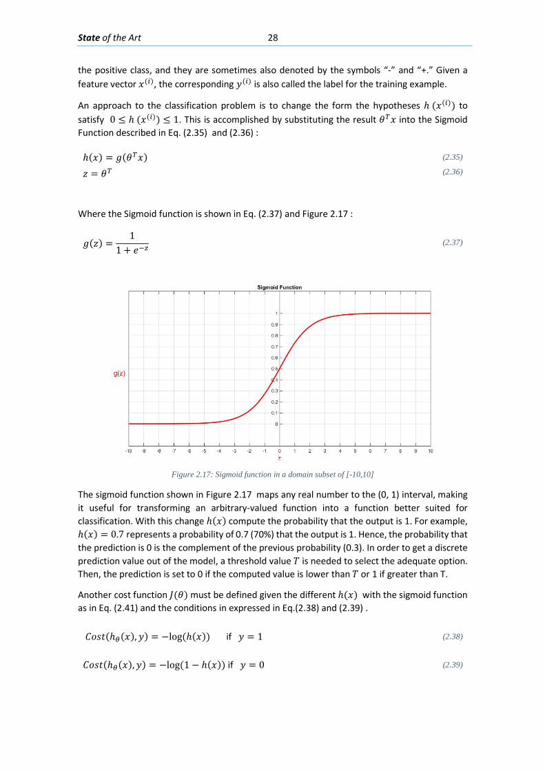
State of the Art 28

the positive class, and they are sometimes also denoted by the symbols “-” and “+.” Given a feature vector 𝑥𝑥(𝑖𝑖), the corresponding 𝑦𝑦(𝑖𝑖) is also called the label for the training example.

An approach to the classification problem is to change the form the hypotheses ℎ (𝑥𝑥(𝑖𝑖)) to satisfy 0 ≤ ℎ (𝑥𝑥(𝑖𝑖)) ≤ 1. This is accomplished by substituting the result 𝜃𝜃𝑇𝑇𝑥𝑥 into the Sigmoid Function described in Eq. (2.35) and (2.36) :

ℎ(𝑥𝑥) = 𝑔𝑔(𝜃𝜃𝑇𝑇𝑥𝑥) (2.35)

𝑧𝑧 = 𝜃𝜃𝑇𝑇 (2.36)

Where the Sigmoid function is shown in Eq. (2.37) and Figure 2.17 :

𝑔𝑔(𝑧𝑧) =1

1 + 𝑉𝑉−𝑧𝑧 (2.37)

Figure 2.17: Sigmoid function in a domain subset of [-10,10]

The sigmoid function shown in Figure 2.17 maps any real number to the (0, 1) interval, making it useful for transforming an arbitrary-valued function into a function better suited for classification. With this change ℎ(𝑥𝑥) compute the probability that the output is 1. For example, ℎ(𝑥𝑥) = 0.7 represents a probability of 0.7 (70%) that the output is 1. Hence, the probability that the prediction is 0 is the complement of the previous probability (0.3). In order to get a discrete prediction value out of the model, a threshold value 𝑇𝑇 is needed to select the adequate option. Then, the prediction is set to 0 if the computed value is lower than 𝑇𝑇 or 1 if greater than T.

Another cost function 𝐽𝐽(𝜃𝜃) must be defined given the different ℎ(𝑥𝑥) with the sigmoid function as in Eq. (2.41) and the conditions in expressed in Eq.(2.38) and (2.39) .

𝐶𝐶𝑐𝑐𝑀𝑀𝑡𝑡(ℎ𝜕𝜕(𝑥𝑥),𝑦𝑦) = −log (ℎ(𝑥𝑥)) if 𝑦𝑦 = 1 (2.38)

𝐶𝐶𝑐𝑐𝑀𝑀𝑡𝑡(ℎ𝜕𝜕(𝑥𝑥),𝑦𝑦) = −log (1 − ℎ(𝑥𝑥)) if 𝑦𝑦 = 0 (2.39)

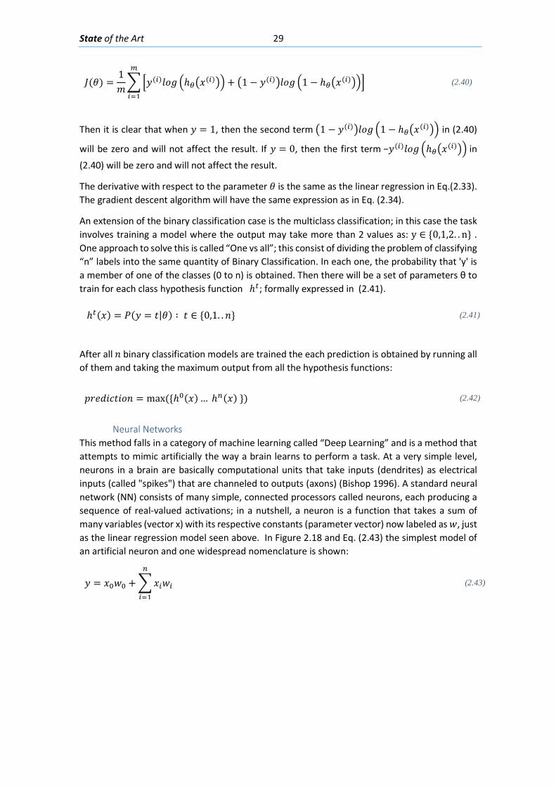
State of the Art 29

𝐽𝐽(𝜃𝜃) =1𝑚𝑚��𝑦𝑦(𝑖𝑖)𝑙𝑙𝑐𝑐𝑔𝑔 �ℎ𝜕𝜕�𝑥𝑥(𝑖𝑖)�� + �1 − 𝑦𝑦(𝑖𝑖)�𝑙𝑙𝑐𝑐𝑔𝑔 �1 − ℎ𝜕𝜕�𝑥𝑥(𝑖𝑖)���𝑚𝑚

𝑖𝑖=1

(2.40)

Then it is clear that when 𝑦𝑦 = 1, then the second term �1 − 𝑦𝑦(𝑖𝑖)�𝑙𝑙𝑐𝑐𝑔𝑔 �1 − ℎ𝜕𝜕�𝑥𝑥(𝑖𝑖)�� in (2.40)

will be zero and will not affect the result. If 𝑦𝑦 = 0, then the first term −𝑦𝑦(𝑖𝑖)𝑙𝑙𝑐𝑐𝑔𝑔 �ℎ𝜕𝜕�𝑥𝑥(𝑖𝑖)�� in

(2.40) will be zero and will not affect the result.

The derivative with respect to the parameter 𝜃𝜃 is the same as the linear regression in Eq.(2.33). The gradient descent algorithm will have the same expression as in Eq. (2.34).

An extension of the binary classification case is the multiclass classification; in this case the task involves training a model where the output may take more than 2 values as: y ∈ {0,1,2. . n} . One approach to solve this is called “One vs all”; this consist of dividing the problem of classifying “n” labels into the same quantity of Binary Classification. In each one, the probability that 'y' is a member of one of the classes (0 to n) is obtained. Then there will be a set of parameters θ to train for each class hypothesis function ℎ𝑡𝑡; formally expressed in (2.41).

ℎ𝑡𝑡(𝑥𝑥) = 𝑃𝑃(𝑦𝑦 = 𝑡𝑡|𝜃𝜃) ∶ 𝑡𝑡 ∈ {0,1. .𝐿𝐿} (2.41)

After all 𝐿𝐿 binary classification models are trained the each prediction is obtained by running all of them and taking the maximum output from all the hypothesis functions:

𝑝𝑝𝑟𝑟𝑉𝑉𝑤𝑤𝐿𝐿𝑐𝑐𝑡𝑡𝐿𝐿𝑐𝑐𝐿𝐿 = max ({ℎ0(𝑥𝑥) … ℎ𝑛𝑛(𝑥𝑥) }) (2.42)

Neural Networks This method falls in a category of machine learning called “Deep Learning” and is a method that attempts to mimic artificially the way a brain learns to perform a task. At a very simple level, neurons in a brain are basically computational units that take inputs (dendrites) as electrical inputs (called "spikes") that are channeled to outputs (axons) (Bishop 1996). A standard neural network (NN) consists of many simple, connected processors called neurons, each producing a sequence of real-valued activations; in a nutshell, a neuron is a function that takes a sum of many variables (vector x) with its respective constants (parameter vector) now labeled as 𝑤𝑤, just as the linear regression model seen above. In Figure 2.18 and Eq. (2.43) the simplest model of an artificial neuron and one widespread nomenclature is shown:

𝑦𝑦 = 𝑥𝑥0𝑤𝑤0 + �𝑥𝑥𝑖𝑖𝑤𝑤𝑖𝑖

𝑛𝑛

𝑖𝑖=1

(2.43)

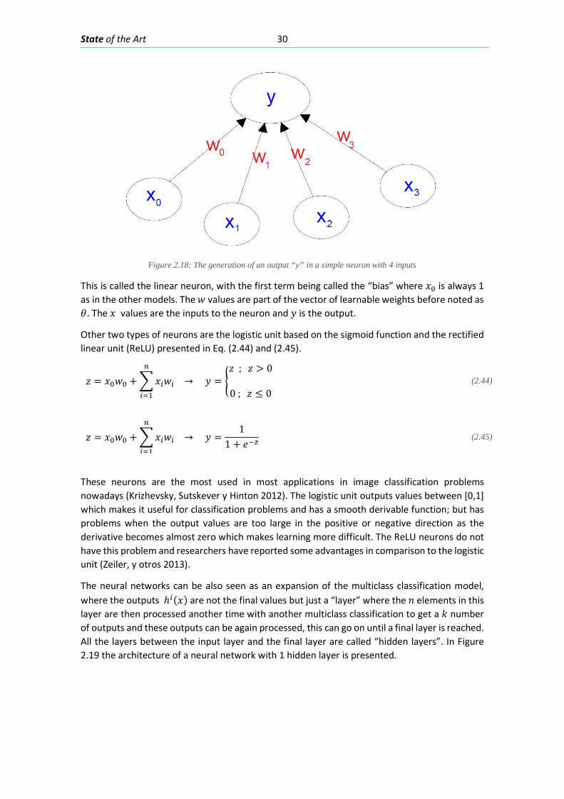
State of the Art 30

Figure 2.18: The generation of an output “y” in a simple neuron with 4 inputs

This is called the linear neuron, with the first term being called the “bias” where 𝑥𝑥0 is always 1 as in the other models. The 𝑤𝑤 values are part of the vector of learnable weights before noted as 𝜃𝜃. The 𝑥𝑥 values are the inputs to the neuron and 𝑦𝑦 is the output.

Other two types of neurons are the logistic unit based on the sigmoid function and the rectified linear unit (ReLU) presented in Eq. (2.44) and (2.45).

𝑧𝑧 = 𝑥𝑥0𝑤𝑤0 + �𝑥𝑥𝑖𝑖𝑤𝑤𝑖𝑖

𝑛𝑛

𝑖𝑖=1

→ 𝑦𝑦 = �𝑧𝑧 ; 𝑧𝑧 > 0

0 ; 𝑧𝑧 ≤ 0 (2.44)

𝑧𝑧 = 𝑥𝑥0𝑤𝑤0 + �𝑥𝑥𝑖𝑖𝑤𝑤𝑖𝑖

𝑛𝑛

𝑖𝑖=1

→ 𝑦𝑦 =1

1 + 𝑉𝑉−𝑧𝑧 (2.45)

These neurons are the most used in most applications in image classification problems nowadays (Krizhevsky, Sutskever y Hinton 2012). The logistic unit outputs values between [0,1] which makes it useful for classification problems and has a smooth derivable function; but has problems when the output values are too large in the positive or negative direction as the derivative becomes almost zero which makes learning more difficult. The ReLU neurons do not have this problem and researchers have reported some advantages in comparison to the logistic unit (Zeiler, y otros 2013).

The neural networks can be also seen as an expansion of the multiclass classification model, where the outputs ℎ𝑖𝑖(𝑥𝑥) are not the final values but just a “layer” where the 𝐿𝐿 elements in this layer are then processed another time with another multiclass classification to get a 𝐿𝐿 number of outputs and these outputs can be again processed, this can go on until a final layer is reached. All the layers between the input layer and the final layer are called “hidden layers”. In Figure 2.19 the architecture of a neural network with 1 hidden layer is presented.

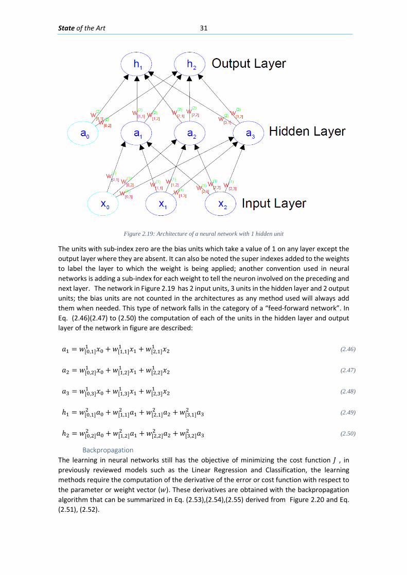
State of the Art 31

Figure 2.19: Architecture of a neural network with 1 hidden unit

The units with sub-index zero are the bias units which take a value of 1 on any layer except the output layer where they are absent. It can also be noted the super indexes added to the weights to label the layer to which the weight is being applied; another convention used in neural networks is adding a sub-index for each weight to tell the neuron involved on the preceding and next layer. The network in Figure 2.19 has 2 input units, 3 units in the hidden layer and 2 output units; the bias units are not counted in the architectures as any method used will always add them when needed. This type of network falls in the category of a “feed-forward network”. In Eq. (2.46)(2.47) to (2.50) the computation of each of the units in the hidden layer and output layer of the network in figure are described:

𝑎𝑎1 = 𝑤𝑤[0,1]1 𝑥𝑥0 + 𝑤𝑤[1,1]

1 𝑥𝑥1 + 𝑤𝑤[2,1]1 𝑥𝑥2 (2.46)

𝑎𝑎2 = 𝑤𝑤[0,2]1 𝑥𝑥0 + 𝑤𝑤[1,2]

1 𝑥𝑥1 + 𝑤𝑤[2,2]1 𝑥𝑥2 (2.47)

𝑎𝑎3 = 𝑤𝑤[0,3]1 𝑥𝑥0 + 𝑤𝑤[1,3]

1 𝑥𝑥1 + 𝑤𝑤[2,3]1 𝑥𝑥2 (2.48)

ℎ1 = 𝑤𝑤[0,1]2 𝑎𝑎0 + 𝑤𝑤[1,1]

2 𝑎𝑎1 + 𝑤𝑤[2,1]2 𝑎𝑎2 +𝑤𝑤[3,1]

2 𝑎𝑎3 (2.49)

ℎ2 = 𝑤𝑤[0,2]2 𝑎𝑎0 + 𝑤𝑤[1,2]

2 𝑎𝑎1 + 𝑤𝑤[2,2]2 𝑎𝑎2 +𝑤𝑤[3,2]

2 𝑎𝑎3 (2.50)

Backpropagation The learning in neural networks still has the objective of minimizing the cost function 𝐽𝐽 , in previously reviewed models such as the Linear Regression and Classification, the learning methods require the computation of the derivative of the error or cost function with respect to the parameter or weight vector (𝑤𝑤). These derivatives are obtained with the backpropagation algorithm that can be summarized in Eq. (2.53),(2.54),(2.55) derived from Figure 2.20 and Eq. (2.51), (2.52).

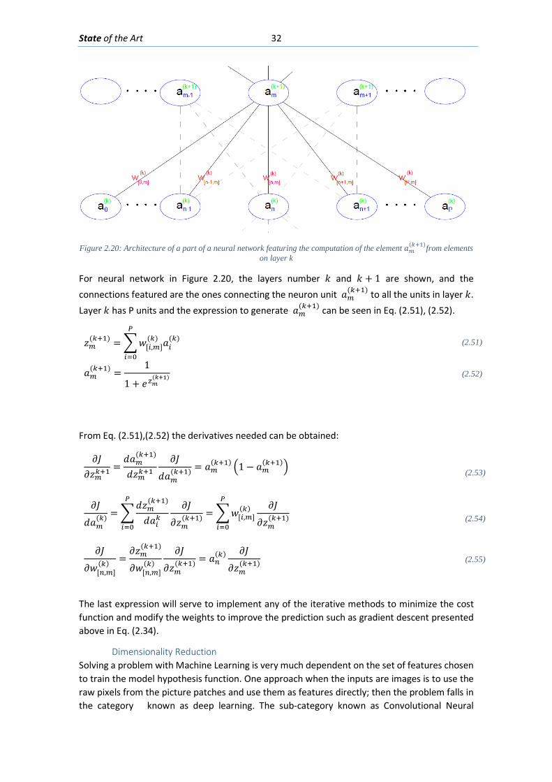
State of the Art 32

Figure 2.20: Architecture of a part of a neural network featuring the computation of the element 𝑎𝑎𝑚𝑚(𝑘𝑘+1)from elements

on layer k

For neural network in Figure 2.20, the layers number 𝐿𝐿 and 𝐿𝐿 + 1 are shown, and the connections featured are the ones connecting the neuron unit 𝑎𝑎𝑚𝑚

(𝑘𝑘+1) to all the units in layer 𝐿𝐿. Layer 𝐿𝐿 has P units and the expression to generate 𝑎𝑎𝑚𝑚

(𝑘𝑘+1) can be seen in Eq. (2.51), (2.52).

𝑧𝑧𝑚𝑚(𝑘𝑘+1) = �𝑤𝑤[𝑖𝑖,𝑚𝑚]

(𝑘𝑘) 𝑎𝑎𝑖𝑖(𝑘𝑘)

𝑃𝑃

𝑖𝑖=0

(2.51)

𝑎𝑎𝑚𝑚(𝑘𝑘+1) =

1

1 + 𝑉𝑉𝑧𝑧𝑚𝑚(𝑘𝑘+1) (2.52)

From Eq. (2.51),(2.52) the derivatives needed can be obtained:

𝜕𝜕𝐽𝐽𝜕𝜕𝑧𝑧𝑚𝑚𝑘𝑘+1

=𝑤𝑤𝑎𝑎𝑚𝑚

(𝑘𝑘+1)

𝑤𝑤𝑧𝑧𝑚𝑚𝑘𝑘+1𝜕𝜕𝐽𝐽

𝑤𝑤𝑎𝑎𝑚𝑚(𝑘𝑘+1) = 𝑎𝑎𝑚𝑚

(𝑘𝑘+1) �1 − 𝑎𝑎𝑚𝑚(𝑘𝑘+1)�

(2.53)

𝜕𝜕𝐽𝐽

𝑤𝑤𝑎𝑎𝑚𝑚(𝑘𝑘) = �

𝑤𝑤𝑧𝑧𝑚𝑚(𝑘𝑘+1)

𝑤𝑤𝑎𝑎𝑖𝑖𝑘𝑘𝜕𝜕𝐽𝐽

𝜕𝜕𝑧𝑧𝑚𝑚(𝑘𝑘+1)

𝑃𝑃

𝑖𝑖=0

= �𝑤𝑤[𝑖𝑖,𝑚𝑚](𝑘𝑘) 𝜕𝜕𝐽𝐽

𝜕𝜕𝑧𝑧𝑚𝑚(𝑘𝑘+1)

𝑃𝑃

𝑖𝑖=0

(2.54)

𝜕𝜕𝐽𝐽

𝜕𝜕𝑤𝑤[𝑛𝑛,𝑚𝑚](𝑘𝑘) =

𝜕𝜕𝑧𝑧𝑚𝑚(𝑘𝑘+1)

𝜕𝜕𝑤𝑤[𝑛𝑛,𝑚𝑚](𝑘𝑘)

𝜕𝜕𝐽𝐽

𝜕𝜕𝑧𝑧𝑚𝑚(𝑘𝑘+1) = 𝑎𝑎𝑛𝑛

(𝑘𝑘) 𝜕𝜕𝐽𝐽

𝜕𝜕𝑧𝑧𝑚𝑚(𝑘𝑘+1) (2.55)

The last expression will serve to implement any of the iterative methods to minimize the cost function and modify the weights to improve the prediction such as gradient descent presented above in Eq. (2.34).

Dimensionality Reduction Solving a problem with Machine Learning is very much dependent on the set of features chosen to train the model hypothesis function. One approach when the inputs are images is to use the raw pixels from the picture patches and use them as features directly; then the problem falls in the category known as deep learning. The sub-category known as Convolutional Neural

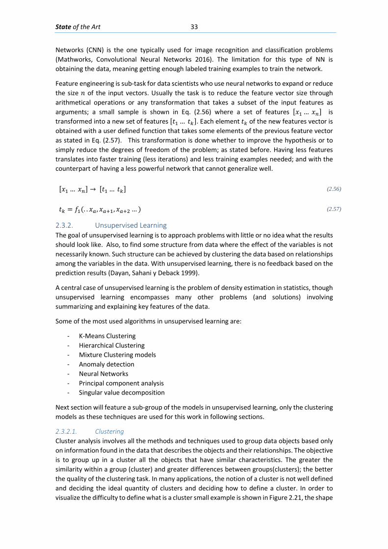
State of the Art 33

Networks (CNN) is the one typically used for image recognition and classification problems (Mathworks, Convolutional Neural Networks 2016). The limitation for this type of NN is obtaining the data, meaning getting enough labeled training examples to train the network.

Feature engineering is sub-task for data scientists who use neural networks to expand or reduce the size 𝐿𝐿 of the input vectors. Usually the task is to reduce the feature vector size through arithmetical operations or any transformation that takes a subset of the input features as arguments; a small sample is shown in Eq. (2.56) where a set of features [𝑥𝑥1 … 𝑥𝑥𝑛𝑛] is transformed into a new set of features [𝑡𝑡1 … 𝑡𝑡𝑘𝑘]. Each element 𝑡𝑡𝑘𝑘 of the new features vector is obtained with a user defined function that takes some elements of the previous feature vector as stated in Eq. (2.57). This transformation is done whether to improve the hypothesis or to simply reduce the degrees of freedom of the problem; as stated before. Having less features translates into faster training (less iterations) and less training examples needed; and with the counterpart of having a less powerful network that cannot generalize well.

[𝑥𝑥1 … 𝑥𝑥𝑛𝑛] → [𝑡𝑡1 … 𝑡𝑡𝑘𝑘] (2.56)

𝑡𝑡𝑘𝑘 = 𝑓𝑓1(. . 𝑥𝑥𝑟𝑟 ,𝑥𝑥𝑟𝑟+1,𝑥𝑥𝑟𝑟+2 … ) (2.57)

2.3.2. Unsupervised Learning The goal of unsupervised learning is to approach problems with little or no idea what the results should look like. Also, to find some structure from data where the effect of the variables is not necessarily known. Such structure can be achieved by clustering the data based on relationships among the variables in the data. With unsupervised learning, there is no feedback based on the prediction results (Dayan, Sahani y Deback 1999).

A central case of unsupervised learning is the problem of density estimation in statistics, though unsupervised learning encompasses many other problems (and solutions) involving summarizing and explaining key features of the data.

Some of the most used algorithms in unsupervised learning are:

- K-Means Clustering - Hierarchical Clustering - Mixture Clustering models - Anomaly detection - Neural Networks - Principal component analysis - Singular value decomposition

Next section will feature a sub-group of the models in unsupervised learning, only the clustering models as these techniques are used for this work in following sections.

2.3.2.1. Clustering Cluster analysis involves all the methods and techniques used to group data objects based only on information found in the data that describes the objects and their relationships. The objective is to group up in a cluster all the objects that have similar characteristics. The greater the similarity within a group (cluster) and greater differences between groups(clusters); the better the quality of the clustering task. In many applications, the notion of a cluster is not well defined and deciding the ideal quantity of clusters and deciding how to define a cluster. In order to visualize the difficulty to define what is a cluster small example is shown in Figure 2.21, the shape

State of the Art 34

of the markers define the membership of the cluster; (a) the original points are shown, in (b) the data is divided in two clusters, in (c) the data is divided in 4 clusters and in (d) is divided in six clusters. This shows that the definition of a cluster is imprecise and that the best definition depends on the nature and the desired results (Tan, Steinback y Kumar 2006).

Figure 2.21: Four different ways of forming clusters from a dataset (Tan, Steinback y Kumar 2006)

Among the clustering algorithms only the type that will be used for this work will be reviewed in the following sub-section.

Hierarchical Clustering This clustering approach refer to a collection of clustering techniques that produce each cluster in steps. There are two types of hierarchical approaches:

Agglomerative: This method can be resumed in the following steps:

1. Each data object is assigned to its own cluster.

2. Then, the similarity is computed (e.g., distance) between each of the clusters and join the two most similar clusters.

3. Finally, repeat steps 2 and 3 until there is only a single cluster left.

Divisive: This is a "top down" approach: all data objects start in one cluster, and splits are performed recursively as one moves down the hierarchy.

A hierarchical agglomerative clustering is often displayed graphically using a tree like diagram called dendogram, which displays both the cluster-sub cluster relationships and the order in which the clusters were merged. Also, if the data has 2 or 3 dimensions the clustering can be represented by a nested cluster diagram. Both of these are presented in a simple example with only 4 data objects in Figure 2.22. It can be seen that both observations or data p2 and p3 are the closest ones and are joined in a cluster in the first step, then the point p4 is the one closest to cluster created by p2 and p3; so, they are joined to make the cluster with p2, p3 and p4. Last, the cluster (p2,p3,p4) is joined with the last point p1 (Tan, Steinback y Kumar 2006).

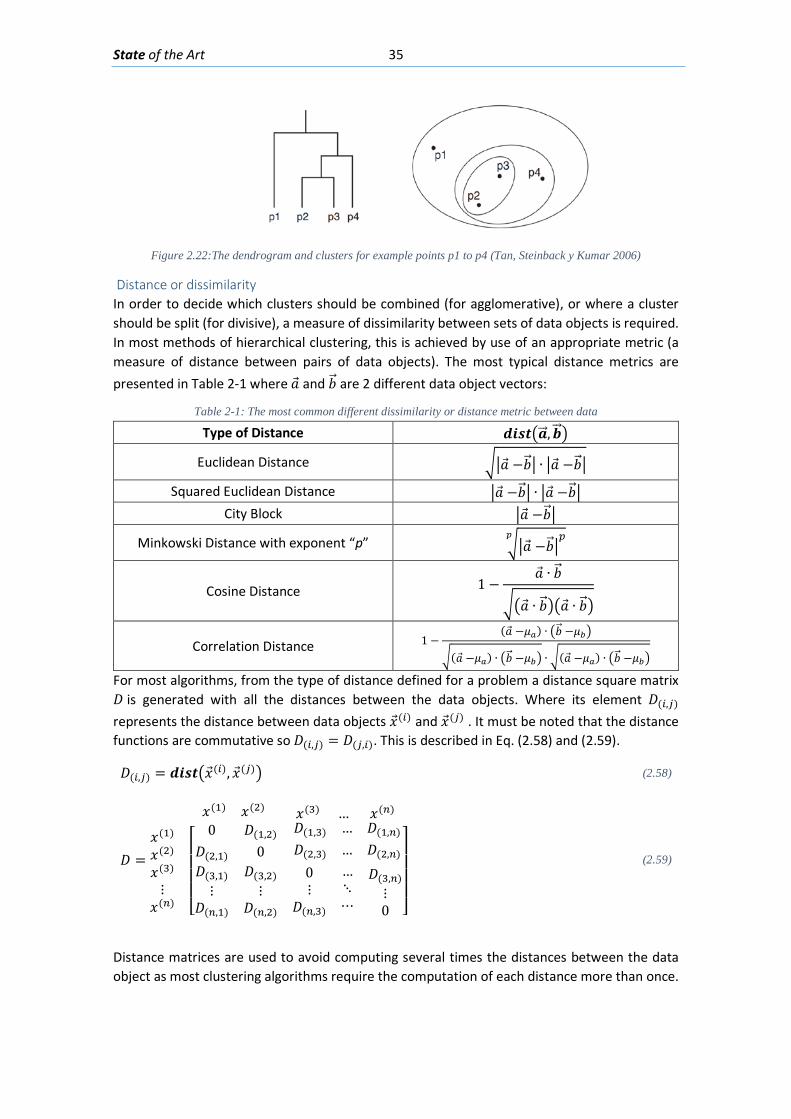
State of the Art 35

Figure 2.22:The dendrogram and clusters for example points p1 to p4 (Tan, Steinback y Kumar 2006)

Distance or dissimilarity In order to decide which clusters should be combined (for agglomerative), or where a cluster should be split (for divisive), a measure of dissimilarity between sets of data objects is required. In most methods of hierarchical clustering, this is achieved by use of an appropriate metric (a measure of distance between pairs of data objects). The most typical distance metrics are presented in Table 2-1 where �⃗�𝑎 and 𝑏𝑏�⃗ are 2 different data object vectors:

Table 2-1: The most common different dissimilarity or distance metric between data

Type of Distance 𝒅𝒅𝒅𝒅𝒅𝒅𝒅𝒅�𝒂𝒂��⃗ ,𝒃𝒃��⃗ �

Euclidean Distance ���⃗�𝑎 −𝑏𝑏�⃗ � ∙ ��⃗�𝑎 −𝑏𝑏�⃗ �

Squared Euclidean Distance ��⃗�𝑎 −𝑏𝑏�⃗ � ∙ ��⃗�𝑎 −𝑏𝑏�⃗ � City Block ��⃗�𝑎 −𝑏𝑏�⃗ �

Minkowski Distance with exponent “p” ���⃗�𝑎 −𝑏𝑏�⃗ �𝑝𝑝𝑝𝑝

Cosine Distance 1 −�⃗�𝑎 ∙ 𝑏𝑏�⃗

���⃗�𝑎 ∙ 𝑏𝑏�⃗ ���⃗�𝑎 ∙ 𝑏𝑏�⃗ �

Correlation Distance 1 −(�⃗�𝑎 −𝜇𝜇𝑟𝑟) ∙ �𝑏𝑏�⃗ −𝜇𝜇𝑏𝑏�

�(�⃗�𝑎 −𝜇𝜇𝑟𝑟) ∙ �𝑏𝑏�⃗ −𝜇𝜇𝑏𝑏� ∙ �(�⃗�𝑎 −𝜇𝜇𝑟𝑟) ∙ �𝑏𝑏�⃗ −𝜇𝜇𝑏𝑏�

For most algorithms, from the type of distance defined for a problem a distance square matrix 𝐷𝐷 is generated with all the distances between the data objects. Where its element 𝐷𝐷(𝑖𝑖,𝑗𝑗) represents the distance between data objects �⃗�𝑥(𝑖𝑖) and �⃗�𝑥(𝑗𝑗) . It must be noted that the distance functions are commutative so 𝐷𝐷(𝑖𝑖,𝑗𝑗) = 𝐷𝐷(𝑗𝑗,𝑖𝑖). This is described in Eq. (2.58) and (2.59).

𝐷𝐷(𝑖𝑖,𝑗𝑗) = 𝒅𝒅𝒅𝒅𝒅𝒅𝒅𝒅��⃗�𝑥(𝑖𝑖), �⃗�𝑥(𝑗𝑗)� (2.58)

𝐷𝐷 =

𝑥𝑥(1) 𝑥𝑥(2) 𝑥𝑥(3) … 𝑥𝑥(𝑛𝑛)

𝑥𝑥(1)

𝑥𝑥(2)

𝑥𝑥(3)

⋮𝑥𝑥(𝑛𝑛) ⎣

⎢⎢⎢⎢⎡ 0 𝐷𝐷(1,2) 𝐷𝐷(1,3) … 𝐷𝐷(1,𝑛𝑛)

𝐷𝐷(2,1) 0 𝐷𝐷(2,3) … 𝐷𝐷(2,𝑛𝑛)

𝐷𝐷(3,1)⋮

𝐷𝐷(𝑛𝑛,1)

𝐷𝐷(3,2)⋮

𝐷𝐷(𝑛𝑛,2)

0⋮

𝐷𝐷(𝑛𝑛,3)

…⋱⋯

𝐷𝐷(3,𝑛𝑛)⋮0 ⎦

⎥⎥⎥⎥⎤

(2.59)

Distance matrices are used to avoid computing several times the distances between the data object as most clustering algorithms require the computation of each distance more than once.

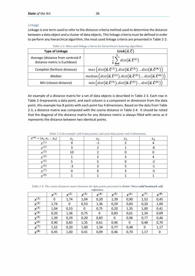
State of the Art 36

Linkage Linkage is one term used to refer to the distance criteria method used to determine the distance between a data object and a cluster of data objects. This linkage criteria must be defined in order to perform any hierarchical algorithm; the most used linkage criteria are presented in Table 2-2:

Table 2-2: Most used linkage criteria for hierarchical clustering algorithms

Type of Linkage 𝑳𝑳𝒅𝒅𝑳𝑳𝑳𝑳�𝒂𝒂��⃗ ,𝑪𝑪��

Average (distance from centroid if distance metric is Euclidean)

1𝐿𝐿�𝑤𝑤𝐿𝐿𝑀𝑀𝑡𝑡�𝒂𝒂��⃗ ,𝑪𝑪�(𝒅𝒅)�𝑘𝑘

𝑡𝑡=1

Complete (farthest distance) 𝑚𝑚𝑎𝑎𝑥𝑥 �𝑤𝑤𝐿𝐿𝑀𝑀𝑡𝑡�𝒂𝒂��⃗ ,𝑪𝑪�(𝟏𝟏)�,𝑤𝑤𝐿𝐿𝑀𝑀𝑡𝑡�𝒂𝒂��⃗ ,𝑪𝑪�(𝟐𝟐)�…𝑤𝑤𝐿𝐿𝑀𝑀𝑡𝑡�𝒂𝒂��⃗ ,𝑪𝑪�(𝑳𝑳)��

Median 𝑚𝑚𝑉𝑉𝑤𝑤𝐿𝐿𝑎𝑎𝐿𝐿 �𝑤𝑤𝐿𝐿𝑀𝑀𝑡𝑡�𝒂𝒂��⃗ ,𝑪𝑪�(𝟏𝟏)�,𝑤𝑤𝐿𝐿𝑀𝑀𝑡𝑡�𝒂𝒂��⃗ ,𝑪𝑪�(𝟐𝟐)�…𝑤𝑤𝐿𝐿𝑀𝑀𝑡𝑡�𝒂𝒂��⃗ ,𝑪𝑪�(𝑳𝑳)��

Min (closest distance) 𝑚𝑚𝐿𝐿𝐿𝐿 �𝑤𝑤𝐿𝐿𝑀𝑀𝑡𝑡�𝒂𝒂��⃗ ,𝑪𝑪�(𝟏𝟏)�,𝑤𝑤𝐿𝐿𝑀𝑀𝑡𝑡�𝒂𝒂��⃗ ,𝑪𝑪�(𝟐𝟐)�…𝑤𝑤𝐿𝐿𝑀𝑀𝑡𝑡�𝒂𝒂��⃗ ,𝑪𝑪�(𝑳𝑳)��

An example of a distance matrix for a set of data objects is described in Table 2-3. Each row in Table 2-3represents a data point, and each column is a component or dimension from the data point, this example has 8 points with each point has 4 dimensions. Based on the data from Table 2-3, a distance matrix was computed with the cosine distance in Table 2-4. It should be noted that the diagonal of the distance matrix for any distance metric is always filled with zeros as it represents the distance between two identical points.

Table 2-3:An example with 8 data points, and each data points with 4 dimensions 𝒙𝒙(𝒎𝒎) = [𝒙𝒙𝟏𝟏,𝒙𝒙𝟏𝟏 . . .𝒙𝒙𝑳𝑳] 𝑥𝑥1 𝑥𝑥2 𝑥𝑥3 𝑥𝑥4

𝑥𝑥(1) 0 -1 2 4 𝑥𝑥(2) 3 2 1 -6 𝑥𝑥(3) 10 2 0 0 𝑥𝑥(4) 1 2 3 4 𝑥𝑥(5) 5 5 0 -2 𝑥𝑥(6) -3 3 5 -1 𝑥𝑥(7) 0 0 3 -5 𝑥𝑥(8) 1 1 1 1

Table 2-4: The cosine distances matrix between the data points presented in Error! Not a valid bookmark self-reference.

𝒙𝒙(𝟏𝟏) 𝒙𝒙(𝟐𝟐) 𝒙𝒙(𝟑𝟑) 𝒙𝒙(𝟒𝟒) 𝒙𝒙(𝟓𝟓) 𝒙𝒙(𝟔𝟔) 𝒙𝒙(𝟕𝟕) 𝒙𝒙(𝟖𝟖) 𝒙𝒙(𝟏𝟏) 0 1,74 1,04 0,20 1,39 0,90 1,52 0,45 𝒙𝒙(𝟐𝟐) 1,74 0 0,53 1,36 0,29 0,83 0,20 1,00 𝒙𝒙(𝟑𝟑) 1,04 0,53 0 0,75 0,20 1,35 1,00 0,41 𝒙𝒙(𝟒𝟒) 0,20 1,36 0,75 0 0,83 0,61 1,34 0,09 𝒙𝒙(𝟓𝟓) 1,39 0,29 0,20 0,83 0 0,96 0,77 0,46 𝒙𝒙(𝟔𝟔) 0,90 0,83 1,35 0,61 0,96 0 0,48 0,70 𝒙𝒙(𝟕𝟕) 1,52 0,20 1,00 1,34 0,77 0,48 0 1,17 𝒙𝒙(𝟖𝟖) 0,45 1,00 0,41 0,09 0,46 0,70 1,17 0

State of the Art 37

2.4. Diagnosis of Structures In this section, the main aspects related to visual inspection and diagnosis will be described in the context of existing structures. Existing guidelines and recommendations to recognize some pathologies with mechanical and chemical origin are described with emphasis on concrete beams. Several books and reports on the topic of diagnosis and rehabilitation of buildings have been consulted ((AENOR) 2009) (Broto Xavier 2006) (Elizalde Javier 1980) (Schenk 1999) to introduce the current knowledge on the philosophy of diagnosing and rehabilitation; on the origins of most pathologies. The focus in this section will be placed into the visual diagnosis of concrete beams.

2.4.1. General Problem The problem of diagnosing the state of a structure has been present for as long as humans have constructed. In modern times, with all the knowledge accumulated on the pathologies and symptoms that structures through history have presented, the task for trained technicians to find the cause or causes for the damage can be described in some way as a detective/medical work. This analogy is made as the technician must first inspect all the structure and acknowledge the damage, but also be very diligent not to miss all the details/clues that may be present. Then with the use of his/her knowledge, expertise, tests, structural plans, numerical models and calculations, the technician must make a hypothesis on the origin of the damage. And based on these allegedly recognized pathologies and causes may propose a course of action for repair or even decide that the structure damage is beyond repair and advise demolition.

Given these characteristics on the problem it is also certain that an ideal technician in charge of the diagnosis and rehabilitation of a structure needs to have experience in construction, on pathologies, knowledge on the testing and structural design to be able to propose a decent plausible hypothesis. And taking into account that these hypotheses may still be wrong as a structure in use will bear its loads in a way different from what numerical models predicted for the design. Also, some pathologies may have their symptoms hidden in locations that are hard to access or to view; and this fact adds another layer of difficulty to the hypothesis accuracy.

Most recorded knowledge on diagnose and rehabilitation of structures is on the topic of buildings as they are the most common structure in Civil Engineering. Therefore already there are many works that serve as guidelines to diagnosis, tests and rehabilitation of existing buildings especially. And each author has its own division for classifying and dividing the methodology for the diagnosis; among these, the division proposed by Broto and Comerma (Broto Xavier 2006) is presented in the subsection below to introduce the origin/causes of the pathologies and the symptoms.

2.4.2. Causes of structural pathologies Within the general causes of lesions on structures derived directly from human error are:

• Deficiencies in the project originated on the phase of design, calculation errors, bad design of the structure or inadequate selection of the materials used.

• Low quality of the construction materials. • Bad execution of the project or constructive errors (most common cause) • The misuse of the building is also cause of many lesions for the application of

unexpected loads or change of use of the structure, lack of maintenance, not controlled remodeling that may suppress or damage structural elements.

State of the Art 38

Among the indirect and sometimes unavoidable causes:

• The aging and fatigue of materials and chemical attacks on elements exposed to aggressive environment (marine, industrial or urban with high levels of pollution) are frequent.

• Earthquakes, settlement of soil and terrain slides. • Extraordinary actions, such as floods, fires, phreatic water and other accidents.

2.4.3. Symptoms in Buildings Constructive structural elements present a broad range of symptoms in the event of the appearance of lesions. From the occurrence of cracks to changes in color, deformations, shedding, crushing, etc. It must be adverted that these symptoms may show with delay on the bearing structures; or, on the other hand, show first on non-structural components.

In all cases the apparition of the first symptoms is sufficient to put the building under surveillance, in order perform the rehabilitation that prevent a critical advance of the lesions and in a latter instance, a real danger to the structure.

Among the different symptoms; cracks, fissures and micro-cracks are the most common symptoms in structural concrete elements. Besides, they are usually the first to become apparent and are given more importance usually as they are more evident and esthetically less pleasant to users and may be consequences of improper structural performance. It is known that the diagnosis of a structure must be done with a global holistic vision, considering possible interaction between causes, but the symptoms may be separated by the type of element where a pathology may be found:

- Structural • Foundations • Retaining Walls • Beams • Columns • Slabs • Joints • Bearing Wall Systems

- Non-Structural • Non-structural walls and façades • Roofs and ornamental Ceilings • Interior partitions • Stairs • Electrical, gas, water and other pipes • Mechanical components and systems including air conditioning equipment, ducts,

elevators, escalators, pumps, and emergency generators

And again, the pathologies may be divided on the material where they appear:

• -Steel • -Concrete • -Wood

State of the Art 39

On the origin of the pathology:

• -Mechanical • -Chemical

2.4.4. Pathologies in concrete beams Among all the pathologies that appear in beams, only the ones that cause cracking will be listed below.

- Thermal gradients - Creep and shrinkage - Freeze thaw - Plastic settlement during casting - Inner volume changes related to delay ettringite formation, alkali-silica reaction, etc. - Compression Stresses - Traction Stresses - Shear Stresses - Bending Moments - Torsion Stresses - Bending-Shear - Corrosion - Bond Slip

From the list above only 4 type of cracks patterns will be discussed in detail below reviewed; the reasoning behind this decision will be explained later in section 2.4.4.5.

2.4.4.1. Flexure An external force applied perpendicularly to the main axis of a beam will induce a reaction known as bending moment. The internal forces representing this moment will divide a cross section in two parts: a compression and tensile zone. In concrete beams, the most common symptoms suggesting high bending moment are cracks. These cracks appear when a concrete section is bearing a moment that surpasses the tensile resistance of the concrete. Their distribution and direction will depend on the boundary conditions of the beam. It should be noted that all reinforced concrete beams are designed to fail by flexion, with the condition that it occurs by the yielding of the flexion reinforcement in the traction zone. Thus, the tensile zone of the section usually cracks before reaching loads close to the beam maximum load, this is desirable because under this situation the steel reinforcement starts bearing the tensile stresses. A failure due to the yielding of the longitudinal reinforcement is the desirable one under all design criteria. This type of failure is ductile meaning it will deform significantly before reaching failure; to feature this, a typical moment-curvature curve for a concrete beam is presented in Figure 2.23. The cracking expected must be limited for durability reasons, as excessive cracking may leave the reinforcement exposed to chemical attacks in aggressive environments; the Eurocode 2 recommends values between 0.2 to 0.4 mm (CEN 2004).

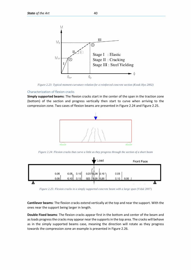
State of the Art 40

Figure 2.23: Typical moment-curvature relation for a reinforced concrete section (Kwak Hyo 2002)

Characterization of flexion cracks Simply supported beams: The flexion cracks start in the center of the span in the traction zone (bottom) of the section and progress vertically then start to curve when arriving to the compression zone. Two cases of flexion beams are presented in Figure 2.24 and Figure 2.25.

Figure 2.24: Flexion cracks that curve a little as they progress through the section of a short beam

Figure 2.25: Flexion cracks in a simply supported concrete beam with a large span (Vidal 2007)

Cantilever beams: The flexion cracks extend vertically at the top and near the support. With the ones near the support being larger in length.

Double Fixed beams: The flexion cracks appear first in the bottom and center of the beam and as loads progress the cracks may appear near the supports in the top area. The cracks will behave as in the simply supported beams case, meaning the direction will rotate as they progress towards the compression zone an example is presented in Figure 2.26.

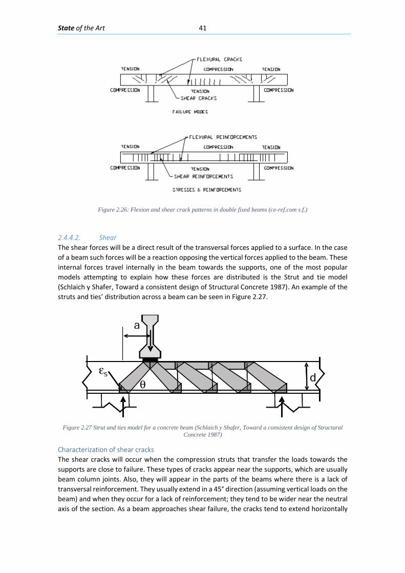
State of the Art 41

Figure 2.26: Flexion and shear crack patterns in double fixed beams (ce-ref.com s.f.)

2.4.4.2. Shear The shear forces will be a direct result of the transversal forces applied to a surface. In the case of a beam such forces will be a reaction opposing the vertical forces applied to the beam. These internal forces travel internally in the beam towards the supports, one of the most popular models attempting to explain how these forces are distributed is the Strut and tie model (Schlaich y Shafer, Toward a consistent design of Structural Concrete 1987). An example of the struts and ties’ distribution across a beam can be seen in Figure 2.27.

Figure 2.27 Strut and ties model for a concrete beam (Schlaich y Shafer, Toward a consistent design of Structural

Concrete 1987)

Characterization of shear cracks The shear cracks will occur when the compression struts that transfer the loads towards the supports are close to failure. These types of cracks appear near the supports, which are usually beam column joints. Also, they will appear in the parts of the beams where there is a lack of transversal reinforcement. They usually extend in a 45° direction (assuming vertical loads on the beam) and when they occur for a lack of reinforcement; they tend to be wider near the neutral axis of the section. As a beam approaches shear failure, the cracks tend to extend horizontally

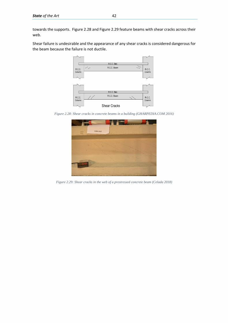
State of the Art 42

towards the supports. Figure 2.28 and Figure 2.29 feature beams with shear cracks across their web.

Shear failure is undesirable and the appearance of any shear cracks is considered dangerous for the beam because the failure is not ductile.

Figure 2.28: Shear cracks in concrete beams in a building (GHARPEDIA.COM 2016)

Figure 2.29: Shear cracks in the web of a prestressed concrete beam (Celada 2018)

State of the Art 43

2.4.4.3. Corrosion in reinforced concrete The corrosion in concrete beams will initiate when the natural alkalinity of the concrete is lost, as this pH condition protects the steel reinforcement. The two most common mechanisms that may cause corrosion are (Mays, 1992):

-Carbonation: the natural reaction of the carbon dioxide present in the atmosphere with the concrete will decrease the alkalinity of the concrete leaving it exposed.

-Chlorides present in aggregates: The presence of chlorides in the aggregates or water for the concrete mix destroys the passive corrosion film that protects the reinforcement.

There are other chemical attacks that may damage the concrete and indirectly cause corrosion by exposing the reinforcement to the environment such as: the alkali-silica reaction, concrete with alumina and sulphate attacks (Mays 1992).

Characterization of corrosion cracks The sub-product of the corrosion of the reinforcement bars expands and pushes the concrete around it. The first visible signs from this is cracking on the surface, when the corrosion advances usually there is delamination and spalling of the concrete cover as a result of the increasing pressure from the expanding corroding reinforcement. The total delamination and loss of the concrete cover would leave the steel reinforcement totally exposed to the environment making the corrosion process even faster. There is also the detrimental effect on the anchoring and bond strength of the reinforcement, if enough concrete is lost around the steel reinforcement.

Another danger of the corrosion is that the sub-product of corrosion is a brittle material with lower resistance (Abdelhamid y Morsyb 2016). The final effect is a reduction of the effective area of steel reinforcement and if this process is advanced enough, it can lead to failure of an element.

Corrosion cracks from carbonation origin will occur on almost the total length of the bar as it is an attack that advances gradually through all the depth of the concrete. On the other hand, cracks from chlorides attacks will appear more locally where the penetration occurred. On either case, the cracks will follow the position of the reinforcement.

Usually corrosion cracks appear to “follow” the longitudinal reinforcement as the corroded bars have a larger diameter and push concrete in the surface. There are cases where cracks appear around the transversal reinforcement. In Figure 2.30 and Figure 2.31 there are two cases of concrete beams cracking as a result of the corrosion of their longitudinal reinforcement are shown.

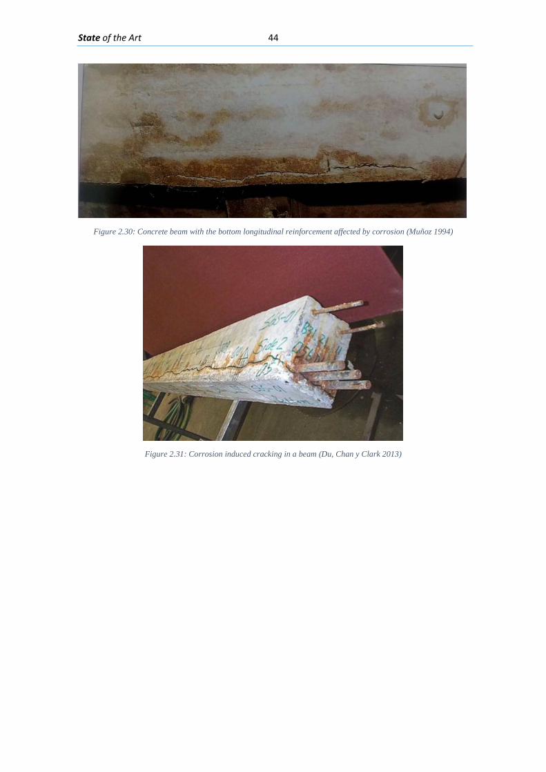
State of the Art 44

Figure 2.30: Concrete beam with the bottom longitudinal reinforcement affected by corrosion (Muñoz 1994)

Figure 2.31: Corrosion induced cracking in a beam (Du, Chan y Clark 2013)

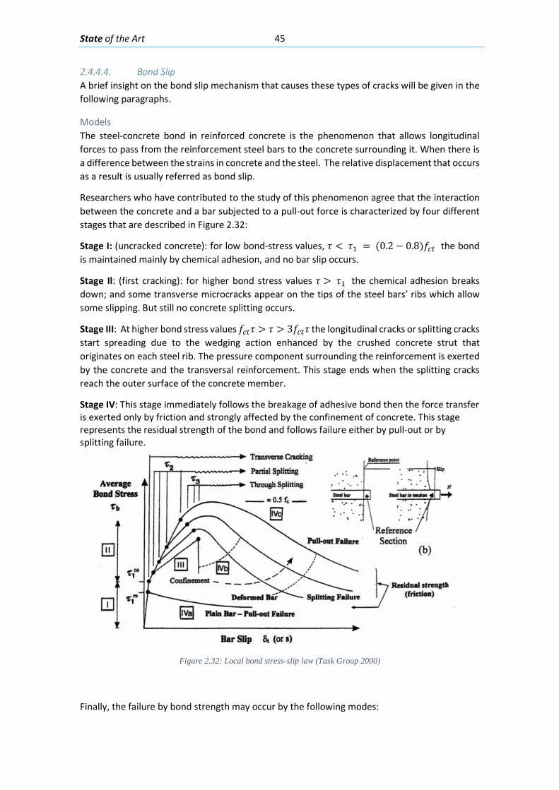
State of the Art 45

2.4.4.4. Bond Slip A brief insight on the bond slip mechanism that causes these types of cracks will be given in the following paragraphs.

Models The steel-concrete bond in reinforced concrete is the phenomenon that allows longitudinal forces to pass from the reinforcement steel bars to the concrete surrounding it. When there is a difference between the strains in concrete and the steel. The relative displacement that occurs as a result is usually referred as bond slip.

Researchers who have contributed to the study of this phenomenon agree that the interaction between the concrete and a bar subjected to a pull-out force is characterized by four different stages that are described in Figure 2.32:

Stage I: (uncracked concrete): for low bond-stress values, 𝜏𝜏 < 𝜏𝜏1 = (0.2 − 0.8)𝑓𝑓𝑐𝑐𝑡𝑡 the bond is maintained mainly by chemical adhesion, and no bar slip occurs.

Stage Il: (first cracking): for higher bond stress values 𝜏𝜏 > 𝜏𝜏1 the chemical adhesion breaks down; and some transverse microcracks appear on the tips of the steel bars’ ribs which allow some slipping. But still no concrete splitting occurs.

Stage III: At higher bond stress values 𝑓𝑓𝑐𝑐𝑡𝑡𝜏𝜏 > 𝜏𝜏 > 3𝑓𝑓𝑐𝑐𝑡𝑡𝜏𝜏 the longitudinal cracks or splitting cracks start spreading due to the wedging action enhanced by the crushed concrete strut that originates on each steel rib. The pressure component surrounding the reinforcement is exerted by the concrete and the transversal reinforcement. This stage ends when the splitting cracks reach the outer surface of the concrete member.

Stage IV: This stage immediately follows the breakage of adhesive bond then the force transfer is exerted only by friction and strongly affected by the confinement of concrete. This stage represents the residual strength of the bond and follows failure either by pull-out or by splitting failure.

Figure 2.32: Local bond stress-slip law (Task Group 2000)

Finally, the failure by bond strength may occur by the following modes:

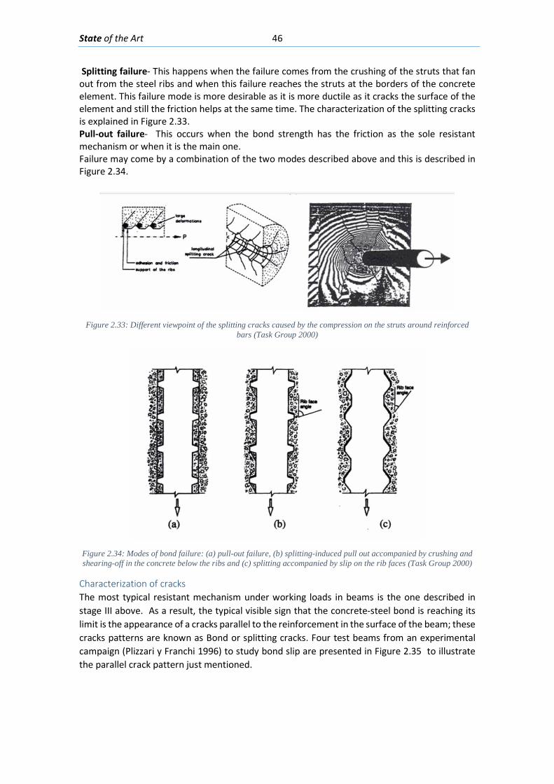
State of the Art 46

Splitting failure- This happens when the failure comes from the crushing of the struts that fan out from the steel ribs and when this failure reaches the struts at the borders of the concrete element. This failure mode is more desirable as it is more ductile as it cracks the surface of the element and still the friction helps at the same time. The characterization of the splitting cracks is explained in Figure 2.33. Pull-out failure- This occurs when the bond strength has the friction as the sole resistant mechanism or when it is the main one. Failure may come by a combination of the two modes described above and this is described in Figure 2.34.

Figure 2.33: Different viewpoint of the splitting cracks caused by the compression on the struts around reinforced

bars (Task Group 2000)

Figure 2.34: Modes of bond failure: (a) pull-out failure, (b) splitting-induced pull out accompanied by crushing and shearing-off in the concrete below the ribs and (c) splitting accompanied by slip on the rib faces (Task Group 2000)

Characterization of cracks The most typical resistant mechanism under working loads in beams is the one described in stage III above. As a result, the typical visible sign that the concrete-steel bond is reaching its limit is the appearance of a cracks parallel to the reinforcement in the surface of the beam; these cracks patterns are known as Bond or splitting cracks. Four test beams from an experimental campaign (Plizzari y Franchi 1996) to study bond slip are presented in Figure 2.35 to illustrate the parallel crack pattern just mentioned.

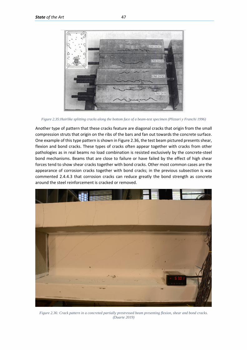
State of the Art 47

Figure 2.35:Hairlike splitting cracks along the bottom face of a beam-test specimen (Plizzari y Franchi 1996)

Another type of pattern that these cracks feature are diagonal cracks that origin from the small compression struts that origin on the ribs of the bars and fan out towards the concrete surface. One example of this type pattern is shown in Figure 2.36, the test beam pictured presents shear, flexion and bond cracks. These types of cracks often appear together with cracks from other pathologies as in real beams no load combination is resisted exclusively by the concrete-steel bond mechanisms. Beams that are close to failure or have failed by the effect of high shear forces tend to show shear cracks together with bond cracks. Other most common cases are the appearance of corrosion cracks together with bond cracks; in the previous subsection is was commented 2.4.4.3 that corrosion cracks can reduce greatly the bond strength as concrete around the steel reinforcement is cracked or removed.

Figure 2.36: Crack pattern in a concreted partially prestressed beam presenting flexion, shear and bond cracks.

(Duarte 2019)

State of the Art 48

2.4.4.5. Crack Patterns and Visual inspection

As commented in this section (2.4.4 Pathologies in concrete beams), only four pathologies and their respective crack pattern types were selected to review. The reason for this choice is that all these crack patterns and their causes can be identified by mere visual inspection. This empirical task done through visual inspection will be modeled with the help of machine learning techniques and models in chapter 5.

Crack Detection and Measurement 49

3. Crack Detection and Measurement

The methods described in this Chapter attempt to solve one of the problems stated in the objectives: To find a way to detect and measure cracks in a ROI within a picture showing a concrete surface; these methods can be divided as follows:

Crack Detection with a Neural Network, in this step a segmentation of the ROI is carried out in order to separate the sub-regions of the ROI that contain cracks and the regions that do not. This segmentation is don with a Neural Network designed to classify concrete image patches as “containing a crack” or “not containing a crack”. The method is explained in detail in section 3.2.

Crack Measurement with Digital Image Processing, in this part techniques such as segmentation and spatial filtering are used to determine which pixels are cracks; then to measure these cracks width and determine their angle. This process will be explained in section 3.3.

Crack Detection and Measurement 50

3.1. Hypothesis In the approach followed, it is assumed that cracks are a type of feature that has the following characteristics:

• Cracks are edges, or close to edges. • Cracks are represented by darker pixels points than the background. • Cracks are similar to lines, so they have a direction or orientation. • Nearby points within a crack will have similar orientation; i.e. it is assumed that crack

orientation does not change abruptly.

The present method also assumes the following:

• The surface plane of the concrete element depicted in the digital image is perpendicular or almost perpendicular to the camera principal axis.

• A region of interest (ROI) has already been chosen from the input image and inside this ROI only a concrete surface is depicted.

• Concrete surfaces in the ROI do not have any markings on them and are not painted.

3.2. Crack detection with a Neural Network

In order to segment the image and obtain a mask with pixels in the areas where cracks are found. The approach implemented is a segmentation using a neural network (NN) to detect the presence of cracks in a picture. The NN will segment the image by classifying each concrete image patch in two classes: “Crack” or “Not Crack”. The generation of the training examples, diagnosis of the NN and an example of this method are presented the subsections below.

3.2.1. Training Examples

In order to train the NN, a collection of training examples is needed to define the labels for the machine learning problem, the size in pixel of the image patches that will be labeled and which pictures or pixel patches will be used for labeling.

Twenty-six (26) image files obtained from web search (added in the Annex I) showing cracked concrete surfaces in *.jpg format have been used as the source of the training examples. From each picture, each 25x25 pixel patch will be labeled as “Crack” or “Not Crack”, with a sliding between the patches of 13 pixels. Figure 3.1 shows the Graphic User Interface (GUI) developed to label the image patches.

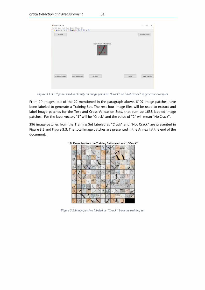
Crack Detection and Measurement 51

Figure 3.1: GUI panel used to classify an image patch as “Crack” or “Not Crack” to generate examples

From 20 images, out of the 22 mentioned in the paragraph above, 6107 image patches have been labeled to generate a Training Set. The rest four image files will be used to extract and label image patches for the Test and Cross-Validation Sets, that sum up 1658 labeled image patches. For the label vector, “1” will be “Crack” and the value of “2” will mean “No Crack”.

296 image patches from the Training Set labeled as “Crack” and “Not Crack” are presented in Figure 3.2 and Figure 3.3. The total image patches are presented in the Annex I at the end of the document.

Figure 3.2:Image patches labeled as “Crack” from the training set

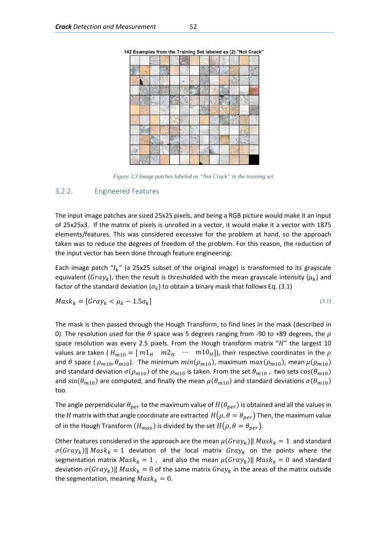
Crack Detection and Measurement 52

Figure 3.3 Image patches labeled as “Not Crack” in the training set

3.2.2. Engineered Features

The input image patches are sized 25x25 pixels, and being a RGB picture would make it an input of 25x25x3. If the matrix of pixels is unrolled in a vector, it would make it a vector with 1875 elements/features. This was considered excessive for the problem at hand, so the approach taken was to reduce the degrees of freedom of the problem. For this reason, the reduction of the input vector has been done through feature engineering:

Each image patch “𝐼𝐼𝑘𝑘” (a 25x25 subset of the original image) is transformed to its grayscale equivalent (𝐺𝐺𝑟𝑟𝑎𝑎𝑦𝑦𝑘𝑘), then the result is thresholded with the mean grayscale intensity (𝜇𝜇𝑘𝑘) and factor of the standard deviation (𝜎𝜎𝑘𝑘) to obtain a binary mask that follows Eq. (3.1)

𝑀𝑀𝑎𝑎𝑀𝑀𝐿𝐿𝑘𝑘 = [𝐺𝐺𝑟𝑟𝑎𝑎𝑦𝑦𝑘𝑘 < 𝜇𝜇𝑘𝑘 − 1.5𝜎𝜎𝑘𝑘] (3.1)

The mask is then passed through the Hough Transform, to find lines in the mask (described in 0). The resolution used for the 𝜃𝜃 space was 5 degrees ranging from -90 to +89 degrees, the 𝜌𝜌 space resolution was every 2.5 pixels. From the Hough transform matrix “𝐻𝐻” the largest 10 values are taken ( 𝐻𝐻𝑚𝑚10 = [ 𝑚𝑚1𝐻𝐻 𝑚𝑚2𝐻𝐻 ⋯ 𝑚𝑚10𝐻𝐻]), their respective coordinates in the 𝜌𝜌 and 𝜃𝜃 space ( 𝜌𝜌𝑚𝑚10,𝜃𝜃𝑚𝑚10). The minimum 𝑚𝑚𝐿𝐿𝐿𝐿(𝜌𝜌𝑚𝑚10), maximum 𝑚𝑚𝑎𝑎𝑥𝑥(𝜌𝜌𝑚𝑚10), mean 𝜇𝜇(𝜌𝜌𝑚𝑚10) and standard deviation 𝜎𝜎(𝜌𝜌𝑚𝑚10) of the 𝜌𝜌𝑚𝑚10 is taken. From the set 𝜃𝜃𝑚𝑚10 , two sets cos (𝜃𝜃𝑚𝑚10) and sin (𝜃𝜃𝑚𝑚10) are computed, and finally the mean 𝜇𝜇(𝜃𝜃𝑚𝑚10) and standard deviations 𝜎𝜎(𝜃𝜃𝑚𝑚10) too.

The angle perpendicular 𝜃𝜃𝑝𝑝𝑒𝑒𝑟𝑟 to the maximum value of 𝐻𝐻(𝜃𝜃𝑝𝑝𝑒𝑒𝑟𝑟) is obtained and all the values in the 𝐻𝐻 matrix with that angle coordinate are extracted 𝐻𝐻�𝜌𝜌, 𝜃𝜃 = 𝜃𝜃𝑝𝑝𝑒𝑒𝑟𝑟� Then, the maximum value of in the Hough Transform (𝐻𝐻𝑚𝑚𝑟𝑟𝑥𝑥) is divided by the set 𝐻𝐻�𝜌𝜌,𝜃𝜃 = 𝜃𝜃𝑝𝑝𝑒𝑒𝑟𝑟�.

Other features considered in the approach are the mean 𝜇𝜇(𝐺𝐺𝑟𝑟𝑎𝑎𝑦𝑦𝑘𝑘)‖ 𝑀𝑀𝑎𝑎𝑀𝑀𝐿𝐿𝑘𝑘 = 1 and standard 𝜎𝜎(𝐺𝐺𝑟𝑟𝑎𝑎𝑦𝑦𝑘𝑘)‖ 𝑀𝑀𝑎𝑎𝑀𝑀𝐿𝐿𝑘𝑘 = 1 deviation of the local matrix 𝐺𝐺𝑟𝑟𝑎𝑎𝑦𝑦𝑘𝑘 on the points where the segmentation matrix 𝑀𝑀𝑎𝑎𝑀𝑀𝐿𝐿𝑘𝑘 = 1 , and also the mean 𝜇𝜇(𝐺𝐺𝑟𝑟𝑎𝑎𝑦𝑦𝑘𝑘)‖ 𝑀𝑀𝑎𝑎𝑀𝑀𝐿𝐿𝑘𝑘 = 0 and standard deviation 𝜎𝜎(𝐺𝐺𝑟𝑟𝑎𝑎𝑦𝑦𝑘𝑘)‖ 𝑀𝑀𝑎𝑎𝑀𝑀𝐿𝐿𝑘𝑘 = 0 of the same matrix 𝐺𝐺𝑟𝑟𝑎𝑎𝑦𝑦𝑘𝑘 in the areas of the matrix outside the segmentation, meaning 𝑀𝑀𝑎𝑎𝑀𝑀𝐿𝐿𝑘𝑘 = 0.

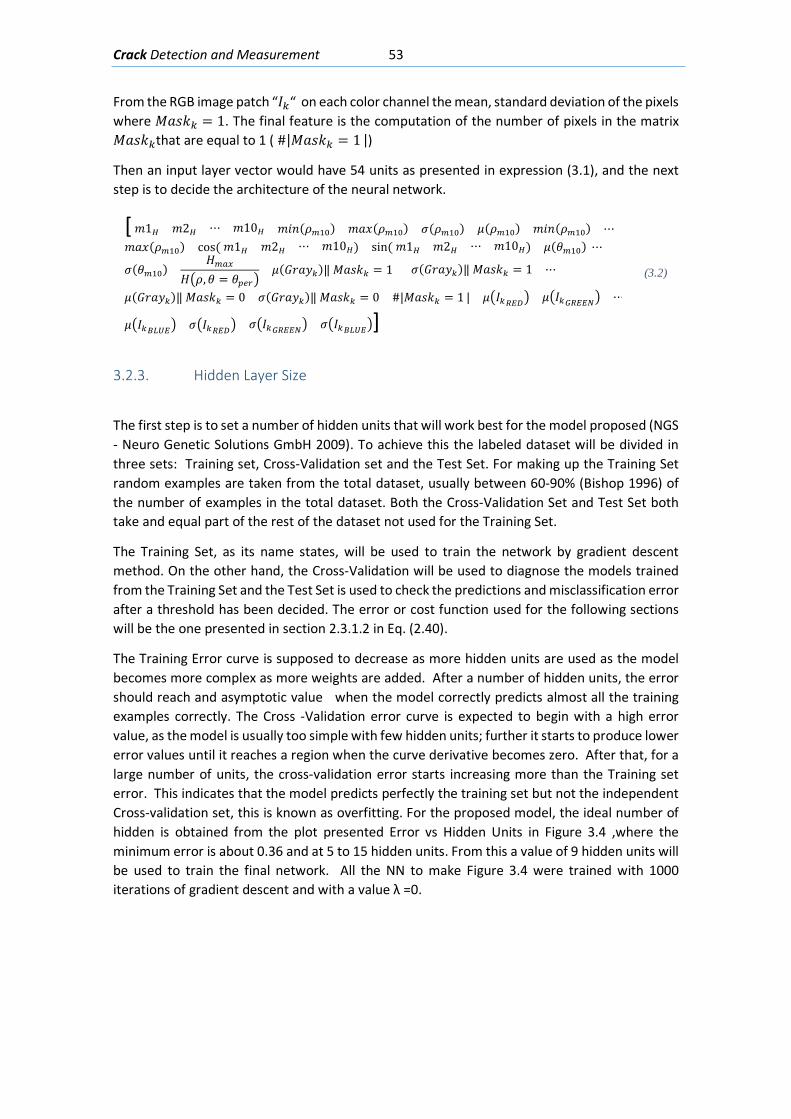
Crack Detection and Measurement 53

From the RGB image patch “𝐼𝐼𝑘𝑘“ on each color channel the mean, standard deviation of the pixels where 𝑀𝑀𝑎𝑎𝑀𝑀𝐿𝐿𝑘𝑘 = 1. The final feature is the computation of the number of pixels in the matrix 𝑀𝑀𝑎𝑎𝑀𝑀𝐿𝐿𝑘𝑘that are equal to 1 ( #|𝑀𝑀𝑎𝑎𝑀𝑀𝐿𝐿𝑘𝑘 = 1 |)

Then an input layer vector would have 54 units as presented in expression (3.1), and the next step is to decide the architecture of the neural network.

[ 𝑚𝑚1𝐻𝐻 𝑚𝑚2𝐻𝐻 ⋯ 𝑚𝑚10𝐻𝐻 𝑚𝑚𝐿𝐿𝐿𝐿(𝜌𝜌𝑚𝑚10) 𝑚𝑚𝑎𝑎𝑥𝑥(𝜌𝜌𝑚𝑚10) 𝜎𝜎(𝜌𝜌𝑚𝑚10) 𝜇𝜇(𝜌𝜌𝑚𝑚10) 𝑚𝑚𝐿𝐿𝐿𝐿(𝜌𝜌𝑚𝑚10) ⋯ 𝑚𝑚𝑎𝑎𝑥𝑥(𝜌𝜌𝑚𝑚10) cos ( 𝑚𝑚1𝐻𝐻 𝑚𝑚2𝐻𝐻 ⋯ 𝑚𝑚10𝐻𝐻) sin ( 𝑚𝑚1𝐻𝐻 𝑚𝑚2𝐻𝐻 ⋯ 𝑚𝑚10𝐻𝐻) 𝜇𝜇(𝜃𝜃𝑚𝑚10) ⋯

𝜎𝜎(𝜃𝜃𝑚𝑚10)𝐻𝐻𝑚𝑚𝑟𝑟𝑥𝑥

𝐻𝐻�𝜌𝜌,𝜃𝜃 = 𝜃𝜃𝑝𝑝𝑒𝑒𝑟𝑟�𝜇𝜇(𝐺𝐺𝑟𝑟𝑎𝑎𝑦𝑦𝑘𝑘)‖ 𝑀𝑀𝑎𝑎𝑀𝑀𝐿𝐿𝑘𝑘 = 1 𝜎𝜎(𝐺𝐺𝑟𝑟𝑎𝑎𝑦𝑦𝑘𝑘)‖ 𝑀𝑀𝑎𝑎𝑀𝑀𝐿𝐿𝑘𝑘 = 1 ⋯

𝜇𝜇(𝐺𝐺𝑟𝑟𝑎𝑎𝑦𝑦𝑘𝑘)‖ 𝑀𝑀𝑎𝑎𝑀𝑀𝐿𝐿𝑘𝑘 = 0 𝜎𝜎(𝐺𝐺𝑟𝑟𝑎𝑎𝑦𝑦𝑘𝑘)‖ 𝑀𝑀𝑎𝑎𝑀𝑀𝐿𝐿𝑘𝑘 = 0 #|𝑀𝑀𝑎𝑎𝑀𝑀𝐿𝐿𝑘𝑘 = 1 | 𝜇𝜇�𝐼𝐼𝑘𝑘𝑅𝑅𝑅𝑅𝑅𝑅� 𝜇𝜇�𝐼𝐼𝑘𝑘𝐺𝐺𝑅𝑅𝑅𝑅𝑅𝑅𝐺𝐺� ⋯

𝜇𝜇�𝐼𝐼𝑘𝑘𝐵𝐵𝐵𝐵𝐵𝐵𝑅𝑅� 𝜎𝜎�𝐼𝐼𝑘𝑘𝑅𝑅𝑅𝑅𝑅𝑅� 𝜎𝜎�𝐼𝐼𝑘𝑘𝐺𝐺𝑅𝑅𝑅𝑅𝑅𝑅𝐺𝐺� 𝜎𝜎�𝐼𝐼𝑘𝑘𝐵𝐵𝐵𝐵𝐵𝐵𝑅𝑅�]

(3.2)

3.2.3. Hidden Layer Size

The first step is to set a number of hidden units that will work best for the model proposed (NGS - Neuro Genetic Solutions GmbH 2009). To achieve this the labeled dataset will be divided in three sets: Training set, Cross-Validation set and the Test Set. For making up the Training Set random examples are taken from the total dataset, usually between 60-90% (Bishop 1996) of the number of examples in the total dataset. Both the Cross-Validation Set and Test Set both take and equal part of the rest of the dataset not used for the Training Set.

The Training Set, as its name states, will be used to train the network by gradient descent method. On the other hand, the Cross-Validation will be used to diagnose the models trained from the Training Set and the Test Set is used to check the predictions and misclassification error after a threshold has been decided. The error or cost function used for the following sections will be the one presented in section 2.3.1.2 in Eq. (2.40).

The Training Error curve is supposed to decrease as more hidden units are used as the model becomes more complex as more weights are added. After a number of hidden units, the error should reach and asymptotic value when the model correctly predicts almost all the training examples correctly. The Cross -Validation error curve is expected to begin with a high error value, as the model is usually too simple with few hidden units; further it starts to produce lower error values until it reaches a region when the curve derivative becomes zero. After that, for a large number of units, the cross-validation error starts increasing more than the Training set error. This indicates that the model predicts perfectly the training set but not the independent Cross-validation set, this is known as overfitting. For the proposed model, the ideal number of hidden is obtained from the plot presented Error vs Hidden Units in Figure 3.4 ,where the minimum error is about 0.36 and at 5 to 15 hidden units. From this a value of 9 hidden units will be used to train the final network. All the NN to make Figure 3.4 were trained with 1000 iterations of gradient descent and with a value λ =0.

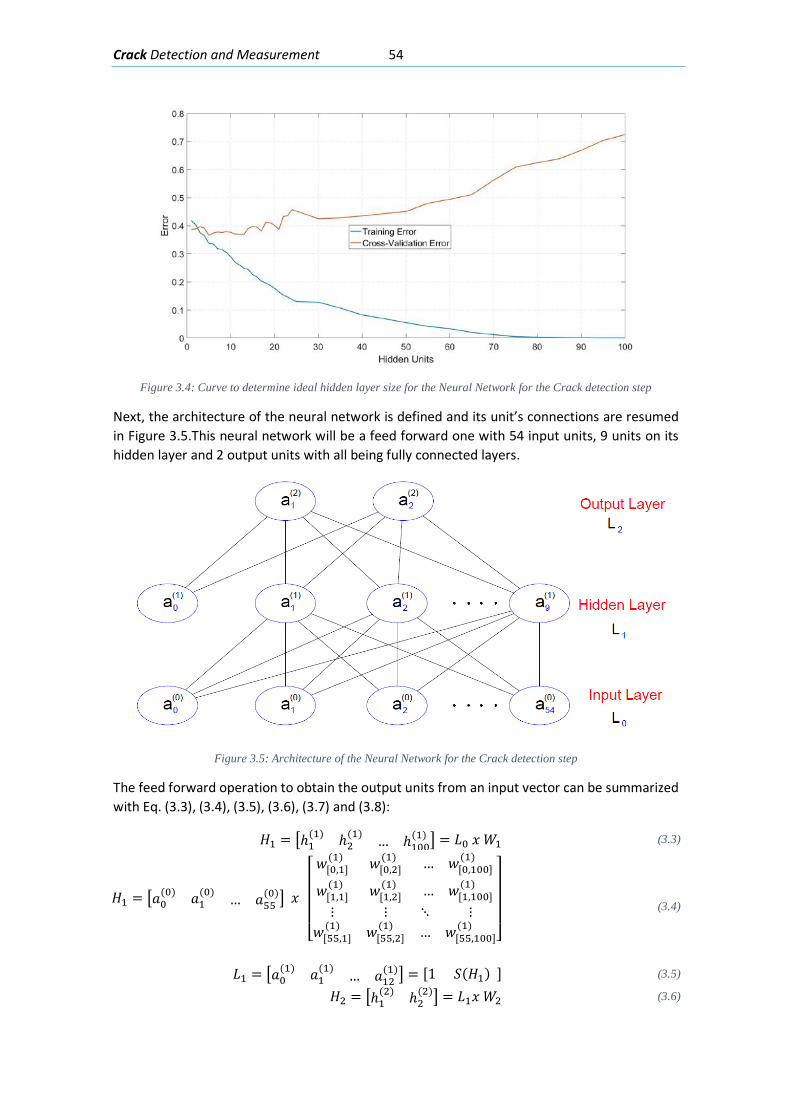
Crack Detection and Measurement 54

Figure 3.4: Curve to determine ideal hidden layer size for the Neural Network for the Crack detection step

Next, the architecture of the neural network is defined and its unit’s connections are resumed in Figure 3.5.This neural network will be a feed forward one with 54 input units, 9 units on its hidden layer and 2 output units with all being fully connected layers.

Figure 3.5: Architecture of the Neural Network for the Crack detection step

The feed forward operation to obtain the output units from an input vector can be summarized with Eq. (3.3), (3.4), (3.5), (3.6), (3.7) and (3.8):

𝐻𝐻1 = �ℎ1(1) ℎ2

(1) … ℎ100(1) � = 𝐿𝐿0 𝑥𝑥 𝑊𝑊1 (3.3)

𝐻𝐻1 = �𝑎𝑎0(0) 𝑎𝑎1

(0) … 𝑎𝑎55(0)� 𝑥𝑥

⎣⎢⎢⎢⎢⎡ 𝑤𝑤[0,1]

(1) 𝑤𝑤[0,2](1) … 𝑤𝑤[0,100]

(1)

𝑤𝑤[1,1](1) 𝑤𝑤[1,2]

(1) … 𝑤𝑤[1,100](1)

⋮𝑤𝑤[55,1]

(1)⋮

𝑤𝑤[55,2](1)

⋱ ⋮… 𝑤𝑤[55,100]

(1)⎦⎥⎥⎥⎥⎤

(3.4)

𝐿𝐿1 = �𝑎𝑎0(1) 𝑎𝑎1

(1) … 𝑎𝑎12(1)� = [1 𝑆𝑆(𝐻𝐻1) ] (3.5)

𝐻𝐻2 = �ℎ1(2) ℎ2

(2)� = 𝐿𝐿1𝑥𝑥 𝑊𝑊2 (3.6)

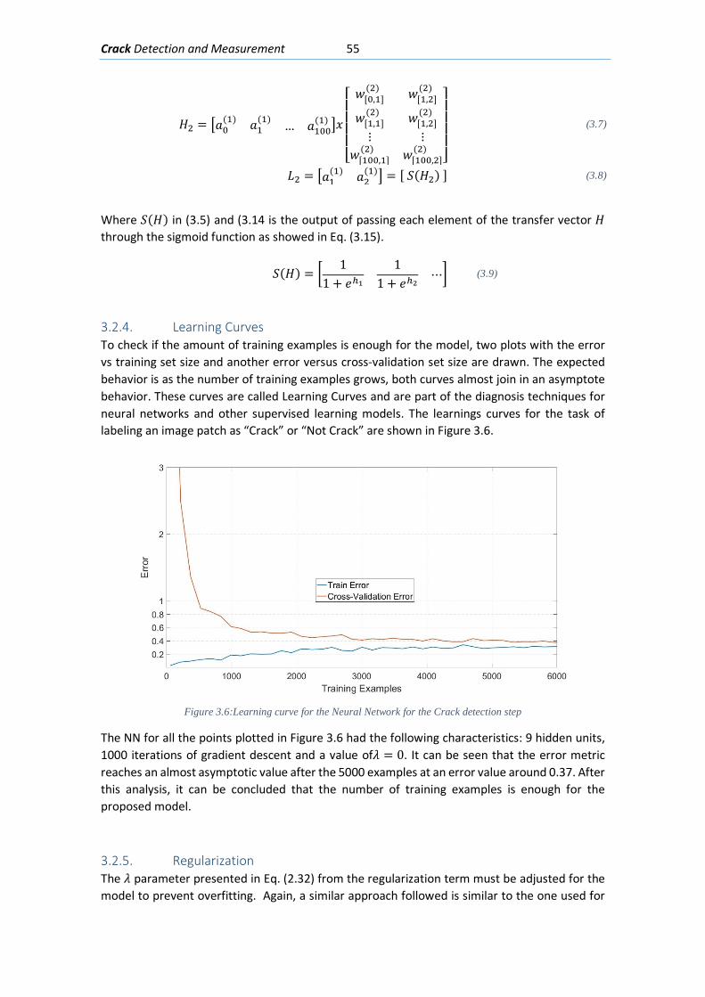
Crack Detection and Measurement 55

𝐻𝐻2 = �𝑎𝑎0(1) 𝑎𝑎1

(1) … 𝑎𝑎100(1) �𝑥𝑥

⎣⎢⎢⎢⎢⎡ 𝑤𝑤[0,1]

(2) 𝑤𝑤[1,2](2)

𝑤𝑤[1,1](2) 𝑤𝑤[1,2]

(2)

⋮𝑤𝑤[100,1]

(2)⋮

𝑤𝑤[100,2](2)

⎦⎥⎥⎥⎥⎤

(3.7)

𝐿𝐿2 = �𝑎𝑎1(1) 𝑎𝑎2

(1)� = [ 𝑆𝑆(𝐻𝐻2) ] (3.8)

Where 𝑆𝑆(𝐻𝐻) in (3.5) and (3.14 is the output of passing each element of the transfer vector 𝐻𝐻 through the sigmoid function as showed in Eq. (3.15).

𝑆𝑆(𝐻𝐻) = �1

1 + 𝑉𝑉ℎ11

1 + 𝑉𝑉ℎ2⋯� (3.9)

3.2.4. Learning Curves To check if the amount of training examples is enough for the model, two plots with the error vs training set size and another error versus cross-validation set size are drawn. The expected behavior is as the number of training examples grows, both curves almost join in an asymptote behavior. These curves are called Learning Curves and are part of the diagnosis techniques for neural networks and other supervised learning models. The learnings curves for the task of labeling an image patch as “Crack” or “Not Crack” are shown in Figure 3.6.

Figure 3.6:Learning curve for the Neural Network for the Crack detection step

The NN for all the points plotted in Figure 3.6 had the following characteristics: 9 hidden units, 1000 iterations of gradient descent and a value of𝜆𝜆 = 0. It can be seen that the error metric reaches an almost asymptotic value after the 5000 examples at an error value around 0.37. After this analysis, it can be concluded that the number of training examples is enough for the proposed model.

3.2.5. Regularization The 𝜆𝜆 parameter presented in Eq. (2.32) from the regularization term must be adjusted for the model to prevent overfitting. Again, a similar approach followed is similar to the one used for

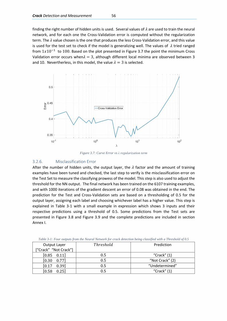
Crack Detection and Measurement 56

finding the right number of hidden units is used. Several values of 𝜆𝜆 are used to train the neural network, and for each one the Cross-Validation error is computed without the regularization term. The 𝜆𝜆 value chosen is the one that produces the less Cross-Validation error, and this value is used for the test set to check if the model is generalizing well. The values of 𝜆𝜆 tried ranged from 1𝑥𝑥10−1 to 100. Based on the plot presented in Figure 3.7 the point the minimum Cross Validation error occurs when𝜆𝜆 = 3, although different local minima are observed between 3 and 10. Nevertherless, in this model, the value 𝜆𝜆 = 3 is selected.

Figure 3.7: Curve Error vs λ regularization term

3.2.6. Misclassification Error After the number of hidden units, the output layer, the 𝜆𝜆 factor and the amount of training examples have been tuned and checked, the last step to verify is the misclassification error on the Test Set to measure the classifying prowess of the model. This step is also used to adjust the threshold for the NN output. The final network has been trained on the 6107 training examples, and with 1000 iterations of the gradient descent an error of 0.08 was obtained in the end. The prediction for the Test and Cross-Validation sets are based on a thresholding of 0.5 for the output layer, assigning each label and choosing whichever label has a higher value. This step is explained in Table 3-1 with a small example in expression which shows 3 inputs and their respective predictions using a threshold of 0.5. Some predictions from the Test sets are presented in Figure 3.8 and Figure 3.9 and the complete predictions are included in section Annex I.

Table 3-1: Four outputs from the Neural Network for crack detection being classified with a Threshold of 0.5

Output Layer [“Crack” “Not Crack”]

𝑇𝑇ℎ𝑟𝑟𝑉𝑉𝑀𝑀ℎ𝑐𝑐𝑙𝑙𝑤𝑤 Prediction

[0.85 0.11] 0.5 “Crack” (1) [0.30 0.77] 0.5 “Not Crack” (2) [0.17 0.39] 0.5 “Undetermined” [0.58 0.25] 0.5 “Crack” (1)

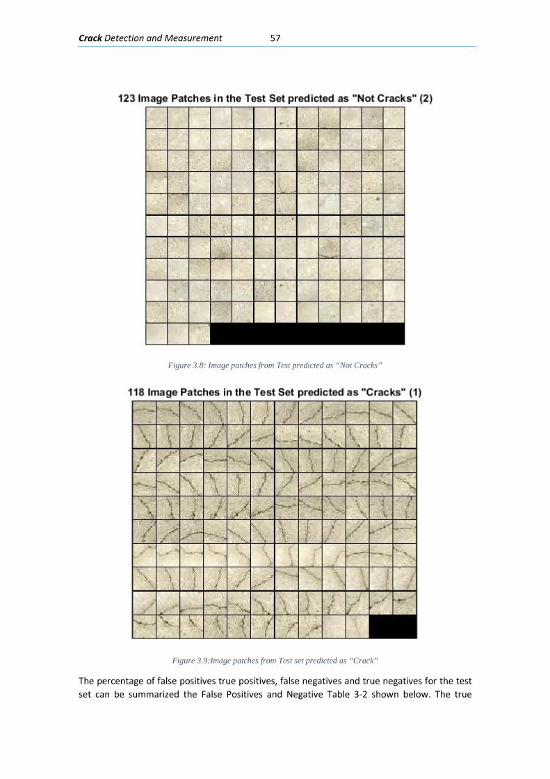
Crack Detection and Measurement 57

Figure 3.8: Image patches from Test predicted as “Not Cracks”

Figure 3.9:Image patches from Test set predicted as “Crack”

The percentage of false positives true positives, false negatives and true negatives for the test set can be summarized the False Positives and Negative Table 3-2 shown below. The true

Crack Detection and Measurement 58

positives will be the all image patches that were classified as “Crack” and are labeled also as “Crack”. The confusion matrix for the Cross-Validation set is shown in Table 3-3.

Test Set Prediction “Crack” (1) Prediction “Not Crack” (2) “Crack” (1) 47.30 0.00

“Not Crack” (2) 0.81 50.20 Table 3-2:Confusion matrix of the result of the NN in the Cross-Validation Set

The percentages in Table 6 and Table 7 do not add up to 100% as there are 4 data examples that were considered as not having a clear prediction, these were simply included in the total misclassification error. With this in mind, the total misclassification Error for the Test Set is 2.45% and the total misclassification error for the Cross-Validation Set is 6.28%.

Cross-Validation Set Prediction “Crack” (1) Prediction “Not Crack” (2) “Crack” (1) 43.05 0.27

“Not Crack” (2) 3.27 50.68 Table 3-3: Confusion matrix of the results of the NN in the Test Set

Given both results on the Cross-Validation and Test Sets, it can be concluded that the neural network proposed is proficient at telling apart un-cracked concrete image patches from cracked concrete patches. The results can be attributed to the simplicity of the classification task and the engineered features that helped the model tell apart the image patches in an efficient way. The following section will feature an example this method to obtain a segmentation with zones with and without cracks in images with cracks.

3.2.7. Example The segmentation was used on a picture of a test beam presented in Figure 3.10 , then a region of interest was picked as seen in Figure 3.11 and the result from the NN segmentation is presented in Figure 3.12.

Figure 3.10: Picture of a prestressed concrete beam during testing

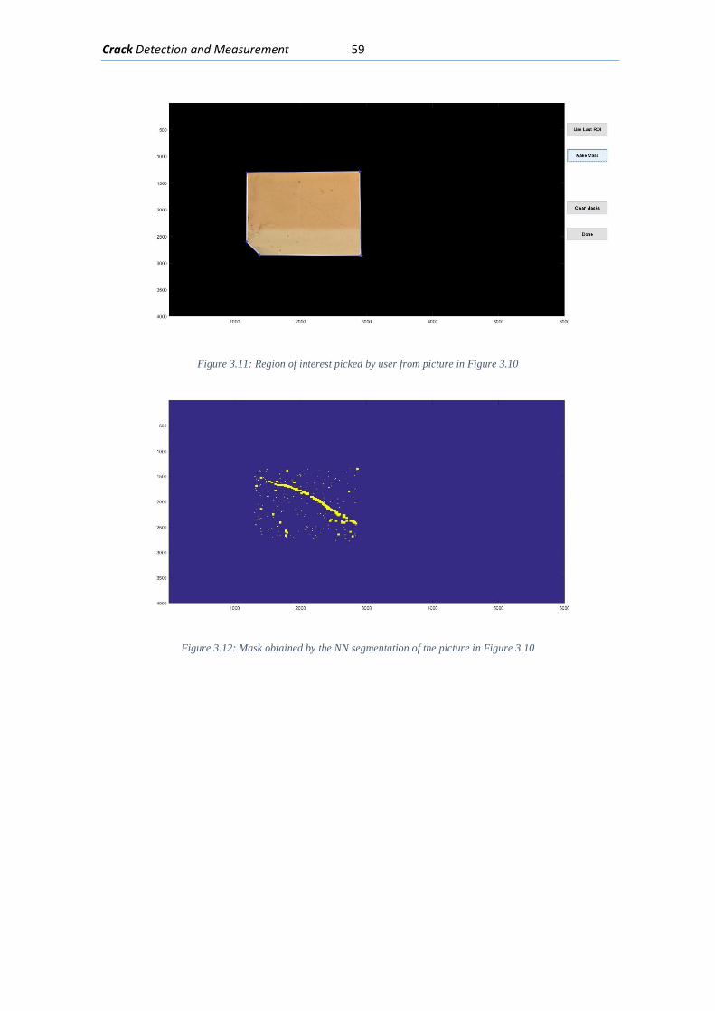
Crack Detection and Measurement 59

Figure 3.11: Region of interest picked by user from picture in Figure 3.10

Figure 3.12: Mask obtained by the NN segmentation of the picture in Figure 3.10

Crack Detection and Measurement 60

3.3. Crack Measurement with Digital Image processing This section will explain a method to detect, measure the width and angle from cracks in a concrete surface. The approach taken is to use several Digital Image Processing techniques such as spatial filtering, edge detection and segmentation. The starting ROI for this method is mask output from the Crack Detection with a Neural Network method explained in section 3.2. The algorithm steps will be explained in detail in the following subsection and can be resumed as:

1. Find thresholded edges in ROI.

2. Obtain a mask from pixels around the edges detected in step 1 and whose pixel intensities are lower than the local mean minus a factor of the local standard deviation.

3. Pass all areas or image patches detected in step 2 through several modified line detection kernels to detect the orientation to obtain a response that will determine if the image patch has a crack or not depending on a tuned threshold.

4. All image patches which were detected as cracks and have an orientation from step 3 will be analyzed to measure the width measured with the help of the gradient of the image patches.

3.3.1. Algorithm 3.3.1.1. Edges From the four statements presented in section 0, the first one argued that crack are edge pixels. Therefore, the next step towards obtaining all pixels which are cracks will be to find edges in the input image.

From the grayscale image 𝐼𝐼𝐺𝐺𝑟𝑟𝑟𝑟𝑦𝑦 an approximation of the gradient 𝐺𝐺 is generated with the

Prewitt kernel help as showed in Eq. (3.10) (3.11) and (3.12). Where 𝑆𝑆𝑥𝑥 = �−1 0 1−1 0 1−1 0 1

� and

𝑆𝑆𝑦𝑦 = �−1 −1 −10 0 01 1 1

� are the 3x3 Prewitt kernels in horizontal and vertical direction

respectively. The symbol “ ∗ " represents the correlation operation between the 2 matrices and all the operations in Eq. (3.12) are element wise operation.

𝐺𝐺𝑥𝑥 = 𝑆𝑆𝑥𝑥 ∗ 𝐼𝐼𝐺𝐺𝑟𝑟𝑟𝑟𝑦𝑦 (3.10)

𝐺𝐺𝑦𝑦 = 𝑆𝑆𝑦𝑦 ∗ 𝐼𝐼𝐺𝐺𝑟𝑟𝑟𝑟𝑦𝑦 (3.11)

𝐺𝐺 = �(𝐺𝐺𝑥𝑥)2 + �𝐺𝐺𝑦𝑦�2

(3.12)

Then an upper and lower threshold (𝑇𝑇ℎ𝑚𝑚𝑟𝑟𝑥𝑥,𝑇𝑇ℎ𝑚𝑚𝑖𝑖𝑛𝑛) is adjusted and applied to the gradient mask 𝐺𝐺 to get potential crack pixels. This new mask 𝐺𝐺𝑇𝑇ℎ will be generated by segmenting all the points where the inequality 𝑇𝑇ℎ𝑚𝑚𝑖𝑖𝑛𝑛 < 𝐺𝐺 < 𝑇𝑇ℎ𝑚𝑚𝑟𝑟𝑥𝑥 is satisfied.

3.3.1.2. Mean detection The pixels in the edge mask 𝐺𝐺𝑇𝑇ℎ from the last step are not exactly the cracks pixels themselves, the edges will be surrounding the crack pixels. The pixels which have an intensity less than the local mean of the neighborhood 𝜇𝜇𝑙𝑙𝑐𝑐𝑐𝑐 will minus the local standard deviation 𝜎𝜎𝑙𝑙𝑐𝑐𝑐𝑐 multiplied by a factor 𝑏𝑏 be picked as potential crack pixels meaning that the new mask 𝑀𝑀𝑉𝑉𝑎𝑎𝐿𝐿𝐷𝐷 would be

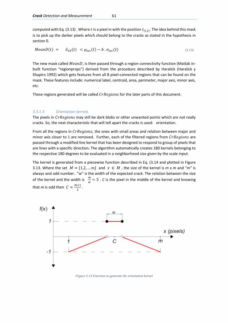
Crack Detection and Measurement 61

computed with Eq. (3.13) . Where 𝑡𝑡 is a pixel in with the position 𝑡𝑡(𝑖𝑖,𝑗𝑗). The idea behind this mask is to pick up the darker pixels which should belong to the cracks as stated in the hypothesis in section 0.

𝑀𝑀𝑉𝑉𝑎𝑎𝐿𝐿𝐷𝐷(𝑡𝑡) = 𝐺𝐺𝑡𝑡ℎ(𝑡𝑡) < 𝜇𝜇𝑙𝑙𝑐𝑐𝑐𝑐(𝑡𝑡) − 𝑏𝑏 .𝜎𝜎𝑙𝑙𝑐𝑐𝑐𝑐(𝑡𝑡) (3.13)

The new mask called 𝑀𝑀𝑉𝑉𝑎𝑎𝐿𝐿𝐷𝐷, is then passed through a region connectivity function (Matlab in-built function “regionprops”) derived from the procedure described by Haralick (Haralick y Shapiro 1992) which gets features from all 8 pixel-connected regions that can be found on the mask. These features include: numerical label, centroid, area, perimeter, major axis, minor axis, etc.

These regions generated will be called 𝐶𝐶𝑟𝑟𝑅𝑅𝑉𝑉𝑔𝑔𝐿𝐿𝑐𝑐𝐿𝐿𝑀𝑀 for the later parts of this document.

3.3.1.3. Orientation kernels The pixels in 𝐶𝐶𝑟𝑟𝑅𝑅𝑉𝑉𝑔𝑔𝐿𝐿𝑐𝑐𝐿𝐿𝑀𝑀 may still be dark blobs or other unwanted points which are not really cracks. So, the next characteristic that will tell apart the cracks is used: orientation.

From all the regions in 𝐶𝐶𝑟𝑟𝑅𝑅𝑉𝑉𝑔𝑔𝐿𝐿𝑐𝑐𝐿𝐿𝑀𝑀, the ones with small areas and relation between major and minor axis closer to 1 are removed. Further, each of the filtered regions from 𝐶𝐶𝑟𝑟𝑅𝑅𝑉𝑉𝑔𝑔𝐿𝐿𝑐𝑐𝐿𝐿𝑀𝑀 are passed through a modified line kernel that has been designed to respond to group of pixels that are lines with a specific direction. The algorithm automatically creates 180 kernels belonging to the respective 180 degrees to be evaluated in a neighborhood size given by the scale input.

The kernel is generated from a piecewise function described in Eq. (3.14 and plotted in Figure 3.13. Where the set 𝑀𝑀 = [1,2, …𝑚𝑚] and 𝑥𝑥 ∈ 𝑀𝑀 , the size of the kernel is m x m and “m” is always and odd number. “w” is the width of the expected crack. The relation between the size of the kernel and the width is 𝑚𝑚

𝑃𝑃= 5 . C is the pixel in the middle of the kernel and knowing

that m is odd then 𝐶𝐶 = 𝑚𝑚+12

.

Figure 3.13:Function to generate the orientation kernel

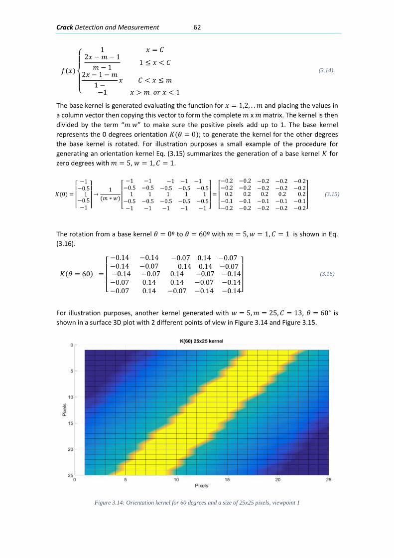
Crack Detection and Measurement 62

𝑓𝑓(𝑥𝑥)

⎩⎪⎨

⎪⎧

1 𝑥𝑥 = 𝐶𝐶2𝑥𝑥 −𝑚𝑚 − 1𝑚𝑚 − 1

1 ≤ 𝑥𝑥 < 𝐶𝐶2𝑥𝑥 − 1 −𝑚𝑚

1 −𝑥𝑥 𝐶𝐶 < 𝑥𝑥 ≤ 𝑚𝑚

−1 𝑥𝑥 > 𝑚𝑚 𝑐𝑐𝑟𝑟 𝑥𝑥 < 1

(3.14)

The base kernel is generated evaluating the function for 𝑥𝑥 = 1,2, . .𝑚𝑚 and placing the values in a column vector then copying this vector to form the complete 𝑚𝑚 x 𝑚𝑚 matrix. The kernel is then divided by the term “𝑚𝑚 𝑤𝑤” to make sure the positive pixels add up to 1. The base kernel represents the 0 degrees orientation 𝐾𝐾(𝜃𝜃 = 0); to generate the kernel for the other degrees the base kernel is rotated. For illustration purposes a small example of the procedure for generating an orientation kernel Eq. (3.15) summarizes the generation of a base kernel 𝐾𝐾 for zero degrees with 𝑚𝑚 = 5, 𝑤𝑤 = 1,𝐶𝐶 = 1.

𝐾𝐾(0) =

⎢⎢⎢⎢⎡−1−0.5 1−0.5−1 ⎥

⎥⎥⎥⎤→

1(𝑚𝑚 ∗ 𝑤𝑤)

⎣⎢⎢⎢⎡−1 −1 −1 −1 −1−0.5 −0.5 −0.5 −0.5 −0.5 1−0.5−1

1−0.5−1

1−0.5−1

1−0.5−1

1−0.5−1 ⎦

⎥⎥⎥⎤

=

⎣⎢⎢⎢⎡−0.2 −0.2 −0.2 −0.2 −0.2−0.2 −0.2 −0.2 −0.2 −0.2 0.2−0.1−0.2

0.2−0.1−0.2

0.2−0.1−0.2

0.2−0.1−0.2

0.2−0.1−0.2⎦

⎥⎥⎥⎤ (3.15)

The rotation from a base kernel 𝜃𝜃 = 0º to 𝜃𝜃 = 60º with 𝑚𝑚 = 5,𝑤𝑤 = 1,𝐶𝐶 = 1 is shown in Eq. (3.16).

𝐾𝐾(𝜃𝜃 = 60) =

⎣⎢⎢⎢⎡−0.14 −0.14 −0.07 0.14 −0.07−0.14 −0.07 0.14 0.14 −0.07 −0.14−0.07−0.07

−0.070.140.14

0.140.14−0.07

−0.07−0.07−0.14

−0.14−0.14−0.14⎦

⎥⎥⎥⎤ (3.16)

For illustration purposes, another kernel generated with 𝑤𝑤 = 5,𝑚𝑚 = 25,𝐶𝐶 = 13, 𝜃𝜃 = 60° is shown in a surface 3D plot with 2 different points of view in Figure 3.14 and Figure 3.15.

Figure 3.14: Orientation kernel for 60 degrees and a size of 25x25 pixels, viewpoint 1

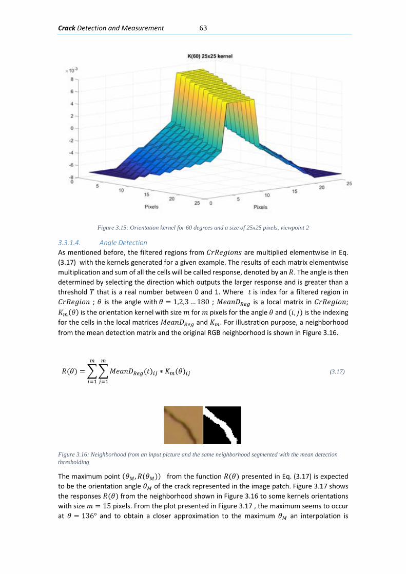
Crack Detection and Measurement 63

Figure 3.15: Orientation kernel for 60 degrees and a size of 25x25 pixels, viewpoint 2

3.3.1.4. Angle Detection As mentioned before, the filtered regions from 𝐶𝐶𝑟𝑟𝑅𝑅𝑉𝑉𝑔𝑔𝐿𝐿𝑐𝑐𝐿𝐿𝑀𝑀 are multiplied elementwise in Eq. (3.17) with the kernels generated for a given example. The results of each matrix elementwise multiplication and sum of all the cells will be called response, denoted by an 𝑅𝑅. The angle is then determined by selecting the direction which outputs the larger response and is greater than a threshold 𝑇𝑇 that is a real number between 0 and 1. Where 𝑡𝑡 is index for a filtered region in 𝐶𝐶𝑟𝑟𝑅𝑅𝑉𝑉𝑔𝑔𝐿𝐿𝑐𝑐𝐿𝐿 ; 𝜃𝜃 is the angle with 𝜃𝜃 = 1,2,3 … 180 ; 𝑀𝑀𝑉𝑉𝑎𝑎𝐿𝐿𝐷𝐷𝑅𝑅𝑒𝑒𝑔𝑔 is a local matrix in 𝐶𝐶𝑟𝑟𝑅𝑅𝑉𝑉𝑔𝑔𝐿𝐿𝑐𝑐𝐿𝐿; 𝐾𝐾𝑚𝑚(𝜃𝜃) is the orientation kernel with size 𝑚𝑚 for 𝑚𝑚 pixels for the angle 𝜃𝜃 and (𝐿𝐿, 𝑗𝑗) is the indexing for the cells in the local matrices 𝑀𝑀𝑉𝑉𝑎𝑎𝐿𝐿𝐷𝐷𝑅𝑅𝑒𝑒𝑔𝑔 and 𝐾𝐾𝑚𝑚. For illustration purpose, a neighborhood from the mean detection matrix and the original RGB neighborhood is shown in Figure 3.16.

𝑅𝑅(𝜃𝜃) = ��𝑀𝑀𝑉𝑉𝑎𝑎𝐿𝐿𝐷𝐷𝑅𝑅𝑒𝑒𝑔𝑔(𝑡𝑡)𝑖𝑖𝑗𝑗 ∗ 𝐾𝐾𝑚𝑚(𝜃𝜃)𝑖𝑖𝑗𝑗

𝑚𝑚

𝑗𝑗=1

𝑚𝑚

𝑖𝑖=1

(3.17)

Figure 3.16: Neighborhood from an input picture and the same neighborhood segmented with the mean detection thresholding

The maximum point (𝜃𝜃𝑀𝑀,𝑅𝑅(𝜃𝜃𝑀𝑀)) from the function 𝑅𝑅(𝜃𝜃) presented in Eq. (3.17) is expected to be the orientation angle 𝜃𝜃𝑀𝑀 of the crack represented in the image patch. Figure 3.17 shows the responses 𝑅𝑅(𝜃𝜃) from the neighborhood shown in Figure 3.16 to some kernels orientations with size 𝑚𝑚 = 15 pixels. From the plot presented in Figure 3.17 , the maximum seems to occur at 𝜃𝜃 = 136° and to obtain a closer approximation to the maximum 𝜃𝜃𝑀𝑀 an interpolation is

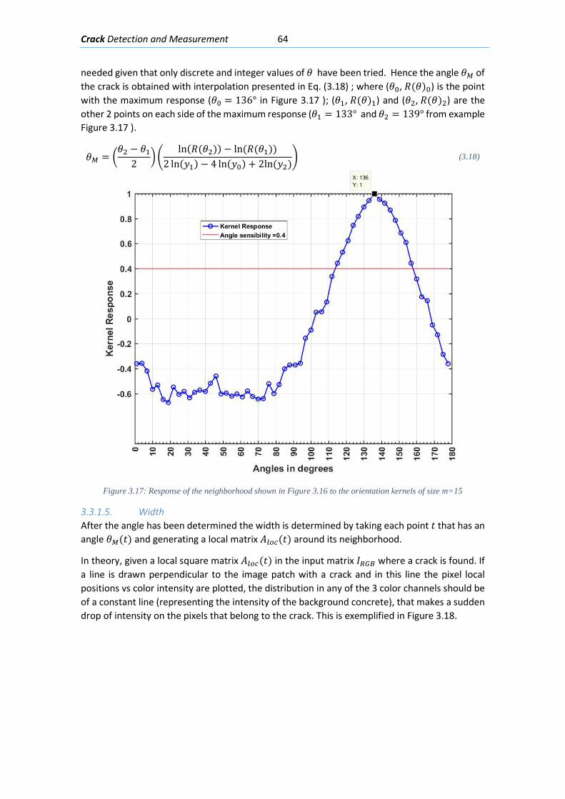
Crack Detection and Measurement 64

needed given that only discrete and integer values of 𝜃𝜃 have been tried. Hence the angle 𝜃𝜃𝑀𝑀 of the crack is obtained with interpolation presented in Eq. (3.18) ; where (𝜃𝜃0, 𝑅𝑅(𝜃𝜃)0) is the point with the maximum response (𝜃𝜃0 = 136° in Figure 3.17 ); (𝜃𝜃1, 𝑅𝑅(𝜃𝜃)1) and (𝜃𝜃2, 𝑅𝑅(𝜃𝜃)2) are the other 2 points on each side of the maximum response (𝜃𝜃1 = 133° and 𝜃𝜃2 = 139° from example Figure 3.17 ).

𝜃𝜃𝑀𝑀 = �𝜃𝜃2 − 𝜃𝜃1

2��

ln(𝑅𝑅(𝜃𝜃2)) − ln (𝑅𝑅(𝜃𝜃1))2 ln(𝑦𝑦1) − 4 ln(𝑦𝑦0) + 2ln (𝑦𝑦2)�

(3.18)

Figure 3.17: Response of the neighborhood shown in Figure 3.16 to the orientation kernels of size m=15

3.3.1.5. Width After the angle has been determined the width is determined by taking each point 𝑡𝑡 that has an angle 𝜃𝜃𝑀𝑀(𝑡𝑡) and generating a local matrix 𝐴𝐴𝑙𝑙𝑐𝑐𝑐𝑐(𝑡𝑡) around its neighborhood.

In theory, given a local square matrix 𝐴𝐴𝑙𝑙𝑐𝑐𝑐𝑐(𝑡𝑡) in the input matrix 𝐼𝐼𝑅𝑅𝐺𝐺𝐵𝐵 where a crack is found. If a line is drawn perpendicular to the image patch with a crack and in this line the pixel local positions vs color intensity are plotted, the distribution in any of the 3 color channels should be of a constant line (representing the intensity of the background concrete), that makes a sudden drop of intensity on the pixels that belong to the crack. This is exemplified in Figure 3.18.

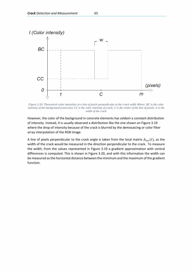
Crack Detection and Measurement 65

Figure 3.18: Theoretical color intensities in a line of pixels perpendicular to the crack width Where: BC is the color intensity of the background (concrete); CC is the color intensity of crack; C is the center of the line of pixels; w is the

width of the crack

However, the color of the background in concrete elements has seldom a constant distribution of intensity. Instead, it is usually observed a distribution like the one shown on Figure 3.19 where the drop of intensity because of the crack is blurred by the demosaicing or color filter array interpolation of the RGB image.

A line of pixels perpendicular to the crack angle is taken from the local matrix 𝐴𝐴𝑙𝑙𝑐𝑐𝑐𝑐(𝑡𝑡), as the width of the crack would be measured in the direction perpendicular to the crack. To measure the width, from the values represented in Figure 3.19 a gradient approximation with central differences is computed. This is shown in Figure 3.20, and with this information the width can be measured as the horizontal distance between the minimum and the maximum of the gradient function.

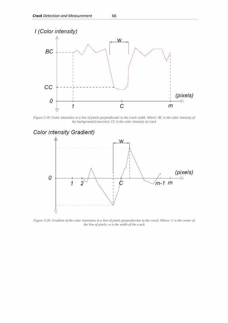
Crack Detection and Measurement 66

Figure 3.19: Color intensities in a line of pixels perpendicular to the crack width. Where: BC is the color intensity of

the background (concrete); CC is the color intensity of crack

Figure 3.20: Gradient of the color intensities in a line of pixels perpendicular to the crack; Where: C is the center of

the line of pixels; w is the width of the crack

Crack Detection and Measurement 67

3.4. Resume on Crack Detection Step

The crack pixels obtained from the method described in 3.3, will be marked on a matrix with the same size of the input picture. Meaning that if the input picture has a resolution of 𝑀𝑀𝑥𝑥𝑁𝑁 pixels, the output matrices will be a matrix of 𝐼𝐼𝑓𝑓𝐿𝐿𝑀𝑀 = 𝑀𝑀𝑥𝑥𝑁𝑁𝑥𝑥3, in which the first layer �𝐼𝐼𝑓𝑓𝐿𝐿𝑀𝑀(𝑍𝑍 = 1)� of the output matrix will have a “1” where a crack pixel is found and “0” elsewhere. This layer will be used for the drawing of the crack pattern. The second layer will have the values of the angle detected where the crack pixels were found and “0” elsewhere and the third layer will have the crack width measured.

The final objective of these algorithms so far is to go from an input RGB picture with a given ROI to two mask matrices with the size of the input picture carrying the information of the crack pattern position and with 2 layers: “angles” and the “width”. This process is resumed by Figure 3.21:

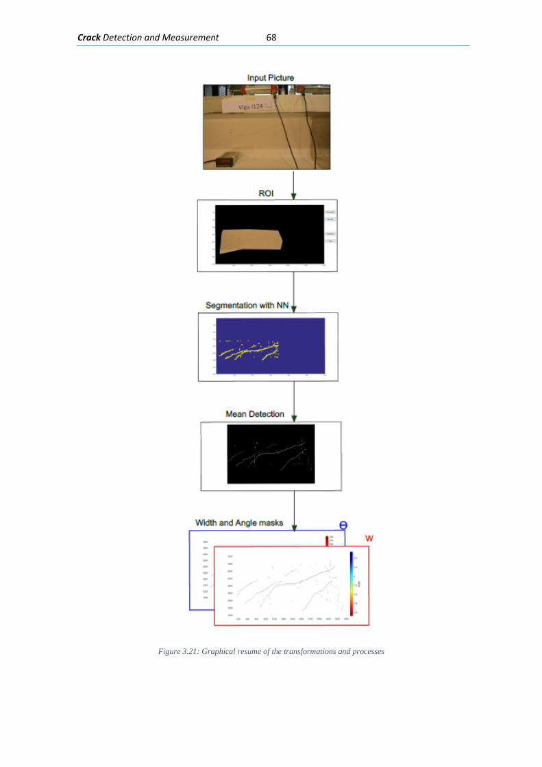
Crack Detection and Measurement 68

Figure 3.21: Graphical resume of the transformations and processes

Cracked Patch Clustering 69

4. Cracked Patch Clustering

For multiple reasons (separation among parallel cracks, recognize longest cracks, recognize wider cracks, etc.), there exists interest to know the quantity of individual cracks that appear in an element.

The previous chapter outputs two masks with the crack width and angle in each pixel; but these values lack information about the individual cracks composed by different pixels in the whole ROI. Hence, it is still unknown how these crack patches group together and make up a single crack in the ROI, also there is no criteria to decide the quantity of cracks. This problem will be addressed in this chapter with the use of clustering techniques.

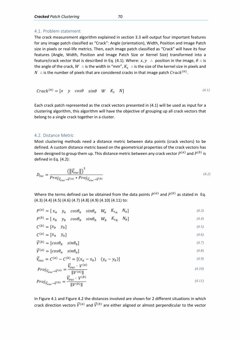
Cracked Patch Clustering 70

4.1. Problem statement The crack measurement algorithm explained in section 3.3 will output four important features for any image patch classified as “Crack”: Angle (orientation), Width, Position and Image Patch size in pixels or real-life metrics. Then, each image patch classified as “Crack” will have its four features (Angle, Width, Position and Image Patch Size or Kernel Size) transformed into a feature/crack vector that is described in Eq. (4.1). Where: 𝑥𝑥,𝑦𝑦 ∴ position in the image, 𝜃𝜃 ∴ is the angle of the crack, 𝑊𝑊 ∴ is the width in “mm”, 𝐾𝐾𝑙𝑙 ∴ is the size of the kernel size in pixels and 𝑁𝑁 ∴ is the number of pixels that are considered cracks in that image patch 𝐶𝐶𝑟𝑟𝑎𝑎𝑐𝑐𝐿𝐿(𝑛𝑛).

𝐶𝐶𝑟𝑟𝑎𝑎𝑐𝑐𝐿𝐿(𝑛𝑛) = [𝑥𝑥 𝑦𝑦 𝑐𝑐𝑐𝑐𝑀𝑀𝜃𝜃 𝑀𝑀𝐿𝐿𝐿𝐿𝜃𝜃 𝑊𝑊 𝐾𝐾𝑙𝑙 𝑁𝑁] (4.1)

Each crack patch represented as the crack vectors presented in (4.1) will be used as input for a clustering algorithm, this algorithm will have the objective of grouping up all crack vectors that belong to a single crack together in a cluster.

4.2. Distance Metric Most clustering methods need a distance metric between data points (crack vectors) to be defined. A custom distance metric based on the geometrical properties of the crack vectors has been designed to group them up. This distance metric between any crack vector 𝑃𝑃(𝑟𝑟) and 𝑃𝑃(𝑏𝑏) is defined in Eq. (4.2):

𝐷𝐷𝑙𝑙𝑙𝑙𝑐𝑐 =��𝑉𝑉�⃗𝑒𝑒𝑒𝑒𝑐𝑐��

3

𝑃𝑃𝑟𝑟𝑐𝑐𝑗𝑗𝑉𝑉��⃗𝑒𝑒𝑒𝑒𝑒𝑒→𝑉𝑉��⃗ (𝑟𝑟) ∗ 𝑃𝑃𝑟𝑟𝑐𝑐𝑗𝑗𝑉𝑉��⃗𝑒𝑒𝑒𝑒𝑒𝑒→𝑉𝑉��⃗ (𝑏𝑏) (4.2)

Where the terms defined can be obtained from the data points 𝑃𝑃(𝑟𝑟) and 𝑃𝑃(𝑏𝑏) as stated in Eq. (4.3) (4.4) (4.5) (4.6) (4.7) (4.8) (4.9) (4.10) (4.11) to:

𝑃𝑃(𝑟𝑟) = [ 𝑥𝑥𝑟𝑟 𝑦𝑦𝑟𝑟 𝑐𝑐𝑐𝑐𝑀𝑀𝜃𝜃𝑟𝑟 𝑀𝑀𝐿𝐿𝐿𝐿𝜃𝜃𝑟𝑟 𝑊𝑊𝑟𝑟 𝐾𝐾𝑙𝑙𝑟𝑟 𝑁𝑁𝑟𝑟] (4.3)

𝑃𝑃(𝑏𝑏) = [ 𝑥𝑥𝑏𝑏 𝑦𝑦𝑏𝑏 𝑐𝑐𝑐𝑐𝑀𝑀𝜃𝜃𝑏𝑏 𝑀𝑀𝐿𝐿𝐿𝐿𝜃𝜃𝑏𝑏 𝑊𝑊𝑏𝑏 𝐾𝐾𝑙𝑙𝑏𝑏 𝑁𝑁𝑏𝑏] (4.4)

𝐶𝐶(𝑏𝑏) = [𝑥𝑥𝑏𝑏 𝑦𝑦𝑏𝑏] (4.5)

𝐶𝐶(𝑟𝑟) = [𝑥𝑥𝑟𝑟 𝑦𝑦𝑟𝑟] (4.6)

𝑉𝑉�⃗ (𝑏𝑏) = [𝑐𝑐𝑐𝑐𝑀𝑀𝜃𝜃𝑏𝑏 𝑀𝑀𝐿𝐿𝐿𝐿𝜃𝜃𝑏𝑏] (4.7)

𝑉𝑉�⃗ (𝑟𝑟) = [𝑐𝑐𝑐𝑐𝑀𝑀𝜃𝜃𝑟𝑟 𝑀𝑀𝐿𝐿𝐿𝐿𝜃𝜃𝑟𝑟] (4.8)

𝑉𝑉�⃗𝑒𝑒𝑒𝑒𝑐𝑐 = 𝐶𝐶(𝑟𝑟) − 𝐶𝐶(𝑏𝑏) = [(𝑥𝑥𝑟𝑟 − 𝑥𝑥𝑏𝑏) (𝑦𝑦𝑟𝑟 − 𝑦𝑦𝑏𝑏)] (4.9)

𝑃𝑃𝑟𝑟𝑐𝑐𝑗𝑗𝑉𝑉��⃗𝑒𝑒𝑒𝑒𝑒𝑒→𝑉𝑉��⃗ (𝑟𝑟) =𝑉𝑉�⃗𝑒𝑒𝑒𝑒𝑐𝑐 ∙ 𝑉𝑉(𝑟𝑟)

‖𝑉𝑉(𝑟𝑟)‖ (4.10)

𝑃𝑃𝑟𝑟𝑐𝑐𝑗𝑗𝑉𝑉��⃗𝑒𝑒𝑒𝑒𝑒𝑒→𝑉𝑉��⃗ (𝑏𝑏) =𝑉𝑉�⃗𝑒𝑒𝑒𝑒𝑐𝑐 ∙ 𝑉𝑉(𝑏𝑏)

‖𝑉𝑉(𝑏𝑏)‖ (4.11)

In Figure 4.1 and Figure 4.2 the distances involved are shown for 2 different situations in which crack direction vectors 𝑉𝑉�⃗ (𝑟𝑟) and 𝑉𝑉�⃗ (𝑏𝑏) are either aligned or almost perpendicular to the vector

Cracked Patch Clustering 71

(𝑉𝑉����⃗𝑒𝑒𝑒𝑒𝑐𝑐) between its coordinates 𝐶𝐶(𝑟𝑟) and 𝐶𝐶(𝑏𝑏). In Figure 4.1 ,both projections 𝑃𝑃𝑟𝑟𝑐𝑐𝑗𝑗𝑉𝑉��⃗𝑒𝑒𝑒𝑒𝑒𝑒→𝑉𝑉��⃗ (𝑟𝑟) and 𝑃𝑃𝑟𝑟𝑐𝑐𝑗𝑗𝑉𝑉��⃗𝑒𝑒𝑒𝑒𝑒𝑒→𝑉𝑉��⃗ (𝑏𝑏) are small and will output a rather low distance 𝐷𝐷𝑙𝑙𝑙𝑙𝑐𝑐 as both projections terms are large and are in the denominator of Eq. (4.2). On the other had in Figure 4.2 when the projections 𝑃𝑃𝑟𝑟𝑐𝑐𝑗𝑗𝑉𝑉��⃗𝑒𝑒𝑒𝑒𝑒𝑒→𝑉𝑉��⃗ (𝑟𝑟) and 𝑃𝑃𝑟𝑟𝑐𝑐𝑗𝑗𝑉𝑉��⃗𝑒𝑒𝑒𝑒𝑒𝑒→𝑉𝑉��⃗ (𝑏𝑏) are larger the distance 𝐷𝐷𝑙𝑙𝑙𝑙𝑐𝑐 is larger. The objective of this distance metric is to make crack data points 𝑃𝑃 that are aligned have a low distance and join them up in a cluster, and from any other situation obtaining a smaller distance 𝐷𝐷𝑙𝑙𝑙𝑙𝑐𝑐.

Figure 4.1: The projection and distances between data points 𝑃𝑃(𝑟𝑟) and 𝑃𝑃(𝑏𝑏)when the Euclidean vector 𝑉𝑉�⃗𝑒𝑒𝑒𝑒𝑐𝑐 is almost perpendicular to both crack direction vectors 𝑉𝑉�⃗ (𝑟𝑟)and 𝑉𝑉�⃗ (𝑏𝑏)

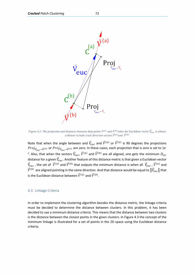
Cracked Patch Clustering 72

Figure 4.2: The projection and distances between data points 𝑃𝑃(𝑟𝑟) and 𝑃𝑃(𝑏𝑏)when the Euclidean vector 𝑉𝑉�⃗𝑒𝑒𝑒𝑒𝑐𝑐 is almost collinear to both crack direction vectors 𝑉𝑉�⃗ (𝑟𝑟)and 𝑉𝑉�⃗ (𝑏𝑏)

Note that when the angle between and 𝑉𝑉�⃗𝑒𝑒𝑒𝑒𝑐𝑐 and 𝑉𝑉�⃗ (𝑟𝑟) or 𝑉𝑉�⃗ (𝑟𝑟) is 90 degrees the projections 𝑃𝑃𝑟𝑟𝑐𝑐𝑗𝑗𝑉𝑉��⃗𝑒𝑒𝑒𝑒𝑒𝑒→𝑉𝑉��⃗ (𝑟𝑟) or 𝑃𝑃𝑟𝑟𝑐𝑐𝑗𝑗𝑉𝑉��⃗𝑒𝑒𝑒𝑒𝑒𝑒→𝑉𝑉��⃗ (𝑟𝑟) are zero. In these cases, each projection that is zero is set to 1e-

4. Also, that when the vectors 𝑉𝑉�⃗𝑒𝑒𝑒𝑒𝑐𝑐, 𝑉𝑉�⃗ (𝑟𝑟) and 𝑉𝑉�⃗ (𝑏𝑏) are all aligned, one gets the minimum 𝐷𝐷𝑙𝑙𝑙𝑙𝑐𝑐 distance for a given 𝑉𝑉�⃗𝑒𝑒𝑒𝑒𝑐𝑐. Another feature of this distance metric is that given a Euclidean vector 𝑉𝑉�⃗𝑒𝑒𝑒𝑒𝑐𝑐 , the set of 𝑉𝑉�⃗ (𝑟𝑟) and 𝑉𝑉�⃗ (𝑏𝑏) that outputs the minimum distance is when all 𝑉𝑉�⃗𝑒𝑒𝑒𝑒𝑐𝑐 , 𝑉𝑉�⃗ (𝑟𝑟) and 𝑉𝑉�⃗ (𝑏𝑏) are aligned pointing in the same direction. And that distance would be equal to �𝑉𝑉�⃗𝑒𝑒𝑒𝑒𝑐𝑐� that is the Euclidean distance between 𝑉𝑉�⃗ (𝑟𝑟) and 𝑉𝑉�⃗ (𝑏𝑏).

4.3. Linkage Criteria

In order to implement the clustering algorithm besides the distance metric, the linkage criteria must be decided to determine the distance between clusters. In this problem, it has been decided to use a minimum distance criteria. This means that the distance between two clusters is the distance between the closest points in the given clusters. In Figure 4.3 the concept of the minimum linkage is illustrated for a set of points in the 2D space using the Euclidean distance criteria.

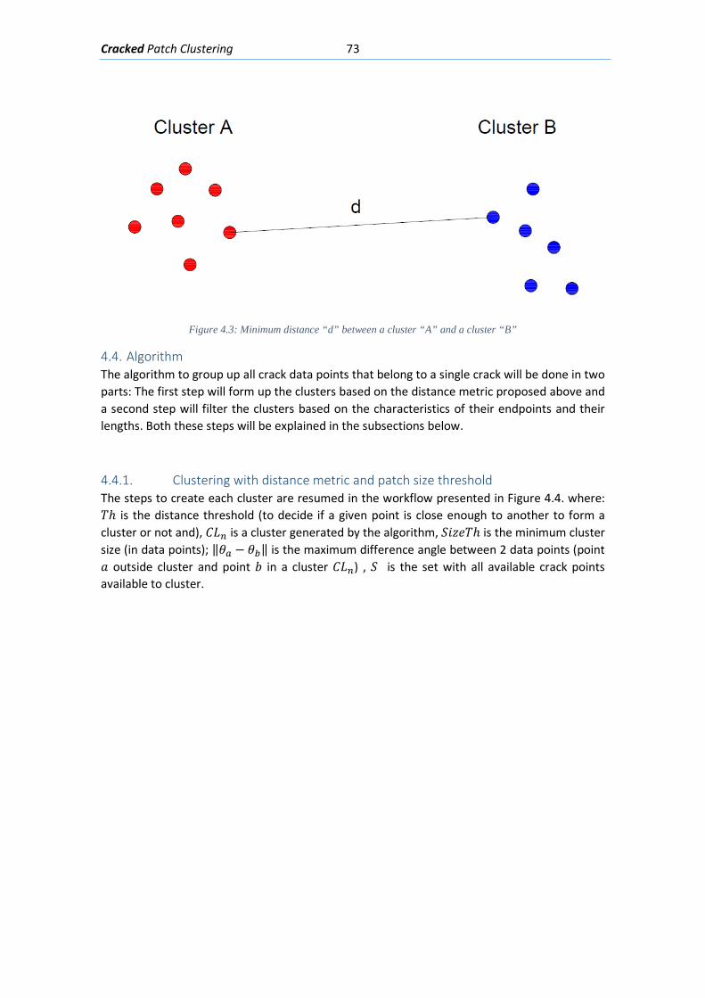
Cracked Patch Clustering 73

Figure 4.3: Minimum distance “d” between a cluster “A” and a cluster “B”

4.4. Algorithm The algorithm to group up all crack data points that belong to a single crack will be done in two parts: The first step will form up the clusters based on the distance metric proposed above and a second step will filter the clusters based on the characteristics of their endpoints and their lengths. Both these steps will be explained in the subsections below.

4.4.1. Clustering with distance metric and patch size threshold The steps to create each cluster are resumed in the workflow presented in Figure 4.4. where: 𝑇𝑇ℎ is the distance threshold (to decide if a given point is close enough to another to form a cluster or not and), 𝐶𝐶𝐿𝐿𝑛𝑛 is a cluster generated by the algorithm, 𝑆𝑆𝐿𝐿𝑧𝑧𝑉𝑉𝑇𝑇ℎ is the minimum cluster size (in data points); ‖𝜃𝜃𝑟𝑟 − 𝜃𝜃𝑏𝑏‖ is the maximum difference angle between 2 data points (point 𝑎𝑎 outside cluster and point 𝑏𝑏 in a cluster 𝐶𝐶𝐿𝐿𝑛𝑛) , 𝑆𝑆 is the set with all available crack points available to cluster.

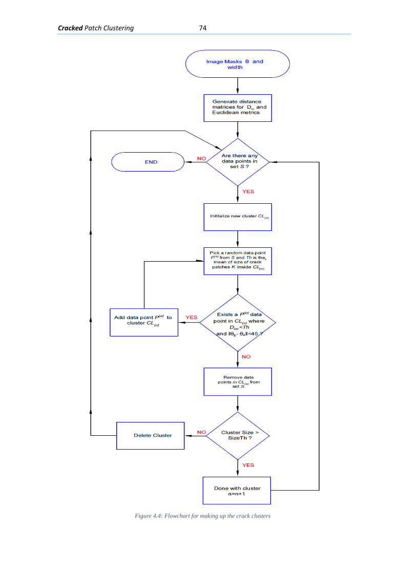
Cracked Patch Clustering 74

Figure 4.4: Flowchart for making up the crack clusters

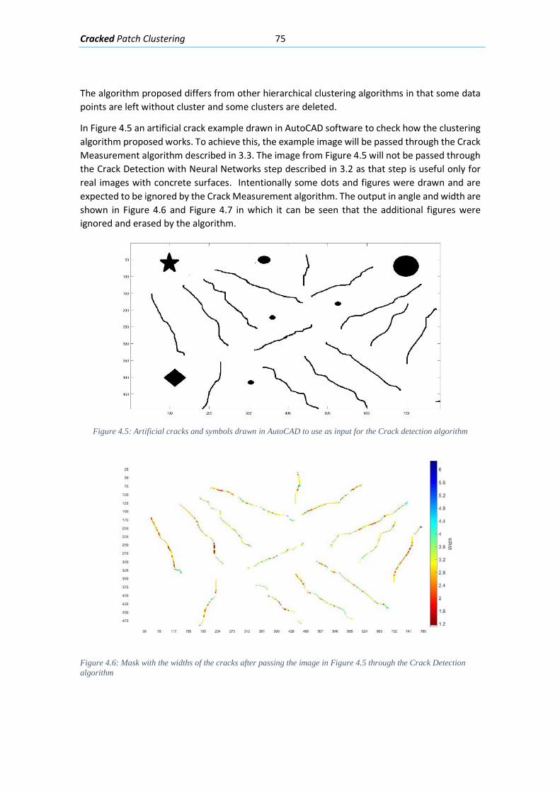
Cracked Patch Clustering 75

The algorithm proposed differs from other hierarchical clustering algorithms in that some data points are left without cluster and some clusters are deleted.

In Figure 4.5 an artificial crack example drawn in AutoCAD software to check how the clustering algorithm proposed works. To achieve this, the example image will be passed through the Crack Measurement algorithm described in 3.3. The image from Figure 4.5 will not be passed through the Crack Detection with Neural Networks step described in 3.2 as that step is useful only for real images with concrete surfaces. Intentionally some dots and figures were drawn and are expected to be ignored by the Crack Measurement algorithm. The output in angle and width are shown in Figure 4.6 and Figure 4.7 in which it can be seen that the additional figures were ignored and erased by the algorithm.

Figure 4.5: Artificial cracks and symbols drawn in AutoCAD to use as input for the Crack detection algorithm

Figure 4.6: Mask with the widths of the cracks after passing the image in Figure 4.5 through the Crack Detection algorithm

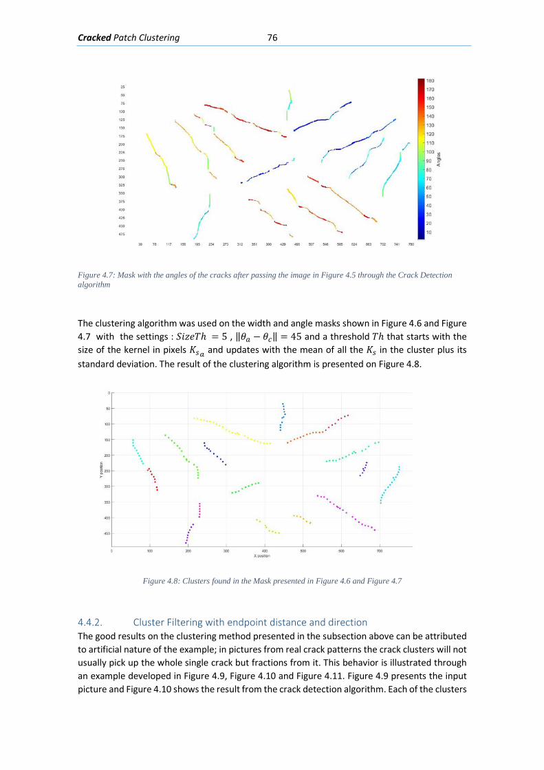
Cracked Patch Clustering 76

Figure 4.7: Mask with the angles of the cracks after passing the image in Figure 4.5 through the Crack Detection algorithm

The clustering algorithm was used on the width and angle masks shown in Figure 4.6 and Figure 4.7 with the settings : 𝑆𝑆𝐿𝐿𝑧𝑧𝑉𝑉𝑇𝑇ℎ = 5 , ‖𝜃𝜃𝑟𝑟 − 𝜃𝜃𝑐𝑐‖ = 45 and a threshold 𝑇𝑇ℎ that starts with the size of the kernel in pixels 𝐾𝐾𝑙𝑙𝑟𝑟 and updates with the mean of all the 𝐾𝐾𝑙𝑙 in the cluster plus its standard deviation. The result of the clustering algorithm is presented on Figure 4.8.

Figure 4.8: Clusters found in the Mask presented in Figure 4.6 and Figure 4.7

4.4.2. Cluster Filtering with endpoint distance and direction The good results on the clustering method presented in the subsection above can be attributed to artificial nature of the example; in pictures from real crack patterns the crack clusters will not usually pick up the whole single crack but fractions from it. This behavior is illustrated through an example developed in Figure 4.9, Figure 4.10 and Figure 4.11. Figure 4.9 presents the input picture and Figure 4.10 shows the result from the crack detection algorithm. Each of the clusters

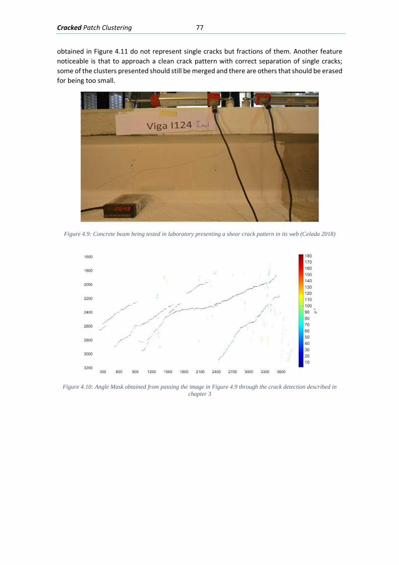
Cracked Patch Clustering 77

obtained in Figure 4.11 do not represent single cracks but fractions of them. Another feature noticeable is that to approach a clean crack pattern with correct separation of single cracks; some of the clusters presented should still be merged and there are others that should be erased for being too small.

Figure 4.9: Concrete beam being tested in laboratory presenting a shear crack pattern in its web (Celada 2018)

Figure 4.10: Angle Mask obtained from passing the image in Figure 4.9 through the crack detection described in

chapter 3

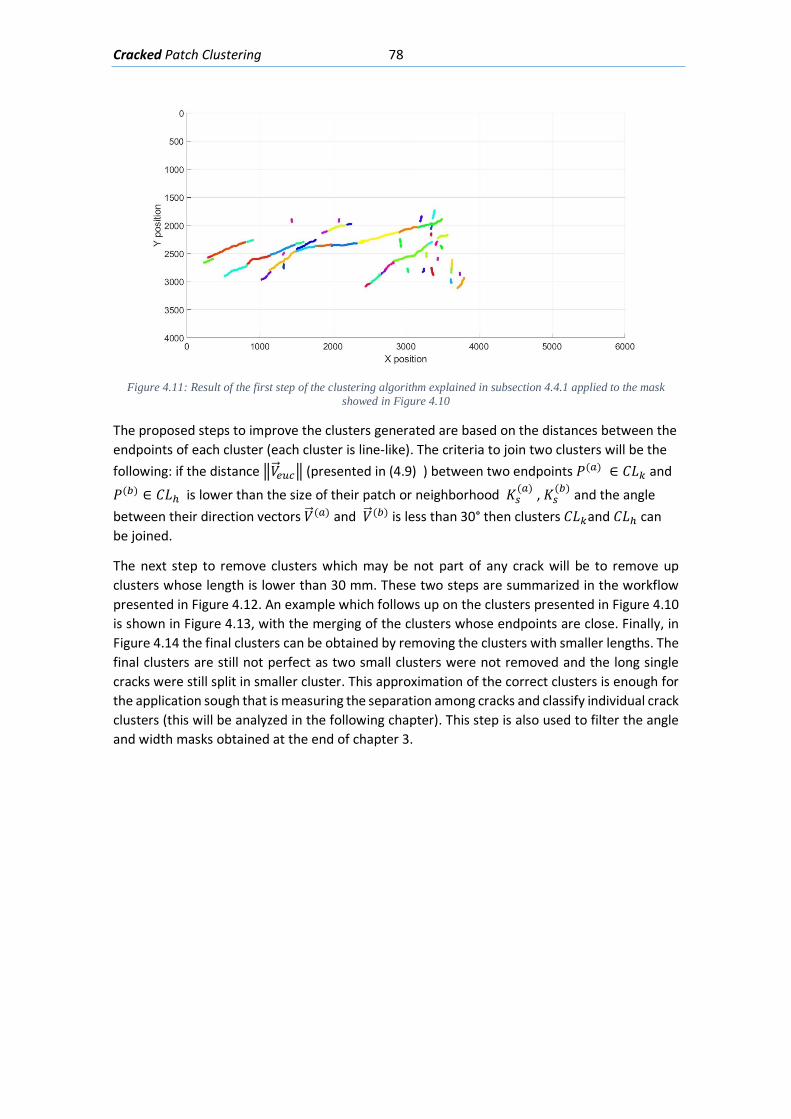
Cracked Patch Clustering 78

Figure 4.11: Result of the first step of the clustering algorithm explained in subsection 4.4.1 applied to the mask

showed in Figure 4.10

The proposed steps to improve the clusters generated are based on the distances between the endpoints of each cluster (each cluster is line-like). The criteria to join two clusters will be the following: if the distance �𝑉𝑉�⃗𝑒𝑒𝑒𝑒𝑐𝑐� (presented in (4.9) ) between two endpoints 𝑃𝑃(𝑟𝑟) ∈ 𝐶𝐶𝐿𝐿𝑘𝑘 and

𝑃𝑃(𝑏𝑏) ∈ 𝐶𝐶𝐿𝐿ℎ is lower than the size of their patch or neighborhood 𝐾𝐾𝑙𝑙(𝑟𝑟) , 𝐾𝐾𝑙𝑙

(𝑏𝑏) and the angle between their direction vectors 𝑉𝑉�⃗ (𝑟𝑟) and 𝑉𝑉�⃗ (𝑏𝑏) is less than 30° then clusters 𝐶𝐶𝐿𝐿𝑘𝑘and 𝐶𝐶𝐿𝐿ℎ can be joined.

The next step to remove clusters which may be not part of any crack will be to remove up clusters whose length is lower than 30 mm. These two steps are summarized in the workflow presented in Figure 4.12. An example which follows up on the clusters presented in Figure 4.10 is shown in Figure 4.13, with the merging of the clusters whose endpoints are close. Finally, in Figure 4.14 the final clusters can be obtained by removing the clusters with smaller lengths. The final clusters are still not perfect as two small clusters were not removed and the long single cracks were still split in smaller cluster. This approximation of the correct clusters is enough for the application sough that is measuring the separation among cracks and classify individual crack clusters (this will be analyzed in the following chapter). This step is also used to filter the angle and width masks obtained at the end of chapter 3.

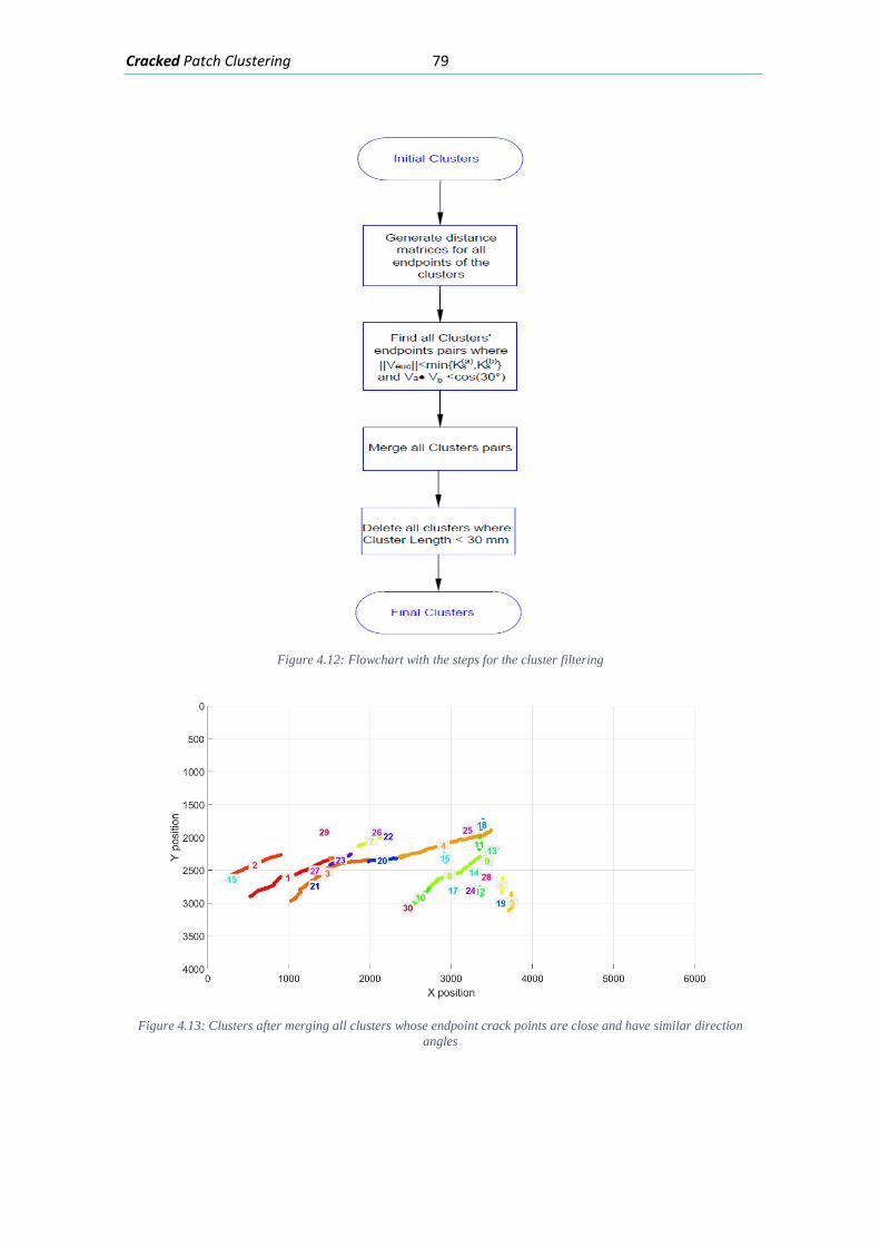
Cracked Patch Clustering 79

Figure 4.12: Flowchart with the steps for the cluster filtering

Figure 4.13: Clusters after merging all clusters whose endpoint crack points are close and have similar direction

angles

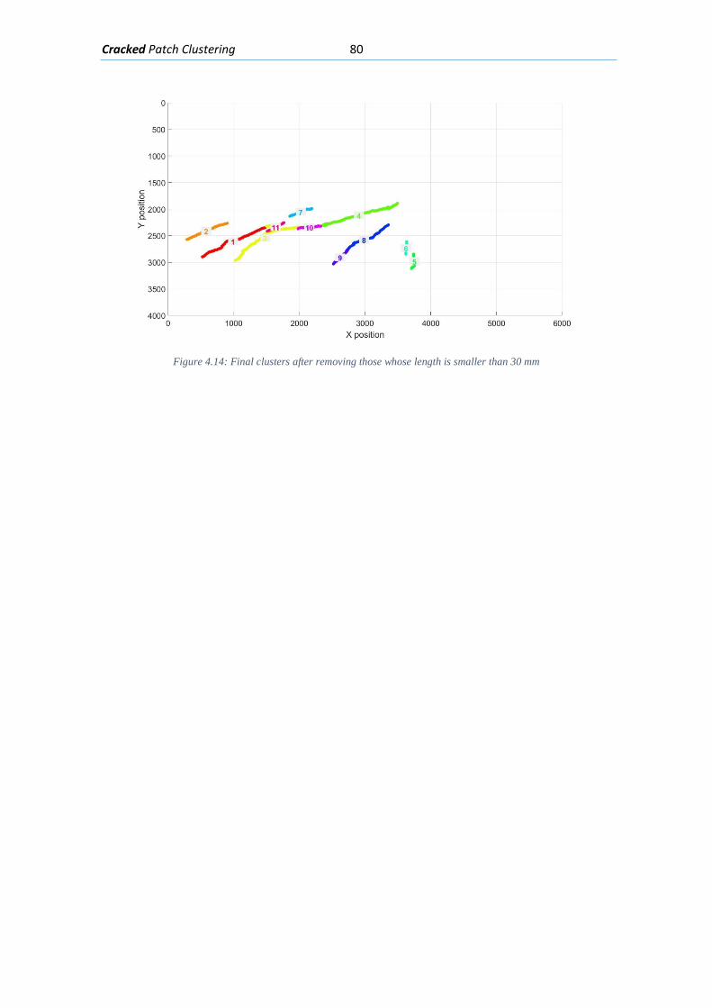
Cracked Patch Clustering 80

Figure 4.14: Final clusters after removing those whose length is smaller than 30 mm

Crack Pattern Classification with Machine Learning 81

5. Crack Pattern Classification with Machine

Learning

The concrete pathologies reviewed in on section 2.4 (flexure, shear, corrosion and bond-slip of the reinforcement bars) express themselves in concrete beams with particular crack patterns that trained technicians can recognize by visual inspection.

In chapters 3 and 4, several methods to identify, measure and cluster cracks have been presented; the main objective of this chapter is to use the output and information obtained from the formerly mentioned methods and use it as an input for a machine learning model to classify the crack patterns into one or several of the reviewed pathologies from section 2.4.

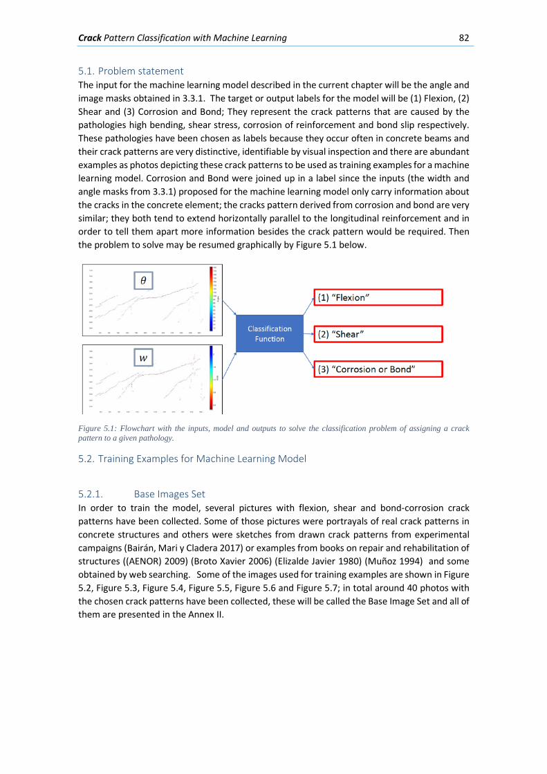
Crack Pattern Classification with Machine Learning 82

5.1. Problem statement The input for the machine learning model described in the current chapter will be the angle and image masks obtained in 3.3.1. The target or output labels for the model will be (1) Flexion, (2) Shear and (3) Corrosion and Bond; They represent the crack patterns that are caused by the pathologies high bending, shear stress, corrosion of reinforcement and bond slip respectively. These pathologies have been chosen as labels because they occur often in concrete beams and their crack patterns are very distinctive, identifiable by visual inspection and there are abundant examples as photos depicting these crack patterns to be used as training examples for a machine learning model. Corrosion and Bond were joined up in a label since the inputs (the width and angle masks from 3.3.1) proposed for the machine learning model only carry information about the cracks in the concrete element; the cracks pattern derived from corrosion and bond are very similar; they both tend to extend horizontally parallel to the longitudinal reinforcement and in order to tell them apart more information besides the crack pattern would be required. Then the problem to solve may be resumed graphically by Figure 5.1 below.

Figure 5.1: Flowchart with the inputs, model and outputs to solve the classification problem of assigning a crack pattern to a given pathology.

5.2. Training Examples for Machine Learning Model

5.2.1. Base Images Set In order to train the model, several pictures with flexion, shear and bond-corrosion crack patterns have been collected. Some of those pictures were portrayals of real crack patterns in concrete structures and others were sketches from drawn crack patterns from experimental campaigns (Bairán, Mari y Cladera 2017) or examples from books on repair and rehabilitation of structures ((AENOR) 2009) (Broto Xavier 2006) (Elizalde Javier 1980) (Muñoz 1994) and some obtained by web searching. Some of the images used for training examples are shown in Figure 5.2, Figure 5.3, Figure 5.4, Figure 5.5, Figure 5.6 and Figure 5.7; in total around 40 photos with the chosen crack patterns have been collected, these will be called the Base Image Set and all of them are presented in the Annex II.

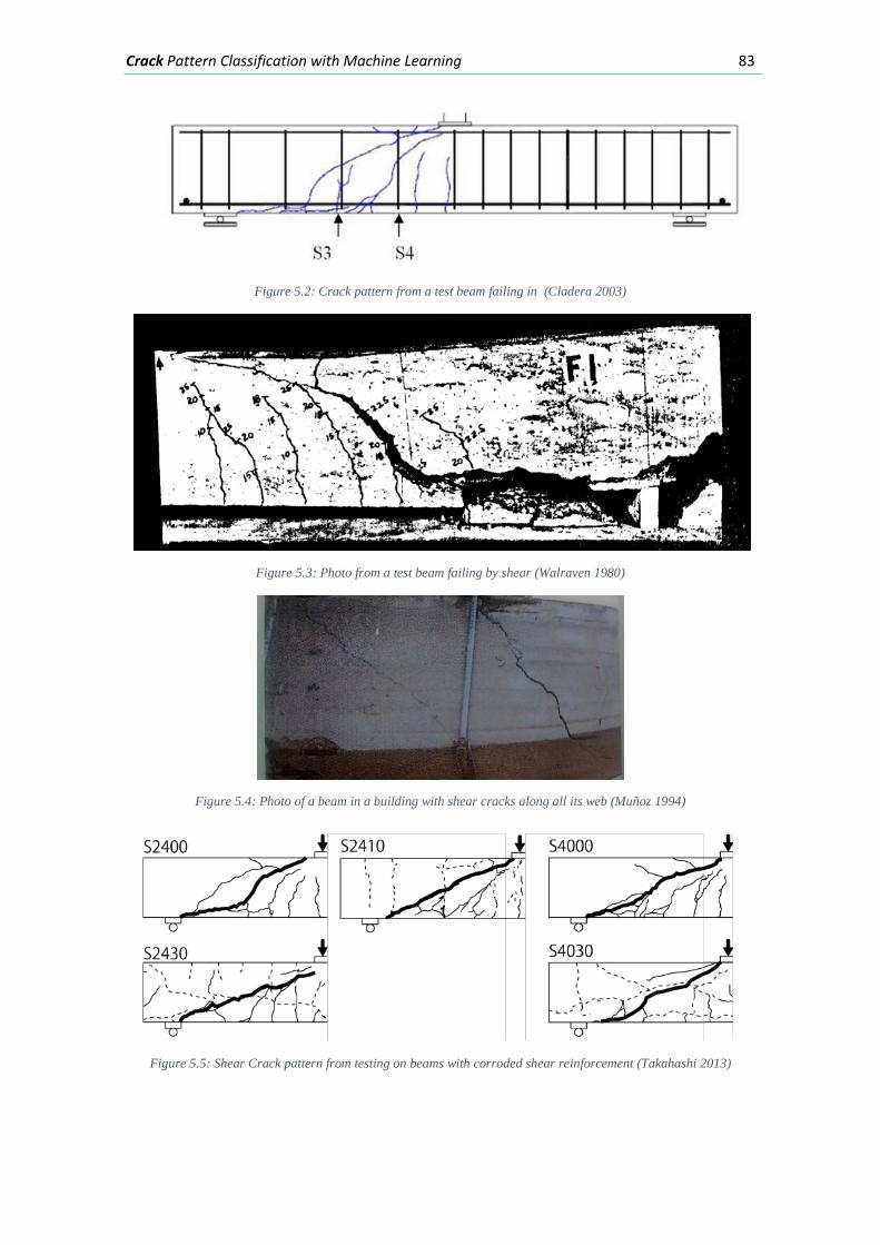
Crack Pattern Classification with Machine Learning 83

Figure 5.2: Crack pattern from a test beam failing in (Cladera 2003)

Figure 5.3: Photo from a test beam failing by shear (Walraven 1980)

Figure 5.4: Photo of a beam in a building with shear cracks along all its web (Muñoz 1994)

Figure 5.5: Shear Crack pattern from testing on beams with corroded shear reinforcement (Takahashi 2013)

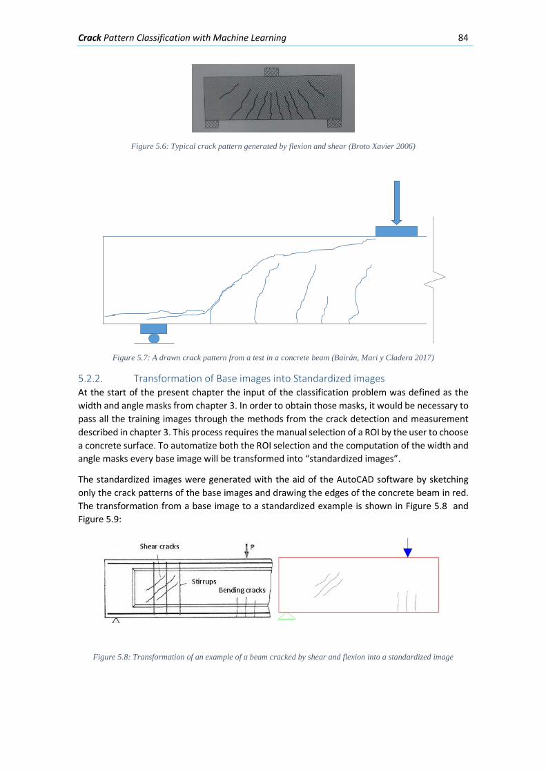
Crack Pattern Classification with Machine Learning 84

Figure 5.6: Typical crack pattern generated by flexion and shear (Broto Xavier 2006)

Figure 5.7: A drawn crack pattern from a test in a concrete beam (Bairán, Mari y Cladera 2017)

5.2.2. Transformation of Base images into Standardized images At the start of the present chapter the input of the classification problem was defined as the width and angle masks from chapter 3. In order to obtain those masks, it would be necessary to pass all the training images through the methods from the crack detection and measurement described in chapter 3. This process requires the manual selection of a ROI by the user to choose a concrete surface. To automatize both the ROI selection and the computation of the width and angle masks every base image will be transformed into “standardized images”.

The standardized images were generated with the aid of the AutoCAD software by sketching only the crack patterns of the base images and drawing the edges of the concrete beam in red. The transformation from a base image to a standardized example is shown in Figure 5.8 and Figure 5.9:

Figure 5.8: Transformation of an example of a beam cracked by shear and flexion into a standardized image

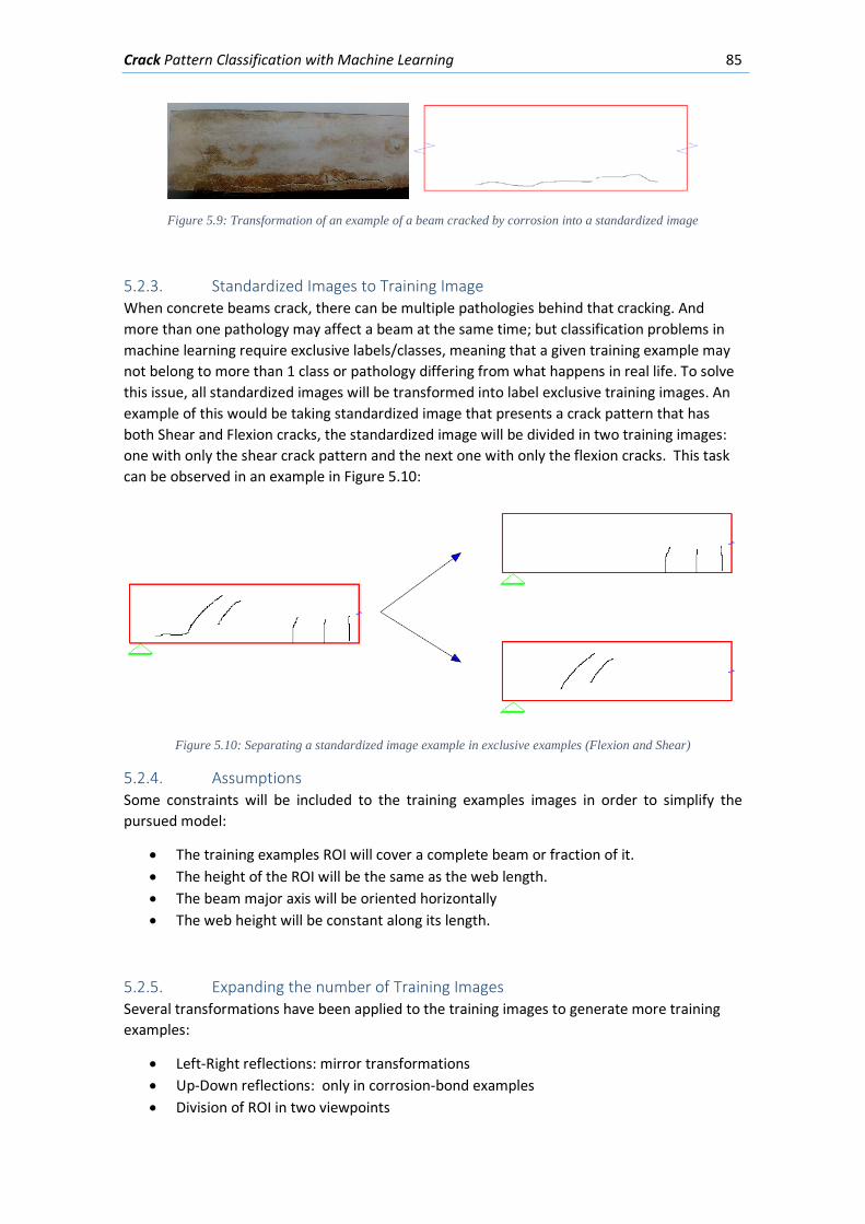
Crack Pattern Classification with Machine Learning 85

Figure 5.9: Transformation of an example of a beam cracked by corrosion into a standardized image

5.2.3. Standardized Images to Training Image When concrete beams crack, there can be multiple pathologies behind that cracking. And more than one pathology may affect a beam at the same time; but classification problems in machine learning require exclusive labels/classes, meaning that a given training example may not belong to more than 1 class or pathology differing from what happens in real life. To solve this issue, all standardized images will be transformed into label exclusive training images. An example of this would be taking standardized image that presents a crack pattern that has both Shear and Flexion cracks, the standardized image will be divided in two training images: one with only the shear crack pattern and the next one with only the flexion cracks. This task can be observed in an example in Figure 5.10:

Figure 5.10: Separating a standardized image example in exclusive examples (Flexion and Shear)

5.2.4. Assumptions Some constraints will be included to the training examples images in order to simplify the pursued model:

• The training examples ROI will cover a complete beam or fraction of it. • The height of the ROI will be the same as the web length. • The beam major axis will be oriented horizontally • The web height will be constant along its length.

5.2.5. Expanding the number of Training Images Several transformations have been applied to the training images to generate more training examples:

• Left-Right reflections: mirror transformations • Up-Down reflections: only in corrosion-bond examples • Division of ROI in two viewpoints

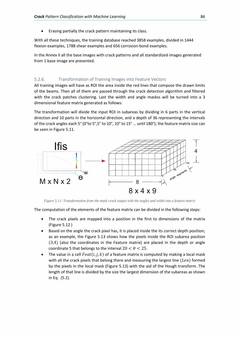
Crack Pattern Classification with Machine Learning 86

• Erasing partially the crack pattern maintaining its class.

With all these techniques, the training database reached 3858 examples, divided in 1444 flexion examples, 1788 shear examples and 656 corrosion-bond examples.

In the Annex II all the base images with crack patterns and all standardized images generated from 1 base image are presented.

5.2.6. Transformation of Training Images into Feature Vectors All training images will have as ROI the area inside the red lines that compose the drawn limits of the beams. Then all of them are passed through the crack detection algorithm and filtered with the crack patches clustering. Last the width and angle maskss will be turned into a 3 dimensional feature matrix generated as follows:

The transformation will divide the input ROI in subareas by dividing in 6 parts in the vertical direction and 10 parts in the horizontal direction, and a depth of 36 representing the intervals of the crack angles each 5° (0°to 5°,5° to 10°, 10° to 15° … until 180°); the feature matrix size can be seen in Figure 5.11.

Figure 5.11: Transformation from the mask crack output with the angles and width into a feature matrix

The computation of the elements of the feature matrix can be divided in the following steps:

• The crack pixels are mapped into a position in the first to dimensions of the matrix (Figure 5.12 )

• Based on the angle the crack pixel has, it is placed inside the its correct depth position; as an example, the Figure 5.13 shows how the pixels inside the ROI subarea position (3,4) (also the coordinates in the Feature matrix) are placed in the depth or angle coordinate 5 that belongs to the interval 20 < 𝜃𝜃 < 25.

• The value in a cell 𝐹𝐹𝑉𝑉𝑎𝑎𝑡𝑡(𝐿𝐿, 𝑗𝑗,𝐿𝐿) of a feature matrix is computed by making a local mask with all the crack pixels that belong there and measuring the largest line (𝐿𝐿𝑉𝑉𝐿𝐿) formed by the pixels in the local mask (Figure 5.13) with the aid of the Hough transform. The length of that line is divided by the size the largest dimension of the subareas as shown in Eq. (5.1).

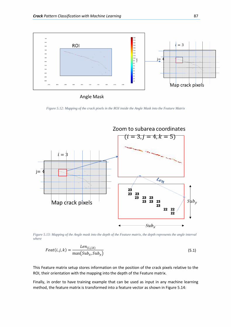
Crack Pattern Classification with Machine Learning 87

Figure 5.12: Mapping of the crack pixels in the ROI inside the Angle Mask into the Feature Matrix

Figure 5.13: Mapping of the Angle mask into the depth of the Feature matrix, the depth represents the angle interval where

𝐹𝐹𝑉𝑉𝑎𝑎𝑡𝑡(𝐿𝐿, 𝑗𝑗,𝐿𝐿) =𝐿𝐿𝑉𝑉𝐿𝐿(𝑖𝑖,𝑗𝑗,𝑘𝑘)

max �𝑆𝑆𝑉𝑉𝑏𝑏𝑥𝑥,𝑆𝑆𝑉𝑉𝑏𝑏𝑦𝑦� (5.1)

This Feature matrix setup stores information on the position of the crack pixels relative to the ROI, their orientation with the mapping into the depth of the Feature matrix.

Finally, in order to have training example that can be used as input in any machine learning method, the feature matrix is transformed into a feature vector as shown in Figure 5.14:

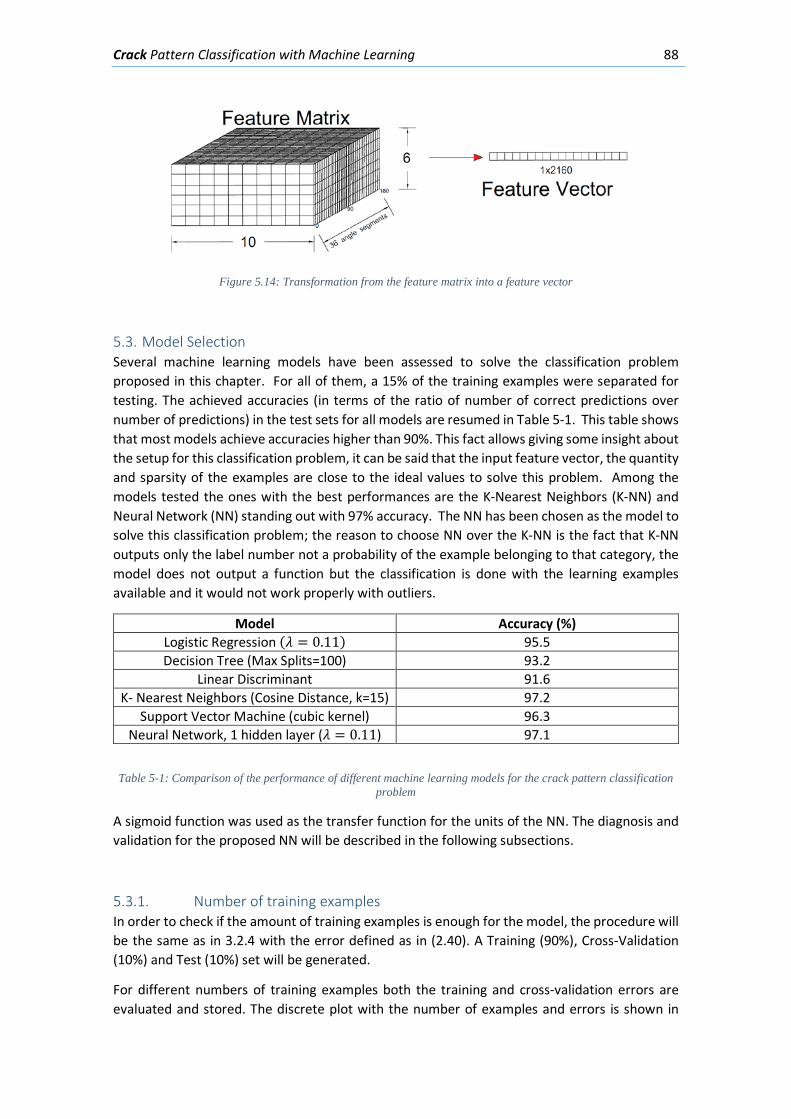
Crack Pattern Classification with Machine Learning 88

Figure 5.14: Transformation from the feature matrix into a feature vector

5.3. Model Selection Several machine learning models have been assessed to solve the classification problem proposed in this chapter. For all of them, a 15% of the training examples were separated for testing. The achieved accuracies (in terms of the ratio of number of correct predictions over number of predictions) in the test sets for all models are resumed in Table 5-1. This table shows that most models achieve accuracies higher than 90%. This fact allows giving some insight about the setup for this classification problem, it can be said that the input feature vector, the quantity and sparsity of the examples are close to the ideal values to solve this problem. Among the models tested the ones with the best performances are the K-Nearest Neighbors (K-NN) and Neural Network (NN) standing out with 97% accuracy. The NN has been chosen as the model to solve this classification problem; the reason to choose NN over the K-NN is the fact that K-NN outputs only the label number not a probability of the example belonging to that category, the model does not output a function but the classification is done with the learning examples available and it would not work properly with outliers.

Model Accuracy (%) Logistic Regression (𝜆𝜆 = 0.11) 95.5 Decision Tree (Max Splits=100) 93.2

Linear Discriminant 91.6 K- Nearest Neighbors (Cosine Distance, k=15) 97.2

Support Vector Machine (cubic kernel) 96.3 Neural Network, 1 hidden layer (𝜆𝜆 = 0.11) 97.1

Table 5-1: Comparison of the performance of different machine learning models for the crack pattern classification problem

A sigmoid function was used as the transfer function for the units of the NN. The diagnosis and validation for the proposed NN will be described in the following subsections.

5.3.1. Number of training examples In order to check if the amount of training examples is enough for the model, the procedure will be the same as in 3.2.4 with the error defined as in (2.40). A Training (90%), Cross-Validation (10%) and Test (10%) set will be generated.

For different numbers of training examples both the training and cross-validation errors are evaluated and stored. The discrete plot with the number of examples and errors is shown in

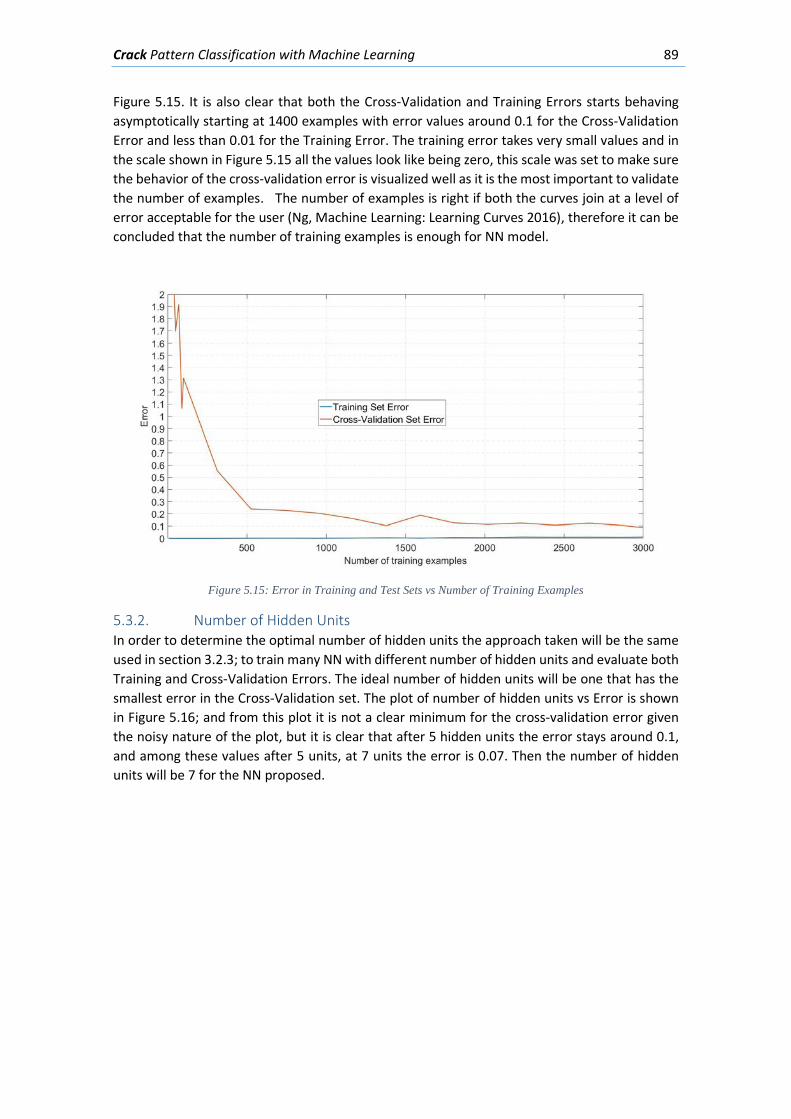
Crack Pattern Classification with Machine Learning 89

Figure 5.15. It is also clear that both the Cross-Validation and Training Errors starts behaving asymptotically starting at 1400 examples with error values around 0.1 for the Cross-Validation Error and less than 0.01 for the Training Error. The training error takes very small values and in the scale shown in Figure 5.15 all the values look like being zero, this scale was set to make sure the behavior of the cross-validation error is visualized well as it is the most important to validate the number of examples. The number of examples is right if both the curves join at a level of error acceptable for the user (Ng, Machine Learning: Learning Curves 2016), therefore it can be concluded that the number of training examples is enough for NN model.

Figure 5.15: Error in Training and Test Sets vs Number of Training Examples

5.3.2. Number of Hidden Units In order to determine the optimal number of hidden units the approach taken will be the same used in section 3.2.3; to train many NN with different number of hidden units and evaluate both Training and Cross-Validation Errors. The ideal number of hidden units will be one that has the smallest error in the Cross-Validation set. The plot of number of hidden units vs Error is shown in Figure 5.16; and from this plot it is not a clear minimum for the cross-validation error given the noisy nature of the plot, but it is clear that after 5 hidden units the error stays around 0.1, and among these values after 5 units, at 7 units the error is 0.07. Then the number of hidden units will be 7 for the NN proposed.

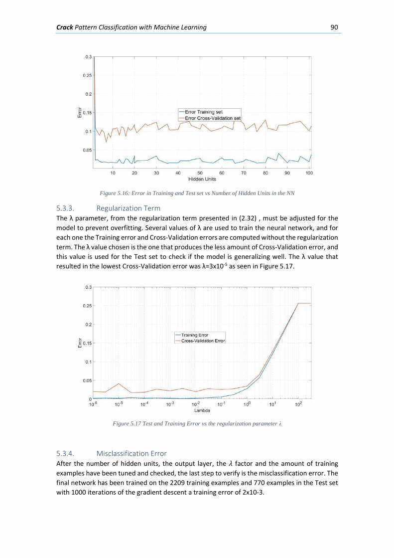
Crack Pattern Classification with Machine Learning 90

Figure 5.16: Error in Training and Test set vs Number of Hidden Units in the NN

5.3.3. Regularization Term The λ parameter, from the regularization term presented in (2.32) , must be adjusted for the model to prevent overfitting. Several values of λ are used to train the neural network, and for each one the Training error and Cross-Validation errors are computed without the regularization term. The λ value chosen is the one that produces the less amount of Cross-Validation error, and this value is used for the Test set to check if the model is generalizing well. The λ value that resulted in the lowest Cross-Validation error was λ=3x10-5 as seen in Figure 5.17.

Figure 5.17 Test and Training Error vs the regularization parameter λ

5.3.4. Misclassification Error After the number of hidden units, the output layer, the 𝜆𝜆 factor and the amount of training examples have been tuned and checked, the last step to verify is the misclassification error. The final network has been trained on the 2209 training examples and 770 examples in the Test set with 1000 iterations of the gradient descent a training error of 2x10-3.

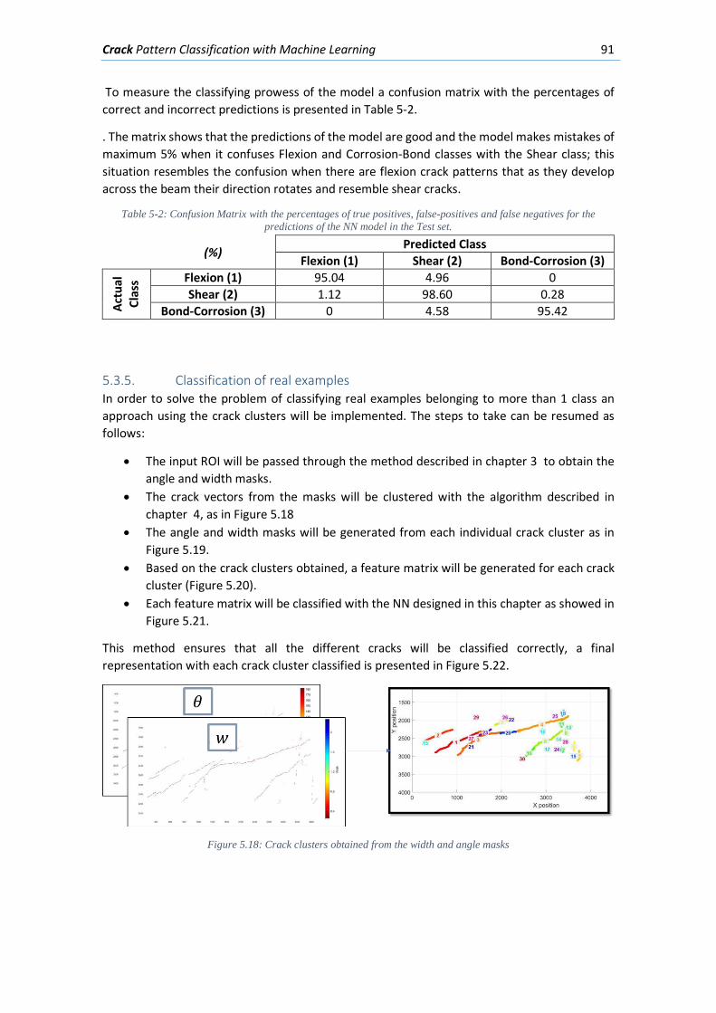
Crack Pattern Classification with Machine Learning 91

To measure the classifying prowess of the model a confusion matrix with the percentages of correct and incorrect predictions is presented in Table 5-2.

. The matrix shows that the predictions of the model are good and the model makes mistakes of maximum 5% when it confuses Flexion and Corrosion-Bond classes with the Shear class; this situation resembles the confusion when there are flexion crack patterns that as they develop across the beam their direction rotates and resemble shear cracks.

Table 5-2: Confusion Matrix with the percentages of true positives, false-positives and false negatives for the predictions of the NN model in the Test set.

(%) Predicted Class Flexion (1) Shear (2) Bond-Corrosion (3)

Actu

al

Clas

s Flexion (1) 95.04 4.96 0 Shear (2) 1.12 98.60 0.28

Bond-Corrosion (3) 0 4.58 95.42

5.3.5. Classification of real examples In order to solve the problem of classifying real examples belonging to more than 1 class an approach using the crack clusters will be implemented. The steps to take can be resumed as follows:

• The input ROI will be passed through the method described in chapter 3 to obtain the angle and width masks.

• The crack vectors from the masks will be clustered with the algorithm described in chapter 4, as in Figure 5.18

• The angle and width masks will be generated from each individual crack cluster as in Figure 5.19.

• Based on the crack clusters obtained, a feature matrix will be generated for each crack cluster (Figure 5.20).

• Each feature matrix will be classified with the NN designed in this chapter as showed in Figure 5.21.

This method ensures that all the different cracks will be classified correctly, a final representation with each crack cluster classified is presented in Figure 5.22.

Figure 5.18: Crack clusters obtained from the width and angle masks

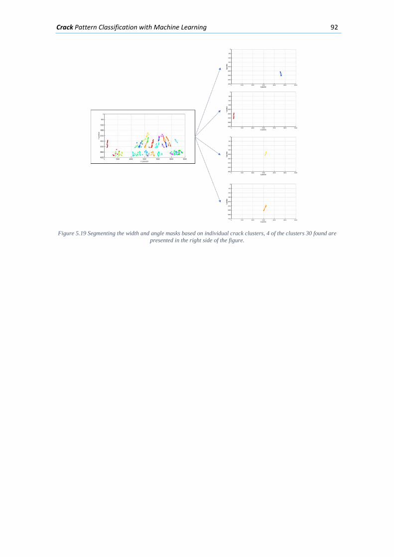
Crack Pattern Classification with Machine Learning 92

Figure 5.19 Segmenting the width and angle masks based on individual crack clusters, 4 of the clusters 30 found are

presented in the right side of the figure.

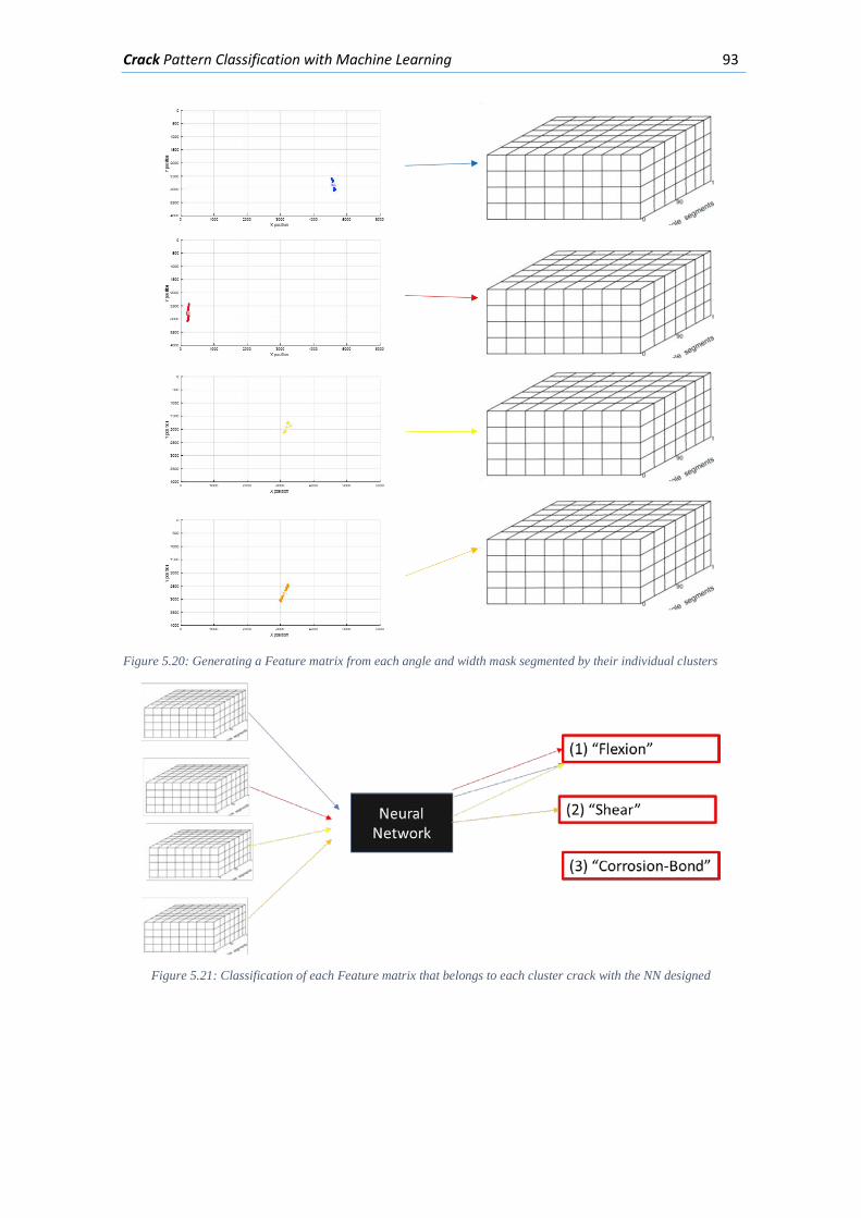
Crack Pattern Classification with Machine Learning 93

Figure 5.20: Generating a Feature matrix from each angle and width mask segmented by their individual clusters

Figure 5.21: Classification of each Feature matrix that belongs to each cluster crack with the NN designed

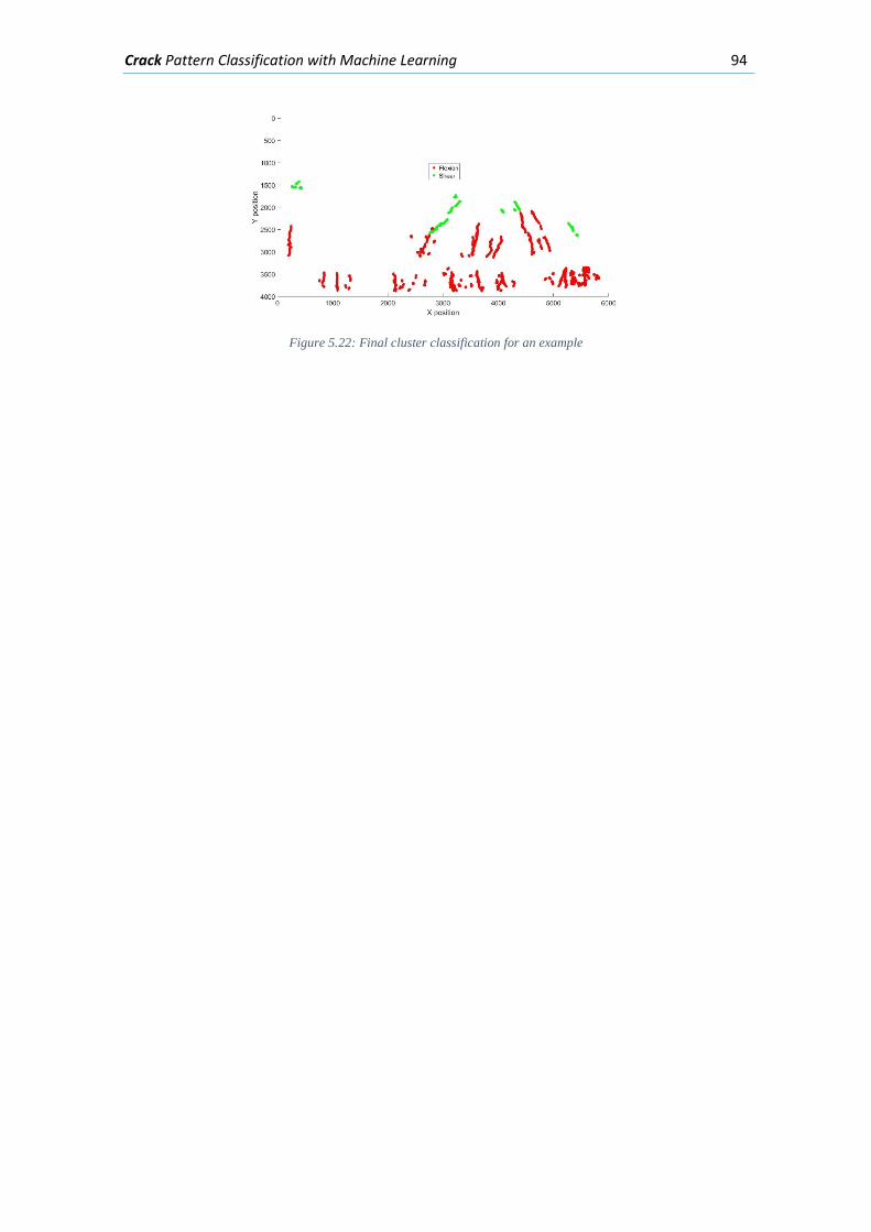
Crack Pattern Classification with Machine Learning 94

Figure 5.22: Final cluster classification for an example

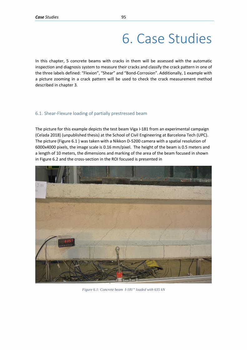
Case Studies 95

6. Case Studies

In this chapter, 5 concrete beams with cracks in them will be assessed with the automatic inspection and diagnosis system to measure their cracks and classify the crack pattern in one of the three labels defined: “Flexion”, “Shear” and “Bond-Corrosion”. Additionally, 1 example with a picture zooming in a crack pattern will be used to check the crack measurement method described in chapter 3.

6.1. Shear-Flexure loading of partially prestressed beam

The picture for this example depicts the test beam Viga I-181 from an experimental campaign (Celada 2018) (unpublished thesis) at the School of Civil Engineering at Barcelona Tech (UPC). The picture (Figure 6.1 ) was taken with a Nikkon D-5200 camera with a spatial resolution of 6000x4000 pixels, the image scale is 0.16 mm/pixel. The height of the beam is 0.5 meters and a length of 10 meters, the dimensions and marking of the area of the beam focused in shown in Figure 6.2 and the cross-section in the ROI focused is presented in

Figure 6.1: Concrete beam I-181” loaded with 635 kN

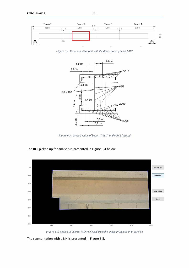
Case Studies 96

Figure 6.2: Elevation viewpoint with the dimensions of beam I-181

Figure 6.3: Cross-Section of beam “I-181” in the ROI focused

The ROI picked up for analysis is presented in Figure 6.4 below.

Figure 6.4: Region of interest (ROI) selected from the image presented in Figure 6.1

The segmentation with a NN is presented in Figure 6.5.

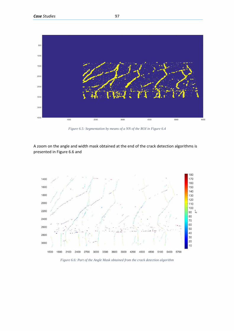
Case Studies 97

Figure 6.5: Segmentation by means of a NN of the ROI in Figure 6.4

A zoom on the angle and width mask obtained at the end of the crack detection algorithms is presented in Figure 6.6 and

Figure 6.6: Part of the Angle Mask obtained from the crack detection algorithm

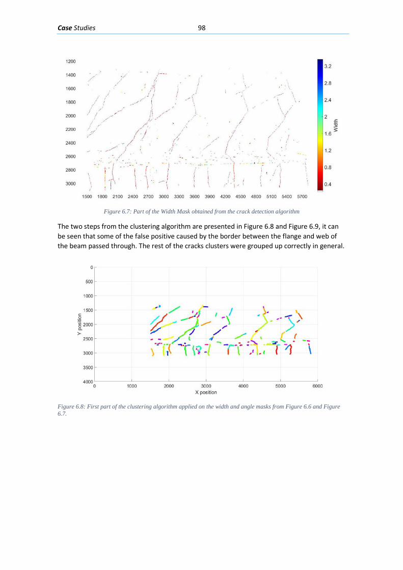
Case Studies 98

Figure 6.7: Part of the Width Mask obtained from the crack detection algorithm

The two steps from the clustering algorithm are presented in Figure 6.8 and Figure 6.9, it can be seen that some of the false positive caused by the border between the flange and web of the beam passed through. The rest of the cracks clusters were grouped up correctly in general.

Figure 6.8: First part of the clustering algorithm applied on the width and angle masks from Figure 6.6 and Figure 6.7.

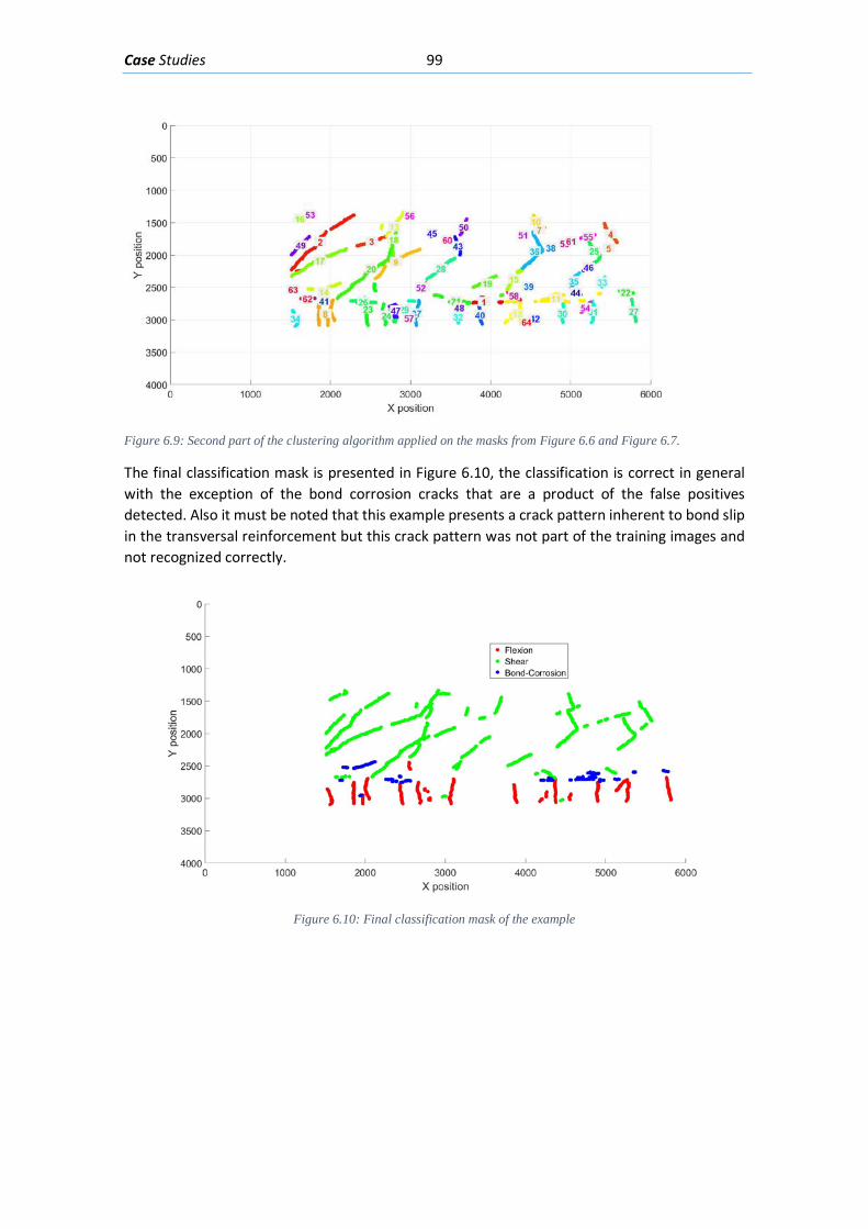
Case Studies 99

Figure 6.9: Second part of the clustering algorithm applied on the masks from Figure 6.6 and Figure 6.7.

The final classification mask is presented in Figure 6.10, the classification is correct in general with the exception of the bond corrosion cracks that are a product of the false positives detected. Also it must be noted that this example presents a crack pattern inherent to bond slip in the transversal reinforcement but this crack pattern was not part of the training images and not recognized correctly.

Figure 6.10: Final classification mask of the example

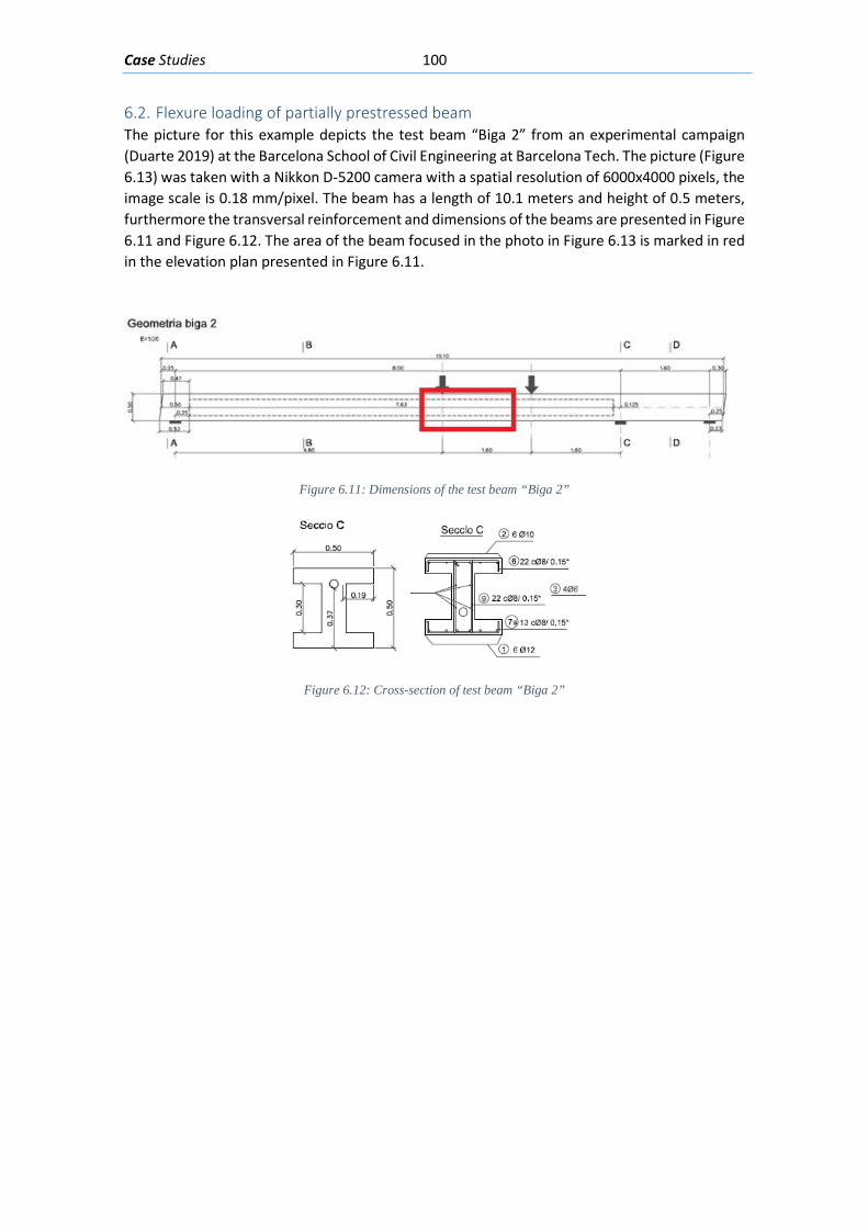
Case Studies 100

6.2. Flexure loading of partially prestressed beam The picture for this example depicts the test beam “Biga 2” from an experimental campaign (Duarte 2019) at the Barcelona School of Civil Engineering at Barcelona Tech. The picture (Figure 6.13) was taken with a Nikkon D-5200 camera with a spatial resolution of 6000x4000 pixels, the image scale is 0.18 mm/pixel. The beam has a length of 10.1 meters and height of 0.5 meters, furthermore the transversal reinforcement and dimensions of the beams are presented in Figure 6.11 and Figure 6.12. The area of the beam focused in the photo in Figure 6.13 is marked in red in the elevation plan presented in Figure 6.11.

Figure 6.11: Dimensions of the test beam “Biga 2”

Figure 6.12: Cross-section of test beam “Biga 2”

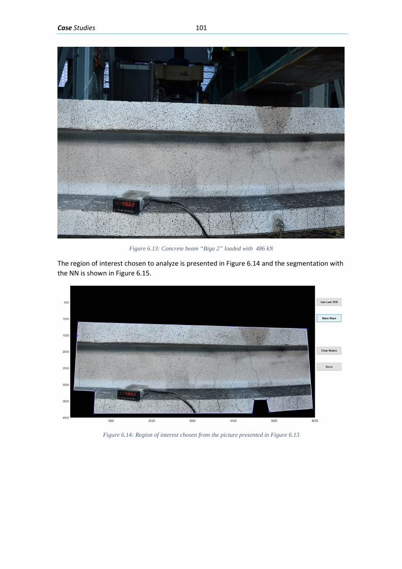
Case Studies 101

Figure 6.13: Concrete beam “Biga 2” loaded with 486 kN

The region of interest chosen to analyze is presented in Figure 6.14 and the segmentation with the NN is shown in Figure 6.15.

Figure 6.14: Region of interest chosen from the picture presented in Figure 6.13

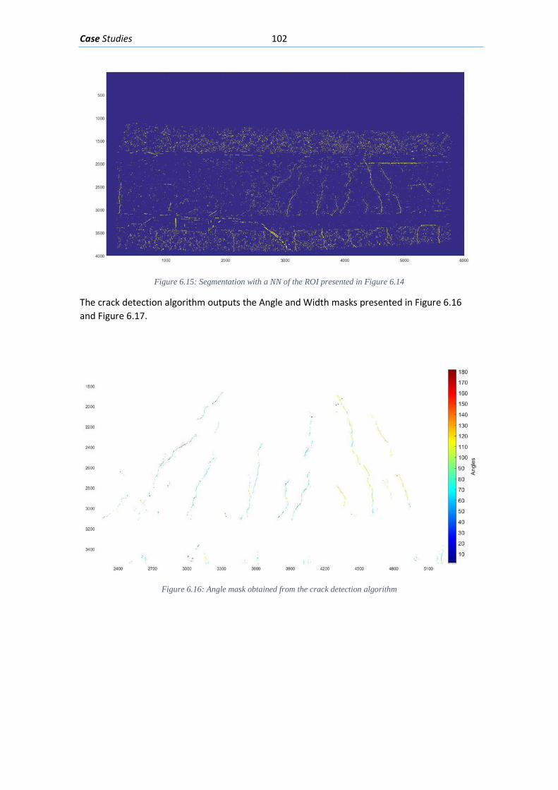
Case Studies 102

Figure 6.15: Segmentation with a NN of the ROI presented in Figure 6.14

The crack detection algorithm outputs the Angle and Width masks presented in Figure 6.16 and Figure 6.17.

Figure 6.16: Angle mask obtained from the crack detection algorithm

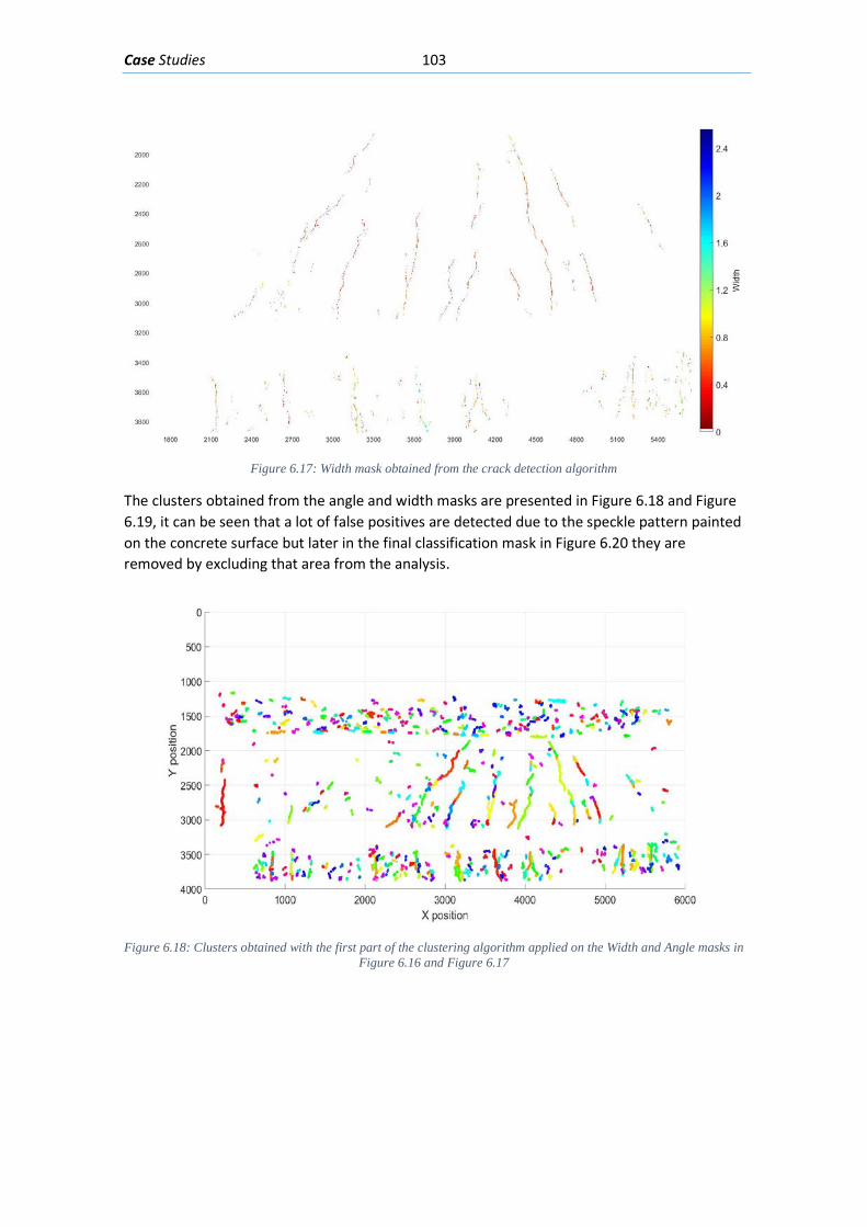
Case Studies 103

Figure 6.17: Width mask obtained from the crack detection algorithm

The clusters obtained from the angle and width masks are presented in Figure 6.18 and Figure 6.19, it can be seen that a lot of false positives are detected due to the speckle pattern painted on the concrete surface but later in the final classification mask in Figure 6.20 they are removed by excluding that area from the analysis.

Figure 6.18: Clusters obtained with the first part of the clustering algorithm applied on the Width and Angle masks in

Figure 6.16 and Figure 6.17

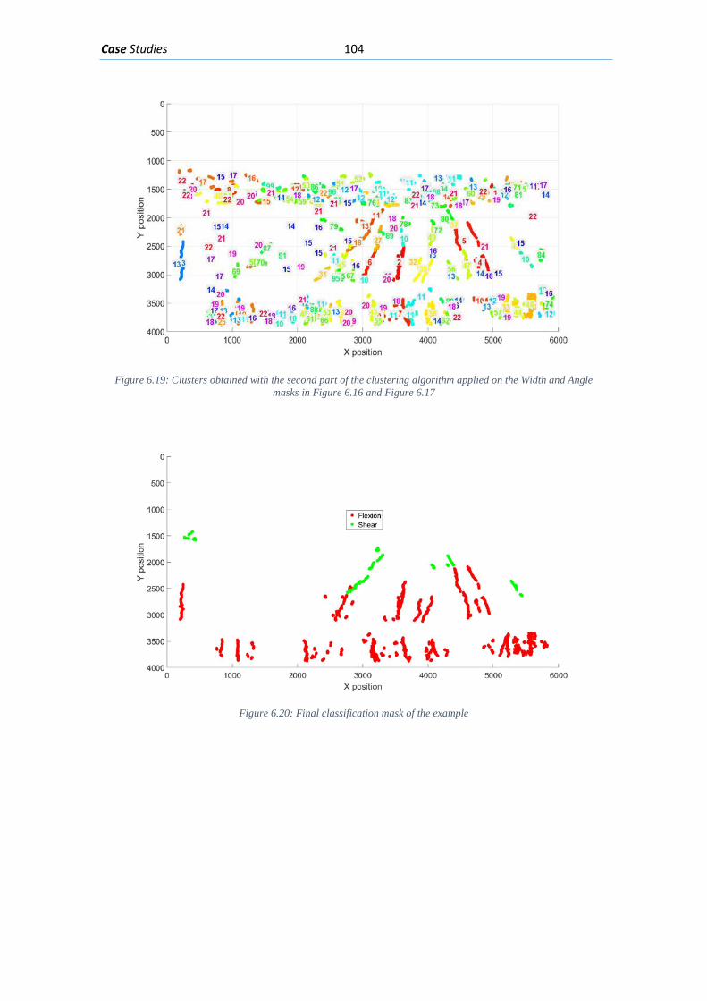
Case Studies 104

Figure 6.19: Clusters obtained with the second part of the clustering algorithm applied on the Width and Angle

masks in Figure 6.16 and Figure 6.17

Figure 6.20: Final classification mask of the example

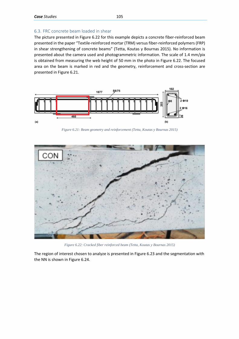
Case Studies 105

6.3. FRC concrete beam loaded in shear The picture presented in Figure 6.22 for this example depicts a concrete fiber-reinforced beam presented in the paper “Textile-reinforced mortar (TRM) versus fiber-reinforced polymers (FRP) in shear strengthening of concrete beams” (Tetta, Koutas y Bournas 2015). No information is presented about the camera used and photogrammetric information. The scale of 1.4 mm/pix is obtained from measuring the web height of 50 mm in the photo in Figure 6.22. The focused area on the beam is marked in red and the geometry, reinforcement and cross-section are presented in Figure 6.21.

Figure 6.21: Beam geometry and reinforcement (Tetta, Koutas y Bournas 2015)

Figure 6.22: Cracked fiber reinforced beam (Tetta, Koutas y Bournas 2015)

The region of interest chosen to analyze is presented in Figure 6.23 and the segmentation with the NN is shown in Figure 6.24.

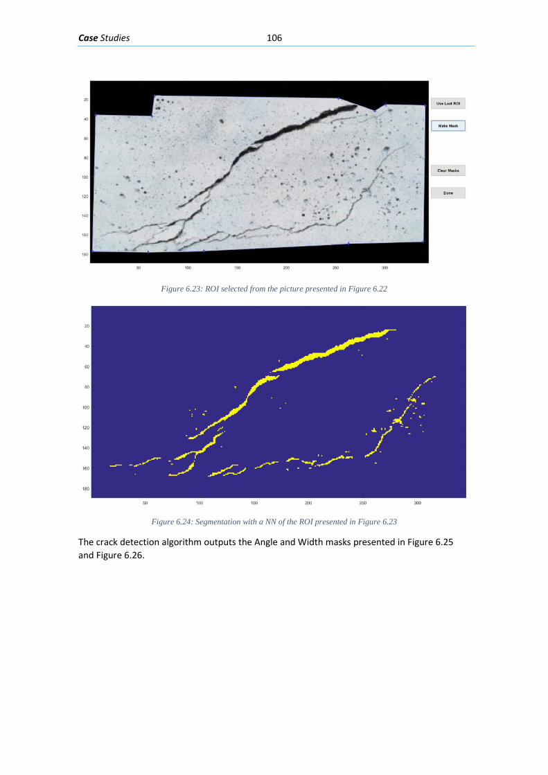
Case Studies 106

Figure 6.23: ROI selected from the picture presented in Figure 6.22

Figure 6.24: Segmentation with a NN of the ROI presented in Figure 6.23

The crack detection algorithm outputs the Angle and Width masks presented in Figure 6.25 and Figure 6.26.

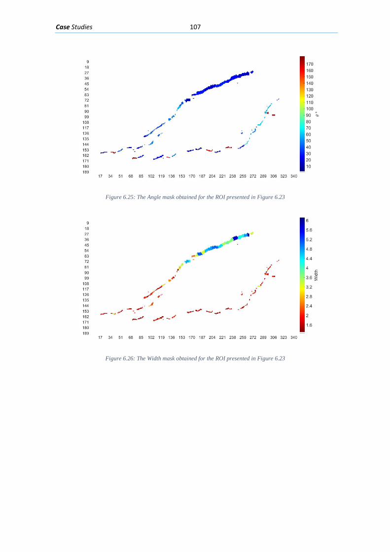
Case Studies 107

Figure 6.25: The Angle mask obtained for the ROI presented in Figure 6.23

Figure 6.26: The Width mask obtained for the ROI presented in Figure 6.23

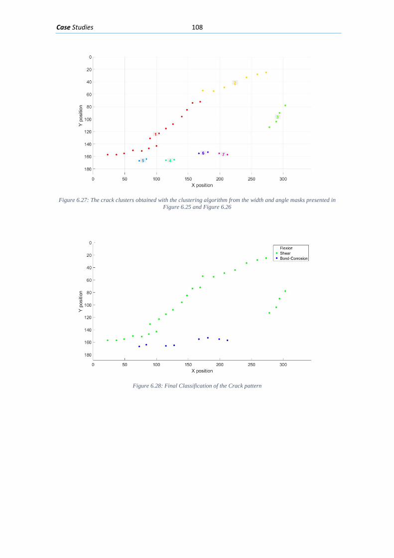
Case Studies 108

Figure 6.27: The crack clusters obtained with the clustering algorithm from the width and angle masks presented in

Figure 6.25 and Figure 6.26

Figure 6.28: Final Classification of the Crack pattern

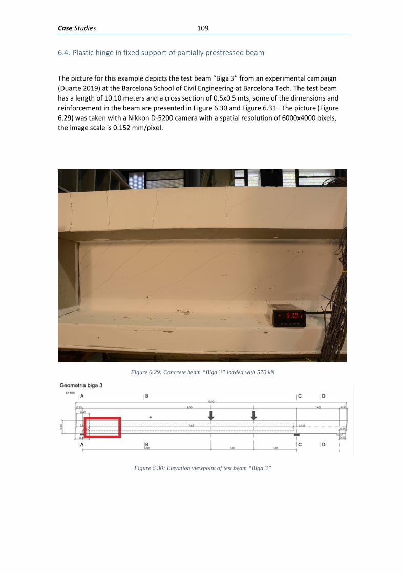
Case Studies 109

6.4. Plastic hinge in fixed support of partially prestressed beam

The picture for this example depicts the test beam “Biga 3” from an experimental campaign (Duarte 2019) at the Barcelona School of Civil Engineering at Barcelona Tech. The test beam has a length of 10.10 meters and a cross section of 0.5x0.5 mts, some of the dimensions and reinforcement in the beam are presented in Figure 6.30 and Figure 6.31 . The picture (Figure 6.29) was taken with a Nikkon D-5200 camera with a spatial resolution of 6000x4000 pixels, the image scale is 0.152 mm/pixel.

Figure 6.29: Concrete beam “Biga 3” loaded with 570 kN

Figure 6.30: Elevation viewpoint of test beam “Biga 3”

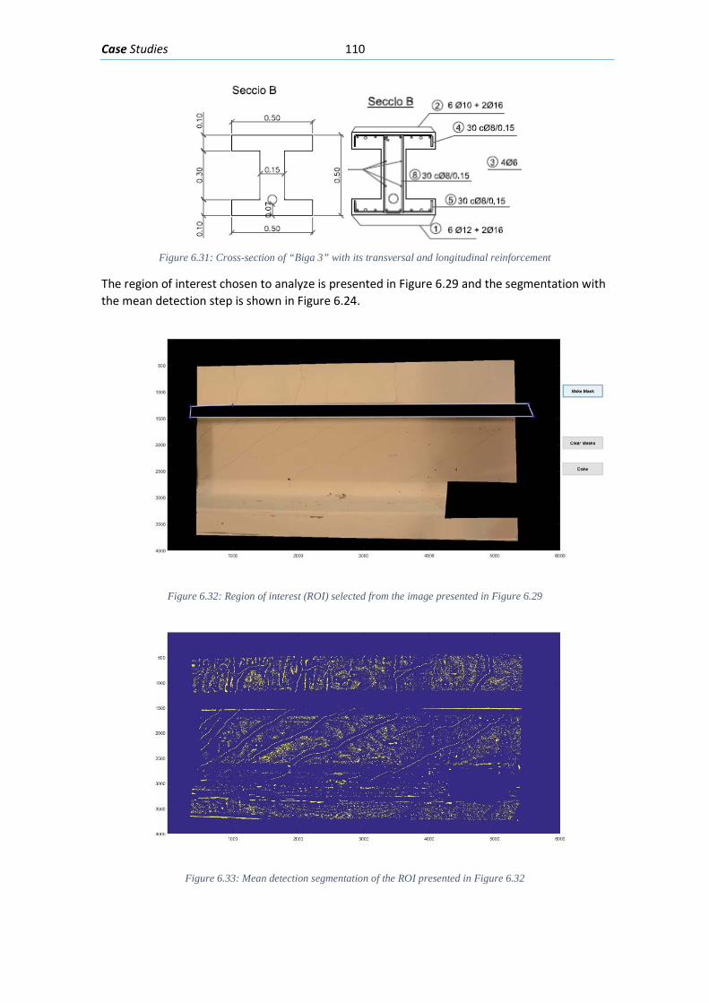
Case Studies 110

Figure 6.31: Cross-section of “Biga 3” with its transversal and longitudinal reinforcement

The region of interest chosen to analyze is presented in Figure 6.29 and the segmentation with the mean detection step is shown in Figure 6.24.

Figure 6.32: Region of interest (ROI) selected from the image presented in Figure 6.29

Figure 6.33: Mean detection segmentation of the ROI presented in Figure 6.32

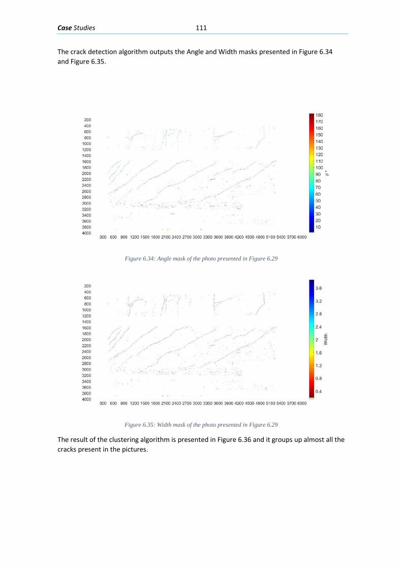
Case Studies 111

The crack detection algorithm outputs the Angle and Width masks presented in Figure 6.34 and Figure 6.35.

Figure 6.34: Angle mask of the photo presented in Figure 6.29

Figure 6.35: Width mask of the photo presented in Figure 6.29

The result of the clustering algorithm is presented in Figure 6.36 and it groups up almost all the cracks present in the pictures.

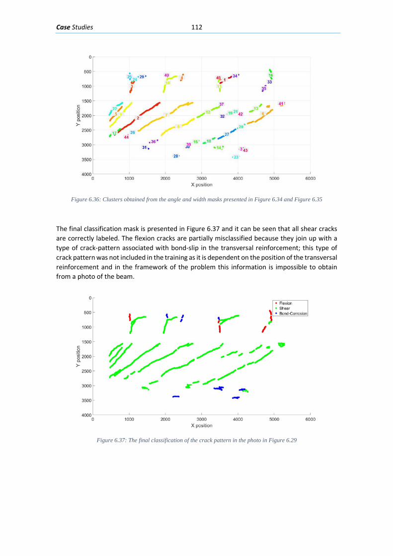
Case Studies 112

Figure 6.36: Clusters obtained from the angle and width masks presented in Figure 6.34 and Figure 6.35

The final classification mask is presented in Figure 6.37 and it can be seen that all shear cracks are correctly labeled. The flexion cracks are partially misclassified because they join up with a type of crack-pattern associated with bond-slip in the transversal reinforcement; this type of crack pattern was not included in the training as it is dependent on the position of the transversal reinforcement and in the framework of the problem this information is impossible to obtain from a photo of the beam.

Figure 6.37: The final classification of the crack pattern in the photo in Figure 6.29

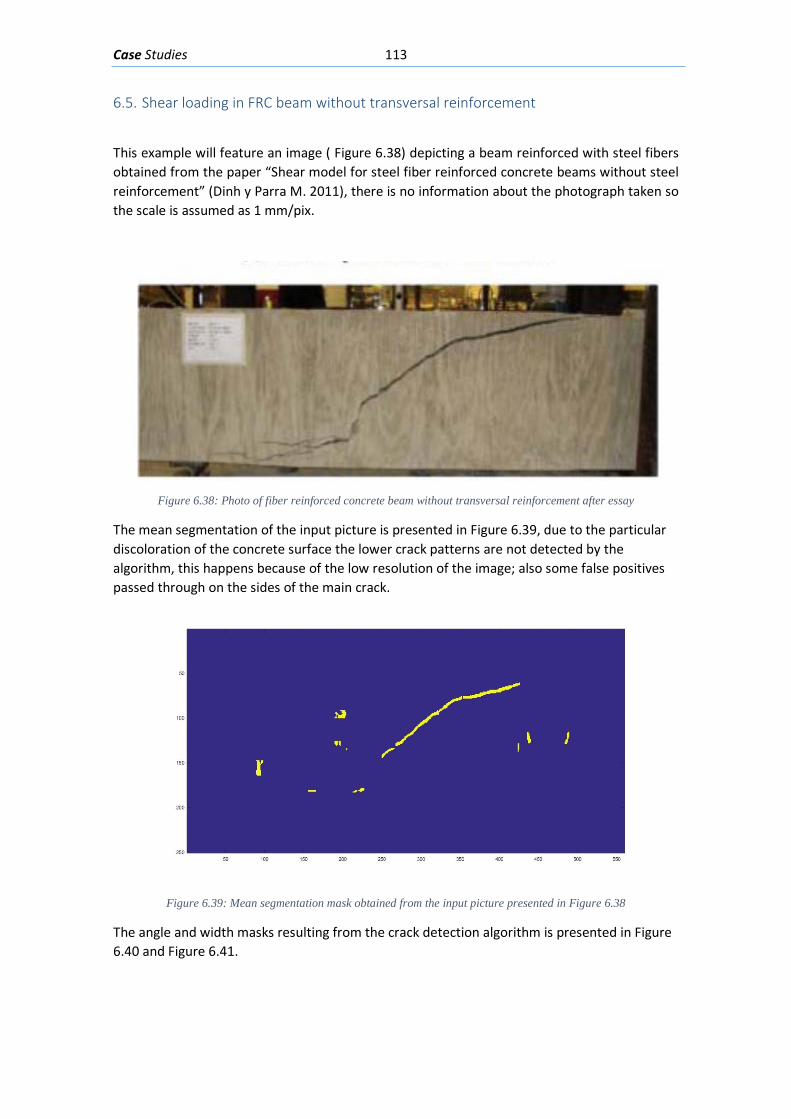
Case Studies 113

6.5. Shear loading in FRC beam without transversal reinforcement

This example will feature an image ( Figure 6.38) depicting a beam reinforced with steel fibers obtained from the paper “Shear model for steel fiber reinforced concrete beams without steel reinforcement” (Dinh y Parra M. 2011), there is no information about the photograph taken so the scale is assumed as 1 mm/pix.

Figure 6.38: Photo of fiber reinforced concrete beam without transversal reinforcement after essay

The mean segmentation of the input picture is presented in Figure 6.39, due to the particular discoloration of the concrete surface the lower crack patterns are not detected by the algorithm, this happens because of the low resolution of the image; also some false positives passed through on the sides of the main crack.

Figure 6.39: Mean segmentation mask obtained from the input picture presented in Figure 6.38

The angle and width masks resulting from the crack detection algorithm is presented in Figure 6.40 and Figure 6.41.

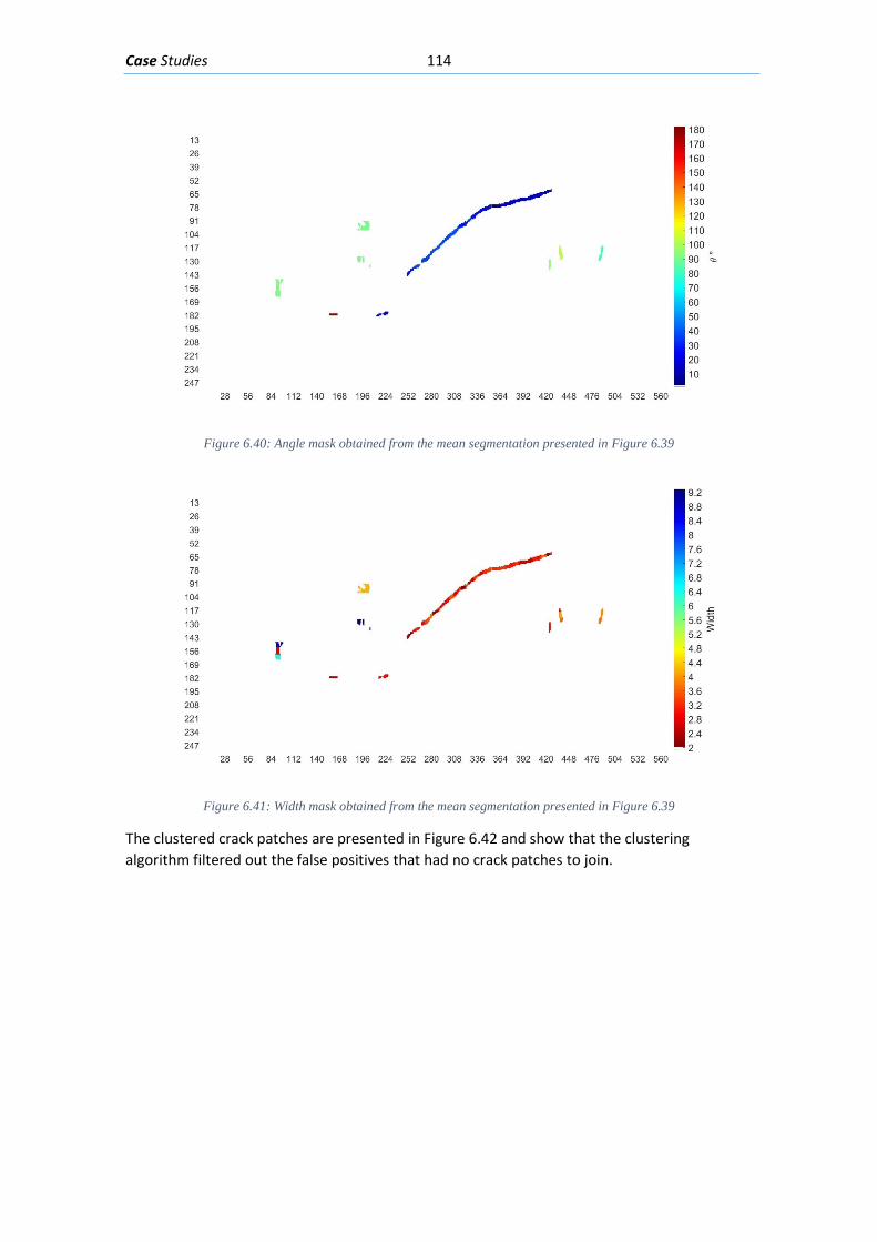
Case Studies 114

Figure 6.40: Angle mask obtained from the mean segmentation presented in Figure 6.39

Figure 6.41: Width mask obtained from the mean segmentation presented in Figure 6.39

The clustered crack patches are presented in Figure 6.42 and show that the clustering algorithm filtered out the false positives that had no crack patches to join.

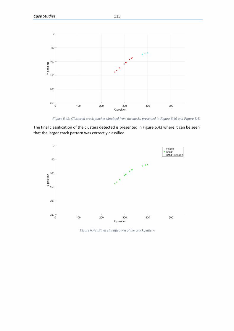
Case Studies 115

Figure 6.42: Clustered crack patches obtained from the masks presented in Figure 6.40 and Figure 6.41

The final classification of the clusters detected is presented in Figure 6.43 where it can be seen that the larger crack pattern was correctly classified.

Figure 6.43: Final classification of the crack pattern

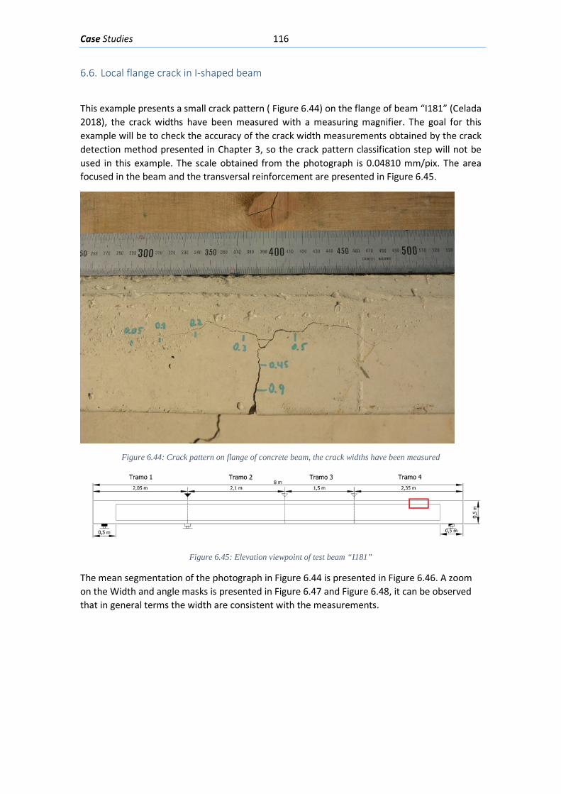
Case Studies 116

6.6. Local flange crack in I-shaped beam

This example presents a small crack pattern ( Figure 6.44) on the flange of beam “I181” (Celada 2018), the crack widths have been measured with a measuring magnifier. The goal for this example will be to check the accuracy of the crack width measurements obtained by the crack detection method presented in Chapter 3, so the crack pattern classification step will not be used in this example. The scale obtained from the photograph is 0.04810 mm/pix. The area focused in the beam and the transversal reinforcement are presented in Figure 6.45.

Figure 6.44: Crack pattern on flange of concrete beam, the crack widths have been measured

Figure 6.45: Elevation viewpoint of test beam “I181”

The mean segmentation of the photograph in Figure 6.44 is presented in Figure 6.46. A zoom on the Width and angle masks is presented in Figure 6.47 and Figure 6.48, it can be observed that in general terms the width are consistent with the measurements.

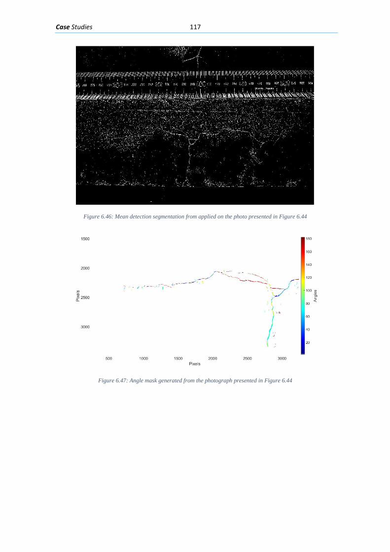
Case Studies 117

Figure 6.46: Mean detection segmentation from applied on the photo presented in Figure 6.44

Figure 6.47: Angle mask generated from the photograph presented in Figure 6.44

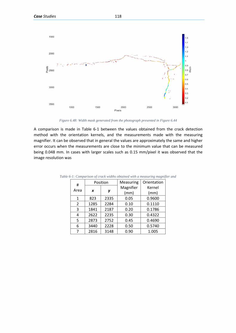
Case Studies 118

Figure 6.48: Width mask generated from the photograph presented in Figure 6.44

A comparison is made in Table 6-1 between the values obtained from the crack detection method with the orientation kernels, and the measurements made with the measuring magnifier. It can be observed that in general the values are approximately the same and higher error occurs when the measurements are close to the minimum value that can be measured being 0.048 mm. In cases with larger scales such as 0.15 mm/pixel it was observed that the image resolution was

Table 6-1: Comparison of crack widths obtained with a measuring magnifier and

# Area

Position Measuring Magnifier

(mm)

Orientation Kernel (mm) x y

1 823 2335 0.05 0.9600 2 1285 2284 0.10 0.1110 3 1841 2187 0.20 0.1786 4 2622 2235 0.30 0.4322 5 2873 2752 0.45 0.4690 6 3440 2228 0.50 0.5740 7 2816 3148 0.90 1.005

Case Studies 119

6.7. Remarks and commentaries

The examples presented were pictures from test beams as they comply with the framework constraints presented in 0 to solve the problems, also they present at least one of the crack patterns associated to the pathologies chosen for this study. The results were generally good, with the system achieving detection of most of the crack pattern when the cracks’ widths were larger than 2 pixels. Detection of cracks which are parallel and really close to each other posed a problem. Most correctly detected crack patterns in the examples were correctly classified in the pathologies chosen to study; except for a type of bond slip crack pattern in Example 4 which was not included in the training of the machine learning model.

Case Studies 120

Conclusions 121

7. Conclusions

7.1. Global conclusion

This work has designed and implemented a semi-automatic system of crack detection and classification of crack pattern in concrete beams. This system is divided in 3 parts: The Crack Detection (chapter 3) step which is done through image processing techniques and machine learning models; the Crack Clustering (chapter 4) which groups up crack patches to attempt to count and extract the cracks in the picture; and the Crack Pattern Classification (chapter 5) which uses machine learning models to classify crack patterns in 3 pathologies. The crack detection segmentation is validated subjectively by inspection; the machine learning models were validated with the typical division in the training, cross-validation and test sets. All steps had good performance in the framework limits set at the start of this work.

7.2. Specific conclusions and problems found

The crack detection algorithm proposed in chapter 3 was proved to be effective in the detection of cracks ranging from 0.2 to 1.2 mm in photos taken from a distance of 0.7 to 1 meters and focusing to areas from 1 to 0.8 meters. The accuracy in the measurement of the crack angle reaches the decimal of a degree.

The segmentation with the NN proposed in 3.2 proved to be good when segmenting relatively clean concrete surfaces with only stains or holes; but it may confuse drawn lines and borders with cracks. This could be solved by modifying the constrains of the problem and also with a different setup (new labels for the different image patches that are not cracks but are lines, numbers, borders, etc.); also, another option would be to use more advanced segmentation techniques. This problem was not directly addressed in the current work as solving it would lose some scope towards the general objective.

The width’s measurement is greatly influenced by the image scale and the demosaicing interpolation inherent to most RGB cameras. To obtain good precision and accuracy levels on measurements between 0.1 and 0.3 mm the pictures had to be focused on areas less than 300 x 300 mm at 0.5 meters from the beams for a camera with 24 Megapixels. This fact translated in a poor accuracy of the width measurement when taking pictures of whole crack patterns. This problem is expected to be tackled with future work on undemosaicing techniques, machine learning models for the measurement algorithm and with cameras with better resolutions.

The crack detection algorithm’s most important contribution is its output mask with all the angle and width of the cracks with the same spatial resolution as the input picture. Another feature from the algorithm is the automated drawing of crack patterns that are used in every single testing of concrete elements and in the data acquisition of the rehabilitation of structures. These masks can help automatize the inspection of concrete structures and combined with the

Conclusions 122

information obtained from magnetic and radar rebar locators could be used to take decisions. Also, the angle and width masks could be used to improve mathematical models for resistance or corrosion that use the width and angle as inputs.

The proposed crack clustering algorithm presented in Chapter 4 computes an approximation of the amount of cracks present in the ROI and assigns these cracks’ centroid, length, mean angle, mean width. This algorithm has also served to separate cracks to ease the classification task from the crack classifier presented in Chapter 5, to eliminate the amount of false positive detections as it excludes clusters with small lengths and number of crack patches.

The crack classifier from Chapter 5 proved to be efficient in the task of separating the 3 different pathologies proposed demonstrating that the empirical visual knowledge from visual diagnosis can be transferred into a machine learning model. This can set up an interest to research in using machine learning models to solve problems in rehabilitation of structures and other Civil Engineering sub-fields.

In general terms the computation time depends on the size of the input picture, photographs with 24 MP (megapixels) could take 40 min, lower resolutions ranging from 0.5 to 1 MP took 1-5 min pass the crack detection step which is the bottleneck of the system and where most of the effort would be made to improve the processing time. The rest of the steps are done faster, the segmentations takes 2-5 seconds; the clustering is in the order of one minute if it takes more than 2000 points; and the crack classification task takes around 1-3 minutes also depending on the clusters found.

7.3. Recommendations for future works Each of the algorithms proposed can still be improved, starting with the crack detection with a Neural Network described in 3.2 uses an engineered feature vector whose computation in every image patch slows downs the computation. It would be interesting to investigate the capabilities of a convolutional neural network taking as input the original image patch.

The crack detection with digital image processing techniques in 3.3 uses mainly basic image processing techniques with the exception of the orientation kernels. These kernels are generally accurate in detecting and measuring cracks but with the drawback that the method and implementation proposed is exhaustive and slow compared to other image processing extractions that take seconds and fraction of seconds. There is a wide field of research in segmentation, edge detection (Amahrir, Sabri y Aarab 2017) (Pereira, Morais y C. 2017) yet to be explored and evaluated as a tool for the crack detection task.

With the aid of machine learning models that can “learn” distance metrics functions such as the one proposed by Andrew Nguyen (Xing, y otros 2002) or other advanced clustering metrics; the algorithm presented in Chapter 4 may be improved to identify longer cracks as single cracks.

This research can be seen as the seed for a bigger project attempting to create an automated diagnosing system for structures used for maintenance and rehabilitation purposes. The system would be implemented in a drone, robot or as a software that takes images from the structure as input; in the meantime, it may be implemented in robots to test the feasibility of automatic inspection.

The future system should be able to identify the type of structural or non-structural element it is focusing on, then obtain a region of interest containing the element, identify the orientation

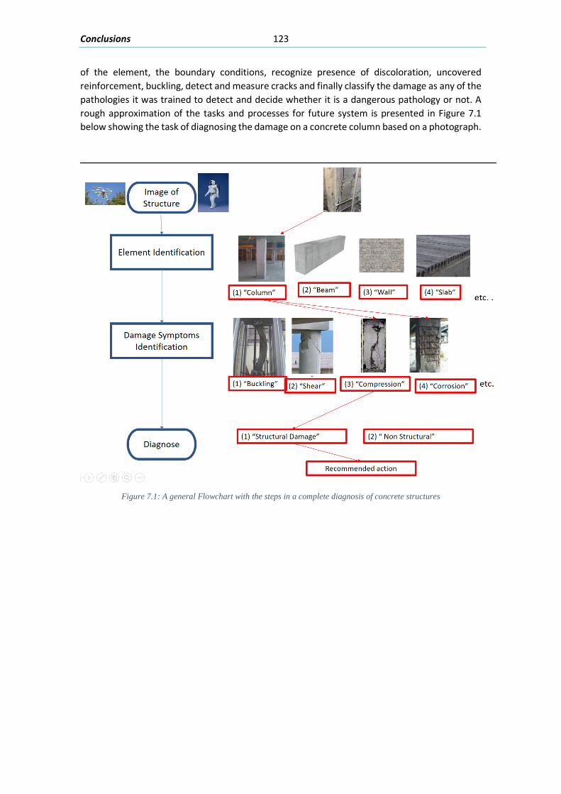
Conclusions 123

of the element, the boundary conditions, recognize presence of discoloration, uncovered reinforcement, buckling, detect and measure cracks and finally classify the damage as any of the pathologies it was trained to detect and decide whether it is a dangerous pathology or not. A rough approximation of the tasks and processes for future system is presented in Figure 7.1 below showing the task of diagnosing the damage on a concrete column based on a photograph.

Figure 7.1: A general Flowchart with the steps in a complete diagnosis of concrete structures

Conclusions 124

References 125

References (AENOR), Asociacion Española de Normalización y Certificación. 2009. Building Diagnosis, Part 6:

Pathological study of the structure of the building. Concrete Structures. Madrid, Spain: AENOR. Abdelhamid, Nihal, y Mohammed Morsyb. 2016. «Study of the behavior of corroded steel bar and

convenient method of repairing.» HBRC Journal 107-113. Albert, J, Hans-Gerd Maas, Andreas Schade, y Willfried Schwarz. 2002. «Pilot studies on photogrammetric

bridge deformation.» Symposium on Geodesy for Geotechnical and Structural Engineering. Amahrir, M., M. A. Sabri, y A. Aarab. 2017. «A Review on Image Segmentation based on Multi-.»

PROCEEDINGS OF THE 2017 INTELLIGENT SYSTEMS CONFERENCE (INTELLISYS). London: IEEE XPLORE. 614-620.

Androutsopoulos, J. Koutsias, K. V. Chandrinos. 2000. «An evaluation of Naive Bayesian anti-spam filtering.» 11th European Conference on Machine Learning. Barcelona. 9-17.

Arfken. 1985. «Convolution Theorem.» En Mathematical Methods for Physicists, 810-814. Orlando: Academic Press.

Bairán, Jesus, Antoni Mari, y Antoni Cladera. 2017. «Analysis of shear resisting actions by means of optimization of strut and tie models accounting for crack patterns.» VII Congreso de ACHE. A Coruña, Spain. 1-10.

Bazant, Z. 1979. «Physical model for steel corrosion in concrete sea structures.» Journal of Structural Division June: 1137–1153.

Bishop, C. 1996. Neural Networks for Pattern Recognition. OXFORD: CLARENDON PRESS. Blaber J, Adair B, Antoniou A. 2015. «Ncorr: Open-Source 2D Digital Image Correlation Matlab

Software.» Experimental Mechanics. Brin, S, y L Page. 1998. «The Anatomy of a Large-Scale Hypertextual Web Search Engine.» WWW7

Proceedings of the seventh international conference on World Wide. Brisbane, Australia: Elsevier Science Publishers. 107-117.

Broto Xavier, Sergio Verruno. 2006. Elementos Constructivos (II). Vol. 2, de Enciclopedia Broto de Patologías de la Construcción, 125-140. Barcelona: Broto i Cormema.

Brown. 1966. «Decentering Distortion and the Definitive Calibration of Metric Cameras.» 29th Annual Meeting of the Americam Society of Photogrammetric Engineering. Chicago.

Brown, M. D., y O. Bayrack. 2005. Design for Shear in Reinforced Concrete Using Strut-and-Tie Models: A Summary. Final Report, Center for Transporation Research, Austin: University of Texas.

Canny, J.,. 1986. « A Computational Approach To Edge Detection.» IEEE Trans. Pattern Analysis and Machine Intelligence, 8 (6): 679–698.

Celada, Ulric. 2018. Estudio teórico y experimental sobre el comportamiento en servicio y rotura de elementos isostáticos de hormigón parcialmente pretensados sometidas a flexión y cortante. unpublished PhD Thesis, Barcelona: Universitat Politecnica de Catalunya, Barcelona Tech (UPC).

CEN, Structural Eurocodes, Technical, Committee, 250, (CEN/TC250). 2004. Eurocode 2: Design of concrete structures , EN1992-1-1. European Committee for Standardization (CEN).

ce-ref.com. s.f. www.ce-ref.com. Último acceso: 28 de August de 2017. http://www.ce-ref.com/RC_Design/RC%20beam/RC_beam.html.

Chau-Khun, Ma, Apandi Nazirah Mohd, Chin Siew Yung Sofrie, y Jen Hau Ng. 2017. «Repair and rehabilitation of concrete structures using confinement: A review.» Construction and Building Materials 502-515.

Cladera, Antoni. 2003. Shear design of reinforced high-strength concrete beams. PhD Thesis, Barcelona: Universitat Politecnica de Catalunya, Barcelona Tech (UPC).

Criado, L, At Llore, y R Ruiz. 2013. Aplicación de técnicas de fotogrametría a la medida de deformaciones de probetas de suelo en laboratorio. Barcelona: Enginyeria del Terreny, Cartogràfica i Geofísica, Universitat Politecnica de Catalunya.

Crow, F. 1984. «Summed-Area Tables for Texture Mapping.» In Proceedings of SIGGRAPH 18 (3): 207-212.

Davison, J., B. Liebald, y J. Liu. 2010. «The YouTube Video Recommendation System.» Proceedings of the 2010 ACM Conference on Recommender Systems. Barcelona: RecSys. 26-30.

Davoudi, Rouzbeh, Gregory Miller, y Nathan Kutz. 2017. «Computer Vision Based Inspection Approach to Predict Damage State and Load Level for RC Members.» 11th International Workshop on Structural Health Monitoring. Stanford : Stanford University, CA, USA.

References 126

Dayan, Peter, Maneesh Sahani, y Grégoire Deback. 1999. «Unsupervised learning.» MIT Encyclopedia of the Cognitive Sciences.

Dinh, Hai, y Gustavo Parra M. 2011. «Shear Strength model for steel fiber reinforced concrete beams without stirrup reinforcement.» Journal of Structural Engineering.

Du, Y, G, A, H, C Chan, y L ,A Clark. 2013. «Finite element analysis of cracking and delamination of concrete beam due to steel corrosion.» Engineering Structures 56: 8-21.

Duarte, Noemi. 2019. Estudio teórico y experimental sobre el comportamiento no lineal de puentes continuos parcialmente pretensados. Unpublished Phd Thesis, Barcelona: Universitat Politecnica de Catalunya, Barcelona Tech (UPC).

Duda R, Hart P. 1972. «Use of the Hough Transform to detect lines and Curves in pictures.» Communications of the ACM 15 (1): 11-15.

Elizalde Javier, Tellez Santiago, Carda Alfredo, Hernandez Eduardo. 1980. Sistematica de la recogida de datos para el diagnostico de la fisuración en estructuras de hormigón armado. Madrid: INCE.

Francois, R, y Maso J.C. 1988. «Effect of damage in reinforced concrete on carbonation or chloride penetration.» Cement and Concrete Research 18 (6): 961-970.

GHARPEDIA.COM. 2016. Gharpedia.com. GHARPEDIA.COM. Último acceso: 7 de August de 2017. https://gharpedia.com/types-summary-of-cracks-in-reinforced-concrete-beams/.

Gonzalez, Woods, y Eddins. 2010. Digital Image Processing uising MATLAB. 2nd. New Delhi: McGraw Hill Education.

Gopalakrishnan, Kasthurirangan, y S.K. Khaitan. 2017. «Deep Convolutional Neural Networks with transfer learning for computer vision-based data-driven pavement distress detection.» Construction and Building Materials 322-330.

Hagan, Martin, Howard B. Demuth, Mark Hudson, y Orlando De Jesus. 1996. Neural Network Design. PWS Pub. Co.

Haralick, Robert M., y Linda G Shapiro. 1992. Computer and Robot Vision. Vol. 1. Addison-Wesley. Hecht, Eugene. 2002. Optics. 4th. San Francisco: Addison Wesley. Hild, F., y S. Roux. 2006. «Digital Image Correlation: from Displacement Measurement to Identification

of Elastic Properties - A review.» Strain - An international journal for experimental mechanics 69-80.

Ho, y Lewis R. 1987. «Carbonation of concrete and its prediction.» Melbourne, Australia. Ihekwaba, Nzeribe M., Brian B. Hope, y Carolyn M. Hansson. 1996. «Structural shape effect on

rehabilitation of vertical concrete structures by ECE technique.» Cement and Concrete Research 26 (1): 165-175.

Karn, Ujjwal. 2016. The data science blog : An Intuitive Explanation of Convolutional Neural Networks. Ujjwal Karn. 08 de 11. Último acceso: 09 de June de 2017. https://ujjwalkarn.me/2016/08/11/intuitive-explanation-convnets/.

Kiening, Hans. 2008. «4K+ Systems: Theory Basics for Motion Picture Imaging.» SMPTE Motion Imaging Journal 117 (3): 50-60.

Kim, Hyunjun, Junhwa Lee, Eunjong Ahn, y Soojin Cho. 2017. «Concrete Crack Identification Using a UAVIncorporating Hybrid Image Processing.» Sensors 2052.

Koren, Norman. 1999. Norman Photography: Understanding image sharpness part 1A. Último acceso: 20 de July de 2017. http://www.normankoren.com/Tutorials/MTF1A.html.

Krizhevsky, Alex, Ilya Sutskever, y Geoffrey E. Hinton. 2012. «ImageNet Classification with Deep Convolutional Neural Networks.» Neural Information Processing Systems (NIPS).

Kwak Hyo, Kim Pil-Sun. 2002. «Nonlinear analysis of RC beams based on moment-curvature relation.» Computers and Structures 80: 615-628.

Lassalle, Mariano. 1941. Fotogrametria Terrestre y aerea. Buenos Aires: El Ateneo. Luhmann T, Robson S, Kyle S, Harley I. 2006. Close Range Photogrammetry, Principles technniques and

applications. Dunbeath: Whittles Publishing. Lüscher, Hermann. 1920. Photogrammetrie; Einfache Stereo- und Luftphotogrammetrie. Berlin: B.G.

Teubner. Maas, H, y U Hampel. 2006. «Photogrammetric Techniques in Civil Engineering Material Testing and

Structure Monitoring.» Photogrammetric Engineering & Remote Sensing 72 (1): 1-7. Mathworks. 2016. Camera Calibration. Mathworks. Último acceso: 25 de July de 2017.

https://es.mathworks.com/help/vision/ug/camera-calibration.html. —. 2016. Convolutional Neural Networks. The MathWorks, Inc. Último acceso: 20 de July de 2017.

https://es.mathworks.com/help/nnet/convolutional-neural-networks.html. Mays, G. 1992. Durability of Concrete Structures Investigation, repair, protection. Chapman & Hall. Mikulica, Karel, Martin Laba, y Rudolf Hela. 2017. «Rehabilitation of Floor Structures Using Foam

Concrete.» Procedia Engineering 195: 108-113.

References 127

Mitchell, T. 1997. Machine Learning. McGraw Hill. Mohr, Steffen. 2011. Nonlinear static and dynamic model for the analysis of reinforced concrete frames

under high shear forces. Doctoral Thesis, Barcelona: Universitat Politecnica de Catalunya, Barcelona Tech.

Muñoz, Hidalgo Manuel. 1994. Diagnosis y causas en patologia de la edificación. Madrid: MATEU CROMO.

Ng, Andrew. 2016. Machine Learning: Learning Curves. 20 de December. https://www.coursera.org/learn/machine-learning/supplement/79woL/learning-curves.

—. 2016. Machine Learning: Supervised Learning. 2 de December. https://www.coursera.org/learn/machine-learning/supplement/NKVJ0/supervised-learning.

—. 2016. Machine Learning: Unsupervised Learning. 12 de June. https://www.coursera.org/learn/machine-learning/supplement/1O0Bk/unsupervised-learning.

NGS - Neuro Genetic Solutions GmbH, Centre for Applied Technology. 2009. Optimal Network Size. 05 de 08. http://www.bestneural.net/Products/cVision/Technologies/NetworkSize.htm.

Pauley, Leo, H Peel, y Luo S. 2017. «Deeper Networks for Pavement Crack Detection.» 34th International Symposium in Automation and Robotics in Construction.

Pereira, Carlos, Raul Morais, y Reis , Manuel ,J. C. 2017. «Recent Advances in Image Processing Techniques for Automated Harvesting Purposes: A Review.» PROCEEDINGS OF THE 2017 INTELLIGENT SYSTEMS CONFERENCE (INTELLISYS). London: IEEE XPLORE. 566-565.

Phillip, Reu. 2012. «Introduction to Digital Image Correlation: Best Practices and Applications.» Experimental Technniques 36 (1): 3-4.

Plizzari, G.A., y A Franchi. 1996. Bond testing according to various European National Codes (in Italian). Brescia, Italy: Department of Civil Engineering, University of Brescia.

Polidori, Laurent , Simonetto, Elisabeth , Labergerie,. 2014. «The teaching of photogrammetry at the National Conservatory of Arts and Crafts: From Laussedat to the training of surveyors in digital photogrammetry.» April: 55-61.

Prewitt, J.W. 1970. «Object Enhancement and Extraction" .» Picture processing and Psychopictorics. Roberts, Lawrence G. 1963. Machine Perception Of Three-Dimensional Solids. Massachusetts Institued of

Technology. Rodriguez, A, J Rabuñal, Pérez J, y Abella F. 2012. «Optical Analysis of Strength Tests Based on Block-

Matching Techniques.» Computer-Aided Civil and Infrastructure Engineering 573-593. Russell, Horowitz C, y Peter Christothoulou. 2010. «Automatically updating performance-based online

advertising system and method.» Saadatmanesh, Hamid. 1997. «Extending service life of concrete and masonry structures with fiber

composites.» Construction and Building Materials 11 (5-6): 327-335. Sanders, Steve. s.f. What is Aerial Photogrammetry? Steve’s Digicams. Último acceso: 01 de July de 2017.

http://www.steves-digicams.com/knowledge-center/how-tos/photography-tips/what-is-aerial-photogrammetry.html.

Santos F., Denise C. 2013. A model for the nonlinear, time-dependent and strengthening analysis of shear critical frame concrete structures. Doctoral Thesis, Departament d'Enginyeria de la Construcció, Universitat Politecnica de Catalunya, Barcelona Tech (UPC), Barcelona: Universitat Politecnica de Catalunya, Barcelona Tech (UPC).

Schenk, Toni. 1999. «Automatic Interior Orientation.» En Digital Photogrammetry, 319-322. Ohio, USA: TerraScience.

Schlaich, J. 1991. «Design and detailing of structural concrete using strut-and-tie models.» Structural Engineer 69 (6).

Schlaich, J., y K. Jennewein, M. Shafer. 1987. «Toward a consistent design of Structural Concrete.» PCI Journal 32 (3): 74-147.

Schmidhuber, Jürgen. 2015. «Deep learning in neural networks: An overview.» Neural Networks 61: 85-112.

Shi, Jianbo. 1994. «Good features to track.» Computer Vision and Pattern Recognition. Seattle: IEEE. Smith, B, y G Linden. 2017. «Two Decades of Recommender Systems at Amazon.com.» IEEE Internet

Computing 21 (3): 12-18. Sobel, Irwin. 1968. «An Isotropic 3 3 Image Gradient Operator.» Stanford Artificial Intelligence Project

(SAIL). Taigman, Yang, Ranzato, Wolf. 2014. «DeepFace: Closing the Gap to Human-Level Performance in Face

Verification.» Conference on Computer Vision and Pattern Recognition (CVPR). Takahashi, Ryosuke. 2013. «Shear failure behavior of RC beam with corroded shear reinforcement.» Third

International on Sustainable Construction Materials and Technnologies. Kyoto, Japan.

References 128

Tan, Steinback, y Kumar. 2006. Introduction to Data Mining. Boston: Addison-Wesley Longman Publishing Co., Inc.

Task Group, Bond Models. 2000. Bond of reinforcement in Concrete. International Federation for Structural Concrete.

Taylor, H. 1970. Investigation of the force carried across the cracks in reinforced concrete beams in shear by interlock of aggregate. London, UK: Cemment and Concrete Association.

Tetta, Zoi, Lampros Koutas, y D. Bournas. 2015. «Textile-reinforced mortar (TRM) versus fiber-reinforced polymers (FRP) in shear strengthening of concrete beams.» Composites Part B 338-348.

Thielicke, William. 2014. The flapping flight of birds. Groningen: University of Groningen. Vidal, Thierry & Castel, Arnaud & Francois, Raoul. 2007. «Corrosion process and structural performance

of a 17 year old reinforced concrete beam stored in chloride environment.» Cement and Concrete Research 37: 1551-1561.

Walford, Alan. 2010. http://www.photogrammetry.com. Último acceso: 20 de July de 2017. Walraven. 1980. Aggregate interlock: A theoretical and experimental investigation. Delf, Holland: Delf

University of Technology. Wanjari, Manish, Keshao Kalaskar, y Mahendra Dhore. 2015. «Document Image Segmentation Using Edge

Detection Method.» International Journal of Computer & Mathematical Sciences 4 (6): 94-99. Woodson, R. Dodge. 2009. Concrete Structures: Protection, repair and rehabilitation. Elsevier. Xing, Eric, Andrew Ng., Michael Jordan, y Stuart Russell. 2002. «Distance metric learning, with

application to clustering with side-information.» Proceedings of the 15th International Conference on Neural Information Processing Systems. MIT Press Cambridge, MA, USA. 521-528.

Zararis, P. 1997. «Aggregate interlock and steel shear forces in the analysis of RC membrane elements.» ACI Structural Journal 94 (2): 159-170.

Zechman, R., y Matamoros A.B. 2002. Use of stut and tie models to calculate the strength of deep beams with openings. Kansas: University of Kansas Center for Research . Inc.

Zeiler, Ranzato M, Nguyen P, y Senior A. 2013. «On Rectified Linear Units for Speech Processing.» Acoustics, Speech and Signal Processing (ICASSP), IEEE International Conference. Vancouver, BC, Canada.

References 129

References 130

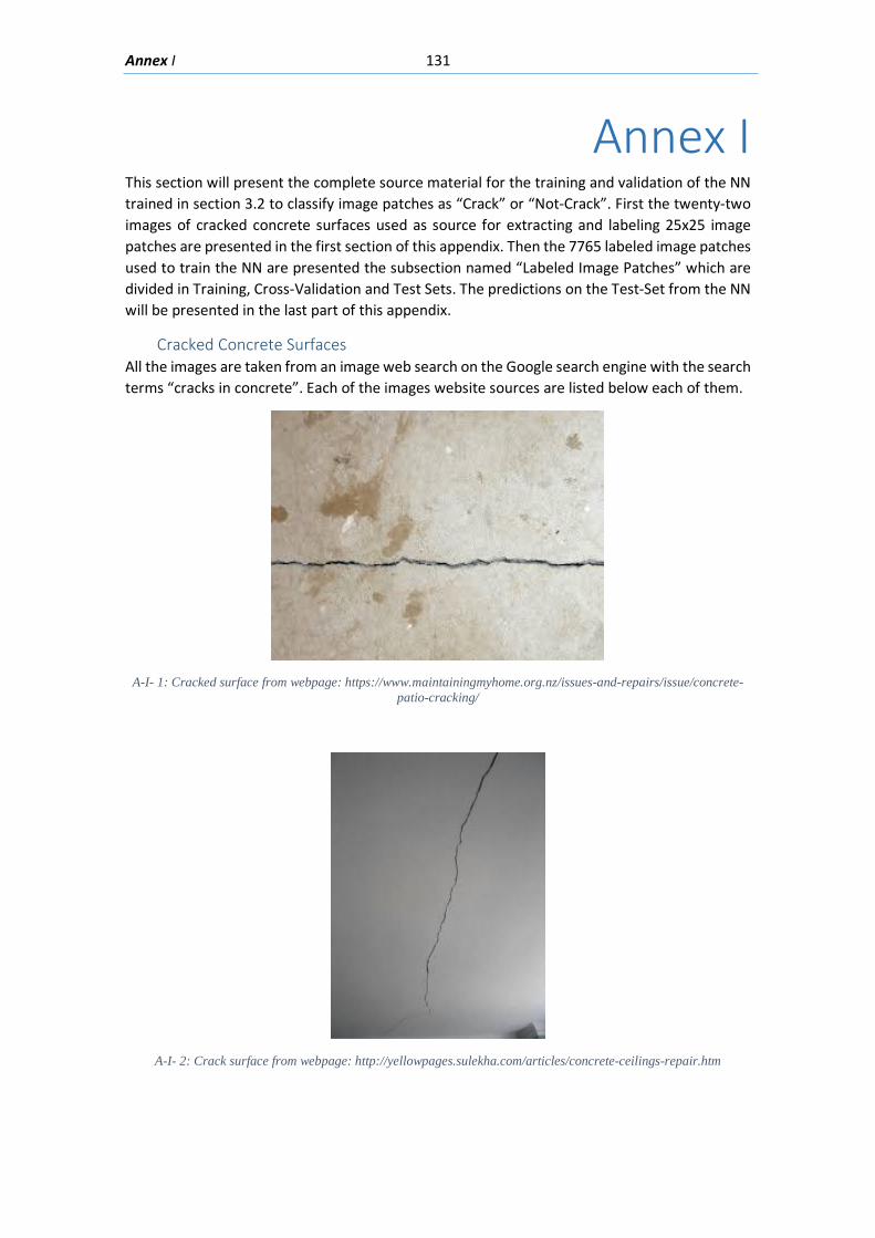
Annex I 131

Annex I This section will present the complete source material for the training and validation of the NN trained in section 3.2 to classify image patches as “Crack” or “Not-Crack”. First the twenty-two images of cracked concrete surfaces used as source for extracting and labeling 25x25 image patches are presented in the first section of this appendix. Then the 7765 labeled image patches used to train the NN are presented the subsection named “Labeled Image Patches” which are divided in Training, Cross-Validation and Test Sets. The predictions on the Test-Set from the NN will be presented in the last part of this appendix.

Cracked Concrete Surfaces All the images are taken from an image web search on the Google search engine with the search terms “cracks in concrete”. Each of the images website sources are listed below each of them.

A-I- 1: Cracked surface from webpage: https://www.maintainingmyhome.org.nz/issues-and-repairs/issue/concrete-

patio-cracking/

A-I- 2: Crack surface from webpage: http://yellowpages.sulekha.com/articles/concrete-ceilings-repair.htm

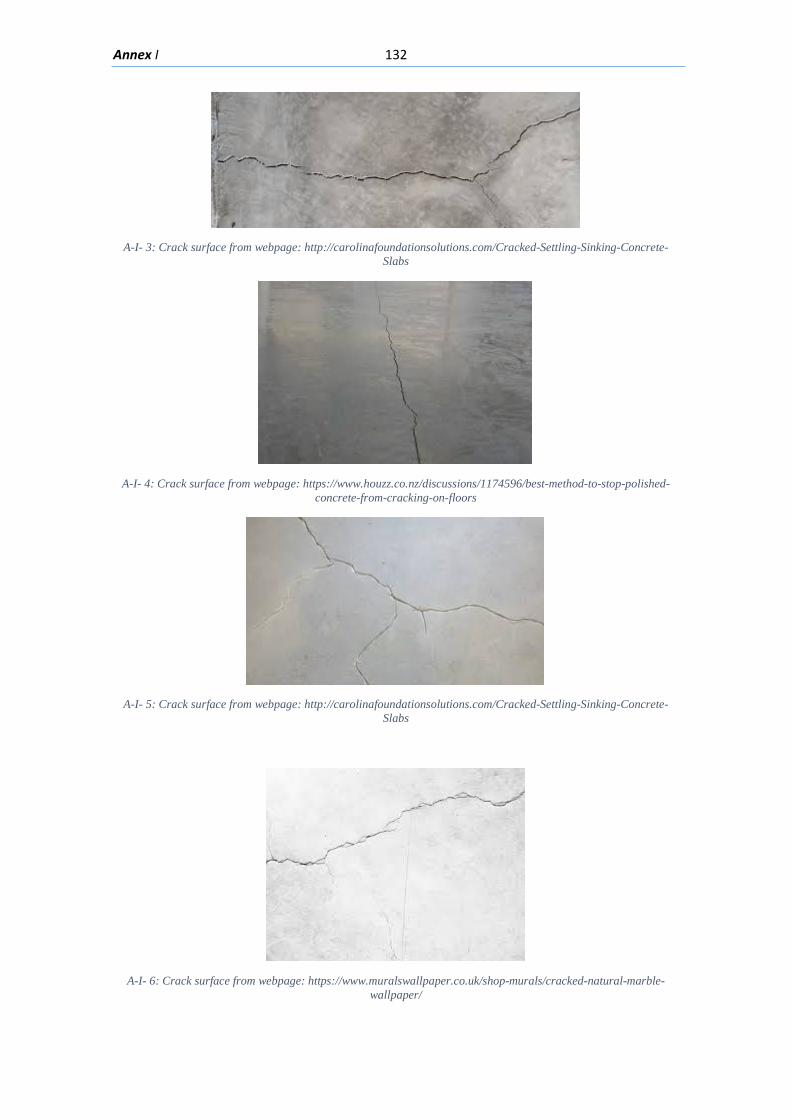
Annex I 132

A-I- 3: Crack surface from webpage: http://carolinafoundationsolutions.com/Cracked-Settling-Sinking-Concrete-

Slabs

A-I- 4: Crack surface from webpage: https://www.houzz.co.nz/discussions/1174596/best-method-to-stop-polished-

concrete-from-cracking-on-floors

A-I- 5: Crack surface from webpage: http://carolinafoundationsolutions.com/Cracked-Settling-Sinking-Concrete-

Slabs

A-I- 6: Crack surface from webpage: https://www.muralswallpaper.co.uk/shop-murals/cracked-natural-marble-

wallpaper/

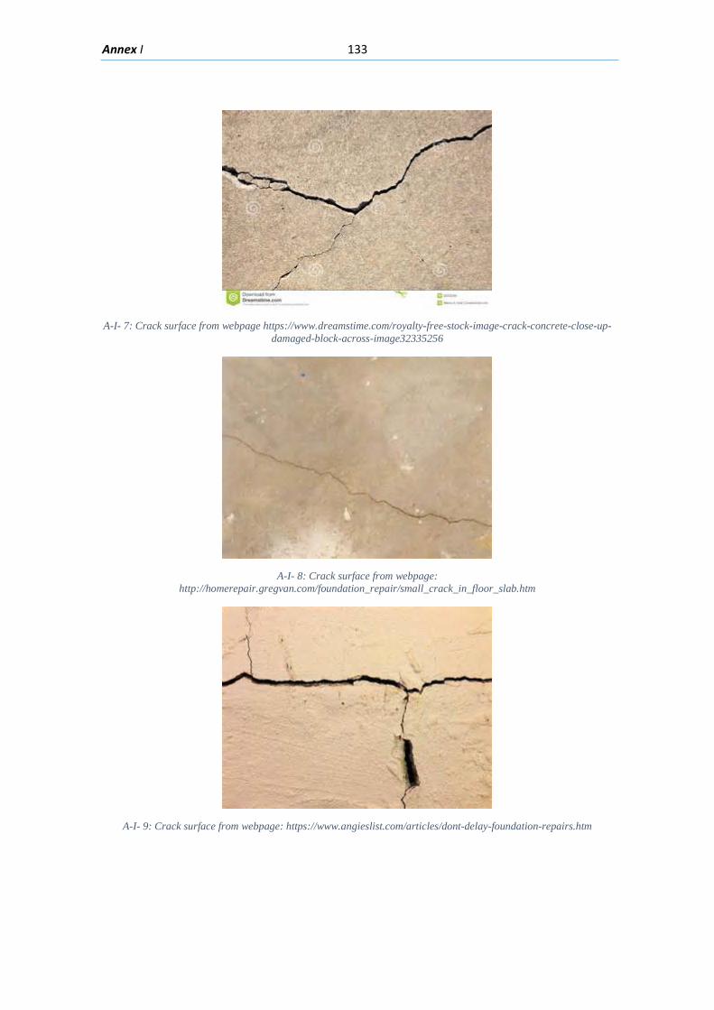
Annex I 133

A-I- 7: Crack surface from webpage https://www.dreamstime.com/royalty-free-stock-image-crack-concrete-close-up-

damaged-block-across-image32335256

A-I- 8: Crack surface from webpage:

http://homerepair.gregvan.com/foundation_repair/small_crack_in_floor_slab.htm

A-I- 9: Crack surface from webpage: https://www.angieslist.com/articles/dont-delay-foundation-repairs.htm

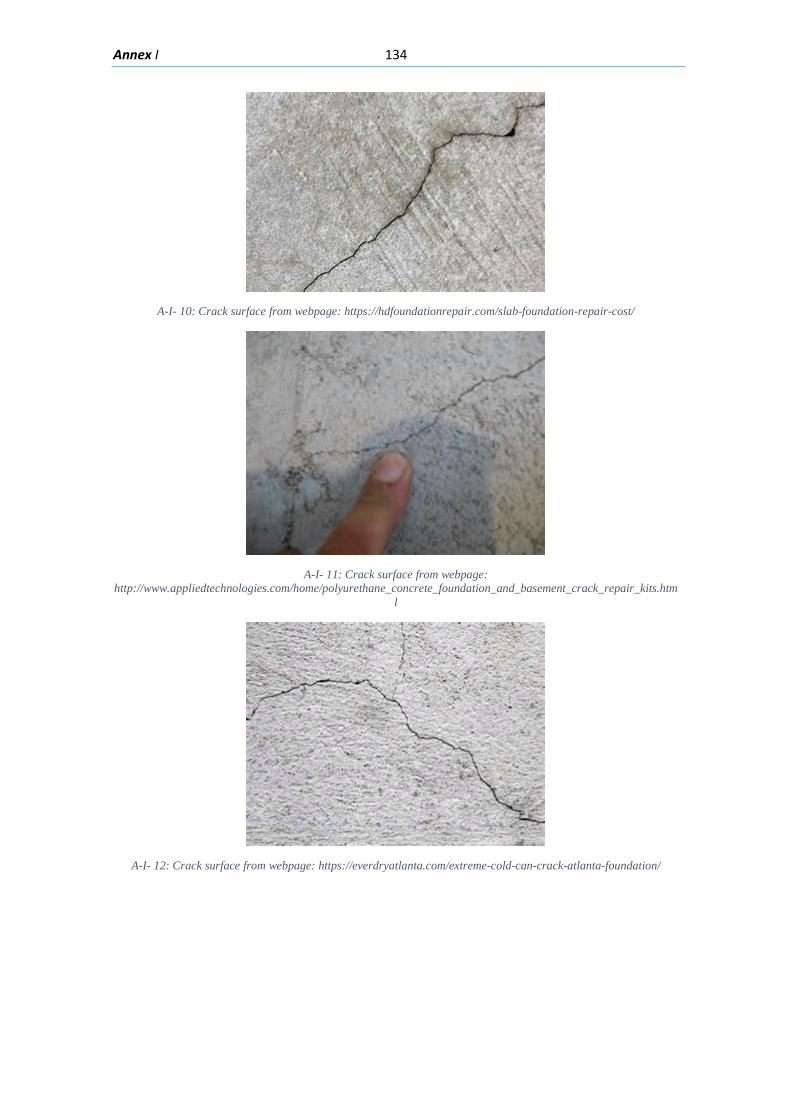
Annex I 134

A-I- 10: Crack surface from webpage: https://hdfoundationrepair.com/slab-foundation-repair-cost/

A-I- 11: Crack surface from webpage:

http://www.appliedtechnologies.com/home/polyurethane_concrete_foundation_and_basement_crack_repair_kits.html

A-I- 12: Crack surface from webpage: https://everdryatlanta.com/extreme-cold-can-crack-atlanta-foundation/

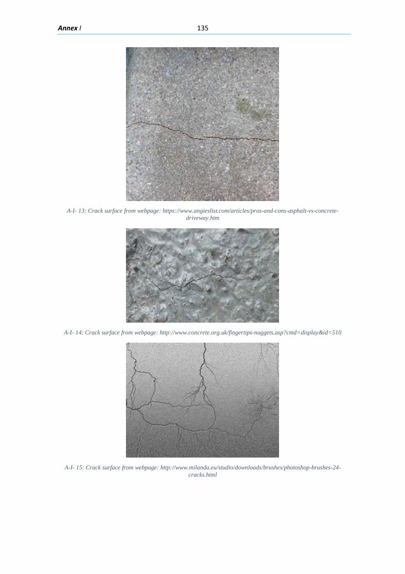
Annex I 135

A-I- 13: Crack surface from webpage: https://www.angieslist.com/articles/pros-and-cons-asphalt-vs-concrete-

driveway.htm

A-I- 14: Crack surface from webpage: http://www.concrete.org.uk/fingertips-nuggets.asp?cmd=display&id=510

A-I- 15: Crack surface from webpage: http://www.milanda.eu/studio/downloads/brushes/photoshop-brushes-24-

cracks.html

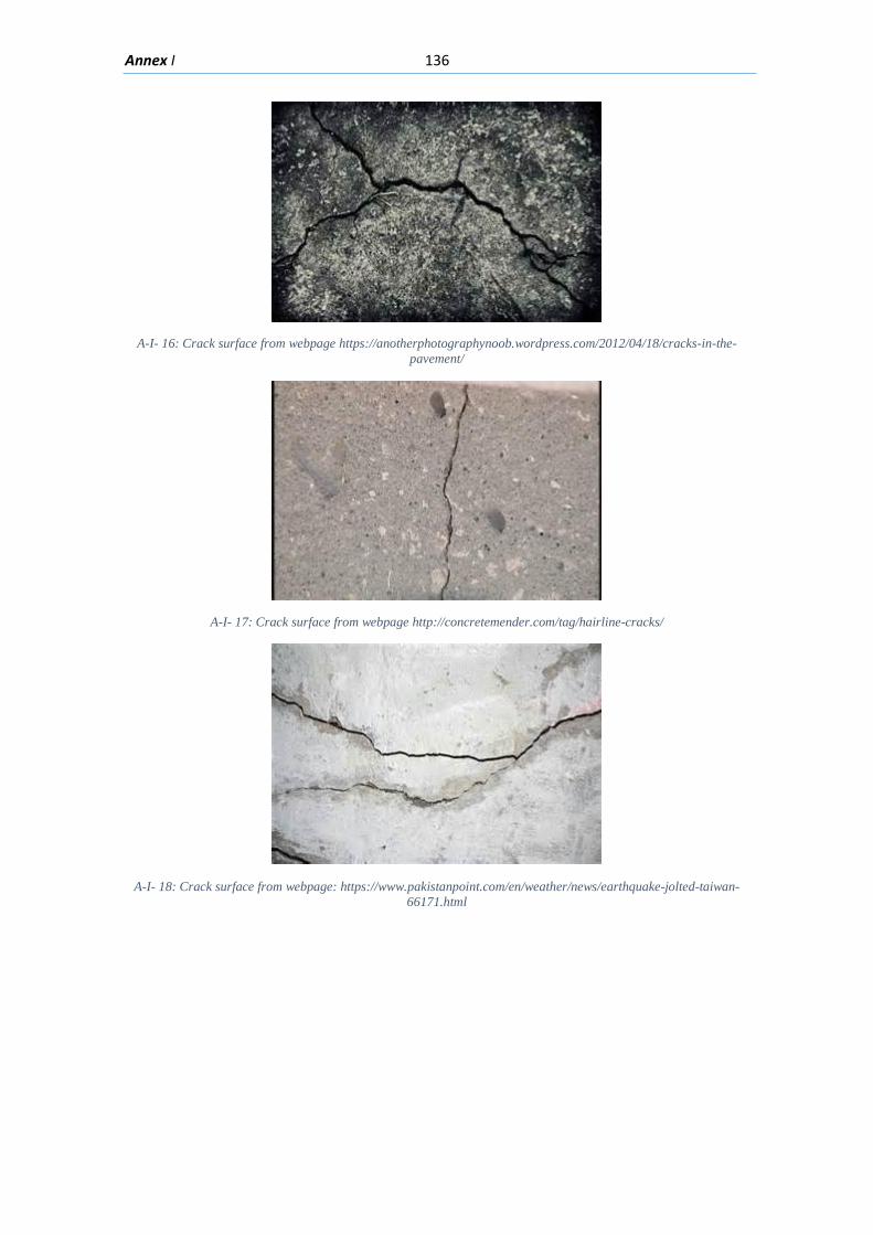
Annex I 136

A-I- 16: Crack surface from webpage https://anotherphotographynoob.wordpress.com/2012/04/18/cracks-in-the-

pavement/

A-I- 17: Crack surface from webpage http://concretemender.com/tag/hairline-cracks/

A-I- 18: Crack surface from webpage: https://www.pakistanpoint.com/en/weather/news/earthquake-jolted-taiwan-66171.html

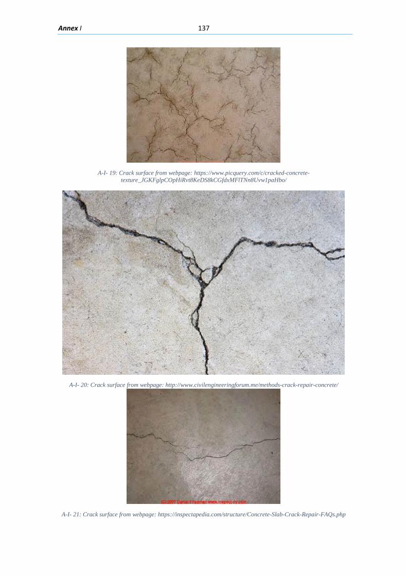
Annex I 137

A-I- 19: Crack surface from webpage: https://www.picquery.com/c/cracked-concrete-

texture_JGKFglpCOpHiRvt8KeDS8kCGfdxMFlTNn8Uvw1paHbo/

A-I- 20: Crack surface from webpage: http://www.civilengineeringforum.me/methods-crack-repair-concrete/

A-I- 21: Crack surface from webpage: https://inspectapedia.com/structure/Concrete-Slab-Crack-Repair-FAQs.php

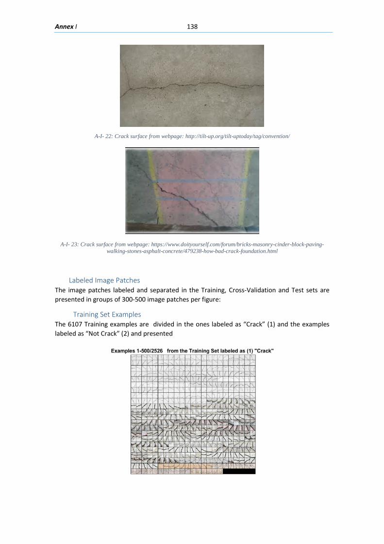
Annex I 138

A-I- 22: Crack surface from webpage: http://tilt-up.org/tilt-uptoday/tag/convention/

A-I- 23: Crack surface from webpage: https://www.doityourself.com/forum/bricks-masonry-cinder-block-paving-

walking-stones-asphalt-concrete/479238-how-bad-crack-foundation.html

Labeled Image Patches The image patches labeled and separated in the Training, Cross-Validation and Test sets are presented in groups of 300-500 image patches per figure:

Training Set Examples The 6107 Training examples are divided in the ones labeled as “Crack” (1) and the examples labeled as “Not Crack” (2) and presented

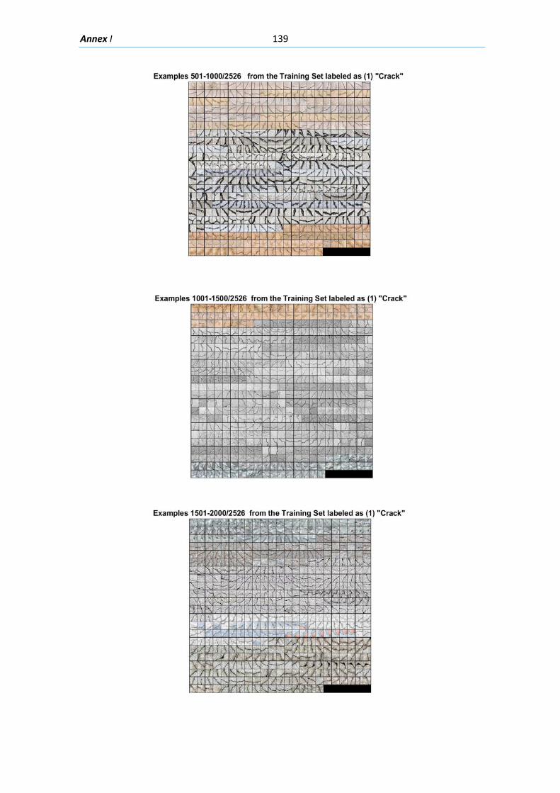
Annex I 139

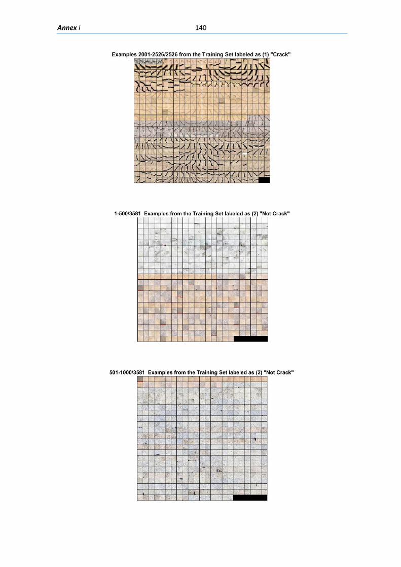
Annex I 140

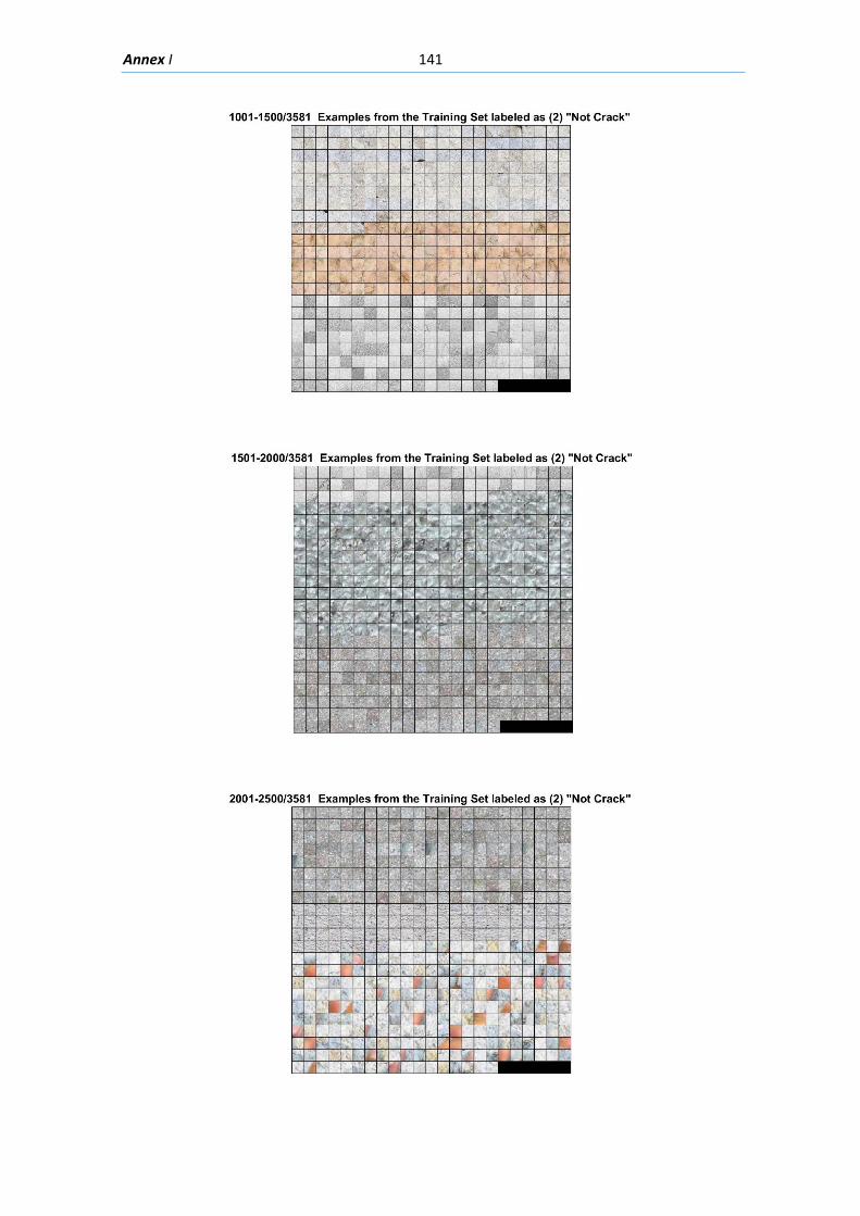
Annex I 141

Annex I 142

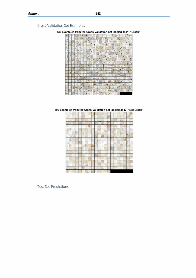
Annex I 143

Cross-Validation Set Examples

Test Set Predictions

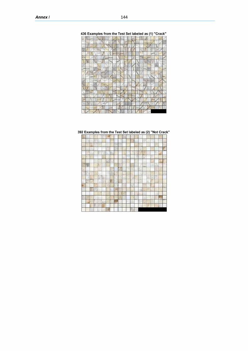
Annex I 144

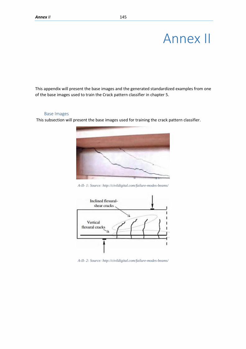
Annex II 145

Annex II

This appendix will present the base images and the generated standardized examples from one of the base images used to train the Crack pattern classifier in chapter 5.

Base Images This subsection will present the base images used for training the crack pattern classifier.

A-II- 1: Source: http://civildigital.com/failure-modes-beams/

A-II- 2: Source: http://civildigital.com/failure-modes-beams/

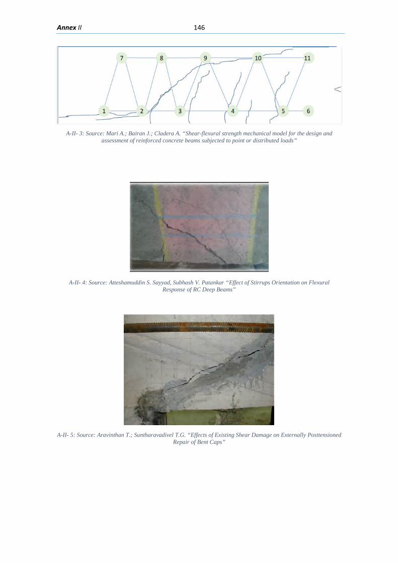
Annex II 146

A-II- 3: Source: Mari A.; Bairan J.; Cladera A. “Shear-flexural strength mechanical model for the design and

assessment of reinforced concrete beams subjected to point or distributed loads”

A-II- 4: Source: Atteshamuddin S. Sayyad, Subhash V. Patankar “Effect of Stirrups Orientation on Flexural

Response of RC Deep Beams”

A-II- 5: Source: Aravinthan T.; Suntharavadivel T.G. “Effects of Existing Shear Damage on Externally Posttensioned

Repair of Bent Caps”

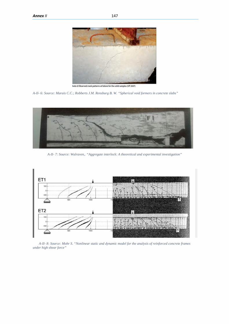
Annex II 147

A-II- 6: Source: Marais C.C.; Robberts J.M. Rensburg B. W. “Spherical void formers in concrete slabs”

A-II- 7: Source: Walraven,. “Aggregate interlock: A theoretical and experimental investigation”

A-II- 8: Source: Mohr S. “Nonlinear static and dynamic model for the analysis of reinforced concrete frames under high shear force”

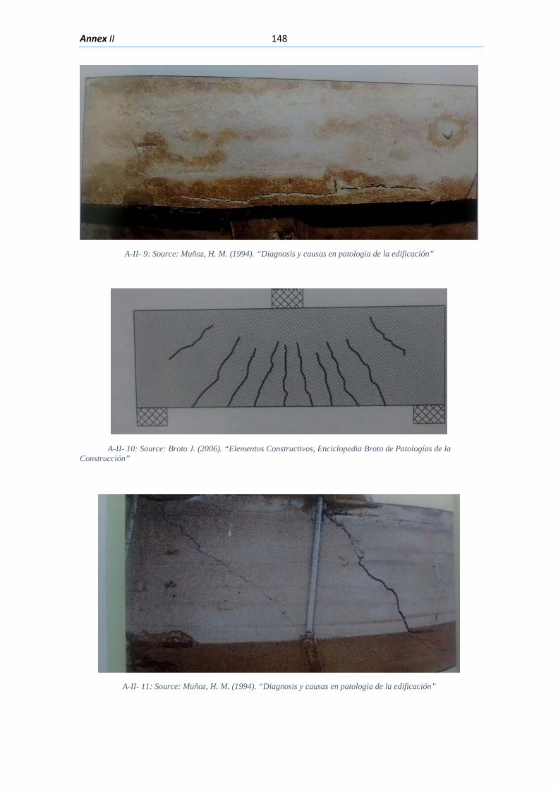
Annex II 148

A-II- 9: Source: Muñoz, H. M. (1994). “Diagnosis y causas en patologia de la edificación”

A-II- 10: Source: Broto J. (2006). “Elementos Constructivos, Enciclopedia Broto de Patologías de la Construcción”

A-II- 11: Source: Muñoz, H. M. (1994). “Diagnosis y causas en patologia de la edificación”

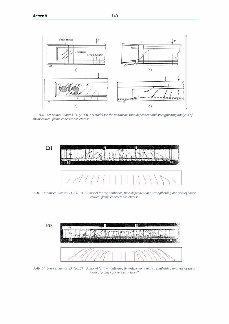
Annex II 149

A-II- 12: Source: Santos .D (2013). “A model for the nonlinear, time-dependent and strengthening analysis of shear critical frame concrete structures”

A-II- 13: Source: Santos .D (2013). “A model for the nonlinear, time-dependent and strengthening analysis of shear

critical frame concrete structures”

A-II- 14: Source: Santos .D (2013). “A model for the nonlinear, time-dependent and strengthening analysis of shear

critical frame concrete structures”

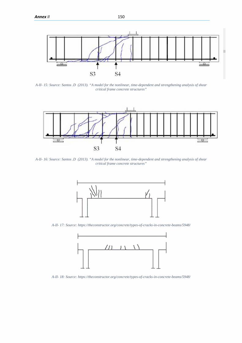
Annex II 150

A-II- 15: Source: Santos .D (2013). “A model for the nonlinear, time-dependent and strengthening analysis of shear

critical frame concrete structures”

A-II- 16: Source: Santos .D (2013). “A model for the nonlinear, time-dependent and strengthening analysis of shear

critical frame concrete structures”

A-II- 17: Source: https://theconstructor.org/concrete/types-of-cracks-in-concrete-beams/5948/

A-II- 18: Source: https://theconstructor.org/concrete/types-of-cracks-in-concrete-beams/5948/

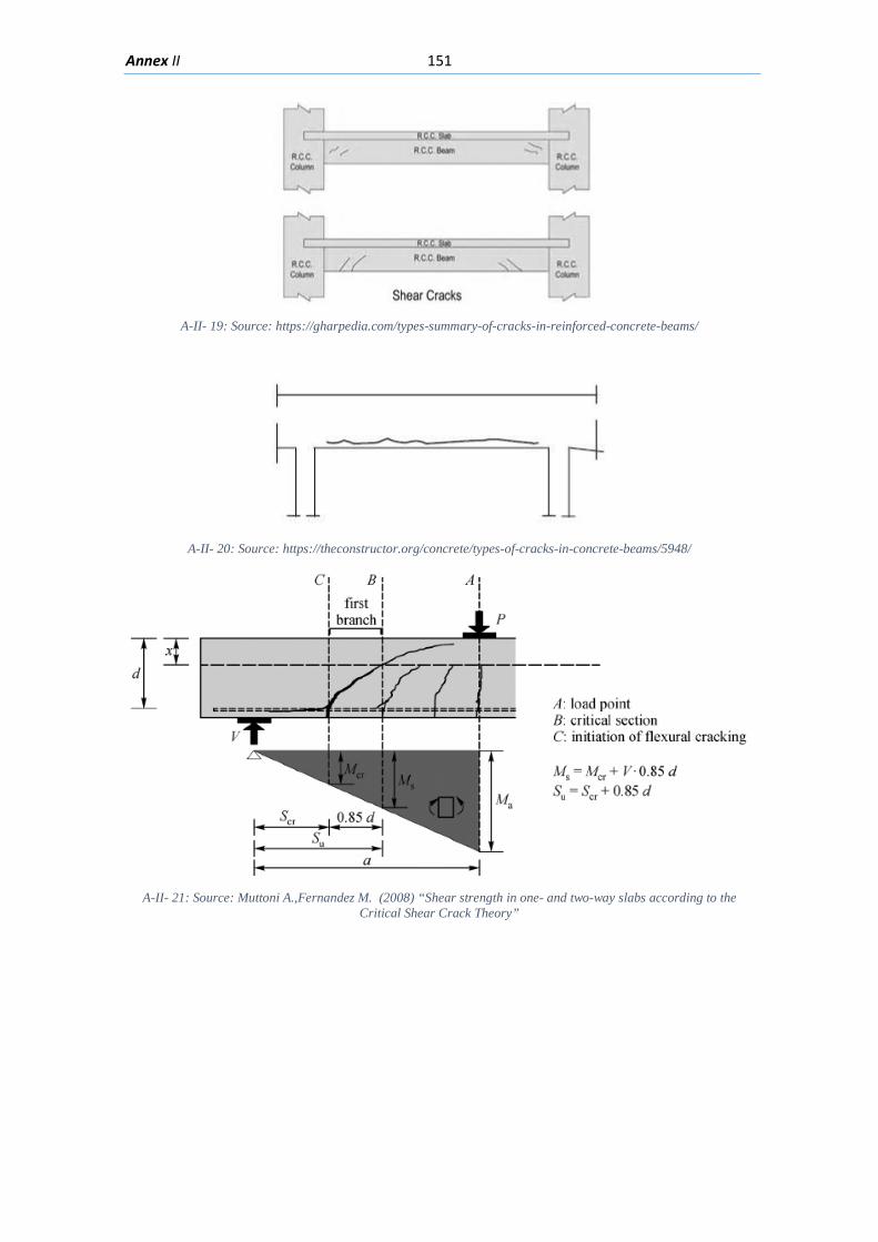
Annex II 151

A-II- 19: Source: https://gharpedia.com/types-summary-of-cracks-in-reinforced-concrete-beams/

A-II- 20: Source: https://theconstructor.org/concrete/types-of-cracks-in-concrete-beams/5948/

A-II- 21: Source: Muttoni A.,Fernandez M. (2008) “Shear strength in one- and two-way slabs according to the

Critical Shear Crack Theory”

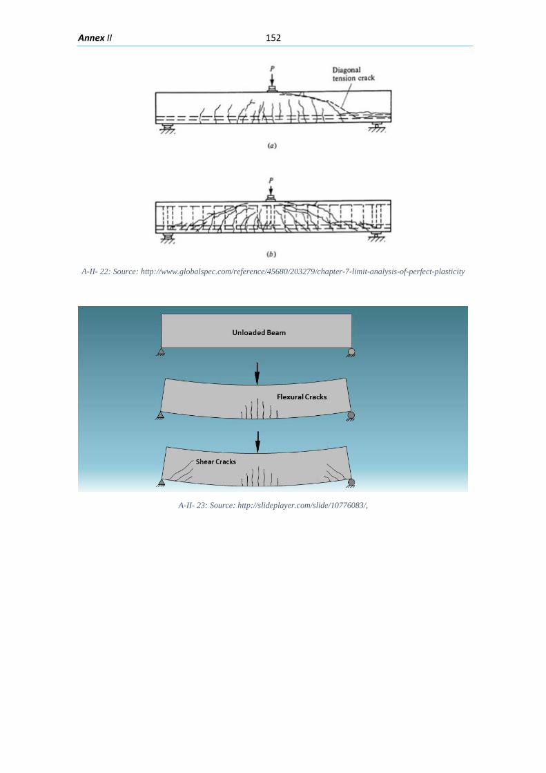
Annex II 152

A-II- 22: Source: http://www.globalspec.com/reference/45680/203279/chapter-7-limit-analysis-of-perfect-plasticity

A-II- 23: Source: http://slideplayer.com/slide/10776083/,

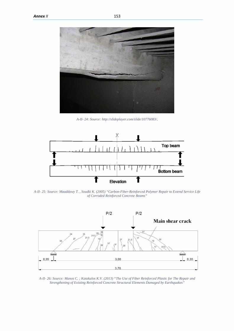
Annex II 153

A-II- 24: Source: http://slideplayer.com/slide/10776083/,

A-II- 25: Source: Maaddawy T. , Soudki K. (2005) “Carbon-Fiber-Reinforced Polymer Repair to Extend Service Life of Corroded Reinforced Concrete Beams”

A-II- 26: Source: Manos C. ; Katakalos K.V. (2013) “The Use of Fiber Reinforced Plastic for The Repair and Strengthening of Existing Reinforced Concrete Structural Elements Damaged by Earthquakes”

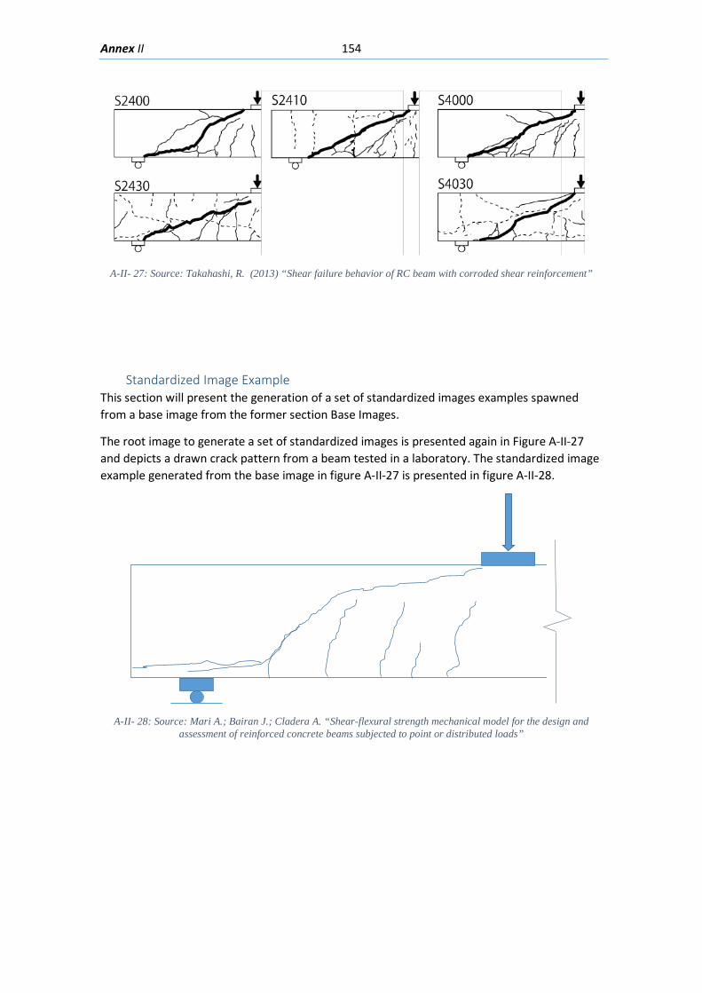
Annex II 154

A-II- 27: Source: Takahashi, R. (2013) “Shear failure behavior of RC beam with corroded shear reinforcement”

Standardized Image Example This section will present the generation of a set of standardized images examples spawned from a base image from the former section Base Images.

The root image to generate a set of standardized images is presented again in Figure A-II-27 and depicts a drawn crack pattern from a beam tested in a laboratory. The standardized image example generated from the base image in figure A-II-27 is presented in figure A-II-28.

A-II- 28: Source: Mari A.; Bairan J.; Cladera A. “Shear-flexural strength mechanical model for the design and

assessment of reinforced concrete beams subjected to point or distributed loads”

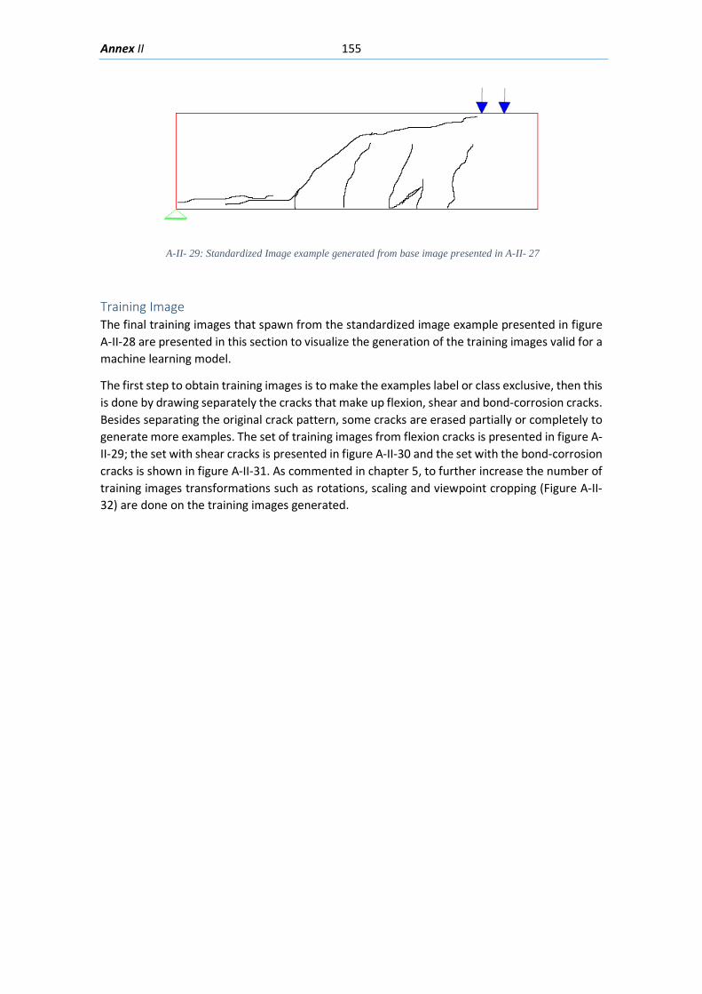
Annex II 155

A-II- 29: Standardized Image example generated from base image presented in A-II- 27

Training Image The final training images that spawn from the standardized image example presented in figure A-II-28 are presented in this section to visualize the generation of the training images valid for a machine learning model.

The first step to obtain training images is to make the examples label or class exclusive, then this is done by drawing separately the cracks that make up flexion, shear and bond-corrosion cracks. Besides separating the original crack pattern, some cracks are erased partially or completely to generate more examples. The set of training images from flexion cracks is presented in figure A-II-29; the set with shear cracks is presented in figure A-II-30 and the set with the bond-corrosion cracks is shown in figure A-II-31. As commented in chapter 5, to further increase the number of training images transformations such as rotations, scaling and viewpoint cropping (Figure A-II-32) are done on the training images generated.

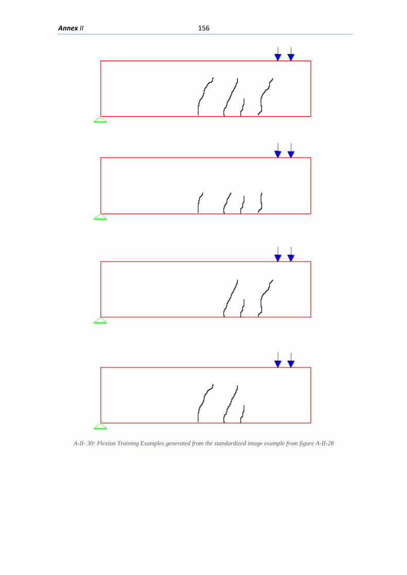
Annex II 156

A-II- 30: Flexion Training Examples generated from the standardized image example from figure A-II-28

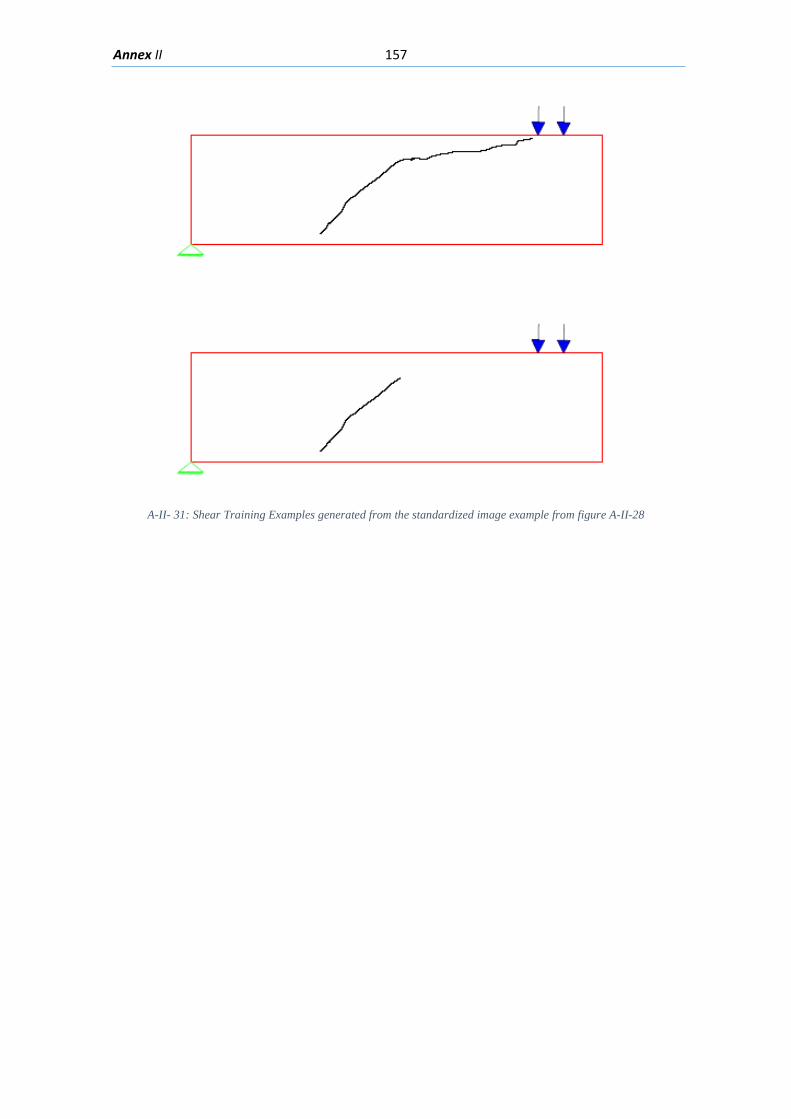
Annex II 157

A-II- 31: Shear Training Examples generated from the standardized image example from figure A-II-28

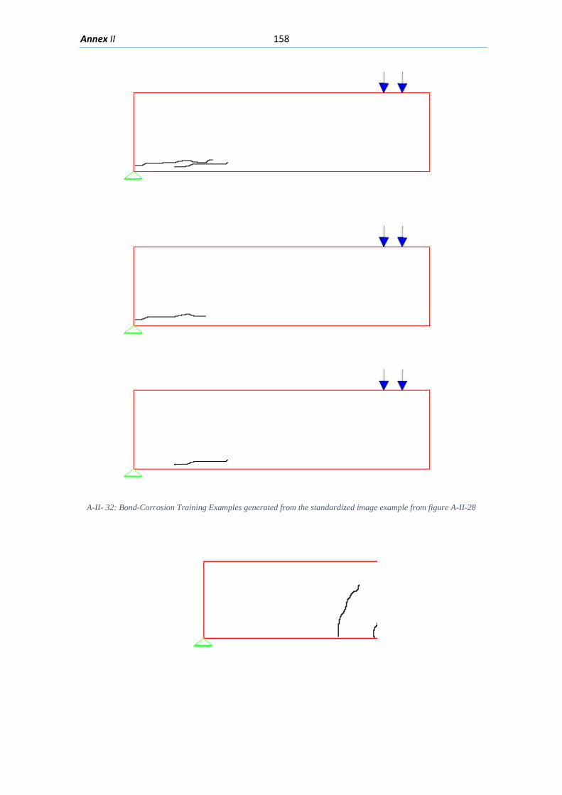
Annex II 158

A-II- 32: Bond-Corrosion Training Examples generated from the standardized image example from figure A-II-28

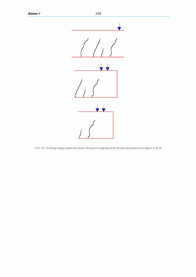
Annex II 159

A-II- 33: Training images generated from Viewpoint cropping of the flexion set presented in figure A-II-29