Digital Control - UPCommons

Control & Guidance2011

Enginyeria Tècnica d'Aeronàuticaesp. en Aeronavegació

Escola d'Enginyeria de TelecomunicacióEscola d Enginyeria de Telecomunicació i Aeroespacial de Castelldefels

Adeline de Villardi de MontlaurAdeline de Villardi de MontlaurMarc Diaz Aguiló

Digital ControlDigital Control

Control and guidance

Slide 1

Di it l t lDi it l t lDigital control1 I t d ti t di t t

Digital control1 I t d ti t di t t1. Introduction to discrete systems

2 Z transform

1. Introduction to discrete systems

2 Z transform2. Z transform

3. Z transfer function

2. Z transform

3. Z transfer function

4. Digital control tools4. Digital control tools

5. Design method with dead beat 5. Design method with dead beat

responseresponse


Slide 2

1.1. Introduction to discrete systemsIntroduction to discrete systems

a. Revision of the sampling theorema. Revision of the sampling theorem

Digital signals present great advantages when transmitted and/orprocessed:

• higher immunity to noise

• easier to process• easier to process

• multiplexing easiness (multiple digital data streams are combinedi t i l h d di )into one signal over a shared medium ),…

• obvious tendence to the usage of digital controllers(microcontrollers, PIC, or even Computers)


Slide 3


As a consequence:


q

There is an latent interest in changing analog signals to digital signals

Analog systems:-- continuous time -- continuous amplitude-- continuous amplitude

Discrete system:discrete time-- discrete time

-- quantized amplitude

T k b f dTasks to be performed: Discretize in time: “sampling”.Discretize in amplitude: “quantization”.


Slide 4



In order to analyze the properties of the discretized signal, we use

the Fourier transform, this transformation is defined on an infinite

continuous interval.

Therefore in order to operate on discrete signals we lead to a digitalTherefore, in order to operate on discrete signals, we lead to a digital

data processing problem.

The signal will be replaced by samples taken at a determined rate.

The objective is to represent the continuous signal and process itThe objective is to represent the continuous signal and process it

without any information loss.


Slide 5



The digital sampling of an analogical signal needs a discretizationThe digital sampling of an analogical signal needs a discretization

both in the temporal domain (time sampling) and in the amplitude

( ti ti )one (quantization).

There are different ways to mathematically describe the temporal

discretization process of a signal that is continuous in time. We will

analyze some of them during these sessions.y g


Slide 6



Th i l li (id l)

Given x(t) a real and continuous signal with limited band,

Theoretical sampling (ideal)

which spectrum X(ω) is null for |ω| > Wmax

d)()( tj

dte)t(x)(X tj


Slide 7



Th i l li (id l)

and we consider the ideal sampling wave with a Ts period:


m

sd )mTt()t(s

the product x(t) · sd(t) is a wave formed by Dirac deltas whose amplitude is the same as the x(t) samples:p ( ) p

sssdd )mTt()mT(x)mTt()t(x)t(s)t(x)t(x m

ssm

sdd )()()()()()()(

Drawing


Slide 8

Drawing



Th i l li (id l)

Consequently, its spectrum in the time domain is:


ss

mssd T

fwithfmXfX 1)2()(

sssd TfwithmffXffX 1)()(

sm TThe spectrum of the signal xd(t) is the replica of the spectrum of the signal x(t) at each multiples of fsignal x(t) at each multiples of fs.Note the scale factor fs.


Slide 9



Theoretical sampling (ideal) f

2

f

W = fmax of the spectrum

Overlap condition

fs/2 > W fs > 2W


Slide 10



Th i l li (id l)Theoretical sampling (ideal)

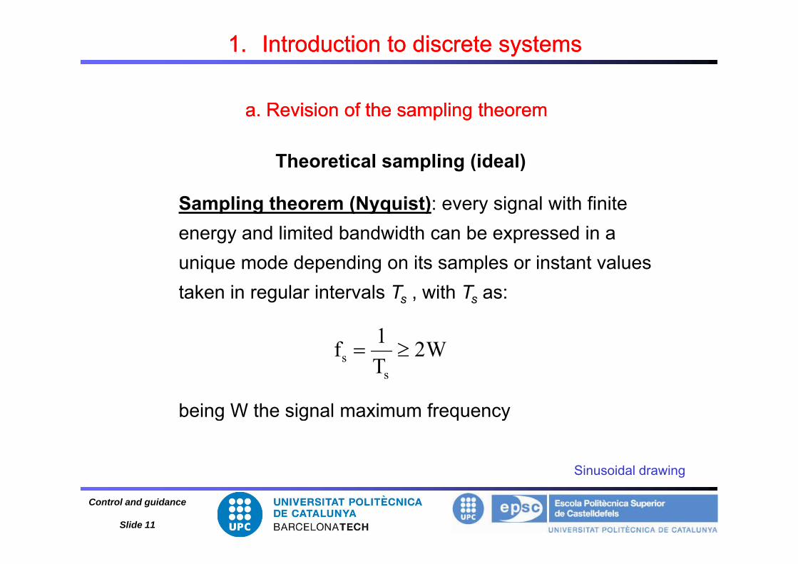
Sampling theorem (Nyquist): every signal with finite energy and limited bandwidth can be expressed in a unique mode depending on its samples or instant values taken in regular intervals Ts , with Ts as:

W21f

being W the signal maximum frequency

W2T

fs

s

being W the signal maximum frequency

Sinusoidal drawing


Slide 11

Sinusoidal drawing



Th i l li (id l)Theoretical sampling (ideal)

The minimum sampling frequency: fs = 2 W (Hz) is called:

→ Nyquist frequency

I th t th i l i l d t l f thIn case that the signal is sampled at a lower frequency, the sampled signal spectrum will overlap and the original message will not be able to be recoveredmessage will not be able to be recovered.


Slide 12

b. Interpolation formulab. Interpolation formula

1.1. Introduction to discrete systemsIntroduction to discrete systemspp

Objective: recovery the continuous signal.By a correct interpolation process, we can mathematically define a continuous-time signal x(t) from the discrete samples x[n]Original message can be recovered using an ideal low-pass filter which cut-off frequency will be W:

else0

Wfif1)f(

dx else0

x(t) is recovered by the inverse Fourier transform:

df)f()( ft2j

dfe)f(X)t(x ft2jd

Then, because of the bandwidth limitation:,

W

W

ft2jd dfe)f(X)t(x


Slide 13



Computing: in the freq domain:

(f)(f)·XX(f)dxd

)i ( /T(f)sinc function: sin(πx)/(πx))sinc(t/T(f) sxd

)sinc(t/T*(t)xx(t)

sin(πx)/(πx)

sd

)sinc(t/T*)nT-(tx[n]·x(t)

)sinc(t/T * (t)xx(t)

s

-ns

nT-t

)sinc(t/T )nT(tx[n]x(t)

s

s

-n TnT-tsinc · x[n]


Slide 14



Finally,

s

TnT-tsinc·x[n]x(t)

Each sample value multiplied by sinc function scaled so that zero-

s-n T

[ ]( )

crossings of sinc occur at sampling instants and that sinc function's central point is shifted to the time of that sample, nT.

All of these shifted and scaled functions added together to recover the i i l i loriginal signal.

The scaled and time shifted sinc functions are continuous making the The scaled and time-shifted sinc functions are continuous making the sum of these also continuous, so the result of this operation is a continuous signalControl and guidance

Slide 15

continuous signal.



normalized sinc function: sin(πx) / (πx) ... showing the central peak at x=0, and zero-crossings at the other integer values of x.


Slide 16

and zero crossings at the other integer values of x.



Problems:

• all the samples are needed in order to re-obtain x(t): in practiceall the samples are needed in order to re obtain x(t): in practice

only a finite number of samples will be considered and are

available → truncation erroravailable → truncation error.

• generally, real signals spectrum tends to 0 for f>Wmax but they

are not exactly zeroare not exactly zero.

• ideal sampling → physically unfeasible (use a sampling wave)

f (f f• non-ideal filter is used (filters with inifinite derivative are not

feasible).


Slide 17



Ideal reconstruction process not possible to be implemented.

(since it implies that each sample contributes to the reconstructed

signal at almost all time points, requiring summing an infinite number

of terms)

approximation of the sinc functions, finite in length (that means

that they cannot be finite in frequency). This leads to the

interpolation error. p

practical digital-to-analog converters produce neither scaled

delayed sinc functions but a sequence of scaled and delayeddelayed sinc functions, but a sequence of scaled and delayed

rectangular pulses: zero-order hold filter.


Slide 18


c. Practical samplingc. Practical sampling

The real sampling systems differ from the theoretical ones in:

• the sampling wave is composed by a pulse series where each pulse has a non zero durationeach pulse has a non-zero duration.

• the affected signals are not strictly bandwidth limited andthe affected signals are not strictly bandwidth limited and they can not be, because they are time-limited signals (not infinite).)


Slide 19



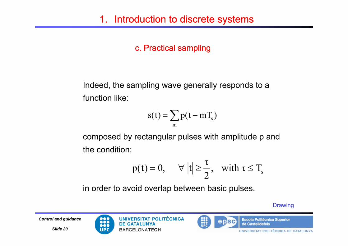
Indeed, the sampling wave generally responds to a f ti likfunction like:

s )mTt(p)t(s

composed by rectangular pulses with amplitude p and the condition:

m

the condition:

sTwith,2

t,0)t(p

in order to avoid overlap between basic pulses.

Drawing


Slide 20

Drawing

c. Practical samplingc. Practical sampling1.1. Introduction to discrete systemsIntroduction to discrete systems

There exists mainly 2 types of practical sampling:

The instantaneous sampling, Sample & Hold in which the p g, pfollowing signal is formed:

mssp )mTt(p)mT(x)t(x

i

which result is a pulse series, where every pulse has a constant amplitude taken as the instantaneous value of x(mTs).

The natural sampling, that is like: sp )mTt(p)t(x)t(xn

in which each pulse varies with x(t) in the existence interval

m

→ In both cases the sampling theorem remains valid even if the ideal sampling wave is not used fs>2W


Slide 21

c. Practical samplingc. Practical sampling1.1. Introduction to discrete systemsIntroduction to discrete systems

In the instantaneous sampling case we can write:

Since the inner expression of the sum is the one obtained for the ideal sampling case, it can be written:

spectrum affected by P(f) value

the effect can be reduced shortening the duration of the samplinglpulse

Advantages: - easy to do with “Sample & Hold” circuitsAdvantages: easy to do with Sample & Hold circuits- immune to noise- pulse form is not important


Slide 22


1.1. Introduction to discrete systemsIntroduction to discrete systemsp gp g

In the natural sampling case the transform is:

whose transform is:

Identical result as the one obtained with an ideal samplingf d b Di d lt i b t ff t d b

Drawing

wave formed by a Dirac delta series, but affected by aconstant coefficient or scale factor P(n fs).


Slide 23

Drawing

d. Aliasingd. Aliasing

1.1. Introduction to discrete systemsIntroduction to discrete systemsgg

Hypothetical spectrum of a properly sampled bandlimited signal (blue)

and images (green) that do not overlap A low pass filter can remove theand images (green) that do not overlap. A low-pass filter can remove the

images and leave the original spectrum, thus recovering the original

i l f h lsignal from the samples

For practical purposes, there can not be a strict limitation of the

analyzed bandwidth, because real signals have a finite length


Slide 24



Hypothetical spectrum of insufficiently sampled bandlimited signal

(blue) X(f) where the images (green) overlap This type of spectrum(blue), X(f), where the images (green) overlap. This type of spectrum

can be considered as bandwidth limited one if the content that exceeds

h i l ( ) i ll b l i ifithe interval (-B, B) is small, or barely significant.

When this type of signal is sampled, an overlap is inevitably created in

the spectrum:


Slide 25



In the process of the signal reconstruction, the frequencies of the

spectrum centered in f lower than f –B that were originally out of the Bspectrum centered in fs, lower than fs B, that were originally out of the B

bandwidth limited now appear inside.

This phenomenon is named aliasingThis phenomenon is named aliasing. The only way to avoid this effect is to properly increase the sampling frequency so that the components out of the taken bandwidth becomefrequency so that the components out of the taken bandwidth become very small and their influence is hardly perceptible.(in practice about 5 to 10 times f1)


Slide 26

(in practice about 5 to 10 times f1)



Properly sampled image of brick wallSubsampled image of brick wall


Slide 27

e. Digital control diagrame. Digital control diagram

1.1. Introduction to discrete systemsIntroduction to discrete systemsg gg g

• y(t), the signal to be controlled, is sampled through an A/D, analogical-digital converter, and compared with the reference value r(nT) stored in a memory position of the micro computation system (where the digital controller is i l t d)implemented)• the result of this comparison is the discrete error signal. This is processed by the microcomputer in order to generate a discrete control signal u(nT) which ismicrocomputer in order to generate a discrete control signal u(nT) which is transformed into an analogical one through a D/A converter.• operation sequence made every Ts seconds, being Ts the sampling period


Slide 28



Two signal types can be distinguished:g yp g• continuous or analog signals: defined for every time instant (u(t), y(t), p(t)).• discrete time signals: only defined in the time instants t = nTs, being n an integer number and Ts the sampling period (r(nT), e(nT), u(nT)).


Slide 29



From the point of view of analysis and design, the following diagram is equivalent:


Slide 30



In order to analyze the behavior of this system using the mathematical tools that are normally used in analogical systems, we notice that:The Laplace transform is not defined for a signal that is only defined at specific time samplesThus, not all the blocks can be modeled using Laplace transfer f ifunctions

we need to model the following part of the digital control diagram:→ we need to model the following part of the digital control diagram:A/D converter – digital controller - D/A converter


Slide 31



A/D D/A part to be modeled:A/D – D/A part to be modeled:


Slide 32



A/D converter: generates an impulse series, each of them being weighted by the analogical signal value at the corresponding time t=nTs

→ sampler


Slide 33



D/A converter: signal re-constructor converts the impulse series into a stepped signal


Slide 34



Digital Controller:

It processes the entry signal providing every Ts seconds and it generates a corrected impulse to act on the system.

→ need of a tool to process discrete signals: z-transform


Slide 35


f. Digital and analog controllersf. Digital and analog controllers

• Digital Controllers only operate on numbers, they can handle non-

linear control equations that involve complicated calculations or

logical operations.

• Larger variety of control laws can be used with Digital Controllers.g y g

• Digital Controllers can execute complex calculations at constant

d t hi h daccuracy and at high speed.

• Due to the availability of cheap μ-computers, Digital Controllers are

used in the vast majority of control systems.


Slide 36



• Analog controllers must represent the variables in an equation

using continuous physical amountsusing continuous physical amounts.

• Analog controllers must be built with physical components such

as transistors, capacitors, inductors, resistances...

• The cost of the Analog Controller increases quickly as the g q y

calculation complexity increases, if a constant accuracy has to

be maintainedbe maintained.


Slide 37



Additional advantages of the Digital Controllers:

• Digital components (A/D converters, D/A, etc..) are robust,

highly trustworthy and usually compact and light.

• Digital systems are scalable• Digital systems are scalable.

• High sensitivity and cheaper.

• Less sensitive to noise signals.

Flexible allow programming changes• Flexible, allow programming changes.

• Less prone to environmental conditions.


Slide 38

2- Z-transform2- Z-transform2- Z-transform2- Z-transform


Slide 39

2. Z2. Z--transformtransform

We consider a sampled signal (ideal):

)kTt()k(f)T2t()2(f)T1t()1(f)t()0(f)t(f )kTt()k(f...)T2t()2(f)T1t()1(f)t()0(f)t(f

Using:th L l t f δ(t) 1• the Laplace transform δ(t)→1

• the temporal delay property of the Laplace transform:

TL )()( · sFenTtf snTL

kTsTs e)k(f...e)1(f)0(f)t(fL)s(F

0k

kTse)k(f


Slide 40

0k

Gi th h f i bl

2. Z2. Z--transformtransformTsezGiven the change of variable : ez

The z transform is obtained for a time function x(t) or x(kT) (T sampling period) :

k1 z)kT(f...z)T(f)0(f)t(fZ)z(F

kz)kT(f

z)kT(f...z)T(f)0(f)t(fZ)z(F

and for a number sequence:

0k

k1 z)k(f...z)1(f)0(f)k(fZ)z(F

q

0k

kz)k(f


Slide 41

0k

2. Z transform2. Z transform

Z transform examples:Z transform examples:

Z-transforms of time functions:• step• ramp

Sequence Z-transforms:• 0 0 1 1 1• 0, 0, 1, 1, 1…• 0, 2, 5, 1 and then 0• aka

Exercices


Slide 42

Exercices

Usual transforms:


zFsFtf )()()(Usual transforms:

using: zzz

stu

zFsFtf

11

11)(

)()()(

1using:

zeezz

ase

zzs

aTaTat

111

11

1

kz)kT(f)z(F

zTz

st

zeezas

11

1

22

0k

z)kT(f)z(F

aTzzaTz

asaat

zs

1)cos(2)sin()sin(

1

222

aTzzaTzz

assat

aTzzas

1)cos(2)cos()cos(

1)cos(2

222

azza

aTzzask

1)cos(2


Slide 43

az


Properties and theoremsProperties and theorems

Linearity:

Properties and theoremsProperties and theorems

)z(Y)z(X)]t(y)t(x[Z

Multiplication by ak:

z)k(xa)]k(xa[Z kkk

)a(Xa)k( 1k1

0k

)za(Xza)k(x 1

0k

1


Slide 44


Real translation theorem:Real translation theorem:

)z(Xz)]nTt(x[Z n )()]([it delays the x(t) function of a time nT

1nkn z)kT(x)z(Xz)]nTt(x[Z

0k

it advances the function x(t) of a time nT

Complex translation theorem:

Example)ze(X)]t(xe[Z aTat


Slide 45

Example


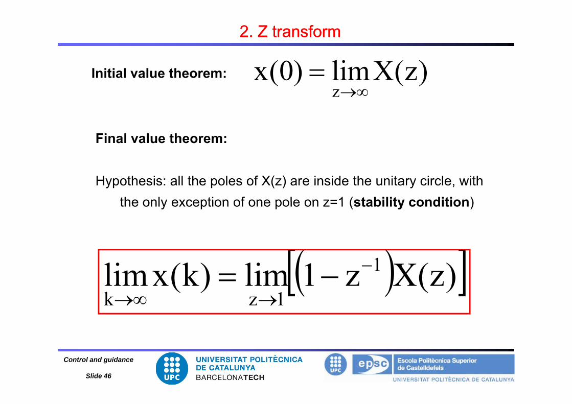
)(Xli)0(Initial value theorem: )z(Xlim)0(xz

Final value theorem:

Hypothesis: all the poles of X(z) are inside the unitary circle, with the only exception of one pole on z=1 (stability condition)the only exception of one pole on z=1 (stability condition)

)z(Xz1lim)k(xlim 1

1k

1zk


Slide 46


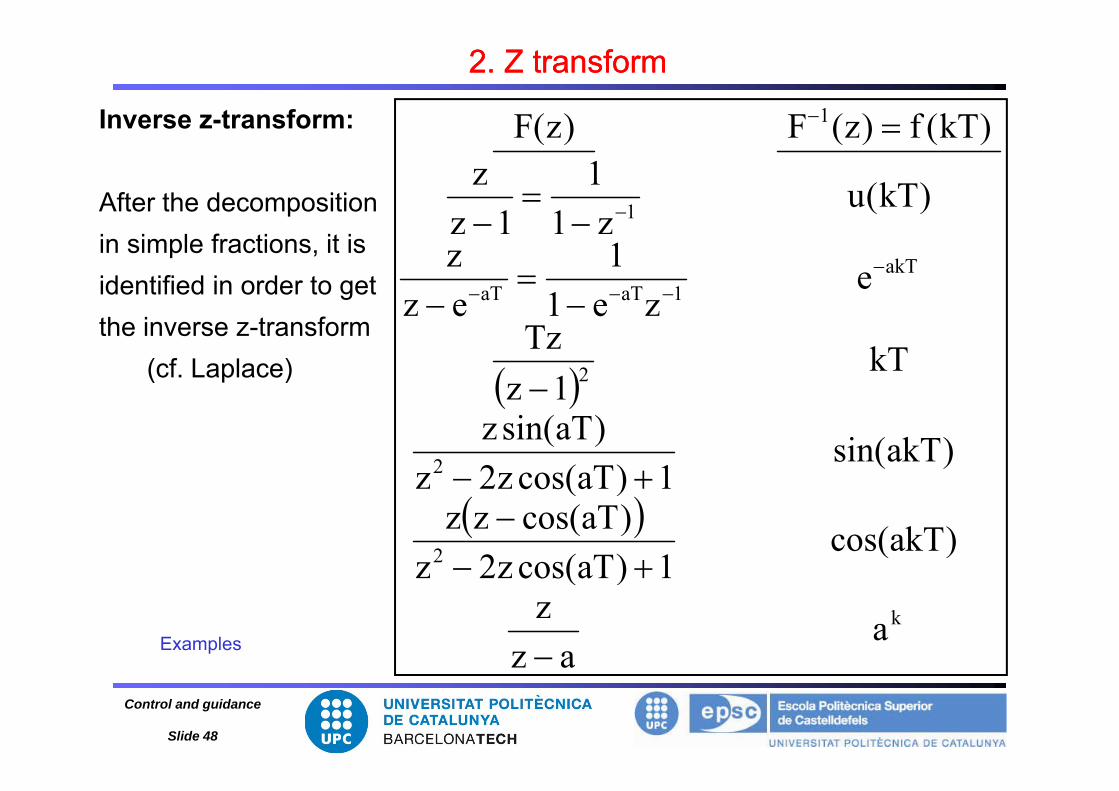
Inverse zInverse z--transform:transform:

Equivalent to the inverse Laplace transform.

Be careful: only the discrete time sequence at the sampling times is obtained from the inverse z transform (not thetimes is obtained from the inverse z-transform (not the continuous signal).


Slide 47


Inverse z-transform: 1 )kT(f)z(F)z(F Inverse z transform:

After the decomposition 1 )kT(u1

11

z)kT(f)z(F)z(F

pin simple fractions, it isidentified in order to get

akT1aTaT

1

eze1

1ezz

z11z

the inverse z-transform (cf. Laplace) 2

kT1z

Tzze1ez

2 )akTsin(1)aTcos(z2z

)aTsin(z1z

2 )akTcos(1)aTcos(z2z

)aTcos(zz1)aTcos(z2z

kaaz

z1)aTcos(z2z

Examples


Slide 48

az

3 Th Z t f f ti3 Th Z t f f tia Convolution suma Convolution sum

3. The Z-transfer function3. The Z-transfer functiona. Convolution suma. Convolution sum

G(s)x(t) x*(t) y(t)

δT

δT

y*(t)

• sampled income signal• if there is another sampler at the exit, it is synchronized

T

with the entry sampler = both have the same sampling period T

• We need to obtain the relation between x*(t) and y*(t) (i.e. the relation between X(z) and Y(z).


Slide 49

a Convolution suma Convolution sum

3. The Z3. The Z--transfer functiontransfer function

a. Convolution suma. Convolution sum

0k0k

)kTt()kT(x)kTt()t(x)t(x 0k0k

0

* )(*)()()(*)()(k

ss tgkTtkTxtxtgty

0

)()(k

kTtgkTx

Given g(t): system weight function (response function to δ(t) entry):Tt0)0(x)t(g

0k

T3tT2T2tT

)T2(x)T2t(g)T(x)Tt(g)0(x)t(g)T(x)Tt(g)0(x)t(g

)()(g

)t(y

T)1k(tkT...

)kT(x)kTt(g...)T(x)Tt(g)0(x)t(g............

)()(g)()(g)()(g)(y


Slide 50

)()()(g)()(g)()(g



response y(t) to the entry x*(t) is the sum of the individual impulse responses

Since g(t)=0 for t<0 is equivalent to g(t-kT)=0 for t<kT, these equations can be added up:equations can be added up:

T)1k(0f)kT()kT()T()T()0()()(

T)1k(t0for)nT(x)nTt(g

T)1k(t0for)kT(x)kTt(g...)T(x)Tt(g)0(x)t(g)t(yk

T)1k(t0for)nT(x)nTt(g0n


Slide 51



Value of y(t) at the sampling moment t=kT:

k )nT(x)nTkT(g)kT(

k

0n

)nT(g)nTkT(x)kT(y

k0n

)kT(g)kT(x)kT(y

)nT(g)nTkT(x0n

)kT(g)kT(x)kT(y


Slide 52


It links the exit z-transform at the sampling times to the b. Zb. Z--TFTF

corresponding sampled entry:

)z(Yz)kT(y)kT(yZ k

k)()k(

)z(Yz)kT(y)kT(yZ

k

0k

nkmz)nT(x)nTkT(g k

0k 0n

z)nT(x)mT(g )nm(

0m 0n

)z(X)z(Gz)nT(xz)mT(g n

0m 0n

m


Slide 53

0m 0n


b. Zb. Z--TFTF

Relates the pulse exit Y(z) to the pulse entry X(z):

)z(Y Pulse transfer function of the

)z(X)z(Y)z(G

Pulse transfer function of the

system in discrete time


Slide 54


c. Rules to obtain the Zc. Rules to obtain the Z--transfer functiontransfer function

Be careful with the difference between:

G(s)x(t)

δ

x*(t)

y*(t)

y(t)

X(z)δT

δT

y*(t)X(z)

Y(z)

G(s)x(t) y(t)

Y(s)X(s)

Examples


Slide 55

Examples

Remember: the idea is to model the following digital control system:

4- Digital control tools4- Digital control toolsControl and guidance

Slide 56


A/D Converter: It generates an impulse series, each of them weighted by the value of the analogical signal at the corresponding time t=nTs


Slide 57


Digital controller:Digital controller:

It processes, through a recursive algorithm, the weights of the entry impulses and it generates (every Ts seconds) an adjusted impulse with the result of the recursive equation.

→ use of a tool to process discrete signals: Z-transform


Slide 58

D/A converter: Zero Order Holder (ZOH)


D/A converter: Zero Order Holder (ZOH)

signal re-builder which transforms the impulse series into asignal re builder which transforms the impulse series into a stepped signal (analog signal with values for every time instant)


Slide 59

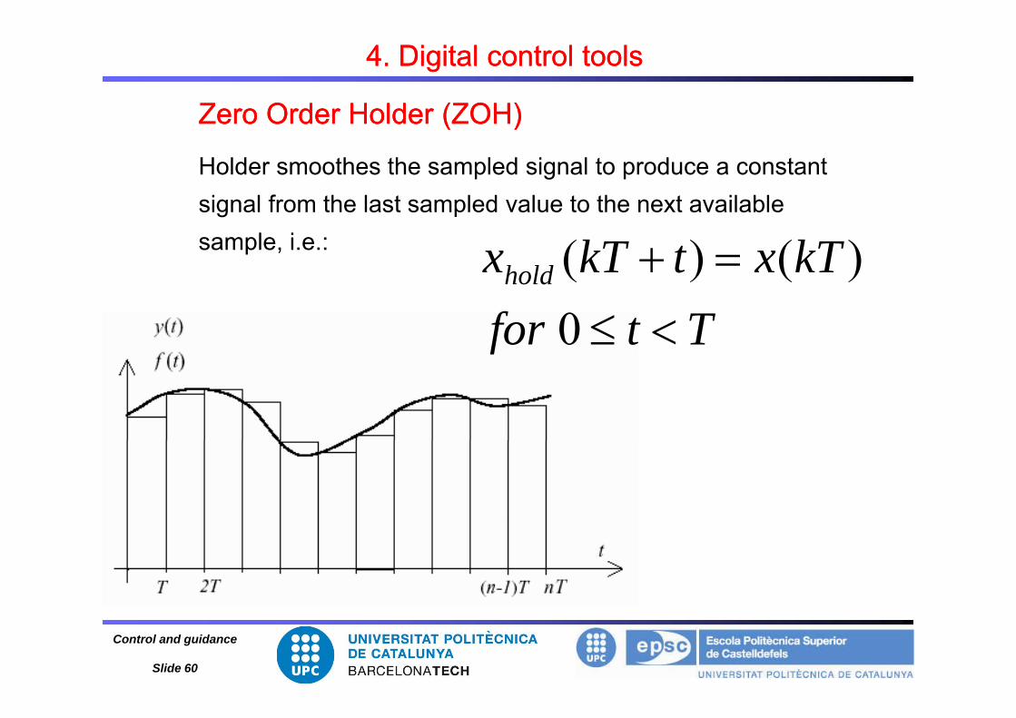
Zero Order Holder (ZOH)Zero Order Holder (ZOH)



Holder smoothes the sampled signal to produce a constant i l f th l t l d l t th t il blsignal from the last sampled value to the next available

sample, i.e.: kTxtkTxhold )()(Ttfor

hold

0)()(


Slide 60



Calculation of its transfer function:


Hypothesis: x(t)=0 for t<0

...)2()()()()()0()(hold TtuTtuTxTtutuxtx )1()()(

)()()()()()()(hold

TktukTtukTx

)1()()()( TktukTtukTxtx

0

)1()()()(k

hold TktukTtukTxtx


Slide 61



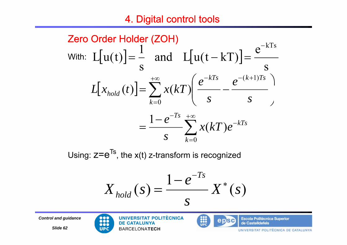
With: s

e)kTt(uLands1)t(uL

kTs


ss

)1(

)()(TskkTs

holdeekTxtxL

0

)(1

)()(

kTsTs

khold

kTe

ss

0

)(1k

kTsekTxse

TUsing: z=eTs, the x(t) z-transform is recognized

1 e Ts

)(1)( sXsesX hold


Slide 62




And the transfer function of the zero order holder is obtained:

e1)(GTs

se1)s(GZOH


Slide 63

Pulse transfer function of a digital control systemPulse transfer function of a digital control system



D*(s)E(s) E*(s)

Y(s)e1 TsGP(s)

R(s)( )

δT sP( )

T

G(s)

)s(Gse1)s(G P

Tswe define:

sAnd its z-transform will be computed: G(z).


Slide 64



*E(s) E*(s)Y(s)e1 TsR(s)


D*(s)E(s)

δT

E (s)

se1

GP(s)R(s)

G(s)

)s(Y)s(R)s(E)s(E)s(D)s(G)s(Y

)s(Y)s(R)s(E)s(E)s(D)s(G)s(Y **

)z(Y)z(R)z(D)z(G)z(Y

)(G)(D)(Y)z(G)z(D1

)z(G)z(D)z(R)z(Y


Slide 65

)()()(

Discrete designDiscrete design


Discrete designDiscrete designStage 1: compute the transfer function of the continuous part

E( ) E*( ) Y(s)R( ) D *(s)E(s)

δT

E*(s) Y(s)GP(s)R(s) ZOH

G(s)

~D(z) Y(z)G(z)R(z)

~


Slide 66



With: se1)s(G

Ts

ZOH


s

sGseZsGsGZ p

Ts

pZOH )(1)()·(

sGeZ pTs )(

1

sGsG

se

T )()(

ssG

eZs

sGZ pTsp )()(

ssG

Zzs

sGZ pp )(

·)( 1


Slide 67



The transfer function of the plant + ZOH is deduced:


)s(G

Zz1)z(G p1

s

)(

And the transfer function in closed loop of the discrete system:

)(G)(1)z(G)z(D

)()z(Y

)z(G)z(D1)z(R


Slide 68



Stage 2:


To study the characteristics of the closed loop behavior we

look for the characteristic equation’s roots:

1+KG(z)=0 (for D(z)=K: proportional controller)

→ root locus technique

Construction rules are the same as in the s plane,

but the interpretation is differentbut the interpretation is different

Example


Slide 69

Relation between the sRelation between the s plane and the zplane and the z planeplane


Relation between the sRelation between the s--plane and the zplane and the z--planeplane

When an impulse sampling is incorporated, the complex variables s and z are related by the equation:

Tsez ez → A pole on the s plane can be placed in the z plane by this

transformationtransformation.

Given: js jTTjT eeez

k2TjT eezControl and guidance

Slide 70



→ poles and zeros in the s-plane, where the frequencies differ


poles and zeros in the s plane, where the frequencies differ in numbers multiples of the sampling frequency ωs=2π/Ts, belong to the same locations in the z plane.→ relationship between the z plane and the s plane is not unique

One point in the z plane corresponds to an infinite number of points in the s plane, but one point in the s plane corresponds to only one point in the z plane.

Examples


Slide 71



The root locus is builded the same way as in the continuous domain

but its interpretation differs:


p

Stability:s plane: σ<0s plane: σ<0

z plane: 1ez T

Equivalence: s plane z plane

• imaginary axis ~ unitary circle

1ez

• left semi-plane ~ inside the circle

• critically stable (s=0) ~ |z|=1 for a pole

→ stability can be determined with the pole positions

→ stability depends on the sampling period T


Slide 72

y p p g p



Geometric locus of constant damping factor and natural frequencyRelation between the sRelation between the s plane and the zplane and the z planeplane


Slide 73



Geometric locus of constant damping factor and natural frequency


1

1.5

1

Root Locus

1

1.5Root Locus

s complex plane z complex plane

0.5

10.7

xis

0.5

11

0.7

xis

-0.5

0

Imag

inar

y A

x

-0.5

0

Imag

inar

y A

x

-10.7

1 -11

-1.5 -1 -0.5 0 0.5 1 1.5-1.5

Real Axis-1.5 -1 -0.5 0 0.5 1 1.5

-1.5

Real Axis


Slide 74


Digital control diagramDigital control diagram

Remember: the idea is to model the following digital control system:


Slide 75

Di t d iDi t d i



E( ) E*( ) Y(s)R( ) D *(s)E(s)

δT


G(s)

~D(z) Y(z)G(z)R(z)

~


Slide 76

Digital controllersDigital controllers


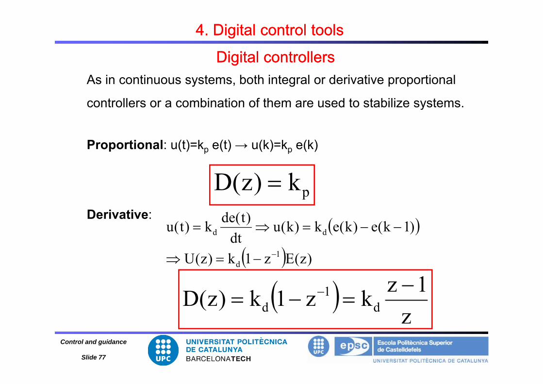
Digital controllersDigital controllersAs in continuous systems, both integral or derivative proportional

controllers or a combination of them are used to stabilize systemscontrollers or a combination of them are used to stabilize systems.

Proportional: u(t)=kp e(t) → u(k)=kp e(k)Proportional: u(t) kp e(t) u(k) kp e(k)

pk)z(D Derivative:

p)( )1k(e)k(ek)k(u

dt)t(dek)t(u dd

)z(Ez1k)z(Udt

1d

1 z

1zkz1k)z(D d1

d


Slide 77

z



Integrator: (k)k1)(k(k)(t)dtk(t)t


Integrator:

E(z)kU(z)zU(z)

e(k)k1)u(ku(k)e(t)dtku(t)

i1

i0i

zkk)z(D ii

1zz1)z(D i

1i


Slide 78

Satellite attitude control system


Satellite attitude control system

dtFMMMtI CDID ).()(

with θ(t) satellite orientation

MD torque of the perturbationsFC(t) applied thrust

If id t b ti dtFtI )()(

If you consider zero perturbations:

or using the Laplace transform:

dtFtI C ).()(

1)()( sG or, using the Laplace transform:2.

)()(IsFd

sGC

P

Design requirements: ωn=0.3rad/s

ζ=0.7Control and guidance

Slide 79

ζ 0.7

Satellite attitude control system without any controller


Satellite attitude control system without any controller

2Root Locus

1

1.5

0.5

y Ax

is

-0.5

0

Imag

inar

y

-1.5

-1

-3.5 -3 -2.5 -2 -1.5 -1 -0.5 0 0.5 1-2

1.5

R l A i


Slide 80

Real Axis

Satellite attitude control system with controller


Satellite attitude control system with controller1.5

1

0.5

0.30.7

y A

xis

0

0 .3Imag

inar

y

1

-0.5

-1 5

-1


Slide 81

-3 -2.5 -2 -1.5 -1 -0.5 0 0.5 11.5

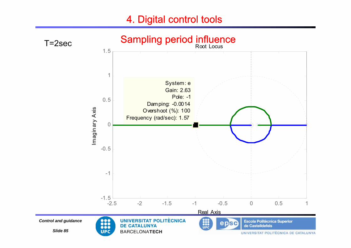
Sampling period influenceSampling period influence



Already seen: destabilizing effect of the zero order holder (ZOH).y g ( )

1s1)s(Gp

1. Compute G(z), for a plant:1s

We introduce an integral digital controller:1z

Kz)z(D

1z

2. Draw the root locus of the transfer function in open loop:

H(z)=D(z).G(z), for: T=0.5s, 1s y 2sec

3. Compute Kcr in the 3 cases


Slide 82



T=0.5sec Root Locus1.5


1System: eGain: 8.17

Pole: -1ar

y A

xis

0

0.5 Pole: -1Damping: -0.0014

Overshoot (%): 100Frequency (rad/sec): 6.28

Imag

ina

-0.5

0

-1

Real Axis-2.5 -2 -1.5 -1 -0.5 0 0.5 1

-1.5


Slide 83

Real Axis



T=1sec Root Locus1.5



Pole: 1ar

y A

xis

0

0.5 Pole: -1Damping: -0.0014


Imag

ina

-0.5

0

-1

R l A i-2.5 -2 -1.5 -1 -0.5 0 0.5 1

-1.5


Slide 84

Real Axis



T=2sec Root Locus1.5



Pole: 1ry

Axi

s

0

0.5 Pole: -1Damping: -0.0014


Imag

ina

-0.5

0

-1

-2.5 -2 -1.5 -1 -0.5 0 0.5 1-1.5


Slide 85

Real Axis

1.4 S li i d i flS li i d i fl


1.2

1.4T=0.5sec Sampling period influenceSampling period influence

1A

mpl

itud

e 0.8

A

0 4

0.6

0.2

0.4

0 5 10 15 200


Slide 86

Time (sec )

1.4T=1sec S li i d i flS li i d i fl


1.2

T 1sec Sampling period influenceSampling period influence

1

0.8

Am

plitu

de

0 .4

0.6

0.2

0 2 4 6 8 10 12 14 16 180

Time (sec )


Slide 87

( )

1.4T=2sec Sampling period influenceSampling period influence


1.2

T 2sec Sampling period influenceSampling period influence

1

0.8

Am

plitu

de

0.4

0.6

0.2

0.4

0 5 10 15 200

Time (sec )


Slide 88

Time (sec )

1.4


1.2


1

Am

plitu

de

0 .8

0.4

0.6

0.2

Time (sec )

0 2 4 6 8 10 12 14 16 18 200


Slide 89

( )



• If the sampling period is small the y(kT) graphic gives a quite


• If the sampling period is small the y(kT) graphic gives a quite

precise image of the y(t) response

I t t t l t li i d b d th ti f ti• Important to select a sampling period based on the satisfaction:

- of the sampling theorem (Nyquist),

- of the system dynamics,

- of the equipment real conditions

• Acceptable rule: 8 to 10 samples per cycle… (for a subdamped

system that shows oscillations in the response)


Slide 90

Error in steady stateError in steady state



• Error in steady state: also defined in discrete time.

• Classification depending on the number of open loop poles in the z=1

point (equivalent to s=0: it corresponds to an integrator).

• System’s type defines the characteristics of the system in steady state

Y(s)D(z)E(s)

δT


T

G(s)


Slide 91



• Error: e(t)=r(t)-y(t)


• For a stable system (poles inside the unitary circle):

Final value theorem gives the error value in steady

state at the sampling times:

k )(li)(li 1

zR

zEzkTezk

)(

)(1lim)(lim 1

1

zGzDzRzEwith

)()(1)()(

ssG

ZzzGand p )(1)( 1


Slide 92

s



)(1li 1 zR


)()(1)(1lim 1

1 zGzDze

zss

Example: Given a digital control system where the plant is a fi t d t d h 2 d l d t k T 1first order system and has a 2 sec. delay and take T=1s

e)(Gs2 e1)s(G

Ts

1s)s(Gp

s)s(GZOH

Compute the error in steady state for a unit step entry.


Slide 93

5. Design method with dead beat response5. Design method with dead beat response

Method principle:

To force the error sequence (for a system subject to a specific

entry type, in this course we will always consider a step entry) to y yp , y p y)

reach and keep a zero value after a finite number of sampling

periods in fact after the minimum possible number of samplingperiods, in fact, after the minimum possible number of sampling

periods


Slide 94


If the response of a closed loop control system to a unitary step entry

shows a minimum possible establishment time with no error in steadyshows a minimum possible establishment time, with no error in steady

state and no oscillatory beat component between sampling instants,

th thi t i ll k d d b tthen this response type is usually known as dead beat response

Drawing


Slide 95


D(z) Y(z)G(z)R(z) E(z) U(z)

s)s(G

Zz1)z(Gwith p1

s

)()()()( zGzDzYF)()(1

)()()()()(

zGzDzRzF


Slide 96


In order to have a finite time of establishment with a zero error in steady state the system will have to show a finite impulse response:steady state, the system will have to show a finite impulse response:

azazaza kN1NN

za...za...zaza)z(F N

Nk10

zazazaa)z(For

Nk1

)ordersystemG:n(nNwithza...za...zaa)z(F

p

Nk10

→ We are looking for the ai


Slide 97


From F(z) the controller transfer function D(z) is calculated

)()( zFzD )(1)(

)(zFzG


Slide 98

C diti t k th d i h i ll f iblC diti t k th d i h i ll f ibl


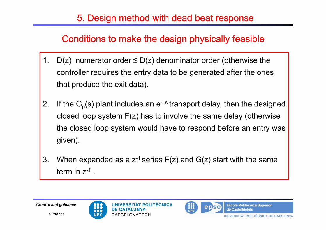
Conditions to make the design physically feasibleConditions to make the design physically feasible

1. D(z) numerator order ≤ D(z) denominator order (otherwise the1. D(z) numerator order D(z) denominator order (otherwise the controller requires the entry data to be generated after the ones that produce the exit data).

2. If the Gp(s) plant includes an e-Ls transport delay, then the designed closed loop system F(z) has to involve the same delay (otherwiseclosed loop system F(z) has to involve the same delay (otherwise the closed loop system would have to respond before an entry was given)given).

3. When expanded as a z-1 series F(z) and G(z) start with the same term in z-1 .


Slide 99

Stability conditionsStability conditions



Avoid the cancellation of an unstable pole of the plant by the use of adigital controller z.

1. If G(z) includes an unstable pole (or critically stable) on z=α

We define:

)z(G)z(G 1

and the tf in closed loop:z

)(

zzGzD

zF

)()()(

1

zzGzD

zF )()(1)(

1


Slide 100

z




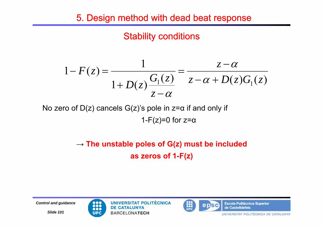
1 )()()()(1

1)(111 zGzDz

zzGzD

zF

No zero of D(z) cancels G(z)’s pole in z=α if and only if

)(1z

zD

1-F(z)=0 for z=α

→ The unstable poles of G(z) must be included as zeros of 1-F(z)


Slide 101




2 In the same way for unstable zeros:2. In the same way for unstable zeros:

zzGzDF )()()( 1

zzGzD

zF)()(1

)()()(1

1

zeros of G(z) that are located on or out the unitary circle must not be cancelled with D(z) poles

→ The unstable zeros of G(z) must be included as zeros of F(z)


Slide 102

DesignDesign


DesignDesign

The error can be written as:

E(z)=R(z)-Y(z)=R(z)(1-F(z))

for a step entry:11

1)z(R 1z1)(

)z(F11)z(E

In order to be sure that the system reaches the steady state in a finite

)z(F1z1

)z(E 1

y y

number of sampling periods and that maintains a null error output, E(z)

must be a polynomial in z-1 with a finite number of termsmust be a polynomial in z with a finite number of terms


Slide 103

DesignDesign


DesignDesign

→ 1-F(z) must cancel the denominator: )z(F1z1

1)z(E 1

with N(z) polynomial in z-1

z1

)z(Nz1)z(F1 1 with N(z) polynomial in z

Then E(z)=N(z) is a polynomial in z-1 with a finite number of terms

)()(

Then, E(z)=N(z) is a polynomial in z 1 with a finite number of terms

and e(k) tends to zero in a finite number of sampling periods


Slide 104

DesignDesign


DesignDesign

D(z)Y(z)

G(z)R(z) E(z) U(z)

D(z) G(z)

For a stable plant Gp(s), the condition so that the exit does not show oscillating components between samplings after theshow oscillating components between samplings after the establishment time is: entrystepafornTty constant

where n is the Gp(s) order

In practice this condition can be applied to u(t)In practice this condition can be applied to u(t)

entrystepafornTtu constant


Slide 105

)()()( G )(F


• Search:)()(1

)()()()()(

zGzDzGzD

zRzYzF

)(1)()()(

zFzGzFzD

•

• if G has a delay F(z) has the same

)orderG:n(nNwithza...za...zaa)z(F pN

Nk

k1

10

if Gp has a delay, F(z) has the same

• D(z) numerator grade ≤ D(z) denominator grade Physically feasible

• F(z) begins with the same order (in z-1) as G(z)

• G(z) unstable poles = (1-F(z)) zeros( ) p ( ( ))

• G(z) unstable zeros = F(z) zeros

Stability condition

• with N(z) polynomial in z-1, for a step entry

• n is the Gp(s) order

)z(Nz1)z(F1 1

entrystepafornTty constantControl and guidance

Slide 106

ypy


Calculator: Disturbance (wind, etc…)

Crew requirement

Calculator: Digital controller

Exit parameter

Dif eq representing the airplane movement


Slide 107


D*(s)E(s) E*(s)

Y(s)e1 TsGP(s)

R(s)( )

δT sP( )

s5

G(s)

With : transfer function of the plant has a 5 sec. delay1s10

e)s(Gs5

p

T=5s is considered


Slide 108


The following exit y(t) is required for a unitary step entry: 1 .5

1

1

1

y(t)

0 .5 0.62

0 1 0 1 2 0 2 3 0 3 4 00

0

no overshoot nor error in steady state, nor oscillations between samples after reaching a zero error

0 5 1 0 1 5 2 0 2 5 3 0 3 5 4 00

t(s )


Slide 109

samples after reaching a zero error


1. Calculate G(z) (depending on z-1)

2. Look for unstable poles and zeros

3. Given the y(nT) sequence, calculate Y(z)

)z(Y4. Calculate

C l l D( ) d if h i i h i ll f ibl

)z(R)z(Y)z(F

5. Calculate D(z) and verify that it is physically feasible


Slide 110


1. Calculate G(z) (depending on z-1)

z61.0z39.0

z61.01z39.0)z(G 21

2

z61.0zz61.01

2. Look for unstable poles and zeros

no zero poles: 0 and 0 61 both stableno zero, poles: 0 and 0.61 both stable


Slide 111

32 380620


3. Given the y(nT) sequence, calculate1

32

z1z38.0z62.0)z(Y

4 C l l t 32 380620)z(Y)(4. Calculate 32 z38.0z62.0)z(R)z(Y)z(F

5. Calculate)380)(1(

)37.0(58.1)3801)(1(

)37.01(58.1)( 2

3

211

2

zzzzD

and verify that it is physically feasible

)38.0)(1()38.01)(1()( 2211 zzzzzz

z61.0z39.0

z61.01z39.0)z(G 21

2


Slide 112



Slide 113

REFERENCESREFERENCESREFERENCESREFERENCES

Ogata, K., Modern Control Engineering (4th Ed.), Prentice Hall, 2001

Kuo B Automatic Control Systems Wiley and Sons (8th Ed ) 2002Kuo, B., Automatic Control Systems, Wiley and Sons, (8 Ed.), 2002

Dorf, R. and Bishop, R., Modern Control Systems, (10th Ed.), Prentice Hall, 2004

Kirk, D. E., Optimal Control Theory: An Introduction, 2004

Athans M A and Falb P L Optimal Control McGraw Hill New York 1966Athans, M. A. and Falb, P. L., Optimal Control, McGraw-Hill, New York, 1966

Levine, W. S., The Control Handbook. New York: CRC Press, 1996


Slide 114

Digital Control - UPCommons

Documents

Transcript of Digital Control - UPCommons