TRUE DIGITAL CONTROL
343
TRUE DIGITAL CONTROL
-
Upload
khangminh22 -
Category
Documents
-
view
0 -
download
0
Transcript of TRUE DIGITAL CONTROL

TRUE DIGITALCONTROL

TRUE DIGITALCONTROLSTATISTICAL MODELLINGAND NON-MINIMAL STATESPACE DESIGN
C. James Taylor, Peter C. Young and Arun ChotaiLancaster University, UK

This edition first published 2013C© 2013 John Wiley & Sons, Ltd
Registered officeJohn Wiley & Sons Ltd, The Atrium, Southern Gate, Chichester, West Sussex, PO19 8SQ, United Kingdom
For details of our global editorial offices, for customer services and for information about how to apply forpermission to reuse the copyright material in this book please see our website at www.wiley.com.
The right of the author to be identified as the author of this work has been asserted in accordance with the Copyright,Designs and Patents Act 1988.
All rights reserved. No part of this publication may be reproduced, stored in a retrieval system, or transmitted, in anyform or by any means, electronic, mechanical, photocopying, recording or otherwise, except as permitted by the UKCopyright, Designs and Patents Act 1988, without the prior permission of the publisher.
Designations used by companies to distinguish their products are often claimed as trademarks. All brand names andproduct names used in this book are trade names, service marks, trademarks or registered trademarks of theirrespective owners. The publisher is not associated with any product or vendor mentioned in this book.
Limit of Liability/Disclaimer of Warranty: While the publisher and author have used their best efforts in preparingthis book, they make no representations or warranties with respect to the accuracy or completeness of the contents ofthis book and specifically disclaim any implied warranties of merchantability or fitness for a particular purpose. It issold on the understanding that the publisher is not engaged in rendering professional services and neither thepublisher nor the author shall be liable for damages arising herefrom. If professional advice or other expertassistance is required, the services of a competent professional should be sought.
MATLAB R© is a trademark of The MathWorks, Inc. and is used with permission. The MathWorks does not warrantthe accuracy of the text or exercises in this book. This books use or discussion of MATLAB R© software or relatedproducts does not constitute endorsement or sponsorship by The MathWorks of a particular pedagogical approach orparticular use of the MATLAB R© software.
Library of Congress Cataloging-in-Publication Data
Taylor, C. James.True digital control : statistical modelling and non-minimal state space design / C. James Taylor, Peter C. Young,
Arun Chotai.pages cm
Includes bibliographical references and index.ISBN 978-1-118-52121-2 (cloth)
1. Digital control systems–Design. I. Young, Peter C., 1939- II. Chotai, Arun. III. Title.TJ223.M53T38 2013629.8′95–dc23
2013004574
A catalogue record for this book is available from the British Library
ISBN: 978-1-118-52121-2
Typeset in 10/12pt Times by Aptara Inc., New Delhi, India
1 2013

To Ting-Li
To Wendy
In memory of Varsha

Contents
Preface xiii
List of Acronyms xv
List of Examples, Theorems and Estimation Algorithms xix
1 Introduction 11.1 Control Engineering and Control Theory 21.2 Classical and Modern Control 51.3 The Evolution of the NMSS Model Form 81.4 True Digital Control 111.5 Book Outline 121.6 Concluding Remarks 13
References 14
2 Discrete-Time Transfer Functions 172.1 Discrete-Time TF Models 18
2.1.1 The Backward Shift Operator 182.1.2 General Discrete-Time TF Model 222.1.3 Steady-State Gain 23
2.2 Stability and the Unit Circle 242.3 Block Diagram Analysis 262.4 Discrete-Time Control 282.5 Continuous to Discrete-Time TF Model Conversion 362.6 Concluding Remarks 38
References 38
3 Minimal State Variable Feedback 413.1 Controllable Canonical Form 44
3.1.1 State Variable Feedback for the General TF Model 493.2 Observable Canonical Form 503.3 General State Space Form 53
3.3.1 Transfer Function Form of a State Space Model 533.3.2 The Characteristic Equation, Eigenvalues and Eigenvectors 553.3.3 The Diagonal Form of a State Space Model 57

viii Contents
3.4 Controllability and Observability 583.4.1 Definition of Controllability (or Reachability) 583.4.2 Rank Test for Controllability 593.4.3 Definition of Observability 593.4.4 Rank Test for Observability 59
3.5 Concluding Remarks 61References 62
4 Non-Minimal State Variable Feedback 634.1 The NMSS Form 64
4.1.1 The NMSS (Regulator) Representation 644.1.2 The Characteristic Polynomial of the NMSS Model 67
4.2 Controllability of the NMSS Model 684.3 The Unity Gain NMSS Regulator 69
4.3.1 The General Unity Gain NMSS Regulator 744.4 Constrained NMSS Control and Transformations 77
4.4.1 Non-Minimal State Space Design Constrained to yield a MinimalSVF Controller 79
4.5 Worked Example with Model Mismatch 814.6 Concluding Remarks 85
References 86
5 True Digital Control for Univariate Systems 895.1 The NMSS Servomechanism Representation 93
5.1.1 Characteristic Polynomial of the NMSS Servomechanism Model 955.2 Proportional-Integral-Plus Control 98
5.2.1 The Closed-Loop Transfer Function 995.3 Pole Assignment for PIP Control 101
5.3.1 State Space Derivation 1015.4 Optimal Design for PIP Control 110
5.4.1 Linear Quadratic Weighting Matrices 1115.4.2 The LQ Closed-loop System and Solution of the Riccati Equation 1125.4.3 Recursive Solution of the Discrete-Time Matrix Riccati Equation 114
5.5 Case Studies 1165.6 Concluding Remarks 119
References 120
6 Control Structures and Interpretations 1236.1 Feedback and Forward Path PIP Control Structures 123
6.1.1 Proportional-Integral-Plus Control in Forward Path Form 1256.1.2 Closed-loop TF for Forward Path PIP Control 1266.1.3 Closed-loop Behaviour and Robustness 127
6.2 Incremental Forms for Practical Implementation 1316.2.1 Incremental Form for Feedback PIP Control 1316.2.2 Incremental Form for Forward Path PIP Control 134

Contents ix
6.3 The Smith Predictor and its Relationship with PIP Design 1376.3.1 Relationship between PIP and SP-PIP Control Gains 1396.3.2 Complete Equivalence of the SP-PIP and Forward Path PIP
Controllers 1406.4 Stochastic Optimal PIP Design 142
6.4.1 Stochastic NMSS Equations and the Kalman Filter 1426.4.2 Polynomial Implementation of the Kalman Filter 1446.4.3 Stochastic Closed-loop System 1496.4.4 Other Stochastic Control Structures 1506.4.5 Modified Kalman Filter for Non-Stationary Disturbances 1516.4.6 Stochastic PIP Control using a Risk Sensitive Criterion 152
6.5 Generalised NMSS Design 1536.5.1 Feed-forward PIP Control based on an Extended Servomechanism
NMSS Model 1536.5.2 Command Anticipation based on an Extended Servomechanism
NMSS Model 1546.6 Model Predictive Control 157
6.6.1 Model Predictive Control based on NMSS Models 1586.6.2 Generalised Predictive Control 1586.6.3 Equivalence Between GPC and PIP Control 1596.6.4 Observer Filters 162
6.7 Concluding Remarks 163References 164
7 True Digital Control for Multivariable Systems 1677.1 The Multivariable NMSS (Servomechanism) Representation 168
7.1.1 The General Multivariable System Description 1707.1.2 Multivariable NMSS Form 1717.1.3 The Characteristic Polynomial of the Multivariable NMSS Model 173
7.2 Multivariable PIP Control 1757.3 Optimal Design for Multivariable PIP Control 1777.4 Multi-Objective Optimisation for PIP Control 186
7.4.1 Goal Attainment 1877.5 Proportional-Integral-Plus Decoupling Control by Algebraic Pole
Assignment 1927.5.1 Decoupling Algorithm I 1937.5.2 Implementation Form 1947.5.3 Decoupling Algorithm II 195
7.6 Concluding Remarks 195References 196
8 Data-Based Identification and Estimation of Transfer Function Models 1998.1 Linear Least Squares, ARX and Finite Impulse Response Models 200
8.1.1 En bloc LLS Estimation 2028.1.2 Recursive LLS Estimation 203

x Contents
8.1.3 Statistical Properties of the RLS Algorithm 2058.1.4 The FIR Model 210
8.2 General TF Models 2118.2.1 The Box–Jenkins and ARMAX Models 2128.2.2 A Brief Review of TF Estimation Algorithms 2138.2.3 Standard IV Estimation 215
8.3 Optimal RIV Estimation 2188.3.1 Initial Motivation for RIV Estimation 2188.3.2 The RIV Algorithm in the Context of ML 2208.3.3 Simple AR Noise Model Estimation 2228.3.4 RIVAR Estimation: RIV with Simple AR Noise Model
Estimation 2238.3.5 Additional RIV Algorithms 2268.3.6 RIVAR and IV4 Estimation Algorithms 227
8.4 Model Structure Identification and Statistical Diagnosis 2318.4.1 Identification Criteria 2328.4.2 Model Structure Identification Procedure 234
8.5 Multivariable Models 2438.5.1 The Common Denominator Polynomial MISO Model 2438.5.2 The MISO Model with Different Denominator Polynomials 246
8.6 Continuous-Time Models 2488.6.1 The SRIV and RIVBJ Algorithms for Continuous-Time Models 2498.6.2 Estimation of δ-Operator Models 253
8.7 Identification and Estimation in the Closed-Loop 2538.7.1 The Generalised Box−Jenkins Model in a Closed-Loop Context 2548.7.2 Two-Stage Closed-Loop Estimation 2558.7.3 Three-Stage Closed-Loop Estimation 2568.7.4 Unstable Systems 260
8.8 Concluding Remarks 260References 261
9 Additional Topics 2659.1 The δ-Operator Model and PIP Control 266
9.1.1 The δ-operator NMSS Representation 2679.1.2 Characteristic Polynomial and Controllability 2689.1.3 The δ-Operator PIP Control Law 2699.1.4 Implementation Structures for δ-Operator PIP Control 2709.1.5 Pole Assignment δ-Operator PIP Design 2719.1.6 Linear Quadratic Optimal δ-Operator PIP Design 272
9.2 Time Variable Parameter Estimation 2799.2.1 Simple Limited Memory Algorithms 2819.2.2 Modelling the Parameter Variations 2829.2.3 State Space Model for DTF Estimation 2849.2.4 Optimisation of the Hyper-parameters 287

Contents xi
9.3 State-Dependent Parameter Modelling and PIP Control 2909.3.1 The SDP-TF Model 2909.3.2 State-Dependent Parameter Model Identification and Estimation 2929.3.3 Proportional-Integral-Plus Control of SDP Modelled Systems 293
9.4 Concluding Remarks 298References 298
Appendix A Matrices and Matrix Algebra 301A.1 Matrices 301A.2 Vectors 302A.3 Matrix Addition (or Subtraction) 302A.4 Matrix or Vector Transpose 302A.5 Matrix Multiplication 303A.6 Determinant of a Matrix 304A.7 Partitioned Matrices 305A.8 Inverse of a Matrix 306A.9 Quadratic Forms 307A.10 Positive Definite or Semi-Definite Matrices 308A.11 The Rank of a Matrix 308A.12 Differentiation of Vectors and Matrices 308
References 310
Appendix B The Time Constant 311Reference 311
Appendix C Proof of Theorem 4.1 313References 314
Appendix D Derivative Action Form of the Controller 315
Appendix E Block Diagram Derivation of PIP Pole Placement Algorithm 317
Appendix F Proof of Theorem 6.1 321Reference 322
Appendix G The CAPTAIN Toolbox 323G.1 Transfer Functions and Control System Design 323G.2 Other Routines 324G.3 Download 325
References 325
Appendix H The Theorem of D.A. Pierce (1972) 327References 328
Index 329

Preface
This book develops a True Digital Control (TDC) design philosophy that encompasses data-based (statistical) model identification, through to control algorithm design, robustness evalua-tion and implementation. Treatment of both stochastic system identification and control designunder one cover highlights the important connections between these disciplines: for example,in quantifying the model uncertainty for use in closed-loop stochastic sensitivity analysis.More generally, the foundations of linear state space control theory that are laid down in earlychapters, with Non-Minimal State Space (NMSS) design as the central worked example, areutilised subsequently to provide an introduction to other selected topics in modern controltheory. MATLAB R©1 functions for TDC design and MATLAB R© scripts for selected examplesare being made available online, which is important in making the book accessible to readersfrom a range of academic backgrounds. Also, the CAPTAIN Toolbox for MATLAB R©, whichis used for the analysis of all the modelling examples in this book, is available for free down-load. Together, these contain computational routines for many aspects of model identificationand estimation; for NMSS design based on these estimated models; and for offline signalprocessing. For more information visit: http://www.wiley.com/go/taylor.
The book and associated software are intended for students, researchers and engineers whowould like to advance their knowledge of control theory and practice into the state spacedomain; and control experts who are interested to learn more about the NMSS approachpromoted by the authors. Indeed, such non-minimal state feedback is utilised throughout thisbook as a unifying framework for generalised digital control system design. This includesthe Proportional-Integral-Plus (PIP) control systems that are the most natural outcome of theNMSS design strategy. As such, the book can also be considered as a primer for potentiallydifficult topics in control, such as optimal, stochastic and multivariable control.
As indicated by the many articles on TDC that are cited in this book, numerous colleaguesand collaborators have contributed to the development of the methods outlined. We would liketo pay particular thanks to our good friend Dr Wlodek Tych of the Lancaster EnvironmentCentre, Lancaster University, UK, who has contributed to much of the underlying researchand in the development of the associated computer algorithms. The first author would alsolike to thank Philip Leigh, Matthew Stables, Essam Shaban, Vasileios Exadaktylos, EleniSidiropoulou, Kester Gunn, Philip Cross and David Robertson for their work on some of thepractical examples highlighted in this book, among other contributions and useful discussionswhile they studied at Lancaster. Philip Leigh designed and constructed the Lancaster forced
1 MATLAB R©, The MathWorks Inc., Natick, MA, USA.

xiv Preface
ventilation test chamber alluded to in the text. Vasileios Exadaktylos made insightful sugges-tions and corrections in relation to early draft chapters of the book. The second author is gratefulto a number of colleagues over many years including: Charles Yancey and Larry Levsen, whoworked with him on early research into NMSS control between 1968 and 1970; Jan Willemswho helped with initial theoretical studies on NMSS control in the early 1970s; and TonyJakeman who helped to develop the Refined Instrumental Variable (RIV) methods of modelidentification and estimation in the late 1970s. We are also grateful to the various researchstudents at Lancaster who worked on PIP methods during the 1980s and 1990s, includingM.A. Behzadi, Changli Wang, Matthew Lees, Laura Price, Roger Dixon, Paul McKenna andAndrew McCabe; to Zaid Chalabi, Bernard Bailey and Bill Day, who helped to investigatethe initial PIP controllers for the control of climate in agricultural glasshouses at the SilsoeResearch Institute; and to Daniel Berckmans and his colleagues at the University of Leuven,who collaborated so much in later research on the PIP regulation of fans for the control oftemperature and humidity in their large experimental chambers at Leuven.
Finally, we would like to express our sincere gratitude to the UK Engineering and Phys-ical Sciences, Biotechnology and Biological Sciences, and Natural Environmental ResearchCouncils for their considerable financial support for our research and development studies atLancaster University.
C. James Taylor, Peter C. Young and Arun ChotaiLancaster, UK

List of Acronyms
ACF AutoCorrelation FunctionAIC Akaike Information CriterionAML Approximate Maximum LikelihoodAR Auto-RegressiveARIMAX Auto-Regressive Integrated Moving-Average eXogenous variablesARMA Auto-Regressive Moving-AverageARMAX Auto-Regressive Moving-Average eXogenous variablesARX Auto-Regressive eXogenous variablesBIC Bayesian Information CriterionBJ Box–JenkinsCAPTAIN Computer-Aided Program for Time series Analysis and Identification
of Noisy systemsCLTF Closed-Loop Transfer FunctionCT Continuous-TimeDARX Dynamic Auto-Regressive eXogenous variablesDBM Data-Based MechanisticDC Direct CurrentDDC Direct Digital ControlDF Directional ForgettingDT Discrete-TimeDTF Dynamic Transfer FunctionEKF Extended or generalised Kalman FilterEWP Exponential-Weighting-into-the-PastFACE Free-Air Carbon dioxide EnrichmentFIR Finite Impulse ResponseFIS Fixed Interval SmoothingFPE Final Prediction ErrorGBJ Generalised Box–JenkinsGPC Generalised Predictive ControlGRIVBJ Generalised RIVBJ or RIVCBJGRW Generalised Random WalkGSRIV Generalised SRIV or SRIVCIPM Instrumental Product MatrixIRW Integrated Random Walk

xvi List of Acronyms
IV Instrumental VariableIVARMA Instrumental Variable Auto-Regressive Moving-AverageKF Kalman FilterLEQG Linear Exponential-of-Quadratic GaussianLLS Linear Least SquaresLLT Local Linear TrendLPV Linear Parameter VaryingLQ Linear QuadraticLQG Linear Quadratic GaussianLTR Loop Transfer RecoveryMCS Monte Carlo SimulationMFD Matrix Fraction DescriptionMIMO Multi-Input, Multi-OutputMISO Multi-Input, Single-OutputML Maximum LikelihoodMPC Model Predictive ControlNEVN Normalised Error Variance NormNLPV Non-Linear Parameter VaryingNMSS Non-Minimal State SpaceNSR Noise–Signal RatioNVR Noise Variance RatioPACF Partial AutoCorrelation FunctionPBH Popov, Belevitch and HautusPEM Prediction Error MinimisationPI Proportional-IntegralPID Proportional-Integral-DerivativePIP Proportional-Integral-PlusPRBS Pseudo Random Binary SignalRBF Radial Basis FunctionRIV Refined Instrumental VariableRIVAR Refined Instrumental Variable with Auto-Regressive noiseRIVBJ Refined Instrumental Variable for Box–Jenkins modelsRIVCBJ Refined Instrumental Variable for hybrid Continuous-time Box–Jenkins modelsRLS Recursive Least SquaresRML Recursive Maximum LikelihoodRW Random WalkRWP Rectangular-Weighting-into-the-PastSD Standard DeviationSDARX State-Dependent Auto-Regressive eXogenous variablesSDP State-Dependent ParameterSE Standard ErrorSISO Single-Input, Single-OutputSP Smith PredictorSRIV Simplified Refined Instrumental VariableSRIVC Simplified Refined Instrumental Variable for hybrid Continuous-time modelsSRW Smoothed Random Walk

List of Acronyms xvii
SVF State Variable FeedbackTDC True Digital ControlTF Transfer FunctionTFM Transfer Function MatrixTVP Time Variable ParameterYIC Young Information Criterion

List of Examples, Theorems andEstimation Algorithms
Examples
2.1 Transfer Function Representation of a First Order System 192.2 Transfer Function Representation of a Third Order System 212.3 Poles, Zeros and Stability 252.4 Proportional Control of a First Order TF Model 282.5 Integral Control of a First Order TF Model 302.6 Proportional-Integral Control of a First Order TF Model 312.7 Pole Assignment Design Based on PI Control Structure 332.8 Limitation of PI Control Structure 352.9 Continuous- and Discrete-Time Rainfall–Flow Models 363.1 State Space Forms for a Third Order TF Model 423.2 State Variable Feedback based on the Controllable Canonical Form 463.3 State Variable Feedback Pole Assignment based on the Controllable
Canonical Form 483.4 State Variable Feedback based on the Observable Canonical Form 513.5 Determining the TF from a State Space Model 543.6 Eigenvalues and Eigenvectors of a State Space Model 563.7 Determining the Diagonal Form of a State Space Model 583.8 Rank Tests for a State Space Model 604.1 Non-Minimal State Space Representation of a Second Order TF Model 674.2 Ranks Test for the NMSS Model 694.3 Regulator Control Law for a NMSS Model with Four State Variables 704.4 Pole Assignment for the Fourth Order NMSS Regulator 724.5 Unity Gain NMSS Regulator for the Wind Turbine Simulation 734.6 Mismatch and Disturbances for the Fourth Order NMSS Regulator 754.7 Transformations between Minimal and Non-Minimal 804.8 The Order of the Closed-loop Characteristic Polynomial 814.9 Numerical Comparison between NMSS and Minimal SVF Controllers 834.10 Model Mismatch and its effect on Robustness 845.1 Proportional-Integral-Plus Control of a First Order TF Model 905.2 Implementation Results for Laboratory Excavator Bucket Position 91

xx List of Examples, Theorems and Estimation Algorithms
5.3 Non-Minimal State Space Servomechanism Representation of a Second OrderTF Model 96
5.4 Rank Test for the NMSS Model 975.5 Proportional-Integral-Plus Control System Design for NMSS Model with Five
State Variables 1005.6 Pole Assignment Design for the NMSS Model with Five State Variables 1065.7 Implementation Results for FACE system with Disturbances 1085.8 PIP-LQ Design for the NMSS Model with Five State Variables 1145.9 PIP-LQ Control of CO2 in Carbon-12 Tracer Experiments 1176.1 Simulation Response for Feedback and Forward Path PIP Control 1286.2 Simulation Experiment with Integral ‘Wind-Up’ Problems 1336.3 Incremental Form for Carbon-12 Tracer Experiments 1346.4 SP-PIP Control of Carbon-12 Tracer Experiments 1406.5 SP-PIP Control of Non-Minimum Phase Oscillator 1416.6 Kalman Filter Design for Noise Attenuation 1476.7 Command Input Anticipation Design Example 1566.8 Generalised Predictive Control and Command Anticipation PIP Control
System Design 1617.1 Multivariable TF Representation of a Two-Input, Two-Output System 1687.2 Multivariable PIP-LQ control of a Two-Input, Two-Output System 1787.3 Multivariable PIP-LQ control of an Unstable System 1797.4 Multivariable PIP-LQ Control of a Coupled Drive System 1837.5 PIP-LQ control of the Shell Heavy Oil Fractionator Simulation 1887.6 Pole Assignment Decoupling of a Two-Input, Two-Output System 1948.1 Estimation of a Simple ARX Model 2068.2 Estimation of a Simple TF Model 2088.3 Estimation of a Simple FIR Model 2118.4 Poles and Zeros of the Estimated ARX [3 3 1] Model 2118.5 SRIV Estimation of a Simple TF model 2268.6 A Full RIVBJ Example 2288.7 A More Difficult Example (Young 2008) 2298.8 Hair-Dryer Experimental Data 2358.9 Axial Fan Ventilation Rate 2408.10 Laboratory Excavator Bucket Position 2418.11 Multivariable System with a Common Denominator 2448.12 Multivariable System with Different Denominators 2468.13 Continuous-Time Estimation of Hair-Dryer Experimental Data 2518.14 Control of CO2 in Carbon-12 Tracer Experiments 2579.1 Proportional-Integral-Plus Design for a Non-Minimum Phase Double Integrator
System 2739.2 Simulation Experiments for Non-Minimum Phase Double Integrator 2759.3 Estimation of a Simulated DARX Model 2879.4 State-Dependent Parameter Representation of the Logistic Growth Equation 2919.5 SDP-PIP Control of the Logistic Growth Equation 295

List of Examples, Theorems and Estimation Algorithms xxi
Theorems
4.1 Controllability of the NMSS Representation 694.2 Transformation from Non-Minimal to Minimal State Vector 775.1 Controllability of the NMSS Servomechanism Model 965.2 Pole Assignability of the PIP Controller 1056.1 Relationship between PIP and SP-PIP Control Gains 1396.2 Equivalence Between GPC and (Constrained) PIP-LQ 1607.1 Controllability of the Multivariable NMSS Model 1749.1 Controllability of the δ-operator NMSS Model 269
The Theorem of D.A. Pierce (1972) 327
Estimation Algorithms
Ie en bloc Least Squares 203I Recursive Least Squares (RLS) 205IIe en bloc Instrumental Variables (IV) 216II Recursive IV 217IIIe en bloc Refined Instrumental Variables (RIV) 223III Recursive RIV 223IIIs Symmetric RIV 225

1Introduction
Until the 1960s, most research on model identification and control system design was con-centrated on continuous-time (or analogue) systems represented by a set of linear differentialequations. Subsequently, major developments in discrete-time model identification, coupledwith the extraordinary rise in importance of the digital computer, led to an explosion of researchon discrete-time, sampled data systems. In this case, a ‘real-world’ continuous-time systemis controlled or ‘regulated’ using a digital computer, by sampling the continuous-time output,normally at regular sampling intervals, in order to obtain a discrete-time signal for sampleddata analysis, modelling and Direct Digital Control (DDC). While adaptive control systems,based directly on such discrete-time models, are now relatively common, many practical con-trol systems still rely on the ubiquitous ‘two-term’, Proportional-Integral (PI) or ‘three-term’,Proportional-Integral-Derivative (PID) controllers, with their predominantly continuous-timeheritage. And when such systems, or their more complex relatives, are designed offline, ratherthan ‘tuned’ online, the design procedure is often based on traditional continuous-time con-cepts. The resultant control algorithm is then, rather artificially, ‘digitised’ into an approximatedigital form prior to implementation.But does this ‘hybrid’ approach to control system design really make sense? Would it
not be both more intellectually satisfying and practically advantageous to evolve a unified,truly digital approach, which would allow for the full exploitation of discrete-time theory anddigital implementation? In this book, we promote such a philosophy, which we term TrueDigital Control (TDC), following from our initial development of the concept in the early1990s (e.g. Young et al. 1991), as well as its further development and application (e.g. Tayloret al. 1996a) since then. TDC encompasses the entire design process, from data collection,data-based model identification and parameter estimation, through to control system design,robustness evaluation and implementation. The TDC approach rejects the idea that a digitalcontrol system should be initially designed in continuous-time terms. Rather it suggests thatthe control systems analyst should consider the design from a digital, sampled-data standpointthroughout. Of course this does not mean that a continuous-time model plays no part in TDCdesign. We believe that an underlying and often physically meaningful continuous-time modelshould still play a part in the TDC system synthesis. The designer needs to be assured that the
True Digital Control: Statistical Modelling and Non-Minimal State Space Design, First Edition.C. James Taylor, Peter C. Young and Arun Chotai.© 2013 John Wiley & Sons, Ltd. Published 2013 by John Wiley & Sons, Ltd.

2 True Digital Control
discrete-time model provides a relevant description of the continuous-time system dynamicsand that the sampling interval is appropriate for control system design purposes. For thisreason, the TDC design procedure includes the data-based identification and estimation ofcontinuous-time models.One of the key methodological tools for TDC system design is the idea of a Non-Minimal
State Space (NMSS) form. Indeed, throughout this book, the NMSS concept is utilised asa unifying framework for generalised digital control system design, with the associatedProportional-Integral-Plus (PIP) control structure providing the basis for the implementa-tion of the designs that emanate from NMSS models. The generic foundations of linear statespace control theory that are laid down in early chapters, with NMSS design as the centralworked example, are utilised subsequently to provide a wide ranging introduction to otherselected topics in modern control theory.We also consider the subject of stochastic system identification, i.e. the estimation of control
models suitable for NMSS design from noisy measured input–output data. Although the cov-erage of both system identification and control design in this unified manner is rather unusualin a book such as this, we feel it is essential in order to fully satisfy the TDC design philos-ophy, as outlined later in this chapter. Furthermore, there are valuable connections betweenthese disciplines: for example, in identifying a parametrically efficient (or parsimonious)‘dominant mode’ model of the kind required for control system design; and in quantify-ing the uncertainty associated with the estimated model for use in closed-loop stochasticuncertainty and sensitivity analysis, based on procedures such as Monte Carlo Simulation(MCS) analysis.This introductory chapter reviews some of the standard terminology and concepts in auto-
matic control, as well as the historical context in which the TDC methodology described inthe present book was developed. Naturally, subjects of particular importance to TDC designare considered in much more detail later and the main aim here is to provide the reader witha selective and necessarily brief overview of the control engineering discipline (sections 1.1and 1.2), before introducing some of the basic concepts behind the NMSS form (section 1.3)and TDC design (section 1.4). This is followed by an outline of the book (section 1.5) andconcluding remarks (section 1.6).
1.1 Control Engineering and Control Theory
Control engineering is the science of altering the dynamic behaviour of a physical processin some desired way (Franklin et al. 2006). The scale of the process (or system) in questionmay vary from a single component, such as a mass flow valve, through to an industrialplant or a power station. Modern examples include aircraft flight control systems, car enginemanagement systems, autonomous robots and even the design of strategies to control carbonemissions into the atmosphere. The control systems shown in Figure 1.1 highlight essentialterminology and will be referred to over the following few pages.This book considers the development of digital systems that control the output variables
of a system, denoted by a vector y in Figure 1.1, which are typically positions or levels,velocities, pressures, torques, temperatures, concentrations, flow rates and other measuredvariables. This is achieved by the design of an online control algorithm (i.e. a set of rulesor mathematical equations) that updates the control input variables, denoted by a vector u in

Introduction 3
(a) Open-loop control system
(b) Closed-loop (feedback) control system
(c) Closed-loop (feedback) control system with state estimation
Commands Outputs Inputs Controller System
yuyd
Outputs
Outputs Commands Inputs Controller System
u yyd
Commands Inputs Controller System
u y
x
yd
State Estimator
Figure 1.1 Three types of control system
Figure 1.1, automatically and without human intervention, in order to achieve some definedcontrol objectives. These control inputs are so named because they can directly change thebehaviour of the system. Indeed, for modelling purposes, the engineering system under studyis defined by these input and output variables, and the assumed causal dynamic relationshipsbetween them. In practice, the control inputs usually represent a source of energy in the formof electric current, hydraulic fluid or pneumatic pressure, and so on. In the case of an aircraft,for example, the control inputs will lead to movement of the ailerons, elevators and fin, inorder to manipulate the attitude of the aircraft during its flight mission. Finally, the commandinput variables, denoted by a vector yd in Figure 1.1, define the problem dependent ‘desired’behaviour of the system: namely, the nature of the short term pitch, roll and yaw of an aircraftin the local reference frame; and its longer term behaviour, such as the gradual descent of anaircraft onto the runway, represented by a time-varying altitude trajectory.Control engineers design the ‘Controller’ in Figure 1.1 on the basis of control system design
theory. This is normally concerned with the mathematical analysis of dynamical systems usingvarious analytical techniques, often including some formof optimisation over time. In this lattercontext, there is a close connection between control theory and the mathematical discipline ofoptimisation. In general terms, the elements needed to define a control optimisation problemare knowledge of: (i) the dynamics of the process; (ii) the system variables that are observableat a given time; and (iii) an optimisation criterion of some type.A well-known general approach to the optimal control of dynamic systems is ‘dynamic
programming’ evolved by Richard Bellman (1957). The solution of the associated Hamilton–Jacobi–Bellman equation is often very difficult or impossible for nonlinear systems but it isfeasible in the case of linear systems optimised in relation to quadratic cost functions withquadratic constraints (see later and Appendix A, section A.9), where the solution is a ‘linearfeedback control’ law (see e.g. Bryson and Ho 1969). The best-known approaches of this type

4 True Digital Control
e u
OutputCommand Input k G
Error
+
−
yyd
Figure 1.2 The archetypal negative feedback system
are the Linear-Quadratic (LQ) method for deterministic systems; and the Linear-Quadratic-Gaussian (LQG) method for uncertain stochastic systems affected by noise. Here the systemrelations are linear, the cost is quadratic and the noise affecting the system is assumed tohave a Gaussian, ‘normal’ amplitude distribution. LQ and LQG optimal feedback control areparticularly important because they have a complete and rigorous theoretical background,while at the same time introduce key concepts in control, such as ‘feedback’, ‘controllability’,‘observability’ and ‘stability’ (see later).Figure 1.1b and Figure 1.1c show two examples of such closed-loop feedback control. These
are in contrast to the open-loop formulation of Figure 1.1a, where, given advanced knowledgeof yd , a sequence of decisions u could be determined offline, i.e. there is no feedback. Thepotential advantages of closed-loop feedback control are revealed by Figure 1.2, where asingle-input, single-output (SISO) system is denoted by G and k is a simple feedback controlgain (that is adjusted by the control systems designer).It is easy to see that y = k G e, where e = yd − y is the error between the desired output
and the actual output, so that after a little manipulation,
y = k G1+ k G
yd (1.1)
This is a fundamental relationship in feedback control theory and we see that if k G � 1and provided the closed-loop system remains stable, then the ratio k G/(1+ k G) approachesunity and the control objective y = yd is achieved, regardless of the system G. Of course,this is a very simplistic way of looking at closed-loop control and ensuring that the gain k isselected so that stability is maintained and the objective is achieved, can be a far from simpleproblem. Nevertheless, this kind of thinking, followed in a more rigorous fashion, showsthat the main advantages of a well designed closed-loop control system include: improvedtransient response; decreased sensitivity to uncertainty in the system (such as modellingerrors); decreased sensitivity to disturbances that may affect the system and tend to drive itaway from the desired state; and the stabilisation of an inherently unstable system.One propertythat the high gain control of equation (1.1) does not achieve is the complete elimination ofsteady-state errors between y and yd , which only occurs when the gain k is infinite, unless thesystem G has special properties. But we will have more to say about this later in the chapter.The disadvantage of a closed-loop system is that it may be more difficult to design because
it has to maintain a good and stable response by taking into account the potentially complexmanner in which the dynamic system and its normally dynamic controller interact within theclosed-loop. And it may be more difficult (and hence more expensive) to implement becauseit requires sensors to accurately measure the output variables, as well as the construction ofeither analogue or digital controller mechanisms. Control system design theory may also haveto account for the uncertain or ‘stochastic’ aspects of the system and its environment, so that

Introduction 5
key variables may be unknown or imperfectly observed. This aspect of the problem is impliedby Figure 1.1c, in which an ‘observer’ or ‘state estimator’ is used to estimate the system statex from the available, and probably noisy, measurements y. However, in order to introduce theconcept of the system state, we need to return to the beginnings of control theory.
1.2 Classical and Modern Control
The mathematical study of feedback dynamics can be traced back to the nineteenth century,with the analysis of the stability of control systems using differential equations. James ClerkMaxwell’s famous paper On Governors1, for example, appeared in 1868 and the stabilitycriteria introduced by Routh in 1877 (Routh 1877) are still commonly taught in undergraduatecontrol courses. With the development of long distance telephony in the 1920s, the problemof signal distortion arose because of nonlinearities in the vacuum tubes used in electronicamplifiers. With a feedback amplifier, this distortion was reduced. Communications engineersat Bell Telephone Laboratories developed graphical methods for analysing the stability ofsuch feedback amplifiers, based on their frequency response and the mathematics of complexvariables. In particular, the approaches described by Nyquist (1932) and Bode (1940) are stillin common usage.The graphical ‘Root Locus’ method for computing the controller parameters was introduced
a few years later by Evans (1948). While working on the control and guidance of aircraft, hedeveloped rules for plotting the changing position of the roots of the closed-loop characteristicequation as a control gain is modified. As we shall see in Chapter 2, such roots, or closed-looppoles, define the stability of the control system and, to a large extent, the transient responsecharacteristics. This root locus approach to control system design became extremely popular.In fact, the very first control systems analysis carried out by the second author in 1960, when hewas an apprentice in the aircraft industry, was to use the device called a ‘spirule’ to manuallyplot root loci: how times have changed! Not surprisingly, numerous textbooks were publishedover this era: typical ones that provide a good background to the methods of analysis used atthis time and since are James et al. (1947) and Brown and Campbell (1948).However, new developments were on the way. Influenced by the earlier work of Hall
(1943), Wiener (1949) and Bode and Shannon (1950), Truxal (1955) discusses an optimal‘least squares’ approach to control system design in chapters 7 and 8 of his excellent bookControl System Synthesis; while the influential book Analytical Design of Linear FeedbackControls, published in 1957 by Newton et al., built a bridge to what is still known as ‘ModernControl’, despite its origins over half a century ago.In contrast to classical control, modern control system design methods are usually derived
from precise algorithmic computations based on a ‘state space’ description of a dynamicsystem, often involving optimisation of some kind. Here, the ‘minimal’ linear state spacemodel of a dynamic system described by an nth order differential equation is a set of n,linked, first order differential equations that describe the dynamic evolution of n associated‘state variables’ in response to the specified inputs. And the output of the system is definedas a linear combination of these state variables. For any nth order differential equation thatdescribes the input–output behaviour of this system, the definition of these state variables is
1 See http://rspl.royalsocietypublishing.org/content/16/270.full.pdf.

6 True Digital Control
not unique and different sets of state variables in the state vector can be defined which yieldthe same input–output behaviour. Moreover, the state variables for any particular realisationoften have some physical interpretation: for instance, in the case of mechanical systems, thestates are often defined to represent physical characteristics, such as the positions, velocitiesand accelerations of a moving body.Conveniently, the state equations can be represented in the following vector-matrix form,
with the state variables forming an n × 1 ‘state vector’ x, in either continuous- or discrete-time,i.e.
Continuous-time:
x(t) = Ax(t)+ Bu(t)(
x(t) = dx(t)dt
)
y(t) = Cx(t)
(1.2)
Discrete-time:
x(k + 1) = Ax(k)+ Bu(k)
y(k) = Cx(k)(1.3)
Referring to Appendix A for the vector-matrix nomenclature, x = [x1 x2 . . . xn]T is then × 1 state vector; y = [y1 y2 . . . yp]T is the p × 1 output vector, where p ≤ n; andu = [u1 u2 . . . uq ]T is the q × 1 input vector (Figure 1.1).Here, A, B and C are constant matrices with appropriate dimensions. The argument t
implies a continuous-time signal; whilst k indicates that the associated variable is sampledwith a uniform sampling interval of �t , so that at the kth sampling instant, the time t = k�t .Using the state space model (1.2) or (1.3), control system synthesis is carried out based on theconcept of State Variable Feedback (SVF). Here, the SVF control law is simply u = −K x,in which K is a q × n matrix of control gains; and the roots of the closed-loop characteristicpolynomial det(λI − A + B K ), can be arbitrarily assigned if and only if the system (1.2)or (1.3) is ‘controllable’ (see Chapter 3 for details). In this case, it can be shown that theclosed-loop system poles can be assigned to desirable locations on the complex plane. Thisis, of course, a very powerful result since, as pointed out previously, the poles determine thestability and transient response characteristics of the control system.This elegant state space approach to control systems analysis and designwas pioneered at the
beginning of the 1960s, particularly by Rudolf Kalman who, in one year, wrote three seminaland enormously influential papers: ‘Contributions to the theory of optimal control’ (1960a2);‘A new approach to linear filtering and prediction problems’ (1960b), which was concernedwith discrete-time systems; and ‘The theory of optimal control and the calculus of variations’(Report 1960c; published 1963). And then, in the next year, together with Richard Bucy, hepublished ‘New results in linear filtering and prediction theory’ (1961), which provided thecontinuous-time equivalent of the 1960b paper. The first paper deals with LQ feedback control,as mentioned above; while the second and fourth ‘Kalman Filter’ papers develop recursive
2 This is not available from the source but can be accessed at: http://citeseerx.ist.psu.edu/viewdoc/summary?doi=10.1.1.26.4070.

Introduction 7
(sequentially updated) algorithms for generating the optimal estimate x of the state vector x inequation (1.3) and equation (1.2), respectively. Here, the design of the optimal deterministic LQcontrol system and the optimal state estimation algorithm are carried out separately and then,invoking the ‘separation’ or ‘certainty equivalence’ principle (see e.g. Joseph and Tau 1961;Wonham 1968), they are combined to produce the optimal LQG stochastic feedback controlsystem. In other words, the discrete or continuous-time Kalman Filter is used to estimate or‘reconstruct’ the state variables from the available input and noisy output measurements; andthen these estimated state variables are used in place of the unobserved state variables in thelinear SVF control law: i.e. u = −K x (Figure 1.1c).Despite their undoubted power and elegance, these modern control system design methods,
as initially conceived by Kalman and others, were not a panacea and there were critics, even atthe theoretical level. For instance Rosenbrock andMcMorran (1971) in their paper ‘Good, bador optimal?’ drew attention to the excessive bandwidth and poor robustness of the LQ-typecontroller. And in 1972, the second author of the present book and Jan Willems, noted thatthe standard LQ controller was only a ‘regulator’: it lacked the integral action required for thekind of Type 1 ‘servomechanism’ performance demanded by most practical control systemdesigners, namely zero steady-state error to constant command inputs. As we shall see later,the solution to this limitation prompted the development, in the 1980s, of the NMSS-PIPdesign methodology discussed in this book.As a result of these and other limitations of LQG control, not the least being its relative
complexity, it was the much simpler, often manually tuned PI and PID algorithms that becameestablished as the standard approaches to control system design. Indeed, all of the classicalmethods mentioned above still have their place in control systems analysis today and involvethe analysis of either continuous or discrete-time Transfer Function (TF) models (Chapter 2),often exploiting graphical methods of some type (see recent texts such as Franklin et al. 2006,pp. 230–313 and Dorf and Bishop 2008, pp. 407–492). But ‘modern’ control systems theoryhas marched on regardless. For instance, the lack of robustness of LQG designs has led toother, related approaches, as when the H2 norm that characterises LQ and LQG optimisationis replaced by the H∞ norm (see e.g. Zames 1981; Green and Limebeer 1995; Grimble 2006).These robust design methods can be considered in the time or frequency domains and havethe virtue that classical design intuition can be used in the design process. An equivalent,‘risk sensitive’ approach is ‘exponential-of-quadratic’ optimisation, where the cost functioninvolves the expectation of the exponential of the standard LQ and LQGcriteria (Whittle 1990).This latter approach has been considered within a NMSS context by the present authors: seeChapter 6.The NMSS-PIP control system design methodology has been developed specifically to
avoid the limitations of standard LQ and LQG design. Rather than considering robust controlin analytical terms by modifying the criterion function, the minimal state space model onwhich the LQ and LQG design is conventionally based is modified so that state estimation, assuch, is eliminated by making all of the state variables available for direct measurement. As weshall see in section 1.3, this is achieved by considering a particular NMSS model form that islinked directly with the discrete-time TF model of the system, with the state variables definedas the present and stored past variables that appear in the discrete-time equation associatedwith this TF model. In this manner, the SVF control law u = −K x can be implementeddirectly using these measured input and output measurements as state variables, rather thanindirectly using u = −K x, with its requirement for estimating the state variables and invoking

8 True Digital Control
the separation principle. As this book will demonstrate, the resulting PIP control system isnot only easier to implement, it is also inherently more robust. Moreover, it can be interpretedin terms of feedback and forward path control filters that resemble those used in previousclassical designs. In a very real sense, therefore, its heritage is in both classical and moderncontrol system synthesis.Finally, any model-based control system design requires a suitable mathematical represen-
tation of the system. Sometimes this may be in the form of a simulation model that has beenbased on a mechanistic analysis of the system and has been ‘calibrated’ in some manner. How-ever, in the present TDC context, it seems more appropriate if the model has been obtainedby statistical identification and estimation, on the basis of either experimental or monitoredsampled data obtained directly from measurements made on the system. In the present book,this task is considered in a manner that can be linked with the Kalman Filter (Young 2010),but where it is the parameters in the model, rather than the state variables, that are estimatedrecursively. Indeed, early publications (see e.g. Young 1984 and the prior references therein)pointed out that the Kalman Filter represents a rediscovery, albeit in more sophisticated form,of theRecursive Least Squares (RLS) estimation algorithm developed byKarl FriedrichGauss,sometime before 1826 (see Appendix A in Young 1984 or Young 2011, where the originalGauss analysis is interpreted in vector-matrix terms).Chapter 8 in the present book utilises RLS as the starting point for an introduction to the
optimal Refined Instrumental Variable (RIV) method for statistically identifying the structureof a discrete or continuous-time TF model and estimating the parameters that characterisethis structure. Here, an optimal instrumental variable approach is used because it is relativelyrobust to the contravention of the assumptions about the noise contamination that affectsany real system. In particular, while RIV estimation yields statistically consistent and efficient(minimum variance) parameter estimates if the additive noise has the required rational spectraldensity and a Gaussian amplitude distribution, it produces consistent, asymptotically unbiasedand often relatively efficient estimates, even if these assumptions are not satisfied. This RIVmethod can also be used to obtain reduced order ‘dominant mode’ control models from largecomputer simulation models; and it can identify and estimate continuous-time models thatprovide a useful link with classical methodology and help in defining an appropriate samplingstrategy for the digital control system.
1.3 The Evolution of the NMSS Model Form
The NMSS representation of the model is central to TDC system design. In more generalterms, the state space formulation of control system design is the most natural and convenientapproach for use with computers. It allows for a unified treatment of both SISO and multivari-able systems, as well as for the implementation of the state variable feedback control designsmentioned above, which can include pole assignment, as well as optimal and robust control.Unfortunately, the standard minimal state space approach has three major difficulties. First, aspointed out in section 1.2, the required state vector is not normally available for direct mea-surement. Secondly, the parameterisation is not unique: for any input–output TF model, thereare an infinite number of possible state-space forms, depending on the definition of the statevariables. Thirdly, the number of parameters in an n-dimensional state space model is muchhigher than that in an equivalent TF model: e.g. a SISO system with an nth order denominator,

Introduction 9
mth order numerator and a one sample time delay has n + m parameters; while the equivalentstate space model can have up to n2 + n parameters. The first problem has motivated the useof state variable estimation and reconstruction algorithms, notably the Kalman Filter (Kalman1960b, 1961) for stochastic systems, as mentioned in section 1.2 and the Luenberger observer(Luenberger 1967, 1971) for deterministic systems. The second and third problems have ledto a reconsideration of the state-space formulation to see if the uniqueness and parametricefficiency of the TF can be reproduced in some manner within a state space context.The first movements in this direction came in the 1960s, when it was realised that it was
useful to extend the standard minimal state space form to a non-minimal form that containedadditional state variables; in particular, state variables that could prove advantageous in controlsystem design. For example, as pointed out previously, Young and Willems (1972) showedhow an ‘integral-of-error’ state variable, defined as the integral of the error between a definedreference or command input yd and the measured output of the system y, could be appendedto an otherwise standard minimal state vector. The advantage of this simple modification isthat a state variable feedback control law then incorporates this additional state, so adding‘integral-of-error’ feedback and ensuring inherent Type 1 servomechanism performance, i.e.zero steady-state error to constant inputs, provided only that the closed-loop system remainsstable. Indeed, in the 1960s, the present second author utilised this approach in the design ofan adaptive autostabilisation system for airborne vehicles (as published later in Young 1981)and showed how Type 1 performance was maintained even when the system was undergoingconsiderable changes in its dynamic behaviour.In the early 1980s, the realisation that NMSS models could form the basis for SVF control
system design raised questions about whether there was a NMSS form that had a moretransparent link with the TF model than the ‘canonical’, minimal state space forms that hadbeen suggested up to this time. More particularly, was it possible to formulate a discrete-timestate space model whose state variables were the present and past sampled inputs and outputsof the system that are associated directly with the discrete-time dynamic equation on whichthe TF model is based? In other words, the NMSS state vector x(k) for a SISO system wouldbe of the form:
x(k) = [y(k) y(k − 1) . . . y(k − n + 1) u(k − 1) u(k − 2) . . . u(k − m + 1)]T (1.4)
where y(k) is the output at sampling instant k; u(k) is the input at the same sampling instant;n and m are integers representing the order of the TF model polynomials (see Chapter 2).Here, the order n + m − 1 of the associated state space model is significantly greater than theorder n of a conventional minimal state space model (see Chapters 3 and 4 for details). Sucha NMSS model would allow the control system to be implemented straightforwardly as a fullstate feedback controller, without resort to state reconstruction, thus simplifying the designprocess and making it more robust to the inevitable model uncertainty.A NMSS model based on the state vector (1.4) was suggested by Hesketh (1982) within
a pole assignment control context. This ‘regulator’ form of the NMSS model is discussed inChapter 4, where the term ‘regulator’ is used because the model is only really appropriateto the situation where the command inputs are zero (or fixed at constant values, in whichcase the model describes the perturbations about these constant levels). The purpose of thecontrol system is then to ‘regulate’ the system behaviour by restoring it to the desired state, asdefined by the command inputs, following any disturbance. In particular, it does not include

10 True Digital Control
any inherent integral action that will ensure Type 1 servomechanism performance and theability to ‘track’ command input changes, with zero steady-state error, when the commandinput remains constant for some time period greater that the settling time of the closed-loopsystem.Fortunately, following the ideas in Young and Willems (1972) mentioned above, an alterna-
tive ‘servomechanism’ NMSS model can be defined straightforwardly by extending the statevector in (1.4) to include an integral-of-error state, i.e. again in the SISO case,
x(k) = [y(k) y(k − 1) . . . y(k − n + 1) u(k − 1) u(k − 2) . . . u(k − m + 1) z(k)]T (1.5)
where, in this discrete-time setting, the integral-of-error state variable is defined by the fol-lowing discrete-time integrator (summer),
z(k) = z(k − 1)+ (yd (k)− y(k)) (1.6)
and yd (k) is the control system command input. This NMSS form, which was first introducedand used for control system design by Young et al. (1987) and Wang and Young (1988), isdiscussed in Chapter 5 and it constitutes the main NMSS description used in the present book.Indeed, as this book shows, the NMSS model provides the most ‘natural’ and transparent statespace description of the discrete-time TF model as required for control system design (Tayloret al. 2000a). State variable feedback control system design based on this NMSS model yieldswhat we have termed Proportional-Integral-Plus (PIP) control algorithms since they providelogical successors to the PI and PID controllers that, as mentioned previously in section 1.2,have dominated control applications for so long. Here, the ‘plus’ refers to the situation withsystems of second and higher order, or systems with pure time delays, where the additionaldelayed output and input variables appearing in the non-minimal state vector (1.5), lead toadditional feedback and forward path control filters that can be interpreted in various ways,including the implicit introduction of first and higher order derivative action (see Chapter 5and Appendix D for details).As this book explains, the servomechanism NMSS model provides a very flexible basis for
control system design. For example, the state vector is readily extended to account for theavailability of additional measured or estimated information, and these additional states can beutilised to develop more sophisticated NMSS model structures and related control algorithms(see Chapter 6 and Chapter 7). Also, the PIP algorithm is quite general in form and resemblesvarious other digital control systems developed previously, as well as various novel forms,including: feedback and forward path structures, incremental forms and the Smith Predictorfor time-delay systems (Taylor et al. 1998a); stochastic optimal and risk sensitive control(Taylor et al. 1996b); feed-forward control (Young et al. 1994); generalised predictive control(Taylor et al. 1994, 2000a); multivariable control (Taylor et al. 2000b); and state-dependentparameter, nonlinear control (see e.g. Taylor et al. 2009, 2011 and the references therein).The multivariable extensions are particularly valuable because they allow for the design offull multi-input, multi-output control structures, where control system requirements, such aschannel decoupling and multi-objective optimisation, can be realised.Of course, a control system is intended for practical application and this book will only
succeed if it persuades the reader to utilise PIP control systems in such applications. In thisregard, its application record and potential is high: in the 25 years that have passed since

Introduction 11
the seminal papers on the servomechanism NMSS model and PIP control were published,the methodology has been extended and applied to numerous systems from the nutrient-film (hydroponic) control of plant growth (e.g. Behzadi et al. 1985); through various otheragricultural (e.g. Lees et al. 1996, 1998; Taylor et al. 2000c, 2004a, 2004b; Stables and Taylor2006), benchmark simulation, laboratory and industrial applications (e.g. Chotai et al. 1991;Fletcher et al. 1994; Taylor et al. 1996a, 1998b, 2004c, 2007; Seward et al. 1997; Ghavipanjehet al. 2001; Quanten et al. 2003; Gu et al. 2004; Taylor and Shaban 2006; Taylor and Seward2010; Shaban et al. 2008); and even to the design of emission strategies for the control ofatmospheric carbon dioxide in connection with climate change (Young 2006; Jarvis et al. 2008,2009). And all such applications have been guided by the underlying TDC design philosophyoutlined in the next subsection.
1.4 True Digital Control
In brief, the TDC design procedure consists of the following three steps:
1. Identification and recursive estimation of discrete and continuous-time models based onthe analysis of either planned or monitored experimental data, or via model reduction fromdata generated by a physically based (mechanistic) simulation model.
2. Offline TDC system design and initial evaluation based on the models from step 1, usingan iterative application of an appropriate discrete-time design methodology, coupled withclosed-loop sensitivity analysis based on MCS.
3. Implementation, testing and evaluation of the control system on the real process: in thecase of self-tuning or self-adaptive control, employing online versions of the recursiveestimation algorithms from step 1.
Step 1 above is concerned with stochastic system identification and estimation, i.e. theidentification of the control model structure and estimation of the parameters that characterisethis structure from the measured input–output data. In the present book, this will normallyinvolve initial identification and estimation of TF models on which the NMSS model form,as required for PIP control system design, is based. It may also involve the identificationand estimation of continuous-time models that allow for the direct evaluation of the model inphysicallymeaningful terms, aswell as the evaluation of different sampling strategies.Here, thecontinuous-time model, whose parameter estimates are not dependent on the sampling intervalunless this is very coarse, can be converted easily (for example using the c2d conversion routineavailable in MATLAB R©3) to discrete-time models defined at different sampling intervals,which can then be evaluated in control system terms in order to define the most suitablesampling frequency.In step 2, the stochastic models also provide a useful means of assessing the robustness of the
TDC designs to the uncertainty in the model parameters, as estimated in step 1 (see e.g. Tayloret al. 2001). However, if experimental data are unavailable, the models are instead obtainedfrom a conventional, usually continuous-time and physically based, simulation model of thesystem (assuming that such a model is available or can be built). In this case, the identification
3 MATLAB R©, The MathWorks Inc., Natick, MA, USA.

12 True Digital Control
step addresses the combined problem of model reduction and linearisation, and forms theconnection between the TDC approach and classical mechanistic control engineeringmethods.Step 3 is, of course, very problem dependent and it is not possible to generalise the approach
that will be used. Implementation will depend on the prevailing conditions and technicalaspects associated with specific case studies. We hope, therefore, that the various examplesdiscussed in later chapters, together with other examples available in the cited references, willbe sufficient to provide some insight into the practical implementation of TDC systems.
1.5 Book Outline
Starting with the ubiquitous PI control structure as a worked example, and briefly introducingessential concepts such as the backward shift operator z−1, we try to make as few prerequisiteassumptions about the reader as possible. Over the first few chapters, generic concepts ofstate variable feedback are introduced, in what we believe is a particularly intuitive manner(although clearly the reader will be the judge of this), largely based on block diagram analysisand straightforward algebraic manipulation. Conventional minimal state space models, basedon selected canonical forms, are considered first, before the text moves onto the non-minimalapproach.More specifically, the book is organised as follows:
• In Chapter 2, we introduce the general discrete-time TF model, define the poles of thesystem and consider its stability properties. Here, as in Chapters 3–6, the analysis is basedon this SISOmodel. Some useful rules of block diagram analysis are reviewed and these arethe utilised to develop three basic, discrete-time control algorithms. The limitations of thesesimple control structures are then discussed, thereby providing motivation for subsequentchapters.
• Chapter 3 considers minimal state space representations of the TF model and shows howthese may be employed in the design of state variable feedback control systems. Twoparticularly well-known representations of this minimal type are considered, namely thecontrollable canonical form and the observable canonical form. These are then used toillustrate the important concepts of controllability and observability.
• We start Chapter 4 by defining the regulator NMSS form, i.e. for a control system inwhich the command input yd = 0 (Figure 1.1). Once the controllability conditions havebeen established, the non-minimal controller can be implemented straightforwardly. Thefinal sections of the chapter elaborate on the relationship between non-minimal and minimalstate variable feedback, while the theoretical and practical advantages of the non-minimalapproach are illustrated by worked examples.
• Chapter 5 develops the complete version of the NMSS-PIP control algorithm for SISOsystems. Most importantly and in contrast to Chapter 4, an integral-of-error state variable(1.6) is introduced into the NMSS form to ensure Type 1 servomechanism performance, i.e.if the closed-loop system is stable, the output will converge asymptotically to a constantscalar command input yd specified by the user. Two main design approaches are considered:pole assignment and optimal LQ control.
• In Chapter 6, we extend the NMSS vector in various ways to develop generalised linearPIP controllers. The robustness and disturbance response characteristics of the main control

Introduction 13
structures that emerge from this analysis are considered, including incremental forms forpractical implementation, the Smith Predictor for time-delay systems, stochastic optimaldesign, feed-forward control and predictive control.
• Chapter 7 is important in practical terms because it considers the full NMSS-PIP controlsystem design approach for more complex multivariable systems of the kind that are likelyto be encountered in practical applications. Here, the system is characterised by multiplecommand and control inputs that affect the state and output variables in a potentiallycomplicated and cross-coupled manner. Two design approaches are discussed: optimalLQ with multi-objective optimisation; and a combined multivariable decoupling and poleassignment algorithm. These can be contrasted with the classical ‘multichannel’ approachto design in which each channel of the system, between a command input and its associatedoutput, is often designed separately and ‘tuned’ to achieve reasonable multivariable controland cross-coupling.
• Chapter 8 provides a review of data-based modelling methods and illustrates, by means ofsimulation and practical examples, how the optimal RIVmethods of statistical identificationand estimation are able to provide the TF models utilised in previous chapters (includingboth SISO and multivariable). We also demonstrate how these stochastic models provide auseful means of assessing the robustness of the NMSS designs to uncertainty in the modelparameters. In order to help connect with classical methods for modelling in engineeringand also allow for the appropriate selection of the sampling interval �t , both discrete-timeand continuous-time estimation algorithms are considered.
• Chapter 9 considers several additional topics that are not central to TDC design but couldhave increased relevance in future design studies. These include control system design forrapidly sampled systems using δ-operator models (Middleton and Goodwin 1990); andnonlinear NMSS control system design using Time-Variable (TVP) and State-Dependent(SDP) parameter models.
• Finally,Appendix A revises matrices and the essentials of matrix algebra, as used at variouspoints in the text. The other appendices cover supplementary topics, such as selected theoremproofs, and are cited in the main text where appropriate.
These chapters blend together, in a systematic and we hope readable manner, the varioustheoretical and applied research contributions made by the authors and others into all aspectsof TDC system design over the past half century. This allows for greater integration of themethodology, as well as providing substantially more background detail and examples thanthe associated academic articles have been able to do.
1.6 Concluding Remarks
The present book, taken as a whole, aims to provide a generalised introduction to TDCmethods, including both NMSS design of PIP control systems, and procedures for the data-based identification and estimation of the dynamicmodels required to define theNMSS form. Inthis initial chapter, we have both introduced the TDC design philosophy, drawing a distinctionbetween it and Direct Digital Control, and reviewed the historical context in which TDC andits associated methodological underpinning have been developed. In TDC design, all aspectsof the control system design procedure are overtly digital by nature, with continuous-time

14 True Digital Control
concepts introduced only where they are essential for the purposes of describing, simulatingand understanding the process in physically meaningful terms; or for making decisions aboutdigitally related aspects, such as the most appropriate sampling strategies. We believe thatthe approach we have used for the development of the NMSS form and the associated PIPclass of control systems provides a relatively gentle learning curve for the reader, from whichpotentially difficult topics, such as stochastic and multivariable control, can be introduced andassimilated in an interesting and straightforward manner.
References
Behzadi, M.A., Young, P.C., Chotai, A. and Davies, P. (1985) The modelling and control of nutrient film systems. InJ.A. Clark (Ed.), Computer Applications in Agricultural Environments, Butterworth, London, Chapter 2.
Bellman, R. (1957) Dynamic Programming, Princeton University Press, Princeton, NJ.Bode, H.W. (1940) Feedback amplifier design, Bell Systems Technical Journal, 19, p. 42.Bode, H.W. and Shannon, C.E. (1950) A Simplified derivation of linear least–squares smoothing and predictiontheory, Proceedinqs IRE, 38, pp. 417–425.
Brown, G.S. and Campbell, D.P. (1948)Principles of Servomechanisms, JohnWiley&Sons, Ltd, NewYork; Chapmanand Hall, London.
Bryson, A.E. and Ho, Y.C. (1969) Applied Optimal Control, Blaisdell, Waltham, MA.Chotai, A., Young, P.C. and Behzadi, M.A. (1991) Self-adaptive design of a non-linear temperature control system,special issue on self-tuning control, IEE Proceedings: Control Theory and Applications, 38, pp. 41–49.
Dorf, R.C. and Bishop, R.H. (2008)Modern Control Systems, Eleventh Edition, Pearson Prentice Hall, Upper SaddleRiver, NJ.
Evans, W.R. (1948) Analysis of Control Systems, AIEE Transactions, 67, pp. 547–551.Fletcher, I., Wilson, I. and Cox, C.S. (1994) A comparison of some multivariable design techniques using a coupledtanks experiment. In R. Whalley (Ed.), Application of Multivariable System Techniques, Mechanical EngineeringPublications Limited, London, pp. 49–60.
Franklin, G.F., Powell, J.D. and Emami-Naeini, A. (2006) Feedback Control of Dynamic Systems, Fifth Edition,Pearson Prentice Hall, Upper Saddle River, NJ.
Ghavipanjeh, F., Taylor, C.J., Young, P.C. and Chotai, A. (2001) Data-based modelling and proportional integral plus(PIP) control of nitrate in an activated sludge benchmark. Water Science and Technology, 44, pp. 87–94.
Green, M. and Limebeer, D. (1995), Linear Robust Control, Prentice Hall, London.Grimble, M. (2006) Robust Industrial Control Systems: Optimal Design Approach for Polynomial Systems, JohnWiley & Sons, Ltd, Chichester.
Gu, J., Taylor, C.J. and Seward, D. (2004) Proportional-Integral-Plus control of an intelligent excavator, Journal ofComputer-Aided Civil and Infrastructure Engineering, 19, pp. 16–27.
Hall, A.C. (1943) The Analysis and Synthesis of Linear Servomechanisms, The Technology Press, MIT, Cambridge,MA.
Hesketh, T. (1982) State-space pole-placing self-tuning regulator using input–output values, IEE Proceedings: ControlTheory and Applications, 129, pp. 123–128.
James, H.M., Nichols, N.B. and Phillips, R.S. (1947) Theory of Servomechanisms, volume 25 of MIT RadiationLaboratory Series, McGraw-Hill, New York.
Jarvis, A., Leedal, D., Taylor, C.J. and Young, P. (2009) Stabilizing global mean surface temperature: a feedbackcontrol perspective, Environmental Modelling and Software, 24, pp. 665–674.
Jarvis, A.J., Young, P.C., Leedal, D.T. and Chotai, A. (2008) A robust sequential emissions strategy based on optimalcontrol of atmospheric concentrations, Climate Change, 86, pp. 357–373.
Joseph, P.D. and Tau, J.T. (1961) On linear control theory, Transactions of the American Institute of ElectricalEngineers, 80, pp. 193–196.
Kalman, R.E. (1960a) Contributions to the theory of optimal control, Boletin de la Sociedad Matematica Mexicana,5, pp. 102–119 (http://garfield.library.upenn.edu/classics1979/A1979HE37100001.pdf).
Kalman, R.E. (1960b) A new approach to linear filtering and prediction problems, ASME Journal Basic Engineering,82, pp. 34–45.

Introduction 15
Kalman, R.E. (1960c) The Theory of Optimal Control and the Calculus of Variations. RIAS Technical Report, DefenseTechnical Information Center, Baltimore Research Institute for Advanced Studies.
Kalman, R.E. (1963) The theory of optimal control and the calculus of variations. In R.E. Bellman (Ed.),MathematicalOptimization Techniques, University of California Press, Berkley, Chapter 16.
Kalman, R.E. and Bucy, R.S. (1961) New results in linear filtering and prediction theory. Transactions of the AmericanSociety of Mechanical Engineers, Journal of Basic Engineering, 83, pp. 95–108.
Lees,M.J., Taylor, C.J., Chotai,A.,Young, P.C., andChalabi, Z.S. (1996)Design and implementation of a Proportional-Integral-Plus (PIP) control system for temperature, humidity, and carbon dioxide in a glasshouse, Acta Horticul-turae (ISHS), 406, pp. 115–124.
Lees, M.J., Taylor, C.J., Young, P.C. and Chotai, A. (1998) Modelling and PIP control design for open top chambers,Control Engineering Practice, 6, pp. 1209–1216.
Luenberger, D.G. (1967) Canonical forms for linear multivariable systems, IEEE Transactions on Automatic Control,12, pp. 290–293.
Luenberger, D.G. (1971) An introduction to observers, IEEE Transactions on Automatic Control, 16, pp. 596–603.Newton, G.C., Gould, L.C. and Kaiser, J.F. (1957) Analytical Design of Linear Feedback Controls, John Wiley &Sons, Ltd, New York.
Middleton, R.H. and Goodwin, G.C. (1990) Digital Control and Estimation – A Unified Approach, Prentice Hall,Englewood Cliffs, NJ.
Nyquist, H. (1932) Regeneration theory, Bell Systems Technical Journal, 11, pp. 126–147.Quanten, S., McKenna, P., Van Brecht, A., Van Hirtum, A., Young, P.C., Janssens, K. and Berckmans, D. (2003)Model-based PIP control of the spatial temperature distribution in cars, International Journal of Control, 76,pp. 1628–1634.
Rosenbrock, H. and McMorran, P. (1971) Good, bad, or optimal? IEEE Transactions on Automatic Control, 16,pp. 552–554.
Routh, E.J. (1877) A Treatise on the Stability of a Given State of Motion, Macmillan, London.Seward, D.W., Scott, J.N., Dixon, R., Findlay, J.D. and Kinniburgh, H. (1997) The automation of piling rig positioningusing satellite GPS, Automation in Construction, 6, pp. 229–240.
Shaban, E.M., Ako, S., Taylor, C.J. and Seward, D.W. (2008) Development of an automated verticality alignmentsystem for a vibro-lance, Automation in Construction, 17, pp. 645–655.
Stables, M.A. and Taylor, C.J. (2006) Nonlinear control of ventilation rate using state dependent parameter models,Biosystems Engineering, 95, pp. 7–18.
Taylor, C.J., Chotai, A. and Burnham, K.J. (2011) Controllable forms for stabilising pole assignment design ofgeneralised bilinear systems, Electronics Letters, 47, pp. 437–439.
Taylor, C.J., Chotai, A. and Young, P.C. (1998a) Proportional-Integral-Plus (PIP) control of time delay systems,IMECHE Proceedings: Journal of Systems and Control Engineering, 212, pp. 37–48.
Taylor, C.J., Chotai, A. andYoung, P.C. (2000a) State space control system design based on non-minimal state-variablefeedback: further generalisation and unification results, International Journal of Control, 73, pp. 1329–1345.
Taylor, C.J., Chotai, A. and Young, P.C. (2001) Design and application of PIP controllers: robust control of theIFAC93 benchmark, Transactions of the Institute of Measurement and Control, 23, pp. 183–200.
Taylor, C.J., Chotai, A. and Young, P.C. (2009) Nonlinear control by input–output state variable feedback poleassignment, International Journal of Control, 82, pp. 1029–1044.
Taylor, C.J., Lees, M.J., Young, P.C. andMinchin, P.E.H. (1996a) True digital control of carbon dioxide in agriculturalcrop growth experiments, International Federation of Automatic Control 13th Triennial World Congress (IFAC-96), 30 June–5 July, San Francisco, USA, Elsevier, Vol. B, pp. 405–410.
Taylor, C.J., Leigh, P.A., Chotai, A., Young, P.C., Vranken, E. and Berckmans, D. (2004a) Cost effective combinedaxial fan and throttling valve control of ventilation rate, IEE Proceedings: Control Theory and Applications, 151,pp. 577–584.
Taylor, C.J., Leigh, P., Price, L., Young, P.C., Berckmans, D. and Vranken, E. (2004b) Proportional-Integral-Plus(PIP) control of ventilation rate in agricultural buildings, Control Engineering Practice, 12, pp. 225–233.
Taylor, C.J., McCabe, A.P., Young, P.C. and Chotai, A. (2000b) Proportional-Integral-Plus (PIP) control of theALSTOM gasifier problem, IMECHE Proceedings: Journal of Systems and Control Engineering, 214, pp. 469–480.
Taylor, C.J., McKenna, P.G., Young, P.C., Chotai, A. and Mackinnon, M. (2004c) Macroscopic traffic flow mod-elling and ramp metering control using Matlab/Simulink, Environmental Modelling and Software, 19, pp. 975–988.

16 True Digital Control
Taylor, J. and Seward, D. (2010) Control of a dual-arm robotic manipulator, Nuclear Engineering International, 55,pp. 24–26.
Taylor, C.J. and Shaban, E.M. (2006)Multivariable Proportional-Integral-Plus (PIP) control of theALSTOMnonlineargasifier simulation, IEE Proceedings: Control Theory and Applications, 153, pp. 277–285.
Taylor, C.J., Shaban, E.M., Stables, M.A. and Ako, S. (2007) Proportional-Integral-Plus (PIP) control applicationsof state dependent parameter models, IMECHE Proceedings: Journal of Systems and Control Engineering, 221,pp. 1019–1032.
Taylor, C.J., Young, P.C. and Chotai, A. (1994) On the relationship between GPC and PIP control. In D.W. Clarke(Ed.), Advances in Model-Based Predictive Control, Oxford University Press, Oxford, pp. 53–68.
Taylor, C.J., Young, P.C. and Chotai, A. (1996b) PIP optimal control with a risk sensitive criterion, UKACC Inter-national Conference (Control–96), 2–5 September, University of Exeter, UK, Institution of Electrical EngineersConference Publication No. 427, Vol. 2, pp. 959–964.
Taylor, C.J., Young, P.C., Chotai, A., McLeod, A.R. and Glasock, A.R. (2000c) Modelling and proportional-integral-plus control design for free air carbon dioxide enrichment systems, Journal of Agricultural Engineering Research,75, pp. 365–374.
Taylor, C.J., Young, P.C., Chotai, A. andWhittaker, J. (1998b)Non-minimal state space approach tomultivariable rampmetering control of motorway bottlenecks, IEE Proceedings: Control Theory and Applications, 145, pp. 568–574.
Truxal, T.G. (1955) Control System Synthesis, McGraw-Hill, New York.Wang, C. and Young, P.C. (1988) Direct digital control by input–output, state variable feedback: theoretical back-ground, International Journal of Control, 47, pp. 97–109.
Whittle, P. (1990) Risk-Sensitive Optimal Control, John Wiley & Sons, Ltd, New York.Wiener, N. (1949) Extrapolation, Interpolation and Smoothing of Stationary Time Series with Engineering Applica-
tions, MIT Press and John Wiley & Sons, Ltd, New York.Wonham, W.M. (1968) On the separation theorem of stochastic control, SIAM Journal on Control and Optimization,
6, pp. 312–326.Young, P.C. (1981) A second generation adaptive autostabilization system for airborne vehicles, Automatica, 17,pp. 459–470.
Young, P.C. (1984) Recursive Estimation and Time-Series Analysis: An Introduction, Springer-Verlag, Berlin.Young, P.C. (2006) The data-based mechanistic approach to the modelling, forecasting and control of environmentalsystems. Annual Reviews in Control, 30, pp. 169–182.
Young, P.C. (2010) Gauss, Kalman and advances in recursive parameter estimation. Journal of Forecasting (specialissue celebrating 50 years of the Kalman Filter), 30, pp. 104–146.
Young, P.C. (2011) Recursive Estimation and Time-Series Analysis: An Introduction for the Student and Practitioner,Springer-Verlag, Berlin.
Young, P.C., Behzadi, M.A., Wang, C.L. and Chotai, A. (1987) Direct digital and adaptive control by input–output,state variable feedback, International Journal of Control, 46, pp. 1861–1881.
Young, P.C., Chotai, A. and Tych, W. (1991) True Digital Control: a unified design procedure for linear sampleddata systems. In K. Warwick, M. Karny and A. Halouskova (Eds), Advanced Methods in Adaptive Control forIndustrial Applications, volume 158 of Lecture Notes in Control and Information Sciences, Springer-Verlag,Berlin, pp. 71–109.
Young, P.C., Lees, M., Chotai, A., Tych, W. and Chalabi, Z.S. (1994) Modelling and PIP control of a glasshousemicro-climate, Control Engineering Practice, 2, pp. 591–604.
Young, P.C. andWillems, J.C. (1972) An approach to the linear multivariable servomechanism problem, InternationalJournal of Control, 15, pp. 961–975.
Zames, G. (1981) Feedback and optimal sensitivity: model reference transformations, multiplicative seminorms, andapproximate inverses, IEEE Transactions on Automatic Control, 26, pp. 301–320.

2Discrete-Time Transfer Functions
Throughout this book, discrete-time Transfer Function (TF) models will be utilised as a basisfor control system design. In this initial, tutorial chapter, the models and control systems arerepresented conveniently in block diagram form, with TF models representing both the controlmodel and control algorithm in various feedback arrangements. Later chapters will focuson state space methods. Although these methods, when implemented in vector-matrix form,yield a concise algorithm that is ideal for computational purposes, the authors feel that blockdiagram analysis provides a more transparent solution and, hence, can offer valuable insightinto the algorithmic approach, particularly for tutorial purposes. Indeed, the development of anon-minimal state space approach to control system design, as discussed in later chapters, hasbeen strongly motivated by the analysis of TF models at the block diagram level.Classically, control systems have been analysed by means of continuous-time TF models.
Here, the TF is the ratio of the Laplace transform of the output to the Laplace transform of theinput, with the assumption that the initial conditions on the system are zero (see e.g. Franklinet al. 2006, pp. 72–165; Dorf and Bishop 2008, pp. 41–143). The numerator and denominatorof this ratio are polynomials in the Laplace operator, s. A similar approach for discrete-timesystems is based on the z-transform (Kuo 1980, pp. 106; Åstrom and Wittenmark 1984,pp. 52–55; Franklin et al. 2006, pp. 598–605; Dorf and Bishop 2008, pp. 901–912) and theTF is a ratio of polynomials in the z-transform operator z. In both the continuous and discrete-time cases, the denominator polynomial of the TF model plays a key role and is called thecharacteristic polynomial. The roots of the denominator polynomial, or the poles, define thestability and transient dynamic behaviour of the system.In this book, we will normally exploit the operator notation in its simplest form, where the s
operator is used to denote the differential operator, i.e. si y(t) = di y(t)/dti ; while the z operatordenotes the forward shift operation, i.e. zi y(k) = y(k + i). The inverse of the latter operation,i.e. z−i y(k) = y(k − i), is particularly important since we are dealing here with digital controlbased on sampled data, so that the controller is normally referring to present and past values ofthe input and output variables. In the present chapter, we introduce the general discrete-timeTF model represented in z−1 terms (section 2.1), define the poles of the system and thenuse standard results (without derivation) to consider its stability properties (section 2.2). Wereview some useful rules of block diagram analysis in section 2.3 and utilise these in section
True Digital Control: Statistical Modelling and Non-Minimal State Space Design, First Edition.C. James Taylor, Peter C. Young and Arun Chotai.© 2013 John Wiley & Sons, Ltd. Published 2013 by John Wiley & Sons, Ltd.

18 True Digital Control
Output Input
u(k) y(k)Transfer
Function
Figure 2.1 Transfer Function (TF) in block diagram form
2.4 to introduce three basic, discrete-time control algorithms: namely, proportional, integraland combined proportional-integral control. The limitations of these simple control structuresare then discussed briefly, thereby providing motivation for subsequent chapters.Finally, it is noted that most discrete-time TF models in the z−1 operator relate to an
underlying continuous-time TF model in the s operator (equivalent to a differential equation)that normally exposes more clearly the physical nature of the system (section 2.5). It alsoraises the question of how the sampling interval should be selected, so that the discrete-timemodel is well identified and suitable for control system design.
2.1 Discrete-Time TF Models
Linear systems theory assumes a cause-and-effect relationship between the input and outputvariables. In this book, we aim to regulate the behaviour of a controlled output variable y(k),typically position or level, velocity, pressure, torque, concentration, flow rate or some othermeasured variable, where the argument k indicates that the associated variable is sampled intime, normally uniformly with a constant sampling interval of�t time units. At each samplinginstant k, the control algorithmupdates the control input variable u(k), which usually representsan actuator of some kind (see Chapter 1).In essence, the TF is a mathematical object that describes the transfer of an input signal to
an output signal. This is illustrated by Figure 2.1, in which u(k) and y(k) denote the sampledinput and output signals, respectively. For example, in the simplest case, the TF in Figure 2.1represents a scalar gain element or multiplier K , and so y(k) = K u(k); or it may describe atime delay (Figure 2.2). In all other cases, however, it describes the dynamic behaviour of thesystem in response to the input.
2.1.1 The Backward Shift Operator
As pointed out above, the basic discrete-time operator is the backward shift operator z−i , i.e.
z−i y(k) = y(k − i) (2.1)
It is clear, therefore, that z−i introduces a time delay of i samples. In Figure 2.2, for example,z−1 denotes a time delay of one sample between the input and output signals.
z−1u(k) y(k) = z−1u(k) = u(k − 1)
Figure 2.2 The backward shift operator

Discrete-Time Transfer Functions 19
1 + a1z−1
b1z−1u(k) y(k)
Figure 2.3 Block diagram form of the TF model (2.4)
Example 2.1 Transfer Function Representation of a First Order System Consider thefollowing first order, scalar difference equation, in which a1 and b1 are constant coefficients:
y(k)+ a1y(k − 1) = b1u(k − 1) (2.2)
Substituting for the backward shift operator yields:
y(k)+ a1z−1y(k) = b1z
−1u(k) (2.3)
and the equivalent TF representation is:
y(k) = b1z−1
1+ a1z−1 u(k) (2.4)
The block diagram of this TF model is illustrated in Figure 2.3.Now consider the following numerical example, based on the TFmodel (2.4), with arbitrarily
chosen a1 = −0.8 and b1 = 1.6,
y(k) = 1.6z−1
1− 0.8z−1 u(k) (2.5)
Figure 2.4 shows the unit step response of this system, i.e. the response of the output variabley(k) to a unit step in the control input variable u(k), with u(k) = 0 for k < 5 and unitythereafter; whilst the initial condition for y(0) is zero.
0 10 20 30 40 50
0
2
4
6
8
Sample no.
output
control input
Figure 2.4 Unit step response of the first order TF model in Example 2.1

20 True Digital Control
Here, y(k) for k = 1, 2, . . . , 50, as plotted in Figure 2.4, is generated recursively fromthis initial condition and u(k), k = 1, 2, . . . , 50, using the difference equation form ofthe model,
y(k) = 0.8y(k − 1)+ 1.6u(k − 1) (2.6)
This system has a time delay of one sample, i.e. there is a delay of one sample before a changein u(k) starts to affect y(k), as shown by equation (2.6) and Figure 2.4.In order to provide the context for the simulation examples later in this chapter, we will
briefly illustrate the practical utility of the TF model (2.4) with four practical examples:
• Permanent magnet Direct Current (DC) motors are commonly used to provide motion fora wide variety of electromechanical devices, including robotic manipulators, disk drivesand machine tools. They convert DC electrical energy into rotational mechanical energy.Assuming linearity and ignoring various second order effects, TF models for DC motorscan be developed from first principles (Dorf and Bishop 2008, pp. 62–66). Furthermore,if the electrical time constant is at least an order of magnitude faster than the mechanicaltime constant, then the behaviour of a DC motor can be approximated by the first order TFmodel (2.4). In this case, y(k) represents the output shaft velocity and u(k) the control inputvoltage, with a typical �t = 0.01 s (100 Hz).
• The civil and construction industries use hydraulic actuators for heavy lifting. The controlproblem is generally made difficult by a range of factors that include highly varying loads,speeds and geometries, as well as the soil–tool interaction in the case of excavators. Acommercial mini-tracked excavator and a 1/5th scale laboratory model have been used toinvestigate such issues at Lancaster University (e.g. Bradley and Seward 1998; Gu et al.2004; Taylor et al. 2007b). In this regard, the laboratory excavator bucket dynamics arewell approximated by the TF model (2.4), where y(k) represents the joint angle and u(k)the control input voltage. Here, the control input is scaled to lie in the range ±1000, withthe sign indicating the direction of movement. Using the statistical identification methodsdescribed in Chapter 8, together with experimental data collected at �t = 0.1 s, yieldsa1 = −1 and b1 = 0.0498. Here, the normalised voltage has been calibrated so that there isno movement when u(k) = 0, which becomes clear when the model is expressed as: y(k) =y(k − 1)+ 0.0498u(k − 1). Similar models have been identified for other hydraulicallyactuated systems (e.g. Shaban et al. 2008; Taylor and Seward 2010), and an example oftheir control is considered in Chapter 5.
• Free Air Carbon dioxide Enrichment (FACE) systems enable the effects of elevated CO2on vegetation and other ecosystem components to be studied in the open air (Hendrey et al.1999). They provide an alternative to studies inside glasshouses, by releasing a gas mixturefrom a distribution system of pipes surrounding an experimental plot. The absence of anyenclosure enables research to be performed with in situ crops, natural vegetation or evenmature forest trees. Using experimental data collected at�t = 10s, the TF model (2.4) wasidentified with a1 = −0.713 and b1 = 2.25 for a FACE system installed in an uncut arablemeadow adjacent to the Monks Wood National Nature Reserve, near Huntingdon in theUnited Kingdom. In this case, y(k) is the CO2 concentration (parts per million) and u(k) isthe voltage regulating a mass flow valve delivering the CO2 gas (Taylor et al. 2000). Thecontrol of this system is considered in Chapter 5.

Discrete-Time Transfer Functions 21
• Rainfall–flow and flow–flow (or ‘flow routing’) models are used in modelling water flowin rivers for the purposes of either forecasting flow at locations along the river (‘floodforecasting’: see e.g. Young 2010 and the previous references therein) or flow controland management (see e.g. Evans et al. 2011; Foo et al. 2011 and the previous referencestherein). A typical TF model (discrete or continuous-time) is of second order, between therainfall (mm) and flow (m3s−1); and it is normally characterised by one short and one longtime constant which, respectively, represent the surface and ground water flow pathways inthe system (this is sometimes referred to as a stiff dynamic system). In such cases, eachflow pathway is alternatively represented by a first order TF model such as (2.4), with thetotal flow obtained by the sum of these components, as shown later in this chapter (seeExample 2.9).
Example 2.2 Transfer Function Representation of a Third Order System Consider thefollowing third order, scalar difference equation:
y(k)+ a1y(k − 1)+ a2y(k − 2)+ a3y(k − 3) = b1u(k − 1)+ b2u(k − 2)
+ b3u(k − 3) (2.7)
where ai and bi (i = 1, 2, 3) are constant coefficients. Substituting for the backward shiftoperator yields:
y(k)+ a1z−1y(k)+ a2z
−2y(k)+ a3z−3y(k) = b1z
−1u(k)+ b2z−2u(k)+ b3z
−3u(k) (2.8)
and the equivalent TF representation is:
y(k) = b1z−1 + b2z−2 + b3z−3
1+ a1z−1 + a2z−2 + a3z−3 u(k) (2.9)
The block diagram of this TF model is illustrated in Figure 2.5.Now consider a numerical example based on the TF model (2.9):
y(k) = 27.4671z−1 + 65.6418z−2 − 91.1006z−3
1− 2.4425z−1 + 2.2794z−2 − 0.8274z−3 u(k) (2.10)
Equation (2.10) has been obtained from a model reduction (or ‘nominal emulation’) exercise(see later, Chapter 8) conducted on a high order, continuous-time simulation model of a hori-zontal axis, grid-connected wind turbine. The original continuous-time simulation representsa medium- to large-scale, constant speed, wind turbine, comprising a three-blade rotor withrigid hub, gearbox and induction generator (Leithead et al. 1991). The output y(k) and input
b1z−1 + b2z−2 + b3z−3
1 + a1z−1 + a2z−2 + a3z−3
u(k) y(k)
Figure 2.5 Block diagram form of the TF model (2.9)

22 True Digital Control
0 2 4 6 8 10
0
200
400
600(a)
(b)
output
0 2 4 6 8 10
0
0.5
1
1.5input
Time (s)
Figure 2.6 Unit step response of the wind turbine system in Example 2.2, comparing the discrete-timeTF model (2.10) with the continuous-time simulation (solid trace)
u(k) are the generator reaction torque and pitch angle of the wind turbine blades, respectively,with �t = 0.2s.Figure 2.6 shows the response of the output variable y(k) to a unit step in the control input
variable u(k), highlighting the oscillatory behaviour typical of this poorly damped system(before the introduction of feedback control). Figure 2.6a compares simulated data obtainedfrom the continuous-time model (solid trace), with the response of the reduced, third order TFmodel (points), based on the numerical values shown in equation (2.10). Figure 2.6b showsthe input, chosen here as a unit step change in the pitch angle.Note that the representation of a continuous-time model by a discrete-time TF model in
this manner is discussed later in section 2.5, as well as in Chapter 8. For the present purposes,it is sufficient to note that equation (2.10) is a relatively straightforward mathematical modelrepresenting the practical wind turbine system. Since it is a linear discrete-time TF model andcan be used subsequently for digital control system design, it will be termed the digital controlmodel.
2.1.2 General Discrete-Time TF Model
Let us consider a general, nth order, deterministic model, with (m + 1) coefficients associatedwith the input variable and no time delay. The system difference equation is given by:
y(k)+ a1y(k − 1)+ · · · + an y(k − n) = b0u(k)+ b1u(k − 1)+ · · · + bmu(k − m) (2.11)
where ai (i = 1 · · · n) and bi (i = 0 · · · m) are constant coefficients. The b0 u(k) componenton the right-hand side of equation (2.11) allows for an instantaneous response to an inputsignal. By contrast, a time delay of τ ≥ 1 samples can be accounted for by setting b0 = b1 =. . . = bτ−1 = 0. Representing the TF models (2.4) and (2.9) in this generalised framework,

Discrete-Time Transfer Functions 23
n = m = 1 and n = m = 3, respectively. The time delay τ = 1 and b0 = 0 in both cases.Later, Example 2.8 considers a system with τ = 2, i.e. b0 = b1 = 0.In fact, discrete-time, model-based control system design generally requires at least one
sample time delay. If there is no delay in the model of the system estimated from data, then itis necessary to introduce a ‘false’ delay of one sample on the control input u(k). Hence, thegeneralised digital control model most commonly used in this book, is defined as follows:
y(k)+ a1y(k − 1)+ · · · + an y(k − n) = b1u(k − 1)+ · · · + bmu(k − m) (2.12)
Following a similar approach to Example 2.1 and Example 2.2, the equivalent TF model is:
y(k) = b1z−1 + b2z−2 + · · · + bm z−m
1+ a1z−1 + a2z−2 + · · · + anz−nu(k) = B(z−1)
A(z−1)u(k) (2.13)
where A(z−1) and B(z−1) are the appropriately defined polynomials in z−1.Chapter 8 considers statistical methods for estimating a TF model such as (2.13), in which
the objective is twofold: first, to ‘identify’ from an input–output data set (u(k), y(k)) of Nsamples (i.e. k = 1, 2, · · · , N ) the best model structure, as defined by the orders of the TFnumerator and denominator polynomials, m and n, respectively, together with any pure timedelay τ [see equation (2.4) and equation (2.9) for examples]; and secondly, to then ‘estimate’numerical values for the coefficients ai (i = 1 · · · n) and bi (i = 1 · · · m) that characterise thisidentified structure. The aim of such an identification–estimation procedure is to ensure that theTF model adequately represents the system under consideration in some statistically definedsense (e.g. ‘least-squares’ where the sum-of-squares of the model error is minimised).Note that the two-stage identification–estimation procedure follows the convention in the
statistical literature. We believe this is a useful dichotomy because it explicitly raises theneed to find the best ‘identifiable’ model prior to the final model parameter estimation, thusheightening awareness of the need for good model identifiability in model-based controlsystem design. In the systems and control literature, however, it is more normal to refer to thewhole procedure as simply ‘identification’.Given its importance in control design and other modelling applications (e.g. forecasting),
it is not surprising that numerous software packages are available for such identification–estimation analysis. One example is the CAPTAIN Toolbox discussed in Chapter 8 (AppendixG; Taylor et al. 2007a), which runs within the MATLAB R©1 software environment and is usedto obtain many of the models used in the present book. For now, however, it will be assumedthat the control model (2.13) has already been estimated in this manner and is available to thedesigner.
2.1.3 Steady-State Gain
If the system is stable and the input signal takes a time invariant value, denoted by u, thenthe output will reach an equilibrium level in which y(k) → y(k − 1) as k → ∞. Hence, thesteady-state gain G of a discrete-time TF is determined straightforwardly by noting that
1 MATLAB R©, The MathWorks Inc., Natick, MA, USA.

24 True Digital Control
y(k)− y(k − 1) = 0 or y(k)(1− z−1) = 0, in the steady state, so that z−1 = 1. Making thissubstitution in the case of the general TF model (2.13) yields the following:
y(k → ∞) = b1 + b2 + · · · + bm
1+ a1 + a2 + · · · + anu = Gu (2.14)
whereG is the steady-state gain. For example, the steady-state gain of the first order TF model(2.5) is given by,
G = 1.6
1− 0.8= 8.0 (2.15)
as would be expected from Figure 2.4. The response of the system to a time invariant inputu will approach Gu in a time that is dependent on the dynamics of the system and will beinsignificantly different from y(∞) thereafter.
2.2 Stability and the Unit Circle
There are numerous definitions of stability, particularly for nonlinear systems in which theconcept of an equilibrium state becomes important (Zak 2003, pp. 149–153). For the presentpurposes, it is sufficient to say that a linear dynamic system is stable if its output is boundedfor any bounded input. It is well known that a continuous-time TF is stable if the roots of thecharacteristic equation (i.e. the poles) lie in the left-hand side of the complex s-plane, where sis the Laplace transform operator (Franklin et al. 2006, pp. 130–131; Dorf and Bishop 2008,pp. 355–360). The equivalent condition for discrete-time systems is based on the z-operator(Franklin et al. 2006, pp. 602–604; Dorf and Bishop 2008, pp. 915–916).In Chapter 3, the characteristic equation is derived directly from the state space model of
the system. For now, however, it is sufficient to note that the TF model (2.13) is convertedto the z-domain by multiplying by zn (see Example 2.3, Example 2.4 and Example 2.7). Inthis regard, A(z) obtained from the denominator of equation (2.13) is called the characteristicpolynomial, while A(z) = 0 is the associated characteristic equation. The roots of A(z) = 0are called the poles of the system and these are plotted on the complex z-plane, as illustratedin Figure 2.7.For stability, all the poles pi must have a magnitude less than unity, i.e.
|pi | < 1 i = 1, 2, . . . , n (2.16)
where n is the order of the system: so that, for stability, the poles must all lie inside the unitcircle on the complex z-plane, as shown in Figure 2.7, where it will be noted that, for n > 1,the poles may occur in complex conjugate pairs.The roots of the numerator polynomial in equation (2.13), i.e. the solutions of B(z) = 0, are
called the zeros. Although the stability of the system is not dependent on these zeros, they doshape the response of the system to an input signal, as illustrated below.

Discrete-Time Transfer Functions 25
1
j
Re
Figure 2.7 Unit circle on the complex z-plane with complex axis j and real axis Re. The shaded areashows the stable region with the magnitude of 1.0 highlighted by the arrow
Example 2.3 Poles, Zeros and Stability Consider a second order TF model based onequation (2.13) with n = m = 2,
y(k) = b1z−1 + b2z−2
1+ a1z−1 + a2z−2 u(k) (2.17)
With arbitrarily chosen numerical values for the coefficients, equation (2.17) becomes
y(k) = 0.5z−1 − 0.4z−2
1− 0.8z−1 + 0.15z−2 u(k) (2.18)
TF models (2.17) and (2.18) will be considered later in Chapter 3 and Chapter 4, wherestate space models and various algorithms for their control are considered. For now, how-ever, we will examine their open-loop behaviour, i.e. before the introduction of feedbackcontrol. In this regard, the unit step response of the TF model (2.18) is illustrated by Fig-ure 2.8a, which also highlights the steady-state gain (2.14) of the system, i.e. in this caseG = (0.5− 0.4)/(1− 0.8+ 0.15) = 0.29.Multiplying the denominator polynomial by z2 and setting this equal to zero yields the
following characteristic equation:
z2 − 0.8z + 0.15 = (z − 0.3)(z − 0.5) = 0 (2.19)
Hence, the system is defined by two poles, i.e. p1 = 0.3 and p2 = 0.5, both lying on the realaxis of the complex z-plane. In this case, |pi | < 1 (i = 1, 2) and the system is stable, whichis quite obvious from Figure 2.8a.Next, consider a model with the same denominator polynomial, but revised numerator
coefficients, as follows:
y(k) = −0.2z−1 + 0.3z−2
1− 0.8z−1 + 0.15z−2 u(k) (2.20)
The stability and steady-state gain are unchanged, as illustrated by Figure 2.8b. However, thenew numerator B(z) = −0.2z + 0.3 = 0 has one zero, which lies outside the unit circle, i.e. a

26 True Digital Control
0 10 20 30 40 50
0
0.2
0.4 stable system
0 10 20 30 40 50
−0.20
0.20.4 stable, non-minimum phase system
0 10 20 30 40 50
0
5
10
Sample no.
marginally stable system
(a)
(b)
(c)
Figure 2.8 Unit step response of (a) stable (2.18), (b) stable non-minimum phase (2.20) and (c)marginally stable (2.21) TF models in Example 2.3
value of 0.3/0.2 = 1.5 on the real axis. Consequently, the system is said to be non-minimumphase (Åstrom and Wittenmark 1984, pp. 59–60) and, in the case of the present example, thisyields an initial negative response to the positive step input (examine the first few samples ofFigure 2.8b).Finally, consider another systembased on equation (2.17) but herewith a1 = −1.7,a2 = 1.0,
b1 = −1 and b2 = 2.0. The characteristic equation
z2 − 1.7z + 1 = 0 (2.21)
in this case yields a complex conjugate pair of poles, i.e. p1,2 = 0.85± 0.5268 j , where the
magnitude |pi | =√0.852 + 0.52682) = 1 (i = 1, 2) and the system is marginally stable.
As a result, the system is characterised by an undamped, limit cycle response, as shown inFigure 2.8c. Furthermore, the numerator B(z) = −z + 2 = 0 has one zero, which again liesoutside the unit circle, i.e. a value of 2 on the real axis. Consequently, this system is alsonon-minimum phase.
2.3 Block Diagram Analysis
When considering feedback control structures in later chapters, three key rules of block diagrammanipulation will prove particularly useful, namely those dealing with series, parallel andfeedback connections, as illustrated by Figure 2.9, Figure 2.10 and Figure 2.11, respectively.Here, G1(z−1) and G2(z−1) represent two connected (arbitrary) TF models.
G1(z−1) G2(z−1)u(k) y(k)
Figure 2.9 Two TF models connected in series

Discrete-Time Transfer Functions 27
G1(z−1)
G2(z−1)
+
+
u(k) y(k)
Figure 2.10 Two TF models connected in parallel
Since we are dealing with linear systems, the order of the blocks in the serial connectiondoes not matter. Therefore, the essential input–output relationship defined by Figure 2.9 isobtained straightforwardly by multiplying the TF models, as follows:
y(k) = G1(z−1)G2(z
−1)u(k) = G2(z−1)G1(z
−1)u(k) (2.22)
In Figure 2.10, u(k) represents an input to both TF models, while the summation yields:
y(k) = G1(z−1)u(k)+ G2(z
−1)u(k) = (G1(z
−1)+ G2(z−1)
)u(k) (2.23)
With regard to the feedback connection, inspection of Figure 2.11 shows that:
y(k) = G1(z−1)
(u(k)− G2(z
−1)y(k))
(2.24)
and straightforward algebra yields the ubiquitous negative feedback relationship:
y(k) = G1(z−1)1+ G1(z−1)G2(z−1)
u(k) (2.25)
For a unity feedback system with G2(z−1) = 1, equation (2.25) reduces to [cf. equation (1.1)]:
y(k) = G1(z−1)1+ G1(z−1)
u(k) (2.26)
+
−
u(k) y(k)G1(z−1)
G2(z−1)
Figure 2.11 Two TF models connected in a negative feedback arrangement

28 True Digital Control
yd(k) e(k) u(k) y(k)+
− 1 + a1z−1
b1z−1
kp
Figure 2.12 Proportional control of a first order TF model
To illustrate these rules of block diagrammanipulation and to review some elementary conceptsin discrete-time control, three basic control algorithms are introduced in section 2.4.
2.4 Discrete-Time Control
The following examples are concernedwith developing discrete-time feedback control systemsfor the illustrative TFmodel (2.4), with parameter values (2.5), where y(k) is the output variableand u(k) is the control input. Note that the simplest first order control model has been chosendeliberately in these examples, for the reasons discussed at the end of the section.
Example 2.4 Proportional Control of a First Order TF Model One of the simplestclosed-loop controllers is based on a negative feedback of the output variable and scalarproportional gain kp, as illustrated in Figure 2.12.In Figure 2.12, yd (k) is the command input, also commonly called the set point or reference
level. Generally, this is dependent on the current requirements of the system: referring to thepractical control systems introduced in Example 2.1, for example, it represents the desiredvalue of the DC motor shaft velocity, bucket joint angle or elevated CO2 concentration.Examination of Figure 2.12 shows that:
u(k) = kpe(k) = kp (yd (k)− y(k)) (2.27)
Equation (2.27) represents the control algorithm for automatically generating the control inputsignal u(k) at each sampling instant. Here, e(k) = yd (k)− y(k) is the difference between thedesired and measured behaviour of the system. Most typically, the control objective is tominimise some measure of this error signal over time.The simulated behaviour of this control system is illustrated by its response to a unit
step in the command level yd (k), as shown by Figure 2.13. Here, the response is based onthe proportional control structure illustrated in Figure 2.12, with a1 = −0.8, b1 = 1.6 andarbitrarily chosen kp = 0.2. It is clear that the output variable y(k) does not converge to thecommand input yd (k), as would be required for most practical control systems.Utilising Figure 2.12, together with equation (2.22) and equation (2.26) yields:
y(k) =kp
(b1z−1
1+ a1z−1
)
1+ kp
(b1z−1
1+ a1z−1
) yd (k) = kpb1z−1
1+ a1z−1 + kpb1z−1 yd (k) (2.28)

Discrete-Time Transfer Functions 29
Equation (2.28) is called the Closed-Loop Transfer Function (CLTF) and this is of particularinterest to control designers. It represents the aggregated relationship between the controlledoutput variable y(k) and the associated command input yd (k).Recall that the TF model (2.4) has constant coefficients a1 and b1 defined by the physical
behaviour of the system. Hence, a1 and b1 cannot be modified except by redesigning thedevice. Therefore, the control designer aims to achieve a satisfactory closed-loop response byselecting a suitable value for the proportional gain kp.The closed-loop characteristic equation:
z + a1 + kpb1 = 0 (2.29)
has one root, i.e. the pole of the CLTF is a real number, p1 = −a1 − kpb1.Utilising (2.16), the system is stable if |p1| < 1. Note that the gain must be a positive real
number to ensure a positive response towards yd (k): hence, for stability,
kp > 0 and kp <1− a1
b1= 1.125 (2.30)
The value of kp = 0.2 utilised in Figure 2.13 clearly lies within this stability range.The steady-state gain of the CLTF, found by setting z−1 = 1 in equation (2.28) is:
G = kpb11+ a1 + kpb1
(2.31)
Assuming that the closed-loop system is stable, y(k → ∞) = G yd = 0.615yd where yd is atime invariant command input [e.g. in Figure 2.13, yd (k) = yd = 1.0 for k > 2].Equation (2.31) shows that the closed-loop steady-state gain is normally less than unity
(except for in the special case that a1 = −1), so that simple proportional control action of
0 5 10 15 20
0
0.2
0.4
0.6
0.8
1
Sample no.
command
output
control input
Figure 2.13 Closed-loop unit step response of the proportional control system in Example 2.4

30 True Digital Control
this type yields a steady-state error, i.e. the output variable y(k) does not converge to a time-invariant command input yd (k) for k → ∞, as noted above. In fact, in Figure 2.13, the outputasymptotically approaches a value of 0.615, yielding a steady-state error of e(k → ∞) =1− 0.615 = 0.385.Although equation (2.31) implies that this steady-state error can be reduced by simply
increasing the value of the control gain, kp, equation (2.30) shows that this will be limitedby the stability requirement. For example, utilising equation (2.31) with a1 = −0.8 and b1 =1.6, as before, together with kp = 1.1, close to the stability limit given by equation (2.30),yields:
y(k → ∞) = 0.9yd (k → ∞) (2.32)
and the steady-state error e(k → ∞) = 0.1.This example demonstrates that, when implemented in isolation, proportional control action
does not have an inherent unity steady-state gain. In the control literature this is referred toas a Type 0 control system. The disadvantages of such Type 0 control systems are consideredfurther in Chapter 4.
Example 2.5 Integral Control of a First Order TF Model An alternative basic controlaction is illustrated by Figure 2.14, which shows an integral control algorithm applied to thefirst order TF model (2.4).Examination of Figure 2.14 shows that the integral control algorithm is written in TF form
as follows:
u(k) = kI
1− z−1 (yd (k)− y(k)) (2.33)
Using equation (2.1) and rearranging, this yields the following difference equation form of thealgorithm:
u(k) = u(k − 1)+ kI (yd (k)− y(k)) (2.34)
showing that the control input signal u(k) is equal to its value at the previous sampling instantu(k − 1), together with a correction term based on the error e(k) = yd (k)− y(k).Although outside the remit of the present book, it is straightforward to implement the control
algorithm (2.34) in electronic hardware, using a micro-controller where, at each samplinginstant k, the control input is determined using the current measured output variable y(k), thestored value of the input variable u(k − 1) and the user specified command input yd (k).
1 − z−1 1 + a1z−1
kIe(k)yd(k) +
−
u(k) y(k)b1z−1
Figure 2.14 Integral control of a first order TF model

Discrete-Time Transfer Functions 31
Utilising equation (2.22) and equation (2.26), the CLTF is determined from Figure 2.14 inthe following form:
y(k) =
(kI
1− z−1
)(b1z−1
1+ a1z−1
)
1+(
kI
1− z−1
) (b1z−1
1+ a1z−1
) yd (k) (2.35)
Noting that z−1 · z−1 = z−2, straightforward algebra yields:
y(k) = kI b1z−1
1+ (kI b1 + a1 − 1) z−1 − a1z−2 yd (k) (2.36)
The steady-state gain of the CLTF, found by setting z−1 = 1 in equation (2.36), is now unity, i.e.
y(k → ∞) = kI b11+ kI b1 + a1 − 1− a1
yd = yd (2.37)
where yd is the time-invariant command input. In other words, if the closed-loop system isstable, the output will converge asymptotically to the constant command input specified bythe user with dynamics defined by the value of the integral gain kI ; see Example 2.7 forillustrations of such steady-state tracking. However, as we shall see, control over the natureof these closed-loop dynamics is limited by the fact that there is only a single control gainkI . Nevertheless, the inherent unity steady-state gain introduced by the integral action is avery useful property of integral control. In the control literature, this is referred to as Type 1servomechanism performance. The subject is discussed more thoroughly in Chapter 5.
Example 2.6 Proportional-Integral Control of a First Order TF Model An importantfeedback algorithm widely used in industrial control systems is the Proportional-Integral-Derivative (PID) controller. An early citation is Challender et al. (1936) but the algorithmremains the focus of much practical and theoretical development into the current decade (e.g.Tan et al. 2006; Tavakoli et al. 2007). The term PID refers only to the structure of the algorithm,whilst a very wide range of design approaches may be utilised to tune the gains (Zhuang andAtherton 1993; Åstrom and Hagglund 1995). Let us consider, however, a special case of thePID controller: the ‘two-term’ Proportional-Integral (PI) control algorithm.The previously cited introductory control engineering textbooks include numerous examples
of both continuous-time (Franklin et al. 2006, p. 187; Dorf and Bishop 2008, p. 445) anddiscrete-time (Åstrom and Wittenmark 1984, p. 373) PI control algorithms. One particularPI control structure that proves particularly significant in the present book is illustrated inFigure 2.15. Here, the controller is implemented in a discrete-time form and again applied tothe TF model (2.4).Figure 2.15 exemplifies the way in which elements of a control algorithm, together with
the control model, can be conveniently represented in block diagram form using TransferFunctions, scalar gains and summations.

32 True Digital Control
1 − z−1
kIyd(k) u(k) y(k)
1 + a1z−1
b1z−1
integral
controller
proportional
controller
control model
−
+
−
+
f0
Figure 2.15 Proportional-Integral control of a first order TF model
Note that, in contrast to Figure 2.12, the proportional action is implemented in the feedbackpath. For this reason, and for consistency with later chapters, the proportional gain is denotedby f0 rather than kp, whilst kI represents the integral gain, as before.Examination of Figure 2.15 shows that the PI control algorithm is written in TF form:
u(k) = kI
1− z−1 (yd (k)− y(k))− f0y(k) (2.38)
Using equation (2.1) and rearranging yields the difference equation form of the algorithm,suitable for implementation on a digital computer:
u(k) = u(k − 1)+ kI (yd (k)− y(k))− f0 (y(k)− y(k − 1)) (2.39)
In a similar manner to the previous examples, we now use the rules of block diagram anal-ysis to determine the closed-loop behaviour of the PI control system. In the first instance,the inner feedback loop of Figure 2.15, consisting of the control model together with anegative feedback of the output variable and the scalar proportional gain f0, is simplifiedusing equation (2.25), so that the control system is equivalently represented as shown inFigure 2.16.Utilising equation (2.22) and equation (2.26), the CLTF determined from Figure 2.16 is:
y(k) = kI b1z−1
1+ ( f0b1 + a1 − 1+ kI b1)z−1 + (−a1 − f0b1)z−2 yd (k) (2.40)
1 − z−1
kI
−
yd(k) y(k)+
1 + a1z−1 + f0b1z−1
b1z−1
Figure 2.16 Reduced form of the control system in Figure 2.15

Discrete-Time Transfer Functions 33
The steady-state gain of the closed-loop system, found by setting z−1 = 1 in equation (2.40)is again unity, i.e.
y(k → ∞) = kI b11+ f0b1 + a1 − 1+ kI b1 − a1 − f0b1
yd = yd (2.41)
where yd is the time-invariant command input.Hence, if the closed-loop system is stable, the output will converge asymptotically to the
constant command input, i.e. Type 1 servomechanism performance.Note that the closed-loop dynamics are now defined by the two control gains f0 and kI so
that, as we see in Example 2.7, the control systems designer has much more control over thenature of the closed-loop dynamics than in the pure integral control situation.
Example 2.7 Pole Assignment Design Based on PI Control Structure Continuingdirectly from the previous example, the poles pi (i = 1, 2) of the CLTF (2.40) are the roots ofthe characteristic equation:
z2 + ( f0b1 + a − 1+ kI b1)z + (−a − f0b1) = 0 (2.42)
Now, if kI and f0 are selected so that both these poles lie at the origin of the complex z-plane,i.e. p1 = p2 = 0, then we obtain the deadbeat response illustrated by Figure 2.17. Here, theoutput signal y(k) follows a step change in the command input yd (k) after just one samplinginstant, the fastest theoretical response of a discrete-time control system. By contrast, theresponse shown in Figure 2.18 is obtained by selecting kI and f0 so that the closed-loop polesare complex with p1,2 = 0.6± 0.3 j .
0 5 10 15 20
0
0.2
0.4
0.6
0.8
1
Sample no.
command
output
control input
Figure 2.17 Closed-loop unit step response of the deadbeat PI control system using the characteristicequation (2.45) in Example 2.7

34 True Digital Control
0 5 10 15 20
0
0.2
0.4
0.6
0.8
1command
output
control input
Sample no.
Figure 2.18 Closed-loop unit step response of the PI control system based on conjugate complex polesusing the characteristic equation (2.43) in Example 2.7
The latter of these two controllers yields a slower speed of response and deliberatelyincorporates a small temporary overshoot of the command level, which is sometimes desirablein practice since it is more likely that the desired steady-state level is achieved despite practicallimitations in the system, such as mechanical friction effects. In practical applications, it isalso more robust to uncertainty in the model parameters and generates a less severe controlinput signal than the deadbeat design (see later chapters for discussions on robustness andother practical matters).The characteristic equation of the closed-loop system associated with p1,2 = 0.6± 0.3 j
and Figure 2.18 is given by:
D(z) = (z − 0.6+ 0.3 j ) (z − 0.6− 0.3 j) = z2 − 1.2z + 0.45 = 0 (2.43)
where D(z) denotes the ‘desired’ characteristic polynomial. In this case, the control gains aredetermined by equating (2.42) and (2.43), as follows:
( f0b1 + a1 − 1+ kI b1) = −1.2; (−a1 − f0b1) = 0.45 (2.44)
For the TF model (2.5) with a1 = −0.8 and b1 = 1.6, the simultaneous equations (2.44) aresolved straightforwardly to obtain f0 = 0.2188 and kI = 0.1563. Using these control gains,the PI controller is implemented in the form of Figure 2.15 or, in practical applications,typically equation (2.39). The simulated response is illustrated in Figure 2.18.The characteristic equation of the closed-loop system associated with p1 = p2 = 0 and the
deadbeat response shown by Figure 2.17, is given by:
D(z) = (z − 0) (z − 0) = z2 = 0 (2.45)

Discrete-Time Transfer Functions 35
and the control gains are obtained by equating (2.42) and (2.45) as follows:
( f0b1 + a1 − 1+ kI b1) = 0; (−a1 − f0b1) = 0 (2.46)
Solving these simultaneous equations yields: f0 = −a1/b1 and kI = 1/b1. For the TF model(2.5) with a1 = −0.8 and b1 = 1.6, these relationships yield f0 = 0.5 and kI = 0.625.In the above manner, the closed-loop behaviour is determined by the pole positions chosen
by the designer. Such an approach to control system design is called pole placement or poleassignment. The important question of how to choose suitable pole positions, in order to satisfya range of control design objectives, is addressed in later chapters.
Example 2.8 Limitation of PI Control Structure Taylor (2004) and Leigh (2002) describea 1.0 m2 by 2.0 m forced ventilation test chamber at Lancaster University. A computer-controlled axial fan is positioned at the outlet in order to draw air through the chamber, whilstan air velocity transducer measures the associated ventilation rate. In this regard, the followingfirst order difference equation with�t = 2 s, and two such sampling intervals defining a puretime delay of 4 s, has been estimated from experimental data collected from the chamber,using the statistical identification methods described in Chapter 8:
y(k) = 0.743y(k − 1)+ 0.027u(k − 2) (2.47)
where y(k) is the air velocity (m s−1) and u(k) is the applied voltage to the fan expressed as apercentage. The TF form of the model is:
y(k) = 0.027
1− 0.743z−1 u(k − 2) = 0.027z−2
1− 0.743z−1 u(k) (2.48)
where it is clear that y(k) is expressed as a function of the delayed input u(k − 2). Comparing(2.48) with the generalised control model (2.13), it is clear that n = 1,m = τ = 2 and b1 = 0.Similar first order models with time delays have been identified and estimated for otherventilation systems (Taylor et al. 2004a, b).Following a similar approach to Example 2.6, application of the PI controller (2.38) to this
TF model yields the following CLTF:
y(k) = 0.027kI z−2
1− 1.743z−1 + (0.743+ 0.027 f0 + 0.027kI ) z−2 − 0.027 f0z−3 yd (k) (2.49)
The CLTF is now third order, so that there are three closed-loop poles but still only two controlgains, f0 and kI , that can be selected to achieve pole assignment. Consequently, the poleassignment problem cannot be solved, i.e. the designer cannot arbitrarily assign the closed-loop poles to any positions in the complex z-plane. Similar results emerge for PI control ofsecond or higher order systems, such as the TF models (2.9) and (2.17). Hence, alternativeapproaches are required in order to handle the general nth order control model (2.13) and/orTF models with pure time delays. These alternative approaches are discussed in subsequentchapters.
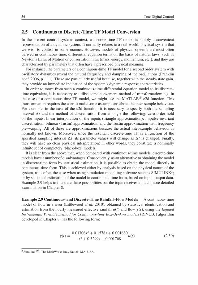
36 True Digital Control
2.5 Continuous to Discrete-Time TF Model Conversion
In the present control systems context, a discrete-time TF model is simply a convenientrepresentation of a dynamic system. It normally relates to a real-world, physical system thatwe wish to control in some manner. However, models of physical systems are most oftenderived in continuous-time, differential equation terms on the basis of natural laws, such asNewton’s Laws of Motion or conservation laws (mass, energy, momentum, etc.); and they arecharacterised by parameters that often have a prescribed physical meaning.For instance, the parameters of a continuous-time TF model for a second order system with
oscillatory dynamics reveal the natural frequency and damping of the oscillations (Franklinet al. 2006, p. 111). These are particularly useful because, together with the steady-state gain,they provide an immediate indication of the system’s dynamic response characteristics.In order to move from such a continuous-time differential equation model to its discrete-
time equivalent, it is necessary to utilise some convenient method of transformation: e.g. inthe case of a continuous-time TF model, we might use the MATLAB R© c2d function. Thistransformation requires the user to make some assumptions about the inter-sample behaviour.For example, in the case of the c2d function, it is necessary to specify both the samplinginterval �t and the method of discretisation from amongst the following: zero order holdon the inputs; linear interpolation of the inputs (triangle approximation); impulse-invariantdiscretisation; bilinear (Tustin) approximation; and the Tustin approximation with frequencypre-warping. All of these are approximations because the actual inter-sample behaviour isnormally not known. Moreover, since the resultant discrete-time TF is a function of thespecified sampling interval �t , its parameter values will change as �t is changed. Finally,they will have no clear physical interpretation: in other words, they constitute a nominallyinfinite set of completely ‘black-box’ models.It is clear from the above that, when compared with continuous-time models, discrete-time
models have a number of disadvantages. Consequently, as an alternative to obtaining the modelin discrete-time form by statistical estimation, it is possible to obtain the model directly incontinuous-time form. This is achieved either by analysis based on the physical nature of thesystem, as is often the case when using simulation modelling software such as SIMULINK2;or by statistical estimation of the model in continuous-time form, based on input–output data.Example 2.9 helps to illustrate these possibilities but the topic receives a much more detailedexamination in Chapter 8.
Example 2.9 Continuous- and Discrete-Time Rainfall–Flow Models A continuous-timemodel of flow in a river (Littlewood et al. 2010), obtained by statistical identification andestimation from the hourly measured effective rainfall u(t) and flow y(t), using the RefinedInstrumental Variable method for Continuous-time Box–Jenkins models (RIVCBJ) algorithmdeveloped in Chapter 8, has the following form:
y(t) = 0.01706s2 + 0.1578s + 0.001680
s2 + 0.3299s + 0.001768u(t) (2.50)
2 SimulinkTM, The MathWorks Inc., Natick, MA, USA.

Discrete-Time Transfer Functions 37
where s is the differential operator, i.e. si y(t) = di y(t)/dti . Applying partial fraction expansionto this TF, the model can be written in the following parallel pathway form:
y(t) ={0.0171+ 0.1496
s + 0.3244+ 0.002573
s + 0.00545
}u(t) (2.51)
This has the following practical interpretation:
1. An instantaneous effect 0.0171 u(t) accounting for the small amount of effective rainfallthat affects the river flow within each hourly sampling period.
2. A ‘quick-flow’ effect with steady-state gain G1 = 0.1496/0.3244 = 0.461 and residencetime (or time constant: see Appendix B) T1 = 1/0.3244 = 3.1 h that is associated withsurface and near surface processes.
3. A ‘slow-flow’ effectwith steady-state gainG2 = 0.002573/0.00545 = 0.472 and residencetime T2 = 1/0.00545 = 183.5 h associated with groundwater processes.
4. The ‘partitioning’ of the flow, defined by P1 = 100(0.0171/0.950) = 1.8%, P2 = 0.461/0.950 = 48.5% and P3 = 0.472/0.950 = 49.7%, where 0.950 is the steady-state gain ofthe composite TF model (2.50).
In other words, the parameters of this continuous-time model have immediate practicalsignificance. Also, note that the model has ‘stiff’ dynamics: i.e. a combination of fairly widelyspaced ‘quick’ and ‘slow’ modes. This has practical implications on model estimation, asdiscussed in Chapter 8.Now, suppose we want to design a digital control system involving this model, initially
considering implementation at a sampling interval of �t = 6 h. MATLAB R© c2d conversionat this sampling interval, using the zero order hold option, yields the following discrete-timemodel:
y(k) = 0.01706+ 0.3915z−1 − 0.3824z−2
1− 1.1106z−1 + 0.1382z−2 u(k) (2.52)
Naturally, this model has the same dynamic behaviour as the continuous-time model fromwhich it is derived. If we only had this description, however, and wished to compute physicalattributes, such as the residence times, it is clear that we would need to convert back tocontinuous time to do this. In other words, unlike the continuous-time model, the parametervalues in this discrete-time model have no immediate physical interpretation. Moreover, it isfound that, if this discrete-time model is actually estimated directly from the data decimatedto the 6 h sampling interval (or, since it is possible in this particular hydrological application,the data are accumulated to yield samples every 6 h), then the estimates are biased away fromthe continuous-time estimates and so are misleading.This biasing problem is a consequence of the rather coarse sampling at this decimation
level. The natural period of the quick mode is: 2π/0.3244 = 19.4 h. Therefore, in order toidentify and control this mode, the data should be sampled faster than the Nyquist period(Franklin et al. 2006, p. 617) 19.4/2=9.7 h: i.e. a sampling interval less than about 10 h.Although�t = 6 h does not contravene this rule, it is quite close to it and so the estimation isaffected by this, as well as the reduced sample size. Clearly, this has implications as regards

38 True Digital Control
control system design and so this important question of choosing a suitable sampling intervalfor identification, estimation and control is considered more fully in Chapter 8.
2.6 Concluding Remarks
This chapter has introduced the nth order discrete-time TF model and examined both thesteady-state gain and stability properties of systems via several simple, worked examples.It has also reviewed basic techniques in block diagram analysis, as demonstrated by theconsideration of three well known control structures: namely, proportional control, integralcontrol and PI control. This has led to the concept of pole assignment, using the PI controlstructure as a worked example. It has been noted that the PI pole assignment approach is limitedto the simplest first order model with unity time delay. Finally, it has been emphasised that thediscrete-time model is a function of the sampling interval and that it is often related to, andcan be obtained from, a continuous-time model that is uniquely parameterised and normallyphysically meaningful. So, although this book is concerned with digital control, continuous-time concepts and models cannot be ignored, both in modelling and control system design.Subsequent chapters of the book will expand on these simple beginnings and consider the
development of control systems to handle the general TF model, with pure time delays andhigher order model polynomials. This will set the scene for the extension of the concepts tothe complexities of optimal, stochastic and multivariable systems.
References
Åstrom, K.J. and Hagglund, T. (1995) PID Controllers: Theory, Design and Tuning, Instrument Society of America,Research Triangle Park, NC.
Åstrom, K.J. andWittenmark, B. (1984) Computer-Controlled Systems Theory and Design, Prentice Hall, EnglewoodCliffs, NJ.
Bradley, D.A. and Seward, D.W. (1998) The development, control and operation of an autonomous robotic excavator,Journal of Intelligent Robotic Systems, 21, pp. 73–97.
Challender, A., Hartree, D.R. and Porter, A. (1936) Time lag in a control system, Philosophical Transactions of theRoyal Society of London Series A Mathematical and Physical Sciences, 235, pp. 415–444.
Dorf, R.C. and Bishop, R.H. (2008)Modern Control Systems, Eleventh Edition, Pearson Prentice Hall, Upper SaddleRiver, NJ.
Evans, R., Li, L., Mareels, I., Okello, N., Pham, M., Qiu, W. and Saleem, S.K. (2011) Real–time optimal controlof river basin networks. In L. Wang and H. Garnier (Eds), System Identification, Environmetric Modelling andControl, Springer-Verlag, Berlin, pp. 403–422.
Foo, M., Ooi, S.K. and Weyer, E. (2011) Modelling of rivers for control design. In L. Wang and H. Garnier (Eds),System Identification, Environmetric Modelling and Control, Springer-Verlag, Berlin, pp. 423–448.
Franklin, G.F., Powell, J.D. and Emami-Naeini, A. (2006) Feedback Control of Dynamic Systems, Fifth Edition,Pearson Prentice Hall, Upper Saddle River, NJ.
Gu, J., Taylor, J. and Seward, D. (2004) Proportional-Integral-Plus control of an intelligent excavator, Journal ofComputer-Aided Civil and Infrastructure Engineering, 19, pp. 16–27.
Hendrey, G.R., Ellsworth, D.S., Lewin, K.F. and Nagy, J. (1999) A free-air enrichment system for exposing tall forestvegetation to elevated atmospheric CO2, Global Change Biology, 5, pp. 293–309.
Kuo, B.C. (1980) Digital Control Systems, Holt, Rinehart and Winston, New York.Leigh, P.A. (2002) Modelling and Control of Micro-Environmental Systems, PhD thesis, Environmental Science
Department, Lancaster University.Leithead, W.E., de la Salle, S.A. and Grimble, M.J. (1991) Wind turbine modelling and control, IEE Conference
Publication No. 332.

Discrete-Time Transfer Functions 39
Littlewood, I.G., Young, P.C. and Croke, B.F.W. (2010) Preliminary comparison of two methods for identifyingrainfall–streamflow model parameters insensitive to data time–step: the Wye at Cefn Brwyn, Plynlimon, Wales.In C. Walsh (Ed.), Role of Hydrology in Managing Consequences of a Changing Global Environment, Universityof Newcastle, British Hydrological Society, Newcastle, UK, pp. 539–543.
Shaban, E.M., Ako, S., Taylor, C.J. and Seward, D.W. (2008) Development of an automated verticality alignmentsystem for a vibro-lance, Automation in Construction, 17, pp. 645–655.
Tan, N., Kaya, I, Yeroglu, C. and Atherton, D.P. (2006) Computation of stabilizing PI and PID controllers using thestability boundary locus, Energy Conversion and Management, 47, pp. 3045–3058.
Tavakoli, S., Griffin, I. and Fleming, P.J. (2007) Robust PI control design: a genetic algorithm approach, InternationalJournal of Soft Computing, 2, pp. 401–407.
Taylor, C.J. (2004) Environmental test chamber for the support of learning and teaching in intelligent control,International Journal of Electrical Engineering Education, 41, pp. 375–387.
Taylor, C.J., Leigh, P.A., Chotai, A., Young, P.C., Vranken, E. and Berckmans, D. (2004a) Cost effective combinedaxial fan and throttling valve control of ventilation rate, IEE Proceedings: Control Theory and Applications, 151,pp. 577–584.
Taylor, C.J., Leigh, P., Price, L., Young, P.C., Berckmans, D. and Vranken, E. (2004b) Proportional-Integral-Plus(PIP) control of ventilation rate in agricultural buildings, Control Engineering Practice, 12, pp. 225–233.
Taylor, C.J., Pedregal, D.J., Young, P.C. and Tych, W. (2007a) Environmental time series analysis and forecastingwith the Captain toolbox, Environmental Modelling and Software, 22, pp. 797–814.
Taylor, C.J. and Seward, D. (2010) Control of a dual-arm robotic manipulator, Nuclear Engineering International,55, pp. 24–26.
Taylor, C.J., Shaban, E.M., Stables, M.A. and Ako, S. (2007b) Proportional-Integral-Plus (PIP) control applications ofstate dependent parameter models, IMECHE Proceedings: Systems and Control Engineering, 221, pp. 1019–1032.
Taylor, C.J., Young, P.C., Chotai, A., McLeod, A.R. and Glasock, A.R. (2000) Modelling and proportional-integral-plus control design for free air carbon dioxide enrichment systems, Journal of Agricultural Engineering Research,75, pp. 365–374.
Young, P.C. (2010) Gauss, Kalman and advances in recursive parameter estimation, Journal of Forecasting, 30, pp.104–146.
Zak, S.H. (2003) Systems and Control, The Oxford Series in Electrical and Computer Engineering, Oxford UniversityPress, New York.
Zhuang, M. and Atherton, D.P. (1993) Automatic tuning of optimum PID controllers, IEE Proceedings: ControlTheory and Applications, 140, pp. 216–224.

3Minimal State Variable Feedback
The classical approach to control systems analysis for Single-Input, Single-Output (SISO) sys-tems involves continuous or discrete-time Transfer Function (TF) models, represented in termsof either the Laplace transform (s-operator) or the backward shift operator (z−1), respectively.Here, closed-loop stability and satisfactory transient responses are obtained through techniquessuch as the Evans Root Locus method (Evans 1948, 1950; Ogata 1970) or Guillimin’s synthe-sis method (Truxal 1955), both of which allow for the specification of closed-loop pole-zeropatterns. Alternatively, a frequency domain approach is utilised involving Nyquist and Bodediagrams (Nyquist 1932; Bode 1940; Truxal 1955). One prominent feature of such classicalapproaches is that they are generally based on graphical analysis of some sort (see e.g. Kuo1980, pp. 393–420; Franklin et al. 2006, pp. 230–313; Dorf and Bishop 2008, pp. 407–492).By contrast, modern control system design methods are usually derived from precise algo-
rithmic computations, often involving numerical optimisation. As mentioned in Chapter 1,one very important concept is the idea of the state space, which originates from the statevariable method of describing differential equations (Kalman 1960, 1961, 1963; Zadeh andDescoer, 1963; Rosenbrock 1970, 1974; Kailath 1980; Franklin et al. 2006, pp. 438–593; Dorfand Bishop 2008, pp. 144–211). While the TF approach discussed in Chapter 2 is concernedonly with input–output characteristics, the state space approach also provides a descriptionof the non-unique, internal behaviour of the system. For mechanical systems, the states areoften defined to represent physical characteristics, such as the positions and velocities of amoving body. However, in the more general case considered here, the state space formulationis derived directly from the previously estimated TF model using special canonical forms.The present chapter considers minimal state space representations of a SISO-TF model and
shows how these may be employed in the design of State Variable Feedback (SVF) controlsystems. In particular, a pole assignment SVF control law is developed for the general linear nthorder system. Such a minimal dimension SVF always involves n states, where n is the highestpower of z in the denominator polynomial of the discrete-time TF model. Two particularlywell-known black-box (i.e. they do not relate obviously to any particular physical system) statespace representations of this minimal type are considered: namely the controllable canonicalform (section 3.1) and the observable canonical form (section 3.2). Some useful mathematicalbackground is introduced in section 3.3, which discusses the transformation between state
True Digital Control: Statistical Modelling and Non-Minimal State Space Design, First Edition.C. James Taylor, Peter C. Young and Arun Chotai.© 2013 John Wiley & Sons, Ltd. Published 2013 by John Wiley & Sons, Ltd.

42 True Digital Control
space and TF models, so defining the characteristic equation, eigenvalues and eigenvectors ofa system.As we shall see, for a particular state variable representation of the system, the TF model
is completely and uniquely specified. There are, however, an infinite number of possible statespace representations for any given TF model. For example, certain state space representationscan include states that are completely decoupled from the control input and so are uncontrol-lable by the control input signal. And again, there may be unobservable states that are entirelydecoupled from the output and thus cannot influence the observed behaviour of the system.Section 3.4 considers these important concepts of controllability and observability. However,let us start with a straightforward example that demonstrates the non-uniqueness of a statespace model.
Example 3.1 State Space Forms for a Third Order TF Model Consider the followingthird order, scalar difference equation:
y(k)+ a1y(k − 1)+ a2y(k − 2)+ a3y(k − 3) = u(k − 1) (3.1)
where y(k) and u(k) are the sampled output and input signals, respectively, whilst a1, a2 anda3 are constant coefficients. These coefficients or parameters would normally be estimatedfrom the data {y(k), u(k)} using the identification and estimation methods discussed later inChapter 8. When the difference between the true system and the estimated model is significantto the analysis, the estimateswill be denoted by ai (i = 1, 2, 3). For simplicity here, however, itwill be assumed initially that the parameters are knownwithout any uncertainty. Consequently,the equivalent TF representation of equation (3.1) is:
y(k) = z−1
1+ a1z−1 + a2z−2 + a3z−3 u(k) (3.2)
in which z−1 denotes the backward shift operator (cf. Example 2.2). The block diagram of thisTF model is illustrated in Figure 3.1.An illustrative minimal state vector x(k) is defined as follows:
x(k) =
⎡⎢⎣
x1(k)
x2(k)
x3(k)
⎤⎥⎦ =
⎡⎢⎣
y(k)
y(k − 1)y(k − 2)
⎤⎥⎦ (3.3)
where x1(k), x2(k) and x3(k) are the state variables.
u(k)
1 + a1z−1 + a2z−2 + a3z−3
z−1 y(k)
Figure 3.1 Block diagram form of the TF model (3.2)

Minimal State Variable Feedback 43
Note that the model (3.1) or (3.2) is third order and there are three state variables. In thisexample, these state variables have been defined straightforwardly as the output signal y(k)and its past values.Equation (3.1) or its equivalent (3.2) can be written in the following state space form:
x(k) =
⎡⎢⎣
x1(k)
x2(k)
x3(k)
⎤⎥⎦ =
⎡⎢⎣
−a1 −a2 −a31 0 0
0 1 0
⎤⎥⎦
⎡⎢⎣
x1(k − 1)x2(k − 1)x3(k − 1)
⎤⎥⎦ +
⎡⎢⎣1
0
0
⎤⎥⎦ u(k − 1) (3.4)
In this case, the output variable y(k) is obtained from an observation equation:
y(k) = [1 0 0
]⎡⎢⎣
x1(k)
x2(k)
x3(k)
⎤⎥⎦ (3.5)
The relationship between (3.1) and (3.4) is most apparent if we explicitly substitute for thestate variables using (3.3), as follows:
x(k) =
⎡⎢⎣
y(k)
y(k − 1)y(k − 2)
⎤⎥⎦ =
⎡⎢⎣
−a1 −a2 −a31 0 0
0 1 0
⎤⎥⎦
⎡⎢⎣
y(k − 1)y(k − 2)y(k − 3)
⎤⎥⎦ +
⎡⎢⎣1
0
0
⎤⎥⎦ u(k − 1) (3.6)
where the first equation (row) relates directly to equation (3.1) and the remaining two aresimply definitions of the delayed output variables (and are necessary to complete the statevector).Equations (3.6) are illustrated in Figure 3.2, which represents a straightforward decompo-
sition of the TF model in Figure 3.1.
+
u(k)
y(k)
y(k − 1) y(k − 2) y(k − 3)+
−
a1
a2
a3
z−1 z−1 z−1 z−1
+
+
+
Figure 3.2 State space model described by equations (3.6)

44 True Digital Control
However, if the state vector is now defined as:
x(k) =
⎡⎢⎣
x1(k)
x2(k)
x3(k)
⎤⎥⎦ =
⎡⎢⎣
−a1x1(k − 1)+ x2(k − 1)+ u(k − 1)−a2x1(k − 1)+ x3(k − 1)
−a3x1(k − 1)
⎤⎥⎦ (3.7)
then equation (3.1) or equation (3.2) is described by the state space form:
x(k) =
⎡⎢⎣
x1(k)
x2(k)
x3(k)
⎤⎥⎦ =
⎡⎢⎣
−a1 1 0
−a2 0 1
−a3 0 0
⎤⎥⎦
⎡⎢⎣
x1(k − 1)x2(k − 1)x3(k − 1)
⎤⎥⎦ +
⎡⎢⎣1
0
0
⎤⎥⎦ u(k − 1) (3.8)
y(k) = [1 0 0
]⎡⎢⎣
x1(k)
x2(k)
x3(k)
⎤⎥⎦ (3.9)
The equivalence between {(3.8), (3.9)} and the TF model can be checked by substituting forthe state vector (3.7).Despite their differences, it is clear that the state space representations developed above,
namely the equation pairs {(3.4), (3.5)} and {(3.8), (3.9)}, both describe the same input–outputrelationship specified by the TF model. And it is clear that these are not unique representationsof the TF model; they are simply two specific examples that illustrate the non-uniqueness ofthe state space representation.
3.1 Controllable Canonical Form
Let us turn to the general nth order deterministic, unit delay control model introduced inChapter 2. However, for notational simplicity, in this chapter we will assume that the orders ofthe numerator and denominator polynomials are the same. This assumption does not constrainthe model in any sense, since different orders may be considered by simply setting the relevantparameters to zero.Hence, the system difference equation is given by:
y(k)+ a1y(k − 1)+ · · · + an y(k − n) = b1u(k − 1)+ b2u(k − 2)+ · · · + bnu(k − n)
(3.10)
where ai (i = 1 · · · n) and bi (i = 1 · · · n) are constant coefficients. The equivalent TF modelis:
y(k) = b1z−1 + b2z−2 + · · · + bnz−n
1+ a1z−1 + a2z−2 + · · · + anz−nu(k) = B(z−1)
A(z−1)u(k) (3.11)

Minimal State Variable Feedback 45
where A(z−1) and B(z−1) are appropriately defined polynomials in z−1. To help develop thestate space form, we can write equation (3.11) as:
y(k) =(b1 + b2z−1 + · · · + bnz−n+1) z−1
1+ a1z−1 + a2z−2 + · · · + anz−nu(k) (3.12)
Furthermore, by introducing an intermediate variable w(k), the TF model can be decomposedinto two components, namely:
w(k) = z−1
1+ a1z−1 + a2z−2 + · · · + anz−nu(k) (3.13)
and,
y(k) = (b1 + b2z
−1 + · · · + bnz−n+1) w(k) (3.14)
Generalising from equation (3.3), it is clear that defining the state vector:
⎡⎢⎢⎢⎢⎢⎢⎢⎣
x1(k)
x2(k)...
xn−1(k)xn(k)
⎤⎥⎥⎥⎥⎥⎥⎥⎦
=
⎡⎢⎢⎢⎢⎢⎢⎢⎣
w(k)
w(k − 1)...
w(k − n + 2)w(k − n + 1)
⎤⎥⎥⎥⎥⎥⎥⎥⎦
(3.15)
yields the following state space representation of the TF model (3.11):
⎡⎢⎢⎢⎢⎢⎢⎢⎣
x1(k)
x2(k)...
xn−1(k)xn(k)
⎤⎥⎥⎥⎥⎥⎥⎥⎦
=
⎡⎢⎢⎢⎢⎢⎢⎢⎣
−a1 −a2 · · · −an−1 −an
1 0 · · · 0 0...
. . ....
......
0 0 1 0 0
0 0 0 1 0
⎤⎥⎥⎥⎥⎥⎥⎥⎦
⎡⎢⎢⎢⎢⎢⎢⎢⎣
x1(k − 1)x2(k − 1)
...
xn−1(k − 1)xn(k − 1)
⎤⎥⎥⎥⎥⎥⎥⎥⎦
+
⎡⎢⎢⎢⎢⎢⎢⎢⎣
1
0...
0
0
⎤⎥⎥⎥⎥⎥⎥⎥⎦
u(k − 1)
(3.16)
y(k) = [b1 b2 · · · bn−1 bn
]⎡⎢⎢⎢⎢⎢⎢⎢⎣
x1(k)
x2(k)...
xn−1(k)xn(k)
⎤⎥⎥⎥⎥⎥⎥⎥⎦
(3.17)
Equations {(3.16), (3.17)} are known as the controllable canonical form1 and are illustratedin block diagram form by Figure 3.3.
1 A standard form: here, the simplest and most significant controllable form possible without loss of generality.

46 True Digital Control
u(k)
y(k)
z−1 z−1 z−1 z−1 z−1+
+
xn(k − 1)
−an−1
x1(k) x2(k) xn(k)
−a1
b1 b2 bn
−an
Figure 3.3 Controllable canonical form for the general discrete-time system (3.11)
The controllable canonical form is an example of a minimal state space model since thereare n states (3.15). The advantage of such a representation is that it is straightforward toconstruct and yields a convenient structure for the computation of a pole assignment controlalgorithm (see below). However, one disadvantage of the controllable canonical form is thatthe state vector is not directly available from the measured output because it consists of theintermediate variable w(k) and its past values.In this regard, it is clear from equation (3.14) that w(k) is given by:
w(k) = y(k)(b1 + b2z−1 + · · · + bnz−n+1) (3.18)
Multiplying by z−1/z−1 yields:
w(k) = z−1y(k)
b1z−1 + b2z−2 + · · · + bnz−n= y(k − 1)
B(z−1)(3.19)
Therefore, in the controllable canonical form, the minimal state vector is implicitly formedfrom the delayed and filtered output variable, where the filter is defined by the numeratorpolynomial of the TF model, i.e. B(z−1).
Example 3.2 State Variable Feedback based on the Controllable Canonical Form Con-sider a second order TF model based on equation (3.11) with n = 2, together with illustrativenumerical values for the parameters:
y(k) = B(z−1)A(z−1)
u(k) = b1z−1 + b2z−2
1+ a1z−1 + a2z−2 u(k) = 0.5z−1 − 0.4z−2
1− 0.8z−1 + 0.15z−2 u(k) (3.20)
This model was first introduced in Chapter 2 (Example 2.3). It will be utilised for severalexamples in this chapter and so is restated here for convenience.

Minimal State Variable Feedback 47
The minimal state vector associated with the TF model (3.20) is:[x1(k)
x2(k)
]=
[w(k)
w(k − 1)
](3.21)
The controllable canonical form is subsequently defined as follows:[x1(k)
x2(k)
]=
[−a1 −a21 0
] [x1(k − 1)x2(k − 1)
]+
[1
0
]u(k − 1) (3.22)
y(k) = [b1 b2
] [x1(k)
x2(k)
](3.23)
A linear SVF control law for this system is simply a linear combination of the statevariables, i.e.
u(k) = −l1x1(k)− l2x2(k)+ yd (k) (3.24)
where yd (k) is the command input, while the control gains l1 and l2 are chosen by the designerto ensure a satisfactory closed-loop response (see below).The general form of a SVF control algorithm, such as equation (3.24), will be discussed in
Chapter 4. For now, it is sufficient to note that the control input signal u(k) is determined usinga negative feedback of each state variable multiplied by a control gain. In the example above,the command input is introduced as a straightforward addition to this feedback law: i.e. usingequation (3.19) and equation (3.21), the control law (3.24) is written as:
u(k) = −l1y∗(k − 1)− l2y∗(k − 2)+ yd (k) (3.25)
in which
y∗(k) = 1
B(z−1)y(k) (3.26)
where B(z−1) is the estimated numerator polynomial of the control model. The ‘hat’ notation,i.e. B(z−1) = b1z−1 + b2z−2 is introduced here in order to emphasise the inevitable mismatchbetween the true system represented by B(z−1)/A(z−1) and the estimated TF model used forcontrol system design, i.e. B(z−1)/ A(z−1), where A(z−1) = 1+ a1z−1 + a2z−2, and {ai , bi }(i = 1, 2) are the parameter estimates.Combining equation (3.25) and equation (3.26) yields:
u(k) = − l1z−1 + l2z−2
B(z−1)y(k)+ yd (k) (3.27)
The block diagram of the resultant closed-loop control system, with potential model mismatch,is illustrated by Figure 3.4. Here, the term plant is used to represent the notional true system,as distinct from the estimated control model.

48 True Digital Control
B(z−1)
B(z−1)
A(z−1)
l1z−1 + l2z−2
yd (k) u(k) y(k)
plant
ˆ
controller
+
−
Figure 3.4 The closed-loop control system for Example 3.2 with model mismatch
Example 3.3 State Variable Feedback Pole Assignment based on the Controllable Canon-ical Form The SVF framework developed in Example 3.2 will now be used to design apole assignment controller (cf. Example 2.6 and Example 2.7). In this regard, block diagramreduction applied to Figure 3.4 yields the following Closed-Loop Transfer Function (CLTF):
y(k) = B(z−1)
A(z−1)+ (l1z−1 + l2z−2) B(z−1)
B(z−1)
yd (k) (3.28)
The denominator of equation (3.28) reveals a cancellation of the numerator polynomial,which is implicit in any SVF controller based on the controllable canonical form. However,using the polynomials defined in equation (3.20) and assuming no plant–model mismatch, i.e.B(z−1) = B(z−1) = b1z−1 + b2z−2, the CLTF reduces to:
y(k) = b1z−1 + b2z−2
1+ (a1 + l1)z−1 + (a2 + l2)z−2 yd (k) (3.29)
Recall from Chapter 2 that the denominator of a TF defines its stability and transient dynamicbehaviour. Therefore, in order to determine the control gains l1 and l2, we consider thecharacteristic equation as follows:
1+ (a1 + l1)z−1 + (a2 + l2)z
−2 = 0 (3.30)
Each of the feedback gains are explicitly associated with different model coefficients inequation (3.30) so that, when using the controllable canonical form, it is a trivial matter forthe control system designer to obtain a desired closed-loop characteristic equation:
D(z−1) = 1+ d1z−1 + d2z
−2 = 0 (3.31)
where d1 and d2 are user chosen coefficients, by setting:
l1 = d1 − a1 and l2 = d2 − a2 (3.32)

Minimal State Variable Feedback 49
0 5 10 15 20 25 30
0
0.5
1
1.5
2
2.5
3
command
output
control input
Sample no.
Figure 3.5 Closed-loop unit step response of the SVF control system in Example 3.3
Since the roots of the CLTF are known as the poles of the closed-loop system, this approachis another example of pole assignment, as introduced in Chapter 2. In this regard, note thatequation (3.31) is equivalent to:
D(z) = z2 + d1z + d2 = 0 (3.33)
Therefore, selecting illustrative closed-loop poles of 0.4 and 0.8 on the complex z-planeyields: (z − 0.4) (z − 0.8) = z2 − 1.2z + 1.32, hence d1 = −1.2 and d2 = 1.32. Now, thecontrol gains can be computed from equation (3.32) using the model coefficients a1 = −0.8and a2 = 0.15, resulting in l1 = −0.4 and l2 = 0.17. The final control system is implementedas shown by Figure 3.4.The closed-loop response to a unit step in the command input is illustrated by Figure
3.5. For comparison, the open-loop response of the TF model (3.20) to the same input,without any control, is shown by Figure 2.8a. It is clear that, in this simple example, theclosed-loop behaviour has been modified considerably. The wider issues of control systemperformance, as well as the selection of control system gains that will achieve desirableclosed-loop performance, will be discussed in later chapters.However, the basic SVF algorithm considered above is a Type 0 control system, as discussed
in Chapter 2, indicating that it does not have an inherent unity steady-state gain. Hence, thefinal value of the step response in Figure 3.5 is not equal to the desired level yd (k) = 1.0. Thisis an obvious disadvantage and its conversion into a Type 1 control system, with inherent unitysteady-state gain, is also discussed in subsequent chapters.
3.1.1 State Variable Feedback for the General TF Model
Following the approach taken in Example 3.3, it is clear that the feedback gains for the generalnth order TF model (3.11) are given by:
li = di − ai (i = 1, 2, · · · n) (3.34)

50 True Digital Control
where di are the coefficients of the following desired characteristic polynomial:
1+ d1z−1 + d2z
−2 + · · · + dnz−n (3.35)
This transparency of the pole assignment control design is the main advantage of the con-trollable canonical form. But, as mentioned previously, while the computation of the controlgains is very straightforward, the practical implementation of this control system is moreproblematic because the state vector is not directly available from the measured output.In Example 3.3, we have extracted the states using equation (3.26) and then implemented the
controller in the form shown by Figure 3.4. Unfortunately, this has disadvantages as a generalsolution to the control problem. In particular, the control system is very much dependentupon the accuracy of the estimated model, with the associated disadvantage of decreasedrobustness in the face of uncertainty, as discussed later in Chapter 4. A particularly importantexample of its limitations arises if the system is non-minimum phase, with zeros (the roots ofthe numerator polynomial) outside the unit circle in the complex z-plane. In this situation, thefeedback loop will have an unstable component, unless there is an exact cancellation of theB(z−1) polynomial in equation (3.28), which is highly unlikely in any real, practical example.
3.2 Observable Canonical Form
Consider now a new state vector for the general nth order system (3.11) defined in the followingmanner [cf. equation (3.7) of Example 3.1]:
⎡⎢⎢⎢⎢⎢⎢⎢⎣
x1(k)
x2(k)...
xn−1(k)xn(k)
⎤⎥⎥⎥⎥⎥⎥⎥⎦
=
⎡⎢⎢⎢⎢⎢⎢⎢⎣
−a1x1(k − 1)+ x2(k − 1)+ b1u(k − 1)−a2x1(k − 1)+ x3(k − 1)+ b2u(k − 1)
...
−an−1x1(k − 1)+ xn(k − 1)+ bn−1u(k − 1)−an x1(k − 1)+ bnu(k − 1)
⎤⎥⎥⎥⎥⎥⎥⎥⎦
(3.36)
The associated state space representation then takes the quite simple form:
⎡⎢⎢⎢⎢⎢⎢⎢⎣
x1(k)
x2(k)...
xn−1(k)xn(k)
⎤⎥⎥⎥⎥⎥⎥⎥⎦
=
⎡⎢⎢⎢⎢⎢⎢⎢⎣
−a1 1 0 · · · 0
−a2 0 1 · · · 0...
....... . .
...
−an−1 0 0 · · · 1
−an 0 0 · · · 0
⎤⎥⎥⎥⎥⎥⎥⎥⎦
⎡⎢⎢⎢⎢⎢⎢⎢⎣
x1(k − 1)x2(k − 1)
...
xn−1(k − 1)xn(k − 1)
⎤⎥⎥⎥⎥⎥⎥⎥⎦
+
⎡⎢⎢⎢⎢⎢⎢⎢⎣
b1b2...
bn−1bn
⎤⎥⎥⎥⎥⎥⎥⎥⎦
u(k − 1) (3.37)
y(k) = [1 0 · · · 0 0
]⎡⎢⎢⎢⎢⎢⎢⎢⎣
x1(k)
x2(k)...
xn−1(k)xn(k)
⎤⎥⎥⎥⎥⎥⎥⎥⎦
(3.38)

Minimal State Variable Feedback 51
u(k)
z−1 z−1 z−1 z−1++
bn
−an −a1−an−1
b1bn−1
xn(k) xn−1(k) x2(k) y(k) = x1(k)
Figure 3.6 Observable canonical form for the general discrete-time system (3.11)
This particular realisation of the system is called the observable canonical form and its blockdiagram structure is shown in Figure 3.6. It is clear from Figure 3.6 that the state vector isformed from a combination of input and output signals, defined by the model parameters.The term ‘observable’ canonical form indicates that it is a particularly convenient state space
model to employ when considering how state variables can be reconstructed (or estimated inthe stochastic situation), based on themeasured signals and knowledge of the state spacemodel(see e.g. Luenberger 1971; Kailath 1980; Åstrom & Wittenmark 1984; Young 2011). Suchtechniques are potentially important in any implementation of SVF control based on a minimalstate space model. However, they are not discussed in detail here, because we obviate theirneed by exploiting the alternative Non-Minimal State Space (NMSS) form that is consideredin Chapter 4.
Example 3.4 State Variable Feedback based on the Observable Canonical Form Con-sider again the second order TF model (3.20). Defining the vector:
[x1(k)
x2(k)
]=
[y(k)
−a2y(k − 1)+ b2u(k − 1)
](3.39)
the observable canonical form is given by the following second order state space model:
[x1(k)
x2(k)
]=
[−a1 1
−a2 0
] [x1(k − 1)x2(k − 1)
]+
[b1b2
]u(k − 1) (3.40)
y(k) = [1 0
] [x1(k)
x2(k)
](3.41)
so that a linear SVF control law for this example is again:
u(k) = −l1x1(k)− l2x2(k)+ yd (k) (3.42)

52 True Digital Control
b1z−1 + b2z−2
1 + a1z−1 + a2z−2
y(k) = x1(k)
l2
yd (k) u(k)
−a2ˆ
b2ˆ
plant
−
+
+
−
+
1l
z−1
z−1
Figure 3.7 The closed-loop control system for Example 3.4 with model mismatch
where yd (k) is the command input. Note that x1(k) is equal to the system output y(k) and is,therefore, directly observed (measured). However, x2(k) is not observed, which once againprevents us from directly implementing the control law. Instead, we employ the model of thesystem:
B(z−1)A(z−1)
= b1z−1 + b2z−2
1+ a1z−1 + a2z−2 (3.43)
to provide estimates of the states (3.39): i.e. in this case:
u(k) = −l1y(k)− l2(−a2y(k − 1)+ b2u(k − 1)) + yd (k) (3.44)
and the closed-loop system is represented in the block diagram form by Figure 3.7.It is interesting to note that, whereas the SVF controller based on a controllable canonical
form only involves feedback of the output variable (Figure 3.4), here the control algorithmrequires y(k), y(k − 1) and u(k − 1) (Figure 3.7). This observation will assume greater sig-nificance when we introduce NMSS models in Chapter 4.Assuming no plant–model mismatch, i.e. B(z−1) = B(z−1) and A(z−1) = A(z−1), the CLTF
associated with Figure 3.7 takes the form:
y(k) = b1z−1 + b2z−2
1+ (a1 + l2b2 + b1l1) z−1 + (a2 + l2b2a1 + b2l1 − b1l2a2) z−2 yd (k) (3.45)
As before, a pole assignment control algorithm can be derived by equating the coefficients ofthe denominator polynomial with the desired coefficients from equation (3.33). In this case,however, the solution of two simultaneous equations is required to find the unknown controlgains l1 and l2. Not surprisingly, therefore, the general nth order system would require the

Minimal State Variable Feedback 53
solution of n simultaneous equations, making the pole assignment solution more computa-tionally intensive when using this observable canonical form than the previous controllablecanonical form.
3.3 General State Space Form
The general state space representation of a linear, discrete-time, SISO system takes the fol-lowing form:
x(k) = Fx(k − 1)+ gu(k − 1) (3.46)
y(k) = hx(k) (3.47)
where x(k) is the state vector, u(k) and y(k) are the input and the output variables, respectively;and the state transition matrix F, input vector g and output vector h are all of appropriatedimensions. For minimal SISO state space representations, as considered in this chapter, F isa n × n square matrix, g is a n × 1 column vector and h is a 1× n row vector. All the statespace models discussed earlier (i.e. Example 3.1, Example 3.2 and Example 3.4) take the form{(3.46), (3.47)}, which is illustrated in Figure 3.8.Note that, as discussed in Chapter 2, discrete-time control system design requires at least
one sample time delay in the control model, which is implicit in the state space representation{(3.46), (3.47)} and the TF model (3.11). Notwithstanding this requirement, a state spacemodel with no time delay can be developed by the inclusion of a ‘feed-through’ u(k) variablein the output equation (3.47), i.e. y(k) = hx(k)+ b0u(k), where b0 is a constant coefficient[see equation (2.11)].
3.3.1 Transfer Function Form of a State Space Model
Using the state equation (3.46):
x(k) = Fz−1x(k)+ gz−1u(k) (3.48)
where, as before, z−1 is the backward shift operator. Hence,
(I − Fz−1)x(k) = gz−1u(k) (3.49)
u(k) x(k) y(k)z−1
z−1
h+
+
F
g
Figure 3.8 Block diagram form for the general state space system description {(3.46), (3.47)}

54 True Digital Control
so that
x(k) = (I − Fz−1)−1gz−1u(k)
and substituting for x(k) in the observation equation (3.47):
y(k) = hx(k) = h(I − Fz−1)−1gz−1u(k) (3.50)
The TF representation G1(z−1) of the state space model {(3.46), (3.47)} is:
y(k)
u(k)= G1(z
−1) = h(I − Fz−1)−1gz−1 (3.51)
This TF can be written equivalently in terms of the forward shift operator z, i.e.
y(k)
u(k)= G1(z) = h(z I − F)−1g (3.52)
As stated above, the TF G1(z) completely defines the input–output behaviour of the systemand is independent of the state space representation. This becomes apparent if we now definea new state vector x∗(k) = T x(k), where T is a non-singular transformation matrix.Replacing x(k) in {(3.46), (3.47)} with T−1x∗(k):
x∗(k) = TFT−1x∗(k − 1)+ Tgu(k − 1) (3.53)
and
y(k) = hT−1x∗(k) (3.54)
The input–output TF from {(3.53), (3.54)} is given by:
y(k)
u(k)= hT−1(I − TFT−1z−1)−1Tgz−1 = h(I − Fz−1)−1gz−1 = G1(z
−1) (3.55)
Hence, the TF model G1(z−1) is independent of the state space representation.
Example 3.5 Determining the TF from a State Space Model Substituting the numericalvalues of the TF model (3.20) into the controllable canonical form {(3.22), (3.23)} yields:
x(k) =[0.8 −0.151.0 0
]x(k − 1)+
[1
0
]u(k − 1) (3.56)
y(k) = [0.5 −0.4 ]
x(k) (3.57)

Minimal State Variable Feedback 55
Using (3.51) and the standard rules of matrix inversion (see Appendix A), the TF is derived interms of the backward shift operator z−1, as follows:
G1(z−1) = [0.5 −0.4 ] [
1− 0.8z−1 0.15z−1
−z−1 1
]−1 [1
0
]z−1
= z−1
1− 0.8z−1 + 0.15z−2[0.5 −0.4 ] [
1 0.15z−1
−z−1 1− 0.8z−1
] [1
0
]
= 0.5z−1 − 0.4z−2
1− 0.8z−1 + 0.15z−2
(3.58)
as expected from equation (3.20). The equivalent forward shift operator form of the TF is:
G1(z) = 0.5z − 0.4z2 − 0.8z + 0.15 (3.59)
The following subsection examines the relationship between TF and state space models inmore detail.
3.3.2 The Characteristic Equation, Eigenvalues and Eigenvectors
Noting the procedure for the inversion of a matrix, the z-operator TF model (3.52) can berewritten as:
G1(z) = h(z I − F)−1g = h (adj(z I − F)) g|(z I − F)| (3.60)
where the determinant |(z I − F)| is called the characteristic polynomial. The characteristicequation of the system is obtained by equating this determinant to zero, i.e.
|(z I − F)| = 0 (3.61)
Evaluating the determinant and equating to zero yields:
|(z I − F)| = zn + a1zn−1 + a2z
n−2 + · · · + an = 0 (3.62)
while, in terms of the backward shift operator, the equivalent result is given by:
∣∣(I − Fz−1)∣∣ = 1+ a1z
−1 + a2z−2 + · · · + anz−n = 0 (3.63)
Note that the dimension of the matrix F, in this minimal state space case, is always equal ton × n, hence the order of the characteristic equation is also n; and it is clear from equation

56 True Digital Control
(3.62) and equation (3.63) that the characteristic equation of F is equivalent to the characteristicequation of the TF model (3.11).In mathematics, the characteristic equation of the n × n matrix F is usually denoted as:
|(λI − F)| = λn + a1λn−1 + a2λ
n−2 + · · · + an = 0 (3.64)
The roots of equation (3.64) are called the eigenvalues of F (see also Hoffman and Kunze1971, p. 182; Marcus and Minc 1988, p. 145; O’Neil 2007, pp. 267–276).As discussed in Chapter 2, the roots of A(z) = 0 obtained from the TF model (3.11) are
called the poles of the system. For a minimal state space model, it follows that the eigenvaluesof the matrix F are equal to the poles of the equivalent TF model. By contrast, in Chapter 4,we will show that if the state space representation is non-minimal, then the poles of the TFmodel represent a subset of the eigenvalues of F.Finally, any non-zero vector wi = [
wi1 wi2 · · · win]Twhich satisfies the following matrix
equation:
(λi I − F)wi = 0 (3.65)
where λi (i = 1, 2, . . . , n) is the ith eigenvalue of F and 0 is a null vector (i.e. zeros), is calledthe eigenvector associated with λi .Note that since the eigenvalues of F are the poles of the system TF, it follows that the
eigenvalues of F = T−1FT are the same. In other words, the eigenvalues are unaffected by asimilarity transformation. To show this, let wi denote an eigenvector of F. Then, by definition,Fwi = λ i wi , where λ i is the eigenvalue corresponding to wi . Now if we define wi = T−1wi
as the transformed eigenvector, then:
Fwi = F(T−1wi ) = (T−1FT )(T−1wi ) = T−1Fwi = T−1λ i wi = λ i wi
Thus, the transformed eigenvector is an eigenvector of the transformed F matrix, and theeigenvalue is unchanged.
Example 3.6 Eigenvalues and Eigenvectors of a State Space Model Returning to the TFmodel (3.20) and the associated state space form {(3.56), (3.57)}, the state transition matrixF is given by:
F =[0.8 −0.151.0 0
](3.66)
so that the characteristic equation (3.64) is simply:
|(λI − F)| =∣∣∣∣∣λ − 0.8 0.15
−1.0 λ
∣∣∣∣∣ = 0 (3.67)

Minimal State Variable Feedback 57
i.e.
λ2 − 0.8λ + 0.15 = 0 or (λ − 0.5)(λ − 0.3) = 0 (3.68)
This shows that the eigenvalues and TF poles are λ1 = 0.3 and λ2 = 0.5. From equation (3.65),therefore, the eigenvectors of F satisfy:
λi wi − Fwi = 0 i = 1, 2 (3.69)
In order to find the corresponding eigenvector, λ = 0.3 is substituted into this equation:
0.3
[w11w12
]−
[0.8 −0.151.0 0
] [w11w12
]=
[0
0
](3.70)
so that, lettingw12 = 1, the eigenvector corresponding toλ1 = 0.3 isw1 = [ 0.3 1 ]T . Similarly,the eigenvector corresponding to λ2 = 0.5 can be found from:
0.5
[w21w22
]−
[0.8 −0.151.0 0
] [w21w22
]=
[0
0
](3.71)
and this is satisfied when w21 = 1 and w22 = 2. Hence, the eigenvector corresponding toλ1 = 0.5 is w2 = [ 1 2 ]T . The eigenvectors are useful in various ways but, within the presentcontext, they facilitate the transformation of the state space model into a diagonal ‘decoupled’form, as shown below.
3.3.3 The Diagonal Form of a State Space Model
In general, if the state transition matrix F has distinct (i.e. non-repeated), real eigenval-ues, the eigenvectors are linearly independent. Furthermore, if the columns of the matrixT−1 in equation (3.53) are chosen as the eigenvectors of F, then TFT−1will be a diagonalmatrix, i.e.
TFT−1 = � =
⎡⎢⎢⎢⎢⎢⎢⎢⎣
λ1 0 0 · · · 0
0 λ2 0 · · · 0
0 0 λ3 · · · 0...
......
. . ....
0 0 0 λn
⎤⎥⎥⎥⎥⎥⎥⎥⎦
(3.72)
where λi (i = 1, 2, . . . , n) are the eigenvalues of F, as before. In this case, the state equationsin (3.53) are conveniently decoupled (i.e. each state variable appears in only one equation).

58 True Digital Control
The state equations in this decoupled form are written as:
x∗(k) = � x∗(k − 1)+ T gu(k − 1)y(k) = hT−1x∗(k)
(3.73)
where x∗(k) = T x(k) is the transformed, decoupled state vector.
Example 3.7 Determining the Diagonal Form of a State Space Model Consider againthe system described by the TF model (3.20) and associated state space form {(3.56), (3.57)}.Noting the eigenvectors obtained in the previous section, T−1 is defined:
T−1 = [w1 w2
] =[0.3 1
1 2
](3.74)
Therefore, the transformation matrix T is:
T =[
−5.0 2.5
2.5 −0.75
](3.75)
and
TFT−1 =[
−5.0 2.5
2.5 −0.75
] [0.8 −0.151.0 0
] [0.3 1
1 2
]=
[0.3 0
0 0.5
]= � (3.76)
Finally, note that if the eigenvalues of F are not all distinct, then it may not be possibleto obtain independent eigenvectors and hence determine the diagonal form. In this case, theF matrix can be transformed into a Jordan form, in which the eigenvalues of F lie on themain diagonal, while some of the elements immediately above the main diagonal are unity.However, this form has no importance for the present book and the reader is advised to consultAyres (1962, p. 206) or Kuo (1980, pp. 195–198) for further information.
3.4 Controllability and Observability
The twin concepts of controllability and observability, first introduced by Kalman (1960), arevery important in SVF control system design, since they are concernedwith the interconnectionbetween the input, state and the output of a state space model. In this book, the controllabilityis particularly significant, since it determines whether or not we can control a system’s stateusing the control input variable.
3.4.1 Definition of Controllability (or Reachability2)
The digital system described by equations {(3.46), (3.47)} is controllable (or reachable) if,for any initial state x(0), it is possible to find an unconstrained control sequence which willtransfer it to any final state x(n) (not necessarily the origin) in a finite time (Kuo 1980, p. 423;Middleton and Goodwin 1990, p. 180).
2 Note that the term reachability is often preferred for discrete-time systems.

Minimal State Variable Feedback 59
3.4.2 Rank Test for Controllability
Using {(3.46), (3.47)}, the desired state x(n), in terms of the initial state x(0) and the inputsequence u(0), u(1), . . . , u(n − 1), is given by:
x(n) = Fn x(0)+ gu(n − 1)+ Fgu(n − 2)+ · · · + Fn−2gu(1)+ Fn−1gu(0) (3.77)
or
x(n)− Fn x(0) = [g Fg · · · Fn−2g Fn−1g
]⎡⎢⎢⎢⎢⎢⎢⎢⎣
u(n − 1)u(n − 2)
...
u(1)
u(0)
⎤⎥⎥⎥⎥⎥⎥⎥⎦
(3.78)
The left-hand side of equation (3.78) is known (as part of the definition above), while theright-hand side is a function of the input signals. Since equation (3.78) also represents nsimultaneous algebraic equations, these equationsmust be linearly independent for the solutionto exist. Hence, a necessary and sufficient condition for controllability, is that the followingcontrollability matrix:
S1 = [g Fg · · · Fn−2g Fn−1g
](3.79)
is of full rank n, i.e. that it is non-singular and can be inverted.
3.4.3 Definition of Observability
The digital system described by equations {(3.46), (3.47)} is observable if the state vectorx(k), at any sample time k, can be determined from the systemmodel and complete knowledgeof the system’s input and output variables (Kuo 1980, p. 430; Middleton and Goodwin 1990,p. 196).
3.4.4 Rank Test for Observability
Consider the system {(3.46), (3.47)} with the initial state vector x(0). Since the effect ofthe known input can always be subtracted from the solution, we will simplify the analysis byassuming u(k − 1) = 0 in {(3.46), (3.47)}. This yields the following linear algebraic equationsfor the output:
y(0) = hx(0)
y(1) = hx(1) = hFx(0)...
y(n − 1) = hFn−1x(0)
(3.80)

60 True Digital Control
or, in vector-matrix form:
⎡⎢⎢⎢⎢⎢⎢⎢⎣
h
hF...
hFn−2
hFn−1
⎤⎥⎥⎥⎥⎥⎥⎥⎦
x(0) =
⎡⎢⎢⎢⎢⎢⎢⎢⎣
y(0)
y(1)...
y(n − 2)y(n − 1)
⎤⎥⎥⎥⎥⎥⎥⎥⎦
(3.81)
and it is clear that the initial state x(0), can be found if and only if the following observabilitymatrix:
S0 =
⎡⎢⎢⎢⎢⎢⎢⎢⎣
h
hF...
hFn−2
hFn−1
⎤⎥⎥⎥⎥⎥⎥⎥⎦
(3.82)
is of full rank n. Once the initial state x(0) is known, then the state equation (3.46) is employedto find x(1), x(2), . . . , x(n − 1) and the definition of observability is satisfied. Finally, note thatthe observable canonical form defined in section 3.2 is always observable, but not necessarilycontrollable, while the opposite is true of the controllable canonical form in section 3.1.
Example 3.8 Rank Tests for a State Space Model Consider the system (3.56). Thecontrollability matrix is:
S1 = [g Fg
] =[1 0.8
0 1
](3.83)
which is non-singular, i.e. it has rank 2. Hence, the state space representation is completelycontrollable, as expected for this controllable canonical form. The observability matrix of thesystem is:
S0 =[
h
hF
]=
[0.5 −0.40 −0.25
](3.84)
which is again non-singular, so the system is also observable.Now consider an arbitrarily chosen third order system based on {(3.46), (3.47)} with:
F =
⎡⎢⎣0.8 −0.15 −0.41 0 0
0 0 0
⎤⎥⎦ ; g =
⎡⎢⎣0.5
0
1
⎤⎥⎦ ; h = [
1 0 0]
(3.85)

Minimal State Variable Feedback 61
The controllability matrix is:
S1 = [g Fg F2 g
] =
⎡⎢⎣0.5 0 −0.0750 0.5 0
1 0 0
⎤⎥⎦ (3.86)
which is non-singular, i.e. it has rank 3. Hence the state space representation is again control-lable. However, the observability matrix of the system is:
S0 =
⎡⎢⎣
h
hF
hF2
⎤⎥⎦ =
⎡⎢⎣1 0 0
0.8 −0.15 −0.40.49 −0.12 −0.32
⎤⎥⎦ (3.87)
which is singular and this system is unobservable.
3.5 Concluding Remarks
This chapter has introduced the concept of SVF, based on the definition of various minimalstate space models for SISO systems. Such non-unique, minimal state space representationsof a TF model always consist of n states, where n is the order of the system (i.e. the highestpower of z in the denominator polynomial of the TF model). The advantage of SVF is that itallows us to completely specify the poles of the closed-loop characteristic equation, therebyensuring the stability and desired transient response of the control system. This concept wasbriefly demonstrated in the present chapter (Example 3.3), but is developed in a more generalform in Chapter 4 and Chapter 5.While the computation of the control gains is straightforward, the practical implementation
of minimal SVF control is more difficult, since the state vector is not normally availabledirectly from the measured output. Therefore, a SVF algorithm is required that generates areconstruction, in the deterministic case, and an estimate, in the stochastic case, of the unknownstates. In the present book, however, we will concentrate on an alternative NMSS formulationof the control problem, where the entire state is directly available from the input and outputmeasurements, hence state reconstruction and/or estimation are unnecessary complications.It will suffice to point out, therefore, that one approach to solving the minimal SVF control
problem is to formulate it in stochastic terms by invoking the separation principle (Franklinet al. 2006, pp. 511–513; Dorf and Bishop 2008, pp. 773–775), as mentioned in Chapter 1, andintroducing an optimal Kalman Filter for state estimation (Kalman 1960): see section 6.4 for anexample of this approach. The deterministic equivalent is the Luenberger observer (Luenberger1971). In either case, however, this adds complexity to the design and the controller becomesmore dependent on the estimated model of the system, with the associated disadvantage ofdecreased robustness. One approach that is aimed at improving the robustness is Loop TransferRecovery (LTR: see e.g. Bitmead et al. 1990; Lecchini et al. 2006): here robustness is obtainedby matching the open-loop return ratio of the designed feedback loop with the open-loopreturn ratio of the Kalman Filter associated with the selected noise model. However, a muchmore straightforward alternative is the NMSS approach considered in subsequent chapters.

62 True Digital Control
References
Åstrom, K.J. andWittenmark, B. (1984) Computer-Controlled Systems Theory and Design, Prentice Hall, EnglewoodCliffs, NJ.
Ayres, F. Jr. (1962) Schaum’s Outline of Theory and Problems of Matrices, Schaum, New York.Bitmead, R.R., Gevers, M. and Wertz, V. (1990) Adaptive Optimal Control: The Thinking Man’s GPC, Prentice Hall,Harlow.
Bode, H.W. (1940) Feedback amplifier design, Bell Systems Technical Journal, 19, p. 42.Dorf, R.C. and Bishop, R.H. (2008)Modern Control Systems, Eleventh Edition, Pearson Prentice Hall, Upper SaddleRiver, NJ.
Evans, W.R. (1948) Analysis of control system, AIEE Transactions, 67, pp. 547–551.Evans, W.R. (1950) Control system synthesis and Root Locus method, AIEE Transactions, 69, pp. 66–69.Franklin, G.F., Powell, J.D. and Emami-Naeini, A. (2006) Feedback Control of Dynamic Systems, Fifth Edition,Pearson Prentice Hall, Upper Saddle River, NJ.
Hoffman, K. and Kunze, R. (1971) Linear Algebra, Second Edition, Prentice Hall, NJ.Kailath, T. (1980) Linear Systems, Prentice Hall, Englewood Cliffs, NJ.Kalman, R.E. (1960) A new approach to linear filtering and prediction problems, ASME Journal Basic Engineering,
82, pp. 34–45.Kalman, R.E. (1961) On the general theory of control systems, Proceedings 1st IFAC Congress, 1, pp. 481–491.Kalman, R.E. (1963)Mathematical description of linear dynamical systems, SIAM Journal of Control, 1, pp. 152–192.Kuo, B.C. (1980) Digital Control Systems, Holt, Rinehart and Winston, New York.Lecchini, A., Gevers, M. and Maciejowski, J. (2006) An iterative feedback tuning procedure for Loop TransferRecovery, 14th IFAC Symposium on System Identification, Newcastle, Australia.
Luenberger, D.G. (1971) An introduction to observers, IEEE Transactions on Automatic Control, 16, pp. 596–603.Marcus, M. and Minc, H. (1988) Introduction to Linear Algebra, Dover, New York.Middleton, R.H. and Goodwin, G.C. (1990) Digital Control and Estimation: A Unified Approach, Prentice Hall,Englewood Cliffs, NJ.
Nyquist, H. (1932) Regeneration theory, Bell Systems Technical Journal, 11, pp. 126–147.Ogata, K. (1970)Modern Control Engineering, Prentice Hall, Englewood Cliffs, NJ.O’Neil, P. V. (2007) Advanced Engineering Mathematics, Seventh Edition, Cengage Learning International Edition,Cengage Learning, Andover.
Rosenbrock, H.H. (1970) State Space and Multivariable Theory, Nelson, London.Rosenbrock, H.H. (1974) Computer-Aided Control System Design, Academic Press, New York.Truxal, J.G. (1955) Automatic Feedback Control System Synthesis, McGraw-Hill, New York.Young, P.C. (2011) Recursive Estimation and Time-Series Analysis: An Introduction for the Student and Practitioner.Springer-Verlag, Berlin.
Zadeh, L.A. and Desoer, C.A. (1963) Linear Systems Theory, McGraw-Hill, New York.

4Non-Minimal State VariableFeedback
The state space formulation of control system design is, perhaps, the most natural and con-venient approach for use with computers. It has the further advantage over Transfer Function(TF) design methods of allowing for a simplified and unified treatment of both Single-Input,Single-Output (SISO) andMulti-Input, Multi-Output (MIMO), multivariable systems (Kailath1980; Kuo 1980; Skogestad and Postlethwaite 2005). Most importantly, the approach allowsfor the implementation of powerful State Variable Feedback (SVF) control designs, includingpole assignment, Linear Quadratic Gaussian (LQG) optimal control (i.e. the optimal controlof linear stochastic systems with Gaussian disturbances, based on a quadratic cost function)and other optimal ‘risk sensitive’ procedures, such as H∞ (e.g. Mustafa and Glover 1990) andthe related Linear Exponential of Quadratic Gaussian (LEQG) approach of Whittle (1990),which allow for a degree of optimism or pessimism in the optimal control system design.Unfortunately, the state space approach has one major difficulty: namely, the state vec-
tor required for SVF control is not normally available for direct measurement. The standardapproach to this problem is the use of state variable estimation and reconstruction algorithms,most notably the Kalman Filter (Kalman 1960) for stochastic systems and the related Luen-berger observer (Luenberger 1964, 1971) for deterministic systems. Here, an estimate orreconstruction of the state vector is generated by the algorithm and can be used in the imple-mentation of the control system, in which it replaces the unmeasurable true state vector in thedeterministic SVF control law. This separation of the deterministic control system design andstate variable estimation functions, followed by their amalgamation in the final control systemimplementation, is justified theoretically by the separation, or certainty equivalence, theoremfor LQG optimal control (see Chapter 6 and e.g.Wonham 1968; Åstrom andWittenmark 1984,pp. 273–275; Green and Limebeer 1995, pp. 179–208; Franklin et al. 2006, pp. 511–513; Dorfand Bishop 2008, pp. 773–775; Gopal 2010, pp. 413–428). Unfortunately, as pointed outin Chapter 3, this elegant LQG approach not only adds complexity to the design but, moreimportantly, the controller becomes more dependent on the estimated model of the system,
True Digital Control: Statistical Modelling and Non-Minimal State Space Design, First Edition.C. James Taylor, Peter C. Young and Arun Chotai.© 2013 John Wiley & Sons, Ltd. Published 2013 by John Wiley & Sons, Ltd.

64 True Digital Control
with the associated disadvantage of decreased robustness (Maciejowski 1985; Bitmead et al.1990).In the present chapter, we introduce another, much simpler solution to this problem, by
defining a Non-Minimal State Space (NMSS) form. Here, the state vector is composed onlyof those variables that can be measured directly and then stored in the digital computer foruse by the control law (section 4.1). In the discrete-time, backward shift operator case, theseare the present and past sampled values of the output variable, and the past sampled valuesof the input variable. Once the controllability conditions have been established for the NMSSmodel (section 4.2), the non-minimal SVF controller can be implemented straightforwardly,without resort to state reconstruction (section 4.3), thus simplifying the control system designand making it more robust to the inevitable uncertainty associated with the estimated modelof the system.The final sections of the chapter elaborate on the relationship between non-minimal and
minimal SVF control (section 4.4), while the theoretical and practical advantages of thenon-minimal approach are illustrated by worked examples (section 4.5).
4.1 The NMSS Form
The major attraction of the NMSS representation of a linear, discrete-time system is thesimplicity of the state vector, which is composed only of the present and past sampled valuesof the input and output signals, all of which are directly measurable (for standard discrete-timemodels, see Hesketh 1982, Young et al. 1987, Wang and Young 1988 and Taylor et al. 2000;and for delta operator discrete-time systems, see Young et al. 1998 and Chotai et al. 1998).Indeed, the NMSS model is the natural state space description of a discrete-time TF model,since its dimension is dictated by the complete structure of the model, i.e. the denominatorpolynomial order n, numerator polynomial order m and time delay τ (see below).This is in contrast to minimal state space descriptions, which only account for the order
of the denominator and whose state variables, therefore, usually represent combinations ofinput and output signals, as exemplified by the observable canonical form of the state spaceintroduced in section 3.2.
4.1.1 The NMSS (Regulator) Representation
A regulation control system, or ‘regulator’, is a Type 0 closed-loop system (see Examples2.4 and 3.3) that is concerned only with ensuring closed-loop stability and the maintenanceof closed-loop transient dynamics that are satisfactory in some sense. It is not intended formaintaining ‘set-points’ or for tracking the changes in a command input [e.g. the yd (k) ofChapters 2 and 3], which requires Type 1 servomechanism control.As we shall see in Chapter 5, it is straightforward to design a NMSS control system that
yields a Type 1 closed-loop systemwith inherent regulatory and tracking behaviour. Moreover,such Type 1 NMSS control can be extended quite straightforwardly to multivariable systems,as shown in Chapter 7. For initial tutorial purposes, however, the present chapter is limited toconsideration of NMSS control in the SISO regulator case, i.e. a Type 0 control system andwith one input–output pathway.

Non-Minimal State Variable Feedback 65
Let us start with the following discrete-time TF model in the backward shift operator z−1:
y(k) = B(z−1)A(z−1)
u(k) (4.1)
where
A(z−1) = 1+ a1z−1 + a2z
−2 + · · · + anz−n (an �= 0) (4.2)
B(z−1) = b1z−1 + b2z
−2 + · · · + bm z−m (bm �= 0) (4.3)
Once again, it is important to note that discrete-time control systems require at least one sampletime delay, which is implicit in the model above. As a result, if there is no delay in the modelof the system estimated from data, then it is necessary to introduce such a ‘false’ delay on thecontrol input u(k).Any additional time delay of τ > 1 samples can be accounted for simply by setting the
τ − 1 leading parameters of the B(z−1) polynomial to zero, i.e. b1 . . . bτ−1 = 0 (see Example4.3). Finally, and in contrast to Chapter 3, it is useful to make the distinction here between thedenominator polynomial order n and the numerator polynomial order m.It is straightforward to show (see Example 4.1, Example 4.3 and Example 4.5) that the
model (4.1) can be written in the following NMSS form:
x(k) = Fx(k − 1)+ gu(k − 1) (4.4)
with an associated output equation:
y(k) = hx(k) (4.5)
where the state transition matrix F, input vector g, and output vector h are defined as follows:
F =
⎡⎢⎢⎢⎢⎢⎢⎢⎢⎢⎢⎢⎢⎢⎢⎢⎢⎣
−a1 −a2 · · · −an−1 −an b2 b3 · · · bm−1 bm
1 0 · · · 0 0 0 0 · · · 0 00 1 · · · 0 0 0 0 · · · 0 0...
.... . .
......
......
. . ....
...0 0 · · · 1 0 0 0 · · · 0 00 0 · · · 0 0 0 0 · · · 0 00 0 · · · 0 0 1 0 · · · 0 00 0 · · · 0 0 0 1 · · · 0 0...
.... . .
......
......
. . ....
...0 0 · · · 0 0 0 0 · · · 1 0
⎤⎥⎥⎥⎥⎥⎥⎥⎥⎥⎥⎥⎥⎥⎥⎥⎥⎦
(4.6)
g = [b1 0 · · · 0 0 1 0 · · · 0 0
]T(4.7)
h = [1 0 · · · 0 0 0 0 · · · 0 0
](4.8)

66 True Digital Control
The non-minimal state vector x(k) is defined in terms of the present and past sampled outputsand the past sampled inputs, i.e.
x(k) = [y(k) y(k − 1) · · · y(k − n + 1) u(k − 1) u(k − 2) · · · u(k − m + 1)
]T
(4.9)
The non-minimal state vector (4.9) has an order of (n + m − 1). When m > 1 (i.e. when thesystem has zeros and/or pure time delays), the NMSS form has more states than the minimalstate space representations discussed in Chapter 3. Hence, as noted above, we refer to thisdescription of the system as a NMSS representation.In the control literature, the idea of extending the state space from its minimal dimension has
a long history: for example, Young andWillems (1972) showed how the addition of integral-of-error states introduced inherent Type 1 servomechanism performance in SVF control systems;and the further extension of this idea to include ‘input–output’ state variables of the abovekind, in addition to the integral-of-error states, was suggested by Young et al. (1987). Theabove, purely regulatory form of the NMSS, was suggested by Hesketh (1982) within a poleassignment control context. More recently, a number of different NMSS forms have beensuggested for a range of application areas (Taylor et al. 1998, 2000, 2009, 2012; Taylor andShaban 2006; Wang and Young 2006; Gonzalez et al. (2009; Exadaktylos and Taylor 2010).They have also appeared in various other areas of science. For example, in the time seriesliterature, Priestley (1988) used an NMSS model in his work on state-dependent parameterestimation, and Burridge and Wallis (1990) use a NMSS model in research on the seasonaladjustment of periodic time series.Before proceeding further, it is important to note the difference between the output signal
y(k) and the output observation vector y(k) = x(k). The latter may be straightforwardlyobtained at every sampling instant, provided that the past sampled values of the input andthe output are stored in the computer control system. In particular, note that while the vectorh in equation (4.8) is chosen to highlight the essential SISO nature of the model, this tendsto conceal the fact that all of the state variables in (4.9) can be observed at the kth samplinginstant. Thus, for some analytical purposes, it makes sense to utilise the following observationequation:
y(k) = H x(k); H = In+m−1 (4.10)
In equation (4.10), In+m−1 is the (n + m − 1)th order identity matrix, i.e.
⎡⎢⎢⎢⎢⎢⎢⎢⎢⎢⎢⎣
y(k)y(k − 1)
...y(k − n + 1
u(k − 1)...
u(k − m + 1
⎤⎥⎥⎥⎥⎥⎥⎥⎥⎥⎥⎦
=
⎡⎢⎢⎢⎢⎢⎢⎢⎢⎢⎢⎣
1 0 · · · 0 0 · · · 00 1 · · · 0 0 · · · 0...
.... . .
......
......
0 0 0 1 0 0 00 0 0 0 1 0 0...
......
......
. . ....
0 0 0 0 0 0 1
⎤⎥⎥⎥⎥⎥⎥⎥⎥⎥⎥⎦
x(k) (4.11)

Non-Minimal State Variable Feedback 67
In this manner, we explicitly acknowledge that all of the state variables can be observed at thekth sampling instant, so that the NMSS form is trivially observable! Moreover, if the systemcan also be shown to be controllable, then any SVF design will yield a control system that canbe directly implemented in practice, utilising only the measured input and output variables,together with their stored past values. In contrast to the SVF examples considered in Chapter3, therefore, a model-based estimation or reconstruction of the states is not required.
4.1.2 The Characteristic Polynomial of the NMSS Model
Using equation (3.64), the characteristic polynomial S(λ) of the NMSS representation isgiven by:
S(λ) = |Iλ − F| =
∣∣∣∣∣∣∣∣∣∣∣∣∣∣∣∣∣∣∣∣∣∣∣
λ + a1 a2 · · · an−1 an −b2 −b3 · · · −bm−1 −bm
−1 λ · · · 0 0 0 0 · · · 0 00 −1 · · · 0 0 0 0 · · · 0 0...
.... . .
......
......
. . ....
...0 0 · · · −1 λ 0 0 · · · 0 0
0 0 · · · 0 0 λ 0 · · · 0 00 0 · · · 0 0 −1 λ · · · 0 00 0 · · · 0 0 0 −1 · · · 0 0...
.... . .
......
......
. . ....
...0 0 · · · 0 0 0 0 · · · −1 λ
∣∣∣∣∣∣∣∣∣∣∣∣∣∣∣∣∣∣∣∣∣∣∣
(4.12)
Evaluating the determinant yields:
S(λ) = |Iλ − F| = λm−1 {λn + a1λ
n−1 + · · · + an} = λm−1A∗(λ) (4.13)
where A∗(λ) = λn + a1λn−1 + · · · + an . Note that S(λ) is the product of the characteristicpolynomial of the original TF model (or the equivalent minimal state space representation)and a term λm−1, where the latter is due to the additional states in the NMSS model.
Example 4.1 Non-Minimal State Space Representation of a Second Order TF ModelConsider the following second order TF model from Chapter 2 and Chapter 3:
y(k) = b1z−1 + b2z−2
1+ a1z−1 + a2z−2 u(k) = 0.5z−1 − 0.4z−2
1− 0.8z−1 + 0.15z−2 u(k) (4.14)
In the context of the general TF model (4.1), n = m = 2 and the system has unity time delay(τ = 1). The non-minimal state vector has an order of n + m − 1 = 3, i.e. there are three state

68 True Digital Control
variables. Using equation (4.4), equation (4.5), equation (4.6), equation (4.7), equation (4.8)and equation (4.9), the NMSS model is defined as follows:
⎡⎣ y(k)
y(k − 1)u(k − 1)
⎤⎦ =
⎡⎣−a1 −a2 b21 0 00 0 0
⎤⎦
⎡⎣ y(k − 1)
y(k − 2)u(k − 2)
⎤⎦ +
⎡⎣ b101
⎤⎦ u(k − 1) (4.15)
y(k) = [1 0 0
] ⎡⎣ y(k)
y(k − 1)u(k − 1)
⎤⎦ (4.16)
Examination of the difference equation obtained from equation (4.14), i.e.
y(k) = −a1y(k − 1)− a2y(k − 2)+ b1u(k − 1)+ b2u(k − 2) (4.17)
verifies that {(4.15),(4.16)} holds as one particular state space representation of the system butone where the coefficients are defined directly from the coefficients in the TF model. Indeed, itcan be considered as the most obvious state space representation of the TF model. Substitutingfor the numerical values (4.14), the state transition matrix F, input vector g and output vectorh are given by:
F =⎡⎣0.8 −0.15 −0.41 0 00 0 0
⎤⎦ ; g =
⎡⎣0.501
⎤⎦ ; h = [
1 0 0]
(4.18)
The observation matrix (4.10) is a 3× 3 dimension identity matrix, i.e. H = I3.The characteristic equation for this NMSS model is determined from equation (4.12):
|(λI − F)| =∣∣∣∣∣∣λ − 0.8 0.15 0.4
−1 λ 00 0 λ
∣∣∣∣∣∣ = 0 (4.19)
Evaluating the determinant yields λ (λ2 − 0.8λ + 0.15) = 0, hence the eigenvalues are 0.5,0.3 and 0. The eigenvalues 0.5 and 0.3 are equivalent to those of the minimal state space model(Example 3.6) and are also the poles of the original TF model (Example 2.3). The eigenvalueat the origin owes its existence to the additional state u(k − 1).
4.2 Controllability of the NMSS Model
If the NMSS model is to be used as the basis for the design of SVF control systems, it isimportant to evaluate the controllability conditions of the model. Since the NMSS form differsfrom the conventional minimal approach, these are fully developed in Appendix C using thePopov, Belevitch and Hautus (PBH) test (Kailath 1980). However, we will see that the standardresults for minimal systems discussed in Chapter 3 are also applicable.

Non-Minimal State Variable Feedback 69
Theorem 4.1 Controllability of the NMSS Representation Given a SISO, discrete-timesystem described by the TF model (4.1), the NMSS representation (4.4), as defined by the pair[F, g], is completely controllable (or reachable) if and only if the polynomials A(z−1) andB(z−1) are coprime (Appendix C).
Comment on the Controllability Conditions of Theorem 4.1 Appendix C shows that themodes of the system specified by λ = 0 are always controllable in the NMSS representation.In fact, from the formulation of the NMSS model, we realise that these modes have beendeliberately introduced into the system by u(k − 1), u(k − 2), . . . , u(k − m + 1). These areobviously controllable since u(k) represents our control input signal.The coprime condition is equivalent to the standard requirement for SVF control systems,
namely that the TF model (4.1) should have no pole-zero cancellations. Consequently, nothinghas been lost in controllability terms bymoving to theNMSS description, except to increase theeffective order of the system from n to n + m − 1. At the same time, an enormous advantagehas been gained: we now have direct access to SVF control based only on the sampled inputand output signals.Finally, the controllability conditions of Theorem 4.1 are equivalent to the normal require-
ment that the controllability matrix associated with the NMSS representation:
S1 = [g Fg F2g · · · Fn+m−2g
](4.20)
has full rank (n + m − 1), i.e. that it is non-singular. Equation (4.20) takes a similar form toequation (3.79), here revised to account for the order of the NMSS model.
Example 4.2 Ranks Test for the NMSS Model Returning to the numerical exampledescribed by equations (4.18), since the TF model (4.14) has no pole-zero cancellations, theNMSS model is clearly controllable. However, this result can be verified by examining thecontrollability matrix:
S1 = [g Fg F2g
] =⎡⎣0.5 0 −0.0750 0.5 01 0 0
⎤⎦ (4.21)
which is non-singular, i.e. it has rank 3.
4.3 The Unity Gain NMSS Regulator
The SVF control law associated with the above NMSS model can be written in the followingvectorised form:
u(k) = −kT x(k)+ kd yd (k) (4.22)

70 True Digital Control
where yd (k) is the command input, kd is a control gain for the command input and k is theSVF gain vector, defined as:
k = [f0 f1 · · · fn−1 g1 · · · gm−1
] T(4.23)
in which the feedback control gains f0, f1, . . . , fn−1, g1, . . . , gm−1 are selected by thedesigner to achieve desired closed-loop characteristics, as illustrated by Example 4.4 (and,more generally, by the various case studies and design approaches considered elsewhere in thisbook). As also shown later, the control gain on the command input, kd is chosen to producea designer-specified steady-state gain (normally unity to provide command input tracking).Expanding the terms in (4.22) yields:
u(k) = − f0y(k)− f1y(k − 1)− · · · − fn−1y(k − n + 1)−g1u(k − 1)− · · · − gm−1u(k − m + 1)+ kd yd (k)
(4.24)
Equation (4.22) and equation (4.24) represent the NMSS regulator control law.
Example 4.3 Regulator Control Law for a NMSS Model with Four State VariablesConsider the following second order TF model with three numerator parameters:
y(k) = b1z−1 + b2z−2 + b3z−3
1+ a1z−1 + a2z−2 u(k) (4.25)
In the context of the general TF model (4.1), it is clear that n = 2, m = 3 and τ = 1. Thenon-minimal state vector has an order of n + m − 1 = 4, i.e. there are four state variables.Utilising equation (4.4), equation (4.5), equation (4.6), equation (4.7), equation (4.8) andequation (4.9), the NMSS model is defined by:
⎡⎢⎢⎣
y(k)y(k − 1)u(k − 1)u(k − 2)
⎤⎥⎥⎦ =
⎡⎢⎢⎣
−a1 −a2 b2 b31 0 0 00 0 0 00 0 1 0
⎤⎥⎥⎦
⎡⎢⎢⎣
y(k − 1)y(k − 2)u(k − 2)u(k − 3)
⎤⎥⎥⎦ +
⎡⎢⎢⎣
b1010
⎤⎥⎥⎦ u(k − 1) (4.26)
The observation matrix (4.10) is a 4× 4 dimension identity matrix, i.e. H = I4.An instructive special case of the TF model (4.25) is when b1 = 0, representing a pure time
delay of two samples (τ = 2). In this regard, consider the following numerical example basedon equation (4.25) with a1 = −1.7, a2 = 1.0, b1 = 0, b2 = −1 and b3 = 2.0, i.e.
y(k) = −1.0z−2 + 2.0z−3
1− 1.7z−1 + 1.0z−2 u(k) = −1.0+ 2.0z−1
1− 1.7z−1 + 1.0z−2 u(k − 2) (4.27)
This second order, non-minimum phase oscillator has been studied by Clarke et al. (1985)and Young et al. (1987). In fact, a unity time-delay version of the model is consideredin Example 2.3, with the marginally stable, oscillatory open-loop step response shown inFigure 2.8c.

Non-Minimal State Variable Feedback 71
The NMSS model takes the same form as equation (4.26). Substituting for the numericalvalues yields the following state transition matrix F and input vector g:
F =
⎡⎢⎢⎣1.7 −1 −1 21 0 0 00 0 0 00 0 1 0
⎤⎥⎥⎦ ; g =
⎡⎢⎢⎣0010
⎤⎥⎥⎦ (4.28)
In general, a pure time delay of τ samples is automatically incorporated into the NMSSdescription by simply setting the first τ − 1 parameters of the numerator polynomial to zero.When τ = 2, as in the present example, the parameter b1 = 0 in both the TF model (4.25) andthe g vector (4.26). It is clear, therefore, that the NMSS formulation has no difficulty handlingpure time delays. The relationship between this approach and more conventional methods ofdealing with long time delays, such as the Smith Predictor (Smith 1957, 1959), is discussedin Chapter 6.The NMSS regulator control law (4.24) for the NMSS model (4.26) is given by:
u(k) = − f0y(k)− f1y(k − 1)− g1u(k − 1)− g2u(k − 2)+ kd yd (k) (4.29)
Utilising the backward shift operator:
u(k) = − (f0 + f1z
−1) y(k)− (g1z
−1 + g2z−2) u(k)+ kd yd (k) (4.30)
so that the closed-loop system is represented by Figure 4.1.However, to simplify the block diagram and subsequent analysis for higher order systems,
the inner feedback loop of Figure 4.1 is usually evaluated first in order to obtain an equivalentforward path input filter, as illustrated by Figure 4.2.This example is instructive: it reveals the simple block diagram structure of the NMSS
regulator, from which we can easily deduce the general NMSS regulator structure for anarbitrary, controllable system.But what degree of control dowe have over these coefficients? In theminimal case (Example
3.3 and Example 3.4), it is possible to compute values for the gains, in order to specify thecoefficients of the closed-loop characteristic equation and, thereby, assign the poles to desiredpositions on the complex z-plane. However, Theorem 4.1 states that this should also be possiblehere, so let us continue with the present example and compute the SVF gains for the NMSSregulator.
plant
yd(k) u(k) y(k)+
−kd
+
−−z−2 + 2z−3
g1z−1 + g2z
−2
1 − 1.7z−1 + z−2
f0 + f1z−1
Figure 4.1 NMSS regulator control of Example 4.3 showing an explicit feedback of the input states

72 True Digital Control
plant
yd(k) u(k) y(k)+
−kd
feedback f ilter
forward path f ilter
−z−2 + 2z−3
1 − 1.7z−1 + z−2
1
1 + g1z−1 + g2z
−2
f0 + f1z−1
Figure 4.2 Simplified NMSS regulator control of Example 4.3 with a forward path filter
Example 4.4 Pole Assignment for the Fourth Order NMSS Regulator Using blockdiagram reduction on either Figure 4.1 or Figure 4.2 produces the following closed-loop TFdescribing the relationship between y(k) and yd (k):
y(k)
yd (k)= kd (−z−2 + 2z−3)1+ (g1 − 1.7)z−1 + (1− 1.7g1 + g2 − f0)z−2 + (g1 − 1.7g2 + 2 f0 − f1)z−3 + (g2 + 2 f1)z−4
(4.31)
showing clearly how the control gains affect all the coefficients of the closed-loop TF denom-inator. Suppose that the design requirement is for the closed-loop system to be criticallydamped, with no possibility of oscillation. This can be achieved, for example, by assigningfour poles to 0.5 on the real axis of the complex z-plane, i.e.
D(z) = (z − 0.5)4 = z4 − 2z3 + 1.5z2 − 0.5z + 0.0625 (4.32)
or, in terms of z−1:
D(z−1) = (1− 0.5z−1)4 = 1− 2z−1 + 1.5z−2 − 0.5z−3 + 0.0625z−4 (4.33)
Here, D(z) = 0 or D(z−1) = 0 represent the desired characteristic equation. In this case, theSVF control gains are obtained by simply equating coefficients in the denominator polynomialof equation (4.31) to like coefficients in D(z−1), i.e.
g1 − 1.7 = −21− 1.7g1 + g2 − f0 = 1.5g1 − 1.7g2 + 2 f0 − f1 = −0.5g2 + 2 f1 = 0.0625
(4.34)
These equations are conveniently written in the following vector-matrix form:
⎡⎢⎢⎣
1 0 0 0−1.7 1 −1 01 −1.7 2 −10 1 0 2
⎤⎥⎥⎦
⎡⎢⎢⎣
g1g2f0f1
⎤⎥⎥⎦ =
⎡⎢⎢⎣
−0.30.5
−0.50.0625
⎤⎥⎥⎦ (4.35)

Non-Minimal State Variable Feedback 73
Since the system is controllable, the matrix in equation (4.35) can be inverted, yielding thefollowing unique solution to these simultaneous equations:
g1 = −0.3; g2 = −0.2359; f0 = −0.2259; f1 = 0.1492 (4.36)
Substituting these values into equation (4.31) and setting z−1 = 1, the steady-state gain of theclosed-loop system is kd/0.0625. Therefore, selecting a command input gain kd = 0.0625 willresult in unity gain closed-loop dynamics.This example illustrates how, in general, the basic minimal and NMSS regulators, without
the input gain kd , have a non-unity steady-state gain. The controller with the gain kd chosen tocorrect this deficiency will be referred to as a unity gain regulator. Note, however, that this doesnot provide Type 1 servomechanism performance because the unity gain is not inherent in theclosed-loop system: this and other deficiencies of the NMSS regulator design are consideredin Example 4.6. In the unlikely event that the model and system are identical, however, theoutput converges to the command input in a time that is defined by the designed closed-loopdynamics, as illustrated in Figure 4.3.Contrast this stable response with the highly oscillatory behaviour of the open-loop system
(without control) shown by Figure 2.8c. However, some aspects of the open-loop systemhave been retained: in addition to the time delay being unaffected, the non-minimum phasebehaviour, characterised by the output moving initially in the wrong direction, remains. Thisis because the closed-loop numerator polynomial is only affected by the input gain kd , so thatthe dynamic behaviour associated with the numerator polynomial is exactly the same in theopen- and closed-loop cases: compare equation (4.27) and equation (4.31).
Example 4.5 Unity Gain NMSS Regulator for the Wind Turbine Simulation Thefollowing third order TF model is introduced in Example 2.2:
y(k) = b1z−1 + b2z−2 + b3z−3
1+ a1z−1 + a2z−2 + a3z−3 u(k) (4.37)
0 10 20 30 40 50−0.2
0
0.2
0.4
0.6
0.8
1
Sample no.
command
output
control input
Figure 4.3 Closed-loop unit step response using the unity gain NMSS regulator of Example 4.4

74 True Digital Control
The model is used to represent a wind turbine system, in which y(k) is the generator reactiontorque and u(k) the pitch angle of the wind turbine blade. Since n = m = 3, there are five statevariables in the NMSS model, which is defined as follows:
⎡⎢⎢⎢⎢⎣
y(k)y(k − 1)y(k − 2)u(k − 1)u(k − 2)
⎤⎥⎥⎥⎥⎦ =
⎡⎢⎢⎢⎢⎣
−a1 −a2 −a3 b2 b31 0 0 0 00 1 0 0 00 0 0 0 00 0 0 1 0
⎤⎥⎥⎥⎥⎦
⎡⎢⎢⎢⎢⎣
y(k − 1)y(k − 2)y(k − 3)u(k − 2)u(k − 3)
⎤⎥⎥⎥⎥⎦+
⎡⎢⎢⎢⎢⎣
b10010
⎤⎥⎥⎥⎥⎦ u(k − 1) (4.38)
The NMSS unity gain regulator control law (4.24) for the model above is:
u(k) = − f0y(k)− f1y(k − 1)− f2y(k − 2)− g1u(k − 1)− g2u(k − 2)+ kd yd (k) (4.39)
The control system is implemented in a similar way to Figure 4.2 but here with a higher orderfeedback filter of the form: f0 + f1z−1 + f2z−2. Although increasingly time consuming toanalyse by hand, the pole assignment problem is solved in a similar way to Example 4.4, butwith five closed-loop poles and an associated set of five simultaneous equations. Note thatChapter 5 will develop a general computer algorithm to carry out these rather tedious manualcalculations for such high order systems.
4.3.1 The General Unity Gain NMSS Regulator
Following from Example 4.3, Example 4.4 and Example 4.5 and, in particular Figure 4.2, it isclear that the block diagram form for the general unity gain NMSS regulator takes the structureshown in Figure 4.4. Here, the feedback and forward path filters are defined as follows:
G(z−1) = 1+ g1z−1 + · · · + gm−1z−m+1 (4.40)
F(z−1) = f0 + f1z−1 + · · · + fn−1z−n+1 (4.41)
where n and m are the order of the denominator and numerator polynomials of the TF model(4.1), respectively.
plant
yd(k) u(k) y(k)+
−kd
feedback f ilter
forward path f ilter
1
G(z−1)
B(z−1)
A(z−1)
F(z−1)
Figure 4.4 Block diagram representation of the unity gain NMSS regulator

Non-Minimal State Variable Feedback 75
plant
yd(k) u(k) y(k)+
+
+
−kd
feedback f ilter
forward path f ilter
1
G(z−1)
B(z−1)
A(z−1)
F1(z−1)
proportional gain
f0
Figure 4.5 Unity gain NMSS regulator with separate proportional gain
By contrast, Figure 4.5 shows how the feedback filter can be divided into two components,with a proportional feedback gain f0 and an additional filter F1(z−1) operating on the presentvalue of the output y(k), where
F1(z−1) = f1z
−1 + · · · + fn−1z−n+1 (4.42)
Figure 4.5 shows how the structure of the NMSS controller compares with conventional digitalcontrol systems that employ simple proportional feedback. One useful interpretation of thedifferences is that the additional feedback and forward path compensators F1(z−1) and G(z−1)are introduced to ensure the controllability of the general TF model and allow for SVF control.The limitations of the unity gain NMSS regulator, indeed of unity gain regulators in general,
are discussed in Example 4.6.
Example 4.6 Mismatch and Disturbances for the Fourth Order NMSS RegulatorReturning to the control system shown in Figure 4.2, suppose there is some uncertainty
associated with the model used to estimate the gains. In particular, let us assume that theplant numerator polynomial is actually −z−2 + 1.8z−3, i.e. there is a 10% error in the secondparameter. In this case, the closed-loop step response is shown in Figure 4.6, which is obtainedusing the SVF control gains (4.36) and kd = 0.0625 as previously calculated.Although the system remains stable and well controlled, despite the error in the model
parameter, the steady-state gain of the closed-loop system has changed, so that y(k) no longerconverges to the final command level of yd (k) = 1, as required. In fact, the new steady-stategain is 0.642. In other words, a 10% error associated with a single parameter results in a 36%reduction in the steady-state gain!The regulator has another important limitation, as illustrated in Figure 4.7. This shows how
the control system, now designed with exact knowledge of the system parameters, reacts tothe imposition of an unmeasured (i.e. unexpected) step disturbance applied to the input of thesystem at the 25th sample: the initial response is identical to that in Figure 4.3 but, followingthe application of the disturbance, the output moves away from the unity set point defined byyd (k) and settles at a new level of 1.37, an offset of 37%.These examples reveal clearly a major shortcoming of the regulator formulation: namely,
that it yields Type 0 control systems that do not have an inherent unity (or user specified)

76 True Digital Control
0 10 20 30 40 50−0.2
0
0.2
0.4
0.6
0.8
1
Sample no.
command
output
control input
Figure 4.6 Closed-loop unit step response using the unity gain NMSS regulator of Example 4.4 whenthe model has a 10% error in one parameter
steady-state gain in the closed-loop. In other words, the output does not automatically ‘follow’the command input yd (k) (or achieve a specified set point) and, in the presence of either modeluncertainty or unmeasured input disturbances, the controlled system will exhibit steady-stateerror, i.e. an offset to step commands or constant set-point inputs. Similar problems occur withload level disturbances at the system output, although these are not considered in this example.These results apply to both the minimal and non-minimal regulator solutions.
Sample no.
0 10 20 30 40 50−0.2
0
0.2
0.4
0.6
0.8
1
1.2
1.4
command
output
control input
Figure 4.7 Closed-loop unit step response using the unity gain NMSS regulator of Example 4.4, withan input step disturbance of 0.05 at the 25th sample

Non-Minimal State Variable Feedback 77
It is possible to alleviate this problem to some extent by introducing a self-tuning or self-adaptive system, where the control system continuously estimates the model parameters andthe input gain kd is adjusted online in an attempt to counteract offsets. Even so, this is still notvery satisfactory: any estimate is always characterised by a degree of uncertainty so that, ingeneral, a steady-state error will normally be present (albeit usually much smaller than withoutadaption).In most realistic practical circumstances, a control systems designer would demand inherent
Type 1 servomechanism performance, obtained using integral control action, as illustrated byExample 2.5 and Example 2.6. Fortunately, it is straightforward to introduce such character-istics into the NMSS control system: Chapter 5 will show how the NMSS regulator can beaugmented by an integral-of-error state variable, in order to guarantee the required Type 1performance. Before moving onto this subject, however, it is useful to consider the simplerregulator form further, in order to examine some of the theoretical and practical consequencesof the NMSS design.
4.4 Constrained NMSS Control and Transformations
Equation (4.13) shows that the NMSS model includes the eigenvalues of the minimal modelin open-loop. This section demonstrates how the NMSS closed-loop control system similarlyencompasses any minimal design as a special constrained case.In the first instance, note that it is always possible to transform the NMSS model into
other (minimal) controllable state space forms describing the same input–output relation-ship. Theorem 4.2 describes one such transformation from a non-minimal to the observablecanonical form, but it is clear that similar transformations are possible for other state spacerepresentations.
Theorem 4.2 Transformation from Non-Minimal to Minimal State Vector Here, forsimplicity, it is assumed that the order of the numerator polynomial is equal to that of thedenominator, i.e. m = n, although this condition is not strictly necessary.Suppose the TF model (4.1) is represented by the following observable canonical form:
xmin(k) = Fminxmin(k − 1)+ gminu(k − 1) (4.43)
y(k) = h xmin(k) (4.44)
where
xmin(k) =
⎡⎢⎢⎢⎢⎢⎣
x1(k)x2(k)...
xn−1(k)xn(k)
⎤⎥⎥⎥⎥⎥⎦ ; Fmin =
⎡⎢⎢⎢⎢⎢⎣
−a1 1 0 · · · 0−a2 0 1 · · · 0...
......
......
−an−1 0 0 · · · 1−an 0 0 · · · 0
⎤⎥⎥⎥⎥⎥⎦ (4.45)
gmin = [b1 b2 · · · bn−1 bn
]T; hmin = [
1 0 . . . 0 0]
(4.46)

78 True Digital Control
The n dimensional minimal state vector xmin(k) is then related to the 2n − 1 dimensionalnon-minimal state vector x(k) by:
xmin(k) = T 1 · x(k) (4.47)
Here, the n by 2n − 1 transformation matrix T 1 is defined:
T 1 =
⎡⎢⎢⎢⎣1 0 · · · 0 0 · · · 00 −a2 · · · −an b2 · · · bn...
... . .. ...
... . .. ...
0 −an · · · 0 bn · · · 0
⎤⎥⎥⎥⎦ (4.48)
Note that the NMSS regulator model has 2n − 1 states since we are assuming that m = n.
Proof of Theorem 4.2 (Taylor et al. 2000) As shown by equation (3.36), the states in theminimal case are:
x1(k) = −a1x1(k − 1)+ x2(k − 1)+ b1u(k − 1)x2(k) = −a2x1(k − 1)+ x3(k − 1)+ b2u(k − 1)
...xn(k) = −an x1(k − 1)+ bnu(k − 1)
(4.49)
From the set of equations (4.49), it is clear that x1(k) = y(k) and Theorem 4.2 follows bystraightforward algebra.
Corollary 4.1 Transformation from Minimal to Non-Minimal SVF Gain Vector Anyminimal state space regulator, given by the following SVF control law:
umin(k) = −kTminxmin(k)+ kd yd (k) (4.50)
where the minimal control gain vector:
kmin = [l1 l2 · · · ln
]T(4.51)
may be converted into an equivalent NMSS form:
u(k) = −kT x(k)+ kd yd (k) (4.52)
where k is the non-minimal control gain vector (4.23), by the following transformation:
kT = kTminT 1 (4.53)
Note again that the NMSS regulator control gain vector is of dimension 2n − 1.

Non-Minimal State Variable Feedback 79
Proof of Corollary 4.1 Noting from Theorem 4.2 that xmin(k) = T 1 · x(k), equation (4.50)can be written as:
umin(k) = −kTminT 1x(k)+ kd yd (k)
Corollary 4.1 demonstrates that any minimal SVF design may be exactly duplicated by anequivalent non-minimal structure.Crucially, however, it should be noted that the reverse is not true: there is no minimal
equivalent of a general, unconstrained, non-minimal SVF controller, since the latter is of ahigher dimension. Specifically, the transformation matrix T 1 cannot be inverted in equation(4.53), even if padded with zeros to ensure that it is a square matrix.
4.4.1 Non-Minimal State Space Design Constrained to yield a MinimalSVF Controller
Corollary 4.1 provides a direct transformation from the minimal gain vector to the NMSSgain vector. However, we can similarly constrain the NMSS solution to yield the same controlalgorithm as the minimal case at the design stage, by using either pole assignment or linearquadratic optimal design. The latter approach is discussed in Chapter 6 (in the context ofGeneralised Predictive Control or GPC) while, in the former case, n poles are simply assignedto their minimal positions and the additional (m − 1) NMSS poles are set to zero, i.e. to lie atthe origin of the complex z-plane.Obviously the pole assignment approach will ensure equivalent characteristic equations and,
since the closed-loop numerator polynomial is simply B(z−1) in both cases, then the minimaland non-minimal solutions will yield exactly the same closed-loop TF when there is no modelmismatch. Furthermore, if the minimal controller has the same structure as the NMSS case,then the two control algorithms will be exactly the same and will yield an identical response,even in the presence of model mismatch or disturbance inputs to the system. In this regard,it is clear that SVF based on the controllable canonical form takes a very different structureto NMSS design, since it only utilises feedback of the output variable. However, as hinted atin Chapter 3 and illustrated in Example 4.7, the NMSS and observable canonical forms doyield an equivalent structure and, therefore, an identical control algorithm when the additional(m − 1) poles in the NMSS case are assigned to zero.It should be stressed that assigning the extra poles to zero is not necessarily the optimal
solution: one advantage of the NMSS approach is that the (m − 1) extra poles can be assignedto desirable locations anywhere on the complex z-plane. This is a particularly useful featurein the linear quadratic optimal case, as discussed in later chapters.Also, it should be pointed out that minimal state space forms cannot automatically handle
the case when m > n, i.e. long time delays or high order numerator polynomials, whereasExample 4.3 shows that the NMSS form has no problems in this regard. This is why, in Chapter3, the examples were selected deliberately so that m = n. In fact, examination of equations{(3.16), (3.17)} and {(3.37), (3.38)} shows that the minimal formulation of the problem canonly deal with cases wherem > n, by changing the state vector to dimensionm and setting thetrailing denominator parameters an+1, . . . , am to zero. Of course, such an approach is itself

80 True Digital Control
non-minimal and so it makes much more sense to explicitly acknowledge this fact by utilisingthe NMSS model introduced above.
Example 4.7 Transformations between Minimal and Non-Minimal Returning to thesystem described in Example 4.1, where the TF model and NMSS form are given by equation(4.14) and equation (4.15), respectively, the non-minimal state vector is:
⎡⎣ x1(k)
x2(k)x3(k)
⎤⎦ =
⎡⎣ y(k)
y(k − 1)u(k − 1)
⎤⎦ (4.54)
and the NMSS regulator control law (4.24) is given by:
u(k) = − f0y(k)− f1y(k − 1)− g1u(k − 1)+ kd yd (k) (4.55)
where f0, f1 and g1 are the SVF control gains and kd is the command input gain.By contrast, the state vector for a (minimal) observable canonical form is:
[x1(k)x2(k)
]min
=[
y(k)−1.5y(k − 1)+ 0.4u(k − 1)
](4.56)
yielding the following SVF control law:
umin(k) = −kTminxmin(k)+ kd yd (k) (4.57)
Hence,
umin(k) = − [l1 l2
] [x1(k)x2(k)
]min
+ kd yd (k) (4.58)
where l1 and l2 are the SVF control gains, while kd is the command input gain. Expanding theterms and substituting for the state vector (4.56) yields:
umin(k) = −l1y(k)+ 1.5l2y(k − 1)− 0.4l2u(k − 1)+ kd yd (k) (4.59)
Equation (4.55) and equation (4.59) take the same structural form, although in the NMSS casethere are three independent control gains, compared with just two in the minimal controller.The 2 × 3 transformation matrix T 1 defined by equation (4.48) is:
T 1 =[1 0 00 −1.5 0.4
](4.60)
and it is easy to show, from equation (4.54) and equation (4.56), that
[x1(k)x2(k)
]min
=[1 0 00 −1.5 0.4
] ⎡⎣ x1(k)
x2(k)x3(k)
⎤⎦ (4.61)

Non-Minimal State Variable Feedback 81
If we wish to constrain the NMSS solution into exactly the same control law as the minimaldesign, then Corollary 4.1 can be utilised to transform the gains, i.e.
kT = kTminT 1 = [
f0 f1 g1] = [
l1 l2] [1 0 00 −1.5 0.4
](4.62)
so that
f0 = l1, f1 = −1.5l2 and g1 = 0.4l2.
4.5 Worked Example with Model Mismatch
The significance of the NMSS formulation is not always immediately apparent from a cursoryexamination of the state space matrices. For this reason, it is worth re-examining one of ourexamples to help clarify the discussion.
Example 4.8 The Order of the Closed-loop Characteristic Polynomial Consider againthe second order TF model (4.14). Since n = 2, minimal SVF controllers are based on thefeedback of two state variables x1(k) and x2(k), as shown by Example 4.7 for the case of anobservable canonical form. For minimal SVF design based on the controllable canonical form,refer to Example 3.2. Although an input gain kd is not included in the latter example, it isstraightforward to do so now.In this regard, Figure 4.8 represents the unity gain minimal SVF regulator based on the
controllable canonical form. Here, the distinction needs to be made between the plant (i.e.the notional true system) represented by B(z−1)/A(z−1) and the estimated control modelrepresented by B(z−1)/ A(z−1). In particular, B(z−1) = b1z−1 + b2z−2 where b1 and b2 are theestimated numerator parameters of the control model.Considering now the NMSS case, the model is based on the three state variables in (4.54).
Converting equation (4.55) into the z−1 operator form:
u(k) = − (f0 + f1z
−1) y(k)− g1z−1u(k)+ kd yd (k) (4.63)
yd(k) y(k)u(k)+
−kd
controller
plant
b1z−1 + b2z
−2
1 + a1z−1 + a2z
−2
ˆ ˆ
l1z−1 + l2z−2
b1z−1 + b2z
−2
Figure 4.8 Unity gain (minimal) SVF regulator for Example 4.8 based on the controllable canonicalform (cf. Figure 3.4)

82 True Digital Control
plant
yd(k) u(k) y(k)+
−kd
+
−
b1z−1 + b2z
−2
g1z−1
1 + a1z−1 + a2z
−2
f0 + f1z−1
Figure 4.9 Unity gain NMSS regulator for Example 4.8
Hence, the unity gain NMSS regulator is illustrated in block diagram form by Figure 4.9.Block diagram or algebraic reduction of Figure 4.9 produces the following closed-loop TF:
y(k)
yd (k)= kd
(b1z−1 + b2z−2)
1+ (a1 + g1 + b1 f0)z−1 + (a2 + a1g1 + b2 f0 + b1 f1)z−2 + (a2g1 + b2 f1)z−3(4.64)
In this NMSS case, the closed-loop characteristic polynomial is third order (n + m − 1 = 3),one more than for minimal design. Initially, this may appear to be a weakness of the NMSSsolution, since higher order systems are potentially more difficult to analyse (at least before theadvent of relatively cheap digital computers) and we have to design for third order closed-loopdynamic behaviour. However, this argument is fundamentally flawed, because the problemof model mismatch has not yet been considered. In fact, evaluation of the closed-loop TFrelationship for the minimal design in Figure 4.8 shows that:
y(k)
yd (k)=
kd
(b1z−1 +
(b1b2b1
+ b2
)z−2 +
(b2b2b1
)z−3
)
1+(
b2b1
+ a1 + l1b1b1
)z−1 +
(a1b2b1
+ a2 + l1b2b1
+ l2b1b1
)z−2 +
(a2b2b1
+ l2b2b1
)z−3
(4.65)
and the closed-loop is third order!Furthermore, the closed-loop TF in the NMSS case, with model mismatch, is the much
simpler third order TF in (4.64); and the parameter estimates do not appear at all in equation(4.64), since the model is not utilised in the NMSS controller of Figure 4.9.This result is clearly significant in practical terms because there will always be mismatch
between the estimated model and the real world, and the ‘minimal’ solution will, in practice,yield a closed-loop TF with a higher order than n. This is one of the key advantages ofthe NMSS approach: the order of the true closed-loop TF is a function of the order ofthe open loop numerator polynomial m and the time delay τ , as well as the denominator.Therefore, in the NMSS formulation, the impact of m and τ is acknowledged at the designstage.

Non-Minimal State Variable Feedback 83
Example 4.9 Numerical Comparison between NMSS and Minimal SVF ControllersContinuing from Example 4.8, let us now assign the numerical values shown in equation
(4.14). For pole assignment design, it is assumed that there is no model mismatch and so theclosed-loop characteristic equation for the minimal SVF controller, based on a controllablecanonical form, is simply:
1+ (l1 − 0.8)z−1 + (l2 + 0.15)z−2 = 0 (4.66)
where l1 and l2 are the control gains. Equation (4.66) is obtained by substituting the parametervalues a1 = −0.8 and a2 = 0.15 into equation (3.30). If the two poles are assigned to valuesof, say, 0.7 and 0.8 on the real axis of the complex z-plane, then the desired characteristicpolynomial is given by:
D(z−1) = (1− 0.7z−1)(1− 0.8z−1) = 1− 1.5z−1 + 0.56z−2 = 0 (4.67)
In this case, equating like coefficients from (4.66) and (4.67), produces the solution:
l1 = −0.7; l2 = 0.41 (4.68)
Using these gains and assuming no model mismatch, i.e. b1 = b1 = 0.5 and b2 = b2 = −0.4,equation (4.65) reduces to:
y(k)
yd (k)= kd
(0.5z−1 − 0.8z−2 + 0.32z−3)
1− 2.3z−1 + 1.76z−2 − 0.448z−3 = kd(0.5z−1 − 0.4z−2)
1− 1.5z−1 + 0.56z−2 (4.69)
The poles of the left-hand side TF in equation (4.69) are 0.8, 0.8 and 0.7, while there are alsotwo zeros at 0.8 on the real axis of the complex z-plane. In this zero mismatch case, one of thezeros exactly cancels with a pole, yielding the second order system shown by the right-handside TF in equation (4.69). The steady-state gain of this TF is kd/0.6 so that selecting kd = 0.6ensures that the closed-loop system has unity gain when there is no model mismatch.For the purposes of this example, the NMSS solution will be constrained to yield exactly
the same closed-loop TF as equation (4.69). This is achieved straightforwardly by assigningtwo of its poles to 0.7 and 0.8 (as in the minimal case) and the additional pole to zero, i.e. theorigin of the complex z-plane. Equating the denominator coefficients of equation (4.64) withequation (4.67) in the usual manner yields:
g1 = −0.8; f0 = 0.2; f1 = −0.3 (4.70)
In this ideal, zeromismatch case, the NMSS and theminimal SVF controllers produce identicalclosed-loop responses. However, consider the effect of the following mismatched values forthe system parameters:
a1 = −0.84, a2 = 0.1425, b1 = 0.525, and b2 = −0.38 (4.71)
The new closed-loop poles and zeros shown in Table 4.1 are obtained by substituting thecontrol gains (4.68) and (4.70), together with the above mismatched system parameters, into

84 True Digital Control
Table 4.1 Comparison of SVF based on NMSS and the (minimal) controllable canonical form
Design poles Actual poles Actual zeros
Minimal NMSS Minimal NMSS Minimal NMSS
0.8 0.8 1.1573 0.8573 0.8000 0.72380.7 0.7 0.6632 0.6777 0.7238 —N/A 0 0.5545 0.0000 — —
the respective closed-loop TF models given by equation (4.64) and equation (4.65). In thelatter case, the control model coefficients b1 = 0.5 and b2 = −0.4 are unchanged.In this realistic casewithmodelmismatch, the pole-zero cancellation of theminimal solution
does not occur and the closed-loop is third order. Furthermore, one of the poles is outside theunit circle, so that the closed-loop system is unstable! By contrast, the NMSS poles are allwithin the unit circle and the response remains stable.This example shows that the NMSS formulation accounts for the higher order of the closed-
loop system at the design stage and that we can assign the additional poles to desirablelocations, in the above case at the origin. As pointed out previously, however, assigning theextra pole to the origin is not necessarily the optimal solution: the advantage of the NMSSapproach is that the (m − 1) extra poles can be assigned anywhere on the complex z-plane(Chapter 6 presents examples that illustrate the benefits of this). Finally, although Table 4.1applies for a single simulation example, the results presage the likely increased robustness ofthe NMSS controller in more general terms, as discussed below.
Example 4.10 Model Mismatch and its effect on Robustness The control algorithmsdiscussed above may be further evaluated by taking advantage of Monte Carlo Simulation(MCS), as described in Chapter 8. MCS is used here to infer the effects of model param-eter uncertainty, based on the estimate of the parametric error covariance matrix P∗(k),obtained when the statistical identification algorithms discussed in Chapter 8 are used toidentify the control model from the analysis of noisy input–output data. With the currentwide availability of powerful desktop computers, MCS provides one of the simplest and mostattractive approaches for assessing the sensitivity of a controller to parametric uncertainty.Here, the model parameters for each realisation in the MCS, are selected randomly from thejoint probability distribution defined by P∗(k) and the sensitivity of the controlled system tothis parametric uncertainty is evaluated from the ensemble of resulting closed-loop responsecharacteristics.Figure 4.10 and Figure 4.11 compare 200 MCS realisations using the minimal and NMSS
designs, respectively, fromExample 4.9. Here, we have constrained theNMSS solution to yieldexactly the same control algorithm as the minimal designs when there is no model mismatch.However, as already suggested by Table 4.1, when these control systems are implemented withmismatch, the minimal state space version, based on the controllable canonical form (Figure4.10), is much less robust than the NMSS equivalent (Figure 4.11), with numerous unstablerealisations.

Non-Minimal State Variable Feedback 85
5 10 15 20 25 30
0
0.5
1
1.5
2
2.5
3
Sample no.
Figure 4.10 MCS using the unity gain controllable canonical form regulator with gains (4.68)
5 10 15 20 25 30
0
0.5
1
1.5
2
2.5
3
Sample no.
Figure 4.11 MCS using the unity gain NMSS regulator with gains (4.70)
4.6 Concluding Remarks
This chapter has introduced some of the most fundamental results in the theory of NMSScontrol system design. Several examples have been used to demonstrate how the approachdiffers from the more conventional minimal SVF approach. In particular, since the state vectoris composed only of the present and past sampled values of the output variable, and thepast sampled values of the input variable, the NMSS controller is very easy to implement in

86 True Digital Control
practice. It does not require any form of state reconstruction, since it always involves full statefeedback based solely on measured input and output signals. In fact, the NMSS form is themost obvious and straightforward way to represent the TF model (4.1) in state space terms.Minimal state space models, based on selected canonical forms, represent the same system ina less intuitive manner, requiring each state to be formed from various, often rather abstract,combinations of the input and output signals that are dictated by the canonical form.This chapter has shown the relationship between the NMSS and minimal state space model
forms and how the NMSS model can be transformed into a minimal form, with the associatedSVF control law constrained to yield exactly the same closed-loop system as a minimal designwhen there is no model mismatch. Even in this constrained form, however, the non-minimaldesign can be more robust than SVF based on the minimal controllable canonical form. Bycontrast, the observable canonical form yields a SVF control system with a similar structureto the NMSS based controller. In this case, when the additional poles in the NMSS case areassigned to the origin of the complex z-plane, the control algorithms are exactly the same.As will become apparent from case studies in later chapters, however, it is not a good idea toconstrain NMSS design in this way. Rather, it is advantageous to utilise the additional polesin the NMSS case to provide extra flexibility and design freedom.In Example 4.7, for instance, when the minimal design shown by equation (4.59) is imple-
mented, there are three control parameters, as in the NMSS controller defined by equation(4.55). But the minimal control gains are really just combinations of two coefficients. This canbe contrasted with NMSS design, where there is complete freedom to either manually assignthe extra m − 1 poles as required, or to employ optimal control with a wider range of possiblesolutions. And the NMSS approach has a further, very important, advantage: it can inherentlyhandle high order numerator polynomials and long time delays, i.e. situations when the modelidentification determines that m > n.In conclusion, NMSS design provides a flexible and logical approach to SVF control
system design based on TF models, because the NMSS model is formulated in the mostobvious way and, at the same time, provides useful degrees of freedom for the control systemdesigner. Unfortunately, the regulator SVF control systems considered in the present chapterdo not necessarily track the command input yd (k) or converge on a required set-point withzero steady-state error. In Chapter 5, therefore, we consider how to remove this limitation byaugmenting the NMSSmodel with an integral-of-error state variable, so guaranteeing inherentType 1 servomechanism performance with zero steady-state error.
References
Åstrom, K.J. andWittenmark, B. (1984) Computer-Controlled Systems Theory and Design, Prentice Hall, EnglewoodCliffs, NJ.
Bitmead, R.R., Gevers, M. and Wertz, V. (1990) Adaptive Optimal Control: The Thinking Man’s GPC, Prentice Hall,Harlow.
Burridge, P. and Wallis, K.F. (1990) Seasonal adjustments and Kalman filtering: extension to periodic variances,Journal of Forecasting, 9, pp. 109–118.
Chotai, A., Young, P.C., McKenna, P.G. and Tych,W. (1998) Proportional-Integral-Plus (PIP) design for delta operatorsystems: Part 2, MIMO systems, International Journal of Control, 70, pp. 149–168.
Clarke, D.W., Kanjilal, P.P. andMohtadi, C. (1985) A generalized LQG approach to self-tuning control. Part I Aspectsof design, International Journal of Control, 41,pp. 1509–1523.

Non-Minimal State Variable Feedback 87
Dorf, R.C. and Bishop, R.H. (2008)Modern Control Systems, Eleventh Edition, Pearson Prentice Hall, Upper SaddleRiver, NJ.
Exadaktylos, V. and Taylor, C.J. (2010) Multi-objective performance optimisation for model predictive control bygoal attainment, International Journal of Control, 83, pp. 1374–1386.
Franklin, G.F., Powell, J.D. and Emami-Naeini, A. (2006) Feedback Control of Dynamic Systems, Fifth Edition,Pearson Prentice Hall, Upper Saddle River, NJ.
Gonzalez, A.H., Perez, J.M. and Odloak, D. (2009) Infinite horizon MPC with non-minimal state space feedback,Journal of Process Control, 19, pp. 473–481.
Gopal, M. (2010) Digital Control and State Variable Methods, McGraw-Hill International Edition, McGraw-Hill,Singapore.
Green, M. and Limebeer, D.J.N. (1995) Linear Robust Control, Prentice Hall, Englewood Cliffs, NJ.Hesketh, T. (1982) State-space pole-placing self-tuning regulator using input–output values, IEE Proceedings: Control
Theory and Applications, 129, pp. 123–128.Kalman, R.E. (1960) A new approach to linear filtering and prediction problems. ASME Journal of Basic Engineering,
82, pp. 34–45.Kailath, T. (1980) Linear Systems, Prentice Hall, Englewood Cliffs, NJ.Kuo, B.C. (1980) Digital Control Systems, Holt, Rinehart and Winston, New York.Luenberger, D.G. (1964) Observing the state of a linear system, IEEE Transactions on Military Electronics, 8, pp.
74–80Luenberger, D.G. (1971) An introduction to observers, IEEE Transactions on Automatic Control, 16, pp. 596–603.Maciejowski, J.M. (1985) Asymptotic recovery for discrete–time systems, IEEE Transactions on Automatic Control,
30, pp. 602–605.Mustafa, D. and Glover, K. (1990) Minimum Entropy H∞Control, Springer-Verlag, Berlin.Priestley, M.B. (1988) Non-Linear and Non–Stationary Time Series Analysis, Academic Press, London.Skogestad, S. and Postlethwaite, I. (2005) Multivariable Feedback Control: Analysis and Design, Second Edition,
John Wiley & Sons, Ltd, London.Smith, O.J. (1959) A controller to overcome dead time, ISA Journal, 6, pp. 28–33.Smith, O.J.M. (1957) Closer control of loops with dead time, Chemical Engineering Progress, 53, pp. 217–219.Taylor, C.J., Chotai, A. and Cross, P. (2012) Non-minimal state variable feedback decoupling control for multivariable
continuous-time systems, International Journal of Control, 85, pp. 722–734.Taylor, C.J., Chotai, A. and Young, P.C. (2000) State space control system design based on non-minimal state-variable
feedback: Further generalisation and unification results, International Journal of Control, 73, pp. 1329–1345.Taylor, C.J., Chotai, A. and Young, P.C. (2009) Nonlinear control by input–output state variable feedback pole
assignment, International Journal of Control, 82, pp.1029–1044.Taylor, C.J. and Shaban, E.M. (2006)Multivariable Proportional-Integral-Plus (PIP) control of theALSTOMnonlinear
gasifier simulation, IEE Proceedings: Control Theory and Applications, 153, pp. 277–285.Taylor, C.J., Young, P.C., Chotai, A. and Whittaker, J. (1998) Non-minimal state space approach to multivariable
ramp metering control of motorway bottlenecks, IEE Proceedings: Control Theory and Applications, 145, pp.568–574.
Wang, C.L. and Young, P.C. (1988) Direct digital control by input–output, state variable feedback: Theoreticalbackground, International Journal of Control, 47, pp. 97–109.
Wang, L. and Young, P. (2006) An improved structure for model predictive control using non-minimal state spacerealisation, Journal of Process Control, 16, pp. 355–371.
Whittle, P. (1990) Risk-Sensitive Optimal Control, John Wiley & Sons, Ltd, London.Wonham, W. (1968) On the separation theorem of stochastic control. SIAM Journal on Control and Optimization, 6,
pp. 312–326.Young, P.C., Behzadi, M.A., Wang, C.L. and Chotai, A. (1987) Direct Digital and Adaptive Control by input-output,
state variable feedback pole assignment, International Journal of Control, 46, pp. 1867–1881.Young, P.C., Chotai, A., McKenna, P.G. and Tych,W. (1998) Proportional-Integral-Plus (PIP) design for delta operator
systems: Part 1, SISO systems, International Journal of Control, 70, pp. 123–147.Young, P.C. andWillems, J.C. (1972) An approach to the linear multivariable servomechanism problem, International
Journal of Control, 15, pp. 961–979.

5True Digital Control forUnivariate Systems
Chapter 4 has demonstrated the theoretical and practical advantages of the Non-Minimal StateSpace (NMSS) model where, in the discrete-time backward shift operator case, the statevariables consist only of the present and past sampled values of the input and output signals. Inthe present chapter, the full power of non-minimal state variable feedback (SVF) is realised,with the introduction of an integral-of-error state variable to ensure Type 1 servomechanismperformance (section 5.1), i.e. if the closed-loop system is stable, the output will convergeasymptotically to a constant command input specified by the user. In this manner, the steady-state errors that were encountered when using the unity gain regulator solutions discussed inthe previous two chapters, are eliminated.Since the SVF control law in the NMSS case involves only the measured input and output
variables and their past values, it avoids the need for an explicit state reconstruction filter(observer). It can be compared directly with a ‘dynamic output feedback’ system that utilisesadditional dynamic compensation elements (control filters) in both the feedback and forwardpathways (see e.g. Kucera 1979; Rosenthal and Wang 1996). Moreover, we will see thatit can be interpreted as a logical extension of conventional Proportional-Integral (PI) andProportional-Integral-Derivative (PID) controllers, here with additional feedback and inputcompensators introduced when the process has either second or higher order dynamics; orpure time delays greater than one sampling interval. Hence, the SVF control law obtained inthis manner is usually called a Proportional-Integral-Plus (PIP) controller (section 5.2).The structure of the PIP controller is quite general in form, and resembles that of various
other digital control systems developed previously. For example, it is closely related to theGeneralised Predictive Control (GPC) of Clarke et al. (1987) and can be interpreted directlyin such model-based predictive control terms. The advantage of the PIP controller over GPCand other earlier, more ad hoc, dynamic output feedback designs, lies in its inherent state spaceformulation. This guarantees closed-loop stability in the fully deterministic case and allowsnot only for SVF pole assignment (section 5.3) or optimal Linear Quadratic (LQ) control
True Digital Control: Statistical Modelling and Non-Minimal State Space Design, First Edition.C. James Taylor, Peter C. Young and Arun Chotai.© 2013 John Wiley & Sons, Ltd. Published 2013 by John Wiley & Sons, Ltd.

90 True Digital Control
(section 5.4), but also for straightforward extension to the control of stochastic (Chapter 6)and multivariable (Chapter 7) dynamic systems.First of all, in order to introduce the idea of an integral-of-error state variable and to highlight
the structural similarity between PIP and PI control, let us consider a simple example.
Example 5.1 Proportional-Integral-Plus Control of a First Order TF Model Thefollowing first order TF model was introduced in Chapter 2:
y(k) = b1z−1
1+ a1z−1 u(k) (5.1)
where y(k) is the output variable and u(k) is the control input. The model has one pole, hencethe associated minimal state space model consists of one state variable. Furthermore, sincethe model also has one numerator parameter and unity time delay, the regulator NMSS form(4.9) also consists of one state variable, i.e. y(k).
By contrast, consider the following non-minimal ‘servomechanism’ state vector:
x(k) = [y(k) z(k)]T (5.2)
where z(k) represents the discrete-time integral (summation) of the error between the outputy(k) and the command input yd (k): i.e. an integral-of-error state variable. In recursive terms,this can be written as:
z(k) = z(k − 1)+ (yd (k)− y(k)) (5.3)
or, in TF form:
z(k) = 1
1− z−1 (yd (k)− y(k)) (5.4)
where the TF:
1
1− z−1
will be recognised as a discrete-time integrator. Comparison of equation (5.4) with equation(2.33) indicates how the z(k) state will introduce integral action into the final control system.Noting from the TF model (5.1) that y(k) = −a1y(k − 1)+ b1u(k − 1), equation (5.3) can
be replaced with:
z(k) = z(k − 1)+ yd (k)+ a1y(k − 1)− b1u(k − 1) (5.5)
Hence, the NMSS model is defined by the following pair of state and observation equations:
x(k) =[
y(k)z(k)
]=
[−a1 0a1 1
] [y(k − 1)z(k − 1)
]+
[b1
−b1
]u(k − 1)+
[01
]yd (k) (5.6)
y(k) = [1 0
]x(k) (5.7)

True Digital Control for Univariate Systems 91
As in Chapter 4, the SVF control law associated with the above NMSS model is based on anegative feedback of the state vector:
u(k) = −kT x(k) (5.8)
where the control gain vector:
kT = [ f0 −kI ] (5.9)
In contrast to the regulator NMSS controller (4.22), the command input yd (k) enters the controlalgorithm by means of the integral-of-error state variable z(k) and so a separate term for yd (k)is not required in equation (5.8).Evaluating the SVF control algorithm (5.8) yields:
u(k) = − [f0 −kI
] [y(k)z(k)
]= − f0y(k)+ kI z(k) (5.10)
Using equation (5.4) and equation (5.10), the control law for this system is given by:
u(k) = − f0y(k)+ kI
1− z−1 (yd (k)− y(k)) (5.11)
In order to distinguish equation (5.8) or its TF equivalent (5.11) from the unity gain NMSSregulator introduced previously, this control law will be termed the PIP controller. In thissimple first order case, however, it is obvious that equation (5.11) is identical to the digital PIcontrol algorithm (2.38) introduced in Chapter 2. Indeed, the block diagram form of this controlsystem has already been illustrated by Figure 2.15, in which f0 represents the proportionalcontrol gain and kI the integral control gain.In other words, for the simplest TF model (5.1), the PIP formulation is equivalent to a
digital PI control system, albeit one implemented in the output feedback arrangement shownby Figure 2.15, rather than a more conventional parallel arrangement (see e.g. Franklin et al.2006, p. 187; Dorf and Bishop 2008, p. 445). In contrast to classical PI design, however, thevagaries of manual tuning are replaced by the systematic application of SVF control theory toyield pole assignment control; or, as discussed later, optimal control. Example 2.7 has alreadydemonstrated how to use pole assignment to determine numerical values for the control gains,f0 and kI , with Figure 2.17 and Figure 2.18 showing illustrative closed-loop simulation results.Note that the negative sign associated with kI in equation (5.9) is utilised for consistency
with the basic PI controller previously discussed. It ensures that the integral action appears inthe forward path of the negative feedback control system. Finally, as shown by equation (2.41),the steady-state gain of the closed-loop system is unity, as required for Type 1 servomechanismperformance.
Example 5.2 Implementation Results for Laboratory Excavator Bucket Position Return-ing to the laboratory robot excavator mentioned in Example 2.1, the TF model (5.1) witha1 = −1 and b1 = 0.0498 has been identified from experimental data (Shaban 2006; Tayloret al. 2007). In this case, y(k) represents the bucket joint angle while u(k) is a scaled control

92 True Digital Control
100 200 300 400 500 600 700
−100
−50
0
(a)
(b)
actual output
100 200 300 400 500 600 700
−100
−50
0
simulated output
Sample no.
Figure 5.1 Closed-loop response using the PIP controller of Example 5.2, showing the output bucketjoint angle in degrees (thick traces) and the time varying command input (thin traces). (a) Experimentaldata collected from the laboratory excavator and (b) the equivalent simulated response based on the TFmodel (5.1). The sampling rate is 0.11s
input voltage. Solving the pole assignment problem for the following complex conjugate pairof poles p1,2 = 0.814± 0.154 j , yields f0 = 6.30 and kI = 1.17 (these particular pole posi-tions are utilised here because they are the closed-loop pole positions obtained using optimalPIP control, as considered later in section 5.5). The response of the closed-loop system to atime varying command input is illustrated by Figure 5.1 and Figure 5.2, which show the bucketposition and voltage input, respectively. The command input has been obtained as part of thehigh-level control objectives for this device, i.e. a practical experiment for digging a trench ina sandpit.Using the PIP control system (implemented here in PI form, so the PIP and PI are exactly
equivalent), themeasured bucket joint angle closely follows this command input. Experimentaland simulated data are very similar in both cases, confirming that the TFmodel (5.1) adequatelyrepresents the laboratory excavator bucket angle and that the PIP control system is robust tomodelling errors in this example.But what have we achieved in this first order example? At first sight, the PIP controller
used to generate these results is also the ubiquitous PI controller. So at the superficial level,we do not seem to have made much progress since Chapter 2 of this book! Nevertheless, oneadvantage of the PIP approach is already clear: although the control algorithm (5.11) retainsthe straightforward implementation structure of classical PI control, it has been derived withinthe powerful framework of SVF design. It is this underlying framework for the PIP design that

True Digital Control for Univariate Systems 93
100 200 300 400 500 600 700
−200
−100
0
100(a)
(b)
actual input
100 200 300 400 500 600 700
−200
−100
0
100
simulated input
Sample no.
Figure 5.2 Control input signals associated with Figure 5.1, showing the scaled voltage. (a) Experi-mental data collected from the laboratory excavator and (b) the equivalent simulated response based onthe TF model (5.1)
differentiates the controllers and foreshadows the advantages of PIP control system designwhen applied to higher order processes with time delays greater than unity. In other words, byfollowing a similar approach to Chapter 4, we should now be able to develop an equivalentNMSS servomechanism form for TF models of any dimension and hence solve the generalpole assignment problem.
5.1 The NMSS Servomechanism Representation
Consider again the general discrete-time TF model with unity time delay:
y(k) = B(z−1)A(z−1)
u(k) = b1z−1 + · · · + bm z−m
1+ a1z−1 + · · · + anz−nu(k) (5.12)
It is straightforward to show (see Example 5.1, Example 5.3 and Example 5.4) that the model(5.12) can be represented by the following NMSS equations (Young et al. 1987; Wang andYoung 1988):
x(k) = Fx(k − 1)+ gu(k − 1)+ dyd (k)y(k) = hx(k)
}(5.13)

94 True Digital Control
The n + m dimensional state vector x(k) consists of the present and past sampled values of theoutput variable y(k) and the past sampled values of the input variable u(k), now enhanced by theintegral-of-error state variable introduced to ensure Type 1 servomechanism performance, i.e.
x(k) = [y(k) y(k − 1) · · · y(k − n + 1) u(k − 1) u(k − 2) · · · u(k − m + 1) z(k)
]T(5.14)
where z(k) is defined by equation (5.3). The associated state transition matrix F, input vectorg, command input vector d and output vector h are:
F =
⎡⎢⎢⎢⎢⎢⎢⎢⎢⎢⎢⎢⎢⎢⎢⎢⎢⎢⎢⎣
−a1 −a2 · · · −an−1 −an b2 b3 · · · bm−1 bm 01 0 · · · 0 0 0 0 · · · 0 0 00 1 · · · 0 0 0 0 · · · 0 0 0...
.... . .
......
......
. . ....
......
0 0 · · · 1 0 0 0 · · · 0 0 00 0 · · · 0 0 0 0 · · · 0 0 00 0 · · · 0 0 1 0 · · · 0 0 00 0 · · · 0 0 0 1 · · · 0 0 0...
.... . .
......
......
. . ....
......
0 0 · · · 0 0 0 0 · · · 1 0 0a1 a2 · · · an−1 an −b2 −b3 · · · −bm−1 −bm 1
⎤⎥⎥⎥⎥⎥⎥⎥⎥⎥⎥⎥⎥⎥⎥⎥⎥⎥⎥⎦
(5.15)
g = [b1 0 0 · · · 0 1 0 0 · · · 0 −b1 ]T
d = [ 0 0 0 · · · 0 0 0 0 · · · 0 1 ]T
h = [ 1 0 · · · 0 0 0 0 · · · 0 0 0 ]
⎫⎪⎪⎬⎪⎪⎭
(5.16)
In this NMSS model, the dimension is increased from the minimum n up to (n + m), onemore than the regulator NMSS form discussed in Chapter 4. It must be emphasised, however,that the NMSS form is not limited to this particular structure and other additional states canbe added in order to introduce other features than can enhance the control system design, asshown by further examples considered in later chapters.The output vector h in (5.16) simply extracts the output variable y(k) from the state vector
and is chosen to highlight the essential Single-Input, Single-Output (SISO) nature of themodel (5.12). But, as in the regulator NMSS case, the observation matrix H can be definedalso as an identity matrix of dimension n + m by n + m, in a similar manner to that shown byequation (4.11), because all of the state variables at any sampling instant k can be stored in thedigital computer (or special purpose micro-controller) that is being used to implement the PIPcontrol system. In other words, equations (5.13), equation (5.14), equation (5.15) and equations(5.16) provide a ‘snapshot’ physical description of the SISO system at the kth sampling instant;while the replacement of h byH in the observation equation provides the ‘control’ description,revealing that the whole of the NMSS state vector is accessible and available for exploitation

True Digital Control for Univariate Systems 95
because of the stored past values y(k − 1) · · · y(k − n + 1) and u(k − 1) · · · u(k − m + 1) ofy(k) and u(k), respectively, that are being retained in the control computer.
5.1.1 Characteristic Polynomial of the NMSS Servomechanism Model
Using equation (3.64), the open-loop characteristic polynomial S(λ) of the NMSS representa-tion (5.13) is given by:
S(λ) = |λI − F| =
⎡⎢⎢⎢⎢⎢⎢⎢⎢⎢⎢⎢⎢⎢⎢⎢⎢⎢⎢⎣
λ + a1 a2 · · · an−1 an −b2 −b3 · · · −bm−1 −bm 0−1 λ · · · 0 0 0 0 · · · 0 0 00 −1 · · · 0 0 0 0 · · · 0 0 0...
.... . .
......
......
. . ....
......
0 0 · · · −1 λ 0 0 · · · 0 0 00 0 · · · 0 0 λ 0 · · · 0 0 00 0 · · · 0 0 −1 λ · · · 0 0 00 0 · · · 0 0 0 −1 · · · 0 0 0...
.... . .
......
......
. . ....
......
0 0 · · · 0 0 0 0 · · · −1 λ 0−a1 −a2 · · · −an−1 −an b2 b3 · · · bm−1 bm λ − 1
⎤⎥⎥⎥⎥⎥⎥⎥⎥⎥⎥⎥⎥⎥⎥⎥⎥⎥⎥⎦
(5.17)
Equation (5.17) can be written as:
|λI − F| = (λ − 1)
⎡⎢⎢⎢⎢⎢⎢⎢⎢⎢⎢⎢⎢⎢⎢⎢⎢⎢⎣
λ + a1 a2 · · · an−1 an −b2 −b3 · · · −bm−1 −bm
−1 λ · · · 0 0 0 0 · · · 0 00 −1 · · · 0 0 0 0 · · · 0 0...
.... . .
......
......
. . ....
...0 0 · · · −1 λ 0 0 · · · 0 0
0 0 · · · 0 0 λ 0 · · · 0 00 0 · · · 0 0 −1 λ · · · 0 00 0 · · · 0 0 0 −1 · · · 0 0...
.... . .
......
......
. . ....
...0 0 · · · 0 0 0 0 · · · −1 λ
⎤⎥⎥⎥⎥⎥⎥⎥⎥⎥⎥⎥⎥⎥⎥⎥⎥⎥⎦
(5.18)
Evaluating the determinant yields the following the open-loop characteristic polynomial:
S(λ) = |λI − F| = (λ − 1)λm−1(λn + a1λn−1 + · · · + an) (5.19)
Note that S(λ) is the product of the characteristic polynomial of the original system (or theequivalent minimal state space representation), a term λm−1 due to the additional input statesin the NMSS case and a third term (λ − 1) associated with the integral-of-error state.

96 True Digital Control
As discussed in Chapter 3 and Chapter 4, SVF design requires that the state space modelshould be controllable, the conditions for which are stated by Theorem 5.1.
Theorem 5.1 Controllability of the NMSS Servomechanism Model Given a SISO,discrete-time system described by a TF model (5.12), the NMSS representation (5.13) definedby the pair [F, g], is completely controllable if and only if the following two conditions aresatisfied (Wang and Young 1988):
(i) the polynomials A(z−1) and B(z−1) are coprime;(ii) b1 + b2 + · · · + bm �= 0.
The first condition restates the normal requirement that the TF representation should haveno pole-zero cancellations. The second condition states that there should be no zeros at unity,which would otherwise cancel with the unity pole introduced to give integral action. The proofof this theorem is very similar to that discussed in Appendix C for the regulator NMSS form,so it will not be repeated here.Finally, the above controllability conditions are equivalent to the normal requirement that
the controllability matrix:
S1 = [g Fg F2g · · · Fn+m−1g ] (5.20)
has full rank, i.e. for controllability in this NMSS servomechanism case, S1 should have rankn + m.
Example 5.3 Non-Minimal State Space Servomechanism Representation of a SecondOrder TF Model Let us return to the following second order TF model with threenumerator parameters, which was introduced in Chapter 4 (Example 4.3):
y(k) = b1z−1 + b2z−2 + b3z−3
1+ a1z−1 + a2z−2 u(k) (5.21)
or, in difference equation form:
y(k) = −a1y(k)− a2y(k − 1)+ b1u(k − 1)+ b2u(k − 2)+ b3u(k − 3) (5.22)
The integral-of-error state variable (5.3) can be replaced with:
z(k) = z(k − 1)+ yd (k)+ a1y(k)+ a2y(k − 1)− b1u(k − 1)− b2u(k − 2)− b3u(k − 3)(5.23)
In the context of the general TF model (5.12), it is clear that n = 2 and m = 3, hence thenon-minimal servomechanism state vector x(k) consists of n + m = 5 state variables:
x(k) = [y(k) y(k − 1) u(k − 1) u(k − 2) z(k)]T (5.24)

True Digital Control for Univariate Systems 97
It is straightforward to confirm that the following NMSS servomechanism model representsequation (5.22) and equation (5.23):
⎡⎢⎢⎢⎢⎣
y(k)y(k − 1)u(k − 1)u(k − 2)
z(k)
⎤⎥⎥⎥⎥⎦ =
⎡⎢⎢⎢⎢⎣
−a1 −a2 b2 b3 01 0 0 0 00 0 0 0 00 0 1 0 0a1 a2 −b2 −b3 1
⎤⎥⎥⎥⎥⎦
⎡⎢⎢⎢⎢⎣
y(k − 1)y(k − 2)u(k − 2)u(k − 3)z(k − 1)
⎤⎥⎥⎥⎥⎦ +
⎡⎢⎢⎢⎢⎣
b1010
−b1
⎤⎥⎥⎥⎥⎦ u(k − 1)+
⎡⎢⎢⎢⎢⎣
00001
⎤⎥⎥⎥⎥⎦ yd (k)
(5.25)
As pointed out above, although the observation equation is usually defined as follows:
y(k) = [ 1 0 0 0 0 ] x(k) (5.26)
all the state variables are readily stored in a digital computer, so that the system is triviallyobservable and the observation matrix can be defined also as y(k) = Hx(k), where, in thisexample, H = I5.
Example 5.4 Rank Test for the NMSS Model Consider again the following non-minimumphase oscillator with a pure time delay of two sampling intervals:
y(k) = −z−2 + 2.0z−3
1− 1.7z−1 + 1.0z−2 u(k) (5.27)
The TF model (5.27) is based on equation (5.21) with a1 = −1.7, a2 = 1.0, b1 = 0, b2 = −1and b3 = 2.0. In a similar manner to Example 4.3, the pure time delay of two samples isaddressed by simply setting b1 to zero in both the TF model and associated NMSS description.Hence, the NMSS servomechanism representation is algebraically equivalent to (5.25) or,equivalently, by substituting the numerical parameter values directly into equation (5.15) andequation (5.16):
F =
⎡⎢⎢⎢⎢⎣
1.7 −1 −1 2 01 0 0 0 00 0 0 0 00 0 1 0 0
−1.7 1 1 −2 1
⎤⎥⎥⎥⎥⎦ ; g =
⎡⎢⎢⎢⎢⎣
00100
⎤⎥⎥⎥⎥⎦ ; and h = [ 1 0 0 0 0 ] (5.28)
Since the TF model (5.27) has no pole-zero cancellations and b1 + b2 + b3 = 1 �= 0, theNMSS model is clearly controllable. This result can be verified formally by examining the5× 5 dimension controllability matrix:
S1 = [g Fg F2g F3g F4g
] =
⎡⎢⎢⎢⎢⎣
0 −1 0.3 1.51 2.2670 0 −1 0.3 1.511 0 0 0 00 1 0 0 00 1 0.7 −0.81 −3.077
⎤⎥⎥⎥⎥⎦ (5.29)
which has full rank 5 and so is non-singular.

98 True Digital Control
5.2 Proportional-Integral-Plus Control
The SVF control law associated with the NMSS model (5.13) takes the usual form:
u(k) = −kT x(k) (5.30)
where k is the n + m dimensional SVF control gain vector:
kT = [ f0 f1 · · · fn−1 g1 · · · gm−1 − kI ] (5.31)
in which the feedback control gains are selected by the designer to achieve desired closed-loopcharacteristics, as discussed in section 5.3 and section 5.4. Expanding the terms in (5.30):
u(k) = − f0y(k)− f1y(k − 1)− · · · − fn−1y(k − n + 1)− g1u(k − 1)− · · · − gm−1u(k − m + 1)+ kI z(k)
(5.32)
Equation (5.30) and equation (5.32)will be referred to as theNMSS servomechanism controlleror, more commonly, as the Proportional-Integral-Plus or PIP control law.Following a similar approach to Example 5.1, the negative sign associated with the integral
gain kI in equation (5.31) is introduced to allow the integral feedback term to take on the formused in conventional PI and PID control laws. The block diagram representation of the closed-loop system in Figure 5.3 showswhy the PIP controller can be considered as a logical extensionof the PI controller. Here, the proportional action f0 and integral action kI (1− z−1)−1, areenhanced by the higher order input G1(z−1) and feedback F1(z−1) compensators (the ‘Plus’elements in the PIP controller), defined as follows:
F1(z−1) = f1z−1 + · · · + fn−1z−n+1
G1(z−1) = g1z−1 + · · · + gm−1z−m+1
}(5.33)
plant
yd(k) u(k) y(k)+ +
− − − −
proportional control
output feedback f ilter
input feedback f ilter
integralcontrol
kI
1 − z−1
B(z−1)
A(z−1)
+ +
f0
G1(z−1)
F1(z−1)
Figure 5.3 Block diagram of the univariate PIP control system explicitly showing the proportional andintegral control action

True Digital Control for Univariate Systems 99
plant
yd(k) u(k) y(k)+
− −
feedback f ilter
integralcontrol
kI
1 − z−1
B(z−1)
A(z−1)
forward path f ilter
1
G(z−1)
+
F(z−1)
Figure 5.4 Block diagram of the univariate PIP control system in reduced form
These additional feedback and input compensators are introduced when the process has eithersecond order or higher dynamics, or pure time delays greater than one sampling interval, i.e.when either n or m are greater than unity in equation (5.12). Straightforward algebra or blockdiagram analysis shows that Figure 5.3 may be represented equivalently by the simplified formillustrated in Figure 5.4, where:
F(z−1) = f0 + F1(z−1) = f0 + f1z−1 + · · · + fn−1z−n+1
G(z−1) = 1+ G1(z−1) = 1+ g1z−1 + · · · + gm−1z−m+1
}(5.34)
In order to derive G(z−1), the inner feedback loop involving G1(z−1), as shown in Figure 5.3,is reduced to a forward path filter, using equation (2.26).Finally, note that the ‘Plus’ term in the PIP name replaces the ‘Derivative’ term associated
with the conventional ‘three-term’ PID controller. Appendix D shows that the PIP controllercan be transformed into a form that explicitly includes derivative action. This analysis revealsthat the NMSS control strategy has resulted in a control system that can be related structurallyto more conventional PI and PID controllers. However, as discussed below, it is inherentlymuch more flexible and sophisticated than such conventional designs. In particular, it is ableto exploit the power of SVF for closed-loop control system design and so introduce inherenthigher order derivative action.
5.2.1 The Closed-Loop Transfer Function
The closed-loop control system can be obtained in TF form directly from Figure 5.4 by blockdiagram reduction:
y(k) = kI B(z−1)(1− z−1) (
G(z−1)A(z−1)+ F(z−1)B(z−1)) + kI B(z−1)
yd (k) (5.35)
The closed-loop characteristic equation of the PIP control system is, therefore:
(1− z−1) (
G(z−1)A(z−1)+ F(z−1)B(z−1)) + kI B(z−1) = 0 (5.36)
Assuming that the closed-loop system is stable and that the command input takes a constantvalue yd , then as k → ∞ the output will reach an equilibrium level where y(k) = y(k − 1). Inother words, the output converges asymptotically to a steady-state value of y(∞), where y(∞)

100 True Digital Control
is found by setting z−1 = 1 in equation (5.35). In this case, the difference operator 1− z−1 inthe denominator of (5.35) becomes zero and the closed-loop TF function reduces to:
y(∞) = kI B(z−1)kI B(z−1)
yd = yd (5.37)
where yd is the time-invariant command input. As required, therefore, the steady-state gain ofthe closed-loop TF is unity and Type 1 servomechanism performance is achieved.The device of introducing integral action into the control law by adjoining an additional
integral-of-error state variable was suggested by a number of authors in the late 1960s andearly 1970s, including Young and Willems (1972). It probably represents the first intentionalexploitation of a non-minimal concept and, therefore, seems particularly apposite for utilisationwithin the present much more general context.
Example 5.5 Proportional-Integral-Plus Control System Design for NMSS Model withFive State Variables Let us return to the non-minimum phase oscillator (5.27) consideredin the previous example. Using equation (5.4), equation (5.24), equation (5.30) and equation(5.31), the PIP control law for this system is given by:
u(k) = − f0y(k)− f1y(k − 1)− g1u(k − 1)− g2u(k − 2)+ kI
1− z−1 (yd (k)− y(k))
(5.38)
The control system is represented in block diagram form by Figure 5.5, in which the controlfilters (5.34) are defined as follows:
F(z−1) = f0 + f1z−1 (5.39)
G(z−1) = 1+ g1z−1 + g2z
−2 (5.40)
Alternatively, using equation (2.1) and rearranging (5.38), yields the difference equation formof the PIP algorithm:
u(k) = u(k − 1)+ kI (yd (k)− y(k))− f0(y(k)− y(k − 1))− f1(y(k − 1)− y(k − 2))− g1(u(k − 1)− u(k − 2))− g2(u(k − 2)− u(k − 3))
(5.41)
yd(k) u(k) y(k)+
− −
feedback f ilter
integralcontrol
kI
1 − z−1
forward path f ilter
+
f0 + f1z−1
1
1 + g1z−1 + g2z
−2
plant
−z−2 + 2z−3
1 − 1.7z−1 + z−2
Figure 5.5 PIP control of the non-minimum phase oscillator in Example 5.5

True Digital Control for Univariate Systems 101
which can be coded straightforwardly for practical applications using a digital computer.Evaluation of the characteristic equation (5.36) for this example reveals that the closed-loop
TF is fifth order. The presence of integral control action has increased the order of the systemby one degree, when compared with the equivalent NMSS regulator solution (4.31). However,there are five control gains so that, once more, the poles of the characteristic equation can beassigned to desired locations in the complex z-plane, here by solving a set of five simultaneousequations. As the order of the system increases, so it becomes more time consuming todetermine the algebraic solution by hand. Fortunately, as discussed below, the pole assignmentsolution for the general TF model (5.12) may be written conveniently in vector-matrix form,and it is then straightforward to compute using standard software packages.
5.3 Pole Assignment for PIP Control
In the present section, the automatic control objective is to design a SVF control law such thatthe closed-loop poles lie at pre-assigned positions in the complex z-plane.Many algorithms have been proposed for calculating the SVF pole assignment control gains
(e.g. Luenberger 1967; Gopinath 1971;Munro 1979; Kailath 1980). However, the special formof the NMSS representation allows us to compute the gains in a particularly straightforwardmanner. Indeed, it is possible to develop a general pole assignment algorithm for PIP controlin one of two main ways that naturally yield the same result:
(i) by polynomial algebra, based on the block diagram Figure 5.4, as discussed in AppendixE; or
(ii) by state space analysis using an approach similar to that proposed previously forcontinuous-time systems (Young and Willems 1972).
The latter approach provides greater insight into the nature of the solution and is the oneconsidered below. Of course, it is not always necessary to utilise these general algorithms: inlow order cases the computations are so simple that special solutions may be computationallymore efficient and so more appropriate to applications such as adaptive control.
5.3.1 State Space Derivation
The closed-loop control system is derived by substituting the PIP control law (5.30) into theNMSS model (5.13). This yields the following closed-loop state space system:
x(k) = (F − gk) x(k − 1)+ dyd (k)y(k) = hx(k)
}(5.42)
Following a similar approach to the analysis of open-loop systems in Chapter 3, the z-operatorTF representation of (5.42) can be written as:
G(z) = h(zI − F + gkT )−1d = h(adj(zI − F + gkT )
)d∣∣(zI − F + gkT )
∣∣ (5.43)

102 True Digital Control
where I represents a n + m dimension identity matrix, adj(zI − F + gkT ) denotes the adjointof the matrix (zI − F + gkT ) and
∣∣(zI − F + gkT )∣∣ denotes its determinant. The characteristic
equation of the closed-loop PIP control system is obtained by equating this determinant tozero, i.e.
∣∣(zI − F + gkT)∣∣ = 0 (5.44)
The eigenvalues of(F − gkT
)are the roots of
∣∣(zI − F + gkT)∣∣ = 0. Provided that the pair
[F, g] is completely controllable and we are dealing with a low order system, it is straight-forward to compute the elements of k by simply equating the coefficients of equation (5.44)with those of a specified characteristic polynomial having the desired roots, as in Example 5.1.This yields a set of (n + m) linear simultaneous algebraic equations, which can be solved inthe normal manner.In the higher order situation, this approach can be unwieldy and amore systematic procedure
seems necessary for general practical applications and for use in Computer Aided ControlSystem Design (CACSD) programs. This requires a method for determining the simultaneousalgebraic equations directly from the NMSS model and the desired characteristic polynomialcoefficients.In order to develop a more general algorithm, we follow the approach of Young (1972) and
let p(z) and r (z) denote the open- and closed-loop characteristic polynomials, respectively:
p(z) = ∣∣zI − FT∣∣ (5.45)
r (z) = ∣∣zI − F + gkT∣∣ (5.46)
Note that
zI − F + gkT = (zI − F)(I + (zI − F)−1gkT
)(5.47)
Therefore, taking the determinant on both sides of (5.47):
∣∣zI − F + gkT∣∣ = |zI − F| ∣∣I + (zI − F)−1gkT
∣∣ (5.48)
where the identity matrices are of appropriate dimensions, and rearranging the terms insidethe determinant:
∣∣I + (zI − F)−1gkT∣∣ = ∣∣I + gkT (zI − F)−1
∣∣ = ∣∣I + kT (zI − F)−1g∣∣ (5.49)
Using equation (5.48) and equation (5.49), we see that
∣∣zI − F + gkT∣∣ = |zI − F| ∣∣I + kT (zI − F)−1g
∣∣ (5.50)

True Digital Control for Univariate Systems 103
Therefore,
r (z) = p(z)∣∣I + kT (zI − F)−1g
∣∣ (5.51)
Recall that
(zI − F)−1 = adj (zI − F)|zI − F| (5.52)
Let the vector q(z) be defined as:
q(z) = adj (zI − F) g (5.53)
so that the closed-loop characteristic equation r (z) can be written in the form:
r (z) = p(z)+ kT q(z) (5.54)
Hence,
kT q(z) = r (z)− p(z) (5.55)
Thus knowing q(z), r (z) and p(z), the solution of equation (5.55) yields the feedback gainvector k, as required.The open-loop characteristic equation of the NMSS model (5.13) is given by:
p(z) = |zI − F| = (z − 1)zm−1 (zn + a1z
n−1 + · · · + an) = zn+m +
n+m∑i=1(ai − ai−1)zn+m−i
(5.56)
where a0 = 1 and ai = 0 for i > n.Now define a desired closed-loop characteristic polynomial D(z):
D(z) = zn+m + d1zn+m−1 + · · · + dn+m = zn+m +
n+m∑i=1
di zn+m−i (5.57)
From equation (5.55) and equation (5.56), and replacing r (z) by the desired closed-loopcharacteristic polynomial D(z), the following equation is obtained:
kT q(z) = d(z)− p(z) =n+m∑i=1
{di − (ai − ai−1)}zn+m−i (5.58)

104 True Digital Control
again with a0 = 1 and ai = 0 for i > n. It can be shown that:
adj (zI − F) =n+m∑j=1
z j−1n+m∑i= j
(an+m−i − an+m−i−1)Fi− j (5.59)
so that equation (5.58) can be written as:
kTn+m∑j=1
z j−1n+m∑i= j
(an+m−i − an+m−i−1)Fi− j g =n+m∑i=1(di − (ai − ai−1))zn+m−i (5.60)
Equating the coefficients of the like powers of z on both sides of (5.60), the following equationscan be generated:
j = 1, kTn+m∑i=1(an+m−i − an+m−i−1) Fi−1g = dn+m − (an+m − an+m−1)
j = 2, kTn+m∑i=2(an+m−i − an+m−i−1) Fi−2g = dn+m−1 − (an+m−1 − an+m−2)
......
...
j = n + m − 1, kTn+m∑
i=n+m−1(an+m−i − an+m−i−1) Fi−(n+m−1)g = d2 − (a2 − a1)
j = n + m, kT a0 g = d1 − (a1 − a0)
(5.61)
Now define the matrixM as follows:
M =
⎡⎢⎢⎢⎢⎢⎢⎢⎢⎢⎢⎢⎢⎢⎢⎣
1 0 0 · · · 0 0 · · · 0 0a1 − 1 1 0 · · · 0 0 · · · 0 0a2 − a1 a1 − 1 1 · · · 0 0 · · · 0 0...
...... · · · ...
......
......
−an an − an−1 an−1 − an−2 · · · 1 0 · · · 0 00 −an an − an−1 · · · a1 − 1 1 · · · 0 0...
......
......
......
......
0 0 0 · · · an − an−1 an−1 − an−2 · · · 1 00 0 0 · · · −an an − an−1 · · · a1 − 1 1
⎤⎥⎥⎥⎥⎥⎥⎥⎥⎥⎥⎥⎥⎥⎥⎦
(5.62)

True Digital Control for Univariate Systems 105
Since a0 = 1 and ai = 0 for i > n, the set of equations (5.61) can be written conveniently inthe following vector-matrix equation form:
M
⎡⎢⎢⎢⎢⎢⎢⎢⎢⎢⎢⎢⎢⎢⎢⎢⎢⎢⎢⎣
gT
gT FT
gT(FT
)2...
gT(FT
)n
gT(FT
)n+1
...
gT(FT
)n+m−2
gT(FT
)n+m−1
⎤⎥⎥⎥⎥⎥⎥⎥⎥⎥⎥⎥⎥⎥⎥⎥⎥⎥⎥⎦
k = d − p (5.63)
where d and p are the vectors of coefficients of the desired closed-loop characteristic polyno-mial and the open-loop characteristic polynomial of the NMSS model, respectively:
dT = [d1 d2 d3 · · · dn dn+1 · · · dn+m−1 dn+m ] (5.64)
pT = [a1 − 1 a2 − a1 a3 − a2 · · · an − an−1 −an · · · 0 0 ] (5.65)
and k is the (n + m) dimensional control gain vector (5.31). Equation (5.63) represents therequired set of (n + m) simultaneous equations in the (n + m) unknown SVF gains.It will be noted thatM on the left-hand side of (5.63) is lower triangular with unity elements
on the main diagonal, hence it is non-singular. The second matrix is the transpose of theNMSS controllability matrix (5.20). As a result, it is clear that a solution to the simultaneousequations (5.63) exists if and only if the NMSS model is controllable, i.e. the controllabilitymatrix S1 must be of full rank (n + m). We have already seen above that this is the case forthe NMSS model, as long as the conditions of Theorem 5.1 hold.In this controllable case, equation (5.63) can be written:
(MST1 )k = d − p (5.66)
whereMST is invertible, so that the control gain vector can be obtained from:
k = (MST1 )
−1(d − p) (5.67)
This is the required algorithm for computing the PIP gains. For later reference, define a matrix� = MST
1 .
Theorem 5.2 Pole Assignability of the PIP Controller Given a SISO discrete-time systemdescribed by the NMSS representation (5.13), all of the poles of the closed-loop system canbe assigned to arbitrary positions in the closed-loop z-plane by the PIP control law (5.30), ifand only if the controllability conditions of Theorem 5.1 are fully satisfied.

106 True Digital Control
Proof of Theorem 5.2 If the matrix � = MST1 in equation (5.67) is non-singular, the
eigenvalues of the closed-loop system can be arbitrarily assigned by the use of the statefeedback algorithm u(k) = −k x(k) and the feedback gain vector k for the PIP control systemwill be uniquely defined. It is not difficult to prove the non-singularity of the � matrix,provided that the conditions of Theorem 5.1 are satisfied. In particular, if we add to each rowin turn, all of the rows below that row, then � becomes:
⎡⎢⎢⎢⎢⎢⎢⎢⎢⎢⎢⎢⎢⎢⎢⎢⎢⎢⎢⎢⎢⎢⎢⎣
0 0 · · · 0 0 0 0 · · · 0 0 b1 + · · · + bm
−b1 0 · · · 0 0 −1 0 · · · 0 0 0−b2 −b1 · · · 0 0 −a1 −1 · · · 0 0 0...
... · · · ......
...... · · · ...
......
−bm−1 −bm−2 · · · −b2 −b1...
... · · · ... −1 0
−bm −bm−1 · · · −b3 −b2 −an−1... · · · −a2 −a1 0
0 −bm · · · −b4 −b3 −an −an−1 · · · −a3 −a2 0... 0 · · · ...
... 0 −an · · · ......
......
... · · · ......
... 0 · · · ......
...0 0 · · · −bm −bm−1 0 0 · · · −an −an−1 00 0 · · · 0 −bm 0 0 · · · 0 −an 0
⎤⎥⎥⎥⎥⎥⎥⎥⎥⎥⎥⎥⎥⎥⎥⎥⎥⎥⎥⎥⎥⎥⎥⎦
Here, the lower left block matrix will be recognised as the well known Sylvester resultantmatrix (see e.g. Kailath 1980), which is non-singular if the polynomials A(z−1) and B(z−1)are coprime. If, in addition b1 + · · · + bm �= 0, then the whole � matrix will be non-singularas required. These are the same conditions as stated in Theorem 5.1.
Thus, provided the system (5.13) satisfies the controllability conditions of Theorem 5.1, wewill always be able to compute the specified PIP pole assignment gains via the solution ofthe set of linear, simultaneous equations (5.67) or their equivalent (E.5) in Appendix E. Theseconditions for pole assignability are intuitively obvious and quite non-restrictive. But they are,of course, based on purely theoretical results. In practice, like all other linear control systemdesign procedures, PIP pole assignment will only apply strictly if the controlled system is, andcontinues to be, described adequately by the linear TF model (5.12) and so maintains a linearmode of behaviour. The robustness consequences of parametric uncertainty will be consideredin Example 5.6.
Example 5.6 Pole Assignment Design for the NMSS Model with Five State Variables Letus return to the non-minimum phase oscillator (5.27) and PIP controller (5.38) consideredin the previous two examples. In order to illustrate the pole assignment approach, let thedesired closed-loop characteristic polynomial (5.57) be specified as D(z) = (z − 0.5)4 or,equivalently:
D(z−1) = (1− 0.5z−1)4 = 1− 2z−1 + 1.5z−2 − 0.5z−3 + 0.0625z−4

True Digital Control for Univariate Systems 107
The desired coefficients (5.64) are then expressed in vector form as follows:
dT = [−2 1.5 −0.5 0.0625 0 ] (5.68)
while the open-loop coefficients (5.65) are:
pT = [−2.7 2.7 −1 0 0 ] (5.69)
and equation (5.66) takes the form:
⎡⎢⎢⎢⎢⎣
0 0 1 0 0−1 0 −2.7 1 −13 −1 2.7 −2.7 2
−2 3 −1 2.7 00 −2 0 −1 0
⎤⎥⎥⎥⎥⎦
⎡⎢⎢⎢⎢⎣
f0f1g1g2kI
⎤⎥⎥⎥⎥⎦ =
⎡⎢⎢⎢⎢⎣
0.7−1.20.50.06250
⎤⎥⎥⎥⎥⎦ (5.70)
Solving (5.70) yields:
k = [ 0.176 −0.464 0.700 0.928 −0.063 ]T (5.71)
Hence, the PIP control law (5.38) is:
u(k) = −0.176y(k)+ 0.464y(k − 1)− 0.7u(k − 1)− 0.928u(k − 2)+ 0.063
1− z−1 (yd (k)− y(k))
(5.72)
Note that, although the dimension of the NMSS servomechanism system here is five, theclosed-loop system has been specified as fourth order by placing the additional pole at theorigin of the complex z-plane, i.e. d5 = 0 in equation (5.68). This allows for a direct comparisonwith the NMSS regulator solution developed in Example 4.3 and Example 4.4. In fact, in theideal case, the response of the PIP (NMSS servomechanism) and NMSS regulator controllersare exactly the same as that shown in Figure 4.3.However, one advantage of the PIP controller is highlighted by Figure 5.6, which shows the
closed-loop response of the systemwhen an unmeasured output disturbance input is introduced.Here, we see that the addition of the integral-of-error state variable in the PIP control law,not only ensures basic steady-state tracking of the command input but also ‘backs-off’ thedisturbance, i.e. the control input brings the system back to the command level following theimposition of the step disturbance at the 25th sample. For comparison, the equivalent unitygain NMSS regulator response, which exhibits a steady-state error, is illustrated by Figure 4.7.Now suppose there is some uncertainty associated with the model used to estimate the gains
and that the system numerator polynomial is actually −z−2 + 1.8z−3, i.e. there is a 10% errorin the second parameter. The closed-loop PIP control system with this model mismatch isillustrated by Figure 5.7, with the unit step response shown in Figure 5.8. This shows that thesystem remains well controlled despite the error in the model parameter and that the steady-state gain of the closed-loop system is still unity. For comparison, the equivalent unity gainNMSS regulator response, again with a steady-state error, is illustrated by Figure 4.6.

108 True Digital Control
0 10 20 30 40 50−0.2
0
0.2
0.4
0.6
0.8
1
1.2
1.4
Sample no.
command
output
control input
Figure 5.6 Closed-loop unit step response using the PIP controller of Example 5.6, with an input stepdisturbance of 0.05 at the 25th sample (cf. Figure 4.7 using the unity gain NMSS regulator)
These results are based on the fourth order closed-loop design. In fact, any order ≤ n + mcould be selected for the closed-loop system, including a dead-beat specification where allthe poles are assigned to the origin of the complex z-plane, i.e. D(z−1) = 1. As discussed inChapter 2 (Example 2.7), such a dead-beat design is superficially attractive since, in theory, ityields a very rapid, critically damped response.In general, however, it represents a rather risky design in practical terms, with numerous
potential disadvantages: for example, it can be too ‘harsh’, often leading to problems such asinput saturation and poor disturbance rejection. Furthermore, such dead-beat control systemscan also have very low stabilitymarginswith considerable sensitivity to parametric uncertainty.Indeed, for the present example, with the model mismatch in Figure 5.7 and Figure 5.8, thedead-beat design yields an unstable closed-loop response.
Example 5.7 Implementation Results for FACE system with Disturbances Let us returnto the FACE system mentioned in Example 2.1, as represented by the TF model (5.1) with
yd(k) y(k)+
− −
feedback f ilter
integralcontrol
0.063
1 − z−1
forward path f ilter
+
0.176 − 0.465z−1
1
1 + 0.7z−1 + 0.927z−2
plant
−z−2 + 1.8z−3
1 − 1.7z−1 + z−2
Figure 5.7 PIP control of the non-minimum phase oscillator in Example 5.6 with model mismatch

True Digital Control for Univariate Systems 109
0 10 20 30 40 50−0.2
0
0.2
0.4
0.6
0.8
1
Sample no.
command
output
control input
Figure 5.8 Closed-loop unit step response using the PIP controller of Example 5.6, when the modelhas a 10% error in one of the parameters (cf. Figure 4.6 using the unity gain NMSS regulator)
a1 = −0.713 and b1 = 2.25. Here, y(k) is the CO2 concentration (parts per million, ppm)and u(k) is the voltage regulating a mass flow valve. Practical FACE systems are dominatedby the wind disturbances (Taylor et al. 2000), hence the PIP control law offers an essentialimprovement over the simpler NMSS regulator solution. However, the question of how tochoose suitable pole positions remains open. Referring back to Example 2.6 (equivalentlyExample 5.1), this is the design decision that has to be made when choosing between thedead-beat response illustrated by Figure 2.17 and slower designs such as Figure 2.18.
In fact, practical implementation results for the FACE system, based on dead-beat design,are very poor, with the mass flow value control input oscillating rapidly between its maxi-mum and minimum extremes. By contrast, trial and error experimentation using the practicalFACE system suggests that satisfactory closed-loop responses, for a wide range of wind con-ditions, are obtained by selecting the following second order desired closed-loop characteristicpolynomial:
D(z−1) = (1− 0.75z−1)2 = 1− 1.5z−1 + 0.5625z−2 (5.73)
In this case, solving (5.67) yields:
k = [ 0.0669 −0.0278 ]T (5.74)
and the PIP control law takes the PI form shown by Figure 2.15, here with f0 = 0.0669 andkI = 0.0278.Figure 5.9 illustrates the response for a typical implementation experiment. Considering
the relatively gusty wind conditions associated with this experiment (indicated by the rapid

110 True Digital Control
100 150 200 250 300−500
0
500
1000
Sample no.
output
control input
wind
Figure 5.9 Closed-loop response using the PIP controller (5.74), showing the output CO2 concentration(ppm), the command input at 500 ppm, the control input (a scaled voltage regulating a mass flow valve)and a scaled voltage representing changes in wind velocity (for which zero represents the mean windspeed). The sampling rate is 10 s
changes required in the control input variable), these results show how the basic PI structurecan, nonetheless, yield acceptable results. Here, the 1 min mean CO2 concentrations (basedon averaging the 10 s means obtained by the data logger) never deviate from the set point bymore than 15%, which is well within the objectives of the study. Note that the wind velocityis represented by an arbitrarily scaled voltage that has not been calibrated in this case – thelower trace in Figure 5.9 is shown only to highlight the time varying nature of this disturbancesignal.
5.4 Optimal Design for PIP Control
In this book, the control design specification considered so far has always been pole assignment,an approach in which the designer directly selects the poles of the closed-loop system. InExample 5.7, these poles were chosen by trial and error experimentation, in order to achievea satisfactory response. In the present section, the PIP control gain vector is chosen to fulfilan alternative closed-loop requirement. Here, we introduce the concept of optimal control,i.e. a control system that simultaneously ensures the completion of the system objectives (e.g.stability) and the minimisation of a performance index (see e.g. Zak 2003, p. 225; Dorf andBishop 2008, p. 781). In the most general terms, the parameters of an optimal control systemare adjusted so that a performance index reaches an extremum value; usually, the performanceindex is defined so that its numerical value decreases as the quality (in some defined sense) ofthe control increases (Zak 2003).More specifically, a well known example of SVF optimal control is when the control gain
vector is chosen tominimise the Linear Quadratic (LQ) type of performance criterion (Kalman

True Digital Control for Univariate Systems 111
1960a; Wonham 1968). For a SISO control system, the aim is to design a feedback gain vectork that will minimise the following quadratic cost function:
J =∞∑
k=0x(k)T Qx(k)+ r (u(k)2) (5.75)
where Q is a (n + m) by (n + m) symmetric, positive semi-definite matrix and r is a positivescalar. As usual, x(k) and u(k) are the state vector and control input variable, respectively. Thequadratic form x(k)T Qx(k) (see Appendix A) represents a very general or weighted (by theelements of Q) ‘sum of squares’ type operation on the elements of x(k), providing a measureof the ‘power’ in the state variables that is being balanced by the power in the input signal.As a result, the minimisation of this cost function over the interval k = 0 → ∞ means that abalance is struck between the minimisation of the state variable changes and the amount ofinput power required to achieve this.Equation (5.75) is a standard formulation of the infinite time, optimal LQ servomechanism
cost function for a SISO system (see e.g. Åstrom and Wittenmark 1984, pp. 254–281; Zak2003, pp. 244–314; Franklin et al. 2006, pp. 487–488; Dorf and Bishop 2008, pp. 781–791).However, it is worth noting that the special structure of the non-minimal state vector means thatthe diagonal elements of Q have particularly simple interpretation. In particular, the diagonalelements of Q represent the weights assigned to squared values not only of the current andpast values of the output but also the integral-of-error term and the past values of the input, asdiscussed below.
5.4.1 Linear Quadratic Weighting Matrices
For now, we will follow the usual convention and let Q be a purely diagonal matrix:
Q = diag(q1 q2 . . . qn qn+1 . . . qn+m−1 qn+m ) (5.76)
Noting the NMSS state vector (5.14), the user-defined output weighting parametersq1, q2, . . . , qn and input weighting parameters qn+1, . . . , qn+m−1 are generally set equal tocommon values of qy and qu , respectively, while qn+m is denoted by qe to indicate that itprovides a weighting constraint on the integral-of-error state variable z(k). Hence,
Q = diag(qy · · · qy qu · · · qu qe ) (5.77)
Also, because of the special nature of the NMSS formulation, we typically set r = qu inequation (5.75). Using this approach, qy , qu and qe represent the partial weightings on theoutput, input and integral-of-error variables in the NMSS vector x(k), usually defined asfollows:
qy = Wy
n; qu = Wu
m; qe = We (5.78)
so that the total weightings are given by scalar weights Wy , Wu and We.

112 True Digital Control
These three scalar weighting factors are chosen by the designer to achieve the desiredclosed-loop performance, as discussed in Example 5.8 and subsequently in section 5.5. In onesense, this formulation is analogous to the PID controller that also has three tuning parameters.Of course, for classical PID control the tuning parameters are simply the proportional, integraland derivative control gains, and changing these directly may yield an unsatisfactory or even anunstable solution. This contrasts with LQ design, in which closed-loop stability is guaranteedin the deterministic case (i.e. no uncertainty in the model coefficients) when the system isrepresented by the TF model (5.12), as shown in section 5.4.2.Satisfactory closed-loop performance can often be obtained by straightforward manual
tuning of the diagonal LQ weights or simply Wy , Wu and We. However, in more difficultsituations, for example in the multivariable case, there can be advantages in considering theexploitation of the off-diagonal elements of Q. Indeed, we will see that the PIP-LQ controlsystem is ideal for incorporation within a multi-objective optimisation framework. In this morecomplex situation, satisfactory compromise can be obtained between conflicting objectives,such as multivariable decoupling, robustness, overshoot, rise times and actuator demands.This is achieved by concurrent optimisation of the diagonal and off-diagonal elements of theweighting matrices in the cost function, as discussed in Chapter 7.For now, however, it is worth noting that the ‘default’ PIP-LQ controller, which is obtained
using total optimal control weights of unity, i.e.
Wy = Wu = We = 1 (5.79)
or, using equations (5.78), equivalently,
qy = 1
n; qu = r = 1
m; qe = 1 (5.80)
is often found to work well in practice. If a faster or slower closed-loop response is desirable,then qe can usually be straightforwardly increased or reduced as required.
5.4.2 The LQ Closed-loop System and Solution of the Riccati Equation
Given the NMSS system description [F, g], the weighting matrix Q and the input weighting r,the SVF gain vector k is given by standard LQ theory (e.g. Willems 1971; Pappas et al. 1980;Åstrom and Wittenmark 1984, p. 260). In particular, the control gains are determined using:
kT = (r + gT Pg)−1gT PF (5.81)
where the matrix P is the steady-state solution of the following discrete-time, matrix Riccatiequation:
P − FT PF + FT Pg(r + gT Pg)−1gT PF − Q = 0 (5.82)

True Digital Control for Univariate Systems 113
in which 0 is a matrix of zeros. Using equation (5.30), the optimal SVF control law takes theform:
u(k) = − ((r + gT Pg)−1gT PF
)x(k) (5.83)
Substituting from (5.83) into (5.42), the closed-loop system becomes:
x(k) = (F − g(r + gT Pg)−1gT PF
)x(k − 1)+ dyd (k) = 0 (5.84)
and the closed-loop poles are obtained from the following characteristic equation:
∣∣λI − F + g(r + gT Pg)−1gT PF∣∣ = 0 (5.85)
It can be shown (e.g. Kuo 1997) that the closed-loop poles are the (n + m) stable eigenvaluesof the following generalised eigenvalue problem:
|VLλ − VR| = 0 (5.86)
where
VR =[
F 0Q −I
]; VL =
[I grgT
Q −FT
](5.87)
This latter result is useful in obtaining a computational solution of the matrix Riccati equation,as required to define the PIP control law. Here, we solve the following eigenvalue–eigenvectorequation:
(VLλ − VR)w = 0 (5.88)
where λ is the eigenvalue, w is the corresponding eigenvector, and the matrices VR and VL aregiven by equations (5.87).Note that the standard approach used for solving the steady-state matrix Riccati equation,
as originally used in the MATLAB R©1 Control System Toolbox (Grace et al. 1990), requiresthat the state transition matrix is non-singular. However, in the NMSS model the Fmatrix canbe singular and so this approach is not applicable. The problem is easily obviated, however,by recourse to one of three methods: the generalised eigenvalue method mentioned above; thetechnique of Hewer (1971, 1973), which relies on the successive (quasi-linear in matrix terms)approximations of the Riccati equation by Lyapunov equations (the numerical solutions ofwhich are well known); or the direct recursive solution of the matrix Riccati equation discussedbelow. None of these approaches requires inversion of F.
1 MATLAB R©, The MathWorks Inc., Natick, MA, USA.

114 True Digital Control
5.4.3 Recursive Solution of the Discrete-Time Matrix Riccati Equation
The direct method of obtaining the feedback gain vector k is given by Bryson and Ho (1969)and Borrie (1986). Here, the equations
kT (i) = (r + gT P(i + 1)g)−1gT P(i + 1)F (5.89)
and
P(i) = Q + FT P(i + 1)F − FT P(i + 1)gkT (i) (5.90)
are solved by a backwards recursion with the boundary conditions (P(N ) = 0; k(N ) = 0),and with the value of N chosen as large as necessary to reach the steady-state solutions(alternatively, a convergence criterion can be evaluated), as in Example 5.8.
Example 5.8 PIP-LQ Design for the NMSS Model with Five State Variables Consideronce again the non-minimum phase oscillator (5.27) and associated PIP controller (5.38). Thedefault PIP-LQ design (5.80) has the following weighting terms: qy = 1/2, qu = 1/3 andqe = 1. Hence,
Q = diag( 0.5 0.5 0.3333 0.3333 1 ); r = 0.3333 (5.91)
Consider N = 20 in (5.89) and (5.90) and set:
kT (20) = [ f0 f1 g1 g2 −kI ] = [ 0 0 0 0 0 ]; P(20) = 0 (5.92)
where 0 is a 5× 5 zero matrix. Solving {(5.89), (5.90)} with these initial conditions and theNMSS matrices (5.28), gives kT (19) = [ 0 0 0 0 0 ] and P(19) = Q. A second iterationyields kT (18) = [ 0 0 0 0 0 ] and
P(18) =
⎡⎢⎢⎢⎢⎣
5.335 −2.55 −2.55 5.1 −1.7−2.55 2 1 −3 1−2.55 1.5 2.1667 −3 15.1 −3 −3 6.3333 −2
−1.7 1 1 −2 2
⎤⎥⎥⎥⎥⎦ (5.93)
The next iteration yields:
kT (17) = [−1.814 1.42 0.22 −2.84 0.4 ] (5.94)
Continuing in the same manner to N = 0, yields:
kT (0) = [ 1.462 −1.886 1.603 3.772 −0.259 ] (5.95)

True Digital Control for Univariate Systems 115
0 5 10 15 20 25 30 35 40
−0.2
0
0.2
0.4
0.6
0.8
1
Sample no.
command
default
slower
Figure 5.10 Closed-loop unit step response using the default (bold solid trace) and modified slower(dashed trace) PIP-LQ controllers of Example 5.8
Unfortunately, for this TF model, the default PIP controller with this gain vector is rather fastand the non-minimum phase behaviour becomes excessive, as shown by the 7th sample in theclosed-loop step response shown in Figure 5.10.However, using trial and error adjustment of only the integral-of-error weighting to change
the speed of response, quickly yields improved closed-loop behaviour. For example, usingqy = 1/2, qu = 1/3 and qe = 0.1 yields:
kT (0) = [ 0.597 −1.008 1.226 2.017 −0.109 ] (5.96)
With these settings, the closed-loop response shown as the dashed trace in Figure 5.10, issimilar to that obtained for the PIP pole assignment controller (5.71) and the equivalent NMSSregulator (4.36). The latter two designs are both based on assigning the poles to 0.5 on thereal axis of the complex z-plane. It is interesting to note, however, that evaluating equation(5.44) for this example reveals the following different closed-loop pole positions λ1 = λ2 = 0,λ3 = 0.748 and λ4,5 = 0.363± 0.162 j for the LQ design.This LQ controller has a higher gain margin (Franklin et al. 2006, pp. 353), compared with
the pole assignment algorithm (5.71), implying that the latter design is closer to the stabilitymargin and potentially less robust. However, a detailed evaluation of these two particularexamples using, for example, Monte Carlo Simulation, is left to the reader. It should be noted,of course, that the poles and weightings selected for this simulation example have been chosenfor illustrative purposes, rather than because they met any particular design objectives (suchas robustness).

116 True Digital Control
5.5 Case Studies
We are now in a position to solve the pole assignment or LQ optimal control problem forany of the TF models considered so far in this book. For example, returning to the laboratoryrobot excavator considered in Example 5.2, it is possible to explain how the closed-loop polepositions were chosen. The PIP-LQ approach was utilised, with straightforward trial and errorexperimentation suggesting that Q = diag (1 20) and r = 10 provides adequate control of thebucket angle for a wide range of operating conditions (Shaban 2006). These weightings yieldf0 = 6.30 and kI = 1.17, while the associated closed-loop poles are p1,2 = 0.814± 0.154 j ,as stated previously in Example 5.2.Using the same sampling rate of 0.1 s, similar first order TF models have been identified for
the other degrees-of-freedom (i.e. hydraulically actuated joints) of the laboratory excavator.However, in some cases, the identified TF model includes two samples pure time delay, i.e.n = 1 and m = τ = 2 and so the NMSS servomechanism representation is defined by thefollowing third order state vector:
x(k) = [ y(k) u(k − 1) z(k) ]T (5.97)
In this case, the PIP control law takes the form:
u(k) = − f0y(k)− g1u(k − 1)+ kI
1− z−1 (yd (k)− y(k)) (5.98)
For more information about the laboratory robot excavator, including PIP control systemdesign for these other joints, see Shaban (2006) and Taylor et al. (2007). For PIP control ofthe full scale, commercial excavator and other examples of PIP control in the constructionindustry, see e.g. Gu et al. (2004) and Shaban et al. (2008).Another previous case study, Example 2.8, considered the control of an axial fan positioned
at the outlet of a forced ventilation test chamber. Here, the identified TF model (2.48) forair velocity is also based on n = 1 and m = τ = 2. Hence, the PIP control law is obtainedsimilarly using equation (5.97) and equation (5.98). For examples of PIP control of ventilationrate and other micro-climatic variables, such as temperature and CO2, see Lees et al. (1996,1998), Price et al. (1999) and Taylor et al. (2000, 2004a, b).A higher order example is the NMSS servomechanism representation of the third order wind
turbine model (2.9), introduced in Example 2.2. This has the following sixth order NMSS statevector:
x(k) = [ y(k) y(k − 1) y(k − 2) u(k − 1) u(k − 2) z(k) ]T (5.99)
so that the PIP control law associated with equation (5.99) takes the form:
u(k) = − f0y(k)− f1y(k − 1)− f2y(k − 2)− g1u(k − 1)− g2u(k − 2)+ kI
1− z−1 yd (k)
(5.100)

True Digital Control for Univariate Systems 117
In all these cases, the pole assignment or LQ design procedure follows in exactly the sameway as for the previous examples.Finally, in order to illustrate the practical utility of the PIP approach, Example 5.9 is based
on a traditionally rather difficult control problem, namely the control of a real system whosemodel is an integrator with a long pure time delay.
Example 5.9 PIP-LQ Control of CO2 in Carbon-12 Tracer Experiments Figure 5.11and Figure 5.12 illustrate the response of a PIP-LQ controller applied to the carbon dioxide(12CO2) tracer system described by Minchin et al. (1994). These experiments, in which theradioactive isotope carbon-12 is employed to study the uptake and transport of carbon inplants, require the tight regulation and control of specified CO2 levels in the leaf chamber.This system is quite difficult to control because of the rather limited pulse-width-modulatedinput signal, where the control input represents the duration of time during each 5 s samplethat the CO2 gas is injected into the system.
Furthermore, the system behaves essentially as an integrator with a 4-sample time delay, i.e.
y(k) = b4z−4
1+ a1z−1 u(k) = 0.0045z−4
1− z−1 u(k) (5.101)
where y(k) is the CO2 concentration (ppm) and u(k) is the CO2 injection time (s). The TFmodel(5.101) has been identified from experimental data using the statistical methods described inChapter 8 (Taylor et al. 1996).
0 100 200 300 400 500 600 700 800 900290
300
310
320
330
340
350
360
Sample no.
command
actual output
simulated andactual output
Figure 5.11 Closed-loop response using the PIP controller of Example 5.9, showing the commandinput (sequence of steps of varying magnitude), together with the simulated (dashed trace) and measuredCO2 concentration (subjected to high frequency chatter). The plant was shaded at the 730th sample

118 True Digital Control
0 100 200 300 400 500 600 700 800 9000
0.2
0.4
0.6
0.8
1
Sample no.
actual input
Figure 5.12 Control input signal (seconds of CO2 injection) associated with Figure 5.11
The NMSS state vector for (5.101) takes the following form:
x(k) = [y(k) u(k − 1) u(k − 2) u(k − 3) z(k)]T (5.102)
and the associated NMSS model (5.13) is defined in the usual manner, here with a1 = −1and b4 = 0.0045. Note that the relatively long time delay of 4 samples (20 s) is automaticallyincorporated into the NMSS description by setting b1 = b2 = b3 = 0 as usual.Utilising the default PIP-LQ settings (5.80) and solving {(5.89), (5.90)} yields:
kT (0) = [ 22.9987 0.0949 0.0992 0.1035 −0.9536 ] (5.103)
The PIP control system is implemented as in equation (5.32).As can be seen in Figure 5.11 andFigure 5.12, the practical performance of this PIP controller
is very good, with the CO2 concentration kept within 1 or 2 ppm of the set point at steadystate. Figure 5.11 also demonstrates the robustness of the controller to changing dynamics inthe system: at the 730th sample, the CO2 level starts to rise following the covering of the leafchamber with a neutral coloured light filter (this has no preferential absorption of particularwavelengths). This filter has the effect of approximately halving the rate of CO2 uptake.Despite this major output disturbance, the PIP controller soon returns the concentration to theset point, where the regulatory performance remains good. This demonstrates the practicalimportance of the integral-of-error state feedback in the PIP controller.Note that the output signal is quantised due to limitations in the measurement device, hence
the input signal in Figure 5.12 also appears noisy. However, it is clear that this does not disruptthe performance of the PIP control system. Indeed, even though the open-loop system is

True Digital Control for Univariate Systems 119
marginally stable (with a pole at unity) and the output measurement is quantised, the practicalimplementation of this PIP-LQ design is very robust.
5.6 Concluding Remarks
This chapter has introduced the PIP controller, in which NMSS models are formulated so thatfull SVF control can be implemented directly from the measured input and output signals ofthe controlled process. We have seen that the PIP controller can be interpreted as a logicalextension of conventional PI and PID controllers, with additional dynamic feedback andinput compensators introduced automatically when the process has second order or higherdynamics; or pure time delays greater than one sampling interval. In contrast to conventionalPI/PID controllers, PIP design has numerous advantages: in particular, its structure exploitsthe power of SVF methods, where the vagaries of manual tuning are replaced by either poleassignment or LQ design.Such SVF techniques become particularly important as we move to multivariable systems
in Chapter 7. However, even in the simplest SISO case discussed in the present chapter, someof the main advantages of the NMSS approach have become apparent:
• As discussed in Chapter 4, the NMSS form is a particularly obvious and rather natural wayof representing the general TF model (5.12) in state space terms.
• In the full servomechanism formulation discussed in the present chapter, the introduction ofan integral-of-error state variable provides a logical approach to ensure Type 1 servomecha-nism performance, i.e. steady state tracking of the set point. Type 2 servomechanism couldalso be obtained, if required, by introducing a double integration of error state.
• Since all the states are available, either by direct measurement or access to the past input andoutput values stored by a digital computer or micro-controller, no observer is required toimplement the controller. The approach often yields a control law of similar complexity tothat of a conventional PID controller. It is clear that full state feedback is always achieved,so neither Kalman filtering (Kalman 1960b) nor Loop Transfer Recovery (Bitmead et al.1990) is required in deterministic PIP design. In this regard, the incorporation of an observeror Kalman Filter is not only more complicated, it can also reduce the robustness of anydesign.
• Not only is the observer a redundant complexity but, equally importantly, the cost functionweighting terms in the PIP case apply only to the present and past values of the outputvariable and past values of the input variables, rather than the far less intuitive combinationsof variables required in the minimal state case. Indeed, the fact that PIP control is straight-forward to implement and has intuitive tuning parameters (i.e. Wy , Wu and We) is one of itskey practical strengths and attractions.
Although one of the original motivations for introducing the PIP controller was simplyto avoid the need for a state observer with its inherent problems, it was quickly realisedthat the non-minimal state vector can form the basis for a wide range of extensions to thebasic algorithm. These include an expanded form of GPC, feed-forward control for improveddisturbance rejection, stochastic optimal control and risk-sensitive (exponential of quadratic

120 True Digital Control
and H∞) optimal control, as discussed in Chapter 6; and multivariable control design, asconsidered in Chapter 7.
References
Åstrom, K.J. andWittenmark, B. (1984) Computer-Controlled Systems Theory and Design, Prentice Hall, EnglewoodCliffs, NJ.
Bitmead, R.R., Gevers, M. and Wertz, V. (1990) Adaptive Optimal Control: The Thinking Man’s GPC, Prentice Hall,Harlow.
Borrie, J.A. (1986) Modern Control Systems: A Manual of Design Methods, Prentice Hall International, EnglewoodCliffs, NJ.
Bryson, A.E. Jr and Ho, Y.C. (1969) Applied Optimal Control: Optimization, Estimation, and Control, Blaisdell,Waltham, MA.
Clarke, D.W., Mohtadi, C. and Tuffs, P.S. (1987) Generalised Predictive Control, Automatica, 23, Part I The basicalgorithm, pp. 137–148, Part II Extensions and interpretations, pp. 149–160.
Dorf, R.C. and Bishop, R.H. (2008)Modern Control Systems, Eleventh Edition, Pearson Prentice Hall, Upper SaddleRiver, NJ.
Franklin, G.F., Powell, J.D. and Emami-Naeini, A. (2006) Feedback Control Of Dynamic Systems, Fifth Edition,Pearson Prentice Hall, Upper Saddle River, NJ.
Gopinath, B. (1971) On the control of linear multiple input-output systems, Bell System Technical Journal, 50, pp.1063–1081.
Grace, A., Laub, A.J., Little, J.N. and Thompson, C. (1990) Matlab: Control System Toolbox Users Guide, TheMathWorks Inc., Natick, MA.
Gu, J. , Taylor, C.J., and Seward, D. (2004) Proportional-Integral-Plus control of an intelligent excavator, Journal ofComputer-Aided Civil and Infrastructure Engineering, 19, pp. 16–27.
Hewer, G.A. (1971) An iterative technique for the computation of the steady-state gains for the discrete optimalregulator. IEEE Transactions on Automatic Control, 16, pp. 382–384.
Hewer, G.A. (1973) Analysis of a discrete matrix Riccati equation of a linear control and Kalman filtering, Journalof Mathematical Analysis and Applications, 42, pp. 226–236.
Kailath, T. (1980) Linear Systems, Prentice Hall, Englewood Cliffs, NJ.Kalman, R.E. (1960a) Contributions to the theory of optimal control, Boletin Sociedad Matematica Mexicana, 5, pp.102–119 (http://garfield.library.upenn.edu/classics1979/A1979HE37100001.pdf).
Kalman, R.E. (1960b) A new approach to linear filtering and prediction problems, ASME Transactions Journal ofBasic Engineering, 82, pp. 34–45.
Kucera, V. (1979)Discrete Linear Control: The Polynomial Equation Approach. JohnWiley & Sons, Ltd, Chichester.Kuo, B.C. (1997)Digital Control Systems, Second Edition, TheOxford Series in Electrical andComputer Engineering,Oxford University Press, New York.
Lees, M.J., Taylor, J., Chotai, A., Young, P.C. and Chalabi, Z.S. (1996) Design and implementation of a Proportional-Integral-Plus (PIP) control system for temperature, humidity, and carbon dioxide in a glasshouse, Acta Horticul-turae (ISHS), 406, pp. 115–124.
Lees, M.J., Taylor, C.J., Young, P.C. and Chotai, A. (1998) Modelling and PIP control design for open top chambers,Control Engineering Practice, 6, pp. 1209–1216.
Luenberger, D.G. (1967) Canonical forms for linear multivariable systems, IEEE Transactions on Automatic Control,12, pp. 290–293.
Minchin, P.E.H., Farrar, J.F. and Thorpe, M.R. (1994) Partitioning of carbon in split root systems of barley: effect oftemperature of the root, Journal of Experimental Botany, 45, pp. 1103–1109.
Munro, N. (1979) Pole-assignment, IEE Proceedings: Control Theory and Applications, 126, pp. 549–554.Pappas, T., Laub, A.J. and Sandell, J.N.R. (1980) On the numerical solution of the discrete-time algebraic Riccatiequation, IEEE Transactions on Automatic Control, 25, pp. 631–641.
Price, L., Young, P., Berckmans, D., Janssens, K. and Taylor, J. (1999) Data-Based Mechanistic Modelling (DBM)and control of mass and energy transfer in agricultural buildings, Annual Reviews in Control, 23, pp. 71–82.
Rosenthal, J. andWang, X.A. (1996) Output feedback pole placement with dynamic compensators, IEEE Transactionson Automatic Control, 41, pp. 830–842.

True Digital Control for Univariate Systems 121
Shaban, E.M. (2006) Nonlinear Control for Construction Robots using State Dependent Parameter Models, PhDthesis, Engineering Department, Lancaster University.
Shaban, E.M., Ako, S., Taylor, C.J. and Seward, D.W. (2008) Development of an automated verticality alignmentsystem for a vibro-lance, Automation in Construction, 17, pp. 645–655.
Taylor, C.J., Lees, M.J., Young, P.C. and Minchin, P.E.H. (1996) True digital control of carbon dioxide in agriculturalcrop growth experiments, International Federation of Automatic Control 13th Triennial World Congress (IFAC-96), 30 June–5 July, San Francisco, USA, Elsevier, Vol. B, pp. 405–410.
Taylor, C.J., Leigh, P.A., Chotai, A., Young, P.C., Vranken, E. and Berckmans, D. (2004a) Cost effective combinedaxial fan and throttling valve control of ventilation rate, IEE Proceedings: Control Theory and Applications, 151,pp. 577–584.
Taylor, C.J., Leigh, P., Price, L., Young, P.C., Berckmans, D., Janssens, K., Vranken, E. and Gevers, R. (2004b)Proportional-Integral-Plus (PIP) control of ventilation rate in agricultural buildings,Control Engineering Practice,12, pp. 225–233.
Taylor, C.J., Shaban, E.M., Stables, M.A. and Ako, S. (2007) Proportional-Integral-Plus (PIP) control applications ofstate dependent parameter models, IMECHE Proceedings: Systems and Control Engineering, 221, pp. 1019–1032.
Taylor, C.J., Young, P.C., Chotai, A., McLeod, A.R. and Glasock, A.R. (2000) Modelling and proportional-integral-plus control design for free air carbon dioxide enrichment systems, Journal of Agricultural Engineering Research,75, pp. 365–374.
Wang, C.L. and Young, P.C. (1988) Direct digital control by input–output, state variable feedback: Theoreticalbackground, International Journal of Control, 47, pp. 97–109.
Willems, J.C. (1971) Least squares stationary optimal control and the algebraic Riccati equation, IEEE Transactionson Automatic Control, 16, pp. 621–634.
Wonham, W.M. (1968) On a matrix Riccati equation of stochastic control, SIAM Journal on Control, 6, pp. 681–697.Young, P.C. (1972) Lectures on Algebraic Methods of Control System Synthesis:Lecture 2, Department of Engineering,University of Cambridge Report Number CUED/B–CONTROL/TR24.
Young, P.C., Behzadi, M.A., Wang, C.L. and Chotai, A. (1987) Direct Digital and Adaptive Control by input–output,state variable feedback pole assignment, International Journal of Control, 46, pp. 1867–1881.
Young, P.C. andWillems, J.C. (1972) An approach to the linear multivariable servomechanism problem, InternationalJournal of Control, 15, pp. 961–979.
Zak, S.H. (2003) Systems and Control, The Oxford Series in Electrical and Computer Engineering, Oxford UniversityPress, New York.

6Control Structuresand Interpretations
In previous chapters, we have examined several State Variable Feedback (SVF) control sys-tems, culminating in Chapter 5 with the introduction of the univariate Proportional-Integral-Plus (PIP) controller. Apart from the integral-of-error state variable, which is introduced specif-ically to ensure Type 1 servomechanism performance, we have seen that theNon-Minimal StateSpace (NMSS) form provides one of the most natural ways to define the Transfer Function(TF) model in state space terms. However, there is no reason to limit the design to this basicform. Indeed, one advantage of the NMSS model is that the state vector is readily extendedto account for the availability of additional measured or estimated information, and theseadditional states can be utilised to develop a more sophisticated Generalised PIP controller.Furthermore, there are a number of different methods available for implementing even the
basic PIP control law, in addition to the straightforward SVF form of equation (5.30), i.e.u(k) = −kT x(k). These are, of course, all based on equation (5.30) but the control input canbe generated using different control structures that can have various advantages in practicalapplications. The present chapter employs both simulated and real examples to discuss therobustness and disturbance response characteristics of the main PIP control structures thatemerge from the analysis. These include the feedback and forward path forms (section 6.1),incremental forms for practical implementation (section 6.2), links to the Smith Predictor fortime-delay systems (section 6.3), stochastic optimal and risk sensitive design (section 6.4),feed-forward control (section 6.5) and predictive control (section 6.6).
6.1 Feedback and Forward Path PIP Control Structures
The structure represented by Figure 5.4 is referred to as PIP control in standard feedback form.When considering other structures, it should be noted that the various forms fall into two broadcategories: in the first place, there are those structures which, although they may illustratecertain features of the controller in a different manner to that normally used, neverthelessremain identical to the nominal form in practice; secondly, and more importantly, there are
True Digital Control: Statistical Modelling and Non-Minimal State Space Design, First Edition.C. James Taylor, Peter C. Young and Arun Chotai.© 2013 John Wiley & Sons, Ltd. Published 2013 by John Wiley & Sons, Ltd.

124 True Digital Control
plant
yd(k) u(k) y(k)+
− −integral
controller
kI
1 − z−1
B(z−1)
A(z−1)
F(z−1)
G(z−1)
1
F(z−1)
+
Figure 6.1 Alternative representation of the feedback PIP control system (equivalent to Figure 5.4)
those structures which have different closed-loop characteristics to the original form: thesedifferences only become apparent when the system is subjected to disturbances or modelmismatch. An example of the former of the two categories is illustrated in Figure 6.1 (Younget al. 1987). This alternative structure results when the two control polynomials are combinedinto a single TF F(z−1)/G(z−1), which can be positioned in either the feedback or forwardpaths. Figure 6.1 illustrates the latter case, where the additional forward path filter 1/F(z−1),is required in order to ensure complete equivalence of the closed-loop system.In Figure 6.1, the general discrete-time TF model:
y(k) = B(z−1)A(z−1)
u(k) = b1z−1 + · · · + bm z−m
1+ a1z−1 + · · · + anz−nu(k) (6.1)
PIP control polynomials:
F(z−1) = f0 + F1(z−1) = f0 + f1z−1 + · · · + fn−1z−n+1
G(z−1) = 1+ G1(z−1) = 1+ g1z−1 + · · · + gm−1z−m+1
}(6.2)
and integral gain kI are all defined inChapter 5 but are repeated here for convenience. Similarly,the closed-loop TF obtained from Figure 5.4 or Figure 6.1 is:
y(k) = kI B(z−1)�(G(z−1)A(z−1)+ F(z−1)B(z−1)
)+ kI B(z−1)yd (k) (6.3)
where � = 1− z−1 denotes the difference operator. Note that � is utilised frequently in thischapter and that 1/� represents an integrator, as shown in Chapter 2 (Example 2.5).Although Figure 5.4 and Figure 6.1 appear to show two quite different structures, in practice
both forms are analytically identical, and yield the same response even in the presence ofmodel mismatch or disturbance inputs to the system. However, Figure 6.1 does have importantramifications for the case of PIP controllers implemented using other operators. For example,the δ-operator PIP algorithm (discussed briefly in Chapter 9) involves discrete derivativesof the input and output signals and is not necessarily realisable in practice, hence alternativestructures (similar to Figure 6.1) are required in this case (seeChapter 9 andYoung et al. 1998)1.
1 A continuous-time equivalent of δ-operator PIP control is also possible, where full time derivatives have to be avoidedin a similar manner (see e.g. Taylor et al. 1998b, 2012; Gawthrop et al. 2007). Although such a continuous-time formof PIP control is not considered in this book because it does not fall within our definition of True Digital Control, itsimplementation follows the same approach used in the δ-operator case.

Control Structures and Interpretations 125
plant
yd(k) e1(k) u(k) y(k)+
−integral
controllerinversemodel
pre-compensation f ilter
kI
1 − z−1
ˆ
ˆ ˆ ˆ
ˆ B(z−1)
A(z−1)
A(z−1)
B(z−1)
B(z−1)
G(z−1) A(z−1) + F(z−1) B(z−1)
Figure 6.2 Forward path PIP control with inverse model
6.1.1 Proportional-Integral-Plus Control in Forward Path Form
It is straightforward to eliminate the inner loop of Figure 5.4 completely, to form a singleforward path TF, in which the control algorithm is based on a unity feedback of the outputvariable. To derive this new structure, consider the inner loop of the feedback PIP systemillustrated in Figure 5.4, consisting only of the plant B(z−1)/A(z−1), feedback filter F(z−1) andinput filter G(z−1). Using the rules of block diagram analysis, this component of the closed-loop system may be reduced to a single TF representation, labelled the ‘pre-compensationfilter’ in Figure 6.2. In practice, however, the system is always distinct from the controller andits behaviour can be determined only from the estimated TF model. Hence, the inverse of theTF model is also required in order to cancel out the plant dynamics. As in earlier chapters, thecircumflex notation is introduced to distinguish the estimated TF model B(z−1)/ A(z−1) fromthe nominal system or plant.Note that a non-minimum phase system does not cause any problems of internal instability
here, despite the inverse model, since the B(z−1) polynomial in the denominator of the inversemodel may be analytically cancelled before practical implementation. In fact, noting theexplicit cancellation of the estimated B(z−1) polynomials in Figure 6.2, the block diagramcan be simplified to yield a single pre-compensation filter, as shown by Figure 6.3. This newstructure is referred to as the forward path PIP controller because of the unity feedback, witha single pre-compensation filter operating on the error signal between the command input andthe measured system output (Taylor et al. 1998a).An equivalent forward path arrangement is illustrated in Figure 6.4 (Lees 1996), which
appears superficially similar to the feedback PIP form of Figure 5.4, with one major difference:the inner feedback loop is based on the model output rather than the measured outputy(k). InFigure 6.4, we see how the estimated TF model acts as a source of information on the outputstate variables, but that the actual measured output from the system is also employed to ensureType 1 servomechanism behaviour.One advantage of using an ‘internal model’ of this type (see later comments), is that
measurement noise does not pass through the feedback filter F(z−1). Instead, the noisy outputvariable is only utilised by the integral component of the control algorithm. Such integral action
plant
yd(k) u(k) y(k)+
−pre-compensation f ilter
B(z−1)
A(z−1)
ˆkI A(z−1)
ˆ ˆ(G(z−1) A(z−1) + F(z−1) B(z−1))Δ
Figure 6.3 Forward path PIP control in reduced form

126 True Digital Control
plant
yd(k) u(k) y(k)+
−
+
−integral
controllerforward path f ilter
internalf ilter
feedback f ilter
kI
1 − z−1
B(z−1)
A(z−1)
F(z−1)
1
G(z−1)
B(z−1)
A(z−1)
Figure 6.4 Forward path PIP control with feedback of an internal model
is effectively a ‘low pass’ filter, i.e. it acts to attenuate any high frequency noise entering viathe output measurement. Therefore, the actuator signal from the forward path implementationis generally smoother than that produced by an equivalent feedback form (see Example 6.3).Yet another way of representing the same controller is illustrated in Figure 6.5. In this case,
the denominator of the TF labelled ‘pre-compensation filter’, is the same as the denominatorof the desired closed-loop system (6.3), whilst the feedback loop consists of an error signal,i.e. the difference between the measured plant output and the response of the internal model.Figure 6.5 is in the form of an Internal Model Controller (IMC) as described, for example, byGarcia and Morari (1982) and Tsypkin and Holmberg (1995).
6.1.2 Closed-loop TF for Forward Path PIP Control
The control algorithm associated with any of the above block diagrams, but most obviouslyobtained from Figure 6.3, is conveniently expressed in the following TF form:
u(k) = kI A(z−1)(G(z−1) A(z−1)+ F(z−1)B(z−1)
)�(yd (k)− y(k)) (6.4)
plant
yd(k) u(k) y(k)+
−
+−
pre-compensation f ilter
B(z−1)
A(z−1)
ˆkI A(z−1)
ˆ ˆ ˆ(G(z−1) A(z−1) + F(z−1) B(z−1))Δ + kI B(z−1)
internalmodel
B(z−1)
A(z−1)
Figure 6.5 Forward path PIP control represented as an internal model controller

Control Structures and Interpretations 127
Retaining the distinction between the model and plant polynomials, the closed-loop TF for theforward path PIP controller is as follows:
y(k) = kI B(z−1) A(z−1)(G(z−1) A(z−1)A(z−1)+ F(z−1)B(z−1)A(z−1)
)� + kI B(z−1) A(z−1)
yd (k) (6.5)
In contrast to the feedback PIP closed-loop TF (6.3), equation (6.5) includes the estimatedmodel polynomials. However, if we now assume that there is nomodelmismatch, i.e. B(z−1) =B(z−1) and A(z−1) = A(z−1), then equation (6.5) reduces to the nominal closed-loop TF (6.3).This has two main consequences: in the first place, the control gains of the forward path formare always the same as the standard feedback structure; and, secondly, the response of the twoforms is identical in this zero mismatch case.Finally, at steady state, � → 0 and the steady-state gain of equation (6.5) is unity, hence
Type 1 servomechanism performance is normally ensured even in the presence of modelmismatch (assuming closed-loop stability). However, there is one special exception to thisresult, which is discussed later in Example 6.3.
6.1.3 Closed-loop Behaviour and Robustness
Although a number of block diagram representations of the PIP controller have now beenconsidered, it should be stressed that there are only two forms that have different closed-loopcharacteristics. In the first instance, the control structures in Figure 5.3, Figure 5.4 and Figure6.1 are all equivalent and are considered as the standard feedback PIP structure. Secondly,Figure 6.2, Figure 6.3, Figure 6.4 and Figure 6.5 are similarly identical and are referred to asthe forward path PIP structure. As we shall see, the choice of control structure has importantconsequences, both for the robustness of the final design to parametric uncertainty and for thedisturbance rejection characteristics.Consider, for example, the imposition of a disturbance v(k) added directly to the output
variable and represented as follows:
y(k) = B(z−1)A(z−1)
u(k)+ v(k) (6.6)
In many control design applications, such load disturbances are an important factor. In thecontrol of a greenhouse environment, for example, there are a number of disturbance inputsto the system which may accumulate to a non-zero mean value (Young et al. 1994). Examplesinclude solar radiation, external temperature, vents and so on. Similarly, in industrial processesit is common to encounter random steps, occurring at random times (such as changes inmaterialquality).In this case, the closed-loop TF for feedback PIP control becomes:
y(k) = kI B(z−1)�(G(z−1)A(z−1)+ F(z−1)B(z−1)
)+ kI B(z−1)yd (k)
+ �G(z−1)A(z−1)�(G(z−1)A(z−1)+ F(z−1)B(z−1)
)+ kI B(z−1)v(k)
(6.7)

128 True Digital Control
while the closed-loop TF for forward path PIP control is:
y(k) = kI B(z−1)�(G(z−1)A(z−1)+ F(z−1)B(z−1)
)+ kI B(z−1)yd (k)
+ �(G(z−1)A(z−1)+ F(z−1)B(z−1)
)�(G(z−1)A(z−1)+ F(z−1)B(z−1)
)+ kI B(z−1)v(k)
(6.8)
Equation (6.7) and equation (6.8) are determined using either straightforward (although timeconsuming) algebra or,more conveniently, by block diagram analysis. Further algebraicmanip-ulation of equation (6.8) shows that:
y(k) = kI B(z−1)�(G(z−1)A(z−1)+ F(z−1)B(z−1)
)+ kI B(z−1)yd (k)
+(1− kI B(z−1)
�(G(z−1)A(z−1)+ F(z−1)B(z−1)
)+ kI B(z−1)
)v(k)
(6.9)
Here, we see that the disturbance response in the forward path case is equal to one minusthe desired closed-loop TF (6.3), thus ensuring similar disturbance response dynamics tothose specified by the designer in relation to the command input response. However, in thecase of the feedback PIP structure, the situation is more complex since past noisy values ofthe disturbed output are involved in the control signal synthesis because of the feedback filterF(z−1). In practice, this can result in a less desirable disturbance response to that obtainedwith the forward path form.Although the forward path control structure is more resilient to disturbances, the explicit
cancellation of the system dynamics with an inverse model ensures that the forward pathPIP controller is generally more sensitive to modelling errors than the feedback form. This isespecially noticeable for marginally stable or unstable systems. These issues are illustrated inExample 6.1.
Example 6.1 Simulation Response for Feedback and Forward Path PIP Control Con-sider again the following non-minimum phase oscillator from earlier chapters:
y(k) = −z−2 + 2.0z−3
1− 1.7z−1 + 1.0z−2 u(k) (6.10)
The present analysis utilises the pole assignment PIP controller developed in Chapter 5(Example 5.4, Example 5.5 and Example 5.6), i.e. based on placing four closed-loop polesat 0.5 on the real axis of the complex z-plane and the fifth at the origin. This approachyields the following gain vector, for implementation using either feedback or forward pathPIP control:
kT = [ fo f1 g1 g2 −kI ] = [ 0.176 −0.464 0.700 0.928 −0.063 ] (6.11)

Control Structures and Interpretations 129
0 20 40 60 80 100
0
0.5
1
1.5
Sample no.
command
output
feedbackforward path
Figure 6.6 Closed-loop response for a unit step in the command level, with the feedback (dashed trace)and forward path (bold solid trace) PIP controllers of Example 6.1, when a load disturbance of magnitude0.5 is applied at sample 30 and removed at sample 60
Figure 6.6 and Figure 6.7 show the closed-loop response for a unit step in the commandlevel, with a constant load disturbance from samples 30 through to 60 (and zero otherwise).The nominal response for the feedback and forward path forms are identical, as shown by thefirst 30 samples of the simulation. However, following each step change in the disturbance, theforward path form of the PIP controller yields a smoother response than the feedback form, sorequiring much reduced actuator movement (Figure 6.7) and, in practical situations, resultingin less actuator wear.To assess the robustness of these designs to parametric uncertainty, we employ Monte
Carlo Simulation (MCS; see Example 4.10 for another example of this approach). Here,all the parameters are considered uncertain, with the uncertainty defined by a diagonalcovariance matrix σ 2 I with σ 2 = 0.00001 and I an identity matrix. Figure 6.8 shows theresponse to a unit step command input for 100 MCSs. In the case of forward path PIP con-trol, most of responses are oscillatory and many of the realisations are, in fact, unstable, asconfirmed by the closed-loop poles. These closed-loop poles for each realisation or stochasticroot loci are plotted on the complex z-plane, which also shows the unit circle mark-ing the stability boundary. Figure 6.8 clearly demonstrates the expected superior robust-ness of the feedback PIP structure when it comes to uncertainties in the estimated systemdynamics.Finally, in considering these results, it should be emphasised that, not only is the system in
this case quite difficult to control [the TF model (6.10) is marginally stable], but the parametricuncertainty has been artificially scaled to facilitate the comparison. Both forms of PIP controlare usually quite robust to more realistic modelling uncertainties, as demonstrated in thevarious practical examples considered elsewhere in this book.

130 True Digital Control
0 20 40 60 80 100−0.1
0
0.1
0.2
0.3
0.4
Sample no.
control input
feedbackforward path
Figure 6.7 Control input signals associated with Figure 6.6
0 50 100
0
0.5
1
(a) Feedback output
−1 0 1−1
0
1(b) Feedback poles
0 50 100
0
0.5
1
(c) Forward path output
−1 0 1−1
0
1(d) Forward path poles
Figure 6.8 Closed-loop response for a unit step in the command level with 100 realisations, showingthe output (a and c) and closed-loop poles (b and d), for the feedback (a and b) and forward path (c andd) PIP controllers of Example 6.1

Control Structures and Interpretations 131
6.2 Incremental Forms for Practical Implementation
The block diagrams considered above are useful for analysis and design. However, in mostpractical circumstances, PIP controllers should be implemented using an appropriate feedbackor forward path incremental form, so as to avoid problems of integral ‘wind-up’ when thecontroller is subject to constraints on the actuator signal. Without the correction discussedbelow, a prolonged period when the input is at its practical limit and unable to keep the outputat the set point, causes the integrated error signal to build up, resulting in ever larger inputsignals that are not achievable in practice. In such instances, when the saturation finally ends,the controller could take several samples to recover and might even drive the system intoinstability.
6.2.1 Incremental Form for Feedback PIP Control
Substituting the integral-of-error state (5.4) into the PIP control law (5.32) yields:
u(k) = − f0y(k) − f1y(k − 1) − · · · − fn−1y(k − n + 1)
− g1u(k − 1) − · · · − gm−1u(k − m + 1) + kI
�(yd (k)− y(k))
(6.12)
Multiplying through by � yields:
�u(k) = − f0�y(k) − f1�y(k − 1)− · · · − fn−1�y(k − n + 1)− g1�u(k − 1)− · · · − gm−1�u(k − m + 1) + kI (yd (k)− y(k))
(6.13)
Noting that �u(k) = u(k)− u(k − 1), we obtain the following difference equation:
u(k) = u(k − 1)− f0 (y(k)− y(k − 1)) − f1 (y(k − 1)− y(k − 2))· · · − fn−1 (y(k − n + 1)− y(k − n))− g1 (u(k − 1)− u(k − 2))· · · − gm−1 (u(k − m + 1)− u(k − m)) + kI (yd (k)− y(k))
(6.14)
The PIP feedback control law given by equation (6.14) is a linear function of the system vari-ables, together with their delayed values and control gains. It is straightforward to implementsuch an algorithm using standard software code. Furthermore, we can specify the followinglimits for the input:
{u, u
} →{if u(k) ≥ u then u(k) = u
if u(k) ≤ u then u(k) = u(6.15)
with u and u representing the maximum and minimum realisable input signals. For brevityin the block diagrams that follow, the correction (6.15) is denoted
{u,u
}. In this manner, the
delayed control input variables utilised in equation (6.14) remain within these practical limits,hence avoiding integral ‘wind-up’ problems.

132 True Digital Control
plant
yd(k) u(k)x(k) y(k)+
−
+
−integrator
kIB(z−1)
A(z−1)
1
Δ
+
−
ΔG1(z−1)
ΔF(z−1)
Figure 6.9 Block diagram representation of equation (6.16)
Now consider the block diagram representation of equation (6.14) and equation (6.15).Substituting the control polynomials F(z−1) and G1(z−1) = G(z−1)− 1 = g1z−1 + · · · +gm−1z−m+1 into equation (6.13), and dividing through by � yields:
u(k) = 1
�
[−F(z−1)�y(k)− G1(z−1)�u(k) + kI (yd (k) − y(k))
](6.16)
Defining x(k) = −F(z−1)�y(k)− G1(z−1)�u(k) + kI (yd (k) − y(k)), it is clear that u(k) =x(k)/�, as illustrated by Figure 6.9. The significance of this arrangement is that the integratorcan be expanded subsequently to accommodate the correction (6.15), as illustrated by Figure6.10. Noting that x(k) = �u(k), Figure 6.10 is obtained by replacing equation (6.16) with:
u(k) = 1
�
(−F(z−1) �y(k)− G1(z−1)x(k)+ kI (yd (k)− y(k))
)(6.17)
In Figure 6.10, the integrator 1/� is implemented bymeans of a positive feedback arrangement.The reader can verify the validity of this approach by reconsidering Figure 2.11 and equation
(2.26), albeit with a sign change. Figure 6.10 represents the PIP feedback structure in blockdiagram form, expressed in a manner that allows for implementation of (6.15), denoted
{u, u
}.
plantlimits
yd(k) u(k)x(k) y(k)+
−
+
−kI
B(z−1)
A(z−1)
+
−
G1(z−1)
+
+
z−1
{u, u}
ΔF(z−1)
Figure 6.10 Block diagram representation of equation (6.15) and equation (6.17): the feedback PIPcontrol system represented in incremental form with input limits

Control Structures and Interpretations 133
0 20 40 60 80 100
0
0.2
0.4
0.6
0.8
1
Sample no.
command
output
Figure 6.11 Closed-loop response with a steady-state error because of limits on the input, showingthe command level (sequence of steps of varying magnitude), together with the output obtained using acontroller with (bold solid trace) and without (dashed trace) the correction in equations (6.15)
This block diagram is particularly useful when using iconographic simulation or real-timecontrol packages to represent problems with control input limits, as in Example 6.2.
Example 6.2 Simulation Experiment with Integral ‘Wind-Up’ Problems Consideragain the pole assignment PI controller from Example 2.6 and Example 2.7, with a1 = −0.8,b1 = 1.6, f0 = 0.2188 and kI = 0.1563. Figure 6.11 and Figure 6.12 show the output andinput variables respectively, in response to a sequence of changes in the command level.Here, the solid traces are based on the incremental form of the algorithm (2.39), utilising thecorrection (6.15), whilst the dashed traces show the response of the same controller without thiscorrection. In both cases, however, the control input is arbitrarily limited to a maximum valueof 0.11 before it is connected to the TF model in simulation, representing a level constraint onthe actuator.Note that a constant maximum control input of 0.11 yields a steady-state output y(k →
∞) = 0.11× 1.6/(1− 0.8) = 0.88, hence there is an error between the unity command leveland the output in Figure 6.11 (for both controllers). Significantly, without the correction(6.15), the integrated error signal quickly builds up during the middle part of the simulation,resulting in ever larger input signals that are not achievable in practice: these are shown asthe dashed trace in Figure 6.12. Integral wind-up can sometimes lead to instability although,in this example, control is maintained. However, when the saturation finally ends follow-ing a step down in the command level, the basic controller without the correction takesalmost 20 samples to recover. By contrast, the incremental form of the algorithm has nosuch problems.

134 True Digital Control
0 20 40 60 80 100
−0.2
0
0.2
0.4
0.6
0.8
1
1.2
1.4
Sample no.
incremental form
integral wind-up
Figure 6.12 Control input signals associated with Figure 6.11
6.2.2 Incremental Form for Forward Path PIP Control
Since the integrator already appears in the denominator of the pre-compensation filter in Figure6.3, the block diagram for the incremental form of forward path PIP control, with input limits,is straightforward to obtain, as illustrated by Figure 6.13.The algorithm is equivalently expressed as follows, in which the correction (6.15) is again
utilised to avoid integral wind-up problems:
u(k) = u(k − 1)+ kI A(z−1)G(z−1) A(z−1)+ F(z−1)B(z−1)
(yd (k)− y(k)) (6.18)
However, for practical implementation, equation (6.18) is usually converted into a differenceequation form, as shown by Example 6.3.
Example 6.3 Incremental Form for Carbon-12 Tracer Experiments All engineeringsystems have constraints on the input signal or signals, including both level and rate of changelimits. For these reasons, the practical examples considered in this book are all based on
plantlimits
yd(k) u(k) y(k)+
−
B(z−1)
A(z−1)
+
+
z−1
{u, u}ˆkI A(z−1)
ˆ ˆG(z−1) A(z−1) + F(z−1) B(z−1)
Figure 6.13 Forward path PIP control system represented in incremental form with input limits

Control Structures and Interpretations 135
implementing PIP control algorithms using an appropriate incremental form, as a precautionagainst these constraints being reached. This includes the experimental results for control ofcarbon dioxide (12CO2) level in carbon tracer experiments (Example 5.9). In fact, Figure 5.11and Figure 5.12 were obtained as follows, using the feedback algorithm in incremental form(6.14), together with the PIP control gains (5.103):
u(k) = u(k − 1)− 23.00 (y(k)− y(k − 1))− 0.095 (u(k − 1)− u(k − 2))− 0.099 (u(k − 2)− u(k − 3))− 0.104 (u(k − 3)− u(k − 4))+ 0.954 (yd (k)− y(k))
(6.19)
For comparison, Figure 6.14 illustrates the response of the system using the incrementalforward path PIP algorithm. The advantage of the forward path design in this example is itsability to yield a smoother control input signal and, therefore, a more desirable constant CO2level, without as much ‘chatter’ as that occurring in the feedback case: compare the controlinput shown in Figure 5.12 with Figure 6.14b.However, examination of the estimated TF model (5.101) reveals a potential problem with
the forward path structure: the estimated A(z−1) = 1− z−1 polynomial is an exact integratorin this case, which would cancel with the integral action of the forward path PIP controller, asshown in Figure 6.3 or equation (6.4). Unfortunately, the real system is not an exact integrator
0 200 400 600 800 1000 1200 1400340
360
380
400
420(a)
(b)
commandoutput
0 200 400 600 800 1000 1200 1400
1
2
3
Sample no.
control input
Figure 6.14 Closed-loop response using the forward path PIP controller of Example 6.3. (a) Thecommand input (sequence of steps of varyingmagnitude), together with the measured CO2 concentration(ppm). (b) The control input (seconds of CO2 injection)

136 True Digital Control
and, in practice, there is a small net loss of CO2 from the leaf chamber over time; as a result,the forward path structure yields an undesirable steady-state error.By contrast, if the CO2 uptake rate is particularly high because there is a large amount of leaf
in the chamber, then the decay time constant may become significant and the estimated modelwill have a lag coefficient significantly different from unity, as in the following example:
y(k) = b4z−4
1+ a1z−1 u(k) = 0.0047z−4
1− 0.9788z−1 u(k) (6.20)
where y(k) is the CO2 concentration (ppm), u(k) is the CO2 injection time (seconds) and thesampling period is 5 s. In fact, the experimental results shown by Figure 6.14 are based onthis non-conservative model, together with Linear Quadratic (LQ) weights (5.78) obtained bytrial and error experimentation in order to obtain a satisfactory closed-loop response; namelyqy = 1, qu = 1/4 and qe = 1/100. These settings yield the control gain vector:
k = [ fo g1 g2 g3 −kI ]T = [ 3.464 0.0164 0.0165 0.0166 −0.0992 ]T (6.21)
Evaluating equation (6.4), we obtain the incremental forward path PIP algorithm:
u(k) = 0.0992− 0.0971z−1
1− 1.9624z−1 + 0.9629z−2 − 0.0005z−4 (yd (k)− y(k)) (6.22)
Expressing this as a difference equation, yields a forward path PIP algorithm that is particularlystraightforward to implement using standard software code:
u(k) = u(k − 1)+ 0.0992 (yd (k)− y(k))− 0.0971 (yd (k − 1)− y(k − 1))+ 0.9624u(k − 1)− 0.9629u(k − 2)+ 0.0005u(k − 4) (6.23)
Note that the coefficient associated with u(k − 3) in equation (6.22) and equation (6.23) iszero.The TF model (6.20) is still relatively close to being an integrator, hence the small 4 ppm
steady-state error seen in Figure 6.14. In practical terms, this arises because the two yd (k)−y(k) components of equation (6.23) almost sum to zero. Hence, the integral action is actingrather slowly and, although the error is eliminated eventually (beyond the time frame ofthe graph), the response time is very slow. Chapter 9 introduces an alternative, δ-operatorapproach to the control of such systems, i.e. for models with poles that are close to theunit circle.Nonetheless, in general terms, these results are instructive: they illustrate important dif-
ferences between the two main PIP implementation structures; and act as a timely reminderthat we must always consider the effect of parametric uncertainty in our designs. However,the example raises another interesting issue, one that requires detailed comment over the nextfew pages. The numerator polynomial of the TF model (6.20) includes a time delay of fourcontrol samples, representing 20 s pure time delay. This is sometimes referred to as a transportdelay or dead time: it is a common feature of many physical systems and is a major concernin control system design.

Control Structures and Interpretations 137
When the time delay is relatively short in comparison with the dominant time constantsof the system it can be handled fairly easily. In the case of discrete—time, sampled datacontrol systems, where the time delay can be approximated by an integral number of samplingintervals, NMSS design methods are able to absorb the delay directly into the system model,as shown in Chapter 4 and Chapter 5. In this case, the PIP controller automatically handlesthe time delay by simply feeding back sufficient past values of the input variable by means ofthe G(z−1) filter.However, for systems with a particularly long time delay, and where the choice of a coarser
sampling interval is not possible as a means of reducing the dimension of the NMSS model,this may require an unacceptably large number of gains in the G(z−1) filter. Indeed, it isnoteworthy that the present example, for which the open-loop TF model (6.20) is first order,yields a fifth order PIP control system (6.21) including a third order input filter, i.e. G(z−1) =1+ 0.0164z−1 + 0.0165z−2 + 0.0166z−3. The following section considers one method forreducing the order of the PIP control system in such cases.
6.3 The Smith Predictor and its Relationship with PIP Design
Over many years, the Smith Predictor (SP) has proven to be one of the most popularapproaches to the design of controllers for time-delay systems. Although initially formu-lated for continuous-time systems (Smith 1957, 1959), the SP can be implemented in anydiscrete-time control scheme, such as digital PIP control. In the latter case, a unit time-delaymodel of the system provides an estimate of the output variable, which is utilised by thefeedback control filters as shown in Figure 6.15 (Taylor et al. 1998a). Here, τ > 0 is the puretime delay of the plant in sampling intervals of �t time units.When the time delay is much larger than the dominant time constants of the system, it
seems more efficient and parsimonious to employ a SP in this way, rather than to exces-sively extend the non-minimal state vector. In the present section, however, we demonstrate
plant
yd(k) u(k) y(k)+
−
+
−
+
−
integralcontroller
forward pathf ilter
unit delaymodel
feedback f ilter
kI
1 − z−1
Bs(z−1)z−τ+1
A(z−1)
F(z−1)
z−τ+1
1
Gs(z−1)
Bs(z−1)
A(z−1)
+
+
Figure 6.15 PIP control with the Smith Predictor

138 True Digital Control
how, under certain non-restrictive pole assignment conditions, the forward PIP controller isexactly equivalent to the digital SP controller but has much greater inherent flexibility indesign terms.Discrete-time control system design assumes a delay of at least one sampling interval.
In the SP-PIP controller, time delays greater than unity are external to the control loop(Figure 6.15), and so the specification of system performance is obtained by defining thefollowing modified TF control model:
y(k) = Bs(z−1)A(z−1)
u(k − τ + 1) = bτ z−1 + bτ+1z−2 + · · · + bm z−m+τ−1
1+ a1z−1 + · · · + anz−nu(k − τ + 1) (6.24)
This is based on equation (6.1) but τ − 1 samples time delay are removed from the numeratorpolynomial and added to the input variable. To illustrate this, in the case of the TF model forcarbon-12 tracer experiments (6.20), m = τ = 4, hence A(z−1) = 1+ a1z−1 and B(z−1) =b4z−4 as usual, whilst Bs(z−1) = b4z−1.The SP-NMSS form is based on equation (5.13), equation (5.14), equation (5.15) and
equation (5.16), albeit with the following modifications to address the reduced order of thenumerator polynomial. The n + m − τ + 1 non-minimal state vector is:
x(k) = [y(k) · · · y(k − n + 1) u(k − 1) · · · u(k − m + τ ) z(k)]T (6.25)
while
F=
⎡⎢⎢⎢⎢⎢⎢⎢⎢⎢⎢⎢⎢⎢⎢⎢⎢⎢⎢⎢⎢⎢⎢⎢⎣
−a1 −a2 · · · −an−1 −an bτ+1 bτ+2 · · · bm−1 bm 0
1 0 · · · 0 0 0 0 · · · 0 0 0
0 1 · · · 0 0 0 0 · · · 0 0 0...
.... . .
......
......
. . ....
......
0 0 · · · 1 0 0 0 · · · 0 0 0
0 0 · · · 0 0 0 0 · · · 0 0 0
0 0 · · · 0 0 1 0 · · · 0 0 0
0 0 · · · 0 0 0 1 · · · 0 0 0...
.... . .
......
......
. . ....
......
0 0 · · · 0 0 0 0 · · · 1 0 0
a1 a2 · · · an−1 an −bτ+1 −bτ+2 · · · −bm−1 −bm 1
⎤⎥⎥⎥⎥⎥⎥⎥⎥⎥⎥⎥⎥⎥⎥⎥⎥⎥⎥⎥⎥⎥⎥⎥⎦
(6.26)
and g = [bτ 0 0 · · · 0 1 0 0 · · · 0 −bτ ]T .The n + m − τ + 1 dimensional SVF control gain vector is found using pole assignment or
optimal design:
kTs = [ f0 f1 · · · fn−1 g1 · · · gm−τ − kI ] (6.27)

Control Structures and Interpretations 139
The numerical values of these SP-PIP control gains may differ from those of the nominal PIPcontroller, as discussed below. Furthermore, the order of the input filter Gs(z−1):
Gs(z−1) = 1+ g1z
−1 + · · · + gm−τ z−m+τ (6.28)
is reduced by τ − 1 degrees, in comparison with the nominalG(z−1) polynomial (6.2). Indeed,this is the reason for introducing the SP in the first place. It is important to stress that anytime delays larger than unity have been ignored in the model and associated SVF controlalgorithm. Therefore, to account for longer time delays in the plant, the final algorithm mustbe implemented using Figure 6.15.Assuming that there is no model mismatch, i.e. B(z−1) = B(z−1) and A(z−1) = A(z−1), the
closed-loop TF obtained from Figure 6.15 is as follows:
y(k) = kI Bs(z−1)z−τ+1
�(Gs(z−1)A(z−1)+ F(z−1)Bs(z−1)
)+ kI Bs(z−1)yd (k) (6.29)
The characteristic polynomial of the SP-PIP system is of the order n + m − τ + 1, comparedwith n + m in the nominal PIP case.
6.3.1 Relationship between PIP and SP-PIP Control Gains
Equivalence between the two approaches may be obtained using Theorem 6.1.
Theorem 6.1 Relationship between PIP and SP-PIP Control Gains When there is nomodel mismatch nor any disturbance input, the closed-loop TF of the nominal PIP controlsystem (6.3) for a Single-Input, Single-Output (SISO), time-delay system is identical to thatof the SP-PIP closed-loop TF (6.29), if:
(i) τ − 1 poles in the nominal PIP control system are assigned to the origin of the complexz–plane; and
(ii) the remaining n + m − τ + 1 poles of the nominal PIP control system are constrained tobe the same as those of the SP-PIP case.
Moreover, under these simple conditions, the nominal PIP gain vector k is given by:
kT = �−1 • �s • kTs (6.30)
where� is the parametermatrix (5.67) employed for the design of a pole assignment controller;�s is the parameter matrix employed for SP-PIP pole assignment (defined in a similar mannerto � but based on the unit delay model); and ks is the SP-PIP gain vector (6.27). The proof ofthis theorem is given in Appendix F.
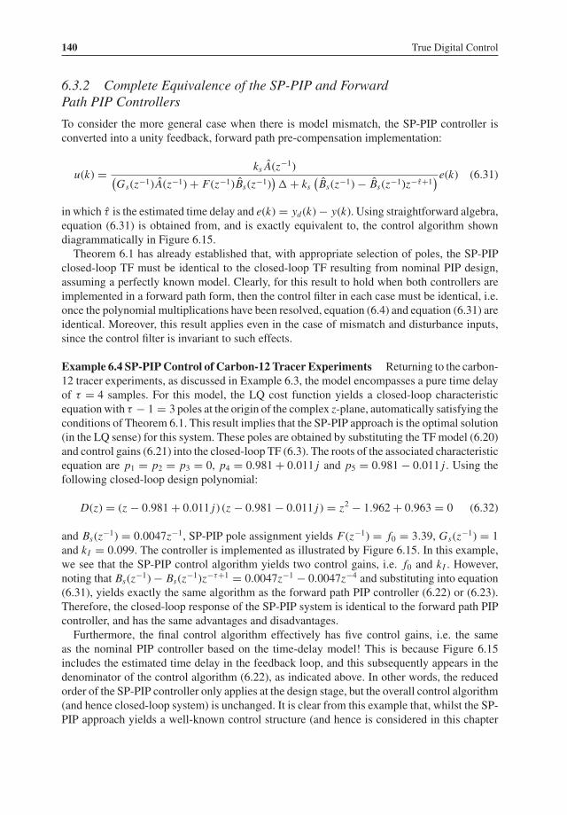
140 True Digital Control
6.3.2 Complete Equivalence of the SP-PIP and ForwardPath PIP Controllers
To consider the more general case when there is model mismatch, the SP-PIP controller isconverted into a unity feedback, forward path pre-compensation implementation:
u(k) = ks A(z−1)(Gs(z−1) A(z−1)+ F(z−1)Bs(z−1)
)� + ks
(Bs(z−1)− Bs(z−1)z−τ+1)e(k) (6.31)
in which τ is the estimated time delay and e(k) = yd (k)− y(k). Using straightforward algebra,equation (6.31) is obtained from, and is exactly equivalent to, the control algorithm showndiagrammatically in Figure 6.15.Theorem 6.1 has already established that, with appropriate selection of poles, the SP-PIP
closed-loop TF must be identical to the closed-loop TF resulting from nominal PIP design,assuming a perfectly known model. Clearly, for this result to hold when both controllers areimplemented in a forward path form, then the control filter in each case must be identical, i.e.once the polynomial multiplications have been resolved, equation (6.4) and equation (6.31) areidentical. Moreover, this result applies even in the case of mismatch and disturbance inputs,since the control filter is invariant to such effects.
Example 6.4 SP-PIP Control of Carbon-12 Tracer Experiments Returning to the carbon-12 tracer experiments, as discussed in Example 6.3, the model encompasses a pure time delayof τ = 4 samples. For this model, the LQ cost function yields a closed-loop characteristicequationwith τ − 1 = 3 poles at the origin of the complex z-plane, automatically satisfying theconditions of Theorem 6.1. This result implies that the SP-PIP approach is the optimal solution(in the LQ sense) for this system. These poles are obtained by substituting the TF model (6.20)and control gains (6.21) into the closed-loop TF (6.3). The roots of the associated characteristicequation are p1 = p2 = p3 = 0, p4 = 0.981+ 0.011 j and p5 = 0.981− 0.011 j . Using thefollowing closed-loop design polynomial:
D(z) = (z − 0.981+ 0.011 j ) (z − 0.981− 0.011 j ) = z2 − 1.962+ 0.963 = 0 (6.32)
and Bs(z−1) = 0.0047z−1, SP-PIP pole assignment yields F(z−1) = f0 = 3.39, Gs(z−1) = 1and kI = 0.099. The controller is implemented as illustrated by Figure 6.15. In this example,we see that the SP-PIP control algorithm yields two control gains, i.e. f0 and kI . However,noting that Bs(z−1)− Bs(z−1)z−τ+1 = 0.0047z−1 − 0.0047z−4 and substituting into equation(6.31), yields exactly the same algorithm as the forward path PIP controller (6.22) or (6.23).Therefore, the closed-loop response of the SP-PIP system is identical to the forward path PIPcontroller, and has the same advantages and disadvantages.Furthermore, the final control algorithm effectively has five control gains, i.e. the same
as the nominal PIP controller based on the time-delay model! This is because Figure 6.15includes the estimated time delay in the feedback loop, and this subsequently appears in thedenominator of the control algorithm (6.22), as indicated above. In other words, the reducedorder of the SP-PIP controller only applies at the design stage, but the overall control algorithm(and hence closed-loop system) is unchanged. It is clear from this example that, whilst the SP-PIP approach yields a well-known control structure (and hence is considered in this chapter

Control Structures and Interpretations 141
for tutorial purposes), it can always be exactly replicated by forward path PIP control andhence does not offer any advantages over such PIP design.
Example 6.5 SP-PIP Control of Non-Minimum Phase Oscillator Consider the TF model(6.10) with τ = 2 samples. The unit delay numerator polynomial is Bs(z−1) = −z−1 + 2.0z−2.In order to satisfy the conditions of Theorem 6.1, we are free to assign four poles anywhereon the complex z-plane, as long as the fifth is at the origin. Once again, this is the designdeliberately employed earlier (Example 6.1). For example, the Monte Carlo realisations inFigure 6.8 illustrate the expected poorer robustness properties of the SP-PIP and equivalentforward path algorithms to model mismatch.Within the context of the present discussion, however, it is interesting to examine the situation
when there is uncertainty in the time delay. For this type of model uncertainty, we find thatthe forward path approach is typically more robust than feedback PIP design. The results inFigure 6.16 are for a controller design based on τ = 2 as above, but with the simulated timedelay changed to τ = 3. This represents a significant error in the original identification of thecontrol model, but is useful here since it exaggerates the difference between the feedback andSP-PIP structures. We can see that while the former yields an unstable closed-loop response,with growing oscillations in the output, the forward path implementation remains stable, albeitwith a small overshoot of the command level.In this regard, it is important to emphasise that PIP pole assignment design of this type, in
which the closed-loop poles associated with the time delay are assigned to the origin of thecomplex z-plane, is not necessarily the most robust solution. In the present example, if wespecify all five closed-loop poles to lie at 0.5 on the real axis, then the feedback PIP controller
0 5 10 15 20 25 30 35−0.2
0
0.2
0.4
0.6
0.8
1
1.2
Sample no.
command
output
feedbackSP-PIP
Figure 6.16 Closed-loop response for a unit step in the command level, with the feedback (dashedtrace) and SP-PIP (bold solid trace) controllers of Example 6.5, when there are time-delay modellingerrors

142 True Digital Control
yields a stable closed-loop response similar to the bold solid trace in Figure 6.16. Here, we seethe benefit of having complete freedom to assign the n + m poles anywhere on the complexz-plane (including those associated with the time delay).
6.4 Stochastic Optimal PIP Design
The discussion so far has concentrated on a deterministic NMSS model of the system andassociated PIP pole assignment or LQ design. However, since it is formulated in state spaceterms, the NMSS approach to control system design can be converted into stochastic form,by invoking the separation theorem and introducing an optimal Kalman Filter (Kalman 1960,1961, 1963) for state estimation.Here, the Kalman filter is employed as an observer to generate a surrogate state vector, which
converges asymptotically to the true state vector in the presence of state and measurementnoise. The separation theorem states that the SVF control algorithm and observer can bedesigned separately. When connected, they will function as an integrated control system inthe desired manner (see e.g. Åstrom and Wittenmark 1984, pp. 273–275; Green and Limebeer1995, pp. 179–208; Franklin et al. 2006, pp. 511–513; Dorf and Bishop 2008, pp. 773–775;Gopal 2010, pp. 413–428). In the present context, the approach yields PIP-Linear QuadraticGaussian (PIP-LQG) designs that may be implemented in either state space or polynomialform, as demonstrated below.Such a Kalman Filter formation is not strictly necessary for basic PIP design, but it is
introduced here for completeness and as a useful starting point for some of the analysis laterin this chapter. The objective of the stochastic approach is to reduce the detrimental effectsof measurement noise, so as to yield a smoother input signal in the closed-loop response.This provides an alternative to the forward path PIP structure considered above. As we haveseen, forward path PIP control is a pragmatic solution to the problem of measurement noise,obtained using straightforward block diagram analysis.By contrast, the Kalman Filter approach is optimal (given assumptions about the noise) but
more complex to design and implement in practical situations. Furthermore, like the forwardpath implementation of deterministic PIP control, it carries with it the potential disadvantage ofdecreased robustness. Therefore, in this chapter, we will concentrate on the use of an observerfilter D(z−1), since this offers a practical compromise between filtering, robust design andstraightforward implementation2.
6.4.1 Stochastic NMSS Equations and the Kalman Filter
We initially formulate the PIP-LQG control problem by introducing stochastic white noisedisturbances into the regulator NMSS equations, as follows:
x(k) = Fx(k − 1)+ gu(k − 1)+ w(k)
y(k) = hx(k)+ ε(k)
}(6.33)
2 Although the observer polynomial is sometimes denoted (e.g. Clarke 1994) byC(z−1) or T (z−1), we will use D(z−1)for consistency with the various stochastic TF models considered in Chapter 8.

Control Structures and Interpretations 143
where x(k), F, g and h are defined by equation (4.4), equation (4.5), equation (4.6), equation(4.7), equation (4.8) and equation (4.9), w(k) is a zero mean, discrete-time, Gaussian, vectorwhite noise process with positive semi-definite covariancematrixN and ε(k) is an independent,zero mean, white measurement noise signal with variance σ 2. The innovations, or KalmanFilter, representation of this system is:
x(k + 1/k) = Fx(k/k − 1)+ gu(k − 1)+ L(k)e(k)
y(k) = hx(k/k − 1)+ e(k)
}(6.34)
where L(k) is the Kalman gain vector and e(k) = y(k)− hx(k/k − 1) is the innovationssequence (see e.g. Young 2011). From equations (6.34), it is clear that the optimal stateestimator has the form:
x(k + 1/k) = Fx(k/k − 1)+ gu(k − 1)+ L(k) (y(k)− hx(k/k − 1)) (6.35)
Here, we see that x(k + 1/k) represents a one step ahead estimate of the non-minimal statevector, conditional on the ‘latest’ measured output y(k). Note that only the latest scalarobservation of y(k) is used to update the NMSS state at each sampling instant since theNMSS vector is composed of past values of y(k) that have already been processed, as wellas the present and past values of the input u(k), that are known exactly. Subsequently, we usey(k) = hx(k/k − 1) to represent the optimal estimate of the output, hence,
e(k) = y(k)− y(k) (6.36)
The SVF control law is now formulated by reference to the separation theorem in theusual manner (see e.g. Åstrom and Wittenmark 1984, pp. 273–275; Green and Limebeer 1995pp. 179–208; Franklin et al. 2006, pp. 511–513; Dorf and Bishop 2008, pp. 773–775; Gopal2010, pp. 413–428):
u(k) = −kT x(k/k − 1) (6.37)
where k is the PIP control gain vector (5.31). Equation (6.37) is based on the deterministiccontrol law (5.30) but adapted here to utilise the optimal estimate of the state vector.Once the Kalman gain vector has converged to its steady-state value, i.e. L(k → ∞) = L,
it can be shown that e(k) in equations (6.34) constitutes a zero mean white noise sequencewith constant variance σ 2 (e.g. Young 2011). Here, L is determined from the steady-statesolution of the discrete-time, matrix Riccati equations, involving the state transition matrixand observation vector, together with the covariances of the state disturbance andmeasurementnoise inputs. In particular, L is obtained from equation (5.81) and equation (5.82) but replacingF with FT , g with hT , Q with the covariance matrix NT and r with σ (see e.g. Åstrom andWittenmark 1984, pp. 259 and 270), as follows:
LT = (σ + hPhT )−1hPFT (6.38)

144 True Digital Control
where P is the steady-state solution of the matrix Riccati equation:
P − FPFT + FPhT (r + hPhT )−1hPFT − N = 0 (6.39)
in which 0 is a matrix of zeros. For more information about this interesting duality betweenLQ control and optimal filtering, refer to the textbook references on linear control theoryhighlighted above.For regulator NMSS design, the state covariance matrix N is chosen to represent the noise
on the output states, while zeros are utilised to correspond to the exactly known past values ofthe calculated control input signal, i.e.
N =[
Nn 0
0 0
](6.40)
where Nn is an n × n disturbance covariance matrix and 0 is an appropriately defined matrixof zeros. Therefore, the general form of this minimal Kalman gain vector, where only theoptimal estimate of the output and its past values are filtered, is as follows:
L(k) = [ l1(k) l2(k) . . . ln(k) 0 . . . 0 0 ]T (6.41)
Finally, in the servomechanism formulation of the problem, the integral-of-error state variablez(k), defined in equation (5.4), is included as normal, with either the measured output y(k) orthe optimal estimate of the output y(k) fed back to the integral controller, as discussed below.
6.4.2 Polynomial Implementation of the Kalman Filter
An important consequence of the convergence of L(k) to a steady-state value L is that theinnovations representation of the system (6.34) may be expressed as the following Auto-Regressive, Moving-Average eXogenous variables (ARMAX) model:
y(k) = b1z−1 + · · · + bm z−m
1+ a1z−1 + · · · + anz−nu(k)+ 1+ d1z−1 + · · · + dnz−n
1+ a1z−1 + · · · + anz−ne(k) (6.42)
or, in shorthand form:
y(k) = B(z−1)A(z−1)
u(k) + D(z−1)A(z−1)
e(k) (6.43)
Equation (6.43) is derived by Young (1979) for a minimal stochastic state space representationof the system, i.e. based on the observable canonical form (3.37) introduced in Chapter 3. Thispaper also shows how a Kalman Filter can be constructed from polynomial filters that are usedin the Refined Instrumental Variable (RIV) method of TF model estimation (see Chapter 8);and that, in this minimal state situation, the coefficients of the D(z−1) polynomial are definedby di = ai + li , where ai are the parameters of the deterministic characteristic equation A(z−1)

Control Structures and Interpretations 145
and li are the minimal state Kalman Filter gains3. Again noting the duality between LQ controland optimal filtering, this result can be compared with equation (3.34), in which li are the SVFcontrol gains obtained using the controllable canonical form.In the non-minimal case, the coefficients of D(z−1) are defined as follows (Hesketh 1992):
di = ai + li (6.44)
where
⎡⎢⎢⎢⎢⎢⎢⎢⎢⎢⎣
l1l2l3...
ln−1ln
⎤⎥⎥⎥⎥⎥⎥⎥⎥⎥⎦
=
⎡⎢⎢⎢⎢⎢⎢⎢⎢⎢⎣
1 0 0 · · · 0 0
0 −a2 −a3 · · · −an−1 −an
0 −a3 −a4 · · · −an 0...
......
......
...
0 −an−1 −an · · · 0 0
0 an 0 · · · 0 0
⎤⎥⎥⎥⎥⎥⎥⎥⎥⎥⎦
⎡⎢⎢⎢⎢⎢⎢⎢⎢⎢⎣
l1l2l3...
ln−1ln
⎤⎥⎥⎥⎥⎥⎥⎥⎥⎥⎦
(6.45)
With this formulation, the noise polynomial D(z−1) is either derived from L or obtaineddirectly from observed data using the system identification tools discussed in Chapter 8. Inthe latter case, equation (6.44) and equation (6.45) could then be used in reverse to determinethe equivalent Kalman gains from the estimated model. Alternatively, the Kalman Filter canbe implemented in a number of ways that directly employ D(z−1), as shown below.Using equation (6.36) and equation (6.43):
y(k) = B(z−1)A(z−1)
u(k)+ D(z−1)A(z−1)
(y(k)− y(k)) (6.46)
After rearranging,
y(k) = D(z−1)− A(z−1)D(z−1)
y(k)+ B(z−1)D(z−1)
u(k) (6.47)
In other words,
y(k) = (d1 − a1)
[z−1
D(z−1)y(k)
]+ · · · + (dn − an)
[z−n
D(z−1)y(k)
]
+ b1
[z−1
D(z−1)u(k)
]+ · · · + bm
[z−m
D(z−1)u(k)
] (6.48)
so that the optimal estimate y(k) is the linear sum of the pre-filtered output and input variables,where the pre-filter is the numerator of the Auto-Regressive, Moving-Average (ARMA) noisemodel. SeeChapter 8 for discussion on this pre-filter, as used forARMAnoisemodel parameter
3 The multivariable version of this analysis is developed in Jakeman and Young (1979).

146 True Digital Control
plant
yd(k) u(k) y(k)+
−
+
−
++
+ +
integralcontroller
kI
1 − z−1
B(z−1)
A(z−1)
B(z−1)
D(z−1)
D(z−1) − A(z−1)
D(z−1)
D(z−1)
A(z−1)
F(z−1)
1
G(z−1)
e(k)
y(k)
Figure 6.17 Polynomial implementation of the PIP-LQG control system with the integral controlleroperating on the optimal estimate of the output
estimation. On the basis of the above results, the optimal estimate y(k) can be simply fed backin place of the measured output, as shown in Figure 6.17.In an alternative structure, the feedback filter F(z−1) utilises y(k) but the integral controller
operates on the measured unfiltered output y(k), as illustrated by Figure 6.18 (cf. Figure 6.4).In the latter case, note that the scalar gain on the integral controller does not amplify the noise.The relative merits of these and other polynomial structures are discussed after the followingintroductory example.
plant
yd(k) u(k) y(k)+
−
+
−
++
+ +
integralcontroller
kI
1 − z−1
B(z−1)
A(z−1)
B(z−1)
D(z−1)
D(z−1) − A(z−1)
D(z−1)
D(z−1)
A(z−1)
F(z−1)
1
G(z−1)
e(k)
y(k)
Figure 6.18 Polynomial implementation of the PIP-LQG control system with the integral controlleroperating on the measured output

Control Structures and Interpretations 147
Example 6.6 Kalman Filter Design for Noise Attenuation Consider again the non-minimum phase oscillator (6.10) and associated deterministic PIP-LQ controller developedin Chapter 5 (Example 5.8), i.e. based on the weights (5.78) with qy = 1/2, qu = 1/3 andqe = 0.1, which yields the following control gain vector:
kT = [ fo f1 g1 g2 −kI ] = [ 0.597 −1.008 1.226 2.017 −0.109 ] (6.49)
With regard to Kalman Filter design, the system is represented using the stochastic NMSSmodel (6.33), a measurement noise variance σ 2 = 0.1 and the following state covariancematrix chosen to provide a reasonably balanced amount of noise filtration:
N =
⎡⎢⎢⎢⎣0.003 0 0 0
0 0.003 0 0
0 0 0 0
0 0 0 0
⎤⎥⎥⎥⎦ (6.50)
The regulator NMSS state transition matrix is:
F =
⎡⎢⎢⎢⎣
−a1 −a2 b2 b31 0 0 0
0 0 0 0
0 0 1 0
⎤⎥⎥⎥⎦ =
⎡⎢⎢⎢⎣1.7 −1 −1 2
1 0 0 0
0 0 0 0
0 0 1 0
⎤⎥⎥⎥⎦ (6.51)
and the observation vector is h = [ 1 0 0 0 ].In this case, the discrete-time, matrix Riccati equation (6.38) and equation (6.39) yield the
following Kalman gain vector:
L = [ 0.365 0.353 0 0 ]T (6.52)
and equation (6.45) becomes
[l1l2
]=[1 0
0 −a2
][l1l2
]=[1 0
0 −1
][0.365
0.353
]=[
0.365
−0.353
](6.53)
Hence, D(z−1) = 1+ (l1 + a1)z−1 + (l2 + a2)z−2 = 1− 1.335z−1 + 0.647z−2 and the opti-mal estimate of the output (6.47) is determined from:
y(k) = 0.365z−1 − 0.353z−2
1− 1.335z−1 + 0.647z−2 y(k)+ −z−2 + 2.0z−3
1− 1.335z−1 + 0.647z−2 u(k) (6.54)
with the final control algorithm implemented as shown by Figure 6.17.The response of the PIP-LQG and standard PIP-LQ (i.e. with and without the filtering)
closed-loop system is illustrated by Figure 6.19 and Figure 6.20. The main advantage of using

148 True Digital Control
20 40 60 80 100−4
−2
0
2
4
6
8
10
12
Sample no.
command
output
no f ilteringf iltering
Figure 6.19 Closed-loop response for a unit step in the command level, comparing the output of thestochastic system both with (stochastic PIP-LQG design) and without (deterministic PIP-LQ design) theKalman Filter
20 40 60 80 100−2
−1
0
1
2
3
4
5
Sample no.
control input
no f ilteringf iltering
Figure 6.20 Control inputs associated with Figure 6.19

Control Structures and Interpretations 149
an optimally filtered output variable is that the control input is generally smoothed in someway, as demonstrated by Figure 6.20.
6.4.3 Stochastic Closed-loop System
Algebraic or block diagram analysis of Figure 6.17, reveals that the closed-loop response isgiven by the deterministic closed-loop TF (6.3) and a stochastic component, as follows:
y(k) = kI B(z−1)�(G(z−1)A(z−1)+ F(z−1)B(z−1)
)+ kI B(z−1)yd (k)
+�(G(z−1)D(z−1)+ F(z−1)B(z−1)
)+ kI B(z−1)�(G(z−1)A(z−1)+ F(z−1)B(z−1)
)+ kI B(z−1)e(k)
(6.55)
Similarly for Figure 6.18:
y(k) = kI B(z−1)�(G(z−1)A(z−1)+ F(z−1)B(z−1)
)+ kI B(z−1)yd (k)
+ �(G(z−1)D(z−1)+ F(z−1)B(z−1)
)�(G(z−1)A(z−1)+ F(z−1)B(z−1)
)+ kI B(z−1)e(k)
(6.56)
These take a similar form to the deterministic disturbance response TF models consideredearlier, i.e. equation (6.7) and equation (6.8). In the present analysis, however, the numeratorof the stochastic component includes the expression G(z−1)D(z−1), which contrasts with theG(z−1)A(z−1) term in the denominator.It is clear that, as usual for observer design, the D(z−1) polynomial cancels out in the com-
mand response (Clarke 1994; Yoon and Clarke 1994). By contrast, the stochastic componentin equation (6.55) relates to the disturbance vector w(k) of the stochastic NMSS model (6.33).As discussed above, the Kalman Filter is designed to attenuate the measurement noise ε(k) butto pass the state disturbancesw(k). The latter are regarded as ‘real’ disturbances that have to behandled by the control system and, for example, could be dealt with by feed-forward control(see section 6.5). Of course, Figure 6.17 and Figure 6.18 have actually been derived from theinnovations representation (6.34), hence the noise is encompassed by the D(z−1)/A(z−1) TFmodel.In the ideal case represented by Figure 6.17 or Figure 6.18, it is straightforward to verify
that y(k) = y(k)− e(k) exactly. In this context, it is interesting to also consider the spe-cial case of a white noise disturbance i.e. D(z−1) = A(z−1). Here, the open-loop TF model(6.43) is:
y(k) = B(z−1)A(z−1)
u(k)+ e(k) (6.57)

150 True Digital Control
Since D(z−1)− A(z−1) = 0, the optimal estimate of the output (6.47) is determined using thedeterministic open-loop TF model, as follows:
y(k) = B(z−1)A(z−1)
u(k) (6.58)
This is a very unsatisfactory solution in practical terms because y(k) is generated from u(k),with no reference at all to the measured output, and it clearly exposes some lack of robustnessin the Kalman Filter when used in the minimal state feedback context.To further illustrate the implication of a white noise disturbance D(z−1) = A(z−1), consider
Figure 6.17 or Figure 6.18 again. Combining equation (6.58) and Figure 6.18 yields theblock diagram for the deterministic forward path PIP controller (Figure 6.4). Equivalently, theclosed-loop response (6.56) based on Figure 6.18 reduces to the forward path load disturbanceclosed-loop response (6.8). This interpretation shows that, in the absence of state disturbancenoise, forward path PIP design is optimal.By contrast, with D(z−1) = A(z−1), equation (6.55) based on Figure 6.17 becomes:
y(k) = kI B(z−1)�(G(z−1)A(z−1)+ F(z−1)B(z−1)
)+ kI B(z−1)yd (k)+ e(k) (6.59)
In other words, when the output is contaminated by white measurement noise only, Figure6.17 simply yields the closed-loop form of equation (6.57).
6.4.4 Other Stochastic Control Structures
At this juncture, it should be remembered that the NMSS approach to control system designdoes not need any form of state reconstruction. In essence, therefore, the Kalman Filter is onlyrequired for noise attenuation and not for state estimation per se. Furthermore, like the forwardpath implementation of basic PIP control, the Kalman Filter carries with it the disadvantageof decreased robustness, as revealed also by equation (6.58): in particular, the state estimationis dependent upon the input-driven model of the system and the cancellation of the observerdynamics.This limitation has led to the concept of Loop Transfer Recovery (LTR: see e.g. Maciejowski
1985; Bitmead et al. 1990), which attempts to recover the robustness of the full state feed-back properties. However, full state feedback is always achieved in the NMSS case, so LTRis not required. For this reason, it is sometimes advantageous to utilise different, nominallysub-optimal, approaches to noise attenuation which do not involve the Kalman Filter anddo not necessitate complicated design manipulation such as LTR. In this regard, it shouldbe stressed that Figure 6.17 and Figure 6.18 illustrate just two possible polynomial imple-mentations of the PIP-LQG control system, among a wide range of other options availablein the literature. For example, Dixon (1996) and Taylor (1996) consider a number of otherapproaches to noise attenuation that utilise either the Kalman Filter (implemented in variousforms, including a special non-minimal filter), explicit pre-filtering of the non-minimal statesand/or the introduction of additional filters.

Control Structures and Interpretations 151
One limitation of the stochastic model (6.43), is that it does not allow for non-stationary(time-varying) disturbance inputs to the system. This problem manifests itself in the form ofa non-zero steady-state error, if the controller shown by Figure 6.17 is utilised on a systemthat is affected by such disturbances. This is verified by noting that the steady-state gain of thestochastic component of equation (6.55) is unity. To combat the problem, we could follow asimilar approach to forward path PIP control, by utilising Figure 6.18, where the steady-stategain of the stochastic component of equation (6.56) is zero, as required. Arguably, however,a more satisfactory solution in the context of optimal filtering, can be achieved by explicitlyrepresenting the disturbance in the NMSS model, as shown below.
6.4.5 Modified Kalman Filter for Non-Stationary Disturbances
To address the problem of non-stationary disturbances, consider the following modified inno-vations representation, which is based on equations (6.34) but with the introduction of arandom walk state variable r (k) to represent the unknown disturbance:
[x(k + 1/k)
r (k + 1/k)
]=[
F Om+n,1
O1,n+m 1
][x(k/k − 1)r (k/k − 1)
]+[
g
0
]u(k)+
[L(k)
ln+1(k)
]e(k)
y(k) = [h 1
] [ x(k/k − 1)r (k/k − 1)
]+ e(k)
⎫⎪⎪⎪⎪⎬⎪⎪⎪⎪⎭(6.60)
where 0 represents a vector of n + m zeros, while r (k) = r (k − 1)+ ξ (k), in which ξ (k) isa zero mean white noise sequence with constant variance. As usual, the Kalman gain vectorobtained from equations (6.60), including the gain associated with r (k), is estimated using thesteady-state solution of the discrete-time, matrix Riccati equations.Following again a similar approach to Young (1979) and Hesketh (1992), the polynomial
representation of the modified system is the following Auto–Regressive, Integrated Moving-Average eXogenous variables (ARIMAX) model4:
y(k) = B(z−1)A(z−1)
u(k) + D1(z−1)�A(z−1)
e(k) (6.61)
where D1(z−1) = D(z−1)� + ln+1A(z−1). Utilising equation (6.36) and rearranging (6.61)yields the optimal estimate of the output:
y(k) = D1(z−1)− �A(z−1)D1(z−1)
y(k)+ �B(z−1)D1(z−1)
u(k) (6.62)
The PIP control algorithm is now implemented in either SVF form based on equation (6.35)and equation (6.37), or in polynomial form in a similar manner to Figure 6.17. In both cases, the
4 This is sometimes called the CARIMA (Controlled Auto-Regressive Integrated Moving-Average) model.

152 True Digital Control
optimal estimate y(k) now includes the difference operator� = 1− z−1, which automaticallyintroduces the necessary integral action into the observer.The discussion above has utilised the stochastic NMSS model to develop PIP-LQG control
systems. In section 6.4.6, we will briefly consider the introduction of a risk sensitive, LinearExponential-of-Quadratic Gaussian (LEQG) cost function.
6.4.6 Stochastic PIP Control using a Risk Sensitive Criterion
Robust control design aims to minimise problems caused by uncertainty in the control system(e.g. Green and Limebeer 1995). For example, H∞ control ensures that bounds on the H∞-norm of certain TF models, representing the relationship between disturbance signals andparticular variables of interest, are achieved. This contrasts with the more conventional H2approach where, in the optimal stochastic LQG case considered above, the deterministiccontrol law involves the minimisation of the LQ criterion:
J =N−1∑k=0
x(k)T Qx(k)+ r (u(k)2) (6.63)
in which Q is a symmetric, positive semi-definite matrix, r is a positive scalar and N is aninteger number of samples (the optimisation window). The cost function is presented in thisN − 1 step ahead form for the purposes of the later discussion on predictive control (section6.6). However, N → ∞ ensures equivalence with the standard implementation of optimalPIP-LQ control introduced in Chapter 5, i.e. the steady-state or infinite time solution (5.75).Unlike in the LQG formulation, a particular H∞ criterion does not yield a unique solution.
One approach, for example, is the minimum entropy solution of Mustafa and Glover (1990)which, in turn, is closely related to the following LEQG cost function:
γ (θ ) = −2θ−1 loge E{e−θ J/2} (6.64)
where θ a scalar ‘risk-sensitive’ parameter and E {·} represents the expectation (Jacobson1973; Kumar and van Schuppen 1981; Whittle 1981, 1990). An interesting result in thepresent context is the relationship between LEQG optimisation and the H∞ approach. Thisrelationship means that the LEQG formulation has certain robustness properties that enhanceits potential importance to control engineers (Glover and Doyle 1988).To develop the PIP-LEQG control system, we first define a stochastic servomechanism
NMSSmodel, similar to equations (6.33) but here including the integral-of-error state variable.The control gains are obtained using the following backwards Riccati recursion:
P(k) = Q + FT[gr−1gT + θ N + P(k + 1)−1]−1 F
kT (k) = r−1gT[gr−1gT + θ N + P(k + 1)−1]−1 F
}(6.65)
where k(k) is the state variable feedback control gain matrix (Whittle 1981). In contrast to theminimal approach, the PIP-LEQG algorithm may be implemented in entirely deterministicform without filtering if desired, i.e. the NMSS equations employed here ensure that it is

Control Structures and Interpretations 153
possible to implement what is referred to, in this context, as the ‘complete observations’solution. In this case, LEQG design does not include any consideration of the measurementnoise.In deterministic PIP-LEQG design, solving (6.65) with θ > 0 generally moves the closed-
loop pole positions towards the origin of the complex z-plane and so increases the speedof response in comparison with the PIP-LQ solution (Taylor et al. 1996). By contrast, withθ < 0, the control input signal is generally smoother than in the LQ case, but at the expenseof a slower output response. In other words, θ is essentially an additional tuning parameterfor optimal PIP control design. For this reason, it is best combined with a multi-objectiveoptimisation approach to control system design, as discussed in Chapter 7.
6.5 Generalised NMSS Design
One advantage of the NMSS model is that the state vector is readily extended to accountfor the availability of additional measured or estimated information. As we have seen, suchadditional states can be utilised to develop more sophisticated algorithms that address specificcontrol problems. This concept is illustrated by the modified Kalman Filter for non-stationarydisturbances (6.60). In the present section, the flexibility of the NMSS model is furtherillustrated using two new examples, namely feed-forward control design and command inputanticipation.
6.5.1 Feed-forward PIP Control based on an Extended ServomechanismNMSS Model
Here, we aim to improve the response of the controller to measured system disturbances (seee.g. Figure 6.6), by utilising these measurements in a feed-forward structure. Therefore, thefollowing multi-input, single-output TF model is estimated using the system identificationtools in Chapter 8. The model takes a similar form to equation (6.43), but the unknown noisesignal is replaced with the measured disturbance v(k), i.e.
y(k) = B(z−1)A(z−1)
u(k) + D(z−1)A(z−1)
v(k) (6.66)
Although equation (6.66) suffices for the present illustrative discussion, generalised versionsof this model are also possible, including multiple disturbance signals with independentdenominator polynomials (Young et al. 1994). In conventional feed-forward design, we derivea control structure algebraically to exactly cancel the disturbance signal in the zero modelmismatch case (e.g. Ogata 2001). This cancellation approach can also be utilised for PIPdesign (Cross et al. 2011), but an alternative is to extend the NMSS model, as follows:
x(k) = Fx(k − 1)+ gu(k − 1)+ d yd (k)+ b v(k)
y(k) = hx(k)
}(6.67)
154 True Digital Control
where the non-minimal state vector is, for example
x(k) = [y(k) · · · y(k − n) u(k − 1) · · · u(k − m + 1) z(k) v(k − N + 1) · · · v(k)]T(6.68)
in which N is the order of the disturbance polynomial D(z−1). Here, F, g, d, b and h aredefined in the obvious way, following a similar approach to the nominal servomechanismNMSS model of Chapter 5, but here extended to represent equation (6.66) in differenceequation form. The SVF control gain vector:
kT = [ f0 f1 · · · fn−1 g1 · · · gm−1 − kI − pN · · · − p1 − p0] (6.69)
is obtained by minimising the LQ cost function (5.75) or (6.63) in the usual manner5. In blockdiagram terms, an additional control filter operates on the measured disturbance signal:
P(z−1) = p0 + p1z−1 + · · · + pN−1z−(N−1) (6.70)
Young et al. (1994), for example, utilise a feed-forward PIP approach based on these equationsto control temperature in a greenhouse, significantly reducing the effects of the solar radiationdisturbance. More recently, Cross et al. (2011) developed feed-forward PIP control systemsfor regulating the power take-off of a nonlinear wave energy convertor simulation. In this case,the feed-forward approach addresses the influence of the wave force disturbance, ultimatelyimproving power capture.
6.5.2 Command Anticipation based on an Extended ServomechanismNMSS Model
In many applications of control, the command level is either constant or any adjustmentsare known well in advance. In the case of robotic manipulators, for example, the joint angletrajectory is often determined by solving the kinematics offline. This is the approach taken forthe laboratory excavator discussed in Chapter 5 (Example 5.2), in which the PIP controlledmanipulator joint angles are planned at the start of each manoeuvre. In this situation, theNMSS model can be extended to handle N future known commands by simply appending thestate vector with these values (Taylor et al. 2000a):
x(k) = [y(k) · · · y(k − n) u(k − 1) · · · u(k − m + 1) z(k) yd(k)T ]T (6.71)
5 For consistency with the later discussion on command anticipation and model predictive control, the order of thedisturbance polynomial is given by N, which is also the number of iterations of the finite-horizon LQ cost function(6.63). However, this connection is not a general requirement of the feed-forward PIP formulation. Indeed, the practicalimplementation results discussed by Young et al. (1994) are based on the infinite horizon cost function (5.75), withthe order of the disturbance polynomial obtained independently using the system identification algorithms discussedin Chapter 8.

Control Structures and Interpretations 155
where
yd (k) = [yd (k + 1) yd (k + 2) . . . yd (k + N )]T (6.72)
The command input NMSS form with these modifications is:
x(k) = Fx(k − 1)+ gu(k − 1)+ d yd (k + N )
y(k) = hx(k)
}(6.73)
where
g = [ g 0 · · · 0 0 ]T , d = [ 0 0 · · · 0 d ]T , h = [ h 0 · · · 0 0 ] and
F =
⎡⎢⎣
F d On+m,N−1O N−1,n+m O N−1,1 I N−10 . . . 0
⎤⎥⎦ (6.74)
in which F, g and d are from the servomechanism NMSS model, i.e. they are defined byequation (5.15) and equation (5.16). Finally, O is an appropriately defined matrix of zeros andIN−1 an identity matrix.The extended PIP control algorithm is implemented in either SVF or incremental form,
with the SVF control gain vector (6.69) again obtained by minimising the infinite-horizonLQ cost function (5.75). Because of the integral-of-error state variable, and in contrast to theminimal approach (see e.g. Bitmead et al. 1990), no special LQ state weighting arrangementsare required to ensure steady-state tracking. ThereforeQ is usually formed as a diagonal matrixsimilar to equation (5.77), with the additional elements set to zero:
Q = diag(
qy · · · qy qu · · · qu qe 0 · · · 0)
(6.75)
In fact, the command input is clearly not controllable, so the choice of associated weights inthe Q matrix has no effect on the final PIP gains. Furthermore, for a given model and LQweights, the gain associated with each future command input is always the same, regardlessof the value of N. Hence, above a certain level, the closed-loop response is not particularlysensitive to the value of N and selecting a high value (say greater than 10) has little effect,since the gains trail off to zero.In block diagram terms, the controller can be implemented as shown in Figure 6.21, in
which P(z−1) is given by equation (6.70).Note that P(z−1) operates on the N-step ahead command input yd (k + N ), whilst that the
integral-of-error state variable z(k) is defined using the ‘current’ command yd (k). Inspectionof Figure 6.21 shows:
u(k) = 1
G(z−1)
(−F(z−1)y(k) + P(z−1)yd (k + N ) + kI
�
(z−N yd (k + N ) − y(k)
))(6.76)

156 True Digital Control
plantforward path f ilter
commandf ilter
feedback f ilter
u(k) y(k)+
− −integral
controller
kI
1 − z−1
B(z−1)
A(z−1)
F(z−1)
1
G(z−1)
++
P(z−1)yd(k + N)
z−N
Figure 6.21 Feedback PIP control with command input anticipation
Rearranging gives:
G(z−1)�u(k) = − (F(z−1)� + kI
)y(k) + (
kI z−N + P(z−1)�)
yd (k + N ) (6.77)
Further algebraic or block diagram analysis yields:
y(k) = B(z−1)(kI z−N + P(z−1)�
)�(G(z−1)A(z−1)+ F(z−1)B(z−1)
)+ kI B(z−1)yd (k + N ) (6.78)
Here, only the numerator polynomial of the closed-loop TF is modified in comparison withequation (6.3), hence LQ design yields the same closed-loop poles as for the nominal case.Furthermore, since � = 1− z−1 → 0 for k → ∞, the steady-state gain of equation (6.78) isunity and Type 1 servomechanism performance is obtained, as required.Other NMSS implementations of command anticipation are also possible, including forward
path and stochastic solutions. Finally, as Hesketh (1992) points out, the z−N time delayemployed in Figure 6.21 could be replaced by a TF model, in order to induce a modelfollowing response in the closed-loop.
Example 6.7 Command Input Anticipation Design Example There are two major advan-tages of introducing the future command input states: in the first place, the closed-loop systemanticipates changes and reacts to the command input sooner; and, secondly, simulation studiesshow that the control input is generally smoothed in some manner. An attractive consequenceof the latter point can be seen in the control of the familiar model (6.10), where the open-loop non-minimum phase characteristics have been completely eliminated, as illustrated byFigure 6.22.To emphasise the difference between the command anticipation and nominal responses,
the PIP-LQ controller in Figure 6.22 is based on an increased integral-of-error weighting

Control Structures and Interpretations 157
0 5 10 15 20 25 30 35 40−0.5
0
0.5
1
1.5
command level and outputs
anticipationnominal
0 5 10 15 20 25 30 35 40−0.2
0
0.2
0.4control inputs
Sample no.
Figure 6.22 Closed-loop response for positive and negative unit steps in the command level, comparingthe output of the PIP-LQ optimal control system with (bold solid trace) and without (dashed trace) acommand anticipation filter
compared with Example 6.1, hence a faster closed-loop response, i.e. based on the weights(5.78) with qy = 1/2, qu = 1/3 and qe = 10, which yields:
kT = [ f0 f1 g1 g2 −kI ] = [ 2.440 −2.877 2.023 5.753 −0.428 ] (6.79)
With command anticipation based on N = 10, the above SVF gains remain unchanged, whilstthe additional gains (6.70) are p0 = 0.006, p1 = 0.012, p2 = 0.023, p3 = 0.045, p4 = 0.089,p5 = 0.182, p6 = 0.369, p7 = 0.611, p8 = 0.428 and p9 = 0.428. Another example of PIPcommand anticipation, in which the NMSS model is stated in full for tutorial purposes, isdiscussed later (Example 6.8).
6.6 Model Predictive Control
Model Predictive Control (MPC) is a popular approach to control system design with manysuccessful applications, particularly in the chemical and process engineering industries (Morariand Lee 1999). An attractive feature of MPC is the ability to handle constraints on the systemvariables, such as equations (6.15), as an inherent part of the design process, albeit at thecost of increased complexity (Maciejowski 2002; Rossiter 2003). MPC algorithms based onminimal state space models typically utilise an observer and exploit the separation theorem ina similar manner to equation (6.37). Hence, much research effort has been directed towards

158 True Digital Control
increasing the robustness of MPC design and to reducing the online computational load (e.g.Bemporad et al. 2002).
6.6.1 Model Predictive Control based on NMSS Models
Aswe have seen, PIP control systems are generally implemented using an incremental form, inorder to avoid integral ‘wind-up’ problems. To address more general system constraint prob-lems, such as limits on the output signal and other measured variables, we will consider laterthe use of multi-objective optimisation techniques where the PIP-LQ weights are optimisedoffline using computer simulation, as described in Chapter 7. However, in recent years, variousdeterministic NMSS model structures have also been utilised for MPC design (see e.g. Tayloret al. 2000a; Wang and Young 2006; Exadaktylos et al. 2009; Gonzales et al. 2009). Thelatter citations all define a modified form of the regulator NMSS model, in which differencedvalues of the control input signal�u(k) are utilised as state variables. By contrast, the relativemerits of various integral action schemes for MPC have been considered by Pannocchia andRawlings (2003), and these results are exploited by Exadaktylos and Taylor (2010) to developMPC systems using the servomechanism NMSS model of Chapter 5.The MPC cost function is generally solved online to address the problem of system con-
straints. In particular, the future constrained control input variables, u(k), u(k + 1), u(k + 2)through to u(k + N ), are determined by solving a quadratic optimisation problem at everysampling instant k. Following standard MPC practice, a receding-horizon approach is sub-sequently employed, with only the first of these actually utilised at each control sample. Bycontrast, the focus of the present book is on linear control theory and on the development offixed gain controllers that can be analysed in block diagram terms. In this context, an importantstep in the evolution of MPC is the Generalised Predictive Control (GPC) approach of Clarkeet al. (1987). Hence, the final part of this chapter focuses on the relationship between GPCand PIP control.
6.6.2 Generalised Predictive Control
Unlike PIP control, GPC was not originally formulated overtly in an optimal state spacecontext. Rather, it is normally presented in an alternative receding-horizon optimal setting,defined by the following cost function:
J = E
⎧⎨⎩
N∑j=1(y(k + j)− yd (k + j))2 +
NU∑j=1
λ (�u(k + j − 1))2⎫⎬⎭ (6.80)
where N and NU are the output and input costing horizons, respectively, and E {·} representsthe expectation.Here, the control strategy is posed in terms of the differenced input signal, i.e. �u(k) =
u(k)− u(k − 1). The approach utilises the ARIMAX model (6.61), which can be rearrangedand restated as follows:
A(z−1)y(k) = B(z−1)�u(k)+ D(z−1) e(k) (6.81)

Control Structures and Interpretations 159
plantforward path f iltercommand
f ilter
feedback f ilter
u(k)yd(k + N) y(k)
−
B(z−1)
A(z−1)
S(z−1)
1
ΔR(z−1)
+W(z−1)
Figure 6.23 The NMSS servomechanism system in predictive form
where A(z−1) = �A(z−1) = 1+ a1z−1 + · · · + an+1z−(n+1), A(z−1) and B(z−1) are definedby equation (6.1), and the generalised noise polynomial D(z−1) = 1+ d1z−1 + · · · + dpz−p.The simplest form of GPC is based on the ARIMAX system model (6.81) with the noise
polynomial set to unity, i.e. D(z−1) = 1. We will consider the general case using the noisepolynomial for filtering purposes later on. Minimising the cost function (6.80) yields:
�u(k) = gT ( yd − f ) (6.82)
in which gT = [g1 g2 . . . gN ] is a vector of gain coefficients, yd is a vector of futurecommand inputs (6.72) and f = [ f (k + 1) f (k + 2) . . . f (k + N )]T is called themodel freeresponse prediction. As shown, for example, by Clarke et al. (1987) and Bitmead et al. (1990),evaluation of equation (6.82) yields a fixed gain control algorithm that can be convenientlyexpressed in block diagram form, as illustrated by Figure 6.23.The control polynomials in Figure 6.23 are defined:
S(z−1) = s0 + s1z−1 + · · · + snz−n
R(z−1) = 1+ r1z−1 + · · · + rm−1z−(m−1)
W (z−1) = w0 + w1z−1 + · · · + wN−1z−(N−1)
⎫⎪⎬⎪⎭ (6.83)
Using Figure 6.23, the GPC algorithm can be expressed:
R(z−1)�u(k) = −S(z−1)y(k) + W (z−1)yd (k + N ) (6.84)
Further algebraic or block diagram analysis yields the closed-loop TF:
y(k) = W (z−1)B(z−1)�R(z−1)A(z−1)+ S(z−1)B(z−1)
yd (k + N ) (6.85)
Note that s0 + s1 + · · · + sn = w0 + w1 + · · · + wN−1, hence the steady-state gain of closed-loop system (6.85) is unity. The integral action implicit in the model (6.81), ensures anintegrator in the forward path control filter and so yields Type 1 servomechanism performance.
6.6.3 Equivalence Between GPC and PIP Control
Returning now to the command anticipation form of PIP control, Figure 6.21 can be alge-braically transformed so that it conforms to the same structure as GPC in Figure 6.23 (Taylor

160 True Digital Control
et al. 1994, 2000a). In fact, comparing equation (6.77) and equation (6.84), it is straightforwardto determine the equivalent terms, as follows:
S(z−1) ≡ (F(z−1)� + kI
) = F∗(z−1)R(z−1) ≡ G(z−1)W (z−1) ≡ (
kI z−N + P(z−1)�) = P∗(z−1)
⎫⎪⎬⎪⎭ (6.86)
where F∗(z−1) and P∗(z−1) can be considered as modified versions of the F(z−1) and P(z−1)polynomials in the command anticipation PIP controller.Furthermore, it can be seen from their definitions in equation (6.2) and equation (6.83), that
theGPC polynomials S(z−1), R(z−1) andW (z−1) are of the same order as their PIP equivalents,F∗(z−1),G(z−1) and P∗(z−1). Note, however, that the control gains and corresponding closed-loop response will only match if, for example, PIP pole assignment is employed to ensure thesame pole positions or, as shown by Theorem 6.2, appropriate LQ conditions are specified.The relationship betweenGPC andminimal LQG control is verywell known (see e.g. Clarke
et al. 1987; Bitmead et al. 1990). For NMSS design, the control gains are usually obtainedfrom the infinite time solution of (6.63), withN set to infinity. However, in order to demonstratefull equivalence with the finite horizon cost function employed in GPC, Theorem 6.2 (Tayloret al. 2000a) instead selects suitable initial conditions for the matrix Riccati equations andonly completes N − 1 recursions over the selected horizon.
Theorem 6.2 Equivalence Between GPC and (Constrained) PIP-LQ The commandanticipation PIP-LQ control law, based on the NMSS model (6.73), is identical to that of theGPC algorithm (6.82) when N = NU (for simplicity), if the following three conditions allhold:
(i) Q = hT1 h1
(ii) P0 = hT1 h1
(iii) r = λ
Here, Q is the state weighting matrix and r is the scalar weight on the input in the LQ costfunction (6.63), P0 is the initial value for the Riccati equation P matrix in equation (5.82),whilst h1 = [0 . . . 0 1 0 . . . 0] is a specially defined vector, of dimension n + m + N , chosento ensure that the LQ cost function weights apply only to the integral-of-error state.The details of this theorem are similar to those in Bitmead et al. (1990), since the NMSS
form is just another equivalent state space representation of themodel (6.81). In particular, notethat the GPC cost function (6.80) involves differencing the control input, which is equivalentto integrating the error term. Therefore, the basis for the equivalence is that the only stateassigned a positive weighting in the Qmatrix is the one equivalent to the GPC predicted error.As in the case of Theorem 4.2 (for the relationship between minimal and non-minimal
forms), it should be stressed that, while any GPC design can be exactly replicated withan equivalent PIP controller, the reverse is not true: the relationship only holds under theconstraining conditions above. Finally, in this example, N in the LQ criterion (6.63) takesthe same value as the GPC forecasting horizon. However, it is clear that this is not a generalrequirement of the command anticipation PIP formulation and, in practice, N is a free design

Control Structures and Interpretations 161
parameter, independent of the number of iterations of the Riccati equation. To illustrate this,the PIP control gains (6.79) are based on the infinite solution of (6.63), while the order of thecommand anticipation filter, N = 10.
Example 6.8 Generalised Predictive Control and Command Anticipation PIP ControlSystem Design In order to illustrate the discussion above, the example considered byBitmead et al. (1990, p. 78) is extended to the non-minimal case. The system is defined by(6.81), with D(z−1) = 1, A(z−1) = 1− 0.7z−1, A(z−1) = 1− 1.7z−1 + 0.7z−2 and B(z−1) =0.9z−1 − 0.6z−2. Hence, n = 1 andm = 2, while the difference equation representation of themodel is:
y(k) = 1.7y(k − 1)− 0.7y(k − 2)+ 0.9�u(k − 1)− 0.6�u(k − 2)+ e(k) (6.87)
Selecting N = NU = 3 and λ = 0.1 in the GPC cost function (6.80) and evaluating equation(6.82) in the manner of Clarke et al. (1987), the GPC polynomials (6.83) for implementationusing Figure 6.23 are:
S(z−1) = 1.748− 0.751z−1
R(z−1) = 1− 0.644z−1
W (z−1) = 0.010+ 0.093z−1 + 0.895z−2
⎫⎪⎬⎪⎭ (6.88)
The non-minimal state vector (6.71) for PIP design is:
x(k) = [ y(k) u(k − 1) z(k) yd (k + 1) yd (k + 2) yd (k + 3) ]T (6.89)
The command anticipation servomechanism NMSS model (6.73) is defined by:
F =
⎡⎢⎢⎢⎢⎢⎢⎢⎢⎣
0.7 −0.6 0 0 0 0
0 0 0 0 0 0
−0.7 0.6 1 1 0 0
0 0 0 0 1 0
0 0 0 0 0 1
0 0 0 0 0 0
⎤⎥⎥⎥⎥⎥⎥⎥⎥⎦; g =
⎡⎢⎢⎢⎢⎢⎢⎢⎢⎣
0.9
1
−0.90
0
0
⎤⎥⎥⎥⎥⎥⎥⎥⎥⎦; d =
⎡⎢⎢⎢⎢⎢⎢⎢⎢⎣
0
0
0
0
0
1
⎤⎥⎥⎥⎥⎥⎥⎥⎥⎦; hT =
⎡⎢⎢⎢⎢⎢⎢⎢⎢⎣
1
0
0
0
0
0
⎤⎥⎥⎥⎥⎥⎥⎥⎥⎦(6.90)
Using Theorem 6.2 to obtain equivalence with GPC, the LQ cost function weights are r = 0.1and Q = P0 = diag[0 0 1 0 0 0]. Two iterations of the Riccati equation yield kI = 0.997and
F(z−1) = f0 = 0.751
G(z−1) = 1+ g1z−1 = 1− 0.644z−1
P(z−1) = p0 + p1z−1 + p2z−2 = 0.010+ 0.102z−1 + 0.997z−2
⎫⎪⎬⎪⎭ (6.91)

162 True Digital Control
The PIP control system is implemented as shown by Figure 6.21. Finally, utilising equations(6.86), the following modified control polynomials are obtained:
F∗(z−1) = (0.751� + 0.997) = 1.748− 0.751z−1
P∗(z−1) = (0.997z−3 + P(z−1)�
) = 0.010+ 0.093z−1 + 0.895z−2
}(6.92)
It is clear that F∗(z−1) = S(z−1), P∗(z−1) = W (z−1) and G(z−1) = R(z−1) as expected.
6.6.4 Observer Filters
For brevity, the discussion above has assumed that D(z−1) = 1 in the model (6.81). However,we have already seen in section 6.4 that such an observer polynomial can be introduced intoPIP design: the optimally filtered output is obtained using the asymptotic gain, innovationsrepresentation of theKalman Filter, converted into TF form (6.62). Subsequently, the stochasticPIP control law can be implemented using a similar approach to Figure 6.17 or Figure 6.18(modified to use the non-stationary disturbances version of the model).Alternatively, the observer polynomial can be treated as a design ‘parameter’ [sometimes
denoted by T (z−1) to highlight its generic form]. For GPC, it is chosen by the designerto improve disturbance rejection or to improve the robustness of the closed-loop system tomismatch between the model and the real plant (Clarke 1994; Yoon and Clarke 1994). In orderto mimic this GPC approach for PIP design, using equation (6.77) [here replacing y(k) withthe optimal estimate y(k)] and equation (6.86),
�u(k) = − F∗(z−1)G(z−1)
y(k)+ P∗(z−1)G(z−1)
yd (k + N ) (6.93)
In this case, substituting from equation (6.62) [here based on the generalized noise polynomialdefined below equation (6.81)] yields:
�u(k)=− F∗(z−1)G(z−1)
{D(z−1)− �A(z−1)
D(z−1)y(k)+ �B(z−1)
D(z−1)u(k)
}+ P∗(z−1)
G(z−1)yd (k+N ) (6.94)
which can be reduced to the following form:
�u(k) = − Fa(z−1)D(z−1)
D(z−1)Ga(z−1)
y(k) + D(z−1)P∗(z−1)Ga(z−1)
yd (k + N ) (6.95)
where
Fa(z−1) = F∗(z−1)(D(z−1)− �A(z−1)
)Ga(z−1) = G(z−1)D(z−1)+ B(z−1)F∗(z−1)
}(6.96)
The block diagram of the complete closed-loop stochastic PIP system using this controlstructure is shown in Figure 6.24, which is equivalent to the usual GPC formulation. Ofcourse, as in the GPC case, it is possible to replace D(z−1) by the more general filter T (z−1)and select it either heuristically or optimally to satisfy other requirements.

Control Structures and Interpretations 163
plantcommand
f ilter
u(k)yd(k + N) y(k)
−
B(z−1)
A(z−1)
D(z−1)
Ga(z−1)
Fa(z−1)
D(z−1)
+P∗(z−1)
++
D(z−1)
Δ
Δ
A(z−1)
e(k)
Figure 6.24 Stochastic PIP-LQG control conformed to show its relationship with the equivalent GPCsystem
6.7 Concluding Remarks
In this chapter, we have examined the two main structures for implementing PIP controlsystems, namely the incremental feedback and forward path forms. We have seen howthe latter utilises an internal deterministic model to generate a noise-free estimate of theoutput. For this reason, the feedback form is inherently more robust to parametric uncer-tainty, especially for open-loop unstable and marginally stable systems. Practical examplesof feedback PIP control are described by Chotai et al. (1991), Young et al. (1994), Sewardet al. (1997), Taylor et al. (2000b, 2004a, b), Gu et al. (2004) and Shaban et al. (2008),among others.However, many systems in industry and the environment are inherently open-loop stable, so
that the reduced robustness of the forward path PIP controller is often less important. In suchcircumstances, the improved disturbance rejection and input characteristics of the forwardpath structure can prove advantageous. Example applications of forward path PIP control aregiven by Lees et al. (1996, 1998) and Taylor and Shaban (2006).We have also considered various ways of either extending or modifying the basic NMSS
form to include stochastic, disturbance and command input elements. An interesting aspectof such generalised NMSS models and the associated PIP control systems is the manner inwhich they may be readily compared with other approaches to control system design. Figure5.3 and Appendix D show how the PIP controller may be considered as one extension to theclassical Proportional-Integral-Derivative algorithm. In the present chapter, we have seen howthe SP for time-delay systems and the GPC may similarly be treated as special constrainedcases of PIP design. In demonstrating this ability to mimic exactly other control approaches,we see again the power and flexibility of the PIP algorithm.It is important to emphasise that PIP pole assignment or optimal design of this type, in
which the closed-loop poles or optimisation weights, are constrained in some manner toensure equivalence with the other control system design methodologies, is not necessarilythe most robust solution to the design problem. For example, the feedback PIP approach,which effectively subsumes the SP in the time-delay situation, will normally yield better andmore robust closed-loop behaviour, making it more desirable for practical applications. Theadvantage of the PIP approach is that full order pole assignment or optimal control can be

164 True Digital Control
handled in these various forms, with the final implementation structure chosen according tothe particular control objectives and plant in question.Finally, it is noteworthy that the discussion so far has been entirely limited to SISO systems.
This is largely for reasons of brevity and for tutorial purposes. Therefore, before we can claimthat NMSS methods provide a unified approach to digital control system design, we firstneed to consider, in Chapter 7, the more general multivariable (Multi-Input, Multi-Output orMIMO) case.
References
Åstrom, K.J. andWittenmark, B. (1984) Computer-Controlled Systems Theory and Design, Prentice Hall, EnglewoodCliffs, NJ.
Bemporad, A., Morari, M., Dua, V. and Pistikopoulos, E. (2002) The explicit linear quadratic regulator for constrainedsystems, Automatica, 38, pp. 3–20.
Bitmead, R.R., Gevers, M. and Wertz, V. (1990) Adaptive Optimal Control: The Thinking Man’s GPC, Prentice Hall,Harlow.
Chotai, A., Young, P.C. and Behzadi, M.A. (1991) Self-adaptive design of a non-linear temperature control system,IEE Proceedings: Control Theory and Applications, 38, pp. 41–49.
Clarke, D.W. (1994) Advances in model-based predictive control. In D.W. Clarke (Ed.), Advances in Model-BasedPredictive Control, Oxford University Press, Oxford, pp. 3–21.
Clarke, D.W., Mohtadi, C. and Tuffs, P.S. (1987) Generalised Predictive Control Automatica, 23, Part I The basicalgorithm, pp. 137–148, Part II Extensions and interpretations, pp. 149–160.
Cross, P., Taylor, C.J. and Aggidis, G.A. (2011) State dependent feed-forward control of a wave energy convertermodel, 9th European Wave and Tidal Energy Conference (EWTEC-11), 5–9 September 2011, University ofSouthampton, UK, Paper 61.
Dixon, R. (1996) Design and Application of Proportional-Integral-Plus (PIP) Control Systems, PhD thesis, Environ-mental Science Department, Lancaster University.
Dorf, R.C. and Bishop, R.H. (2008)Modern Control Systems, Eleventh Edition, Pearson Prentice Hall, Upper SaddleRiver, NJ.
Exadaktylos, V. and Taylor, C.J. (2010) Multi-objective performance optimisation for model predictive control bygoal attainment, International Journal of Control, 83, pp. 1374–1386.
Exadaktylos, V., Taylor, C.J., Wang, L. and Young, P.C. (2009) Forward path model predictive control usinga non-minimal state space form, IMECHE Proceedings: Systems and Control Engineering, 223, pp. 353–369.
Franklin, G.F., Powell, J.D. and Emami-Naeini, A. (2006) Feedback Control of Dynamic Systems, Fifth Edition,Pearson Prentice Hall, Upper Saddle River, NJ.
Garcia, C.E. and Morari, M. (1982) Internal model control. A unifying review and some new results, Industrial &Engineering Chemistry Process Design and Development, 21, pp. 308–323.
Gawthrop, P.J., Wang, L. and Young, P.C. (2007) Continuous-time non-minimal state-space design, InternationalJournal of Control, 80, pp. 1690–1697.
Glover, K. and Doyle, J.C. (1988) State-space formulae for all stabilising controllers that satisfy an H-norm boundand relations to risk sensitivity, System and Control Letters, 11, 167–172.
Gonzalez, A., Perez, J. and Odloak, D. (2009) Infinite horizon with non-minimal state space feedback, Journal ofProcess Control, 19, pp. 473–481.
Gopal, M. (2010) Digital Control and State Variable Methods, McGraw-Hill International Edition, McGraw-Hill,Singapore.
Green, M. and Limebeer, D.J.N. (1995) Linear Robust Control, Prentice Hall, Englewood Cliffs, NJ.Gu, J., Taylor, J. and Seward, D. (2004) Proportional-Integral-Plus control of an intelligent excavator, Journal of
Computer-Aided Civil and Infrastructure Engineering, 19, pp. 16–27.Hesketh, T. (1992) Linear Quadratic methods for adaptive control – A tutorial, Control Systems Centre Report 765,UMIST, Manchester.
Jakeman, A.J. and Young, P.C. (1979) Joint parameter/state estimation, Electronics Letters, 15, 19, pp. 582–583.

Control Structures and Interpretations 165
Jacobson, D.H. (1973) Optimal stochastic linear systems with exponential performance criteria and their relation todeterministic differential games, IEEE Transactions on Automatic Control, AC-18, pp. 124–131.
Kalman, R.E. (1960) A new approach to linear filtering and prediction problems, ASME Journal of Basic Engineering,82, pp. 34–45.
Kalman, R.E. (1961) On the general theory of control systems, Proceedings 1st IFAC Congress, 1, pp. 481–491.Kalman, R.E. (1963)Mathematical description of linear dynamical systems, SIAM Journal of Control, 1, pp. 152–192.Kumar, P.R. and van Schuppen, J.H. (1981) On the optimal control of stochastic systems with an exponential ofintegral performance index, Journal of Mathematical Analysis and Applications, 80, pp. 312–332.
Lees, M.J. (1996) Multivariable Modelling and Proportional-Integral-Plus Control of Greenhouse Climate, PhDthesis, Environmental Science Department, Lancaster University.
Lees, M.J., Taylor, J., Chotai, A., Young, P.C. and Chalabi, Z.S. (1996) Design and implementation of a Proportional-Integral-Plus (PIP) control system for temperature, humidity, and carbon dioxide in a glasshouse, Acta Horticul-turae, 406, pp. 115–123.
Lees, M.J., Taylor, C.J., Young, P.C. and Chotai, A. (1998) Modelling and PIP control design for open top chambers,Control Engineering Practice, 6, pp. 1209–1216.
Maciejowski, J. (2002) Predictive Control with Constraints, Prentice Hall, Harlow, UK.Maciejowski, J.M. (1985) Asymptotic recovery for discrete-time systems, IEEE Transactions on Automatic Control,
30, pp. 602–605.Morari, M. and Lee, J.H. (1999) Model Predictive Control: past, present and future, Computers and Chemical
Engineering, 23, 5, pp. 667–682.Mustafa, D. and Glover, K. (1990)Minimum Entropy H∞ Control, Springer-Verlag, Berlin.Ogata, K. (2001)Modern Control Engineering, Prentice Hall, New York.Pannocchia, G. and Rawlings, J. (2003) Disturbance models for offset-free model predictive control, AIChE Journal,
39, pp. 262–287.Rossiter, J.A. (2003)Model Based Predictive Control: A Practical Approach, CRC Press, Boca Raton, FL.Seward, D.W., Scott, J.N., Dixon, R., Findlay, J.D. and Kinniburgh, H. (1997) The automation of piling rig positioningusing satellite GPS, Automation in Construction, 6, pp. 229–240.
Shaban, E.M., Ako, S., Taylor, C.J. and Seward, D.W. (2008) Development of an automated verticality alignmentsystem for a vibro-lance, Automation in Construction, 17, pp. 645–655.
Smith, O.J. (1959) A controller to overcome dead time, ISA Journal, 6, pp. 28–33.Smith, O.J.M. (1957) Closer control of loops with dead time, Chemical Engineering Progress, 53, pp. 217–219.Taylor, C.J. (1996) Generalised Proportional-Integral-Plus Control, PhD thesis, Environmental Science Department,Lancaster University.
Taylor, C.J., Chotai, A. and Cross, P. (2012) Non-minimal state variable feedback decoupling control for multivariablecontinuous-time systems, International Journal of Control, 85, pp. 722–734.
Taylor, C.J., Chotai, A. and Young, P.C. (1998a) Proportional-Integral-Plus (PIP) control of time-delay systems,IMECHE Proceedings: Systems and Control Engineering, 212, Part I, pp. 37–48.
Taylor, C.J., Chotai,A. andYoung, P.C. (1998b)Continuous timeProportional-Integral-Plus (PIP) controlwith filteringpolynomials,UKACC International Conference (Control-98), 1–4 September, University of Wales, Swansea, UK,Institution of Electrical Engineers Conference Publication No. 455, Vol. 2, pp. 1391–1396.
Taylor, C.J., Chotai, A. and Young, P.C. (2000a) State space control system design based on non-minimal state-variable feedback: further generalisation and unification results, International Journal of Control, 73, pp. 1329–1345.
Taylor, C.J., Leigh, P.A., Chotai, A., Young, P.C., Vranken, E. and Berckmans, D. (2004a) Cost effective combinedaxial fan and throttling valve control of ventilation rate, IEE Proceedings: Control Theory and Applications, 151,pp. 577–584.
Taylor, C.J., Leigh, P., Price, L., Young, P.C., Berckmans, D., Janssens, K., Vranken, E. and Gevers, R. (2004b)Proportional-Integral-Plus (PIP) control of ventilation rate in agricultural buildings,Control Engineering Practice,12, pp. 225–233.
Taylor, C.J. and Shaban, E.M. (2006)Multivariable Proportional-Integral-Plus (PIP) control of theALSTOMnonlineargasifier simulation, IEE Proceedings: Control Theory and Applications, 153, pp. 277–285.
Taylor, J., Young, P.C. and Chotai, A. (1994) On the relationship between GPC and PIP control. In D.W. Clarke (Ed.),Advances in Model-Based Predictive Control, Oxford University Press, Oxford, pp. 53–68.
Taylor, C.J., Young, P.C. andChotai, A. (1996) PIP optimal controlwith a risk sensitive criterion,UKACC InternationalConference, 2–5 September, University of Exeter, UK, pp. 959–964.

166 True Digital Control
Taylor, C.J., Young, P.C., Chotai, A., McLeod, A.R. and Glasock, A.R. (2000b) Modelling and proportional-integral-plus control design for free air carbon dioxide enrichment systems, Journal of Agricultural Engineering Research,75, pp. 365–374.
Tsypkin, Y.A.Z. and Holmberg, U. (1995) Robust stochastic control using the internal model principle and internalmodel control, International Journal of Control, 61, pp. 809–822.
Wang, L. and Young, P. (2006) An improved structure for model predictive control using non-minimal state spacerealisation, Journal of Process Control, 16, pp. 355–371.
Whittle, P. (1981) Risk sensitive Linear/Quadratic/Gaussian control, Advances in Applied Probability, 13, pp. 764–777.
Whittle, P. (1990) Risk-Sensitive Optimal Control, John Wiley & Sons, Ltd, Chichester.Yoon, T.-W. and Clarke, D.W. (1994) Towards robust adaptive predictive control. In D.W. Clarke (Ed.), Advances in
Model-Based Predictive Control, Oxford University Press, Oxford, pp. 402–414.Young, P.C. (1979) Self-Adaptive Kalman filter, Electronics Letters, 15, pp. 358–360.Young, P.C. (2011) Recursive Estimation and Time-Series Analysis: An Introduction for the Student and Practitioner,Springer-Verlag, Berlin.
Young, P.C., Behzadi, M.A., Wang, C.L. and Chotai, A. (1987) Direct Digital and Adaptive Control by input–output,state variable feedback pole assignment, International Journal of Control, 46, pp. 1867–1881.
Young, P.C., Chotai, A., McKenna, P.G. and Tych,W. (1998) Proportional-Integral-Plus (PIP) design for delta operatorsystems: Part 1, SISO systems, International Journal of Control, 70, pp. 149–168.
Young, P.C., Lees, M., Chotai, A., Tych, W. and Chalabi, Z.S. (1994) Modelling and PIP control of a glasshousemicro-climate, Control Engineering Practice, 2, pp. 591–604.

7True Digital Control forMultivariable Systems
The general state space formulation of the linear Single-Input, Single-Output (SISO)Proportional-Integral-Plus (PIP) control system, introduced in Chapter 5, facilitates straight-forward extension to the multivariable case. This chapter describes the True Digital Control(TDC) design philosophy for such Multi-Input, Multi-Output (MIMO) systems. Here, thesystem is characterised by multiple control inputs that affect the state and output variables ina potentially complicated and cross-coupled manner (Wolovich 1974; Kailath 1980; Albertosand Sala 2004; Skogestad and Postlethwaite 2005).Multivariable PIP design should take account of this natural cross-coupling and generate
control inputs which ameliorate any unsatisfactory aspects of the system behaviour that arisefrom it. In particular, it is often an advantage if the control system is able to decouple theeffects of different command inputs and their related outputs. In this case, each commandsignal leads only to the required changes in the specified output variable, without disturbingthe other output variables. This can be a rather difficult task, which is achieved bymanipulatingthe control inputs for all of the input–output channels simultaneously, so that the effects of thenatural coupling are neutralised.We start with the Transfer Function Matrix (TFM) model and use it to derive a left Matrix
Fraction Description (MFD) of the multivariable system. In the TDC approach to controlsystem design, these models are obtained from either experimental or simulated data usingmultiple SISO or Multi-Input, Single-Output (MISO) versions of the system identificationtools described in Chapter 8. The control approach is subsequently based on the definitionof a suitable multivariable Non-Minimal State Space (NMSS) form constructed from thesemultiple SISO or MISO models. As in the univariate case, the NMSS setting of the controlproblem allows for the use of full State Variable Feedback (SVF), involving only the measuredinput and output variables and their past values, so avoiding the need for an explicit statereconstruction filter or observer (section 7.1).
True Digital Control: Statistical Modelling and Non-Minimal State Space Design, First Edition.C. James Taylor, Peter C. Young and Arun Chotai.© 2013 John Wiley & Sons, Ltd. Published 2013 by John Wiley & Sons, Ltd.

168 True Digital Control
The resulting multivariable PIP control system is, therefore, relatively straightforward todesign and implement in practical applications (section 7.2). For example, the weightingmatrices required for optimal Linear Quadratic (LQ) design are directly related to the inputand output state variables, and so can be manually tuned in a similar manner to univariatesystems (section 7.3).In addition to multivariable decoupling control, we often require different response charac-
teristics between each command input and the associated output variable, so that the controlsystem has to satisfy these and other conflicting requirements: in other words, we need tosimultaneously satisfy multiple objectives. In this regard, the PIP-LQ control system is idealfor incorporation within a multi-objective optimisation framework. Often, it is possible toobtain a satisfactory compromise between conflicting objectives such as robustness, systemconstraints, overshoot, rise times and multivariable decoupling, by concurrent numerical opti-misation of the diagonal and off-diagonal elements of the weighting matrices in the costfunction (section 7.4).By contrast, one approach to multivariable PIP pole assignment is based on a transformation
of the NMSS model into the Luenberger controller canonical form (Luenberger 1971). Thismethod, while achieving the desired pole assignment, does not address the problem of ensuringgood transient cross-coupling characteristics. However, it is well known that assignment of theclosed-loop poles of the multivariable system does not, in itself, uniquely specify the SVF gainmatrix (see e.g. Luenberger 1967; Gopinath 1971; Young and Willems 1972; Munro 1979;Kailath 1980). Consequently, this extra design freedom can be used to instead develop a PIPalgorithm that provides combined multivariable decoupling and pole assignment (section 7.5).
7.1 The Multivariable NMSS (Servomechanism) Representation
One approach for the control of multivariable systems is to utilise a number of independentSISO controllers. However, an important advantage of model-based multivariable design oversuch multiple-loop SISO controllers is the ability of the former to dynamically decouple thecontrol channels. This is achieved by exploiting information about the interactions containedin the control model. Example 7.1 illustrates how a matrix of Transfer Function (TF) modelsmay be employed to describe these interactions.
Example 7.1 Multivariable TF Representation of a Two-Input, Two-Output SystemConsider the following pair of two-input, single-output models, which have been arbitrarily
chosen here for tutorial purposes:
y1(k) = 0.9z−1
1− 0.5z−1 u1(k)+ 2z−1
1− 0.5z−1 u2(k)
y2(k) = 1.1z−1
1− 0.8z−1 u1(k)+ z−1
1− 0.8z−1 u2(k)
(7.1)
Here, the dynamic response of the two output variables, y1(k) and y2(k), are both deter-mined by the two control input signals, u1(k) and u2(k). Such a coupled two-input,

True Digital Control for Multivariable Systems 169
two-output system can be represented equivalently in the following TF matrix or TFMform:
[y1(k)y2(k)
]=
⎡⎢⎢⎣
0.9z−1
1− 0.5z−12z−1
1− 0.5z−1
1.1z−1
1− 0.8z−1z−1
1− 0.8z−1
⎤⎥⎥⎦
[u1(k)u2(k)
](7.2)
Here, the open-loop system consists of four first order TF models, with common denominatorpolynomials, unity time delay in each case, and no zeros. Despite the apparent simplicityin this model, Figure 7.1 shows clear evidence of cross-coupling, with each input variableinfluencing both outputs, as expected from the above system definition.Similar figures will be employed on several further occasions in the present chapter, so
it is worthwhile clarifying exactly what is presented here: Figure 7.1 shows the response oftwo separate open-loop simulation experiments: it illustrates the open-loop response of y1(k)(Figure 7.1a) and y2(k) (Figure 7.1b) to a unit step change in u1(k) when u2(k) = 0; and theresponse of y1(k) (Figure 7.1c) and y2(k) (Figure 7.1d) to a unit step change in u2(k) whenu1(k) = 0. Later, a similar arrangement will be utilised to illustrate the closed-loop responseto step changes in each command input.
5 10 15 20
0
2
4
6(a)
(c)
(b)
(d)
u1 to y1
u2 to y1
u1 to y2
u2 to y2
5 10 15 20
0
2
4
6
5 10 15 20
0
2
4
Sample no.5 10 15 20
0
2
4
Sample no.
Figure 7.1 Open-loop unit step response of the multivariable system in Example 7.1

170 True Digital Control
For analogy with the SISO case described in earlier chapters, we can write equation (7.2)in the following form:
[y1(k)y2(k)
]= (A(z−1))−1B(z−1)
[u1(k)u2(k)
](7.3)
Alternatively,
A(z−1)[
y1(k)y2(k)
]= B(z−1)
[u1(k)u2(k)
](7.4)
where, for this example,
A(z−1) =[1− 0.5z−1 0
0 1− 0.8z−1
]=
[1 00 1
]+
[−0.5 00 −0.8
]z−1 (7.5)
and
B(z−1) =[0.9z−1 2z−1
1.1z−1 z−1
]=
[0.9 21.1 1
]z−1 (7.6)
Compare these matrix equations with their scalar equivalents (5.12) in Chapter 5. Hence,following a similar approach to the state equation in equations (5.13), we can define thefollowing servomechanism NMSS form:
⎡⎢⎢⎣
y1(k)y2(k)z1(k)z2(k)
⎤⎥⎥⎦ =
⎡⎢⎢⎣0.5 0 0 00 0.8 0 0
−0.5 0 1 00 −0.8 0 1
⎤⎥⎥⎦
⎡⎢⎢⎣
y1(k − 1)y2(k − 1)z1(k − 1)z2(k − 1)
⎤⎥⎥⎦ +
⎡⎢⎢⎣0.9 21.1 1
−0.9 −2−1.1 −1
⎤⎥⎥⎦ u(k)+
⎡⎢⎢⎣0 00 01 00 1
⎤⎥⎥⎦ yd (k)
(7.7)
where u(k) = [u1(k − 1) u2(k − 1) ]T and yd (k) = [ yd1(k) yd2(k) ]T , in which yd1(k) andyd2(k) are the command levels associated with y1(k) and y2(k), respectively. As usual, theintegral-of-error state variables are based on equation (5.3), i.e.
z1(k) = z1(k − 1)+ (yd1(k)− y1(k)) ; z2(k) = z2(k − 1)+ (yd2(k)− y2(k)) (7.8)
Note that no input states are required for this simplest example. However, a higher ordersystem requiring input state variables is described later (Example 7.3).
7.1.1 The General Multivariable System Description
Generalising from Example 7.1, consider a multivariable discrete-time system described by aset of ordinary difference equations, represented in the following TFM form:
y(k) = G(z−1)u(k) (7.9)

True Digital Control for Multivariable Systems 171
where u(k) and y(k) are the following vectors of r input and p output variables, respectively:
y(k) = [y1(k) y2(k) · · · yp(k)
]T
u(k) = [u1(k) u2(k) · · · ur (k)
]T (7.10)
and G(z−1) is a matrix of TF models, such as (7.2). Here, the TF model for each input–outputpathway takes the same general univariate form as employed in earlier chapters: see e.g.equation (5.12). In general, no prior assumptions are made about the nature of this TF matrix,which may be marginally stable, unstable, or possess non-minimum phase characteristics. Thepresentation here is based on the general case when the number of input and output variablesmay differ. However, in practice, Type 1 servomechanism performance requires at least thesame number of input variables as outputs.The TFM (7.9) can be transformed into the following left MFD form (Wolovich 1974;
Kailath 1980), which represents a generalisation of equation (7.3):
y(k) = (A(z−1))−1B(z−1)u(k) (7.11)
Alternatively,
A(z−1)y(k) = B(z−1)u(k) (7.12)
where
A(z−1) = I + A1z−1 + · · · + Anz−n (An �= 0)B(z−1) = B1z−1 + B2z−2 + · · · + Bm z−m (Bm �= 0)
(7.13)
Here, Ai (i = 1, 2, . . . , n) are p × p and Bi (i = 1, 2, . . . , m) are p × r matrices, while I isan p × p identity matrix. In a similar manner to that described in Chapter 5 for the univariatecase, some of the initial B(z−1) terms could take null values to accommodate pure time delaysin the system. Note that, in the context of the system identification and parameter estimationliterature, the left MFDmodel (7.11) is known as a vector TFmodel and, in the stochastic case,the associated, additive, multivariable noise model is known as the vector Auto-Regressive,Moving Average (ARMA)model. Finally, its relationship with the nominal minimal state spacerepresentation of a multivariable system is well established (see e.g. Wolovich 1974; Kailath1980; Gevers and Wertz 1984).
7.1.2 Multivariable NMSS Form
The multivariable non-minimal state vector is defined as follows1:
x(k) = [y(k)T · · · y(k − n + 1)T u(k − 1)T · · · u(k − m + 1)T z(k)T
]T(7.14)
1 In this book, the multivariable non-minimal state vector (7.14) is assigned the same notation as for the SISO case;see e.g. equation (5.14). Of course, the dimension of the multivariable state vector (7.14) will generally be higher,since it includes present and past values of all the system variables.

172 True Digital Control
where x(k) is composed of vectors of sampled past and present system outputs and past controlinputs, while the integral-of-error state vector z(k) is defined:
z(k) =(yd (k)− y(k)
)1− z−1 (7.15)
Alternatively,
z(k) = z(k − 1)+ (yd (k)− y(k)
)(7.16)
in which yd (k) is the reference or command input vector:
yd (k) = [yd1(k) yd2(k) · · · ydp(k)
]T(7.17)
and, finally, z(k) similarly consists of p elements:
z(k) = [z1(k) z2(k) · · · z p(k)
]T(7.18)
Type 1 servomechanism performance is automatically accommodated by the introduction ofthis integral-of-error vector z(k), in which the definitions of each element follow a similarapproach to equations (7.8). Consequently, provided the closed-loop system is stable, thensteady state decoupling is inherent in the basic design, i.e. each output variable yi (k) willasymptotically converge to its associated command level ydi (k): in other words, there is theautomatic steady-state decoupling in the sense that although, in general, any maintained stepcommand input signal will cause perturbations in all the output variables, it will lead eventuallyto a steady-state change only in its associated output.It should be noticed that the NMSS state vector (7.14) has an order of p(n + 1)+ r (m − 1),
which is usually higher than that of the original system representation, as expected for anynon-minimal formulation of the problem.With the above definitions, the NMSS representation associated with the MFDmodel (7.11)
is defined directly in terms of the following discrete-time state equations:
x(k) = Fx(k − 1)+ Gu(k − 1)+ Dyd (k) (7.19)
where
F =
⎡⎢⎢⎢⎢⎢⎢⎢⎢⎢⎢⎢⎢⎢⎢⎢⎢⎢⎢⎣
−A1 −A2 · · · −An−1 −An B2 B3 · · · Bm−1 Bm 0Ip 0 · · · 0 0 0 0 · · · 0 0 00 Ip · · · 0 0 0 0 · · · 0 0 0...
.... . .
......
......
. . ....
......
0 0 · · · Ip 0 0 0 · · · 0 0 00 0 · · · 0 0 0 0 · · · 0 0 00 0 · · · 0 0 Ir 0 · · · 0 0 00 0 · · · 0 0 0 Ir · · · 0 0 0...
.... . .
......
......
. . ....
......
0 0 · · · 0 0 0 0 · · · Ir 0 0A1 A2 · · · An−1 An −B2 −B3 · · · −Bm−1 −Bm Ip
⎤⎥⎥⎥⎥⎥⎥⎥⎥⎥⎥⎥⎥⎥⎥⎥⎥⎥⎥⎦
(7.20)

True Digital Control for Multivariable Systems 173
and
G =
⎡⎢⎢⎢⎢⎢⎢⎢⎢⎢⎢⎢⎢⎢⎢⎢⎢⎢⎢⎣
B100...0Ir
00...0
−B1
⎤⎥⎥⎥⎥⎥⎥⎥⎥⎥⎥⎥⎥⎥⎥⎥⎥⎥⎥⎦
; D =
⎡⎢⎢⎢⎢⎢⎢⎢⎢⎢⎢⎢⎢⎢⎢⎢⎢⎢⎢⎣
000...0000...0Ip
⎤⎥⎥⎥⎥⎥⎥⎥⎥⎥⎥⎥⎥⎥⎥⎥⎥⎥⎥⎦
(7.21)
Here, the block matrices Ip and Ir denote p × p and p × r identity matrices, respectively.The leftMFDmodel is particularly convenient to use here, because it allows for the formation
of an appropriateNMSSmodel in a very similarmanner to that described for univariate systemsin Chapter 5. Although the multivariable case naturally requires a vector-matrix notation, theanalogy with equation (5.12), equation (5.13), equation (5.14), equation (5.15) and equation(5.16) is clear.
7.1.3 The Characteristic Polynomial of the Multivariable NMSS Model
The open-loop characteristic polynomial S(λ) of themultivariable NMSS representation (7.19)is given by:
S(λ) = |Iλ − F| = (λ − 1)pλr (m−1) det(A∗(λ)) (7.22)
where det(A∗(λ)) is the determinant of A∗(λ) and
A∗(λ) = Iλn + A1λn−1 + · · · + An (7.23)
Equation (7.22) is obtained from the transition matrix of the state space model, as shown inearlier chapters; see e.g. equation (3.64). It shows that S(λ) is the product of three compo-nents: (λ − 1)p are associated with the integral-of-error state vector; λr (m−1) are due to theinput variables, i.e. u(k − 1), u(k − 2), . . . , u(k − m + 1); and det(A∗(λ)) is composed ofthe modes of the original open-loop representation (7.9), together with extra modes at λ = 0.The latter are called ‘transmission zeros’ and are introduced by the delayed output variableswhen the p row degrees n1, n2, . . . , n p of the polynomial matrix A(z−1) are not equal (thisoccurs when the TF models associated with each input–output pathway are of different orders:see Example 7.4).Chapter 3 introduced the concept of controllability. To obtain a satisfactory SVF control
law, the NMSS model must be controllable. In this case, all of the p(n + 1)+ r (m − 1)eigenvalues may be assigned to any desired positions in the complex z-plane, subject only to

174 True Digital Control
the normal restriction that complex eigenvalues appear in conjugate pairs. If the NMSS modelis not completely controllable, then the controllable eigenvalues can be assigned arbitrarily,while the uncontrollable ones remain invariant (as in the case of the coupled drives systemconsidered in Example 7.4). The conditions for controllability are listed below.
Theorem 7.1 Controllability of the Multivariable NMSS Model Given a multivariablelinear discrete-time system represented in the leftMFD form (7.11), theNMSSmodel (7.19), asdescribed by the pair [F, G], is completely controllable if and only if the following conditionsare all satisfied:
(i) the two polynomial matrices A(z−1) and B(z−1) are left coprime;(ii) the row degrees of A(z−1) and B(z−1) satisfy the following identity,
(n − ni ) (m − mi ) = 0 for i = 1, 2, . . . , p
where ni and mi are the ith row degrees of A(z−1) and B(z−1), respectively;(iii) when z = 1, Rank
(B(z−1)
) = p.
The proof of Theorem 7.1 is a straightforward extension of the regulator SISO case describedby Theorem 4.1 (see also Appendix C) and so, for brevity, is omitted here.The first controllability condition simply ensures that there are no pole-zero cancellations
in the original system, i.e. the system representation should be derived from a controllableand observable state space representation. The second condition requires that A(z−1) andB(z−1) should possess no lower degrees in the same row than their highest row degrees n andm, respectively. When this condition is not satisfied, redundant delayed output variables areintroduced into the non-minimal state vector and these redundant variables add uncontrollablemodes at the origin (z = 0). However, such uncontrollable modes cause no problem since theyare all at the origin and are, therefore, stable. In fact, they are cancelled out in the TFM andhave no effect upon the closed-loop system response. Note that the extra r (m − 1) modes atz = 0, which are introduced into the NMSS model by u(k − 1), u(k − 2), . . . , u(k − m + 1)are always inherently controllable, since u(k) represents the vector of control input signals.The third condition of Theorem 7.1 requires that, as for all multivariable SVF servomecha-
nism systems, there must be at least the same number of independent input variables as thereare independent output variables. Hence, for simplicity, we usually define the control systemsuch that p = r in equations (7.10). This condition also avoids the presence of zeros at z = 1on the complex z-plane, which would otherwise cancel with the poles associated with theintegral-of-error states.In a similar manner to the SISO case, the controllability conditions of Theorem 7.1 are
equivalent to the normal requirement that the following controllability matrix:
S1 = [G FG F2G · · · Fp(n+1)+r (m−1)−1 G
](7.24)
has full rank p(n + 1)+ r (m − 1). Equation (7.24) takes a similar form to equation (3.79),here revised to account for the order of the multivariable NMSS model.

True Digital Control for Multivariable Systems 175
7.2 Multivariable PIP Control
The SVF control law associated with the NMSS model (7.19) takes the usual form:
u(k) = −Kx(k) (7.25)
where the control gain matrix:
K = [L0 L1 · · · Ln−1 M1 · · · Mm−1 −KI
](7.26)
Expanding the terms in (7.25) yields:
u(k) = −L0y(k)− L1y(k − 1)− · · · − Ln−1y(k − n + 1)−M1u(k − 1)− · · · − Mm−1u(k − m + 1)+ KI z(k)
(7.27)
The gainmatrixK is usually decomposed into the following output feedback and input feedbackpolynomial matrices L(z−1) andM(z−1), respectively, together with the integral-of-error gainmatrix KI , where
L(z−1) = L0 + L1z−1 + · · · + Ln−1z−n+1
M(z−1) = M1z−1 + M2z−2 + · · · + Mm−1z−m+1 (7.28)
From equation (7.27) and equation (7.28), the control law becomes:
u(k) = −L(z−1)y(k)− M(z−1)u(k)+ KI z(k) (7.29)
The block diagram for such a PIP control system is illustrated by Figure 7.2, whichreveals the structural similarity between this approach and multivariable Proportional-Integral(PI) and Proportional-Integral-Derivative (PID) design. As for the SISO case, the nega-tive sign associated with KI in (7.26) is introduced to allow the integral states to takeon the same structural form as multivariable PI and PID control. In this manner, the PIPapproach can be interpreted as a logical extension of these standard industrial controllers,
yd(k) u(k) y(k)+
−
+
−
+
integral controlplant
input feedback
output feedback
kI(1 − z−1)−1
L(z−1)
G(z−1)
M(z−1)
−
Figure 7.2 Multivariable PIP control in feedback form

176 True Digital Control
yd(k) u(k) y(k)+
−
+
−
+
integral control
input feedback
ˆ
KI(1 − z−1)−1
L(z−1)
model
G(z−1)
G(z−1)
M(z−1)
−plant
Figure 7.3 Multivariable PIP control in forward path form
with additional dynamic feedback and input compensators introduced automatically whenthe process has second order or higher dynamics; or more than a single sample puretime delay.As we have already seen in the univariate case, the PIP formulation is inherently much
more flexible than conventional PI or PID designs, allowing for the implementation of wellknown SVF control strategies such as closed-loop pole assignment, with complete (or partial)decoupling control; or deterministic LQ optimal design. It also facilitates consideration ofother control strategies based on state space concepts, such as the risk averse designs proposedbyWhittle (1981), the related robust H∞ design (e.g. Green and Limebeer 1995) and predictivecontrol (e.g. Rossiter 2003). These approaches are readily extended from the SISO solutionsdiscussed in Chapter 6. Examples of multivariable NMSS based control in various contextsare given by Dixon and Lees (1994), Lees et al. (1994), Young et al. (1994), Dixon et al.(1997), Chotai et al. (1998), Taylor et al. (1998), Taylor and Shaban (2006) and Exadaktylosand Taylor (2010), among others.The multivariable PIP controller can be implemented in an alternative forward path form, as
illustrated in Figure 7.3 (cf. Figure 6.4). Here, the disturbance response and relative parametricsensitivity of the two control structures are similar to the SISO case described in Chapter 6.Finally, in practice PIP controllers are generally implemented in an equivalent incrementalform to avoid problems associated with integral wind-up. Again, these are simply the vector-matrix form of the scalar examples discussed in section 6.2.For example, the incremental feedback algorithm is as follows:
u(k) = u(k − 1)− L(z−1)�y(k)− M(z−1)�u(k)+ KI(yd (k)− y(k)
)(7.30)
where � = 1− z−1 is the difference operator, and the correction:
{u, u
} →{
if u(k) ≥ u then u(k) = uif u(k) ≤ u then u(k) = u
(7.31)
in which u and u are the specified constraints on the input control signals u(k).

True Digital Control for Multivariable Systems 177
7.3 Optimal Design for Multivariable PIP Control
For optimal design, the aim is to design a feedback gain matrix K that minimises the followingLQ cost function:
J = 1
2
∞∑k=0
x(k)T Qx(k)+ u(k)T Ru(k) (7.32)
Here Q = qT q is a positive semi-definite symmetric state weighting matrix and R = rT r is apositive definite symmetric input weighting matrix, where q and r are the associated Choleskifactors. Equation (7.32) is the multivariable equivalent of the univariate cost function (5.75) inChapter 5. It is the standard formulation of the infinite time, LQ optimal servomechanism costfunction for a multivariable system. The optimal control law that minimises the performancemeasure (7.32) is given by:
u(k) = − (R + GT PG
)−1GT PFx(k) (7.33)
where the matrix P is the steady-state solution of the following discrete-time, algebraic Riccatiequation (e.g. Kuo 1997):
P − FT PF + FT PG(R + GT PG)−1GT PF − Q = O (7.34)
Using equation (7.26), the optimal feedback gain matrix K is given by:
K = (R + GT PG
)−1GT PF = [
L0 L1 · · · Ln−1 M1 · · · Mm−1 −KI]
(7.35)
It is important to note that, with a perfect model, the control law (7.33) guarantees theasymptotic stability of the resulting closed-loop system, as long as the NMSS model is eithercompletely controllable or at least stabilisable. The closed-loop control system in this case isgiven by:
x(k) =(
F − G(R + GT PG
)−1GT PF
)x(k − 1)+ Dyd (k) (7.36)
and the associated closed-loop poles or eigenvalues can be obtained from the followingcharacteristic equation:
det{λI − F + G
(R + GT PG
)−1GT PF
}= 0 (7.37)
It is clear that, due to the special structure of the non-minimal state vector, the elements of theLQ weighting matrices have a particularly simple interpretation, since the diagonal elementsdirectly define the weights assigned to the measured input and output variables, together withthe integral-of-error states. In this regard, the following convention is sometimes employed

178 True Digital Control
for the choice of the multivariable weighting matrices Q and R (Taylor et al. 2000; Taylor andShaban 2006):
Q = diag[y1 . . . yn u1 . . . um−1 z] (7.38)
where yi (i = 1 . . . n), ui (i = 1 . . . m − 1) and z are defined as follows:
yi (i = 1 . . . n) =[
yw1
n. . .
ywp
n
]
ui (i = 1 . . . m − 1) =[
uw1
m. . .
uwr
m
]
z = [zw1 . . . zw
p
](7.39)
in which, yw1 . . . yw
p , uw1 . . . uw
r and zw1 . . . zw
p are the user selected weighting parameters.In this case, the corresponding input weighting matrix takes the following form:
R = diag
[uw1
m. . .
uwr
m
](7.40)
Although convoluted in description, the purpose of equation (7.38), equation (7.39) andequation (7.40) is to simplify the choice of the LQ weightings, so that the designer selects onlya total weight associated with all the present and past values of each input and output signal,together with each integral-of-error state. This formulation is the multivariable equivalent ofequation (5.78) and, in a similar manner, the ‘default’ weightings are obtained by setting eachof the user selected parameters to unity.
Example 7.2 Multivariable PIP-LQ control of a Two-Input, Two-Output System Con-sider again the first order multivariable system described in Example 7.1, i.e. the TFM model(7.2) and NMSS form (7.7). Since p = r = 2 and n = m = 1:
Q = diag[yw1 yw
2 zw1 zw
2
]; R = diag
[uw1 uw
2
](7.41)
In this case, the default state weighting matrix Q and input weighting matrix R, are 4 × 4 and2 × 2 identity matrices, respectively. Solving the LQ cost function (7.32), using (7.34) and(7.35) yields:
K =[−0.2079 0.7891 0.2347 −0.48380.3005 −0.2807 −0.3569 0.1469
](7.42)
Hence, the control gain matrices associated with Figure 7.2 or Figure 7.3 are:
L(z−1) = L0 =[−0.2079 0.78910.3005 −0.2807
]; KI =
[−0.2347 0.48380.3569 −0.1469
](7.43)

True Digital Control for Multivariable Systems 179
5 10 15 20
0
0.5
1output 1
5 10 15 20
0
0.1
0.2
output 2
5 10 15 20
0
0.1
0.2
Sample no.
output 1
5 10 15 20
0
0.5
1
Sample no.
output 2
(a) (b)
(c) (d)
Figure 7.4 Closed-loop response of the multivariable system in Example 7.2, comparing optimaldesign using diagonal weights (thin traces) and algebraic decoupling by pole assignment (thick traces:see Example 7.6)
The various closed-loop responses are illustrated by the thin traces in Figure 7.4, which showsthe response of y1(k) (Figure 7.4a) and y2(k) (Figure 7.4b) to a unit step change in yd1(k)when yd2(k) = 0; and the response of y1(k) (Figure 7.4c) and y2(k) (Figure 7.4d) to a unit stepchange in yd2(k) when yd1(k) = 0. In other words, the diagonal subplots show the response ofeach output variable to a unit step in the associated command level, whilst the off-diagonalsshow the cross-coupling dynamics.For this example with these default weights, the closed-loop cross-coupling dynamics are
relatively small (10–15%), as shown by the off-diagonal subplots, noting the differing scaleson the axis. Of course, improved responses may be obtained by utilising either analyticaldecoupling by pole assignment or numerical optimisation of the LQ weighting matrices, asdiscussed later. For example, a pole assignment solution with analytical decoupling is shownby the thick traces in Figure 7.4 (see Example 7.6 for details).
Example 7.3 Multivariable PIP-LQ control of an Unstable System Consider anothertwo-input, two-output system represented in TFM form (7.9):
G(z−1) =
⎡⎢⎢⎣
z−1 + z−2
1− 2z−1 + z−2z−1
1− z−1
2z−1
1− 2z−13z−1
1− 0.5z−1
⎤⎥⎥⎦ (7.44)
where it will be noted that 1− 2z−1 + z−2 = (1− z−1) (
1− z−1).

180 True Digital Control
For stability analysis, the TFM is usually expressed in terms of the forward shift operator (seeExample 2.3), as follows:
G(z) =
⎡⎢⎢⎣
z + 1z2 − 2z + 1
1
z − 12
z − 23
z − 0.5
⎤⎥⎥⎦ =
⎡⎢⎢⎣
z + 1(z − 1)(z − 1)
1
z − 12
z − 23
z − 0.5
⎤⎥⎥⎦ (7.45)
Hence, the open-loop system is rather badly behaved with the TF models for the first outputvariable consisting of a double integrator and a single integrator; while those associatedwith the second output variable are both first order systems, one of which is unstable. Todevelop the MFD form, we first determine common denominators for each output variable,as follows:
y1(k) = z−1 + z−2
1− 2z−1 + z−2 u1(k)+z−1 (
1− z−1)(1− z−1) (
1− z−1)u2(k)
y2(k) = 2z−1 (1− 0.5z−1)(
1− 2z−1) (1− 0.5z−1)u1(k)+
3z−1 (1− 2z−1)(
1− 2z−1) (1− 0.5z−1)u2(k)
(7.46)
where y1(k), y2(k), u1(k) and u2(k) are the output and input variables associated with the TFMmodel (7.44). Hence,
G(z−1) =
⎡⎢⎢⎣
z−1 + z−2
1− 2z−1 + z−2z−1 − z−2
1− 2z−1 + z−2
2z−1 − z−2
1− 2.5z−1 + z−23z−1 − 6z−2
1− 2.5z−1 + z−2
⎤⎥⎥⎦ (7.47)
The system representation is next transformed into the following left MFD description:
A(z−1)[
y1(k)y2(k)
]= B(z−1)
[u1(k)u2(k)
](7.48)
in which
A(z−1) =[1− 2z−1 + z−2 0
0 1− 2.5z−1 + z−2
]=
[1 00 1
]+
[−2 00 −2.5
]z−1 +
[1 00 1
]z−2
(7.49)
and
B(z−1) =[
z−1 + z−2 z−1 − z−2
2z−1 − z−2 3z−1 − 6z−2
]=
[1 12 3
]z−1 +
[1 −1
−1 −6]
z−2 (7.50)

True Digital Control for Multivariable Systems 181
Finally, the NMSS model is:
⎡⎢⎢⎢⎢⎢⎢⎢⎢⎢⎢⎣
y1(k)y2(k)
y1(k − 1)y2(k − 1)u1(k − 1)u2(k − 1)
z1(k)z2(k)
⎤⎥⎥⎥⎥⎥⎥⎥⎥⎥⎥⎦
=
⎡⎢⎢⎢⎢⎢⎢⎢⎢⎢⎢⎣
2 0 −1 0 1 −1 0 00 2.5 0 −1 −1 −6 0 01 0 0 0 0 0 0 00 1 0 0 0 0 0 00 0 0 0 0 0 0 00 0 0 0 0 0 0 0
−2 0 1 0 −1 1 1 00 −2.5 0 1 1 6 0 1
⎤⎥⎥⎥⎥⎥⎥⎥⎥⎥⎥⎦
⎡⎢⎢⎢⎢⎢⎢⎢⎢⎢⎢⎣
y1(k − 1)y2(k − 1)y1(k − 2)y2(k − 2)u1(k − 2)u2(k − 2)z1(k − 1)z2(k − 1)
⎤⎥⎥⎥⎥⎥⎥⎥⎥⎥⎥⎦
+
⎡⎢⎢⎢⎢⎢⎢⎢⎢⎢⎢⎣
1 12 30 00 01 00 1
−1 −1−2 −3
⎤⎥⎥⎥⎥⎥⎥⎥⎥⎥⎥⎦
[u1(k − 1)u2(k − 1)
]+
⎡⎢⎢⎢⎢⎢⎢⎢⎢⎢⎢⎣
0 00 00 00 00 00 01 00 1
⎤⎥⎥⎥⎥⎥⎥⎥⎥⎥⎥⎦
[yd1(k)yd2(k)
]
(7.51)
where z1(k) and z2(k) are the integral-of-error states (7.8). The weighting matrices in thequadratic cost function are selected as follows:
Q = diag[0.5 0.5 0.5 0.5 0.5 0.5 0.1 0.1
];R = diag
[0.5 0.5
](7.52)
These particular Q and R matrices were tuned by trial and error to obtain a desirable closed-loop response, using (7.39) with yw
1 = 1, yw2 = 1, uw
1 = 1, uw2 = 1, zw
1 = 0.1 and zw2 = 0.1. In
contrast to the default solution, we have simply reduced the integral-of-error weightings by afactor of 10, in order to slow down the speed of response. Solving the LQ cost function (7.32),using (7.34) and (7.35) yields:
K = [L0 L1 M1 −KI
](7.53)
where the control gain matrices associated with Figure 7.2 or Figure 7.3 are:
L0 =[−1.3568 3.67901.4314 −2.2330
]; L1 =
[1.0537 −1.831
−1.0324 1.1610
]
M1 =[−2.8669 −9.82512.1934 5.9339
]; KI =
[−0.0402 0.03970.0716 0.0392
] (7.54)
The resulting closed-loop step responses are shown in Figure 7.5a–d, with the correspondingcontrol input signals shown in Figure 7.6a–d.As usual, (a) and (b) show the response to a unit step change in yd1(k) when yd2(k) = 0,
whilst (c) and (d) are for a unit step change in yd2(k) when yd1(k) = 0. Although the outputvariables shown in Figure 7.5 are not completely decoupled, the closed-loop response of this

182 True Digital Control
10 20 30
0
1output 1
10 20 30
0
0.50.5
1
output 2
10 20 30
0
0.5 0.5
1
Sample no.
output 1
10 20 30
0
1
Sample no.
output 2
(a)
(c)
(b)
(d)
Figure 7.5 Closed-loop output response of the multivariable system in Example 7.3
10 20 30
−0.05
0
0.05
input 1
10 20 30
0
0.1
0.2
input 2
10 20 30
−0.05
0
0.05
Sample no.
input 1
10 20 30
0
0.1
0.2
Sample no.
input 2
(a)
(c)
(b)
(d)
Figure 7.6 Control input variables associated with Figure 7.5

True Digital Control for Multivariable Systems 183
−1 −0.5 0 0.5 1−1
−0.5
0
0.5
1
Real
Com
plex
Figure 7.7 Closed-loop pole positions associated with Figure 7.5
open-loop unstable system is quite satisfactory, i.e. stable and with relatively small interactioneffects.Finally, the closed-loop pole locations obtained from equation (7.37), including a complex
conjugate pair and two poles at the origin are: p1 = 0.0443, p2 = 0.4036, p3 = 0.7301,p4 = 0.7320, p5 = p6 = 0, p7 = 0.2805+ 0.3553 j and p8 = 0.2805− 0.3553 j . These areplotted on the complex z-plane in Figure 7.7.
Example 7.4 Multivariable PIP-LQ Control of a Coupled Drive System The coupleddrive system illustrated in Figure 7.8 is described, for example, by Dixon and Lees (1994),Dixon (1996), Young et al. (1998) and Chotai et al. (1998). It is a two-input, two-output,
belt
motor 1 motor 2
pivot
tension
speed
Figure 7.8 Schematic diagram of the coupled drives apparatus

184 True Digital Control
0 20 40−0.2
0
0.2
0.4
0.6
u1 to y1
0 20 40−0.2
0
0.2
0.4
0.6
u1 to y2
0 20 40−0.2
0
0.2
0.4
0.6
Sample no.
u2 to y1
0 20 40
−0.6
−0.4
−0.2
0
Sample no.
u2 to y2
(a)
(c)
(b)
(d)
Figure 7.9 Open-loop unit step response of the coupled drives model in Example 7.4
laboratory scale apparatus, analogous in its dynamic behaviour to systems employed in themanufacturing of strip metal, wire, paper and textile fibres. The rig consists of three pulleywheels connected by a single rubber band. Two of these wheels are in fixed positions andconnected to independently driven motors. The third is mounted upon a pivoting arm that, inturn, is attached to the main body of the rig by a spring.There is a high degree of dynamical coupling between the tension and the speed of the
rig, as shown in Figure 7.9a–d. Furthermore, the tension variable exhibits oscillatory dynamicbehaviour. The multivariable design problem is to independently control both the speed of thethird pulley and the tension in the spring, thus decoupling these two control channels.Hence, in the equations that follow, y1(k) and y2(k) are the measured speed and tension,
respectively; whilst the control inputs u1(k) and u2(k) relate to the motor 1 and motor 2 appliedtoque, respectively. These variables are all scaled for the purposes of the present example, sono units are given; details of the instrumentation set-up are given by Dixon (1996).Statistical analysis of data obtained from open-loop experiments with a sampling rate of 40
Hz (0.025 s), utilising the Simplified Refined Instrumental Variable (SRIV) algorithm describedin Chapter 8, yields the following TFM (7.9):
G(z−1) =
⎡⎢⎢⎣
0.0602z−1
1− 0.8696z−10.0666z−1
1− 0.8696z−1
−0.1150z−1 + 0.2603z−2
1− 1.3077z−1 + 0.7374z−20.1385z−1 − 0.2610z−2
1− 1.3077z−1 + 0.7374z−2
⎤⎥⎥⎦ (7.55)

True Digital Control for Multivariable Systems 185
The TFM is converted into MFD form (7.11) with:
A(z−1) =[1 00 1
]+
[−0.8696 00 −1.3077
]z−1 +
[0 00 0.7374
]z−2 (7.56)
and
B(z1) =[0.0602 0.0666
−0.1150 0.1385
]z−1 +
[0 0
0.2603 −0.261]
z−2 (7.57)
The associated multivariate NMSS model (7.19) is defined by:
F =
⎡⎢⎢⎢⎢⎢⎢⎢⎢⎢⎢⎣
0.8696 0 0 0 0 0 0 00 1.3077 0 −0.7374 0.2603 −0.2610 0 01 0 0 0 0 0 0 00 1 0 0 0 0 0 00 0 0 0 0 0 0 00 0 0 0 0 0 0 0
−0.8696 0 0 0 0 0 1 00 −1.3077 0 0.7374 −0.2603 0.2610 0 1
⎤⎥⎥⎥⎥⎥⎥⎥⎥⎥⎥⎦
G =
⎡⎢⎢⎢⎢⎢⎢⎢⎢⎢⎢⎣
0.0602 0.0666−0.1150 0.1385
0 00 01 00 1
−0.0602 −0.06660.1150 −0.1385
⎤⎥⎥⎥⎥⎥⎥⎥⎥⎥⎥⎦; D =
⎡⎢⎢⎢⎢⎢⎢⎢⎢⎢⎢⎣
0 00 00 00 00 00 01 00 1
⎤⎥⎥⎥⎥⎥⎥⎥⎥⎥⎥⎦
(7.58)
Here, the non-minimal state vector is:
x(k) = [y1(k) y2(k) y1(k − 1) y2(k − 1) u1(k − 1) u2(k − 1) z1(k) z2(k)
]T
(7.59)
where z1(k) and z2(k) are the integral-of-error states for the speed and tension signals, respec-tively, defined in the same way as (7.8). Trial and error tuning, using both simulation and thelaboratory apparatus, yields the following weighting matrices for a satisfactory closed-loopresponse:
Q = diag[0.25 0.25 0.25 0.25 0.5 0.5 0.01 0.01
]R = diag
[1.0 1.0
] (7.60)

186 True Digital Control
In this case, solving the LQ cost function (7.32), using (7.34) and (7.35) yields:
K =[0.3452 0.0636 0 −0.1936 0.0683 −0.0685 −0.0519 −0.05790.3990 −0.0249 0 0.1545 −0.0545 0.0547 −0.0600 0.0497
]
(7.61)
Consequently, the control gain matrices associated with Figure 7.2 or Figure 7.3 are:
L(z−1) =[0.3452 0.06360.3990 −0.0249
]+
[0 −0.19360 0.1545
]z−1 (7.62)
M(z−1) =[0.0683 −0.0685
−0.0545 0.0547
]z−1; KI =
[0.0519 0.05790.0600 −0.0497
](7.63)
For this coupled drive system, both polynomial matrices A(z−1) and B(z−1) are left coprime,hence condition (i) of Theorem 7.1 is fulfilled. However, the two row degrees of A(z−1) aredifferent so that condition (ii) is not satisfied. As a result, there is one uncontrollable mode atthe origin in the NMSS model. Furthermore, both terms in the output feedback polynomialmatrix (7.62) corresponding to y1(k − 1) are zero, i.e. although y1(k − 1) is introduced intothe NMSS representation, it does not appear in the optimal control law and hence this modehas no effect upon the closed-loop response.Nonetheless, laboratory experiments reveal that the PIP–LQ control system effectively
removes almost all the coupling between the output variables, as illustrated in Figure 7.10a–dfor simulated data. The subplots in Figure 7.10 are arranged in the same manner as for theearlier examples. Similar results based on closed-loop experimental data are illustrated in thereferences given earlier.
7.4 Multi-Objective Optimisation for PIP Control
In many cases, satisfactory closed-loop performance of the optimal PIP-LQ control systemis obtained by straightforward manual tuning of the diagonal weights, as discussed in Exam-ple 7.2, Example 7.3 and Example 7.4 and, for univariate controllers, in Chapter 5 and Chapter6. In more difficult situations, the PIP approach is ideal for incorporation within a multi-objective optimisation framework. Here satisfactory compromise can be obtained betweenconflicting objectives such as robustness, overshoot, settling times, rise times, control inputlevel and rate constraints, frequency domain band-pass and, for multivariable systems, decou-pling control. Examples of such multi-objective optimisation can be found in Fleming andPashkevich (1986), Dixon and Pike (2006), Simm and Liu (2006), Wojsznis et al. (2007) andExadaktylos and Taylor (2010), among others. In the case of PIP-LQ design, this is achieved byconcurrent optimisation of the diagonal and off-diagonal elements of the weighting matricesin the LQ cost function (Chotai et al. 1998).Such multi-objective optimisation is a convenient and practical approach to mapping the
technical characteristics into elements of the LQ weighting matrices. It is straightforwardly

True Digital Control for Multivariable Systems 187
0 100 200
0
0.5
1output 1
0 100 200
0
0.5
1
output 2
0 100 200
0
0.5
1
Sample no.
output 1
0 100 200
0
0.5
1
Sample no.
output 2
(a) (b)
(c) (d)
Figure 7.10 Closed-loop output of the coupled drives model in Example 7.4
implemented by exploitation of goal-attainment functions in readily available numerical opti-misation packages, such as MATLAB R©2. Here, our novel approach is to numerically optimisethe Cholesky factors of theweightingmatrices in order to satisfy the user-defined requirements,while ensuring the positive definiteness of the LQ weighting matrices (Tych and Taylor 1996;Chotai et al. 1998). The approach differs from related methods that involve direct optimisationof the control gains themselves (e.g. Fleming and Pashkevitch 1986). The optimisation ofthe LQ weights has the advantage of generating only guaranteed stable optimal solutions (inthe case of no model mismatch), thus allowing for better (smoother) defined optimisationproblems.
7.4.1 Goal Attainment
In order to meet the multiple objectives, a solution is sought within a subspace of controllerparameters which fulfil both the LQ optimality criteria (7.32) and the technical conditions,such as multivariable decoupling. The goal attainment method involves expressing a set ofdesign objectives or goals F∗ associated with a set of objective functions F(f), where f isa vector of optimisation parameters. The problem formulation permits the objectives to beover- or under-achieved, allowing for very optimistic goals to be defined without leading to
2 MATLAB R©, TheMathWorks Inc., Natick, MA, USA. Various commercial and freely available tools address genericoptimisation problems. The examples in this book all utilise the fgoalattain function in the Optimisation Toolbox forMATLAB R©.

188 True Digital Control
an infeasible problem. A relative weighting ω among the objectives is also specified, whichenables the designer to include every desirable objective but to assign a relative importanceto each. With a set of h goals, we define the goal, objective function and weighting vectors asfollows:
F∗ = [F∗1 F∗
2 · · · F∗h
]F(f) = [F1(f) F2(f) · · · Fh(f)]ω = [ω1 ω2 · · · ωh]
(7.64)
The optimisation problem is then to minimise the real scalar variable λ such that:
F(f)− ωλ ≤ F∗ (7.65)
In the case that an element ωi of the weighting vector is zero, the associated objective isintended as ‘hard’ and (if possible) the solution will explicitly satisfy the inequality above.Depending on their nature, it can be necessary to constrain the optimisation parameters fto a specified region (linear or nonlinear) imposed by process-related factors. In the presentcontext, therefore, f is a vector containing the elements of the lower triangular matrices q andr, where q and r are the Choleski factors of the weighting matrices in the LQ cost function(7.32).In fact, it is not always necessary to exploit the full dimension of the weighting matrices.
In practice, excellent results are often achieved by simply optimising the combined diagonalweighting parameters yw
1 . . . ywp , uw
1 . . . uwp and zw
1 . . . zwp defined by equations (7.39).
However, in the case of multivariable decoupling, practical experience reveals that the off-diagonals associated with the z(k) states can be very important. As discussed above, thesestates are explicitly introduced into the PIP control system to ensure steady-state trackingand, in the multivariable case, static decoupling. Example 7.5 shows how optimisation of thediagonal elements of Q and R, together with the off-diagonals associated with the z(k) statesonly, yields almost complete dynamic decoupling of a three-input, three-output system.
Example 7.5 PIP-LQ control of the Shell Heavy Oil Fractionator Simulation The ShellHeavy Oil Fractionator simulation was introduced by Shell in 1987. It is a highly coupledcontinuous-time linear model that illustrates some of the control problems associated witha typical multivariable industrial plant (Sandoz et al. 2000). The full benchmark simulation,with 7 outputs and 5 inputs, is based on 35 differential equations with various time delays.However, four of the outputs are auxiliary variables that do not have to be controlled, whiletwo of the input variables are uncontrollable disturbances. Hence, in the simplest design termsconsidered here, the system is limited to 3 control inputs and 3 measured outputs.For convenience, the time units employed in this study are minutes. Clearly, however, any
consistent set of units may be applied to the simulation, which is illustrative of a typicalindustrial plant, rather than a specific case. Experimentation reveals that a sampling rate of 10units (minutes) yields a good compromise between simplicity, in the form of a relatively loworder state vector, while ensuring the ability to maintain tight control at all times. In order toobtain suitable models for control system design, three open-loop experiments are carried outon the continuous-time simulation, the responses of which are illustrated in Figure 7.11.

True Digital Control for Multivariable Systems 189
0 100 2000
0.2
0.4y1
0 100 2000
0.2
0.4y2
0 100 2000
0.2
0.4y3
0 100 2000
0.2
0.4
0 100 2000
0.2
0.4
0 100 2000
0.2
0.4
0 100 2000
0.2
0.4
Sample no.0 100 200
0
0.2
0.4
Sample no.0 100 200
0
0.2
0.4
Sample no.
Figure 7.11 Open-loop response of the Shell Heavy Oil Fractionator simulation model in Example 7.5
Each row in Figure 7.11 represents an open-loop simulation experiment, in which one ofthe control input variables is a Pseudo Random Binary Signal (PRBS), while the other twoare held at zero and there are no disturbances. As usual, each column represents one outputvariable. Figure 7.11 clearly illustrates the high degree of coupling between the variables,confirmed by the similar steady-state gains and time constants for many of the input–outputpathways. Although PIP control will, of course, achieve steady-state decoupling of the outputs,Figure 7.11 suggests that good transient decoupling will be a difficult objective to achieve.Statistical analysis of simulation data for each input–output pathway, utilising the SRIV
algorithm developed in Chapter 8, yields discrete-time TF models that follow the simulatedresponse almost exactly, as would be expected since the simulation is a linear model withno noise. Any time delays of the continuous-time model that are a non-integral number ofsampling intervals are approximated, where necessary, by the estimation of two numeratorparameters. These models are converted into the following MFD form based on equation(7.11):
A1 =⎡⎣−1.6637 0 0
0 −2.4418 00 0 −1.9578
⎤⎦ ; A2 =
⎡⎣0.6918 0 0
0 1.9864 00 0 1.2373
⎤⎦
A3 =⎡⎣0 0 00 −0.5383 00 0 −0.2487
⎤⎦

190 True Digital Control
B1 =⎡⎣0 0 00 0.4173 0.58510 0 3.9022
⎤⎦ ; B2 =
⎡⎣0.1232 0 0.17890.9853 −0.2036 −0.03010.9993 0.8873 −5.9895
⎤⎦ (7.66)
B3 =⎡⎣ 0.5079 0.2737 0.7375
−1.6010 −0.4722 −1.1641−1.0715 −0.6107 2.2950
⎤⎦ ; B4 =
⎡⎣−0.5173 −0.2241 −0.7511
0.6493 0.2940 0.65200.1574 −0.2103 0
⎤⎦
B5 =⎡⎣ 0 0 0
0 0 00.0495 0.1311 0
⎤⎦
where the input and output vectors are:
y(k) = [y1(k) y2(k) y3(k)]T ; u(k) = [u1(k) u2(k) u3(k)]
T (7.67)
Here, the various input and output signals, which represent pressures, temperatures and so on,are defined by Sandoz et al. (2000). The NMSS model (7.19) and PIP-LQ controller (7.25) isobtained in the usual manner, to determine a 3×24 matrix of feedback gains K. The responseof the PIP-LQ controller is illustrated in Figure 7.12, in which the thin traces are based onidentity matrices for both Q and R, while the thick traces show the optimised response. In
0 10 20 300
0.5
1
output 1
0 10 20 30
0
0.1
0.2
output 2
0 10 20 30
0
0.1
0.2
output 3
0 10 20 30
0
0.1
0.2
output 1
0 10 20 300
0.5
1
output 2
0 10 20 30
0
0.1
0.2
output 3
0 10 20 30
0
0.1
0.2
output 1
Sample no.0 10 20 30
0
0.1
0.2
Sample no.
output 2
0 10 20 300
0.5
1
output 3
Sample no.
Figure 7.12 Closed-loop response of the multivariable system in Example 7.5, comparing design usingdiagonal unity weights (thin traces) and optimised weights (thick traces)

True Digital Control for Multivariable Systems 191
a similar manner to the earlier simulation examples, the subplots along the diagonal of thefigure show the response to a unit step in the command input, with the off-diagonal subplotsillustrating the various cross-coupled responses.In order to obtain the optimised traces in Figure 7.12, the objective functions F(f) in (7.65)
are based on the six cross-coupled responses: specifically, the sum of the absolute errorsbetween the command input and the output that occur in two of the variables, when there is astep change in the third. The off-diagonal subplots in Figure 7.12 illustrate these cross-coupledresponses. In other words, to obtain the values of the goals at each iterative step, the commandresponse is determined for each output variable in turn, while the other two variables arecontrolled to zero. The associated (desired) goals inF∗ are all set to zero. However, the desiredspeed of response is also included in F(f), in the form of the rise time for each of the threeoutputs. Without this balance, the decoupling objective could be achieved by simply ensuringan unacceptably slow command response. The rise times are obtained from the diagonalsubplots in Figure 7.12. For the present example, the rise time goals in F∗ are specified tobe the same as those obtained with the initial PIP-LQ design based on identity weightingmatrices. Hence, three of nine optimisation goals are to maintain these rise times, while theremainder are associated with the decoupling.In this example, it is not necessary to employ the entire Q and R matrices in order to obtain
reasonable transient decoupling. In fact, the optimisation is based mainly on the diagonalelements, together with the off-diagonals associated with the z(k) states. For completeness,the numerical values of the optimised weights are quoted below. The diagonal elementsof R are:
diag(R) = [0.1187 0.0137 0.0471] (7.68)
while
diag(Q) = [2.1039, 2.8282, 1.7701, 2.1050, 2.8279, 1.7714, 2.1031, 2.8281,1.7714, 0.1187, 0.0137, 0.0471, 0.1039, 0.0133, 0.0461, 0.1185,0.0137, 0.0458, 0.1190, 0.0138, 0.0463, 0.2711, 5.2028, 1.3661]
(7.69)
and the 3× 3 submatrix of Q associated with the z(k) states is:
Q(22 : 24, 22 : 24) =⎡⎣0.2711 0.1102 0.02360.1102 5.2028 0.06060.0236 0.0606 1.3661
⎤⎦ (7.70)
All the other elements of Q and R are set to zero (they are not optimised). It is clear from Fig-ure 7.12 that the improved decoupling performance has been achieved without any significantreduction in the speed of response. Note the different scales for the axis of the off-diagonalcross-coupling subplots in this figure. Note also that Figure 7.12 is based on the discrete-timemodel (7.66) but similar results are obtained using the original continuous-time system.

192 True Digital Control
7.5 Proportional-Integral-Plus Decoupling Control by AlgebraicPole Assignment
As we have seen, an important advantage of model-based multivariable controllers overmultiple-loop SISO controllers is their ability to dynamically decouple the various con-trol channels, exploiting information about the interactions contained in the control model.Although the examples in the previous subsection show that the standard PIP-LQ con-troller can often provide good closed-loop performance, with relatively low cross-couplingterms, the present section considers how PIP control systems can be used for full dynamicdecoupling.Since Morgan (1964) initiated research on the design and synthesis of non-interacting
control systems for multivariable systems, various techniques for decoupling a multivariablesystem by SVF (e.g. Falb and Wolovich 1967; Gilbert 1969; Morse and Wonham 1970) andoutput feedback (e.g. Wolovich 1975; Bayoumi and Duffield 1977; Argoun and van de Vegte1980) have appeared in the literature. Similarly, numerous approaches have been presentedfor analytical decoupling of PI and PID type controllers. Examples are given by Plummer andVaughan (1997), Wang et al. (2000, 2002), Gilbert et al. (2003), Liu and Zhang (2007) andLiu et al. (2007).In the remainder of this chapter, we formulate two different methods for non-minimal
SVF decoupling design. The first method uses a combined algebraic pole assignment anddecoupling algorithm to achieve complete decoupling, with the closed-loop response shapedby the desired pole positions. The second method algebraically decouples the open-loopsystem, so that multiple loop univariate PIP control systems can be employed to obtain therequired dynamics for each input–output channel.From equation (7.19) and equation (7.25), the closed-loop system becomes:
x(k) = (F − GK) x(k − 1)+ Dyd (k) (7.71)
and the characteristic polynomial associated with this equation is given by:
det (λI − F + GK) (7.72)
The poles of the closed-loop system can be arbitrarily assigned by SVFprovided that the systemis completely controllable, i.e. the pair [F, G] is controllable (Theorem 7.1). Unfortunately,assignment of the closed-loop poles of a multivariable system does not, in itself, uniquelyspecify the feedback gain matrixK. Consequently, a number of algorithms have been proposedfor obviating this difficulty, e.g. the use of dyadic feedback (Gopinath 1971;Young andWillems1972) or the Luenberger canonical form (Luenberger 1967; Munro 1979; Kailath 1980). Thedetails of the Luenberger canonical form for the multivariable NMSS discrete-time system aredeveloped byWang (1988) and Chotai et al. (1991). However, in this book, we consider insteada special PIP pole assignment algorithm that takes advantage of the extra design freedom inthe multivariable case to achieve complete decoupling of the output variables.

True Digital Control for Multivariable Systems 193
7.5.1 Decoupling Algorithm I
In order to develop this joint decoupling and pole assignment problem, the nominal PIP controlalgorithm (7.25) is modified as follows:
u(k) = −Kx(k)− M0u(k) (7.73)
where M0 is an additional control gain matrix. Hence, using equation (7.29) and equation(7.73), the modified control law is:
u(k) = −L(z−1)y(k)− Mou(k)− M(z−1)u(k)+ KI z(k) (7.74)
Alternatively,
u(k) = −L(z−1)y(k)− M∗(z−1)u(k)+ KI z(k) (7.75)
where L(z−1) is defined by (7.28),
M∗(z−1) = M0 + M1z−1 + M2z
−2 + · · · + Mm−1z−m+1 (7.76)
and KI is the integral gain matrix, as usual. Using (7.12), (7.15) and (7.74), we can determinethe following relationship between y(k) and yd (k):
A(z−1)y(k) = B(z−1)yd (k) (7.77)
where
A(z−1) = �{
A(z−1)+ B(z−1)[I + M∗(z−1)
]−1L(z−1)
}+ B(z−1)
[I + M∗(z−1)
]−1KI
B(z−1) = B(z−1)[I + M∗(z−1)
]−1KI
(7.78)
with � = 1− z−1. Consequently, the combined decoupling and pole assignment algorithmcan be obtained if the matrices L(z−1),M∗(z−1) and KI are chosen such that:
(i) B(z−1) is diagonal and non-singular; and(ii) A(z−1) is diagonal and its zeros (i.e. the closed-loop poles) are located at desired positions
in the complex z-plane.
If B−1(z−1) exists and B1 is not a null matrix, then we can chooseM∗(z−1) such that:
B(z−1)(I + M∗(z−1)
)−1 = Iz−1 (7.79)
where I is the identity matrix. Furthermore, A(z−1) in equations (7.78) can be written as:
A(z−1) = �(A(z−1)+ z−1L(z−1)
) + z−1KI (7.80)

194 True Digital Control
where
A(z−1) = I + A1z−1 + · · · + An+1z−(n+1) (7.81)
is the desired closed-loop polynomial matrix, in which Ai (i = 1, 2, . . . , n + 1) are diagonalmatrices. In this case, L(z−1) and KI can be selected such that (7.80) is satisfied, to yield thefollowing combined decoupling and pole assignment algorithm:
M0 = B1 − I
Mi = Bi+1 i = 1, 2, . . . , m − 1
Li = −n+1∑
j=i+2A j − Ai+1 i = 0, 1, . . . , n − 1
KI = I +n+1∑j=1
A j
(7.82)
It is important to note, however, that this approach has limitations: in particular, the transmis-sion poles and zeros of the system are cancelled by the controller, so that it is not applicableto systems with unstable poles or non-minimum phase zeros.
7.5.2 Implementation Form
In structural terms, the decoupling algorithm is particularly straightforward to implement byincorporating the new M0 component into the nominal PIP gain matrix K. Here, K is definedby equation (7.26), with the various control gain matrices obtained using (7.82). In this case,rearranging from the modified control law (7.73) yields:
u(k) = − (I + M0)−1 Kx(k) = −Kx(k) (7.83)
where K is the combined decoupling and pole assignment control gain matrix, now in a formthat can be implemented using standard PIP methods. In other words, equation (7.83) takesthe same form as the PIP state variable feedback algorithm (7.25), and hence can also beimplemented in using any of the other control structures derived from (7.25), including theincremental form (7.30), Figure 7.2 or Figure 7.3.
Example 7.6 Pole Assignment Decoupling of a Two-Input, Two-Output System Consideragain the multivariable system from Example 7.1, represented by the TFM (7.2), which canbe factorised into the MFD form shown by equation (7.5) and equation (7.6). It is clearfrom G(z−1) and the open-loop unit step responses illustrated in Figure 7.1, that the naturalcross-coupling effects are large. Since B−1(z−1) exists and there are no unstable poles ornon-minimum phase zeros, we can use the algorithm above for full decoupling and poleassignment. For example, define the desired closed-loop diagonal polynomial matrix (7.81):
A(z−1) =[1 00 1
]+
[−0.5 00 −0.5
]z−1 (7.84)

True Digital Control for Multivariable Systems 195
Here, we require both channels to have the same, first order response. In fact, (7.84) yieldsa PIP pole assignment control system with a similar speed of response as the PIP-LQ designdiscussed in Example 7.2, as illustrated by the diagonal subplots of Figure 7.4.The decoupling and pole assignment algorithm (7.82) yields:
M0 = B1 − I =[0.9 21.1 1
]−
[1 00 1
]=
[−0.1 21.1 0
]
L0 = −A1 =[0.5 00 0.8
]; KI = I + A1 =
[0.5 00 0.5
] (7.85)
Hence, the control law (7.83) becomes:
u(k) = − (I + M0)−1 [L0 − KI ] x(k) = −
[0.9 21.1 1
]−1 [0.5 0 −0.5 00 0.8 0 −0.5
]x(k)
(7.86)
Resolving (7.86) yields:
u(k) = −[−0.3846 1.2308 0.3846 −0.76920.4231 −0.5538 −0.4231 0.3462
]x(k) (7.87)
The earlier Figure 7.4 compares the response of the combined decoupling and pole assignmentalgorithm (7.87) with the PIP-LQ design (7.42) discussed previously. As noted above, bothapproaches yield a similar damped first order response to a unit step in the command level,but only (7.87) achieves complete decoupling control (shown by the thick traces).
7.5.3 Decoupling Algorithm II
In this second approach to analytic decoupling design, we assume that A(z−1) is a diagonalpolynomial matrix (see section 3.3.3) and that there exists an open-loop, feed-forward com-pensation polynomial matrix Kc(z−1), such that P(z−1) = B(z−1)Kc(z−1) is also diagonal. Thenecessary and sufficient conditions for the minimal order of Kc(z−1) are given by Teng andLedwich (1992). Since A(z−1) is diagonal, if Kc(z−1) can be found such that P(z−1) is alsodiagonal, then the plant outputs of each channel are affected only by the input associated withthe same channel, i.e. the open-loop system is decoupled. For closed-loop pole assignmentdesign, we can then utilise the standard SISO algorithm of Chapter 5, to obtain the requireddynamics for each channel, using either pole assignment or optimal LQ control as usual. Incontrast to Algorithm I, this approach can be used even when det(B(z−1)) is zero; and thedesign method can be applied to stable, unstable or non-minimum phase systems.
7.6 Concluding Remarks
This chapter has generalised the PIP control system to address multivariable systems. Wehave seen how, as in the univariate case, the NMSS setting of the control problem allows for

196 True Digital Control
the use of full SVF, involving only the measured input and output variables and their pastvalues, so avoiding the need for an explicit state reconstruction filter or observer. The resultingmultivariable PIP control system is designed on the basis of either pole assignment or LQoptimisation.In the pole assignment case, the PIP control law can be defined so as to exactly dynamically
decouple the various control channels. Of course, this result assumes an ideal model withno mismatch. We have also introduced a multi-objective optimisation procedure for optimalPIP-LQ design, in which the weighting matrices in the quadratic cost function are tuned bynumerical goal attainment. This latter approach to dynamic decoupling has the advantagethat it is more generally applicable and less sensitive to both modelling errors and stochasticdisturbances than the analytical pole assignment solution. Although utilised here for multivari-able decoupling, the approach is generic in nature and enables the designer to simultaneouslymeet other objectives, such as the combination of rapid response, smooth input activationand robustness. Furthermore, the approach can be applied to both multivariable (as here) andunivariate (see e.g. Taylor et al. 2001) systems.
References
Albertos, P. and Sala, A. (2004)Multivariable Control Systems: An Engineering Approach, Springer-Verlag, London.Argoun, M.B. and van de Vegte, J. (1980) Output feedback decoupling in the frequency domain, International Journal
of Control, 31, pp. 665–675.Bayoumi, M. and Duffield, T. (1977) Output feedback decoupling and pole placement in linear time-invariant systems,
IEEE Transactions on Automatic Control, 22, pp. 142–143.Chotai, A., Young, P.C. and Behzadi, M.A. (1991) Self-adaptive design of a non-linear temperature control system,
IEE Proceedings: Control Theory and Applications, 38, pp. 41–49.Chotai, A., Young, P., McKenna, P. and Tych, W. (1998) Proportional-Integral-Plus (PIP) design for delta operatorsystems. Part 2: MIMO systems, International Journal of Control, 70, pp. 149–168.
Dixon, R. (1996) Design and Application of Proportional-Integral-Plus (PIP) Control Systems, PhD thesis, Environ-mental Science Department, Lancaster University.
Dixon, R., Chotai, A., Young, P.C and Scott, J.N. (1997) The automation of piling rig positioning utilisingmultivariableproportional-integral-plus (PIP) control, 12th International Conference on Systems Engineering, 9–11 September,Coventry University, UK, pp. 211–216.
Dixon, R. and Lees, M. (1994) Implementation of multivariable proportional-integral-plus (PIP) control designfor a coupled drive system, 10th International Conference on Systems Engineering, 6–8 September, CoventryUniversity, UK, pp. 286–293.
Dixon, R. and Pike, A.W. (2006) Alstom Benchmark Challenge II on Gasifier Control, IEE Proceedings: ControlTheory Applications, 153, pp. 254–261.
Exadaktylos, V. and Taylor, C.J. (2010) Multi-objective performance optimisation for model predictive control bygoal attainment, International Journal of Control, 83, pp. 1374–1386.
Falb, P. and Wolovich, W. (1967) Decoupling in the design and synthesis of multivariable control systems, IEEETransactions on Automatic Control, 12, pp. 651–659.
Fleming, P. and Pashkevich, A. (1986) Application of multi-objective optimisation to compensator design for SISOcontrol systems, Electronics Letters, 22, pp. 258–259.
Gevers, M. and Wertz, V. (1984) Uniquely identifiable state-space and ARMA parametrizations for multivariablelinear systems, Automatica, 20, pp. 333–347.
Gilbert, A., Yousef, A., Natarajan, K. and Deighton, S. (2003) Tuning of PI Controllers with one-way decoupling in2 × 2 MIMO systems based on finite frequency response data, Journal of Process Control, 13, pp. 553–567.
Gilbert, E.G. (1969) The decoupling of multivariable systems by state feedback, SIAM Journal of Control, 7, 50–63.Gopinath, B. (1971) On the control of linear multiple input–output systems, Bell System Technical Journal, 50,1063–1081.

True Digital Control for Multivariable Systems 197
Green, M. and Limebeer, D.J.N. (1995) Linear Robust Control, Prentice Hall, Englewood Cliffs, NJ.Kailath, T. (1980) Linear Systems, Prentice Hall, Englewood Cliffs, NJ.Kuo, B.C. (1997)Digital Control Systems, Second Edition, TheOxford Series in Electrical andComputer Engineering,Oxford University Press, New York.
Lees, M.J., Young, P.C., Chotai, A. and Tych, W. (1994) Multivariable true digital control of glasshouse climate. In R.Whalley (Ed.), Application of Multivariable System Techniques, Mechanical Engineering Publications, London,pp. 255–267.
Liu, Y. and Zhang, W. (2007) Analytical Design of Two degree–of–freedom decoupling control scheme for two–by–two systems with integrator(s), IET Proceedings: Control Theory and Applications, 1, pp. 1380–1389.
Liu, T., Zhang, W. and Gao, F. (2007) Analytical decoupling control strategy using a unity feedback control structurefor MIMO processes with time delays, Journal of Process Control, 17, pp. 173–186.
Luenberger, D.G. (1967) Canonical forms for linear multivariable systems, IEEE Transactions on Automatic Control,12, pp. 290–293.
Luenberger, D.G. (1971) An introduction to observers, IEEE Transactions on Automatic Control, 16, pp. 596–603.
Morgan, B.S. (1964) The synthesis of linear multivariable systems by state-variable feedback, IEEE Transactions onAutomatic Control, 9, pp. 405–411.
Morse, A.S. and Wonham, W.M. (1970) Decoupling and pole assignment by dynamic compensation, SIAM Journalof Control, 8, pp. 317–337.
Munro, N. (1979) Pole assignment, IEE Proceedings: Control Theory and Applications, 126, pp. 549–554.Plummer, A. and Vaughan, N. (1997) Decoupling pole-placement control with application to a multi-channel elec-trohydraulic servosystem, Control Engineering Practice, 5, pp. 313–323.
Rossiter, J.A. (2003)Model Based Predictive Control: A Practical Approach, CRC Press, Boca Raton, FL.Sandoz, D., Desforges, M., Lennox, B. and Goulding, P. (2000) Algorithms for industrial model predictive control,
Computing and Control Engineering Journal, 11, pp. 125–134.Simm, A. and Liu, G.P. (2006) Improving the performance of the ALSTOM baseline controller using multiobjectiveoptimisation, IEE Proceedings: Control Theory Applications, 153, pp. 286–292.
Skogestad, S. and Postlethwaite, I. (2005) Multivariable Feedback Control: Analysis and Design, Wiley-Blackwell,Chichester.
Taylor, C.J., Chotai, A. and Young, P.C. (2001) Design and application of PIP controllers: robust control of theIFAC93 benchmark, Transactions of the Institute of Measurement and Control, 23, pp. 183–200.
Taylor, C.J.,McCabe,A.P.,Young, P.C. andChotai,A. (2000) Proportional-Integral-Plus (PIP) control of theALSTOMgasifier problem, IMECHE Proceedings: Systems and Control Engineering, 214, pp. 469–480.
Taylor, C.J. and Shaban, E.M. (2006)Multivariable Proportional-Integral-Plus (PIP) control of theALSTOMnonlineargasifier simulation, IEE Proceedings: Control Theory and Applications, 153, pp. 277–285.
Taylor, C.J., Young, P.C., Chotai, A. and Whittaker, J. (1998) Non-minimal state space approach to multivariableramp metering control of motorway bottlenecks, IEE Proceedings: Control Theory and Applications, 145, pp.568–574.
Teng, F.C. and Ledwich, G.F. (1992) Adaptive decouplers for multivariable systems: input dynamics compensationand output feedback approaches, International Journal of Control, 55, pp. 373–391.
Tych, W. and Taylor, C.J. (1996) True Digital Control CACSD package: decoupling control of the Shell heavy oilfractionator simulation, Institution of Electrical Engineers Colloquium on Advances in Computer-Aided ControlSystem Design, 14 March, University of Sheffield.
Wang, C.L. (1988) New Methods of the Direct Digital Control of Discrete-Time Systems, PhD thesis, EnvironmentalScience Department, Lancaster University.
Wang, Q.G., Huang, B. and Guo, X. (2000) Auto-tuning of TITO decoupling controllers from step tests, ISATransactions, 39, pp. 407–418.
Wang, Q.G., Zhang, Y. and Chiu, M.S. (2002) Decoupling internal model control for multivariable systems withmultiple time delays, Chemical Engineering Science, 57, pp. 115–124.
Whittle, P. (1981) Risk sensitive Linear/Quadratic/Gaussian control, Advances in Applied Probability, 13, pp. 764–777.
Wojsznis, W., Mehta, A., Wojsznis, P., Thiele, D. and Blevins, T. (2007) Multi-objective optimisation for ModelPredictive Control, ISA Transactions, 46, pp. 351–361.
Wolovich, W. (1975) Output feedback decoupling, IEEE Transactions on Automatic Control, 20, pp. 148–149.Wolovich, W.A. (1974) Linear Multivariable Systems, Springer-Verlag, Berlin.

198 True Digital Control
Young, P.C., Chotai, A., McKenna, P.G. and Tych,W. (1998) Proportional-Integral-Plus (PIP) design for delta operatorsystems: Part 1, SISO systems, International Journal of Control, 70, 149–168.
Young, P.C., Lees, M., Chotai, A., Tych, W. and Chalabi, Z.S. (1994) Modelling and PIP control of a glasshousemicro-climate, Control Engineering Practice, 2, pp. 591–604.
Young, P.C. andWillems, J.C. (1972) An approach to the linear multivariable servomechanism problem, InternationalJournal of Control, 15, pp. 961–979.

8Data-Based Identificationand Estimation of TransferFunction Models
So far in this book, it has been assumed that the model of the system is available to thecontrol systems designer. Sometimes such a model may be in the form of a simulation modelthat has been based on a mechanistic analysis of the system and has been ‘calibrated’ insome manner. However, in the context of True Digital Control (TDC) design, as formulatedin this book, it seems more appropriate if the model has been obtained on the basis ofexperimental or monitored, digitally sampled data obtained directly from the system. In thischapter, therefore, we consider such data-based modelling methods and illustrate, mainly bymeans of simulation examples, how they are able to provide stochastic models that are wellsuited to the control system design methods described in previous chapters. They also indicatehow these stochasticmodels allow for the use ofMonte Carlo Simulation (MCS) analysis basedon the estimated uncertainty in the model parameters, as quantified by the model estimationprocedures. Previous chapters have demonstrated how MCS provides a useful means forassessing the robustness of the TDC designs to such uncertainty.In particular, the chapter provides an introduction to the en bloc and recursive algorithms that
are used in the previous chapters of the book for estimating parameters in Transfer Function(TF) models of stochastic dynamic systems. Although there are numerous approaches in theliterature (a brief overview is given in section 8.2), the present book initially focuses on threealgorithms for the estimation of Single-Input, Single-Output (SISO) discrete-time TF models,namely the Recursive Least Squares (RLS) (I), standard instrumental variable (II) and optimalRefined Instrumental Variable (RIV; III) algorithms, as considered in section 8.1, section 8.2and section 8.3 respectively1.
1 The en bloc versions of each algorithm are denoted Ie, IIe and IIIe and a special ‘symmetric’ version of the latteris called IIIs (see later).
True Digital Control: Statistical Modelling and Non-Minimal State Space Design, First Edition.C. James Taylor, Peter C. Young and Arun Chotai.© 2013 John Wiley & Sons, Ltd. Published 2013 by John Wiley & Sons, Ltd.

200 True Digital Control
The present authors have utilised RIV estimation for most of the practical Proportional-Integral-Plus (PIP) control applications cited in earlier chapters, hence important variationsof this algorithm, in the context of TDC design, are discussed in section 8.3. A generalprocedure for model structure identification is suggested and illustrated by several case studies(section 8.4). The algorithms are extended to the multivariable (section 8.5), continuous-time(section 8.6) and closed-loop (section 8.7) situation. All these algorithms are described in atutorial style that avoids unnecessary theoretical rigour and is intended to provide the readerwith a basic understanding of their development and application.Finally, the main identification and estimation algorithms considered in the chapter are
available as computational routines in either the authors’ CAPTAIN Toolbox (Appendix G;Taylor et al. 2007a; Young 2011a) or the MATLAB R© System Identification Toolbox, bothavailable for use in the MATLAB R©2 software environment.
8.1 Linear Least Squares, ARX and Finite Impulse Response Models
Let us consider the following, slightly modified version of the deterministic, discrete-timemodel (2.11) introduced in Chapter 2. In the more general modelling context consideredhere, the model may contain a pure time-delay effect of δ ≥ 0 samples3. Depending upon theconvention that is preferred by the analyst, the TF form of the model is:
y(k) = bδz−δ + bδ+1z−(δ+1) + bδ+2z−(δ+2) + · · · + bδ+m z−(δ+m)
1+ a1z−1 + a2z−2 + · · · + anz−nu(k) = B(z−1)
A(z−1)u(k) (8.1a)
or
y(k) = b0 + b1z−1 + b2z−2 + · · · + bm z−m
1+ a1z−1 + a2z−2 + · · · + anz−nu(k − δ) = B(z−1)
A(z−1)u(k − δ) (8.1b)
Here, the numerator polynomial B(z−1) has been modified from that shown in (2.13) so thatit includes the explicit presence of a pure time delay of δ samples. Also, when δ = 0, thisdefinition allows the input to affect the output instantaneously through the addition of the b0coefficient. Note that the structure of the model (8.1) can be characterised by the triad [n m δ],which defines the orders of the polynomials and the size of the time delay. However, since thenumber of parameters in the numerator is m + 1, the modified triad [n (m + 1) δ ] is usedin the CAPTAIN Toolbox and the examples below.It is easy to see that the discrete-time equation associated with (8.1b) takes the form:
y(k) = −a1y(k − 1)− a2y(k − 2)− · · · − an y(k − n)
+ b0u(k − δ)+ · · · + bmu(k − δ − m) (8.2)
2 MATLAB R©, The MathWorks Inc., Natick, MA, USA.3 Earlier chapters have denoted the sampled time delay by τ . In this chapter τ will be reserved for the time delay ofcontinuous-time models, such as equation (8.100); for discrete-time systems, as here, we will instead use δ (as alsoused by many of the publications on system identification cited in this chapter).

Data-Based Identification and Estimation of Transfer Function Models 201
which can be written concisely in the following vector inner product terms:
y(k) = φT (k) ρ (8.3)
where
φT (k) = [−y(k − 1),−y(k − 2), . . . ,−y(k − n), u(k − δ), u(k − δ − 1), . . . ,u(k − δ − m)]
ρ = [a1 a2 . . . an b0 b1 . . . bm]T(8.4)
Alternatively, for the model (8.1a), ρ = [a1 a2 . . . an bδ bδ+1 . . . bδ+m]T .In statistical identification and estimation, it is necessary to assume that the data
{y(k), u(k)}, k = 1, 2, . . . , N , are corrupted in some manner by errors or noise. The sim-plest such assumption in this case is to add a noise variable ξ (k) to equation (8.3), i.e.
y(k) = φT (k) ρ + ξ (k) (8.5a)
where ξ (k) represents all those components in the measured output y(k) that are not caused bythe input excitation u(k): for example, the effects ofmeasurement noise, unmeasured stochasticinputs and modelling errors. In TF terms, the reader can easily verify that this model is:
y(k) = B(z−1)A(z−1)
u(k − δ)+ 1
A(z−1)ξ (k) (8.5b)
which exposes its rather special form, with the noise ξ (k) being filtered by the TF defined by1/A(z−1). It is not the same, for example, as the more obvious (and, as we shall see, morepractically useful) general TF model:
y(k) = B(z−1)A(z−1)
u(k − δ)+ ξ (k) (8.5c)
We might expect ξ (k) in the above models to have quite general stochastic properties thatrequire a similarly general stochastic representation and this will be considered later. To beginwith, however, let us make a simplifying assumption and consider the model (8.5a) whereξ (k) = e(k), in which e(k) is a simple ‘white noise’ process:
E{e(k)} = 0; E{e( j)e(k)} = σ 2δ jk (8.6)
where E is the expectation operator and δ jk is the Kronecker delta function:
δ jk ={1 if j = k0 if j �= k
(8.7)
In other words, e(k) is a sequence of uncorrelated random variables with zero mean value andvariance σ 2. In this special case, the model (8.5a) takes the special form:
y(k) = φT (k) ρ + e(k) (8.8a)

202 True Digital Control
Note, for later reference, that this equation could be written in the operator form:
A(z−1)y(k) = B(z−1)u(k − δ)+ e(k) (8.8b)
This is normally referred to as the Auto Regressive eXogenous variable (ARX) model becauseit is in the form of a linear regression relationship, in which the output y(k) depends uponpast values of itself (autoregressive terms), as well as present and past values of the input or‘exogenous’ variable u(k).
8.1.1 En bloc LLS Estimation
The assumption that the stochastic noise ξ (k) in (8.5a) is the simple white noise process e(k)in (8.6) is important, albeit rather restrictive, because it considerably simplifies the problem ofestimating the parameter vector ρ that characterises the model (8.8a). In particular, the LinearLeast Squares (LLS) estimate ρ(N ) of the vector ρ, based on the N data samples, is veryeasy to compute by minimisation of the least squares cost function in the ‘prediction error’e(k), i.e.
ρ(N ) = argminρ
J2(ρ) J2(ρ) =N∑
k=1[e(k)]2 =
N∑k=1[y(k)− φT (k)ρ]2 (8.9)
The minimum is obtained in the usual manner by partially differentiating with respect to eachelement of the estimated parameter vector ρ, and then setting these derivatives to zero. Thisanalysis, using matrix algebra (see Appendix A), is as follows:
∇ρ(J2 ) = ∂
∂ρ
{N∑
k=1
[y(k)− φT (k)ρ
]2 }= − 2
N∑k=1
φ(k)[y(k)− φT (k)ρ
](8.10)
so that
1
2∇ρ(J2 ) = −
N∑k=1
φ(k)y(k) +[
N∑k=1
φ(k)φT (k)
]ρ = 0 (8.11a)
or
[N∑
k=1φ(k)φT (k)
]ρ =
N∑k=1
φ(k)y(k) (8.11b)
where ∇ρ(J2 ) denotes the gradient of J2 with respect to all the elements of ρ.The vector-matrix equation (8.11b) represents n + m + 1 equations in the n + m + 1 ele-
ments of the parameter estimate vector ρ. These equations are usually referred to as the‘normal equations’ of LLS analysis. Consequently, provided that the matrix
∑φ(k)φT (k) is

Data-Based Identification and Estimation of Transfer Function Models 203
non-singular and can be inverted, the en bloc LLS estimate ρ(N ) based on the N data samplesis given by the solution of these equations, which can be written concisely as:
ρ(N ) = P(N )b(N ) (i) le
where the (n + m + 1)× (n + m + 1) matrix P(N ) and the (n + m + 1)× 1 vector b(N ) aredefined as follows:
P(N ) =[
N∑i=1
φ(i)φT (i)
]−1
; b(N ) =N∑
i=1φ(i)y(i) (ii) Ie
At any intermediate sampling instant k, the estimate ρ(k) is given by:
ρ(k) = P(k)b(k) (8.12)
This is referred to in the next section, which considers the recursive or sequentially updatedversion of LLS estimation.
8.1.2 Recursive LLS Estimation
In model-based automatic control system design of the kind discussed in this book, it issometimes useful to be able to ‘tune’ or ‘adapt’ the design online and in real-time. One wayof doing this is to estimate the parameters on the basis of data being received online fromsensors, and then use these updated parameters to update the control system gains based onthe PIP design algorithm. This can be achieved by developing a recursive version of the enbloc solution (Ie). Here, the estimate ρ(k) at the kth sampling instant is updated on the basisof (i) the previous estimate ρ(k − 1) at the previous (k − 1)th sampling instant and (ii) theerror between the predicted model output φT (k)ρ(k − 1) and the measured output y(k), i.e.the ‘recursive residual’ or ‘model prediction error’:
ε(k) = y(k)− φT (k)ρ(k − 1)
This is often called the ‘innovation’ error because it provides the new (latest) information onthe quality of the estimates. In order to develop this Recursive Least Squares (RLS) estimationalgorithm, note from equations (Ie) that, after k < N sampling intervals:
P−1(k) = P−1(k − 1)+ φ(k)φT (k) (8.13)
and
b(k) = b(k − 1)+ φ(k)y(k) (8.14)
Now pre-multiply equation (8.13) by P(k) and post-multiply by P(k − 1) to give:
P(k − 1) = P(k)+ P(k)φ(k)φT (k)P(k − 1) (8.15)

204 True Digital Control
Post multiplying by φ(k) then yields:
P(k − 1)φ(k) = P(k)φ(k)+ P(k)φ(k)φT (k)P(k − 1)φ(k)= P(k)φ(k)[1+ φT (k)P(k − 1)φ(k)] (8.16)
Post-multiplying by [1 + φT (k)P(k − 1)φ(k)]−1φT (k)P(k − 1):
P(k − 1)φ(k)[1 + φT (k)P(k − 1)φ(k)]−1φT (k)P(k − 1) = P(k)φ(k)φT (k)P(k − 1)(8.17)
Hence, we obtain finally:
P(k) = P(k − 1)− P(k − 1)φ(k)[1+ φT (k)P(k − 1)φ(k)]−1φT (k)P(k − 1) (8.18)
which is termed the ‘matrix inversion lemma’ (Bodewig 1956;Ho1962) since, at each samplinginstant, it provides the inverse of the accumulated ‘cross-product’ matrix, i.e.
P(k) =[
k∑i=1
φ(i)φT (i)
]−1
(8.19)
By now substituting in equation (8.12) from (8.18) and (8.14), it is a simple matter to obtainthe equivalent recursive equation for ρ(k), i.e.
ρ(k) = {P(k − 1)− P(k − 1)φ(k)[1 + φT (k)P(k − 1)φ(k)]−1φT (k)P(k − 1)}{b(k − 1)+ φ(k)y(k)}
= ρ(k − 1)− P(k − 1)φ(k)[1+ φT (k)P(k − 1)φ(k)]−1φT (k)ρ(k − 1)+ P(k − 1)φ(k)y(k)− P(k − 1)φ(k)[1 + φT (k)P(k − 1)φ(k)]−1φT (k)P(k − 1)φ(k)y(k)
So that finally:
ρ(k) = ρ(k − 1)+ g(k)[y(k)− φT (k)ρ(k − 1)] (8.20a)
where
g(k) = P(k − 1)φ(k)[1+ φT (k)P(k − 1)φ(k)]−1
An alternative expression for g(k) can be obtained straightforwardly by manipulation, i.e.
g(k) = [P(k)P−1(k)]P(k − 1)φ(k)[1+ φT (k)P(k − 1)φ(k)]−1= P(k)[P−1(k − 1)+ φ(k)φT (k)]P(k − 1)φ(k)[1 + φT (k)P(k − 1)φ(k)]−1= P(k)[φ(k)+ φ(k)φT (k)P(k − 1)φ(k)][1+ φT (k)P(k − 1)φ(k)]−1= P(k)φ(k)[1+ φT (k)P(k − 1)φ(k)][1 + φT (k)P(k − 1)φ(k)]−1 = P(k)φ(k)

Data-Based Identification and Estimation of Transfer Function Models 205
Thus an alternative form of the recursion (8.20a) is the following:
ρ(k) = ρ(k − 1) + P(k)[φ(k)y(k)− φ(k)φT (k)ρ(k − 1) ] (8.20b)
This second form exposes nicely that the RLS algorithm is a ‘gradient’ algorithm, since theexpression in the square brackets will be recognised as being proportional to the gradient of theinstantaneous squared error (y(k)− φT (k) ρ)2. However, equation (8.20a) is usually preferredin computational terms.To summarise, the RLS algorithm consists of equation (8.20a) and equation (8.18), i.e.
ρ(k) = ρ(k − 1)+ P(k − 1)φ(k)[1+ φT (k)P(k − 1)φ(k)]−1[y(k)− φT (k)ρ(k − 1)]−1 (i)
IP(k) = P(k − 1)− P(k − 1)φ(k)[1 + φT (k)P(k − 1)φ(k)]−1φT (k)P(k − 1) (ii)
Since the algorithm I is recursive, it is necessary to specify starting values ρ(0) and P(0) for thevector ρ(k) and the matrix P(k), respectively. This presents no real problem, however, sinceit can be shown that the criterion function–parameter hypersurface is unimodal and that anarbitrary finite ρ(0) [say ρ(0) = 0] coupled with a P(0) having large diagonal elements (say106 in general) will yield convergence and performance commensurate with the stage-wisesolution of the same problem (Lee 1964).
8.1.3 Statistical Properties of the RLS Algorithm
As pointed out by Ho (1962), P(k) is a strictly decreasing function of k and this results inthe matrix having a smoothing effect on the innovation error ε(k) = y(k)− φT (k)ρ(k − 1)in the algorithm I(i). At the beginning of the RLS estimation, when the P(k) matrix is stillquite large, it takes a lot of notice of the innovation error, since this is most likely to be dueto parameter estimation error. However, as k increases and P(k) becomes much smaller, it ismore likely that the error is due to the noise e(k). Note that ε(k) is different from the final aposteriori model residuals or least squares residuals:
e(k) = y(k)− φT (k)ρ(N ) (8.21)
obtained in the same manner but with φ(k − 1) replaced by the final en bloc estimate ρ(N ).It is also interesting to note that the instantaneous gradient of the squared innovation error
can be written in the form:
1
2∇ρ[e
2(k)] = φ(k){y(k)− φT (k)ρ(k − 1)} = ∇ρ[e(k)]e(k) (8.22)
revealing that this gradient measure can also be considered as the product of the derivative∇ρ[e(k)] and the innovation error e(k). As a result, and noting equation (8.20b), the recursiveestimation equation I(i) can be written in the form:
ρ(k) = ρ(k − 1)+ P(k)∇ρ[e(k)]e(k) (8.23)

206 True Digital Control
This is a more general form of the recursive algorithm, one that has relevance to situationswhere the error variable e(k) is not, as here, a simple linear function of the unknown parameters.The algorithm I provides some considerable advantage over the stage-wise solution of
equation (8.12). In addition to the now convenient recursive form, which provides for aminimum of computer storage, note that the term [1+ φT (k)P(k − 1)φ(k)] is simply a scalarquantity. As a result, there is no requirement for direct matrix inversion, even though therepeated, stage-wise solution of the equivalent classical en bloc solution (8.12) entails invertingan (m + n + 1)×(m + n + 1) matrix for each solution update.Finally, it is beneficial to introduce the additional statistical assumption that the white
noise e(k) has a Gaussian normal probability distribution function. This has the advantagethat it is completely defined by the first two moments: the mean value (here zero) and thevariance σ 2. It can then be shown that the estimate ρ(k) of ρ(k), whether obtained by enbloc or recursive estimation, is asymptotically unbiased, consistent and statistically efficient(minimum variance). This means that, in statistical terms, the asymptotically unbiased natureof the estimate can be written as:
p. limk→N
ρ(k) = ρ or p. limk→N
ρ(k) = 0 (8.24)
where ρ = ρ − ρ is the estimation error and p. lim denotes the ‘probability-in-the-limit’, inthis case as the sample size N → ∞. Young (2011a) provides the mathematical backgroundand offers a fuller discussion of these results. Put simply, however, they show that the recursiveestimate ρ(k) becomes more accurate (in the sense that the probability of it being close to thetrue value ρ increases) as the sample size k increases; and that for large k, it has minimumvariance. Moreover, because the sole source of the stochasticity in the model, e(k), has anormal probability density function, it is straightforward to show that the LLS estimate can beconsidered as a multivariate normal probability density function. In this case its first moment,the vector mean, is defined by the estimated parameter vector ρ(k) and its second moment,the covariance matrix, is conveniently given by σ 2P(k). Here P(k) is the matrix computed inthe above estimation algorithms and σ 2 is an estimate of the noise variance σ 2. These resultswill be considered in more detail later but we will first make use of them in Example 8.1 andExample 8.2.
Example 8.1 Estimation of a Simple ARX Model Consider the following simple ARXmodel:
y(k) = −a1y(k − 1)+ b1u(k − 1)+ e(k) k = 1, 2, . . . , 1000 (8.25)
with a1 = −0.5 and b1 = 0.5. Noting the triad [n (m + 1) δ ] defined above, this will bereferred to as the ARX [1 1 1] model (i.e. n = δ = 1 and m = 0). For the purpose of thisexample, the input u(k) is a Pseudo Random Binary Signal (PRBS) with switching interval of5 samples and an amplitude 2.0; and e(k) is a zero mean white noise process with varianceσ 2 = 0.3, giving a Noise–Signal Ratio (NSR) based on the Standard Deviations (SDs) ofthe e(k) and y(k) of 0.52 (52% noise by SD4), i.e. NSRy = std{e(k)}/std{y(k)} = 0.52. Atypical section of the input–output data is shown in Figure 8.1 where the dashed line is the
4 Quoting the noise level in decibels is often the tradition in the control literature but we feel that the NSR defined interms of the SDs is a more transparent and physically obvious definition.

Data-Based Identification and Estimation of Transfer Function Models 207
noisy output
noise–free output
noisy (TF)
2.5
3
2
1
0
2
1.5
Input,
u(t
)O
utp
ut,
x(t
), y
(t)
1
0.5
−0.5
−1
−2
0
40 45 50 55 60 65 70 75 80 85 90
40 45 50 55 60 65
Time (number of samples)
70 75 80 85 90
Figure 8.1 Representative section of the input–output data for the ARX model in Example 8.1
‘noise-free’ output obtained by generating y(k) from equation (8.25) with e(k) zero for all k.The NSRx = std{e(k)}/std{x(k)} based on this noise-free signal x(k) is 0.61. The noisy outputshown as a dash–dot line [referred to as ‘noisy (TF)’ in Figure 8.1] is discussed in Example8.2. The ARX results obtained by LLS using arx in the MATLAB R© System IdentificationToolbox, or by using MATLAB R© directly to compute the estimates, are as follows:
a1 = −0.513 (0.019); b1 = 0.484 (0.019) (8.26)
where the figures in parentheses are the estimated Standard Errors (SEs) computed from thesquare root of the diagonal elements of the estimated covariance matrix σ 2P(k), as suppliedby the algorithm.This model has a coefficient of determination R2T = 0.63. As discussed more fully in section
8.4, R2T is a statisticalmeasure of howwell the simulatedmodel explains the data: if the varianceof the simulated model residuals is low compared with the variance of the data, then R2T tendstowards unity. In this case, the result R2T = 0.63 is based on the error between the measuredoutput y(k) and the ARX model output x(k), where
x(k) = −a1 x(k − 1)+ b1u(k − 1) or x(k) = b11+ a1z−1 u(k − 1) (8.27)
However, when evaluated in relation to the noise-free output x(k), R2T = 0.999; i.e. 99.9%of the noise-free output is explained by the ARX model. In other words, the ARX procedure

208 True Digital Control
has estimated the parameters very well and so it is able to obtain a very good estimate of theunderlying dynamics and output of the system.
Example 8.2 Estimation of a Simple TF Model As already emphasised, the LLS estimationof theARXmodel is quite restrictive in practice. In order to illustrate these limitations, let us seewhat LLS estimation yields if the model (8.25) is modified slightly to the following TF form:
y(k) = b11+ a1z−1 u(k − 1)+ e(k); k = 1, 2, . . . , 1000 (8.28a)
still with a1 = −0.5 and b1 = 0.5. Note that this model can be written in the alternative,decomposed form:
System equation: x(k) = b11+ a1z−1 u(k − 1)
Output equation: y(k) = x(k)+ e(k)(8.28b)
and it results in the following discrete-time difference equation form:
y(k) = −a1y(k − 1)+ b1u(k − 1)+ e(k)+ a1e(k − 1) (8.28c)
which reveals that the main change in the data generation process is the inclusion of anadditional noise term a1e(k − 1) that is dependent on the model parameter a1. As we shallsee, although relatively small at first sight, this change has a profound and deleterious effecton the ARX estimates.The output of the model (8.28) with the same noise as used in Example 8.1, is shown as the
dash-dot line in Figure 8.1. Despite the apparently very small change in the data generationprocess and the input–output data, the ARX estimates are now found to be very poor, with:
a1 = −0.307 (0.022) ; b1 = 0.655 (0.022) (8.29)
Not only are the estimates badly biased away from their true values but the estimated SEsare much too optimistic: in other words, the modeller seeing these results would be verymisled about the nature of the system. The reason for this bias is discussed more fully insection 8.2 when the estimation of more general TF models is considered. The poor qualityof these results is also illustrated in Figure 8.2. Here, Figure 8.2a compares the output of thefirst order ARX estimated model [ARX(1): solid line] with the noise-free output x(k) (dashedtrace), as obtained from (8.28b), over a small, step response portion of the data; while Figure8.2b shows the associated model error [for the model (8.29), these errors are shown as thesolid line: the other lines are explained later].It is possible to obtain better results with the above example using ARX estimation, but
only at the cost of estimating a higher order model, i.e. by using LLS methods to estimate anARX model that is higher order than the [1 1 1] model used to generate the input–output data!Åstrom and Eykhoff (1971) refer to this approach as ‘repeated least squares’ but a better nameis ‘high order ARX modelling’. Here, ARX models of increasing order are estimated againstthe data, each time checking on the significance of the result in some manner. Åstrom andEykhoff suggested evaluating the significance of the decrease in the sum of the squares using a

Data-Based Identification and Estimation of Transfer Function Models 209
40 45 50 55−0.5
0
0.5
1
1.5
2
2.5
Model Responses(a) (b)
Time (number of samples)
40 45 50 55−0.4
−0.3
−0.2
−0.1
0
0.1
0.2
Model Errors
Time (number of samples)
noise–free
ARX (1) model
ARX (3) model
RIV model
ARX (1) model
ARX (3) model
RIV model
Figure 8.2 Comparison of model outputs with the noise-free output from samples 40 to 55, showingthe limitations of the ARX estimated model in Example 8.2
Student t-test (see e.g. Kendall and Stuart 1961). An alternative approach, exploited below, isto utilise AutoCorrelation Function (ACF) and Partial AutoCorrelation Function (PACF) tests(e.g. Box and Jenkins 1970), as well as the Akaike Information Criterion (AIC; Akaike 1974).Given the ARX model, it is clear that the model residuals e(k) provide an estimate of the
white noise input e(k) and so should possess similar statistical characteristics, as specified inequation (8.6) and equation (8.7). These require that e(k) should have no significant autocorre-lation at any lag. The ACF and PACF of e(k) obtained from the above analysis, using the modelstructure ARX [1 1 1] show that the series represents ‘coloured’, rather than white noise. Inparticular, there is significant lag 1 autocorrelation; and significant partial autocorrelation upto lag 3, the latter suggesting an autoregressive model of at least order 3, i.e. AR(3) is requiredto model e(k) (Box and Jenkins 1970). This is confirmed by the AIC (see section 8.4), whichalso clearly identifies an AR(3) model for e(k). These results suggest that estimation of anARX model [3 3 1] may yield white residuals and this is indeed the case, with the ACF of theresiduals e(k) showing that the significant autocorrelations have been removed.The ARX [3 3 1] model parameters are estimated as:
a1 = −0.0455 (0.032); a2 = −0.0440 (0.030); a3 = −0.0606 (0.0230)b1 = 0.5094 (0.029); b2 = 0.2037 (0.043); b3 = 0.1260 (0.040)
(8.30)
where the ai , i = 1, 2 are not significantly different from their SEs, suggesting that the modelis not very well identified. Nevertheless, it explains the data quite well, as shown by the

210 True Digital Control
dotted lines in Figure 8.2. Here, we see that the model response x(k) in Figure 8.2a (dottedline) matches the actual noise-free output x(k) very well; and in Figure 8.2b, that the modelerror x(k)− x(k) (again the dotted line) is quite small. Indeed this error is only a little largerthan that obtained using an optimal, RIV estimation algorithm (dash-dot line) to estimate the[1 1 1] model, as discussed in section 8.3 (Example 8.5). Of course, the difference is that,whereas the two optimal RIV parameter estimates are, as we shall see, statistically very welldefined because the model is parametrically efficient (or ‘parsimonious’), the six ARX [3 31] parameter estimates (8.30) are poorly defined, suggesting that the model is considerablyover-parameterised (as is obviously the case for this simulation example, which is based ondata generated using an ARX [1 1 1] model). We will consider why this over-parameterised[3 3 1] model is able to explain the data well in Example 8.4.
8.1.4 The FIR Model
The only other modelling approach that can directly exploit simple LLS is the estimation ofthe Finite Impulse Response (FIR) model, which takes the form:
y(k) = B(z−1)A(z−1)
u(k − δ)+ e(k) ≈ G(z−1) u(k − δ)+ e(k)
G(z−1) = g0 + g1z−1 + g2z−2 + · · · + gpz−p(8.31)
Here, the coefficients gi , i = 0, 1, 2, . . . , p provide a finite dimensional approximation to theinfinite dimensional, discrete-time impulse response, as obtained when B(z−1) is dividedby A(z−1). In other words, (8.31) is the discrete-time approximation of the well-knowncontinuous-time convolution integral equation model, where y(k) is simply a weighted linearsum of a finite number of past inputs u(k − δ), u(k − δ − 1), . . . , u(k − δ − p), with p chosento provide a reasonable description of the impulse response and the system dynamics.The FIR model can be formulated in a similar vector inner product manner to the ARX
model (8.8), i.e.
y(k) = φT (k)ρ + e(k) (8.32a)
but now
φT (k) = [u(k − δ) u(k − δ − 1) u(k − δ − 2) . . . u(k − δ − p)]ρT = [gδ gδ+1 gδ+2 . . . gδ+p]
(8.32b)
As a result, the FIR parameters can be estimated by LLS using either the en bloc or recursivesolution. However, there are twomain problems in this case. First, themodel is not in a TF formand so is not particularly useful in relation to the PIP design methods discussed in previouschapters of this book. Secondly, it is not a parsimonious description, requiring a sufficientnumber of parameters to reasonably describe the impulse response at the sampling interval ofthe data. This will often mean that the model is severely over-parameterised, particularly whenthe system is characterised by long time constants. In such cases, the parameter estimates willnot be well estimated, as shown in Example 8.3.

Data-Based Identification and Estimation of Transfer Function Models 211
Example 8.3 Estimation of a Simple FIR Model Using the same data set as in Example8.1 (i.e. Figure 8.1 with the TF model output shown as a dash-dot line), there is little advantagein terms of the coefficient of determination for FIR lengths p > 5 samples. The resulting LLSestimates and SEs for this FIR(5) model are:
g1 = 0.513 (0.029); g2 = 0.225 (0.039); g3 = 0.108 (0.039) ;g4 = 0.099 (0.040); g5 = 0.044 (0.029)
(8.33)
Although this model does not explain the data as well as the ARX [3 3 1] and RIV [1 1 1]models, the result is reasonably acceptable. However, if the first order model parameters inequation (8.25) are changed to a1 = −0.95 and b1 = 0.05, the FIR model is now highly over-parameterised and performs poorly. For example, let us consider the results obtained with thismodel using a PRBS input u(k) with a switching interval of 65 samples and amplitude 2.0.The noise e(k) is once again a zero mean white noise process with variance σ 2 = 0.3, givinga NSR commensurate with that used in Example 8.1. Here, in order to obtain a reasonableexplanation of the data, the FIR model has to have 94 parameters which, not surprisingly, areestimated with high variance. As a result, the model does not estimate the noise-free outputx(k) very well with a quite high error variance var{x(k)− x(k)} = 0.046 and R2T = 0.928.By contrast, the RIV estimated [1 1 1] model (see section 8.3, Example 8.5) has an errorvariance of 0.0007 and R2T = 0.999; and its two parameters are estimated very well indeed.This poor FIR estimation performance arises because the high variance associated with theFIR parameter estimates means that the estimated impulse response is very noisy indeed.
8.2 General TF Models
How can we explain the results presented in Example 8.2, in which the LLS estimates arebiased away from their true values? In order to answer this question, it is first necessary toconsider the form of the general ARX model in TF terms. In this case, equation (8.8b) takesthe form:
y(k) = B(z−1)A(z−1)
u(k − δ)+ 1
A(z−1)e(k) (8.34)
revealing that the additive noise, in this important TF context, is not white noise but colourednoise that is strongly influenced by the nature of the TF denominator polynomial A(z−1).The only exception is the case where A(z−1) = 1.0, which then forms the special FIR modeldiscussed above.
Example 8.4 Poles and Zeros of the Estimated ARX [3 3 1] Model If the ARX [3 3 1]model from Example 8.2, with the estimated parameters (8.30), is now considered in the formof equation (8.34), then:
y(k) = B(z−1)A(z−1)
u(k − 1)+ 1
A(z−1)e(k)
= b1 + b2z−1 + b3z−2
1+ a1z−1 + a2z−2 + a3z−3 u(k − 1)+ 1
1+ a1z−1 + a2z−2 + a3z−3 e(k)
(8.35)

212 True Digital Control
A clue to what is happening is obtained if the poles and zeros of the TF are computed basedon the estimated parameters in (8.30). This yields:
Roots of A(z−1):− 0.2008+/−0.3086 j ; 0.4471
Roots of B(z−1):− 0.2000+/ − 0.4553 j
There is a complex conjugate pair of poles that are similar to a complex conjugate pair of zeros.These will tend to cancel each other out, resulting in a model that behaves approximately asa first order, rather than a third order, dynamic system. Moreover, if the MATLAB R© functiondeconv is used to divide A(z−1) by B(z−1), we obtain:
A(z−1)B(z−1)
= 1.9631 (1− 0.8743z−1)+ remainder (8.36)
Consequently, the model can be written in the approximate form:
y(k) ≈ 0.509
1− 0.445z−1 u(k − 1)+ e(k) (8.37)
This reduced order model (8.37) can be compared with the original simulated TF (8.28a),with a1 = −0.5 and b1 = 0.5, and we see now why the ARX [3 3 1] model is able to achievethe good response matching shown in Figure 8.2. In fact, if more data are used, then theapproximation becomes closer: e.g. for a very large N=100 000, the two parameter estimatesare –0.504 and 0.496.As a general approach to TF modelling, the problem with high order ARX estimation is
two-fold. First, it is a rather ‘messy’ ad hoc procedure. Secondly, and more important, it yieldsa model with rather poorly defined estimates. For example, if we use MCS analysis to carryout the above model reduction, based on the covariance matrix of the ARX [3 3 1] modelestimates and 5000 realisations, then the mean estimate of the a1 parameter is –0.450, witha high SE of 0.1. As we shall see later, this is ten times worse than the RIV algorithm MCSestimate of −0.4997 (0.0182). So, although LLS estimation of an ARX model seems, at firstsight, to be a reasonable approach to TF model estimation, it has proven necessary to developother, less restrictive and more generally applicable algorithms.
8.2.1 The Box–Jenkins and ARMAX Models
The most common stochastic TF models are obtained from the model form (8.5c) by assumingthat the additive noise ξ (k) has rational spectral density, i.e. it is coloured noise obtained hereby passing white noise through a linear TF model consisting of a ratio of rational polynomials.These include, most importantly, the Box–Jenkins (BJ) model:
y(k) = B(z−1)A(z−1)
u(k − δ)+ D(z−1)C(z−1)
e(k); e(k) = N (0, σ 2); k = 1, 2, . . . , N (8.38)

Data-Based Identification and Estimation of Transfer Function Models 213
and the Auto-Regressive Moving Average eXogenous variables (ARMAX) model:
A(z−1)y(k) = B(z−1)u(k − δ)+ D(z−1)e(k); e(k) = N (0, σ 2); k = 1, 2, . . . , N (8.39a)
or [cf. equation (6.43)]
y(k) = B(z−1)A(z−1)
u(k − δ)+ D(z−1)A(z−1)
e(k); e(k) = N (0, σ 2); k = 1, 2, . . . , N (8.39b)
where N is the available sample size and e(k) = N (0, σ 2) denotes a zero mean, inde-pendent and identically distributed, white noise process with Gaussian normal amplitudedistribution.In the above models, the noise TF or Auto-Regressive Moving Average (ARMA) model
polynomials C(z−1) and D(z−1) are defined as follows:
C(z−1) = 1+ c1z−1 + c2z−2 + · · · + cpz−p
D(z−1) = 1+ d1z−1 + d2z−2 + · · · + dq z−q (8.40)
and the associated noise model parameter vector is denoted by:
η = [c1 c2 · · · cp d1 d2 · · · dq ]T (8.41)
With the additional noise model polynomials in (8.40) introduced into the stochastic model,the model structure is now defined by the pentad [n m δ p q]5. Note that both BJ and theARMAX models can be extended straightforwardly to include the effects of more than oneinput, as we will see in section 8.5 which deals with suchMulti-Input, Single-Output (MISO)and full Multi-Input, Multi-Output (MIMO) models.
8.2.2 A Brief Review of TF Estimation Algorithms
The estimation problem associated with time series models such as (8.38) and (8.39) is wellknown and various procedures have been suggested over the past 50 years. A good survey ofthese techniques was first given by Åstrom and Eykhoff (1971) and Eykhoff (1974), althoughthere have been many books on the topic published since then (e.g. Goodwin and Payne1977; Ljung and Soderstrom 1983; Young 1984; Norton 1986; Soderstrom and Stoica 1989;Wellstead and Zarrop 1991; Young 2011a). Probably the best known method of estimation isthe Maximum Likelihood (ML) method suggested by Box and Jenkins in the 1960s (Box andJenkins 1970); and by Åstrom and Bohlin (1966) for ARMAX models. Here, the problem ofbias is obviated by simultaneously estimating the parameters of all the polynomials A, B,C andD in the BJ model; or A, B and D in the ARMAXmodel. This is clearly a nonlinear estimationproblem that, in general, requires either numerical hill-climbing (gradient) procedures todetermine the parameters that maximise the likelihood function, or some alternative iterativeapproach of the kind considered in section 8.3 and subsequently in the present chapter. Here,
5 As noted earlier, the number of parameters in the polynomial B(z−1) is given by m + 1, hence the modified pentad[n (m + 1) δ p q] is used in the CAPTAIN Toolbox and Example 8.8 and Example 8.9.

214 True Digital Control
the data are normally analysed in block form so that online utilisation and time variableparameter estimation are not nearly so straightforward as in the LLS case.If a recursive solution with online and time variable parameter estimation potential is
required, then there are a number of alternatives. One approach is to reformulate the problemin state space terms and consider the Extended Kalman Filter (EKF) estimation methods ofanalysis (Jazwinski 1970) or some of the more recent methods based on discrete-time statespace models (see Chapter 10 in Young 2011a). Another is to use the recursive form ofGeneralised Least Squares (GLS) analysis as suggested by Hastings-James and Sage (1969),which applies to the so-called ‘Dynamic Adjustment’ model with autoregressive residuals.The iterative GLS approach was discussed originally by Johnston (1963) and applied to timeseries analysis by Clarke (1967).Since 1970, a number of other recursive approaches have been suggested (see Chapter 7
in Eykhoff 1974), such as the Extended Matrix method (Talmon and Van den Boom 1973,which is related to the Approximate Maximum Likelihood (AML) procedure (Young 1968;Panuska 1969) and is also referred to as the Recursive Maximum Likelihood 1 (RML1) bySoderstrom et al. (1974); the Recursive Maximum Likelihood 2 (RML2), which is applied tothe ARMAX model (8.39); the Prediction Error Recursion (PER) approach of Ljung (1979;see also Ljung and Soderstrom 1983 and Ljung 1987, 1999), which is similar to the RML2for the ARMAX model but can be applied to general time series model forms; the variousrecursive algorithms suggested by Landau (1976) which are closely related to some of the otherprocedures mentioned above, but are derived from an alternative theoretical standpoint basedon hyperstability theory; and, finally, the real-time recursive version of the RIV algorithmdiscussed in section 8.3.In the present context, it would serve little useful purpose to describe all of these alternative
methods. It will suffice to note that all of the above procedures require simultaneous esti-mation of the system [ai ; bi ] and noise [ci ; di ] parameters and are, therefore, relativelycomplex to implement. There is one procedure, however, that does not require this andis able to obtain consistent, asymptotically unbiased and relatively efficient (i.e. low, butnot in general minimum variance) en bloc or recursive estimates of the [ai ; bi ] parame-ters without simultaneous noise model parameter estimation. This is the Instrumental Vari-able (IV) method proposed by the second author of the present book (Young 1965, 1969,1970) in connection with continuous-time TF model estimation and by Wong and Polak(1967) and again by the second author (Young 1974) in relation to discrete-time TF mod-els (see also Mayne 1963). Other publications that deal in detail with such IV estimationare by Durbin (1954), Kendall and Stuart (1961), Young (1984, 2011a) and Soderstrom andStoica (1989).If the noise can be assumed to have rational spectral density then the IV method can be
extended into an optimal or RIV form mentioned above (Young 1976, 1984, 2011a; Youngand Jakeman 1979) that allows for simultaneous noise model estimation and yields asymp-totically efficient, ML parameter estimates. As we shall see in section 8.3, one attractionof the RIV approach is that the associated algorithms retain some of the appearance andcharacteristics of LLS estimation, so the estimation solution can always be implementednaturally in a recursive manner. In contrast to this, the Recursive Prediction Error Method(RPEM) approach represents an approximation to en bloc PEM optimisation and so does notproduce parameter estimates that are exactly the same as those produced by the stage-wisePEM solution.

Data-Based Identification and Estimation of Transfer Function Models 215
8.2.3 Standard IV Estimation
The general TF model (8.5c) can be written in the alternative form:
x(k) = B(z−1)A(z−1)
u(k) (i)
y(k) = x(k)+ ξ (k) (ii)(8.42a)
where x(k) can be considered as underlying ‘noise-free’ output of the system. Now, the vectorφ(k) in (8.8a) can be decomposed in the following manner, where
◦φ(k) is the ‘noise-free’
vector containing x(k − i) in place of y(k − i), for i = 1,2, . . . n, i.e.
φ(k) =◦φ(k)+ ξ (k) (8.42b)
in which
◦φ(k) = [−x(k − 1)− x(k − 2)− · · · − x(k − n) u(k − δ) u(k − δ − 1) · · · u(k − δ − m)]T
ξ T (k) = [−ξ (k − 1) − ξ (k − 2) · · · − ξ (k − n) 0 0 · · · 0]
Equations (8.42) reveal that the estimation problem is one that has been termed errors-in-variables6 and that the model (8.5a) is a ‘structural’ rather than a ‘regression’ model. Thestructural nature of the model (8.5a) has serious consequences that become apparent if (8.42b)is used to modify the LLS normal equations (8.11b) to the following form:
[N∑
k=1[
◦φ(k)+ ξ (k)][
◦φ(k)+ ξ (k)]T (k)
]ρ −
N∑k=1[
◦φ(k)+ ξ (k)](k)y(k) = 0 (8.43)
In general, because the noise matrix∑N
k=1 ξ (k)ξ T (k) arising from the expansion of the left-hand side of this equation has noise-squared elements on its first n diagonal elements, thefollowing result applies:
p limN → ∞
1
N
N∑k=1
ξ (k) ξ T (k) �= 0 (8.44)
even if the noise ξ (k) is zero mean, white noise. We have seen in Example 8.2 that, in the caseof general TFs, the estimates obtained from the solution of these equations can be badly biased[see the estimates in equation (8.29)]. It can be shown (e.g. Young 1984, 2011a; Soderstromand Stoica 1989) that this bias is induced in direct consequence of the result (8.44). And thisis the reason why, in general, estimation methods other than simple LLS are required for TFmodel estimation.
6 The situation where there is noise also on the input variable u(k) is not considered here since it is assumed that thecontrol input will normally be measured without noise.

216 True Digital Control
Although there are a number of such methods available (see those mentioned in section8.2.2), the only solution to the above structural model problem that retains much of thesimplicity and robustness of LLS estimation is the IV method. This is an extremely simpletechnique that does not require detailed a priori information on the noise statistics in orderto yield consistent, asymptotically unbiased estimates. It entails modifying the LLS normalequations (8.11b), for the purposes of estimation, to the following IV form:
[N∑
k=1φ(k)φT (k)
]ρ −
N∑k=1
φ(k)y(k) = 0 (8.45)
so that the IV estimate is obtained as:
ρ =[
N∑k=1
φ(k)φT (k)
]−1 N∑k=1
φ(k)y(k) (8.46a)
or
ρ = [�T (k)�(k)]−1�T (k) y (8.46b)
where �(k) is a k × N matrix with rows φT(k); �(k) is a similarly dimensioned matrix with
rows φT (k), k = 1, 2, . . . ., N; and [�T (k)�(k)] is called the Instrumental Product Matrix(IPM). In equation (8.46a), φ(k) is a vector of ‘instrumental variables’ (variables that are‘instrumental’ in solving the estimation problem) which are chosen to be as highly correlated
as possible with the equivalent variables in the noise-free vector◦φ(k) in equation (8.42b); but
totally statistically independent of the noise, i.e.
E{φ(i)φ( j)} >> 0 and E{φ(i)e( j)} = 0 ∀i, j (8.47)
Of course, the highest correlation occurs when φ(k) =◦φ(k), ∀k. It is not surprising, therefore,
that this notion is important in developing good IV algorithms which attempt to generate andexploit, in variousways, a variable that is as good an approximation as possible to the noise-freeoutput.The en bloc solution (8.46) can be written in the form:
ρ(k) = P(k)b(k) IIe
where
P(k) = C(k)−1 =[
k∑i=1
φ(i)φT (i)
]−1
(8.48)
b(k) =k∑
i=1φ(i)y(i) (8.49)

Data-Based Identification and Estimation of Transfer Function Models 217
As a result, it is a simple matter to obtain a recursive IV algorithm using an approach similarto that employed in the RLS algorithm discussed earlier. We will leave the reader to derivethese equations, which take the following form (cf. algorithm I):
ρ(k) = ρ(k − 1) + P(k − 1)φ(k)[1 + φT (k) P(k − 1)φ(k)]−1{y(k)− φT (k)ρ(k − 1)}P(k) = P(k − 1)− P(k − 1)φ(k)[1 + φT (k) P(k − 1)φ(k)]−1φT (k) P(k − 1) (i) II
The major problem with the general application of algorithm II is that of choosing the IVsthemselves: how can we obtain or generate variables with such specific statistical properties?The difficulty of answering this question in any general manner has acted as a strong deterrentto the widespread use of the IV approach in statistics (Kendall and Stuart 1961). But thequestion is surprisingly easy to answer in the TF modelling context considered here. The IVx(k), at the j th iteration of an iterative (or ‘relaxation’) estimation algorithm, is generated asthe output of an iteratively updated ‘auxiliary model’:
x(k) = B(z−1, ρ j−1)A(z−1, ρ j−1)
u(k − δ) (ii) II
where A(z−1, ρ j−1) and B(z−1, ρ j−1) are the TF polynomials based on the IV estimate ρ j−1of the TF model parameter vector ρ at the ( j − 1) th iteration of the algorithm. Thus, if thealgorithm converges, the IV x(k) will converge on the noise-free output x(k) (recall our earliercomments) and the IV estimates will have good, albeit not optimal, statistical properties. Thisstandard IV algorithm is summarised as follows:
Overview of the Standard IV Algorithm
Step 1: Use LLS or RLS to estimate the parameters in the ARX model.
Step 2: Iterative or recursive-iterative IV estimation:
for j = 1 : convergence
1. If the estimated TF model is unstable, reflect the unstable eigenvalues of the estimated A j
polynomial into the stable region of the complex z-plane (using, for example, the polystabroutine in MATLAB R©). This is not essential to the functioning of the algorithm: it allowsfor rarely occurring situations, normally with very poor data, when the initially estimatedARX model is found to be unstable. Generate the IV series x(k) from the system auxiliarymodel II(ii), with the polynomials based on the estimated parameter vector ρ j−1 obtainedat the previous iteration of the algorithm; for j = 1, ρ0 is the estimate obtained at step 1.
2. Compute the estimate ρ j of the TF system model parameter vector using the en blocalgorithm IIe, or the recursive equivalent of this II(i).
end

218 True Digital Control
The iteration is continued for j = 1, 2, . . . , it , where it is defined so that the IV param-eter estimate ρ j converges in some sense (e.g. an insignificant change between iterations).Normally, only 3–4 iterations are required for a reasonable sample length N.
8.3 Optimal RIV Estimation
The standard recursive (or en bloc) IV algorithm is simply amodification of the RLS (or en blocLLS) algorithm applied to the TF model (8.5c), without making, or exploiting, any statisticalassumptions about the nature of the noise ξ (k). In fact, the standard IV algorithm is no longerused very much because the more sophisicated alternatives that are based on such assumptionsperform much better in practice. However, its successful iterative implementation served as aprimary stimulus to the development of its successor, the more advanced RIV algorithm for theestimation of parameters in the full BJmodel (8.38) which include, of course, the parameters ofthe ARMA noise model defined in (8.40). The reason for considering this BJ model rather thanthe ARMAXmodel, which is probably better known in the control literature, is that it has someadvantages in statistical estimation terms; advantages that are exploited in RIV estimation.These advantages are exposed by an important theorem due to Pierce (1972: see AppendixH) concerning the asymptotic statistical properities of the ML estimates for the BJ modelparameters. In particular, it reveals that the system and noise model parameter estimates ρ andη are asymptotically independent, so that the covariance matrix of the parametric estimationerrors is block diagonal, with zero off-diagonal blocks. As we shall see, this motivates andjustifies an important structural aspect of the iterative RIV algorithm.
8.3.1 Initial Motivation for RIV Estimation
Before considering the development of the RIV algorithm in more detail, it is worthwhileconsidering the motivation for the algorithm in the simplest terms. Bearing in mind equations(8.9) and considering the BJ model (8.38), minimisation of a least squares criterion functionof the form:
J2 =k=N∑k=1
[e(k)]2 (8.50)
provides the basis for stochastic estimation and is the criterion function used by Box andJenkins (1970). From equation (8.39b):
e(k) = C
D
[y(k)− B
Au(k − δ)
]= C
D A[Ay(k)− Bu(k − δ)] k = 1, 2, . . . , N
where A,B, C,D denote the model polynomials with the z−1 argument removed for simplicity.However, since the polynomial operators commute in this linear case, the filter C/D A can betaken inside the square brackets:
e(k) = Ay f (k)− Bu f (k − δ) (8.51)

Data-Based Identification and Estimation of Transfer Function Models 219
or [cf. equation (8.2)]
e(k) = y f (k)+ a1y f (k − 1) · · · + an y f (k − n)− b0u f (k − δ) · · · − bmu f (k − δ − m)(8.52)
where y f (k) and u f (k) are ‘prefiltered’ output and input signals, respectively, i.e.
y f (k) = C
ADy(k) and u f (k) = C
ADu(k) (8.53)
and the associated estimation equation at the kth sampling instant can be written as:
y(k) = φT (k)ρ + e(k) (8.54)
where
φT (k) = [−y f (k)− y f (k − 1) − · · · − y f (k − n) u f (k − δ) · · · u f (k − δ − m)]ρ = [a1 a2 . . . an b0 . . . bm]T
(8.55)
This is of the same form as the equivalent simple regression model (8.8a) and (8.8b) buthere all the variables are prefiltered. Thus, provided we assume that A, Cand D are knowna priori, the estimation model forms a basis for the definition of a likelihood function and MLestimation.The most interesting feature of the estimation model (8.54) is the introduction of the
prefilters. In this regard, it is important to note that, although the prefiltering operations arisenaturally from the above analysis, they make sense in a more heuristic manner and confirmthe veracity of earlier heuristic IV algorithms that exploited prefilters for continuous-timeTF estimation (e.g. see section 8.6 and Young 1981). In particular, the prefilter C/AD willpass signals with components within the frequency pass-band of the system, as defined by thetransfer function 1/A, while attenuating components at higher frequencies that are likely toconstitute noise on the data. At the same time, the ‘inverse’ noise filter C/D will ‘prewhiten’those noise components within the pass-band of the system that have not been attenuated bythe 1/A part of the prefilter. Such a prewhitening procedure is either explicit or implicit inmany optimal time series estimation algorithms because it yields serially uncorrelated residualsand so improves the statistical efficiency (reduces the variance) of the resulting estimates. Itachieves the same objective in the present context.Themajor problemwith this formulation of the estimation problem in terms of the estimation
equation (8.54) is, of course, that the polynomials A, C andD are not known a priori: indeed itis the estimation of their parameters, together with those of B, that is the whole purpose of theestimation procedure! Fortunately, as in the case of the standard IV algorithm, it is possible toconstruct an iterative algorithm where these polynomials are updated at each iteration, basedon the estimation results obtained at the previous iteration. The formulation of this algorithm,within the context of ML, is discussed in the following subsections.

220 True Digital Control
8.3.2 The RIV Algorithm in the Context of ML
The standard IV algorithm is simply a modification of the LLS algorithm and so, unlike theLLS algorithm, it is not defined in optimal statistical terms. In order to consider the RIValgorithm in optimal terms, therefore, it is necessary to consider the ML approach to theestimation of the BJ model (Box and Jenkins 1970), where the log-likelihood function for theobservations takes the form (Young 1984, 2011a):
L(ρ, ψ, σ 2, y, u) = −T
2loge(2π ) − T
2loge σ 2 − 1
2σ 2
[C
Dy − BC
ADu]T [
C
Dy − BC
ADu]
(8.56)
Maximisation of this log-likelihood function clearly requires the minimisation of the final termon the right-hand side of (8.56), i.e.
J2 =k=N∑k=1
[e(k)]2 = eT e =[
C
Dy − BC
ADu]T [
C
Dy − BC
ADu]
(8.57)
In this cost function, e is the vector of white noise inputs, i.e.
e = N (0, σ 2 I); e = [e1 e2 . . . eN ]T
while y and u are defined as follows:
y = [y1y2 . . . yN ]T ; u = [u1u2 . . . uN ]
T
As shown, the inner product eT e is just another representation of the sum of the squares ofthe noise e(k). Thus we need to find those estimates A, B, C and D of the polynomials A, B,C and D which minimise the sum of the squares of e(k) – a classical nonlinear least squaresproblem that makes obvious sense.If, for the moment, we assume that C and D are known, then the conditions for the min-
imisation of J2 in (8.57) are obtained in the usual manner by partially differentiating withrespect to ai , i = 1, 2, . . . , n, bi , i = 0, 1, . . . , m and σ 2, respectively; and then setting thesederivatives to zero. This yields the following three equations:
∂L
∂ ai= 1
σ 2
T∑k=2n+1
[C
Dy(k) − BC
ADu(k)
]BC
A2Dz−i u(k) = 0 (8.58a)
∂L
∂ bi= 1
σ 2
T∑k=2n+1
[C
Dy(k) − BC
ADu(k)
]C
ADz−i u(k) = 0 (8.58b)
∂L
∂ σ 2= − T
σ 2+ 1
σ 4
T∑k=2n+1
[C
Dy(k) − BC
ADu(k)
]2= 0 (8.58c)

Data-Based Identification and Estimation of Transfer Function Models 221
These equations are highly nonlinear in the ai and bi parameters but are linear in the bi fora given ai. Moreover, if estimates of the ai and bi are available, an estimate of σ 2 can beobtained easily from condition (8.58c).The best known method for obtaining estimates of the ai and bi that satisfy conditions
(8.58) is to search the whole parameter space of the BJ model in some manner; for example,using a numerical optimisation scheme. However, bearing in mind the prefiltering operationsin (8.53), together with an equivalent prefiltered auxiliary model II(ii), i.e.
y f (k) = C
ADy(k) ; u f (k) = C
ADu(k); x f (k) = B
Au f (k) (8.59)
equation (8.58a) and equation (8.58b) can be rewritten as follows in terms of these prefilteredvariables, where for simplicity m is assumed equal to n:
∑[Ay f (k) − Bu f (k)] x f (k − i) = 0; for i = 1, 2, . . . , n (8.60a)∑[Ay f (k) − Bu f (k)]u f (k − i) = 0; for i = 0, 1, 2, . . . , n (8.60b)
which are now linear in the ai and bi parameters, provided we assume knowledge of theprefiltered or transformed variables y f (k), u f (k) and x f (k); in which case, they can be solvedto yield ML estimates of these parameters.Perhaps the most interesting aspect of the equations (8.60) is their remarkable similarity to
the equivalent IV equations for the same problem. This becomes clear if we examine the IVnormal equations (8.45) again, which represent a set of 2n + 1 linear simultaneous equations.Upon expansion, the first n equations can be written in the form:
∑y(k)+ a1 y(k − 1)+ · · · + an y(k − n)− b0 u(k)− bnu(k − n)] x(k − i) = 0,
i = 0, 1, . . . , n (8.61)
while the subsequent n + 1 equations become:∑
y(k) + a1 y(k − 1) + · · · + an y(k − n) − b0 u(k) − bnu(k − n)]u(k − i) = 0,
i = 0, 1, . . . , n (8.62)
which, on introduction of the operator notation, and the A and B polynomials, becomes:
∑[Ay(k) − Bu(k)] x(k − i) = 0 i = 0, 1, . . . , n (8.63a)∑[Ay(k) − Bu(k)] u(k − i) = 0 i = 0, 1, . . . , n (8.63b)
Comparison of equation (8.60) and equation (8.63) shows immediately that the former canbe interpreted as the IV normal equations for the system, with the input u(k), the output y(k)and the auxiliary model output x(k) replaced by their prefiltered equivalents u f (k), y f (k) andx f (k), respectively.

222 True Digital Control
As a result of the similarities between equation (8.60) and equation (8.63), it is clear that theiterative and recursive methods of solution used in the standard IV case, can also be utilisedin the present context. Moreover, upon convergence of the iterations, this solution representsa solution of the ML optimisation equations (8.57) and the estimate provides a ML estimateof the parameters in the BJ model (8.38). However, the implementation is obviously morecomplex in this case. In particular, it requires the introduction of the additional prefilteringoperations; and the parameters of these prefilters need to be updated, either iteratively orrecursively, using similar adaptive mechanisms to those used to update the auxiliary modelparameters in the basic IV case. Furthermore, in order to do this, it is necessary to introducean algorithm to estimate the noise model parameters C and D that are required to implementthe prefilters, as discussed in the following subsection.
8.3.3 Simple AR Noise Model Estimation
The estimation of the noise model parameters can be aided by two simplifications. First,we note, again from the Pierce Theorem (Appendix H), that the ML estimate of η (8.41)is asymptotically independent of the system parameter vector ρ (8.55), suggesting that theestimation of η can be carried out by a separate algorithm that follows the RIV estimation ofρ. Secondly, we can approximate the ARMA noise model in the BJ model by a simpler Auto-Regressive (AR) model, whose parameters can be estimated, as we shall see, by simple LLSor RLS algorithms. This latter modification can also be justified because any ARMA process,as defined by a transfer function say G/F, can be represented by an AR model 1/H, where H isobtained from the polynomial division F/G [i.e. G/F=1/(F/G)]. Although this AR model willusually be of infinite order, arising from the polynomial division, a finite order approximationwill normally suffice, particularly in the present context, where the main objective of the noisemodel estimation is to define the nature of the prewhitening filter.With this AR modification, the BJ model takes the following simpler form:
y(k) = B(z−1)A(z−1)
u(k − δ)+ 1
C(z−1)e(k) e(k) =N (0,σ 2) (8.64)
Thismodel structure can be defined by the tetrad [n m δ p]. Following the above reasoning, andassuming that we have consistent estimates A(z−1) and B(z−1) of the TF model polynomials,an estimate ξ (k) of the noise series ξ (k) can be obtained from:
ξ (k) = y(k)− B(z−1)A(z−1)
u(k − δ) (8.65)
An AR model for ξ (k) can then be obtained from either the LLS en-bloc algorithm Ie or theRLS algorithm I, with the data vector φ(k) and parameter vector ρ replaced by ψ(k) and η,respectively, where:
ψT (k) = [−ξ (k − 1)− ξ (k − 2) · · · − ξ (k − p)]η = [c1 c2 · · · cp]T
(8.66a)

Data-Based Identification and Estimation of Transfer Function Models 223
These define the AR noise model, which is written in the vector form:
ξ (k) = ψT (k)η + e(k) (8.66b)
Since this is a linear regression model in which all of the elements in the vector are available,the parameter vector η can be estimated using the LLS or RLS algorithms. The RefinedInstrumental Variable algorithm with Auto-Regressive noise (RIVAR) model is now simplythe conjunction of the IV algorithm II, incorporating the appropriate prefilters on the input,output and IV variables, and this AR estimation algorithm, linked through the noise estimationdefined in equation (8.65).
8.3.4 RIVAR Estimation: RIV with Simple AR Noise Model Estimation
Based on the above arguments, the separate en bloc algorithms for the system and noise modelstake the following form:
System model estimation: ρ(N ) = P(N )b(N ) (i) IIIe
Noise model estimation: η(N ) = Pη(N )bη(N ) (ii) IIIe
where
P(N ) = C(N )−1 =[
N∑k=1
φ (k)φT (k)
]−1and b(N ) =
N∑k=1
φ (k)y f (k)
Pη(N ) = Cη(N )−1 =[
N∑k=1
ψ(k)ψT (k)
]−1and bη(N ) =
N∑k=1
ψ(k)ξ (k)
(8.67)
The two equivalent recursive algorithms are given below.System model estimation:
ρ(k) = ρ(k − 1) + P(k − 1)φ(k)[1 + φ T (k) P(k − 1)φ(k)]−1[ y f (k)− φ T (k)ρ(k − 1) ] (i)
IIIP(k) = P(k − 1) − P(k − 1)φ(k)[1 + φT (k) P(k − 1)φ(k)]−1φ T (k) P(k − 1) (ii)
Noise model estimation:
η(k) = η(k − 1)+ Pη(k − 1)ψ(k)[1+ ψT (k)Pη(k − 1)ψ(k)]−1[ξ (k)− ψT (k)η(k − 1)]−1 (iii)
Pη(k) = Pη(k − 1)− Pη(k − 1)ψ(k)[1 + ψT (k)Pη(k − 1) IIIψ(k)]−1ψT (k)Pn(k − 1) (iv)

224 True Digital Control
Here, the prefiltered φ(k) and φ(k) vectors are defined:
φ(k) = [−x f (k − 1) − x f (k − 2) · · · − x f (k − n) u f (k − δ) u f (k − δ − 1) · · ·u f (k − δ − m)]T
φ(k) = [−y f (k − 1) − y f (k − 2) · · · − y f (k − n) u f (k − δ) u f (k − δ − 1) · · ·u f (k − δ − m)]T
(8.68)
in which the prefiltered IV x(k), u(k) and y(k) are given by:
x f (k) = C(z−1)A(z−1)
x(k); u f (k) = C(z−1)A(z−1)
u(k); y f (k) = C(z−1)A(z−1)
y(k) (8.69)
The RIVAR algorithm uses the above component algorithms in an iterative manner similarto the standard IV algorithm but modified in a manner motivated by the Pierce Theorem(Appendix H). This shows that the system and noise model parameter estimates obtained byML optimisation are asymptotically independent, so that for large sample size, they can beestimated sequentially, linked by the noise estimation equation (8.65). As far as the authors areaware, the small sample performance of the MLmethod has not been analysed theoretically sothis independence cannot necessarily be guaranteed for small sample size. However, extensiveMCS analysis and experience over many years has revealed no discernible difference betweenthe results obtained using the RIVAR algorithm and the standard, non-recursive ML and PEMalgorithms that utilise alternative gradient methods of optimisation.Based on these considerations, the main steps in the iterative RIVAR algorithm are outlined
below. As in the standard IV algorithm, the iteration is continued for j = 1, 2, . . . , it , whereit is defined so that the IV parameter estimate ρ j converges in some sense (e.g. an insignif-icant change between iterations). And again, normally only 3–4 iterations are required for areasonable sample length N. The RIVAR algorithm is summarised as follows:
Overview of the RIVAR Algorithm
Step 1: Use LLS or RLS to estimate the parameters in the ARX model.
Step 2: Iterative or recursive-iterative IV estimation with prefilters:
for j = 1: convergence
1. If the estimated TF model is unstable, reflect the unstable eigenvalues of the estimatedA j polynomial into the stable region of the complex z-plane. This is not essential to thefunctioning of the algorithm: it allows for rarely occurring situations, normally with verypoor data, when the initially estimated ARX model is found to be unstable. Generate theIV series x(k) from the system auxiliary model:
x(k) = B(z−1, ρ j−1)A(z−1, ρ j−1)
u(k − δ) (8.70)

Data-Based Identification and Estimation of Transfer Function Models 225
with the polynomials based on the estimated parameter vector ρ j−1 obtained at the previousiteration of the algorithm; for j = 1, ρ0 is the estimate obtained at step 1.
2. Use standard LLS estimation to obtain the latest estimate η j of the AR noise modelparameter vector based on the estimated noise sequence ξ (k) from the equation ξ (k) =y(k)− x(k) and the regression model (8.66b).
3. Prefilter the input u(k), output y(k) and instrumental variable x(k) signals by the filter:
f1(z−1, ρ j−1, η j ) = C(z−1, η j )
A(z−1, ρ j−1)(8.71)
with the polynomials based on the estimated parameter vector ρ j−1 obtained at the previousiteration of the algorithm and η j obtained in (2); for j = 1, ρ0 is the estimate obtained atstep 1.
4. Based on these prefiltered data, compute the estimate ρ j of the TF system model param-eter vector using the en bloc algorithm IIIe(i), or the recursive equivalent of this, III(i)and (ii).
end
Step 3: Subsequent to convergence of the estimates, carry out a final iteration using thefollowing ‘symmetric’ version (Young 1970, 1984) of the algorithm [cf. III(i) and (ii)]:
ρ(k) = ρ(k − 1) + P(k − 1)φ(k)[1+ φT(k) P(k − 1)φ(k)]−1
[y f (k)− φ T (k)ρ(k − 1) ] (i)IIIs
P(k) = P(k − 1) − P(k − 1)φ(k)[1+ φT(k) P(k − 1)φ(k)]−1φ T
(k) P(k − 1) (ii)
This generates superior estimates of the covariance matrix P∗(N ) in equation (H.1) of thePierce Theorem (Appendix H), i.e. at k = N:
P∗(N ) = σ 2
N
[p lim
1
N
N∑k=1
φ(k)φT
]−1
≈ σ 2 P(N ) (8.72)
so providing an estimate of the statistical properties of ρ(N ), with the SEs on the individualparameter estimates obtained as the square root of the diagonal elements of P∗(N ). Thecovariance matrix P∗
η(N ) associated with the AR(p) noise model parameters is obtained in theusual manner for AR estimation, i.e.
P∗η(N ) = σ 2
[N∑
i=1ψ(k)ψT (k)
]−1
(8.73)

226 True Digital Control
Here, the estimate σ 2 of the residual noise variance σ 2 is obtained from the estimated ARmodel residuals e(k) = ξ (k)− ψT (k) η(N ), i.e.
σ 2 = 1
N
N∑k=1
e(k)2
In the case of recursive estimation, the covariance matrices at all recursive steps are obtainedin the same manner as (8.72) and (8.73) but with N = k, k = 1, 2, . . . , N .
8.3.5 Additional RIV Algorithms
Some simplifications and additions to the RIVAR algorithm are presented below, and linkedto their implementation in the CAPTAIN Toolbox (Appendix G).
1. First, if it is assumed that the noise is zero mean white noise, then AR noise modelestimation is not included and the algorithm is called the Simplified Refined InstrumentalVariable (SRIV) algorithm. This is an extremely useful algorithm in practical terms, beingrobust to assumptions about the noise and computationally very efficient: as a result, it isuseful during the initial stages of model structure identification (section 8.4); for initiationof the RIVAR algorithm rather than LLS/RLS estimation of the ARX model; and for theestimation of deterministic models for control system design. In the CAPTAIN Toolbox,SRIV estimation is available as an option using either the riv or rivbj routines (see item 2).
2. A similar but more complex version of the RIVAR algorithm can be obtained by replacingthe AR noise model estimation by full ARMA noise model estimation. In the CAPTAINToolbox, the relevant algorithm is called RIVBJ (and the associated function similarly rivbj)to differentiate it from RIVAR (called riv in CAPTAIN) as described above. In RIVBJ, theARMA estimation can be carried out using the Instrumental Variable ARMA (IVARMA)algorithm (Young 2008, 2011a), or an alternative ARMA estimation algorithm, such as theARMA option of the armax routine from the MATLAB R© System Identification Toolbox, ifthe latter is available to the user. Of course, this RIVBJ algorithm is computationally moreexpensive than the RIVAR algorithm if used in its full form with the ARMA noise modelincluded. However, it reverts to RIVAR if AR noise is selected by the user; and SRIV if thewhite noise option is used. Consequently, it is recommended that rivbj is used in preferenceto riv in CAPTAIN because it has more options.
Example 8.5 SRIV Estimation of a Simple TF model The model (8.28) is an examplewhere the SRIV algorithm produces optimal results because the additive noise is white. Usingthe same noise as in Example 8.1, the SRIV estimation results are as follows:
a1 = −0.4883 (0.0176)b1 = 0.5100 (0.0168)
; cov(a) = 10−3[0.2507 0.22240.2224 0.2342
](8.74)
MCS analysis provides a more discerning evaluation of estimation methods than a single run,such as this. Below are the results obtained using such analysis based on 5000 realisations, i.e.

Data-Based Identification and Estimation of Transfer Function Models 227
5000 separate SRIV estimation runs, each using the same u(k) and x(k) sequences but with anindependent noise sequence ξ (k) = e(k), k = 1, 2, . . . , 1000 added for each realisation.
Mean:a1 = −0.4997 (0.0167)b1 = 0.5003 (0.0160)
; Covariance: cov (a) = 10−3[0.2790 0.24660.2466 0.2554
](8.75)
As might be expected, since they are based on an ML approach to estimation, these SRIVresults are virtually the same as those obtained using the PEM algorithm in the MATLAB R©
System Identification Toolbox, which is also an ML-based estimation algorithm.
8.3.6 RIVAR and IV4 Estimation Algorithms
The RIVAR algorithm is sometimes confused with the IV4 algorithm in the MATLAB R©
System Identification Toolbox (Soderstrom and Stoica 1989, p. 276) when, in fact, they arequite different. As we shall see, the IV4 algorithm is a four-step (not an iterative) algorithmand it is not nearly as robust as the RIVAR algorithm. It is based on the following modifiedARMAX-type model but with AR rather than moving average noise:
A(z−1)y(k) = B(z−1)u(k − δ)+ 1
C(z−1)e(k) (8.76a)
or
y(k) = B(z−1)A(z−1)
u(k − δ)+ 1
A(z−1)C(z−1)e(k) (8.76b)
where we see that the model of the noise ξ (k) is effectively constrained to include the TFdenominator polynomial A(z−1). Following Soderstrom and Stoica (1989, p. 276), IV4 is thefollowing four-step algorithm:
1. Initialisation: use LLS or RLS to estimate the parameters in the ARX model.2. Obtain first stage, ordinary IV estimates A(z−1) and B(z−1) of the A(z−1) and B(z−1)polynomials, with the auxiliary model parameters set to the ARX estimates obtained in (1).
3. Compute the residuals of the IV model obtained in (2), and estimate an AR model of ordern + m for these. Prefilter the input and output signals by a moving average filter based onthis estimated AR(n+m) polynomial C(z−1).
4. Obtain the IV estimates based on these prefiltered data.
Note that the prefilter of IV4 is of a high pass, pure moving average type based on C(z−1),rather than the prefilter used in RIVAR, which is of the ARMA type with the additional ARpart based on A(z−1). Thus the IV4 prefilter will tend to amplify high frequency noise, whilethe low-pass element in the RIVAR pre-filter will compensate for this and attenuate the highfrequency noise components. Such a smoothing effect, based adaptively on the pass-band ofthe system, is obviously an advantage in estimation terms, as we see in Example 8.6. Finally,note that the RIVAR algorithm is based on the TF model (8.64), where the noise model is onlyconstrained to AR form and so is able to exploit the special properties revealed by the Pierce

228 True Digital Control
Theorem (Appendix H). Moreover, full RIVBJ estimation of the BJ model with ARMA noiseis completely unconstrained.
Example 8.6 A Full RIVBJ Example Here, the RIV algorithm is applied to N=1700samples of simulated data generated by the following BJ TF model:
y(k) = 0.016+ 0.026z−1 − 0.0375z−2
1− 1.6252z−1 + 0.642z−2 u(k)+ 1+ 0.5z−1
1− 0.85z−1 e(k)
u(k) = N (0, 8.8) e(k) = N (0, 0.0009)
(8.77)
This is a ‘stiff’ dynamic system, with widely spaced eigenvalues, and it has a reasonable noiselevel (NSR of 0.33 by SD). The TF can be decomposed into a parallel connection of three TFs:one a simple gain, 0.015964; and two with first order TFs having time constants (AppendixB) of 2.6 and 18.7 samples. This is a common model form in the environmental and naturalsciences but it appears to pose some problems for the PEM algorithm.Table 8.1 compares the results of single run andMCS analysis, based on 100 realisations, for
the RIVBJ, SRIV, PEM and IV4 algorithms. It also presents the results obtained with the RIValgorithm when the ARMA model is approximated by an AIC identified AR(5) model (i.e.
Table 8.1 Estimation results for the model (8.77) [SR refers to a single run]
Method Value a1 a2 b0 b1 b2 c1 d1 Fails
True −1.6252 0.642 0.016 0.026 −0.0375 −0.85 0.5RIVBJ Estimated −1.611 0.633 0.0162 0.026 −0.0375 0.845 0.494(SR) (SE) 0.045 0.033 0.0003 0.0007 0.0018 0.010 0.021
RIVBJ Estimated −1.626 0.642 0.0160 0.0260 −0.0375 −0.847 0.501(MCS) (SD) 0.0254 0.0200 0.0002 0.0004 0.0010 0.011 0.021
SRIV Estimated −1.631 0.649 0.0165 0.0256 −0.0379 −0.848 0.485(SR) (SE) 0.0199 0.0159 0.0007 0.0014 0.0009 0.011 0.020
SRIV Estimated −1.616 0.635 0.0159 0.0262 −0.0372 — —(MCS) (SD) 0.0535 0.0428 0.0005 0.0013 0.0014 — —
PEM Estimated −1.594 0.620 0.0161 0.0266 −0.0367 −0.849 0.502(SR) (SE) 0.0650 0.0480 0.0003 0.0010 0.0026 0.010 0.021
PEM Estimated −1.617 0.635 0.0160 0.0261 −0.0371 −0.849 0.502 9(MCS: 91/100) (SD) 0.0400 0.0300 0.0003 0.0007 0.00164 0.011 0.021
RIVAR Estimated −1.611 0.6328 0.0162 0.0263 −0.0375 —a —(SR) (SE) 0.0440 0.0328 0.0003 0.0007 0.0017
RIVAR Estimated −1.619 0.6371 0.0161 0.0261 −0.0373 —a —(MCS) (SD) 0.0356 0.0270 0.0002 0.0006 0.0014
IV4 Estimated −1.568 0.6019 0.0162 0.0270 −0.0357 — —(SR) (SE) 0.0991 0.0716 0.0003 0.0016 0.0040
IV4 Estimated −1.609 0.6300 0.0160 0.0262 −0.0369 — —(MCS) (SD) 0.0513 0.0384 0.0002 0.0008 0.0021
aHigh order so estimates not cited here.

Data-Based Identification and Estimation of Transfer Function Models 229
RIVAR estimation). In Table 8.1 and later, the estimated SEs from the single runs and theMCSmean SDs are stated below the parameter estimates. As would be expected because of theircommon basis in ML estimation, both of the RIVBJ and PEM algorithms perform similarlywhen convergence occurs, with the single run predicted SEs on the parameter estimatesmatching reasonably the SDs computed from the MCS analysis. However, in this example,the PEM algorithm fails to converge in 9 of the 100 MCS realisations (these realisations wereremoved in computing the statistics shown in Table 8.1), while the RIVBJ algorithm does notfail at all.The SRIV algorithm also performswell: in fact, in terms of the single run andMCS estimated
mean parameter estimates, it performs better than PEM in the sense that it has no failures.However, we see that its estimated SEs are too optimistic, as might be expected. Also, notethat an estimate of an ARMA model for the noise can be obtained by applying the IVARMAalgorithm separately to the residual noise estimate obtained from the SRIV estimation results.For illustration, this is shown in Table 8.1 only for the single run case, i.e the row labelledSRIV (SR). Of course, it had no influence on the TF system model parameter estimates andit was not computed at all in the MCS results presented in the following row, SRIV (MCS).Note that this SRIV algorithm is computationally a quite efficient algorithm (a little faster thanPEM in this case and only marginally slower than IV4) and so, as pointed out previously, itprovides the best algorithm for initial model structure/order identification analysis.The results in Table 8.1 are typical of the performance comparison in the case of examples
such as that considered here. The somewhat poorer performance of the PEM algorithm appearsto be due to the ‘stiff’ nature of the TF model in this example and a consequent failure toconverge from the initial conditions specified for the parameter estimates in the PEM gradientoptimisation algorithm. It is clear from the results that the RIVBJ algorithm does not sufferfrom this problem and is always providing statistically consistent and efficient estimates. Itis, in other words, another approach to optimal estimation of discrete-time TF models of theBJ type (which includes the ARMAX model as a special constrained case, as pointed outpreviously). In more general ‘non-stiff’ examples, however, the results obtained by RIVBJand PEM are very similar.We see that the RIVAR results are comparable with those of RIVBJ. They demonstrate
how this ‘approximate’ implementation of the RIVBJ algorithm, in the ARMA noise case,is appealing because it is computationally much more efficient than RIVBJ and yet performssimilarly in most cases. For this reason, as pointed out previously, it is has been an implemen-tation used in the CAPTAIN Toolbox for many years. In this case, the IV4 algorithm producesreasonable results but they are noticeably poorer than those of the RIVBJ/RIVAR/SRIV algo-rithms. However, like them, it has no failures amongst the MCS realisations. This is not alwaysthe case, however, as we see in Example 8.7.
Example 8.7 A More Difficult Example (Young 2008) This example is concerned with asimulation model based on a [2 2 4] TF model identified and estimated from the real effectiverainfall−flow data shown in Figure 8.3. Figure 8.3b shows the hourly flow y(k) measured ina river over most of a year (7500 h or 312.5 days); while Figure 8.3a shows the associated‘effective rainfall’ u(k) (Young 2008). The simulation data are generated by passing thiseffective rainfall input through the model, with its parameters set to those estimated from thereal data. For the purposes of this example, the output is then contaminated by white noisewith variance σ 2 = 5, giving a high NSR (by SD) of 0.62.

230 True Digital Control
1000 2000 3000 4000 5000 6000 70000
100
200
300(a)
(b)
Time (h)
Eff
ecti
ve
rain
fall
1000 2000 3000 4000 5000 6000 70000
10
20
30
40
Time (h)
Riv
er fl
ow
Figure 8.3 Hourly effective rainfall (a) and flow (b) from a UK catchment
Table 8.2 compares the results of the RIVBJ estimation (here effectively SRIV becausethe additive noise is white) with those obtained using the PEM and IV4 algorithms. Again,as would be expected, both of the RIVBJ and PEM algorithms perform similarly (whenconvergence occurs), with the single run predicted SEs on the parameter estimates matchingthe SDs computed from the MCS analysis. However, the PEM algorithm has a quite high
Table 8.2 Estimation results for the effective rainfall−flow simulated data in Example 8.7
Method Value a1 a2 b0 b1 Failures
True −1.8563 0.8565 0.0545 −0.0542RIVBJ (SR) Estimated −1.8575 0.8578 0.0543 −0.0541 —
(SE) (0.0028) 0.0027) (0.0009) (0.0009)RIVBJ (MCS) Estimated −1.8560 0.8563 0.0545 −0.0543 0
(SD) (0.0027) (0.0026) (0.0008) (0.0008)PEM (SR) Estimated −1.8561 0.8563 0.0546 −0.0543 —
(SE) (0.0028) (0.0028) (0.0008) (0.0008)PEM (MCS) Estimated −1.8585 0.8587 0.0541 −0.0539 24
(SD) (0.0027) (0.0027) (0.0008) (0.0009)IV4 (MCS) Estimated 0.0954 −0.8806 0.0585 0.0481 114
(SD) (13.0) (11.6) (0.0224) (0.694)

Data-Based Identification and Estimation of Transfer Function Models 231
failure rate of 19% in the MCS analysis: it fails to converge satisfactorily in 24 of the 124realisations (these realisations were removed in computing the statistics shown in Table 8.2)while, as in the previous example, the RIVBJ algorithm does not fail at all. The performanceof IV4 is much worse: it fails to converge satisfactorily in 114 of the 124 realisations, anunacceptable failure rate of 92%.This model is an even ‘stiffer’ dynamic system than the previous example, with time
constants of 6.5 and 605 h7 and PEM problems seem, once again, to be connected with thisproperty. When the PEM algorithm fails to converge on the correct system, it most oftenconverges on a false optimum with one root of the denominator polynomial A(z−1) negativeand very close to the unit circle; while the other is positive and just greater than 0.9 (a typicalexample is −0.99943, 0.91657). And, in all cases such as this, the explanation of the data ispoor: e.g. the coefficient of determination R2T based on the simulated noise-free output x(k), isonly ca. 0.85, compared with values very close to unity when the correct convergence occurs(as in all the RIV estimated models).
8.4 Model Structure Identification and Statistical Diagnosis
Model structure identification is an important aspect of data-based model building. In thepresent linear modelling context, the model structure is defined by the orders of both thesystem (n, m) and noise (p, q) TF polynomials; and the size of any pure time delay, δ: i.e.the model structure pentad [n m δ p q]; see e.g. equation (8.38). An essential adjunct toidentification is the statistical diagnosis of the model, in particular the analysis of the modelresiduals and the evaluation of the model time and frequency response characteristics. Suchstatistical measures, in themselves, are rarely sufficient to completely and unambiguouslyidentify the ‘best’ model structure: normally a number of models prove acceptable and it isnecessary to look further at the physical nature of the system being modelled. In the context ofthe present book, the practical utility of the estimated model for model-based control systemdesign is an additional consideration: in general, relatively low order, ‘dominant mode’ modelsare required.An important aspect of model structure identification is that the model should, if at all
possible, relate clearly to the physical nature of the system being modelled, where the term‘physical’ is interpreted within the particular engineering, scientific or social scientific areaunder study. The Data-Based Mechanistic (DBM) approach to modelling (see Young andLees 1993; Young 1998, 2011a, b, and references therein; Price et al. 1999) emphasises thisimportance by requiring that the model should only be considered credible and, therefore,fully acceptable, if it also is capable of interpretation in such a physically meaningful manner.This differs from ‘grey-box’ modelling because it is an inductive, rather than a hypothetico-deductive process (e.g. Young 2011b): in other words, the interpretation of the model inphysical terms is carried out subsequent to inductive, data-based modelling based on a genericclass of models (here linear TF models); in contrast to grey-box modelling, where the modelinterpretation and structure are assumed mainly prior to data-based modelling.
7 Note that these time constants are sensitive to the estimated model parameter values and were computed fromestimates with more decimal places than those shown in Table 8.2.
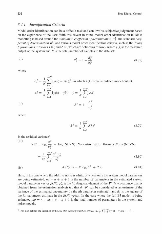
232 True Digital Control
8.4.1 Identification Criteria
Model order identification can be a difficult task and can involve subjective judgement basedon the experience of the user. With this caveat in mind, model order identification in DBMmodelling is based around the simulation coefficient of determination R2T ; the standard coef-ficient of determination R2; and various model order identification criteria, such as the YoungInformation Criterion (YIC) andAIC,which are defined as follows, where y(k) is themeasuredoutput of the system and N is the total number of samples in the data set:
(i) R2T = 1− σ 2s
σ 2y(8.78)
where
σ 2s = 1
N
k=N∑k=1
[y(k)− x(k)]2, in which x(k) is the simulated model output
σ 2y = 1
N
t=N∑t=1[y(k)− y]2; y = 1
N
k=N∑k=1
y(k)
(ii) R2 = 1− σ 2
σ 2y
where
σ 2 = 1
N
k=N∑k=1
e(k)2 (8.79)
is the residual variance8
(iii)YIC = loge
σ 2
σ 2y+ loge{NEVN}; Normalised Error Variance Norm (NEVN)
= 1
np
i=np∑i=1
σ 2.p∗i i
a2i(8.80)
(iv) AIC(np) = N loge σ 2 + 2.np (8.81)
Here, in the case where the additive noise is white, or where only the systemmodel parametersare being estimated, np = n + m + 1 is the number of parameters in the estimated systemmodel parameter vector ρ(N ); p∗
i i is the ith diagonal element of the P∗(N ) covariance matrixobtained from the estimation analysis (so that σ 2. p∗
i i can be considered as an estimate of thevariance of the estimated uncertainty on the ith parameter estimate); and a2i is the square ofthe ith parameter estimate in the ρ(N ) vector. In the case where the full BJ model is beingestimated, np = n + m + p + q + 1 is the total number of parameters in the system andnoise models.
8 This also defines the variance of the one step ahead prediction errors, i.e. 1N∑k=N
k=1 [y(k)− y(k|k − 1)]2.

Data-Based Identification and Estimation of Transfer Function Models 233
We see that R2T is a statistical measure of how well the simulated model explains the data:if the variance of the simulated (deterministic) model residuals σ 2s is low compared with thevariance of the data σ 2y , then R2T tends towards unity; while if σ 2 is of similar magnitude toσ 2y then it tends towards zero (and can become negative). Note, however, that R2T is based onthe variance of the model errors y(k)− x(k), where
x(k) = B(z−1)A(z−1)
u(k − δ) (8.82)
which is identical to the auxiliary model used in RIV/RIVBJ estimation. This needs to bedifferentiated from the more conventional coefficient of determination R2, which is based onthe variance of the noise model residual variance, which is identical to the one step aheadprediction errors. This is because R2T is a more discerning measure than R2 for TF modelidentification: R2 can often be quite close to unity even if the model is relatively poor (i.e. itis easy to predict reasonably well only one sample ahead); while R2T shows how much of themeasured output is being explained by the deterministic output of the system model and willonly be close to unity if the noise level on the measured output is low.The YIC is more a more complex, heuristic criterion (Young 1989) based on the properties
of the IPM (Wellstead 1978; Young et al. 1980), which is defined below equation (8.46b), andthe statistical interpretation of its inverse P(N ) in (8.73). We see that the first term of YICis simply a relative measure of how well the model explains the data: the smaller the modelresiduals the more negative the term becomes. The second term, on the other hand, providesa measure of the conditioning of the IPM, which needs to be inverted when the IV normalequations are solved: if the model is over-parameterised, then it can be shown that the IPMwill tend to singularity and, because of its ill-conditioning, the elements of its inverse P(N )will increase in value, often by several orders of magnitude. When this happens, the secondterm in the YIC tends to dominate the criterion function, indicating over-parameterisation.An alternative justification of the YIC can be obtained from statistical considerations (e.g.Young 1989).Although heuristic, the YIC has proven very useful in practical identification terms over the
past 20 years, notably for the estimation of control models. Indeed, the authors have utilisedYIC for most of the practical PIP control applications cited in earlier chapters. However, itshould not be used as a sole arbiter of model order since, in some cases, it tends to favour loworder models that do not provide a sufficiently good explanation of the data compared withother models that have a low, albeit not the lowest, YIC value. For this reason, it should beused to select the best model only from those models that provide a satisfactory explanationof the data (see Example 8.8, Example 8.9 and Example 8.10).The AIC is a well known identification criterion for AR processes (Akaike 1974) and is
related to the Final Prediction Error (FPE). It is used to identify the order of AR or ARMAmodels for the noise process ξ (k), based on the model residuals e(k) and the number of modelparameters. Here, the first term is a measure of how well the model explains the data; whilethe second term is simply a penalty on the number of parameters. Thus, as in the YIC, theAIC seeks a compromise between the degree of model fit and the complexity of the model:the smaller the value of the AIC (that is the more negative it is since it is based on a logarithmicmeasure) the better identified is the model. As we shall see in later examples, it can also beused as an aid in identifying the whole BJ transfer function model.

234 True Digital Control
Following from the publication of Akaike’s seminal paper (Akaike 1974), the topic of modelorder identification criteria has received a lot of attention and several different modificationsto the AIC have been suggested. All of these are in the general form (Shibata 1985):
T + α.np (8.83)
where T is a test statistic and the second term is the penalty term on the number of parametersin the model, with α > 1. The test statistic T can take several forms, as discussed by Shibata,but the best known is the maximum log likelihood, where the dominant term is the one stepprediction error variance σ 2, as in the AIC defined above. The most controversial point is howto choose α: this is 2 in the case of the AIC, log(N) in the Bayesian Information Criterion(BIC) of Schwarz (1978) and c.loglog(N) for some c>2 in the criterion suggested by Hannanand Quinn (1979). We have found that the AIC and BIC both work well, although the AIC ismore prone to over-fitting.
8.4.2 Model Structure Identification Procedure
Using the above statistical measures, a generally useful approach to model structure identifi-cation is as follows:
1. Use the SRIV estimation algorithm to estimate a range of different models for min(n) ≤n ≤ max(n) andmin(m) ≤ m ≤ max(m), where the maximum and minimum values of nand m are selected by the user, and sort these by the value of R2T , so exposing those modelstructures that best explain the data in a simulation sense. This can be accomplished easilyusing the rivbjid identification routine in CAPTAIN with the ARMA noise model orders pand q set to zero.
2. Amongst the best models in step 1, select one that has a relatively low YIC value: normallythis will be a large negative value, since it is a logarithmic measure, but the choice is notcritical provided the associated R2T is relatively high compared with that of other models.But do not select a model that has a high R2T and a relatively large YIC, since the YICis then indicating over-parameterisation. Use this selected model to generate an estimateξ (k) of the additive noise ξ (k). Then estimate ARMA(p,q) models for this estimated noiseover a range of p and q, min(p) ≤ p ≤ max(p) and min(q) ≤ q ≤ max(q), again with themaximum and minimum values selected by the user, and sort these in terms of the AIC orBIC. In CAPTAIN, this can be accomplished straightforwardly using the ivarmaid routine.
3. Re-estimate the full model, with the ARMA noise model included, over a smaller rangeof n, m, p and q, based on the results obtained in step 1 and step 2, using the full RIVBJalgorithm and sorting on the basis of the AIC or BIC. Select the best model from the resultsobtained in this manner.
4. In some cases, particularly if the system is a ‘stiff’ system characterised by widely spacedeigenvalues, it may be that the model estimated in step 3 provides a poor estimate of thedeterministic system output compared with the simpler SRIV estimated output. In this case,it is better to use the SRIV estimate, together with the ARMA noise model estimated instep 2, to define the full stochastic model that is referred to as the SRIV-ARMA modelby Young (2011a, p. 213 and the example on pp. 383–388). In this case, the covariancematrix provided by the SRIV algorithm will not necessarily provide a good estimate of theparametric uncertainty.

Data-Based Identification and Estimation of Transfer Function Models 235
Typical examples of this model identification process are discussed in the following casestudies, including one well-known laboratory example (Example 8.8) and selected controlapplications from earlier chapters (Example 8.9 and Example 8.10).
Example 8.8 Hair-Dryer Experimental Data For the first example, let us consider a wellknown demonstration in the MATLAB R© System Identification Toolbox, where the data areshown in Figure 8.4. These data are derived from an experiment on a laboratory scale ‘hair-dryer’ system (see Ljung 1987, p. 440, who refers to this as a ‘nice’ example). A fan blowsheated air through a tube and the air temperature is measured by a thermocouple at the outlet.The input u(k) is the voltage over the heating device, which is just a mesh of resistor wires. Theoutput y(k) is the voltage from the thermocouple at the output. Finally, the sampling intervalis �t = 0.08 seconds. Model structure identification, based on the the first 500 samples ofthe data shown in Figure 8.4 and using the approach suggested above, yields the initial SRIVresults shown in Table 8.3 (obtained here using the CAPTAIN Toolbox rivbjid routine). Thissuggests that, based on YIC considerations, the best model structure is [2 2 3 0 0]. However,a number of other models of second and third order perform well and the BIC identifies a [23 2 0 0] model, which has the same R2T = 0.9881. In addition, the model structure with thehighest R2T = 0.9886 is [3 2 3 0 0]. So at the next stage in identification, we should considera tighter range of models that include these as well as noise models.
When AIC and BIC identification is applied to the error series from both the [2 2 3 0 0]and [2 3 2 0 0] models they identify either a first order AR(1) or a second order AR(2) noise
0 100 200 300 400 500 600 700 800 900 10003
4
5
6
7
Outp
ut
0 100 200 300 400 500 600 700 800 900 10003
4
5
6
7
Input
Time (samples)
Figure 8.4 Hair-dryer experimental data for Example 8.8

236 True Digital Control
Table 8.3 Initial SRIV structure identification for Example 8.8
Structure YIC (TF) R2T σ 2s NEVN
[2 2 3 0 0] −7.806 0.9881 0.008280 −7.894[2 2 2 0 0] −6.815 0.9867 0.009273 −8.994[3 3 3 0 0] −5.561 0.9883 0.008181 −7.093[2 3 3 0 0] −5.056 0.9882 0.008229 −6.452[3 3 2 0 0] −4.302 0.9708 0.02042 −6.881[3 2 3 0 0] −3.890 0.9886 0.007952 −4.957[2 3 2 0 0] −0.783 0.9881 0.008283 −8.002[3 2 2 0 0] 0.578 0.9884 0.008081 −6.290
model. So the final stage of model identification is applied to all models in the range [2 2 2 00] to [3 3 3 2 2] again using the rivbjid routine in CAPTAIN. The best five models identifiedin this manner by the BIC are shown in Table 8.4.From Table 8.4, the best identified model structure is [2 3 2 1 0], which defines a general
TF model of the form:
y(k) = b0 + b1z−1 + b2z−2
1+ a1z−1 + a2z−2 u(k − 2)+ 1
1+ c1z−1 e(k) (8.84)
The associated full RIVBJ estimated parameter estimates are given by:
a1 = −1.3145 (0.016); a2 = 0.4325 (0.015)b0 = 0.00173 (0.0020); b1 = 0.0655 (0.0029); b2 = 0.0406 (0.0034)c1 = −0.9230 (0.0229); σ 2 = 0.00142
(8.85)
As we see in Figure 8.5, this model explains the data very well, with a coefficient of determi-nation R2T = 0.9873 and the measured output (dots) is always within the 95% (twice the SD)confidence bounds. All the parameters of the system TF are well defined statistically, with SEsmuch lower than the estimated value.However, it is necessary to evaluate the model in other regards before it is finally accepted.
An important aspect of such evaluation is the investigation of the model errors and thefinal residuals. The model simulation errors, based on the difference between the measuredoutput and the simulated model output have a near zero mean value, as required but they
Table 8.4 Final RIVBJ structure identification for Example 8.8
Structure BIC R2T σ 2s NEVN R2
[2 3 2 1 0] −1955 0.9873 0.001421 −9.197 0.998[3 3 2 1 0] −1952 0.9879 0.001411 −5.656 0.998[2 3 3 1 0] −1951 0.9877 0.001416 −7.755 0.998[2 3 2 2 0] −1950 0.9873 0.001422 −9.214 0.998[2 3 2 1 1] −1949 0.9873 0.001423 −9.165 0.998

Data-Based Identification and Estimation of Transfer Function Models 237
2
1.5
1
0.5
0 50 100 150
Time (samples)
200 250 300
0
Mea
sure
d a
nd M
odel
Outp
ut
Res
ponse
−0.5
−1
−1.5
−2
95% conf idence BoundsModel OutputMeasured Output
Figure 8.5 Estimation: model output (8.84) compared with the measured dryer data
are quite highly coloured. However, the ACF of the final model residuals e(k) (one stepahead prediction errors), resulting from the inclusion of the AR(1) noise model, have nosignificant lag correlation, as shown by Figure 8.6a. Furthermore, as shown in Figure 8.6b,the residuals are not significantly cross-correlated with the input series u(k), confirming thatthe model is explaining the data very satisfactorily. The coefficient of determination basedon the final residuals is R2T = 0.9980 (i.e. 99.8% of the output data are explained by thefull stochastic general TF model). The unexplained 0.02% remaining is accounted for bythe final residuals, which have the properties of white noise and are, therefore, completelyunpredictable.Validation is important in data-based modelling: the model should not be accepted unless it
continues to explain measured data that were not used in its identification. Figure 8.7 showsthe validation results: here, the simulated deterministic output of the estimated model (8.84) iscompared with the measured output from samples 500 to 900. The results are very good, fullyconfirming the efficacy of themodel, with R2T = 0.9935, which is better than that obtained overthe estimation data; and the standard coefficient of determination based on the final residuals,which is also marginally better at R2 = 0.9983.The above results can be compared with those obtained by Ljung (1987) and those available
as a demonstration example in the MATLAB R© System Identification Toolbox. In both, anARX model with structure [2 2 3 0 0] is selected, although with the caveat that a numberof models provide a similar explanation of the data. This performs similarly to the RIVBJ

238 True Digital Control
0.1
0.05
Co
rrel
atio
n
0
−0.05
−0.1
0.1
0 4 8 12 16
PACF
(a)
ACF
20 24 28
0 4 8 12 16 20 24 28
0.05
Co
rrel
atio
n
0
−0.05
−0.1
2
3
1
0
−1
−2
−3
0.1
(b)
−24 −12 0
500 100 150
Input (dashed) Residual (full)
200 250 300
12 24
0.05
0
−0.05
−0.1
Figure 8.6 (a) Autocorrelation (ACF) and partial autocorrelation (PACF) functions; and (b) crosscorrelation function for the dryer model residuals in Example 8.8

Data-Based Identification and Estimation of Transfer Function Models 239
2
1.5
1
0.5
0
−0.5
−1
−1.5
−2500 550 600 650 700
Time (samples)
Mea
sure
d a
nd M
odel
Outp
ut
Res
ponse
95% Conf idence BoundsModel OutputMeasured Output
750 800 850 900
Figure 8.7 Validation: model output (8.84) compared with the validation data for Example 8.8
identified and estimated [2 3 2 1 0] model at the deterministic validation stage of the analysisbut, not surprisingly, the ACF/PACF tests show that its residuals are significantly coloured,with the PACF showing a large lag one value of 0.9028, implying a first order AR modelfor the residuals. Also, the cross correlation test shows that the residual is significantly cross-correlatedwith the input. This suggests that theARXmodelmightwell be acceptable for certainapplications, such as deterministic control system design, but that for gaining understandingabout the nature of the system, stochastic control system design or forecasting applications,the [2 3 2 1 0] model identified here would be a much better choice.Perhaps the most important limitation of ARX models is the statistical inconsistency and
noise-induced asymptotic bias on the parameter estimates, particularly when the noise isheavily coloured, as in this case. Here, the poles of the estimated ARX model are at 0.748and 0.527, indicating associated time constants of 0.107 and 0.152 s. On the other hand, theRIVBJ estimate of the same structure system but with AR(1) noise, i.e. a [2 2 3 1 0] model, hascomplex poles of 0.657± 0.028j. Since the complex part is so small, this is effectively two realpoles: in fact, the ddamp routine in MATLAB R© reports two real roots at 0.658; i.e. two equaltime constants of 0.122 s. This is confirmed by our preferred identified model (8.84), whichhas virtually the same estimated poles at 0.657 ± 0.023j. Further confirmation is obtainedby continuous-time model estimation (see section 8.6, Example 8.13) and constrained RIVBJ

240 True Digital Control
estimation with the roots of the denominator polynomial constrained to be real, although notnecessarily equal. The latter yields:
y(k) = 0.001712+ 0.06534z−1 + 0.04120z−2
(1− 0.6556z−1)2u(k − 2)+ 1
1− 0.9215z−1 e(k) (8.86)
where e(k) is a zeromean, serially uncorrelated, white noise input with variance σ 2 = 0.00142,the same as that estimated for the unconstrained model (8.84).Whether the differences in the models discussed above are important in practical terms will
depend upon the use of the model. However, given the limitations of the ARX estimationalgorithm, there is no doubt, in statistical terms, that we should have more confidence in theRIVBJ estimatedmodel. As a result, the constrainedmodel (8.86), which is more parsimoniousthan (8.84) with one less parameter, would seem to be the best model to use in initial PIPcontrol system design, although subsequent practical implementation over a wider range ofinput perturbations might suggest re-estimation and evaluation.
Example 8.9 Axial Fan Ventilation Rate Chapter 2 (Example 2.8) considers the ventilationrate in a 1.0 m2 by 2.0 m test chamber at Lancaster University (Taylor 2004). Illustrative open-loop experimental data based on a sampling rate �t = 2 s are shown in Figure 8.8, wherey(k) is the air velocity (m s−1) and u(k) is the control input (the applied voltage to the fan,which is scaled to lie in the range zero to 100%, i.e. full power). It is clear that the noise levels
0 20 40 60 80 100
0.6
0.8
1
1.2(a)
(b)
Outp
ut
(m s
−1)
0 20 40 60 80 10026
28
30
32
Sample
Input
(%)
Figure 8.8 Axial fan experimental data in Example 8.9. (a) Ventilation rate (points) andmodel response(thin trace). (b) Control input. Sampling rate 2 s

Data-Based Identification and Estimation of Transfer Function Models 241
are relatively low, especially when the small perturbation of the system for this particularexperiment is noted (i.e. the input changes over only 5% of its full range).In Example 2.8, the model was estimated using the CAPTAIN rivbj routine with the simpler
SRIV settings and the model structure was intentionally restricted to [1 1 1] in order to simplifythe control system design. Here, however, wewill utilise the full rivbj analysis, which identifiesa more complicated [1 3 1 4 0] model structure, based on the smallest BIC value:
y(k) = b1z−1 + b2z−2 + b3z−3
1+ a1z−1 u(k)+ 1
1+ c1z−1 + c2z−2 + c3z−3 + c4z−4 e(k);
e(k) = N (0, σ 2)
The estimated parameters and SEs are as follows:
a1 = −0.682(0.0063); b1 = −0.00177(0.0009); b2 = 0.0121(0.0015); b3 = 0.0230(0.0012)
c1 = −0.363(0.053); c2 = −0.137(0.055); c3 = −0.155(0.055); c4 = −0.116(0.053);σ 2 = 8.6× 10⁻⁵
These estimates and the associated step response, suggests a more complicated initial responsethat includes a small non-minimum phase effect. The model explains the data very well, ascan be seen from Figure 8.8, with a high R2T = 0.997. The auto and cross correlation functionsshow that the estimates e(k) of the white noise e(k) are serially uncorrelated and not correlatedwith the input signal u(k), as required. By contrast and not surprisingly given the need foran AR(4) noise process in the above model, the SRIV estimated residuals of the first order[1 1 1] model are both serially correlated and significant correlated with u(k), so the modelis clearly not optimal in statistical terms. Nevertheless, it was clearly good enough for PIPcontrol system design, showing how robust the PIP control system is to modelling errors. Theabove model is based on an illustrative operating level of ≈ 1 m s−1. Similar models havebeen used for other operating conditions and have provided an excellent basis for successfulPIP control system design (e.g. Taylor et al. 2004a,b).
Example 8.10 Laboratory Excavator Bucket Position The laboratory excavator bucketposition discussed in Chapter 2 (Example 2.1) and Chapter 5 (Example 5.2) is a little unusual,since the system essentially behaves as a first order integrator. In fact, preliminary data-basedanalysis using the methods discussed above, suggests that an adequate description of theexcavator bucket position is generally given by equation (8.1a) with n = δ = 1, m = 0 anda1 ≈ −1.0. This is because the joint angle y(k) changes at a relatively constant rate for a steadyinput voltage u(k). Furthermore, the normalised voltage has been calibrated so that there isno movement of the manipulator when the input is zero. The deterministic control model is,therefore:
y(k) = b1z−1
1− z−1 u(k) (8.87)
Assuming that the value of a1 is known a priori to be very close to −1.0, it is possible toestimate b1 in equation (8.87) using the recursive option of the rivbj routine in CAPTAIN.

242 True Digital Control
5 10 15 20
0
5
10(a)
(b)
Outp
ut
0
20
40
Time (samples)
Input
5 10 15 20
Figure 8.9 Open-loop experimental data collected from the laboratory excavator in Example 8.10. (a)Joint angle data (points) and model response (solid trace) in degrees. (b) Control input (scaled voltagesignal). Sampling rate 0.1 s
This allows the user to specify the a priori conditions on the estimated parameter vector andits associated covariance matrix. In this case, these were set to ρ(0) = [−0.99999 0] andP(0) = diag[0 106], so that a1(k) does not change at all from its initially specified −0.99999value because the associated variance p11(k) in P(k) is maintained at the its initially set zerovalue. However, the value of p22 = 1× 10⁶ allows the algorithm to generate the recursiveestimate b1(k), k = 1, 2, . . . , N . Of course, equation (8.87) is an approximation of the actualsystem, as always, but similar models have been identified and successfully used for the controlof this and other hydraulically actuated manipulators (Shaban et al. 2008). An illustrativeexperiment and model response are shown in Figure 8.9.For the illustrated data set, the estimated b1 parameter and its SE obtained using the SRIV
settings in rivbj is b1 = 0.01489 (0.00012) and R2T = 0.997, reflecting the good explanationof the data in Figure 8.9. However, further analysis suggests that the estimated value of b1can vary depending on the applied voltage used in the experiment. In fact, as discussed byTaylor et al. (2007b), b1 is best represented as a graphical function of this voltage, an exampleof a state-dependent parameter. Further discussion of the concept is deferred until Chapter 9.At this juncture, it is sufficient to point out that, for the purposes of the linear PIP controlexperiments considered in Example 5.2, an optimised value for b1 was used, based on severalopen-loop experiments at a range of different operating levels (i.e. voltages) and with PRBSinputs. The details of this latter analysis (and related state-dependent estimation) are somewhatperipheral to the present discussion and so are omitted (Shaban 2006).

Data-Based Identification and Estimation of Transfer Function Models 243
8.5 Multivariable Models
The most general multivariable TFmodel is the stochastic version of theMIMO representationgiven previously by equation (7.9) with an additive noise vector, i.e.
y(k) = G(z−1)u(k)+ ξ (k) (8.88)
where
y(k) = [y1(k) y2(k) · · · yp(k)]T
u(k) = [u1(k) u2(k) · · · ur (k)]T
ξ (k) = [ξ1(k) ξ2(k) · · · ξp(k)]T(8.89)
Methods for estimating such models are available (Jakeman and Young 1979). From anestimation point of view, however, it is simpler to consider the MISO models representingeach row of (8.88). In general, such a model can be written in the form (where time delayshave been explicitly introduced for generality):
yi (k) =j=r∑j=1
Bi j (z−1)Ai j (z−1)
u j (k − δ j )+ ξi (k) (8.90)
where ξi (k) is a coloured noise process and i = 1, . . . , p. In the case where the noise hasrational spectral density, this can be considered as an ARMA(p,q) process, i.e.
yi (k) =j=r∑j=1
Bi j (z−1)Ai j (z−1)
u j (k − δ j )+ D(z−1)C(z−1)
ei (k) (8.91)
where ei (k) is a zeromean, serially uncorrelated, white noise process. This is theMISO versionof the BJ model.
8.5.1 The Common Denominator Polynomial MISO Model
If the MIMO model (8.88) has been obtained from a state-space representation of the system,then all of the elemental TFs will have a common denominator polynomial (as is the case forthe examples in Chapter 7), i.e.
y(k) = 1
A(z−1)Gn(z
−1)u(k)+ ξ (k) (8.92)
where Gn(z−1) is the associated matrix of numerator polynomials. In this case, the MISOmodel (8.90) becomes:
yi (k) =j=r∑j=1
Bi j (z−1)A(z−1)
u j (k − δ j )+ ξi (k) (8.93)
with a similar change to (8.91). One potential identifiability problem with this commondenominator MISO model form is that, in general, it will involve some elemental TFs that

244 True Digital Control
have pole-zero cancellations. However, if this is not the case, it is the simplest model form toidentify and estimate. In fact, in this form, the RIVBJ estimation algorithm is the same as inthe SISO case: all that is required is to extend the relevant data vectors to include the additionalinput terms. For instance the ith vector becomes:
φTi (k) = [−yi (k − 1)− · · · − yi (k − n) ui1(k − δi ) · · · ui1(k − δi − mi )+ · · ·
+ uir (k − δi ) · · · uir (k − δi − mi )](8.94)
with similar changes to all other data vectors, including the IV vector. And, of course, in thisMISO environment, the IV auxiliary model will also be a common denominator MISO model.
Example 8.11 Multivariable System with a Common Denominator A simple exampleof the common denominator model identification and estimation is the following first ordermodel: [
y1(k)y2(k)
]= 1
1− 0.5z−1
[z−1 2z−1
z−1 z−1
] [u1(k)u2(k)
]+
[ξ1(k)ξ2(k)
](8.95)
or, in MISO form:
y1(k) = 1
1− 0.5z−1 u1(k − 1)+ 2
1− 0.5z−1 u2(k − 1)+ ξ1(k)
y2(k) = 1
1− 0.5z−1 u1(k − 1)+ 1
1− 0.5z−1 u2(k − 1)+ ξ2(k)
(8.96)
where u1(k) and u2(k) are independent PRBS sequences with a switching period of 10; whileξ1(k) and ξ2(k) are additive measurement noise inputs, in the form of zero mean, white noisesequences with variances 0.55 and 0.20, respectively. For both MISO models, the resultingNSR by SD is 0.35 (35% noise) and a sample of the output data is shown in Figure 8.10.MCS results for both MISO channels, based on 100 realisations, each with a sample size
of 2000 samples, are compared with the results from an illustrative single estimation run inTable 8.5 and Table 8.6. It is clear that the RIVBJ estimates are well defined and that estimatedSEs from the single runs are consistent with the MCS means and SDs. The single run resultsare good, with the simulation coefficient of determination, based on the error between thedeterministic model output and the noise-free output data, very close to unity. For comparison,Table 8.5 and Table 8.6 also show the equivalent results obtained using the PEM algorithm inthe MATLAB R© System Identification Toolbox. To obtain the PEM results, each MISO modelis best estimated in the following form9:
(1− a1z−1)y(k) = b1u1(k)+ b2u2(k)+ (1− a2z
−1)ξi (k) (8.97)
since the implementation of the PEM algorithm precludes direct estimation in the commondenominator form of equation (8.96). Since it is not then possible to constrain the estimate of
9 An alternative is the different denominator MISO model form but this also requires the estimate of one moreparameter.

Data-Based Identification and Estimation of Transfer Function Models 245
20 40 60 80 100 120 140 160 180 200−2
0
2
4
6
8y 1
Number of samples
20 40 60 80 100 120 140 160 180 200
−2
0
2
4
6
8
y 2
Number of samples
Noisy
Noise−free
Noisy
Noise−free
Figure 8.10 Representative section of the data used in Example 8.11
Table 8.5 RIV and PEM results for Example 8.11 MISO Channel 1: y1(k)
Parameter a11 b11 b12
True −0.5 1.0 2.0RIVBJ: mean −0.49917 1.0047 2.0024RIVBJ: SD 0.01096 0.027517 0.043935RIVBJ: single run −0.4978 1.0299 2.0117RIVBJ: SE 0.010358 0.026457 0.041748PEM: mean −0.50187 0.99844 1.9922PEM: SD 0.011316 0.028189 0.045492PEM: single run −0.49552 1.0435 2.0125PEM: SE 0.010049 0.02847 0.044774

246 True Digital Control
Table 8.6 RIV and PEM results for Example 8.11 MISO Channel 2: y2(k)
Parameter a21 b21 b22
True −0.5 1.0 1.0RIVBJ: mean −0.49708 1.0058 1.0079RIVBJ: SD 0.009498 0.020543 0.021111RIVBJ: single run −0.50318 0.99114 0.99291RIVBJ: SE 0.010349 0.022151 0.022032PEM: mean −0.4996 1.0001 1.0025PEM: SD 0.0090982 0.020326 0.020666PEM: single run −0.49383 1.0094 1.0211PEM: SE 0.010845 0.023259 0.023094
a2 in (8.97) to be the same as that of a1, this involves the estimation of four rather than threeparameters. The resulting estimates of a2 in (8.97) are not shown in Table 8.5 and Table 8.6but, in each case, they are close but not identical to the estimate of a1.
8.5.2 The MISO Model with Different Denominator Polynomials
The MISO model with different denominator polynomials can be estimated using the PEMalgorithm in the MATLAB R© System Identification Toolbox. However, it presents a moredifficult estimation problem in the case of the RIV algorithm type. The RIV algorithm in thiscase was first suggested by Young and Jakeman (1980) and Jakeman et al. (1980), whilst arecent description of its RIVBJ successor is given in section 7.6 of Chapter 7 in Young (2011a).The CAPTAIN routine (Taylor et al. 2012) for this algorithm is denoted by rivdd and this isused in Example 8.12.
Example 8.12 Multivariable System with Different Denominators A simple first orderexample of different denominator model identification and estimation is the following MISOmultivariable model:
y(k) = 1
1− 0.5z−1 u1(k − 1)+ 2
1− 0.9z−1 u2(k − 1)+ ξ (k) (8.98)
Here, as in the previous example, u1(k) and u2(k) are independent PRBS sequences with aswitching period of 10; while ξ (k) is an additive, coloured measurement noise input generatedas the output of the following ARMA(1,1) model:
ξ (k) = 0.1
1− 0.95z−1 e(k) (8.99)
where e(k) is a zero mean, white noise input sequence with variance 4.5. The resulting noiseis highly coloured, as can be seen in the section of the data shown in Figure 8.11, and the NSRby SD is 0.35.

Data-Based Identification and Estimation of Transfer Function Models 247
20 40 60 80 100 120 140 160 180 200−2
−1
0
1
2
3
4
5
6
7
8
y(k)
Number of samples
NoisyNoise−free
Figure 8.11 A representative section of the noisy output used in Example 8.12 compared with thenoise-free output, showing the heavily coloured nature of the noise
MCS results for the RIV and PEM algorithms, based on a 100 realisations, each with a sizeof 2000 samples, are compared with the results from a single estimation run in Table 8.7. Onceagain, as in the previous common denominator example, it is clear that the estimates are welldefined and that the estimated SEs from the single runs are consistent with the MCS meansand SDs. The comparative PEM results in Table 8.8 were obtained using the standard MISOmodel form with different denominators.Finally, Figure 8.12a compares the deterministic output of the RIV estimated model with
the noise-free output measurement and it is clear that they are hardly distinguishable, with acoefficient of determination R2T = 0.999. By contrast, the ARX estimated model has a poor
Table 8.7 RIVBJ results for different denominator MISO model in Example 8.12
Parameters a11 a12 b11 b12 c1 d1
True −0.5 −0.9 1.0 2.0 −0.95 0.1RIVBJ: mean −0.4929 −0.9000 0.9951 2.003 −0.9478 0.1020RIVBJ: SD 0.0433 0.0029 0.0658 0.0399 0.0073 0.0270RIVBJ −0.5059 −0.8996 1.0062 2.0244 −0.95 0.1163RIVBJ: SE 0.0390 0.0027 0.0587 0.0366 0.0076 0.0241

248 True Digital Control
Table 8.8 PEM results for different denominator MISO model in Example 8.12
PEM: mean −0.4952 −0.9000 0.9930 2.006 −0.94762 0.1022PEM: SD 0.0518 0.0034 0.0717 0.0443 0.0072 0.0268PEM −0.5152 −0.8987 0.9324 2.0582 −0.9518 0.1203PEM: SE 0.0434 0.0029 0.0603 0.0385 0.0075 0.0238
fit to the noise-free data and its parameter estimates (not shown) are heavily biased, as wouldbe expected.
8.6 Continuous-Time Models
At first sight, the reader might find it strange to see a section on continuous-time modelidentification and estimation included in a book on true digital control.However, it is sometimesmore convenient to model a system in continuous-time terms since the model can then beconverted to a discrete-time form with any selected sampling interval �t . This clearly addsflexibility to the design process since it is often not clear what sampling interval will be best forpractical control system implementation and the closed-loop performance needs to be assessed
20 40 60 80 100 120 140 160 180 200
0
2
4
6
8(a)
(b)
x(k)
20 40 60 80 100 120 140 160 180 200
0
2
4
6
8
x(k)
Number of samples
Model
Noise−free
Model
Noise−free
Figure 8.12 Comparison of (a) RIV (solid trace) and (b) ARX (solid trace) estimated model outputswith the noise-free output (dashed trace) for Example 8.12

Data-Based Identification and Estimation of Transfer Function Models 249
in this regard. Moreover, continuous-time models have other advantages (see also Garnier andYoung 2012):
1. There is only one continuous-time model, regardless of the sampling interval, whereas theparameters of the discrete-time model are a function of �t .
2. Most models of physical systems are obtained by the application of physical laws (e.g.conservation of mass, energy, etc.) that are normally formulated in continuous-time terms.Because of this, the parameters of the continuous-timemodel normally have a clear physicalsignificance which is independent of the sampling interval and which is useful whencommunicating with practitioners who are normally familiar with such parameters andtheir meaning.
3. If the data are sampled rapidly in relation to the dominant time constants of the system, thediscrete-time model estimation can be very poor because the eigenvalues of the discrete-time model will be close to the unit circle in the complex z-plane. As a result, the parameterestimates can be poorly defined10, particularly if the system is ‘stiff’, with widely spacedeigenvalues (see Example 8.6 and Example 8.7). By contrast, the continuous-time modelestimates are advantaged by rapid sampling.
4. Continuous-time models can be estimated from non-uniformly sampled data and caninclude ‘fractional’ time delays where the time delay is not an integral number of samplingintervals (e.g. Young 2006; Ahmed et al. 2008).
8.6.1 The SRIV and RIVBJ Algorithms for Continuous-Time Models
The RIV approach to model identification and estimation is, as far as the authors are aware, theonly discrete-timeTF estimation algorithm that can be applied straightforwardly to continuous-time models, with only fairly minor modifications to the definition of the vectors and theiterative prefiltering procedures. The Simplified Refined Instrumental Variable method forhybrid Continuous-time models (SRIVC) was first suggested and evaluated by Young andJakeman (1980), under the simplifying theoretical assumption of additive white noise. Morespecifically, in the SISO case, it is concerned with the estimation of the following multi-ordercontinuous-time differential equation model:
dn x(t)
dtn+ α1
dn−1x(t)dtn−1 + · · · + αn x(t) = β0
dmu(t − τ )
dtm+ · · · + βmu(t − τ ) (8.100)
or, using simpler nomenclature where the bracketed superscript denotes the differentiationorder:
x (n)(t)+ α1x(n−1)(t)+ · · · + αn x (0)(t) = β0u
(m)(t − τ )+ · · · + βmu(0)(t − τ ) (8.101)
Here, the pure time delay τ , in time units, is often assumed to be an integer number relatedto the sampling time, as in the discrete-time case: that is τ = δ�t , but this is not essential. In
10 The data could be sub-sampled by decimation but this clearly involves a loss of information on any higher frequencydynamic modes.

250 True Digital Control
this continuous-time environment, ‘fractional’ time delays can be introduced if required (seeearlier cited references). In TF terms, equation (8.100) or equation (8.101) take the form:
x(t) = B(s)
A(s)u(t − τ ) (8.102)
where
B(s) = β0sm + β1s
m−1 + · · · + βm ; A(s) = sn + α1sn−1 + · · · + αn (8.103)
and s is the differential operator, i.e. s px(t) = d px(t)/dt p. It is now assumed that the inputsignal u(t), t1 < t < tN , is applied to the system and that this input and the output x(t) aresampled at discrete times tk , not necessarily uniformly spaced.In the case of uniformly sampled data at a sampling interval�t , the measured output y(tk),
where tk = k�t , is assumed to be corrupted by an additive measurement noise:
y(tk) = x(tk)+ e(tk) e(tk) = N (0, σ 2) (8.104)
where the argument tk indicates that the associated variable is sampled11 at time t1 to tN and,as shown, e(tk) is a zero mean, normally distributed, white noise sequence with variance σ 2.Combining the continuous-time model equation with the discrete-time observation equation,the complete theoretical model takes the following hybrid form:
x(t) = B(s)
A(s)u(t − τ ) (i)
y(tk) = x(tk)+ e(tk) (ii)(8.105)
As in the case of the SRIV algorithm, the statistical model (8.105) is assumed for theoreticalpurposes and, if its assumptions are correct in any practical situation, then the SRIVC algo-rithm yields statistically optimal estimates of the model parameters that are both consistentand asymptotically efficient. However, even if the assumptions about the noise e(tk) are notsatisfied, the estimates remain consistent because of the IV implementation. Moreover, practi-cal experience with the SRIVC algorithm shows that the estimates are relatively efficient, thatis they normally have relatively low variance.The more complex RIVCBJ algorithm (Young 2008; Young et al. 2008) is based on the
following hybrid theoretical model:
x(t) = B(s)
A(s)u(t − τ ) (i)
ξ (tk) = D(z−1)C(z−1)
e(tk) e(tk) = N (0, σ 2) (ii)
y(tk) = x(tk)+ ξ (tk) (iii)
(8.106)
11 Note that in the uniform sampling situation, y(tk ) means the same as y(k) and this changed nomenclature for samplevariables is utilised simply to emphasise the continuous-time nature of the estimation problem.

Data-Based Identification and Estimation of Transfer Function Models 251
where the white additive noise has been replaced by a discrete-time ARMA noise process ofthe same kind as that assumed previously.In fact, the RIVCBJ algorithm is very similar to the RIVBJ algorithm: the steps in the
algorithm are exactly the same and the only differences are the use of the continuous-timeTF model of the system to generate the source of the instrumental variables, and the intro-duction of hybrid prefilters in the iterative prefiltering procedure. The initial prefiltering by1/ A(s) is carried out in continuous-time (e.g. exploiting the numerical integration facilities inMATLAB R©), while the inverse noise model prefiltering is carried out in discrete-time, basedon the sampled output from the continuous-time prefilters.The continuous-time prefilters now have an additional advantage and role: the inputs to
the integrators that appear in the implementaion of the prefilter 1/ A(s) are clearly the timederivatives of their outputs and are precisely the variables that are required to define the nthderivative of the measured, prefiltered output y(n)f and the vector φT in the estimation modelwhich, in this case, takes the form:
y(n)f (tk) = φT (tk)ρc + e(tk) (8.107)
where
φT (tk) = [ − y(n−1)f (tk) · · · − y(0)f (tk) u(m)f (tk − τ ) · · · u(0)f (tk − τ )
]ρc = [α1 . . . αn β0 . . . βm]T
(8.108)
Further details of the SRIVC and RIVCBJ algorithms are given in Young (2008, 2011a) andYoung et al. (2008). They are implemented in the rivcbj and rivcbjid routines in CAPTAIN;while similar routines are available in the CONTSID Toolbox12. A continuous-time algorithmfor estimating MISO models with different denominator polynomials, using a similar back-fitting procedure to that used for discrete-time systems (section 8.5) was developed by Garnieret al. (2007). Other related publications that provide additional information on continuous-time model estimation and its applications are the edited books by Garnier and Wang (2008)and Wang and Garnier (2011), which contain numerous contributions; Young and Garnier(2006) show how these algorithms can be used to model linear and state-dependent parameternonlinear systems in environmental applications; and Laurain et al. (2010) also consider howthey can be used for modelling related linear parameter varying nonlinear systems.
Example 8.13 Continuous-Time Estimation of Hair-Dryer Experimental Data Let usconsider again the hair-dryer data from Example 8.8 and see how the RIVC algorithm can beuseful in producing multiple discrete-time models at different sampling intervals from a singlecontinuous-time model. In this example, the RIVC estimated [2 3 2 1 0] model is as follows(data sampling interval �t = 0.08 s):
x(t) = 0.00164s2 + 0.139s + 25.18s2 + 10.47s+ 27.82 u(t − 0.16)
y(tk) = x(tk)+ 1
1− 0.927z−1 e(tk) σ 2 = 0.00147
(8.109)
12 See http://www.iris.cran.uhp-nancy.fr/contsid/.

252 True Digital Control
0 0.5 1 1.5 20
0.2
0.4
0.6
0.8
1
Δt = 0.05
Time (s)
0 0.5 1 1.5 20
0.2
0.4
0.6
0.8
1Δt = 0.02
Time (s)
0 0.5 1 1.5 20
0.2
0.4
0.6
0.8
1
Δt = 0.2
Time (s)
0 0.5 1 1.5 20
0.2
0.4
0.6
0.8
1
Δt = 0.08
Time (s)
CT responseDT response
CT responseDT response
CT responseDT response
CT responseDT response
Figure 8.13 Comparison of the four inferred Discrete-Time (DT) step responses (dots) with theContinuous-Time (CT) step response (solid trace) in Example 8.13
Now, using the continuous-to-discrete time c2d routine in MATLAB R©, we are able to generatediscrete-time TF models at any specified sampling interval �t . For example, the results for�t = 0.02, 0.05, 0.08 and 0.2 s are13:
F0.02(z−1) = 0.001642+ 0.003928z−1 + 0.00351z−2
1− 1.801z−1 + 0.8111z−2
F0.05(z−1) = 0.001642+ 0.0286z−1 + 0.01849z−2
1− 1.539z−1 + 0.5925z−2
F0.08(z−1) = 0.001642+ 0.06539z−1 + 0.04053z−2
1− 1.314z−1 + 0.4329z−2
F0.2(z−1) = 0.001642+ 0.2653z−1 + 0.1196z−2
1− 0.6962z−1 + 0.1233z−2
(8.110)
The step responses of each TF are compared with the step response of the continuous-timemodel (8.109) in Figure 8.13: it is clear that, at each sampling instant, the response of eachdiscrete-time model corresponds exactly with the continuous-time response, as expected. Inthis case, the most appropriate sampling interval for discrete-time control design is probablythat of the data used to estimate the continuous-time model (�t = 0.08 s), where it will benoted that the model parameters obtained here are very similar to those obtained by directdiscrete-time model estimation in Example 8.8. This is not surprising because the data were
13 Note that, for simplicity, the pure time delay in the continuous-time model (8.109) was omitted in this analysis.

Data-Based Identification and Estimation of Transfer Function Models 253
obtained through a planned laboratory experiment on the dryer, but this may not always be thecase in practical situations.A typical scenario for utilising a continuous-time model within digital control system
design would be when data are sampled very rapidly, as is often the case with modern dataacquisition systems. These data can be used to identify and estimate a continuous-time modeland the derived discrete-time models, at different sampling intervals, then provide the basis forcontrol system design exercises, normally via simulation modelling. Here, the discrete-timemodel to be used for final control system design and implementation is selected on the basisof the best overall closed-loop performance, as evaluated in terms of factors such as inputsignal and response characteristics, robustness to uncertainty on the model parameters andmulti-objective performance.
8.6.2 Estimation of δ-Operator Models
An alternative to continuous-time TF model estimation is to consider a δ-operator model(Middleton and Goodwin 1990). As discussed in Chapter 9, the δ-operator is the discrete-time, sampled data equivalent of the differential operator s. The RIVBJ approach to theestimation of such δ-operator TF models follows directly from the RIVCBJ method outlinedabove and was suggested by Young et al. (1991). However, the model can be obtained from theRIVCBJ estimated continuous-time model using a continuous-time to delta conversion, suchas the c2del routine developed by I. Kaspura in Goodwin and Middleton’s original δ-operatorToolbox for MATLAB R©. Chapter 9 considers PIP control system design based on such δ-operator models. The advantage of the δ-operator approach is that it retains the completelydigital approach to model estimation and control system design, while being superior to thestandard discrete-time approach when the data are sampled rapidly, as discussed at length byMiddleton and Goodwin (1990). Its disadvantage is that the parameters are not quite the sameas those of the continuous-time model, except when the sampling rate is very fast, so that theirphysical interpretation is not as clear as in the completely continuous-time model case.
8.7 Identification and Estimation in the Closed-Loop
The identification and estimation of TF models in a closed-loop situation has received a lotof attention in the control systems literature (see e.g. Soderstrom and Stoica 1989; Verhaegen1993; Van den Hof 1998; Ljung 1999; Gilson and Van den Hof 2005). Provided there isan external command input signal, simple, sub-optimal transfer function estimation withina closed automatic control loop has always been straightforward when using IV estimationmethodology (see e.g. Young 1970). However, themore recent RIVBJ andRIVCBJ algorithms,as discussed in previous sections of this chapter, provide a stimulus to the development ofstatistically optimal methods for closed-loop estimation and a number of possible solutionsare discussed by Gilson et al. (2008, 2009) within a continuous-time setting.These latest optimal RIVBJ procedures are fairly complicated and so, in the spirit of the
present practically orientated book, we will consider here a new and particularly simple gen-eralised RIV method for estimating discrete- and continuous-time TF models enclosed withina feedback control system. This ‘three-stage’ method (Young 2011a) derives from a simpletwo-stage algorithm (Young 2008; Young et al. 2009) that yields consistent, but statisticallyinefficient, parameter estimates. The additional third stage allows for statistically efficient

254 True Digital Control
yd(tk) x(tk)ε (tk) y(tk)+ +P(z−1)
Q(z−1)
D(z−1)
C(z−1)
B( )
e(tk)
ρ
A( )ρ
νu(tk)ν
u(tk) = u(tk) +ν u(tk)η x(tk) = x(tk) +ν x(tk)η
(tk)ξ
Figure 8.14 Typical closed-loop system: GBJ model (8.111)
estimation of the enclosed TF model parameters when the system within the closed-loop isstable. The attraction of this new approach is its relative simplicity: in particular, the resultingclosed-loop RIVBJ and closed-loop RIVCBJ algorithms, for discrete-time and continuous-timemodels, are straightforward to implement since they use the existing estimation algorithmsdescribed in previous sections of this chapter, as implemented by the rivbj and rivcbj routinesin the CAPTAIN Toolbox. As a result, the coding of the new closed-loop routines in CAPTAINis straightforward, requiring only three calls to these existing algorithms.
8.7.1 The Generalised Box−Jenkins Model in a Closed-Loop Context
Consider the feedback control system shown in Figure 8.14.The Generalised Box−Jenkins (GBJ) model then takes the following form:
vx (tk) = G(ρ)vu(tk)y(tk) = vx (tk)+ ξ (tk)ξ (tk) = H (z−1)e(tk) e(tk) = N (0, σ 2)
(8.111)
The system and ARMA noise TFs, G(ρ) and H (z−1), are defined as the following ratios ofrational polynomials in a generalised ρ operator14 and z−1, respectively:
G(ρ) = B(ρ)
A(ρ); H (z−1) = D(z−1)
C(z−1)(8.112)
More specifically,
A(ρ) = 1+ a1ρ + a2ρ2 + · · · + anρn
B(ρ) = b0 + b1ρ + b2ρ2 + · · · + bmρm
C(z−1) = 1+ c1z−1 + c2z−2 + · · · + cpz−p
D(z−1) = 1+ d1z−1 + d2z−2 + · · · + dq z−q
(8.113)
The generalised operator ρ represents the backward shift operator z−1 in the discrete-time caseand the inverse of the differential operator s−1, where s = d/dt , in the hybrid continuous-time case. Referring to Figure 8.14, yd (tk) is the command input to the closed-loop system;
14 Do not confuse the lower case ρ used here with the boldface ρ used to denote the system model parameter vector:ρ is used here because it is employed as a generalised operator by Middleton and Goodwin (1990).

Data-Based Identification and Estimation of Transfer Function Models 255
ε(tk) = yd (tk)− y(tk) is the control system error; and the forward path controller is denotedby P(z−1)/Q(z−1). The control input to the system, vu(tk), is generated by the controller andis affected by additive circulatory noise ζu(tk), with u(tk) denoting the underlying ‘noise-free’control input to the system that would be measured at this point if ξ (tk) = ζu(tk) = 0 ∀ tk . Theoutput from the system vx (tk) is also affected by additive circulatory noise ζx (tk), with thenoise-free output x(tk) defined in a similar manner to the noise-free input. Finally, the noisymeasured output y(tk) is the sum of vx (tk) and the additive ARMA noise ξ (tk), while e(tk)is the zero mean, normally distributed white noise source to the ARMA noise model. All ofthese signals are sampled at a uniform sampling interval �t .Note that the ARMA noise model is always considered in discrete-time terms and that ρ
could also represent the δ-operator mentioned in the previous section. It must also be stressedthat Figure 8.14 is purely illustrative: the closed-loop identification and estimation proceduresoutlined below can be applied to any standard control structure.The primary aim of this section is to show how the various RIV algorithms described in
previous sections of this chapter can be exploited for closed-loop TF model identification andestimation. In order to simplify the presentation, however, the acronyms GRIVBJ and GSRIVare used in unified situations where both discrete- and continuous-time estimation is beingconsidered, so that all of the SRIV/RIVBJ and SRIVC/RIVCBJ acronyms introduced earlierapply in the context of the model (8.111).Section 8.7.2 outlines two very simple methods of closed-loop model estimation that exploit
the GSRIV algorithms and yield consistent, asymptotically unbiased estimates of the param-eters in both discrete or hybrid continuous-time TF models of the enclosed system. Thesesimple, two-stage algorithms can be applied reasonably successfully if the noise ξ (tk) doesnot comply with the theoretical assumptions; and even if the enclosed system is inherentlyunstable, although convergence cannot be guaranteed in this unstable situation. Section 8.7.3then goes on to describe how one of these simple algorithms can be enhanced by the additionof a third stage to induce asymptotic efficiency and ensure that the estimates have desirableminimum variance characteristics in the case where ξ (tk) can be described by an ARMAmodel, but only when the enclosed system is stable.Note that an important aspect of all these methods, not referred to specifically in the
following descriptions of the estimation procedures, is the identification of appropriate ordersfor the TF model polynomials in the model (8.111). However, these would be identifiednormally using standard GRIVBJ structure identification statistics available from the rivbjidand rivcbjid routines in the CAPTAIN Toolbox (section 8.4).
8.7.2 Two-Stage Closed-Loop Estimation
Provided the command input yd (tk) is free of noise and persistently exciting (see e.g. Young2011a) it can be used as a source on instrumental variables. Note that neither ε(tk) = yd (tk)−y(tk) nor vu(tk) could be used as the source of the IVs because both are contaminated bythe circulatory noise within the closed-loop system. Now, because both vu(tk) and y(tk) areavailable for measurement, in addition to yd (tk), two rather obvious approaches to closed-loopestimation are possible:
1. Method 1. Estimate the parameters of the TFmodel between between yd (tk) and the controlinput vu(tk) using the appropriate GSRIV algorithm. Note that vu(tk) is a function of y(tk)and so is affected by the component of the noise circulating around the closed-loop at

256 True Digital Control
this location, denoted by ηu(tk), i.e. vu(tk) = u(tk)+ ηu(tk), where u(tk) is the underlyingnoise-free control input to the system (see Figure 8.14 and the associated definition of thevariables). As a result, the deterministic output of this estimated TF model provides a goodbut sub-optimal estimate u(tk) of the noise-free input u(tk) to the enclosed system. Hence,either the GSRIV or the GRIVBJ algorithm can be used again to estimate the required TFbetween u(tk) and the noisy y(tk). This is the two-stage approach first suggested by Young(2008): see also Young et al. (2009)15.
2. Method 2. Estimate the parameters of the TF model for the whole closed-loop systembetween yd (tk) and the measured, noisy output y(tk). The deterministic output of thismodel then provides a good estimate x(tk) of the noise-free output from the system andthe appropriate GSRIV algorithm can be used again, this time in order to estimate theTF between the two estimated variables u(tk) obtained from Method 1, and x(tk). Thisapproach is less satisfying than the first method in statistical terms because the finalestimation involves two estimated noise-free variables, without direct reference to themeasured output y(tk).
8.7.3 Three-Stage Closed-Loop Estimation
The three stages of the estimation algorithm are as follows, where it will be noted that the firsttwo stages are very similar to the two-stage Method 1, outlined in Section 8.7.2, except thatfull GRIVBJ, rather than GSRIV algorithms are utilised throughout:
1. Stage 1. Estimate the TF between the command input yd (tk) and the noisy control inputvu(tk) using the appropriate GRIVBJ algorithm, and generate an estimate u(tk) of theunderlying noise-free control input u(tk) using this model.
2. Stage 2. Use the appropriate GRIVBJ algorithm to obtain initial, two stage estimates A(ρ)and B(ρ) of the system TF model polynomials A(ρ) and B(ρ), respectively, based on theestimated noise-free control input signal u(tk) obtained in Stage 1 and the noisy measuredoutput signal y(tk). Note that (Figure 8.14), y(tk) = vx (tk)+ ξ (tk) = x(tk)+ ηx (tk)+ ξ (tk)where x(tk) is the underlying ‘noise-free’ output of the system that would be measuredat this point if ξ (tk) = ηu(tk) = 0 ∀ tk . Note also that, because of this, y(tk)− ηx (tk) =x(tk)+ ξ (tk), which is referred to below.
3. Stage 3. Compute the estimate ηu(tk) = u(tk)− u(tk) of the circulatory noise componentof the control input signal, ηu(tk), and transfer this to the output of the system using thesystem model obtained in Stage 2, i.e.
ηx (tk) = B(ρ)
A(ρ)ηu(tk) (8.114)
where it provides an estimate of the component of the circulatory noise at the output of thesystem, ηx (tk), that derives from ζu(tk). Consequently, if this estimate is subtracted fromthe measured output it yields an estimate y(tk) = y(tk)− ηx (tk) of the output signal thatdoes not include the circulatory noise component from the closed-loop. It is, therefore,an estimate of the noise-free output x(tk) plus only the additive noise ξ (tk) [cf. equation
15 This is conceptually similar to the two-stage algorithm suggested by Van den Hof and Schrama (1993) but theyused output error estimation of an FIR model, rather than SRIV.

Data-Based Identification and Estimation of Transfer Function Models 257
(8.111)]. As a result, the data set {u(tk) ; y(tk)} provides an estimate of the data set thatwould have been obtained if the system was being estimated in the open-loop situation.Finally, therefore, use the appropriate open-loop GRIVBJ algorithm for a second time tore-estimate the system model based on this constructed data set.
In computational terms, this three-stage procedure is straightforward to implement becauseit makes use of estimation routines rivbj or rivcbj already available in CAPTAIN.
Example 8.14 Control of CO2 in Carbon-12 Tracer Experiments Let us think again aboutthe control of the carbon dioxide (12CO2) level in carbon tracer experiments, as previouslyconsidered in Chapter 5 and Chapter 6 (Example 5.9, Example 6.3 and Example 6.4). Themodel of the systemwas considered as an integrator in Chapter 5 but as a first order systemwitha long time constant in Chapter 6. The latter model proved sufficient to design a PIP controllerthat, when implemented, produced reasonable closed-loop behaviour. An interesting question,therefore, is given the measured closed-loop signals, does closed-loop analysis confirm theinitial assumptions about the system model?In completely objective identification and estimation terms, the answer to this question is
in the negative: the two-stage analysis suggests that the system is second order, with two realeigenvalues having associated time constants of 523 and 92.5 s. Two-stage estimation is usedhere because the noise is rather odd, as a result of the pulse-width modulated control input.Although it can be modelled as an AR(5) process, the three-stage parameter estimates areclearly not as good as those obtained by the more robust two-stage algorithm. In particular,the model takes the form (�t = 5 s):
y(k) = b0 + b1z−1
1+ a1z−1 + b2z−2 u(k − 4)+ ξ (k)
ξ (k) = 1
1+ c1z−1 + c2z−2 + c3z−3 + c4z−4 + c5z−5 e(k); e(k) = N (0, σ 2)(8.115)
where the estimated parameters are as follows, with the estimated SEs shown in parentheses:
a1 = −1.9379 (0.0048); a2 = 0.9384 (0.0048); b0 = 0.005953 (0.00014)b1 = −0.005771 (0.00013); c1 = −0.499 (0.035); c2 = −0.036 (0.039)c3 = −0.042 (0.039); c4 = −0.0068 (0.040); c5 = 0.120 (0.035); σ 2 = 9.97× 10⁻⁷
Given the high R2T = 0.996, it is not surprising that the estimated model outputs explainboth the measured output and the control input of the system very well, as shown in Figure8.15. Note that the above parameter estimates are cited to four significant figures because thetime contant values and any decomposition of the TF model (for instance to a parallel formobtained by partial fraction expansion using the MATLAB R© routine residuez) are sensitive tothese values.Fortunately, this uncertainty only affects the estimation of these derived parameters: the
uncertainty on the model parameters and the system as a whole is very small: see, for example,the three times SE uncertainty bounds on the frequency response for the second order modelshown in Figure 8.16. One word of caution is necessary, however, since these uncertainty

258 True Digital Control
0
0
100 200 300 400 5000.29
0.3
0.31
0.32
0.33
0.34
0.35
0.36
0.37
100 200 300
Model outputMeasured output
400 500 100 200 300 400 500−0.01
0.01
(a) (b)
0
Res
po
nse
Res
idu
als
0.29
0.3
0.31
0.32
0.33
0.34
0.35
0.36
0.37
−0.1
0.1
0
Co
ntr
ol
inp
ut
Err
or
Time (sampling intervals)
0
0
100 200 300 400 500
Time (sampling intervals)
Measured control intputModel control input
Figure 8.15 Comparison of model and measured responses for Example 8.14. (a) Output responsesand (b) control input responses. The residuals in (a) are the final stochastic residuals e(k)
bounds are based on the statistical assumptions about the nature of the AR noise process andthese are contravened to some extent in this case. For instance, the estimated final residualse(k) are small, zero mean, and serially uncorrelated but, as we can see from the error plot at thetop of Figure 8.15a, they do not have a normal distribution. Indeed, as pointed out above, onemight question the use of an AR model in this case, where the noise has special characteristicscaused by the pulse-width-modulation control method implemented in the plant physiologyresearch laboratory. But these are the kind of difficult ambiguities that can beset our real world,which does not always conform to the assumptions of theorists! For practical purposes in thiscase, the residual error is small and one can have reasonable confidence in the model, despiteits violation of the assumptions.As noted above, PIP control of this system represents one of the early practical examples
of the TDC approach (Taylor et al. 1996) but was based on a first order model. If the aboveanalysis is repeated and the model is constrained to be first order then the system model isestimated as follows:
y(k) = 0.00439
1− 0.986z−1 u(k − 4)+ ξ (k) (8.116)

Data-Based Identification and Estimation of Transfer Function Models 259
10−4 10−3 10−2 10−1 100 101
0.4
0.35
0.3
0.25
0.2
Mag
nit
ud
e
0.15
0.1
0.05
0
1st order model2nd order model3xstandard error bounds
Frequency (rad/sampling interval)
Figure 8.16 Magnitude frequency response of the estimated first and second order models with thethree times SE bounds for the latter shown as dotted lines
where the noise ξ (k) is now identified as an AR(11) process. However, the explanation of thedata is visibly poorer than that shown in Figure 8.15 and on these grounds the model wouldbe rejected. Despite this, when the frequency response characteristics of this model and thesecond order model are compared, as shown in Figure 8.16, they are quite similar, except atlow frequencies. A comparison with the model (6.20) used for PIP design in Chapter 6 showssimilar results, although the low frequency magnitude is smaller still. Consequently, the maindifferences between the various models are in their steady-state gains; differences that can beaccommodated for in the servomechanism PIP design procedure, where the control weightingsare always adjusted to provide the required closed-loop response characteristics. Of course,given these closed-loop estimation results, the robustness of the closed-loop response to thesekind of differences should be checked by MCS analysis of the kind considered in Chapter 4and Chapter 6.Finally, continuous-time estimation yields similar but not identical results. The estimated
model, in factorised form, is as follows:
y(t) = 52.5s+ 0.344(1+ 488s)(1+ 89.5s)u(t − 20) (8.117)
which reveals straightaway that the time constants are 488 and 89.5 s and the steady-state gainis 0.344. Earlier, in section 8.4, it was stressed that, in DBM modelling, the model shouldbe credible when interpreted in physically meaningful terms and this continuous-time TF

260 True Digital Control
provides an immediate interpretation of the system dynamics for consideration in such terms.In this regard, the Principle Investigator who managed the research that generated the dataused in this example was Dr Peter Minchin, then of the Department of Scientific and IndustrialResearch in New Zealand. Dr Minchin found the present results interesting and confirmedthat the system could be of the identified second order form. Paraphrasing his comments (P.C.Young, personal communication, 2012):
There was a water bubbler system containing approximately one litre of water in the closed-loop,in order to maintain a dew point of 4◦C in the circulated air and avoiding any increase in the dewpoint caused by the leaf. So when a correction pulse of CO2 was introduced, the bubbler wouldhave taken some time to come to a new CO2 equilibrium, which is probably the cause of the longtime constant. The short time constant is likely to be that associated with the gas loop. Also, the12CO2 used in the experiments must be conserved and the closed-loop into which this was injectedhad to have a route for the volume increase of gas to be released, and this would have resulted insome loss of CO2. This leak, controlled to maintain the pressure of the leaf chamber at just belowatmospheric, would result in loss of CO2 from the loop. Also the injected CO2 was not pure, buta CO2/air mix. Given these considerations the estimated gain of less than unity is not surprising.
8.7.4 Unstable Systems
One major reason why one would wish to identify and estimate a system within a closed-loop is when the system is open-loop unstable, so that open-loop estimation is difficult,if not impossible. However, the three-stage estimation procedure described in the previoussubsection includes explicit simulation of the estimated model in the form of the iterativelyupdated ‘auxiliary model’ and utilisation of the estimated system denominator polynomialA(ρ) in the iteratively updated prefilters. In the normal CAPTAIN Toolbox implementationof the GRIVBJ-type algorithms for open-loop systems, therefore, the auxiliary model andprefilter denominator polynomials are stabilised at each iteration in order to avoid any (rare)transient violations of stability during the iterative updating process (using the MATLAB R©
routines polystab for discrete-time models and polystc for continuous-time models). Despitethese precautions, the full three-stage algorithm fails to produce satisfactory estimation resultswhen applied to open-loop unstable systems, even when they are contained within a stableclosed-loop. Fortunately, however, the simple two-stage methods function satisfactorily inthis closed-loop environment: comprehensive MCS analysis (Young 2011a) suggests thatthey normally yield consistent, asymptotically unbiased parameter estimates with acceptableconfidence bounds, provided sufficient data are available from the closed-loop experimentswhen the data are noisy.
8.8 Concluding Remarks
This chapter has presented most of the background information to TF model identification andestimation that is required for TDC design. However, some other important concepts, such asidentifiability and the required nature of input signals that will ensure model identifiabilityhave not been discussed. A much more complete coverage of this topic is available in thesecond author’s recent book (Young 2011a), to which the reader is directed for these and otherdetails, particularly in the areas of recursive and closed-loop estimation. The present chapter

Data-Based Identification and Estimation of Transfer Function Models 261
has also concentrated on algorithmic details and the practical application of these algorithmsthat will be of most use to the practitioner, rather than the theoretical fundamentals of optimal‘PEM’-type methods, which are covered well in books such as by Ljung (1987, 1999). How-ever, note that this latter book does not consider the full RIVBJ methods specifically, eventhough their estimates have the same statistical properties as the PEM estimates obtained bygradient optimisation procedures, so it is useful mainly in a more general theoretical sense.
References
Ahmed, S., Huang, B. and Shah, S.L. (2008) Process parameter and delay estimation from non–uniformly sampleddata. In H. Garnier and L. Wang (Eds), Identification of Continuous-Time Models from Sampled Data, Springer-Verlag, London.
Akaike, H. (1974) A new look at statistical model identification, IEEE Transactions on Automatic Control, 19,pp. 716–723.
Åstrom, K.J. and Bohlin, T. (1966) Numerical identification of linear dynamic systems from normal operating records.In P.H. Hammond (Ed.), Theory of Self Adaptive Control Systems, Plenum Press, New York.
Åstrom, K.J. and Eykhoff, P. (1971) System identification – a survey, Automatica, 7, pp. 123–162.Bodewig, E. (1956)Matrix Calculus, North Holland, Amsterdam.Box, G.E.P. and Jenkins, G.M. (1970) Time Series Analysis Forecasting and Control, Holden-Day, San Francisco.Clarke, D.W. (1967) Generalised least squares estimation of the parameters of a dynamic model. Proceedings IFAC
Congress, Paper 3.17.Durbin, J. (1954) Errors in variables. Review of the International Statistical Institute, 22, pp. 23–32.Eykhoff, P. (1974) System Identification – Parameter and State Estimation, John Wiley & Sons, Ltd, Chichester.Garnier, H., Gilson, M., Young, P.C. and Huselstein, E. (2007) An optimal IV technique for identifying continuous-time transfer function model of multiple input systems, Control Engineering Practice, 15, pp. 471–486.
Garnier, H. andWang, L. (Eds) (2008) Identification of Continuous–Time Models from Sampled data, Springer-Verlag,London.
Garnier, H. and Young, P.C. (2012) What does continuous-time model identification have to offer? Proceedings 14thIFAC Symposium on System Identification SYSID12, pp. 810–815.
Gilson, M., Garnier, H., Young, P.C. and Van den Hof, P. (2008) Instrumental variable methods for closed-loopcontinuous-time model identification. In H. Garnier and L. Wang (Eds), Identification of Continuous-Time Modelsfrom Sampled Data, Springer-Verlag, London, pp. 133–160.
Gilson,M., Garnier, H., Young, P.C. andVan denHof, P. (2009) Refined instrumental variable methods for closed-loopsystem identification. Proceedings 15th IFAC Symposium on System Identification SYSID09, pp. 284–289.
Gilson, M. and Van den Hof, P. (2005) Instrumental variable methods for closed–loop system identification, Auto-matica, 41, pp. 241–249.
Goodwin, G.C. and Payne, R.P. (1977) Dynamic System Identification. Experiment Design and Data Analysis,Academic Press, New York.
Hannan, E.J. and Quinn, B.G. (1979) The determination of the order of an autoregression. Journal of Royal StatisticalSociety, Series B, 41, pp. 190–195.
Hastings-James, R. and Sage, M.W. (1969). Recursive generalised least squares procedure for on–line identificationof process parameters. Prococeedings of the Institute of Electrical Engineers, 116, pp. 2057–2062.
Ho, Y.C. (1962) On the stochastic approximation method and optimal filtering theory, Journal of MathematicalAnalysis and Applications, 6, p. 152.
Jakeman, A.J., Steele, L.P. and Young, P.C. (1980) Instrumental variable algorithms for multiple input systemsdescribed by multiple transfer functions. IEEE Transactions on Systems, Man, and Cybernetics, SMC-10, pp.593–602.
Jakeman, A.J. and Young, P.C. (1979) Refined instrumental variable methods of time-series analysis: Part II, multi-variable systems. International Journal of Control, 29, pp. 621–644.
Jazwinski, A.H. (1970) Stochastic Processes and Filtering Theory, Academic Press, San Diego.Johnston, J. (1963) Econometric Methods, McGraw-Hill, New York.Kendall, M.G. and Stuart, A. (1961) The Advanced Theory of Statistics, volume 2, Griffin, London.

262 True Digital Control
Landau, I.D. (1976) Unbiased recursive estimation using model reference adaptive techniques. IEEE Transactions onAutomatic Control, AC-21, pp. 194–202.
Laurain, V., Toth, R., Gilson, M. and Garnier, H. (2010) Refined instrumental variable methods for identification ofLPV Box–Jenkins models. Automatica, 46, pp. 959–967.
Lee, R.C.K. (1964) Optimal Identification, Estimation and Control, MIT Press, Cambridge, MA.Ljung, L. (1979) Asymptotic behaviour of the extended Kalman filter as a parameter estimator for linear systems,
IEEE Transactions on Automatic Control, AC-24, pp. 36–50.Ljung, L. (1987) System Identification. Theory for the User, Prentice Hall, Englewood Cliffs, NJ.Ljung, L. (1999) System Identification. Theory for the User, Second Edition, Prentice Hall, Upper Saddle River, NJ.Ljung, L. and Soderstrom, T. (1983) Theory and Practice of Recursive Identification, MIT Press, Cambridge, MA.Mayne, D.Q. (1963) Optimal nonstationary estimation of the parameters of a dynamic system, Journal of Electronics
and Control, 14, pp. 101–112.Middleton, R.H. and Goodwin, G.C. (1990) Digital Control and Estimation – A Unified Approach, Prentice Hall,Englewood Cliffs, NJ.
Norton, J.P. (1986) An Introduction to Identification, Academic Press, New York.Panuska, V. (1969) An adaptive recursive least squares identification algorithm. Proceedings 8th IEEE Symposium
on Adaptive Processes, Paper 6e.Pierce, D.A. (1972) Least squares estimation in dynamic disturbance time-series models. Biometrika, 5, pp. 73–78.Price, L., Young, P., Berckmans, D., Janssens, K. and Taylor, J. (1999) Data-Based Mechanistic Modelling (DBM)and control of mass and energy transfer in agricultural buildings, Annual Reviews in Control, 23, pp. 71–82.
Schwarz, G. (1978) Estimating the dimension of a model. Annals of Statistics, 6, pp. 461–464.Shaban, E.M. (2006) Nonlinear Control for Construction Robots using State Dependent Parameter Models, PhDthesis, Engineering Department, Lancaster University.
Shaban, E.M., Ako, S., Taylor, C.J. and Seward, D.W. (2008) Development of an automated verticality alignmentsystem for a vibro-lance, Automation in Construction, 17, pp. 645–655.
Shibata, R. (1985) Various model selection techniques in time series analysis. In E.J. Hannan, P.R. Krishnaiah and M.Rao (Eds), Handbook of Statistics 5: Time Series in the Time Domain, North-Holland, Amsterdam, pp. 179–187.
Soderstrom, T., Ljung, L. andGustavsson, I. (1974)A comparative study of recursive identificationmethods. TechnicalReport TR 7308, Lund Institute of Technology, Division of Automatic Control.
Soderstrom, T. and Stoica, P. (1989) System Identification, Series in Systems and Control Engineering, Prentice Hall,New York.
Talmon, J.L. and van den Boom, A.J.W. (1973) On the estimation of the transfer function parameters of processand noise dynamics using a single stage estimator. In P. Eykhoff (Ed.), Preprints of the 3rd IFAC Symposiumon Identification and System Parameter Estimation, 12–15 June, The Hague–Delft, North-Holland, Amsterdam,pp. 711–720.
Taylor, C.J. (2004) Environmental test chamber for the support of learning and teaching in intelligent control,International Journal of Electrical Engineering Education, 41, pp. 375–387.
Taylor, C.J., Lees, M.J., Young, P.C. and Minchin, P.E.H. (1996) True digital control of carbon dioxide in agriculturalcrop growth experiments, International Federation of Automatic Control 13th Triennial World Congress (IFAC-96), 30 June–5 July, San Francisco, Elsevier, Vol. B, pp. 405–410.
Taylor, C.J., Leigh, P.A., Chotai, A., Young, P.C., Vranken, E. and Berckmans, D. (2004a) Cost effective combinedaxial fan and throttling valve control of ventilation rate, IEE Proceedings: Control Theory and Applications, 151,pp. 577–584.
Taylor, C.J., Leigh, P., Price, L., Young, P.C., Berckmans, D. and Vranken, E. (2004b) Proportional-Integral-Plus(PIP) control of ventilation rate in agricultural buildings, Control Engineering Practice, 12, pp. 225–233.
Taylor, C.J., Pedregal, D.J., Young, P.C. and Tych, W. (2007a) Environmental time series analysis and forecastingwith the Captain toolbox, Environmental Modelling and Software, 22, pp. 797–814.
Taylor, C.J., Shaban, E.M., Stables, M.A. and Ako, S. (2007b) Proportional-Integral-Plus (PIP) control applications ofstate dependent parameter models, IMECHE Proceedings: Systems and Control Engineering, 221, pp. 1019–1032.
Taylor, C.J., Young, P.C. and Cross, P. (2012) Practical experience with unified discrete and continuous-time, multi-input identification for control system design, 16th IFAC Symposium on System Identification (SYSID-2012),Paper 123.
Van den Hof, P.M.J. (1998) Closed-loop issues in system identification, Annual Reviews in Control, 22, 173–186.Van den Hof, P.M.J. and Schrama, R.J.P. (1993) An indirect method for transfer function estimation from closed loopdata, Automatica, 29, pp. 1523–1527.

Data-Based Identification and Estimation of Transfer Function Models 263
Verhaegen, M. (1993) Application of a subspace model identification technique to identify LTI systems operating inclosed-loop, Automatica, 29, pp. 1027–1040.
Wang, L. and Garnier, H. (Eds) (2011) System Identification, Environmental Modelling, and Control System Design,Springer-Verlag, London.
Wellstead, P.E. (1978) An instrumental product moment test for model order estimation. Automatica, 14, pp. 89–91.Wellstead, P.E. and Zarrop, M.B. (1991) Self-Tuning Systems: Control and Signal Processing, John Wiley & Sons,Ltd, New York.
Wong, K.Y. and Polak, E. (1967) Identification of linear discrete-time systems using the instrumental variableapproach. IEEE Transactions on Automatic Control, AC-12, pp. 707–718.
Young, P.C. (1965) Process parameter estimation and self-adaptive control. In P.H. Hammond (Ed.), Theory of SelfAdaptive Control Systems, Plenum Press, New York, pp. 118–140.
Young, P.C. (1968) The use of linear regression and related procedures for the identification of dynamic processes.Proceedings 7th IEEE Symposium on Adaptive Processes, pp. 501–505.
Young, P.C. (1969) Applying parameter estimation to dynamic systems: Part I – theory. Control Engineering, 16, pp.119–125.
Young, P.C. (1970) An instrumental variable method for real–time identification of a noisy process, Automatica, 6,pp. 271–287.
Young, P.C. (1974) Recursive approaches to time-series analysis. Bulletin of the Institute of Mathematics and itsApplications, 10, pp. 209–224.
Young, P.C. (1976) Some observations on instrumental variable methods of time-series analysis. International Journalof Control, 23, pp. 593–612.
Young, P.C. (1981) Parameter estimation for continuous-time models – a survey. Automatica, 17, pp. 23–39.Young, P.C. (1984) Recursive Estimation and Time–Series Analysis: An Introduction, Springer-Verlag, Berlin.Young, P.C. (1989) Recursive estimation, forecasting and adaptive control. In C.T. Leondes (Ed.), Control and
Dynamic Systems, Academic Press, San Diego, pp. 119–166.Young, P.C. (1998) Data-based mechanistic modelling of environmental, ecological, economic and engineeringsystems, Environmental Modelling and Software, 13, pp. 105–122.
Young, P.C. (2006) An instrumental variable approach to ARMA model identification and estimation. Proceedings14th IFAC Symposium on System Identification SYSID06, pp. 410–415.
Young, P.C. (2008) The refined instrumental variable method: unified estimation of discrete and continuous-timetransfer function models. Journal Europeen des Systemes Automatises, 42, pp. 149–179.
Young, P.C. (2011a) Recursive Estimation and Time-Series Analysis: An Introduction for the Student and Practitioner,Springer-Verlag, Berlin.
Young, P.C. (2011b) Data-based mechanistic modelling: natural philosophy revisited? In L. Wang and H. Garnier(Eds), System Identification, Environmetric Modelling and Control, Springer-Verlag, Berlin, pp. 321–340.
Young, P.C., Chotai, A. and Tych, W. (1991) Identification, estimation and control of continuous-time systemsdescribed by delta operator models. In N. Sinha and G. Rao (Eds), Identification of Continuous-Time Systems,Kluwer, Dordrecht, pp. 363–418.
Young, P.C. and Garnier, H. (2006) Identification and estimation of continuous-time, data-based mechanistic modelsfor environmental systems. Environmental Modelling & Software, 21, pp. 1055–1072.
Young, P.C., Garnier, H. and Gilson, M. (2008) Refined instrumental variable identification of continuous-time hybridBox–Jenkins models. In H. Garnier and L. Wang (Eds), Identification of Continuous-Time Models from SampledData, Springer-Verlag, London, pp. 91–131.
Young, P.C., Garnier, H. and Gilson, M. (2009) Simple refined IV methods of closed-loop system identification.Proceedings 15th IFAC Symposium on System Identification SYSID09, pp. 1151–1156.
Young, P.C. and Jakeman, A.J. (1979) Refined instrumental variable methods of time-series analysis: Part I, SISOsystems. International Journal of Control, 29, pp. 1–30.
Young, P.C. and Jakeman, A.J. (1980) Refined instrumental variable methods of time-series analysis: Part III,extensions. International Journal of Control, 31, pp. 741–764.
Young, P.C., Jakeman, A.J. andMcMurtrie, R. (1980) An instrumental variable method for model order identification.Automatica, 16, pp. 281–296.
Young, P.C. and Lees, M.J. (1993) The active mixing volume: a new concept in modelling environmental systems. InV. Barnett and K. Turkman (Eds), Statistics for the Environment, John Wiley & Sons, Ltd, Chichester, pp. 3–43.

9Additional Topics
In this book, we are concerned mainly with True Digital Control (TDC) based on discrete-timeTransfer Function (TF) models of dynamic systems. In Chapter 8, however, we discussed theidentification and estimation of continuous-time TF models, pointing out that many systemswere more easily considered in continuous-time terms at the conceptual level and that acontinuous-time TF model could be converted into discrete-time for the purposes of TDCdesign. An alternative approach is to exploit the δ-operator TF model, which is the discrete-time equivalent of the continuous-time model. In recent times, the main impetus for the useof δ-operator TF models in control system design has come from the book by Middleton andGoodwin (1990), to which the reader is referred for background information. In section 9.1,we will simply introduce the δ-operator TF model; show how it can be presented in Non-Minimal State Space (NMSS) form; and develop the δ-operator Proportional-Integral-Plus(PIP) control algorithm.The recursive nature of all the Refined Instrumental Variable (RIV) algorithms discussed
in Chapter 8, also allows for the development of Time Variable Parameter (TVP) versionsthat can be used for real-time applications, such as self-tuning or adaptive control, i.e. inthose situations where the model parameters are changing relatively slowly over time. Here,the algorithm updates the parameter estimates as the input–output data are acquired and thelatest estimates are used to update the control system design on a continuing basis. However,if these changes in the parameters are much more rapidly changing as functions of the stateor input variables (i.e. they actually constitute stochastic state variables), then the systemis truly nonlinear and likely to exhibit severe nonlinear behaviour. Normally, this cannot beapproximated in a simple TVP manner; in which case, recourse must be made to alternativeState-Dependent Parameter (SDP) modelling methods. Section 9.2 and section 9.3 providea review of recursive TVP and SDP estimation but a much more comprehensive treatmentis available in Young (2011). The reader is also referred to recent research on the widerapplication of SDP modelling within a PIP design context (Taylor et al. 2007b, 2009, 2011).Finally in relation to SDP models, note that the terms Linear Parameter Varying (LPV) and
NonLinear Parameter Varying (NLPV) are often used in the systems and control literature todescribe SDP-type models. However LPV, in particular, is a quite misleading term since SDP
True Digital Control: Statistical Modelling and Non-Minimal State Space Design, First Edition.C. James Taylor, Peter C. Young and Arun Chotai.© 2013 John Wiley & Sons, Ltd. Published 2013 by John Wiley & Sons, Ltd.

266 True Digital Control
models are truly nonlinear dynamic systems and, as we shall see, can even exhibit chaoticdynamic behaviour.
9.1 The δ-Operator Model and PIP Control
The δ-operator was first utilised in a PIP design context by Young et al. (1991). Later papersformalised this approach for both Single-Input, Single-Output (SISO; Young et al. 1998)and multivariable (Chotai et al. 1998) systems (see also McKenna 1997). An outline ofthe modelling and PIP design approaches are discussed in these references, with the presentchapter concentrating on the following nth order, SISO system, whose input and output signalsare sampled regularly with a sampling interval of �t time units. The discrete differential orδ-operator TF model of this system takes the form:
y(k) = B(δ)
A(δ)u(k) (9.1)
where y(k) and u (k) denote, respectively, the sampled output and input signals at the kthsampling instant; while A (δ) and B (δ) are the following polynomials in the δ-operator:
A(δ) = δn + a1δn−1 + · · · + an; B(δ) = b1δ
n−1 + b2δn−2 + · · · + bn (9.2)
Here, the δ-operator is defined as follows in terms of the forward shift operator z:
δ = z − 1�t
i.e. δy(k) = y(k + 1)− y(k)
�t(9.3)
In general, no prior assumptions are made about the nature of the TF, which may be marginallystable, unstable, or possess non-minimum phase characteristics. The order of the numeratorpolynomial B (δ) is set to n–1 to ensure that the TF is proper. However, it can be of lessdimension than this if identification and estimation analysis shows that it is more appropriate.Any pure time delay in the system can be handled in various ways: e.g. by introducingadditional poles at−1/�t to accommodate the time delay; or, in the case of long time delays,by introducing the δ form of the Smith Predictor using a similar approach to that described insection 6.3 (see also e.g. Taylor et al. 1998).It is clear that the δ-operator is the discrete-time, sampled data equivalent of the differential
operator s = d/dt considered in Chapter 8. One attraction of the δ-operator model (9.1) is thatit can be applied to a wide range of discrete-time systems, from sampled data systems withcoarse sampling intervals to rapidly sampled, near continuous-time systems. For example, itis easy to see that the unit circle in the complex z-plane (see section 2.2) maps to a circlewith centre −1/�t and radius 1/�t in the complex δ-plane; so that, as �t → 0, this circularstability region is transformed to the left half of the complex s-plane. For very rapidly sampledsystems, therefore, the δ-operator model can be considered in almost continuous-time terms,with the pole positions in the δ-plane close to those of the equivalent continuous-time systemin the s-plane. As such, the δ-operator model provides a rather natural digital representationfor a rapidly sampled, continuous-time system; one which avoids the approximate digitisationof continuous-time designs and provides a direct basis for TDC system design. However, itshould be realised that, unless the sampling rate is very high, the parameters of the δ-operator

Additional Topics 267
plant
yd(k) u(k)v(k) y(k)+ +
− − − −
proportional control
integral
control
kI
δ1
δ
+ +n
fn
B( )δ
F1( )δ
G1( )δ
A( )δ
Figure 9.1 The δ-operator PIP servomechanism system (see section 9.1.3 for control polynomials)
model will not be the same as those of the continuous-time model, so that they do not have thesame physically meaningful interpretation as the parameters of the continuous-time model.
9.1.1 The δ-operator NMSS Representation
The most obvious NMSS representation of the TF model (9.1) is formulated directly in termsof the discrete-time δ derivatives of the output and input signals and takes the form [cf.equations (5.13)]:
δ x(k) = Fx(k)+ gv(k)+ d yd (k) (9.4)
where v(k) is an intermediate control variable: see below and Figure 9.1. The system transitionmatrix F , input vector g and command input vector d are defined as follows:
F =
⎡⎢⎢⎢⎢⎢⎢⎢⎢⎢⎢⎢⎢⎢⎢⎢⎢⎢⎢⎢⎢⎢⎢⎢⎣
−a1 −a2 · · · −an−1 −an b1 b2 · · · bn−1 bn 0
1 0 · · · 0 0 0 0 · · · 0 0 0
0 1 · · · 0 0 0 0 · · · 0 0 0...
.... . .
......
......
. . ....
......
0 0 · · · 1 0 0 0 · · · 0 0 0
0 0 · · · 0 0 0 0 · · · 0 0 0
0 0 · · · 0 0 1 0 · · · 0 0 0
0 0 · · · 0 0 0 1 · · · 0 0 0...
.... . .
......
......
. . ....
......
0 0 · · · 0 0 0 0 · · · 1 0 0
0 0 · · · 0 −1 0 0 · · · 0 0 0
⎤⎥⎥⎥⎥⎥⎥⎥⎥⎥⎥⎥⎥⎥⎥⎥⎥⎥⎥⎥⎥⎥⎥⎥⎦
(9.5)

268 True Digital Control
d = [0 0 · · · 0 0 0 0 · · · 0 0 1
]T(9.6)
g = [0 0 · · · 0 0 1 0 · · · 0 0 0
]T(9.7)
In this formulation, the control variable v(k) is defined as the nth δ differential of the actualcontrol input u(k), i.e.
ν(k) = δnu(k) (9.8)
and the non-minimal state vector x(k) is defined as:
x(k) = [δn−1y(k) δn−2y(k) · · · δy(k) y(k) δn−1u(k) · · · u(k) z(k)
]T(9.9)
In these equations, z(k) will be recognised from earlier chapters as an additional integral-of-error state of the form:
z(k) = δ −1 {yd (k)− y(k)} (9.10)
in which yd (k) is the reference or command input to the servomechanism system.
9.1.2 Characteristic Polynomial and Controllability
The open-loop characteristic polynomial of the NMSS representation (9.4) can be written as[cf. equation (5.17)]:
|λI − F| =λ
∣∣∣∣∣∣∣∣∣∣∣∣∣∣∣∣∣∣∣∣∣∣∣∣∣∣∣∣
λ + a1 a2 · · · an−1 an −b1 −b2 · · · −bn−1 −bn
−1 λ · · · 0 0 0 0 · · · 0 0
0 −1 · · · 0 0 0 0 · · · 0 0...
.... . .
......
......
. . ....
...
0 0 · · · −1 λ 0 0 · · · 0 0
0 0 · · · 0 0 λ 0 · · · 0 0
0 0 · · · 0 0 −1 λ · · · 0 0
0 0 · · · 0 0 0 −1 · · · 0 0...
.... . .
......
......
. . ....
...
0 0 · · · 0 0 0 0 · · · −1 λ
∣∣∣∣∣∣∣∣∣∣∣∣∣∣∣∣∣∣∣∣∣∣∣∣∣∣∣∣
(9.11)
As a result, the open-loop characteristic polynomial is given by:
|λI − F| = λn+1A(λ) (9.12)
which is a product of the characteristic polynomial of the minimal state space representation,i.e. A(λ), and a term λn+1 due to the introduction of the additional states.If the NMSS model (9.4) is to be used as the basis for the design of State Variable Feedback
(SVF) control systems, such as closed-loop pole assignment or Linear Quadratic (LQ) optimal

Additional Topics 269
control, it is important to evaluate the conditions for controllability of this model. These areprovided by Theorem 9.1.
Theorem 9.1 Controllability of the δ-operator NMSS Model Given a SISO discrete-timeδ-operator system described by (9.1), the NMSS representation (9.4), as described by the pair[F, g], is completely controllable if, and only if, the following conditions are satisfied:
(i) the polynomials A (δ) and B (δ) are coprime;(ii) bn �= 0.
The proof of this theorem is given by Young et al. (1998).The conditions in Theorem 9.1 have obvious physical interpretations. The coprimeness
condition is equivalent to the normal requirement that the δ-operator TF (9.1) should haveno pole-zero cancellations. The second condition avoids the presence of a zero at the ori-gin in the complex δ-plane, which would cancel with the pole associated with the inherentintegral action. The controllability conditions of the above theorem are, of course, equiv-alent to the normal requirement that the controllability matrix associated with the NMSSrepresentation, i.e.
S1 = [g Fg F2g · · · F2n g] (9.13)
has full rank 2n + 1.
9.1.3 The δ-Operator PIP Control Law
In the context of the NMSS model (9.4), the automatic control objective is to design a SVFcontrol law [cf. equation (5.32)]:
v(k) = −kT x(k)
= − f1 δn−1y(k)− f2 δn−2y(k) − · · · − fn y(k)
−g1 δn−1u(k)− · · · − gnu(k)+ kI z(k)
(9.14)
such that either the closed-loop poles are at pre-assigned positions in the complex δ-plane; orthe system is optimised in some manner; for example, in an LQ sense. Here, the SVF gainvector k is defined as:
k = [ f1 f2 . . . fn g1 . . . gn − kI ]T (9.15)
The closed-loop system block diagram obtained directly from the SVF control law (9.14) takesthe form shown in Figure 9.1 (cf. Figure 5.3).The control polynomials in Figure 9.1 are defined as follows:
F1(δ) = f1 δn−1 + · · · + fn−1 δ; G1(δ) = g1 δ
n−1 + · · · + gn (9.16)
This shows that, as in the standard discrete-time PIP control design, the controller designedin this manner has a basic structure similar to a conventional PI controller with inherentproportional and integral-of-error feedback terms; but, for systems higher than first order,

270 True Digital Control
plant
yd(k) u(k) y(k)+
− −integral
control
kI
δ
1 + B( )δ
A( )δ
F( )δ
G( )δ
G( )δ
plant
yd(k) u(k) y(k)+
− −integral
control
kI
δ
1 + B( )δ
A( )δ
F( )δ
G( )δF( )δ
plant
yd(k) u(k) y(k)+
−integral
control
kI
δ
B( )δ
A( )δ
A( )δ
+ ˆˆG( )δ A( )δ F( )δ B( )δ
(a)
(b)
(c)
Figure 9.2 Alternative realisable implementations of the system shown in Figure 9.1. (a) F(δ)/G(δ)in the feedback path; (b) F(δ)/G(δ) in the forward path; (c) Unity gain feedback with a single pre-compensation filter
these basic control actions are enhanced by additional feedback and forward path compensationfilters, i.e. F1(δ) andG1(δ), which exploit the information on the higher order system dynamicsthat is provided by the TF model and so introduce a general form of derivative action.
9.1.4 Implementation Structures for δ-Operator PIP Control
One of the major attractions of the z−1 operator PIP control system designs discussed inprevious chapters is that they are easy to implement in practice because the NMSS vector onlyinvolves the present and past sampled values of the system output and the past values of itsinput, all of which are available for direct utilisation in any digital computer implementation ofthe control system. In contrast, the δ-operator control law involves the discrete δ derivatives ofthe input and output signals which, as in the case of the continuous-time derivatives requiredfor continuous-time TF model estimation, are not available for direct measurement and cannotbe generated directly because of the need for multiple δ differentiation with its associated,unacceptable, noise amplification. This is, of course, a similar situation to that discussed inconnection with the estimation of continuous-time TF models in Chapter 8. And the solutionis also similar: we look for a way in which realisable prefiltered derivatives that do not amplifyhigh frequency noise can be generated and used in the PIP implementation. The most obviousway to introduce a suitable prefilter into the PIP control system is shown in Figure 9.2, where

Additional Topics 271
the two filters:
F(δ) = F1(δ) + fn; G(δ) = G1(δ) + δn (9.17)
are combined into a single filter positioned in either the feedback or forward paths of thecontrol system. This filter takes the following general form:
F(δ)
G(δ)= f1 δn−1 + · · · + fn−1 δ + fn
δn + g1 δn−1 + · · · + gn(9.18)
In Figure 9.2a, the filter is incorporated into the inner feedback loop; while in Figure 9.2b,it appears in the forward path (cf. Figure 6.1).The alternative full forward path is shown in Figure 9.2c (cf. Figure 6.2). Here, the forward
path filter reveals the implicit cancellation of the system denominator polynomial by the PIPcontroller when there is no plant–model mismatch, i.e. A(δ) = A(δ), where A(δ) representsthe model estimate of A(δ). As we shall see in Example 9.1, the sensitivity to plant–modelmismatch and noise rejection properties are quite different for all three forms of the PIPcontroller and so the implemented form of the resultant PIP control system becomes a designconsideration.More generally, the design method for δ-operator PIP control of SISO systems follows
the same general approach as that used in the standard discrete-time TF model case ofChapter 5, but with the δ-operator equivalents of the various design steps replacing the standardones. The pole assignment and optimal LQ calculations are outlined below.
9.1.5 Pole Assignment δ-Operator PIP Design
If the Closed-Loop (CL) and Open-Loop (OL) characteristic polynomials of the PIP systemare defined as follows:
CL(δ) = det{δI − F + gkT
}(9.19)
OL(δ) = det{δI − F} = δ n+1A(δ) = δ2n+1 +2n+1∑i=1
aiδ2n+1−i (9.20)
where ai = 0 for i > n, then, by simple algebraic manipulation, it is easy to show that the twopolynomials are related to the SVF vector k by:
kT q(δ) = CL(δ)− OL(δ) (9.21)
where q(δ) = Adj {δ I − F} g. Thus, knowing q(δ) and OL(δ), it is possible to solve (9.21) forthe feedback gain vector k that ensures any desired closed-loop polynomial CL(δ), providedonly that the pair [F, g] is completely controllable.

272 True Digital Control
To gain greater theoretical insight into the nature of equation (9.21), however, we cansubstitute from (9.20) into (9.21) and replace CL(δ) by the desired closed-loop characteristicpolynomial d(δ), where:
d(δ) = δ2n+1 +2n+1∑i=1
diδ2n+1−i (9.22)
It is then straightforward to obtain the following equation for the computation of the SVF gainvector k which will ensure that the closed-loop characteristic polynomial is as specified byd(δ) and, therefore, that the closed-loop poles are at their required locations in the complexδ-plane:
M ST1 k = d − p (9.23)
In this equation, d and p are the vectors of coefficients of the desired closed- and open-loopcharacteristic polynomials of the NMSS system, respectively, i.e.
dT = [d1 d2 d3 · · · dn dn+1 · · · d2n d2n+1
](9.24)
pT = [a1 a2 a3 · · · an 0 · · · 0 0
]while S1 is the controllability matrix (9.13) and the matrix M is defined as
M =
⎡⎢⎢⎢⎢⎢⎢⎢⎢⎢⎢⎢⎢⎢⎢⎢⎢⎢⎢⎣
1 0 0 · · · 0 0 · · · 0 0
a1 1 0 · · · 0 0 · · · 0 0
a2 a1 1 · · · 0 0 · · · 0 0...
......
. . ....
.... . .
......
an an−1 an−2 · · · 1 0 · · · 0 0
0 an an−1 · · · a1 1 · · · 0 0...
.... . .
. . ....
.... . .
......
0 0 0 an an−1 an−2 · · · 1 0
0 0 0 · · · an an−1 · · · a1 1
⎤⎥⎥⎥⎥⎥⎥⎥⎥⎥⎥⎥⎥⎥⎥⎥⎥⎥⎥⎦
(9.25)
As noted in the case of standard z-operator PIP pole assignment (section 5.3), this derivationis particularly useful in theoretical terms because it reveals very clearly that a solution to thesimultaneous equations exists if and only if the system is controllable, i.e. if the controllabilitymatrix S1 is of full rank (2n + 1).
9.1.6 Linear Quadratic Optimal δ-Operator PIP Design
In the case of LQ optimal control, the aim is to design a feedback gain vector k that willminimise the following quadratic cost function [cf. equation (5.75)]:
J =∞∑
i=0x(i)T Q x(i)+ rv(i)2 (9.26)

Additional Topics 273
where, because of the NMSS formulation, Q is a (2n + 1× 2n + 1) symmetric, positive semi-definite matrix; and r is a positive scalar. In this δ−operator context, the optimum feedbackgain vector k is given by (Middleton and Goodwin 1990):
kT = (r + �t gT P g)−1gT P(I + F�t) (9.27)
where �t is the sampling rate and the matrix P is the steady-state solution of the followingalgebraic matrix Riccati equation:
Q + FT P + PF + �t FT PF − k(r + �t gT Pg)kT = 0 (9.28)
The optimal SVF control law then takes the form:
v(k) = −kT x(k) = − (r + �t gT P g)−1gT P(I + F�t)x(k) (9.29)
In general, this LQ design appears to provide a more satisfactory PIP controller than the poleassignment alternative, normally yielding higher phase and gain margins, and control whichappears more robust to uncertainty in the model parameters1. However, the pole assignmentdesign reveals more clearly the nature of the design and so this is used in Example 9.1.
Example 9.1 Proportional-Integral-Plus Design for a Non-Minimum Phase Double Inte-grator System In this section, we consider a simulation example in the form of a non-minimum phase double integrator system that demonstrates the utility of the δ-operator PIPdesign method. A practical example concerned with the control of a laboratory scale coupleddrives rig is described in Young et al. (1998). As pointed out in Chapter 8, in a practicalsituation where suitable input–output, sampled data are available, the identification and esti-mation of the δ-operator models from data can be accomplished by either directly using aRIV δ-operator estimation algorithm (Young et al. 1991), or by conversion of the RIVC esti-mated continuous-time model to δ-operator form (e.g. in MATLAB R©2 using the c2del routinedeveloped by I. Kaspura in Goodwin and Middleton’s original δ-operator Toolbox). Since thesystem here is a double integrator and so open-loop unstable, this would require the designof an initial stabilising controller and identification within the resulting closed-loop, using amethod such as that described in section 8.7.The simulated system is described by the following δ-operator TF model:
y(k) = −0.5δ + 1δ2
u(k) (9.30)
1 This statement refers to a typical ‘hand-tuned’ design in which the poles are adjusted in simulation by trial anderror; of course, any given LQ design can always be reproduced by pole assignment using the LQ closed-loop polepositions.2 MATLAB R©, The MathWorks Inc., Natick, MA, USA.

274 True Digital Control
where the sampling interval�t = 0.05 time units. The NMSS δ-operator model for this systemtakes the form:
δx(k) =
⎡⎢⎢⎢⎢⎢⎢⎣
0 0 −0.5 1 0
1 0 0 0 0
0 0 0 0 0
0 0 1 0 0
0 −1 0 0 0
⎤⎥⎥⎥⎥⎥⎥⎦
x(k)+
⎡⎢⎢⎢⎢⎢⎢⎣
0
0
1
0
0
⎤⎥⎥⎥⎥⎥⎥⎦
v(k)+
⎡⎢⎢⎢⎢⎢⎢⎣
0
0
0
0
1
⎤⎥⎥⎥⎥⎥⎥⎦
yd (k) (9.31)
in which the NMSS state vector, x(k) is defined as:
x(k) = [δy(k) y(k) δu(k) u(k) z(k)
]T(9.32)
The control input to the system u(k) is related to the intermediate variable v(k) by the equation:
u(k) = 1
δ2v(k) (9.33)
where v(k) = − [ f1 f2 g1 g2 −kI ] x(k) is the SVF control law (9.14).Since the NMSS order is 5, the closed-loop system will be fifth order. The desired closed-
loop characteristic polynomial d(δ) is selected so that all five closed-loop poles are at –4 inthe complex δ−plane, i.e.
d(δ) = (δ + 4)5 = δ5 + 20δ4 + 160δ3 + 640δ2 + 1280δ + 1024 (9.34)
These pole positions have been arbitrarily chosen for the purposes of this tutorial simula-tion example. The vectors of the coefficients of the desired closed-loop and the open-loopcharacteristic polynomials, d and p are then defined as:
dT = [ 20 160 640 1280 1024 ]
pT = [ 0 0 0 0 0 ](9.35)
The controllability matrix S1 (9.13) in this case is given by:
S1 = [g Fg F2g F3g F4g] =
⎡⎢⎢⎢⎢⎢⎢⎣
0 −0.5 1 0 0
0 0 −0.5 1 0
1 0 0 0 0
0 1 0 0 0
0 0 0 0.5 −1
⎤⎥⎥⎥⎥⎥⎥⎦
(9.36)

Additional Topics 275
and the matrix M (9.25) is the identity matrix. As a result, the vector-matrix equation for theSVF control gains (9.23) takes the form:
MST1 k = d − p =
⎡⎢⎢⎢⎢⎢⎢⎣
0 0 1 0 0
−0.5 0 0 1 0
1 −0.5 0 0 0
0 1 0 0 0.5
0 0 0 0 −1
⎤⎥⎥⎥⎥⎥⎥⎦
⎡⎢⎢⎢⎢⎢⎢⎣
f1f2g1g2
−kI
⎤⎥⎥⎥⎥⎥⎥⎦
=
⎡⎢⎢⎢⎢⎢⎢⎣
20
160
640
1280
1024
⎤⎥⎥⎥⎥⎥⎥⎦
−
⎡⎢⎢⎢⎢⎢⎢⎣
0
0
0
0
0
⎤⎥⎥⎥⎥⎥⎥⎦
(9.37)
which, since the system is controllable, has the unique solution:
f1 = 1536; f2 = 1792; g1 = 20; g2 = 928; kI = 1024 (9.38)
Example 9.2 Simulation Experiments for Non-Minimum Phase Double IntegratorUsing the control gains (9.38) and system model (9.30), all of the three realisable forms ofthe δ-operator PIP controller (Figure 9.2) produce the same closed-loop response, as shown inFigure 9.3. This is because the closed-loop TF between the command input and the output isexactly the same in each case. The differences between the various PIP control implementationsonly become evident when either a load disturbance is applied to the plant, or when there is amismatch between the characteristics of the model used to calculate the gains and the actualsystem [i.e. when A (δ) �= A (δ) or B (δ) �= B (δ), where A (δ) and B (δ) are the estimatedmodel polynomials]. In such cases, the advantages and disadvantages of each control structureare similar to those discussed in section 6.1 (i.e. using the feedback and forward path formsof the standard PIP controller).
0 2 4 6 8 10−1
−0.5
0
0.5
1
1.5
2
Time (s)
command
output
control input
Figure 9.3 Closed-loop response for a unit step in the command level (thin trace) for δ-operator PIPcontrol of non-minimum phase double integrator system in Example 9.1, with desired closed-loop polesall set to –4 in the complex δ-plane, showing the output (bold solid trace) and control input (dashed trace)

276 True Digital Control
0 10 20 30 40 50
0
0.5
1
1.5
Time (s)
output
feedbackforward path
0 10 20 30 40 50−1
−0.5
0
0.5
1
Time (s)
control input
feedbackforward path
(a)
(b)
Figure 9.4 Closed-loop response for a unit step in the command level (thin trace) for δ-operator PIPcontrol of non-minimum phase double integrator system in Example 9.1, with a mismatch between themodel and system denominator polynomials. (a) Output response obtained using the feedback (dashedtrace) and forward path (bold solid trace) forms; (b) Control input signals
For the main two control implementations, i.e. Figure 9.2a and c, the responses whenthere is a mismatch between the model and plant denominator polynomials are illustrated inFigure 9.4. Here, the model denominator polynomial is set to A (δ) = δ2 + 0.2δ + 0.09 ratherthan the true polynomial A (δ) = δ2: hence the design is based on open-loop poles that arestable and located at −0.1± 0.2828 j in the complex δ-plane, whereas the true system polesare at the origin. The step responses in Figure 9.4 show that, whilst the output generated bythe standard PIP feedback form of Figure 9.2a becomes somewhat oscillatory in the presence

Additional Topics 277
of this mismatch, the oscillations are reasonably damped, in contrast to those from the pre-compensator implementation of Figure 9.2c, which is characterised by very poorly dampedand unacceptable oscillations.Figure 9.5 shows that the performances of the same two PIP control implementations are
reversed when there is mismatch between the model and actual numerator polynomials inthe system TF. In contrast to the results in Figure 9.4, the sensitivity of the forward path pre-compensation form to model mismatch in B(δ) is quite small, resulting in a small overshoot
0 2 4 6 8 10
0
0.5
1
1.5
Time (s)
command
output
feedbackforward path
0 2 4 6 8 10−2
−1.5
−1
−0.5
0
0.5
1
1.5
2
2.5
Time (s)
control input
feedbackforward path
(a)
(b)
Figure 9.5 Closed-loop response for a unit step in the command level (thin trace) for δ-operator PIPcontrol of non-minimum phase double integrator system in Example 9.1, with a mismatch between themodel and system numerator polynomials. (a) Output response obtained using the feedback (dashedtrace) and forward path (bold solid trace) forms; (b) Control input signals

278 True Digital Control
above the desired output; whereas the standard feedback implementation response is nowsluggish with a pronounced, lowly damped oscillation, which is particularly noticeable on thecontrol input. In this example B (δ) = −0.5δ + 0.77 rather than the actual system numeratorpolynomial B (δ) = −0.5δ + 1.The responses of the two PIP control implementations to the addition of a step load dis-
turbance of magnitude 0.1 after 5 time units are shown in Figure 9.6. Again, the forward
0 2 4 6 8 10
0
0.5
1
1.5
Time (s)
command
output
feedbackforward path
0 1 2 3 4 5 6 7 8 9 10−10
−8
−6
−4
−2
0
2
4
6
Time (s)
control input
feedbackforward path
(a)
(b)
Figure 9.6 Closed-loop response for a unit step in the command level (thin trace) for δ-operator PIPcontrol of non-minimum phase double integrator system in Example 9.1, with the addition of a stepload disturbance (magnitude 0.1) to the output signal after 5 s. (a) Output response obtained using thefeedback (dashed trace) and forward path (bold solid trace) forms; (b) Control input signals

Additional Topics 279
0 2 4 6 8 10−1
−0.5
0
0.5
1
1.5
2
Time (s)
command
output
control input
Figure 9.7 Closed-loop response for a unit step in the command level (thin trace) for δ-operator PIP-LQoptimal control of non-minimum phase double integrator system in Example 9.1, showing the output(bold solid trace) and control input (dashed trace)
path pre-compensation implementation of Figure 9.2c yields superior performance: the outputis only slightly displaced away from the desired level by the load disturbance and there islittle effect on the input signal. In contrast, the feedback form of the controller produces anoscillation in the output that is much larger than the magnitude of the disturbance itself and isaccompanied by an even greater oscillation in the control input.Finally, Figure 9.7 shows the closed-loop responses obtained using the LQ design procedure.
Here, the input weighting in the cost function r is set to unity and the Q weighting matrixis chosen to be diagonal, with the first four elements set to unity and the integral of errorweighting set to 104. The control gains generated by this LQ design are:
f1 = 175.074; f2 = 169.938; g1 = 8.631; g2 = 123.699; k1 = 80.521 (9.39)
These gains produce closed-loop poles at –1.15± 2.44j, –2.27± 1.01j and –1.78. This choiceof Q and r yields a closed-loop response time similar to that of the pole assignment design,as shown in Figure 9.7 but with somewhat less non-minimum phase undershoot and a smallovershoot.
9.2 Time Variable Parameter Estimation
The present section briefly reviews an approach to TVP modelling that can be used for real-time TDC applications, such as self-tuning or adaptive control. More significantly, however,the approach also facilitates the development of SDP techniques for nonlinear PIP control, as

280 True Digital Control
discussed in section 9.3. In self-tuning control, it is assumed that the controlled system dynam-ics are not changing over time, so that the model parameters are constant. In this situation, thevariance of the recursive parameter estimates becomes smaller as time progresses and the datasize increases, so that the model used for control system design becomes ever more accurate.In many practical situations, however, the assumption of time-invariant parameters will beinappropriate since, at least to some extent, most real systems exhibit dynamic characteristicsthat change over time. Consequently, it is probably safer to assume that parameter changesmay occur and introduce some method of recursive estimation that allows for the estimation ofsuch changes. Amongst the different approaches to such TVP estimation, the following threeare deserving of most attention here:
1. The Extended (or re-linearised) Kalman Filter (EKF) (e.g. Kopp and Orford 1963; Ljung1979). Here, the stochastic state space model of the dynamic system is extended to includesimple stochastic models for the TVPs (e.g. the simple random walk model: see later). Theresulting model is nonlinear because the original system state variables are multiplied bythe state variables arising from the adjoined TVPs. As a result, the state estimates of thisnonlinear model are then updated by a KF-type algorithm with the equations linearised insome manner at each recursive update, based on the current recursive parameter estimates.This is widely applicable but the parameter tracking ability is dependent on the application.
2. Shaping the memory of the algorithm (e.g. Bray et al. 1965; Young 1969; Wellstead andZarrop 1991). Here, the predecessor of the Kalman Filter (KF), the recursive algorithmdeveloped by K.F. Gauss (1826) for estimating the constant parameters in linear regressionmodels (Young 2011), is modified to include a ‘forgetting factor’ or ‘weighting kernel’that shapes the memory of the estimator and so allows for TVP estimation. This is muchthe most popular approach to TVP estimation but its performance is rather limited whencompared with the third approach.
3. Modelling the parameter variations (e.g. Mayne 1963; Lee 1964; Young 1969). Here,the roles of the state equations and observation equations are reversed. The model of thesystem now appears in the observation equation and the state equations are used to modelthe TVPs appearing in this model, again using simple stochastic models such as the randomwalk. This is the most sophisticated and flexible approach and represents the current stateof the art in TVP estimation.
Until comparatively recently, the main emphasis in all three of these approaches has beenthe ‘online’ or ‘real-time’ estimation of the TVPs. As a result, most algorithms have been ofthe ‘filtering’ type, where the estimate ρ(k|k) of the TVP vector ρ(k), at any sampling instant k,is a function of all the data up to and including this kth instant. Surprisingly, given its ultimatepower, the extension of thesemethods to the ‘offline’ analysis situationwas not considered verymuch at first, despite the fact that mechanisms for such ‘smoothing’ estimation were suggestedin the 1960s. In these Fixed Interval Smoothing (FIS) algorithms (e.g. Bryson and Ho 1969 andthe prior references therein; Norton 1975, 1986; Young 1984, 1999, 2011), the FIS estimateρ(k|N ) of ρ(k) is based on all of the data available over a ‘fixed interval’ of N samples, usuallythe full sample length of the time series data. The later research in the above references placedthis approach in an optimal context based on Maximum Likelihood (ML) estimation of theassociated ‘hyper-parameters’ that control the nature of the smoothing operations (see later).MATLAB R© Toolboxes that allow for the estimation of such TVP models based on KF/FIS

Additional Topics 281
methods, and with ML optimisation of the hyper-parameters, include CAPTAIN (AppendixG; Taylor et al. 2007a) and SSpace (Pedregal and Taylor 2012).
9.2.1 Simple Limited Memory Algorithms
Before illustrating the value of a unified, statistical approach to TVP estimation based onmodelling the parameter variations, it is instructive to take a brief look at the less sophisticated,deterministic algorithms based on explicitly restricting the memory of the recursive estimationalgorithm. For simplicity, let us consider a SISO system (although the extension to multi-input systems is straightforward). In the case of a TVP or Dynamic3 Transfer Function (DTF)representation, the model takes the following form:
y(k) = B(z−1, k)
A(z−1, k)u(k − δ)+ ξ (k) t = 1, . . . , N (9.40)
where δ ≥ 0 represents the time delay (not to be confused with the δ-operator of the previoussubsection) and ξ (k) is the additive noise, while A(z−1, k) and B(z−1, k) are now time variablecoefficient polynomials in z−1 of the following form:
A(z−1, k) = 1+ a1(k)z−1 + a2(k)z−2 + · · · + an(k)z−n
B(z−1, k) = b0(k)+ b1(k)z−1 + b2(k)z−2 + · · · + bm(k)z−m (9.41)
In the more restricted case of the Dynamic Auto-Regressive, eXogenous variables (DARX)model, the additive noise ξ (k) is defined as:
ξ (k) = 1
A(z−1, k)e(k) ek = N (0, σ 2) (9.42)
where, as in the constant parameter situation, e(k) is assumed to be is a zero mean, normallydistributed, white noise sequence with variance σ 2. This model has the advantage that equation(9.40) can be written in the following alternative vector equation or ‘regression’ form:
y(k) = φT (k)ρ(k)+ e(k) (9.43)
where
φT (k) = [−y(k) − y(k − 1) · · · − y(k − n) u(k − δ) · · · u(k − δ − m)]
ρ(k) = [a1(k) a2(k) · · · an(k) b0(k) b1(k) · · · bm(k)]T = [ρ1(k) ρ2(k) · · · ρn+m+1(k)]T
(9.44)
Equation (9.40) and equation (9.42), or equivalently equation (9.43), can be compared withthe time-invariant model given by equations (8.8).
3 The term ‘dynamic’ is used here for historical reasons, primarily because the parameters are defined as evolving ina stochastic, dynamic manner.

282 True Digital Control
If we wish to limit the memory of the estimation algorithm, it is necessary to specify thenature of thememory process. Twomainmemory functions have been suggested:Rectangular-Weighting-into-the-Past (RWP); and Exponential-Weighting-into-the-Past (EWP). The latterapproach is the most popular and can be introduced into the least squares problem formulationby considering EWP least squares optimisation of the form [cf. equation (8.9)]:
ρ(N ) = argminρ
J EWP2 (ρ) J EWP
2 (ρ) =N∑
k=1[y(k)− φT (k)ρ]2α(N − k) (9.45)
where 0 < α < 1.0 is a constant related to the time constant Te of the exponential weightingby the expression α = exp(−�t/Te), and�t is the sampling interval in time units appropriateto the application. Of course, with α = 1.0, J EW P
2 becomes the usual, constant parameter,least squares cost function J2.The recursive algorithm derived by the minimisation of the EWP cost function (9.45) takes
the form:
ρ(k) = ρ(k − 1) + P(k − 1)φ (k)[α + φT (k)P(k − 1)φ(k)]−1 {y(k) − φT (k − 1)ρ(k − 1)}P(k) = 1
α{P(k − 1) − P(k − 1)φ(k)[α + φT (k)P(k − 1)φ(k)]−1 φT (k)P(k − 1)}
(9.46)
This estimation algorithm is one form of the recursive EWP least squares algorithm, althoughother forms are possible. These can all be considered in terms of the EWP coefficient α,or ‘forgetting factor’, as it is often called. Amongst the possibilities (see e.g. Wellstead andZarrop 1991) are constant trace algorithms, the use of variable or adaptive forgetting factors,including start-up forgetting factors; and Directional Forgetting (DF), first suggested byKulhavy (1987).In the latter DF algorithm, the P(k) matrix update takes the form:
P(k) = {P(k − 1) − P(k − 1)φ(k)[r−1(k − 1) + φT (k)P(k − 1)φ(k)]−1 φT (k)P(k − 1) }(9.47)
where a typical choice for r (k) is:
r (k) = α∗ + 1− α∗
φT (k + 1)P(k)φ(k + 1) (9.48)
in which α∗ plays a similar role to α in the EWP algorithm (9.46).
9.2.2 Modelling the Parameter Variations
TVP estimation is best considered as a unified operation that involves both recursive filteringand smoothing, based on modelling the parameter variations in a stochastic, state spacemanner. Here, the time series data are processed sequentially, first by the ‘forward-pass’

Additional Topics 283
filtering algorithm that provides the online parametric estimate ρ(k | k) k = 1, 2, . . . N , aswell as any predictions (forecasts) ρ(k + f | k) into the future, where f is the forecastinghorizon. Following this, the ‘backward-pass’ FIS algorithm updates these filtered estimatesto yield the smoothed estimate ρ(k | N ) k = N , N − 1, . . . , 1, as well as any interpolationsover gaps in the data; or backcasts ρ(k − b|k), where b is the backcasting horizon (normallyfor k = 1 at the beginning of the data set to yield a backcast into the past). Although TVPestimation of this type can be applied most easily to ARX and ARMAX models, we will nowconsider how it has been extended (Young 2000) to the DTF model (9.40).Reflecting the statistical setting of the analysis and referring to previous research on this
topic, it seems desirable if the temporal variability of the model parameter vector ρ(k) ischaracterised in some stochastic manner. Normally, when little is known about the natureof the time variability, this model needs to be both simple and flexible. One of the simplestand most generally useful class of stochastic, state space models involves the assumptionthe ith parameter, ρi (k), i = 1, 2, . . . , n + m + 1, in ρ(k) is defined by a two-dimensionalstochastic state vector xi (k) = [ρi (k) ∇ρi (k)]T , where ρi (k) and ∇ρi (k) are, respectively, thechanging ‘level’ and ‘slope’ of the associated TVP. This selection of a two-dimensional staterepresentation of the TVPs is based on practical experience over a number of years. Initialresearch tended to use a simple scalar random walk model for the parameter variations butsubsequent research showed the value of modelling not only the level changes in the TVPsbut also their rates of change.The stochastic evolution of each xi (k) [and, therefore, of each of the n + m + 1 parameters
in ρ(k)] is assumed to be described by one of the Generalised Random Walk (GRW: Youngand Ng 1989; Young 1999, 2011) family defined in the following state space terms:
xi (k) = Fi xi (k − 1)+ Giηi (k) i = 1, 2, . . . , n + m + 1 (9.49)
where4
Fi =[
αi βi
0 γi
]; Gi =
[δi 0
0 εi
](9.50)
and ηi (k) = [η1i (k)η2i (k)]T is a 2× 1, zero mean, white noise vector that allows for stochasticvariability in the parameters and is assumed to be characterised by a (normally diagonal)covariance matrix Qηi . Of course, equation (9.49) is a generic model formulated in thismanner only to unify various random walk-type models: it is never used in its entirety since itis clearly over-parameterised.This general model comprises, as special cases, the integrated random walk (IRW:
αi = βi = γi = εi = 1; δi = 0); the scalar random walk [RW: scalar but equivalent to (9.49)if βi = γi = εi = 0;αi = δi = 1]; the first order auto-regressive AR(1) model (also scalar,with βi = γi = εi = 0; 0 < αi < 1; δi = 1); the intermediate case of smoothed random walk(SRW: 0 < αi < 1; βi = γi = εi = 1; δ = 0); and, finally, both the local linear trend (LLT:αi = βi = γi = εi = 1; δi = 1) and damped trend (αi = βi = δi = εi = 1; 0 < γiv < 1).Note that the LLT model can be considered simply as the combination of the simpler
4 Do not confuse the subscripted αi here with the α used in the limited memory algorithms.

284 True Digital Control
RW and IRW models. The various, normally constant, parameters in this GRW model(αi , βi , γi , δi , εi ) and the elements of Qηi are normally referred to as ‘hyper-parameters’.This is to differentiate them from the TVPs that are the main object of the estimation analy-sis. However, the hyper-parameters are also assumed to be unknown a priori and need to beestimated from the data, normally under the assumption that they are time-invariant.In the case of the RW model, i.e.
ρi (k) = ρi (k − 1)+ η1i (k) (9.51)
each parameter can be assumed to be time-invariant if the variance of the white noise inputη1i (k) is set to zero. Then the stochastic TVP setting reverts to the more normal, constantparameter TF model situation. In other words, if RW models with zero variance, white noiseinputs are specified for the model parameters, the recursive Instrumental Variable (IV) esti-mation algorithm described below for the general stochastic TVP case will provide recursiveestimates that are identical to those obtained with the normal recursive IV estimation algorithmfor TF models with constant parameters (see section 8.2).
9.2.3 State Space Model for DTF Estimation
Having introduced the GRW models for the individual parameter variations, an overall statespace model can then be constructed straightforwardly by the aggregation of the subsystemmatrices defined in (9.50), with the ‘observation’ equation defined by the model equation(9.43), i.e.
Observation equation : y(k) = hT (k)x(k)+ μ(k) (i)
State equations : x(k) = Fx(k − 1)+ Gη(k) (ii)(9.52)
If n p = n + m + 1, then
x(k) = [ρ 1(k) ∇ρ 1(k) ρ 2(k) ∇ρ 2(k) . . . ρn p
(k) ∇ρn p(k)
]T(9.53)
while F is a 2n p × 2n p block diagonal with blocks defined by the Fi matrices in (9.50); Gis a 2n p × 2n p block diagonal matrix with blocks defined by the corresponding sub–systemmatricesGi in (9.50); andη(k) is a 2n p-dimensional vector containing, in appropriate locations,the white noise input vectors ηi (k) (‘system disturbances’ in normal state space terminology)to each of the GRW models. These white noise inputs, which provide the stochastic degreeof freedom to allow for parametric change in the model, are assumed to be independent ofthe observation noise e(k) and have a block-diagonal covariance matrix Q formed from thecombination of the individual covariance matrices Qηi . Finally, hT (k) is a 1× 2n pvector ofthe following form:
hT (k) = [−y(k − 1) 0 − y(k − 2) 0 · · · − y(k − n) 0 u(k − δ) 0 · · · u(k − δ − 1) 0](9.54)
that relates the scalar observation y(k) to the state variables defined by (9.52) (ii), so thatit represents the DTF model (9.40), with each parameter defined as a GRW process and

Additional Topics 285
μ(k) = A(z−1, k)ξ (k), which is a complex, non-stationary noise process. In the case of thescalar RW and AR(1) models for parameter variation, the alternate zeros are omitted.In the unlikely event that the noise variableμ(k) in (9.52) (i) happens to be zero mean, white
noise, then the above TVP model reduces to the simpler DARX model in which the systemnoise component is defined by equation (9.42). It is well known that this DARX model canbe treated as a ‘linear regression’ relationship and that the standard forms of the KF and FISalgorithms can be used, very successfully, to estimate the TVPs. The problem is, of course, thatμ(k) is not white and Gaussian, even if ξ (k) has these desirable properties. This difference isvery important in the DTF context since it can be shown that the TVP estimates obtained fromthe standard recursive filtering/smoothing algorithmwill be inconsistent and so asymptoticallybiased away from their ‘true’ values. Note that, strictly, the terms ‘consistency’ and ‘bias’, asused here, apply only to constant parameter, stationary models but they are used informallyhere because similar behaviour is encountered with TVP models.The level of this asymptotic bias is dependent on the magnitude of the measurement noise
and it can be problematic in high noise situations, particularly if the parameters are physicallymeaningful. For this reason, it is necessary to modify the standard algorithms to avoid biasingproblems. This can be achieved by attempting to model the noiseμ(k) in somemoving averagemanner (see e.g. Norton 1975, 1986). However, since μ(k) is a complex, non-stationary noiseprocess, its complete estimation is not straightforward.An alternative approach, which does not require modelling μ(k) provided it is independent
of the input u(k), is the recursive-iterative DTF algorithm. This algorithm can be implementedin various ways (Young 2011). The simplest version is outlined below to give some ideaof its main features, while the interested reader can use the dtfm routine in the CAPTAINToolbox (Appendix G; Taylor et al. 2007a) for applications. In the first part of the algorithm, a‘symmetric matrix’ version of the standard iterative IV algorithm, as described in section 8.2,is used to estimate the time variable parameters. The results obtained at the final iteration arethen processed by the recursive FIS algorithm.
1. Forward-Pass Symmetric IV Equations (iterative)Iterate recursive equation (9.55) and equation (9.56) for j = 1, 2, . . . , IT , with RecursiveLeast Squares (RLS) estimation used at the first iteration, i.e. h(k) = h(k) for j = 1:
Prediction:
x(k | k − 1) = Fx(k − 1)P(k | k − 1) = FP(k − 1)FT + G Qr GT
(9.55)
Correction:
x(k) = x(k | k − 1)+ P(k | k − 1)h(k)[1+ hT (k) P(k | k − 1)h(k)
]−1
{ y(k)− hT (k)x(k | k − 1) }P(k) = P(k | k − 1)+ P(k | k − 1)h(k)
[1+ hT (k) P(k | k − 1)h(k)
]−1
hT (k) P(k | k − 1)
(9.56)

286 True Digital Control
where, for j > 1,
hT (k) = [−x(k − 1), 0,−x(k − 2), 0, . . . , x(k − n), 0, . . . , u(k − δ),0, . . . , u(k − δ − m), 0]
x(k) = B j−1(z−1, k)
A j−1(z−1, k)u(k − δ)
(9.57)
The following FIS algorithm is in the form of a backward recursion operating from the endof the sample set to the beginning.
2. Backward-Pass Fixed Interval Smoothing IV equations (single pass)
x(k | N ) = F−1 [x(k + 1 | N )+ GQr GT L(k)
]L(k) = [I − P(k + 1)h(k + 1)hT (k + 1)]T
[FT L(k + 1)− h(k + 1){ y(k + 1)− hT (k + 1)x(k + 1) }]P(k | N ) = P(k)+ P(k)FT P−1(k + 1 | k)
[P(k + 1 | N )− P(k + 1 | k)
]P−1(k + 1 | k)FP(k)
(9.58)
with L(N ) = 0. In these recursions, the n p × n p Noise Variance Ratio (NVR) matrix Qr
and the n p × n p matrix P(k) are defined as follows:
Qr = Qσ 2; P(k) = P(k)
σ 2(9.59)
Here, P(k) = σ 2 P(k) is the estimated parametric covariance matrix in the DARX case, wherethe square roots of its diagonal elements provide an estimate of the Standard Errors (SEs) onthe TVP estimates. However, care must be taken with its interpretation in the DTF case, wherethe estimation provides only an approximation in this regard. Note also that an alternative FISalgorithm is available in which, at each backwards recursion, the estimate x(k | N ) is based onan update of the filtering estimate x(k). This can be specified as an alternative to (9.58) in thedtfm algorithm of the CAPTAIN Toolbox. The advantage of the smoothing recursions is thatthey provide ‘lag-free’, lower variance estimates of the TVPs.The main difference between the above algorithm and the standard recursive filtering–
smoothing algorithms is the introduction of ‘hats’ on the h(k) and the P(k) matrix, and theuse of an iterative IV solution in the forward-pass algorithm. In the standard algorithm, whichapplies for the simpler DARX model, h(k) is replaced by h(k) in (9.57) and there is no needfor iteration in the forward-pass. In equations (9.56) h(k) is the IV vector, which is used bythe algorithm in the generation of all the P(k) terms and is the main vehicle in removing thebias from the TVP estimates, as discussed in Chapter 8. The subscript j–1 on A j−1(z−1, k)and B j−1(z−1, k) indicates that the estimated DTF polynomials in the auxiliary model (9.57),which generates the instrumental variables x(k) that appear in the definition of h(k), areupdated in an iterative manner, starting with the least squares estimates of these polynomialsfor j = 1. In order to ensure the stability of the auxiliary model at each iteration a stabilitycheck is applied to the estimated denominator polynomial A(z−1, k) and, if necessary, thepolynomial is stabilised (using, for example, the MATLAB R© polystab routine). Iteration is

Additional Topics 287
continued until the forward pass IV estimates are no longer changing significantly: normallyonly 4 or 5 iterations are required.This recursive-iterative approach exploits the ‘symmetric gain’ version (see IIIs in section
8.3.4) of the IV algorithm (Young 1970), rather than the more usual asymmetric version.This is necessary in order that the standard recursive FIS algorithm in (9.58) can be usedto generate the smoothed estimates of the TVPs. As we have seen previously in Chapter 8,optimal RIV algorithms exploit adaptive prefiltering to induce optimality in a ML sense. It ispossible to extend the above algorithm to include such adaptive prefiltering but this requiresTVP prefilters, increasing the complexity of the algorithm.Note that when it is applied to the general TF model, the DTF algorithm is an offline
algorithm used for investigating the nature of any time variable parameters prior to online, real-time estimation (e.g. in self-tuning or adaptive control applications). The DARX option can beused in real-time but is limited to ARX models. The recently developed Real-Time Refined IValgorithm does include adaptive prefiltering (Young 2010) and the Recursive Prediction ErrorMinimisation (RPEM) algorithm in the MATLAB R© System Identification Toolbox fulfils asimilar role, although it does not use IV estimation or have a facility (such as dtfmopt in theCAPTAIN Toolbox) for optimising the hyper-parameters. However, neither of these real-timealgorithms have been extended yet to include FIS estimation for offline estimation purposes.
9.2.4 Optimisation of the Hyper-parameters
In order to utilise the above TVP estimation algorithm, it is necessary to optimise the values ofthe hyper-parameters in relation to the data being modelled, including Qr in equations (9.59).This optimisation can be achieved in various ways but the best known approach is to useML optimisation based on ‘prediction error decomposition’ (Schweppe 1965). This derivesoriginally from research that showed how to generate likelihood functions for Gaussian signalsusing the Kalman Filter (see also Bryson and Ho 1969). Its importance in the present contextwas probably first recognised by Harvey (1981) and Kitagawa (1981). It has become one ofthe two standard approaches to the problem [the other being the Expectation and Minimisa-tion (EM) algorithm]. Other alternatives are simply to optimise the hyper-parameters so thatthey minimise the sum of the squares of the innovation errors y(k)− hT (k)x(k | k − 1) in(9.56); or to use frequency domain optimisation. The advantages of an optimal approach tohyper-parameter estimation is that it is relatively objective and removes the need for manualselection of the hyper-parameters that characterises less sophisticated TVP estimation algo-rithms, such as theEWP forgetting algorithm. This is illustrated for a simulatedDARXmodel inExample 9.3. An example of full DTF estimation applied to simulated data is given by Young(2000); and its application to real data is described in the second example of Young (2002).
Example 9.3 Estimation of a Simulated DARX Model This example is based on anexample given in Wellstead and Zarrop (1991) and the results obtained here are similar tothose of Young (2011). These results are obtained using the statistical DARX option of theDTF algorithm described above. The simulation model takes the following DARX form:
y(k) = b0(k)
1+ a1z−1 + a2z−2 u(k − 1)+ 1
1+ a1z−1 + a2z−2 e(k) (9.60)

288 True Digital Control
or, in discrete-time equation terms:
y(k) = −a1y(k − 1)− a2y(k − 2)+ b0(k)u(k − 1)+ e(k) (9.61)
where e(k) is zero mean, white noise with variance 0.16 [10% noise by Standard Deviation(SD)]. The b0 parameter changes from 1.0 to 2.0 at t = 200, and then back to 1.0 at t = 900;while a1 = −1.0 and a2 = 0.25 are time-invariant. The simulated input–output data are shownin Figure 9.8: the input u(k) changes from a square wave between plus and minus one to avery small amplitude square wave of plus and minus 0.002 at t = 400, reverting to the originallarge square wave at k = 800. This choice of input signal induces ‘estimator wind-up’ in thecase of the standard EWP algorithm because the information content in the data during theperiod of low input activity is not sufficient to ensure good performance from this rather crudeTVP estimation algorithm. The DF algorithm, which is designed specifically to limit estimatorwind-up produces a distinct improvement over the standard EWP algorithm, with the worstexcesses of the wind-up no longer occurring. However, the response to the parametric changeis relatively slow and there is considerable interaction between the estimates over the periodof input inactivity.
Input
Sig
nal
−1.5
Nois
y O
utp
ut
Sig
nal
−10
−5
0
5
10
−1
−0.5
0
0.5
1
1.5(a)
(b)
100 200 300 400 500 600 700 800 900 1000 1100 1200
Time (Number of samples)
100 200 300 400 500 600 700 800 900 1000 1100 1200
Time (Number of samples)
Figure 9.8 Input u(k) (a) and noisy output y(k) (b) for Example 9.3

Additional Topics 289
Tru
e an
d E
stim
ated
Par
amet
ers
−2
−1
0
1
2000
0
Time (Number of samples)
(b)
(a)
2
3
Tru
e an
d E
stim
ated
Par
amet
ers
−2
−1
0
1
2
3
400 600 800 1000 1200
200
Time (Number of samples)
400 600 800 1000 1200
Figure 9.9 Estimation results for Example 9.3 using the ML optimised DARX estimation algorithm:filtering results (a) and smoothing results (b). Estimated SE bounds are shown as the grey area in bothcases
By far the best results are those shown in Figure 9.9, as obtained using the dtfmopt anddtfm routines in CAPTAIN, based on the simpler DARX model form, which is then of similarcomplexity to the EWP and DF algorithms. Here, however, the elements of the diagonal NVRmatrix Qr are the ML-optimised NVR hyper-parameters:
NVRa1 = 1.5× 10⁻¹⁶; NVRa2 = 4.6× 10⁻²⁰; NVRb0 = 0.0186. (9.62)
We see that the NVRa1and NVRa2 are both insignificantly different from zero, illustrating howthe ML optimisation has, quite objectively, inferred from the data that the associated a1 anda2 parameters are time-invariant. However, NVRb0 is significant and has been optimised at avalue that gives good tracking of the step changes in the b0 parameter.Figure 9.9b shows the backward-pass FIS estimation results, as obtained from the simplest
RW version of the FIS algorithm (9.58). In comparison with the filtering results in Figure 9.9a,it will be noted that the smoothed estimates are more accurate; the step changes are anticipatedbecause the estimates are based on the whole data set; and the estimates of the constantparameters are now themselves constant. Note also that, since both the filtering and smoothing

290 True Digital Control
algorithms are statistical in nature, they provide information on the statistical properties ofthe estimates, as shown here by the SE bounds plotted as the shaded area either side of theestimates. As expected, the SE bounds on the smoothed estimates are visibly smaller thanthose of the filtered estimates, particularly over the period of input inactivity.
9.3 State-Dependent Parameter Modelling and PIP Control
The previous section has shown that the estimation of time variable parameters can help tomodel ‘non-stationary’ systems whose static and dynamic behaviour changes over time. Onthe other hand, if the changes in the parameters are functions of the state or input variables(i.e. the parameters and/or their changes actually constitute stochastic state variables), then thestochastic system is truly nonlinear and likely to exhibit severe nonlinear behaviour. Normally,this cannot be approximated in a simple TVP manner; in which case, recourse must be madeto other approaches, such as the SDP modelling methods of the kind proposed by Young(2000) and Young et al. (2001). The use of SDP models in the design of PIP control systemsfor nonlinear systems was briefly outlined by Young (1996) and McCabe et al. (2000). Inthis chapter, we will introduce the basic SDP control approach and refer the reader to recentresearch by Taylor et al. (2007b, 2009, 2011) on its wider application within a control systemsdesign context.
9.3.1 The SDP-TF Model
While the DARX model (9.40) can produce fairly complex response characteristics, it is onlywhen the parameters are functions of the system variables, and so vary at a rate commensuratewith these variables, that the resultant model can behave in a heavily nonlinear or even chaoticmanner. In its simplest SISO form, the State-Dependent Parameter ARX (SDARX) model canbe written most conveniently in the following form:
y(k) = φT (k)ρ(k)+ e(k); e(k) = N (0, σ 2) (9.63)
where
φT (k) = [−y(k − 1)− y(k − 2) · · · − y(k − n) u(k − δ) · · · u(k − δ − m)]
ρ(k) = [a1 {χ (k)} a2 {χ(k)} · · · an {χ (k)} b0 {χ(k)} · · · bm {χ(k)}]T (9.64)
inwhich ai {χ (k)}, i = 1, 2, . . . , n, and b j {χ (k)}, j = 0, 1, 2, . . . , m, are the state-dependentparameters, which are each assumed to be functions of one or more of the variables in a non-minimal state vector χT (k) = [φT (k) U T (k)]. Here U(k) = [U1(k) U2(k) · · · Ur (k)]T is avector of other variables that may affect the relationship between the two primary input–output variables but do not appear in φ(k): for example, measured ‘air data’ variables used inthe self-adaptive autostabilisation of airborne vehicles (see e.g. Young 1981, 1984 and Chapter4 in Young 2011); or, in the case of the joint angle (or velocity) of a robotic manipulator, theangles of other joints, representing the present configuration of the device (Taylor and Seward2010). Finally, δ represents a pure time delay on the input variable and e(k) is a zero mean,

Additional Topics 291
white noise input with Gaussian normal amplitude distribution and variance σ 2 (although thisassumption is not essential to the practical application of the resulting estimation algorithms).The SDARX model (9.63) can be written in the alternative pseudo-TF form:
y(k) = B{χ(k), z−1}
A{χ (k), z−1}u(k − δ)+ 1
A{χ (k), z−1}e(k) (9.65)
where
B{χ (k), z−1} = b0 {χ (k)} + b1 {χ(k)} z−1 + · · · + bm {χ (k)} z−m
A{χ (k), z−1} = 1+ a1 {χ (k)} z−1 + a2 {χ (k)} z−2 + · · · + an {χ(k)} z−n
(9.66)
The more general SDP-TF model is:
y(k) = B{χ (k), z−1}
A{χ (k), z−1}u(k − δ)+ ξ (k) (9.67)
where ξ (k) is a general additive noise term: e.g. it could be ARMA noise or, indeed, nonlinearnoise described by a SDP relationship. Note that multi-state SDP models, where each TFmodel parameter is a function of several variables, are now being considered (e.g. Sadhegiet al. 2010; Tych et al. 2012) and offer the possibility of still richer nonlinear models. However,these have not yet been applied to the analysis of real-time series data and their practical utilitystill has to be evaluated.
Example 9.4 State-Dependent Parameter Representation of the Logistic Growth Equa-tion A typical, simple deterministic example of equation (9.63) is a SDARX model in theform of the following nonlinear ‘forced logistic growth’ equation:
y(k) = α1y(k − 1)− α2y(k − 1)2 + u(k) (9.68)
or
y(k) = −a1 {y(k − 1)} y(k − 1)+ b0 {u(k)} u(k) (9.69)
where, in this example, b0 is not state-dependent, i.e.
a1 {y(k − 1)} = −α1 + α2y(k − 1) and b0 {u(k)} = 1.0 ∀k (9.70)
Although it is simple, this model can exhibit rich behavioural patterns: from simple to chaoticresponses, depending on α1 and α2 (Young 2000). For example, Figure 9.10 shows the typicalchaotic response of themodel obtained when α1 = α2 = 4 and the initial condition y(0) = 0.1.The noisy response shown in Figure 9.10 relates to aMonte Carlo Simulation (MSC) study inExample 9.5.

292 True Digital Control
Ou
tpu
t R
esp
on
se
−0.4
−0.2
0
0.2
0.4
0.6
0.8
1
1.2
1.4
Number of samples
Noise-free response
Measured noisy response
0 10 20 30 40 50 60 70 80 90 100
Figure 9.10 Typical chaotic response of the logistic growth equation (9.68)
9.3.2 State-Dependent Parameter Model Identification and Estimation
The SDP modelling procedure is briefly summarised as follows:
1. If feasible linear models can be obtained (e.g. for small perturbations close to an operatingcondition), then the underlying model structure and potential state variables are first iden-tified by statistical estimation of discrete- or continuous-time, linear TF models, using themethods discussed in Chapter 8. Otherwise, the modeller can move straight to stage 2 but,in this case, further investigations into possible model structures are required.
2. The second stage of the analysis is based on the estimation of stochastic state space modelswith TVPs, using the recursive KF and FIS algorithms discussed in section 9.2. However,in order to address systems that exhibit severe nonlinear or chaotic behaviour, these areembedded within an iterative ‘back-fitting’ routine (i.e. the sdp function in the CAPTAINToolbox) that involves re-ordering of the time series data into an SDP space which is ableto reveal the nature of the state-dependency using standard TVP estimation. Here, eachparameter in the model has a different value at each sample and can only be viewed instate-dependent form as a graph, so that the model is effectively ‘non-parametric’.
3. In the final optimisation stage, the non-parametrically defined nonlinearities obtained ini-tially by SDP estimation are now parameterised in somemanner, in terms of their associateddependent variables. This can be achieved by defining an appropriate parametric model,such as polynomial functions, trigonometric functions, wavelets, radial basis functions,etc., estimated directly from the input–output data using some method of dynamic modeloptimisation, such as fminsearch in MATLAB R© (see e.g. Taylor et al. 2007b; Beven et al.

Additional Topics 293
2012). Initial conditions for this optimisation are based on the SDP estimates obtained fromthe KF/FIS stage of the analysis, which helps to avoid the potential problem of finding alocally optimal set of parameters.
It should be noted that SDP models can be linked with what are referred to as Non-LinearParameter Varying (NLPV) models in the control and systems literature (see e.g. Previdiand Lovera 2004); a link that is demonstrated in Young (2005). This name derives from theearlier LPV models, while the state on which the parameters are assumed to depend is calledthe ‘scheduling’ variable because of the link with scheduled gain control systems. The maindifference between the SDP and NLPV modelling approaches is that the former involves aninitial non-parametric SDP identification stage to identify the location and nature (in graphicalor look-up table terms) of any significant nonlinearities in the model. This stage is normallyomitted in NLPV (and LPV) modelling, where the location of the SDPs and their parametricform appear to be selected either by assuming that all parameters are state-dependent andmodelling them using parametric functions of various kinds (neural/neuro-fuzzy networks,wavelets, etc.), or by selecting them based on prior knowledge of the physical system beingmodelled. Although such parametric modelling is also used in SDP estimation, the selectionof the parametric functions is guided by the shapes of the non-parametric functions identifiedin stage 2 above.SDP estimation is not discussed further here because it is dealt with in detail elsewhere (e.g.
Pedregal et al. 2007; Young 2011). Nonetheless, as a pointer to future TDC design studies, wewill briefly consider the control of such SDP identified systems.
9.3.3 Proportional-Integral-Plus Control of SDP Modelled Systems
The SDP-NMSS representation of the deterministic SDPmodel (9.67)with δ > 0 and ξ (k) = 0is as follows:
x(k + 1) = F {χ (k)} x(k)+ g {χ(k)} u(k)+ d yd (k); y(k) = hx(k) (9.71)
where x(k) is the usual servomechanism non-minimal state vector, i.e. equation (5.14), andthe various matrices are defined in a similar manner to before. In this case, however, F {χ(k)}and g {χ (k)} are expressed in terms of the SDPs, i.e. the model coefficients ai (i = 1 . . . n)and bi (i = 1 . . . m) in equation (5.15) and equation (5.16) are straightforwardly replaced byai {χ (k)} and bi {χ(k)}: see Example 9.5.The SDP-PIP control law takes the following state variable feedback form:
u(k) = −kT {χ (k)} x(k) (9.72)
where, at an arbitrary kth sampling instant, the state dependent control gain vector:
kT {χ(k)} = [ f0 {χ (k)} , . . . , fn−1 {χ(k)} , g1 {χ(k)} , . . . gm−1 {χ (k)} ,−kI {χ (k)}] (9.73)
could be selected using any of the methods discussed for PIP control in previous chapters,i.e. based on the ‘snapshot’ of the SDP model at this same kth sampling instant. The block

294 True Digital Control
diagram form of the controller takes a similar form to Figure 5.3, here with the SDP modeland state dependent control gains replacing the linear TF models and time-invariant controlfilters of the standard controller. The SDP-PIP algorithm could also be implemented using thealternative control structures discussed in Chapter 6.Consider the following three approaches for determining the control gains:
1. Scheduled LQ design. The standard LQ control problem (see section 5.4) can be solvedonline at each sampling instant, on an assumption of point-wise controllability. Sincethe functional representations of each parameter are estimated offline, this pragmaticapproach yields scheduled rather than adaptive control systems (although this dependson the viewpoint of the designer). Unfortunately, the optimality of the design is deter-mined by the choice of SDP model, with suboptimal solutions obtained in the generalcase (Taylor et al. 2007b). Furthermore, while some theoretical advances have beenmade regarding the asymptotic stability of this type of ‘state-dependent Riccati equa-tion’ approach, the conditions obtained can be difficult to fulfil in practical applications(Banks et al. 2007).
2. Scheduled pole assignment. Another approach is to solve a version of the standard linearpole assignment problem at each sampling interval, i.e. by equating the closed-loop char-acteristic equation at sample k with the elements of a desired (user-defined) characteristicpolynomial. Section 5.3 develops an algorithmic pole assignment method that is ideal foran online implementation of the resulting SDP-PIP controller. Alternatively, an algebraicsolution can be determined for the system under study, which can simplify the practicalimplementation (see Taylor et al. 2009 and Example 9.5). For time-invariant systems, theassociated eigenvalues are, of course, equivalent to the poles of the closed-loop systemand hence determine the dynamic behaviour of the control system. Unfortunately, it iswell known that, for time-varying systems as here, these eigenvalues do not completelydetermine the transient response and stability of the closed-loop system.
3. Stabilising pole assignment for all-pole SDP models. The limitations noted above forstandard pole assignment have motivated the development of a new algorithm for SDP-NMSS systems, as discussed in recent articles by Taylor et al. (2009, 2011). The initiallydeveloped approach is constrained to ‘all-pole’ systems in which there are no open-loopzeros. The required pole assignability conditions are particularly transparent in this caseand can be identified offline. Furthermore, using this formulation, the closed-loop systemreduces to a linear TF with the specified (design) poles. Hence, assuming pole assignabilityat each sample and no model mismatch, stability of the nonlinear system is guaranteedfor stable design poles. Present research is evaluating the robustness and performanceproperties of the algorithm when there is model mismatch, as there always will be inpractical applications.
Notwithstanding the various caveats above, practical examples show that SDP-PIP controlsystem design can yield robust and practically useful control systems for nonlinear prob-lems. For example, the scheduled LQ design, scheduled pole assignment and stabilisingpole assignment methods have been utilised for the hydraulic manipulator of a vibro-lanceground compaction system (Taylor et al. 2007b), ventilation rate in a micro-climate testchamber (Stables and Taylor 2006) and for a mobile nuclear decommissioning robot (e.g.Taylor and Seward 2010; Robertson and Taylor 2012), respectively. However, for tutorial

Additional Topics 295
purposes, the final example of this book returns to the simulated logistic growth equationintroduced above.
Example 9.5 SDP-PIP Control of the Logistic Growth Equation This example isconcerned with the logistic growth equation model (9.68) with α1 = α2 = 4, where the naturalopen-loop, chaotic response is shown in Figure 9.10. The reader should verify from the aboveequations that the nonlinear NMSS form of this SDP model is as follows:
[y(k)
z(k)
]=
[4− 4y(k − 1) 0
−4+ 4y(k − 1) 1
] [y(k − 1)z(k − 1)
]+
[1
−1
]u(k − 1)+
[0
1
]yd (k) (9.74)
Here, z(k) = yd (k)− y(k) is the integral-of-error state as usual; yd (k) is the command inputsignal; and the control input u(k) is generated by the following SVF control law:
u(k) = − f0(k)y(k)+ kI (k)z(k) (9.75)
where the control gains f0(k) and kI (k) at an arbitrary kth sampling instant are selected usingone of the methods discussed above. Equation (9.74) and equation (9.75) can be comparedwith the time-invariant equivalents (for a similar model structure) given by equation (5.6) andequation (5.10). Using the scheduled pole assignment approach, let the desired polynomial [thegeneral form of which is given by equation (5.57)] have roots at 0.5 and zero: i.e. D(z−1) =1− 0.5z−1, so that d1 = −0.5 and d2 = 0. At the kth sampling instant, the parameters ofthe SDP model are a1(k) = 4− 4y(k − 1) and b1 = 1, hence the linear PIP pole assignmentcomputation algorithm (5.67) yields5:
f0(k) = 4− 4y(k − 1)− d2 = 4− 4y(k − 1) and kI = b0 + d1 + d2 = 1− 0.5 = 0.5
(9.76)
In this case, f0(k) varieswith time because it is state dependent but kI is constant. Consequently,the controller is of the standard PIP form but with the control gain f0(k) being changed at eachsample to reflect the nonlinearity introduced by the SDP.It might be assumed that this SDP-PIP controller would be sensitive to uncertainty in the
model parameters but this is not necessarily the case, as shown in Figure 9.11, which givesplots of the results obtained from a MCS exercise. Here, the uncertainty was quantified byestimating the model from 110 samples of data generated by the uncontrolled (chaotic) system,in which u(k) is not present and white noise is added to the measurement y(k) to yield a noise–signal ratio of 0.27 by SD: these noisy open-loop data are shown in Figure 9.10. The resultingLinear Least Squares (LLS) estimates and their estimated covariance matrix P, are as follows:
α1 = 3.89 (0.07); α2 = 3.89 (0.08); P =[
0.0054 −0.0061−0.0061 0.0072
](9.77)
5 For this low order example, it is alternatively straightforward to obtain (9.76) directly by equating the closed-loopcharacteristic polynomial with the desired polynomial; see Example 2.7.

296 True Digital Control
Co
ntr
oll
ed O
utp
ut
and
Co
mm
and
Sig
nal
−0.2
0
0.2
Number of samples
30 40 50 60
Number of samples
30 40 50 60
0.4
0.6
0.8
1
1.2
95 percentile bounds
Mean responseDeterministic response
95 percentile bounds
Mean responseDeterministic response
Co
ntr
ol
inp
ut
−1
−0.5
0
0.5
1
1.5
Figure 9.11 MCS response of SDP-PIP controlled logistic growth equation in Example 9.5 to asequence of step changes in the command input, showing the relative insensitivity of the controller touncertainty in the model parameters
where the estimated parameters are asymptotically biased away from their true values becauseof the crude least squares estimation. These estimates were used in the usual MCS manner togenerate 1000 realisations of the SDP-PIP controlled system (this time without the additivenoise in order to more clearly illustrate the closed-loop dynamic behaviour), as shown inFigure 9.11. The associated changes in the SDP gain f0(k) are plotted in Figure 9.12.It is clear that the controlled system is robust to this level of uncertainty: indeed all the
realisations remain stable even if the uncertainty in the parameters was increased 10-fold. Onemight expect that the performance would be degraded if the controller was designed for muchmore rapid ‘dead-beat’ operation (i.e. d1 = d2 = 0) but, once again, this is not the case, asshown in Figure 9.13, where the 95 percentile bounds remain relatively small.Unfortunately, it is not possible to guarantee the robustness and apparently strong stability
shown in this example to all SDP-PIP implementations. Research is proceeding to investigatewhat conditions are required to guarantee stability, at least in the deterministic (no modelmismatch) case. The most recent research in this regard (Taylor et al. 2009, 2011) has shownthat such a guarantee is possible in the ‘all-pole’ system situation, i.e. when the numeratorpolynomial B{χ (k), z−1} in the SDP model (9.67) is limited to:
B{χ (k), z−1} = b0{χ (k)} (9.78)
Furthermore, for unity time-delay systems that are also constrained by (9.78), the basicscheduled pole assignment and new stabilising pole assignment algorithms mentioned above
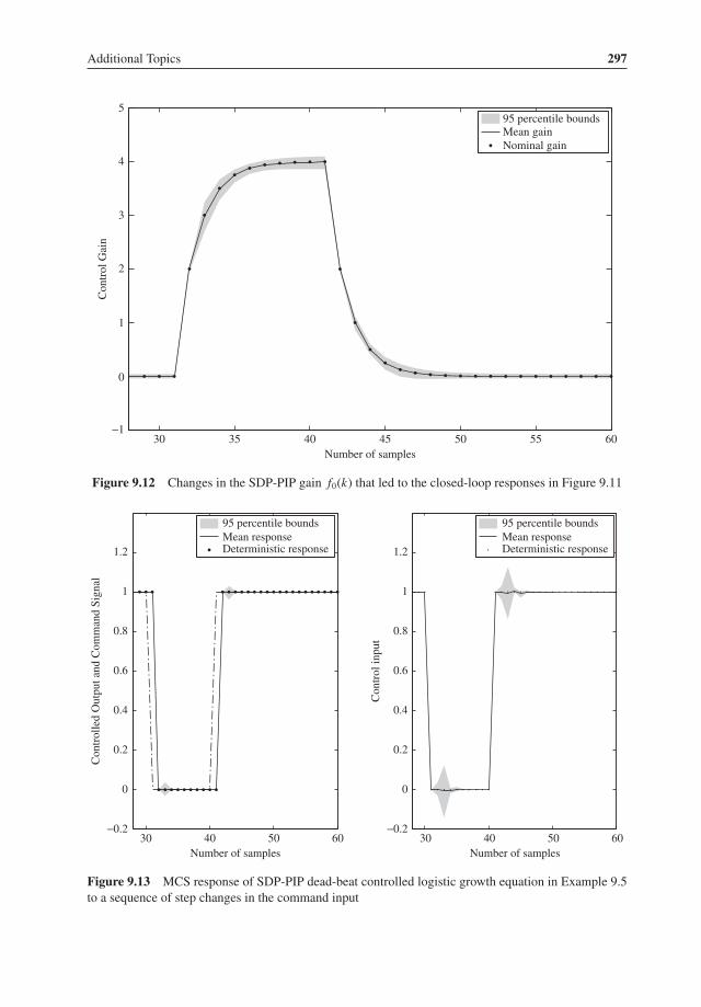
Additional Topics 297
Contr
ol
Gai
n
−1
0
1
2
3
4
5
Number of samples
95 percentile boundsMean gainNominal gain
30 35 40 45 50 55 60
Figure 9.12 Changes in the SDP-PIP gain f0(k) that led to the closed-loop responses in Figure 9.11
Co
ntr
oll
ed O
utp
ut
and
Co
mm
and
Sig
nal
−0.2
Number of samples
30
95 percentile bounds
Mean responseDeterministic response
95 percentile bounds
Mean responseDeterministic response
0
0.2
0.4
0.6
0.8
1
1.2
Co
ntr
ol
inp
ut
−0.2
0
0.2
0.4
0.6
0.8
1
1.2
40 50 60
Number of samples
30 40 50 60
Figure 9.13 MCS response of SDP-PIP dead-beat controlled logistic growth equation in Example 9.5to a sequence of step changes in the command input

298 True Digital Control
are equivalent: this is why the expected design responses, such as dead-beat, are successfullyobtained for the present example. Although limited, the time-delay SDP model (9.67) with(9.78), still encompasses a wide range of nonlinear structures and has proven particularlyuseful for the control of hydraulically operated robotic manipulators (e.g. Taylor et al. 2010;Taylor and Seward 2010; Robertson and Taylor 2012).
9.4 Concluding Remarks
This final chapter has considered two additional topics that illustrate the wide applicability ofthe TDC concepts and methods discussed in previous chapters of this book. We believe thatthe PIP control of δ-operator systems has important practical implications in those situationswhere rapid sampling is essential and we are surprised that, so far, it has not been exploitedmore in practical applications. Similarly, adaptive TVP and scheduled SDP control methodsare important because they open the door to the PIP control of nonlinear stochastic systems.Although the SDP-PIP pole assignment approach demonstrated above has initially been limitedin general terms to systems that can be described by all-pole SDP models, without modelmismatch, this does not mean that systems that are described by the more general SDP-TFmodel (9.67), with model mismatch, cannot be controlled at all; it simply means that a generalproof of closed-loop stability has not been established so far in this situation. Indeed, it seemslikely that SDP-PIP control can be applied to such systems within some defined region of theSDP model parameter space and research is proceeding in this direction. Clearly, therefore,SDP modelling and nonlinear SDP-PIP control are both subjects that have great potential forpractical application, and are an attractive topic for future theoretical and practical research.
References
Banks, H.T., Lewis, B.M. and Tran, H.T. (2007) Nonlinear feedback controllers and compensators: a state-dependentRiccati equation approach, Computational Optimization and Applications, 37, pp. 177–218.
Beven, K.J., Leedal, D.T., Smith, P.J. and Young, P.C. (2012) Identification and representation of state dependentnon-linearities in flood forecasting using the DBM methodology. In L. Wang and H. Garnier (Eds), SystemIdentification, Environmetric Modelling and Control, Springer-Verlag, Berlin, pp. 341–366.
Bray, J.W., High, R.J., McCann, A.D. and Jemmeson, H. (1965) On-line model making for chemical plant, Transac-tions of the Society of Instrument Technology, 17, pp. 1–9.
Bryson, A.E. and Ho, Y.C. (1969) Applied Optimal Control, Blaisdell, Waltham, MA.Chotai, A., Young, P.C., McKenna, P.G. and Tych,W. (1998) Proportional-Integral-Plus (PIP) design for delta operatorsystems: Part 2, MIMO systems, International Journal of Control, 70, pp. 149–168.
Gauss, K. (1826) Theoria combinationis observationum erroribus minimis obnoxiae.Werke, 4 (Parts 1, 2 and Supple-ment), pp. 1–108.
Harvey, A.C. (1981) Time Series Models, Phillip Allen, Oxford.Kitagawa, G. (1981) A non-stationary time series model and its fitting by a recursive filter, Journal of Time Series
Analysis, 2, pp. 103–116.Kopp, R.E. and Orford, R.J. (1963) Linear regression applied to system identification for adaptive control systems,
American Institution of Aeronautics and Astronautics Journal, 1, pp. 2300–236.Kulhavy, R. (1987) Restricted exponential forgetting in real time identification. Automatica, 23, pp. 589–600.Lee, R.C.K. (1964) Optimal Identification, Estimation and Control, MIT Press, Cambridge, MA.Ljung, L. (1979) Asymptotic behaviour of the extended Kalman filter as a parameter estimator for linear systems,
IEEE Transactions on Automatic Control, 24, pp. 36–50.Mayne, D.Q. (1963) Optimal nonstationary estimation of the parameters of a dynamic system, Journal of Electronics
and Control, 14, pp. 101–112.

Additional Topics 299
McCabe, A.P., Young, P., Chotai, A. and Taylor, C.J. (2000) Proportional-Integral-Plus (PIP) control of non-linearsystems, Systems Science (Wrocław), 26, pp. 25–46.
McKenna, P.G. (1997) Delta Operator Modelling, Forecasting and Control, PhD thesis, Environmental ScienceDepartment, Lancaster University.
Middleton, R.H. and Goodwin, G.C. (1990) Digital Control and Estimation – A Unified Approach, Prentice Hall,Englewood Cliffs, NJ.
Norton, J.P. (1975) Optimal smoothing in the identification of linear time-varying systems, Proceedings InstituteElectrical Engineers, 122, pp. 663–668.
Norton, J.P. (1986) An Introduction to Identification, Academic Press, New York.Pedregal, D.J. and Taylor, C.J. (2012) SSpace: A flexible and general state space toolbox forMATLAB. In L.Wang andH. Garnier (Eds), System Identification, Environmental Modelling and Control System Design, Springer-Verlag,Berlin, pp. 615–635.
Pedregal, D.J., Taylor, C.J. and Young, P.C. (2007) System Identification, Time Series Analysis and Forecasting: TheCaptain Toolbox Handbook, Lancaster University, Lancaster.
Previdi, F. and Lovera, M. (2004) Identification on non-linear parametrically varying models using separable leastsquares, International Journal of Control, 77, pp. 1382–1392.
Robertson, D. and Taylor, C.J (2012) State-dependent control of a hydraulically-actuated nuclear decommissioningrobot, UKACC International Conference Control, September, Cardiff, UK, Paper 48.
Sadeghi, J., Tych, W., Chotai, A. and Young, P.C. (2010) Multi-state dependent parameter model identification andestimation for control system design, Electronics Letters, 46, pp. 1265–1266.
Schweppe, F. (1965) Evaluation of likelihood functions for gaussian signals, IEEE Transactions on InformationTheory, 11, pp. 61–70.
Stables, M.A. and Taylor, C.J. (2006) Nonlinear control of ventilation rate using state dependent parameter models,Biosystems Engineering, 95, pp. 7–18.
Taylor, C.J., Chotai, A. and Burnham, K.J. (2011) Controllable forms for stabilising pole assignment design ofgeneralised bilinear systems, Electronics Letters, 47, pp. 437–439.
Taylor, C.J., Chotai, A. and Robertson, D. (2010) State dependent control of a robotic manipulator used for nucleardecommissioning activities, IEEE RSJ International Conference on Intelligent Robots and Systems (IROS-10),October, Taipei, Taiwan, pp. 2413–2418.
Taylor, C.J., Chotai, A. and Young, P.C. (1998) Proportional-Integral-Plus (PIP) control of time-delay systems,IMECHE Proceedings: Systems and Control Engineering, 212, pp. 37–48.
Taylor, C.J., Chotai, A. and Young, P.C. (2009) Nonlinear control by input–output state variable feedback poleassignment, International Journal of Control, 82, pp. 1029–1044.
Taylor, C.J., Pedregal, D.J., Young, P.C. and Tych, W. (2007a) Environmental time series analysis and forecastingwith the Captain toolbox, Environmental Modelling and Software, 22, pp. 797–814.
Taylor, J. and Seward, D. (2010) Control of a dual-arm robotic manipulator, Nuclear Engineering International, 55,pp. 24–26.
Taylor, C.J., Shaban, E.M., Stables, M.A. and Ako, S. (2007b) Proportional-Integral-Plus (PIP) control applicationsof state dependent parameter models, IMECHE Proceedings: Systems and Control Engineering, 221, pp. 1019–1032.
Tych, W., Sadeghi, J., Smith, P., Chotai, A. and Taylor, C.J. (2012) Multi-state dependent parameter model identi-fication and estimation. In L. Wang and H. Garnier (Eds), System Identification, Environmetric Modelling andControl, Springer-Verlag, Berlin, pp. 191–210.
Wellstead, P.E. and Zarrop, M. B. (1991) Self-Tuning Systems: Control and Signal Processing, John Wiley & Sons,Ltd, New York.
Young, P.C. (1969) Applying parameter estimation to dynamic systems: Part I – theory. Control Engineering, 16, pp.119–125.
Young, P.C. (1970) An instrumental variable method for real-time identification of a noisy process. Automatica, 6,pp. 271–287.
Young, P.C. (1981) A second generation adaptive autostabilization system for airborne vehicles, Automatica, 17, pp.459–470.
Young, P.C. (1984) Recursive Estimation and Time-Series Analysis: An Introduction, Springer-Verlag, Berlin.Young, P.C. (1996) A general approach to identification, estimation and control for a class of nonlinear dynamicsystems. In M.I. Friswell and J.E. Mottershead (Eds), Identification in Engineering Systems, University of Wales,Swansea, pp. 436–445.

300 True Digital Control
Young, P.C. (1999) Nonstationary time series analysis and forecasting. Progress in Environmental Science, 1, pp.3–48.
Young, P.C. (2000) Stochastic, dynamic modelling and signal processing: time variable and state dependent parameterestimation. In W.J. Fitzgerald, A. Walden, R. Smith and P.C. Young (Eds), Nonlinear and Nonstationary SignalProcessing, Cambridge University Press, Cambridge, pp. 74–114.
Young, P.C. (2002) Identification of time varying systems. In H. Unbehauen (Ed.), Encyclopedia of Life SupportSystems (EOLSS), volume 6.43: Control Systems, Robotics and Automation, UNESCO, EOLSS Publishers,Oxford.
Young, P.C. (2005) Comments on ‘identification on non-linear parametrically varying models using separable leastsquares’ by F. Previdi and M. Lovera: black-box or open box? International Journal of Control, 78, pp. 122–127.
Young, P.C. (2010) Gauss, Kalman and advances in recursive parameter estimation. Journal of Forecasting (specialissue celebrating 50 years of the Kalman Filter), 30, pp. 104–146
Young, P.C. (2011) Recursive Estimation and Time-Series Analysis: An Introduction for the Student and Practitioner,Springer-Verlag, Berlin.
Young, P.C., Chotai, A., McKenna, P.G. and Tych,W. (1998) Proportional-Integral-Plus (PIP) design for delta operatorsystems: Part 1, SISO systems. International Journal of Control, 70, pp. 123–147.
Young, P.C., Chotai, A. and Tych, W. (1991) Identification, estimation and control of continuous–time systemsdescribed by delta operator models. In N. Sinha and G. Rao (Eds), Identification of Continuous-Time Systems,Kluwer, Dordrecht, pp. 363–418.
Young, P.C., McKenna, P.G. and Bruun, J. (2001) Identification of nonlinear stochastic systems by state dependentparameter estimation, International Journal of Control, 74, pp. 1837–1857.
Young, P.C. and Ng, C.N. (1989) Variance intervention, Journal of Forecasting, 8, pp. 399–416.

AMatrices and Matrix Algebra
A.1 Matrices
A matrix is defined as a rectangular array of elements arranged in rows and columns; in thisbook it is denoted by a bold italics capital letter, e.g.
A =
⎡⎢⎢⎢⎣
a11 a12 · · · a1na21 a22 · · · a2n· · · · · · · · · · · ·am1 am2 · · · amn
⎤⎥⎥⎥⎦ (A.1)
Often A is alternatively denoted by [ai j ] to indicate that it is characterised by elements ai j ,
i = 1, 2, . . . , m; j = 1, 2, . . . , n
If it has mn elements arranged in m rows and n columns, then it is said to be of order m by n,usually written m × n.The following should be noted in relation to matrices:
(i) A null matrix has all of its elements set to zero, i.e. ai j= 0 for all i, j.(ii) A symmetric matrix is a square matrix in which ai j = a ji ; i.e. it is symmetric about the
diagonal elements.(iii) The trace of a square n × n matrix, denoted by Tr., is the sum of its diagonal elements,
i.e. Tr. A = a11 + a22 + · · · + ann .(iv) A diagonal matrix is a square matrix with all its elements except those on the diagonal
set to zero, i.e.
A =
⎡⎢⎢⎢⎣
a11 0 · · · 0
0 a22 · · · 0
· · · · · · · · · · · ·0 0 · · · ann
⎤⎥⎥⎥⎦
True Digital Control: Statistical Modelling and Non-Minimal State Space Design, First Edition.C. James Taylor, Peter C. Young and Arun Chotai.© 2013 John Wiley & Sons, Ltd. Published 2013 by John Wiley & Sons, Ltd.

302 True Digital Control
(v) An n × n diagonal matrix with elements set to unity is denoted by In and termed theidentity (or unit) matrix of order n, e.g. for a 3 × 3 identity matrix:
I3 =
⎡⎢⎣1 0 0
0 1 0
0 0 1
⎤⎥⎦ .
Sometimes the subscript is omitted if the order is obvious.(vi) An idempotent matrix is a square matrix such that A2 = AA = A, i.e. it remains
unchanged when multiplied by itself.
A.2 Vectors
Amatrix of orderm × 1 contains a single column ofm elements and is termed a column vector(or sometimes just a vector); in this book, it is denoted by a bold italics lower case letter, i.e.for a vector b:
b =
⎡⎢⎢⎢⎢⎣
b1b2...
bn
⎤⎥⎥⎥⎥⎦ (A.2)
A.3 Matrix Addition (or Subtraction)
If two matrices A and B are of the same order then we define A + B to be a new matrix C,where
ci j = ai j + bi j
In other words, the addition of thematrices is accomplished by adding corresponding elements,with A − B defined in an analogous manner.
A.4 Matrix or Vector Transpose
The transpose of a matrix A is obtained from A by interchanging the rows and columns; inthis book, it is denoted by a superscript capital T, e.g. for A defined in (A.1):
AT =
⎡⎢⎢⎢⎣
a11 a21 · · · am1
a12 a22 · · · am2
· · · · · · · · · · · ·a1n a2n · · · amn
⎤⎥⎥⎥⎦

Appendix A: Matrices and Matrix Algebra 303
The transpose of a column vector b, denoted by bT is termed a row vector, e.g. for b in (A.2),bT = [b1 b2 . . . bn].Note that:
(i) in the case of a symmetric matrix AT = A;(ii) [AT ]T = A;(iii) [A + B] T = AT + BT .
A.5 Matrix Multiplication
If A is of order m × n and B is of order n × p then the product AB is defined to be a matrix oforder m × p whose (ij)th element ci j is given by:
ci j =n∑
k=1aikbk j
i.e. the (ij)th element is obtained by, in turn, multiplying the elements of the ith row of thematrix A by the jth column of the matrixB and summing over all terms. Therefore, the numberof elements (n) in each row of A must be equal to the number of elements in each column ofB. Note that, in general, the commutative law of multiplication which applies for scalars doesnot apply for matrices, i.e.
AB �= B A
so that pre-multiplication of B by A does not, in general, yield the same as post-multiplicationof B byA. However, pre-multiplying or post-multiplying by the identity matrix leaves thematrix unchanged, i.e.
AI n = I n A = A
Note also that for A of order m × n, B of order n × p and C of order p × q the followingresults apply:
(i) (AB)C = A(BC);(ii) A(B + C) = AB + AC with orders m, n, p and q chosen appropriately;(iii) (B + C)A = B A + C A;(iv) for A, B and C, the multiplication by a scalar λ yields a corresponding matrix with all its
elements multiplied by λ, i.e .λA = [λai j ];(v) [AB]T = BT AT ;(vi) [ABC]T = CT BT AT , since [ABC]T = [(AB)C]T = CT [AB]T = CT BT AT from (v).

304 True Digital Control
Finally, it should be observed that, for a vector x = [x1 x2 · · · xn]T , the inner product xT xyields a scalar quantity which is the sum of the squares of the elements of x, i.e.
[x1 x2 · · · xn]
⎡⎢⎢⎢⎢⎣
x1x2...
xn
⎤⎥⎥⎥⎥⎦ = x21 + x22 + · · · + x2n
The product xxT , on the other hand yields a symmetric square matrix of order n × n, whoseelements are the squares (on the diagonal) and cross products (elsewhere) of the x elements,i.e.
⎡⎢⎢⎢⎣
x1x2· · ·xn
⎤⎥⎥⎥⎦ [x1 x2 · · · xn] =
⎡⎢⎢⎢⎣
x21 x1x2 · · · x1xn
x2x1 x22 · · · x2xn
· · · · · · · · · · · ·xn x1 xn x2 · · · x2n
⎤⎥⎥⎥⎦
Both products are of importance in the present text.
A.6 Determinant of a Matrix
The determinant of a square n × n matrix A is a scalar quantity, denoted by |A| or det.[A],obtained by performing certain systematic operations on the matrix elements. In particular, ifthe cofactors ci j of A are defined as follows:
ci j = (−1)i+ j |Ai j | (A.3)
where |Ai j | is the determinant of the submatrix obtained when the ith row and jth column aredeleted from A, then the determinant of A can be defined as follows in terms of the elementsof the ith row or their cofactors:
|A| = ai1ci1 + ai2ci2 + · · · + aincin (A.4)
|A| may be similarly expanded in terms of the elements of any row or column.Note that, for a matrix of order greater than 2, it is necessary to nest the operation (A.3) and
operation (A.4) and apply them repeatedly until Ai j is reduced to a scalar, in which case thedeterminant is equal to the scalar. The following example demonstrates this process:
A =
⎡⎢⎣
a11 a12 a13a21 a22 a23a31 a32 a33
⎤⎥⎦

Appendix A: Matrices and Matrix Algebra 305
then
|A| = a11
∣∣∣∣∣ a22 a23a32 a33
∣∣∣∣∣ − a12
∣∣∣∣∣ a21 a23a31 a33
∣∣∣∣∣ + a13
∣∣∣∣∣ a21 a22a31 a32
∣∣∣∣∣so that, applying (A.3) and (A.4) again to the subdeterminants, we obtain:
|A| = a11(a22a33 − a32a23)− a12(a21a33 − a31a23)+ a13(a21a32 − a31a22)
For further discussion on determinants see e.g. Johnston (1963).
A.7 Partitioned Matrices
Since a matrix is a rectangular array of elements, we may divide it up by means of horizontaland vertical dotted lines into smaller rectangular arrays of submatrices, e.g.
A =
⎡⎢⎣
a11 a12 a13 a14a21 a22 a23 a24a31 a32 a33 a34
⎤⎥⎦
has been divided in this manner into four submatrices:
A11 =[
a11 a12 a13a21 a22 a23
]; A12 =
[a14a24
]; A21 = [a31 a32 a33] ; A22 = a34
So that A11 is a 2× 3 submatrix, A12 is a 2× 1 column vector, A21 is a 1× 3 row vector, andA22 is a scalar. As a result A can be denoted by:
A =[
A11 A12A21 A22
]
The basic operations for addition, multiplication and transposition apply for partitioned matri-ces but the matrices must be partitioned conformably to allow for such operations. A multi-plicative example is:
AB =[
A11 A12A21 A22
] [B11B21
]=
[A11B11 + A12B21A21B11 + A22B21
]
The results of such operations will be the same as would be obtained by multiplying theunpartitioned matrices element by element (as in section A.5) but the partitioning approachmay be extremely useful in simplifying the analysis.

306 True Digital Control
One theorem for partitioned matrices that is sometimes useful in the context of this bookconcerns the determinant of a partitioned matrix A, where
A =[
A11 A12A21 A22
]
It can be shown (e.g. Gantmacher 1960; Dhrymes 1970) that:
|A| = |A22|.|A11 − A12A−122 A21|
or, alternatively,
|A| = |A11|.|A22 − A21A−111 A12|
where A−111 and A−1
22 are, respectively, the inverses of the matrices A11 and A22, respectively,as defined in section A.8.
A.8 Inverse of a Matrix
If a matrix A−1 exists such that:
AA−1 = A−1A = I
where I is an appropriately ordered identity matrix, then A−1 is termed the inverse (or recip-rocal) of A by analogy with the scalar situation.The inverse of a square matrix A of order n × n is obtained from A bymeans of the formula:
A−1 = 1
|A| [Adj.A] =
⎡⎢⎣
c11|A|
c21|A| · · · cn1
|A|· · · · · · · · · · · ·c1n|A|
c2n|A| · · · cnn
|A|
⎤⎥⎦
where Adj.A denotes the adjoint of the matrix A and is obtained as the transpose of an n × nmatrix C with elements ci j which are the cofactors of A as defined by (A.3), i.e.
c11 = ∣∣A−111
∣∣ ; c12 = − ∣∣A−112
∣∣ ; c22 = ∣∣A−122
∣∣ , etc.Note that, by definition, the inverse will only exist if |A| �= 0; otherwise the matrix is non-invertible or singular. A non-singular matrix is, therefore, invertible.Several theorems on inverse matrices are useful, e.g.
(i) [AB]−1 = B−1A−1;(ii) [AB][B−1A−1] = A[B B−1]A−1 = AI A−1 = AA−1 = I ;(iii) [ABC]−1 = C−1B−1A−1;
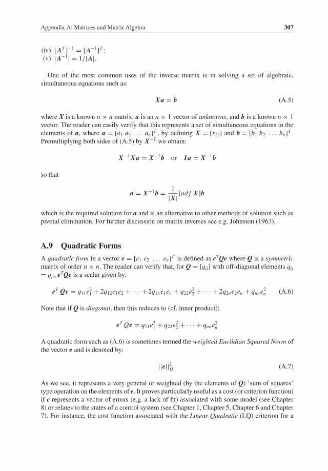
Appendix A: Matrices and Matrix Algebra 307
(iv) [AT ]−1 = [A−1]T ;(v) |A−1| = 1/|A|.
One of the most common uses of the inverse matrix is in solving a set of algebraic,simultaneous equations such as:
Xa = b (A.5)
where X is a known n × n matrix, a is an n × 1 vector of unknowns, and b is a known n × 1vector. The reader can easily verify that this represents a set of simultaneous equations in theelements of a, where a = [a1 a2 . . . an]T , by defining X = [xi j ] and b = [b1 b2 . . . bn]T .Premultiplying both sides of (A.5) by X−1 we obtain:
X−1Xa = X−1b or I a = X−1b
so that
a = X−1b = 1
|X| [ad j.X]b
which is the required solution for a and is an alternative to other methods of solution such aspivotal elimination. For further discussion on matrix inverses see e.g. Johnston (1963).
A.9 Quadratic Forms
A quadratic form in a vector e = [e1 e2 . . . en]T is defined as eTQe where Q is a symmetricmatrix of order n × n. The reader can verify that, for Q = [qij] with off-diagonal elements qij
= qji, eTQe is a scalar given by:
eT Qe = q11e21 + 2q12e1e2 + · · · + 2q1ne1en + q22e
22 + · · · + 2q2ne2en + qnne2n (A.6)
Note that if Q is diagonal, then this reduces to (cf. inner product):
eT Qe = q11e21 + q22e
22 + · · · + qnne2n
A quadratic form such as (A.6) is sometimes termed the weighted Euclidian Squared Norm ofthe vector e and is denoted by:
||e||2Q (A.7)
As we see, it represents a very general or weighted (by the elements of Q) ‘sum of squares’type operation on the elements of e. It proves particularly useful as a cost (or criterion function)if e represents a vector of errors (e.g. a lack of fit) associated with some model (see Chapter8) or relates to the states of a control system (see Chapter 1, Chapter 5, Chapter 6 and Chapter7). For instance, the cost function associated with the Linear Quadratic (LQ) criterion for a

308 True Digital Control
discrete-time state space model, as utilised extensively in this book, is based on (A.6): see e.g.equation (5.75).
A.10 Positive Definite or Semi-Definite Matrices
A symmetric matrix A is said to be positive definite (p.d.) if xT Qx > 0 where x is any non-nullvector. It is termed positive semi-definite (p.s.d.) if xT Qx ≥ 0.For an n × n p.d. matrix A, aii > 0, i = 1, 2, . . . , n; for a p.s.d. matrix aii ≥ 0, i = 1, 2, . . . ,
n.Note that if A is p.d. then A is non-singular and can be inverted; if A is p.s.d. (but not p.d.)
then A is singular (Dhrymes 1970).
A.11 The Rank of a Matrix
The rank of a matrix is the order of its largest submatrix that is non-singular and so has anon-zero determinant. Thus for a square nxnmatrix the rank must be n (i.e. the matrix must befull rank) for the matrix to be non-singular and invertible. For further discussion on the rankof a matrix see e.g. Johnston (1963). The rank of a matrix is particularly useful in this book inrelation to the rank test for controllability (e.g. section 3.4).
A.12 Differentiation of Vectors and Matrices
The differentiation of vectors and matrices is most important in optimisation and statisticalanalysis. The main result concerns the differentiation of an inner product of two vectors withrespect to the elements of one of the vectors.Consider the inner product of two (n × 1) vectors x and a, i.e.
xT a = [x1 x2 . . . xn]
⎡⎢⎢⎢⎢⎣
a1a2...
an
⎤⎥⎥⎥⎥⎦
It is clear that for all i, i = l, 2, . . . , n, the partial differentials with respect to ai are given by:
∂ (xT a)∂ ai
= xi
As a result, if the partial differentials are arranged in order of their subscripts as a vector, thenthis vector is simply x. Thus it is convenient to refer to the process of vector differentiation inshorthand as:
∂ (xT a)∂ a
= x or∂ (xT a)∂ aT
= xT

Appendix A: Matrices and Matrix Algebra 309
The analogy with scalar differentiation is apparent from the above result. A particularlyimportant example of vector differentiation, which occurs in Chapter 8 of this book, isconcerned with the differentiation of a least squares cost function J2 which, in its simplestform, is defined as:
k∑i=1
e2i
where ei = xTi a − yi is an error measure based on a vector of estimated coefficients or
parameters a. In order to obtain the estimate a, it is necessary to differentiate J2 with respectto all of the elements ai , i = l, 2, . . . n, of a. Using the above results, we see that since
J2 =k∑
i=1[xT (i) a)2 − 2x(i)T a y(i)+ y(i)2]
then
∂ J2∂ a
=k∑
i=1[2x(i)x(i)T a − 2x(i)y(i)] = 2
k∑i=1
x(i)x(i)T a − x(i)y(i) (A.8)
which, when set to zero in the usual manner, constitutes a set of n simultaneous equations inthe n unknowns ai , i = 1, 2, . . . , n; the normal equations.Alternatively, we can proceed by forming the k × n matrix X with rows defined by xT (i), i
= 1,2, . . . , k. The reader can then verify that the vector e = [e1 e2 . . . en]T is defined by:
e = Xa − y
where e = [y1 y2 . . . yk]T , and so
J2 = [Xa − y]T [Xa − y] = aT XT Xa − 2aT XT y + yT y
since yT X a is a scalar and so equal to its transpose aT XT y. It now follows straightforwardlythat
∂ J2∂ a
= 2XT Xa − 2XT y
which will be seen as identical to (A.8) by substituting for X in terms of x(i).If J2 is replaced by the more general weighted least squares cost function, i.e.
J2 = [Xa − y]T [QX a − y] = ||Xa − y||2Q (A.9)

310 True Digital Control
where Q is a symmetric p.d. weighting matrix, then it is straightforward to show that
∂ J2∂ a
= 2XT QX a − 2XT Qy
References
Dhrymes, P.J. (1970) Econometrics: Statistical Foundations and Applications, Harper and Row, New York.Gantmacher, F.R. (1960) Matrix Theory, volume 1, Chelsea, New York.Johnston, J. (1963) Econometric Methods, McGraw-Hill, New York.
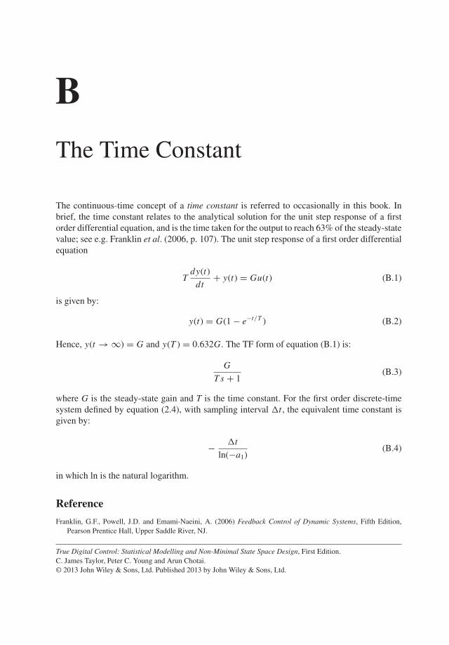
BThe Time Constant
The continuous-time concept of a time constant is referred to occasionally in this book. Inbrief, the time constant relates to the analytical solution for the unit step response of a firstorder differential equation, and is the time taken for the output to reach 63% of the steady-statevalue; see e.g. Franklin et al. (2006, p. 107). The unit step response of a first order differentialequation
Tdy(t)
dt+ y(t) = Gu(t) (B.1)
is given by:
y(t) = G(1− e−t/T ) (B.2)
Hence, y(t → ∞) = G and y(T ) = 0.632G. The TF form of equation (B.1) is:
G
T s + 1 (B.3)
where G is the steady-state gain and T is the time constant. For the first order discrete-timesystem defined by equation (2.4), with sampling interval �t , the equivalent time constant isgiven by:
− �t
ln(−a1)(B.4)
in which ln is the natural logarithm.
Reference
Franklin, G.F., Powell, J.D. and Emami-Naeini, A. (2006) Feedback Control of Dynamic Systems, Fifth Edition,Pearson Prentice Hall, Upper Saddle River, NJ.
True Digital Control: Statistical Modelling and Non-Minimal State Space Design, First Edition.C. James Taylor, Peter C. Young and Arun Chotai.© 2013 John Wiley & Sons, Ltd. Published 2013 by John Wiley & Sons, Ltd.

CProof of Theorem 4.1
Theorem 4.1 Controllability of the Non-Minimal State Space (NMSS) Representation is statedin section 4.2. The proof is based on Wang and Young (1988). According to the Popov,Belevitch and Hautus (PBH) test (Kailath 1980), the state space system (4.4) defined by[F, g] is uncontrollable (or unreachable) if and only if there exists a non-zero row vector q (aleft eigenvector of F), which is orthogonal to g, i.e. we need to find a vector:
q = [q1 q2 · · · qn+m−1
] �= 0 (C.1)
such that the following two equations hold simultaneously:
q F = λ q (C.2)
q g = 0 (C.3)
where λ is an eigenvalue of F. If there exists a row vector q such that equation (C.2) and (C.3)are fulfilled, then expanding these yields the following scalar equations:
−q1a1 + q2 = λq1 (1)
−q1a2 + q3 = λq2 (2)...
...
−q1an−1 + qn = λqn−1 (n − 1)−q1an = λqn (n)
q1b2 + qn+2 = λqn+1 (n + 1)...
...
q1bm−1 + qn+m−1 = λqn+m−2 (n + m − 2)q1bm = λqn+m−1 (n + m − 1)q1b1 = −qn+1 (n + m)
⎫⎪⎪⎪⎪⎪⎪⎪⎪⎪⎪⎪⎪⎪⎪⎪⎪⎪⎪⎪⎪⎬⎪⎪⎪⎪⎪⎪⎪⎪⎪⎪⎪⎪⎪⎪⎪⎪⎪⎪⎪⎪⎭
(C.4)
True Digital Control: Statistical Modelling and Non-Minimal State Space Design, First Edition.C. James Taylor, Peter C. Young and Arun Chotai.© 2013 John Wiley & Sons, Ltd. Published 2013 by John Wiley & Sons, Ltd.

314 True Digital Control
Let us consider the implications of the above scalar equations under the conditions λ = 0and λ �= 0 separately.
(i) λ = 0. In the first instance, we note that since an �= 0, then λ = 0 is not a root of A∗(λ) inequation (4.13). Also, from the nth equation in (C.4), we know that q1 = 0 which, fromthe other equations of (C.4), implies that the row vector q is a zero vector. As a result, themodes λ = 0 are completely controllable.
(ii) λ = λ1 �= 0 and A∗(λ1) = 0.
In order to consider this case, we need to manipulate equations (C.4). By multiplyingequation (1) to equation (n − 1) of (C.4) by λn−1, λn−2, . . . , λ, respectively, and subsequentlyadding all of them to equation n, we obtain:
− q1(a1λn−1 + · · · + an) = λn q1 (C.5)
which can be written as:
q1(λn + a1λ
n−1 + · · · + an) = q1A∗(λ) = 0 (C.6)
Similarly, by multiplying equation (n + m) of (C.4) by λn−1 and equation (n + 1) to equation(n + m − 2) by λm−2, λm−3, . . . ,λ, respectively, before finally adding all of them to equation(n + m − 1), we obtain:
q1B∗(λ) = 0 (C.7)
where
B∗(λ) = b1λm−1 + b2λ
m−2 + · · · + bm (C.8)
Now assume that A∗(λ) and B∗(λ) are not coprime, i.e. that there is at least one commonfactor between A∗(λ) and B∗(λ). In this case, there is a λ = λ1, such that A∗(λ1) = 0 andB∗(λ1) = 0. Therefore, we can always find a non-zero vector q, so that equations (C.4) allhold. Conversely, if A∗(λ) and B∗(λ) are coprime, then B∗(λ1) �= 0, which implies fromequation (C.7) that q1 = 0. It follows from equations (C.4) that the whole vector q is a zerovector, so that the modes specified by the roots of A∗(λ) = 0 are controllable if and onlyif A∗(λ) and B∗(λ) are coprime. Finally, in this scalar case, coprime A∗(λ) and B∗(λ) isequivalent to coprime A(z−1) and B(z−1), i.e. the controllability conditions stated by Theorem4.1.
References
Kailath, T. (1980) Linear Systems, Prentice Hall, Englewood Cliffs, NJ.Wang, C.L. and Young, P.C. (1988) Direct digital control by input–output, state variable feedback: theoreticalbackground, International Journal of Control, 47, pp. 97–109.

DDerivative Action Formof the Controller
In order to demonstrate that Proportional-Integral-Plus (PIP) control contains derivativeaction, as noted in section 5.2, we need to find the polynomials F (�) and G(�) using thedifference operator � = 1− z−1, such that:
F(�) ≡ F(z−1) and G(�) ≡ G(z−1) (D.1)
where F(z−1) and G(z−1) are defined by equations (5.34).Let
F(�) = k0 + k1� + k2�2 + · · · + kn−1�n−1 (D.2)
and
G(�) = l0 + l1� + l2�2 + · · · + lm−1�m−1 (D.3)
After substituting for � = 1− z−1, the expression for F(�) is expanded and the coefficientsfor like powers of zi equated to those of the polynomial F(z−1). This results in the followingrelationships between the coefficients of both polynomials:
f j =n−1∑i= j
i C j ki (D.4)
where
i C j = (−1) j i !
(i − j) ! j !(D.5)
True Digital Control: Statistical Modelling and Non-Minimal State Space Design, First Edition.C. James Taylor, Peter C. Young and Arun Chotai.© 2013 John Wiley & Sons, Ltd. Published 2013 by John Wiley & Sons, Ltd.

316 True Digital Control
are binomial coefficients and j = 0, 1, . . . , n − 1. Here i! is the i factorial and 0! = 1 bydefinition. These relationships are expressed in vector matrix form as follows:
⎡⎢⎢⎢⎢⎢⎢⎢⎣
f0f1f2...
fn−1
⎤⎥⎥⎥⎥⎥⎥⎥⎦
= T
⎡⎢⎢⎢⎢⎢⎢⎢⎣
k0k1k2...
kn−1
⎤⎥⎥⎥⎥⎥⎥⎥⎦
=
⎡⎢⎢⎢⎢⎢⎢⎢⎣
1 1 1 · · · 1
0 1C1 2C1 · · · n−1C10 0 2C2 · · · n−1C2...
.... . .
...
0 0 0 0 n−1Cn−1
⎤⎥⎥⎥⎥⎥⎥⎥⎦
⎡⎢⎢⎢⎢⎢⎢⎢⎣
k0k1k2...
kn−1
⎤⎥⎥⎥⎥⎥⎥⎥⎦
(D.6)
Similarly, we can show that the coefficients gi (i = 0, 1, . . . , m − 1) are related to the derivativeaction coefficients l j ( j = 0, 1, . . . , m − 1) by the following vector-matrix equations, withg0 = 1:
⎡⎢⎢⎢⎢⎢⎢⎢⎣
g0g1g2...
gm−1
⎤⎥⎥⎥⎥⎥⎥⎥⎦
= T
⎡⎢⎢⎢⎢⎢⎢⎢⎣
l0l1l2...
lm−1
⎤⎥⎥⎥⎥⎥⎥⎥⎦
=
⎡⎢⎢⎢⎢⎢⎢⎢⎣
1 1 1 · · · 1
0 1C1 2C1 · · · m−1C10 0 2C2 · · · m−1C2...
.... . .
...
0 0 0 0 m−1Cm−1
⎤⎥⎥⎥⎥⎥⎥⎥⎦
⎡⎢⎢⎢⎢⎢⎢⎢⎣
l0l1l2...
lm−1
⎤⎥⎥⎥⎥⎥⎥⎥⎦
(D.7)
Finally, it should be noted that the transformation matrices T in equation (D.6) and equation(D.7) are both upper triangular matrices, such that T = T−1.Hence, equation (D.6) can be written alternatively:
⎡⎢⎢⎢⎢⎢⎢⎢⎣
k0k1k2...
kn−1
⎤⎥⎥⎥⎥⎥⎥⎥⎦
=
⎡⎢⎢⎢⎢⎢⎢⎢⎣
1 1 1 · · · 1
0 1C1 2C1 · · · n−1C10 0 2C2 · · · n−1C2...
.... . .
...
0 0 0 0 n−1Cn−1
⎤⎥⎥⎥⎥⎥⎥⎥⎦
⎡⎢⎢⎢⎢⎢⎢⎢⎣
f0f1f2...
fn−1
⎤⎥⎥⎥⎥⎥⎥⎥⎦
(D.8)

EBlock Diagram Derivationof PIP Pole Placement Algorithm
One approach for developing a general pole assignment algorithm for Proportional-Integral-Plus (PIP) control utilises polynomial algebra based on Figure 5.4 and the closed-loop charac-teristic polynomial (5.36). The closed-loop characteristic polynomial is equated to the desiredcharacteristic polynomial as follows:
�(G(z−1)A(z−1)+ F(z−1)B(z−1)
) + kI B(z−1) = D(z−1) (E.1)
where � = 1− z−1 is the difference operator and
D(z−1) = 1+ d1z−1 + d2z
−2 + · · · + dn+m z−(n+m) (E.2)
in which di are the user-specified coefficients. The left-hand side of equation (E.1) is writtenin the form of the following Diophantine equation:
A′(z−1)G(z−1)+ B(z−1)F ′(z−1) (E.3)
where
A′(z−1) = � A(z−1)F ′(z−1) = � F(z−1)+ kI
}(E.4)
If the system is controllable, the Diophantine equation has a unique solution. This solution canbe obtained straightforwardly by equating the coefficients of like powers of z−i in equation(E.1) to yield a set of simultaneous algebraic equations in the (n + m) unknown pole assign-ment control gains: f0, f1, . . . fn−1, g1, . . . gm−1, kI . These equations are, of course, identicalwith those obtained from the state space analysis in themain text, except that the controllabilityrequirement is not so transparent.
True Digital Control: Statistical Modelling and Non-Minimal State Space Design, First Edition.C. James Taylor, Peter C. Young and Arun Chotai.© 2013 John Wiley & Sons, Ltd. Published 2013 by John Wiley & Sons, Ltd.

318 True Digital Control
For computational purposes, the pole assignment equations obtained in the above mannerare conveniently written in the following general form:
Σ k = d − p (E.5)
where d and p are defined by equation (5.64) and equation (5.65), respectively, while Σ is a(n + m) by (n + m) matrix:
Σ = [Σ1 Σ2 Σ3
](E.6)
in which the component matrices are as follows:
Σ1 =
⎡⎢⎢⎢⎢⎢⎢⎢⎢⎢⎢⎢⎢⎢⎢⎢⎢⎢⎢⎢⎢⎢⎢⎢⎢⎣
b1 0 · · · 0 0
b2 − b1 b1 · · · 0 0
b3 − b2 b2 − b1 · · · 0 0...
... · · · ......
bm − bm−1 bm−1 − bm−2 · · · b2 − b1 b1−bm bm − bm−1 · · · b3 − b2 b2 − b10 −bm · · · b4 − b3 b3 − b2... 0 · · · ...
......
... · · · ......
0 0 · · · −bm bm − bm−10 0 · · · 0 −bm
⎤⎥⎥⎥⎥⎥⎥⎥⎥⎥⎥⎥⎥⎥⎥⎥⎥⎥⎥⎥⎥⎥⎥⎥⎥⎦
(E.7)
Σ2 =
⎡⎢⎢⎢⎢⎢⎢⎢⎢⎢⎢⎢⎢⎢⎢⎢⎢⎢⎢⎢⎢⎢⎢⎢⎢⎢⎣
1 0 · · · 0 0
a1 − 1 1 · · · 0 0
a2 − a1 a1 − 1 · · · 0 0...
... · · · ......
...... · · · a2 − a1 a1 − 1
an − an−1 an−1 − an−2 · · · a3 − a2 a2 − a1−an an − an−1 · · · a4 − a3 a3 − a2
0 −an · · · ......
...... · · · ...
...
0 0 · · · −an an − an−10 0 · · · 0 −an
⎤⎥⎥⎥⎥⎥⎥⎥⎥⎥⎥⎥⎥⎥⎥⎥⎥⎥⎥⎥⎥⎥⎥⎥⎥⎥⎦
(E.8)
Σ3 = [b1 b2 b3 · · · bm 0 0 · · · · · · 0 0
]T(E.9)

Appendix E: Block Diagram Derivation of PIP Pole Placement Algorithm 319
Comparing (E.6) and (5.66) in the main text, it is clear that Σ = M ST1 .
We can see from these equations that the PIP control gain vector k can only be computed if thematrix Σ = M ST
1 is non-singular. This ‘pole assignability’ condition (a practical requirementof the above approach) and the controllability conditions developed in Chapter 5 are equivalent(see Theorem 5.1 and Theorem 5.2).

FProof of Theorem 6.1
Theorem 6.1 Relationship between Proportional-Integral-Plus (PIP) and Smith Predictor(SP)-PIP Control Gains is stated in section 6.3. The proof is based on Taylor et al. (1998).With the conditions of Theorem 6.1, the closed-loop systems (6.3) and (6.29) in Chapter 6 haveexactly the same denominator polynomials. Since both systems have a gain of unity, by virtueof the inherent integral action, then the closed-loop numerator polynomials must also be equalat steady state. Moreover, the scalar integral gains are equal, since Bs(z−1)z−τ+1 = B(z−1) bydefinition. In this case, the numerator polynomials of the nominal PIP and SP-PIP closed loopsystems are always equal.To derive equation (6.30), consider the PIP pole assignment algorithm (E.5) developed in
Appendix E, i.e.
Σk = d − p
where d and p are the vectors of coefficients of the desired closed-loop characteristic poly-nomial of the nominal PIP system and the open-loop characteristic polynomial of the NMSSmodel, respectively, modified here to explicitly show the time delay [see equation (6.24)], i.e.
dT = [d ′1 d ′
2 d ′3 · · · d ′
n d ′n+1 · · · d ′
n+m+τ−2 d ′n+m+τ−1
](F.1)
pT = [a1 − 1 a2 − a1 a3 − a2 · · · an − an−1 −an · · · 0 0
](F.2)
The equivalent result for the SP-PIP case is:
Σ s · ks = ds − ps (F.3)
where
ds = [d ′′1 d ′′
2 · · · d ′′n+m−1 d ′′
n+m
]T
ps = [a1 − 1 a2 − a1 · · · an − an−1 −an 0 · · · 0
]T (F.4)
True Digital Control: Statistical Modelling and Non-Minimal State Space Design, First Edition.C. James Taylor, Peter C. Young and Arun Chotai.© 2013 John Wiley & Sons, Ltd. Published 2013 by John Wiley & Sons, Ltd.

322 True Digital Control
Using the conditions of Theorem 6.1:
d ′1 = d ′′
1 , d ′2 = d ′′
2 , . . . , d ′n+m−1 = d ′′
n+m−1, d ′n+m = d ′′
n+m (F.5)
and
d ′n+m+1 = d ′
n+m+2 = · · · = d ′n+m+τ−2 = d ′
n+m+τ−1 = 0 (F.6)
If the SP-PIP Σ s matrix and the vector of gains ks are padded with an appropriate number ofzeros, in order to ensure that the matrices and vectors are all of the same order:
Σ · k = Σ s · ks (F.7)
Note that theΣ matrix is always invertible if the system satisfies the controllability conditions,i.e. the pole assignability conditions of Theorem 5.2, hence k = Σ−1Σ s · ks .
Reference
Taylor, C.J., Chotai, A. and Young, P.C. (1998) Proportional-Integral-Plus (PIP) control of time-delay systems,IMECHE Proceedings: Systems and Control Engineering, 212, pp. 37–48.

GThe CAPTAIN Toolbox
The Computer-Aided Program for Time series Analysis and Identification of Noisy systems(CAPTAIN) Toolbox provides access to novel algorithms for various important aspects ofidentification, estimation, non-stationary time series analysis, signal processing, adaptive fore-casting and automatic control system design. These have been developed between 1981 andthe present at Lancaster University, UK. Much of the underlying research into the modellingtools in CAPTAIN was carried out by the second author at the University of Cambridge,UK (1965–1975) and the Australian National University, Canberra, Australia (1975–1981).Although it has its origins in the CAPTAIN and micro-CAPTAIN (Young and Benner 1991)packages, the CAPTAIN Toolbox (Taylor et al. 2007) developed for theMATLAB R©1 softwareenvironment is much more flexible, and provides access to many more algorithms that havebeen added over the 1990s and continue to be developed up to the present day, most of themonly available in this Toolbox.Essentially, the CAPTAIN Toolbox is a collection of routines (MATLAB R© m-file scripts)
for: the identification and estimation of the various Transfer Function (TF) model typesdiscussed in Chapter 8, together with numerous other model types considered elsewhere(e.g. Pedregal et al. 2007; Young 2011), including the Time Varying Parameter (TVP) andState-Dependent Parameter (SDP) models defined in Chapter 9. These are organised arounda core of the Recursive Least Squares (RLS), Kalman Filter (KF), Fixed Interval Smoothing(FIS) and Refined Instrumental Variable (RIV) algorithms. However, in order to allow forstraightforward user access, CAPTAIN consists of numerous ‘shells’, i.e. top level functionsthat automatically generate the necessary model structures, with default options based on theexperience of the developers (but user-adjustable to override these). In this regard, the mainareas of functionality related to the present book are listed below.
G.1 Transfer Functions and Control System Design
The functional pairs rivid/riv (for discrete-time models) and rivcid/rivc (for continuous-time models estimated from discrete-time sampled data) are provided for order/structure
1 MATLAB R©, The MathWorks Inc., Natick, MA, USA.
True Digital Control: Statistical Modelling and Non-Minimal State Space Design, First Edition.C. James Taylor, Peter C. Young and Arun Chotai.© 2013 John Wiley & Sons, Ltd. Published 2013 by John Wiley & Sons, Ltd.

324 True Digital Control
identification and parameter estimation in the case of constant parameter, linear TF models.These routines include, as options, both recursive and en bloc versions of the optimal RIV andSimplified Refined Instrumental Variable (SRIV) algorithms, in addition to conventional leastsquares based approaches. More recent enhancements are the introduction of the rivbj/rivcbjand rivbjid/rivcbjid routines for full Box–Jenkins (BJ) models with Auto-Regressive Moving-Average eXogenous variables (ARMA) additive noise.In all of the order/structure identification routines (the above routines ending in ‘id’), the
model listing, for the selection of models chosen, can be reported in the order of variousstatistics, such as the coefficient of determination R2T and various identification statistics,including the Akaike Information Criterion (AIC), Bayesian Information Criterion (BIC)and Young Information Criterion (YIC), as discussed in Chapter 8. The ivarmaid/ivarmaroutines are for the identification and estimation of ARMA noise models; ivarma is part of therivbj/rivcbj routines but is made available separately for univariate noise model estimation.The Proportional-Integral-Plus (PIP) control system design routines in CAPTAIN include
the pip algorithm for pole assignment and pipopt for Linear Quadratic (LQ) design, togetherwith other required support routines. These are integrated into SIMULINK2 objects that canbe used in simulation studies and, potentially, for online use. Generalised PIP control routinesand multivariable versions of the algorithms are also available from the first author.
G.2 Other Routines
Various other model structures are unified in terms of the unobserved components model. Here,the output time series is assumed to be composed of an additive ormultiplicative combination ofdifferent components that have defined statistical characteristics but which cannot be observeddirectly. Such components may include a trend or low frequency component, a seasonalcomponent (e.g. annual), additional sustained cyclical or quasi-cyclical components, stochasticperturbations, and a component that captures the influence of exogenous input signals. If thesystem is non-stationary, then the analysis typically utilises statistical estimation methodsthat are based on the identification and estimation of stochastic TVP models, as discussedin Chapter 9. An important example that is used for nonlinear PIP control is the SDP modelconsidered in section 9.3. The modelling approach is based around the sdp routine whichyields non-parametric (graphical) estimates of SDPs. If required, the user can parameterisethese graphically defined nonlinearities using specified nonlinear functions (e.g. exponential,power law, radial basis functions, etc.) that can then be optimised using standard MATLAB R©
functions.Various conventional models, identification tools and auxiliary functions, too numerous
to list individually here are included. Of these, the largest is the kalmanfis routine, whichprovides a shell to the KF/FIS algorithms for general state space filtering, smoothing andforecasting purposes.System identification is inherent to the modelling approach utilised by most of the functions
already discussed. Other routines include: acf to determine the sample and partial autocor-relation function; ccf for the sample cross-correlation; period to estimate the periodogram;and statist for some sample descriptive statistics. Additional statistical diagnostics include:
2 SIMULINKTM, The MathWorks Inc., Natick, MA, USA.

Appendix G: The CAPTAIN Toolbox 325
boxcox (optimal Box–Cox transformation for homoscedasticity); cusum (cusum recursivetest for time varying mean) and cusumsq (recursive test for time varying variance); and histon(histogram over normal distribution and Bera–Jarque statistical test); while useful general rou-tines are: del for generating a matrix of delayed variables; irwsm for smoothing, decimation orfor fitting a simple trend to a time series; prepz to prepare data for TF modelling (e.g. baselineremoval and input scaling); stand to standardise or de-standardise a matrix by columns; andreconst to reconstruct a time series by removing any dramatic jumps in the trend.Note that almost all of the recursive estimation and smoothing procedures outlined above
will automatically handle missing data in the time series, represented in MATLAB R© by Not-a-Number (NaN) variables. Indeed, by appending or pre-pending such variables to the dataset using the fcast function, the routines will forecast, interpolate or backcast as appropriate,without requiring further user intervention.Finally, the toolbox is supported by online help and numerous demonstration examples.
These demonstrations, including several for control system design, are invoked by typing theinstruction captdemo in the MATLAB R© command line. The various command line demoscan also be opened and edited, as conventional scripts.
G.3 Download
http://www.lancs.ac.uk/staff/taylorcj/tdc/
References
Pedregal, D.J., Taylor, C.J. and Young, P.C. (2007) System Identification, Time Series Analysis and Forecasting: TheCaptain Toolbox Handbook, Lancaster University, Lancaster.
Taylor, C.J., Pedregal, D.J., Young, P.C. and Tych, W. (2007) Environmental time series analysis and forecasting withthe Captain toolbox, Environmental Modelling and Software, 22, pp. 797–814.
Young, P.C. (2011) Recursive Estimation and Time-Series Analysis: An Introduction for the Student and Practitioner,Springer-Verlag, Berlin.
Young, P.C. and Benner, S. (1991) microCAPTAIN 2 User Handbook, Lancaster University, Lancaster.

HThe Theorem of D.A. Pierce (1972)
The theoretical justification for theRefined Instrumental Variable (RIV) algorithmdeveloped inChapter 8 is twofold. First, the development of the normal equations (8.60) for the estimationof the parameters in the Box–Jenkins model (8.38) when it is considered in pseudo-linearform; and secondly, the following theorem of D.A. Pierce (1972) that establishes the statisticalproperties of theMaximum Likelihood (ML) estimates obtained as the solution to these normalequations and shows that the ML estimates ρ and η of the system and noise parameter vectors,respectively, are asymptotically independent, so justifying an important aspect of the iterativeRIV algorithm.
If, in the model (8.38) of Chapter 8:
1. the e(k) are independent and identically distributed with zero mean, variance σ 2 andskewness and kurtosis κ1 and κ2;
2. the parameter values are admissible (i.e. the model is stable and identifiable); and3. the u(k) are persistently exciting1
then the ML estimates ρ(N ), η(N ) and σ 2 obtained from a data set of N samples, possess alimiting normal distribution, such that:
1. The asymptotic covariance matrix of the estimation errors associated with the estimateρ(N ) is of the form:
P∗ = σ 2
N
[p lim
1
N
∑φ f (k)φ
Tf (k)
]−1(H.1)
1 Identifiability and persistent excitation are important concepts discussed in most books on transfer function identi-fication and estimation (e.g. Ljung 1999; Young 2011).
True Digital Control: Statistical Modelling and Non-Minimal State Space Design, First Edition.C. James Taylor, Peter C. Young and Arun Chotai.© 2013 John Wiley & Sons, Ltd. Published 2013 by John Wiley & Sons, Ltd.

328 True Digital Control
2. The estimate η(N ) is asymptotically independent of ρ(N ) and has an error covariancematrix of the form:
P∗η = σ 2
N[E{ψ(k)ψT
(k)}]−1 (H.2)
3. The estimate σ 2 has asymptotic variance (2σ 4/T )(1 + 0.5κ2) and, if κ1 = 0, is independentof the above estimates.
References
Ljung, L. (1999) System Identification. Theory for the User, Second Edition, Prentice Hall, Upper Saddle River, NJ.Pierce, D.A. (1972) Least squares estimation in dynamic disturbance time-series models. Biometrika, 5, pp. 73–78.Young, P.C. (2011) Recursive Estimation and Time-Series Analysis: An Introduction for the Student and Practitioner,Springer-Verlag, Berlin.

Index
δ-operator, see delta-operators-operator, see differential operatorz-operator, see forward shift operatorz−1-operator, see backward shift operator
auto-correlation function (ACF), 209, 324
backward shift operator, 17–18block diagram analysis, 26–28, 32Bode diagram, 41
CAPTAIN Toolbox, 23, 200, 226, 323–325certainty equivalence principle, see separation
principlecharacteristic equation, 5, 24–26characteristic polynomial, 6, 24–26Cholesky factors, 177, 187–188classical synthesis, 5–8, 17, 41closed-loop transfer function (CLTF), 29, 48command input, 3, 28, 90–91continuous to discrete-time conversion, 36–38,
251–253control, algorithms and design methods foradaptive, 11, 77, 101, 279, 294classical, 5–8, 17, 41closed-loop, 3–4deadbeat, 33–34, 296–297decoupling, 167–168, 186, 192–195digital, 1–2, 17–18direct digital control (DDC), 1eigenvalue assignment, see pole assignmentfeedforward, 153–154, 195
frequency domain, 7, 41, 186generalised predictive control (GPC), 158–163integral control, 30–33, 98–100, 146, 175–176linear exponential of quadratic Gaussian
(LEQG), 152–153linear quadratic Gaussian (LQG), 3–7,
142–153, 163linear quadratic (LQ), 3–7, 110–119,
142–153, 177–191, 272–273, 294loop transfer recovery (LTR), 61, 119, 150model-based, 8, 23, 168model predictive control (MPC), 157–163modern synthesis, 5–8, 41multivariable, 167–196nonlinear, 279–298open-loop, 3–4optimal, see linear quadratic (LQ)pole assignment, 33–35, 48–53, 101–110,
192–195, 271–279, 294–298pole placement, see pole assignmentproportional, 28–30, 98, 267proportional-integral (PI), see proportional-
integral-derivative (PID)proportional-integral-derivative (PID), 1, 7,
31–35, 98–99, 175–176proportional-integral-plus (PIP), 2, 10–11,
89–196, 265–279, 290–298risk-sensitive, see linear exponential of
quadratic gaussian (LEQG)robust, see linear exponential of quadratic
gaussian (LEQG)scheduled, 293–296
True Digital Control: Statistical Modelling and Non-Minimal State Space Design, First Edition.C. James Taylor, Peter C. Young and Arun Chotai.© 2013 John Wiley & Sons, Ltd. Published 2013 by John Wiley & Sons, Ltd.

330 Index
control, algorithms and design methods for(Continued )
self-tuning, 11, 279–280state-dependent parameter (SDP), 290–298state variable feedback (SVF), 5–10stochastic, see linear quadratic gaussian
(LQG)true digital control (TDC), 1–2, 11–12
control, applications ofagricultural systems, 11, 20, 35, 116, 240, 294aircraft and airborne vehicles, 2–3, 5, 9, 290carbon dioxide, 11, 20, 108–110, 117,
134–135, 140, 257coupled drive system, 183–187direct current (DC) motor, 20hair-dryer system, 235–240, 251–253rainfall-flow, 21, 36–38, 229–231robotic manipulators, 20, 91–93, 116,
241–242, 290, 294, 298Shell heavy oil fractionator, 188–191wind turbine, 21–22, 73–74, 116
control input, 2–3, 18controllability, 58–59control model, 22–23covariance matrix, 143, 206, 225, 284
delta-operator, 266difference equation, 22differential operator, 17, 250Diophantine equation, 317double integrator system, 180, 273–279dynamic programming, 3
eigenvalues, 56–58eigenvectors, 56–58estimation, see parameter estimation
false delay, 23, 65feedback form, 123–124, 131–134, 175, 270–271final prediction error (FPE), 233first order system, 19–20forward path form, 125–130, 134–137, 176,
270–271forward shift operator, 17, 24–26frequency domain, 41
gain margin, 115, 273goal-attainment, 187–191
hyper-parameter, 280–281, 284, 287–290
identification, see stochastic system identificationidentification criteria, 232–234
Akaike information criterion (AIC), 232–234Bayesian information criterion (BIC), 234coefficient of determination, 232–233Young information criterion (YIC), 232–233
identification in the closed-loop, 253–260identification procedure, 234incremental form, 131–137input-output models, see transfer function (TF)instrumental product matrix (IPM), 216instrumental variables, 216integral-of-error, 9–10, 90, 94
Kalman filter (KF), 6–9, 142–152, 162–163, 214,280–287
Laplace transform, 17least squares, 199–211linearization, 12linear quadratic Gaussian (LQG) control, 3–7,
142–153, 163linear quadratic (LQ) control, 3–7, 110–119,
142–153, 177–191, 272–273, 294logistic growth equation, 291, 295loop transfer recovery (LTR), 61, 119, 150Luenberger observer, 9, 63Lyapunov equations, 113
MATLAB R©, 23, 323–325MATLAB R© Control System Toolbox, 113MATLAB R© Optimisation Toolbox, 187MATLAB R© System Identification Toolbox,
200, 226–227matrices, 301–310adjoint, 306covariance, 143, 206, 225, 284determinant, 304diagonal, 301identity, 302inverse, 306null, 301positive definite, 308positive semi-definite, 308rank, 308Sylvester resultant, 106symmetric, 301transpose, 302
matrix fraction description (MFD), 171minimal state space form, 5, 8–9, 41–61

Index 331
modelling the parameter variations, 280–284model mismatch, see robustnessmodel reduction, 11–12, 21model residuals, 205model structure identification, 23, 231–242model, types of
auto-regressive (AR), 222–223auto-regressive exogenous variables (ARX),
202, 211auto-regressive integrated moving-average
exogeneous variables (ARIMAX), 151,158
auto-regressive moving-average (ARMA),145, 171, 213, 243
auto-regressive moving-average exogenousvariables (ARMAX), 144, 213, 227
black-box, 36, 41Box-Jenkins (BJ), 212, 222control, 22–23controlled auto-regressive integrated
moving-average (CARIMA), 151data-based, 1–2, 199, 231data-based mechanistic (DBM), 231, 259–260dominant mode, 2, 231dynamic auto-regressive exogenous variables
(DARX), 281dynamic transfer function (DTF), 281, 284finite impulse response (FIR), 210–211generalized Box-Jenkins (GBJ), 254generalized random walk (GRW), 283–284general transfer function, 22–23, 201, 215integrated random walk (IRW), 283–284linear parameter varying (LPV), 265, 293local linear trend (LLT), 283matrix fraction description (MFD), 171mechanistic, see physically-basedmulti-input, multi-output (MIMO), 167,
170–171, 243multi-input, single-output (MISO), 167, 243nonlinear, 279–298non-linear parameter varying (NLPV), 265,
293physically-based, 11, 231, 259–260random walk (RW), 151, 280, 283–284single-input, single-output (SISO), 41, 53, 199smoothed random walk (SRW), 283state-dependent auto-regressive exogenous
variables (SDARX), 290–291state-dependent parameter (SDP), 242,
290–298
time variable parameter (TVP), 279–290transfer function (TF), 7, 17, 22–23, 53–55,
199–201, 212–213transfer function matrix (TFM), 167–171, 243
model uncertainty, see Monte Carlo Simulation(MCS)
modern synthesis, 5–8, 41Monte Carlo Simulation (MCS), 2, 11, 84–85,
129–130, 228–231, 244–247, 295–297multi-objective optimisation, 186–191multivariable control, 167–196
noise variance ratio (NVR), 286nonlinear systems, 279–298non-minimal state space (NMSS) form, 2, 8–11delta-operator, 267–269generalised, 153–157multivariable, 171–173regulator, 64–68servomechanism, 93–97state-dependent, 293stochastic, 142–143
non-minimum phase, 26non-minimum phase oscillator, 70, 97, 100, 106,
128, 141normalised error variance norm (NEVN), 232Nyquist diagram, 5, 41Nyquist period, 37
observability, 59–60observation equation, 53–54observer, 5, 9, 61, 63, 89, 119, 142–152, 162–163operatorsbackward shift operator, 17–18delta-operator, 266differential operator, 17, 250forward shift operator, 17, 24–26
optimal control, see linear quadratic (LQ) controloptimal filtering, see Kalman filter (KF)optimisation, 3, 186–191output equation, 53–54output variable, 2–4, 17–18
parameter estimation, algorithms forapproximate maximum likelihood (AML), 214directional forgetting (DF), 282, 288–289exponential-weighting-into-the-past (EWP),
282, 287–289extended Kalman filter (EKF), 214, 280fixed interval smoothing (FIS), 280–287

332 Index
parameter estimation, algorithms for (Continued )instrumental variable auto-regressive
moving-average (IVARMA), 226Kalman filter (KF), 6–9, 142–152, 162–163,
214, 280–287least squares, 199–211limited memory algorithms, 281–283linear least squares (LLS), 199–211maximum likelihood (ML), 213–214,
218–222, 280–281, 287–289, 327prediction error minimization (PEM), 214,
227–231rectangular-weighting-into-the-past (RWP),
282recursive least squares (RLS), 8, 203–210recursive maximum likelihood (RML), 214refined instrumental variables (RIV), 8, 199,
218–231refined instrumental variables for Box-Jenkins
models (RIVBJ), 226refined instrumental variables for hybrid
continuous-time Box-Jenkins models(RIVCBJ), 249–251
refined instrumental variables withauto-regressive noise (RIVAR),223–227
simplified refined instrumental variables(SRIV), 226–230
simplified refined instrumental variables forhybrid continuous-time models(SRIVC), 249–251
partial auto-correlation function (PACF), 209,324
physically-based model, 11, 231, 259–260plant, 47pole assignment, 33–35, 48–53, 101–110,
192–195, 271–279, 294–298poles, 5–6, 17, 24–26, 56–57Popov, Belevitch and Hautus (PBH), 68, 313prediction error minimization (PEM), 214,
227–231prefiltering, 219–222, 249–251, 287proportional-integral-derivative (PID) control, 1,
7, 31–35, 98–99, 175–176proportional-integral-plus (PIP) control, 2,
10–11, 89–196, 265–279, 290–298pseudo-random binary signal (PRBS), 189, 206
quadratic forms, 3–4, 307–308
radial basis function (RBF), 292, 324reference level, see command inputrefined instrumental variables (RIV), 8, 199,
218–231regulator, 7, 9, 64, 73–75Riccati equation, 112–114, 143–144, 177, 273robustness, 1–2, 11, 81–85, 106–109, 127–130,
150–152, 295–297root locus method, 5, 41
sampling interval, 1–2, 6, 18, 36–38, 248–253sensitivity analysis, see Monte Carlo Simulation
(MCS)separation principle, 7–8, 61, 63, 142–143servomechanism, see type 1 servomechanismset point, see command inputsimplified refined instrumental variables (SRIV),
226–230simulation model, 8, 11, 36, 199SIMULINK, 36, 324Smith predictor (SP), 137–142, 321–322stability, 24–26standard deviation (SD), 206, 228–229standard error (SE), 207, 228–229state-dependent parameter (SDP), 242, 290–298state equation, 6, 53state estimator, see observerstate reconstruction, see observerstate space representationscontrollable canonical, 44–50diagonal, 57–58Jordan canonical, 58Luenberger controller canonical, 168, 192minimal, 5, 8–9, 41–61non-minimal state space (NMSS), 2, 8–11delta-operator, 267–269generalised, 153–157multivariable, 171–173regulator, 64–68servomechanism, 93–97state-dependent, 293stochastic, 142–143
observable canonical, 50–53state transition matrix, 53, 65, 94state variable feedback (SVF), 5–10statistical modelling, see stochastic system
identificationsteady state error, 30, 76–77steady state gain, 23–25

Index 333
steady state tracking, see type 1 servomechanismstiff system, 21, 37, 228–231stochastic system identification, 2, 11, 23,
199–261, 279–293, 323–325system identification, see stochastic system
identification
time constant, 20–21, 37, 311time-delay, 18, 22–23, 137–142, 200transfer function (TF), 7, 17, 22–23, 53–55,
199–201, 212–213transfer function matrix (TFM), 167–171,
243true digital control (TDC), 1–2, 11–12
type 0 regulator, 30, 49, 64type 1 servomechanism, 7, 9–10, 31–33, 89–91,
171–172
uncertainty analysis, see Monte Carlo Simulation(MCS)
unit circle, 24–26unity gain regulator, 73–75
vectors, 302
zero-order hold, 36–37zeros, 24–26z-transform, 17, 24