ECE 484: Digital Control Applications
239
ECE 484: Digital Control Applications Course Notes: Fall 2019 John W. Simpson-Porco https://ece.uwaterloo.ca/~jwsimpso/ Department of Electrical and Computer Engineering University of Waterloo Instructor Version Acknowledgements These notes are loosely based on material from many sources, including UW ECE 481 lecture notes by Christopher Nielsen and Daniel Miller, JHU ECE 454 notes by Pablo Iglesias, ETH Zürich Regelsysteme II notes by Roy Smith, Stanford EE263 notes by Stephen Boyd, and on parts of several textbooks listed as supplementary reading, most notably Åström, Åström & Wittenmark, and Åström & Murray.
-
Upload
khangminh22 -
Category
Documents
-
view
0 -
download
0
Transcript of ECE 484: Digital Control Applications
ECE 484: Digital Control ApplicationsCourse Notes: Fall 2019
John W. Simpson-Porcohttps://ece.uwaterloo.ca/~jwsimpso/
Department of Electrical and Computer EngineeringUniversity of Waterloo
Instructor Version
Acknowledgements
These notes are loosely based on material from many sources,including UW ECE 481 lecture notes by Christopher Nielsenand Daniel Miller, JHU ECE 454 notes by Pablo Iglesias, ETHZürich Regelsysteme II notes by Roy Smith, Stanford EE263notes by Stephen Boyd, and on parts of several textbooks listedas supplementary reading, most notably Åström, Åström &Wittenmark, and Åström & Murray.

Table of Contents
1. Introduction to digital control
2. Classical continuous-time control systems
3. Emulation design of digital controllers
4. Pole placement for continuous-time systems
5. Continuous-time LTI control systems
6. Discrete-time LTI control systems
7. Discretizing plants for direct design
8. Direct design of digital controllers
9. Introduction to system identification
10. Appendix: mathematics review
1. Introduction to digital control
• course mechanics• topics & outline• what is digital control?• why study digital control?• continuous/discrete/sampled-data systems• A/D, D/A, and aliasing
Section 1: Introduction to digital control 1-1

Course mechanics
I syllabus is authoritative reference
learn.uwaterloo.ca
course requirements:
I laboratory completion (attendance and report submission)
I midterm test (outside of class, scheduling by MME)
I final exam (scheduling by Registrar)
problem sets will be posted weekly (not graded)Section 1: Introduction to digital control 1-2
Prerequities
I working knowledge of linear algebra (e.g., MATH 115)• vectors, matrix-vector algebra, linear independence . . .• matrices: rank, nullity, invertibility, eigenvalues . . .• solvability of linear systems of equations
I signals and systems (e.g., SYDE 252)• differential and difference equations• Laplace and z-transforms
I analog control systems (e.g., MTE 360)• details to follow
I brief mathematics review in appendix of these notes
Section 1: Introduction to digital control 1-3

Course notes
I these notes are
• designed to be accompanied by lecture
• full of blank spaces (we will fill these together)
I these notes are not a textbook
• they give a bare-bones (but complete) presentation
• supplementary reference chapters listed at the end of each chapter ofthese notes; these contain additional information and problems
• blank space at end of each chapter for personal notes / digressions
• all MATLAB code used in notes is on LEARN! Experiment with it!
Section 1: Introduction to digital control 1-4
Major topics & outline
I models of LTI systems
• differential and difference equations (old)
• transfer functions (old)
• state-space models (new?)
I nonlinear continuous-time state-space models, linearization
I advanced continuous-time control design
I emulation design for sampled-data systems
I direct design for sampled-data systems
Section 1: Introduction to digital control 1-5

What you’ll be able to do
I analyze complex models in both continuous and discrete-time
I design stable feedback systems in both continuous and discrete-time
I apply design principles to sampled-data control systems
Controller Actuator System
Sensor
r e u y
−
Section 1: Introduction to digital control 1-6
Strategies for success in ECE 484
I brush up on signals & systems, linear algebra, analog control
I attend lectures to complete notes
I understand the ideas, including key steps in derivations
I in very broad strokes, course emphasizes
(i) understanding advantages/disadvantages of digital design methods
(ii) developing comfort with state-space models
I midterm and final will reflect this emphasis
Section 1: Introduction to digital control 1-7

Decision making in an uncertain world
I making decisions with your eyes closed (feedforward)
DecisionMaking The World
Desired result Action Result
I making decisions with your eyes open (feedback)
DecisionMaking The World
Desired result Action Result
Observation
Section 1: Introduction to digital control 1-8
Can I please have a volunteer . . .
Y. P. Leong and J. C. Doyle, “Understanding Robust Control Theory Via Stick Balancing”, in IEEE CDC, 2016.
Section 1: Introduction to digital control 1-9

What is feedback?
I feedback is a scientific phenomena where the output of a systeminfluences the input, which again influences the output, which . . .
I the broad field of control is concerned with• the mathematical study of feedback systems (control theory)• the application of feedback to engineering (control engineering)
I benefits of feedback• improves dynamic response of controlled variables• reduces or eliminates effect of disturbances on controlled variables• reduces sensitivity to modelling error/uncertainty• allows for stabilization of unstable processes
Section 1: Introduction to digital control 1-10
Consequences of feedback instability
Boeing illustration (Courtesy of/Boeing)
I sensor failure produced wrong angle-of-attack measurementI MCAS control system repeatedly pitched nose downward
Section 1: Introduction to digital control 1-11

History of digital control
I a long time ago, in a galaxy far, far away . . .
• controllers were implemented using analog circuits (30’s–60’s)
−+
u
R2C
R1
e
exercise: u(s)e(s) = −R2
R1
(1 + 1
R2Cs
)Section 1: Introduction to digital control 1-12
Advantages/disadvantages of analog control
I advantages of analog controllers
• infinite resolution
• no computational delays
• allows for exact realization of controller transfer function C(s)
I disadvantages of analog controllers
• single purpose circuit
• maintenance
• component drift
Section 1: Introduction to digital control 1-13

History of digital control
I theory pioneered in 40’s/50’s at Columbia (Ragazzini, Franklin, . . . )
I invention of transistor (1947)
I application to paper mills and chemical plants (late 1950’s)
I Apollo missions relied heavily on digital control (late 60’s)
I personal computers (1980’s), massive growth
I relatively cheap ICs and microcontrollers (1990’s)
I ubiquitous dirt cheap sensing and computing (present)
Section 1: Introduction to digital control 1-14
Terminology issues
digital control is “feedback control using a computer”, including
I sensing: real-time signal acquisition
I computation: real-time control law calculation
I actuation: real-time control input generation
digital control is not:
I sequencing / digital logic (consumer electronics)
I supervisory software
Section 1: Introduction to digital control 1-15

Why study digital control?
all modern control systems are digital control systems
I robotics (humanoid, quad-coptors, teams, swarms . . . )I intelligent automotive and transportation systemsI renewable energy and smart gridI smart buildings and citiesI synthetic biologyI aerospaceI medical (e.g., artificial organs, closed-loop anesthesia)I smart materials (e.g., energy harvesting)I various evil disciplines like finance, advertising . . .
Section 1: Introduction to digital control 1-16
Advantages/disadvantages of digital control
I advantages of digital controllers
• programmable and cheap
• complex controllers possible
• single-chip solutions possible
• no component nonlinearities
• more reliable
I disadvantages of digital controllers
• sampling/computational issues
• more complex to analyze/design
Section 1: Introduction to digital control 1-17

Issues arising in digital control
I physics is continuous-time, computers are discrete-time
I two methods for designing discrete-time controllers
• approximate a given continuous-time controller (emulation)
• directly design a new discrete-time controller (direct design)
I DAQ issues (sampling, conditioning, quantization)
I component selection (sensors, actuators, microprocessor)
I computing aspects (memory, computation time, priority, . . . )
Section 1: Introduction to digital control 1-18
Continuous-time control systems
C P
dr e u y
n
−
I standard unity-gain negative feedback configuration
I P is the plant or system, C is the controller
I u(t) is the plant input, y(t) is the plant output
I r(t) is ref. signal, d(t) is disturbance, n(t) is noise
I 0 ≤ t <∞ is the continuous time variable
Section 1: Introduction to digital control 1-19

Typical step response of continuous control system
0 1 2 3 4 5 6 7 8
0
0.5
1
1.5
2
0 1 2 3 4 5 6 7 8
-10
-5
0
5
10
15
Section 1: Introduction to digital control 1-20
Continuous-time control systems contd.
linear time-invariant systems can be analyzed with Laplace transforms
y(s) := L {y(t)} =∫ ∞
0y(t)e−st dt .
typical control system objectives are
I closed-loop stability
I good transient performance for step response
I robustness to model uncertainty (property of feedback)
I attenuation (or outright rejection) of disturbances d(t)
I tracking limt→∞ |y(t)− r(t)| = 0Section 1: Introduction to digital control 1-21
Continuous-time control systems contd.
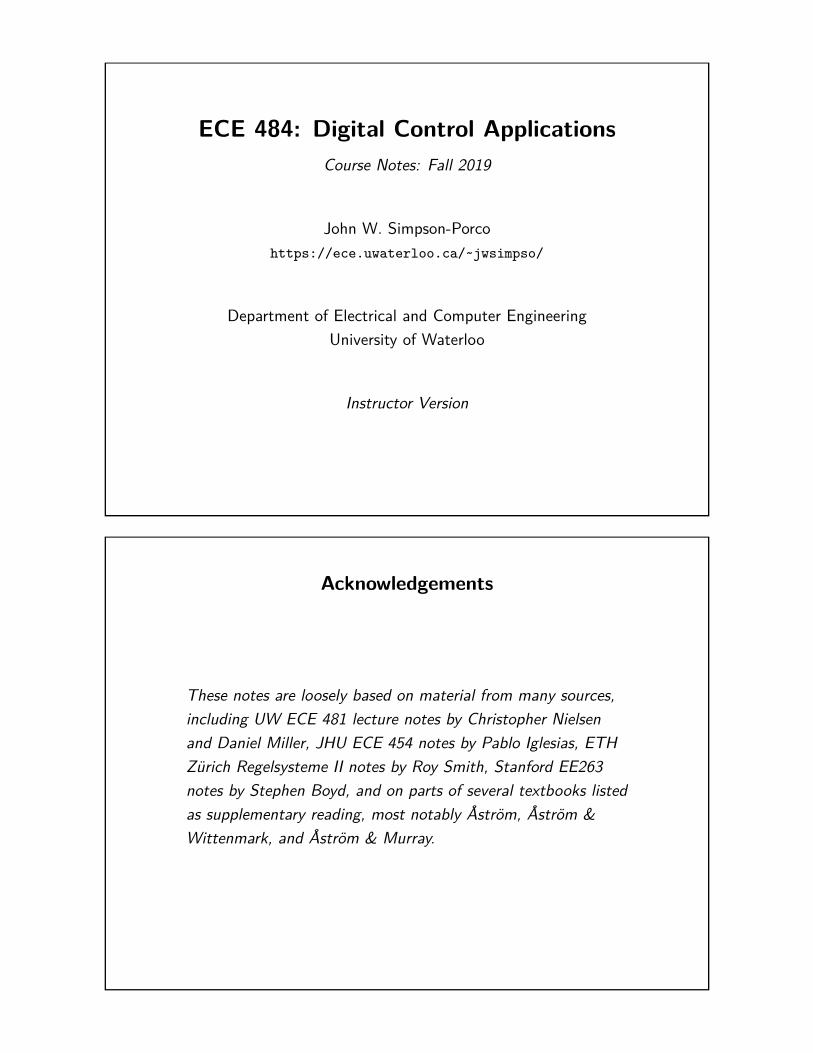
Goal: Design controller C(s) to achieve objectives. You already knowtools for analyzing and designing these systems:
I stability analysis: poles, Routh-Hurwitz test
I stability margins: gain and phase margins
I steady-state analysis: final value theorem
I transient specs: settling time, rise time, overshoot
I frequency domain analysis: Bode plots, Nyquist plots
I controller designs: PID, possibly lead/lag as well
Section 1: Introduction to digital control 1-22
Discrete-time control systems
C P
dr e u y
n
−
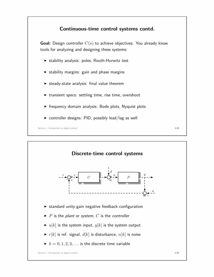
I standard unity-gain negative feedback configuration
I P is the plant or system, C is the controller
I u[k] is the system input, y[k] is the system output
I r[k] is ref. signal, d[k] is disturbance, n[k] is noise
I k = 0, 1, 2, 3, . . . is the discrete time variable
Section 1: Introduction to digital control 1-23
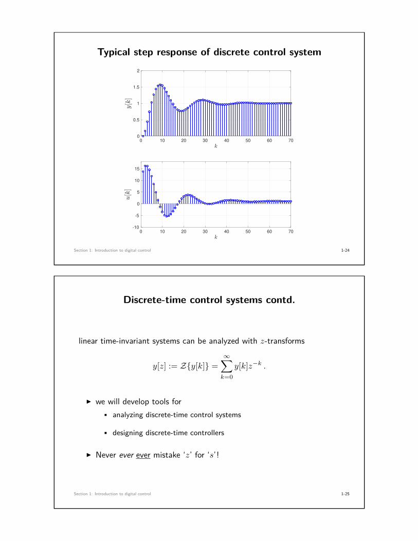
Typical step response of discrete control system
0
0.5
1
1.5
2
0 10 20 30 40 50 60 70
-10
-5
0
5
10
15
0 10 20 30 40 50 60 70
Section 1: Introduction to digital control 1-24
Discrete-time control systems contd.
linear time-invariant systems can be analyzed with z-transforms
y[z] := Z{y[k]} =∞∑k=0
y[k]z−k .
I we will develop tools for• analyzing discrete-time control systems
• designing discrete-time controllers
I Never ever ever mistake ‘z’ for ‘s’!
Section 1: Introduction to digital control 1-25
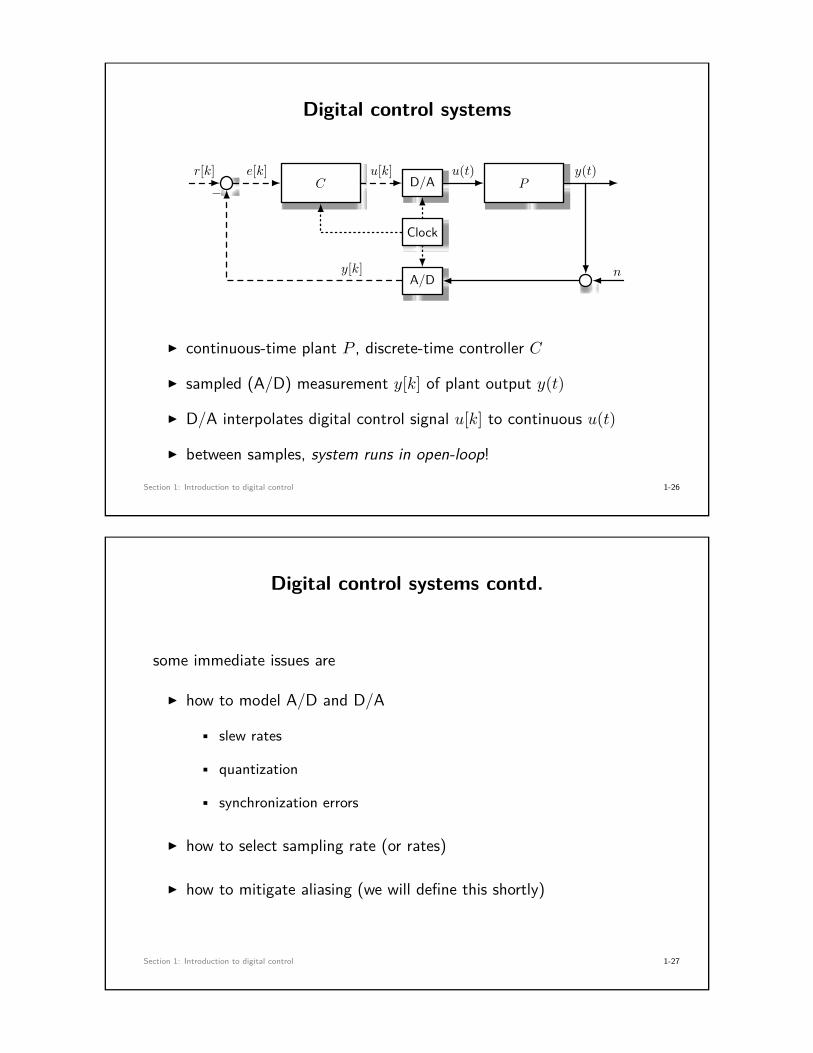
Digital control systems
C D/A P
A/D
Clock
r[k] e[k] u[k] u(t) y(t)−
y[k] n
I continuous-time plant P , discrete-time controller C
I sampled (A/D) measurement y[k] of plant output y(t)
I D/A interpolates digital control signal u[k] to continuous u(t)
I between samples, system runs in open-loop!
Section 1: Introduction to digital control 1-26
Digital control systems contd.
some immediate issues are
I how to model A/D and D/A
• slew rates
• quantization
• synchronization errors
I how to select sampling rate (or rates)
I how to mitigate aliasing (we will define this shortly)
Section 1: Introduction to digital control 1-27

Sampled-data control systems
C[z] HT P (s)
ST
r[k] e[k] u[k] u(t) y(t)−
y[k]
I sampled-data system is an idealized digital control system
I sampler ST and hold HT are perfectly timed, infinite precision
I sampled-data systems are not linear time-invariant systems!
I nonetheless, some simple analysis and design tools exist
Section 1: Introduction to digital control 1-28
Typical step response of sampled-data control system
0 1 2 3 4 5 6
0
0.5
1
1.5
2
0 1 2 3 4 5 6
-10
-5
0
5
10
15
Section 1: Introduction to digital control 1-29

Design methods for sampled-data systems
I emulation (discrete equivalent)
• design C(s) for P (s), the discretize C(s) to obtain C[z]
• advantage: simple
• disadvantage: requires “fast” sampling
I direct design (discrete design)
• discretize P (s) to obtain P [z], then directly design C[z] for P [z]
• advantage: can handle “slow” sampling rates
• disadvantage: more complicated to design and analyze
Section 1: Introduction to digital control 1-30
Ideal model for A/D conversion
I A/D modeled using ideal sampler block with period T
STy(t) y[k] = y(kT )
k = 0, 1, 2, 3 . . .
0 2 4 6 8 10 12
-150
-100
-50
0
50
100
-150
-100
-50
0
50
100
0 2 4 6 8 10 12
(note: T = 1s in figure)
Section 1: Introduction to digital control 1-31
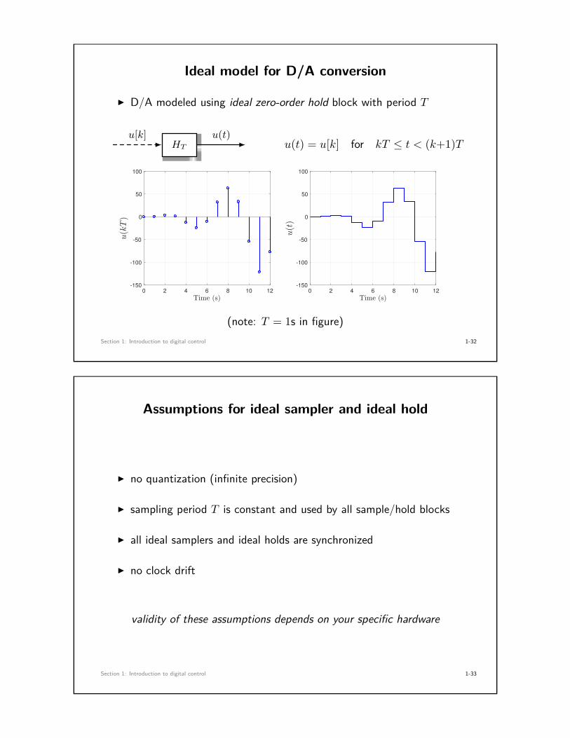
Ideal model for D/A conversion
I D/A modeled using ideal zero-order hold block with period T
HTu[k] u(t)
u(t) = u[k] for kT ≤ t < (k+1)T
-150
-100
-50
0
50
100
0 2 4 6 8 10 12 0 2 4 6 8 10 12
-150
-100
-50
0
50
100
(note: T = 1s in figure)Section 1: Introduction to digital control 1-32
Assumptions for ideal sampler and ideal hold
I no quantization (infinite precision)
I sampling period T is constant and used by all sample/hold blocks
I all ideal samplers and ideal holds are synchronized
I no clock drift
validity of these assumptions depends on your specific hardware
Section 1: Introduction to digital control 1-33

Aliasing
I suppose we sample a signal f(t) with sampling frequency ωs = 2πT
I aliasing occurs when f(t) contains frequency components higherthan ωNyq := ωs/2 (this is called the Nyquist frequency)
5 10 15 20 25
−1
−0.5
0.5
1
t
f(t)
Section 1: Introduction to digital control 1-34
Aliasing contd.
I sampling signal u1(t) = cos(ωt) at times tk = kT :
u1[k] = cos(ωkT ) = cos(
2π ωωsk
)I sampling signal u2(t) = cos((ω + ωs)t) yields
u2[k] = cos((ω + ωs)kT ) = cos(
2πω + ωs
ωsk
)= cos
(2π ωωsk + 2πk
)= cos
(2π ωωsk
)= u1[k]
I even though u1(t) 6= u2(t), we have identical sampled signals
Section 1: Introduction to digital control 1-35

Aliasing contd.
5 10 15 20
−1
−0.5
0.5
1
t
f(t)
Section 1: Introduction to digital control 1-36
Aliasing contd.
I sampling any member of the family of continuous-time signals
un(t) = cos ((ω ± nωs)t) , n ∈ Z
produces the same discrete-time signal
u[k] = cos(
2π ωωsk
)I we say the frequencies {ω± nωs} are aliases of the base frequency ω
with respect to the sampling frequency ωs
Section 1: Introduction to digital control 1-37

Example: Data acquisition in a lab
I sampling frequency 50Hz, T = 1/50
I signal of interest is at frequency 4Hz
I noise from lights at 60Hz, 120Hz, 180Hz
I sampled signal will only have components less than 25HzI 60Hz noise will be aliased to 60± n50
{. . . ,−40,10, 60, 110, . . .}
I 120Hz and 180Hz noise will be aliased to
{. . . ,−30,20, 70, . . .} and {. . . ,−70,−20, 30, 80, . . .}
Section 1: Introduction to digital control 1-38
Aliasing in control systems
I why care about aliasing for digital control?
I aliased noise enters controller, generating spurious control actions
C[z] HT P (s)
ST
r[k] e[k] u[k] u(t) y(t)
n(t)
−
y[k]
I example: 1 kHz noise in a motor control system, aliased down to10Hz, will then generate a real 10Hz oscillation on the motor shaft
Section 1: Introduction to digital control 1-39

Strategies for avoiding aliasing
two possible strategies for avoiding aliasing
1. sample very fast: ωs > 2× (highest frequency in meas. noise)
• often infeasible due to hardware limitations
2. include an analog low-pass filter f(s) in loop with cutoff ωcut
C[z] HT P (s)
ST f(s)
r[k] e[k] u[k] u(t) y(t)−
y[k] n(t)
• added expense, inflexible, introduces phase lag in loop
Section 1: Introduction to digital control 1-40
Example: prefiltering before sampling
I square wave with 0.9Hz oscillation, 1Hz sampling
0 10 20 30
-1
0
1
0 10 20 30
-1
0
1
0 10 20 30
-1
0
1
0 10 20 30
-1
0
1
Section 1: Introduction to digital control 1-41

Competing constraints on sampling rates
I many competing constraints on sampling frequency ωs
1. faster sampling = more expensive hardware
2. in emulation approach to digital control, we need to sample fast, orthe system will perform poorly
3. if we sample very fast, might not be able to compute control actionsbetween samples
4. sampling rates often fixed by installed sensors and actuators
Section 1: Introduction to digital control 1-42
Guidelines for filter design
I achievable performance depends on frequency spectrum of noise andfixed sampling rates of system
I filter cutoff design is a compromise between
1. introducing phase shift into the feedback loop
2. successfully filtering out the noise
I to minimize extra phase lag at crossover, want ωcut > ωbw
I to filter noise above Nyquist, want ωcut < ωNyq = ωs/2
I rough rule of thumb is therefore
ωbw < ωcut < ωs/2
Section 1: Introduction to digital control 1-43

Quick review: bandwidth of a system
I for “low-pass” transfer function, bandwidth ωbw is the frequencywhere the magnitude drops −3 dB below low-frequency magnitude
I first order system P (s) = 1τs+1 , τ > 0
−20
−40
1/τ
−3
Frequency (rad/s)
Amplitu
de(dB)
I Bandwidth is ωbw = 1/τ , and 90% rise time ≈ 2τ .Section 1: Introduction to digital control 1-44
Example: DC Motor Position Control
I goal: fast step reference tracking for motor control• θ = angular position, V = voltage applied• measurement noise of 0.02 rad at fnoise = 1005 Hz
PID[z] HT P (s)
ST
θref [k] e[k] V [k] V (t) θ(t)
n(t)
−
θ[k]
I motor model and controller given by
P (s) =1s
K
(Js+ b)(Ls+R) +K2 , PID[z] = Kp +Kdz − 1z
+Kiz
z − 1
Section 1: Introduction to digital control 1-45

Example: DC Motor Position Control
I controller designed with sampling period T = 0.001s
I unit step response of sampled-data system looks great . . .
0 0.01 0.02 0.03 0.04 0.05 0.06 0.07 0.08 0.09 0.1
0
0.2
0.4
0.6
0.8
1
1.2
Section 1: Introduction to digital control 1-46
Example: DC Motor Position Control
I but response contains unexpected ≈ 5 Hz oscillation
0 0.2 0.4 0.6 0.8 1 1.2 1.4 1.6 1.8 2
0
0.2
0.4
0.6
0.8
1
1.2
I Why? fs = 1000 Hz, fnoise = 1005 Hz!Section 1: Introduction to digital control 1-47
Example: DC Motor Position Control
I let’s add a low-pass anti-aliasing filter
PID[z] HT P (s)
ST(
ωcuts+ωcut
)N
θref [k] e[k] V [k] V (t) θ(t)−
θ[k] n(t)
I need to choose corner frequency ωcut and order N of filter• system bandwidth: rise time ≈ 0.01 s ⇒ ωbw ≈ 200 rad/s• Nyquist frequency: ωNyq = (2πfs)/2 ≈ 3100 rad/s
I not a lot of room (≈ one decade): use high-order for sharper cutoff
Section 1: Introduction to digital control 1-48
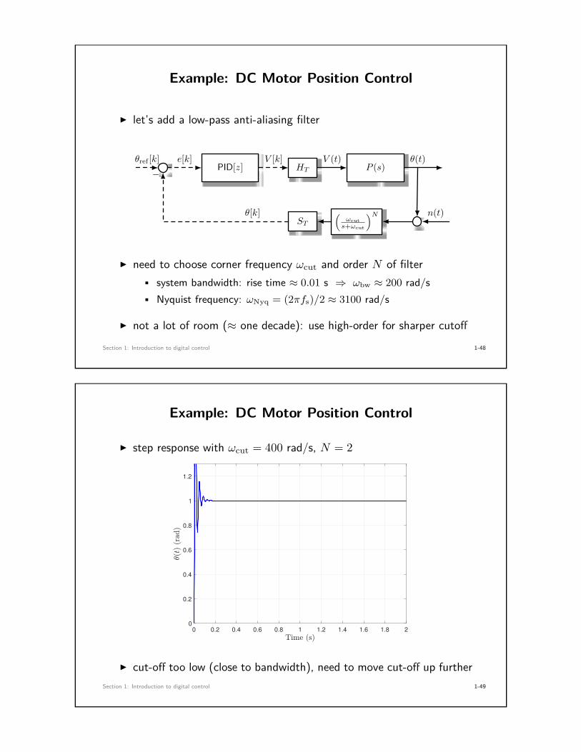
Example: DC Motor Position Control
I step response with ωcut = 400 rad/s, N = 2
0 0.2 0.4 0.6 0.8 1 1.2 1.4 1.6 1.8 2
0
0.2
0.4
0.6
0.8
1
1.2
I cut-off too low (close to bandwidth), need to move cut-off up furtherSection 1: Introduction to digital control 1-49

Example: DC Motor Position Control
I step response with ωcut = 3200 rad/s, N = 3
0 0.2 0.4 0.6 0.8 1 1.2 1.4 1.6 1.8 2
0
0.2
0.4
0.6
0.8
1
1.2
I exercise: play with ωs and N yourself in MATLAB codeSection 1: Introduction to digital control 1-50
MATLAB commands
I Plotting discrete-time signals: stem(t,y)
I Plotting held signals: stairs(t,y)
I Analog filtering signals (many different options)
s = tf(‘s’);f = (2*pi*f_cut)^2 / ...
(s^2 + 2*damping*2*pi*f_cut*s + (2*pi*f_cut)^2);u_filt = lsim(f,u,t);
Section 1: Introduction to digital control 1-51
Additional references
I introduction to digital control• Nielsen, Chapter 0
• Franklin, Powell, & Emami-Naeini, Chapter 8
• Franklin, Powell, & Workman, Chapter 1 and Chapter 3
• Phillips, Nagle, & Chakrabortty, Chapter 1
• Astrom & Wittenmark, Chapter 1
I sampling• Phillips, Nagle, & Chakrabortty, Chapter 3.2
I signal reconstruction• Phillips, Nagle, & Chakrabortty, Chapter 3.7
Section 1: Introduction to digital control 1-52
Personal Notes
Section 1: Introduction to digital control 1-53

Personal Notes
Section 1: Introduction to digital control 1-54
Personal Notes
Section 1: Introduction to digital control 1-55

2. Classical continuous-time control systems
• modeling for controller design• notation and Laplace transforms• continuous-time LTI systems• feedback stability• time-domain analysis• system approximation• PID control and its variants• static nonlinearities in control systems• reference tracking and the internal model principle• minor loop design
Section 2: Classical continuous-time control systems 2-56
Modeling for controller design
I models can be obtained from
• physics (Newton, Kirchhoff, Maxwell, fluid mechanics, . . . )• experiments on the system• combinations of these two
I many classes of possible models• finite-dimensional vs. infinite-dimensional• deterministic vs. random• linear vs. nonlinear• time-invariant vs. time-dependent• continuous-time vs. discrete-time vs. hybrid
I for control purposes, models just need to be “good enough”
Section 2: Classical continuous-time control systems 2-57

Steps for successful modeling
1. model for design (simplified) vs. model for simulation (complex)
2. break system into collection of subsystems with inputs and outputs
3. model each subsystem, keeping track of assumptions,approximations, etc.
4. interconnect subsystems to form full model
5. validate model experimentally, repeat steps as needed
Section 2: Classical continuous-time control systems 2-58
Notation
I set of real numbers R
I x ∈ S means x is a member of the set S
I set of complex numbers C
I strictly left/right-hand complex plane C−/C+
I the Laplace transform of a signal f(t) is given by
f(s) := L {f(t)} =∫ ∞
0f(t)e−st dt .
I Unit step function
1(t) =
1 if t ≥ 0
0 if else
Section 2: Classical continuous-time control systems 2-59

Key properties of Laplace transforms
I linearityL {α1f1 + α2f2} = α1f1(s) + α2f2(s)
I delayL {f(t− τ)} = e−τsf(s)
I integral formula
L
{∫ t
0f(τ) dτ
}= 1sf(s)
I derivative formula
L
{dfdt
}= sf(s)− f(0)
I convolutionL {g ∗ f} = g(s)f(s)
Section 2: Classical continuous-time control systems 2-60
Continuous-time causal LTI systems
I a system takes an input signal u(t) and produces output signal y(t)
Gu(t) y(t)
I linearity: if y1 = G(u1) and y2 = G(u2), then
G(α1u1 + α2u2) = α1G(u1) + α2G(u2) = α1y1 + α2y2 .
I time-invariance: if input u(t) produces output y(t), then for anydelay τ , input u(t− τ) produces output y(t− τ).
I causality: if u1(t) = u2(t) for all 0 ≤ t ≤ T , then y1(t) = y2(t) forall 0 ≤ t ≤ T .
Section 2: Classical continuous-time control systems 2-61

Representations of LTI systems
Gu y
I in Laplace-domain, multiplication with transfer function G(s)
y(s) = G(s)u(s)
I in time-domain, convolution with impulse response g(t)
y(t) = (g ∗ u)(t) =∫ t
0g(t− τ)u(τ) dτ .
I these are equivalent, can show that
G(s) = L {g(t)} and g(t) = L −1{G(s)}
Section 2: Classical continuous-time control systems 2-62
Transfer function representation contd.
G(s)u(s) y(s)
I we call G(s) rational if G(s) = N(s)D(s) for some polynomials N(s) and
D(s) with real coefficients
I a pole p ∈ C of G(s) satisfies lims→p |G(s)| =∞
I a zero z ∈ C of G(s) satisfies G(z) = 0
I the degree deg(D) of the denominator is the order of the system
I G(s) is proper if deg(N) ≤ deg(D), strictly proper ifdeg(N) < deg(D)
Section 2: Classical continuous-time control systems 2-63

Bounded-input bounded-output (BIBO) stability
I signal y(t) is bounded if there is M ≥ 0 s.t. |y(t)| ≤M for all t ≥ 0
Gu(t) y(t)
I BIBO stability: every bounded u(t) produces a bounded y(t)
I if the LTI system G is rational and proper, then G is BIBO stable ifand only if either of the following equivalent statements hold:
• every pole of transfer function G(s) belongs to C−
• the integral∫∞
0 |g(t)| dt of the impulse response is finite.
Section 2: Classical continuous-time control systems 2-64
Examples
1s+ 1
1s− 1
1s2 + 2s+ 1
Kp + Ki
s
s− 1s+ 1
1s2 + 2s− 1
e−t t100e−t 1(t) sin(ω0t)
Section 2: Classical continuous-time control systems 2-65

Feedback stability
C(s) P (s)
d(s)r(s) e(s) u(s) y(s)−
I r and d are external signals, e, u and y are internal signals
I definition: the closed-loop is feedback stable if every bounded pairof external inputs (r, d) leads to bounded internal responses (e, u, y)
I 2 external signals, 3 internal signals =⇒ 6 transfer functionse(s)r(s)
=1
1 + PC
u(s)r(s)
=C
1 + PC
y(s)r(s)
=PC
1 + PC
e(s)d(s)
=−P
1 + PC
u(s)d(s)
=1
1 + PC
y(s)d(s)
=P
1 + PC
I feedback stable if and only if all transfer func. are BIBO stableSection 2: Classical continuous-time control systems 2-66
Feedback stability contd.
I assume P (s) is rational and strictly proper: P (s) = Np(s)Dp(s)
I assume C(s) is rational and proper: C(s) = Nc(s)Dc(s)
I for example, we can calculate that
y(s)r(s) = PC
1 + PC=
NpDp
NcDc
1 + NpDp
NcDc
= NpNc
NpNc +DpDc
I the denominator is the characteristic polynomial
Π(s) := Np(s)Nc(s) +Dp(s)Dc(s)
I under these assumptions, the closed-loop is feedback stableif and only if all roots of Π(s) belong to C−.
Section 2: Classical continuous-time control systems 2-67

Pole-zero cancellations
plant: P (s) = Np(s)Dp(s) controller: C(s) = Nc(s)
Dc(s)
I a plant P and a controller C have a pole-zero cancellation if either
(a) Nc(s) and Dp(s) have a common root, or
(b) Np(s) and Dc(s) have a common root
I pole-zero cancellation is stable if the common root is in C−;otherwise, cancellation is unstable and must be avoided
I we only worry about pole-zero cancellations between systems;pole-zero cancellation between a system and a signal is fine!
Section 2: Classical continuous-time control systems 2-68
Example of unstable pole-zero cancellation
1s−1
s−1(s+1)2
r(s) e(s) u(s) y(s)−
=⇒ Π(s) = (s+ 1)2(s− 1) + (s− 1)
= (s− 1)(s2 + 2s+ 2)
I root at s = 1, feedback system is unstable. Note that
y(s)r(s) = 1
s2 + 2s+ 2 ,u(s)r(s) = (s+ 1)2
(s− 1)(s2 + 2s+ 2)
Section 2: Classical continuous-time control systems 2-69

Example of unstable pole-zero cancellation
1s−1
s−1(s+1)2
r(s) e(s) u(s) y(s)−
0 1 2 3 4 5 6
0
200
400
600
800
1000
1200
1400
0 1 2 3 4 5 6
0
0.5
1
1.5
I Output y(t) looks fine, but control u(t) blows up!Section 2: Classical continuous-time control systems 2-70
Time-domain analysis
Gu(t) y(t)
(i) rise time Tr, settling time Ts
(ii) peak time Tp, peak max Mp
(iii) steady state value yss? t
y(t)Mp
yss r
TpTr Ts
I Final value theorem: if f(s) = L {f(t)} is rational and proper,with all poles of sf(s) contained in C− then fss = limt→∞ f(t)exists and
fss = limt→∞
f(t) = lims→0
sf(s) .
Section 2: Classical continuous-time control systems 2-71

The “DC gain” of G(s) is G(0)
I suppose G(s) is rational, proper, and BIBO stable T.F.
I response to step input of amplitude A, i.e., u(s) = As is
y(s) = G(s)u(s) = G(s)As
I final value of response given by
yss = limt→∞
y(t) = lims→0
sy(s) = lims→0
sG(s)1s·A = G(0) ·A
I G(0) is therefore the steady-state gain of the system, i.e., theamplification a constant input will experience
Section 2: Classical continuous-time control systems 2-72
Second-order systems
G(s) = Kω2n
s2 + 2ζωns+ ω2n
I natural frequency ωn > 0, damping ratio ζ > 0, DC gain K
I many systems can be well-approximated as second-order
I overdamped (ζ > 1), critically damped (ζ = 1)
I underdamped (ζ < 1)
s = −ζωn ± jωn√
1− ζ2
= ωne±j(π−θ)
θ = arccos(ζ) .
Re(s)
Im(s)
ωn
√1− ζ2
−ζωnθ
×
×
Section 2: Classical continuous-time control systems 2-73

Second-order systems contd.
t
y(t)Mp
yss r
TpTr Ts
I closed-form results
Tp = π
ωn√
1− ζ2, Ts ≈
4ζωn
%OS = Mp −KK
= exp(−ζπ√1− ζ2
)I to identify parameter values
• apply step
• measure yss,%OS, and Tp
• solve for ωn, ζ,K
Section 2: Classical continuous-time control systems 2-74
System approximation
I approximate higher-order system with lower-order oneI example:
G(s) = s+ 10(s+ 11)(s+ 12)(s2 + 2s+ 2)
Re(s)
Im(s)
×× ◦×
×
Section 2: Classical continuous-time control systems 2-75

System approximation contd.
G(s) = s+ 10(s+ 11)(s+ 12)(s2 + 2s+ 2)
= s+ 10(s+ 11)(s+ 12)︸ ︷︷ ︸
Gfast(s)
· 1s2 + 2s+ 2︸ ︷︷ ︸Gslow(s)
I if Gfast(s) is BIBO stable=⇒ response due to Gfast(s) quickly reaches steady-state
I replace Gfast(s) with its steady-state value (DC gain) Gfast(0)
G(s) ≈ Gfast(0)Gslow(s) .
I valid if fast poles/zeros are approx. 10x faster than slow poles/zerosSection 2: Classical continuous-time control systems 2-76
Step response for example
0 1 2 3 4 5 6 7
0
0.01
0.02
0.03
0.04
0.05
I note: approximation very good for step inputsSection 2: Classical continuous-time control systems 2-77

Bode diagram for example
10-2
10-1
100
101
102
103
-200
-150
-100
-50
0
10-2
10-1
100
101
102
103
-300
-250
-200
-150
-100
-50
0
I note: approximation very good up to ≈ 1 rad/sSection 2: Classical continuous-time control systems 2-78
PID control
I most basic proportional-integral-derivative controller
u(t) = K
(e(t) + 1
Ti
∫ t
0e(τ) dτ + Td
de(t)dt
)where K is the proportional gain, Ti is the integral time constant,and Td is the derivative time constant
I in transfer function form, we have
C(s) = K
(1 + 1
sTi+ Tds
)I this form is called the “non-interacting” parameterization; other
parameterizations are also common (e.g., with gains Kp,Ki,Kd);
Section 2: Classical continuous-time control systems 2-79

PID control contd.
I the rough interpretation of the terms is• present: proportional term reacts to present error• past: integral term reacts to cumulative error in the past• future: derivative term reacts to rate of change of error (tries to
predict where error is going)
I PID is bread-and-butter: likely 90% of all controllers in industry arePID, and 90% of those are PI controllers
I standard tuning methods available (e.g., Ziegler-Nichols, or fancierones like pidtool in MATLAB)
I we will not review the basics of tuning PID loops here, but willinstead look at some refinements and advanced topics
Section 2: Classical continuous-time control systems 2-80
PID control with derivative filter
I pure derivative control is never implemented, as it is very sensitive tohigh-frequency noise (to convince yourself, plot the Bode plot)
I all implementations add a low-pass filter to derivative term
C(s) = K
(1 + 1
sTi+ Tds
Tds/N + 1
)I time constant of low-pass filter is Td/N
I N ranges between roughly 5 and 20• larger N =⇒ less noise filtering, but better control performance• smaller N =⇒ more noise filtering, but worse control performance
Section 2: Classical continuous-time control systems 2-81

Example: PID with derivative filter
I consider PID control system with measurement noise
PID 1(s+1)3
r e u y
n
−
I PID controller gains K = 3, Ti = 2 s, Td = 0.5 s, N = 10
I measurements y(t) corrupted by measurement noise
Section 2: Classical continuous-time control systems 2-82
Example: PID with derivative filter contd.
0 5 10 15 20
-1
0
1
2
3
0 5 10 15 20
-5
0
510
4
-50
0
50
I note the two y-axes on the plots of u(t); standard PID controlgenerates huge control signals due to fast-varying noise
Section 2: Classical continuous-time control systems 2-83
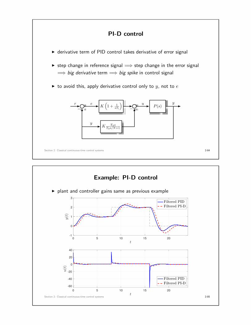
PI-D control
I derivative term of PID control takes derivative of error signal
I step change in reference signal =⇒ step change in the error signal=⇒ big derivative term =⇒ big spike in control signal
I to avoid this, apply derivative control only to y, not to e
K(
1 + 1sTi
)
K TdsTds/N+1
P (s)r e u y
−
y
−
Section 2: Classical continuous-time control systems 2-84
Example: PI-D control
I plant and controller gains same as previous example
0 5 10 15 20
-1
0
1
2
3
0 5 10 15 20
-60
-40
-20
0
20
40
Section 2: Classical continuous-time control systems 2-85

Static nonlinearities in control systems
I sensors and actuators are often nonlinear
C(s) ϕ(·) P (s)ur e y
−
I example: suppose you want to shine light on a semiconductorsurface by applying a voltage to a filament: irradiance ∼ voltage2
I common nonlinearities: hysteresis, relay, saturation, deadzone . . .
Section 2: Classical continuous-time control systems 2-86
Inverting actuator nonlinearities
I a function ϕ(·) is right-invertible if there is a function ψ(·) such that
ϕ(ψ(x)) = x
I example: ψ(x) =√x is a right-inverse for ϕ(x) = x2 for all x ≥ 0
I many actuator nonlinearities can be handled by using a right-inverse
C(s) ψ(·) ϕ(·) P (s)ur e y
−
I now can design C(s) for P (s) like usualSection 2: Classical continuous-time control systems 2-87

Limit cycles due to nonlinearities
I a limit cycle is a sustained nonlinear oscillation
I common in nature (heart beats, planetary orbits, animal populations)
I limit cycles occur in feedback systems with certain nonlinearities
I example: thermostat control systems
on
off1s+a
ur e y
−
Section 2: Classical continuous-time control systems 2-88
Thermostat temperature response to 20◦ setpoint
0 10 20 30 40 50 60 70 80 90 100
17
18
19
20
21
22
23
0 10 20 30 40 50 60 70 80 90 100
0
0.5
1
1.5
2
Section 2: Classical continuous-time control systems 2-89

Saturation in control systems
I another very common nonlinearity is saturation
KTi
1s
K
1s
ure
u y
−
PI Controller
I saturation limits output from controller
I when saturation is reached, control loop is “broken”
I can cause steady-state error, bad performance, or instabilitySection 2: Classical continuous-time control systems 2-90
Example: step response of system with saturation
0 5 10 15 20
-3
-2
-1
0
1
2
3
0 5 10 15 20
-3
-2
-1
0
1
2
3
Section 2: Classical continuous-time control systems 2-91
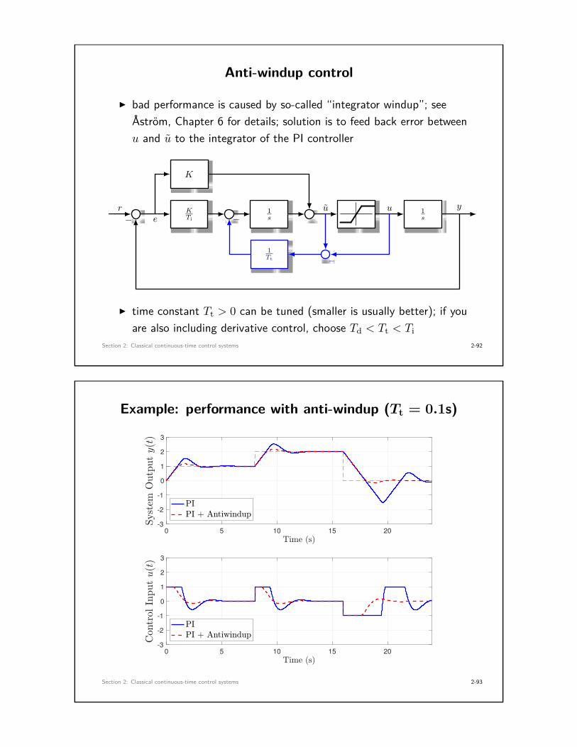
Anti-windup control
I bad performance is caused by so-called “integrator windup”; seeÅström, Chapter 6 for details; solution is to feed back error betweenu and u to the integrator of the PI controller
KTi
1s
K
1s
ure
u y
−
1Tt −
−
I time constant Tt > 0 can be tuned (smaller is usually better); if youare also including derivative control, choose Td < Tt < Ti
Section 2: Classical continuous-time control systems 2-92
Example: performance with anti-windup (Tt = 0.1s)
0 5 10 15 20
-3
-2
-1
0
1
2
3
0 5 10 15 20
-3
-2
-1
0
1
2
3
Section 2: Classical continuous-time control systems 2-93

Static friction in mechanical control systems
I very common nonlinearity, difficult to model accurately
I can lead to tracking errors, oscillations, instability
I deadzone model of static friction
1ms2
u y
PID 1ms2
r e y
−
Section 2: Classical continuous-time control systems 2-94
Example: step response of mass with PID + stiction
0 50 100 150 200 250 300 350 400
0
0.5
1
1.5
2
0 50 100 150 200 250 300 350 400
-0.05
0
0.05
Section 2: Classical continuous-time control systems 2-95

Control strategies for static friction
I one approach: invert deadzone nonlinearity in controller
PID 1ms2
r e y
−
I size of inverted deadzone must be tuned
I other approaches: dither signal, dynamic friction estimator
Section 2: Classical continuous-time control systems 2-96
Example: PID with friction compensation
0 5 10 15 20
-1
0
1
2
3
0 5 10 15 20
-0.3
-0.2
-0.1
0
0.1
0.2
Section 2: Classical continuous-time control systems 2-97

Tracking reference signals
C(s) P (s)r e u y
− P (s) = Np(s)Dp(s)
C(s) = Nc(s)Dc(s)
I Perfect asymptotic tracking problem: Given P (s), designcontroller C(s) such that closed-loop system is feedback stable and
limt→∞
(r(t)− y(t)) = 0 .
I step tracking is special case when r(t) is a step function
I application areas: power electronics, position control, robotics, . . .
Section 2: Classical continuous-time control systems 2-98
Requirements for step tracking
transfer function from r(s) to e(s) = r(s)− y(s) is
e(s)r(s) = 1
1 + P (s)C(s) = Dp(s)Dc(s)Np(s)Nc(s) +Dp(s)Dc(s) = Dp(s)Dc(s)
Π(s) .
I suppose we had a step r(t) = 1(t) =⇒ r(s) = 1s
e(s) = Dp(s)Dc(s)Π(s) · 1
s
I by final value theorem e(t)→ 0 if
(a) Π(s) has all roots in C− (i.e., system is feedback stable)(b) lims→0
Dp(s)Dc(s)Π(s) = 0 ⇐⇒ Dp(0)Dc(0) = 0.
I therefore, product of P and C must have a pole at s = 0Section 2: Classical continuous-time control systems 2-99

Three cases for step-tracking
I if P (s) has a zero at s = 0, then step-tracking is not possible (why?)
I if P (s) has a pole at s = 0, C(s) can be any stabilizing controller
I if P (s) does not have a pole or zero at s = 0, then C(s) must havea pole at s = 0
• design approach: let C(s) = 1sC1(s), then design stabilizing C1(s)
I having a pole at s = 0 in the controller is integral control
u(s) = 1se(s) =⇒ u(t) =
∫ t
0e(τ) dτ
I how does this generalize for other reference signals?Section 2: Classical continuous-time control systems 2-100
The Internal Model Principle
I definition: a transfer function G(s) contains an internal model of areference signal r(s) if every pole of r(s) is a pole of G(s)
I example:
G(s) = s+ 1(s2 + 1)(s2 − 4) r(s) = s+ 2
(s2 + 1)(s+ 3)
Internal Model Principle: Assume P (s) is strictly proper,C(s) is proper, and that the closed-loop system is feedbackstable. Then limt→∞(y(t)− r(t)) = 0 if and only if P (s)C(s)contains an internal model of the unstable part of r(s).
Section 2: Classical continuous-time control systems 2-101

Example: sinusoidal tracking
P (s) = 1s+ 1 r(t) = r0 sin(t) =⇒ r(s) = r0
s2 + 1
Let’s choose: C(s) = 1s2 + 1C1(s)
I exercise: check using Routh that C1(s) = sτs+1 is stabilizing for
sufficiently small τ > 0
I exercise: check by hand using FVT that limt→∞ e(t) = 0
Section 2: Classical continuous-time control systems 2-102
Example: sinusoidal tracking
0 5 10 15 20 25 30 35
-1.5
-1
-0.5
0
0.5
1
1.5
Section 2: Classical continuous-time control systems 2-103

Example: ramp tracking
I plant is double-integrator
P (s) = 1s2
I reference signal is ramp
r(t) = 2t =⇒ r(s) = 2s2
I plant contains internal model, just design stabilizing C(s)
I for example, filtered PD controller
C(s) = Kp +Kds
τs+ 1
Section 2: Classical continuous-time control systems 2-104
Example: ramp tracking
0 2 4 6 8 10
0
5
10
15
20
Section 2: Classical continuous-time control systems 2-105

More comments on stabilization step for tracking
I our controller is C(s) = Φ(s)C1(s), where Φ(s) includes the polesthat we know we need for tracking – how do we design C1(s)?
C1(s) Φ(s) P (s)r e u y
−
C(s)
I we can equivalently group Φ(s) with P (s) (same block diagram)
I use the augmented plant Paug(s) = Φ(s)P (s), and design C1(s)using any technique you want to stabilize the system Paug(s)
Section 2: Classical continuous-time control systems 2-106
Minor loop design
I a.k.a. master/slave, primary/secondary, or cascade design
I extremely common (process control, motors, power electronics . . . )
I very useful when you have an intermediate measurement (e.g., plantis a series combination of two subsystems)
Controller Plant 1 Plant 2yr e y
−
I if we can also measure y, lets use another feedback loop
Section 2: Classical continuous-time control systems 2-107

Minor loop design
I idea: design sequence of nested feedback loops
Cmajor Cminor Plt 1 Plt 2ry ry y y
− −
I minor/inner loop is designed first• control such that y quickly tracks ry (high-bandwidth)
I major/outer loop is designed second• lets y track ry (lower bandwidth by factor 5–10)
Section 2: Classical continuous-time control systems 2-108
Example: single phase inverter
Inverter
vinLf if vf
Cf
igridvgrid
I LC filter removes harmonics from switching inside inverter
I objective: design input voltage vin such that vf (t) tracks signal
vref(t) =√
2 · 120 · cos(ω0t) , ω0 = 2π60 rad/s
I we can measure both current if and voltage vf
Section 2: Classical continuous-time control systems 2-109

Response of single-phase inverter
I open-loop response with vin(t) = vref(t) =√
2 · 120 · cos(ω0t)I disturbance igrid(t) =
√2 · 20 · sin(ω0t) applied after 3 cycles
0 1 2 3 4 5 6
-300
-200
-100
0
100
200
300
Section 2: Classical continuous-time control systems 2-110
Single phase inverter contd.
I Laplace-domain representation of circuit
−+vin(s)
sLf if vf (s)
1sCf
igridvgrid(s)
inductor current: if (s) = 1sLf
(vin(s)− vf (s))
current balance: sCfvf (s) = if (s)− igrid(s)
Section 2: Classical continuous-time control systems 2-111

Single phase inverter contd.
I feedback diagram for plant
1sLf
1sCf
vin if vf−
igrid
−
I design minor current loop so current if tracks reference ireff
1sLf
1sCf
if vf−
igrid
Cminorviniref
f −−
Section 2: Classical continuous-time control systems 2-112
Single phase inverter contd.
I typically use a PI controller
Cminor(s) = Kp1 + τs
τs
where Kp is the proportional gain, τ is time constant
I key point: minor loop must be fast (Kp big, τ small)
I over time-scale of minor loop, vf is a constant disturbance
Πminor(s) = Kp(1 + τs) + τs(sLf ) = τLfs2 +Kpτs+Kp
I for critical damping, take Kp = 4Lf/τ , then make τ << 1ω0
Section 2: Classical continuous-time control systems 2-113

Single phase inverter contd.
I design major voltage loop so vf tracks vreff
1sLf
1sCf
if vf−
igrid
Kp1+τsτs
Cmajorviniref
fvreff −
−−
I to track sinusoidal vreff , Cmajor(s) needs internal model
L {cos(ω0t)} = s
s2 + ω20
=⇒ Cmajor(s) = K1 +K2s
s2 + ω20.
I called a proportional-resonant controller
Section 2: Classical continuous-time control systems 2-114
Single phase inverter contd.
I now design major loop separately
Πmajor(s) = Cfs3 +K1s
2 + (Cfω20 +K2)s+K1ω
20
I exercise: derive the stability conditions K1 > 0, K2 > 0
1sLf
1sCf
if vf−
igrid
Kp1+τsτs
K1 +K2s
s2+ω20
vinireffvref
f −−−
Section 2: Classical continuous-time control systems 2-115

Single phase inverter contd.
I inverter with Cf = 50µF, Lf = 1.5mH, vref is 60Hz 120V RMSI disturbance igrid =
√2 · 20 · sin(ω0t) applied after 3 cycles
0 1 2 3 4 5 6
-200
-150
-100
-50
0
50
100
150
200
Section 2: Classical continuous-time control systems 2-116
MATLAB commands
I computing Laplace transform F (s) of f(t) = sin(ωt)
syms t w s; F = laplace(sin(w*t),s);
I inverse Laplace transform
f = ilaplace(w/(s^2 + w^2),t);
I defining transfer functions
s = tf(‘s’); G = (s-2)/(s^2+3);
I pole(G); zero(G); step(G); bode(G);
I feedback interconnection
T = feedback(P*C,1);
Section 2: Classical continuous-time control systems 2-117

Additional references
I Nielsen, Chapters 1 and 2
I Franklin, Powell, and Workman, Chapter 2
I Franklin, Powell, and Emami-Naeini, Chapter 3 and Chapter 4
I MTE 360 / ECE 380 course notes
I Åström & Murray, Chapters 8, 9, 10, 11
I Åström, Chapter 6 (pdf)
Section 2: Classical continuous-time control systems 2-118
Additional references
I tracking reference signals
• Franklin, Powell, & Emami, Chapter 4.2• Nielsen, Chapter 1.6
I minor loop design
• Wikipedia, Minor loop feedback
I Smith predictor
• Franklin, Powell, & Emami, Chapter 7.13
Section 2: Classical continuous-time control systems 2-119

Personal Notes
Section 2: Classical continuous-time control systems 2-120
Personal Notes
Section 2: Classical continuous-time control systems 2-121

Personal Notes
Section 2: Classical continuous-time control systems 2-122
3. Emulation design of digital controllers
• controller emulation• emulation techniques• stability of discretized controllers• emulation design procedure• modified emulation design procedure
Section 3: Emulation design of digital controllers 3-123

Controller emulation
C(s) P (s)d
r e u y
−
I suppose we have designed a continuous controller C(s) for P (s)
I need to convert C(s) to digital controller C[z]
I some immediate questions:• is there a unique way to do this?• how do we select sampling rates?
Section 3: Emulation design of digital controllers 3-124
The emulation problem
I given an analog controller C(s), select a sampling period T > 0 anda discrete controller Cd[z] such that the sampled-data control system
Cd[z] HT P (s)
ST
r[k] e[k] u[k] u(t) y(t)−
y[k]
closely approximates the continuous-time control system
C(s)e(t) u(t) '
ST Cd[z] HTe(t) u(t)
Section 3: Emulation design of digital controllers 3-125

Quick review: z-transforms
I discrete signal f [k] is a sequence f [0], f [1], f [2], . . .
I the z-transform of a discrete-time signal f [k] is
f [z] := Z{f [k]} =∞∑k=0
f [k]z−k , z ∈ C .
I linearity: Z{α1f1 + α2f2} = α1f1[z] + α2f2[z]
I delay formulaZ {f [k − 1]} = z−1f [z]
I convolution
Z{g ∗ f} = Z{
k∑m=0
g[k −m]f [m]}
= g[z]f [z]
Section 3: Emulation design of digital controllers 3-126
Controller emulation
I we will not do a general derivation, but motivate through an example
I integral controller C(s) = 1/s
u(s) = 1se(s) ⇐⇒ u(t) = e(t) ⇐⇒ u(t) = u(t0) +
∫ t
t0
e(τ) dτ
I how to implement this in discrete-time? For sampling period T
u(kT ) = u((k − 1)T ) +∫ kT
(k−1)Te(τ) dτ
u[k] = u[k − 1] +∫ kT
(k−1)Te(τ) dτ
I need to approximate integral over interval between samplesSection 3: Emulation design of digital controllers 3-127

The bilinear discretization
I also called trapezoidal or Tustin discretization
t
e(t)
(k − 1)T kT
•
•slope = e(kT )− e((k − 1)T )
T
∫ kT
(k−1)T≈ Te[k − 1]︸ ︷︷ ︸
rectangle
+ 12T (e[k]− e[k − 1])︸ ︷︷ ︸
triangle
= T
2 (e[k − 1] + e[k])
Section 3: Emulation design of digital controllers 3-128
The bilinear discretization contd.
I we therefore have the difference equation
u[k] = u[k − 1] + T
2 (e[k − 1] + e[k])
I taking z-transforms, we obtain
u[z] = z−1u[z]+ T
2(z−1 + 1
)e[z] =⇒ u[z]
e[z] = Cd[z] = T
2z + 1z − 1
I but our original controller was C(s) = 1s . Comparing, we find
Cd[z] = C(s)∣∣∣s= 2
Tz−1z+1
⇐⇒ s = 2T
z − 1z + 1
I derivation was for integral controller, but this rule is general
Section 3: Emulation design of digital controllers 3-129

Example: PID controller
C(s) = Kp +Kds+ 1sKi =⇒ Cd[z] = Kp +Kd
2T
z − 1z + 1 +Ki
T
2z + 1z − 1
Cd[z] = 2TKp(z + 1)(z − 1) + 4Kd(z − 1)2 + T 2Ki(z + 1)2
2T (z + 1)(z − 1)
therefore, we obtain Cd[z] = β0z2 + β1z + β2
z2 − 1
β0 = (2TKp + 4Kd + T 2Ki)/(2T ) , β1 = (2T 2Ki − 8Kd)/(2T )
β2 = (4Kd + T 2Ki − 2TKp)/(2T )
Section 3: Emulation design of digital controllers 3-130
From transfer function to difference equation
I after simplifying Cd[z], we always get a rational TF (why?)
Cd[z] = β0zn + β1z
n−1 + · · ·+ βnzn + α1zn−1 + · · ·+ αn
I for implementation need a difference equation
1. divide top and bottom through by zn
C[z] = u[z]e[z] = β0 + β1z
−1 + · · ·+ βnz−n
1 + α1z−1 + · · ·+ αnz−n
2. rearrange
(1 + α1z−1 + · · ·+ αnz
−n)u[z] = (β0 + β1z−1 + · · ·+ βnz
−n)e[z]
3. inverse z-transform both sides
u[k] + α1u[k − 1] + · · ·+ αnu[k − n] = β0e[k] + β1e[k − 1] + · · ·
Section 3: Emulation design of digital controllers 3-131

Implementing difference equation
I suppose we want to implement controller u[k] = u[k − 1] + e[k]I loop the following code
read y from A/De = r - y;u = u_old + e;
output u from D/Au_old = u;
return to ‘read’ after T seconds from last ‘read’
I note: we always output new value for u[k] as soon as it is available
Section 3: Emulation design of digital controllers 3-132
Example: PID controller
Cd[z] = u[z]e[z] = β0z
2 + β1z + β2
z2 − 1
divide top and bottom by z2
u[z]e[z] = β0 + β1z
−1 + β2z−2
1− z−2
multiply through and invert term-by-term
u[k]− u[k − 2] = β0e[k] + β1e[k − 1] + β2e[k − 2]
oru[k] = u[k − 2] + β0e[k] + β1e[k − 1] + β2e[k − 2]
Section 3: Emulation design of digital controllers 3-133
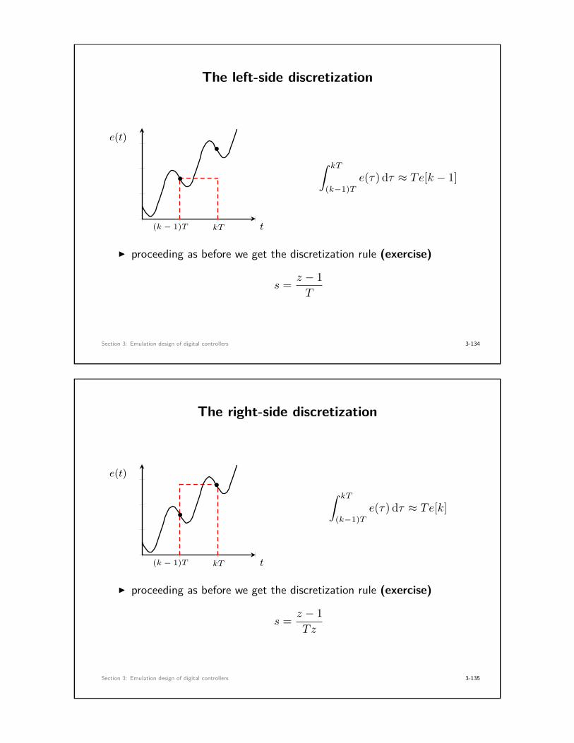
The left-side discretization
t
e(t)
(k − 1)T kT
•
•∫ kT
(k−1)Te(τ) dτ ≈ Te[k − 1]
I proceeding as before we get the discretization rule (exercise)
s = z − 1T
Section 3: Emulation design of digital controllers 3-134
The right-side discretization
t
e(t)
(k − 1)T kT
•
•
∫ kT
(k−1)Te(τ) dτ ≈ Te[k]
I proceeding as before we get the discretization rule (exercise)
s = z − 1Tz
Section 3: Emulation design of digital controllers 3-135
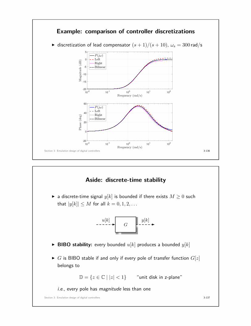
Example: comparison of controller discretizations
I discretization of lead compensator (s+ 1)/(s+ 10), ωs = 300 rad/s
10-2
10-1
100
101
102
-20
-15
-10
-5
0
5
10-2
10-1
100
101
102
-20
0
20
40
60
Section 3: Emulation design of digital controllers 3-136
Aside: discrete-time stability
I a discrete-time signal y[k] is bounded if there exists M ≥ 0 suchthat |y[k]| ≤M for all k = 0, 1, 2, . . .
Gu[k] y[k]
I BIBO stability: every bounded u[k] produces a bounded y[k]
I G is BIBO stable if and only if every pole of transfer function G[z]belongs to
D = {z ∈ C | |z| < 1} “unit disk in z-plane”
i.e., every pole has magnitude less than oneSection 3: Emulation design of digital controllers 3-137

Stability of discretized controllers
I any good discretization should be such that as T → 0, theapproximation becomes perfect; bilinear, left-side, and right-side allsatisfy this
I how else should we compare/contrast discretization schemes?
I can ask: does discretization preserves stability of the controller?
I of our three schemes, only bilinear does so!
I proof:
s = 2T
z − 1z + 1 ⇐⇒ z =
1 + T2 s
1− T2 s
Section 3: Emulation design of digital controllers 3-138
Bilinear discretization preserves BIBO stability
I suppose C(s) has a pole at s ∈ C−
I then Cd[z] must have a pole at z = 1+T2 s
1−T2 s
Re(z)
Im(z)
+1−1
T2 s ×∣∣1 + T
2 s∣∣ ∣∣1− T
2 s∣∣ |z| =
∣∣1 + T2 s∣∣∣∣1− T
2 s∣∣ < 1
therefore, z ∈ D(converse also true)
Section 3: Emulation design of digital controllers 3-139

Summary of bilinear discretization
s-plane z-plane
Re(s)
Im(s) z = 1+T2 s
1−T2 s
s = 2Tz−1z+1
Re(z)
Im(z)
+1−1
D
C(s) BIBO stable ⇐⇒ Cd[z] BIBO stable
Section 3: Emulation design of digital controllers 3-140
Final comments on stability
I the previous stability results refer to stability of the controller, andnot feedback stability of the sampled-data system
I feedback stability of sampled-data control system determined by theratio of the sampling frequency ωs to the bandwidth of theclosed-loop continuous-time control system ωbw
I rule of thumb: for best performance, choose ωs = 2πT to be 25
times the bandwidth of the closed-loop continuous-time system
I for sample rates slower than 20 times the closed-loop bandwidth,consider instead using direct digital design.
Section 3: Emulation design of digital controllers 3-141

Design procedure for controller emulation
1. design – by any method – a controller C(s) for P (s) to meet designspecifications
2. select a sampling period and emulate C(s) to obtain Cd[z]
3. simulate the closed-loop sampled data-system, and adjust designor sampling period as needed
4. implement Cd[z] as a difference equation
I once again, rule of thumb: ωs = 2πT ≥ 25ωbw
Section 3: Emulation design of digital controllers 3-142
Design example: cruise control
mFengine = u(t)Fdrag = bv
+v
I objective: track constant reference velocity commandsI design specs: 5% overshoot, 7s settling time for 0 to 100 km/hI m = 1200 kg, b = 10000Ns/m
P (s) = (8.33× 10⁻⁷)s+ (8.33× 10⁻³) , C(s) = 1
s
(8.6× 10⁵)s+ (5.2× 10³)s+ 1.2
Section 3: Emulation design of digital controllers 3-143

Design example: cruise control contd.
I check bandwidth of closed-loop transfer function T (s) = y(s)/r(s)
10-1
100
101
102
-100
-80
-60
-40
-20
0
20
ωbw ≈ 1.2 rad/s =⇒ ωs ≥ 25(1.2) = 30 rad/s
=⇒ T ≤ 2π30 ≈ 0.2 s
Section 3: Emulation design of digital controllers 3-144
Design example: cruise control contd.
I discretize controller using bilinear transform with T = 0.2s
T = 0.2;C_d = c2d(C,T,‘tustin’)
Cd[z] = (7.742× 10⁴)z2 + (154.3)z − (7.727× 10⁴)z2 − 1.785z + 0.7854
I simulate sampled-data system
Cd[z] HT P (s)
ST
r[k] e[k] u[k] u(t) y(t)−
y[k]
Section 3: Emulation design of digital controllers 3-145

Design example: cruise control contd.
0 2 4 6 8 10 12 14 16 18 20
0
20
40
60
80
100
120
Section 3: Emulation design of digital controllers 3-146
Design example: cruise control contd.
0 2 4 6 8 10 12 14 16 18 20
-2
0
2
4
6
8
10
12
14
Section 3: Emulation design of digital controllers 3-147

Design example: cruise control contd.
0 2 4 6 8 10 12 14 16 18 20
0
20
40
60
80
100
120
140
I system becomes unstable for T ≥ 4I performance getting worse with slower sampling rates – why?
Section 3: Emulation design of digital controllers 3-148
Design example: cruise control contd.
I control input for T = 1.5s sampling rate
0 2 4 6 8 10 12 14 16 18 20
-5
0
5
10
15
20
Section 3: Emulation design of digital controllers 3-149

Effect of sample-and-hold blocks
I consider the sample-hold combination
ST HTf(t) g(t)
I if we ignore the effects of sample-and-hold, then g(t) ≈ f(t)
f(t)
g(t)
f(t− T2 )
t
better approximation is
g(t) ≈ f(t− T
2
)(time delay!)
Section 3: Emulation design of digital controllers 3-150
“Proof” of T/2 delay
I exercise: sample-and-hold HTST has impulse response
g(t) =
1T if 0 ≤ t ≤ T
0 otherwise
I exercise: compute the transfer function G(s)
G(s) = L {g(t)} = 1− e−sT
sT
=−∑∞k=1(−sT )k/k!
sT
= 1− sT/2 + · · ·
≈ e−T2 s
Section 3: Emulation design of digital controllers 3-151

Approximating sample-and-hold with delay
I to account for sample-and-hold effects, we can lump in this timedelay with the plant, and design for the augmented plant
Paug(s) = e−T2 sP (s) .
I if computational delay Tcomp is significant, we can also include thatin the augmented plant as Paug(s) = e−(T2 +Tcomp)sP (s)
I to obtain rational Paug(s), formulas for approximating delay:
e−T2 s ≈ 1
1 + T2 s
, e−T2 s ≈
1− T4 s
1 + T4 s
, e−T2 s ≈ 1(
1 + 1nT2 s)n
Section 3: Emulation design of digital controllers 3-152
Comparison of delay approximations for τ = 10 s
10-3
10-2
10-1
100
101
-40
-30
-20
-10
0
10-3
10-2
10-1
100
101
-200
-150
-100
-50
0
I both approximations are pretty good up to ω ≈ 1/τSection 3: Emulation design of digital controllers 3-153

Modified design procedure for emulation
1. select sampling period T and use rational approximation of e−T2 s
2. build augmented plant model Paug(s)
3. design a controller C(s) for augmented plant Paug(s) to meet designspecifications
4. emulate C(s) to obtain Cd[z] with sampling period T
5. check performance by simulating the sampled data-system
6. implement Cd[z] as a difference equation
Section 3: Emulation design of digital controllers 3-154
Design example: cruise control contd.
I with T = 0.2 s, apply modified design procedure to augmented plant
Paug(s) = (8.33× 10⁻⁷)s+ (8.33× 10⁻³)
11 + T
2 s
0 2 4 6 8 10 12 14 16 18 20
0
20
40
60
80
100
120
Section 3: Emulation design of digital controllers 3-155

Design example: cruise control contd.
0 2 4 6 8 10 12 14 16 18 20
-2
0
2
4
6
8
10
12
14
Section 3: Emulation design of digital controllers 3-156
Design example: cruise control contd.
I can use modified design procedure to get decent performance withlarger sampling periods
0 2 4 6 8 10 12 14 16 18 20
0
20
40
60
80
100
120
Section 3: Emulation design of digital controllers 3-157

Design example: cruise control contd.
0 2 4 6 8 10 12 14 16 18 20
-5
0
5
10
15
20
Section 3: Emulation design of digital controllers 3-158
MATLAB commands
I discretizing a continuous-time controller
s = tf(‘s’);C = (s+2)/(s+1);T = 0.01;C_d = c2d(C,T,‘tustin’)
I Simulink code for sampled-data system on LEARN
Section 3: Emulation design of digital controllers 3-159

Additional references
I Nielsen, Chapter 6
I Åström & Wittenmark, Chapter 8
I Franklin, Powell, & Emami-Naeini, Chapter 8.3
I Franklin, Powell, & Workman, Chapter 6
Section 3: Emulation design of digital controllers 3-160
Personal Notes
Section 3: Emulation design of digital controllers 3-161

Personal Notes
Section 3: Emulation design of digital controllers 3-162
Personal Notes
Section 3: Emulation design of digital controllers 3-163

4. Pole placement for continuous-time systems
• pole placement• pole placement and reference tracking
Section 4: Pole placement for continuous-time systems 4-164
Motivation for pole placement designs
I suppose we need to stabilize the following plant
P (s) = s2 − 1s4 − s2 − 1
I how would you design a stabilizing controller? let’s try PID
C(s) = Kp +Kds+ 1sKi = Kds
2 +Kps+Ki
s
I characteristic polynomial is
Π(s) = s5 +Kds4 + (Kp − 1)s3 + (Ki −Kd)s2 − (1 +Kp)s−Ki
I there is no choice of gains which makes all the coefficients positiveI system cannot be stabilized by PID!
Section 4: Pole placement for continuous-time systems 4-165

Pole placement
C(s) P (s)r e u y
− P (s) = Np(s)Dp(s)
C(s) = Nc(s)Dc(s)
I feedback stability of closed-loop system determined by roots of
Π(s) = Np(s)Nc(s) +Dp(s)Dc(s)
I usually have step response specs on Tsettling, %OS, tracking, . . .
I idea: convert performance specs into “good region” of C−, thendesign C(s) so that all closed-loop poles are in this region
Section 4: Pole placement for continuous-time systems 4-166
Converting performance specs into pole locations
I first step: relate pole locations to response for second-order system
G(s) = ω2n
s2 + 2ζωns+ ω2n
, 0 < ζ < 1
Re(s)
Im(s)
×
ωn
√1− ζ2
−ζωn
ζ = cos(θ)
×
θ
t
y(t)Mp
yss r
TpTr Ts
Section 4: Pole placement for continuous-time systems 4-167

Settling time spec
I 2% settling time for second-order system is approximately
Ts '4ζωn
=⇒ Ts ≤ Tmaxs if ζωn ≥
4Tmax
s
Re(s)
Im(s)
4Tmax
s
Section 4: Pole placement for continuous-time systems 4-168
Overshoot spec
I percentage overshoot for a second-order system is
%OS = exp(−ζπ√1− ζ2
)≤ %OSmax =⇒ ζ ≥ − ln(%OSmax)√
π2 + ln(%OSmax)2
Re(s)
Im(s)
θ
Section 4: Pole placement for continuous-time systems 4-169

Settling time and overshoot specs
Re(s)
Im(s)
Cgood
I think of Cgood as a very rough first guess for where to place poles
I we will see shortly that this guess often needs adjustment
Section 4: Pole placement for continuous-time systems 4-170
The pole-placement design problem
I suppose we have a strictly proper plant transfer function
P (s) = Np(s)Dp(s) = bms
m + · · ·+ b1s+ b0sn + an−1sn−1 + · · ·+ a1s+ a0
and k > 0 desired closed-loop poles, symmetric w.r.t. the real axis
Λ = {λ1, λ2, . . . , λk} ⊂ Cgood
Re(s)
Im(s)
Cgood
× ×
×
×
×
×
Section 4: Pole placement for continuous-time systems 4-171

The pole-placement design problem contd.
I the pole placement problem (P.P.P.) is to find a controller C(s) suchthat the roots of the closed-loop characteristic polynomial areexactly the poles specified by Λ = {λ1, λ2, . . . , λk}
I fact: if Np(s) and Dp(s) are coprime, the P.P.P. is solvable• for proof details, look up Sylvester matrix and diophantine equations
I question: how complicated does our controller need to be to freelyplace k poles?
Section 4: Pole placement for continuous-time systems 4-172
The pole-placement design problem contd.
I if C(s) is chosen to have order n− 1, P.P.P. has unique solution
C(s) = gn−1sn−1 + · · ·+ g1s+ g0
fn−1sn−1 + · · · f1s+ f0
I with this choice, Π(s) is a polynomial of order 2n− 1
I need to choose 2n− 1 poles for set Λ, obtain desired polynomial
Πdes(s) = (s− λ1)(s− λ2) · · · (s− λ2n−1)
I note: due to symmetry of pole choices Λ, coefficients of Πdes(s)will be real, as poles with non-zero imaginary part will appear ascomplex conjugate pairs
Section 4: Pole placement for continuous-time systems 4-173

Example: first-order plant
P (s) = 1s− 1
I since P (s) has order n = 1, take C(s) of order zero
C(s) = g0
I choose 2n− 1 = 1 poles based on specs, compute desired polynomial
Λ = {λ1} , Πdes(s) = (s− λ1)
I characteristic polynomial of closed-loop system
Π(s) = s− 1 + g0 .
I set Π(s) = Πdes(s) and equate powers of s =⇒ g0 = 1− λ1
Section 4: Pole placement for continuous-time systems 4-174
Example: second-order plant
P (s) = s+ 1s(s− 1)
I plant is second order, so take
C(s) = g1s+ g0
f1s+ f0
I we need 2n− 1 = 3 poles. for simplicity here, let’s choose
Λ = {−3,−4,−5} =⇒ Πdes(s) = s3 + 12s2 + 47s+ 60
I characteristic polynomial is
Π(s) = (s+ 1)(g1s+ g0) + s(s− 1)(f1s+ f0)
= f1s3 + (f0 − f1 + g1)s2 + (−f0 + g1 + g0)s+ g0
Section 4: Pole placement for continuous-time systems 4-175

Example: second-order plant contd
I set Π(s) = Πdes(s) and equate powers of s
f1 = 1
f0 − f1 + g1 = 12
−f0 + g1 + g0 = 47
g0 = 60
=⇒
1 0 0 0−1 1 1 00 −1 1 10 0 0 1
f1
f0
g1
g0
=
1124760
and solve for solution
f1
f0
g1
g0
=
113060
=⇒ C(s) = 60s+ 13
Section 4: Pole placement for continuous-time systems 4-176
Example: general second-order plant
I for a general plant of second order
P (s) = b2s2 + b1s+ b0
a2s2 + a1s+ a0, C(s) = g1s+ g0
f1s+ f0
and a desired characteristic polynomial
Πdes(s) = s3 + c2s2 + c1s+ c0
the same procedure yields (exercise)a2 0 b2 0a1 a2 b1 b2
a0 a1 b0 b1
0 a0 0 b0
f1
f0
g1
g0
=
1c2
c1
c0
Section 4: Pole placement for continuous-time systems 4-177

Example: second-order plant contd.
0 0.5 1 1.5 2 2.5 3 3.5
0
0.5
1
1.5
(note: response is not very good, would want to tune further)
Section 4: Pole placement for continuous-time systems 4-178
Example: fourth-order plant from earlier
0 10 20 30 40 50 60
-15
-10
-5
0
5
10
(note: response is unacceptably bad! What is going on?)
Section 4: Pole placement for continuous-time systems 4-179

Pole placement and closed-loop zeros
I recall closed-loop transfer function from r(s) to y(s)
y(s)r(s) = P (s)C(s)
1 + P (s)C(s) = NpNc
NpNc +DpDc
I closed-loop TF shares zeros with plant and controller
I we specify poles (roots of denominator); cannot directly specifyzeros (roots of numerator)!
I slow or unstable zeros lead to bad closed-loop performance
Section 4: Pole placement for continuous-time systems 4-180
Tips for tuning pole placement designs
I no definitive recipe (mix of “art and science”)
I don’t choose all closed-loop poles far away from plant poles• intuition: moving poles requires effort!• example: if plant has poles at −a and −b, start by trying to place
poles at −1.1a, −1.1b, and ≈ −20a, then iterate
I sometimes useful to cancel stable zeros by forcing controller to haveappropriate poles
• example:
P (s) = s+ 1(s+ 10)3 , C(s) = g2s
2 + g1s+ g0
(s+ 1)(f1s+ f0)
Section 4: Pole placement for continuous-time systems 4-181

Comments on pole placement
I easy to implement – just need to solve a linear equation
I MATLAB function C(s) = pp(P(s), Λ) on course website
I limitation: cannot specify zeros of closed-loop transfer functions,can lead to poor bandwidth or high sensitivity to disturbances
I always simulate pole-placement designs, then adjust pole locationsto obtain a good response
I common exam mistake: do not conflate pole placement with theemulation approach; these are independent concepts
Section 4: Pole placement for continuous-time systems 4-182
Pole placement and reference tracking
I want to track step reference with zero error (integral control)
I from previous discussion on tracking, there are three cases
(i) if P (s) has a zero at s = 0, step tracking is not possible
(ii) if P (s) has a pole at s = 0, we just need to stabilize the feedbackloop (e.g., use pole placement as above)
(iii) otherwise, need to include pole at s = 0 in controller: for example,let C(s) = 1
sC1(s)
C1(s) 1s P (s)r e u y
−
C(s)
Section 4: Pole placement for continuous-time systems 4-183

Pole placement and reference tracking
I for design, we can group the 1s block with P (s)
C1(s) 1s P (s)r e y
−
Paug(s)
I now just design C1(s) for Paug(s) using normal pole placement
I final controller given by C(s) = 1sC1(s) – order of controller?
I similar procedure for other ref. signals (internal model principle)Section 4: Pole placement for continuous-time systems 4-184
Example: cruise control
mFengine = u(t)Fdrag = bv
+v
I objective: track constant reference velocity commandsI design specs: ≤ 1% overshoot, 7s settling time for 0 to 100 km/hI m = 1200 kg, b = 10000Ns/m
mv = −bv + u =⇒ P (s) = 1/ms+ b/m
I single pole at s = −0.0083 rad/s (i.e., τ ≈ 120s)Section 4: Pole placement for continuous-time systems 4-185

Example: cruise control contd.
I augment plant with integrator
Paug(s) = 1s
1/ms+ b/m
I overshoot and settling time specs yield Cgood
cos(θ) ≥ − ln(0.05)√π2 + ln(0.05)2
= 0.82
ξωn ≥47s = 0.57 s−1
Re(s)
Im(s)
34◦
−0.57
Section 4: Pole placement for continuous-time systems 4-186
Example: cruise control contd.
I must choose n+ (n− 1) = (2) + (1) = 3 poles; first attempt
Λfirst = {−0.009,−0.7,−0.7}
to obtain corresponding desired polynomial
Πdes(s) = (s+ 0.009)(s+ 0.7)(s+ 0.7) = s3 + c2s2 + c1s+ c0
I solve pole placement equations1 0 0 0
b/m 1 0 00 b/m 1/m 00 0 0 1/m
f1
f0
g1
g0
=
1c2
c1
c0
Section 4: Pole placement for continuous-time systems 4-187

Example: cruise control contd.
Λfirst = {−0.009,−0.7,−0.7}
0 2 4 6 8 10
0
20
40
60
80
100
120
0 2 4 6 8 10
0
5
10
15
20
25
30
I almost meeting specs, would like response a bit faster
Section 4: Pole placement for continuous-time systems 4-188
Example: cruise control contd.
I try slightly modified poles
Λsecond = {−0.012,−1,−1}
0 2 4 6 8 10
0
20
40
60
80
100
120
0 2 4 6 8 10
0
5
10
15
20
25
30
I looks great, but just for fun, can we go even faster?Section 4: Pole placement for continuous-time systems 4-189

Example: cruise control contd.
I try even faster poles Λthird = {−0.02,−5,−5}
0 2 4 6 8 10
0
20
40
60
80
100
120
0 2 4 6 8 10
0
5
10
15
20
25
30
I note: driver would pull about 3 g’s in this car :)
I question: pole at s = −0.02 should lead to a response with a timeconstant of τ ≈ 50s . . . why don’t we see a slower response then?To find the answer, go explore the MATLAB code . . .
Section 4: Pole placement for continuous-time systems 4-190
MATLAB commands
I simulate system response[r,t] = gensig(’sin’,2*pi);y = lsim(G,r,t);
I calculate pole placement controller (code on LEARN)P = (s+1)/(s^2+3*s+2);poles = [-3,-4,-5];C = pp(P,poles);
I connecting systems with named inputs/outputsC = pid(2,1); C.u = ’e’; C.y = ’u’;P.u = ’u’; P.y = ’y’;Sum = sumblk(’e = r - y’);T = connect(G,C,Sum,’r’,’y’);
Section 4: Pole placement for continuous-time systems 4-191

Additional references
I pole placement
• Nielsen, Chapter 4• Åström & Wittenmark, Chapter 10• Iglesias, John’s Hopkins ECE 484, Chapter 4
Section 4: Pole placement for continuous-time systems 4-192
Personal Notes
Section 4: Pole placement for continuous-time systems 4-193

Personal Notes
Section 4: Pole placement for continuous-time systems 4-194
Personal Notes
Section 4: Pole placement for continuous-time systems 4-195

5. Continuous-time LTI control systems
• models of continuous-time LTI systems• LTI state-space models• solutions and stability of state-space models• transfer functions from state models• nonlinear systems and linearization
Section 5: Continuous-time LTI control systems 5-196
equivalent models of SISO LTI systems
I linear, constant-coefficient differential equations
y + 2ζωny + ω2ny = ω2
nu
I transfer functions
G(s) = ω2n
s2 + 2ζωns+ ω2n
I impulse response (for 0 < ζ < 1)
g(t) = ωn√1− ζ2
e−ζωnt sin(√
1− ζ2ωnt)
1(t)
I state-space modelsx = Ax+Bu
y = Cx+Du
Section 5: Continuous-time LTI control systems 5-197
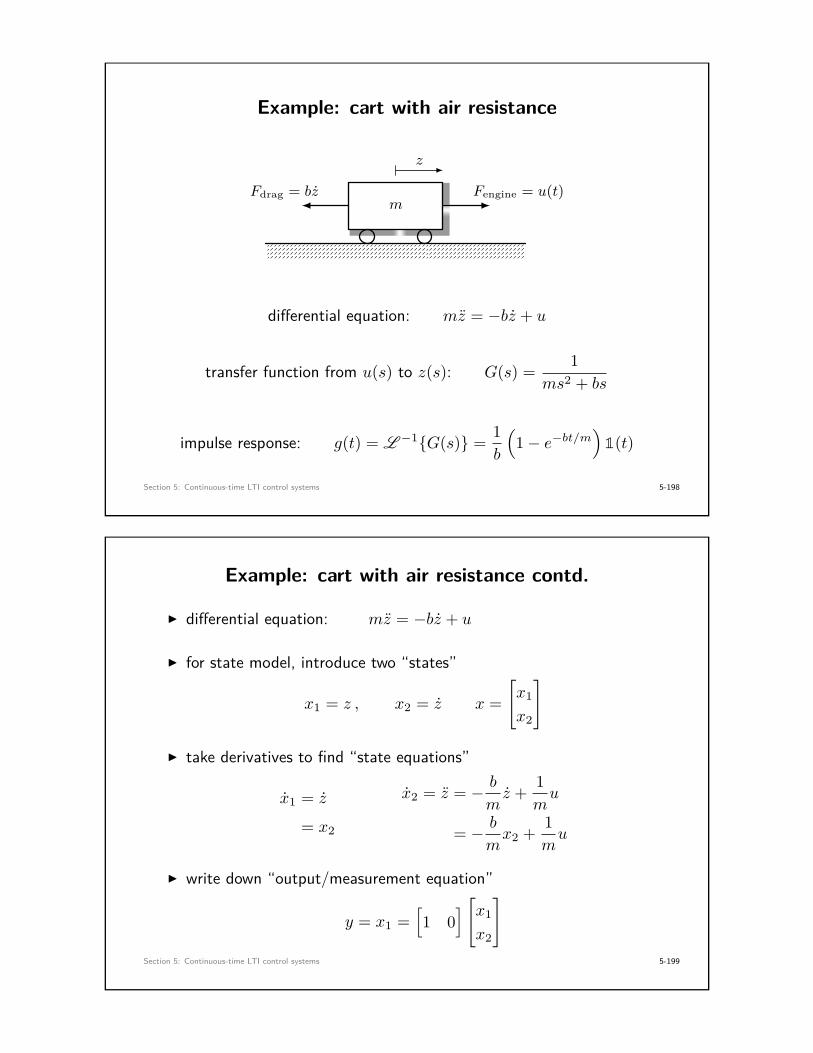
Example: cart with air resistance
mFengine = u(t)Fdrag = bz
z
differential equation: mz = −bz + u
transfer function from u(s) to z(s): G(s) = 1ms2 + bs
impulse response: g(t) = L −1{G(s)} = 1b
(1− e−bt/m
)1(t)
Section 5: Continuous-time LTI control systems 5-198
Example: cart with air resistance contd.
I differential equation: mz = −bz + u
I for state model, introduce two “states”
x1 = z , x2 = z x =[x1
x2
]
I take derivatives to find “state equations”
x1 = z
= x2
x2 = z = − b
mz + 1
mu
= − b
mx2 + 1
mu
I write down “output/measurement equation”
y = x1 =[1 0
] [x1
x2
]Section 5: Continuous-time LTI control systems 5-199

Example: cart with air resistance contd.
In matrix form, the equations are
[x1
x2
]=[
0 10 −b/m
]︸ ︷︷ ︸
=A
[x1
x2
]+[
01/m
]︸ ︷︷ ︸
=B
u
y =[1 0
]︸ ︷︷ ︸
=C
[x1
x2
]+ [0]︸︷︷︸
=D
u
I LTI state model completely specified by (A,B,C,D)
Section 5: Continuous-time LTI control systems 5-200
LTI state-space models
a continuous time LTI state-space model has the form
x(t) = Ax(t) +Bu(t)
y(t) = Cx(t) +Du(t)
I x(t) ∈ Rn is the state vector
I n ∈ N is the order
I u(t) ∈ Rm is the input vector
I y(t) ∈ Rp is the output vector
I A ∈ Rn×n
I B ∈ Rn×m
I C ∈ Rp×n
I D ∈ Rp×m
We focus on single-input single-output (SISO) systems: m = p = 1
Section 5: Continuous-time LTI control systems 5-201

Why study state-space models?
I abstraction allows for systematic analysis and design
I extends to multi-input multi-output systems
I extends to nonlinear systems, stochastic systems, PDEs . . .
I (almost) all advanced control design is based on state models
• linear quadratic control (1960s–)• robust control (1980s–)• receding horizon / model predictive control (1990s–)
Section 5: Continuous-time LTI control systems 5-202
Example: mass spring damper
m
k
b
u(t)
z
mz + bz + kz = u
choose states
x1 = z , x2 = z
x =[
0 1−k/m −b/m
][x1
x2
]+[
01/m
]u
y =[1 0
] [x1
x2
]+ [0]u
Section 5: Continuous-time LTI control systems 5-203

Example: thermal control system
T1(t)
T2(t)
T0(t)
q(t)
T0 external temperature
T1, T2 temperatures of volumes
q heat flux into outer volume
m1,m2 masses of volumes
c1, c2 heat capacities
gij thermal conductances
m1c1T1 = g12 (T2 − T1)
m2c2T2 = −g12 (T2 − T1)− g20 (T2 − T0) + q(t)
Section 5: Continuous-time LTI control systems 5-204
Example: thermal control system
I states: x = (x1, x2) = (T1, T2)I output: y = T1
I inputs: u = (T0, q) (note: example of two input system)
m1c1T1 = −g12T1 + g12T2
m2c2T2 = −(g12 + g20)T2 + g12T1 + g20T0 + q(t)
[T1
T2
]=[− g12m1c1
g12m1c1
g12m2c2
− g12+g20m2c2
][T1
T2
]+[
0 0g20m2c2
1m2c2
][T0
q
]
y =[1 0
] [T1
T2
]+[0 0
] [T0
q
]
Section 5: Continuous-time LTI control systems 5-205

Example: PI controller
I proportional-integral controller:
u(s)e(s) = Kp + Ki
s⇐⇒ u(t) = Kpe(t) +Ki
∫ t
0e(τ) dτ
I define controller state variable xc ∈ R to be integral of error
xc(t) = e(t)
I state-space model is therefore
xc = [0]x+ [1]e
u = [Ki]xc + [Kp]e
I “A” matrix equal to zero, “D” matrix equal to proportional gain
Section 5: Continuous-time LTI control systems 5-206
Example: high-order ODEs
y(n) + an−1y(n−1) + · · ·+ a1y
(1) + a0y = u
x =
x1
x2...xn
=
y
y(1)
...y(n−1)
x1 = x2
x2 = x3
...
xn = −an−1xn − · · · − a0x1 + u
x =
0 1 0 · · · 00 0 1 · · · 0
0 0 0. . . 0
......
...... 1
−a0 −a1 · · · −an−2 −an−1
x1x2...xn
+
00...01
uy =[1 0 · · · 0 0
]x+ [0]u
Section 5: Continuous-time LTI control systems 5-207

Example: high-order ODEs w/ input derivatives (m < n)
y(n) + an−1y(n−1) + · · ·+ a1y
(1) + a0y
= bmu(m) + bm−1u
(m−1) + · · ·+ b0u
x =
0 1 0 · · · 00 0 1 · · · 0
0 0 0. . . 0
......
...... 1
−a0 −a1 · · · −an−2 −an−1
x1
x2...xn
+
00...01
u
y =[b0 · · · bm 0 · · · 0
]x+ [0]u
(details for this example in a handout on LEARN)
Section 5: Continuous-time LTI control systems 5-208
Example: generalized mechanical systems
mechanical systems with k degrees of freedom undergoing small motions
Mq +Dq +Kq = τ
I q ∈ Rk is the vector of generalized coordinates (positions, angles)
I M,D,K ∈ Rk×k are mass, damping, stiffness matrices
I with state vector x = (x1, x2) = (q, q), output y = q
x =[q
q
]=[
0 I
−M−1K −M−1D
][q
q
]+[
0
M−1
]τ
y =[0 I
]
Section 5: Continuous-time LTI control systems 5-209
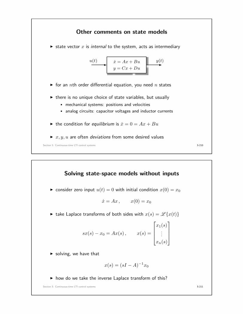
Other comments on state models
I state vector x is internal to the system, acts as intermediary
x = Ax+Bu
y = Cx+Du
u(t) y(t)
I for an nth order differential equation, you need n states
I there is no unique choice of state variables, but usually• mechanical systems: positions and velocities• analog circuits: capacitor voltages and inductor currents
I the condition for equilibrium is x = 0 = Ax+Bu
I x, y, u are often deviations from some desired valuesSection 5: Continuous-time LTI control systems 5-210
Solving state-space models without inputs
I consider zero input u(t) = 0 with initial condition x(0) = x0
x = Ax , x(0) = x0
I take Laplace transforms of both sides with x(s) = L {x(t)}
sx(s)− x0 = Ax(s) , x(s) =
x1(s)...
xn(s)
I solving, we have that
x(s) = (sI −A)−1x0
I how do we take the inverse Laplace transform of this?Section 5: Continuous-time LTI control systems 5-211

Diagonalization and powers of matrices
I diagonalization A = V ΛV −1 provides a method to compute Ak
I if A is diagonalizable, then
Ak = (V ΛV −1)k
= (V ΛV −1)(V ΛV −1) · · · (V ΛV −1)
= V ΛkV −1
where
Λk =
λk1 0 · · · 00 λk2 · · · 0...
.... . .
...0 0 0 λkn
Section 5: Continuous-time LTI control systems 5-212
The matrix exponential
I for a scalar variable x ∈ R, regular exponential
ex = 1 + x+ x2
2 + x3
3! + · · · =∞∑k=0
xk
k!
I for a square matrix A ∈ Rn×n, matrix exponential
eA = In +A+ A2
2 + A3
3! + · · · =∞∑k=0
Ak
k! ∈ Rn×n
I if A is diagonalizable
eA =∞∑k=0
Ak
k! =∞∑k=0
V ΛkV −1
k! = V
( ∞∑k=0
Λk
k!
)V −1 = V eΛV −1
Section 5: Continuous-time LTI control systems 5-213
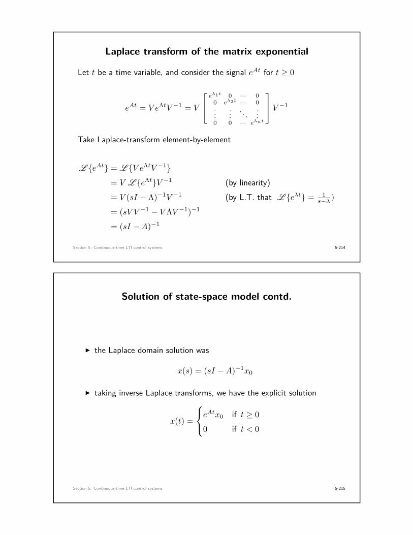
Laplace transform of the matrix exponential
Let t be a time variable, and consider the signal eAt for t ≥ 0
eAt = V eΛtV −1 = V
eλ1t 0 ··· 00 eλ2t ··· 0...
.... . .
...0 0 ··· eλnt
V −1
Take Laplace-transform element-by-element
L {eAt} = L {V eΛtV −1}
= V L {eΛt}V −1 (by linearity)
= V (sI − Λ)−1V −1 (by L.T. that L {eλt} = 1s−λ )
= (sV V −1 − V ΛV −1)−1
= (sI −A)−1
Section 5: Continuous-time LTI control systems 5-214
Solution of state-space model contd.
I the Laplace domain solution was
x(s) = (sI −A)−1x0
I taking inverse Laplace transforms, we have the explicit solution
x(t) =
eAtx0 if t ≥ 0
0 if t < 0
Section 5: Continuous-time LTI control systems 5-215

Internal stability of state models
I state-space system x = Ax is internally asymptotically stable ifx(t)→ 0 as t→∞ from any initial condition x(0)
I interpretation: with no control input, system “dissipates energy”
I suppose A is diagonalizable with V −1AV = Λ
• change of state variables z = V −1x =⇒ z(0) = V −1x(0)
z(t) = V −1x(t) = V −1eAtx(0) = V −1eAtV z(0) = eΛtz(0)
this says that zi(t) = eλitzi(0)
A continuous-time LTI state model is internally asymptoticallystable if and only if λi ∈ C− for all λi ∈ eig(A), i.e., all
eigenvalues of A have negative real partSection 5: Continuous-time LTI control systems 5-216
Example: second-order system with damping
x =[
0 1−ω2
n −2ζωn
]x , x(0) =
[22
]Re(s)
Im(s)
×
×
-10 -5 0 5 10
-3
-2
-1
0
1
2
3
0 100 200 300
-10
-5
0
5
10
0 100 200 300
-2
-1
0
1
2
Section 5: Continuous-time LTI control systems 5-217

Example: second-order system with no damping
x =[
0 1−ω2
n 0
]x , x(0) =
[22
]Re(s)
Im(s)
×
×
-10 -5 0 5 10
-3
-2
-1
0
1
2
3
0 100 200 300
-20
-10
0
10
20
0 100 200 300
-4
-2
0
2
4
Section 5: Continuous-time LTI control systems 5-218
Example: second-order system with negative damping
x =[
0 1−ω2
n 2ζωn
]x , x(0) =
[22
]Re(s)
Im(s)
×
×
-4 -2 0 2
105
-4
-3
-2
-1
0
1
2
310
4
0 100 200 300
-4000
-2000
0
2000
4000
0 100 200 300
-1000
-500
0
500
1000
Section 5: Continuous-time LTI control systems 5-219

Solution of state-space model with input
I back to our general model with inputs
x(t) = Ax(t) +Bu(t) , x(0) = x0
I take L.T. of both sides with x(s) = L {x(t)}, u(s) = L {u(t)}
sx(s)− x(0) = Ax(s) +Bu(s)
=⇒ x(s) = (sI −A)−1x(0) + (sI −A)−1Bu(s)
I therefore
x(t) = eAtx(0) +∫ t
0eA(t−τ)Bu(τ) dτ , t ≥ 0
I we will use this formula for direct design of digital controllers
Section 5: Continuous-time LTI control systems 5-220
Transfer function from state models
x = Ax+Bu
y = Cx+Du
u(t) y(t)
I taking Laplace transforms with zero initial condition x(0) = 0
sx(s) = Ax(s) +Bu(s)
y(s) = Cx(s) +Du(s)=⇒
x(s) = (sI −A)−1Bu(s)
y(s) = Cx(s) +Du(s)
I eliminate x(s) to obtain
y(s)u(s) = P (s) = C(sI −A)−1B +D
I state-space model uniquely determines P (s)Section 5: Continuous-time LTI control systems 5-221

Example: cart with air resistance contd.
mu(t)bz
z
mz = −bz + u
P (s) = 1ms2 + bs
[x1x2
]=[
0 10 −b/m
][x1x2
]+[
01/m
]u
y =[1 0
][x1x2
] (sI −A)−1 =[s −10 s+ b/m
]−1
=1
s(s+ b/m)
[s+ b/m 1
0 s
]
P (s) = C(sI −A)−1B =1/m
s(s+ b/m)=
1ms2 + bs
Section 5: Continuous-time LTI control systems 5-222
Internal asymptotic stability vs. BIBO stability
I we have two stability concepts: internal stability and BIBO stabilityI are they related? yes.
P (s) = C(sI −A)−1B +D
= Cadj(sI −A)det(sI −A) B +D
= C adj(sI −A)B +D det(sI −A)det(sI −A) = (some polynomial)
ΠA(s)
I all poles of P (s) come from eigenvalues of matrix A
I if state-space system internally stable, then P (s) is BIBO stable
Section 5: Continuous-time LTI control systems 5-223

Nonlinear systems
I All real systems are nonlinear• robot manipulator arms (Lagrangian dynamics)• drones, UAV’s (aerodynamics)• chemical reactors (mass-action kinetics)• power systems (AC power flow)• population dynamics (Lotka-Volterra models)• . . .
I nonlinear systems do not have transfer functions
I nonlinear systems do have state models, but they do not look likex(t) = Ax(t) +Bu(t)
Section 5: Continuous-time LTI control systems 5-224
Example: state model for simple pendulum
`
mg
θ
torque = um`2θ = −mg` sin θ − bθ + u
choose state variables
x1 = θ x2 = θ
I state space model is given by[x1
x2
]=[
x2
− g` sin x1 − bm`2x2 + 1
m`2u
]⇐⇒ x = f(x, u) .
Section 5: Continuous-time LTI control systems 5-225

Nonlinear state models
a nonlinear state-space model has the form
x = f(x, u)
y = h(x, u)
I x ∈ Rn is the state vector, u ∈ R is the input, y ∈ R is the output
I f(x, u) is a nonlinear function which describes the dynamics
I h(x, u) is a nonlinear function which describes the measurement
I if f and h are both linear in (x, u), then we have
x = Ax+Bu
y = Cx+Du
Section 5: Continuous-time LTI control systems 5-226
Equilibrium configurations
x = f(x, u)
y = h(x, u)
I an equilibrium configuration is any state/input pair (x, u) such that
f(x, u) = 0
I at an equilibrium configuration, x = 0 =⇒ x(t) = x for all t
I the output is then fixed at y = h(x, u)
Section 5: Continuous-time LTI control systems 5-227

Example: simple pendulum contd.
general case
x1
hanging down balancing up
0 = x2
0 = −g`
sin x1 + 1m`2
u(x, u) =
([00
], 0)
(x, u) =([
π
0
], 0)
Section 5: Continuous-time LTI control systems 5-228
Example: simple pendulum contd.
I what if we wanted the angle to stay at 90◦?
0 = −g`
sin π2 + 1m`2
u ⇐⇒ u = mg`
(x, u) =([
π/20
],mg`
)
I torque balances gravity to create equilibrium
Section 5: Continuous-time LTI control systems 5-229

Linearization of nonlinear systems
I nonlinear model is usually too difficult to design with
I linearization around an equilibrium yields approximate linear model
I Idea: for small changes around equilibrium (x, u), functions f(x, u)and h(x, u) are well-approximated by linear functions
I linearization will be dynamic model which uses deviation variables
δx = x− x
δu = u− u
δy = y − y
Section 5: Continuous-time LTI control systems 5-230
Linearization and derivative matrices
I from vector calculus, Taylor expand f(x, u) around (x, u)
f(x, u) ≈ f(x, u) + ∂f
∂x(x, u) · (x− x) + ∂f
∂u(x, u) · (u− u)
I matrices of partial derivatives, evaluated at equilibrium
A := ∂f
∂x(x, u) =
∂f1∂x1
· · · ∂f1∂xn......
∂fn∂x1
· · · ∂fn∂xn
B := ∂f
∂u(x, u) =
∂f1∂u...
∂fn∂u
I δx = x− x approximately satisfies the differential equation
ddt (δx) = x = f(x, u) ≈ f(x, u) +Aδx+Bδu
Section 5: Continuous-time LTI control systems 5-231

Linearization and derivative matrices contd.
I for output y = h(x, u), Taylor expand h(x, u) around (x, u)
h(x, u) ≈ h(x, u) + ∂h
∂x(x, u) · (x− x) + ∂h
∂u(x, u) · (u− u)
I matrices of partial derivatives, evaluated at equilibrium
C := ∂h
∂x(x, u) =
[∂h∂x1
· · · ∂h∂xn
]D := ∂h
∂u(x, u)
I output deviation δy = y − y therefore satisfies
δy = y − y = h(x, u)− y
≈ (h(x, u) + Cδx+Dδu)− y
= Cδx+Dδu
Section 5: Continuous-time LTI control systems 5-232
Linearization contd.
around equilibrium configuration (x, u), we have the LTI model
˙δx = Aδx+Bδu
δy = Cδx+Dδu
I will be accurate as long as (x, u) stays close to (x, u)
I works unbelievably well in practice (why?)
I computation of (A,B,C,D) easily automated using symbolic tools
syms x1 x2 u k b realf = [x2;-k*sin(x1) - b*x2 + u];A = subs(jacobian(f,[x1;x2]),[x1,x2,u],[0,0,0]);
Section 5: Continuous-time LTI control systems 5-233

Controlling around an equilibrium via linearization
1. use science to find nonlinear model x = f(x, u), y = h(x, u)
2. for your desired output y, find appropriate equilibrium (x, u)
3. linearize the nonlinear model around (x, u) yielding
˙δx = Aδx+Bδu
δy = Cδx+Dδu=⇒ P (s) = δy(s)
δu(s) = C(sIn −A)−1B +D
4. design a controller C(s) for the linearized system
5. check performance by simulating the nonlinear closed-loop system
Section 5: Continuous-time LTI control systems 5-234
Control design based on linearization
C(s)x = f(x, u)y = h(x, u)
y δu u y
−+u
Section 5: Continuous-time LTI control systems 5-235

Note: this toy example is quite important . . .
Section 5: Continuous-time LTI control systems 5-236
Example: inverted pendulum
(x, u) =([
π
0
], 0) [
x1
x2
]=[
x2
− g` sin x1 − bm`2x2 + 1
m`2u
]y = x1
∂f
∂x=
∂f1∂x1
∂f1∂x2
∂f2∂x1
∂f2∂x2
=
0 1
− g`
cosx1 − bm`2
=⇒ A =
0 1g`− bm`2
∂f
∂u=
∂f1∂u
∂f2∂u
=
0
1m`2
=⇒ B =
0
1m`2
Section 5: Continuous-time LTI control systems 5-237

Example: inverted pendulum contd.
∂h
∂x=[∂h∂x1
∂h∂x2
]=[
1 0]
=⇒ C =∂h
∂x(x, u) =
[1 0
]∂h
∂u= 0 =⇒ D =
∂h
∂u(x, u) = 0
I linearized model is therefore
ddt
[δx1
δx2
]=[
0 1g` − b
m`2
][δx1
δx2
]+[
01m`2
]δu
δy =[1 0
] [δx1
δx2
]+ [0]δu
Section 5: Continuous-time LTI control systems 5-238
Example: inverted pendulum contd.
I intuitively, this equilibrium is unstable. check internal stability
det(sI −A) = det[s −1− g` s+ b
mg`
]= s
(s+ b
m`2
)− g
`
= s2 + b
m`2s− g
`
Re(s)Im(s)
× ×
I linearized system is internally unstable
Section 5: Continuous-time LTI control systems 5-239

Example inverted pendulum contd.
I we hit the pendulum with torque disturbanceI open-loop response
0 2 4 6 8 10
200
250
300
350
400
450
500
Section 5: Continuous-time LTI control systems 5-240
Example inverted pendulum contd.
I we now design a controller to stabilize upright equilibrium point
I for now, use transfer function methods
P (s) = C(sI −A)−1B +D =1m`2
s2 + bm`2 s− g
`
I exercise: design a stabilizing controller, e.g.,
Cpd(s) = Kp +Kds
τs+ 1 or Clead(s) = Ks+ z
s+ p
Section 5: Continuous-time LTI control systems 5-241
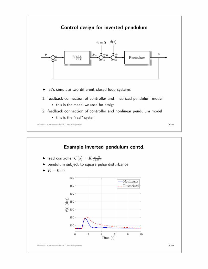
Control design for inverted pendulum
K s+zs+p Pendulum
π δu u θ
−+
u = 0
+
d(t)
I let’s simulate two different closed-loop systems
1. feedback connection of controller and linearized pendulum model• this is the model we used for design
2. feedback connection of controller and nonlinear pendulum model• this is the “real” system
Section 5: Continuous-time LTI control systems 5-242
Example inverted pendulum contd.
I lead controller C(s) = K s+2s+2.5
I pendulum subject to square pulse disturbanceI K = 0.65
0 2 4 6 8 10
200
250
300
350
400
450
500
Section 5: Continuous-time LTI control systems 5-243
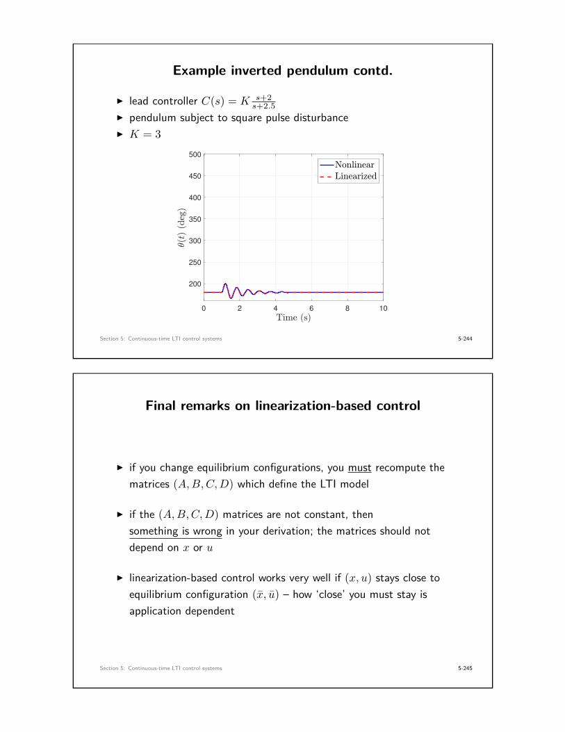
Example inverted pendulum contd.
I lead controller C(s) = K s+2s+2.5
I pendulum subject to square pulse disturbanceI K = 3
0 2 4 6 8 10
200
250
300
350
400
450
500
Section 5: Continuous-time LTI control systems 5-244
Final remarks on linearization-based control
I if you change equilibrium configurations, you must recompute thematrices (A,B,C,D) which define the LTI model
I if the (A,B,C,D) matrices are not constant, thensomething is wrong in your derivation; the matrices should notdepend on x or u
I linearization-based control works very well if (x, u) stays close toequilibrium configuration (x, u) – how ‘close’ you must stay isapplication dependent
Section 5: Continuous-time LTI control systems 5-245
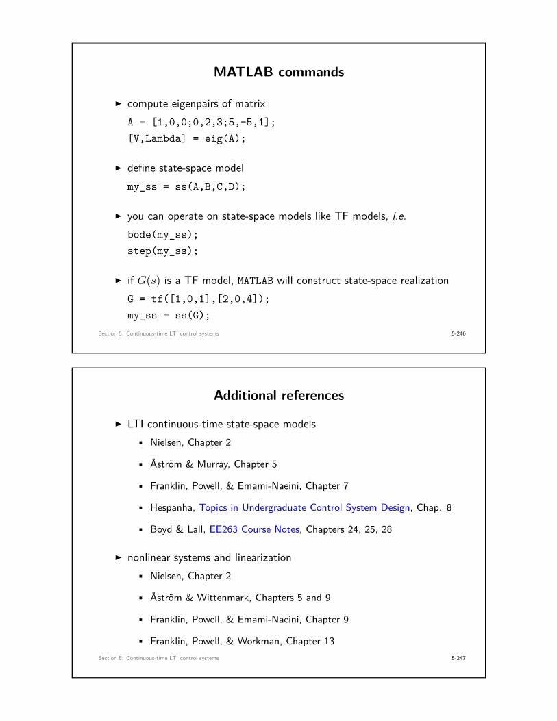
MATLAB commands
I compute eigenpairs of matrixA = [1,0,0;0,2,3;5,-5,1];[V,Lambda] = eig(A);
I define state-space modelmy_ss = ss(A,B,C,D);
I you can operate on state-space models like TF models, i.e.bode(my_ss);step(my_ss);
I if G(s) is a TF model, MATLAB will construct state-space realizationG = tf([1,0,1],[2,0,4]);my_ss = ss(G);
Section 5: Continuous-time LTI control systems 5-246
Additional references
I LTI continuous-time state-space models• Nielsen, Chapter 2
• Åström & Murray, Chapter 5
• Franklin, Powell, & Emami-Naeini, Chapter 7
• Hespanha, Topics in Undergraduate Control System Design, Chap. 8
• Boyd & Lall, EE263 Course Notes, Chapters 24, 25, 28
I nonlinear systems and linearization• Nielsen, Chapter 2
• Åström & Wittenmark, Chapters 5 and 9
• Franklin, Powell, & Emami-Naeini, Chapter 9
• Franklin, Powell, & Workman, Chapter 13Section 5: Continuous-time LTI control systems 5-247

Personal Notes
Section 5: Continuous-time LTI control systems 5-248
Personal Notes
Section 5: Continuous-time LTI control systems 5-249

Personal Notes
Section 5: Continuous-time LTI control systems 5-250
6. Discrete-time LTI control systems
• discrete-time signals and z-transforms• discrete-time LTI systems• feedback stability• time-domain analysis• discrete-time frequency response• state-space models: solutions, stability, transfer functions• discrete-time stability analysis: Routh & Jury conditions
Section 6: Discrete-time LTI control systems 6-251

Notation
I set of integers Z
I interior of the unit disk is D = {z ∈ C | |z| < 1}
I Unit step function
1[k] =
1 if k = 0, 1, 2, . . .
0 if else
δ[k] =
1 if k = 0
0 if else1 2 3 4 5 6 7 8 9 10
0.5
1
1.5
k
1[k]
Section 6: Discrete-time LTI control systems 6-252
Discrete-time signals
I a discrete-time signal is a sequence of numbers f [0], f [1], f [2], . . .
5 10 15
−1
−0.5
0.5
1
k
f [k]
I only defined at discrete points, not inbetween
I may be a sampled signal, with associated sampling period
I in this chapter, we effectively assume sampling period T = 1Section 6: Discrete-time LTI control systems 6-253

The z-transform
I discrete equivalent of Laplace transform
I the (unilateral or one-sided) z-transform of a signal f [k] is
F [z] := Z{f [k]} =∞∑k=0
f [k]z−k , z ∈ C .
I if signal f [k] does not grow too fast, i.e., if
|f [k]| ≤Mρk
for some M,ρ > 0, then z-transform sum converges for all values ofz ∈ C satisfying |z| > ρ
Section 6: Discrete-time LTI control systems 6-254
Convergence of z-transform
I suppose f [k] satisfies |f [k]| ≤Mρk, and write z = rejθ. Then
|F [z]| =
∣∣∣∣∣∞∑k=0
f [k]z−k∣∣∣∣∣ =
∣∣∣∣∣∞∑k=0
f [k](rejθ)−k∣∣∣∣∣ ≤
∞∑k=0
∣∣f [k]r−ke−jkθ∣∣
≤∞∑k=0
|f [k]| · |r−k| · |e−jkθ|︸ ︷︷ ︸=1
=∞∑k=0
|f [k]| · r−k
≤∞∑k=0
Mρkr−k = M
∞∑k=0
(ρ
r
)k(geometric series sum)
= M1
1− ρ/rif r > ρ
Section 6: Discrete-time LTI control systems 6-255

Convergence of z-transform contd.
I F [z] is well-defined for all z outside a disk of radius ρ
Re(z)
Im(z)
ρ
Region of Convergence
I in general, ρ equals magnitude of largest pole of F [z]Section 6: Discrete-time LTI control systems 6-256
Example: exponential function
f [k] = ak , a ∈ R
F [z] =∞∑k=0
akz−k =∞∑k=0
(az
)k= 1
1− a/z = z
z − a, for |z| > |a|
Re(z)
Im(z)
|a|
Region of Convergence
I note that f [k] satisfies bound|f [k]| ≤Mρk with
M = 1 ρ = |a|
Section 6: Discrete-time LTI control systems 6-257

Example: impulse function
f [k] = δ[k] =
1 if k = 0
0 if else
F [z] =∞∑k=0
δ[k]z−k = z−0 = 1 , for all z ∈ C
Re(z)
Im(z)
Region of Convergence
I note that f [k] satisfies bound|f [k]| ≤Mρk with
M = 1 ρ = 0
Section 6: Discrete-time LTI control systems 6-258
Key properties of z-transform
I linearityZ{α1f1 + α2f2} = α1F1[z] + α2F2[z]
I accumulation formula
Z
{k∑`=0
f [`]}
= z
z − 1F [z]
I time-shifting formula (with zero initial conditions)
Z {f [k −m]} = z−mF [z]
I convolution
Z{g ∗ f} = Z{
k∑`=0
g[k − `]f [`]}
= G[z]F [z]
Section 6: Discrete-time LTI control systems 6-259
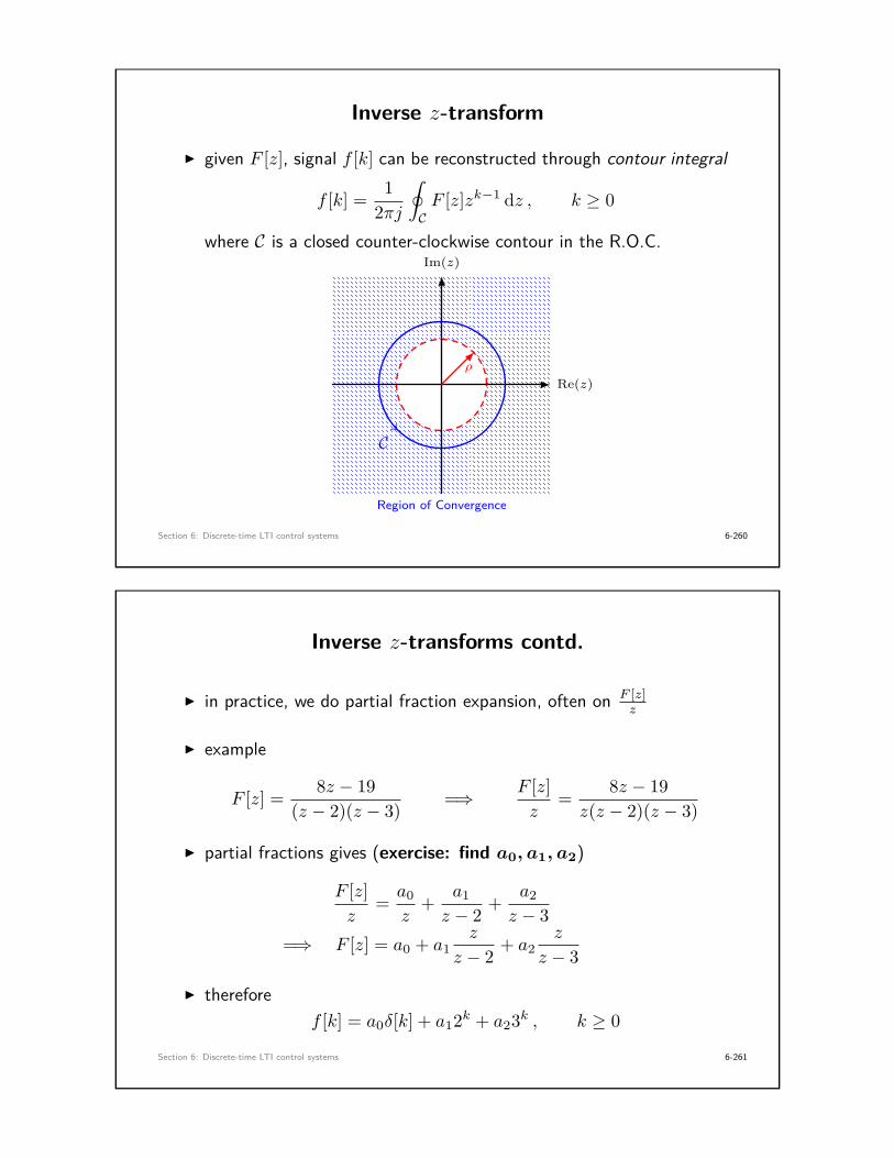
Inverse z-transform
I given F [z], signal f [k] can be reconstructed through contour integral
f [k] = 12πj
∮CF [z]zk−1 dz , k ≥ 0
where C is a closed counter-clockwise contour in the R.O.C.
Re(z)
Im(z)
ρ
Region of Convergence
C
Section 6: Discrete-time LTI control systems 6-260
Inverse z-transforms contd.
I in practice, we do partial fraction expansion, often on F [z]z
I example
F [z] = 8z − 19(z − 2)(z − 3) =⇒ F [z]
z= 8z − 19z(z − 2)(z − 3)
I partial fractions gives (exercise: find a0, a1, a2)
F [z]z
= a0
z+ a1
z − 2 + a2
z − 3=⇒ F [z] = a0 + a1
z
z − 2 + a2z
z − 3
I thereforef [k] = a0δ[k] + a12k + a23k , k ≥ 0
Section 6: Discrete-time LTI control systems 6-261
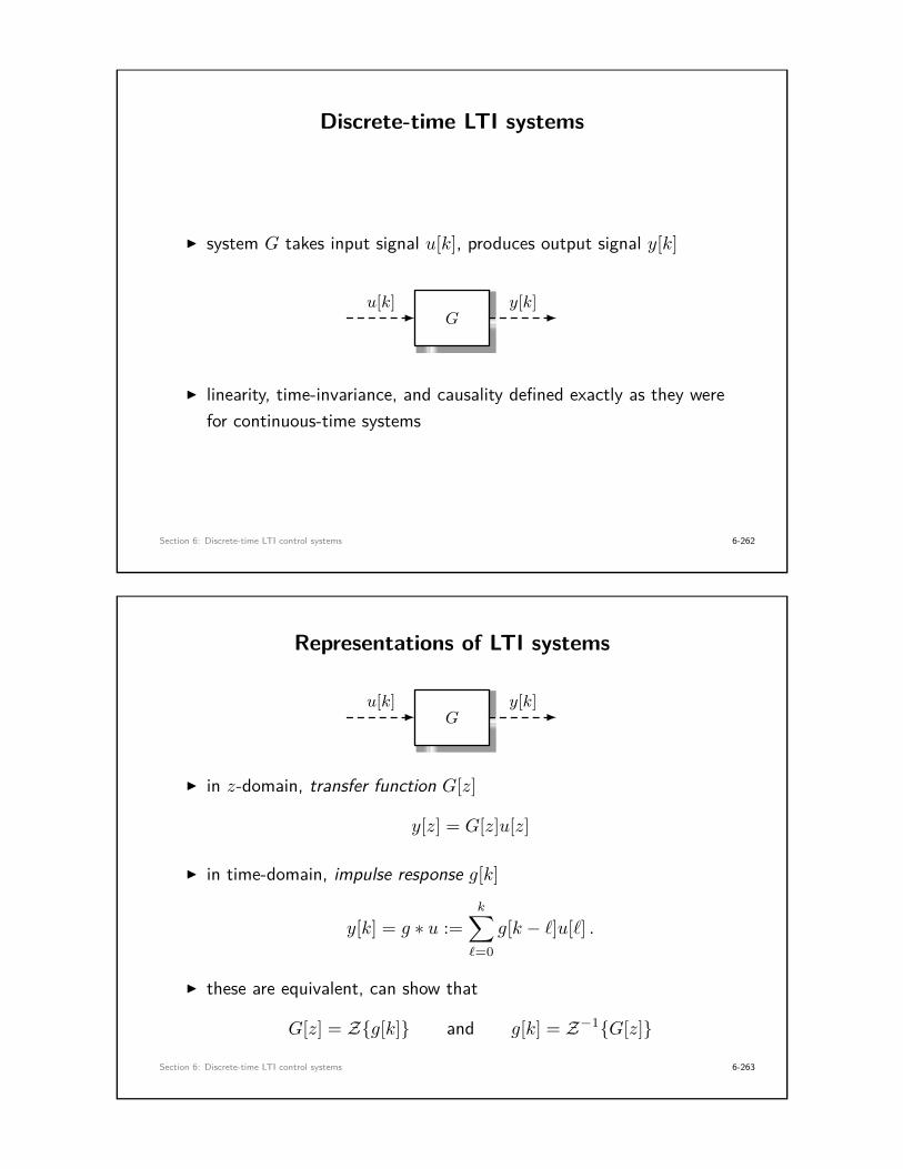
Discrete-time LTI systems
I system G takes input signal u[k], produces output signal y[k]
Gu[k] y[k]
I linearity, time-invariance, and causality defined exactly as they werefor continuous-time systems
Section 6: Discrete-time LTI control systems 6-262
Representations of LTI systems
Gu[k] y[k]
I in z-domain, transfer function G[z]
y[z] = G[z]u[z]
I in time-domain, impulse response g[k]
y[k] = g ∗ u :=k∑`=0
g[k − `]u[`] .
I these are equivalent, can show that
G[z] = Z{g[k]} and g[k] = Z−1{G[z]}
Section 6: Discrete-time LTI control systems 6-263

Transfer function representation contd.
G[z]u[z] y[z]
I we call G[z] rational if G[z] = N [z]D[z] for some polynomials N [z] and
D[z] with real coefficients
I a pole p of G[z] satisfies limz→p |G[z]| =∞
I a zero ζ of G[z] satisfies G[ζ] = 0
I the degree deg(D) of the denominator is the order of the system
I G[z] is proper if deg(N) ≤ deg(D), and is strictly proper ifdeg(N) < deg(D)
I DC gain of G[z] is G[1] (not G[0]!)Section 6: Discrete-time LTI control systems 6-264
Bounded-input bounded-output stability
I a signal y[k] is bounded if |y[k]| ≤ C for all k ≥ 0
Gu[k] y[k]
I BIBO stability: every bounded u[k] produces a bounded y[k]
I if the LTI system G is rational and proper, then G is BIBO stable ifand only if either of the following equivalent statements hold:
• every pole of the transfer function G[z] belongs to D
• the sum∑∞
k=0 |g[k]| of the impulse response is finite.
Section 6: Discrete-time LTI control systems 6-265
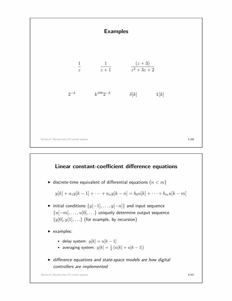
Examples
1z
1z + 1
(z + 3)z2 + 3z + 2
2−k k1002−k δ[k] 1[k]
Section 6: Discrete-time LTI control systems 6-266
Linear constant-coefficient difference equations
I discrete-time equivalent of differential equations (n < m)
y[k] + a1y[k − 1] + · · ·+ any[k − n] = b0u[k] + · · ·+ bmu[k −m]
I initial conditions {y[−1], . . . , y[−n]} and input sequence{u[−m], . . . , u[0], . . .} uniquely determine output sequence{y[0], y[1], . . .} (for example, by recursion)
I examples:
• delay system: y[k] = u[k − 1]• averaging system: y[k] = 1
2 (u[k] + u[k − 1])
I difference equations and state-space models are how digitalcontrollers are implemented
Section 6: Discrete-time LTI control systems 6-267
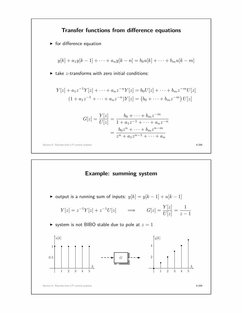
Transfer functions from difference equations
I for difference equation
y[k] + a1y[k − 1] + · · ·+ any[k − n] = b0u[k] + · · ·+ bmu[k −m]
I take z-transforms with zero initial conditions:
Y [z] + a1z−1Y [z] + · · ·+ anz
−nY [z] = b0U [z] + · · ·+ bmz−mU [z]
(1 + a1z−1 + · · ·+ anz
−n)Y [z] =(b0 + · · ·+ bmz
−m)U [z]
G[z] = Y [z]U [z] = b0 + · · ·+ bmz
−m
1 + a1z−1 + · · ·+ anz−n
= b0zn + · · ·+ bmz
n−m
zn + a1zn−1 + · · ·+ an
Section 6: Discrete-time LTI control systems 6-268
Example: summing system
I output is a running sum of inputs: y[k] = y[k − 1] + u[k − 1]
Y [z] = z−1Y [z] + z−1U [z] =⇒ G[z] = Y [z]U [z] = 1
z − 1
I system is not BIBO stable due to pole at z = 1
1 2 3 4 5
0.5
1
k
u[k]
G
1 2 3 4 5
2
4
k
y[k]
Section 6: Discrete-time LTI control systems 6-269

Example: finite impulse response (FIR) filters
I the impulse response of an FIR filter is non-zero for only a finitenumber of time steps
g[k] = b0δ[k] + b1δ[k − 1] + · · ·+ bmδ[k −m]
−2 2 4 6 8 10 12 14 16
2
4
6
8
k
g[k]
I transfer function G[z] = Z{g[k]} is
G[z] = b0 + b1z−1 + · · ·+ bmz
−m
and has all of its poles at z = 0Section 6: Discrete-time LTI control systems 6-270
Example: unit step response of FIR filter
0
2
4
6
8
10
12
14
0 5 10 15 20
Section 6: Discrete-time LTI control systems 6-271

Feedback stability of discrete-time control systems
C[z] P [z]+
d[z]r[z] e[z] u[z] y[z]−
I r and d are external signals, e, u and y are internal signals
I the closed-loop is feedback stable if every bounded (r, d) leads tobounded (e, u, y)
I 2 inputs, 3 outputs =⇒ 6 transfer functionse[z]r[z] = 1
1 + PC
u[z]r[z] = C
1 + PC
y[z]r[z] = PC
1 + PC
e[z]d[z] = −P
1 + PC
u[z]d[z] = 1
1 + PC
y[z]r[z] = P
1 + PC
Section 6: Discrete-time LTI control systems 6-272
Feedback stability contd.
I assume P [z] is rational and strictly proper: P [z] = Np[z]Dp[z]
I assume C[z] is rational and proper: C[z] = Nc[z]Dc[z]
I we calculate that
y[z]r[z] = PC
1 + PC=
NpDp
NcDc
1 + NpDp
NcDc
= NpNc
NpNc +DpDc
I characteristic polynomial: Π[z] := Np[z]Nc[z] +Dp[z]Dc[z]
I the closed-loop is feedback stable if and only if all roots of Π[z]belong to D
Section 6: Discrete-time LTI control systems 6-273

Example: feedback stability
I plant: y[k] = y[k − 1] + u[k − 1], or T.F. P [z] = 1z−1
I controller: u[k] = 12 (e[k] + e[k − 1]), or T.F. C[z] = z+1
2z
I compute characteristic polynomial
Π[z] = (z + 1) + 2z(z − 1) = 2(z − 1
4 + j
√7
4
)(z − 1
4 − j√
74
)I magnitude of pole(s) is[(
14
)2+(√
74
)2]1/2
= 1√2< 1
I closed-loop system is feedback stableSection 6: Discrete-time LTI control systems 6-274
Example: feedback stability contd.
I unit step response of unity-gain feedback system
0
0.5
1
1.5
2
0 5 10 15 20
Section 6: Discrete-time LTI control systems 6-275

Time-domain analysis
Gu[k] y[k]
(i) rise time Tr, settling time Tp
(ii) peak time Tp, peak max Mp
(iii) steady state value yss? 5 10 15 20
0.5
1
1.5
r
k
y[k]
I Final value theorem: if F [z] = Z{f [k]} is rational and proper,with all poles of (z − 1)F [z] contained in D, thenfss = limk→∞ f [k] exists and
fss = limk→∞
f [k] = limz→1
(z − 1)F [z] .
Section 6: Discrete-time LTI control systems 6-276
Example: second-order system
for a step u[k] = 1[k], find steady-state value for y[k]
G[z] = z + 2z(z − 0.5)
Y [z] = G[z]U [z] = z + 2z(z − 0.5)
z
z − 1
(z − 1)Y [z] = z + 2(z − 0.5)
this has all poles inside the unit circle, therefore
limk→∞
y[k] = limz→1
(z − 1)Y [z] = 6 = G[1]
I DC gain G[1] gives steady-state value of step responseSection 6: Discrete-time LTI control systems 6-277

First-order discrete-time systems
I prototypical first-order system is described by
y[k] = −a1y[k − 1] + b1u[k − 1] =⇒ G[z] = b1z + a1
I pole at z = −a1, system is BIBO stable if |a1| < 1
I to normalize DC gain such that G[1] = 1, set b1 = 1 + a1
G[z] = 1 + a1
z + a1
I unit step response
Y [z] = 1 + a1
z + a1
z
z − 1Z−1
7−−−→ y[k] = 1− (−a1)k
Section 6: Discrete-time LTI control systems 6-278
Step response of first-order system
y[k] = 1− (−a1)k , k ≥ 0
for −1 < a1 < 0
5 10 15 20
0.5
1
1.5
r
k
y[k]
for 0 < a1 < 1
5 10 15 20
0.5
1
1.5
r
k
y[k]
Section 6: Discrete-time LTI control systems 6-279

Step response of first-order system contd.
I in discrete-time, first-order systems can have overshoot
I magnitude of a1 controls settling time
Re(z)
Im(z)
D
× × × × ×
1-step-delay system
overshootslowerfaster
Section 6: Discrete-time LTI control systems 6-280
Second-order discrete-time systems
I prototypical second-order system is described by
y[k] + a1y[k − 1] + a2y[k − 2] = b2u[k − 2]
I transfer functionG[z] = b2
z2 + a1z + a2
I to normalized DC gain G[1] = 1, set b2 = 1 + a1 + a2
I three cases of interest: a2 > 0, a2 < 0, and a2 = 0
I if a2 > 0, two conjugate poles z± = re±jθ, determined by
a2 = r2 a1 = −2r cos(θ)
I system BIBO stable if r < 1 ⇐⇒ a2 < 1Section 6: Discrete-time LTI control systems 6-281
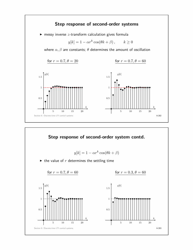
Step response of second-order systems
I messy inverse z-transform calculation gives formula
y[k] = 1− αrk cos(θk + β) , k ≥ 0
where α, β are constants; θ determines the amount of oscillation
for r = 0.7, θ = 20
5 10 15 20
0.5
1
1.5
k
y[k]
for r = 0.7, θ = 60
5 10 15 20
0.5
1
1.5
k
y[k]
Section 6: Discrete-time LTI control systems 6-282
Step response of second-order system contd.
y[k] = 1− αrk cos(θk + β)
I the value of r determines the settling time
for r = 0.7, θ = 60
5 10 15 20
0.5
1
1.5
k
y[k]
for r = 0.3, θ = 60
5 10 15 20
0.5
1
1.5
k
y[k]
Section 6: Discrete-time LTI control systems 6-283

Step-response of second-order systems contd.
I responses very similar to continuous-time second-order systemsI pole location meanings are very different
Re(z)
Im(z)
D
θ
decay rate
×
×
oscillation freq.
Section 6: Discrete-time LTI control systems 6-284
Frequency response of discrete-time systems
I for a continuous-time LTI system which is BIBO stable
G(s)cos(ωt) yss(t) = A cos(ωt+ φ)
where A = |G(jω)| and φ = ∠G(jω)
I is something similar true for discrete-time systems?
I assume G[z] is rational, proper, and BIBO stable
I output y[k] of system is given by convolution
y[k] =∞∑
m=−∞g[m]u[k −m]
Section 6: Discrete-time LTI control systems 6-285

Frequency response contd.
I let’s try the complex exponential input u[k] = ejωk
I annoying technical note: we will start applying input at k = −∞, sothat system can reach a nice steady-state by time k = 0.
y[k] =∞∑
m=−∞g[m]ejω(k−m)
= ejωk∞∑
m=−∞g[m]e−jωm
= ejωkG[ejω] (discrete Fourier transform)
G[z]ejωk yss[k] = G[ejω]ejωk
Section 6: Discrete-time LTI control systems 6-286
Frequency response contd.
I we may now take the real part of each signal
Re(ejωk) = cos(ωk)
Re(G[ejω]ejωk) =∣∣G[ejω]
∣∣ cos(ωk + ∠G[ejω])
G[z]cos(ωk) A cos(ωk + φ)
whereA =
∣∣G[ejω]∣∣ φ = ∠G[ejω]
I G[ejω] is the frequency response of the system
I cosine applied at input yields shifted and scaled cosine at the outputSection 6: Discrete-time LTI control systems 6-287
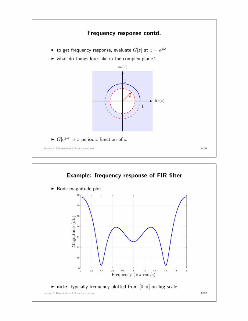
Frequency response contd.
I to get frequency response, evaluate G[z] at z = ejω
I what do things look like in the complex plane?
Re(z)
Im(z)
ρ
1
1
I G[ejω] is a periodic function of ωSection 6: Discrete-time LTI control systems 6-288
Example: frequency response of FIR filter
I Bode magnitude plot
0 0.2 0.4 0.6 0.8 1 1.2 1.4 1.6 1.8 2
8
10
12
14
16
18
20
22
I note: typically frequency plotted from [0, π] on log scaleSection 6: Discrete-time LTI control systems 6-289
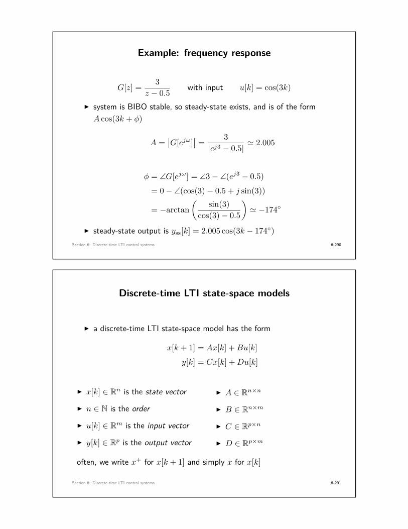
Example: frequency response
G[z] = 3z − 0.5 with input u[k] = cos(3k)
I system is BIBO stable, so steady-state exists, and is of the formA cos(3k + φ)
A =∣∣G[ejω]
∣∣ = 3|ej3 − 0.5| ' 2.005
φ = ∠G[ejω] = ∠3− ∠(ej3 − 0.5)
= 0− ∠(cos(3)− 0.5 + j sin(3))
= −arctan(
sin(3)cos(3)− 0.5
)' −174◦
I steady-state output is yss[k] = 2.005 cos(3k − 174◦)Section 6: Discrete-time LTI control systems 6-290
Discrete-time LTI state-space models
I a discrete-time LTI state-space model has the form
x[k + 1] = Ax[k] +Bu[k]
y[k] = Cx[k] +Du[k]
I x[k] ∈ Rn is the state vector
I n ∈ N is the order
I u[k] ∈ Rm is the input vector
I y[k] ∈ Rp is the output vector
I A ∈ Rn×n
I B ∈ Rn×m
I C ∈ Rp×n
I D ∈ Rp×m
often, we write x+ for x[k + 1] and simply x for x[k]
Section 6: Discrete-time LTI control systems 6-291
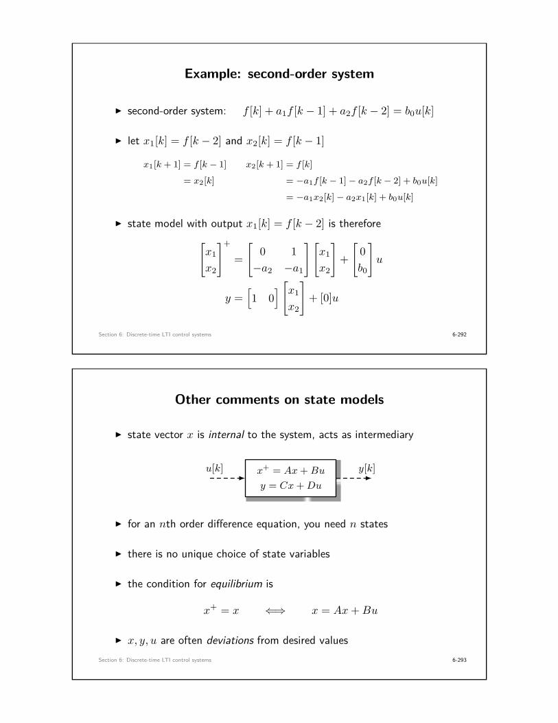
Example: second-order system
I second-order system: f [k] + a1f [k − 1] + a2f [k − 2] = b0u[k]
I let x1[k] = f [k − 2] and x2[k] = f [k − 1]
x1[k + 1] = f [k − 1]
= x2[k]
x2[k + 1] = f [k]
= −a1f [k − 1]− a2f [k − 2] + b0u[k]
= −a1x2[k]− a2x1[k] + b0u[k]
I state model with output x1[k] = f [k − 2] is therefore[x1
x2
]+
=[
0 1−a2 −a1
][x1
x2
]+[
0b0
]u
y =[1 0
] [x1
x2
]+ [0]u
Section 6: Discrete-time LTI control systems 6-292
Other comments on state models
I state vector x is internal to the system, acts as intermediary
x+ = Ax+Bu
y = Cx+Du
u[k] y[k]
I for an nth order difference equation, you need n states
I there is no unique choice of state variables
I the condition for equilibrium is
x+ = x ⇐⇒ x = Ax+Bu
I x, y, u are often deviations from desired valuesSection 6: Discrete-time LTI control systems 6-293

Solving state-space models without inputs
I consider zero input u[k] = 0 with initial condition x[0] = x0 ∈ Rn
x[k + 1] = Ax[k] , x[0] = x0
I just by iterating, we find that
x[1] = Ax0
x[2] = A(Ax0) = A2x0
...
x[k] = Akx0
I so with no input, the solution is
x[k] = Akx0 , k ≥ 0
Section 6: Discrete-time LTI control systems 6-294
Computing Ak via z-transforms
I we know solution to x+ = Ax is x[k] = Akx[0]
I we could also z-transform (element-by-element) both sides to find
zX[z]− zx[0] = AX[z] ⇐⇒ (zI −A)X[z] = zx[0]
⇐⇒ (I − z−1A)X[z] = x[0]
⇐⇒ X[z] = (I − z−1A)−1x[0]
⇐⇒ x[k] = Z−1{(I − z−1A)−1}x[0]
I comparing the solutions, we find that
Ak = Z−1{(I − z−1A)−1}
Section 6: Discrete-time LTI control systems 6-295

Example: computing Ak
x[k + 1] =[
0 1−2 −3
]x[k] , x[0] =
[10
]compute that
(I − z−1A)−1 = z(zI −A)−1 = z
[z −12 z + 3
]−1
=z
z2 + 3z + 2
[z + 3 1−2 z
]therefore
Ak = Z−1
{[z(z+3)
(z+1)(z+2)z
(z+1)(z+2)−2z
(z+1)(z+2)z2
(z+1)(z+2)
]}
=[
2(−1)k − (−2)k (−1)k − (−2)k
2(−2)k − 2(−1)k 2(−2)k − (−1)k
]
Section 6: Discrete-time LTI control systems 6-296
Internal stability of state models
I state-space system x+ = Ax is internally asymptotically stable ifx[k]→ 0 as k →∞ from any initial condition x[0]
I with no external inputs, the state goes to zero
I suppose A is diagonalizable with V −1AV = Λ
• change of state variables z = V −1x =⇒ z[0] = V −1x[0]
z[k] = V −1x[k] = V −1Akx[0] = V −1AkV z[0] = Λkz[0]
• this says that zi[k] = λki zi[0]
A discrete-time LTI state model is internally asymptoticallystable if and only if λi ∈ D for all λi ∈ eig(A), i.e., all
eigenvalues of A have magnitude less than oneSection 6: Discrete-time LTI control systems 6-297

Example: internally stable second-order system
x+ =[
0 1−0.6 −0.6
]x , x[0] =
[22
]Re(z)
Im(z)
D×
×
-2 0 2
-3
-2
-1
0
1
2
3
-2
0
2
0 10 20 30
-2
0
2
0 10 20 30
Section 6: Discrete-time LTI control systems 6-298
Example: unstable second-order system
x+ =[
0 1−1 0
]x , x[0] =
[22
]Re(z)
Im(z)
D×
×
-2 0 2
-3
-2
-1
0
1
2
3
-2
0
2
0 5 10 15 20
-2
0
2
0 5 10 15 20
Section 6: Discrete-time LTI control systems 6-299

Example: unstable second-order system
x+ =[
0 1.2−1 0
]x , x[0] =
[22
]Re(z)
Im(z)
D×
×
-10 -5 0 5 10
-10
-5
0
5
10
-10
0
10
0 5 10 15 20
-10
0
10
0 5 10 15 20
Section 6: Discrete-time LTI control systems 6-300
Solution of state-space model with input
back to our general model with inputs
x[k + 1] = Ax[k] +Bu[k] , x[0] ∈ Rn
we can just iterate to find the solution
x[1] = Ax[0] +Bu[0]
x[2] = A2x[0] +ABu[0] +Bu[1]
x[3] = A3x[0] +A2Bu[0] +ABu[1] +Bu[2]...
x[k] = Akx[0] +k−1∑j=0
Ak−j−1Bu[j]
I combination of natural response and forced responseSection 6: Discrete-time LTI control systems 6-301

Transfer function from state models
x+ = Ax+Bu
y = Cx+Du
u[k] y[k]
taking z-transforms with zero initial conditions x[0] = 0
zX[z] = AX[z] +BU [z]
Y [z] = CX[z] +DU [z]=⇒
X[z] = (zI −A)−1BU [z]
Y [z] = CX[z] +DU [z]
Y [z]U [z] = P [z] = C(zI −A)−1B +D
I state-space model uniquely determines P [z]I transfer functions from state-space models are always proper
Section 6: Discrete-time LTI control systems 6-302
Internal asymptotic stability vs. BIBO stability
I internal stability and BIBO stability are related
P [z] = C(zI −A)−1B +D
= Cadj(zI −A)det(zI −A) B +D
= C adj(zI −A)B +D det(zI −A)det(zI −A) = (some polynomial)
ΠA[z]
I every pole of P [z] is an eigenvalue of A
I state model internally asymptotically stable =⇒ TF is BIBO stable
Section 6: Discrete-time LTI control systems 6-303

Feedback stability of state-space models
I we can understand feedback stability using state models
x+c = Acxc +Bce
yc = Ccxc +Dce
x+p = Apxp +Bpu
y = Cpxp
+d
r e u y
−
PlantController
I idea: eliminate e, yc, u and find write state model with statesx = (xp, xc), inputs (r, d) and output y
I note: in this case, our state-space model will have two inputs
Section 6: Discrete-time LTI control systems 6-304
Feedback stability using state-space models
x+c = Acxc +Bce
yc = Ccxc +Dce
x+p = Apxp +Bpu
y = Cpxp
+d
r e u y
−
x+p = Apxp +Bp(d+ yc)
y = Cpxp
x+c = Acxc +Bc(r − y)
yc = Ccxc +Dc(r − y)
combine:[xp
xc
]+
=[Ap −BpDcCp BpCc
−BcCp Ac
]︸ ︷︷ ︸
:=Acl
[xp
xc
]︸ ︷︷ ︸:=xcl
+[BpDc Bp
Bc 0
]︸ ︷︷ ︸
:=Bcl
[r
d
]
y =[Cp 0
]︸ ︷︷ ︸
Ccl
[xp
xc
]Section 6: Discrete-time LTI control systems 6-305

Feedback stability using state-space models
I the closed-loop state model has the form
x+cl = Aclxcl +Bcl
[r
d
], y = Cclxcl
I from before: internal asymptotic stability of state model =⇒ BIBOstability of transfer function
I similarly now, internal asymptotic stability of closed-loop model =⇒BIBO stability of any closed-loop transfer function (i.e., feedbackstability)
λi ∈ D for all
λi ∈ eig(Acl)=⇒
all transfer func.
are BIBO stable⇐⇒
feedback stability of
feedback system
Section 6: Discrete-time LTI control systems 6-306
Discrete-time stability analysis
I we have seen several discrete-time stability concepts
(i) BIBO stability of a transfer function G[z]
(ii) feedback stability with plant P [z] and controller C[z]
(iii) internal asymptotic stability of state-space models
(iv) feedback stability with state-space plant and controller
I in all cases, we must ask whether all roots of some polynomial
Π[z] = a0zn + a1z
n−1 + · · ·+ an−1z + an
are contained in D
I we now develop a tool for actually checking stabilitySection 6: Discrete-time LTI control systems 6-307

Review: Routh-Hurwitz for continuous-time systems
I goal: determine whether all roots of polynomial Π(s) are in C−
Π(s) = ansn + an−1s
n−1 + · · ·+ a1s+ a0
I algorithmic test through the Routh array
row n an an−2 an−4 · · ·row n-1 an−1 an−3 an−5 · · ·row n-2 b1 b2 b3 · · ·row n-3 c1 c2 c3 · · ·· · · · · · · · · · · · · · ·row 2 ∗ ∗row 1 ∗row 0 ∗
bi = an−1an−2i − anan−2i−1
an−1
ci = b1an−2i−1 − an−1bi+1
b1
di = · · ·
Section 6: Discrete-time LTI control systems 6-308
Routh-Hurwitz contd.
I necessary conditions for all roots in C−• the coefficients ai must all be non-zero
• the coefficients ai must all be positive
I sufficient conditions for all roots in C−• if all entries in the first column are positive, then all roots are in C−
• there is one pole in C+ for every sign change in the first column
I useful for tuning controller gains
Section 6: Discrete-time LTI control systems 6-309

Routh-Hurwitz for discrete-time systems
I Routh-Hurwitz addresses roots in C−, not in D
I key trick: use the transformation z = 1+v1−v between C− and D
v-plane z-plane
Re(v)
Im(v)
C−
z = 1+v1−v
v = z−1z+1
Re(z)
Im(z)
+1−1
D
Section 6: Discrete-time LTI control systems 6-310
Routh-Hurwitz for discrete-time systems contd.
given a polynomial
Π[z] = zn + a1zn−1 + · · ·+ an−1z + an
(i) evaluate Π[z] at z = 1+v1−v , that is, form Π
[1+v1−v
](ii) multiply through by (1− v)n to obtain a new polynomial Π(v)
(iii) apply standard Routh-Hurwitz test to Π(v)
The polynomial Π[z] has all roots in D if and only if thepolynomial Π(v) has all roots in C−
Section 6: Discrete-time LTI control systems 6-311

Example: second-order system
Π[z] = z2 + a1z + a2
I form Π(v)
Π[
1 + v
1− v
]=(
1 + v
1− v
)2+ a1
(1 + v
1− v
)+ a2
Π(v) = (1− v)2Π[
1 + v
1− v
]= (1 + v)2 + a1(1 + v)(1− v) + a2(1− v)2
= (1 + a2 − a1)v2 + 2(1− a2)v + (1 + a2 + a1)
Section 6: Discrete-time LTI control systems 6-312
Example: second-order system contd.
Π(v) = (1 + a2 − a1)v2 + 2(1− a2)v + (1 + a2 + a1)
row 2 1 + a2 − a1 1 + a2 + a1
row 1 2(1− a2) 0row 0 1 + a2 + a1 0
I we need all first column entries to be positive
1 + a2 − a1 > 0 and 1− a2 > 0 and 1 + a2 + a1 > 0
Section 6: Discrete-time LTI control systems 6-313

Example: second-order system contd.
I we have three inequalities
1 + a2 − a1 > 0 1− a2 > 0 1 + a2 + a1 > 0
1 + a2 > a1 a2 < 1 1 + a2 > −a1
I if a2 ≤ −1, first and third inequalities are impossible, so a2 > −1
I conditions are therefore
|a2| < 1
|a1| < 1 + a2
Section 6: Discrete-time LTI control systems 6-314
Example: second-order system contd.
Π[z] = z2 + a1z + a2|a2| < 1
|a1| < |1 + a2|
a2 = 1.1 a1 = 0.3 a2 = −0.4 a1 = 0.7
Re(z)
Im(z)
D×
×
Re(z)
Im(z)
D
× ×
Section 6: Discrete-time LTI control systems 6-315

Jury’s necessary conditions
I alternative set of tests for all roots of polynomial
Π[z] = a0zn + a1z
n−1 + · · ·+ an−1z + an
to be contained in D
I Jury’s necessary stability conditions are
(i) Π[1] > 0
(ii) (−1)nΠ[−1] > 0
(iii) |an| < |a0|
I equivalently, these conditions are sufficient for instability
Section 6: Discrete-time LTI control systems 6-316
Example: testing feedback stability
I first-order plant with “PI” controller
P [z] = z
z + a, C[z] = Kp +Ki
z
z − 1 , where a > 0
I characteristic polynomial
Π[z] = (Kp +Ki)z2 −Kpz + (z + a)(z − 1)
= (1 +Kp +Ki)z2 + (a− 1−Kp)z − a
I Jury’s necessary conditions tell us that — at least — we need
(i) Ki > 0
(ii) 1 +Kp + 12Ki > a
(iii) |1 +Kp +Ki| > a
Section 6: Discrete-time LTI control systems 6-317

Example: testing feedback stability contd.
I the necessary & sufficient conditions from Routh-Hurwtiz are∣∣∣∣ −a1 +Kp +Ki
∣∣∣∣ < 1 ,∣∣∣∣ a− 1−Kp
1 +Kp +Ki
∣∣∣∣ < ∣∣∣∣1− a
1 +Kp +Ki
∣∣∣∣I first condition says |1 +Kp +Ki| > a
I second condition says that
|1 +Kp − a| < 1 +Kp +Ki − a
• if LHS is positive, this says Ki > 0
• if LHS is negative, this says 1 +Kp + 12Ki > a
Section 6: Discrete-time LTI control systems 6-318
MATLAB commands
I specifying discrete-time model
T = 1; z = tf(‘z’,T); G = z/(z-1);
I computing z-transform
syms k zf = k^2*sin(2*pi*k); F = ztrans(f,k,z);f_again = iztrans(F,z,k);
I specifying state models
my_ss = ss(A,B,C,D,T);
I pole, zero, feedback, connect, bode, pzplot, . . .
I custom command routh (on LEARN)
Section 6: Discrete-time LTI control systems 6-319

Additional references
I discrete time systems and control systems
• Nielsen, Chapter 5
• Phillips, Nagle, & Chakrabortty, Chapter 2
• Franklin, Powell, & Workman, Chapter 4
• Franklin, Powell, & Emami-Naeini, Chapter 5
I discrete-time stability tests
• Nielsen, Chapter 8
• Phillips, Nagle, & Chakrabortty, Chapter 7
Section 6: Discrete-time LTI control systems 6-320
Personal Notes
Section 6: Discrete-time LTI control systems 6-321

Personal Notes
Section 6: Discrete-time LTI control systems 6-322
Personal Notes
Section 6: Discrete-time LTI control systems 6-323

7. Discretizing plants for direct design
• step-invariant discretization• stability of sampled-data systems• frequency response of discretized model
Section 7: Discretizing plants for direct design 7-324
Back to sampled-data systems
I we have been doing emulation design: design C(s) then discretize it
I alternative approach: take plant P , discretize it, then designdiscrete-time controller for the discrete-time plant
C[z] HT P
ST
r[k] e[k] u[k] u(t) y(t)−
y[k]
I lets slightly redraw this block diagram
Section 7: Discretizing plants for direct design 7-325

Step-invariant discretization
C HT P STr[k] e[k] u[k] u(t) y(t) y[k]−
Discrete-time system Pd
I the system inside brackets is a discrete-time system: we call it
Pd = c2d(P )
I remarkably, we will show Pd is an LTI systemI therefore, controller “sees” a discrete-time LTI system!
Section 7: Discretizing plants for direct design 7-326
Step-invariant discretization
I we will represent P by a state-space model (other choices possible)
HTx = Ax+Bu
y = Cx+DuST
u[k] u(t) y(t) y[k]
I if x(0) is the initial condition at time t0 = 0, then
x(t) = eAtx(0) +∫ t
0eA(t−τ)Bu(τ) dτ , t ≥ 0
I more generally, if x(t0) is the initial condition at time t0, then
x(t) = eA(t−t0)x(t0) +∫ t
t0
eA(t−τ)Bu(τ) dτ , t ≥ t0
Section 7: Discretizing plants for direct design 7-327

Step-invariant discretization contd.
I let tk = kT be the sampling times, T > 0 sampling period
I set initial time t0 = tk, solution at time t = tk+1 is
x(tk+1) = eA(tk+1−tk)x(tk) +∫ tk+1
tk
eA(tk+1−τ)Bu(τ) dτ
HTx = Ax+Bu
y = Cx+DuST
u[k] u(t) y(t) y[k]
I u(t) comes from hold block =⇒ u(t) = u(tk) = const. over [tk, tk+1]
x(tk+1) = eA(tk+1−tk)x(tk) +(∫ tk+1
tk
eA(tk+1−τ)B dτ)u(tk)
Section 7: Discretizing plants for direct design 7-328
Step-invariant discretization contd.
I change of variables σ = tk+1 − τ inside integral
x(tk+1) = eATx(tk) +(∫ T
0eAσB dσ
)u(tk)
I with x[k] = x(tk) and u[k] = u(tk), get discrete-time system
x[k + 1] = Adx[k] +Bdu[k]Ad = eAT
Bd =∫ T
0eAσB dσ
I output equation is simply y[k] = Cx[k] +Du[k], therefore
Cd = C , Dd = D
Section 7: Discretizing plants for direct design 7-329

Comments on step-invariant discretization
x(t) = Ax(t) +Bu(t)
y(t) = Cx(t) +Du(t)“c2d′′7−−−→
x[k + 1] = Adx[k] +Bdu[k]
y[k] = Cdx[k] +Ddu[k]
I notation: Pd = c2d(P )
I we made no approximations – Pd is an exact description of P atthe sampling instants (analogy: stroboscope)
I also called “zero-order hold” discretization
I if A is invertible, then a simplified formula for Bd is (exercise)
Bd = A−1(eAT − In)B
Section 7: Discretizing plants for direct design 7-330
Transfer function formula for step-invariant trans.
I what if we have a transfer function instead of state model?
I can also show that step-invariant transform given by
Pd[z] = z − 1zZ{ST
(L −1
{P (s)s
})}
1. compute inverse L.T. of P (s) 1s(continuous-time step applied to P )
2. sample the resulting signal
3. take the z-transform of the resulting sequence
4. divide by z/(z − 1) (divide by discrete-time step)
Section 7: Discretizing plants for direct design 7-331

Equivalent roads step-invariant transform
x = Ax+Bu
y = Cx+Du
x+ = Adx+Bdu
y = Cdx+Ddu
P (s) Pd[z]
Section 7: Discretizing plants for direct design 7-332
Example: first-order system
P (s) = α
s+ α=⇒
x = −αx+ u
y = αx=⇒
A = −α , B = 1
C = α , D = 0
compute discretization
Ad = e−αT Bd = A−1(eAT − 1)B = 1α
(1− e−αT
)Cd = α Dd = 0
therefore
x[k + 1] = e−αTx[k] + 1− e−αT
αu[k]
y[k + 1] = αx[k]Pd[z] = 1− e−αT
z − e−αT
Section 7: Discretizing plants for direct design 7-333

Example: satellite attitude control model
Jθ = τ
states: x = (θ, θ)
input: u = τ
output: y = θ
=⇒x(t) =
[0 10 0
]x(t) +
[01J
]u(t)
y(t) =[1 0
]x(t)
I need to compute eAT
(sI −A)−1 =[s −10 s
]−1
=[
1s
1s2
0 1s
]
eAt = L −1{(sI −A)−1} =[
1 t
0 1
]=⇒ eAT =
[1 T
0 1
]Section 7: Discretizing plants for direct design 7-334
Example: satellite model contd.
Bd =∫ T
0eAσB dσ =
∫ T
0
[1 σ
0 1
][01J
]dσ = · · · =
[T 2
2JTJ
]
I therefore, we find the discrete-time model
x =[
0 10 0
]x+
[01J
]u
y =[1 0
]x
c2d7−−→x[k + 1] =
[1 T
0 1
]x[k] +
[T 2
2JTJ
]u[k]
y[k] =[1 0
]x[k]
I exercise:Pd[z] = T 2
2Jz + 1
(z − 1)2
Section 7: Discretizing plants for direct design 7-335

Stability of step-invariant discretization
I from before, eigenvalues of matrix eA are {e(eigenvalues ofA)}
I said differently, if λ ∈ eig(A), then eλ ∈ eig(eA)
I claim: Pd is internally stable if and only if P is internally stable
I proof: suppose s = α+ jβ is an eigenvalue of A. Thenz = esT = e(α+jβ)T = eαT ejβT is an eigenvalue of Ad = eAT , and
|z| = |eαT | × |ejβT | = eαT
I since T > 0, we therefore have that
eαT < 1 ⇐⇒ α < 0
I moral: step-invariant discretization preserves plant stabilitySection 7: Discretizing plants for direct design 7-336
Feedback stability of sampled-data systems
I the discrete-time system
C Pd
dr e u y
−
represents the sampled-data system at the sampling instants.
I question: if the discrete-time system is feedback stable, can we saythe original sampled-data system is also feedback stable?
I answer: yes (modulo a detail we will now discuss)
Section 7: Discretizing plants for direct design 7-337

Pathological sampling
I particular sampling rates can cause an issue with c2d
I example
x =[
0 1−1 0
]x+
[01
]u
y =[1 0
]x
=⇒ P (s) = 1s2 + 1
I compute c2d with sampling period T = 2π
Ad = eA(2π) =[
1 00 1
]Bd = A−1(eA(2π) − I2)B =
[00
]
I thereforePd[z] = C(zI2 −Ad)−1Bd = 0 (!!!)
Section 7: Discretizing plants for direct design 7-338
Pathological sampling contd.
I we say a sampling period T is pathological if the number of poles ofPd[z] (counting multiplicities) is less than the number of poles ofP (s) (counting multiplicities)
I problem is “resonance” of sampling period with complex poles
I in practice, pathological sampling never happens (need very finelytuned sampling rate)
If the sampling period is not pathological, then thesampled-data system is feedback stable if and only if the
discrete-time system is feedback stable
I for the rest of the course, all statements are implicitly prefixed with“assuming the sampling rate is not pathological”
Section 7: Discretizing plants for direct design 7-339
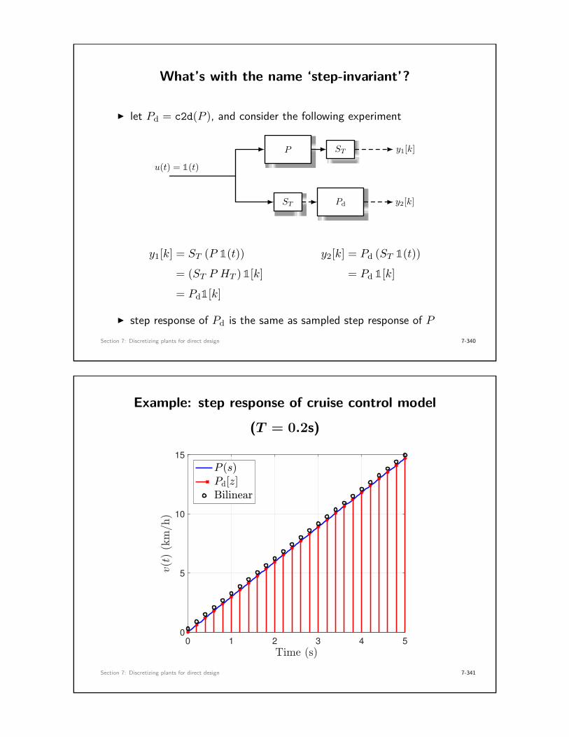
What’s with the name ‘step-invariant’?
I let Pd = c2d(P ), and consider the following experiment
P
PdST
ST
u(t) = 1(t)
y1[k]
y2[k]
y1[k] = ST (P 1(t)) y2[k] = Pd (ST 1(t))
= (ST P HT ) 1[k] = Pd 1[k]
= Pd1[k]
I step response of Pd is the same as sampled step response of PSection 7: Discretizing plants for direct design 7-340
Example: step response of cruise control model
(T = 0.2s)
0 1 2 3 4 5
0
5
10
15
Section 7: Discretizing plants for direct design 7-341

Frequency response of discretized plant
I we know the frequency response P (jω) of the plant is very useful
I the discretized plant Pd = c2d(P ) has frequency response Pd[ejωT ]
I what is the relationship between these two? thought experiment:
P (s)
Pd[z]ST
u(t) = ejωt
y(t)
y[k]
I how do y(t) and y[k] compare in steady-state?
Section 7: Discretizing plants for direct design 7-342
Frequency response of discretized plant contd.
I top branch of diagram gives y(t) = P (jω)ejωt, bottom branch gives
ST HT P (s) STejωt (2) (3) (4) (5)
Pd[z]
I signal (2) is ejωkT =⇒ signal (5) is Pd[ejωT ] · ejωkT
I at low frequencies where ω << ωNyquist = ωs/2, there is no aliasing• signal (3) is close to signal (1)• signal (4) is close to P (jω)ejωt
• signal (5) is close to P (jω)ejωkT
=⇒ Pd[ejωT ] ' P (jω) at low frequenciesSection 7: Discretizing plants for direct design 7-343

Example: cruise control model (T = 0.2s)
10-4
10-3
10-2
10-1
100
101
-200
-150
-100
-50
10-4
10-3
10-2
10-1
100
101
-200
-150
-100
-50
0
P (s) =1/m
s+ b/m
Pd[z] =1b
1− e−Tb/m
z − e−Tb/m
Section 7: Discretizing plants for direct design 7-344
MATLAB commands
I computing step-invariant transformation (explicitly)
Ad = expm(A*T);Bd = inv(A)*(Ad-eye(n));
I computing step-invariant transformation (built-in)
P = ss(A,B,C,D);Pd = c2d(P,T,‘zoh’);
Section 7: Discretizing plants for direct design 7-345

Additional references
I step-invariant discretization (ZOH)
• Nielsen, Chapter 7
• Franklin, Powell, & Workman, Chapter 4.3.3
• Åström & Wittenmark, Chapter 3
Section 7: Discretizing plants for direct design 7-346
Personal Notes
Section 7: Discretizing plants for direct design 7-347

Personal Notes
Section 7: Discretizing plants for direct design 7-348
Personal Notes
Section 7: Discretizing plants for direct design 7-349

8. Direct design of digital controllers
• pole placement for discrete-time systems• tracking reference signals (transfer functions)• state-space control design• state feedback, controllability, and pole placement• observers, observability, and output feedback• preview of optimal control
Section 8: Direct design of digital controllers 8-350
Sampled-data control problem
C HT P STr[k] e[k] u[k] u(t) y(t) y[k]−
Discrete-time system Pd
I plant and controller described by LTI transfer function or LTIstate-space models
Sampled-data design problem: given plant P and a set ofdesign specifications, design a discrete-time controller C suchthat the closed-loop sampled-data system meets the designspecifications.
Section 8: Direct design of digital controllers 8-351

Big picture for direct design
1. choose an initial sampling period T• possibly dictated by hardware, informed by design specs
2. discretize plant P to obtain Pd
• note: Pd is implicitly a function of T
3. design — by any method — a discrete-time controller C for Pd tomeet your design specs
• note: C is also a function of T , since it was tuned for the plant Pd
4. simulate sampled-data system; if performance specs are not met,adjust controller design and/or decrease T
Section 8: Direct design of digital controllers 8-352
Pole placement for discrete-time systems
I in continuous-time, we selected a subset Cgood of C− in which toplace the poles of the closed-loop system
I from step-invariant transformation, we saw that if s ∈ C is aeigenvalue/pole of P , then z = esT is an eigenvalue/pole of Pd
I idea: we can map Cgood ⊂ C− to a subset Dgood ⊂ D
Re(s)
Im(s)
Cgood
z = esT
Re(z)
Im(z)
D
Dgood
Section 8: Direct design of digital controllers 8-353

Pole placement procedure in discrete-time
1. use design specs to find Cgood
2. choose a set of symmetric pole locations
Λ = {λ1, . . . , λ2n−1} ⊂ Cgood
3. map pole locations from Cgood to Dgood
E = {eλ1T , . . . , eλ2n−1T }
Πdes[z] = (z − eλ1T ) · · · (z − eλ2n−1T )
4. solve discrete-time pole placement problem for controller
Pd[z] = Np[z]Dp[z] , C[z] = Nc[z]
Dc[z] = gn−1zn−1 + · · ·+ g1z + g0
fn−1zn−1 + · · ·+ f1z + f0
Π[z] = NpNc +DpDc
Section 8: Direct design of digital controllers 8-354
Tracking reference signals
C[z] Pd[z]r e u y
−
Tracking problem: Given a plant Pd[z], design a controller C[z] suchthat the closed-loop system is feedback stable and
limk→∞
(r[k]− y[k]) = 0 .
Internal Model Principle: Assume Pd[z] is strictly proper, C[z] isproper, and that the closed-loop system is feedback stable. Then
limk→∞ (r[k]− y[k]) = 0 if and only if Pd[z]C[z] contains an internalmodel of the unstable part of r[z].
Section 8: Direct design of digital controllers 8-355

Example: step tracking
I for a step r[k] = 1[k], r[z] = zz−1
I there are three cases
(i) if Pd[z] has a zero at z = 1, then step-tracking is not possible
(ii) if Pd[z] has a pole at z = 1, C[z] can be any stabilizing controller
(iii) if Pd[z] does not have a pole or zero at z = 1, then C[z] must havea pole at z = 1
I pole at z = 1 is “integral control” (running sum of tracking error)
u[k] = Z−1{u[z]} = Z−1{
z
z − 1e[z]}
=k∑`=0
e[`]
Section 8: Direct design of digital controllers 8-356
Control design for LTI state-space models
I all MIMO (multi-input multi-output) control techniques are basedon state-space models
I allows for use of powerful computational techniques, optimization
I we will keep things as simple as possible, introduce the basic ideasfor single-input single-output discrete-time models
x[k + 1] = Ax[k] +Bu[k]
y[k] = Cx[k] +Du[k]
I nearly identical theory for continuous-time state models
Section 8: Direct design of digital controllers 8-357

State-space regulation problem
x+ = Ax+Bu
y = Cx+Du
u[k] y[k]
I regulation problem: find a controller such that x[k]→ 0 for anychoice of initial condition x[0]
I in other words: closed-loop system is internally asymptotically stable(recall that this implies feedback stability of the closed-loop system)
I designing a regulating controller (“regulator”) can be extended toreference tracking
Section 8: Direct design of digital controllers 8-358
Regulation by state feedback
I simplest case: assume we can measure the entire state x[k], and wetry to design a state-feedback controller
u[k] = Fx[k] ,F =
[f1 f2 · · · fn
]“state-feedback gain”
F x+ = Ax+Bu0 u[k] x[k]
+
Section 8: Direct design of digital controllers 8-359

State feedback and controllability
I closed-loop system is
x+ = Ax+Bu = Ax+BFx = (A+BF )︸ ︷︷ ︸Acl
x
I to achieve internal asymptotic stability, need to find F such that
eig(A+BF ) ⊂ D
I when can we find such an F? Need new idea of controllability
I definition: a state-space system is controllable if from every initialstate x[0] ∈ Rn, there is a sequence of control inputs{u[0], u[1], . . . , u[n− 1]} such that x[n] = 0
I idea: can choose inputs to “deliver” the state to the originSection 8: Direct design of digital controllers 8-360
Controllability contd.
I let’s think about how system state changes over time
x[1] = Ax[0] +Bu[0]
x[2] = Ax[1] +Bu[1] = A2x[0] +Bu[1] +ABu[0]...
x[n] = Anx[0] +Bu[n− 1] +ABu[n− 2] + · · ·+An−1Bu[0]
I since we want x[n] = 0, we can also write this as
−Anx[0] =[B AB · · · An−1B
]︸ ︷︷ ︸
Controllability matrix Wc
u[n− 1]u[n− 2]
...u[0]
︸ ︷︷ ︸
:=uc
Section 8: Direct design of digital controllers 8-361

Controllability contd.
I required input sequence is determined by linear equation
−Anx[0] = Wcuc
I if rank(Wc) = n, we can solve for uc for any x[0]
conclusion: a state-space system is controllable if thecontrollability matrix
Wc =[B AB · · · An−1B
]∈ Rn×n
has rank n.
I vectors {B,AB,A2B, . . . , An−1B} tell us about the directions instate-space that we can “push” the system using our input
Section 8: Direct design of digital controllers 8-362
State-feedback control and pole placement
I controllability lets us do “pole” placement for state-space systems
I suppose we have a desired (symmetric w.r.t. real axis) set ofclosed-loop eigenvalues
{z1, . . . , zn} ⊂ D
for closed-loop system x+ = (A+BF )x
Pole-placement theorem for state feedback: there exists astate-feedback matrix F ∈ R1×n such that A+BF has thedesired eigenvalues if and only if the system is controllable
Section 8: Direct design of digital controllers 8-363

Calculating state-feedback gain F
I to calculate F =[f1 f2 · · · fn
], there are two approaches
1. let Πdes[z] = (z − z1) · · · (z − zn) be the desired characteristicpolynomial, and match coefficients of z from the equation
Π[z] = det(zI − (A+BF )) = Πdes[z]
2. use Ackerman’s Formula
F = −[0 0 · · · 1
]W−1
c Πdes[A]
whereΠdes[A] = (A− z1I) · · · (A− znI)
I both implemented in MATLAB as place and acker
Section 8: Direct design of digital controllers 8-364
Example: satellite attitude control
I discretized model of satellite Jθ = τ
x[k + 1] =[
1 T
0 1
]x[k] +
[T 2
2JTJ
]u[k]
y[k] =[1 0
]x[k]
I system is internally unstable (repeated eigenvalue at z = 1)
I objective: stabilize x = 0 using state-feedback
I system is controllable for all sampling periods T > 0
Wc =[B AB
]=[T 2
2J3T 2
2JTJ
TJ
], det(Wc) = −T
3
J2 6= 0
Section 8: Direct design of digital controllers 8-365

Example: satellite attitude control contd.
I we must select two eigenvalues for A+BF , let them be z1, z2
Πdes[z] = (z − z1)(z − z2) = z2 + (−z1 − z2)z + z1z2
I we can form the closed-loop system matrix
A+BF =[
1 T
0 1
]+[T 2
2JTJ
] [f1 f2
]=[
1 + f1T2
2J T + f2T2
2Jf1TJ 1 + f2T
J
]
I characteristic polynomial Π[z] = det(zI − (A+BF ))
Π[z] = z2 +(f1T
2 + 2f2T − 4J2J
)z +
(f1T
2 − 2f2T + 2J2J
)
Section 8: Direct design of digital controllers 8-366
Example: satellite attitude control contd.
I comparing coefficients, we get two simultaneous equations
−(z1 + z2) = f1T2 + 2f2T − 4J
2J z1z2 = f1T2 − 2f2T + 2J
2Jwhich we can solve to find f1 and f2:
f1 = −JT
(1− z1 − z2 + z1z2) , f2 = − J
2T (3− z1 − z2 − z1z2)
and our controller is then
u[k] =[f1 f2
] [x1[k]x2[k]
]
I since states x1 and x2 are position and velocity, f1 is the feedbackgain on position, while f2 is the gain on velocity (PD control)
Section 8: Direct design of digital controllers 8-367

Example: satellite attitude control contd.
I z1,2 = 0.4± 0.3j, x[0] = (1.5, 1.5), J = 1 kg ·m2, T = 1 s
-2 -1 0 1 2 3
-3
-2
-1
0
1
2
3
-2
0
2
0 5 10 15 20
-2
0
2
0 5 10 15 20
Section 8: Direct design of digital controllers 8-368
Example: satellite attitude control contd.
-2.5
-2
-1.5
-1
-0.5
0
0.5
0 5 10 15
Section 8: Direct design of digital controllers 8-369

Deadbeat control
I deadbeat design is fastest (most aggressive) design possible
I we place all eigenvalues of A+BF at the origin z = 0 (nilpotency)
det(zI − (A+BF )) = zn
I fact: if M ∈ Rn×n is nilpotent, there exists p ≤ n s.t. Mp = 0
I recall: solution to state model from initial condition x[0] is
x[k + 1] = (A+BF )x[k] =⇒ x[k] = (A+BF )kx[0]
I therefore, x[p] = 0; state goes to the origin after p time steps!
Section 8: Direct design of digital controllers 8-370
Example: satellite attitude control (deadbeat tuning)
I z1,2 = 0, x[0] = (1.5, 1.5), J = 1 kg ·m2, T = 1 s
-2 -1 0 1 2 3
-3
-2
-1
0
1
2
3
-2
0
2
0 5 10 15 20
-2
0
2
0 5 10 15 20
I deadbeat tuning results in convergence in 2 time steps, but with alarger swing in velocity (x2) compared to previous tuning
Section 8: Direct design of digital controllers 8-371

Example: satellite attitude control (deadbeat tuning)
-4
-3
-2
-1
0
1
2
3
0 5 10 15
Section 8: Direct design of digital controllers 8-372
Intersample ripple
I suppose we have designed a state-feedback F for discretized plant
I what happens when implemented in a sampled-data system?
F HT x = Ax+Bu
ST
0 u[k] u(t) x(t)
x[k]
+
I we know that x[k] = x(kT )→ 0
I question: what is happening between samples?
Section 8: Direct design of digital controllers 8-373
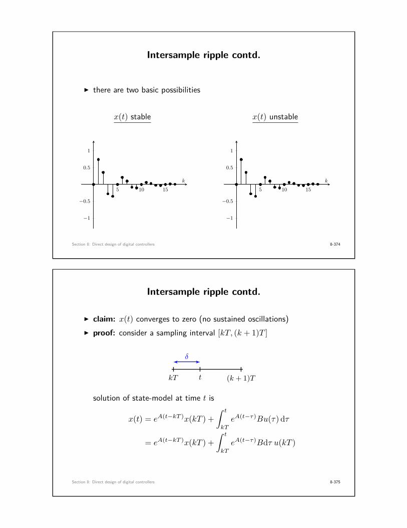
Intersample ripple contd.
I there are two basic possibilities
x(t) stable
5 10 15
−1
−0.5
0.5
1
k
x(t) unstable
5 10 15
−1
−0.5
0.5
1
k
Section 8: Direct design of digital controllers 8-374
Intersample ripple contd.
I claim: x(t) converges to zero (no sustained oscillations)I proof: consider a sampling interval [kT, (k + 1)T ]
(k + 1)TkT t
δ
solution of state-model at time t is
x(t) = eA(t−kT )x(kT ) +∫ t
kT
eA(t−τ)Bu(τ) dτ
= eA(t−kT )x(kT ) +∫ t
kT
eA(t−τ)Bdτ u(kT )
Section 8: Direct design of digital controllers 8-375

Intersample ripple contd.
I change variables σ = t− τ
x(t) = eA(t−kT )x(kT ) +∫ 0
t−kTeAσB(−dσ)u(kT )
= eAδx(kT ) +∫ δ
0eAσB dσ u(kT )
I but u(kT ) = Fx(kT ), therefore
x(t) =(eAδ +
∫ δ
0eAσ dσ BF
)x(kT ) = Mδx(kT )
or simply x(kT + δ) = Mδx(kT ).
I x(kT )→ 0, and therefore x(kT + δ)→ 0
I but δ was arbitrary, therefore x(t)→ 0 as t→∞Section 8: Direct design of digital controllers 8-376
Example: satellite attitude control contd.
I z1,2 = 0.4± 0.3j, x[0] = (1.5, 1.5), J = 1 kg ·m2, T = 1 s
-2 -1 0 1 2 3
-3
-2
-1
0
1
2
3
0 5 10 15 20
-1
0
1
2
0 5 10 15 20
-2
0
2
I takeaway: everything is fine between the samplesSection 8: Direct design of digital controllers 8-377

Example: satellite attitude control contd.
I z1,2 = 0, x[0] = (1.5, 1.5), J = 1 kg ·m2, T = 1 s
-2 -1 0 1 2 3
-3
-2
-1
0
1
2
3
0 5 10 15 20
-1
0
1
2
0 5 10 15 20
-2
0
2
I takeaway: everything is fine between the samplesSection 8: Direct design of digital controllers 8-378
Output feedback for state-space systems
I usually, we cannot measure the entire state x[k] ∈ Rn
• some variables in model not easy to measure
• might require too many sensors
I when we design transfer function controllers, we only use themeasured output y[k], so state feedback looks quite restrictive
I the solution to this problem is to use an observer, which takes theoutput y[k] and produces an estimate x[k] of the state x[k]
I we can then use the estimated state for state-feedback control
u[k] = Fx[k]
Section 8: Direct design of digital controllers 8-379

Observers for state-space systems
I naively, knowing y[k] and u[k], we could try to solve equation
y[k] = Cx[k] +Du[k]
for current state x[k] at each time k (not a great idea, why?)
I if we apply an input and look at the corresponding time series of theoutput, we will be able to infer something more information aboutthe state
I key idea: use the sequence of inputs and measurements over time
Section 8: Direct design of digital controllers 8-380
The Luenberger observer
x+ = Ax+Bu
y = Cx+Du
Observer
u[k] y[k]
x[k]
I the observer is a discrete-time LTI system with state x[k]
x+ = Ax+Bu+ L(y − y)
y = Cx+Du
L =
l1...ln
∈ Rn×1
“observer gain”
Section 8: Direct design of digital controllers 8-381
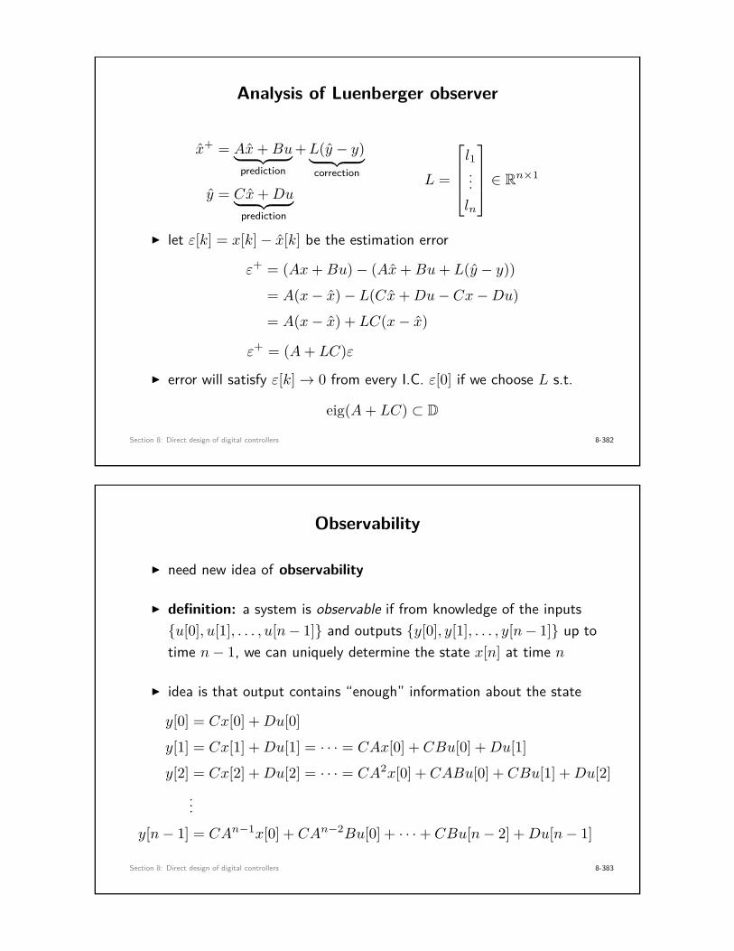
Analysis of Luenberger observer
x+ = Ax+Bu︸ ︷︷ ︸prediction
+L(y − y)︸ ︷︷ ︸correction
y = Cx+Du︸ ︷︷ ︸prediction
L =
l1...ln
∈ Rn×1
I let ε[k] = x[k]− x[k] be the estimation error
ε+ = (Ax+Bu)− (Ax+Bu+ L(y − y))
= A(x− x)− L(Cx+Du− Cx−Du)
= A(x− x) + LC(x− x)
ε+ = (A+ LC)ε
I error will satisfy ε[k]→ 0 from every I.C. ε[0] if we choose L s.t.
eig(A+ LC) ⊂ D
Section 8: Direct design of digital controllers 8-382
Observability
I need new idea of observability
I definition: a system is observable if from knowledge of the inputs{u[0], u[1], . . . , u[n− 1]} and outputs {y[0], y[1], . . . , y[n− 1]} up totime n− 1, we can uniquely determine the state x[n] at time n
I idea is that output contains “enough” information about the state
y[0] = Cx[0] +Du[0]
y[1] = Cx[1] +Du[1] = · · · = CAx[0] + CBu[0] +Du[1]
y[2] = Cx[2] +Du[2] = · · · = CA2x[0] + CABu[0] + CBu[1] +Du[2]...
y[n− 1] = CAn−1x[0] + CAn−2Bu[0] + · · ·+ CBu[n− 2] +Du[n− 1]
Section 8: Direct design of digital controllers 8-383

Observability contd.
I we can write this as a linear system of equations for x[0]y[0]y[1]. . .
y[n− 1]
︸ ︷︷ ︸
:=yo
=
C
CA...
CAn−1
︸ ︷︷ ︸
:=Wo
x[0]+
D 0 · · · 0CB D · · · 0...
.... . .
...CAn−2B · · · CB D
u[0]u[1]...
u[n− 1]
︸ ︷︷ ︸
:=ξ
or simplyyo − ξ = Wo x[0]
I if we could solve for x[0] ∈ Rn, then we can immediately find x[n] as
x[n] = Anx[0] +n−1∑j=0
An−j−1Bu[j]
Section 8: Direct design of digital controllers 8-384
Observability contd.
I if rank(Wo) = n, we can uniquely solve for the linear equation
yo − ξ = Wo x[0]
for x[0] and then uniquely determine x[n]!
I conclusion: a state-space system is observable if the observabilitymatrix
Wo =
C
CA...
CAn−1
∈ Rn×n
has rank n.
Section 8: Direct design of digital controllers 8-385

Observability and observer design
I observability guarantees we can design an observer
I suppose we have a desired (symmetric w.r.t. real axis) set ofeigenvalues
{ζ1, . . . , ζn} ⊂ D
for estimation error dynamics ε+ = (A+ LC)ε
Pole-placement theorem for observer design: There existsan observer gain matrix L ∈ Rn×1 such that A+ LC has thedesired eigenvalues if and only if the system is observable
Section 8: Direct design of digital controllers 8-386
Calculating the observer gain L
I to calculate L =[l1 l2 · · · ln
]T, there are two approaches
1. let Πdes[z] = (z − ζ1) · · · (z − ζn) be the desired characteristicpolynomial, and match coefficients of z from the equation
Π[z] = det(zI − (A+ LC)) = Πdes[z]
2. use Ackerman’s Formula
L = −Πdes[A]W−1o[0 0 · · · 1
]T
whereΠdes[A] = (A− ζ1I) · · · (A− ζnI)
I both implemented in MATLAB as place and acker
Section 8: Direct design of digital controllers 8-387

Example: observer for satellite system
I discretized model of satellite Jθ = τ
x[k + 1] =[
1 T
0 1
]x[k] +
[T 2
2JTJ
]u[k]
y[k] =[1 0
]x[k]
I objective: design observer to estimate x[k] from y[k]
I system is observable for all sampling periods T :
Wo =[C
CA
]=[
1 01 T
], det(Wo) = T 6= 0
Section 8: Direct design of digital controllers 8-388
Example: observer for satellite system contd.
I we must select two eigenvalues for A+ LC, let them be ζ1, ζ2
Πdes[z] = (z − ζ1)(z − ζ2) = z2 + (−ζ1 − ζ2)z + ζ1ζ2
I we can form the system matrix for the estimation error
A+ LC =[
1 T
0 1
]+[l1
l2
] [1 0
]=[
1 + l1 T
l2 1
]
I characteristic polynomial Π[z] = det(zI − (A+ LC))
Π[z] = z2 + (−2− l1)z + (1 + l1 − l2T )
Section 8: Direct design of digital controllers 8-389

Example: observer for satellite system contd.
I comparing coefficients, we get two simultaneous equations
−(ζ1 + ζ2) = −2− l1 ζ1ζ2 = 1 + l1 − l2T
which we can solve to find l1 and l2:
l1 = ζ1 + ζ2 − 2 , l2 = 1T
(ζ1 + ζ2 − ζ1ζ2 − 1)
I our observer is therefore
x+ =[
1 T
0 1
]x+
[T 2
2JTJ
]u+
[l1
l2
](y − y)
y =[1 0
]x
Section 8: Direct design of digital controllers 8-390
Example: observer for satellite system contd.
I satellite system subject to sinusoidal force input, ζ1,2 = 0.4± 0.3jI initial conditions x[0] = (4,−2), x[0] = (0, 0)
-20 0 20 40 60
-3
-2
-1
0
1
2
3
4
0 20 40 60
-50
0
50
0 20 40 60
-5
0
5
Section 8: Direct design of digital controllers 8-391

Example: observer for satellite system contd.
I satellite system subject to sinusoidal toruqe input, ζ1,2 = 0I initial conditions x[0] = (4,−2), x[0] = (0, 0)
-20 0 20 40 60
-3
-2
-1
0
1
2
3
4
0 20 40 60
-50
0
50
0 20 40 60
-5
0
5
I takeaway: estimates converge in 2 steps with deadbeat tuning, butwith large error at time step k = 1 compared to previous tuning
Section 8: Direct design of digital controllers 8-392
Comments on state feedback / observer design
I for state-feedback controllers, aggressive pole placements (i.e., closerto the origin) will give very stable system, but
• control effort will be very large
• state variables may have poor transient response (overshoot)
I for observers, aggressive pole placements (i.e., closer to the origin)will make estimation error go to zero quickly, but
• measurement noise will be amplified
• estimation error may have poor transient response (overshoot)
I usually, want to select least aggressive pole placements which stillgive a response meeting specs; this is a trial-and-error procedure
Section 8: Direct design of digital controllers 8-393

Combining state-feedback and observers
I combination of observer and state-feedback controller can be usedto solve the state-space regulation problem
Fx+ = Ax+Bu
y = Cx
Observer
u[k] y[k]
x[k]
0
I control input produced using estimated state
u[k] = Fx[k]
Section 8: Direct design of digital controllers 8-394
Output feedback control
I observer and state-feedback matrix F form dynamic controller
x+ = Ax+Bu+ L(y − y)
u = Fx
where eig(A+BF ) ⊂ D and eig(A+ LC) ⊂ D
I substituting for y = Cx and u = Fx, controller has state model
x+ = (A+BF + LC)x− Ly
u = Fx
with input y and output u
Section 8: Direct design of digital controllers 8-395

Output feedback control cpntd.
I observer + state feedback controller:
x+ = (A+BF + LC)x− Ly
u = Fx
with input y and output u
I controller has same order as plant
I if you prefer transfer functions, controller has the TF
u[z]y[z] = −F (zIn − (A+BF + LC))−1L
Section 8: Direct design of digital controllers 8-396
Sampled-data implementation
F HTx = Ax+Bu
y = Cx
STx+ = (Ad +BdF + LCd)x− Ly
0 u[k] u(t) y(t)
y[k]x[k]
+
Section 8: Direct design of digital controllers 8-397

Example: output feedback for satellite system contd.
I observer and feedback gain with poles z1,2 = 0.4± 0.3j
-1 0 1 2 3 4
-4
-3
-2
-1
0
1
2
0 5 10 15 20
-4
-2
0
2
4
0 5 10 15 20
-4
-2
0
2
4
Section 8: Direct design of digital controllers 8-398
Example: output feedback for satellite system contd.
I observer and feedback gain with deadbeat poles z1,2 = 0
-1 0 1 2 3 4
-4
-3
-2
-1
0
1
2
0 5 10 15 20
-4
-2
0
2
4
0 5 10 15 20
-4
-2
0
2
4
I same story as before: deadbeat tuning is more “aggressive”: it givesfaster convergence, but with worse transients
Section 8: Direct design of digital controllers 8-399

Incorporating reference signals
I output reference r included by slight twist on previous controller
I if we want y = r in steady-state, need to find x and u such that
x = Ax+Bu
r = Cx+Du⇐⇒
[A− In B
C D
][x
u
]=[
0
r
]
therefore [x
u
]=[A− In B
C D
]−1 [0
1
]r :=
[Mx
Mu
]r
I now use modified control law
u[k] = u+ F (x[k]− x) = Fx+ (Mu − FMx)r
Section 8: Direct design of digital controllers 8-400
Incorporating reference signals contd.
Mu − FMx
F
x+ = Ax+Bu
y = Cx
Observer
y[k]
x[k]
r u[k]
I this solution can work quite well; a more sophisticated approachwould introduce an integral state (see problem set for details)
xI [k + 1] = xI [k] + (Cx[k]− r[k])︸ ︷︷ ︸tracking error
Section 8: Direct design of digital controllers 8-401

Example: reference tracking for satellite system contd.
I observer and feedback gain with poles z1,2 = 0.4± 0.3j
-2 0 2 4
-4
-3
-2
-1
0
1
2
0 10 20 30 40
-2
0
2
0 10 20 30 40
-4
-2
0
2
Section 8: Direct design of digital controllers 8-402
Example: reference tracking for satellite system contd.
I observer and feedback gain with deadbeat poles z1,2 = 0
-2 0 2 4
-4
-3
-2
-1
0
1
2
0 10 20 30 40
-2
0
2
0 10 20 30 40
-4
-2
0
2
I as expected, deadbeat tuning gives fast response at the cost ofworse transient behaviour
Section 8: Direct design of digital controllers 8-403

Preview of optimal control
I picking locations for poles/eigenvalues is hard work, and for largecontrol problems is simply not a realistic solution
I in optimal control, we specify a “cost” that we want to minimize,and find the controller that minimizes that cost
I problem of selecting poles is transformed into the problem ofdesigning a cost; what should our cost include?
• for regulation, we want x[k] and y[k] to stay small• to minimize control effort, u[k] should stay small also
I therefore, cost should penalize both u[k] and y[k]
Section 8: Direct design of digital controllers 8-404
The linear quadratic regulator
I the linear quadratic regulator (LQR) cost is
Cost/Loss Function = JLQR :=∞∑k=0
(y[k]2 + ρu[k]2
)where ρ > 0 is a tuning parameter
I if JLQR is finite, then y[k] and u[k] converge to zero (duh)
I cost captures transient of output and transient of control input
• if ρ is big, we are saying that control effort is expensive
• if ρ is small, we are saying that control effort is inexpensive
I goal: find control sequence {u[0], u[1], . . .} that minimizes JLQR
Section 8: Direct design of digital controllers 8-405

Solution of LQR problem
I if state-space system is controllable and observable, LQR problemcan be solved, and solution is a state feedback
u[k] = FLQRx[k]
I feedback matrix FLQR ∈ R1×n computed in MATLAB as
F = -lqr(sys, C’*C, rho, zeros(n,1));
I control design problem reduced to picking a single constant ρ
Section 8: Direct design of digital controllers 8-406
Example: LQR feedback for satellite
I deadbeat observer with LQR feedback gain, ρ = 10
-2 0 2 4
-4
-3
-2
-1
0
1
2
0 10 20 30 40
-2
0
2
0 10 20 30 40
-4
-2
0
2
Section 8: Direct design of digital controllers 8-407

Example: LQR feedback for satellite
I deadbeat observer with LQR feedback gain, ρ = 1
-2 0 2 4
-4
-3
-2
-1
0
1
2
0 10 20 30 40
-2
0
2
0 10 20 30 40
-4
-2
0
2
Section 8: Direct design of digital controllers 8-408
Example: LQR feedback for satellite
I deadbeat observer with LQR feedback gain, ρ = 0.1
-2 0 2 4
-4
-3
-2
-1
0
1
2
0 10 20 30 40
-2
0
2
0 10 20 30 40
-4
-2
0
2
Section 8: Direct design of digital controllers 8-409

Example: LQR feedback for satellite
I comparison of control efforts during third step change
20 25 30 35
-3
-2
-1
0
1
2
3
Section 8: Direct design of digital controllers 8-410
Modelling of simple pendulum on cart
M
m
`
θ
(0, 0)
g
u(t)
+p
I p = position of cartI rtip = pendulum tip
rtip =[p+ ` sin θ` cos θ
]
rtip =[p+ `θ cos θ−`θ sin θ
]
kinetic energy: T =12Mp2 +
12m‖rtip‖22
=12
(M +m)p2 +m`pθ cos θ +12m`2θ2
potential energy: U = Utip = −mg`(1− cos θ)
Section 8: Direct design of digital controllers 8-411

Modelling of simple pendulum on cart
I the Lagrangian L is kinetic minus potential
L =12
(M +m)p2 +m`pθ cos θ +12m`2θ2 +mg`(1− cos θ)
I equations of motion given by two Lagrange equationsddt
(∂L
∂p
)−∂L
∂p= u ,
ddt
(∂L
∂θ
)−∂L
∂θ= 0
which yield
(M +m)p+m` cos(θ)θ −m`θ2 sin(θ) = u
m`2θ +m` cos(θ)p−mg` sin(θ) = 0
Section 8: Direct design of digital controllers 8-412
Design example: pendulum on cart
I equations can be transformed into[p
θ
]=[M +m m` cos(θ)m` cos(θ) m`2
]−1 [m`θ2 sin(θ) + u
mg` sin(θ)
]
can can subsequently be put into state-space form
x = f(x, u) , y = h(x, u)
with x = (p, p, θ, θ)T, y = position of cart
I control objectives:
1. stabilize upright position θ = 0 with constant position p = 0
2. track constant position references
Section 8: Direct design of digital controllers 8-413

Design example: pendulum on cart
I exercise: linearized model around (p, p, θ, θ) = (0, 0, 0, 0) isx1
x2
x3
x4
=
0 1 0 00 0 −m
M g 00 0 0 10 0 M+m
Mg` 0
x1
x2
x3
x4
+
01M
0− 1M`
uy =
[1 0 0 0
]x
I poles and zeros of transfer function
Re(s)Im(s)× ×√
M+mM
g`
◦ ◦√g`
×
Section 8: Direct design of digital controllers 8-414
Design example: pendulum on cart
I parameters are m = 1 kg, M = 0.5 kg, ` = 1m
I take T = 0.05s, and build discrete-time modelpend_ct = ss(A,B,C,D);pend_dt = c2d(pend_ct,T);
I can check system is controllable and observableW_c = ctrb(Ad,Bd);W_o = obsv(Ad,Cd);
I design controller and observer gainsrho=0.5;F = -lqr(pend_dt, Cd’*Cd, rho, zeros(n,1));L = acker(Ad’, -Cd’, [0;0;0;0])’;
Section 8: Direct design of digital controllers 8-415
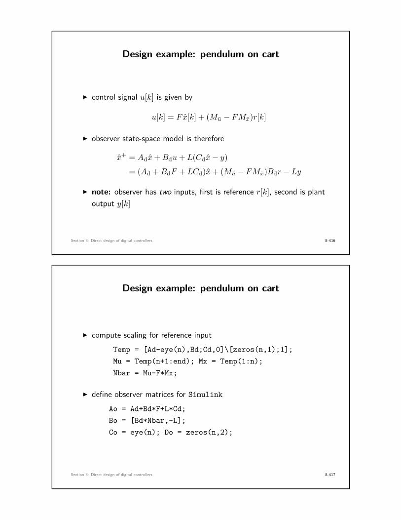
Design example: pendulum on cart
I control signal u[k] is given by
u[k] = Fx[k] + (Mu − FMx)r[k]
I observer state-space model is therefore
x+ = Adx+Bdu+ L(Cdx− y)
= (Ad +BdF + LCd)x+ (Mu − FMx)Bdr − Ly
I note: observer has two inputs, first is reference r[k], second is plantoutput y[k]
Section 8: Direct design of digital controllers 8-416
Design example: pendulum on cart
I compute scaling for reference input
Temp = [Ad-eye(n),Bd;Cd,0]\[zeros(n,1);1];Mu = Temp(n+1:end); Mx = Temp(1:n);Nbar = Mu-F*Mx;
I define observer matrices for Simulink
Ao = Ad+Bd*F+L*Cd;Bo = [Bd*Nbar,-L];Co = eye(n); Do = zeros(n,2);
Section 8: Direct design of digital controllers 8-417

Design example: pendulum on cart
Section 8: Direct design of digital controllers 8-418
State-space control of pendulum on cart T = 0.05s
0 5 10 15 20 25 30 35 40
-0.5
0
0.5
0 5 10 15 20 25 30 35 40
-5
0
5
0 5 10 15 20 25 30 35 40
-2
-1
0
1
2
Section 8: Direct design of digital controllers 8-419

State-space control of pendulum on cart T = 0.2s
0 5 10 15 20 25 30 35 40
-0.5
0
0.5
0 5 10 15 20 25 30 35 40
-5
0
5
0 5 10 15 20 25 30 35 40
-2
-1
0
1
2
Section 8: Direct design of digital controllers 8-420
State-space control of pendulum on cart T = 0.4s
0 5 10 15 20 25 30 35 40
-0.5
0
0.5
0 5 10 15 20 25 30 35 40
-5
0
5
0 5 10 15 20 25 30 35 40
-2
-1
0
1
2
I can maintain performance with quite large sampling period!Section 8: Direct design of digital controllers 8-421

MATLAB commands
I controllability and observability matrices
sys_dt = ss(Ad,Bd,Cd,Dd,T);sys_dt = c2d(sys,T);W_o = obsv(sys);W_c = ctrb(sys);
I pole-placement using Ackerman
F = -acker(Ad, Bd, pole_vec);L = -acker(Ad’, Cd’, pole_vec)’;
I LQR controller
F = -lqr(sys_dt, Cd’*Cd, rho, zeros(n,1));
Section 8: Direct design of digital controllers 8-422
Additional references
I Nielsen, Chapter 9
I Åström & Wittenmark, Chapters 5 and 9
I Phillips, Nagle, & Chakrabortty, Chapter 9
I Franklin, Powell, & Workman, Chapter 8
I Hespanha, Topics in Undergraduate Control System Design, Chapter8, 9, 11 (topics are discussed for continuous-time models)
Section 8: Direct design of digital controllers 8-423

Personal Notes
Section 8: Direct design of digital controllers 8-424
Personal Notes
Section 8: Direct design of digital controllers 8-425

Personal Notes
Section 8: Direct design of digital controllers 8-426
9. Introduction to system identification
• identification of functions• identification of dynamic systems
Section 9: Introduction to system identification 9-427

Motivation for system identification
I nearly all of the control design we have done is model-based, in thatour controller is designed based on a model of the plant
I in principle, feedback gives us robustness against model uncertainty;in practice, we still want/need to have a decent model
I sometimes it is impossible to model a system from first principles
• may be unclear how to model some components
• functional forms of nonlinearities may be unknown
I other times, an accurate first-principles model may be unnecessarilycomplex for control purposes
Section 9: Introduction to system identification 9-428
System identification
I system identification is the process of determining a dynamicmodel from measured input/output data
I identification can be
• unstructured, where we assume a general class of models (e.g., LTI)
• structured, where we fix a model structure and estimate parameters
I system identification aims for simple (e.g., LTI) models that areuseful for actually doing control
Section 9: Introduction to system identification 9-429

Identification of functions
I suppose we have a static input/output relationship
f(·)u(t) y(t)
I example: u is voltage applied to a load, y is the current drawn
I the precise function f is unknown (and probably unknowable)
I idea: apply inputs, measure outputs, and fit a model f for f
f(u) = θ1ϕ1(u) + θ2ϕ2(u) + · · ·+ θnϕn(u)
where {θ1, . . . , θn} are unknown parameters and {ϕi(·)} are basisfunctions that we must choose
Section 9: Introduction to system identification 9-430
Identification of functions contd.
I example: if we have a nonlinear resistive load, we may choose
f(u) = θ1 + θ2u+ θ3u2 + θ4u
3
I we now run N > 0 experiments, where we apply an input ui andrecord the output yi, generating N pairs of data points
(ui, yi) , i ∈ {1, . . . , N}.
I for each input ui, we can estimate the output using our model f
yi = f(ui) = θ1ϕ1(ui) + · · ·+ θnϕn(ui) , i ∈ {1, . . . , N}
Section 9: Introduction to system identification 9-431

Least squares
I stacking all these equations, we obtainy1
y2...yN
︸ ︷︷ ︸
:=y
=
ϕ1(u1) ϕ2(u1) · · · ϕn(u1)ϕ2(u2) ϕ2(u2) · · · ϕn(u2)
......
. . ....
ϕ1(uN ) ϕ2(uN ) · · · ϕn(uN )
︸ ︷︷ ︸
:=Φ
θ1
θ2...θn
︸ ︷︷ ︸
:=θ
I least squares identification minimizes measurement and predictionmismatch in mean-square sense
minimizeθ∈Rn
Jls(θ) =N∑i=1
(yi − yi)2 = (y − y)T(y − y) .
I any solution θ∗ ∈ Rn to this problem is a least squares minimizerSection 9: Introduction to system identification 9-432
Least squares contd.
I least squares cost is
Jls(θ) = (y − y)T(y − y) = yTy + yTy − 2yTy
= yTy + θTΦTΦθ − 2yTΦθ
I take gradient of cost w.r.t. θ and set to zero
∇θJls(θ) = 2ΦTΦθ − 2ΦTy = 0 =⇒ θ∗ = (ΦTΦ)−1ΦTy
I inverse will exist as long as N ≥ n and {ui} are sufficiently diverse
I quality of fit expressed as
Jls(θ∗)yTy
= 1− yTΦθ∗
yTy(ideally << 1)
Section 9: Introduction to system identification 9-433
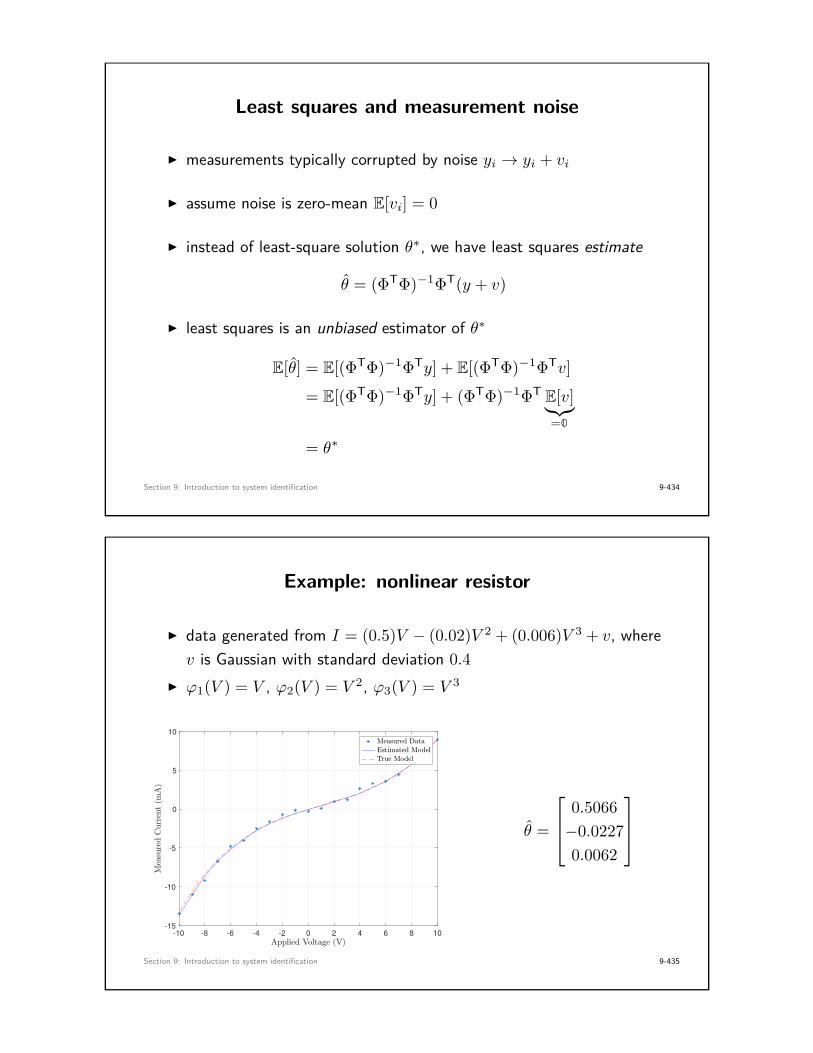
Least squares and measurement noise
I measurements typically corrupted by noise yi → yi + vi
I assume noise is zero-mean E[vi] = 0
I instead of least-square solution θ∗, we have least squares estimate
θ = (ΦTΦ)−1ΦT(y + v)
I least squares is an unbiased estimator of θ∗
E[θ] = E[(ΦTΦ)−1ΦTy] + E[(ΦTΦ)−1ΦTv]
= E[(ΦTΦ)−1ΦTy] + (ΦTΦ)−1ΦT E[v]︸︷︷︸=0
= θ∗
Section 9: Introduction to system identification 9-434
Example: nonlinear resistor
I data generated from I = (0.5)V − (0.02)V 2 + (0.006)V 3 + v, wherev is Gaussian with standard deviation 0.4
I ϕ1(V ) = V , ϕ2(V ) = V 2, ϕ3(V ) = V 3
-10 -8 -6 -4 -2 0 2 4 6 8 10
-15
-10
-5
0
5
10
θ =
0.5066−0.02270.0062
Section 9: Introduction to system identification 9-435
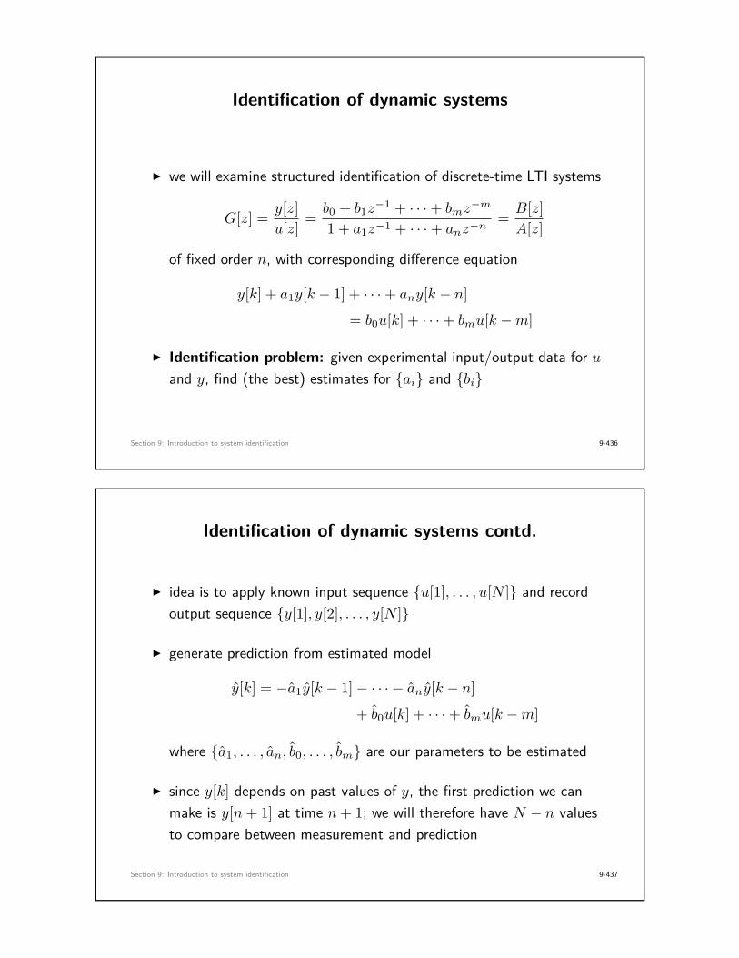
Identification of dynamic systems
I we will examine structured identification of discrete-time LTI systems
G[z] = y[z]u[z] = b0 + b1z
−1 + · · ·+ bmz−m
1 + a1z−1 + · · ·+ anz−n= B[z]A[z]
of fixed order n, with corresponding difference equation
y[k] + a1y[k − 1] + · · ·+ any[k − n]
= b0u[k] + · · ·+ bmu[k −m]
I Identification problem: given experimental input/output data for uand y, find (the best) estimates for {ai} and {bi}
Section 9: Introduction to system identification 9-436
Identification of dynamic systems contd.
I idea is to apply known input sequence {u[1], . . . , u[N ]} and recordoutput sequence {y[1], y[2], . . . , y[N ]}
I generate prediction from estimated model
y[k] = −a1y[k − 1]− · · · − any[k − n]
+ b0u[k] + · · ·+ bmu[k −m]
where {a1, . . . , an, b0, . . . , bm} are our parameters to be estimated
I since y[k] depends on past values of y, the first prediction we canmake is y[n+ 1] at time n+ 1; we will therefore have N − n valuesto compare between measurement and prediction
Section 9: Introduction to system identification 9-437

Identification of dynamic systems contd.
I lay out all equations for estimatesy[n+ 1]y[n+ 2]
...y[N ]
︸ ︷︷ ︸
y
=
y[n] · · · y[1] u[n+ 1] · · · u[n+ 1−m]
y[n+ 1] · · · y[2] u[n+ 2] · · · u[n+ 2−m]...
......
...y[N − 1] · · · y[N − n] u[N ] · · · u[N −m]
︸ ︷︷ ︸
Φ
−a1...−anb0...bm
︸ ︷︷ ︸
θ
I like before, form least squares problem
minimizeθ∈Rn+m+1
Jls(θ) =N∑
i=n+1(y[i]− y[i])2 = (y − y)T(y − y) .
with solutionθ∗ = (ΦTΦ)−1ΦTy
Section 9: Introduction to system identification 9-438
Example: mass with friction
I we wish to identify mass and damping for model (m = 2, b = 0.3)
mv = −bv + u =⇒ v = − b
mv + 1
mu
200 400 600 800 1000 1200 1400 1600 1800 2000
-1
0
1
200 400 600 800 1000 1200 1400 1600 1800 2000
-0.2
0
0.2
0.4
Section 9: Introduction to system identification 9-439

Example: mass with friction
I applying the c2d transformation, we obtain discrete model
v[k + 1] = e−bT/m︸ ︷︷ ︸−a1
v[k] + 1b
(1− e−bT/m
)︸ ︷︷ ︸
b1
u[k]
or in standard difference equation form with y[k] := v[k]
y[k] + a1y[k − 1] = b1u[k − 1]
I therefore, we will fit a model Pd of the form
y[k] = −a1y[k − 1] + b1u[k − 1]
Section 9: Introduction to system identification 9-440
Example: mass with friction
I m = 2, b = 0.3, T = 0.01, N = 2000 samples
10-6
10-4
10-2
100
102
104
-60
-40
-20
0
20
10-6
10-4
10-2
100
102
104
-200
-150
-100
-50
0
Section 9: Introduction to system identification 9-441

Noise and dynamic system identification
I if least squares is unbiased, why are our results so poor?
I as before, the expected value of our estimate is
E[θ] = E[(ΦTΦ)−1ΦTy] + E[(ΦTΦ)−1ΦTv] .
but Φ depends on y, which depend on noise v, therefore
E[(ΦTΦ)−1ΦTv] 6= (ΦTΦ)−1ΦTE[v] = 0
I our estimate θ is biased
I need a methodology for removing this bias
Section 9: Introduction to system identification 9-442
Noise and dynamic system identification contd.
I our underlying system is described by the model
x[k] + a1x[k − 1] + · · ·+ anx[k − n]
= b0u[k] + · · ·+ bmu[k −m]
from which we take noisy measurements y[k] = x[k] + v[k]
I take z-transforms with zero initial conditions:
(1 + a1z−1 + · · ·+ anz
−n)X[z] = (b0 + · · ·+ bmz−m)U [z]
Y [z] = X[z] + V [z]
or, eliminating X[z],
A[z]Y [z] = B[z]U [z] + A[z]V [z]︸ ︷︷ ︸noise filtered by system!
Section 9: Introduction to system identification 9-443

Noise and dynamic system identification contd.
I dividing by A[z], we obtain
A[z](Y [z]A[z]
)︸ ︷︷ ︸
:=Y [z]
= B[z](U [z]A[z]
)︸ ︷︷ ︸
:=U [z]
+V [z]
I we have “unmixed” the noise and the system
I TF from U to Y is G[z], i.e., the same as TF from U to Y
I therefore: to estimate the transfer function G[z], it makes nodifference where we use the original measured data (u[k], y[k]), orthe filtered data (u[k], y[k])!
Section 9: Introduction to system identification 9-444
Noise and dynamic system identification contd.
I since Y [z] = Y [z]/A[z], we have A[z]Y [z] = Y [z], and the signaly[k] may be constructed as
y[k] = −a1y[k − 1]− · · · − any[k − n] + y[k]
I similarly, can construct signal u[k] via
u[k] = −a1u[k − 1]− · · · − anu[k − n] + u[k]
I problem: we don’t know the coefficients {a1, . . . , an}
I idea: instead use current estimates {a1, . . . , an}
Section 9: Introduction to system identification 9-445

Iterative least-squares for dynamic system id
1. run least squares with unfiltered data u[k] and y[k], obtaining initialestimates {a1, . . . , an} and {b1, . . . , bm}
2. build the approximate system denominator
A[z] = 1 + a1z−1 + · · ·+ anz
−n
and filter the input/output data (u[k], y[k]) to obtain (u[k], y[k])
3. using the filtered data (u[k], y[k]), recompute the least squaressolution to find updated estimates {a1, . . . , an} and {b1, . . . , bm}
4. repeat steps (2)–(4) until coefficients stop changing
Section 9: Introduction to system identification 9-446
Example: mass with friction
I filter data with filter A[z] = 1 + a1z−1
Ahat = [1,ahat_1];u_filt = filter(1,Ahat,u);y_filt = filter(1,AHat,y);
I resolve least-squares problem
Phi = [y_filt(n:N-1),u_filt(n:N-1)];theta = Phi\y_filt(n+1:N);
Section 9: Introduction to system identification 9-447

Example: mass with friction (data filtered once)
10-6
10-4
10-2
100
102
104
-60
-40
-20
0
20
10-6
10-4
10-2
100
102
104
-200
-150
-100
-50
0
Section 9: Introduction to system identification 9-448
Example: mass with friction (data filtered twice)
10-6
10-4
10-2
100
102
104
-60
-40
-20
0
20
10-6
10-4
10-2
100
102
104
-200
-150
-100
-50
0
Section 9: Introduction to system identification 9-449

Final comments on system identification
I many more non-trivial issues such as
• selecting appropriate test inputs
• numerical conditioning of data for least squares
• choice of sampling frequency in discretization of c.t. model
• combining multiple experiments
• identifying systems in closed-loop
• recursive (online) system ID
• other choices for objective function
• . . .
Section 9: Introduction to system identification 9-450
MATLAB commands
I solve non-square linear system
x = A\b;
I filter vector x using filter F [z] = 1+8z−2
1+z−1+2z−2
x_filt = filter([1,0,8],[1,1,2],x);
I extract coefficients from transfer function
[Bd,Ad]=tfdata(Pd);Bd=Bd{1}; Ad=Ad{1};
Section 9: Introduction to system identification 9-451

Additional references
I Nielsen Chapter 3
I Åström & Wittenmark, Chapter 13
I Swevers, Introduction to System Identification (slides)
I Keesman (System Identification) Chapter 6
I Franklin, Powell, & Workman, Chapter 12
I Phillips, Nagle, & Chakrabortty, Chapter 10
I Hespanha, Topics in Undergraduate Control System Design,Chapters 2–4
Section 9: Introduction to system identification 9-452
Parting thoughts on ECE 484 . . .
I broadly speaking, control design is about managing dynamics anduncertainty in real-time using feedback (and feedforward)
I state-of-the-art control design looks like fancy versions of the LQRproblem, but with
• many sensors and actuators, distributed architectures
• more emphasis on optimization theory
• stochastic, robust, nonlinear, large-scale . . .
I multivariable optimal control in ECE 488 (planes, robots, etc.)
I the really good stuff is in graduate school
Section 9: Introduction to system identification 9-453

Personal Notes
Section 9: Introduction to system identification 9-454
Personal Notes
Section 9: Introduction to system identification 9-455
Personal Notes
Section 9: Introduction to system identification 9-456
10. Appendix: mathematics review
Section 10: Appendix: mathematics review 10-457

Important Laplace transforms
Name f(t) F (s) = L {f(t)}
Delta δ(t) 1
Step 1(t) 1/s
Ramp t 1/s2
Monomial tn n!/tn+1
Sine sin(ω0t) ω0/(s2 + ω20)
Cosine cos(ω0t) s/(s2 + ω20)
Exponential e−αt 1/(s+ a)
Exp/Sin e−αt sin(ω0t) ω0/[(s+ α)2 + ω20 ]
Exp/Cos e−αt cos(ω0t) (s+ α)/[(s+ α)2 + ω20 ]
(note: all signals assumed to be zero for t < 0)
Section 10: Appendix: mathematics review 10-458
Properties of the Laplace transform
Name f(t) L {f(t)}
Superposition αf1(t) + βf2(t) αF1(s) + βF2(s)
Delay f(t− τ) e−τsF (s)
Derivative rule f(t) sF (s)− f(0)
Integral rule∫ t
0 f(τ) dτ 1sF (s)
Convolution f1(t) ∗ f2(t) F1(s)F2(s)
Initial value theorem f(0+) lims→∞ sF (s)
Final value theorem limt→∞ f(t) lims→0 sF (s)
(note: all signals assumed to be zero for t < 0)
Section 10: Appendix: mathematics review 10-459

Important z-transforms
Name f [k] F [z] = Z{f [k]}
Delta δ[k] 1
Step 1[k] z/(z − 1)
Ramp k z/(z − 1)2
Exponential ak z/(z − a)
Sine sin(ω0k) z sin(ω0)/(z2 − 2z cos(ω0) + 1)
Cosine cos(ω0k) z(z − cos(ω0))/(z2 − 2z cos(ω0) + 1)
(note: all signals assumed to be zero for k < 0)
Section 10: Appendix: mathematics review 10-460
Properties of the z-transform
Name f [k] Z{f [k]}
Superposition αf1[k] + βf2[k] αF1[z] + βF2[z]
Delay-by-n f [k − n] z−nF [z]
Advance-by-1 f [k + 1] zF [z]− zf [0]
Sum rule∑k
`=0 f [`] zz−1F [z]
Convolution f1[k] ∗ f2[k] F1[z]F2[z]
Initial value theorem f [0+] limz→∞ F [z]
Final value theorem limk→∞ f [k] limz→1(z − 1)F [z]
(note: all signals assumed to be zero for k < 0)
Section 10: Appendix: mathematics review 10-461
Linear algebra and matrices
I vector spaces and subspaces
I matrix definitions
I invertibility
I eigenvalues/eigenvectors
I diagonalization
Section 10: Appendix: mathematics review 10-462
Vector spaces and subspaces
I a space of objects which can be added and scaled by constantsI most important vector space for our purposes is Rn with elements
x =
x1...xn
, xi ∈ R,
where addition and scalar multiplication are defined by
x+ y =
x1 + y1
...xn + yn
, αx =
αx1...
αxn
, α ∈ R.
Section 10: Appendix: mathematics review 10-463
Vector spaces and subspaces contd.
I a set X = {x1, x2, . . . , xk} of vectors is linearly independent if
α1x1 + · · ·+ αnxn = 0 =⇒ α1 = · · · = αn = 0 .
I the span of X is the set of all possible linear combinations
span(X) = {α1x1 + · · ·+ αnxn | α1, . . . , αn ∈ R}
I a subspace S of Rn is a subset which is also a vector space• all subspaces of Rn are hyperplanes passing through the origin
I a basis for a subspace S is a set X = {x1, x2, . . . , xk} of linearlyindependent vectors such that span(X) = S, and the dimensiondim(S) of the subspace is the smallest number of vectors required insuch a basis (in this case, k vectors)
Section 10: Appendix: mathematics review 10-464
Matrices
A square n× n matrix is a collection of n2 real numbers
A =
a11 a12 · · · a1n
a21 a22 · · · a2n...
.... . .
...an1 an2 · · · ann
I A ∈ Rn×n means that A is an n× n matrix with real entires
I A defines a linear transformation from Rn to Rn via matrix-vectormultiplication
y = Ax ⇐⇒ yi =n∑j=1
Aijxj , i = 1, . . . , n.
Section 10: Appendix: mathematics review 10-465

Range, nullspace, and the rank-nullity theorem
For a matrix A ∈ Rn×n
I nullspace: null(A) := {x ∈ Rn | Ax = 0}• the subspace of input vectors that get “zeroed out” by A• nullity(A) := dim(null(A))
I range: range(A) := {Ax | x ∈ Rn}• the subspace of linear combinations of columns of A• rank(A) = dim(range(A))
Rank-Nullity Theorem: rank(A) + nullity(A) = n
Section 10: Appendix: mathematics review 10-466
Invertibility of matrices
I square matrix A ∈ Rn×n is invertible or nonsingular if there existsanother matrix B ∈ Rn×n such that AB = BA = In
I the inverse is always unique and we denote it by A−1
I the following statements are all equivalent:• A is invertible
• rank(A) = n
• nullity(A) = 0
• the columns of A form a basis for Rn
• 0 /∈ eig(A)
• det(A) 6= 0
I if A,B,C are all invertible, then (ABC)−1 = C−1B−1A−1
Section 10: Appendix: mathematics review 10-467

Solvability of linear systems of equations
For A ∈ Rn×n and b ∈ Rn, consider the equation
Ax = b
in the unknown vector x ∈ Rn.
I the equation is solvable if and only if b ∈ range(A)
I in this case, all solutions can be written as x = p+ v, where p is aparticular solution satisfying Ap = b and v ∈ null(A) is anyhomogeneous solution, i.e., a solution to Ax = 0.
I for every b ∈ Rn there exists a unique x solving Ax = b if and only ifA is invertible.
Section 10: Appendix: mathematics review 10-468
Constructing inverses
For A ∈ R2×2
A =[a b
c d
]A−1 = 1
ad− bc
[d −b−c a
]
assuming det(A) = ad− bc 6= 0.
I For A ∈ Rn×n there is a formula similar to the above
A−1 = 1det(A)adj(A) .
I adj(A) is the adjugate matrix
• [adj(A)]ij is formed from (j, i)th minor of A• important for relating state-space and transfer function models
Section 10: Appendix: mathematics review 10-469

Eigenvalues and eigenvectors
I Eigenvalue equation: Ax = λx
• λ ∈ C is the eigenvalue• x ∈ Cn is the (right) eigenvector
I eigenvalues obtained from characteristic polynomial ΠA(s)
ΠA(s) := det(sIn −A)
set of eigenvalues = eig(A) := {λ ∈ C | ΠA(λ) = 0}
I given eigenvalue λi, eigenvector xi obtained by solving
(A− λiIn)xi = 0
I eigenvalues are unique, eigenvectors are not
Section 10: Appendix: mathematics review 10-470
Diagonalization
I A ∈ Rn×n, with eigenvalues λi and eigenvectors vi ∈ Rn
Avi = λivi
form matrix of eigenvectors: V =[v1 v2 · · · vn
]∈ Rn×n
I if {v1, v2, . . . , vn} are linearly independent then V is invertible
V −1AV = Λ =
λ1 0 · · · 00 λ2 · · · 0...
.... . .
...0 0 0 λn
I similar ideas (Jordan form) when diagonalization is not possible
Section 10: Appendix: mathematics review 10-471

Example
A =[−1 12 −2
]λI2 −A =
[λ+ 1 −1−2 λ+ 2
]
ΠA(λ) = det(λI2 −A) = λ2 + 3λ+ 2− 2 = λ(λ+ 3)
eig(A) = {λ1, λ2} = {0,−3} with vλ1 =[
11
]vλ2 =
[1−2
]
Λ = V −1AV =[
1 11 2
]−1 [−1 12 −2
][1 11 2
]=[
0 00 −3
]
Section 10: Appendix: mathematics review 10-472
Personal Notes
Section 10: Appendix: mathematics review 10-473

Personal Notes
Section 10: Appendix: mathematics review 10-474
Personal Notes
Section 10: Appendix: mathematics review 10-475