Pervaporation mass transfer with liquid flow in the transition regime

Journal of Membrane Science 183 (2001) 119–133

Pervaporation mass transfer with liquid flowin the transition regime

Teresa A.C. Oliveira, Ugo Cocchini, Justin T. Scarpello, Andrew G. Livingston∗Department of Chemical Engineering, Imperial College of Science, Technology and Medicine, London SW7 2BY, UK

Received 30 June 2000; received in revised form 13 September 2000; accepted 13 September 2000

Abstract

In this work, the mass transfer of a model volatile organic compound through silicone rubber membrane tubes has beeninvestigated for the transition between laminar and turbulent flow regimes. Results showed that a flow transition region occurredover the expected Reynolds number range, from 2300 to 5500. Two correlations have been established for flow during transitionand early turbulence:Sh= 1.1Re0.35 Sc0.33, for 2800< Re≤ 5500, andSh= 0.010Re0.93 Sc0.33, for 5500< Re< 10,000.A cost analysis showed that significant reductions in total costs are obtained for operating conditions in the nonlaminar regime,although membrane burst pressure may prevent working at cost optimal Reynolds numbers. © 2001 Elsevier Science B.V.All rights reserved.

Keywords:Mass transfer; Transition region; Pervaporation; Cost analysis; Volatile organic compounds

1. Introduction

Membrane processes are growing in importance andutilisation. Among the different membrane separationtechnologies, pervaporation is presently considered aunit operation with high potential, particularly withintreatment of wastewaters from chemical industries [1].

Prediction of the mass transfer coefficient is centralin the design of membrane modules, for processes suchas pervaporation and membrane extraction. The fluxthrough the membrane can be expressed in terms ofan overall mass transfer coefficient

Ji = kov,i

(cf ,i − cr,i

K

)(1)

where Ji is the flux of compound i,kov the overallmass transfer coefficient,cf the concentration in the

∗ Corresponding author. Tel.:+44-20-75945582;fax: +44-20-75945604.E-mail address:[email protected] (A.G. Livingston).

feed side,cr the concentration in the receiving side andK the partition coefficient of i between receiving andfeed phases. A resistances-in-series model is usuallyused to describe the performance of a pervaporationmodule [2–4]. Two main resistances may contribute tothe overall resistance to mass transfer: the membraneresistance, and the feed boundary layer resistance,as the permeate or gas phase resistance is usuallynegligible.

1

kov,i= 1

km,i+ 1

kl,i(2)

where kov,i , km,i , kl,i are the overall mass transfercoefficient, the membrane mass transfer coefficient,and the liquid mass transfer coefficient, respectively,of compound i.

Although the overall mass transfer resistance has inthe past been dominated by the membrane resistancebecause of low permeabilities and thick membranes,developments of membrane materials and ultra-thin

0376-7388/01/$ – see front matter © 2001 Elsevier Science B.V. All rights reserved.PII: S0376-7388(00)00576-7

120 T.A.C. Oliveira et al. / Journal of Membrane Science 183 (2001) 119–133

Nomenclature

a, b, c, e constantsA membrane area (m2)awh annual working hours (per year)BM bare module factorCcapital capital costs (Euro per year)Ccond condenser costs (Euro per year)cf feed concentration (kg m−3)Cfp feed pump(s) costs (Euro per year)cli inlet concentration in the

membrane (kg m−3)clo outlet concentration from

the membrane (kg m−3)Cmem membrane costs (Euro per year)Cmod module costs (Euro per year)Coperating operating costs (Euro per year)Cpw power costs (Euro per year)cr receiving side concentration

(kg m−3)crs recirculating solution

concentration (kg m−3)Ctotal total costs (Euro per year)Cvp vacuum pump costs (Euro per year)D diffusivity in water (m2 s−1)d membrane diameter (m)f friction factorFf feed flowrate (m3 s−1)Fl liquid flowrate per membrane

tube (m3 s−1)F total

l total liquid flowrate (m3 s−1)Gz Graetz number,Gz= vd2/(DL)J flux through the membrane

(kg m−2 s−1)K partition coefficient between the

receiving phase and the feed phasekl liquid mass transfer coefficient

(m s−1)km membrane mass transfer

coefficient (m s−1)kov overall mass transfer

coefficient (m s−1)L membrane length (m)MS68 Marshall and Swift Index value 1968MS00 Marshall and Swift Index value 2000n number of points

nmodseries number of membrane modulesin series

ntubes number of tubesPburst membrane burst pressure (bar)Pm membrane permeability (m2 s−1)1P pressure drop (Pa)r membrane radius (m)Re Reynolds number,Re= ρvd/µ

rt Euro to Dollar ratio (Euro:US $)Sc Schmidt number,Sc= µ/(ρD)

scpw specific electrical power cost(Euro (Wh)−1)

Sh Sherwood number,Sh= kd/DSSR sum of squares of residualsv velocity inside the membrane (m s−1)Wcond energy required to operate the

condenser (W)Wfp energy required to operate the feed

pump (W)Wvp energy required to operate the

vacuum pump (W)

Greek symbolsεfp feed pump efficiencyµ liquid viscosity (kg m−1 s−1)ρ liquid density (kg m−3)

Subscriptsi innero outerp pooled regression1 regression 12 regression 2

composite membranes have led to much smaller mem-brane mass transfer resistances [5]. Additionally, forsolutes having high intrinsic permeabilities throughthe membrane and/or selectivities, the mass transferresistance at the liquid boundary layer adjacent to themembrane can contribute significantly to the overalltransport resistance and in some cases, depending onthe existing hydrodynamic conditions, can completelyoverwhelm the membrane resistance [3]. For exam-ple, the removal of volatile organic compounds fromwastewaters by pervaporation is often significantlymore limited by the resistance of a boundary layer

T.A.C. Oliveira et al. / Journal of Membrane Science 183 (2001) 119–133 121

adjacent to the membrane surface than by the resis-tance of the membrane [4,6,7].

The liquid boundary layer resistance depends onthe hydrodynamic conditions, physical properties ofthe fluid and the solute, and the system geometry.For flow in tubes, several dimensionless correlationsexist relating the mass transfer coefficient to physicalproperties of the fluid and the solute, hydrodynamicparameters, and tube dimensions. Some of these cor-relations are theoretical, although most of them havean empirical origin. Several of these mass transfercorrelations have been obtained from heat transferanalogies. Correlations have been derived for estima-tion of fluid boundary layer mass transfer coefficientin both the tube side and the shell side of membranemodules, for liquids and for gases, for laminar andturbulent regimes, and for different module configu-rations. These correlations have the generic form

Sh= a Reb Scc(

d

L

)e

(3)

and they change considerably from the laminar to theturbulent regime.

For the laminar flow regime, corresponding to aReynolds number lower than 2300 for flow inside atube [8], the most commonly used correlation is theLévêque correlation [9]

Sh= 1.62

(Re Sc

(d

L

))0.33

(4)

Several studies and simulations use the Lévêque cor-relation to estimate the mass transfer in the laminarregime [1], and many present experimental validationof this correlation [5], although some authors dis-pute its accuracy [10,11]. However, this correlationis valid only for high values of the Graetz number(Gz > 400, [12]), as this theory is based on the as-sumption that the concentration at the centre of thetube is unchanged over the length of the tube. Thiswill not be true for slow flows or long tubes. At lowGraetz numbers, Sherwood numbers deviate from thetheoretical prediction. Other correlations for laminarregimes exist which differ simply in the constant:1.64 [13]; 1.86 [14]; 1.5 [15].

For turbulent regimes, a wider range of correla-tions has been published, most of them obtained forReynolds numbers between 104 and 105 or higher.

The Reynolds number exponent varies between 0.7and 1.0, and the Schmidt number exponent varies be-tween 0.25 and 0.44 [16,17]. In turbulent regimes, nodependence on the tube diameter to length ratio (d/L)is found, contrary to what is suggested for the laminarregime. One of the most widely used correlations forturbulent regimes is [18]

Sh= 0.026Re0.8 Sc0.33 (5)

Some reviews of mass transfer correlations for turbu-lent regimes have been published. The most completeappears to be the one by Gekas and Hallström [16],which gives a general overview of mass transfer cor-relations that appeared in the literature between 1934and 1984.

In between laminar and turbulent regimes, there isa transition region where flow may be either laminaror turbulent, depending on the tube surface roughness,tube entrance conditions, and fluctuations in the inletstream [8]. Gekas and Hallström [16] in their reviewstate that the region 2300< Re< 10,000 is unclear,and no simple form of theShequation is available. Al-though most correlations for the turbulent regime havebeen determined forRe> 104 or even higher valuesof Reynolds numbers, some authors have used themto predict mass transfer coefficients at lower Reynoldsnumbers. Lipski and Côté [2] used Eq. (5) to estimatethe Sherwood number forRe> 4000, and Côté andLipski [7], and Lipnizki and Field [1] used the sameequation forRe > 2000. However, no experimentalverification was performed in either of the studies.Brookes [19] established a correlation for the tube sideof a membrane forRe> 4800.

Sh= 0.032Re0.8 Sc0.33 (6)

Crowder and Cussler [20] established a correlationbased on experimental data obtained for the transitionregion. Their data was obtained for flow inside hol-low fibre membranes, for Reynolds numbers between1000 and 5000. However, the boundaries of the flowregimes were not characterised (e.g. by pressure dropmeasurements), and the investigation was not extendedto the fully turbulent regime. Furthermore, two of thepoints used in the correlation correspond toRe <

2000 (laminar regime), but the effect of (d/L) was notinvestigated.

Plotting Sherwood number as a function ofReynolds number using a correlation for the laminar


Fig. 1. Sherwood number vs. Reynolds number calculated from the Levêque correlation for the laminar regime (Eq. (4)) and from theCussler correlation for the turbulent regime (Eq. (5)),Sc= 1170, (d/L) = 3 × 10−3.

regime (Eq. (4)) and one for the turbulent regime (Eq.(5)), for Sc = 1170 and(d/L) = 3 × 10−3, whichare typical values for pervaporation applications in-volving removal of VOCs from aqueous streams, alarge jump in the Sherwood number is observablein the transition region (Fig. 1). This jump may beof a very significant economic importance, as stepimprovements in mass transfer should correspond toa large decrease in the required membrane area, andsubsequently to a reduction in the membrane costs.This improvement in mass transfer is at the penaltyof increased pressure drop. The exact point at whichthe jump occurs is not known, and it may differdepending on the operating conditions.

In this work, the mass transfer of a model volatileorganic compound through a tubular silicone rubbermembrane for Reynolds numbers between 2000 and10,000 is studied. The transition between laminar andturbulent flow regimes is investigated, and correlationsfor estimation of mass transfer coefficients are estab-lished. A cost analysis is also presented for the case of

pervaporation for removal of a VOC from an aqueousstream, considering capital and operating costs, andthe restriction imposed by membrane burst pressure.

2. Experimental

A schematic of the experimental set-up can befound in Fig. 2. This was used to calculate the over-all mass transfer coefficient of monochlorobenzene(MCB) through silicone rubber for various Reynoldsnumbers. The membrane used was polydimethylsilox-ane (PDMS) with 30% of silica filler (Esco Rubber,UK), with 3.0 mm internal diameter (i.d.) and wallthickness varying between 0.25 and 1 mm. The airvelocity in the fumehood was, on average, 0.69 m s−1.

MCB was used as it is a typical VOC and has beenused in previous studies of mass transfer [10,21]. Anaqueous solution of MCB was recirculated through asingle tube membrane by means of a gear pump, cov-ering the range of Reynolds numbers from 1700 to


Fig. 2. Experimental set-up for determination of steady-state mass transfer coefficient of monochlorobenzene through silicone rubber in apervaporation system.

10,000. Liquid flowrate was measured by volume col-lection. A constant flow of a feed MCB solution wassupplied to the mixing chamber by a peristaltic pumpand an equal flow withdrawn from it. After startingeach run, the concentrations of MCB in both the feedand in the recirculating solution were measured untilsteady state was reached. Steady state was assumed tohave been reached when the organic compound con-centrations in each solution varied by less than 5%over a minimum of 1 h. It typically took between 3and 4 h to reach steady state. The experiment was runat ambient temperature, 21± 1◦C, giving a Schmidtnumber of 1170 for the system of MCB in water.

A mass balance on the system can be used todetermine the overall mass transfer coefficient

kov = Ff

A

(cf

crs− 1

)(7)

where Ff is the peristaltic pump feed flowrate,cfand crs the concentrations of MCB in the feed solu-tion measured at a sampling point after the peristalticpump, and in the recirculating solution in the mixingchamber, respectively, andA the membrane area.

For the determination ofkov as a function ofReynolds number, the membrane length was approxi-mately 0.80 m long, with 0.35 mm wall thickness. Fordetermination of the membrane resistance, the mem-brane wall thickness was varied at a constant liquidflowrate (constant Reynolds number). Three differentthicknesses were tested: 0.25, 0.35 and 1.0 mm. Froma Wilson plot of 1/kov againstr i ln(ro/r i ), a linear re-gression is expected, the slope of which correspondsto the inverse of the membrane permeability.

1

kov= 1

kl+ ri ln(ro/ri)

Pm(8)

The pressure drop in the membrane tubing was mea-sured as a function of the Reynolds number in orderto evaluate the changes in the flow regimes. T-pieceswere inserted at either end of the membrane tubing,and connected by means of vertical glass tubing toa digital manometer (Air Instrument Resources Ltd.,England). The liquid height and the pressure read inthe manometer were considered in calculation of pres-sure drop between the two points. Water was pumpedthrough the membrane in these runs. The Reynolds


number was varied from 100 to approximately 9000,after which the rig became unstable, preventing workat higher Reynolds numbers.

2.1. Analytical methods

MCB was determined by gas chromatography in aPerkin Elmer gas chromatograph with a flame ioni-sation detector (FID) and a megabore column 25 mlong and 0.23 mm i.d. with BP1 (SGE, Australia)as the stationary phase. The temperature programmeran from 50 to 140◦C at a rate of 20◦C min−1.The samples were first extracted into a solution ofdichloromethane with aniline as the internal standard.1ml of the extracted sample was injected into the GC.The uncertainty in this assay (quoted as the coeffi-cient of variation, standard deviation divided by themean, of four separate determinations) was 4.6% atthe 10 ppm concentration level.

2.2. Chemicals

The organic compounds were obtained from Sigma(UK), and were 99.5% pure.

3. Statistical analysis

To determine whether and at what point the flowregime changed from laminar to turbulent, it was nec-essary to test for a statistically significant break in thedata for mass transfer coefficient and pressure drop asa function of Reynolds number. The Chow test, whichtests if a set of experimental points is better correlatedin multiple regressions rather than in a pooled regres-sion [22], was applied.

The following procedure was applied to data forpressure drop as a function of Reynolds number, andfor mass transfer coefficient (as Sherwood number)as a function of Reynolds number, in the logarithmicform

ln 1P = f (ln Re)

ln Sh= f (ln Re)

The data points were divided into two subgroups,starting with the first two points in the first group and

the remainder in the second group. Linear regressionswere applied to both groups of points and the sumof the squares between predicted and experimentalresults (SSR= sum of squares of residuals) wascalculated. This was done for an increasing numberof data points in the first group with the second onecontaining the remainder of the points.

The sum of the sum of the squares of residuals foreach pair of linear regressions was calculated and theminimum determined. This minimum was consideredto provide the optimum separation between the datapoints. The Chow test was then applied.

The Chow test is a method that tests if a set ofexperimental points consists of different subgroups,that is, if it is better correlated by multiple regressionsthan by a pooled regression. AnF-statistic is usedto see if the improvement in the fit by breaking thesample is significant

F = [SSRp − SSR1 − SSR2]/2

[SSR1 + SSR2]/[n − 4](9)

where subscript p refers to the pooled regression, sub-script 1 to the first regression and 2 to the second one;n is the total number of points.

The calculatedF is compared with the critical valueof F with 2 and (n−4) degrees of freedom at a requiredlevel of significance. ForF calculated> F critical, it wasconcluded that separate regressions are a better fit forthe results at the specified level of significance.

4. Cost analysis

The use of higher flowrates improves mass transferand allows a reduction of the membrane area for thesame removal efficiency. However, it also increasesthe pressure drop, requiring higher pumping energy.There is a reduction of membrane costs at the expenseof increased power requirement. A study of the waytotal costs evolve with increasing Reynolds numberwas performed for a pervaporation system for removalof MCB from wastewater.

Calculations were based on the results obtainedfrom this work, considering a wastewater flowrate of10 m3 h−1, and 99% removal of MCB required, usinga silicone rubber membrane of a kind employed in-dustrially [11]. The analysis presented in this paperapplies to all types of membranes, provided that


liquid resistance to mass transfer is significant, whichcommonly occurs in pervaporation [4,6]. However, itis not an exhaustive analysis, and is based on severalsimplifications. The aim is to include the major con-tributions to the overall cost of a pervaporation unit,and to show how the flow regime is important andmay make a significant difference to total costs. Thecost factors, cost equations and assumptions are fullydescribed, so that the reader can make any necessaryadjustments. For a more complete cost analysis, thereader should refer to Hickey and Gooding [23], andJi et al. [24].

Two different internal diameters of the membranetubing were considered, 3 and 5 mm, as well as differ-ent wall thicknesses. The range of Reynolds numbersfrom 1700 to 10,000 was investigated.

The following assumptions were made:

• PDMS membrane with 30% of silica filler;• one pass through of the wastewater inside the

membrane tubes;• gas phase concentration always zero;• isothermal process, operation at 21◦C;• liquid mass transfer coefficient estimated by the cor-

relations determined in this work forRe > 2800;for lower values of Reynolds numbers the pointsdetermined experimentally were used;

• maximum length of membrane tubes 100 m [11];• constant load of MCB into the vacuum pump and

condenser;• operating vacuum of 117 Pa (10% of the saturation

vapour pressure of MCB at 20◦C [2]);• the water flux through the membrane was assumed

to be constant and independent of Reynolds num-ber, with a water permeability of 1.36 × 10−11

mol m−1 s−1 Pa−1 [2];• negligible expansion of membrane tubes;• annual working hours 8000 h per year.

All calculations started from a specified Reynoldsnumber. This number determined, for a given i.d. of themembrane, the feed flowrate per membrane tube. Theliquid mass transfer coefficient was estimated from theexperimental results of this work, and the overall masstransfer coefficient was calculated from the membranemass transfer coefficient and the liquid mass transfercoefficient.

For the specified removal efficiency, the requiredmembrane area was calculated. Under the assumptions

made, the membrane area required is given as

A = Fl

kovln

(cli

clo

)(10)

From the total length required and assuming amaximum length of tube of 100 m, the number ofmodules in series was determined. From the length ofmembrane required, the pressure drop was estimated.Pressure drop is given by

1P = fL

dρ

v2

2(11)

wheref is the friction factor. For laminar regimes

f = 64

Re(12)

For turbulent regimes, 4000< Re < 105, f is givenby the Blasius equation

f = 0.316Re−0.25 (13)

For reasons discussed later, the application of Eq. (13)was extended to friction factor estimations for allRe> 2300.

From the feed flowrate per tube specified by theReynolds number and the overall feed flowrate tobe treated, the number of tubes required was deter-mined. It was assumed that a module would containa maximum of 70 tubes 3 mm i.d. and a maximum of40 tubes 5 mm i.d. (Dr. A.T. Boam, Membrane Extrac-tive Technology, Ltd, UK, personal communication).This determined the necessary number of modules inparallel. The total membrane area considered was ob-tained from the number of tubes required multipliedby the area required as determined from Eq. (10).

Both capital and operating costs were considered.The capital costs were estimated using the bare mod-ule method [2,23], with a bare module factor of 3. Themajor components of the pervaporation system wereassumed to be the membranes, modules, feed pump(s),vacuum pump and condenser [2]. The operating costsincluded the power supply for the feed pump(s), vac-uum pump and condenser, and the replacement ofmembrane modules. A lifetime of 3 years has been as-sumed for the membranes. A capital charge factor of25% was taken each year for depreciation and labour.

Ctotal = 0.25Ccapital+ Coperating (14)


Ccapital = BM(Cmem+ Cmod + Cfp + Cvp + Ccond)

(15)

Coperating= Cpw + 13(Cmem+ Cmod) (16)

The membrane cost was estimated as 180 Euro per m2,independently of i.d. and thickness of the membranetubes, for the combinations considered. The modulecost was estimated as 240 Euro per module. Thesecosts were based on Hickey and Gooding [23] prices,updated with the Marshall and Swift Index.

The feed pump costs depend on the pressure dropalong the membranes and on the feed flowrate accord-ing to the equation

Cfp = rtMS00

MS6815nmodseries

×(

2.3F totall

1P

nmodseries

)0.52

1.93 (17)

where rt is the Euro to Dollar ratio, taken as 1.12, MSthe Marshall and Swift Index values, 1081 for 2000and 280 for 1968 [25]. The vacuum pump cost wascalculated according to Lipski and Côté [2], and thecondenser cost was taken from Douglas [26].

Power costs were calculated for the feed pump, thevacuum pump and the condenser. The power cost wasset as Euro 0.09 kWh−1. The energy consumption ofthe feed pump is a linear function of the volumetricflowrate entering the module, the pressure drop alongthe modules and the pump efficiency.

Wfp =(

1

εfpFl 1P

)ntubes (18)

Power consumption of the vacuum pump and the con-denser were calculated as given by Ji et al. [24]. Thetotal power cost is given as

Cpw = awh scpw(Wfp + Wvp + Wcond) (19)

The burst pressure (bar) for silicone rubber has beenpredicted according to Eq. (20) [27] as

Pburst = 6.6 ln

(do

di

)(20)

When pressure drop went beyond the membrane burstpressure, the possibility of modules in series was con-sidered together with booster pumps between the mod-ules in series. Although this increases the capital costs

due to a larger number of modules and feed pumps, itallows working at higher Reynolds numbers, withoutthe burst pressure restrictions.

5. Results and discussion

5.1. Pressure drop and mass transfer

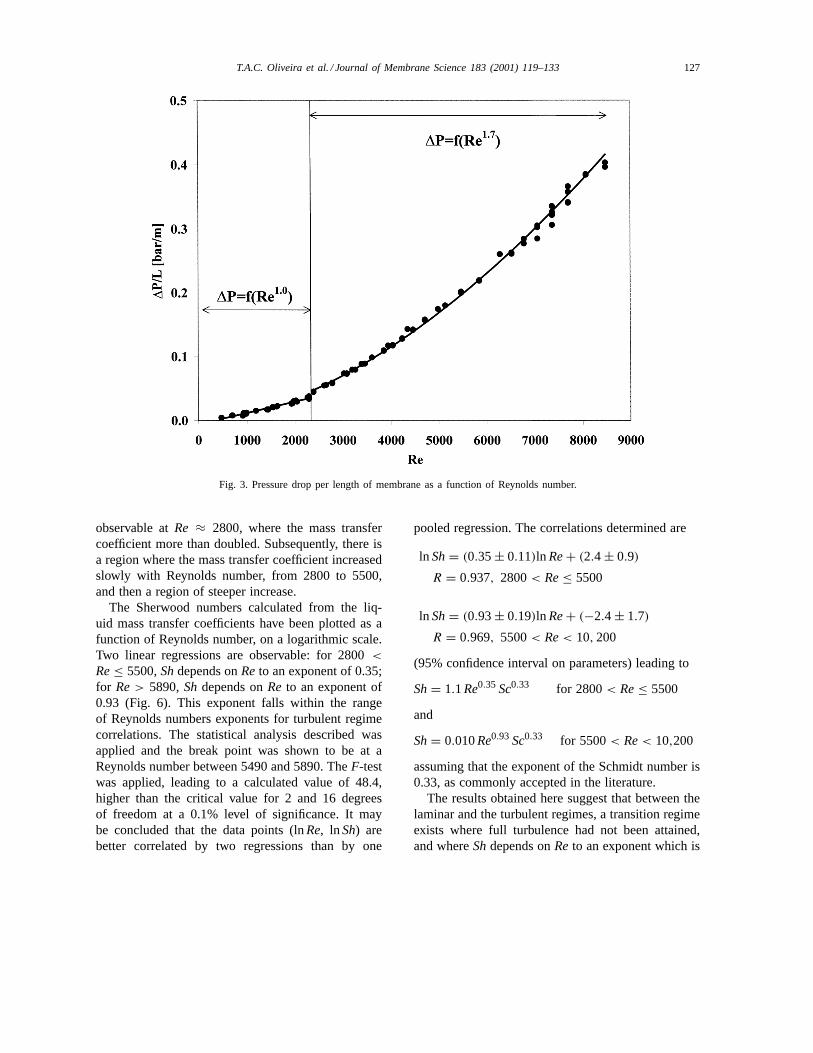
The pressure drop as a function of Reynolds num-ber is presented in Fig. 3. The measured pressure dropvalues were in accordance with the values predictedby the correlations in Eqs. (11)–(13). ForRe< 2300,the pressure drop was found to vary linearly with theflowrate, which is characteristic of laminar flow. Forhigher Re, the pressure drop varied with Reynoldsnumber to the exponent 1.7, which is characteristicof turbulent regime. The statistical analysis showedthat the break point between the two correlations withthe lowest sum of sum of squares of residuals cor-responded to a Reynolds number between 2291 and2387. Doing theF-test a value of 152 was obtained,which is much higher than the criticalF for 2 and 96degrees of freedom at 0.1% level of significance [28],confirming that the data comprises two statisticallydifferent sets. The experimental value obtained for thechange from laminar into turbulent regime agrees wellwith the value of Reynolds number generally acceptedas corresponding to the end of laminar regime, whichis between 2000 and 2300.

From the Wilson plot of 1/kov as a functionof r i ln(ro/r i ) at a constant Reynolds number, thepermeability of MCB through silicone rubber was de-termined (Fig. 4). A value of 9.1 × 10−8 m2 s−1 wasobtained, which is approximately four times higherthan the value determined by Raghunath and Hwang[29]. This difference may be partially due to differ-ences in the membrane material. In this study, the sil-icone rubber membrane contained 30% of silica filler,whereas Raghunath and Hwang simply described themembrane as a PDMS membrane.

The liquid phase mass transfer coefficients as afunction of Reynolds number are presented in Fig. 5.These values have been obtained from the overallmass transfer coefficients determined experimentallyand the membrane mass transfer coefficients ob-tained from the Wilson plot represented in Fig. 4. Asignificant jump in the mass transfer coefficient is


Fig. 3. Pressure drop per length of membrane as a function of Reynolds number.

observable atRe ≈ 2800, where the mass transfercoefficient more than doubled. Subsequently, there isa region where the mass transfer coefficient increasedslowly with Reynolds number, from 2800 to 5500,and then a region of steeper increase.

The Sherwood numbers calculated from the liq-uid mass transfer coefficients have been plotted as afunction of Reynolds number, on a logarithmic scale.Two linear regressions are observable: for 2800<

Re≤ 5500,Shdepends onReto an exponent of 0.35;for Re> 5890,Shdepends onRe to an exponent of0.93 (Fig. 6). This exponent falls within the rangeof Reynolds numbers exponents for turbulent regimecorrelations. The statistical analysis described wasapplied and the break point was shown to be at aReynolds number between 5490 and 5890. TheF-testwas applied, leading to a calculated value of 48.4,higher than the critical value for 2 and 16 degreesof freedom at a 0.1% level of significance. It maybe concluded that the data points (lnRe, lnSh) arebetter correlated by two regressions than by one

pooled regression. The correlations determined are

ln Sh= (0.35± 0.11)ln Re+ (2.4 ± 0.9)

R = 0.937, 2800< Re≤ 5500

ln Sh= (0.93± 0.19)ln Re+ (−2.4 ± 1.7)

R = 0.969, 5500< Re< 10, 200

(95% confidence interval on parameters) leading to

Sh= 1.1Re0.35 Sc0.33 for 2800< Re≤ 5500

and

Sh= 0.010Re0.93 Sc0.33 for 5500< Re< 10,200

assuming that the exponent of the Schmidt number is0.33, as commonly accepted in the literature.

The results obtained here suggest that between thelaminar and the turbulent regimes, a transition regimeexists where full turbulence had not been attained,and whereShdepends onReto an exponent which is


Fig. 4. Wilson plot: inverse of the overall mass transfer coefficient as a function of the membrane thickness.Re= 6230.

Fig. 5. Liquid mass transfer coefficients as a function of the Reynolds number: (m) experimental values; (—) Levêque correlation, Brookescorrelation and Cussler correlation.


Fig. 6. Sherwood number as a function of the Reynolds number, experimental data obtained in this work. Correlations determined in thiswork.

lower than that for the fully turbulent regime. How-ever, it is important to note that between laminar andthis so-called transition regime, a significant jump inmass transfer coefficient occurred. Furthermore, thecorresponding pressure drop did not undergo such ajump, although its dependence on Reynolds numberchanged. No discontinuity in pressure drop was ob-served. This is important as it suggests that if a systemis operated at a Reynolds number immediately abovethe “jump” point, a more than doubling of the masstransfer coefficient can be obtained for a minimal in-crease in pressure drop.

Comparing the experimental results obtained withthe values of mass transfer coefficients predictedby published correlations (Fig. 5), it is observablethat for the laminar regime, the Lêvéque correlationunderestimates the experimental data. Deviations ofapproximately 55% from the experimental values areobservable. Although the Lêvéque correlation is themost widely used for prediction of the mass transfercoefficient in the laminar regime, previous work in ourresearch group suggested its inadequacy in predicting

the mass transfer coefficient [10,11]. In these works,the experimental mass transfer coefficients were sig-nificantly underestimated by the Lêvéque correlation.For Re > 2800, the Brookes correlation (Eq. (6))agrees very well with experimental data, except inthe intermediate range of Reynolds numbers from4000 to 5500. For this range, the Cussler correlation(Eq. (5)) seems to provide a better estimation.

For heat transfer in the transition region, an equationthat introduces an intermittency factor has been pro-posed, which was found to represent the experimentaldata of several authors very well [30]. This equationand data for the transition region [30] shows that thereis an inflexion point at the end of the laminar regime.The lower the ratio of (d/L), the stronger the inflexion.However, the jump in heat transfer is usually moregradual than the one observed in this work.

The breakpoints between laminar and transitionregime for pressure drop and for mass transfer didnot coincide perfectly. For the pressure drop it oc-curred at a Reynolds number of 2300, whereas for themass transfer coefficient, the jump occurred at 2800.


Fig. 7. Total cost evolution with Reynolds number for a pervaporation system removing 99% of MCB from wastewater at 10 m3 h−1, usingsilicone rubber membranes 3 mm i.d., 0.35 mm wall thickness.

Furthermore, atRe ≈ 5500 a further change in themass transfer coefficient behaviour with Reynoldsnumber was observed, with no corresponding changein the pressure drop dependence.

5.2. Cost analysis

A cost analysis of a pervaporation system designedfor 99% removal of MCB from a wastewater witha flowrate of 10 m3 h−1, and using silicone rubbertubing, was performed. For a 3 mm i.d. and 0.35 mmthickness membrane, the results are presented inFig. 7. For a silicone rubber tube 3 mm i.d., 0.35 mmwall thickness, the predicted burst pressure is 1.4 bar,preventing the use of this type of membrane if modules100 m long are considered. Shorter modules in serieswith feed pumps in between have to be considered, sothat the membrane burst pressure is never reached. Thecontribution of the burst pressure restriction to the to-tal costs is not very significant for Reynolds numbersup to 3000. However, for higher values of Reynoldsnumbers, it significantly increases the total costs.

It is apparent that total costs decrease with increas-ing Reynolds number in a sharp step at two points: atRe≈ 2800, where the cost drops by 39%, and atRe≈5500, where a further drop of 15% occurs. Further in-creases in the Reynolds number lead to an increase ofthe total cost with Reynolds number. For these con-ditions, a minimum cost is obtained forRe ≈ 2900,with a value of Euro 109,000 per year, for a membranearea of 280 m2, four modules in series and a powerrequirement of approximately Euro 3500 per year.

For a membrane with 3 mm i.d. and 1.5 mm thick-ness, the results are presented in Fig. 8. The burstpressure is 4.6 bar, which is reached at a Reynoldsnumber of 2400. The minimum total cost is attainedat Reynolds number of 3200, three modules in se-ries, with a value of Euro 129,000 per year. This costis higher than the one obtained for the 3 mm i.d.,0.35 mm wall thickness membrane. The gain in havinga thicker membrane, allowing operation at higher pres-sure drops, is lost due to the effect of the membraneresistance on mass transfer. The optimum point corre-sponds to a membrane area of 380 m2, three modules


Fig. 8. Total cost evolution with Reynolds number for a pervaporation system removing 99% of MCB from wastewater at 10 m3 h−1, usingsilicone rubber membranes 3 mm i.d., 1.5 mm wall thickness.

Fig. 9. Total cost evolution with Reynolds number for a pervaporation system removing 99% of MCB from wastewater at 10 m3 h−1, usingsilicone rubber membranes 5 mm i.d., 1 mm wall thickness.


in series and a power consumption of approximatelyEuro 5000 per year.

For a membrane with 5 mm i.d. and a wall thick-ness of 1 mm, the cost analysis results are presentedin Fig. 9. For this membrane, the burst pressure hasbeen predicted as 2.2 bar. This restriction would notoccur until a Reynolds number of approximately2800. A minimum total cost of Euro 124,000 per yearwas determined, corresponding to a Reynolds numberof 5800, 345 m2 of membrane area, four modules inseries and a power cost of approximately Euro 5100per year.

Sensitivity analysis shows that the factors that con-tribute most to the variation of total costs with theReynolds number are the membrane cost and the oper-ating cost of feed pumps. Membrane cost significantlydecreases with an increase in the Reynolds number,while the operating cost of the feed pumps increases.

The decrease in the total cost when passing fromthe laminar to the transition regime is more significantfor higher relative contributions of the liquid phaseresistance to the overall resistance to mass transfer.This is observable when comparing Fig. 7 with Figs. 8and 9, where the drop in the total cost is smaller dueto the higher membrane resistance to mass transfer inthe later cases.

For a 99% removal, the most economical choiceof the different silicone rubber membranes analysedis the use of membranes 3 mm i.d. and 0.35 mm wallthickness, working at a Reynolds number of 2900.However, for all the membranes analysed, the mini-mum cost is approximate. In all the cases, a significantreduction in the total costs is obtained when workingbeyond the laminar regime. This is primarily a resultof the large increase in mass transfer coefficient whichoccurs at a Reynolds number of 2800.

6. Conclusions

A transition region was apparent over the range ofReynolds number from 2300 to 5500, where a laminarregime no longer existed, but where the flow was notfully turbulent. In this transition region, for 2300<Re≤ 5500, turbulence seemed to affect first the pres-sure drop and then, atRe≈ 2800, resulted in a steepincrease in the mass transfer coefficient. Only forRe>

5500 was a fully turbulent regime observed, causing

the mass transfer coefficient to depend on a higherReexponent, characteristic of turbulent flow.

The following correlations have been determined:

Sh= 1.1Re0.35 Sc0.33 for 2800< Re≤ 5500

and

Sh= 0.010Re0.93 Sc0.33 for 5500< Re< 10,000

A cost analysis showed that working in the nonlaminarflow regime is potentially economically advantageous,as mass transfer coefficient undergoes a considerableincrease when the laminar flow ceases. When enteringthe transition region, a small increase in pressure dropmight allow a large increase in mass transfer. Whenentering the fully turbulent regime, the mass transfercontinues to increase, but at a higher cost, as pressuredrop also increases. The transition region is thus ofpractical interest. Often, however, burst pressure re-stricts the working range of Reynolds number. Shortermodules in series, with intermediate booster pumpsin between modules, proves more economical, allow-ing operation at higher Reynolds numbers without theburst pressure constraint being reached.

The benefits due to increasing the Reynolds num-ber and consequently improving the mass transfer aremore obvious for higher relative contributions of theliquid phase mass transfer resistance to the overallresistance.

Extrapolations of these results should not be madewithout experimental validation, as transition from thelaminar regime depends on several factors and it maydiffer from system to system. However, this work callsattention to the possibility of significant reductions intotal costs by moving beyond the laminar regime, andworking in a transition region.

Acknowledgements

Teresa A.C. Oliveira wishes to acknowledge finan-cial support from Fundação para a Ciência e Tecnolo-gia, Grant reference PRAXIS XXI/BD/11542/97.

References

[1] F. Lipnizki, R.W. Field, Simulation and process design ofpervaporation plate-and-frame modules to recover organic


compounds from waste water, Trans. IchemE (Part A) 77(1999) 231.

[2] C. Lipski, P. Côté, The use of pervaporation for the removal oforganic contaminants from water, Environ. Progress 9 (1990)254.

[3] B. Raghunath, S.-T. Hwang, Effect of boundary layer masstransfer resistance in the pervaporation of dilute organics, J.Membr. Sci. 65 (1992) 147.

[4] J.G. Wijmans, A.L. Athayde, R. Daniels, J.H. Ly, H.D.Kamaruddin, I. Pinnau, The role of boundary layers inthe removal of volatile organic compounds from water bypervaporation, J. Membr. Sci. 109 (1996) 135.

[5] S.R. Wickramasinghe, M.J. Semmens, E.L. Cussler, Masstransfer in various hollow fiber geometries, J. Membr. Sci.69 (1992) 235.

[6] R. Psaume, P. Aptel, Y. Aurelle, J.C. Mora, J.L. Bersillon,Pervaporation: importance of concentration polarization in theextraction of trace organics from water, J. Membr. Sci. 36(1988) 373.

[7] P. Côté, C. Lipski, Mass transfer limitations in pervaporationfor water and wastewater treatment, in: Proceedings of theThird International Conference on Pervaporation Processesin the Chemical Industry, Nancy, France, 19–22 September1988.

[8] F.M. White, Fluid Mechanics, 3rd Edition, McGraw-Hill, NewYork, 1994.

[9] M.A. Lévêque, Les lois de transmission de chaleur parconvection, Annal. Mines 13 (1928) 201.

[10] L.F. Strachan, A.G. Livingston, The effect of membranemodule configuration on extraction efficiency in an extractivemembrane bioreactor, J. Membr. Sci. 128 (1997) 231.

[11] A.G. Livingston, J.-P. Arcangeli, A.T. Boam, S. Zhang, M.Marangon, L.M. Freitas dos Santos, Extractive membranebioreactors for detoxification of chemical industry wastes:process development, J. Membr. Sci. 151 (1998) 29.

[12] R. Prasad, K.K. Sirkar, Dispersion-free solvent extraction withmicroporous hollow-fiber modules, AIChE J. 34 (1988) 177.

[13] M.-C. Yang, E.L. Cussler, Designing hollow-fiber contactors,AIChE J. 32 (1986) 1910.

[14] E.N. Sieder, G.E. Tate, Heat transfer and pressure drop ofliquids in tubes, Ind. Eng. Chem. 28 (1936) 1429.

[15] L. Dahuron, E.L. Cussler, Protein extractions with hollowfibers, AIChE J. 34 (1988) 130.

[16] V. Gekas, B. Hallström, Mass transfer in the membraneconcentration polarization layer under turbulent cross flow.Critical literature review and adaptation of existing Sherwoodcorrelations to membrane operations, J. Membr. Sci. 30 (1987)153.

[17] R.M.C. Viegas, M. Rodrıguez, S. Luque, J.R. Alvarez, I.M.Coelhoso, J.P.S.G. Crespo, Mass transfer correlations inmembrane extraction: analysis of Wilson-plot methodology,J. Membr. Sci. 145 (1998) 129.

[18] E.L. Cussler, Diffusion: Mass Transfer in Fluid Systems, 2ndEdition, Cambridge University Press, Cambridge, 1997.

[19] P.R. Brookes, Detoxification of point source industrialwastewaters using an extractive membrane bioreactor, Ph.D.thesis, Imperial College, London, UK, 1996.

[20] R.O. Crowder, E.L. Cussler, Mass transfer resistances inhollow fiber pervaporation, J. Membr. Sci. 145 (1998) 173.

[21] P.R. Brookes, A.G. Livingston, Aqueous–aqueous extractionof organic pollutants through tubular silicone rubber mem-branes, J. Membr. Sci. 104 (1995) 119.

[22] C. Dougherty, Introduction to Econometrics, Oxford Univer-sity Press, New York, 1992.

[23] P.J. Hickey, C.H. Gooding, The economic optimizationof spiral wound membrane modules for the pervaporativeremoval of VOCs from water, J. Membr. Sci. 97 (1994)53.

[24] W. Ji, A. Hilaly, S.K. Sikdar, S.-T. Hwang, Optimization ofmulticomponent pervaporation for removal of volatile organiccompounds from water, J. Membr. Sci. 97 (1994) 109.

[25] K.M. Guthrie, Capital cost estimation, Chem. Eng. 76 (1969)114.

[26] J.M. Douglas, Conceptual Design of Chemical Processes,McGraw-Hill, New York, 1988.

[27] T.Z. Blazynski, Applied Elasto-Plasticity of Solids, Macmi-llan, London, 1983.

[28] S. Dowdy, S. Wearden, Statistics for Research, 2nd Edition,Wiley, New York, 1991.

[29] B. Raghunath, S.-T. Hwang, General treatment of liquid-phaseboundary layer resistance in the pervaporation of diluteaqueous organics through tubular membranes, J. Membr. Sci.75 (1992) 29.

[30] V. Gnielinski, Forced convection in ducts, in: G.F. Hewitt(Ed.), Handbook of Heat Exchanger Design, Begell House,New York, 1999, pp. 2.5.1.1–2.5.1.21.

Pervaporation mass transfer with liquid flow in the transition regime

Documents

Transcript of Pervaporation mass transfer with liquid flow in the transition regime