Personal exposure to PM2.5, black smoke and NO2 in Copenhagen:

relationship to bedroom and outdoor concentrations covering

seasonal variation

METTE SØRENSEN,a STEFFEN LOFT,a HELLE VIBEKE ANDERSEN,b OLE RAASCHOU-NIELSEN,c

LENE THEIL SKOVGAARD,d LISBETH E. KNUDSEN,a IVAN V. NIELSENb AND OLE HERTELb

aInstitute of Public Health, University of Copenhagen, DenmarkbNational Environmental Research Institute, Department of Atmospheric Environment, Roskilde, DenmarkcInstitute of Cancer Epidemiology, Danish Cancer Society, Copenhagen, DenmarkdDepartment of Biostatistics, University of Copenhagen, Denmark

Epidemiological studies have found negative associations between human health and particulate matter in urban air. In most studies outdoor monitoring

of urban background has been used to assess exposure. In a field study, personal exposure as well as bedroom, front door and background concentrations

of PM2.5, black smoke (BS), and nitrogen dioxide (NO2) were measured during 2-day periods in 30 subjects (20–33 years old) living and studying in

central parts of Copenhagen. The measurements were repeated in the four seasons. Information on indoor exposure sources such as environmental

tobacco smoke (ETS) and burning of candles was collected by questionnaires. The personal exposure, the bedroom concentration and the front door

concentration was set as outcome variable in separate models and analysed by mixed effect model regression methodology, regarding subject levels as a

random factor. Seasons were defined as a dichotomised grouping of outdoor temperature (above and below 81C). For NO2 there was a significant

association between personal exposure and both the bedroom, the front door and the background concentrations, whereas for PM2.5 and BS only the

bedroom and the front door concentrations, and not the background concentration, were significantly associated to the personal exposure. The bedroom

concentration was the strongest predictor of all three pollution measurements. The association between the bedroom and front door concentrations was

significant for all three measurements, and the association between the front door and the background concentrations was significant for PM2.5 and NO2,

but not for BS, indicating greater spatial variation for BS than for PM2.5 and NO2. For NO2, the relationship between the personal exposure and the

front door concentration was dependent upon the ‘‘season’’, with a stronger association in the warm season compared with the cold season, and for PM2.5

and BS the same tendency was seen. Time exposed to burning of candles was a significant predictor of personal PM2.5, BS and NO2 exposure, and time

exposed to ETS only associated with personal PM2.5 exposure. These findings imply that the personal exposure to PM2.5, BS and NO2 depends on many

factors besides the outdoor levels, and that information on, for example, time of season or outdoor temperature and residence exposure, could improve

the accuracy of the personal exposure estimation.

Journal of Exposure Analysis and Environmental Epidemiology (2005) 15, 413–422. doi:10.1038/sj.jea.7500419; published online 26 January 2005

Keywords: urban air, particulate matter, PM2.5, black smoke, nitrogen dioxide, personal exposure, seasonal variation.

Introduction

Numerous studies have shown that exposure to high outdoor

particle levels causes increased morbidity and mortality of

respiratory diseases and cardiovascular diseases (Brunekreef

and Holgate, 2002; Pope et al., 2002). Exposure to particles

has been assessed by outdoor monitoring of urban back-

ground levels in most of these studies. It has been shown that

people spend most of their time indoor and that indoors

sources to air pollutants are numerous (Jenkins et al., 1992;

Ozkaynak et al., 1996). Also, some studies have found that

biomarkers believed to be related to cardiovascular diseases

and cancer show stronger association with personal exposure

to particles than to urban background measurements (Seaton

et al., 1999; Sorensen et al., 2003a, b). This indicates that the

exposure to particles generated indoor could cause an

additional increase in morbidity and mortality. Investigation

of sources to indoor air pollution have identified smoking and

cooking as some of the important sources (Koutrakis and

Briggs, 1992; Abt et al., 2000). Other factors that influence

the indoor air quality are air exchange rates, ventilation and

indoor work (Thatcher and Layton, 1995; Abt et al., 2000).

In the recent years, several studies have investigated the

relationship between personal exposure and indoor–outdoor

monitoring of particles in terms of PM2.5 or PM10

(Ozkaynak et al., 1996; Pellizzari et al., 1999; Ebelt et al.,Received 28 February 2002; accepted 6 December 2004; published online

26 January 2005

1. Abbreviations: BS, black smoke; NO2, nitrogen dioxide; ETS,

environmental tobacco smoke; SEF, standardised effect

2. Address all correspondence to: Professor Steffen Loft, Institute of Public

Health, c/o Department of Pharmacology, The Panum Institute, Room

18-5-32, Blegdamsvej 3, DK-2200 Copenhagen N, Denmark. Tel.: þ 45

35327649. Fax: þ 45 35327610. E-mail: s.loft@pubhealth.ku.dk

Journal of Exposure Analysis and Environmental Epidemiology (2005) 15, 413–422r 2005 Nature Publishing Group All rights reserved 1053-4245/05/$30.00

www.nature.com/jea

2000; Brauer et al., 2001; Koistinen et al., 2001). In most of

the cross-sectional studies strong associations between

personal exposure and indoor concentrations, and weak or

no associations between personal and outdoor concentrations

have been found (Ozkaynak et al., 1996), whereas in studies

with repeated measurements reasonable relationships be-

tween daily variations in personal and outdoor levels have

been found (Pellizzari et al., 1999; Brauer et al., 2001). In

studies conducted at latitudes with considerable changes in

the weather, the time of year could affect the relationship

between the outdoor pollution levels and the personal

exposure as behavioural patterns change through the seasons.

Little is, however, known about this issue.

Although PM2.5 is the most commonly used particle

measurement, also BS is believed to be an important

parameter as the method responds mainly to particles in

the submicrometre range, which to a large extent, will be

directly emitted ultrafine particles from diesel vehicles

(Horvath, 1995; Kinney et al., 2000; Gotschi et al., 2002).

A third air pollution measurement believed to be of relevance

is NO2 (McConnell et al., 2003), although it is uncertain

whether NO2 is important as a single pollutant or as an

indicator of an ambient mixture. However, in the European

Union, NO2 has significance from a regulatory perspective,

since EU directives will be exceeded in high traffic situations.

The aim of this study was to investigate to what extent

outdoor concentrations at the residence and urban back-

ground influenced the personal exposure to particles (in terms

of PM2.5 and BS) and NO2 in different seasons and at the

same time to try to identify additional predictors of the

personal exposure. We measured in four seasons: fall, winter,

spring and summer, on 30 students living and studying in

central parts of Copenhagen.

Materials and methods

Experimental DesignIn four measuring campaigns distributed over a period of 1

year, we aimed to record 120 measurements of personal

exposure, bedroom and front door concentration to particles

(PM2.5 and BS) and NO2. In each measuring campaign 30

subjects participated. The first measuring campaign was

conducted in November 1999 (autumn), the second in

January–February 2000 (winter), the third in April–May

2000 (spring) and the last and fourth campaign in August

2000 (summer). Each campaign lasted 5 weeks and six

subjects were monitored each week. Measurements were

performed over 2-day periods for each subject, with three

subjects being monitored from Monday morning to Wednes-

day morning and three other subjects being monitored from

Wednesday morning to Friday morning. In each 2-day

monitoring period, levels of PM2.5, BS and NO2 were also

measured at a street monitoring station placed at a busy

central street (H.C. Andersens Boulevard) with three lanes in

each direction and buildings on one side of the street and

about 60,000 vehicles passing daily and at an urban

background monitoring station placed on a roof of a

building on the Copenhagen University campus site.

The subjects were recruited through a notice in the local

university newspaper. All of the participating subjects were

nonsmokers, living and studying in central parts of

Copenhagen. The subjects were between 20 and 33 years of

age and the median age was 24 years. Not all of the 30

subjects could continue to participate in all four campaigns.

Therefore, new subjects were recruited so that 30 subjects

participated in every campaign. In total 47 subjects

participated in the study. In all four campaigns, there was

an even distribution of men and women. Owing to occasional

equipment failure such as missing charge from batteries and

breakage of the filters, the number of subjects with complete

set of PM2.5 and BS measurements in the four seasons was 22

in autumn; 18 in winter; 23 in spring and 24 for PM2.5 and

26 for BS in summer. For NO2 the number was 0 in autumn

(due to a technical error); 22 in winter; 24 in spring and 27 in

summer. The subjects filled in a questionnaire including

registration of exposure to environmental tobacco smoke

(ETS), burning of candles and frying of food and also

registration of time spent at home and outdoors and time

with windows opened in the residence. Outdoor temperature

was registered on hourly basis at the roof of one of the

university buildings (20 metres above ground) throughout

the 48-h measuring periods and averaged for each 2-day

measuring period.

In this report, we analyse the measurements from subjects

with complete datasets of personal exposure, bedroom

concentration and front door concentration. This sums up

to 87 for PM2.5, 89 for the BS and 73 for NO2, out of 120

possible measurements distributed over the four seasons.

Air Sampling and AnalysisThe particles were sampled by using a system from BGI

(Kenny and Gussman, 1997), a KTL PM2.5 cyclone

developed for the European EXPOLIS study (Jantunen

et al., 1998), a BGI400 pump (flow 4 l/min) and a battery for

48 h operation. The equipment for the personal sampling was

placed in a backpack that the study subjects carried during

the campaign or placed nearby when they were indoors. The

equipment for the indoor sampling was installed in a plastic

box and during sampling it was placed on the floor in an

open spot in the bedroom. A similar plastic box with

equipment was mounted on a bike, which was placed next to

the front door of the subjects. Sampling was performed on

37mm Teflon filters (Biotech Line, Denmark). Before and

after sampling the filters were weighted on a Micro weight

MT5 (Mettler-Toledo) after conditioning for 24 h in the

laboratory. The detection limit was found to be about 26mgdefined as three times the standard deviation on laboratory

Personal exposure to PM2.5Sørensen et al.

414 Journal of Exposure Analysis and Environmental Epidemiology (2005) 15(5)

blanks (field blanks showed only minor increase in weight),

which typically amounts to 5–20% for the performed

samples. The same eight blanks were used during the four

seasons without any changes. On the basis of four parallel

measurements repeated six times (outdoor sampling) the

coefficient of variation was calculated to 8.4%, which is

similar to the coefficient of variation obtained in a study

using similar measuring equipment (Janssen et al., 2000).

The measurement of BS detects the blackness of the PM2.5

filters and is an indicator of the black carbon content of the

particles. It was measured on a Model 43 Smokestain

Reflectometer (Diffusion Systems Ltd, UK). On each filter,

the reflectance was measured with triple determinations in

five different spots. These 15 measurements were averaged

and the value was transformed into the absorption coefficient

(a, m�1) using the following formula (ISO 9835, 1993):

a¼ (A/2V) ln(R0/R), where A is the area of the stain on the

filter paper (m2), V the air volume sampled (m3), R the

intensity of reflected light from the exposed filter and R0 the

intensity of reflected light from a clean filter. On the basis of

four parallel measurements repeated six times (outdoor

sampling) the coefficient of variation was calculated to

6.4%, which is similar to the coefficient of variation obtained

in a study using similar measuring equipment (Janssen et al.,

2000). Three of the BS measurements of the personal

exposure were found to be below the detection limit on

0.01� 10�6m�1. To be able to include these measurements in

a logarithmic model they were given the value of

0.007� 10�6m�1 estimated according to the formula:

detection limit/square root 2, suggested by Hornung and

Reed (1990).

The NO2 measurements were performed by Radiello

passive samplers (Cocheo et al., 1996). The sampler uses

thiethanolamine as substrate, which absorbs nearly 100%

NO2 and converts it to nitrite. Afterwards, the nitrite was

analysed on segmented flow analyser using Saltzman’s

reagent (sulfanilic acidþN(1-naphthyl)ethylenediamine di-

hydrochloride), followed by spectrophotometric detection at

540 nm. The NO2 samples for the autumn campaign were

not analysed due to a mistake in handling. On the basis of

nine replicant measurements the coefficient of variation was

determined to 7.6%.

StatisticsAll statistical analyses were performed using the SAS

software (version 8e). Mixed effect model repeated measures

analysis (proc mixed) was used to describe the dependent

variable as a function of various predictors including subject

level as random factor. Subject level was included as a

random factor to account for factors as, for example,

exposure at university and transport route to the university,

which could possibly influence the personal exposure but is

not included in the model. The personal exposure and the

front door, the bedroom and the background concentrations

to PM2.5, BS and NO2 were logarithmically transformed to

obtain normal distribution of the residuals and variance

homogeneity.

The personal exposure of PM2.5, BS or NO2 was set as the

dependent variable in separate models that included the

following explanatory variables (predictors): the front door,

the bedroom and the background concentrations, as well as

time exposed to ETS, burning of candles and frying of food

and ‘‘season’’. We also included all three predictors (the front

door, the bedroom and the background concentrations) in

one model to test which of them were the strongest predictor.

The interaction between front door concentrations and

dichotomization of outdoor temperature was also included

in a model to analyse whether the outdoor temperature

modified the association between the front door concentra-

tion and personal exposure. In another model, the natural

logarithm of the bedroom concentration was included as the

dependent variable and in separate models the front door

concentration, the background concentration and the time

with open windows in the residence were included as

predictor.

Results

Descriptive StatisticsTable 1 shows the levels of personal, bedroom, front door,

urban background and street station concentrations of

PM2.5, BS and NO2 according to temperature. The

experimental part of this study spanned one year and

included one measuring campaign in each season (autumn,

winter, spring and summer). We chose to group the

observations according to a temperature cut off at 81C

resulting in a ‘‘warm season’’ and a ‘‘cold season’’ instead of

according to the four seasons, due to three reasons: (1)

seasons vary substantially at different latitudes, (2) the

measuring campaigns only spanned one third of each season

(5 weeks) and (3) more than the actual season the

temperature decides many behavioural patterns of the

subjects. This grouping placed 43% of the observations in

the ‘‘warm season’’ and 57% of the observations in the ‘‘cold

season’’. In general, the values were higher for all the

measurements during the cold season (o81C) compared with

the warm season (481C). This was strongest for the NO2

concentrations with significant differences at all five measur-

ing positions and weakest for BS where only the front door

and the street station concentrations showed significant

differences (Table 1). The personal exposure exceeded indoor

concentrations for all three pollutants, and for PM2.5, and

not BS and NO2, the personal exposure exceeded the home

outdoor concentrations. For BS and NO2, and not PM2.5,

the concentrations measured at the street station were

considerably higher than those measured at other positions.

Personal exposure to PM2.5 Sørensen et al.

Journal of Exposure Analysis and Environmental Epidemiology (2005) 15(5) 415

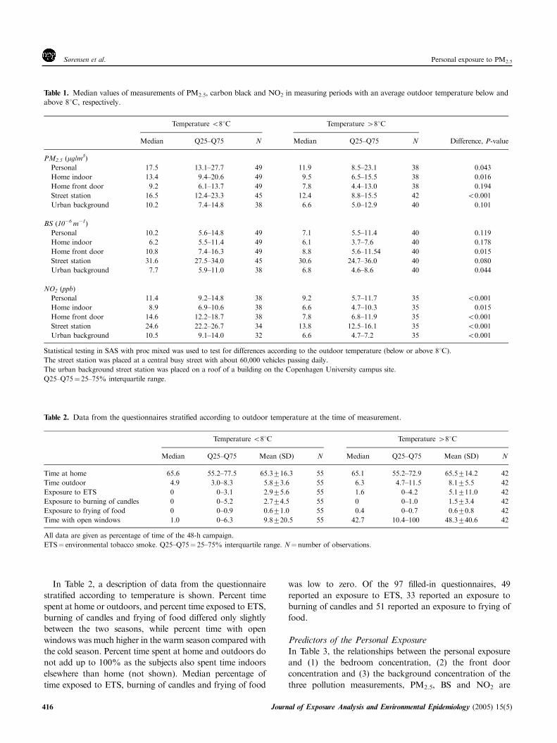
In Table 2, a description of data from the questionnaire

stratified according to temperature is shown. Percent time

spent at home or outdoors, and percent time exposed to ETS,

burning of candles and frying of food differed only slightly

between the two seasons, while percent time with open

windows was much higher in the warm season compared with

the cold season. Percent time spent at home and outdoors do

not add up to 100% as the subjects also spent time indoors

elsewhere than home (not shown). Median percentage of

time exposed to ETS, burning of candles and frying of food

was low to zero. Of the 97 filled-in questionnaires, 49

reported an exposure to ETS, 33 reported an exposure to

burning of candles and 51 reported an exposure to frying of

food.

Predictors of the Personal ExposureIn Table 3, the relationships between the personal exposure

and (1) the bedroom concentration, (2) the front door

concentration and (3) the background concentration of the

three pollution measurements, PM2.5, BS and NO2 are

Table 1. Median values of measurements of PM2.5, carbon black and NO2 in measuring periods with an average outdoor temperature below and

above 81C, respectively.

Temperature o81C Temperature 481C

Median Q25–Q75 N Median Q25–Q75 N Difference, P-value

PM2.5 (mg/m3)

Personal 17.5 13.1–27.7 49 11.9 8.5–23.1 38 0.043

Home indoor 13.4 9.4–20.6 49 9.5 6.5–15.5 38 0.016

Home front door 9.2 6.1–13.7 49 7.8 4.4–13.0 38 0.194

Street station 16.5 12.4–23.3 45 12.4 8.8–15.5 42 o0.001

Urban background 10.2 7.4–14.8 38 6.6 5.0–12.9 40 0.101

BS (10�6 m�1)

Personal 10.2 5.6–14.8 49 7.1 5.5–11.4 40 0.119

Home indoor 6.2 5.5–11.4 49 6.1 3.7–7.6 40 0.178

Home front door 10.8 7.4–16.3 49 8.8 5.6–11.54 40 0.015

Street station 31.6 27.5–34.0 45 30.6 24.7–36.0 40 0.080

Urban background 7.7 5.9–11.0 38 6.8 4.6–8.6 40 0.044

NO2 (ppb)

Personal 11.4 9.2–14.8 38 9.2 5.7–11.7 35 o0.001

Home indoor 8.9 6.9–10.6 38 6.6 4.7–10.3 35 0.015

Home front door 14.6 12.2–18.7 38 7.8 6.8–11.9 35 o0.001

Street station 24.6 22.2–26.7 34 13.8 12.5–16.1 35 o0.001

Urban background 10.5 9.1–14.0 32 6.6 4.7–7.2 35 o0.001

Statistical testing in SAS with proc mixed was used to test for differences according to the outdoor temperature (below or above 81C).

The street station was placed at a central busy street with about 60,000 vehicles passing daily.

The urban background street station was placed on a roof of a building on the Copenhagen University campus site.

Q25–Q75¼ 25–75% interquartile range.

Table 2. Data from the questionnaires stratified according to outdoor temperature at the time of measurement.

Temperature o81C Temperature 481C

Median Q25–Q75 Mean (SD) N Median Q25–Q75 Mean (SD) N

Time at home 65.6 55.2–77.5 65.3716.3 55 65.1 55.2–72.9 65.5714.2 42

Time outdoor 4.9 3.0–8.3 5.873.6 55 6.3 4.7–11.5 8.175.5 42

Exposure to ETS 0 0–3.1 2.975.6 55 1.6 0–4.2 5.1711.0 42

Exposure to burning of candles 0 0–5.2 2.774.5 55 0 0–1.0 1.573.4 42

Exposure to frying of food 0 0–0.9 0.671.0 55 0.4 0–0.7 0.670.8 42

Time with open windows 1.0 0–6.3 9.8720.5 55 42.7 10.4–100 48.3740.6 42

All data are given as percentage of time of the 48-h campaign.

ETS¼ environmental tobacco smoke. Q25–Q75¼ 25–75% interquartile range. N¼ number of observations.

Personal exposure to PM2.5Sørensen et al.

416 Journal of Exposure Analysis and Environmental Epidemiology (2005) 15(5)

shown. For PM2.5, the bedroom and the front door

concentrations were found to be significant predictors of

the personal exposure, whereas the background concentra-

tion only reached borderline significance (P¼ 0.053). For BS

a similar pattern was seen, with the exception that the

background concentration was far from being a significant

predictor (P¼ 0.86). For NO2, all three measurements

significantly predicted the personal exposure. When including

all three predictors in one model, the predictor that explained

most of the variation was the bedroom concentration

(Po0.01 for all) followed by the front door concentration

(Po0.01 for PM2.5, P¼ 0.08 for BS and Po0.05 for NO2),

whereas the background measurement became insignificant

for all three pollution markers (P40.4 for all). The inclusion

of subject as a random factor in the model corresponds to

specifying the responses observed on the same subject to be

correlated. When all three predictors were included, this

correlation was estimated to zero for PM2.5, indicating no

unexplained similarity between observations on the same

subject. For the BS model, the between-subject variance was

estimated to 0.082 and the within-subject variance to 0.880,

showing that the majority of the total unexplained variation

was within-subject variation, while only 8.6% (0.082/

(0.082þ 0.880)100) of the variation was between-subject

variation. For NO2, the within-subject variation was

estimated to 17.0% of the total unexplained variation.

When including only the front door and the background

concentration as predictors in one model, the front door

concentration significantly predicted the personal exposure

(Po0.001 for all), whereas the background measurement

was insignificant (P40.5 for all) for all three pollution

markers.

When examining the association between the personal

exposure and front door concentrations of PM2.5 according

to temperature, a borderline significant difference between

this association in the two temperature groups was found

(P¼ 0.08) (Table 4, Figure 1). In the warm season, a 10%

increase in the front door concentration resulted in a highly

significant 6.6% increase in the personal exposure, whereas in

the cold season this increase was only 2.7% and insignificant

(P¼ 0.064). For BS the interaction between the temperature

dichotomisation and the front door BS concentration was

not significant for the personal BS exposure (P¼ 0.21),

though also here the association between the personal

exposure and front door concentrations was strongest during

the summer. For the NO2 measurements, the association

between personal exposure and front door concentration was

significantly different in the two temperature groups

(P¼ 0.026), with a 10% increase in the front door

concentration causing a 8.5% increase in personal exposure

in the warm period and a 3.1% increase in personal exposure

in the cold period.

Table 5 shows the associations between the personal

exposure to PM2.5, BS and NO2 and exposure to the possible

indoor pollution sources: ETS, burning of candles and frying

of food. Time exposed to burning of candles was a significant

predictor of all three pollutants whereas time exposed to

frying of food did not predict any of them. Exposure to ETS

Table 3. Associations between personal exposure (outcome variable) and bedroom, front door and background concentrations (predictors) of

PM2.5, black smoke (BS) and NO2.

Predictor Regression

coefficients

Standard

error

N % increase in personal

exposure per 10%

increase in predictor

indicated

95% CI

(%)

P-value

PM2.5 (mg/m3)

Bedroom concentration 0.72 0.08 87 7.1 5.5–8.7 o0.0001

Front door concentration 0.46 0.12 87 4.5 2.1–6.9 0.0002

Background concentration 0.29 0.15 69 2.8 �0.1 to 5.7 0.053

BS (10�6 m�1)

Bedroom concentration 0.47 0.08 89 4.6 3.0–6.2 o0.0001

Front door concentration 0.61 0.15 89 6.0 3.0–9.1 0.0002

Background concentration 0.03 0.16 73 0.3 �2.7 to 3.4 0.86

NO2 (ppb)

Bedroom concentration 0.70 0.06 73 6.9 5.7–8.1 o0.0001

Front door concentration 0.60 0.07 73 5.9 4.5–7.3 o0.0001

Background concentration 0.56 0.09 66 5.5 3.7–7.3 o0.0001

Results from the mixed-model analysis.

The personal exposure, the front door concentration and the background concentration of PM2.5, black smoke (BS) and NO2 were transformed by the

natural logarithm.

CI¼ confidence interval.

Personal exposure to PM2.5 Sørensen et al.

Journal of Exposure Analysis and Environmental Epidemiology (2005) 15(5) 417

Table 4. Associations between the personal exposure and the front door concentration of PM2.5, black smoke (BS) and NO2, in relation to the

temperature dichotomisation.

Predictor Regression

coefficients

Standard

error

N % increase in personal

exposure per 10%

increase in predictor

indicated

95%

CI (%)

P-value

PM2.5 (mg/m3): Front door concentration * temperature at 0.082a

481C 0.67 0.18 38 6.6 3.0–10.3 o0.001b

o81C 0.28 0.14 49 2.7 �0.0 to 5.4 0.064b

BS (10�6 m�1): Front door concentration * temperature at 0.21a

481C 0.86 0.26 40 8.5 3.3–14.1 0.001b

o81C 0.45 0.20 49 4.4 0.5–8.4 0.027b

NO2 (ppb): Front door concentration * temperature at 0.026a

481C 0.68 0.09 35 6.7 4.9–8.5 o0.0001b

o81C 0.32 0.13 38 3.1 0.6–5.7 0.019b

The data were tested in a mixed-model analysis.

The personal exposure and the front door concentration of PM2.5, black smoke (BS) and NO2 were transformed by the natural logarithm.aP-value for the effect modification of the temperature grouping.bP-value for the estimate.

CI¼ confidence interval.

1

10

100

1 10 100Front door NO2 (ppb)

Per

sona

l NO

2 (p

pb)

1

10

100

1 10 100Front door NO2 (ppb)

Per

sona

l NO

2 (p

pb)

0.001

0.01

0.1

1 1

10

0.01 0.1 1 10Front door BS (10-6m-1)

Per

sona

l BS

(10

-6m

-1)

0.001

0.01

0.1

10

0.01 0.1 1 10Front door BS (10-6m-1)

Per

sona

l BS

(10

-6m

-1)

1

10

100

1 10 100Front door PM2.5(ug/m3)

Per

sona

l PM

2.5

(ug/

m3 ) Cold season Warm season

N = 38P = 0.001

N = 49P = 0.06

N = 49P = 0.03

N = 40P = 0.001

N = 35P < 0.0001

N = 38P = 0.02

1

10

100

1 10 100Front door PM2.5 (ug/m3)

Per

sona

l PM

2.5

(ug/

m3 )

Figure 1. Relationship between personal exposure and front door residence concentrations of PM2.5, BS and NO2 during the warm season(temperature above 81C) and the cold season (temperature below 81C).

Personal exposure to PM2.5Sørensen et al.

418 Journal of Exposure Analysis and Environmental Epidemiology (2005) 15(5)

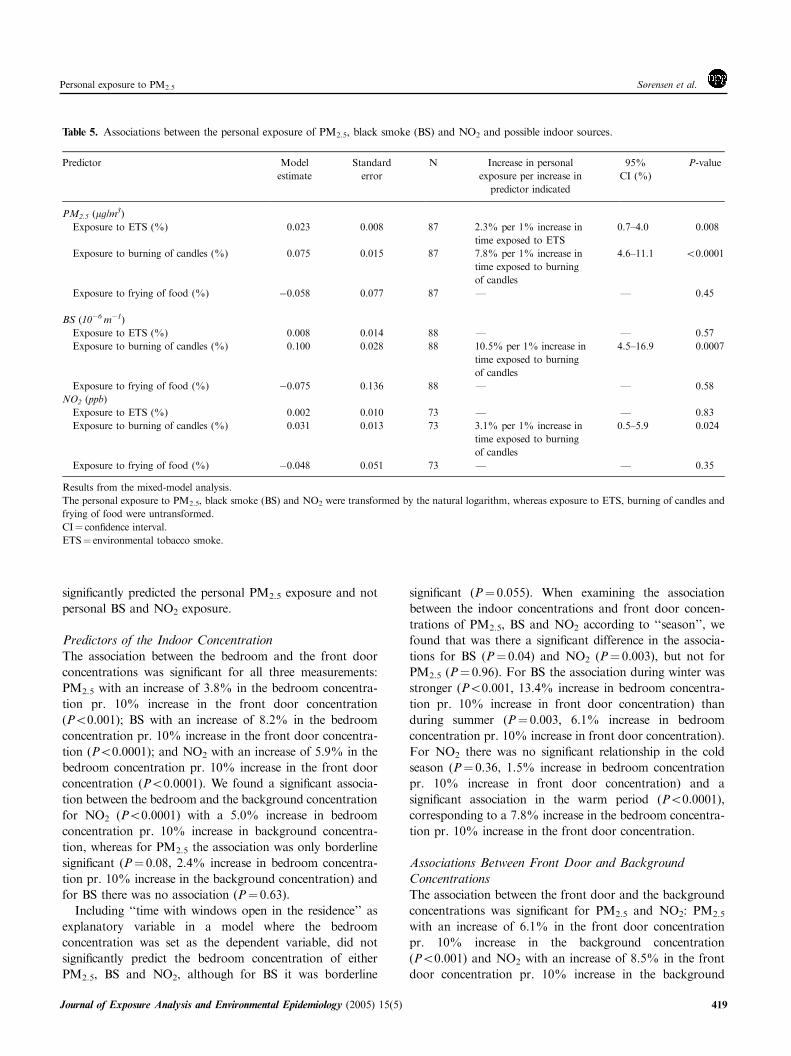
significantly predicted the personal PM2.5 exposure and not

personal BS and NO2 exposure.

Predictors of the Indoor ConcentrationThe association between the bedroom and the front door

concentrations was significant for all three measurements:

PM2.5 with an increase of 3.8% in the bedroom concentra-

tion pr. 10% increase in the front door concentration

(Po0.001); BS with an increase of 8.2% in the bedroom

concentration pr. 10% increase in the front door concentra-

tion (Po0.0001); and NO2 with an increase of 5.9% in the

bedroom concentration pr. 10% increase in the front door

concentration (Po0.0001). We found a significant associa-

tion between the bedroom and the background concentration

for NO2 (Po0.0001) with a 5.0% increase in bedroom

concentration pr. 10% increase in background concentra-

tion, whereas for PM2.5 the association was only borderline

significant (P¼ 0.08, 2.4% increase in bedroom concentra-

tion pr. 10% increase in the background concentration) and

for BS there was no association (P¼ 0.63).

Including ‘‘time with windows open in the residence’’ as

explanatory variable in a model where the bedroom

concentration was set as the dependent variable, did not

significantly predict the bedroom concentration of either

PM2.5, BS and NO2, although for BS it was borderline

significant (P¼ 0.055). When examining the association

between the indoor concentrations and front door concen-

trations of PM2.5, BS and NO2 according to ‘‘season’’, we

found that was there a significant difference in the associa-

tions for BS (P¼ 0.04) and NO2 (P¼ 0.003), but not for

PM2.5 (P¼ 0.96). For BS the association during winter was

stronger (Po0.001, 13.4% increase in bedroom concentra-

tion pr. 10% increase in front door concentration) than

during summer (P¼ 0.003, 6.1% increase in bedroom

concentration pr. 10% increase in front door concentration).

For NO2 there was no significant relationship in the cold

season (P¼ 0.36, 1.5% increase in bedroom concentration

pr. 10% increase in front door concentration) and a

significant association in the warm period (Po0.0001),

corresponding to a 7.8% increase in the bedroom concentra-

tion pr. 10% increase in the front door concentration.

Associations Between Front Door and BackgroundConcentrationsThe association between the front door and the background

concentrations was significant for PM2.5 and NO2: PM2.5

with an increase of 6.1% in the front door concentration

pr. 10% increase in the background concentration

(Po0.001) and NO2 with an increase of 8.5% in the front

door concentration pr. 10% increase in the background

Table 5. Associations between the personal exposure of PM2.5, black smoke (BS) and NO2 and possible indoor sources.

Predictor Model

estimate

Standard

error

N Increase in personal

exposure per increase in

predictor indicated

95%

CI (%)

P-value

PM2.5 (mg/m3)

Exposure to ETS (%) 0.023 0.008 87 2.3% per 1% increase in

time exposed to ETS

0.7–4.0 0.008

Exposure to burning of candles (%) 0.075 0.015 87 7.8% per 1% increase in

time exposed to burning

of candles

4.6–11.1 o0.0001

Exposure to frying of food (%) �0.058 0.077 87 F F 0.45

BS (10�6 m�1)

Exposure to ETS (%) 0.008 0.014 88 F F 0.57

Exposure to burning of candles (%) 0.100 0.028 88 10.5% per 1% increase in

time exposed to burning

of candles

4.5–16.9 0.0007

Exposure to frying of food (%) �0.075 0.136 88 F F 0.58

NO2 (ppb)

Exposure to ETS (%) 0.002 0.010 73 F F 0.83

Exposure to burning of candles (%) 0.031 0.013 73 3.1% per 1% increase in

time exposed to burning

of candles

0.5–5.9 0.024

Exposure to frying of food (%) �0.048 0.051 73 F F 0.35

Results from the mixed-model analysis.

The personal exposure to PM2.5, black smoke (BS) and NO2 were transformed by the natural logarithm, whereas exposure to ETS, burning of candles and

frying of food were untransformed.

CI¼ confidence interval.

ETS¼ environmental tobacco smoke.

Personal exposure to PM2.5 Sørensen et al.

Journal of Exposure Analysis and Environmental Epidemiology (2005) 15(5) 419

concentration (Po0.0001). There was no significant associa-

tion between the front door and the background concentra-

tions of BS (P¼ 0.15).

Discussion

In this study, outdoor and indoor concentrations of PM2.5,

BS and NO2 as well as information on indoor exposure

sources and seasons were measured and registered in order to

investigate their potential in predicting the personal exposure.

We found that the home indoor air pollution level was the

strongest predictor of the personal exposure, and that

burning of candles and exposure to ETS were two indoor

air pollution sources that predicted the personal exposure.

The season seemed to be important when looking on the

relationship between personal exposure and outdoor air

pollution concentrations, especially for NO2 and PM2.5, and

BS seemed to show greater spatial variations than NO2 and

PM2.5

The strongest predictor of the personal exposure in our

model was the bedroom concentration, which is in agreement

with the results from previous studies (Ozkaynak et al., 1996;

Pellizzari et al., 1999; Williams et al., 2000; Koistinen et al.,

2001). It implies that there are other sources than the outdoor

traffic that contribute to the personal exposure. This is

important, as particles generated indoors might be at least as

bioactive as ambient particles and therefore important when

investigating impact on health effects (Long et al., 2001b).

The fact that we found ‘time exposed to burning of candles’

to be a significant predictor of personal PM2.5, BS and NO2

exposure, and ‘time exposed to ETS’ to be associated with

personal PM2.5 exposure helps explain why the bedroom

concentration is such a strong predictor, together with the

fact that the subjects spend most of their time indoors. The

results on exposure to ETS are comparable to another study

that compared PM2.5 and BS measurements and found that

cigarettes had a stronger impact on PM2.5 than on BS

(Gotschi et al., 2002). Another important indoor source of

NO2 is gas stoves (Levy et al., 1998), but we do not have

information of this in the present study.

The variance of the PM2.5 model at subject level was found

to be zero from which we, surprisingly, can conclude that on

subject level there were no individual factors such as, for

example, home address and transport route to the university,

that influenced the personal exposure in repeated measure-

ments. A possible explanation may be that the subjects were

all students, who do not have an ordinary ‘8-h work day’ and

perhaps therefore a larger variation in behavioural patterns

than other sections of the population. For BS and NO2 the

variance at subject level was close to zero showing that also

for these two measurements there was almost no between

subject variation.

We found that the personal PM2.5 exposure and the

bedroom concentration exceeded the home outdoor PM2.5

concentration and was similar to the street station concen-

tration of PM2.5, whereas for NO2 and BS the concentrations

at the home front door and at the street station were at the

same level and much higher, respectively, as the personal

exposure. This is similar to results obtained in other studies

(Koistinen et al., 2001; Kousa et al., 2001), and indicates

that PM2.5 are more strongly affected by indoor sources than

NO2 and BS and that personal NO2 and BS exposure thus

are more strongly associated to traffic than PM2.5. Another

reason to why the personal exposure to PM2.5 exceeds the

front door concentration and also the home indoor

concentration could be the existence of the ‘personal aerosol

cloud’ affecting PM2.5 and not NO2 and BS (Wallace, 1996).

As outdoor concentrations of PM2.5, BS or NO2 are the

most commonly used measurements in ‘‘estimating’’ personal

PM2.5, BS and NO2 exposure, respectively, the association

between personal exposure and outdoor concentrations is

especially important (Dockery et al., 1993; Pope et al., 1995,

2002). When we included both the front door and back-

ground concentration in one model the background mea-

surement did not significantly predict the personal exposure

for either PM2.5, BS or NO2, indicating that the contribution

of this measurement is already accounted for in the front

door measurement, and that the front door measurement

thus is a better predictor than the background measurement.

When including only one predictor in each model, we found

that the front door and background concentrations of PM2.5

and NO2 predicted some of the personal exposure whereas

for BS only the front door concentration was a significant

predictor. It therefore seems that the background measure-

ment of BS is unsuitable as predictor of personal exposure,

when longer term exposures are of interest. It also indicates

more spatial variability for BS compared with PM2.5 and

NO2, which is supported by our findings of a significant

association between the front door and the background

concentrations for PM2.5 and NO2, and not for BS. This is

similar to results obtained in other studies, and also fits with

the results in Table 1 that show higher street station/front

door station ratios of BS compared with PM2.5 and NO2

(Kinney et al., 2000; Roosli et al., 2001; Hoek et al., 2002).

BS is believed to be a measurement of particles in the sub-

micrometre range (Horvath, 1995), which to some extent will

be directly emitted ultrafine particles from diesel vehicles. The

spatial variation found for BS is probably due to a rapid

dilution of the BS sources, such as diesel exhaust, rather than

condensation to larger particles (Vignati et al., 1999).

When we compared the relationship between the personal

exposure and the front door concentration we found that all

three pollution measurements seemed to be dependent of the

seasonal categorisation (though only significant for NO2),

such that during the warm season the outdoor exposure

contributed more to the personal exposure than during cold

Personal exposure to PM2.5Sørensen et al.

420 Journal of Exposure Analysis and Environmental Epidemiology (2005) 15(5)

periods. This could partly relate to differences in air exchange

between indoor and outdoor environments in the two

periods. In addition to this, the subjects on average spent

6.3% time outdoors during the warmer period compared

to 4.9% during the colder period, which could also

explain some of the difference in associations between the

‘‘seasons’’.

Ventilation of the residence has been found to affect the

relationship between the indoor–outdoor concentrations, and

thus the relationship between personal exposure and outdoor

concentration as people spent most of their time indoors

(Rodes et al., 2001; Gotschi et al., 2002). In our study

including ‘‘time with windows open in the residence’’ as

explanatory variable, did not significantly predict the bed-

room concentration of either PM2.5, BS and NO2, although

for BS it was borderline significant. Another way to examine

the ventilation, as suggested by another study (Gotschi et al.,

2002), is to compare indoors and outdoors associations

stratified by winter (cold season) and summer (warm season),

representing periods with low and high ventilation rates,

respectively. Lower associations would be expected during

the cold season where the ventilation is low, and for NO2 this

was what we found. For BS we found that the association

was highest during the cold season, suggesting that BS is less

affected by different ventilation rates than NO2. No

difference in association between the cold and warm season

was seen for PM2.5. This is somewhat surprising as PM2.5 in

other studies has been found to be more affected by different

ventilation rates than BS (Long et al., 2001a; Gotschi et al.,

2002). If we compare the increase in the bedroom

concentration pr. 10% increase in front concentration, we

found a higher increase for BS (8.2%) and NO2 (5.9%) than

for PM2.5 (3.8%), which is similar to results obtained in

other studies (Gotschi et al., 2002). This indicates that BS

and NO2 penetrate buildings more easily than PM2.5.

In conclusion, our findings imply that the personal

exposure to PM2.5, BS and NO2 depends on many factors

besides the outdoor levels, and that information on, for

example, time of season or temperature and indoor

exposures, will improve the accuracy of the personal

exposure estimation.

Acknowledgements

Financial support was obtained from the Danish National

Environmental Research Programme under the Centre for

the Environment and the Respiratory System (CML).

References

Abt E., Suh H.H., Catalano P.J., and Koutrakis P. Relative contribution of

outdoor and indoor particle sources to indoor concentrations. Environ Sci

Technol 2000: 34: 3579–3587.

Brauer M., Hruba F., Mihalikova E., Fabianova E., Miskovic P., Plzikova A.,

Lendacka M., Vanderberg J., and Cullen A. Personal exposure to particles in

Banska Bystrica, Slovakia. J Expos Anal Environ Epidemiol 2001: 10: 478–487.

Brunekreef B., and Holgate S.T. Air pollution and health. Lancet 2002: 360:

1233–1242.

Cocheo V., Boaretto C., and Sacco P. High uptake rate radial diffusive sampler

suitable for both solvent and thermal desorption. Am Ind Hyg Assoc 1996: 57:

897–904.

Dockery D.W., Pope III A.C., Xu X., Spengler J.D., Ware J.H., Fay M.E., Ferris

Jr B.G., and Speizer F.E. An association between air pollution and mortality

in six U.S. cities. N Engl J Med 1993: 329: 1753–1759.

Ebelt S.T., Petkau A.J., Vedal S., Fishe T.V., and Brauer M. Exposure of chronic

obstructive pulmonary disease patients to particulate matter: relationship

between personal and ambient air concentration. J Air Waste Manage Assoc

2000: 50: 1081–1094.

Gotschi T., Oglesby L., Mathys P., Monn C., Manalis N., Koistinen K., Jantunen

M., Hanninen O., Polanska L., and Kunzli N. Comparison of black smoke

and PM2.5 levels in indoor and outdoor environments of four European cities.

Environ Sci Technol 2002: 36: 1191–1197.

Hoek G., Meliefste K., Cyrys J., Lewne M., Bellander T., Brauer M., Fischer P.,

Gehring U., Heinrich J., van Vliet P., and Brunekreef B. Spatial variation of

fine particle concentrations in three European areas. Atmos Environ 2002: 36:

4077–4088.

Hornung R.W., and Reed L.D. Estimation of average concentration in the

presence of nondetectable values. Appl Occup Environ Hyg 1990: 5: 46–51.

Horvath H. Size segregated light absorption coefficient of the aerosol. Atmos

Environ 1995: 29: 875–883.

ISO 9835. Determination of a black smoke index in ambient air. British Standard

Specifications, 1747[11] 1993.

Janssen N.A., de Hartog J.J., Hoek G., Brunekreef B., Lanki T., Timonen K.L.,

and Pekkanen J. Personal exposure to fine particulate matter in elderly

subjects: relation between personal, indoor, and outdoor concentrations. J Air

Waste Manage Assoc 2000: 50: 1133–1143.

Jantunen M.J., Hanninen O., Katsouyanni K., Knoppel H., Kuenzli N., Lebret

E., Maroni M., Saarela K., Sram R., and Zmirou D. Air pollution exposure

in European cities: The ‘EXPOLIS’ study. J Expos Anal Environ Epidemiol

1998: 8: 495–518.

Jenkins P.L., Phillips T.J., Mulberg E.J., and Hui S.P. Activity patterns of

Californians: use and proximity to indoor pollutant sources. Atmos Environ

1992: 26A: 2141–2148.

Kenny L.C., and Gussman R.A. Characterization and modelling of a family of

cyclone aerosol preseparators. J Aerosol Sci 1997: 28: 677–688.

Kinney P.L., Aggarwal M., Northridge M.E., Janssen N.A., and Shepard P.

Airborne concentrations of PM(2.5) and diesel exhaust particles on Harlem

sidewalks: a community-based pilot study. Environ Health Perspect 2000: 108:

213–218.

Koistinen K.J., Hanninen O., Rotko T., Edwards R.D., Moschandreas D., and

Jantunen M.J. Behavioral and environmental determinants of personal

exposures to PM2.5 in EXPOLIS F Helsinki, Finland. Atmos Environ

2001: 35: 2473–2481.

Kousa A., Monn C., Rotko T., Alm S., Oglesby L., and Jantunen M.J. Personal

exposure to NO2 in the EXPOLIS-study: relation to residential indoor,

outdoor and workplace concentration in Basel, Helsinki and Prague. Atmos

Environ 2001: 35: 3405–3412.

Koutrakis P., and Briggs S.L.K. Source apportionment of indoor aerosols in

Suffolk and Onondaga counties, New York. Environ Sci Technol 1992: 26:

521–527.

Levy J.I., Lee K., Spengler J.D., and Yanagisawa Y. Impact of residential nitrogen

dioxide exposure on personal exposure: an international study. J Air Waste

Manage Assoc 1998: 48: 553–560.

Long C.M., Suh H.H., Catalano P.J., and Koutrakis P. Using time- and size-

resolved particulate data to quantify indoor penetration and deposition

behavior. Environ Sci Technol 2001a: 35: 2089–2099.

Long C.M., Suh H.H., Kobzik L., Catalano P.J., Ning Y.Y., and Koutrakis P. A

pilot investigation of the relative toxicity of indoor and outdoor fine particles:

in vitro effects of endotoxin and other particulate properties. Environ Health

Perspect 2001b: 109: 1019–1026.

McConnell R., Berhane K., Gilliland F., Molitor J., Thomas D., Lurmann F.,

Avol E., Gauderman W.J., and Peters J.M. Prospective study of air pollution

and bronchitic symptoms in children with asthma. Am J Respir Crit Care Med

2003: 168: 790–797.

Personal exposure to PM2.5 Sørensen et al.

Journal of Exposure Analysis and Environmental Epidemiology (2005) 15(5) 421

Ozkaynak H., Xue J., Spengler J., Wallace L., Pellizzari E., and Jenkins P.

Personal exposure to airborne particles and metals: results from the Particle

TEAM study in Riverside, California. J Expos Anal Environ Epidemiol 1996:

6: 57–78.

Pellizzari E., Clayton C.A., Rodes C., Mason R.E., Piper L.L., Fort B., Pfeifer

G., and Lynam D. Particulate matter and manganese exposure in Toronto,

Canada. Atmos Environ 1999: 33: 721–734.

Pope C.A., Burnett R.T., Thun M.J., Calle E.E., Krewski D., Ito K., and

Thurston G.D. Lung cancer, cardiopulmonary mortality, and long-term

exposure to fine particulate air pollution. JAMA 2002: 287: 1132–1141.

Pope C.A., Thun M.J., Namboodiri M.M., Dockery D.W., Evans J.S., Speizer

F.E., and Heath Jr C.W. Particulate air pollution as a predictor of mortality in

a prospective study of U.S. adults. Am J Respir Crit Care Med 1995: 151:

669–674.

Rodes C.E., Lawless P.A., Evans G.F., Sheldon L.S., Williams R.W., Vette A.F.,

Creason J.P., and Walsh D. The relationships between personal PM exposures

for elderly populations and indoor and outdoor concentrations for three

retirement center scenarios. J Expos Anal Environ Epidemiol 2001: 11:

103–115.

Roosli M., Theis G., Staehelin J., Mathys P., Oglesby L., Camenzind M., and

Braun-Fahrlander C. Temporal and spatial variation of the chemical

composition of PM10 at urban and rural sites in the Basel area, Switzerland.

Atmos Environ 2001: 35: 3701–3713.

Seaton A., Soutar A., Crawford V., Elton R., McNerlan S., Cherrie J., Watt M.,

Agius R., and Stout R. Particulate air pollution and the blood. Thorax 1999:

54: 1027–1032.

Sorensen M., Autrup H., Hertel O., Wallin H., Knudsen L.E., and Loft S.

Personal exposure to PM2.5 and biomarkers of DNA damage. Cancer

Epidemiol Biomarkers Prev 2003a: 12: 191–196.

Sorensen M., Daneshvar B., Hansen M., Dragsted L.O., Hertel O., Knudsen L.,

and Loft S. Personal PM(2.5) exposure and markers of oxidative stress in

blood. Environ Health Perspect 2003b: 111: 161–166.

Thatcher T.L., and Layton D.W. Deposition, resuspension, and penetration of

particles within a residence. Atmos Environ 1995: 29: 1487–1497.

Vignati E., Berkowicz R., Palmgren F., Lyck E., and Hummelsh�j P.

Transformation of size distributions of emitted particles in streets. Sci Total

Environ 1999: 235: 37–49.

Wallace L. Indoor particles: a review. J Air Waste Manage Assoc 1996: 46: 98–126.

Williams R., Suggs J., Creason J., Rodes C., Lawless P., Kwok R., Zweidinger

R., and Sheldon L. The 1998 Baltimore Particulate Matter Epidemiology FExposure Study: part 2. Personal exposure assessment associated with an

elderly study population. J Expos Anal Environ Epidemiol 2000: 10: 533–543.

Personal exposure to PM2.5Sørensen et al.

422 Journal of Exposure Analysis and Environmental Epidemiology (2005) 15(5)