FINAL REPORT Characterization of PM2.5 Dust Emissions from Training/Testing Range Operations

SERDP Project SI-1190

August 2008 John M. Veranth University of Utah

Kevin Perry University of Utah

Eric Pardyjak University of Utah

Scott Speckart University of Utah

Raed Labban University of Utah

Erin Kaser University of Utah

John Watson Desert Research Institute

Judy C. Chow Desert Research Institute

Vic Etyemezian Desert Research Institute

Steve Kohl Desert Research Institute

Report Documentation Page Form ApprovedOMB No. 0704-0188

Public reporting burden for the collection of information is estimated to average 1 hour per response, including the time for reviewing instructions, searching existing data sources, gathering andmaintaining the data needed, and completing and reviewing the collection of information. Send comments regarding this burden estimate or any other aspect of this collection of information,including suggestions for reducing this burden, to Washington Headquarters Services, Directorate for Information Operations and Reports, 1215 Jefferson Davis Highway, Suite 1204, ArlingtonVA 22202-4302. Respondents should be aware that notwithstanding any other provision of law, no person shall be subject to a penalty for failing to comply with a collection of information if itdoes not display a currently valid OMB control number.

1. REPORT DATE 01 AUG 2008

2. REPORT TYPE N/A

3. DATES COVERED -

4. TITLE AND SUBTITLE Characterization of PM2.5 Dust Emissions from Training/Testing Range Operations

5a. CONTRACT NUMBER

5b. GRANT NUMBER

5c. PROGRAM ELEMENT NUMBER

6. AUTHOR(S) 5d. PROJECT NUMBER

5e. TASK NUMBER

5f. WORK UNIT NUMBER

7. PERFORMING ORGANIZATION NAME(S) AND ADDRESS(ES) University of Utah, Salt Lake City UT

8. PERFORMING ORGANIZATIONREPORT NUMBER

9. SPONSORING/MONITORING AGENCY NAME(S) AND ADDRESS(ES) 10. SPONSOR/MONITOR’S ACRONYM(S)

11. SPONSOR/MONITOR’S REPORT NUMBER(S)

12. DISTRIBUTION/AVAILABILITY STATEMENT Approved for public release, distribution unlimited

13. SUPPLEMENTARY NOTES The original document contains color images.

14. ABSTRACT

15. SUBJECT TERMS

16. SECURITY CLASSIFICATION OF: 17. LIMITATION OF ABSTRACT

UU

18. NUMBEROF PAGES

57

19a. NAME OFRESPONSIBLE PERSON

a. REPORT unclassified

b. ABSTRACT unclassified

c. THIS PAGE unclassified

Standard Form 298 (Rev. 8-98) Prescribed by ANSI Std Z39-18

CHARACTERIZATION OF PM2.5 DUST EMISSIONS

FROM TRAINING/TESTING RANGE OPERATIONS SI-1190

(ORIGINALLY CP-1190)

Final Report

Revision 1 January 2008

John M. Veranth, Kevin Perry, Eric Pardyjak, Scott Speckart, Raed Labban, Erin Kaser

University of Utah, Salt Lake City UT

and

John G. Watson, Judy C. Chow, Vic Etyemezian, Steve Kohl Desert Research Institute, Reno NV

Approved for public release; Distribution is unlimited

This report was prepared under contract to the Department of Defense Strategic Environmental Research and Development Program (SERDP). The publication of this report does not indicate endorsement by the Department of Defense, nor should the contents be construed as reflecting the official policy or position of the Department of Defense. Reference herein to any specific commercial product, process, or service by trade name, trademark, manufacturer, or otherwise, does not necessarily constitute or imply its endorsement, recommendation, or favoring by the Department of Defense.

ii

Table of Contents

Table Of Contents ....................................................................................................................................................iii 

FIGURES .........................................................................................................................................V

TABLES..........................................................................................................................................VI

Acknowledgements....................................................................................................................... vii

Executive Summary...................................................................................................................... 1

1. Objective .................................................................................................................................... 3

1.1 GOAL STATEMENT .................................................................................................................. 3

1.2 SCIENTIFIC OBJECTIVES ........................................................................................................ 3

1.3 FY 2005 (INCLUDING NO COST EXTENSION FOR 2006) TECHNICAL APPROACH ............. 3

2. Background ............................................................................................................................... 4

2. 1 SERDP PROJECT BACKGROUND .......................................................................................... 4

2.2 PRIOR WORK ON THIS TOPIC ................................................................................................ 4

3. Materials and Methods............................................................................................................. 7

3.1 DUST FLUX FIELD STUDY METHODS .................................................................................... 7

3.2 DUST FLUX DATA ANALYSIS METHODS ............................................................................. 10

3.3 NEAR-SOURCE PARTICLE DEPOSITION .............................................................................. 13

3.4 SOURCE APPORTIONMENT STUDY METHODS.................................................................... 18

3.5 ENHANCED SOURCE APPORTIONMENT FEASIBILITY STUDY METHODS......................... 20

4. Results and Accomplishments ............................................................................................... 23

4.1 DUST TRANSPORT FIELD STUDY ......................................................................................... 22

4.2 NEAR-SOURCE DEPOSITION STUDY .................................................................................... 28

4.3 SOURCE APPORTIONMENT STUDY ...................................................................................... 31

4.4 ENHANCED SOURCE APPORTIONMENT FEASIBILITY STUDY ........................................... 34

5. Conclusion ............................................................................................................................... 40

5.1 DUST TRANSPORT ................................................................................................................. 40

5.2 SOURCE APPORTIONMENT ................................................................................................... 41

iii

5.3 RESULTS APPLICABLE TO TRAINING RANGE ENVIRONMENTAL PROGRAMS ................ 42

6. Literature Cited ..................................................................................................................... 44

Appendices................................................................................................................................... 48

APPENDIX A. SUPPORTING DATA ............................................................................................. 48

APPENDIX B.1 LIST OF TECHNICAL PUBLICATIONS................................................................ 48

APPENDIX B.2 INTERNAL TECHNICAL REPORTS AND MANUSCRIPTS IN PROGRESS .......... 49

APPENIDX B.3 CONFERENCE/SYMPOSIUM PROCEEDINGS ..................................................... 49

APPENIDX B.4 PUBLISHED TECHNICAL ABSTRACTS............................................................... 49

iv

Figures

Figure 1. This schematic representation of vehicle generated dust within one grid cell of a regional airshed model illustrates the hypothesis that emission inventories of road dust may need to be adjusted for near source dust removal. ........................................................6

Figure 2. Schematic of the MUST site at Dugway Proving Ground showing the array of shipping containers representing buildings and the location of the monitoring towers use for the road dust study. ...................................................................................................8

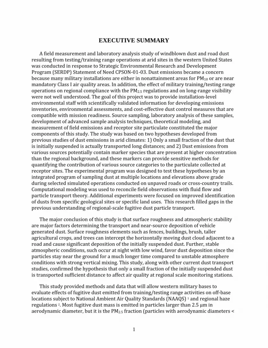
Figure 3. Field Instrumentation: Top - Field measurement of deposition velocity of vehicle-generated dust near an unpaved road. Middle - Detail of directional flat substrates prior to removal of the covers for collection. Bottom - Detail of the plastic fir garland artificial vegetation assembly and the control tub prior to removal of cover. ..17

Figure 4. Dust concentration versus time as measured by DustTraks. Vehicle passes generated well defined spikes near at 3 m horizontal and 1 m vertical from the road (bottom). The spikes were broader but still well defined 95 m downwind and 4.6 m above grade (middle). Most vehicle trips did not cause a noticeable spike at 95 m downwind and 18.3 m above grade (top). Note that full scale for the top graph is 1/1000, and for the middle graph is 1/50, of full scale for the near road measurements. 17..........................................................................................................................................25

Figure 5. Differential flux versus height at the 3 m and 95 m locations for four of the integration methods used in this study: stepwise wind and concentration; power law wind and exponential concentration (recommended method); power law wind and Gaussian concentration; and logarithmic wind and power law concentration. 17...............28

Figure 6. Directional deposition velocity from two independent sets of directional substrates measurements at each site: Ft Bliss (black squares, ) and Vado Road (open circle, ). Data are normalized by the deposition velocity for the +Z (horizontal facing up) direction. Deposition is enhanced on the surfaces facing upwind or crosswind (-X and -Y at Ft Bliss) and deposition is nearly isotropic under low wind conditions encountered at Vado Road. 30............................................................................30

Figure 8. Model simulations showing the shape of the dust cloud versus time for actual and hypothetical cases with the inputs summarized in Table 4. The contour represents 0.03% of initial dust cloud concentration ...........................................................................32

Figure 9. Military and civilian sites for CMB source apportionment study. The sites analyzed but not reported were used to study regional versus local variation but chemical composition tables were not included in the journal publication due to space limitations. ..........................................................................................................................36

Figure 10. Military and civilian sites at Camp Williams and Dugway Proving Ground............38

Figure 11 . Fraction of organic species showing a statistical significance greater than indicated P-value in a pair wise ANOVA. A large fraction indicates a higher

v

probability the two sites compared may be distinguished using organic Py-GC/MS data. Distant sites (Pair A) showed the greatest number of statistically different species but nearby sites with different soil units also showed statistical difference (Pairs B and C). Adjacent sites with the same soil unit but different land uses (Pairs D and E) showed the fewest organic species with statistically different concentrations. ......39

Tables

Table 1. Field measurements of particle deposition on surfaces. ...............................................15

Table 2. Wind speed versus height. ............................................................................................24

Table 3. Mean ± one standard deviation wind and concentration data for the entire 1.5 hr test period with 44 vehicle trips. Wind standard deviation based on variation between 15-minute averages. Concentration standard deviation based on variation between individual vehicle trips. Pulse area is the time integrated concentration for the interval corresponding to one vehicle pass. .....................................................................................23

Table 4. Dust flux (mg dust per meter of vehicle travel) adjacent to the road (near) and 90 m downwind (far) calculated by integrating the indicated interpolation functions for wind speed and dust concentration versus height. ..............................................................26

Table 5. Screen analysis of road on training range.....................................................................28

Table 6. Soil source profile sample sites. ..................................................................................32

Acronyms/Abbreviations

CMB Chemical Mass Balance NAAQS National Ambient Air Quality Standards PM Particulate Matter PM2.5 Particulate Matter less than 2.5 micrometers in diameter PM10 Particulate Matter less than 10 micrometers in diameter SERDP Strategic Environmental Research and Development Program TSP Total Suspended Particulate U.S. EPA U.S. Environmental Protection Agency

vi

Acknowledgements

The authors thank Clyde Durham and Elsa Cushing at Fort Bliss, Todd Caldwell, Jack Gillies, Steve Kohl and Vic Etyemezian at Desert Research Institute, and Gauri Seshadri at University of Utah for assistance with field sampling and analysis. Henk Meuzelaar, Neil Arnold and Barbara Zielinska, and Steve Kohl provided essential resources for the pyrolysis analysis feasibility study. A University of Utah mechanical engineering faculty member with expertise in atmospheric fluid mechanics, Eric Pardyjak, collaborated with this project, but did not receive salary funding. A University of Utah meteorology faculty member with experience and prior publications regarding chemical analysis of atmospheric dust samples, Kevin Perry, collaborated with CP1190 and received partial salary funding. These faculty collaborators strengthened the technical team and provided opportunities to leverage multiple research projects. Staff support at the U of U was provided by Martha Veranth, Research Scientist, and by Erin Kaser, Laboratory Technician.  

A PhD candidate graduate student, Raed Labban, worked on the project with emphasis on Chemical Mass Balance source‐receptor studies and Thermal Desorption / Gas Chromatography analysis of soil samples. A PhD candidate graduate student, Fang Yin, worked on computational modeling of near‐source dust transport in 2003‐04. A Mechanical Engineering graduate student, Scott Speckart, also worked on the computational modeling. Additional technical support at Desert Research Institute was provided by Steve Kohl, Anthony Chen, and Johann Englebricht and by the ongoing collaboration with John Gillies and project SI‐1191. 

The authors also thank the Department of Army, Bureau of Land Management, New Mexico State Land Office, and private landowners for site access.  

The authors thank the Strategic Environmental Research and Development Program (SERDP) for the financial assistance which enabled us to undertake this project.  Appreciation for technical assistance is extended to Mr. Bradley Smith, Executive Director and Drs. Robert Holst and John Hall, Sustainable Infrastructure Program Managers, former and present, and to the HydroGeoLogic, Inc., staff for their administrative assistance.

1

EXECUTIVE SUMMARY

A field measurement and laboratory analysis study of windblown dust and road dust resulting from testing/training range operations at arid sites in the western United States was conducted in response to Strategic Environmental Research and Development Program (SERDP) Statement of Need CPSON‐01‐03. Dust emissions became a concern because many military installations are either in nonattainment areas for PM10 or are near mandatory Class I air quality areas. In addition, the effect of military training/testing range operations on regional compliance with the PM2.5 regulations and on long‐range visibility were not well understood. The goal of this project was to provide installation‐level environmental staff with scientifically validated information for developing emissions inventories, environmental assessments, and cost‐effective dust control measures that are compatible with mission readiness. Source sampling, laboratory analysis of these samples, development of advanced sample analysis techniques, theoretical modeling, and measurement of field emissions and receptor site particulate constituted the major components of this study. The study was based on two hypotheses developed from previous studies of dust emissions in arid climates: 1) Only a small fraction of the dust that is initially suspended is actually transported long distances; and 2) Dust emissions from various sources potentially contain marker species that are present at higher concentration than the regional background, and these markers can provide sensitive methods for quantifying the contribution of various source categories to the particulate collected at receptor sites. The experimental program was designed to test these hypotheses by an integrated program of sampling dust at multiple locations and elevations above grade during selected simulated operations conducted on unpaved roads or cross‐country trails. Computational modeling was used to reconcile field observations with fluid flow and particle transport theory. Additional experiments were focused on improved identification of dusts from specific geological sites or specific land uses.  This research filled gaps in the previous understanding of regional‐scale fugitive dust particle transport.  

The major conclusion of this study is that surface roughness and atmospheric stability are major factors determining the transport and near‐source deposition of vehicle generated dust. Surface roughness elements such as fences, buildings, brush, taller agricultural crops, and trees can intercept the horizontally moving dust cloud adjacent to a road and cause significant deposition of the initially suspended dust. Further, stable atmospheric conditions, such occur at night with low wind, favor dust deposition since the particles stay near the ground for a much longer time compared to unstable atmosphere conditions with strong vertical mixing. This study, along with other current dust transport studies, confirmed the hypothesis that only a small fraction of the initially suspended dust is transported sufficient distance to affect air quality at regional scale monitoring stations. 

This study provided methods and data that will allow western military bases to evaluate effects of fugitive dust emitted from training/testing range activities on off‐base locations subject to National Ambient Air Quality Standards (NAAQS) 1 and regional haze regulations 2. Most fugitive dust mass is emitted in particles larger than 2.5 µm in aerodynamic diameter, but it is the PM2.5 fraction (particles with aerodynamic diameters < 

2

2.5 µm) that is most likely to remain suspended for several days and to travel long distances. This is also the size range that affects light extinction and is implicated in adverse health effects. Although much work has been done on fugitive dust emissions, 3‐7 little of this is specific to PM2.5. Practically none of the literature relates to the heavy‐duty vehicle, aircraft, ordnance testing, and alkaline desert soils that are typical of western military bases. 

A secondary outcome of this SERDP research, unanticipated at the time the project started, was that the work on chemical composition of fugitive dust from different sources proved useful during the public comment period on the initially proposed U.S. EPA coarse PM standard. Two papers from the SI‐1190 project regarding chemical composition of fugitive dust were cited in the preamble to the final U.S. EPA rule.  

Project SI‐1190 generated published papers on the results of the field studies and on the feasibility of identifying different sources of fugitive dust by receptor modeling techniques. There were also presentations at both the SERDP/ESTCP conference and at atmospheric science technical meetings dealing with the near source transportation and deposition of vehicle‐generated dust. Additional manuscripts anticipated to be published following official project closeout are included as chapters in this report. 

The information generated as result of this work as well as a number of dust related projects in the past five years has lead to the publication of The Western Regional Air Partnership Fugitive Dust Handbook which will be used by the military as well as civilian personnel. 

3

1. OBJECTIVE

1.1 Goal Statement

The goal of this study was to provide installation‐level environmental staff with scientifically validated information for developing dust emission inventories, environmental assessments, and cost‐effective dust control measures that are compatible with mission readiness. Source sampling, laboratory analysis of these samples, development of advanced sample analysis techniques, theoretical modeling, and measurement of field emissions and receptor site particulate samples constituted the major components of this study.  

1.2 Scientific Objectives

The scientific objectives of Project SI‐1190 were:  

1) Develop and apply methods to measure particle size distribution, particle number concentration, and chemical characteristics of dust from vehicle travel and troop maneuvers at selected training/testing range sites.  

2) Evaluate fugitive dust particle characteristics that allow emissions from military operations to be distinguished from other fugitive dust contributions at receptor sites.  

3) Evaluate the hypothesis that current PM2.5 emission factors overstate the regional impact of fugitive dust because they do not properly account for vertical mixing (downward and upward), deposition, and impaction near the source.  

These objectives were achieved by: 1) acquiring representative samples of suspendable dust from selected military bases and surrounding areas; 2) resuspending these samples in the laboratory study and extracting samples for chemical and physical analyses; 3) theoretically and empirically evaluating the chemical source profiles and processes that suspend and transport dust on military bases; and 4) performing ambient experiments during operations and training to evaluate source characterization and transport mechanisms. The data from these experiments were combined with those from other previous and concurrent studies to provide a valid scientific basis for future air quality planning.  

1.3 FY 2005 Technical Approach

The technical approach for the closeout year of the project emphasized analysis of data from prior work and publication of results.  

The major efforts included: 

1) Computational studies to extract information from source profile databases and to simulate near‐source behavior of dust clouds. 

4

2) Development of a web page that serves as a technical user resource providing broad access to the results of this project.  

2. BACKGROUND

2.1 SERDP Project Background

A field measurement and laboratory analysis study of windblown dust and road dust resulting from testing/training range operations at arid sites in the western United States was conducted in response to SERDP Statement of Need CPSON‐01‐03. Dust emissions became a concern because many military installations are either in non‐attainment areas for PM10 or are near mandatory Class I air quality areas. In addition, the effect of military training/testing range operations on regional compliance with the PM2.5 regulations and on long‐range visibility was not well understood. The goal of this project was to provide installation‐level environmental staff with scientifically validated information for developing emissions inventories, environmental assessments, and cost‐effective dust control measures that are compatible with mission readiness. Source sampling, laboratory analysis of these samples, development of advanced sample analysis techniques, theoretical modeling, and measurement of field emissions and receptor site particulate constituted the major components of this study. The study was based on two hypotheses developed from previous studies of dust emissions in arid climates: 1) Only a small fraction of the dust that is initially suspended is actually transported long distances; and 2) Dust emissions from various sources potentially contain marker species that are present at higher concentrations than the regional background, and these markers can provide sensitive methods for quantifying the contribution of various source categories to the particulate collected at receptor sites. The experimental program was designed to test these hypotheses by an integrated program of sampling dust at multiple locations and elevations above grade during selected simulated operations conducted on unpaved roads or cross‐country trails. Computational modeling was used to reconcile field observations with fluid flow and particle transport theory. Additional experiments were focused on improved identification of dusts from specific geological sites or specific land uses.  

2.2 Prior Work on this Topic

Source apportionment studies 3, 8 showed that geological material contributes an average of ~40% to more than 60% of PM10 (particles with aerodynamic diameters <10 µm) and ~5% to ~20% of PM2.5 in areas where NAAQS have been or might be exceeded. Annual average estimates of light extinction in the interior, non‐urban western United States due to fine (PM2.5) soil and coarse particles are typically 2.5 to 4 inverse megameters (Mm‐1) or about 8‐15% of total (including Rayleigh) light extinction. Regional emissions inventories show dust emissions contributing ~70% to ~90% of primary PM10 and ~50% to ~80% of PM2.5. Military operations are often part of these inventories, or they have been absent but were suspected of significant contributions. 

5

Prior to the start of this SERDP project the U.S. EPA convened a panel of experts to advance hypotheses concerning why large discrepancies exist between emissions inventories and ambient contributions of geological material.4  Among other considerations, these experts concluded that emissions factors may be improperly formulated and not representative of dust‐emitting sources. Fugitive dust emissions factors are determined empirically from tests of a relatively small number of representative sources. The number and nature of these tests is small compared to the variability found in many different emissions types and geographical settings. Many of the current emissions factors for PM10 and PM2.5 were derived from measures of Total Suspended Particulate (TSP), rather from direct measurement of these size fractions. If the sources tested and the particle size modifiers applied in current emissions factors do not represent the sources in an inventory, then higher or lower estimates of particle emissions will result.  

Related to these discrepancies is an insufficient accounting for injection heights, deposition losses, and horizontal impaction losses. Most fugitive dust particles are larger than 2 µm in aerodynamic diameter and deposit rapidly to the ground after suspension. If particles do not attain injection heights above a few meters above ground level, they probably settle to the surface within a few minutes after release. Particles entrained in airflows that encounter trees, shrubs, and buildings may impact on these surfaces and be removed from the atmosphere. Under these conditions, suspended dust may cause neighborhood‐scale “hot spots,” but much of it will be removed before contributing to urban‐ or regional‐scale PM10 or PM2.5 concentrations. “Effective” emissions rates from fugitive dust sources would be lower than current estimates if this hypothesis were true. 

The U.S. EPA Panel of Experts identified a major flaw with current emissions factors based on upwind/downwind tests: not all suspendable particles are transportable particles.4 Available data from road dust emissions tests show that ~75% (ranging from ~60% to ~90%) of suspended PM10 remains within 1 to 2 m above ground level. These particles deposit to the surface or impact on nearby vertical structures within a few minutes after suspension. Although horizontal fluxes commonly used in empirically‐derived emission factors represent the mass of dust particles suspended from a surface, they do not represent the mass entrained into the atmosphere and transported over distances of 1 to >10 km.  

In support of this hypothesis Watson et al. have presented data on the PM10 concentration measured 2 m above ground level that shows about 90% attenuation of dust concentration within 50 m of an unpaved road. 6, 9 Under Las Vegas, Nevada conditions, the zone of influence for sources of PM10 fugitive dust was found to be less than 1 km. 5 Postulated subgrid scale process that could remove dust include gravity settling of particles that are suspended less than 1 m above the road and impaction on vegetation, terrain irregularities, and other surfaces. However, the observed decrease in concentration at 2 m can be due to dispersion or vertical mixing rather than particle removal. A technical recommendation was using measurements from previous fugitive dust emissions tests to estimate horizontal dust fluxes above elevations of 1 m, 2 m, and 5 m. Separate estimates for emissions above these heights can then be used for different modeling and planning 

6

purposes. Urban‐scale source or receptor modeling (grid sizes ~1 km) could use the >2 m above ground level horizontal fluxes while regional scale modeling (grid sizes ~10 km) could use the >5 m above ground level horizontal fluxes. 

Finally, the experts 4 believed that activity levels to which fugitive dust emissions factors are applied are insufficient and uncertain, especially with respect to the reservoir of suspendable particles, particle size distributions in the reservoir, meteorological variables, and human intervention. Most emissions inventories assume replenishment of particle reservoirs between emissions events and a minimal effectiveness of emissions reduction strategies. These assumptions would result in estimated emissions being higher than actual values. Silt loadings (used as a surrogate for PM10 and defined operationally as the mass of particles per unit area of road that passes through a 75 μm sieve) for an entire roadway system are usually represented by a small number of samples. Sequential samples taken at the same locations over a period of time can vary by orders of magnitude in their loading. Specific activity data that correspond to PM10 or PM2.5 samples on a specific day are seldom available. Only long‐term averages or statistical distributions of dust‐generating activities are technically practical. 

Figure 1 illustrates the underlying hypotheses regarding vehicle‐generated dust transport and deposition and the effect of dust sources in regional‐scale air models.  

TraditionalAP-42Emission Factor

Transport toDownwind Grid Cells

Transport to Higher Grid Cells

Sub-grid Scale Processes:Vertical MixingNear-source Redeposition5 m

5 - 50 km Scale

Transport fromUpwind Grid Cells

0.5

- 5 k

m S

cale

 

Figure 1. This schematic representation of vehicle generated dust within one grid cell of a regional airshed model illustrates the hypothesis that emission inventories of road dust may need to be adjusted for near source dust removal. 

Receptor‐based models such as Chemical Mass Balance 10, 11 have been applied to distinguish contributions from several different source types at distant receptors. 

7

However, with currently measured elements, ions, and carbon fractions, many different sources of geological material possess profiles too similar to one another to allow their contributions to be separated. Several studies are attempting to find particle characteristics such as mineral compounds, single particle characteristics, organic compounds, and biological markers in fugitive dust that will allow their identification and quantification at receptors.  

The variation in soil dust source profiles within a geographical location has been studied in California’s San Joaquin Valley (Chow et al., 2003), but limited data are available for other regions in the western United States. Some early studies characterized soil dust from sites surrounding national parks in the Four Corners region, but only composite soil profiles were reported (Flocchini et al., 1981). Alternative hypotheses are that different geological strata are likely to produce different composition soils characteristic of the bedrock chemistry, compared to the assumption that wind mixing makes the surface dust composition uniform and independent of the underlying bedrock  

The Fugitive Dust Characterization Study conducted in central California 12 applied several novel analytical methods to urban and agricultural dusts. For example, dust from agricultural soils may be associated with pollen, spores, plant proteins, and pesticide residues associated with particular crops while dust from roads may be associated with brake and tire residue, deposited vehicle exhaust, and debris from attrition of the road surface. Coal fly ash can be distinguished from crustal particles with similar elemental composition by the spherical shape and layered composition produced by melting, vaporization, and condensation during combustion. The techniques to improve source apportionment analysis have been an active area of research. 13  

3. MATERIALS AND METHODS

3.1 Dust Flux Field Study Methods

The field measurements were conducted during September 2001 at the U.S. Army Dugway Proving Ground, Tooele County, Utah in collaboration with the Mock Urban Setting Test (MUST), an atmospheric dispersion test funded by the Defense Threat Reduction Agency. 14, 15 The site was located at 1310 m above sea level. The configuration, shown schematically in Figure 2, consisted of an array of 2.4 m high by 2.4 m wide by 12.2 m long rectangular cargo shipping containers simulating buildings. Container spacing was 6 m in the easterly direction (62.7°) and 12 m in the southerly direction (152.9°) in a 176 by 180 m array. The containers correspond to a plan area fraction of 0.13. The soil is classified as Skumpah silt loam 16 with 15% silt content. Annual precipitation is 6‐8 inches and vegetation is a thin cover of brush (shadscale and black greasewood) 0.5 to 1 m high. The area surrounding the test site has a slope of 0.5 m / km rising to the south. Terrain obstacles influencing the local wind included 4‐6 m high sand dunes 1 km to the north and 

8

700 m high Granite Mountain 12 km to the southwest. Figure 2 illustrates the field experiment. 17 

32 Met er Tower(105 f t )Dust Traks at6, 15, 30, 60 f t .

70 m

3- D Wi nd at4, 8, 16, 32 m

6- Axi sSubst rat esf or SEM

Soni c Anemomet erf or vehi cl e wake

Wind

Figure 2. Schematic of the MUST site at Dugway Proving Ground showing the array of shipping containers representing buildings and the location of the monitoring towers use for the road dust study. 

 

The emission source was a 3900 kg maximum GVW, 1994 Ford pickup truck driven on a graded, native soil road running parallel to the upwind edge of the container grid. At 1‐1.5 minute intervals the vehicle was driven at 20 mph (32 kph) along a test section of road that extended beyond the end of the container grid in each direction. This created a dust cloud which was carried through the container array by the wind. The time between vehicle passes was selected to allow dust concentration to return to near background before the next trip. 

Dust concentration was measured using seven portable DustTrak analyzers (TSI, Inc. St Paul, MN) with PM10 inlets. The DustTrak uses a 90° light scattering laser diode sensor 

9

which has a range of 0.001 ‐ 100 mg/m3. Data reported are based on the default factory calibration which uses the respirable fraction of ISO 12103‐1, A1 test dust (formerly Arizona Test Dust). Flow rate, zero on filtered air, and the instrument clock were checked daily. The instruments were programmed to record the time average concentration at 5 second intervals. Previous testing of collocated instruments showed that multiple DustTraks give consistent time average concentration and that the DustTrak output tracks the PM mass concentration measured by the TEOM at a state Department of Air Quality monitoring station. 18 

The measurement locations, shown in Figure 2, consisted of an upwind sonic anemometers, dust concentration and sonic anemometers near the road and at the center of the container array.  

The near‐source dust concentration measurement consisted of DustTraks at 0.91, 1.68, and 3.66 m above grade located 3 m from the edge of the road or about 4.5 m from centerline of vehicle travel. Two DustTraks were mounted on a stepladder placed in the open aisle between containers and the highest DustTrak was offset parallel to the road and located 1.2 m above the top of the first row of shipping containers. The downwind dust concentration was measured at a 32 m high tower located near the center of the container array, 95 m from the centerline of vehicle travel. The DustTraks were mounted on the tower at 1.8, 4.6, 9.1, and 18.3 m above grade. The height of the highest downwind measurement was established after visual observation of top of the dust cloud during preliminary runs. 

A suite of meteorological equipment was employed to characterize the mean and turbulent wind field near and within the container array. Wind profiles were made 30 m upstream of the container array using three 2D ATI Sx (Applied Technologies, Inc., Longmont, Colorado) sonic anemometers at mounted at heights of 4, 8, and 16 m. In the center of the building array, the 32 m tower was instrumented with 3D ATI Vx probes at 4, 8, 16 and 32 m above the ground. Both sets of ATI sonic anemometers sampled at 10 Hz. Three 3D Metek (Elmshorn, Germany) USA‐1 sonic anemometers (20 Hz sampling frequency) were placed between the first containers and the road. Ambient conditions were monitored at a permanent meteorological station (DPG08) located about 1 km from the test site.  

The dust concentration versus time data was downloaded, transferred to a spreadsheet, and edited to retain the periods of controlled vehicle activity and exclude setup and shutdown periods. The data were divided into intervals corresponding to each vehicle pass. This allowed treating the experiment as a series of 44 measurements of a separate vehicle generated dust cloud. The area under the curve (time integral of concentration) was calculated by summation of the discrete concentration readings multiplied by the constant delta time between DustTrak measurements. The peak concentration and the time integrated concentration for the dust cloud resulting from each vehicle trip were recorded in a summary table. 

10

Field measurements of dust emissions from roads are ideally performed when there is sufficient wind to result in a well defined downwind direction but when the wind is below the threshold for pickup of soil dust from non‐road surfaces. 19, 20 The field experiment was scheduled for September 6‐27, 2001. Most of the useable data were collected on the night of September 25‐26, a period when personnel were in the field, wind was favorable, and all essential instruments worked.  

3.2 Dust Flux Data Analysis Methods

The horizontal flux of dust is the product of the dust concentration times the wind speed integrated from ground level to the top of the dust cloud. For a unit distance along the road, the units are particulate matter mass/length/vehicle trip. Defining the coordinate axes as x perpendicular to the road, y parallel to the road and z vertical, and assuming dust concentration and wind profile do not vary parallel to the road, the flux (F) is: 

Fdust = C(x,z,t)u(x,z,t)dzz= 0

z=∞

∫ dt  (1) 

where C is the dust concentration (mg/m3) and u (m/s) is the wind component perpendicular to the y,z plane.  

There are practical problems in applying this equation. The variation in C and u are continuous but data are available only at discrete locations set by the instrument budget and field logistics. The upper limit of the dust cloud is diffuse and the cloud may extend above the highest measurement. Venkatram [Venkatram, 2000 #735] has pointed out that the time averaged flux is not equal to the product of average concentration and average wind speed. Decomposing the wind into mean and fluctuating components, we see that the time average product is: 

C(t)u(t) = C u + ′ C ′ u   (2)  

where the over bar indicates a time average and the prime indicates a fluctuating quantity. The simplifying assumption that dust concentration varies with vehicle activity and is independent of wind is reasonable for the far station but may be questionable near the road where the vehicle wake may result in maximum wind coinciding with high dust concentration. For the present study the second term on the RHS was assumed to be small and was neglected.  

 The emission factors in AP‐42 21 are estimates of the horizontal dust flux near the road. Based on supporting documentation, it appears that the emissions were calculated by graphical integration of mass concentrations measured by filter samples collected 1, 2, 3, and 4 meters above grade. 19, 22 Further details of the graphical integration technique have not been located. In a recent study of unpaved road dust suppressant efficiency, the horizontal flux at a single plane was calculated using step functions for wind speed and dust concentration where the steps occurred halfway between measurement heights.9, 23 Integrating step functions does not provide details of the variation in dust flux with height 

11

and assumes constant values between grade and the lowest measurement, while the calculated flux depends on the upper limit of integration, zmax. 

The dust flux calculation approach used in this study was to fit plausible interpolation functions to the measurements and then numerically integrate using the interpolation function values evaluated at each height step. This algorithm has the advantage of being mathematically well defined and providing insight into the sensitivity of the results to wind speed and concentration vertical profiles. 

The mean wind velocity was assumed to vary with height according to the widely used equation for a logarithmic profile: 24, 25 

uu*

=1k

ln zzo

⎛

⎝ ⎜

⎞

⎠ ⎟   (3) 

 where Uref and Zref are measured values at some convenient height in the surface layer and zo is the roughness height. Within the container array a modified logarithmic equation [Paulson 1970; Stull 1988] was used, 

uu*

=1k

lnz − d( )

zo

⎛

⎝ ⎜

⎞

⎠ ⎟ −ψ

⎡

⎣ ⎢

⎤

⎦ ⎥   (4) 

 where d is the displacement length and ψ  is the correction for atmospheric stability. A logarithmic wind velocity interpolation equation was obtained by a least‐squares fit of equation (2) or (3) to the measured velocities at multiple heights. Although the logarithmic wind profile has a theoretical basis, there are some problems with this type of expression. These equations are valid only for heights greater than zo. Curve fitting with field data can result in apparent values of zo that are negative or that greatly differ from the generally accepted literature values based on physical roughness element height.24,26  Visual observation of the dust cloud and measurements with a vane anemometer indicate horizontal dust transport down to near ground level. Equation (3) involves four adjustable parameters that must be fit to the data or estimated from other measurements.  

Alternatively, an empirical power law equation can give a reasonable approximation to the wind profile over a limited range of height:  

u = urefz

zref

⎛

⎝ ⎜ ⎜

⎞

⎠ ⎟ ⎟

P

  (5) 

 The power law interpolation function extrapolates to zero velocity at ground level and is mathematically convenient, as will be discussed later.  

The vehicle activity was intended to provide situations that could be represented by a line puff model where discrete releases created a cloud that was uniform in the crosswind 

12

(y) direction. The dust concentration was measured as a function of time at the selected x,z locations. The amount of dust resulting from vehicle travel was calculated as a time average over fixed intervals and as a discrete cloud corresponding to each trip. The discrete dust clouds were quantified by both the peak concentration value for each vehicle event (mg/m3) and by the time integrated area under the concentration curve (mg sec / m3 trip). The concentration of dust resulting from a vehicle pass was sufficiently high that subtracting background would have had a negligible effect on the integral.  

Three types of equations were considered for fitting the vertical change of particle concentration (CZ): a first‐order exponential, a Gaussian distribution, and a power law. The power law equation 

C(Z) = CrefZ

Zref

⎛

⎝ ⎜ ⎜

⎞

⎠ ⎟ ⎟

−B

  (6) 

 

is derived assuming a quasi steady‐state distribution of particles where the downward flow due to gravity settling is balanced by the upward flow due to turbulent fluctuations. {Goosens, 1985 #1315; Watson, 1996 #660} The Gaussian distribution which can be simplified to  

C(Z) = Aexp −BZ 2( )  (7)  

is derived based on diffusion from a point source {Seinfeld, 1998 #603} and was considered as a alternative model. The first‐order exponential decay equation 

C(Z) = Aexp −BZ( )  (8)  

has less theoretical basis that the other two forms. However the exponential equation is a mathematically convenient function and gives a good empirical fit to the available data. 

Coefficients for each of the three equations were obtained by a least‐squares fit to the average values for each measurement height. Fitting was done using JMP software (SAS Institute, Cary, NC).  

The horizontal flux (Qdust) was calculated by trapezoidal rule numerical integration of the dust concentration times the wind velocity. 

Qdust = C(Z)Vx (Z)ΔZ0

Z max∑               (9) 

 

Variable step size was used to provide good resolution near the ground where both concentration and wind speed change rapidly with height.  

A stepwise integration was also calculated for comparison to the interpolation function method. For the stepwise method, concentration and wind speed were assumed to be constant and the value of the lowest reading for an interval from ground level to the midpoint between the lowest and second measurement. At that height there was a 

13

discontinuous change to the new value which was assumed to be constant up to the midpoint between the second and third measurement, and so on.  

 The power law wind profile is appealing since analytical solutions exist for the integral. The product of a power law for wind times either an exponential or Gaussian functions for dust concentration results in a definite integral from zero to infinity that converges. 

Ae−Bz( )0

∞

∫ urefz

zref

⎛

⎝ ⎜ ⎜

⎞

⎠ ⎟ ⎟

Q⎛

⎝

⎜ ⎜

⎞

⎠

⎟ ⎟

= KΓ Q +1( )

B(Q +1)  (10) 

 Using a converging definite integral avoids any uncertainty about what value to assume for Zmaximum. The integral of the product of a power law for wind times a power law for dust concentration has an analytic solution but does not converge.  

The gradient Richardson number (Ri) was calculated at the 8 m level as follows: 

Ri =

gΘ

∂θ ∂z

∂θ∂z

⎛ ⎝ ⎜

⎞ ⎠ ⎟

2   (11) 

where Θ is the reference potential temperature taken here as the average potential temperature at 8 m, θ  is the average potential temperature, and V is the average wind speed. The derivative of the potential temperature was calculated using a linear temperature profile fit, while the wind speed gradient was calculated assuming a log profile. 

3.3 Near-Source Particle Deposition

 The deposition of vehicle‐generated dust on flat substrates and on artificial vegetation adjacent to a road was measured using the experimental setup illustrated in Figure 3. The site conditions and vehicle activity for the two field experiments are summarized in Table 1. The Fort Bliss experiment was conducted under hot, sunny spring conditions. The Vado Road experiment was conducted under early winter conditions, but the soil moisture was still only 0.7%. Vehicles were driven repeatedly along a test section of unpaved road and a log was kept of the vehicle type, nominal speed, and time of each trip past the instrument station. Dust mass concentration was measured using a DustTrak (TSI Inc., St, Paul MN), which measures light scattering and calculates particle concentration by a proprietary algorithm. A GRIMM Series 1.100 aerosol spectrometer (GRIMM Technologies Inc., Douglasville, GA) measured size‐resolved particle number by light scattering. The instrument inlets were placed near the deposition surfaces. Time resolution was 6 s for both the DustTrak and the GRIMM. These instruments provide precise real‐time data, but accurate conversion of light scattering data to mass requires a sample‐specific adjustment since the particle size distribution, shape, and optical properties may differ from the standard dust used for the manufacturer’s calibration. However, the vehicle activity period was too short to collect an adequate filter sample for gravimetric calibration. To avoid 

14

artifacts from the uncertainty in the actual mass concentration, the flat substrate data were based on particle number, and mass deposition on artificial vegetation was compared to a control surface to estimate the relative enhancement. 

Deposition on Flat Substrates   Collection on flat substrates allowed number‐based calculation of deposition velocity by equation 1 since the collection area and direction were precisely known. A three‐axis support stand (Figure 2, middle) was used to hold the sets of six polycarbonate membranes (Millipore type GTTP, Fisher Scientific) taped to the bottom of a 47 mm plastic dish. Substrates faced the ± x, ± y and ± z directions which corresponded to streamwise, crosswind and vertical respectively. A standard, right hand coordinate system was used for reference with the direction names being the outward normal vector. The +x direction was facing downwind perpendicular to the road and the +z direction was facing vertical upward. Under field conditions, the wind is seldom perpendicular to the road so there was a wind component in the ± y direction. After exposure in the field, the dish covers were replaced and the samples were taken to the laboratory where a section of each substrate was mounted using conductive double‐sided carbon tape, gold coated and imaged with a Hitachi S3000N scanning electron microscope. 

Deposition as a function of particle size and direction of the collection surface was determined by using scanning electron microscopy (SEM) to measure and count the particles on the flat substrates. SEM images for counting were taken in a non‐overlapping structured grid pattern and sufficient images were made to have 500‐1000 particles available for determining the size distribution. Using Scion Image software (Scion Corp., Fredrick, MD) the SEM images were displayed on the computer screen, the particle sizes determined by image analysis, and particles were digitally marked to avoid double counting. To quantify both the infrequent, large, high‐mass particles and the abundant, less massive smaller particles, the particles d>20 µm were measured on 100X images, particles 5<d<20 µm were measured on 500X images and particles 0.3<d<5 µm were measured on 2500X images. The results were compiled in a spreadsheet and mathematically corrected for the relative deposition surface area counted at each magnification. These raw counts were converted into sectional bins corresponding to the particle sizes reported by the GRIMM using a histogram function, Vd was calculated using equation 1, and data were tabulated by particle size and direction.  

Deposition on Artificial Vegetation   Enhanced particle removal caused by flow obstructions in the impact zone was measured using artificial vegetation placed near the edge of the road as shown in Figure 2, bottom. Plastic "fir" Christmas garland was used because the total surface area of the artificial needles and branches could be readily determined and real vegetation is subject to artifacts from natural variation, biogenic debris, and moisture changes. The "fir" created a dense but porous obstruction to the dust flow. Total surface area of the artificial branches and needles was 3.7 m2 compared to the horizontal projected area of the container, which was 0.18 m2, and the frontal projected area of the vegetation assembly above the container, which was 0.26 m2. A control container was used to measure particle settling thorough a horizontal plane in the absence of artificial vegetation. The control and artificial vegetation assemblies were exposed to the vehicle cloud on the downwind side of the road. The deposited material was recovered first 

15

by dry shaking and then by water washing. The recovered particles were weighed then separated into four sizes (d≥30 µm, 10≤d<30 µm, 3≤d<10 µm and d<3 µm) by gravity settling in water using the Stokes velocity difference between various size particles. The quality of the gravity settling size separations was verified using SEM, and the fractionated particles were dried and weighed. 

16

Table 1. Field measurements of particle deposition on surfaces. 

Deposition Velocity Experiment

Vado Road Fort Bliss

Location UTM Coordinates

Southern New Mexico 13 3 46 100 E 35 53 900 N

West Texas 13 3 70 500 E 35 28 100 N

Month November 2002 April 2002

Time of Day Morning Afternoon

Atmospheric Stability Stable Unstable

Solar Radiation Overcast Clear, Sunny

Wind Calm < 1 m/s (2 mph) Gusty 6 m/s (14 mph) average

Vehicles SUV and pickup truck Sedan, cargo van, heavy military transporter, 18-wheel flatbed

Driving Pattern Constant nominal speed 30 mph for all trips

Cycle of runs at increasing speeds from 5 -50 mph

Distance from vehicle travel to test surfaces

3 m 5 m

Trips for flat substrates 20 15

Trips for artificial vegetation 50 ≅100

 

17

 

Figure 3. Field instrumentation: Top ‐ Field measurement of deposition velocity of vehicle‐generated dust near an unpaved road. Middle ‐ Detail of directional flat substrates prior to removal of the covers for collection. Bottom ‐ Detail of the plastic 

18

fir garland artificial vegetation assembly and the control tub prior to removal of cover. 

3.4 Source Apportionment Study Methods

Representative soil samples from unpaved roads and unmaintained vehicle trails were obtained during 2001‐2002 from 29 military and civilian sites in the western United States. This paper examines a subset of samples from the Fort Bliss region of western Texas and southern New Mexico, the Dugway Proving Ground region of northwestern Utah, and the Canyonlands region of southeastern Utah. Figure 9 shows the sample locations, and Table 1 lists the source profile mnemonics, source subtypes, and site descriptions. The Fort Irwin cluster data were obtained from archived samples from a previous study (McDonald and Caldwell, 2003). The sampled roads were graded native soil, not engineered fill material. Loose soil was collected by sweeping with a whisk broom. Multiple traverses were made across the road to create an approximately 5 kg composite field sample that contained material from both the travel lane and adjacent berms. Bulk samples were air‐dried (~15% relative humidity and 65 °F) in the laboratory. Samples were screened using a mechanical shaker sieve stack to obtain both silt content (<75 µm, 200 mesh) and a fine powder (<38 µm, 400 mesh) that was bottled for subsequent resuspension. A laboratory resuspension procedure was used to acquire PM10, PM2.5, and PM1 particles from the bulk field sample (Chow et al., 1994). Small batches of the sieved fine powder were blown into a chamber and samples were drawn through size‐selective inlets at 10 L/min onto Teflon®‐membrane, quartz‐fiber, and Nuclepore polycarbonate‐membrane filters for chemical analysis. 

The methods to analyze the samples are similar to those used in recently published source apportionment studies (Chow et al., 1992; Watson and Chow, 2001a,b; Chow et al., 2003). Teflon®‐membrane filters were analyzed for mass by gravimetry and for 40 elements (Na, Mg, Al, Si, P, S, Cl, K, Ca, Ti, V, Cr, Mn, Fe, Co, Ni, Cu, Zn, Ga, As, Se, Br, Rb, Sr, Y, Zr, Mo, Pd, Ag, Cd, In, Sn, Sb, Ba, La, Au, Hg, Tl, Pb, U) by x‐ray fluorescence (XRF; Watson et al., 1999). Half of each quartz‐fiber filter was extracted in deionized‐distilled water and analyzed for chloride (Cl–), nitrate (NO3–), phosphate (PO4=), and sulfate (SO4=) by ion chromatography (Chow and Watson, 1999); for ammonium (NH4+) by automated colorimetry; and for soluble sodium (Na+) and soluble potassium (K+) by atomic absorption spectrophotometry. A 0.5 cm2 punch from the remaining half of each quartz‐fiber filter was analyzed for eight carbon fractions following the IMPROVE thermal/optical reflectance (TOR) protocol (Chow et al., 1993, 2001; Fung et al., 2002). This produced four organic carbon (OC) fractions (OC1, OC2, OC3, and OC4 at 120, 250, 450, and 550 °C, respectively, in a helium atmosphere), a pyrolyzed carbon fraction (OP, determined when reflected laser light attained its original intensity after oxygen was added to the combustion atmosphere), and three elemental carbon (EC) fractions (EC1, EC2, and EC3 at 550, 700, and 800 °C, respectively, in a 2% oxygen/98% helium atmosphere). The carbonate carbon abundance was determined by acidification of the sample prior to thermal analysis with subsequent detection of the evolved CO2. The IMPROVE protocol does not achieve sufficient temperatures to thermally decompose calcium carbonate (Chow and Watson, 2002b). IMPROVE OC is operationally defined as OC1+OC2+OC3+OC4+OP, and EC is defined as 

19

EC1+EC2+EC3‐OP. Nuclepore polycarbonate‐membrane filters were archived for future analysis by scanning electron microscopy (results not reported here). 

Source profiles are the percent mass of each chemical species ± the uncertainty. Mass fraction is based on the total weight on the Teflon®‐membrane filter. The uncertainty value is calculated by error propagation methods and reflects the contributions of blank corrections and the variation between replicate analyses on the same sample. 

Similarities and differences were examined between the three particle size fractions from the same site and between different geographical sites for the same particle size. The comparison tests were based on the framework established by Chow et al. (2003). Two performance measures were used. First, the correlation coefficient (r) was calculated for each sample pair using the concentration value (Xij) for each chemical species, where X is the mass concentration, i is the chemical species and j is the sample. The correlation coefficient is defined by:  

∑ ∑∑=

2i1i

2i1iXX

XXr (12)

If the samples are identical, the pairs of mass concentration values will plot as a straight line with an r of unity. The second performance measure was to calculate the residual divided by the uncertainty, R/ U. The R/U statistic is defined by the ratio of the difference between the concentration of each chemical species to the pooled analytical uncertainty: 

UU ii

ii

i

XXUR

2

2

2

1

21

+

−=⎟

⎠⎞

⎜⎝⎛ (13)

where Uij is a calculated analytical uncertainty for each pair of chemical species for each specific sample. 

If R/U=0, all abundances are equal and the profiles are identical. Assuming that the value for U calculated by error propagation is an approximation to the standard deviation that would be observed in a normal distribution resulting from multiple analyses, one would expect about 95% of the R/U values for a given pair of samples (56 out of 58 reported chemical species) to be less than 2.0 if the source materials are identical.  

Field samples from 29 sites were examined to quantify the degree of variation with particle size and geographic location. Variation between PM10, PM2.5, and PM1 sample profiles was evaluated by comparing each of the three independent sample pairs. 

Geographical variation was evaluated by grouping sites into five separate geographical clusters defined by political or land management boundaries (i.e., Fort Bliss, TX, Fort Irwin, CA, Dona Ana County, NM, Dugway Proving Ground, UT, and Canyonlands region, UT). All samples within a cluster were from sites within 100 km with no intervening mountain ranges. 

20

The geographical variation in soil dust source profiles was studied by comparing differences within a single geographical cluster with differences between clusters. A cluster’s source profiles were calculated by averaging the available compositions for individual samples (N=3 to7) from that cluster. This cluster composite source profile was used in the analysis as an approximate surrogate for the mixed dust cloud resulting from multiple sources within a single airshed. 

 

 

3.5 Enhanced Source Apportionment Feasibility Study Methods

Field samples were collected from multiple locations at and near two military training range sites, Camp Williams in Salt Lake County and Dugway Proving Ground, Tooele County, Utah. The samples included agricultural and non‐agricultural land uses and different soil units as indicated on the USDA soil survey maps. Camp Williams is in an urban airshed with Salt Lake City to the north and Provo‐Orem to the south. Skull Valley is a remote, sparsely populated desert area. Each sample was a composite of three aliquots from an area with a radius of five meters, collected by sweeping the top layer of soil into a bag. Sample groups comprised three field samples collected within 20 meters of each other, to investigate variations within a single land use and USDA soil unit. Global positioning system (GPS) coordinates and photographs were taken to document exact locations of sampling. Potting soil as a control comparison sample (a mix of sand, hypnum peat, forest products, compost and perlite) was purchased from a hardware store. 

Samples were dried at 40 °C for five hours, screened to obtain the minus 400 mesh powder (< 38 μm) fraction, and dispersed into a laboratory resuspension chamber with size‐selective filter outlets to generate filters for chemical analysis. 27  Three grams of sieved powder were blown into the uniform flow re‐suspension chamber where large particles settled while fine particles were drawn through PM10 size‐selective inlets at 10 L/min onto Teflon® membranes (47 mm diameter, Pall, Ann Arbor, MI) and quartz fiber filters (47 mm, Whatman, England). The Teflon® filter was used to record the weights and provide for inorganic analysis. The target loading per filter was 3 mg and one‐eighth of the filter was used in the analysis. The resuspension device was also used to produce composite soil samples containing known mixtures of three different soils (Table 1).  

The following analyses were performed at Desert Research Institute, Reno, NV. Teflon®‐membrane filters were analyzed for mass by gravimetry and for 40 elements (Na, Mg, Al, Si, P, S, Cl, K, Ca, Ti, V, Cr, Mn, Fe, Co, Ni, Cu, Zn, Ga, As, Se, Br, Rb, Sr, Y, Zr, Mo, Pd, Ag, Cd, In, Sn, Sb, Ba, La, Au, Hg, Tl, Pb, U) by x‐ray fluorescence (XRF). 12  Half of each quartz‐fiber filter was extracted in distilled water and analyzed for chloride (Cl–), nitrate (NO3–), phosphate (PO4‐2), and sulfate (SO4‐2) by ion chromatography; 5 for ammonium (NH4+) by automated colorimetry; and for soluble sodium (Na+) and soluble potassium (K+) by atomic absorption spectrophotometry. A 0.5 cm2 punch from the remaining half of each quartz‐fiber filter was analyzed for eight carbon fractions following the IMPROVE thermal/optical 

21

reflectance (TOR) protocol. 28  This produced four organic carbon (OC) fractions (OC1, OC2, OC3, and OC4 at 120, 250, 450, and 550 °C, respectively, in a helium atmosphere), a pyrolyzed carbon fraction (OP, determined when reflected laser light attained its original intensity after oxygen was added to the combustion atmosphere), and three elemental carbon (EC) fractions (EC1, EC2, and EC3 at 550, 700, and 800 °C, respectively, in a 2% oxygen/98% helium atmosphere). The carbonate carbon abundance was determined by acidification of the sample prior to thermal analysis with subsequent detection of the evolved CO2.  

The samples were analyzed using an apparatus consisting of a Curie point inlet and a GC/MS (Hewlett Packard (HP) 5890 GC, and HP 5972 MSD, Palo Alto, CA). This specific apparatus is similar to units commercially available from Japan Analytical Industry Co. (Tokyo, Japan). A 740 °C foil (Pyrofoil F740, Japan Analytical) was used to achieve the pyrolysis of organic compounds from the PM10 soil particles on the quartz fiber filter. A 315 °C foil (Pyrofoil F315, Japan Analytical) was used to conduct thermal desorption of the PM10 filters. The quartz filter sample portion was centered in the foil without any further pre‐treatment (i.e. derivatization). A holding time of 10 s at the target temperature was used for each of the respective methods, pyrolysis and thermal desorption. Following sample heat up, a continuous flow of He transferred the analytes from the reaction zone into an Rtx‐5MS capillary column (30 m, 0.25 mm, 0.25 µm, Restek, Bellefonte, PA). Head pressure on the column was maintained at 10 psig and the split at 1ml/min. The GC was temperature programmed from 50 to 220 °C at a rate of 10 °C /min, then from 220 to 320 °C at 33 °C /min and maintained for 5 min. The mass scan range was from 35 to 450 amu at the rate of two scans per s and operated at a standard energy of 70 eV, which enabled the mass spectrum obtained from the organic constituents to be compared to standard mass spectral libraries. 

The time‐resolved compounds in the soil dust samples were identified using the National Institute of Standards and Technology (NIST98) library and quantified using HP Chemstation software. The large number of fragments resulting from pyrolysis of soils results in a complex chromatogram with many overlapping peaks. Where peaks in the total ion chromatogram overlapped, the primary ion for each overlapping peak was identified; then the ion count for each of the primary ions was integrated between manually set time limits.  

Data for source apportionment were obtained by ion area count and by comparison to a limited set of standards. Quantification by ion area count assumes that the sum of primary ion area counts for all resolved compounds is proportional to the OC mass analyzed by TOR (OC = OC1 + OC2 + OC3 + OC4+OP) according to the formula: 

∑ (primary ion area counts for all compounds on the filter) = K * OC (µg/filter)        (14)  

where K is assumed constant across all soil samples and has a unit of ion area counts / µg. The mass for each compound is then calculated by the formula: 

Mass of compound on the filter (µg) = compound’s primary ion area count / K        (15) 

22

Quantification by ion area count was used as a surrogate for compound mass in this feasibility study. However, source apportionment requires a quantitative relationship between the mass fraction of a species in the receptor sample and in the source profile. This requires having appropriate standards. Standards were not obtained for all compounds, as an aim of this feasibility study was to identify the species that have high diagnostic value for future studies. Quantification by standards measured resolved compounds by direct comparison of every primary ion area count with a corresponding standard. Baked quartz filters were spiked with a 1 µL mixture containing the 46 standard compounds identified in Table 2. TD‐GC/MS data were quantified using area count only. 

Analysis precision was measured using relative standard deviation:  

(RSD =mean

deviation standard ) of replicates. U.S. EPA method 8270c (U.S. Environmental 

Protection Agency, 1996) lists typical precision results for a large number of semi‐volatile compounds analyzed by GC/MS, with most having method RSDs < 20% and some as high as 40%. This study considered compounds having an RSD < 20% to have good precision and those with an RSD < 30% but > 20% to have acceptable precision. Instrument precision was checked by analyzing replicates of a standard mixture of 54 polycyclic aromatic hydrocarbons (PAH) spiked onto a quartz filter. Method precision was investigated by analyzing replicates of a single quartz filter loaded with sample PO1. Field sampling reproducibility was tested with replicates from the same site. 

Variation within and between sites was tested by ANOVA using JMP5 software (SAS Institute Inc., Cary, NC). For every pair of sites examined (N=3 field replicates), each compound was compared using similarity as the null hypothesis. Compounds with P<0.05 showed statistical difference between the two sites for that compound. The number of compounds showing P<0.05, P<0.01, P<0.005 and P not significant were determined.  

Ward’s hierarchical clustering technique (JMP5 software) was utilized to group all the samples using total ion area count Py‐GC/MS data. The same clustering technique was also used to group the samples according to elemental analysis (N=1 since field replicates were not analyzed by this method). 

Source apportionment of laboratory‐generated mixtures was conducted by CMB8 software. 29 The real components of the mixture, RN1, UN4 and PO3, were used as the input source profiles, and the mixture filter analysis was used as the receptor composition. Ninety‐one out of the 178 compounds identified were chosen as organic input data. These 91 compounds exhibited statistical differences between various sites (P<0.001) by ANOVA. The standard deviation (SD) between the three replicates of Skull Valley’s non‐agricultural samples (RN1, RN2 and RN3) was used as the uncertainty input for the organic compounds in the CMB calculations.  

23

4. RESULTS AND ACCOMPLISHMENTS

The technical objectives of the project were met. The major technical accomplishments of this study were to provide: 1) a better quantitative understanding of the variation in composition of fugitive dust from various sources, land uses, and locations; 2) a feasibility demonstration of the use of thermal desorption and pyrolysis for gas chromatography analysis of soil samples; and 3) experimental and theoretical demonstration that atmospheric stability and surface roughness are important variables affecting the transport of vehicle‐generated dust. Understanding the composition variation of fugitive dust is important for evaluating the use of receptor‐based modeling study emission sources in an airshed. Enhanced analytical techniques have the potential to better distinguish between different sources of air pollution and thereby develop more effective strategies for achieving air quality goals. An improved understanding of dust suspension, deposition, and transport is valuable for improving computational modeling of air quality and for development of techniques for reducing air quality impacts of vehicle activity. All these areas of progress are of value to military base environmental staff who are responsible for sustainable use of training ranges. 

4.1 Dust Transport Field Study

The field data presented in this section were collected at Dugway Proving Ground, Utah between 01:00 and 02:30 Mountain Daylight Time on September 26, 2001. This period had the best wind conditions encountered during the three‐week field campaign (steady speed and correct direction relative to the sampling towers). Wind speed was between 1 and 5 m/s which was sufficient to move the dust cloud toward the downwind tower. The clear sky, night time, desert conditions resulted in a stable atmosphere during the sampling period. Tables 2 and 3 summarize the wind speed and dust concentration data. 

24

Table 2. Wind speed versus height (Dugway PG Study). 

Wind

Height

m

Upwind

m/s

32 m Tower m/s

4 3.42 ± 0.51 2.22 ± 0.20 8 4.07 ± 0.50 3.44 ± 0.32 16 4.72 ± 0.52 4.59 ± 0.25 32 4.89 ± 0.31

Table 3. Mean ± one standard deviation wind and concentration data for the entire 1.5 hr test period with 44 vehicle trips. Wind standard deviation based on variation between 15‐minute averages. Concentration standard deviation based on variation between individual vehicle trips. Pulse area is the time integrated concentration for the interval corresponding to one vehicle pass. 

Concentration

Near Measurement 3 m from road

Far Measurement 95 m from road

Height m

Pulse Area mg s/m3 trip

Peak Height mg /m3

Pulse Area mg s/m3 trip

Peak Height mg /m3

1 302 ± 171 38.9 ± 21 1.68 144 ± 92 19.9 ± 11 1.83 24.3 ± 17 0.72 ± 0.52 3.66 77.8 ± 56 10.3 ± 7.2 4.57 10.7 ± 7.2 0.41 ± 0.31 9.14 3.18 ± 3.1 0.21 ± 0.17 18.28 0.35 ± 0.1 0.019 ± 0.016

Typical dust concentration versus time data at multiple locations is shown in Figure 4. Dust clouds from individual vehicle trips are clearly defined spikes in concentration at the 3 m downwind, 1 m high station near the road. The dust clouds were lower in magnitude and had longer duration as they passed the instrument tower 95 m downwind. It was still possible to resolve peaks corresponding to the individual vehicle trips as shown by the time trend for the 95 m downwind (labeled 70 on graphic), 4.57 m high monitor. A floodlight mounted on the 32 m tower allowed visual observation of the dust cloud under nighttime conditions. The visible cloud was generally less that half the height of the 32 m tower as it passed this location. The trend for the highest measurement, 18.3 m above grade, confirms that this height was above the top of the dust cloud for most trips. Note that the vertical scale for the 18.3 m readings is 1000 times the scale used for the near station measurements at 1 m. The background dust concentration was approximately 10 µg/m3 as shown by the baseline reading on all DustTraks during periods of no vehicle activity. 

25

The dust flux, that is the amount of dust passing through a vertical plane downwind of the road, was calculated by integrating the product of dust concentration and wind speed using alternative interpolation functions. The method used in this study applied analytical functions, based on theory, to interpolate values between the discrete vertical measurement heights. The analysis considered exponential, Gaussian, and power law equations to interpolate values of dust concentration versus height. Power law and logarithmic equations were used to model wind speed. As shown in Table 4 below, the calculated dust flux 95 m downwind (far plane) was substantially less than the dust flux adjacent to the road (near plane) regardless of the interpolation equations used to fit the data.  

70, 18.28

0

0.025

0.05

0.075

0.1

2:14 2:15 2:16 2:17 2:18 2:19 2:20 2:21 2:22 2:23 2:24 2:25

3,1

0

25

50

75

100

2:14 2:16 2:19 2:22Time

70, 4.57

0

0.5

1

1.5

2

2:14 2:15 2:16 2:17 2:18 2:19 2:20 2:21 2:22 2:23 2:24 2:25

 

Figure 4. Dust concentration versus time as measured by DustTraks. Vehicle passes generated well defined spikes near at 3 m horizontal and 1 m vertical from the road (bottom). The spikes were broader but still well defined 95 m downwind and 4.6 m above grade (middle). Most vehicle trips did not cause 

26

a noticeable spike at 95 m downwind and 18.3 m above grade (top). Note that full scale for the top graph is 1/1000, and for the middle graph is 1/50, of full scale for the near road measurements (bottom). 17 

27

Table 4. Dust flux (mg dust per meter of vehicle travel) adjacent to the road (near) and 90 m downwind (far) calculated by integrating the indicated interpolation functions for wind speed and dust concentration versus height.  

Exponential concentration

Gaussian concentration

Power law concentration

Power law wind profile

Near 1925 1402 4356 Far 261 209 484 Ratio 0.14 0.15 0.11 Logarithmic wind profile

Near 1669 1162 3553 Far 210 155 382 Ratio 0.13 0.13 0.11

Analytical integration - Power law wind Near 1990 Far 263 Ratio 0.13 Stepwise integration

Zmax near = 5 m Zmax near = 10 m Zmax near = 20 m Near 2736 4407 7937 Far 386 386 385 Ratio 0.14 0.09 0.05

The dust flux decreased between 3 and 95 m downwind and the analysis shows that the horizontal flux of dust decreased to less than 15% of the original value as the cloud passed over and through the container array. This result is robust and holds for integration of different interpolation equations. The near road dust flux varied from 1.1 to 4.4 g per vehicle meter traveled which can be compared to a value of 1.8 g per vehicle meter traveled computed substituting the vehicle weight and silt content into the unpaved roads empirical formula from U.S. EPA AP‐42. 

Figure 5 shows the differential dust transport versus height for three combinations of wind speed and concentration equations. The graph shows that most of the dust flux is below 5 m. Examination of Figure 7 shows some interesting differences between the cases. The stepwise integration case shows sudden increases in dust flux that are artifacts of the different heights of the wind and concentration measurements. The stepwise integration has a more serious problem for the near‐road flux. Since the highest measurement was non‐zero the stepwise model constant dust flux above this measurement height. As shown in Table 4, the ratio of far to near dust flux for the stepwise model depends on the arbitrary upper limit of integration. Both the power law and logarithmic wind profiles result in the differential dust flux decreasing near the ground as the wind speed goes to zero. The 

28

combination of a power law wind profile with a power law (not shown) results in extremely high dust flux near the ground. The combination of the power law wind speed and exponential concentration equation, shown in bold, is considered the most plausible estimate of dust flux for this experiment since these equations fit the data well and the downwind profile agrees with the visual observation of dust clouds traveling near the ground. Use of a power law function for wind also allows the integral of wind speed times concentration to be calculated analytically as shown in Table 4. 

 

Near Road

0

5

10

15

20

25

30

0 500 1000 1500

d Flux / d z

StepwisePower-ExponentialPwr - GaussianLog-Power

78 m Downwind

0

5

10

15

20

25

30

0 50 100 150

d Flux / d z

 

Figure 5. Differential flux versus height at the 3 m and 95 m locations for four of the integration methods used in this study: stepwise wind and concentration; power law wind and exponential concentration (recommended method); power law wind and Gaussian concentration; and logarithmic wind and power law concentration. 17 

29

Figures 4 and 5 indicate that more accurate measurements of dust flux will require better characterization of dust concentration and wind speed near the ground, for example at 0.2 and 0.5m. These graphs also show that the fitted equations predict a relatively small effect from dust transport at higher elevations under stable atmospheric conditions. 

 

4.2 Near-Source Deposition Study

The sieve analysis of the surface material from two test roads is presented in Table 5. 18 Comparing the two entries for Fort Bliss shows that several days of intense vehicle activity resulted in a decrease of the silt and smaller sand and a relative increase in the coarser sand. Both graded dirt test roads had a finer size distribution than typically specified for the surface fill used on engineered gravel roads, but neither was as fine as pure dry clay. 

 Table 5. Screen analysis of road on training range.

Site -3/8-4

mesh-20

mesh-30

mesh -50

mesh -100 mesh

-200 mesh

Fort Bliss, after dust storm 1.00 1.00 0.97 0.85 0.64 0.36 0.07Fort Bliss, after extensive driving 0.99 0.98 0.87 0.81 0.59 0.28 0.04Vado Road 1.00 1.00 0.89 0.79 0.44 0.17 0.08 Commercial sand 1.00 0.98 0.71 0.62 0.42 0.05 0.00Kaolin Clay (dry screen) 1.00 1.00 1.00 1.00 0.99 0.72 0.08

Microscopy counting of particles on the six‐directional flat substrate sets showed that particle deposition in the near‐source impact zone was reasonably isotropic. Figure 6 gives the directional variation in the deposition velocities normalized by the measurement for the + Z direction (horizontal surface facing up). If gravity settling was the dominant mass transfer mechanism the maximum deposition would be on the +Z surface and all other directions would have negligible deposition. Under the low‐wind Vado Road conditions the deposition in different directions ranged from 0.25 to 2 times the deposition on the +Z substrate. The observed enhancement of deposition on the surfaces facing upwind (‐X and ±Y) indicates that impaction and interception from advection are major contributors to particle removal. The similar particle counts on the surfaces facing downward (‐Z), vertical facing crosswind (+Y) and vertical facing downwind (+X) suggests that small‐scale turbulent eddies are also an important deposition mechanism.  

 

30

Figure 6. Directional deposition velocity from two independent sets of directional substrates measurements at each site: Ft Bliss (black squares,  ) and Vado Road (open circle,  ). Data are normalized by the deposition velocity for the +Z (horizontal facing up) direction. Deposition is enhanced on the surfaces facing upwind or crosswind (‐X and ‐Y at Ft Bliss) and deposition is nearly isotropic under low wind conditions encountered at Vado Road. 30 

 

Figure 7 shows the particle number‐based deposition velocity on flat surfaces as a function of particle size. The data are averaged over all six directions. Comparing these results to the literature correlation equations in Figure 1 suggests that our measurements of deposition on flat surfaces in the near‐source impact zone were higher than the Slinn model but within the range of the Raupach model. The two field experiments agree very well in the smaller sizes, but diverge for the 3<d<20 μm particles. The larger suspended particles may have been systematically undercounted at Fort Bliss because a longer instrument inlet tube was used for this experiment. Any artifact that lowers the measured suspended aerosol will result in overstating deposition velocity. 

31

Figure 7. Deposition velocity versus aerodynamic diameter based on particle number data from two field experiments using flat substrates. Results are an average over all six directions. 30 

Figure 8 shows some simulation results for the dust concentration versus time downwind of an unpaved road. The “Dugway/Stable” and “Fort Bliss/Unstable” cases represent model predictions for the actual conditions of the field experiments. The “Dugway/Unstable” and “Fort Bliss/Stable” cases represent the model predictions using the same terrain roughness but with changed atmospheric conditions. The fluid mechanics and aerosol mechanics incorporated into the model predicts that the high surface roughness at Dugway (shipping containers simulating urban buildings) causes removal of dust from the lower portion of the cloud, and this matches the field measurements. Full details are found in the journal papers by Veranth et al., 17, 30,  and Pardyjak et al. 31  

32

Figure 8. Model simulations showing the shape of the dust cloud versus time for actual and hypothetical cases with the inputs summarized in Table 4. The contour represents 0.03% of initial dust cloud concentration. 

 

4.3 Source Apportionment Study

Source profiles (fractional mass abundances and uncertainties)  for soil dust from unpaved roads and desert lands for use in chemical mass balance (CMB) source apportionment are summarized in Table 6 and full chemical composition data tables reported in the Appendix.  A map of the collection sites is shown in Figure 9.  The objectives were to add to the library of source composition profiles available for CMB studies, and to provide data on the variation in wind‐blown dust composition between particle sizes and between geographical locations. Samples were resuspended and sampled through PM1, PM2.5 and PM10 inlets onto filters, then chemically analyzed for 40 elements, seven ions and eight carbon fractions. Five geographical clusters representing Fort Bliss, TX, Dona Ana County, NM, Fort Irwin, CA, the west desert and the Canyonlands, UT., were examined. Distinctive differences were found between sites within a cluster and these differences 

33

were comparable to the differences between cluster averages. Some sites showed small differences in chemical composition between particle sizes, but these differences were less than the differences observed between nearby geographical locations. Dust emissions from sites with uniform geology have distinctive source profiles that may be useful for CMB receptor modeling. Heterogeneous regions, defined by land management boundaries, will require extensive field sampling to develop representative composite source profiles.   Table 6. Soil source profile sample sites.  Profile Name 

Site and Geological Material  

Description 

FTBTS  Unpaved road, sand  Fort Bliss, test road. Unpaved road in the flat sandy area that was used during emission factor and dust transport field experiments. (Etyemezian et al., 2002). Sample included dune sand encroaching on road. 

FTBTSR  Unpaved road, sand  Field sample duplicate of FTBTS 

FTBW  Unpaved road, wind‐deposited soil 

Fort Bliss, west fence site on the boundary with civilian areas to the west. Aerial photos showed a large fan of wind‐deposited material transported into the pass between two mountain ranges from the west. Fine gray sand. 

FTBR  Military training, gravel 

Fort Bliss, Range 40. Site in a higher elevation area in the foothills of the Doña Ana mountain range. The area is relatively free of sand drifts with rock and gravel mixed into the surface soil. 

UTWD  Unpaved road, sand/gravel 

Utah west desert. Unpaved road following Pony Express route in Tooele County. Sand and gravel soil in foothill area.  

UTDG  Unmaintained vehicle route, playa, silty loam 

Utah Dugway Proving Grounds. Fine silty loam soil collected from soft areas in the road that produced large clouds of dust from passing vehicles. Mix of native soil and more granular imported road fill. 

UTDGR  Unmaintained vehicle route, playa 

Resuspension duplicate of UTDG. 

UTMC  Unpaved road, clay  Utah Canyonlands. Unpaved road in Grand County, UT crossing the Mancos Shale which erodes to form clay hills. 

UTCH  Unpaved road, sand   Utah Canyonlands. Unpaved road in Garfield County, UT crossing the soft gray‐green Chinle formation. 

34

Profile Name 

Site and Geological Material  

Description 

UTMP  Unpaved road, alluvial fan  

Utah Canyonlands. Unpaved road in Garfield County, UT crossing fans of erosion deposits from the dark red‐brown sedimentary rock from the Moenkopi formation. 

UT8M  Desert soil, playa, silty loam 

Utah west desert. Eight Mile Road in Tooele County crosses silty soil. USDA soil maps show this as the same soil unit as UTDG. 

FILZ  Revegetated training site 

Fort Irwin, CA. Langford impact zone.  

FIWH  Revegetated training site 

Fort Irwin, CA. John Wayne Hill.  

NMWM  Unpaved shoulder soil, dune sand 

New Mexico, West Mesa. Roadside drift material collected upwind of Fort Bliss in Doña Ana County. 

NMAC  Unpaved road in developed area 

New Mexico. Doña Ana County, Achenbach Canyon Road surface sample of native soil. 

FTBSA  Multiple unpaved road composite, sand 

Fort Bliss average. Five samples from the flat sandy area. has similar profiles and were averaged. Three size fractions are reported. 

FTBA  Average  Nine Fort Bliss PM2.5 samples 

NMA  Average  Three Doña Ana County New Mexico PM2.5 samples. 

FTIA  Average  Five Fort Irwin training area PM2.5 samples  

UTDA  Average  Four Utah Dugway PM2.5 samples  

UTCA  Average  Three Utah Canyonlands PM2.5 samples 

 Profile difference with PM size  The variation of the source profile with particle size was examined. Carbonate carbon and OC4 were the species showing large differences between size fractions. UTWD represents sandy soil collected on the alluvial fan in the foothills of a mountain range while UTDG represents silty loam soil from a flat playa enriched in evaporated minerals.  The r‐correlation and R/U between the three UTWD size fractions are comparable to those between the most similar geographical clusters. Therefore variation in profiles of different size fractions from the same bulk soil is small compared with the variation between profiles from different geographical sites. PM10, PM2.5, and PM1 profiles can be used interchangeably for most types of source apportionment analysis. The PM10, PM2.5 and PM1 profiles indicate that some soils have slight differences between size fractions, albeit not large enough to warrant the extra cost 

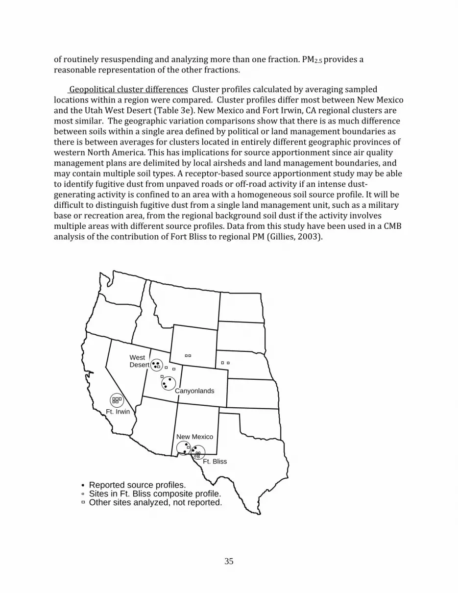
35

of routinely resuspending and analyzing more than one fraction. PM2.5 provides a reasonable representation of the other fractions. 

 Geopolitical cluster differences  Cluster profiles calculated by averaging sampled locations within a region were compared.  Cluster profiles differ most between New Mexico and the Utah West Desert (Table 3e). New Mexico and Fort Irwin, CA regional clusters are most similar.  The geographic variation comparisons show that there is as much difference between soils within a single area defined by political or land management boundaries as there is between averages for clusters located in entirely different geographic provinces of western North America. This has implications for source apportionment since air quality management plans are delimited by local airsheds and land management boundaries, and may contain multiple soil types. A receptor‐based source apportionment study may be able to identify fugitive dust from unpaved roads or off‐road activity if an intense dust‐generating activity is confined to an area with a homogeneous soil source profile. It will be difficult to distinguish fugitive dust from a single land management unit, such as a military base or recreation area, from the regional background soil dust if the activity involves multiple areas with different source profiles. Data from this study have been used in a CMB analysis of the contribution of Fort Bliss to regional PM (Gillies, 2003). 

 

Reported source profiles.Sites in Ft. Bliss composite profile.Other sites analyzed, not reported.

Ft. Irwin

WestDesert

Canyonlands

Ft. Bliss

New Mexico

 

36

Figure 9. Military and civilian sites for CMB source apportionment study. The sites analyzed but not reported were used to study regional versus local variation but chemical composition tables were not included in the journal publication due to space limitations. 

4.4 Enhanced Source Apportionment Feasibility Study

This study tested the feasibility of using pyrolysis‐gas chromatography / mass spectrometry (Py‐GC/MS) to obtain organic chemical species data suitable for source apportionment modeling of soil‐derived PM10 dust on ambient filters. The sources of the field samples are indicated in Figure 10. A laboratory re‐suspension apparatus was used with known soils to generate simulated receptor filter samples loaded with about 0.4 mg of PM10 dust, which is within the range of mass loading on ambient filters. Py‐GC/MS at 740 °C generated five times more resolvable compounds than were obtained with thermal desorption GC/MS (TD‐GC/MS) at 315 °C. The identified compounds were consistent with literature from pyrolysis experiments using larger samples of bulk soils. A subset of 91 organic species out of the 178 identified pyrolysis products was used as input to CMB8 software in a demonstration of source apportionment using laboratory‐generated mixtures simulating ambient filter samples. The 178 quantified organic species obtained by pyrolysis of soil samples is an improvement compared to the 38 organic species obtained by thermal desorption of soils and the four functionally defined organic fractions reported by thermal/optical reflectance. Significant differences in the concentration of specific species were seen between samples from different sites, both geographically distant and close, using analysis of variance (ANOVA) and cluster analysis. This feasibility study showed that Py‐GC/MS can generate useful source profile data for receptor modeling, and justifies continued method development. 

Fugitive dust is a major contributor to ambient particulate matter (PM) in arid climates. Air quality managers would benefit from the ability to distinguish PM soil dust sources from different geographical sites and land uses. This paper shows the feasibility of a pyrolysis gas chromatography mass spectrometry technique to analyze organic compounds from PM soil dust on quartz filters and demonstrates the practical value of these data by using CMB8 source apportionment software to apportion soil mixtures. 

 Pyrolysis of the soil‐derived samples yielded more resolved organic species in the gas chromatogram than were observed in the same samples when analyzed by thermal desorption. Typical chromatograms obtained by using both methods on the same filter sample (UN4) are shown in Figure 3. There were only 38 compounds found by thermal desorption at 315 °C. In contrast, pyrolysis at 740 °C yielded five times more resolved peaks. Table 2 shows the 178 compounds found by pyrolysis in the PO sample and which were previously reported in studies conducted with larger samples of bulk soil. The number of organic species obtained by Py‐GC/MS is much larger than the 2 carbon fractions obtained by current thermal / optical reflectance anaysis.28 

37

The organic composition profiles were determined by analyzing sections representing one‐eighth of a 47 mm diameter filter (217 mm2). These filter wedges have about 0.4 mg of soil dust. This is an order of magnitude reduction in sample size compared to previously published studies of organic material in soils, and indicates that the method has high sensitivity. 

The hypothesis that differences in soil dust organic compounds between sample groups (USDA soil unit plus surface land use) are sufficiently large to be useful for source apportionment modeling was first tested by ANOVA within the three replicates from each sample group and between pairs of sample groups (Figure 11). The composite of all samples from Skull Valley and from Camp Williams had 54 out of 91 compounds showing statistically significant differences (P<0.005) between the two sites and are shown as pair A in Figure 11. The two sample groups exhibiting the least difference, the agricultural and non‐agricultural samples belonging to the same USDA soil unit from the Camp Williams location (pair E in Figure 11), had no compounds with (P<0.005) differences and only 8 compounds with differences at the (P<0.05) level. Two comparisons of sample group pairs from different soil classifications at the Camp Williams location showed significant differences in the organic species. Pair B in Figure 11, both non‐agricultural land use, showed 45 compounds with P< 0.05. Pair C in Figure 11, agricultural and non‐agricultural land use, showed 43 compounds with (P<0.05) differences The agricultural and non‐agricultural sample groups from the same soil classification at the Skull Valley location showed only 13 compounds with (P<0.05) differences. The results of this preliminary feasibility study suggest that differences in soil organic compounds analyzed by pyrolysis are more correlated with USDA soil unit and less correlated with surface land use, but the data set is insufficient for testing this hypothesis.  

 

38

Figure 10. Military and civilian sites at Camp Williams (CW) and Dugway Proving Ground (SV). 

39

A B C D E Site 1 Skull Valley Camp Williams Camp Williams Skull Valley Camp Williams Land use 1 Native and Agriculture Native vegetation Native vegetation Native vegetation Native vegetation Soil unit 1 Timpie loam Parleys loam Parleys loam Timpie loam Red rock loam Sample # 1 RN1,2,3 RA1,2,3 UN1,2,3 UN1,2,3 RN1,2,3 UN4,5,6 Site 2 Camp Williams Camp Williams Camp Williams Skull Valley Camp Williams Land use 2 Native and Agriculture Native vegetation Agricultural Agricultural Agricultural Soil unit 2 Mixed Red rock loam Red rock loam Timpie loam Red rock loam Sample # 2 UN1,2,3,4,5,6 UA1,2,3 UN4,5,6 UA1,2,3 RA1,2,3 UA1,2,3 Distance between sites 1 and 2 50 miles 60 meters 10 meters 150 meters 70 meters

Figure 11 . Fraction of organic species showing a statistical significance greater than indicated P‐value in a pair wise ANOVA. A large fraction indicates a higher probability the two sites compared may be distinguished using organic Py‐GC/MS data. Distant sites (Pair A) showed the greatest number of statistically different species but nearby sites with different soil units also showed statistical difference (Pairs B and C). Adjacent sites with the same soil unit but different land uses (Pairs D and E) showed the fewest organic species with statistically different concentrations.  

40

5. CONCLUSIONS

5.1 Dust Transport

This SERDP‐funded study supported the hypothesis 4 that not all dust initially suspended by vehicles is transported far enough to influence air quality on the scales used for airshed modeling. It also supports the related hypotheses that near‐source redeposition of vehicle generated dust may be sufficient to justify applying a correction to AP‐42 emission factors when compiling regional inventories. However, there is considerable disagreement between field study results.  

Two SERDP‐funded field studies published measurements of the change in dust flux in the first 100 m downwind of an unpaved test road. 17, 32, 33 These studies were at Dugway Proving Ground, Utah and Fort Bliss, Texas, respectively.  Both studies used towers equipped with continuous‐reading light scattering instruments to measure dust concentration and anemometers to measure wind speed. These data were used to calculate the flux of dust perpendicular to the road. Flux through a plane perpendicular to the road was calculated by integrating the product of wind speed and dust concentration from ground level to the top of the dust cloud. The experiment at U.S. Army Dugway Proving Ground, UT 17 reported that approximately 85% of the dust was removed within 100 m when passing under nighttime conditions across an array of shipping containers simulating buildings in an urban setting. In contrast, the experiment at Fort Bliss, TX 32, 33 showed negligible removal of dust under sunny daytime conditions with flat, sparsely vegetated terrain. The major differences between these field studies were the atmospheric stability and the surface roughness. These differing field results motivated further experimental and computational studies to better quantify the magnitude of near‐source deposition as a function of atmospheric stability and surface roughness.  

A computational model for fugitive dust deposition30, 31 was used to reanalyze data from the two published field studies, Dugway and Fort Bliss that compared dust flux adjacent to an unpaved road versus approximately 100 m downwind. This new model considers deposition velocity, effective deposition surface area, the height of the canopy, and wind profile. Model simulation results were compared to field measurements and the effects of alternative site conditions are summarized. Canopy height relative to the initial dust cloud height, the area of surface roughness available for deposition, and the atmospheric stability are predicted to affect the partitioning of the initially suspended dust between transport and near‐source redeposition. This modeling work reconciled the two field studies and supports the hypothesis that the accuracy of emission inventory‐based air quality modeling of fugitive dust can be improved by including an adjustment for near‐source deposition. 

 These fugitive dust transport field studies under a range of atmospheric and terrain conditions provided unique new information that has helped to determine how the competition between dust redeposition and dispersion depends on atmospheric stability and surface roughness elements. The newest air models used by the Western Regional Air Partnership for regional haze planning reflect the current understanding that fugitive dust 

41

was overstated in early models such as the Grand Canyon Visibility Transport Commission study. 

5.2 Source Apportionment

This SERDP‐funded work has contributed to the large and growing body of literature on source apportionment of the particulate matter arriving at a receptor site. The techniques for source apportionment have been evolving since the seminal work by Friedlander in the 1970’s.34 This project investigated several timely topics regarding coarse versus fine soil‐derived dust, effects of land use, and incorporating detailed organic speciation into the chemical composition profiles. 

The PM10, PM2.5 and PM1 profiles indicate that some soils have slight differences between size fractions, albeit not large enough to warrant the extra cost of routinely resuspending and analyzing more than one fraction. PM2.5 provides a reasonable representation of the other fractions. 35 

The geographic variation comparisons showed that there is as much difference between soils within a single area defined by political or land management boundaries as there is between averages for clusters located in entirely different geographic provinces of western North America. 35 This has implications for source apportionment since air quality management plans are delimited by local airsheds and land management boundaries, and may contain multiple soil types. A receptor‐based source apportionment study may be able to identify fugitive dust from unpaved roads or off‐road activity if an intense dust‐generating activity is confined to an area with a homogeneous soil source profile. It will be difficult to distinguish fugitive dust from a single land management unit, such as a military base or recreation area, from the regional background soil dust if the activity involves multiple areas with different source profiles. Data from this study have been used in a CMB analysis of the contribution of Fort Bliss to regional PM. 36 

Given the limitations of current source profiles to distinguish soil dust sources, we investigated enhancing source apportionment technology by using detailed organic chemical composition data. Many soil dusts source profiles are similar in the concentrations of the elements and ions currently used for receptor‐based source apportionment modeling.35, 37  We have now shown the feasibility of increasing the number of chemical species available for source apportionment by using Py‐GC/MS for analysis of organic species in soil‐derived dust samples. The filter loading need for Py‐GC/MS analysis depends on the organic content of the source PM. The quartz filter mass loading used for Py‐GC/MS of soil dust in this study was on the order of 300‐400 µg on a filter slice for each analysis. This sample size is comparable to the mass used for TD‐GC of urban samples by Falkovich, and for Py‐GC of atmospheric aerosol samples by Neususs, but about 20 times the mass used for a source apportionment demonstration of TD‐GC/MS of urban aerosol from sites dominated by vehicle emissions, waste burning and vegetative detritus.  

The scope of this study was to test the feasibility using organic species to do source apportionment modeling of soil‐derived dusts, and the results suggest that further method development and field testing are justified. Even with the small mass of soil dust on the 

42

filter, the pyrolysis method produced similar instrument precision to that obtained using U.S. EPA method 8270 for solvent extraction of semivolatile compounds in solids. Standards provided confirmation for 46 of the 178 tentatively identified peaks, but standard mixtures customized for soil pyrolysis products can be developed. Initial quantification using HP Chemstation software to automatically integrate and calculate ion area count was unsatisfactory because of the complex and crowded chromatogram which necessitated manual integration. Future research can investigate alternative chromatography conditions to achieve optimum peak resolution and specialized data reduction software to deconvolute the spectra. The incorporation of sample pre‐treatment techniques (i.e. derivatization) may also add to the resolved species list.  

The limited field sampling conducted for this feasibility study suggests that for nearby sites the organic composition of the soil‐derived dust varies more with the USDA soil unit and less with the surface land use. This is contrary to soil science work that showed large differences between agricultural and non‐agricultural soil.  Follow up studies are needed to further test this observation. 

Improving air quality management strategies will require accurately quantifying PM sources that are difficult to distinguish with current receptor modeling techniques. Distinguishing soil dusts from different geographic sites and different land uses would allow better regulation of fugitive dust from roads, construction sites, mineral processing operations, and open grazing lands. This study has shown that Py‐GC/MS is a technically feasible approach for generating organic species source profiles for soil‐derived PM, and that statistically significant differences in soil‐derived organic species exist between adjacent soil units and between geographically separated sites. 

5.3 Results Applicable to Military Training Range Environmental Programs

The impact of unpaved road dust on air quality needed to be determined in order to develop implementation plans as required by the PM10 and PM2.5 NAAQS and the regional haze rule. This study indicated that there may be justification to adjust current emission factors when calculating regional impacts of widely distributed unpaved road travel due to subgrid scale processes that result in dust removal within 5‐ 500 m from the source. Atmospheric stability and the downwind terrain irregularities have not been variables in most studies of unpaved road dust. This study suggested that these factors need to be considered in developing possible adjustments to current emission factors. Local impacts of road dust are also significant and this study suggests that walls or buildings may serve as mitigation measures that can reduce the dust exposure to persons living near unpaved roads. This information was provided to technical committees such as the Western Regional Air Partnership Fugitive Dust Forum. The results of this SERDP‐funded work have contributed to new handbooks for fugitive dust control strategies, 38 and air regulatory agencies are accepting modeling results that have used adjusted dust emissions on a regional scale.  

The analytical interpolation equations and the empirical results from the Dugway study 17 can be used to determine the optimum allocation of measurement locations for future 

43

field measurements from roads, off‐road training, aircraft operations, and similar activities. All wind and dust concentration interpolation models showed a decrease in horizontal dust flux, but the absolute magnitude of dust per vehicle trip varied by nearly an order of magnitude between methods. Sources the difference include the assumptions of how the dust concentration varies below the lowest measurement and assumptions about the lower and upper bounds of height used for the integration. This indicates the importance of obtaining measurements near the ground where the dust concentration models predict the highest values and where the logarithmic and power law wind profiles give different results. 

The study of using Pyrolysis combined with Gas Chromatography and Mass Spectrometry for chemical analysis of soil dust samples for source apportionment built upon the previous research by soil scientists that showed that Py‐GC/MS analysis of bulk soil can be used to differentiate between varying soil type and land use sources. The feasibility study 39 showed that this technique as promise and is capable of detecting organic compounds at levels approaching 1 ng on a filter sample. This technique may prove especially useful in cases where a specific organic compound (such as from improper waste disposal) is a potential marker of a suspected fugitive dust source. An example would be in remediation studies of potential Superfund sites on military training ranges.  

With regard to the specific question of whether source apportionment could distinguish fugitive dust from military training range activities from other local and regional dust sources, the short answer is “maybe, but not likely.” This is good news for installation‐level personnel who must deal with air quality regulatory agencies. The “maybe” refers to the fact that this study has shown that soil type (as determined by USDA soil maps) is more important than land use. Therefore, fugitive emissions from training activities are expected to show a unique chemical composition source profile only if the training takes place on a soil type distinct from the surrounding area. The “not likely” comes from the experimental data and qualitative observations that suggest military training activities are not large dust sources on an annual average regional scale. During the course of this study, the investigators became aware of many techniques being used by installation personnel to reduce dust emissions. These techniques include vehicle speed limitations and minimizing land disturbance on easily eroded soil types. As discussed above, atmospheric stability (time of day) and surface roughness (wind breaks, terrain irregularity) affect near‐source dust transport. Consideration of these factors may allow minimizing local‐scale impacts such as dust moving from training ranges onto immediately adjacent civilian areas. 

The past five years have been an active period for fugitive dust research. Many concurrent projects, funded by multiple agencies, have contributed to a greatly improved understanding of fugitive dust emissions and control strategies. The Western Regional Air Partnership Fugitive Dust Handbook 38 is the most up‐to‐date compilation of fugitive dust information applicable to sites in the arid southwest.  

44

6, LITUREATURE CITED

1. CFR National Ambient Air Quality Standard for Particulate Matter, Federal Register, 1997, 62(138), 38652-38760.

2. EPA Final Regional Haze Regulations for Protection of Visibility in National Parks and Wilderness Areas, Federal Register, 1999, 64(126), 35713-35774.

3. Chow, J.C.; Watson, J.G.; Lowenthal, D.H.; Solomon, P.A.; Magliano, K.L.; Ziman, S.D.; Richards, L.W. PM10 source apportionment in California's San Joaquin Valley, Atmos. Environ., 1992, 26A(18), 3335-3354.

4. Watson, J.G.; Chow, J.C., Reconciling Urban Fugitive Dust Emissions Inventory and Ambient Source Concentration Estimates: Summary of Current Knowledge and Needed Research, Desert Research Institute, DRI Document No. 6110.45, 2000.

5. Chow, J.C.; Watson, J.G.; Green, M.C.; Douglas H, L.; DuBois, D.W.; Khol, S.D.; Egami, R.T.; Gillies, J.; Rogers, C.F.; Fraizer, C.A.; Cates, W. Middle- and neighborhood-scale variations of PM10 source contributions in Las Vegas, Nevada, J. Air & Waste Manage. Assoc., 1999, 49, 641-654.

6. Watson, J.G.; Chow, J.C.; Pace, T.G., "Fugitive Dust Emissions," in Air Pollution Engineering Manual, W.T. Davis, Ed. Wiley: New York, 2000 pp. 117-135.

7. Chow, J.C.; Watson, J.G.; Green, M.C.; Lowenthal, D.H.; Bates, B.; Oslund, W.; Torres, G. Cross-border transport and spatial variability of suspended particles in Mexicali and California's Imperial Valley, Atmos. Environ., 2000, 34, 1833-1843.

8. Chow, J.C.; Watson, J.G. Fugitive emissions add to air pollution, Environmental Protection, 1982, (June 1992).

9. Watson, J.G.; Chow, J.C.; Gillies, J.A.; Moosmüller, H.; Rogers, C.F.; D., D.; Derby, J.C., Effectiveness demonstration of fugitive dust control methods for public unpaved roads and unpaved shoulders on paved roads, Desert Research Institute, Reno NV, Report No. 685-5200.1F Prepared for San Joaquin Unified Air Pollution Control District, 1996.

10. Watson, J.G.; Chow, J.C.; Pace, T.G., "Chemical Mass Balance," in Receptor Modeling for Air Quality Management, P.K. Hopke, Ed. Elsevier: New York, 1991 pp. 83-116.

11. Hopke, P.K., ed. Receptor Modeling for Air Quality Management. Data Handling in Science and Technology, Elsevier: New York, 1991.

12. Watson, J.G.; Ashbaugh, L.; Casuccio, G.; Chow, J.C.; Francis, S.; et al, The Fugitive Dust Characterization Study: Potential Methods and Research Needs for Receptor Methods to Distinguish Among Fugitive Dust Sources, Desert Research Institute, 1999.

45

13. Chow, J.C.; Watson, J.G. Review of PM2.5 and PM10 apportionment for fossil fuel combustion and other sources by the chemical mass balance receptor model, Energy Fuels, 2002, 16(2), 222-260.

14. Biltoft, C., Customer Report for Mock Urban Setting Test, Meteorology & Obscurants Division, West Desert Test Center. Defense Threat Reduction Agency, Alexandria, VA, DTC Project No. 8-CO-160-000-052, DPG Document WDTC-FR-01-121, 2001.

15. Yee, E.; Biltoft, C.A. Concentration fluctation measurements in a plume dispersing through a large rectangular array of obstacles, Boundary Layer Meterology, 2002, Submitted.

16. Natural Resources Conservation Service, Soil Survey of Tooele Area, Utah, U.S. Department of Agriculture, 2000.

17. Veranth, J.M.; Seshadri, G.; Pardyjak, E. Vehicle-generated fugitive dust transport: Analytic models and field study, Atmos. Environ., 2003, 37(16), 2295-2303.

18. Seshadri, G., "Fugitive Dust Transport from Unpaved Roads in Arid Climates," Department of Chemical and Fuels Engineering, University of Utah, Salt Lake City, Utah, 2002.

19. Cowherd, C.; Maxwell, C.M.; Nelson, D.W., Quantification of Dust Entrainment from Paved Roadways, U.S. Environmental Protection Agency, EPA-450/3-77-027, 1977.

20. Cowherd, C., "Fugitive Dust Emissions," in Aerosol Measurement, B.P. A., K. Willeke, Eds., Wiley: New York, 2001 pp. 845-858.

21. EPA, AP-42, Chapter 13.2.2 Unpaved Roads, U.S. Environmental Protection Agency, AP-42, Chapter 13.2.2 Unpaved Roads, 1998.

22. EPA, Emission factor documentation for AP-42 Section 13.2.2, unpaved roads, U.S. Environmental Protection Agency, Office of Air Quality Planning and Standards, MRI Project No. 4864, EPA Purchase Order 7D-1554-NALX, 1998.

23. Gillies, J.A.; Watson, J.G.; Rogers, C.F.; Dubois, D.; Chow, J.; Langston, R.; Sweet, J. Long-term efficiencies of dust suppressants to reduce PM10 emissions from unpaved roads, J. Air & Waste Manage. Assoc., 1999, 49, 3-16.

24. Panofsky, H.A.; Dutton, J.A., Atmospheric Turbulence Models and Methods for Engineering Applications, Wiley: New York, 1984.

25. Seinfeld, J.H.; Pandis, S.N., Atmospheric Chemistry and Physics — From Air Pollution to Climate Change, Wiley: New York, 1998.

26. McRae, G.J.; Goodin, W.R.; Seinfeld, J.H. Development of a second-generation mathematical model for urban air pollution 1. Model formulation, Atmos. Environ., 1982, 16, 679-696.

46

27. Chow, J.C.; Watson, J.G.; Houck, J.E.; Pritchett, L.C.; Rogers, C.F.; Frazier, C.A.; Egami, R.T.; Ball, B.M. A Laboratory Resuspension Chamber to Measure Fugitive Dust Size Distributions and Chemical Compositions, Atmos. Environ., 1994, 28(21), 3463-3481.

28. Chow, J.C.; Watson, J.G.; Pritchett, L.C.; Pierson, W.R.; Frazier, C.A.; Purcell, R.G. The DRI Thermal/Optical Reflectance Carbon Analysis System: Description, Evaluation and Application in U.S. Air Quality Studies, Atmos. Environ., 1993, 27A(8), 1185-1201.

29. Watson, J.G.; Robinson, N.F.; Fujita, E.M.; Chow, J.C.; Pace, T.G.; Lewis, C.; Coulter, T., CMB8 - Applications and Validation Protocol for PM2.5 and VOCS, Desert Research Institute, DRI Document No. 1980.2D1, 1998.

30. Veranth, J.M.; Speckart, S.O.; Yin, F.; Etyemezian, V.; Pardyjak, E.R. Near-source deposition of vehicle generated fugitive dust on vegetation and buildings. Part 2: Field measurements and model validation, 2007, In Preparation.

31. Pardyjak, E.R.; Speckart, S.O.; Yin, F.; Veranth, J.M. Near-source deposition of vehicle generated fugitive dust on vegetation and buildings. Part 1: Model development and theory, 2007, In Preparation.

32. Etyemezian, V.; Ahonen, S.; Nikolic, D.; Gillies, J.; Kuhns, H.; Gillette, D.; Veranth, J. Dust deposition and removal in the arid southwestern United States: measurements and model results, J. Air & Waste Manage. Assoc., 2004, 54, 1099-1111.

33. Etyemezian, V.; Gillies, J.; Kuhns, H.; Nikolic, D.; Watson, J.; Veranth, J.; Labban, R.; Seshadri, G.; Gillette, D., Field Testing and Evaluation of Dust Deposition and Removal Mechanisms: Final Report, Western States Air Resources Council (WESTAR), 2003.

34. Friedlander, S.K., Smoke, Dust, and Haze, Fundamentals of Aerosol Behavior, John Wiley & Sons: New York, 1976.

35. Labban, R.; Veranth, J.M.; Chow, J.C.; Englebrecht, J.; Watson, J. Size and geographical variation in PM1, PM2.5, and PM10 source profiles from soils in the western United States, Water Air Soil Pollut., 2004, 157, 13-21.

36. Gillies, J.A.; Abu-Allaban, M.; Huhns, H.; Etyemezian, V.; Durham, C.; Veranth, J.; Labban, R. Assessment of the contribution from Fort Bliss, Texas to regional PM10, Manuscript in preparation, 2003, Pending.

37. Chow, J.C.; Watson, J.G.; Ashbaugh, L.L.; Magliano, K.L. Similarities and differences in PM10 chemical source profiles for geological dust from the San Joaquin Valley, California, Atmos. Environ., 2003, 37, 1317-1340.

38. Western Regional Air Partnership Dust Emissions Forum, ""Fugitive Dust Handbook," in, R. Countess, Editor 2006, Western Regional Air Partnership.

39. Labban, R.; Veranth, J.M.; Watson, J.G.; Chow, J.C. Feasibility of soil dust source apportionment using pyrolysis-gas chromatography analysis of organic compounds on filter samples, J. Air & Waste Manage. Assoc., 2006, 56, 1186-1198.

47

 

48

Appendices

Appendix A. Supporting Data

Excel spreadsheets containing numerical data. 

Filename Contents

SI1190 Dugway dust data.XLS Data for Atmospheric Environment paper

SI1190 Dugway Wind data.xls Data for Atmospheric Environment paper

SI1190 Source Profile Chemical Data.xls Chemical Mass Balance source apportionment composition data.

SI1190 Source Profile statistics.xls Size and geographic variation.

SI1190 Source Profile Summary Table.xls Size and geographic variation.

SI1190 TDGC data .xls Feasibility study of enhanced CMB analysis by organic composition.

SI1190 Enhanced CMB sampling.doc Feasibility study of enhanced CMB analysis by organic composition.

XI.B List of Technical Publications

PDF files of published papers and MS Word files of manuscripts. 

Filename Contents Labban JAWMA 2006.pdf Labban, R., J. M. Veranth, J. G. Watson and J. C. Chow (2006).

“Feasibility of soil dust source apportionment using pyrolysis-gas chromatography analysis of organic compounds on filter samples.” Journal of the Air & Waste Management Association 56: 1186-1198.

Labban WATE 2004.pdf Labban, R.; Veranth, J.M.; Chow, J.C.; Englebrecht, J.; Watson, J.

Size and geographical variation in PM1, PM2.5, and PM10 source profiles from soils in the western United States, Water Air Soil Pollut., 2004, 157, 13-21.

49

VicE JAWMA 2003.pdf Etyemezian, V.; Ahonen, S.; Nikolic, D.; Gillies, J.; Kuhns, H.; Gillette, D.; Veranth, J. Dust deposition and removal in the arid southwestern United States: measurements and model results, J. Air & Waste Manage. Assoc., 2004, 54, 1099-1111.

Veranth AE 2003.pdf Veranth, J.M.; Seshadri, G.; Pardyjak, E. Vehicle-generated

fugitive dust transport: Analytic models and field study, Atmos. Environ., 2003, 37(16), 2295-2303.

Veranth AE.doc Veranth, J.M.; Speckart, S.O.; Yin, F.; Etyemezian, V.; Pardyjak,

E.R. Near-source deposition of vehicle generated fugitive dust on vegetation and buildings. Part 2: Field measurements and model validation, 2007, In Preparation.

XI.2 Internal Technical Reports and Manuscripts in Progress

Filename Contents Perry SXRF.doc Application of Synchrotron X-Ray Fluorescence Analysis

Microscopy to the Study of Atmospheric Aerosols UserResource.doc Text version of material posted to web regarding fugitive dust. www.cc.utah.edu/~jmv2090/1190UserResource.htm WRAP_Synopsis.doc Technical material supplied to the Western Regional Air

Partnership Fugitive Dust Forum as part of the SI-1190 technology transfer.

5XI.3 Conference/Symposium Proceedings

Filename Contents Paper 546.pdf Computational modeling of near-source depositon of fugitive dust

on vegetative surfaces. Presented at the Air and Waste Management Association Meeting 2005.

XI.4 Published Technical Abstracts

Filename Contents Abstract 2002.doc SERDP/ESTCP Conference Abstract 2003.doc SERDP/ESTCP Conference Abstract 2004.doc SERDP/ESTCP Conference