Near-real time retrieval of tropospheric NO2 from OMI

ACPD6, 12301–12345, 2006

Tropospheric NO2from OMI

K. F. Boersma et al.

Title Page

Abstract Introduction

Conclusions References

Tables Figures

J I

J I

Back Close

Full Screen / Esc

Printer-friendly Version

Interactive Discussion

EGU

Atmos. Chem. Phys. Discuss., 6, 12301–12345, 2006www.atmos-chem-phys-discuss.net/6/12301/2006/© Author(s) 2006. This work is licensedunder a Creative Commons License.

AtmosphericChemistry

and PhysicsDiscussions

Near-real time retrieval of troposphericNO2 from OMI

K. F. Boersma1,*, H. J. Eskes1, J. P. Veefkind1, E. J. Brinksma1, R. J. van der A1,M. Sneep1, G. H. J. van den Oord1, P. F. Levelt1, P. Stammes1, J. F. Gleason2, andE. J. Bucsela2

1KNMI, De Bilt, The Netherlands2NASA GSFC, Greenbelt, Maryland, USA*now at: Harvard University, Cambridge, USA

Received: 7 November 2006 – Accepted: 17 November 2006 – Published: 29 November 2006

Correspondence to: K. F. Boersma ([email protected])

12301

http://www.atmos-chem-phys-discuss.net

http://www.atmos-chem-phys-discuss.net/6/12301/2006/acpd-6-12301-2006-print.pdf

http://www.atmos-chem-phys-discuss.net/6/12301/2006/acpd-6-12301-2006-discussion.html

http://www.copernicus.org/EGU/EGU.html

ACPD6, 12301–12345, 2006



Title Page



Tables Figures

J I

J I

Back Close

Full Screen / Esc



EGU

Abstract

We present a new algorithm for the near-real time retrieval – within 3 h of the actualsatellite measurement – of tropospheric NO2 columns from the Ozone Monitoring In-strument (OMI). The retrieval system is based on the combined retrieval-assimilation-modelling approach developed at KNMI for off-line tropospheric NO2 from the GOME5

and SCIAMACHY satellite instruments. We have adapted the off-line system suchthat the required a priori information – profile shapes and stratospheric backgroundNO2 – is now immediately available upon arrival of the OMI NO2 slant columns andcloud data at KNMI. Slant column NO2 and cloud information arrives at KNMI typi-cally within 80 min of actual OMI observations. Slant columns for NO2 are retrieved10

using differential optical absorption spectroscopy (DOAS) in the 405–465 nm range.Cloud fraction and cloud pressure are provided by a new cloud retrieval algorithm thatuses the absorption of the O2–O2 collision complex near 477 nm. On-line availabil-ity of stratospheric slant columns and NO2 profiles is achieved by running the TM4chemistry transport model (CTM) forward in time based on forecast ECMWF meteo15

and assimilated NO2 information from all previously observed orbits. OMI NO2 slantcolumns, after correction for spurious across-track variability, show a random error forindividual pixels of approximately 0.7×1015 molec.cm−2. As NO2 retrievals are verysensitive to clouds, we evaluated the consistency of cloud fraction and cloud pressurefrom the new O2–O2 (OMI) algorithm and from the Fast Retrieval Scheme for Cloud Ob-20

servables (FRESCO). Cloud parameters from the O2–O2 (OMI) algorithm have similarfrequency distributions as cloud parameters retrieved from FRESCO (SCIAMACHY)for August 2006. On average, OMI cloud fractions are higher by 0.011, and OMI cloudpressures exceed FRESCO cloud pressures by 60 hPa. As a consistency check, weintercompared OMI near-real time NO2 columns measured at 13:45 h local time to25

SCIAMACHY off-line NO2 columns measured at 10:00 h local time. In August 2006,both instruments observe very similar spatial patterns of tropospheric NO2 columns,and small differences for most locations on Earth where tropospheric NO2 columns

12302





ACPD6, 12301–12345, 2006



Title Page



Tables Figures

J I

J I

Back Close

Full Screen / Esc



EGU

are small. For regions that are strongly polluted, SCIAMACHY observes higher tropo-spheric NO2 columns than OMI.

1 Introduction

The daily global coverage and the pixel size of 24×13 km2 make the Ozone MonitoringInstrument (OMI) on the Earth Observing System (EOS) Aura satellite well suited to5

observe the sources of air pollution with an unprecedented spatial and temporal cov-erage. Recently, satellite-based observations of tropospheric NO2 have been provenuseful in estimating anthropogenic emissions of nitrogen oxides (Leue et al., 2001;Martin et al., 2003, 2006; Beirle et al., 2003; Richter et al., 2005; van der A et al.,2006), in observing emissions by soils (Jaegle et al., 2004), and in putting constraints10

on NOx production by lightning (Beirle et al., 2004, 2005; Boersma et al., 2005). Tropo-spheric NO2 columns derived from the Global Ozone Monitoring Experiment (GOME)have been compared with outputs from various-scale models (Velders et al., 2001;Lauer et al., 2002; Savage et al., 2004; Ma et al., 2006). The results of the regional-scale chemistry-transport model CHIMERE have been evaluated against GOME and15

SCIAMACHY-derived tropospheric NO2 columns (Konovalov et al., 2004; Blond et al.,20061). These comparisons have clearly demonstrated the potential of satellite NO2data sets for model evaluation and emission estimates. On the other hand, sometimeslarge and often systematic differences persist between retrievals by different groups(van Noije et al., 2006), calling into question the quality of space-based constraints on20

NOx sources. However, validation efforts for various retrievals show acceptable accu-racy (Heland et al., 2002; Petritoli et al., 2004; Martin et al., 2004, 2006; Cede et al.,2006; Ordonez et al., 2006; Schaub et al., 2006) for GOME and SCIAMACHY NO2.

1Blond, N., Boersma, K. F., Eskes, H. J., van der A, R., Van Roozendael, J. M., De Smedt,I., Bergametti, G., and Vautard, R.: Intercomparison of SCIAMACHY nitrogen dioxide observa-tions, in-situ measurements and air quality modeling results over Western Europe, submitted,J. Geophys. Res., 2006.

12303





ACPD6, 12301–12345, 2006



Title Page



Tables Figures

J I

J I

Back Close

Full Screen / Esc



EGU

The unique characteristics of OMI -the small pixel size and daily global coverage– al-low for an important contribution to air quality monitoring and modelling. GOME hasa resolution of 320×40 km2, too coarse to resolve the areas with high emissions thatare relevant in regional air quality modelling, e.g. medium-sized cities. SCIAMACHY’shorizontal resolution is 60×30 km2 but needs six days to achieve global coverage. De-5

spite the fact that interesting regional-scale daily variability has been observed withSCIAMACHY by Blond et al. (2006)1, it is not well suited for a day-to-day monitoring ofair quality. The daily coverage of OMI has been an important motivation to set up thenear-real time NO2 retrieval system described in this paper. An additional motivationoriginates from the data set of tropospheric NO2 columns retrieved from the GOME10

and SCIAMACHY instruments that now spans more than 10 years (1996–2006) and ispublicly available through http://www.temis.nl. NO2 data sets from GOME and SCIA-MACHY have been retrieved with one and the same retrieval-assimilation-modellingapproach described in Boersma et al. (2004) and show excellent mutual consistency(van der A et al., 2006). The OMI NO2-retrievals described here are expected to add15

considerable value to the GOME and SCIAMACHY dataset. Health regulations con-cerning air quality require a routine monitoring, typically on an hourly basis, of surfaceconcentrations of several species including NO2. Clearly, this requirement cannot bedirectly fulfilled by satellite instruments in general, nor by OMI in particular. Never-theless we anticipate that instruments like OMI will make essential contributions to air20

quality monitoring and modelling:

– Daily maps of NO2 columns provided by OMI show extensive transport featuresthat are changing from day to day, and that are politically interesting as theydirectly show air pollution being transported across national borders. Thesechangeable distributions can be directly compared with model output, and they25

constitute strong tests for the description of horizontal and vertical transport pro-cesses, as well as NOx removal processes.

– A direct relationship exists between columns of NO2 and surface emissions of

12304





http://www.temis.nl

ACPD6, 12301–12345, 2006



Title Page



Tables Figures

J I

J I

Back Close

Full Screen / Esc



EGU

NOx. OMI data can thus be combined with regional-scale models through in-verse modeling or data assimilation to adjust or improve emission estimates inthe model and to detect unknown sources.

– Incidental releases, such as from major fires, can be monitored and quantified,and subsequent plumes can be tracked from day to day.5

– A routine assimilation of satellite data may improve air quality “nowcasting” andforecasting capabilities, and may thereby contribute to the monitoring of emissionand health regulations.

All these applications are new and largely untested. Despite this, there exists aconsiderable interest in the community to establish atmospheric chemistry data as-10

similation systems that will exploit the available satellite data sets of atmosphericcomposition and air pollution. One example is the European GEMS project (Globaland regional Earth-system (Atmosphere) Monitoring using Satellite and in-situ data;(http://www.ecmwf.int/research/EU/projects/GEMS/) which is scheduled to deliver anoperational atmospheric composition assimilation system by 2009.15

This paper presents a new retrieval algorithm designed for near-real time retrievalof tropospheric NO2 from OMI. This algorithm differs from the standard, off-line OMINO2 retrieval-procedure that is a joint NASA/KNMI effort and has been described byBucsela et al. (2006). The differences are shortly discussed in Sect. 3.1. In Sect. 2we shortly discuss Ozone Monitoring Instrument characteristics, and describe the fast20

transport of measurement data from the satellite to the computer system where theretrievals take place. The retrieval itself is discussed in Sect. 3, with a focus on theinnovations with respect to previous NO2 column retrieval work at KNMI. Section 4is devoted to errors in the NO2 slant columns that occur through calibration errors incurrent the level 1 data, and through the propagation of measurement noise in the25

spectral fitting. The stratospheric correction and computation of the air mass factor(AMF) are described in Sect. 5. As SCIAMACHY and OMI cloud retrieval use differentspectral features, we also discuss in Sect. 5 the consistency of the OMI O2−O2 cloud

12305





http://www.ecmwf.int/research/EU/projects/GEMS/

ACPD6, 12301–12345, 2006



Title Page



Tables Figures

J I

J I

Back Close

Full Screen / Esc



EGU

product with the SCIAMACHY FRESCO cloud retrievals. As a first order quality-checkof OMI near-real time NO2 retrievals, in Sect. 6 we compare SCIAMACHY and OMItropospheric NO2 columns for the month August 2006 and show some examples ofOMI’s capabilities. This is followed by conclusions in Sect. 7.

2 OMI overview5

2.1 Ozone Monitoring Instrument

The Dutch-Finnish Ozone Monitoring Instrument (OMI) on NASA’s EOS Aura satellite isa nadir-viewing imaging spectrograph measuring direct and atmosphere-backscatteredsunlight in the ultraviolet-visible (UV-VIS) range from 270 nm to 500 nm (Levelt et al.,2006a). EOS Aura was launched on 15 July 2004 and traces a Sun-synchronous, po-10

lar orbit at approximately 705 km altitude with a period of 100 min and a local equatorcrossing time between 13.40 h and 13.50 h. In contrast to its predecessors GOMEand SCIAMACHY, instruments operating with scanning mirrors and one-dimensionalphoto diode array detectors, OMI has been equipped with two two-dimensional CCDdetectors. The CCDs record the complete 270–500 nm spectrum in one direction, and15

observe the Earth’s atmosphere with a 114◦ field of view, distributed over 60 discreteviewing angles, perpendicular to the flight direction. OMI’s wide field of view corre-sponds to a 2600 km wide spatial swath on the Earth’s surface for one orbit, largeenough to achieve complete global coverage in one day. The exposure time of theCCD-camera measures 2 s, corresponding to a spatial sampling of 13 km along track20

(2 s × 6.5 km/s, the latter being the orbital velocity projected onto the Earth’s surface).Across track the size of an OMI pixel varies with viewing zenith angle from 24 km in thenadir to approximately 60 km for the extreme viewing angles of 57◦ at the edges of theswath. OMI has three spectral channels; UV1 (270–310 nm) and UV2 (310–365 nm)are covered by CCD1. CCD2 covers the VIS-channel from 365–500 nm with a spectral25

sampling of 0.21 nm and a spectral resolution of 0.63 nm. It is in this channel that the

12306





ACPD6, 12301–12345, 2006



Title Page



Tables Figures

J I

J I

Back Close

Full Screen / Esc



EGU

spectral features of NO2 are most prominent. The spectral resolution and samplingof OMI have been designed to resolve trace gas absorption signatures of chemicallyimportant atmospheric species. The spectral sampling rate (resolution/sampling) is∼3, large enough to avoid spectral undersampling or aliasing difficulties in the spec-tral fitting process. A polarization scrambler makes the instrument insensitive to the5

polarization state of the reflected Earth radiance to less than 0.5%. During nominaloperations OMI takes one measurement of the solar irradiance per day. Radiometriccalibration is accomplished in-flight by a series of special on-board measurements thatinvolve a.o. monitoring detector degradation with a white-light source, and dark sig-nal measurements when OMI is at the dark side of the Earth. Spectral calibration is10

achieved by a cross-correlation of Fraunhofer lines in theoretical and observed in-flightirradiance spectra. For more details on the instrument and calibration procedures, thereader is referred to Dobber et al. (2005, 2006).

Retrievals of ozone column and vertical distribution (as well as BrO and OClO) aremeant to address the first EOS Aura science question whether the ozone layer is recov-15

ering. Of no less importance are the retrievals of trace gases related to air pollution andthe production of photochemical smog, i.e. NO2, HCHO, and SO2. In addition, cloudand aerosol parameters, and UV-B surface flux are derived from OMI. For an overviewof EOS-AURA and OMI targets, see Levelt et al. (2006b). In this paper we focus on thefast delivery of OMI NO2 data relevant for the purposes of air quality monitoring and20

forecasting.

2.2 Data transport

OMI science data is stored on-board on a solid-state recorder. These unprocesseddata are down-linked once every orbit (100 min) to one of the Polar Ground Stations inAlaska or Svalsbard (Spitsbergen) or to the Wallops Ground Station in Virginia (USA).25

As soon as a spacecraft contact session has finished, the OMI data are sent to theEOS Data Operations System (EDOS) at NASA GSFC in Maryland (USA). At GSFC,the raw OMI data are processed in three different ways, resulting in Rate-Buffered

12307





ACPD6, 12301–12345, 2006



Title Page



Tables Figures

J I

J I

Back Close

Full Screen / Esc



EGU

Data, Expedited Data, and Production Data. Near-real time processing is based onRate-Buffered Data (RBD). RBD data are made available with the highest priority, atthe expense of data integrity. The other data types are scheduled for off-line level 2retrievals.

EDOS subsequently forwards the RBD data to the OMI Science Investigator-led Pro-5

cessing System (SIPS), where production starts as soon as all engineering, ancillaryand science data have been received. A preprocessor run improves data integrity, re-moves duplicate packages, and time-orders the data. Then, the resulting level 0 datasets (in Analog to Digital Units) are processed into level 1b data, i.e. estimated radi-ances and irradiances in units of W/m2/nm(/sr) (van den Oord et al., 2006). The only10

difference with standard production at this time is that the near-real time processinguses the predicted altitude and ephemeris data received from the spacecraft ratherthan definitive altitude and ephemeris data. Using predicted orbital parameters maylead to errors in geolocation parameters (latitude, longitude, solar, viewing, and az-imuth angles) that influence the retrievals, but in practice, these errors are small. Once15

OMI level 1b data has been generated at the SIPS, the O2−O2 cloud level 1–2 algo-rithm (Acarreta et al., 2004) is run, followed by the DOAS ozone (Veefkind and DeHaan, 2002) and NO2 slant column spectral fitting retrieval algorithms. As soon asthe ozone and NO2 slant column files are available, they are picked up by the OMIDutch Processing system (ODPS) and forwarded to the processing system at KNMI20

developed within the DOMINO project (see acknowledgment). Subsequent steps areintrinsic parts of the DOMINO retrieval algorithm and are described in the next section.

Typical data volumes per orbit are 450 MB level 0 data, 400 MB level 1b data, and17 MB NO2 slant column data (including cloud retrievals). Processed orbital data ar-rives at KNMI on average within three hours after the start of an orbit. An orbit takes25

100 min (indicated as the red part of Fig. 1) and the process described above (downlink,transfer to EDOS, transfer to SIPS, level 1b and 2 processing, and transfer to KNMI)takes 80 min (the orange part in Fig. 1). Final processing from NO2 slant columns totropospheric vertical columns at KNMI is typically faster than 2 min on a linux worksta-

12308





ACPD6, 12301–12345, 2006



Title Page



Tables Figures

J I

J I

Back Close

Full Screen / Esc



EGU

tion. Including the generation of images and web publishing, the processing step takesless than 45 min (the green part of Fig. 1), so that data and images are available forthe public at approximately 16:00 h local time.

3 Algorithm description

3.1 Heritage: the retrieval-assimilation-modelling approach5

The near-real time NO2 retrieval algorithm (DOMINO version: TM4NO2A-OMI v0.8,February 2006) in this work is based on the retrieval-assimilation-modelling approach(hereafter: RAM) described in Boersma et al. (2004). The first DOAS slant col-umn fitting part is identical to the standard, off-line OMI NO2 product discussed byBucsela et al. (2006). The RAM-approach has been applied at KNMI to generate a tro-10

pospheric NO2 data base from GOME and SCIAMACHY measurements. The off-lineRAM approach consists of a three-step procedure:

1. a slant column density is determined from a spectral fit to the Earth reflectancespectrum with the so-called DOAS approach (differential absorption spectroscopy,e.g. Platt, 1994; Boersma et al., 2002; Bucsela et al., 2006),15

2. the stratospheric contribution to the slant column is estimated from assimilatingslant columns into a CTM including stratospheric chemistry and wind fields, and

3. the residual tropospheric slant column is converted into a vertical column by ap-plication of a tropospheric air mass factor (AMF).

The standard, off-line NO2 product and the near-real time retrieval have step 1 in20

common. This step is discussed in detail in Sects. 3.2 and 3.3. Step 2 and 3 aredifferent between the OMI off-line and NRT algorithms, for details the reader is referredto Bucsela et al. (2006); Boersma et al. (2004) and this work.

12309





ACPD6, 12301–12345, 2006



Title Page



Tables Figures

J I

J I

Back Close

Full Screen / Esc



EGU

Until now, a large NO2 data set has been generated with the RAM-approach for theGOME and SCIAMACHY instruments. The data sets cover the period April 1996–June2003 for GOME and from January 2003 onwards for SCIAMACHY. The two data setscontain tropospheric NO2 columns along with error estimates and averaging kernels(Eskes and Boersma, 2003) for every individual pixel and they are publicly available5

through http://www.temis.nl. NO2 retrieved from GOME with the RAM approach hasbeen used to estimate the production of NOx by lightning in the tropics (Boersma et al.,2005). Furthermore, Schaub et al. (2006) showed that GOME tropospheric NO2 overNorthern Switzerland in the period 1996–2003 compares favourably to NO2 profiles ob-served with in-situ techniques. Blond et al. (2006)1 reported considerable consistency10

between SCIAMACHY tropospheric NO2 columns and both surface observations aswell as simulations from the regional air-quality model CHIMERE over Europe, espe-cially over moderately polluted rural areas. Merged GOME and SCIAMACHY obser-vations showed a distinct increase in NO2 columns from 1996 to 2003 over China,consistent with a strong growth of NOx emissions in that area (van der A et al., 2006).15

Moreover, this paper showed an almost seamless continuity from GOME to SCIA-MACHY NO2 values retrieved with the same RAM-approach. This finding providesconfidence in the consistency of the two data sets and their retrieval method, eventhough they originated from two different satellite instruments (with similar overpasstimes of 10:30 h (GOME) and 10:00 h (SCIAMACHY)).20

Tropospheric NO2 columns are generally retrieved as follows:

Vtr =S − Sst

Mtr (xa,tr,b), (1)

with S the slant column density from step 1, Sst the stratospheric slant column ob-tained from step 2, and Mtr the tropospheric AMF that depends on the a priori NO2profile xa,tr and the set of forward model paramaters b including cloud fraction, cloud25

pressure, surface albedo, and viewing geometry.For the RAM-approach as well as the NRT-retrieval described here, AMFs and av-

eraging kernels are computed with a pseudo-spherical version of the DAK radiative12310





http://www.temis.nl

ACPD6, 12301–12345, 2006



Title Page



Tables Figures

J I

J I

Back Close

Full Screen / Esc



EGU

transfer model (Stammes, 2001). Given the best estimate of the forward model param-eters the DAK forward model describes the scattering and absorbing processes thatdefine the average optical path of photons from the Sun through the atmosphere to theOMI.

Also similar as in our RAM-approach for off-line retrievals, we obtain here the a priori5

NO2 profile shapes (xa,tr) from the global chemistry-transport model TM4 at a reso-lution of 2◦ latitude by 3◦ longitude and 35 vertical levels extending up to 0.38 hPa.Given the very few available in situ NO2 measurements, a global 3-D model of tropo-spheric chemistry is the best source of information for the vertical distribution of NO2 atthe time and location of the OMI measurement. The TM4 model is driven by forecast10

and analysed six hourly meteorological fields from the European Centre for MediumRange Weather Forecast (ECMWF) operational data. These fields include global dis-tributions for horizontal wind, surface pressure, temperature, humidity, liquid and icewater content, cloud cover and precipitation. A mass conserving preprocessing of themeteorological input is applied according to Bregman et al. (2003). Key processes15

included are mass conserved tracer advection, convective tracer transport, boundarylayer diffusion, photolysis, dry and wet deposition as well as tropospheric chemistryincluding non-methane hydrocarbons to account for chemical loss by reaction with OH(Houweling et al., 1998). In TM4, anthropogenic and natural emissions of NOx arebased on results from the EU POET-project (Precursors of Ozone and their Effects on20

the Troposphere) for the year 1997 (Olivier et al., 2003). Including free troposphericemissions from air traffic (0.8 Tg N/yr) and lightning (5 Tg N/yr), total NOx emissionsfor 1997 amount to 46 Tg N/yr.

As in the RAM-approach for GOME and SCIAMACHY retrievals, cloud fraction andcloud pressure are determined from the actual satellite measurements. Because OMI25

does not detect the O2 A band at 760 nm, we use cloud parameters retrieved from theVIS-channel using the O2−O2 absorption feature at 477 nm (Acarreta et al., 2004). Thecloud retrieval is based on the same set of assumptions (i.e. clouds are modelled asLambertian reflectors with albedo 0.8) as the FRESCO-algorithm (Koelemeijer et al.,

12311





ACPD6, 12301–12345, 2006



Title Page



Tables Figures

J I

J I

Back Close

Full Screen / Esc



EGU

2001). Before launch, the precision of the O2−O2 cloud fraction and cloud pressurewas discussed in Acarreta et al. (2004) with encouraging results. In Sect. 5.2.1 we testthe accuracy of the O2−O2 cloud parameters by comparing them to FRESCO cloudparameters retrieved by SCIAMACHY on the same days and same locations.

As for GOME and SCIAMACHY retrievals, we use a surface albedo database de-5

rived from TOMS and GOME Lambert-equivalent reflectivity (LER) measurements at380 nm and 440 nm as described in Boersma et al. (2004). These monthly averagesurface albedo maps have a spatial resolution of 1◦×1.25◦ and represent climatologi-cal (monthly) mean situations. The uncertainty in the surface albedo is estimated to beapproximately 0.01 (Koelemeijer et al., 2003; Boersma et al., 2004).10

In summary, the near-real time algorithm is based on the RAM-approach used forGOME and SCIAMACHY retrievals at KNMI. The main differences with RAM are: (1)near-real time requirement, (2) different spectral fitting method, and (3) cloud inputsderived from (similar but) different algorithms. The near-real time algorithm differs fromthe off-line standard NASA/KNMI NO2 algorithm in the method to estimate the strato-15

spheric NO2 content, in the choice of radiative transfer model, and in the a priori NO2profiles and different surface albedo data sets for AMF computations

3.2 Near-real time retrieval

The most important difference between the RAM-approach and the NRT-retrieval isrelated to the required near-real time delivery of the retrieval product. In the RAM-20

approach, the estimated stratospheric NO2 column (step 2) and the modelled profileshape (required for step 3), are provided by off-line assimilation and modelling basedon analysed ECMWF meteorological data. In contrast, for the NRT-retrieval, the as-similation and modelling steps are operational, based on daily ECMWF meteorologicalanalyses and forecasts.25

The NRT-retrieval consists of two distinct subsystems. The first is the TM forecastsubsystem shown in Fig. 2. This forecast system is run once per day, as soon meteo-rological data becomes available. The second subsystem is activated each and every

12312





ACPD6, 12301–12345, 2006



Title Page



Tables Figures

J I

J I

Back Close

Full Screen / Esc



EGU

time that new OMI data becomes available, and incorporates the model informationprovided by subsystem 1.

In the forecast subsystem (1), the actual chemical state of the atmosphere is basedon the analysis and forecast run starting from the analysis of the previous day. Theupdate consists of running the chemistry-transport model forward in time with the fore-5

cast ECMWF meteorological data and the assimilation of all available OMI NO2 slantcolumns measurements. The updated analysis, the new actual state, is then stored asinput for a subsequent time step. The outputs are the necessary inputs to the near-real time subsystem (2); the stratospheric NO2 column and the NO2 and temperatureprofiles (needed in AMF computations).10

The NRT-subsystem is illustrated in Fig. 2. As soon as an orbit of observed NO2slant columns arrives at KNMI, the forecast TM stratospheric slant column, preparedby the TM forecast subsystem, is ready and is subtracted. Subsequently, the residualtropospheric slant column is converted into a vertical column by the tropospheric AMF.The AMF is computed as described as in Sect. 3.1. The averaging kernel is also15

calculated for output and furthermore serves as the observation operator required inthe assimilation part of the TM forecast subsystem.

3.3 Slant column retrieval

A second difference between the OMI near-real time and SCIAMACHY off-line imple-mentation is the wide spectral window that is used in the DOAS retrieval. For GOME20

and SCIAMACHY, it has been conventional wisdom that a 425–450 nm window yieldsthe most precise and stable fitting results. For OMI a much wider fit window, 405–465 nm, has been proposed by Boersma et al. (2002) in order to compensate for OMI’slower signal-to-noise ratio (approximately 1400 under normal mid-latitude conditions)compared to GOME and SCIAMACHY (approximately 2000, Bovensmann et al., 1999)25

in this wavelength region. Pre-flight testing showed that a least squares fitting of refer-ence spectra from NO2, O3, a theoretical Ring function, and a 3rd order polynomial tothe reflectance spectrum yields results that are stable for multiple viewing geometries

12313





ACPD6, 12301–12345, 2006



Title Page



Tables Figures

J I

J I

Back Close

Full Screen / Esc



EGU

with a better than 10% NO2 slant column precision (Boersma et al., 2002). The NO2absorption cross section spectrum is taken from Vandaele et al. (1998), who tabulatedthe cross section at different temperatures. To account for the temperature sensitiv-ity of the NO2 cross section spectrum – determined from the data by Vandaele et al.(1998) – an effective atmospheric temperature is calculated for the NO2 along the av-5

erage photon path. Subsequently an a posteriori correction for the difference betweenthe computed effective temperature and the 220 K cross section spectrum used inthe fitting procedure is applied (Boersma et al., 2002). The ozone absorption crosssection spectrum is taken from WMO (1975) and the theoretical Ring spectrum fromDe Haan (personal communication, 2006) based on irradiance data by Voors et al.10

(2006). All reference spectra have been convolved with the OMI instrument transferfunction (Dobber et al., 2005). OMI NO2 slant column retrieval with synthetic and flightmodel data (Dobber et al., 2005) yields results that fulfill the OMI science requirementof better than 10% slant column precision (Boersma et al., 2002; Bucsela et al., 2006).However, upon first inspection of actual flight-data, systematic enhancements in the15

OMI NO2 slant columns show up at specific satellite viewing angles. This across-trackvariability is has also been reported by Kurosu et al. (2005) for HCHO-retrievals. Be-low we discuss a procedure to reduce across-track variability and investigate the errorbudget of the OMI NO2 slant columns.

4 Slant column density errors20

4.1 Across-track variability

Calibration errors in the level 1b OMI irradiance measurements used here are likely re-sponsible for across-track variability observed in the NO2 slant columns. This variabilitywill likely be significantly reduced in future level 1b releases with improved calibrationdata (expected in Spring 2007), using daily dark current corrections. Across-track vari-25

ability appears as constant offsets for specific satellite viewing angles along an orbit,

12314





ACPD6, 12301–12345, 2006



Title Page



Tables Figures

J I

J I

Back Close

Full Screen / Esc



EGU

allowing for an a posteriori correction that consists of four steps:

1. Determine the orbital segment (50 along track by 60 across track pixels in size)with the minimum variance in NO2 columns.

2. Within this window, average the 50 NO2 columns with the same viewing angle.This gives 60 average across-track NO2 columns.5

3. Separate low and high frequencies of the across-track columns with a Fourieranalysis.

4. Perform the correction by subtracting the (high-frequency) across-track variabilityfor all across-track rows along the orbit.

In this scheme, the selection of the minimum variance window avoids areas with10

large anthropogenic emissions. The high-frequencies are then interpreted as theacross-track variability due to calibration errors in the OMI level 1b data. Similarly,the low frequencies describe any (weak, stratospheric) natural variability. The low fre-quencies are described by the first three Fourier terms. Subsequently we subtract thehigh-frequency signal obtained for the minimum variance window for all rows along the15

orbit. If it turns out to be not possible to determine a correction for a particular orbit,the across-track variability correction from the previous orbit is taken.

Figure 4 shows corrections for across-track variability computed from 10 consecu-tive orbits measured on the same day (22 September 2004). Although the correctionshave been computed from independent data, they are remarkably similar. This justifies20

taking the correction determined from the previous orbit if for some reason a correc-tion cannot be determined from the actual orbit. Furthermore, Fig. 4 provides furtherevidence that irradiance data are most likely at the basis of the across-track variability.All orbits shown have been retrieved with the same irradiance measurement. How-ever, when the correction was plotted for the first orbit retrieved with a new irradiance25

measurement, a distinctly different correction pattern was seen (not shown).

12315





ACPD6, 12301–12345, 2006



Title Page



Tables Figures

J I

J I

Back Close

Full Screen / Esc



EGU

4.2 Slant column precision

In this section we estimate the DOAS fitting error of individual NO2 slant columns.We do so by a statistical analysis of OMI NO2 columns observed over separate 2◦×2◦

boxes in the meridional band between 178◦ and 180◦ W. The basic assumption is thatthe OMI pixels within a 2◦×2◦ box observe the same total vertical column over this5

clean part of the Pacific Ocean. Any variability in the observed total vertical columns isassumed to originate from errors in the slant columns if the ensemble of AMFs within abox has little variability. Boxes with appreciable AMF variability were rejected if the box-mean vertical column computed by averaging the ensemble of individual slant columnsratioed by a box-mean AMF (V ′) differed by more than 0.1% with the box-mean vertical10

column computed by averaging the ensemble of individual slant columns ratioed bythe original AMFs (V ). We find that for most of the 2◦×2◦ boxes, V and V ′indeed donot differ by more than 0.1%, and thus the slant columns have been observed underalmost identical viewing geometries. For these boxes, we take the standard deviationof the ensemble of slant-column as a reasonable estimate for the precision of the slant15

columns.For 7 August 2006, we computed estimates for the slant column errors for every

box between 60◦ S and 60◦ N. The results are shown in Fig. 5a for boxes with a rel-ative difference between V and V ′ of less than 0.1%. The figure shows that there isno appreciable change of fitting error with latitude. Averaged over all latitudes, the20

fitting error is close to 0.75×1015 molec.cm−2 (dashed line). For the vertical columnerror, the contribution from the fitting error is smaller than 0.4×1015 molec.cm−2 (solidline, computed as σN /Mtr ). We also made a distribution of all member deviations frombox means and collected these deviations in a histogram (n=2893). This is shown inFig. 5b. The distribution closely follows a Gaussian shape that is fitted to the histogram25

data. The fact that the distribution follows a Gaussian distribution is consistent withour assumption that the variability within each box is dominated by random errors inthe slant columns, originating from measurement noise. The corresponding width of

12316





ACPD6, 12301–12345, 2006



Title Page



Tables Figures

J I

J I

Back Close

Full Screen / Esc



EGU

the Gaussian for this day is 0.67×1015 molec.cm−2, and we interpret this as a rea-sonable estimate for the average slant column error of all 2893 pixels we investigatedon 7 August 2006. We also looked into a few other days and other longitude bandswith different across-track variability corrections, and found very similar numbers. Theslant column error for an individual OMI pixel is somewhat larger than the better-than-5

10% (≈0.3×1015 molec.cm−2) number quoted in Boersma et al. (2002). This numberwas computed from synthetic spectra (i.e. without across-track variability) under theassumption that 4 OMI pixels would be binned (increasing signal-to-noise by a factor of2). For individual pixels, the OMI fitting error is larger than the 0.45×1015 molec.cm−2

found for GOME (Boersma et al., 2004) and SCIAMACHY (I. DeSmedt, personal com-10

munication), consistent with the higher signal-to-noise ratios for individual GOME andSCIAMACHY pixels than for OMI pixels.

5 Stratospheric contribution and tropospheric air mass factor

5.1 Stratospheric slant column

In order to determine the tropospheric NO2 column accurately, the stratospheric com-15

ponent of the slant column density needs to be predicted. We attain this by data-assimilation of OMI slant columns in TM4:

– Modelled NO2 profiles are convolved with the appropriate averaging kernel togive model-predicted slant column densities. The differences between observedand modelled columns (the model innovations) are used to force the modelled20

columns to generate an analysed state that is based on the modelled NO2 distri-bution and the OMI observations.

– The forcing depends on weights (from observation representativeness and modelerrors) attributed to model and observation columns. Observed columns are at-tributed a low weight in regions and times with large tropospheric model columns.25

12317





ACPD6, 12301–12345, 2006



Title Page



Tables Figures

J I

J I

Back Close

Full Screen / Esc



EGU

This reflects the uncertainty in the averaging kernel, and minimizes the influenceof slant columns with an estimated large tropospheric contribution.

– The forcing equation (based on the Kalman filter technique) is solved with the sta-tistical interpolation method. This involves a covariance matrix that describes theforecast error and spatial correlations. The most important characteristics of this5

forecast covariance matrix are: (1) the conservation of modelled profile shapes.The altitude dependence of the forecast error is set to be proportional to the localNO2 profile shape. (2) The horizontal correlation model function is assumed tofollow a Gaussian shape with a 1/e correlation length of 600 km. This length wasderived from the assimilation of ozone in the stratosphere (Eskes et al., 2003)10

and should be a reasonable guess for stratospheric NO2 as well. (3) In additionwe introduce a correlation scaling to reduce the correlation with increasing differ-ences in concentration (Riishøjgaard, 1998). This avoids problems with negativeconcentrations near sharp gradients that occur for instance at the polar vortexedge. (4) The vertical distribution of the assimilation increments is determined15

by the covariance matrix and the averaging kernel profile. The kernel peaks inmost cases in the stratosphere, which is an additional reason why the adjustmentcaused by the assimilation is mainly taking place in the stratosphere.

– The adjustments made by the assimilation are therefore mainly occurring in thestratosphere at places where the tropospheric concentrations are low. The strato-20

spheric information inserted by the assimilation is transported to the stratosphereabove more polluted areas by the advection in the model.

– The model NOx species (NO, NO2, NO3, N2O5, HNO4) are assumed to be fullycorrelated and are all scaled in the same way as NO2.

– Based on the most recent analysed state, a forecast run of the model predicts the25

stratospheric field. This is used by the near-real time retrieval branch as shown inFig. 2.

12318





ACPD6, 12301–12345, 2006



Title Page



Tables Figures

J I

J I

Back Close

Full Screen / Esc



EGU

For further reading on the assimilation method we refer to Eskes et al. (2003). Theadvantage of the approach is that slant column variations due to stratospheric dynam-ics are now accounted for in the retrieval. The purpose is to improve the detectionlimit for tropospheric NO2 columns that can be retrieved. An additional advantage isthat the assimilation scheme provides a statistical estimate of the uncertainty in the5

stratospheric slant column. Generally, this statistical estimate is on the order of 0.1–0.2×1015 molec.cm−2, much smaller than the slant column uncertainty reported on inthe previous section. Hence, the detection limit in our method is mainly determinedby the random slant column error (σS ) that is easily averaged out by taking large num-bers of observations. Not accounting for stratospheric dynamics however, would lead10

to systematic errors in the estimate of the stratospheric column (Boersma et al., 2004)that cannot be easily averaged out and would raise the detection treshold.

5.2 Tropospheric air mass factor

We convert the tropospheric slant column into a vertical column by using a troposphericAMF (Eq. 1). For OMI NRT we follow as much as possible the same approach (same15

look-up tables, computational methods) as for the GOME and SCIAMACHY data setdescribed in Sect. 3.1. But the forward model input parameters cloud fraction andcloud pressure differ between the OMI NRT and the GOME and SCIAMACHY RAMretrievals. This, along with the much finer spatial resolution of OMI compared to GOME,is expected to lead to different error budgets for OMI tropospheric NO2 than for GOME20

and SCIAMACHY.

5.2.1 Cloud parameters

DOAS-type retrievals are very sensitive to errors in cloud parameters. Boersma etal. (2004) showed that errors in FRESCO cloud fractions of ±0.05 lead to retrieval er-rors of up to 30% for situations with strong NO2 pollution. Errors in the cloud pressure25

may also affect retrievals, especially in situations where the retrieved cloud top is lo-

12319





ACPD6, 12301–12345, 2006



Title Page



Tables Figures

J I

J I

Back Close

Full Screen / Esc



EGU

cated within a polluted layer. In such situations, errors in the cloud pressure of 50 hPalead to retrieval errors of up to 25%.

Here we evaluate any differences between cloud parameters retrieved by SCIA-MACHY and OMI. Cloud retrievals using FRESCO have been the subject of intensivevalidation. FRESCO applied on GOME measurements compared favourably to AVHRR5

(Koelemeijer et al., 2001) and ISCCP (Koelemeijer et al., 2002) cloud fractions (differ-ences <0.02) and cloud pressure (differences <50–80 hPa). Of more relevance to ourwork is the application of FRESCO on SCIAMACHY measurements, as reported onby Fournier et al. (2006). They showed that FRESCO cloud parameters are in goodagreement with other SCIAMACHY cloud algorithms, and estimate that the accuracy10

of the effective cloud fraction from FRESCO is better than 0.05 for all surfaces apartfrom snow and ice.

The retrieval methods for SCIAMACHY (FRESCO) and OMI (O2−O2) are based onthe same principles, i.e. they both retrieve an effective cloud fraction, that holds fora cloud albedo of 0.8, and to do so, they both use the continuum top-of-atmosphere15

reflectance as a measure for the brightness, or cloudiness, of a scene. Furthermorethey both use the depth of an oxygen band as a measure for the length of the averagephoton path from the Sun, through the atmosphere back to the satellite instrument. Thelength of this light path is converted to cloud pressure. On the other hand, there aresome distinct differences between the cloud parameter retrievals from SCIAMACHY20

and OMI:

1. FRESCO uses reflectances measured inside and outside of the strong oxygen Aband (758–766 nm), whereas the OMI cloud retrieval uses the weakly absorbingO2−O2 band at 477 nm.

2. FRESCO and O2−O2 have different sensitivities to cloud pressure. This originates25

from the use of absorption by a single molecule (FRESCO, O2 A band), scaledwith oxygen number density, versus the use of absorption by a collision complex(O2−O2), scaled with oxygen number density squared. This is expected to lead

12320





ACPD6, 12301–12345, 2006



Title Page



Tables Figures

J I

J I

Back Close

Full Screen / Esc



EGU

to higher cloud pressures for the O2−O2 cloud algorithm.

3. SCIAMACHY observes clouds at 10:00 h local time, and OMI at 13:45 h local time.

Because SCIAMACHY and OMI observe the Earth at different times, FRESCO andO2−O2 cloud parameters cannot be compared directly. However, since temporal vari-ation in global cloud fraction and cloud pressure between 10:00 h and 13:30 h is small5

(Bergman and Salby, 1996), frequency distributions of cloud parameters may be com-pared as a first evaluation of consistency between the two cloud retrievals. Here wecompare SCIAMACHY FRESCO cloud retrievals version SC-v4 (August 2006, withimproved desert surface albedos) to OMI O2−O2 retrievals v1.0.1.1 (available since 7October 2005, orbit 6541). We compare the cloud retrievals for locations between 60◦ N10

and 60◦ S to avoid situations with ice and snow, where cloud retrieval traditionally is dif-ficult. We gridded FRESCO and O2−O2 cloud parameters to a common 0.5◦×0.5◦gridand selected only grid cells filled with successfully retrieved cloud values for bothFRESCO and O2−O2. Doing so, we obtain SCIAMACHY and OMI cloud parameterdistributions on a spatial grid comparable to the SCIAMACHY grid (30×60 km2) that15

have been sampled on the same days and locations.Figure 6a shows the cloud fraction distribution as observed by FRESCO (dashed

line) and O2−O2 averaged over the period 5–11 August 2006. The distributions showa high degree of similarity, with the smallest effective cloud fractions observed mostoften. The differences between the two distributions are most appreciable for small20

effective cloud fractions, with OMI more frequently observing cloud fractions smallerthan 0.05, and SCIAMACHY more frequently observing cloud fractions in the 0.05–0.20 range. These differences are likely related to different surface albedo data basesused in the cloud retrievals, and the way effective cloud fractions outside the 0.0–1.0 range are treated. The O2−O2 retrieval uses the TOMS/GOME surface albedo25

datasets at 463 and 494.5 nm, consistent with albedos used for NO2 AMF computa-tions. But for FRESCO, the GOME albedo dataset at 760 nm is used. Since OMI’shorizontal resolution is much finer than the 1◦×1◦surface albedo datasets, this will lead

12321





ACPD6, 12301–12345, 2006



Title Page



Tables Figures

J I

J I

Back Close

Full Screen / Esc



EGU

to cloud fraction errors, especially for small cloud fractions. On average for 5–11 Au-gust 2006, FRESCO observes a mean effective cloud fraction of 0.311, and O2−O2observes 0.300. The small mean difference between FRESCO and O2−O2 of 0.011is encouraging and gives a first order indication of the accuracy of the O2−O2 cloudfraction retrieval.5

Because the FRESCO version SC-v4 (August 2006) does not account for Rayleighscattering (reflectances at the top-of-atmosphere are modelled by a purely O2-absorbing atmosphere), FRESCO cloud pressures are likely to be underestimated forsmall cloud fractions. This effect has been discussed by Wang et al. (2006) for GOMEand they showed that taking into account Rayleigh scattering in the GOME FRESCO10

retrieval on average increases cloud pressures by 60 hPa (for cloud fractions largerthan 0.1). To avoid the effects of neglecting Rayleigh scattering in our comparisonof FRESCO (that does not account for Rayleigh scattering) and O2−O2 (that doesaccount for Rayleigh scattering), we have restricted ourselves to situations with cloudfractions higher or equal to 0.05, where the signal from Rayleigh scattering is outshined15

by the signal from the cloudy part of the scene. Figure 6b shows the distributions ofcloud pressures observed by FRESCO (dashed line) and O2−O2 averaged over theperiod 5–11 August 2006. The figure shows that O2−O2 more frequently retrieveshigh cloud pressures than FRESCO. On average, O2−O2 cloud pressures are 58 hPahigher than FRESCO cloud pressures. As discussed above, O2−O2 retrievals are more20

sensitive to levels deeper in the cloud, as the absorber slant column scales with theoxygen number density (or pressure) squared profile rather than with the single oxy-gen molecule number density profile as in the FRESCO retrieval. It is important forthe NO2 retrieval to use the most appropriate cloud pressure in the context of the AMFcomputation. The “best” cloud pressure is the pressure level that, within the concept25

of the Lambertian reflector, indicates the effective scattering height for photons (in the405–465 nm range). Dedicated validation campaigns with simultaneous observationsof NO2 profiles and cloud parameters that coincide with OMI observations will helpaddress these issues.

12322





ACPD6, 12301–12345, 2006



Title Page



Tables Figures

J I

J I

Back Close

Full Screen / Esc



EGU

5.2.2 Profile shape and representativity issues

In previous work, we estimated that errors in the a priori profiles obtained from a 3-DCTM give rise to approximately 10% error in the retrieved NO2 columns (Boersma et al.,2004). Since then, Martin et al. (2004) and Schaub et al. (2006) showed that verticaldistributions of NO2 over southern U.S. and over northern Switzerland calculated with5

a CTM (GEOS-Chem and TM4 respectively) are consistent with observed NO2 profilesin these regions, increasing confidence in the model-derived a priori profile shapes.

For OMI (as well as for reprocessed GOME and SCIAMACHY data), a priori NO2profile shapes are obtained from TM4, the successor of TM3. In earlier retrievals, the apriori profile shape was sampled at the TM3 spatial resolution of 5◦×3.75◦. TM4 vertical10

distributions are now sampled at 3◦×2◦. This resolution is still too coarse to properlyresolve vertical distributions at OMI-scale resolution (roughly 0.1◦×0.1◦). Thus a cer-tain degree of spatial smearing or smoothing may be expected. This also holds forthe surface albedo (Koelemeijer et al., 2003; Herman and Celarier, 1997), stored ona 1.0◦×1.25◦-grid. Sub-grid variation in albedo, for instance as a result of land-sea or15

land-snow transitions, will lead to smearing errors in the final retrieval product. Oneother source of error that may lead to significant retrieval errors for high spatial res-olution instruments such as SCIAMACHY and OMI is surface pressure (or altitude).Retrieval algorithms that use surface pressures from a coarse-resolution CTM-run typ-ically undersample surface pressure over regions with marked topography. For in-20

stance over northern Switzerland this leads to significant retrieval errors (Schaub et al.,2006b), suggesting that future retrievals need to use surface pressure fields at a reso-lution compatible with the satellite observations.

5.2.3 Error budget

Table 1 compares contributions to AMF errors for polluted situations as presented in25

Boersma et al. (2004) for GOME to our best estimates for OMI in this work. We es-timate that the uncertainty in the O2−O2 cloud fractions is ±0.05. Although the cloud

12323





ACPD6, 12301–12345, 2006



Title Page



Tables Figures

J I

J I

Back Close

Full Screen / Esc



EGU

pressure uncertainty for OMI is comparable to that for GOME, there is a stronger sen-sitivity to cloud pressure errors for low clouds (OMI cloud pressures are on average 58hPa higher than FRESCO coud pressures) within the polluted NO2 layer (see Fig. 5bin Boersma et al., 2004). For GOME, with pixel sizes comparable to the grid size of theforward model input parameters (albedo, profile shape, surface pressure), undersam-5

pling errors could be discarded. But for OMI with its much smaller pixel size this canno longer be done. However, undersampling effects are relevant for some regions andtimes only. For instance, coarse-gridded surface pressures and albedos over a flat,rather homogeneous area like northern Germany will have little effect on fine-scaleOMI retrievals. Over that same area though, spatial gradients in NO2 profiles are not10

resolved by the 3◦ by 2◦ TM4 model, and this may lead to smearing errors. Since wehave little quantitative information about undersampling errors, and because their effectis limited to certain locations and times (and highly variable), we indicate them in ourtable as εu (unknown undersampling error). Table 1 shows that the AMF error budgetfor individual retrievals from well quantified error sources is similar: 29% for GOME and15

31% for OMI. However, previously discarded undersampling, or representativity errors,may contribute considerably to especially OMI AMF errors for specific locations andtimes. Again, these issues may be addressed through dedicated validation efforts andretrieval improvements including the use of high(er)-resolution surface pressure andalbedo data bases, and improved spatial resolution chemistry-transport models.20

Table 2 summarizes the contribution of various errors to the overall error budget forindividual retrievals in cloud-free situations. Pixels are defined as cloud-free when thecloud radiance fraction does not exceed 50%, which corresponds to effective cloudfractions smaller than 15–20%. For comparison, in Table 2 we also included errorestimates for GOME and SCIAMACHY retrievals computed with the RAM-approach.25

The uncertainty in the AMF is determined by errors in the forward model parametersas shown in Table 1. These error contributions are quite similar as in Boersma et al.(2004), although we expect that in certain locations and times smearing effects arelarger for OMI than for SCIAMACHY and especially GOME. We estimate that a rough

12324





ACPD6, 12301–12345, 2006



Title Page



Tables Figures

J I

J I

Back Close

Full Screen / Esc



EGU

1-sigma uncertainty for an individual OMI retrieval can be expressed as a base com-ponent (from spectral fitting uncertainty divided by AMF value, see Eq. 5 in Boersmaet al., 2004) plus a relative uncertainty in the 10%–40% range due to AMF uncertainty.The base component is in the 0.5–1.5×1015 molec.cm−2 range (0.5×1015 molec.cm−2

for situations with high tropospheric AMF values, 1.5×1015 molec.cm−2 for situations5

with low tropospheric AMF values).

6 Intercomparison of OMI and SCIAMACHY tropospheric NO2

We evaluate the consistency of OMI and SCIAMACHY tropospheric NO2 retrievals forAugust 2006. The SCIAMACHY set has been retrieved with the RAM-approach, andhas been described and validated in Blond et al. (2006)1 and van der A et al. (2006).10

For all days on which both SCIAMACHY and OMI reported a cloud-free observationin the same 0.5◦×0.5◦grid cell, we averaged the data. Doing so, we avoid artificial dif-ferences that would otherwise show up as a consequence of the differences in spatialand day-to-day sampling between the two satellite instruments. As in the cloud pa-rameter comparison, we have averaged the satellite data on a 0.5◦×0.5◦grid, as the15

size of these grid cells is in the same range as the size of an individual SCIAMACHYpixel (30×60 km2). One important sampling difference remains as SCIAMACHY obser-vations have been taken at 10:00 hr local time whereas OMI observations have beentaken at 13:45 h local time.

Figure 7 shows the monthly mean tropospheric NO2 field derived from SCIAMACHY20

and OMI for August 2006. For grey grid cells, the requirement that both SCIAMACHYand OMI have observed at least one, cloud-free scene in August 2006 has not beenfulfilled. The spatial distributions tropospheric NO2 observed by SCIAMACHY andOMI look consistent. Both satellite instruments observe the highest values over theindustrial regions of North America, Europe, and China, and moderate levels of pollu-25

tion in the biomass burning regions of South America, Southern Africa, and NorthernAustralia. Also, weak plumes of NO2 over tropical oceans originating from especially

12325





ACPD6, 12301–12345, 2006



Title Page



Tables Figures

J I

J I

Back Close

Full Screen / Esc



EGU

biomass burning and lightning in Africa, South America, and Australia, are observedby both SCIAMACHY and OMI.

The OMI mean tropospheric NO2 field is much smoother than the SCIAMACHY field.This can be understood from the fact that 10× more pixels have been used in the OMIcomposite than in the SCIAMACHY composite, leading to much better statistics for5

the OMI average. Figure 7b also shows that after averaging the data over a month,features related to across-track variability may still be visible.

SCIAMACHY and OMI tropospheric NO2 show appreciable consistency (r=0.77,n=1.9×105). For clean, unpolluted regions that make up the bulk of the grid cells,Fig. 7 shows quantitative agreement between OMI and SCIAMACHY. However, for10

strongly polluted regions, SCIAMACHY observes up to 30% higher values than OMI.We expect that these differences are to considerable extent due to differences in emis-sions, meteorological (boundary layer mixing, transport) and (photo) chemical regimesbetween 10:00 h and 13:45 h. Furthermore, we observe a strong land-sea contrastin tropospheric NO2, especially over the Mediterranean. A manuscript with a detailed15

investigation of these differences is in preparation.As a further illustration of OMI’s capabilities, we show monthly averaged tropo-

spheric NO2 columns over Europe. Other than in Fig. 7, here we did not sampleSCIAMACHY and OMI identically in space and time. We computed monthly averageson a 0.1◦×0.1◦grid to emphasize OMI’s spatial resolution and sampled whenever a20

cloud-free observation was available. Figure 8 shows monthly mean tropospheric NO2columns from OMI (left panel) and from SCIAMACHY (right panel) in August 2006, amonth with almost permanent cloud-cover over north-western Europe. The left panelshows that it was still possible to compute a monthly mean based on cloud-free OMImeasurements. But SCIAMACHY – with less spatial and temporal coverage – did not25

record any cloud-free measurements over large parts of Europe, so that many gridcells show up grey in Fig. 8b. Apart from the better spatial and temporal coverage, theOMI average also shows much more spatial detail in the tropospheric NO2 field. Forinstance, individual large cities including Madrid, Paris, and Moscow can be tracked

12326





ACPD6, 12301–12345, 2006



Title Page



Tables Figures

J I

J I

Back Close

Full Screen / Esc



EGU

down easily on the OMI map. Industrial regions such as the Po Valley, the Ruhr Area,and large parts of the UK also stand out.

7 Conclusions

The DOMINO near-real time algorithm retrieves tropospheric NO2 columns from OMIwithin 3 h after measurement. This is possible with a new technique that is based on5

the assimilation of recently observed OMI NO2 slant columns in the TM4 CTM. Afterthe most recent observations have been digested by the assimilation scheme, TM4 isrun forward in time with forecast ECMWF meteorological fields to predict the requiredretrieval inputs. Because of this, these inputs (stratospheric slant column, NO2 andtemperature profile) are available when a newly processed orbit of NO2 and cloud data10

arrives at KNMI, and retrieval of tropospheric NO2 columns is completed within a fewminutes upon arrival of the data. We introduced a correction method for across-trackvariability associated with calibration errors in the OMI level 1b data and show that ourprocedure removes most of the spurious across-track variability. A simple statisticalapproach has been used to estimate the uncertainty in the slant columns. We find15

that the random error in the slant column is approximately 0.70×1015molec.cm−2 for asingle OMI observation.

From a comparison of SCIAMACHY cloud parameters retrieved by FRESCO fromthe O2 A band, and OMI cloud parameters retrieved from the O2−O2 absorption bandat 477 nm, we find similar distributions of cloud fractions and cloud pressures. On20

average, SCIAMACHY cloud fractions are higher by 0.011 than OMI cloud fractions.OMI cloud pressures are approximately 60 hPa higher than FRESCO cloud pressures,consistent with different sensitivities of the two algorithms. The consistency betweenthe SCIAMACHY and OMI cloud parameters, and the similar design and inputs for theNO2 algorithms provide confidence in the OMI retrieval approach.25

As a first-order test of OMI NRT NO2 retrievals, we compared SCIAMACHY andOMI tropospheric NO2 columns – identically sampled – for the month August 2006.

12327





ACPD6, 12301–12345, 2006



Title Page



Tables Figures

J I

J I

Back Close

Full Screen / Esc



EGU

After regridding to a common 0.5◦×0.5◦ grid, the only sampling difference is due tothe 10:00 h SCIAMACHY and the OMI 13:45 h equator crossing time. The comparisonshows that the two instruments observe the same spatial NO2 patterns over the globe(r=0.77, n=1.9×105). The quantitative agreement between SCIAMACHY and OMI isappreciable over areas with little NO2 pollution. Over polluted areas, OMI observes up5

to 30% smaller tropospheric NO2 amounts than SCIAMACHY, related to differencesin emissions, meteorology (boundary layer mixing, transport), and (photo) chemistrybetween 10:00 h and 13:45 h. This issue will be further investigated in a future study.Monthly mean maps of Europe, the U.S., and eastern Asia show the distribution of NO2with a large amount of detail.10

We expect that for NO2 from OMI, in contrast with the previous error analyses forGOME, a new type of retrieval error becomes increasingly relevant. Forward modelparameters, including a priori profile shapes, surface albedo’s, and surface pressures,are currently obtained from data bases with spatial resolutions much coarser than theactual spatial resolution of the retrieval. This is expected to lead to significant retrieval15

errors for some locations and times. We recommend detailed studies into the extent ofthese errors, and furthermore strongly encourage validation activities. Higher spatialresolution a priori information and models are needed for the full exploitation of thehigh resolution OMI data.

Acknowledgements. The near-real time retrieval was developed within the DOMINO project,20

“Derivation of Ozone Monitoring Instrument tropospheric NO2 in near-real time”, funded by theNIVR and the Dutch User Support Programme, project code USP 4.2 DE-31. The authorswould like to thank D. Schaub (EMPA) and J. de Haan for useful discussions. Thanks to theNASA SIPS for processing the slant column near-real time NO2 and cloud data, and deliveryto the KNMI system. I. DeSmedt and M. Van Roozendael (BIRA) are kindly acknowledged for25

their retrievals of SCIAMACHY NO2 slant columns.

12328





ACPD6, 12301–12345, 2006



Title Page



Tables Figures

J I

J I

Back Close

Full Screen / Esc



EGU

References

Acarreta, J. R., De Haan, J. F., and Stammes, P.: Cloud pressure retrieval using the O2−O2absorption band at 477 nm, J. Geophys. Res., 109, D05204, doi:10.1029/2003JD003915.12308, 12311, 12312

Acarreta, J. R. and Stammes, P.: Calibration comparison between SCIAMACHY and MERIS5

on board ENVISAT, IEEE Geoscience and Remote Sensing Letters (GRSL), 2, 31–35,doi:10.1109/LGRS.2004.838348, 2005.

Beirle, S., Platt, U., Wenig, M., and Wagner, T.: Weekly cycle of NO2 by GOME measurements:A signature of anthropogenic sources, Atmos. Chem. Phys., 3, 2225–2232, 2003. 12303

Beirle, S., Platt, U., Wenig, M., and Wagner, T. : NOx production by lightning estimated with10

GOME, Adv. Space Res., 34, 793–797, 2004. 12303Beirle, S., Spichtinger, N., Stohl, A., Cummins, K. L., Turner, T., Boccippio, D., Cooper, O.

R., Wenig, M., Grzegorski, M., Platt, U., and Wagner, T.: Estimating the NOx produced bylightning from GOME and NLDN data: a case study in the Gulf of Mexico, Atmos. Chem.Phys. Discuss., 5, 11 295–11 329, 2005. 1230315

Bergman, J. W. and Salby, M. L.: Diurnal Variations of Cloud Cover and Their Relationship toClimatological Conditions, J. Climate, 9, 2802–2820, 1996. 12321

Boersma, K. F., Bucsela, E. J., Brinksma, E. J., and Gleason, J. F.: NO2, in: OMI AlgorithmTheoretical Basis Document, vol. 4, OMI Trace Gas Algorithms, ATB-OMI-04, Version 2.0,edited by: Chance, K., pp. 13–36, NASA Distrib. Active Archive Cent., Greenbelt, Md., Aug.20

2002. 12309, 12313, 12314, 12317Boersma, K. F., Eskes, H. J., and Brinksma, E. J.: Error analysis for tropospheric NO2 re-

trieval from space, J. Geophys. Res., 109, doi:10.1029/2003JD003962, 2004. 12304, 12309,12312, 12317, 12319, 12323, 12324, 12325, 12335, 12336

Boersma, K. F., Eskes, H. J., Meijer, E. W., and Kelder, H. M.: Estimates of lightning NOx25

production from GOME satellite observations, Atmos. Phys. Chem., 5, 2311–2331, 2005.12303, 12310

Bogumil, K., Orphal, J., Homann, T., Voigt, S., Spietz, P., Fleischmann, O. C., Vogel, A., Hart-mann, M., Bovensmann, H., Frerick, J., and Burrows, J. P.: Measurements of molecularabsorption spectra with the SCIAMACHY Pre-Flight Model: instrument characterization and30

reference data for atmospheric remote-sensing in the 230–2380 nm region, J. Photoch. Pho-tobio. A: Chemistry, 157, 167–184, 2003.

12329





ACPD6, 12301–12345, 2006



Title Page



Tables Figures

J I

J I

Back Close

Full Screen / Esc



EGU

Bovensmann, H., Burrows, J. P., Buchwitz, M., Frerick, J., Noel, S., Rozanov, V. V., Chance,K. V., and Goede, A. P. H., SCIAMACHY: Mission Objectives and Measurement Modes, J.Atmos. Sci., 56(2), 127–150, 1999. 12313

Bregman, A., Segers, A. J., Krol, M., Meijer, E. W., and Van Velthoven,P. F.: On the use ofmass-conserving wind fields in chemistry-transport models, Atmos. Chem. Phys., 2, 447–5

457, 2003. 12311Bucsela, E. J., Celarier, E. A., Wenig, M. O., Gleason, J. F., Veefkind, J. P., Boersma, K. F.,

and Brinksma, E. J.: Algorithm for NO2 vertical column retrieval from the Ozone MonitoringInstrument, IEEE trans. on Geosci. Rem. Sens., 44, no. 5, doi:10.1109/TGRS.2005.863715.12305, 12309, 12314, 1233610

Cede, A., Herman, J., Richter, A., Krotkov, N., and Burrows, J.: Measurements of nitrogendioxide total column amounts using a Brewer double spectrophotometer in direct sun mode,J. Geophys. Res., 111, D05304, doi:10.1029/2005JD006585, 2006. 12303

Dentener, F., Peters, W., Krol, M., van Weele, M., Bergamaschi, P., and Lelieveld, J.: Inter-annual variability and trend of CH4 lifetime as a measure of OH changes in the 1979-200315

period, J. Geophys. Res., 108(D15), 4442, doi:10.1029/2002JD002916, 2003.Dobber, M., Dirksen, R., Voors, R., Mount, G. H., and Levelt, P.: Ground-based zenith sky

abundances and in situ gas cross sections for ozone and nitrogen dioxide with the EarthObserving System Aura Ozone Monitoring Instrument, Appl. Opt., 44(14), 2846–2856, 2005.12307, 1231420

Dobber, M., Dirksen, R., Levelt, P. F., van den Oord, G. H. J., Voors, R. H. M. et al.:Ozone Monitoring Instrument Calibration, IEEE T. Geosci. Remote., 44(5), 1209–1238,doi:10.1109/TGRS.2006.869987, 2006. 12307

Eskes, H. J and Boersma, K. F.: Averaging kernels for DOAS total-column satellite retrievals,Atmos. Chem. Phys., 3, 1285–1291, 2003. 1231025

Eskes, H. J., van Velthoven, P. F. J., Valks, P., and Kelder, H. M.: Assimilation of GOME totalozone satellite observations in a three-dimensional tracer transport model, Q. J. R. Meteo-rol.Soc., 129, 1663, 2003. 12318, 12319

Fournier, N., Stammes, P., de Graaf, M., van der A, R., Piters, A., Grzegorski, M., andKokhanovsky, A.: Improving cloud information over deserts from SCIAMACHY oxygen A-30

band measurements, Atmos. Chem. Phys., 6, 163–172, 2006. 12320Heland, J., Schlager, H., Richter, A., and Burrows, J. P.: First comparison of tropospheric NO2

column densities retrieved from GOME measurements and in situ aircraft profile measure-

12330





ACPD6, 12301–12345, 2006



Title Page



Tables Figures

J I

J I

Back Close

Full Screen / Esc



EGU

ments, Geophys. Res. Lett. 29, 44, doi:10.1029/2002GL015528, 2002. 12303Herman, J. R. and Celarier, E. A.: Earth surface reflectivity climatology at 340–380 nm from

TOMS data, J. Geophys. Res., 102, 28 003–28 011, 1997. 12323Houweling, S., Dentener, F. J., and Lelieveld, J.: The impact of nonmethane hydrocarbon com-

pounds on tropospheric chemistry, J. Geophys. Res., 103, 10 673–10 696, 1998. 123115

Jaegle, L., Martin, R. V., Chance, K. V., Steinberger, L., Kurosu, T. P. Jacob, D. J., Modi, A. I.,Yoboue, V., Sigha-Nkamdjou, L., Galy-Lacaux, C.: Satellite mapping of rain-induced nitricoxide emissions from soils, J. Geophys. Res., 109, D21310, 10.1029/2004JD004787, 2004.12303

Koelemeijer, R. B. A., Stammes, P., Hovenier, J. W., and de Haan, J. F.: A fast method for10

retrieval of cloud parameters using oxygen A-band measurements from the Global OzoneMonitoring Experiment, J. Geophys. Res., 106, 3475–3490, 2001. 12311, 12320

Koelemeijer, R. B. A., Stammes, P., Hovenier, J. W., and de Haan, J. F.: Global distributionsof effective cloud fraction and cloud top derived from oxygen A band spectra measured bythe Global Ozone Monitoring Experiment: Comparison to ISCCP data, J. Geophys. Res.,15

107(D12), 4151, doi:10.1029/2001JD000840, 2002. 12320Koelemeijer, R. B. A., de Haan, J. F., and Stammes, P.: A database of spectral surface reflec-

tivity in the range 335–772 nm derived from 5.5 years of GOME observations, J. Geophys.Res., 108 (D2), 4070, 10.1029/2002JD002429, 2003. 12312, 12323

Konovalov, I. B., Beekmann, M., Vautard, R., Burrows, J. P., Richter, A., Nuß, H., and Elansky,20

N.: Comparison and evaluation of modelled and GOME derived tropospheric NO2 columnsover Western and Eastern Europe, Atmos. Chem. Phys., 5, 169–190, 2005. 12303

Kurosu, T. P., K. Chance, and C. E. Sioris, Preliminary Results for HCHO and BrO from theEos-Aura Ozone Monitorinhg Instrument, Proc. of SPIE, Vol. 5652, 116–123, 2005. 12314

Lauer, A., M. Dameris, A. Richter, and J. P. Burrows, Tropospheric NO2 columns: a comparison25

between model and retrieved data from GOME measurements, Atmos. Chem. Phys., 2, 67–78, 2002. 12303

Leue, C., Wenig, M., Wagner, T., Klimm, O., Platt, U., and Jahne, B.: Quantitative analysis ofNOx emissions from GOME satellite image sequences, J. Geophys. Res., 106, 5493–5505,2001. 1230330

Levelt, P. F., van den Oord, G. H. J., Dobber, M. R., Malkki, A., Visser, H. de Vries, J., Stammes,P., Lundell, J. O. V., and Saari, H.: The Ozone Monitoring Instrument, IEEE Trans. on Geosci.Rem. Sens., 44, no. 5, doi: 10.1109/TGRS.2006.872333, 2006(a). 12306

12331





ACPD6, 12301–12345, 2006



Title Page



Tables Figures

J I

J I

Back Close

Full Screen / Esc



EGU

Levelt, P. F., Hilsenrath, E., Leppelmeier, G. W., van den Oord, G. H. J., Bhartia, P. K., Tammi-nen; J., de Haan, J. F., Veefkind, J. P., Science Objectives of the Ozone Monitoring Instru-ment, IEEE Trans. on Geosci. Rem. Sens., 44, 5, doi: 10.1109/TGRS.2006.872336, 2006(b).12307

Ma, J., Richter, A., Burrows, J. P., Nuß, H., and van Aardenne, J. A.: Comparison of model-5

simulated tropospheric NO2 over China with GOME-satellite data, Atmos. Environ., 40, 593–604, 2006. 12303

Martin, R. V., Jacob, D. J., Chance, K. V., Kurosu, T. P., Palmer, P. I., and Evans, M. J.: Globalinventory of Nitrogen Dioxide Emissions Constrained by Space-based Observations of NO2Columns, J. Geophys. Res., 108, 4537, doi:10.1029/2003/JD003453, 2003. 1230310

Martin, R. V., Parrish, D. D., Ryerson, T. B., Nicks, D. K., Jr., Chance, K., Kurosu, T. P., Jacob,D. J., Sturges, E. D., Fried, A., Wert, B. P.: Evaluation of GOME satellite measurements oftropospheric NO2 and HCHO using regional data from aircraft campaigns in the southeasternUnited States, J. Geophys. Res., 109(D24), D24307, 10.1029/2004JD004869, 2004. 12303,1232315

Martin, R. V., Sioris, C. E., Chance, K., Ryerson, T. B., Bertram, T. H., Wooldridge, P. J., Cohen,R. C., Neuman, J. A., Swanson, A., and Flocke, F. M.: Evaluation of space-based constraintson global nitrogen oxide emissions with regional aircraft measurements over and downwindof eastern North America, J. Geophys. Res., 111, D15308, doi:10.1029/2005JD006680,2006. 1230320

van Noije, T. P. C., Eskes, H. J., Dentener, F. J., Stevenson, D. S., Ellingsen, K., et al.: Multi-model ensemble simulations of tropospheric NO2 compared with GOME retrievals for theyear 2000, Atmos. Chem. Phys. Discuss., 6, 2965–3047, 2006. 12303

Olivier, J., Peters, J., Granier, C., Petron, G., Muller, J-F., and Wallens, S.: Present and futuresurface emissions of atmospheric compounds, POET report #2, EU project EVK2-1999-25

00011, 2003. 12311van den Oord, G. H. J., Rozemeijer, N. C., Schenkelaars, V., Levelt, P. F., Dobber, M. R.,

Voors, R. H. M., Claas, J., ter Linden, M., de Haan, C., van de Berg, T.: OMI Level 0 to1b Processing and Operational Aspects, IEEE Trans. on Geosci. Rem. Sens., 44, 5, doi:10.1109/TGRS.2006.872935, 2006. 1230830

Ordonez, C., Richter, A., Steinbacher, M., Zellweger, C., Nuß, H., Burrows, J. P., and Prevot,A. S. H.: Comparison of 7 years of satellite-borne and ground-based tropospheric NO2 mea-surements around Milan, Italy, J. Geophys. Res., 111, D05310, doi:10.1029/2005JD006305,

12332





ACPD6, 12301–12345, 2006



Title Page



Tables Figures

J I

J I

Back Close

Full Screen / Esc



EGU

2006. 12303Petritoli, A., Bonasoni, P., Giovanelli, G., et al.: : First comparison between ground-based and

satellite-borne measurements of tropospheric nitrogen dioxide in the Po basin, J. Geophys.Res., 109, D15307, doi:10.1029/2004JD004547, 2004. 12303

Platt, U.: Differential Optical Absorption Spectroscopy(DOAS), in Air monitoring by Spectro-5

scopic Techniques, edited by: Sigrist, M. W., Chemical Analysis, 127, 1994. 12309Richter, A., Burrows, J. P., Nuß, H., Granier, C., and Niemeier, U.: Increase in tro-

pospheric nitrogen dioxide over China observed from space, Nature, 437, 129–132,doi:10.1038/nature04092, 2005. 12303

Riishøjgaard, L. P.: A direct way of specifying flow-dependent background error cor-10

relations for meteorological analysis systems, Tellus A 50, 42–57, doi:10.1034/j.1600-0870.1998.00004.x, 1998. 12318

Savage, N. H., Law, K. S., Pyle, J. A., Richter, A., Nuß, H., Burrows, J. P.: Using GOME NO2satellite data to examine regional differences in TOMCAT model performance, Atmos. Chem.Phys., 4, 1895–1912, 2004. 1230315

Schaub, D., Boersma, K. F., Kaiser, J. W., Weiss, A. K., Folini, D., Eskes, H. J. and Buch-mann, B.: Comparison of GOME tropospheric NO2 columns with NO2 profiles deduced fromground-based in situ measurements, Atmos. Chem. Phys., 6, 3211–3229, 2006. 12303,12310, 12323

Schaub, D., Brunner, D., Boersma, K. F., Folini, D., Keller, J., Buchmann, B., and Staehelin, J.:20

Space-borne tropospheric NO2 above the Alpine region: evidences for systematic retrievalerrors and effect of inaccurate pixel surface pressure, submitted to ESA-ENVISAT confer-ence 2007. 12323

Stammes, P.: Spectral radiance modeling in the UV-Visible range, IRS2000: Current problemsin atmospheric radiation, edited by: Smith, W. L. and Timofeyev, Y. J., 385–388, A. Deepak,25

Hampton, Va, USA. 12311Vandaele, A. C., Hermans, C., Simon, P. C., Carleer, M., Colin, R. S., Fally, M. F. Merienne,

Jenouvrier, A., and Cocquart, B.: Measurements of the NO2 absorption cross-section from42 000 cm-1 to 10 000 cm-1 (238–1000 nm) at 220 K and 294 K, J. Quant. Spectrosc. Radiat.Transfer, 59, 171–184, 1998. 1231430

van der A, R. J., Peters, D. H. M. U., Eskes, H. J., Boersma, K. F., Van Roozendael, M., DeSmedt, I., and Kelder, H. M.: Detection of the trend and seasonal variation in troposphericNO2 over China, accepted, J. Geophys. Res., 111, D12317, doi:10.1029/2005JD006594,

12333





ACPD6, 12301–12345, 2006



Title Page



Tables Figures

J I

J I

Back Close

Full Screen / Esc



EGU

2006. 12303, 12304, 12310, 12325Veefkind, J. P. and de Haan, J. F.: DOAS total O3 algorithm, in OMI Algorithm Theoretical Basis

Document, vol. 2, OMI Ozone Product, ATB-OMI-02, Version 2.0, edited by: Bhartia, P. K.,NASA Distrib. Active Archive Cent., Greenbelt, Md., Aug., 2002. 12308

Veihelmann, B. and Kleipool, Q.: Reducing Along-Track Stripes in OMI-Level 2 Products, TN-5

OMIE-KNMI-785, 2006.Velders, G. J. M., Granier, C., Portmann, R. W., Pfeilsticker, K., Wenig, M., Wagner, T., Platt,

U., Richter, A., and Burrows, J. P.: Global tropospheric NO2 column distributions: Comparing3-D model calculations with GOME measurements, J. Geophys. Res., 106, 12 643–12 660,2001. 1230310

Voors, R., Dobber, M., Dirksen, R., and Levelt, P.: Method of calibration to correct for cloud-induced wavelength shifts in the Aura satellites Ozone Monitoring Instrument, Appl. Opt., 45,15, 3652–3658, 2006. 12314

Wang, P., Stammes, P., and Fournier, N.: Test and first validation of FRESCO+, accepted bySPIE Proceedings, 2006. 1232215

Wenig, M., Kuhl, S., Beirle, S., Bucsela, E., Jahne, B., Platt, U., Gleason, J., and Wagner, T.:Retrieval and analysis of stratospheric NO2 from GOME, J. Geophys. Res., 109, D04315,doi:10.1029/2003JD003652, 2004.

WMO, Annual Report, Bass, Johnsten, 1975. 12314

12334





ACPD6, 12301–12345, 2006



Title Page



Tables Figures

J I

J I

Back Close

Full Screen / Esc



EGU

Table 1. Overview of forward model error contributions to the (relative) AMF uncertainty forGOME and OMI. εua

is the unknown error due to albedo undersampling, εupdue to profile

shape undersampling, and εU the overall undersampling AMF error that is highly variable inspace and time.

GOME (Boersma et al., 2004) OMI (this work)Error source Uncertainty Uncertainty Mtr Uncertainty Uncertainty Mtr

Surface albedo 0.02 15% 0.02+εua15%+εua

Cloud fraction 0.05 30% 0.05 30%Cloud pressure 50–80 hPa 2% 60 hPa 15%Profile shape N.A. 9% N.A. 9%+εup

Total AMF error 29% 31%+εU

12335





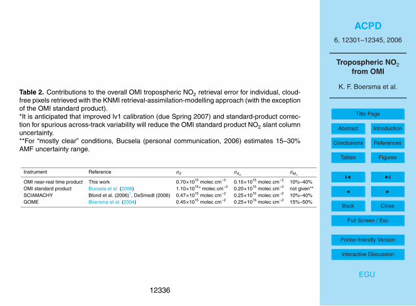
ACPD6, 12301–12345, 2006



Title Page



Tables Figures

J I

J I

Back Close

Full Screen / Esc



EGU

Table 2. Contributions to the overall OMI tropospheric NO2 retrieval error for individual, cloud-free pixels retrieved with the KNMI retrieval-assimilation-modelling approach (with the exceptionof the OMI standard product).*It is anticipated that improved lv1 calibration (due Spring 2007) and standard-product correc-tion for spurious across-track variability will reduce the OMI standard product NO2 slant columnuncertainty.**For “mostly clear” conditions, Bucsela (personal communication, 2006) estimates 15–30%AMF uncertainty range.

Instrument Reference σS σSstσMtr

OMI near-real time product This work 0.70×1015 molec.cm−2 0.15×1015 molec.cm−2 10%–40%OMI standard product Bucsela et al. (2006) 1.10×1015* molec.cm−2 0.20×1015 molec.cm−2 not given**SCIAMACHY Blond et al. (2006)1, DeSmedt (2006) 0.47×1015 molec.cm−2 0.25×1015 molec.cm−2 10%–40%GOME Boersma et al. (2004) 0.45×1015 molec.cm−2 0.25×1015 molec.cm−2 15%–50%

12336





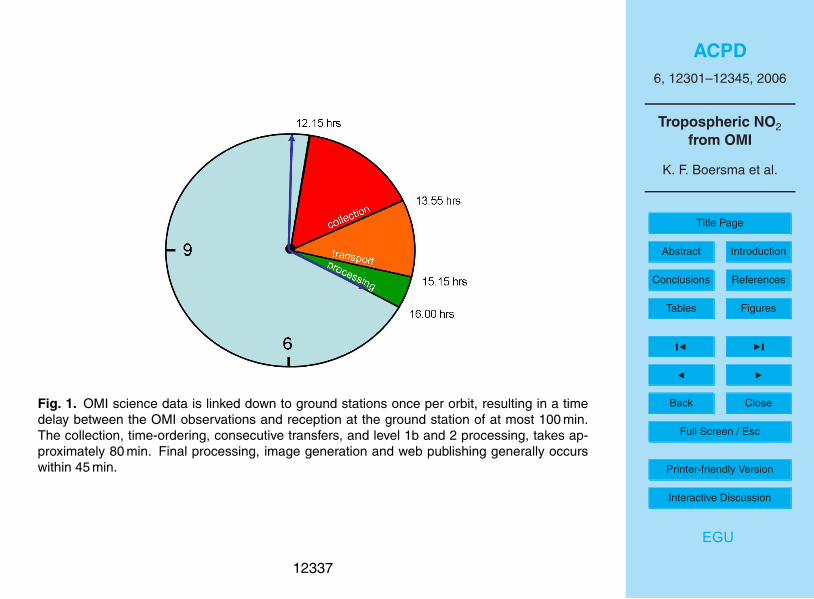
ACPD6, 12301–12345, 2006



Title Page



Tables Figures

J I

J I

Back Close

Full Screen / Esc



EGU

Fig. 1. OMI science data is linked down to ground stations once per orbit, resulting in a timedelay between the OMI observations and reception at the ground station of at most 100 min.The collection, time-ordering, consecutive transfers, and level 1b and 2 processing, takes ap-proximately 80 min. Final processing, image generation and web publishing generally occurswithin 45 min.

12337





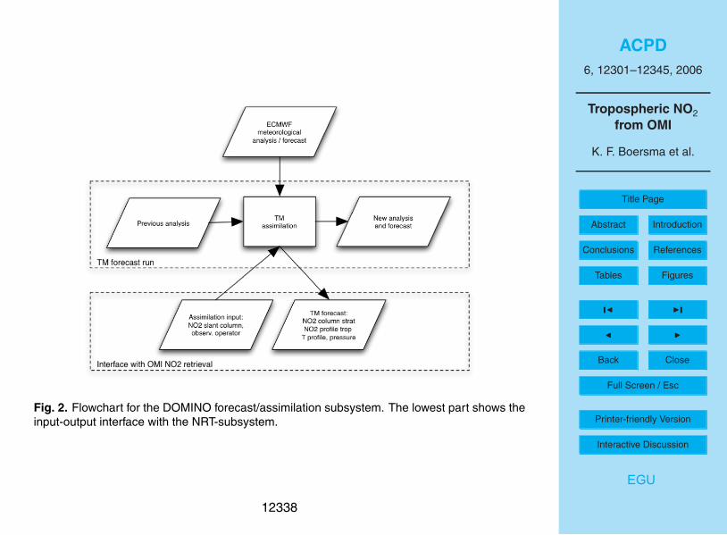
ACPD6, 12301–12345, 2006



Title Page



Tables Figures

J I

J I

Back Close

Full Screen / Esc



EGU

Fig. 2. Flowchart for the DOMINO forecast/assimilation subsystem. The lowest part shows theinput-output interface with the NRT-subsystem.

12338





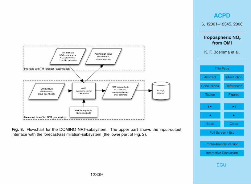
ACPD6, 12301–12345, 2006



Title Page



Tables Figures

J I

J I

Back Close

Full Screen / Esc



EGU

Fig. 3. Flowchart for the DOMINO NRT-subsystem. The upper part shows the input-outputinterface with the forecast/assimilation-subsystem (the lower part of Fig. 2).

12339





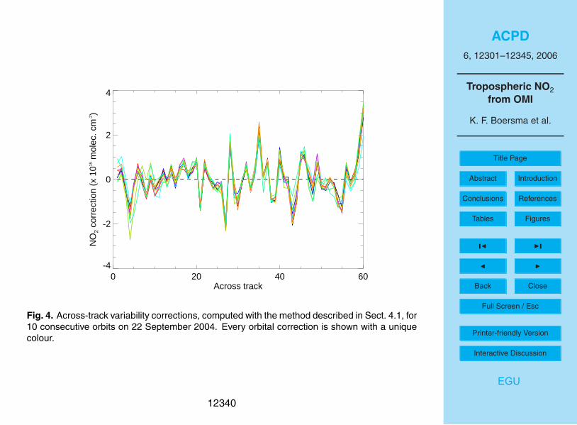
ACPD6, 12301–12345, 2006



Title Page



Tables Figures

J I

J I

Back Close

Full Screen / Esc



EGU

0 20 40 60Across track

-4

-2

0

2

4N

O2

corr

ectio

n (x

1015

mol

ec. c

m-2)

Fig. 4. Across-track variability corrections, computed with the method described in Sect. 4.1, for10 consecutive orbits on 22 September 2004. Every orbital correction is shown with a uniquecolour.

12340





ACPD6, 12301–12345, 2006



Title Page



Tables Figures

J I

J I

Back Close

Full Screen / Esc



EGU

-60 -40 -20 0 20 40 60Latitude

0.0

0.5

1.0

1.5

Unc

erta

inty

OM

I NO

2 S

CD

(10

15 m

olec

. cm

-2)

Cell standard deviationAverage standard deviationVertical column fitting error

(a)

7 August 2006

-4 -2 0 2 4Deviation (1015 molec. cm-2)

0

20

40

60

80

Num

ber

of o

ccur

ence

s

Histogram dataFitted Gaussian

(b)

Fig. 5. (a) Left panel: standard deviation of slant columns within a 2◦×2◦(longitudes between178◦ and 180◦ W) box as a function of latitude. The dashed line shows the meridional averageof the standard deviations for all the boxes. The solid line shows the contribution of the (slantcolumn) fitting error to the vertical column error (i.e. S/Mtr ). (b) Right panel: distribution ofmember deviations from box means for 2893 pixels. The dashed line shows a Gaussian func-tion fitted to the histogram data. The width of the Gaussian corresponds to a slant column errorof 0.67×1015 molec.cm−2.

12341





ACPD6, 12301–12345, 2006



Title Page



Tables Figures

J I

J I

Back Close

Full Screen / Esc



EGU

0.0 0.2 0.4 0.6 0.8 1.0Cloud fraction

0

2000

4000

6000

8000

Occ

uren

ces

SCIAMACHY FRESCOOMI O2-O2

(a)

200 400 600 800 1000Cloud pressure (hPa)

0

200

400

600

800

1000

1200

Occ

uren

ces

SCIAMACHY FRESCOOMI O2-O2

(b)

Fig. 6. (a) Left panel: histogram of 0.5◦×0.5◦ gridded effective cloud fractions from SCIA-MACHY FRESCO (dashed line) and OMI O2−O2 for seven consecutive days (5–11 August2006). (b) Right panel: histogram of 0.5◦×0.5◦ gridded effective cloud pressures from SCIA-MACHY FRESCO (dashed line) and OMI O2−O2 for seven consecutive days (5–11 August2006). Only observations with a cloud fraction higher or equal to 0.05 are shown.

12342





ACPD6, 12301–12345, 2006



Title Page



Tables Figures

J I

J I

Back Close

Full Screen / Esc



EGU

(a)

(b)

Fig. 7. (a) Monthly mean tropospheric NO2 column from SCIAMACHY for situations when bothSCIAMACHY and OMI observed a cloud-free scene. Grey grid cells have not been observedor had persistent cloud cover over August 2006. (b) Same as (a), but now for OMI.

12343





ACPD6, 12301–12345, 2006



Title Page



Tables Figures

J I

J I

Back Close

Full Screen / Esc



EGU

(a)

(b)

Fig. 8. (a) Monthly mean tropospheric NO2 column from SCIAMACHY (left panel) for cloud-freesituations. Grey grid cells have not been observed or had persistent cloud cover over August2006. (b) Same as (a), but now for OMI.

12344





ACPD6, 12301–12345, 2006



Title Page



Tables Figures

J I

J I

Back Close

Full Screen / Esc



EGU

(a)

(b)

Fig. 9. (a) Monthly mean tropospheric NO2 column from OMI over the U.S. for cloud-freesituations. Grey grid cells have not been observed or had persistent cloud cover over October2004. (b) Same as (a), but now over eastern Asia.

12345





Near-real time retrieval of tropospheric NO2 from OMI

Documents

Transcript of Near-real time retrieval of tropospheric NO2 from OMI