1

1

Observed Vertical Distribution of Tropospheric Ozone 2

During the Asian Summertime Monsoon 3

4

John Worden1, Dylan B. A. Jones2, Jane Liu2, Kevin Bowman1, Reinhard Beer1, 5

Jonathan Jiang1, Valérie Thouret3, Susan Kulawik1, Jui-Lin F. Li1, Sunita Verma1, and 6

Helen Worden3 7

8

1. Jet Propulsion Laboratory / California Institute of Technology 9

10

2. Department of Physics University of Toronto, Toronto, ON, Canada 11

12

3. Laboratoire d'Aérologie, UMR 5560, CNRS, Université de Toulouse, 14 Avenue 13

Edouard Belin, 31400 Toulouse, France 14

15

4. National Center for Atmospheric Research16

2

17

18

Abstract 19

20

We present new satellite measurements of vertically resolved tropospheric ozone profiles 21

from the Aura Tropospheric Emission Spectrometer (TES) and Microwave Limb Sounder 22

(MLS) instruments over the region affected by deep convection and summertime upper 23

tropospheric anticyclones associated with the Asian Monsoon. The TES observations 24

show that ozone enhancements of up to 100 ppbv or more occur in the upper and middle 25

troposphere between 300 hPa and 450 hPa. Lower ozone values of 70 ppb or less are 26

generally observed by both TES and MLS at 215 hPa but MLS also shows relative ozone 27

enhancements of 100 ppbv or more at the tropopause that TES cannot resolve due to 28

limited sensitivity to ozone at the tropopause. Over India the enhanced tropospheric 29

ozone layer is at approximately 300 hPa whereas this layer drops to approximately 450 30

hPa over the Middle East. Enhanced ozone values are observed in June and July, 31

corresponding to the onset of the Asian summertime monsoon, and begin to dissipate in 32

August. Over Central Asia and the Tibetan Plateau, we observe significantly enhanced 33

ozone of 150 ppbv or more at pressures greater than 300 hPa; these high ozone amounts 34

suggest a stratospheric source consistent with previous modeling and analysis of surface 35

ozone on the Tibetan Plateau. 36

37

38

1. Introduction 39

3

40

The summertime Asian Monsoon significantly affects the climate over North 41

Africa, the Middle East and Central Asia [Hoskins and Rodwell, 1995; Rodwell and 42

Hoskins, 1996; 2001]. However, only recently have observations begun to provide 43

understanding on how the Asian Monsoon affects the chemical composition of the 44

troposphere. For example, space based observations from Measurements of Pollution in 45

the Troposphere (MOPITT) [Kar, et al., 2004], the Microwave Limb Sounder (MLS) 46

[Jiang, et al., 2007; Park, et al., 2007], the Atmospheric Composition Experiment (ACE) 47

[Park, et al., 2008], and the Atmospheric Infrared Sounder (AIRS) [Randel and Park, 48

2006] have shown how deep convection associated with the Asian monsoon lofts 49

boundary layer air with low ozone and high water as well as surface emissions such as 50

CO from Asia into the upper troposphere and lower stratosphere [Fu, et al., 2006; 51

Gettelman, et al., 2004] . These surface emissions and boundary layer air can then be 52

trapped and transported in the upper tropospheric anti-cyclone that forms during the 53

summer time in this region [Barret, et al., 2008; Dunkerton, 1995; Hoskins and Rodwell, 54

1995; Park, et al., 2008; Park, et al., 2007; Randel and Park, 2006, Kunhikrishnan et al., 55

2006]. 56

Understanding the effects of the Asian summertime monsoon on the distribution 57

of tropospheric ozone must also include the vertical and horizontal distribution of 58

lightning produced NOx, and the subsequent photochemical production [Li, et al., 2001] 59

as well as stratospheric / tropospheric exchange [Gettelman, et al., 2004] and long range 60

transport of pollutants from Europe and Asia [Duncan, et al., 2008; Li, et al., 2001]. 61

Based on modeling simulations using the GEOS-CHEM model, it was suggested by Li et 62

4

al. [2001] that enhanced summertime ozone (greater then 80 ppbv) should be observed in 63

the middle troposphere over Africa the Middle East and Central Asia with peak values 64

over the Middle East. This prominent feature in the GEOS-CHEM model was shown by 65

Li et al. [2001] to be dynamically driven by the anticyclones which forms in response to 66

the Asian Monsoon; the anti cyclone traps ozone and ozone-precursors that are 67

transported from Asia and Europe. Observations using solar occultation as discussed in 68

[Kar, et al., 2002] does suggest the existence of peak ozone amounts at 7 km over North 69

East Africa and North West Saudi Arabia relative to the rest of the globe; however, 70

observations of total tropospheric ozone from the Ozone Monitoring Instrument (OMI) 71

and the Global Ozone Monitoring Instrument (GOME) show that tropospheric ozone 72

columns are enhanced between the latitudes of 25 and 35 degrees and particularly over 73

Northwest Saudi Arabia [Liu et al., 2006]. However ozone abundances as observed by 74

GOME are not enhanced in the Eastern hemisphere relative to the Western hemisphere 75

[Liu et al., 2006]. 76

Both the model predictions as well as the satellite observations of total 77

tropospheric ozone and upper tropospheric ozone, suggests that the vertical and 78

horizontal distribution of ozone varies strongly in response to the dynamics of the Asian 79

Monsoon and the horizontal and vertical distribution of ozone precursors in this region. 80

Understanding the distribution of the middle and upper tropospheric ozone from these 81

chemical and dynamical processes has both climate and air quality implications. For 82

example, upper tropospheric ozone is a greenhouse gas that affects global outgoing 83

longwave radiation [Worden, et al., 2008]. Furthermore, the collected ozone can act as a 84

pollution “reservoir” if it is transported to the boundary layer [Fiore, et al., 2002]. 85

5

In this paper we present three years of TES vertical profile observations of 86

tropospheric ozone, taken during the summers of 2005, 2006 and 2007 that show the 87

temporal, horizontal, and vertical distribution of tropospheric ozone over the region 88

extending from North East Africa through Asia. The vertical distributions are compared 89

with MLS observations of the upper troposphere for pressures below 200 hPa, and 90

aircraft ozone measurements for pressures above 200 hPa from the Measurements of 91

OZone and water vapour by in-service AIrbus aircraft (MOZAIC) program over Delhi, 92

Teheran, and Dubai [Marenco, et al., 1998] (http://mozaic.aero.obs-mip.fr/web/). 93

Characterizing the spatial and temporal variability of this feature is a critical first step 94

towards understanding how the dynamics controls this ozone and identifying the 95

corresponding sources of ozone-precursors. A subsequent study by J. Liu et al. [2008] 96

will conduct a detailed model analysis to better understand the transport and chemical 97

processes responsible for observed ozone enhancements across North Africa, the Middle 98

East. Verma et al; [In Preperation] will focus on the formation of ozone over South and 99

East Asia. 100

101

2. Satellite Ozone observations 102

103

2.1 Overview of TES instrument and sampling 104

TES is an infrared, high resolution, Fourier Transform spectrometer covering the 105

spectral range between 650 to 3050 cm-1 (3.3 to 15.4 µm) with an apodized spectral 106

resolution of 0.1 cm-1 for the nadir viewing [Beer, et al., 2001]. Spectral radiances 107

measured by TES are used to infer the atmospheric profiles through a non-linear optimal 108

6

estimation algorithm that minimizes the difference between these radiances and those 109

calculated with the equation of radiative transfer subject to the constraint that the 110

parameters are consistent with a statistical a priori description of the atmosphere 111

[Bowman, et al., 2006; Rodgers, 2000]. TES provides a global view of tropospheric trace 112

gas profiles including ozone, water vapor, and carbon monoxide along with atmospheric 113

temperature, surface temperature and emissivity, and an estimate of effective cloud top 114

pressure and an effective optical depth [Kulawik, et al., 2006; Worden, et al., 2004] . 115

For cloud free conditions, the vertical resolution of TES ozone profile observations are 116

typically 6 km in the tropics and mid-latitude summers [Jourdain, et al., 2007; Worden, 117

et al., 2004]. TES observations have been validated against ozone-sondes and lidar 118

measurements and it is generally found that upper tropospheric values are systematically 119

biased high by about 15% after accounting for the TES vertical resolution and a priori 120

constraint. 121

This analysis uses TES data taken during the summers of 2005, 2006 and 2007, 122

from both the nominal operation mode or “global survey” and from special observations 123

using the “Step-and-Stare” mode [Beer, 2006]. The sampling for the global survey mode 124

is one observation every 160 km with 16 orbits per global survey, over a time period of 125

12 hours. The step-and-stare mode spatial sampling is approximately 30 km but covering 126

only part of an orbit over 60 degrees latitude. 127

128

2.2 MLS 129

We also use monthly mean ozone observations from the Aura Microwave Limb 130

Sounder (MLS) [Livesey, et al., 2008; Waters, et al., 2006] using Version 2 MLS 131

7

products. The MLS observes thermal microwave emission from the Earths limb in order 132

to infer upper tropospheric and stratospheric profiles of ozone and many other 133

stratospheric trace gasses. The precision from noise (or measurement error) for any give 134

ozone measurement is at most 40 ppbv. For the monthly mean data shown in this paper 135

we ignore the measurement error as it is about 4 ppbv or less through averaging of 136

approximately 100 profiles or more. 137

138

3. Ozone Observations 139

140

The Asian Monsoon forms in late spring and dissipates in the fall; therefore we 141

focus our analysis for the June, July and August time period. We first examine TES 142

monthly averaged observations of the upper troposphere followed by vertical ozone 143

distributions as observed by TES and MLS. 144

145

3.1 TES Observed Monthly Mean Ozone In The Upper Troposphere 146

147

Figure 1 shows TES ozone estimates for the summers of 2005, 2006, and 2007 for 148

the pressure level at 464 hPa. Data for June 2005 are not shown as the TES instrument 149

was not operating at that time. All data for which the TES master data quality is set to 150

unity are used. Furthermore, only those data for which the degrees-of-freedom of signal 151

(DOFS) for the upper troposphere between 300 and 600 hPa is 0.3 or larger are selected 152

to ensure the estimate is sensitive to this part of the atmosphere. The grid used for Figure 153

1 is 6 degrees in both longitude and latitude. The figure is constructed by calculating the 154

8

average value of all ozone observations within the grid box. Because of the 155

approximately 6 km vertical resolution the estimated ozone at 464 hPa is influenced by 156

variations in the ozone abundance throughout the upper troposphere and into the the 157

lower stratosphere. However, we use a single level to show the ozone distribution in the 158

upper troposphere as opposed to averaging over many pressure levels because an 159

averaged upper tropospheric quantity would have a latitude dependence due to 160

tropopause variations. 161

At the 464 hPa pressure level, mean ozone values greater then 90 ppbv are 162

observed over north-east Africa, the Middle East, the Eastern Mediterranean, and over 163

Central Asia north of the Tibetan plateau between 35 and 50 degrees latitude and 164

approximately 75 degrees longitude. Although we should note that we have not corrected 165

for the 5% – 15% high bias that exists in the TES data in the middle troposphere when 166

stating this value of 90 ppbv [Worden et al., 2006; Parrington et al., 2008]. High ozone 167

values are also observed over East Asia but that is the subject for other analysis. This 168

observed spatial variability is persistent from year-to-year with July typically showing the 169

most enhanced values. In July 2005 the largest ozone values are observed over the 170

Middle-East but not necessarily in July 2006 and July 2007. However, as discussed in 171

the next section, many of the grid points shown in Figure 1 over the Middle-East had two 172

or less overlapping observations; consequently, TES observations over the Middle-East 173

during July of 2006 and 2007 are likely not be representative of the true ozone 174

distribution during these time periods. In general, the number of observations in each grid 175

point ranged from 3 to 30. 176

9

The spatial distribution of ozone in Figure1 show differences from the total 177

tropospheric ozone amounts from the GOME instrument as shown in [Liu, et al., 2006] in 178

that the largest ozone values in the upper troposphere are shown in the Eastern 179

Hemisphere as opposed to similar total tropospheric ozone amounts in both hemispheres. 180

However, [Liu, et al., 2006] does show peak total tropospheric ozone columns over the 181

Eastern Mediterranean and Northwestern Saudi Arabia which is somewhat consistent 182

with these TES distributions. Differences between the two ozone measurements are likely 183

due to differences in the sensitivity of the instruments to tropospheric ozone, sampling, 184

and the retrieval approach as well as the vertical distribution of ozone as discussed in 185

Sections 3.3 and 3.4. 186

187

3.2 Sensitivity And Errors Of TES Ozone Estimates 188

189

The sensitivity of the TES ozone estimates to the true ozone distribution depends 190

primarily on atmospheric temperature, clouds, and trace gas amounts. As these quantities 191

are strongly influenced by the summertime Asian monsoon it is necessary to determine 192

how their variability impact the TES retrievals in this region. In this section we examine 193

the errors, sensitivity, and retrieval bias of the TES ozone retrievals to show that the 194

observed spatial distribution of ozone is statistically significant. For brevity we limit the 195

error characterization to the ozone values of July 2006 as we do not find a significant 196

difference in the error characterization from month to month and season to season. 197

The error on the mean values shown in Figure 1 can in principle be theoretically 198

calculated by averaging over the expected random errors for the distribution of retrievals 199

10

in each grid box. However, this approach assumes that the statistics of the atmosphere in 200

the region of interest are well known, which may not be a good assumption for the Asian 201

monsoon region given the scarcity of ozone profile observations in this region. We can 202

empirically calculate the error on the mean by dividing the root-mean-square (RMS) of 203

the mean within each grid point by the square-root of the number of observations in each 204

grid [Worden, et al., 2007b]. As seen in Figure 2a (top panel), the error on the mean for 205

July 2006 is typically 5 ppbv or less for the regions with the largest ozone values, but can 206

be higher over parts of Central Asia due to the larger variance over this region. The 207

topography in this region can also make atmospheric retrievals more challenging, which 208

limits the number of available ozone profile estimates within some of the grid boxes, 209

thereby increasing the error of the mean. In particular the error on the mean is large over 210

parts of Saudi Arabia due to limited (one to two) observations per grid box for the July 211

2006 (and also July 2007, not shown). Consequently, the TES retrievals over this part of 212

Saudi Arabia may not provide a representative description of the spatial distribution of 213

ozone in this region. 214

The TES estimates for ozone, or other trace gasses, are dependent on the 215

sensitivity of the estimate to the true distribution of ozone as well as the a priori 216

constraint used for the ozone retrieval; this dependency is represented by the following 217

equation: 218

x̂ = xa+ A(x ! x

a) (0.1) 219

where x̂ , in this case, is the logarithm of the TES ozone profile estimate. The a priori 220

constraint is given by xa. The log of the true ozone distribution is given by x and the 221

sensitivity of the estimate to this ozone is given by the averaging kernel matrix, A =!x̂

!x. 222

11

The TES ozone estimate, a priori constraint and averaging kernel matrix, as well as the 223

various error covariances, are provided with all TES observations. The averaging kernel 224

is a function of the sensitivity of the TES measured radiance to the distribution of ozone, 225

the noise in the radiance, and the constraint matrix used to regularize the retrieval. For 226

ozone, the constraints and constraint matrices are computed using the MOZART global 227

chemistry model as input [Worden, et al., 2004] and are gridded onto a 60 degree 228

longitude by 10 degree latitude bins. 229

As seen in Equation (0.1), TES estimates are biased towards an a priori constraint. 230

The bias in TES estimates from the a priori constraint is given by the difference between 231

the true distribution of the logarithm of ozone and the TES estimate of this true 232

distribution: 233

234

x̂ ! x = (I ! A)(xa! x) , (0.2) 235

236

A useful metric for the sensitivity of the estimate to the true distribution is the degrees-of-237

freedom for signal (DOFS) which is the sum of the diagonal elements of the averaging 238

kernel matrix; recall that a diagonal element of the averaging kernel matrix describes the 239

sensitivity of the ozone estimate for the corresponding pressure level to the true 240

distribution of ozone at that pressure level. In order to determine if the ozone estimates 241

shown in Figure 1 are sensitive to the true distribution we examine the average DOFS for 242

the altitude region between 300-600 hPa as shown in Figure 2b (middle panel). For the 243

geographical and altitude region of interest there is, on average, 0.65 DOFS. 244

Consequently, while the estimate is sensitive to the true distribution of ozone in this 245

12

region, it is useful to determine the extent to which the retrieval bias might contribute to 246

the spatial variability in the ozone retrievals. 247

An approach for estimating an upper bound on the retrieval bias is to replace the 248

“true-state” ozone (x) on the right side of Equation (0.2), with some value that is unlikely, 249

although not unphysical. For this test we use the a priori constraint equivalent to clean 250

pacific air at approximately 30 degrees latitude and -180 degrees longitude. Ozone 251

values are about 30-40 ppbv in the lower troposphere and 40-50 ppbv in the upper 252

troposphere. Note that this linear operation is equivalent to calculating a different 253

estimate by swapping in a fixed a priori constraint [Rodgers and Connor, 2003]. 254

x̂2= x̂

1+ (I ! A)(x

a

2! x

a

1) (0.3) 255

where x̂1is the original TES (log) ozone estimate and x̂

2is the new TES (log) ozone 256

estimate, xa

1 is the constraint used for the original TES ozone retrieval and xa

2 is the fixed 257

constraint used to change the TES estimate. The expression (I ! A)(xa

2! x

a

1) is now 258

equivalent to the right hand side of Equation (0.2) if we replace the true distribution of 259

the logarithm of ozone with this new constraint in order to estimate an upper bound on 260

the bias from the constraint vector. 261

Therefore, instead of showing the difference as seen in Equation (0.2), we instead 262

re-calculate the ozone estimate assuming a fixed a priori constraint vector [Kulawik, et 263

al., 2008]. This new estimate is shown in Figure 2c (bottom panel) for the July 2006 264

monthly mean. Comparison between the middle panel of Figure 1 and Figure 2c shows 265

differences on the order of 5 ppbv with little change in the spatial variability in the region 266

of enhanced ozone over Northeast Africa, the Eastern Mediterranean, and North of the 267

Tibetan plateau. We can therefore conclude that the a priori constraint does not affect our 268

13

conclusions about the spatial variability of ozone. However, the a priori constraint could 269

be introducing a bias as high as 5 ppbv into the ozone estimates for these regions. Note 270

that a bias from the a priori constraint is removed when comparing to ozonesondes or 271

model profiles because these profiles are first transformed using Equation (0.1) before 272

comparing to TES observations [Worden, et al., 2007a]. 273

274

275

3.3 Vertical Distribution of Ozone over India, the Tibetan Plateau, and Central Asia 276

Having established the spatial extent of the summertime ozone distribution across 277

North Africa and Asia, we now show the vertical ozone distributions over this expansive 278

region between 30 and 90 degrees longitude using observations from the Aura TES and 279

MLS instruments. The objective is to characterize the vertical distribution of ozone over 280

this expansive region. Characterizing the vertical distribution of ozone is needed for 281

understanding how surface emissions, deep convection, long range transport, and 282

lightning transport or produce ozone in the troposphere during this time period. 283

Figure 3 shows the vertical distribution of ozone from TES for longitudes 284

between 70 and 90 degrees and between 20 and 50 degrees latitude; this is the region 285

covering India, the Tibetan Plateau, and Central Asia. Pressures shown are between 100 286

and 1000 hPa on the TES pressure grid. However, all data are interpolated to a latitudinal 287

grid of 0.5 degrees; we choose a finer latitudinal spacing then shown in Figure 1 because 288

the coarser longitudinal spacing allow for more data to be used in this figure. The 289

average surface pressure over this 20 degree longitudinal swath is shown as a white line 290

on the bottom. The surface pressure changes in each plot because of the different 291

14

sampling in each month of observations. A dashed line in the middle of each figure 292

represents the pressure at 464 hPa for comparison of these vertical distributions with 293

Figure 1. Only profiles where the DOFS in the upper troposphere is larger then 0.3 are 294

selected to ensure sensitivity of the TES estimates to variations in upper tropospheric 295

ozone. 296

The vertical distribution of ozone shown in Figure 3 is characterized by an 297

enhanced layer of ozone, with values that can exceed 100 ppbv, at approximately 300 hPa 298

between 25 and 40 degrees latitude. This enhanced layer of ozone is present in June and 299

July and begins to dissipate by August. The enhanced layer is not apparent in Figure 1 300

because it is at higher altitudes than the 464 hPa pressure level shown in Figure 1. The 301

lower ozone amounts of approximately 60 – 70 ppbvat 200 hPa, between 20 and 30°N, 302

during July and August (or 360 K potential temperature) are consistent with AIRS ozone 303

observations shown by [Randel and Park, 2006]. 304

An additional test to determine the altitude location of the enhanced ozone in this 305

region is to swap in a fixed a priori constrain using the approach discussed in Section 3.2. 306

Vertical ozone distributions from TES using a fixed a priori constraint vector are shown 307

in Figure 4. The vertical distributions for June show slight changes. However, the 308

differences in the vertical distributions of ozone using a fixed a priori constraint do not 309

change our conclusion about ozone enhancements near 350 hPa for latitudes between 20 310

and 300 N for the July and August time period. 311

Another feature shown in the TES data is high ozone past 40 degrees longitude 312

and pressures less then 300 hPa that appears to be a mix of stratospheric and tropospheric 313

air as indicated by the lines of potential temperature in the TES data; however the coarse 314

15

20 degree longitudinal gridding used to create these figures makes the determination of 315

the ozone source difficult. Consequently, we show a special-observation from TES in 316

Figure 5 that has a 35 km spacing between observations taken over a couple of minutes as 317

opposed to the 160 km spacing from the TES global survey; this special observation is 318

part of a yearly set of observations used to study boreal fires and Asian pollution. 319

As with the vertical distributions shown in Figure 3, enhanced ozone at 300 hPa is 320

observed near 30 degrees latitude. However, significantly high ozone greater than 150 321

ppbv is observed North of 35 degrees also at 300 hPa. This high ozone is co-located with 322

regions of low upper tropospheric water and the Westerly jet as shown in [Randel and 323

Park, 2006] indicate subsiding air. The high ozone and low water suggest a stratospheric 324

origin which is consistent with of the analysis of Moore and Semple, [2005] who found 325

that ozone at the surface in this region can originate from the stratosphere. They are also 326

consistent with the analysis of Sprenger and Wernli [2003] who examined 15 years of 327

ERA15 meteorological data from the European Center for Medium-Range Weather 328

Forecasting and found that stratosphere to troposphere exchange is at a maximum over 329

central Asia in summer. More recently, Ding and Wang [2006] suggested that 330

stratosphere intrusions were primarily responsible for enhanced surface ozone 331

abundances observed in over the Tibetan Plateau. Other TES step and stares taken during 332

the summer of this same region show similar behavior but are not shown because they 333

had significant data gaps due to clouds and increased retrieval failure rate over the 334

mountain regions. 335

336

3.4. Vertical Distribution of Ozone over the Middle East 337

16

338

We next show the vertical distribution of ozone ranging between 30 to 70 degrees 339

longitude and between 20 to 50 degrees latitude. These distributions are shown in 340

Figures 6 and 7 for longitudes between 50 – 70 degrees and 30 to 50 degrees 341

respectively. Both figures again show enhanced ozone amounts of 100 ppbv in the 342

middle or upper troposphere. A difference between the ozone distributions in Figures 7 343

and 8 and those over India and Tibet (Figure 3) are that the peak ozone amounts for 344

latitudes less then 30 degrees appear at lower altitudes as indicated by the dashed line at 345

450 hPa shown in each figure. For latitudes above 30 degrees, peak ozone values appear 346

to shift to higher altitudes near 200 hPa although an ozone minima can appear at these 347

altitudes during August for longitudes between 50 and 70 degrees. For brevity, we do not 348

show ozone amounts using a fixed a priori constraint although we note that our 349

conclusions about the vertical distribution of ozone would not change using a fixed prior. 350

351

352

3.5 Comparison to MOZAIC and MLS 353

354

Monthly mean ozone profiles over Delhi, Tehran, and Dubai from the MOZAIC 355

program are shown in Figure 8 for June, July, and August. We use here monthly mean 356

ozone climatologies generated from MOZAIC data between 1996 and 2005 because there 357

is no overlap between these measurements and the TES and MLS data. However, the 358

climatology provides sufficient statistics to capture the vertical distribution of ozone for 359

comparison of the seasonal variations in the vertical structure of ozone. The precision of 360

17

the MOZAIC ozone data is 2 ppbv and the sensors are calibrated every 500 flights hours 361

[Thouret et al., 1998a]. They number of profiles used to calculated the monthly means 362

range from 47 to 110. The constructed climatologies from these profiles are consistent 363

with those based on ozonesondes [Thouret et al., 1998b]. As shown in Figure 8, the 364

profiles are characterized by low ozone amounts in the lower troposphere with higher 365

amounts of up to 80 ppbv between 200 to 400 hPa. The ozone in the free troposphere 366

also decreases from June to August. This seasonal variability is consistent with TES data 367

in that ozone is typically highest in the middle troposphere in June and lowest in August. 368

The MOZAIC climatology over Delhi, Tehran, and Dubai are compared directly 369

with TES and MLS observations for July in Figure 9. Since there are no overlapping TES 370

or MLS data available to compare with the MOZAIC profile, we average both TES and 371

MLS across a 5 degree by 5 degree bin in which each of the cities is a midpoint. Shown 372

in Figure 9 is the mean value of all TES ozone profiles for July 2005, 2006, and 2007 for 373

the grid points centered over Delhi, Tehra, and Dubai. The dotted lines represent the root-374

mean-square (RMS) about the mean of the TES ozone. A major challenge in comparing 375

the TES and MOZAIC profiles is that accounting for the TES vertical resolution and bias 376

introduced by the a priori constraint is not accurate (e.g., Worden et al., 2006) because of 377

the error introduced by truncating the TES profile at approximately 200 hPa, the upper 378

limit of the MOZAIC profiles. This truncation introduced a “cross-state” error [Worden 379

et al., 2004] that is due to uncertainties in the TES estimated ozone in the upper 380

troposphere and lower stratosphere. This cross-state error is largest at 200 hPa and 381

becomes smaller at higher pressures. Taking into account the lower sensitivity to ozone 382

of the TES estimates for pressures above 800 hPa, the best overall comparison between 383

18

the TES and MOZAIC data will be between 400 and 800 hPa. As can be seen in Figure 9, 384

in this region the MOZAIC data agree well with TES, within the mean and RMS, with 385

the exception of Dubai at approximately 550 hPa. Previous comparison of TES data with 386

sondes suggest that TES is biased high in the middle troposphere by approximately 5% to 387

15% [Worden et al., 2006; Nassarr et al. 2008]. This bias is consistent with the TES 388

comparison to MOZAIC. 389

The comparison between TES and MLS in Figure 9 reveals that there is 390

significantly more variability in the MLS data than in TES in the upper troposphere and 391

lower stratosphere for these regions. The variability of MLS data is much less than the 392

expected precision (about 4%) or bias which could be 0 – 15% [Livesey et al. 2008]. 393

Averaged between 100-215 hPa, the observed MLS ozone amounts are within the 394

range of variability observed by TES. For example, the average mean ozone between 100 395

and 215 hPa over Delhi is approximately 91 ppbv for the MLS data versus approximately 396

83 ppbv for the TES data. However, the TES sensitivity to ozone variability is lowest at 397

the tropopause and highly correlated above and below the tropopause because the 398

temperature above and below the tropopause will have matching values. Consequently, 399

we would not expect the observed TES variability to match that observed by MLS, but, 400

on average, the two instruments should observe similar ozone amounts. 401

402

403

4. Discussion and Conclusions 404

405

19

Previous observations of tropospheric and stratospheric trace gasses in the Asian 406

Monsoon region reveal a complex system involving deep convection of boundary layer 407

air followed by entrainment into strong westerly and easterly winds as well as re-408

circulation of air along the summertime upper tropospheric / lower stratospheric 409

anticyclones. These dynamical processes are indicated by low ozone, high water, and 410

significant surface emissions such as CO and HCN in the upper troposphere and lower 411

stratosphere during summertime [Fu, et al., 2006; Gettelman, et al., 2004; Kar, et al., 412

2004; Park, et al., 2007; Randel and Park, 2006]. 413

Deep convection of surface emissions, lightning, as well as long range transport 414

of European and Asian emissions and re-circulation in middle tropospheric anticyclones, 415

are expected by the GEOS-CHEM model to significantly enhance ozone in the middle 416

troposphere [Li, et al., 2001] over the Middle East. These model predictions are 417

corroborated by satellite observations showing significant ozone enhancements over 418

Northeast Africa and Northwest Saudi Arabia [Kar, et al., 2002; Liu, et al., 2006] as well 419

as MOZAIC observations over Middle-Eastern cities [Li, et al., 2001]. 420

TES observations of the vertical and horizontal distribution of tropospheric ozone 421

enhance this picture of how tropospheric ozone responds to the dynamics of the Asian 422

monsoon and subsequent chemical processes by showing a highly stratified vertical 423

ozone distribution stretching from North East Africa through India for latitudes less then 424

300N. Peak ozone amounts over India appear near 300 hPa whereas over the Middle East 425

they appear near 450 hPa with values that can exceed 100 ppbv. Lower ozone values of 426

about 50 ppbv are present above and below this enhanced layer as discussed by [Fu, et 427

al., 2006; Gettelman, et al., 2004; Kar, et al., 2004; Park, et al., 2007; Randel and Park, 428

20

2006]. An enhanced ozone layer over the middle East near 450 hPa is consistent with 429

the results from [Li, et al., 2001]. 430

This stratified distribution is corroborated by MLS observations of ozone for 431

pressures less than 200 hPa and by MOZAIC summertime ozone climatologies for 432

pressures above 200 hPa in Tehran, Dubai, and Delhi. As also observed by the MOZAIC 433

climatologies, TES observed ozone values in the middle troposphere peak in June and 434

begin to dissipate in August. After accounting for the TES upper tropospheric bias of 435

15%, we find that ozone in this enhanced layer can exceed 100 PPBV. We are currently 436

studying whether this bias is instrumental or due to increased surface emissions since the 437

MOZAIC climatology was generated. 438

In addition to these layers of ozone, enhanced upper tropospheric ozone with 439

values exceeding 150 PPBV is observed for latitudes above 40 degrees; initial analysis 440

suggests a significant stratospheric influence, likely due to subsidence along the Westerly 441

Jet. A companion paper by J. Liu et al. [this journal] as well as a subsequent work by 442

Verma et al. [In Preperation] will relate these vertical distributions of ozone to the 443

complex dynamics over this expansive region as well as the horizontal and vertical 444

distribution of ozone pre-cursors and ozone production. 445

446

447

Acknowledgement 448

The work described here is performed at the Jet Propulsion Laboratory, California 449 Institute of Technology under contracts from the National Aeronautics and Space 450 Administration. D. Jones and J. Liu were funded by the Natural Sciences and Engineering 451 Council of Canada and the Canadian Foundation for Climate and Atmospheric Sciences. 452 We thank Jay Kar for helpful discussions. The views, opinions, and findings contained in 453 this report are those of the author(s) and should not be construed as an official National 454

21

Oceanic and Atmospheric Administration or U.S. Government position, policy, or 455 decision. 456 457

References 458

459

Barret, B., et al. (2008), Transport pathways of CO in the African upper troposphere 460 during the monsoon season: a study based upon the assimilation of spaceborne 461 observations, Atmos. Chem. Phys. Discuss., 8, 2863 - 2902. 462

Beer, R., et al. (2001), Tropospheric emission spectrometer for the Earth Observing 463 System's Aura Satellite, Applied Optics, 40, 2356-2367. 464

Bowman, K. W., et al. (2006), Tropospheric emission spectrometer: Retrieval method 465 and error analysis, Ieee Transactions on Geoscience and Remote Sensing, 44, 1297-1307. 466

Ding, A., and T. Wang (2006), Influence of stratosphere-to-troposphere exchange on the 467 seasonal cycle of surface ozone at Mount Waliguan in western China, Geophys. Res. 468 Lett., 33, L03803, doi:10.1029/2005GL024760. 469

Duncan, B. N., et al. (2008), The influence of European pollution on ozone in the Near 470 East and northern Africa, Atmospheric Chemistry and Physics, 8, 2267-2283. 471

Dunkerton, T. J. (1995), Evidence of Meridional Motion in the Summer Lower 472 Stratosphere Adjacent to Monsoon Regions, Journal of Geophysical Research-473 Atmospheres, 100, 16675-16688. 474

Fiore, A. M., et al. (2002), Background ozone over the United States in summer: Origin, 475 trend, and contribution to pollution episodes, Journal of Geophysical Research-476 Atmospheres, 107, -. 477

Fu, R., et al. (2006), Short circuit of water vapor and polluted air to the global 478 stratosphere by convective transport over the Tibetan Plateau, Proceedings of the 479 National Academy of Sciences of the United States of America, 103, 5664-5669. 480

Gettelman, A., et al. (2004), Impact of monsoon circulations on the upper troposphere 481 and lower stratosphere, Journal of Geophysical Research-Atmospheres, 109, -. 482

Hoskins, B. J., and M. J. Rodwell (1995), A Model of the Asian Summer Monsoon .1. 483 The Global-Scale, Journal of the Atmospheric Sciences, 52, 1329-1340. 484

Jiang, J. H., et al. (2007), Connecting surface emissions, convective uplifting, and long-485 range transport of carbon monoxide in the upper troposphere: New observations from the 486 Aura Microwave Limb Sounder, Geophysical Research Letters, 34, -. 487

22

Jourdain, L., et al. (2007), Tropospheric vertical distribution of tropical Atlantic ozone 488 observed by TES during the northern African biomass burning season, Geophysical 489 Research Letters, 34. 490

Kar, J., et al. (2004), Evidence of vertical transport of carbon monoxide from 491 Measurements of Pollution in the Troposphere (MOPITT), Geophysical Research 492 Letters, 31, -. 493

Kar, J., et al. (2002), On the tropospheric measurements of ozone by the Stratospheric 494 Aerosol and Gas Experiment II (SAGE II, version 6.1) in the tropics, Geophysical 495 Research Letters, 29, -. 496

Kulawik, S. S., et al. (2008), Technical Note: Impact of nonlinearity on changing the a 497 priori of trace gas profiles estimates from the Tropospheric Emission Spectrometer 498 (TES), Atmospheric Chemistry and Physics Discussion, 8, 1261 - 1289. 499

Kulawik, S. S., et al. (2006), Implementation of cloud retrievals for Tropospheric 500 Emission Spectrometer (TES) atmospheric retrievals: part 1. Description and 501 characterization of errors on trace gas retrievals, Journal of Geophysical Research-502 Atmospheres, 111, -. 503

Kunhikrishnan T., M. G. Lawrence, R. von Kuhlmann, M. O. Wenig, W. A. H. Asman, 504 A. Richter, J. P. Burrows (2006), Regional NO x emission strength for the Indian 505 subcontinent and the impact of emissions from India and neighboring countries on 506 regional O 3 chemistry, J. Geophys. Res., 111, 507

Li, Q. B., et al. (2001), A tropospheric ozone maximum over the Middle East, 508 Geophysical Research Letters, 28, 3235-3238. 509

Liu, X., et al. (2006), First directly retrieved global distribution of tropospheric column 510 ozone from GOME: Comparison with the GEOS-CHEM model (vol 111, art D10399, 511 2006), Journal of Geophysical Research-Atmospheres, 111, -. 512

Livesey, N. J., et al. (2008), Validation of Aura Microwave Limb Sounder O-3 and CO 513 observations in the upper troposphere and lower stratosphere, Journal of Geophysical 514 Research-Atmospheres, 113, -. 515

Marenco, A., et al. (1998), Measurement of ozone and water vapor by Airbus in-service 516 aircraft: The MOZAIC airborne program, An overview, Journal of Geophysical 517 Research-Atmospheres, 103, 25631-25642. 518

Moore, G. W. K., and J. L. Semple (2005), A Tibetan Taylor Cap and a halo of 519 stratospheric ozone over the Himalaya, Geophysical Research Letters, 32, L21810, 520 doi:10.1029/2005GL024186. 521 522

23

Nassar, R., et al. (2008), Validation of Tropospheric Emission Spectrometer (TES) 523 nadir ozone profiles using ozonesonde measurements, J. Geophys. Res., 113, 524 D15S17, doi:10.1029/2007JD008819. 525

Park, M., et al. (2008), Chemical isolation in the Asian monsoon anticyclone observed in 526 Atmospheric Chemistry Experiment (ACE-FTS) data, Atmospheric Chemistry and 527 Physics, 8, 757-764. 528

Park, M., et al. (2007), Transport above the Asian summer monsoon anticyclone inferred 529 from Aura Microwave Limb Sounder tracers, Journal of Geophysical Research-530 Atmospheres, 112, -. 531

Randel, W. J., and M. Park (2006), Deep convective influence on the Asian summer 532 monsoon anticyclone and associated tracer variability observed with Atmospheric 533 Infrared Sounder (AIRS), Journal of Geophysical Research-Atmospheres, 111, -. 534

Rodgers, C. D. (2000), Inverse methods for atmospheric sounding : theory and practice, 535 xvi, 238 p. pp., World Scientific, Singapore ; London. 536

Rodgers, C. D., and B. J. Connor (2003), Intercomparison of remote sounding 537 instruments, Journal of Geophysical Research-Atmospheres, 108, -. 538

Rodwell, M. J., and B. J. Hoskins (1996), Monsoons and the dynamics of deserts, 539 Quarterly Journal of the Royal Meteorological Society, 122, 1385-1404. 540

Rodwell, M. J., and B. J. Hoskins (2001), Subtropical anticyclones and summer 541 monsoons, Journal of Climate, 14, 3192-3211. 542

Sprenger, M., and H. Wernli (2003), A northern hemispheric climatology of cross-543 tropopause exchange for the ERA15 time period (1979 – 1993), J. Geophys. Res., 544 108(D12), 8521, doi:10.1029/2002JD002636. 545

Thouret, V., Marenco, A., Nédélec, P., et Grouhel, C. (1998a), Ozone climatologies at 9-546 12 km altitude as seen by the MOZAIC Airborne Programme between September 1994 547 and August 1996, J. Geophys. Res., 103, D19, 25,653-25,679. 548

Thouret, V., Marenco, A., Logan, J., Nédélec, P., et Grouhel, C., Comparisons of ozone 549 measurements from the MOZAIC airborne programme and the ozone sounding network 550 at eight locations, J. Geophys. Res., 103, D19, 25,695-25,720, 1998b. 551

Waters, J. W., et al. (2006), The Earth Observing System Microwave Limb Sounder 552 (EOS MLS) on the Aura satellite, Ieee Transactions on Geoscience and Remote Sensing, 553 44, 1075-1092. 554

Worden, H. M., et al. (2008), Satellite measurements of the clear-sky greenhouse effect 555 from tropospheric ozone, Nature Geoscience. 556

24

Worden, H. M., et al. (2007a), Comparisons of Tropospheric Emission Spectrometer 557 (TES) ozone profiles to ozonesondes: Methods and initial results, Journal of Geophysical 558 Research-Atmospheres, 112. 559

Worden, J., et al. (2004), Predicted errors of tropospheric emission spectrometer nadir 560 retrievals from spectral window selection, Journal of Geophysical Research-561 Atmospheres, 109, D09308. 562

Worden, J., et al. (2007b), Importance of rain evaporation and continental convection in 563 the tropical water cycle, Nature, 445, 528-532. 564 565 566

Figure 1: TES monthly averaged ozone at 464 hPa. Data are gridded on a 6x6 degree

bin. There are no data for June 2005 as TES was undergoing operational

difficulties during that time period.

Figure 2 (Top Panel) Error on the Mean for the July 2006 Ozone values at the 464 hPa

level. (Middle Panel) The DOFS for the region between 300 and 600 hPa.

(Bottom Panel) The TES estimate of ozone at 464 hPa if we use a fixed a priori

constraint vector.

Figure 3: TES vertical ozone distributions during the Summers of 2005, 2006, and 2007

for longitudes between 70 – 90 degrees East. The vertical scale is the log of

pressure. The dashed line indicates the 464 hPa level for comparison with Figure

1. The bottom white line shows the average surface pressure for the set of

observations during the specified time period and latitude / longitude range.

Figure 4: Same as in Figure 3 except the ozone profiles have been re-calculated using a

fixed a priori constraint.

Figure 5: TES ozone profiles from the “step-and-stare” mode. There is approximately 1

observation every 35 km. The white line is the average surface pressure.

Figure 6: TES observed vertical ozone distributions for longitudes between 50 and 70

degrees East. The white line indicates the average surface pressure.

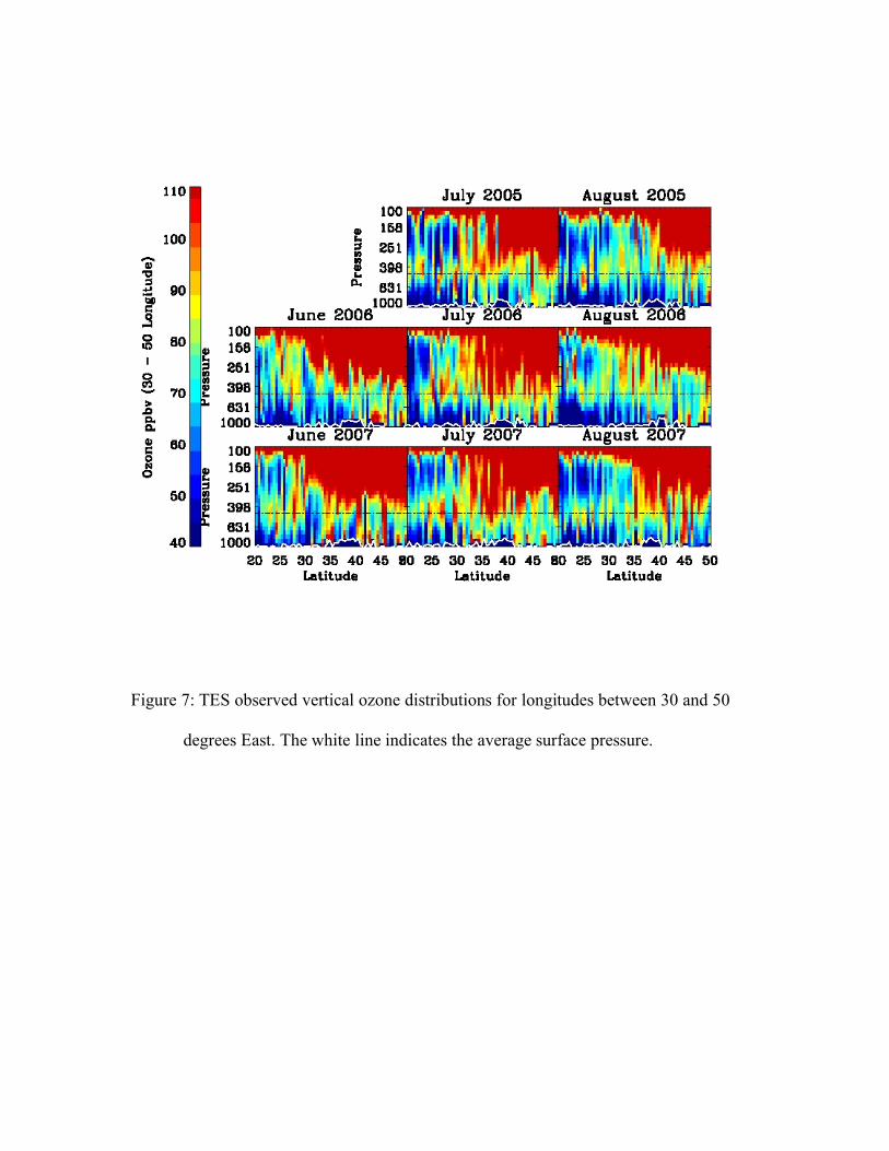
Figure 7: TES observed vertical ozone distributions for longitudes between 30 and 50

degrees East. The white line indicates the average surface pressure.

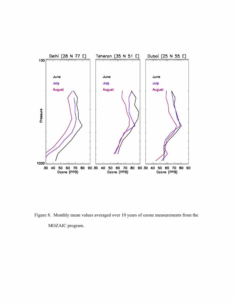
Figure 8. Monthly mean values averaged over 10 years of ozone measurements from the

MOZAIC program.

Figure 9: TES, MLS, and MOZAIC ozone over Delhi, Teheran, and Dubai. The TES and

MLS data (purple and orange respectively) are averages of all available profiles

within a 5x5 degree grid box over the respective cities for July of 2005, 2006, and

2007. The ten year (1995 – 2005) MOZAIC climatology is shown as the black

line. Dotted lines are the RMS of the TES ozone profiles within the 5x5 degree

grid.